Spatial and temporal runoff oscillation analysis of the main rivers of ...

Spatial and temporal runoff oscillation analysis of the main rivers

of the world during the 19th–20th centuries

Pavla Pekarovaa,*, Pavol Miklanekb,1, Jan Pekarc,2

aInstitute of Hydrology of Slovak Academy of Science, Racianska 75, 838 11 Bratislava, SlovakiabInstitute of Hydrology of Slovak Academy of Science, Racianska 75, 838 11 Bratislava, Slovakia

cDepartment of Economic and Financial Models, Comenius University, Mlynska dolina, 842 48 Bratislava, Slovakia

Received 19 July 2001; revised 4 November 2002; accepted 15 November 2002

Abstract

The annual discharge time series of selected large rivers in the world were tested for wet and dry periods. The 28–29-years

cycle, as well as 20–22-years cycle of extremes occurrence were identified. From the trend analysis it follows that the

hydrological characteristics of the rivers must be stated at least for one 28-year period. If we want to identify any trend

uninfluenced by the 28-year periodicity of the discharge time series, we must determine the trend during a single or multiple

curve cycle, starting and terminating by either minima (e.g. 1861–1946 in West/Central Europe) or maxima (e.g. 1847–1930 or

1931–1984 in West/Central Europe). Trends determined for other periods are influenced by the periodicity of the series and

depend on the position of the starting point on the increasing or recession curve. Long-term trends during the period 1860–1990

have not been detected for the West/Central European runoff.

Further, the temporal shift in the discharge extremes occurrence (both, maxima and minima) was shown to depend on the

longitude and latitude. The time shift between Neva and Amur discharge time series is about four years, between Amur and St

Lawrence is about 16 years, and between St. Lawrence and Neva is about nine years. The time shift between Congo and

Amazon is about seven years.

q 2003 Elsevier Science B.V. All rights reserved.

Keywords: Long-term runoff fluctuation; Discharge; Time series analysis; Spectral analysis; Temporal pattern; Teleconnection

1. Introduction

The development of mankind has depended on

availability of water resources. Already the first

agricultural civilisations noticed the temporal varia-

bility of water resources and oscillation of the dry and

wet periods.

Statistical analysis of the runoff oscillations

depends on availability of long time series of

data. Systematic measurements of discharge in

modern era started relatively late. The longest

time series are available in Europe, but they do not

exceed 200 years (Probst and Tardy, 1987). Such

long series are exceptional and in most of the

world only much shorted series exist.

Journal of Hydrology 274 (2003) 62–79

www.elsevier.com/locate/jhydrol

0022-1694/03/$ - see front matter q 2003 Elsevier Science B.V. All rights reserved.

PII: S0 02 2 -1 69 4 (0 2) 00 3 97 -9

1 Tel/Fax: þ4212-44259311.2 Tel.: þ4212-60295713; fax: þ4212-65412305.

* Corresponding author. Tel.: þ421-2-44259311; fax: þ421-2-

44259311.

E-mail addresses: [email protected] (P. Pekarova),

[email protected] (P. Miklanek), [email protected] (J.

Pekar).

http://www.elsevier.com/locate/jhydrol

Forty years ago, Williams (1961) investigated

the nature and causes of cyclical changes in

hydrological data of the world. He attempted

correlation between hydrologic data and sunspot

with varying success. Brazdil and Tam (1990),

Walanaus and Soja (1995), Sosedko (1997), Smith

et al. (1997) and Lukjanetz and Sosedko (1998)

found several different dry and moisture periods

(2.6; 3.5; 5; 13.3-year) in the precipitation and

discharge time series in Europe. Using an improved

numerical procedure the variance contribution of

both, the luni-solar 18.6-year and 10–11-year solar

cycle signals to 3234 yearly sampled climate

records were studied by Currie (1996) and Probst

and Tardy (1987) studied mean annual discharge

fluctuations of fifty major rivers distributed around

the world by filtering methods. They showed, that

North American and European runoffs fluctuate in

opposition while South American and African

runoffs present synchronous fluctuations.

The changes of runoff in last decades may by

related to climate change, but there exist also other

natural factors that influence the runoff variability

and may reinforce the runoff changes. The

hydrologists and climatologists concentrate on the

relationship between both, precipitation and runoff

variability and large air pressure oscillations over

the oceans during the last 15 years. A typical

example is the SO (Southern Oscillation) over the

Pacific (Rodriguez-Puebla et al., 1998) and NAO

(North Atlantic Oscillation) over the Atlantic Ocean

(Hurrell, 1995; Stephenson, 1999; Stephenson et al.,

2000). The change of air pressure fields over large

areas influences the transport of amount of

precipitation over neighbouring continents.

For example Shorthouse and Arnell (1997)

analysed relationships between inter-annual climatic

variability—as measured by the NAOI—and spatial

patterns of anomalous hydrological behaviour across

Europe. The analysis was based on regional average

monthly discharge series, derived from 477 drainage

basins on the FRIEND European Water Archive

between 1961 and 1990. It was shown that

European river flows are strongly correlated, most

particularly in winter, with the NAO and that this

relationship exhibits a strong spatial pattern. North-

ern European river flows, particularly in

the Scandinavian region, tend to be positively

correlated with the NAOI, and rivers in southern

Europe reveal negative correlation with the index.

This result is consistent with the previously explored

correlation between the NAO and precipitation.

Cluis (1998) shows that in most areas of the Asia-

Pacific region, a strong El Nino related signal can be

found in the historical river series stored at the Global

Runoff Data Center (GRDC). This signal is particu-

larly strong in the Australian rivers whose regimes are

known to be highly contrasted. Cluis showed that

during El Nino the runoff is lower in these areas, while

during La Nina it is higher than the mean runoff

(despite the fact that for some of the New Zealand

rivers the results were contrary).

Yang et al. (2000) investigated the ENSO tele-

connection with annual precipitation series (Tiberian

Plateau, China) from 1690 to 1987 (nearly 300 years).

The results showed that negative precipitation

anomalies are significantly associated with El Nino

years.

On the other hand Kane (1997) investigated, that

the relationship between El Nino and droughts in

north–east Brazil is poor. Thus, forecasts of droughts

based on the appearance of El Nino alone would be

wrong half the time. Instead, predictions based on

significant periodicities (ca 13 and ca 26 years) give

reasonably good results.

Our previous analysis of the long-term runoff

oscillation shows the regular dry and wet periods

occurrence in central Europe (Pekarova, 2002;

Pekarova and Pekar, 2002; Svoboda et al., 2000).

The scope of the study is:

(i) To demonstrate the existence of the long-term

discharge fluctuations (20–30 years) in rivers of

all continents;

(ii) To pronounce the hypothesis of the shift in long-

term runoff extremes occurrence over the earth.

2. Temporal and spatial discharge analysis of main

world rivers

2.1. Material

The longest available time series of mean annual

discharge of the selected world largest rivers were

used to analyse the long-term runoff oscillation.

P. Pekarova et al. / Journal of Hydrology 274 (2003) 62–79 63

The annual precipitation time series are usually the

basis for study of the long-term oscillation of dry and

wet periods in the basin. We will analyse the annual

discharge time series due to following reasons:

† The increase of precipitation by one third may

increase the runoff by one half. Therefore changes

in precipitation series are even more evident in

discharge series.

† The water balance of the basin depends not only on

precipitation, but on temperature as well (evapo-

transpiration). The discharge series combine both

these influences.

† The problems of precipitation measurements and

evaluation of the areal precipitation in mountain

basins are well known. Discharge measurement in

the outlet profile of the basin is simpler and more

accurate in comparison to areal precipitation.

† The analyses of the long-term runoff oscillations

of the large rivers eliminates the local disturb-

ances in precipitation and temperature series due

to local orographic peculiarities.

The long annual discharge data series of all the

continents were obtained from following data sources:

(i) Global Runoff Data Center in Koblenz, Germany;

(ii) CD ROM of the Hydro-Climatic Data Network

(HCDN), US Geological Survey Streamflow Data

Set for the United States;

(iii) CD-ROM World Freshwater Resources

prepared by Shiklomanov in the framework of

the International Hydrological Programme (IHP)

of UNESCO;

(iv) URL http://waterdata.usgs.gov.

A set of more than a hundred of annual discharge

time series with long periods of observation in all

continents were analysed in the study. The river

basins were grouped into two regions:

I. Extra tropics zone of the Northern Hemisphere

(between 30 –75 8N);

II. Equatorial zone and mild zone of the Southern

Hemisphere (30 8N–408S).

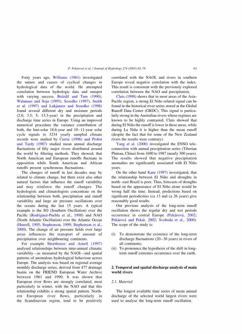
For the final analysis twenty river basins were

selected in each region. The selected rivers and

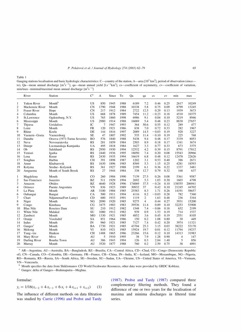
stations are in Fig. 1. In Table 1 there are basic

hydrologic characteristics of the series and basins.

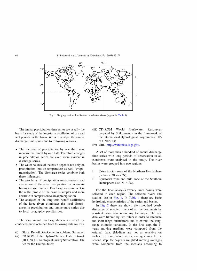
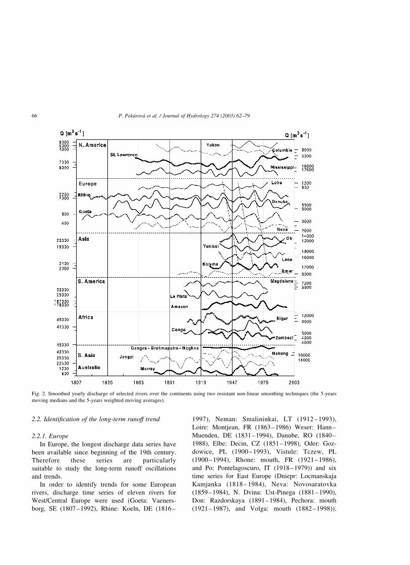
In Fig. 2 there are shown the smoothed yearly

discharge of selected rivers of all the continents by

resistant non-linear smoothing technique. The raw

data were filtered by two filters in order to attenuate

the short-range fluctuations and to extract the long-

range climatic variations. In the first step, the 5-

years moving medians were computed from the

original data. (Medians are not as sensitive on

isolated extreme values as the averages are). In the

second step, the 5-years weighted moving averages

were computed from the medians according to

Fig. 1. Gauging stations localisation on selected rivers (legend in Table 1).

P. Pekarova et al. / Journal of Hydrology 274 (2003) 62–7964

http://waterdata.usgs.gov

formulae:

yi ¼ 1=16ðxi22 þ 4·xi21 þ 6·xi þ 4·xiþ1 þ xiþ2Þ ð1Þ

The influence of different methods on data filtration

was studied by Currie (1996) and Probst and Tardy

(1987). Probst and Tardy (1987) compared three

complementary filtering methods. They found a

difference of one or two years for the localisation of

maxima and minima discharges in filtered time

series.

Table 1

Gauging stations localisation and basic hydrologic characteristics: C—country of the station, A—area [103 km2], period of observation (since—

to), Qa—mean annual discharge [m3s21], qa—mean annual yield [l.s21km2], cs—coefficient of asymmetry, cv—coefficient of variation,

min/max–minimal/maximal mean annual discharge [m3s21]

River Station Ca A Since To Qa qa cs cv min max

1 Yukon River Mouthb US 850 1945 1988 6189 7.2 0.46 0.25 2617 102492 Mackenzie River Mouth CN 1790 1948 1988 10338 5.8 0.75 0.09 8799 132453 Fraser River Hope CN 217 1912 1984 2722 12.5 0.29 0.13 1939 36734 Columbia Mouth US 668 1878 1989 7454 11.2 20.23 0.18 4510 103755 St.Lawrence Ogdensburg, N.Y. US 765 1860 1998 6986 9.1 0.04 0.10 5219 89466 Mississippi Mouth US 2980 1914 1988 16069 5.4 0.48 0.23 8830 276577 Thjorsa Urridafoss IC 7 1947 1993 364 50.6 0.55 0.12 289 4778 Loire Mouth FR 120 1921 1986 838 7.0 0.72 0.33 282 19679 Rhine Koeln DE 144 1816 1997 2089 14.5 20.03 0.19 920 322710 Vaenern–Goeta Vaenersborg SE 47 1807 1992 535 11.4 20.10 0.19 225 76811 Danube Orsova (1971:Turnu Severin) RO 576 1840 1988 5438 9.4 0.48 0.17 3339 805312 Neva Novosaratovka RS 281 1859 1984 2503 8.9 0.18 0.17 1341 367413 Dniepr Locmanskaja Kamjanka UA 495 1818 1984 1627 3.3 0.77 0.33 673 337514 Ob Salekhard RS 2950 1930 1994 12532 4.2 0.39 0.15 8791 1781215 Yenisei Igarka RS 2440 1936 1995 18050 7.4 0.20 0.08 15543 2096616 Lena Kusur RS 2430 1935 1994 16619 6.8 0.48 0.12 12478 2262617 Songhua Harbin CH 391 1898 1987 1202 3.1 0.53 0.40 386 267118 Amur Khabarovsk RS 1630 1896 1985 8569 5.3 1.15 0.25 4281 1859319 Kolyma Sredne–Kolymsk RS 361 1927 1988 2199 6.1 0.36 0.22 1337 348120 Amguema Mouth of South Brook RS 27 1944 1984 338 12.7 0.79 0.32 168 637

1 Magdelena Mouth CO 260 1904 1990 7139 27.5 0.26 0.08 5361 95872 Sao Francisco Juazeiro BZ 511 1929 1994 2692 5.3 1.03 0.30 1603 47983 Amazon Obidos BZ 4640 1928 1996 174069 37.5 20.24 0.10 138555 2069414 Orinoco Puente Angostura VN 836 1923 1989 30932 37 0.42 0.10 21245 447025 La Plata Mouth AR 3100 1904 1985 25583 8.3 1.71 0.26 14191 586576 Oubangui Bangui CA 500 1911 1994 4116 8.2 20.03 0.28 782 73607 Chari Ndjamena(Fort Lamy) CD 600 1933 1991 1119 2 1.63 0.48 236 33448 Niger Mouth NG 2090 1920 1985 9275 4 0.44 0.27 3931 152009 Congo Kinshasa CG 3475 1903 1983 39536 11.4 0.89 0.10 32253 5390810 Blue Nile Roseires Dam SU 210 1912 1982 1548 7.4 20.06 0.18 652 219911 White Nile Malakal SU 1080 1912 1982 939 0.9 1.53 0.19 714 153712 Zambezi Mouth MO 1330 1921 1985 4852 3.6 0.45 0.19 2551 810513 Oranje Vioolsdrif SA 851 1964 1986 150 0.2 1.08 0.80 30 44914 Indus Mouth IN 960 1921 1985 7127 7.4 0.42 0.20 3974 1132115 Gangesc Mouth BA 1730 1921 1985 43704 25.3 3.15 0.03 38222 5317016 Mekong Mouth VI 810 1921 1985 15924 19.7 0.01 0.12 11794 1923717 Yang–tze Hankou CH 1488 1865 1986 23266 15.6 0.12 0.10 14313 3198318 Mary River Miva AU 5 1910 1995 38 7.9 1.28 0.90 4 14719 Darling River Bourke Town AU 386 1943 1994 126 0.3 2.84 1.40 5 85620 Murray Mouth AU 3520 1877 1988 760 0.2 2.59 0.75 38 4091

a AR—Argentina, AU—Australia, BA—Bangladesh, BZ—Brasilia, CA—Central Africa, CD—Chad, CG—Congo (Democratic Republic

of), CN—Canada, CO—Colombia, DE—Germany, FR—France, CH—China, IN—India, IC—Iceland, MO—Mozambique, NG—Nigeria,

RO—Romania, RS—Russia, SA—South Africa, SE—Sweden, SU—Sudan, UA—Ukraine, US—United States of America, VI—Vietnam,

VN—Venezuela.b Mouth specifies the data from Shiklomanov CD World Freshwater Resources, other data were provided by GRDC Koblenz.c Ganges: delta of Ganges—Brahmaputra—Meghna.


2.2. Identification of the long-term runoff trend

2.2.1. Europe

In Europe, the longest discharge data series have

been available since beginning of the 19th century.

Therefore these series are particularly

suitable to study the long-term runoff oscillations

and trends.

In order to identify trends for some European

rivers, discharge time series of eleven rivers for

West/Central Europe were used (Goeta: Vaeners-

borg, SE (1807–1992), Rhine: Koeln, DE (1816–

1997), Neman: Smalininkai, LT (1912 – 1993),

Loire: Montjean, FR (1863–1986) Weser: Hann–

Muenden, DE (1831–1994), Danube, RO (1840–

1988), Elbe: Decin, CZ (1851–1998), Oder: Goz-

dowice, PL (1900–1993), Vistule: Tczew, PL

(1900–1994), Rhone: mouth, FR (1921–1986),

and Po: Pontelagoscuro, IT (1918–1979)) and six

time series for East Europe (Dniepr: Locmanskaja

Kamjanka (1818 – 1984), Neva: Novosaratovka

(1859–1984), N. Dvina: Ust-Pinega (1881–1990),

Don: Razdorskaya (1891–1984), Pechora: mouth

(1921–1987), and Volga: mouth (1882–1998)).

Fig. 2. Smoothed yearly discharge of selected rivers over the continents using two resistant non-linear smoothing techniques (the 5-years

moving medians and the 5-years weighted moving averages).


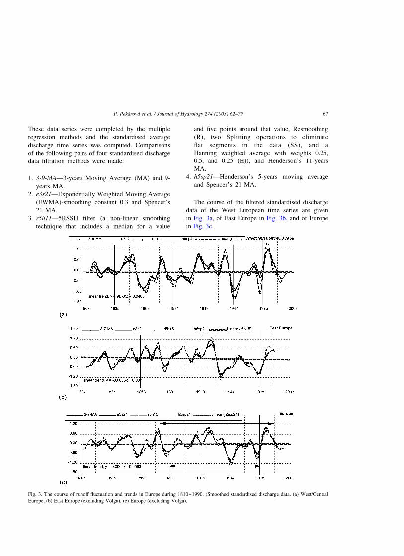
These data series were completed by the multiple

regression methods and the standardised average

discharge time series was computed. Comparisons

of the following pairs of four standardised discharge

data filtration methods were made:

1. 3-9-MA—3-years Moving Average (MA) and 9-

years MA.

2. e3s21—Exponentially Weighted Moving Average

(EWMA)-smoothing constant 0.3 and Spencer’s

21 MA.

3. r5h11—5RSSH filter (a non-linear smoothing

technique that includes a median for a value

and five points around that value, Resmoothing

(R), two Splitting operations to eliminate

flat segments in the data (SS), and a

Hanning weighted average with weights 0.25,

0.5, and 0.25 (H)), and Henderson’s 11-years

MA.

4. h5sp21—Henderson’s 5-years moving average

and Spencer’s 21 MA.

The course of the filtered standardised discharge

data of the West European time series are given

in Fig. 3a, of East Europe in Fig. 3b, and of Europe

in Fig. 3c.

Fig. 3. The course of runoff fluctuation and trends in Europe during 1810–1990. (Smoothed standardised discharge data. (a) West/Central

Europe, (b) East Europe (excluding Volga), (c) Europe (excluding Volga).


If we want to identify any trend uninfluenced by

the 28-year periodicity (this periodicity will be shown

later in the paper) of the discharge time series, we

must determine the trend during a closed multiple

loop, starting and terminating by either minima (e.g.

1861–1946 in Central Europe) or maxima (e.g.

1847–1930 or 1931–1984 in Central Europe). Trends

determined for other periods are influenced by

the periodicity of the series and depend on the

position of the starting point on the increasing or

recession curve.

The trend analysis does not show any significant

trend change in long-term discharge series (1810–

1990) in representative European rivers (Fig. 3a).

Nevertheless, it is possible to identify multiannual

cycles of wet and dry periods. The dry period

occurred in Europe around 1835 and the years

1857–1862 were very dry. In the 20th century the

period 1946–1948 was very dry. Another dry period

occurred in 1975. If we consider the 28-year cycle,

described in next sections, we can expect the next

dry period in Central Europe to occur in next years

(around 2003).

The largest rivers in the Central Europe are Rhine

and Danube. Both rivers are highly influenced by the

Alps and their long-term variability of runoff is very

similar (Fig. 2). The north–eastern European rivers,

e.g. Neman, Neva, Pechora, Northern Dvina, as well

as south–eastern European rivers Dnieper, Don, Ural

and Volga show very similar occurrence of the dry

periods. The Neva river drains the large Finnish and

Russian lake basins (Arpe et al., 2000). The big lake

rivers are very suitable for the identification of the

long-term-multiannual cycles, as the lakes eliminate

and smooth the annual variability of the dry and wet

years.

2.2.2. Northern Asia

The regular decrease and increase of discharge

is observed in the large rivers of Russia–Siberia

(Ob, Yenisei, Lena, Kolyma). Systematic obser-

vation of discharge of these rivers started only after

1930. The length of these series is sufficient for

identification of the 14-year cycle (Lukjanetz and

Sossedko, 1998), only. However, the 28-year cycle

can be found in the Amur river.

In these rivers the maximum and minimum

values do not occur in the same years (see Fig. 2),

e.g. a local maximum occurred in 1972 on Ob, in

1975 on Yenisei, and in 1980 on Kolyma. The time

shift (delay) of the extremes in eastward direction

will be analysed by cross-correlation in the next

paragraph.

2.2.3. North America

The annual discharge data series of the largest

rivers were used for the identification of the cycles

(Mississippi, St Lawrence, Mackenzie, Yukon, and

Columbia, see Fig. 2). The St Lawrence River,

similar to Neva in Russia, drains a large lake

district.

Unlike Europe, where it was very dry, the years

1945–1949 were wet in North America. The runoff

extremes in Europe and in the North America do not

occur in the same years. A prevailing wet period in

Europe corresponds to a dry period in the North

America. This hypothesis will be analysed by cross-

correlation in next sections.

2.2.4. South America

Discharge series of three large rivers of the South

America are in Fig. 2 (Amazon, Magdalena, La Plata).

It is interesting that the series of Magdalena (Northern

Hemisphere) create a mirror image of the La Plata

series (Southern Hemisphere).

The discharge measurements of the world’s largest

river Amazon were unsound in the past. The available

data series are ambiguous before 1950 and different

values are published in different databases (e.g.

GRDC or Shiklomanov 2000). If we compare

Amazon’s data to those of another large Equatorial

river, Congo in Africa, we can observe a shift of

several years in the extremes occurrence.

2.2.5. Africa

The alternating of the dry and wet periods is much

stronger in African rivers compared to European ones.

Whereas the time series of rivers in the Northern

Hemisphere require smoothing by moving averages in

order to identify the long-term discharge oscillations,

the African rivers show the oscillations without

smoothing.

The African rivers with relatively long discharge

series are Niger, Congo (Fig. 2), White and Blue

Nile (about 90 years). The length of the series is

sufficient to prove the 14-years cycles only, but not


longer ones. Unfortunately, no long discharge series

are available in the South Africa.

The African rivers north of the Equator (Niger,

Chari, Ubangi) have dry periods in the same years

as the central European rivers, while the rivers

southern of the Equator (Zambezi, Shire) have a

reverse occurrence of the extremes. The Congo

River is influenced by its tributaries from the

Northern Hemisphere (Ubangi) as well as from

the Southern Hemisphere (Kasai, Lualaba). From

the long-term point of view the runoff of Congo

is similar to the runoff of the White Nile, which

drains the Victoria Lake situated exactly on the

Equator.

2.2.6. South–eastern Asia and Australia

Cluis (1998) analysed trends of the Pacific and

Asia rivers. According to his analysis the runoff

decreased or remained stable between the Equator

and 408N at the end of the last century. In

Australia the runoff did not change after elimin-

ation of the cyclic component.

The longest discharge data series in south–eastern

Asia are those of Yangzi. The data show a regular 14-

year cycle.

The Ganges (Ganges – Brahmaputra – Meghna)

river is characterised by the steadiest runoff, and the

coefficient of variation of the annual discharge is only

0.03. The mean annual discharge varies between 41

000 and 45 000 m3 s21 except 1957 (38 221 m3 s21)

and 1974 (51 169 m3 s21). The long-term runoff is

relatively constant.

Unlike Ganges the Australian rivers exhibit a clear

periodicity and variability. The coefficient of varia-

bility of Darling discharge series is up to 1.36 (the

minimum and maximum annual discharge was 5 and

856 m3 s21, respectively). Cluis (1998) related the

variability of runoff to El Nino and La Nina episodes.

Similar to South America and Africa, the occur-

rence of wet periods northern of the Equator in south–

eastern Asia and Australia seems to go along with dry

periods southern of the Equator (see Murray and

Yangzi in Fig. 2).

2.3. Identification of the long-term periodicity

It is possible to identify the cyclicity or

randomness in the time series by auto-correlation

and periodogram. Both methods were used to

look for the long-term cycles of runoff

decrease and increase in the analysed runoff time

series.

2.3.1. Brief overview of the spectral analysis

of random processes

The spectral analysis is used to examine the

periodical properties of random processes {xi}ni¼1:

The spectral analysis generalises a classical harmo-

nic analysis by introducing the mean value in time,

of the periodogram obtained from the individual

realisations (Nachazel 1978). The fundamental

statistical characteristic of a spectral analysis is

its spectral density.

The basic tool in estimating the spectral density

is the periodogram (Venables and Ripley, 1999;

Stulajter, 2001). A periodogram (a line spectrum)

is a plot of frequency and ordinate pairs for a

specific time period. This graph breaks a time

series into a set of sine waves of various

frequencies. It is used to construct a frequency

spectrum. If the periodogram contains one spike,

the data may not be random. The spectral density

is defined as a mean value of the set of

periodogram for n ! 1.

The periodogram is calculated according to:

IðliÞ¼1

2pn

Xn

t¼1

xte2itlj

��2

¼1

2pn

Xn

t¼1

xt·sinðt·ljÞ

!2

þXn

t¼1

xt·cosðt·ljÞ

!2( ):

ð2Þ

We compute the squared correlation between the

series and the sine/cosine waves of frequency lj: By

the symmetry IðljÞ¼Ið2ljÞ we need only to consider

IðljÞ on 0#lj#ðp:

For real centred series the periodogram IðljÞ can be

estimated by auto-covariance function as

IðljÞ ¼1

2p· R0 þ 2

Xn21

t¼1

Rt·cosðt·ljÞ

!; ð3Þ


for Fourier frequencies:

lj0 ¼2p·j

n; where j ¼ 1;

n

2

� �ð4Þ

2.3.2. Combined periodogram method

It is clear that from the relationship Eq. (4) it

follows that for low frequencies, i.e. for long

periods, we compute the periodogram with a sparse

step. For example, if a time series is 100 years

long, the periodogram is only computed for periods

of 100/2 ¼ 50 years, 100/3 ¼ 33.3 years, 100/

4 ¼ 25 years, etc. If the real period is of 29

years, then we do not get the correct period. This is

why it is necessary to pay the maximum attention

to the analysis and not to rely only on results

provided by mathematical tests without the appro-

priate analysis.

One way how to reveal the real period is decreasing

the length of the measured series, i.e. computing the

periodogram for different ‘random’ selections of

the series followed by computing the average value

of the periodogram. The result of this process we will

name as combined periodogram. In order to obtain

such a combined periodogram a code PERIOD was

written. This program computes periodogram for

series successively shortened by two years (Pekarova,

2002).

2.3.3. Results

Neva and St. Lawrence rivers are very suitable for

study of the long-term runoff oscillations, because the

variability is smoothed by the great water accumu-

lation in the lakes they drain.

As an example, there are the auto-correlations and

periodograms of St. Lawrence (North America), Neva

(Europe), Amur, Yangzi (both Asia), and Congo

(Africa) in Fig. 4. There were used raw data.

The auto-correlation and periodogram of St

Lawrence River show very marked 30-year period-

icity of runoff increase and decrease. In Amur time

series there is the 28-year period combined with the

14-year period. In Rhine, Yenisei, Lena, Yangzi,

Congo, and Amazon time series the 14- and 7-years

periods are more evident. We must realise that the 28-

year period could not be identified due to short time

series.

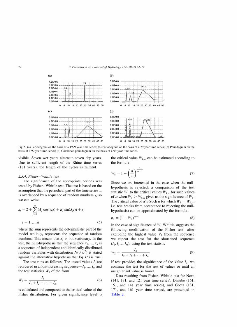
Hydrological time series are of maximum length of

200 years. Using periodograms in order to identify the

significant periods can lead to important errors. This is

why a new, above described, method of combined

periodogram was used.

To illustrate the proposed method we analysed an

artificial series of the length of 1999 members

(years) that was created as a cosine combination of

three periods 29, 11, and 6.4 years. If we analyse

this series in the ordinary way (1999 members), we

get a periodogram as it is shown in Fig. 5a Here,

all three periods are clearly identified. The length of

the series of 1999 members is sufficient for

exact identification of long-term 30–50 years

periods.

If we draw a periodogram on the basis of a 79 year

time series (in the case we have only a 79 year series

of observations), among the long periods we get a

significant period of 26.3-year (see Fig. 5b). On the

other hand, if we draw a periodogram on the basis of a

99 year time series (in the case we have a 99 year

series of observations), among the long periods we get

a significant period of 33 years (see Fig. 5c). Hence,

the difference in the long period identification is

significant.

The combined periodogram method sufficiently

thickens the spectrum. In the spectrum a 28–30 years

spike, which at best corresponds to the reality, gets

distinct (Fig. 5d).

In Fig. 6 you can see combined periodograms of

such sixteen rivers from different continents that

have the longest discharge time series. For these

rivers the cycles of about 3.6–4; 6–7; 11; 14; 20–

22; and 26–30 years were identified. The longest

cycle of about 26–30 years was found for Neva,

Goeta, Danube, Amur, La Plata rivers. In the data

of Yangzi, Rhine, Vltava, Ural, Mississippi, Congo,

and Amazon an about 14 years cycle dominates.

For these river another 7 years cycle can be

identified. Another significant cycle of 20–22-years

can be found for Murray, Zambezi, Vltava (CZ),

Danube, Dniepr, and St Lawrence.

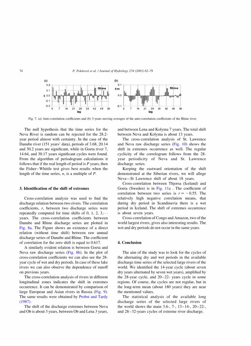
The auto-correlation analysis leads to similar

results; see the auto-correlation of Rhine River raw

discharge series in Fig. 7a. Here, it is difficult to

identify the 14-years period. But if we plot the 3-

years moving averages of the auto-correlation

coefficients (Fig. 7b), the 14-years period becomes


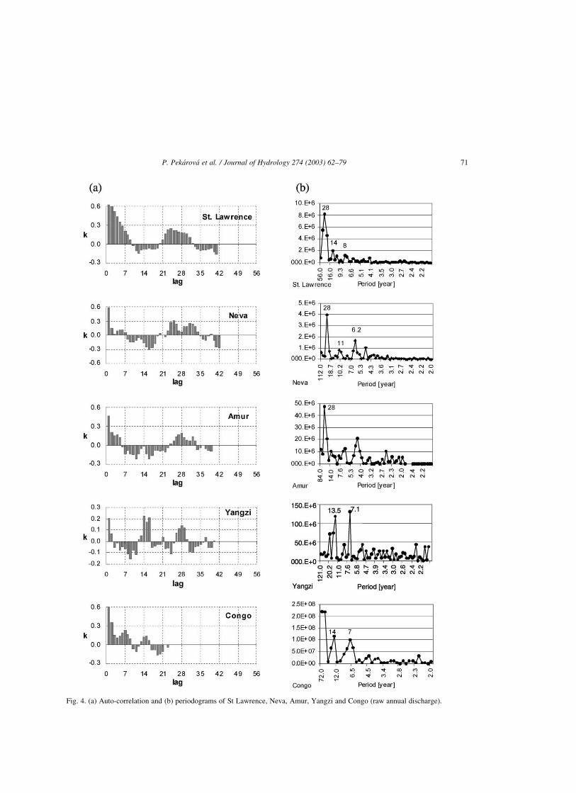
Fig. 4. (a) Auto-correlation and (b) periodograms of St Lawrence, Neva, Amur, Yangzi and Congo (raw annual discharge).


visible. Seven wet years alternate seven dry years.

Due to sufficient length of the Rhine time series

(181 years), the length of the cycles is faithful.

2.3.4. Fisher–Whittle test

The significance of the appropriate periods was

tested by Fisher–Whittle test. The test is based on the

assumption that the periodical part of the time series xt

is overlapped by a sequence of random numbers yt so

we can write

xt ¼ �x þXmj¼1

ðAj cosðljtÞ þ Bj sinðljtÞÞ þ yt

t ¼ 1;…; n ð5Þ

where the sum represents the deterministic part of the

model while yt represents the sequence of random

numbers. This means that xt is not stationary. In the

test, the null-hypothesis that the sequence x1;…; xn is

a sequence of independent and identically distributed

random variables with distribution Nð0;s2Þ is stated

against the alternative hypothesis that Eq. (5) is true.

The test runs as follows: The tested values Ij are

reordered in a non-increasing sequence—I1;…; Im and

the test statistics W1 of the form

W1 ¼I1

I1 þ I2 þ · · · þ Im

ð6Þ

is calculated and compared to the critical value of the

Fisher distribution. For given significance level a

the critical value Wk;a can be estimated according to

the formula

Wk ¼ 1 2a

m

1m21

ð7Þ

Since we are interested in the case when the null-

hypothesis is rejected, a comparison of the test

statistic W1 to the critical values Wk;a for such values

of a when W1 . Wk;a gives us the significance of W1:

The critical value of a’s (such a for which W1 ¼ Wk;a;

i.e. test breaks from acceptance to rejecting the null-

hypothesis) can be approximated by the formula

p0 ¼ ð1 2 W1Þm21 ð8Þ

In the case of significance of W1 Whittle suggests the

following modification of the Fisher test: after

excluding the highest value V1 from the sequence

we repeat the test for the shortened sequence

ðI2; I3;…ImÞ; using the test statistic

W2 ¼I2

I2 þ I3 þ · · · þ Im

ð9Þ

If test provides the significance of the value I2; we

continue the test for the rest of values or until an

insignificant value is found.

Data resulting from Fisher–Whittle test for Neva

(141, 131, and 121 year time series), Danube (161,

151, and 141 year time series), and Goeta (181,

171, and 161 year time series), are presented in

Table 2.

Fig. 5. (a) Periodogram on the basis of a 1999 year time series; (b) Periodogram on the basis of a 79 year time series; (c) Periodogram on the

basis of a 99 year time series; (d) Combined periodogram on the basis of a 99 year time series.


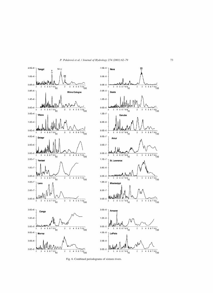
Fig. 6. Combined periodograms of sixteen rivers.


The null hypothesis that the time series for the

Neva River is random can be rejected for the 28.2-

year period almost with certainty. In the case of the

Danube river (151 years’ data), periods of 3.68, 20.14

and 30.2 years are significant, while in Goeta river 7,

14.64, and 30.17 years significant cycles were found.

From the algorithm of periodogram calculations it

follows that if the real length of period is P years, then

the Fisher–Whittle test gives best results when the

length of the time series, n, is a multiple of P.

3. Identification of the shift of extremes

Cross-correlation analysis was used to find the

discharge relation between two rivers. The correlation

coefficients, r, between two discharge series were

repeatedly computed for time shifts of 0, 1, 2, 3,· · ·

years. The cross-correlation coefficients between

Danube and Rhine discharge series are plotted in

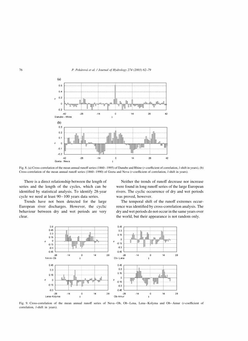
Fig. 8a. The Figure shows an existence of a direct

relation (without time shift) between raw annual

discharge series of Danube and Rhine. The coefficient

of correlation for the zero shift is equal to 0.617.

A similarly evident relation is between Goeta and

Neva raw discharge series (Fig. 8b). In the plot of

cross-correlation coefficients we can also see the 28-

year cycle of wet and dry periods. In case of these lake

rivers we can also observe the dependence of runoff

on previous years.

The cross-correlation analysis of rivers in different

longitudinal zones indicates the shift in extremes

occurrence. It can be demonstrated by comparison of

large European and Asian rivers in Russia (Fig. 9).

The same results were obtained by Probst and Tardy

(1987).

The shift of the discharge extremes between Neva

and Ob is about 3 years, between Ob and Lena 3 years,

and between Lena and Kolyma 7 years. The total shift

between Neva and Kolyma is about 13 years.

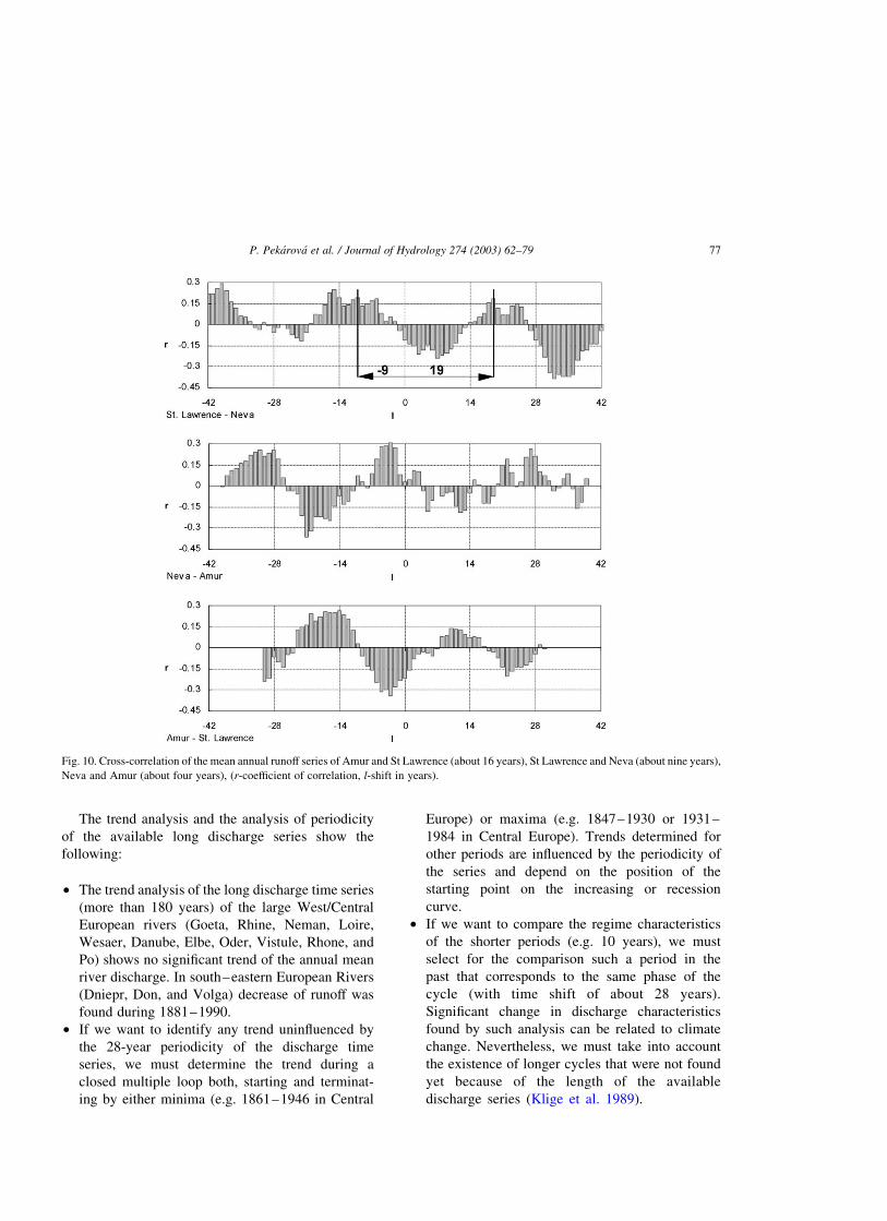
The cross-correlation analysis of St. Lawrence

and Neva raw discharge series (Fig. 10) shows the

shift in extremes occurrence as well. The regular

cyclicity of the correlogram follows from the 28-

year periodicity of Neva and St. Lawrence

discharge series.

Keeping the eastward orientation of the shift

demonstrated at the Siberian rivers, we will allege

Neva—St Lawrence shift of about 18 years.

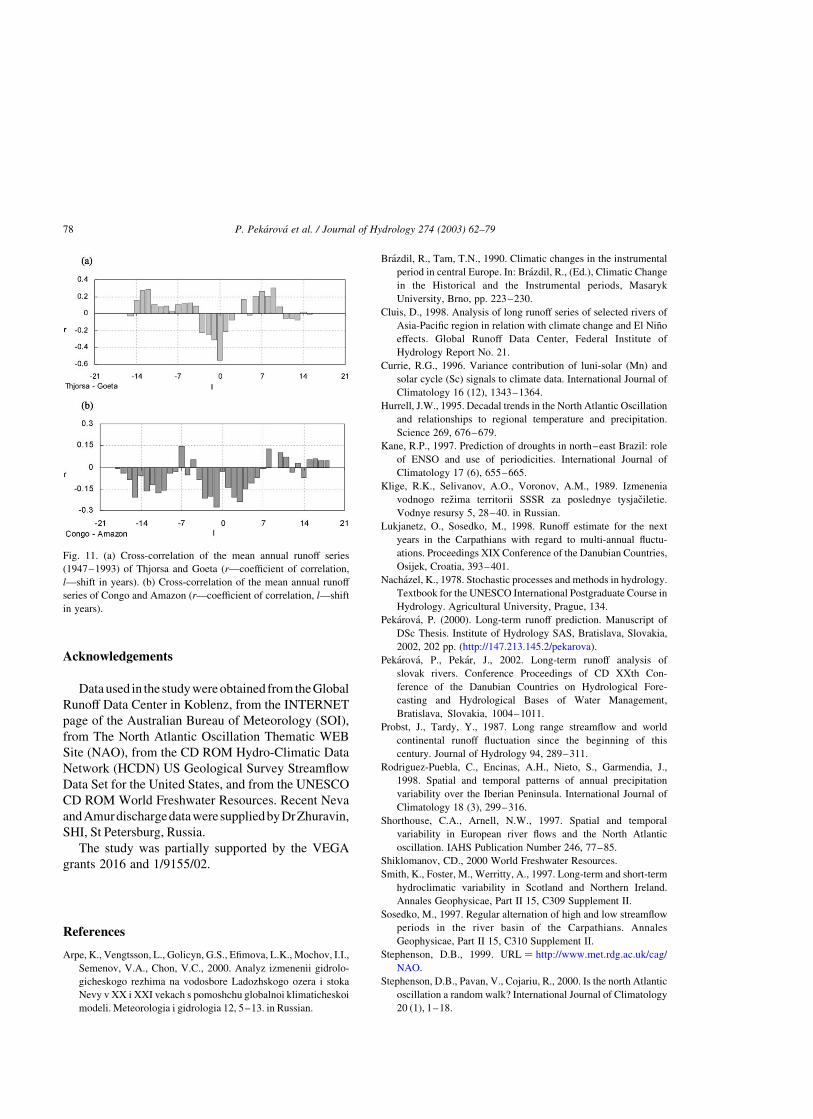
Cross-correlation between Thjorsa (Iceland) and

Goeta (Sweden) is in Fig. 11a . The coefficient of

correlation between two series is r ¼ 20.55. The

relatively high negative correlation means, that

during dry period in Scandinavia there is a wet

period in Iceland. The shift of extremes occurrence

is about seven years.

Cross-correlation of Congo and Amazon, two of the

world largest rivers, gives also interesting results. The

wet and dry periods do not occur in the same years.

4. Conclusion

The aim of the study was to look for the cycles of

the alternating dry and wet periods in the available

discharge time series of the selected large rivers of the

world. We identified the 14-year cycle (about seven

dry years alternated by seven wet years), amplified by

the 28-year cycle, and 20–22- years cycle in some

regions. Of course, the cycles are not regular, but in

the long-term mean (about 180 years) they are near

the mentioned values.

The statistical analysis of the available long

discharge series of the selected large rivers of

the world shows the main 3.6-, 7-, 13–14-, 20–22-,

and 28–32-years cycles of extreme river discharge.

Fig. 7. (a) Auto-correlation coefficients and (b) 3-years moving averages of the auto-correlation coefficients of the Rhine river.


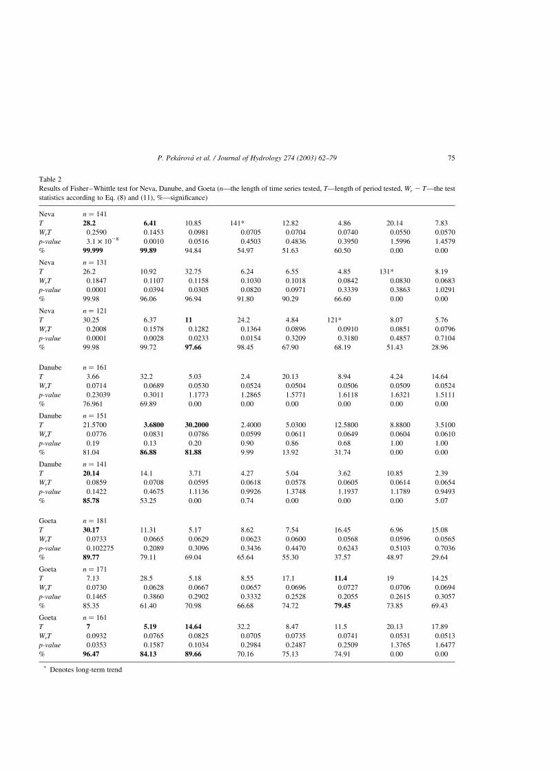
Table 2

Results of Fisher–Whittle test for Neva, Danube, and Goeta (n—the length of time series tested, T—length of period tested, Wr 2 T—the test

statistics according to Eq. (8) and (11), %—significance)

Neva n ¼ 141

T 28.2 6.41 10.85 141* 12.82 4.86 20.14 7.83

WrT 0.2590 0.1453 0.0981 0.0705 0.0704 0.0740 0.0550 0.0570

p-value 3.1 £ 1028 0.0010 0.0516 0.4503 0.4836 0.3950 1.5996 1.4579

% 99.999 99.89 94.84 54.97 51.63 60.50 0.00 0.00

Neva n ¼ 131

T 26.2 10.92 32.75 6.24 6.55 4.85 131* 8.19

WrT 0.1847 0.1107 0.1158 0.1030 0.1018 0.0842 0.0830 0.0683

p-value 0.0001 0.0394 0.0305 0.0820 0.0971 0.3339 0.3863 1.0291

% 99.98 96.06 96.94 91.80 90.29 66.60 0.00 0.00

Neva n ¼ 121

T 30.25 6.37 11 24.2 4.84 121* 8.07 5.76

WrT 0.2008 0.1578 0.1282 0.1364 0.0896 0.0910 0.0851 0.0796

p-value 0.0001 0.0028 0.0233 0.0154 0.3209 0.3180 0.4857 0.7104

% 99.98 99.72 97.66 98.45 67.90 68.19 51.43 28.96

Danube n ¼ 161

T 3.66 32.2 5.03 2.4 20.13 8.94 4.24 14.64

WrT 0.0714 0.0689 0.0530 0.0524 0.0504 0.0506 0.0509 0.0524

p-value 0.23039 0.3011 1.1773 1.2865 1.5771 1.6118 1.6321 1.5111

% 76.961 69.89 0.00 0.00 0.00 0.00 0.00 0.00

Danube n ¼ 151

T 21.5700 3.6800 30.2000 2.4000 5.0300 12.5800 8.8800 3.5100

WrT 0.0776 0.0831 0.0786 0.0599 0.0611 0.0649 0.0604 0.0610

p-value 0.19 0.13 0.20 0.90 0.86 0.68 1.00 1.00

% 81.04 86.88 81.88 9.99 13.92 31.74 0.00 0.00

Danube n ¼ 141

T 20.14 14.1 3.71 4.27 5.04 3.62 10.85 2.39

WrT 0.0859 0.0708 0.0595 0.0618 0.0578 0.0605 0.0614 0.0654

p-value 0.1422 0.4675 1.1136 0.9926 1.3748 1.1937 1.1789 0.9493

% 85.78 53.25 0.00 0.74 0.00 0.00 0.00 5.07

Goeta n ¼ 181

T 30.17 11.31 5.17 8.62 7.54 16.45 6.96 15.08

WrT 0.0733 0.0665 0.0629 0.0623 0.0600 0.0568 0.0596 0.0565

p-value 0.102275 0.2089 0.3096 0.3436 0.4470 0.6243 0.5103 0.7036

% 89.77 79.11 69.04 65.64 55.30 37.57 48.97 29.64

Goeta n ¼ 171

T 7.13 28.5 5.18 8.55 17.1 11.4 19 14.25

WrT 0.0730 0.0628 0.0667 0.0657 0.0696 0.0727 0.0706 0.0694

p-value 0.1465 0.3860 0.2902 0.3332 0.2528 0.2055 0.2615 0.3057

% 85.35 61.40 70.98 66.68 74.72 79.45 73.85 69.43

Goeta n ¼ 161

T 7 5.19 14.64 32.2 8.47 11.5 20.13 17.89

WrT 0.0932 0.0765 0.0825 0.0705 0.0735 0.0741 0.0531 0.0513

p-value 0.0353 0.1587 0.1034 0.2984 0.2487 0.2509 1.3765 1.6477

% 96.47 84.13 89.66 70.16 75.13 74.91 0.00 0.00

p Denotes long-term trend


There is a direct relationship between the length of

series and the length of the cycles, which can be

identified by statistical analysis. To identify 28-year

cycle we need at least 90–100 years data series.

Trends have not been detected for the large

European river discharges. However, the cyclic

behaviour between dry and wet periods are very

clear.

Neither the trends of runoff decrease nor increase

were found in long runoff series of the large European

rivers. The cyclic occurrence of dry and wet periods

was proved, however.

The temporal shift of the runoff extremes occur-

rence was identified by cross-correlation analysis. The

dry and wet periods do not occur in the same years over

the world, but their appearance is not random only.

Fig. 9. Cross-correlation of the mean annual runoff series of Neva–Ob, Ob–Lena, Lena–Kolyma and Ob–Amur (r-coefficient of

correlation, l-shift in years).

Fig. 8. (a) Cross-correlation of the mean annual runoff series (1860–1995) of Danube and Rhine (r-coefficient of correlation, l-shift in years), (b)

Cross-correlation of the mean annual runoff series (1860–1990) of Goeta and Neva (r-coefficient of correlation, l-shift in years).


The trend analysis and the analysis of periodicity

of the available long discharge series show the

following:

† The trend analysis of the long discharge time series

(more than 180 years) of the large West/Central

European rivers (Goeta, Rhine, Neman, Loire,

Wesaer, Danube, Elbe, Oder, Vistule, Rhone, and

Po) shows no significant trend of the annual mean

river discharge. In south–eastern European Rivers

(Dniepr, Don, and Volga) decrease of runoff was

found during 1881–1990.

† If we want to identify any trend uninfluenced by

the 28-year periodicity of the discharge time

series, we must determine the trend during a

closed multiple loop both, starting and terminat-

ing by either minima (e.g. 1861–1946 in Central

Europe) or maxima (e.g. 1847–1930 or 1931–

1984 in Central Europe). Trends determined for

other periods are influenced by the periodicity of

the series and depend on the position of the

starting point on the increasing or recession

curve.

† If we want to compare the regime characteristics

of the shorter periods (e.g. 10 years), we must

select for the comparison such a period in the

past that corresponds to the same phase of the

cycle (with time shift of about 28 years).

Significant change in discharge characteristics

found by such analysis can be related to climate

change. Nevertheless, we must take into account

the existence of longer cycles that were not found

yet because of the length of the available

discharge series (Klige et al. 1989).

Fig. 10. Cross-correlation of the mean annual runoff series of Amur and St Lawrence (about 16 years), St Lawrence and Neva (about nine years),

Neva and Amur (about four years), (r-coefficient of correlation, l-shift in years).


Acknowledgements

Data used in the study were obtained from the Global

Runoff Data Center in Koblenz, from the INTERNET

page of the Australian Bureau of Meteorology (SOI),

from The North Atlantic Oscillation Thematic WEB

Site (NAO), from the CD ROM Hydro-Climatic Data

Network (HCDN) US Geological Survey Streamflow

Data Set for the United States, and from the UNESCO

CD ROM World Freshwater Resources. Recent Neva

andAmurdischargedataweresuppliedbyDrZhuravin,

SHI, St Petersburg, Russia.

The study was partially supported by the VEGA

grants 2016 and 1/9155/02.

References

Arpe, K., Vengtsson, L., Golicyn, G.S., Efimova, L.K., Mochov, I.I.,

Semenov, V.A., Chon, V.C., 2000. Analyz izmenenii gidrolo-

gicheskogo rezhima na vodosbore Ladozhskogo ozera i stoka

Nevy v XX i XXI vekach s pomoshchu globalnoi klimaticheskoi

modeli. Meteorologia i gidrologia 12, 5–13. in Russian.

Brazdil, R., Tam, T.N., 1990. Climatic changes in the instrumental

period in central Europe. In: Brazdil, R., (Ed.), Climatic Change

in the Historical and the Instrumental periods, Masaryk

University, Brno, pp. 223–230.

Cluis, D., 1998. Analysis of long runoff series of selected rivers of

Asia-Pacific region in relation with climate change and El Nino

effects. Global Runoff Data Center, Federal Institute of

Hydrology Report No. 21.

Currie, R.G., 1996. Variance contribution of luni-solar (Mn) and

solar cycle (Sc) signals to climate data. International Journal of

Climatology 16 (12), 1343–1364.

Hurrell, J.W., 1995. Decadal trends in the North Atlantic Oscillation

and relationships to regional temperature and precipitation.

Science 269, 676–679.

Kane, R.P., 1997. Prediction of droughts in north–east Brazil: role

of ENSO and use of periodicities. International Journal of

Climatology 17 (6), 655–665.

Klige, R.K., Selivanov, A.O., Voronov, A.M., 1989. Izmenenia

vodnogo rezima territorii SSSR za poslednye tysjaciletie.

Vodnye resursy 5, 28–40. in Russian.

Lukjanetz, O., Sosedko, M., 1998. Runoff estimate for the next

years in the Carpathians with regard to multi-annual fluctu-

ations. Proceedings XIX Conference of the Danubian Countries,

Osijek, Croatia, 393–401.

Nachazel, K., 1978. Stochastic processes and methods in hydrology.

Textbook for the UNESCO International Postgraduate Course in

Hydrology. Agricultural University, Prague, 134.

Pekarova, P. (2000). Long-term runoff prediction. Manuscript of

DSc Thesis. Institute of Hydrology SAS, Bratislava, Slovakia,

2002, 202 pp. (http://147.213.145.2/pekarova).

Pekarova, P., Pekar, J., 2002. Long-term runoff analysis of

slovak rivers. Conference Proceedings of CD XXth Con-

ference of the Danubian Countries on Hydrological Fore-

casting and Hydrological Bases of Water Management,

Bratislava, Slovakia, 1004–1011.

Probst, J., Tardy, Y., 1987. Long range streamflow and world

continental runoff fluctuation since the beginning of this

century. Journal of Hydrology 94, 289–311.

Rodriguez-Puebla, C., Encinas, A.H., Nieto, S., Garmendia, J.,

1998. Spatial and temporal patterns of annual precipitation

variability over the Iberian Peninsula. International Journal of

Climatology 18 (3), 299–316.

Shorthouse, C.A., Arnell, N.W., 1997. Spatial and temporal

variability in European river flows and the North Atlantic

oscillation. IAHS Publication Number 246, 77–85.

Shiklomanov, CD., 2000 World Freshwater Resources.

Smith, K., Foster, M., Werritty, A., 1997. Long-term and short-term

hydroclimatic variability in Scotland and Northern Ireland.

Annales Geophysicae, Part II 15, C309 Supplement II.

Sosedko, M., 1997. Regular alternation of high and low streamflow

periods in the river basin of the Carpathians. Annales

Geophysicae, Part II 15, C310 Supplement II.

Stephenson, D.B., 1999. URL ¼ http://www.met.rdg.ac.uk/cag/

NAO.

Stephenson, D.B., Pavan, V., Cojariu, R., 2000. Is the north Atlantic

oscillation a random walk? International Journal of Climatology

20 (1), 1–18.

Fig. 11. (a) Cross-correlation of the mean annual runoff series

(1947–1993) of Thjorsa and Goeta (r—coefficient of correlation,

l—shift in years). (b) Cross-correlation of the mean annual runoff

series of Congo and Amazon (r—coefficient of correlation, l—shift

in years).


http://147.213.145.2/pekarova

http://www.met.rdg.ac.uk/cag/NAO

http://www.met.rdg.ac.uk/cag/NAO

Stulajter, F., 2001. Random Processes and Time Series. FMFI, UK

Bratislava, 212.

Svoboda, A., Pekarova, P., Miklanek, P., 2000. Flood hydrology of

Danube between Devın and Nagymaros. Institute of Hydrology

and Slovak Committee for Hydrology, Bratislava.

Venables, W.N., Ripley, B.D., 1999. Modern Applied Statistics

with S-Plus, Springer Edition, New York.

Walanaus, A., Soja, R., 1995. The 3.5 yr period in river runoff—is it

random fluctuation? Proceedings Hydrological Processes in the

Catchment, Cracow, Poland, 141–148.

Williams, G.R., 1961. Cyclical variations in the world-wide

hydrological data. Journal of Hydraulic division 6, 71–88.

Yang, M., Yao, T., He, Y., Thompson, L.G., 2000. ENSO events

recorded in the Guliya ice core. Climatic Change 47, 401–409.


Spatial and temporal runoff oscillation analysis of the main rivers of ...

Documents