The Spatial and Temporal Distributions of U.S. Winds and Windpower at 80 m Derived from Measurements Cristina L. Archer and Mark Z. Jacobson Department of Civil and Environmental Engineering, Stanford University, Stanford, CA Submitted to Journal of Geophysical Research, Atmospheres, January 9, 2002, Revised December 14, 2002. Abstract. This is a study to quantify U.S. wind power at 80 m (the hub height of large wind turbines) and to investigate whether winds from a network of farms can provide a steady and reliable source of electric power. Data from 1327 surface stations and 87 soundings in the U.S. for the year 2000 were used. Several methods were tested to extrapolate 10-m wind measurements to 80 m. The most accurate, a least-squares fit based on twice-a-day wind profiles from the soundings, resulted in 80-m wind speeds that are, on average, 1.3-1.7 m/s faster than those obtained from the most common methods previously used to obtain elevated data for U.S. windpower maps, a logarithmic law and a power law, both with constant coefficients. The results suggest that U.S. windpower at 80 m may be substantially greater than previously estimated. It was found that 24% of all stations (and 37% of all coastal/offshore stations) are characterized by mean annual speeds ≥ 6.9 m/s at 80 m, implying that the winds over possibly one quarter of the U.S. are strong enough to provide electric power at a direct cost equal to that of a new natural gas or coal power plant. The greatest previously uncharted reservoir of windpower in the continental U.S. is offshore and near shore along the southeastern and southern coasts. When multiple wind sites are considered, the number of days with no wind power and the standard deviation of the wind speed, integrated across all sites, are substantially reduced in comparison with when one wind site is considered. Therefore a network of wind farms 1

Welcome message from author
This document is posted to help you gain knowledge. Please leave a comment to let me know what you think about it! Share it to your friends and learn new things together.
Transcript
The Spatial and Temporal Distributions of U.S. Winds and Windpower at 80 m Derived from Measurements
Cristina L. Archer and Mark Z. Jacobson
Department of Civil and Environmental Engineering, Stanford University, Stanford, CA
Submitted to Journal of Geophysical Research, Atmospheres, January 9, 2002, Revised
December 14, 2002.
Abstract. This is a study to quantify U.S. wind power at 80 m (the hub height of large
wind turbines) and to investigate whether winds from a network of farms can provide a
steady and reliable source of electric power. Data from 1327 surface stations and 87
soundings in the U.S. for the year 2000 were used. Several methods were tested to
extrapolate 10-m wind measurements to 80 m. The most accurate, a least-squares fit
based on twice-a-day wind profiles from the soundings, resulted in 80-m wind speeds that
are, on average, 1.3-1.7 m/s faster than those obtained from the most common methods
previously used to obtain elevated data for U.S. windpower maps, a logarithmic law and
a power law, both with constant coefficients. The results suggest that U.S. windpower at
80 m may be substantially greater than previously estimated. It was found that 24% of all
stations (and 37% of all coastal/offshore stations) are characterized by mean annual
speeds ≥ 6.9 m/s at 80 m, implying that the winds over possibly one quarter of the U.S.
are strong enough to provide electric power at a direct cost equal to that of a new natural
gas or coal power plant. The greatest previously uncharted reservoir of windpower in the
continental U.S. is offshore and near shore along the southeastern and southern coasts.
When multiple wind sites are considered, the number of days with no wind power and the
standard deviation of the wind speed, integrated across all sites, are substantially reduced
in comparison with when one wind site is considered. Therefore a network of wind farms
1
in locations with high annual mean wind speeds may provide a reliable and abundant
source of electric power.
1 Introduction
In 1999, coal (50.8%) and natural gas (15.4%) generated about 66.2% of electric power
in the United States. Wind generated only 0.12% of electric power [Energy Information
Agency, 2001].
The direct cost of energy from a large (1.5 MW, 77-m blade) modern wind turbine in
the presence of mean annual Rayleigh-distributed winds of speed 7-7.5 m/s appears to
have decreased to 2.9-3.9 cents/kWh [Jacobson and Masters, 2001; Bolinger and Wiser,
2001]. This compares with 3.5-4 cents/kWh from a new pulverized coal-fired power plant
and 3.3-3.6 cents/kWh from a new natural gas combined cycle power plant [Office of
Fossil Energy, 2001]. The one-tail Rayleigh wind speed distribution is often used for
calculating wind speed statistics and will be discussed in detail in Section 2.4.
Coal and natural gas both emit CO2, CH4, SO2, NOx, CO, NH3, reactive organic
gases, particulate black carbon, particulate organic matter, and other particulate
components. The emissions from coal and natural gas enhance global warming,
respiratory and cardiovascular disease, air-pollution-related mortality, urban smog, acid
deposition, and visibility degradation. Coal mining also results in black-lung disease,
land-surface stripping, water pollution, and mercury emissions. Wind energy causes no
air pollution past the manufacturing and scrapping process.
Despite the relatively even direct cost of new wind turbines versus new coal and
natural gas power plants, subsidies to both, and the high health/environmental costs of
coal and natural gas versus wind, many still argue that an advantage of coal and natural
gas power plants is that they are more reliable sources of energy because winds are
intermittent. They argue that the intermittency results in two costs. The first is the cost of
2
"regulation ancillary service," which is the cost incurred when grid operators must
instantaneously switch to another power source when the first source does not produce
power temporarily. Hirst [2001] and Hudson et al. [2001] showed that this cost is
relatively trivial, 0.005 to 0.030 cents/kWh (< 1 % the direct cost of wind energy), when
wind is a small fraction of the total energy supply. The second is the cost of maintaining
and using backup (contingency) reserves (usually in the form of "peaker" fossil-fuel
power plants) when wind is a large fraction (e.g., 30%) of the total energy supply and
wind's output is low for a given hour.
The real issue in the second case is not the intermittency cost to wind, if any, but the
difference between the intermittency cost to wind and that to coal or natural gas. Coal and
natural gas have their own intermittency problems. For example, the forced outage rate of
fossil-fuel power plants is about 8 % [North American Electric Reliability Council, 2000],
whereas the forced plus unforced outage rate of modern turbines is about 2 % [Danish
Windturbine Manufacturers Assoc., 2001]. In addition, the variation of natural gas
supplies results in monthly to yearly price fluctuations of electric power of 50-100%
[McFeat, 2001].
In addition, even though contingency reserves may be required for wind, they do not
always need to result in an extra cost. For example, one source of contingency reserves is
hydroelectric power, which supplies about 10 % of the electric power in the United States
(mostly in California, Oregon, and Washington). This source does not incur a cost if its
output must be increased on short notice. Additional hydroelectric power used when wind
power is low can be balanced by less hydroelectric power used when wind power is high,
stabilizing the summed energy supplied by hydroelectric power and wind.
Finally, if wind becomes 30% of the energy supply, wind farms would be distributed
over greater areas, and grid interconnections would expand, enabling easier transmission
of excess wind, solar, hydroelectric, fossil, and nuclear energy from outside the local grid
to the local grid, thereby reducing the need for contingency reserves. Yet, the main issue
3
that has not been resolved is whether wind's instantaneous intermittency at a given
location translates into intermittency of hourly-averaged electric power, summed over
wind farms on a larger scale. If, indeed, wind can provide a stable amount of electric
power when all turbines over a large number of farms are considered, then backup
requirements and associated costs can be minimized.
For this study, wind data from the United States for the year 2000 were used to
examine whether a large network of wind farms can provide electric power more or less
reliably than a small network or a single farm. The paper also provides an analysis of the
time of peak wind production during the day, a map of the mean-annual wind speeds at
80 m at all wind measurement sites in the U.S. for the year 2000, an analysis of the
Rayleigh nature of wind speeds, and other wind-related statistics.
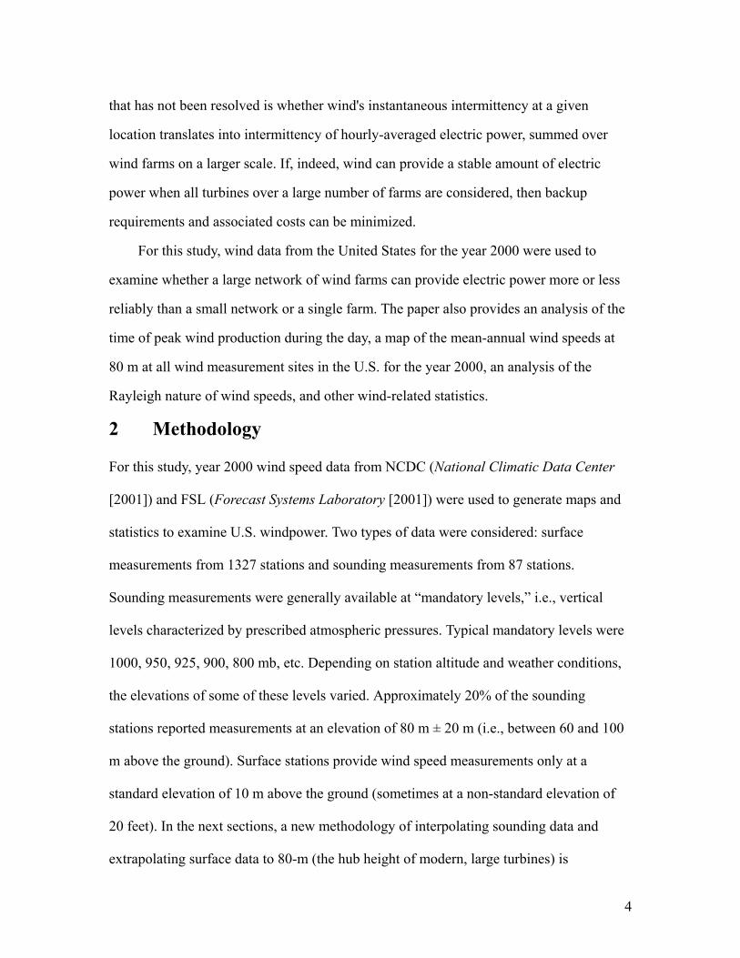
2 Methodology
For this study, year 2000 wind speed data from NCDC (National Climatic Data Center
[2001]) and FSL (Forecast Systems Laboratory [2001]) were used to generate maps and
statistics to examine U.S. windpower. Two types of data were considered: surface
measurements from 1327 stations and sounding measurements from 87 stations.
Sounding measurements were generally available at “mandatory levels,” i.e., vertical
levels characterized by prescribed atmospheric pressures. Typical mandatory levels were
1000, 950, 925, 900, 800 mb, etc. Depending on station altitude and weather conditions,
the elevations of some of these levels varied. Approximately 20% of the sounding
stations reported measurements at an elevation of 80 m ± 20 m (i.e., between 60 and 100
m above the ground). Surface stations provide wind speed measurements only at a
standard elevation of 10 m above the ground (sometimes at a non-standard elevation of
20 feet). In the next sections, a new methodology of interpolating sounding data and
extrapolating surface data to 80-m (the hub height of modern, large turbines) is
4
developed.
2.1 Methodology for 80-m wind speed determination Two approaches are commonly used to extrapolate 10-m wind speed data to 80-m. The
first one is the power-law relation [e.g., Elliott et al., 1986a; Arya, 1988],
V(z) = VRzzR
α
(1)
where V(z) is wind speed at elevation z above the topographical surface (80 m in this case,
i.e., V(80)), VR is wind speed at the reference elevation zR (10 m above the topographical
surface in the rest of this paper), and α (typically 1/7) is the friction coefficient. The
second one is the logarithmic law [e.g., Arya, 1988; Jacobson, 1999],
V(z) = VR
ln( zz0
)
ln( zR
z0
) (2)
where z0 (typically 0.01 m) is the roughness length. Note that both curves must pass
through VR (i.e., at z=zR=10 m, they return the value V(10)=VR) and they both require one
fitting parameter, either α or z0. The logarithmic law is theoretically valid for neutral
atmospheric conditions only (i.e., when vertical motions are neither inhibited nor
supported by the atmosphere). It can be obtained by similarity theory after assuming no
Coriolis effect and a flat, uniform surface [Arya, 1988]. The power law does not have a
theoretical basis, but it often provides a reasonable fit to observed vertical wind profiles
[Arya, 1988]. The advantage of these two approaches is their simplicity (only one,
constant parameter is required). However, atmospheric conditions are rarely neutral and
diurnal, seasonal or stability-dependant variations cannot be taken into account by using
one constant parameter.
5
Given these limitations, a new methodology of extrapolating wind speed above a
surface station measurement was developed. The methodology is referred to here as the
Least-Squares fitting approach (LS hereafter), and it involves three steps:
1. For each sounding station, four fitting parameters are calculated for each hour
(typically at 0000 and 1200 UTC) of each day to reproduce empirically the wind
speed variation with height at the sounding. Of the four parameters, the “best” fitting
parameter, calculated as the one giving the lowest residual (described shortly) is
saved.
2. For each surface station, the five nearest-in-space sounding stations are selected.
Then, VR from the surface station and the “best” fitting parameter from each sounding
station are used to calculate a new V(80) at each of the five sounding stations. Note
that the average distance between sounding stations in the contiguous U.S. is
approximately 300 km [Steurer, 1996].
3. Finally, V(80) at the surface station is calculated as the weighted average of the five
new V(80)s from the sounding stations, where the weighting is the inverse square of
the distance between the surface station and each sounding station.
The four fitting parameters for each hour of available data (typically twice a day) at
each sounding station were determined as follows. An equation for the residual R of the
squares of the error in wind speed was written as
[ ]∑=
−=N
iii zVVR
1
2)( , (3)
where N is a selected number of points in the bottom part of a sounding (N=3 in this
case), Vi is the wind speed observed at vertical point i in the sounding (the first vertical
point is at 10 m, i.e., z1=zR=10 m), and V(zi) is the wind speed calculated by one of
several possible equations, such as Eqs. 1 or 2. Setting the partial derivative of R with
6
respect to the fitting parameter in Eqs 1 and 2 (α and z0, respectively) to zero and solving
for the fitting parameter gives two LS fitting parameters,
α LS =ln Vi
VR
ln z i
zR
i=1
N
∑
ln zi
zR
2
i=1
N
∑ (4)
ln(z0LS) =
VR { [ln(zi)]2 − ln(zR ) ln(zi)} − ln(zR ) (Vi ln( zi
zR
)i=1
N
∑i=1
N
∑i=1
N
∑
{VR ln(zi) − [Vi ln( zi
zR
)]− NVR ln(zR )}i=1
N
∑i=1
N
∑. (5)
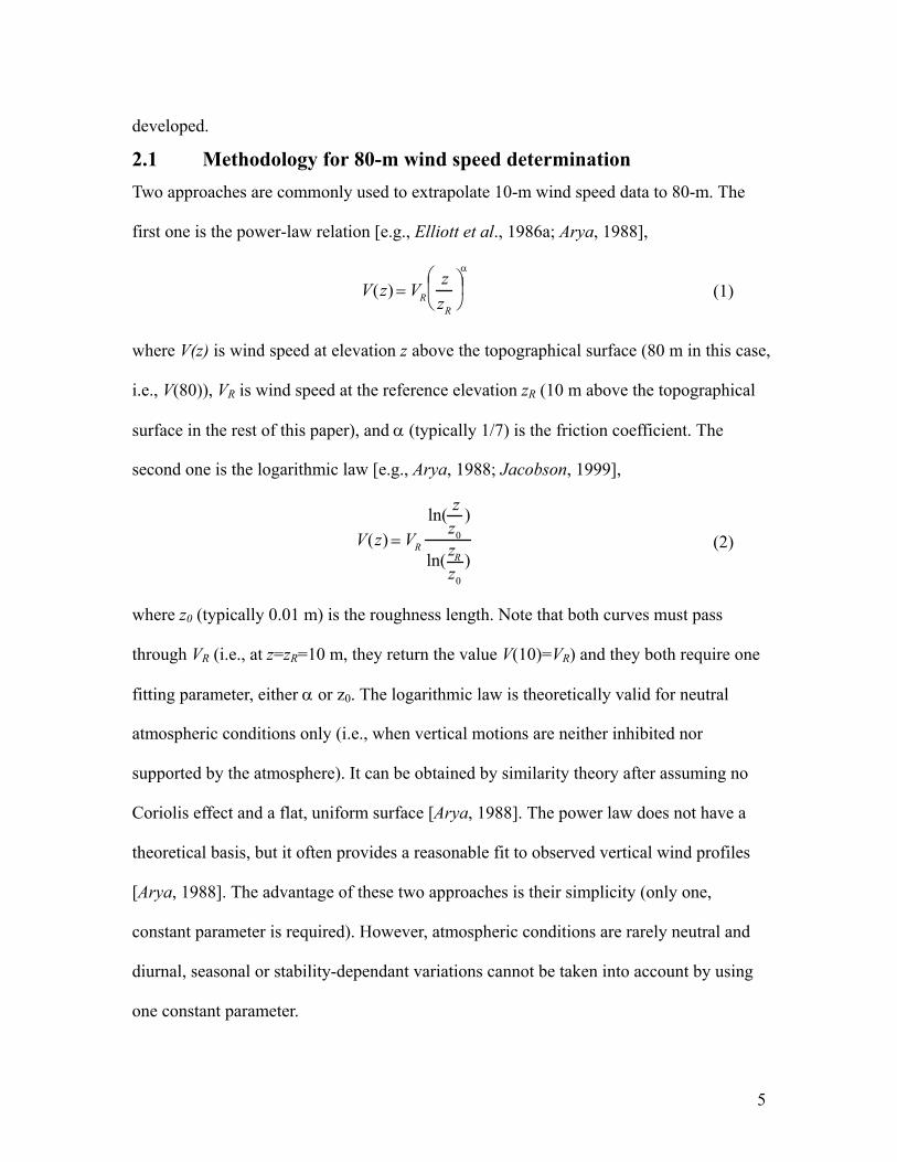
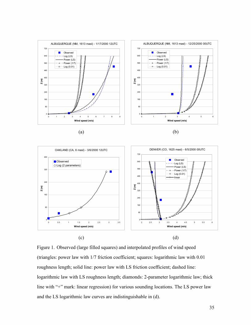
Note that α and z0, acquire different values for each observed wind profile. Figure
1a,b shows an example of curves interpolated with LS parameters obtained from Eq. 4
and Eq. 5 for N=3. For comparison, curves with α=1/7 and z0=0.01 m are plotted too. In
this study, curves with α=1/7 and z0=0.01 m underestimated the value of V(80) (as in
Figure 1a) in about 60% of the cases tested, but the opposite occurred in less than 40% of
the cases (e.g., Figure 1b). The power law with α=1/7 led to an average underestimate of
annual mean 80-m wind speed of 1.3 m/s. The logarithmic law with z0=0.01 m
underestimated the annual mean 80-m wind speed by 1.7 m/s on average. Both the power
law with α=1/7 and the logarithmic law with z0=0.01 m led to greater underestimates at
night (i.e., 1200 UTC) than during the day (i.e., 0000 UTC), averaging 2.5 and 2.8 m/s
(respectively) below the LS mean 80-m wind speed at night, and 0.1 and 0.5 m/s
(respectively) during the day.
Some unusual weather conditions cause wind speed either to decrease with height
(Figure 1d) or to be zero at 10 m (Figure 1c). For these special cases, the two remaining
7
fitting parameters were determined.
Since Eq. 1 and Eq. 2 have VR as a multiplying factor, they unrealistically predict
zero wind speed for all vertical points when VR=0. The solution is to use a two-parameter
logarithmic law of the form
)ln(* ii zBAV += , (6)
where coefficients A and B, derived by replacing Eq. 6 in Eq. 3, are
N
zBVA
zzN
zVzVNB
N
i
N
iii
N
ii
N
ii
N
i
N
iii
N
iii ∑ ∑
∑∑
∑ ∑∑= =
==
= ==
−=
−
−= 1 1
2
11
2
1 11
)ln(
)ln(])[ln(
)ln()]ln([. (7)
An example of Eq. 6 is shown in Figure 1c. Note that the fitting curve obtained with Eq.
6 is not forced to pass through VR.
If wind speed decreases with height for the lowest N points, then both the power and
logarithmic curves show a wrong concavity, due to the fact that either the LS friction
coefficient would become negative or the LS roughness length would become too large.
In this case, both the 1/7 friction coefficient curve and the 0.01 roughness length curve
overestimate V(80) substantially. A solution to this problem is to extrapolate V(80) with a
linear regression,
ii zDCV *+= , (8)
where C and D, obtained from Eq. 3 by replacing Vi with Eq. 8, are
RRN
ii
N
ii
N
i
N
iii
N
iii
zDVCzzN
zVzVND *
)(
)(
2
11
2
1 11 −=
−
−=
∑∑
∑ ∑∑
==
= == . (9)
8
Figure 1d shows an example of this fit. Note that the interpolation line is forced to pass
through VR.
In sum, the four fitting parameters calculated for each of the two soundings per day
at each sounding station were αLS from Eq. 4, z0LS from Eq. 5, A and B from Eq. 6, C and
D from Eq. 8. The “best” fitting parameter, used for Step 1 in the LS procedure, was
calculated as the one associated with the lowest residual R.
2.2 Methodology for hourly pattern determination At surface stations for which hourly data were available, it was necessary to introduce a
methodology for determining the hourly trend of V(80) given only the values calculated
at 0000 and 1200 UTC, hereafter referred to as V00(80) and V12(80), obtained with the LS
methodology described above. Depending on the time zone of the surface stations, V00(80)
and V12(80) were valid within 1500-1900 LST (Local Standard Time) and 0300-0700
LST respectively.
In general, surface (and 10-m) wind speed peaks in the early afternoon, due to the
turbulent vertical mixing of horizontal momentum from the upper levels, which is
strongest during the afternoon due to the increased thermal instability of the Planetary
Boundary Layer (PBL) [Arya 1988; Riehl 1972]. Conversely, at some upper level zrev, this
trend is reversed, as higher momentum is transferred downward to the surface in the early
afternoon by the same mechanism. The elevation of zrev depends on turbulent mixing
efficiency, atmospheric thermal stability, and PBL height. It is located at a level far
enough from the surface not to be influenced by friction but low enough to be affected by
PBL mixing. Without high resolution sounding data in the vertical and in time, though, it
is difficult to estimate exactly whether each 80-m level is above or below zrev, and
consequently whether the 80-m hourly trend would follow the surface trend or a reversed
9
pattern.
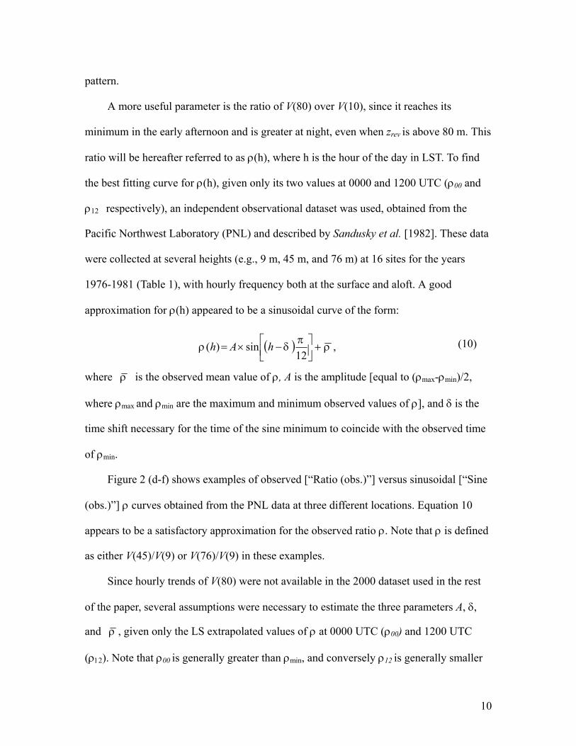
A more useful parameter is the ratio of V(80) over V(10), since it reaches its
minimum in the early afternoon and is greater at night, even when zrev is above 80 m. This
ratio will be hereafter referred to as ρ(h), where h is the hour of the day in LST. To find
the best fitting curve for ρ(h), given only its two values at 0000 and 1200 UTC (ρ00 and
ρ12 respectively), an independent observational dataset was used, obtained from the
Pacific Northwest Laboratory (PNL) and described by Sandusky et al. [1982]. These data
were collected at several heights (e.g., 9 m, 45 m, and 76 m) at 16 sites for the years
1976-1981 (Table 1), with hourly frequency both at the surface and aloft. A good
approximation for ρ(h) appeared to be a sinusoidal curve of the form:
( ) ρπ
δρ +
−×=
12sin)( hAh , (10)
where ρ is the observed mean value of ρ, A is the amplitude [equal to (ρmax-ρmin)/2,
where ρmax and ρmin are the maximum and minimum observed values of ρ], and δ is the
time shift necessary for the time of the sine minimum to coincide with the observed time
of ρmin.
Figure 2 (d-f) shows examples of observed [“Ratio (obs.)”] versus sinusoidal [“Sine
(obs.)”] ρ curves obtained from the PNL data at three different locations. Equation 10
appears to be a satisfactory approximation for the observed ratio ρ. Note that ρ is defined
as either V(45)/V(9) or V(76)/V(9) in these examples.
Since hourly trends of V(80) were not available in the 2000 dataset used in the rest
of the paper, several assumptions were necessary to estimate the three parameters A, δ,
and ρ , given only the LS extrapolated values of ρ at 0000 UTC (ρ00) and 1200 UTC
(ρ12). Note that ρ00 is generally greater than ρmin, and conversely ρ12 is generally smaller
10
than ρmax. First, the time of the minimum varied between 0800 and 1400 LST, being in
average at about 1300 LST. It was thus assumed that the minimum occurs at 1300 LST,
giving an estimated value of δ equal to -5. Second, since ρmin generally occurs at about
1300 LST, but the closest value ρ 00 is at 0000 UTC (i.e., 1500-1900 LST), and
analogously ρmax does not occur at 1200 UTC (i.e., 0300-0700 LST), an amplification
factor α is needed to correctly estimate the amplitude A, such that A=α( ρ12−ρ00). Several
values of α were tested and the corresponding total errors were calculated. It was found
that the value of α associated with the lowest total error can vary between 0.9 and 5 at 45
m, and between 0.9 and 1.5 at 76 m, therefore suggesting that α is not as important at ~80
m as it is at 45 m. Since the goal is to find the best A for 80 m, a value of 1.2 was chosen
as the best estimate of the amplification factor α. Finally, ρ was estimated as
(ρ12+ρ00)/(2×0.95), where 0.95 is the average ratio between (ρ12+ρ00)/2 and ρ , based on
the PNL dataset.
In Figure 2, the curves obtained with the three parameters estimated as described are
named “fixed”, to remind that both the time of the minimum and the amplification factor
were assumed constant and equal to 1300 LST and 1.2 respectively. Note that this
methodology consents to correctly create both hourly trends at 45 m with afternoon peaks
(such as Russell, Figure 2a) and hourly trends at 45 m with nighttime maxima (such as
Amarillo, Figure 2b), given surface trends with peaks in the afternoon. The figures also
show curves (color-coded) obtained with several values of α, but the same A and δ. It
appears that, the greater α, the more likely a surface trend with a maximum during the
day will result in a reversed trend at 80 m.
These findings were applied to the 2000 database as follows. For each surface
station reporting hourly data, the L.S. values of V(80) were calculated only for those
11
hours for which sounding data were available, i.e., typically at 0000 and 1200 UTC. The
corresponding values of ρ00 and ρ12 were calculated and the corresponding sinusoidal
curve ρ with “fixed” parameters (determined as described above) was calculated as well.
The hourly trend of V(80) was then estimated by multiplying, at each hour, V(10) by ρ.
3 Data analysis
The above methodology was applied to the year 2000 database to generate spatial and
temporal distributions and statistics of 80-m wind speeds. For the spatial distribution,
daily averages were used, whereas hourly averages were used for studying the temporal
evolutions.
3.1 Spatial distribution The first step in the data analysis was to calculate yearly mean wind speeds at 80 m for
all U.S. sounding and surface stations. Previously, the Pacific Northwest Laboratory
produced an annual-average map of U.S. wind power (at 10 or 50 m), by interpolating
data from about 3500 stations [Elliott et al., 1986b]. Data were obtained from several
sources, including the National Climatic Data Center and the U.S. Forest Service, and for
a variety of years, depending on station data availability. In mountainous regions
(elevation greater than 300 m), interpolations were performed based on upper-air
climatologies from 1959 for the 850-, 700-, and 500-mb levels [Elliott et al., 1986a]. For
most locations, vertical interpolation to 10 or 50 m were obtained with the 1/7 friction
coefficient power law (i.e., Eq. 1). That map represents so far the most complete work on
yearly-averaged wind power in the U.S.
Although the climatological approach used by Elliott et al. [1996b] is necessary to
evaluate wind potential, it is also useful to look at more recent data (some of which are
obtained by newer, more reliable instruments), at raw data (without any horizontal
12
interpolation or assumption), at 80-m rather than 50-m data since wind turbines are now
larger, and at elevated winds derived from a combination of soundings and surface
measurements. For these reasons, a map with annual mean 80-m wind speeds from U.S.
sounding and surface stations was derived here. Figure 3 shows the resulting map for the
continental U.S. and offshore sites. Mean speeds at 80 m were separated into seven
windpower classes, as defined in Table 1. Figures for Alaska and Hawaii are shown on
the Internet in Archer and Jacobson [2001].
Figure 3 shows statistics only for locations at which measurements were available.
Since wind speeds can change over relatively short distances, a fast wind speed at one
location does not necessarily mean the wind speed will be fast a few kilometers away.
Likewise, the lack of wind measurements in, for example, Maine, does not mean that
wind speeds in Maine are generally slow. Wind-farm developers may be able to use
Figure 3 to search for general areas where winds may be fast, but additional
measurements at the individual site of the proposed farm are necessary to determine
better the wind conditions there. However, for analysis purposes, it is assumed here that
each station is representative of an area comparable with that of a wind farm.
Figure 3 shows that most of the continental U.S. experienced wind speeds < 6.9 m/s
at 80 m (classes 1-2 at 80 m, not suitable for wind farms). However, several areas offer
appreciable wind power potential. Approximately 24% of the U.S. stations were
characterized by mean annual wind speeds ≥ 6.9 m/s (class 3 or higher at 80 m). At these
speeds, the direct cost of electric power from a large 1.5 MW, 77-m modern wind turbine
compares with those from a new natural gas or coal power plant [see Introduction]. As
such, the unexploited electric power potential from winds in the U.S. appears enormous.
Of the class 3 or higher wind stations, 22% (Table 3) were coastal/offshore,
13
distributed mainly along the southeastern and southern coasts. In fact of all coastal/
offshore wind stations in North Carolina, Louisiana, and Texas, 60%, 50%, and 89%
were in class 3 or higher, respectively. This great reservoir of windpower was not
previously identified in Elliott et al. [1986b], who show winds in these regions (except
off the coast of Texas and the northern part of North Carolina), entirely in class 2 (5.9-6.9
m/s at 80 m). Overall, 37% of the U.S. coastal/offshore sites were in class 3 or higher.
The five states with the highest percentage of class 3 or higher stations were
Oklahoma, South Dakota, North Dakota, Kansas, and Nebraska (Table 3). Those with the
highest number of class 3 or higher stations were Texas, Alaska, Kansas, Nebraska,
Oklahoma, and Minnesota. Elliott et al. [1986b] found that North Dakota was almost
entirely in class 4 (7.5-8.1 m/s at 80 m) or higher. Here, it is found that 64% of stations in
North Dakota are in class 4 or higher and 82% are in class 3 or higher. In a recent
re-mapping study of the Midwest, Schwartz and Elliott [2001] similarly found somewhat
less windpower in North Dakota than originally found in Elliott et al. [1986b]. The
highest mean speed at 80 m (23.3 m/s) was at Mount Washington (NH). In Alaska, eight
stations had annual mean winds ≥ 9.4 m/s (class 7), three of which were on small islands
or oil platforms. Hawaii had one station (Lahaina) with winds in class 5.
Surface and sounding stations were also grouped into eleven regions, described in
Elliott et al. [1986c]. Table 4 lists the number of stations falling into each wind speed
class for each region. The North-Central region (Nebraska, Iowa, Minnesota, South and
North Dakota), had the highest percent (50.3%) of stations in class 3 or higher, followed
closely by the South-Central region (Arkansas, Kansas, Louisiana, Oklahoma, Texas, and
Missouri) (46.8%). If it can be assumed that the stations in each region are representative
of the region, then these two regions have the greatest wind power potential in the U.S. in
14
terms of land area.
Figure 3 also shows an area of relatively high mean speeds in the Great Plains
region (comprising Texas, Kansas, and Oklahoma), one of the greatest land-based sources
of wind energy. This area will be analyzed in greater detail in the next sections, to
evaluate diurnal and monthly variations of wind speeds and wind speeds and power
averaged over different areas.
3.2 Means and standard deviations Ten stations were selected for a detailed statistical analysis. They were chosen based on
two criteria: availability of hourly data in the NCDC dataset and high wind speed
potential (i.e., mean-annual 80-m wind speeds at least in class 3, the minimum
recommended for operational wind farms). Surface raw data generally included hourly
wind speeds, but in some cases a station reported more than one measurement in an hour,
increasing the number of observations in a day to more than 24. In such cases, an average
of all values reported for the same hour was used. In addition, hourly raw data were
reported in knots (1 knot = 0.515 m/s), and wind speeds of 2 knots (1.03 m/s) or less were
generally reported as zero. A value of 1 knot, i.e., an average between 0 and 2 knots, was
used to replace all hourly wind speed values reported as zero when extrapolations to 80 m
were performed. No such substitution was applied when 10-m wind speed statistics were
calculated.
Table 5 lists the stations, their mean-annual 80-m speeds and power output, and the
standard deviations of their mean-annual wind speeds and power output. Since these
values were calculated from hourly data, some inconsistencies may be found while
comparing them with Figure 3, in which values were obtained from daily averages (e.g.,
CAO is in class 7 in Table 5 but in class 6 in Figure 3). For each station, the 80-m
15
mean-annual wind speed and its standard deviation were calculated for each hour of the
day (Figure 4). Since in the rest of the paper all hours will refer to Local Standard Time
(LST), the specification “LST” will be omitted hereafter. The 80-m monthly mean wind
speed and its standard deviation were also calculated for each hour of the day (e.g.,
Figure 5 and Figure 6 for two selected stations).
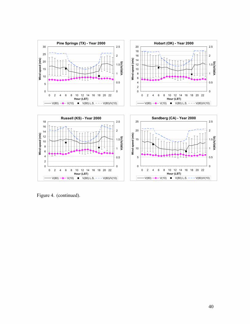
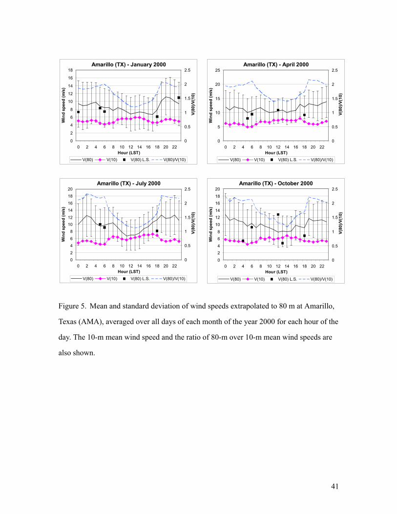
The statistics suggest that the wind speed at a given hour, averaged over either a
year or a month, is a fairly steady parameter. Figures 4 and 5 show that the monthly mean
for a given hour was within –45% and +60% of the annual mean for that hour. For
example, the mean-annual 80-m wind speed at Amarillo (AMA) at 1700 was 9.8 m/s
(Figure 4, first graph). Figure 5 shows that the lowest mean speed at 1700 was 6.7 m/s in
January, 32% less than the annual mean at that hour. The highest mean speed at that hour
was 12.9 m/s in April (32% greater than the annual mean). High variability of the
monthly mean at Amarillo occurred in March (Figure 5), when the monthly mean wind
speed was 10.0 m/s. The highest mean speed for an individual hour during that month
was 12.6 m/s at 1900 (26% greater than the monthly mean), and the lowest mean was 6.7
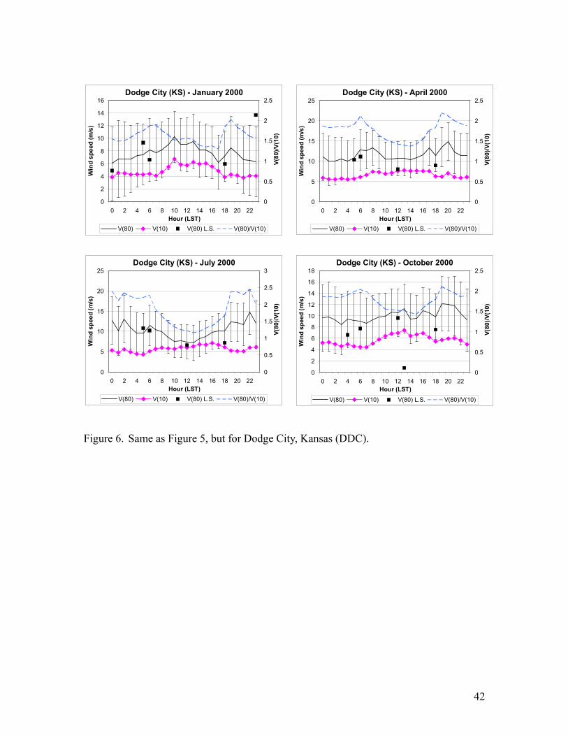
m/s at 1100 (33% lower than the monthly mean). For Dodge City (DDC), the greatest
variability occurred in July (Figure 6), when the monthly mean speed was 10.2 m/s, the
highest mean was 14.7 m/s at 2300 (44% of the monthly mean), and the lowest mean was
7.2 m/s at 1300 (29% lower than the monthly mean).
Second, mean wind speed at 80 m was generally lower in the early afternoon than
during any other time of the day, for the reason explained in Section 2.2. At Dodge City
(DDC), for example, the minimum mean speed occurred between 1100 and 1400 in
~60% of the cases, whereas the maximum was more likely to occur either in the evening
(50%) or in the morning (42%) (Figure 6). Note, however, that there are cases (such as
16
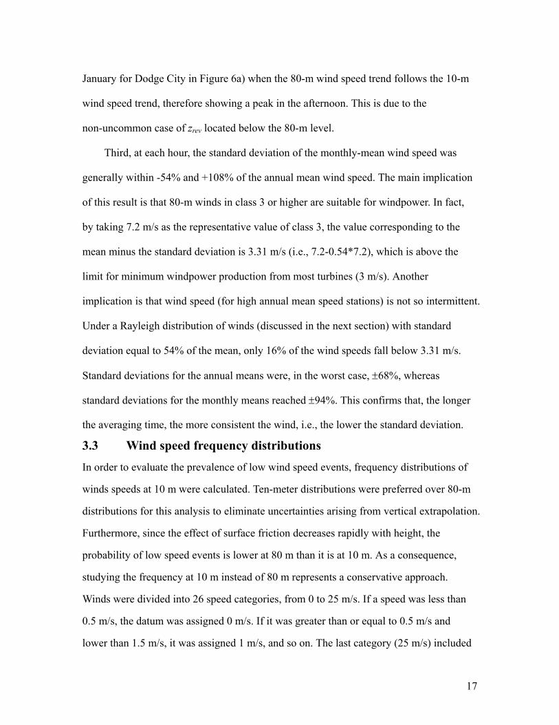
January for Dodge City in Figure 6a) when the 80-m wind speed trend follows the 10-m
wind speed trend, therefore showing a peak in the afternoon. This is due to the
non-uncommon case of zrev located below the 80-m level.
Third, at each hour, the standard deviation of the monthly-mean wind speed was
generally within -54% and +108% of the annual mean wind speed. The main implication
of this result is that 80-m winds in class 3 or higher are suitable for windpower. In fact,
by taking 7.2 m/s as the representative value of class 3, the value corresponding to the
mean minus the standard deviation is 3.31 m/s (i.e., 7.2-0.54*7.2), which is above the
limit for minimum windpower production from most turbines (3 m/s). Another
implication is that wind speed (for high annual mean speed stations) is not so intermittent.
Under a Rayleigh distribution of winds (discussed in the next section) with standard
deviation equal to 54% of the mean, only 16% of the wind speeds fall below 3.31 m/s.
Standard deviations for the annual means were, in the worst case, ±68%, whereas
standard deviations for the monthly means reached ±94%. This confirms that, the longer
the averaging time, the more consistent the wind, i.e., the lower the standard deviation.
3.3 Wind speed frequency distributions
In order to evaluate the prevalence of low wind speed events, frequency distributions of
winds speeds at 10 m were calculated. Ten-meter distributions were preferred over 80-m
distributions for this analysis to eliminate uncertainties arising from vertical extrapolation.
Furthermore, since the effect of surface friction decreases rapidly with height, the
probability of low speed events is lower at 80 m than it is at 10 m. As a consequence,
studying the frequency at 10 m instead of 80 m represents a conservative approach.
Winds were divided into 26 speed categories, from 0 to 25 m/s. If a speed was less than
0.5 m/s, the datum was assigned 0 m/s. If it was greater than or equal to 0.5 m/s and
lower than 1.5 m/s, it was assigned 1 m/s, and so on. The last category (25 m/s) included
17
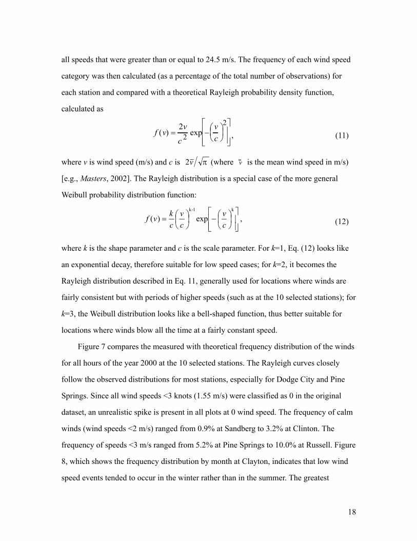
all speeds that were greater than or equal to 24.5 m/s. The frequency of each wind speed
category was then calculated (as a percentage of the total number of observations) for
each station and compared with a theoretical Rayleigh probability density function,
calculated as
f (v) =2v
c 2 exp −vc
2
, (11)
where v is wind speed (m/s) and c is πv2 (where v is the mean wind speed in m/s)
[e.g., Masters, 2002]. The Rayleigh distribution is a special case of the more general
Weibull probability distribution function:
−
=
k1-k
exp)(cv
cv
ckvf , (12)
where k is the shape parameter and c is the scale parameter. For k=1, Eq. (12) looks like
an exponential decay, therefore suitable for low speed cases; for k=2, it becomes the
Rayleigh distribution described in Eq. 11, generally used for locations where winds are
fairly consistent but with periods of higher speeds (such as at the 10 selected stations); for
k=3, the Weibull distribution looks like a bell-shaped function, thus better suitable for
locations where winds blow all the time at a fairly constant speed.
Figure 7 compares the measured with theoretical frequency distribution of the winds
for all hours of the year 2000 at the 10 selected stations. The Rayleigh curves closely
follow the observed distributions for most stations, especially for Dodge City and Pine
Springs. Since all wind speeds <3 knots (1.55 m/s) were classified as 0 in the original
dataset, an unrealistic spike is present in all plots at 0 wind speed. The frequency of calm
winds (wind speeds <2 m/s) ranged from 0.9% at Sandberg to 3.2% at Clinton. The
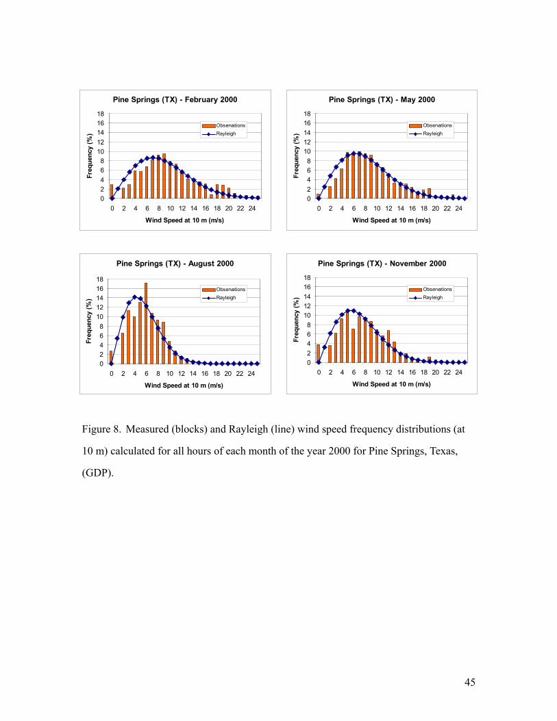
frequency of speeds <3 m/s ranged from 5.2% at Pine Springs to 10.0% at Russell. Figure
8, which shows the frequency distribution by month at Clayton, indicates that low wind
speed events tended to occur in the winter rather than in the summer. The greatest
18
frequency of wind speeds <2 m/s at Clayton were in December (7.7%) and January
(5.3%).
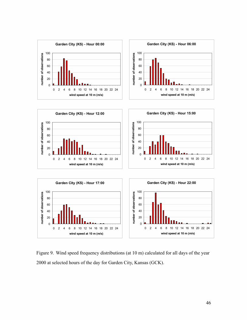
Hourly frequency distributions for the whole year were calculated to determine if
low wind speed events occurred preferentially at specific hours. Results suggest that such
events could occur at any hour of the day, but with a slightly higher frequency at night.
Figure 9 shows that, at Garden City, for example, the frequency of calm winds varied
from a minimum of 0.7% at 2200 to a maximum of 3.9% at 1700. The frequency of the
fastest winds was greatest from 1400 to 1600 in the afternoon.
In summary, low wind speed events (<3 m/s at 10 m) were infrequent, occurring less
than 10.1% of the total hours of the year in the worst case. Such events were more
frequent in winter than in summer. 3.4 Wind power distributions
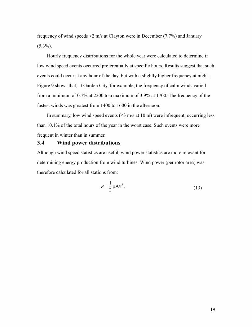
Although wind speed statistics are useful, wind power statistics are more relevant for
determining energy production from wind turbines. Wind power (per rotor area) was
therefore calculated for all stations from:
P =12
ρAv3 , (13)
19
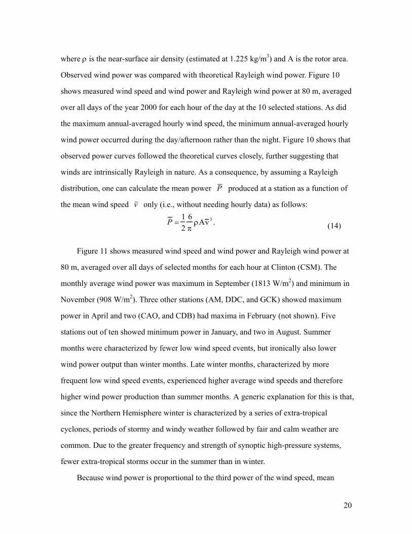
where ρ is the near-surface air density (estimated at 1.225 kg/m3) and A is the rotor area.
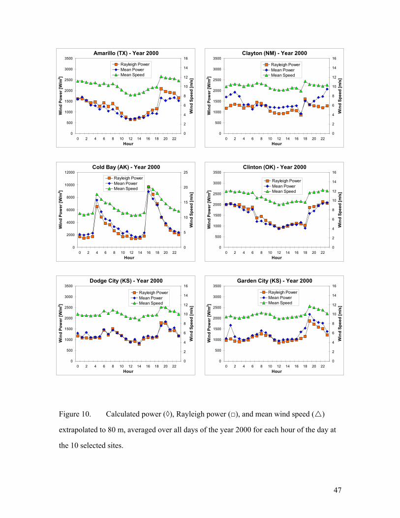
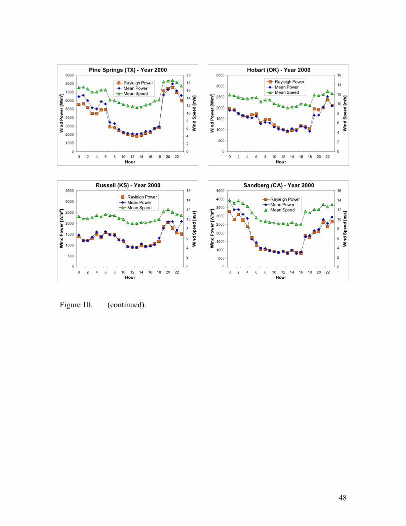
Observed wind power was compared with theoretical Rayleigh wind power. Figure 10
shows measured wind speed and wind power and Rayleigh wind power at 80 m, averaged
over all days of the year 2000 for each hour of the day at the 10 selected stations. As did
the maximum annual-averaged hourly wind speed, the minimum annual-averaged hourly
wind power occurred during the day/afternoon rather than the night. Figure 10 shows that
observed power curves followed the theoretical curves closely, further suggesting that
winds are intrinsically Rayleigh in nature. As a consequence, by assuming a Rayleigh
distribution, one can calculate the mean power P produced at a station as a function of
the mean wind speed v only (i.e., without needing hourly data) as follows:
P =12
6π
ρAv 3 . (14)
Figure 11 shows measured wind speed and wind power and Rayleigh wind power at
80 m, averaged over all days of selected months for each hour at Clinton (CSM). The
monthly average wind power was maximum in September (1813 W/m2) and minimum in
November (908 W/m2). Three other stations (AM, DDC, and GCK) showed maximum
power in April and two (CAO, and CDB) had maxima in February (not shown). Five
stations out of ten showed minimum power in January, and two in August. Summer
months were characterized by fewer low wind speed events, but ironically also lower
wind power output than winter months. Late winter months, characterized by more
frequent low wind speed events, experienced higher average wind speeds and therefore
higher wind power production than summer months. A generic explanation for this is that,
since the Northern Hemisphere winter is characterized by a series of extra-tropical
cyclones, periods of stormy and windy weather followed by fair and calm weather are
common. Due to the greater frequency and strength of synoptic high-pressure systems,
fewer extra-tropical storms occur in the summer than in winter.
Because wind power is proportional to the third power of the wind speed, mean
20
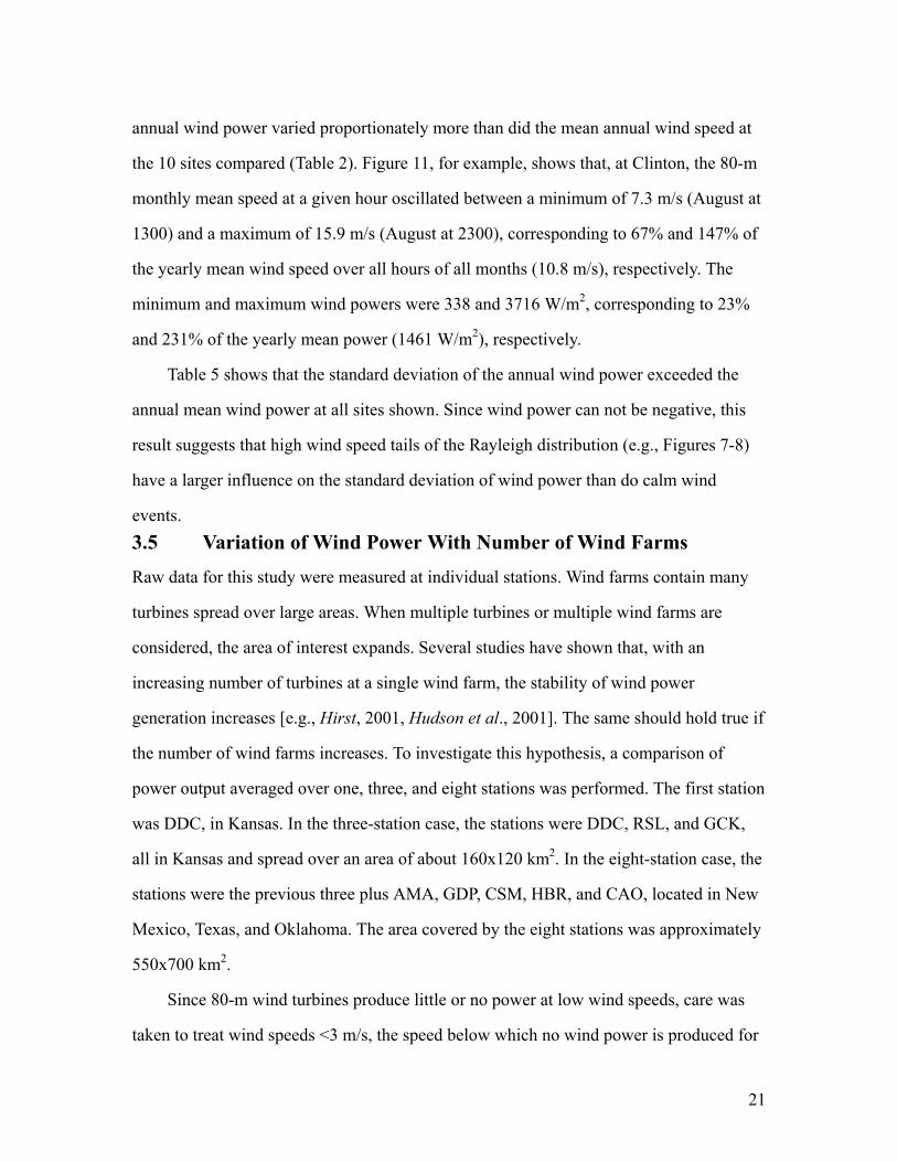
annual wind power varied proportionately more than did the mean annual wind speed at
the 10 sites compared (Table 2). Figure 11, for example, shows that, at Clinton, the 80-m
monthly mean speed at a given hour oscillated between a minimum of 7.3 m/s (August at
1300) and a maximum of 15.9 m/s (August at 2300), corresponding to 67% and 147% of
the yearly mean wind speed over all hours of all months (10.8 m/s), respectively. The
minimum and maximum wind powers were 338 and 3716 W/m2, corresponding to 23%
and 231% of the yearly mean power (1461 W/m2), respectively.
Table 5 shows that the standard deviation of the annual wind power exceeded the
annual mean wind power at all sites shown. Since wind power can not be negative, this
result suggests that high wind speed tails of the Rayleigh distribution (e.g., Figures 7-8)
have a larger influence on the standard deviation of wind power than do calm wind
events. 3.5 Variation of Wind Power With Number of Wind Farms
Raw data for this study were measured at individual stations. Wind farms contain many
turbines spread over large areas. When multiple turbines or multiple wind farms are
considered, the area of interest expands. Several studies have shown that, with an
increasing number of turbines at a single wind farm, the stability of wind power
generation increases [e.g., Hirst, 2001, Hudson et al., 2001]. The same should hold true if
the number of wind farms increases. To investigate this hypothesis, a comparison of
power output averaged over one, three, and eight stations was performed. The first station
was DDC, in Kansas. In the three-station case, the stations were DDC, RSL, and GCK,
all in Kansas and spread over an area of about 160x120 km2. In the eight-station case, the
stations were the previous three plus AMA, GDP, CSM, HBR, and CAO, located in New
Mexico, Texas, and Oklahoma. The area covered by the eight stations was approximately
550x700 km2.
Since 80-m wind turbines produce little or no power at low wind speeds, care was
taken to treat wind speeds <3 m/s, the speed below which no wind power is produced for
21
many turbines. Even when the area-averaged wind speed is lower than 3 m/s, the
area-averaged wind power generated by all turbines is not necessarily zero because some
turbines may experience wind speeds above 3 m/s, whereas others may experience no
winds. To take this into account, a different type of area-averaged wind speed was
introduced, named “area-averaged power wind speed” V p . First, the area-averaged
power P at a given hour of a given day was tabulated as
P =1N
12
ρvi3
i=1
N∑ , (15)
where vi is the 80-m wind speed at station i (set to zero if <3 m/s) and N is the number of
stations (i.e., 1, 3 or 8). The area-averaged power wind speed V p at a given hour of a
given day was then calculated as:
V p = 2Pρ
1 3
. (16)
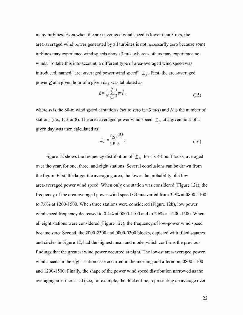
Figure 12 shows the frequency distribution of V p for six 4-hour blocks, averaged
over the year, for one, three, and eight stations. Several conclusions can be drawn from
the figure. First, the larger the averaging area, the lower the probability of a low
area-averaged power wind speed. When only one station was considered (Figure 12a), the
frequency of the area-averaged power wind speed <3 m/s varied from 3.9% at 0800-1100
to 7.6% at 1200-1500. When three stations were considered (Figure 12b), low power
wind speed frequency decreased to 0.4% at 0800-1100 and to 2.6% at 1200-1500. When
all eight stations were considered (Figure 12c), the frequency of low-power wind speed
became zero. Second, the 2000-2300 and 0000-0300 blocks, depicted with filled squares
and circles in Figure 12, had the highest mean and mode, which confirms the previous
findings that the greatest wind power occurred at night. The lowest area-averaged power
wind speeds in the eight-station case occurred in the morning and afternoon, 0800-1100
and 1200-1500. Finally, the shape of the power wind speed distribution narrowed as the
averaging area increased (see, for example, the thicker line, representing an average over
22
all hours, in Figure 12). Therefore the standard deviation of the power wind speed
decreased with an increasing averaging area. Furthermore, for the eight station case, a
Weibull distribution with k=3 fits the data better than one with k=2 (i.e., a Rayleigh
distribution), as expected for locations with constant and high wind speeds.
4 Conclusions
In this paper, a methodology for determining 80-m wind speeds given 10-m wind speed
measurements was introduced and applied to the U.S. for the year 2000. The results were
analyzed to judge the regularity and spatial distribution of U.S. windpower at 80 m.
Conclusions of the study are as follows:
(1) In the year 2000, mean-annual wind speeds at 80 m may have exceeded 6.9 m/s at
approximately 24% of the measurement stations in the U.S., implying that
possibly one quarter of the country is suitable for providing electric power from
wind at a direct cost equal to that from a new natural gas or coal power plant.
(2) The greatest previously uncharted reservoir of windpower in the continental U.S.
is offshore and onshore along the southeastern and southern coasts.
(3) The other great wind reservoirs are the north- and south-central regions, charted
previously.
(4) The five states with the highest percentage of stations with annual mean 80-m
wind speed ≥ 6.9 m/s were Oklahoma, South Dakota, North Dakota, Kansas, and
Nebraska;
(5) The standard deviation of the wind speed averaged over multiple locations is less
than that at any individual location. As such, intermittency of wind energy from
multiple wind farms may be less than that from a single farm, and contingency
reserve requirements may decrease with increasing spatial distribution of wind
farms;
23
(6) The minimum wind speed during the year increases when more wind sites are
considered. Thus, the probability of no wind power production due to low wind
speed events may be greatly reduced (if not eliminated) by a network of wind
farms;
(7) Winds are Rayleigh in nature, and actual wind power at any hour of the day
during a year is close to Rayleigh wind power;
(8) Because winds, even at a given hour, are Rayleigh in nature, the average wind
power over a month at a given hour at a location is a reliable quantity compared
with wind power at the same hour, but on any random day of the month.
Therefore, requiring turbine owners to produce a summed quantity of energy over
a month at a given hour of the day entails little risk once monthly-averaged
Rayleigh wind speeds at the given hour and location are known;
(9) Even when the standard deviation of the wind speed is high, the total wind power
during an averaging period follows the mean wind speed.
ACKNOWLEDGMENTS. This work was supported by the Environmental Protection
Agency, the NASA New Investigator Program in Earth Sciences, the National Science
Foundation, and the David and Lucile Packard Foundation and the Hewlett-Packard
company. Data were obtained from: National Climatic Data Center, Forecast System
Laboratory, and Pacific Northwest Laboratory. We would also like to thank Scott Archer,
Gil Master, Paul Veers, Henry Dodd, and Donald Anderson for helpful comments.
24
References
Archer, C. L., and M. Z. Jacobson, The regularity and spatial distribution of U.S.
windpower, Supplemental Information, http://www.stanford.edu/efmh/winds, 2001.
Arya, S. P., Introduction to micrometeorology, Academic Press Inc., 307 pp., 1988.
Bolinger, M., and R. Wiser, Summary of power authority letters of intent for renewable
energy, Memorandum, Lawrence Berkeley National Laboratory, October 30, 2001.
Danish Windturbine Manufacturers Assoc., 21 Frequently Asked Questions About Wind
Energy, (updated April 16, 2001), http://www.windpower.dk/faqs.htm, 2001.
Elliott, D. L., C. G. Holladay, w. R. Barchet, H. P. Foote, and W. F. Sandusky, Wind
energy resource atlas of the United States, Appendix A, DOE/CH 10093-4,
http://rredc.nrel.gov/wind/pubs/atlas/appendix_A.html, 1986a.
Elliott, D. L., C. G. Holladay, w. R. Barchet, H. P. Foote, and W. F. Sandusky, Wind
energy resource atlas of the United States, DOE/CH 10093-4,
http://rredc.nrel.gov/wind/pubs/atlas/maps/chap2/2-01m.html, 1986b.
Elliott, D. L., C. G. Holladay, W. R. Barchet, H. P. Foote, and W. F. Sandusky, Wind
energy resource atlas of the United States, DOE/CH 10093-4,
http://rredc.nrel.gov/wind/pubs/atlas/chp3.html, 1986c.
Energy Information Administration (EIA),
http://www.eia.doe.gov/cneaf/electricity/epav2/epav2t1.txt, 2001.
25
Forecast Systems Laboratory, Radiosonde data archive, http://raob.fsl.noaa.gov/, 2001.
Hirst, E., Interactions of wind farms with bulk-power operations and markets,
http://www.EHirst.com/PDF/WindIntegration.pdf, 2001.
Hudson, R., B. Kirby, and Y.-H. Wan, The impact of wind generation on system
regulation requirements, AWEA Wind Power Conference, 2001.
Jacobson, M. Z., Fundamentals of atmospheric modeling, Cambridge University Press,
656 pp., 1999.
Jacobson, M. Z., and G. M. Masters, Exploiting wind versus coal, Science, 293,
1438-1438, 2001.
Masters, G. M., Electric Power: Renewables and Efficiency, Chapter 6:
Wind Power Systems, textbook in preparation, 2002.
McFeat, T., The unnatural price of natural gas, CBC News Online,
http://www.cbc.ca/news/indepth/background/gas_hikes.html, 2001.
National Climatic Data Center, Hourly Surface Data,
http://lwf.ncdc.noaa.gov/oa/climate/climatedata.html, 2001.
North American Electric Reliability Council, Generating Unit Statistical Brochure,
1995-1999, Princeton, NJ, October, 2000.
26
Office of Fossil Energy, Department of Energy,
http://www.fe.doe.gov/coal_power/special_rpts/market_systems/market_sys.html,
Section 9, 2001.
Riehl, H., Introduction to the atmosphere, McGraw-Hill Inc., 516 pp., 1972.
Sandusky, W. F., D. S. Renné and D. L. Hadley, Candidate Wind Turbine Generator Site
Summarized Meteorological Data for December 1976 Through December 1981.
PNL-4407, Pacific Northwest Laboratory, Richland, Washington, 1982.
Schwartz, M., and D. Elliott, Remapping of the wind energy resource in the Midwestern
United States, NREL/AB-500-31083, Golden, CO, 2002.
Steurer, P., Six second upper air data, TD-9948, National Climatic Data Center, Asheville,
NC, http://www1.ncdc.noaa.gov/pub/data/documentlibrary/tddoc/td9948.pdf, 1996.
27
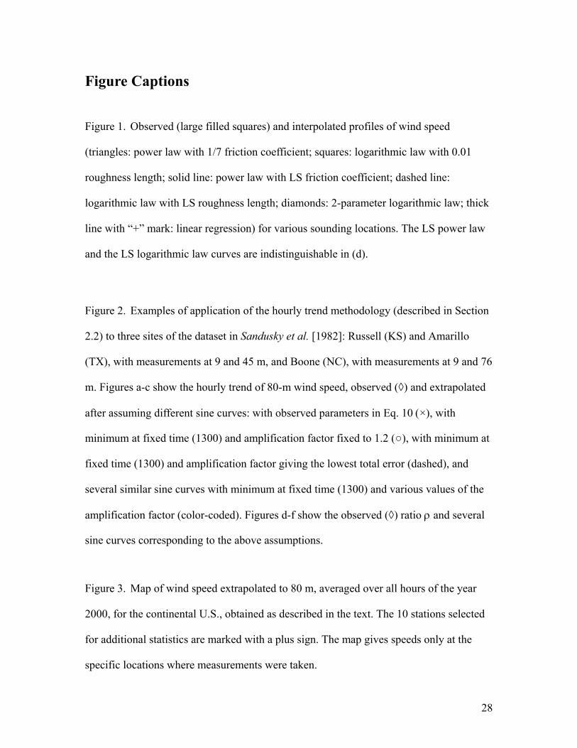
Figure Captions
Figure 1. Observed (large filled squares) and interpolated profiles of wind speed
(triangles: power law with 1/7 friction coefficient; squares: logarithmic law with 0.01
roughness length; solid line: power law with LS friction coefficient; dashed line:
logarithmic law with LS roughness length; diamonds: 2-parameter logarithmic law; thick
line with “+” mark: linear regression) for various sounding locations. The LS power law
and the LS logarithmic law curves are indistinguishable in (d).
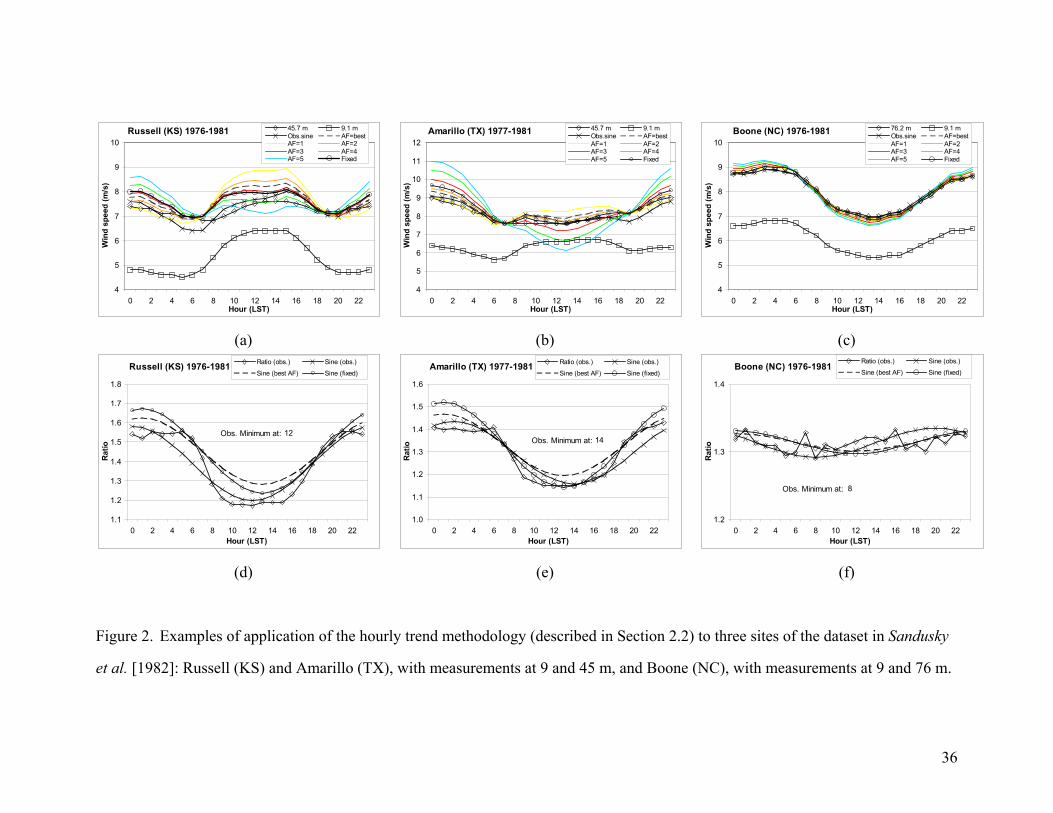
Figure 2. Examples of application of the hourly trend methodology (described in Section
2.2) to three sites of the dataset in Sandusky et al. [1982]: Russell (KS) and Amarillo
(TX), with measurements at 9 and 45 m, and Boone (NC), with measurements at 9 and 76
m. Figures a-c show the hourly trend of 80-m wind speed, observed (◊) and extrapolated
after assuming different sine curves: with observed parameters in Eq. 10 (×), with
minimum at fixed time (1300) and amplification factor fixed to 1.2 (○), with minimum at
fixed time (1300) and amplification factor giving the lowest total error (dashed), and
several similar sine curves with minimum at fixed time (1300) and various values of the
amplification factor (color-coded). Figures d-f show the observed (◊) ratio ρ and several
sine curves corresponding to the above assumptions.
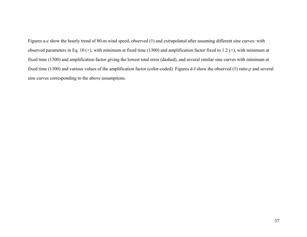
Figure 3. Map of wind speed extrapolated to 80 m, averaged over all hours of the year
2000, for the continental U.S., obtained as described in the text. The 10 stations selected
for additional statistics are marked with a plus sign. The map gives speeds only at the
specific locations where measurements were taken.
28

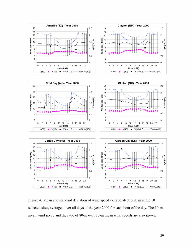
Figure 4. Mean and standard deviation of wind speed extrapolated to 80 m at the 10
selected sites, averaged over all days of the year 2000 for each hour of the day. The 10-m
mean wind speed and the ratio of 80-m over 10-m mean wind speeds are also shown.
Figure 5. Mean and standard deviation of wind speeds extrapolated to 80 m at Amarillo,
Texas (AMA), averaged over all days of each month of the year 2000 for each hour of the
day. The 10-m mean wind speed and the ratio of 80-m over 10-m mean wind speeds are
also shown.
Figure 6. Same as Figure 5, but for Dodge City, Kansas (DDC).
Figure 7. Measured (blocks) and Rayleigh (line) wind speed frequency distributions (at
10 m) calculated for all hours of the year 2000 for the 10 selected stations.
Figure 8. Measured (blocks) and Rayleigh (line) wind speed frequency distributions (at
10 m) calculated for all hours of each month of the year 2000 for Pine Springs, Texas,
(GDP).
Figure 9. Wind speed frequency distributions (at 10 m) calculated for all days of the year
2000 at selected hours of the day for Garden City, Kansas (GCK).
Figure 10. Calculated power (◊), Rayleigh power (□), and mean wind speed ( )
extrapolated to 80 m, averaged over all days of the year 2000 for each hour of the day at
29

the 10 selected sites.
Figure 11. Calculated power (◊), Rayleigh power (□), and mean wind speed ( )
extrapolated to 80 m, averaged over all days of each month of the year 2000 for each
hour of the day at Clinton, Oklahoma (CSM).
Figure 12. Power wind speed distribution, divided into six 4-hour blocks, for (a) one
station, (b) three stations, and (c) eight stations.
30

Tables
Table 1. Location and elevations at the 16 sites selected by Sandusky [1982]. Site location Lower level (m) Middle level (m) Upper level (m) Augspurger Mt. (WA) 9.1 - 45.7 Amarillo (TX) 9.1 - 45.7 Block Island (RI) 9.1 30.0 45.7 Boardman (OR) 9.1 39.6 70.1 Boone (NC) 18.2 45.7 76.2 Clayton (NM) 9.1 30.0 45.7 Cold Bay (AK) 9.1 - 21.8 Culebra (PR) 9.1 - 45.7 Holyoke (MA) 18.2 - 45.7 Huron (SD) 9.1 - 45.7 Kingsley Dam (NB) 9.1 - 45.7 Ludington (MI) 18.2 - 45.7 Montaulk (NY) 18.2 - 45.7 Point Arena (CA) 9.1 - 45.7 Russell (KS) 9.1 - 45.7 San Gorgonio (CA) 9.1 30.0 45.7
Table 2. Wind speeds corresponding to different power classes at 10 m and 80 m.
Class Wind speed at 10 m (m/s)
Wind speed at 80 m (m/s)
1 < 4.4 <5.9 2 4.4-5.1 5.9-6.9 3 5.1-5.6 6.9-7.5 4 5.6-6.0 7.5-8.1 5 6.0-6.4 8.1-8.6 6 6.4-7.0 8.6-9.4 7 >7.0 ≥9.4
31
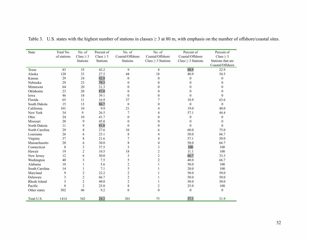
Table 3. U.S. states with the highest number of stations in classes ≥ 3 at 80 m, with emphasis on the number of offshore/coastal sites. State Total No.
of stations No. of
Class ≥ 3
Stations
Percent of Class ≥ 3 Stations
No. of Coastal/Offshore
Stations
No. of Coastal/Offshore Class ≥ 3 Stations
Percent of Coastal/Offshore Class ≥ 3 Stations
Percent of Class ≥ 3
Stations that are Coastal/Offshore
Texas 83 35 42.2 9 8 88.9 22.9Alaska
120 33 27.5 44 18 40.9 54.5
Kansas 29 24 82.8 0 0 0 0 Nebraska 29 23 79.3 0 0 0 0 Minnesota 64 20 31.3 0 0 0 0 Oklahoma 23 20 87.0 0 0 0 0 Iowa 46 18
39.1 0 0 0 0
Florida 65 11 16.9 37 7 18.9 63.6 South Dakota 15 13 86.7 0 0 0 0 California 101 10 9.9 21 4 19.0 40.0 New York 34 9 26.5 7 4 57.1 44.4 Ohio 24 10 41.7 0 0 0 0 Missouri 20 9 45.0 0 0 0 0 North Dakota 11 9 81.8 0 0 0 0 North Carolina 29 8 27.6 10 6 60.0 75.0 Louisiana 26 6 23.1 8 4 50.0 66.7 Virginia 37 8 21.6 7 4 57.1 50.0 Massachusetts 20 6 30.0 8 4 50.0 66.7 Connecticut 8 3 37.5 3 3 100
100
Hawaii 19 2 10.5 18 2 11.1 100 New Jersey 12 6 50.0 3 2 66.7
33.3Washington 40 3 7.5 5 2 40.0 66.7 Alabama 18 1 5.6 2 1 50.0 100 South Carolina 14 1 7.1 5 1 20.0 100 Maryland 9 2 22.2 2 1 50.0 50.0 Delaware 3 2 66.7 2 1 50.0 50.0 Rhode Island 5 2 40.0 2 1 50.0 50.0 Pacific 8 2 25.0 8 2 25.0 100 Other states
502 46
9.2
0 0 0 0
Total U.S. 1414 342 24.2 201 75 37.3 21.9
32
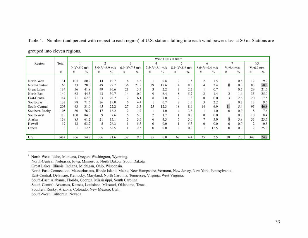
Table 4. Number (and percent with respect to each region) of U.S. stations falling into each wind power class at 80 m. Stations are
grouped into eleven regions. Wind Class at 80 m
Region1 Total 10≤V<5.9 m/s
2 5.9≤V<6.9 m/s
3 6.9≤V<7.5 m/s
4 7.5≤V<8.1 m/s
5 8.1≤V<8.6 m/s
6 8.6≤V<9.4 m/s
7 V≥9.4 m/s
≥3 V≥6.9 m/s
# # % # % # % # % # % # % # % # %
North-West 131 105 80.2 14 10.7 6 4.6 1 0.8 2 1.5 2 1.5 1 0.8 12 9.2North-Central 165 33 20.0 49 29.7 36 21.8 29 17.6 14 8.5 4 2.4 0 0.0 83 50.3 Great Lakes 134 56 41.8 49 36.6 21 15.7 3 2.2 3 2.2 1 0.7 1 0.7 29 21.6North-East 140 62 44.3 43 30.7 14 10.0 9 6.4 8 5.7 2 1.4 2 1.4 35 25.0East-Central 114 71 62.3 23 20.2 7 6.1 8 7.0 2 1.8 0 0.0 3 2.6 20 17.5South-East 137 98 71.5 26 19.0 6 4.4 1 0.7 2 1.5 3 2.2 1 0.7 13 9.5South-Central 203 63 31.0 45 22.2 27 13.3 25 12.3 18 8.9 14 6.9 11 5.4 95 46.8 Southern Rocky 105 80 76.2 17 16.2 2 1.9 1 1.0 4 3.8 1 1.0 0 0.0 8 7.6South-West 119 100 84.0 9 7.6 6 5.0 2 1.7 1 0.8 0 0.0 1 0.8 10 8.4Alaska 139 85 61.2 21 15.1 5 3.6 6 4.3 7 5.0 7 5.0 8 5.8 33 23.7Hawaii 19 12 63.2 5 26.3 1 5.3 0 0.0 1 5.3 0 0.0 0 0.0 2 10.5Others 8 1 12.5 5 62.5 1 12.5 0 0.0 0 0.0 1 12.5 0 0.0 2 25.0 U.S. 1414 766 54.2 306 21.6 132 9.3 85 6.0 62 4.4 35 2.5 28 2.0 342 24.2
1 North-West: Idaho, Montana, Oregon, Washington, Wyoming.
North-Central: Nebraska, Iowa, Minnesota, North Dakota, South Dakota. Great Lakes: Illinois, Indiana, Michigan, Ohio, Wisconsin. North-East: Connecticut, Massachusetts, Rhode Island, Maine, New Hampshire, Vermont, New Jersey, New York, Pennsylvania. East-Central: Delaware, Kentucky, Maryland, North Carolina, Tennessee, Virginia, West Virginia. South-East: Alabama, Florida, Georgia, Mississippi, South Carolina. South-Central: Arkansas, Kansas, Louisiana, Missouri, Oklahoma, Texas. Southern Rocky: Arizona, Colorado, New Mexico, Utah. South-West: California, Nevada.
33
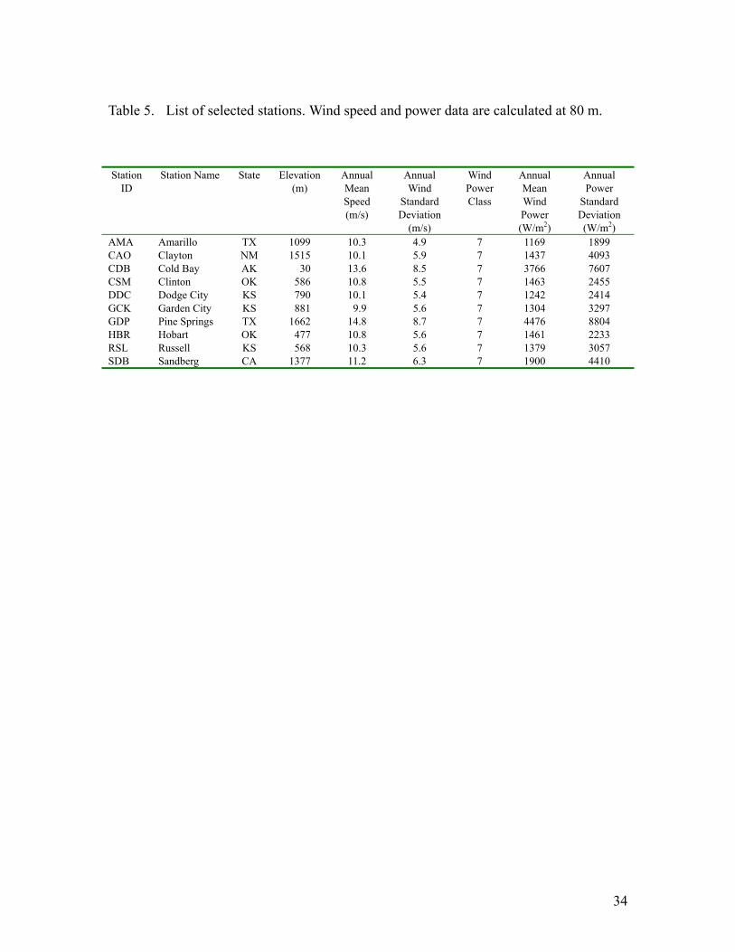
Table 5. List of selected stations. Wind speed and power data are calculated at 80 m.
Station
ID Station Name State Elevation
(m) Annual Mean Speed (m/s)
Annual Wind
Standard Deviation
(m/s)
Wind Power Class
Annual Mean Wind Power (W/m2)
Annual Power
Standard Deviation (W/m2)
AMA Amarillo TX 1099 10.3 4.9 7 1169 1899 CAO Clayton NM 1515 10.1 5.9 7 1437 4093 CDB Cold Bay AK 30 13.6 8.5 7 3766 7607 CSM Clinton OK 586 10.8 5.5 7 1463 2455 DDC Dodge City KS 790 10.1 5.4 7 1242 2414 GCK Garden City KS 881 9.9 5.6 7 1304 3297 GDP Pine Springs TX 1662 14.8 8.7 7 4476 8804 HBR Hobart OK 477 10.8 5.6 7 1461 2233 RSL Russell KS 568 10.3 5.6 7 1379 3057 SDB Sandberg CA 1377 11.2 6.3 7 1900 4410
34
ALBUQUERQUE (NM, 1613 masl) - 1/17/2000 12UTC
0
80
160
240
320
400
480
560
640
720
0 1 2 3 4 5 6 7 8 9
Wind speed (m/s)
Z (m
)
ObservedLog (LS)Power (LS)Power (1/7)Log (0.01)
ALBUQUERQUE (NM, 1613 masl) - 12/25/2000 00UTC
0
80
160
240
320
400
480
560
640
720
0 1 2 3 4 5 6
Wind speed (m/s)
Z (m
)
ObservedLog (LS)Power (LS)Power (1/7)Log (0.01)
(a) (b)
(c) (d)
OAKLAND (CA, 6 masl) - 3/6/2000 12UTC
0
80
160
240
320
400
0 0.5 1 1.5 2 2.5 3 3.5
Wind speed (m/s)
Z (m
)
ObservedLog (2 parameters)
DENVER (CO, 1625 masl) - 6/5/2000 00UTC
0
80
160
240
320
400
480
560
640
720
2 2.5 3 3.5 4 4.5 5 5.5 6
Wind speed (m/s)
Z (m
)
ObservedLog (LS)Power (LS)Power (1/7)Log (0.01)linear
Figure 1. Observed (large filled squares) and interpolated profiles of wind speed
(triangles: power law with 1/7 friction coefficient; squares: logarithmic law with 0.01
roughness length; solid line: power law with LS friction coefficient; dashed line:
logarithmic law with LS roughness length; diamonds: 2-parameter logarithmic law; thick
line with “+” mark: linear regression) for various sounding locations. The LS power law
and the LS logarithmic law curves are indistinguishable in (d).
35
Russell (KS) 1976-1981
4
5
6
7
8
9
10
0 2 4 6 8 10 12 14 16 18 20 22Hour (LST)
Win
d sp
eed
(m/s
)
45.7 m 9.1 mObs.sine AF=bestAF=1 AF=2AF=3 AF=4AF=5 Fixed
Amarillo (TX) 1977-1981
4
5
6
7
8
9
10
11
12
0 2 4 6 8 10 12 14 16 18 20 22Hour (LST)
Win
d sp
eed
(m/s
)
45.7 m 9.1 mObs.sine AF=bestAF=1 AF=2AF=3 AF=4AF=5 Fixed
Boone (NC) 1976-1981
4
5
6
7
8
9
10
0 2 4 6 8 10 12 14 16 18 20 22Hour (LST)
Win
d sp
eed
(m/s
)
76.2 m 9.1 mObs.sine AF=bestAF=1 AF=2AF=3 AF=4AF=5 Fixed
(a) (b)
(c)
(d) (e) (f)
Russell (KS) 1976-1981
12
1.1
1.2
1.3
1.4
1.5
1.6
1.7
1.8
0 2 4 6 8 10 12 14 16 18 20 22Hour (LST)
Ratio
Ratio (obs.) Sine (obs.)Sine (best AF) Sine (fixed)
Obs. Minimum at:
Amarillo (TX) 1977-1981
14
1.0
1.1
1.2
1.3
1.4
1.5
1.6
0 2 4 6 8 10 12 14 16 18 20 22Hour (LST)
Ratio
Ratio (obs.) Sine (obs.)Sine (best AF) Sine (fixed)
Obs. Minimum at:
Boone (NC) 1976-1981
8
1.2
1.3
1.4
0 2 4 6 8 10 12 14 16 18 20 22Hour (LST)
Ratio
Ratio (obs.) Sine (obs.)Sine (best AF) Sine (fixed)
Obs. Minimum at:
Figure 2. Examples of application of the hourly trend methodology (described in Section 2.2) to three sites of the dataset in Sandusky
et al. [1982]: Russell (KS) and Amarillo (TX), with measurements at 9 and 45 m, and Boone (NC), with measurements at 9 and 76 m.
36
Figures a-c show the hourly trend of 80-m wind speed, observed (◊) and extrapolated after assuming different sine curves: with
observed parameters in Eq. 10 (×), with minimum at fixed time (1300) and amplification factor fixed to 1.2 (○), with minimum at
fixed time (1300) and amplification factor giving the lowest total error (dashed), and several similar sine curves with minimum at
fixed time (1300) and various values of the amplification factor (color-coded). Figures d-f show the observed (◊) ratio ρ and several
sine curves corresponding to the above assumptions.
37
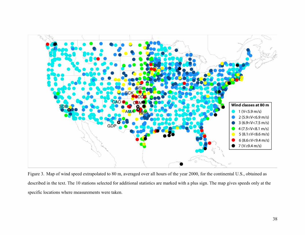
Figure 3. Map of wind speed extrapolated to 80 m, averaged over all hours of the year 2000, for the continental U.S., obtained as
described in the text. The 10 stations selected for additional statistics are marked with a plus sign. The map gives speeds only at the
specific locations where measurements were taken.
38
Clayton (NM) - Year 2000
0
2
4
6
8
10
12
14
16
18
0 2 4 6 8 10 12 14 16 18 20 22Hour (LST)
Win
d sp
eed
(m/s
)
0
0.5
1
1.5
2
2.5
V(80
)/V(1
0)
V(80) V(10) V(80) L.S. V(80)/V(10)
Amarillo (TX) - Year 2000
02468
101214161820
0 2 4 6 8 10 12 14 16 18 20 22Hour (LST)
Win
d sp
eed
(m/s
)
0
0.5
1
1.5
2
2.5
V(80
)/V(1
0)
V(80) V(10) V(80) L.S. V(80)/V(10)
Cold Bay (AK) - Year 2000
0
5
10
15
20
25
30
0 2 4 6 8 10 12 14 16 18 20 22Hour (LST)
Win
d sp
eed
(m/s
)
0
0.5
1
1.5
2
2.5
3
V(80
)/V(1
0)
V(80) V(10) V(80) L.S. V(80)/V(10)
Clinton (OK) - Year 2000
02468
101214161820
0 2 4 6 8 10 12 14 16 18 20 22Hour (LST)
Win
d sp
eed
(m/s
)
0
0.5
1
1.5
2
2.5
V(80
)/V(1
0)
V(80) V(10) V(80) L.S. V(80)/V(10)
Dodge City (KS) - Year 2000
0
2
4
6
8
10
12
14
16
18
0 2 4 6 8 10 12 14 16 18 20 22Hour (LST)
Win
d sp
eed
(m/s
)
0
0.5
1
1.5
2
2.5
V(80
)/V(1
0)
V(80) V(10) V(80) L.S. V(80)/V(10)
Garden City (KS) - Year 2000
0
2
4
6
8
10
12
14
16
18
0 2 4 6 8 10 12 14 16 18 20 22Hour (LST)
Win
d sp
eed
(m/s
)
0
0.5
1
1.5
2
2.5
V(80
)/V(1
0)
V(80) V(10) V(80) L.S. V(80)/V(10)
Figure 4. Mean and standard deviation of wind speed extrapolated to 80 m at the 10
selected sites, averaged over all days of the year 2000 for each hour of the day. The 10-m
mean wind speed and the ratio of 80-m over 10-m mean wind speeds are also shown.
39
Hobart (OK) - Year 2000
02468
101214161820
0 2 4 6 8 10 12 14 16 18 20 22Hour (LST)
Win
d sp
eed
(m/s
)
0
0.5
1
1.5
2
2.5
V(80
)/V(1
0)
V(80) V(10) V(80) L.S. V(80)/V(10)
Pine Springs (TX) - Year 2000
0
5
10
15
20
25
30
0 2 4 6 8 10 12 14 16 18 20 22Hour (LST)
Win
d sp
eed
(m/s
)
0
0.5
1
1.5
2
2.5
V(80
)/V(1
0)
V(80) V(10) V(80) L.S. V(80)/V(10)
Russell (KS) - Year 2000
0
2
4
6
8
10
12
14
16
18
0 2 4 6 8 10 12 14 16 18 20 22Hour (LST)
Win
d sp
eed
(m/s
)
0
0.5
1
1.5
2
2.5V(
80)/V
(10)
V(80) V(10) V(80) L.S. V(80)/V(10)
Sandberg (CA) - Year 2000
0
5
10
15
20
25
0 2 4 6 8 10 12 14 16 18 20 22Hour (LST)
Win
d sp
eed
(m/s
)
0
0.5
1
1.5
2
2.5
V(80
)/V(1
0)
V(80) V(10) V(80) L.S. V(80)/V(10)
Figure 4. (continued).
40
Amarillo (TX) - January 2000
0
2
4
6
8
10
12
14
16
18
0 2 4 6 8 10 12 14 16 18 20 22Hour (LST)
Win
d sp
eed
(m/s
)
0
0.5
1
1.5
2
2.5
V(80
)/V(1
0)
V(80) V(10) V(80) L.S. V(80)/V(10)
Amarillo (TX) - April 2000
0
5
10
15
20
25
0 2 4 6 8 10 12 14 16 18 20 22Hour (LST)
Win
d sp
eed
(m/s
)
0
0.5
1
1.5
2
2.5
V(80
)/V(1
0)
V(80) V(10) V(80) L.S. V(80)/V(10)
Amarillo (TX) - July 2000
02468
101214161820
0 2 4 6 8 10 12 14 16 18 20 22Hour (LST)
Win
d sp
eed
(m/s
)
0
0.5
1
1.5
2
2.5V(
80)/V
(10)
V(80) V(10) V(80) L.S. V(80)/V(10)
Amarillo (TX) - October 2000
02468
101214161820
0 2 4 6 8 10 12 14 16 18 20 22Hour (LST)
Win
d sp
eed
(m/s
)
0
0.5
1
1.5
2
2.5
V(80
)/V(1
0)
V(80) V(10) V(80) L.S. V(80)/V(10)
Figure 5. Mean and standard deviation of wind speeds extrapolated to 80 m at Amarillo,
Texas (AMA), averaged over all days of each month of the year 2000 for each hour of the
day. The 10-m mean wind speed and the ratio of 80-m over 10-m mean wind speeds are
also shown.
41
Dodge City (KS) - January 2000
0
2
4
6
8
10
12
14
16
0 2 4 6 8 10 12 14 16 18 20 22Hour (LST)
Win
d sp
eed
(m/s
)
0
0.5
1
1.5
2
2.5
V(80
)/V(1
0)
V(80) V(10) V(80) L.S. V(80)/V(10)
Dodge City (KS) - April 2000
0
5
10
15
20
25
0 2 4 6 8 10 12 14 16 18 20 22Hour (LST)
Win
d sp
eed
(m/s
)
0
0.5
1
1.5
2
2.5
V(80
)/V(1
0)
V(80) V(10) V(80) L.S. V(80)/V(10)
Dodge City (KS) - October 2000
0
2
4
6
8
10
12
14
16
18
0 2 4 6 8 10 12 14 16 18 20 22Hour (LST)
Win
d sp
eed
(m/s
)
0
0.5
1
1.5
2
2.5
V(80
)/V(1
0)
V(80) V(10) V(80) L.S. V(80)/V(10)
Dodge City (KS) - July 2000
0
5
10
15
20
25
0 2 4 6 8 10 12 14 16 18 20 22Hour (LST)
Win
d sp
eed
(m/s
)
0
0.5
1
1.5
2
2.5
3V(
80)/V
(10)
V(80) V(10) V(80) L.S. V(80)/V(10)
Figure 6. Same as Figure 5, but for Dodge City, Kansas (DDC).
42
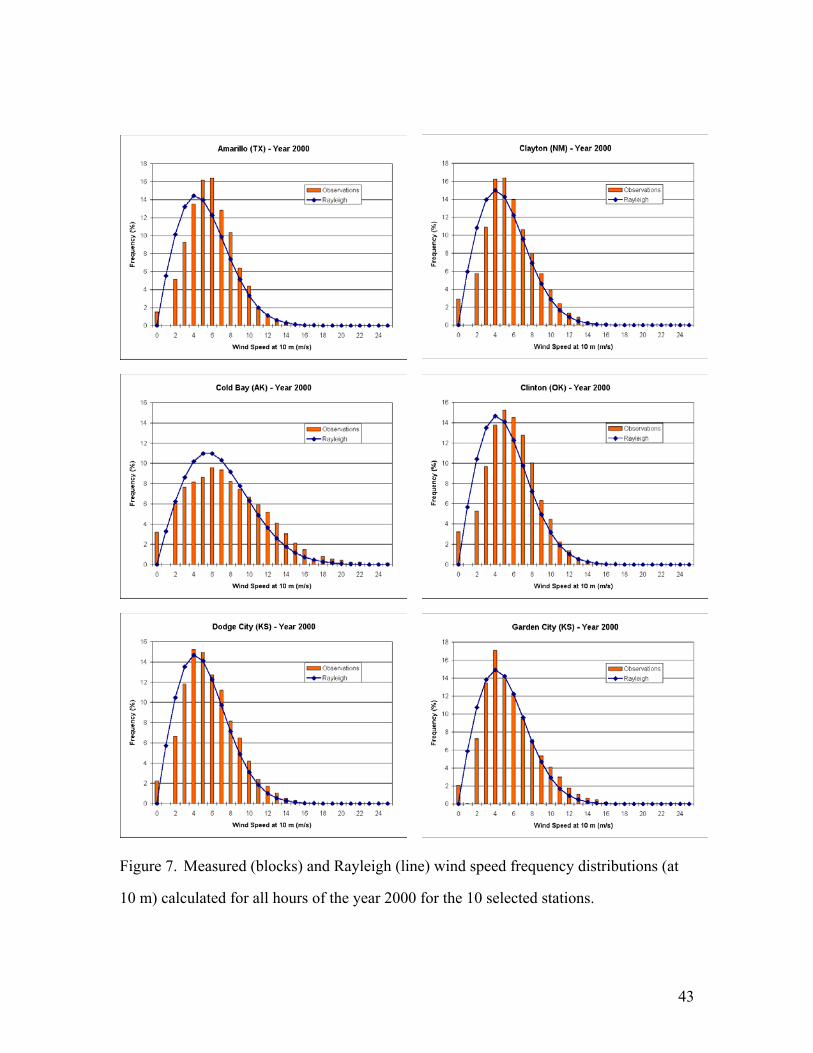
Figure 7. Measured (blocks) and Rayleigh (line) wind speed frequency distributions (at
10 m) calculated for all hours of the year 2000 for the 10 selected stations.
43
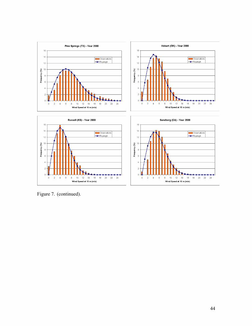
Figure 7. (continued).
44
Pine Springs (TX) - February 2000
02468
1012141618
0 2 4 6 8 10 12 14 16 18 20 22 24
Wind Speed at 10 m (m/s)
Freq
uenc
y (%
)
ObservationsRayleigh
Pine Springs (TX) - May 2000
02468
1012141618
0 2 4 6 8 10 12 14 16 18 20 22 24
Wind Speed at 10 m (m/s)
Freq
uenc
y (%
)
ObservationsRayleigh
Pine Springs (TX) - August 2000
02468
1012141618
0 2 4 6 8 10 12 14 16 18 20 22 24
Wind Speed at 10 m (m/s)
Freq
uenc
y (%
)
ObservationsRayleigh
Pine Springs (TX) - November 2000
02468
1012141618
0 2 4 6 8 10 12 14 16 18 20 22 24
Wind Speed at 10 m (m/s)
Freq
uenc
y (%
)ObservationsRayleigh
Figure 8. Measured (blocks) and Rayleigh (line) wind speed frequency distributions (at
10 m) calculated for all hours of each month of the year 2000 for Pine Springs, Texas,
(GDP).
45
Garden City (KS) - Hour 00:00
0
20
40
60
80
100
0 2 4 6 8 10 12 14 16 18 20 22 24
wind speed at 10 m (m/s)
num
ber o
f obs
erva
tions
Garden City (KS) - Hour 06:00
0
20
40
60
80
100
0 2 4 6 8 10 12 14 16 18 20 22 24
wind speed at 10 m (m/s)
num
ber o
f obs
erva
tions
Garden City (KS) - Hour 12:00
0
20
40
60
80
100
0 2 4 6 8 10 12 14 16 18 20 22 24
wind speed at 10 m (m/s)
num
ber o
f obs
erva
tions
Garden City (KS) - Hour 15:00
0
20
40
60
80
100
0 2 4 6 8 10 12 14 16 18 20 22 24
wind speed at 10 m (m/s)
num
ber o
f obs
erva
tions
Garden City (KS) - Hour 17:00
0
20
40
60
80
100
0 2 4 6 8 10 12 14 16 18 20 22 24
wind speed at 10 m (m/s)
num
ber o
f obs
erva
tions
Garden City (KS) - Hour 22:00
0
20
40
60
80
100
0 2 4 6 8 10 12 14 16 18 20 22 24
wind speed at 10 m (m/s)
num
ber o
f obs
erva
tions
Figure 9. Wind speed frequency distributions (at 10 m) calculated for all days of the year
2000 at selected hours of the day for Garden City, Kansas (GCK).
46
Amarillo (TX) - Year 2000
0
500
1000
1500
2000
2500
3000
3500
0 2 4 6 8 10 12 14 16 18 20 22Hour
Win
d Po
wer
[W/m
2 ]
0
2
4
6
8
10
12
14
16
Win
d Sp
eed
[m/s
]
Rayleigh PowerMean PowerMean Speed
Clayton (NM) - Year 2000
0
500
1000
1500
2000
2500
3000
3500
0 2 4 6 8 10 12 14 16 18 20 22Hour
Win
d Po
wer
[W/m
2 ]
0
2
4
6
8
10
12
14
16
Win
d Sp
eed
[m/s
]
Rayleigh PowerMean PowerMean Speed
Cold Bay (AK) - Year 2000
0
2000
4000
6000
8000
10000
12000
0 2 4 6 8 10 12 14 16 18 20 22Hour
Win
d Po
wer
[W/m
2 ]
0
5
10
15
20
25
Win
d Sp
eed
[m/s
]
Rayleigh PowerMean PowerMean Speed
Clinton (OK) - Year 2000
0
500
1000
1500
2000
2500
3000
3500
0 2 4 6 8 10 12 14 16 18 20 22Hour
Win
d Po
wer
[W/m
2 ]
0
2
4
6
8
10
12
14
16
Win
d Sp
eed
[m/s
]
Rayleigh PowerMean PowerMean Speed
Dodge City (KS) - Year 2000
0
500
1000
1500
2000
2500
3000
3500
0 2 4 6 8 10 12 14 16 18 20 22Hour
Win
d Po
wer
[W/m
2 ]
0
2
4
6
8
10
12
14
16
Win
d Sp
eed
[m/s
]
Rayleigh PowerMean PowerMean Speed
Garden City (KS) - Year 2000
0
500
1000
1500
2000
2500
3000
3500
0 2 4 6 8 10 12 14 16 18 20 22Hour
Win
d Po
wer
[W/m
2 ]
0
2
4
6
8
10
12
14
16
Win
d Sp
eed
[m/s
]
Rayleigh PowerMean PowerMean Speed
Figure 10. Calculated power (◊), Rayleigh power (□), and mean wind speed ( )
extrapolated to 80 m, averaged over all days of the year 2000 for each hour of the day at
the 10 selected sites.
47
Pine Springs (TX) - Year 2000
0
1000
2000
3000
4000
5000
6000
7000
8000
9000
0 2 4 6 8 10 12 14 16 18 20 22Hour
Win
d Po
wer
[W/m
2 ]
0
2
4
6
8
10
12
14
16
18
20
Win
d Sp
eed
[m/s
]
Rayleigh PowerMean PowerMean Speed
Hobart (OK) - Year 2000
0
500
1000
1500
2000
2500
3000
3500
0 2 4 6 8 10 12 14 16 18 20 22Hour
Win
d Po
wer
[W/m
2 ]
0
2
4
6
8
10
12
14
16
Win
d Sp
eed
[m/s
]
Rayleigh PowerMean PowerMean Speed
Russell (KS) - Year 2000
0
500
1000
1500
2000
2500
3000
3500
0 2 4 6 8 10 12 14 16 18 20 22Hour
Win
d Po
wer
[W/m
2 ]
0
2
4
6
8
10
12
14
16W
ind
Spee
d [m
/s]
Rayleigh PowerMean PowerMean Speed
Sandberg (CA) - Year 2000
0
500
1000
1500
2000
2500
3000
3500
4000
4500
0 2 4 6 8 10 12 14 16 18 20 22Hour
Win
d Po
wer
[W/m
2 ]
0
2
4
6
8
10
12
14
16
Win
d Sp
eed
[m/s
]
Rayleigh PowerMean PowerMean Speed
Figure 10. (continued).
48
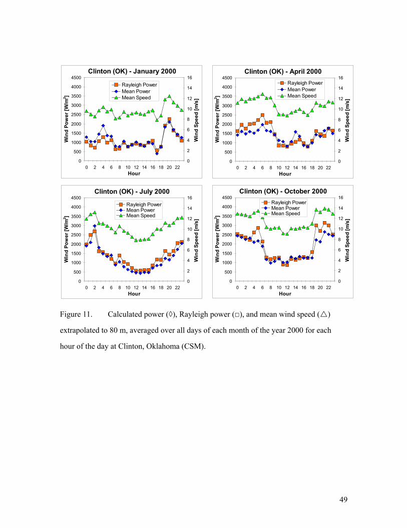
Clinton (OK) - April 2000
0
500
1000
1500
2000
2500
3000
3500
4000
4500
0 2 4 6 8 10 12 14 16 18 20 22Hour
Win
d Po
wer
[W/m
2 ]
0
2
4
6
8
10
12
14
16
Win
d Sp
eed
[m/s
]
Rayleigh PowerMean PowerMean Speed
Clinton (OK) - January 2000
0
500
1000
1500
2000
2500
3000
3500
4000
4500
0 2 4 6 8 10 12 14 16 18 20 22Hour
Win
d Po
wer
[W/m
2 ]
0
2
4
6
8
10
12
14
16
Win
d Sp
eed
[m/s
]
Rayleigh PowerMean PowerMean Speed
Clinton (OK) - October 2000
0
500
1000
1500
2000
2500
3000
3500
4000
4500
0 2 4 6 8 10 12 14 16 18 20 22Hour
Win
d Po
wer
[W/m
2 ]
0
2
4
6
8
10
12
14
16
Win
d Sp
eed
[m/s
]
Rayleigh PowerMean PowerMean Speed
Clinton (OK) - July 2000
0
500
1000
1500
2000
2500
3000
3500
4000
4500
0 2 4 6 8 10 12 14 16 18 20 22Hour
Win
d Po
wer
[W/m
2 ]
0
2
4
6
8
10
12
14
16W
ind
Spee
d [m
/s]
Rayleigh PowerMean PowerMean Speed
Figure 11. Calculated power (◊), Rayleigh power (□), and mean wind speed ( )
extrapolated to 80 m, averaged over all days of each month of the year 2000 for each
hour of the day at Clinton, Oklahoma (CSM).
49
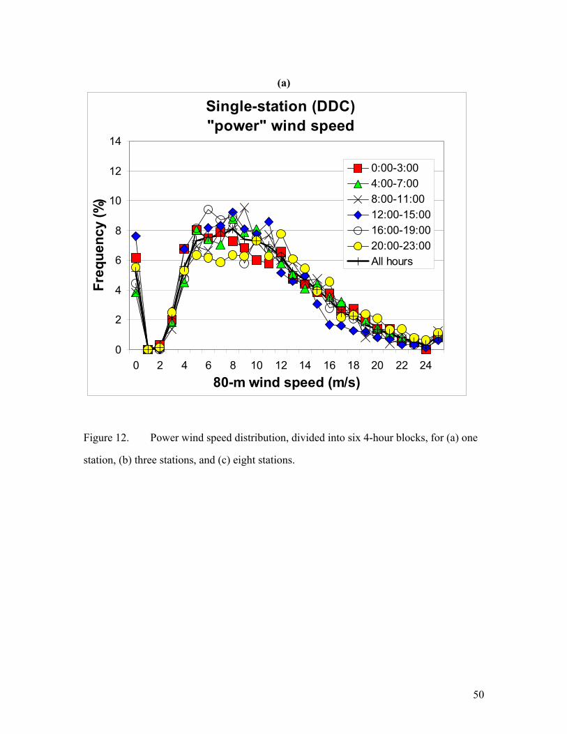
(a)
Figure 12. Power wind speed distribution, divided into six 4-hour blocks, for (a) one
Single-station (DDC) "power" wind speed
0
2
4
6
8
10
12
14
0 2 4 6 8 10 12 14 16 18 20 22 2480-m wind speed (m/s)
Freq
uenc
y (%
)
0:00-3:004:00-7:008:00-11:0012:00-15:0016:00-19:0020:00-23:00All hours
station, (b) three stations, and (c) eight stations.
50
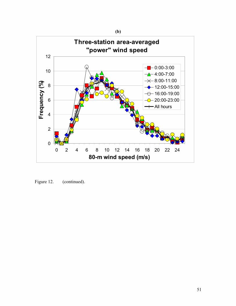
(b)
igure 12. (continued).
Three-station area-averaged
"power" wind speed
0
2
4
6
8
10
12
0 2 4 6 8 10 12 14 16 18 20 22 2480-m wind speed (m/s)
Freq
uenc
y (%
)
0:00-3:004:00-7:008:00-11:0012:00-15:0016:00-19:0020:00-23:00All hours
F
51
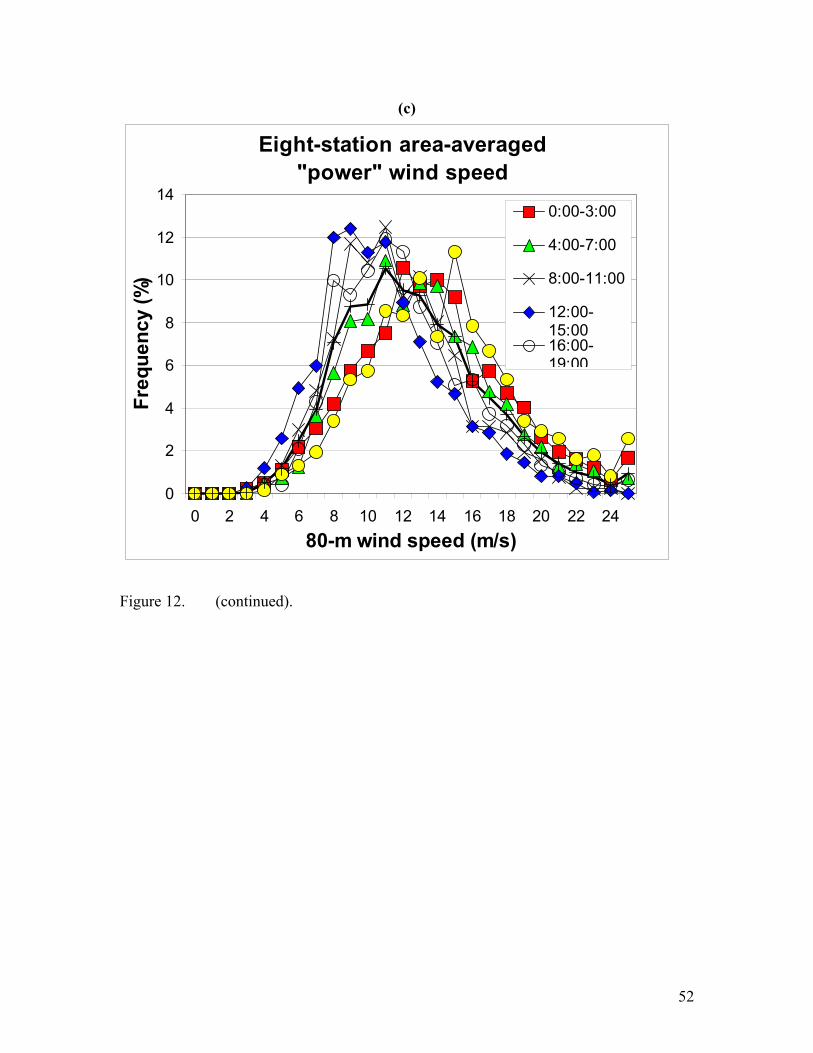
52
(c)
Figure 12. (continued).
Eight-station area-averaged
"power" wind speed
0
2
4
6
8
10
12
14
0 2 4 6 8 10 12 14 16 18 20 22 2480-m wind speed (m/s)
Freq
uenc
y (%
)
0:00-3:00
4:00-7:00
8:00-11:00
12:00-15:0016:00-19:00
Related Documents


![SwellandWind-SeaDistributionsovertheMid …downloads.hindawi.com/archive/2012/306723.pdfwith local wind, over the altimeter derived winds [17]. For the present paper, the wind data](https://static.cupdf.com/doc/110x72/5f4b08001c19827d55340593/swellandwind-seadistributionsoverthemid-with-local-wind-over-the-altimeter-derived.jpg)


