Foundations and Trends R in Signal Processing Vol. 4, Nos. 1–2 (2010) 1–222 c 2011 T. Wiegand and H. Schwarz DOI: 10.1561/2000000010 Source Coding: Part I of Fundamentals of Source and Video Coding By Thomas Wiegand and Heiko Schwarz Contents 1 Introduction 2 1.1 The Communication Problem 3 1.2 Scope and Overview of the Text 4 1.3 The Source Coding Principle 6 2 Random Processes 8 2.1 Probability 9 2.2 Random Variables 10 2.3 Random Processes 15 2.4 Summary of Random Processes 20 3 Lossless Source Coding 22 3.1 Classification of Lossless Source Codes 23 3.2 Variable-Length Coding for Scalars 24 3.3 Variable-Length Coding for Vectors 36 3.4 Elias Coding and Arithmetic Coding 42 3.5 Probability Interval Partitioning Entropy Coding 55 3.6 Comparison of Lossless Coding Techniques 64 3.7 Adaptive Coding 66 3.8 Summary of Lossless Source Coding 67

Welcome message from author
This document is posted to help you gain knowledge. Please leave a comment to let me know what you think about it! Share it to your friends and learn new things together.
Transcript
Foundations and TrendsR© inSignal ProcessingVol. 4, Nos. 1–2 (2010) 1–222c© 2011 T. Wiegand and H. SchwarzDOI: 10.1561/2000000010
Source Coding: Part I of Fundamentals ofSource and Video Coding
By Thomas Wiegand and Heiko Schwarz
Contents
1 Introduction 2
1.1 The Communication Problem 31.2 Scope and Overview of the Text 41.3 The Source Coding Principle 6
2 Random Processes 8
2.1 Probability 92.2 Random Variables 102.3 Random Processes 152.4 Summary of Random Processes 20
3 Lossless Source Coding 22
3.1 Classification of Lossless Source Codes 233.2 Variable-Length Coding for Scalars 243.3 Variable-Length Coding for Vectors 363.4 Elias Coding and Arithmetic Coding 423.5 Probability Interval Partitioning Entropy Coding 553.6 Comparison of Lossless Coding Techniques 643.7 Adaptive Coding 663.8 Summary of Lossless Source Coding 67
4 Rate Distortion Theory 69
4.1 The Operational Rate Distortion Function 704.2 The Information Rate Distortion Function 754.3 The Shannon Lower Bound 844.4 Rate Distortion Function for Gaussian Sources 934.5 Summary of Rate Distortion Theory 101
5 Quantization 103
5.1 Structure and Performance of Quantizers 1045.2 Scalar Quantization 1075.3 Vector Quantization 1365.4 Summary of Quantization 148
6 Predictive Coding 150
6.1 Prediction 1526.2 Linear Prediction 1566.3 Optimal Linear Prediction 1586.4 Differential Pulse Code Modulation (DPCM) 1676.5 Summary of Predictive Coding 178
7 Transform Coding 180
7.1 Structure of Transform Coding Systems 1837.2 Orthogonal Block Transforms 1847.3 Bit Allocation for Transform Coefficients 1917.4 The Karhunen Loeve Transform (KLT) 1967.5 Signal-Independent Unitary Transforms 2047.6 Transform Coding Example 2107.7 Summary of Transform Coding 212
8 Summary 214
Acknowledgments 217
References 218
Foundations and TrendsR© inSignal ProcessingVol. 4, Nos. 1–2 (2010) 1–222c© 2011 T. Wiegand and H. SchwarzDOI: 10.1561/2000000010
Source Coding: Part I of Fundamentals ofSource and Video Coding
Thomas Wiegand1 and Heiko Schwarz2
1 Berlin Institute of Technology and Fraunhofer Institute forTelecommunications — Heinrich Hertz Institute, Germany,[email protected]
2 Fraunhofer Institute for Telecommunications — Heinrich Hertz Institute,Germany, [email protected]
Abstract
Digital media technologies have become an integral part of the way wecreate, communicate, and consume information. At the core of thesetechnologies are source coding methods that are described in this mono-graph. Based on the fundamentals of information and rate distortiontheory, the most relevant techniques used in source coding algorithmsare described: entropy coding, quantization as well as predictive andtransform coding. The emphasis is put onto algorithms that are alsoused in video coding, which will be explained in the other part of thistwo-part monograph.
1Introduction
The advances in source coding technology along with the rapiddevelopments and improvements of network infrastructures, storagecapacity, and computing power are enabling an increasing number ofmultimedia applications. In this monograph, we will describe and ana-lyze fundamental source coding techniques that are found in a varietyof multimedia applications, with the emphasis on algorithms that areused in video coding applications. The present first part of the mono-graph concentrates on the description of fundamental source codingtechniques, while the second part describes their application in mod-ern video coding.
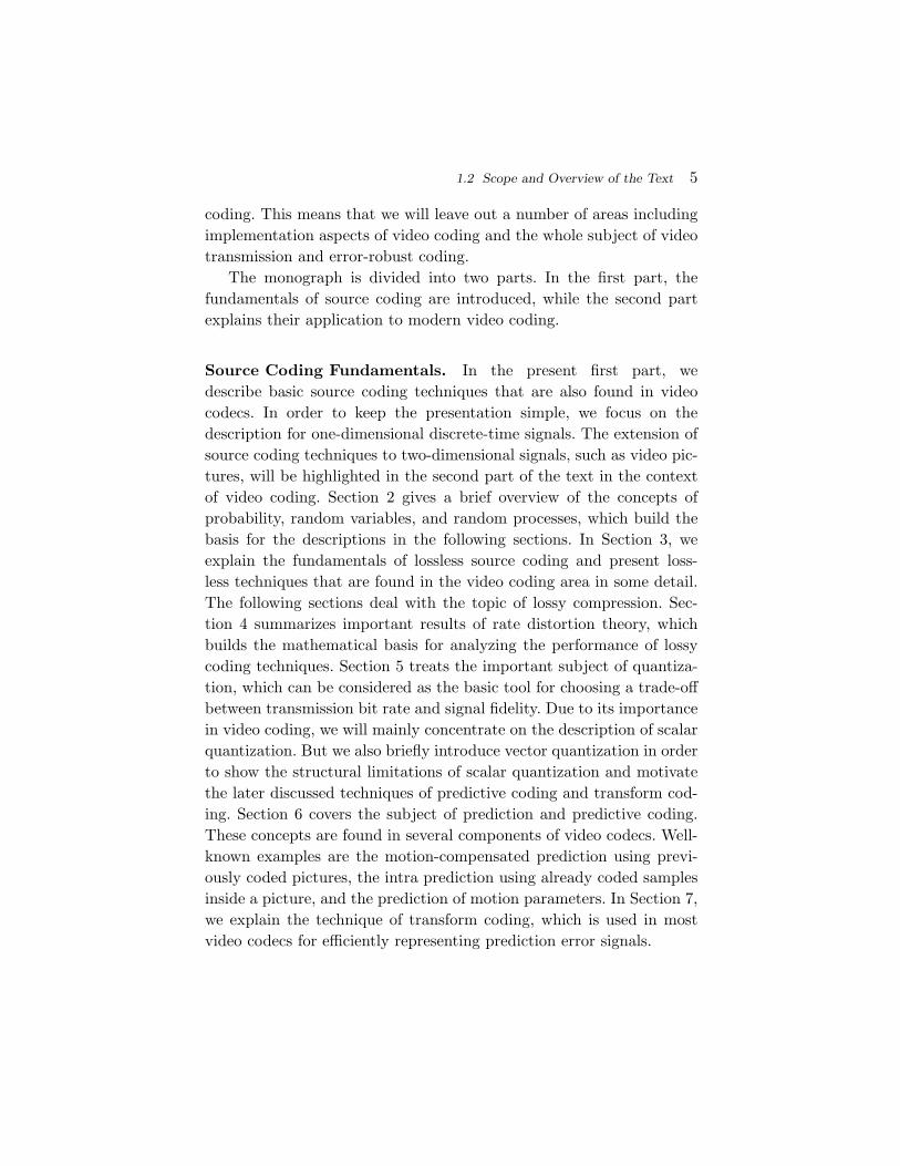
The block structure for a typical transmission scenario is illustratedin Figure 1.1. The source generates a signal s. The source encoder mapsthe signal s into the bitstream b. The bitstream is transmitted over theerror control channel and the received bitstream b′ is processed by thesource decoder that reconstructs the decoded signal s′ and delivers it tothe sink which is typically a human observer. This monograph focuseson the source encoder and decoder parts, which is together called asource codec.
The error characteristic of the digital channel can be controlled bythe channel encoder, which adds redundancy to the bits at the source
2

1.1 The Communication Problem 3
Fig. 1.1 Typical structure of a transmission system.
encoder output b. The modulator maps the channel encoder outputto an analog signal, which is suitable for transmission over a physi-cal channel. The demodulator interprets the received analog signal asa digital signal, which is fed into the channel decoder. The channeldecoder processes the digital signal and produces the received bit-stream b′, which may be identical to b even in the presence of channelnoise. The sequence of the five components, channel encoder, modula-tor, channel, demodulator, and channel decoder, are lumped into onebox, which is called the error control channel. According to Shannon’sbasic work [63, 64] that also laid the ground to the subject of this text,by introducing redundancy at the channel encoder and by introducingdelay, the amount of transmission errors can be controlled.
1.1 The Communication Problem
The basic communication problem may be posed as conveying sourcedata with the highest fidelity possible without exceeding an available bitrate, or it may be posed as conveying the source data using the lowestbit rate possible while maintaining a specified reproduction fidelity [63].In either case, a fundamental trade-off is made between bit rate andsignal fidelity. The ability of a source coding system to suitably choosethis trade-off is referred to as its coding efficiency or rate distortionperformance. Source codecs are thus primarily characterized in terms of:
• throughput of the channel: a characteristic influenced by thetransmission channel bit rate and the amount of protocol

4 Introduction
and error-correction coding overhead incurred by the trans-mission system; and
• distortion of the decoded signal: primarily induced by thesource codec and by channel errors introduced in the path tothe source decoder.
However, in practical transmission systems, the following additionalissues must be considered:
• delay: a characteristic specifying the start-up latency andend-to-end delay. The delay is influenced by many parame-ters, including the processing and buffering delay, structuraldelays of source and channel codecs, and the speed at whichdata are conveyed through the transmission channel;
• complexity: a characteristic specifying the computationalcomplexity, the memory capacity, and memory accessrequirements. It includes the complexity of the source codec,protocol stacks, and network.
The practical source coding design problem can be stated as follows:
Given a maximum allowed delay and a maximumallowed complexity, achieve an optimal trade-off betweenbit rate and distortion for the range of network environ-ments envisioned in the scope of the applications.
1.2 Scope and Overview of the Text
This monograph provides a description of the fundamentals of sourceand video coding. It is aimed at aiding students and engineers to inves-tigate the subject. When we felt that a result is of fundamental impor-tance to the video codec design problem, we chose to deal with it ingreater depth. However, we make no attempt to exhaustive coverage ofthe subject, since it is too broad and too deep to fit the compact presen-tation format that is chosen here (and our time limit to write this text).We will also not be able to cover all the possible applications of videocoding. Instead our focus is on the source coding fundamentals of video
1.2 Scope and Overview of the Text 5
coding. This means that we will leave out a number of areas includingimplementation aspects of video coding and the whole subject of videotransmission and error-robust coding.
The monograph is divided into two parts. In the first part, thefundamentals of source coding are introduced, while the second partexplains their application to modern video coding.
Source Coding Fundamentals. In the present first part, wedescribe basic source coding techniques that are also found in videocodecs. In order to keep the presentation simple, we focus on thedescription for one-dimensional discrete-time signals. The extension ofsource coding techniques to two-dimensional signals, such as video pic-tures, will be highlighted in the second part of the text in the contextof video coding. Section 2 gives a brief overview of the concepts ofprobability, random variables, and random processes, which build thebasis for the descriptions in the following sections. In Section 3, weexplain the fundamentals of lossless source coding and present loss-less techniques that are found in the video coding area in some detail.The following sections deal with the topic of lossy compression. Sec-tion 4 summarizes important results of rate distortion theory, whichbuilds the mathematical basis for analyzing the performance of lossycoding techniques. Section 5 treats the important subject of quantiza-tion, which can be considered as the basic tool for choosing a trade-offbetween transmission bit rate and signal fidelity. Due to its importancein video coding, we will mainly concentrate on the description of scalarquantization. But we also briefly introduce vector quantization in orderto show the structural limitations of scalar quantization and motivatethe later discussed techniques of predictive coding and transform cod-ing. Section 6 covers the subject of prediction and predictive coding.These concepts are found in several components of video codecs. Well-known examples are the motion-compensated prediction using previ-ously coded pictures, the intra prediction using already coded samplesinside a picture, and the prediction of motion parameters. In Section 7,we explain the technique of transform coding, which is used in mostvideo codecs for efficiently representing prediction error signals.

6 Introduction
Application to Video Coding. The second part of the monographwill describe the application of the fundamental source coding tech-niques to video coding. We will discuss the basic structure and thebasic concepts that are used in video coding and highlight their appli-cation in modern video coding standards. Additionally, we will consideradvanced encoder optimization techniques that are relevant for achiev-ing a high coding efficiency. The effectiveness of various design aspectswill be demonstrated based on experimental results.
1.3 The Source Coding Principle
The present first part of the monograph describes the fundamentalconcepts of source coding. We explain various known source codingprinciples and demonstrate their efficiency based on one-dimensionalmodel sources. For additional information on information theoreticalaspects of source coding the reader is referred to the excellent mono-graphs in [4, 11, 22]. For the overall subject of source coding includingalgorithmic design questions, we recommend the two fundamental textsby Gersho and Gray [16] and Jayant and Noll [40].
The primary task of a source codec is to represent a signal with theminimum number of (binary) symbols without exceeding an “accept-able level of distortion”, which is determined by the application. Twotypes of source coding techniques are typically named:
• Lossless coding: describes coding algorithms that allow theexact reconstruction of the original source data from the com-pressed data. Lossless coding can provide a reduction in bitrate compared to the original data, when the original sig-nal contains dependencies or statistical properties that canbe exploited for data compaction. It is also referred to asnoiseless coding or entropy coding. Lossless coding can onlybe employed for discrete-amplitude and discrete-time signals.A well-known use for this type of compression for picture andvideo signals is JPEG-LS [35].
• Lossy coding: describes coding algorithms that are character-ized by an irreversible loss of information. Only an approxi-mation of the original source data can be reconstructed from
1.3 The Source Coding Principle 7
the compressed data. Lossy coding is the primary codingtype for the compression of speech, audio, picture, and videosignals, where an exact reconstruction of the source data isnot required. The practically relevant bit rate reduction thatcan be achieved with lossy source coding techniques is typi-cally more than an order of magnitude larger than that forlossless source coding techniques. Well known examples forthe application of lossy coding techniques are JPEG [33]for still picture coding, and H.262/MPEG-2 Video [34] andH.264/AVC [38] for video coding.
Section 2 briefly reviews the concepts of probability, random vari-ables, and random processes. Lossless source coding will be describedin Section 3. Sections 5–7 give an introduction to the lossy coding tech-niques that are found in modern video coding applications. In Section 4,we provide some important results of rate distortion theory, whichwill be used for discussing the efficiency of the presented lossy cod-ing techniques.
2Random Processes
The primary goal of video communication, and signal transmission ingeneral, is the transmission of new information to a receiver. Since thereceiver does not know the transmitted signal in advance, the source ofinformation can be modeled as a random process. This permits thedescription of source coding and communication systems using themathematical framework of the theory of probability and random pro-cesses. If reasonable assumptions are made with respect to the sourceof information, the performance of source coding algorithms can becharacterized based on probabilistic averages. The modeling of informa-tion sources as random processes builds the basis for the mathematicaltheory of source coding and communication.
In this section, we give a brief overview of the concepts of proba-bility, random variables, and random processes and introduce modelsfor random processes, which will be used in the following sections forevaluating the efficiency of the described source coding algorithms. Forfurther information on the theory of probability, random variables, andrandom processes, the interested reader is referred to [25, 41, 56].
8
2.1 Probability 9
2.1 Probability
Probability theory is a branch of mathematics, which concerns thedescription and modeling of random events. The basis for modernprobability theory is the axiomatic definition of probability that wasintroduced by Kolmogorov [41] using the concepts from set theory.
We consider an experiment with an uncertain outcome, which iscalled a random experiment. The union of all possible outcomes ζ ofthe random experiment is referred to as the certain event or samplespace of the random experiment and is denoted by O. A subset A ofthe sample space O is called an event. To each event A a measure P (A)is assigned, which is referred to as the probability of the event A. Themeasure of probability satisfies the following three axioms:
• Probabilities are non-negative real numbers,
P (A) ≥ 0, ∀A ⊆ O. (2.1)
• The probability of the certain event O is equal to 1,
P (O) = 1. (2.2)
• The probability of the union of any countable set of pairwisedisjoint events is the sum of the probabilities of the individualevents; that is, if {Ai: i = 0,1, . . .} is a countable set of eventssuch that Ai ∩ Aj = ∅ for i �= j, then
P
(⋃i
Ai
)=∑
i
P (Ai). (2.3)
In addition to the axioms, the notion of the independence of two eventsand the conditional probability are introduced:
• Two events Ai and Aj are independent if the probability oftheir intersection is the product of their probabilities,
P (Ai ∩ Aj) = P (Ai)P (Aj). (2.4)
• The conditional probability of an event Ai given anotherevent Aj , with P (Aj) > 0, is denoted by P (Ai|Aj) and is

10 Random Processes
defined as
P (Ai|Aj) =P (Ai ∩ Aj)
P (Aj). (2.5)
The definitions (2.4) and (2.5) imply that, if two events Ai and Aj areindependent and P (Aj) > 0, the conditional probability of the event Ai
given the event Aj is equal to the marginal probability of Ai,
P (Ai |Aj) = P (Ai). (2.6)
A direct consequence of the definition of conditional probability in (2.5)is Bayes’ theorem,
P (Ai|Aj) = P (Aj |Ai)P (Ai)P (Aj)
, with P (Ai), P (Aj) > 0, (2.7)
which described the interdependency of the conditional probabilitiesP (Ai|Aj) and P (Aj |Ai) for two events Ai and Aj .
2.2 Random Variables
A concept that we will use throughout this monograph are randomvariables, which will be denoted by upper-case letters. A random vari-able S is a function of the sample space O that assigns a real value S(ζ)to each outcome ζ ∈ O of a random experiment.
The cumulative distribution function (cdf) of a random variable S
is denoted by FS(s) and specifies the probability of the event {S ≤ s},
FS(s) = P (S ≤ s) = P ({ζ : S(ζ)≤ s}). (2.8)
The cdf is a non-decreasing function with FS(−∞) = 0 and FS(∞) = 1.The concept of defining a cdf can be extended to sets of two or morerandom variables S = {S0, . . . ,SN−1}. The function
FS(s) = P (S ≤ s) = P (S0 ≤ s0, . . . ,SN−1 ≤ sN−1) (2.9)
is referred to as N -dimensional cdf, joint cdf, or joint distribution.A set S of random variables is also referred to as a random vectorand is also denoted using the vector notation S = (S0, . . . ,SN−1)T. Forthe joint cdf of two random variables X and Y we will use the notation
2.2 Random Variables 11
FXY (x,y) = P (X ≤ x,Y ≤ y). The joint cdf of two random vectors X
and Y will be denoted by FXY (x,y) = P (X ≤ x,Y ≤ y).The conditional cdf or conditional distribution of a random vari-
able S given an event B, with P (B)> 0, is defined as the conditionalprobability of the event {S ≤ s} given the event B,
FS|B(s |B) = P (S ≤ s |B) =P ({S ≤ s} ∩ B)
P (B). (2.10)
The conditional distribution of a random variable X, given anotherrandom variable Y , is denoted by FX|Y (x|y) and is defined as
FX|Y (x|y) =FXY (x,y)
FY (y)=
P (X ≤ x,Y ≤ y)P (Y ≤ y)
. (2.11)
Similarly, the conditional cdf of a random vector X, given anotherrandom vector Y , is given by FX|Y (x|y) = FXY (x,y)/FY (y).
2.2.1 Continuous Random Variables
A random variable S is called a continuous random variable, if its cdfFS(s) is a continuous function. The probability P (S = s) is equal tozero for all values of s. An important function of continuous randomvariables is the probability density function (pdf), which is defined asthe derivative of the cdf,
fS(s) =dFS(s)
ds⇔ FS(s) =
∫ s
−∞fS(t) dt. (2.12)
Since the cdf FS(s) is a monotonically non-decreasing function, thepdf fS(s) is greater than or equal to zero for all values of s. Importantexamples for pdfs, which we will use later in this monograph, are givenbelow.
Uniform pdf:
fS(s) = 1/A for − A/2 ≤ s ≤ A/2, A > 0 (2.13)
Laplacian pdf:
fS(s) =1
σS
√2
e−|s−µS |√2/σS , σS > 0 (2.14)
12 Random Processes
Gaussian pdf:
fS(s) =1
σS
√2π
e−(s−µS)2/(2σ2S), σS > 0 (2.15)
The concept of defining a probability density function is also extendedto random vectors S = (S0, . . . ,SN−1)T. The multivariate derivative ofthe joint cdf FS(s),
fS(s) =∂NFS(s)
∂s0 · · · ∂sN−1, (2.16)
is referred to as the N -dimensional pdf, joint pdf, or joint density. Fortwo random variables X and Y , we will use the notation fXY (x,y) fordenoting the joint pdf of X and Y . The joint density of two randomvectors X and Y will be denoted by fXY (x,y).
The conditional pdf or conditional density fS|B(s|B) of a randomvariable S given an event B, with P (B) > 0, is defined as the derivativeof the conditional distribution FS|B(s|B), fS|B(s|B) = dFS|B(s|B)/ds.The conditional density of a random variable X, given another randomvariable Y , is denoted by fX|Y (x|y) and is defined as
fX|Y (x|y) =fXY (x,y)
fY (y). (2.17)
Similarly, the conditional pdf of a random vector X, given anotherrandom vector Y , is given by fX|Y (x|y) = fXY (x,y)/fY (y).
2.2.2 Discrete Random Variables
A random variable S is said to be a discrete random variable if itscdf FS(s) represents a staircase function. A discrete random variable S
can only take values of a countable set A = {a0,a1, . . .}, which is calledthe alphabet of the random variable. For a discrete random variable S
with an alphabet A, the function
pS(a) = P (S = a) = P ({ζ : S(ζ)= a}), (2.18)
which gives the probabilities that S is equal to a particular alphabetletter, is referred to as probability mass function (pmf). The cdf FS(s)
2.2 Random Variables 13
of a discrete random variable S is given by the sum of the probabilitymasses p(a) with a≤ s,
FS(s) =∑a≤s
p(a). (2.19)
With the Dirac delta function δ it is also possible to use a pdf fS fordescribing the statistical properties of a discrete random variable S
with a pmf pS(a),
fS(s) =∑a∈A
δ(s − a) pS(a). (2.20)
Examples for pmfs that will be used in this monograph are listed below.The pmfs are specified in terms of parameters p and M , where p is areal number in the open interval (0,1) and M is an integer greaterthan 1. The binary and uniform pmfs are specified for discrete randomvariables with a finite alphabet, while the geometric pmf is specifiedfor random variables with a countably infinite alphabet.
Binary pmf:
A = {a0,a1}, pS(a0) = p, pS(a1) = 1 − p (2.21)
Uniform pmf:
A = {a0,a1, . . .,aM−1}, pS(ai) = 1/M, ∀ai ∈ A (2.22)
Geometric pmf:
A = {a0,a1, . . .}, pS(ai) = (1 − p)pi, ∀ai ∈ A (2.23)
The pmf for a random vector S = (S0, . . . ,SN−1)T is defined by
pS(a) = P (S = a) = P (S0 = a0, . . . ,SN−1 = aN−1) (2.24)
and is also referred to as N -dimensional pmf or joint pmf. The jointpmf for two random variables X and Y or two random vectors X and Y
will be denoted by pXY (ax,ay) or pXY (ax,ay), respectively.The conditional pmf pS|B(a |B) of a random variable S, given an
event B, with P (B) > 0, specifies the conditional probabilities of the
14 Random Processes
events {S = a} given the event B, pS|B(a |B) = P (S = a |B). The con-ditional pmf of a random variable X, given another random variable Y ,is denoted by pX|Y (ax|ay) and is defined as
pX|Y (ax|ay) =pXY (ax,ay)
pY (ay). (2.25)
Similarly, the conditional pmf of a random vector X, given anotherrandom vector Y , is given by pX|Y (ax|ay) = pXY (ax,ay)/pY (ay).
2.2.3 Expectation
Statistical properties of random variables are often expressed usingprobabilistic averages, which are referred to as expectation values orexpected values. The expectation value of an arbitrary function g(S) ofa continuous random variable S is defined by the integral
E{g(S)} =∫ ∞
−∞g(s) fS(s) ds. (2.26)
For discrete random variables S, it is defined as the sum
E{g(S)} =∑a∈A
g(a) pS(a). (2.27)
Two important expectation values are the mean µS and the variance σ2S
of a random variable S, which are given by
µS = E{S} and σ2S = E
{(S − µs)2
}. (2.28)
For the following discussion of expectation values, we consider continu-ous random variables. For discrete random variables, the integrals haveto be replaced by sums and the pdfs have to be replaced by pmfs.
The expectation value of a function g(S) of a set N random variablesS = {S0, . . . ,SN−1} is given by
E{g(S)} =∫
RN
g(s)fS(s)ds. (2.29)
The conditional expectation value of a function g(S) of a randomvariable S given an event B, with P (B) > 0, is defined by
E{g(S) |B} =∫ ∞
−∞g(s)fS|B(s |B) ds. (2.30)
2.3 Random Processes 15
The conditional expectation value of a function g(X) of random vari-able X given a particular value y for another random variable Y isspecified by
E{g(X) |y} = E{g(X) |Y =y} =∫ ∞
−∞g(x)fX|Y (x,y) dx (2.31)
and represents a deterministic function of the value y. If the value y isreplaced by the random variable Y , the expression E{g(X)|Y } specifiesa new random variable that is a function of the random variable Y . Theexpectation value E{Z} of a random variable Z = E{g(X)|Y } can becomputed using the iterative expectation rule,
E{E{g(X)|Y }} =∫ ∞
−∞
(∫ ∞
−∞g(x)fX|Y (x,y)dx
)fY (y)dy
=∫ ∞
−∞g(x)
(∫ ∞
−∞fX|Y (x,y)fY (y)dy
)dx
=∫ ∞
−∞g(x)fX(x)dx = E{g(X)} . (2.32)
In analogy to (2.29), the concept of conditional expectation values isalso extended to random vectors.
2.3 Random Processes
We now consider a series of random experiments that are performed attime instants tn, with n being an integer greater than or equal to 0. Theoutcome of each random experiment at a particular time instant tn ischaracterized by a random variable Sn = S(tn). The series of randomvariables S = {Sn} is called a discrete-time1 random process. The sta-tistical properties of a discrete-time random process S can be charac-terized by the Nth order joint cdf
FSk(s) = P (S(N)
k ≤ s) = P (Sk ≤ s0, . . . ,Sk+N−1 ≤ sN−1). (2.33)
Random processes S that represent a series of continuous random vari-ables Sn are called continuous random processes and random processesfor which the random variables Sn are of discrete type are referred
1 Continuous-time random processes are not considered in this monograph.
16 Random Processes
to as discrete random processes. For continuous random processes, thestatistical properties can also be described by the Nth order joint pdf,which is given by the multivariate derivative
fSk(s) =
∂N
∂s0 · · · ∂sN−1FSk
(s). (2.34)
For discrete random processes, the Nth order joint cdf FSk(s) can also
be specified using the Nth order joint pmf,
FSk(s) =
∑a∈AN
pSk(a), (2.35)
where AN represent the product space of the alphabets An for therandom variables Sn with n = k, . . . ,k + N − 1 and
pSk(a) = P (Sk = a0, . . . ,Sk+N−1 = aN−1). (2.36)
represents the Nth order joint pmf.The statistical properties of random processes S = {Sn} are often
characterized by an Nth order autocovariance matrix CN (tk) or an Nthorder autocorrelation matrix RN (tk). The Nth order autocovariancematrix is defined by
CN (tk) = E{
(S(N)k − µN (tk))(S
(N)k − µN (tk))T
}, (2.37)
where S(N)k represents the vector (Sk, . . . ,Sk+N−1)T of N successive
random variables and µN (tk) = E{S(N)k } is the Nth order mean. The
Nth order autocorrelation matrix is defined by
RN (tk) = E{
(S(N)k )(S(N)
k )T}
. (2.38)
A random process is called stationary if its statistical properties areinvariant to a shift in time. For stationary random processes, the Nthorder joint cdf FSk
(s), pdf fSk(s), and pmf pSk
(a) are independent ofthe first time instant tk and are denoted by FS(s), fS(s), and pS(a),respectively. For the random variables Sn of stationary processes wewill often omit the index n and use the notation S.
For stationary random processes, the Nth order mean, the Nthorder autocovariance matrix, and the Nth order autocorrelation matrix
2.3 Random Processes 17
are independent of the time instant tk and are denoted by µN , CN ,and RN , respectively. The Nth order mean µN is a vector with all N
elements being equal to the mean µS of the random variable S. TheNth order autocovariance matrix CN = E{(S(N) − µN )(S(N) − µN )T}is a symmetric Toeplitz matrix,
CN = σ2S
1 ρ1 ρ2 · · · ρN−1
ρ1 1 ρ1 · · · ρN−2
ρ2 ρ1 1 · · · ρN−3...
......
. . ....
ρN−1 ρN−2 ρN−3 · · · 1
. (2.39)
A Toepliz matrix is a matrix with constant values along all descend-ing diagonals from left to right. For information on the theory andapplication of Toeplitz matrices the reader is referred to the stan-dard reference [29] and the tutorial [23]. The (k, l)th element of theautocovariance matrix CN is given by the autocovariance functionφk,l = E{(Sk − µS)(Sl − µS)}. For stationary processes, the autoco-variance function depends only on the absolute values |k − l| and canbe written as φk,l = φ|k−l| = σ2
S ρ|k−l|. The Nth order autocorrelationmatrix RN is also a symmetric Toeplitz matrix. The (k, l)th element ofRN is given by rk,l = φk,l + µ2
S .A random process S = {Sn} for which the random variables Sn are
independent is referred to as memoryless random process. If a mem-oryless random process is additionally stationary it is also said to beindependent and identical distributed (iid), since the random variablesSn are independent and their cdfs FSn(s) = P (Sn ≤ s) do not depend onthe time instant tn. The Nth order cdf FS(s), pdf fS(s), and pmf pS(a)for iid processes, with s = (s0, . . . ,sN−1)T and a = (a0, . . . ,aN−1)T, aregiven by the products
FS(s) =N−1∏k=0
FS(sk), fS(s) =N−1∏k=0
fS(sk), pS(a) =N−1∏k=0
pS(ak),
(2.40)where FS(s), fS(s), and pS(a) are the marginal cdf, pdf, and pmf,respectively, for the random variables Sn.
18 Random Processes
2.3.1 Markov Processes
A Markov process is characterized by the property that future outcomesdo not depend on past outcomes, but only on the present outcome,
P (Sn ≤sn |Sn−1 =sn−1, . . .) = P (Sn ≤sn |Sn−1 =sn−1). (2.41)
This property can also be expressed in terms of the pdf,
fSn(sn | sn−1, . . .) = fSn(sn | sn−1), (2.42)
for continuous random processes, or in terms of the pmf,
pSn(an | an−1, . . .) = pSn(an | an−1), (2.43)
for discrete random processes,Given a continuous zero-mean iid process Z = {Zn}, a stationary
continuous Markov process S = {Sn} with mean µS can be constructedby the recursive rule
Sn = Zn + ρ (Sn−1 − µS) + µS , (2.44)
where ρ, with |ρ| < 1, represents the correlation coefficient between suc-cessive random variables Sn−1 and Sn. Since the random variables Zn
are independent, a random variable Sn only depends on the preced-ing random variable Sn−1. The variance σ2
S of the stationary Markovprocess S is given by
σ2S = E
{(Sn − µS)2
}= E{(Zn − ρ(Sn−1 − µS))2
}=
σ2Z
1 − ρ2 , (2.45)
where σ2Z = E
{Z2
n
}denotes the variance of the zero-mean iid process Z.
The autocovariance function of the process S is given by
φk,l = φ|k−l| = E{(Sk − µS)(Sl − µS)
}= σ2
S ρ|k−l|. (2.46)
Each element φk,l of the Nth order autocorrelation matrix CN repre-sents a non-negative integer power of the correlation coefficient ρ.
In the following sections, we will often obtain expressions thatdepend on the determinant |CN | of the Nth order autocovari-ance matrix CN . For stationary continuous Markov processes given

2.3 Random Processes 19
by (2.44), the determinant |CN | can be expressed by a simple relation-ship. Using Laplace’s formula, we can expand the determinant of theNth order autocovariance matrix along the first column,
∣∣CN
∣∣ = N−1∑k=0
(−1)k φk,0∣∣C(k,0)
N
∣∣ = N−1∑k=0
(−1)k σ2S ρk∣∣C(k,0)
N
∣∣, (2.47)
where C(k,l)N represents the matrix that is obtained by removing the
kth row and lth column from CN . The first row of each matrix C(k,l)N ,
with k > 1, is equal to the second row of the same matrix multiplied bythe correlation coefficient ρ. Hence, the first two rows of these matricesare linearly dependent and the determinants |C(k,l)
N |, with k > 1, areequal to 0. Thus, we obtain∣∣CN
∣∣ = σ2S
∣∣C(0,0)N
∣∣ − σ2S ρ∣∣C(1,0)
N
∣∣. (2.48)
The matrix C(0,0)N represents the autocovariance matrix CN−1 of the
order (N − 1). The matrix C(1,0)N is equal to CN−1 except that the first
row is multiplied by the correlation coefficient ρ. Hence, the determi-nant |C(1,0)
N | is equal to ρ |CN−1|, which yields the recursive rule∣∣CN
∣∣ = σ2S (1 − ρ2)
∣∣CN−1∣∣. (2.49)
By using the expression |C1| = σ2S for the determinant of the first order
autocovariance matrix, we obtain the relationship∣∣CN
∣∣ = σ2NS (1 − ρ2)N−1. (2.50)
2.3.2 Gaussian Processes
A continuous random process S ={Sn} is said to be a Gaussian pro-cess if all finite collections of random variables Sn represent Gaussianrandom vectors. The Nth order pdf of a stationary Gaussian process S
with mean µS and variance σ2S is given by
fS(s) =1
(2π)N/2 |CN |1/2 e− 12 (s−µN )TC−1
N (s−µN ), (2.51)
where s is a vector of N consecutive samples, µN is the Nth order mean(a vector with all N elements being equal to the mean µS), and CN isan Nth order nonsingular autocovariance matrix given by (2.39).
20 Random Processes
2.3.3 Gauss–Markov Processes
A continuous random process is called a Gauss–Markov process if itsatisfies the requirements for both Gaussian processes and Markovprocesses. The statistical properties of a stationary Gauss–Markov arecompletely specified by its mean µS , its variance σ2
S , and its correlationcoefficient ρ. The stationary continuous process in (2.44) is a stationaryGauss–Markov process if the random variables Zn of the zero-mean iidprocess Z have a Gaussian pdf fZ(s).
The Nth order pdf of a stationary Gauss–Markov process S withthe mean µS , the variance σ2
S , and the correlation coefficient ρ is givenby (2.51), where the elements φk,l of the Nth order autocovariancematrix CN depend on the variance σ2
S and the correlation coefficient ρ
and are given by (2.46). The determinant |CN | of the Nth order auto-covariance matrix of a stationary Gauss–Markov process can be writtenaccording to (2.50).
2.4 Summary of Random Processes
In this section, we gave a brief review of the concepts of random vari-ables and random processes. A random variable is a function of thesample space of a random experiment. It assigns a real value to eachpossible outcome of the random experiment. The statistical propertiesof random variables can be characterized by cumulative distributionfunctions (cdfs), probability density functions (pdfs), probability massfunctions (pmfs), or expectation values.
Finite collections of random variables are called random vectors.A countably infinite sequence of random variables is referred to as(discrete-time) random process. Random processes for which the sta-tistical properties are invariant to a shift in time are called stationaryprocesses. If the random variables of a process are independent, the pro-cess is said to be memoryless. Random processes that are stationaryand memoryless are also referred to as independent and identically dis-tributed (iid) processes. Important models for random processes, whichwill also be used in this monograph, are Markov processes, Gaussianprocesses, and Gauss–Markov processes.

2.4 Summary of Random Processes 21
Beside reviewing the basic concepts of random variables and randomprocesses, we also introduced the notations that will be used throughoutthe monograph. For simplifying formulas in the following sections, wewill often omit the subscripts that characterize the random variable(s)or random vector(s) in the notations of cdfs, pdfs, and pmfs.
3Lossless Source Coding
Lossless source coding describes a reversible mapping of sequences ofdiscrete source symbols into sequences of codewords. In contrast tolossy coding techniques, the original sequence of source symbols can beexactly reconstructed from the sequence of codewords. Lossless codingis also referred to as noiseless coding or entropy coding. If the origi-nal signal contains statistical properties or dependencies that can beexploited for data compression, lossless coding techniques can providea reduction in transmission rate. Basically all source codecs, and inparticular all video codecs, include a lossless coding part by which thecoding symbols are efficiently represented inside a bitstream.
In this section, we give an introduction to lossless source cod-ing. We analyze the requirements for unique decodability, introducea fundamental bound for the minimum average codeword length persource symbol that can be achieved with lossless coding techniques,and discuss various lossless source codes with respect to their efficiency,applicability, and complexity. For further information on lossless codingtechniques, the reader is referred to the overview of lossless compressiontechniques in [62].
22
3.1 Classification of Lossless Source Codes 23
3.1 Classification of Lossless Source Codes
In this text, we restrict our considerations to the practically importantcase of binary codewords. A codeword is a sequence of binary symbols(bits) of the alphabet B ={0,1}. Let S ={Sn} be a stochastic processthat generates sequences of discrete source symbols. The source sym-bols sn are realizations of the random variables Sn, which are associatedwith Mn-ary alphabets An. By the process of lossless coding, a messages(L) ={s0, . . . ,sL−1} consisting of L source symbols is converted into asequence b(K) ={b0, . . . , bK−1} of K bits.
In practical coding algorithms, a message s(L) is often split intoblocks s(N) = {sn, . . . ,sn+N−1} of N symbols, with 1 ≤ N ≤ L, and acodeword b(�)(s(N)) = {b0, . . . , b�−1} of � bits is assigned to each of theseblocks s(N). The length � of a codeword b�(s(N)) can depend on thesymbol block s(N). The codeword sequence b(K) that represents themessage s(L) is obtained by concatenating the codewords b�(s(N)) forthe symbol blocks s(N). A lossless source code can be described by theencoder mapping
b(�) = γ(s(N) ), (3.1)
which specifies a mapping from the set of finite length symbol blocksto the set of finite length binary codewords. The decoder mapping
s(N) = γ−1(b(�) ) = γ−1(γ(s(N) )) (3.2)
is the inverse of the encoder mapping γ.Depending on whether the number N of symbols in the blocks s(N)
and the number � of bits for the associated codewords are fixed orvariable, the following categories can be distinguished:
(1) Fixed-to-fixed mapping: a fixed number of symbols is mappedto fixed-length codewords. The assignment of a fixed num-ber � of bits to a fixed number N of symbols yields a codewordlength of �/N bit per symbol. We will consider this type oflossless source codes as a special case of the next type.
(2) Fixed-to-variable mapping: a fixed number of symbols ismapped to variable-length codewords. A well-known methodfor designing fixed-to-variable mappings is the Huffman

24 Lossless Source Coding
algorithm for scalars and vectors, which we will describe inSections 3.2 and 3.3, respectively.
(3) Variable-to-fixed mapping: a variable number of symbols ismapped to fixed-length codewords. An example for this typeof lossless source codes are Tunstall codes [61, 67]. We willnot further describe variable-to-fixed mappings in this text,because of its limited use in video coding.
(4) Variable-to-variable mapping: a variable number of symbolsis mapped to variable-length codewords. A typical examplefor this type of lossless source codes are arithmetic codes,which we will describe in Section 3.4. As a less-complex alter-native to arithmetic coding, we will also present the proba-bility interval projection entropy code in Section 3.5.
3.2 Variable-Length Coding for Scalars
In this section, we consider lossless source codes that assign a sepa-rate codeword to each symbol sn of a message s(L). It is supposed thatthe symbols of the message s(L) are generated by a stationary discreterandom process S = {Sn}. The random variables Sn = S are character-ized by a finite1 symbol alphabet A = {a0, . . . ,aM−1} and a marginalpmf p(a) = P (S = a). The lossless source code associates each letter ai
of the alphabet A with a binary codeword bi = {bi0, . . . , b
i�(ai)−1} of a
length �(ai) ≥ 1. The goal of the lossless code design is to minimize theaverage codeword length
� = E{�(S)} =M−1∑i=0
p(ai) �(ai), (3.3)
while ensuring that each message s(L) is uniquely decodable given theircoded representation b(K).
1 The fundamental concepts and results shown in this section are also valid for countablyinfinite symbol alphabets (M → ∞).
3.2 Variable-Length Coding for Scalars 25
3.2.1 Unique Decodability
A code is said to be uniquely decodable if and only if each valid codedrepresentation b(K) of a finite number K of bits can be produced byonly one possible sequence of source symbols s(L).
A necessary condition for unique decodability is that each letter ai
of the symbol alphabet A is associated with a different codeword. Codeswith this property are called non-singular codes and ensure that a singlesource symbol is unambiguously represented. But if messages with morethan one symbol are transmitted, non-singularity is not sufficient toguarantee unique decodability, as will be illustrated in the following.
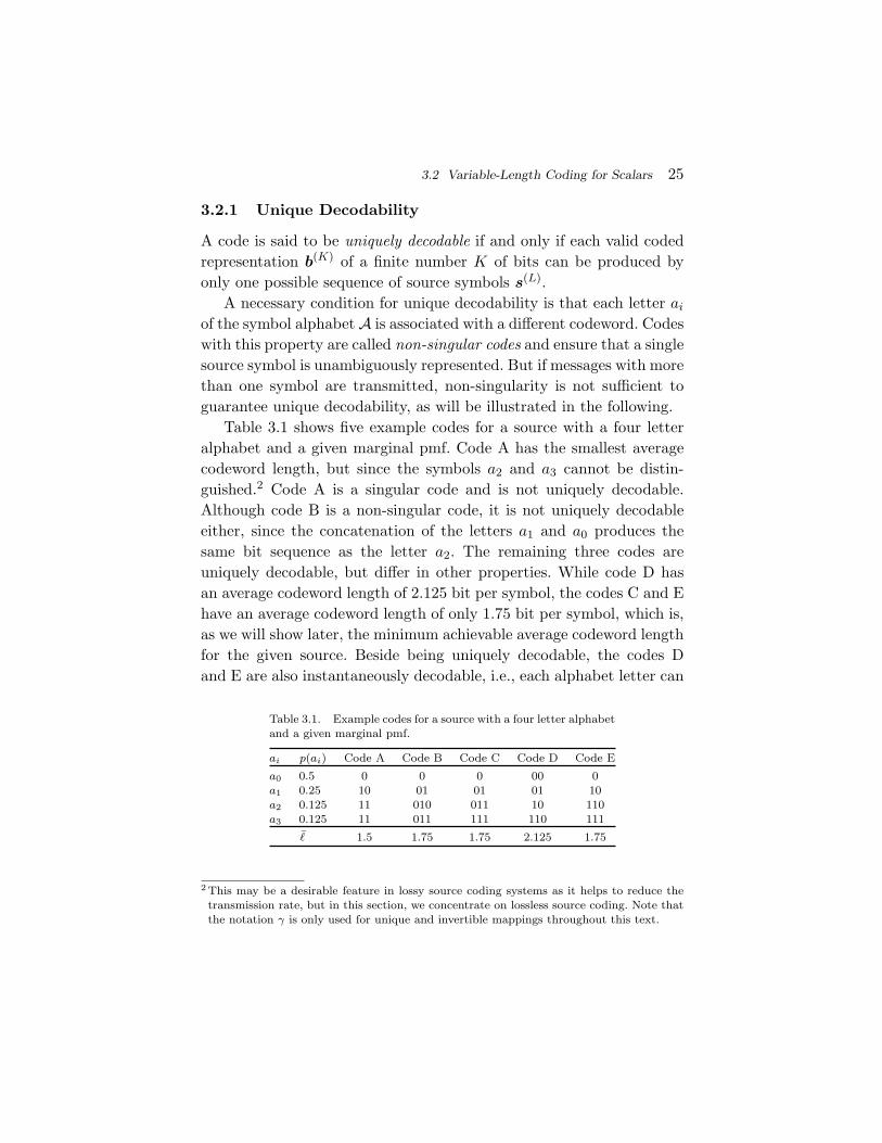
Table 3.1 shows five example codes for a source with a four letteralphabet and a given marginal pmf. Code A has the smallest averagecodeword length, but since the symbols a2 and a3 cannot be distin-guished.2 Code A is a singular code and is not uniquely decodable.Although code B is a non-singular code, it is not uniquely decodableeither, since the concatenation of the letters a1 and a0 produces thesame bit sequence as the letter a2. The remaining three codes areuniquely decodable, but differ in other properties. While code D hasan average codeword length of 2.125 bit per symbol, the codes C and Ehave an average codeword length of only 1.75 bit per symbol, which is,as we will show later, the minimum achievable average codeword lengthfor the given source. Beside being uniquely decodable, the codes Dand E are also instantaneously decodable, i.e., each alphabet letter can
Table 3.1. Example codes for a source with a four letter alphabetand a given marginal pmf.
ai p(ai) Code A Code B Code C Code D Code E
a0 0.5 0 0 0 00 0a1 0.25 10 01 01 01 10a2 0.125 11 010 011 10 110a3 0.125 11 011 111 110 111
� 1.5 1.75 1.75 2.125 1.75
2 This may be a desirable feature in lossy source coding systems as it helps to reduce thetransmission rate, but in this section, we concentrate on lossless source coding. Note thatthe notation γ is only used for unique and invertible mappings throughout this text.
26 Lossless Source Coding
be decoded right after the bits of its codeword are received. The code Cdoes not have this property. If a decoder for the code C receives a bitequal to 0, it has to wait for the next bit equal to 0 before a symbolcan be decoded. Theoretically, the decoder might need to wait untilthe end of the message. The value of the next symbol depends on howmany bits equal to 1 are received between the zero bits.
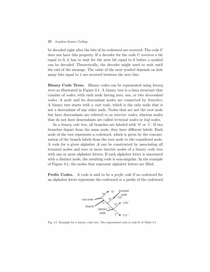
Binary Code Trees. Binary codes can be represented using binarytrees as illustrated in Figure 3.1. A binary tree is a data structure thatconsists of nodes, with each node having zero, one, or two descendantnodes. A node and its descendant nodes are connected by branches.A binary tree starts with a root node, which is the only node that isnot a descendant of any other node. Nodes that are not the root nodebut have descendants are referred to as interior nodes, whereas nodesthat do not have descendants are called terminal nodes or leaf nodes.
In a binary code tree, all branches are labeled with ‘0’ or ‘1’. If twobranches depart from the same node, they have different labels. Eachnode of the tree represents a codeword, which is given by the concate-nation of the branch labels from the root node to the considered node.A code for a given alphabet A can be constructed by associating allterminal nodes and zero or more interior nodes of a binary code treewith one or more alphabet letters. If each alphabet letter is associatedwith a distinct node, the resulting code is non-singular. In the exampleof Figure 3.1, the nodes that represent alphabet letters are filled.
Prefix Codes. A code is said to be a prefix code if no codeword foran alphabet letter represents the codeword or a prefix of the codeword
‘0’
‘0’
‘0’
‘0’
‘10’
‘1’
‘1’
‘1’ ‘110’
‘111’
root node
interiornode
terminalnode
branch
Fig. 3.1 Example for a binary code tree. The represented code is code E of Table 3.1.
3.2 Variable-Length Coding for Scalars 27
for any other alphabet letter. If a prefix code is represented by a binarycode tree, this implies that each alphabet letter is assigned to a distinctterminal node, but not to any interior node. It is obvious that everyprefix code is uniquely decodable. Furthermore, we will prove later thatfor every uniquely decodable code there exists a prefix code with exactlythe same codeword lengths. Examples for prefix codes are codes Dand E in Table 3.1.
Based on the binary code tree representation the parsing rule forprefix codes can be specified as follows:
(1) Set the current node ni equal to the root node.
(2) Read the next bit b from the bitstream.
(3) Follow the branch labeled with the value of b from the currentnode ni to the descendant node nj .
(4) If nj is a terminal node, return the associated alphabet letterand proceed with step 1. Otherwise, set the current node ni
equal to nj and repeat the previous two steps.
The parsing rule reveals that prefix codes are not only uniquely decod-able, but also instantaneously decodable. As soon as all bits of a code-word are received, the transmitted symbol is immediately known. Dueto this property, it is also possible to switch between different indepen-dently designed prefix codes inside a bitstream (i.e., because symbolswith different alphabets are interleaved according to a given bitstreamsyntax) without impacting the unique decodability.
Kraft Inequality. A necessary condition for uniquely decodablecodes is given by the Kraft inequality,
M−1∑i=0
2−�(ai) ≤ 1. (3.4)
For proving this inequality, we consider the term(M−1∑i=0
2−�(ai)
)L=
M−1∑i0=0
M−1∑i1=0
· · ·M−1∑
iL−1=0
2−(�(ai0 )+�(ai1 )+···+�(aiL−1 )
). (3.5)
28 Lossless Source Coding
The term �L = �(ai0) + �(ai1) + · · · + �(aiL−1) represents the combinedcodeword length for coding L symbols. Let A(�L) denote the num-ber of distinct symbol sequences that produce a bit sequence with thesame length �L. A(�L) is equal to the number of terms 2−�L that arecontained in the sum of the right-hand side of (3.5). For a uniquelydecodable code, A(�L) must be less than or equal to 2�L , since thereare only 2�L distinct bit sequences of length �L. If the maximum lengthof a codeword is �max, the combined codeword length �L lies inside theinterval [L,L · �max]. Hence, a uniquely decodable code must fulfill theinequality(
M−1∑i=0
2−�(ai)
)L=
L·�max∑�L=L
A(�L)2−�L ≤L·�max∑�L=L
2�L 2−�L = L(�max − 1) + 1.
(3.6)The left-hand side of this inequality grows exponentially with L, whilethe right-hand side grows only linearly with L. If the Kraft inequality(3.4) is not fulfilled, we can always find a value of L for which the con-dition (3.6) is violated. And since the constraint (3.6) must be obeyedfor all values of L ≥ 1, this proves that the Kraft inequality specifies anecessary condition for uniquely decodable codes.
The Kraft inequality does not only provide a necessary conditionfor uniquely decodable codes, it is also always possible to constructa uniquely decodable code for any given set of codeword lengths{�0, �1, . . . , �M−1} that satisfies the Kraft inequality. We prove this state-ment for prefix codes, which represent a subset of uniquely decodablecodes. Without loss of generality, we assume that the given codewordlengths are ordered as �0 ≤ �1 ≤ ·· · ≤ �M−1. Starting with an infinitebinary code tree, we chose an arbitrary node of depth �0 (i.e., a nodethat represents a codeword of length �0) for the first codeword andprune the code tree at this node. For the next codeword length �1, oneof the remaining nodes with depth �1 is selected. A continuation of thisprocedure yields a prefix code for the given set of codeword lengths,unless we cannot select a node for a codeword length �i because allnodes of depth �i have already been removed in previous steps. It shouldbe noted that the selection of a codeword of length �k removes 2�i−�k
codewords with a length of �i ≥ �k. Consequently, for the assignment
3.2 Variable-Length Coding for Scalars 29
of a codeword length �i, the number of available codewords is given by
n(�i) = 2�i −i−1∑k=0
2�i−�k = 2�i
(1 −
i−1∑k=0
2−�k
). (3.7)
If the Kraft inequality (3.4) is fulfilled, we obtain
n(�i) ≥ 2�i
(M−1∑k=0
2−�k −i−1∑k=0
2−�k
)= 1 +
M−1∑k=i+1
2−�k ≥ 1. (3.8)
Hence, it is always possible to construct a prefix code, and thus auniquely decodable code, for a given set of codeword lengths that sat-isfies the Kraft inequality.
The proof shows another important property of prefix codes. Sinceall uniquely decodable codes fulfill the Kraft inequality and it is alwayspossible to construct a prefix code for any set of codeword lengths thatsatisfies the Kraft inequality, there do not exist uniquely decodablecodes that have a smaller average codeword length than the best prefixcode. Due to this property and since prefix codes additionally provideinstantaneous decodability and are easy to construct, all variable-lengthcodes that are used in practice are prefix codes.
3.2.2 Entropy
Based on the Kraft inequality, we now derive a lower bound for theaverage codeword length of uniquely decodable codes. The expression(3.3) for the average codeword length � can be rewritten as
� =M−1∑i=0
p(ai)�(ai) = −M−1∑i=0
p(ai) log2
(2−�(ai)
p(ai)
)−
M−1∑i=0
p(ai) log2 p(ai).
(3.9)With the definition q(ai) = 2−�(ai)/
(∑M−1k=0 2−�(ak)
), we obtain
� = − log2
(M−1∑i=0
2−�(ai)
)−
M−1∑i=0
p(ai) log2
(q(ai)p(ai)
)−
M−1∑i=0
p(ai) log2 p(ai).
(3.10)Since the Kraft inequality is fulfilled for all uniquely decodable codes,the first term on the right-hand side of (3.10) is greater than or equal
30 Lossless Source Coding
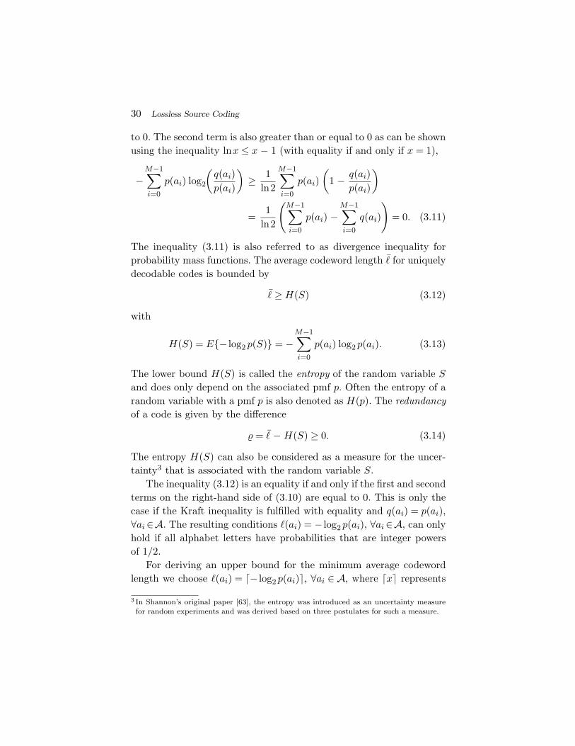
to 0. The second term is also greater than or equal to 0 as can be shownusing the inequality lnx ≤ x − 1 (with equality if and only if x = 1),
−M−1∑i=0
p(ai) log2
(q(ai)p(ai)
)≥ 1
ln2
M−1∑i=0
p(ai)(
1 − q(ai)p(ai)
)
=1
ln2
(M−1∑i=0
p(ai) −M−1∑i=0
q(ai)
)= 0. (3.11)
The inequality (3.11) is also referred to as divergence inequality forprobability mass functions. The average codeword length � for uniquelydecodable codes is bounded by
� ≥ H(S) (3.12)
with
H(S) = E{− log2 p(S)} = −M−1∑i=0
p(ai) log2 p(ai). (3.13)
The lower bound H(S) is called the entropy of the random variable S
and does only depend on the associated pmf p. Often the entropy of arandom variable with a pmf p is also denoted as H(p). The redundancyof a code is given by the difference
= � − H(S) ≥ 0. (3.14)
The entropy H(S) can also be considered as a measure for the uncer-tainty3 that is associated with the random variable S.
The inequality (3.12) is an equality if and only if the first and secondterms on the right-hand side of (3.10) are equal to 0. This is only thecase if the Kraft inequality is fulfilled with equality and q(ai) = p(ai),∀ai ∈A. The resulting conditions �(ai) = − log2 p(ai), ∀ai ∈A, can onlyhold if all alphabet letters have probabilities that are integer powersof 1/2.
For deriving an upper bound for the minimum average codewordlength we choose �(ai) = �− log2 p(ai) , ∀ai ∈ A, where �x represents
3 In Shannon’s original paper [63], the entropy was introduced as an uncertainty measurefor random experiments and was derived based on three postulates for such a measure.

3.2 Variable-Length Coding for Scalars 31
the smallest integer greater than or equal to x. Since these codewordlengths satisfy the Kraft inequality, as can be shown using �x ≥ x,
M−1∑i=0
2−�− log2 p(ai) ≤M−1∑i=0
2log2 p(ai) =M−1∑i=0
p(ai) = 1, (3.15)
we can always construct a uniquely decodable code. For the averagecodeword length of such a code, we obtain, using �x < x + 1,
� =M−1∑i=0
p(ai)�− log2 p(ai) <
M−1∑i=0
p(ai) (1− log2 p(ai)) = H(S) + 1.
(3.16)The minimum average codeword length �min that can be achieved withuniquely decodable codes that assign a separate codeword to each letterof an alphabet always satisfies the inequality
H(S) ≤ �min < H(S) + 1. (3.17)
The upper limit is approached for a source with a two-letter alphabetand a pmf {p,1 − p} if the letter probability p approaches 0 or 1 [15].
3.2.3 The Huffman Algorithm
For deriving an upper bound for the minimum average codeword lengthwe chose �(ai) = �− log2 p(ai) , ∀ai ∈ A. The resulting code has a redun-dancy = � − H(Sn) that is always less than 1 bit per symbol, but itdoes not necessarily achieve the minimum average codeword length.For developing an optimal uniquely decodable code, i.e., a code thatachieves the minimum average codeword length, it is sufficient to con-sider the class of prefix codes, since for every uniquely decodable codethere exists a prefix code with the exactly same codeword length. Anoptimal prefix code has the following properties:
• For any two symbols ai,aj ∈ A with p(ai)> p(aj), the asso-ciated codeword lengths satisfy �(ai) ≤ �(aj).
• There are always two codewords that have the maximumcodeword length and differ only in the final bit.
These conditions can be proved as follows. If the first condition is notfulfilled, an exchange of the codewords for the symbols ai and aj would
32 Lossless Source Coding
decrease the average codeword length while preserving the prefix prop-erty. And if the second condition is not satisfied, i.e., if for a particularcodeword with the maximum codeword length there does not exist acodeword that has the same length and differs only in the final bit, theremoval of the last bit of the particular codeword would preserve theprefix property and decrease the average codeword length.
Both conditions for optimal prefix codes are obeyed if two code-words with the maximum length that differ only in the final bit areassigned to the two letters ai and aj with the smallest probabilities. Inthe corresponding binary code tree, a parent node for the two leaf nodesthat represent these two letters is created. The two letters ai and aj
can then be treated as a new letter with a probability of p(ai) + p(aj)and the procedure of creating a parent node for the nodes that repre-sent the two letters with the smallest probabilities can be repeated forthe new alphabet. The resulting iterative algorithm was developed andproved to be optimal by Huffman in [30]. Based on the construction ofa binary code tree, the Huffman algorithm for a given alphabet A witha marginal pmf p can be summarized as follows:
(1) Select the two letters ai and aj with the smallest probabilitiesand create a parent node for the nodes that represent thesetwo letters in the binary code tree.
(2) Replace the letters ai and aj by a new letter with an associ-ated probability of p(ai) + p(aj).
(3) If more than one letter remains, repeat the previous steps.
(4) Convert the binary code tree into a prefix code.
A detailed example for the application of the Huffman algorithm isgiven in Figure 3.2. Optimal prefix codes are often generally referred toas Huffman codes. It should be noted that there exist multiple optimalprefix codes for a given marginal pmf. A tighter bound than in (3.17)on the redundancy of Huffman codes is provided in [15].
3.2.4 Conditional Huffman Codes
Until now, we considered the design of variable-length codes for themarginal pmf of stationary random processes. However, for random
3.2 Variable-Length Coding for Scalars 33
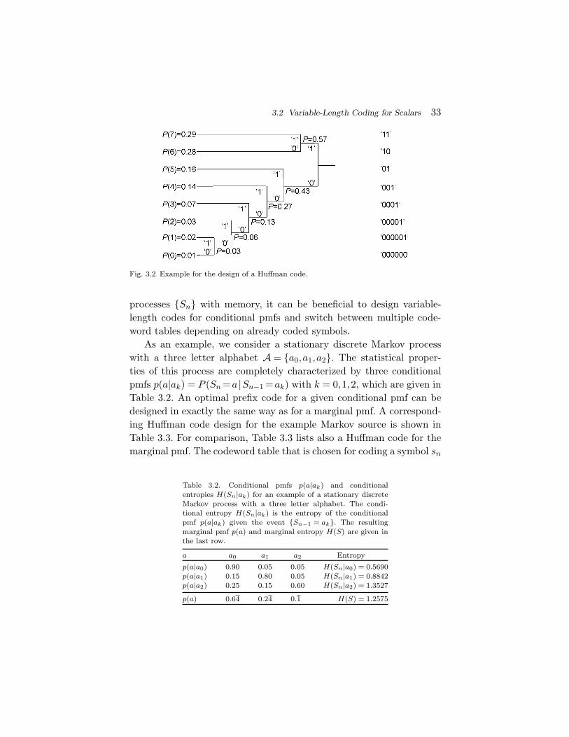
Fig. 3.2 Example for the design of a Huffman code.
processes {Sn} with memory, it can be beneficial to design variable-length codes for conditional pmfs and switch between multiple code-word tables depending on already coded symbols.
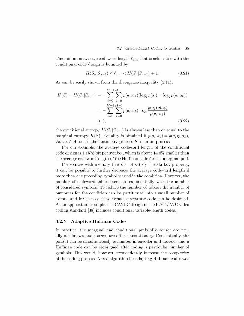
As an example, we consider a stationary discrete Markov processwith a three letter alphabet A = {a0,a1,a2}. The statistical proper-ties of this process are completely characterized by three conditionalpmfs p(a|ak) = P (Sn =a |Sn−1 =ak) with k = 0,1,2, which are given inTable 3.2. An optimal prefix code for a given conditional pmf can bedesigned in exactly the same way as for a marginal pmf. A correspond-ing Huffman code design for the example Markov source is shown inTable 3.3. For comparison, Table 3.3 lists also a Huffman code for themarginal pmf. The codeword table that is chosen for coding a symbol sn
Table 3.2. Conditional pmfs p(a|ak) and conditionalentropies H(Sn|ak) for an example of a stationary discreteMarkov process with a three letter alphabet. The condi-tional entropy H(Sn|ak) is the entropy of the conditionalpmf p(a|ak) given the event {Sn−1 = ak}. The resultingmarginal pmf p(a) and marginal entropy H(S) are given inthe last row.
a a0 a1 a2 Entropy
p(a|a0) 0.90 0.05 0.05 H(Sn|a0) = 0.5690p(a|a1) 0.15 0.80 0.05 H(Sn|a1) = 0.8842p(a|a2) 0.25 0.15 0.60 H(Sn|a2) = 1.3527
p(a) 0.64 0.24 0.1 H(S) = 1.2575

34 Lossless Source Coding
Table 3.3. Huffman codes for the conditional pmfs and the marginal pmf ofthe Markov process specified in Table 3.2.
Huffman codes for conditional pmfs
ai Sn−1 = a0 Sn−1 = a2 Sn−1 = a2 Huffman code for marginal pmf
a0 1 00 00 1a1 00 1 01 00a2 01 01 1 01
� 1.1 1.2 1.4 1.3556
depends on the value of the preceding symbol sn−1. It is important tonote that an independent code design for the conditional pmfs is onlypossible for instantaneously decodable codes, i.e., for prefix codes.
The average codeword length �k = �(Sn−1 =ak) of an optimal prefixcode for each of the conditional pmfs is guaranteed to lie in the half-open interval [H(Sn|ak),H(Sn|ak) + 1), where
H(Sn|ak) = H(Sn|Sn−1 =ak) = −M−1∑i=0
p(ai|ak) log2 p(ai|ak) (3.18)
denotes the conditional entropy of the random variable Sn given theevent {Sn−1 =ak}. The resulting average codeword length � for theconditional code is
� =M−1∑k=0
p(ak) �k. (3.19)
The resulting lower bound for the average codeword length � is referredto as the conditional entropy H(Sn|Sn−1) of the random variable Sn
assuming the random variable Sn−1 and is given by
H(Sn|Sn−1) = E{− log2 p(Sn|Sn−1)} =M−1∑k=0
p(ak)H(Sn|Sn−1 =ak)
= −M−1∑i=0
M−1∑k=0
p(ai,ak) log2 p(ai|ak), (3.20)
where p(ai,ak) = P (Sn =ai,Sn−1 =ak) denotes the joint pmf of the ran-dom variables Sn and Sn−1. The conditional entropy H(Sn|Sn−1) spec-ifies a measure for the uncertainty about Sn given the value of Sn−1.
3.2 Variable-Length Coding for Scalars 35
The minimum average codeword length �min that is achievable with theconditional code design is bounded by
H(Sn|Sn−1) ≤ �min < H(Sn|Sn−1) + 1. (3.21)
As can be easily shown from the divergence inequality (3.11),
H(S) − H(Sn|Sn−1) = −M−1∑i=0
M−1∑k=0
p(ai,ak)(log2 p(ai) − log2 p(ai|ak))
= −M−1∑i=0
M−1∑k=0
p(ai,ak) log2p(ai)p(ak)p(ai,ak)
≥ 0, (3.22)
the conditional entropy H(Sn|Sn−1) is always less than or equal to themarginal entropy H(S). Equality is obtained if p(ai,ak) = p(ai)p(ak),∀ai,ak ∈ A, i.e., if the stationary process S is an iid process.
For our example, the average codeword length of the conditionalcode design is 1.1578 bit per symbol, which is about 14.6% smaller thanthe average codeword length of the Huffman code for the marginal pmf.
For sources with memory that do not satisfy the Markov property,it can be possible to further decrease the average codeword length ifmore than one preceding symbol is used in the condition. However, thenumber of codeword tables increases exponentially with the numberof considered symbols. To reduce the number of tables, the number ofoutcomes for the condition can be partitioned into a small number ofevents, and for each of these events, a separate code can be designed.As an application example, the CAVLC design in the H.264/AVC videocoding standard [38] includes conditional variable-length codes.
3.2.5 Adaptive Huffman Codes
In practice, the marginal and conditional pmfs of a source are usu-ally not known and sources are often nonstationary. Conceptually, thepmf(s) can be simultaneously estimated in encoder and decoder and aHuffman code can be redesigned after coding a particular number ofsymbols. This would, however, tremendously increase the complexityof the coding process. A fast algorithm for adapting Huffman codes was

36 Lossless Source Coding
proposed by Gallager [15]. But even this algorithm is considered as toocomplex for video coding application, so that adaptive Huffman codesare rarely used in this area.
3.3 Variable-Length Coding for Vectors
Although scalar Huffman codes achieve the smallest average codewordlength among all uniquely decodable codes that assign a separate code-word to each letter of an alphabet, they can be very inefficient if thereare strong dependencies between the random variables of a process. Forsources with memory, the average codeword length per symbol can bedecreased if multiple symbols are coded jointly. Huffman codes thatassign a codeword to a block of two or more successive symbols arereferred to as block Huffman codes or vector Huffman codes and repre-sent an alternative to conditional Huffman codes.4 The joint coding ofmultiple symbols is also advantageous for iid processes for which oneof the probabilities masses is close to 1.
3.3.1 Huffman Codes for Fixed-Length Vectors
We consider stationary discrete random sources S = {Sn} with anM -ary alphabet A = {a0, . . . ,aM−1}. If N symbols are coded jointly,the Huffman code has to be designed for the joint pmf
p(a0, . . . ,aN−1) = P (Sn =a0, . . . ,Sn+N−1 =aN−1)
of a block of N successive symbols. The average codeword length �min
per symbol for an optimum block Huffman code is bounded by
H(Sn, . . . ,Sn+N−1)N
≤ �min <H(Sn, . . . ,Sn+N−1)
N+
1N
, (3.23)
where
H(Sn, . . . ,Sn+N−1) = E{− log2 p(Sn, . . . ,Sn+N−1)} (3.24)
4 The concepts of conditional and block Huffman codes can also be combined by switchingcodeword tables for a block of symbols depending on the values of already coded symbols.
3.3 Variable-Length Coding for Vectors 37
is referred to as the block entropy for a set of N successive randomvariables {Sn, . . . ,Sn+N−1}. The limit
H(S) = limN→∞
H(S0, . . . ,SN−1)N
(3.25)
is called the entropy rate of a source S. It can be shown that the limit in(3.25) always exists for stationary sources [14]. The entropy rate H(S)represents the greatest lower bound for the average codeword length �
per symbol that can be achieved with lossless source coding techniques,
� ≥ H(S). (3.26)
For iid processes, the entropy rate
H(S) = limN→∞
E{− log2 p(S0,S1, . . . ,SN−1)}N
= limN→∞
∑N−1n=0 E{− log2 p(Sn)}
N= H(S) (3.27)
is equal to the marginal entropy H(S). For stationary Markov pro-cesses, the entropy rate
H(S) = limN→∞
E{− log2 p(S0,S1, . . . ,SN−1)}N
= limN→∞
E{− log2 p(S0)} +∑N−1
n=1 E{− log2 p(Sn|Sn−1)}N
= H(Sn|Sn+1) (3.28)
is equal to the conditional entropy H(Sn|Sn−1).As an example for the design of block Huffman codes, we con-
sider the discrete Markov process specified in Table 3.2. The entropyrate H(S) for this source is 0.7331 bit per symbol. Table 3.4(a) showsa Huffman code for the joint coding of two symbols. The average code-word length per symbol for this code is 1.0094 bit per symbol, which issmaller than the average codeword length obtained with the Huffmancode for the marginal pmf and the conditional Huffman code that wedeveloped in Section 3.2. As shown in Table 3.4(b), the average code-word length can be further reduced by increasing the number N ofjointly coded symbols. If N approaches infinity, the average codeword
38 Lossless Source Coding
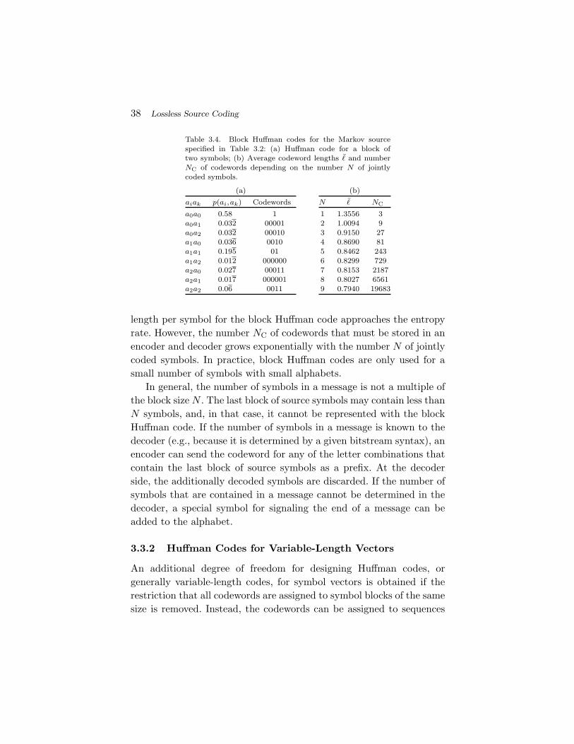
Table 3.4. Block Huffman codes for the Markov sourcespecified in Table 3.2: (a) Huffman code for a block oftwo symbols; (b) Average codeword lengths � and numberNC of codewords depending on the number N of jointlycoded symbols.
(a) (b)
aiak p(ai,ak) Codewords
a0a0 0.58 1a0a1 0.032 00001a0a2 0.032 00010a1a0 0.036 0010a1a1 0.195 01a1a2 0.012 000000a2a0 0.027 00011a2a1 0.017 000001a2a2 0.06 0011
N � NC
1 1.3556 32 1.0094 93 0.9150 274 0.8690 815 0.8462 2436 0.8299 7297 0.8153 21878 0.8027 65619 0.7940 19683
length per symbol for the block Huffman code approaches the entropyrate. However, the number NC of codewords that must be stored in anencoder and decoder grows exponentially with the number N of jointlycoded symbols. In practice, block Huffman codes are only used for asmall number of symbols with small alphabets.
In general, the number of symbols in a message is not a multiple ofthe block size N . The last block of source symbols may contain less thanN symbols, and, in that case, it cannot be represented with the blockHuffman code. If the number of symbols in a message is known to thedecoder (e.g., because it is determined by a given bitstream syntax), anencoder can send the codeword for any of the letter combinations thatcontain the last block of source symbols as a prefix. At the decoderside, the additionally decoded symbols are discarded. If the number ofsymbols that are contained in a message cannot be determined in thedecoder, a special symbol for signaling the end of a message can beadded to the alphabet.
3.3.2 Huffman Codes for Variable-Length Vectors
An additional degree of freedom for designing Huffman codes, orgenerally variable-length codes, for symbol vectors is obtained if therestriction that all codewords are assigned to symbol blocks of the samesize is removed. Instead, the codewords can be assigned to sequences

3.3 Variable-Length Coding for Vectors 39
of a variable number of successive symbols. Such a code is also referredto as V2V code in this text. In order to construct a V2V code, a setof letter sequences with a variable number of letters is selected anda codeword is associated with each of these letter sequences. The setof letter sequences has to be chosen in a way that each message canbe represented by a concatenation of the selected letter sequences. Anexception is the end of a message, for which the same concepts as forblock Huffman codes (see above) can be used.
Similarly as for binary codes, the set of letter sequences can berepresented by an M -ary tree as depicted in Figure 3.3. In contrast tobinary code trees, each node has up to M descendants and each branchis labeled with a letter of the M -ary alphabet A = {a0,a1, . . . ,aM−1}.All branches that depart from a particular node are labeled with differ-ent letters. The letter sequence that is represented by a particular nodeis given by a concatenation of the branch labels from the root node tothe particular node. An M -ary tree is said to be a full tree if each nodeis either a leaf node or has exactly M descendants.
We constrain our considerations to full M -ary trees for which allleaf nodes and only the leaf nodes are associated with codewords. Thisrestriction yields a V2V code that fulfills the necessary condition statedabove and has additionally the following useful properties:
• Redundancy-free set of letter sequences: none of the lettersequences can be removed without violating the constraintthat each symbol sequence must be representable using theselected letter sequences.
Fig. 3.3 Example for an M -ary tree representing sequences of a variable number of letters,of the alphabet A = {a0,a1,a2}, with an associated variable length code.

40 Lossless Source Coding
• Instantaneously encodable codes: a codeword can be sentimmediately after all symbols of the associated lettersequence have been received.
The first property implies that any message can only be representedby a single sequence of codewords. The only exception is that, if thelast symbols of a message do not represent a letter sequence that isassociated with a codeword, one of multiple codewords can be selectedas discussed above.
Let NL denote the number of leaf nodes in a full M -ary tree T .Each leaf node Lk represents a sequence ak = {ak
0,ak1, . . . ,a
kNk−1} of Nk
alphabet letters. The associated probability p(Lk) for coding a symbolsequence {Sn, . . . ,Sn+Nk−1} is given by
p(Lk) = p(ak0 |B) p(ak
1 |ak0, B) · · · p(ak
Nk−1 |ak0, . . . , ak
Nk−2, B), (3.29)
where B represents the event that the preceding symbols {S0, . . . ,Sn−1}were coded using a sequence of complete codewords of the V2V tree.The term p(am |a0, . . . ,am−1,B) denotes the conditional pmf for a ran-dom variable Sn+m given the random variables Sn to Sn+m−1 and theevent B. For iid sources, the probability p(Lk) for a leaf node Lk sim-plifies to
p(Lk) = p(ak0) p(ak
1) · · · p(akNk−1). (3.30)
For stationary Markov sources, the probabilities p(Lk) are given by
p(Lk) = p(ak0 |B) p(ak
1 |ak0) · · · p(ak
Nk−1 |akNk−2). (3.31)
The conditional pmfs p(am |a0, . . . ,am−1,B) are given by the structureof the M -ary tree T and the conditional pmfs p(am |a0, . . . ,am−1) forthe random variables Sn+m assuming the preceding random variablesSn to Sn+m−1.
As an example, we show how the pmf p(a|B) = P (Sn =a|B) that isconditioned on the event B can be determined for Markov sources. Inthis case, the probability p(am|B) = P (Sn =am|B) that a codeword isassigned to a letter sequence that starts with a particular letter am of
3.3 Variable-Length Coding for Vectors 41
the alphabet A = {a0,a1, . . . ,aM−1} is given by
p(am|B) =NL−1∑k=0
p(am|akNk−1)p(ak
Nk−1|akNk−2) · · · p(ak
1|ak0)p(ak
0|B).
(3.32)These M equations form a homogeneous linear equation system thathas one set of non-trivial solutions p(a|B) = κ · {x0,x1, . . . ,xM−1}. Thescale factor κ and thus the pmf p(a|B) can be uniquely determined byusing the constraint
∑M−1m=0 p(am|B) = 1.
After the conditional pmfs p(am |a0, . . . ,am−1,B) have been deter-mined, the pmf p(L) for the leaf nodes can be calculated. An optimalprefix code for the selected set of letter sequences, which is representedby the leaf nodes of a full M -ary tree T , can be designed using theHuffman algorithm for the pmf p(L). Each leaf node Lk is associatedwith a codeword of �k bits. The average codeword length per symbol �
is given by the ratio of the average codeword length per letter sequenceand the average number of letters per letter sequence,
� =∑NL−1
k=0 p(Lk)�k∑NL−1k=0 p(Lk)Nk
. (3.33)
For selecting the set of letter sequences or the full M -ary tree T , weassume that the set of applicable V2V codes for an application is givenby parameters such as the maximum number of codewords (number ofleaf nodes). Given such a finite set of full M -ary trees, we can selectthe full M -ary tree T , for which the Huffman code yields the smallestaverage codeword length per symbol �.
As an example for the design of a V2V Huffman code, we againconsider the stationary discrete Markov source specified in Table 3.2.Table 3.5(a) shows a V2V code that minimizes the average codewordlength per symbol among all V2V codes with up to nine codewords.The average codeword length is 1.0049 bit per symbol, which is about0.4% smaller than the average codeword length for the block Huffmancode with the same number of codewords. As indicated in Table 3.5(b),when increasing the number of codewords, the average codeword lengthfor V2V codes usually decreases faster as for block Huffman codes. The
42 Lossless Source Coding
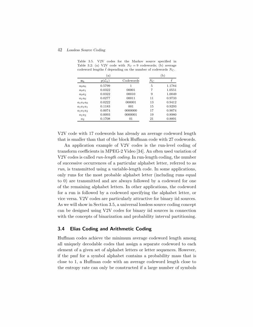
Table 3.5. V2V codes for the Markov source specified inTable 3.2: (a) V2V code with NC = 9 codewords; (b) averagecodeword lengths � depending on the number of codewords NC.
(a) (b)
ak p(Lk) Codewords
a0a0 0.5799 1a0a1 0.0322 00001a0a2 0.0322 00010a1a0 0.0277 00011
a1a1a0 0.0222 000001a1a1a1 0.1183 001a1a1a2 0.0074 0000000a1a2 0.0093 0000001a2 0.1708 01
NC �
5 1.17847 1.05519 1.004911 0.973313 0.941215 0.929317 0.907419 0.898021 0.8891
V2V code with 17 codewords has already an average codeword lengththat is smaller than that of the block Huffman code with 27 codewords.
An application example of V2V codes is the run-level coding oftransform coefficients in MPEG-2 Video [34]. An often used variation ofV2V codes is called run-length coding. In run-length coding, the numberof successive occurrences of a particular alphabet letter, referred to asrun, is transmitted using a variable-length code. In some applications,only runs for the most probable alphabet letter (including runs equalto 0) are transmitted and are always followed by a codeword for oneof the remaining alphabet letters. In other applications, the codewordfor a run is followed by a codeword specifying the alphabet letter, orvice versa. V2V codes are particularly attractive for binary iid sources.As we will show in Section 3.5, a universal lossless source coding conceptcan be designed using V2V codes for binary iid sources in connectionwith the concepts of binarization and probability interval partitioning.
3.4 Elias Coding and Arithmetic Coding
Huffman codes achieve the minimum average codeword length amongall uniquely decodable codes that assign a separate codeword to eachelement of a given set of alphabet letters or letter sequences. However,if the pmf for a symbol alphabet contains a probability mass that isclose to 1, a Huffman code with an average codeword length close tothe entropy rate can only be constructed if a large number of symbols

3.4 Elias Coding and Arithmetic Coding 43
is coded jointly. Such a block Huffman code does, however, requirea huge codeword table and is thus impractical for real applications.Additionally, a Huffman code for fixed- or variable-length vectors isnot applicable or at least very inefficient for symbol sequences in whichsymbols with different alphabets and pmfs are irregularly interleaved,as it is often found in image and video coding applications, where theorder of symbols is determined by a sophisticated syntax.
Furthermore, the adaptation of Huffman codes to sources withunknown or varying statistical properties is usually considered as toocomplex for real-time applications. It is desirable to develop a codeconstruction method that is capable of achieving an average codewordlength close to the entropy rate, but also provides a simple mecha-nism for dealing with nonstationary sources and is characterized by acomplexity that increases linearly with the number of coded symbols.
The popular method of arithmetic coding provides these properties.The initial idea is attributed to P. Elias (as reported in [1]) and isalso referred to as Elias coding. The first practical arithmetic codingschemes have been published by Pasco [57] and Rissanen [59]. In thefollowing, we first present the basic concept of Elias coding and con-tinue with highlighting some aspects of practical implementations. Forfurther details, the interested reader is referred to [72], [54] and [60].
3.4.1 Elias Coding
We consider the coding of symbol sequences s = {s0,s1, . . . ,sN−1}that represent realizations of a sequence of discrete random variablesS = {S0,S1, . . . ,SN−1}. The number N of symbols is assumed to beknown to both encoder and decoder. Each random variable Sn can becharacterized by a distinct Mn-ary alphabet An. The statistical prop-erties of the sequence of random variables S are completely describedby the joint pmf
p(s) = P (S =s) = P (S0 =s0,S1 =s1, . . . ,SN−1 =sN−1).
A symbol sequence sa ={sa0,s
a1, . . . ,s
aN−1} is considered to be less than
another symbol sequence sb ={sb0,s
b1, . . . ,s
bN−1} if and only if there
44 Lossless Source Coding
exists an integer n, with 0 ≤ n ≤ N − 1, so that
sak = sb
k for k = 0, . . . ,n − 1 and san < sb
n. (3.34)
Using this definition, the probability mass of a particular symbolsequence s can written as
p(s) = P (S =s) = P (S ≤s) − P (S <s). (3.35)
This expression indicates that a symbol sequence s can be representedby an interval IN between two successive values of the cumulative prob-ability mass function P (S ≤ s). The corresponding mapping of a sym-bol sequence s to a half-open interval IN ⊂ [0,1) is given by
IN (s) = [LN ,LN +WN ) = [P (S <s), P (S ≤s)). (3.36)
The interval width WN is equal to the probability P (S = s) of theassociated symbol sequence s. In addition, the intervals for differentrealizations of the random vector S are always disjoint. This can beshown by considering two symbol sequences sa and sb, with sa <sb.The lower interval boundary Lb
N of the interval IN (sb),
LbN = P (S <sb)
= P ({S ≤sa} ∪ {sa < S ≤ sb})
= P (S ≤sa) + P (S >sa, S <sb)
≥ P (S ≤ sa) = LaN + W a
N , (3.37)
is always greater than or equal to the upper interval boundary of thehalf-open interval IN (sa). Consequently, an N -symbol sequence s canbe uniquely represented by any real number v ∈ IN , which can be writ-ten as binary fraction with K bits after the binary point,
v =K−1∑i=0
bi 2i−1 = 0.b0b1 · · ·bK−1. (3.38)
In order to identify the symbol sequence s we only need to transmitthe bit sequence b = {b0, b1, . . . , bK−1}. The Elias code for the sequenceof random variables S is given by the assignment of bit sequences b tothe N -symbol sequences s.
3.4 Elias Coding and Arithmetic Coding 45
For obtaining codewords that are as short as possible, we shouldchoose the real numbers v that can be represented with the minimumamount of bits. The distance between successive binary fractions withK bits after the binary point is 2−K . In order to guarantee that anybinary fraction with K bits after the binary point falls in an intervalof size WN , we need K ≥ − log2 WN bits. Consequently, we choose
K = K(s) = �− log2 WN = �− log2 p(s) , (3.39)
where �x represents the smallest integer greater than or equal to x.The binary fraction v, and thus the bit sequence b, is determined by
v = �LN 2K · 2−K . (3.40)
An application of the inequalities �x ≥ x and �x < x + 1 to (3.40)and (3.39) yields
LN ≤ v < LN + 2−K ≤ LN + WN , (3.41)
which proves that the selected binary fraction v always lies inside theinterval IN . The Elias code obtained by choosing K = �− log2 WN associates each N -symbol sequence s with a distinct codeword b.
Iterative Coding. An important property of the Elias code is thatthe codewords can be iteratively constructed. For deriving the itera-tion rules, we consider sub-sequences s(n) = {s0,s1, . . . ,sn−1} that con-sist of the first n symbols, with 1 ≤ n ≤ N , of the symbol sequence s.Each of these sub-sequences s(n) can be treated in the same way asthe symbol sequence s. Given the interval width Wn for the sub-sequence s(n) = {s0,s1, . . . ,sn−1}, the interval width Wn+1 for the sub-sequence s(n+1) = {s(n),sn} can be derived by
Wn+1 = P(S(n+1) = s(n+1))
= P(S(n) = s(n), Sn =sn
)= P
(S(n) = s(n)) · P
(Sn = sn
∣∣ S(n) =s(n))= Wn · p(sn |s0,s1, . . . ,sn−1), (3.42)
46 Lossless Source Coding
with p(sn |s0,s1, . . . ,sn−1) being the conditional probability mass func-tion P (Sn =sn | S0 =s0,S1 =s1, . . . ,Sn−1 =sn−1). Similarly, the itera-tion rule for the lower interval border Ln is given by
Ln+1 = P(S(n+1) <s(n+1))
= P(S(n) <s(n)) + P
(S(n) =s(n), Sn <sn
)= P
(S(n) <s(n)) + P
(S(n) =s(n)) · P
(Sn <sn
∣∣S(n) =s(n))= Ln + Wn · c(sn |s0,s1, . . . ,sn−1), (3.43)
where c(sn |s0,s1, . . . ,sn−1) represents a cumulative probability massfunction (cmf) and is given by
c(sn |s0,s1, . . . ,sn−1) =∑
∀a∈An:a<sn
p(a |s0,s1, . . . ,sn−1). (3.44)
By setting W0 = 1 and L0 = 0, the iteration rules (3.42) and (3.43) canalso be used for calculating the interval width and lower interval borderof the first sub-sequence s(1) = {s0}. Equation (3.43) directly impliesLn+1 ≥ Ln. By combining (3.43) and (3.42), we also obtain
Ln+1 + Wn+1 = Ln + Wn · P(Sn ≤sn
∣∣S(n) =s(n))= Ln + Wn − Wn · P
(Sn >sn
∣∣S(n) =s(n))≤ Ln + Wn. (3.45)
The interval In+1 for a symbol sequence s(n+1) is nested inside the inter-val In for the symbol sequence s(n) that excludes the last symbol sn.
The iteration rules have been derived for the general case of depen-dent and differently distributed random variables Sn. For iid processesand Markov processes, the general conditional pmf in (3.42) and (3.44)can be replaced with the marginal pmf p(sn) = P (Sn =sn) and theconditional pmf p(sn|sn−1) = P (Sn =sn|Sn−1 =sn−1), respectively.
As an example, we consider the iid process in Table 3.6. Beside thepmf p(a) and cmf c(a), the table also specifies a Huffman code. Supposewe intend to transmit the symbol sequence s =‘CABAC’. If we use theHuffman code, the transmitted bit sequence would be b =‘10001001’.The iterative code construction process for the Elias coding is illus-trated in Table 3.7. The constructed codeword is identical to the code-word that is obtained with the Huffman code. Note that the codewords
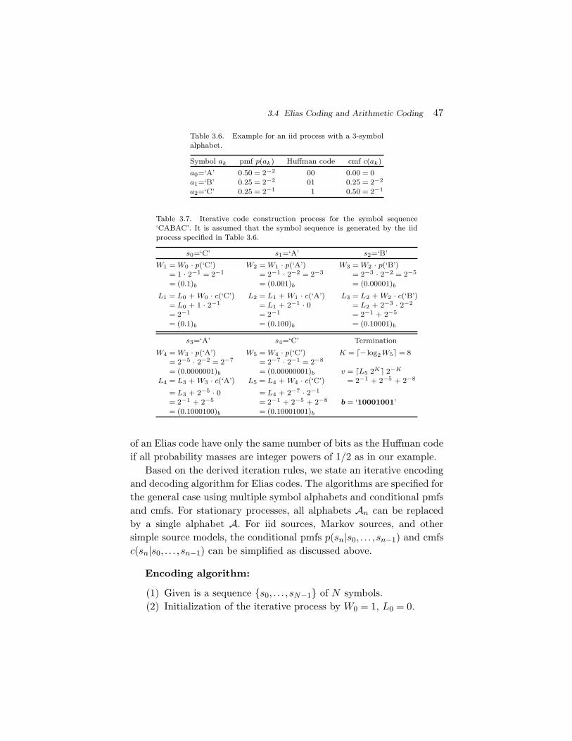
3.4 Elias Coding and Arithmetic Coding 47
Table 3.6. Example for an iid process with a 3-symbolalphabet.
Symbol ak pmf p(ak) Huffman code cmf c(ak)
a0=‘A’ 0.50 = 2−2 00 0.00 = 0a1=‘B’ 0.25 = 2−2 01 0.25 = 2−2
a2=‘C’ 0.25 = 2−1 1 0.50 = 2−1
Table 3.7. Iterative code construction process for the symbol sequence‘CABAC’. It is assumed that the symbol sequence is generated by the iidprocess specified in Table 3.6.
s0=‘C’ s1=‘A’ s2=‘B’
W1 = W0 · p(‘C’) W2 = W1 · p(‘A’) W3 = W2 · p(‘B’)= 1 · 2−1 = 2−1 = 2−1 · 2−2 = 2−3 = 2−3 · 2−2 = 2−5
= (0.1)b = (0.001)b = (0.00001)b
L1 = L0 + W0 · c(‘C’) L2 = L1 + W1 · c(‘A’) L3 = L2 + W2 · c(‘B’)= L0 + 1 · 2−1 = L1 + 2−1 · 0 = L2 + 2−3 · 2−2
= 2−1 = 2−1 = 2−1 + 2−5
= (0.1)b = (0.100)b = (0.10001)b
s3=‘A’ s4=‘C’ Termination
W4 = W3 · p(‘A’) W5 = W4 · p(‘C’) K = �− log2 W5 = 8= 2−5 · 2−2 = 2−7 = 2−7 · 2−1 = 2−8
= (0.0000001)b = (0.00000001)b v = �L5 2K 2−K
L4 = L3 + W3 · c(‘A’) L5 = L4 + W4 · c(‘C’) = 2−1 + 2−5 + 2−8
= L3 + 2−5 · 0 = L4 + 2−7 · 2−1
= 2−1 + 2−5 = 2−1 + 2−5 + 2−8 b = ‘10001001’= (0.1000100)b = (0.10001001)b
of an Elias code have only the same number of bits as the Huffman codeif all probability masses are integer powers of 1/2 as in our example.
Based on the derived iteration rules, we state an iterative encodingand decoding algorithm for Elias codes. The algorithms are specified forthe general case using multiple symbol alphabets and conditional pmfsand cmfs. For stationary processes, all alphabets An can be replacedby a single alphabet A. For iid sources, Markov sources, and othersimple source models, the conditional pmfs p(sn|s0, . . . ,sn−1) and cmfsc(sn|s0, . . . ,sn−1) can be simplified as discussed above.
Encoding algorithm:
(1) Given is a sequence {s0, . . . ,sN−1} of N symbols.(2) Initialization of the iterative process by W0 = 1, L0 = 0.

48 Lossless Source Coding
(3) For each n = 0,1, . . . ,N − 1, determine the interval In+1 by
Wn+1 = Wn · p(sn|s0, . . . ,sn−1),
Ln+1 = Ln + Wn · c(sn|s0, . . . ,sn−1).
(4) Determine the codeword length by K = �− log2 WN .(5) Transmit the codeword b(K) of K bits that represents
the fractional part of v = �LN 2K 2−K .
Decoding algorithm:
(1) Given is the number N of symbols to be decoded anda codeword b(K) = {b0, . . . , bK−1} of KN bits.
(2) Determine the interval representative v according to
v =K−1∑i=0
bi 2−i.
(3) Initialization of the iterative process by W0 = 1, L0 = 0.(4) For each n = 0,1, . . . ,N − 1, do the following:
(a) For each ai ∈ An, determine the interval In+1(ai) by
Wn+1(ai) = Wn · p(ai|s0, . . . ,sn−1),
Ln+1(ai) = Ln + Wn · c(ai|s0, . . . ,sn−1).
(b) Select the letter ai ∈ An for which v ∈ In+1(ai),and set sn = ai, Wn+1 = Wn+1(ai), Ln+1 = Ln+1(ai).
Adaptive Elias Coding. Since the iterative interval refinement isthe same at encoder and decoder sides, Elias coding provides a simplemechanism for the adaptation to sources with unknown or nonstation-ary statistical properties. Conceptually, for each source symbol sn, thepmf p(sn|s0, . . . ,sn−1) can be simultaneously estimated at encoder anddecoder sides based on the already coded symbols s0 to sn−1. For thispurpose, a source can often be modeled as a process with indepen-dent random variables or as a Markov process. For the simple model ofindependent random variables, the pmf p(sn) for a particular symbol sn
3.4 Elias Coding and Arithmetic Coding 49
can be approximated by the relative frequencies of the alphabet lettersinside the sequence of the preceding NW coded symbols. The choseninterval size NW adjusts the trade-off between a fast adaptation andan accurate probability estimation. The same approach can also beapplied for higher order probability models as the Markov model. Inthis case, the conditional pmf is approximated by the correspondingrelative conditional frequencies.
Efficiency of Elias Coding. The average codeword length per sym-bol for the Elias code is given by
� =1N
E{K(S)} =1N
E{⌈
− log2 p(S)⌉}
. (3.46)
By applying the inequalities �x ≥ x and �x < x + 1, we obtain
1N
E{− log2 p(S)} ≤ � <1N
E{1 − log2 p(S)}1N
H(S0, . . . ,SN−1) ≤ � <1N
H(S0, . . . ,SN−1) +1N
. (3.47)
If the number N of coded symbols approaches infinity, the averagecodeword length approaches the entropy rate.
It should be noted that the Elias code is not guaranteed to be prefixfree, i.e., a codeword for a particular symbol sequence may be a prefixof the codeword for any other symbol sequence. Hence, the Elias codeas described above can only be used if the length of the codeword isknown at the decoder side.5 A prefix-free Elias code can be constructedif the lengths of all codewords are increased by one, i.e., by choosing
KN =⌈
− log2 WN
⌉+ 1. (3.48)
3.4.2 Arithmetic Coding
The Elias code has several desirable properties, but it is still imprac-tical, since the precision that is required for representing the intervalwidths and lower interval boundaries grows without bound for longsymbol sequences. The widely used approach of arithmetic coding is a
5 In image and video coding applications, the end of a bit sequence for the symbols of apicture or slice is often given by the high-level bitstream syntax.

50 Lossless Source Coding
variant of Elias coding that can be implemented with fixed-precisioninteger arithmetic.
For the following considerations, we assume that the probabilitymasses p(sn|s0, . . . ,sn−1) are given with a fixed number V of binarydigits after the binary point. We will omit the conditions “s0, . . . ,sn−1”and represent the pmfs p(a) and cmfs c(a) by
p(a) = pV (a) · 2−V , c(a) = cV (a) · 2−V =∑ai<a
pV (ai) · 2−V , (3.49)
where pV (a) and cV (a) are V -bit positive integers.The key observation for designing arithmetic coding schemes is that
the Elias code remains decodable if the interval width Wn+1 satisfies
0 < Wn+1 ≤ Wn · p(sn). (3.50)
This guarantees that the interval In+1 is always nested inside the inter-val In. Equation (3.43) implies Ln+1 ≥ Ln, and by combining (3.43)with the inequality (3.50), we obtain
Ln+1 + Wn+1 ≤ Ln + Wn · [c(sn) + p(sn)] ≤ Ln + Wn. (3.51)
Hence, we can represent the interval width Wn with a fixed number ofprecision bits if we round it toward zero in each iteration step.
Let the interval width Wn be represented by a U -bit integer An andan integer zn ≥ U according to
Wn = An · 2−zn . (3.52)
We restrict An to the range
2U−1 ≤ An < 2U , (3.53)
so that the Wn is represented with a maximum precision of U bits. Inorder to suitably approximate W0 = 1, the values of A0 and z0 are setequal to 2U − 1 and U , respectively. The interval refinement can thenbe specified by
An+1 = �An · pV (sn) · 2−yn�, (3.54)
zn+1 = zn + V − yn, (3.55)

3.4 Elias Coding and Arithmetic Coding 51
where yn is a bit shift parameter with 0 ≤ yn ≤ V . These iteration rulesguarantee that (3.50) is fulfilled. It should also be noted that the opera-tion �x · 2−y� specifies a simple right shift of the binary representationof x by y binary digits. To fulfill the constraint in (3.53), the bit shiftparameter yn has to be chosen according to
yn = �log2(An · pV (sn) + 1) − U. (3.56)
The value of yn can be determined by a series of comparison operations.Given the fixed-precision representation of the interval width Wn,
we investigate the impact on the lower interval boundary Ln. Thebinary representation of the product
Wn · c(sn) = An · cV (sn) · 2−(zn+V )
= 0. 00000 · · ·0︸ ︷︷ ︸zn −U bits
xxxxx · · ·x︸ ︷︷ ︸U +V bits
00000 · · · (3.57)
consists of zn − U 0-bits after the binary point followed by U +V bitsrepresenting the integer An · cV (sn). The bits after the binary point inthe binary representation of the lower interval boundary,
Ln = 0. aaaaa · · ·a︸ ︷︷ ︸zn − cn −U
settled bits
0111111 · · ·1︸ ︷︷ ︸cn
outstanding bits
xxxxx · · ·x︸ ︷︷ ︸U +V
active bits
00000 · · ·︸ ︷︷ ︸trailing bits
, (3.58)
can be classified into four categories. The trailing bits that follow the(zn + V )th bit after the binary point are equal to 0, but may be modi-fied by following interval updates. The preceding U +V bits are directlymodified by the update Ln+1 = Ln + Wn c(sn) and are referred to asactive bits. The active bits are preceded by a sequence of zero or more1-bits and a leading 0-bit (if present). These cn bits are called out-standing bits and may be modified by a carry from the active bits.The zn − cn −U bits after the binary point, which are referred to assettled bits, are not modified in any following interval update. Further-more, these bits cannot be modified by the rounding operation thatgenerates the final codeword, since all intervals In+k, with k > 0, arenested inside the interval In and the binary representation of the inter-val width Wn =An 2−zn also consists of zn − U 0-bits after the binary
52 Lossless Source Coding
point. And since the number of bits in the final codeword,
K = �− log2 WN ≥ �− log2 Wn = zn − �log2 An� = zn − U + 1,
(3.59)is always greater than or equal to the number of settled bits, the settledbits can be transmitted as soon as they have become settled. Hence,in order to represent the lower interval boundary Ln, it is sufficient tostore the U +V active bits and a counter for the number of 1-bits thatprecede the active bits.
For the decoding of a particular symbol sn it has to be deter-mined whether the binary fraction v in (3.40) that is representedby the transmitted codeword falls inside the interval Wn+1(ai) foran alphabet letter ai. Given the described fixed-precision intervalrefinement, it is sufficient to compare the cn+1 outstanding bits andthe U +V active bits of the lower interval boundary Ln+1 with thecorresponding bits of the transmitted codeword and the upper intervalboundary Ln+1 +Wn+1.
It should be noted that the number of outstanding bits can becomearbitrarily large. In order to force an output of bits, the encoder caninsert a 0-bit if it detects a sequence of a particular number of 1-bits.The decoder can identify the additionally inserted bit and interpret itas extra carry information. This technique is, for example, used in theMQ-coder [66] of JPEG 2000 [36].
Efficiency of Arithmetic Coding. In comparison to Elias coding,the usage of the presented fixed precision approximation increases thecodeword length for coding a symbol sequence s = {s0,s1, . . . ,sN−1}.Given WN for n = N in (3.52), the excess rate of arithmetic codingover Elias coding is given by
∆� = �− log2 WN − �− log2 p(s) < 1 +N−1∑n=0
log2Wn p(sn)
Wn+1, (3.60)
where we used the inequalities �x < x + 1 and �x ≥ x to derive theupper bound on the right-hand side. We shall further take into accountthat we may have to approximate the real pmfs p(a) in order to rep-resent the probability masses as multiples of 2−V . Let q(a) representan approximated pmf that is used for arithmetic coding and let pmin
3.4 Elias Coding and Arithmetic Coding 53
denote the minimum probability mass of the corresponding real pmfp(a). The pmf approximation can always be done in a way that thedifference p(a) − q(a) is less than 2−V , which gives
p(a) − q(a)p(a)
<2−V
pmin⇒ p(a)
q(a)<
(1 − 2−V
pmin
)−1
. (3.61)
An application of the inequality �x� > x − 1 to the interval refinement(3.54) with the approximated pmf q(a) yields
An+1 > An q(sn) 2V −yn − 1
Wn+1 > An q(sn) 2V −yn−zn+1 − 2−zn+1
Wn+1 > An q(sn) 2−zn − 2−zn+1
Wn q(sn) − Wn+1 < 2−zn+1 . (3.62)
By using the relationship Wn+1 ≥ 2U−1−zn+1 , which is a direct conse-quence of (3.53), we obtain
Wn q(sn)Wn+1
= 1 +Wn q(sn) − Wn+1
Wn+1< 1 + 21−U . (3.63)
Substituting the expressions (3.61) and (3.63) into (3.60) yields anupper bound for the increase in codeword length per symbol,
∆� <1N
+ log2(1 + 21−U ) − log2
(1 − 2−V
pmin
). (3.64)
If we consider, for example, the coding of N =1000 symbols withU =12, V =16, and pmin =0.02, the increase in codeword length inrelation to Elias coding is guaranteed to be less than 0.003 bit persymbol.
Binary Arithmetic Coding. Arithmetic coding with binary sym-bol alphabets is referred to as binary arithmetic coding. It is the mostpopular type of arithmetic coding in image and video coding appli-cations. The main reason for using binary arithmetic coding is itsreduced complexity. It is particularly advantageous for adaptive cod-ing, since the rather complex estimation of M -ary pmfs can be replacedby the simpler estimation of binary pmfs. Well-known examples of effi-cient binary arithmetic coding schemes that are used in image and

54 Lossless Source Coding
video coding are the MQ-coder [66] in the picture coding standardJPEG 2000 [36] and the M-coder [50] in the video coding standardH.264/AVC [38].
In general, a symbol sequence s= {s0,s1, . . . ,sN−1} has to be firstconverted into a sequence c= {c0, c1, . . . , cB−1} of binary symbols,before binary arithmetic coding can be applied. This conversion pro-cess is often referred to as binarization and the elements of the result-ing binary sequences c are also called bins. The number B of bins in asequence c can depend on the actual source symbol sequence s. Hence,the bin sequences c can be interpreted as realizations of a variable-length sequence of binary random variables C = {C0,C1, . . . ,CB−1}.
Conceptually, the binarization mapping S → C represents a losslesscoding step and any lossless source code could be applied for this pur-pose. It is, however, only important that the used lossless source codeis uniquely decodable. The average codeword length that is achieved bythe binarization mapping does not have any impact on the efficiency ofbinary arithmetic coding, since the block entropy for the sequence ofrandom variables S = {S0,S1, . . . ,SN−1},
H(S) = E{− log2 p(S)} = E{− log2 p(C)} = H(C),
is equal to entropy of the variable-length binary random vectorC = {C0,C1, . . . ,CB−1}. The actual compression is achieved by thearithmetic coding. The above result also shows that binary arithmeticcoding can provide the same coding efficiency as M -ary arithmetic cod-ing, if the influence of the finite precision arithmetic is negligible.
In practice, the binarization is usually done with very simple pre-fix codes for the random variables Sn. If we assume that the orderof different random variables is known to both, encoder and decoder,different prefix codes can be used for each random variable withoutimpacting unique decodability. A typical example for a binarizationmapping, which is called truncated unary binarization, is illustratedin Table 3.8.
The binary pmfs for the random variables Ci can be directly derivedfrom the pmfs of the random variables Sn. For the example in Table 3.8,the binary pmf {P (Ci =0),1 − P (Ci =0)} for a random variable Ci is
3.5 Probability Interval Partitioning Entropy Coding 55
Table 3.8. Mapping of a random variable Sn with an M -ary alphabetonto a variable-length binary random vector C = {C0,C1, . . . ,CB−1}using truncated unary binarization.
Sn Number of bins B C0 C1 C2 · · · CM−2 CM−1
a0 1 1a1 2 0 1a2 3 0 0 1...
......
.... . .
. . .
aM−3 M − 3 0 0 0. . . 1
aM−2 M − 2 0 0 0 · · · 0 1aM−1 M − 2 0 0 0 · · · 0 0
given by
P (Ci =0) =P (Sn >ai |S0 =s0, S1 =s1, . . . , Sn−1 =sn−1)P (Sn ≥ai |S0 =s0, S1 =s1, . . . , Sn−1 =sn−1)
, (3.65)
where we omitted the condition for the binary pmf. For coding nonsta-tionary sources, it is usually preferable to directly estimate the marginalor conditional pmfs for the binary random variables instead of the pmfsfor the source signal.
3.5 Probability Interval Partitioning Entropy Coding
For a some applications, arithmetic coding is still considered as toocomplex. As a less-complex alternative, a lossless coding schemecalled probability interval partitioning entropy (PIPE) coding has beenrecently proposed [51]. It combines concepts from binary arithmeticcoding and Huffman coding for variable-length vectors with a quanti-zation of the binary probability interval.
A block diagram of the PIPE coding structure is shown in Fig-ure 3.4. It is assumed that the input symbol sequences s = {s0,
s1, . . . ,sN−1} represent realizations of a sequence S = {S0,S1, . . . ,SN−1}of random variables. Each random variable can be characterized by adistinct alphabet An. The number N of source symbols is assumed tobe known to encoder and decoder. Similarly as for binary arithmeticcoding, a symbol sequence s = {s0,s1, . . . ,sN−1} is first converted intoa sequence c= {c0, c1, . . . , cB−1} of B binary symbols (bins). Each bin ci
can be considered as a realization of a corresponding random variable
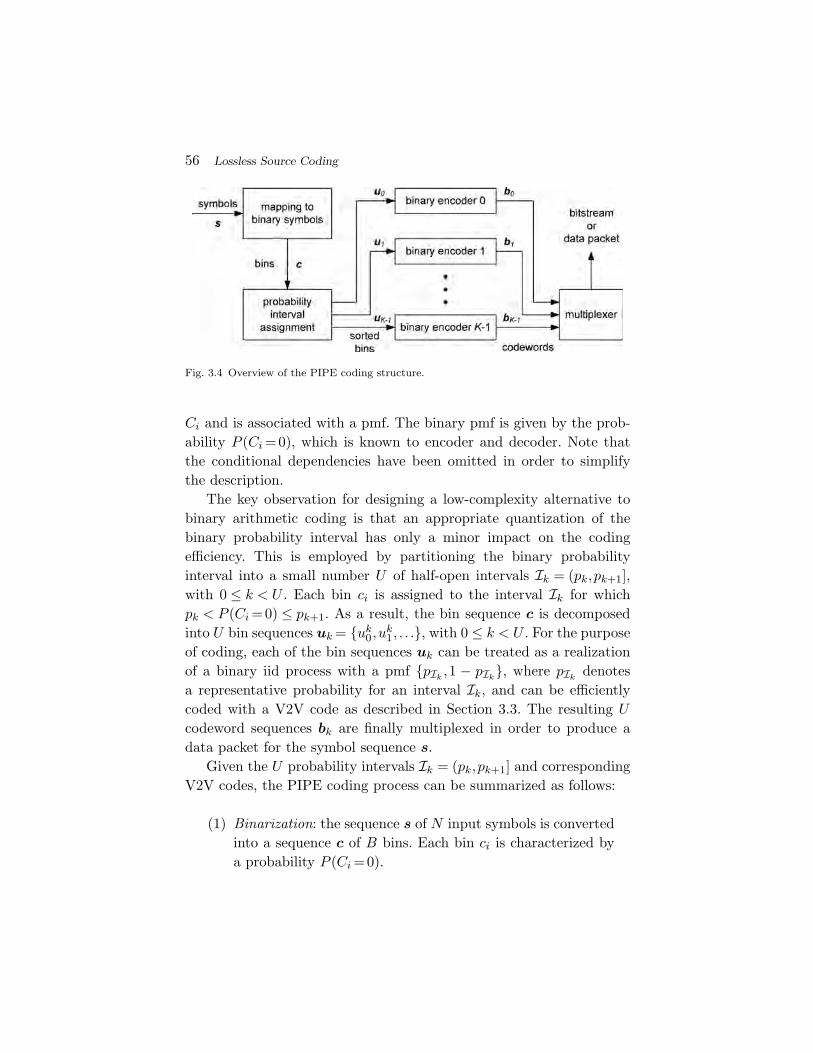
56 Lossless Source Coding
Fig. 3.4 Overview of the PIPE coding structure.
Ci and is associated with a pmf. The binary pmf is given by the prob-ability P (Ci =0), which is known to encoder and decoder. Note thatthe conditional dependencies have been omitted in order to simplifythe description.
The key observation for designing a low-complexity alternative tobinary arithmetic coding is that an appropriate quantization of thebinary probability interval has only a minor impact on the codingefficiency. This is employed by partitioning the binary probabilityinterval into a small number U of half-open intervals Ik = (pk,pk+1],with 0 ≤ k < U . Each bin ci is assigned to the interval Ik for whichpk < P (Ci =0) ≤ pk+1. As a result, the bin sequence c is decomposedinto U bin sequences uk = {uk
0,uk1, . . .}, with 0 ≤ k < U . For the purpose
of coding, each of the bin sequences uk can be treated as a realizationof a binary iid process with a pmf {pIk
,1 − pIk}, where pIk
denotesa representative probability for an interval Ik, and can be efficientlycoded with a V2V code as described in Section 3.3. The resulting U
codeword sequences bk are finally multiplexed in order to produce adata packet for the symbol sequence s.
Given the U probability intervals Ik = (pk,pk+1] and correspondingV2V codes, the PIPE coding process can be summarized as follows:
(1) Binarization: the sequence s of N input symbols is convertedinto a sequence c of B bins. Each bin ci is characterized bya probability P (Ci =0).
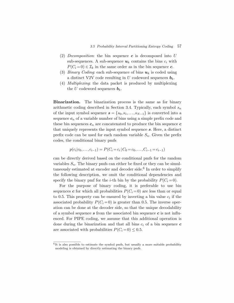
3.5 Probability Interval Partitioning Entropy Coding 57
(2) Decomposition: the bin sequence c is decomposed into U
sub-sequences. A sub-sequence uk contains the bins ci withP (Ci =0) ∈ Ik in the same order as in the bin sequence c.
(3) Binary Coding: each sub-sequence of bins uk is coded usinga distinct V2V code resulting in U codeword sequences bk.
(4) Multiplexing: the data packet is produced by multiplexingthe U codeword sequences bk.
Binarization. The binarization process is the same as for binaryarithmetic coding described in Section 3.4. Typically, each symbol sn
of the input symbol sequence s = {s0,s1, . . . ,sN−1} is converted into asequence cn of a variable number of bins using a simple prefix code andthese bin sequences cn are concatenated to produce the bin sequence c
that uniquely represents the input symbol sequence s. Here, a distinctprefix code can be used for each random variable Sn. Given the prefixcodes, the conditional binary pmfs
p(ci|c0, . . . , ci−1) = P (Ci = ci |C0 = c0, . . . ,Ci−1 = ci−1)
can be directly derived based on the conditional pmfs for the randomvariables Sn. The binary pmfs can either be fixed or they can be simul-taneously estimated at encoder and decoder side.6 In order to simplifythe following description, we omit the conditional dependencies andspecify the binary pmf for the i-th bin by the probability P (Ci =0).
For the purpose of binary coding, it is preferable to use binsequences c for which all probabilities P (Ci =0) are less than or equalto 0.5. This property can be ensured by inverting a bin value ci if theassociated probability P (Ci =0) is greater than 0.5. The inverse oper-ation can be done at the decoder side, so that the unique decodabilityof a symbol sequence s from the associated bin sequence c is not influ-enced. For PIPE coding, we assume that this additional operation isdone during the binarization and that all bins ci of a bin sequence c
are associated with probabilities P (Ci =0) ≤ 0.5.
6 It is also possible to estimate the symbol pmfs, but usually a more suitable probabilitymodeling is obtained by directly estimating the binary pmfs.
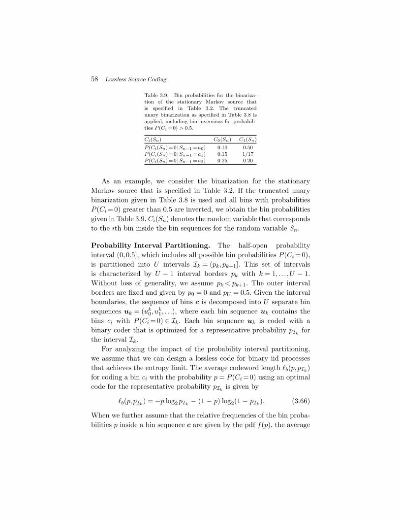
58 Lossless Source Coding
Table 3.9. Bin probabilities for the binariza-tion of the stationary Markov source thatis specified in Table 3.2. The truncatedunary binarization as specified in Table 3.8 isapplied, including bin inversions for probabili-ties P (Ci =0) > 0.5.
Ci(Sn) C0(Sn) C1(Sn)
P (Ci(Sn)=0 |Sn−1 =a0) 0.10 0.50P (Ci(Sn)=0 |Sn−1 =a1) 0.15 1/17P (Ci(Sn)=0 |Sn−1 =a2) 0.25 0.20
As an example, we consider the binarization for the stationaryMarkov source that is specified in Table 3.2. If the truncated unarybinarization given in Table 3.8 is used and all bins with probabilitiesP (Ci =0) greater than 0.5 are inverted, we obtain the bin probabilitiesgiven in Table 3.9. Ci(Sn) denotes the random variable that correspondsto the ith bin inside the bin sequences for the random variable Sn.
Probability Interval Partitioning. The half-open probabilityinterval (0,0.5], which includes all possible bin probabilities P (Ci =0),is partitioned into U intervals Ik = (pk,pk+1]. This set of intervalsis characterized by U − 1 interval borders pk with k = 1, . . . ,U − 1.Without loss of generality, we assume pk < pk+1. The outer intervalborders are fixed and given by p0 = 0 and pU = 0.5. Given the intervalboundaries, the sequence of bins c is decomposed into U separate binsequences uk = (uk
0,uk1, . . .), where each bin sequence uk contains the
bins ci with P (Ci =0) ∈ Ik. Each bin sequence uk is coded with abinary coder that is optimized for a representative probability pIk
forthe interval Ik.
For analyzing the impact of the probability interval partitioning,we assume that we can design a lossless code for binary iid processesthat achieves the entropy limit. The average codeword length �b(p,pIk
)for coding a bin ci with the probability p = P (Ci =0) using an optimalcode for the representative probability pIk
is given by
�b(p,pIk) = −p log2 pIk
− (1 − p) log2(1 − pIk). (3.66)
When we further assume that the relative frequencies of the bin proba-bilities p inside a bin sequence c are given by the pdf f(p), the average

3.5 Probability Interval Partitioning Entropy Coding 59
codeword length per bin �b for a given set of U intervals Ik with rep-resentative probabilities pIk
can then be written as
�b =K−1∑k=0
(∫ pk+1
pk
�b(p,pIk) f(p) dp
). (3.67)
Minimization with respect to the interval boundaries pk and represen-tative probabilities pIk
yields the equation system,
p∗Ik
=
∫ pk+1pk
p f(p) dp∫ pk+1pk
f(p) dp, (3.68)
p∗k = p with �b(p,pIk−1) = �b(p,pIk
). (3.69)
Given the pdf f(p) and the number of intervals U , the interval partition-ing can be derived by an iterative algorithm that alternately updatesthe interval borders pk and interval representatives pIk
. As an exam-ple, Figure 3.5 shows the probability interval partitioning for a uniformdistribution f(p) of the bin probabilities and U = 4 intervals. As canbe seen, the probability interval partitioning leads to a piecewise linearapproximation �b(p,pIk
)|Ikof the binary entropy function H(p).
Fig. 3.5 Example for the partitioning of the probability interval (0,0.5] into four intervalsassuming a uniform distribution of the bin probabilities p = P (Ci =0).
60 Lossless Source Coding
Table 3.10. Increase in average codeword length perbin for a uniform and a linear increasing distribu-tion f(p) of bin probabilities and various numbers ofprobability intervals.
U 1 2 4 8 12 16
�uni [%] 12.47 3.67 1.01 0.27 0.12 0.07�lin [%] 5.68 1.77 0.50 0.14 0.06 0.04
The increase of the average codeword length per bin is given by
= �b /
(∫ 0.5
0H(p)f(p) dp
)− 1. (3.70)
Table 3.10 lists the increases in average codeword length per bin fora uniform and a linear increasing (f(p) = 8p) distribution of the binprobabilities for selected numbers U of intervals.
We now consider the probability interval partitioning for the Markovsource specified in Table 3.2. As shown in Table 3.9, the binarizationdescribed above led to six different bin probabilities. For the truncatedunary binarization of a Markov source, the relative frequency h(pij )that a bin with probability pij = P (Ci(Sn)|Sn−1 =aj) occurs inside thebin sequence c is equal to
h(pij ) =p(aj)
∑M−1k=i p(ak|aj)∑M−2
m=0∑M−1
k=m p(ak). (3.71)
The distribution of the bin probabilities is given by
f(p) = 0.1533 · δ(p− 1/17) + 0.4754 · δ(p− 0.1) + 0.1803 · δ(p− 0.15)
+0.0615 · δ(p− 0.2) + 0.0820 · δ(p− 0.25) + 0.0475 · δ(p− 0.5),
where δ represents the Direct delta function. An optimal partitioningof the probability interval (0,0.5] into three intervals for this source isshown in Table 3.11. The increase in average codeword length per binfor this example is approximately 0.85%.
Binary Coding. For the purpose of binary coding, a bin sequence uk
for the probability interval Ik can be treated as a realization of abinary iid process with a pmf {pIk
,1 − pIk}. The statistical depen-
dencies between the bins have already been exploited by associating
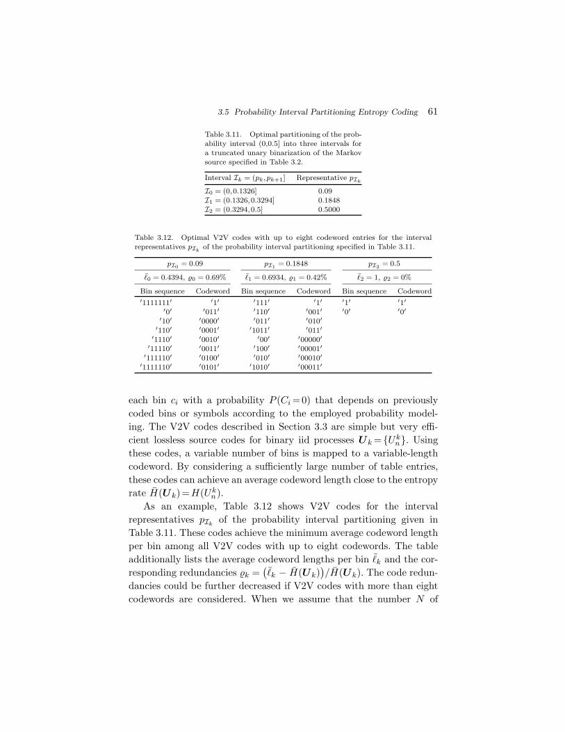
3.5 Probability Interval Partitioning Entropy Coding 61
Table 3.11. Optimal partitioning of the prob-ability interval (0,0.5] into three intervals fora truncated unary binarization of the Markovsource specified in Table 3.2.
Interval Ik = (pk,pk+1] Representative pIk
I0 = (0,0.1326] 0.09I1 = (0.1326,0.3294] 0.1848I2 = (0.3294,0.5] 0.5000
Table 3.12. Optimal V2V codes with up to eight codeword entries for the intervalrepresentatives pIk
of the probability interval partitioning specified in Table 3.11.
pI0 = 0.09 pI1 = 0.1848 pI2 = 0.5
�0 = 0.4394, �0 = 0.69% �1 = 0.6934, �1 = 0.42% �2 = 1, �2 = 0%
Bin sequence Codeword Bin sequence Codeword Bin sequence Codeword′1111111′ ′1′ ′111′ ′1′ ′1′ ′1′
′0′ ′011′ ′110′ ′001′ ′0′ ′0′′10′ ′0000′ ′011′ ′010′
′110′ ′0001′ ′1011′ ′011′′1110′ ′0010′ ′00′ ′00000′
′11110′ ′0011′ ′100′ ′00001′′111110′ ′0100′ ′010′ ′00010′
′1111110′ ′0101′ ′1010′ ′00011′
each bin ci with a probability P (Ci =0) that depends on previouslycoded bins or symbols according to the employed probability model-ing. The V2V codes described in Section 3.3 are simple but very effi-cient lossless source codes for binary iid processes Uk ={Uk
n}. Usingthese codes, a variable number of bins is mapped to a variable-lengthcodeword. By considering a sufficiently large number of table entries,these codes can achieve an average codeword length close to the entropyrate H(Uk)=H(Uk
n).As an example, Table 3.12 shows V2V codes for the interval
representatives pIkof the probability interval partitioning given in
Table 3.11. These codes achieve the minimum average codeword lengthper bin among all V2V codes with up to eight codewords. The tableadditionally lists the average codeword lengths per bin �k and the cor-responding redundancies k =
(�k − H(Uk)
)/H(Uk). The code redun-
dancies could be further decreased if V2V codes with more than eightcodewords are considered. When we assume that the number N of
62 Lossless Source Coding
symbols approaches infinity, the average codeword length per symbolfor the applied truncated unary binarization is given by
� =
(U−1∑k=0
�k
∫ pk+1
pk
f(p)dp
)·(
M−2∑m=0
M−1∑k=m
p(ak)
), (3.72)
where the first term represents the average codeword length per bin forthe bin sequence c and the second term is the bin-to-symbol ratio. Forour simple example, the average codeword length for the PIPE codingis � = 0.7432 bit per symbol. It is only 1.37% larger than the entropyrate and significantly smaller than the average codeword length for thescalar, conditional, and block Huffman codes that we have developedin Sections 3.2 and 3.3.
In general, the average codeword length per symbol can be furtherdecreased if the V2V codes and the probability interval partitioning arejointly optimized. This can be achieved by an iterative algorithm thatalternately optimizes the interval representatives pIk
, the V2V codesfor the interval representatives, and the interval boundaries pk. Eachcodeword entry m of a binary V2V code Ck is characterized by thenumber xm of 0-bins, the number ym of 1-bins, and the length �m ofthe codeword. As can be concluded from the description of V2V codesin Section 3.3, the average codeword length for coding a bin ci with aprobability p = P (Ci =0) using a V2V code Ck is given by
�b(p,Ck) =∑V −1
m=0 pxm (1 − p)ym �m∑V −1m=0 pxm (1 − p)ym (xm + ym)
, (3.73)
where V denotes the number of codeword entries. Hence, an optimalinterval border pk is given by the intersection point of the functions�b(p,Ck−1) and �b(p,Ck) for the V2V codes of the neighboring intervals.
As an example, we jointly derived the partitioning into U = 12 prob-ability intervals and corresponding V2V codes with up to 65 codewordentries for a uniform distribution of bin probabilities. Figure 3.6 showsthe difference between the average codeword length per bin and thebinary entropy function H(p) for this design and a theoretically opti-mal probability interval partitioning assuming optimal binary codeswith �k = H(pIk
). The overall redundancy with respect to the entropy
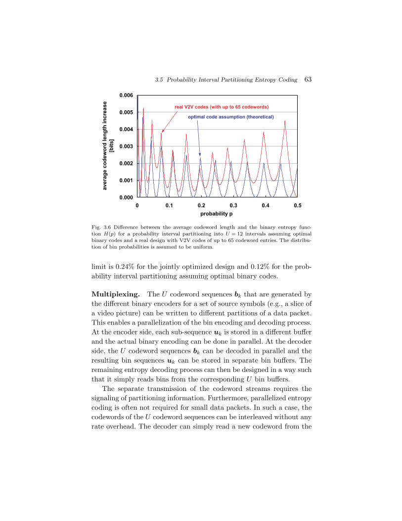
3.5 Probability Interval Partitioning Entropy Coding 63
Fig. 3.6 Difference between the average codeword length and the binary entropy func-tion H(p) for a probability interval partitioning into U = 12 intervals assuming optimalbinary codes and a real design with V2V codes of up to 65 codeword entries. The distribu-tion of bin probabilities is assumed to be uniform.
limit is 0.24% for the jointly optimized design and 0.12% for the prob-ability interval partitioning assuming optimal binary codes.
Multiplexing. The U codeword sequences bk that are generated bythe different binary encoders for a set of source symbols (e.g., a slice ofa video picture) can be written to different partitions of a data packet.This enables a parallelization of the bin encoding and decoding process.At the encoder side, each sub-sequence uk is stored in a different bufferand the actual binary encoding can be done in parallel. At the decoderside, the U codeword sequences bk can be decoded in parallel and theresulting bin sequences uk can be stored in separate bin buffers. Theremaining entropy decoding process can then be designed in a way suchthat it simply reads bins from the corresponding U bin buffers.
The separate transmission of the codeword streams requires thesignaling of partitioning information. Furthermore, parallelized entropycoding is often not required for small data packets. In such a case, thecodewords of the U codeword sequences can be interleaved without anyrate overhead. The decoder can simply read a new codeword from the
64 Lossless Source Coding
bitstream if a new bin is requested by the decoding process and all binsof the previously read codeword for the corresponding interval Ik havebeen used. At the encoder side, it has to be ensured that the codewordsare written in the same order in which they are read at the decoderside. This can be efficiently realized by introducing a codeword buffer.
Unique Decodability. For PIPE coding, the concept of uniquedecodability has to be extended. Since the binarization is done usingprefix codes, it is always invertible.7 However, the resulting sequenceof bins c is partitioned into U sub-sequences uk
{u0, . . . ,uU−1} = γp(b), (3.74)
and each of these sub-sequences uk is separately coded. The binsequence c is uniquely decodable, if each sub-sequence of bins uk
is uniquely decodable and the partitioning rule γp is known to thedecoder. The partitioning rule γp is given by the probability intervalpartitioning {Ik} and the probabilities P (Ci =0) that are associatedwith the coding bins ci. Hence, the probability interval partitioning{Ik} has to be known at the decoder side and the probability P (Ci =0)for each bin ci has to be derived in the same way at encoder and decoderside.
3.6 Comparison of Lossless Coding Techniques
In the preceding sections, we presented different lossless coding tech-niques. We now compare these techniques with respect to their codingefficiency for the stationary Markov source specified in Table 3.2 anddifferent message sizes L. In Figure 3.7, the average codeword lengthsper symbol for the different lossless source codes are plotted over thenumber L of coded symbols. For each number of coded symbols, theshown average codeword lengths were calculated as mean values overa set of one million different realizations of the example Markov sourceand can be considered as accurate approximations of the expected
7 The additionally introduced bin inversion depending on the associated probabilitiesP (Ci =0) is invertible, if the probabilities P (Ci =0) are derived in the same way at encoderand decoder side as stated below.
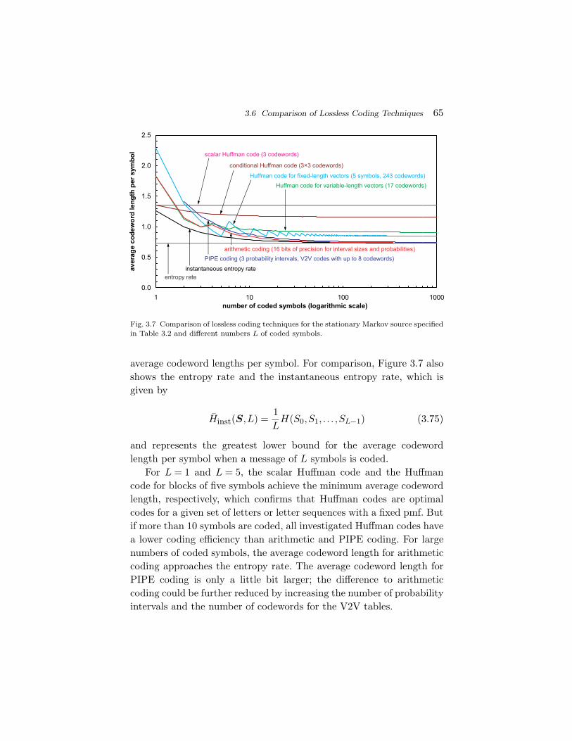
3.6 Comparison of Lossless Coding Techniques 65
Fig. 3.7 Comparison of lossless coding techniques for the stationary Markov source specifiedin Table 3.2 and different numbers L of coded symbols.
average codeword lengths per symbol. For comparison, Figure 3.7 alsoshows the entropy rate and the instantaneous entropy rate, which isgiven by
Hinst(S,L) =1L
H(S0,S1, . . . ,SL−1) (3.75)
and represents the greatest lower bound for the average codewordlength per symbol when a message of L symbols is coded.
For L = 1 and L = 5, the scalar Huffman code and the Huffmancode for blocks of five symbols achieve the minimum average codewordlength, respectively, which confirms that Huffman codes are optimalcodes for a given set of letters or letter sequences with a fixed pmf. Butif more than 10 symbols are coded, all investigated Huffman codes havea lower coding efficiency than arithmetic and PIPE coding. For largenumbers of coded symbols, the average codeword length for arithmeticcoding approaches the entropy rate. The average codeword length forPIPE coding is only a little bit larger; the difference to arithmeticcoding could be further reduced by increasing the number of probabilityintervals and the number of codewords for the V2V tables.
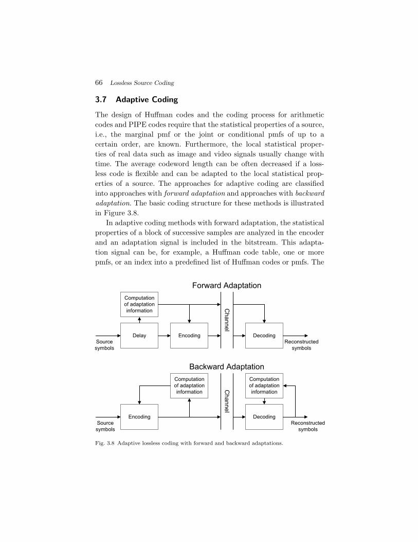
66 Lossless Source Coding
3.7 Adaptive Coding
The design of Huffman codes and the coding process for arithmeticcodes and PIPE codes require that the statistical properties of a source,i.e., the marginal pmf or the joint or conditional pmfs of up to acertain order, are known. Furthermore, the local statistical proper-ties of real data such as image and video signals usually change withtime. The average codeword length can be often decreased if a loss-less code is flexible and can be adapted to the local statistical prop-erties of a source. The approaches for adaptive coding are classifiedinto approaches with forward adaptation and approaches with backwardadaptation. The basic coding structure for these methods is illustratedin Figure 3.8.
In adaptive coding methods with forward adaptation, the statisticalproperties of a block of successive samples are analyzed in the encoderand an adaptation signal is included in the bitstream. This adapta-tion signal can be, for example, a Huffman code table, one or morepmfs, or an index into a predefined list of Huffman codes or pmfs. The
Fig. 3.8 Adaptive lossless coding with forward and backward adaptations.
3.8 Summary of Lossless Source Coding 67
decoder adjusts the used code for the block of samples according tothe transmitted information. Disadvantages of this approach are thatthe required side information increases the transmission rate and thatforward adaptation introduces a delay.
Methods with backward adaptation estimate the local statisticalproperties based on already coded symbols simultaneously at encoderand decoder side. As mentioned in Section 3.2, the adaptation of Huff-man codes is a quite complex task, so that backward adaptive VLCcoding is rarely used in practice. But for arithmetic coding, in partic-ular, binary arithmetic coding, and PIPE coding, the backward adap-tive estimation of pmfs can be easily integrated in the coding process.Backward adaptive coding methods do not introduce a delay and donot require the transmission of any side information. However, theyare not robust against transmission errors. For this reason, backwardadaptation is usually only used inside a transmission packet. It is alsopossible to combine backward and forward adaptation. As an example,the arithmetic coding design in H.264/AVC [38] supports the trans-mission of a parameter inside a data packet that specifies one of threeinitial sets of pmfs, which are then adapted based on the actually codedsymbols.
3.8 Summary of Lossless Source Coding
We have introduced the concept of uniquely decodable codes and inves-tigated the design of prefix codes. Prefix codes provide the usefulproperty of instantaneous decodability and it is possible to achievean average codeword length that is not larger than the average code-word length for any other uniquely decodable code. The measures ofentropy and block entropy have been derived as lower bounds for theaverage codeword length for coding a single symbol and a block of sym-bols, respectively. A lower bound for the average codeword length persymbol for any lossless source coding technique is the entropy rate.
Huffman codes have been introduced as optimal codes that assigna separate codeword to a given set of letters or letter sequences witha fixed pmf. However, for sources with memory, an average codewordlength close to the entropy rate can only be achieved if a large number

68 Lossless Source Coding
of symbols is coded jointly, which requires large codeword tables and isnot feasible in practical coding systems. Furthermore, the adaptationof Huffman codes to time-varying statistical properties is typically con-sidered as too complex for video coding applications, which often havereal-time requirements.
Arithmetic coding represents a fixed-precision variant of Elias cod-ing and can be considered as a universal lossless coding method. It doesnot require the storage of a codeword table. The arithmetic code fora symbol sequence is iteratively constructed by successively refining acumulative probability interval, which requires a fixed number of arith-metic operations per coded symbol. Arithmetic coding can be elegantlycombined with backward adaptation to the local statistical behavior ofthe input source. For the coding of long symbol sequences, the averagecodeword length per symbol approaches the entropy rate.
As an alternative to arithmetic coding, we presented the probabil-ity interval partitioning entropy (PIPE) coding. The input symbols arebinarized using simple prefix codes and the resulting sequence of binarysymbols is partitioned into a small number of bin sequences, whichare then coded using simple binary V2V codes. PIPE coding providesthe same simple mechanism for probability modeling and backwardadaptation as arithmetic coding. However, the complexity is reducedin comparison to arithmetic coding and PIPE coding provides the possi-bility to parallelize the encoding and decoding process. For long symbolsequences, the average codeword length per symbol is similar to thatof arithmetic coding.
It should be noted that there are various other approaches to losslesscoding including Lempel–Ziv coding [73], Tunstall coding [61, 67], orBurrows–Wheeler coding [7]. These methods are not considered in thismonograph, since they are not used in the video coding area.
4Rate Distortion Theory
In lossy coding, the reconstructed signal is not identical to the sourcesignal, but represents only an approximation of it. A measure of thedeviation between the approximation and the original signal is referredto as distortion. Rate distortion theory addresses the problem of deter-mining the minimum average number of bits per sample that is requiredfor representing a given source without exceeding a given distortion.The greatest lower bound for the average number of bits is referredto as the rate distortion function and represents a fundamental boundon the performance of lossy source coding algorithms, similarly as theentropy rate represents a fundamental bound for lossless source coding.For deriving the results of rate distortion theory, no particular cod-ing technique is assumed. The applicability of rate distortion theoryincludes discrete and continuous random processes.
In this section, we give an introduction to rate distortion theoryand derive rate distortion bounds for some important model processes.We will use these results in the following sections for evaluating theperformance of different lossy coding techniques. For further details,the reader is referred to the comprehensive treatments of the subjectin [4, 22] and the overview in [11].
69
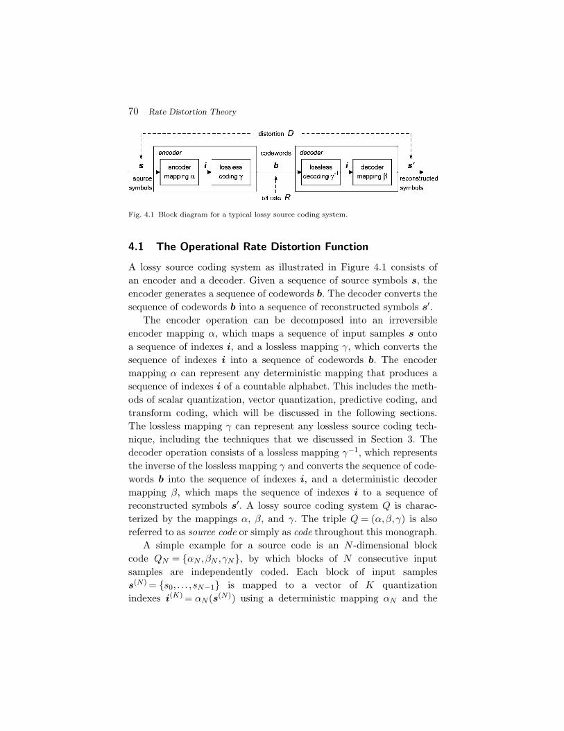
70 Rate Distortion Theory
Fig. 4.1 Block diagram for a typical lossy source coding system.
4.1 The Operational Rate Distortion Function
A lossy source coding system as illustrated in Figure 4.1 consists ofan encoder and a decoder. Given a sequence of source symbols s, theencoder generates a sequence of codewords b. The decoder converts thesequence of codewords b into a sequence of reconstructed symbols s′.
The encoder operation can be decomposed into an irreversibleencoder mapping α, which maps a sequence of input samples s ontoa sequence of indexes i, and a lossless mapping γ, which converts thesequence of indexes i into a sequence of codewords b. The encodermapping α can represent any deterministic mapping that produces asequence of indexes i of a countable alphabet. This includes the meth-ods of scalar quantization, vector quantization, predictive coding, andtransform coding, which will be discussed in the following sections.The lossless mapping γ can represent any lossless source coding tech-nique, including the techniques that we discussed in Section 3. Thedecoder operation consists of a lossless mapping γ−1, which representsthe inverse of the lossless mapping γ and converts the sequence of code-words b into the sequence of indexes i, and a deterministic decodermapping β, which maps the sequence of indexes i to a sequence ofreconstructed symbols s′. A lossy source coding system Q is charac-terized by the mappings α, β, and γ. The triple Q = (α,β,γ) is alsoreferred to as source code or simply as code throughout this monograph.
A simple example for a source code is an N -dimensional blockcode QN = {αN ,βN ,γN}, by which blocks of N consecutive inputsamples are independently coded. Each block of input sampless(N) = {s0, . . . ,sN−1} is mapped to a vector of K quantizationindexes i(K) = αN (s(N)) using a deterministic mapping αN and the
4.1 The Operational Rate Distortion Function 71
resulting vector of indexes i is converted into a variable-length bitsequence b(�) = γN (i(K)). At the decoder side, the recovered vectori(K) = γ−1
N (b(�)) of indexes is mapped to a block s′(N) = βN (i(K)) ofN reconstructed samples using the deterministic decoder mapping βN .
In the following, we will use the notations αN , βN , and γN also forrepresenting the encoder, decoder, and lossless mappings for the firstN samples of an input sequence, independently of whether the sourcecode Q represents an N -dimensional block code.
4.1.1 Distortion
For continuous random processes, the encoder mapping α cannot beinvertible, since real numbers cannot be represented by indexes of acountable alphabet and they cannot be losslessly described by a finitenumber of bits. Consequently, the reproduced symbol sequence s′ is notthe same as the original symbol sequence s. In general, if the decodermapping β is not the inverse of the encoder mapping α, the recon-structed symbols are only an approximation of the original symbols. Formeasuring the goodness of such an approximation, distortion measuresare defined that express the difference between a set of reconstructedsamples and the corresponding original samples as a non-negative realvalue. A smaller distortion corresponds to a higher approximation qual-ity. A distortion of zero specifies that the reproduced samples are iden-tical to the corresponding original samples.
In this monograph, we restrict our considerations to the importantclass of additive distortion measures. The distortion between a singlereconstructed symbol s′ and the corresponding original symbol s isdefined as a function d1(s,s′), which satisfies
d1(s,s′) ≥ 0, (4.1)
with equality if and only if s = s′. Given such a distortion mea-sure d1(s,s′), the distortion between a set of N reconstructed sam-ples s′ = {s′
0,s′1, . . . ,s
′N−1} and the corresponding original samples
s = {s0,s1, . . . ,sN−1} is defined by
dN (s,s′) =1N
N−1∑i=0
d1(si,s′i). (4.2)
72 Rate Distortion Theory
The most commonly used additive distortion measure is the squarederror, d1(s,s′) = (s − s′)2. The resulting distortion measure for sets ofsamples is the mean squared error (MSE),
dN (s,s′) =1N
N−1∑i=0
(si − s′i)
2. (4.3)
The reasons for the popularity of squared error distortion measuresare their simplicity and the mathematical tractability of the associatedoptimization problems. Throughout this monograph, we will explicitlyuse the squared error and mean squared error as distortion measures forsingle samples and sets of samples, respectively. It should, however, benoted that in most video coding applications the quality of the recon-struction signal is finally judged by human observers. But the MSEdoes not well correlate with the quality that is perceived by humanobservers. Nonetheless, MSE-based quality measures are widely usedin the video coding community. The investigation of alternative dis-tortion measures for video coding applications is still an active field ofresearch.
In order to evaluate the approximation quality of a code Q, ratherthan measuring distortion for a given finite symbol sequence, we areinterested in a measure for the expected distortion for very long symbolsequences. Given a random process S = {Sn}, the distortion δ(Q) asso-ciated with a code Q is defined as the limit of the expected distortionas the number of coded symbols approaches infinity,
δ(Q) = limN→∞
E{
dN
(S(N), βN (αN (S(N)))
)}, (4.4)
if the limit exists. S(N) = {S0,S1, . . . ,SN−1} represents the sequence ofthe first N random variables of the random process S and βN (αN (·))specifies the mapping of the first N input symbols to the correspondingreconstructed symbols as given by the code Q.
For stationary processes S with a multivariate pdf f(s) and a blockcode QN = (αN ,βN ,γN ), the distortion δ(QN ) is given by
δ(QN ) =∫
RN
f(s)dN
(s, βN (αN (s))
)ds. (4.5)

4.1 The Operational Rate Distortion Function 73
4.1.2 Rate
Beside the distortion δ(Q), another important property required forevaluating the performance of a code Q is its rate. For coding of afinite symbol sequence s(N), we define the transmission rate as theaverage number of bits per input symbol,
rN (s(N)) =1N
|γN (αN (s(N)))|, (4.6)
where γN (αN (·)) specifies the mapping of the N input symbols to thebit sequence b(�) of � bits as given by the code Q and the operator | · | isdefined to return the number of bits in the bit sequence that is specifiedas argument. Similarly as for the distortion, we are interested in ameasure for the expected number of bits per symbol for long sequences.For a given random process S = {Sn}, the rate r(Q) associated witha code Q is defined as the limit of the expected number of bits persymbol as the number of transmitted symbols approaches infinity,
r(Q) = limN→∞
1N
E{
|γN (αN (S(N)))|}
, (4.7)
if the limit exists. For stationary random processes S and a block codesQN = (αN ,βN ,γN ), the rate r(QN ) is given by
r(QN ) =1N
∫RN
f(s)∣∣γN (αN (s))
∣∣ds, (4.8)
where f(s) is the Nth order joint pdf of the random process S.
4.1.3 Operational Rate Distortion Function
For a given source S, each code Q is associated with a rate distortionpoint (R,D), which is given by R = r(Q) and D = δ(Q). In Figure 4.2,the rate distortion points for selected codes are illustrated as dots.The rate distortion plane can be partitioned into a region of achievablerate distortion points and a region of non-achievable rate distortionpoints. A rate distortion point (R,D) is called achievable if there isa code Q with r(Q) ≤ R and δ(Q) ≤ D. The boundary between theregions of achievable and non-achievable rate distortion points specifiesthe minimum rate R that is required for representing the source S with
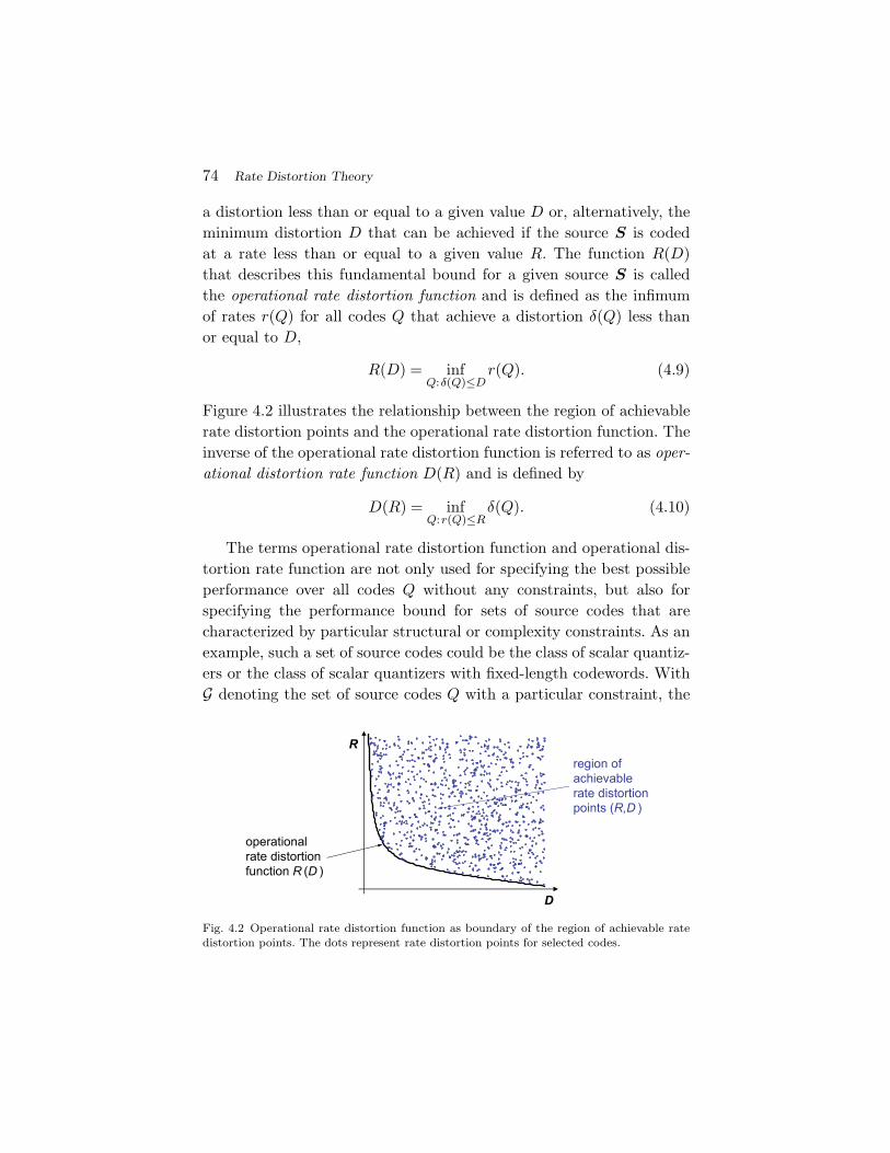
74 Rate Distortion Theory
a distortion less than or equal to a given value D or, alternatively, theminimum distortion D that can be achieved if the source S is codedat a rate less than or equal to a given value R. The function R(D)that describes this fundamental bound for a given source S is calledthe operational rate distortion function and is defined as the infimumof rates r(Q) for all codes Q that achieve a distortion δ(Q) less thanor equal to D,
R(D) = infQ:δ(Q)≤D
r(Q). (4.9)
Figure 4.2 illustrates the relationship between the region of achievablerate distortion points and the operational rate distortion function. Theinverse of the operational rate distortion function is referred to as oper-ational distortion rate function D(R) and is defined by
D(R) = infQ:r(Q)≤R
δ(Q). (4.10)
The terms operational rate distortion function and operational dis-tortion rate function are not only used for specifying the best possibleperformance over all codes Q without any constraints, but also forspecifying the performance bound for sets of source codes that arecharacterized by particular structural or complexity constraints. As anexample, such a set of source codes could be the class of scalar quantiz-ers or the class of scalar quantizers with fixed-length codewords. WithG denoting the set of source codes Q with a particular constraint, the
Fig. 4.2 Operational rate distortion function as boundary of the region of achievable ratedistortion points. The dots represent rate distortion points for selected codes.
4.2 The Information Rate Distortion Function 75
operational rate distortion function for a given source S and codes withthe particular constraint is defined by
RG(D) = infQ∈G:δ(Q)≤D
r(Q). (4.11)
Similarly, the operational distortion rate function for a given source S
and a set G of codes with a particular constraint is defined by
DG(R) = infQ∈G:r(Q)≤R
δ(Q). (4.12)
It should be noted that in contrast to information rate distortionfunctions, which will be introduced in the next section, operationalrate distortion functions are not convex. They are more likely to bestep functions, i.e., piecewise constant functions.
4.2 The Information Rate Distortion Function
In the previous section, we have shown that the operational rate dis-tortion function specifies a fundamental performance bound for lossysource coding techniques. But unless we suitably restrict the set of con-sidered codes, it is virtually impossible to determine the operationalrate distortion function according to the definition in (4.9). A moreaccessible expression for a performance bound of lossy codes is givenby the information rate distortion function, which was originally intro-duced by Shannon in [63, 64].
In the following, we first introduce the concept of mutual infor-mation before we define the information rate distortion function andinvestigate its relationship to the operational rate distortion function.
4.2.1 Mutual Information
Although this section deals with the lossy coding of random sources, wewill introduce the quantity of mutual information for general randomvariables and vectors of random variables.
Let X and Y be two discrete random variables with alphabetsAX = {x0,x1, . . .,xMX−1} and AY = {y0,y1, . . .,yMY −1}, respectively.As shown in Section 3.2, the entropy H(X) represents a lower boundfor the average codeword length of a lossless source code for the random
76 Rate Distortion Theory
variable X. It can also be considered as a measure for the uncertaintythat is associated with the random variable X or as a measure for theaverage amount of information that is required to describe the ran-dom variable X. The conditional entropy H(X|Y ) can be interpretedas a measure for the uncertainty that we have about the random vari-able X if we observe the random variable Y or as the average amountof information that is required to describe the random variable X ifthe random variable Y is known. The mutual information between thediscrete random variables X and Y is defined as the difference
I(X;Y ) = H(X) − H(X|Y ). (4.13)
The mutual information I(X;Y ) is a measure for the reduction of theuncertainty about the random variable X due to the observation of Y .It represents the average amount of information that the random vari-able Y contains about the random variable X. Inserting the formulasfor the entropy (3.13) and conditional entropy (3.20) yields
I(X;Y ) =MX∑i=0
MY∑j=0
pXY (xi,yj) log2pXY (xi,yi)
pX(xi)pY (yj), (4.14)
where pX and pY represent the marginal pmfs of the random variablesX and Y , respectively, and pXY denotes the joint pmf.
For extending the concept of mutual information to general randomvariables we consider two random variables X and Y with marginal pdfsfX and fY , respectively, and the joint pdf fXY . Either or both of therandom variables may be discrete or continuous or of mixed type. Sincethe entropy, as introduced in Section 3.2, is only defined for discreterandom variables, we investigate the mutual information for discreteapproximations X∆ and Y∆ of the random variables X and Y .
With ∆ being a step size, the alphabet of the discrete approximationX∆ of a random variable X is defined by AX∆ = {. . . ,x−1,x0,x1, . . .}with xi = i · ∆. The event {X∆ =xi} is defined to be equal to the event{xi ≤ X < xi+1}. Furthermore, we define an approximation f
(∆)X of the
pdf fX for the random variable X, which is constant inside each half-open interval [xi,xi+1), as illustrated in Figure 4.3, and is given by
∀x:xi ≤ x < xi+1, f(∆)X (x) =
1∆
∫ xi+1
xi
fX(x′)dx′. (4.15)
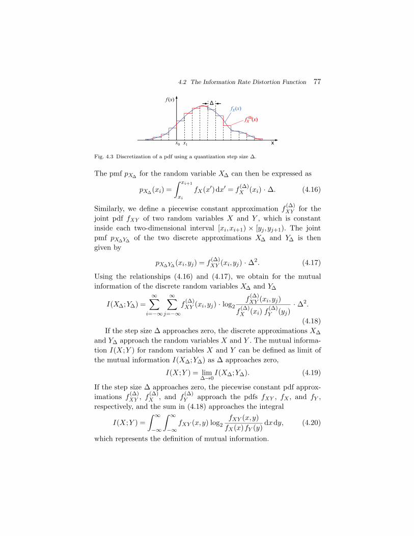
4.2 The Information Rate Distortion Function 77
Fig. 4.3 Discretization of a pdf using a quantization step size ∆.
The pmf pX∆ for the random variable X∆ can then be expressed as
pX∆(xi) =∫ xi+1
xi
fX(x′)dx′ = f(∆)X (xi) · ∆. (4.16)
Similarly, we define a piecewise constant approximation f(∆)XY for the
joint pdf fXY of two random variables X and Y , which is constantinside each two-dimensional interval [xi,xi+1) × [yj ,yj+1). The jointpmf pX∆Y∆ of the two discrete approximations X∆ and Y∆ is thengiven by
pX∆Y∆(xi,yj) = f(∆)XY (xi,yj) · ∆2. (4.17)
Using the relationships (4.16) and (4.17), we obtain for the mutualinformation of the discrete random variables X∆ and Y∆
I(X∆;Y∆) =∞∑
i=−∞
∞∑j=−∞
f(∆)XY (xi,yj) · log2
f(∆)XY (xi,yj)
f(∆)X (xi) f
(∆)Y (yj)
· ∆2.
(4.18)If the step size ∆ approaches zero, the discrete approximations X∆
and Y∆ approach the random variables X and Y . The mutual informa-tion I(X;Y ) for random variables X and Y can be defined as limit ofthe mutual information I(X∆;Y∆) as ∆ approaches zero,
I(X;Y ) = lim∆→0
I(X∆;Y∆). (4.19)
If the step size ∆ approaches zero, the piecewise constant pdf approx-imations f
(∆)XY , f
(∆)X , and f
(∆)Y approach the pdfs fXY , fX , and fY ,
respectively, and the sum in (4.18) approaches the integral
I(X;Y ) =∫ ∞
−∞
∫ ∞
−∞fXY (x,y) log2
fXY (x,y)fX(x)fY (y)
dxdy, (4.20)
which represents the definition of mutual information.

78 Rate Distortion Theory
The formula (4.20) shows that the mutual information I(X;Y ) issymmetric with respect to the random variables X and Y . The aver-age amount of information that a random variable X contains aboutanother random variable Y is equal to the average amount of informa-tion that Y contains about X. Furthermore, the mutual informationI(X;Y ) is greater than or equal to zero, with equality if and onlyif fXY (x,y) = fX(x)fY (x), ∀x,y ∈ R, i.e., if and only if the randomvariables X and Y are independent. This is a direct consequence of thedivergence inequality for probability density functions f and g,
−∫ ∞
−∞f(s) log2
g(s)f(s)
≥ 0, (4.21)
which is fulfilled with equality if and only if the pdfs f and g are thesame. The divergence inequality can be proved using the inequalitylnx ≥ x − 1 (with equality if and only if x = 1),
−∫ ∞
−∞f(s) log2
g(s)f(s)
ds ≥ − 1ln2
∫ ∞
−∞f(s)
(g(s)f(s)
− 1)
ds
=1
ln2
(∫ ∞
−∞f(s)ds −
∫ ∞
−∞g(s)ds
)= 0. (4.22)
For N -dimensional random vectors X = (X0,X1, . . . ,XN−1)T andY = (Y0,Y1, . . . ,YN−1)T, the definition of mutual information can beextended according to
I(X;Y ) =∫
RN
∫RN
fXY (x,y) log2fXY (x,y)
fX(x)fY (y)dxdy, (4.23)
where fX and fY denote the marginal pdfs for the random vectors X
and Y , respectively, and fXY represents the joint pdf.We now assume that the random vector Y is a discrete random
vector and is associated with an alphabet ANY . Then, the pdf fY and
the conditional pdf fY |X can be written as
fY (y) =∑
a∈ANY
δ(y − a)pY (a), (4.24)
fY |X(y|x) =∑
a∈ANY
δ(y − a)pY |X(a|x), (4.25)

4.2 The Information Rate Distortion Function 79
where pY denotes the pmf of the discrete random vector Y , and pY |Xdenotes the conditional pmf of Y given the random vector X. Insert-ing fXY = fY |X · fX and the expressions (4.24) and (4.25) into thedefinition (4.23) of mutual information for vectors yields
I(X;Y ) =∫
RN
fX(x)∑
a∈ANY
pY |X(a|x) log2pY |X(a|x)
pY (a)dx. (4.26)
This expression can be re-written as
I(X;Y ) = H(Y ) −∫ ∞
−∞fX(x)H(Y |X =x)dx, (4.27)
where H(Y ) is the entropy of the discrete random vector Y and
H(Y |X =x) = −∑
a∈ANY
pY |X(a|x) log2 pY |X(a|x) (4.28)
is the conditional entropy of Y given the event {X =x}. Since theconditional entropy H(Y |X =x) is always non-negative, we have
I(X;Y ) ≤ H(Y ). (4.29)
Equality is obtained if and only if H(Y |X =x) is zero for all x and,hence, if and only if the random vector Y is given by a deterministicfunction of the random vector X.
If we consider two random processes X = {Xn} and Y = {Yn} andrepresent the random variables for N consecutive time instants as ran-dom vectors X(N) and Y (N), the mutual information I(X(N);Y (N))between the random vectors X(N) and Y (N) is also referred to as Nthorder mutual information and denoted by IN (X;Y ).
4.2.2 Information Rate Distortion Function
Suppose we have a source S = {Sn} that is coded using a lossysource coding system given by a code Q = (α,β,γ). The output of thelossy coding system can be described by the random process S′ = {S′
n}.Since coding is a deterministic process given by the mapping β(α(·)),the random process S′ describing the reconstructed samples is a deter-ministic function of the input process S. Nonetheless, the statistical

80 Rate Distortion Theory
properties of the deterministic mapping given by a code Q can bedescribed by a conditional pdf gQ(s′|s) = gS′
n|Sn(s′|s). If we consider,
as an example, simple scalar quantization, the conditional pdf gQ(s′|s)represents, for each value of s, a shifted Dirac delta function. In general,gQ(s′|s) consists of a sum of scaled and shifted Dirac delta functions.Note that the random variables S′
n are always discrete and, hence, theconditional pdf gQ(s′|s) can also be represented by a conditional pmf.Instead of single samples, we can also consider the mapping of blocksof N successive input samples S to blocks of N successive output sam-ples S′. For each value of N > 0, the statistical properties of a code Q
can then be described by the conditional pdf gQN (s′|s) = gS′|S(s′|s).
For the following considerations, we define the Nth order distortion
δN (gN ) =∫
RN
∫RN
fS(s)gN (s′|s)dN (s,s′)dsds′. (4.30)
Given a source S, with an Nth order pdf fS , and an additive distortionmeasure dN , the Nth order distortion δN (gN ) is completely determinedby the conditional pdf gN = gS′|S . The distortion δ(Q) that is associ-ated with a code Q and was defined in (4.4) can be written as
δ(Q) = limN→∞
δN (gQN ). (4.31)
Similarly, the Nth order mutual information IN (S;S′) between blocksof N successive input samples and the corresponding blocks of outputsamples can be written as
IN (gN ) =∫
RN
∫RN
fS(s)gN (s′|s) log2gN (s′|s)fS′(s′)
dsds′, (4.32)
with
fS′(s′) =∫
RN
fS(s)gN (s′|s)ds. (4.33)
For a given source S, the Nth order mutual information only dependson the Nth order conditional pdf gN .
We now consider any source code Q with a distortion δ(Q) that isless than or equal to a given value D. As mentioned above, the outputprocess S′ of a source coding system is always discrete. We have shown
4.2 The Information Rate Distortion Function 81
in Section 3.3.1 that the average codeword length for lossless coding ofa discrete source cannot be smaller than the entropy rate of the source.Hence, the rate r(Q) of the code Q is greater than or equal to theentropy rate of S′,
r(Q) ≥ H(S′). (4.34)
By using the definition of the entropy rate H(S′) in (3.25) and therelationship (4.29), we obtain
r(Q) ≥ limN→∞
HN (S)N
≥ limN→∞
IN (S;S′)N
= limN→∞
IN (gQN )
N, (4.35)
where HN (S′) denotes the block entropy for the random vectors S′
of N successive reconstructed samples and IN (S;S′) is the mutualinformation between the N -dimensional random vectors S and thecorresponding reconstructions S′. A deterministic mapping as givenby a source code is a special case of a random mapping. Hence, theNth order mutual information IN (gQ
N ) for a particular code Q withδN (gQ
N ) ≤ D cannot be smaller than the smallest Nth order mutualinformation IN (gN ) that can be achieved using any random mappinggN = gS′|S with δN (gN ) ≤ D,
IN (gQN ) ≥ inf
gN :δN (gN )≤DIN (gN ). (4.36)
Consequently, the rate r(Q) is always greater than or equal to
R(I)(D) = limN→∞
infgN :δN (gN )≤D
IN (gN )N
. (4.37)
This fundamental lower bound for all lossy source coding techniquesis called the information rate distortion function. Every code Q thatyields a distortion δ(Q) less than or equal to any given value D for asource S is associated with a rate r(Q) that is greater than or equal tothe information rate distortion function R(I)(D) for the source S,
∀Q:δ(Q) ≤ D, r(Q) ≥ R(I)(D). (4.38)
This relationship is called the fundamental source coding theorem. Theinformation rate distortion function was first derived by Shannon for

82 Rate Distortion Theory
iid sources [63, 64] and is for that reason also referred to as Shannonrate distortion function.
If we restrict our considerations to iid sources, the Nth orderjoint pdf fS(s) can be represented as the product
∏N−1i=0 fS(si) of the
marginal pdf fS(s), with s = {s0, . . . ,sN−1}. Hence, for every N , theNth order distortion δN (gQ
N ) and mutual information IN (gQN ) for a
code Q can be expressed using a scalar conditional pdf gQ = gS′|S ,
δN (gQN ) = δ1(gQ) and IN (gQ
N ) = N · I1(gQ). (4.39)
Consequently, the information rate distortion function R(I)(D) for iidsources is equal to the so-called first order information rate distortionfunction,
R(I)1 (D) = inf
g:δ1(g)≤DI1(g). (4.40)
In general, the function
R(I)N (D) = inf
gN :δN (gN )≤D
IN (gN )N
. (4.41)
is referred to as the N th order information rate distortion function. If N
approaches infinity, the Nth order information rate distortion functionapproaches the information rate distortion function,
R(I)(D) = limN→∞
R(I)N (D). (4.42)
We have shown that the information rate distortion function repre-sents a fundamental lower bound for all lossy coding algorithms. Usingthe concept of typical sequences, it can additionally be shown thatthe information rate distortion function is also asymptotically achiev-able [4, 22, 11], meaning that for any ε > 0 there exists a code Q withδ(Q) ≤ D and r(Q) ≤ R(I)(D) + ε. Hence, subject to suitable techni-cal assumptions the information rate distortion function is equal tothe operational rate distortion function. In the following text, we usethe notation R(D) and the term rate distortion function to denoteboth the operational and information rate distortion function. The termoperational rate distortion function will mainly be used for denotingthe operational rate distortion function for restricted classes of codes.
4.2 The Information Rate Distortion Function 83
The inverse of the information rate distortion function is called theinformation distortion rate function or simply the distortion rate func-tion and is given by
D(R) = limN→∞
infgN :IN (gN )/N≤R
δN (gN ). (4.43)
Using this definition, the fundamental source coding theorem (4.38)can also be written as
∀Q:r(Q) ≤ R, δ(Q) ≥ D(R). (4.44)
The information rate distortion function is defined as a mathemati-cal function of a source. However, an analytical derivation of the infor-mation rate distortion function is still very difficult or even impossible,except for some special random processes. An iterative technique fornumerically computing close approximations of the rate distortion func-tion for iid sources was developed by Blahut and Arimoto in [3, 6] and isreferred to as Blahut–Arimoto algorithm. An overview of the algorithmcan be found in [11, 22].
4.2.3 Properties of the Rate Distortion Function
In the following, we state some important properties of the rate dis-tortion function R(D) for the MSE distortion measure.1 For proofs ofthese properties, the reader is referred to [4, 11, 22].
• The rate distortion function R(D) is a non-increasing andconvex function of D.
• There exists a value Dmax, so that
∀D ≥ Dmax, R(D) = 0. (4.45)
For the MSE distortion measure, the value of Dmax is equalto the variance σ2 of the source.
• For continuous sources S, the rate distortion function R(D)approaches infinity as D approaches zero.
1 The properties hold more generally. In particular, all stated properties are valid for additivedistortion measures for which the single-letter distortion d1(s,s′) is equal to 0 if s = s′and is greater than 0 if s �= s′.
84 Rate Distortion Theory
• For discrete sources S, the minimum rate that is required fora lossless transmission is equal to the entropy rate,
R(0) = H(S). (4.46)
The last property shows that the fundamental bound for lossless codingis a special case of the fundamental bound for lossy coding.
4.3 The Shannon Lower Bound
For most random processes, an analytical expression for the rate distor-tion function cannot be given. In the following, we show how a usefullower bound for the rate distortion function of continuous random pro-cesses can be calculated. Before we derive this so-called Shannon lowerbound, we introduce the quantity of differential entropy.
4.3.1 Differential Entropy
The mutual information I(X;Y ) of two continuous N -dimensional ran-dom vectors X and Y is defined in (4.23). Using the relationshipfXY = fX|Y · fY , the integral in this definition can be decomposedinto a part that only depends on one of the random vectors and a partthat depends on both random vectors,
I(X;Y ) = h(X) − h(X|Y ), (4.47)
with
h(X) = E{− log2 fX(X)}
= −∫
RN
fX(x) log2 fX(x)dx (4.48)
and
h(X|Y ) = E{− log2 fX|Y (X|Y )
}= −
∫RN
∫RN
fXY (x,y) log2 fX|Y (x|y)dxdy. (4.49)
In analogy to the discrete entropy introduced in Section 3, the quantityh(X) is called the differential entropy of the random vector X and the
4.3 The Shannon Lower Bound 85
quantity h(X|Y ) is referred to as conditional differential entropy of therandom vector X given the random vector Y .
Since I(X;Y ) is always non-negative, we can conclude that condi-tioning reduces the differential entropy,
h(X|Y ) ≤ h(X), (4.50)
similarly as conditioning reduces the discrete entropy.For continuous random processes S = {Sn}, the random vari-
ables Sn for N consecutive time instants can be represented as a randomvector S(N) = (S0, . . . ,SN−1)T. The differential entropy h(S(N)) for thevectors S(N) is then also referred to as N th order differential entropyand is denoted by
hN (S) = h(S(N)) = h(S0, . . . ,SN−1) (4.51)
If, for a continuous random process S, the limit
h(S) = limN→∞
hN (S)N
= limN→∞
h(S0, . . . ,SN−1)N
(4.52)
exists, it is called the differential entropy rate of the process S.The differential entropy has a different meaning than the discrete
entropy. This can be illustrated by considering an iid process S = {Sn}with a uniform pdf f(s), with f(s) = 1/A for |s| ≤ A/2 and f(s) = 0for |s| > A/2. The first order differential entropy for this process is
h(S) = −∫ A/2
−A/2
1A
log21A
ds = log2 A1A
∫ A/2
−A/2ds = log2 A. (4.53)
In Figure 4.4, the differential entropy h(S) for the uniform iid processis shown as a function of the parameter A. In contrast to the discreteentropy, the differential entropy can be either positive or negative. Thediscrete entropy is only finite for discrete alphabet sources, it is infinitefor continuous alphabet sources. The differential entropy, however, ismainly useful for continuous random processes. For discrete randomprocesses, it can be considered to be −∞.
As an example, we consider a stationary Gaussian random processwith a mean µ and an Nth order autocovariance matrix CN . The Nthorder pdf fG(s) is given in (2.51), where µN represents a vector with all
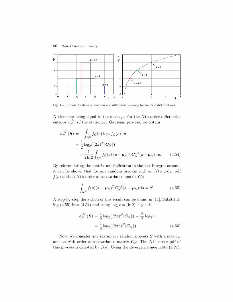
86 Rate Distortion Theory
Fig. 4.4 Probability density function and differential entropy for uniform distributions.
N elements being equal to the mean µ. For the Nth order differentialentropy h
(G)N of the stationary Gaussian process, we obtain
h(G)N (S) = −
∫RN
fG(s) log2 fG(s)ds
=12
log2((2π)N |CN |
)+
12ln2
∫RN
fG(s) (s−µN )T C−1N (s−µN )ds. (4.54)
By reformulating the matrix multiplication in the last integral as sum,it can be shown that for any random process with an Nth order pdff(s) and an Nth order autocovariance matrix CN ,∫
RN
f(s)(s − µN )T C−1N (s − µN )ds = N. (4.55)
A step-by-step derivation of this result can be found in [11]. Substitut-ing (4.55) into (4.54) and using log2 e = (ln2)−1 yields
h(G)N (S) =
12
log2((2π)N |CN |
)+
N
2log2 e
=12
log2((2πe)N |CN |
). (4.56)
Now, we consider any stationary random process S with a mean µ
and an Nth order autocovariance matrix CN . The Nth order pdf ofthis process is denoted by f(s). Using the divergence inequality (4.21),

4.3 The Shannon Lower Bound 87
we obtain for its Nth order differential entropy,
hN (S) = −∫
RN
f(s) log2 f(s)ds
≤ −∫
RN
f(s) log2 fG(s)ds
=12
log2((2π)N |CN |
)+
12ln2
∫RN
f(s)(s−µN )T C−1N (s−µN )ds, (4.57)
where fG(s) represents the Nth order pdf of the stationary Gaussianprocess with the same mean µ and the same Nth order autocovariancematrix CN . Inserting (4.55) and (4.56) yields
hN (S) ≤ h(G)N (S) =
12
log2((2πe)N |CN |). (4.58)
Hence, the Nth order differential entropy of any stationary non-Gaussian process is less than the Nth order differential entropy of astationary Gaussian process with the same Nth order autocovariancematrix CN .
As shown in (4.56), the Nth order differential entropy of a stationaryGaussian process depends on the determinant of its Nth order autoco-variance matrix |CN |. The determinant |CN | is given by the productof the eigenvalues ξi of the matrix CN , |CN | =
∏N−1i=0 ξi. The trace of
the Nth order autocovariance matrix tr(CN ) is given by the sum ofits eigenvalues, tr(CN ) =
∑N−1i=0 ξi, and, according to (2.39), also by
tr(CN ) = N · σ2, with σ2 being the variance of the Gaussian process.Hence, for a given variance σ2, the sum of the eigenvalues is constant.With the inequality of arithmetic and geometric means,(
N−1∏i=0
xi
)1N
≤ 1N
N−1∑i=0
xi, (4.59)
which holds with equality if and only if x0 =x1 = · · ·=xN−1, we obtainthe inequality
|CN | =N−1∏i=0
ξi ≤(
1N
N−1∑i=0
ξi
)N
= σ2N . (4.60)
88 Rate Distortion Theory
Equality holds if and only if all eigenvalues of CN are the same, i.e., ifand only if the Gaussian process is iid. Consequently, the Nth orderdifferential entropy of a stationary process S with a variance σ2 isbounded by
hN (S) ≤ N
2log2(2πeσ2). (4.61)
It is maximized if and only if the process is a Gaussian iid process.
4.3.2 Shannon Lower Bound
Using the relationship (4.47) and the notation IN (gN ) = IN (S;S′), therate distortion function R(D) defined in (4.37) can be written as
R(D) = limN→∞
infgN :δN (gN )≤D
IN (S;S′)N
= limN→∞
infgN :δN (gN )≤D
hN (S) − hN (S|S′)N
= limN→∞
hN (S)N
− limN→∞
supgN :δN (gN )≤D
hN (S|S′)N
= h(S) − limN→∞
supgN :δN (gN )≤D
hN (S − S′|S′)N
, (4.62)
where the subscripts N indicate the Nth order mutual informationand differential entropy. The last equality follows from the fact thatthe differential entropy is independent of the mean of a given pdf.
Since conditioning reduces the differential entropy, as has beenshown in (4.50), the rate distortion function is bounded by
R(D) ≥ RL(D), (4.63)
with
RL(D) = h(S) − limN→∞
supgN :δN (gN )≤D
hN (S − S′)N
. (4.64)
The lower bound RL(D) is called the Shannon lower bound (SLB).For stationary processes and the MSE distortion measure, the dis-
tortion δN (gN ) in (4.64) is equal to the variance σ2Z of the process
4.3 The Shannon Lower Bound 89
Z = S − S′. Furthermore, we have shown in (4.61) that the maximumNth order differential entropy for a stationary process with a given vari-ance σ2
Z is equal to N2 log2(2πeσ2
Z). Hence, the Shannon lower boundfor stationary processes and MSE distortion is given by
RL(D) = h(S) − 12
log2(2πeD
). (4.65)
Since we concentrate on the MSE distortion measure in this monograph,we call RL(D) given in (4.65) the Shannon lower bound in the followingwithout mentioning that it is only valid for the MSE distortion measure.
Shannon Lower Bound for IID Sources. The Nth order differ-ential entropy for iid sources S = {Sn} is equal to
hN (S) = E{− log2fS(S)} =N−1∑i=0
E{− log2fS(Sn)} = N · h(S), (4.66)
where h(S) denotes the first order differential entropy. Hence, the Shan-non lower bound for iid sources is given by
RL(D) = h(S) − 12
log2(2πeD
), (4.67)
DL(R) =1
2πe· 22h(S) · 2−2R. (4.68)
In the following, the differential entropy h(S) and the Shannon lowerbound DL(R) are given for three distributions. For the example of theLaplacian iid process with σ2 = 1, Figure 4.5 compares the Shannonlower bound DL(R) with the distortion rate function D(R), which wascalculated using the Blahut–Arimoto algorithm [3, 6].
Uniform pdf:
h(S) =12
log2(12σ2) ⇒ DL(R) =6πe
· σ2 · 2−2R (4.69)
Laplacian pdf:
h(S) =12
log2(2e2σ2) ⇒ DL(R) =e
π· σ2 · 2−2R (4.70)
Gaussian pdf:
h(S) =12
log2(2πeσ2) ⇒ DL(R) = σ2 · 2−2R (4.71)
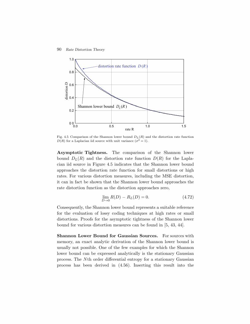
90 Rate Distortion Theory
Fig. 4.5 Comparison of the Shannon lower bound DL(R) and the distortion rate functionD(R) for a Laplacian iid source with unit variance (σ2 = 1).
Asymptotic Tightness. The comparison of the Shannon lowerbound DL(R) and the distortion rate function D(R) for the Lapla-cian iid source in Figure 4.5 indicates that the Shannon lower boundapproaches the distortion rate function for small distortions or highrates. For various distortion measures, including the MSE distortion,it can in fact be shown that the Shannon lower bound approaches therate distortion function as the distortion approaches zero,
limD→0
R(D) − RL(D) = 0. (4.72)
Consequently, the Shannon lower bound represents a suitable referencefor the evaluation of lossy coding techniques at high rates or smalldistortions. Proofs for the asymptotic tightness of the Shannon lowerbound for various distortion measures can be found in [5, 43, 44].
Shannon Lower Bound for Gaussian Sources. For sources withmemory, an exact analytic derivation of the Shannon lower bound isusually not possible. One of the few examples for which the Shannonlower bound can be expressed analytically is the stationary Gaussianprocess. The Nth order differential entropy for a stationary Gaussianprocess has been derived in (4.56). Inserting this result into the
4.3 The Shannon Lower Bound 91
definition of the Shannon lower bound (4.65) yields
RL(D) = limN→∞
12N
log2 |CN | − 12
log2 D, (4.73)
where CN is the Nth order autocorrelation matrix. The determinantof a matrix is given by the product of its eigenvalues. With ξ
(N)i , for
i = 0,1, . . . ,N − 1, denoting the N eigenvalues of the Nth order auto-correlation matrix CN , we obtain
RL(D) = limN→∞
12N
N−1∑i=0
log2 ξ(N)i − 1
2log2 D. (4.74)
In order to proceed, we restrict our considerations to Gaussian processeswith zero mean, in which case the autocovariance matrix CN is equalto the autocorrelation matrix RN , and apply Grenander and Szego’stheorem [29] for sequences of Toeplitz matrices. For a review of Toeplitzmatrices, including the theorem for sequences of Toeplitz matrices, werecommend the tutorial [23]. Grenander and Szego’s theorem can bestated as follows:
If RN is a sequence of Hermitian Toeplitz matriceswith elements φk on the kth diagonal, the infimumΦinf = infω Φ(ω) and supremum Φsup = supω Φ(ω) ofthe Fourier series
Φ(ω) =∞∑
k=−∞φk e−jωk (4.75)
are finite, and the function G is continuous in the inter-val [Φinf ,Φsup], then
limN→∞
1N
N−1∑i=0
G(ξ(N)i ) =
12π
∫ π
−πG(Φ(ω))dω, (4.76)
where ξ(N)i , for i = 0,1, . . . ,N − 1, denote the eigenval-
ues of the Nth matrix RN .
A matrix is called Hermitian if it is equal to its conjugate trans-pose. This property is always fulfilled for real symmetric matrices as

92 Rate Distortion Theory
the autocorrelation matrices of stationary processes. Furthermore, theFourier series (4.75) for the elements of the autocorrelation matrix RN
is the power spectral density ΦSS (ω). If we assume that the power spec-tral density is finite and greater than 0 for all frequencies ω, the limit in(4.74) can be replaced by an integral according to (4.76). The Shannonlower bound RL(D) of a stationary Gaussian process with zero-meanand a power spectral density ΦSS (ω) is given by
RL(D) =14π
∫ π
−πlog2
ΦSS (ω)D
dω. (4.77)
A nonzero mean does not have any impact on the Shannon lowerbound RL(D), but on the power spectral density ΦSS (ω).
For a stationary zero-mean Gauss–Markov process, the entries of theautocorrelation matrix are given by φk = σ2ρ|k|, where σ2 is the signalvariance and ρ is the correlation coefficient between successive samples.Using the relationship
∑∞k=1 ak e−jkx = a/(e−jx − a), we obtain
ΦSS (ω) =∞∑
k=−∞σ2 ρ|k| e−jωk = σ2
(1 +
ρ
e−jω − ρ+
ρ
ejω − ρ
)
= σ2 1 − ρ2
1 − 2ρcosω + ρ2 . (4.78)
Inserting this relationship into (4.77) yields
RL(D) =14π
∫ π
−πlog2
σ2(1 − ρ2)D
dω − 14π
∫ π
−πlog2(1− 2ρcosω + ρ2)dω︸ ︷︷ ︸
=0
=12
log2σ2 (1 − ρ2)
D, (4.79)
where we used∫ π0 ln(a2 − 2abcosx + b2)dx = 2π lna, for a ≥ b > 0. As
discussed above, the mean of a stationary process does not have anyimpact on the Shannon rate distortion function or the Shannon lowerbound. Hence, the distortion rate function DL(R) for the Shannonlower bound of a stationary Gauss–Markov process with a variance σ2
and a correlation coefficient ρ is given by
DL(R) = (1 − ρ2)σ2 2−2R. (4.80)
4.4 Rate Distortion Function for Gaussian Sources 93
This result can also be obtained by directly inserting the formula (2.50)for the determinant |CN | of the Nth order autocovariance matrix forGauss–Markov processes into the expression (4.73).
4.4 Rate Distortion Function for Gaussian Sources
Stationary Gaussian sources play a fundamental role in rate distortiontheory. We have shown that the Gaussian source maximize the differ-ential entropy, and thus also the Shannon lower bound, for a givenvariance or autocovariance function. Stationary Gaussian sources arealso one of the few examples, for which the rate distortion function canbe exactly derived.
4.4.1 Gaussian IID Sources
Before stating another important property of Gaussian iid sources, wecalculate their rate distortion function. Therefore, we first derive a lowerbound and then show that this lower bound is achievable. To prove thatthe lower bound is achievable, it is sufficient to show that there is aconditional pdf gS′|S(s′|s) for which the mutual information I1(gS′|S)is equal to the lower bound for a given distortion D.
The Shannon lower bound for Gaussian iid sources as distortion ratefunction DL(R) has been derived in Section 4.3. The corresponding ratedistortion function is given by
RL(D) =12
log2σ2
D, (4.81)
where σ2 is the signal variance. For proving that the rate distortionfunction is achievable, it is more convenient to look at the pdf of thereconstruction fS′(s′) and the conditional pdf gS|S′(s|s′) of the inputgiven the reconstruction.
For distortions D < σ2, we choose
fS′(s′) =1√
2π(σ2 − D)e− (s′−µ)2
2(σ2−D) , (4.82)
gS|S′(s|s′) =1√2πD
e− (s−s′)22D , (4.83)
94 Rate Distortion Theory
where µ denotes the mean of the Gaussian iid process. It should benoted that the conditional pdf gS|S′ represents a Gaussian pdf for therandom variables Zn = Sn − S′
n, which are given by the difference ofthe corresponding random variables Sn and S′
n. We now verify that thepdf fS(s) that we obtain with the choices (4.82) and (4.83) representsthe Gaussian pdf with a mean µ and a variance σ2. Since the randomvariables Sn can be represented as the sum S′
n + Zn, the pdf fS(s) isgiven by the convolution of fS′(s′) and gS|S′(s|s′). And since means andvariances add when normal densities are convolved, the pdf fS(s) thatis obtained is a Gaussian pdf with a mean µ = µ + 0 and a varianceσ2 = (σ2 − D) + D. Hence, the choices (4.82) and (4.83) are valid, andthe conditional pdf gS′|S(s′|s) could be calculated using Bayes rule
gS′|S(s′|s) = gS|S′(s|s′)fS′(s′)fS(s)
. (4.84)
The resulting distortion is given by the variance of the difference processZn = Sn − S′
n,
δ1(gS′|S) = E{(Sn − S′
n)2}
= E{Z2
n
}= D. (4.85)
For the mutual information, we obtain
I1(gS′|S) = h(Sn) − h(Sn|S′n) = h(Sn) − h(Sn − S′
n)
=12
log2(2πeσ2 ) − 1
2log2(2πeD
)=
12
log2σ2
D. (4.86)
Here, we used the fact that the conditional pdf gS|S′(s|s′) only dependson the difference s − s′ as given by the choice (4.83).
The results show that, for any distortion D < σ2, we can finda conditional pdf gS′|S that achieves the Shannon lower bound. Forgreater distortions, we choose gS′|S equal to the Dirac delta function,gS′|S(s′|s) = δ(0), which gives a distortion of σ2 and a rate of zero.Consequently, the rate distortion function for Gaussian iid sources isgiven by
R(D) =
12
log2σ2
D: D < σ2
0 : D ≥ σ2
. (4.87)
4.4 Rate Distortion Function for Gaussian Sources 95
The corresponding distortion rate function is given by
D(R) = σ2 2−2R. (4.88)
It is important to note that the rate distortion function for a Gaus-sian iid process is equal to the Shannon lower bound for the entirerange of rates. Furthermore, it can be shown [4] that for every iid pro-cess with a given variance σ2, the rate distortion function lies belowthat of the Gaussian iid process with the same variance.
4.4.2 Gaussian Sources with Memory
For deriving the rate distortion function R(D) for a stationary Gaus-sian process with memory, we decompose it into a number N of inde-pendent stationary Gaussian sources. The Nth order rate distortionfunction RN (D) can then be expressed using the rate distortion func-tion for Gaussian iid processes and the rate distortion function R(D) isobtained by considering the limit of RN (D) as N approaches infinity.
As we stated in Section 2.3, the Nth order pdf of a stationary Gaus-sian process is given by
fS(s) =1
(2π)N/2 |CN |1/2 e− 12 (s−µN )T C−1
N (s−µN ) (4.89)
where s is a vector of N consecutive samples, µN is a vector withall N elements being equal to the mean µ, and CN is the Nth orderautocovariance matrix. Since CN is a symmetric and real matrix, ithas N real eigenvalues ξ
(N)i , for i = 0,1, . . . ,N − 1. The eigenvalues are
solutions of the equation
CNv(N)i = ξ
(N)i v
(N)i , (4.90)
where v(N)i represents a nonzero vector with unit norm, which is called a
unit-norm eigenvector corresponding to the eigenvalue ξ(N)i . Let AN be
the matrix whose columns are build by the N unit-norm eigenvectors,
AN = (v(N)0 ,v
(N)1 , . . . ,v
(N)N−1). (4.91)
By combining the N equations (4.90) for i = 0,1, . . . ,N − 1, we obtainthe matrix equation
CN AN = AN ΞN , (4.92)
96 Rate Distortion Theory
where
ΞN =
ξ(N)0 0 . . . 00 ξ
(N)1 . . . 0
......
. . . 00 0 0 ξ
(N)N−1
(4.93)
is a diagonal matrix that contains the N eigenvalues of CN on its maindiagonal. The eigenvectors are orthogonal to each other and AN is anorthogonal matrix.
Given the stationary Gaussian source {Sn}, we construct a source{Un} by decomposing the source {Sn} into vectors S of N successiverandom variables and applying the transform
U = A−1N (S − µN ) = AT
N (S − µN ) (4.94)
to each of these vectors. Since AN is orthogonal, its inverse A−1 existsand is equal to its transpose AT. The resulting source {Un} is givenby the concatenation of the random vectors U . Similarly, the inversetransform for the reconstructions {U ′
n} and {S′n} is given by
S′ = AN U ′ + µN , (4.95)
with U ′ and S′ denoting the corresponding vectors of N successiverandom variables. Since the coordinate mapping (4.95) is the inverseof the mapping (4.94), the Nth order mutual information IN (U ;U ′) isequal to the Nth order mutual information IN (S;S′). A proof of thisstatement can be found in [4]. Furthermore, since AN is orthogonal,the transform
(U ′ − U) = AN (S′ − S) (4.96)
preserves the Euclidean norm.2 The MSE distortion between any real-ization s of the random vector S and its reconstruction s′
dN (s;s′) =1N
N−1∑i=0
(si − s′i)
2 =1N
N−1∑i=0
(ui − u′i)
2 = dN (u;u′) (4.97)
2 We will show in Section 7.2 that every orthogonal transform preserves the MSE distortion.
4.4 Rate Distortion Function for Gaussian Sources 97
is equal to the distortion between the corresponding vector u and itsreconstruction u′. Hence, the Nth order rate distortion function RN (D)for the stationary Gaussian source {Sn} is equal to the Nth order ratedistortion function for the random process {Un}.
A linear transformation of a Gaussian random vector results inanother Gaussian random vector. For the mean vector and the auto-correlation matrix of U , we obtain
E{U} = ATN (E{S} − µN ) = AT
N (µN − µN ) = 0 (4.98)
and
E{U UT} = AT
N E{(S − µN )(S − µN )T
}AN
= ATN CN AN = ΞN . (4.99)
Since ΞN is a diagonal matrix, the pdf of the random vectors U is givenby the product
fU (u) =1
(2π)N/2 |ΞN |1/2 e− 12u
TΞ−1N u =
N−1∏i=0
1√2πξ
(N)i
e− u2
i
2ξ(N)i
(4.100)of the pdfs of the Gaussian components Ui. Consequently, the compo-nents Ui are independent of each other.
In Section 4.2.2, we have shown how the Nth order mutual infor-mation and the Nth order distortion for a code Q can be describedby a conditional pdf gQ
N = gU ′|U that characterizes the mapping of therandom vectors U onto the corresponding reconstruction vectors U ′.Due to the independence of the components Ui of the random vec-tors U , the Nth order mutual information IN (gQ
N ) and the Nth orderdistortion δN (gQ
N ) for a code Q can be written as
IN (gQN ) =
N−1∑i=0
I1(gQi ) and δN (gQ
N ) =1N
N−1∑i=0
δ1(gQi ), (4.101)
where gQi = gU ′
i |Uispecifies the conditional pdf for the mapping of a
vector component Ui onto its reconstruction U ′i . Consequently, the Nth
98 Rate Distortion Theory
order distortion rate function DN (R) can be expressed by
DN (R) =1N
N−1∑i=0
Di(Ri) with R =1N
N−1∑i=0
Ri, (4.102)
where Ri(Di) denotes the first order rate distortion function for a vectorcomponent Ui. The first order distortion rate function for Gaussiansources has been derived in Section 4.4.1 and is given by
Di(Ri) = σ2i 2−2Ri . (4.103)
The variances σ2i of the vector component Ui are equal to the eigenval-
ues ξ(N)i of the Nth order autocovariance matrix CN . Hence, the Nth
order distortion rate function can be written as
DN (R) =1N
N−1∑i=0
ξ(N)i 2−2Ri with R =
1N
N−1∑i=0
Ri. (4.104)
With the inequality of arithmetic and geometric means, which holdswith equality if and only if all elements have the same value, we obtain
DN (R) ≥(
N−1∏i=0
ξ(N)i 2−2Ri
) 1N
=
(N−1∏i=0
ξ(N)i
) 1N
· 2−2R = ξ(N) · 2−2R,
(4.105)where ξ(N) denotes the geometric mean of the eigenvalues ξ
(N)i . For
a given Nth order mutual information R, the distortion is minimizedif and only if ξ
(N)i 2−2Ri is equal to ξ(N)2−2R for all i = 0, . . . ,N − 1,
which yields
Ri = R +12
log2ξ(N)i
ξ(N). (4.106)
In the above result, we have ignored the fact that the mutual infor-mation Ri for a component Ui cannot be less than zero. Since the dis-tortion rate function given in (4.103) is steeper at low Ri, the mutualinformation Ri for components with ξ
(N)i < ξ(N)2−2R has to be set equal
to zero and the mutual information R has to be distributed among theremaining components in order to minimize the distortion. This can

4.4 Rate Distortion Function for Gaussian Sources 99
be elegantly specified by introducing a parameter θ, with θ ≥ 0, andsetting the component distortions according to
Di = min(θ, ξ(N)i ). (4.107)
This concept is also known as inverse water-filling for independentGaussian sources [53], where the parameter θ can be interpreted as thewater level. Using (4.103), we obtain for the mutual information Ri,
Ri =12
log2ξ(N)i
min(θ, ξ
(N)i
) = max
(0,
12
log2ξ(N)i
θ
). (4.108)
The Nth order rate distortion function RN (D) can be expressed by thefollowing parametric formulation, with θ ≥ 0,
DN (θ) =1N
N−1∑i=0
Di =1N
N−1∑i=0
min(θ, ξ(N)i ), (4.109)
RN (θ) =1N
N−1∑i=0
Ri =1N
N−1∑i=0
max
(0,
12
log2ξ(N)i
θ
). (4.110)
The rate distortion function R(D) for the stationary Gaussian ran-dom process {Sn} is given by the limit
R(D) = limN→∞
RN (D), (4.111)
which yields the parametric formulation, with θ > 0,
D(θ) = limN→∞
DN (θ), R(θ) = limN→∞
RN (θ). (4.112)
For Gaussian processes with zero mean (CN = RN ), we can apply thetheorem for sequences of Toeplitz matrices (4.76) to express the ratedistortion function using the power spectral density ΦSS (ω) of thesource. A parametric formulation, with θ ≥ 0, for the rate distortionfunction R(D) for a stationary Gaussian source with zero mean and apower spectral density ΦSS (ω) is given by
D(θ) =12π
∫ π
−πmin(θ, ΦSS (ω)) dω, (4.113)
R(θ) =12π
∫ π
−πmax
(0,
12
log2ΦSS (ω)
θ
)dω. (4.114)
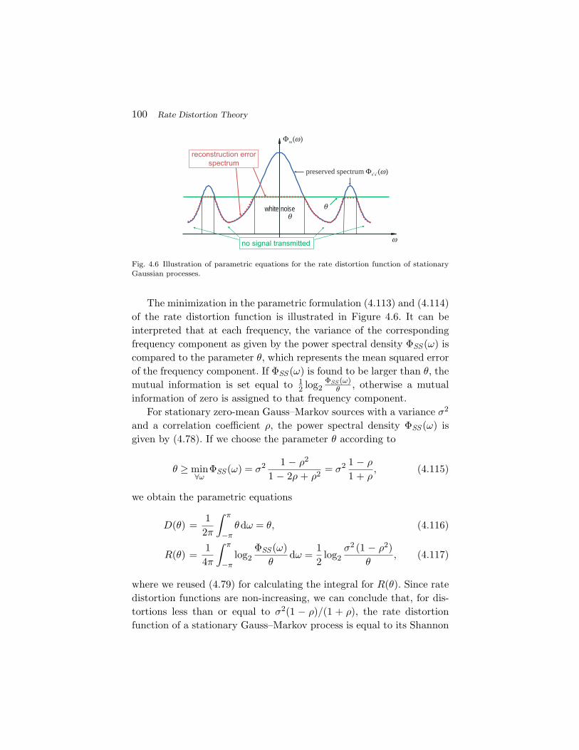
100 Rate Distortion Theory
white noise
reconstruction errorspectrum
no signal transmitted
Φss(ω)
θ
ω
preserved spectrum Φ ′s ′s (ω)
θ
Fig. 4.6 Illustration of parametric equations for the rate distortion function of stationaryGaussian processes.
The minimization in the parametric formulation (4.113) and (4.114)of the rate distortion function is illustrated in Figure 4.6. It can beinterpreted that at each frequency, the variance of the correspondingfrequency component as given by the power spectral density ΦSS (ω) iscompared to the parameter θ, which represents the mean squared errorof the frequency component. If ΦSS (ω) is found to be larger than θ, themutual information is set equal to 1
2 log2ΦSS (ω)
θ , otherwise a mutualinformation of zero is assigned to that frequency component.
For stationary zero-mean Gauss–Markov sources with a variance σ2
and a correlation coefficient ρ, the power spectral density ΦSS (ω) isgiven by (4.78). If we choose the parameter θ according to
θ ≥ min∀ω
ΦSS (ω) = σ2 1 − ρ2
1 − 2ρ + ρ2 = σ2 1 − ρ
1 + ρ, (4.115)
we obtain the parametric equations
D(θ) =12π
∫ π
−πθdω = θ, (4.116)
R(θ) =14π
∫ π
−πlog2
ΦSS (ω)θ
dω =12
log2σ2 (1 − ρ2)
θ, (4.117)
where we reused (4.79) for calculating the integral for R(θ). Since ratedistortion functions are non-increasing, we can conclude that, for dis-tortions less than or equal to σ2(1 − ρ)/(1 + ρ), the rate distortionfunction of a stationary Gauss–Markov process is equal to its Shannon

4.5 Summary of Rate Distortion Theory 101
R [bits]0 0.5 1 1.5 2 2.5 3 3.5 4
0
5
10
15
2025
30
35
40
45ρ=0.99ρ=0.95ρ=0.9ρ=0.78ρ=0.5ρ=0
SNR [dB]
D*
σ 2 # 1− ρ1+ ρ
Fig. 4.7 Distortion rate functions for Gauss–Markov processes with different correlationfactors ρ. The distortion D is plotted as signal-to-noise ratio SNR = 10log10(σ2/D).
lower bound,
R(D) =12
log2σ2 (1 − ρ2)
Dfor D ≤ σ2 1 − ρ
1 + ρ. (4.118)
Conversely, for rates R ≥ log2(1 + ρ), the distortion rate function of astationary Gauss–Markov process coincides with Shannon lower bound,
D(R) = (1 − ρ)2 · σ2 · 2−2R for R ≥ log2(1 + ρ). (4.119)
For Gaussian iid sources (ρ = 0), these results are identical to (4.87) and(4.88). Figure 4.7 shows distortion rate functions for stationary Gauss–Markov processes with different correlation factors ρ. The distortion isplotted as signal-to-noise ratio SNR = 10log10(σ2/D).
We have noted above that the rate distortion function of the Gaus-sian iid process with a given variance specifies an upper bound for therate distortion functions of all iid processes with the same variance.This statement can be generalized to stationary Gaussian processeswith memory. The rate distortion function of the stationary zero-meanGaussian process as given parametrically by (4.113) and (4.114) speci-fies an upper bound for the rate distortion functions of all other station-ary processes with the same power spectral density ΦSS (ω). A proof ofthis statement can be found in [4].
4.5 Summary of Rate Distortion Theory
Rate distortion theory addresses the problem of finding the great-est lower bound for the average number of bits that is required for

102 Rate Distortion Theory
representing a signal without exceeding a given distortion. We intro-duced the operational rate distortion function that specifies this funda-mental bound as infimum of over all source codes. A fundamental resultof rate distortion theory is that the operational rate distortion functionis equal to the information rate distortion function, which is defined asinfimum over all conditional pdfs for the reconstructed samples giventhe original samples. Due to this equality, both the operational and theinformation rate distortion functions are usually referred to as the ratedistortion function. It has further been noted that, for the MSE distor-tion measure, the lossless coding theorem specifying that the averagecodeword length per symbol cannot be less than the entropy rate rep-resents a special case of rate distortion theory for discrete sources withzero distortion.
For most sources and distortion measures, it is not known how toanalytically derive the rate distortion function. A useful lower boundfor the rate distortion function is given by the so-called Shannon lowerbound. The difference between the Shannon lower bound and the ratedistortion function approaches zero as the distortion approaches zero orthe rate approaches infinity. Due to this property, it represents a suit-able reference for evaluating the performance of lossy coding schemesat high rates. For the MSE distortion measure, an analytical expressionfor the Shannon lower bound can be given for typical iid sources as wellas for general stationary Gaussian sources.
An important class of processes is the class of stationary Gaussianprocesses. For Gaussian iid processes and MSE distortion, the rate dis-tortion function coincides with the Shannon lower bound for all rates.The rate distortion function for general stationary Gaussian sourceswith zero mean and MSE distortion can be specified as a paramet-ric expression using the power spectral density. It has also been notedthat the rate distortion function of the stationary Gaussian processwith zero mean and a particular power spectral density represents anupper bound for all stationary processes with the same power spectraldensity, which leads to the conclusion that Gaussian sources are themost difficult to code.
5Quantization
Lossy source coding systems, which we have introduced in Section 4,are characterized by the fact that the reconstructed signal is not identi-cal to the source signal. The process that introduces the correspondingloss of information (or signal fidelity) is called quantization. An appara-tus or algorithmic specification that performs the quantization processis referred to as quantizer. Each lossy source coding system includes aquantizer. The rate distortion point associated with a lossy source cod-ing system is, to a wide extent, determined by the used quantizationprocess. For this reason, the analysis of quantization techniques is offundamental interest for the design of source coding systems.
In this section, we analyze the quantizer design and the perfor-mance of various quantization techniques with the emphasis on scalarquantization, since it is the most widely used quantization techniquein video coding. To illustrate the inherent limitation of scalar quanti-zation, we will also briefly introduce the concept of vector quantizationand show its advantage with respect to the achievable rate distortionperformance. For further details, the reader is referred to the compre-hensive treatment of quantization in [16] and the overview of the historyand theory of quantization in [28].
103

104 Quantization
5.1 Structure and Performance of Quantizers
In the broadest sense, quantization is an irreversible deterministic map-ping of an input quantity to an output quantity. For all cases of prac-tical interest, the set of obtainable values for the output quantity isfinite and includes fewer elements than the set of possible values forthe input quantity. If the input quantity and the output quantity arescalars, the process of quantization is referred to as scalar quantiza-tion. A very simple variant of scalar quantization is the rounding of areal input value to its nearest integer value. Scalar quantization is byfar the most popular form of quantization and is used in virtually allvideo coding applications. However, as we will see later, there is a gapbetween the operational rate distortion curve for optimal scalar quan-tizers and the fundamental rate distortion bound. This gap can onlybe reduced if a vector of more than one input sample is mapped toa corresponding vector of output samples. In this case, the input andoutput quantities are vectors and the quantization process is referred toas vector quantization. Vector quantization can asymptotically achievethe fundamental rate distortion bound if the number of samples in theinput and output vectors approaches infinity.
A quantizer Q of dimension N specifies a mapping of theN -dimensional Euclidean space RN into a finite1 set of reconstructionvectors inside the N -dimensional Euclidean space RN,
Q : RN → {s′0,s
′1, . . . ,s
′K−1}. (5.1)
If the dimension N of the quantizer Q is equal to 1, it is a scalarquantizer; otherwise, it is a vector quantizer. The number K ofreconstruction vectors is also referred to as the size of the quan-tizer Q. The deterministic mapping Q associates a subset Ci of theN -dimensional Euclidean space RN with each of the reconstructionvectors s′
i. The subsets Ci, with 0 ≤ i < K, are called quantization cellsand are defined by
Ci = {s ∈ RN : Q(s) = s′i}. (5.2)
1 Although we restrict our considerations to finite sets of reconstruction vectors, some ofthe presented quantization methods and derivations are also valid for countably infinitesets of reconstruction vectors.
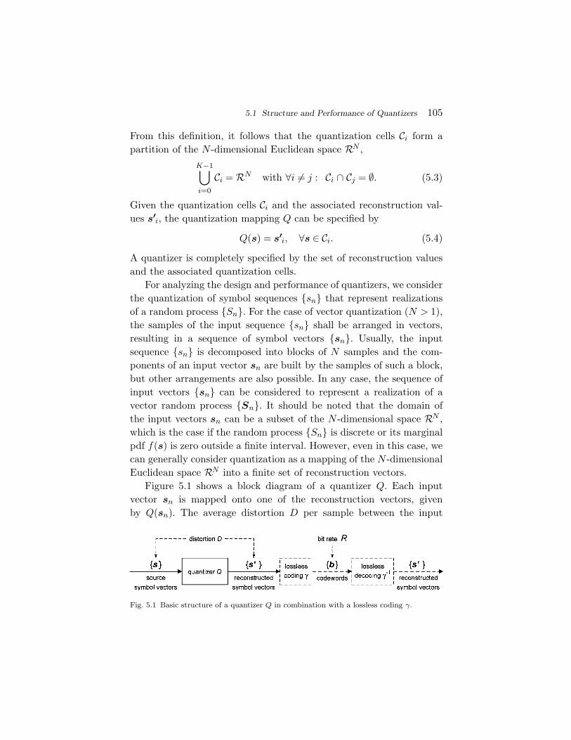
5.1 Structure and Performance of Quantizers 105
From this definition, it follows that the quantization cells Ci form apartition of the N -dimensional Euclidean space RN ,
K−1⋃i=0
Ci = RN with ∀i �= j : Ci ∩ Cj = ∅. (5.3)
Given the quantization cells Ci and the associated reconstruction val-ues s′
i, the quantization mapping Q can be specified by
Q(s) = s′i, ∀s ∈ Ci. (5.4)
A quantizer is completely specified by the set of reconstruction valuesand the associated quantization cells.
For analyzing the design and performance of quantizers, we considerthe quantization of symbol sequences {sn} that represent realizationsof a random process {Sn}. For the case of vector quantization (N > 1),the samples of the input sequence {sn} shall be arranged in vectors,resulting in a sequence of symbol vectors {sn}. Usually, the inputsequence {sn} is decomposed into blocks of N samples and the com-ponents of an input vector sn are built by the samples of such a block,but other arrangements are also possible. In any case, the sequence ofinput vectors {sn} can be considered to represent a realization of avector random process {Sn}. It should be noted that the domain ofthe input vectors sn can be a subset of the N -dimensional space RN ,which is the case if the random process {Sn} is discrete or its marginalpdf f(s) is zero outside a finite interval. However, even in this case, wecan generally consider quantization as a mapping of the N -dimensionalEuclidean space RN into a finite set of reconstruction vectors.
Figure 5.1 shows a block diagram of a quantizer Q. Each inputvector sn is mapped onto one of the reconstruction vectors, givenby Q(sn). The average distortion D per sample between the input
Fig. 5.1 Basic structure of a quantizer Q in combination with a lossless coding γ.
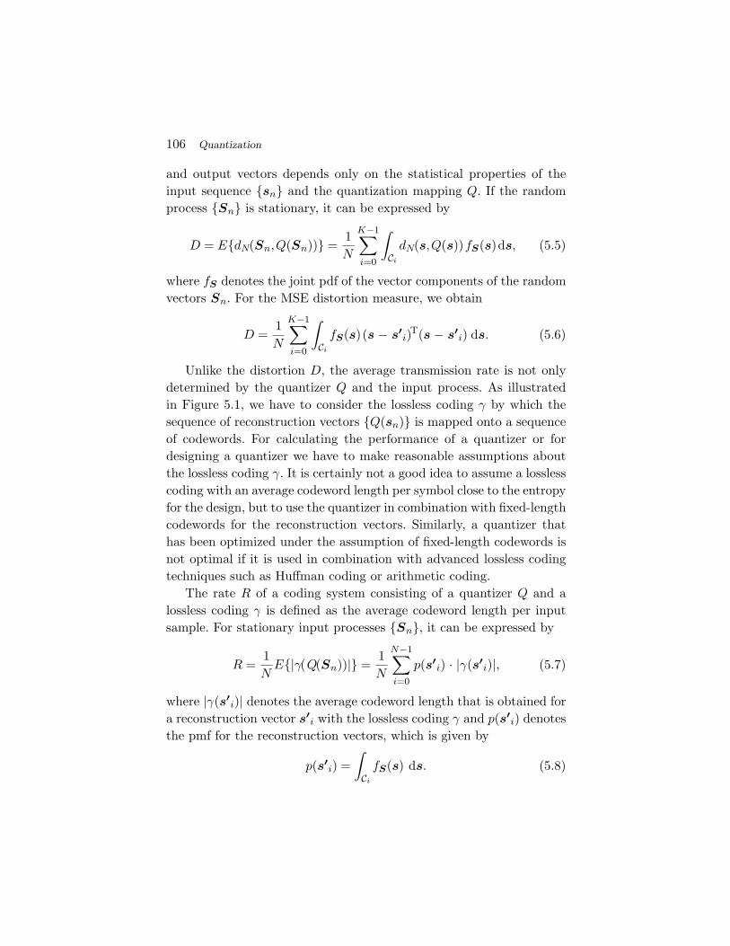
106 Quantization
and output vectors depends only on the statistical properties of theinput sequence {sn} and the quantization mapping Q. If the randomprocess {Sn} is stationary, it can be expressed by
D = E{dN(Sn,Q(Sn))} =1N
K−1∑i=0
∫Ci
dN(s,Q(s))fS(s)ds, (5.5)
where fS denotes the joint pdf of the vector components of the randomvectors Sn. For the MSE distortion measure, we obtain
D =1N
K−1∑i=0
∫Ci
fS(s)(s − s′i)T(s − s′
i) ds. (5.6)
Unlike the distortion D, the average transmission rate is not onlydetermined by the quantizer Q and the input process. As illustratedin Figure 5.1, we have to consider the lossless coding γ by which thesequence of reconstruction vectors {Q(sn)} is mapped onto a sequenceof codewords. For calculating the performance of a quantizer or fordesigning a quantizer we have to make reasonable assumptions aboutthe lossless coding γ. It is certainly not a good idea to assume a losslesscoding with an average codeword length per symbol close to the entropyfor the design, but to use the quantizer in combination with fixed-lengthcodewords for the reconstruction vectors. Similarly, a quantizer thathas been optimized under the assumption of fixed-length codewords isnot optimal if it is used in combination with advanced lossless codingtechniques such as Huffman coding or arithmetic coding.
The rate R of a coding system consisting of a quantizer Q and alossless coding γ is defined as the average codeword length per inputsample. For stationary input processes {Sn}, it can be expressed by
R =1N
E{|γ(Q(Sn))|} =1N
N−1∑i=0
p(s′i) · |γ(s′
i)|, (5.7)
where |γ(s′i)| denotes the average codeword length that is obtained for
a reconstruction vector s′i with the lossless coding γ and p(s′
i) denotesthe pmf for the reconstruction vectors, which is given by
p(s′i) =
∫Ci
fS(s) ds. (5.8)
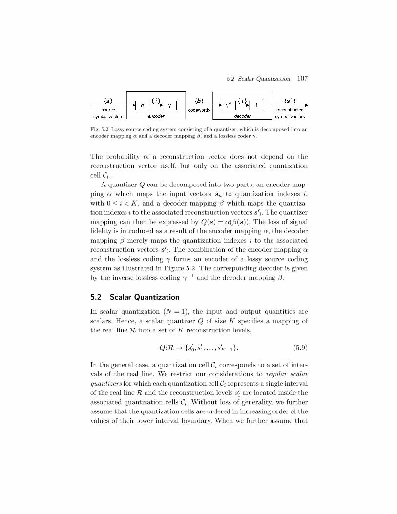
5.2 Scalar Quantization 107
Fig. 5.2 Lossy source coding system consisting of a quantizer, which is decomposed into anencoder mapping α and a decoder mapping β, and a lossless coder γ.
The probability of a reconstruction vector does not depend on thereconstruction vector itself, but only on the associated quantizationcell Ci.
A quantizer Q can be decomposed into two parts, an encoder map-ping α which maps the input vectors sn to quantization indexes i,with 0 ≤ i < K, and a decoder mapping β which maps the quantiza-tion indexes i to the associated reconstruction vectors s′
i. The quantizermapping can then be expressed by Q(s) = α(β(s)). The loss of signalfidelity is introduced as a result of the encoder mapping α, the decodermapping β merely maps the quantization indexes i to the associatedreconstruction vectors s′
i. The combination of the encoder mapping α
and the lossless coding γ forms an encoder of a lossy source codingsystem as illustrated in Figure 5.2. The corresponding decoder is givenby the inverse lossless coding γ−1 and the decoder mapping β.
5.2 Scalar Quantization
In scalar quantization (N = 1), the input and output quantities arescalars. Hence, a scalar quantizer Q of size K specifies a mapping ofthe real line R into a set of K reconstruction levels,
Q:R → {s′0,s
′1, . . . ,s
′K−1}. (5.9)
In the general case, a quantization cell Ci corresponds to a set of inter-vals of the real line. We restrict our considerations to regular scalarquantizers for which each quantization cell Ci represents a single intervalof the real line R and the reconstruction levels s′
i are located inside theassociated quantization cells Ci. Without loss of generality, we furtherassume that the quantization cells are ordered in increasing order of thevalues of their lower interval boundary. When we further assume that

108 Quantization
the quantization intervals include the lower, but not the higher inter-val boundary, each quantization cell can be represented by a half-open2
interval Ci = [ui,ui+1). The interval boundaries ui are also referred to asdecision thresholds. The interval sizes ∆i = ui+1 − ui are called quanti-zation step sizes. Since the quantization cells must form a partition ofthe real line R, the values u0 and uK are fixed and given by u0 = −∞and uK = ∞. Consequently, K reconstruction levels and K − 1 decisionthresholds can be chosen in the quantizer design.
The quantizer mapping Q of a scalar quantizer, as defined above,can be represented by a piecewise-constant input–output function asillustrated in Figure 5.3. All input values s with ui ≤ s < ui+1 areassigned to the corresponding reproduction level s′
i.In the following treatment of scalar quantization, we generally
assume that the input process is stationary. For continuous randomprocesses, scalar quantization can then can be interpreted as a dis-cretization of the marginal pdf f(s) as illustrated in Figure 5.4.
For any stationary process {S} with a marginal pdf f(s), the quan-tizer output is a discrete random process {S′} with a marginal pmf
p(s′i) =
∫ ui+1
ui
f(s) ds. (5.10)
Fig. 5.3 Input–output function Q of a scalar quantizer.
2 In strict mathematical sense, the first quantization cell is an open interval C0 = (−∞,u1).
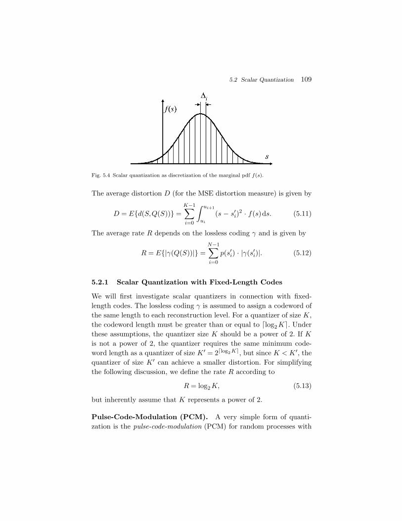
5.2 Scalar Quantization 109
Fig. 5.4 Scalar quantization as discretization of the marginal pdf f(s).
The average distortion D (for the MSE distortion measure) is given by
D = E{d(S,Q(S))} =K−1∑i=0
∫ ui+1
ui
(s − s′i)
2 · f(s)ds. (5.11)
The average rate R depends on the lossless coding γ and is given by
R = E{|γ(Q(S))|} =N−1∑i=0
p(s′i) · |γ(s′
i)|. (5.12)
5.2.1 Scalar Quantization with Fixed-Length Codes
We will first investigate scalar quantizers in connection with fixed-length codes. The lossless coding γ is assumed to assign a codeword ofthe same length to each reconstruction level. For a quantizer of size K,the codeword length must be greater than or equal to �log2 K . Underthese assumptions, the quantizer size K should be a power of 2. If K
is not a power of 2, the quantizer requires the same minimum code-word length as a quantizer of size K ′ = 2�log2 K, but since K < K ′, thequantizer of size K ′ can achieve a smaller distortion. For simplifyingthe following discussion, we define the rate R according to
R = log2 K, (5.13)
but inherently assume that K represents a power of 2.
Pulse-Code-Modulation (PCM). A very simple form of quanti-zation is the pulse-code-modulation (PCM) for random processes with
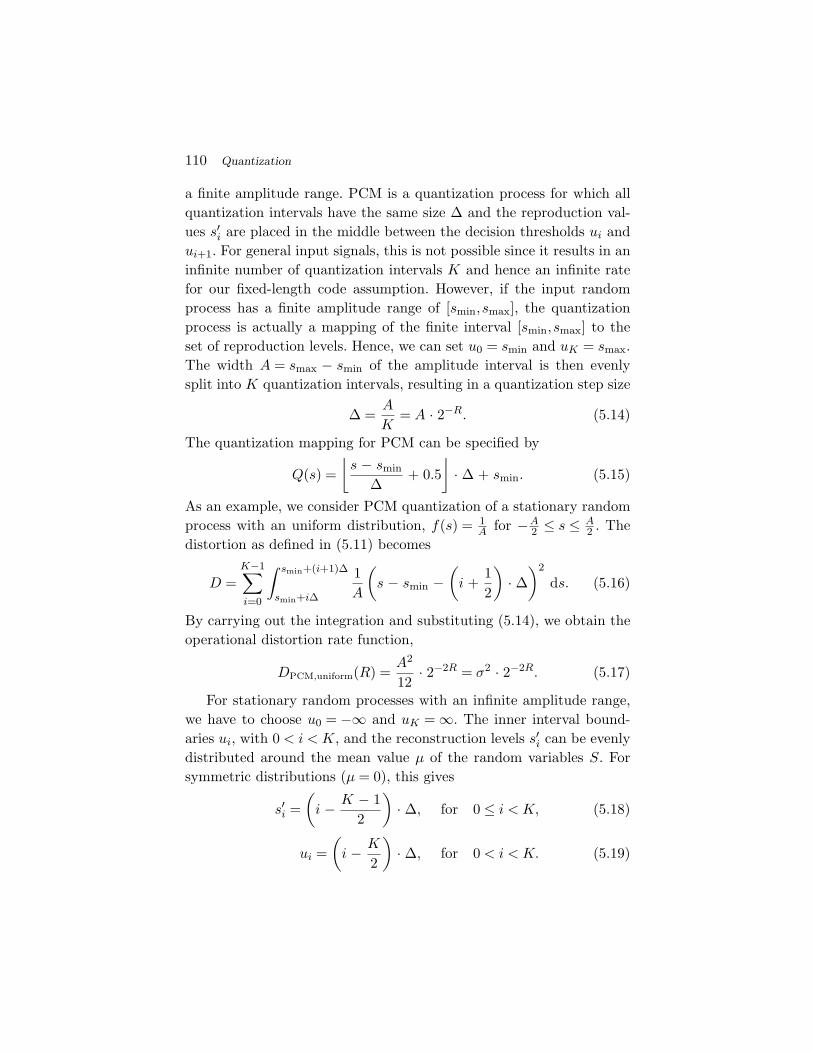
110 Quantization
a finite amplitude range. PCM is a quantization process for which allquantization intervals have the same size ∆ and the reproduction val-ues s′
i are placed in the middle between the decision thresholds ui andui+1. For general input signals, this is not possible since it results in aninfinite number of quantization intervals K and hence an infinite ratefor our fixed-length code assumption. However, if the input randomprocess has a finite amplitude range of [smin,smax], the quantizationprocess is actually a mapping of the finite interval [smin,smax] to theset of reproduction levels. Hence, we can set u0 = smin and uK = smax.The width A = smax − smin of the amplitude interval is then evenlysplit into K quantization intervals, resulting in a quantization step size
∆ =A
K= A · 2−R. (5.14)
The quantization mapping for PCM can be specified by
Q(s) =⌊
s − smin
∆+ 0.5
⌋· ∆ + smin. (5.15)
As an example, we consider PCM quantization of a stationary randomprocess with an uniform distribution, f(s) = 1
A for −A2 ≤ s ≤ A
2 . Thedistortion as defined in (5.11) becomes
D =K−1∑i=0
∫ smin+(i+1)∆
smin+i∆
1A
(s − smin −
(i +
12
)· ∆)2
ds. (5.16)
By carrying out the integration and substituting (5.14), we obtain theoperational distortion rate function,
DPCM,uniform(R) =A2
12· 2−2R = σ2 · 2−2R. (5.17)
For stationary random processes with an infinite amplitude range,we have to choose u0 = −∞ and uK = ∞. The inner interval bound-aries ui, with 0 < i < K, and the reconstruction levels s′
i can be evenlydistributed around the mean value µ of the random variables S. Forsymmetric distributions (µ = 0), this gives
s′i =(
i − K − 12
)· ∆, for 0 ≤ i < K, (5.18)
ui =(
i − K
2
)· ∆, for 0 < i < K. (5.19)
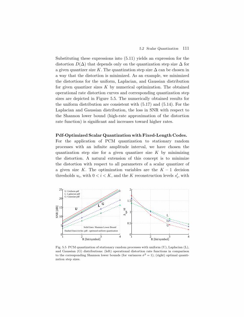
5.2 Scalar Quantization 111
Substituting these expressions into (5.11) yields an expression for thedistortion D(∆) that depends only on the quantization step size ∆ fora given quantizer size K. The quantization step size ∆ can be chosen ina way that the distortion is minimized. As an example, we minimizedthe distortions for the uniform, Laplacian, and Gaussian distributionfor given quantizer sizes K by numerical optimization. The obtainedoperational rate distortion curves and corresponding quantization stepsizes are depicted in Figure 5.5. The numerically obtained results forthe uniform distribution are consistent with (5.17) and (5.14). For theLaplacian and Gaussian distribution, the loss in SNR with respect tothe Shannon lower bound (high-rate approximation of the distortionrate function) is significant and increases toward higher rates.
Pdf-Optimized Scalar Quantization with Fixed-Length Codes.For the application of PCM quantization to stationary randomprocesses with an infinite amplitude interval, we have chosen thequantization step size for a given quantizer size K by minimizingthe distortion. A natural extension of this concept is to minimizethe distortion with respect to all parameters of a scalar quantizer ofa given size K. The optimization variables are the K − 1 decisionthresholds ui, with 0 < i < K, and the K reconstruction levels s′
i, with
1 2 3 40
5
10
15
20
25
R [bit/symbol]
SNR
[dB
]
Solid lines: Shannon Lower Bound
Dashed lines/circles: pdf− optimzed uniform quantization
UL
G
U: Uniform pdfL: Laplacian pdfG: Gaussian pdf
UL
G
UL
G
1 2 3 40
0.5
1
1.5
2
R [bit/symbol]
∆ opt/σ
U
L
G
Fig. 5.5 PCM quantization of stationary random processes with uniform (U), Laplacian (L),and Gaussian (G) distributions: (left) operational distortion rate functions in comparisonto the corresponding Shannon lower bounds (for variances σ2 = 1); (right) optimal quanti-zation step sizes.

112 Quantization
0 ≤ i < K. The obtained quantizer is called a pdf-optimized scalarquantizer with fixed-length codes.
For deriving a condition for the reconstruction levels s′i, we first
assume that the decision thresholds ui are given. The overall distortion(5.11) is the sum of the distortions Di for the quantization intervalsCi = [ui,uu+1). For given decision thresholds, the interval distortions Di
are mutually independent and are determined by the correspondingreconstruction levels s′
i,
Di(s′i) =
∫ ui+1
ui
d1(s,s′i) · f(s) ds. (5.20)
By using the conditional distribution f(s|s′i) = f(s) · p(s′
i), we obtain
Di(s′i) =
1p(s′
i)
∫ ui+1
ui
d1(s,s′i) · f(s|s′
i) ds =E{d1(S,s′
i)|S ∈ Ci}p(s′
i).
(5.21)Since p(s′
i) does not depend on s′i, the optimal reconstruction levels s′∗
i
are given by
s′∗i = arg min
s′∈RE{d1(S,s′)|S ∈ Ci
}, (5.22)
which is also called the generalized centroid condition. For the squarederror distortion measure d1(s,s′) = (s − s′)2, the optimal reconstruc-tion levels s′∗
i are the conditional means (centroids)
s′∗i = E{S|S ∈ Ci} =
∫ ui+1ui
s · f(s) ds∫ ui+1ui
f(s) ds. (5.23)
This can be easily proved by the inequality
E{(S − s′
i)2} = E
{(S − E{S} + E{S} − s′
i)2}
= E{(S − E{S})2
}+ (E{S} − s′
i)2
≥ E{(S − E{S})2
}. (5.24)
If the reproduction levels s′i are given, the overall distortion D is
minimized if each input value s is mapped to the reproduction level s′i
that minimizes the corresponding sample distortion d1(s,s′i),
Q(s) = argmin∀s′
i
d1(s,s′i). (5.25)

5.2 Scalar Quantization 113
This condition is also referred to as the nearest neighbor condition.Since a decision threshold ui influences only the distortions Di of theneighboring intervals, the overall distortion is minimized if
d1(ui,s′i−1) = d1(ui,s
′i) (5.26)
holds for all decision thresholds ui, with 0 < i < K. For the squarederror distortion measure, the optimal decision thresholds u∗
i , with0 < i < K, are given by
u∗i =
12(s′
i−1 + s′i). (5.27)
The expressions (5.23) and (5.27) can also be obtained by setting thepartial derivatives of the distortion (5.11) with respect to the decisionthresholds ui and the reconstruction levels s′
i equal to zero [52].
The Lloyd Algorithm. The necessary conditions for the optimalreconstruction levels (5.22) and decision thresholds (5.25) depend oneach other. A corresponding iterative algorithm for minimizing the dis-tortion of a quantizer of given size K was suggested by Lloyd [45]and is commonly called the Lloyd algorithm. The obtained quantizeris referred to as Lloyd quantizer or Lloyd-Max3 quantizer. For a givenpdf f(s), first an initial set of unique reconstruction levels {s′
i} is arbi-trarily chosen, then the decision thresholds {ui} and reconstructionlevels {s′
i} are alternately determined according to (5.25) and (5.22),respectively, until the algorithm converges. It should be noted that thefulfillment of the conditions (5.22) and (5.25) is in general not sufficientto guarantee the optimality of the quantizer. The conditions are onlysufficient if the pdf f(s) is log-concave. One of the examples, for whichthe Lloyd algorithm yields a unique solution independent of the initialset of reconstruction levels, is the Gaussian pdf.
Often, the marginal pdf f(s) of a random process is not knowna priori. In such a case, the Lloyd algorithm can be applied using atraining set. If the training set includes a sufficiently large number ofsamples, the obtained quantizer is an accurate approximation of theLloyd quantizer. Using the encoder mapping α (see Section 5.1), the
3 Lloyd and Max independently observed the two necessary conditions for optimality.
114 Quantization
Lloyd algorithm for a training set of samples {sn} and a given quantizersize K can be stated as follows:
(1) Choose an initial set of unique reconstruction levels {s′i}.
(2) Associate all samples of the training set {sn} with one of thequantization intervals Ci according to
α(sn) = argmin∀i
d1(sn,s′i) (nearest neighbor condition)
and update the decision thresholds {ui} accordingly.
(3) Update the reconstruction levels {s′i} according to
s′i = arg min
s′∈RE{d1(S,s′) |α(S) = i
}, (centroid condition)
where the expectation value is taken over the training set.
(4) Repeat the previous two steps until convergence.
Examples for the Lloyd Algorithm. As a first example, weapplied the Lloyd algorithm with a training set of more than10,000 samples and the MSE distortion measure to a Gaussian pdfwith unit variance. We used two different initializations for thereconstruction levels. Convergence was determined if the relative dis-tortion reduction between two iterations steps was less than 1%,(Dk − Dk+1)/Dk+1 < 0.01. The algorithm quickly converged after sixiterations for both initializations to the same overall distortion D∗
F .The obtained reconstruction levels {s′
i} and decision thresholds {ui} aswell as the iteration processes for the two initializations are illustratedin Figure 5.6.
The same algorithm with the same two initializations was alsoapplied to a Laplacian pdf with unit variance. Also for this distribution,the algorithm quickly converged after six iterations for both initializa-tions to the same overall distortion D∗
F . The obtained quantizer andthe iteration processes are illustrated in Figure 5.7.
5.2.2 Scalar Quantization with Variable-Length Codes
We have investigated the design of quantizers that minimize thedistortion for a given number K of reconstruction levels, which is
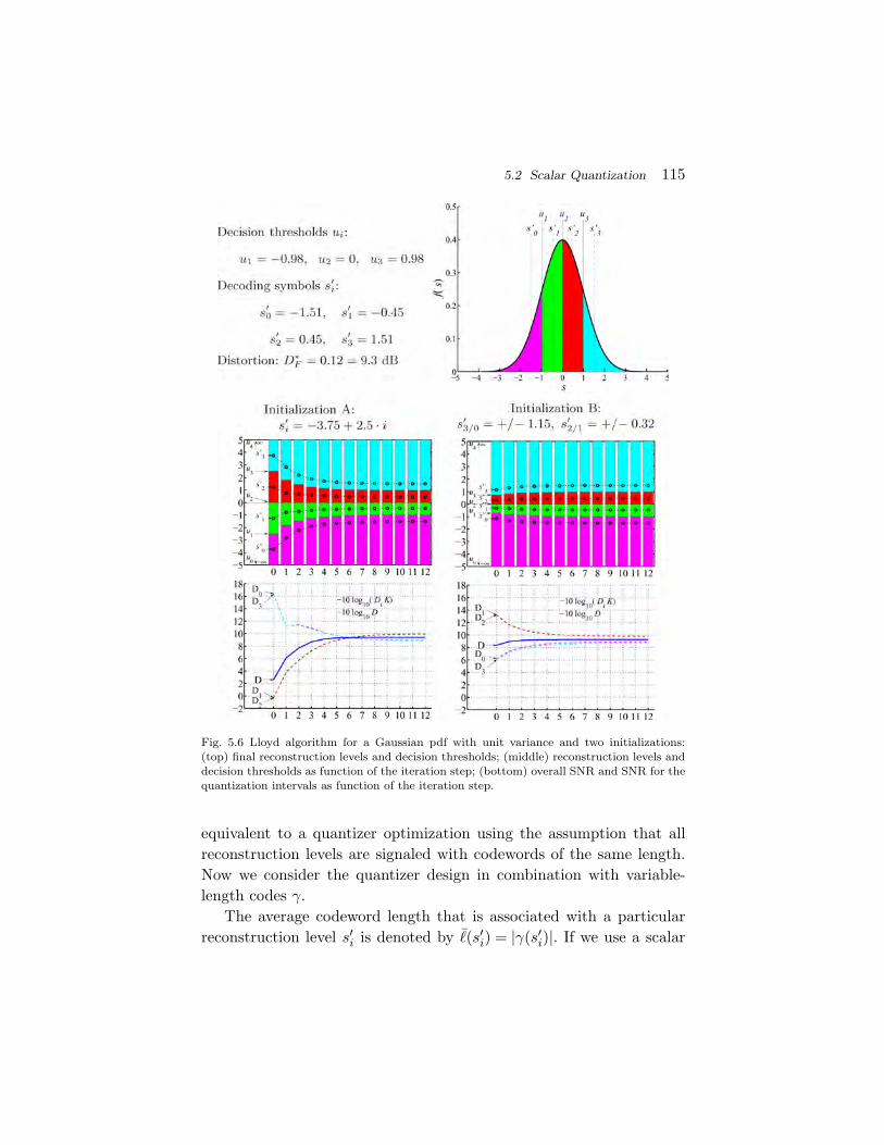
5.2 Scalar Quantization 115
Fig. 5.6 Lloyd algorithm for a Gaussian pdf with unit variance and two initializations:(top) final reconstruction levels and decision thresholds; (middle) reconstruction levels anddecision thresholds as function of the iteration step; (bottom) overall SNR and SNR for thequantization intervals as function of the iteration step.
equivalent to a quantizer optimization using the assumption that allreconstruction levels are signaled with codewords of the same length.Now we consider the quantizer design in combination with variable-length codes γ.
The average codeword length that is associated with a particularreconstruction level s′
i is denoted by �(s′i) = |γ(s′
i)|. If we use a scalar
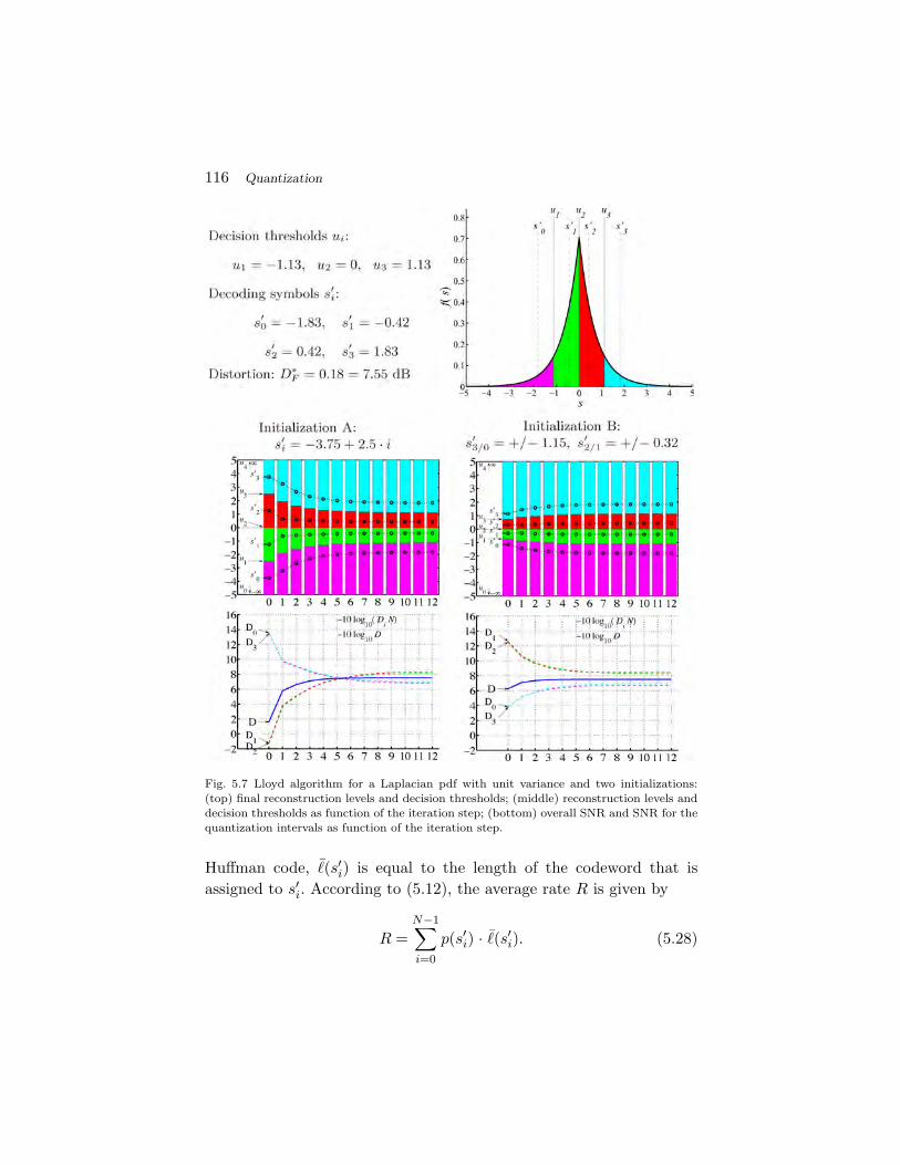
116 Quantization
Fig. 5.7 Lloyd algorithm for a Laplacian pdf with unit variance and two initializations:(top) final reconstruction levels and decision thresholds; (middle) reconstruction levels anddecision thresholds as function of the iteration step; (bottom) overall SNR and SNR for thequantization intervals as function of the iteration step.
Huffman code, �(s′i) is equal to the length of the codeword that is
assigned to s′i. According to (5.12), the average rate R is given by
R =N−1∑i=0
p(s′i) · �(s′
i). (5.28)

5.2 Scalar Quantization 117
The average distortion is the same as for scalar quantization with fixed-length codes and is given by (5.11).
Rate-Constrained Scalar Quantization. Since distortion andrate influence each other, they cannot be minimized independently.The optimization problem can be stated as
minD subject to R ≤ Rmax, (5.29)
or equivalently,
minR subject to D ≤ Dmax, (5.30)
with Rmax and Dmax being a given maximum rate and a maximumdistortion, respectively. The constraint minimization problem can beformulated as unconstrained minimization of the Lagrangian functional
J = D + λR = E{d1(S,Q(S))} + λE{�(Q(S))
}. (5.31)
The parameter λ, with 0 ≤ λ < ∞, is referred to as Lagrange param-eter. The solution of the minimization of (5.31) is a solution of theconstrained minimization problems (5.29) and (5.30) in the followingsense: if there is a Lagrangian parameter λ that yields a particular rateRmax (or particular distortion Dmax), the corresponding distortion D
(or rate R) is a solution of the constraint optimization problem.In order to derive necessary conditions similarly as for the quantizer
design with fixed-length codes, we first assume that the decision thresh-olds ui are given. Since the rate R is independent of the reconstructionlevels s′
i, the optimal reconstruction levels are found by minimizing thedistortion D. This is the same optimization problem as for the scalarquantizer with fixed-length codes. Hence, the optimal reconstructionlevels s′∗
i are given by the generalized centroid condition (5.22).The optimal average codeword lengths �(s′
i) also depend only on thedecision thresholds ui. Given the decision thresholds and thus the prob-abilities p(s′
i), the average codeword lengths �(s′i) can be determined. If
we, for example, assume that the reconstruction levels are coded usinga scalar Huffman code, the Huffman code could be constructed giventhe pmf p(s′
i), which directly yields the codeword length �(s′i). In gen-
eral, it is however justified to approximate the average rate R by the
118 Quantization
entropy H(S) and set the average codeword length equal to
�(s′i) = − log2 p(s′
i). (5.32)
This underestimates the true rate by a small amount. For Huffmancoding the difference is always less than 1 bit per symbol and for arith-metic coding it is usually much smaller. When using the entropy asapproximation for the rate during the quantizer design, the obtainedquantizer is also called an entropy-constrained scalar quantizer. At thispoint, we ignore that, for sources with memory, the lossless coding γ canemploy dependencies between output samples, for example, by usingblock Huffman coding or arithmetic coding with conditional probabil-ities. This extension is discussed in Section 5.2.6.
For deriving a necessary condition for the decision thresholds ui, wenow assume that the reconstruction levels s′
i and the average codewordlength �(s′
i) are given. Similarly as for the nearest neighbor conditionin Section 5.2.1, the quantization mapping Q(s) that minimizes theLagrangian functional J is given by
Q(s) = argmin∀s′
i
d1(s,s′i) + λ�(s′
i). (5.33)
A mapping Q(s) that minimizes the term d(s,s′i) + λ�(s′
i) for eachsource symbol s minimizes also the expected value in (5.31). A rigorousproof of this statement can be found in [65]. The decision thresholds ui
have to be selected in a way that the term d(s,s′i) + λ�(s′
i) is the samefor both neighboring intervals,
d1(ui,s′i−1) + λ�(s′
i−1) = d1(ui,s′i) + λ�(s′
i). (5.34)
For the MSE distortion measure, we obtain
u∗i =
12(s′
i + s′i+1) +
λ
2·�(s′
i+1) − �(s′i)
s′i+1 − s′
i
. (5.35)
The consequence is a shift of the decision threshold ui from the mid-point between the reconstruction levels toward the interval with thelonger average codeword length, i.e., the less probable interval.
Lagrangian Minimization. Lagrangian minimization as in (5.33)is a very important concept in modern video coding. Hence, we have
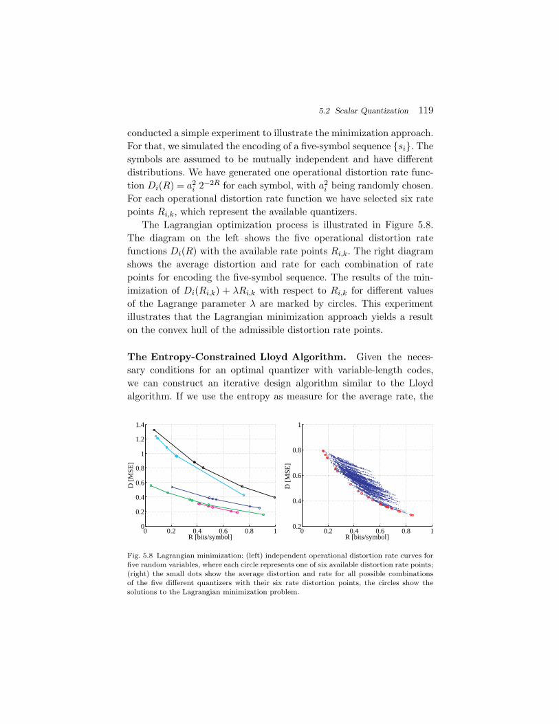
5.2 Scalar Quantization 119
conducted a simple experiment to illustrate the minimization approach.For that, we simulated the encoding of a five-symbol sequence {si}. Thesymbols are assumed to be mutually independent and have differentdistributions. We have generated one operational distortion rate func-tion Di(R) = a2
i 2−2R for each symbol, with a2i being randomly chosen.
For each operational distortion rate function we have selected six ratepoints Ri,k, which represent the available quantizers.
The Lagrangian optimization process is illustrated in Figure 5.8.The diagram on the left shows the five operational distortion ratefunctions Di(R) with the available rate points Ri,k. The right diagramshows the average distortion and rate for each combination of ratepoints for encoding the five-symbol sequence. The results of the min-imization of Di(Ri,k) + λRi,k with respect to Ri,k for different valuesof the Lagrange parameter λ are marked by circles. This experimentillustrates that the Lagrangian minimization approach yields a resulton the convex hull of the admissible distortion rate points.
The Entropy-Constrained Lloyd Algorithm. Given the neces-sary conditions for an optimal quantizer with variable-length codes,we can construct an iterative design algorithm similar to the Lloydalgorithm. If we use the entropy as measure for the average rate, the
0 0.2 0.4 0.6 0.8 10
0.2
0.4
0.6
0.8
1
1.2
1.4
D [
MSE
]
R [bits/symbol]0 0.2 0.4 0.6 0.8 1
0.2
0.4
0.6
0.8
1
D [
MSE
]
R [bits/symbol]
Fig. 5.8 Lagrangian minimization: (left) independent operational distortion rate curves forfive random variables, where each circle represents one of six available distortion rate points;(right) the small dots show the average distortion and rate for all possible combinationsof the five different quantizers with their six rate distortion points, the circles show thesolutions to the Lagrangian minimization problem.

120 Quantization
algorithm is also referred to as entropy-constrained Lloyd algorithm.Using the encoder mapping α, the variant that uses a sufficiently largetraining set {sn} can be stated as follows for a given value of λ:
(1) Choose an initial quantizer size N , an initial set of recon-struction levels {s′
i}, and an initial set of average codewordlengths �(s′
i).
(2) Associate all samples of the training set {sn} with one of thequantization intervals Ci according to
α(sn) = argmin∀i
d1(sn,s′i) + λ�(s′
i)
and update the decision thresholds {ui} accordingly.
(3) Update the reconstruction levels {s′i} according to
s′i = arg min
s′∈RE{d1(S,s′) |α(S) = i
},
where the expectation value is taken over the training set.
(4) Update the average codeword length �(s′i) according to4
�(s′i) = − log2 p(s′
i).
(5) Repeat the previous three steps until convergence.
As mentioned above, the entropy constraint in the algorithm causesa shift of the cost function depending on the pmf p(s′
i). If two decodingsymbols s′
i and s′i+1 are competing, the symbol with larger popularity
has higher chance of being chosen. The probability of a reconstructionlevel that is rarely chosen is further reduced. As a consequence, symbolsget “removed” and the quantizer size K of the final result can be smallerthan the initial quantizer size N .
The number N of initial reconstruction levels is critical to quantizerperformance after convergence. Figure 5.9 illustrates the result of theentropy-constrained Lloyd algorithm after convergence for a Laplacianpdf and different numbers of initial reconstruction levels, where therate is measured as the entropy of the reconstruction symbols. It can
4 In a variation of the entropy-constrained Lloyd algorithm, the average codewordlengths �(s′
i) can be determined by constructing a lossless code γ given the pmf p(s′i).
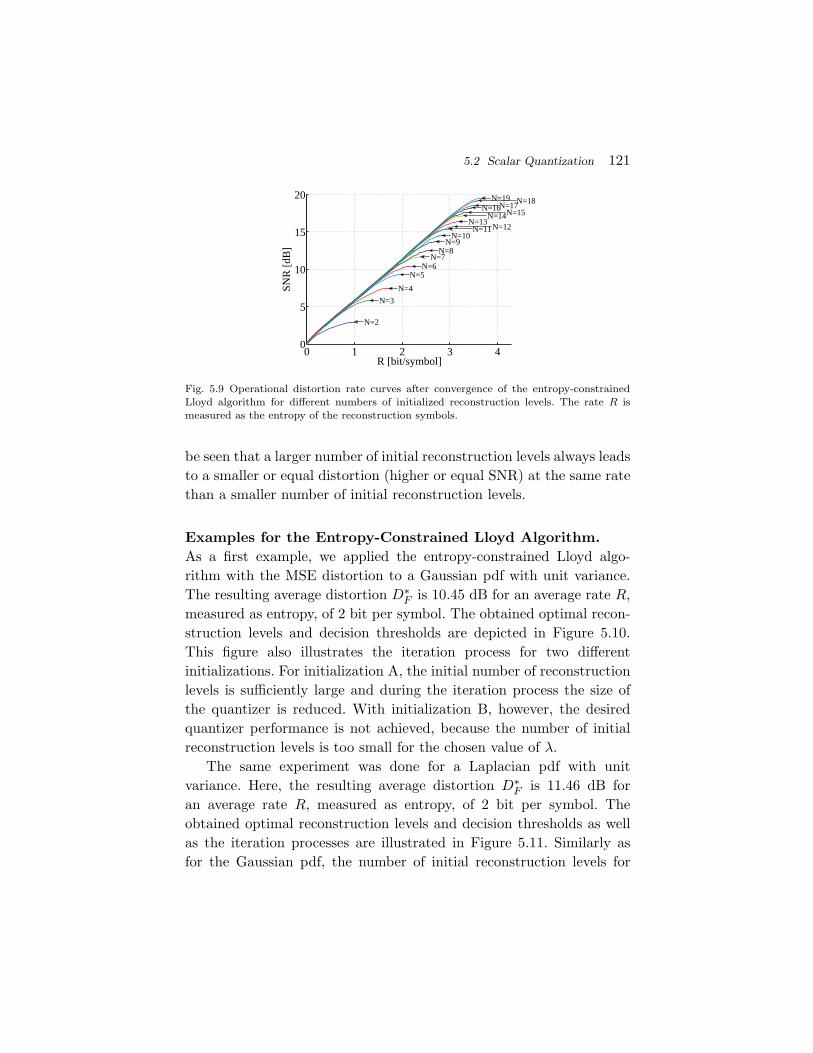
5.2 Scalar Quantization 121
0 1 2 3 40
5
10
15
20
R [bit/symbol]
SNR
[dB
]
N=2
N=3
N=4
N=5N=6
N=7N=8
N=9N=10
N=11N=12N=13
N=14N=15N=16N=17N=18N=19
Fig. 5.9 Operational distortion rate curves after convergence of the entropy-constrainedLloyd algorithm for different numbers of initialized reconstruction levels. The rate R ismeasured as the entropy of the reconstruction symbols.
be seen that a larger number of initial reconstruction levels always leadsto a smaller or equal distortion (higher or equal SNR) at the same ratethan a smaller number of initial reconstruction levels.
Examples for the Entropy-Constrained Lloyd Algorithm.As a first example, we applied the entropy-constrained Lloyd algo-rithm with the MSE distortion to a Gaussian pdf with unit variance.The resulting average distortion D∗
F is 10.45 dB for an average rate R,measured as entropy, of 2 bit per symbol. The obtained optimal recon-struction levels and decision thresholds are depicted in Figure 5.10.This figure also illustrates the iteration process for two differentinitializations. For initialization A, the initial number of reconstructionlevels is sufficiently large and during the iteration process the size ofthe quantizer is reduced. With initialization B, however, the desiredquantizer performance is not achieved, because the number of initialreconstruction levels is too small for the chosen value of λ.
The same experiment was done for a Laplacian pdf with unitvariance. Here, the resulting average distortion D∗
F is 11.46 dB foran average rate R, measured as entropy, of 2 bit per symbol. Theobtained optimal reconstruction levels and decision thresholds as wellas the iteration processes are illustrated in Figure 5.11. Similarly asfor the Gaussian pdf, the number of initial reconstruction levels for
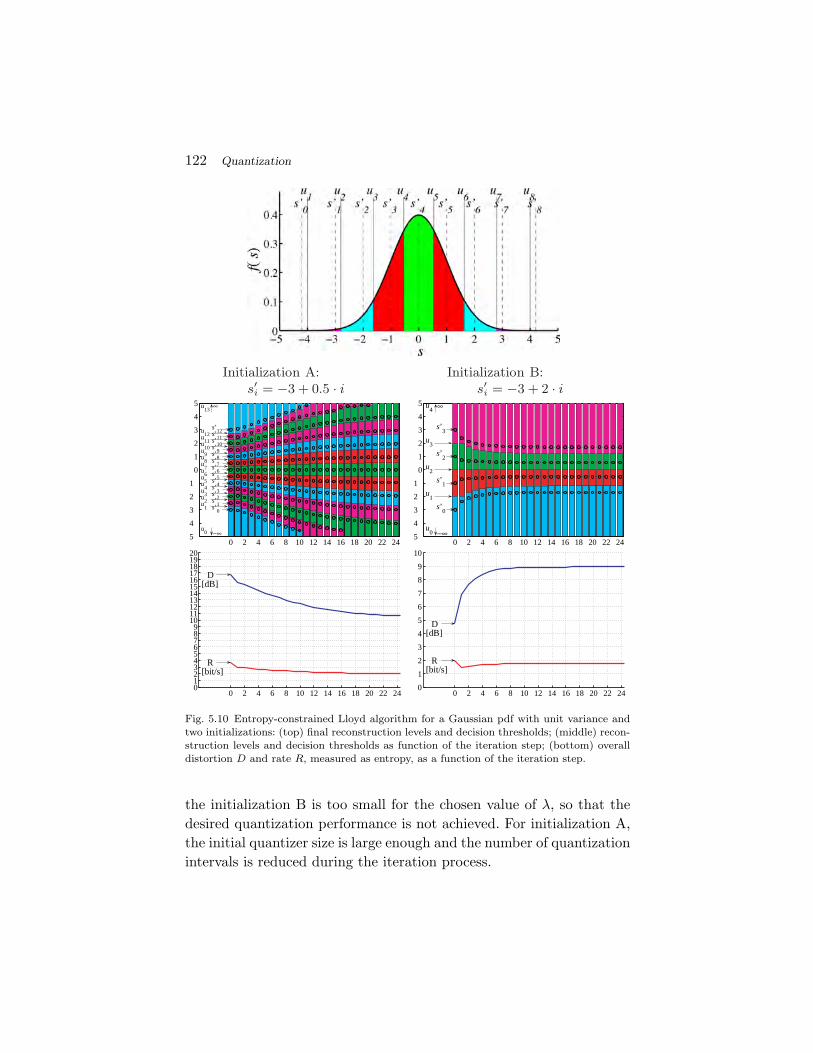
122 Quantization
0 2 4 6 8 10 12 14 16 18 20 22 245
4
3
2
1
0
1
2
3
4
5
u1
u2
u3
u4
u5
u6
u7
u8
u9
u10
u11
u12
u13
u0
∞
−∞
s’0
s’1
s’2
s’3
s’4
s’5
s’6
s’7
s’8
s’9
s’10
s’11
s’12
0 2 4 6 8 10 12 14 16 18 20 22 240123456789
1011121314151617181920
D[dB]
R[bit/s]
0 2 4 6 8 10 12 14 16 18 20 22 245
4
3
2
1
0
1
2
3
4
5
u1
u2
u3
u4
u0
∞
−∞
s’0
s’1
s’2
s’3
0 2 4 6 8 10 12 14 16 18 20 22 240
1
2
3
4
5
6
7
8
9
10
D[dB]
R[bit/s]
Fig. 5.10 Entropy-constrained Lloyd algorithm for a Gaussian pdf with unit variance andtwo initializations: (top) final reconstruction levels and decision thresholds; (middle) recon-struction levels and decision thresholds as function of the iteration step; (bottom) overalldistortion D and rate R, measured as entropy, as a function of the iteration step.
the initialization B is too small for the chosen value of λ, so that thedesired quantization performance is not achieved. For initialization A,the initial quantizer size is large enough and the number of quantizationintervals is reduced during the iteration process.
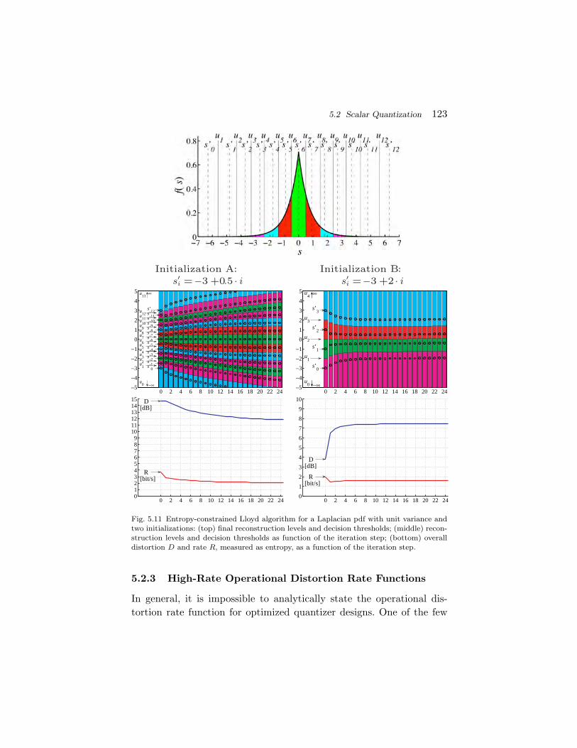
5.2 Scalar Quantization 123
0 2 4 6 8 10 12 14 16 18 20 22 24−5
−4
−3
−2
−1
0
1
2
3
4
5
u1
u2
u3
u4
u5
u6
u7
u8
u9
u10
u11
u12
u13
u0
∞
−∞
s’0
s’1
s’2
s’3
s’4
s’5
s’6
s’7
s’8
s’9
s’10
s’11
s’12
0 2 4 6 8 10 12 14 16 18 20 22 240123456789
101112131415 D
[dB]
R[bit/s]
0 2 4 6 8 10 12 14 16 18 20 22 24−5
−4
−3
−2
−1
0
1
2
3
4
5
u1
u2
u3
u4
u0
∞
−∞
s’0
s’1
s’2
s’3
0 2 4 6 8 10 12 14 16 18 20 22 240
1
2
3
4
5
6
7
8
9
10
D[dB]
R[bit/s]
Fig. 5.11 Entropy-constrained Lloyd algorithm for a Laplacian pdf with unit variance andtwo initializations: (top) final reconstruction levels and decision thresholds; (middle) recon-struction levels and decision thresholds as function of the iteration step; (bottom) overalldistortion D and rate R, measured as entropy, as a function of the iteration step.
5.2.3 High-Rate Operational Distortion Rate Functions
In general, it is impossible to analytically state the operational dis-tortion rate function for optimized quantizer designs. One of the few

124 Quantization
exceptions is the uniform distribution, for which the operational distor-tion rate function for all discussed quantizer designs is given in (5.17).For stationary input processes with continuous random variables, wecan, however, derive the asymptotic operational distortion rate func-tions for very high rates (R → ∞) or equivalently for small distortions(D → 0). The resulting relationships are referred to as high-rate approx-imations and approach the true operational distortion rate functions asthe rate approaches infinity. We remember that as the rate approachesinfinity, the (information) distortion rate function approaches the Shan-non lower bound. Hence, for high rates, the performance of a quantizerdesign can be evaluated by comparing the high rate approximation ofthe operational distortion rate function with the Shannon lower bound.
The general assumption that we use for deriving high-rate approx-imations is that the sizes ∆i of the quantization intervals [ui,ui+1) areso small that the marginal pdf f(s) of a continuous input process isnearly constant inside each interval,
f(s) ≈ f(s′i) for s ∈ [ui,ui+1). (5.36)
The probabilities of the reconstruction levels can be approximated by
p(s′i) =
∫ ui+1
ui
f(s)ds ≈ (ui+1 − ui)f(s′i) = ∆i · f(s′
i). (5.37)
For the average distortion D, we obtain
D = E{d(S,Q(S))} ≈K−1∑i=0
f(s′i)∫ ui+1
ui
(s − s′i)
2 ds. (5.38)
An integration of the right-hand side of (5.38) yields
D ≈ 13
K−1∑i=0
f(s′i)((ui+1 − s′
i)3 − (ui − s′
i)3). (5.39)
For each quantization interval, the distortion is minimized if the term(ui+1 − s′
i)3 is equal to the term (ui − s′
i)3, which yields
s′i =
12(ui + ui+1). (5.40)
5.2 Scalar Quantization 125
By substituting (5.40) into (5.39), we obtain the following expressionfor the average distortion at high rates,
D ≈ 112
K−1∑i=0
f(s′i)∆3
i =112
K−1∑i=0
p(s′i)∆2
i . (5.41)
For deriving the asymptotic operational distortion rate functions, wewill use the expression (5.41) with equality, but keep in mind that it isonly asymptotically correct for ∆i → 0.
PCM Quantization. For PCM quantization of random processeswith a finite amplitude range of width A, we can directly substitutethe expression (5.14) into the distortion approximation (5.41). Since∑K−1
i=0 p(s′i) is equal to 1, this yields the asymptotic operational distor-
tion rate function
DPCM(R) =112
A2 2−2R. (5.42)
Scalar Quantizers with Fixed-Length Codes. In order toderive the asymptotic operational distortion rate function for optimalscalar quantizers in combination with fixed-length codes, we againstart with the distortion approximation in (5.41). By using therelationship
∑K−1i=0 K−1 = 1, it can be reformulated as
D =112
K−1∑i=0
f(s′i)∆
3i =
112
(K−1∑
i=0
f(s′i)∆
3i
)13
·(
K−1∑i=0
1K
)23
3
. (5.43)
Using Holders inequality
α + β = 1 ⇒(
b∑i=a
xi
)α
·(
b∑i=a
yi
)β
≥b∑
i=a
xαi · yβ
i (5.44)
with equality if and only if xi is proportional to yi, it follows
D ≥ 112
(K−1∑i=0
f(s′i)
13 ·∆i ·
(1K
)23
)3
=1
12K2
(K−1∑i=0
3√
f(s′i)∆i
)3
.
(5.45)
126 Quantization
Equality is achieved if the terms f(s′i)∆3
i are proportional to 1/K.Hence, the average distortion for high rates is minimized if all quanti-zation intervals have the same contribution to the overall distortion D.
We have intentionally chosen α = 1/3, in order to obtain an expres-sion of the sum in which ∆i has no exponent. Remembering that theused distortion approximation is asymptotically valid for small inter-vals ∆i, the summation in (5.45) can be written as integral,
D =1
12K2
(∫ ∞
−∞3√
f(s)ds
)3
. (5.46)
As discussed in Section 5.2.1, the rate R for a scalar quantizer withfixed-length codes is given by R = log2 K. This yields the followingasymptotic operational distortion rate function for optimal scalar quan-tizers with fixed-length codes,
DF (R) = σ2 · ε2F · 2−2R with ε2
F =1σ2
(∫ ∞
−∞3√
f(s)ds
)3
, (5.47)
where the factor ε2F only depends on the marginal pdf f(s) of the input
process. The result (5.47) was reported by Panter and Dite in [55] andis also referred to as the Panter and Dite formula.
Scalar Quantizers with Variable-Length Codes.In Section 5.2.2, we have discussed that the rate R for an opti-mized scalar quantizer with variable-length codes can be approximatedby the entropy H(S′) of the output random variables S′. We ignorethat, for the quantization of sources with memory, the output samplesare not mutually independent and hence a lossless code that employsthe dependencies between the output samples may achieve a ratebelow the scalar entropy H(S′).
By using the entropy H(S′) of the output random variables S′ asapproximation for the rate R and applying the high-rate approxima-tion p(s′
i) = f(s′i)∆i, we obtain
R = H(S′) = −K−1∑i=0
p(s′i) log2 p(s′
i) = −K−1∑i=0
f(s′i)∆i log2(f(s′
i)∆i)
= −K−1∑i=0
f(s′i) log2 f(s′
i)∆i −K−1∑i=0
f(s′i)∆i log2 ∆i. (5.48)
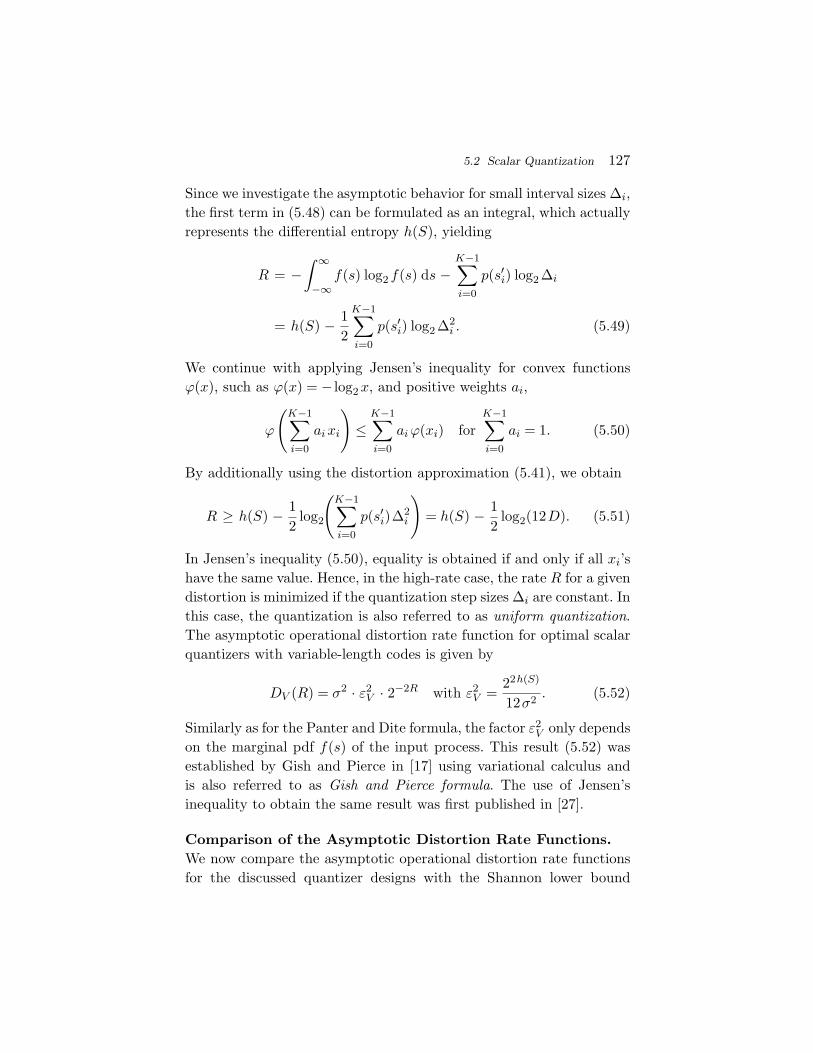
5.2 Scalar Quantization 127
Since we investigate the asymptotic behavior for small interval sizes ∆i,the first term in (5.48) can be formulated as an integral, which actuallyrepresents the differential entropy h(S), yielding
R = −∫ ∞
−∞f(s) log2 f(s) ds −
K−1∑i=0
p(s′i) log2 ∆i
= h(S) − 12
K−1∑i=0
p(s′i) log2 ∆2
i . (5.49)
We continue with applying Jensen’s inequality for convex functionsϕ(x), such as ϕ(x) = − log2 x, and positive weights ai,
ϕ
(K−1∑i=0
ai xi
)≤
K−1∑i=0
ai ϕ(xi) forK−1∑i=0
ai = 1. (5.50)
By additionally using the distortion approximation (5.41), we obtain
R ≥ h(S) − 12
log2
(K−1∑i=0
p(s′i)∆2
i
)= h(S) − 1
2log2(12D). (5.51)
In Jensen’s inequality (5.50), equality is obtained if and only if all xi’shave the same value. Hence, in the high-rate case, the rate R for a givendistortion is minimized if the quantization step sizes ∆i are constant. Inthis case, the quantization is also referred to as uniform quantization.The asymptotic operational distortion rate function for optimal scalarquantizers with variable-length codes is given by
DV (R) = σ2 · ε2V · 2−2R with ε2
V =22h(S)
12σ2 . (5.52)
Similarly as for the Panter and Dite formula, the factor ε2V only depends
on the marginal pdf f(s) of the input process. This result (5.52) wasestablished by Gish and Pierce in [17] using variational calculus andis also referred to as Gish and Pierce formula. The use of Jensen’sinequality to obtain the same result was first published in [27].
Comparison of the Asymptotic Distortion Rate Functions.We now compare the asymptotic operational distortion rate functionsfor the discussed quantizer designs with the Shannon lower bound
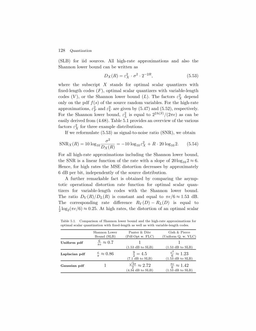
128 Quantization
(SLB) for iid sources. All high-rate approximations and also theShannon lower bound can be written as
DX(R) = ε2X · σ2 · 2−2R, (5.53)
where the subscript X stands for optimal scalar quantizers withfixed-length codes (F ), optimal scalar quantizers with variable-lengthcodes (V ), or the Shannon lower bound (L). The factors ε2
X dependonly on the pdf f(s) of the source random variables. For the high-rateapproximations, ε2
F and ε2V are given by (5.47) and (5.52), respectively.
For the Shannon lower bound, ε2L is equal to 22h(S)/(2πe) as can be
easily derived from (4.68). Table 5.1 provides an overview of the variousfactors ε2
X for three example distributions.If we reformulate (5.53) as signal-to-noise ratio (SNR), we obtain
SNRX(R) = 10 log10σ2
DX(R)= −10 log10 ε2
X + R · 20 log10 2. (5.54)
For all high-rate approximations including the Shannon lower bound,the SNR is a linear function of the rate with a slope of 20log10 2 ≈ 6.Hence, for high rates the MSE distortion decreases by approximately6 dB per bit, independently of the source distribution.
A further remarkable fact is obtained by comparing the asymp-totic operational distortion rate function for optimal scalar quan-tizers for variable-length codes with the Shannon lower bound.The ratio DV (R)/DL(R) is constant and equal to πe/6 ≈ 1.53 dB.The corresponding rate difference RV (D) − RL(D) is equal to12 log2(πe/6) ≈ 0.25. At high rates, the distortion of an optimal scalar
Table 5.1. Comparison of Shannon lower bound and the high-rate approximations foroptimal scalar quantization with fixed-length as well as with variable-length codes.
Shannon Lower Panter & Dite Gish & PierceBound (SLB) (Pdf-Opt w. FLC) (Uniform Q. w. VLC)
Uniform pdf 6πe ≈ 0.7 1 1
(1.53 dB to SLB) (1.53 dB to SLB)
Laplacian pdf eπ ≈ 0.86 9
2 = 4.5 e2
6 ≈ 1.23(7.1 dB to SLB) (1.53 dB to SLB)
Gaussian pdf 1√
3π2 ≈ 2.72 πe
6 ≈ 1.42(4.34 dB to SLB) (1.53 dB to SLB)
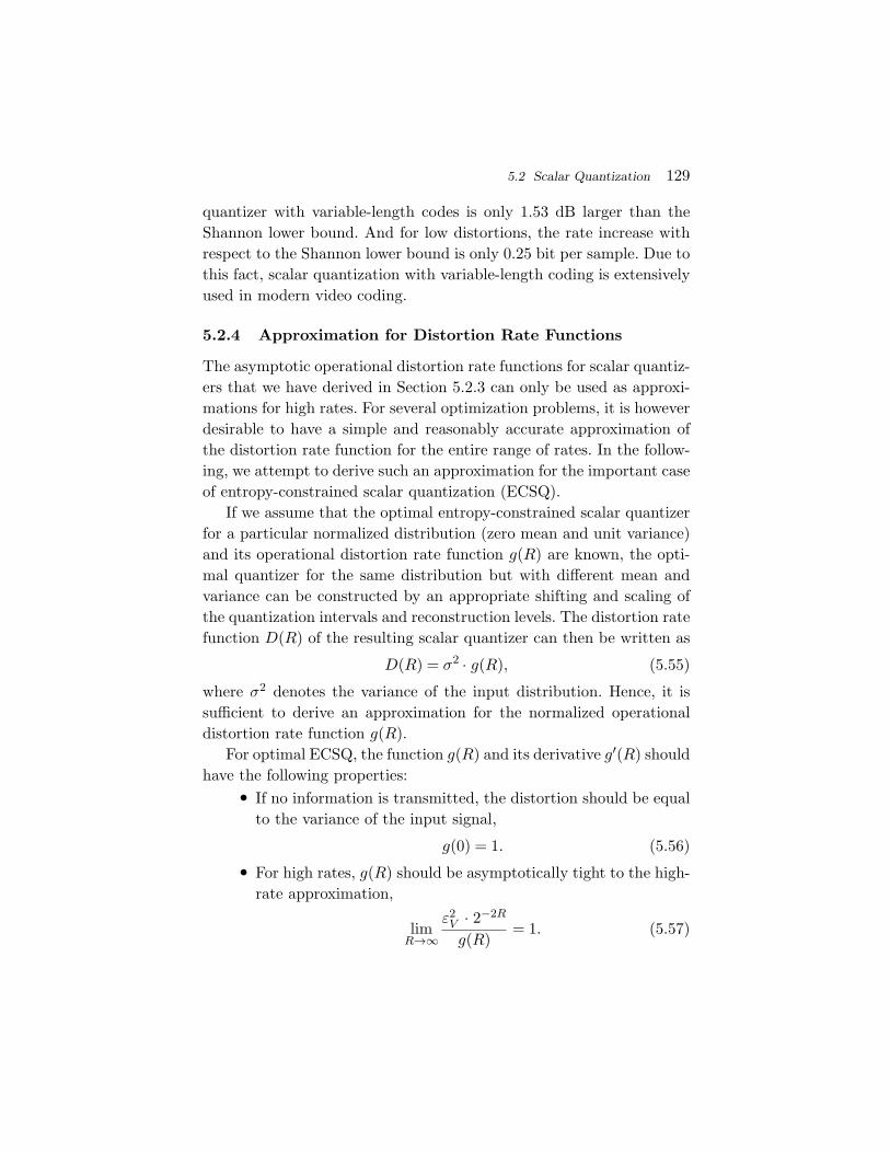
5.2 Scalar Quantization 129
quantizer with variable-length codes is only 1.53 dB larger than theShannon lower bound. And for low distortions, the rate increase withrespect to the Shannon lower bound is only 0.25 bit per sample. Due tothis fact, scalar quantization with variable-length coding is extensivelyused in modern video coding.
5.2.4 Approximation for Distortion Rate Functions
The asymptotic operational distortion rate functions for scalar quantiz-ers that we have derived in Section 5.2.3 can only be used as approxi-mations for high rates. For several optimization problems, it is howeverdesirable to have a simple and reasonably accurate approximation ofthe distortion rate function for the entire range of rates. In the follow-ing, we attempt to derive such an approximation for the important caseof entropy-constrained scalar quantization (ECSQ).
If we assume that the optimal entropy-constrained scalar quantizerfor a particular normalized distribution (zero mean and unit variance)and its operational distortion rate function g(R) are known, the opti-mal quantizer for the same distribution but with different mean andvariance can be constructed by an appropriate shifting and scaling ofthe quantization intervals and reconstruction levels. The distortion ratefunction D(R) of the resulting scalar quantizer can then be written as
D(R) = σ2 · g(R), (5.55)
where σ2 denotes the variance of the input distribution. Hence, it issufficient to derive an approximation for the normalized operationaldistortion rate function g(R).
For optimal ECSQ, the function g(R) and its derivative g′(R) shouldhave the following properties:
• If no information is transmitted, the distortion should be equalto the variance of the input signal,
g(0) = 1. (5.56)
• For high rates, g(R) should be asymptotically tight to the high-rate approximation,
limR→∞
ε2V · 2−2R
g(R)= 1. (5.57)

130 Quantization
• For ensuring the mathematical tractability of optimizationproblems the derivative g′(R) should be continuous.
• An increase in rate should result in a distortion reduction,
g′(R) < 0 for R ∈ [0,∞). (5.58)
A function that satisfies the above conditions is
g(R) =ε2V
a· ln(a · 2−2R + 1). (5.59)
The factor a is chosen in a way that g(0) is equal to 1. By numericaloptimization, we obtained a = 0.9519 for the Gaussian pdf and a = 0.5for the Laplacian pdf. For proving that condition (5.57) is fulfilled, wecan substitute x = 2−2R and develop the Taylor series of the resultingfunction
g(x) =ε2V
aln(a · x + 1) (5.60)
around x0 = 0, which gives
g(x) ≈ g(0) + g′(0) · x = ε2V · x. (5.61)
Since the remaining terms of the Taylor series are negligible forsmall values of x (large rates R), (5.59) approaches the high-rateapproximation ε2
V 2−2R as the rate R approaches infinity. The firstderivative of (5.59) is given by
g′(R) = −ε2V · 2ln2a + 22R
. (5.62)
It is a continuous and always less than zero.The quality of the approximations for the operational distortion rate
functions of an entropy-constrained quantizer for a Gaussian and Lapla-cian pdf is illustrated in Figure 5.12. For the Gaussian pdf, the approx-imation (5.59) provides a sufficiently accurate match to the results ofthe entropy-constrained Lloyd algorithm and will be used later. For theLaplacian pdf, the approximation is less accurate for low bit rates.
5.2.5 Performance Comparison for Gaussian Sources
In the following, we compare the rate distortion performance of thediscussed scalar quantizers designs with the rate distortion bound for
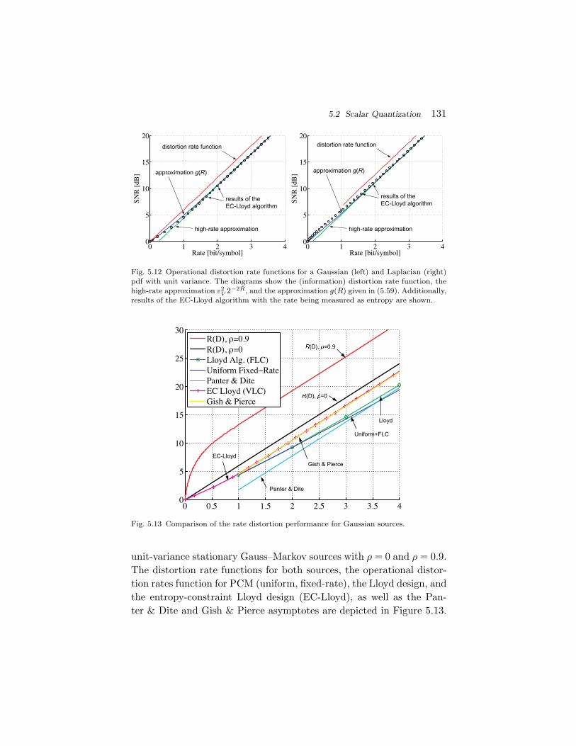
5.2 Scalar Quantization 131
Fig. 5.12 Operational distortion rate functions for a Gaussian (left) and Laplacian (right)pdf with unit variance. The diagrams show the (information) distortion rate function, thehigh-rate approximation ε2
V 2−2R, and the approximation g(R) given in (5.59). Additionally,results of the EC-Lloyd algorithm with the rate being measured as entropy are shown.
Fig. 5.13 Comparison of the rate distortion performance for Gaussian sources.
unit-variance stationary Gauss–Markov sources with ρ = 0 and ρ = 0.9.The distortion rate functions for both sources, the operational distor-tion rates function for PCM (uniform, fixed-rate), the Lloyd design, andthe entropy-constraint Lloyd design (EC-Lloyd), as well as the Pan-ter & Dite and Gish & Pierce asymptotes are depicted in Figure 5.13.
132 Quantization
The rate for quantizers with fixed-length codes is given by the binarylogarithm of the quantizer size K. For quantizers with variable-lengthcodes, it is measured as the entropy of the reconstruction levels.
The scalar quantizer designs behave identical for both sources asonly the marginal pdf f(s) is relevant for the quantizer design algo-rithms. For high rates, the entropy-constrained Lloyd design and theGish & Pierce approximation yield an SNR that is 1.53 dB smallerthan the (information) distortion rate function for the Gauss–Markovsource with ρ = 0. The rate distortion performance of the quantizerswith fixed-length codes is worse, particularly for rates above 1 bit persample. It is, however, important to note that it cannot be concludedthat the Lloyd algorithm yields a worse performance than the entropy-constrained Lloyd algorithm. Both quantizers are (locally) optimal withrespect to their application area. The Lloyd algorithm results in an opti-mized quantizer for fixed-length coding, while the entropy-constrainedLloyd algorithm yields an optimized quantizer for variable-length cod-ing (with an average codeword length close to the entropy).
The distortion rate function for the Gauss–Markov source withρ = 0.9 is far away from the operational distortion rate functions of theinvestigated scalar quantizer designs. The reason is that we assumeda lossless coding γ that achieves a rate close to the entropy H(S′) ofthe output process. A combination of scalar quantization and advancedlossless coding techniques that exploit dependencies between the out-put samples is discussed in the next section.
5.2.6 Scalar Quantization for Sources with Memory
In the previous sections, we concentrated on combinations of scalarquantization with lossless coding techniques that do not exploitdependencies between the output samples. As a consequence, the ratedistortion performance did only depend on the marginal pdf of theinput process, and for stationary sources with memory the perfor-mance was identical to the performance for iid sources with the samemarginal distribution. If we, however, apply scalar quantization tosources with memory, the output samples are not independent. The
5.2 Scalar Quantization 133
dependencies can be exploited by advanced lossless coding techniquessuch as conditional Huffman codes, block Huffman codes, or arithmeticcodes that use conditional pmfs in the probability modeling stage.
The design goal of Lloyd quantizers was to minimize the distor-tion for a quantizer of a given size K. Hence, the Lloyd quantizerdesign does not change for source with memory. But the design ofthe entropy-constrained Lloyd quantizer can be extended by consider-ing advanced entropy coding techniques. The conditions for the deter-mination of the reconstruction levels and interval boundaries (giventhe decision thresholds and average codeword lengths) do not change,only the determination of the average codeword lengths in step 4 ofthe entropy-constrained Lloyd algorithm needs to be modified. We candesign a lossless code such as a conditional or block Huffman codebased on the joint pmf of the output samples (which is given by thejoint pdf of the input source and the decision thresholds) and deter-mine the resulting average codeword lengths. But, following the samearguments as in Section 5.2.2, we can also approximate the averagecodeword lengths based on the corresponding conditional entropy orblock entropy.
For the following consideration, we assume that the input source isstationary and that its joint pdf for N successive samples is given byfN (s). If we employ a conditional lossless code (conditional Huffmancode or arithmetic code) that exploits the conditional pmf of a currentoutput sample S′ given the last N output samples S′, the averagecodeword lengths �(s′
i) can be set equal to the ratio of the conditionalentropy H(S′|S′) and the symbol probability p(s′
i),
�(s′i) =
H(S′|S′)p(s′
i)= − 1
p(s′i)
KN−1∑k=0
pN+1(s′i,s
′k) log2
pN+1(s′i,s
′k)
pN (s′k)
, (5.63)
where k is an index that indicates any of the KN combinations of thelast N output samples, p is the marginal pmf of the output samples,and pN and pN+1 are the joint pmfs for N and N + 1 successive out-put samples, respectively. It should be noted that the argument of thelogarithm represents the conditional pmf for an output sample S′ giventhe N preceding output samples S′.
134 Quantization
Each joint pmf for N successive output samples, including themarginal pmf p with N =1, is determined by the joint pdf fN of theinput source and the decision thresholds,
pN (s′k) =
∫ uk+1
uk
fN (s) ds, (5.64)
where uk and uk+1 represent the ordered sets of lower and upper inter-val boundaries, respectively, for the vector s′
k of output samples. Hence,the average codeword length �(s′
i) can be directly derived based on thejoint pdf for the input process and the decision thresholds. In a similarway, the average codeword lengths for block codes of N samples canbe approximated based on the block entropy for N successive outputsamples.
We now investigate the asymptotic operational distortion rate func-tion for high rates. If we again assume that we employ a conditionallossless code that exploits the conditional pmf using the preceding N
output samples, the rate R can be approximated by the correspondingconditional entropy H(Sn|Sn−1, . . . ,Sn−N ),
R = −K−1∑i=0
KN−1∑k=0
pN+1(s′i,s
′k) log2
pN+1(s′i,s
′k)
pN (s′k)
. (5.65)
For small quantization intervals ∆i (high rates), we can assume thatthe joint pdfs fN for the input sources are nearly constant inside eachN -dimensional hypercube given by a combination of quantization inter-vals, which yields the approximations
pN (s′k) = fN (s′
k)∆k and pN+1(s′i,s
′k) = fN+1(s′
i,s′k)∆k ∆i,
(5.66)where ∆k represents the Cartesian product of quantization intervalsizes that are associated with the vector of reconstruction levels s′
k.By inserting these approximations in (5.65), we obtain
R = −K−1∑i=0
KN−1∑k=0
fN+1(s′i,s
′k)∆k ∆i log2
fN+1(s′i,s
′k)
fN (s′k)
−K−1∑i=0
KN−1∑k=0
fN+1(s′i,s
′k)∆k ∆i log2 ∆i. (5.67)
5.2 Scalar Quantization 135
Since we consider the asymptotic behavior for infinitesimal quantiza-tion intervals, the sums can be replaced by integrals, which gives
R = −∫
R
∫RN
fn+1(s,s) log2fn+1(s,s)
fN (s)ds ds
−K−1∑i=0
(∫RN
fn+1(s′i,s) ds
)∆i log2 ∆i. (5.68)
The first integral (including the minus sign) is the conditional differ-ential entropy h(Sn|Sn−1, . . . ,Sn−N ) for an input sample given the pre-ceding N input symbols and the second integral is the value f(s′
i) ofmarginal pdf of the input source. Using the high rate approximationp(s′
i) = f(s′i)∆i, we obtain
R = h(Sn|Sn−1, . . . ,Sn−N ) − 12
K−1∑i=0
p(s′i) log2 ∆2
i , (5.69)
which is similar to (5.49). In the same way as for (5.49) in Section 5.2.3,we can now apply Jensen’s inequality and then substitute the high rateapproximation (5.41) for the MSE distortion measure. As a consequenceof Jensen’s inequality, we note that also for conditional lossless codes,the optimal quantizer design for high rates has uniform quantizationstep sizes. The asymptotic operational distortion rate function for anoptimum quantizer with conditional lossless codes is given by
DC(R) =112
· 2h(Sn|Sn−1,...,Sn−N ) · 2−2R. (5.70)
In comparison to the Gish & Pierce asymptote (5.52), the first orderdifferential entropy h(S) is replaced by the conditional entropy giventhe N preceding input samples.
In a similar way, we can also derive the asymptotic distortion ratefunction for block entropy codes (as the block Huffman code) of size N .We obtain the result that also for block entropy codes, the optimalquantizer design for high rates has uniform quantization step sizes.The corresponding asymptotic operational distortion rate function is
DB(R) =112
· 2h(Sn,...,Sn+N−1)
N · 2−2R, (5.71)
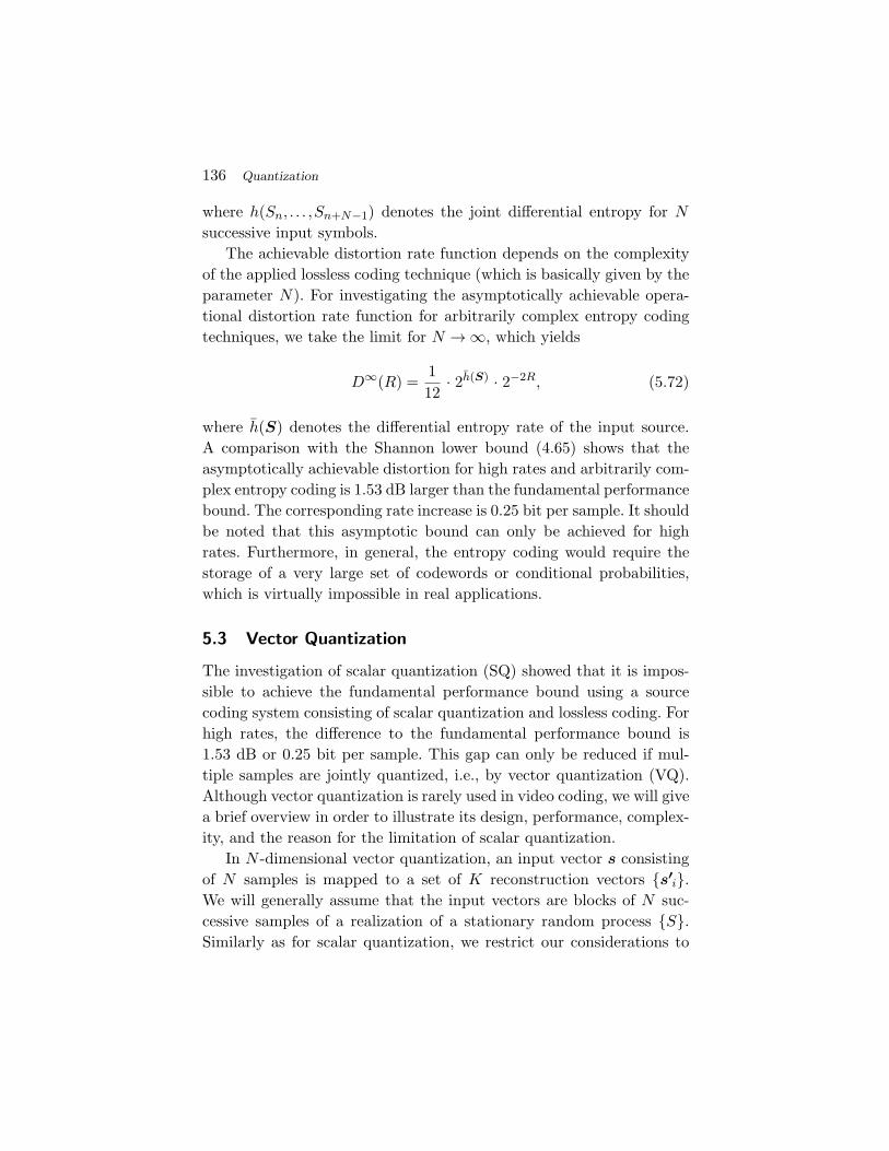
136 Quantization
where h(Sn, . . . ,Sn+N−1) denotes the joint differential entropy for N
successive input symbols.The achievable distortion rate function depends on the complexity
of the applied lossless coding technique (which is basically given by theparameter N). For investigating the asymptotically achievable opera-tional distortion rate function for arbitrarily complex entropy codingtechniques, we take the limit for N → ∞, which yields
D∞(R) =112
· 2h(S) · 2−2R, (5.72)
where h(S) denotes the differential entropy rate of the input source.A comparison with the Shannon lower bound (4.65) shows that theasymptotically achievable distortion for high rates and arbitrarily com-plex entropy coding is 1.53 dB larger than the fundamental performancebound. The corresponding rate increase is 0.25 bit per sample. It shouldbe noted that this asymptotic bound can only be achieved for highrates. Furthermore, in general, the entropy coding would require thestorage of a very large set of codewords or conditional probabilities,which is virtually impossible in real applications.
5.3 Vector Quantization
The investigation of scalar quantization (SQ) showed that it is impos-sible to achieve the fundamental performance bound using a sourcecoding system consisting of scalar quantization and lossless coding. Forhigh rates, the difference to the fundamental performance bound is1.53 dB or 0.25 bit per sample. This gap can only be reduced if mul-tiple samples are jointly quantized, i.e., by vector quantization (VQ).Although vector quantization is rarely used in video coding, we will givea brief overview in order to illustrate its design, performance, complex-ity, and the reason for the limitation of scalar quantization.
In N -dimensional vector quantization, an input vector s consistingof N samples is mapped to a set of K reconstruction vectors {s′
i}.We will generally assume that the input vectors are blocks of N suc-cessive samples of a realization of a stationary random process {S}.Similarly as for scalar quantization, we restrict our considerations to
5.3 Vector Quantization 137
regular vector quantizers5 for which the quantization cells are convexsets6 and each reconstruction vector is an element of the associatedquantization cell. The average distortion and average rate of a vectorquantizer are given by (5.5) and (5.7), respectively.
5.3.1 Vector Quantization with Fixed-Length Codes
We first investigate a vector quantizer design that minimizes the dis-tortion D for a given quantizer size K, i.e., the counterpart of the Lloydquantizer. The necessary conditions for the reconstruction vectors andquantization cells can be derived in the same way as for the Lloydquantizer in Section 5.2.1 and are given by
s′i = arg min
s′∈RN
E{dN(S,s′) | S ∈ Ci} , (5.73)
and
Q(s) = argmin∀s′
i
dN (s,s′i). (5.74)
The Linde–Buzo–Gray Algorithm. The extension of the Lloydalgorithm to vector quantization [42] is referred to as Linde–Buzo–Gray algorithm (LBG). For a sufficiently large training set {sn} and agiven quantizer size K, the algorithm can be stated as follows:
(1) Choose an initial set of reconstruction vectors {s′i}.
(2) Associate all samples of the training set {sn} with one of thequantization cells Ci according to
a(sn) = argmin∀i
dN (sn,s′i).
(3) Update the reconstruction vectors {s′i} according to
s′i = arg min
s′∈RN
E{dN(S,s′) | α(S) = i} ,
where the expectation value is taken over the training set.
(4) Repeat the previous two steps until convergence.
5 Regular quantizers are optimal with respect to the MSE distortion measure.6 A set of points in RN is convex, if for any two points of the set, all points on the straightline connecting the two points are also elements of the set.

138 Quantization
Examples for the LBG Algorithm. As an example, we designeda two-dimensional vector quantizer for a Gaussian iid process with unitvariance. The selected quantizer size is K = 16 corresponding to a rateof 2 bit per (scalar) sample. The chosen initialization as well as theobtained quantization cells and reconstruction vectors after the 8th and49th iterations of the LBG algorithm are illustrated in Figure 5.14. InFigure 5.15, the distortion is plotted as a function of the iteration step.
After the 8th iteration, the two-dimensional vector quantizer showsa similar distortion (9.30 dB) as the scalar Lloyd quantizer at the same
Fig. 5.14 Illustration of the LBG algorithm for a quantizer with N = 2 and K = 16 and aGaussian iid process with unit variance. The lines mark the boundaries of the quantizationcells, the crosses show the reconstruction vectors, and the light-colored dots represent thesamples of the training set.
Fig. 5.15 Distortion as a function of the iteration step for the LBG algorithm with N = 2,K = 16, and a Gaussian iid process with unit variance. The dashed line represents thedistortion for a Lloyd quantizer with the same rate of R = 2 bit per sample.

5.3 Vector Quantization 139
0 10 20 30 40 5002468
1012141618202224
Iteration
SNR
[dB
], H
[bi
t/s] 1.31 dB
H=3.69 bit/s
Conjectured VQ performance for R=4 bit/s
Fixedlength SQ performance for R=4 bit/s
Fig. 5.16 Illustration of the LBG algorithm for a quantizer with N = 2 and K = 256 and aGaussian iid process with unit variance: (left) resulting quantization cells and reconstructionvectors after 49 iterations; (right) distortion as function of the iteration step.
rate of R = 2 bit per (scalar) sample. This can be explained by thefact that the quantization cells are approximately rectangular shapedand that such rectangular cells would also be constructed by a corre-sponding scalar quantizer (if we illustrate the result for two consecutivesamples). After the 49th iteration, the cells of the vector quantizer areshaped in a way that a scalar quantizer cannot create and the SNR isincreased to 9.67 dB.
Figure 5.16 shows the result of the LBG algorithm for a vectorquantizer with N = 2 and K = 256, corresponding to a rate of R = 4bit per sample, for the Gaussian iid source with unit variance. Afterthe 49th iteration, the gain for two-dimensional VQ is around 0.9 dBcompared to SQ with fixed-length codes resulting in an SNR of 20.64 dB(of conjectured 21.05 dB [46]). The result indicates that at higher bitrates, the gain of VQ relative to SQ with fixed-length codes increases.
Figure 5.17 illustrates the results for a two-dimensional VQ designfor a Laplacian iid source with unit variance and two different quantizersizes K. For K = 16, which corresponds to a rate of R = 2 bit persample, the SNR is 8.87 dB. Compared to SQ with fixed-length codesat the same rate, a gain of 1.32 dB has been achieved. For a rate ofR = 4 bit per sample (K = 256), the SNR gain is increased to 1.84 dBresulting in an SNR of 19.4 dB (of conjectured 19.99 dB [46]).
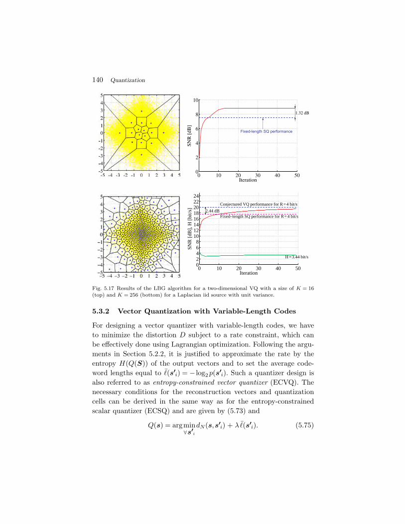
140 Quantization
0 10 20 30 40 5002468
1012141618202224
Iteration
SNR
[dB
], H
[bi
t/s]
2.44 dB
H =3.44 bit/s
Conjectured VQ performance for R=4 bit/s
Fixed–length SQ performance for R= 4 bit/s
Fig. 5.17 Results of the LBG algorithm for a two-dimensional VQ with a size of K = 16(top) and K = 256 (bottom) for a Laplacian iid source with unit variance.
5.3.2 Vector Quantization with Variable-Length Codes
For designing a vector quantizer with variable-length codes, we haveto minimize the distortion D subject to a rate constraint, which canbe effectively done using Lagrangian optimization. Following the argu-ments in Section 5.2.2, it is justified to approximate the rate by theentropy H(Q(S)) of the output vectors and to set the average code-word lengths equal to �(s′
i) = − log2 p(s′i). Such a quantizer design is
also referred to as entropy-constrained vector quantizer (ECVQ). Thenecessary conditions for the reconstruction vectors and quantizationcells can be derived in the same way as for the entropy-constrainedscalar quantizer (ECSQ) and are given by (5.73) and
Q(s) = argmin∀s′
i
dN (s,s′i) + λ�(s′
i). (5.75)
5.3 Vector Quantization 141
The Chou–Lookabaugh–Gray Algorithm. The extension of theentropy-constrained Lloyd algorithm to vector quantization [9] is alsoreferred to as Chou–Lookabaugh–Gray algorithm (CLG). For a suffi-ciently large training set {sn} and a given Lagrange parameter λ, theCLG algorithm can be stated as follows:
(1) Choose an initial quantizer size N and initial sets of recon-struction vectors {s′
i} and average codeword lengths �(s′i).
(2) Associate all samples of the training set {sn} with one of thequantization cells Ci according to
α(s) = argmin∀s′
i
dN (s,s′i) + λ�(s′
i).
(3) Update the reconstruction vectors {s′i} according to
s′i = arg min
s′∈RN
E{dN(S,s′) | α(S) = i} ,
where the expectation value is taken over the training set.
(4) Update the average codeword length �(s′i) according to
�(s′i) = − log2 p(s′
i).
(5) Repeat the previous three steps until convergence.
Examples for the CLG Algorithm. As examples, we designed atwo-dimensional ECVQ for a Gaussian and Laplacian iid process withunit variance and an average rate, measured as entropy, of R = 2 bit persample. The results of the CLG algorithm are illustrated in Figure 5.18.The SNR gain compared to an ECSQ design with the same rate is0.26 dB for the Gaussian and 0.37 dB for the Laplacian distribution.
5.3.3 The Vector Quantization Advantage
The examples for the LBG and CLG algorithms showed that vectorquantization increases the coding efficiency compared to scalar quan-tization. According to the intuitive analysis in [48], the performancegain can be attributed to three different effects: the space filling advan-tage, the shape advantage, and the memory advantage. In the following,

142 Quantization
Fig. 5.18 Results of the CLG algorithm for N = 2 and a Gaussian (top) and Laplacian(bottom) iid source with unit variance and a rate (entropy) of R = 2 bit per sample. Thedashed line in the diagrams on the right shows the distortion for an ECSQ design with thesame rate.
we will briefly explain and discuss these advantages. We will see thatthe space filling advantage is the only effect that can be exclusivelyachieved with vector quantization. The associated performance gainis bounded to 1.53 dB or 0.25 bit per sample. This bound is asymp-totically achieved for large quantizer dimensions and large rates, andcorresponds exactly to the gap between the operational rate distor-tion function for scalar quantization with arbitrarily complex entropycoding and the rate distortion bound at high rates. For a deeper anal-ysis of the vector quantization advantages, the reader is referred to thediscussion in [48] and the quantitative analysis in [46].
Space Filling Advantage. When we analyze the results of scalarquantization in higher dimension, we see that the N -dimensional space
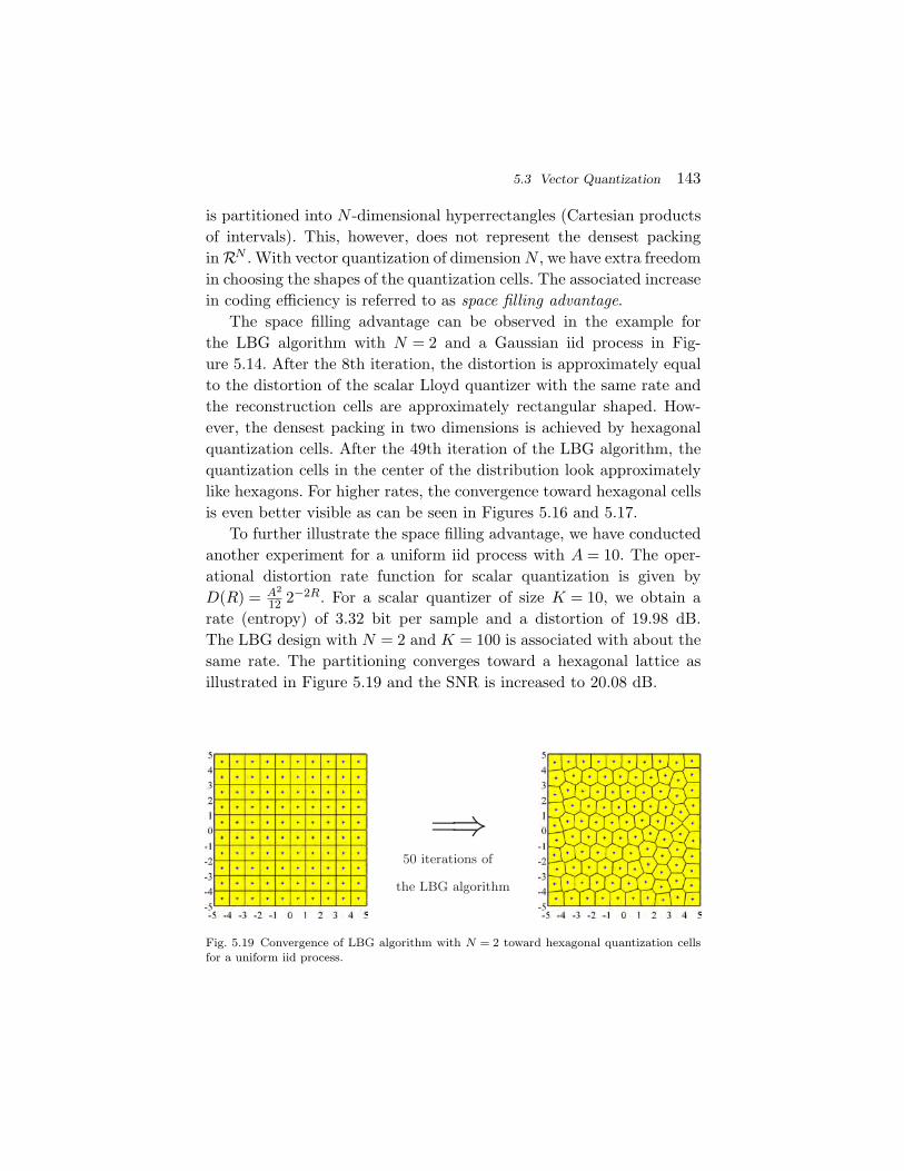
5.3 Vector Quantization 143
is partitioned into N -dimensional hyperrectangles (Cartesian productsof intervals). This, however, does not represent the densest packingin RN . With vector quantization of dimension N , we have extra freedomin choosing the shapes of the quantization cells. The associated increasein coding efficiency is referred to as space filling advantage.
The space filling advantage can be observed in the example forthe LBG algorithm with N = 2 and a Gaussian iid process in Fig-ure 5.14. After the 8th iteration, the distortion is approximately equalto the distortion of the scalar Lloyd quantizer with the same rate andthe reconstruction cells are approximately rectangular shaped. How-ever, the densest packing in two dimensions is achieved by hexagonalquantization cells. After the 49th iteration of the LBG algorithm, thequantization cells in the center of the distribution look approximatelylike hexagons. For higher rates, the convergence toward hexagonal cellsis even better visible as can be seen in Figures 5.16 and 5.17.
To further illustrate the space filling advantage, we have conductedanother experiment for a uniform iid process with A = 10. The oper-ational distortion rate function for scalar quantization is given byD(R) = A2
12 2−2R. For a scalar quantizer of size K = 10, we obtain arate (entropy) of 3.32 bit per sample and a distortion of 19.98 dB.The LBG design with N = 2 and K = 100 is associated with about thesame rate. The partitioning converges toward a hexagonal lattice asillustrated in Figure 5.19 and the SNR is increased to 20.08 dB.
Fig. 5.19 Convergence of LBG algorithm with N = 2 toward hexagonal quantization cellsfor a uniform iid process.

144 Quantization
The gain due to choosing the densest packing is independent of thesource distribution or any statistical dependencies between the randomvariables of the input process. The space filling gain is bounded to1.53 dB, which can be asymptotically achieved for high rates if thedimensionality of the vector quantizer approaches infinity [46].
Shape advantage. The shape advantage describes the effect thatthe quantization cells of optimal VQ designs adapt to the shape of thesource pdf. In the examples for the CLG algorithm, we have howeverseen that, even though ECVQ provides a better performance than VQwith fixed-length codes, the gain due to VQ is reduced if we employvariable-length coding for both VQ and SQ. When comparing ECVQwith ECSQ for iid sources, the gain of VQ reduces to the space fillingadvantage, while the shape advantage is exploited by variable-lengthcoding. However, VQ with fixed-length codes can also exploit the gainthat ECSQ shows compared to SQ with fixed-length codes [46].
The shape advantage for high rates has been estimated in [46].Figure 5.20 shows this gain for Gaussian and Laplacian iid randomprocesses. In practice, the shape advantage is exploited by using scalarquantization in combination with entropy coding techniques such asHuffman coding or arithmetic coding.
Memory advantage. For sources with memory, there are linear ornonlinear dependencies between the samples. In optimal VQ designs,
1 2 4 8 160
1
2
3
4
5
6
Dimension N
SNR
Gai
n [d
B]
Gaussian pdf
Laplacian pdf
∞
Fig. 5.20 Shape advantage for Gaussian and Laplacian iid sources as a function of the vectorquantizer dimension N .
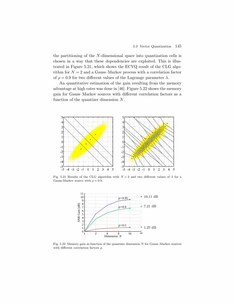
5.3 Vector Quantization 145
the partitioning of the N -dimensional space into quantization cells ischosen in a way that these dependencies are exploited. This is illus-trated in Figure 5.21, which shows the ECVQ result of the CLG algo-rithm for N = 2 and a Gauss–Markov process with a correlation factorof ρ = 0.9 for two different values of the Lagrange parameter λ.
An quantitative estimation of the gain resulting from the memoryadvantage at high rates was done in [46]. Figure 5.22 shows the memorygain for Gauss–Markov sources with different correlation factors as afunction of the quantizer dimension N .
Fig. 5.21 Results of the CLG algorithm with N = 2 and two different values of λ for aGauss-Markov source with ρ = 0.9.
1 2 4 8 160123456789
1011
Dimension N
SNR
Gai
n [d
B]
ρ=0.5
ρ=0.9
ρ=0.95
∞
Fig. 5.22 Memory gain as function of the quantizer dimension N for Gauss–Markov sourceswith different correlation factors ρ.
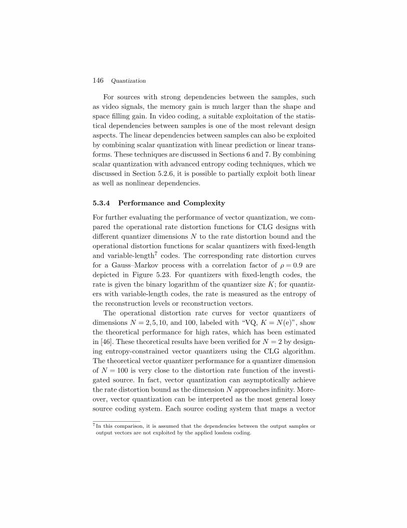
146 Quantization
For sources with strong dependencies between the samples, suchas video signals, the memory gain is much larger than the shape andspace filling gain. In video coding, a suitable exploitation of the statis-tical dependencies between samples is one of the most relevant designaspects. The linear dependencies between samples can also be exploitedby combining scalar quantization with linear prediction or linear trans-forms. These techniques are discussed in Sections 6 and 7. By combiningscalar quantization with advanced entropy coding techniques, which wediscussed in Section 5.2.6, it is possible to partially exploit both linearas well as nonlinear dependencies.
5.3.4 Performance and Complexity
For further evaluating the performance of vector quantization, we com-pared the operational rate distortion functions for CLG designs withdifferent quantizer dimensions N to the rate distortion bound and theoperational distortion functions for scalar quantizers with fixed-lengthand variable-length7 codes. The corresponding rate distortion curvesfor a Gauss–Markov process with a correlation factor of ρ = 0.9 aredepicted in Figure 5.23. For quantizers with fixed-length codes, therate is given the binary logarithm of the quantizer size K; for quantiz-ers with variable-length codes, the rate is measured as the entropy ofthe reconstruction levels or reconstruction vectors.
The operational distortion rate curves for vector quantizers ofdimensions N = 2,5,10, and 100, labeled with “VQ, K = N(e)”, showthe theoretical performance for high rates, which has been estimatedin [46]. These theoretical results have been verified for N = 2 by design-ing entropy-constrained vector quantizers using the CLG algorithm.The theoretical vector quantizer performance for a quantizer dimensionof N = 100 is very close to the distortion rate function of the investi-gated source. In fact, vector quantization can asymptotically achievethe rate distortion bound as the dimension N approaches infinity. More-over, vector quantization can be interpreted as the most general lossysource coding system. Each source coding system that maps a vector
7 In this comparison, it is assumed that the dependencies between the output samples oroutput vectors are not exploited by the applied lossless coding.
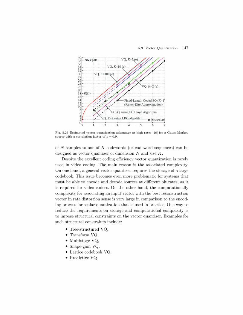
5.3 Vector Quantization 147
Fixed-Length Coded SQ (K=1) (Panter-Dite Approximation)
ECSQ using EC Lloyd Algorithm
VQ, K=2 (e)
VQ, K=2 using LBG algorithm
VQ, K=5 (e)
VQ, K=10 (e)
VQ, K=100 (e)
R(D)
SNR [dB]
R [bit/scalar]
Fig. 5.23 Estimated vector quantization advantage at high rates [46] for a Gauss-Markovsource with a correlation factor of ρ = 0.9.
of N samples to one of K codewords (or codeword sequences) can bedesigned as vector quantizer of dimension N and size K.
Despite the excellent coding efficiency vector quantization is rarelyused in video coding. The main reason is the associated complexity.On one hand, a general vector quantizer requires the storage of a largecodebook. This issue becomes even more problematic for systems thatmust be able to encode and decode sources at different bit rates, as itis required for video codecs. On the other hand, the computationallycomplexity for associating an input vector with the best reconstructionvector in rate distortion sense is very large in comparison to the encod-ing process for scalar quantization that is used in practice. One way toreduce the requirements on storage and computational complexity isto impose structural constraints on the vector quantizer. Examples forsuch structural constraints include:
• Tree-structured VQ,• Transform VQ,• Multistage VQ,• Shape-gain VQ,• Lattice codebook VQ,• Predictive VQ.
148 Quantization
In particular, predictive VQ can be seen as a generalization of a numberof very popular techniques including motion compensation in video cod-ing. For the actual quantization, video codecs mostly include a simplescalar quantizer with uniformly distributed reconstruction levels (some-times with a deadzone around zero), which is combined with entropycoding and techniques such as linear prediction or linear transforms inorder to exploit the shape of the source distribution and the statisticaldependencies of the source. For video coding, the complexity of vectorquantizers including those with structural constraints is considered astoo large in relation to the achievable performance gains.
5.4 Summary of Quantization
In this section, we have discussed quantization starting with scalarquantizers. The Lloyd quantizer that is constructed using an iterativeprocedure provides the minimum distortion for a given number of recon-struction levels. It is the optimal quantizer design if the reconstructionlevels are transmitted using fixed-length codes. The extension of thequantizer design for variable-length codes is achieved by minimizingthe distortion D subject to a rate constraint R < Rmax, which can beformulated as a minimization of a Lagrangian functional D + λR. Thecorresponding iterative design algorithm includes a sufficiently accurateestimation of the codeword lengths that are associated with the recon-struction levels. Usually the codeword lengths are estimated based onthe entropy of the output signal, in which case the quantizer design isalso referred to as entropy-constrained Lloyd quantizer.
At high rates, the operational distortion rate functions for scalarquantization with fixed- and variable-length codes as well as the Shan-non lower bound can be described by
DX(R) = σ2 · ε2X · 2−2R, (5.76)
where X either indicates the Shannon lower bound or scalar quantiza-tion with fixed- or variable-length codes. For a given X, the factors ε2
X
depend only on the statistical properties of the input source. If theoutput samples are coded with an arbitrarily complex entropy coding
5.4 Summary of Quantization 149
scheme, the difference between the operational distortion rate func-tion for optimal scalar quantization with variable-length codes and theShannon lower bound is 1.53 dB or 0.25 bit per sample at high rates.Another remarkable result is that at high rates, optimal scalar quanti-zation with variable-length codes is achieved if all quantization intervalshave the same size.
In the second part of the section, we discussed the extension of scalarquantization to vector quantization, by which the rate distortion boundcan be asymptotically achieved as the quantizer dimension approachesinfinity. The coding efficiency improvements of vector quantization rel-ative to scalar quantization can be attributed to three different effects:the space filling advantage, the shape advantage, and the memoryadvantage. While the space filling advantage can be only achievedby vector quantizers, the shape and memory advantage can also beexploited by combining scalar quantization with a suitable entropy cod-ing and techniques such as linear prediction and linear transforms.
Despite its superior rate distortion performance, vector quantizationis rarely used in video coding applications because of its complexity.Instead, modern video codecs combine scalar quantization with entropycoding, linear prediction, and linear transforms in order to achieve ahigh coding efficiency at a moderate complexity level.

6Predictive Coding
In the previous section, we investigated the design and rate distortionperformance of quantizers. We showed that the fundamental rate dis-tortion bound can be virtually achieved by unconstrained vector quan-tization of a sufficiently large dimension. However, due to the very largeamount of data in video sequences and the real-time requirements thatare found in most video coding applications, only low-complex scalarquantizers are typically used in this area. For iid sources, the achievableoperational rate distortion function for high rate scalar quantizationlies at most 1.53 dB or 0.25 bit per sample above the fundamental ratedistortion bound. This represents a suitable trade-off between codingefficiency and complexity. But if there is a large amount of dependen-cies between the samples of an input signal, as it is the case in videosequences, the rate distortion performance for simple scalar quantizersbecomes significantly worse than the rate distortion bound. A sourcecoding system consisting of a scalar quantizer and an entropy codercan exploit the statistical dependencies in the input signal only if theentropy coder uses higher order conditional or joint probability mod-els. The complexity of such an entropy coder is however close to thatof a vector quantizer, so that such a design is unsuitable in practice.Furthermore, video sequences are highly nonstationary and conditional
150
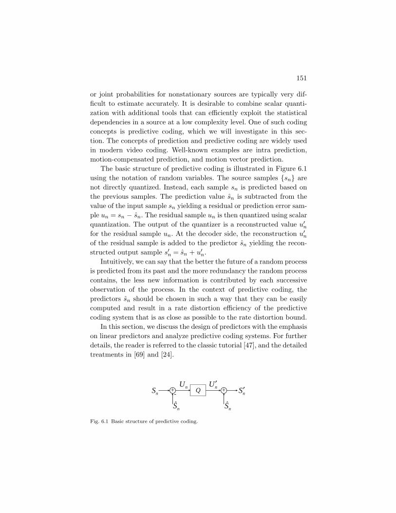
151
or joint probabilities for nonstationary sources are typically very dif-ficult to estimate accurately. It is desirable to combine scalar quanti-zation with additional tools that can efficiently exploit the statisticaldependencies in a source at a low complexity level. One of such codingconcepts is predictive coding, which we will investigate in this sec-tion. The concepts of prediction and predictive coding are widely usedin modern video coding. Well-known examples are intra prediction,motion-compensated prediction, and motion vector prediction.
The basic structure of predictive coding is illustrated in Figure 6.1using the notation of random variables. The source samples {sn} arenot directly quantized. Instead, each sample sn is predicted based onthe previous samples. The prediction value sn is subtracted from thevalue of the input sample sn yielding a residual or prediction error sam-ple un = sn − sn. The residual sample un is then quantized using scalarquantization. The output of the quantizer is a reconstructed value u′
n
for the residual sample un. At the decoder side, the reconstruction u′n
of the residual sample is added to the predictor sn yielding the recon-structed output sample s′
n = sn + u′n.
Intuitively, we can say that the better the future of a random processis predicted from its past and the more redundancy the random processcontains, the less new information is contributed by each successiveobservation of the process. In the context of predictive coding, thepredictors sn should be chosen in such a way that they can be easilycomputed and result in a rate distortion efficiency of the predictivecoding system that is as close as possible to the rate distortion bound.
In this section, we discuss the design of predictors with the emphasison linear predictors and analyze predictive coding systems. For furtherdetails, the reader is referred to the classic tutorial [47], and the detailedtreatments in [69] and [24].
Q ++
S n S n
Sn ′S nUn ′U n
-
Fig. 6.1 Basic structure of predictive coding.
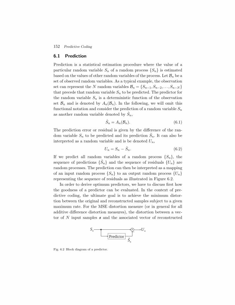
152 Predictive Coding
6.1 Prediction
Prediction is a statistical estimation procedure where the value of aparticular random variable Sn of a random process {Sn} is estimatedbased on the values of other random variables of the process. Let Bn be aset of observed random variables. As a typical example, the observationset can represent the N random variables Bn = {Sn−1,Sn−2, . . . ,Sn−N}that precede that random variable Sn to be predicted. The predictor forthe random variable Sn is a deterministic function of the observationset Bn and is denoted by An(Bn). In the following, we will omit thisfunctional notation and consider the prediction of a random variable Sn
as another random variable denoted by Sn,
Sn = An(Bn). (6.1)
The prediction error or residual is given by the difference of the ran-dom variable Sn to be predicted and its prediction Sn. It can also beinterpreted as a random variable and is be denoted Un,
Un = Sn − Sn. (6.2)
If we predict all random variables of a random process {Sn}, thesequence of predictions {Sn} and the sequence of residuals {Un} arerandom processes. The prediction can then be interpreted as a mappingof an input random process {Sn} to an output random process {Un}representing the sequence of residuals as illustrated in Figure 6.2.
In order to derive optimum predictors, we have to discuss first howthe goodness of a predictor can be evaluated. In the context of pre-dictive coding, the ultimate goal is to achieve the minimum distor-tion between the original and reconstructed samples subject to a givenmaximum rate. For the MSE distortion measure (or in general for alladditive difference distortion measures), the distortion between a vec-tor of N input samples s and the associated vector of reconstructed
Predictor
+
S n
Sn Un-
Fig. 6.2 Block diagram of a predictor.
6.1 Prediction 153
samples s′ is equal to the distortion between the correspondingvector of residuals u and the associated vector of reconstructedresiduals u′,
dN (s,s′) =1N
N−1∑i=0
(si − s′i)
2 =1N
N−1∑i=0
(ui + si − u′i − si)2 = dN (u,u′).
(6.3)Hence, the operational distortion rate function of a predictive codingsystems is equal to the operational distortion rate function for scalarquantization of the prediction residuals. As stated in Section 5.2.4, theoperational distortion rate function for scalar quantization of the resid-uals can be stated as D(R) = σ2
U · g(R), where σ2U is the variance of the
residuals and the function g(R) depends only on the type of the distri-bution of the residuals. Hence, the rate distortion efficiency of a pre-dictive coding system depends on the variance of the residuals and thetype of their distribution. We will neglect the dependency on the dis-tribution type and define that a predictor An(Bn) given an observationset Bn is optimal if it minimizes the variance σ2
U of the prediction error.In the literature [24, 47, 69], the most commonly used criterion for theoptimality of a predictor is the minimization of the MSE between theinput signal and its prediction. This is equivalent to the minimizationof the second moment ε2U = σ2
U + µ2U , or the energy, of the prediction
error signal. Since the minimization of the second moment ε2U implies1 aminimization of the variance σ2
U and the mean µU , we will also considerthe minimization of the mean squared prediction error ε2U .
When considering the more general criterion of the mean squaredprediction error, the selection of the optimal predictor An(Bn), givenan observation set Bn, is equivalent to the minimization of
ε2U = E{U2
n
}= E{(Sn − Sn)2
}= E{(Sn − An(Bn))2
}. (6.4)
The solution to this minimization problem is given by the conditionalmean of the random variable Sn given the observation set Bn,
S∗n = A∗
n(Bn) = E{Sn |Bn} . (6.5)
1 We will later prove this statement for linear prediction.

154 Predictive Coding
This can be proved by using the formulation
ε2U = E{(
Sn − E{Sn |Bn} + E{Sn |Bn} − An(Bn))2}
= E{(
Sn − E{Sn |Bn})2} +
(E{Sn |Bn} − An(Bn)
)2−2E
{(Sn − E{Sn |Bn}
)(E{Sn |Bn} − An(Bn)
)}. (6.6)
Since E{Sn |Bn} and An(Bn) are deterministic functions given theobservation set Bn, we can write
E{(
Sn − E{Sn |Bn})(
E{Sn |Bn} − An(Bn))|Bn
}=(E{Sn |Bn} − An(Bn)
)· E{Sn − E{Sn |Bn} |Bn}
=(E{Sn |Bn} − An(Bn)
)·(E{Sn |Bn} − E{Sn |Bn}
)= 0. (6.7)
By using the iterative expectation rule E{E{g(S)|X}} = E{g(S)},which was derived in (2.32), we obtain for the cross-term in (6.6),
E{(
Sn − E{Sn |Bn})(
E{Sn |Bn} − An(Bn))}
= E{E{(
Sn − E{Sn |Bn})(
E{Sn |Bn} − An(Bn))|Bn
}}= E{0} = 0. (6.8)
Inserting this relationship into (6.6) yields
ε2U = E{(
Sn − E{Sn |Bn})2} +
(E{Sn |Bn} − An(Bn)
)2, (6.9)
which proves that the conditional mean E{Sn |Bn} minimizes the meansquared prediction error for a given observation set Bn.
We will show later that in predictive coding the observation set Bn
must consist of reconstructed samples. If we, for example, use the last N
reconstructed samples as observation set, Bn = {S′n−1, . . . ,S
′n−N}, it is
conceptually possible to construct a table in which the conditionalexpectations E
{Sn |s′
n−1, . . . ,s′n−N
}are stored for all possible combi-
nations of the values of s′n−1 to s′
n−N . This is in some way similar toscalar quantization with an entropy coder that employs the conditionalprobabilities p(sn |s′
n−1, . . . ,s′n−N ) and does not significantly reduce the
complexity. For obtaining a low-complexity alternative to this scenario,we have to introduce structural constraints for the predictor An(Bn).Before we state a reasonable structural constraint, we derive the opti-mal predictors according to (6.5) for two examples.
6.1 Prediction 155
Stationary Gaussian Sources. As a first example, we consider astationary Gaussian source and derive the optimal predictor for arandom variable Sn given a vector Sn−k = (Sn−k, . . . ,Sn−k−N+1)T,with k > 0, of N preceding samples. The conditional distributionf(Sn |Sn−k) of joint Gaussian random variables is also Gaussian. Theconditional mean E{Sn |Sn−k} and thus the optimal predictor is givenby (see for example [26])
An(Sn−k) = E{Sn |Sn−k} = µS + cTk C−1
N (Sn−k − µS eN ), (6.10)
where µS represents the mean of the Gaussian process, eN is theN -dimensional vector with all elements equal to 1, and CN is the Nthorder autocovariance matrix, which is given by
CN = E{(Sn − µS eN )(Sn − µS eN )T
}. (6.11)
The vector ck is an autocovariance vector and is given by
ck = E{(Sn − µ)(Sn−k − µS eN )} . (6.12)
Autoregressive processes. Autoregressive processes are an impor-tant model for random sources. An autoregressive process of order m,also referred to as AR(m) process, is given by the recursive formula
Sn = Zn + µS +m∑
i=1
ai (Sn−1 − µS)
= Zn + µS(1 − aTmem) + aT
mS(m)n−1, (6.13)
where µS is the mean of the random process, am = (a1, . . . ,am)T is aconstant parameter vector, and {Zn} is a zero-mean iid process. Weconsider the prediction of a random variable Sn given the vector Sn−1
of the N directly preceding samples, where N is greater than or equalto the order m. The optimal predictor is given by the conditionalmean E{Sn |Sn−1}. By defining an N -dimensional parameter vectoraN = (a1, . . . ,am,0, . . . ,0)T, we obtain
E{Sn |Sn−1} = E{Zn + µS(1 − aT
NeN ) + aTN Sn−1 |Sn−1
}= µS(1 − aT
NeN ) + aTN Sn−1. (6.14)

156 Predictive Coding
For both considered examples, the optimal predictor is given bya linear function of the observation vector. In a strict sense, it is anaffine function if the mean µ of the considered processes is nonzero.If we only want to minimize the variance of the prediction residual, wedo not need the constant offset and can use strictly linear predictors.For predictive coding systems, affine predictors have the advantagethat the scalar quantizer can be designed for zero-mean sources. Dueto their simplicity and their effectiveness for a wide range of randomprocesses, linear (and affine) predictors are the most important class ofpredictors for video coding applications. It should, however, be notedthat nonlinear dependencies in the input process cannot be exploitedusing linear or affine predictors. In the following, we will concentrateon the investigation of linear prediction and linear predictive coding.
6.2 Linear Prediction
In the following, we consider linear and affine prediction of a randomvariable Sn given an observation vector Sn−k = [Sn−k, . . . ,Sn−k−N+1]T,with k > 0, of N preceding samples. We restrict our considerations tostationary processes. In this case, the prediction function An(Sn−k)is independent of the time instant of the random variable to be pre-dicted and is denoted by A(Sn−k). For the more general affine form,the predictor is given by
Sn = A(Sn−k) = h0 + hTNSn−k, (6.15)
where the constant vector hN = (h1, . . . ,hN )T and the constant offset h0
are the parameters that characterize the predictor. For linear predic-tors, the constant offset h0 is equal to zero.
The variance σ2U of the prediction residual depends on the predictor
parameters and can be written as
σ2U (h0,hN ) = E
{(Un −E{Un}
)2}= E
{(Sn −h0 −hT
NSn−k − E{Sn −h0 −hT
NSn−k
})2}= E
{(Sn −E{Sn} − hT
N
(Sn−k −E{Sn−k}
))2}. (6.16)

6.2 Linear Prediction 157
The constant offset h0 has no influence on the variance of the residual.The variance σ2
U depends only on the parameter vector hN . By furtherreformulating the expression (6.16), we obtain
σ2U (hN ) = E
{(Sn −E{Sn}
)2}−2 hT
N E{(
Sn −E{Sn})(
Sn−k −E{Sn−k})}
+hTN E{(
Sn−k −E{Sn−k})(
Sn−k −E{Sn−k})T}
hN
= σ2S − 2hT
N ck + hTN CN hN , (6.17)
where σ2S is the variance of the input process and CN and ck are the
autocovariance matrix and the autocovariance vector of the input pro-cess given by (6.11) and (6.12), respectively.
The mean squared prediction error is given by
ε2U (h0,hN ) = σ2U (hN ) + µ2
U (h0,hN )
= σ2U (hN ) + E
{Sn − h0 − hT
N Sn−k
}2
= σ2U (hN ) +
(µS(1 − hT
NeN ) − h0)2
, (6.18)
with µS being the mean of the input process and eN denoting theN -dimensional vector with all elements equal to 1. Consequently, theminimization of the mean squared prediction error ε2U is equivalent tochoosing the parameter vector hN that minimizes the variance σ2
U andadditionally setting the constant offset h0 equal to
h∗0 = µS (1 − hT
N eN ). (6.19)
This selection of h0 yields a mean of µU =0 for the prediction errorsignal, and the MSE between the input signal and the prediction ε2U isequal to the variance of the prediction residual σ2
U . Due to this simplerelationship, we restrict the following considerations to linear predictors
Sn = A(Sn−k) = hTN Sn−k (6.20)
and the minimization of the variance σ2U . But we keep in mind that the
affine predictor that minimizes the mean squared prediction error canbe obtained by additionally selecting an offset h0 according to (6.19).The structure of a linear predictor is illustrated in Figure 6.3.
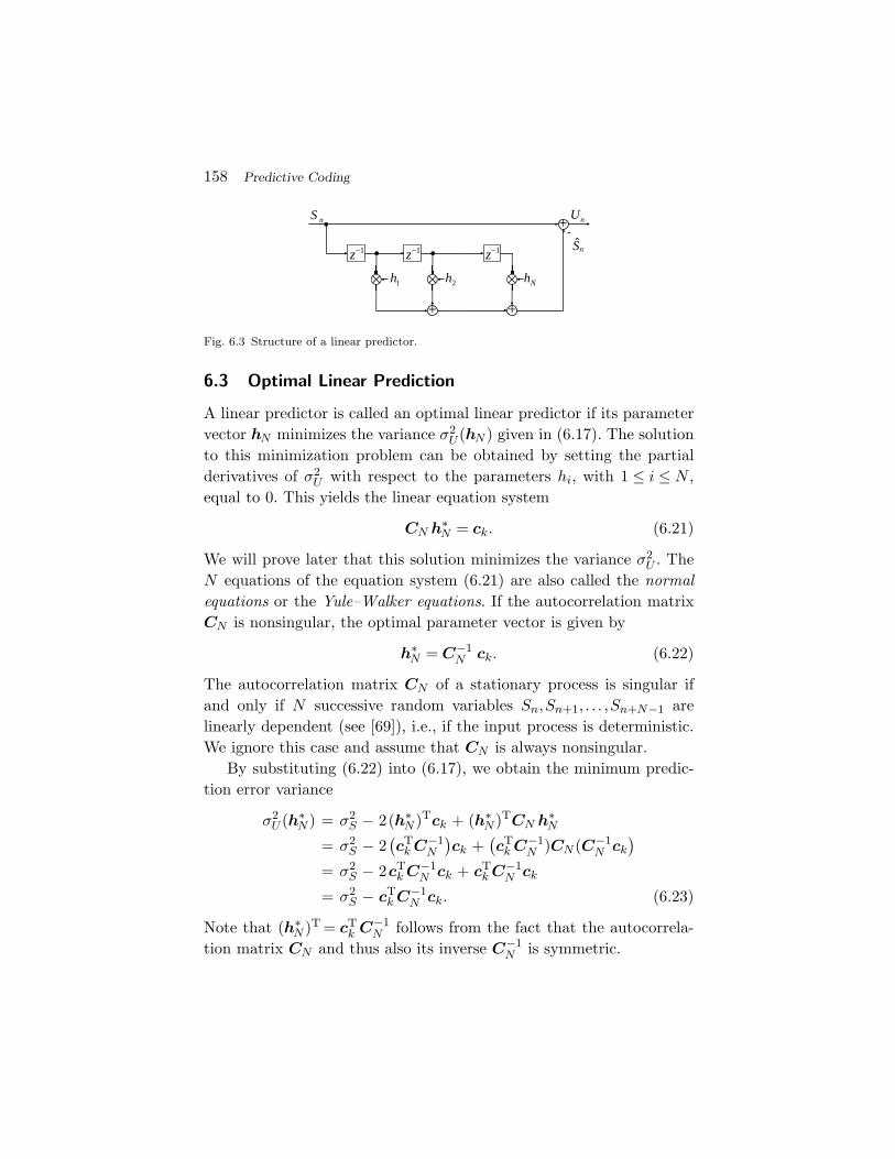
158 Predictive Coding
S n
nz−1
h1
z−1
+
h
S
2
z−1
+
hN
+-
Un
Fig. 6.3 Structure of a linear predictor.
6.3 Optimal Linear Prediction
A linear predictor is called an optimal linear predictor if its parametervector hN minimizes the variance σ2
U (hN ) given in (6.17). The solutionto this minimization problem can be obtained by setting the partialderivatives of σ2
U with respect to the parameters hi, with 1 ≤ i ≤ N ,equal to 0. This yields the linear equation system
CN h∗N = ck. (6.21)
We will prove later that this solution minimizes the variance σ2U . The
N equations of the equation system (6.21) are also called the normalequations or the Yule–Walker equations. If the autocorrelation matrixCN is nonsingular, the optimal parameter vector is given by
h∗N = C−1
N ck. (6.22)
The autocorrelation matrix CN of a stationary process is singular ifand only if N successive random variables Sn,Sn+1, . . . ,Sn+N−1 arelinearly dependent (see [69]), i.e., if the input process is deterministic.We ignore this case and assume that CN is always nonsingular.
By substituting (6.22) into (6.17), we obtain the minimum predic-tion error variance
σ2U (h∗
N ) = σ2S − 2(h∗
N )Tck + (h∗N )TCN h∗
N
= σ2S − 2
(cT
k C−1N
)ck +
(cT
k C−1N )CN (C−1
N ck
)= σ2
S − 2cTk C−1
N ck + cTk C−1
N ck
= σ2S − cT
k C−1N ck. (6.23)
Note that (h∗N )T = cT
k C−1N follows from the fact that the autocorrela-
tion matrix CN and thus also its inverse C−1N is symmetric.
6.3 Optimal Linear Prediction 159
We now prove that the solution given by the normal equations (6.21)indeed minimizes the prediction error variance. Therefore, we investi-gate the prediction error variance for an arbitrary parameter vector hN ,which can be represented as hN = h∗
N + δN . Substituting this relation-ship into (6.17) and using (6.21) yields
σ2U (hN ) = σ2
S − 2(h∗N + δN )Tck + (h∗
N + δN )TCN (h∗N + δN )
= σ2S − 2(h∗
N )Tck − 2δTNck + (h∗
N )TCN h∗N
+(h∗N )TCN δN + δT
NCN h∗N + δT
NCN δN
= σ2U (h∗
N ) − 2δTNck + 2δT
NCN h∗N + δT
NCnδN
= σ2U (h∗
N ) + δTNCN δN . (6.24)
It should be noted that the term δTN CN δN represents the variance
E{(δT
NSn − E{δTNSn
})2}
of the random variable δTNSn and is thus
always greater than or equal to 0. Hence, we have
σ2U (hN ) ≥ σ2
U (h∗N ), (6.25)
which proves that (6.21) specifies the parameter vector h∗N that mini-
mizes the prediction error variance.
The Orthogonality Principle. In the following, we derive anotherimportant property for optimal linear predictors. We consider the moregeneral affine predictor and investigate the correlation between theobservation vector Sn−k and the prediction residual Un,
E{Un Sn−k} = E{(
Sn − h0 − hTNSn−k
)Sn−k
}= E{Sn Sn−k} − h0 E{Sn−k} − E
{Sn−kS
Tn−k
}hN
= ck + µ2S eN − h0 µS eN − (CN + µ2
S eN eTN ) hN
= ck − CNhN + µS eN
(µS (1 − hT
N eN ) − h0). (6.26)
By inserting the conditions (6.19) and (6.21) for optimal affine predic-tion, we obtain
E{Un Sn−k} = 0. (6.27)
Hence, optimal affine prediction yields a prediction residual Un thatis uncorrelated with the observation vector Sn−k. For optimal linear
160 Predictive Coding
predictors, Equation (6.27) holds only for zero-mean input signals. Ingeneral, only the covariance between the prediction residual and eachobservation is equal to zero,
E{(
Un − E{Un}))(
Sn−k − E{Sn−k})}
= 0. (6.28)
Prediction of vectors. The linear prediction for a single randomvariable Sn given an observation vector Sn−k can also be extendedto the prediction of a vector Sn+K−1 = (Sn+K−1,Sn+K−2, . . . ,Sn)T ofK random variables. For each random variable of Sn+K−1, the opti-mal linear or affine predictor can be derived as discussed above. If theparameter vectors hN are arranged in a matrix and the offsets h0 arearranged in a vector, the prediction can be written as
Sn+K−1 = HKSn−k + hK , (6.29)
where HK is an K × N matrix whose rows are given by the correspond-ing parameter vectors hN and hK is a K-dimensional vector whoseelements are given by the corresponding offsets h0.
6.3.1 One-Step Prediction
The most often used prediction is the one-step prediction in which arandom variable Sn is predicted using the N directly preceding randomvariables Sn−1 = (Sn−1, . . . ,Sn−N )T. For this case, we now derive someuseful expressions for the minimum prediction error variance σ2
U (h∗N ),
which will be used later for deriving an asymptotic bound.For the one-step prediction, the normal Equation (6.21) can be writ-
ten in matrix notation as
φ0 φ1 · · · φN−1
φ1 φ0 · · · φN−2
......
. . ....
φN−1 φN−2 · · · φ0
hN1
hN2...
hNN
=
φ1
φ2
...φN
, (6.30)
where the factors hNk represent the elements of the optimal parameter
vector h∗N = (hN
1 , . . . ,hNN )T for linear prediction using the N preceding
samples. The covariances E{(
Sn − E{Sn})(
Sn+k − E{Sn+k})}
aredenoted by φk. By adding a matrix column to the left, multiplying
6.3 Optimal Linear Prediction 161
the parameter vector h∗N with −1, and adding an element equal to 1
at the top of the parameter vector, we obtain
φ1 φ0 φ1 · · · φN−1
φ2 φ1 φ0 · · · φN−2
......
.... . .
...φN φN−1 φN−2 · · · φ0
1−hN
1
−hN2
...−hN
N
=
00...0
. (6.31)
We now include the expression for the minimum prediction varianceinto the matrix equation. The prediction error variance for optimallinear prediction using the N preceding samples is denoted by σ2
N . Using(6.23) and (6.22), we obtain
σ2N = σ2
S − cT1 h∗
N = φ0 − hN1 φ1 − hN
2 φ2 − ·· · − hNNφN . (6.32)
Adding this relationship to the matrix Equation (6.31) yields
φ0 φ1 φ2 · · · φN
φ1 φ0 φ1 · · · φN−1
φ2 φ1 φ0 · · · φN−2
......
.... . .
...φN φN−1 φN−2 · · · φ0
1−hN
1
−hN2
...−hN
N
=
σ2N
00...0
. (6.33)
This equation is also referred to as the augmented normal equation.It should be noted that the matrix on the left represents the autoco-variance matrix CN+1. We denote the modified parameter vector byaN = (1,−hN
1 , . . . ,−hNN )T. By multiplying both sides of (6.33) from the
left with the transpose of aN , we obtain
σ2N = aT
N CN+1 aN . (6.34)
We have one augmented normal Equation (6.33) for each particularnumber N of preceding samples in the observation vector. Combiningthe equations for 0 to N preceding samples into one matrix equationyields
CN+1
1 0 · · · 0 0
−hN1 1
. . . 0 0
−hN2 −hN−1
1
. . . 0 0...
.... . . 1 0
−hNN −hN−1
N−1 · · · −h11 1
=
σ2N X · · · X X
0 σ2N−1
. . . X X
0 0. . . X X
......
. . . σ21 X
0 0 0 0 σ20
,
(6.35)

162 Predictive Coding
where X represents arbitrary values and σ20 is the variance of the input
signal. Taking the determinant on both sides of the equation gives
|CN+1| = σ2Nσ2
N−1 · · ·σ20. (6.36)
Note that the determinant of a triangular matrix is the product of theelements on its main diagonal. Hence, the prediction error variance σ2
N
for optimal linear prediction using the N preceding samples can alsobe written as
σ2N =
|CN+1||CN | . (6.37)
6.3.2 One-Step Prediction for Autoregressive Processes
In the following, we consider the particularly interesting case of optimallinear one-step prediction for autoregressive processes. As stated inSection 6.1, an AR(m) process with the mean µS is defined by
Sn = Zn + µS(1 − aTmem) + aT
mS(m)n−1, (6.38)
where {Zn} is a zero-mean iid process and am = (a1, . . . ,am)T is aconstant parameter vector. We consider the one-step prediction usingthe N preceding samples and the prediction parameter vector hN . Weassume that the number N of preceding samples in the observationvector Sn−1 is greater than or equal to the process order m and definea vector aN = (a1, . . . ,am,0, . . . ,0)T whose first m elements are given bythe process parameter vector am and whose last N − m elements areequal to 0. The prediction residual can then be written as
Un = Zn + µS(1 − aTNeN ) + (aN − hN )TSn−1. (6.39)
By subtracting the mean E{Un} we obtain
Un − E{Un} = Zn + (aN − hN )T(Sn−1 − E{Sn−1}
). (6.40)
According to (6.28), the covariances between the residual Un and therandom variables of the observation vector must be equal to 0 for opti-mal linear prediction. This gives
0 = E{(
Un − E{Un})(
Sn−k − E{Sn−k})}
= E{Zn
(Sn−k − E{Sn−k}
)}+ CN (aN − hN ). (6.41)
6.3 Optimal Linear Prediction 163
Since {Zn} is an iid process, Zn is independent of the past Sn−k, and theexpectation value in (6.41) is equal to 0. The optimal linear predictoris given by
h∗N = aN . (6.42)
Hence, for AR(m) processes, optimal linear prediction can be achievedby using the m preceding samples as observation vector and settingthe prediction parameter vector hm equal to the parameter vector am
of the AR(m) process. An increase of the prediction order N doesnot result in a decrease of the prediction error variance. All predictionparameters hk with k > m are equal to 0. It should be noted that ifthe prediction order N is less than the process order m, the optimalprediction coefficients hk are in general not equal to the correspondingprocess parameters ak. In that case, the optimal prediction vector mustbe determined according to the normal Equation (6.21).
If the prediction order N is greater than or equal to the processorder m, the prediction residual becomes
Un = Zn + µU with µU = µS(1 − aTmem). (6.43)
The prediction residual is an iid process. Consequently, optimal linearprediction of AR(m) processes with a prediction order N greater thanor equal to the process order m yields an iid residual process {Un}(white noise) with a mean µU and a variance σ2
U = E{Z2
n
}.
Gauss–Markov Processes. A Gauss–Markov process is a particu-lar AR(1) process,
Sn = Zn + µS(1 − ρ) + ρ · Sn−1, (6.44)
for which the iid process {Zn} has a Gaussian distribution. It is com-pletely characterized by its mean µS , its variance σ2
S , and the correla-tion coefficient ρ with −1 < ρ < 1. According to the analysis above, theoptimal linear predictor for Gauss–Markov processes consists of a singlecoefficient h1 that is equal to ρ. The obtained prediction residual pro-cess {Un} represents white Gaussian noise with a mean µU = µS(1 − ρ)and a variance
σ2U =
|C2||C1|
=σ4
S − σ4S ρ2
σ2S
= σ2S (1 − ρ2). (6.45)

164 Predictive Coding
6.3.3 Prediction Gain
For measuring the effectiveness of a prediction, often the prediction gainGP is used, which can be defined as the ratio of the signal variance andthe variance of the prediction residual,
GP =σ2
S
σ2U
. (6.46)
For a fixed prediction structure, the prediction gain for optimal linearprediction does depend only on the autocovariances of the sources pro-cess. The prediction gain for optimal linear one-step prediction usingthe N preceding samples is given by
GP =σ2
S
σ2S − cT
1 CN c1=
11 − φT
1 ΦN φ1, (6.47)
where ΦN = CN/σ2S and φi = c1/σ2
S are the normalized autocovariancematrix and the normalized autocovariance vector, respectively.
The prediction gain for the one-step prediction of Gauss–Markovprocesses with a prediction coefficient h1 is given by
GP =σ2
S
σ2S − 2h1σ2
Sρ + h21σ
2S
=1
1 − 2h1ρ + h21. (6.48)
For optimal linear one-step prediction (h1 = ρ), we obtain
GP =1
1 − ρ2 . (6.49)
For demonstrating the impact of choosing the prediction coefficient h1
for the linear one-step prediction of Gauss–Markov sources, Figure 6.4shows the prediction error variance and the prediction gain for a linearpredictor with a fixed prediction coefficient of h1 = 0.5 and for theoptimal linear predictor (h1 = ρ) as function of the correlation factor ρ.
6.3.4 Asymptotic Prediction Gain
In the previous sections, we have focused on linear and affine predictionwith a fixed-length observation vector. Theoretically, we can make theprediction order N very large and for N approaching infinity we obtain
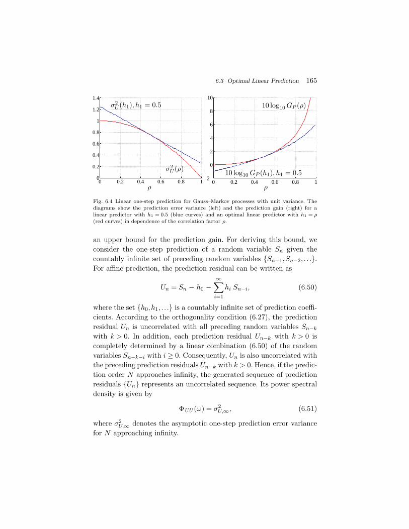
6.3 Optimal Linear Prediction 165
0 0.2 0.4 0.6 0.8 10
0.2
0.4
0.6
0.8
1
1.2
1.4
0 0.2 0.4 0.6 0.8 12
0
2
4
6
8
10
Fig. 6.4 Linear one-step prediction for Gauss–Markov processes with unit variance. Thediagrams show the prediction error variance (left) and the prediction gain (right) for alinear predictor with h1 = 0.5 (blue curves) and an optimal linear predictor with h1 = ρ(red curves) in dependence of the correlation factor ρ.
an upper bound for the prediction gain. For deriving this bound, weconsider the one-step prediction of a random variable Sn given thecountably infinite set of preceding random variables {Sn−1,Sn−2, . . .}.For affine prediction, the prediction residual can be written as
Un = Sn − h0 −∞∑i=1
hi Sn−i, (6.50)
where the set {h0,h1, . . .} is a countably infinite set of prediction coeffi-cients. According to the orthogonality condition (6.27), the predictionresidual Un is uncorrelated with all preceding random variables Sn−k
with k > 0. In addition, each prediction residual Un−k with k > 0 iscompletely determined by a linear combination (6.50) of the randomvariables Sn−k−i with i ≥ 0. Consequently, Un is also uncorrelated withthe preceding prediction residuals Un−k with k > 0. Hence, if the predic-tion order N approaches infinity, the generated sequence of predictionresiduals {Un} represents an uncorrelated sequence. Its power spectraldensity is given by
ΦUU (ω) = σ2U,∞, (6.51)
where σ2U,∞ denotes the asymptotic one-step prediction error variance
for N approaching infinity.

166 Predictive Coding
For deriving an expression for the asymptotic one-step predictionerror variance σ2
U,∞, we restrict our considerations to zero-mean inputprocesses, for which the autocovariance matrix CN is equal to the cor-responding autocorrelation matrix RN , and first consider the limit
limN→∞
|CN | 1N . (6.52)
Since the determinant of a N ×N matrix is given by the product of itseigenvalues ξ
(N)i , with i = 0,1, . . . ,N − 1, we can write
limN→∞
|CN | 1N = lim
N→∞
(N−1∏i=0
ξ(N)i
)1N
= 2(
limN→∞∑N−1
i=01N
log2 ξ(N)i
).
(6.53)By applying Grenander and Szego’s theorem for sequences of Toeplitzmatrices (4.76), we obtain
limN→∞
|CN | 1N = 2
12π
∫ π−π log2 ΦSS (ω)dω, (6.54)
where ΦSS (ω) denotes the power spectral density of the input pro-cess {Sn}. As a further consequence of the convergence of the limit in(6.52), we can state
limN→∞
|CN+1|1
N+1
|CN | 1N
= 1. (6.55)
According to (6.37), we can express the asymptotic one-step predictionerror variance σ2
U,∞ by
σ2U,∞ = lim
N→∞|CN+1||CN | = lim
N→∞
(|CN+1|
1N+1
|CN | 1N |CN |−
1N(N+1)
)N+1
. (6.56)
Applying (6.54) and (6.55) yields
σ2U,∞ = lim
N→∞|CN | 1
N = 212π
∫ π−π log2 ΦSS (ω)dω. (6.57)
Hence, the asymptotic linear prediction gain for zero-mean inputsources is given by
G∞P =
σ2S
σ2U,∞
=12π
∫ π−π ΦSS (ω)dω
212π
∫ π−π log2 ΦSS (ω)dω
. (6.58)
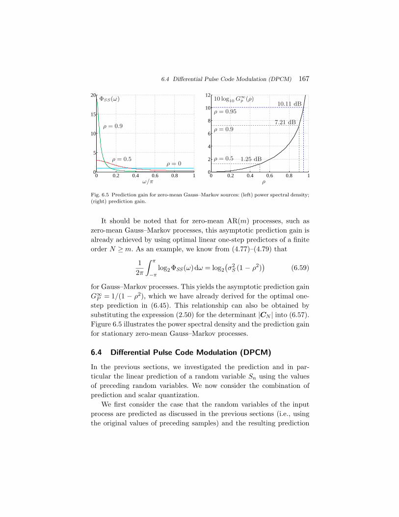
6.4 Differential Pulse Code Modulation (DPCM) 167
0 0.2 0.4 0.6 0.8 10
5
10
15
20
0 0.2 0.4 0.6 0.8 10
2
4
6
8
10
12
Fig. 6.5 Prediction gain for zero-mean Gauss–Markov sources: (left) power spectral density;(right) prediction gain.
It should be noted that for zero-mean AR(m) processes, such aszero-mean Gauss–Markov processes, this asymptotic prediction gain isalready achieved by using optimal linear one-step predictors of a finiteorder N ≥ m. As an example, we know from (4.77)–(4.79) that
12π
∫ π
−πlog2 ΦSS (ω)dω = log2
(σ2
S (1 − ρ2))
(6.59)
for Gauss–Markov processes. This yields the asymptotic prediction gainG∞
P = 1/(1 − ρ2), which we have already derived for the optimal one-step prediction in (6.45). This relationship can also be obtained bysubstituting the expression (2.50) for the determinant |CN | into (6.57).Figure 6.5 illustrates the power spectral density and the prediction gainfor stationary zero-mean Gauss–Markov processes.
6.4 Differential Pulse Code Modulation (DPCM)
In the previous sections, we investigated the prediction and in par-ticular the linear prediction of a random variable Sn using the valuesof preceding random variables. We now consider the combination ofprediction and scalar quantization.
We first consider the case that the random variables of the inputprocess are predicted as discussed in the previous sections (i.e., usingthe original values of preceding samples) and the resulting prediction
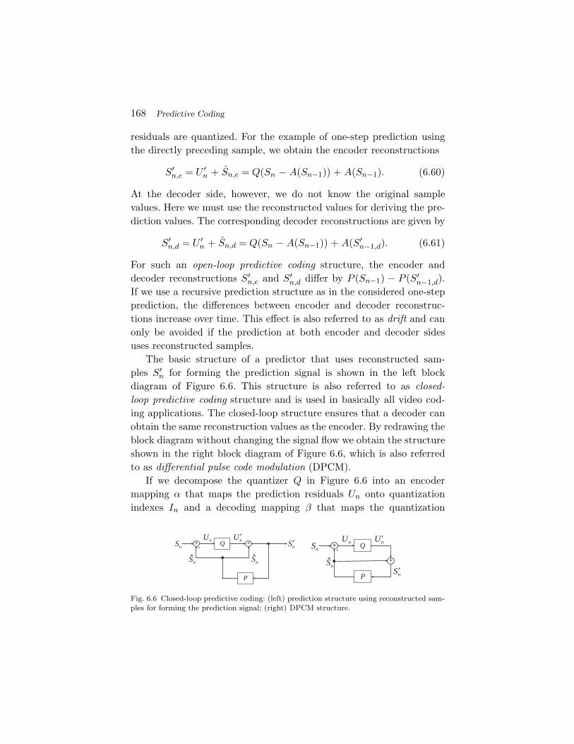
168 Predictive Coding
residuals are quantized. For the example of one-step prediction usingthe directly preceding sample, we obtain the encoder reconstructions
S′n,e = U ′
n + Sn,e = Q(Sn − A(Sn−1)) + A(Sn−1). (6.60)
At the decoder side, however, we do not know the original samplevalues. Here we must use the reconstructed values for deriving the pre-diction values. The corresponding decoder reconstructions are given by
S′n,d = U ′
n + Sn,d = Q(Sn − A(Sn−1)) + A(S′n−1,d). (6.61)
For such an open-loop predictive coding structure, the encoder anddecoder reconstructions S′
n,e and S′n,d differ by P (Sn−1) − P (S′
n−1,d).If we use a recursive prediction structure as in the considered one-stepprediction, the differences between encoder and decoder reconstruc-tions increase over time. This effect is also referred to as drift and canonly be avoided if the prediction at both encoder and decoder sidesuses reconstructed samples.
The basic structure of a predictor that uses reconstructed sam-ples S′
n for forming the prediction signal is shown in the left blockdiagram of Figure 6.6. This structure is also referred to as closed-loop predictive coding structure and is used in basically all video cod-ing applications. The closed-loop structure ensures that a decoder canobtain the same reconstruction values as the encoder. By redrawing theblock diagram without changing the signal flow we obtain the structureshown in the right block diagram of Figure 6.6, which is also referredto as differential pulse code modulation (DPCM).
If we decompose the quantizer Q in Figure 6.6 into an encodermapping α that maps the prediction residuals Un onto quantizationindexes In and a decoding mapping β that maps the quantization
Q ++
S n
Sn ′S nUn ′U n
-
P
S n
Q
+
+Sn
′S n
Un ′U n-
P
S n
Fig. 6.6 Closed-loop predictive coding: (left) prediction structure using reconstructed sam-ples for forming the prediction signal; (right) DPCM structure.
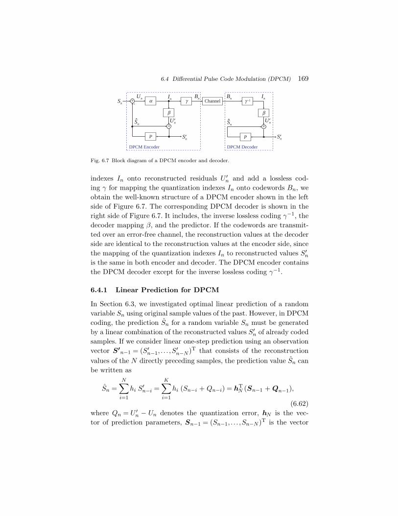
6.4 Differential Pulse Code Modulation (DPCM) 169
α
+
+Sn
′S n
Un
′U n
-
P
S n
β
In
+
γ γ -1Bn
β
′S nP
′U n
InBnChannel
DPCM Encoder DPCM Decoder
S n
Fig. 6.7 Block diagram of a DPCM encoder and decoder.
indexes In onto reconstructed residuals U ′n and add a lossless cod-
ing γ for mapping the quantization indexes In onto codewords Bn, weobtain the well-known structure of a DPCM encoder shown in the leftside of Figure 6.7. The corresponding DPCM decoder is shown in theright side of Figure 6.7. It includes, the inverse lossless coding γ−1, thedecoder mapping β, and the predictor. If the codewords are transmit-ted over an error-free channel, the reconstruction values at the decoderside are identical to the reconstruction values at the encoder side, sincethe mapping of the quantization indexes In to reconstructed values S′
n
is the same in both encoder and decoder. The DPCM encoder containsthe DPCM decoder except for the inverse lossless coding γ−1.
6.4.1 Linear Prediction for DPCM
In Section 6.3, we investigated optimal linear prediction of a randomvariable Sn using original sample values of the past. However, in DPCMcoding, the prediction Sn for a random variable Sn must be generatedby a linear combination of the reconstructed values S′
n of already codedsamples. If we consider linear one-step prediction using an observationvector S′
n−1 = (S′n−1, . . . ,S
′n−N )T that consists of the reconstruction
values of the N directly preceding samples, the prediction value Sn canbe written as
Sn =N∑
i=1
hi S′n−i =
K∑i=1
hi (Sn−i + Qn−i) = hTN (Sn−1 + Qn−1),
(6.62)where Qn = U ′
n − Un denotes the quantization error, hN is the vec-tor of prediction parameters, Sn−1 = (Sn−1, . . . ,Sn−N )T is the vector
170 Predictive Coding
of the N original sample values that precede the current sample Sn
to be predicted, and Qn−1 = (Qn−1, . . . ,Qn−N )T is the vector of thequantization errors for the N preceding samples. The variance σ2
U ofthe prediction residual Un is given by
σ2U = E
{(Un −E{Un})2
}= E
{(Sn −E{Sn} − hT
N
(Sn−1 −E{Sn−1} + Qn−1 −E
{Qn−1
}))2}= σ2
S − 2hTN c1 + hT
N CN hN
−2hTN E{(
Sn −E{Sn})(
Qn−1 −E{Qn−1
})}−2hT
N E{(
Sn−1 −E{Sn−1})(
Qn−1 −E{Qn−1
})T}hN
+hTN E{(
Qn−1 −E{Qn−1
})(Qn−1 −E
{Qn−1
})T}hN . (6.63)
The optimal prediction parameter vector hN does not only depend onthe autocovariances of the input process {Sn}, but also on the auto-covariances of the quantization errors {Qn} and the cross-covariancesbetween the input process and the quantization errors. Thus, we needto know the quantizer in order to design an optimal linear predictor.But on the other hand, we also need to know the predictor parame-ters for designing the quantizer. Thus, for designing a optimal DPCMcoder the predictor and quantizer have to be optimized jointly. Numer-ical algorithms that iteratively optimize the predictor and quantizerbased on conjugate gradient numerical techniques are discussed in [8].
For high rates, the reconstructed samples S′n are a close approxima-
tion of the original samples Sn, and the optimal prediction parametervector hN for linear prediction using reconstructed sample values isvirtually identical to the optimal prediction parameter vector for linearprediction using original sample values. In the following, we concentrateon DPCM systems for which the linear prediction parameter vector isoptimized for a prediction using original sample values, but we notethat such DPCM systems are suboptimal for low rates.
One-Tap Prediction for Gauss–Markov Sources. As an impor-tant example, we investigate the rate distortion efficiency of linear pre-dictive coding for stationary Gauss–Markov sources,
Sn = Zn + µS (1 − ρ) + ρSn−1. (6.64)
6.4 Differential Pulse Code Modulation (DPCM) 171
We have shown in Section 6.3.2 that the optimal linear predictor usingoriginal sample values is the one-tap predictor for which the predictioncoefficient h1 is equal to the correlation coefficient ρ of the Gauss–Markov process. If we use the same linear predictor with reconstructedsamples, the prediction Sn for a random variable Sn can be written as
Sn = h1 S′n−1 = ρ(Sn−1 + Qn−1), (6.65)
where Qn−1 = U ′n−1 − Un−1 denotes the quantization error. The pre-
diction residual Un is given by
Un = Sn − Sn = Zn + µS (1 − ρ) − ρQn−1. (6.66)
For the prediction error variance σ2U , we obtain
σ2U = E
{(Un − E{Un})2
}= E{(
Zn − ρ(Qn−1 − E{Qn−1}))2}
= σ2Z − 2ρE{Zn (Qn−1 − E{Qn−1})} + ρ2 σ2
Q, (6.67)
where σ2Z = E
{Z2
n
}denotes the variance of the innovation process {Zn}
and σ2Q = E
{(Qn − E{Qn})2
}denotes the variance of the quantization
errors. Since {Zn} is an iid process and thus Zn is independent ofthe past quantization errors Qn−1, the middle term in (6.67) is equalto 0. Furthermore, as shown in Section 2.3.1, the variance σ2
Z of theinnovation process is given by σ2
S (1 − ρ2). Hence, we obtain
σ2U = σ2
S (1 − ρ2) + ρ2 σ2Q. (6.68)
We further note that the quantization error variance σ2Q represents the
distortion D of the DPCM quantizer and is a function of the rate R.As explained in Section 5.2.4, we can generally express the distortionrate function of scalar quantizers by
D(R) = σ2Q(R) = σ2
U (R) g(R), (6.69)
where σ2U (R) represents the variance of the signal that is quantized. The
function g(R) represents the operational distortion rate function forquantizing random variables that have the same distribution type as theprediction residual Un, but unit variance. Consequently, the varianceof the prediction residual is given by
σ2U (R) = σ2
S
1 − ρ2
1 − ρ2 g(R). (6.70)
172 Predictive Coding
Using (6.69), we obtain the following operational distortion rate func-tion for linear predictive coding of Gauss–Markov processes with aone-tap predictor for which the prediction coefficient h1 is equal to thecorrelation coefficient of the Gauss–Markov source,
D(R) = σ2S
1 − ρ2
1 − ρ2 g(R)g(R). (6.71)
By deriving the asymptote for g(R) approaching zero, we obtain thefollowing asymptotic operational distortion rate function for high rates,
D(R) = σ2S (1 − ρ2)g(R). (6.72)
The function g(R) represents the operational distortion rate func-tion for scalar quantization of random variables that have unit varianceand the same distribution type as the prediction residuals. It should bementioned that, even at high rates, the distribution of the predictionresiduals cannot be derived in a straightforward way, since it is deter-mined by a complicated process that includes linear prediction andquantization. As a rule of thumb based on intuition, at high rates, thereconstructed values S′
n are a very close approximation of the originalsamples Sn and thus the quantization errors Qn = S′
n − Sn are verysmall in comparison to the innovation Zn. Then, we can argue thatthe prediction residuals Un given by (6.66) are nearly identical to theinnovation samples Zn and have thus nearly a Gaussian distribution.Another reason for assuming a Gaussian model is the fact that Gaus-sian sources are the most difficult to code among all processes with agiven autocovariance function. Using a Gaussian model for the predic-tion residuals, we can replace g(R) in (6.72) by the high rate asymptotefor entropy-constrained quantization of Gaussian sources, which yieldsthe following high rate approximation of the operational distortion ratefunction,
D(R) =πe
6σ2
S (1 − ρ2)2−2R. (6.73)
Hence, under the intuitive assumption that the distribution of theprediction residuals at high rates is nearly Gaussian, we obtain anasymptotic operational distortion rate function for DPCM quantiza-tion of stationary Gauss–Markov processes at high rates that lies
6.4 Differential Pulse Code Modulation (DPCM) 173
1.53 dB or 0.25 bit per sample above the fundamental rate distor-tion bound (4.119). The experimental results presented below indicatethat our intuitive assumption provides a useful approximation of theoperational distortion rate function for DPCM coding of stationaryGauss–Markov processes at high rates.
Entropy-constrained Lloyd algorithm for DPCM. Even if weuse the optimal linear predictor for original sample values inside theDPCM loop, the quantizer design algorithm is not straightforward,since the distribution of the prediction residuals depends on the recon-structed sample values and thus on the quantizer itself.
In order to provide some experimental results for DPCM quanti-zation of Gauss–Markov sources, we use a very simple ECSQ designin combination with a given linear predictor. The vector of predic-tion parameters hN is given and only the entropy-constrained scalarquantizer is designed. Given a sufficiently large training set {sn}, thequantizer design algorithm can be stated as follows:
(1) Initialize the Lagrange multiplier λ with small value and ini-tialize all reconstructed samples s′
n with the correspondingoriginal samples sn of the training set.
(2) Generate the residual samples using linear prediction giventhe original and reconstructed samples sn and s′
n.(3) Design an entropy-constrained Lloyd quantizer as described
in Section 5.2.2 given the value of λ and using the predictionerror sequence {un} as training set.
(4) Conduct the DPCM coding of the training set {sn} given thelinear predictor and the designed quantizer, which yields theset of reconstructed samples {s′
n}.(5) Increase λ by a small amount and start again with Step 2.
The quantizer design algorithm starts with a small value of λ and thusa high rate for which we can assume that reconstruction values arenearly identical to the original sample values. In each iteration of thealgorithm, a quantizer is designed for a slightly larger value of λ andthus a slightly lower rate by assuming that the optimal quantizer designdoes not change significantly. By executing the algorithm, we obtain a
174 Predictive Coding
sequence of quantizers for different rates. It should however be notedthat the quantizer design inside a feedback loop is a complicated prob-lem. We noted that when the value of λ is changed too much fromone iteration to the next, the algorithm becomes unstable at low rates.An alternative algorithm for designing predictive quantizers based onconjugate gradient techniques can be found in [8].
Experimental Results for a Gauss–Markov Source. For provid-ing experimental results, we considered the stationary Gauss–Markovsource with zero mean, unit variance, and a correlation factor of 0.9that we have used as reference throughout this monograph. We haverun the entropy-constrained Lloyd algorithm for DPCM stated aboveand measured the prediction error variance σ2
U , the distortion D, andthe entropy of the reconstructed sample values as a measure for thetransmission rate R. The results of the algorithm are compared to thedistortion rate function and to the derived functions for σ2
U (R) andD(R) for stationary Gauss–Markov sources that are given in (6.70)and (6.71), respectively. For the function g(R) we used the experimen-tally obtained approximation (5.59) for Gaussian pdfs. It should benoted that the corresponding functional relationships σ2
U (R) and D(R)are only a rough approximation, since the distribution of the predictionresidual Un cannot be assumed to be Gaussian, at least not at low andmedium rates.
In Figure 6.8, the experimentally obtained data for DPCM cod-ing with entropy-constrained scalar quantization and for entropy-constrained scalar quantization without prediction are compared tothe derived operational distortion rate functions using the approxima-tion g(R) for Gaussian sources given in (5.59) and the information ratedistortion function. For the shown experimental data and the derivedoperational distortion rate functions, the rate has been measured as theentropy of the quantizer output. The experimental data clearly indicatethat DPCM coding significantly increases the rate distortion efficiencyfor sources with memory. Furthermore, we note that the derived oper-ational distortion rate functions using the simple approximation forg(R) represent suitable approximations for the experimentally obtaineddata. At high rates, the measured difference between the experimental
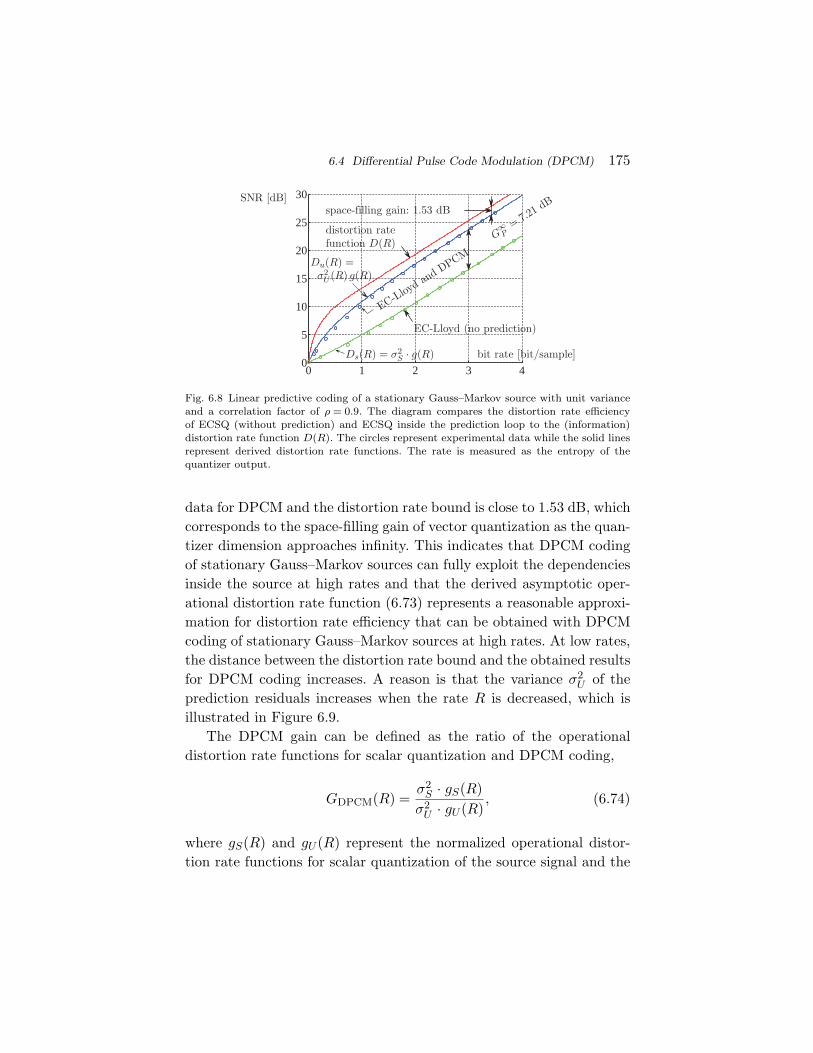
6.4 Differential Pulse Code Modulation (DPCM) 175
0 1 2 3 40
5
10
15
20
25
30
Fig. 6.8 Linear predictive coding of a stationary Gauss–Markov source with unit varianceand a correlation factor of ρ = 0.9. The diagram compares the distortion rate efficiencyof ECSQ (without prediction) and ECSQ inside the prediction loop to the (information)distortion rate function D(R). The circles represent experimental data while the solid linesrepresent derived distortion rate functions. The rate is measured as the entropy of thequantizer output.
data for DPCM and the distortion rate bound is close to 1.53 dB, whichcorresponds to the space-filling gain of vector quantization as the quan-tizer dimension approaches infinity. This indicates that DPCM codingof stationary Gauss–Markov sources can fully exploit the dependenciesinside the source at high rates and that the derived asymptotic oper-ational distortion rate function (6.73) represents a reasonable approxi-mation for distortion rate efficiency that can be obtained with DPCMcoding of stationary Gauss–Markov sources at high rates. At low rates,the distance between the distortion rate bound and the obtained resultsfor DPCM coding increases. A reason is that the variance σ2
U of theprediction residuals increases when the rate R is decreased, which isillustrated in Figure 6.9.
The DPCM gain can be defined as the ratio of the operationaldistortion rate functions for scalar quantization and DPCM coding,
GDPCM(R) =σ2
S · gS(R)σ2
U · gU (R), (6.74)
where gS(R) and gU (R) represent the normalized operational distor-tion rate functions for scalar quantization of the source signal and the
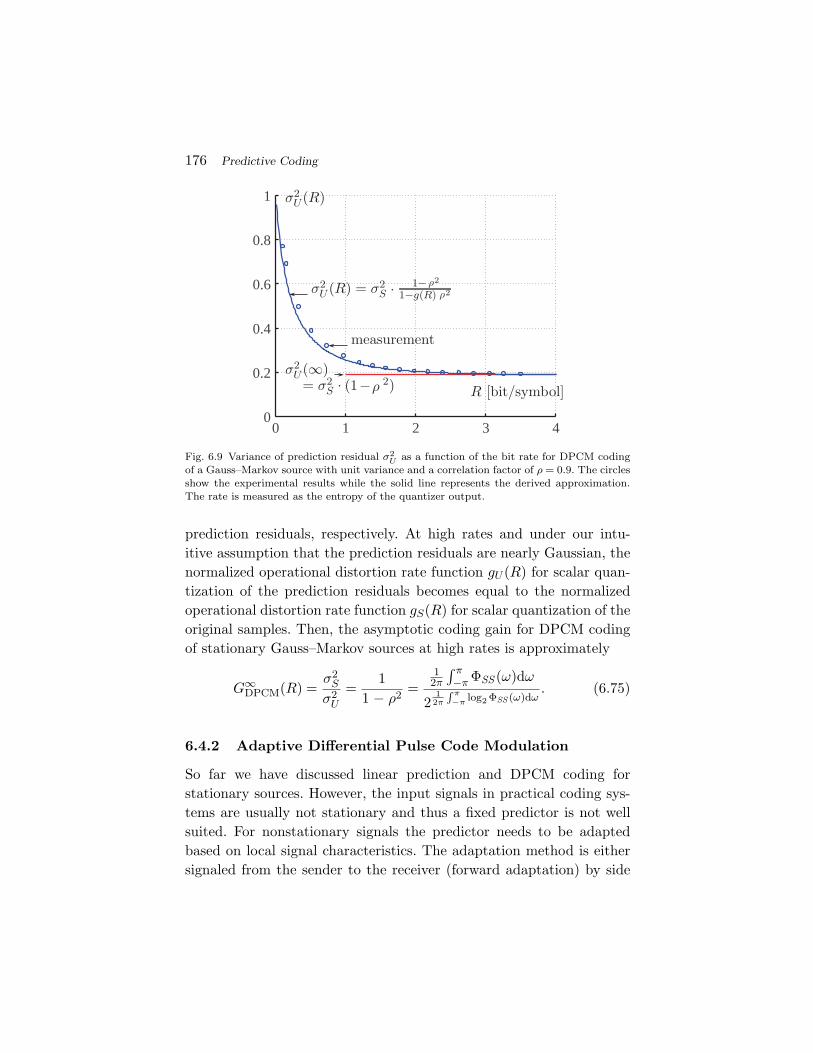
176 Predictive Coding
0 1 2 3 40
0.2
0.4
0.6
0.8
1
Fig. 6.9 Variance of prediction residual σ2U as a function of the bit rate for DPCM coding
of a Gauss–Markov source with unit variance and a correlation factor of ρ = 0.9. The circlesshow the experimental results while the solid line represents the derived approximation.The rate is measured as the entropy of the quantizer output.
prediction residuals, respectively. At high rates and under our intu-itive assumption that the prediction residuals are nearly Gaussian, thenormalized operational distortion rate function gU (R) for scalar quan-tization of the prediction residuals becomes equal to the normalizedoperational distortion rate function gS(R) for scalar quantization of theoriginal samples. Then, the asymptotic coding gain for DPCM codingof stationary Gauss–Markov sources at high rates is approximately
G∞DPCM(R) =
σ2S
σ2U
=1
1 − ρ2 =12π
∫ π−π ΦSS (ω)dω
212π
∫ π−π log2 ΦSS (ω)dω
. (6.75)
6.4.2 Adaptive Differential Pulse Code Modulation
So far we have discussed linear prediction and DPCM coding forstationary sources. However, the input signals in practical coding sys-tems are usually not stationary and thus a fixed predictor is not wellsuited. For nonstationary signals the predictor needs to be adaptedbased on local signal characteristics. The adaptation method is eithersignaled from the sender to the receiver (forward adaptation) by side
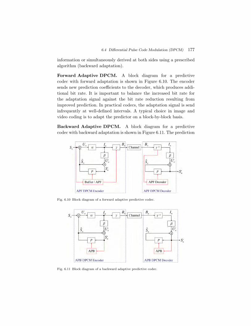
6.4 Differential Pulse Code Modulation (DPCM) 177
information or simultaneously derived at both sides using a prescribedalgorithm (backward adaptation).
Forward Adaptive DPCM. A block diagram for a predictivecodec with forward adaptation is shown in Figure 6.10. The encodersends new prediction coefficients to the decoder, which produces addi-tional bit rate. It is important to balance the increased bit rate forthe adaptation signal against the bit rate reduction resulting fromimproved prediction. In practical codecs, the adaptation signal is sendinfrequently at well-defined intervals. A typical choice in image andvideo coding is to adapt the predictor on a block-by-block basis.
Backward Adaptive DPCM. A block diagram for a predictivecodec with backward adaptation is shown in Figure 6.11. The prediction
Fig. 6.10 Block diagram of a forward adaptive predictive codec.
Fig. 6.11 Block diagram of a backward adaptive predictive codec.
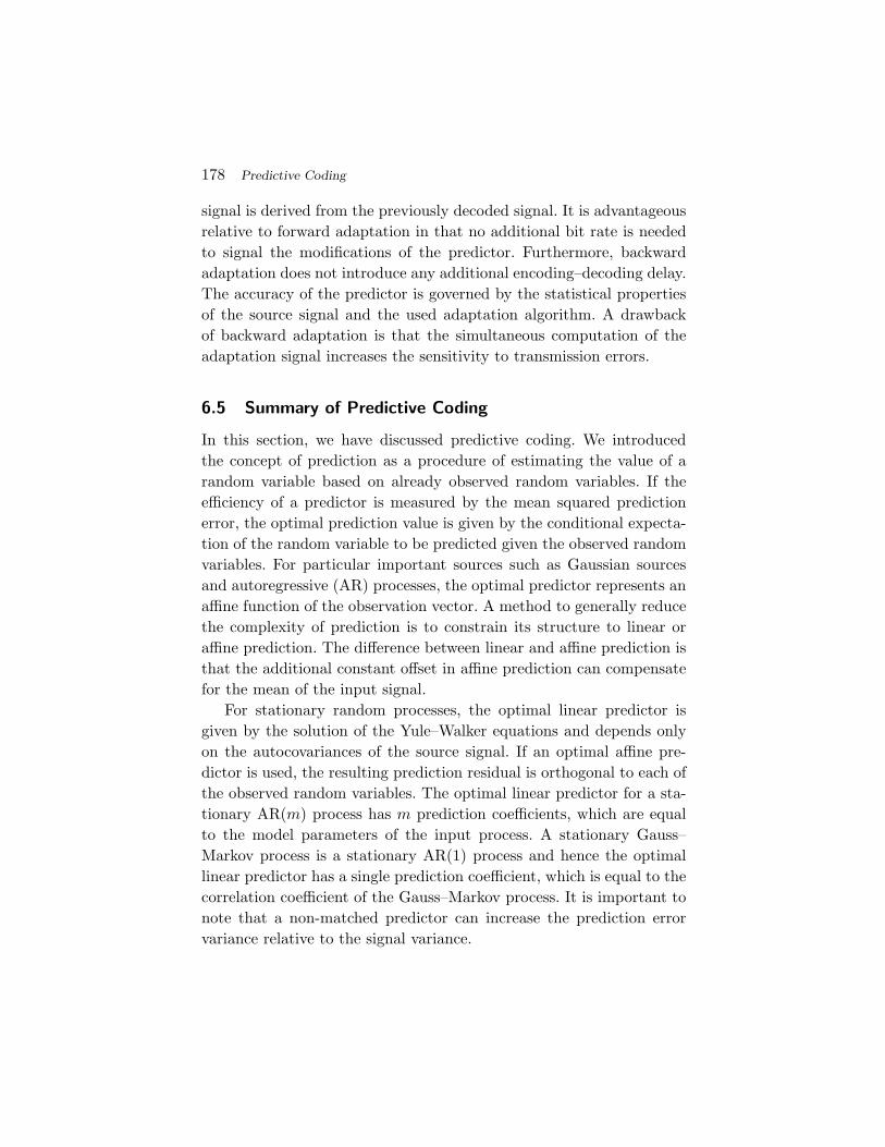
178 Predictive Coding
signal is derived from the previously decoded signal. It is advantageousrelative to forward adaptation in that no additional bit rate is neededto signal the modifications of the predictor. Furthermore, backwardadaptation does not introduce any additional encoding–decoding delay.The accuracy of the predictor is governed by the statistical propertiesof the source signal and the used adaptation algorithm. A drawbackof backward adaptation is that the simultaneous computation of theadaptation signal increases the sensitivity to transmission errors.
6.5 Summary of Predictive Coding
In this section, we have discussed predictive coding. We introducedthe concept of prediction as a procedure of estimating the value of arandom variable based on already observed random variables. If theefficiency of a predictor is measured by the mean squared predictionerror, the optimal prediction value is given by the conditional expecta-tion of the random variable to be predicted given the observed randomvariables. For particular important sources such as Gaussian sourcesand autoregressive (AR) processes, the optimal predictor represents anaffine function of the observation vector. A method to generally reducethe complexity of prediction is to constrain its structure to linear oraffine prediction. The difference between linear and affine prediction isthat the additional constant offset in affine prediction can compensatefor the mean of the input signal.
For stationary random processes, the optimal linear predictor isgiven by the solution of the Yule–Walker equations and depends onlyon the autocovariances of the source signal. If an optimal affine pre-dictor is used, the resulting prediction residual is orthogonal to each ofthe observed random variables. The optimal linear predictor for a sta-tionary AR(m) process has m prediction coefficients, which are equalto the model parameters of the input process. A stationary Gauss–Markov process is a stationary AR(1) process and hence the optimallinear predictor has a single prediction coefficient, which is equal to thecorrelation coefficient of the Gauss–Markov process. It is important tonote that a non-matched predictor can increase the prediction errorvariance relative to the signal variance.
6.5 Summary of Predictive Coding 179
Differential pulse code modulation (DPCM) is the dominant struc-ture for the combination of prediction and scalar quantization. InDPCM, the prediction is based on quantized samples. The combina-tion of DPCM and entropy-constrained scalar quantization (ECSQ)has been analyzed in great detail for the special case of stationaryGauss–Markov processes. It has been shown that the prediction errorvariance is dependent on the bit rate. The derived approximation forhigh rates, which has been verified by experimental data, indicated thatfor stationary Gauss–Markov sources the combination of DPCM andECSQ achieves the shape and memory gain of vector quantization athigh rates.
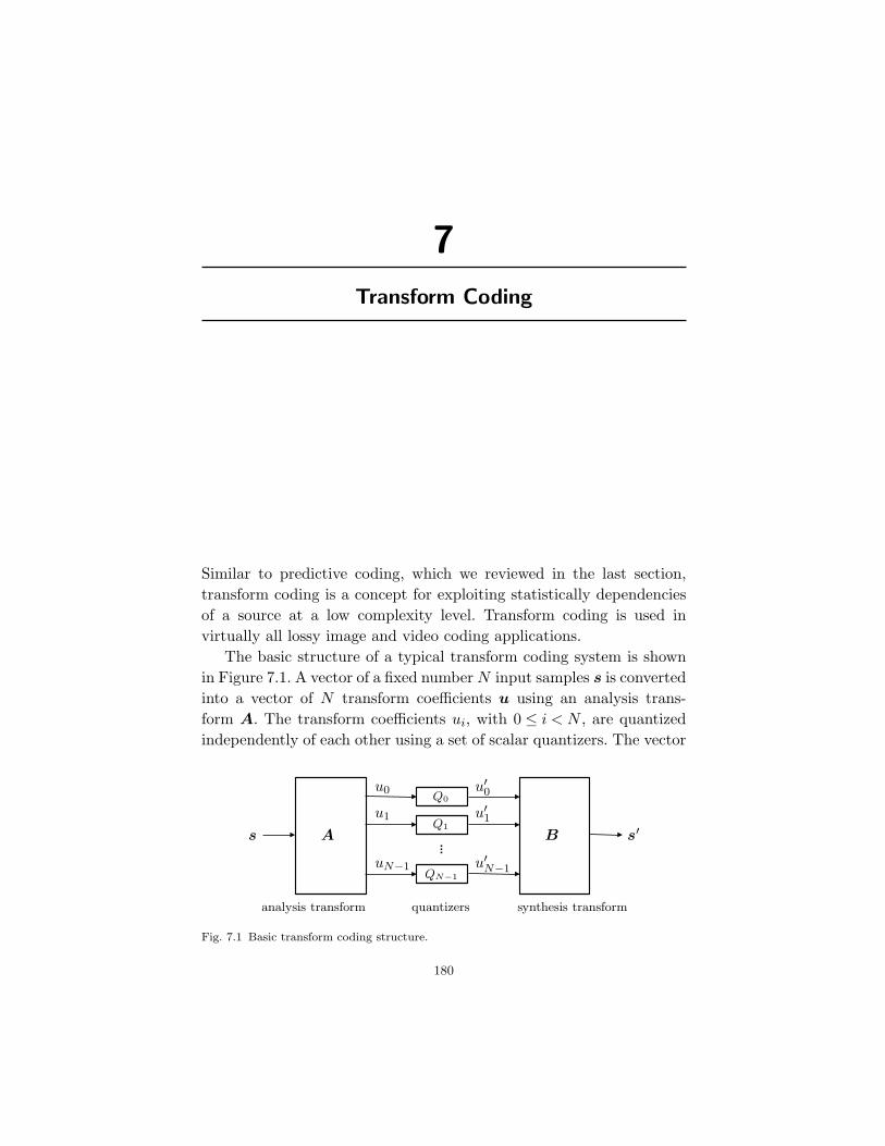
7Transform Coding
Similar to predictive coding, which we reviewed in the last section,transform coding is a concept for exploiting statistically dependenciesof a source at a low complexity level. Transform coding is used invirtually all lossy image and video coding applications.
The basic structure of a typical transform coding system is shownin Figure 7.1. A vector of a fixed number N input samples s is convertedinto a vector of N transform coefficients u using an analysis trans-form A. The transform coefficients ui, with 0 ≤ i < N , are quantizedindependently of each other using a set of scalar quantizers. The vector
Fig. 7.1 Basic transform coding structure.
180

181
of N reconstructed samples s′ is obtained by transforming the vector ofreconstructed transform coefficients u′ using a synthesis transform B.
In all practically used video coding systems, the analysis and synthe-sis transforms A and B are orthogonal block transforms. The sequenceof source samples {sn} is partitioned into vectors s of adjacent sam-ples and the transform coding consisting of an orthogonal analysistransform, scalar quantization of the transform coefficients, and anorthogonal synthesis transform is independently applied to each vec-tor of samples. Since finally a vector s of source samples is mapped toa vector s′ of reconstructed samples, transform coding systems forma particular class of vector quantizers. The benefit in comparison tounconstrained vector quantization is that the imposed structural con-straint allows implementations at a significantly lower complexity level.
The typical motivation for transform coding is the decorrelation andenergy concentration effect. Transforms are designed in a way that, fortypical input signals, the transform coefficients are much less correlatedthan the original source samples and the signal energy is concentratedin a few transform coefficients. As a result, the obtained transformcoefficients have a different importance and simple scalar quantiza-tion becomes more effective in the transform domain than in the orig-inal signal space. Due to this effect, the memory advantage of vectorquantization can be exploited to a large extent for typical source sig-nals. Furthermore, by using entropy-constrained quantization for thetransform coefficients also the shape advantage can be obtained. Incomparison to unconstrained vector quantization, the rate distortionefficiency is basically reduced by the space-filling advantage, which canonly be obtained by a significant increase in complexity.
For image and video coding applications, another advantage oftransform coding is that the quantization in the transform domainoften leads to an improvement of the subjective quality relative to adirect quantization of the source samples with the same distortion,in particular for low rates. The reason is that the transform coeffi-cients contain information with different importance for the viewer andcan therefore be treated differently. All perceptual distortion measuresthat are known to provide reasonable results weight the distortion inthe transform domain. The quantization of the transform coefficients

182 Transform Coding
can also be designed in a way that perceptual criteria are taken intoaccount.
In contrast to video coding, the transforms that are used in stillimage coding are not restricted to the class of orthogonal block trans-forms. Instead, transforms that do not process the input signal on ablock-by-block basis have been extensively studied and included intorecent image coding standards. One of these transforms is the so-calleddiscrete wavelet transform, which decomposes an image into compo-nents that correspond to band-pass filtered and downsampled versionsof the image. Discrete wavelet transforms can be efficiently imple-mented using cascaded filter banks. Transform coding that is based on adiscrete wavelet transform is also referred to as sub-band coding and isfor example used in the JPEG 2000 standard [36, 66]. Another class oftransforms are the lapped block transforms, which are basically appliedon a block-by-block basis, but are characterized by basis functions thatoverlap the block boundaries. As a result, the transform coefficients fora block do not only depend on the samples inside the block, but also onsamples of neighboring blocks. The vector of reconstructed samples fora block is obtained by transforming a vector that includes the trans-form coefficients of the block and of neighboring blocks. A hierarchicallapped transform with biorthogonal basis functions is included in thelatest image coding standard JPEG XR [37]. The typical motivationfor using wavelet transforms or lapped block transforms in image cod-ing is that the nature of these transforms avoids the blocking artifactswhich are obtained by transform coding with block-based transformsat low bit rates and are considered as one of the most disturbing codingartifacts. In video coding, wavelet transforms and lapped block trans-forms are rarely used due to the difficulties in efficiently combiningthese transforms with inter-picture prediction techniques.
In this section, we discuss transform coding with orthogonal blocktransforms, since this is the predominant transform coding structure invideo coding. For further information on transform coding in general,the reader is referred to the tutorials [20] and [10]. An introduction towavelet transforms and sub-band coding is given in the tutorials [68,70] and [71]. As a reference for lapped blocks transforms and theirapplication in image coding we recommend [58] and [49].
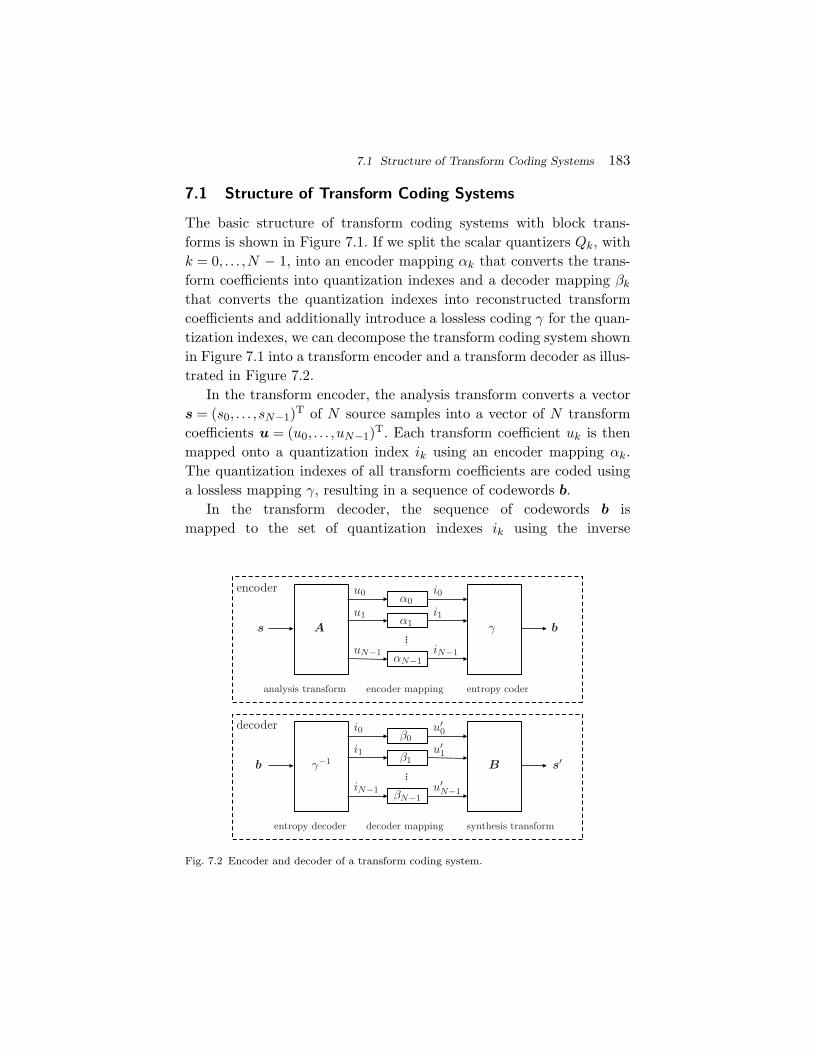
7.1 Structure of Transform Coding Systems 183
7.1 Structure of Transform Coding Systems
The basic structure of transform coding systems with block trans-forms is shown in Figure 7.1. If we split the scalar quantizers Qk, withk = 0, . . . ,N − 1, into an encoder mapping αk that converts the trans-form coefficients into quantization indexes and a decoder mapping βk
that converts the quantization indexes into reconstructed transformcoefficients and additionally introduce a lossless coding γ for the quan-tization indexes, we can decompose the transform coding system shownin Figure 7.1 into a transform encoder and a transform decoder as illus-trated in Figure 7.2.
In the transform encoder, the analysis transform converts a vectors = (s0, . . . ,sN−1)T of N source samples into a vector of N transformcoefficients u = (u0, . . . ,uN−1)T. Each transform coefficient uk is thenmapped onto a quantization index ik using an encoder mapping αk.The quantization indexes of all transform coefficients are coded usinga lossless mapping γ, resulting in a sequence of codewords b.
In the transform decoder, the sequence of codewords b ismapped to the set of quantization indexes ik using the inverse
Fig. 7.2 Encoder and decoder of a transform coding system.
184 Transform Coding
lossless mapping γ−1. The decoder mappings βk convert the quan-tization indexes ik into reconstructed transform coefficients u′
k. Thevector of N reconstructed samples s′ = (s′
0, . . . ,s′N−1)
T is obtainedby transforming the vector of N reconstructed transform coefficientsu′ = (u′
0, . . . ,u′N−1)
T using the synthesis transform.
7.2 Orthogonal Block Transforms
In the following discussion of transform coding, we restrict our consid-erations to stationary sources and transform coding systems with thefollowing properties:
(1) Linear block transforms: the analysis and synthesis transformare linear block transforms.
(2) Perfect reconstruction: the synthesis transform is the inverseof the analysis transform.
(3) Orthonormal basis: the basis vectors of the analysis transformform an orthonormal basis.
Linear Block Transforms. For linear block transforms of size N ,each component of an N -dimensional output vector represents a lin-ear combination of the components of the N -dimensional input vector.A linear block transform can be written as a matrix multiplication.The analysis transform, which maps a vector of source samples s to avector of transform coefficients u, is given by
u = A s, (7.1)
where the matrix A is referred to as the analysis transform matrix.Similarly, the synthesis transform, which maps a vector of reconstructedtransform coefficients u′ to a vector of reconstructed samples s′, canbe written as
s′ = B u′, (7.2)
where the matrix B represents the synthesis transform matrix.
Perfect Reconstruction. The perfect reconstruction propertyspecifies that the synthesis transform matrix is the inverse of the

7.2 Orthogonal Block Transforms 185
analysis transform matrix, B =A−1. If the transform coefficients arenot quantized, i.e., if u′ = u, the vector of reconstructed samples isequal to the vector of source samples,
s′ = B u = B A s = A−1 A s = s. (7.3)
If an invertible analysis transform A produces independent transformcoefficients and the component quantizers reconstruct the centroids ofthe quantization intervals, the inverse of the analysis transform is theoptimal synthesis transform in the sense that it yields the minimumdistortion among all linear transforms given the coded transform coef-ficients. It should, however, be noted that if these conditions are notfulfilled, a synthesis transform B that is not equal to the inverse of theanalysis transform may reduce the distortion [20].
Orthonormal basis. An analysis transform matrix A forms anorthonormal basis if its basis vectors given by the rows of the matrixare orthogonal to each other and have the length 1. Matrices with thisproperty are referred to as unitary matrices. The corresponding trans-form is said to be an orthogonal transform. The inverse of a unitarymatrix A is its conjugate transpose, A−1 =A†. A unitary matrix withreal entries is called an orthogonal matrix and its inverse is equal toits transpose, A−1 =AT. For linear transform coding systems with theperfect reconstruction property and orthogonal matrices, the synthesistransform is given by
s′ = B u′ = AT u′. (7.4)
Unitary transform matrices are often desirable, because the meansquare error between a reconstruction and source vector can beminimized with independent scalar quantization of the transform coeffi-cients. Furthermore, as we will show below, the distortion in the trans-form domain is equal to the distortion in the original signal space.In practical transform coding systems, it is usually sufficient to requirethat the basis vectors are orthogonal to each other. The different normscan be easily taken into account in the quantizer design.
We can consider a linear analysis transform A as optimal if thetransform coding system consisting of the analysis transform A, opti-mal entropy-constrained scalar quantizers for the transform coefficients
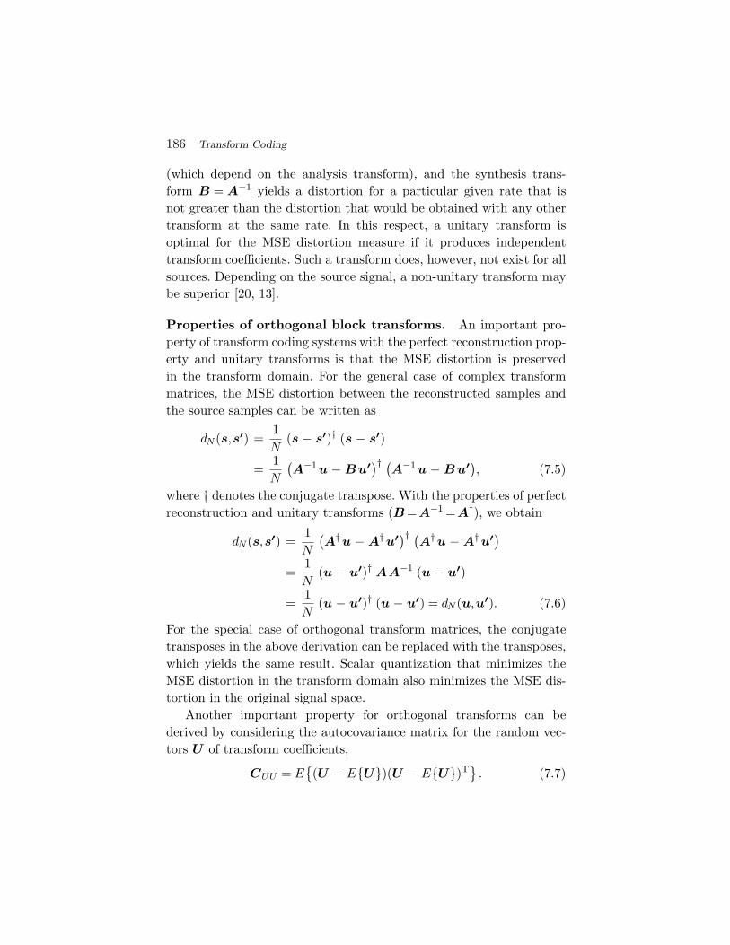
186 Transform Coding
(which depend on the analysis transform), and the synthesis trans-form B = A−1 yields a distortion for a particular given rate that isnot greater than the distortion that would be obtained with any othertransform at the same rate. In this respect, a unitary transform isoptimal for the MSE distortion measure if it produces independenttransform coefficients. Such a transform does, however, not exist for allsources. Depending on the source signal, a non-unitary transform maybe superior [20, 13].
Properties of orthogonal block transforms. An important pro-perty of transform coding systems with the perfect reconstruction prop-erty and unitary transforms is that the MSE distortion is preservedin the transform domain. For the general case of complex transformmatrices, the MSE distortion between the reconstructed samples andthe source samples can be written as
dN (s,s′) =1N
(s − s′)† (s − s′)
=1N
(A−1 u − Bu′)† (A−1 u − Bu′), (7.5)
where † denotes the conjugate transpose. With the properties of perfectreconstruction and unitary transforms (B =A−1 =A†), we obtain
dN (s,s′) =1N
(A† u − A† u′)† (A† u − A† u′)
=1N
(u − u′)† AA−1 (u − u′)
=1N
(u − u′)† (u − u′) = dN (u,u′). (7.6)
For the special case of orthogonal transform matrices, the conjugatetransposes in the above derivation can be replaced with the transposes,which yields the same result. Scalar quantization that minimizes theMSE distortion in the transform domain also minimizes the MSE dis-tortion in the original signal space.
Another important property for orthogonal transforms can bederived by considering the autocovariance matrix for the random vec-tors U of transform coefficients,
CUU = E{(U − E{U})(U − E{U})T
}. (7.7)

7.2 Orthogonal Block Transforms 187
With U = AS and A−1 = AT, we obtain
CUU = E{A(S − E{S})(S − E{S})T AT} = A CSS A−1, (7.8)
where CSS denotes the autocovariance matrix for the random vectors S
of original source samples. It is known from linear algebra that thetrace tr(X) of a matrix X is similarity-invariant,
tr(X) = tr(P X P −1), (7.9)
with P being an arbitrary invertible matrix. Since the trace of an auto-covariance matrix is the sum of the variances of the vector components,the arithmetic mean of the variances σ2
i of the transform coefficients isequal to the variance σ2
S of the original samples,
1N
N−1∑i=0
σ2i = σ2
S . (7.10)
Geometrical interpretation. An interpretation of the matrix mul-tiplication in (7.2) is that the vector of reconstructed samples s′ isrepresented as a linear combination of the columns of the synthesistransform matrix B, which are also referred to as the basis vectors bk
of the synthesis transform. The weights in this linear combination aregiven by the reconstructed transform coefficients u′
k and we can write
s′ =N−1∑k=0
u′k bk = u′
0 b0 + u′1 b1 + · · · + u′
N−1 bN−1. (7.11)
Similarly, the original signal vector s is represented by a linear combi-nation of the basis vectors ak of the inverse analysis transform, givenby the columns of A−1,
s =N−1∑k=0
uk ak = u0 a0 + u1 a1 + · · · + uN−1 aN−1, (7.12)
where the weighting factors are the transform coefficients uk. If theanalysis transform matrix is orthogonal (A−1 = AT), the columnsof A−1 are equal to the rows of A. Furthermore, the basis vectors ak are
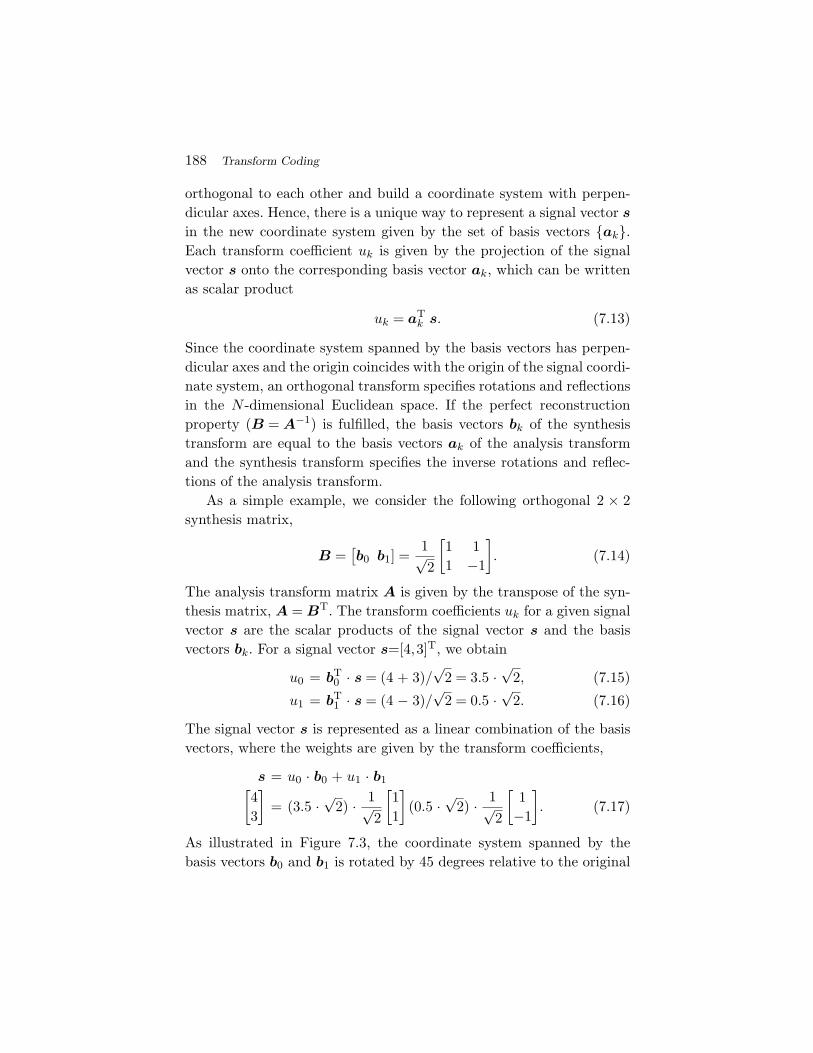
188 Transform Coding
orthogonal to each other and build a coordinate system with perpen-dicular axes. Hence, there is a unique way to represent a signal vector s
in the new coordinate system given by the set of basis vectors {ak}.Each transform coefficient uk is given by the projection of the signalvector s onto the corresponding basis vector ak, which can be writtenas scalar product
uk = aTk s. (7.13)
Since the coordinate system spanned by the basis vectors has perpen-dicular axes and the origin coincides with the origin of the signal coordi-nate system, an orthogonal transform specifies rotations and reflectionsin the N -dimensional Euclidean space. If the perfect reconstructionproperty (B = A−1) is fulfilled, the basis vectors bk of the synthesistransform are equal to the basis vectors ak of the analysis transformand the synthesis transform specifies the inverse rotations and reflec-tions of the analysis transform.
As a simple example, we consider the following orthogonal 2 × 2synthesis matrix,
B =[b0 b1] =
1√2
[1 11 −1
]. (7.14)
The analysis transform matrix A is given by the transpose of the syn-thesis matrix, A = BT. The transform coefficients uk for a given signalvector s are the scalar products of the signal vector s and the basisvectors bk. For a signal vector s=[4,3]T, we obtain
u0 = bT0 · s = (4 + 3)/
√2 = 3.5 ·
√2, (7.15)
u1 = bT1 · s = (4 − 3)/
√2 = 0.5 ·
√2. (7.16)
The signal vector s is represented as a linear combination of the basisvectors, where the weights are given by the transform coefficients,
s = u0 · b0 + u1 · b1[43
]= (3.5 ·
√2) · 1√
2
[11
](0.5 ·
√2) · 1√
2
[1
−1
]. (7.17)
As illustrated in Figure 7.3, the coordinate system spanned by thebasis vectors b0 and b1 is rotated by 45 degrees relative to the original
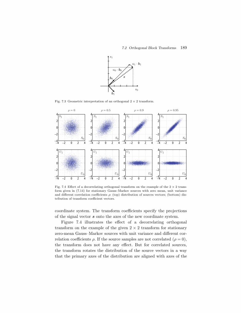
7.2 Orthogonal Block Transforms 189
Fig. 7.3 Geometric interpretation of an orthogonal 2 × 2 transform.
−4 −2 0 2 4−4
−2
0
2
4
−4 −2 0 2 4−4
−2
0
2
4
−4 −2 0 2 4−4
−2
0
2
4
−4 −2 0 2 4−4
−2
0
2
4
−4 −2 0 2 4−4
−2
0
2
4
−4 −2 0 2 4−4
−2
0
2
4
−4 −2 0 2 4−4
−2
0
2
4
−4 −2 0 2 4−4
−2
0
2
4
Fig. 7.4 Effect of a decorrelating orthogonal transform on the example of the 2 × 2 trans-form given in (7.14) for stationary Gauss–Markov sources with zero mean, unit varianceand different correlation coefficients ρ: (top) distribution of sources vectors; (bottom) dis-tribution of transform coefficient vectors.
coordinate system. The transform coefficients specify the projectionsof the signal vector s onto the axes of the new coordinate system.
Figure 7.4 illustrates the effect of a decorrelating orthogonaltransform on the example of the given 2 × 2 transform for stationaryzero-mean Gauss–Markov sources with unit variance and different cor-relation coefficients ρ. If the source samples are not correlated (ρ = 0),the transform does not have any effect. But for correlated sources,the transform rotates the distribution of the source vectors in a waythat the primary axes of the distribution are aligned with axes of the
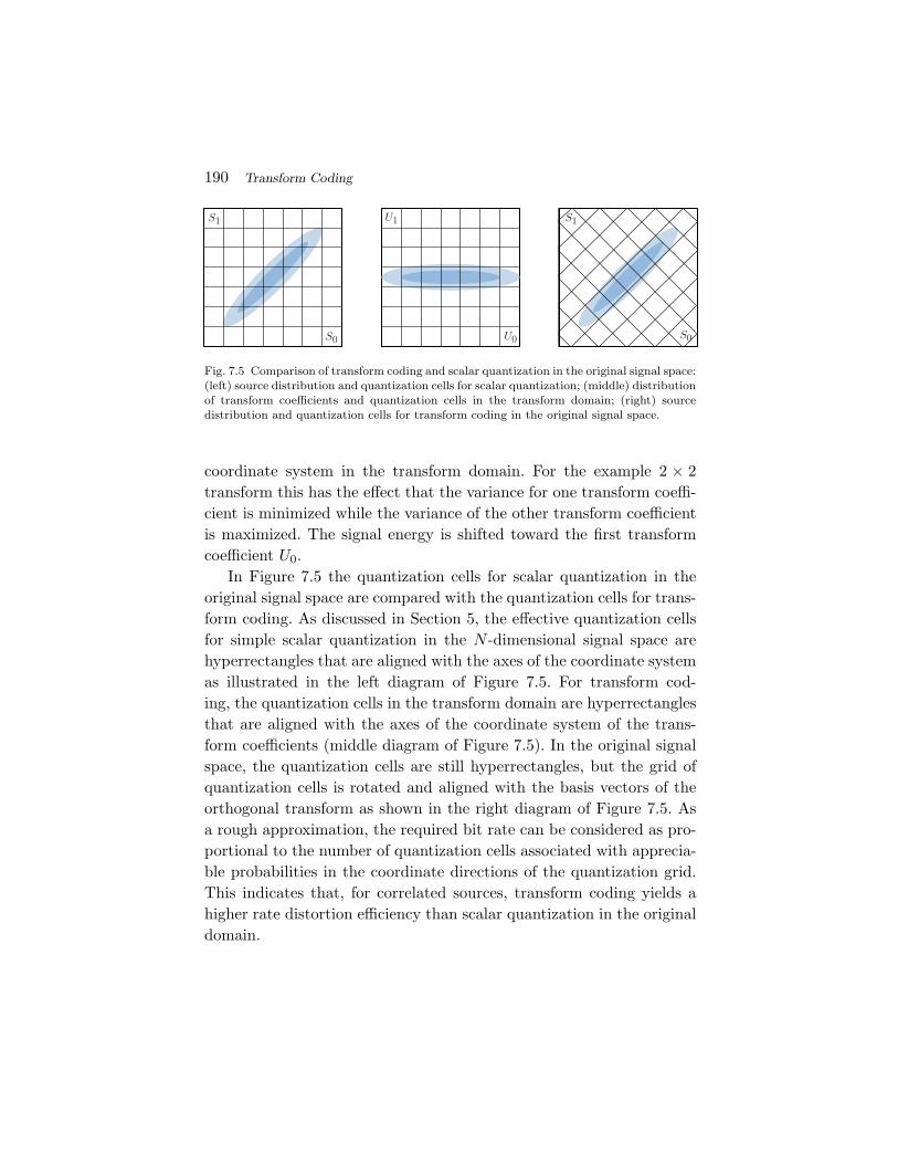
190 Transform Coding
Fig. 7.5 Comparison of transform coding and scalar quantization in the original signal space:(left) source distribution and quantization cells for scalar quantization; (middle) distributionof transform coefficients and quantization cells in the transform domain; (right) sourcedistribution and quantization cells for transform coding in the original signal space.
coordinate system in the transform domain. For the example 2 × 2transform this has the effect that the variance for one transform coeffi-cient is minimized while the variance of the other transform coefficientis maximized. The signal energy is shifted toward the first transformcoefficient U0.
In Figure 7.5 the quantization cells for scalar quantization in theoriginal signal space are compared with the quantization cells for trans-form coding. As discussed in Section 5, the effective quantization cellsfor simple scalar quantization in the N -dimensional signal space arehyperrectangles that are aligned with the axes of the coordinate systemas illustrated in the left diagram of Figure 7.5. For transform cod-ing, the quantization cells in the transform domain are hyperrectanglesthat are aligned with the axes of the coordinate system of the trans-form coefficients (middle diagram of Figure 7.5). In the original signalspace, the quantization cells are still hyperrectangles, but the grid ofquantization cells is rotated and aligned with the basis vectors of theorthogonal transform as shown in the right diagram of Figure 7.5. Asa rough approximation, the required bit rate can be considered as pro-portional to the number of quantization cells associated with apprecia-ble probabilities in the coordinate directions of the quantization grid.This indicates that, for correlated sources, transform coding yields ahigher rate distortion efficiency than scalar quantization in the originaldomain.
7.3 Bit Allocation for Transform Coefficients 191
7.3 Bit Allocation for Transform Coefficients
Before we discuss decorrelating transforms in more detail, we analyzethe problem of bit allocation for transform coefficients. As mentionedabove, the transform coefficients have usually a different importanceand hence the overall rate distortion efficiency of a transform codingsystem depends on a suitable distribution of the overall rate R amongthe transform coefficients. A bit allocation is optimal if a given overallrate R is distributed in a way that the resulting overall distortion D isminimized. If we use the MSE distortion measure, the distortion in theoriginal signal space is equal to the distortion in the transform domain.Hence, with Ri representing the component rates for the transform coef-ficients ui and Di(Ri) being the operational distortion rate functionsfor the component quantizers, we want to minimize
D(R) =1N
N−1∑i=0
Di(Ri) subject to1N
N−1∑i=0
Ri = R. (7.18)
As has been discussed in Section 5.2.2, the constrained optimizationproblem (7.18) can be reformulated as an unconstrained minimizationof the Lagrangian cost functional J = D + λR. If we assume that theoperational distortion rate functions Di(Ri) for the component quan-tizers are convex, the optimal rate allocation can be found by settingthe partial derivatives of the Lagrangian functional J with respect tothe component rates Ri equal to 0,
∂
∂Ri
(1N
N∑i=1
Di(Ri) +λ
N
N∑i=1
Ri
)=
1N
∂Di(Ri)∂Ri
+λ
N= 0, (7.19)
which yields
∂
∂RiDi(Ri) = −λ = const. (7.20)
This so-called Pareto condition states that, for optimal bit allocation,all component quantizers should be operated at equal slopes of theiroperational distortion rate functions Di(Ri).
192 Transform Coding
In Section 5.2.4, we have shown that the operational distortion ratefunction of scalar quantizers can be written as
Di(Ri) = σ2i · gi(Ri), (7.21)
where σ2i is the variance of the input source and gi(Ri) is the oper-
ational distortion rate function for the normalized distribution withunit variance. In general, it is justified to assume that gi(Ri) is a non-negative, strictly convex function and has a continuous first derivativeg′i(Ri) with g′
i(∞) = 0. Then, the Pareto condition yields
−σ2i g′
i(Ri) = λ. (7.22)
As discussed in Section 4.4, it has to be taken into account that the com-ponent rate Ri for a particular transform coefficient cannot be negative.If λ ≥ −σ2
i g′i(0), the quantizer for the transform coefficient ui cannot
be operated at the given slope λ. In this case, it is optimal to set thecomponent rate Ri equal to zero. The overall distortion is minimized ifthe overall rate is spent for coding only the transform coefficients with−σ2
i g′i(0) > λ. This yields the following bit allocation rule,
Ri =
0 : −σ2i g
′i(0) ≤ λ
ηi
(− λ
σ2i
): −σ2
i g′i(0) > λ
, (7.23)
where ηi(·) denotes the inverse of the derivative g′i(·). Since g′
i(Ri) is acontinuous strictly increasing function for Ri ≥ 0 with g′
i(∞) = 0, theinverse ηi(x) is a continuous strictly increasing function for the rangeg′i(0) ≤ x ≤ 0 with ηi(f ′
i(0)) = 0 and ηi(0) = ∞.
7.3.1 Approximation for Gaussian Sources
If the input signal has a Gaussian distribution, the distributions for alltransform coefficients are also Gaussian, since the signal for each trans-form coefficient represents a linear combination of Gaussian sources.Hence, we can assume that the operational distortion rate function forall component quantizers is given by
Di(Ri) = σ2i · g(R), (7.24)
7.3 Bit Allocation for Transform Coefficients 193
where g(R) represents the operational distortion rate function forGaussian sources with unit variance. In order to derive an approx-imate formula for the optimal bit allocation, we assume that thecomponent quantizers are entropy-constrained scalar quantizers anduse the approximation (5.59) for g(R) that has been experimentallyfound for entropy-constrained scalar quantization of Gaussian sourcesin Section 5.2.4,
g(R) =ε2
aln(a · 2−2R + 1). (7.25)
The factor ε2 is equal to πe/6 and the model parameter a is approxi-mately 0.9519. The derivative g′(R) and its inverse η(x) are given by
g′(R) = −ε2 · 2ln2a + 22R
, (7.26)
η(x) =12
log2
(−ε2 · 2ln2
x− a
). (7.27)
As stated above, for an optimal bit allocation, the component rate Ri
for a transform coefficient has to be set equal to 0, if
λ ≥ −σ2i g
′(0) = σ2i
ε2 · 2ln2a + 1
. (7.28)
With the parameter
θ = λa + 1
ε2 · 2ln2, (7.29)
we obtain the bit allocation rule
Ri(θ) =
0 : θ ≥ σ2i
12
log2
(σ2
i
θ(a + 1) − a
): θ < σ2
i
. (7.30)
The resulting component distortions are given by
Di(θ) =
σ2i : θ ≥ σ2
i
−ε2 ln2a
· σ2i · log2
(1 − θ
σ2i
a
a + 1
): θ < σ2
i
. (7.31)
194 Transform Coding
If the variances σ2i of the transform coefficients are known, the
approximation of the operational distortion rate function for transformcoding of Gaussian sources with entropy-constrained scalar quantiza-tion is given by the parametric formulation
R(θ) =1N
N−1∑i=0
Ri(θ), D(θ) =1N
N−1∑i=0
Di(θ), (7.32)
where R(θ) and D(θ) are specified by (7.30) and (7.31), respectively.The approximation of the operational distortion rate function can becalculated by varying the parameter θ in the range from 0 to σ2
max,with σ2
max being the maximum variance of the transform coefficients.
7.3.2 High-Rate Approximation
In the following, we assume that the overall rate R is high enough sothat all component quantizers are operated at high component rates Ri.In Section 5.2.3, we have shown that the asymptotic operational dis-tortion rate functions for scalar quantizers can be written as
Di(Ri) = ε2i σ2
i 2−2Ri , (7.33)
where the factor ε2i depends only on the type of the source distribution
and the used scalar quantizer. Using these high rate approximationsfor the component quantizers, the Pareto condition becomes
∂
∂RiDi(Ri) = −2 ln2ε2
i σ2i
−2Ri = −2 ln2Di(Ri) = const. (7.34)
At high rates, an optimal bit allocation is obtained if all componentdistortions Di are the same. Setting the component distortions Di equalto the overall distortion D, yields
Ri(D) =12
log2
(σ2
i ε2i
D
). (7.35)
For the overall operational rate distortion function, we obtain
R(D) =1N
N−1∑i=0
Ri(D) =1
2N
N−1∑i=0
log2
(σ2
i ε2i
D
)(7.36)

7.3 Bit Allocation for Transform Coefficients 195
With the geometric means of the variances σ2i and the factors ε2i ,
σ2 =
(N−1∏i=0
σ2i
)1N
and ε2 =
(N−1∏i=0
ε2i
)1N
, (7.37)
the asymptotic operational distortion rate function for high rates canbe written as
D(R) = ε2 · σ2 · 2−2R. (7.38)
It should be noted that this result can also be derived without using thePareto condition, which was obtained by calculus. Instead, we can usethe inequality of arithmetic and geometric means and derive the highrate approximation similar to the rate distortion function for Gaussiansources with memory in Section 4.4.
For Gaussian sources, all transform coefficients have a Gaussiandistribution (see Section 7.3.1), and thus all factors ε2
i are the same. Ifentropy-constrained scalar quantizers are used, the factors ε2
i are equalto πe/6 (see Section 5.2.3) and the asymptotic operational distortionrate function for high rates is given by
D(R) =πe
6· σ2 · 2−2R. (7.39)
Transform coding gain. The effectiveness of a transform is oftenspecified by the transform coding gain, which is defined as the ratioof the operational distortion rate functions for scalar quantization andtransform coding. At high rates, the transform coding gain is given by
GT =ε2S · σ2
S · 2−2R
ε2 · σ2 · 2−2R, (7.40)
where ε2S is the factor of the high rate approximation of the operational
distortion rate function for scalar quantization in the original signalspace and σ2
S is the variance of the input signal.By using the relationship (7.10), the high rate transform gain for
Gaussian sources can be expressed as the ratio of the arithmetic andgeometric mean of the transform coefficient variances,
GT =1N
∑N−1i=0 σ2
i
N
√∏N−1i=0 σ2
i
. (7.41)
196 Transform Coding
The high rate transform gain for Gaussian sources is maximized if thegeometric mean is minimized. The transform that minimizes the geo-metric mean is the Karhunen Loeve Transform, which will be discussedin the next section.
7.4 The Karhunen Loeve Transform (KLT)
Due to its importance in the theoretical analysis of transform codingwe discuss the Karhunen Loeve Transform (KLT) in some detail inthe following. The KLT is an orthogonal transform that decorrelates thevectors of input samples. The transform matrix A is dependent on thestatistics of the input signal.
Let S represent the random vectors of original samples of a sta-tionary input sources. The random vectors of transform coefficients aregiven by U = AS and for the autocorrelation matrix of the transformcoefficients we obtain
RUU = E{U UT} = E
{(AS)(AS)T
}= ARSSAT, (7.42)
where
RSS = E{SST} (7.43)
denotes the autocorrelation matrix of the input process. To get uncor-related transform coefficients, the orthogonal transform matrix A hasto be chosen in a way that the autocorrelation matrix RUU becomes adiagonal matrix. Equation (7.42) can be slightly reformulated as
RSSAT = ATRSS . (7.44)
With bi representing the basis vectors of the synthesis transform, i.e.,the column vectors of A−1 = AT and the row vectors of A, it becomesobvious that RUU is a diagonal matrix if the eigenvector equation
RSS bi = ξi bi (7.45)
is fulfilled for all basis vectors bi. The eigenvalues ξi represents the ele-ments rii on the main diagonal of the diagonal matrix RUU . The rowsof the transform matrix A are build by a set of unit-norm eigenvectorsof RSS that are orthogonal to each other. The autocorrelation matrix
7.4 The Karhunen Loeve Transform (KLT) 197
for the transform coefficients RUU is a diagonal matrix with the eigen-values of RSS on its main diagonal. The transform coefficient variancesσ2
i are equal to the eigenvalues ξi of the autocorrelation matrix RSS .A KLT exists for all sources, since symmetric matrices as the auto-
correlation matrix RSS are always orthogonally diagonizable. Thereexist more than one KLT of any particular size N > 1 for all stationarysources, because the rows of A can be multiplied by −1 or permutedwithout influencing the orthogonality of A or the diagonal form ofRUU . If the eigenvalues of RSS are not distinct, there are additionaldegrees of freedom for constructing KLT transform matrices. Numericalmethods for calculating the eigendecomposition RSS = ATdiag(ξi)Aof real symmetric matrices RSS are the classical and the cyclic Jacobialgorithm [18, 39].
Nonstationary sources. For nonstationary sources, transform cod-ing with a single KLT transform matrix is suboptimal. Similar to thepredictor in predictive coding, the transform matrix should be adaptedbased on the local signal statistics. The adaptation can be realizedeither as forward adaptation or as backward adaptation. With for-ward adaptive techniques, the transform matrix is estimated at theencoder and an adaptation signal is transmitted as side information,which increases the overall bit rate and usually introduces an additionaldelay. In backward adaptive schemes, the transform matrix is simulta-neously estimated at the encoder and decoder sides based on alreadycoded samples. Forward adaptive transform coding is discussed in [12]and transform coding with backward adaptation is investigated in [21].
7.4.1 On the Optimality of the KLT
We showed that the KLT is an orthogonal transform that yields decor-related transform coefficients. In the following, we show that the KLTis also the orthogonal transform that maximizes the rate distortionefficiency for stationary zero-mean Gaussian sources if optimal scalarquantizers are used for quantizing the transform coefficients. The fol-lowing proof was first delineated in [19].
We consider a transform coding system with an orthogonal N ×N
analysis transform matrix A, the synthesis transform matrix B = AT,
198 Transform Coding
and scalar quantization of the transform coefficients. We further assumethat we use a set of scalar quantizers that are given by scaled versionsof a quantizer for unit variance for which the operational distortionrate function is given by a nonincreasing function g(R). The decisionthresholds and reconstruction levels of the quantizers are scaled accord-ing to the variances of the transform coefficients. Then, the operationaldistortion rate function for each component quantizer is given by
Di(Ri) = σ2i · g(Ri), (7.46)
where σ2i denotes the variance of the corresponding transform coeffi-
cient (cf. Section 5.2.4). It should be noted that such a setup is optimalfor Gaussian sources if the function g(R) is the operational distor-tion rate function of an optimal scalar quantizer. The optimality of aquantizer may depend on the application. As an example, we couldconsider entropy-constrained Lloyd quantizers as optimal if we assumea lossless coding that achieves an average codeword length close to theentropy. For Gaussian sources, the transform coefficients have also aGaussian distribution. The corresponding optimal component quantiz-ers are scaled versions of the optimal quantizer for unit variance andtheir operational distortion rate functions are given by (7.46).
We consider an arbitrary orthogonal transform matrix A0 and anarbitrary bit allocation given by the vector b = (R0, . . . ,RN−1)T with∑N−1
i=0 Ri = R. Starting with the given transform matrix A0 we applyan iterative algorithm that generates a sequence of orthonormal trans-form matrices {Ak}. The corresponding autocorrelation matrices aregiven by R(Ak) = AkRSSAT
k with RSS denoting the autocorrelationmatrix of the source signal. The transform coefficient variances σ2
i (Ak)are the elements on the main diagonal of R(Ak) and the distortion ratefunction for the transform coding system is given by
D(Ak,R) =N−1∑i=0
σ2i (Ak) · g(Ri). (7.47)
Each iteration Ak �→ Ak+1 shall consists of the following two steps:
(1) Consider the class of orthogonal reordering matrices {P },for which each row and column consists of a single one and
7.4 The Karhunen Loeve Transform (KLT) 199
N − 1 zeros. The basis vectors given by the rows of Ak arereordered by a multiplication with the reordering matrix P k
that minimizes the distortion rate function D(P kAk,R).
(2) Apply a Jacobi rotation1 Ak+1 = Qk(P kAk). The orthogo-nal matrix Qk is determined in a way that the element rij
on a secondary diagonal of R(P kAk) that has the largestabsolute value becomes zero in R(Ak+1). Qk is an elemen-tary rotation matrix. It is an identity matrix where the maindiagonal elements qii and qjj are replaced by a value cosϕ
and the secondary diagonal elements qij and qji are replacedby the values sinϕ and −sinϕ, respectively.
It is obvious that the reordering step does not increase the distortion,i.e., D(P kAk,R) ≤ D(Ak,R). Furthermore, for each pair of variancesσ2
i (P kAk) ≥ σ2j (P kAk), it implies g(Ri) ≤ g(Rj); otherwise, the dis-
tortion D(P kAk,R) could be decreased by switching the ith andjth row of the matrix P kAk. A Jacobi rotation that zeros the ele-ment rij of the autocorrelation matrix R(P kAk) in R(Ak+1) doesonly change the variances for the ith and jth transform coefficient.If σ2
i (P kAk) ≥ σ2j (P kAk), the variances are modified according to
σ2i (Ak+1) = σ2
i (P kAk) + δ(P kAk), (7.48)
σ2j (Ak+1) = σ2
j (P kAk) − δ(P kAk), (7.49)
with
δ(P kAk) =2r2
ij
(rii − rjj ) +√
(rii − rjj )2 + 4r2ij
≥ 0, (7.50)
and rij being the elements of the matrix R(P kAk). The overall distor-tion for the transform matrix Ak+1 will never become smaller than the
1 The classical Jacobi algorithm [18, 39] for determining the eigendecomposition of realsymmetric matrices consist of a sequence of Jacobi rotations.
200 Transform Coding
overall distortion for the transform matrix Ak,
D(Ak+1,R) =N−1∑i=0
σ2i (Ak+1) × g(Ri)
= D(P kAk,R) + δ(P kAk) · (g(Ri) − g(Rj))
≤ D(P kAk,R) ≤ D(Ak,R). (7.51)
The described algorithm represents the classical Jacobi algorithm[18, 39] with additional reordering steps. The reordering steps do notaffect the basis vectors of the transform (rows of the matrices Ak), butonly their ordering. As the number of iteration steps approaches infin-ity, the transform matrix Ak approaches the transform matrix of a KLTand the autocorrelation matrix R(Ak) approaches a diagonal matrix.Hence, for each possible bit allocation, there exists a KLT that gives anoverall distortion that is smaller than or equal to the distortion for anyother orthogonal transform. While the basis vectors of the transformare determined by the source signal, their ordering is determined bythe relative ordering of the partial rates Ri inside the bit allocationvector b and the normalized operational distortion rate function g(Ri).
We have shown that the KLT is the orthogonal transform that min-imizes the distortion for a set of scalar quantizers that represent scaledversions of a given quantizer for unit variance. In particular, the KLT isthe optimal transform for Gaussian sources if optimal scalar quantizersare used [19]. The KLT produces decorrelated transform coefficients.However, decorrelation does not necessarily imply independence. Fornon-Gaussian sources, other orthogonal transforms or nonorthogonaltransforms can be superior with respect to the coding efficiency [13, 20].
Example for a Gauss–Markov Process. As an example, we con-sider the 3× 3 KLT for a stationary Gauss–Markov process with zeromean, unit variance, and a correlation coefficient of ρ = 0.9. We assumea bit allocation vector b = [5,3,2] and consider entropy-constrainedscalar quantizers. We further assume that the high-rate approximationof the operational distortion rate function Di(Ri) = ε2σ2
i 2−2Ri with
ε2 =πe/6 is valid for the considered rates. The initial transform matrixA0 shall be the matrix of the DCT-II transform, which we will later
7.4 The Karhunen Loeve Transform (KLT) 201
introduce in Section 7.5.3. The autocorrelation matrix RSS and theinitial transform matrix A0 are given by
Rs =
[1 0.9 0.81
0.9 1 0.90.81 0.9 1
], A0 =
[0.5774 0.5774 0.57740.7071 0 −0.70710.4082 −0.8165 0.4082
]. (7.52)
For the transform coefficients, we obtain the autocorrelation matrix
R(A0) =
[2.74 0 −0.0424
0 0.19 0−0.0424 0 0.07
]. (7.53)
The distortion D(A0,R) for the initial transform is equal to 0.01426.We now investigate the effect of the first iteration of the algorithmdescribed above. For the given relative ordering in the bit allocationvector b, the optimal reordering matrix P 0 is the identity matrix. TheJacobi rotation matrix Q0 and the resulting new transform matrix A1
are given by
Q0 =
[0.9999 0 −0.0159
0 1 00.0159 0 0.9999
], A1 =
[0.5708 0.5902 0.57080.7071 0 −0.70710.4174 −0.8072 0.4174
]. (7.54)
The parameter δ(P 0A0) is equal to 0.000674. The distortion D(A1,R)is equal to 0.01420. In comparison to the distortion for the initial trans-form matrix A0, it has been reduced by about 0.018 dB. The autocor-relation matrix R(A1) for the new transform coefficients is given by
R(A1) =
[2.7407 0 0
0 0.19 00 0 0.0693
]. (7.55)
The autocorrelation matrix has already become a diagonal matrix afterthe first iteration. The transform given by A1 represents a KLT for thegiven source signal.
7.4.2 Asymptotic Operational Distortion Rate Function
In Section 7.3.2, we considered the bit allocation for transform codingat high rates. An optimal bit allocation results in constant componentdistortions Di, which are equal to the overall distortion D. By using the
202 Transform Coding
high rate approximation Di(Ri) = ε2i σ2
i 2−2Ri for the operational dis-tortion rate function of the component quantizers, we derived the over-all operational distortion rate function given in (7.36). For Gaussiansources and entropy-constrained scalar quantization, all parameters ε2
i
are equal to ε = πe/6. And if we use a KLT of size N as transformmatrix, the transform coefficient variances σ2
i are equal to the eigen-values ξ
(N)i of the Nth order autocorrelation matrix RN for the input
process. Hence, for Gaussian sources and a transform coding systemthat consists of a KLT of size N and entropy-constrained scalar quan-tizers for the transform coefficients, the high rate approximation forthe overall distortion rate function can be written as
DN (R) =πe
6
(N−1∏i=0
ξ(N)i
) 1N
2−2R. (7.56)
The larger we choose the transform size N of the KLT, the more thesamples of the input source are decorrelated. For deriving a bound forthe operational distortion rate function at high rates, we consider thelimit for N approaching infinity. By applying Grenander and Szego’stheorem (4.76) for sequences of Toeplitz matrices, the limit of (7.56)for N approaching infinity can be reformulated using the power spectraldensity ΦSS (ω) of the input source. For Gaussian sources, the asymp-totic operational distortion rate function for high rates and large trans-form dimensions is given by
D∞(R) =πe
6· 2
12π
∫ π−π log2ΦSS (ω) dω · 2−2R. (7.57)
A comparison with the Shannon lower bound (4.77) for zero-meanGaussian sources shows that the asymptotic operational distortion ratefunction lies 1.53 dB or 0.25 bit per sample above this fundamentalbound. The difference is equal to the space-filling advantage of high-dimensional vector quantization. For zero-mean Gaussian sources andhigh rates, the memory and shape advantage of vector quantization canbe completely exploited using a high-dimensional transform coding.
By using the relationship σ2S = 1
2π
∫ π−π ΦSS (ω)dω for the variance of
the input source, the asymptotic transform coding gain for zero-meanGaussian sources can be expressed as the ratio of the arithmetic and

7.4 The Karhunen Loeve Transform (KLT) 203
geometric means of the power spectral density,
G∞T =
ε2σ2S2−2R
D∞(R)=
12π
∫ π−π ΦSS (ω)dω
212π
∫ π−π log2 ΦSS (ω)dω
(7.58)
The asymptotic transform coding gain at high rates is identical to theapproximation for the DPCM coding gain at high rates (6.75).
Zero-Mean Gauss–Markov Sources. We now consider the spe-cial case of zero-mean Gauss–Markov sources. The product of the eigen-values ξ
(N)i of a matrix RN is always equal to the determinant |RN |
of the matrix. And for zero-mean sources, the Nth order autocorrela-tion matrix RN is equal to the Nth order autocovariance matrix CN .Hence, we can replace the product of the eigenvalues in (7.56) withthe determinant |CN | of the Nth order autocovariance matrix. Fur-thermore, for Gauss–Markov sources, the determinant of the Nthorder autocovariance matrix can be expressed according to (2.50).Using these relationships, the operational distortion rate function forzero-mean Gauss–Markov sources and a transform coding system withan N -dimensional KLT and entropy-constrained component quantizersis given by
DN (R) =πe
6σ2
S (1 − ρ2)N−1
N 2−2R, (7.59)
where σ2S and ρ denote the variance and the correlation coefficient of
the input source, respectively. For the corresponding transform gain,we obtain
GNT = (1 − ρ2)
1−NN . (7.60)
The asymptotic operational distortion rate function and the asymptotictransform gain for high rates and N approaching infinity are given by
D∞(R) =πe
6σ2
S (1 − ρ2) 2−2R, G∞T =
1(1 − ρ2)
. (7.61)
7.4.3 Performance for Gauss–Markov Sources
For demonstrating the effectiveness of transform coding for correlatedinput sources, we used a Gauss–Markov source with zero mean, unitvariance, and a correlation coefficient of ρ = 0.9 and compared the

204 Transform Coding
Fig. 7.6 Transform coding of a Gauss–Markov source with zero mean, unit variance, and acorrelation coefficient of ρ = 0.9. The diagram compares the efficiency of direct ECSQ andtransform coding with ECSQ to the distortion rate function D(R). The circles representexperimental data while the solid lines represent calculated curves. The rate is measured asthe average of the entropies for the outputs of the component quantizers.
rate distortion efficiency of transform coding with KLT’s of differentsizes N and entropy-constrained scalar quantization (ECSQ) with thefundamental rate distortion bound and the rate distortion efficiency forECSQ of the input samples. The experimentally obtained data and thecalculated distortion rate curves are shown in Figure 7.6. The rate wasdetermined as average of the entropies of the quantizer outputs. It canbe seen that transform coding significantly increases the coding effi-ciency relative to direct ECSQ. An interesting fact is that for transformsizes larger than N = 4 the distance to the fundamental rate distortionbound at low rates is less than at high rates. A larger transform size N
generally yields a higher coding efficiency. However, the asymptoticbound (7.61) is already nearly achieved for a moderate transform sizeof N = 16 samples. A further increase of the transform size N wouldonly slightly improve the coding efficiency for the example source. Thisis further illustrated in Figure 7.7, which shows the transform codinggain as function of the transform size N .
7.5 Signal-Independent Unitary Transforms
Although the KLT has several desirable properties, it is not used inpractically video coding applications. One of the reasons is that there
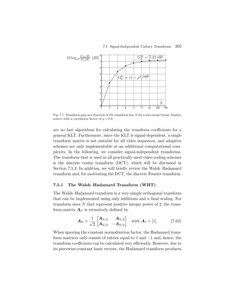
7.5 Signal-Independent Unitary Transforms 205
Fig. 7.7 Transform gain as a function of the transform size N for a zero-mean Gauss–Markovsource with a correlation factor of ρ = 0.9.
are no fast algorithms for calculating the transform coefficients for ageneral KLT. Furthermore, since the KLT is signal-dependent, a singletransform matrix is not suitable for all video sequences, and adaptiveschemes are only implementable at an additional computational com-plexity. In the following, we consider signal-independent transforms.The transform that is used in all practically used video coding schemesis the discrete cosine transform (DCT), which will be discussed inSection 7.5.3. In addition, we will briefly review the Walsh–Hadamardtransform and, for motivating the DCT, the discrete Fourier transform.
7.5.1 The Walsh–Hadamard Transform (WHT)
The Walsh–Hadamard transform is a very simple orthogonal transformthat can be implemented using only additions and a final scaling. Fortransform sizes N that represent positive integer power of 2, the trans-form matrix AN is recursively defined by
AN =1√2
[AN/2 AN/2AN/2 −AN/2
]with A1 = [1]. (7.62)
When ignoring the constant normalization factor, the Hadamard trans-form matrices only consist of entries equal to 1 and −1 and, hence, thetransform coefficients can be calculated very efficiently. However, due toits piecewise-constant basis vectors, the Hadamard transform produces
206 Transform Coding
subjectively disturbing artifacts if it is combined with strong quanti-zation of the transform coefficients. In video coding, the Hadamardtransform is only used for some special purposes. An example is thesecond-level transform for chroma coefficients in H.264/AVC [38].
7.5.2 The Discrete Fourier Transform (DFT)
One of the most important transforms in communications engineeringand signal processing is the Fourier transform. For discrete-time signalsof a finite length N , the discrete Fourier transform (DFT) is given by
u[k] =1√N
N−1∑n=0
s[n] e−j 2πknN , (7.63)
where s[n], with 0 ≤ n < N , and u[k], with 0 ≤ k < N , represent thecomponents of the signal vector s and the vector of transform coeffi-cients u, respectively, and j is the imaginary unit. The inverse DFT isgiven by
s[n] =1√N
N−1∑k=0
u[k] ej 2πknN . (7.64)
For computing both the forward and inverse transform fast algorithms(FFT) exist, which use sparse matrix factorization. The DFT gener-ally produces complex transform coefficients. However, for real inputsignals, the DFT obeys the symmetry u[k] = u∗[N − k], where theasterisk denotes complex conjugation. Hence, an input signal of N realsamples is always completely specified by N real coefficients.
The discrete Fourier transform is rarely used in compression sys-tems. One reason is its complex nature. Another reason is the fact thatthe DFT implies a periodic signal extension. The basis functions of theDFT are complex exponentials, which are periodic functions. For eachbasis function, a particular integer multiple of the period is equal tothe length of the input signal. Hence, the signal that is actually rep-resented by the DFT coefficients is a periodically extended version ofthe finite-length input signal, as illustrated in Figure 7.8. Any discon-tinuity between the left and right signal boundary reduces the rate ofconvergence of the Fourier series, i.e., more basis functions are needed

7.5 Signal-Independent Unitary Transforms 207
Fig. 7.8 Periodic signal extensions for the DFT and the DCT: (a) input signal; (b) signalreplica for the DFT; (c) signal replica for the DCT-II.
to represent the input signal with a given accuracy. In combination withstrong quantization this leads also to significant high-frequent artifactsin the reconstruction signal.
7.5.3 The Discrete Cosine Transform (DCT)
The magnitudes of the high-frequency DFT coefficients can be reducedby symmetrically extending the finite-length input signal at its bound-aries and applying a DFT of approximately double size. If the extendedsignal is mirror symmetric around the origin, the imaginary sine termsget eliminated and only real cosine terms remain. Such a transform isdenoted as discrete cosine transform (DCT). There are several DCTs,which differ in the introduced signal symmetry. The most commonlyused form is the DCT-II, which can be derived by introducing mir-ror symmetry with sample repetition at both boundaries as illustratedin Figure 7.8(c). For obtaining mirror symmetry around the origin, thesignal has to be shifted by half a sample. The signal s′ of 2N samplesthat is actually transformed using the DFT is given by
s′[n] ={
s[n − 1/2] : 0 ≤ n < N,
s[2N − n − 3/2] : N ≤ n < 2N.(7.65)
208 Transform Coding
For the transform coefficients u′[k], we obtain
u′[k] =1√2N
2N−1∑n=0
s′[n]e−j 2πkn2N
=1√2N
N−1∑n=0
s[n − 1/2](e−j π
Nkn + e−j π
Nk(2N−n−1))
=1√2N
N−1∑n=0
s[n](e−j π
Nk(n+ 1
2 ) + ej πN
k(n+ 12 ))
=
√2N
N−1∑n=0
s[n] cos(
π
Nk
(n +
12
)). (7.66)
In order to get an orthogonal transform, the DC coefficient u′[0] has tobe divided by
√2. The forward transform of the DCT-II is given by
u[k] =N−1∑n=0
s[n] αk cos(
π
Nk
(n +
12
)), (7.67)
with
αn =
√1N
·{
1 : n = 0√2 : n > 0
. (7.68)
The inverse transform is given by
s[n] =N−1∑k=0
u[k] · αk · cos(
π
Nk
(n +
12
)). (7.69)
The DCT-II is the most commonly used transform in imageand video coding application. It is included in the following codingstandards: JPEG [33], H.261 [32], H.262/MPEG-2 [34], H.263 [38],and MPEG-4 [31]. Although, the most recent video coding standardH.264/AVC [38] does not include a DCT as discussed above, it includesan integer approximation of the DCT that has similar properties, butcan be implemented more efficiently and does not cause an accumula-tion of rounding errors inside the motion-compensation loop. The jus-tification for the wide usage of the DCT includes the following points:
• The DCT does not depend on the input signal.
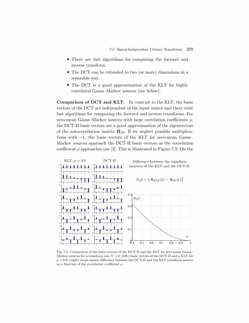
7.5 Signal-Independent Unitary Transforms 209
• There are fast algorithms for computing the forward andinverse transform.
• The DCT can be extended to two (or more) dimensions in aseparable way.
• The DCT is a good approximation of the KLT for highlycorrelated Gauss–Markov sources (see below).
Comparison of DCT and KLT. In contrast to the KLT, the basisvectors of the DCT are independent of the input source and there existfast algorithms for computing the forward and inverse transforms. Forzero-mean Gauss–Markov sources with large correlation coefficients ρ,the DCT-II basis vectors are a good approximation of the eigenvectorsof the autocorrelation matrix RSS . If we neglect possible multiplica-tions with −1, the basis vectors of the KLT for zero-mean Gauss–Markov sources approach the DCT-II basis vectors as the correlationcoefficient ρ approaches one [2]. This is illustrated in Figure 7.9. On the
0 1 2 3 4 5 6 7−0.5
0
0.5
0 1 2 3 4 5 6 7−0.5
0
0.5
0 1 2 3 4 5 6 7−0.5
0
0.5
0 1 2 3 4 5 6 7−0.5
0
0.5
0 1 2 3 4 5 6 7−0.5
0
0.5
0 1 2 3 4 5 6 7−0.5
0
0.5
0 1 2 3 4 5 6 7−0.5
0
0.5
0 1 2 3 4 5 6 7−0.5
0
0.5
0 1 2 3 4 5 6 7−0.5
0
0.5
0 1 2 3 4 5 6 7−0.5
0
0.5
0 1 2 3 4 5 6 7−0.5
0
0.5
0 1 2 3 4 5 6 7−0.5
0
0.5
0 1 2 3 4 5 6 7−0.5
0
0.5
0 1 2 3 4 5 6 7−0.5
0
0.5
0 1 2 3 4 5 6 7−0.5
0
0.5
0 1 2 3 4 5 6 7−0.5
0
0.5
0.4 0.5 0.6 0.7 0.8 0.9 10
0.1
0.2
0.3
0.4
Fig. 7.9 Comparison of the basis vectors of the DCT-II and the KLT for zero-mean Gauss–Markov sources for a transform size N = 8: (left) basis vectors of the DCT-II and a KLT forρ = 0.9; (right) mean square difference between the DCT-II and the KLT transform matrixas a function of the correlation coefficient ρ.
210 Transform Coding
left side of this figure, the basis vectors of a KLT for zero-mean Gauss–Markov sources with a correlation coefficient of ρ = 0.9 are comparedwith the basis vectors of the DCT-II. On the right side of Figure 7.9,the mean square difference δ(ρ) between the transform matrix of theDCT-II ADCT and the KLT transform matrix AKLT is shown as func-tion of the correlation coefficient ρ. For this experiment, we used theKLT transform matrices AKLT for which the basis vectors (rows) areordered in decreasing order of the associated eigenvalues and all entriesin the first column are non-negative.
7.6 Transform Coding Example
As a simple transform coding example, we consider the Hadamardtransform of the size N = 2 for a zero-mean Gauss–Markov processwith a variance σ2
S and a correlation coefficient ρ. The input vectors s
and the orthogonal analysis transform matrix A are given by
s =[s0
s1
]and A =
1√2
[1 11 −1
]. (7.70)
The analysis transform
u =[u0
u1
]= As =
1√2
[1 11 −1
][s0
s1
](7.71)
yields the transform coefficients
u0 =1√2
(s0 + s1), u0 =1√2
(s0 − s1). (7.72)
For the Hadamard transform, the synthesis transform matrix B is equalto the analysis transform matrix, B = AT = A.
The transform coefficient variances are given by
σ20 = E
{U2
0}
= E
{12(S0 + S1)2
}=
12(E{S2
0}
+ E{S2
1}
+ 2E{S0S1})
=12(σ2
S + σ2S + 2σ2
S ρ) = σ2S(1 + ρ), (7.73)
σ2u1
= E{U2
1}
= σ2S(1 − ρ), (7.74)
7.6 Transform Coding Example 211
where Si and Ui denote the random variables for the signal componentsand transform coefficients, respectively. The cross-correlation of thetransform coefficients is
E{U0U1} =12
E{(S0 + S1)(S0 − S1)}
=12
E{(S2
0 − S21)}
=12(σ2
S − σ2S) = 0. (7.75)
The Hadamard transform of size N = 2 generates independent trans-form coefficients for zero-mean Gauss–Markov sources. Hence, it is aKLT for all correlation coefficients ρ. It is also the DCT-II for N = 2.
In the following, we consider entropy-constrained scalar quan-tization of the transform coefficients at high rates. The high-rateapproximation of the operational distortion rate function for entropy-constrained scalar quantization of Gaussian sources is given byDi(Ri) = ε2σ2
i 2−2Ri with ε2 = πe/6. The optimal bit allocation rule
for high rates (cf. Section 7.3.2) yields the component rates
R0 = R +14
log2
(1 + ρ
1 − ρ
), (7.76)
R1 = R − 14
log2
(1 + ρ
1 − ρ
), (7.77)
where R denotes the overall rate. If ρ > 0, the rate R0 for the DCcoefficient u0 is always 1
2 log2(1+ρ1−ρ) bits larger than the rate R1 for the
AC coefficient u1. The high-rate operational distortion rate functionfor the considered transform coder is given by
D(R) = ε2σ2S
√1 − ρ2 · 2−2R. (7.78)
A comparison with the Shannon Lower bound (4.80) shows that, forhigh rates, the loss against the fundamental rate distortion bound is
D(R)DL(R)
=π e
6√
1 − ρ2. (7.79)
For zero-mean Gauss–Markov sources with ρ = 0.9 and high rates, thetransform coding gain is about 3.61 dB, while the loss against theShannon lower bound is about 5.14 dB. The transform coding gain canbe increased by applying larger decorrelating transforms.

212 Transform Coding
7.7 Summary of Transform Coding
In this section, we discussed transform coding with orthogonal blocktransforms. An orthogonal block transform of size N specifies a rotationor reflection of the coordinate system in the N -dimensional signal space.We showed that a transform coding system with an orthogonal blocktransform and scalar quantization of the transform coefficients repre-sents a vector quantizer for which the quantization cells are hyperrect-angles in the N -dimensional signal space. In contrast to scalar quan-tization in the original domain, the grid of quantization cells is notaligned with the coordinate axes of the original space. A decorrelationtransform rotates the coordinate system toward the primary axes ofthe N -dimensional joint pdf, which has the effect that, for correlatedsources, scalar quantization in the transform domain becomes moreeffective than in the original signal space.
The optimal distribution of the overall bit rate among the trans-form coefficients was discussed in some detail with the emphasis onGaussian sources and high rates. In general, an optimal bit allocationis obtained if all component quantizers are operated at the same slopeof their operational distortion rate functions. For high rates, this isequivalent to a bit allocation that yields equal component distortions.For stationary sources with memory the effect of the unitary transformis a nonuniform assignment of variances to the transform coefficients.This nonuniform distribution is the reason for the transform gain incase of optimal bit allocation.
The KLT was introduced as the transform that generates decorre-lated transform coefficients. We have shown that the KLT is the opti-mal transform for Gaussian sources if we use the same type of optimalquantizers, with appropriately scaled reconstruction levels and decisionthresholds, for all transform coefficients. For the example of Gaussiansources, we also derived the asymptotic operational distortion rate func-tion for large transform sizes and high rates. It has been shown that, forzero-mean Gaussian sources and entropy-constrained scalar quantiza-tion, the distance of the asymptotic operational distortion rate functionto the fundamental rate distortion bounds is basically reduced to thespace-filling advantage of vector quantization.
7.7 Summary of Transform Coding 213
In practical video coding systems, KLT’s are not used, since theyare signal-dependent and cannot be implemented using fast algorithms.The most widely used transform is the DCT-II, which can be derivedfrom the discrete Fourier transform (DFT) by introducing mirror sym-metry with sample repetition at the signal boundaries and applyinga DFT of double size. Due to the mirror symmetry, the DCT signifi-cantly reduces the blocking artifacts compared to the DFT. For zero-mean Gauss–Markov sources, the basis vectors of the KLT approachthe basis vectors of the DCT-II as the correlation coefficient approachesone.
For highly-correlated sources, a transform coding system with aDCT-II and entropy-constrained scalar quantization of the transformcoefficients is highly efficient in terms of both rate distortion perfor-mance and computational complexity.

8Summary
The problem of communication may be posed as conveying source datawith the highest fidelity possible without exceeding an available bitrate, or it may be posed as conveying the source data using the lowestbit rate possible while maintaining a specified reproduction fidelity. Ineither case, a fundamental trade-off is made between bit rate and signalfidelity. Source coding as described in this text provides the means toeffectively control this trade-off.
Two types of source coding techniques are typically named: losslessand lossy coding. The goal of lossless coding is to reduce the averagebit rate while incurring no loss in fidelity. Lossless coding can providea reduction in bit rate compared to the original data, when the orig-inal signal contains dependencies or statistical properties that can beexploited for data compaction. The lower bound for the achievable bitrate of a lossless code is the discrete entropy rate of the source. Tech-niques that attempt to approach the entropy limit are called entropycoding algorithms. The presented entropy coding algorithms includeHuffman codes, arithmetic codes, and the novel PIPE codes. Theirapplication to discrete sources with and without consideration of sta-tistical dependencies inside a source is described.
214
215
The main goal of lossy coding is to achieve lower bit rates than withlossless coding techniques while accepting some loss in signal fidelity.Lossy coding is the primary coding type for the compression of speech,audio, picture, and video signals, where an exact reconstruction of thesource data is often not required. The fundamental limit for lossy codingalgorithms is given by the rate distortion function, which specifies theminimum bit rate that is required for representing a source withoutexceeding a given distortion. The rate distortion function is derivedas a mathematical function of the input source, without making anyassumptions about the coding technique.
The practical process of incurring a reduction of signal fidelity iscalled quantization. Quantizers allow to effectively trade-off bit rateand signal fidelity and are at the core of every lossy source codingsystem. They can be classified into scalar and vector quantizers. Fordata containing none or little statistical dependencies, the combinationof scalar quantization and scalar entropy coding is capable of providinga high coding efficiency at a low complexity level.
When the input data contain relevant statistical dependencies, thesecan be exploited via various techniques that are applied prior to or afterscalar quantization. Prior to scalar quantization and scalar entropy cod-ing, the statistical dependencies contained in the signal can be exploitedthrough prediction or transforms. Since the scalar quantizer perfor-mance only depends on the marginal probability distribution of theinput samples, both techniques, prediction and transforms, modify themarginal probability distribution of the samples to be quantized, incomparison to the marginal probability distribution of the input sam-ples, via applying signal processing to two or more samples.
After scalar quantization, the applied entropy coding method couldalso exploit the statistical dependencies between the quantized samples.When the high rate assumptions are valid, it has been shown that thisapproach achieves a similar level of efficiency as techniques applied priorto scalar quantization. Such advanced entropy coding techniques are,however, associated with a significant complexity and, from practicalexperience, they appear to be inferior in particular at low bit rates.
The alternative to scalar quantization is vector quantization. Vectorquantization allows the exploitation of statistical dependencies within
216 Summary
the data without the application of any signal processing algorithmsin advance of the quantization process. Moreover, vector quantizationoffers a benefit that is unique to this techniques as it is a property of thequantization in high-dimensional spaces: the space filling advantage.The space filling advantage is caused by the fact that a partitioningof high-dimensional spaces into hyperrectangles, as achieved by scalarquantization, does not represent the densest packing. However, thisgain can be only achieved by significantly increasing the complexity inrelation to scalar quantization. In practical coding systems, the spacefilling advantage is usually ignored. Vector quantization is typically onlyused with certain structural constraints, which significantly reduce theassociated complexity.
The present first part of the monograph describes the subject ofsource coding for one-dimensional discrete-time signals. For the quan-titative analysis of the efficiency of the presented coding techniques, thesource signals are considered as realizations of simple stationary ran-dom processes. The second part of the monograph discusses the subjectof video coding. There are several important differences between sourcecoding of one-dimensional stationary model sources and the compres-sion of natural camera-view video signals. The first and most obviousdifference is that we move from one-dimensional to two-dimensionalsignals in case of picture coding and to three-dimensional signals incase of video coding. Hence, the one-dimensional concepts need to beextended accordingly. Another important difference is that the statis-tical properties of natural camera-view video signals are nonstationaryand, at least to a significant extend, unknown in advance. For an effi-cient coding of video signals, the source coding algorithms need to beadapted to the local statistics of the video signal as we will discuss inthe second part of this monograph.
Acknowledgments
This text is based on a lecture that was held by one of us (T.W.)at the Berlin Institute of Technology during 2008–2010. The originallecture slides were inspired by lectures of Bernd Girod, Thomas Sikora,and Peter Noll as well as tutorial slides of Robert M. Gray. Theseindividuals are greatly acknowledged for the generous sharing of theircourse material.
In the preparation of the lecture, Haricharan Lakshman was ofexceptional help and his contributions are hereby acknowledged. Wealso want to thank Detlev Marpe, Gary J. Sullivan, and Martin Winkenfor the many helpful discussions on various subjects covered in the textthat led to substantial improvements.
The impulse toward actually turning the lecture slides into thepresent monograph was given by Robert M. Gray, Editor-in-Chief ofNow Publisher’s Foundations and Trends in Signal Processing, throughhis invitation to write this text. During the lengthy process of writing,his and the anonymous reviewers’ numerous valuable and detailed com-ments and suggestions greatly improved the final result.
The authors would also like to thank their families and friends fortheir patience and encouragement to write this monograph.
217
References
[1] N. M. Abramson, Information Theory and Coding. New York, NY, USA:McGraw-Hill, 1963.
[2] N. Ahmed, T. Natarajan, and K. R. Rao, “Discrete cosine transform,” IEEETransactions on Computers, vol. 23, no. 1, pp. 90–93, 1974.
[3] S. Arimoto, “An algorithm for calculating the capacity of an arbitrary dis-crete memoryless channel,” IEEE Transactions on Information Theory, vol. 18,pp. 14–20, January 1972.
[4] T. Berger, Rate Distortion Theory. NJ, USA: Prentice-Hall, Englewood Cliffs,1971.
[5] J. Binia, M. Zakai, and J. Ziv, “On the ε-entropy and the rate-distortion func-tion of certain non-gaussian processes,” IEEE Transactions on InformationTheory, vol. 20, pp. 514–524, July 1974.
[6] R. E. Blahut, “Computation of channel capacity and rate-distortion functions,”IEEE Transactions on Information Theory, vol. 18, pp. 460–473, April 1972.
[7] M. Burrows and D. Wheeler, A block-sorting lossless data compression algo-rithm. CA, USA: Research Report 124, Digital Equipment Corporation, PaloAlto, May 1994.
[8] P.-C. Chang and R. M. Gray, “Gradient algorithms for designing predictivevector quantizers,” IEEE Transactions on Acoustics, Speech and Signal Pro-cessing, vol. 34, no. 4, pp. 679–690, August 1986.
[9] P. A. Chou, T. Lookabaugh, and R. M. Gray, “Entropy-constrained vectorquantization,” IEEE Transactions on Acoustics, Speech and Signal Processing,vol. 37, no. 1, pp. 31–42, January 1989.
[10] R. J. Clarke, Transform Coding of Images. Orlando, FL: Academic Press, 1985.
218
References 219
[11] T. M. Cover and J. A. Thomas, Elements of Information Theory. Hoboken,NJ, USA: John Wiley and Sons, 2nd Edition, 2006.
[12] R. D. Dony and S. Haykin, “Optimally adaptive transform coding,” IEEETransactions on Image Processing, vol. 4, no. 10, pp. 1358–1370, October 1995.
[13] M. Effros, H. Feng, and K. Zeger, “Suboptimality of the Karhunen-Loeve trans-form for transform coding,” IEEE Transactions on Information Theory, vol. 50,no. 8, pp. 1605–1619, August 2004.
[14] R. G. Gallager, Information Theory and Reliable Communication. New York,USA: John Wiley & Sons, 1968.
[15] R. G. Gallager, “Variations on a theme by huffman,” IEEE Transactions onInformation Theory, vol. 24, no. 6, pp. 668–674, November 1978.
[16] A. Gersho and R. M. Gray, Vector Quantization and Signal Compression.Boston, Dordrecht, London: Kluwer Academic Publishers, 1992.
[17] H. Gish and J. N. Pierce, “Asymptotically efficient quantizing,” IEEE Trans-actions on Information Theory, vol. 14, pp. 676–683, September 1968.
[18] G. H. Golub and H. A. van der Vorst, “Eigenvalue computation in the 20th cen-tury,” Journal of Computational and Applied Mathematics, vol. 123, pp. 35–65,2000.
[19] V. K. Goyal, “High-rate transform coding: How high is high, and does it mat-ter?,” in Proceedings of the IEEE International Symposium on InformationTheory, Sorento, Italy, June 2000.
[20] V. K. Goyal, “Theoretical foundations of transform coding,” IEEE Signal Pro-cessing Magazine, vol. 18, no. 5, pp. 9–21, September 2001.
[21] V. K. Goyal, J. Zhuang, and M. Vetterli, “Transform coding with backwardadaptive updates,” IEEE Transactions on Information Theory, vol. 46, no. 4,pp. 1623–1633, July 2000.
[22] R. M. Gray, Source Coding Theory. Norwell, MA, USA: Kluwer AcademicPublishers, 1990.
[23] R. M. Gray, “Toeplitz and circulant matrices: A review,” Foundations andTrends in Communication and Information Theory, vol. 2, no. 3, pp. 155–329,2005.
[24] R. M. Gray, Linear Predictive Coding and the Internet Protocol. Boston-Delft:Now Publishers Inc, 2010.
[25] R. M. Gray and L. D. Davisson, Random Processes: A Mathematical Approachfor Engineers. Englewood Cliffs, NJ, USA: Prentice Hall, 1985.
[26] R. M. Gray and L. D. Davisson, An Introduction to Statistical Signal Processing.Cambridge University Press, 2004.
[27] R. M. Gray and A. H. Gray, “Asymptotically optimal quantizers,” IEEE Trans-actions on Information Theory, vol. 23, pp. 143–144, January 1977.
[28] R. M. Gray and D. L. Neuhoff, “Quantization,” IEEE Transactions on Infor-mation Theory, vol. 44, no. 6, pp. 2325–2383, October 1998.
[29] U. Grenander and G. Szego, Toeplitz Forms and Their Applications. Berkeleyand Los Angeles, USA: University of California Press, 1958.
[30] D. A. Huffman, “A method for the construction of minimum redundancycodes,” in Proceddings IRE, pp. 1098–1101, September 1952.
[31] ISO/IEC, “Coding of audio-visual objects — part 2: Visual,” ISO/IEC 14496-2,April 1999.
220 References
[32] ITU-T, “Video codec for audiovisual services at p × 64 kbit/s,” ITU-T Rec.H.261, March 1993.
[33] ITU-T and ISO/IEC, “Digital compression and coding of continuous-tone stillimages,” ITU-T Rec. T.81 and ISO/IEC 10918-1 (JPEG), September 1992.
[34] ITU-T and ISO/IEC, “Generic coding of moving pictures and associated audioinformation — part 2: Video,” ITU-T Rec. H.262 and ISO/IEC 13818-2,November 1994.
[35] ITU-T and ISO/IEC, “Lossless and near-lossless compression of continuous-tone still images,” ITU-T Rec. T.87 and ISO/IEC 14495-1 (JPEG-LS), June1998.
[36] ITU-T and ISO/IEC, “JPEG 2000 image coding system — core coding system,”ITU-T Rec. T.800 and ISO/IEC 15444-1 (JPEG 2000), 2002.
[37] ITU-T and ISO/IEC, “JPEG XR image coding system — image coding speci-fication,” ITU-T Rec. T.832 and ISO/IEC 29199-2 (JPEG XR), 2009.
[38] ITU-T and ISO/IEC, “Advanced video coding for generic audiovisual services,”ITU-T Rec. H.264 and ISO/IEC 14496-10 (MPEG-4 AVC), March 2010.
[39] C. G. J. Jacobi, “Uber ein leichtes Verfahren, die in der Theorie derSacularstromungen vorkommenden Gleichungen numerisch aufzulosen,” Jour-nal fur reine und angewandte Mathematik, vol. 30, pp. 51–94, 1846.
[40] N. S. Jayant and P. Noll, Digital Coding of Waveforms. Englewood Cliffs, NJ,USA: Prentice-Hall, 1994.
[41] A. N. Kolmogorov, Grundbegriffe der Wahrscheinlichkeitsrechnung. Springer,Berlin, Germany, 1933. An English translation by N. Morrison appeared underthe title Foundations of the Theory of Probability (Chelsea, New York) in 1950,with a second edition in 1956.
[42] Y. Linde, A. Buzo, and R. M. Gray, “An algorithm for vector quantizer design,”IEEE Transactions on Communications, vol. 28, no. 1, pp. 84–95, January 1980.
[43] T. Linder and R. Zamir, “On the asymptotic tightness of the Shannon lowerbound,” IEEE Transactions on Information Theory, vol. 40, no. 6, pp. 2026–2031, November 1994.
[44] Y. N. Linkov, “Evaluation of Epsilon entropy of random variables for smallesilon,” Problems of Information Transmission, vol. 1, pp. 12–18, 1965.
[45] S. P. Lloyd, “Least squares quantization in PCM,” IEEE Transactions onInformation Theory, vol. 28, pp. 127–135, Unpublished Bell Laboratories Tech-nical Note, 1957, March 1982.
[46] T. D. Lookabaugh and R. M. Gray, “High-resolution quantization theory andthe vector quantizer advantage,” IEEE Transactions on Information Theory,vol. 35, no. 5, pp. 1020–1033, September 1989.
[47] J. Makhoul, “Linear prediction: A tutorial review,” Proceedings of the IEEE,vol. 63, no. 4, pp. 561–580, April 1975.
[48] J. Makhoul, S. Roucos, and H. Gish, “Vector quantization in speech coding,”Proceedings of the IEEE, vol. 73, no. 11, pp. 1551–1587, November 1985.
[49] H. S. Malvar, Signal Processing with Lapped Transforms. Norwood, MA, USA:Artech House, 1992.
[50] D. Marpe, H. Schwarz, and T. Wiegand, “Context-adaptive binary arithmeticcoding for H.264/AVC,” IEEE Transactions on Circuits and Systems for VideoTechnology, vol. 13, no. 7, pp. 620–636, July 2003.
References 221
[51] D. Marpe, H. Schwarz, and T. Wiegand, “Probability interval partitioningentropy codes,” in Submitted to IEEE Transactions on Information Theory,Available at http://iphome.hhi.de/marpe/download/pipe-subm-ieee10.pdf,2010.
[52] J. Max, “Quantizing for minimum distortion,” IRE Transactions on Informa-tion Theory, vol. 6, no. 1, pp. 7–12, March 1960.
[53] R. A. McDonald and P. M. Schultheiss, “Information rates of Gaussian sig-nals under criteria constraining the error spectrum,” Proceedings of the IEEE,vol. 52, pp. 415–416, 1964.
[54] A. Moffat, R. M. Neil, and I. H. Witten, “Arithmetic coding revisited,” ACMTransactions on Information Systems, vol. 16, no. 3, pp. 256–294, July 1998.
[55] P. F. Panter and W. Dite, “Quantization distortion in pulse code modulationwith nonuniform spacing of levels,” Proceedings of IRE, vol. 39, pp. 44–48,January 1951.
[56] A. Papoulis and S. U. Pillai, Probability, Random Variables and StochasticProcesses. New York, NY, USA: McGraw-Hill, 2002.
[57] R. Pasco, “Source coding algorithms for fast data compression,” Ph.D. disser-tation, Stanford University, 1976.
[58] R. L. D. Queiroz and T. D. Tran, “Lapped transforms for image compression,”in The Transform and Data Compression Handbook. CRC, pp. 197–265, BocaRaton, FL, 2001.
[59] J. Rissanen, “Generalized Kraft inequality and arithmetic coding,” IBM Jour-nal of Research Development, vol. 20, pp. 198–203, 1976.
[60] A. Said, “Arithmetic coding,” in Lossless Compression Handbook, (K. Sayood,ed.), San Diego, CA: Academic Press, 2003.
[61] S. A. Savari and R. G. Gallager, “Generalized tunstall codes for soures withmemory,” IEEE Transactions on Information Theory, vol. 43, no. 2, pp. 658–668, March 1997.
[62] K. Sayood, ed., Lossless Compression Handbook. San Diego, CA: AcademicPress, 2003.
[63] C. E. Shannon, “A mathematical theory of communication,” The Bell SystemTechnical Journal, vol. 27, no. 3, pp. 2163–2177, July 1948.
[64] C. E. Shannon, “Coding theorems for a discrete source with a fidelity criterion,”IRE National Convention Record, Part 4, pp. 142–163, 1959.
[65] Y. Shoham and A. Gersho, “Efficient bit allocation for an arbitrary set ofquantizers,” IEEE Transactions on Acoustics, Speech and Signal Processing,vol. 36, pp. 1445–1453, September 1988.
[66] D. S. Taubman and M. M. Marcellin, JPEG2000: Image Compression Funda-mentals, Standards and Practice. Kluwer Academic Publishers, 2001.
[67] B. P. Tunstall, “Synthesis of noiseless compression codes,” Ph.D. dissertation,Georgia Inst. Technol., 1967.
[68] B. E. Usevitch, “A tutorial on mondern lossy wavelet image compression: Foun-dations of JPEG 2000,” IEEE Signal Processing Magazine, vol. 18, no. 5,pp. 22–35, September 2001.
[69] P. P. Vaidyanathan, The Theory of Linear Prediction. Morgan & ClaypoolPublishers, 2008.
222 References
[70] M. Vetterli, “Wavelets, approximation, and compression,” IEEE Signal Pro-cessing Magazine, vol. 18, no. 5, pp. 59–73, September 2001.
[71] M. Vetterli and J. Kovacevic, Wavelets and Subband Coding. Englewood Cliffs,NJ: Prentice-Hall, 1995.
[72] I. H. Witten, R. M. Neal, and J. G. Cleary, “Arithmetic coding for data com-pression,” Communications of the ACM, vol. 30, no. 6, pp. 520–540, June 1987.
[73] J. Ziv and A. Lempel, “A universal algorithm for data compression,” IEEETransactions on Information Theory, vol. 23, no. 3, pp. 337–343, May 1977.
Related Documents