Solution Guide III-B 2D Measuring

Welcome message from author
This document is posted to help you gain knowledge. Please leave a comment to let me know what you think about it! Share it to your friends and learn new things together.
Transcript

Solution Guide III-B2D Measuring

How to measure in 2D with high accuracy, Version 11.0.5
All rights reserved. No part of this publication may be reproduced, stored in a retrieval system, ortransmitted in any form or by any means, electronic, mechanical, photocopying, recording, or otherwise,without prior written permission of the publisher.
Edition 1 June 2007 (HALCON 8.0)Edition 2 December 2008 (HALCON 9.0)Edition 3 October 2010 (HALCON 10.0)Edition 4 May 2012 (HALCON 11.0)
Copyright © 2007-2015 by MVTec Software GmbH, München, Germany MVTec Software GmbH
Protected by the following patents: US 7,062,093, US 7,239,929, US 7,751,625, US 7,953,290, US7,953,291, US 8,260,059, US 8,379,014, US 8,830,229. Further patents pending.
Microsoft, Windows, Windows XP, Windows Server 2003, Windows Vista, Windows Server 2008, Windows 7,Windows 8, Microsoft .NET, Visual C++, Visual Basic, and ActiveX are either trademarks or registered trademarksof Microsoft Corporation.
All other nationally and internationally recognized trademarks and tradenames are hereby recognized.
More information about HALCON can be found at: http://www.halcon.com/

About This Manual
In a broad range of applications 2D measuring is applied to get spatial information about planar objectsor object parts that are extracted from images. This Solution Guide leads you through a variety ofapproaches suited to measure in 2D with HALCON.
After a short introduction to the general topic in section 1 on page 7, section 2 on page 9 presents a firstexample that gives an impression on the variety of methods usable for 2D measuring tasks. Section 3on page 13 then provides you with the basic knowledge about the suitable measuring tools, which com-prise methods like region processing or contour processing, 2D metrology, and some simple geometricoperations.
Section 4 on page 31 provides rules how to select the appropriate measuring tools for a specific measuringtask. Practical guidance is given by a comprehensive collection of HDevelop examples in section 5 onpage 41.
Section 6 on page 77 introduces miscellaneous topics that may be of interest when measuring in images.In particular, it provides you with approaches for finding corresponding object parts in different imagesand for measuring in world coordinates.
The HDevelop example programs that are presented in this Solution Guide can be found in the specifiedsubdirectories of the directory %HALCONROOT%.


Contents
1 Introduction 7
2 A First Example 9
3 Basic Tools 133.1 Region Processing . . . . . . . . . . . . . . . . . . . . . . . . . . . . . . . . . . . . . 13
3.1.1 Preprocess Image or Region . . . . . . . . . . . . . . . . . . . . . . . . . . . . 143.1.2 Segment the Image into Regions . . . . . . . . . . . . . . . . . . . . . . . . . . 143.1.3 Select and Modify Regions . . . . . . . . . . . . . . . . . . . . . . . . . . . . . 153.1.4 Extract Features . . . . . . . . . . . . . . . . . . . . . . . . . . . . . . . . . . 16
3.2 Contour Processing . . . . . . . . . . . . . . . . . . . . . . . . . . . . . . . . . . . . . 173.2.1 Create Contours . . . . . . . . . . . . . . . . . . . . . . . . . . . . . . . . . . 183.2.2 Get Relevant Contours . . . . . . . . . . . . . . . . . . . . . . . . . . . . . . . 203.2.3 Segment Contours . . . . . . . . . . . . . . . . . . . . . . . . . . . . . . . . . 233.2.4 Extract Features of Contour Segments by Approximating them by known Shapes 233.2.5 Extract Features of Contours Without Knowing Their Shapes . . . . . . . . . . . 25
3.3 2D Metrology . . . . . . . . . . . . . . . . . . . . . . . . . . . . . . . . . . . . . . . . 263.4 Geometric Operations . . . . . . . . . . . . . . . . . . . . . . . . . . . . . . . . . . . . 28
4 Tool Selection 314.1 From the Feature to the Tool . . . . . . . . . . . . . . . . . . . . . . . . . . . . . . . . 31
4.1.1 Area . . . . . . . . . . . . . . . . . . . . . . . . . . . . . . . . . . . . . . . . . 334.1.2 Orientation and Angle . . . . . . . . . . . . . . . . . . . . . . . . . . . . . . . 334.1.3 Position . . . . . . . . . . . . . . . . . . . . . . . . . . . . . . . . . . . . . . . 344.1.4 Dimension and Distance . . . . . . . . . . . . . . . . . . . . . . . . . . . . . . 354.1.5 Number of Objects . . . . . . . . . . . . . . . . . . . . . . . . . . . . . . . . . 36
4.2 Region Processing vs. Contour Processing . . . . . . . . . . . . . . . . . . . . . . . . . 36
5 Examples for Practical Guidance 415.1 Rotate Image and Region (2D Transformation) . . . . . . . . . . . . . . . . . . . . . . 415.2 Get Width of Screw Thread . . . . . . . . . . . . . . . . . . . . . . . . . . . . . . . . . 435.3 Get Deviation of a Contour from a Straight Line . . . . . . . . . . . . . . . . . . . . . . 445.4 Get the Distance between Straight Parallel Contours . . . . . . . . . . . . . . . . . . . . 495.5 Get Width of Linear Structures . . . . . . . . . . . . . . . . . . . . . . . . . . . . . . . 515.6 Get Lines and Junctions of a Grid . . . . . . . . . . . . . . . . . . . . . . . . . . . . . 535.7 Get Positions of Corner Points . . . . . . . . . . . . . . . . . . . . . . . . . . . . . . . 57

5.8 Get Angle between Adjacent Lines . . . . . . . . . . . . . . . . . . . . . . . . . . . . . 595.9 Get Positions, Orientations, and Extents of Rectangles . . . . . . . . . . . . . . . . . . 595.10 Get Radii of Circles and Circular Arcs . . . . . . . . . . . . . . . . . . . . . . . . . . . 625.11 Get Deviation of a Contour from a Circle . . . . . . . . . . . . . . . . . . . . . . . . . 655.12 Inspect Ball Grid Array (BGA) . . . . . . . . . . . . . . . . . . . . . . . . . . . . . . . 685.13 Extract Contours from Color Images . . . . . . . . . . . . . . . . . . . . . . . . . . . . 74
6 Miscellaneous 776.1 Identify Corresponding Object Parts . . . . . . . . . . . . . . . . . . . . . . . . . . . . 776.2 Measure in World Coordinates . . . . . . . . . . . . . . . . . . . . . . . . . . . . . . . 84
Index 89
Introduction B-7
Chapter 1
Introduction
HALCON provides various methods and operations that are suited for a broad range of different 2Dmeasurement tasks. Measuring in images corresponds to the extraction of specific features of objects.2D features that are often extracted comprise
• the area of an object, i.e., the number of pixels representing the object,
• the orientation of the object,
• the angle between objects or segments of objects,
• the position of an object,
• the dimension of an object, i.e., its diameter, width, height, or the distance between objects or partsof objects, and
• the number of objects.
To extract the features, several tools are available. Which tool to choose depends on the goal of themeasuring task, the required accuracy, and the way the object is represented in the image. This SolutionGuide leads you through the alternative approaches common for 2D measuring applications.
Section 2 on page 9 gives a first impression on 2D measuring by illustrating a first HDevelop example.In section 3 on page 13, the different HALCON methods that can be used to extract objects and theirfeatures are introduced. The methods comprise
• region processing (see section 3.1 on page 13),
• contour processing (see section 3.2 on page 17),
• 2D metrology (see section 3.3 on page 26), and
• simple geometric operations (see section 3.4 on page 28).
Intr
oduc
tion

B-8 Introduction
Section 4 on page 31 provides you with practical tips for the tool selection. In particular, section 4.1on page 31 helps to guide you from the features to extract to the methods to choose and section 4.2on page 36 compares the two most common and competing approaches, region processing and contourprocessing. Both can be used for similar goals but are differently suited dependent on the requiredprecision and the appearance of the object in the image.
A collection of HDevelop examples then provides you with practical guidance in section 5 on page 41.
Additional aspects that may be of interest are discussed in section 6. In particular, the identification ofcorresponding object parts in different images (see section 6.1 on page 77) and means to measure inworld coordinates (see section 6.2 on page 84) are discussed.

A First Example B-9
Chapter 2
A First Example
This section shows a first example for a 2D measuring application that uses different basic measuringtools. To follow the example actively, start the HDevelop program solution_guide\2d_measuring\
measure_metal_part_first_example.hdev, which extracts several features from a flat metal part;the steps described below start after the initialization of the application (press Run once to reach thispoint).
Step 1: Create regions and extract basic features
threshold (Image, Region, 100, 255)
In a first step, region processing is used to extract some basic features. The image is segmented by asimple threshold operator. The result of the operator is a single region that can consist of severalconnected components. If more than one connected component is returned, the components can beseparated by the operator connection, which is recommended for most applications. Here, the returnedregion consists of only one connected component, so no separation is necessary.
For the obtained region representing the metal part, the operators area_center and orienta-
tion_region calculate the area, position, and orientation (see figure 2.1).
area_center (Region, AreaRegion, RowCenterRegion, ColumnCenterRegion)
orientation_region (Region, OrientationRegion)
dev_display (Region)
A more advanced task is the extraction of features using the object’s outline, e.g., if you want to extractthe radii of the circular contour segments:
Step 2: Extract contours
edges_sub_pix (Image, Edges, 'canny', 0.6, 30, 70)
Here, instead of a region the contours of the object are used to get information about the object. Theedges of the metal part are extracted as subpixel-precise XLD contours (see Quick Guide, section 2.1.2.3
Firs
tExa
mpl
e

B-10 A First Example
Figure 2.1: Region obtained by a threshold and display of extracted features.
on page 20 for XLDs) using the edge extractor edges_sub_pix. Figure 2.2 shows the metal part overlaidwith the extracted edges.
Figure 2.2: XLD contours obtained by a subpixel-precise edge extraction.
Step 3: Segment contours
segment_contours_xld (Edges, ContoursSplit, 'lines_circles', 6, 4, 4)
The operator segment_contours_xld segments the contours into linear and circular segments using the

B-11
parameter ’lines_circles’. Alternative parameter values are ’lines’ to segment only into lines and’lines_ellipses’ to segment into lines and ellipses. Figure 2.3 shows the line and circle segmentsfor the metal part in different colors.
Figure 2.3: Individual segments of the contours.
Step 4: Divide contour segments into linear and circular segments
Now, the circular segments are selected from the list of contour segments. To achieve this, the opera-tor segment_contours_xld sets the global contour attribute ’cont_approx’ for each segment. Thevalue of this variable can be queried by the operator get_contour_global_attrib_xld. It deter-mines, whether the segment represents a line (’cont_approx’ =-1), an elliptic arc (’cont_approx’=0), or a circular arc (’cont_approx’ =1). As we selected the parameter ’lines_circles’ insidesegment_contours_xld, ’cont_approx’ can be -1 or 1. Depending on this value, each contour canbe approximated either by a circle or a line.
select_obj (ContoursSplit, SingleSegment, i)
get_contour_global_attrib_xld (SingleSegment, 'cont_approx', Attrib)
Step 5: Extract radii of circular contour segments
if (Attrib == 1)
fit_circle_contour_xld (SingleSegment, 'atukey', -1, 2, 0, 5, 2, \
Row, Column, Radius, StartPhi, EndPhi, \
PointOrder)
gen_circle_contour_xld (ContCircle, Row, Column, Radius, 0, \
rad(360), 'positive', 1)
RowsCenterCircle := [RowsCenterCircle,Row]
ColumnsCenterCircle := [ColumnsCenterCircle,Column]
endif
Firs
tExa
mpl
e

B-12 A First Example
The operator fit_circle_contour_xld approximates segments with the value 1 by circles, i.e., it de-termines the parameters describing the circle that can be fitted best into the selected contour segment.The parameters ’StartPhi’ and ’EndPhi’ determine the part of the circle belonging to the actualcontour segment. The parameters ’Radius’, ’Row’, and ’Column’ describe the radius and the posi-tion of the circle and are used as input for the operator gen_circle_contour_xld that generates thecorresponding circles. These are then displayed.
Step 6: Extract distance between circle centers
distance_pp (RowsCenterCircle[1], ColumnsCenterCircle[1], \
RowsCenterCircle[2], ColumnsCenterCircle[2], Distance_2_3)
distance_pp (RowsCenterCircle[0], ColumnsCenterCircle[0], \
RowsCenterCircle[2], ColumnsCenterCircle[2], Distance_1_3)
distance_pp (RowsCenterCircle[3], ColumnsCenterCircle[3], \
RowsCenterCircle[4], ColumnsCenterCircle[4], Distance_4_5)
Finally, distance_pp, a simple geometric operation, uses the obtained positions of the circles to com-pute the distance between selected circle centers, in particular between the circles C2 and C3, C1 andC3, as well as C4 and C5. Figure 2.4 shows the metal part, the approximated circles, the lines betweenthe selected circle centers for which the distance was computed, as well as the numerical results of themeasurement.
Figure 2.4: Visualization of the fitted circles, selected distances, and numerical results.

Basic Tools B-13
Chapter 3
Basic Tools
In our first example the measuring task started with the creation of regions or contours extracted from animage. In general, the extraction of elements from an image is preceded by another step: the image ac-quisition. A good measurement result highly depends on the quality of the image. Thus, we recommendto read the Solution Guide II-A, appendix C on page 59, which discusses how to obtain a good quality !image.
Having a suitable image at hand, the appropriate tool to extract the object feature of interest must bechosen. Here, we shortly introduce the available basic tools, before section 4 on page 31 shows how toselect the tools suited best for specific applications. The basic tools partially correspond to the HALCONmethods described in the Solution Guide I. In particular, the basic tools comprise
• region processing (see section 3.1), which corresponds mainly to the method blob analysis (Solu-tion Guide I, chapter 4 on page 45),
• contour processing (see section 3.2), which here comprises the methods edge filtering (SolutionGuide I, chapter 6 on page 77), edge and line extraction (Solution Guide I, chapter 7 on page 87)as well as contour processing (Solution Guide I, chapter 8 on page 97),
• 2D metrology (see section 3.3), which is an easy to use method to measure simple shapes forwhich the parameters are approximately known, and
• geometric operations (see section 3.4).
3.1 Region Processing
For objects or object parts that are represented by regions of similar gray value, color, or texture, blobanalysis is a fast and simple way to extract objects and their features. Here, the image is segmented intoso-called blobs, which are regions in the image that comprise a specific range or behavior of pixel values(see Solution Guide I, chapter 4 on page 45). The blob analysis consists of different essential steps, inparticular
Bas
icTo
ols

B-14 Basic Tools
• the preprocessing (see section 3.1.1),
• the segmentation of the image into regions (see section 3.1.2),
• the modification of the regions (see section 3.1.3), and
• the extraction of the region features that are searched for (see section 3.1.4).
The steps are not necessarily applied in that order. Especially the segmentation and the modification ofregions are often applied with changing sequence.
The following descriptions introduce several operators. Details about them can be found in the cor-responding parts of the Reference Manual (just follow the links) or in the Solution Guide I. Practicalexamples are provided in section 5 on page 41. Here, a short overview about the general proceeding isgiven.
3.1.1 Preprocess Image or Region
A preprocessing is recommended if the conditions during the image acquisition are not ideal, e.g., theimage is noisy, cluttered, or the object is disturbed or overlapped by objects of small extent so that smallspots or thin lines prevent the actual object of interest from being described by a homogeneous region.
Often applied preprocessing steps comprise the elimination of noise using mean_image or bi-
nomial_filter and the suppression of small spots or thin lines with median_image. Fur-ther operators common to preprocess the whole image comprise, e.g., gray_opening_shape andgray_closing_shape. A smoothing of the image can be realized with smooth_image. If you want tosmooth the image but you want to preserve edges, you can apply anisotropic_diffusion instead.
For regions, holes can be filled up using fill_up or a morphological operator. Morphological oper-ators modify regions to suppress small areas, regions of a given orientation, or regions that are closeto other regions. For example, opening_circle and opening_rectangle1 suppress noise, whereasclosing_circle and closing_rectangle1 fill gaps.
When having an inhomogeneous background, a shading correction is suitable to compensate the influ-ence of the background. There, a reference image of the background without the object to measure istaken and subtracted from the images containing the object (using, e.g., the operator sub_image).
3.1.2 Segment the Image into Regions
After the preprocessing the image must be segmented into suitable regions that represent the objects ofinterest. Several kinds of threshold operators are available that segment a gray-value image or a singlechannel of a multichannel image according to its gray value distribution. Common threshold operatorsare auto_threshold, bin_threshold, dyn_threshold, fast_threshold, and threshold.
When choosing a threshold manually, it may be helpful to get information about the gray value distri-bution of the image. Suitable operators are, e.g., gray_histo, histo_to_thresh, and intensity.Additionally, you can use the online Gray Histogram inspection in HDevelop with Display set to’threshold’ to interactively search for a suitable threshold.

3.1 Region Processing B-15
After segmenting the image with a threshold operator, the image parts of interest are available as oneregion. To split this region into several regions, i.e., one region for every connected component, theoperator connection must be applied.
For objects with a honeycomb structure, watershed operators are better suited than a threshold operator,as they segment the image based on the topology instead of the distribution of the gray values. If you wantto obtain regions having the same intensity, apply regiongrowing. For both operators a preprocessingusing a low pass filter like binomial_filter is recommended.
3.1.3 Select and Modify Regions
After segmenting the image into a set of regions, regions having specific features can be selected usingoperators like select_shape or select_gray. Common features are, e.g., a specific area range, acertain shape, or a specific gray value. For the list of all features that can be used for the selection, see,e.g., the entry in the Reference Manual for select_shape.
In many cases, a modification of the regions is necessary. For example, small gaps or small connec-tions can be eliminated by a morphological operator like opening_circle or dilation_rectangle.Furthermore, different regions can be combined by the set-theoretical operators shown in figure 3.1.There,
• union1 or union2 merge regions,
• intersection returns the intersection of regions,
• difference subtracts the overlapping part of two regions from the first region, and
• complement obtains the complement of a region.
If you need the intersection of regions with a rectangle, e.g., created by gen_rectangle1, you shoulduse clip_region. It works similar to intersection but is more efficient.
Another way of modifying a region is to transform it, in particular to approximate it by a specific shapeusing the operator shape_trans. This approach is suited if the features of the approximating shapedescribe the features you try to obtain. For example, if you search for the maximum width of an object,you can approximate the shape by its smallest enclosing rectangle or circle and extract its width or radius.A set of common shapes is illustrated in figure 3.2. The possible shapes comprise
• the convex hull (’convex’),
• the smallest enclosing circle (’outer_circle’),
• the largest circle fitting into the region (’inner_circle’),
• the smallest enclosing rectangle parallel to the coordinate axis (’rectangle1’),
• the smallest enclosing rectangle with arbitrary orientation (’rectangle2’),
• the largest rectangle parallel to the coordinate axis that fits completely into the region(’inner_rectangle1’),
Bas
icTo
ols

B-16 Basic Tools
complement
clip_region
differenceintersectionunion1, union2
Figure 3.1: Common set-theoretical operations to combine regions.
• the ellipse with the same moments as the input region (’ellipse’), and
• the point on the skeleton of the input region having the smallest distance to the center of gravity ofthe input region (’inner_center’).
convex hull outer_circle inner_circle rectangle1 rectangle2 inner_rectangle1
Figure 3.2: Common shapes to approximate a region.
A skeleton describes the medial axis of an input region and can be obtained by the operator skeleton.Furthermore, the regions can be processed by the operators sort_region, partition_dynamic, andrank_region.
3.1.4 Extract Features
Having obtained the region that represents the object to measure, the features of the object, i.e., the actualmeasurement results, can be extracted.
3.2 Contour Processing B-17
Several operators are provided to compute features like the area, position, orientation, or dimension of aregion. Some of them can be used as alternatives to the shape transformations described in the precedingsection. Common operators are, e.g.:
• area_center computes the area and the position of the center of an arbitrarily shaped region,
• smallest_rectangle1 and smallest_rectangle2 compute the smallest enclosing rectangle.In particular, smallest_rectangle1 computes the corner coordinates for the smallest surround-ing rectangle being parallel to the image coordinate axes, and smallest_rectangle2 computesthe radii (half lengths), position, and orientation of the smallest enclosing rectangle with arbitraryorientation.
• inner_rectangle1 computes the corner coordinates for the largest rectangle parallel to the co-ordinate axes that fits completely into the region,
• inner_circle determines the radius and position of the largest circle fitting into the region,
• diameter_region obtains the maximum distance between two boundary points of a region, and
• orientation_region is used to get the orientation of a region.
Note that orientation_region and smallest_rectangle2 both compute the orientation of the ob-ject, but the results of both can differ, depending on the shape of the object (see section 4.1.2 on page33).
If you prefer to work with contour processing instead of region processing, and a pixel-precise measuringis sufficient, you can also start with region processing and at any time convert the regions into contourswith gen_contour_region_xld. The contours then can be used for measuring purposes as describedin the following section. A conversion may be necessary, e.g., if an object describes a simple shape buthas large deformations, so that the contour processing approach described in section 3.2.4 on page 23 isbetter suited. For the advantages of contour processing see section 4.2 on page 36.
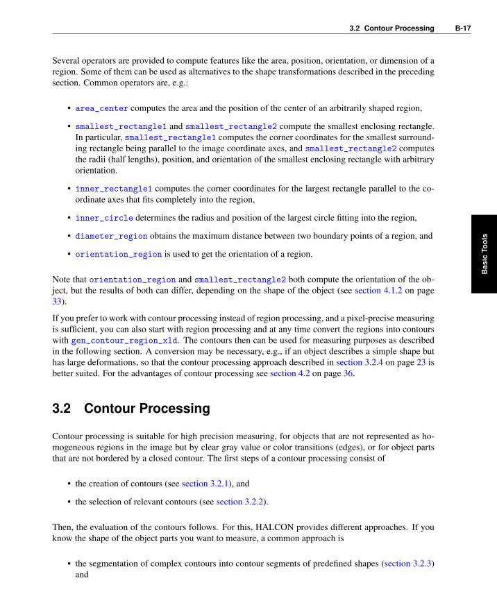
3.2 Contour Processing
Contour processing is suitable for high precision measuring, for objects that are not represented as ho-mogeneous regions in the image but by clear gray value or color transitions (edges), or for object partsthat are not bordered by a closed contour. The first steps of a contour processing consist of
• the creation of contours (see section 3.2.1), and
• the selection of relevant contours (see section 3.2.2).
Then, the evaluation of the contours follows. For this, HALCON provides different approaches. If youknow the shape of the object parts you want to measure, a common approach is
• the segmentation of complex contours into contour segments of predefined shapes (section 3.2.3)and
Bas
icTo
ols

B-18 Basic Tools
• the extraction of the parameters of shape primitives that approximate the contours or contour seg-ments (section 3.2.4).
If you have no knowledge about the object’s shape or the shapes cannot be approximated by a simpleshape like a line, circle, ellipse, or rectangle without loosing essential information, HALCON providesoperators similar to the ones introduced for the region processing, i.e., operators for
• the extraction of general contour features like the diameter, length, or orientation of contours ofunknown shape (section 3.2.5).
In some cases, contour processing is needed not for precision requirements but for one of its otheradvantages, which are introduced in section 4.2 on page 36. If a pixel-precise measuring is sufficient andthe contour processing is needed only for a part of the measuring process, you can afterwards switch tothe faster region processing. To do so, you can transform the contours into regions using the operatorgen_region_contour_xld.
3.2.1 Create Contours
Contour processing starts with the creation of contours. The common way to obtain contours is toextract edges. Edges are transitions between dark and light areas in an image and can be mathematicallydetermined by computing the image gradient, which can also be represented as edge amplitude and edgedirection. By selecting pixels with a high edge amplitude or a specific edge direction, contours betweenareas can be extracted. This can be done in various ways and with varying precision.
3.2.1.1 Pixel-Precise Edges and Lines
If a pixel-precise edge extraction is sufficient, an edge filter can be applied (see also Solution Guide I,chapter 6 on page 77). It leads to one or two edge images, for which the edge regions can be extracted byselecting the pixels with a given minimum edge amplitude using a threshold operator. To get edges witha thickness of one pixel, the obtained regions have to be thinned, e.g., by using the operator skeleton.Common pixel-precise edge filters are the operator sobel_amp, which is fast, and edges_image, whichis not that fast but already includes a hysteresis threshold and a thinning and leads to more accurateresults than sobel_amp. edges_image and also its equivalent for color images, edges_color, can alsobe applied with the parameter Filter set to ’sobel_fast’. Then, it is fast as well, but this parameteris recommended only for images with little noise or texture and sharp edges.
Besides edges, you can extract also lines that are built by thin structures on a contrasting background.In contrast to edges or the XLD lines that are obtained by a line fitting as described in section 3.2.4on page 23, they have a certain (not necessarily constant) width. A common filter for these lines isbandpass_image, which is again applied in combination with a threshold and a thinning.
For edge filters, after applying the filter, threshold, and thinning, the result typically is trans-formed into XLD contours. With this approach, a broad range of further processing methods isavailable. For the transformation of the thinned edge regions into contours, e.g., the operatorgen_contours_skeleton_xld is provided. Figure 3.3 (left) shows a pixel-precise edge obtained withedges_image.

3.2 Contour Processing B-19
3.2.1.2 Subpixel-Precise Edges and Lines
If a pixel-precise extraction is not sufficient, operators for the subpixel-precise edge and line extractioncan be applied (see Solution Guide I, chapter 7 on page 87). These immediately return XLD contours.Common operators to extract subpixel-precise edges are edges_sub_pix for the general edge extrac-tion, edges_color_sub_pix for extracting edges in color images, and zero_crossing_sub_pix forextracting zero crossings in an image, or respectively, to extract edges in Laplace-filtered images. Com-mon operators for the extraction of subpixel-precise lines, i.e., thin linear structures with a certain (notnecessarily constant) width, are lines_gauss for the general line extraction, lines_facet for extract-ing lines using a facet model, and lines_color for extracting lines in color images. Figure 3.3 (right)shows a subpixel-precise edge obtained with edges_sub_pix.
pixel precise edges subpixel precise edges
Figure 3.3: Edge extracted: (left) pixel-precise, (right) subpixel-precise.
3.2.1.3 Speed up the Contour Extraction
The subpixel-precise approaches are often slower than the pixel-precise approaches. To speed up thesubpixel-precise edge extraction, it is recommended to apply it only to a small region of interest (ROI).To obtain a suitable ROI you can, e.g., determine the region enclosed by the contour with a threshold-ing (e.g., using fast_threshold). The returned region then must be reduced to its boundary by theoperator boundary and possibly clipped by clip_region_rel. With a morphological operator, e.g.,dilation_circle, the region is expanded by a small amount, the image is reduced to the returned re-gion by reduce_domain, and the reduced image is used as an ROI. The ROI builds the search space forthe subpixel-precise edge extraction (see figure 3.4). One of the various HDevelop examples illustratingthis proceeding is described in section 5.3 on page 44.
3.2.1.4 Subpixel-Precise Thresholding
Another fast way to extract contours is provided by the subpixel-precise thresholding using the operatorthreshold_sub_pix, which can be applied in real time to a whole image. It is a thresholding operatorsimilar to the ones used for the region processing (see section 3.1.2 on page 14), but in contrast to themit does not result in a closed region but in subpixel-precise contours describing the border or parts of aborder of the region. Thus, in contrast to the threshold operators introduced for the region processing
Bas
icTo
ols

B-20 Basic Tools
b)a) c)
e)d) f)
Figure 3.4: Creation of ROI for subpixel-precise edge extraction: a) original image, b) pixel-precise edgeextraction, c) boundary for the edge region, d) dilation of the region, e) reduced domain (ROI),f) subpixel-precise edge extraction within the ROI.
the returned contours need not be closed, multiple contours can be obtained for the same region, andjunctions between contours are possible (see image figure 3.5 on page 21). Like for the thresholdingoperators used for a region processing, you can search for a suitable threshold using, e.g., the onlineGray Histogram inspection in HDevelop (with Display set to ’threshold’), or obtain informationabout the gray value distribution of the image by the operators gray_histo, histo_to_thresh, andintensity.
3.2.2 Get Relevant Contours
If the creation of the contours led to more contours than needed for the further processing, there aremeans to reduce the set of extracted contours to a set of contours relevant for the specific measuring task.
3.2.2.1 Suppress Irrelevant Contours
You can, e.g., suppress irrelevant contours by selecting only those contours fulfilling specific constraints.For example, the operator select_shape_xld can be used to select closed contours with a specificshape feature concerning, e.g., the contour’s convexity, circularity, or area. Almost 30 different shapefeatures are available, which are listed in the corresponding part of the Reference Manual. A similaroperator for the selection of specific contours is select_contours_xld. It can be used to select openand closed contours according to typical line features like length, curvature, or direction. The operator

3.2 Contour Processing B-21
Figure 3.5: Contours obtained by threshold_sub_pix. The border of a region consists of different, notnecessarily closed contours. Junctions are possible.
select_xld_point can be used in combination with mouse functions to interactively select contours.One of the various examples how to select significant features is given in section 5.11 on page 65.
3.2.2.2 Combine Contours
When having several contours that approximate the same object part, the number of segments can furtherbe reduced by a contour merging. Suitable operators are provided for the case that the contours
• lie approximately on the same line (union_collinear_contours_xld),
• on the same circle (union_cocircular_contours_xld, see figure 3.6),
• are adjacent (union_adjacent_contours_xld), or
• are cotangential (union_cotangential_contours_xld).
One of the examples applying a contour merging is described in section 5.9 on page 59.
For closed contours or polygons, you can also use set-theoretical operators to combine the enclosedregions of different closed contours or polygons. This is similar to the approach described for the regionprocessing in section 3.1.3 on page 15. Available operators are
• intersection_closed_contours_xld and intersection_closed_polygons_xld for thecalculation of the intersection of regions that are enclosed by closed contours or polygons,
• difference_closed_contours_xld and difference_closed_polygons_xld for the calcu-lation of the difference between regions that are enclosed by closed contours or polygons,
Bas
icTo
ols

B-22 Basic Tools
a) b)
c) d)
Figure 3.6: Get relevant contours: a) original image, b) subpixel-precise edges, c) selected contours withminimum length, d) cocircular contours merged.
• symm_difference_closed_contours_xld and symm_difference_closed_polygons_xld
for the calculation of the symmetric difference between regions that are enclosed by closed con-tours or polygons, and
• union2_closed_contours_xld and union2_closed_polygons_xld for merging regions thatare enclosed by closed contours or polygons.
3.2.2.3 Simplify Contours
Further, you can simplify contours by directly transforming them into shape primitives, which is similarto the approach described for the region processing in section 3.1.3 on page 15, but now works oncontours instead of regions. With shape_trans_xld you can transform a contour into
• the smallest enclosing circle,
• the ellipse having the same moments,
• the convex hull,
• or the smallest enclosing rectangle (either parallel to the coordinate axis or with arbitrary orienta-tion) (see figure 3.7).

3.2 Contour Processing B-23
b) c)a)
d) f)e)
Figure 3.7: Contours transformed into approximating shapes: a) original image, b) extracted contours aftersuppression of irrelevant contours, c) contours transformed into ellipses with the same mo-ments, d) contours transformed into their smallest enclosing circles, e) contours transformedinto their convex hulls, and f) contours transformed into their smallest enclosing rectangleswith arbitrary orientation.
3.2.3 Segment Contours
The obtained contours typically have more or less complex shapes. If a contour consists of elements ofknown shape, e.g., straight lines or circular arcs, a segmentation of the contour into these less complexcontours helps to make the investigation of the object easier, as now each segment can be measuredindividually. For the measuring, primitive shapes like lines or circles are fitted to the segments andtheir parameters, e.g., the diameter of a circle or the length of a line, can be obtained (see next section).Available shape primitives for a shape fitting comprise lines, circles, ellipses, and rectangles.
For the contour segmentation the operator segment_contours_xld can be applied. Dependent on theparameters you choose, a contour can be segmented into linear segments (see figure 3.8), linear and cir-cular segments, or linear and elliptic segments. The information by which shape each individual segmentis approximated is stored in the attribute ’cont_approx’. If you need only straight line segments, youcan alternatively use the operator gen_polygons_xld instead. To get the individual line segments ofthe polygon, apply the operator split_contours_xld.
3.2.4 Extract Features of Contour Segments by Approximating them byknown Shapes
The common step after the selection and possibly a segmentation is to fit shape primitives to the contoursor contour segments to get their specific shape parameters. The available shape primitives are lines,
Bas
icTo
ols

B-24 Basic Tools
Figure 3.8: Segment a contour: (left) original image with edges, (right) segmented contour.
circles, ellipses, and rectangles. The obtained features may be, e.g., the end points of the lines or thecenters and radii of the circles.
If you have applied a segmentation in a preceding step, for each segment the value of ’cont_approx’,i.e., the shape of the segment, can be queried with the operator get_contour_global_attrib_xld.Depending on its value, the best-suited shape primitive can be fitted into the contour segment using thecorresponding fitting approach:
• For linear segments (’cont_approx’ = -1), fit_line_contour_xld gets the parameters of eachline segment, e.g., the coordinates for both end points.
• For circular arcs (’cont_approx’ = 1), fit_circle_contour_xld and
• for elliptic arcs (’cont_approx’ = 0), fit_ellipse_contour_xld are used to compute thecenter positions, the radii, and the parts of the circles or ellipses that are covered by the contoursegments (determined by the angles of the start and end points).
• Rectangles consist either of a pure (unsegmented) contour or of linear contours thathave been merged, e.g., by union_adjacent_contours_xld. For them, the operatorfit_rectangle2_contour_xld is provided.
Examples for the application of the fitting operators are described, e.g., in section 5.6 on page 53 forlines, section 5.10 on page 62 for circles, and section 5.9 on page 59 for rectangles.
With the obtained parameters the corresponding contour can be generated for a visualiza-tion or a further processing. Lines can be generated with gen_contour_polygon_xld, cir-cles with gen_circle_contour_xld, ellipses with gen_ellipse_contour_xld, and rectangleswith gen_rectangle2_contour_xld. For the visualization, common visualization operators likedev_display are used. Figure 3.9 shows an example for fitting circles into circular contours and dis-playing their parameters.

3.2 Contour Processing B-25
b)a)
c) d)
Figure 3.9: Fit circles to circular contours: a) original image, b) contours after suppression of irrelevantcontours c) circles fitted into the contours d) visualization of radius R for each circle.
3.2.5 Extract Features of Contours Without Knowing Their Shapes
If the object to investigate cannot be described by a predefined shape primitive, HALCON providesseveral operators that compute general features of contours. Similar to the operators used for the featureextraction within a region processing (see section 3.1.4 on page 16), features like orientation or area canbe queried. Common operators used for 2D measuring with contours are:
• area_center_xld: area and center of gravity for the region enclosed by the contour or polygon,and the order of the points along the boundary.
• diameter_xld: the coordinates of the two extreme points of the contour having the maximumdistance, and the distance between them.
• elliptic_axis_xld: the two radii and the orientation of the ellipse having the same orientationand aspect ratio as the contour.
• length_xld: length of the contour or polygon.
• orientation_xld: orientation of the contour.
• smallest_circle_xld: center position and radius of the smallest enclosing circle.
Bas
icTo
ols

B-26 Basic Tools
• smallest_rectangle1_xld: coordinates of the corners describing the smallest enclosing rect-angle that is parallel to the coordinate axis.
• smallest_rectangle2_xld: center position, orientation, and the two radii (half lengths) of thesmallest enclosing rectangle with arbitrary orientation.
Some of the operators only work on contours that have no self intersections. Self intersections arenot always obvious as they can occur due to internal calculations of an operator, e.g., if an opencontour is closed for the needed operation (see figure 3.10). To check if a contour intersects it-self you can apply the operator test_self_intersection_xld. If you face problems because ofself intersections, you can also use the corresponding point-based operators. The available oper-ators are area_center_points_xld, moments_points_xld, orientation_points_xld, ellip-tic_axis_points_xld, eccentricity_points_xld, and moments_any_points_xld.
Figure 3.10: Self intersection: (left) curved contour, (right) self intersections occur because the contour isclosed for internal calculations of an operator.
3.3 2D Metrology
If you want to measure objects that are represented by simple shapes like circles, ellipses, rectangles, orlines, and you have approximate knowledge about their positions, orientations, and dimensions, you canuse 2D metrology to determine the exact shape parameters.
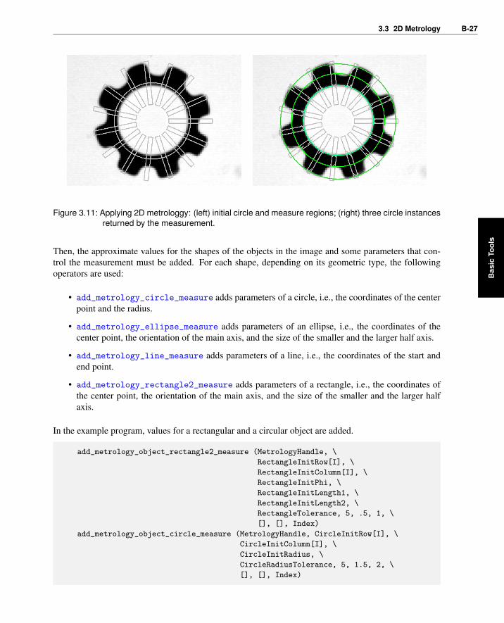
In particular, the values of the initial shape parameters are refined by a measurement that is based on theexact location of edges within so-called measure regions. These are rectangular regions that are evenlydistributed along the boundaries of the approximately known shapes. As shown in figure 3.11, for asingle inital shape also more than one refined instance may be returned.
The HDevelop example program hdevelop\2D-Metrology\apply_metrology_model.hdev showsthe basic steps of 2D metrology. First, a metrology model must be created using cre-
ate_metrology_model. In this model, all needed information related to the objects to measure willbe stored. To enable an efficient measurement, the size of the image in which the measurements will beperformed should be added to the model using the operator set_metrology_model_image_size.
read_image (Image, 'pads')get_image_size (Image, Width, Height)
create_metrology_model (MetrologyHandle)
set_metrology_model_image_size (MetrologyHandle, Width, Height)
3.3 2D Metrology B-27
Figure 3.11: Applying 2D metrologgy: (left) initial circle and measure regions; (right) three circle instancesreturned by the measurement.
Then, the approximate values for the shapes of the objects in the image and some parameters that con-trol the measurement must be added. For each shape, depending on its geometric type, the followingoperators are used:
• add_metrology_circle_measure adds parameters of a circle, i.e., the coordinates of the centerpoint and the radius.
• add_metrology_ellipse_measure adds parameters of an ellipse, i.e., the coordinates of thecenter point, the orientation of the main axis, and the size of the smaller and the larger half axis.
• add_metrology_line_measure adds parameters of a line, i.e., the coordinates of the start andend point.
• add_metrology_rectangle2_measure adds parameters of a rectangle, i.e., the coordinates ofthe center point, the orientation of the main axis, and the size of the smaller and the larger halfaxis.
In the example program, values for a rectangular and a circular object are added.
add_metrology_object_rectangle2_measure (MetrologyHandle, \
RectangleInitRow[I], \
RectangleInitColumn[I], \
RectangleInitPhi, \
RectangleInitLength1, \
RectangleInitLength2, \
RectangleTolerance, 5, .5, 1, \
[], [], Index)
add_metrology_object_circle_measure (MetrologyHandle, CircleInitRow[I], \
CircleInitColumn[I], \
CircleInitRadius, \
CircleRadiusTolerance, 5, 1.5, 2, \
[], [], Index)
Bas
icTo
ols

B-28 Basic Tools
The actual measurement in the image is performed with the operator apply_metrology_model. Therefined shape parameters that result from the measurement can be accessed from the metrology modelwith the operator get_metrology_object_result.
apply_metrology_model (Image, MetrologyHandle)
get_metrology_object_result (MetrologyHandle, MetrologyRectangleIndices, \
'all', 'result_type', 'param', \
RectangleParameter)
get_metrology_object_result (MetrologyHandle, MetrologyCircleIndices, 'all', \
'result_type', 'param', CircleParameter)
If the metrology model is not needed anymore, it is destroyed with clear_metrology_model.
clear_metrology_model (MetrologyHandle)
Besides the basic steps, several other steps may be performed. Amongst others, you can adjustparameters of the metrology model before you apply the measurement. For example, you canadd the results of a camera calibration to the model to obtain the measurement results in worldcoordinates, or you can change several parameters that control the measurement. The parame-ters are adjusted with the operator set_metrology_object_param. To access the measure re-gions, which may be helpful when adjusting the parameters that control the measurement, you callthe operator get_metrology_object_measures. Furthermore, you can use the operator trans-
form_metrology_object to transform the objects of the metrology model, e.g., to align them withthe positions and rotation angles obtained by an operator like find_shape_model (see Solution GuideII-B, section 2.4.3.2 on page 42 for further information about alignment). For details about 2D metrol-ogy, see the entry in the Reference Manual for create_metrology_model.
3.4 Geometric Operations
HALCON provides a selection of operators for geometric operations to calculate the relation betweenelements like points, lines, line segments, contours, or regions. Points can be determined by several pointoperators, e.g., points_foerstner, or by the intersection of lines. Lines, line segments, contours,and regions can be obtained as described in section 3.1 on page 13 and section 3.2 on page 17. Therelations between the individual elements can be calculated by several operators. Most of the operatorsare constructed to calculate the distance relation between the elements. The operators for the distancerelations are summarized in the following list:
Point Line Line Segment ContourPoint distance_pp distance_pl distance_ps distance_pc
Line distance_pl – distance_sl distance_lc
Line Segment distance_ps distance_sl distance_ss distance_sc
Contour distance_pc distance_lc distance_sc distance_cc
distance_cc_min
Region distance_pr distance_lr distance_sr –

3.4 Geometric Operations B-29
RegionPoint distance_pr
Line distance_lr
Line Segment distance_sr
Contour –Region distance_rr_min
distance_rr_min_dil
Further operators for geometric operations are provided, which can be used to calculate, e.g.,
• the angle between two lines: angle_ll,
• the angle between a line and the vertical axis: angle_lx,
• a point on an ellipse corresponding to a specific angle: get_points_ellipse,
• the intersection of two lines: intersection_lines, and
• the projection of a point onto a line: projection_pl.
Bas
icTo
ols

B-30 Basic Tools

Tool Selection B-31
Chapter 4
Tool Selection
Because many tools are available, it is not obvious which tool to use in which situation. Section 4.1guides you from the feature you want to extract and the object’s appearance in the image to the ap-propriate tool to use. In section 4.2, additionally the two most important tools, region processing andcontour processing, are compared. Practical guidance is provided in section 5 by a selection of HDevelopexample programs that solve common measuring tasks.
4.1 From the Feature to the Tool
If you have no special requirements like precision or speed, often several measuring approaches areavailable to obtain the same feature as result. The graph in figure 4.1 leads you from a single feature youwant to measure and the appearance of the object in the image to the part of section 3 that describes thebasic tools suited best for your task. If you have specific requirements like precision or speed, you shouldadditionally consider the different characteristics of region processing and contour processing discussedin section 4.2 on page 36.
Tool
Sel
ectio
n

B-32 Tool Selection
Measure thedimension or area ofan object
-Object represented byregions of similar grayvalue, color, or texture
-Region Processing(section 3.1 on page13)
-
Objects represented byclear-cut edges,contours can bedecomposed intosimple shapes
-Contour Processing(section 3.2 on page17)
-
Objects have simpleshapes with shapeparameters that areapproximately known
-2D Metrologoy(section 3.3 on page26)
Measure theorientation, position,or number of objects
Objects all have thesame, complex shape
-
-
-
-
- -Matching (SolutionGuide I, chapter 9 onpage 111)
Objects are edgesperpendicular to a lineor an arc
-
1D Measuring(Solution Guide I,chapter 5 on page 63),or Solution GuideIII-A
Measure an angle ordistance
- between objects orobject parts
-
-between segments likepositions, edges, orregions
Calculate the angle ordistance from theirorientations orpositions
6
Geometric Operations(section 3.4 on page28)
-
-
Figure 4.1: From the feature to measure to the corresponding basics section.

4.1 From the Feature to the Tool B-33
In most applications, it is not sufficient to obtain a single feature from an image since many featuresare needed to obtain the final feature that is searched for. Thus, dependent on the specific task and thecharacteristics of the object the basic tools are combined in different ways. The decision which toolto use does not only depend on the appearance of the object and the special requirements concerningprecision or speed, but also on the interdependencies of the several tasks of an application and thereforealso on the features you have already obtained during a preceding step of your program. Because there isa huge amount of influences, this guide can not be all-embracing, but hopefully conveys to you a feelingfor the available tools.
Therefore, we shortly summarize which tools or approaches are common to obtain the different objectfeatures. Most of the corresponding examples, which can be used as practical guidance, are provided insection 5 on page 41.
4.1.1 Area
The area of an object is in most cases obtained by the operator area_center, i.e., via a region processing(see, e.g., the example in section 5.1 on page 41).
If a subpixel-precise measuring requires contour processing, you can use the corresponding operatorarea_center_xld or area_center_points_xld (see example in section 6.2 on page 84) instead.
Be aware that when computing the area of a region, possible holes in the region are considered, whereaswhen computing the area of a contour, the whole area enclosed by the contour is obtained. In the lattercase, you therefore have to extract also the contours of the holes, get their areas, and subtract them fromthe area enclosed by the outer contour.
The mentioned operators were introduced in section 3.1.4 on page 16 for regions and in section 3.2.5 onpage 25 for contours.
In addition, the operator area_holes calculates the area of the holes in the input regions.
4.1.2 Orientation and Angle
For the orientation of an arbitrary object, typically the operator orientation_region (see, e.g., theexample in section 5.1 on page 41) is used and can be replaced for contours by the corresponding operatororientation_xld (see example in section 5.4 on page 49).
The operators elliptic_axis and elliptic_axis_xld compute the orientation and radii of the el-lipse having the same moments as the input region or contour, respectively.
For very small symmetric objects, the operator elliptic_axis_gray is recommended (see example insection 5.12 on page 68).
If you want to obtain the orientation and extents of the smallest enclosing rectangle of an object, you candetermine them via smallest_rectangle2 for regions (see also example in section 5.12 on page 68)and smallest_rectangle2_xld for contours.
The mentioned operators were introduced in section 3.1.4 on page 16 for regions and in section 3.2.5 onpage 25 for contours.
Tool
Sel
ectio
n
B-34 Tool Selection
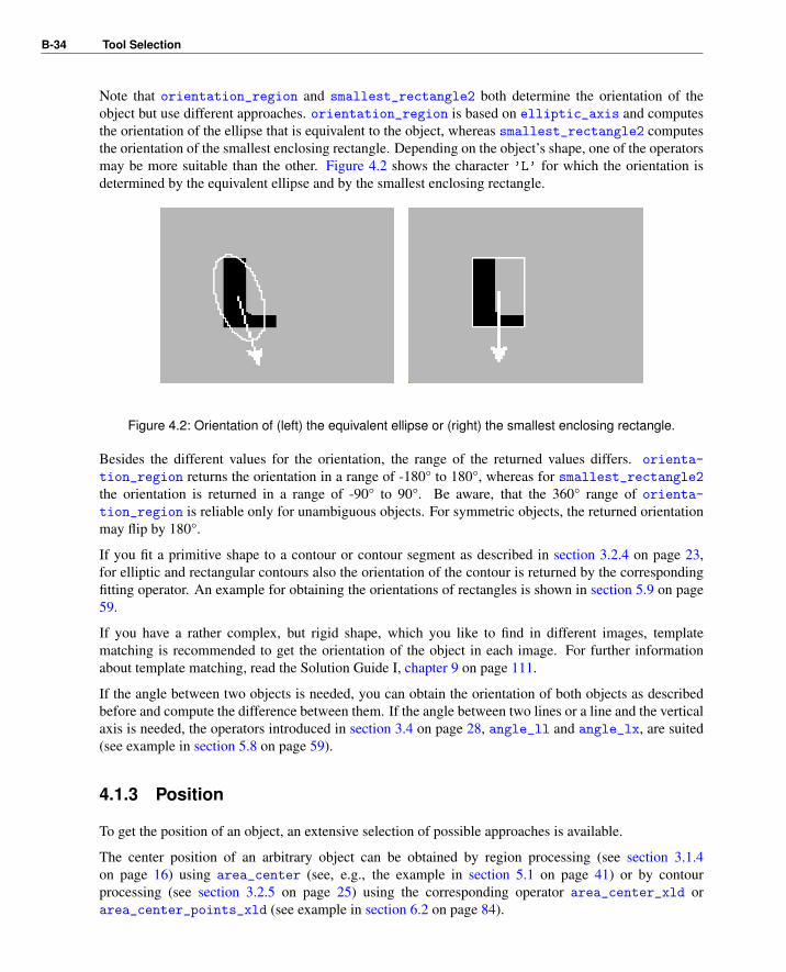
Note that orientation_region and smallest_rectangle2 both determine the orientation of theobject but use different approaches. orientation_region is based on elliptic_axis and computesthe orientation of the ellipse that is equivalent to the object, whereas smallest_rectangle2 computesthe orientation of the smallest enclosing rectangle. Depending on the object’s shape, one of the operatorsmay be more suitable than the other. Figure 4.2 shows the character ’L’ for which the orientation isdetermined by the equivalent ellipse and by the smallest enclosing rectangle.
Figure 4.2: Orientation of (left) the equivalent ellipse or (right) the smallest enclosing rectangle.
Besides the different values for the orientation, the range of the returned values differs. orienta-
tion_region returns the orientation in a range of -180° to 180°, whereas for smallest_rectangle2the orientation is returned in a range of -90° to 90°. Be aware, that the 360° range of orienta-
tion_region is reliable only for unambiguous objects. For symmetric objects, the returned orientationmay flip by 180°.
If you fit a primitive shape to a contour or contour segment as described in section 3.2.4 on page 23,for elliptic and rectangular contours also the orientation of the contour is returned by the correspondingfitting operator. An example for obtaining the orientations of rectangles is shown in section 5.9 on page59.
If you have a rather complex, but rigid shape, which you like to find in different images, templatematching is recommended to get the orientation of the object in each image. For further informationabout template matching, read the Solution Guide I, chapter 9 on page 111.
If the angle between two objects is needed, you can obtain the orientation of both objects as describedbefore and compute the difference between them. If the angle between two lines or a line and the verticalaxis is needed, the operators introduced in section 3.4 on page 28, angle_ll and angle_lx, are suited(see example in section 5.8 on page 59).
4.1.3 Position
To get the position of an object, an extensive selection of possible approaches is available.
The center position of an arbitrary object can be obtained by region processing (see section 3.1.4on page 16) using area_center (see, e.g., the example in section 5.1 on page 41) or by contourprocessing (see section 3.2.5 on page 25) using the corresponding operator area_center_xld orarea_center_points_xld (see example in section 6.2 on page 84).
4.1 From the Feature to the Tool B-35
For very small symmetric objects, the operator area_center_gray is recommended (see example insection 5.12 on page 68).
If the objects can be split into primitive shapes like lines, circles, ellipses, or rectangles, and theseprimitives are the objects of interest for the further investigation, fitting primitive shapes to the contours(see section 3.2.4 on page 23) leads to the positions of their center points or, in case of a line fitting, theirend points. In section 5.9 on page 59, e.g., the fitting of rectangles to contours is described to obtain theposition and orientation of rectangular objects. The examples in section 5.10 on page 62 and section 5.11on page 65 show the corresponding process for fitting circles to circular contour segments.
If you have a rather complex, but rigid shape, which you like to find in different images, templatematching is recommended to get the position of the object in each image. For further information abouttemplate matching, read the Solution Guide I, chapter 9 on page 111.
How to measure the positions of edges and the distances between them along a line or an arc that isapproximately perpendicular to them is briefly described in the Solution Guide I, chapter 5 on page 63.Details can be found in the Solution Guide III-A.
If the position of a corner point of a contour is searched for, either point operators can be used (seesection 3.4 on page 28), or lines, obtained by line fitting (see section 3.2.4 on page 23), are intersectedusing intersection_lines. Both approaches are used by the example in section 5.7 on page 57.
The intersection of lines can be applied also to get, e.g., the junction points of a grid (see example insection 5.6 on page 53). Additionally, contours or also regions can be intersected with other contours orregions to get the positions of points of intersection.
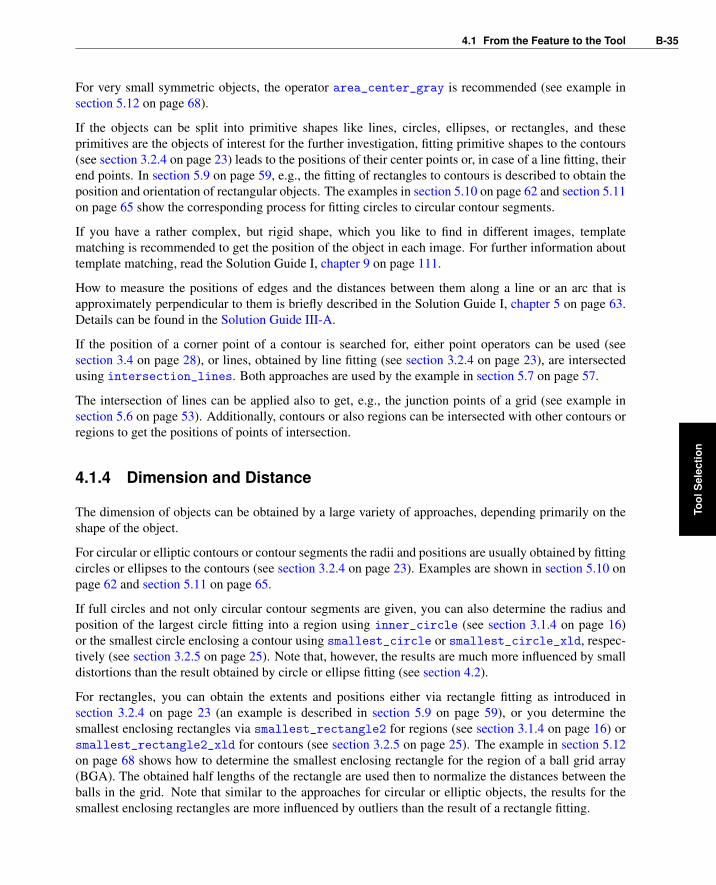
4.1.4 Dimension and Distance
The dimension of objects can be obtained by a large variety of approaches, depending primarily on theshape of the object.
For circular or elliptic contours or contour segments the radii and positions are usually obtained by fittingcircles or ellipses to the contours (see section 3.2.4 on page 23). Examples are shown in section 5.10 onpage 62 and section 5.11 on page 65.
If full circles and not only circular contour segments are given, you can also determine the radius andposition of the largest circle fitting into a region using inner_circle (see section 3.1.4 on page 16)or the smallest circle enclosing a contour using smallest_circle or smallest_circle_xld, respec-tively (see section 3.2.5 on page 25). Note that, however, the results are much more influenced by smalldistortions than the result obtained by circle or ellipse fitting (see section 4.2).
For rectangles, you can obtain the extents and positions either via rectangle fitting as introduced insection 3.2.4 on page 23 (an example is described in section 5.9 on page 59), or you determine thesmallest enclosing rectangles via smallest_rectangle2 for regions (see section 3.1.4 on page 16) orsmallest_rectangle2_xld for contours (see section 3.2.5 on page 25). The example in section 5.12on page 68 shows how to determine the smallest enclosing rectangle for the region of a ball grid array(BGA). The obtained half lengths of the rectangle are used then to normalize the distances between theballs in the grid. Note that similar to the approaches for circular or elliptic objects, the results for thesmallest enclosing rectangles are more influenced by outliers than the result of a rectangle fitting.
Tool
Sel
ectio
n

B-36 Tool Selection
Many applications that aim to get the distance between objects or object parts extract suitable positions,e.g., the intersection points of two intersecting lines, and use them to measure distances between themand another point, line, line segment, contour, or region by a geometric operation (see section 3.4 onpage 28). The example in section 5.6 on page 53, e.g., intersects the lines of a grid to calculate thepositions of its junctions, which then could be used, e.g., to get the extent of the grid. Another example(section 5.7 on page 57) intersects lines to get the positions of the corner points of a metal plate andafterwards calculates the distance between them and the positions of the same points obtained by a pointoperator (for point operators see section 3.4 on page 28). The maximum distance between a contour andits approximating line (regression line) is determined in the example in section 5.3 on page 44.
How to measure the positions of edges and the distances between them along a line or an arc that isapproximately perpendicular to them is briefly described in the Solution Guide I, chapter 5 on page 63.Details can be found in the Solution Guide III-A.
The width of an object can be obtained by different means, depending on the object. For example, thewidth of thin lines like cables, rivers, or arteries are often obtained by lines_gauss as described insection 5.5 on page 51, whereas the width of a strictly polygonal object is better obtained by calculatingthe distance between individual lines or points via geometric operations, which are possibly applied afterchecking the lines for parallelism (see example in section 5.4 on page 49). The width of an object maybe also obtained via region processing, e.g., by using the smallest enclosing rectangle or, if the objectconsists of jagged lines, orient the object and its region parallel to the vertical axis and calculate thedifference between the column coordinates of the region’s border in each row to get the mean, minimum,and maximum width (see example in section 5.2 on page 43).
For objects with an arbitrary shape, region-based feature extraction, as described in section 3.1.4 on page16, or the corresponding contour-based operators introduced in section 3.2.5 on page 25 can be usedto get some general features of their region or contour. The example in section 6.2 on page 84, e.g.,uses the operator length_xld to compute the length of a contour representing a scratch in an anodizedaluminum surface.
4.1.5 Number of Objects
To get the number of objects, the common method is to work with tuples and to count their elements. InHDevelop, if a tuple contains iconic data, e.g., regions or contours, you can query the number of elementsusing the operator count_obj. If the tuple contains control data, e.g., the numeric results obtained forthe rows or columns of a set of positions, you can query the number of elements via the correspondingHDevelop operation (|tuple|) inside the operator assign. Note also that the indices of numerical tuplesdo not correspond to the indices of the iconic tuples. Numerical tuples start with 0 and iconic tuplesstart with 1. For more information about the HDevelop syntax related to tuples, see the HDevelop User’sGuide, section 8.5.3 on page 349.
The next section goes deeper into the main differences between region processing and contour process-ing.
4.2 Region Processing vs. Contour Processing
The basic tools needed for 2D measuring are region processing and contour processing. Both can be usedto get the area, orientation, position, dimension, or number of objects. This section helps you decide

4.2 Region Processing vs. Contour Processing B-37
which approach is suited best for your task. For this, the appearance of the object in the image is takeninto account. The following table summarizes the main differences between both tools. Afterwards, theindividual topics are explained in more detail.
Region Processing Contour Processinga) pixel-precise pixel- or subpixel-preciseb) fast not as fast as region processingc) works on closed contours works on open and closed contoursd) outliers strongly influence the result of a outliers can be compensated
shape approximatione) gray-value behavior of object may not change gray-value behavior of object may changef) not sensitive to bad contrast sensitive to bad contrast
a) The methods belonging to region processing can be applied only with pixel precision. Therefore, themethods are rather fast and easy to apply. For contour processing both pixel- as well as subpixel-precisemethods are provided. The speed of an application varies depending on the used operators.
b) Region processing is not as precise, but in most cases significantly faster than contour processing. TheHDevelop program solution_guide\2d_measuring\measure_metal_part_extended.hdev ex-tracts an object and its area, center position, and orientation using region processing on one hand and con-tour processing on the other hand. For the region processing, the operators threshold, area_centerand orientation_region are applied. The contour processing is preceded by the creation of an ROIto speed up the edge extraction. For this, the operators threshold, boundary, and reduce_domain areused. The actual contour processing then consists of the operators edges_sub_pix, area_center_xldand orientation_xld. For the contour processing, the areas of the holes of the metal plate have to besubtracted to get the actual area of the plate. Figure 4.3 shows the run time needed for both approaches.The region processing is significantly faster.
Figure 4.3: With region processing the extraction of area, center, and orientation is significantly faster thanwith contour processing.
c) Region processing only works for closed areas. For open contours, e.g., if only parts of the border
Tool
Sel
ectio
n
B-38 Tool Selection
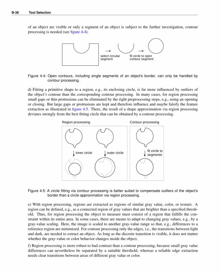
of an object are visible or only a segment of an object is subject to the further investigation, contourprocessing is needed (see figure 4.4).
segmentselect circular
contour segmentfit circle to open
Figure 4.4: Open contours, including single segments of an object’s border, can only be handled bycontour processing.
d) Fitting a primitive shape to a region, e.g., its enclosing circle, is far more influenced by outliers ofthe object’s contour than the corresponding contour processing. In many cases, for region processingsmall gaps or thin protrusions can be eliminated by the right preprocessing steps, e.g., using an openingor closing. But large gaps or protrusions are kept and therefore influence and maybe falsify the featureextraction as illustrated in figure 4.5. There, the result of a shape approximation via region processingdeviates strongly from the best fitting circle that can be obtained by a contour processing.
Region processing Contour processing
inner circle outer circle segmentsfit circle to
Figure 4.5: A circle fitting via contour processing is better suited to compensate outliers of the object’sborder than a circle approximation via region processing.
e) With region processing, regions are extracted as regions of similar gray value, color, or texture. Aregion can be defined, e.g., as a connected region of gray values that are brighter than a specified thresh-old. Thus, for region processing the object to measure must consist of a region that fulfills the con-straint within its entire area. In some cases, there are means to adapt to changing gray values, e.g., by agray-value scaling. Here, the image is scaled to another gray-value range so that, e.g., differences to areference region are minimized. For contour processing only the edges, i.e., the transitions between lightand dark, are needed to extract an object. As long as the discrete transition is visible, it does not matterwhether the gray-value or color behavior changes inside the object.
f) Region processing is more robust to bad contrast than a contour processing, because small gray valuedifferences can nevertheless be separated by a suitable threshold, whereas a reliable edge extractionneeds clear transitions between areas of different gray value or color.

4.2 Region Processing vs. Contour Processing B-39
The following section provides you with a comprehensive collection of example applications that solvedifferent tasks and can be used as a guide for your applications.
Tool
Sel
ectio
n

B-40 Tool Selection

Examples for Practical Guidance B-41
Chapter 5
Examples for Practical Guidance
The previous sections described theoretically how to use several tools provided by HALCON. Sinceevery measuring task is unique, different influences must be considered for each special case. The puretheory may not be sufficient to get a feeling for choosing the right tool for a specific task. To give you alsopractical guidance, the following sections describe a collection of examples solving common measuringtasks.
5.1 Rotate Image and Region (2D Transformation)
For many measuring tasks, it is useful to align the object of interest parallel to the coordinate axis of theimage. If the object cannot be aligned already at the image acquisition, the image or the extracted regionsmust be rotated by image processing. A rotation as well as a translation or a scaling can be realized byan affine 2D transformation, which is easily applied with HALCON.
The HDevelop program solution_guide\2d_measuring\measure_screw.hdev measures differentdimension-related features of a screw. The image of the screw is acquired using a back light to geta good contrast between fore- and background. For the approach described in section 5.2, piecewisedistance measuring is needed to obtain the minimum, maximum, and mean width of the screw. If thescrew is vertical, the measuring can be applied easily row by row. Otherwise, the calculations becomemore complex. Thus, the first task of the program is to rotate the region of the screw so that it becomesvertical.
The necessary steps for the rotation comprise
• the determination of the parameters for the rotation,
• the creation of a homogeneous transformation matrix, and
• the transformation of the region.
Tool
Sel
ectio
n

B-42 Examples for Practical Guidance
Figure 5.1: Affine 2D transformation: (left) original image, (right) rotated region.
Step 1: Determine parameters for the rotation
threshold (Image, Region, 0, 100)
orientation_region (Region, OrientationRegion)
area_center (Region, Area, RowCenter, ColumnCenter)
Before applying a 2D transformation, the parameters for the transformation must be determined. Here,the region of the object is extracted using threshold and the orientation of the region is determinedvia orientation_region. The orientation intended for the following measuring is 90°. As center forthe rotation we choose the center position of the region, which we obtain with area_center. Note thatbecause of the approximately symmetrical shape of the screw, the screw can be twisted by 180°, but forthe described task it is not important at which side of the screw we start to measure.
Step 2: Create the homogeneous transformation matrix
vector_angle_to_rigid (RowCenter, ColumnCenter, OrientationRegion, \
RowCenter, ColumnCenter, rad(90), HomMat2DRotate)
Now, vector_angle_to_rigid is applied. The operator creates a homogeneous transformation matrixfor a simultaneous rotation and translation. Here, only a rotation is applied, i.e., the center point isthe same for the original and the transformed region and only the angle is changing from the originalorientation to the vertical direction. An additional translation is recommended, e.g., if similar objectsin several images have to be placed in the same position so that a direct comparison between themis possible. Another need for a translation occurs if the object or parts of it moved out of the imagebecause of the rotation. Alternatively to vector_angle_to_rigid, you can also create a homogeneoustransformation matrix for the identical 2D transformation by hom_mat2d_identity and add a rotationand a translation to it by hom_mat2d_rotate and hom_mat2d_translate, respectively. Furthermore,if needed, also a scaling can be added to the homogeneous transformation matrix by hom_mat2d_scale,but you have to consider carefully that a scaling significantly influences the absolute values obtained by

5.2 Get Width of Screw Thread B-43
the measuring. To compensate this, you can afterwards transform the measurement results back to theoriginal dimension by applying the inverse transformation matrix to them.
Step 3: Transform region
affine_trans_region (Region, RegionAffineTrans, HomMat2DRotate, \
'nearest_neighbor')
The actual transformation of the region is realized by the operator affine_trans_region (see fig-ure 5.1). The rotated region is now used for the measuring task described in the next section.
5.2 Get Width of Screw Thread
The first measuring approach of the HDevelop program solution_guide\2d_measuring\
measure_screw.hdev measures the minimum, maximum, and mean width of a screw thread. Forthis, we use the vertical region of the screw obtained in section 5.1 and measure the difference betweenthe column coordinates of the region’s border in each row.
Figure 5.2: Between the two white lines for each row, the distance is measured via a region processing.
The general steps for this task comprise
• the extraction of the width of the object in each row and
• the calculation of the mean, minimum, and maximum width.
Tool
Sel
ectio
n

B-44 Examples for Practical Guidance
Step 1: Get object width for each row
closing_circle (RegionAffineTrans, RegionToProcess, 4.5)
get_region_runs (RegionToProcess, RowRegionRuns, ColumnBegin, ColumnEnd)
NumberLines := |RowRegionRuns|
ColumnBeginSelected := ColumnBegin[90:NumberLines - 90]
ColumnEndSelected := ColumnEnd[90:NumberLines - 90]
Diameter := ColumnEndSelected - ColumnBeginSelected + 1
The operator get_region_runs examines a region row by row. In particular, it returns three tuples,one containing the row coordinates of the region and two containing the column coordinates where theregion begins and ends in the corresponding rows (seen from left to right). The difference between thetwo tuples containing column coordinates results in a tuple containing the widths of the object for eachrow. Note that this proceeding works only for regions having exactly one start and one end point per row.Thus, before applying get_region_runs, small gaps that lead to more than one start and end point areeliminated by a closing using closing_circle.
Step 2: Calculate mean, minimum, and maximum width
meanDiameter := mean(Diameter)
minDiameter := min(Diameter)
The tuple containing the widths of the object in each row are used now to calculate the mean, minimum,and maximum horizontal distance of the object (see figure 5.2).
In this approach, the column coordinates of the screw’s border, which are used to calculate the horizontaldistance in each row, are obtained by region processing. Alternatively, contour points can be obtained bya contour processing and their coordinates can be used for the width calculation. How to obtain contourpoints is, e.g., described in section 5.3 for the two thread edges EdgeContour0 and EdgeContour1.
5.3 Get Deviation of a Contour from a Straight Line
The second measuring approach in the HDevelop program solution_guide\2d_measuring\
measure_screw.hdev uses contour processing to measure the deviations of the thread edges from theirapproximating straight lines, the so-called regression lines.
Individual points on the thread edges alternatively can be obtained by region processing, e.g., using theoperator get_region_points, but for the calculation of the regression lines, a contour processing isnecessary. The general steps applied here comprise
• the creation of an ROI,
• the extraction and alignment of contours,
• the determination of regression lines,
• the extraction of the contour points of the thread edges,
• the calculation of the horizontal distances between the thread edges and the regression lines, and
5.3 Get Deviation of a Contour from a Straight Line B-45
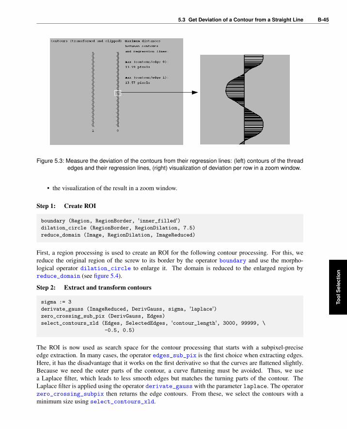
Figure 5.3: Measure the deviation of the contours from their regression lines: (left) contours of the threadedges and their regression lines, (right) visualization of deviation per row in a zoom window.
• the visualization of the result in a zoom window.
Step 1: Create ROI
boundary (Region, RegionBorder, 'inner_filled')dilation_circle (RegionBorder, RegionDilation, 7.5)
reduce_domain (Image, RegionDilation, ImageReduced)
First, a region processing is used to create an ROI for the following contour processing. For this, wereduce the original region of the screw to its border by the operator boundary and use the morpho-logical operator dilation_circle to enlarge it. The domain is reduced to the enlarged region byreduce_domain (see figure 5.4).
Step 2: Extract and transform contours
sigma := 3
derivate_gauss (ImageReduced, DerivGauss, sigma, 'laplace')zero_crossing_sub_pix (DerivGauss, Edges)
select_contours_xld (Edges, SelectedEdges, 'contour_length', 3000, 99999, \
-0.5, 0.5)
The ROI is now used as search space for the contour processing that starts with a subpixel-preciseedge extraction. In many cases, the operator edges_sub_pix is the first choice when extracting edges.Here, it has the disadvantage that it works on the first derivative so that the curves are flattened slightly.Because we need the outer parts of the contour, a curve flattening must be avoided. Thus, we usea Laplace filter, which leads to less smooth edges but matches the turning parts of the contour. TheLaplace filter is applied using the operator derivate_gauss with the parameter laplace. The operatorzero_crossing_subpix then returns the edge contours. From these, we select the contours with aminimum size using select_contours_xld.
Tool
Sel
ectio
n
B-46 Examples for Practical Guidance
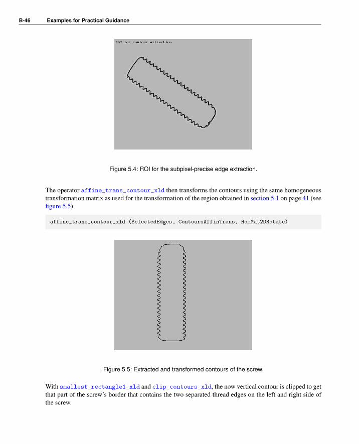
Figure 5.4: ROI for the subpixel-precise edge extraction.
The operator affine_trans_contour_xld then transforms the contours using the same homogeneoustransformation matrix as used for the transformation of the region obtained in section 5.1 on page 41 (seefigure 5.5).
affine_trans_contour_xld (SelectedEdges, ContoursAffinTrans, HomMat2DRotate)
Figure 5.5: Extracted and transformed contours of the screw.
With smallest_rectangle1_xld and clip_contours_xld, the now vertical contour is clipped to getthat part of the screw’s border that contains the two separated thread edges on the left and right side ofthe screw.

5.3 Get Deviation of a Contour from a Straight Line B-47
smallest_rectangle1_xld (ContoursAffinTrans, Row11, Column11, Row21, \
Column21)
clip_contours_xld (ContoursAffinTrans, ClippedContours, Row11 + 90, 0, \
Row21 - 90, Width)
Step 3: Get regression lines
fit_line_contour_xld (ClippedContours, 'regression', -1, 0, 5, 2, RowBegin, \
ColBegin, RowEnd, ColEnd, Nr, Nc, Dist1)
The operator fit_line_contour_xld now uses the contours to compute the start (RowBegin, ColBe-gin) and end (RowEnd, ColEnd) points for the regression lines (see figure 5.6). To get the points of theregression lines, the parameter Algorithm must be set to ’regression’.
Figure 5.6: Clipped contours and the corresponding regression lines.
Until now, we handled both contours together in tuples. The tuple Edges contains the contours of thetwo thread edges, and the tuples for the start and end points of the regression lines contain the points forboth regression lines. With the operator gen_contour_polygon_xld we explicitly create the contoursof the individual regression lines. For this, we use the corresponding start and end points as input, i.e.,for the first regression line (RegressContour0) we use the start and end points with the index 0, and forthe second regression line (RegressContour1) we use the elements with index 1.
gen_contour_polygon_xld (RegressContour0, [RowBegin[0],RowEnd[0]], \
[ColBegin[0],ColEnd[0]])
gen_contour_polygon_xld (RegressContour1, [RowBegin[1],RowEnd[1]], \
[ColBegin[1],ColEnd[1]])
Tool
Sel
ectio
n

B-48 Examples for Practical Guidance
Step 4: Extract contour points of the thread edges
select_obj (ClippedContours, EdgeContour0, 1)
get_contour_xld (EdgeContour0, RowEdge0, ColEdge0)
select_obj (ClippedContours, EdgeContour1, 2)
get_contour_xld (EdgeContour1, RowEdge1, ColEdge1)
To get the deviation between the thread contours and their corresponding regression lines, we addition-ally need the contour points of the thread contours. The thread contours are stored both in the tupleEdges. Since we want to access the individual contours more than once, the usage of the indices maybecome a little bit confusing. To make the code clearer and also to apply further tuple operations toeach contour later on, we select the elements of the tuple individually and assign concise names to them:EdgeContour0 and EdgeContour1. In HDevelop, the selection of iconic objects is not realized via theoperator assign but by the operator select_obj. Note that the index of iconic objects starts with 1
instead of 0. For the thread contours EdgeContour0 and EdgeContour1, a tuple containing the rowsand columns of the contour points is obtained with get_contour_xld.
Step 5: Calculate the horizontal distances
distance_pc (RegressContour0, RowEdge0, ColEdge0, DistanceMin0, \
DistanceMax0)
minDistance0 := min(DistanceMin0)
maxDistance0 := max(DistanceMin0)
meanDistance0 := mean(DistanceMin0)
The obtained contour points are used to calculate the distances between each contour point of the threadedge and the contour of the corresponding regression line. The operator distance_pc returns the min-imum and maximum distances. The minimum distances between the contour points and the contour ofthe regression line correspond to the horizontal distances in approximately each row (as long as the screwis vertical). These in turn can be used to query the minimum, maximum, and mean horizontal distancebetween both contours (see figure 5.3, left). The code only shows the proceeding for EdgeContour0and RegressContour0.
Step 6: Visualize the result in a zoom window
dev_display (EdgeContour0)
dev_display (RegressContour0)
get_contour_xld (RegressContour0, RowContour0, ColContour0)
for i := 800 to 950 by 1
projection_pl (RowEdge0[i], ColEdge0[i], RowContour0[0], ColContour0[0], \
RowContour0[1], ColContour0[1], RowProj0, ColProj0)
gen_contour_polygon_xld (Contour, [RowEdge0[i],RowProj0], [ColEdge0[i], \
ColProj0])
dev_display (Contour)
endfor
To visualize the individual horizontal distances between a thread contour and its regression line ina zoom window (see figure 5.3, right), the endpoints of the regression line are made explicit by
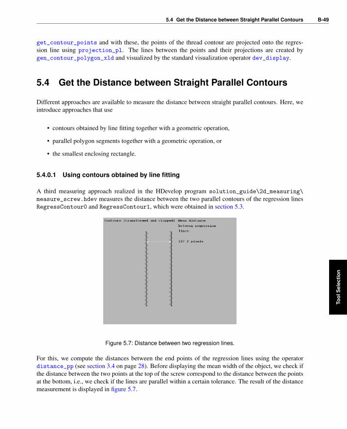
5.4 Get the Distance between Straight Parallel Contours B-49
get_contour_points and with these, the points of the thread contour are projected onto the regres-sion line using projection_pl. The lines between the points and their projections are created bygen_contour_polygon_xld and visualized by the standard visualization operator dev_display.
5.4 Get the Distance between Straight Parallel Contours
Different approaches are available to measure the distance between straight parallel contours. Here, weintroduce approaches that use
• contours obtained by line fitting together with a geometric operation,
• parallel polygon segments together with a geometric operation, or
• the smallest enclosing rectangle.
5.4.0.1 Using contours obtained by line fitting
A third measuring approach realized in the HDevelop program solution_guide\2d_measuring\
measure_screw.hdev measures the distance between the two parallel contours of the regression linesRegressContour0 and RegressContour1, which were obtained in section 5.3.
Figure 5.7: Distance between two regression lines.
For this, we compute the distances between the end points of the regression lines using the operatordistance_pp (see section 3.4 on page 28). Before displaying the mean width of the object, we check ifthe distance between the two points at the top of the screw correspond to the distance between the pointsat the bottom, i.e., we check if the lines are parallel within a certain tolerance. The result of the distancemeasurement is displayed in figure 5.7.
Tool
Sel
ectio
n

B-50 Examples for Practical Guidance
distance_pp (RowBegin[1], ColBegin[1], RowEnd[0], ColEnd[0], Distance1)
distance_pp (RowBegin[0], ColBegin[0], RowEnd[1], ColEnd[1], Distance2)
if (abs(Distance1 - Distance2) < 1)
disp_message (WindowID, 'Mean distance', 'image', 10, 720, 'black', \
'false')disp_message (WindowID, 'between regression', 'image', 60, 720, 'black', \
'false')disp_message (WindowID, 'lines:', 'image', 110, 720, 'black', 'false')disp_message (WindowID, ((Distance1 + Distance2) / 2)$'.4' + ' pixels', \
'image', 210, 720, 'black', 'false')endif
5.4.0.2 Using polygons instead of lines
The HDevelop program solution_guide\2d_measuring\measure_metal_part_extended.hdev
demonstrates a similar approach. As before, a contour is extracted and segmented into linear and cir-cular contour segments (the segments are stored in the tuple ContoursSplit). In contrast to the ap-proach described before, instead of fitting lines, the linear segments are approximated by Polygons
using gen_polygons_xld. From these polygons the approximately parallel lines Parallels can beexplicitly extracted by gen_parallels_xld.
Figure 5.8: Distance between the endpoints of parallel polygon segments.
To get the end points and orientation of the corresponding line segments, we apply the operatorget_parallels_xld for each pair of parallel lines. In HDevelop, the number of pairs, needed forcreating the for-loop, is obtained by the operator count_obj, which counts the number of objects of atuple containing iconic data. For control data, the operator assign would be used (see HDevelop User’sGuide, section 8.5.3 on page 349). For a pair of parallel lines we now calculate the distances between the
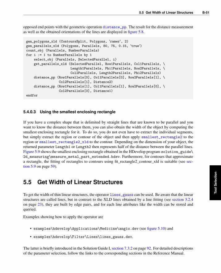
5.5 Get Width of Linear Structures B-51
opposed end points with the geometric operation distance_pp. The result for the distance measurementas well as the obtained orientations of the lines are displayed in figure 5.8.
gen_polygons_xld (ContoursSplit, Polygons, 'ramer', 2)
gen_parallels_xld (Polygons, Parallels, 80, 75, 0.15, 'true')count_obj (Parallels, NumberParallels)
for i := 1 to NumberParallels by 1
select_obj (Parallels, SelectedParallel, i)
get_parallels_xld (SelectedParallel, Row1Parallels, Col1Parallels, \
Length1Parallels, Phi1Parallels, Row2Parallels, \
Col2Parallels, Length2Parallels, Phi2Parallels)
distance_pp (Row1Parallels[0], Col1Parallels[0], Row2Parallels[1], \
Col2Parallels[1], Distance2)
distance_pp (Row1Parallels[1], Col1Parallels[1], Row2Parallels[0], \
Col2Parallels[0], Distance1)
endfor
5.4.0.3 Using the smallest enclosing rectangle
If you have a complex shape that is delimited by straight lines that are known to be parallel and youwant to know the distance between them, you can also obtain the width of the object by computing thesmallest enclosing rectangle for it. To do so, you do not even have to extract the individual segments,but simply extract the region or contour of the object and then apply smallest_rectangle2 to theregion or smallest_rectangle2_xld to the contour. Depending on the dimension of your object, thereturned parameter Length1 or Length2 then represents half of the distance between the parallel lines.Figure 5.9 shows the smallest enclosing rectangle obtained in the HDevelop program solution_guide\
2d_measuring\measure_metal_part_extended.hdev. Furthermore, for contours that approximatea rectangle, the fitting of rectangles to contours using fit_rectangle2_contour_xld is suitable (see sec-tion 5.9 on page 59).
5.5 Get Width of Linear Structures
To get the width of thin linear structures, the operator lines_gauss can be used. Be aware that the linearstructures are called lines, but in contrast to the XLD lines obtained by a line fitting (see section 3.2.4on page 23), they are built by edge pairs, and for each line attributes like the width can be stored andqueried.
Examples showing how to apply the operator are
• examples\hdevelop\Applications\Medicine\angio.dev (see figure 5.10) and
• examples\hdevelop\Filter\Lines\lines_gauss.dev.
The latter is briefly introduced in the Solution Guide I, section 7.3.2 on page 92. For detailed descriptionsof the parameter selection, follow the links to the corresponding sections in the Reference Manual.
Tool
Sel
ectio
n

B-52 Examples for Practical Guidance
Figure 5.9: Length and width of the smallest enclosing rectangle of a region.
Figure 5.10: Linear structures obtained by lines_gauss in the HDevelop example angio.dev: (left) theextracted lines, (right) visualization of the diameters of the selected lines.
Briefly, you can select whether bright or dark lines are detected and adjust parameters for the general lineextraction. Additionally, you can set parameters that control which attributes are stored with the obtainedlines. These attributes can then be queried with the operator get_contour_attrib_xld. Dependingon the selected parameters in lines_gauss you can query the following parameters: the angle of thedirection perpendicular to the line (’angle’), the magnitude of the second derivative (’response’), theline widths to the left or to the right of the line (’width_left’, ’width_right’), the asymmetry of aline point (’asymmetry’), or the contrast of a line point (’contrast’).

5.6 Get Lines and Junctions of a Grid B-53
5.6 Get Lines and Junctions of a Grid
The HDevelop program solution_guide\2d_measuring\measure_grid.hdev inspects a numerickeypad. In particular, the positions of the junctions of the grid separating the keys are measured.
Figure 5.11: Lines and junction points representing the grid that separates the keys.
The general steps of the program comprise
• the extraction of the region between and around the keys,
• the determination of the region’s skeleton and the extraction of the corresponding linear contours,
• the separation of the horizontal and vertical lines,
• the intersection of the horizontal lines with the vertical lines to get the junction points of a regulargrid, and
• the reduction of the point set to those points that represent a real existing junction.
• Additionally, the usability of region processing for the extraction of junction points is discussed.
Step 1: Get region between and around the keys
mean_image (Image, ImageMean, 7, 7)
dyn_threshold (Image, ImageMean, RegionDynThresh, 4, 'dark')connection (RegionDynThresh, ConnectedRegions)
select_shape (ConnectedRegions, SelectedRegions, ['max_diameter', \
'contlength'], 'and', [200,800], [99999,99999])
closing_circle (SelectedRegions, RegionClosing, 1.5)
First, the region representing the space between and around the keys is segmented and further processedvia region processing. This includes the coarse segmentation of the image via a dynamic threshold
Tool
Sel
ectio
n

B-54 Examples for Practical Guidance
(dyn_threshold), the selection of a connected region of a certain size (connection followed by se-
lect_shape), as well as the closing of small gaps by closing_circle. This is illustrated in figure 5.12,a-d.
Step 2: Get skeleton and the corresponding horizontal and vertical linear contours
skeleton (RegionClosing, Skeleton)
gen_contours_skeleton_xld (Skeleton, ContoursSkeleton, 1, 'filter')segment_contours_xld (ContoursSkeleton, ContoursSplitSkeleton, 'lines', 5, \
2, 1)
select_contours_xld (ContoursSplitSkeleton, SelectedContours, \
'contour_length', 30, 1000, -0.5, 0.5)
union_collinear_contours_xld (SelectedContours, UnionCollinearContours, 100, \
10, 20, rad(10), 'attr_keep')
Then, the region is reduced to its skeleton, which is then transformed to a contourby gen_contours_skeleton_xld. The contour is segmented into individual lines (seg-ment_contours_xld), from which those are selected by select_contours_xld that have aminimum contour length (see figure 5.12, e-f). Additionally, collinear lines are merged byunion_collinear_contours_xld (see figure 5.13, left).
a) b) c)
d) e) f)
Figure 5.12: Extraction of region: (a) original image, (b) image processed by mean_image, (c) extractedregion with gaps, (d) region after closing gaps by a morphological operator, (e) skeleton, (f)selected contour segments.
Now, lines are fitted to each contour by fit_line_contour_xld and the corresponding line contoursare generated by gen_contour_polygon_xld. For each contour the orientation is checked within atolerance of 0.05 rad in both directions and horizontal lines are stored in the tuple LinesHorizontal

5.6 Get Lines and Junctions of a Grid B-55
and vertical lines in the tuple LinesVertical. Both are first created by gen_empty_obj and thensuccessively filled using concat_obj.
count_obj (UnionCollinearContours, NumberContours)
gen_empty_obj (LinesHorizontal)
gen_empty_obj (LinesVertical)
for i := 1 to NumberContours by 1
select_obj (UnionCollinearContours, ObjectSelected, i)
fit_line_contour_xld (ObjectSelected, 'tukey', -1, 0, 5, 2, RowBegin, \
ColBegin, RowEnd, ColEnd, Nr, Nc, Dist)
gen_contour_polygon_xld (Contour, [RowBegin,RowEnd], [ColBegin,ColEnd])
Phi := atan2(-Nr,Nc)
if (abs(Phi) < rad(5))
concat_obj (LinesVertical, Contour, LinesVertical)
endif
if (rad(85) < abs(Phi) and abs(Phi) < rad(95))
concat_obj (LinesHorizontal, Contour, LinesHorizontal)
endif
endfor
Step 3: Get junction points
Now, inside a loop, each horizontal line is intersected (intersection_lines) with each vertical lineto get the junction points of the regular grid. This grid is built by lines of infinite length, so that theintersection leads to junction points also at the large keys (see figure 5.13, right).
RowJunction := []
ColJunction := []
RowRealJunction := []
ColRealJunction := []
count_obj (LinesHorizontal, NumberLH)
count_obj (LinesVertical, NumberLV)
for i := 1 to NumberLH by 1
select_obj (LinesHorizontal, HorizontalLine, i)
get_contour_xld (HorizontalLine, RowHorizontal, ColHorizontal)
for j := 1 to NumberLV by 1
select_obj (LinesVertical, VerticalLine, j)
get_contour_xld (VerticalLine, RowVertical, ColVertical)
intersection_lines (RowHorizontal[0], ColHorizontal[0], \
RowHorizontal[1], ColHorizontal[1], \
RowVertical[0], ColVertical[0], RowVertical[1], \
ColVertical[1], Row, Column, IsOverlapping)
distance_ps (Row, Column, RowHorizontal[0], ColHorizontal[0], \
RowHorizontal[1], ColHorizontal[1], DistanceH, \
DistanceHMax)
distance_ps (Row, Column, RowVertical[0], ColVertical[0], \
RowVertical[1], ColVertical[1], DistanceV, \
DistanceVMax)
RowJunction := [RowJunction,Row]
ColJunction := [ColJunction,Column]
Tool
Sel
ectio
n

B-56 Examples for Practical Guidance
Figure 5.13: Get junction points: (left) collinear horizontal and vertical contours obtained by line fitting,(right) all junctions of the regular grid including junctions that do not represent a real existingjunction between keys.
Step 4: Reduce the point set
if ((DistanceH <= 30) and (DistanceV <= 30))
RowRealJunction := [RowRealJunction,Row]
ColRealJunction := [ColRealJunction,Column]
endif
endfor
endfor
To get only those points of the grid that represent a real existing junction, for each junction point thedistances to the two line segments used for its creation are computed by distance_ps. If both distancesare less than 30 pixels, the point is assumed to be a real junction point (see figure 5.14, left).
Step 5: Junction points via region processing
Alternatively, junction points can also be obtained via region processing. Here, we apply junc-
tions_skeleton to the skeleton we obtained in a preceding step. Since the operator returns regionsinstead of points, we apply get_region_points to get the center positions of each junction. Notethat in contrast to contour processing these junction positions are not based on a grid obtained by straightlines but on the region extracted between the keys. Depending on the region, the resulting junction pointsmay be ambiguous and may not represent junctions of a regular grid (see figure 5.14, right).
junctions_skeleton (Skeleton, EndPoints, JuncPoints)
get_region_points (JuncPoints, RowJunctionRegionProcessing, \
ColumnJunctionRegionProcessing)
gen_cross_contour_xld (CrossCenter, RowJunctionRegionProcessing, \
ColumnJunctionRegionProcessing, 12, 0.785398)

5.7 Get Positions of Corner Points B-57
Figure 5.14: Get junction points: (left) lines fitted into linear contours and the junction points of the gridseparating the keys, (right), skeleton and irregular junction points obtained by region pro-cessing.
5.7 Get Positions of Corner Points
Corner points are extracted in different ways. The HDevelop program solution_guide\
2d_measuring\measure_metal_part_extended.hdev extracts the positions of the corners of ametal plate in an image by two different approaches. The first approach applies a point operator andthe other one determines the corner points by intersecting lines.
Figure 5.15: Förstner points (crosses parallel to coordinate axes) versus intersection points (inclinedcrosses).
The general steps of the program comprise
Tool
Sel
ectio
n
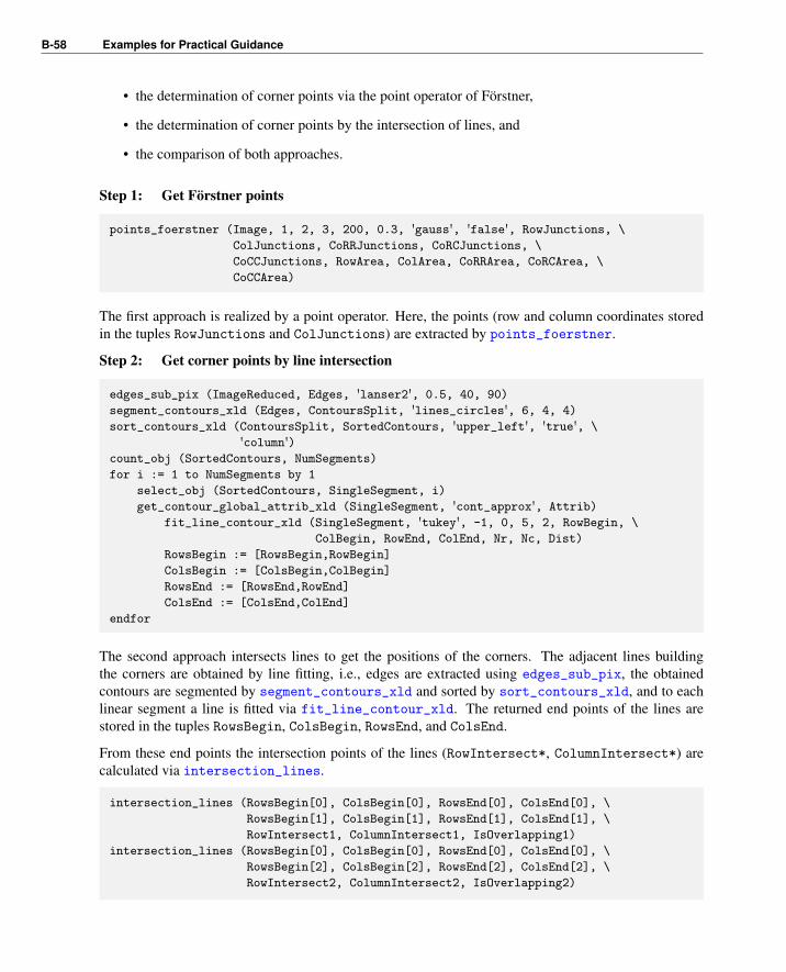
B-58 Examples for Practical Guidance
• the determination of corner points via the point operator of Förstner,
• the determination of corner points by the intersection of lines, and
• the comparison of both approaches.
Step 1: Get Förstner points
points_foerstner (Image, 1, 2, 3, 200, 0.3, 'gauss', 'false', RowJunctions, \
ColJunctions, CoRRJunctions, CoRCJunctions, \
CoCCJunctions, RowArea, ColArea, CoRRArea, CoRCArea, \
CoCCArea)
The first approach is realized by a point operator. Here, the points (row and column coordinates storedin the tuples RowJunctions and ColJunctions) are extracted by points_foerstner.
Step 2: Get corner points by line intersection
edges_sub_pix (ImageReduced, Edges, 'lanser2', 0.5, 40, 90)
segment_contours_xld (Edges, ContoursSplit, 'lines_circles', 6, 4, 4)
sort_contours_xld (ContoursSplit, SortedContours, 'upper_left', 'true', \
'column')count_obj (SortedContours, NumSegments)
for i := 1 to NumSegments by 1
select_obj (SortedContours, SingleSegment, i)
get_contour_global_attrib_xld (SingleSegment, 'cont_approx', Attrib)
fit_line_contour_xld (SingleSegment, 'tukey', -1, 0, 5, 2, RowBegin, \
ColBegin, RowEnd, ColEnd, Nr, Nc, Dist)
RowsBegin := [RowsBegin,RowBegin]
ColsBegin := [ColsBegin,ColBegin]
RowsEnd := [RowsEnd,RowEnd]
ColsEnd := [ColsEnd,ColEnd]
endfor
The second approach intersects lines to get the positions of the corners. The adjacent lines buildingthe corners are obtained by line fitting, i.e., edges are extracted using edges_sub_pix, the obtainedcontours are segmented by segment_contours_xld and sorted by sort_contours_xld, and to eachlinear segment a line is fitted via fit_line_contour_xld. The returned end points of the lines arestored in the tuples RowsBegin, ColsBegin, RowsEnd, and ColsEnd.
From these end points the intersection points of the lines (RowIntersect*, ColumnIntersect*) arecalculated via intersection_lines.
intersection_lines (RowsBegin[0], ColsBegin[0], RowsEnd[0], ColsEnd[0], \
RowsBegin[1], ColsBegin[1], RowsEnd[1], ColsEnd[1], \
RowIntersect1, ColumnIntersect1, IsOverlapping1)
intersection_lines (RowsBegin[0], ColsBegin[0], RowsEnd[0], ColsEnd[0], \
RowsBegin[2], ColsBegin[2], RowsEnd[2], ColsEnd[2], \
RowIntersect2, ColumnIntersect2, IsOverlapping2)
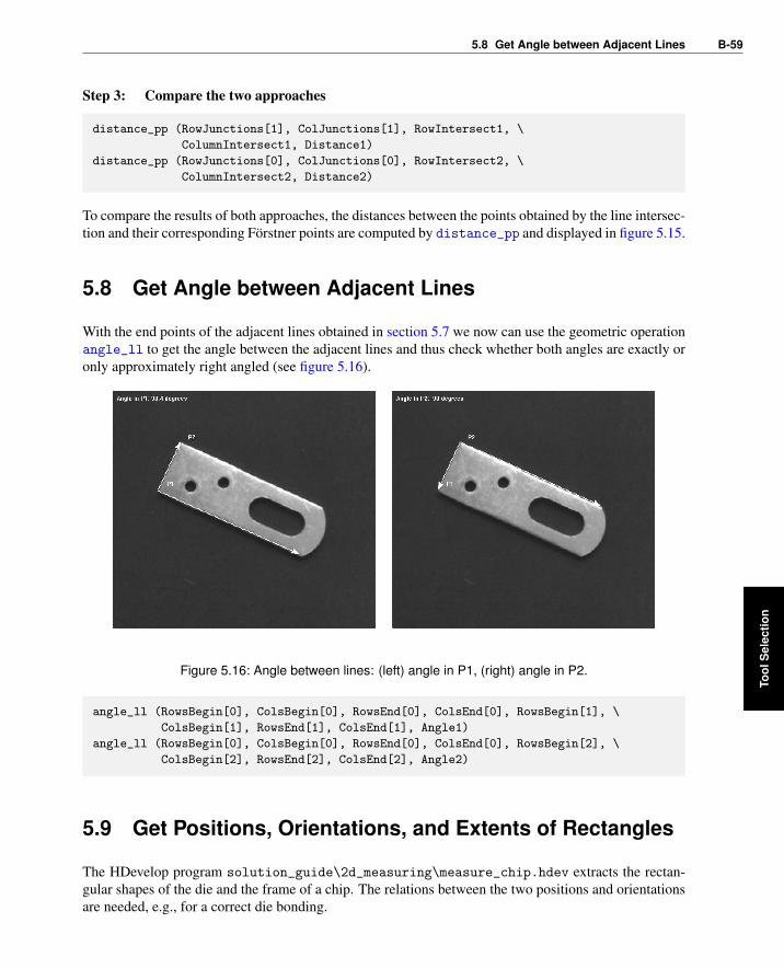
5.8 Get Angle between Adjacent Lines B-59
Step 3: Compare the two approaches
distance_pp (RowJunctions[1], ColJunctions[1], RowIntersect1, \
ColumnIntersect1, Distance1)
distance_pp (RowJunctions[0], ColJunctions[0], RowIntersect2, \
ColumnIntersect2, Distance2)
To compare the results of both approaches, the distances between the points obtained by the line intersec-tion and their corresponding Förstner points are computed by distance_pp and displayed in figure 5.15.
5.8 Get Angle between Adjacent Lines
With the end points of the adjacent lines obtained in section 5.7 we now can use the geometric operationangle_ll to get the angle between the adjacent lines and thus check whether both angles are exactly oronly approximately right angled (see figure 5.16).
Figure 5.16: Angle between lines: (left) angle in P1, (right) angle in P2.
angle_ll (RowsBegin[0], ColsBegin[0], RowsEnd[0], ColsEnd[0], RowsBegin[1], \
ColsBegin[1], RowsEnd[1], ColsEnd[1], Angle1)
angle_ll (RowsBegin[0], ColsBegin[0], RowsEnd[0], ColsEnd[0], RowsBegin[2], \
ColsBegin[2], RowsEnd[2], ColsEnd[2], Angle2)
5.9 Get Positions, Orientations, and Extents of Rectangles
The HDevelop program solution_guide\2d_measuring\measure_chip.hdev extracts the rectan-gular shapes of the die and the frame of a chip. The relations between the two positions and orientationsare needed, e.g., for a correct die bonding.
Tool
Sel
ectio
n
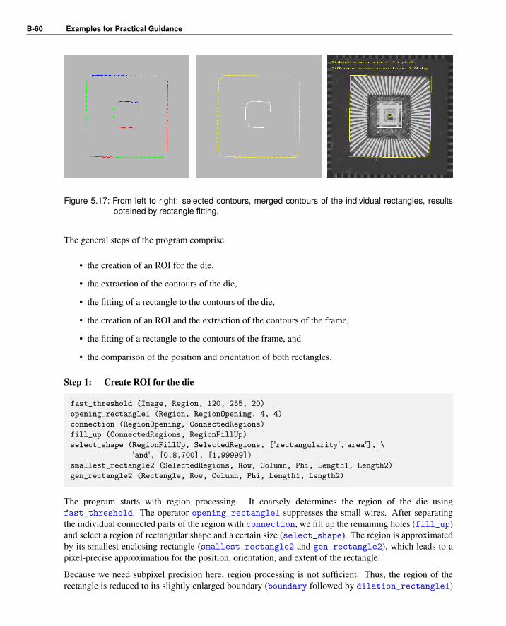
B-60 Examples for Practical Guidance
Figure 5.17: From left to right: selected contours, merged contours of the individual rectangles, resultsobtained by rectangle fitting.
The general steps of the program comprise
• the creation of an ROI for the die,
• the extraction of the contours of the die,
• the fitting of a rectangle to the contours of the die,
• the creation of an ROI and the extraction of the contours of the frame,
• the fitting of a rectangle to the contours of the frame, and
• the comparison of the position and orientation of both rectangles.
Step 1: Create ROI for the die
fast_threshold (Image, Region, 120, 255, 20)
opening_rectangle1 (Region, RegionOpening, 4, 4)
connection (RegionOpening, ConnectedRegions)
fill_up (ConnectedRegions, RegionFillUp)
select_shape (RegionFillUp, SelectedRegions, ['rectangularity','area'], \
'and', [0.8,700], [1,99999])
smallest_rectangle2 (SelectedRegions, Row, Column, Phi, Length1, Length2)
gen_rectangle2 (Rectangle, Row, Column, Phi, Length1, Length2)
The program starts with region processing. It coarsely determines the region of the die usingfast_threshold. The operator opening_rectangle1 suppresses the small wires. After separatingthe individual connected parts of the region with connection, we fill up the remaining holes (fill_up)and select a region of rectangular shape and a certain size (select_shape). The region is approximatedby its smallest enclosing rectangle (smallest_rectangle2 and gen_rectangle2), which leads to apixel-precise approximation for the position, orientation, and extent of the rectangle.
Because we need subpixel precision here, region processing is not sufficient. Thus, the region of therectangle is reduced to its slightly enlarged boundary (boundary followed by dilation_rectangle1)
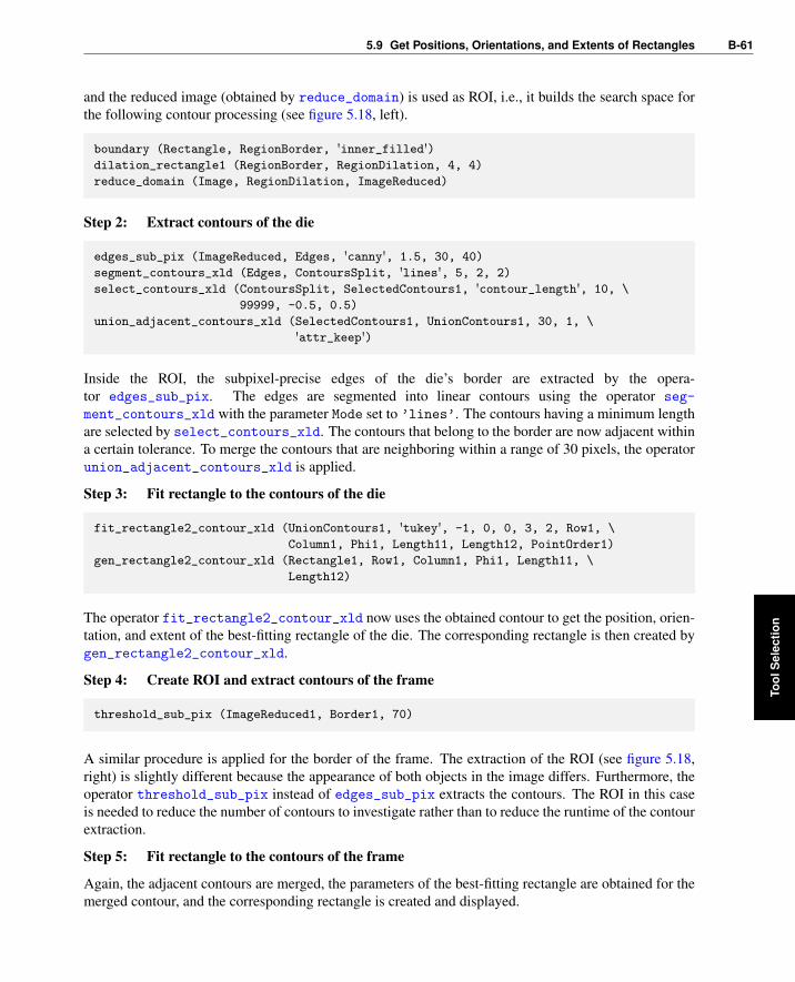
5.9 Get Positions, Orientations, and Extents of Rectangles B-61
and the reduced image (obtained by reduce_domain) is used as ROI, i.e., it builds the search space forthe following contour processing (see figure 5.18, left).
boundary (Rectangle, RegionBorder, 'inner_filled')dilation_rectangle1 (RegionBorder, RegionDilation, 4, 4)
reduce_domain (Image, RegionDilation, ImageReduced)
Step 2: Extract contours of the die
edges_sub_pix (ImageReduced, Edges, 'canny', 1.5, 30, 40)
segment_contours_xld (Edges, ContoursSplit, 'lines', 5, 2, 2)
select_contours_xld (ContoursSplit, SelectedContours1, 'contour_length', 10, \
99999, -0.5, 0.5)
union_adjacent_contours_xld (SelectedContours1, UnionContours1, 30, 1, \
'attr_keep')
Inside the ROI, the subpixel-precise edges of the die’s border are extracted by the opera-tor edges_sub_pix. The edges are segmented into linear contours using the operator seg-
ment_contours_xld with the parameter Mode set to ’lines’. The contours having a minimum lengthare selected by select_contours_xld. The contours that belong to the border are now adjacent withina certain tolerance. To merge the contours that are neighboring within a range of 30 pixels, the operatorunion_adjacent_contours_xld is applied.
Step 3: Fit rectangle to the contours of the die
fit_rectangle2_contour_xld (UnionContours1, 'tukey', -1, 0, 0, 3, 2, Row1, \
Column1, Phi1, Length11, Length12, PointOrder1)
gen_rectangle2_contour_xld (Rectangle1, Row1, Column1, Phi1, Length11, \
Length12)
The operator fit_rectangle2_contour_xld now uses the obtained contour to get the position, orien-tation, and extent of the best-fitting rectangle of the die. The corresponding rectangle is then created bygen_rectangle2_contour_xld.
Step 4: Create ROI and extract contours of the frame
threshold_sub_pix (ImageReduced1, Border1, 70)
A similar procedure is applied for the border of the frame. The extraction of the ROI (see figure 5.18,right) is slightly different because the appearance of both objects in the image differs. Furthermore, theoperator threshold_sub_pix instead of edges_sub_pix extracts the contours. The ROI in this caseis needed to reduce the number of contours to investigate rather than to reduce the runtime of the contourextraction.
Step 5: Fit rectangle to the contours of the frame
Again, the adjacent contours are merged, the parameters of the best-fitting rectangle are obtained for themerged contour, and the corresponding rectangle is created and displayed.
Tool
Sel
ectio
n
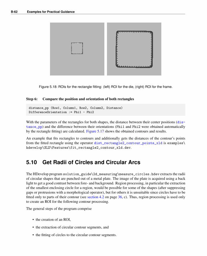
B-62 Examples for Practical Guidance
Figure 5.18: ROIs for the rectangle fitting: (left) ROI for the die, (right) ROI for the frame.
Step 6: Compare the position and orientation of both rectangles
distance_pp (Row1, Column1, Row2, Column2, Distance)
DifferenceOrientation := Phi1 - Phi2
With the parameters of the rectangles for both shapes, the distance between their center positions (dis-tance_pp) and the difference between their orientations (Phi1 and Phi2 were obtained automaticallyby the rectangle fitting) are calculated. Figure 5.17 shows the obtained contours and results.
An example that fits rectangles to contours and additionally gets the distances of the contour’s pointsfrom the fitted rectangle using the operator dist_rectangle2_contour_points_xld is examples\hdevelop\XLD\Features\fit_rectangle2_contour_xld.dev.
5.10 Get Radii of Circles and Circular Arcs
The HDevelop program solution_guide\2d_measuring\measure_circles.hdev extracts the radiiof circular shapes that are punched out of a metal plate. The image of the plate is acquired using a backlight to get a good contrast between fore- and background. Region processing, in particular the extractionof the smallest enclosing circle for a region, would be possible for some of the shapes (after suppressinggaps or protrusions with a morphological operator), but for others it is unsuitable since circles have to befitted only to parts of their contour (see section 4.2 on page 36, c). Thus, region processing is used onlyto create an ROI for the following contour processing.
The general steps of the program comprise
• the creation of an ROI,
• the extraction of circular contour segments, and
• the fitting of circles to the circular contour segments.

5.10 Get Radii of Circles and Circular Arcs B-63
Figure 5.19: Circle fitting: black contours overlaid by the white fitted circles and display of their radii.
Step 1: Create ROI
fast_threshold (Image, Region, 200, 255, 20)
connection (Region, ConnectedRegions)
select_shape (ConnectedRegions, SelectedRegions, 'area', 'and', 70, 50000)
boundary (SelectedRegions, RegionBorder, 'inner_filled')dilation_circle (RegionBorder, RegionDilation, 3.5)
union1 (RegionDilation, RegionUnion)
reduce_domain (Image, RegionUnion, ImageReduced)
To extract the bright regions of the circular shapes a fast_threshold is applied. Connected regionsare separated by connection and regions with a minimum size are selected for the further processingusing select_shape (see figure 5.20, left). The regions are restricted to their borders by the operatorboundary. These borders are enlarged a bit by a dilation (dilation_circle). The dilated regionsare merged (union1) so that the image can be reduced to a region that contains all parts needed for thefurther tasks (reduce_domain). The reduced image is used as an ROI, i.e., it builds the search space forthe subpixel-precise edge extraction.
Tool
Sel
ectio
n

B-64 Examples for Practical Guidance
Step 2: Extract circular contour segments
edges_sub_pix (ImageReduced, Edges, 'canny', 1.5, 10, 40)
segment_contours_xld (Edges, ContoursSplit, 'lines_circles', 5, 2, 2)
select_contours_xld (ContoursSplit, SelectedContours, 'contour_length', 25, \
99999, -0.5, 0.5)
count_obj (SelectedContours, NumberContours)
gen_empty_obj (Circles)
for i := 1 to NumberContours by 1
select_obj (SelectedContours, ObjectSelected, i)
get_contour_global_attrib_xld (ObjectSelected, 'cont_approx', Attrib)
if (Attrib == 1)
concat_obj (Circles, ObjectSelected, Circles)
endif
endfor
union_cocircular_contours_xld (Circles, UnionContours, rad(60), rad(10), \
rad(30), 100, 50, 10, 'true', 1)
The edges obtained by edges_sub_pix are segmented into linear and circular segments by seg-
ment_contours_xld. Because more contours exist than needed for the circle extraction, onlythe contours having a minimum contour length are selected by select_contours_xld. Forthese, it is checked if they are circular, i.e., the value for ’cont_approx’ is queried byget_contour_global_attrib_xld and if it is 1 the contour is stored in the tuple Circles. Now,all circular contours that lie approximately on the same circle (i.e., they are cocircular) are merged byunion_cocircular_contours_xld (see figure 5.20, right). These contours are now used for the circlefitting.
Figure 5.20: Circle fitting: (left) original image overlaid by the extracted regions, (right) circular contoursselected for the circle fitting.
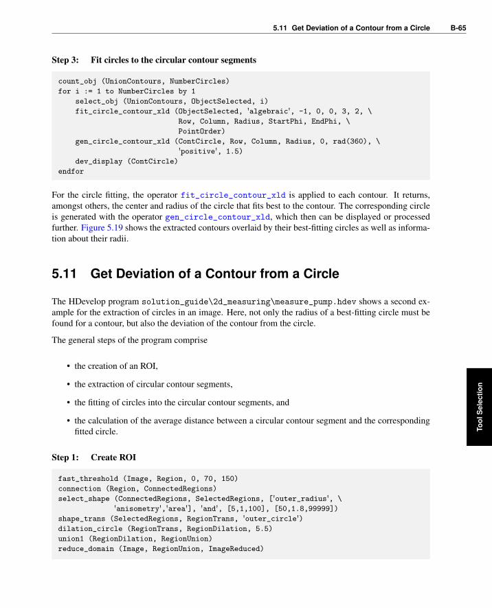
5.11 Get Deviation of a Contour from a Circle B-65
Step 3: Fit circles to the circular contour segments
count_obj (UnionContours, NumberCircles)
for i := 1 to NumberCircles by 1
select_obj (UnionContours, ObjectSelected, i)
fit_circle_contour_xld (ObjectSelected, 'algebraic', -1, 0, 0, 3, 2, \
Row, Column, Radius, StartPhi, EndPhi, \
PointOrder)
gen_circle_contour_xld (ContCircle, Row, Column, Radius, 0, rad(360), \
'positive', 1.5)
dev_display (ContCircle)
endfor
For the circle fitting, the operator fit_circle_contour_xld is applied to each contour. It returns,amongst others, the center and radius of the circle that fits best to the contour. The corresponding circleis generated with the operator gen_circle_contour_xld, which then can be displayed or processedfurther. Figure 5.19 shows the extracted contours overlaid by their best-fitting circles as well as informa-tion about their radii.
5.11 Get Deviation of a Contour from a Circle
The HDevelop program solution_guide\2d_measuring\measure_pump.hdev shows a second ex-ample for the extraction of circles in an image. Here, not only the radius of a best-fitting circle must befound for a contour, but also the deviation of the contour from the circle.
The general steps of the program comprise
• the creation of an ROI,
• the extraction of circular contour segments,
• the fitting of circles into the circular contour segments, and
• the calculation of the average distance between a circular contour segment and the correspondingfitted circle.
Step 1: Create ROI
fast_threshold (Image, Region, 0, 70, 150)
connection (Region, ConnectedRegions)
select_shape (ConnectedRegions, SelectedRegions, ['outer_radius', \
'anisometry','area'], 'and', [5,1,100], [50,1.8,99999])
shape_trans (SelectedRegions, RegionTrans, 'outer_circle')dilation_circle (RegionTrans, RegionDilation, 5.5)
union1 (RegionDilation, RegionUnion)
reduce_domain (Image, RegionUnion, ImageReduced)
Tool
Sel
ectio
n

B-66 Examples for Practical Guidance
Figure 5.21: Circles are fitted into the circular contours and for each circle the radius and the deviation ofthe contour from the circle are displayed.
The approach, like others before, starts with the creation of a suitable ROI. To do so, fast_thresholdis applied, the connected regions are separated by connection, shapes with a certain outer radius,anisometry, and area are selected using select_shape, and the regions are transformed into their outercircles by shape_trans. These circles are enlarged by dilation_circle, the regions are merged intoa single region by union1, and the image is reduced to the obtained region (reduce_domain). Thereduced image builds the search space for the contour processing.
Step 2: Extract circular contour segments
threshold_sub_pix (ImageReduced, Border, 80)
select_shape_xld (Border, SelectedXLD, ['contlength','outer_radius'], 'and', \
[70,15], [99999,99999])
segment_contours_xld (SelectedXLD, ContoursSplit, 'lines_circles', 4, 2, 2)
select_shape_xld (ContoursSplit, SelectedXLD3, ['outer_radius', \
'contlength'], 'and', [15,30], [45,99999])
union_cocircular_contours_xld (SelectedXLD3, UnionContours2, 0.5, 0.1, 0.2, \
2, 10, 10, 'true', 1)
sort_contours_xld (UnionContours2, SortedContours, 'upper_left', 'true', \
'column')
Contours are created using the operator threshold_sub_pix. To select the relevant contours from theobtained set of contours, the operator select_shape_xld is applied, searching for contours of a specificlength and with a certain outer radius. The relevant contours are then segmented into lines and circleswith segment_contours_xld. From the segments, again contours with a specific contour length andouter radius are selected. Cocircular contours are merged by union_cocircular_contours_xld (see

5.11 Get Deviation of a Contour from a Circle B-67
figure 5.22) and finally the contours are sorted by sort_contours_xld.
Figure 5.22: ROI for circle fitting: (left) original image of a pump, (right) ROI and extracted circular con-tours.
Step 3: Fit circles to the circular contour segments
count_obj (SortedContours, NumSegments)
for i := 1 to NumSegments by 1
select_obj (SortedContours, SingleSegment, i)
NumCircles := NumCircles + 1
fit_circle_contour_xld (SingleSegment, 'atukey', -1, 2, 0, 5, 2, Row, \
Column, Radius, StartPhi, EndPhi, PointOrder)
gen_circle_contour_xld (ContCircle, Row, Column, Radius, 0, rad(360), \
'positive', 1)
Since the final contours are all circular, the best fitting circle is calculated for each contour byfit_circle_contour_xld. If also linear contours were contained in the set of contours, you wouldhave to extract the circular segments first, like in the example in section 5.10 on page 62. The best fittingcircles are now generated by gen_circle_contour_xld.
Step 4: Calculate the deviation of the circular contour segments from the fitted circles
dist_ellipse_contour_xld (SingleSegment, 'algebraic', -1, 0, Row, \
Column, 0, Radius, Radius, MinDist, MaxDist, \
AvgDist, SigmaDist)
endfor
To get the deviation of the contour from the generated ellipses (or circles in this case), the operatordist_ellipse_contour_xld is applied. Be aware that only the deviation between the fitted circle andthe contour segment used for the fitting is calculated. The quality of the fitting in relation to the realcircle also depends on the coverage of the circle by the contour segment. For the circle with the index6 in figure 5.21, e.g., less than half of the circle was covered by the contour segment (see figure 5.22,right). Thus, despite the good result for the deviation between contour segment and fitted circle, the
Tool
Sel
ectio
n

B-68 Examples for Practical Guidance
result is less satisfying in an optical inspection than for the other circles that have a larger deviation buta bigger coverage.
5.12 Inspect Ball Grid Array (BGA)
Another application with circular objects is the inspection of a ball grid array (BGA). A BGA con-sists of very small objects, which have an approximately symmetrical gray value distribution, and forwhich the transition area between fore- and background can be rather large compared to the region ofthe object. Because the standard region or contour-based approaches work with hard transitions (seefigure 5.23), for symmetric objects with a large transition area it is recommended to extract object fea-tures with an approach that considers the gray value features instead. Available operators comprisearea_center_gray, which is used to check the gray value volume and center position of each ball, andelliptic_axis_gray, which returns the length of the axes and the orientation of the ellipse having thesame orientation and aspect ratio as the input region.
0
255
0
255
255
0
hard transition afterregion segmentation
smooth transition whenweighting with gray values
Figure 5.23: Weighting with gray values leads to smooth transitions, opposite to the hard transition of astandard region segmentation.
The HDevelop program solution_guide\2d_measuring\inspect_bga.hdev shows how the ballsof a BGA can be checked for deformations and their correct positions in the grid. The latter is realizedby comparing them with the balls of a reference BGA.
The general steps of the program comprise
• the extraction of the balls of the reference BGA and the determination of their positions,
• the sorting of the balls of the reference BGA,
• the extraction of the balls in a second BGA and their sorting according to the reference BGA, and
• the inspection of the second BGA, as well as a comparison between the positions of both BGAs.

5.12 Inspect Ball Grid Array (BGA) B-69
Figure 5.24: Irregularities of a BGA: (left) missing ball marked by a cross, (right) balls with center positionsthat deviate from the reference positions marked by ellipses.
Step 1: Extract balls in the reference BGA and determine their positions
fast_threshold (Image, Region, 95, 255, 3)
connection (Region, ConnectedRegions)
select_shape (ConnectedRegions, SelectedRegions, ['area','anisometry'], \
'and', [20,1.0], [100,1.7])
dilation_rectangle1 (SelectedRegions, RegionDilation, 3, 3)
area_center_gray (RegionDilation, Image, Volume, Row, Column)
The program starts with the extraction of the balls from the reference image via a region processing. Of-ten, an additional gray value scaling is recommended, which adapts the gray value distribution accordingto two thresholds that depend on the fore- and background of the balls. Here, it is not necessary as thegray value distribution for all balls is rather constant. The obtained regions are slightly enlarged andinside each region the operator area_center_gray computes the gray value volume, i.e., the sum ofthe gray values of all pixels of the region, and the position of the region’s center of gravity.
Step 2: Sort the balls of the reference BGA
The obtained center positions of the balls (Row, Column) are returned in an arbitrary order, i.e., the indexof a variable does not contain information about the position of the corresponding ball in the grid. Tocompare the center positions of corresponding balls in different BGAs, a comparable sequence of theballs is needed, i.e., we have to spatially sort the balls. In a first step, we determine their positions inthe grid separately for the rows and columns. To do so, we normalize the BGA as follows: We applygen_region_points to create a region described by the center points of the balls and use its enclosingrectangle (obtained by smallest_rectangle2, see figure 5.25, left) to define a transformation matrix.
Tool
Sel
ectio
n

B-70 Examples for Practical Guidance
gen_region_points (RegionBGACenters, Row, Column)
smallest_rectangle2 (RegionBGACenters, RowBGARect, ColumnBGARect, \
PhiBGARect, Length1BGARect, Length2BGARect)
BallsPerRow := 14
BallsPerCol := 14
BallDistCol := 2 * Length1BGARect / (BallsPerCol - 1)
BallDistRow := 2 * Length2BGARect / (BallsPerRow - 1)
hom_mat2d_identity (HomMat2DIdentity)
hom_mat2d_rotate (HomMat2DIdentity, -PhiBGARect, RowBGARect, ColumnBGARect, \
HomMat2DRotate)
hom_mat2d_translate (HomMat2DRotate, -RowBGARect + Length2BGARect, \
-ColumnBGARect + Length1BGARect, HomMat2DTranslate)
hom_mat2d_scale (HomMat2DTranslate, 1 / BallDistRow, 1 / BallDistCol, 0, 0, \
HomMat2DScale)
affine_trans_point_2d (HomMat2DScale, Row, Column, RowNormalized, \
ColNormalized)
BGARowIndex := round(RowNormalized)
BGAColIndex := round(ColNormalized)
With it, we transform the balls so that the grid becomes horizontal, the center position of the ball in theupper left corner is placed in the origin of the coordinate system, and the distance between the individualballs becomes 1. The rounded values for the transformed ball positions then describe the indices of theball’s positions separately for the rows and columns of a regular grid. Figure 5.25, right, shows thenormalized grid, which is scaled again for visualization purposes.
Figure 5.25: Normalization of the grid for the reference BGA: (left) smallest rectangle enclosing the regionthat is built by the center points of the balls, (right) transformed and normalized grid (scaledfor visualization purposes).
Instead of separate lists for the rows and columns, we want to obtain a single sorted list of indices, whichis ordered consecutively from left to right and from top to bottom. Therefore, we create a tuple thathas the capacity for all grid points of the BGA (BallMatrix), i.e., its size is defined by the maximumnumbers of balls per row and column. Because the actual balls of the BGA are not placed all over thisgrid, we first assign the start value -1 to all instances. Now, with the help of the indices that we have

5.12 Inspect Ball Grid Array (BGA) B-71
obtained separately for the rows and columns of the extracted balls (BGARowIndex, BGAColIndex), wesort the balls by assigning new values to the corresponding instances of BallMatrix. After the sorting,the value of BallMatrix with the index of a point coordinate in the sorted grid returns either the indexof the corresponding point coordinate in the unsorted grid (see figure 5.26), or the value -1 if the gridposition is not occupied by a ball.
NumBalls := |Row|
BallMatrix := gen_tuple_const(BallsPerRow * BallsPerCol,-1)
for i := 0 to NumBalls - 1 by 1
BallMatrix[BGARowIndex[i] * BallsPerCol + BGAColIndex[i]] := i
endfor
10 23 4 56 7 8
0 123
4
5 67
8
Link from point index of sorted
e.g., MatrixBalls[2]=4index of unsorted grid:
grid to corresponding point
Sorting of the indices of the point positions
unsorted grid sorted grid
Figure 5.26: Sorting of the point indices.
Step 3: Extract balls in a second BGA and sort them according to the reference
elliptic_axis_gray (RegionDilation, Image, RaCheck, RbCheck, PhiCheck)
AnisometryCheck := RaCheck / RbCheck
Now, a second image is processed, which contains the BGA we want to check for irregularities. Again,the regions of the balls are extracted and slightly enlarged via a region processing. The operatorsarea_center_gray and elliptic_axis_gray are applied to get the features of the regions underconsideration of their gray values. The latter operator returns the radii and orientation of the ellipse hav-ing the same moments as the region. The center points obtained by area_center_gray are transformed(see figure 5.27) and sorted like the center points of the reference image. Except for the additional ap-plication of elliptic_axis_gray and an anisometry check, which are both needed to investigate theballs in a later step, the processing is the same as for the reference BGA.
Tool
Sel
ectio
n

B-72 Examples for Practical Guidance
Figure 5.27: Transformed and normalized grid of the BGA to be checked (scaled for visualization pur-poses).
Step 4: Inspect the second BGA and compare it to the reference BGA
j := 0
for i := 0 to BallsPerRow * BallsPerCol - 1 by 1
if (BallMatrix[i] >= 0 and BallMatrixCheck[i] >= 0)
Rows1[j] := Row[BallMatrix[i]]
Cols1[j] := Column[BallMatrix[i]]
Rows2[j] := RowCheck[BallMatrixCheck[i]]
Cols2[j] := ColumnCheck[BallMatrixCheck[i]]
Phi2[j] := PhiCheck[BallMatrixCheck[i]]
Ra2[j] := RaCheck[BallMatrixCheck[i]]
Rb2[j] := RbCheck[BallMatrixCheck[i]]
Anisometry2[j] := AnisometryCheck[BallMatrixCheck[i]]
Volume2[j] := VolumeCheck[BallMatrixCheck[i]]
j := j + 1
endif
endfor
Then, the BGA of the second image is evaluated further. Until now, we have only links from the pointindices in the sorted grid to the point indices in the unsorted grid. Now, we create tuples that containthe actual data of the existing balls in the specified order. In particular, tuples for the row and columncoordinates of the balls in the reference BGA (Rows1, Cols1) and in the BGA to be checked (Rows2,Cols2), as well as for the ellipse radii (Ra2, Rb2), anisometry values (Anisometry2), and the gray valuevolumes (Volume2) of the second BGA are created. These tuples are reduced sets of data as they containonly the data for the grid positions that are occupied by balls in both BGAs, i.e., the size of the tuplesis related to the actual number of extracted balls in the second image and not to the number of possiblegrid positions.
To compare the center positions of the balls of the second BGA with the center positions of the ballsof the reference BGA, we superimpose both (reduced) sets of positions, i.e., we transform the ballsof the reference BGA so that they have the same position, orientation, and scale as the correspondingballs of the BGA to be checked. For the superimposition, the operator vector_to_rigid determines

5.12 Inspect Ball Grid Array (BGA) B-73
the affine 2D transformation by the point correspondences between both sets of coordinates. With theobtained transformation matrix the reduced set of positions for the reference BGA (Rows1, Cols1) istransformed into RowTrans and ColumnTrans. To check also for missing balls in the second BGA,we further transform the set of unsorted reference positions originally obtained by area_center_gray
(Row, Column), i.e., the set that still contains all positions of the regular grid, including the positions thatregularly do not contain balls (marked by the value -1 in BallMatrix) and the positions of the balls thatare only detected in the reference BGA.
vector_to_rigid (Rows1, Cols1, Rows2, Cols2, HomMat2D)
affine_trans_point_2d (HomMat2D, Rows1, Cols1, RowTrans, ColumnTrans)
affine_trans_point_2d (HomMat2D, Row, Column, RowTransFull, ColumnTransFull)
Then, the distance between the sorted points of the BGA to be checked (Rows2, Cols2) and the sortedand transformed points of the reference BGA (RowTrans, ColumnTrans) is calculated by distance_pp.
distance_pp (Rows2, Cols2, RowTrans, ColumnTrans, Distance)
Now, the complete grid is investigated again. For each position of the regular grid, the existence ofa corresponding ball in both BGAs is checked. If the grid position contains a ball in both sets (bothindices are larger than -1), the sorted and reduced sets of data can be used for the comparison. First,the distance between the corresponding center positions is queried. If it is larger than 0.05 pixels, theellipse for the ball is stored in the tuple Deviation. If it is smaller than 0.05 pixels, further features arechecked, in particular the anisometry, i.e., the deformation of the circle (ellipse for deformed ball storedin Deformation), and the range of the gray value volume (ellipse for outlier stored in Volume).
j := 0
for i := 0 to BallsPerRow * BallsPerCol - 1 by 1
if (BallMatrix[i] >= 0 and BallMatrixCheck[i] >= 0)
gen_ellipse (Ellipse, Rows2[j], Cols2[j], Phi2[j], Ra2[j], Rb2[j])
if (Distance[j] > 0.05)
concat_obj (EllipseDeviation, Ellipse, EllipseDeviation)
else
if (Anisometry2[j] > 1.2)
concat_obj (EllipseDeformation, Ellipse, EllipseDeformation)
else
if (Volume2[j] < 5500 or Volume2[j] > 10000)
concat_obj (EllipseVolume, Ellipse, EllipseVolume)
else
concat_obj (EllipseCorrect, Ellipse, EllipseCorrect)
endif
endif
endif
j := j + 1
If a ball exists in the reference BGA but not in the BGA to be checked, a cross at the ball’s position iscreated (gen_cross_contour_xld) and stored in the tuple Missing. The different results can then bevisualized. In figure 5.24, e.g., the missing balls (left) and the balls with deviating center positions (right)are displayed by a cross or ellipse, respectively.
Tool
Sel
ectio
n
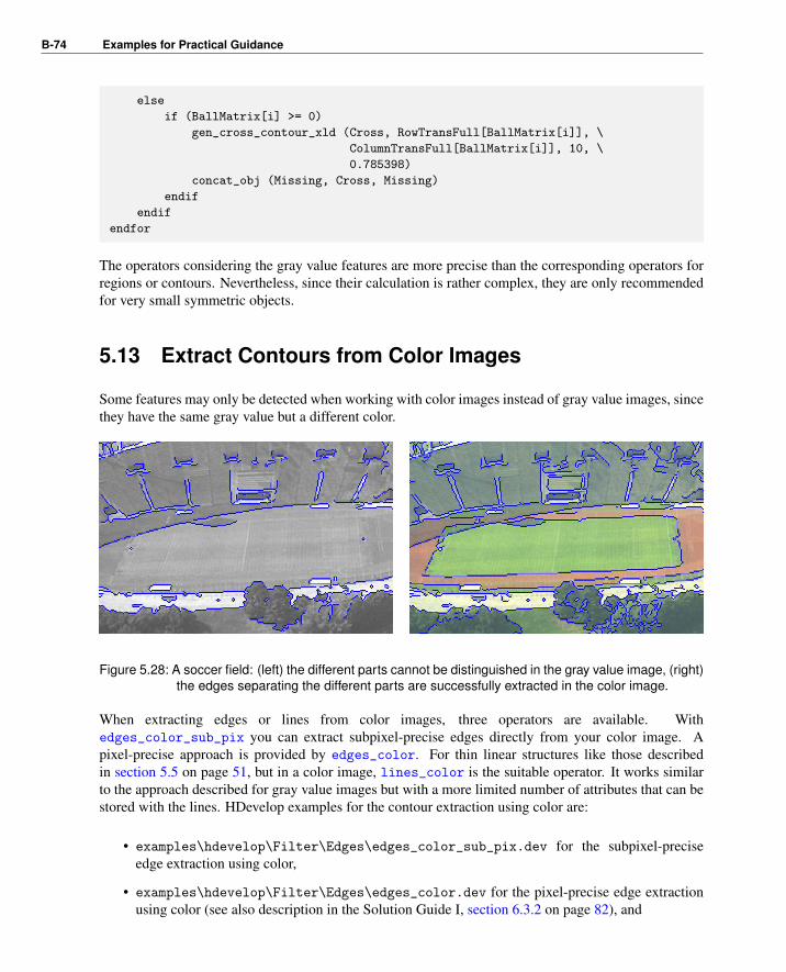
B-74 Examples for Practical Guidance
else
if (BallMatrix[i] >= 0)
gen_cross_contour_xld (Cross, RowTransFull[BallMatrix[i]], \
ColumnTransFull[BallMatrix[i]], 10, \
0.785398)
concat_obj (Missing, Cross, Missing)
endif
endif
endfor
The operators considering the gray value features are more precise than the corresponding operators forregions or contours. Nevertheless, since their calculation is rather complex, they are only recommendedfor very small symmetric objects.
5.13 Extract Contours from Color Images
Some features may only be detected when working with color images instead of gray value images, sincethey have the same gray value but a different color.
Figure 5.28: A soccer field: (left) the different parts cannot be distinguished in the gray value image, (right)the edges separating the different parts are successfully extracted in the color image.
When extracting edges or lines from color images, three operators are available. Withedges_color_sub_pix you can extract subpixel-precise edges directly from your color image. Apixel-precise approach is provided by edges_color. For thin linear structures like those describedin section 5.5 on page 51, but in a color image, lines_color is the suitable operator. It works similarto the approach described for gray value images but with a more limited number of attributes that can bestored with the lines. HDevelop examples for the contour extraction using color are:
• examples\hdevelop\Filter\Edges\edges_color_sub_pix.dev for the subpixel-preciseedge extraction using color,
• examples\hdevelop\Filter\Edges\edges_color.dev for the pixel-precise edge extractionusing color (see also description in the Solution Guide I, section 6.3.2 on page 82), and

5.13 Extract Contours from Color Images B-75
• examples\hdevelop\Filter\Lines\lines_color.dev for the extraction of thin linear struc-tures using color (see also the description in the Solution Guide I, section 13.3.4 on page 199),
Figure 5.28 shows some results of the second example in the list. A soccer field contains red and greenparts in the color image. In the gray value image (left) the red and green parts cannot be distinguished.In the color image (right), the separating edges are successfully extracted using edges_color.
After the extraction of the edges, measurements can be applied as described in the previous sections.
Tool
Sel
ectio
n

B-76 Examples for Practical Guidance

Miscellaneous B-77
Chapter 6
Miscellaneous
The previous sections mainly handled the actual measuring approaches that are common for measuringtasks in machine vision. Several tasks need further processing that is applied in addition to the actualmeasuring tools:
• If you need to compare parts of similar objects with each other, section 6.1 proposes an approachfor the unambiguous identification of the corresponding object parts.
• In many applications, the dimensions of the measured objects must be determined in world coor-dinates, e.g., in µm. Section 6.2 shortly shows how to measure in world coordinates. There, theapplied camera calibration additionally compensates perspective distortions in the image. Moredetailed information about measuring in world coordinates can be found in the Solution GuideIII-C.
• The application of a simple affine 2D transformation, which is needed for various reasons to trans-late, rotate, or scale an image, a region, or a contour, is shortly described in section 5.1 on page41.
• When working with a line scan camera, we recommend to read the Solution Guide II-A, section 6.6on page 46.
6.1 Identify Corresponding Object Parts
In many applications, similar objects must be measured and the results must be compared to the resultsobtained for a reference image or reference data stored in a Computer Aided Design (CAD) model.In the latter case, you can import ARC/INFO or DXF files via read_contour_xld_arc_info orread_contour_xld_dxf, respectively. If you wish to create an image containing the CAD model youcan create an artificial image by gen_image_const and paint the contour of the CAD model into it usingpaint_xld. To identify errors of an object, e.g. a specific drill hole that is missing, the correspondingparts of the measured object and the reference object must be clearly identified. The HDevelop programsolution_guide\2d_measuring\measure_metal_part_id.hdev measures the drill holes of metal
Mis
cella
neou
s

B-78 Miscellaneous
parts. The first image is used as reference image. The program detects missing drill holes as well as drillholes that deviate more than 2 pixels in their center position or radius from the corresponding drill holesof the part in the reference image.
Figure 6.1: Compare parts of two similar objects: (left) reference object with indices of the parts, (right)object to inspect, deviations marked.
The general steps of the program comprise
• the alignment (here, the rotation into a defined orientation) of the object,
• the measurements in the image coordinate system,
• the creation of an object coordinate system,
• the transformation of the measurement results into the object coordinate system,
• the storage of the reference data, and
• the comparison of the results for other images to the reference data.
Step 1: Extract and rotate contours to get a horizontal object
threshold (Image, Region, 90, 255)
dilation_rectangle1 (Region, RegionDilation, 10, 10)
reduce_domain (Image, RegionDilation, ImageReduced)
For each image, an ROI for the following contour processing is created. To do so, the region of theobject is obtained with threshold, the region is enlarged with dilation_rectangle1, and the imageis reduced to this region by reduce_domain. Inside the ROI, threshold_sub_pix is applied to extractthe contours of the metal part’s boundary.
threshold_sub_pix (ImageReduced, Edges, 75)
The metal parts can be arbitrarily positioned and oriented in the image. Thus, we rotate their con-tours, so that every metal part is horizontal when being inspected. To realize the rotation, for each im-age the orientation and center position of the object’s region are obtained by orientation_region

6.1 Identify Corresponding Object Parts B-79
and area_center. These are used to create a transformation matrix (vector_angle_to_rigid)and the transformation matrix is used for the affine 2D transformation that rotates the contours(affine_trans_contour_xld).
orientation_region (Region, OrientationRegion)
area_center (Region, Area, RowCenter, ColumnCenter)
vector_angle_to_rigid (RowCenter, ColumnCenter, OrientationRegion, \
RowCenter, ColumnCenter, 0, HomMat2DRotate)
affine_trans_contour_xld (Edges, ContoursAffinTrans, HomMat2DRotate)
Step 2: Measure
segment_contours_xld (ContoursAffinTrans, ContoursSplit, \
'lines_circles', 6, 4, 4)
sort_contours_xld (ContoursSplit, SortedContours, 'upper_left', 'true', \
'column')
The rotated contours of each metal part are segmented into lines and circles, which are sorted accordingto their spatial position. The sorting of the segments is important to have the circles of the images tomeasure and the circles of the reference image in the same sequence. The sorted contours are now usedto find the best-fitting lines and circles for the segments (see also, e.g., section 5.10 on page 62).
for i := 1 to NumberSegments by 1
select_obj (SortedContours, ObjectSelected, i)
get_contour_global_attrib_xld (ObjectSelected, 'cont_approx', \
Attrib)
if (Attrib == 1)
fit_circle_contour_xld (ObjectSelected, 'algebraic', -1, 0, 0, \
3, 2, Row, Column, Radius, StartPhi, \
EndPhi, PointOrder)
gen_circle_contour_xld (ContCircle, Row, Column, Radius, \
StartPhi, EndPhi, PointOrder, 1.5)
RowsE := [RowsE,Row]
ColsE := [ColsE,Column]
RadiiE := [RadiiE,Radius]
dev_display (ContCircle)
else
fit_line_contour_xld (ObjectSelected, 'tukey', -1, 0, 5, 2, \
RowBegin, ColBegin, RowEnd, ColEnd, Nr, \
Nc, Dist)
gen_contour_polygon_xld (Line, [RowBegin,RowEnd], [ColBegin, \
ColEnd])
concat_obj (Lines, Line, Lines)
endif
endfor
The circle data is the actual feature we want to obtain for each image and which we want to compare tothe results of the reference image.
Mis
cella
neou
s

B-80 Miscellaneous
Step 3: Create object coordinate system
select_contours_xld (Lines, LinesVertical, 'direction', rad(88), \
rad(92), 0, 0)
count_obj (LinesVertical, NumberLV)
select_contours_xld (Lines, LinesHorizontal, 'direction', rad(-2), \
rad(2), 0, 0)
count_obj (LinesHorizontal, NumberLH)
The lines are now used to create an object coordinate system with the lower left corner of the horizontalmetal part as origin. The axes are built by the vertical line on the left border and the horizontal line atthe lower border of the metal part. To determine the coordinates of the origin in the image coordinatesystem, both lines are intersected similar to the approach used in section 5.6 on page 53. To do so, firstall horizontal and vertical lines are separated by selecting the lines with a specific direction.
Whereas the example in section 5.6 on page 53 intersected all vertical lines with all horizontal lines, hereonly the two lines needed as coordinate axes for the object coordinate system are intersected. Thus, wefirst determine the row and column coordinates of the endpoints belonging to the vertical line with thelowest column coordinate.
ColVmin := 0
RowHmax := 0
for i := 1 to NumberLV by 1
select_obj (LinesVertical, SelectedV, i)
get_contour_xld (SelectedV, RowV, ColV)
if (i == 1)
ColVmin := ColV[0]
RowA1 := RowV[0]
ColA1 := ColV[0]
RowA2 := RowV[1]
ColA2 := ColV[1]
else
if (ColV[0] < ColVmin)
ColVmin := ColV[0]
RowA1 := RowV[0]
ColA1 := ColV[0]
RowA2 := RowV[1]
ColA2 := ColV[1]
endif
endif
endfor
Then, we determine the row and column coordinates of the horizontal line with the highest row coordi-nate (in the image coordinate system).

6.1 Identify Corresponding Object Parts B-81
for j := 1 to NumberLH by 1
select_obj (LinesHorizontal, SelectedH, j)
get_contour_xld (SelectedH, RowH, ColH)
if (RowH[0] > RowHmax)
RowHmax := RowH[0]
RowB1 := RowH[0]
ColB1 := ColH[0]
RowB2 := RowH[1]
ColB2 := ColH[1]
endif
endfor
The intersection is done via the operator intersection_lines and results in the point coordinatesRow0 and Col0, i.e., the origin of the object coordinate system.
intersection_lines (RowA1, ColA1, RowA2, ColA2, RowB1, ColB1, RowB2, \
ColB2, RowO, ColO, IsOverlapping)
Step 4: Transform results into the object coordinate system
hom_mat2d_identity (HomMat2DIdentityResults)
hom_mat2d_slant (HomMat2DIdentityResults, rad(180), 'x', 0, 0, \
HomMat2DSlantResults)
hom_mat2d_translate (HomMat2DSlantResults, RowO, -ColO, \
HomMat2DTranslateResults)
affine_trans_pixel (HomMat2DTranslateResults, RowsE, ColsE, RowsELocal, \
ColsELocal)
To transform the already obtained center points of the fitted circles from the image coordinate system intothe object coordinate system, we create a transformation matrix. Because the coordinates of the imagecoordinate system are seen from left to right and from top to bottom, and we want the local coordinatesystem seen from left to right but from bottom to top, we horizontally mirror the coordinate system byadding a slant of 180° to the transformation matrix using the operator hom_mat2d_slant. Because thelocal coordinate system is parallel to the image coordinate system, no rotation is necessary, but we add atranslation by hom_mat2d_translate so that Row0 and Col0 describe the new origin. The final affine2D transformation is now applied to the positions of the circle centers, so that the actual results of themeasurement are available in the local coordinate system. The transformation of the results is done viaaffine_trans_pixel.
Step 5: Store the results for the first image as reference
RowsELocalRef := RowsELocal
ColsELocalRef := ColsELocal
RadiiERef := RadiiE
NumberRowsERef := |RowsELocal|
For the first image, we store the results so that we have them still available as reference when measuringthe metal parts of the other images. The circles of the reference image are shown in figure 6.2.
Mis
cella
neou
s

B-82 Miscellaneous
Figure 6.2: Circles fitted to the rotated contours of the reference image.
Step 6: Compare the results for other images to the reference image
ID_Deviation := []
ID_Missing := []
NumberRowsE := |RowsE|
if (NumberRowsE == NumberRowsERef)
distance_pp (RowsELocalRef, ColsELocalRef, RowsELocal, \
ColsELocal, DistanceEllipseCenters)
DiffRadius := abs(RadiiE - RadiiERef)
for i := 0 to |DistanceEllipseCenters| - 1 by 1
if (DistanceEllipseCenters[i] > 2 or DiffRadius[i] > 2)
ID_Deviation := [ID_Deviation,i + 1]
endif
endfor
endif
For the comparison of the reference image with the image to measure, we first check whether the numberof obtained circles is equal. If so, we check for small deviations of the positions or radii between thecorresponding circles. To check the deviation, the distance between the center points of the circles aredetermined by distance_pp and the difference between the circle radii is computed. If at least one ofthem is bigger than 2 pixels, the deviating circles are marked in the image.
If the number of circles in both images are not equal, the sorted circles are compared with each other asshown in the following code. In particular, each result of the image to measure is compared to the resultof the reference image having the same index (this is the reason for sorting the segments at the beginningof the contour processing). If the position and the radius allow us to conclude that the circle is the samein both images, i.e., the deviation for both is less than 10 pixels, it is checked for deviations that arelarger than 2 pixels. If the deviations of position and radius are larger than 10 pixels, we assume that thecircle is not the same. Then, we compare the same circle of the image to measure with the circle of the

6.1 Identify Corresponding Object Parts B-83
reference image having the next higher index. This procedure continues until either the correspondingcircle is found or all remaining circles of the reference image were checked. Figure 6.3 shows the resultfor one of the images to measure.
if (NumberRowsE < NumberRowsERef)
j := 0
for i := 0 to NumberRowsE - 1 by 1
ok := 0
while (ok == 0)
distance_pp (RowsELocalRef[j], ColsELocalRef[j], \
RowsELocal[i], ColsELocal[i], Distance)
DiffRadius := abs(RadiiE[i] - RadiiERef[j])
if ((Distance < 10) and (DiffRadius < 10))
if (Distance > 2 or DiffRadius > 2)
ID_Deviation := [ID_Deviation,j + 1]
endif
ok := 1
else
ID_Missing := [ID_Missing,j + 1]
endif
if (j == NumberRowsERef - 1)
ok := 1
endif
j := j + 1
endwhile
endfor
endif
Figure 6.3: Comparison of the circle data to the circle data of a reference image: in image 2, the circle withindex 2 deviates more than 2 pixels in its size or position, the circle with index 3 is missing.
Mis
cella
neou
s

B-84 Miscellaneous
6.2 Measure in World Coordinates
In many applications, the dimensions of the measured objects must be determined in world coordinates,e.g., in µm. A second reason for measuring in world coordinates is to compensate radial and perspectivedistortions. For measuring in world coordinates, a camera calibration must be applied. It results in theexterior camera parameters, i.e., data describing the relation of the camera to the plane in which the 2Dmeasurements are realized. With the obtained data, two kinds of transformations can be applied:
• You can either measure the features of interest in the distorted image and afterwards transformthem into the world plane, or
• you use the data to first transform the image and then apply your measurings in the transformedimage.
Which approach to choose depends on the basic tools you use for the measuring. If you obtain yourmeasurement results by contour processing, it is recommended to first measure and then transform theresulting points or contours into world coordinates. To do so, after the camera calibration you applythe operators image_points_to_world_plane or contour_to_world_plane_xld, respectively. Fordetailed information about how to transform image into world coordinates or vice versa we recommendto read the Solution Guide III-C, section 3.3 on page 79.
If you measure via region processing, the transformation of results can become rather complex, so it isrecommended to first transform, i.e., rectify, the image and then measure in the transformed image. Fordetailed information about rectifying images, we recommend to read the Solution Guide III-C, section 3.4on page 85.
In the following, we briefly show how to apply a camera calibration, rectify an image that has perspectivedistortions because of an oblique view, and apply measurements in the rectified image. In particular, theHDevelop example solution_guide\2d_measuring\measure_perspective_scratch.hdev mea-sures the lengths of scratches on a planar anodized aluminum surface.
Figure 6.4: Image to measure: (left) original image with perspective distortions, (right) transformed imageand the results of the measurement (L=length).
The general steps of the program comprise
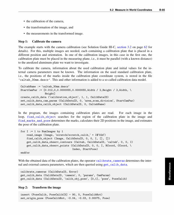
6.2 Measure in World Coordinates B-85
• the calibration of the camera,
• the transformation of the image, and
• the measurements in the transformed image.
Step 1: Calibrate the camera
The example starts with the camera calibration (see Solution Guide III-C, section 3.2 on page 62 fordetails). For this, multiple images are needed, each containing a calibration plate that is placed in adifferent position and orientation. In one of the calibration images, in this case in the first one, thecalibration plate must be placed in the measuring plane, i.e., it must be parallel (with a known distance)to the anodized aluminum plate we want to investigate.
To calibrate the camera, information about the used calibration plate and initial values for the in-ternal camera parameters must be known. The information on the used standard calibration plate,i.e., the positions of the marks inside the calibration plate coordinate system, is stored in the file’caltab_30mm.descr’. This and other information is added to a so-called calibration data model.
CaltabName := 'caltab_30mm.descr'StartCamPar := [0.012,0,0.0000055,0.0000055,Width / 2,Height / 2,Width, \
Height]
create_calib_data ('calibration_object', 1, 1, CalibDataID)
set_calib_data_cam_param (CalibDataID, 0, 'area_scan_division', StartCamPar)
set_calib_data_calib_object (CalibDataID, 0, CaltabName)
In the program, the images containing calibration plates are read. For each image in theloop, find_calib_object searches for the region of the calibration plate in the image andfind_marks_and_pose determines the marks, calculates their 2D positions in the image, and estimatesthe pose of the calibration plate.
for I := 1 to NumImages by 1
read_image (Image, 'scratch/scratch_calib_' + I$'02d')find_calib_object (Image, CalibDataID, 0, 0, I, [], [])
get_calib_data_observ_contours (Caltab, CalibDataID, 'caltab', 0, 0, I)
get_calib_data_observ_points (CalibDataID, 0, 0, I, RCoord, CCoord, \
Index, StartPose)
endfor
With the obtained data of the calibration plates, the operator calibrate_cameras determines the inter-nal and external camera parameters, which are then queried using get_calib_data.
calibrate_cameras (CalibDataID, Error)
get_calib_data (CalibDataID, 'camera', 0, 'params', CamParam)
get_calib_data (CalibDataID, 'calib_obj_pose', [0,1], 'pose', PoseCalib)
Step 2: Transform the image
insert (PoseCalib, PoseCalib[5] - 90, 5, PoseCalibRot)
set_origin_pose (PoseCalibRot, -0.04, -0.03, 0.00075, Pose)
Mis
cella
neou
s

B-86 Miscellaneous
The pose of the measuring plane, i.e., the external camera parameters obtained for the image in whichthe calibration plate lies in the measuring plane, is now stored in the variable PoseCalib. Since thecalibration plate was rotated by 90° (the black triangular mark normally has to be placed in the upper leftcorner), we add a rotation to the corresponding parameter of the pose using insert. Note that poses canbe defined by different sequences of translations and rotations (see Solution Guide III-C, section 2.1.5on page 25). If you are not sure about the sequence used for the pose you want to change, you canalso convert the pose to a homogeneous transformation matrix with pose_to_hom_mat3d, explicitlyadd a local rotation to the axis you want to change using hom_mat_3d_rotate_local, and convert theresulting homogeneous transformation matrix back to a pose using hom_mat3d_to_pose.
Additionally, we apply the operator set_origin_pose to the pose to add a translation to the z-coordinate to compensate for the distance between the calibration pattern and the measuring plane, whichis described by the known thickness of the calibration plate. The translations in x- and y- direction areapplied mainly so that the rectified image optimally fits the displaying window.
From the corrected pose, the operator pose_to_hom_mat3d creates a homogeneous transformation ma-trix. This is used by gen_image_to_world_plane_map to generate a projection map that describes themapping between the image plane and the plane z=0 of a world coordinate system. This map can be usednow to transform the images with the operator map_image so that the measuring plane is rectified witha scaling described by PixelDist. Here, we transform two images, one containing the calibration platethat is placed in the measuring plane (see figure 6.5), and the other containing the scratches we want toinvestigate (see figure 6.4). The first one is transformed mainly for visualization purposes, whereas thelatter is the actual image we wanted to obtain. This image (ModelImageMapped) is used now for theactual measurement.
PixelDist := 0.00013
pose_to_hom_mat3d (Pose, HomMat3D)
gen_image_to_world_plane_map (Map, CamParam, Pose, Width, Height, Width, \
Height, PixelDist, 'bilinear')Imagefiles := ['scratch/scratch_calib_01','scratch/scratch_perspective']for I := 1 to 2 by 1
read_image (Image, Imagefiles[I - 1])
map_image (Image, Map, ModelImageMapped)
endfor
Step 3: Measure in the transformed image
fast_threshold (ModelImageMapped, Region, 0, 80, 20)
fill_up (Region, RegionFillUp)
erosion_rectangle1 (RegionFillUp, RegionErosion, 5, 5)
reduce_domain (ModelImageMapped, RegionErosion, ImageReduced)
fast_threshold (ImageReduced, Region1, 55, 100, 20)
dilation_circle (Region1, RegionDilation1, 2.0)
erosion_circle (RegionDilation1, RegionErosion1, 1.0)
connection (RegionErosion1, ConnectedRegions)
select_shape (ConnectedRegions, SelectedRegions, ['area','ra'], 'and', [40, \
15], [2000,1000])
The measurement starts with the extraction of the aluminum plate and the following code searchesfor scratches having a minimum size and extent. For this, a classical region processing is applied
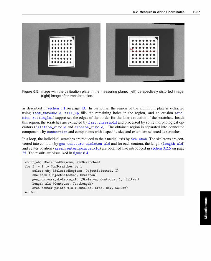
6.2 Measure in World Coordinates B-87
Figure 6.5: Image with the calibration plate in the measuring plane: (left) perspectively distorted image,(right) image after transformation.
as described in section 3.1 on page 13. In particular, the region of the aluminum plate is extractedusing fast_threshold, fill_up fills the remaining holes in the region, and an erosion (ero-sion_rectangle1) suppresses the edges of the border for the later extraction of the scratches. Insidethis region, the scratches are extracted by fast_threshold and processed by some morphological op-erators (dilation_circle and erosion_circle). The obtained region is separated into connectedcomponents by connection and components with a specific size and extent are selected as scratches.
In a loop, the individual scratches are reduced to their medial axis by skeleton. The skeletons are con-verted into contours by gen_contours_skeleton_xld and for each contour, the length (length_xld)and center position (area_center_points_xld) are obtained like introduced in section 3.2.5 on page25. The results are visualized in figure 6.4.
count_obj (SelectedRegions, NumScratches)
for I := 1 to NumScratches by 1
select_obj (SelectedRegions, ObjectSelected, I)
skeleton (ObjectSelected, Skeleton)
gen_contours_skeleton_xld (Skeleton, Contours, 1, 'filter')length_xld (Contours, ContLength)
area_center_points_xld (Contours, Area, Row, Column)
endfor
Mis
cella
neou
s

B-88 Miscellaneous

Index B-89
Index
2D measuringfirst example, 41overview, 7
2D measuring in color image, 742D measuring tools, 13
overview, 312D measuring with blob analysis, 132D measuring with contour processing, 172D measuring with geometric operations, 282D measuring with template, 772D metrology, 26
align image or region for 2D measuring, 41
blob analysis vs. contour processing, 36
combine XLD contours, 21compute mean of values, 44compute parallel XLD contours, 50count objects, 36create XLD contours, 18
edge extraction (pixel-precise), 18edge extraction (subpixel-precise), 19extract features for blob analysis, 16extract features of XLD contours, 25extract subpixel edges without smoothing, 45
fit XLD contours to polygons, 50fit XLD contours to regression line, 47
measure 2D area, 33measure 2D area with gray-value moments, 68measure 2D dimensions, 35measure 2D distance, 35measure 2D distance between point and con-
tour, 48measure 2D distance of parallel XLD contours,
49
measure 2D orientation, 33measure 2D orientation of rectangle, 59measure 2D orientation with gray-value mo-
ments, 68measure 2D position, 34measure 2D position of corner points, 57measure 2D position of grid junctions, 53measure 2D position of rectangle, 59measure 2D position with gray-value moments,
68measure 2D radius of circle, 62measure 2D size of rectangle, 59measure 2D width (pixel-precise), 43measure 2D width of lines, 51measure angle between 2D lines, 59measure angle between 2D objects, 33measure deviation from straight 2D line, 44measure deviation of XLD contour from 2D cir-
cle, 65measuring and comparison 2D, 7
perform fitting of XLD contours, 23preprocess image, 14process regions, 15process XLD contours, 20
rectify image for 2D measuring, 84
segment image(s) for blob analysis, 14segment XLD contours, 23simplify XLD contours, 22subpixel thresholding, 19suppress XLD contours, 20
transform results of 2D measuring into 3D(world) coordinates, 84
use region of interest for edge extraction(subpixel-precise), 45
Inde
x

B-90 Index
XLD contour coordinates, 48
Related Documents


