a product of MVTec Solution Guide II-D Classification HALCON 21.11 Progress

Welcome message from author
This document is posted to help you gain knowledge. Please leave a comment to let me know what you think about it! Share it to your friends and learn new things together.
Transcript

a product of MVTec
Solution Guide II-DClassification
HALCON 21.11 Progress

How to use classification, Version 21.11.0.0
All rights reserved. No part of this publication may be reproduced, stored in a retrieval system, or transmitted in any form or by any means,electronic, mechanical, photocopying, recording, or otherwise, without prior written permission of the publisher.
Copyright © 2008-2021 by MVTec Software GmbH, München, Germany MVTec Software GmbH
Protected by the following patents: US 7,239,929, US 7,751,625, US 7,953,290, US 7,953,291, US 8,260,059, US 8,379,014,US 8,830,229. Further patents pending.
Microsoft, Windows, Windows Server 2008/2012/2012 R2/2016, Windows 7/8/8.1/10, Microsoft .NET, Visual C++, and VisualBasic are either trademarks or registered trademarks of Microsoft Corporation.
All other nationally and internationally recognized trademarks and tradenames are hereby recognized.
More information about HALCON can be found at: http://www.halcon.com/

About This Manual
In a broad range of applications classification is suitable to find specific objects or detect defects in images. ThisSolution Guide leads you through the variety of approaches that are provided by HALCON.
After a short introduction to the general topic in section 1 on page 7, a first example is presented in section 2 onpage 11 that gives an idea on how to apply a classification with HALCON.
Section 3 on page 15 then provides you with the basic theories related to the available approaches. Some hints howto select the suitable classification approach, a set of features or images that is used to define the class boundaries,and some samples that are used for the training of the classifier are given in section 4 on page 27.
Section 5 on page 31 describes how to generally apply a classification for various objects like pixels or regionsbased on various features like color, texture, or region features. Section 6 on page 57 shows how to apply classi-fication for a pure pixel-based image segmentation and section 7 on page 75 provides a short introduction to theclassification for optical character recognition (OCR). For the latter regions are classified by region features.
Finally, section 8 on page 93 provides some general tips that may be suitable when working with complex classi-fication tasks.
The HDevelop example programs that are presented in this Solution Guide can be found in the specified subdirec-tories of the directory %HALCONEXAMPLES%. The path to this directory can be determined with the operator callget_system ('example_dir', ExampleDir).
Symbols
The following symbol is used within the manual:
! This symbol indicates an information you should pay attention to.


Contents
1 Introduction 7
2 A First Example 11
3 Classification: Theoretical Background 153.1 Classification in General . . . . . . . . . . . . . . . . . . . . . . . . . . . . . . . . . . . . . . . 153.2 Euclidean and Hyperbox Classifiers . . . . . . . . . . . . . . . . . . . . . . . . . . . . . . . . . 163.3 Multi-Layer Perceptrons (MLP) . . . . . . . . . . . . . . . . . . . . . . . . . . . . . . . . . . . 183.4 Support-Vector Machines (SVM) . . . . . . . . . . . . . . . . . . . . . . . . . . . . . . . . . . . 193.5 Gaussian Mixture Models (GMM) . . . . . . . . . . . . . . . . . . . . . . . . . . . . . . . . . . 203.6 K-Nearest Neighbors (k-NN) . . . . . . . . . . . . . . . . . . . . . . . . . . . . . . . . . . . . . 223.7 Deep Learning (DL) and Convolutional Neural Networks (CNNs) . . . . . . . . . . . . . . . . . 23
4 Decisions to Make 274.1 Select a Suitable Classification Approach . . . . . . . . . . . . . . . . . . . . . . . . . . . . . . 274.2 Select Suitable Features . . . . . . . . . . . . . . . . . . . . . . . . . . . . . . . . . . . . . . . . 284.3 Select Suitable Training Samples . . . . . . . . . . . . . . . . . . . . . . . . . . . . . . . . . . . 29
5 Classification of General Features 315.1 General Approach (Classification of Arbitrary Features) . . . . . . . . . . . . . . . . . . . . . . . 315.2 Involved Operators (Overview) . . . . . . . . . . . . . . . . . . . . . . . . . . . . . . . . . . . . 34
5.2.1 Basic Steps: MLP, SVM, GMM, and k-NN . . . . . . . . . . . . . . . . . . . . . . . . . 345.2.2 Advanced Steps: MLP, SVM, GMM, and k-NN . . . . . . . . . . . . . . . . . . . . . . . 35
5.3 Parameter Setting for MLP . . . . . . . . . . . . . . . . . . . . . . . . . . . . . . . . . . . . . . 375.3.1 Adjusting create_class_mlp . . . . . . . . . . . . . . . . . . . . . . . . . . . . . . . 375.3.2 Adjusting add_sample_class_mlp . . . . . . . . . . . . . . . . . . . . . . . . . . . . . 395.3.3 Adjusting train_class_mlp . . . . . . . . . . . . . . . . . . . . . . . . . . . . . . . . 405.3.4 Adjusting evaluate_class_mlp . . . . . . . . . . . . . . . . . . . . . . . . . . . . . . 415.3.5 Adjusting classify_class_mlp . . . . . . . . . . . . . . . . . . . . . . . . . . . . . . 41
5.4 Parameter Setting for SVM . . . . . . . . . . . . . . . . . . . . . . . . . . . . . . . . . . . . . . 425.4.1 Adjusting create_class_svm . . . . . . . . . . . . . . . . . . . . . . . . . . . . . . . 425.4.2 Adjusting add_sample_class_svm . . . . . . . . . . . . . . . . . . . . . . . . . . . . . 455.4.3 Adjusting train_class_svm . . . . . . . . . . . . . . . . . . . . . . . . . . . . . . . . 455.4.4 Adjusting reduce_class_svm . . . . . . . . . . . . . . . . . . . . . . . . . . . . . . . 465.4.5 Adjusting classify_class_svm . . . . . . . . . . . . . . . . . . . . . . . . . . . . . . 47
5.5 Parameter Setting for GMM . . . . . . . . . . . . . . . . . . . . . . . . . . . . . . . . . . . . . 475.5.1 Adjusting create_class_gmm . . . . . . . . . . . . . . . . . . . . . . . . . . . . . . . 485.5.2 Adjusting add_sample_class_gmm . . . . . . . . . . . . . . . . . . . . . . . . . . . . . 495.5.3 Adjusting train_class_gmm . . . . . . . . . . . . . . . . . . . . . . . . . . . . . . . . 505.5.4 Adjusting evaluate_class_gmm . . . . . . . . . . . . . . . . . . . . . . . . . . . . . . 515.5.5 Adjusting classify_class_gmm . . . . . . . . . . . . . . . . . . . . . . . . . . . . . . 52
5.6 Parameter Setting for k-NN . . . . . . . . . . . . . . . . . . . . . . . . . . . . . . . . . . . . . . 525.6.1 Adjusting create_class_knn . . . . . . . . . . . . . . . . . . . . . . . . . . . . . . . 535.6.2 Adjusting add_sample_class_knn . . . . . . . . . . . . . . . . . . . . . . . . . . . . . 535.6.3 Adjusting train_class_knn . . . . . . . . . . . . . . . . . . . . . . . . . . . . . . . . 535.6.4 Adjusting set_params_class_knn . . . . . . . . . . . . . . . . . . . . . . . . . . . . . 545.6.5 Adjusting classify_class_knn . . . . . . . . . . . . . . . . . . . . . . . . . . . . . . 55
6 Classification for Image Segmentation 576.1 Approach for MLP, SVM, GMM, and k-NN . . . . . . . . . . . . . . . . . . . . . . . . . . . . . 57
6.1.1 General Approach . . . . . . . . . . . . . . . . . . . . . . . . . . . . . . . . . . . . . . 576.1.2 Involved Operators (Overview) . . . . . . . . . . . . . . . . . . . . . . . . . . . . . . . . 646.1.3 Parameter Setting for MLP . . . . . . . . . . . . . . . . . . . . . . . . . . . . . . . . . . 676.1.4 Parameter Setting for SVM . . . . . . . . . . . . . . . . . . . . . . . . . . . . . . . . . . 676.1.5 Parameter Setting for GMM . . . . . . . . . . . . . . . . . . . . . . . . . . . . . . . . . 686.1.6 Parameter Setting for k-NN . . . . . . . . . . . . . . . . . . . . . . . . . . . . . . . . . 696.1.7 Classification Based on Look-Up Tables . . . . . . . . . . . . . . . . . . . . . . . . . . . 70
6.2 Approach for a Two-Channel Image Segmentation . . . . . . . . . . . . . . . . . . . . . . . . . . 726.3 Approach for Euclidean and Hyperbox Classification . . . . . . . . . . . . . . . . . . . . . . . . 73
7 Classification for Optical Character Recognition (OCR) 757.1 General Approach . . . . . . . . . . . . . . . . . . . . . . . . . . . . . . . . . . . . . . . . . . . 757.2 Involved Operators (Overview) . . . . . . . . . . . . . . . . . . . . . . . . . . . . . . . . . . . . 787.3 Parameter Setting for MLP . . . . . . . . . . . . . . . . . . . . . . . . . . . . . . . . . . . . . . 80
7.3.1 Adjusting create_ocr_class_mlp . . . . . . . . . . . . . . . . . . . . . . . . . . . . . 807.3.2 Adjusting write_ocr_trainf / append_ocr_trainf . . . . . . . . . . . . . . . . . . 827.3.3 Adjusting trainf_ocr_class_mlp . . . . . . . . . . . . . . . . . . . . . . . . . . . . . 827.3.4 Adjusting do_ocr_multi_class_mlp . . . . . . . . . . . . . . . . . . . . . . . . . . . 827.3.5 Adjusting do_ocr_single_class_mlp . . . . . . . . . . . . . . . . . . . . . . . . . . . 83
7.4 Parameter Setting for SVM . . . . . . . . . . . . . . . . . . . . . . . . . . . . . . . . . . . . . . 837.4.1 Adjusting create_ocr_class_svm . . . . . . . . . . . . . . . . . . . . . . . . . . . . . 847.4.2 Adjusting write_ocr_trainf / append_ocr_trainf . . . . . . . . . . . . . . . . . . 857.4.3 Adjusting trainf_ocr_class_svm . . . . . . . . . . . . . . . . . . . . . . . . . . . . . 857.4.4 Adjusting do_ocr_multi_class_svm . . . . . . . . . . . . . . . . . . . . . . . . . . . 857.4.5 Adjusting do_ocr_single_class_svm . . . . . . . . . . . . . . . . . . . . . . . . . . . 85
7.5 Parameter Setting for k-NN . . . . . . . . . . . . . . . . . . . . . . . . . . . . . . . . . . . . . . 867.5.1 Adjusting create_ocr_class_knn . . . . . . . . . . . . . . . . . . . . . . . . . . . . . 867.5.2 Adjusting write_ocr_trainf / append_ocr_trainf . . . . . . . . . . . . . . . . . . 877.5.3 Adjusting trainf_ocr_class_knn . . . . . . . . . . . . . . . . . . . . . . . . . . . . . 877.5.4 Adjusting do_ocr_multi_class_knn . . . . . . . . . . . . . . . . . . . . . . . . . . . 877.5.5 Adjusting do_ocr_single_class_knn . . . . . . . . . . . . . . . . . . . . . . . . . . . 88
7.6 Parameter Setting for CNNs . . . . . . . . . . . . . . . . . . . . . . . . . . . . . . . . . . . . . 887.6.1 Adjusting do_ocr_multi_class_cnn . . . . . . . . . . . . . . . . . . . . . . . . . . . 887.6.2 Adjusting do_ocr_single_class_cnn . . . . . . . . . . . . . . . . . . . . . . . . . . . 89
7.7 OCR Features . . . . . . . . . . . . . . . . . . . . . . . . . . . . . . . . . . . . . . . . . . . . . 89
8 General Tips 938.1 Optimize Critical Parameters with a Test Application . . . . . . . . . . . . . . . . . . . . . . . . 938.2 Classify General Regions using OCR . . . . . . . . . . . . . . . . . . . . . . . . . . . . . . . . . 948.3 Visualize the Feature Space (2D and 3D) . . . . . . . . . . . . . . . . . . . . . . . . . . . . . . . 96
8.3.1 Visualize the 2D Feature Space . . . . . . . . . . . . . . . . . . . . . . . . . . . . . . . 968.3.2 Visualize the 3D Feature Space . . . . . . . . . . . . . . . . . . . . . . . . . . . . . . . 99
Index 105

Introduction D-7
Chapter 1
Introduction
What is classification?
Classifying an object means to assign an object to one of several available classes. When working with images, theobjects usually are pixels or regions. Objects are described by features, which comprise, e.g., the color or texturefor pixel objects, and the size or specific shape features for region objects. To assign an object to a specific class,the individual class boundaries have to be known. These are built in most cases by a training using the featuresof sample objects for which the classes are known. Then, when classifying an unknown object, the class withthe largest correspondence between the feature values used for its training and the feature values of the unknownobject is returned.
What can you do with classification?
Classification is reasonable in all cases where objects have similarities, but within unknown variations. If yousearch for objects of a certain fixed shape, and the points of a found contour may not deviate from this shapemore than a small defined distance, a template matching will be faster and easier to apply. But if the shapesof your objects are similar, but you can not define exactly what the similarities are and what distinguishes theseobjects from other objects in the image, you can show a classifier some samples of known objects (with a set offeatures that you roughly imagine to describe the characteristics of the object types) and let the classifier find therules to distinguish between the object types. Classification can be used for a lot of different tasks. You can useclassification, e.g., for
• image segmentation, i.e., you segment images into regions of similar color or texture,
• object recognition, i.e., you find objects of a specific type within a set of different object types,
• quality control, i.e., you decide if objects are good or bad,
• novelty detection, i.e., you detect changes or defects of objects, or
• optical character recognition (OCR).
What can HALCON do for you?
To solve the different requirements on classification, HALCON provides different types of classifiers. The mostimportant HALCON classifiers are
• a classifier that uses neural nets, in particular multi-layer perceptrons (MLP, see section 3.3 on page 18),
• a classifier that is based on support-vector machines (SVM, see section 3.4 on page 19),
• a classifier that is based on Gaussian mixture models (GMM, see section 3.5 on page 20), and
• a classifier that is based on the k-nearest neighbors (k-NN, see section 3.6 on page 22).
• a classifier that is based on deep learning using a convolutional neural network (DL for general classification,CNN for OCR, see section 3.7 on page 23).
Intr
oduc
tion

D-8 Introduction
• Furthermore, for image segmentation also some simple but fast classifiers are available. These comprise aclassifier that segments two-channel images based on the corresponding 2D histogram (see section 6.2 onpage 72), a hyperbox classifier, and a classifier that can be applied using either a Euclidean or a hyperboxmetric (see section 3.2 on page 16 and section 6.3 on page 73).
For specific classification tasks, specific sets of HALCON operators are available. We distinguish between thethree following basic tasks:
• You can apply a general classification. Here, arbitrary objects like pixels or regions are classified based onarbitrary features like color, texture, shape, or size. table 4.1 on page 28 may give a hint which method ismost suitable for your task. Section 5 on page 31 shows how to apply the suitable operators for MLP, SVM,GMM, k-NN, and DL-based classification.
• You can apply classification for image segmentation. Here, the classification is used to segment images intoregions of different classes. For that, the individual pixels of an image are classified due to the features coloror texture and all pixels belonging to the same class are combined in a region. Section 6 on page 57 showshow to apply the suitable operators for MLP, SVM, GMM, and k-NN classification (section 6.1 on page 57)as well as for some simple but fast classifiers that segment the images using the 2D histogram of two imagechannels (section 6.2 on page 72) or that apply an Euclidean or hyperbox classification (section 6.3 on page73).
• You can apply classification for OCR, i.e., individual regions are investigated with regard to region featuresand assigned to classes that typically (but not necessarily) represent individual characters or numbers. Sec-tion 7 on page 75 shows how to apply the suitable operators for MLP, SVM, k-NN, and CNN classification.
What are the basic steps of a classification with HALCON?
There are different methods for classification implemented in HALCON, each one having its own assets anddrawbacks. For a brief comparison we refer to table 4.1 on page 28. These classification approaches can bedivided into two major groups. The first group consists of the methods MLP, SVM, GMM, and k-NN, where thedistinguishing features of each class have to be specified. The second group is given by DL-based methods, wherethe network is trained by considering the inputs and outputs directly. For the user, it has the nice outcome of noneed for feature specification. Accordingly the basic approach for a classification with HALCON depends on themethod group. For the first one, thus MLP, SVM, GMM, and k-NN, it is as follows:
1. First, some sample objects, i.e., objects of known classes, are investigated. That is, a set of characteristicfeatures is extracted from each sample object and stored in a so-called feature vector (explicitly by the useror implicitly by a specific operator).
2. The feature vectors of many sample objects are used to train a classifier. With the training, the classifierderives suitable boundaries between the classes.
3. Then, unknown objects, i.e., the objects to classify, are investigated with the help of the same set of featuresthat was already used for the training samples. This step leads to feature vectors for the unknown objects.
4. Finally, the trained classifier uses the class boundaries that were derived during the training to decide for thenew feature vectors to which classes they belong.
For deep-learning-based methods, to train the classifier (or rather the network) one does not have to specify thefeatures but to provide labeled (hence, already classified) images. Therefore the basic approach is as follows:
1. Providing data: For each class one wants the classifier to distinguish, much data in form of already labeledimages has to be provided.
2. Training: From this data the algorithm learns how to classify your images. This is achieved by retraining thealready pretrained, more general network. As a result, the network is adapted to your specific classificationtask.
3. Inference phase: Classify images using the adapted network.

D-9
What information do you find in this solution guide?
This manual provides you with
• basic theoretical background for the provided classifiers (section 3 on page 15),
• tips for the decision making, in particular tips for the selection of a suitable classification approach, theselection of suitable training samples and, if needed, the selection of suitable features that describe theobjects to classify (section 4 on page 27),
• guidance for the practical application of classification for general classification (section 5 on page 31), imagesegmentation (section 6 on page 57), and OCR (section 7 on page 75), and
• additional tips that may be useful when applying classification (section 8 on page 93). In particular, whennot applying deep-learning-based methods or only using it for OCR, tips how to adjust the most criticalparameters, tips how to use OCR for the classification of arbitrary regions, and tips how to visualize thefeature space for 2D and 3D feature vectors are provided.
What do you have to consider before classifying?
Note that the decision which classifier to use for a specific application is a challenging task. There are no fixedrules which approach works better for which application, as the number of possible fields of applications is verylarge. At least, section 4.1 on page 27 provides some hints about the advantages and disadvantages of the individualapproaches.
Additionally, if you have decided to use a specific classifier, it is not guaranteed that you get a satisfying resultwithin a short time. Actually, in almost any case you have to apply a lot of tests with different parameters until youget the result you aimed at. Classification is very complex! So, plan enough time for your application.
Intr
oduc
tion

D-10 Introduction

A First Example D-11
Chapter 2
A First Example
This section shows a first example for a classification that classifies metal parts based on selected shape fea-tures. To follow the example actively, start the HDevelop program %HALCONEXAMPLES%\solution_guide\
classification\classify_metal_parts.hdev; the steps described below start after the initialization of theapplication.
Step 1: Create classifier
First, a classifier is created. Here, we want to apply an MLP classification, so a classifier of type MLP is createdwith create_class_mlp. The returned handle MLPHandle is needed for all following classification steps.
create_class_mlp (6, 5, 3, 'softmax', 'normalization', 3, 42, MLPHandle)
Step 2: Add training samples to the classifier
Then, the training images, i.e., images that contain objects of known class, are investigated. Each image containsseveral metal parts that belong to the same class. The index of the class for a specific image is stored in the tupleClasses. In this case, nine images are available (see figure 2.1). The objects in the first three images belong toclass 0, the objects of the next three images belong to class 1, and the last three images show objects of class 2.
FileNames := ['nuts_01', 'nuts_02', 'nuts_03', 'washers_01', 'washers_02', \
'washers_03', 'retainers_01', 'retainers_02', \
'retainers_03']Classes := [0, 0, 0, 1, 1, 1, 2, 2, 2]
Now, each training image is processed by the two procedures segment and add_samples.
for J := 0 to |FileNames| - 1 by 1
read_image (Image, 'rings/' + FileNames[J])
segment (Image, Objects)
add_samples (Objects, MLPHandle, Classes[J])
endfor
The procedure segment segments and separates the objects that are contained in the image using a simple blobanalysis (for blob analysis see Solution Guide I, chapter 4 on page 35).
procedure segment (Image, Regions)
binary_threshold (Image, Region, 'max_separability', 'dark', UsedThreshold)
connection (Region, ConnectedRegions)
fill_up (ConnectedRegions, Regions)
return ()
For each region, the procedure add_samples determines a feature vector using the procedure get_features.The feature vector and the known class index build the training sample, which is added to the classifier with theoperator add_sample_class_mlp.
Firs
tExa
mpl
e

D-12 A First Example
Class 0 Class 1 Class 2
Figure 2.1: Training images.
procedure add_samples (Regions, MLPHandle, Class)
count_obj (Regions, Number)
for J := 1 to Number by 1
select_obj (Regions, Region, J)
get_features (Region, Features)
add_sample_class_mlp (MLPHandle, Features, Class)
endfor
return ()
The features extracted in the procedure get_features are region features, in particular the ’circularity’,’roundness’, and the four moments (obtained by the operator moments_region_central_invar) of the region.
procedure get_features (Region, Features)
select_obj (Region, SingleRegion, 1)
circularity (SingleRegion, Circularity)
roundness (SingleRegion, Distance, Sigma, Roundness, Sides)
moments_region_central_invar (SingleRegion, PSI1, PSI2, PSI3, PSI4)
Features := [Circularity,Roundness,PSI1,PSI2,PSI3,PSI4]
return ()
Step 3: Train the classifier
After adding all available samples, the classifier is trained with train_class_mlp.
train_class_mlp (MLPHandle, 200, 1, 0.01, Error, ErrorLog)
Step 4: Classify new objects
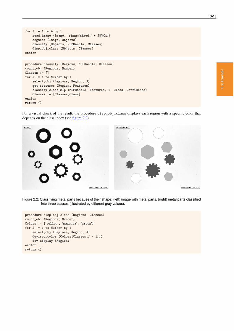
Now, images with different unknown objects are investigated. The segmentation of the objects and the extractionof their feature vectors is realized by the same procedures that were used for the training images (segment andget_features). But this time, the class of a feature vector is not yet known and has to be determined by theclassification. Thus, opposite to the procedure add_samples, within the procedure classify the extracted featurevector is used as input to the operator classify_class_mlp and not to add_sample_class_mlp. The result isthe class index that is suited best for the feature vector extracted for the specific region.
D-13
for J := 1 to 4 by 1
read_image (Image, 'rings/mixed_' + J$'02d')segment (Image, Objects)
classify (Objects, MLPHandle, Classes)
disp_obj_class (Objects, Classes)
endfor
procedure classify (Regions, MLPHandle, Classes)
count_obj (Regions, Number)
Classes := []
for J := 1 to Number by 1
select_obj (Regions, Region, J)
get_features (Region, Features)
classify_class_mlp (MLPHandle, Features, 1, Class, Confidence)
Classes := [Classes,Class]
endfor
return ()
For a visual check of the result, the procedure disp_obj_class displays each region with a specific color thatdepends on the class index (see figure 2.2).
Figure 2.2: Classifying metal parts because of their shape: (left) image with metal parts, (right) metal parts classifiedinto three classes (illustrated by different gray values).
procedure disp_obj_class (Regions, Classes)
count_obj (Regions, Number)
Colors := ['yellow', 'magenta', 'green']for J := 1 to Number by 1
select_obj (Regions, Region, J)
dev_set_color (Colors[Classes[J - 1]])
dev_display (Region)
endfor
return ()
Firs
tExa
mpl
e

D-14 A First Example

Classification: Theoretical Background D-15
Chapter 3
Classification: TheoreticalBackground
This section introduces you to the basics of classification (section 3.1) and the specific classifiers that can be ap-plied with HALCON. In particular, the Euclidean and hyperbox classifiers (section 3.2), the classifier based onmulti-layer perceptrons (neural nets, section 3.3), the classifier based on support-vector machines (section 3.4),the classifier based on Gaussian mixture models (section 3.5), the classifier based on k-nearest neighbors (sec-tion 3.6), and the classifier based on deep learning, with a focus on convolutional neural networks (section 3.7),are introduced.
3.1 Classification in General
Generally, a classifier is used to assign an object to one of several available classes. For example, you have grayvalue images containing citrus fruits. You have extracted regions1 from the images and each region representsa fruit. Now, you want to separate the oranges from the lemons. To distinguish the fruits, you can apply aclassification. Then, the extracted regions of the fruits are your objects and the task of the classification is to decidefor each region if it belongs to the class ’oranges’ or to the class ’lemons’.
In order to decide to which class an image or a region belongs, the classifier needs to know how to distinguish theclasses. Thus, differences between the classes and the similarities within each individual class have to be known.With deep-learning-based classification, the network learns this information automatically from the images. Forfurther information, see section 3.7 on page 23. However, for all other approaches, you as user need to provide theknowledge, which you can obtain by analyzing typical features of the objects to classify. Let us illustrate the lattercase with the example of citrus fruits (an actual program is described in more detail in section 8.3.1 on page 96).Suitable features can be, e.g., the ’area’ (an orange is usually bigger than a lemon) and the shape, in particular the’circularity’ of the regions (the outline of an orange is closer to a circle than that of a lemon). Figure 3.1 showssome oranges and lemons for which the regions are extracted and the region features ’area’ and ’circularity’
are calculated.
The features are arranged in an array that is called feature vector. The features of the feature vector span a so-called feature space, i.e., a vector space in which each feature is represented by an axis. Generally, a feature spacecan have any dimension, depending on the number of features contained in the feature vector. For visualizationpurpose, here a 2D feature space is shown. In practice, feature spaces of higher dimension are very common.
In figure 3.2 the feature vectors of the fruits shown in figure 3.1 are visualized in a 2D graph, for which one axisrepresents the ’area’ values and the other axis represents the ’circularity’ values. Although the regions varyin size and circularity, we can see that they are similar enough to build clusters. The goal of a classifier is toseparate the clusters and to assign each feature vector to one of the clusters. Here, the oranges and lemons canbe separated, e.g., by a straight line. All objects on the lower left side of the line are classified as lemons and allobjects on the upper right side of the line are classified as oranges.
As we can see, the feature vector of a very small orange and that of a rather circular lemon are close to theseparating line. With a little bit different data, e.g., if the small orange additionally would be less circular, the
1How to extract regions from images is described, e.g., in Solution Guide I, chapter 4 on page 35
Ove
rvie
w

D-16 Classification: Theoretical Background
Figure 3.1: Region features of oranges and lemons are extracted and can be added as samples to the classifier.
feature vectors may be classified incorrectly. To minimize errors, a lot of different samples and in many cases alsoadditional features are needed. An additional feature for the citrus fruits may be, e.g., the gray value. Then, not aline but a plane is needed to separate the clusters. If color images are available, you can combine the area and thecircularity with the gray values of three channels. For feature vectors of more than three features, an n-dimensionalplane, also called hyperplane, is needed.
Classifiers that use separating lines or hyperplanes are called linear classifiers. Other classifiers, i.e., non-linearclassifiers, can separate clusters using arbitrary surfaces and may be able to separate clusters more conveniently insome cases.
Summarized, we need a suitable set of features and we have to select the classifier that is suited best for a spe-cific classification application. To select the most appropriate approach, we have to know some basics about theavailable classifiers and the algorithms they use.
3.2 Euclidean and Hyperbox Classifiers
One of the simple classifiers is the Euclidean or minimum distance classifier. With HALCON, the Euclideanclassification is available for image segmentation, i.e., the objects to classify are pixels and the feature vectorscontain the gray values of the pixels. The dimension of the feature space depends on the number of channels usedfor the image segmentation. Geometrically interpreted, this classifier builds circles (in 2D; see figure 3.3a) or n-dimensional hyperspheres (in nD) around the cluster centers to separate the clusters from each other. In section 6.3on page 73 it is described how to apply the Euclidean classifier for image segmentation. With HALCON, theEuclidean metric is used only for image segmentation, not for the classification of general features or OCR. Thisis because the approach is stable only for feature vectors of low dimension.
Whereas the Euclidean classifier uses n-dimensional spheres, the hyperbox approach uses axis-parallel cubes, so-called hyperboxes (see figure 3.3b). This can be imagined as a threshold approach in multidimensional space.

3.2 Euclidean and Hyperbox Classifiers D-17
1
1
Figure 3.2: The normalized values for the ’area’ and ’circularity’ of the fruits span a feature space. The twoclasses can be separated by a line.
xxxxxx
x
xxxxxxxx
xxx x
x x
xxxxxxxx
xx xx
xx
x xx
xx
x
x x
x
Feature 1:
Feature 2:
x xxxxxx
x
xxxxxxxx
xxx x
x x
xxxxxxxx
xx xx
xx
x xx
xx
x
x x
x
Feature 1:
Feature 2:
x
(a) (b)
Figure 3.3: (a) Euclidean classifier and (b) hyperbox classifier.
That is, for each class specific value ranges for each axis of the feature space are determined. If a feature vectorlies within all the ranges of a specific class, it will be assigned to this class. The hyperboxes can overlap. Forobjects that are ambiguous, the hyperbox approach can be combined with another classification approach, e.g., anEuclidean classification or a maximum likelihood classification. Within HALCON, the Euclidean distance is usedand additionally weighted with the variance of the feature vector. In section 6.3 on page 73 it is described how toapply the hyperbox classifier for image segmentation.
HALCON provides also operators for hyperbox classification of general features as well as for OCR, but theseshow almost no advantage but a lot of disadvantages compared to the MLP, SVM, GMM, and k-NN approaches,and thus are not described further in this solution guide.
Ove
rvie
w

D-18 Classification: Theoretical Background
3.3 Multi-Layer Perceptrons (MLP)
Neural nets directly determine the separating hyperplanes between the classes. For two classes the hyperplaneactually separates the feature vectors of the two classes, i.e., the feature vectors that lie on one side of the plane areassigned to class 1 and the feature vectors that lie on the other side of the plane are assigned to class 2. In contrastto this, for more than two classes the planes are chosen such that the feature vectors of the correct class have thelargest positive distance of all feature vectors from the plane.
A linear classifier can be built, e.g., using a neural net with a single layer like shown in figure 3.4 (a,b). There,so-called processing units (neurons) first compute the linear combinations of the feature vectors and the networkweights and then apply a nonlinear activation function.
A classification with single-layer neural nets needs linearly separable classes, which is not sufficient in manyclassification applications. To get a classifier that can separate also classes that are not linearly separable, you canadd more layers, so-called hidden layers, to the net. The obtained multi-layer neural net (see figure 3.4, c) thenconsists of an input layer, one or several hidden layers and an output layer. Note that one hidden layer is sufficientto approximate any separating hypersurface and any output function with values in [0,1] as long as the hidden layerhas a sufficient number of processing units.
x1
x2
w1
w2
wn
xn
x1
xn
x2
x1
x2
xn
b
Two−class single−layer neural net n−class single−layer neural net
Single−layer neural networks Multi−layer neural network
c)b)a)
Figure 3.4: Neural networks: single-layered for (a) two classes and (b) n classes, (c) multi-layered: (from left to right)input layer, hidden layer, output layer.
Within the neural net, the processing units of each layer (see figure 3.5) compute the linear combination of thefeature vector or of the results from a previous layer.
x1
x2
xn wn
y
w1
w2
weighted summation activation function
Hidden unit OutputInput
Figure 3.5: Processing unit of an MLP.
That is, each processing unit first computes its activation as a linear combination of the input values:
a(l)j =
nl∑i=1
w(l)ij x
(l−1)i + b
(l)j
with

3.4 Support-Vector Machines (SVM) D-19
• x0i : feature vector
• x(j)i : result vector of layer l
• w(l)ji and b(l)j : weights of layer l
Then the results are passed through a nonlinear activation function:
x(l)j = f(a
(l)j )
With HALCON, for the hidden units the activation function is the hyperbolic tangent function:
f(x) = tanh(x) =ex − e−x
ex + e−x
For the output function (when using the MLP for classification) the softmax activation function is used, whichmaps the output values into the range (0, 1) such that they add up to 1:
f(xi) =exi
Σnj=1exj
To derive the separating hypersurfaces for a classification using a multi-layer neural net, the network weightshave to be adjusted. This is done by a training. That is, data with known output is inserted to the input layerand processed by the hidden units. The output is then compared to the expected output. If the output does notcorrespond to the expected output (within a certain error tolerance), the weights are incrementally adjusted so thatthe error is minimized. Note that the weight adjustment using HALCON is realized by a very stable numericalgorithm that leads to better results than obtained by the classical back propagation algorithm.
The MLP method works for classification of general features, image segmentation, and OCR. Note that MLP canalso be used for least squares fitting (regression) and for classification problems with multiple independent logicalattributes.
An MLP can have more than one hidden layer and is then considered as a deep learning method. In HALCONwe only have a single hidden layer implemented in our MLPs. That is why, whenever we refer to deep learningmethods, we exclude the MLP method.
3.4 Support-Vector Machines (SVM)
Another classification approach that can handle classes that are not linearly separable uses support-vector machines(SVM). Here, no non-linear hypersurface is obtained, but the feature space is transformed into a space of higherdimension, so that the features become linearly separable. Then, the feature vectors can be classified with a linearclassifier.
In figure 3.6, e.g., two classes in a 2D feature space are illustrated by black and white squares, respectively. In the2D feature space, no line can be found that separates the classes. When adding a third dimension by deforming theplane built by Feature1 and Feature2, the classes become separable by a plane.
To avoid the curse of dimensionality (see section 3.5) for SVM, not the features but a kernel is transformed. Thechallenging task is to find the suitable kernel to transform the feature space into a higher dimension so that theblack squares in figure 3.6 go up and the white ones stay in their place (or at least stay in another value range ofthe axis for the additional dimension). Common kernels are, e.g., the inhomogeneous polynomial kernel or theGaussian radial basis function kernel.
With SVM, the separating hypersurface for two classes is constructed such that the margin between the two classesbecomes as large as possible. The margin is defined as the closest distance between the separating hyperplane andany training sample. That is, several possible separating hypersurfaces are tested and the surface with the largestmargin is selected. The training samples from both classes that have exactly the closest distance to the hypersurfaceare called ’support vectors’ (see figure 3.7 for two linearly separable classes).
Ove
rvie
w

D-20 Classification: Theoretical Background
Separating Hyperplane
Additional DimensionFeature 1:
Feature 1
Feature 2Feature 2:
Figure 3.6: Separate two classes (black and white squares): (left) In the 2D feature space the classes can notbe separated by a straight line, (right) by addition of a further dimension, the classes become linearlyseparable.
w
Hyperplane
Support vectors
Figure 3.7: Support vectors are those feature vectors that have exactly the closest distance to the hyperplane.
By nature SVM can handle only two-class problems. Two approaches can be used to extend the SVM to a multi-class problem: With the first approach pairs of classes are built and for each pair a binary classifier is created.Then, the class that wins most of the comparisons is the best suited class. With the second approach, each classis compared to the rest of the training data and then, the class with the maximum distance to the hypersurface isselected (see also section 5.4.1 on page 44).
SVM works for classification of general features, image segmentation, and OCR.
3.5 Gaussian Mixture Models (GMM)
The theory for the classification with Gaussian mixture models (GMM) is a bit more complex. One of the basictheories when dealing with classification comprises the Bayes decision rule. Generally, the Bayes decision ruletells us to minimize the probability of erroneously classifying a feature vector by maximizing the probability forthe feature vector x to belong to a class. This so-called ’a posteriori probability’ should be maximized over allclasses. Then, the Bayes decision rule partitions the feature space into mutually disjoint regions. The regions areseparated by hypersurfaces, e.g., by points for 1D data or by curves for 2D data. In particular, the hypersurfacesare defined by the points in which two neighboring classes are equally probable.
The Bayes decision rule can be expressed by
P (wi|x) =P (x|wi)× P (wi)
P (x)
with
• P (wi|x): a posteriori probability

3.5 Gaussian Mixture Models (GMM) D-21
• P (x|wi): a priori probability that the feature vector x occurs given that the class of the feature vector is wi
• P (wi): Probability, that the class wi occurs
• P (x): Probability that the feature vector x occurs
For classification, the a posteriori probability should be maximized over all classes. Here, we coarsely show howto obtain the a posteriori probability for a feature vector x. First, we can remark that P (x), i.e., the probability ofthe class, is a constant if x exists.
The first problem of the Bayes classifier is how to obtain P (wi), i.e., the probability of the occurrence of a class.Two strategies can be followed. First, you can estimate it from the used training set. This is recommended only ifyou have a training set that is representative not only with regard to the quality of the samples but also with regardto the frequency of the individual classes inside the set of samples. As this strategy is rather uncertain, a secondstrategy is recommended in most cases. There, it is assumed that each class has the same probability to occur, i.e.,P (wi) is set to 1/m with m being the number of available classes.
The second problem of the Bayes classifier is how to obtain the a priori probability P (x|wi). In principle, a his-togram over all feature vectors of the training set can be used. The apparent solution is to subdivide each dimensionof the feature space into a number of bins. But as the number of bins grows exponentially with the dimension of thefeature space, you face the so-called ’curse of dimensionality’. That is, to get a good approximation for P (x|wi),you need more memory than can be handled properly. With another solution, instead of keeping the size of a binconstant and varying the number of samples in the bin, the number of samples k for a class wi is kept constantwhile varying the volume of the region in space around the feature vector x that contains the k samples (v(x,wi)).The volume depends on the k nearest neighbors of the class wi, so the solution is called k nearest-neighbor densityestimation. It has the disadvantage that all training samples have to be stored with the classifier and the search forthe k nearest neighbors is rather time-consuming. Because of that, it is seldom used in practice. A solution thatcan be used in practice assumes that P (x|wi) follows a certain distribution, e.g., a normal distribution. Then, youonly have to estimate the two parameters of the normal distribution, i.e., the mean vector µi and the covariancematrix Σi. This can be achieved, e.g., by a maximum likelihood estimator.
In some cases, a single normal distribution is not sufficient, as there are large variations inside a class. The character’a’, e.g., can be represented by ’a’ or ’a’, which have significantly different shapes. Nevertheless, both belong tothe same character, i.e., to the same class. Inside a class with large variations, a mixture of li different densitiesexists. If these are again assumed to be normal distributed, we have a Gaussian mixture model. Classifying witha Gaussian mixture model means to estimate to which specific mixture density a sample belongs. This is done bythe so-called expectation minimization algorithm.
Coarsely spoken, the GMM classifier uses probability density functions of the individual classes and expressesthem as linear combinations of Gaussian distributions (see figure 3.8). Comparing the approach to the simple clas-sification approaches described in section 3.2 on page 16, you can imagine the GMM to construct n-dimensionalerror (covariance) ellipsoids around the cluster centers (see figure 3.9).
Feature Vector X
Feature Vectors
Class 1 Class 2
Figure 3.8: The variance of class 1 is significantly larger than that of class 2. In such a case, the distance to theGauss error distribution curve is a better criteria for the class membership than the distance to thecluster center.
GMM are reliable only for low dimensional feature vectors (approximately up to 15 features), so HALCON pro-vides GMM only for the classification of general features and image segmentation, but not for OCR. TypicalApplications are image segmentation and novelty detection. Novelty detection is specific for GMM and meansthat feature vectors that do not belong to one of the trained classes can be rejected. Note that novelty detection can
Ove
rvie
w

D-22 Classification: Theoretical Background
Feature 2
Feature 1
Class 1
Class 2
Feature Vector X
Figure 3.9: The feature vector X is nearer to the error ellipse of class 1 although the distance to the cluster center ofclass 1 is larger than the distance to the cluster center of class 2.
also be applied with SVM, but then a specific parameter has to be set and only two-class problems can be handled,i.e., a single class can be trained and the feature vectors that do not belong to that single class are rejected.
There are two general approaches for the construction of a classifier. First, you can estimate the a posterioriprobability from the a priori probabilities of the different classes (statistical approach), which we have introducedhere for classification with the GMM classifier. Second, you can explicitly construct the separating hypersurfacesbetween the classes (geometrical approach). This can be realized in HALCON either with a neural net usingmulti-layer perceptrons (see section 3.3 on page 18) or with support-vector machines (see section 3.4 on page 19).
3.6 K-Nearest Neighbors (k-NN)
K-Nearest Neighbors (k-NN) is a simple yet powerful approach that stores the features and classes of all giventraining data and classifies each new sample based on its k-nearest neighbors in the training data.
The following example illustrates the basic principle of k-NN classification. Here, a two dimensional feature spaceis used, i.e., each training sample consists of two feature values and a class label (see figure 3.10). The two classesA and B are represented by three training samples, each. We can now use the training data to classify the newsample N. For this, the k-nearest neighbors of N are determined in the training data.
N
A1
A2
A3
B1
B2
B3
Feature 1
Feature 21
1
Figure 3.10: Example for k-NN classification. Class A is represented by the three samples A1, A2, and A3, andclass B is represented by the three samples B1, B2, and B3. The class of the new sample N is to bedetermined with k-NN classification.
If we are using k=1, only the nearest neighbor of N is determined and we can directly assign its class label to thenew sample. Here, the training sample A2 is closest to N. Therefore, the new sample N is classified as being ofclass A.

3.7 Deep Learning (DL) and Convolutional Neural Networks (CNNs) D-23
In case k is set to a value larger than 1, the class of the new sample N must be derived from its k-nearest neighborsin the training data. The two approaches, which are most frequently used for this task, are a simple majority voteand a weighted majority vote that takes into account the distances to the k nearest neighbors.
For example, if we are using k=3, we need to determine the three nearest neighbors of N. In the above example,the distances from N to the training samples are:
DistanceA1 5.2A2 1.1A3 4.7B1 2.8B2 4.2B3 3.1
Thus, the three nearest neighbors of N are A2, B1, and B3.
A simple majority vote would assign class B to the new sample N, because two of the three nearest neighbors of Nbelong to the class B.
The weighted majority vote takes into account the distances from N to the k-nearest neighbors. In the example,class A would be assigned to N, because N lies very close to A2 and significantly further away from B1 and B3.
Despite the simplicity of this approach, k-NN typically yields very good classification results. One big advantageof the k-NN classifier is that it works directly on the training data, which leads to a blazingly fast training step. Dueto this, it is especially well suited for testing various configurations of training data. Furthermore, newly availabletraining data can be added to the classifier at any time. However, the classification itself is slower than, e.g., theMLP classification, and the k-NN classifier may consume a lot of memory because it contains the complete trainingdata.
3.7 Deep Learning (DL) and Convolutional Neural Networks(CNNs)
The term "deep learning" was originally used to describe the training of neural networks with multiple hidden lay-ers. Today it is rather used as a generic term for several different concepts in machine learning. Only recently, withthe advent of processing power, large datasets, and proper algorithms, it led to breakthroughs in many applications.One particular successful example is image classification based on CNNs (Convolutional Neural Networks), char-acterized by the presence of at least one convolutional layer in the network. CNNs are inspired by the visual cortexof humans and animals. When we see edges with certain orientations, some individual neural cells in the brainrespond. Some neurons, e.g., fire when exposed to vertical edges and some when shown horizontal or diagonaledges. Similarly, convolutional neural networks perform classification by looking for low level features, like edgesand curves, and then building up to more abstract concepts. These concepts might be similar to text, logos, ormachine components. These features are selected automatically during the training.
As this Solution Guide is about classification, we will restrict this chapter to the deep learning method classification.Note that there are also other deep learning methods, geared to fields of application according to their peculiarities.For an overview of the different methods implemented in HALCON, please see the chapter “Deep Learning” inthe Reference Manual.
As already mentioned, CNNs used for deep-learning-based methods have multiple layers. A layer is a buildingblock performing specific tasks (e.g., convolution, pooling, etc., see below). It can be seen as a container, whichreceives an input, applies an operation on it, and returns an output, for most layers feature maps. This outputserves as input for the next layer. Input and output layers are connected to the dataset, i.e., the image pixels orthe labels, respectively. The layers in between are called hidden layers. All layers together form a network, afunction mapping the input data onto classes. An illustration is shown in figure 3.11. Many of these layers, alsocalled filters, have weights, the filter weights. These are the parameters optimized when training a network. Butthere are other, additional parameters, which are not directly learned during the regular training. These parametershave values set before starting the training. We refer to this last type of parameters as hyperparameters in order todistinguish them from the network parameters that are optimized during training. Note, training a network is nota pure optimization problem: Machine learning usually acts indirectly. This means, we do not directly optimize
Ove
rvie
w

D-24 Classification: Theoretical Background
the mapping function predicting the classes. Instead, the loss function is introduced, a function penalizing thedeviation between the predicted and true classes. The loss function is now optimized, in the hope of doing so willalso improve our performance measure. Thus, training the network for the specific classification tasks, one strivesto minimize the loss (an error function) of the mapping function. In practice, this optimization is done calculatingthe gradient and updating the parameters (weights) accordingly and iterating multiple times over the training data.For more details we refer to the Reference Manual entry of the operator train_dl_model_batch.
apple
lemonorange
Input Output
Output LayerHidden Layers
Feature mapsFeature maps
Input Layer
Feature map
Figure 3.11: A neural network as used for deep learning consists of multiple layers, potentially a huge number whichled to the name ’deep’ learning. The illustrated network classifies images (taken as input) by assigningit a confidence value for each of the three distinguished classes (the output).
The network is trained by only considering the input and output, which is also called end-to-end learning. Ba-sically, using the provided labeled images, the training algorithm adjusts the CNN filter weights such that thenetwork is able to distinguish the classes properly. For the user, it has the nice outcome of no need for manualfeature specification. Instead, however, the order, type, and number of layers of the neural network (also calledarchitecture of the network), as well as hyperparameters have to be specified. On top of this, for general classifica-tion tasks, a lot of appropriate data has to be provided.Currently, deep-learning-based classification can be used for two tasks within HALCON: a) for general classi-fication, and b) for dedicated OCR classification. This differentiation is also reflected in the operator names,where operators for general classification are part of the deep learning model and as a consequence marked withdl_model while operators for OCR classification are marked with cnn.Additionally, in the general case one can neither create a network from scratch nor create its own network archi-tecture. Instead we use a technique called transfer learning, as will be explained below. In the OCR case it canonly be applied using the pretrained font Universal (see Solution Guide I,section 18.8 on page 222). That is, it isnot yet possible to train your own deep-learning-based OCR classifiers. In the following, some basic ideas on thetheory of CNN classifiers are described.
Building up and training a network from scratch takes a lot of time, computing power, expert knowledge, and ahuge amount of data. HALCON provides you with a trained network and uses a technique called transfer learning.This means, we use a pretrained network, where the output layer is adapted to the respective application. Now, thehidden layers are retrained for a specific task with potentially completely different classes. Thus, using transferlearning, you will need fewer images and resources. More information about this can be found in the chapter“Deep Learning” of the Reference Manual.
In the last stage, the inference phase, the network (which is now trained for your specific task) is applied to inferinput images. Unlike during training phase, the network is not changed anymore.
The classifier takes an image as input. But as an output it will not directly tell, that it belongs to a certain class.Instead the classifier returns the inferred confidence values, expressing how likely the image belongs to everydistinguished class. E.g., the two classes ’apple’, and ’lemon’ are distinguished. Now we give an image of anapple to the classifier. As a result, we get a confidence value for each class, like ’apple’: 0.97, and ’lemon’: 0.03.
To give you a basic idea about such a network, some common types of the hidden layers are introduced, in particularconvolutional, pooling, ReLU, and fully connected layers.
Convolutional layer
The first hidden layer is often a convolutional layer. Its functioning in a nutshell: A filter, also called kernel, ismoved across a feature map out of an other layer (which can be regarded as image and thus is sometimes namedas such), see figure 3.12. The covered part of the input feature map is taken, an operation applied, and the result

3.7 Deep Learning (DL) and Convolutional Neural Networks (CNNs) D-25
determines the value of the corresponding output feature map entry. The kernel moves forward to select the nextpart of the input feature map. Thereby, the stride determines how the kernel is moved, usually how many pixelsto the right and, once the end of the feature map width is reached, how many pixels down the next row is started.The kernel itself is an array of given size, filled with numbers. These numbers are the filter’s weights, which arelearned during training.
Output feature mapInput feature map
Figure 3.12: A 3x3 kernel is moved across a 6x6 feature map. The first selected feature map section is on the topleft corner, the second one with a stride of 1,1 on the top, but starting at the second pixel from the left.The result is a 4x4 output feature map.
In convolutional layers the operation performed is a Hadamard-product: The pixel values of the feature map sectionare multiplied element-wise with the filter weights and summed up. An example for the first two selected parts isshown in figure 3.13. As this operation represents a convolution, the name of this layer is ’convolutional layer’.
2122
Input feature map
-1-1
110 00-1
1
00 2 3
00
994
02 3 3
60
999
-1-1
110 00-1
1
0*(-1)+0*(-1)+6*(-1) + 2*0 +3*0 +3*0 + 9*1 +9*1 +9*1
0*(-1)+0*(-1)+0*(-1) + 0*0 +2*0 +3*0 + 4*1 +9*1 +9*1*
*
=22
=21
with pixel valuesSelected parts
with weightsFilter
Output feature map
Figure 3.13: A 3x3 kernel is moved across a 6x6 feature map with a 1,1 stride. Here, the calculation of the first twoentries is demonstrated. The shown filter is designed to look for horizontal edges, as such give rise toa larger absolute values.
This convolution is performed for the whole input feature map. In figure 3.13, the filtering leads to a featuremap that provides information where to find horizontal edges in the input feature map. In practice, many dif-ferent learned filters are used to determine features of the image. As a result, the individual filters produce two-dimensional activation maps, which are then stacked along the third dimension to produce the three-dimensionaloutput volume (see figure 3.15). For more details we refer to the HALCON Reference Manual entry of the operatorcreate_dl_layer_convolution.
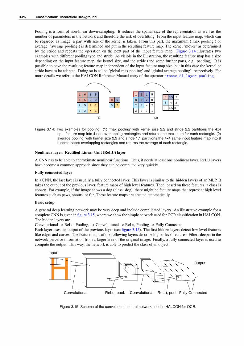
Pooling layer
Ove
rvie
w
D-26 Classification: Theoretical Background
Pooling is a form of non-linear down-sampling. It reduces the spatial size of the representation as well as thenumber of parameters in the network and therefore the risk of overfitting. From the input feature map, which canbe regarded as image, a part with size of the kernel is taken. From this part, the maximum (’max pooling’) oraverage (’average pooling’) is determined and put in the resulting feature map. The kernel ’moves’ as determinedby the stride and repeats the operation on the next part of the input feature map. Figure 3.14 illustrates twoexamples with different pooling type and stride. As visible in the illustration, the resulting feature map has a sizedepending on the input feature map, the kernel size, and the stride (and some further parts, e.g., padding). It ispossible to have the resulting feature map independent of the input feature map size, but in this case the kernel orstride have to be adapted. Doing so is called ’global max pooling’ and ’global average pooling’, respectively. Formore details we refer to the HALCON Reference Manual entry of the operator create_dl_layer_pooling.
(1) (2)
1
8
3 2 7 1
5 2 0
516
2452
8
5 7
5
3 2 7 1
2
51
24
05 4 2
3.55
4.53 3.5
28 5
52
61
Figure 3.14: Two examples for pooling: (1) ’max pooling’ with kernel size 2,2 and stride 2,2 partitions the 4x4input feature map into 4 non-overlapping rectangles and returns the maximum for each rectangle. (2)’average pooling’ with kernel size 2,2 and stride 1,1 partitions the 4x4 same input feature map into 9in some cases overlapping rectangles and returns the average of each rectangle.
Nonlinear layer: Rectified Linear Unit (ReLU) layer
A CNN has to be able to approximate nonlinear functions. Thus, it needs at least one nonlinear layer. ReLU layershave become a common approach since they can be computed very quickly.
Fully connected layer
In a CNN, the last layer is usually a fully connected layer. This layer is similar to the hidden layers of an MLP. Ittakes the output of the previous layer, feature maps of high level features. Then, based on these features, a class ischosen. For example, if the image shows a dog (class: dog), there might be feature maps that represent high levelfeatures such as paws, snouts, or fur. These feature maps are created automatically.
Basic setup
A general deep learning network may be very deep and include complicated layers. An illustrative example for acomplete CNN is given in figure 3.15, where we show the simple network used for OCR classification in HALCON.The hidden layers areConvolutional –> ReLu, Pooling, –> Convolutional –> ReLu, Pooling –> Fully ConnectedEach layer uses the output of the previous layer (see figure 3.15). The first hidden layers detect low level featureslike edges and curves. The feature maps of the following layers describe higher level features. Filters deeper in thenetwork perceive information from a larger area of the original image. Finally, a fully connected layer is used tocompute the output. This way, the network is able to predict the class of an object.
HInput
Convolutional ReLu, pool. ReLu, pool.Convolutional Fully Connected
Output
Figure 3.15: Schema of the convolutional neural network used in HALCON for OCR.

Decisions to Make D-27
Chapter 4
Decisions to Make
This section gives you some hints how to select a suitable classification approach (section 4.1), the suitable featuresthat build the feature vectors (section 4.2), and the suitable training samples (section 4.3 on page 29). Note thatonly some hints but no absolute rules can be given for almost all decisions that are related to classification, as thebest suited approach, features, and samples depend strongly on the specific application.
4.1 Select a Suitable Classification Approach
In most cases, we recommend to use either a DL, MLP, SVM, GMM, or k-NN classifier, as these classificationapproaches are the most powerful and flexible ones. In table 4.1, the characteristics of these five classificationapproaches are put together in a very brief way.
Based on the requirements and restrictions imposed by your application, you can use table 4.1 to select the bestsuited classification approach. If you are not satisfied with the quality of the classification results, it is typicallynot because of the chosen classifier but because of the used features or because of the quality and amount of thetraining samples. Only if you are sure that the training data describes all the relevant characteristics of the objectsto be classified, it is worth to test if another classifier may produce better results.
For image segmentation, the four classification approaches MLP, SVM, GMM, and k-NN can be sped up signif-icantly using a look-up table (see section 6.1.7 on page 70). But note that the so-called LUT-accelerated classifi-cation is only suitable for images with a maximum of three channels. Furthermore, LUT-accelerated classificationleads to a slower offline phase and to higher memory requirements.
• You probably want to use the CNN deep learning classifier when you need a method able to achieve veryhigh accuracy and/or it is difficult to define the features necessary for your image classification problem. Forthis approach, in comparison to our other classifiers, you do not need to define the features manually. Instead,the training algorithm uses the images you already labeled (and therewith you assigned these images a class).With this data the algorithm carries out transfer learning (see e.g., section 4.3 on page 29 or the referencemanual chapter “Deep Learning”), thus adapts an existing neural network for your specific application. Moredata should help the training algorithm to train the network better. This means, the network should generalizebetter from the given samples to a general case concerning your specific classification task. On the flip sidethe training will take longer.
• The MLP classifier is especially well suited for applications that require a fast classification but allow for aslow offline training phase. The complete training data should be available right from the beginning becauseotherwise the time consuming training must be repeated from scratch. MLP classification does not supportnovelty detection.
• The SVM classifier may often be tuned to achieve a slightly higher classification quality than the otherclassifiers. But the classification speed is typically significantly slower than that of the MLP classifier. Thetraining of the SVM classifier is substantially faster than that of the MLP classifier, but it is typically tooslow for being used in the online phase. The SVM classifier requires significantly more memory than theMLP classifier, while it requires less memory than the k-NN classifier. Typically, the memory requirementsrise with the number of training samples, i.e., for classification tasks with a huge number of training samples,like OCR, the SVM classifier may become very large.
Sel
ectA
ppro
ach

D-28 Decisions to Make
DL1 MLP SVM GMM k-NNTraining speed slow slow medium fast fastClassification speed medium fast medium fast mediumAutomatic featureextraction
yes no no no no
Highest classificationspeed is reached for 2
low numberof classesand smallnetwork
low numberof hiddennodes andclasses
low numberof supportvectors 3
low numberof classes
low numberof trainingsamples
Memory require-ments 4
networkdepending:medium tohigh
low medium low high5
Use of additionaltraining data 6
yes no not recom-mended
not recom-mended
yes
Suited for high di-mensional featurespaces
yes yes yes no yes
Suited for noveltydetection
no no yes yes yes
1Regarding only deep-learning-based models of type classification2Besides having a low dimensional feature space3The number of support vectors can be reduced with reduce_class_svm or reduce_ocr_class_svm4After removing the training samples from the classifier5The training samples cannot be removed from the k-NN classifier6Use of additional training data is possible without the need to retrain the whole classifier from scratch. Note, depending on the method you
may still use your whole dataset, see e.g., the reference manual entry for “Deep Learning”.
Table 4.1: Comparison of the characteristics of the four classifiers MLP, SVM, GMM, and k-NN.
• The GMM classifier is very fast both in training and classification, especially if the number of classes islow. It is also very well suited for novelty detection. However it is restricted to applications that do notrequire a high dimensional feature space.
• The k-NN classifier is especially well suited to test various configurations of features and training databecause the training of a k-NN classifier is very fast and it has no restrictions concerning the dimensionalityof the feature space. Furthermore, the classifier can be extended with additional training data very quickly.Note that the k-NN classification is typically slower than the MLP classification and it requires substantiallymore memory, which might be prohibitive in some applications.
• The classifier based on a 2D histogram is suitable for the pixel-based image segmentation of two-channelimages. It provides a very fast alternative if a 2D feature vector is sufficient for the classification task.
• The hyperbox and Euclidean classifiers are suitable for feature vectors of low dimension, e.g., when ap-plying a color classification for image segmentation. Especially for classes that are built by rather compactclusters, they are very fast. Compared to a LUT-accelerated classification using MLP, SVM, GMM, or k-NN,the storage requirements are low and the feature space can easily be visualized.
For OCR, it is recommended to first try the pretrained font Universal (see Solution Guide I,section 18.8 on page222), which is based on CNNs (see section 3.7 on page 23), before you try any other OCR classification approach.
4.2 Select Suitable Features
For all our classification approaches (except for the deep-learning-based ones), you need to select features that aresuitable for a classification. These features strongly depend on the specific application and the objects that haveto be classified. Thus, no fixed rules for their selection can be provided. For each application, you have to decideindividually , which features describe the object best. Generally, the following features can be used for the differentclassification tasks:

4.3 Select Suitable Training Samples D-29
• For a general classification all types of features, i.e., region features as well as color or texture, can be usedto build the feature vectors. The feature vectors have to be explicitly built by feature values that are derivedwith a set of suitable operators.
• For image segmentation, the pixel values of a multi-channel color or texture image are used as features.Here, you do not have to explicitly extract the feature vectors as they are derived automatically by thecorresponding image segmentation operators from the color or texture image.
• For OCR, a restricted set of region features is used to build the feature vectors. Here, you do not have toexplicitly calculate the features but select the feature types that are implicitly and internally calculated by thecorresponding OCR specific operators. The dimension of the resulting feature vector is equal or larger thanthe number of selected feature types, as some feature types lead to several feature values (see section 7.7 onpage 89 for the list of available features).
If your objects are described best by texture, you can follow different approaches. You can, e.g., create a textureimage by applying the operator texture_laws with different parameters and combining the thus obtained indi-vidual channels into a single image, e.g., using compose6 for a texture image containing six channels. Anothercommon approach is to use, e.g., the operator cooc_feature_image to calculate texture features like energy, cor-relation, homogeneity, and contrast. We refer to Solution Guide I, chapter 15 on page 161 for further informationabout texture.
If your objects are described best by region features, you can use any of the operators that are described in theReference Manual in section Regions/Features. For OCR, the set of available region features is restricted tothe set of features introduced in section 7.7 on page 89.
HDevelop provides convenience procedures (see calculate_features) to calculate multiple featureswith given properties like rotational invariance, etc. in just a few calls. Additionally, HALCON of-fers functionality to select suitable features automatically using the operators select_feature_set_mlp,select_feature_set_svm, select_feature_set_gmm, and select_feature_set_knn. Ifyou are not sure which features to chose, you can use the HDevelop example programshdevelop/Classification/Feature-Selection/auto_select_region_features.hdev andhdevelop/Applications/Object-Recognition-2D/classify_pills_auto_select_features.hdev
as a starting point, which make use of both, the procedures and the automatic feature selection.
4.3 Select Suitable Training Samples
In section 1 on page 7 we learned that classification is reasonable in all cases where objects have similarities, butwithin undefined variations. To learn the similarities and variations, the classifier needs representative samples.That is, the samples should not only show the significant features of the objects to classify but should also show alarge variety of allowed deviations. That is, if an object is described by a specific texture, small deviations from thetexture that are caused, e.g., by noise, should be covered by the samples. Or if an object is described by a regionhaving a specific size and orientation, the samples should contain several objects that deviate from both ’ideal’values within a certain tolerance. Otherwise, only objects that exactly fit to the ’ideal’ object are found in the laterclassification. In other words, the classifier has no sufficient generalization ability.
Generally, for the training of a classifier a large amount of samples with a realistic set of variations for the calculatedfeatures should be provided for every available class. Otherwise, the result of the later classification may beunsatisfying as the unknown objects show deviations from the trained data that were not considered during training.
Note that when applying transfer learning for deep-learning-based classification of general features (see e.g., sec-tion 4.3 or the reference manual chapter “Deep Learning”), many already labeled images have to be provided foreach class. This means the tricks described below cannot be recommended in general and their appropriatenessdepends strongly on the specific case and goal.
If, for any reason, no sufficient number of samples can be provided, some tricks may help:
• One trick is to generate artificial samples by copying the few available samples and slightly modifying them.The modifications depend on the object to classify and the features used to find the class boundaries. Whenworking with texture images, e.g., noise can be added to slightly modify the copies of the samples. Or giventhe example with the objects of a specific size and orientation, you can modify copies of the samples by, e.g.,
Sel
ectS
ampl
es

D-30 Decisions to Make
slightly changing their size using an erosion or dilation. And you can change their orientation by rotatingthe image by different, but small angles. Ideally, you create several copies and modify them so that severaldeviations in all allowed directions are covered.
• A second trick can be applied if the number of samples is unequally distributed for the different classes. Forexample, you want to apply classification for quality inspection and you have a large amount of samplesfor the good objects, but only a few samples for each of several error classes. Then, you can split theclassification task into two classification tasks. In the first instance, you merge all error classes into oneclass, i.e., you have reduced the multi-class problem to a two-class problem. You have now a class withgood objects and the rejection class contains all erroneous objects, which in the sum are represented by alarger number of samples. Then, if the type of error attached to the rejected objects is of interest, you applya second classification, this time without the lot of good examples. That is, you only use the samples of thedifferent error classes for the training and classify the objects that were rejected during the first classificationinto one of these error classes.

Classification of General Features D-31
Chapter 5
Classification of General Features
This section shows how to apply the different classifiers. The classification approaches implemented in HALCONcan be divided into two major groups. The first group consists of the methods MLP, SVM, GMM, and k-NN, wherethe distinguishing features of each class have to be specified. The second group is given by deep-learning-basedmethods (DL), where the network is trained by considering the inputs and outputs directly. Accordingly, the basicapproach for a classification with HALCON depends on the method group.
For the first group, thus MLP, SVM, GMM, and k-NN, it is possible to apply the classifier on arbitrary objects likepixels or regions due to arbitrary features like color, texture, shape, or size. Here, pixels as well as regions canbe classified, in contrast to the image segmentation approach described in section 6 on page 57, which classifiesonly pixels, or the OCR approach in section 7 on page 75, which classifies regions with focus on optical characterrecognition. For all operators of this group, the general approach for a classification of arbitrary features, i.e., thesequence of operators used, is similar. This approach is illustrated in section 5.1 by an example, which checksthe quality of halogen bulbs using shape features. In section 5.2, the steps of a classification and the involvedoperators are listed for a brief overview. The parameters used for the operators are in many cases specific to theindividual approach because of the different underlying algorithms (see section 3 on page 15 for the theoreticalbackground). They are introduced in more detail in section 5.3 for MLP, section 5.4 for SVM, section 5.5 forGMM, and section 5.6 for k-NN.
The second group consists of general deep-learning-based classification, where the classifier is applied to images.The ’features’ are not hand-picked as for the other approaches, but chosen automatically during training. Thegeneral approach is described in the chapter “Deep Learning . Model” and the workflow in the chapter “DeepLearning . Classification”. A list of possible model parameters and an explanation to them is given in the referencemanual entry of get_dl_model_param.
5.1 General Approach (Classification of Arbitrary Features)
The general approach is similar for MLP, SVM, GMM, and k-NN classification (see figure 5.1). In all cases, aclassifier with specific properties is created. Then, known objects are investigated, i.e., you extract the features ofobjects for which the classes are known and add the feature vectors together with the corresponding known classID to the classifier. With a training, the classifier then derives the rules for the classification, i.e., it decides how toseparate the classes from each other. To investigate unknown objects, i.e., to classify them, you extract the sameset of features for them that was used for the training, and classify the feature vectors with the trained classifier.
In the following, we illustrate the general approach with the example %HALCONEXAMPLES%\solution_guide\
classification\classify_halogen_bulbs.hdev. Here, halogen bulbs are classified into good, bad, and notexistent halogen bulbs (see figure 5.2). For that, the regions representing the insulation of the halogen bulbs areinvestigated. The classification is applied with the SVM approach. The operator names for the MLP, GMM, andk-NN classification differ only in their ending. That is, if you want to apply an MLP, GMM, or k-NN classification,you mainly have to replace the ’svm’ by ’mlp’, ’gmm’, or ’knn’ in the corresponding operator names and adjustdifferent parameters. The parameters and their selection are described in section 6.1.3 for MLP, section 6.1.4 forSVM, section 6.1.5 for GMM, and section 6.1.6 for k-NN.
The program starts with the assignment of the available classes. The halogen bulbs can be classified into the classes’good’ (halogen bulb with sufficient insulation), ’bad’ (halogen bulb with insufficient insulation), or ’none’ (nohalogen bulb can be found in the image).
Gen
eral
Feat
ures

D-32 Classification of General Features
Create Classifier
Investigate Known Objects
Train Classifier
Extract Features −> Feature Vectors
Assign Feature Vectors to Classes by Knowledge −> Samples
Add Samples to Classifier
Investigate Unknown Objects
Extract Features −> Feature Vectors
Assign Feature Vectors to Classes by Classification
Figure 5.1: The basic steps of a general classification.
Figure 5.2: Classifying halogen bulbs into (from left to right): good, bad, and not existent halogen bulbs.
ClassNames := ['good', 'bad', 'none']
As the first step of the actual classification, an SVM classifier is created with the operator create_class_svm.The returned handle of the classifier SVMHandle is needed for all classification specific operators that are appliedafterwards.
Nu := 0.05
KernelParam := 0.02
create_class_svm (7, 'rbf', KernelParam, Nu, |ClassNames|, 'one-versus-one', \
'principal_components', 5, SVMHandle)
As each classification application is unique, the classifier has to be trained for the current application. That is, therules for the classification have to be derived from a set of samples. In case of the SVM approach, e.g., the trainingdetermines the optimal support vectors that separate the classes from each other (see section 3.4 on page 19).
A sample is an object for which the class membership is known. Generally, each kind of object can be classifiedwith the general classification approach as long as it can be described by a set of features or respectively thefeature’s values. Common objects for image processing are regions, pixels, or a combination of both. For theexample with the halogen bulbs, the objects that have to be trained and classified are the regions that representinsulations of halogen bulbs. For each known object, the feature vector, which consists of values that are derivedfrom the extracted region, and the corresponding (known) class name build the training sample. For each class arepresentative set of training samples must be provided to achieve suitable class boundaries. In the example, thesamples are added within the procedure add_samples_to_svm.
Within the procedure, for each class the corresponding images are obtained. Note that different methods can beused to assign the class memberships for the objects of an image. In the example described in section 2 on page 11,a tuple was used to assign the class name for each image. There, the sequence of the images and the sequence ofthe elements in the tuple had to correspond. Here, the images of each class are stored in a directory that is named

5.1 General Approach (Classification of Arbitrary Features) D-33
like the class. Thus, the procedure add_samples_to_svm uses the directory names to assign the feature vectors tothe classes. For example, the images containing the good halogen bulbs are stored in the directory ’good’. Then,for each class, all images are read from the corresponding directory.
Now, for each image the region of the halogen bulb’s insulation is extracted by the operator threshold, thefeatures of the region are extracted inside the procedure calculate_features, and the feature vector is addedtogether with the corresponding class ID to the classifier using the operator add_sample_class_svm.
procedure add_samples_to_svm (ClassNames, SVMHandle, WindowHandle, ReadPath):::
for ClassNumber := 0 to |ClassNames| - 1 by 1
list_files (ReadPath + ClassNames[ClassNumber], 'files', Files)
Selection := regexp_select(Files,'.*[.]png')for Index := 0 to |Selection| - 1 by 1
read_image (Image, Selection[Index])
threshold (Image, Region, 0, 40)
calculate_features (Region, Features)
add_sample_class_svm (SVMHandle, Features, ClassNumber)
endfor
endfor
return ()
The feature vectors that are used to train the classifier and those that are classified for new objects must con-sist of the same set of features. In the example program, the features are calculated inside the procedurecalculate_features and comprise
• the ’area’ of the region,
• the ’compactness’ of the region,
• the four geometric moments (’PSI1’, ’PSI2’, ’PSI3’, and ’PSI4’) of the region, which are invariant totranslation and general linear transformations, and
• the ’convexity’ of the region.
Note that feature vectors have to consist of real values. As some of the calculated features are described by integervalues, e.g., the feature ’area’, which corresponds to the number of pixels contained in a region, the featurevector is transformed into a tuple of real values before it is added to the classifier.
procedure calculate_features (Region, Features)
area_center (Region, Area, Row, Column)
compactness (Region, Compactness)
moments_region_central_invar (Region, PSI1, PSI2, PSI3, PSI4)
convexity (Region, Convexity)
Features := real([Area,Compactness,PSI1,PSI2,PSI3,PSI4,Convexity])
return ()
After adding all samples to the classifier with the procedure add_samples_to_svm, the actual training is appliedwith the operator train_class_svm. In this step, the classifier derives its classification rules.
train_class_svm (SVMHandle, 0.001, 'default')
These classification rules are applied now inside the procedure classify_regions_with_svm to halogen bulbsof unknown classes. The procedure works similar as the procedure for adding the training samples. But now, theimages that contain the unknown types of halogen bulbs are read, no class information is available, and insteadof adding samples to the classifier, the operator classify_class_svm is applied to classify the unknown featurevectors with the derived classification rules.
Gen
eral
Feat
ures

D-34 Classification of General Features
procedure classify_regions_with_svm (SVMHandle, Colors, ClassNames,
ReadPath):::
list_files (ReadPath, ['files', 'recursive'], Files)
Selection := regexp_select(Files,'.*[.]png')read_image (Image, Selection[0])
for Index := 0 to |Selection| - 1 by 1
read_image (Image, Selection[Index])
threshold (Image, Region, 0, 40)
calculate_features (Region, Features)
classify_class_svm (SVMHandle, Features, 1, Class)
endfor
return ()
The example shows the application of operators that are essential for a classification. Further operators are providedthat can be used, e.g., to separate the training from the classification. That is, you run a program that applies thetraining offline, save the trained classifier to file with write_class_svm, and in another program you read theclassifier from file again with read_class_svm to classify your data in an online process. When closing thetraining program, the samples are not stored automatically. To store them to file for later access you apply theoperator write_samples_class_svm. A later access using read_samples_class_svm may be necessary, e.g.,if you want to repeat the training with additional training samples.
The following sections provide you with a list of involved operators (section 5.2) and go deeper into the specific pa-rameter adjustment needed for MLP (section 5.3), SVM (section 5.4), GMM (section 5.5), and k-NN (section 5.6).
5.2 Involved Operators (Overview)
This section gives a brief overview on the operators that are provided for a general MLP, SVM, GMM, and k-NNclassification. First, the operators for the basic steps of a classification are introduced in section 5.2.1. Then, someadvanced operators are introduced in section 5.2.2. The following sections introduce the individual parameters forthe basic operators and provide tips for their adjustment.
DL classification is implemented within the more general deep learning model. For the general workflow we referto “Deep Learning . Classification”, mentioning the important steps with their involved operators and helpfulprocedures.
5.2.1 Basic Steps: MLP, SVM, GMM, and k-NN
Summarizing the information obtained in section 5.1 on page 31, the classification consists of the following basicsteps and operators, which are applied in the same order as listed here:
1. Create a classifier. Here, some important properties of the classifier are defined. The returned handle isneeded in all later classification steps.
• create_class_mlp
• create_class_svm
• create_class_gmm
• create_class_knn
2. Predefine the sequence in which the classes are defined and later accessed, i.e., define the correspondencesbetween the class IDs and the class names. This step may as well be applied before the creation of theclassifier.
3. Get feature vectors for sample objects of known class IDs. The operators that are suitable to obtain thefeatures depend strongly on the specific application and thus are not part of this overview.
4. Successively add samples, i.e., feature vectors and their corresponding class IDs to the classifier.
• add_sample_class_mlp
• add_sample_class_svm

5.2 Involved Operators (Overview) D-35
• add_sample_class_gmm
• add_sample_class_knn
5. Train the classifier. Here, the boundaries between the classes are derived from the training samples.
• train_class_mlp
• train_class_svm
• train_class_gmm
• train_class_knn
6. Store the used samples to file and access them in a later step (optionally).
• write_samples_class_mlp and read_samples_class_mlp
• write_samples_class_svm and read_samples_class_svm
• write_samples_class_gmm and read_samples_class_gmm
• Note that there are no operators for writing and reading the samples of a k-NN classifier separatelybecause the samples are an intrinsic component of the k-NN classifier. Use write_class_knn andread_class_knn instead.
7. Store the trained classifier to file and read it from file again.
• write_class_mlp (default file extension: .gmc) and read_class_mlp
• write_class_svm (default file extension: .gsc) and read_class_svm
• write_class_gmm (default file extension: .ggc) and read_class_gmm
• write_class_knn (default file extension: .gnc) and read_class_knn
Note that the samples cannot be deleted from a k-NN classifier because they are an intrinsic componentof this classifier.
8. Get feature vectors for objects of unknown class. These feature vectors have to contain the same features (inthe same order) that were used to define the training samples.
9. Classify the new feature vectors. That is, insert the new feature vector to one of the following operators andget the corresponding class ID.
• classify_class_mlp
• classify_class_svm
• classify_class_gmm
• classify_class_knn
5.2.2 Advanced Steps: MLP, SVM, GMM, and k-NN
This section mentions advanced operators, which can be applied for possible additional steps. Especially if thetraining and classification do not lead to a satisfying result, it is helpful to access some information that is implicitlycontained in the model. Available steps to query information are:
• Access an individual sample from the training data. This is needed, e.g., to check the correctness ofits class assignment. The sample had to be stored previously by the operator add_sample_class_mlp,add_sample_class_svm, add_sample_class_gmm, or add_sample_class_knn, respectively.
– get_sample_class_mlp
– get_sample_class_svm
– get_sample_class_gmm
– get_sample_class_knn
• Get the number of samples that are stored in the training data. The obtained number is needed, e.g., to accessthe individual samples or to know how much individual samples you can access.
– get_sample_num_class_mlp
Gen
eral
Feat
ures

D-36 Classification of General Features
– get_sample_num_class_svm
– get_sample_num_class_gmm
– get_sample_num_class_knn
• Get information about the content of the preprocessed feature vectors. This information is reasonable, if theparameter Preprocessing was set to ’principal_components’ or ’canonical_variates’ during thecreation of the classifier. Then, you can check if the information that is contained in the preprocessed featurevector still contains significant data or if a different preprocessing parameter, e.g., ’normalization’, is tobe preferred.
– get_prep_info_class_mlp
– get_prep_info_class_svm
– get_prep_info_class_gmm
– Note that this information cannot be retrieved from a k-NN classifier because the respective kind ofpreprocessing is not available for k-NN classifiers.
• Get the parameter values that were set during the creation of the classifier. This is needed if the offlinetraining and the online classification are separated and the information about the training part is not availableanymore.
– get_params_class_mlp
– get_params_class_svm
– get_params_class_gmm
– get_params_class_knn
Furthermore, there are operators that are available only for specific classifiers:
• For MLP and GMM you can evaluate the probabilities of a feature vector to belong to a specific class. Thatis, you can determine the probabilities for each available class and not only for the most probable classes. Ifonly the most probable classes are of interest, no explicit evaluation is necessary, as these probabilities arereturned also when classifying the feature vector.
– evaluate_class_mlp
– evaluate_class_gmm
• For SVM you can reduce the number of support vectors returned by the offline training to speed up thefollowing online classification.
– reduce_class_svm
• Additionally, for SVM the number or index of the support vectors can be determined after the training. Thisis suitable for the visualization of the support vectors and for diagnostic reasons.
– get_support_vector_num_class
– get_support_vector_class
• For k-NN you can set various parameters that control the behavior of the classifier with the operator
– set_params_class_knn.
This includes the number k of nearest neighbors, the kind of result that is to be returned by the classifier, andparameters that control the trade-off between quality and speed of the classification.

5.3 Parameter Setting for MLP D-37
5.3 Parameter Setting for MLP
This section goes deeper into the parameter adjustment for an MLP classification. We recommend to first adjustthe parameters so that the classification result is satisfying. The most important parameter that has to be adjustedto get the MLP classifier work optimally is
• NumHidden (create_class_mlp).
If the classification generally works, you can start to tune the speed. The most important parameters to enhancethe speed are
• Preprocessing / NumComponents (create_class_mlp) and
• MaxIterations (train_class_mlp).
In the following, we introduce the parameters of the basic MLP operators. The focus is on the parameters forwhich the setting is not immediately obvious or for which it is not immediately obvious how they influence theclassification. These are mainly the parameters needed for the creation and training of the classifier. Furtherinformation about these operators as well as the usage of the operators with obvious parameter settings can befound in the Reference Manual entries for the individual operators.
5.3.1 Adjusting create_class_mlp
An MLP classifier is created with the operator create_class_mlp. There, several properties of the classifier aredefined that are important for the following classification steps. The returned handle is needed (and modified) inall following steps. The following parameters can be adjusted:
Parameter NumInput
The input parameter NumInput specifies the dimension of the feature vectors used for the training as well as forthe classification. Opposite to the GMM classifier (see section 5.5 on page 47), a number of 500 features is stillrealistic.
Parameter NumHidden
The input parameter NumHidden defines the number of units of the hidden layer of the multi-layer neural net (seesection 3.3 on page 18) and significantly influences the result of the classification and thus should be adjusted verycarefully. Its value should be in a similar value range as NumInput and NumOutput. Smaller values lead to a lesscomplex separating hyperplane, but in many cases nevertheless may lead to good results. With a very large valuefor NumHidden, you run the risk of overfitting (see figure 5.3). That is, the classifier uses unimportant details likenoise to build the class boundaries. That way, the classifier works very well for the training data, but fails forunknown feature vectors that do not contain the same unimportant details. In other words, overfitting means thatthe classifier looses its generalization ability.
To adjust NumHidden, it is recommended to apply tests with independent test data, e.g., using the crossvalidation introduced in section 8.1 on page 93. Note that the example %HALCONEXAMPLES%\hdevelop\
Classification\Neural-Nets\class_overlap.hdev provides further hints about the influence of differentvalues for NumHidden.
Parameter NumOutput
The input parameter NumOutput specifies the number of classes.
Parameter OutputFunction
The input parameter OutputFunction describes the functions used by the output unit of the neural net. Availablevalues are ’softmax’, ’logistic’, and ’linear’. In almost all classification applications, OutputFunctionshould be set to ’softmax’. The value ’logistic’ can be used for classification problems with multiple in-dependent logical attributes as output, but this kind of classification problems is very rare in practice. The value’linear’ is used for least squares fitting (regression) and not for classification. Thus, you can ignore it here.
Gen
eral
Feat
ures

D-38 Classification of General Features
Error
NumHidden
Ideal ValueRange
OverfittingUnderfitting
Figure 5.3: The value of NumHidden should be adjusted carefully to avoid under- or overfitting (note that the illus-trated curve is idealized and in practice would be less straight).
Parameters Preprocessing /NumComponents
The input parameter Preprocessing defines the type of preprocessing applied to the feature vector for the trainingas well as later for the classification or evaluation. A preprocessing of the feature vector can be used to speed upthe training as well as the classification. Sometimes, even the recognition rate can be enhanced.
Available values are ’none’, ’normalization’, ’principal_components’, and ’canonical_variates’. Inmost cases, the preprocessing should be set to ’normalization’ as it enhances the speed without loosing relevantinformation compared to using no preprocessing (’none’). The feature vectors are normalized by subtracting themean of the training vectors and dividing the result by the standard deviation of the individual components of thetraining vectors. Hence, the transformed feature vectors have a mean of 0 and a standard deviation of 1. Thenormalization does not change the length of the feature vector.
If speed is important and your data is expected to be highly correlated, you can reduce the dimension of thefeature vector using a principal component analysis (’principal_components’). There, the feature vectors arenormalized and additionally transformed such that the covariance matrix becomes a diagonal matrix. Thus, theamount of data can be reduced without losing a large amount of information.
If you know that your classes are linearly separable, you can also use canonical variates(’canonical_variates’). This approach is known also as linear discriminant analysis. There, the trans-formation of the normalized feature vectors decorrelates the training vectors on average over all classes. At thesame time, the transformation maximally separates the mean values of the individual classes. This approachcombines the advantages of a principal component analysis with an optimized separability of the classes after thedata reduction. But note that the parameter ’canonical_variates’ is recommended only for linearly separableclasses. For MLP, ’canonical_variates’ can only be used if OutputFunction is set to ’softmax’.
Figure 5.4 and figure 5.5 illustrate how ’principal_components’ and ’canonical_variates’, dependenton the distribution of the feature vectors, can reduce the feature vectors to a lower number of components bytransforming the feature space and projecting the feature vectors to one of the principal axes.
The input parameter NumComponents defines the number of components to which the feature vector is reduced ifa preprocessing is selected that reduces the dimension of the feature vector. In particular, NumComponents has tobe adjusted only if Preprocessing is set to ’principal_components’ or ’canonical_variates’.
If Preprocessing is set to ’principal_components’ or ’canonical_variates’ you can use the operatorget_prep_info_class_mlp to check if the content of the transformed feature vectors still contain significantdata. Furthermore, you can use the operator to determine the optimum number of components. Then, you firstcreate a test classifier with, e.g., NumComponents set to NumInput, generate and add the training samples to theclassifier, and then apply get_prep_info_class_mlp. The output parameter CumInformationCont is a tuplecontaining numbers between 0 and 1. These numbers describe the amount of the original data that is covered bythe transformed data. That is, if you want to have at least 90% of the original data covered by the transformeddata, you search for the first value that is larger than 0.9 and use the corresponding index number of the tupleCumInformationCont as value for a new NumComponents. Then, you create a new classifier for the final training

5.3 Parameter Setting for MLP D-39
0
0
0
0
Feature 2:
Feature 1:
principal components
Feature 2:
Feature 1:
xxx xx
xx x
x
xx x
x
x
x
x xx x
xx
x x
xx
x
x x
x x x x
Figure 5.4: After transforming the feature space via principal component analysis, the illustrated linearly separableclasses can be separated using only one feature.
0
0
0
00
0
Feature 2:
Feature 1:
Feature 2:
Feature 1:
x xx x
xx x
x xx
x
xx
x x x
Feature 2:
Feature 1:
x
xx
x
xx
xx
xxx
xx
x
x
x
xx
xx
x xx
x xx
xx
x
xx
x
canonical variates principal components
Figure 5.5: Here, after transforming the feature space via principal component analysis, the illustrated linearlyseparable classes still need two features to be separated. After transforming the feature space usingcanonical variates they can be separated by a single feature.
(this time NumComponents is set to the new value). Note that it is suitable to store the samples into a file duringthe test training (write_samples_class_mlp) so that you do not have to successively add the training samplesagain but simply read in the sample file using read_samples_class_mlp.
Parameter RandSeed
The weights of the MLP (see section 3.3 on page 18) are initialized by a random number. For the sake of repro-ducibility the seed value for this random number is stored in the input parameter RandSeed.
Parameter MLPHandle
The output parameter of create_class_mlp is the MLPHandle, which is needed for all following classificationspecific operators.
5.3.2 Adjusting add_sample_class_mlp
A single sample is added to the MLP classifier using add_sample_class_mlp. For the training, several sam-ples have to be added by successively calling add_sample_class_mlp with different samples. The followingparameters can be adjusted:
Parameter MLPHandle
The input and output parameter MLPHandle is the handle of the classifier that was created withcreate_class_mlp and to which the samples subsequently were added with add_sample_class_mlp. Afterapplying add_sample_class_mlp for all available samples, the handle is prepared for the actual training of theclassifier.
Gen
eral
Feat
ures

D-40 Classification of General Features
Parameter Features
The input parameter Features contains the feature vector of a sample to be added to the classifier withadd_sample_class_mlp. This feature vector is a tuple of values. Each value describes a specific numeric feature.Note that the feature vector must consist of real numbers. If you have integer numbers, you have to transform theminto real numbers. Otherwise, an error message is raised.
Parameter Target
The input parameter Target describes the target vector, i.e., you assign the corresponding class ID to the featurevector.
If OutputFunction is set to ’softmax’, the target vector is a tuple that contains exactly one element with thevalue 1 and several elements with the value 0. The size of the vector corresponds to the number of available classesspecified by NumOutput inside create_class_mlp. The index of the element with the value 1 defines the classthe feature vector Features belongs to. Alternatively, a single integer containing the class number (counted from0) can be specified.
For OutputFunction set to ’logistic’, the target vector consists of values that are either 0 or 1. Each 1 showsthat the corresponding feature is present.
If OutputFunction is set to ’linear’, the target vector can contain arbitrary real numbers. As this parametervalue is used for least squares fitting (regression) and not for classification, it is not explained further.
5.3.3 Adjusting train_class_mlp
The training of the MLP classifier is applied with train_class_mlp. Training the MLP means to determine theoptimum values of the MLP weights (see section 3.3 on page 18). For this, a sufficient number of training samplesis necessary. Training is performed by a complex nonlinear optimization process that minimizes the discrepancy ofthe MLP output and the target vectors that were defined with add_sample_class_mlp. The following parameterscan be adjusted:
Parameter MLPHandle
The input and output parameter MLPHandle is the handle of the classifier that was created withcreate_class_mlp and for which samples were stored either by adding them via add_sample_class_mlp or byreading them in with read_samples_class_mlp. After applying train_class_mlp, the handle is prepared forthe actual classification of unknown data. That is, it then contains information about how to separate the classes.
Parameters MaxIterations / WeightTolerance / ErrorTolerance
The input parameters MaxIterations, WeightTolerance, and ErrorTolerance control the nonlinear opti-mization algorithm. MaxIterations specifies the number of iterations of the optimization algorithm. The op-timization is terminated if the weight change is smaller than WeightTolerance and the change of the error issmaller than ErrorTolerance. In any case, the optimization is terminated after at most MaxIterations itera-tions. For the latter, values between 100 and 200 are sufficient in most cases. The default value is 200. By reducingthis value, the speed of the training can be enhanced. For the parameters WeightTolerance and ErrorTolerancethe default values do not have to be changed in most cases.
Parameter Error
The output parameter Error returns the error of the MLP with the optimal weights on the training samples.
Parameter ErrorLog
The output parameter ErrorLog returns the error value as a function of the number of iterations. This function canbe used to decide if a second training with the same training samples but a different value for RandSeed should beapplied, which is the case if the function runs into a local minimum.

5.3 Parameter Setting for MLP D-41
5.3.4 Adjusting evaluate_class_mlp
The operator evaluate_class_mlp can be used to evaluate the probabilities for a feature vector to belong to eachof the available classes. If only the probabilities for the two classes to which the feature vector most likely belongsare searched for, no evaluation is necessary, as these probabilities are returned also for the final classification of thefeature vector. The following parameters can be adjusted:
Parameter MLPHandle
The input parameter MLPHandle is the handle of the classifier that was previously trained with the operatortrain_class_mlp.
Parameter Features
The input parameter Features contains the feature vector that is evaluated. The feature vector must consist of thesame features as the feature vectors used for the training samples within add_sample_class_mlp.
Parameter Result
The output parameter Result returns the result of the evaluation. This result has different meanings, dependent onthe OutputFunction that was set with create_class_mlp. If OutputFunction was set to ’softmax’, whichshould be the case for most classification applications, the returned tuple consists of probability values. Each valuedescribes the probability of the given feature vector to belong to the corresponding class. If OutputFunctionwas set to ’logistic’, the elements of the returned tuple represent the presences of the respective independentattributes.
5.3.5 Adjusting classify_class_mlp
The operator classify_class_mlp classifies a feature vector according to the class boundaries that were derivedduring the training. It can only be called if OutputFunction was set to ’softmax’ in create_class_mlp. Thefollowing parameters can be adjusted:
Parameter MLPHandle
The input parameter MLPHandle describes the handle that was created with create_class_mlp, to which sampleswere added with add_sample_class_mlp, and that was trained with train_class_mlp. The handle containsall the information that the classifier needs to assign an unknown feature vector to one of the available classes.
Parameter Features
The input parameter Features contains the feature vector of the object that is to be classified. The fea-ture vector must consist of the same features as the feature vectors used for the training samples withinadd_sample_class_mlp.
Parameter Num
The input parameter Num specifies the number of best classes to be searched for. Generally, Num is set to 1 if onlythe class with the best probability is searched for, and to 2 if the second best class is also of interest, e.g., becausethe classes overlap.
Parameter Class
The output parameter Class returns the result of classifying the feature vector with the trained MLP classifier, i.e.,a tuple containing Num elements. That is, if Num is set to 1, a single value is returned that corresponds to the classwith the highest probability. If Num is set to 2, the first element contains the class with the highest probability andthe second element contains the second best class.
Gen
eral
Feat
ures

D-42 Classification of General Features
Parameter Confidence
The output parameter Confidence outputs the confidence of the classification. Note that in comparison to theprobabilities returned for a GMM classification, here the returned values can be influenced by outliers, which iscaused by the specific way an MLP is calculated. For example, the confidence may be high for a feature vector thatis far from the rest of the training samples of the specific class but significantly on the same side of the separatinghypersurface. On the other side, the confidence can be low for objects that are significantly within the cluster oftraining samples of a specific class but near to the separating hypersurface as two classes overlap at this part of thecluster (see figure 5.6).
xx
x
x
x xx
xx
xx
x xxxx
xx
xx
xx
x
x x
x
xx
xxx
x
Low Confidence
Hyperplane
x
x High Confidence
Figure 5.6: The confidence calculated for an MLP classification can be unexpected for outliers. That is, featurevectors that are far away from their class centers can be classified with high confidence or those thatare near to the class centers but inside an overlapping area between two classes can be classified withlow confidence.
5.4 Parameter Setting for SVM
This section goes deeper into the parameter adjustment for an SVM classification. We recommend to first adjustthe parameters so that the classification result is satisfying. The most important parameters that have to be adjustedto get the SVM classifier work optimally are:
• Nu (create_class_svm)
• KernelParam (create_class_svm)
If the classification generally works, you can start to tune the speed. The most important parameters to enhancethe speed are:
• Preprocessing (create_class_svm):
A combination of KernelType set to ’rbf’ and the Preprocessing set to ’principal_components’
speeds up the SVM significantly (even faster than MLP), as the features are reduced and thus the dimensionfor the support vectors are reduced as well.
• MaxError (reduce_class_svm)
In the following, we introduce the parameters of the basic SVM operators. The focus is on the parameters forwhich the setting is not immediately obvious or for which it is not immediately obvious how they influence theclassification. These are mainly the parameters needed for the creation and training of the classifier. Furtherinformation about these operators as well as the usage of the operators with obvious parameter settings are providedin the Reference Manual entries for the individual operators.
5.4.1 Adjusting create_class_svm
An SVM classifier is created with the operator create_class_svm. There, several properties of the classifier aredefined that are important for the following classification steps. The returned handle is needed (and modified) inall following steps. For the operator, the following parameters can be adjusted:

5.4 Parameter Setting for SVM D-43
Parameter NumFeatures
The input parameter NumFeatures specifies the dimension of the feature vectors used for the training as well asfor the classification. Opposite to the GMM classifier (see section 5.5 on page 47), a number of 500 features is stillrealistic.
Parameters KernelType / KernelParam
In section 3.4 on page 19 we saw for an SVM classification that the feature space is transformed into a higherfeature space by a kernel to get linearly separable classes. The input parameter KernelType defines how thefeature space is mapped into this higher dimension. The mapping that is suitable and recommended in most casesuses a kernel that is based on the Gauss error distribution curve and is called Gaussian radial basis function kernel(’rbf’).
If KernelType is set to ’rbf’, the input parameter KernelParam is used to adjust the γ of the error curve (seefigure 5.7) and should be adjusted very carefully. If the value for γ is very high, the number of support vectorsincreases, which results on one hand in an overfitting, i.e., the generalization ability of the classifier is lost (foroverfitting see also the description of NumHidden in section 5.3.1 on page 37) and on the other hand the speed isreduced. On the other side, with a very low value for γ, an underfitting occurs, i.e., the number of support vectorsis not sufficient to obtain a satisfying classification result.
It is recommended to start with a small γ and then progressively increase it. Generally, it is recommended tosimultaneously search for a suitable Nu-γ pair, as these together define how complex the separating hypersurfacebecomes. The search can be applied, e.g., using the cross validation that is described in section 8.1 on page 93.
Figure 5.7: γ describes the amount of influence of a support vector upon its surrounding.
Besides ’rbf’, you can also select a linear or polynomial kernel for KernelType, but these kernels should beused only in very special cases (see below).
The linear kernel (KernelType set to ’linear’) transforms the feature space using a dot product. The linearkernel should be used only if the classes are expected to be linearly separable. If a linear kernel is selected, theparameter KernelParam has no meaning and can be ignored.
The polynomial kernels (KernelType set to ’polynomial_homogeneous’ or ’polynomial_inhomogeneous’)in very rare cases can be used if the classification with ’rbf’ was not successful, but in most cases, ’rbf’ leadsto a better result. If a polynomial kernel is selected, the parameter KernelParam describes the degree ’d’ of thepolynom. Note that a degree higher than 10 might result in numerical problems.
Parameter Nu
For classes that are not linearly separable, data from different classes may overlap. The input parameter Nu regu-larizes the separation of the classes, i.e., with Nu, the upper bound for training errors within the overlapping areasbetween the classes is adjusted (see figure 5.8) and at the same time the lower bound for the number of supportvectors is determined. Nu should be adjusted very carefully. Its value must be a real number between 0 and 1. Asa rule of thumb, it should be set to the expected error ratio of the specific dataset, e.g., to 0.05 when expecting amaximum training error of 5%. The training error occurs because of, e.g., overlapping classes. Note that a verylarge Nu results in a large dataset and thus reduces the speed significantly. Additionally, with a very large Nu thetraining may be aborted and an error handling message is raised. Then, Nu has to be chosen smaller. On the otherhand, a very small Nu leads to instable numerics, i.e., many feature vectors would be classified incorrectly.
Gen
eral
Feat
ures

D-44 Classification of General Features
incorrectly classifiedtraining data
Figure 5.8: The parameter Nu determines the amount of the incorrectly classified training data within the overlapbetween two classes.
To select a suitable value for Nu, it is recommended to start with a small value and then progressively increaseit. Generally, it is recommended to simultaneously search for a suitable Nu-γ pair, as these together define howcomplex the separating hypersurface becomes. The search can be applied, i.e., using the cross validation that isdescribed in section 8.1 on page 93.
Parameter NumClasses
The input parameter NumClasses specifies the number of classes.
Parameter Mode
As we saw in section 3.4 on page 19, SVM can handle only two-class problems. With the input parameter Modeyou define if your application is a two-class problem or if you want to extent the SVM to a multi-class problem.
Having a two-class problem, you have training data for a single class and decide during the classification if afeature vector belongs to the trained class or not. That is, the hyperplane lies around the training data and implicitlyseparates the training data from a rejection class. This Mode is called ’novelty-detection’ and can only beapplied if KernelType is set to ’rbf’.
If you want to extent the SVM to a multi-class problem, you have to divide the decision into binary sub-cases. There, you have two possibilities. Either, you set Mode to ’one-versus-one’ or you set it to’one-versus-all’.
When using the mode ’one-versus-one’, for each pair of classes a binary classifier is created and the classthat wins most comparisons is selected. Here, n classes result in n(n-1)/2 classifiers. This approach is fast butsuitable only for a small number of classes (approximately up to 10).
For ’one-versus-all’, each class is compared to the rest of the training data and the class with the maximumdistance to the hypersurface is selected. Here, the number of needed binary classifiers corresponds to the numberof classes. This approach is not as fast as ’one-versus-one’, but can and should be used for a higher number ofclasses.
Parameters Preprocessing / NumComponents
The input parameter Preprocessing defines the type of preprocessing applied to the feature vector for the trainingas well as later for the classification or evaluation. A preprocessing of the feature vector can be used to speed upthe training as well as the classification. Sometimes, even the recognition rate can be enhanced.
Available values are ’none’, ’normalization’, ’principal_components’, and ’canonical_variates’.In most cases, the preprocessing should be set to ’normalization’ as it enhances the speed without loosingrelevant information compared to using no preprocessing (’none’). The values ’principal_components’ andin rare cases ’canonical_variates’ can be used to enhance the speed. As the preprocessing types are the sameas used for an MLP classification, we refer to section 5.3.1 on page 38 for further information.

5.4 Parameter Setting for SVM D-45
The input parameter NumComponents defines the number of components to which the feature vector is reducedif a preprocessing is selected that reduces the dimension of the feature vector. In particular, NumComponentshas to be adjusted only if Preprocessing is set to ’principal_components’ or ’canonical_variates’.If Preprocessing is set to ’principal_components’ or ’canonical_variates’ you can use the operatorget_prep_info_class_svm to determine the optimum number of components as described in section 5.3.1 onpage 38.
Parameter SVMHandle
The output parameter of create_class_svm is the SVMHandle, which is needed for all following classificationspecific operators.
5.4.2 Adjusting add_sample_class_svm
A single sample is added to the SVM classifier using add_sample_class_svm. For the training, several sam-ples have to be added by successively calling add_sample_class_svm with different samples. The followingparameters can be adjusted:
Parameter SVMHandle
The input and output parameter SVMHandle is the handle of the classifier that was created withcreate_class_svm and to which the samples subsequently are added with add_sample_class_svm. Afterapplying add_sample_class_svm for all available samples, the handle is prepared for the actual training of theclassifier.
Parameter Features
The input parameter Features contains the feature vector of a sample to be added to the classifier withadd_sample_class_svm. This feature vector is a tuple of values. Each value describes a specific numeric feature.Note that the feature vector must consist of real numbers. If you have integer numbers, you have to transform theminto real numbers. Otherwise, an error message is raised.
Parameter Class
The input parameter Class contains the ID of the class the feature vector belongs to. The ID is an integer numberbetween 0 and ’Number of Classes -1’. If you created a tuple with class names, the class ID is the index ofthe corresponding class name in the tuple.
5.4.3 Adjusting train_class_svm
The training of the SVM classifier is applied with train_class_svm. The following parameters can be adjusted:
Parameter SVMHandle
The input and output parameter SVMHandle is the handle of the classifier that was created withcreate_class_svm and for which samples were stored either by adding them via add_sample_class_svm or byreading them in with read_samples_class_svm. After applying train_class_svm, the handle is prepared forthe actual classification of unknown data. That is, it then contains information about how to separate the classes.
Parameter Epsilon
Training the SVM means to gradually optimize the function that determines the class boundaries. This optimizationstops if the gradient of the function falls below a certain threshold. This threshold is set with the input parameterEpsilon. In most cases it should be set to the default value, which is 0.001. With a too small threshold, the opti-mization becomes slower without leading to a better recognition rate. With a too large threshold, the optimizationstops before the optimum is found, i.e., the recognition rate may be not satisfying.
There are two cases, in which changing the value of Epsilon might be reasonable. First, when having a very smallNu and a small or unbalanced set of training data, it may be suitable to set Epsilon smaller than the default value
Gen
eral
Feat
ures

D-46 Classification of General Features
to enhance the resulting recognition rate. Second, when applying a cross validation to search for a suitable Nu-γpair (see section 8.1 on page 93), it is recommended to select a larger value for Epsilon during the search. Thus,the cross validation is sped up without significantly changing the parameters for the optimal kernel. Having foundthe optimal Nu-γ pair, the final training is applied again with the small (default) value.
Parameter TrainMode
The input parameter TrainMode determines the mode for the training. We recommend to use the mode ’default’in most cases. There, the whole set of available samples is trained in one step. Appending a new set of samples to apreviously applied training is possible with the mode ’add_sv_to_train_set’. This mode has some advantagesthat are listed in the Reference Manual entry for train_class_svm, but you have to be aware that only the supportvectors that resulted from the previously applied training are reused. The samples of the previously applied trainingare ignored. This most likely leads to a different hypersurface than obtained with a training that uses all availabletraining samples in one step. The risk of obtaining a hypersurface that is not suitable for all available samples isillustrated in figure 5.9.
ox
xx
oo
xx
o oo
o
o
oo
xx
xx x
ox
xx
oo
xx
o oo
o
o
oo
xx
xx x
o o
ox
xx
oo
xx
o oo
o
o
oo
xx
xx x
o o
ox
xx
oo
xx
o oo
o
o
oo
xx
xx x
o o
New Training Samples
a) b) c) d)
Figure 5.9: Risk of appending a second training: a) training samples of the first training and the obtained hypersur-face, b) new samples added for a second training, c) hypersurface obtained by a second training usingthe new samples with the support vectors obtained by the first training, d) hypersurface obtained by anew training that uses all available samples.
5.4.4 Adjusting reduce_class_svm
The operator reduce_class_svm can be used to reduce the number of support vectors that were returned by thetraining. This is suitable to speed up the online classification. The following parameters can be adjusted:
Parameter SVMHandle
The input parameter SVMHandle is the handle of the classifier that was created with create_class_svm, to whichtraining samples were added with add_sample_class_svm, and which was trained with train_class_svm.reduce_class_svm does not modify the handle but creates a copy of it (SVMHandleReduced) and modifies thecopy.
Parameters Method / MinRemainingSV / MaxError
The input parameter Method defines the method used to reduce the number of support vectors. Momentarily, onlythe method ’bottom_up’ is available. There, the number of support vectors is reduced by iteratively merging thesupport vectors until either the minimum number of support vectors that is set with MinRemainingSV is reached,or until the accumulated maximum error exceeds the threshold that is set with MaxError.
Note that the approximation of the original support vectors by a reduced number of support vectors reduces alsothe complexity of the hypersurface and thus can lead to a poor classification rate. A common approach is to startwith a small value for MaxError, e.g, 0.0001, and to increase it step by step. To control the reduction ratio, thenumber of remaining support vectors is checked by get_support_vector_num_class and the classification rateis checked by classifying a separate test data with classify_class_svm.
Parameter SVMHandleReduced
The output parameter SVMHandleReduced returns the copied and modified handle of a classifier that has the sameparameterization as the original handle but a different support vector expansion. Additionally, it does not containthe training samples that are stored with the original handle.

5.5 Parameter Setting for GMM D-47
5.4.5 Adjusting classify_class_svm
The operator classify_class_svm is used to decide to which of the trained classes an unknown feature vectorbelongs. The following parameters can be adjusted:
Parameter SVMHandle
The input parameter SVMHandle describes the handle that was created with create_class_svm, to which sampleswere added with add_sample_class_svm, and that was trained with train_class_svm. The handle containsall the information that the classifier needs to assign an unknown feature vector to one of the available classes.
Parameter Features
The input parameter Features contains the feature vector of the object that is to be classified. The fea-ture vector must consist of the same features as the feature vectors used for the training samples withinadd_sample_class_svm.
Parameter Num
The input parameter Num specifies the number of best classes to be searched for. Generally, Num is set to 1 if onlythe class with the best probability is searched for, and to 2 if the second best class is also of interest, e.g., becausethe classes overlap. If Mode was set to ’novelty-detection’ in create_class_svm, Num must be set to 1.
Parameter Class
The output parameter Class returns the result of classifying the feature vector with the trained SVM classifier. Thisresult depends on the Mode that was selected in create_class_svm. If Mode was set to ’one-versus-one’, itcontains the classes ordered by the number of votes of the sub-classifiers. That is, the first element of the returnedtuple is the class with the most votes, the second is the class with the second most votes etc. If Mode was set to’one-versus-all’, it contains the classes ordered by the value of each sub-classifier. That is, the first element ofthe returned tuple is the class with the highest value, the second element is the class with the second best value. IfMode was set to ’novelty-detection’, a single value is returned (Num must be set to 1). In particular, the valueis 1 if the feature vector belongs to the trained class and 0 if the feature vector belongs to the rejection class.
5.5 Parameter Setting for GMM
This section goes deeper into the parameter adjustment for a GMM classification. We recommend to first adjustthe parameters so that the classification result is satisfying. The most important parameters that have to be adjustedto get the GMM classifier work optimally are:
• NumDim (create_class_gmm)
• NumCenters (create_class_gmm)
• CovarType (create_class_gmm)
• ClassPriors (train_class_gmm)
If the classification generally works, you can start to tune the speed. The most important parameters to enhancethe speed are:
• CovarType (create_class_gmm)
• Preprocessing / NumComponents (create_class_gmm)
In the following, we introduce the parameters of the basic GMM operators. The focus is on the parameters forwhich the setting is not immediately obvious or for which it is not immediately obvious how they influence theclassification. These are mainly the parameters needed for the creation and training of the classifier. Furtherinformation about these operators as well as the usage of the operators with obvious parameter settings are providedin the Reference Manual entries for the individual operators.
Gen
eral
Feat
ures

D-48 Classification of General Features
5.5.1 Adjusting create_class_gmm
A GMM classifier is created with the operator create_class_gmm. There, several properties of the classifier aredefined that are important for the following classification steps. The returned handle is needed (and modified) inall following steps. The following parameters can be adjusted:
Parameter NumDim
The input parameter NumDim specifies the dimension of the feature vectors used for the training as well as for theclassification.
Note that GMM works optimally only for a limited number of features! If the result of the classification is notsatisfying, maybe you have used too much features as input. As a rule of thumb, a number of 15 features shouldnot be exceeded (although some applications work also for larger feature vectors). If your application needssignificantly more features, in many cases an MLP, SVM, or k-NN classification is to be preferred.
Parameter NumClasses
The input parameter NumClasses specifies the number of classes.
Parameter NumCenters
As we learned in section 3.5 on page 20 a GMM class can consist of different Gaussian centers (see also fig-ure 5.10). The input parameter NumCenters defines the number of Gaussian centers per class. You can specifythis number in different ways. That is, you can either specify a single number of centers, then each class has exactlythis number of class centers. Or you can specify the allowed lower and upper bound for the number of centers.This can be done either with a single range for all classes or with a range for each class individually. From thesebounds, the optimum of centers is determined with the help of the Minimum Message Length Criterion (MML). Inmost cases, it is recommended to specify a range for all classes and to start with a high value as upper bound andthe expected number of centers as lower bound. If the classification is successful, you can try to reduce the rangeto enhance the speed.
x
xx
xx
xx
xx
x xx
x
xx x
xx
xx
xx
xx
x xx
x
xx
Feature 1:
Feature 2:
xx
xxx x
xxx
xx x
NumCenters = 2 NumCenters = 1
Feature 1:
Feature 2:
xx
xxx x
xxx
xx x
Figure 5.10: Number of Gaussian centers of a class: (left) 2 and (right) 1.
Note that if the training is canceled with the error message 3335 (’Internal error while training the GMM’), mostprobably the value for NumCenters is not optimal.
Parameter CovarType
The input parameter CovarType defines the type of the covariance matrix used to calculate the probabilities. Withthis, you can further constrain the MML, which is used to determine the optimum of centers. Three types ofcovariance matrices are available. If you use the default, ’spherical’, the covariance matrix is a scalar multipleof the identity matrix. With the value ’diag’ a diagonal matrix is obtained and with ’full’ the covariancematrix is positive definite (see figure 5.11). Note that the flexibility of the centers but also the complexity of thecalculations increases from ’spherical’ over ’diag’ to ’full’. That is, you have to decide whether you wantto increase the flexibility of the classifier or if you want to increase the speed.

5.5 Parameter Setting for GMM D-49
x
xx
xxx
xxxx
xx
x
xx
x
xx
xxx
xxxx
xx
x
xxFeature 1:
Feature 2:
’full’
Feature 1:
Feature 2:
Feature 1:
Feature 2:
xx xx
xx
xx
xx xxxx x
xxx
x
xx
xx
’spherical’
xxxx
xx
x
xx
xx
xx xx
x
’diag’
xx xx
xx
xx
xx xx
Figure 5.11: The covariance type set to (from left to right) ’spherical’, ’diag’, and ’full’.
Parameters Preprocessing / NumComponents
The input parameter Preprocessing defines the type of preprocessing applied to the feature vector for the trainingas well as later for the classification or evaluation. A preprocessing of the feature vector can be used to speed upthe training as well as the classification. Sometimes, even the recognition rate can be enhanced.
Available values are ’none’, ’normalization’, ’principal_components’, and ’canonical_variates’.In most cases, Preprocessing should be set to ’normalization’ as it enhances the speed without loosingrelevant information compared to using no preprocessing (’none’). The values ’principal_components’ andin rare cases ’canonical_variates’ can be used to enhance the speed. As the preprocessing types are the sameas used for an MLP classification, we refer to section 5.3.1 on page 38 for further information.
The input parameter NumComponents defines the number of components to which the feature vector is reducedif a preprocessing is selected that reduces the dimension of the feature vector. In particular, NumComponentshas to be adjusted only if Preprocessing is set to ’principal_components’ or ’canonical_variates’.If Preprocessing is set to ’principal_components’ or ’canonical_variates’ you can use the operatorget_prep_info_class_gmm to determine the optimum number of components as described in section 5.3.1 onpage 38.
Parameter RandSeed
The coordinates of the centers are initialized by a random number. For the sake of reproducibility the seed valuefor this random number is stored in the input parameter RandSeed.
Parameter GMMHandle
The output parameter of create_class_gmm is the GMMHandle, which is needed for all following classificationspecific operators.
5.5.2 Adjusting add_sample_class_gmm
A single sample is added to the GMM classifier using add_sample_class_gmm. For the training, several sam-ples have to be added by successively calling add_sample_class_gmm with different samples. The followingparameters can be adjusted:
Parameter GMMHandle
The input and output parameter GMMHandle is the handle of the classifier that was created withcreate_class_gmm and to which the samples subsequently were added with add_sample_class_gmm. Afterapplying add_sample_class_gmm for all available samples, the handle is prepared for the actual training of theclassifier.
Parameter Features
The input parameter Features contains the feature vector of a sample to be added to the classifier withadd_sample_class_gmm. This feature vector is a tuple of values. Each value describes a specific numeric feature.Note that the feature vector must consist of real numbers. If you have integer numbers, you have to transform theminto real numbers. Otherwise, an error message is raised.
Gen
eral
Feat
ures

D-50 Classification of General Features
Parameter ClassID
The input parameter ClassID contains the ID of the class the feature vector belongs to. The ID is an integernumber between 0 and ’Number of Classes -1’. If you created a tuple with class names, the class ID is theindex of the corresponding class name in the tuple.
Parameter Randomize
The input parameter Randomize defines the standard deviation of the Gaussian noise that is added to the trainingdata. This value is needed mainly for originally integer feature values. There, the modeled Gaussians may bealigned along axis directions and thus lead to an unusually high number of centers returned by train_class_gmm
(see figure 5.12). This effect can be prevented by setting Randomize to a value larger than 0. According toexperience, a value between 1.5 and 2 in most cases leads to a satisfying result. If the feature vector has beencreated from integer data by scaling, Randomize must be scaled with the same scale factor that was used to scalethe original data.
x
xx
x x
x
Feature 1:
Feature 2:
Feature 1:
Feature 2:
x
xx
x
Randomized Feature Vectors
Integer Feature Vectors
x
x x
x
xx x
x
xx
Figure 5.12: Adding noise to integer values: (left) the integer feature vectors lead to many classes, whereas for the(right) randomized feature vectors one class is obtained.
5.5.3 Adjusting train_class_gmm
The training of the GMM classifier is applied with train_class_gmm. The following parameters can be adjusted:
Parameter GMMHandle
The input and output parameter GMMHandle is the handle of the classifier that was created withcreate_class_gmm and for which samples were stored either by adding them via add_sample_class_gmm or byreading them in with read_samples_class_gmm. After applying train_class_gmm, the handle is prepared forthe actual classification of unknown data. That is, it then contains information about how to separate the classes.
Parameters MaxIter / Threshold
The input parameter MaxIter defines the maximum number of iterations used for the expectation minimizationalgorithm. The input parameter Threshold defines the threshold for the relative change of the error for theexpectation minimization algorithm to terminate. By reducing the number of iterations, the speed can be optimizedfor specific applications. But note that in most cases, the parameters MaxIter and Threshold should be used withthe default values.
Parameter ClassPriors
The input parameter ClassPriors is used to select the mode for determining the probability of the occurrenceof a class (see also section 3.5 on page 20). That is, ClassPriors determines if a weighting of the classes isused that is derived from the proportion of the corresponding sample data used for the training (ClassPriorsset to ’training’) or if all classes have the same weight (ClassPriors set to ’uniform’), i.e., the weight is1/NumClasses for all classes (see figure 5.13). By default, the mode ’training’ is selected, i.e., the probabilityof the occurrence of a class is derived from the frequency of the class in the training set. If your training data is notrepresentative for the frequency of the individual classes, you should use ’uniform’ instead.

5.5 Parameter Setting for GMM D-51
’training’’uniform’
Class 2Class 1Class 2Class 1
Figure 5.13: Probability of the occurrence of a class set to (left) ’uniform’ and (right) ’training’.
Parameter Regularize
The input parameter Regularize is used to prevent the covariance matrix from a collapse which can occur forlinearly dependent data. Here, we recommend to use the default value, which is 0.0001.
Parameter Centers
The output parameter Centers returns the number of found centers per class.
Parameter Iter
The output parameter Iter returns the number of iterations that were executed for the expectation minimizationalgorithm for each class.
5.5.4 Adjusting evaluate_class_gmm
The operator evaluate_class_gmm can be used to evaluate the probabilities for a feature vector to belong to eachof the available classes. If only the probabilities for the most probable classes are searched for, no evaluation isnecessary, as these probabilities are returned also for the final classification of the feature vector. The followingparameters can be adjusted:
Parameter GMMHandle
The input parameter GMMHandle is the handle of the classifier that was previously trained with the operatortrain_class_gmm.
Parameter Features
The input parameter Features contains the feature vector that is evaluated. The feature vector must consist of thesame features as the feature vectors used for the training samples within add_sample_class_gmm.
Parameter ClassProb
The output parameter ClassProb returns the a-posteriori probabilities of the given feature vector to belong to eachof the classes.
Parameter Density
The output parameter Density returns the probability density of the feature vector.
Parameter KSigmaProb
The output parameter KSigmaProb describes the probability that another sample lies farther away from the mean.This value can be used for novelty detection. Then, all feature vectors with a KSigmaProb value below a certaink-sigma probability, e.g., 0.0001, can be rejected.
Gen
eral
Feat
ures

D-52 Classification of General Features
5.5.5 Adjusting classify_class_gmm
The operator classify_class_gmm is used to decide to which of the trained classes an unknown feature vectorbelongs. The following parameters can be adjusted:
Parameter GMMHandle
The input parameter GMMHandle describes the handle that was created with create_class_gmm, to which sampleswere added with add_sample_class_gmm, and that was trained with train_class_gmm. The handle containsall the information that the classifier needs to assign an unknown feature vector to one of the available classes.
Parameter Features
The input parameter Features contains the feature vector of the object that is to be classified. The fea-ture vector must consist of the same features as the feature vectors used for the training samples withinadd_sample_class_gmm.
Parameter Num
The input parameter Num specifies the number of best classes to be searched for. Generally, Num is set to 1 if onlythe class with the best probability is searched for, and to 2 if the second best class is also of interest, e.g., becausethe classes overlap.
Parameter ClassID
The output parameter ClassID returns the result of classifying the feature vector with the trained GMM classifier,i.e., a tuple containing Num elements. That is, if Num is set to 1, a single value is returned that corresponds to theclass with the highest probability. If Num is set to 2, the first element contains the class with the highest probabilityand the second element contains the second best class.
The following parameters output the probabilities of the classes. In comparison to the confidence value returnedfor an MLP classification (see section 5.3.5 on page 41), the returned values are rather reliable.
Parameter ClassProb
The output parameter ClassProb returns the a-posteriori probabilities of the given feature vector to belong toeach of the classes. In contrast to the ClassProb returned by evaluate_class_gmm, the probability is furthernormalized.
Parameter Density
The output parameter Density returns the probability density of the feature vector.
Parameter KSigmaProb
The output parameter KSigmaProb describes the probability that another sample lies farther away from the mean.This value can be used for novelty detection. Then, all feature vectors with a KSigmaProb value below a certaink-sigma probability, e.g., 0.0001, can be rejected.
5.6 Parameter Setting for k-NN
This section goes deeper into the parameter adjustment for a k-NN classification. We recommend to first adjust theparameters so that the classification result is satisfying. The most important parameters that have to be adjusted toget the k-NN classifier work optimally are:
• NumDim (create_class_knn)
• The kind of results that is returned by classify_class_knn (controlled by the parameter ’method’, whichis set with set_params_class_knn).
5.6 Parameter Setting for k-NN D-53
If the classification generally works, you can start to tune the speed. The most important parameters to enhancethe speed are:
• The number of neighbors (’k’).
• The maximum number of returned classes (’max_num_classes’).
• The accuracy of the search for nearest neighbors, which is controlled by the parameters ’num_checks’ and’epsilon’.
All these parameters can be set with the operator set_params_class_knn.
In the following, we introduce the parameters of the basic k-NN operators. The focus is on the parameters forwhich the setting is not immediately obvious or for which it is not immediately obvious how they influence theclassification. These are mainly the parameters needed for controlling the kind of result that is returned as wellas the parameters that are used to speed up the classification. Further information about these operators as wellas the usage of the operators with obvious parameter settings is provided in the Reference Manual entries for theindividual operators.
5.6.1 Adjusting create_class_knn
A k-NN classifier is created with the operator create_class_knn. The returned handle is needed in all followingsteps. The only parameter that can be set is
Parameter NumDim
The input parameter NumDim specifies the dimension of the feature vectors used for the training as well as for theclassification.
5.6.2 Adjusting add_sample_class_knn
A single sample is added to the k-NN classifier using add_sample_class_knn. For the training, several sam-ples have to be added by successively calling add_sample_class_knn with different samples. The followingparameters can be adjusted:
Parameter KNNHandle
The input and output parameter KNNHandle is the handle of the classifier that was created withcreate_class_knn and to which the samples subsequently were added with add_sample_class_knn. Afterapplying add_sample_class_knn for all available samples, the handle is prepared for the actual training of theclassifier.
Parameter Features
The input parameter Features contains the feature vector of a sample to be added to the classifier withadd_sample_class_knn. This feature vector is a tuple of values. Each value describes a specific numeric feature.
Parameter ClassID
The input parameter ClassID contains the ID of the class the feature vector belongs to. The ID is an integernumber between 0 and ’Number of Classes -1’. If you have created a tuple with class names, the class ID isthe index of the corresponding class name in the tuple.
5.6.3 Adjusting train_class_knn
The training of the k-NN classifier is applied with train_class_knn. The following parameters can be adjusted:
Gen
eral
Feat
ures

D-54 Classification of General Features
Parameter KNNHandle
The input and output parameter KNNHandle is the handle of the classifier that was created withcreate_class_knn and for which samples were stored by adding them via add_sample_class_knn. Afterapplying train_class_knn, the handle is prepared for the actual classification of unknown data, i.e., the internalrepresentation of the samples is optimized for an efficient search.
Generic parameter ’num_trees’
This parameter influences the internal representation of the samples and thus the accuracy of the k-NN classificationas well as its runtime. The default value for ’num_trees’ is 4. To speed up the classification, the number of treesmust be set to a lower value. To achieve a more accurate classification result, ’num_trees’ must be set to a highervalue.
Generic parameter ’normalization’
If ’normalization’ is set to ’true’, the feature vectors are normalized by subtracting the mean of the individualcomponents of the training vectors and dividing the result by the standard deviation of the individual componentsof the training vectors. Hence, the normalized feature vectors have a mean of 0 and a standard deviation of 1. Thenormalization does not change the length of the feature vector.
Note that the training samples stored in the k-NN classifier are modified if train_class_knn is called with’normalization’ set to ’true’, but the original data can be restored at any time by calling train_class_knn with’normalization’ set to ’false’. If normalization is used, the operator classify_class_knn interprets the input dataas unnormalized and performs normalization internally as it has been defined in the last call to train_class_knn.
If you know the relation between the dimensions of the different features, it is best to apply the normalizationexplicitly. For example, if the first feature is given in ’mm’ and the second feature is given in ’m’, scaling the firstwith 0.001 (or the second with 1000.0) will typically produce better classification results than using the built-innormalization of train_class_knn.
5.6.4 Adjusting set_params_class_knn
With set_params_class_knn, some parameters can be set that control the behavior of classify_class_knn.
Generic parameter ’k’
The parameter ’k’ defines the number of nearest neighbors that are determined during the classification. Theselection of a suitable value for ’k’ depends heavily on the classification task. Generally, larger values of ’k’ leadto higher robustness against noise, smooth the boundaries between the classes, and lead to longer runtimes duringthe classification.
In practice, the best way of finding a suitable value for ’k’ is indeed to try different values and to select the valuefor ’k’ that yields the best classification results under the constraint of an acceptable runtime.
Generic parameters ’method’ and ’max_num_classes’
The parameter ’method’ controls the kind of result that is returned by classify_class_knn while the param-eter ’max_num_classes’ controls how many different classes may be returned. Note that ’max_num_classes’is an upper bound for the number of returned classes because the ’k’ nearest neighbors may contain less than’max_num_classes’ classes.
The default value for ’max_num_classes’ is 1. In this case, only the best rated class is returned, which is oftensufficient. If you need information about the reliability of the classification result, ’max_num_classes’ should beset to a value larger than 1 and the ratings of the returned classes, which are given in the output parameter Ratingof the operator classify_class_knn, should be analyzed. For example, you can check if the rating of the firstreturned class is significantly better than that of the second one. If this is not the case, the classification of thisspecific sample is not reliable. In this case, application knowledge may help to decide, which of the best ratedresults is the correct one.
If ’method’ is set to ’classes_distance’, classify_class_knn returns each class that exists in the set of the k-nearest neighbors. For each returned class, its smallest distance to the sample to be classified is returned. The

5.6 Parameter Setting for k-NN D-55
returned classes are sorted according to this distance, i.e., the first element of the returned classes contains thenearest neighbor. ’classes_distance’ is the default value for the ’method’.
If ’method’ is set to ’classes_frequency’, classify_class_knn performs a simple majority vote (see section 3.6on page 22) and returns those classes that occur among the ’k’ nearest neighbors sorted according to their relativefrequency. For example, if ’k’ is set to 10 and among the 10 nearest neighbors, there are 7 samples that belong toclass 9 and 3 samples that belong to class 4, the tuple [9, 4] is returned.
If ’method’ is set to ’classes_weighted_frequencies’, classify_class_knn performs a weighted majority vote(see section 3.6 on page 22) and returns those classes that occur among the ’k’ nearest neighbors sorted accordingto their relative frequency weighted with the distances of the individual neighbors from the sample to be classified.Thus, classes are better rated if they provide neighbors very close to the sample to be classified.
If ’method’ is set to ’neighbors_distance’, classify_class_knn returns the indices of the ’k’ nearest neighborsand their distances. This may be useful if none of the above described options fits your requirements. In thiscase, you can use the information about the nearest neighbors and their distances to the sample to be classified toimplement your own voting scheme.
Generic parameters ’num_checks’ and ’epsilon’
In order to provide a really fast k-NN classifier, HALCON uses an approximate algorithm for the search for the’k’ nearest neighbors. The two parameters ’num_checks’ and ’epsilon’ allow to control the trade-off betweenspeed and accuracy of this search. Typically, adjusting the parameter ’num_checks’ has a greater effect thanadjusting the parameter ’epsilon’.
’num_checks’ sets the maximum number of runs through the internal search trees. The default value is 32. Tospeed up the search, use a lower value (that is greater than 0). To perform an exact search, ’num_checks’ mustbe set to 0.
’epsilon’ sets a stop criterion for the search. The default value is 0.0. To potentially speed up the search, use ahigher value.
5.6.5 Adjusting classify_class_knn
The operator classify_class_knn is used to decide to which of the trained classes an unknown feature vectorbelongs. The following parameters can be adjusted:
Parameter KNNHandle
The input parameter KNNHandle describes the handle that was created with create_class_knn, to which sampleswere added with add_sample_class_knn, and that was trained with train_class_knn. The handle containsall the information that the classifier needs to assign an unknown feature vector to one of the available classes.
Parameter Features
The input parameter Features contains the feature vector of the object that is to be classified. The featurevector must consist of the same kind of features as the feature vectors used for the training samples withinadd_sample_class_knn.
Parameter Result
The output parameter Result returns the result of classifying the feature vector with the trained k-NN classifier.This result depends on the ’method’ that was selected in set_params_class_knn (see section 5.6.4 on page 54above for a detailed description of set_params_class_knn).
Parameter Rating
The output parameter Rating returns the distances of the returned classes from their nearest neighbor(s). Thisresult depends on the ’method’ that was selected in set_params_class_knn (see section 5.6.4 on page 54 for thedescription of set_params_class_knn).
Gen
eral
Feat
ures

D-56 Classification of General Features

Classification for Image Segmentation D-57
Chapter 6
Classification for Image Segmentation
If classification is used to find objects in an image, the individual pixels of an image are classified according to thefeatures ’color’ or ’texture’ and all pixels belonging to the same class are combined in a region representing thedesired object. That is, the image is segmented into regions of different classes.
For image segmentation, the pixels of an image are classified according to a set of available classes, which aredefined by the training samples. The training samples are image regions of known classes. The features used forthe training of the classes as well as for the classification are color or texture. Such a pixel-based classification canbe realized by several approaches in HALCON. These are MLP, SVM, GMM, and k-NN classifiers (see section 6.1)and some simple but fast classifiers that use a 2D histogram to segment two-channel images (see section 6.2 onpage 72) or that apply a hyperbox or Euclidean classification for multi-channel images (see section 6.3 on page73).
6.1 Approach for MLP, SVM, GMM, and k-NN
The set of operators used for image segmentation with MLP, SVM, GMM, and k-NN in parts corresponds to theset of operators used for the general classification described in section 5 on page 31. Operators that are specific forimage segmentation are those that add the training samples to the classifier and the operators used for the actualclassification. These are used instead of the corresponding general operators.
In section 6.1.1, the general approach for image segmentation is illustrated by different examples that on the onehand show how to segment different citrus fruits from the background using color and on the other hand show howto apply novelty detection for a regular mesh using texture. In section 6.1.2 the steps of an image segmentationand the involved operators are listed for a brief overview. The parameters of the operators that are specific forimage segmentation are introduced in more detail in section 6.1.3 for MLP, section 6.1.4 for SVM, section 6.1.5for GMM, and section 6.1.6 for k-NN.
Finally, section 6.1.7 shows how to speed up image segmentation for images with a maximum of three imagechannels by applying a classification that is based on look-up tables (LUT). Here, the trained classifier is used tocreate a look-up table that stores every possible response of the MLP, SVM, GMM, or k-NN classifier, respectively.Using the LUT-accelerated classifier instead of the original trained classifier, the class of every image point canbe taken directly from the LUT instead of being calculated expensively. But note that for a LUT-acceleratedclassification also additional memory is needed and the runtime for the offline part is increasing.
6.1.1 General Approach
Figure 6.1 shows the general approach for image segmentation. The main difference to the general classificationapproach is that on the one hand the objects to classify are restricted to pixels and on the other hand the featuresare not explicitly extracted but automatically derived from the different channels of a color or texture image. Thus,you do not have to apply a feature extraction for the training and once again for the classification, but simply applya training using some sample regions of multi-channel images. Then you can immediately use the trained classifierto segment images into regions of the trained color or texture classes.
Seg
men
tatio
n

D-58 Classification for Image Segmentation
Create Classifier
Train ClassifierF
or e
ach
Imag
e
Investigate Known Regions of Multi−Channel Images
Add Sample Image and Sample Classes to Classifier
Use Color Image or Create Texture Image −> Sample Image
Specify Regions of Known Color or Texture Class −> Sample Classes
Investigate Unknown Image
Segment Image into Regions of Different Classes (Classification)
Figure 6.1: The basic steps of image segmentation.
Besides the classical image segmentation, the operators for SVM, GMM, and k-NN can be used also for noveltydetection. In this case, for SVM only one class is trained and the classification returns the pixels that significantlydeviate from the class. For GMM and k-NN, one or more classes can be trained and the classification rejects thepixels that significantly deviate from any of the classes. That is, the “novelties” (or defects, respectively) withinan image are those pixels that are not assigned to one of the trained classes. The following examples demonstratehow to apply classical image segmentation and novelty detection.
6.1.1.1 Image Segmentation
The example %HALCONEXAMPLES%\solution_guide\classification\segment_citrus_fruits.hdev
shows how to segment an image to separate lemons and oranges from their background. The lemons and orangeswere already introduced in section 3 on page 15. There, a general classification with shape features was proposedto distinguish between lemons and oranges. The corresponding example can be found in section 8.3.1 on page 96.Here, the lemons and oranges are separated from the background using their color, i.e., the feature vectors are builtby the gray values of three image channels. The classification is applied with the MLP approach. The operatornames for the GMM, SVM, and k-NN classification differ only in their ending. That is, if you want to apply aGMM, SVM, or k-NN classification, you mainly have to replace ’mlp’ by ’gmm’, ’svm’, or ’knn’, respectively inthe specific operator names and adjust different parameters. The parameters of the operators that correspond tothe general classification and their selection are described in section 5.3 for MLP, section 5.4 for SVM, section 5.5for GMM, and section 5.6 for k-NN. The parameters of the operators that are specific for image segmentationand their selection are described in section 6.1.3 for MLP, section 6.1.4 for SVM, section 6.1.5 for GMM, andsection 6.1.6 for k-NN.
The program starts with the creation of an MLP classifier. Following the instructions given in section 5.3.1 onpage 37 the parameter NumInput is set to 3 as the images consist of three channels, which leads to three featuresfor the feature vectors, the parameter NumHidden is set to 3 so that it is in a similar value range as NumInput andNumOutput. NumOutput is set to 3 as three classes are used: one for the oranges, one for the lemons, and one forthe background. OutputFunction must be set to ’softmax’ for image segmentation. Preprocessing is set to’normalization’, so NumComponents can be ignored. The operator returns the handle of the new classifier thatis needed for the following steps.
create_class_mlp (3, 3, 3, 'softmax', 'normalization', 10, 42, MLPHandle)
Now, an image containing oranges is read and a region for the class ’orange’ and one for the class ’background’are created (see figure 6.2, left). As no lemon is contained in the image, an empty region is created bygen_empty_region. All three regions are concatenated to a tuple with concat_obj and are then added togetherwith the input image and the handle of the classifier to the classifier with add_samples_image_class_mlp.

6.1 Approach for MLP, SVM, GMM, and k-NN D-59
read_image (Image, 'color/citrus_fruits_01')gen_rectangle1 (OrangeRegion, 100, 130, 230, 200)
gen_rectangle1 (BackgroundRegion, 30, 20, 50, 50)
gen_empty_region (EmptyRegion)
gen_empty_obj (TrainingRegions1)
concat_obj (TrainingRegions1, OrangeRegion, TrainingRegions1)
concat_obj (TrainingRegions1, EmptyRegion, TrainingRegions1)
concat_obj (TrainingRegions1, BackgroundRegion, TrainingRegions1)
add_samples_image_class_mlp (Image, TrainingRegions1, MLPHandle)
A second image is read that contains lemons. Now, a region for the class ’lemons’ and one for the class’background’ are generated (see figure 6.2, right) and are concatenated together with an empty region toa tuple of regions. The sequence of the contained regions is the same as for the image with the oranges,i.e., the first element contains the region for oranges (in this case an empty region), the second element con-tains the region for lemons, and the third element contains the region for the background. Then, the operatoradd_samples_image_class_mlp is called again to extent the samples that are already added to the classifier.
Figure 6.2: Regions from two images are used as training regions.
read_image (Image, 'color/citrus_fruits_03')gen_rectangle1 (LemonRegion, 180, 130, 230, 240)
gen_rectangle1 (BackgroundRegion, 400, 20, 430, 50)
gen_empty_obj (TrainingRegions2)
concat_obj (TrainingRegions2, EmptyRegion, TrainingRegions2)
concat_obj (TrainingRegions2, LemonRegion, TrainingRegions2)
concat_obj (TrainingRegions2, BackgroundRegion, TrainingRegions2)
add_samples_image_class_mlp (Image, TrainingRegions2, MLPHandle)
After adding all training regions, the classifier is trained.
train_class_mlp (MLPHandle, 200, 1, 0.01, Error, ErrorLog)
Now, a set of images is read and segmented according to the rules that the classifier derived from the training. Theresult is a region for each class.
Seg
men
tatio
n

D-60 Classification for Image Segmentation
for I := 1 to 15 by 1
read_image (Image, 'color/citrus_fruits_' + I$'.2d')classify_image_class_mlp (Image, ClassRegions, MLPHandle, 0.5)
select_obj (ClassRegions, ClassOranges, 1)
select_obj (ClassRegions, ClassLemons, 2)
select_obj (ClassRegions, ClassBackground, 3)
dev_set_draw ('fill')dev_display (Image)
dev_set_color ('slate blue')dev_display (ClassBackground)
dev_set_color ('goldenrod')dev_display (ClassOranges)
dev_set_color ('yellow')dev_display (ClassLemons)
The result of the segmentation is visualized by three different colors. Note that the colors applied in the exampleand the colors used for the representation in figure 6.3 vary because different colors are suited for print purposes andfor the presentation on a screen. Note further, that the erroneously classified pixels are caused by the overlappingclasses that occur because of gray shadings that affected both types of fruits.
Figure 6.3: Segmentation of the image into the classes (dim gray) ’background’, (gray) ’oranges’, and (white)’lemons’. Erroneously classified pixels at the border of the lemons occur, because the shadows at theborder of both fruit types have the same color.
For a better result, the illumination could have been adjusted more carefully to avoid shadings and reflections of thefruits. Additionally, many more samples would have been required for a ’real’ application. Note that this examplemainly aims to demonstrate the general approach of an image segmentation. But even with the few erroneouslyclassified pixels, a class decision can be found for each fruit. For that, we apply a post processing. That is, foreach fruit class we use morphological operators to close small gaps, apply the operator connection to separateconnected components, and then select those shapes from the connected components that exceed a specific size.Additionally, holes inside the regions are filled up with fill_up and the shapes of the regions are transformed totheir convex hulls with shape_trans. The result is shown in figure 6.4.

6.1 Approach for MLP, SVM, GMM, and k-NN D-61
closing_circle (ClassOranges, RegionClosingOranges, 3.5)
connection (RegionClosingOranges, ConnectedRegionsOranges)
select_shape (ConnectedRegionsOranges, SelectedRegionsOranges, 'area', \
'and', 20000, 99999)
fill_up (SelectedRegionsOranges, RegionFillUpOranges)
shape_trans (RegionFillUpOranges, RegionFillUpOranges, 'convex')closing_circle (ClassLemons, RegionClosingLemons, 3.5)
connection (RegionClosingLemons, ConnectedRegionsLemons)
select_shape (ConnectedRegionsLemons, SelectedRegionsLemons, 'area', \
'and', 15000, 99999)
fill_up (SelectedRegionsLemons, RegionFillUpLemons)
shape_trans (RegionFillUpLemons, RegionFillUpLemons, 'convex')dev_display (Image)
dev_set_draw ('margin')dev_set_color ('goldenrod')dev_display (RegionFillUpOranges)
dev_set_color ('yellow')dev_display (RegionFillUpLemons)
endfor
Figure 6.4: Segmentation result after postprocessing.
For the images at hand, alternatively also a general classification using shape features can be applied like describedin section 8.3.1 on page 96.
6.1.1.2 Novelty Detection with SVM
The example program %HALCONEXAMPLES%\hdevelop\Segmentation\Classification\
novelty_detection_svm.hdev shows how to apply a novelty detection with SVM. For a novelty detectionwith SVM, a single class is trained and the classification is used to find all regions of an image that do not belongto this class.
The program trains the texture of a regular plastic mesh. Before creating a classifier, a rectangle is generated thatis used later as region of interest. This region of interest is necessary, because the images of the plastic mesh to beinspected do not contain an integer number of mesh cells. Thus, if the original image would have been trained andclassified, the texture filters that are applied to create a multi-channel texture image would probably return artifactsat the image borders.
gen_rectangle1 (Rectangle, 10, 10, Height / 2 - 11, Width / 2 - 11)
The SVM classifier is created with create_class_svm. With SVM, novelty detection is a two-class problem(see also section 5.4.1 on page 44) and the classifier must be explicitly set to ’novelty-detection’ using theparameter Mode. Additionally, the KernelType must be set to ’rbf’.
Seg
men
tatio
n

D-62 Classification for Image Segmentation
create_class_svm (5, 'rbf', 0.01, 0.0005, 1, 'novelty-detection', \
'normalization', 5, SVMHandle)
Then, all training images, i.e., images containing a good mesh, are read in a loop and scaled down by a factor oftwo. This is done, so that the textures can be optimally filtered with a filter size of 5x5 when creating a multi-channel texture image within the procedure gen_texture_image. Theoretically, also the original size could beused with a filter size of 10x10, but this would need too much time and the accuracy for the smaller image issufficient for the application. The procedure gen_texture_image creates a multi-channel texture image for eachimage. This is then passed together with the region of interest to the operator add_samples_image_class_svmto add the sample region to the classifier.
for J := 1 to 5 by 1
read_image (Image, 'plastic_mesh/plastic_mesh_' + J$'02')zoom_image_factor (Image, ImageZoomed, 0.5, 0.5, 'constant')disp_message (WindowHandle, 'Adding training samples...', 'window', 12, \
12, 'black', 'true')gen_texture_image (ImageZoomed, ImageTexture)
add_samples_image_class_svm (ImageTexture, Rectangle, SVMHandle)
endfor
The procedure gen_texture_image creates the multi-channel image by applying the texture filter texture_lawsto the zoomed image with varying parameters and combining the differently filtered images to one image usingcompose5. The result is additionally smoothed before the procedure returns the final texture image.
texture_laws (Image, ImageEL, 'el', 5, 5)
texture_laws (Image, ImageLE, 'le', 5, 5)
texture_laws (Image, ImageES, 'es', 1, 5)
texture_laws (Image, ImageSE, 'se', 1, 5)
texture_laws (Image, ImageEE, 'ee', 2, 5)
compose5 (ImageEL, ImageLE, ImageES, ImageSE, ImageEE, ImageLaws)
smooth_image (ImageLaws, ImageTexture, 'gauss', 5)
After adding all training regions to the classifier, the classifier is trained with train_class_svm. To speed up theclassification, the resulting support vectors are reduced with reduce_class_svm, which leads to the new classifierSVMHandleReduced. Note, that this operator is specific for SVM.
train_class_svm (SVMHandle, 0.001, 'default')reduce_class_svm (SVMHandle, 'bottom_up', 2, 0.001, SVMHandleReduced)
Now, the novelty detection is applied to several images. That is, each image is transformed to a multi-channeltexture image like described for the training part. This time, as classify_class_svm needs only the image andnot a region as input, the image is additionally reduced to the domain of the region of interest. The reduced imageis then passed to the operator classify_class_svm for novelty detection. The output parameter ClassRegions(here called Errors) returns all pixels of the image that do not belong to the trained texture. With a set ofmorphological operators and a blob analysis it is checked if connected components that exceed a certain size exist,i.e., if the image contains significant ’novelties’.
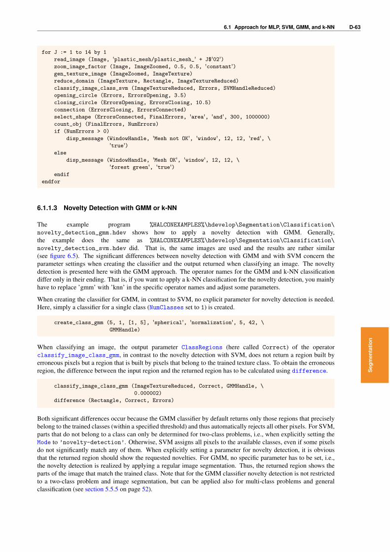
6.1 Approach for MLP, SVM, GMM, and k-NN D-63
for J := 1 to 14 by 1
read_image (Image, 'plastic_mesh/plastic_mesh_' + J$'02')zoom_image_factor (Image, ImageZoomed, 0.5, 0.5, 'constant')gen_texture_image (ImageZoomed, ImageTexture)
reduce_domain (ImageTexture, Rectangle, ImageTextureReduced)
classify_image_class_svm (ImageTextureReduced, Errors, SVMHandleReduced)
opening_circle (Errors, ErrorsOpening, 3.5)
closing_circle (ErrorsOpening, ErrorsClosing, 10.5)
connection (ErrorsClosing, ErrorsConnected)
select_shape (ErrorsConnected, FinalErrors, 'area', 'and', 300, 1000000)
count_obj (FinalErrors, NumErrors)
if (NumErrors > 0)
disp_message (WindowHandle, 'Mesh not OK', 'window', 12, 12, 'red', \
'true')else
disp_message (WindowHandle, 'Mesh OK', 'window', 12, 12, \
'forest green', 'true')endif
endfor
6.1.1.3 Novelty Detection with GMM or k-NN
The example program %HALCONEXAMPLES%\hdevelop\Segmentation\Classification\
novelty_detection_gmm.hdev shows how to apply a novelty detection with GMM. Generally,the example does the same as %HALCONEXAMPLES%\hdevelop\Segmentation\Classification\
novelty_detection_svm.hdev did. That is, the same images are used and the results are rather similar(see figure 6.5). The significant differences between novelty detection with GMM and with SVM concern theparameter settings when creating the classifier and the output returned when classifying an image. The noveltydetection is presented here with the GMM approach. The operator names for the GMM and k-NN classificationdiffer only in their ending. That is, if you want to apply a k-NN classification for the novelty detection, you mainlyhave to replace ’gmm’ with ’knn’ in the specific operator names and adjust some parameters.
When creating the classifier for GMM, in contrast to SVM, no explicit parameter for novelty detection is needed.Here, simply a classifier for a single class (NumClasses set to 1) is created.
create_class_gmm (5, 1, [1, 5], 'spherical', 'normalization', 5, 42, \
GMMHandle)
When classifying an image, the output parameter ClassRegions (here called Correct) of the operatorclassify_image_class_gmm, in contrast to the novelty detection with SVM, does not return a region built byerroneous pixels but a region that is built by pixels that belong to the trained texture class. To obtain the erroneousregion, the difference between the input region and the returned region has to be calculated using difference.
classify_image_class_gmm (ImageTextureReduced, Correct, GMMHandle, \
0.000002)
difference (Rectangle, Correct, Errors)
Both significant differences occur because the GMM classifier by default returns only those regions that preciselybelong to the trained classes (within a specified threshold) and thus automatically rejects all other pixels. For SVM,parts that do not belong to a class can only be determined for two-class problems, i.e., when explicitly setting theMode to ’novelty-detection’. Otherwise, SVM assigns all pixels to the available classes, even if some pixelsdo not significantly match any of them. When explicitly setting a parameter for novelty detection, it is obviousthat the returned region should show the requested novelties. For GMM, no specific parameter has to be set, i.e.,the novelty detection is realized by applying a regular image segmentation. Thus, the returned region shows theparts of the image that match the trained class. Note that for the GMM classifier novelty detection is not restrictedto a two-class problem and image segmentation, but can be applied also for multi-class problems and generalclassification (see section 5.5.5 on page 52).
Seg
men
tatio
n

D-64 Classification for Image Segmentation
Novelty−Detection with GMMNovelty−Detection with SVM
Figure 6.5: Novelty detection is used to extract parts of an image or region that do not fit to a trained pattern andcan be applied with SVM or GMM.
6.1.2 Involved Operators (Overview)
This section gives a brief overview on the operators that are provided for MLP, SVM, GMM, and k-NN classifica-tion for image segmentation. In particular, first the operators for the basic steps and then the advanced operatorsused for image segmentation are introduced.
6.1.2.1 Basic Operators
Summarizing the information obtained in section 6.1.1 on page 57, the image segmentation consists of the follow-ing basic steps and operators, which are applied in the same order as listed here. Note that the steps are similar tothe steps applied for a general classification (see section 5.2.1 on page 34), mainly the step for adding the samplesand the step for the actual classification vary.
1. Create a classifier. Here, some important properties of the classifier are defined. The returned handle isneeded in all later classification steps. Each classification step modifies this handle. This step correspondsto the approach of the general classification.
• create_class_mlp
• create_class_svm
• create_class_gmm
• create_class_knn
2. Predefine the sequence in which the classes are defined and later accessed, i.e., define the correspondencesbetween the class IDs and the class names, respectively define the colors that visualize the different classes.This step may as well be applied before the creation of the classifier.
3. Add samples, i.e., a region for each class to the classifier. In contrast to the general classification, a singleoperator call can be used to add all sample regions at once. The sequence of the added regions define theclasses, i.e., the first region is class 0, the second is class 1 etc. Having several images for the training, theoperator can be called multiple times, then the sample regions for the classes must be defined in the samesequence. If one of the classes is not represented in an image, an empty region has to be passed. This stepsignificantly differs from the approach of the general classification.
• add_samples_image_class_mlp
• add_samples_image_class_svm
• add_samples_image_class_gmm
• add_samples_image_class_knn

6.1 Approach for MLP, SVM, GMM, and k-NN D-65
4. Train the classifier, i.e., use the added samples to obtain the boundaries between the classes. This stepcorresponds to the approach of the general classification.
• train_class_mlp
• train_class_svm
• train_class_gmm
• train_class_knn
5. Store the used samples to file and access them in a later step (optionally). This step corresponds to theapproach of the general classification.
• write_samples_class_mlp and read_samples_class_mlp
• write_samples_class_svm and read_samples_class_svm
• write_samples_class_gmm and read_samples_class_gmm
• Note that there are no operators for writing and reading the samples of a k-NN classifier separatelybecause the samples are an intrinsic component of the k-NN classifier. Use write_class_knn andread_class_knn instead.
6. Store the trained classifier to file and read it from file again. This step corresponds to the approach of thegeneral classification.
• write_class_mlp (default file extension: .gmc) and read_class_mlp
• write_class_svm (default file extension: .gsc) and read_class_svm
• write_class_gmm (default file extension: .ggc) and read_class_gmm
• write_class_knn (default file extension: .gnc) and read_class_knn
Note that the samples cannot be deleted from a k-NN classifier because they are an intrinsic componentof this classifier.
7. Segment the image by classification. That is, insert a new image and use one of the following operators tosegment the image into regions of different classes. This step significantly differs from the approach of thegeneral classification.
• classify_image_class_mlp
• classify_image_class_svm
• classify_image_class_gmm
• classify_image_class_knn
Besides the basic steps of a classification, some additional steps and operators can be applied if suitable. Theseadvanced operators are similar for image segmentation and general classification.
6.1.2.2 Advanced Operators
Especially if the training and classification do not lead to a satisfying result, it is helpful to access some informationthat is implicitly contained in the model. Available steps to query information are:
• Access an individual sample from the training data. This is needed, e.g., to checkthe correctness of its class assignment. The sample had to be stored previouslyby the operator add_samples_image_class_mlp, add_samples_image_class_svm,add_samples_image_class_gmm, or add_samples_image_class_knn, respectively.
– get_sample_class_mlp
– get_sample_class_svm
– get_sample_class_gmm
– get_sample_class_knn
• Get the number of samples that are stored in the training data. The obtained number is needed, e.g., to accessthe individual samples or to know how much individual samples you can access.
Seg
men
tatio
n

D-66 Classification for Image Segmentation
– get_sample_num_class_mlp
– get_sample_num_class_svm
– get_sample_num_class_gmm
– get_sample_num_class_knn
• Get information about the content of the preprocessed feature vectors. This information is reasonable, if theparameter Preprocessing was set to ’principal_components’ or ’canonical_variates’ during thecreation of the classifier. Then, you can check if the information that is contained in the preprocessed featurevector still contains significant data or if a different preprocessing parameter, e.g., ’normalization’, is tobe preferred.
– get_prep_info_class_mlp
– get_prep_info_class_svm
– get_prep_info_class_gmm
– Note that this kind of operator is not available for k-NN classifiers, because they do not provide theabove mentioned preprocessing options.
• Get the parameter values that were set during the creation of the classifier. This is needed if the offlinetraining and the online classification are separated and the information about the training part is not availableanymore.
– get_params_class_mlp
– get_params_class_svm
– get_params_class_gmm
– get_params_class_knn
Furthermore, there are operators that are available only for specific classifiers. In particular,
• For SVM you can reduce the number of support vectors returned by the offline training to speed up thefollowing online classification.
– reduce_class_svm
• Additionally, for SVM the number or index of the support vectors can be determined after the training. Thisis suitable for the visualization of the support vectors and thus for diagnostic reasons.
– get_support_vector_num_class
– get_support_vector_class
• For k-NN classifiers, you can set various parameters with
– set_params_class_knn.
See section 5.6.4 on page 54 for a detailed descriptions of this operator.
If you want to speed up an image segmentation for images with a maximum of three image channels, you canapply a classification that is based on look-up tables (LUT, see also section 6.1.7 on page 70). Then, the approachdiffers from the basic image segmentation as follows:
• After creating a classifier, adding samples to it and training it, the result of the training is stored in a LUT-accelerated classifier.
– create_class_lut_mlp
– create_class_lut_svm
– create_class_lut_gmm
– create_class_lut_knn
• For the actual image segmentation, instead of classify_image_class_mlp,classify_image_class_svm, classify_image_class_gmm, or classify_image_class_knn,respectively, the LUT-accelerated classifier is applied.
– classify_image_class_lut

6.1 Approach for MLP, SVM, GMM, and k-NN D-67
6.1.3 Parameter Setting for MLP
Most rules for the parameter setting for an image segmentation using MLP classification correspond to the rules forthe general classification with MLP (see section 5.3 on page 37). As the most important operators and parametersto adjust are listed and described there, here only the parameter settings for the operators that are specific forimage segmentation are described. These are the operators that add the training samples, i.e., sample regions, tothe classifier and those that segment the unknown image.
6.1.3.1 Adjusting add_samples_image_class_mlp
For image segmentation with MLP, sample regions are added to the classifier withadd_samples_image_class_mlp. In contrast to the samples used for a general classification, here, nofeature vectors have to be generated explicitly but are implicitly given by the gray values of each pixel of therespective input region in all channels of the input image. The dimension of the feature vectors depends on thenumber of channels of the image containing the sample regions. The quality of the samples is very important forthe quality of the classification. Section 4.3 on page 29 provides hints how to select a set of suitable samples. Forthe operator add_samples_image_class_mlp, the following parameters have to be set:
• Image: The image that contains the sample regions
• ClassRegions: The tuple containing the training regions. Here, one region per class is defined. The numberof classes corresponds to the number of regions, and thus, the label of an individual class corresponds to theposition of the training region in the tuple, i.e., its index.
• MLPHandle: The handle of the classifier that was created with create_class_gmm
The operator returns the modified handle of the classifier (MLPHandle).
6.1.3.2 Adjusting classify_image_class_mlp
With the operator classify_image_class_mlp a new image is segmented into regions of the classes that weretrained with train_class_mlp using the samples that were added with add_samples_image_class_mlp. Thefollowing parameters have to be set:
• Image: The image that has to be segmented into the classes that were trained with train_class_gmm.
• MLPHandle: The handle of the classifier that was created with create_class_mlp, to which samples wereadded with add_samples_image_class_mlp, and that was trained with train_class_mlp.
• RejectionThreshold: The threshold on the probability measure returned by the classification. All pixelshaving a probability below RejectionThreshold are not assigned to any class.
The operator returns a tuple of regions in ClassRegions. This tuple contains one region for each class. Thesequence of the classes corresponds to the sequence used for the training regions that were added to the classifierwith add_samples_image_class_mlp.
In contrast to the general classification using classify_class_mlp described in section 5.3.5 on page 41, noconfidence for the classification but a rejection class is returned. This rejection class depends on the selectedrejection threshold. Note that the returned rejection class has not the same quality than the rejection class returnedfor a GMM classification, as the MLP classification is typically influenced by outliers (see section 5.3.5 on page42). Thus, for MLP the explicit training of a rejection class is recommended.
6.1.4 Parameter Setting for SVM
Most rules for the parameter setting for an image segmentation using SVM classification correspond to the rules forthe general classification with SVM (see section 5.4 on page 42). As the most important operators and parametersto adjust are listed and described there, here only the parameter settings for the operators that are specific forimage segmentation are described. These are the operators that add the training samples, i.e., sample regions, tothe classifier and those that segment the unknown image.
Seg
men
tatio
n

D-68 Classification for Image Segmentation
6.1.4.1 Adjusting add_samples_image_class_svm
For image segmentation with SVM, sample regions are added to the classifier withadd_samples_image_class_svm. In contrast to the samples used for a general classification, here, nofeature vectors have to be generated explicitly but are implicitly given by the gray values of each pixel of therespective input region in all channels of the input image. The dimension of the feature vectors depends on thenumber of channels of the image containing the sample regions. The quality of the samples is very important forthe quality of the classification. Section 4.3 on page 29 provides hints how to select a set of suitable samples. Forthe operator add_samples_image_class_svm, the following parameters have to be set:
• Image: The image that contains the sample regions
• ClassRegions: The tuple containing the training regions. Here, one region per class is defined. The numberof classes corresponds to the number of regions, and thus, the label of an individual class corresponds to theposition of the training region in the tuple, i.e., its index.
• SVMHandle: The handle of the classifier that was created with create_class_svm
The operator returns the modified handle of the classifier (SVMHandle).
6.1.4.2 Adjusting classify_image_class_svm
With the operator classify_image_class_svm a new image is segmented into regions of the classes that weretrained with train_class_svm using the samples that were added with add_samples_image_class_svm. Thefollowing parameters have to be set:
• Image: The image that has to be segmented into the classes that were trained with train_class_svm.
• SVMHandle: The handle of the classifier that was created with create_class_svm, to which samples wereadded with add_samples_image_class_svm, and that was trained with train_class_svm.
The operator returns a tuple of regions in ClassRegions. This tuple contains one region for each class. Thesequence of the classes corresponds to the sequence used for the training regions that were added to the classifierwith add_samples_image_class_svm.
6.1.5 Parameter Setting for GMM
Most rules for the parameter setting for an image segmentation using GMM classification correspond to the rulesfor the general classification with GMM (see section 5.5 on page 47). As the most important operators and param-eters to adjust are listed and described there, here only the parameter settings for the operators that are specific forimage segmentation are described. These are the operators that add the training samples, i.e., sample regions, tothe classifier and those that segment the unknown image.
6.1.5.1 Adjusting add_samples_image_class_gmm
For image segmentation with GMM, sample regions are added to the classifier withadd_samples_image_class_gmm. In contrast to the samples used for a general classification, here, nofeature vectors have to be generated explicitly but are implicitly given by the gray values of each pixel of therespective input region in all channels of the input image. The dimension of the feature vectors depends on thenumber of channels of the image containing the sample regions. The quality of the samples is very important forthe quality of the classification. Section 4.3 on page 29 provides hints how to select a set of suitable samples. Forthe operator add_samples_image_class_gmm, the following parameters have to be set:
• Image: The image that contains the sample regions
• ClassRegions: The tuple containing the training regions. Here, one region per class is defined. The numberof classes corresponds to the number of regions, and thus, the label of an individual class corresponds to theposition of the training region in the tuple, i.e., its index.

6.1 Approach for MLP, SVM, GMM, and k-NN D-69
• GMMHandle: The handle of the classifier that was created with create_class_gmm
• Randomize: The parameter that handles undesired effects that may occur for originally integer feature values(see also section 5.5.2 on page 50).
The operator returns the modified handle of the classifier (GMMHandle).
6.1.5.2 Adjusting classify_image_class_gmm
With the operator classify_image_class_gmm a new image is segmented into regions of the classes that weretrained with train_class_gmm using the samples that were added with add_samples_image_class_gmm. Thefollowing parameters have to be set:
• Image: The image that has to be segmented into the classes that were trained with train_class_gmm.
• GMMHandle: The handle of the classifier that was created with create_class_gmm, to which samples wereadded with add_samples_image_class_gmm, and that was trained with train_class_gmm.
• RejectionThreshold: The threshold on the K-sigma probability (KSigmaProb) measure returnedby the classification (see also section 5.5.5 on page 52). All pixels having a probability belowRejectionThreshold are not assigned to any class.
The operator returns a tuple of regions in ClassRegions. This tuple contains one region for each class. Thesequence of the classes corresponds to the sequence used for the training regions that were added to the classifierwith add_samples_image_class_gmm.
In contrast to the general classification using classify_class_gmm described in section 5.5.5 on page 52, noprobabilities for the classes but a rejection class is returned. This rejection class depends on the selected rejectionthreshold.
6.1.6 Parameter Setting for k-NN
Most rules for the parameter setting for an image segmentation using k-NN classification correspond to the rules forthe general classification with k-NN (see section 5.6 on page 52). As the most important operators and parametersto adjust are listed and described there, here only the parameter settings for the operators that are specific forimage segmentation are described. These are the operators that add the training samples, i.e., sample regions, tothe classifier and those that segment the unknown image.
6.1.6.1 Adjusting add_samples_image_class_knn
For image segmentation with k-NN, sample regions are added to the classifier withadd_samples_image_class_knn. In contrast to the samples used for a general classification, here, nofeature vectors have to be generated explicitly but are implicitly given by the gray values of each pixel of therespective input region in all channels of the input image. The dimension of the feature vectors depends on thenumber of channels of the image containing the sample regions. The quality of the samples determines the qualityof the classification. Section 4.3 on page 29 provides hints how to select a set of suitable samples. For the operatoradd_samples_image_class_knn, the following parameters have to be set:
• Image: The image that contains the sample regions
• ClassRegions: The tuple containing the training regions. Here, one region per class is defined. The numberof classes corresponds to the number of regions, and thus, the label of an individual class corresponds to theposition of the training region in the tuple, i.e., its index.
• KNNHandle: The handle of the classifier that was created with create_class_knn
The operator returns the modified handle of the classifier (KNNHandle).
Seg
men
tatio
n

D-70 Classification for Image Segmentation
6.1.6.2 Adjusting classify_image_class_knn
With the operator classify_image_class_knn a new image is segmented into regions of the classes that weretrained with train_class_knn using the samples that were added with add_samples_image_class_knn. Thefollowing parameters have to be set:
• Image: The image that has to be segmented into the classes that were trained with train_class_knn.
• KNNHandle: The handle of the classifier that was created with create_class_knn, to which samples wereadded with add_samples_image_class_knn, and that was trained with train_class_knn.
• RejectionThreshold: The threshold on the distance returned by the classification (see also section 5.6.5on page 55). All pixels having a distance above RejectionThreshold are not assigned to any class.
The operator returns a tuple of regions in ClassRegions. This tuple contains one region for each class. Thesequence of the classes corresponds to the sequence used for the training regions that were added to the classifierwith add_samples_image_class_knn.
The returned image DistanceImage, contains the distance of each pixel of the input image Image to its nearestneighbor.
6.1.7 Classification Based on Look-Up Tables
A significant speed-up for the image segmentation can be obtained by applying a classification that is based onlook-up tables (LUT). That is, you store the content of a trained classifier into a LUT und use the LUT-acceleratedclassifier instead of the original classifier for the classification. The approach is as follows:
First, you create an MLP, SVM, GMM, or k-NN classifier, add samples to it, and apply the training as describedfor the basic image segmentation in the previous sections.
Then, the LUT-accelerated classifier is created using the operator create_class_lut_mlp,create_class_lut_svm, create_class_lut_gmm, or create_class_lut_knn, respectively. Here, youinsert the handle of the trained classifier and you can adjust the following parameters.
• ’bit_depth’ (for all classifiers)The parameter ’bit_depth’ describes the number of bits used from the pixels. It controls the storagerequirement of the LUT-accelerated classifier and the runtime needed for the LUT-accelerated classification.A byte image has a bit depth of 8. If the bit depth is set to a value of 7 or 6, the storage requirement can bereduced. But note that a bit depth that is smaller than the bit depth of the image will usually lead to a loweraccuracy of the classification.
• ’class_selection’ (for MLP, SVM, and GMM classifiers)the parameter ’class_selection’ is used to control the accuracy and the runtime needed for the creationof the LUT-accelerated classifier. A higher accuracy slows down the runtime and a lower accuracy leads toa speed-up. The value of ’class_selection’ is ignored if the bit depth of the LUT is maximal.
• ’rejection_threshold’ (for MLP, GMM, and k-NN classifiers)The parameter ’rejection_threshold’ corresponds to the rejection threshold that is described for thebasic image segmentation in section 6.1.3.2 for MLP, in section 6.1.5.2 for GMM, and in section 6.1.6.2 fork-NN.
For the actual image segmentation, the operator classify_image_class_lut is applied instead of theoperator classify_image_class_mlp, classify_image_class_svm, classify_image_class_gmm, orclassify_image_class_knn, respectively. Note that the number of channels of the image that has to be clas-sified must correspond to the value specified for the dimension of the feature space when creating the originalclassifier, i.e., the value of NumInput in create_class_mlp, NumFeatures in create_class_svm, NumDim increate_class_gmm, or NumDim in create_class_knn.
If you need the original trained classifier for further applications, you should store it to file (see section 6.1.2.1 onpage 64). The LUT-accelerated classifier cannot be stored to file, as it needs a lot of memory and thus, it is moresuitable to create it again from the reused original classifier when starting a new application.

6.1 Approach for MLP, SVM, GMM, and k-NN D-71
Figure 6.6: Fuses of different color are segmented using a LUT-accelerated GMM classifier.
The HDevelop example program %HALCONEXAMPLES%\hdevelop\Applications\Color-Inspection\
classify_fuses_gmm_based_lut.hdev uses a LUT-accelerated classifier that is based on a trained GMMclassifier to segment fuses of different color (see figure 6.6).
First, the ROIs that serve as training samples for different color classes are selected and concatenated into the tupleClasses. Then, a GMM classifier is created, the training samples are added, and the classifier is trained. Untilnow, the approach is the same as for the image segmentation that was described in the previous sections.
create_class_gmm (3, 5, 1, 'full', 'none', 3, 42, GMMHandle)
add_samples_image_class_gmm (Image, Classes, GMMHandle, 0)
train_class_gmm (GMMHandle, 100, 0.001, 'training', 0.001, Centers, Iter)
In contrast to the basic image segmentation, the training result, i.e., the classifier, is then stored in a LUT-accelerated classifier using create_class_lut_gmm.
create_class_lut_gmm (GMMHandle, ['bit_depth', 'rejection_threshold'], [6, \
0.03], ClassLUTHandle)
Now, for each image that has to be classified, the operator classify_image_class_lut is applied to segmentthe images based on the LUT of the new classifier.
for Img := 0 to 3 by 1
read_image (Image, ImageRootName + Img)
classify_image_class_lut (Image, ClassRegions, ClassLUTHandle)
endfor
The HDevelop example program %HALCONEXAMPLES%\hdevelop\Segmentation\Classification\
classify_image_class_lut.hdev compares the runtime needed by MLP, SVM, GMM, and k-NN clas-sification using the basic image segmentation on the one hand and the LUT-accelerated classification on the otherhand. It exemplarily shows that the online part of the LUT-accelerated classification is significantly faster thanthat of the basic image segmentation. But note that it needs also additional memory and the runtime for the
!offline part is increasing. Because of that the LUT-accelerated classification is restricted to feature spaces witha maximum of three dimensions. Figure 6.7 shows the interdependencies between the number of classes, the bitdepth, and the required memory for a three-channel image. Furthermore, depending on the selected bit depth ofthe look-up table, the accuracy of the classification may be decreased. Summarized, if a three-channel imagehas to be segmented, a speed-up of the online part is required, and the runtime for the offline part is not critical,LUT-accelerated classification is a good alternative to the basic image segmentation.
Seg
men
tatio
n

D-72 Classification for Image Segmentation
Number of classes Bit depth Needed memory256 3 x 8 Bit 32 MB
1 3 x 8 Bit 2 MB10 3 x 6 Bit 0,125 MB
Figure 6.7: Memory needed for a LUT-accelerated classifier for three-channel images with different numbers ofclasses and different bit depths.
6.2 Approach for a Two-Channel Image Segmentation
For two-channel images a simple and very fast pixel classification can be applied using the operatorclass_2dim_sup. As we already learned, a class is defined as a well-defined part of the feature space and thedimension of the feature space depends on the number of features used for the classification. In case of a two-channel image and a pure pixel based classification, the classification is based only on the two gray values that areassigned to each pixel position and thus the two-dimensional feature space can be visualized in a 2D graph or in a2D image, respectively. There, for each position of the image or a specific image region the gray value of the firstimage ImageCol is used as column coordinate and the gray value of the second image ImageRow is used as rowcoordinate (see figure 6.8, left). A class is defined by the feature space of a manually specified image region.
The general approach using class_2dim_sup for a two-channel image segmentation is as follows: you firstspecify a class by a region in the two-channel image that is typical for the class. Then, you apply the oper-ator histo_2dim, which needs the two channels and the specified image region as input and returns the two-dimensional histogram, i.e., an image in which the position of a pixel is built by the combination of the gray valuesof the two channels and its gray value is defined by the frequency of the specific gray value combination. Toextract the essential region of the feature space, a threshold is applied. Now, the result can be preprocessed forgeneralization purposes (see figure 6.8, right), e.g., by a morphological operation like closing_circle. For theactual classification, the feature space region and the two channels of the image that has to be classified are usedas input for the operator class_2dim_sup. The returned region RegionClass2Dim consists of all pixels in theclassified two-channel image, for which the gray value distribution is similar to the gray value distribution of thetraining region, i.e., for which the position in the feature space lies inside the preprocessed feature space regionthat defines the class.
g(ImageCol)
2550
0
255 255
0
0
g(ImageCol)
255
g(ImageRow) g(ImageRow)
Figure 6.8: Positions of the 2D feature space for a supervised classification: (left) gray values of the two images ina 2D graph, (right) feature space region (class) after generalization.
The example %HALCONEXAMPLES%\hdevelop\Segmentation\Classification\class_2dim_sup.hdev
shows the approach for the segmentation of a two-channel image that contains several capacitors. First the colorimage is decomposed into its three channels, so that two of them can be accessed for the classification. Then,a sample region for one of the capacitors is defined and used as input for histo_2dim, which together withthreshold and closing_circle is used to derive a generalized feature space region. Finally, the two channelsof the image and the trained feature space region are used by class_2dim_sup to get the region with all pixelsthat correspond to the trained feature space.

6.3 Approach for Euclidean and Hyperbox Classification D-73
read_image (Image, 'ic')decompose3 (Image, Red, Green, Blue)
gen_rectangle1 (Pattern, 362, 276, 371, 298)
histo_2dim (Pattern, Red, Blue, Histo2Dim)
threshold (Histo2Dim, Features, 1, 255)
closing_circle (Features, FeaturesClosed, 11.5)
class_2dim_sup (Red, Blue, FeaturesClosed, RegionClass2Dim)
This image segmentation approach is very fast. To select the two channels of a multi-channel image that should beused for the classification, different approaches exist. For color images, i.e., three-channel ’rgb’ images, you can,e.g., apply a color transformation using trans_from_rgb to transform the ’rgb’ image into a, e.g., ’hsi’ image.This image contains one channel for the ’hue’, one for the ’saturation’, and one for the ’intensity’ of the pixels.When using the ’hue’ and ’saturation’ channels for the classification, you obtain a classifier that is invariant toillumination changes (see also Solution Guide I, chapter 14 on page 147 for color transformations). For arbitrarymulti-channel images you can also transform your image by a principal component analysis using the operatorprincipal_comp. Then, the first two channels of the returned image are the channels with the largest informationcontent and thus are predestinated to be input to the two-channel image segmentation.
6.3 Approach for Euclidean and Hyperbox Classification
For the simple image segmentation of multi-channel images, class_ndim_norm is available. It can be appliedeither using a hyperbox or an Euclidean metric (for hyperbox and Euclidean classification see section 3.2 on page16). It can be applied following the general idea of hyperbox classification.
For learn_ndim_norm, an overlap between the classes ’Foreground’ and ’Background’ is allowed. Thishas its effect on the return value Quality. The larger the overlap, the smaller the value. Note that the operatorclass_ndim_norm is very efficient. Compared, e.g., to the classic image segmentation using GMM (section 6.1.5on page 68), it is significantly faster (approximately by factor 3). Compared to a LUT-accelerated classification ithas the advantage that the storage requirements are low and the feature space can be easily visualized. Thus, if theclasses are build by compact clusters, it is a good alternative.
6.3.0.1 Classification with class_ndim_norm
When segmenting an image using class_ndim_norm, you do not explicitly create and destroy a classifier, butimmediately apply the training using learn_ndim_norm. Instead of storing the training results in a classifier andusing the classifier as input for the classification, the training returns explicit information about the centers andradii of the clusters related to the trained patterns and this information is used as input for the classification, whichis applied with class_ndim_norm. You can choose between a classification using hyperboxes and a classificationusing hyperspheres (Euclidean classification).
With learn_ndim_norm you generate the classification clusters from the region Foreground. The regionBackground can be used to define a rejection class, but may also be empty (an empty region can be createdby gen_empty_region). Note that the rejection class does not influence the clustering, but can be used to detectproblems that might occur because of overlapping classes.
To choose between the two available clustering approaches, the parameter Metric is used. It can be either set to’euclid’, which uses a minimum distance algorithm (n-dimensional hyperspheres) or to ’maximum’, which usesn-dimensional hyperboxes to built the clusters. Metric must be set to the same value for the training as well as forthe classification. The Euclidean metric usually yields the better results but needs more run time.
The parameter Distance describes the minimum distance between two cluster centers and thus determines themaximum value allowed for the output parameter Radius. Note that the cluster centers depend on the sequenceused to add the training samples (pixels). Thus, it is recommended to select a small value for Distance. Then,the (small) hyperboxes or hyperspheres can approximate the feature space well. But simultaneously, the runtimeduring classification increases.
The ratio of the number of pixels in a cluster to the total number of pixels (in percent) must be larger than thevalue of the parameter MinNumberPercent, otherwise the cluster is not returned. MinNumberPercent serves toeliminate outliers in the training set. If it is chosen too large many clusters are suppressed.
Seg
men
tatio
n

D-74 Classification for Image Segmentation
As result of the operator, the parameter Radius returns the minimum distance between two cluster centers, i.e.,radii for hyperspheres or half edge lengths for hyperboxes, and Center returns the coordinates of the clustercenters. Furthermore, the parameter Quality returns the quality of the clustering, i.e., a measure of overlapbetween the rejection class and the classifier classes. Values larger than 0 denote the corresponding ratio of overlap.If no rejection region is given, its value is set to 1. The regions in Background do not influence the clustering.They are merely used to check the results that can be expected.
When classifying a multi-channel image with class_ndim_norm, you set the same metric (Metric) used alsofor the training and set the parameter SingleMultiple to ’single’ if one region has to be generated or to’multiple’ if multiple regions have to be generated for each cluster. Additionally, Radius and Center, whichwere returned by learn_ndim_norm, are inserted. The result of class_ndim_norm is returned in Regions, whicheither contains a single region or a tuple of regions, depending on the value of SingleMultiple.
The example %HALCONEXAMPLES%\hdevelop\Segmentation\Classification\class_ndim_norm.hdev
shows how to apply an image segmentation with class_ndim_norm. The image is read and within the image aregion for the class to be trained and an empty region for the rejection class are generated and used as input for thetraining with learn_ndim_norm. The classification is then applied with class_ndim_norm. The result of theimage segmentation is shown in figure 6.9.
read_image (Image, 'ic')gen_rectangle1 (Region, 360, 198, 369, 226)
gen_empty_region (EmptyRegion)
learn_ndim_norm (Region, EmptyRegion, Image, 'euclid', 10, 0.01, Radius, \
Center, Quality)
class_ndim_norm (Image, Regions, 'euclid', 'multiple', Radius, Center)
Figure 6.9: Result of image segmentation using class_ndim_norm (returned regions marked in white).

Classification for Optical Character Recognition (OCR) D-75
Chapter 7
Classification for Optical CharacterRecognition (OCR)
If classification is used for optical character recognition (OCR), individual regions are first extracted from theimage by a segmentation and then, with the help of some region features, assigned to classes that typically (butnot necessarily) represent individual characters or numbers. Approaches that are suitable for this feature-basedOCR comprise the MLP, the SVM, and the k-NN classifiers. A hyperbox classifier is also provided, but is notrecommended anymore. With Deep OCR a further OCR method is provided by HALCON (see Solution Guide I,chapter 19 on page 229). This deep-learning-based method is not a classifier and as a consequence ignored in theexplanations within this manual.
In section 7.1 the general approach for OCR is illustrated by an example that trains and reads the characters ’A’to ’G’. In section 7.2 the steps of OCR and the involved operators are listed for a brief overview. The parametersused for the basic OCR operators are introduced in section 7.3 for MLP, section 7.4 for SVM, section 7.5 for k-NN,and section 7.6 for CNNs. Section 7.7 finally lists all features that are available for OCR.
In general, when trying OCR for your application, it is recommended to first try the pretrained CNN-based OCRfont Universal and evaluate the result before you try any other OCR classification approaches, since the CNN-based OCR classifier can generalize quite well.
7.1 General Approach
Figure 7.1 shows the general approach for OCR. Typically, the approach is divided into an offline and an onlineprocess. The offline process comprises the training of the font, i.e., regions that represent characters or numbers(in the following just called ’characters’) are extracted and stored together with the corresponding character namesin training files. The content of a training file optionally can be accessed again. The access is needed for differentreasons. First, they can be used to find errors that occurred during the training, which is needed on one hand foryour general quality assurance and on the other hand for the correspondence with your HALCON support team(if needed), and second, you can reuse the contained information for the case that you want to apply a similarapplication in the future.
Now, the training files are used to train the font. To access the font in the later online process, the classifier iswritten into a font file.
If you want to read a font that is rather common and you want to use the MLP approach, you can also use oneof the pretrained fonts provided by HALCON (see Solution Guide I, chapter 13 on page 133 for illustrations ofthe provided fonts). The pretrained fonts are stored in the subdirectory ocr of the directory where you installedHALCON. Then, you can skip the offline training process. For SVM and k-NN classifiers, no pretrained fonts areavailable.
In the online process, the font file is read so that the classifier can be accessed again. Then, the regions of unknowncharacters are extracted, most suitably by the same method that was used within the offline training process, andclassified, i.e., the characters are read.
OC
R

D-76 Classification for Optical Character Recognition (OCR)
Store Classifier to File
Store Regions and Character Names to Training Files
Segment Regions of Known Characters
Segment Regions of Unknown Characters
Train New Classifier (Font) Use Pretrained Font
Read Characters
Check Correctness of Training Files
Classify Regions (Read Characters)
Offl
ine
Onl
ine
Train Classifier (Font)
or
Read Classifier (Font) from File
Figure 7.1: The basic steps of OCR.
In the following, we illustrate the general approach for OCR classification with the examples %HALCONEXAMPLES%\solution_guide\classification\train_characters_ocr.hdev and %HALCONEXAMPLES%\
solution_guide\classification\classify_characters_ocr.hdev. These examples show how thecharacters ’A’, ’B’, ’C’, ’D’, ’E’, ’F’, and ’G’ are first trained (see figure 7.2) and then read (see figure 7.3)with an SVM-based OCR classification. Note that the number of classes as well as the number of training samplesis very small as the example is used only to demonstrate the general approach. Typically, a larger number ofclasses is trained with OCR and a lot of samples and probably a different set of features are needed to get a robustclassification.
The examples use SVM-based OCR classification. For MLP and k-NN, the general approach and the operators aresimilar. Then, you mainly have to replace ’svm’ by ’mlp’ or ’knn’, respectively in the specific operator namesand adjust different parameters. The specific parameters are explained in more detail in section 7.3 on page 80 forMLP, in section 7.4 on page 83 for SVM, and in section 7.5 on page 86 for k-NN.
Figure 7.2: Training images for the characters ’A’, ’B’, ’C’, ’D’, ’E’, ’F’, and ’G’.
The program %HALCONEXAMPLES%\solution_guide\classification\train_characters_ocr.hdev startswith the creation of an SVM-based OCR classifier using the operator create_ocr_class_svm. Here, the mostimportant parameters are adjusted. The width and height of a normalized character is defined (the reason for this

7.1 General Approach D-77
is explained in more detail in section 7.3.1 on page 80) and the mode for the interpolation that is used to scalethe characters to the average character size is set. Further, the features that should be calculated to get the featurevector are selected. OCR can be applied for a broad set of features, which is listed in section 7.7 on page 89.The default features are ’ratio’ and ’pixel_invar’. Here, the default does not lead to a satisfying result, sowe use the features ’convexity’, ’num_holes’, ’projection_horizontal’, and ’projection_vertical’
instead. Now, the names of the available classes (the characters A to G) are assigned, which were previouslystored in the tuple ClassNames. Furthermore, some SVM specific parameters are adjusted that are described inmore detail for the general classification in section 5.4 on page 42. The output of create_ocr_class_svm is thehandle of the classifier (OCRHandle), which is needed for the following classification steps.
ClassNames := ['A', 'B', 'C', 'D', 'E', 'F', 'G']create_ocr_class_svm (8, 10, 'constant', ['convexity', 'num_holes', \
'projection_horizontal', 'projection_vertical'], \
ClassNames, 'rbf', 0.02, 0.05, 'one-versus-one', \
'normalization', 10, OCRHandle)
For the training of the characters, the training images are read and the regions of the characters are extracted via ablob analysis within the procedure get_regions. Alternatively you can use also a combination of the operatorssegment_characters and select_characters to extract regions.
In the program, the first region is added together with its class name (which is obtained from the tuple ClassName)to a new training file with write_ocr_trainf. All following regions and their corresponding class names areappended to this training file with append_ocr_trainf.
for I := 1 to 7 by 1
read_image (Image, 'ocr/chars_training_' + I$'.2d')get_regions (Image, SortedRegions)
count_obj (SortedRegions, NumberObjects)
for J := 1 to NumberObjects by 1
select_obj (SortedRegions, ObjectSelected, J)
if (I == 1 and J == 1)
write_ocr_trainf (ObjectSelected, Image, ClassNames[J - 1], \
'train_characters_ocr.trf')else
append_ocr_trainf (ObjectSelected, Image, ClassNames[J - 1], \
'train_characters_ocr.trf')endif
endfor
endfor
After all samples were added to the training file, the operator read_ocr_trainf is applied to check if the trainingsamples and the corresponding class names were correctly assigned within the training file. In a short for-loop,the individual characters and their corresponding class names are visualized. Note that the index for iconic objects(Characters) starts with 1 and that of numeric objects (CharacterNames) with 0.
read_ocr_trainf (Characters, 'train_characters_ocr.trf', CharacterNames)
count_obj (Characters, NumberCharacters)
for I := 1 to NumberCharacters by 1
select_obj (Characters, CharacterSelected, I)
dev_display (CharacterSelected)
disp_message (WindowHandle, CharacterNames[I - 1], 'window', 10, 10, \
'black', 'true')endfor
Then, the OCR classifier is trained with trainf_ocr_class_svm, which needs the training file as input. ForSVM, the number of support vectors obtained from the training can be reduced to enhance the speed of the laterclassification. This is done with reduce_ocr_class_svm. The resulting handle is stored in a font file withwrite_ocr_class_svm for later access. For MLP the handle obtained directly by the training would be stored.
trainf_ocr_class_svm (OCRHandle, 'train_characters_ocr.trf', 0.001, \
'default')reduce_ocr_class_svm (OCRHandle, 'bottom_up', 2, 0.001, OCRHandleReduced)
write_ocr_class_svm (OCRHandleReduced, 'font_characters_ocr')
OC
R

D-78 Classification for Optical Character Recognition (OCR)
Now, the example program %HALCONEXAMPLES%\solution_guide\classification\
classify_characters_ocr.hdev is used to read unknown characters of the same font type used for thetraining.
A font is read from file with read_ocr_class_svm. Then, the images with unknown characters are read, and theregions that most probably represent characters are extracted. If possible, the method to extract the regions shouldbe the same for the offline and online process. Of course this advice can only be followed if the methods used inthe offline process are known, i.e., it can not be followed when using pretrained fonts.
The extracted regions are then classified, i.e., the characters are read. In the example, we read all regions si-multaneously with do_ocr_multi_class_svm. Alternatively, you can also read the regions individually withdo_ocr_single_class_svm. Then, not only the best class for each region is returned, but also the second best(and third best etc.) class can be obtained, which might be suitable when having overlapping classing. But if onlythe best class is of interest, do_ocr_multi_class_svm is faster and therefore recommended.
Figure 7.3: Classifying the characters ’A’, ’B’, ’C’, ’D’, ’E’, ’F’, and ’G’ with OCR.
read_ocr_class_svm ('font_characters_ocr', OCRHandle)
for I := 1 to 3 by 1
read_image (Image, 'ocr/chars_' + I$'.2d')get_regions (Image, SortedRegions)
do_ocr_multi_class_svm (SortedRegions, Image, OCRHandle, Classes)
area_center (SortedRegions, AreaCenter, Row, Column)
count_obj (SortedRegions, NumberObjects)
disp_message (WindowHandle, Classes, 'window', Row - 100, Column, \
'black', 'true')if (I < 3)
endif
endfor
endfor
7.2 Involved Operators (Overview)
This section gives a brief overview on the operators that are provided for OCR. In particular, first the operators forthe basic steps and then the advanced operators used for OCR are introduced.

7.2 Involved Operators (Overview) D-79
7.2.0.2 Basic Operators
The basic steps apply the following operators in the following sequence.
1. Create an OCR classifier using create_ocr_class_mlp, create_ocr_class_svm, orcreate_ocr_class_knn.
2. Extract the regions that represent the characters that have to be trained.
3. Store the samples, i.e., the training regions and the corresponding class names to a training file. This can bedone in different ways. Either
• store all samples at once using write_ocr_trainf. Then the regions as well as the correspondingclass names have to be available in a tuple. Or
• successively add the individual regions (characters) and their corresponding class names to the trainingfile using append_ocr_trainf.
• Write characters into a training file with write_ocr_trainf_image. That is, regions, represent-ing characters, including their gray values (region and pixel) and the corresponding class name arewritten into a file. An arbitrary number of regions within one image is supported. In contrast towrite_ocr_trainf one image per character is passed. The domain of this image defines the pixelswhich belong to the character. The file format can be defined by the parameter ’ocr_trainf_version’ ofthe operator set_system.
Additionally, several training files can be concatenated with concat_ocr_trainf.
4. Read the training characters from the training file and convert them into images with read_ocr_trainf tocheck the correctness of the training file content.
5. Train the OCR classifier with trainf_ocr_class_mlp, trainf_ocr_class_svm, ortrainf_ocr_class_knn.
6. Write the OCR classifier to a font file with write_ocr_class_mlp (default file extension: .omc),write_ocr_class_svm (default file extension: .osc), or write_ocr_class_knn (default file extension:.onc).
7. Read the OCR classifier from the font file with read_ocr_class_mlp, read_ocr_class_svm,read_ocr_class_knn, or read_ocr_class_cnn.
8. Extract the regions of the characters that have to be classified according to the trained font.
9. Classify the regions of the characters to be classified. Here, you have different possibilities:
• Classify multiple characters with an OCR classifier with do_ocr_multi_class_mlp,do_ocr_multi_class_svm, do_ocr_multi_class_knn, or do_ocr_multi_class_cnn.
• Classify a single character with an OCR classifier with do_ocr_single_class_mlp,do_ocr_single_class_svm, do_ocr_single_class_knn, or do_ocr_single_class_cnn.
7.2.0.3 Advanced Operators
Besides the basic steps of an OCR classification, some additional steps and operators can be applied if suitable. Inparticular, you can
• compute the features of a character with get_features_ocr_class_mlp,get_features_ocr_class_svm, or get_features_ocr_class_knn,
• return the parameters of an OCR classifier with get_params_ocr_class_mlp,get_params_ocr_class_svm, get_params_ocr_class_knn, or get_params_ocr_class_cnn,
• compute the information content of the preprocessed feature vectors of an OCR classifier withget_prep_info_ocr_class_mlp or get_prep_info_ocr_class_svm (if Preprocessing was set to’principal_components’ or ’canonical_variates’; note that this kind of operator is not availablefor k-NN classifiers, because they do not provide the respective preprocessing options),
OC
R

D-80 Classification for Optical Character Recognition (OCR)
• query which characters are stored in a training file with read_ocr_trainf_names,
• read training specific characters from files and convert them to images with read_ocr_trainf_select, or
• classify a related group of characters with an OCR classifier with do_ocr_word_mlp,do_ocr_word_svm, do_ocr_word_cnm, do_ocr_word_knn, or do_ocr_word_cnn. This is an al-ternative to do_ocr_multi_class_mlp, do_ocr_multi_class_svm, do_ocr_multi_class_cnn, ordo_ocr_multi_class_knn and is suitable when searching for specific words or regular expressions thatare specified in a lexicon that has been created with create_lexicon or imported with import_lexicon.
Besides these operators, some operators are provided that are available only for SVM:
• To enhance the speed, the trained SVM-based OCR classifier can be approximated with a reduced numberof support vectors by applying reduce_ocr_class_svm after the training.
• The number of support vectors that are stored within the SVM-based OCR classifier is returned withget_support_vector_num_ocr_class_svm.
• The index of a support vector from a trained SVM-based OCR classifier is returned withget_support_vector_ocr_class_svm.
In the following, the parameters for the basic operators are introduced and tips for their adjustment are provided.
7.3 Parameter Setting for MLP
The following sections introduce you to the parameters that have to be set for the basic operators needed for anMLP-based classification for OCR.
7.3.1 Adjusting create_ocr_class_mlp
An MLP classifier for OCR is created using create_ocr_class_mlp. Here, most of the important parametershave to be set.
Parameter WidthCharacter / HeightCharacter
Like for the general classification described in section 5 on page 31, OCR uses a set of features to classify regionsinto classes, which in this case correspond to specific characters and numbers. Some of the features that can beused for OCR are gray value features for which the number of returned features varies dependent on the region’ssize. As a classifier requires a constant number of features, i.e., the dimension of the feature vector has to be thesame for all training samples and all regions to be classified, the region of a character has to be transformed (scaled)to a standard size. This size is determined by WidthCharacter and HeightCharacter. In most applications,sizes between 6x8 and 10x14 should be used. As a rule of thumb, the values may be small if only few charactershave to be distinguished but large when classifying characters with complex shapes (e.g., Japanese signs).
Parameter Interpolation
The input parameter Interpolation is needed to control the transformation of the region to the size specifiedwith WidthCharacter and HeightCharacter. Generally, when transforming a region, transformed points willlie between discrete pixel coordinates. To assign each point to its final pixel coordinate and additionally to avoidaliasing, which typically occurs for scaled regions, an appropriate interpolation scheme is needed. Three typesof interpolation with different quality and speed properties are provided by HALCON and can be selected for theparameter Interpolation:
• ’nearest_neighbor’
If ’nearest_neighbor’ is selected, a nearest-neighbor interpolation is applied. There, the gray value isdetermined from the nearest pixel’s gray value. This interpolation scheme is very fast but may lead to a lowinterpolation quality.

7.3 Parameter Setting for MLP D-81
• ’bilinear’
If ’bilinear’ is selected, a bilinear interpolation is applied. There, the gray value is determined from thefour nearest pixels through bilinear interpolation. This interpolation scheme is of medium speed and quality.Do not use it if the characters in the image appear larger than WidthCharacter times HeightCharacter.In this case, the interpolation method ’constant’ or ’weighted’ should be used.
• ’constant’
If ’constant’ is selected, a bilinear interpolation is applied. There, the gray value is determined fromthe four nearest pixels through bilinear interpolation. If the transformation contains a scaling with a scalefactor smaller than 1, a kind of mean filter is used to prevent aliasing effects. This interpolation scheme is ofmedium speed and quality.
• ’weighted’
If ’weighted’ is selected, again a bilinear interpolation is applied, but now, aliasing effects for a scalingwith a scale factor smaller than 1 are prevented by a kind of Gaussian filter instead of a mean filter. Thisinterpolation scheme is slow but leads to the best quality.
The interpolation should be chosen such that no aliasing effects occur in the transformation. For most applications,Interpolation should be set to ’constant’.
Parameter Features
The input parameter Features specifies the features that are used for the classification. Features can contain atuple of several feature names. Each of these feature names results in one or more features to be calculated for theclassifier. That is, the length of the tuple in Features is similar or smaller than the dimension of the final featurevector. In section 7.7 on page 89 all features that are available for OCR are listed. To classify characters, in mostcases the ’default’ setting can be used. Then, the features ’ratio’ and ’pixel_invar’ are selected. Notethat the selection of the features significantly influences the quality of the classification.
Parameter Characters
The input parameter Characters contains a tuple with the names of the characters that will be trained. Each namemust be passed as a string. The number of elements in the tuple determines the number of available classes.
Parameter NumHidden
The input parameter NumHidden follows the same rules as provided for the corresponding operator used to createan MLP classifier for a general classification (see section 5.3.1 on page 37).
Parameters Preprocessing / NumComponents
The parameters Preprocessing and NumComponents follow the same rules as provided for the correspondingoperator used to create an MLP classifier for a general classification (see section 5.3.1 on page 37). The only excep-tion is that for the OCR classification the features are already approximately normalized. Thus, Preprocessingcan typically be set to ’none’.
If Preprocessing is set to ’principal_components’ or ’canonical_variates’ you can use the operatorget_prep_info_ocr_class_mlp to determine the optimum number of components as described for the generalclassification in section 5.3.1 on page 38.
Parameter RandSeed
The parameter RandSeed follows the same rules as provided for the corresponding operator used to create an MLPclassifier for a general classification (see section 5.3.1 on page 37).
Parameter OCRHandle
The output parameter OCRHandle is the handle of the classifier that is needed and modified throughout the follow-ing classification steps.
OC
R

D-82 Classification for Optical Character Recognition (OCR)
7.3.2 Adjusting write_ocr_trainf / append_ocr_trainf
After creating a classifier and segmenting the regions for the characters of known classes, i.e., character names, thesamples must be stored to a training file. Here, the same operators are used for MLP and SVM classifiers.
Different operators are provided for storing training samples to file. You can either store all samples to file inone step by inserting a tuple containing all regions and a tuple containing all corresponding class names to theoperator write_ocr_trainf. Or you can successively append single training samples to the training file usingappend_ocr_trainf. If you choose the latter, be aware that the training file is extended every time you runthe program, i.e., it is not created anew. So, if you want to successively add samples, it is recommended to usewrite_ocr_trainf for the first sample and append_ocr_trainf for all following samples. The operators areapplied as follows:
• Store training samples to a new training file:
When storing all training samples simultaneously into a file using write_ocr_trainf, you have to assigna tuple of regions that represent characters to the parameter Character. The image that contains the regionsmust be set in Image so that knowledge about the gray values within the regions is available. In Class atuple of class names that correspond to the regions with the same tuple index must be inserted. Finally, youspecify the name and path of the stored training file in FileName.
• Append training samples to a training file:
When successively storing individual training samples into a file using append_ocr_trainf, the sameparameters as for write_ocr_trainf have to be set. But in contrast to the operator write_ocr_trainfthe characters are appended to an existing file using the same training file format. If the file does not exist, anew file is generated.
If no file extension is specified in FileName the extension ’.trf’ is appended to the file name. The version ofthe file format used for writing data can be defined by the parameter ’ocr_trainf_version’ of the operatorset_system.
If you have several training files that you want to combine, you can concatenate them with the operatorconcat_ocr_trainf.
7.3.3 Adjusting trainf_ocr_class_mlp
trainf_ocr_class_mlp trains the OCR classifier OCRHandle with the training characters stored in theOCR training file given by TrainingFile. The remaining parameters MaxIterations, WeightTolerance,ErrorTolerance, Error, and ErrorLog have the same meaning as introduced for the training of an MLP classi-fier for a general classification (see section 5.3.3 on page 40).
7.3.4 Adjusting do_ocr_multi_class_mlp
With do_ocr_multi_class_mlp multiple characters can be classified in a single call. Typically, this is fasterthan successively applying do_ocr_single_class_mlp, which classifies single characters, in a loop. However,do_ocr_multi_class_mlp can only return the best class of each character. If the second best class is needed,e.g., because the classes significantly overlap (see section 5.3.5 on page 42 for the possible outliers related to theconfidence values of MLP classifications), do_ocr_single_class_cnn should be used instead. The followingparameters have to be set for do_ocr_multi_class_mlp:
Parameter Character
The input parameter Character contains a tuple of regions that have to be classified.
Parameter Image
The input parameter Image contains the image that provides the gray value information for the regions that haveto be classified.

7.4 Parameter Setting for SVM D-83
Parameter OCRHandle
The input parameter OCRHandle is the handle of the classifier that was trained with trainf_ocr_class_mlp.
Parameter Class
The output parameter Class returns the result of the classification, i.e., a tuple of character names that correspondto the input regions that were given in the tuple Character. If the result is ’\0x1A’ or ’\032’, the respective regionhas been classified as rejection class.
Parameter Confidence
The output parameter Confidence returns the confidence value for the classification. Note, that for the confidenceof MLP classifications, outliers are possible as described for the general classification in section 5.3.5 on page 42.
7.3.5 Adjusting do_ocr_single_class_mlp
Instead of using do_ocr_multi_class_mlp to add all samples in a single call, do_ocr_single_class_mlp canbe used to successively add samples. Then, besides the best class for a region, also the second best (and third bestetc.) class can be obtained. This may be suitable, if the class membership of a region is uncertain because of, e.g.,overlapping classes. If only the best class for each region is searched for, do_ocr_multi_class_mlp is fasterand therefore recommended.
Parameter Character
The input parameter Character contains a single region that has to be classified.
Parameter Image
The input parameter Image contains the image that provides the gray value information for the region that has tobe classified.
Parameter OCRHandle
The input parameter OCRHandle is the handle of the classifier that was trained with trainf_ocr_class_mlp.
Parameter Num
The input parameter Num specifies the number of best classes to be searched for. Generally, Num is set to 1 if onlythe class with the best probability is searched for, and to 2 if the second best class is also of interest, e.g., becausethe classes overlap.
Parameter Class
The output parameter Class returns the result of the classification, i.e., the Num best character names that corre-spond to the input region that was specified in Character. If the result is ’\0x1A’ or ’\032’, the respective regionhas been classified as rejection class.
Parameter Confidence
The output parameter Confidence returns the Num best confidence values for the classification. Note, that for theconfidence of MLP classifications, outliers are possible as described for the general classification in section 5.3.5on page 42.
7.4 Parameter Setting for SVM
The following sections introduce you to the parameters that have to be set for the basic operators needed for anSVM-based classification for OCR.
OC
R

D-84 Classification for Optical Character Recognition (OCR)
7.4.1 Adjusting create_ocr_class_svm
An SVM classifier for OCR is created using create_ocr_class_svm. Here, most of the important parametershave to be set.
Parameters WidthCharacter / HeightCharacter
Like for the general classification described in section 5 on page 31, OCR uses a set of features to classify regionsinto classes, which in this case correspond to specific characters and numbers. Some of the features that can beused for OCR are gray value features for which the number of returned features varies dependent on the region’ssize. As a classifier requires a constant number of features, i.e., the dimension of the feature vector has to be thesame for all training samples and all regions to be classified, the region of a character has to be transformed (scaled)to a standard size. This size is determined by WidthCharacter and HeightCharacter. In most applications,sizes between 6x8 and 10x14 should be used.
Parameter Interpolation
The input parameter Interpolation is needed to control the transformation of the region to the size speci-fied with WidthCharacter and HeightCharacter. Generally, when transforming a region, transformed pointswill lie between discrete pixel coordinates. To assign each point to its final pixel coordinate and additionally toavoid aliasing, which typically occurs for scaled regions, an appropriate interpolation scheme is needed. The fourtypes of interpolation that are provided by HALCON are ’nearest_neighbor’, ’bilinear’, ’constant’, and’weighted’. The properties of the individual interpolation schemes were already introduced for the creation ofan MLP-based OCR classifier in section 7.3.1 on page 80. For most applications, Interpolation should be setto ’constant’.
Parameter Features
The input parameter Features specifies the features that are used for the classification. Features can contain atuple of several feature names. Each of these feature names results in one or more features to be calculated for theclassifier. That is, the length of the tuple in Features is similar or smaller than the dimension of the final featurevector. In section 7.7 on page 89 all features that are available for OCR are listed. To classify characters, in mostcases the ’default’ setting can be used. Then, the features ’ratio’ and ’pixel_invar’ are selected. Notethat the selection of the features significantly influences the quality of the classification.
Parameter Characters
The input parameter Characters contains a tuple with the names of the characters that will be trained. Each namemust be passed as a string. The number of elements in the tuple determines the number of available classes.
Parameters KernelType, KernelParam
The input parameters KernelType and KernelParam follow the same rules as provided for the correspondingoperator used to create an SVM classifier for a general classification (see section 5.4.1 on page 42).
Parameter Nu
The input parameter Nu follows the same rules as provided for the corresponding operator used to create an SVMclassifier for a general classification (see section 5.4.1 on page 42).
Parameter Mode
The input parameter Mode follows the same rules as provided for the corresponding operator used to create anSVM classifier for a general classification (see section 5.4.1 on page 42).
Parameters Preprocessing / NumComponents
The parameters Preprocessing and NumComponents follow the same rules as provided for the correspondingoperator used to create a classifier for a general classification (see section 5.3.1 on page 37). For the sake ofnumerical stability, Preprocessing can typically be set to ’normalization’. In order to speed up classification

7.4 Parameter Setting for SVM D-85
time, ’principal_components’ or ’canonical_variates’ can be used, as the number of input features canbe significantly reduced without deterioration of the recognition rate.
If Preprocessing is set to ’principal_components’ or ’canonical_variates’ you can use the operatorget_prep_info_ocr_class_svm to determine the optimum number of components as described for the generalclassification in section 5.3.1 on page 38.
Parameter OCRHandle
The output parameter OCRHandle is the handle of the classifier that is needed and modified throughout the follow-ing classification steps.
7.4.2 Adjusting write_ocr_trainf / append_ocr_trainf
The approach to store the training samples into a training file is the same for MLP-based and SVM-based OCRclassification. See section 7.3.2 on page 82 for details.
7.4.3 Adjusting trainf_ocr_class_svm
trainf_ocr_class_svm trains the OCR classifier OCRHandle with the training characters stored in the OCRtraining file given by TrainingFile. The remaining parameters Epsilon and TrainMode have the same meaningas introduced for the training of an SVM classifier for a general classification (see section 5.4.3 on page 45).
7.4.4 Adjusting do_ocr_multi_class_svm
With do_ocr_multi_class_svm multiple characters can be classified in a single call. Typically, this is fasterthan successively applying do_ocr_single_class_svm, which classifies single characters, in a loop. How-ever, do_ocr_multi_class_svm can only return the best class of each character. If the second best class isof interest, do_ocr_single_class_svm should be used instead. The following parameters have to be set fordo_ocr_multi_class_svm:
Parameter Character
The input parameter Character contains a tuple of regions that have to be classified.
Parameter Image
The input parameter Image contains the image that provides the gray value information for the regions that haveto be classified.
Parameter OCRHandle
The input parameter OCRHandle is the handle of the classifier that was trained with trainf_ocr_class_svm.
Parameter Class
The output parameter Class returns the result of the classification, i.e., a tuple of character names that correspondto the input regions that were given in the tuple Character.
7.4.5 Adjusting do_ocr_single_class_svm
Instead of using do_ocr_multi_class_svm to add all samples in a single call, do_ocr_single_class_svm canbe used to successively add samples. Then, besides the best class for a region, also the second best (and third bestetc.) class can be obtained. If only the best class for each region is searched for, do_ocr_multi_class_mlp isfaster and therefore recommended.
OC
R

D-86 Classification for Optical Character Recognition (OCR)
Parameter Character
The input parameter Character contains a single region that has to be classified.
Parameter Image
The input parameter Image contains the image that provides the gray value information for the region that has tobe classified.
Parameter OCRHandle
The input parameter OCRHandle is the handle of the classifier that was trained with trainf_ocr_class_svm.
Parameter Num
The input parameter Num specifies the number of best classes to be searched for. Generally, Num is set to 1 if onlythe class with the best probability is searched for, and to 2 if the second best class is also of interest.
Parameter Class
The output parameter Class returns the result of the classification, i.e., the Num best character names that corre-spond to the input region that was specified in Character.
7.5 Parameter Setting for k-NN
The following sections introduce you to the parameters that have to be set for the basic operators needed for ank-NN-based classification for OCR.
7.5.1 Adjusting create_ocr_class_knn
A k-NN classifier for OCR is created using create_ocr_class_knn.
Parameters WidthCharacter / HeightCharacter
Like for the general classification described in section 5 on page 31, OCR uses a set of features to classify regionsinto classes, which in this case correspond to specific characters and numbers. Some of the features that can be usedfor OCR are gray value features for which the number of returned features varies dependent on the region’s size.As a classifier requires a constant number of features, i.e., the dimension of the feature vector has to be constantfor all training samples and all regions to be classified, the region of a character has to be transformed (scaled) toa standard size. This size is determined by WidthCharacter and HeightCharacter. In most applications, sizesbetween 6x8 and 10x14 should be used.
Parameter Interpolation
The input parameter Interpolation is needed to control the transformation of the region to the size speci-fied with WidthCharacter and HeightCharacter. Generally, when transforming a region, transformed pointswill lie between discrete pixel coordinates. To assign each point to its final pixel coordinate and additionally toavoid aliasing, which typically occurs for scaled regions, an appropriate interpolation scheme is needed. The fourtypes of interpolation that are provided by HALCON are ’nearest_neighbor’, ’bilinear’, ’constant’, and’weighted’. The properties of the individual interpolation schemes were already introduced for the creation ofan MLP-based OCR classifier in section 7.3.1 on page 80. For most applications, Interpolation should be setto ’constant’.
Parameter Features
The input parameter Features specifies the features that are used for the classification. Features can contain atuple of several feature names. Each of these feature names results in one or more features to be calculated for theclassifier. That is, the length of the tuple in Features is identical or smaller than the dimension of the final featurevector. In section 7.7 on page 89 all features that are available for OCR are listed. To classify characters, in mostcases the ’default’ setting can be used. Then, the features ’ratio’ and ’pixel_invar’ are selected. Notethat the selection of the features significantly influences the quality of the classification.

7.5 Parameter Setting for k-NN D-87
Parameter Characters
The input parameter Characters contains a tuple with the names of the characters that will be trained. Each namemust be passed as a string. The number of elements in the tuple determines the number of classes.
Generic parameters
The pair of input parameters GenParamName and GenParamValues is provided for future use only.
Parameter OCRHandle
The output parameter OCRHandle is the handle of the classifier that is needed and modified throughout the follow-ing classification steps.
7.5.2 Adjusting write_ocr_trainf / append_ocr_trainf
The approach to store the training samples into a training file is the same for MLP-based and k-NN-based OCRclassification. See section 7.3.2 on page 82 for details.
7.5.3 Adjusting trainf_ocr_class_knn
trainf_ocr_class_knn trains the OCR classifier OCRHandle with the training characters stored in the OCRtraining file given by TrainingFile. The generic parameters ’num_trees’ and ’normalization’ can be setwith GenParamName and GenParamValues. They have the same meaning as introduced for the training of ank-NN classifier for a general classification (see section 5.6.3 on page 53).
7.5.4 Adjusting do_ocr_multi_class_knn
With do_ocr_multi_class_knn multiple characters can be classified in a single call. Typically, this is fasterthan successively applying do_ocr_single_class_knn, which classifies single characters, in a loop. However,do_ocr_multi_class_knn can only return the best class of each character. If the second best class is of inter-est, as well, do_ocr_single_class_knn should be used instead. The following parameters have to be set fordo_ocr_multi_class_knn:
Parameter Character
The input parameter Character contains a tuple of regions that have to be classified.
Parameter Image
The input parameter Image contains the image that provides the gray value information for the regions that haveto be classified.
Parameter OCRHandle
The input parameter OCRHandle is the handle of the classifier that was trained with trainf_ocr_class_knn.
Parameter Class
The output parameter Class returns the result of the classification, i.e., a tuple of character names that correspondto the input regions that were given in the tuple Character.
Parameter Confidence
The output parameter Confidence returns the confidence value for the classification.
OC
R

D-88 Classification for Optical Character Recognition (OCR)
7.5.5 Adjusting do_ocr_single_class_knn
Instead of using do_ocr_multi_class_knn to classify all samples in a single call, do_ocr_single_class_svmcan be used to successively classify samples. Then, besides the best class for a given region, also the sec-ond best (and third best etc.) class can be obtained. If only the best class for each region is searched for,do_ocr_multi_class_knn will be faster and is therefore recommended.
Parameter Character
The input parameter Character contains a single region that has to be classified.
Parameter Image
The input parameter Image contains the image that provides the gray value information for the region that has tobe classified.
Parameter OCRHandle
The input parameter OCRHandle is the handle of the classifier that has been trained with trainf_ocr_class_knn.
Parameter NumClasses
The input parameter NumClasses specifies the maximum number of best classes to be returned. For example,NumClasses is set to 1 if only the class with the best probability is searched for, and to 2 if the second best class isalso of interest. Note that less than NumClasses are returned, if the nearest NumNeighbors do not contain enoughdifferent classes.
Parameter NumNeighbors
The parameter NumNeighbors defines the number of nearest neighbors that are determined during the classifica-tion. The selection of a suitable value for NumNeighbors depends heavily on the particular application. Generally,larger values of NumNeighbors lead to higher robustness against noise, smooth the boundaries between the classes,and lead to longer runtimes during the classification.
In practice, the best way of finding a suitable value for NumNeighbors is indeed to try different values and toselect the value for NumNeighbors that yields the best classification results under the constraint of an acceptableruntime.
Parameter Class
The output parameter Class returns the result of the classification, i.e., the maximally NumClasses best characternames that correspond to the input region that was specified in Character.
7.6 Parameter Setting for CNNs
Since training for CNN-based OCR classification is not available in HALCON, we only take a look at the operatorsthat are used to classify text using the pretrained font Universal (see Solution Guide I, section 18.8 on page 222).
7.6.1 Adjusting do_ocr_multi_class_cnn
With do_ocr_multi_class_cnn, multiple characters can be classified in a single call. Typically, this is fasterthan successively applying do_ocr_single_class_cnn, which classifies single characters, in a loop. How-ever, do_ocr_multi_class_cnn can only return the best class of each character. If the second best class isof interest, do_ocr_single_class_mlp should be used instead. The following parameters have to be set fordo_ocr_multi_class_cnn:
Parameter Character
The input parameter Character contains a tuple of regions that have to be classified.

7.7 OCR Features D-89
Parameter Image
The input parameter Image contains the image that provides the gray value information for the regions that haveto be classified.
Parameter OCRHandle
The input parameter OCRHandle is the handle of the classifier that was read with read_ocr_class_cnn.
Parameter Class
The output parameter Class returns the result of the classification, i.e., a tuple of character names that correspondto the input regions that were given in the tuple Character.
7.6.2 Adjusting do_ocr_single_class_cnn
Instead of using do_ocr_multi_class_cnn to add all samples in a single call, do_ocr_single_class_cnn canbe used to successively add samples. Then, besides the best class for a region, also the second best (and third bestetc.) class can be obtained. If only the best class for each region is searched for, do_ocr_multi_class_cnn isfaster and therefore recommended.
Parameter Character
The input parameter Character contains a single region that has to be classified.
Parameter Image
The input parameter Image contains the image that provides the gray value information for the region that has tobe classified.
Parameter OCRHandle
The input parameter OCRHandle is the handle of the classifier that was read with read_ocr_class_cnn.
Parameter Num
The input parameter Num specifies the number of best classes to be searched for. Generally, Num is set to 1 if onlythe class with the best probability is searched for, and to 2 if the second best class is also of interest.
Parameter Class
The output parameter Class returns the result of the classification, i.e., the Num best character names that corre-spond to the input region that was specified in Character.
7.7 OCR Features
The features that determine the feature vector for an OCR specific classification are selected via the parameterFeature in the operator create_ocr_class_mlp or create_ocr_class_svm, respectively. Note that some ofthe features lead to more than one feature value, i.e., the dimension of the feature vector can be larger than thenumber of selected feature types. The following feature types can be set individually or in combinations:
Feature ’anisometry’
Anisometry of the character. If Ra and Rb are the two radii of an ellipse that has the “same orientation” and the“same side relation” as the input region, the anisometry is defined as:
anisometry = Ra
Rb
OC
R

D-90 Classification for Optical Character Recognition (OCR)
Feature ’chord_histo’
Frequency of the runs per row. The number of returned features depends on the height of the pattern. Note thatthis feature is not scale-invariant.
Feature ’compactness’
Compactness of the character. If L is the length of the contour and F the area of the region, the compactness isdefined as:
OCR Feature compactness = L2
4πF
The compactness of a circle is 1. If the region is long or has holes, the compactness is larger than 1. Thecompactness responds to the run of the contour (roughness) and to holes.
Feature ’convexity’
Convexity of the character. If Fc is the area of the convex hull and Fo the original area of the region, the convexityis defined as:
convexity = Fo
Fc
The convexity is 1 if the region is convex (e.g., rectangle, circle etc.). If there are indentations or holes, theconvexity is smaller than 1.
Feature ’cooc’
Values of the binary co-occurrence matrices. A binary co-occurrence matrix describes how often the values 0
(outside the region) and 1 (inside the region) are located next to each other in a certain direction (0, 45, 90, 135degrees). This numbers are stored in the co-occurrence matrix at the locations (0,0), (0,1), (1,0), and (1,1). Dueto the symmetric nature of the co-occurrence matrix, each matrix contains two independent entries, e.g., (0,0) and(0,1). These two entries are taken from each of the four matrices. The feature type ’cooc’ returns eight features.
Feature ’foreground’
Fraction of pixels in the foreground.
Feature ’foreground_grid_16’
Fraction of pixels in the foreground in a 4x4 grid within the smallest enclosing rectangle of the character. Thefeature type ’foreground_grid_16’ returns 16 features.
Feature ’foreground_grid_9’
Fraction of pixels in the foreground in a 3x3 grid within the smallest enclosing rectangle of the character. Thefeature type ’foreground_grid_9’ returns nine features.
Feature ’gradient_8dir’
Gradients are computed on the character image. The gradient directions are discretized into 8 directions. Theamplitude image is decomposed into 8 channels according to these discretized directions. 25 samples on a 5x5grid are extracted from each channel. These samples are used as features (200 features).
Feature ’height’
Height of the character before scaling the character to the standard size (not scale-invariant).
Feature ’moments_central’
Normalized central moments of the character. The feature type ’moments_central’ is invariant under otheraffine transformations, e.g., rotation or stretching, and returns the four features psi1, psi2, psi3, and psi4.

7.7 OCR Features D-91
Feature ’moments_gray_plane’
Normalized gray value moments and the angle of the gray value plane. This incorporates the gray value cen-ter of gravity (gr;g c) together with the parameters α and β, which describe the orientation of the plane whichapproximates the gray values. The feature type ’moments_gray_plane’ returns four features.
Feature ’moments_region_2nd_invar’
Normalized 2nd moments of the character. The feature type ’moments_region_2nd_invar’ returns the threefeatures µ11, µ20, and µ02.
Feature ’moments_region_2nd_rel_invar’
Normalized 2nd relative moments of the character. The feature type ’moments_region_2nd_rel_invar’ returnsthe two features phi1 and phi2.
Feature ’moments_region_3rd_invar’
Normalized 3rd moments of the character. The feature type ’moments_region_3rd_invar’ returns the fourfeatures µ21, µ12, µ03, and µ30.
Feature ’num_connect’
Number of connected components.
Feature ’num_holes’
Number of holes.
Feature ’num_runs’
Number of runs in the region normalized by the area.
Feature ’phi’
Sine and cosine of the orientation of an ellipse that has the “same orientation” and the “same side relation” as theinput region. The feature type ’phi’ returns two features.
Feature ’pixel’
Gray values of the character. The number of returned features depends on the height and width of the pattern.
Feature ’pixel_binary’
Region of the character as a binary image. The number of returned features depends on the height and width of thepattern.
Feature ’pixel_invar’
Gray values of the character with maximum scaling of the gray values. The number of returned features dependson the height and width of the pattern.
Feature ’projection_horizontal’
Horizontal projection of the gray values, i.e., the mean values in the horizontal direction of the gray values of theinput image. The number of returned features depends on the height of the pattern.
Feature ’projection_horizontal_invar’
Maximally scaled horizontal projection of the gray values. The number of returned features depends on the heightof the pattern.
OC
R

D-92 Classification for Optical Character Recognition (OCR)
Feature ’projection_vertical’
Vertical projection of the gray values, i.e., the mean values in the vertical direction of the gray values of the inputimage. The number of returned features depends on the width of the pattern.
Feature ’projection_vertical_invar’
Maximally scaled vertical projection of the gray values. The number of returned features depends on the width ofthe pattern.
Feature ’ratio’
Aspect ratio of the character.
Feature ’width’
Width of the character before scaling the character to the standard size (not scale-invariant).
Feature ’zoom_factor’
Difference in size between the character and the values of PatternWidth and PatternHeight (not scale-invariant).
Further information about the individual features and their calculation can be accessed via the Reference Manualentries for create_ocr_class_mlp or create_ocr_class_svm, respectively.

General Tips D-93
Chapter 8
General Tips
This sections provides you with some additional tips that may help you to optimize your classification application.In particular, a method for optimizing the most critical parameters is introduced in section 8.1, the classificationof general region features with the OCR specific classification operators is described in section 8.2, and means tovisualize the feature space for low dimensional feature vectors (2D and 3D) are given in section 8.3.
8.1 Optimize Critical Parameters with a Test Application
To optimize the most critical parameters for a classification, different parameter values should be tested with theavailable training data. To optimize the generalization ability of a classifier, the parameter optimization should becombined with a cross validation. There, the training data is divided into typically five sub sets and the training isperformed rotative with four of the five sub sets and tested with the fifth sub set (see figure 8.1). Take care, thatthe training data is uniformly distributed in the sub sets. That is, if for one class only five samples are available,each sub set should contain one of it, and if for another class hundred samples are available, each sub set shouldcontain twenty of them. Note that a cross validation needs a lot of time as it is reasonable mainly for a very largeset of training data, i.e., for applications that are challenging because of the many variations inside the classes andthe overlaps between the classes.
Set 3
Set 4
Set 5
Set 5
Set 5
Set 5
Set 5
Set 3
Set 3
Set 3
Set 3
Set 4
Set 4
Set 4
Set 4
Set 2
Set 2
Set 2
Set 2
Set 1
Set 1
Set 1
Set 1 Set 2
Set 1
Training 1
Training 2
Training 3
Training 4
Training 5
Figure 8.1: Cross validation: The training data is divided into 5 sub sets. Each set is used once as test data (black)that is classified by a classifier trained by the training data of the other 4 sub sets (gray).
The actual test application can be applied as follows:
• You first split up the training data into five uniformly distributed data sets.
• Then, you create a loop over the different parameter values that are to be tested, e.g., over different valuesfor NumHidden in case of an MLP classification. When adjusting two parameters simultaneously, e.g., theNu-KernelParam pair for SVM, you have to nest two loops into each other.
Tips

D-94 General Tips
• Within the (inner) loop, the cross validation is applied, i.e., each sub set of the training data is once classifiedwith a classifier that is trained by the other four sub sets using the tested parameters. The sum of the correctlyclassified samples of the test dataset is stored so that later the sum of correct classifications can be assignedto the corresponding tested parameter values.
• After testing all parameter values, you select the best result, i.e., the parameter values that led to the largestnumber of correctly classified test samples within the test application are used for the actual classificationapplication.
For the cross validation, a number of five sub sets is sufficient. When increasing this number, no advantageis obtained, but the training is slowed down significantly. The parameters for which such a test application isreasonable mainly comprise NumCenters for GMM (then, the parameter CovarType should be set to ’full’),NumHidden for MLP, and the Nu-KernelParam pair for SVM.
8.2 Classify General Regions using OCR
Sometimes it may be convenient to use the operators provided for OCR also for the classification of general objects.This is possible as long as the objects can be described by the features that are provided for OCR (see section 7.7on page 89). Note that many of the provided features are not rotation invariant. That is, if your objects havedifferent orientations in the images, you have to apply an alignment before applying the classification. The ex-ample %HALCONEXAMPLES%\solution_guide\classification\classify_metal_parts_ocr.hdev showshow to use OCR to classify the metal parts that were already classified with a general classification in the ex-ample program %HALCONEXAMPLES%\solution_guide\classification\classify_metal_parts.hdev insection 2 on page 11.
The program starts with the creation of an OCR classifier using create_ocr_class_mlp. There, the approx-imated dimensions of the regions that represent the objects are specified by the parameters WidthCharacter
and HeightCharacter. The parameter Features is set to ’moments_central’. In contrast to the gen-eral classification, no feature vectors have to be explicitly calculated and stored. This may enhance the speedof the training as well as of the actual classification, and by the way needs less programming effort. Theparameter Characters contains a tuple of strings that defines the available class names, in this case theclasses ’circle’, ’hexagon’, and ’polygon’ are available. In %HALCONEXAMPLES%\solution_guide\
classification\classify_metal_parts.hdev the classes were addressed simply by their index, i.e., 0, 1,and 2. There, the assignment of names for each class would have been possible, too, but then an additional tuplewith names must have been assigned and the correspondence between the class index and the class name musthave been made explicit.
create_ocr_class_mlp (110, 110, 'constant', 'moments_central', ['circle', \
'hexagon', 'polygon'], 10, 'normalization', 10, 42, \
OCRHandle)
Now, the input images, which are the same as already illustrated in figure 2.1 on page 12, and the class names forthe objects of each image are defined (FileNames and ClassNamesImage).
FileNames := ['nuts_01', 'nuts_02', 'nuts_03', 'washers_01', 'washers_02', \
'washers_03', 'retainers_01', 'retainers_02', \
'retainers_03']ClassNamesImage := ['hexagon', 'hexagon', 'hexagon', 'circle', 'circle', \
'circle', 'polygon', 'polygon', 'polygon']
Then, the individual training regions of the objects are extracted from the training images. The procedureto segment the regions is the same as used for %HALCONEXAMPLES%\solution_guide\classification\
classify_metal_parts.hdev in section 2 on page 11. The first region and its corresponding class name isstored into an OCR training file using write_ocr_trainf. All following regions and their class names are storedinto the same training file by appending them via append_ocr_trainf.

8.2 Classify General Regions using OCR D-95
for J := 0 to |FileNames| - 1 by 1
read_image (Image, 'rings/' + FileNames[J])
segment (Image, Objects)
count_obj (Objects, NumberObjects)
for k := 1 to NumberObjects by 1
select_obj (Objects, ObjectSelected, k)
if (J == 0 and k == 1)
write_ocr_trainf (ObjectSelected, Image, ClassNamesImage[J], \
'train_metal_parts_ocr.trf')else
append_ocr_trainf (ObjectSelected, Image, ClassNamesImage[J], \
'train_metal_parts_ocr.trf')endif
endfor
endfor
After adding all training samples to the training file, the training file is used by trainf_ocr_class_mlp to trainthe ’font’, which here consists of three different shapes.
trainf_ocr_class_mlp (OCRHandle, 'train_metal_parts_ocr.trf', 200, 1, 0.01, \
Error1, ErrorLog1)
The images with the objects to classify are read in a loop and for each image the regions that represent the ob-jects are extracted using the same procedure that was used for the training. Now, each region is classified usingdo_ocr_single_class_mlp. Dependent on the classification result, the regions are visualized by different colors(see figure 8.2).
Figure 8.2: Classifying metal parts because of their shape using the OCR specific classification operators: (left)image with metal parts, (right) metal parts classified into three classes (illustrated by different grayvalues).
Tips

D-96 General Tips
for J := 1 to 4 by 1
read_image (Image, 'rings/mixed_' + J$'02d')segment (Image, Objects)
for k := 1 to NumberObjects by 1
select_obj (Objects, ObjectSelected, k)
do_ocr_single_class_mlp (ObjectSelected, Image, OCRHandle, 1, Class, \
Confidence)
if (Class == 'circle')dev_set_color ('blue')
endif
if (Class == 'hexagon')dev_set_color ('coral')
endif
if (Class == 'polygon')dev_set_color ('green')
endif
dev_display (ObjectSelected)
endfor
endfor
8.3 Visualize the Feature Space (2D and 3D)
Sometimes, it may be suitable to have a look at the feature space, e.g., to check if the selected features buildclearly separable clusters. If not, another set of features should be preferred or further features should be added.A reasonable visualization is possible only for the 2D (section 8.3.1) and 3D feature space (section 8.3.2), i.e.,feature vectors or parts of feature vectors that contain only two to three features.
8.3.1 Visualize the 2D Feature Space
In section 3 on page 15, the example %HALCONEXAMPLES%\solution_guide\classification\
classify_citrus_fruits.hdev was coarsely introduced to explain what a feature space is. The exampleclassifies citrus fruits into the classes ’oranges’ and ’lemons’ and visualizes the 2D feature space for thetraining samples. This feature space is built by the two shape features ’area’ and ’circularity’. In thefollowing, we summarize the steps of the example with the focus on how to visualize the 2D feature space.
At the beginning of the program, the names of the classes are defined and a GMM classifier is created. Then, insidea for-loop the training images are read, the regions of the contained fruits are segmented from the red channel ofthe color image (inside the procedure get_regions) and the features ’area’ and ’circularity’ are calculatedfor each region (inside the procedure get_features). The values for the area of the regions are integer values.As the feature vector has to consist of real values, the feature vector is converted into a tuple of real values beforeit is added to the classifier together with the corresponding known class ID.

8.3 Visualize the Feature Space (2D and 3D) D-97
ClassName := ['orange', 'lemon']create_class_gmm (2, 2, 1, 'spherical', 'normalization', 10, 42, GMMHandle)
for I := 1 to 4 by 1
read_image (Image, 'color/citrus_fruits_' + I$'.2d')get_regions (Image, SelectedRegions)
count_obj (SelectedRegions, NumberObjects)
for J := 1 to NumberObjects by 1
select_obj (SelectedRegions, ObjectSelected, J)
get_features (ObjectSelected, WindowHandle, Circularity, Area, \
RowRegionCenter, ColumnRegionCenter)
FeaturesArea := [FeaturesArea,Area]
FeaturesCircularity := [FeaturesCircularity,Circularity]
FeatureVector := real([Circularity,Area])
if (I <= 2)
add_sample_class_gmm (GMMHandle, FeatureVector, 0, 0)
else
add_sample_class_gmm (GMMHandle, FeatureVector, 1, 0)
endif
endfor
endfor
Now, the feature space for the oranges (dim gray) and lemons (light gray) of the training samples is visualized bythe procedure visualize_2D_feature_space (see figure 8.3).
visualize_2D_feature_space (Cross, Height, Width, WindowHandle, \
FeaturesArea[0:5], FeaturesCircularity[0:5], \
'dim gray', 18)
visualize_2D_feature_space (Cross, Height, Width, WindowHandle, \
FeaturesArea[6:11], FeaturesCircularity[6:11], \
'light gray', 18)
Figure 8.3: The feature space for the oranges (black) and lemons (gray) of the training samples.
Inside the procedure, first a 2D graph is created, i.e., depending on the width and height of the window, theorigin of the 2D graph is defined in image coordinates (OriginOfGraph), each axis of the graph is visualized byan arrow (disp_arrow), and each axis is labeled with the name of the corresponding feature (set_tposition,write_string).
Tips

D-98 General Tips
procedure visualize_2D_feature_space (Cross, Height, Width, WindowID,
FeaturesA, FeaturesC,
ColorFeatureVector, CrossSize):::
dev_set_color ('black')OriginOfGraph := [Height - 0.1 * Height,0.1 * Width]
disp_arrow (WindowID, OriginOfGraph[0], OriginOfGraph[1], OriginOfGraph[0], \
Width - 0.2 * Width, 2)
disp_arrow (WindowID, OriginOfGraph[0], OriginOfGraph[1], 0.1 * Height, \
OriginOfGraph[1], 2)
set_tposition (WindowID, OriginOfGraph[0], Width - 0.2 * Width)
write_string (WindowID, 'Area')set_tposition (WindowID, 0.07 * Height, OriginOfGraph[1])
write_string (WindowID, 'Circularity')
Then, the procedure determines the relations between the image coordinates and the feature values. For that, theextent of the graph is defined on one hand in pixels for the image coordinate system (ExtentOfGraph) and on theother hand in feature value units (RangeC, RangeA). Inside the image coordinate system, the extent is the samefor both axes and depends on the window height. For the feature values, the extent is defined for each feature axisindividually so that it covers the whole range of the corresponding feature values that is expected for the given setof feature vectors. That is, for each feature, the extent corresponds to the approximated difference between theexpected maximum and minimum feature value. Having the extent of the graph in image coordinates as well asthe individual value ranges for the features, the scaling factor for each axis between feature values and the imagecoordinate system is known (ScaleC, ScaleA).
ExtentOfGraph := Height - 0.3 * Height
RangeC := 0.5
RangeA := 24000
ScaleC := ExtentOfGraph / RangeC
ScaleA := ExtentOfGraph / RangeA
In addition to the scaling, a translation of the feature vectors is needed. Otherwise, the points representing thefeature vectors would be outside of the window. Here, the feature vectors are moved such that the position that isbuilt by the expected minimum feature values corresponds to the origin of the 2D graph in image coordinates. Thefeature values at the origin are then described by MinC and MinA.
MinC := 0.5
MinA := 20000
In figure 8.4 the relations between the image coordinates and the feature values are illustrated.
Knowing the relations between the feature values and the image coordinate system, the procedure calculates theimage coordinates for each individual feature vector (RowFeature, ColumnFeature). For that, the distance ofeach feature value to the origin of the 2D graph is calculated (in feature value units) and multiplied with the scalingfactor. The obtained distance in pixels (DiffC, DiffA) then simply is subtracted from respectively added to thecorresponding image coordinates of the graph’s origin (OriginOfGraph[0], OriginOfGraph[1]). The resultingimage coordinates are visualized by a cross contour that is created with the operator gen_cross_contour_xldand displayed with dev_display.
NumberFeatureVectors := |FeaturesA|
for I := 0 to NumberFeatureVectors - 1 by 1
DiffC := ScaleC * (FeaturesC[I] - MinC)
DiffA := ScaleA * (FeaturesA[I] - MinA)
RowFeature := OriginOfGraph[0] - DiffC
ColumnFeature := OriginOfGraph[1] + DiffA
gen_cross_contour_xld (Cross, RowFeature, ColumnFeature, CrossSize, \
0.785398)
dev_display (Cross)
endfor
return ()
After visualizing the feature space for the training samples with the procedure visualize_2D_feature_space,the training and classification is applied by the approach described in more detail in the sections of section 5 on

8.3 Visualize the Feature Space (2D and 3D) D-99
Circularity
Area
Column
Row
ImageOrigin of
<=
> E
xten
tOfG
raph
<=> ExtentOfGraph
x
XFeature Vector i
DiffC=(ExtentOfGraph/RangeC)*(C_i−MinC)
Column i = OriginOfGraph[1] + DiffADiffA=(ExtentOfGraph/RangeA)*(A_i−MinA)
yOrig
inO
fGra
ph[0
]
OriginOfGraph[1]
Row i = OriginOfGraph[0] − DiffC
MaxC
C_i
MinCMinA MaxA
Ran
geC
RangeA
A_i
Figure 8.4: Relations between image coordinates (gray) and feature values (black).
page 31.
train_class_gmm (GMMHandle, 100, 0.001, 'training', 0.0001, Centers, Iter)
for I := 1 to 15 by 1
read_image (Image, 'color/citrus_fruits_' + I$'.2d')get_regions (Image, SelectedRegions)
count_obj (SelectedRegions, NumberObjects)
for J := 1 to NumberObjects by 1
select_obj (SelectedRegions, ObjectSelected, J)
get_features (ObjectSelected, WindowHandle, Circularity, Area, \
RowRegionCenter, ColumnRegionCenter)
FeaturesArea := [FeaturesArea,Area]
FeaturesCircularity := [FeaturesCircularity,Circularity]
FeatureVector := real([Circularity,Area])
classify_class_gmm (GMMHandle, FeatureVector, 1, ClassID, ClassProb, \
Density, KSigmaProb)
endfor
endfor
8.3.2 Visualize the 3D Feature Space
The example %HALCONEXAMPLES%\solution_guide\classification\visualize_3d_feature_space.hdevshows how to visualize a 3D feature space for the pixels of two regions that contain differently texturized patterns.The feature vector for each pixel is built by three gray values.
First, the feature vectors, i.e., the three gray values for each pixel have to be derived. For that, a texture imageis created by applying different texture filters (texture_laws), which are combined with a linear smoothing(mean_image), to the original image. As we do not exactly know which laws filters are suited best to separate
Tips

D-100 General Tips
Figure 8.5: The two texture classes that have to be classified are marked by rectangles.
the specific texture classes from each other, we construct six differently filtered images and combine them to a sixchannel image (compose6).
set_system ('clip_region', 'false')read_image (Image, 'combine')get_part (WindowHandle, Row1, Column1, Row2, Column2)
texture_laws (Image, ImageTexture1, 'ee', 5, 7)
texture_laws (Image, ImageTexture2, 'ss', 2, 7)
texture_laws (Image, ImageTexture3, 'rr', 0, 7)
texture_laws (Image, ImageTexture4, 'ww', 0, 7)
texture_laws (Image, ImageTexture5, 'le', 7, 7)
texture_laws (Image, ImageTexture6, 'el', 7, 7)
mean_image (ImageTexture1, ImageMean1, 41, 41)
mean_image (ImageTexture2, ImageMean2, 41, 41)
mean_image (ImageTexture3, ImageMean3, 41, 41)
mean_image (ImageTexture4, ImageMean4, 41, 41)
mean_image (ImageTexture5, ImageMean5, 41, 41)
mean_image (ImageTexture6, ImageMean6, 41, 41)
compose6 (ImageMean1, ImageMean2, ImageMean3, ImageMean4, ImageMean5, \
ImageMean6, TextureImage)
To get uncorrelated images, i.e., to discard data with little information, and to save storage, the six-channel imageis transformed by a principal component analysis. The resulting transformed image is then input to the proceduregen_sample_tuples.
principal_comp (TextureImage, PCAImage, InfoPerComp)
gen_sample_tuples (PCAImage, Rectangles, Sample1, Sample2, Sample3)
Within the procedure, the first three images of the transformed texture image, i.e, the three channels with thelargest information content, are accessed via access_channel. Then, inside the image, for the two texture classesrectangles are generated (see figure 8.5) and all pixel coordinates within these rectangles are determined and storedin the tuples RowsSample and ColsSample. For each pixel the gray values of the first three channels of thetransformed texture image are determined and stored in the tuples Sample1, Sample2, and Sample3.

8.3 Visualize the Feature Space (2D and 3D) D-101
procedure gen_sample_tuples (PCAImage, Rectangles, Sample1, Sample2,
Sample3):::
gen_empty_obj (ClassSamples)
Sample1 := []
Sample2 := []
Sample3 := []
gen_empty_obj (Rectangles)
access_channel (PCAImage, Image1, 1)
access_channel (PCAImage, Image2, 2)
access_channel (PCAImage, Image3, 3)
ClassNum := 0
I := 0
for Row := 80 to 340 by 260
for Col := 40 to 460 by 460
gen_rectangle1 (ClassSample, Row, Col, Row + 60, Col + 60)
concat_obj (Rectangles, ClassSample, Rectangles)
RowsSample := []
ColsSample := []
for RSample := Row to Row + 60 by 1
for CSample := Col to Col + 60 by 1
RowsSample := [RowsSample,RSample]
ColsSample := [ColsSample,CSample]
endfor
endfor
get_grayval (Image1, RowsSample, ColsSample, Grayvals1)
get_grayval (Image2, RowsSample, ColsSample, Grayvals2)
get_grayval (Image3, RowsSample, ColsSample, Grayvals3)
Sample1 := [Grayvals1,Sample1]
Sample2 := [Grayvals2,Sample2]
Sample3 := [Grayvals3,Sample3]
endfor
endfor
return ()
The feature vectors that are built by the gray values of the three channels are now displayed by the procedurevisualize_3d. To show the feature space from different views, it is by default rotated in discrete steps aroundthe y axis (RotY). Furthermore, the view can be changed by dragging the mouse. Then, dependent on the positionof the mouse pointer in the graphics window, the feature space is additionally rotated around the x and z axes.
for j := 0 to 360 by 1
dev_set_check ('~give_error')get_mposition (WindowHandle, Row, Column, Button)
dev_set_check ('give_error')if (Button != [])
RotX := fmod(Row,360)
RotZ := fmod(Column,360)
else
RotX := 75
RotZ := 45
endif
RotY := j
visualize_3d (WindowHandle, Sample1, Sample2, Sample3, RotX, RotY, \
RotZ)
endfor
Within the procedure visualize_3d, similar to the visualization of 2D feature vectors described in section 8.3.1on page 96, the minimum and maximum values for the three feature axes are determined. Then, the maximumvalue range of the features is determined and is used to define the scale factor for the visualization. In contrastto the example used for the visualization of 2D feature vectors, the same scale factor is used here for all featureaxes. This is because all features are of the same type (gray values), and thus the ranges are in the same order ofmagnitude.
Tips

D-102 General Tips
Min1 := min(Sample1)
Max1 := max(Sample1)
Min2 := min(Sample2)
Max2 := max(Sample2)
Min3 := min(Sample3)
Max3 := max(Sample3)
MaxFeatureRange := max([Max1 - Min1,Max2 - Min2,Max3 - Min3])
Scale := 1. / MaxFeatureRange
After defining a value for the virtual z axis, a homogeneous transformation matrix is generated and trans-formed so that the feature space of interest fits completely into the image and can be visualized under the viewspecified before calling the procedure. The homogeneous transformation matrix is built using the operatorshom_mat3d_translate, hom_mat3d_scale, and hom_mat3d_rotate. The actual transformation of the fea-ture vectors with the created transformation matrix is applied with affine_trans_point_3d. To project the 3Dpoints into the 2D image, the operator project_3d_point is used. Here, camera parameters are needed. Theseare defined as follows: the focal length is set to 0.1 to simulate a candid camera. The distortion coefficient κ isset to 0, because no distortions caused by the lens have to be modeled. The two scale factors correspond to thehorizontal and vertical distance between two cells of the sensor, and the image center point as well as the widthand height of the image are derived from the image size.
DistZ := 7
hom_mat3d_identity (HomMat3DIdentity)
hom_mat3d_translate (HomMat3DIdentity, -(Min1 + Max1) / 2, \
-(Min2 + Max2) / 2, -(Min3 + Max3) / 2 + DistZ, \
HomMat3DTranslate)
hom_mat3d_scale (HomMat3DTranslate, Scale, Scale, Scale, 0, 0, DistZ, \
HomMat3DScale)
hom_mat3d_rotate (HomMat3DScale, rad(RotX), 'x', 0, 0, DistZ, \
HomMat3DRotateX)
hom_mat3d_rotate (HomMat3DRotateX, rad(RotY), 'y', 0, 0, DistZ, \
HomMat3DRotateY)
hom_mat3d_rotate (HomMat3DRotateY, rad(RotZ), 'z', 0, 0, DistZ, \
HomMat3DRotateZ)
affine_trans_point_3d (HomMat3DRotateZ, Sample1, Sample2, Sample3, Qx, Qy, \
Qz)
gen_cam_par_area_scan_division (0.1, 0, 0.00005, 0.00005, 360, 240, 720, \
480, CamParam)
project_3d_point (Qx, Qy, Qz, CamParam, Row, Column)
The result of the projection is a row and column coordinate for each feature vector. At this position, a region pointis generated and displayed (see figure 8.6).
gen_region_points (Region, Row, Column)
set_part (WindowHandle, 0, 0, 479, 719)
set_system ('flush_graphic', 'false')clear_window (WindowHandle)
disp_obj (Region, WindowHandle)
set_system ('flush_graphic', 'true')

8.3 Visualize the Feature Space (2D and 3D) D-103
Figure 8.6: The feature space shows two clearly separated clusters for the two texture classes.
Tips

D-104 General Tips

Index D-105
Index
add characters to optical character recognition(OCR) training file, 82, 85, 87
add image training sample (GMM), 68add image training sample (kNN), 69add image training sample (MLP), 67add image training sample (SVM), 68add training sample (GMM), 49add training sample (kNN), 53add training sample (MLP), 39add training sample (SVM), 45approximate trained classifier (SVM), 46
classificationfirst example, 11overview, 7theoretical background, 15
classification for optical character recognition(OCR), 75
operators, 78classifier (deep learning), 23classifier (GMM), 20, 47classifier (Hyperbox), 16classifier (kNN), 22, 52classifier (MLP), 18, 37classifier (SVM), 19, 42classify data (GMM), 52classify data (kNN), 55classify data (MLP), 41classify data (SVM), 47classify regions with optical character recognition,
94create classifier (GMM), 48create classifier (kNN), 53create classifier (MLP), 37create classifier (SVM), 42
Euclidean classifier, 16evaluate feature vector (GMM), 51evaluate feature vector (MLP), 41
features for OCR classifier, 89
general classification, 31operators, 34
novelty detection (classification), 7novelty detection (with GMM classifier), 52novelty detection (with kNN classifier), 55novelty detection (with SVM classifier), 44
object recognition 2D, 7OCR classifier (CNN), 88
OCR classifier (kNN), 86OCR classifier (MLP), 80OCR classifier (SVM), 83optical character recognition (OCR), 7optimize classification parameters, 93
pixel classificationdetailed description, 57operators, 64
pixel classification (Euclidean), 73pixel classification (GMM), 57, 68pixel classification (Hyperbox), 73pixel classification (kNN), 57, 69pixel classification (MLP), 57, 67pixel classification (SVM), 57, 67
read symbol (CNN), 88read symbol (kNN), 87read symbol (MLP), 82read symbol (SVM), 85
segment image with pixel classification (GMM), 69segment image with pixel classification (kNN), 70segment image with pixel classification (MLP), 67segment image with pixel classification (SVM), 68segmentation, 7select approach for classification, 27select classifier training samples
guide, 29select features for classification, 28set classification parameters (kNN), 54speed up classifier (GMM), 47speed up classifier (kNN), 52speed up classifier (MLP), 37speed up classifier (SVM), 42
train classifier (GMM), 50train classifier (kNN), 53train classifier (MLP), 40train classifier (SVM), 45train optical character recognition (OCR) (kNN), 86,
87train optical character recognition (OCR) (MLP), 80,
82train optical character recognition (OCR) (SVM), 84,
85two-channel pixel classification, 72
visualize classification feature space, 96
write optical character recognition (OCR) trainingfile, 82, 85, 87
Inde
x

D-106 Index
Related Documents


![Civil Vii Environmental Engineering. II [10cv71] Solution](https://static.cupdf.com/doc/110x72/563db8d4550346aa9a97508e/civil-vii-environmental-engineering-ii-10cv71-solution.jpg)


