Solid-state lighting: an energy-economics perspectivesiteresources.worldbank.org/INTEAER/Resources/Sao.Simmons.pdf · Solid-state lighting: an energy-economics perspective ... Chemical

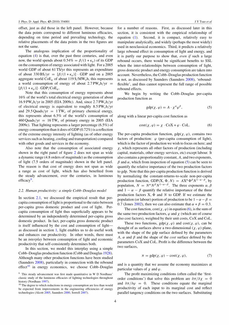
Solid-state lighting: an energy-economics perspective

This article has been downloaded from IOPscience. Please scroll down to see the full text article.

2010 J. Phys. D: Appl. Phys. 43 354001

(http://iopscience.iop.org/0022-3727/43/35/354001)

Download details:

IP Address: 192.86.100.34

The article was downloaded on 01/09/2010 at 13:20

Please note that terms and conditions apply.

View the table of contents for this issue, or go to the journal homepage for more

Home Search Collections Journals About Contact us My IOPscience

IOP PUBLISHING JOURNAL OF PHYSICS D: APPLIED PHYSICS

J. Phys. D: Appl. Phys. 43 (2010) 354001 (17pp) doi:10.1088/0022-3727/43/35/354001

Solid-state lighting: an energy-economicsperspectiveJ Y Tsao1, H D Saunders2, J R Creighton1, M E Coltrin1 andJ A Simmons1

1 Physical, Chemical and Nano Sciences Center, Sandia National Laboratories, PO Box 5800,Albuquerque, NM 87185-0601, USA2 Decision Processes Incorporated, 2308 Saddleback Drive, Danville, CA 94506, USA

E-mail: [email protected], [email protected], [email protected], [email protected] [email protected]

Received 12 March 2010, in final form 10 June 2010Published 19 August 2010Online at stacks.iop.org/JPhysD/43/354001

AbstractArtificial light has long been a significant factor contributing to the quality and productivity ofhuman life. As a consequence, we are willing to use huge amounts of energy to produce it.Solid-state lighting (SSL) is an emerging technology that promises performance features andefficiencies well beyond those of traditional artificial lighting, accompanied by potentiallymassive shifts in (a) the consumption of light, (b) the human productivity and energy useassociated with that consumption and (c) the semiconductor chip area inventory and turnoverrequired to support that consumption. In this paper, we provide estimates of the baselinemagnitudes of these shifts using simple extrapolations of past behaviour into the future. Forpast behaviour, we use recent studies of historical and contemporary consumption patternsanalysed within a simple energy-economics framework (a Cobb–Douglas production functionand profit maximization). For extrapolations into the future, we use recent reviews ofbelieved-achievable long-term performance targets for SSL. We also discuss ways in which theactual magnitudes could differ from the baseline magnitudes of these shifts. These include:changes in human societal demand for light; possible demand for features beyond lumens; andguidelines and regulations aimed at economizing on consumption of light and associatedenergy.

(Some figures in this article are in colour only in the electronic version)

1. Introduction

The importance of artificial light to humans and human societyhas long been recognized. Though fire may have been usedby our primate ancestors as far back as 2–6 million yearsago (Burton 2009), it is still thought of as the quintessentialhuman invention. Indeed, artificial light is so integrated intothe human lifestyle as to be barely noticeable. As is sometimessaid, artificial light ‘extends the day’ so that humans may benearly as productive at night as during the day (Bowers 1998)and ‘opens up the indoors’ so that humans may be as productiveindoors as outdoors, while enjoying the benefits of shelter fromthe vagaries of the environment (Schivelbusch 1988).

Indeed, the importance of (and demand for) artificiallight is such that technologies for its more-efficient production

evolved spectacularly during the 18th, 19th and 20th centuries.This evolution is illustrated in figure 1, which shows a 5-order-of-magnitude increase in the consumption of artificial lightover the past three centuries in the UK (Fouquet and Pearson2006).

At this point in human history, artificial lighting consumesan estimated 0.72% of world gross domestic product and,because of its high energy intensity relative to that of othergoods and services, an estimated 6.5% of world primaryenergy (Tsao and Waide 2010). These percentages are largeand, coupled with increasing concern over world energyconsumption, have inspired a number of projections of theconsumption of light and associated energy into the future(Kendall and Scholand 2001, Tsao 2002, Navigant 2003,2010, Schubert et al 2006). Such projections are of special

0022-3727/10/354001+17$30.00 1 © 2010 IOP Publishing Ltd Printed in the UK & the USA

J. Phys. D: Appl. Phys. 43 (2010) 354001 J Y Tsao et al

Figure 1. Three centuries of light consumption in the UK, adaptedfrom Fouquet and Pearson (2006). The left axis has the unitsTlm h/yr (teralumen-hours per year). The coloured lines representconsumption of light produced by technologies powered byparticular fuels; the black line represents total consumption of lightproduced by all technologies. (Colour online.)

interest at this point in history when lighting technologiesare evolving rapidly. Filament-based incandescent technologyis giving way to gas-plasma-based fluorescent and high-intensity-discharge (HID) technology; and over the coming10–20 years both may give way to solid-state lighting (SSL)technology (Schubert and Kim 2005, Shur and Zukauskas2005, Krames et al 2007, Tsao et al 2010).

All these projections, however, have shared a commonassumption—that consumption of light is relatively insensitiveto the cost of light, and that evolution of lighting technologyresulting in an increase in efficiency and a decrease in costleads to a decrease in the consumption of energy rather thanan increase in the consumption of light.

In this paper, we provide new projections of theconsumption of light and associated energy. Rather thanassuming that consumption of light is insensitive to the costof light, we assume a sensitivity consistent with simpleextrapolations of past behaviour into the future. In addition,we analyse the interplay between lighting, human productivityand energy consumption. After all, lighting is consumed notto waste energy, but to increase human productivity—energyconsumption is simply the cost of that increased productivity.That this has been so in the past is self-evident; that it will beso in the future is not unlikely.

The rest of this paper is organized as follows3.In section 2, we discuss recent studies of historical

and contemporary consumption patterns and analyse themwithin the energy-economics framework of a simple Cobb–Douglas production function and profit maximization. Inthis framework, lighting is considered a factor affecting bothproduction and energy consumption.

3 Because this paper lies at the intersection between physical and socialscience, different sections of the paper may be difficult for the twocommunities. For the physical-science community, we recommend (Sorrell2007) for an introduction to the economic concepts discussed in this paper.For the social-science community, we recommend (EERE 2010) and (Tsao2002) for an introduction to the physics and engineering concepts discussedin this paper.

In section 3, we discuss recent estimates of theperformance potential of SSL. Aside from its many otherunique and beneficial attributes, SSL has the potential toincrease the efficiency, and decrease the cost, of light factors2–5× beyond that of current lighting technologies, includingmodern compact fluorescent lighting.

In section 4, we build on sections 2 and 3 to estimatethe impact of SSL on human productivity (gdp) and the rateof energy consumption (e). We discuss how, within theCobb–Douglas framework, human productivity and energyconsumption are affected differently by improvements in theefficiency of lighting and by the cost of the energy that isconverted into light. We also discuss the semiconductor chiparea inventory and turnover associated with the lamps andluminaires that would be necessary in a world in which artificiallighting is dominated by SSL.

Finally, in section 5, we discuss alternative possiblefutures that deviate from the baseline future predicted froma simple extrapolation from the past. These include possiblesaturation in societal demand for lighting; possible demandfor features beyond lumens; and government policies andregulations aimed at economizing on consumption of light.

2. Lighting, human productivity and energy

In this section, we discuss recent studies of historical andcontemporary consumption patterns, and analyse them withinthe simple energy-economics framework of a Cobb–Douglas(Cobb and Douglas 1928) production function and profitmaximization.

2.1. Consumption of light and associated energy

We begin with a discussion of a recent comprehensive studyof historical and contemporary consumption of light (Tsaoand Waide 2010). In that study, it was found that empiricaldata, drawn from a wide range of sources (Min et al 1997,Navigant 2002, Mills 2005, Fouquet and Pearson 2006, IEA2006, Li 2007a, 2007b), were consistent with a per-capitaconsumption of light that is proportional to the ratio betweenper-capita gross domestic product and cost of light:

ϕ = β · gdp

CoL. (1)

In this equation: ϕ is per-capita consumption of light, inMlmh/(per-yr) (megalumen-hours per person-year); gdp is per-capita gross domestic product, in $/(per-yr) (dollars per person-year); CoL is the ownership cost of light in $/Mlmh (dollarsper megalumen-hour) and β = 0.0072 is a fixed constant4.

The consistency of this proportionality with empirical datais illustrated by the filled circles in the left panel5 of figure 2.Each filled circle corresponds to independent empirical data

4 Monetary units here and throughout this paper are year 2005 US$.5 Note that, for our later purpose of comparing past and future total worldconsumption of light, in the left panel of figure 2 we plot total rather than per-capita quantities against each other. In other words, we plot � = β ·GDP/CoL,which differs from equation (1) in that total quantities, denoted by upper-case symbols, are the per-capita quantities, denoted by lower-case symbols,multiplied by an appropriate population N .

2

J. Phys. D: Appl. Phys. 43 (2010) 354001 J Y Tsao et al

Figure 2. The left panel shows consumption of light (�) plotted against β · GDP/CoL, both in units of petalumen-hours per year. The rightpanel shows consumption of associated energy (Eϕ) plotted against [β/(1 + κϕ)] · [GDP/CoEϕ], both in units of petawatt-hours per year.The two relationships are the same as those of equations (1) and (4), except total rather than per-capita units are used (i.e. the left and rightsides of those equations have been multiplied by population, N , as discussed in footnotes 2 and 5). The filled circles are data points (Tsaoand Waide 2010) that illustrate the relationships represented by equations (1) and (4). The diagonal black lines have unity slope and zerooffset. The various nation abbreviations are US = United States; CN = China; UK = United Kingdom; FSU = Former Soviet Union;OECD-EU = Organization for Economic Cooperation and Development Europe = Austria, Belgium, Denmark, Finland, France, Germany,Italy, Netherlands, Norway, Sweden, Switzerland, UK, Ireland, Greece, Portugal, Spain, Hungary, Poland, Czech Republic, SlovakRepublic, Turkey, Iceland, Luxembourg; JP + KR = Japan + South Korea; AU + NZ = Australia + NewZealand; WRLD = World;WRLD-NONGRID = World not on grid electricity; WRLD-GRID = World on grid electricity. The diamonds represent the consumptionsof light and energy projected for the world in 2030, assuming the evolution and market penetration of SSL discussed in section 4, and abusiness-as-usual cost of energy.

for the three quantities in equation (1) for a nation or groupof nations at a particular historical time. The filled circles fallvery closely along a line of slope unity with zero offset.

The implication of the proportionality represented byequation (1) is that, over the past three centuries, and evennow, the world spends about 0.72% of its GDP on light. Thiswas the case in the UK in 1700 (UK 1700), is the case in theundeveloped world not on grid electricity (WRLD-NONGRID1999) in modern times, and is the case for the developed worldin modern times using the most advanced lighting technologies(WRLD-GRID 2005). For a 2005 world GDP of about61 T$/yr (Maddison 2007) this represents an expenditure ofabout 440 B$/yr = β · GDP and on a 2005 aggregate worldCoL of about 3.35 $/Mlmh this represents a world consumptionof light of about 131 Plm h/yr = β · GDP/CoL (Tsao andWaide 2010).

Note that, from equation (1) and a knowledge of theluminous efficacies (ηϕ , in units of lm W−1) associated witheach data point, we can also estimate the consumption ofenergy associated with the consumption of light6. The reasonis that luminous efficacy connects two pairs of quantities.

The first pair is per-capita consumption of light (ϕ) andper-capita rate of consumption of associated energy (eϕ) toproduce the light:

ϕ = eϕ · ηϕ. (2)

6 Note that we will often refer to these quantities simply as consumption oflight or energy, though precisely speaking they are rates of consumption oflight or energy.

Consumption of light is simply the product of the rate ofconsumption of energy and luminous efficacy.

The second pair is the cost of light (CoL, in units of$/Mlmh) and the cost of the associated energy (CoEϕ , in unitsof $/MWeh)7:

CoL = CoEϕ

ηϕ

· (1 + κϕ). (3)

Cost of light is basically the cost of the associated energydivided by luminous efficacy, within a correction factor, κϕ ≈1/3, which takes into account the approximately fixed ratio ofthe capital cost (lamp and luminaire) to operating cost (fuel)of light (Tsao and Waide 2010).

Thus, we can rewrite equation (1) as

eϕ = β

(1 + κϕ)· gdp

CoEϕ

, (4)

and can replot the data in the left panel of figure 2 using themodified axes in the right panel. Because equation (4) isessentially equivalent to equation (1), the data points in theright panel8 of figure 2 fall on a line of slope unity with zero

7 For energy units here and throughout this paper we use Wch, Btu or Quads(1015 or a quadrillion BTUs) for primary chemical energy, Weh for equivalentelectrical energy and a factor 0.316 We/Wc to convert between them.8 Note that, for our later purpose of comparing past and future total worldconsumption of energy, in the right panel of figure 2 we plot total ratherthan per-capita quantities against each other. In other words, we plotEϕ = [β/(1 + κϕ)] · GDP/CoEϕ , which differs from equation (4) in thattotal quantities, denoted by upper-case symbols, are the per-capita quantities,denoted by lower-case symbols, multiplied by an appropriate population N .

3

J. Phys. D: Appl. Phys. 43 (2010) 354001 J Y Tsao et al

offset, just as did those in the left panel. However, becausethe data points correspond to different luminous efficacies,depending on time period and prevailing technology, therelative placements of the data points in the two figures arenot the same.

The analogous implication of the proportionality ofequation (4) is that, over the past three centuries, and evennow, the world spends about 0.54% = β/(1 + κϕ) of its GDPon the consumption of energy associated with light. For a 2005world GDP of about 61 T$/yr this represents an expenditureof about 330 B$/yr = [β/(1 + κϕ)] · GDP and on a 2005aggregate world CoEϕ of about 119 $/MWeh, this representsa world consumption of energy of about 2.7 PWeh/yr =[β/(1 + κϕ)] · GDP/CoEϕ.

Note that this consumption of energy represents about16% of the world’s total electrical energy generation of about16.9 PWeh/yr in 2005 (EIA 2009c). And, since 2.7 PWeh/yrof electrical energy is equivalent to roughly 8.5 PWch/yrand 29.5 Quads/yr = 1 TWc of primary chemical energy,this represents about 6.5% of the world’s consumption of460 Quads/yr = 16 TWc of primary energy in 2005 (EIA2009c). That lighting represents a larger percentage (6.5%) ofenergy consumption than it does of GDP (0.72%) is a reflectionof the extreme energy intensity of lighting (as of other energyservices such as heating, cooling and transportation) comparedwith other goods and services in the economy.

Also note that the consumption of associated energyshown in the right panel of figure 2 does not span as widea dynamic range (4.8 orders of magnitude) as the consumptionof light (7.5 orders of magnitude) shown in the left panel.The reason is that cost of energy does not span as widea range as cost of light, which has also benefited fromthe steady advancement, over the centuries, in luminousefficacy9.

2.2. Human productivity: a simple Cobb–Douglas model

In section 2.1, we discussed the empirical result that per-capita consumption of light is proportional to the ratio betweenper-capita gross domestic product and cost of light. Per-capita consumption of light thus superficially appears to bedetermined by an independently determined per-capita grossdomestic product. In fact, per-capita gross domestic productis itself influenced by the cost and consumption of light—as discussed in section 1, light enables us to do useful workand enhances our productivity. In other words, there mustbe an interplay between consumption of light and economicproductivity that self-consistently determines both.

In this section, we model this interplay using a simpleCobb–Douglas production function (Cobb and Douglas 1928).Although many other production functions have been studied(Saunders 2008), particularly in connection with the reboundeffect10 in energy economics, we choose Cobb–Douglas

9 This steady advancement was first made quantitative in W D Nordhaus’classic study of the luminous efficacies of lighting technologies throughouthistory (Nordhaus 1997).10 The degree to which reductions in energy consumption are less than wouldbe expected from improvements in the engineering efficiencies of energytechnologies (Alcott 2005, Saunders 2000, Sorrell 2007).

for a number of reasons. First, as discussed later in thissection, it is consistent with the empirical relationship ofequation (1). Second, it is compact, relatively easy tomanipulate analytically, and widely (perhaps the most widely)used in neoclassical economics. Third, it predicts a relativelylarge rebound effect in consumption of light and energy, andit is partly our purpose to show that, even if such a largerebound occurs, there would be significant benefits to SSLwhen the inter-relationships between consumption of light,gross domestic product and energy consumption are taken intoaccount. Nevertheless, the Cobb–Douglas production functionis not, as discussed by Saunders (Saunders 2008), ‘rebound-flexible’, and thus cannot represent the full range of possiblerebound effects.

We begin by writing the Cobb–Douglas per-capitaproduction function as

gdp(χ, ϕ) = A · χαϕβ, (5)

along with a linear per-capita cost function as

cost(χ, ϕ) = χ · CoX + ϕ · CoL. (6)

The per-capita production function, gdp(χ, ϕ), contains twofactors of production: ϕ (per-capita consumption of light),which is the factor of production we wish to focus on here; andχ , which represents all other factors of production (includingcapital, materials, other energy services, etc) except labour. Italso contains a proportionality constant, A, and two exponents,β and α, which from inspection of equation (5) can be seen toquantify the relative importance of the two production factorsto gdp. Note that this per-capita production function is derivedby normalizing the constant-returns-to-scale non-per-capitaproduction function, GDP(X, �, N) = AXα�βN1−α−β , bypopulation, N = NαNβN1−α−β . The three exponents α, β

and 1 − α − β quantify the relative importance of the threeproduction factors X, � and N to GDP. If we estimate thepopulation (or labour) portion of production to be 1−α −β =0.7 (Jones 2002), then we can also estimate that α + β = 0.3.

The cost function, cost(χ, ϕ) in equation (6), is the sum ofthe same two production factors, ϕ and χ (which are of coursealso cost factors), weighted by their unit costs, CoX and CoL.

These two functions, gdp(χ, ϕ) and cost(χ, ϕ), can bethought of as surfaces above a two-dimensional (χ , ϕ) plane,with the shape of the gdp surface defined by the parametersA, α and β and the shape of the cost surface defined by theparameters CoX and CoL. Profit is the difference between thetwo surfaces,

π = gdp(χ, ϕ) − cost(χ, ϕ), (7)

and is a quantity that we assume the economy maximizes atparticular values of χ and ϕ.

The profit maximizing conditions (often called the ‘first-order conditions’) that solve this problem are ∂π/∂χ = 0and ∂π/∂ϕ = 0. These conditions equate the marginalproductivity of each input to its marginal cost and reflectparallel tangency conditions on the two surfaces. Substituting

4

J. Phys. D: Appl. Phys. 43 (2010) 354001 J Y Tsao et al

the per-capita production and cost functions of equations (5)and (6) then gives

∂gdp(χ, ϕ)

∂ϕ− CoL = β

ϕ· gdp(χ, ϕ) − CoL = 0, (8a)

∂gdp(χ, ϕ)

∂χ− CoX = α

χ· gdp(χ, ϕ) − CoX = 0. (8b)

Solving these yields

ϕ = βgdp

CoL, (9a)

χ = αgdp

CoX. (9b)

Re-substituting these two equations back into equation (5) thenleads to an expression for gdp at the profit maximization point:

gdp = A1/(1−α−β) ·( α

CoX

)α/(1−α−β)

·(

β

CoL

)β/(1−α−β)

.

(10)Finally, substituting equation (10) back into equations (9a) and(9b) enables the point (χ , ϕ) where profit is maximized to bedefined exactly:

χ = A1/(1−α−β)( α

CoX

)(1−β)/(1−α−β)

·(

β

CoL

)β/(1−α−β)

,

(11a)

ϕ = A1/(1−α−β) ·( α

CoX

)α/(1−α−β)

·(

β

CoL

)(1−α)/(1−α−β)

.

(11b)

Interestingly, the model equation (9a) is identical to theempirical equation (1). The Cobb–Douglas productionfunction, as mentioned earlier, is therefore consistent withempirical findings with respect to ϕ. Given a similar empiricalfinding (analogous to equation (1)) for χ , it could be shown thatthe two factors of production must then have unity elasticityof substitution between them11, and that only a Cobb–Douglasproduction would be consistent with our empirical findings(Saunders 2009). To our knowledge, however, such a similarempirical finding for χ does not exist. Nevertheless, it is notimplausible, for complex and nested multi-stage productionsystems (Lowe 2003), and over very long (decades to centuries)historical time periods, that elasticity of substitution tendstowards unity and that Cobb–Douglas is a reasonable baselinemodel for our current purpose.

Also, since the model equation (9a) is identical to theempirical equation (1), we can equate the two β’s, withβ = 0.0072. Using α +β = 0.3, we then have α = 0.2928. Inother words, lighting, though important, is nonetheless a smallfraction of a large world economy, with β � α.

With these relative magnitudes of α and β in mind, onecan now see from equation (9a) the effect on ϕ of a unitdecrease in CoL. The larger effect is a direct unit increase

11 Elasticity of substitution is a measure of the ease with which various factorsof production may be substituted for each other: formally (Varian 1984), theelasticity of the ratio of two inputs to a production function with respect to theratio of their marginal rates of substitution.

in ϕ for a unit decrease in CoL. The smaller effect is anindirect subunit increase in ϕ due, from equation (10), to asmall (0.01 = β/[1 − α − β]) subunit increase in gdp for aunit decrease in CoL. Put another way, consumption of lightincreases as cost of light decreases. But consumption of light,as a production factor, also mediates a small increase in gdp,and this causes consumption of light to increase very slightlymore. Thus, in total, ϕ increases by 1.01 units for a 1 unitdecrease in CoL.

2.3. Energy intensity: the cost of human productivity

As mentioned in section 1, just as the two factors of productionenable production, they also consume energy. If we write theirper-capita energy-consumption rates as

eχ = χ

ηχ

, (12)

eϕ = ϕ

ηϕ

, (13)

where ηχ and ηϕ are the efficacies with which energy is usedto produce χ and ϕ, then we can write for total per-capitaenergy-consumption rate:

e = eχ + eϕ = χ

ηχ

+ϕ

ηϕ

. (14)

The energy intensity12 is this total per-capita energy-consumption rate (equation (14)) divided by gdp (equa-tion (10). This gives, substituting equations (9a) and (9b) intoequation (14):

e

gdp= α

ηχ · CoX+

β

ηϕ · CoL. (15)

From this equation, it appears that energy intensity decreaseswith increases in the energy efficacies ηχ and ηϕ . For anenergy service such as lighting, whose dominant cost is thecost of energy, however, this is not the case. Because thecost of light (CoL) is dominated by the cost of energy (upto the correction factor 1 + κϕ), and therefore decreases asthe luminous efficacy ηϕ with which it is produced increases,energy intensity is actually independent of that luminousefficacy (Saunders 2008). This can be seen by substitutingequation (3) into equation (15) to get

e

gdp= α

ηχ · CoX+

β

CoEϕ · (1 + κϕ

) . (16)

Note that this independence of energy intensity on energyefficiency will not be the case for χ , the other factor ofproduction, as the cost of χ (CoX) will contain additionalsignificant costs that are independent of (do not decrease with)the energy efficacy with which χ is produced.

The independence of energy intensity on luminousefficacy might seem paradoxical, but can be understood bysubstituting equation (3) into equations (9a) and (10) to

12 As indicated in table 1, we use for energy intensity the units Btu/$, or BritishThermal Units per US dollar.

5

J. Phys. D: Appl. Phys. 43 (2010) 354001 J Y Tsao et al

2000 2005 2010 2015 2020

Year

Co

L($

/Mlm

h)

100

10

1

0.1

Incandescent

Fluorescent

“Perfect” SSL

2008

.3

2011

.8

SSL 2011

.8HID

Figure 3. Evolution of SSL cost of light (CoL). Solid tan-coloureddata points are from 2004–2009 state-of-the-art commercial devicesdescribed in (Tsao et al 2010), with CoL calculated assumingequivalent Ra = 85 and CCT = 3800 K. The white curved linethrough the data points is an exponential fit with a 1.95-year timeconstant and a saturation CoL corresponding to an RGB lightsource, also described in (Tsao et al 2010). The coloured horizontallines represent the 6.0, 1.3 and 1.3 $/Mlmh costs of light forincandescent, fluorescent and HID lamps in 2001. The colouredvertical dashed lines represent the years at which SSL lampsachieved, or might be projected to achieve, parity with traditionallamps. Note that, unlike in the rest of this paper, the CoL plottedhere includes only the operating cost of light and the capital cost ofthe lamp. Luminaire costs are not included, as these are evolvingrapidly and are difficult to quantify.

separate the dependence of per-capita light consumption andgdp on luminous efficacy and cost of energy:

ϕ = β

(1 + κϕ)· gdp · ηϕ

CoEϕ

, (17)

gdp = A1

1−α−β ·( α

CoX

)α/(1−α−β)

·(

β · ηϕ

CoEϕ · (1 + κϕ)

)β/(1−α−β)

.

(18)

From equation (17), as luminous efficacy increases, per-capitaconsumption of light increases. This increase exactly cancelsthe reduction in per-capita energy consumption that wouldotherwise have occurred, and hence does not alter energyintensity. From equation (18), as luminous efficacy increases,there is also a smaller increase in per-capita gdp. But thisincrease is exactly matched by a concomitant and proportionalsmall increase in per-capita energy consumption, and hencealso does not alter energy intensity.

3. SSL: performance and cost projections

In this section, we recapitulate recent estimates of theperformance potential of SSL (Tsao et al 2010). We choose ayear, 2030, distant enough for the performance of SSL to benearly saturated and the transition to SSL nearly complete. Wechoose a performance metric, cost of light (CoL), which is the

key parameter that enters into consumption of light, and whichthen couples to gdp, energy consumption and energy intensity.We discuss first the operating cost of light, then the capital costof light, then the cost of light, which is sum of the two.

3.1. Operating cost of light

The operating cost of light (CoLope, in units of $/Mlmh) issimply the cost of electricity divided by luminous efficacy:

CoLope = CoEϕ

ηϕ

. (19)

For the cost of electricity, we assume the estimated worldaggregate of 119 $/MWeh for 2005 (Tsao et al 2010, Tsaoand Waide 2010). One might anticipate that this cost will haveincreased by 2030. Here, however, we assume a business-as-usual scenario in which this increase is small, as has beenprojected for the US (EIA 2009b). In section 4, though,we relax this assumption, and allow the cost of electricity toincrease.

For luminous efficacy, we note that, as has been discussedrecently (Phillips et al 2007), there is a limiting luminousefficacy for the production of high quality white light whichrenders well the colours of typical environments. For acorrelated colour temperature (CCT) of 3800 K and a colourrendering index (CRI) of 85 (market-weighted averages forthe US in 2001), this limiting luminous efficacy is roughly400 lm/We (Tsao et al 2010). In practice, the present luminousefficacies of SSL technology are far less than this limitingvalue. However, they are improving rapidly, and mightultimately reach 65–70% of this limiting value or ηϕ ≈268 lm W−1. Indeed, one might anticipate many variantsof SSL with different combinations of luminous efficacy,colour rendering and colour temperature, tailored to particularapplications. Some might have efficiencies as high as 86%,the current best efficiency for any semiconductor light emitter(Peters et al 2007). Our assumption of 268 lm W−1 is thusconsidered to be in the mid-range of these variants.

Putting these two projections together, we assume thatthe operating cost of light, in 2030, will be on the order ofCoLope = (119 $/MWeh)/(268 lm W−1) = 0.44 $/Mlmh.13

3.2. Capital cost of light

The capital cost of light (CoLcap, in units of $/Mlmh) is thecost of the lamps and luminaires that produce the light. As wasmentioned earlier, for traditional lighting this cost is about 1/3of the operating cost of light, with roughly 1/6 due to the lampsand 1/6 due to the luminaires. For SSL technology, the capitalcost of light is currently significantly higher than the operatingcost. This is true both for the lamps that produce the light aswell as for the luminaires that house the lamps and direct thelight.

For SSL luminaires, costs are decreasing rapidly.Moreover, because SSL lamps are small, SSL luminaires

13 As a point of reference, this operating cost is equivalent to 0.44 ¢ (less thanhalf a penny) to produce 1000 lm (that produced by a typical 75 W incandescentbulb) for 10 h. The operating cost of an actual 75 W incandescent bulb run for10 h, in comparison, would be 9 ¢.

6

J. Phys. D: Appl. Phys. 43 (2010) 354001 J Y Tsao et al

can also be small and therefore have more headroom thantraditional-lamp luminaires for continued cost decrease. Inaddition, because SSL lamps and luminaires have comparablelifetimes, tighter integration of the two in design andmanufacturing may provide even more headroom for costdecrease. We thus make a reasonable assumption here thatSSL luminaire costs have the potential to decrease to 1/6 ofSSL operating costs.

For SSL lamps, costs are also decreasing rapidly. In fact,it has been shown that believed-achievable increases in thedensity of current injected into the semiconductor chips at theheart of SSL can by themselves enable lamp costs of 1/6 orless than the operating cost (Tsao et al 2010). Anticipatedmanufacturing and yield improvements that will accompanylarge-scale production will decrease lamp cost further. Indeed,as with semiconductor technologies in general, the capitalcost of SSL per unit performance has significant potential tocontinue its Haitz’s Law decrease (Haitz et al 1999, Martin2001, NP 2007). We conclude that SSL lamp costs also havethe potential to decrease to 1/6 of SSL operating costs.

Taken together, then, we assume here that the capital-cost-to-operating-cost ratio of SSL will be the same, in 2030, asthe 1/3 that characterizes current traditional lighting. In otherwords,

CoLcap = κϕ · CoLope, (20)

where κϕ = 1/3. Indeed, κϕ has the potential to be lower thanthis. However, if it were much lower than this, the lamp andluminaire would essentially be free, and manufacturers wouldhave incentive to add features so as to add back cost.

Note that, in assuming that the capital cost of SSL lampsand luminaires will be about 1/3 of their operating cost, we haveimplicitly assumed that subcosts associated with this capitalcost are even less than this. Among these subcosts is that forthe energy required to manufacture the lamp and luminaire orthe energy ‘embodied’ in the lamp and luminaire. Hence, wehave basically assumed that the energy embodied in the lampand luminaire is much lower than the energy consumed by thelamp during its life. In fact, it is much less (Tsao and Waide2010). Recent estimates are 1/66 for a 2009 state-of-the-artSSL lamp (Siemens AG 2009), and 1/36 for a 2009 state-of-the-art SSL integrated lamp and luminaire combination (Navigant2009b). Thus, the dominant costs to manufacture SSL lampsand luminaires are materials and labour rather than embodiedenergy.

3.3. Ownership cost of light

The ownership cost of light (CoL, in units of $/Mlmh) is thesum (Rea 2000, Dowling 2003, Azevedo et al 2009) of theoperating and capital costs of light we have just discussed:

CoL = CoEϕ

ηϕ

· (1 + κϕ). (21)

This equation (21) is identical to (and forms the basis for)equation (3). The two terms summed on the right sideof these equations are simply the operating and capitalcontributions to the cost of light, with the operating fraction

equal to 1/(1 + κϕ) ∼ 3/4 and the capital fraction equal toκϕ/(1 + κϕ) ∼ 1/4.

Note that, in principle, ownership cost of light shouldinclude the entire life cycle cost of light—not only theoperating and capital costs but also the environmental impactsof the materials, manufacturing and transport-to-point-of-use associated with the lamp and luminaire, the powerconsumed during operation of the lamp and the end-of-liferecycling or disposal of the lamp and luminaire. In fact,it has been shown that the environmental impact of SSL isdominated by that associated with the power consumed duringoperation of the lamp (Navigant 2009b, Siemens AG 2009).Hence, we assume the environmental impact of SSL can beaccounted for by a shift in (or tax on) the cost of energy(to account for that environmental impact). A business-as-usual scenario would be the absence, while an environmentallyproactive scenario would be the presence, of such a shift(or tax).

Note also that the absence or presence of shifts in thecost of energy affects all lighting technologies. Hence,the dominant factor affecting the relative competitiveness ofSSL relative to traditional lighting is not cost of energy, buttechnology improvement in manufacturing (basically κϕ inequation (21)) and performance (basically ηϕ in equation (21))of SSL.

Recently, the prospects for such technology improvement(for the lamp, but not the luminaire) have been analysed (Tsaoet al 2010), and the results are shown in figure 3. Fromthis evolution, one sees that the cost of light for SSL lampsbecame less than that of incandescent lamps in ∼2008 and,if it continues to decrease at its past-several-year rate, willreach parity with those of fluorescent and HID lamps in ∼2012.Assuming progress at a similar rate beyond this, but an eventualsaturation in luminous efficacy at 268 lm W−1 (correspondingto a 67%-efficient all-LED approach), one can project that SSLwill approach this saturation in ∼2020.

We note that these projections do not include SSLluminaires, whose evolution will very likely trail that of solid-state lamps somewhat. Hence, including luminaires will shiftall of these dates out somewhat, perhaps by several years.

4. SSL: baseline futures (β = 0.0072)

In section 2 we considered what is known empirically aboutconsumption of light in the past: that it scales as gdp/CoL witha proportionality constant β = 0.0072. We also developed asimple Cobb–Douglas model within which one can view theinterplay between consumption of light, human productivityand energy consumption.

In section 3 we reviewed recent projections of SSLluminous efficacies (ηϕ) into the future. Given variousscenarios for the cost of energy for lighting (CoEϕ), one canthen infer various scenarios for cost of light (CoL).

In this section, we describe ‘baseline future’ scenarios inwhich SSL is assumed to be the dominant lighting technology,and in which consumption of light in the future is characterizedby the same proportionality constant β = 0.0072 that has beencharacteristic of it in the past. Note that these baseline futures

7

J. Phys. D: Appl. Phys. 43 (2010) 354001 J Y Tsao et al

Table 1. Macroeconomic 2030 scenarios for various assumptions on the luminous efficacy of lighting and on the cost of energy for lighting.As discussed in the text, in scenarios FLU-L and FLU-H fluorescent lamps are dominant. In scenarios SSL-L, SSL-M and SSL-H solid-statelamps are dominant. In scenarios FLU-L and SSL-L cost of energy is low and similar to that in 2005 (business as usual). In scenariosSSL-M, SSL-H and FLU-H cost of energy is medium or high, and increased over business-as-usual projections. As a point of comparison,the unlabelled scenario in the first row represents actual luminous efficacies of lighting, costs of energy for lighting, and gdp and energyconsumptions for 2005.

Sce

nario

Yea

r

Pre

dom

inan

t ene

rgy

sour

ce o

rlig

htin

g te

chno

logy

Lum

inou

s ef

ficac

y (h

j)

Cos

t of e

lect

ricity

for

light

ing

(CoE

j)

Cos

t of p

rimar

y en

ergy

for

light

ing

(Co E

j)

Cos

t of l

ight

(C

oL)

per

capi

ta c

onsu

mpt

ion

of li

ght

(j=

b·gd

p/C

oL)

per

capi

ta c

onsu

mpt

ion

ofel

ectr

icity

ass

ocia

ted

with

ligh

t

(ej

= b

·gdp

/[(1

+k j

)·C

oE])

Con

sum

ptio

n of

ligh

t(F

=b·

GD

P/C

oL)

Con

sum

ptio

n of

ele

ctric

ityas

soci

ated

with

ligh

t

(Ej

= b

·GD

P/[(

1+k j

)·C

oEj]

)

Pop

ulat

ion

(N)

Gro

ss d

omes

tic p

rodu

ct (

GD

P)

per

capi

ta g

ross

dom

estic

pro

duct

(gdp

)

Ene

rgy

inte

nsity

(E

/GD

P)

Con

sum

ptio

n of

prim

ary

ener

gy (

E)

per

capi

ta c

onsu

mpt

ion

of p

rimar

yen

ergy

(e)

Sem

icon

duct

or c

hip

area

inve

ntor

y

Sem

icon

duct

or c

hip

area

ann

ual

prod

uctio

n (t

rans

ition

per

iod)

Sem

icon

duct

or c

hip

area

ann

ual

prod

uctio

n (s

tead

y st

ate)

lm

We

$

MWeh$

MBtu$

MlmhMlmhper-yr

MWeh

per-yr

Plmhyr

PWeh

yrGper

G$yr

$per-yr

Btu$

Quadyr

MBtuper-yr

km2 km2

yrkm2

yr

2005Ker+Inc+Flu+HID 48 119 11.0 3.35 20.0 0.42 131 2.7 6.5 60 670 9 317 8 071 490 75.2

FLU-L 2030 Flu 87 119 11.0 1.84 64.7 0.75 539 6.2 8.3 137 484 16 511 4 934 678 81.5SSL-L 2030 SSL 268 119 11.0 0.59 202.7 0.76 1688 6.3 8.3 139 091 16 704 4 934 686 82.4 1.31 0.174 0.076SSL-M 2030 SSL 268 133 12.3 0.66 181.2 0.68 1508 5.6 8.3 138 932 16 685 4 882 678 81.5 1.17 0.156 0.068SSL-H 2030 SSL 268 369 34.2 1.84 64.8 0.24 539 2.0 8.3 137 484 16 511 4 603 633 76.0 0.42 0.056 0.024FLU-H 2030 Flu 87 369 34.2 5.68 20.7 0.24 172 2.0 8.3 135 896 16 320 4 603 625 75.1

ScenarioLighting efficiency and

costWorld economy

Consumption of light andassociated energy

Chip area

within this discussion may have very different costs of energyfor lighting, and hence very different costs of light, but wenonetheless consider them baseline in that the historical patternof consumption of light does not change.

We begin by discussing various luminous-efficacy andcosts-of-energy-for-lighting scenarios, analysing these withinthe Cobb–Douglas framework. Then we discuss thesemiconductor chip area inventory and turnover that wouldbe necessary to sustain these baseline futures. Finally, wecompare these industry-scale figures with those of otherimportant semiconductor technologies.

Because we are interested in the long-term impact of SSL,we choose a year, 2030, distant enough into the future that itsultimate performance potential, at least in terms of raw cost,might be expected to have been achieved. Moreover, this is ayear in which the transition to SSL, anticipated to be massiveand worldwide in scope, might also be expected to be wellunderway.

4.1. Human productivity and energy consumption

Our starting point for understanding the impact of SSL onhuman productivity and energy consumption is equations (18)and (16). From initial values of per-capita gross domesticproduct (gdpo) and energy intensity (eo/gdpo) given initialvalues of luminous efficacy (ηϕo) and cost of energy for lighting(CoEϕo), these equations can be used to estimate modifiedvalues of per-capita gross domestic product (gdp) and energyintensity (e/gdp) given modified values of luminous efficacy

(ηϕ) and cost of energy for lighting (CoEϕ):

gdp

gdpo=

(CoLo

CoL

)β/(1−α−β)

=(

CoEϕo

CoEϕ

· ηϕ

ηϕo

)β/(1−α−β)

,

(22)e

gdp− eo

gdpo= β

CoEϕ · (1 + κϕ)− β

CoEϕo · (1 + κϕ). (23)

In this manner, we can essentially normalize the Cobb–Douglas model around initial projections for humanproductivity and energy consumption in the year 2030. Usingthese normalizations, various future scenarios are calculatedin table 1 and illustrated in figure 414.

Scenario FLU-L shows a hypothetical initial world in2030 based on Energy Information Agency projections (EIA2009a). In this world, per-capita world gross domestic productis gdp = 16 511 $/(per-yr), per-capita world primary energyconsumption is e = 81.5 MBtu/(per-yr), energy intensity is4934 Btu/$ and world population is N = 8.33 billion. Asthese are business-as-usual projections, we assume they donot take into account breakthrough technologies such as SSLand hence use ηϕ = 87 lm/We, that anticipated for improvedfluorescent lamps (Navigant 2009a), to be the initial worldaggregate luminous efficacy. As mentioned in section 3.1, wealso assume that the cost of electricity does not change much

14 We note that, in deriving these equations, we have implicitly assumed thatCoX is fixed. In practice, CoX cannot be fixed, as at minimum a shift incost of energy is likely to apply to all energy consumption and not just tothat for lighting. We have not modelled this, as economy-wide effects ofincreases in cost of energy are beyond the scope of this paper. However, thesame qualitative behaviour discussed in this section would result, even if thequantitative results would be different.

8

J. Phys. D: Appl. Phys. 43 (2010) 354001 J Y Tsao et al

Figure 4. Projected world 2030 per-capita primary energyconsumption and per-capita gross domestic product scenarios forvarious assumptions on luminous efficacy (ηϕ) and cost of energyfor lighting (CoEϕ). Both axes are gridded so that equal vertical orhorizontal grid spacings represent equal percentage changes. Thepoint labelled FLU-L can be considered the ‘reference’ values for(gdp, e) from which the other values are calculated from equations(22) and (23).

between now and the year 2030, an assumption similar to thatmade for the US (EIA 2009b). Hence, we assume the same,CoEϕ = 119 $/MWeh, as that estimated for 2005 (Tsao andWaide 2010).

Scenario SSL-L shows a hypothetical world similar to thatof scenario FLU-L except with a luminous efficacy increased,due to a complete transition to SSL, to ηϕ = 268 lm/We.As anticipated from equations (22) and (23), the roughly102% = 2 · (268 − 87)/(268 + 87) increase in ηϕ manifestsitself as roughly 102% · [β/(1 − α − β)] ∼ 1.02 · 0.01 ∼ 1%increases in both gdp and e, to gdp = 16 704 $/(per-yr) ande = 82.4 MBtu/(per-yr). But because, as discussed above, gdpand e both increase in the same proportion, energy intensity isconstant at e/gdp = 4934 Btu/$.

In other words, an increase in luminous efficacy, all otherthings held constant, has increased gdp with no penalty toenergy intensity, though at the expense of an increase inabsolute energy consumption.

Scenario SSL-M shows a hypothetical world similar tothat of scenario SSL-L except with a cost of energy for lightingincreased to CoEϕ = 133 $/MWeh. From equation (23), onesees that the result will be a decrease in energy intensity, so thate makes a greater than proportional decrease than gdp does. Itis then possible to return to exactly the same e (81.5 MBtu/(per-yr)) as that of scenario FLU-L, while maintaining a largeportion of the increase in gdp (now 16 685 $/(per-yr)). Indeed,this modest increase in CoEϕ was chosen precisely to enablea return to the per-capita energy consumption of scenarioFLU-L. The strikingly larger percentage decrease in e than ingdp is due to the energy service nature of lighting and the largerpercentage of e (6.5%) than of gdp (0.72%) that it consumes.

Scenario SSL-H shows a hypothetical world similar to thatof scenario SSL-M except with a cost of energy for lightingincreased further to CoEϕ = 369 $/MWeh. This increase incost of energy for lighting causes a further decrease in energyintensity, so that e continues its greater than proportionaldecrease relative to gdp. It is then possible for e to decreasebelow that of scenario FLU-L, to e = 76 Btu/(per-yr), whilegdp has exactly returned to that of scenario FLU-L, to gdp =16 511 $/(per-yr).

Scenarios SSL-L, SSL-M and SSL-H together illustratethe benefit of an increase in luminous efficacy. On the onehand, for a constant cost of energy for lighting, increasedluminous efficacy enables per-capita gdp to increase, albeitat the expense of an increased per-capita energy consumption.In other words, increased luminous efficacy does not decreaseper-capita energy consumption, but it does increase humanproductivity and standard of living.

On the other hand, for a non-constant (increased) cost ofenergy for lighting, increased luminous efficacy can offset thedecrease in per-capita gdp that would otherwise occur. In otherwords, increased luminous efficacy allows human productivityand standard of living to be maintained even if policy or marketforces cause increases in the cost of energy for lighting.

Indeed, scenario FLU-H shows a hypothetical world inwhich the cost of energy for lighting is as high as for scenarioSSL-H, but luminous efficacy has returned to that (ηϕ =87 lm/We) of starting scenario FLU-L. Scenario FLU-H is thusthe same as scenario FLU-L except with a cost of energy forlighting that has increased to CoEϕ = 369 $/MWeh. Withoutthe benefit of an increase in luminous efficacy, the effect ofthis increase in the cost of energy for lighting is to decreasegdp by 1% and e by 6% to gdp = 16 320 $/(per-yr) ande = 75.1 MBtu/(per-yr).

4.2. Semiconductor chip inventory and turnover

In this section, we discuss the semiconductor chip areainventory and turnover associated with SSL. We considermainly scenario SSL-L outlined in section 4.1. In this scenario,luminous efficacy increases have not been ‘compensated’ bycost of energy increases. We do not discuss the other scenariosSSL-M and SSL-H explicitly, but do list their projectedsemiconductor chip area inventories and turnovers in table 1.These chip area inventories and turnovers are lower, of course,because, in these scenarios, luminous efficacies have beencompensated to various degrees by increases in cost of energyfor lighting, so that consumption of lighting is lower.

We begin by calculating the semiconductor chip area, A,that would be required to ‘light the world’ with SSL. Fromequation (17), scaled by population, N , the global consumptionof light (in Plm h/yr) is

� = β

(1 + κϕ)· GDP · ηϕ

CoEϕ

. (24)

We also know that global consumption of light � (againin Plm h/yr) will depend on the total area A (in km2) ofsemiconductor chips used to produce light, the average densityp (in W cm−2) of input electrical power that the semiconductor

9

J. Phys. D: Appl. Phys. 43 (2010) 354001 J Y Tsao et al

is driven by, the duty cycle D (proportion of time a lamp isoperated) and the luminous efficacy ηϕ (in lm W−1):

� = A · p · D · ηϕ ·{

1010 cm2

km2 · 10−15 Plm

lm· 24 · 365.25

h

yr

}.

(25)

Equating the two expressions for � gives the followingexpression for A:

A = β · GDP/[CoEϕ · (1 + κϕ)]

p · D ·{

1010 cm2

km2 · 10−15 Plmlm · 24 · 365.25 h

yr

} . (26)

Note that equation (26) for A does not involve luminousefficacy. The reason is that increasing luminous efficacydecreases the cost of light and increases consumption of light,but also decreases the semiconductor area needed to produce aunit of light. This expression for A does involve cost of energy,however. The reason is that increasing cost of energy increasesthe cost of light and decreases consumption of light, but doesnot decrease the semiconductor area needed to produce a unitof light.

Equation (26) for A does involve a number of otherquantities as well. Two of these quantities, CoEϕ and GDP,are macroeconomic, and for these we assume the business-as-usual estimates discussed for scenarios FLU-L and SSL-Lin section 4.1: a 2030 CoEϕ of 119 $/MWh and a 2030 worldGDP of 137 484 G$/yr. Two of these quantities, duty cycle andaverage input power density, are microeconomic and depend onthe details of how solid-state lamps and their use co-evolve inthe future with residential, commercial, industrial and outdoorspaces and their use.

To estimate these latter two quantities, one can imaginetwo extremes of this co-evolution. At one extreme, controlof the spatial distribution of illumination remains relativelycoarse, as it is today. Then, fewer lamps would be necessary,but these few lamps would be on most of the time, and wouldbe driven nearly to their maximum. At the other extreme,control of the spatial distribution of illumination becomes finer(Moreno et al 2006, Yang et al 2009), enabled by the abilityof solid-state lamps to be fractionated into smaller units andto have their light output and spatial distribution manipulatedwithout efficiency loss. Then, more lamps would be necessary,but these lamps might be off most of the time, and even whenon would be driven less hard.

Here, we assume a co-evolution that is in between thesetwo extremes. Rather than the duty cycle of roughly 1/2characteristic of traditional lighting today (Navigant 2002), weassume a duty cycle of 1/4. Rather than assuming an averageinput power density of 3 kW cm−2, the maximum one mightimagine driving a solid-state lamp (Tsao 2004), we assumean average input power density of 220 W cm−2, near that of alate-2009 state-of-the-art warm-white LED lamp (Tsao et al2010).

The result is that the area of semiconductor requiredto ‘light the world’ would be A = 1.31 km2 (roughly 250American football fields). Note that this area scales inverselyas the cost of energy for lighting: if the cost of energy forlighting (and therefore the cost of lighting) were to roughly

triple, to 369 $/MWeh as in scenario SSL-H, then consumptionof light and the area required to sustain that consumption oflight would decrease to 1/3 of A = 1.3 km2 or A = 0.42 km2.Also note that this area scales inversely as power density: ifaverage input power density were to double, the area woulddecrease further from A = 0.42 km2 to A = 0.21 km2.

4.2.1. Chip area turnover: transition period. To build upthe steady-state semiconductor chip area inventory requiredto light the world, a yearly production dAtransition/dt (inkm2 yr−1) will be necessary. This yearly production, duringa transient period when traditional lighting is being displacedby SSL, depends on the area A (in km2) necessary to light theworld, the duration T (in yrs) of the transition period and themanufacturing yield Y :

dAtransition

dt= A

Y · T. (27)

Assuming the transition period is T = 10 years and themanufacturing yield is a relatively high Y = 3/4, onewould need a dAtransition/dt = 0.17 km2 yr−1. Note that themanufacturing yield could easily be much lower than Y = 3/4during the transition period.

This simple estimate assumes that traditional lighting isdisplaced by SSL of near-saturated performance. Having donethe displacement, subsequent turnover in SSL chip area wouldnot occur until SSL lamp end-of-life.

It is entirely possible, however, that traditional lightinginstead be displaced by less-mature generations of SSL witha lower performance, themselves to be displaced by more-mature generations with higher performance. Such higherperformance might include the simple economic cost of lumensas well as new features beyond simple lumen output (asdiscussed later in section 5.2). Here, we note that the economiccondition for obsolescence-induced turnover based simply oneconomic cost is that the total (operating plus capital) cost oflight of the next generation be less than the operating cost ofthe previous generation. We can estimate the rate at whichluminous efficacy would need to improve in order to satisfythis condition if we assume a cost structure (the ratio of capitalto operating cost) of light similar to that of traditional lighting(Tsao and Waide 2010). Then, κϕ ≈ 1/3, as discussed insection 2.1, and it can be shown that d(log ηϕ,)/dt > κϕ/T ,where T is the duration of one generation in SSL chip areaturnover. For example, for a duration of T = 3.3 years, theyearly percentage change in luminous efficacy would need tobe κϕ/T = (1/3)/(3.3 years) = 10%/year.

Because a 10%/year improvement in luminous efficacyis well within the realm of possibility, area turnovers withT ∼ 3.3 years are also within the realm of possibility, withproportional increases in dAtransition/dt in equation (27).

4.2.2. Chip area turnover: steady-state. After the steady-state semiconductor chip area inventory is in place (aftertraditional lighting has been fully displaced by SSL with near-saturated performance), a yearly production dAsteady-state/dt

(in km2 yr−1) will still be necessary to maintain that

10

J. Phys. D: Appl. Phys. 43 (2010) 354001 J Y Tsao et al

semiconductor chip area. This yearly production will dependon the area A (in km2), the manufacturing yield Y , theoperating lifetime, τ (in h) of the semiconductor lamps andthe duty cycle D:

dAsteady-state

dt= A · D · {

24 · 365.25 h yr−1}

Y · τ. (28)

Here, we assume an operating lifetime τ = 50 000 h, similarto that of current state-of-the-art LEDs; a manufacturing yieldY = 3/4 and the same duty cycle D = 1/4 assumed above.The result is a steady-state annual production of semiconductorarea of dAsteady-state/dt = 0.076 km2 yr−1.15

Note that this steady-state yearly production scalesinversely with lamp lifetime. One might easily imaginethe effective lifetime being smaller by more than a factorof two (to 20 000 h) for a number of reasons, including: alack of demand for lifetimes that significantly exceed typicaloccupancy periods of residents in buildings or continuingevolution of SSL performance or features that effectively makeSSL lamps obsolete before burn-out. Then, the yearly turnoverwould increase to dAsteady-state/dt = 0.19 km2 yr−1.

4.3. Semiconductor chip epitaxy

These semiconductor chip area turnovers are not insignificant,and it is of interest to assess the manufacturing infrastructurethat would be required to sustain them. Central to thisinfrastructure is epitaxial growth by metalorganic vapour phaseepitaxy (MOVPE), for which it is of interest to estimate both thenumbers of necessary MOVPE tools as well as the throughputof raw materials necessary for operation of the MOVPE tools.

With respect to the numbers of MOVPE tools, we assume,similar to the current state-of-the-art, that these tools arecapable of roughly twelve 4 inch wafers per growth run,three growth runs per day, and an up-time of 330 days/yr.Growth of 0.076 km2 yr−1, the estimated semiconductor chiparea turnover required after the transition to SSL has reachedsteady-state, would thus require the equivalent of roughly800 such MOVPE tools. Growth of 0.174 km2 yr−1, theestimated semiconductor chip area turnover required duringthe transition to SSL, would require the equivalent of roughly1800 such MOVPE tools. Interestingly, these projectednumbers are in the range of the numbers of GaN-based MOVPEtools currently in place for applications other than generalillumination (Hackenberg 2010). If such applications continueto require similar numbers of MOVPE tools in the future, it maybe necessary to double the number of such MOVPE tools inorder to satisfy anticipated needs for SSL chip epitaxy.

With respect to the throughput of raw materials necessaryfor operation of the MOVPE tools, we consider here only thegroup-III elements, Ga and In, as these are relatively rare andproduced primarily as minor byproducts of other base metalmining operations (USGS 2007a, 2007b).

15 This is roughly (and perhaps surprisingly) consistent with a separateestimate (http://compoundsemiconductor.net/csc/features-details.php?cat=features&id=20012) of 25 million 2 inch wafers per year or 25 × 106·π · [2 inch · (2.54 cm inch−1) · (10−5 km cm−1)/2]2 = 0.05 km2 yr−1.

To calculate the Ga consumption rate (dMGa/dt), we use

dMGa

dt∼= hGaN

εGa· ρGaN · (70/84) · dA

dt, (29)

where hGaN is the thickness of the relevant epitaxial layers,dA/dt is the chip area turnover per year, εGa is the utilizationefficiency of the Ga-containing metalorganic precursor, ρGaN

is the density of GaN and 70/84 is the Ga/GaN weight ratio.In other words, the Ga consumption rate is just the chiparea turnover multiplied by the Ga content of that chip area.Using an efficiency of ε = 0.10, an epitaxial thickness ofhGaN = 2 µm and a dA/dt = dAtransition/dt = 0.17 km2 yr−1,we deduce dMGa/dt = 20 000 kg yr−1 or 20 metric tons of Gaper year. This Ga consumption rate is large, but only about20% of current Ga refinery production16. It can be viewedas driving a moderate increase in demand for Ga over itscurrent dominant use in compound semiconductor electronicsand optoelectronics (USGS 2007a).

To calculate the In consumption rate (dMIndt), we use

dMIn

dt∼= hInN

εIn· ρInN · (115/129) · dA

dt, (30)

where the various quantities have the same meanings asin equation (29) but have substantially different values.In particular, the MOVPE utilization efficiency of theIn-containing metalorganic precursor is considerably lowerthan that of the Ga-containing metalorganic precursor: onthe order εIn = 0.005. Also, InN is typically present onlyin five or so thin (3 nm) quantum wells and even then onlyas a small (20%) percentage of the overall composition: theeffective epitaxial thickness of InN is thus on the order h =5 · (3 nm) · 0.2 = 10 nm. We deduce dMIn/dt = 600 kg yr−1

or 0.6 metric tons of In per year.This In consumption rate is 0.1% of current In refinery

production17, a much smaller percentage than the Gaconsumption rate was of current Ga refinery production.The reason is twofold. First, the In consumption rate ismuch lower than the Ga consumption rate, because currentSSL device structures use much less In than they do Ga.Second, current In refinery production is much larger thanGa refinery production, because In is required in several verylarge applications unrelated to SSL or even to semiconductorapplications. Specifically, 97% of all In is used for non-semiconductor applications (O’Neill 2004), and of this 75% isconsumed as indium tin oxide (ITO) for transparent conductingoxide applications (TCO) (O’Neill 2004, USGS 2007b). Weconclude that depletion of In reserves, if it were to become anissue (Cohen 2007), is not likely to be due to SSL, but to theother much larger applications for In.

4.4. Comparison with other electronic thin-film technologies

It is also of interest to assess the magnitude of thesemiconductor chip area turnover required for SSL relative

16 Worldwide Ga primary production was 111 metric tons in 2008 and 78metric tons in 2009 (USGS 2010a).17 Worldwide In refinery production was 570 metric tons in 2008 and 600metric tons in 2009 (USGS 2010b).

11

J. Phys. D: Appl. Phys. 43 (2010) 354001 J Y Tsao et al

to the current manufactured areas of other electronic thin-filmtechnologies.

The electronic thin-film technology with perhaps thelargest current manufactured area is that for liquid crystaldisplays. An estimate18 for 2009 of ∼200 km2 yr−1 is ∼3000×larger than that projected in section 4.2 for SSL.

The electronic thin-film technology with perhaps thelargest future potential19 is semiconductor photovoltaicsfor solar electricity generation. Currently, though, themanufactured area is modest. An estimate20 for the peakwatts shipped in 2009 is ∼9.6 GWp/yr. Assuming an averageefficiency of ∼15% (or ∼150 Wp/m−2) gives a manufacturedarea of (9.6 GWp/yr)/(150 Wp/m−2) ∼60 km2 yr−1. This issignificantly smaller than the manufactured area of liquidcrystal displays, though still ∼800× larger than that projectedin section 4.2 for SSL.

A third electronic thin-film technology with a fairly largemanufactured area is silicon electronics21: ∼4 km2 yr−1. Thisfigure is smaller than the potential discussed above for solarphotovoltaics. However, it is itself larger, by two orders ofmagnitude, than the steady-state chip area turnover requiredfor SSL.

Finally, the highest area-turnover compound semiconduc-tor substrate at present is GaAs (both electronics and optoelec-tronics), which in 2009 had an estimated semiconductor chiparea turnover of22 ∼0.03 km2 yr−1. This figure is much smallerthan the chip area turnover discussed above for silicon elec-tronics. However, it is on the order of the steady-state chiparea turnover required for SSL.

We conclude that SSL will likely be one of the largest ofthe compound semiconductor applications (assuming that inthe future, as now, the vast majority of solar cells continue to bemade entirely from Si), but will also likely be dwarfed by otherelectronic thin-film applications such as liquid crystal displays,solar cells and silicon electronics (in terms of electronic thin-film area turnover).

5. SSL: alternative futures (β �= 0.0072)

In section 4, we considered only ‘baseline future’ scenariosin which the historical pattern of consumption of light waspreserved in the future—scenarios, in other words, in which

18 Rosenblum S S, Corning, private communication.19 The most extreme scenario for semiconductor photovoltaics is one in whichit generates all the world’s energy. If we assume an average solar flux strikingthe earth of 174.7 W m−2 and a photovoltaic efficiency of 20%, then the arearequired to generate a projected world primary energy consumption in 2030 of20 TW would be 575 000 km2. Assuming an operational lifetime of 10 years,the semiconductor chip area turnover required for such massive solar electricitygeneration would be 115 000 km2 yr−1, a figure which dwarfs by more thansix orders of magnitude the steady-state chip area turnover required for solid-state lighting. The primary reason is power density: the 174.7 W m−2 powerdensity associated with the average solar flux is over four orders of magnitudelower than the 220 W cm−2 power density we have assumed for solid-statelighting. The secondary reason is that world primary energy consumption isroughly 1.5 orders of magnitude higher than primary energy consumption forsolid-state lighting would be.20 See, e.g., http://www.displaybank.com/eng/info/sread.php?id=573021 See, e.g., http://www.yole.fr/pagesAn/products/csmat.asp or http://www.fabtech.org/news/ a/gartner revises silicon wafer demand forecast/22 Anwar A, Strategy Analytics, private communication.

the proportionality constant β = 0.0072 is preserved in thefuture. We call these baseline scenarios because they representthe simplest extrapolations of the past into the future.

That such a simple extrapolation from the past will bepredictive of the future, however, cannot be known, and it mayvery well be that β �= 0.0072 in the future. Indeed there areat least three ways in which the historical variation might bemodified in the future.

First, we may be approaching a saturation in the demandfor light. Though this is difficult to imagine for the developingworld, whose per-capita consumption of light is much lowerthan for the developed world, perhaps at least the developedworld is approaching a saturation. Second, countering thefirst, new features associated with SSL may actually cause anincrease in the demand for light. Third, apart from how theintrinsic demand for light is increased or decreased throughSSL technology, guidelines and regulations aimed at efficientlighting system designs and light usage may nonetheless bringabout a saturation.

In this section we discuss these three possibilities in turn.

5.1. Saturation in demand for raw lumens

As has been discussed, at current levels of per-capitaconsumption of light, there is no evidence that we have reacheda saturation in the demand for light. It is nevertheless an openquestion whether we will approach such a saturation in thefuture or whether per-capita consumption of light will continueto scale linearly with gdp/CoL. To understand this questionmore quantitatively, we decompose per-capita consumptionof light into the product of three factors: IN , the averageilluminance23 (or light per unit area, in units of lm m−2) thata person is surrounded by during his or her waking hours;τon/(τon + τoff), a dimensionless illumination duty factor thataccounts for how many hours per year the area around aperson is actually illuminated and aN/(1 + aNρN), the averageunshared illuminated area (in units of m2) that a person issurrounded by24. In other words,

ϕ = IN ·(

τon

τon + τoff

)·(

aN

1 + aNρN

). (31)

It is possible that, in developed countries, each of thesefactors is nearing saturation. As we discuss in the rest of thissection, however, plausible arguments can be made that, evenin developed countries, the first and third factors may each yetbe a factor of 10 or more below saturation.

5.1.1. Illuminance: IN . The first term in equation (31) is IN ,the average illuminance (or light per unit area, in units of luxor lm m−2) that a person is surrounded by during his or herwaking hours.

23 We use the symbol I rather than the usual symbol for illuminance, E, as inthis paper E refers to energy. The subscript ‘N ’ refers to local illuminancefrom the perspective of an average person, as opposed to global illuminancefrom the perspective of an average area of land.24 Just as for the symbol I , for the symbols a and ρ the subscript ‘N ’ refers tolocal illuminated area and local population density from the perspective of anaverage person, as opposed to from the perspective of an average area of land.

12

J. Phys. D: Appl. Phys. 43 (2010) 354001 J Y Tsao et al

Illuminance levels have gradually increased over thecenturies and, for modern indoor office or living spaces, arenow on the order of IN ≈ 500 lm m−2. Such illuminances are,from a purely visual acuity point of view, clearly enough formost people for most tasks, and might be anticipated to be neara saturation level.

Moreover, we do not always wish to be surrounded byilluminances suitable for tasks requiring high visual acuity.Ambient illuminances for enhancing particular moods oremotional states of mind can be much lower than 500 lm m−2.And even when high visual acuity is desired, not all illuminancemust be supplied artificially—artful use of sunlight can be animportant supplement.

Nevertheless, arguments can be made that we havenot yet approached saturation levels for illuminance.Considerable uncertainty exists regarding what constitutesoptimal lighting—despite over a century of research,recommended levels for comparable spaces still vary by afactor of up to 20. It is now recognized that optimal lightingconditions are contingent on numerous factors other thanjust average horizontal illuminance levels and include visualcontrast and light distribution parameters.

And, even if one considers only horizontal illuminance,the evidence regarding the levels that people would choosewere affordability not a factor is far from complete. Peoplemight well choose higher illuminances than they do today,particularly to help mitigate losses in visual acuity in anageing world population, but perhaps also to function asneuropsychological modifiers helping, e.g., to synchronizecircadian rhythms (Arendt 2006, Figueiro et al 2009), to reduceseasonal affective disorder or to enhance mood.

Indeed, the generally comfortable outdoor illuminancecharacteristic of an overcast or cloudy day is of the order5000 lm m−2–10× higher than the 500 lm m−2 mentionedabove as typical of modern indoor office or living spaces.And the outdoor illuminance characteristic of a bright sunnyday is of the order 30 000 lm m−2, 60× higher than today’s500 lm m−2. Though this latter illuminance is uncomfortableviewed from a close distance (requiring the use of sunglasses),it may well be desirable viewed from a farther distance (e.g.viewing scenery).

We conclude that it is possible that the developed countriesare nearing a saturation point in average illuminance, butplausible arguments can be made that the saturation point mayyet be a factor of 10 or more higher25.

5.1.2. Illumination duty factor: τon/(τon + τoff). The secondterm in equation (31) is τon/(τon + τoff), a dimensionless

25 We note in passing that, whatever its saturation value, average illuminancemight be expected to vary with geography. In countries further from theequator, illuminance from the sun is lower and illuminance from artificialsources might be expected to increase to compensate. The limited data whichis available appears not to support this, however. For example, Japan consumessignificantly more light per-capita than Northern Europe despite being nearerthe equator and despite a similar standard of living. A proximate explanationfor this is the greater penetration of higher luminous efficacy fluorescencelighting technology, hence lower cost of light, in Japan than in NorthernEurope. But an ultimate explanation for the greater penetration of fluorescencetechnology itself may be a desire for higher artificial illuminance levels so asnot to provide too stark a contrast with outdoor illuminance levels.

illumination duty factor that accounts for how many hoursper year the area around a person is actually illuminated.The duty factor for a person who spends most of his orher time indoors, either at work or at home, is roughly thenumber of waking hours per day or about τon/(τon + τoff) ≈(16 h/day)/(24 h/day) = 2/3.

This is the term that is most clearly nearing saturation.Most people need on the order of 8 h of sleep each day. Andmost people need darkness to sleep, and even apart from sleep,to reset their human circadian rhythms (IEA 2006).

5.1.3. Unshared illuminated area: aN/(1 + aNρN). Thethird term in equation (31) is aN/(1 + aNρN), the averageunshared illuminated area (in units of m2) that a person issurrounded by. This area aN is the average illuminated area(in units of m2) that a person is surrounded by (regardless ofhow many other persons share that area), divided by 1 +aNρN ,the number of persons that share that area. Here, ρN (in unitsof per/m2) is the density of people within the illuminated areathat a person is surrounded by. When ρN � 1/aN , light is notshared, andaN/(1 + aNρN) approachesaN ; whenρN � 1/aN ,light is shared amongst many people, and aN/(1 + aNρN)

approaches 1/ρN .The order of magnitude of aN can be estimated as follows.

Per-capita consumption of light in the US, representative ofthe high end in the world, was about ϕ ≈ 136 Mlm h/(per-yr) in 2001 (Tsao and Waide 2010). As discussed above, theaverage illuminance in modern indoor office or living spaces isroughly IN ≈ 500 lm m−2, and let us assume the illuminationduty factor of τon/(τon + τoff) ≈ 2/3 estimated above. Inthe absence of light sharing (ρN � aN), the illuminated areathat the average person in the US is surrounded by is thus,using equation (31), roughly aN ≈ ϕ · (τon + τoff)/(IN · τon) ≈41 m2. This area is plausible: larger than a typical one-personoffice area, but smaller than a typical one-person residentialarea.

Regarding how the unshared illuminated area aN/

(1 + aNρN) might evolve in the future, plausible arguments canbe made in both directions: that it is either saturated and mighteven decrease or that it has considerable room for growth.

On the one hand, humans, often characterized as denanimals, find comfort in enclosed areas, and to be surroundedby a (41 m2/π)1/2 = 3.6 m ≈ 11.8 ft radius of illuminatedarea is surely sufficient for most people most of the time.Indeed, an increasing trend in modern buildings is the use ofmotion sensors to turn lights on and off when a person entersor exits a space, with typical coverage areas comparable to41 m2. With new technologies such as SSL, such opportunitiesfor sensor-based intelligent control will only increase in thefuture, potentially decreasing aN .

Moreover, humans are not only den animals, they aresocial animals and tend to cluster in groups. Indeed, localpopulation density26 can, in a typical office building or urbanpublic space, easily be on the order of ρN ≈ 0.1 m−2. Hence,

26 By local population density, we mean as seen from the perspective of aperson, which includes the tendency towards clustering. As seen from theperspective of the land, median world population density is much lower, onthe order of 4 × 10−6 m−2 (Cohen and Small 1998).

13

J. Phys. D: Appl. Phys. 43 (2010) 354001 J Y Tsao et al

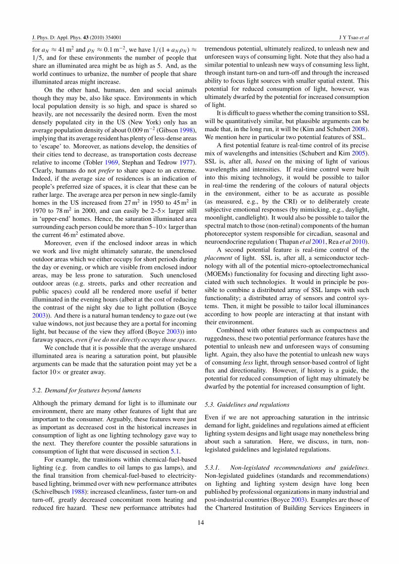
for aN ≈ 41 m2 and ρN ≈ 0.1 m−2, we have 1/(1 + aNρN) ≈1/5, and for these environments the number of people thatshare an illuminated area might be as high as 5. And, as theworld continues to urbanize, the number of people that shareilluminated areas might increase.

On the other hand, humans, den and social animalsthough they may be, also like space. Environments in whichlocal population density is so high, and space is shared soheavily, are not necessarily the desired norm. Even the mostdensely populated city in the US (New York) only has anaverage population density of about 0.009 m−2 (Gibson 1998),implying that its average resident has plenty of less-dense areasto ‘escape’ to. Moreover, as nations develop, the densities oftheir cities tend to decrease, as transportation costs decreaserelative to income (Tobler 1969, Stephan and Tedrow 1977).Clearly, humans do not prefer to share space to an extreme.Indeed, if the average size of residences is an indication ofpeople’s preferred size of spaces, it is clear that these can berather large. The average area per person in new single-familyhomes in the US increased from 27 m2 in 1950 to 45 m2 in1970 to 78 m2 in 2000, and can easily be 2–5× larger stillin ‘upper-end’ homes. Hence, the saturation illuminated areasurrounding each person could be more than 5–10× larger thanthe current 46 m2 estimated above.

Moreover, even if the enclosed indoor areas in whichwe work and live might ultimately saturate, the unenclosedoutdoor areas which we either occupy for short periods duringthe day or evening, or which are visible from enclosed indoorareas, may be less prone to saturation. Such unenclosedoutdoor areas (e.g. streets, parks and other recreation andpublic spaces) could all be rendered more useful if betterilluminated in the evening hours (albeit at the cost of reducingthe contrast of the night sky due to light pollution (Boyce2003)). And there is a natural human tendency to gaze out (wevalue windows, not just because they are a portal for incominglight, but because of the view they afford (Boyce 2003)) intofaraway spaces, even if we do not directly occupy those spaces.

We conclude that it is possible that the average unsharedilluminated area is nearing a saturation point, but plausiblearguments can be made that the saturation point may yet be afactor 10× or greater away.

5.2. Demand for features beyond lumens

Although the primary demand for light is to illuminate ourenvironment, there are many other features of light that areimportant to the consumer. Arguably, these features were justas important as decreased cost in the historical increases inconsumption of light as one lighting technology gave way tothe next. They therefore counter the possible saturations inconsumption of light that were discussed in section 5.1.

For example, the transitions within chemical-fuel-basedlighting (e.g. from candles to oil lamps to gas lamps), andthe final transition from chemical-fuel-based to electricity-based lighting, brimmed over with new performance attributes(Schivelbusch 1988): increased cleanliness, faster turn-on andturn-off, greatly decreased concomitant room heating andreduced fire hazard. These new performance attributes had

tremendous potential, ultimately realized, to unleash new andunforeseen ways of consuming light. Note that they also had asimilar potential to unleash new ways of consuming less light,through instant turn-on and turn-off and through the increasedability to focus light sources with smaller spatial extent. Thispotential for reduced consumption of light, however, wasultimately dwarfed by the potential for increased consumptionof light.

It is difficult to guess whether the coming transition to SSLwill be quantitatively similar, but plausible arguments can bemade that, in the long run, it will be (Kim and Schubert 2008).We mention here in particular two potential features of SSL.

A first potential feature is real-time control of its precisemix of wavelengths and intensities (Schubert and Kim 2005).SSL is, after all, based on the mixing of light of variouswavelengths and intensities. If real-time control were builtinto this mixing technology, it would be possible to tailorin real-time the rendering of the colours of natural objectsin the environment, either to be as accurate as possible(as measured, e.g., by the CRI) or to deliberately createsubjective emotional responses (by mimicking, e.g., daylight,moonlight, candlelight). It would also be possible to tailor thespectral match to those (non-retinal) components of the humanphotoreceptor system responsible for circadian, seasonal andneuroendocrine regulation ( Thapan et al 2001, Rea et al 2010).

A second potential feature is real-time control of theplacement of light. SSL is, after all, a semiconductor tech-nology with all of the potential micro-optoelectromechanical(MOEMs) functionality for focusing and directing light asso-ciated with such technologies. It would in principle be pos-sible to combine a distributed array of SSL lamps with suchfunctionality; a distributed array of sensors and control sys-tems. Then, it might be possible to tailor local illuminancesaccording to how people are interacting at that instant withtheir environment.

Combined with other features such as compactness andruggedness, these two potential performance features have thepotential to unleash new and unforeseen ways of consuminglight. Again, they also have the potential to unleash new waysof consuming less light, through sensor-based control of lightflux and directionality. However, if history is a guide, thepotential for reduced consumption of light may ultimately bedwarfed by the potential for increased consumption of light.

5.3. Guidelines and regulations

Even if we are not approaching saturation in the intrinsicdemand for light, guidelines and regulations aimed at efficientlighting system designs and light usage may nonetheless bringabout such a saturation. Here, we discuss, in turn, non-legislated guidelines and legislated regulations.

5.3.1. Non-legislated recommendations and guidelines.Non-legislated guidelines (standards and recommendations)on lighting and lighting system design have long beenpublished by professional organizations in many industrial andpost-industrial countries (Boyce 2003). Examples are those ofthe Chartered Institution of Building Services Engineers in

14

J. Phys. D: Appl. Phys. 43 (2010) 354001 J Y Tsao et al

the UK (CIBSE 2002) and of the Illumination EngineeringSociety of North America (Rea 2000). Such guidelinescover recommended illuminance levels for spaces with variousfunctional purposes and, though without formal legal status,could be a mechanism by which light usage might be curtailedor even reduced.

Note, though, that the intent of these guidelines is not somuch to reduce light usage but to enhance the ways in whichhumans experience and use light. Such guidelines would notnecessarily limit the expansion of light usage into spaces thatare currently only poorly lit (e.g. the outdoor spaces discussedat the end of section 5.1), but rather might guide such usageafter such an expansion has begun.

Moreover, even in spaces, such as indoor offices, whichare currently well lit, the effectiveness of guidelines islimited by a lack of consensus on how much light is neededto satisfy human needs. In many OECD (Organizationfor Economic Cooperation and Development) countriesrecommended interior lighting levels peaked in the late 1970sand then declined as performance on visual reading and writingtasks, previously the main consideration, was extended toinclude more holistic criteria. It is now recognized that optimallighting conditions are contingent on numerous factors otherthan just average horizontal illuminance levels and includevisual contrast and light distribution parameters. Glare, e.g.,caused by a sharp imbalance in the brightness of adjacentareas in the field of view, is an important consideration. Asmentioned above, the result is that, despite over a century ofresearch into the topic, recommended levels for comparablespaces in different countries still vary by a factor of 10× ormore: typical office spaces in most countries are illuminatedto 500 lux but national recommendations can be as high as2000 lux and as low as 250 lux (IEA 2006).

We conclude that non-legislated recommendations andguidelines may have a limited ability to cause a saturation inthe consumption of light, if such a saturation would not alreadyhave naturally occurred.

5.3.2. Legislated regulations. Legislated regulations havemore recently (over the last decade) been introduced in manycountries.

A first type of regulation limits maximum permissibleenergy consumption, either within a building on a per-unit-floor-area basis or for whole buildings. The limits can eitherbe on energy consumption as a whole (of which lightingis a key piece) or on energy consumption for lighting asa separate piece. These limits are derived by assuming ablend of reasonably efficient lighting technologies inserted intolighting designs sufficient to provide recommended lightingrequirements.

If luminous efficacies are constant, such regulationseffectively constrain the degree to which interior light levelscan be increased (IEA 2006). They also provide incentives tooptimize light usage, and in particular to limit illumination ofunoccupied or daylit spaces. If, however, luminous efficaciesare not constant, but increase with new lighting technologies,light usage within a building can increase even while satisfyingan older generation of energy-consumption regulations. It

would then be necessary for such regulations to be continuallyupdated to keep pace with new lighting technologies. Inaddition, new lighting technologies can enable new uses notassociated with buildings and hence not covered by suchregulations.

A second type of regulation governs the luminousefficacies of lamps that may be sold. These regulationseffectively force consumers to upgrade their lamp stock totechnologies with ever increasing efficiencies. Incandescentbulbs, e.g., have now been effectively banned in manyjurisdictions (Simmons et al 2007). However, theseregulations do nothing to limit the use of a given stock oflamps, and hence to limit overall consumption of light.

We conclude that legislated regulations may also have alimited ability to cause a saturation in the consumption of light,if such a saturation would not already have naturally occurred.

6. Summary

In this paper we have provided baseline projections of theconsumption of light in a world in which SSL is the dominantartificial lighting technology. Our projections are based onsimple extrapolations of past behaviour into the future, andhence represent the historically consistent baseline assumptionfor constructing future scenarios for consumption of light andassociated energy.

For past behaviour, we have used recent studies ofhistorical and contemporary consumption patterns, analysedwithin a simple energy-economics framework of a Cobb–Douglas production function and profit maximization. Forextrapolations into the future, we have used recent reviews ofbelieved-achievable long-term performance targets for SSL.

A principal conclusion is that there is a massive potentialfor growth in the consumption of light if new lightingtechnologies are developed with higher luminous efficaciesand lower cost of light. A secondary conclusion is that thisincreased consumption of light has the potential to increaseboth human productivity and the consumption of energyassociated with that productivity. These conclusions suggesta subtle but important shift in how one views the baselineconsequence of the increased energy efficiency associated withSSL. The consequence is not a simple ‘engineering’ decreasein energy consumption with consumption of light fixed, butrather an increase in human productivity and quality of lifedue to an increase in consumption of light.

Moreover, if one views the efficiency of lighting andthe cost of energy associated with lighting as being twoindependent variables, one can see that these have differentand complementary effects on human productivity and energyconsumption. Changes in the efficiency of lighting affectboth the cost of light and the amount of light that can beconsumed per unit energy; while changes in the cost of energyassociated with lighting affect only the cost of light. Thus,an increase in the cost of energy associated with lighting,which would normally reduce both human productivity andenergy consumption, can be mitigated by an increase inthe efficiency of lighting: energy consumption can be heldconstant while maintaining some human productivity increase

15

J. Phys. D: Appl. Phys. 43 (2010) 354001 J Y Tsao et al

or energy consumption can be reduced without a decrease inhuman productivity.

Whether history can be used in this case to predict thefuture cannot be known, of course, and there are at least twoways in which this growth might be moderated. First, asdiscussed in section 5.1, demand for light may be nearingsaturation, both in terms of illuminances (lm m−2) as well as interms of the per-capita illuminated areas surrounding people.Second, as discussed in section 5.3, even if intrinsic demandfor light is not nearing saturation, non-legislated guidelines andlegislated regulations aimed at efficient lighting system designsand light usage may nonetheless bring about a saturation.

However, reasonable arguments can also be made that as ahuman society we are not near a saturation in consumption oflight. As discussed in section 5.1, the average illuminancethat a person is surrounded by during his or her wakinghours and the average unshared illuminated area that aperson is surrounded by may each yet be 10× or more fromsaturation. As discussed in section 5.2, new performanceattributes associated with SSL have the potential to unleashnew and unforeseen ways of consuming light. As discussed insection 5.3, guidelines and regulations may also have limitedinfluence on light consumption.

Acknowledgments

The authors acknowledge helpful input and comments fromEric Shaner, Paul Waide and a very thorough anonymousreferee; and permission from Roger Fouquet and Peter Pearsonfor our adaptation of figure 1 from their monumental workon the consumption of light in the UK. Work at SandiaNational Laboratories was supported by Sandia’s Solid-State-Lighting Science Energy Frontier Research Center, fundedby the US Department of Energy, Office of Basic EnergySciences. Sandia is a multi-program laboratory operatedby Sandia Corporation, a Lockheed Martin Company, forthe US Department of Energy’s National Nuclear SecurityAdministration under Contract No DE-AC04-94AL85000.

References

Alcott B 2005 Jevons’ paradox Ecol. Econ. 54 9–21Arendt J 2006 Melatonin and human rhythms Chronobiol. Int.

23 21–37Azevedo I L, Morgan M G and Morgan F 2009 The transition to

solid-state lighting Proc. IEEE 97 481–510Bowers B 1998 Lengthening the Day: a History of Lighting

Technology (Oxford: Oxford University Press)Boyce P B 2003 Human Factors in Lighting 2nd edn (London:

Taylor and Francis)Burton F D 2009 Fire: The Spark that Ignited Human Evolution

(University of New Mexico Press)CIBSE 2002 Code for Lighting (Butterworth–Heinemann)

(Chartered Institution of Building Services Engineers)Cobb C W and Douglas P H 1928 A theory of production Am. Econ.

Rev. 18 139–65Cohen D 2007 Earth’s natural wealth: an audit New Sci.Cohen J E and Small C 1998 Hypsographic demography: the

distribution of human population by altitude Proc. NationalAcademy of Science 95 14009–14

Dowling K 2003 The Cost of Light, Color Kinetics Whitepaperhttp://www.colorkinetics.com/whitepapers/CostofLight.pdf

EERE 2010 Solid-State Lighting Multi-Year Program PlanFY’10-FY’16 US Department of Energy, Office of EnergyEfficiency and Renewable Energy, Building TechnologiesProgram

EIA 2009a Annual Energy Outlook 2010 Early Release Overview(http://www.eia.doe.gov/oiaf/aeo/) Energy InformationAdministration

EIA 2009b Annual Energy Outlook 2010 Early Release withProjections to 2035 (http://www.eia.doe.gov/oiaf/aeo/) EnergyInformation Administration

Figueiro M G, Bierman A, Plitnick B and Rea M S 2009Preliminary evidence that both blue and red light can inducealertness at night BMC Neurosc. 10 105–15

Fouquet R and Pearson P J G 2006 Seven centuries of energyservices: the price and use of light in the United Kingdom(1300–2000) Energy J. 27 139–77

Gibson C 1998 Population of the 100 Largest cities and other urbanplaces in the United States: 1790 to 1990 US Bureau of theCensus Population Division Working Paper No 27

Hackenberg S 2010 IMS Research Launches New Quarterly Reporton LED Supply, Demand, Market Size and MOCVD Market(http://www.solidstatelighting.net/documents/view/sectornews.php?id=118760&sector=leddev#top) LIGHTimes Online

Haitz R, Kish F, Tsao J and Nelson J 1999 The Case for a NationalResearch Program on Semiconductor Lighting:(Optoelectronics Industry Development Association)

IEA 2006 Light’s Labour’s Lost: Policies for Energy-efficientLighting (International Energy Agency)

Jones C I 2002 Introduction to Economic Growth 2nd edn(New York: W.W. Norton & Company)

Kendall M and Scholand M 2001 Energy Savings Potential of SolidState Lighting in General Lighting Applications [0.5], USDepartment of Energy, Office of Building Technology, Stateand Community Programs

Kim J K and Schubert E F 2008 Transcending the replacementparadigm of solid-state lighting Opt. Express 16 21835–42

Krames M R et al 2007 Status and future of high-powerlight-emitting diodes for solid-state lighting J. Disp. Technol.3 160–75

Li J M 2007a Estimate of consumption of light and associatedenergy in China 2006 unpublished

Li J M 2007b Estimates of the cost of electricity in China1993–2006 unpublished

Lowe R 2003 A theoretical analysis of price elasticity of energydemand in multi-stage energy conversion systems EnergyPolicy 31 1699–704

Maddison A 2007 World Population, GDP and Per Capita GDP,1-2003 AD

Martin P 2001 The future looks bright for solid-state lighting LaserFocus World 37 81–4

Mills E 2005 Environment—the specter of fuel-based lightingScience 308 1263–4

Min G F, Mills E and Zhang Q 1997 Energy efficient lighting inChina—problems and prospects Energy Policy 25 77–83

Moreno I, Avendano-Alejo M and Tzonchev R I 2006 Designinglight-emitting diode arrays for uniform near-field irradianceAppl. Opt. 45 2265–72

Navigant 2002 US Lighting Market Characterization Volume I:National Lighting Inventory and Energy Consumption EstimateUS Department of Energy, Office of Energy Efficiency andRenewable Energy, Building Technologies Program

Navigant 2003 Energy Savings Potential of Solid State Lighting inGeneral Illumination Applications Washington DC: BuildingTechnologies Program, Office of Energy Efficiency andRenewable Energy, US Department of Energy

Navigant 2009a Energy Savings Potential of Solid State Lighting inGeneral Lighting Applications 2010 to 2030 US Department of

16

J. Phys. D: Appl. Phys. 43 (2010) 354001 J Y Tsao et al

Energy, Office of Energy Efficiency and Renewable Energy,Building Technology Programs

Navigant 2009b Life Cycle Assessment of Ultra-Efficient LampsDepartment for Environment, Food and Rural Affairs (UK)

Navigant 2010 Energy Savings Potential of Solid State Lighting inGeneral Lighting Applications 2010 to 2030 US Department ofEnergy, Office of Energy Efficiency and Renewable Energy,Building Technology Programs

Nordhaus W D 1997 Do Real-Output and Real-Wage MeasuresCapture Reality? The History of Lighting Suggests Noted T F Breshnahan and R J Gordon (The Economics of NewGoods) pp 29–70 (Chicago, IL: University of Chicago Press)

NP 2007 Haitz’s law Nature Photon. 1 23–23O’Neill B 2004 Indium: Supply, Demand & Flat Panel Displays

Paper presented at the Minor Metals 2004. Retrieved fromhttp://www.nrel.gov/pv/thin film/docs/indium supply anddemand%5B1%5D.doc

Peters M, Rossin V, Everett M and Zucker E 2007 High power, highefficiency laser diodes at JDSU Proc. SPIE 6456 64560G

Phillips J M et al 2007 Research challenges to ultra-efficientinorganic solid-state lighting Laser Photon. Rev.1 307–33

Rea M S 2000 The IESNA Lighting Handbook (New York:Illumination Engineering Society of North America)

Rea M S, Figueiro M G, Bierman A and Bullough J D 2010Circadian light J. Circadian Rhythms 8

Saunders H 2000 A view from the macro side: rebound, backfire,and khazzoom-brookes Energy Policy 28 439–49

Saunders H D 2008 Fuel conserving (and using) productionfunctions Energy Econ. 30 2184–235

Saunders H D 2008 Specifying Technology for Analyzing ReboundEnergy Efficiency and Sustainable Consumption: the ReboundEffect ed H Herring and S Sorrell (London: PalgraveMacmillan)

Saunders H D 2009 unpublishedSchivelbusch W 1988 Disenchanted Night: The Industrialization of

Light in the Nineteenth Century (Berkeley, CA: University ofCalifornia Press)

Schubert E, Kim J, Luo H and Xi J 2006 Solid-state lighting-abenevolent technology Rep. Prog. Phys. 69 3069–99

Schubert E F and Kim J K 2005 Solid-state light sources gettingsmart Science 308 1274–8

Shur M S and Zukauskas A 2005 Solid-state lighting: towardsuperior illumination Proc. IEEE 93 1691–703

Siemens AG, CT 2009 Life Cycle Assessment of Illuminants: AComparison of Light Bulbs, Compact Fluorescent Lamps andLED Lamps (Executive Summary)

Simmons J A, Coltrin M E and Tsao J Y 2007 Beyond the vacuumtube: lighting solutions for the 21st century Opt. Photon. News18 14

Sorrell S 2007 The Rebound Effect: an Assessment of the Evidencefor Economy-Wide energy Savings from Improved EnergyEfficiency UK Energy Research Centre

Stephan G E and Tedrow L M 1977 A theory of time-minimization:the relationship between urban area and population Pac. Sociol.Rev. 20 105–12

Thapan K, Arendt J and Skene D J 2001 An action spectrum formelatonin suppression: evidence for a novel non-rod, non-conephotoreceptor system in humans J. Physiol. Lond. 535 261–7

Tobler W R 1969 Satellite confirmation of settlement sizecoefficients Area 1 31–4

Tsao J Y 2002 Light Emitting Diodes (LEDs) for GeneralIllumination Update 2002 full edn (0) (Washington, DC:Optoelectronics Industry Development Association)

Tsao J Y 2004 Solid-state lighting: lamps, chips, and materials fortomorrow IEEE Circuits Devices Mag. 20 28–37

Tsao J Y, Coltrin M E, Crawford M H and Simmons J A 2010Solid-state lighting: an integrated human factors, technologyand economic perspective Proc. IEEE 98 1162–79

Tsao J Y and Waide P 2010 The world’s appetite for light: empiricaldata and trends spanning three centuries and six continentsLEUKOS 6 259–81

USGS 2007a USGS Mineral Yearbook 2007: GalliumUSGS 2007b USGS Mineral Yearbook 2008: IndiumUSGS 2010a USGS Mineral Commodity Summaries, January 2010:

GalliumUSGS 2010b USGS Mineral Commodity Summaries, January 2010:

IndiumVarian H R 1984 Microeconomic Analysis 2nd edn (W.W. Norton &

Company)Yang H M, Bergmans J W M, Schenk T C W, Linnartz J and

Rietman R 2009 Uniform illumination rendering using an arrayof LEDs: a signal processing perspective IEEE Trans. SignalProcess. 57 1044–57

17