Solar Sails and Lunar South Pole Coverage

Solar Sails and Lunar South Pole Coverage

M. T. Ozimek,∗ D. J. Grebow,∗ K. C. Howell†

Purdue University, West Lafayette, IN, 47907-2045, USA

Potential orbits for continuous surveillance of the lunar south pole with just one space-craft and a solar sail are investigated. Periodic orbits are first computed in the Earth-Moon Restricted Three-Body Problem, using Hermite-Simpson and seventh-degree Gauss-Lobatto collocation schemes. The schemes are easily adapted to include path constraints fa-vorable for lunar south pole coverage. The methods are robust, generating a control historyand a nearby solution with little information required for an initial guess. Five solutionsof interest are identified and, using collocation, transitioned to the full ephemeris model(including the actual Sun-to-spacecraft line and lunar librations). Of the options investi-gated, orbits near the Earth-Moon L2 point yield the best coverage results. Propellant-freetransfers from a geosynchronous transfer orbit to the coverage orbits are also computed.A steering law is discussed and refined by the collocation methods. The study indicatesthat solar sails remain a feasible option for constant lunar south pole coverage.

Nomenclature

x State Variable Vectort Timeu Control Variable Vectorr,v Position and Velocity Vectors, Earth-Moon Rotating FrameU Potential Functiona Sail Acceleration VectorR,V Position and Velocity Vectors, EMEJ2000 Frameκ Characteristic Accelerationl Sun-to-Spacecraft Unit-Vectorωs Angular Rate of Sun, Earth-Moon Rotating Framen Number of Nodes∆i Defect VectorTi Segment Timeψi Control Magnitude Constraintgi Path Constraint Vectorhk General Node States and/or Control ConstraintX Total Design Variable VectorF Full Constraint VectorDF Jacobian Matrixφ Elevation Angle from the Lunar South Polea Altitude from the Lunar South Poleδ Sail Clock Angleα Sail Pitch AngleE Two-Body Energy with Respect to EarthH Two-Body Angular Momentum with Respect to Earth

∗Ph.D. Candidate, School of Aeronautics and Astronautics, Purdue University, Armstrong Hall of Engineering, 701 W.Stadium Ave, West Lafayette, Indiana 47907-2045; Student Member AIAA.†Hsu Lo Professor of Aeronautical and Astronautical Engineering, School of Aeronautics and Astronautics, Purdue Univer-

sity, Armstrong Hall of Engineering, 701 W. Stadium Ave, West Lafayette, Indiana 47907-2045; Fellow AAS; Associate FellowAIAA.

1 of 25

American Institute of Aeronautics and Astronautics

I. Introduction

Communications satellites are an important component of long-duration autonomous surveillance andmanned exploration of the lunar south pole. Generally, studies have been focused on deployment of

at least two spacecraft for complete coverage. One solution approach involves constellations of primarilylow-altitude, elliptically inclined lunar orbits, where the Earth gravity and lunar spherical harmonics areincluded as perturbations to a predominately two-body problem. By averaging, the variations in orbitaleccentricity, argument of periapsis, and inclination are eliminated, resulting in the well-known frozen orbits.1

According to Ely,2 a lunar constellation of three spacecraft can be assembled, where two vehicles are alwaysin view from the lunar surface for the polar regions. Additional long-term numerical simulations confirmthat constant coverage can be achieved with two spacecraft in similar low-altitude, elliptically inclined lunarorbits.3 Alternatively, the problem might be approached from a multi-body investigation of libration pointorbits. For example, Grebow et al.4 demonstrated that constant communications can be achieved withtwo spacecraft in many different combinations of Earth-Moon libration point orbits. Low-thrust transfersto these orbits were later computed by Howell and Ozimek.5 These two approaches, namely frozen orbitsand multi-body orbits, were later compared by Hamera et al.6 Grebow et al. also proposed adaptingNASA’s Living with a Star (LWS) north and south Earth “pole-sitters” to the Moon, for possible south polearchitectures.4,7 Furthermore, NASA engineers are currently collaborating with the aerospace companyTeam Encounter and the National Oceanic and Atmospheric Administration (NOAA) to investigate the useof solar sails for constant surveillance of the atmosphere over the north and south poles of the Earth.8 If suchsolar sail orbits exist near the lunar south pole, then only one spacecraft would be necessary to maintaincontinuous coverage.

The concept of practical solar sailing was introduced as early as the 1920’s, according to the writingsof the Soviet pioneer Tsiolkovsky and his colleague Tsander.9 Following a proposal by Richard Garwin ofIMB Watson Laboratory at Columbia University in 1958, who coined the term “solar sailing”, more detailedstudies of solar sailing ensued in the later 1950’s, and the 1960’s. Aided in part by mission applicationsenvisioned by prominent science-fiction authors,10 these studies have continued to the present. In 1976-1978,NASA initiated the first major mission design study incorporating a solar sail to rendezvous with Halley’sComet. In 1991, Robert L. Forward proposed an interesting and relevant mission concept using solar sails, notfor transporting a spacecraft, but to maintain a stationary position. These “statites” would use solar radiationpressure to levitate in non-Keplerian trajectories. More specifically, Forward also proposed “polestats”, i.e.,statites that hover above the polar regions of the Earth.11 Solar sails were also previously identified asone of five technological capabilities under consideration in NASA’s Millennium Space Technology 9 (ST-9)mission. Proposals for ST-9 have included solar sails that produce thrust on the order of 0.58 mm/s2 tovalues as high as 1.70 mm/s2.12 Assuming the latest levels of thrust acceleration available, the questionremains: Can a solar sailing spacecraft employ a non-Keplerian orbit to achieve continuous line-of-sight withthe lunar south pole? This feasibility study is an attempt to answer this question, and further, to develop asystematic and general method for computing these trajectories.

Trajectory design in the lunar south pole coverage problem requires a procedure for determining theorientation of the solar sail at every point in time to meet the mission objectives. Even the baseline dynamicalmodel, that is, the Earth-Moon Restricted Three-Body Problem (RTBP), adds complexity since a closed-form solution is not available. Insight is gained by generating analytical solutions through linearization of thedynamics in the vicinity of the L1 and L2 libration points and exploitation of simplifying assumptions on thecontrol, such as a constant sail orientation. The results of such an approach are limited, however, becauselinearized periodic orbits require stationkeeping propellant or additional sail logic to follow the referencetrajectory in the nonlinear model.13 A constant orientation of the sail also renders only a subset of thepossible solutions, and eliminates potentially superior trajectories from consideration. Alternatively, if thecontrol is allowed to vary freely, a scheme must then be identified to search for a control history that generatesthe desired coverage orbits. The RTBP might be exploited to generate an instantaneous equilibrium surface,with a varying solar sail orientation. Such a surface changes shape over time in the Earth-Moon system dueto the changing position of the Sun.14,15 Similar difficulties may be encountered, however, in constructing acontinuous trajectory that moves along the changing equilibrium surface. Optimal control theory is anotherpossibility for obtaining an algebraic control law, but the trajectories for lunar south pole coverage are not

2 of 25


easily defined by a single scalar performance index. In this preliminary design phase, the problem constraintsand design objectives continue to change for different desired trajectories. The necessity to analytically re-derive and solve a complex two-point boundary value problem for continually changing objectives is a verylarge obstacle with this approach. In terms of numerical implementation, the lack of an algebraic control lawa priori implies that any method for computing trajectories in the nonlinear RTPB with explicit integrationis limited unless the control is estimated by some function. Additionally, the convergence radius for shootingmethods using explicit integration will suffer due to long integration times.

Perhaps the best means to establish a control history in the solar sail problem, is to employ a collocationscheme.16 These schemes are so named because the solution is a piecewise continuous polynomial that col-locates, i.e., satisfies the equations of motion at discrete points. Collocation schemes can be applied with orwithout optimizing a performance index. In contrast to other methods, no a priori information on the con-trol structure is required. A collocation scheme can easily incorporate path constraints, a step that is moredifficult for explicit integration schemes. A wider convergence radius compared to shooting methods is alsoexpected since the sensitivity of the trajectory is distributed across many segments. Collocation methodshave been thoroughly investigated for solving boundary value problems17 and optimization problems.18 Col-location strategies are also implemented in some capacity in software packages such as COLSYS,19 AUTO,20

OTIS,21 and SOCS.22 While early uses of these methods were heavily restricted by computing speed, a recentsurvey by Betts18 indicates that schemes with up to 100,000 variables are now possible.

In this study, the collocation approaches detailed in work by Hargraves and Paris,21 Enright and Con-way,23 and Herman24 are applied to the solar sail problem, incorporating the realistic sail thrust magnitudesfrom ST-9. Procedures for solving the problem with Hermite-Simpson and seventh-degree Gauss-Lobattoquadrature rules are discussed. Computational efficiency is increased by considering the sparse structure ofthe Jacobian matrix, enabling problems to be solved with over 100, 000 design variables. The collocationstrategies are well-suited for the lunar south pole coverage problem. The proper constraints for computingperiodic orbits in the Earth-Moon RTBP are introduced, and path constraints such as elevation angle andaltitude relative to the lunar south pole are presented. The seventh-degree Gauss-Lobatto scheme fromHerman is adapted to compute many different periodic orbits that are favorable for lunar south pole cover-age. A nearby solution with smooth control is then computed using Newton’s method to meet the desiredconstraints. The solution procedure is very robust, converging when almost no information about the initialguess is available. The schemes are also modified to transition five candidate orbits to the full model, wherethe actual Sun-to-spacecraft line and lunar librations are incorporated. The final trajectories from this pro-cess confirm that orbits designed in the solar sail RTBP are sufficiently accurate to be transitioned to the fullmodel. Furthermore, most of the orbits maintain constant surveillance of the lunar south pole even in thefull ephemeris model, with orbits near L2 yielding the best coverage results. Finally, to demonstrate transferfeasibility using the sail, a steering law is presented for spiraling backwards in time from the coverage orbitsto a potential geosynchronous transfer orbit. The steering law is based on evenly reducing two-body angularmomentum and energy with respect to the Earth, and provides an accurate initial guess for refinement withcollocation. The transfers are propellant-free, requiring only the proper alignment of the sail with the Sun,and no insertion maneuver is necessary. In total, the study demonstrates the feasibility of solar sails forconstant lunar south pole coverage, and thus, further study of these mission applications is warranted.

II. System Model

A. Equations of Motion

Designing orbits for lunar south pole coverage with one spacecraft requires a simplified dynamical modelbefore higher levels of fidelity are considered. Orbits are initially designed in the RTBP with the additionof solar sail acceleration forces. It is assumed that the Earth and the Moon move in circular orbits, andthe spacecraft possesses negligible mass in comparison to the Earth and Moon. A rotating, barycentriccoordinate frame is employed, with the x-axis directed from the Earth to the Moon. The z-axis is parallelto the Earth-Moon angular velocity. A solar sail provides additional acceleration a to the system. Then,the equations of motion for the system in the rotating frame are

x = f (t,x,u) =

(r

v

)=

v

a (t,u)− 2Ω× v +∇TU (r)

, (1)

3 of 25


where the ∇T operator refers to the gradient-transpose. (Note that bold indicates vectors.) The componentsincluding position in the dynamical model are derivable from the potential function U ,

U =1− µ‖r − r1‖

+µ

‖r − r2‖+

12(x2 + y2

), (2)

and x, y, and z are the components of the spacecraft’s position relative to the rotating, barycentric frame.The mass parameter is µ, the Earth-Moon angular velocity is Ω, and r1 and r2 are the positions of theEarth and Moon, respectively. Equation (1) is also nondimensional, where the characteristic quantities arethe total mass of the system, the distance between the Earth and Moon, and the magnitude of the systemangular velocity.

For the full model, the equations of motion in the EMEJ2000 frame are

x = f (t,x,u) =

(R

V

)=

V

a (t,u)− µcR

‖R‖3−

N−2∑i=1

µi

(Ri

‖Ri‖3+

R−Ri

‖R−Ri‖3

) , (3)

where X, Y , and Z are now the spacecraft’s position in the inertial frame relative the central body c.Equation (3) is also nondimensional with respect to the characteristic quantities associated with the RTBP.Note that the central body is selected to be either the Earth (µc = 1− µ) or the Moon (µc = µ), dependingon the most dominant body for the current problem. An additional body, the Sun, appears in the gravitymodel for N = 4. The relative positions of the perturbing bodies are determined from the JPL DE405ephemeris file. The magnitude of the solar radiation pressure force provided by the sail is defined as thecharacteristic acceleration κ, and it is directed along a unit-vector u, the control parameter normal to thesurface and fixed on one side of the sail. Either side of the sail may be used to provide thrust. Althoughthe force changes when modeling the effects of a real sail, the idealized, perfectly reflective model is assumedsince this study is primarily concerned with feasibility. The proper thrust direction of the two-sided sail isrealized when its acceleration is modeled as

a = κu (l · u)2 sgn (l · u) , (4)

where l is the unit-vector directed from the Sun to the spacecraft. In the model associated with the RTBP,l is simplified to rotate in a circular orbit within the Earth-Moon plane once per synodic lunar month, orwith angular rate ωs, i.e.

l = cos (ωst) ,− sin (ωst) , 0T . (5)

For the higher fidelity model, the actual Sun-to-spacecraft line is available from the ephemeris file. Despitethe many simplifications in the RTBP model, it will be demonstrated that trajectories are still sufficientlyaccurate for transitioning to the full ephemeris model.

B. Natural Dynamics in the Restricted Three-Body Problem

The ability of the sail-controlled spacecraft to achieve suitable line-of-sight coverage in orbit depends onthe characteristic acceleration κ. An estimate of the regions that contain feasible orbits for a given valueof κ is valuable for predicting the limits of coverage capability, as well as providing an initial guess fora numerical solution. The value of ‖∇U‖ offers the required sail acceleration to remain stationary in aregion given only knowledge of position. Due to the symmetry and time-invariance of the restricted three-body potential, only the two-dimensional x-z projection, as it appears in figure 1, is necessary to visualizeacceptable regions for orbits that yield lunar south pole coverage. For example, the contours of constant‖∇U‖ indicate that a solar sail with a κ = 0.58 mm

/s2 is restricted near the red regions that surround

the collinear libration points L1 and L2. If a larger solar sail with κ = 1.70 mm/

s2 is available, then thefeasibility region extends from L1 and L2 to the yellow and green locations that wrap below the lunar southpole. Given the proper corrections algorithms to adjust the trajectory, this simple visual inspection methodfor estimating the location for stationary points is ultimately a powerful tool that instantly bypasses theneed for more complicated numerical or analytical initial guess schemes.

4 of 25


−1 −0.5 0 0.5 1

−2

−1.5

−1

−0.5

0

0.5

1

1.5

2

x (× 105 km)

z(×

105

km)

0

0.5

1

1.5

2

2.5

Figure 1. Contours of ‖∇U‖ in mm/s2, Moon-Centered Rotating Frame.

III. Implicit Integration

Perhaps the best method to solve this specific problem is an implicit integration scheme. By allowingmost of the states and controls at points along the entire trajectory to enter the problem as unknownparameters, a numerical method is then employed to obtain a feasible trajectory. With implicit integration,no numerical integration subroutine or knowledge of a control law is required, and the sail is oriented exactlyas needed at every instant to ensure that the desired trajectory is determined. An implicit integrationscheme is also readily adaptable to changing mission requirements. With the increasing computationalcapabilities of computers and the latest advancements in linear algebra,25 large-dimensioned problems (inthis case, from long duration trajectories) are still solvable. Finally, due to the majority of the points inthe trajectory entering as free variables, a more robust convergence radius is expected in comparison toother candidate methods when obtaining numerical solutions. Thus, less intuition is required even when themission requirements may be sophisticated.

A. Collocation

With a collocation method, the infinite-dimensional problem of solving for a desired solar sail trajectory isrepresented by a finite set of discrete variables defined along the path. Let the trajectory be composed of nnodes, and n− 1 total segments, where a segment is the path that connects two neighboring nodes. The setof times over all of the nodes is denoted as t1, t2, ..., ti, ti+1, ..., tn−1, tn, where t1 is the initial time, tn is

5 of 25


the final time, and the time interval for the ith segment is Ti = ti+1− ti. In general, the system equations area function of time, but during the numerical implementation all the segment times Ti are predetermined. Itis not necessarily true, however, that each value Ti must be equal over all of the segments. Each node timeti corresponds to a free state vector xi, and control vector ui. Using the Gauss-Lobatto quadrature rules,26

an interpolating polynomial is constructed to ensure that the segment connecting any pair of nodes lies on acontinuous trajectory. The interpolating polynomial must then satisfy system constraints known as defects,∆i.

Two independant procedures that employ polynomials with the Gauss-Lobatto quadrature rules areutilized to generate trajectories. The first technique is the well-known Hermite-Simpson method21,23 that isequivalent to incorporating a third-degree Gauss-Lobatto integration rule of order four and yields a quadraticpolynomial interpolant. A diagram of the ith segment in this method appears in figure 2. Let the endpointstates and controls for the ith segment, xi, ui, xi1 , and ui+1, be denoted node points, and the state andcontrol at the center of the segment, xi,c and ui,c, be labeled a defect point. The resulting defect point statevector is

xi,c =12

(xi + xi+1) +Ti

8f (xi,ui)− f (xi+1,ui+1) . (6)

The defect point control is computed as a linearly interpolated vector

ui,c =12

(ui + ui+1) . (7)

Then, the implicit integration must satisfy

∆i,c (xi,ui,xi+1,ui+1) = xi − xi+1 +Ti

6f (xi,ui) + 4f (xi,c,ui,c) + f (xi+1,ui+1) = 0. (8)

Once xi, ui, xi+1, and ui+1 are selected such that eq. (8) meets a prescribed numerical tolerance, theinterpolation is an accurate approximation to the differential equations of the ith segment. The third-degree,

Figure 2. Illustration of Implicit Integration with the Hermite-Simpson Method.

Hermite-Simpson method is useful for fast implementation, and initial design purposes. However, the schemesuffers potential truncation error issues with a large number of nodes.26 The procedure also requires morenodes for the same accuracy as those based on higher-order Gauss-Lobatto rules. For high-fidelity simulation,the highest possible accuracy is desired. Therefore, a seventh-degree method with an order of accuracy equalto 12, as developed by Herman,24 is used to produce all numerical results here. For the seventh-degreemethod, the ith trajectory segment is represented in figure 3. In addition to the node points, there are nowthree total defect points, xi,1, ui,1, xi,c, ui,c, xi,4, and ui,4. There are also two internal points, xi,2, ui,2,xi,3, and ui,3, at which the state vectors are allowed to vary, but several options are available to specify thevalue of the controls.21,26,27 In this study, all of the defect point and internal point controls are linearlyinterpolated from the node point controls for a given segment to allow for a smoother control history as wellas computational efficiency. Since there are three defect points, there are now three corresponding defects,

6 of 25


i.e.∆i,1 (xi,ui,xi,2,xi,3,xi+1,ui+1) = 0,∆i,c (xi,ui,xi,2,xi,3,xi+1,ui+1) = 0,∆i,4 (xi,ui,xi,2,xi,3,xi+1,ui+1) = 0.

(9)

The full expressions for the seventh-degree defect states and the defects in eq. (9) are long and require severalcoefficients. (See Herman.24) All of the coefficients, however, are constants and only computed once. Fornumerical considerations, they are stored in a table for speed and efficiency. The third-degree and seventh-degree methods will hereafter be identified strictly as “Hermite-Simpson” and “Gauss-Lobatto,” respectively,for brevity.

Figure 3. The Seventh-Degree Gauss-Lobatto Trajectory Segment.

B. Constraints Versus Free-Variables

To compute a continuous solution using the Hermite-Simpson method, the defects ∆i,c for each segmentmust be reduced to zero. This step is accomplished by allowing xi and ui to vary at every node point.Currently, there are 6n− 6 constraint equations and 9n free variables for n nodes. Recall that to implementthe Gauss-Lobatto method, three defects ∆i,1, ∆i,c, and ∆i,4, for every segment must be reduced to zero.The internal collocation points xi,2 and xi,3 are also specified as free parameters. Therefore, for the Gauss-Lobatto scheme, there are currently a total of 18n− 12 constraint equations and 21n− 12 free variables forn nodes.

For the solar sail problem, it is necessary to apply additional constraints. For example, ui as indicatedin eq. (4) must possess unit magnitude. This requirement is enforced by adding n additional constraints

ψi (ui) = ‖ui‖ − 1 = 0, for i = 1, 2, .., n. (10)

Additional inequality path constraints are also easily included in the collocation schemes. These constraintsare useful in bounding the entire solution to a particular region of the phase space. The path constraints forthe Hermite-Simpson method are of the form gi (xi,ui) < 0, where gi is a m-element column vector. Theconstraints are converted to the product of nm equality constraints by introducing nm slack variables, i.e.

gi (xi,ui,ηi) = gi (xi,ui) + η2i = 0, for i = 1, 2, .., n, (11)

where η2i is a vector, i.e., the element-wise square of the m-element slack variable ηi, and of the same

dimension. Thus, for the Gauss-Lobatto formulation, there are m (3n− 2) path constraints. The firstm (3n− 1) constraints are

gi (xi,ui,ηi) = gi (xi,ui) + η2i = 0,

gi,2 (xi,2,ηi,2) = gi,2 (xi2) + η2i,2 = 0, for i = 1, 2, .., n− 1.

gi,3 (xi,3,ηi,3) = gi,3 (xi3) + η2i,3 = 0,

(12)

The final m constraints (the constraints for the nth node) are given by eq. (11). Finally, for either theHermite-Simpson or Gauss-Lobatto scheme, it is sometimes useful to constrain specific node states and/orcontrol. The general form for these constraints is

hk = 0, for k = 1, 2, .., l. (13)

In contrast to the constraints in eqs. (11)-(12), the constraints in eq. (10) and eq. (13) are scalar-valued.

7 of 25


In summary, for the Hermite-Simpson approach there are a total of n (m+ 9) free parameters: 6n asso-ciated with the node states, 3n associated with the node controls, and nm for the slack variables. All thefree parameters are specified in the total design variable vector X, where

XT =(xT

1 ,uT1 ,x

T2 ,u

T2 , ...,x

Tn ,u

Tn ,η

T1 ,η

T2 , ...,η

Tn

). (14)

Additionally, there are a total of n (m+ 7) + l−6 constraints: 6n−6 for the defects, n for the node controls,nm for the path constraints, and l for any additional node constraints. Together the constraints comprisethe full constraint vector F , i.e.

F (X)T =(∆T

1,c,∆T2,c, ...,∆

Tn−1,c, ψ1, ψ2, ..., ψn, g

T1 , g

T2 , ..., g

Tn , h1, h2, ..., hl

)= 0, (15)

where F (X)T denotes the transpose of F . For the Gauss-Lobatto scheme there are a total of 21n +m (3n− 2)− 12 free parameters: 6n associated with the node states, 3n associated with the node controls,12n−12 associated with the states at the internal points, and m (3n− 2) for all the slack variables. Therefore,for the Gauss-Lobatto method, X is defined as

XT =(xT

1 ,uT1 ,x

T1,2,x

T1,3,x

T2 ,u

T2 ,x

T2,2,x

T2,3, ...,x

Tn ,u

Tn ,η

T1 ,η

T1,2,η

T1,3,η

T2 ,η

T2,2,η

T2,3, ...,η

Tn

). (16)

There are also a total of 19n + m (3n− 2) + l − 18 constraints: 18n − 18 for the defects, n for the nodecontrols, m (3n− 2) for the path constraints, and l for additional node constraints. The full constraint vectoris

F (X)T =(∆T

1,1,∆T1,c,∆

T1,4,∆

T2,1,∆

T2,c,∆

T2,4, ...,∆

Tn−1,1,∆

Tn−1,c,∆

Tn−1,4,

ψ1, ψ2, ..., ψn, gT1 , g

T1,2, g

T1,3, g

T2 , g

T2,2, g

T2,3, ..., g

Tn , h1, h2, ..., hl

)= 0.

(17)

Then, for either the Hermite-Simpson or the Gauss-Lobatto procedures, the goal is to determine a nearbysolution X∗ that satisfies the constraint F (X∗) = 0.

C. A Nearby Solution and Newton’s Method

A solution Xj+1 such that ‖F (Xj+1)‖ < ‖F (Xj)‖ is available by solving for Xj+1 in

F (Xj) = DF (Xj) · (Xj −Xj+1) . (18)

Both the Hermite-Simpson and the Gauss-Lobatto methods include exactly 2n−l+6 more free variables thancontrols, and therefore DF (Xj) in eq. (18) is a non-square matrix. As a consequence, there are generally aninfinite number of solutions Xj+1 that satisfy eq. (18). A unique solution Xj+1 is determined by computingthe Xj+1 closest to Xj , or the minimum-norm solution. In this case, Xj+1 is

Xj+1 = Xj −DF (Xj)T[DF (Xj) ·DF (Xj)T

]−1

F (Xj) . (19)

The variable vector Xj+1 is updated iteratively using eq. (19) until ‖F (Xj+1)‖ is satisfied within a user-defined tolerance. The process converges quadratically to the nearby solution X∗ = Xj+1.

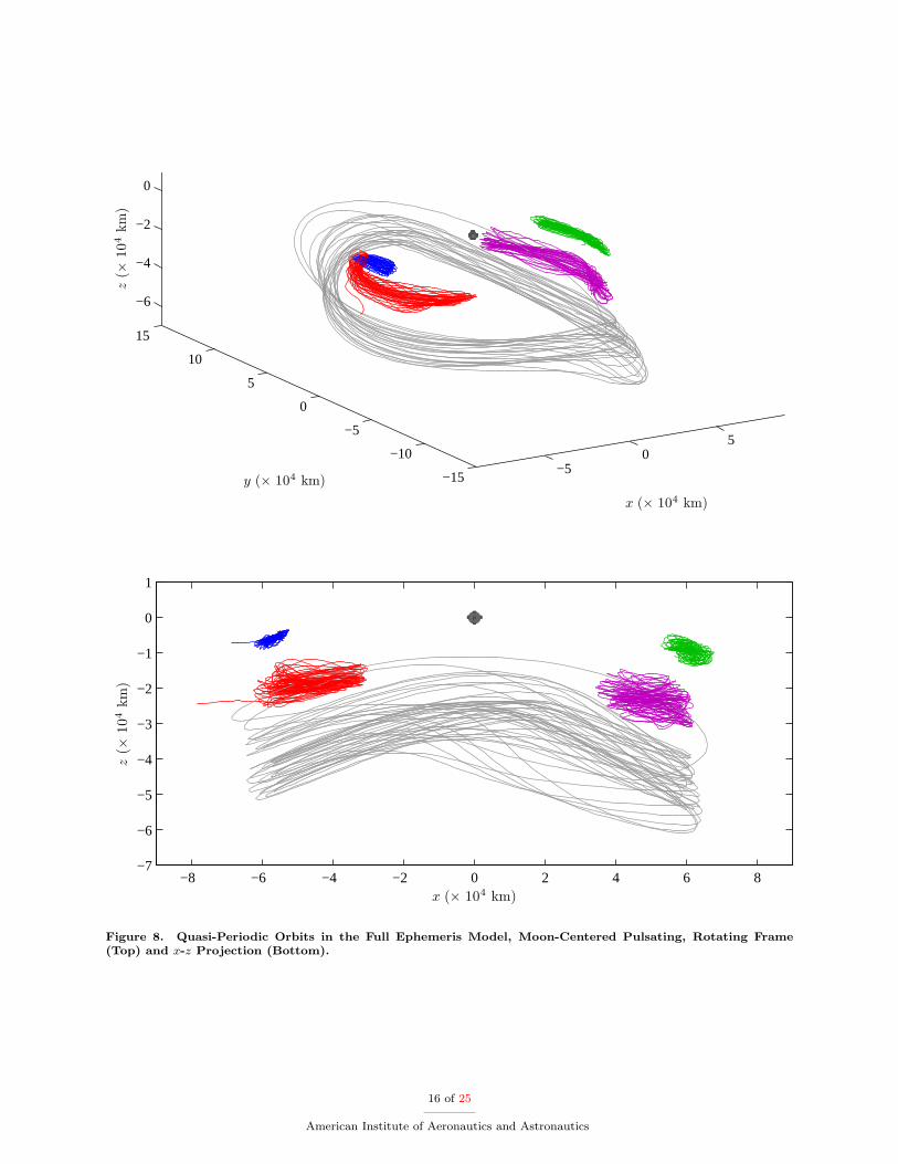
In general, the Jacobian matrix DF is very large and sparse. The general form of DF for the Gauss-Lobatto method and l = 0 appears in the Appendix. Consider a problem with only 100 nodes where gi ineq. (11) is scalar-valued, i.e., m = 1. For the Hermite-Simpson scheme, the length of the design variable vectorX is 1,000. If there are no other node constraints (l = 0), the length of the corresponding constraint vector Fis 794. Then the size of DF is 794×1, 000. In solving the same problem with the Gauss-Lobatto method, thelengths of X and F are 2,386 and 2,180, respectively. Therefore, in this case DF is a 2, 180× 2, 386 matrix.Due to the large number of design variables, it is apparent that even these relatively smaller problems (wheren = 100, m = 1, and l = 0) require efficient methods for the implementation of eq. (19). The efficiency of thecomputation is increased by utilizing the sparseness of DF . Recall from eq. (8) that for the Hermite-Simpsonscheme, ∆i,c depends only on the adjacent node states and controls, and is independent of all the other nodestates and controls and also any other variables that appear in eq. (14). As a result, DF is primarily ablock diagonal matrix of non-zero sub-matrices D∆i,c. The sparsity of DF is even more apparent whenconsidering Dψi, Dgi, and Dhk, all of which only depend on specific node states and/or controls. In fact, for

8 of 25


the Hermite-Simpson scheme, there cannot be more than n (18m+ 9l + 111)− 108 non-zero entries in DF .This implies that for the case when n = 100, m = 1, and l = 0 (recall DF is then a 794 × 1, 000 matrix),there exist no more than 12,792 non-zero entries, which is about 1.61% of the total number of entries in DF .Alternatively, for the Gauss-Lobatto method, there must be less than n (60m+ 30l + 543)−24m−12l−540non-zero entries. Then, for the case where n = 100, m = 1, and l = 0, less than 1.15% of the entries arenon-zero.

There are a number of ways to exploit the sparsity to increase efficiency. First, when pre-allocatingthe size of DF , memory is only allocated for the maximum number of non-zero entries, and not for allof the zero entries (which can be very large). Also, considering the sparsity of DF , perhaps the mostefficient means of computing

[DF ·DF T

]−1F is to implement the Unsymmetric Multifrontal Method.

The standard package UMFPACK is commonly used and appears in MATLAB R©.25 Finally, to avoid thecost of computing derivatives numerically, the non-zero elements in DF are computed analytically whenevertractable. For example, Dψi, Dgi, Dgi,2, Dgi,3, and Dhk are all computed analytically, and their expressionsare, in general, straightforward. Unfortunately, the derivatives D∆i may be quite complicated. In fact, forthe Gauss-Lobatto approach, the expressions for ∆i are already very involved, and it is difficult to computeD∆i analytically. In these cases, a numerical scheme may be more tractable. Consider computing the

6 × 18 sub-matrix D∆i,c for the Hermite-Simpson method. If xi =(x

(1)i , x

(2)i , x

(3)i , x

(4)i , x

(5)i , x

(6)i

)T

and

ui =(u

(1)i , u

(2)i , u

(3)i

)T

, then

D∆i,c =∂∆i,c

∂xi

∂∆i,c

∂ui

∂∆i,c

∂xi+1

∂∆i,c

∂ui+1

, (20)

where

∂∆i,c

∂x(j)i

=Imag

∆i,c

(x

(j)i + ε

√−1)

ε,

∂∆i,c

∂u(j)i

=Imag

∆i,c

(u

(j)i + ε

√−1)

ε,

∂∆i,c

∂x(j)i+1

=Imag

∆i,c

(x

(j)i+1 + ε

√−1)

ε,

∂∆i,c

∂u(j)i+1

=Imag

∆i,c

(u

(j)i+1 + ε

√−1)

ε,

(21)

and ε is a small step-size. Therefore, all the columns of D∆i,c in eq. (20) can be computed using eqs. (21).Similar schemes can be constructed for computing the 6×30 sub-matricesD∆i,1, D∆i,c, andD∆i,4 necessaryfor the Gauss-Lobatto scheme. Note that eqs. (21) are only numerical approximations of the actual partialderivatives ∂∆i,c

∂x(j)i

, ∂∆i,c

∂u(j)i

,∂∆i,c

∂x(j)i+1

, and ∂∆i,c

∂u(j)i+1

. However, the expressions are written as equalities in eqs. (21)

because, while they are only approximations, the full advantages of double-precision accuracy are exploited.Furthermore, unlike alternative finite-differencing schemes (most of which are only accurate up to single-precision just for first derivative information), it is not necessary to determine an optimal value for ε. Thetotal error in the numerical scheme asymptotically approaches the round-off error as ε goes to zero.28

IV. Periodic Orbits in the Earth-Moon Restricted Three-Body Problem

Locating periodic or quasi-periodic orbits is an essential part of any long-duration mission design process.For these types of orbits, the complexity of the problem is reduced by searching for feasible solutions thatare simply-periodic. Then, due to their ergodic behavior, the solutions are preserved for all time. For asolar sail in the RTBP, periodic orbits occur at periods commensurate with the lunar synodic month. Forthis study, only orbits with periods equal to one lunar synodic month are investigated. The periodic orbitsare not embedded in families since solutions for the controlled sail are not unique. As a consequence, thisstudy is primarily an investigation of suitable point-solutions for several orbits that support lunar southpole coverage. The general periodicity constraints are introduced, and path constraints amenable for lunarsouth pole coverage are derived. The method is very robust, converging on periodic solutions when almost noinformation about the initial guess (besides feasibility) is known. Finally, the process is employed to computemany point-solutions, however, five near-optimal solutions for lunar south pole coverage are presented.

9 of 25


A. Periodicity and Path Constraints

Periodic orbits are determined with periods equal to one lunar synodic month, or period P = 29.64 days.For the orbits in this investigation, the magnitude of the gravity gradient experienced by the spacecraftremains relatively constant. Therefore, during implementation of the collocation schemes for these orbits, afixed value of Ti is adequate for a given number of nodes n. Then, let Ti = P/ (n− 1). For a periodic orbit,the initial state and control must equal the final state and control, or

h1 (x1, xn) = xn − x1 = 0, h2 (y1, yn) = yn − y1 = 0, h3 (z1, zn) = zn − z1 = 0,h4 (x1, xn) = xn − x1 = 0, h5 (y1, yn) = yn − y1 = 0, h6 (z1, zn) = zn − z1 = 0, (22)

h7

(u

(1)1 , u(1)

n

)= u(1)

n − u(1)1 = 0,

h8

(u

(2)1 , u(2)

n

)= u(2)

n − u(2)1 = 0,

h9

(u

(3)1 , u(3)

n

)= u(3)

n − u(3)1 = 0,

(23)

where ui =(u

(1)i , u

(2)i , u

(3)i

)T

, as previously defined. These constraints, in addition to the defect constraintsand control constraints ψi = 0 in eq. (10), are the only constraints necessary for computing periodic orbitswith the collocation schemes.

It is also quite useful to apply path constraints that completely confine the spacecraft to a region of phasespace. For example, it may be desirable to force a solution to remain inside a pre-defined box in positionspace. For lunar south pole coverage, this is particularly useful when the bounding box is located beneaththe south pole of the Moon. Let the lower and upper bounds of the bounding box be rlb = (xlb, ylb, zlb)

T

and rub = (xub, yub, zub)T , respectively. Then the corresponding path constraints for the Hermite-Simpson

method, where m = 6 in eq. (11), are

gi (ri,ηi) =rlb − ri

ri − rub

+ η2

i = 0, for i = 1, 2, .., n. (24)

Similar constraint equations apply for the Gauss-Lobatto scheme, i.e.

gi (ri,ηi) =rlb − ri

ri − rub

+ η2

i = 0,

gi,2 (ri,2,ηi,2) =rlb − ri,2

ri,2 − rub

+ η2

i2 = 0, for i = 1, 2, .., n− 1,

gi,3 (ri,3,ηi,3) =rlb − ri,3

ri,3 − rub

+ η2

i3 = 0,

(25)

where the last 6 constraints are given by eq. (24) for i = n. However, perhaps a more appropriate set ofpath constraints, specifically designed for lunar south pole coverage, are constraints on the elevation angleand altitude of the spacecraft from the lunar south pole. For example, it may be desired to maintain thespacecraft above a certain elevation angle φlb at all times and yet always remain below some altitude aub.Ignoring lunar librations, for the Hermite-Simpson scheme the constraints that accomplish this objective are

gi (ri,ηi) =

sinφlb +

zi +RM

ai

ai − aub

+ η2

i = 0, for i = 1, 2, .., n, (26)

where ai =√

(xi − 1 + µ)2 + y2i + (zi +RM )2 and RM is the non-dimensional mean radius of the Moon.

Similarly, these constraints for the Gauss-Lobatto scheme possess the form

gi (ri,ηi) =

sinφlb +

zi +RM

ai

ai − aub

+ η2

i = 0,

gi,2 (ri,2,ηi,2) =

sinφlb +zi,2 +RM

ai,2

ai,2 − aub

+ η2i,2 = 0,

gi,3 (ri,3,ηi,3) =

sinφlb +zi,3 +RM

ai,3

ai,3 − aub

+ η2i,3 = 0.

(27)

10 of 25


Unlike the constraints for the bounding box, where m = 6, the constraints on elevation angle and altitudeonly require m = 2. The problem is now fully defined. The design variable vector X and constraint vectorF can be constructed as indicated in eqs. (14)-(17).

B. Example Periodic Orbits

To compute some periodic orbits, assume that the elevation and altitude constraints are a priority. For thissample scenario, no initial guess is available for X, which includes all the node states and controls, slackvariables, and additional states and slack variables for internal points when X is associated with the Gauss-Lobatto scheme. However, the approach to the problem developed in this effort is very robust and only a fewpieces of information are necessary to determine an initial guess that converges to periodic solutions usingeq. (19). In general, the initial guess is established as follows:

1. Examine figure 1 and approximate a feasible region given a desired characteristic solarsail acceleration κ

2. Specify desirable values of φlb and aub that encompass this region3. Within the bounds imposed by φlb and aub, select any set of feasible positions for all

the position variables

It should be noted that the first two steps in the process may be interchanged. For example, another optionis to first specify a region of interest with φlb and aub and then determine the value of κ necessary tomaintain the spacecraft within this region. For application in the RTBP, the orbits are initially assumed tobe stationary, therefore all the velocity variables are always initially set to zero. The initial time is also zero,i.e., t1 = 0. An initial guess for the slack variables is determined by solving for ηi that satisfy eq. (11) andηi, ηi,2, and ηi,3 satisfying eq. (12). In the RTBP, let the clock angle δ be the angle between the projectionof the sail normal unit vector ui in the Earth-Moon plane and the vector l. Then, the pitch angle α is theout-of-plane angle measured from the Earth-Moon plane to ui. (See figure 4.) Initially, for all node points,

Figure 4. Relation of Control Angles to ui.

δ = 0, and α = −35.26 to maximize the out-of-plane component of sail thrust in the negative z direction.13

Then the components of ui in the rotating frame can be computed from the angles δ and α, i.e.

ui =

cosα cos (δ − ωsti)cosα sin (δ − ωsti)

sinα

. (28)

Except for selecting a realistic value of κ from figure 1, very little information about the natural dynamics isnecessary for computing the periodic orbits that satisfy the boundary constraints with this scheme. A controlpattern is established for a solution that is close to the initial guess and meets the specified constraints. Givena feasible value of κ and an appropriate number of nodes n, the method generally determines a solution witha smooth control history in less than five iterations of eq. (19). Difficulties are only encountered when thepath constraints that are selected force the spacecraft to a region that is physically impossible to maintainfor the given characteristic acceleration κ, implying that, for the bounds selected, a nearby solution does notexist.

Using this strategy, many orbits favorable for lunar south pole coverage are easily computed. From allthe orbits investigated, five orbits of interest are selected from three different regions. (See figure 5.) Forcomparison, in figure 6 the elevation angle histories for the five orbits are plotted versus time. (Hereafterthe color schemes for the different orbits will remain as defined in figure 5.) Recall from figure 1, that for

11 of 25


the realistic sail κ = 0.58 mm/s2, any orbits favorable for lunar south pole coverage will be located justbelow L1 and L2. Positioning the initial guess just below the L1 and L2 points, φlb is selected to be aslarge as physically possible for the characteristic acceleration value κ = 0.58 mm/s2. The limiting boundaryfor feasible trajectories that maintain constant south pole surveillance occurs at elevation angles φlb = 4.2

for L1 and φlb = 6.8 for L2. A sail can reach even greater elevation angles of constant surveillance whenthe characteristic acceleration κ is slightly increased. For example, when κ = 1.70 mm/s2, the limitingboundaries are φlb = 15.8 and φlb = 18.8 for L1 and L2, respectively. In fact, an entirely new type of orbitthat appears to “hover” under the lunar south pole, is available for κ = 1.70 mm/s2 and this trajectorycan be computed from an initial guess just under the lunar south pole. The boundary of feasible solutionsfor this orbit is φlb = 15.0. From these results, and several other orbits investigated, it appears that forconstant surveillance of the lunar south pole with a solar sail, a spacecraft near L2 may yield the highestminimum elevation angle for both κ = 0.58 mm/s2 and κ = 1.70 mm/s2. Such a conclusion is consistentwith figure 1, where the contours corresponding to these characteristic accelerations near L2 extend furtherbelow the x-axis than the L1 contours. A spacecraft in any one of these orbits also maintains constantline-of-sight with the Earth, since the solar sail orbits are displaced sufficiently far below the x-y plane. TheL2 orbits are in constant view of the far-side of the Moon as well, a feature that may be useful for futurelunar missions.

The control time histories for the L2 orbit with κ = 0.58 mm/s2 appear in figure 7. For this study,fluctuations in the control are not constrained, but the method is general enough that they could be added.The possible off-nominal accelerations of the sail have not been modeled. Though the system allows thespacecraft to use both sides of the sail, all the orbits investigated only employ one side. For example, fromfigure 7 it is clear that for the L2 orbit with κ = 0.58 mm/s2, −90 < δ < 90. Also, since the drivingfactor in the investigation is φlb, for all computations aub is set to some arbitrarily large value. For allsimulations, the Gauss-Lobatto scheme is employed with the constraints described previously and n = 100.This corresponds to a time-step of about 0.3 days or roughly 0.07 nondimensional time units. With theconstraints implemented, the sizes of X and F are 2, 684 and 2, 487, respectively. Thus, over 98.6% of theentries in the matrix DF are zero.

V. Transition to Ephemeris

From a number of simplifications in the RTBP model, two critical assumptions must be further examined.First, in the RTBP the Sun-to-spacecraft line is assumed to move in the Earth-Moon plane. In reality, theMoon’s orbit plane is inclined with respect to that of the Earth by about 5.15. This difference is significant,and it is therefore necessary to demonstrate that any solar sail trajectory modeled in the RTBP (irrespectiveof the mission design objective) is sufficiently accurate for transitioning into the full ephemeris model. Second,the simplified RTBP model currently ignores lunar librations, instead assuming that the south pole of theMoon is directly below the Moon’s center and stationary. In the real model, the lunar equatorial plane isinclined to Earth’s orbit plane by about 1.55. Considering these two angles, that is, the angles betweenthe Earth orbit plane and both the lunar orbit plane and the lunar equatorial plane, it appears likely thateven if the orbits can be transferred to the full model, some of the orbits from the RTBP, for example, theL1 orbit for κ = 0.58 mm/s2 with a minimum elevation angle of φmin = 4.2, will not maintain a positiveelevation angle with respect to the actual lunar south pole. However, the collocation schemes can be adaptedfor computations in the full model. In fact, all the orbits can be transitioned to the full model while ensuringthat most do maintain a positive elevation angle φmin.

A. Path Constraints and Control Transformation

Given multiple revolutions of any baseline orbits from the RTBP, the goal is computation of a nearby periodicsolution in the full ephemeris model. The only constraints necessary for computing the nearby solution arethe usual defect constraints and the control constraints ψi = 0. It is still, however, useful to enforce thepath constraints that are ideal for lunar south pole coverage. To ensure that the desired elevation angles andaltitudes are satisfied with respect to the actual lunar south pole, eqs. (26)-(27) must be modified. At anygiven time ti, the exact position of the lunar south pole rsp

i can be determined by manipulating the Euler 3-1-3 sequence for lunar librations available in the JPL DE405 ephemeris file.3 Then for the Hermite-Simpson

12 of 25


−6 −4 −2 0 2 4 6

−10

−5

0

5

10−5

−4

−3

−2

−1

0

1

x (× 104 km)y (× 104 km)

z(×

104

km)

−6 −4 −2 0 2 4 6−5

−4

−3

−2

−1

0

1

L2

κ = 0.58 mm/s2

L2

κ = 1.70 mm/s2

x (× 104 km)

hoverκ = 1.70 mm/s2

L1

κ = 1.70 mm/s2

L1

κ = 0.58 mm/s2

z(×

104

km)

Figure 5. Periodic Orbits in the RTBP, Moon-Centered Rotating Frame (Top) and x-z Projection (Bottom).

13 of 25


0 5 10 15 20 250

10

20

30

40

time (days)

φ(

)

Figure 6. Elevation Angle φ for Periodic Orbits in the RTBP.

0 5 10 15 20 25−45

−40

−35

−30

α(

)

0 5 10 15 20 25

−10

0

10

time (days)

δ(

)

Figure 7. Control History for the L2 Periodic Orbit in the RTBP with κ = 0.58 mm/s2.

scheme, the path constraints for elevation angle and altitude in the full model are

gi (ri,ηi) =

sinφlb +rsp

i · (rspi − ri)

ai ‖rspi ‖

ai − aub

+ η2i = 0, for i = 1, 2, .., n, (29)

where now ai = ‖ri − rspi ‖. Using eq. (29), similar equations can be derived for the Gauss-Lobatto scheme.

Although the vector bases are now associated with the Moon-centered EMEJ2000 frame, all quantities arestill nondimensional based on the characteristic quantities in the RTBP.

Before the application of a Newton iteration procedure, it is first necessary to transform all the statesfrom the RTBP to the EMEJ2000 frame. Since the orbits are relatively close to the Moon, the Moon is setas the central body in eq. (3). The additional perturbing bodies include the Earth and the Sun, and thedefects in eqs. (8)-(9) are now computed with respect to eq. (3). The controls ui must also be adjusted to be

defined relative to the real Sun-to-spacecraft line. Therefore, given ui =(u

(1)i , u

(2)i , u

(3)i

)T

from the RTBP,

14 of 25


first αi and δi are computed, i.e.

αi = sin−1 u(3)i ,

δi = tan−1

(u

(1)i sinωsti + u

(2)i cosωsti

u(1)i cosωsti − u(2)

i sinωsti

),

(30)

where −90 ≤ sin−1 (·) ≤ 90 and −180 ≤ tan−1 (·) ≤ 180, and ωs is as calculated in RTBP. Then, todetermine ui in the EMEJ2000 frame given αi and δi, consider using

ui =[li

hi × li‖hi × li‖

li ×hi × li‖hi × li‖

]cosαi cos δicosαi sin δi

sinαi

, (31)

where both li and hi possess unit magnitudes. Here the instantaneous direction of the Sun-to-spacecraft lineli is extracted from the ephemeris files. The vector hi is the unit vector parallel to the angular momentumassociated with the Earth’s orbit relative to the Sun, and is also determined from the files.

B. Results

Since the orbits are periodic in the RTBP, multiple revolutions can be quickly obtained by “stacking” thenode states and controls for a baseline 25-revolution, two-year mission. The number of nodes per revolutionis adjusted to 35, for a total number of nodes n = 851. From eqs. (4)-(5), it is apparent that an epoch must beidentified when the Moon is at opposition to match the conditions at t = 0 for the simple RTBP model. Thetotal lunar eclipse of 2011 December 10, 14:31:46 UTC meets this requirement and is selected as the epochfor all of the orbits. Since the segment time Ti remains fixed, all the body locations in the system model, aswell as the location of the lunar south pole, are computed prior to applying the collocation scheme and storedin memory for future access. Therefore, the ephemeris files are never called during implementation of thecollocation schemes. As previously stated, the node states and controls (as well as the states correspondingto the internal points for the Gauss-Lobatto scheme) are transformed into the Moon-centered EMEJ2000frame, and the values of φlb and aub are selected. The values for the bounds φlb and aub must be suchthat the initial guess is feasible or at least very close to feasible. If the initial guess is infeasible, then usingeqs. (11)-(12) to compute initial values for the slack variables, the variables are defined in terms of the realpart. Using the transformed guess from the RTBP and the bounds described in eq. (29), eq. (19) is once againapplied in an iterative manner. In just a few iterations, the scheme successfully computes quasi-periodicsolutions for solar sail trajectories in the ephemeris Earth-Moon pulsating, rotating frame.

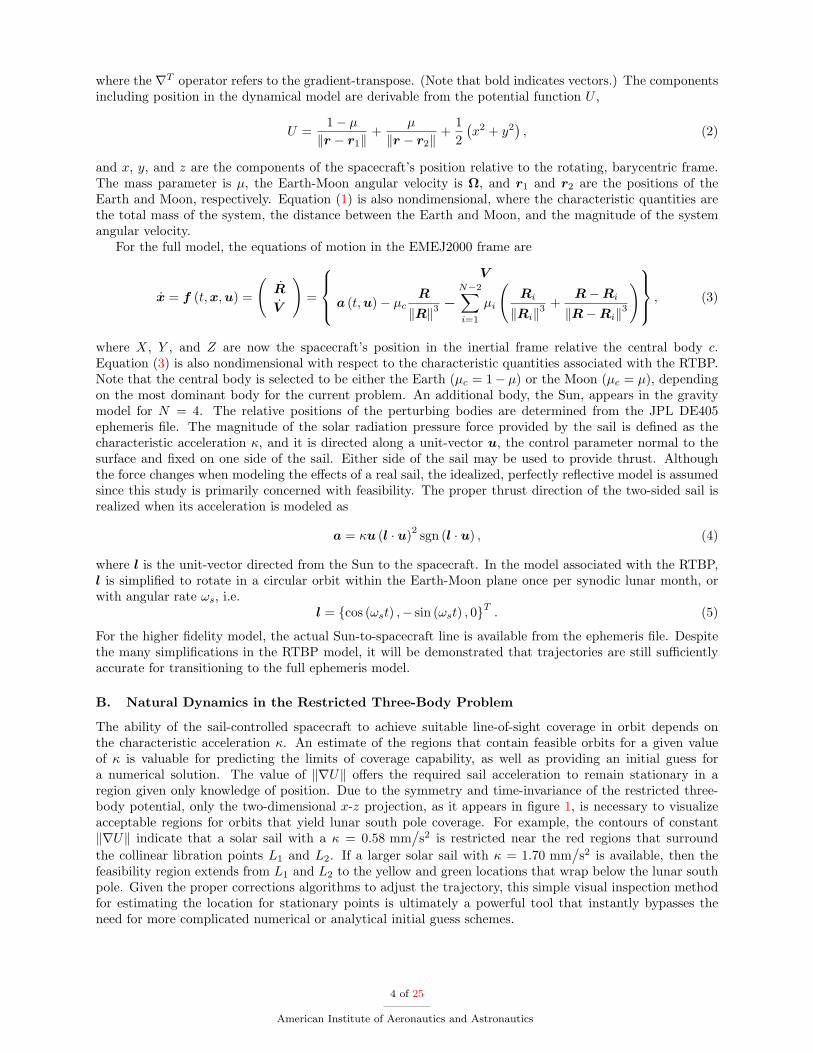
All five orbits designed in the RTBP are successfully transitioned to the full model using the Gauss-Lobatto method, and the results appear in figure 8 where the orbits are plotted in the Earth-Moon pulsating,rotating frame. For comparison, elevation angle is plotted as a function of time for both L2 orbits in figure 9.After transition, the L1 orbit with κ = 0.58 mm/s2 possesses a minimum elevation angle φmin = −2.70,that is, “below” the horizon and out of sight of the south pole. In contrast, for this κ, the L2 orbit is barelyfeasible after transitioning to the full model, where φmin = 0.01. Therefore, it appears that for the morerealistic sail with κ = 0.58 mm/s2, only orbits near L2 maintain constant surveillance of the lunar southpole in the full model. For the slightly larger characteristic acceleration κ = 1.70 mm/s2, however, all theorbits maintain positive elevation angles in the ephemeris model. The minimum elevation angles for L1 andL2 are φmin = 9.10 and φmin = 11.91, respectively, and φmin = 8.20 for the hover orbit. Due to thelunar librations, it is not surprising that nearly all the orbits lose about 6.7 of elevation between the RTBPand ephemeris models.

A sample of the control time histories for the L2 orbit for κ = 0.58 mm/s2 appear in figure 10. Notethat upon transition to the full model, the control histories remain smooth, and are also relatively slow. (Atmost, only a few degrees of re-orientation are required per day.) Quasi-periodic orbits may be computedfor up to 100 revolutions of the baseline orbit, and the results do not vary. Note that for 100 revolutions(approximately 8 years), n = 3, 401, setting the size of X and F to 91,811 and 85,003, respectively. However,roughly 99.97% of the entries in the matrix DF are zero.

15 of 25


−50

5

−15

−10

−5

0

5

10

15

−6

−4

−2

0

x (× 104 km)

y (× 104 km)

z(×

104

km)

−8 −6 −4 −2 0 2 4 6 8−7

−6

−5

−4

−3

−2

−1

0

1

x (× 104 km)

z(×

104

km)

Figure 8. Quasi-Periodic Orbits in the Full Ephemeris Model, Moon-Centered Pulsating, Rotating Frame(Top) and x-z Projection (Bottom).

16 of 25


0 100 200 300 400 500 600 7000

10

20

30φ

()

time (days)

Figure 9. Elevation Angle φ for the L2 Quasi-Periodic Orbits in the Full Ephemeris Model.

0 100 200 300 400 500 600 700−50

−40

−30

α(

)

0 100 200 300 400 500 600 700−20

0

20

time (days)

δ(

)

Figure 10. Control History for the L2 Quasi-Periodic Orbit in the Full Ephemeris Model with κ = 0.58 mm/s2.

VI. Transfer Trajectories

The use of a solar sail for lunar south pole coverage implies that the spacecraft ideally inserts into the orbitfrom a propellant-free transfer trajectory. (Alternative schemes are also available, but the use of propellantfor thrusting is required.5) Although a spiral-out from low-Earth orbit is impractical due to atmosphericdrag, an initial “piggy-back” leg along a geosynchronous transfer orbit (GTO) has been proposed as a viableoption by previous researchers.9 To reduce the potential effects of drag, which are not modeled in this study,periapsis for the GTO is defined as 1,000 km.

A. Backwards Integration

Due to very long flight times and sensitive, nonlinear dynamical behavior near the Earth, an accurate initialguess is required to refine a transfer trajectory with the collocation procedure. An intuitive, explicitlyintegrated initial guess scheme is developed by assuming a steering law for the solar sail. All integrationoccurs in the EMEJ2000 coordinate frame in the full ephemeris model, since the RTBP offers no majorsimplifying assumptions that can be exploited with this transfer scheme. Numerical integration also occursin backwards time, allowing the initial state to be fixed on the lunar south pole coverage orbit at the properinsertion date in the ephemeris model; as a consequence, the exact GTO remains unspecified. Then, theinitial guess scheme requires only that the two-body energy E and the angular momentum H with respectto the Earth, are matched as close as possible to the corresponding GTO values when the propagationterminates.

17 of 25


To reduce the energy during backwards numerical integration, the velocity-pointing steering law detailedin figure 11 is employed. The sail acceleration a is initially aligned along the inertial velocity vector V , butwhen l · V is negative, the sail is oriented such that u⊥l to produce no thrust. For a two-sided sail, u flips180 at the completion of every cycle, and as a consequence u is either parallel or anti-parallel to V duringthrusting. When the sail requires re-orientation to an attitude that yields no acceleration, i.e., the sail is“off”, δ = ±90 and α is oriented such that u is as close as possible to V (or −V depending on the cycle)to ensure a smooth control transition the next time the sail is activated.

Using only this algorithm, E is reduced without any attention to the rate of decrease in H. Problemsarise during backwards propagation because H decreases too quickly, resulting in a highly elliptical orbitthat passes through the Earth. Other possible approaches, such as McInnes’ locally optimal steering law,9

reduce H even faster, since most thrusting occurs in the vicinity of apoapsis. For similar rates of decrease inE and H, the velocity-pointing steering law is, therefore, modified to force maneuvers away from apoapsisduring the transfer. This modification is accomplished by selecting the Earth-relative flight-path-angle γas an additional switching condition. Thus, the sail is now always off unless l · V = 0 and γ lies withinan acceptable region, at which point the sail switches on. This new “E-H” steering law corresponds towait-times until the correct phasing of the transfer with the Sun-to-spacecraft line occurs. Details for thefull implementation of this method are available by examination of the function generator in figure 12.

For numerical considerations upon transition into collocation, initial guesses that pass through the Earthare avoided. The stopping condition for the integration, that is, E = 0 and H > 0, is sufficient to ensure thisbehavior. Backwards integration of the E-H steering law is also repeated at initial conditions correspondingto nodes around the baseline ephemeris coverage orbit until an accurate initial guess is obtained. Since thecoverage orbit is a converged ephemeris solution, a successful transfer obtained in collocation will result ina continuous insertion without a maneuver.

Figure 11. Velocity-Pointing Steering Law.

B. Refinement with Collocation

From an accurate initial guess obtained with the E-H thrusting law, the trajectory must be refined withcollocation to generate a feasible solution. In formulating the new constraint vector (eq. (17)), the defectconstraints ∆i (eq. (9)) and control-magnitude constraints ψi (eq. (10)) must be enforced as usual, but nopath constraints (eq. (12)) are required, i.e. m = 0. The boundary conditions that bracket the transferare enforced by adding general constraints (eq. (13)) at the 1st node and the nth node. These boundaryconditions are defined as the insertion state on the lunar south pole coverage orbit and the energy and

18 of 25


Input γmin & EGTO, and set s = 1.

DO WHILE E < EGTO

DO WHILE γ < γmin

Propagate eq. (3) with a (t,u) = 0 untill · V = 0 & d(l · V )/dt < 0.

Update γ.

END

Propagate eq. (3) with u ‖ (sV ) untill · V = 0 & d(l · V )/dt > 0.

Update E, and set s = −s.END

Figure 12. Function Generator for the E-H Steering Law.

angular momentum associated with GTO, i.e.

h1 (Xn) = Xn − X∗,

h2 (Yn) = Yn − Y ∗,

h3 (Zn) = Zn − Z∗, h1 (x1) = ‖V1‖2 /2− (1− µ) / ‖R1‖ − EGTO,

h4

(Xn

)= Xn − X∗, h8 (x1) = ‖R1 × V1‖ −HGTO,

h5

(Yn

)= Yn − Y ∗,

h6

(Zn

)= Zn − Z∗,

(32)

where the superscript “*” identifies a condition along the coverage orbit. Since the transfer involves a largenumber of spirals around the Earth, one strategy to compensate for the sensitive dynamical region is toemploy an adaptive refinement in the nodal distribution.29 However, the complications of such a process arebypassed by using pre-specified time ratios from the explicit integration of the E-H thrusting law. Thesetime ratios are already spaced in recognition of the sensitive dynamics, and since an accurate initial guessis inputted into the procedure, there is no need for adaptive refinement. Since the time on each trajectorysegment is fixed, the locations of all celestial bodies within the DE405 ephemeris file are only initialized once.The Earth is selected as the central body in eq. (3), with the Sun and Moon acting as perturbing bodies.This configuration is useful for numerical accuracy due to the many spirals that pass near the Earth. Foreach transfer, 5,000 nodes are selected, resulting in 104,988 free variables, 94,990 total constraints, and aDF matrix including over 99.96% zero entries. The states and controls are adjusted until a control historyis determined along a continuous trajectory that satisfies the constraints in eq. (17).

A successfully converged, full ephemeris sample transfer to the L2 orbit corresponding to κ = 0.58 mm/s2

appears in figure 13. The total transfer time from GTO is 401 days, with 106 days of on-time, and 397 on/offswitches of the sail to arrive at the orbit (shown in green). These switches can be visualized in figure 13 sincethe red arcs correspond to on-times and the blue phases correspond to off-times. Inspection of the controlhistory in figure 14 reveals these switch times as the instances when δ = ±90. Proper phasing of the Sun,orbit, and sail is important, since the sail is only active 26% of the time. It is again emphasized that thisresulting transfer requires no actual propellant, despite the fact that the transfer time appears long. Suchlong times are feasible for the mission concept of satellites designed for purposes of communications.

VII. Mission Design Summary

Hundreds of orbit scenarios were generated during the course of this investigation, but five orbits werespecifically selected as feasible and also possessed the largest elevation angle lower bound φlb. Therefore, theorbits are near-optimal for purposes of lunar south pole coverage. Each scenario of interest is successfullygenerated in the full ephemeris model. (See table 1.) Results associated with the transfer phase and the

19 of 25


−5

0

5

−5

0

5−2

−1

0

1

2

X (× 105 km)Y (× 105 km)

Z(×

105

km)

−2 −1 0 1 2 3 4 5−2.5

−2

−1.5

−1

−0.5

0

0.5

1

1.5

2

2.5

x (× 105 km)

y(×

105

km)

Figure 13. Transfer to the L2, κ = 0.58 mm/s2 Quasi-Periodic Orbit in the Full Ephemeris Model, Earth-Centered EMEJ200 Frame (Top) and x-y projection in the Earth-Centered Pulsating, Rotating Frame (Bot-tom).

20 of 25


−400 −350 −300 −250 −200 −150 −100 −50 0

−50

0

50

α(

)

−400 −350 −300 −250 −200 −150 −100 −50 0

−100

0

100

time (days)

δ(

)

Figure 14. Control History for Transfer to the L2, κ = 0.58 mm/s2 Quasi-Periodic Orbit in the Full EphemerisModel.

orbit phase are separated by the horizontal lines in the row corresponding to insertion. For the transfers,a higher percentage of sail on-time is observed in the orbits with a lower characteristic acceleration. Whenmore thrust acceleration is available, the transfer time is not necessarily faster due to the unique phasingrequired in the system. As expected, the best coverage is obtained by the orbits in the vicinity of L2. In fact,lunar librations completely eliminate the possibility for continuous line-of-sight with the lunar south pole forthe set of orbits near L1 when κ = 0.58 mm/s2. As characteristic acceleration increases for the sails, a largeincrease in elevation angle is observed as a larger out-of-plane force is available. The unique “hover orbit”possesses the best maximum elevation angle, but suffers a smaller minimum elevation angle and a greatermaximum altitude than the other orbits. All of the altitudes for the orbits in this study are comparableto the maximum apolune altitudes in the previous investigation by Grebow et al.4 Other studies, however,indicate that these altitudes are feasible for use with existing communications hardware.6

VIII. Conclusions

A systematic, robust approach is developed to compute periodic orbits in the RTBP and quasi-periodicorbits in the full ephemeris model for lunar south pole coverage. The numerical process converges on solutionswith very little a priori knowledge of the shape of these orbits or a control history. Furthermore, iterationon the largest possible minimum elevation angle reveals that the best coverage for a single spacecraft isachieved in the vicinity of the L2 point. The implicit integration scheme that is developed to generatethe orbits is adaptable to changing mission requirements, even beyond the problem of lunar south polecoverage. A transfer scheme based on simultaneously decreasing energy and angular momentum may beused in conjunction with the collocation strategy to yield feasible transfer trajectories. The collocationmethod successfully converges these trajectories, even when the number of design variables exceeds 100,000.The baseline transfers require no propellant and no additional insertion maneuvers are necessary. Thisfeasibility study demonstrates that, with current technology, solar sails remain an option for continuouslunar south pole coverage with a single spacecraft. Further study of this mission application is, thus, clearlywarranted.

IX. Acknowledgements

The authors thank Professor Robert Melton for suggesting the investigation of Gauss-Lobatto quadraturerules, and potential procedures for increasing computational efficiency. The authors also thank Mr. BruceCampbell for initially suggesting research on solar sails for lunar south pole coverage. This work was carriedout at Purdue University and the NASA Goddard Spaceflight Center with the Flight Dynamics AnalysisBranch under the supervision of Mr. David Folta. Portions of this work were supported by the NASA

21 of 25


Graduate Student Researchers Program (GSRP) fellowship and the Purdue Graduate Assistance in Areasof National Need (GAANN) fellowship.

References

1Elipe, A., and Lara, M., “Frozen Orbits about the Moon,” Journal of Guidance, Control, and Dynamics, Vol. 26, No. 2,2003, pp. 238-243.

2Ely, T., “Stable Constellations of Frozen Elliptical Inclined Orbits,” Journal of the Astronautical Sciences, Vol. 53, No.3, 2005, pp. 301-316.

3Howell, K., Grebow, D., and Olikara, Z., “Design Using Gauss’ Perturbing Equations with Applications to Lunar SouthPole Coverage,” Paper AAS 07-143, 17th AAS/AIAA Spaceflight Mechanics Meeting, Sedona, Arizona, January 28-February1, 2007.

4Grebow, D., Ozimek, M., and Howell, K., “Multi-Body Orbit Architectures for Lunar South Pole Coverage,” Journal ofSpacecraft and Rockets, Vol. 45, No. 2, 2008, pp. 344-358.

5Howell, K., and Ozimek, M., “Low-Thrust Transfers in the Earth-Moon System Including Applications to Libration PointOrbits,” Paper AAS-343, 2007 AAS/AIAA Astrodynamics Specialist Conference, Mackinac Island, Michigan, August 19-23,2007.

6Hamera, K., Mosher, T., Gefreh, M., Paul, R., Slavkin L., and Trojan, J., “An Evolvable Lunar Communication and Nav-igation Constellation Architecture,” Paper AIAA-2008-5480, 26th International Communications Satellite Systems Conference,San Diego, California, June 10-12, 2008.

7“Space Science Enterprise 2000 Strategic Plan,” [online publication],http://spacescience.nasa.gov/admin/pubs/strategy/2000/ [retrieved 11 December 2007].

8Garner, C., Price, H., Edwards, D., and Baggett, R., “Developments and Activities in Solar Sail Propulsion,” PaperAIAA-2001-3234, 37th AIAA/ASME/SAE/ASEE Joint Propulsion Conference and Exhibit, Salt Lake City, Utah, July 8-11,2001.

9McInnes, C., Solar Sailing: Technology, Dynamics and Mission Applications, Springer-Verlag, Berlin, 1999.10Clarke, A., The Wind from the Sun, Harcourt Brace Jovanovich, inc., New York, 1972.11Forward, R., “Statite Apparatus and Method of Use,” World International Property Organization, International Patent

Classification B64G 1/36, International Publication Number WO 90/07450, July, 1990.12Lichodzeijewski, D., and Derbes, B., “Vacuum Deployment and Testing of a 20M Solar Sail System,” Paper AIAA-2006-

1705, 47th AIAA/ASME/ASCE/AHS/ASC Structures, Structural Dynamics, and Materials Conference, Newport, RhodeIsland, May 1-4, 2006.

13McInnes, C., “Solar Sail Trajectories at the Lunar L2 Lagrange Point,” Journal of Spacecraft and Rockets, Vol. 30, No.6, 1993, pp. 344-358.

14McInnes, C., McDonald, A., Simmons, J., and MacDonald, E.,“Solar Sail Parking in Restricted Three-Body Systems,”Journal of Guidance, Control, and Dynamics, Vol. 17, No. 2, 1994, pp. 399-406.

15Wawrzyniak, G., “The Solar Sail Lunar Relay Station: An Application of Solar Sails in the Earth-Moon System,” 59th

IAC Congress, Glasgow, Scotland, September 29-October 3, 2008.16Melton, R., “Comparison of Direct Optimization Methods Applied to Solar Sail Problems,” Paper AIAA 2002-4728, 2002

AIAA/AAS Astrodynamics Specialist Conference and Exhibit, Monterey, California, August 5-8, 2002.17Russell, R., and Shampine, L., “A Collocation Method for Boundary Value Problems,” Numerical Mathematics, Vol. 19,

1972, pp. 1-28.18Betts, J.,“Survey of Numerical Methods for Trajectory Optimization,” Journal of Guidance, Control, and Dynamics,

Vol. 21, No. 2, 1998, pp. 193-207.19Ascher, U., Christiansen, J., and Russell, R., “COLSYS-A Collocation Code for Boundary-Value Problems,” Codes for

Boundary Value Problems in Ordinary Differential Equations, Vol. 76, Springer-Verlag, Berlin, 1979.20Dodel, E., Paffenroth, R., Champneys, A., Fairgrieve, T., Kuznetsov, Y., Sandstede, B., and Wang, X., “AUTO2000: Con-

tinuation and Bifurcation Software for Ordinary Differential Equations,” [online publication], http://personal.maths.surrey.ac[retrieved 17 July 2008], 2000.

21Hargraves, C., and Paris, S., “Direct Trajectory Optimization Using Nonlinear Programming and Collocation,” Journalof Guidance, Control, and Dynamics, Vol. 10, No. 4, 1987, pp. 338-342.

22Betts, J., and Huffman, W., “Sparse Optimal Control Software SOCS,” Boeing Information and Support Services,Mathematics and Engineering Analysis Technical Document MEA-LR-085, The Boeing Co., Seattle, Washington, July 1997.

23Enright, P., and Conway, B., “Optimal Finite-Thrust Spacecraft Trajectories Using Collocation and Nonlinear Program-ming,” Journal of Guidance, Control, and Dynamics, Vol. 14, No. 5, 1991, pp. 981-985.

24Herman, A., “Improved Collocation Methods With Applications to Direct Trajectory Optimization,” Ph.D. Dissertation,Department of Aerospace Engineering, University of Illinois at Urbana-Champaign, Urbana, Illinois, September 1995.

25Davis, T., “UMFPACK Version 4.6 User Guide,” [online publication], http://www.cise.ufl.edu/research/sparse/umfpack[retrieved 18 July 2008], Department of Computer and Information Science and Engineering, University of Florida, Gainesville,Florida, 2002.

26Herman, A., and Conway, B., “Direct Optimization Using Collocation Based on High-Order Gauss-Lobatto QuadratureRules,” Journal of Guidance, Control, and Dynamics, Vol. 19, No. 3, 1996, pp. 592-599.

27Enright, P., “Optimal Finite-Thrust Spacecraft Trajectories Using Direct Transcription and Nonlinear Programming,”Ph.D. Dissertation, Department of Aerospace Engineering, University of Illinois at Urbana-Champaign, Urbana, Illinois, January1991.

22 of 25


28Martins, J., Kroo, I., and Alonso, J., “An Automated Method for Sensitivity Analysis using Complex Variables,” PaperAIAA-2000-0689, 38th Aerospace Sciences Meeting and Exhibit, Reno, Nevada, January 10-13, 2000.

29Russell, R., and Christiansen, J., “Adaptive Mesh Selection Strategies for Solving Boundary Value Problems,” SIAMJournal on Numerical Analysis, Vol. 15, No. 1, 1978, pp. 59-80.

23 of 25


Table

1.

Sum

mary

ofExam

ple

Scenario

sin

the

Full

Ephem

eris

Model.

κ=

0.58

mm/s2

κ=

1.70

mm/s2

Typ

eL

1L

2L

1L

2ho

ver

Epo

ch(U

TC

)4

Feb

2011

16:4

8:00

8N

ov20

1004

:48:

0026

May

2011

02:2

4:00

17O

ct20

1007

:12:

0023

Apr

2011

16:4

8:00

Tra

nsfe

rT

ime

(day

s)30

940

119

944

624

8O

n-T

ime

(day

s)99

106

3534

35%

On-

Tim

e32

2617

814

No.

Swit

ches

429

397

113

113

119

Inse

rtio

nD

ate

(UT

C)

10D

ec20

1114

:24:

0014

Dec

2011

02:2

4:00

10D

ec20

1114

:24:

006

Jan

2012

14:2

4:00

27D

ec20

1104

:48:

00φ

min

()

-2.7

00.

019.

1011

.91

8.20

φm

ax

()

12.4

617

.21

27.4

334

.68

45.6

8φ

avg

()

4.18

7.13

16.1

419

.37

22.3

7a

min

(km

)53

,000

58,0

0055

,500

57,0

0068

,500

am

ax

(km

)70

,000

70,5

0084

,500

76,0

0013

8,00

0

24 of 25


Appendix

Fig

ure

15.

GeneralForm

ofth

eG

auss

-Lobatt

oJacobia

nM

atr

ixD

Ffo

rl

=0,w

here

(·)D

=dia

g(·

).

25 of 25


Solar Sails and Lunar South Pole Coverage

Documents