SOLAR INFLUENCES ON CLIMATE - Stanford Solar Centersolar-center.stanford.edu/sun-on-earth/2009RG000282.pdf · SOLAR INFLUENCES ON CLIMATE L. J. Gray,1,2 J. Beer,3 M. Geller,4 J. D.

SOLAR INFLUENCES ON CLIMATE

L. J. Gray,1,2 J. Beer,3 M. Geller,4 J. D. Haigh,5 M. Lockwood,6,7 K. Matthes,8,9 U. Cubasch,8

D. Fleitmann,10,11 G. Harrison,12 L. Hood,13 J. Luterbacher,14 G. A. Meehl,15 D. Shindell,16

B. van Geel,17 and W. White18

Received 5 January 2009; revised 23 April 2010; accepted 24 May 2010; published 30 October 2010.

[1] Understanding the influence of solar variability on theEarth’s climate requires knowledge of solar variability,solar‐terrestrial interactions, and the mechanisms determin-ing the response of the Earth’s climate system. We providea summary of our current understanding in each of thesethree areas. Observations and mechanisms for the Sun’s var-iability are described, including solar irradiance variationson both decadal and centennial time scales and their relationto galactic cosmic rays. Corresponding observations of var-iations of the Earth’s climate on associated time scales are

described, including variations in ozone, temperatures,winds, clouds, precipitation, and regional modes of variabil-ity such as the monsoons and the North Atlantic Oscillation.A discussion of the available solar and climate proxies isprovided. Mechanisms proposed to explain these climateobservations are described, including the effects of varia-tions in solar irradiance and of charged particles. Finally,the contributions of solar variations to recent observationsof global climate change are discussed.

Citation: Gray, L. J., et al. (2010), Solar influences on climate, Rev. Geophys., 48, RG4001, doi:10.1029/2009RG000282.

1. INTRODUCTION

[2] The Sun is the source of energy for the Earth’s climatesystem, and observations show it to be a variable star. Theterm “solar variability” is used to describe a number ofdifferent processes occurring mostly in the Sun’s convectionzone, surface (photosphere), and atmosphere. A full under-standing of the influence of solar variability on the Earth’sclimate requires knowledge of (1) the short‐ and long‐termsolar variability, (2) solar‐terrestrial interactions, and (3) themechanisms determining the response of the Earth’s climatesystem to these interactions [Rind, 2002]. There have beensubstantial increases in our knowledge of each of these areas

in recent years and renewed interest because of the impor-tance of understanding and characterizing natural variabilityand its contribution to the observed climate change [WorldMeteorological Organization, 2007; IntergovernmentalPanel on Climate Change (IPCC), 2007]. Correct attribu-tion of past changes is key to the prediction of future change.[3] Herschel [1801] was the first to speculate that the

Sun’s variations may play a role in the variability of theEarth’s climate. This has been followed by a great numberof papers that presented evidence [see, e.g., Herman andGoldberg, 1978; National Research Council (NRC), 1994;Hoyt and Schatten, 1997, and references therein], althoughmany of the early investigations have been criticized onstatistical grounds [Pittock, 1978]. Notwithstanding issuesof statistical significance, many of these solar‐climate1National Centre for Atmospheric Science, Meteorology

Department, University of Reading, Reading, UK.2Now at National Centre for Atmospheric Sciences, Department of

Atmospheric, Oceanic and Planetary Physics, University of Oxford,Oxford, UK.

3Swiss Federal Institute for Environmental Science andTechnology, Dubendorf, Switzerland.

4Institute for Terrestrial and Planetary Atmosphere, State Universityof New York at Stony Brook, Stony Brook, New York, USA.

5Physics Department, Imperial College London, London, UK.6Meteorology Department, University of Reading, Reading, UK.7Also at Space Science Department, Rutherford Appleton

Laboratory, Didcot, UK.8Institut fur Meteorologie, Freie Universität Berlin, Berlin, Germany.9Now at Section 1.3: Earth System Modeling, Deutsches

GeoForschungsZentrum Potsdam, Potsdam, Germany.10Department of Geosciences, University of Massachusetts Amherst,

Amherst, Massachusetts, USA.

Copyright 2010 by the American Geophysical Union. Reviews of Geophysics, 48, RG4001 / 20101 of 53

8755‐1209/10/2009RG000282 Paper number 2009RG000282

11Now at Oeschger Centre for Climate Change Research andInstitute of Geological Sciences, University of Bern, Bern, Switzerland.

12Department of Meteorology, University of Reading, Reading, UK.13Lunar and Planetary Laboratory, University of Arizona, Tucson,

Arizona, USA.14Department of Geography, Justus Liebig University Giessen,

Giessen, Germany.15National Center for Atmospheric Research, Boulder, Colorado,

USA.16NASA Goddard Institute for Space Studies, New York, New

York, USA.17Institute for Biodiversity and Ecosystem Dynamics, Research

Group Paleoecology and Landscape Ecology, Faculty of Science,Universiteit van Amsterdam, Amsterdam, Netherlands.

18Scripps Institution of Oceanography, University of California, SanDiego, La Jolla, California, USA.

RG4001

associations also seemed highly improbable simply on thebasis of quantitative energetic considerations. On averagethe Earth absorbs solar energy at the rate of (1 – A)ITS/4,where A is the Earth’s albedo and ITS is the total solarirradiance (TSI), i.e., the total electromagnetic power perunit area of cross section arriving at the mean distance ofEarth from the Sun (149,597,890 km). The factor of 4 arisessince the Earth intercepts pRE

2ITS solar energy per unit time(where RE is a mean Earth radius), but this is averaged overthe surface area of the Earth sphere, 4pRE

2. TSI monitorsshow a clear 11 year solar cycle (SC) variation betweensunspot minimum (Smin) and sunspot maximum (Smax) ofabout 1 W m−2 [Fröhlich, 2006]. Taking ITS = 1366 W m−2

and A = 0.3, the solar power available to the Earth system is(1 – A)ITS/4 = 239 W m−2 with an 11 year SC variation of∼0.17 W m−2, or ∼0.07%, a very small percentage of thetotal. Of greater importance to climate change issues arelonger‐term drifts in this radiative forcing. Recent estimatessuggest a radiative forcing drift over the past 30 yearsassociated with solar irradiance changes of 0.017 W m−2

decade−1 (see section 2). In comparison, the current rate ofincrease in trace greenhouse gas radiative forcing is about0.30 W m−2 decade−1 [Hofmann et al., 2008].[4] We can estimate the impact at the surface of the

11 year SC variation in total solar radiation at the top of theatmosphere using the climate sensitivity parameter l. This isdefined by DTS = lDF, where DF is the change in forcingat the top of the atmosphere (in this case ∼0.17 W m−2) andTS is the globally averaged surface temperature. Using avalue of 0.5 K (W m−2)−1 for l [IPCC, 2007], we wouldexpect the Earth’s global temperature to vary by a mere0.07 K. However, observations indicate, at least regionally,larger solar‐induced climate variations than would beexpected from this simple calculation, suggesting that morecomplicated mechanisms are required to explain them.[5] Figure 1b shows a time series of sunspot number for

the last three solar cycles, together with various otherindicators of solar variation and a composite of satellitemeasurements of TSI. Sunspots appear as dark spots on thesurface of the Sun and have temperatures as low as ∼4200 K(in the central umbra) and ∼5700 K (in the surroundingpenumbra), compared to ∼6050 K for the surrounding quietphotosphere. Sunspots typically last between several daysand several weeks. They are regions with magnetic strengthsthousands of times stronger than the Earth’s magnetic field.Figure 1c shows a commonly used indicator of solaractivity, the flux of 10.7 cm radio emissions from the Sun(F10.7), which is highly correlated with the number of sun-spots. This also correlates very highly with the core‐wingratio of the Mg ii line (Figure 1d), which is often taken as anindex of solar UV variability. Additional indices include theopen solar magnetic flux, FS (Figure 1e), dragged out of theSun because it is “frozen” into the solar wind; the galacticcosmic ray (GCR) count (Figure 1f); satellite‐measuredirradiance (Figure 1g); and the geomagnetic Ap index(Figure 1h). The flux of neutrons generated in the Earth’satmosphere by galactic cosmic rays (Figure 1f) is reducedby the cosmic ray effect of FS and therefore varies in the

opposite sense to the other indices. Despite the darkobscuring effect of sunspots, comparison of Figures 1b and1g shows that the TSI (and its components, including theUV) is a maximum around the time when the number ofsunspots is at its maximum. This is because the number ofcompensating smaller, much more numerous, brighterregions, called faculae, also peaks around sunspot maxi-mum. These are less readily visible than sunspots becausethey are smaller, but they have a high surface temperature of∼6200 K near the edge of the solar disk (where they arebrightest).[6] Going back farther in time, various other proxy solar

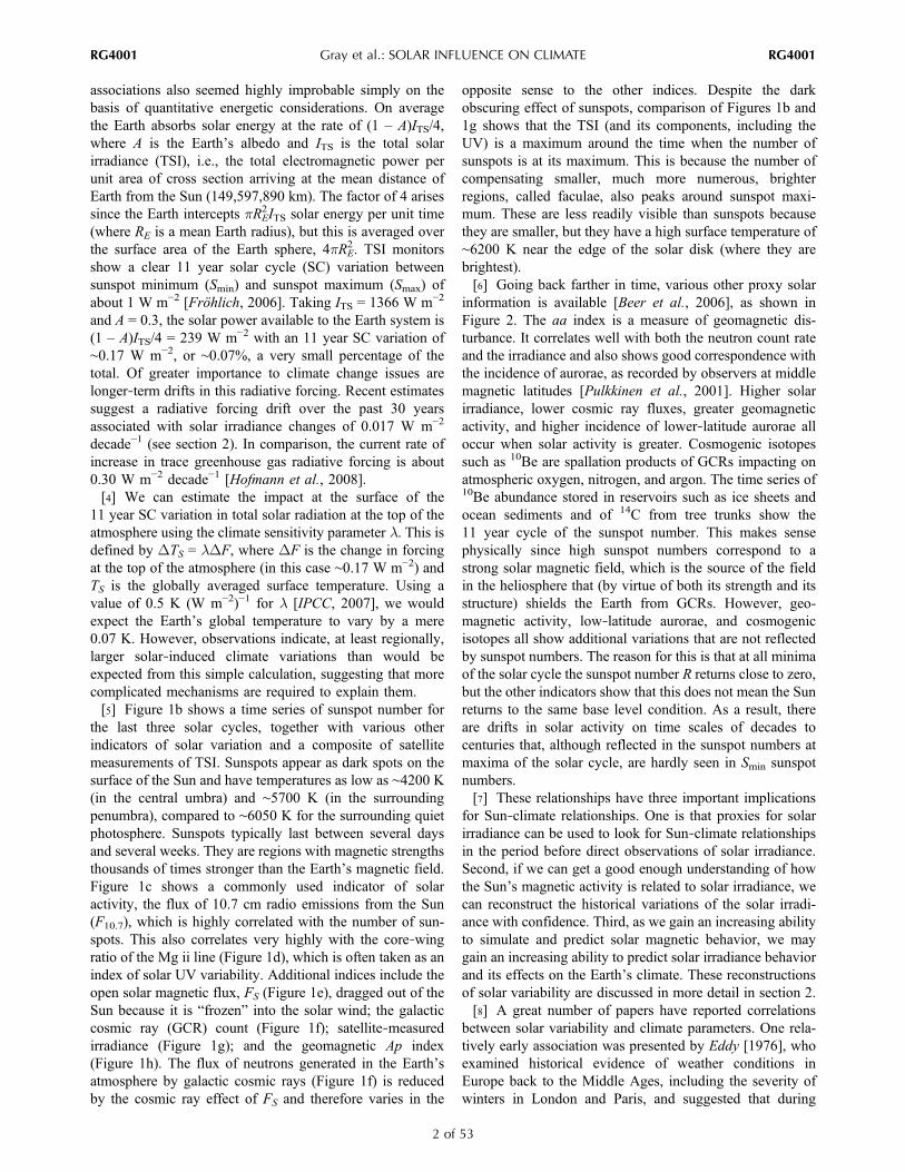
information is available [Beer et al., 2006], as shown inFigure 2. The aa index is a measure of geomagnetic dis-turbance. It correlates well with both the neutron count rateand the irradiance and also shows good correspondence withthe incidence of aurorae, as recorded by observers at middlemagnetic latitudes [Pulkkinen et al., 2001]. Higher solarirradiance, lower cosmic ray fluxes, greater geomagneticactivity, and higher incidence of lower‐latitude aurorae alloccur when solar activity is greater. Cosmogenic isotopessuch as 10Be are spallation products of GCRs impacting onatmospheric oxygen, nitrogen, and argon. The time series of10Be abundance stored in reservoirs such as ice sheets andocean sediments and of 14C from tree trunks show the11 year cycle of the sunspot number. This makes sensephysically since high sunspot numbers correspond to astrong solar magnetic field, which is the source of the fieldin the heliosphere that (by virtue of both its strength and itsstructure) shields the Earth from GCRs. However, geo-magnetic activity, low‐latitude aurorae, and cosmogenicisotopes all show additional variations that are not reflectedby sunspot numbers. The reason for this is that at all minimaof the solar cycle the sunspot number R returns close to zero,but the other indicators show that this does not mean the Sunreturns to the same base level condition. As a result, thereare drifts in solar activity on time scales of decades tocenturies that, although reflected in the sunspot numbers atmaxima of the solar cycle, are hardly seen in Smin sunspotnumbers.[7] These relationships have three important implications

for Sun‐climate relationships. One is that proxies for solarirradiance can be used to look for Sun‐climate relationshipsin the period before direct observations of solar irradiance.Second, if we can get a good enough understanding of howthe Sun’s magnetic activity is related to solar irradiance, wecan reconstruct the historical variations of the solar irradi-ance with confidence. Third, as we gain an increasing abilityto simulate and predict solar magnetic behavior, we maygain an increasing ability to predict solar irradiance behaviorand its effects on the Earth’s climate. These reconstructionsof solar variability are discussed in more detail in section 2.[8] A great number of papers have reported correlations

between solar variability and climate parameters. One rela-tively early association was presented by Eddy [1976], whoexamined historical evidence of weather conditions inEurope back to the Middle Ages, including the severity ofwinters in London and Paris, and suggested that during

Gray et al.: SOLAR INFLUENCE ON CLIMATE RG4001RG4001

2 of 53

times of few or no sunspots, e.g., during the MaunderMinimum (∼1645–1715), the Sun’s radiative output wasreduced, leading to a colder climate. Although many of theearly reported relationships between solar variability andclimate have been questioned on statistical grounds, somecorrelations have been found to be more robust, and theaddition of more years of data has confirmed their signifi-cance. In what was the start of a series of classic papers,Labitzke [1987] and Labitzke and van Loon [1988] sug-

gested that while a direct influence of solar activity ontemperatures in the stratosphere (∼10–50 km) was hard tosee, an influence became apparent when the winters weregrouped according to the phase of the quasi‐biennial oscil-lation (QBO). The QBO is an approximately 2 year oscil-lation of easterly and westerly zonal winds in the equatoriallower stratosphere [Baldwin et al., 2001; Gray, 2010].Labitzke’s initial study used data for the period 1958–1986.It is very convincing that this relationship still continues to

Figure 1. (a) Images of the Sun at sunspot minimum and sunspot maximum. Observed variations of(b) the sunspot number R (a dimensionless weighted mean from a global network of solar observatories,given by R = 10N + n, where N is the number of sunspot groups on the visible solar disk and n is thenumber of individual sunspots); (c) the 10.7 cm solar radio flux, F10.7 (in W m−2 Hz−1, measured atOttawa, Canada); (d) the Mg ii line (280 nm) core‐to‐wing ratio (a measure of the amplitude of the chro-mospheric Mg II ion emission, which on time scales up to the solar cycle length has been found to becorrelated with solar UV irradiance at 150–400 nm); (e) the open solar flux FS derived from the observedradial component of interplanetary field near Earth; (f) the GCR counts per minute recorded by the neu-tron monitor at McMurdo, Antarctica; (g) the PMOD composite of TSI observations; and (h) the geomag-netic Ap index. All data are monthly means except the light blue line in Figure 1g, which shows daily TSIvalues. (Updated from Lockwood and Fröhlich [2007].)


3 of 53

hold for the extended period 1942–2008 (i.e., with theaddition of data from a further four solar cycles). Manyother relationships between proxies for solar activity andclimate have been noted, including variations in ozone,temperatures, winds, clouds, precipitation, and modes ofvariability such as the monsoons and the North AtlanticOscillation (NAO). More details of these are provided insection 3.[9] Mechanisms proposed to explain the climate response

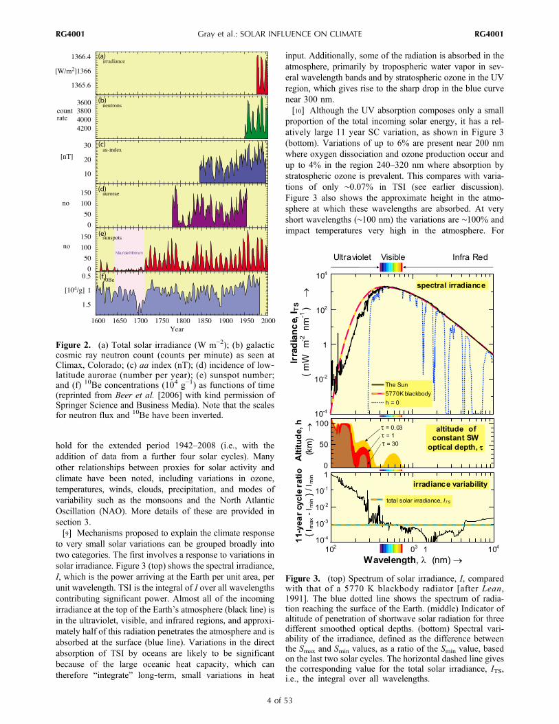
to very small solar variations can be grouped broadly intotwo categories. The first involves a response to variations insolar irradiance. Figure 3 (top) shows the spectral irradiance,I, which is the power arriving at the Earth per unit area, perunit wavelength. TSI is the integral of I over all wavelengthscontributing significant power. Almost all of the incomingirradiance at the top of the Earth’s atmosphere (black line) isin the ultraviolet, visible, and infrared regions, and approxi-mately half of this radiation penetrates the atmosphere and isabsorbed at the surface (blue line). Variations in the directabsorption of TSI by oceans are likely to be significantbecause of the large oceanic heat capacity, which cantherefore “integrate” long‐term, small variations in heat

input. Additionally, some of the radiation is absorbed in theatmosphere, primarily by tropospheric water vapor in sev-eral wavelength bands and by stratospheric ozone in the UVregion, which gives rise to the sharp drop in the blue curvenear 300 nm.[10] Although the UV absorption composes only a small

proportion of the total incoming solar energy, it has a rel-atively large 11 year SC variation, as shown in Figure 3(bottom). Variations of up to 6% are present near 200 nmwhere oxygen dissociation and ozone production occur andup to 4% in the region 240–320 nm where absorption bystratospheric ozone is prevalent. This compares with varia-tions of only ∼0.07% in TSI (see earlier discussion).Figure 3 also shows the approximate height in the atmo-sphere at which these wavelengths are absorbed. At veryshort wavelengths (∼100 nm) the variations are ∼100% andimpact temperatures very high in the atmosphere. For

Figure 3. (top) Spectrum of solar irradiance, I, comparedwith that of a 5770 K blackbody radiator [after Lean,1991]. The blue dotted line shows the spectrum of radia-tion reaching the surface of the Earth. (middle) Indicator ofaltitude of penetration of shortwave solar radiation for threedifferent smoothed optical depths. (bottom) Spectral vari-ability of the irradiance, defined as the difference betweenthe Smax and Smin values, as a ratio of the Smin value, basedon the last two solar cycles. The horizontal dashed line givesthe corresponding value for the total solar irradiance, ITS,i.e., the integral over all wavelengths.

Figure 2. (a) Total solar irradiance (W m−2); (b) galacticcosmic ray neutron count (counts per minute) as seen atClimax, Colorado; (c) aa index (nT); (d) incidence of low‐latitude aurorae (number per year); (e) sunspot number;and (f) 10Be concentrations (104 g−1) as functions of time(reprinted from Beer et al. [2006] with kind permission ofSpringer Science and Business Media). Note that the scalesfor neutron flux and 10Be have been inverted.


4 of 53

example, the Earth’s exosphere (∼500–1000 km above theEarth’s surface) has 11 year SC variations of ∼1000 K.However, we concentrate in this review on describingobservations and mechanisms that involve the atmospherebelow 100 km because at present there is little evidence tosuggest a downward influence on climate from regionsabove this. Transfer mechanisms from the overlying ther-mosphere have been proposed, such as through wavepropagation feedbacks suggested by Arnold and Robinson[2000]. However, there is little observational evidence forany significant influence, although this cannot be ruled out.[11] At stratospheric heights Figure 3 shows a variation of

∼6% at UV wavelengths over the SC. This region of theatmosphere has the potential to affect the troposphereimmediately below it and hence the surface climate. Esti-mated stratospheric temperature changes associated with the11 year SC show a signal of ∼2 K over the equatorialstratopause (∼50 km) with a secondary maximum in thelower stratosphere (20–25 km [see, e.g., Frame and Gray,2010]). The direct effect of irradiance variations is ampli-fied by an important feedback mechanism involving ozoneproduction, which is an additional source of heating [Haigh,1994; see also Gray et al., 2009]. The origins of the lowerstratospheric maximum and the observed signal that pene-trates deep into the troposphere at midlatitudes are less wellunderstood and require feedback/transfer mechanisms bothwithin the stratosphere and between the stratosphere andunderlying troposphere, further details of which are pro-vided in section 4.[12] The second mechanism category involves energetic

particles, including solar energetic particle (SEP) events andGCRs. Low‐energy (thermal) solar wind particles modulatethe thermosphere above 100 km via both particle precipi-tation and induced ionospheric currents. Whereas it is longer‐wavelength (lower‐energy) photons that deposit their energyin the upper atmospheric layers, it is the more energeticparticle precipitations that penetrate to lower altitudes. SEPsare generated at the shock fronts ahead of major solarmagnetic eruptions and penetrate the Earth’s geomagneticfield over the poles where they enter the thermosphere,mesosphere, and, on rare occasions, the stratosphere. Alarge fraction of SEP ions are protons (so events are alsoreferred to as “solar proton events” (SPEs)), but they areaccompanied by a wide spectrum of heavier ions [e.g.,Reames, 1999]. All cause ionization, dissociation, and theproduction of odd hydrogen and odd nitrogen species thatcan catalytically destroy ozone [e.g., Solomon et al., 1982;Jackman et al., 2008].[13] The idea that cosmic ray changes could directly

influence the weather originated with Ney [1959]. Althoughadmitting to some skepticism, Dickinson [1975] consideredthat modulation of GCR fluxes into the atmosphere by solaractivity might affect cloudiness and hence might be a viableSun‐climate mechanism. For instance, during Smin, the GCRflux is enhanced, increasing atmospheric ion production.Dickinson discussed ion‐induced formation of sulphateaerosol (which can act as efficient cloud condensation nuclei(CCN)) as a possible route by which the atmospheric ion

changes could influence cloudiness. A further GCR‐cloudlink has been proposed through the global atmosphericelectric circuit [e.g., Tinsley, 2000]. The global circuit cau-ses a vertical current density in fair (nonthunderstorm)weather, flowing between the ionosphere and the surface.This fair weather current density passes through stratiformclouds causing local droplet and aerosol charging at theirupper and lower boundaries. Charging modifies the cloudmicrophysics, and hence, as the current density is modulatedby cosmic ray ion production, the global circuit provides apossible link between solar variability and clouds.[14] While the testing of solar influence on climate via

changes in solar irradiance is relatively well advanced, theGCR cloud mechanisms have only just begun to be quan-tified. The connection between GCRs and CCN (the “ion‐aerosol clear air” mechanism) has recently been tested in aclimate model that calculates aerosol microphysics inresponse to GCR [Pierce and Adams, 2009]. They find thatGCR‐induced changes in CCN are 2 orders of magnitudetoo small to account for observed changes in cloud prop-erties. Quite apart from the sign or amplitude of the GCR‐cloud effects, the sign of the net effect on climate would alsodepend on the altitude of the cloud affected. For enhancedlow‐altitude cloud the dominant effect would be reflectionof incoming shortwave solar radiation (a cooling effect). Forenhanced high‐altitude cloud, the dominant effect would bethe trapping of reradiated, outgoing longwave radiation (awarming effect). Thus, if GCRs act to enhance low‐altitudecloud, the enhanced fluxes would lead to cooler surfacetemperatures during Smin and enhanced surface temperaturesduring Smax. This temperature change therefore has the samesense as that which would arise from a direct modulation byTSI. Solar modulation of climate by any of the proposedmechanisms described above may result in associatedchanges in cloudiness, so that any observational evidencelinking solar changes with cloud changes does not uniquelyargue for a solar effect through cosmic rays [Udelhofen andCess, 2001]. The current status of research into the variousmechanisms is described in more detail in section 4.[15] In the context of assessing the contribution of solar

forcing to climate change, an important question is whetherthere has been a long‐term drift in solar irradiance thatmight have contributed to the observed surface warming inthe latter half of the last century. Reconstructions of past TSIvariations have been employed in model studies and allowus to examine how the climate might respond to suchimposed forcings. The direct effects of 11 year SC irradi-ance variations are relatively small at the surface and aredamped by the long response time of the ocean‐atmospheresystem. However, model estimates of the response to cen-tennial time scale irradiance variations are larger since theaccumulated effect of small signals over long time periodswould not be damped to the same extent as decadal‐scaleresponses.[16] There are also large uncertainties in estimates of

long‐term irradiance changes (see section 2). The proxyquantities are indicators of magnetic activity on the Sun, andthere are problems relating these magnetic indicators to TSI.


5 of 53

For example, we know that TSI is greater at times of greatersunspot activity, but we do not know how much smaller theTSI was during extended periods when there were no sun-spots, e.g., during the Maunder Minimum. However, themost recent minimum, between solar cycles 22 and 23, wasunusually low and has provided a glimpse of what a grandminimum might look like.[17] Recent estimates [IPCC, 2007] (see Figure 4) suggest

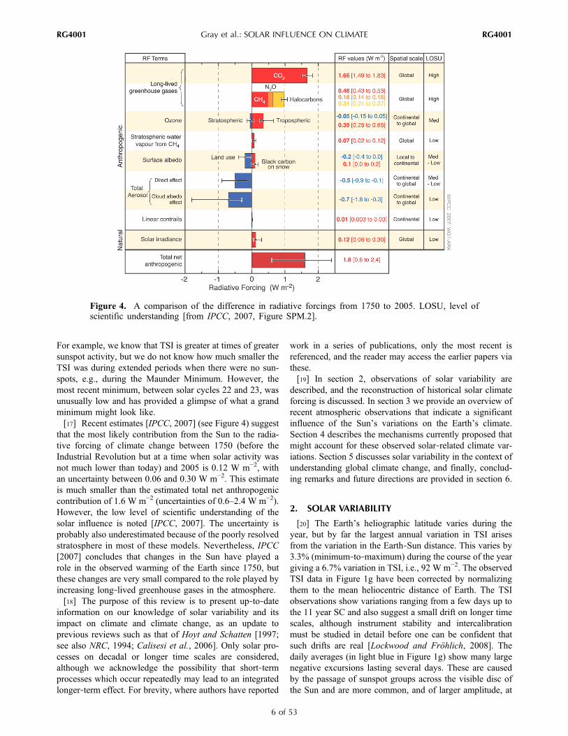
that the most likely contribution from the Sun to the radia-tive forcing of climate change between 1750 (before theIndustrial Revolution but at a time when solar activity wasnot much lower than today) and 2005 is 0.12 W m−2, withan uncertainty between 0.06 and 0.30 W m−2. This estimateis much smaller than the estimated total net anthropogeniccontribution of 1.6 W m−2 (uncertainties of 0.6–2.4 W m−2).However, the low level of scientific understanding of thesolar influence is noted [IPCC, 2007]. The uncertainty isprobably also underestimated because of the poorly resolvedstratosphere in most of these models. Nevertheless, IPCC[2007] concludes that changes in the Sun have played arole in the observed warming of the Earth since 1750, butthese changes are very small compared to the role played byincreasing long‐lived greenhouse gases in the atmosphere.[18] The purpose of this review is to present up‐to‐date

information on our knowledge of solar variability and itsimpact on climate and climate change, as an update toprevious reviews such as that of Hoyt and Schatten [1997;see also NRC, 1994; Calisesi et al., 2006]. Only solar pro-cesses on decadal or longer time scales are considered,although we acknowledge the possibility that short‐termprocesses which occur repeatedly may lead to an integratedlonger‐term effect. For brevity, where authors have reported

work in a series of publications, only the most recent isreferenced, and the reader may access the earlier papers viathese.[19] In section 2, observations of solar variability are

described, and the reconstruction of historical solar climateforcing is discussed. In section 3 we provide an overview ofrecent atmospheric observations that indicate a significantinfluence of the Sun’s variations on the Earth’s climate.Section 4 describes the mechanisms currently proposed thatmight account for these observed solar‐related climate var-iations. Section 5 discusses solar variability in the context ofunderstanding global climate change, and finally, conclud-ing remarks and future directions are provided in section 6.

2. SOLAR VARIABILITY

[20] The Earth’s heliographic latitude varies during theyear, but by far the largest annual variation in TSI arisesfrom the variation in the Earth‐Sun distance. This varies by3.3% (minimum‐to‐maximum) during the course of the yeargiving a 6.7% variation in TSI, i.e., 92 W m−2. The observedTSI data in Figure 1g have been corrected by normalizingthem to the mean heliocentric distance of Earth. The TSIobservations show variations ranging from a few days up tothe 11 year SC and also suggest a small drift on longer timescales, although instrument stability and intercalibrationmust be studied in detail before one can be confident thatsuch drifts are real [Lockwood and Fröhlich, 2008]. Thedaily averages (in light blue in Figure 1g) show many largenegative excursions lasting several days. These are causedby the passage of sunspot groups across the visible disc ofthe Sun and are more common, and of larger amplitude, at

Figure 4. A comparison of the difference in radiative forcings from 1750 to 2005. LOSU, level ofscientific understanding [from IPCC, 2007, Figure SPM.2].


6 of 53

Smax. The mean rotation period of the Sun as seen fromEarth is 27 days, and so a sunspot group lasting severalrotations can cause several of these negative excursionslasting almost 13 days each. On the other hand, thebrightening effect of faculae is contributed by many smallfeatures that are more uniformly spread over the solar disc(but are brighter when seen closer to the limb). As a result,the faculae effects are less visible in solar rotations, and themain variation is the 11 year SC.

2.1. Causes of TSI Variability[21] Recent research indicates that variability in total solar

irradiance associated with the 11 year SC arises almostentirely from the distribution of sizes of the patches wheremagnetic field threads through the visible surface of the Sun(the photosphere). The advent of solar magnetographs,measuring the line‐of‐sight component of the photosphericfield by exploiting the Zeeman effect, has revolutionized ourunderstanding of how these vary over the SC [Harvey,1992]. Spruit [2000], for example, has developed the theoryof how these photospheric magnetic fields influence TSI.The dominant effect for large‐diameter (greater than about250 km) magnetic flux tubes is that they inhibit the con-vective upflow of energy to the surface and cause cool, darksunspots with a typical temperature of TS ≈ 5420 K (aver-aged over umbral and penumbral areas) compared with themore typical value of the quiescent photospheric temperatureof TQS ≈ 6050 K. The blocked energy is mainly returned tothe convection zone which, because it has such a hugethermal capacity, is not perturbed. However, a small fractionof the blocked energy may move around the flux tube andenhance the surface intensity in a slightly brighter ringaround the spot with effective photospheric temperatureTBR ≈ 6065 K.[22] The key difference between sunspots and the mag-

netic flux tubes called faculae is that the magnetic flux tubediameter is smaller for faculae. This allows the temperatureinside smaller flux tubes to be maintained by radiation fromthe tube walls, and the enhanced magnetic pressure withinthe tube means that density is reduced in pressure equilib-rium. This allows radiation to escape from lower, hotterlayers in a facula, so that the effective temperature is in theregion of Tf ≈ 6200 K (see review by Lockwood [2004]).The additional brightness is greatest near the solar limbwhere more of the bright flux tube walls are visible [e.g.,Topka et al., 1997]. Because the ratio of the total areas of theSun’s surface covered by faculae and by sunspots hasremained roughly constant over recent solar cycles [e.g.,Chapman et al., 2001] and because the net effect of faculaeis approximately twice that of sunspots, the TSI is increasedat Smax [Foukal et al., 1991; Lean, 1991]. The facularcontribution is made up of many smaller flux tubes, andhence, the net brightening they cause is a smoother variationin both time and space than the darkening effect of the lessnumerous but bigger sunspots.[23] The variation of the effect of faculae is often quan-

tified using emissions from the overlying bright regions inthe chromosphere, the thin layer of the solar atmosphere

immediately above the photosphere [e.g., Fröhlich, 2002].These bright spots in the chromosphere are called plages,and they lie immediately above photospheric faculae. Theireffect is thought to be quantified by the Mg ii line “core‐to‐wing” index (see Figure 1d). Faculae contribute to TSIincreases whether they are around sunspots in active regionsor in other regions of the Sun’s surface [Walton et al., 2003].Sunspots and faculae are two extremes of a continuousdistribution of flux tube sizes: at intermediate sizes, fluxtubes form micropores which appear bright near the limb,like faculae, but dark near the center of the solar disk, likespots.[24] An additional source of TSI and solar spectral irra-

diance (SSI) variability has been proposed. These are called“shadow” effects and are associated with magnetic fieldsbelow the photosphere in the convection zone (CZ) inter-rupting the upflow of energy [Kuhn and Libbrecht, 1991]. Itis now thought that solar magnetic field is generated andstored just below the CZ in an “overshoot layer” whichextends into the radiation zone beneath (see reviews byLockwood [2004, 2010]). This blocks upward heat flux, butthe huge time constant of the CZ above it means that var-iations on time scales shorter than about 106 years would notbe seen. The stored field can bubble up through the CZ(breaking through the surface in sunspots and faculae) in aninterval of only about 1 month. Thus, it is thought that theflux below (but not threading) the photosphere, yet closeenough to it to give shadow effects on decadal and cen-tennial time scales, would be small. An interesting test ofthis may well be provided by the exceptionally low TSIvalues being observed at the time of writing (late 2009). Ifthese are not fully explained by the loss of solar minimumfaculae, we would need to invoke shadow and associatedsolar radius effects as well as the known effects of surfaceemissivity in sunspots and faculae.

2.2. Decadal‐Scale Solar Variability

2.2.1. Total Solar Irradiance[25] TSI has been monitored continuously from space

since 1977. The individual TSI monitors have operated foronly limited intervals so a combination of data from severaldifferent instruments is required to compile a continuousdata set. This means that intercalibration of those instru-ments, and how they change with time as the instrumentsdegrade, is a key issue in the compilation of a compositedata set. There are many corrections that are needed [e.g.,Fröhlich, 2006].[26] Figures 5a–5c show a comparison of the three main

TSI composites: Institut Royal Meteorologique Belgique(IRMB) [Dewitte et al., 2004], Active Cavity RadiometerIrradiance Monitor (ACRIM) [Willson and Mordvinov,2003], and Physikalisch‐Meteorologisches ObservatoriumDavos (PMOD) [Fröhlich, 2006]. All three use time seriesof the early data from the Hickey‐Frieden (HF) Radiometerinstrument on the Nimbus 7 satellite and the ACRIM I andII instruments (on UARS and ACRIMsat, respectively) untilearly 1996. The IRMB composite is constructed by firstreferring all data sets to the Space Absolute Radiometric


7 of 53

Reference [Crommelynck et al., 1995], although this abso-lute calibration has recently been called into questionbecause the Total Irradiance Monitor instrument on theSORCE satellite has obtained values about 5 W m−2 lower[Kopp et al., 2005]. After 1996 the ACRIM compositecontinues to use ACRIM II supplemented by ACRIM III,

whereas the PMOD composite uses data from the Variabilityof Solar Irradiance and Gravity Oscillations (VIRGO)instrument on the SoHO spacecraft (specifically the Dif-ferential Absolute Radiometer (DIARAD) and PM06 cavityradiometer data), and IRMB uses just the DIARAD VIRGOdata. Besides the different time series used after 1996(during solar cycle 23), the main difference is the way thedata have been combined and corrected.[27] The most significant difference between the PMOD,

IRMB, and ACRIM composites is in their long‐term trends.Figure 5d shows the largest and most significant disagree-ment, which is that between the PMOD and ACRIM com-posites [Lean, 2006; Lockwood and Fröhlich, 2008]. Therapid relative drift between the two before 1981 arisesbecause although both employ the Nimbus HF data, ACRIM(like IRMB) has not used the reevaluation of the earlydegradation of the HF instrument. The second major dif-ference is a step function change within what is termed the“ACRIM gap” between the loss of the ACRIM I instrumentin mid‐1989 and the start of the ACRIM II data late in 1991.Both the ACRIM and the PMOD composites use theNimbus HF data for this interval as these are the bestavailable data for this interval. The HF data series showsseveral sudden jumps attributable to changes in the orien-tation of the spacecraft and associated with switch‐off andswitch‐on. PMOD makes allowance for such a jump in theACRIM gap, but the ACRIM composite does not, whichgives rise to the step change in late 1989 and accounts forvirtually all of the difference between the long‐term drifts ofthe two composites over the first two solar cycles [seeFröhlich, 2006; Lockwood, 2010, and references therein].[28] Additional support for the inclusion of the glitch

effect in the PMOD composite has recently come from ananalysis of solar magnetogram data [Wenzler et al., 2006].In recent years, modeling has developed to the point where>93% of the TSI variation observed by the SoHO satellitehas been reproduced by sorting pixels of the correspondingmagnetograms into five photospheric surface classifications(sunspot umbra; sunspot penumbra; active region faculae;network faculae; and the quiet, field‐free Sun). Each pixel isthen assigned a time‐independent spectrum for that classi-fication on the basis of a model of the surface in question, asdeveloped by Unruh et al. [1999]. From this and the disclocation, the intensity can be estimated, and the TSI iscomputed by summation over the whole disc [Krivova et al.,2003]. This work has further developed into the so‐calledfour‐component Spectral and Total Irradiance Reconstruc-tions (SATIRE) model [Solanki, 2002; Krivova et al., 2003].Figure 6 shows a scatterplot of the daily TSI values for1996–2002 derived by this method using magnetogramsfrom the Michelson Doppler Interferometer (MDI) instru-ment on board the SoHO spacecraft, as a function of thesimultaneous TSI value observed by the VIRGO instrument,also on SoHO. The agreement is exceptional: the correlationcoefficient is 0.96, and the best fit linear regression (dashedmauve and orange line) is very close to ideal agreement(light blue). Recently, Wenzler et al. [2006] have extendedthis analysis to ground‐based magnetograms. This is not

Figure 5. Composites of total solar irradiance 1978–2007:(a) PMOD (TSIPMOD), (b) ACRIM (TSIACRIM), and (c) IRMB(TSIIRMB). Colored lines show daily values, with color indi-cating the instrumental source. Thick black lines indicate81 day running means. Horizontal black lines drawn throughthe minimum around 1985 (between solar cycles 21 and 22)to highlight the trends in minimum values of the composites.For each plot the bottom horizontal scale gives the year, andthe top scale gives the day number, where day 1 is 1 January1980. (d) Difference between the PMOD and ACRIM com-posites, TSIPMOD – TSIACRIM. Grey line indicates dailyvalues; black line indicates 81 day running means. Duringseveral intervals, the gray line is hidden behind the blackline because the two composites employ data from the sameinstruments (but the difference is not zero as they apply dif-ferent calibrations).


8 of 53

trivial because additional factors such as (partial) cloudcover must be corrected for. The use of ground‐based data issignificant as it extends the interval which can be studiedback to 1979 so that it covers the same interval as theACRIM and PMOD composites (including the ACRIMgap).[29] These TSI model reconstructions are so accurate that

they provide a definitive test of the solar surface contribu-tion to the various TSI composites. They confirm that unlessshadow effects are significant, the PMOD composite is moreaccurate and that the ACRIM composite is in error becauseit fails to account for the Nimbus HF pointing anomalyduring the ACRIM gap [Lockwood and Fröhlich, 2008].Note that this conclusion does not depend on tuning theSATIRE model to the PMOD composite: the model hasonly one free fit parameter, and the glitch in the ACRIM gapcannot be matched even if the ACRIM composite is used totune the model.[30] To understand the implications of this correction,

note that in Figures 5a and 5b the PMOD composite gives adecline in TSI since 1985 [Lockwood and Fröhlich, 2007],whereas the ACRIM composite gives a rise up until 1996and a fall since then [Lockwood, 2010]. The differencearises entirely from the pointing direction glitch during theACRIM gap. The PMOD composite trend matches that inthe sunspot number, whereas the ACRIM composite trendmatches that in the galactic cosmic ray counts. Hence, thelong‐term trend in the PMOD composite is in the samedirection as the solar cycle variation, whereas the ACRIMcomposite trend is in the opposite direction (remember thatTSI peaks at sunspot maximum when the GCR flux is aminimum). To explain this inconsistency of the ACRIMcomposite would require two competing effects in therelationship between TSI and GCR fluxes that work inopposite directions, such that the TSI and GCR fluxes are

anticorrelated on time scales of the 11 year SC and shorter,yet are correlated on time scales longer than the 11 year SC.The PMOD TSI data have fallen to unprecedentedly lowlevels during the current solar minimum, although estimatesvary on the magnitude of this decline [Lockwood, 2010].The mean of the PMOD TSI composite for September 2008is 1365.1 W m−2, which is lower than that for the previousminimum by more than 0.5 W m−2.2.2.2. Spectral Irradiance[31] Measurements of SSI were made by the Solar Stellar

Irradiance Comparison Experiment and Solar UV SpectralIrradiance instruments on the UARS satellite in the 1980sand 1990s. They revealed variations of the order of a fewpercent in the near UV over an 11 year SC. The launch ofthe SORCE satellite in 2003 carrying the Spectral IrradianceMonitor (SIM) has provided the first measurements of SSIacross the whole spectrum from X‐ray to near IR. Themeasurements suggest that over the declining phase of thesolar cycle between 2004 and 2007 there was a much larger(factor of 4–6) decline in UV than indicated in Figure 3, andthis is partially compensated in the TSI variation by anincrease in radiation at visible wavelengths [Harder et al.,2009]. These observed changes to the shape of the solarspectrum variations were completely unexpected, and ifcorrect they will require the associated temperature and ozoneresponses to be reassessed (see also sections 4.2.1 and 5).[32] For longer time periods, reconstructions of SSI can be

made using multicomponent models. For example, theSATIRE modeling concept can be applied independently todifferent spectral wavelengths, and so the variability withinthe irradiance spectrum can be estimated. The mainrequirement is that the contrasts of the different types ofsolar surface be known at each wavelength [Unruh et al.,2008]. Work at present is aimed at improving our knowl-edge of the short UV wavelengths, which is required foraccurate modeling of irradiance absorption in the strato-sphere and upper atmosphere (see Figure 3). Improvementsmade to date suggest that UV irradiance during the MaunderMinimum was lower by as much as a factor of 2 at andaround the Ly‐a wavelength (121.6 nm) compared to recentSmin periods and up to 5%–30% lower in the 150–300 nmregion [Krivova and Solanki, 2005]. However, this work isstill in its infancy. The model estimates match observedspectra between 400 and 1300 nm very well but begin to failbelow 220 nm and also for some of the strong spectral lines.[33] Interestingly, the large change observed by the

SORCE SIM instrument was not reflected in TSI, the Mg iiindex, F10.7, nor existing models of the UV variation. Theimplications are not yet clear, but these recent data open upthe possibility that long‐term variability of the part of the UVspectrum relevant to ozone production is considerably largerin amplitude and has a different temporal variation comparedwith the commonly used proxy solar indices (Mg ii index,F10.7, sunspot number, etc.) and reconstructions.

2.3. Century‐Scale Solar Variability[34] Apart from a few isolated naked eye observations

by ancient Chinese and Korean astronomers, sunspot data

Figure 6. Scatterplot of daily values of TSI, as simulatedfrom SoHO MDI magnetograms using the SATIRE proce-dure, as a function of the simultaneous value observed bythe VIRGO instrument on SoHO. Data are for 1996–2002;correlation coefficient is 0.96. Dashed mauve and orangeline indicates the best least squares linear regression fit; lightblue line indicates the ideal line of perfect agreement.


9 of 53

series only extend back to the invention of the telescope(around 1610), and well‐calibrated systematic measurementsonly began about 100 years later. However, solar variabilityon time scales of centuries to millennia can be reconstructedusing cosmogenic radionuclides such as 10Be and 14C whoseproduction rate in the atmosphere is modulated by solaractivity. In this way, at least the past 10,000 years can bereconstructed [Vonmoos et al., 2006], although the temporalresolution is poorer, signal‐to‐noise ratio is lower, and therecord must be corrected for variations in the geomagneticfield. Recently, Steinhilber et al. [2009] derived from 10Bethe first TSI record covering almost 10,000 years. First,they calculated the interplanetary magnetic field (IMF)necessary to explain the observed production changescorrected for the geomagnetic dipole effects. They thenused the relationship between instrumental IMF and TSIdata during sunspot cycle minima to derive an estimate ofthe TSI record.[35] Sunspot numbers clearly reveal trends in solar mag-

netic phenomena, e.g., during the first half of the twentiethcentury. There are also clear indications of cycles longerthan the 11 year SC, e.g., the Gleissberg cycle (80–90 years)with variable amplitudes. The cosmogenic radionuclidesconfirm the existence of these and other longer periodicities(e.g., 208 year DeVries or Suess cycle, 2300 year Hallstatt

cycle, and others) and also the present relatively high levelof solar activity, although there is some controversy as tohow unusually high it really is [Muscheler et al., 2007;Usoskin et al., 2004; Steinhilber et al., 2008].[36] Periodicities, trends, and grand minima are features

of solar activity which, if detectable in climate records, canbe used to attribute climate changes to solar forcing [Beeret al., 2000; Beer and van Geel, 2008]. However, one mustbe aware that this may not always work well because thereare other forcings as well and the climate is a nonlinearsystem which can react in a variety of ways. There are twocommon methods employed to estimate TSI variations. Oneis based on sunspot numbers and chromospheric indices toquantify sunspot darkening and facular brightening, respec-tively [Fröhlich, 2006]. The second uses solar magneto-grams and the SATIRE irradiance modeling [Wenzler et al.,2006]. While both are very successful in explaining short‐term TSI changes over the past 3 decades [Solanki et al.,2005], it is not yet clear to what extent TSI has changedon multidecadal to centennial time scales [Krivova et al.,2007], for example, to what extent TSI and SSI are reducedduring the Maunder Minimum, although estimates haveconverged somewhat in recent years.[37] Through the sunspot record we have good informa-

tion about the effect of sunspot darkening on TSI on thesetime scales. Unfortunately, we have no direct measurements,nor even a proxy indicator, of the corresponding variationof facular brightening on these time scales, nor of the cor-responding effect in the overlying chromosphere that mod-ulates UV emission. As mentioned in section 2.1, therecould be effects of magnetic fields deeper in the convectionzone, the so‐called shadow effects, and there may be smallsolar radius changes [Lockwood, 2010]. The SATIREmodeling has shown that surface emissivity effects explainrecent solar cycles in TSI rather well, and these shadow (andsolar radius) effects are not significant effects over the past30 years or so. However, this does not eliminate them asfactors on longer time scales.[38] Several reconstructions of TSI variations on century

time scales have been made (see Figure 7) on the basis of avariety of proxies including the envelope of the sunspotnumber cycle R [Reid, 1997]; the length of the sunspotcycle, L [Hoyt and Schatten, 1993]; the structure and decayrate of individual sunspots [Hoyt and Schatten, 1993]; theaverage sunspot number R and/or the group sunspot numberRG [Hoyt and Schatten, 1993; Zhang et al., 1994; Reid,1997; Krivova et al., 2007]; the solar rotation and diame-ter [Nesme‐Ribes et al., 1993; Mendoza, 1997]; a combi-nation of R and its 11 year running mean, R11 [e.g., Lean,2000a, 2000b], or a combination of R and L [e.g., Solankiand Fligge, 2000]; sunspot group areas [Fligge andSolanki, 1998]; Greenwich sunspot maps [Lockwood,2004]; p mode amplitudes (estimated from R) [Bhatnagaret al., 2002]; cosmogenic isotopes deposited in terrestrialreservoirs [Bard et al., 2000; Steinhilber et al., 2009]; andthe open magnetic flux of the Sun derived from geomagneticactivity data [Lockwood, 2002].

Figure 7. Reconstructions of past variations in TSI usingdifferent solar proxies. Hoyt and Schatten [1993] estimatesare based on solar cycle length, L. Solanki and Fligge [1999,2000] used the annual sunspot number, R (available back to1713, dashed line). Lean et al. [1995] and Lean [2000a]used a combination of the group sunspot number RG

(available back to 1611) and its 11 year running mean. Inthese early reconstructions, the amplitude of the slowlyvarying component was derived by comparison of themodern‐day Sun and Maunder Minimum Sun with dis-tributions of cyclic and noncyclic Sun‐like stars. Lockwoodand Stamper [1999] used the observed, but unexplained,correlation between the variations of TSI and the opencoronal source flux on decadal time scales [Lockwood,2002]. Wang et al. [2005] used a solar magnetic fluxtransport model constrained to fit the observed open solarflux variation [Lockwood et al., 1999]: the prediction pre-sented here allows for a secular variation of ephemeralmagnetic flux. Foster [2004] and Lockwood [2004] usedGreenwich sunspot observations (available back to 1874).Krivova et al. [2007] used RG.


10 of 53

[39] For most of the early reconstructions (specificallythose by Lean et al. [1995], Lean [2000a, 2000b], Solankiand Fligge [1999, 2000], and Hoyt and Schatten [1993])the change in mean TSI between the Maunder Minimumand recent decades was estimated using the observed dis-tribution of the brightness of Sun‐like stars in their chro-mospheric emissions. This scaling assumed that brighterSun‐like stars (of similar age and chemical abundance to theSun) show a decadal‐scale activity cycle and are analogousto the present‐day Sun, whereas the less bright stars werefound to be noncyclic and are analogous to the Sun duringits Maunder Minimum state. The use of such stellar analogsfor estimating the long‐term changes in TSI was based onthe work of Baliunas and Jastrow [1990], who surveyedobservations of Sun‐like stars. However, recent surveyshave not reproduced their results and suggest that theselection of the original set may have been flawed [Hall andLockwood, 2004; Giampapa, 2004]. Thus, the extent of thepositive drift in TSI between the Maunder Minimum and thepresent day is uncertain.[40] Some authors suggest there may be no actual change

[Foukal et al., 2004], while others suggest a long‐termpositive drift which is smaller than previously estimated[Lean et al., 2002] (see, e.g., the Krivova et al. [2007]estimate in Figure 7). There are, however, two reasons tobelieve that the latter is the most likely. First, there is acorrelation of TSI with open solar flux [see, e.g., Lockwood,2002]. The numerical modeling of emerged flux transportand evolution [e.g., Wang et al., 2005] suggests that thelong‐term drift in open flux is matched by a similar drift inthe TSI [see also Krivova et al., 2007]. Second, Lockwoodand Fröhlich [2007] have recently demonstrated that thereis a coherent variation between the minimum TSI and themean sunspot number R11, as employed by Lean et al.[1995, 2002] (although the TSI data sequence is short andcovers only three solar minima, so that extrapolating back tothe Maunder Minimum is full of uncertainty). Between 1985and 2007, R11 fell from 83 to 63, and the Smin value in 2007is 0.39 W m−2 lower than that in the 1985 minimum. Linearextrapolation gives a value of TSI in the Maunder Minimum(R11 = 0) that is 1.6 W m−2 lower than the 1985 Smin value.

This agrees well with the field‐free irradiance estimated byFoster [2004] and Lockwood [2004] and with the reconstruc-tions by Lean [2000a] and Lockwood and Stamper [1999](also shown in Figure 7). Krivova et al. [2007] used sun-spot data and the open flux modeling of Solanki et al. [2002]and found a value of 1.3 W m−2 with an uncertainty range of0.9–1.5 Wm−2, which is similar to but slightly lower than theabove estimate. These estimates for century‐scale TSIchanges of ∼0.9–1.6 W m−2 correspond to a change inmean global radiative forcing of only 0.16–0.28 W m−2.

2.4. TSI and Galactic Cosmic Rays[41] Paleoclimate studies have revealed links between

cosmogenic isotopes and climate indicators. For example,one very striking result, shown in Figure 8, is due toNeff et al.[2001], who correlated the d18O from a stalagmite in a cavein northern Oman with theD14C from tree rings. They arguethat d18O is a good proxy for monsoonal rainfall in thatregion, while D14C is a proxy for solar activity derived fromthe abundance of 14C found in ancient tree trunks around theworld. The remarkable similarity between the d18O andD14C time series has been interpreted to indicate a north-ward shift in the Intertropical Convergence Zone (ITCZ),which is believed to have been a controlling influence on thestrength of the monsoon at the stalagmite location, whichplays a key role in its formation. It is usually assumed thatthe link between cosmogenic isotopes and climate indicatorsarises because the cosmogenic isotopes are inversely cor-related with TSI [e.g., Bond et al., 2001; Neff et al., 2001].Indeed, Bard et al. [2000] and Steinhilber et al. [2010] haveused cosmogenic nuclides to reconstruct TSI over the past1200 years. Figure 9 demonstrates that such an anti-correlation exists over recent solar cycles in both monthlyand annual mean data. Comparison of Figures 7 and 2shows that this anticorrelation is also predicted on centurytime scales by most TSI reconstructions [Lean et al., 1995].[42] The processes by which the Sun’s magnetic field

modulates GCR fluxes are complex. However, simpleanticorrelations [e.g., Rouillard and Lockwood, 2004] sug-gest that much of the variation (∼75%) of the GCR flux atEarth is explained by the open solar flux, FS. The productionrate of 10Be and other cosmogenic radionuclides in theatmosphere is directly proportional to the flux of cosmic rayprotons with energy from 1 to 3 GeV. On decadal to cen-tennial time scales it is dominated by solar activity; onlonger time scales it is dominated by the geomagnetic dipolefield [Masarik and Beer, 2009]. After production, on theway from the atmosphere to the polar ice caps, 10Be isinfluenced by changes in climate. However, comparisonbetween Greenland and Antarctic records, as well as mod-eling, shows that these effects are relatively small for pro-duction changes on decadal and longer time scales [Heikkiläet al., 2009] but become increasingly more serious forannual resolution. Another issue is the accuracy of ice corescovering thousands of years. Hence, there are severalcomplications in interpreting these indirect measures ofsolar irradiance.

Figure 8. The d18O time series from the Hoti cave in north-ern Oman compared with D14C [from Neff et al., 2001].


11 of 53

[43] The connection between GCR and TSI is anothermethod for reconstructing TSI, with the potential toencompass recent millennia using cosmogenic isotopemeasurements [Usoskin et al., 2003; Solanki et al., 2004].However, there is a key unknown parameter: the averagequiet Sun photospheric field [B]QS at sunspot minimumduring the Maunder Minimum [see Lockwood, 2004].[44] In summary, a number of studies have demonstrated

that cosmogenic isotopes may indeed provide a proxyindicator of long‐term TSI variations. The TSI does not varylinearly with cosmogenic isotopes, but it does vary mono-tonically with the isotope production rate [Lockwood, 2006].We note, however, that the available observational data setis of the polar deposition of 10Be and not of the actualproduction rate P[10Be]. The production is influenced byadditional factors such as geomagnetic activity and geo-magnetic field strength, for which the data can be adjusted,and the abundance in any one terrestrial reservoir is alsomodified by climate‐induced changes in deposition rate,which is more difficult to estimate and account for. How-ever, these are usually checked for using a combination ofthe 10Be and 14C (and other) cosmogenic isotopes becausetheir deposition and history is so different they cannot beinfluenced in the same way by climate changes. Because14C is exchanged with the biomass and oceans in the carboncycle it does not show the SC variation seen in 10Be

abundances; however, centennial‐scale changes in the twogenerally match very closely.

3. CLIMATE OBSERVATIONS

[45] Perhaps the first place to look for solar impact on theEarth’s climate is in the upper atmosphere because it inter-acts most directly with the radiation, particles, and magneticfields emitted by the Sun. Solar signals in the stratosphereare relatively large and well documented during the past few11 year SCs since satellite observations became widespreadand are described in section 3.1. We then move down in theatmosphere and describe the 11 year SC signals in the tro-posphere (section 3.2) and the surface (section 3.3). Finally,because of its inertia and slow feedback mechanisms, theclimate system is also sensitive to long‐term solar changes,and an overview of these observations is provided insection 3.4.

3.1. Decadal Variations in the Stratosphere

3.1.1. Stratospheric Ozone[46] Ozone is the main gas involved in radiative heating

of the stratosphere. Solar‐induced variations in ozone cantherefore directly affect the radiative balance of the strato-sphere with indirect effects on circulation. Solar‐inducedozone variations are possible through (1) changes in solarUV spectral solar irradiance, which modifies the ozone

Figure 9. The anticorrelation of GCR fluxes with the TSI since 1978. Variations of (top left) PMOD TSIcomposite and (bottom left) counts, C, detected by the neutron monitor at Climax. The grey line indicatesdaily values, and the black line indicates the monthly means. (right) Scatterplot of TSI as a function of C.Grey points are monthly means; black diamonds are annual means. The best fit linear regression to theannual data is also plotted. The correlation coefficients (and significance levels) are −0.68 (99.99%)and −0.85 (91.5%) for monthly and annual data, respectively (reprinted from Lockwood [2006] withkind permission of Springer Science and Business Media).


12 of 53

production rate through photolysis of molecular oxygen,primarily in the middle to upper stratosphere at low latitudes[Haigh, 1994], and (2) changes in the precipitation rate ofenergetic charged particles, which can indirectly modifyozone concentrations through changes in the abundance oftrace species that catalytically destroy ozone, primarily atpolar latitudes [e.g., Randall et al., 2007]. In addition,transport‐induced changes in ozone can occur [e.g.,Hood andSoukharev, 2003;Rind et al., 2004; Shindell et al., 2006;Grayet al., 2009] as a consequence of indirect effects on circulationcaused by the above two processes.[47] On the 11 year time scale, the mean irradiance near

200 nm has varied by ∼6%, over the past two solar cycles

(see Figure 3). Figure 10 shows the mean solar cycle ozonevariation as a function of latitude and altitude obtained froma multiple regression statistical analysis of SAGE satellitedata for 1985–2003, excluding several years following theMt. Pinatubo volcanic eruption [see also Chandra andMcPeters, 1994; McCormack and Hood, 1996; Soukharevand Hood, 2006; Randel and Wu, 2007]. In the upperstratosphere where solar UV variations directly affect ozoneproduction rates, a statistically significant response of 2%–4% is evident. Positive responses are also present at middleand higher latitudes in the middle stratosphere and in thetropics below the 20 hPa level. A statistically insignificantresponse is obtained in the tropical middle stratosphere. Thelower stratospheric ozone response occurs at altitudes whereozone is not in photochemical equilibrium and the ozonelifetime exceeds dynamical transport time scales, whichimplies that these ozone changes are induced by changes intransport arising from a secondary dynamical response (seealso section 4).[48] The density‐weighted height integral of ozone at each

latitude gives the “total column” ozone, and a clear decadaloscillation in phase with the 11 year solar cycle is evident inboth satellite data [Soukharev and Hood, 2006] and ground‐based (Dobson) data; the latter show a signal going back atleast to the middle 1960s (four cycles) [Chipperfield et al.,2007; see also Zerefos et al., 1997]. The ozone responsein the lower stratosphere is believed to be the main cause ofthe total column ozone signal because of the high numberdensities at those levels.3.1.2. Stratospheric Temperaturesand Winds[49] There is also statistically significant evidence for

11 year SC variations in stratospheric temperature and zonalwinds. Figure 11 shows the temperature signal estimated

Figure 10. Annual averaged estimate of Smax minus Smin

ozone differences (%) from a multiple regression analysisof SAGE II ozone data for the 1985–2003 period. Shadedareas are significant at the 5% level [from Soukharev andHood, 2006].

Figure 11. Annual averaged estimate of Smax minus Smin temperature difference (K) derived from amultiple regression analysis of the European Centre for Medium Range Weather Forecasts (ECMWF)Reanalysis (ERA‐40) data set (adapted from Frame and Gray [2010]). Dark and light shaded areasdenote statistical significance at the 1% and 5% levels, respectively.


13 of 53

from a multiple regression analysis of European Centre forMedium Range Weather Forecasts (ECMWF) reanalysis(ERA‐40) data, in which observations have been assimilatedinto model data [Frame and Gray, 2010; see also Crooksand Gray, 2005; Shibata and Deushi, 2008]. A maximumresponse of ∼2 K is found in the tropical upper stratosphere,at around the level of the maximum percentage ozoneresponse in Figure 10. Estimates suggest that approximatelyhalf of this signal is the direct result of solar irradiancechanges and half is due to the additional ozone feedbackmechanism [e.g., Gray et al., 2009]. A second statisticallysignificant response is seen in the tropical and subtropicallower stratosphere, similar to the ozone regression result ofFigure 10. As in the ozone analysis, the lower stratospherictemperature response is indicative of a large‐scale dynami-cal response, e.g., changes in net equatorial upwelling rates[Shibata and Kodera, 2005; Gray et al., 2009].[50] An alternative approach to estimating the 11 year SC

temperature signal has been to directly analyze the satelliteobservations, which are recalibrated data from the TIROSOperational Vertical Sounder (TOVS) infrared radiometers[Scaife et al., 2000; Randel et al., 2009]. This approach hasthe advantage of avoiding model influences and minimizinginstrument intercalibration errors that were not taken intoaccount by the ERA‐40 (or National Centers for Environ-mental Prediction (NCEP)) reanalysis data sets. On the otherhand, the TOVS data have a somewhat lower vertical res-olution of ∼10 km. The TOVS data analysis yields a reducedresponse in the upper stratosphere of ∼1.1 K, and theresponse is much broader in height, decreasing monotoni-cally to ∼0.5 K in the lower stratosphere, without the two-fold maximum in the tropical middle stratosphere that isevident in Figure 11. This difference may be due to the lowvertical resolution of the TOVS observations [Gray et al.,2009], or it may be a spurious feature of the regressiontechnique [Lee and Smith, 2003; Smith and Matthes, 2008].[51] There is also an 11 year SC signal in zonal wind

fields. Figure 12 shows a strong positive zonal wind

response in the ERA‐40 regression analysis in the sub-tropical lower mesosphere and upper stratosphere, whichhas been shown to come predominantly from the wintersignal in each hemisphere [Crooks and Gray, 2005; Frameand Gray, 2010]. This lower mesospheric subtropical jetresponse near winter solstice had also been noted in previ-ous analyses of rocketsonde and NCEP data [Kodera andYamazaki, 1990; Hood et al., 1993]. The zonal windanomaly is observed to propagate downward with time overthe course of the winter [Kodera and Kuroda, 2002], andwave‐mean‐flow interactions are likely involved in pro-ducing this response [Kodera et al., 2003].[52] As already noted in section 1 there is an added

complication from the QBO [Labitzke, 1987; Labitzke andvan Loon, 1988; Labitzke et al., 2006]. Figure 13 showsan updated version of Labitzke’s original results, whichshow a clear dependence of North Pole (NP) 30 hPa geo-potential heights on the 11 year SC, provided the observa-tions are first grouped into QBO phase. In QBO easterlyyears (QBO‐E), the 30 hPa (∼24 km) NP geopotential heightdecreases with increasing solar activity, whereas in QBOwesterly years (QBO‐W) it increases with increasing solaractivity. Increased geopotential height at 30 hPa implies anincrease in the mean temperature below that pressure leveland vice versa. There is a well‐known “Holton‐Tan” rela-tionship between the equatorial QBO and the NP geopo-tential height and temperatures [Holton and Tan, 1980,1982]. In general, the QBO‐E years (i.e., when the lowerstratospheric winds are from the east) tend to favor awarmer, more disturbed Northern Hemisphere (NH) polarvortex than the QBO‐W phase, with frequent large‐scalewave disturbances to the vortex, known as stratosphericsudden warmings (SSWs). However, SSWs are by no meansexclusive to the QBO‐E phase. When they do occur in theQBO‐Wphase, they occur almost exclusively during an Smax

period, so that SSWs tend to be favored in Smin–QBO‐E andSmax–QBO‐W years. Labitzke and van Loon [1988] havesuggested that the Holton‐Tan relationship actually reverses

Figure 12. Annual averaged Smax minus Smin differences in zonally averaged zonal wind (m s−1) fromthe ground to 0.1 hPa (∼65 km) derived from a multiple regression analysis of the ERA‐40 data set(adapted from Frame and Gray [2010]). Dark and light shaded areas denote statistical significance atthe 1% and 5% levels, respectively. Contour values are 0, ±0.5, ±1, ±2, and ±3 m s−1 and a contourinterval of 2 m s−1 thereafter. Solid (dotted) contours denote positive (negative) values, and the dashedline is zero.


14 of 53

during Smax periods, although Gray et al. [2001] find onlythat it is disrupted [see also Naito and Hirota, 1997; Campand Tung, 2007]. There is also a suggestion that the periodof the QBO in the equatorial lower stratosphere is modu-lated by the 11 year solar cycle, with a longer QBO‐Wphase during Smax than during Smin years [Salby andCallaghan, 2000, 2006; see also Pascoe et al., 2005],although this has been questioned by Hamilton [2002] andmore recently by Fischer and Tung [2008].[53] Although most observational studies have focused on

the NH winter period, the 11 year SC is evident in bothhemispheres and all seasons. Figure 14 shows high corre-lations in the NH summer between 10.7 cm solar flux anddetrended 30 hPa temperatures. Although the correlationsare relatively high (0.7) when all years are included(Figure 14, top), when the years are divided according to thephase of the QBO they are even higher (0.9) in QBO‐Ephase (Figure 14, middle), showing once again a depen-dence on the QBO. The seasonal evolution of the SC signal(not shown) also confirms that a temperature signal ispresent throughout the year in both hemispheres but thezonal wind signal is primarily present in the respectivewinter hemisphere [Crooks and Gray, 2005].

3.2. Decadal Variations in the Troposphere

3.2.1. Tropospheric Temperature and Winds[54] Pioneering work of Labitzke and van Loon [1995]

demonstrated an 11 year SC variation in the annual mean30 hPa geopotential height Z30 at a location near Hawaiiwith an amplitude suggesting that the mean temperature ofthe atmosphere below about 24 km is 0.5–1.0 K warmer atSmax than at Smin. This is a large response, but from suchresults it was not clear whether the signal was confinedlocally or how the temperature anomaly was distributed inthe vertical. Later work [van Loon and Shea, 2000] con-firmed an 11 year signal in the mean summertime zonallyaveraged temperature of the NH upper troposphere withamplitude of 0.2–0.4 K. More recently, analysis of theNCEP/National Center for Atmospheric Research reanalysisdata set shows a response in both tropospheric zonallyaveraged temperature and winds in which the midlatitudejets are weaker and farther poleward in Smax years [Haigh,2003; Haigh et al., 2005; Haigh and Blackburn, 2006, seeFigures 4.5c and 4.5d], and these signals are also evident inFigures 11 and 12.3.2.2. Tropical Circulations[55] Estimates of the 11 year solar signal in tropical cir-

culations are difficult to obtain because of the small‐

Figure 13. Scatter diagrams of the monthly mean 30 hPa geopotential heights (geopotential kilometers)in February at the North Pole (1942–2010), plotted against the 10.7 cm solar flux in solar flux units (1 sfu =10−22 W m −2 Hz−1). (left) Years in the east phase of the quasi‐biennial oscillation (QBO) (n = 31). (right)Years in the west phase (n = 38). The numbers indicate the respective years, solid symbols indicate majormidwinter warmings, r is the correlation coefficient, and DH gives the mean difference of the heights(geopotential meters) between solar maxima and minima (minima are defined by solar flux values below100). Updated from Labitzke et al. [2006], http://www.borntraeger‐cramer.de.


15 of 53

amplitude signal, the short period of available data, and,particularly, the large errors associated with estimates ofvertical velocities. However, in their analysis of stationradiosonde data from the tropics and subtropics, Labitzkeand van Loon [1995] suggested that the Hadley cell (inwhich there is generalized upwelling at equatorial latitudesand descent in the subtropics) was stronger at Smax. In ananalysis of NCEP vertical velocities, van Loon et al. [2004,2007] found a similar dependence of the Hadley cellstrength, and Kodera [2004], using the same data, noted asuppression of near equatorial convective activity at Smax

and enhanced off‐equatorial convection in the Indian mon-soon. Haigh [2003] and Haigh et al. [2005] analyzed NCEPzonal mean temperature and zonal wind data and found aweakened and broadened Hadley cell under Smax, togetherwith a poleward shift of the subtropical jet and Ferrel cell.Gleisner and Thejll [2003], again using NCEP verticalvelocities, found a similar poleward expansion of theHadley circulation at Smax with stronger ascending motions atthe edge of the rising branch. Brönnimann et al. [2007] useda new extended upper air temperature and geopotentialheight data set based on radiosonde and aircraft observations

Figure 14. Correlation between the 10.7 cm solar flux and the detrended 30 hPa temperatures in July,shaded for emphasis where correlations are above 0.5. (top) All years (1968–2002). (middle) QBO‐Eyears only. (bottom) QBO‐W years only. (Adapted from Labitzke [2003], http://www.borntraeger‐cramer.de).


16 of 53

and concurred with the poleward displacement of the sub-tropical jet and Ferrel cell but could find no clear solar signalin the strength of the Hadley circulation.[56] Other studies have sought to identify solar influences

on the strength and extent of the Walker circulation (i.e., theeast–west tropical circulation pattern, which is intimatelyconnected with the north–south tropical “Hadley” circula-tion). van Loon et al. [2007] and Meehl et al. [2008] found astrengthened Walker circulation at Smax which was distinctfrom the El Niño–Southern Oscillation (ENSO) signal [vanLoon and Meehl, 2008]. Lee et al. [2009] also found astrengthening of the Walker circulation. The associated seasurface temperature (SST) response at Smax was a coolanomaly in the equatorial eastern Pacific and polewardshifted ITCZ and South Pacific Convergence Zone (SPCZ)[van Loon et al., 2007; Meehl et al., 2008]. This was fol-lowed by a warm anomaly with a lag of a couple of years[Meehl et al., 2008; White and Liu, 2008a, 2008b]. Gleisnerand Thejll [2003] also found a stronger Walker circulation atSmax with enhanced upward motion in the tropical westernPacific connected to stronger descending motions in thetropical eastern Pacific during Smax. Kodera et al. [2007]have also suggested a solar modulation of the ENSO cyclewhich is manifest mainly in the western extent of the Walkercell and links to the behavior of the Indian Ocean monsoon.[57] Unequivocal identification of a solar signal in tro-

pospheric mean circulation (if one is indeed present) mighthelp to disentangle the various proposed mechanisms forsolar influence on climate (see section 4). The “top‐down”influence based on solar heating of the stratosphere [Haigh,1996, 1999; Kodera and Kuroda, 2002; Kodera, 2004;Shindell et al., 1999, 2006] (see section 4.2) tends to suggeststrengthened tropical convection with poleward shiftedITCZ and SPCZ at Smax, as do the “bottom‐up” mechanisms(based on solar heating of the sea surface and dynamicallycoupled air‐sea interaction [Meehl et al., 2003, 2008]).Recent studies suggest that these two mechanisms work inthe same direction and add together to produce an amplifiedSST, precipitation, and cloud response in the tropical Pacificto a relatively small solar forcing [Rind et al., 2008; Meehlet al., 2009]. Results of observational analyses suffer fromthe short data periods available, though the model simula-tions do not have this limitation. There are also indicationsfrom both observations and model studies that the responsesdepend on complex nonlinear interactions between thevarious influencing processes, which makes the task ofidentifying and understanding the detailed tropical responsemuch more difficult.3.2.3. Extratropical Modes of Variability[58] Annular modes are hemispheric‐scale patterns of

climate variability and owe their existence to internalatmospheric dynamics in the middle to high latitudes. Theydescribe variability in deviations from the seasonal cycle. Inthe pressure field, the annular modes are characterized bynorth–south shifts in atmospheric mass between the polarregions and the middle latitudes. In the wind field, theannular modes describe north–south vacillations in theextratropical zonal wind with centers of action located at

∼55°–60° and ∼30°–35° latitude. By convention, a positiveannular mode index is defined as lower than normal pres-sures over the polar regions and stronger westerly windsalong ∼55°–60° latitude. While the terms northern annularmode (NAM) and southern annular mode (SAM) are used todescribe hemispheric behavior at any level in the atmo-sphere, the Arctic Oscillation (AO) and NAO are the cor-responding surface measures of variability in the middle‐ tohigh‐latitude NH and the North Atlantic–European region,respectively.[59] Several authors [e.g., Kuroda and Kodera, 1999;

Castanheira and Graf, 2003] have found evidence formodulation of the NAO by the state of the stratosphere, andsome [e.g., Kodera, 2002; Boberg and Lundstedt, 2002;Thejll et al., 2003; Kuroda and Kodera, 2004, 2005;Kuroda et al., 2007; Lee and Hameed, 2007; Barriopedroet al., 2008; Lee et al., 2008] have found a solar cycle signalin the NAM and SAM, though others such as Moore et al.[2006] have not. Most of these studies, however, have usedsimple linear regression or confined their discussions tocorrelation coefficients and so have not considered theimpact of other potential forcing factors nor found themagnitude of the implied solar signals.[60] In an attempt to refine this, Haigh and Roscoe [2009]

carried out a multiple regression analysis of time series ofthe NAM and SAM indices throughout the depth of theatmosphere. A significant response to the 11 year SC wasnot evident if the solar and QBO terms were included sep-arately, but when they were combined into a single term(solar multiplied by QBO) to represent their interaction, thena statistically significant response was found, particularlynear the surface: the polar vortices were weaker and warmerin Smax–QBO‐W and Smin–QBO‐E years and stronger andcolder in Smax–QBO‐E and Smin–QBO‐W years. This isconsistent with the results shown in Figure 13. Nevertheless,volcanic aerosols also have a large impact on the annularmodes. Given the timing of large eruptions during the latetwentieth century (1982 and 1991), great care is required toavoid confusing the solar and volcanic signals during recentdecades. Recent analysis using a data set extended toinclude the most recent Smax period during which there wasno coincident volcanic eruption has enabled an improvedseparation of the two signals [Frame and Gray, 2010] andshowed that the solar signal is statistically significant.3.2.4. Clouds and Precipitation[61] Marsh and Svensmark [2003] reported a strong pos-

itive correlation of the monthly time series of low cloudamount (LCA) and GCRs over the period 1983–2005. TheGCRs are represented by neutron monitor data measured atClimax in Colorado (see section 2.4), and cloud amountswere taken from the International Satellite Cloud Climatol-ogy Project (ISCCP) D2 data set. However, their studyincluded an adjustment to the cloud data which they pro-posed was required to take account of an intercalibrationproblem with the ISCCP cloud data between September1994 and January 1995, in the absence of a polar satellite. Infact, the various satellites used in the ISCCP composite arenot intercalibrated across the 1994–1995 gap, but each sat-


17 of 53

ellite is calibrated individually against the record consideredto be most reliable, that of the earlier NOAA 9 satellite.Hence, while intercalibration differences between satellitescould lead to a one‐time jump as a new satellite enters thedata set, they cannot produce spurious trends. The contro-versial adjustment applied by Marsh and Svensmark [2003]dramatically alters the entire time series after 1994. If oneexamines the ISCCP data and GCR records directly (seeFigure 15), it becomes clear that without the doubtfulalterations made to the post‐1994 satellite record, there is noevidence for correlation after the early 1990s. As there is nocompelling evidence that the time‐varying adjustment ofMarsh and Svensmark [2003] is required, we conclude thatthe current data do not provide substantial support to thehypothesized cloud cover linkage to cosmic rays.[62] Alternative analyses of correlations between GCR

and low cloud cover, using ISCCP and ship‐based clouddata, also find that the observations do not support thehypothesized cloud cover–cosmic ray linkage. Sun andBradley [2002] found that the effect was only present inthe North Atlantic within specific data sets [see also Marshand Svensmark, 2004; Sun and Bradley, 2004]. Morerecently, Sloan and Wolfendale [2008] found that less than23% of the 11 year cycle in cloud could be attributed to thesolar modulation of cosmic rays.[63] A number of studies have indicated that the ISCCP

data set is not suitable for long‐term trend or variationstudies [Klein and Hartmann, 1993; Kernthaler et al., 1999;Evan et al., 2007]. We note also that the overall (one sigma)accuracy of ISCCP cloud amount at the global mean level isof the order of 2%, and thus, none of the long‐term trends orapparent cyclic behavior, which are at about the 1% level,are significant (G. Tselioudis, personal communication,2008). It is therefore unclear whether current data can

resolve this issue, though it is clear that it cannot offer thestrong support for long‐term impacts of GCR fluxes oncloud cover that have been claimed by some. Nevertheless,using short‐term (3‐hourly) ISSCP data, high‐pass filteredto remove long‐term trends, a positive correlation betweenlow cloud and GCR is still evident, indicating a 3% cloudvariation [Brown, 2008].[64] An analysis which does not suffer from these pro-

blems of long‐term data stability is to search for the effect ofsudden reductions in GCR fluxes called Forbush decreases.These are caused by the transient effect of coronal massejections that pass over or close to the Earth. Using asuperposed epoch (compositing) analysis of the largest ofthese events, Svensmark et al. [2009] have recently reportedlarge (up to 7%) global cloud cover decreases, as detectedby a number of satellites, following these Forbush decreasesin GCR fluxes. The difficulty with this kind of study is thatthere are very few large Forbush decreases when satellitecloud data are available, so results tend to be dominated by asingle event. This possibility is increased because theauthors reduce the set of events to those common to all theavailable satellite cloud data sets used. The cloud responsein this study peaked 7 days after the GCR decrease, which isnot an expected delay. With the greater spatial and spectralresolution available in the Moderate Resolution ImagingSpectroradiometer (MODIS) satellite data,Kristjánsson et al.[2008] found only weak negative correlations between GCRand cloud properties during Forbush events, except for theeastern Atlantic Ocean region in which both the negativecorrelations between GCR and cloud and between GCR andcloud thickness were statistically significant. In a verydetailed correlation analysis of the effective calculatedspatial ionization changes using six Forbush decreases andallowing for different lags between cosmic ray flux and

Figure 15. Monthly averages of ISCCP D2 IR global low cloud amount derived from a combination ofpolar orbiting and geostationary satellites (thin dashed line) and cosmic rays (thick solid line). The lowcloud amount has not been adjusted to allow for a possible intercalibration problem after 1994 suggestedby Marsh and Svensmark [2003].


18 of 53

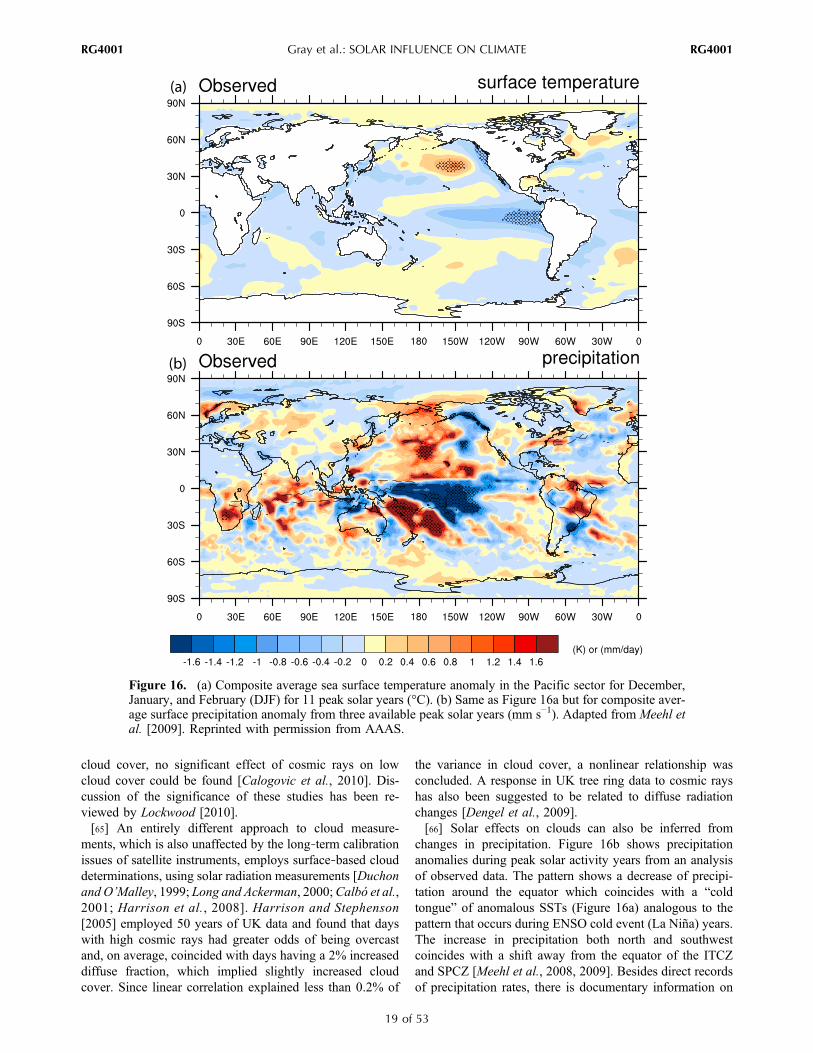
cloud cover, no significant effect of cosmic rays on lowcloud cover could be found [Calogovic et al., 2010]. Dis-cussion of the significance of these studies has been re-viewed by Lockwood [2010].[65] An entirely different approach to cloud measure-

ments, which is also unaffected by the long‐term calibrationissues of satellite instruments, employs surface‐based clouddeterminations, using solar radiation measurements [Duchonand O’Malley, 1999; Long and Ackerman, 2000;Calbó et al.,2001; Harrison et al., 2008]. Harrison and Stephenson[2005] employed 50 years of UK data and found that dayswith high cosmic rays had greater odds of being overcastand, on average, coincided with days having a 2% increaseddiffuse fraction, which implied slightly increased cloudcover. Since linear correlation explained less than 0.2% of

the variance in cloud cover, a nonlinear relationship wasconcluded. A response in UK tree ring data to cosmic rayshas also been suggested to be related to diffuse radiationchanges [Dengel et al., 2009].[66] Solar effects on clouds can also be inferred from

changes in precipitation. Figure 16b shows precipitationanomalies during peak solar activity years from an analysisof observed data. The pattern shows a decrease of precipi-tation around the equator which coincides with a “coldtongue” of anomalous SSTs (Figure 16a) analogous to thepattern that occurs during ENSO cold event (La Niña) years.The increase in precipitation both north and southwestcoincides with a shift away from the equator of the ITCZand SPCZ [Meehl et al., 2008, 2009]. Besides direct recordsof precipitation rates, there is documentary information on

Figure 16. (a) Composite average sea surface temperature anomaly in the Pacific sector for December,January, and February (DJF) for 11 peak solar years (°C). (b) Same as Figure 16a but for composite aver-age surface precipitation anomaly from three available peak solar years (mm s−1). Adapted from Meehl etal. [2009]. Reprinted with permission from AAAS.


19 of 53

lake and river levels (e.g., the Nile [Fraedrich and Bantzer,1991; de Putter et al., 1998; Eltahir and Wang, 1999;Kondrashov et al., 2005]) and catastrophic floods anddroughts [Verschuren et al., 2000; Hong et al., 2001;Ruzmaikin et al., 2006]. These changes do not, however,distinguish direct GCR effects on clouds from othermechanisms.

3.3. Decadal Variations at the Earth’s Surface[67] Many studies have investigated whether 11 year SC

variations can be detected in recent, more accurateobservations of temperatures at the Earth’s surface. Thisposes considerable challenges as many other factors werealso influencing climate during this period, includingincreasing greenhouse gases, volcanic eruptions, and aerosolchanges. Some of these are themselves poorly quantified,such as aerosols, and some may have similar impacts onsurface climate to solar irradiance changes. Additionalcomplications arise when different forcings have similartemporal changes, as has been the case with the solar cycleand volcanic forcing over parts of the twentieth century.Hence, isolation of any solar signal is not straightforward.[68] Nonetheless, some signals of solar forcing appear to

be present at decadal time scales in particular regions. Whiteet al. [1997] examined basin average ocean temperatureswith two independent SST data sets: surface marine weatherobservations (1900–1991) and upper ocean bathythermo-graph temperature profiles (1955–1994). They found var-iations in phase with solar activity across the Indian, Pacific,and Atlantic oceans. Global averages yielded maximumchanges of 0.08 ± 0.02 K on decadal (∼11 year period)scales and 0.14±0.02 K on interdecadal (∼22 year period)scales. The highest correlations were obtained with oceantemperatures lagging solar activity by 1–2 years, which isroughly the time scale expected for the upper layers of theocean (<100 m) to reach equilibrium.[69] A number of studies have also noted a strong regional

response to the 11 year SC. For example, White et al. [1997,1998] found that the 11 year SC associated with SST vari-ability during the twentieth century was remarkably similarto the spatial pattern of the ENSO, which has a 3–5 yearperiod (see section 3.2.2 and Figure 16). Allan [2000] andWhite and Tourre [2003] detected this 11 year signal, whichthey referred to as a quasi‐decadal oscillation, in global SSTand sea level pressure patterns rising significantly above thebackground noise, along with ENSO and QBO periods.White and Liu [2008a, 2008b] have subsequently noted anEl Niño–like warm event in the tropical eastern Pacific SSTsthat is coincident with peaks in solar forcing, preceded andsucceeded by cold events, which they proposed were asso-ciated with nonlinear phase locking of odd harmonics andcould explain a significant fraction of equatorial easternPacific SST variability (see also section 4.1). Meehl et al.[2008], on the other hand, noted a cold (La Niña–like)event which coincided with the peak in sunspot numbers,followed a few years later by a warm El Niño–like event.Thus, there is an apparent disagreement between these twoanalyses. However, Roy and Haigh [2010] have noted that

the peak in sunspot number occurs a year or so in advance ofthe peak in the observed decadal solar irradiance variability,so that the Meehl et al. [2008] cold event coincident withsunspot year maximum is not inconsistent with the Whiteand Liu results.[70] Land temperatures also show SC relationships in

some regions. Recent analyses indicate significant correla-tions between 11 year SC forcing and surface climate thatappear to be robust both to the data set used and themethodology employed [Camp and Tung, 2007; Tung andCamp, 2008].

3.4. Century‐Scale Variations[71] Going back in time, it is inevitable that instrumental

and documentary records of climate become increasinglysparse and unequally distributed around the globe. Onlonger time scales, evidence for a Sun‐climate linkage mustrely entirely on indirect information stored in naturalarchives, such as ice cores, marine and lacustrine (lake bed)sediments, peat deposits, speleothems (stalactites and sta-lagmites), and tree rings. These archival reservoirs provideonly indirect measures of temperature and precipitation byusing climate proxies such as isotopic ratios, elementalconcentrations, layer thicknesses, and biological indicators.Nevertheless, there are many advantages of using climateproxy records: they cover very long time periods of up toseveral 103–104 years with relatively high temporal resolu-tion, providing information on past climate for many partsof the globe. They also allow investigation of solar forcingof climate change prior to large‐scale human influences onthe atmosphere.3.4.1. Solar Proxies[72] As described in section 2, it has been known for

about 50 years that GCR intensity reflects solar activitybecause of modulation by solar magnetic fields carried awayfrom the Sun by the solar wind. The larger the solar activity,the stronger the shielding, and the lower the cosmic rayintensity penetrating into the atmosphere. In the atmospherecosmic rays interact with nitrogen and oxygen, producingcosmogenic radionuclides such as 10Be and 14C, so thatmeasuring 10Be and 14C stored in terrestrial reservoirs pro-vides a means to reconstruct the history of solar activity overmillennia. Precise calibration remains challenging, however,and is based on the comparatively short period of overlapwith modern observations. Hence, these solar proxies pro-vide a much more precise estimate of the temporal variationsof solar irradiance than its magnitude. In addition, the 10Beand 14C signals stored in ice and tree rings do not solelyreflect changes in solar activity. For example, the geomag-netic field also shields Earth from cosmic rays and varies onlong time scales. In the case of 14C, the newly produced 14Cis mixed with 14C already present in the carbon reservoirs(atmosphere, biosphere, and ocean), causing an attenuationand a delay of the production signal. In the case of 10Be theproduction signal can be altered to some extent by thetransport processes from the point in the atmosphere whereit is produced to the site where it becomes stored in an icecore. While the effect of the geomagnetic dipole moment


20 of 53

can be removed relatively easily using paleomagnetic data,the transport effects are more difficult to deal with. Oneapproach makes use of the fact that the 10Be and 14C recordsare produced by a common signal but are transported indifferent ways [Heikkilä et al., 2008; Field et al., 2006].3.4.2. Climate Proxies[73] Care is also required in proxy climate data quality

and chronological control. Although they can be calibratedagainst more recent instrumental records, there is a risk thatcalibration using relatively short periods may not be fullyvalid for preinstrumental times because climate proxies maydepend in a complex way on multiple climatic and envi-ronmental parameters that are likely to change over longertime scales [Jones and Mann, 2004; Jones et al., 2009]. Agood example of a climate proxy is peat, for example, theHolocene peat deposits in the rainwater‐fed raised bogs innorthwest Europe. Plant remains in peat deposits can beidentified, and by using ecological information of peat‐forming species, changes in species composition of sequencesof peat samples can be interpreted as evidence for climatechange in the past. The degree of decomposition of the peat‐forming plants is also related to former climatic conditions(e.g., more decomposed peat when formed under drierconditions and better preserved plant remains during periodsof wetter climatic conditions).[74] Calibration of single radiocarbon dates usually yields

irregular probability distributions in calendar age, quiteoften over long time intervals. This is problematic in paleo-climatological studies, especially when a precise temporalcomparison between different climate proxies is required.However, closely spaced sequences of (uncalibrated) 14Cdates of peat deposits display wiggles, which can be fitted tothe wiggles in the radiocarbon calibration curve. The practiceof dating peat samples using 14C “wiggle‐match dating” hasgreatly improved the precision of radiocarbon chronologiessince its application by van Geel and Mook [1989]. By 14Cwiggle‐matching peat sequences, high‐precision calendarage chronologies can be generated [Blaauw et al., 2003]which show that increased mire surface wetness occurredtogether with suddenly increasing atmospheric production of14C during the early Holocene, the subboreal‐subatlantictransition, and the Little Ice Age (Wolf, Spörer, Maunder, andDalton minima of solar activity). Peat records showing thisphenomenon are available from the Netherlands [van derPlicht et al., 2004; Kilian et al., 1995; van Geel et al., 1998],the Czech Republic [Speranza et al., 2002], the UK, andDenmark [Mauquoy et al., 2002].[75] Precise chronologies are crucial to determine leads

and lags and rates of climate change and to help establishcausal relationships. Chronological uncertainties of paleo-climate time series are typically 1%–2% of the absolute age,for example, between 100 and 200 years for a 10,000 yearold sample. This age error corresponds to a full Gleissberg(∼90 years) and de Vries (208 years) solar cycle. However,recent progress has considerably improved the accuracy, e.g.,in the case of stalagmites to a few years throughout theHolocene. In some cases, there is a well‐established datarecord, e.g., ice core layers containing ash from a well‐

documented historical volcanic eruption. Also, somearchives such as ice cores provide information on climateforcing (solar activity as derived from 10Be) and at the sametime on climate response (e.g., d18O), which is independentof the dating accuracy. Finally, we note that some archives,such as ice cores, are restricted for obvious natural reasonsto certain geographical areas.3.4.3. Twentieth Century Changes[76] In climate models, the pattern of surface response

(i.e., land plus sea) to solar irradiance variations is fairlysimilar to the response to greenhouse gases [Wetherald andManabe, 1975; Nesme‐Ribes et al., 1993; Cubasch et al.,1997, 2006; Santer et al., 2003], with amplification athigh latitudes, where strong positive snow and ice albedofeedbacks operate, and amplification of continental interiorsrelative to oceans. Hence, while century‐scale data showglobal or hemispheric mean surface air temperatures that arecorrelated with solar indices, e.g., using solar cycle length asa proxy for irradiance [Thejll and Lassen, 2000], this simplecorrelation is no guarantee of a causal relationship. In fact, acomparison of solar cycle length over the past several cen-turies shows that if the apparent relationship between solarvariability and mean surface air temperature in twentiethcentury data were indeed real, then solar variations shouldhave driven much larger global or hemispheric temperaturevariations in the longer‐term past than are seen in proxyreconstructions [Laut, 2003]. Similarly, global mean SSTsand sunspot numbers are correlated during the twentiethcentury [Reid, 2000], but attributing this relationship to solarforcing of SSTs implies a climate sensitivity that is incon-sistent with evidence from earlier centuries. More likely, theapparent relationship results from coincidental similarity inthe temporal evolution of sunspots and global or hemi-spheric mean temperatures, with the latter responding togradually increasing greenhouse gases and highly variabletemporal trends in aerosols.[77] Advanced statistical detection and attribution method-

ologies have been developed to take account of uncertainties inthe magnitude of various forcings, including solar irradianceforcing [see, e.g., Stott et al., 2003]. These analyses scale theresponse patterns to each forcing to determine the best matchto observations. Also, to distinguish between the variouspossible forcings, additional observations are incorporated.For example, although the surface response to solar andgreenhouse gas (GHG) forcings is similar, as noted above, theGHG response in the stratosphere is opposite to that in thetroposphere [Ramaswamy et al., 2006], giving a so‐calledGHG “fingerprint” that has a very different vertical structurefrom the solar one.[78] Model simulations of twentieth century climate that

include all the major, known forcings (solar, volcanoes,GHGs, aerosols, and ozone), together with the detection‐attribution techniques based on observed patterns, haveshown that most of the global warming in the first half of thetwentieth century was natural in origin, and much of this canbe attributed to an increase in solar forcing [Tett et al., 2002;Stott et al., 2000, 2003; Shiogama et al., 2006; Meehl et al.,2004; Knutson et al., 2006; Hegerl et al., 2003; IPCC,


21 of 53

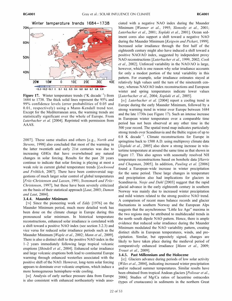
2007]. These same studies and others [e.g., North andStevens, 1998] also concluded that most of the warming inthe latter twentieth and early 21st centuries was due toincreasing GHGs that have overwhelmed any naturalchanges in solar forcing. Results for the past 20 yearscontinue to indicate that solar forcing is playing at most aweak role in current global temperature trends [Lockwoodand Fröhlich, 2007]. There have been controversial sug-gestions of much larger solar control of global temperatures[Friis‐Christensen and Lassen, 1991; Svensmark and Friis‐Christensen, 1997], but these have been severely criticizedon the basis of their statistical approach [Laut, 2003; Damonand Laut, 2004].3.4.4. Maunder Minimum[79] Since the pioneering work of Eddy [1976] on the

Maunder Minimum period, much more detailed work hasbeen done on the climate change in Europe during thispronounced solar minimum. In historical temperaturereconstructions, enhanced solar irradiance is correlated witha shift toward a positive NAO index (see section 3.2.3) andvice versa for reduced solar irradiance periods such as theMaunder Minimum [Waple et al., 2002; Mann et al., 2009].There is also a distinct shift to the positive NAO index in the1–2 years immediately following large tropical volcaniceruptions [Shindell et al., 2004]. Enhanced solar irradianceand large volcanic eruptions both lead to continental Europewarming through enhanced westerlies associated with thepositive shift of the NAO. However, long‐term solar forcingappears to dominate over volcanic eruptions, which induce amore homogeneous hemisphere‐wide cooling.[80] Analysis of early surface pressure data from Europe

is also consistent with enhanced northeasterly winds asso-

ciated with a negative NAO index during the MaunderMinimum [Wanner et al., 1995; Slonosky et al., 2001;Luterbacher et al., 2001; Xoplaki et al., 2001]. Ocean sed-iment cores also support a shift toward a negative NAOduring the Maunder Minimum [Keigwin and Pickart, 1999].Increased solar irradiance through the first half of theeighteenth century might also have induced a shift toward apositive NAO/AO index, suggested by independent proxyNAO reconstructions [Luterbacher et al., 1999, 2002; Cooket al., 2002]. Unforced variability in the NAO/AO is large,however, which is one reason why solar irradiance accountsfor only a modest portion of the total variability in thispattern. For example, solar irradiance estimates stayed atrelatively high values until the turn of the nineteenth cen-tury, whereas NAO/AO index reconstructions and Europeanwinter and spring temperatures indicate lower values[Luterbacher et al., 2004; Xoplaki et al., 2005].[81] Luterbacher et al. [2004] report a cooling trend in

Europe during the early Maunder Minimum, followed by astrong warming trend in winter over Europe between 1684and the late 1730s (see Figure 17). Such an intense increasein European winter temperature over a comparable timeperiod has not been observed at any other time in the500 year record. The spatial trend map indicates particularlystrong trends over Scandinavia and the Baltic region of up to0.8 K decade−1. Climate reconstructions for Europe inspringtime back to 1500 A.D. using multiproxy climate data[Xoplaki et al., 2005] also show a strong increase in win-tertime temperature at around the same time as that shown inFigure 17. This also agrees with seasonally resolved NHtemperature reconstructions based on borehole data [Harrisand Chapman, 2005]. In addition, Pauling et al. [2006]found a European‐wide increase in winter precipitationfor the same period. These large changes in temperatureand precipitation also had implications for glaciers inScandinavia. Nesje and Dahl [2003] suggest that the rapidglacial advance in the early eighteenth century in southernNorway was mainly due to increased winter precipitationand mild winters related to the strong positive NAO trend.A comparison of recent mass balance records and glacierfluctuations in southern Norway and the European Alpssuggests that the asynchronous “Little Ice Age” maxima inthe two regions may be attributed to multidecadal trends inthe north–south dipole NAO pattern. Hence, there is ampleevidence that reduced solar irradiance during the MaunderMinimum modulated the NAO variability pattern, creatingdistinct shifts in European temperatures, winds, and pre-cipitation. Similar, but oppositely signed, changes arelikely to have taken place during the medieval period ofcomparatively enhanced irradiance [Mann et al., 2009;Trouet et al., 2009].3.4.5. Past Millennium and the Holocene[82] Glaciers advance during periods of low solar activity

[Wiles et al., 2004], indicating increased winter precipitationand/or reduced summer temperatures. Similar results havebeen obtained from tropical Andean glaciers [Polissar et al.,2006]. Studies of Mg/Ca ratios of lacustrine ostracodes(types of crustaceans) in sediments in the northern Great

Figure 17. Winter temperature trends (°K decade−1) from1684 to 1738. The thick solid lines represent the 95% and99% confidence levels (error probabilities of 0.05 and0.01, respectively) using a Mann‐Kendall trend test.Except for the Mediterranean area, the warming trends arestatistically significant over the whole of Europe. FromLuterbacher et al. [2004]. Reprinted with permission fromAAAS.


22 of 53

Plains [Yu and Ito, 1999] provide an indication of watertemperature and evaporation/precipitation balance and sug-gest that dry periods coincided with lower solar activity.The abundance of the planktonic foraminifer Globiger-inoides sacculifer in marine sediments from the westernand northern Gulf of Mexico has been used as a proxy forthe mean latitudinal position of the ITCZ and suggeststhat migration of the ITCZ is, in part, linked to solaractivity, with a more southerly position of the ITCZ duringcentennial‐scale intervals of low solar activity [Poore et al.,2004]. This result is consistent with that inferred from the Ticontent of sediment cores in the Cariaco basin off Venezuela[Haug et al., 2001] and from the northward shift of the ITCZduring 11 year peaks in solar forcing noted in section 3.2.2.A comprehensive review of climate variability and forcingsduring the past 6000 years is given by Wanner et al. [2008].[83] These proxies and many others from different areas

provide consistent evidence that solar grand minima affectclimate. At the same time, however, clear differences indi-cate that solar forcing is only one factor among others andcannot explain the full variance of climate change evident inthese proxy records. Furthermore, for example, analyses oflake records from West Africa show opposite results tothose from East African lakes, suggesting complex changesin the hydrologic cycle that resulted in a shift in precipita-tion from the western to the eastern part of the continentduring periods of decreased irradiance [Russell and Johnson,2007]. Such changes may result from solar modulation ofcoupled variability patterns at high and tropical latitudes,such as the NAO and ENSO, in addition to the position ofthe ITCZ.[84] Analyses of NH mean temperatures during the last

millennium reconstructed from a network of proxies,including ice cores, tree rings, corals, and documentary evi-dence, as well as reconstructions based on tree rings alone,show substantial correlations with solar forcing at multi-decadal time scales [Weber, 2005]. Regression of these time

series yields a response of 0.2–0.3 K (W m−2)−1 at multi-decadal time scales. The spatial pattern of the centennial‐scale response shows a distinct regional surface temperatureresponse [Waple et al., 2002;Mann et al., 2009], as illustratedin Figure 18. The response maximizes at time scales of morethan 4 decades and is less for the 11 and 22 year periodicities.The spatial structure resembles that of the AO/NAO, a resultalso seen in the analyses of Trouet et al. [2009] andMannet al. [2009], and also shows an enhanced response in thewestern Pacific warm pool region.[85] Studies over the whole Holocene period (past

approximately 11,000 years) have also indicated clear linksto solar activity [see Wanner et al., 2008, and referencestherein]. Figure 19 shows three comparisons of climateproxies with solar variability on centennial to millennialtime scales, using the 14C production rate as the solar proxy.The ice‐rafted debris (Figure 19, top) found in sedimentcores of the North Atlantic [Bond et al., 2001] originatesfrom well‐defined areas in Greenland, Iceland, and Svalbardwhere particles are picked up by glaciers moving toward thecoast. When the ice melts in the North Atlantic the particlesare released and preserved in the sediment. Their amount istherefore a measure of the transport of cooler, ice‐bearingsurface waters eastward from the Labrador Sea and south-ward from the Nordic seas, probably accompanied by shiftsto strong northerly winds north of Iceland.[86] The biogenic silica content in Lake Arolik in south-

western Alaska (Figure 19, middle) reflects the sedimentaryabundance of diatoms that are single‐celled algae. Detailedcomparisons with other parameters show that these diatomsplay a central role in the primary productivity and are clearlylinked to climate parameters such as moisture (precipitationminus evaporation) and atmospheric temperature. The d18Ofrom a stalagmite in Oman (Figure 19, bottom) is mainly aproxy for the amount of monsoon precipitation [Fleitmannet al., 2003]. Advances in dating techniques for this type

Figure 18. Spatial pattern of surface temperature difference between the Medieval Climate Anomalyand the Little Ice Age derived from proxy‐based temperature reconstructions. Reproduced from Mannet al. [2009]. Reprinted with permission from AAAS.


23 of 53

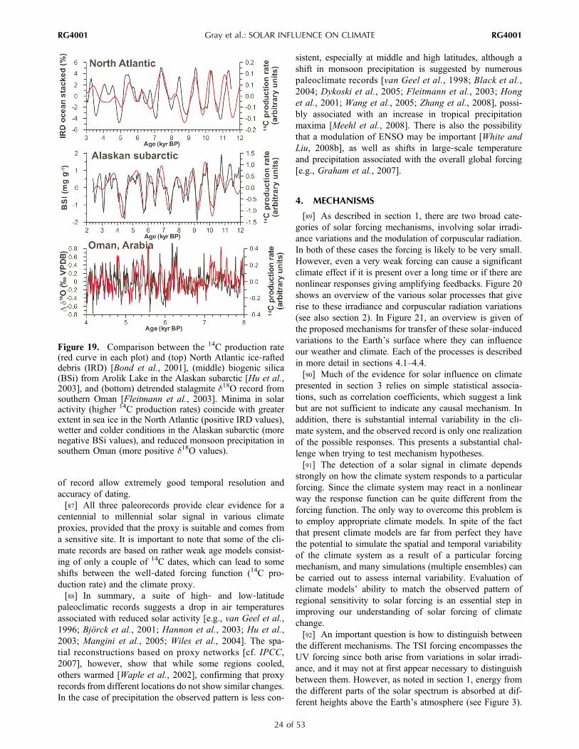
of record allow extremely good temporal resolution andaccuracy of dating.[87] All three paleorecords provide clear evidence for a

centennial to millennial solar signal in various climateproxies, provided that the proxy is suitable and comes froma sensitive site. It is important to note that some of the cli-mate records are based on rather weak age models consist-ing of only a couple of 14C dates, which can lead to someshifts between the well‐dated forcing function (14C pro-duction rate) and the climate proxy.[88] In summary, a suite of high‐ and low‐latitude

paleoclimatic records suggests a drop in air temperaturesassociated with reduced solar activity [e.g., van Geel et al.,1996; Björck et al., 2001; Hannon et al., 2003; Hu et al.,2003; Mangini et al., 2005; Wiles et al., 2004]. The spa-tial reconstructions based on proxy networks [cf. IPCC,2007], however, show that while some regions cooled,others warmed [Waple et al., 2002], confirming that proxyrecords from different locations do not show similar changes.In the case of precipitation the observed pattern is less con-

sistent, especially at middle and high latitudes, although ashift in monsoon precipitation is suggested by numerouspaleoclimate records [van Geel et al., 1998; Black et al.,2004; Dykoski et al., 2005; Fleitmann et al., 2003; Honget al., 2001; Wang et al., 2005; Zhang et al., 2008], possi-bly associated with an increase in tropical precipitationmaxima [Meehl et al., 2008]. There is also the possibilitythat a modulation of ENSO may be important [White andLiu, 2008b], as well as shifts in large‐scale temperatureand precipitation associated with the overall global forcing[e.g., Graham et al., 2007].

4. MECHANISMS

[89] As described in section 1, there are two broad cate-gories of solar forcing mechanisms, involving solar irradi-ance variations and the modulation of corpuscular radiation.In both of these cases the forcing is likely to be very small.However, even a very weak forcing can cause a significantclimate effect if it is present over a long time or if there arenonlinear responses giving amplifying feedbacks. Figure 20shows an overview of the various solar processes that giverise to these irradiance and corpuscular radiation variations(see also section 2). In Figure 21, an overview is given ofthe proposed mechanisms for transfer of these solar‐inducedvariations to the Earth’s surface where they can influenceour weather and climate. Each of the processes is describedin more detail in sections 4.1–4.4.[90] Much of the evidence for solar influence on climate

presented in section 3 relies on simple statistical associa-tions, such as correlation coefficients, which suggest a linkbut are not sufficient to indicate any causal mechanism. Inaddition, there is substantial internal variability in the cli-mate system, and the observed record is only one realizationof the possible responses. This presents a substantial chal-lenge when trying to test mechanism hypotheses.[91] The detection of a solar signal in climate depends

strongly on how the climate system responds to a particularforcing. Since the climate system may react in a nonlinearway the response function can be quite different from theforcing function. The only way to overcome this problem isto employ appropriate climate models. In spite of the factthat present climate models are far from perfect they havethe potential to simulate the spatial and temporal variabilityof the climate system as a result of a particular forcingmechanism, and many simulations (multiple ensembles) canbe carried out to assess internal variability. Evaluation ofclimate models’ ability to match the observed pattern ofregional sensitivity to solar forcing is an essential step inimproving our understanding of solar forcing of climatechange.[92] An important question is how to distinguish between

the different mechanisms. The TSI forcing encompasses theUV forcing since both arise from variations in solar irradi-ance, and it may not at first appear necessary to distinguishbetween them. However, as noted in section 1, energy fromthe different parts of the solar spectrum is absorbed at dif-ferent heights above the Earth’s atmosphere (see Figure 3).

Figure 19. Comparison between the 14C production rate(red curve in each plot) and (top) North Atlantic ice‐rafteddebris (IRD) [Bond et al., 2001], (middle) biogenic silica(BSi) from Arolik Lake in the Alaskan subarctic [Hu et al.,2003], and (bottom) detrended stalagmite d18O record fromsouthern Oman [Fleitmann et al., 2003]. Minima in solaractivity (higher 14C production rates) coincide with greaterextent in sea ice in the North Atlantic (positive IRD values),wetter and colder conditions in the Alaskan subarctic (morenegative BSi values), and reduced monsoon precipitation insouthern Oman (more positive d18O values).


24 of 53

Changes in TSI can directly impact the surface (seeFigure 21), while changes in UV directly impact thestratosphere, so that indirect stratosphere‐troposphere cou-pling mechanisms are required for these stratosphericchanges to impact the surface. It is therefore necessary todistinguish between these mechanisms, in order to deter-mine which of them is required in climate models to accu-rately simulate the past, current, and future climate.[93] Most current climate models include a representation

of TSI variations, but their upper boundary does not extendsufficiently high to fully resolve the stratosphere, so most donot include the UV influence. Hence, the primary solar

influence mechanisms in these models are ocean heat uptakeand SST changes, which affect evaporation and low‐levelmoisture in the atmosphere. This mechanism is oftenreferred to as the bottom‐up mechanism and is described inmore detail in section 4.1.[94] Atmospheric models that include a good representa-

tion of the stratosphere, including interactive ozone chem-istry, are available, but they do not generally include a fullycoupled ocean at present. The prime solar mechanism forinfluence in these models is therefore the change in strato-spheric temperatures and winds due to changes in UV irra-diance and ozone production, and the influence on the

Figure 20. Schematic overview showing various climate forcings of the Earth’s atmosphere, with fac-tors that influence the forcing associated with solar variability (irradiance and corpuscular radiation)shown in more detail on the left‐hand side, as discussed in section 2.

Figure 21. Schematic diagram of solar influence on climate based on Kodera and Kuroda [2002].Shown are the direct and indirect effects through solar irradiance changes (TSI and UV) with respect toSmax as well as corpuscular radiation effects (energetic particles and GCRs). The two dashed arrowsdenote the coupling between the stratosphere and the troposphere and the coupling between the ocean andthe atmosphere.


25 of 53

underlying troposphere and surface climate involves strato-sphere‐troposphere coupling processes. This mechanism isoften referred to as the top‐down mechanism (see section 4.2).Comparison of results from these two types of models can helpassess the contribution from the two mechanisms.[95] However, recent recognition of the influence of

stratospheric processes on climate in general [Baldwin andDunkerton, 2001] has prompted the vertical extension ofcoupled ocean‐atmosphere climate models to include thestratosphere, so that fully coupled ocean‐troposphere‐stratosphere climate and Earth system models are nowbecoming available and the TSI (bottom‐up) and UV (top‐down) influences can be assessed in the same model [e.g.,Meehl et al., 2009].[96] At present, assessment of the various proposed GCR

mechanisms is very much in its infancy, and some of thetheories are not sufficiently well developed to have beentested even in relatively simple mechanistic models. Thehorizontal resolution of global climate models is tightlyconstrained by computing capacity since they must beglobal in nature and run for hundreds of years. Therefore,they do not resolve clouds explicitly, and inclusion of GCRmechanisms for assessment of their impacts requires carefulparameterization [e.g., Pierce and Adams, 2009]. Despitethis very different level of maturity in the testing of theproposed GCR mechanisms compared with the irradiancemechanisms, as well as suggestions of questionable dataanalysis in some of the GCR‐cloud papers, we neverthelessinclude a brief review of the various GCR theories forbalance and completeness in section 4.4.

4.1. TSI Variations[97] The most obvious direct effect of solar variability on

climate is its influence on the Earth’s mean energy balancethrough variations in TSI. The radiative forcing (RF) has animpact on global mean surface temperature that can beestimated for a given climate sensitivity parameter (seesection 1). Because of the large uncertainty in centennial‐scale variations in TSI, however, solar radiative forcing ofclimate change is not well established, as discussed furtherin section 5.[98] For reasonable climate sensitivities, the ∼1 W m−2

variation in TSI associated with the 11 year SC translates toan estimated change in temperature at the Earth’s surface ofa mere 0.07 K (see section 1) and is of the same order ofmagnitude as observed, e.g., in global mean SST (0.08 ±0.02 K [White et al., 1997]). Similarly, simple mean energybalance calculations using the long‐term centennial‐scaleTSI change estimates of ∼1.3 W m−2 (see section 2.3) canexplain the order of magnitude changes in global meantemperatures estimated from the various climate proxies(section 3.4.2). However, much of the observational evi-dence for SC influence in the troposphere and at the surfaceappears to be regional rather than global in extent. Theseregional responses are much larger than the global meanvalues, which suggests that an amplifying mechanism isinvolved, such as changes in the Hadley and Walker cir-culations [Haigh, 1996; van Loon et al., 2007; Kodera et al.,

2007; Meehl et al., 2008, 2009] (see section 3.2.2) andpossible associated cloud feedbacks that could decreaseclouds and hence increase solar input to some regions of thetropics and subtropics [Meehl et al., 2003, 2008, 2009].[99] The principal bottom‐up mechanism proposed for

solar influence on tropical circulations through direct TSIeffects at the surface involves solar absorption over rela-tively cloud‐free subtropical oceans, which increases duringsolar maximum [Cubasch et al., 1997, 2006]. This increasesevaporation, and the increased moisture converges into theprecipitation zones, which then intensifies the climatologicalprecipitation maxima and associated upward vertical motions,resulting in stronger trade winds, greater equatorial Pacificocean upwelling, and colder SSTs consistent with strongerHadley and Walker circulations [Meehl et al., 2003, 2008](see Figure 22). This strengthened circulation also enhancesthe subtropical subsidence, resulting in a positive feedbackthat reduces clouds and thus further increases solar forcing atthe surface [e.g., Meehl et al., 2008, 2009].[100] However, in a series of diagnostic thermal budget

studies of SST and ocean heat storage, White et al. [2003]and White [2006] concluded that the observed 11 year SCsignals in SSTs could not be explained solely by thisbottom‐up direct impact of radiative forcing at the surface(∼0.15 W m−2). They showed that the temperature anoma-lies in the tropical lower troposphere were warmer than thetropical upper ocean anomalies and that these anomaliesincreased upward, from ∼0.2°C in the tropical lower tro-posphere to ∼0.5°C in the tropical middle to upper tropo-sphere and ∼1°C in the tropical lower stratosphere. Thisanomalous lapse rate was matched by a correspondingdownward sensible plus latent heat flux anomaly across theair‐sea interface of ∼0.5 W m−2, which was larger than thedirect solar radiative forcing by a factor of ∼3 and alsoexplained the correct phase of the response. This thereforerepresents a different kind of amplification of the 11 yearsolar cycle and is not associated with changes in trade windstrength or cloud cover since these did not have the correctmagnitude or phase.[101] This result implies a role for the top‐down influence

of UV irradiance via the stratosphere. White et al. [2003]also noted that time sequences of tropical tropospherictemperatures lead those in the lower stratosphere, whichappears to argue against the top‐down influence. Theysuggest, however, that this should not be interpreted as atropospheric signal forcing a stratospheric response becausethe stratospheric temperature response appears to be inradiative balance and hence is in phase with the 11 yearsolar cycle, while the troposphere responds to anomalousheating and advection which peaks during the period lead-ing up to solar maximum and not at the maximum itself.This is a good example of the difficulties and dangers ofinterpreting observed signals from different parts of theatmosphere and especially in using their time response to tryto infer cause and effect.[102] As noted in section 3.3 the observed SC signal in

Pacific SST resembles the ENSO signal, which is thedominant mode of variability in this region. White et al.


26 of 53

[2003] examined the quasi 11 year oscillation and also theENSO and QBO signals in global upper ocean temperatureand surface wind evolution and proposed that they aregoverned by a “tropical Pacific delayed action oscillator”[see also Zebiak and Cane, 1987; Graham and White, 1988;Schopf and Suarez, 1988] associated with negative feedbackby Rossby waves propagating at different equatorial lati-tudes. This hypothesis was tested in a fully coupled ocean‐atmosphere model by White and Liu [2008a], who foundthat the eastern tropical Pacific warm phase of the 11 yearcycle lagged the peak solar forcing by 1–3 years, similar toobservations and consistent with a near‐resonant excitationby the imposed 11 year SC forcing. In a follow‐on study,White and Liu [2008b] noted nonlinear phase locking of oddharmonics of equatorial Pacific SSTs that produced LaNiña–like conditions coincident with peak solar forcing,

followed by El Niño–like conditions a couple of years lateras also noted byMeehl et al. [2008]. In similar observational[e.g., van Loon et al., 2007; van Loon and Meehl, 2008] andcoupled general circulation model (GCM) studies [Meehland Arblaster, 2009; Meehl et al., 2008, 2009], La Niña–like conditions align with peaks in ∼11 year SC forcing,with lagged El Niño–like conditions a year or two later (seealso sections 3.2.2 and 3.3).

4.2. UV Irradiance Variations

4.2.1. Stratospheric Ozone Feedback[103] Most early stratospheric model studies examined

only the response to irradiance variations [e.g., Wetheraldand Manabe, 1975; Kodera et al., 1991; Balachandranand Rind, 1995; Cubasch et al., 1997; Balachandran et al.,1999]. Haigh [1994] first noted that the associated strato-spheric ozone changes (see, e.g., Figure 10) also need to beincluded since these will result in further heating increases inthe stratosphere and thus modulate radiative forcing of theatmosphere below. Studies that included this feedbackmechanism by imposing idealized ozone changes taken fromsimple 2‐D chemistry models [e.g., Haigh, 1999; Shindell etal., 1999, 2001; Larkin et al., 2000; Rind et al., 2002;Matthes et al., 2003; Haigh, 2003] reproduced the maximumwarming around the equatorial stratopause in Figure 11.They also demonstrated that the SC signal extended downinto the troposphere, primarily at subtropical latitudes (seesection 4.2.3) [Haigh, 1996, 1999]. However, they did notreproduce other features, such as the observed poleward anddownward propagation of the signal at polar latitudes[Matthes et al., 2003] or the secondary maximum in theequatorial lower stratosphere (20–30 km). There is generalconsensus that this latter feature results from transport pro-cesses (see section 4.2.2).[104] More recent improved models with fully interactive

stratospheric chemistry have been employed [Labitzke et al.,2002; Tourpali et al., 2003; Egorova et al., 2004; Rozanovet al., 2004; Shindell et al., 2006; Schmidt and Brasseur,2006; McCormack et al., 2007; Marsh et al., 2007; Austinet al., 2007, 2008; Matthes et al., 2007], so that theimposed irradiance variations affect both the radiativeheating and the ozone photolysis rates and, additionally,changes in ozone and its transport can feed back onto thediabatic heating. These models are now simulating animproved vertical structure of the annual mean ozone signalin the tropics, including the lower stratospheric maximum.Figure 23 shows the equatorial ozone distributions froman international comparison of simulations by 11 models[Austin et al., 2008]. Although the peak in the upperstratosphere is slightly lower than observed, the simulationsare generally within the observational error bars. However,it is still not clear to which factor (SSTs, time‐varying solarcycle, or inclusion of a QBO) the improvements can beascribed. Marsh and Garcia [2007] show an aliasing effectof ENSO events in their model that does not appear to besupported in observations [Hood and Soukharev, 2010],while Matthes et al. [2010] highlight the importance of theQBO for the vertical structure of the solar signal in ozone.

Figure 22. Schematic diagram showing processes involvedwith the Pacific coupled air‐sea response coincident withpeak years of solar forcing [after Meehl et al., 2008].


27 of 53

In addition, Figure 23 is an average from 25°S–25°S andmasks the fact that many of the models do not reproduce thelatitudinal structure seen in the observations (Figure 10).Hence, despite these general improvements, there are manydetails that are not reproduced by models. Further studies,including fully coupled ocean‐troposphere‐stratospheremodels with interactive chemistry, will be required to

improve the simulated ozone signal and distinguish betweenthe various influences.[105] Recent measurements of SSI by the SORCE SIM

satellite instrument suggest that variations in the UV may bemuch larger, by a factor of 4–6, than previously assumed[Harder et al., 2009]. If correct, this would imply a verydifferent response in both stratospheric ozone and temper-ature [Haigh et al., 2010] (see also section 5).4.2.2. Planetary Wave Feedback[106] The 11 year SC temperature anomalies of ∼1–2 K

near the equatorial stratopause (Figure 11), resulting fromUV irradiance changes and the ozone feedback mechanism,alter the meridional temperature gradient and hence the windfield through thermal wind balance. Hines [1974] suggesteda mechanism whereby these wind anomalies could influencethe propagation of planetary waves in the winter hemi-sphere. This suggestion was developed by Kodera [1995][see also Geller and Alpert, 1980; Bates, 1981; Geller, 1988;Balachandran and Rind, 1995]. During Smax years, awesterly wind anomaly develops in the subtropical upperstratosphere of the winter hemisphere and vice versa in Smin

years. Planetary wave propagation is sensitive to the back-ground winds, and a positive feedback is suggested throughwhich the wind anomaly moves poleward and downwardwith time and grows significantly in amplitude [Kodera andKuroda, 2002]. Figure 24 illustrates the time evolution ofthis poleward‐downward propagation of the 11 year SCwind anomaly from a model simulation [Matthes et al.,2006] that compares well with observations.[107] Through this mechanism the associated changes in

planetary wave forcing (as indicated by the Eliassen‐Palm

Figure 23. Ozone solar response averaged over 25°S–25°Nfrom a range of different coupled chemistry climate modelsthat included the effect of 11 year SC irradiance variationson radiative heating and photolysis rates (% per 100 unitsof F10.7 flux; multiply by ∼1.3 to obtain average estimateover the past three solar cycles). The red line indicates theaverage of all the modeled estimates. The black line indi-cates the average of estimates from three independent satel-lite instruments taken from Soukharev and Hood [2006]. Alluncertainty ranges are 95% confidence intervals [from Austinet al., 2008].

Figure 24. (top) Long‐term 10 day mean differences of NH zonally averaged zonal wind between Smax

and Smin from GCM experiments for 1–10 November (Nov1) and 11–20 November (Nov2) through to11–20 December (Dec2). Contour interval is 2 m s−1. Light (heavy) shading indicates the 5% (1%)significance level calculated with a Student’s t test. (bottom) Corresponding plots for Eliassen‐Palm fluxvectors (arrows, scaled by the inverse of pressure) and its divergence. Only the 1 m−1 s−1 d−1 contour isshown; negative values are shaded [from Matthes et al., 2006].


28 of 53

flux divergence r·F in Figure 24) also influence thestrength of the large‐scale Brewer‐Dobson (B‐D) circula-tion. Thus, in Smax years the polar winter vortex is lessdisturbed, the B‐D circulation is weaker, and the polar lowerstratosphere is colder than average because of the weakeradiabatic heating in the descending arm of the B‐D circu-lation. The converse would be true in Smin years. In thisway, it has been proposed that a very small temperatureanomaly of 1–2 K at the equatorial stratopause can betransferred to the lower polar stratosphere and significantlyamplified.[108] Through the same mechanism, the return upwelling

arm of the B‐D circulation at the equator would be similarlyweakened in Smax years, which results in less adiabaticcooling and hence a warmer equatorial lower stratosphere,as seen in Figure 11, with the converse in Smin years. Thisdynamical feedback mechanism also modulates the transportof ozone [Hood and Soukharev, 2003; Hood, 2004; Grayet al., 2009] as mentioned in section 4.2.1. The weakerB‐D circulation in Smax years, with reduced upwelling in theequatorial lower stratosphere, would result in positive ozoneanomalies in that region and hence produce a positivetemperature anomaly through diabatic heating. This feed-back mechanism is consistent with the observed lowerstratospheric ozone maximum in Figure 10 and would alsoreinforce the adiabatic temperature mechanism describedabove. Matthes et al. [2004, 2006] included these effects ina model with climatological SSTs so that there could be nosolar signal from the oceans and achieved lower stratosphereand troposphere responses that were similar to the observa-tions. However, they did not reproduce the full magnitude,persistence, or latitudinal structures, suggesting that an oceanfeedback may also be operating (see sections 4.1 and 4.2.3).Further studies using fully coupled ocean‐troposphere‐stratosphere models will be required to explore the relativecontributions and interactions of the top‐down and bottom‐up mechanisms.[109] As already noted in section 3.1.2, observations of

11 year SC variations of the polar lower stratospheric vortexin NH winter are complicated by the QBO (Figure 13),so that anomalously warm polar regions tend to occur inSmin–QBO‐E and Smax–QBO‐W. In a series of model anddata analysis papers, Gray et al. [2001] and Gray [2003]suggested that the observed 11 year SC–QBO interactioncould be due to the interaction of their respective windanomalies in the upper equatorial–subtropical stratosphereinfluencing the development and timing of SSW [Gray et al.,2004, 2006; see also Hardiman and Haynes, 2008]. Thiswork was subsequently supported by the modeling study ofMatthes et al. [2004], which also confirmed the Kodera andKuroda mechanism of the solar modulation of the polarvortex and the B‐D circulation.[110] The transfer of this SC‐QBO interaction in the upper

stratosphere to the tropical low latitudes via modulation ofthe B‐D circulation is only one possible explanation for theobserved SC‐QBO interactions there (see section 3.1.2).Another possible mechanism is a solar modulation of thedescent rates of the QBO [McCormack, 2003; Pascoe et al.,

2005; Salby and Callaghan, 2006; McCormack et al.,2007], which occurs entirely within the equatorial regionand does not rely on the polar route via SSWs and the B‐Dcirculation. A direct modulation of the descent rate of theQBOmay also help to explain the summer hemisphere signal(see Figure 14) since the strength of the subtropical QBOtemperature and ozone anomaly depends on the locallyinduced meridional circulation caused by the descendingQBO zonal wind anomaly. The two mechanisms of polar andequatorial solar influence transfer are not mutually exclusive,and both may be operating.[111] Cordero and Nathan [2005] andNathan and Cordero

[2007] have also proposed a wave‐induced ozone heatingmechanism linking the solar signal to the QBO, althoughMayr et al. [2006] found a solar modulation of the QBOwithout wave‐ozone feedback in their model. This pathwayrequires testing in future coupled chemistry climate model(CCM) studies. Finally, although wave activity plays alesser role in the summertime stratosphere, modeling studiessuggest that the ozone response to solar UV plays animportant role in solar modulation of summer stratosphericcirculation as well as in winter [Lee et al., 2008].4.2.3. Stratosphere Troposphere Coupling[112] It is clear that variations in solar UV radiation directly

influence stratospheric temperatures, and the dynamicalresponse to this heating extends the solar influence bothpoleward and downward to the lower stratosphere and tro-popause region. Evidence that this influence can also pen-etrate into the underlying troposphere is accruing from anumber of different sources. Observational analyses [e.g.,Baldwin and Dunkerton, 2001; Kuroda and Kodera, 2004;Thompson et al., 2005] suggest a downward propagation ofNAM anomalies (see section 3.2.3), although Plumb andSemeniuk [2003] note that this does not necessarily implypropagation of information in the same direction. Similarly,at equatorial latitudes Salby and Callaghan [2005] identifiedan interaction between the stratospheric B‐D circulation andthe tropospheric Hadley circulation; Figure 25 showscoherent variation between observed temperatures in theregion of the tropical tropopause and tropospheric and polarstratospheric temperatures that are consistent with possiblechanges in the Hadley circulation, tropical convection, andlatent heat release, but again, this does not provide a chainof causality.[113] Early model studies of UV variations in the

stratosphere [Haigh, 1996, 1999; Shindell et al., 1999;Balachandran et al., 1999; Larkin et al., 2000] obtained aresponse in the troposphere even though the near surface inthese model runs was constrained by imposed SSTs. Thepattern of the zonal wind anomalies was similar to the tro-pospheric SC response seen in Figure 12. Shindell et al.[2006] have confirmed this response using a fully coupledocean‐atmosphere model with interactive stratosphericchemistry. A more detailed analysis showed that while thegeneral response is a strengthening of the Walker circulationand broadening of the Hadley cell, there were substantialseasonal variations in the response and also dependencies onthe background greenhouse gas abundance of the atmo-


29 of 53

sphere [Lee et al., 2009]. A relatively robust result appearedto be an enhancement of the ascending branch of the Hadleycell and a northward shift of the ITCZ during the borealwinter during increased solar forcing, and this was qualita-tively consistent with the observed signal in NCEP reanal-ysis data.[114] There are many proposed mechanisms for a down-

ward influence from the lower stratosphere into the tropo-sphere (see reviews by Shepherd [2002] andHaynes [2005]).These include quasi‐instantaneous geostrophic adjustmentwithin the troposphere to changes in the potential vorticitystructure of the tropopause region [e.g., Hartley et al., 1998;Black, 2002], modification of the refraction [Hartmann et al.,2000] or reflection [Perlwitz and Harnik, 2003] of upwardpropagating planetary‐scale waves, and feedbacks betweenchanges in the mean flow and tropospheric baroclinic eddies[Kushner and Polvani, 2004; Song and Robinson, 2004].[115] The response to external forcing often has the same

spatial structure as, and involves similar eddy mean flowfeedbacks to, the dominant pattern of variability, e.g., theannular mode (NAO/AO) signal at middle to high latitudesand the ENSO signal at tropical latitudes. The high‐latitudeanomaly patterns represent a shift in position and strength ofthe tropospheric jets. Feedback of these tropospheric zonalwind changes on the tropospheric eddy momentum fluxesappears to be important [e.g., Polvani and Kushner, 2002;Kushner and Polvani, 2006; Song and Robinson, 2004].Coupling between the Hadley circulation and midlatitudeeddies may also play a key part: in a mechanistic study,Haigh et al. [2005] obtained a zonal mean troposphericresponse, qualitatively similar to the observed 11 year SCresponse, by imposing anomalous diabatic heating in thelow‐latitude lower stratosphere (see Figure 26). Consistentwith this, the enhanced Hadley circulation response in thecoupled chemistry simulations of Shindell et al. [2006] was

linked to the additional heating in the upper tropical tropo-sphere and lower stratosphere relative to simulations withfixed ozone. Simpson et al. [2009] have shown that it isthe response of the eddy momentum fluxes to changes instructure of the tropopause region that drives this tropo-spheric response.[116] In the GCM studies by Matthes et al. [2006] and

Meehl et al. [2009], the response in tropical vertical velocitywas not uniformly distributed in longitude but was largestover the Indian and West Pacific oceans, indicating aninfluence on the Walker circulation similar to that found inobservations [Kodera, 2004; Kodera et al., 2007]. Themodel reproduced these signals despite having imposedSSTs, suggesting that their tropospheric signal was aresponse to changes in the stratosphere and not to the bottom‐up mechanism of TSI heating of the ocean surface (seesection 4.1). The weakened ascent during Smax in the zonallyaveraged equatorial troposphere may result from theincreased static stability in the tropopause region suppres-sing equatorial convection but allowing enhanced off‐equatorial convection in the climatological precipitationmaxima [Kodera and Shibata, 2006; Matthes et al., 2006].This would be consistent with the results of Salby andCallaghan [2005] (see Figure 25), whose analysis sug-gested that the stratosphere and troposphere are linked by alarge‐scale transfer of mass across the tropopause resultingin a coupling of the B‐D circulation in the stratosphere andthe tropical Hadley circulation in the troposphere. However,as discussed in section 4.2.2, this does not preclude thepossibility that there is an additional positive feedback fromthe oceans so that both top‐down and bottom‐up mechan-isms are acting in the real world.[117] In addition to the observed ENSO‐like SC response

in SSTs in the Pacific Ocean, Kodera [2004] found a SCmodulation of Indian monsoon circulations and suggested

Figure 25. Correlation between observed DJF averaged zonal mean temperature at 100 hPa over theequator with temperatures throughout the troposphere and lower stratosphere [from Salby andCallaghan, 2005].


30 of 53

Figure 26. Zonally averaged zonal wind fields from (a) January climatology from the GCM experimentof Haigh and Blackburn [2006], (b) solar signal from the GCM experiment, (c) NCEP reanalysis annualmean for 1979–2002, and (d) solar signal from multiple regression analysis of the NCEP data (reprintedfrom Haigh and Blackburn [2006] with kind permission of Springer Science and Business Media).


31 of 53

that stratospheric circulations may suppress equatorial con-vection in Smax years with an enhancement of the off‐equatorial monsoon precipitation over India. Kodera et al.[2007] further suggest a coupling between the PacificENSO and Indian Ocean Dipole, with a SC modulation ofthe extension of ENSO into the Indian Ocean associatedwith a shift in location of the descending branch of theWalker circulation. Much work is still required to fullycharacterize the nature of these complicated interactions andhence to verify these mechanisms. Finally, Meehl et al.[2009] note that the top‐down and bottom‐up mechanismsboth act together in the same sense to intensify the clima-tological precipitation regimes in the tropics, thus addingtogether and reinforcing each other to produce a largerresponse in the troposphere than either one alone.[118] Although details of the mechanisms involved are

still not fully established, it is becoming increasingly clearthat the top‐down mechanism whereby UV heating of thestratosphere indirectly influences the troposphere throughdynamical coupling is viable and may help to explainobserved regional signals in the troposphere.

4.3. Centennial‐Scale Irradiance Variations[119] The majority of model studies of multidecadal effect

of TSI on climate employ “low‐top” models that do notinclude a representation of the stratosphere and hence pri-marily capture only the bottom‐up mechanism described insection 4.1. Early studies [Cubasch et al., 1997; Rind et al.,1999; Cubasch and Voss, 2000] found that the 11 year SC,even though present in the forcing, was rarely seen in themodeled response, but a response to the 70–80 yearGleissberg cycle was seen in the near‐surface temperature.Because of this, the earlier coupled ocean‐atmospheremodel studies of solar impact have concentrated on long‐term climate, e.g., over the last 100–1000 years, andaddressed the question of whether historically documentedclimate events like the Medieval Warm Period or the LittleIce Age could be simulated. The model simulations are thencompared to the climate variations experienced today, andpredictions are made for the future [Ammann et al., 2003;Ammann, 2005; Zorita et al., 2004; Stott et al., 2000, 2003;Stendel et al., 2006; Goosse et al., 2006].[120] In an extension to these low‐top model studies,

Shindell et al. [2001, 2003] employed a high‐topstratosphere‐resolving atmospheric model coupled to amixed layer ocean. They found a tropical‐subtropicalwarming during increased solar activity which induces awarmer tropical upper troposphere via moist convectiveprocesses. The sunlit portion of the stratosphere also warmsbecause of the increased UV irradiance and the ozonefeedback mechanism. These processes led to an increasedlatitudinal temperature gradient in the vicinity of the tro-popause during the extended cold season, resulting inenhanced lower stratosphere westerly winds, causingincreased angular momentum transport to high latitudes andenhanced tropospheric westerlies. This dynamical responsein the lower stratosphere was enhanced by roughly a factorof 2 by the interaction between UV radiation and ozone in

the upper stratosphere, indicating a downward propagationof stratospheric influence, as described in section 4.2.[121] According to this model, prolonged periods of

reduced solar activity (e.g., the Maunder Minimum) areassociated with pronounced cooling over middle‐ to high‐latitude continental interiors, also confirmed by Langematzet al. [2005]. Enhanced solar irradiance increases mid-latitude sea level pressure, generating enhanced westerlyadvection of relatively warm oceanic air over the continentsand of cooler air from continental interiors to their easterncoasts [Shindell et al., 2003]. This effect is most pronouncedin the cold season. Most recently, a set of ensemble simu-lations using a fully coupled ocean‐troposphere‐stratospheremodel including parameterized chemical responses to solarforcing (derived from a full chemistry model) was per-formed for the past 1000 years and compared with multi-proxy reconstructions [Mann et al., 2009]. This comparisonshowed that the model was able to capture many featuresof the northern extratropical surface temperature changebetween the medieval period and the Little Ice Age seenin the proxy data but could not capture the equatorialresponses. Interestingly, a low‐top version (i.e., with apoorly resolved stratosphere) of another GCM withoutchemistry was unable to capture the responses in either area.Variations between ensemble members were large, sug-gesting that patterns in a single period of time (e.g., theLittle Ice Age) may contain a substantial contribution frominternal, unforced variability. However, both the model andthe proxy reconstructions showed pronounced warming inthe medieval period relative to the Little Ice Age overmuch of North America and northern Eurasia.[122] Other multiproxy climate reconstructions (see

section 3.4) show similar spatial structures in correlations ofNH extratropical surface temperatures and solar outputreconstructions [Waple et al., 2002; Luterbacher et al.,2004; Xoplaki et al., 2005]. As the modeled response tosolar forcing shows areas of both regional cooling andwarming, the hemispheric or globally averaged changes arecomparatively small. This result is also consistent with thesmall amplitude of surface temperature variations during thelast millennium in most reconstructions for these spatialscales [Briffa et al., 1998; Mann et al., 1999; Jones et al.,2003; Mann et al., 2009].[123] It appears, therefore, that observational climate evi-

dence from Europe supports the modeled connectionbetween solar forcing and modulation of extratropical var-iability via the NAO/AO/NAM pattern [Shindell et al.,2001, 2003; Ruzmaikin and Feynman, 2002; Tourpaliet al., 2003; Egorova et al., 2004; Stendel et al., 2006],though Palmer et al. [2004] did not find such a link in theirmodel. Solar irradiance changes at multidecadal time scalesmight therefore have been a major trigger to explainregional temperature anomalies over Europe and central andeastern North America such as the Medieval Warm Periodand the Maunder Minimum cold period and might havecontributed substantially to the more recent increases inEuropean winter and spring temperatures and precipita-


32 of 53

tion and the connected exceptional growth of westernScandinavian glaciers.[124] A somewhat different analysis of the influence of

longer‐term solar variations is presented by Clement et al.[1996]. They suggest that heating over the entire tropicalregion will result in the Pacific warming more in the westthan the east because the strong ocean upwelling and surfacedivergence in the east moves some of the heat poleward,strengthening the east–west equatorial SST gradient, thoughthis mechanism does not take into account effects of cloudsthat produce nonspatially uniform solar forcing at the sur-face in the tropics. Emile‐Geay et al. [2007] find a similarresponse to variations in solar irradiance over the Holocene.Modulation of ENSO by solar forcing appears to be con-sistent with at least some paleoclimate evidence, especiallyfor the Americas, where multiple proxies such as fire scars,lake varves (stratified deposits of glacial clay), tree rings,etc., indicate correlations between precipitation and solarirradiance that are similar to ENSO‐related precipitationanomalies [Graham et al., 2007]. As discussed insection 3.2.2, a mechanism of coupled atmosphere‐oceanresponse to solar forcing in the tropical Pacific has beenproposed [e.g., Meehl et al., 2003, 2008]. Additionally, theUV‐ozone feedback mechanism appears to cause enoughheating near the tropical tropopause to significantly affectthe tropical hydrologic cycle, with regional impacts onprecipitation that are also broadly similar to those related toENSO changes [Shindell et al., 2006]. Thus, the twomechanisms may operate together to create the tropical‐subtropical response to solar forcing with associated ampli-fying cloud feedbacks [Meehl et al., 2009].

4.4. Charged Particle Effects[125] Changes in energetic particle fluxes (EPP) (includ-

ing electrons as well as ions of all species and coveringparticles of both solar/heliospheric and galactic origin) areprominent in the upper atmosphere. In particular, SEPevents, often referred to as SPEs (see section 1), occurinfrequently and generally last a few days. They producehigh‐energy particles precipitating into the thermosphere,mesosphere, and upper stratosphere at high geomagneticlatitudes. The resulting ionization and dissociation sub-stantially influence chemical constituents (HOx, NOx, andozone) in the polar middle atmosphere on time scales ofdays to months [Jackman et al., 2006]. As well as this directeffect of SEPs, there is also an indirect effect on thestratosphere from less energetic SEPs and energetic mag-netospheric electrons whose energy is deposited mainly inthe thermosphere and upper mesosphere. The resulting EPP‐NOx can be transported by polar downwelling into thewinter polar stratosphere, where it can influence ozoneabundances [Solomon et al., 1982; Callis et al., 1996;Siskind and Russell, 1996; Randall et al., 1998, 2005, 2006;Siskind et al., 2000]. At high latitudes, at least in theSouthern Hemisphere (SH) polar vortex, which is relativelystrong and stable, observations have established that inter-annual variability of NOx in spring correlates well with thegeomagnetic Ap index (see Figure 1), which can be inter-

preted as a proxy measure of EPP [Randall et al., 1998,2007; Siskind et al., 2000], and up to 10% of the total SHNOx has been attributed to EPP‐NOx [Funke et al., 2005;Randall et al., 2007]. However, this external NOx influenceappears to be confined to the polar vortex region so that itsoverall contribution to the stratospheric ozone 11 year signalis likely to be relatively small.[126] While it is relatively well established that the indi-

rect EPP‐NOx mechanism can significantly perturb ozoneabundances in the SH polar vortex at levels above ∼10 hPa,it is much less clear that these ozone perturbations producedetectable changes in temperature and circulation. A recentstudy of ERA‐40 reanalysis data by Lu et al. [2008], forexample, finds some evidence for polar temperature andzonal wind variations that correlate with the Ap index.However, the inferred temperature and wind variations havea sign that is opposite to that expected from the EPP‐NOx

mechanism; in addition, the detected signals are at least asstrong in the NH as in the SH, which is unexpected in viewof the observed, stronger NOx responses in the SH.[127] Similarly, there is currently little clear evidence that

EPP‐NOx can significantly perturb the stratosphere outsideof the polar vortices, except perhaps during the very largestevents [Thomas et al., 2007; Damiani et al., 2006; Ganguly,2010]. Some sensitivity studies using CCMs suggest thatEPP‐NOx effects on ozone at low latitudes may be compa-rable to the effects of solar UV radiation [Callis et al., 2000,2001; Langematz et al., 2005; Rozanov et al., 2005]. How-ever, analysis of UARS Halogen Occultation Experiment(HALOE) NOx data over a 12 year period indicates nodecadal NOx variations at low latitudes that could signifi-cantly affect the solar cycle variation of global ozone, andthis conclusion is consistent with a more recent CCM sim-ulation by Marsh et al. [2007]. In summary, there is cur-rently little evidence that the EPP‐NOx mechanism has asufficient influence on stratospheric ozone and circulationthat could significantly perturb tropospheric climate.[128] GCRs generate ions throughout the troposphere

down to the surface. GCRs are modulated by the solar wind,so that atmospheric processes influenced by, or dependenton, cosmic ray ion production might also show solar mod-ulation [Ney, 1959]. These processes include current flow inthe global atmospheric electrical circuit, charging of atmo-spheric aerosol particles and cloud edge water droplets, andthe nucleation of ultrafine condensation nuclei (UCN) fromtrace vapors. For these processes to affect climate they mustexert an appreciable influence on the atmosphere’s radiativeproperties. There is a small direct infrared absorption bycluster ions in the atmosphere [e.g., Aplin, 2008], but asaerosol and cloud droplets are known to have large radiativeinfluences, effects of cosmogenic ions on clouds and aero-sols have so far received the most attention. In particular, thegrowth of UCN to sufficient sizes to permit cloud dropletformation (as CCN) has been suggested as a mechanismfor a possible cosmic ray–cloud dependence (see alsosection 3.2.4), though this effect has been shown in a cli-mate model study to be much smaller than observed changesin clouds would suggest [Pierce and Adams, 2009].


33 of 53

[129] It is important to emphasize that direct condensationof water on ions, as occurs in the Wilson cloud chamber atvery high water supersaturations, will not occur in theatmosphere because natural supersaturations are too small[Mason, 1971]. Ion‐induced particle formation is usuallytaken to mean the formation of UCN from the gas phase, inwhich ions take a direct (e.g., by enhancing molecularclustering) or indirect (e.g., by charge stabilizing a molec-ular cluster) part, usually in the initial stages. UCN aretypically a few nanometers in diameter, which is too small toinfluence cloud droplet condensation at atmospheric super-saturation. Growth of UCN to ∼100 nm diameter is requiredfor them to become effective cloud condensation nuclei,which occurs on time scales of many hours. Direct observa-tions have been made of the growth of ions in surface air[Hõrrak et al., 1998] and the growth of cosmogenic ions inthe upper troposphere [Eichkorn et al., 2002]. A relatedmechanism under active investigation is the formation ofparticles via the clustering of a condensable vapor (generallysulphuric acid) with water [Yu, 2002; Kazil and Lovejoy,2004], including through a substantial international labora-tory study [Duplissy et al., 2009].[130] Simple model estimates of ion‐induced particle

production have been made under ambient conditionsappropriate to the troposphere over the oceans [Kazil et al.,2006]. In the tropical lower troposphere these simulationspredicted negligible charged and neutral nucleation ofH2SO4 and H2O, even in the absence of preexisting aerosol.At midlatitudes the charged nucleation exceeded neutralnucleation as long as the preexisting aerosol concentrationwas depleted, e.g., following precipitation. An upper limit of0.24 W m−2 was estimated for the change in daily meanshortwave radiative forcing between Smax and Smin fromcharged nucleation cloud cover changes. This upper limit ismuch smaller than the value of 1.2 W m−2 proposed byMarsh and Svensmark [2000] for the period 1983–1994 butcloser to the value of Kristjánsson and Kristiansen [2000],who found radiative forcing reduced by 0.29 W m−2 in the1986 Smin period compared with the 1990 Smax period, usingthe same satellite cloud data as Marsh and Svensmark.[131] An alternative mechanism has been suggested via

currents flowing in the global atmospheric electrical circuit[Chalmers, 1967; Rycroft et al., 2000]. The combination offinite air conductivity, charge separation in disturbed weatherregions, a conducting planetary surface, and a conductivelower ionosphere permits current flow between “disturbed”and “fair weather” regions [Rycroft et al., 2008]. In fairweather regions, where there is no appreciable local chargeseparation, the vertical global circuit current density is about2 pA m−2. This “conduction current” occurs globally in thefair weather atmosphere and has been directly observed forover a century [Wilson, 1906; Burke and Few, 1978;Harrison and Ingram, 2005; Bennett and Harrison, 2008].Modulation of the global circuit by solar‐induced changes inGCR ionization [Markson, 1981] provides a conceivableroute by which solar changes can be communicated to thelower atmosphere [Tinsley et al., 1989; Tinsley, 2000].Evidence for modulation of the conduction current by solar

activity exists in balloon measurements obtained between1966 and 1977 [Markson and Muir, 1980], continuing insurface measurements between 1978 and 1985 [Harrisonand Usoskin, 2010].[132] Studies of the effect of the conduction current den-

sity on clouds have concentrated on the edges of horizontallayer clouds, where sharp gradients in air conductivity canoccur, causing space charge to be accumulated [Chalmers,1967; Gunn, 1965; Zhou and Tinsley, 2007]. A necessaryrequirement is that the current density passes through suchlayer clouds, which has been demonstrated in recent work[Nicoll and Harrison, 2009; Bennett and Harrison, 2009].Charge inhibits evaporation and influences particle‐particleand droplet‐particle collisions. Importantly, particle anddroplet collection processes are not polarity dependent atsmall separations because of induced electrostatic imageforces [Tinsley et al., 2000; Khain et al., 2004]. Two dif-ferent mechanisms have been proposed which employ theattractive forces of image effects. In “electroscavenging” thecollision efficiency of charged particles with liquid droplets isthought to be electrically enhanced [e.g., Tinsley et al., 2001;Tripathi et al., 2006], and for supercooled water clouds,electroscavenging could increase freezing by enhancing therate of contact nucleation [Harrison, 2000; Tinsley et al.,2000; Tripathi and Harrison, 2002]. Second, the increasedcharge could influence droplet size (or number), eitherthrough facilitating droplet formation and diffusive growth orthrough an increase in droplet‐droplet coalescence, neitherof which is restricted to supercooled clouds [Harrison andAmbaum, 2008, 2009; Khain et al., 2004; Kniveton et al.,2008].[133] The development of approaches to discriminate

between irradiance and cosmic ray effects is important.GCRs are so closely correlated with solar activity (seesection 3.2.4) that observed variability in LCA correlatesequally well with GCRs, TSI, or solar UV irradiances, andtherefore, observed variations cannot be uniquely ascribedto a single mechanism [Kristjánsson et al., 2002]. On timescales of days, sudden reductions can occur in GCRs(Forbush decreases), but as described in section 3.2.4, thereis little evidence that these events are apparent in cloud datasets.[134] A property which in principle can distinguish

between TSI and GCR effects is geomagnetism as cosmicrays arriving at Earth are modulated by the geomagneticfield but solar irradiance is not. Variations in the localgeomagnetic field therefore provide a basis on which thecosmic ray ionization effects on clouds can be investigated.Interestingly, no such effect could be found in a study of theLaschamp Event (41,000 years ago) when the geomagneticfield almost reversed its polarity and reduced its intensity to10%–20% of the present value [Wagner et al., 2001; seealso Usoskin et al., 2005; de Jager and Usoskin, 2006;Sloan and Wolfendale, 2008]. On interannual time scales,Voiculescu et al. [2006] studied the relationship betweensatellite cloud data, cosmic rays, and solar UV radiationusing partial correlation analysis. Only in limited geo-graphical regions was the cosmic ray effect robust. These


34 of 53

regional findings have been supported by independentanalysis of surface cloud data, in which signatures charac-teristic of cosmic rays (but not solar UV) have been iden-tified [Harrison, 2008].[135] Table 1 summarizes the different proposed mech-

anisms linking atmospheric charge modulation by solaractivity to changes in cloud properties. For the ion‐induced(“clean air”) mechanism, work is needed in determining therelative importance of this route to produce cloud conden-sation nuclei compared with other routes. This requiresdetailed microphysical modeling, with appropriate rateconstants for the successive processes active to form drop-lets. For the global circuit (“near‐cloud”) mechanisms, mea-surements of droplet and particle charges on layer cloudboundaries are lacking. Modeling of the magnitudes of theeffects requires detailed representation of cloud microphysics,with which the relative contribution of the charged processesto cloud droplet formation, evolution, and lifetime can beassessed. A further difficulty in producing parameterizationsis that measurements and monitoring of the global circuithave been neglected in recent decades, which prevents testingof the basic hypotheses except for some limited regions orby using historical data.

5. SOLAR VARIABILITY AND GLOBAL CLIMATECHANGE

[136] The role of solar variability in climate has receivedmuch public attention because reliable estimates of the solarinfluence on the global mean surface temperature over thepast 150 years are needed to limit uncertainty in the relativeimportance of human activity as a potential explanation forclimate change. The most obvious impact of the Sun is itsinfluence on the Earth’s radiation budget through variationsin TSI. A large body of research has focused on the extent towhich global temperature records over the past millenniumcan be simulated using simple “energy balance models”with prescribed forcings. Thus, for example, Crowley [2000]included estimates of forcing by solar activity, greenhousegas concentrations, volcanic dust, and tropospheric aerosoland was able to reproduce the gross variations of a globaltemperature reconstruction, including the cooler period ofthe seventeenth century and warming during the twentiethcentury. Similar studies using global climate models havebeen carried out, with similar general conclusions. However,comparisons of the model simulations with observationaldata for the seventeenth century are limited by the largeuncertainties in the temperature reconstructions and esti-mated forcings, as well as internal noise/variability in themodel and in the climate system itself.[137] Long‐term trends in solar irradiance have been dis-

cussed in section 2.3, and the choice of historical TSI recordas input to the climate model will determine the simulatedsolar effect on temperature. To assess the importance ofthis uncertainty Ammann et al. [2007] carried out a set of1000 year runs of a coupled atmosphere‐ocean GCM usingdifferent estimates of historical solar irradiance. The TSItime series was based on 10Be records from Antarctic iceT

ABLE

1.Mechan

ismsof

CloudChan

gesThrough

Charge‐R

elated

Processes

Process

Solar

Clim

ateMod

ulation

Requirements

Probable

Circumstances

Effect

Tim

eScale

Num

berof

Elementary

Charges

Required

Upp

erLim

itof

Radiativ

eEffect(W

m−2)

Ion‐indu

cedparticle

form

ation

throug

hcosm

icrayprod

uctio

nof

clusterions,aerosol

physics,andclou

ds

cond

ensablevapo

randcluster

ions

cleanair,marineair,

andup

pertrop

osph

ere

increase

inultrafineparticlesand,

potentially

,clou

dcond

ensatio

nnu

clei

∼5–10h

∼0.2a

Electroscavenging

throug

hfairweather

glob

alcircuitcurrentin

supercoo

ledclou

ds

chargedaerosolparticles

andwater

drop

lets

boun

daries

ofsupercoo

led

layerclou

dslocallatent

heat

releasefrom

freezing

,change

inclou

dprop

erties,and

radiativechanges

∼minutes

∼10–

100el

onparticlesb

Electroactiv

ation

throug

hfairweather

glob

alcircuitcurrentin

liquid

water

clou

ds

chargedaerosolparticles,

insolublecond

ensatio

nnu

clei,andsupersaturation

boun

daries

ofliq

uid

layerclou

dschange

inclou

ddrop

letprop

erties

andradiativechanges

∼minutes

∼100

–100

0el

onpu

redrop

lets

∼0.1c

Electrocoalescenced

throug

hfairweather

glob

alcircuitcurrentin

liquid

water

clou

ds

chargeddrop

lets

boun

daries

ofliq

uid

layerclou

dssize

distribu

tionchange,rain

enhancem

entandfogform

ation,

andradiativechanges

∼500

s∼1

0–10

0el

on∼1

–10mm

drop

lets

a Kazilet

al.[200

6].

bTinsley

etal.[200

0].

c Harrisonan

dAmba

um[200

8].

dKha

inet

al.[200

4].


35 of 53

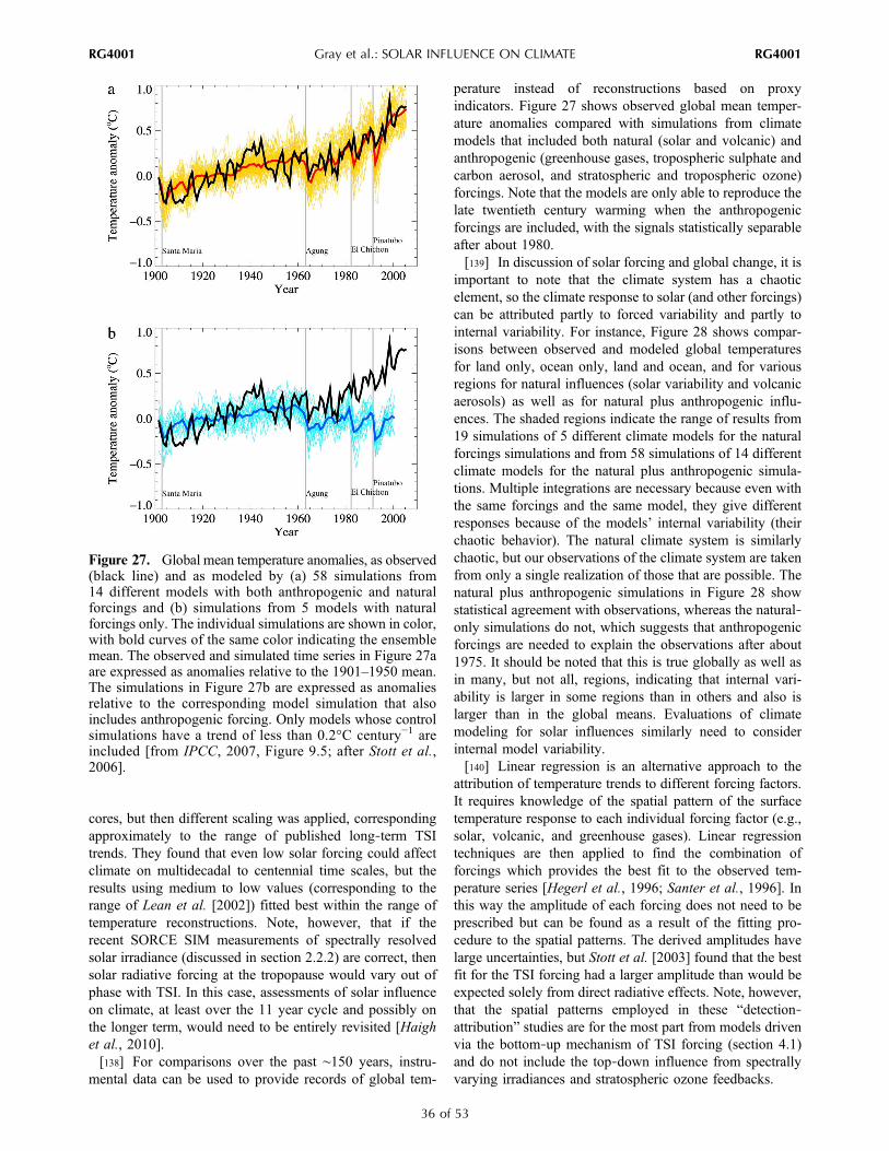
cores, but then different scaling was applied, correspondingapproximately to the range of published long‐term TSItrends. They found that even low solar forcing could affectclimate on multidecadal to centennial time scales, but theresults using medium to low values (corresponding to therange of Lean et al. [2002]) fitted best within the range oftemperature reconstructions. Note, however, that if therecent SORCE SIM measurements of spectrally resolvedsolar irradiance (discussed in section 2.2.2) are correct, thensolar radiative forcing at the tropopause would vary out ofphase with TSI. In this case, assessments of solar influenceon climate, at least over the 11 year cycle and possibly onthe longer term, would need to be entirely revisited [Haighet al., 2010].[138] For comparisons over the past ∼150 years, instru-

mental data can be used to provide records of global tem-

perature instead of reconstructions based on proxyindicators. Figure 27 shows observed global mean temper-ature anomalies compared with simulations from climatemodels that included both natural (solar and volcanic) andanthropogenic (greenhouse gases, tropospheric sulphate andcarbon aerosol, and stratospheric and tropospheric ozone)forcings. Note that the models are only able to reproduce thelate twentieth century warming when the anthropogenicforcings are included, with the signals statistically separableafter about 1980.[139] In discussion of solar forcing and global change, it is

important to note that the climate system has a chaoticelement, so the climate response to solar (and other forcings)can be attributed partly to forced variability and partly tointernal variability. For instance, Figure 28 shows compar-isons between observed and modeled global temperaturesfor land only, ocean only, land and ocean, and for variousregions for natural influences (solar variability and volcanicaerosols) as well as for natural plus anthropogenic influ-ences. The shaded regions indicate the range of results from19 simulations of 5 different climate models for the naturalforcings simulations and from 58 simulations of 14 differentclimate models for the natural plus anthropogenic simula-tions. Multiple integrations are necessary because even withthe same forcings and the same model, they give differentresponses because of the models’ internal variability (theirchaotic behavior). The natural climate system is similarlychaotic, but our observations of the climate system are takenfrom only a single realization of those that are possible. Thenatural plus anthropogenic simulations in Figure 28 showstatistical agreement with observations, whereas the natural‐only simulations do not, which suggests that anthropogenicforcings are needed to explain the observations after about1975. It should be noted that this is true globally as well asin many, but not all, regions, indicating that internal vari-ability is larger in some regions than in others and also islarger than in the global means. Evaluations of climatemodeling for solar influences similarly need to considerinternal model variability.[140] Linear regression is an alternative approach to the

attribution of temperature trends to different forcing factors.It requires knowledge of the spatial pattern of the surfacetemperature response to each individual forcing factor (e.g.,solar, volcanic, and greenhouse gases). Linear regressiontechniques are then applied to find the combination offorcings which provides the best fit to the observed tem-perature series [Hegerl et al., 1996; Santer et al., 1996]. Inthis way the amplitude of each forcing does not need to beprescribed but can be found as a result of the fitting pro-cedure to the spatial patterns. The derived amplitudes havelarge uncertainties, but Stott et al. [2003] found that the bestfit for the TSI forcing had a larger amplitude than would beexpected solely from direct radiative effects. Note, however,that the spatial patterns employed in these “detection‐attribution” studies are for the most part from models drivenvia the bottom‐up mechanism of TSI forcing (section 4.1)and do not include the top‐down influence from spectrallyvarying irradiances and stratospheric ozone feedbacks.

Figure 27. Global mean temperature anomalies, as observed(black line) and as modeled by (a) 58 simulations from14 different models with both anthropogenic and naturalforcings and (b) simulations from 5 models with naturalforcings only. The individual simulations are shown in color,with bold curves of the same color indicating the ensemblemean. The observed and simulated time series in Figure 27aare expressed as anomalies relative to the 1901–1950 mean.The simulations in Figure 27b are expressed as anomaliesrelative to the corresponding model simulation that alsoincludes anthropogenic forcing. Only models whose controlsimulations have a trend of less than 0.2°C century−1 areincluded [from IPCC, 2007, Figure 9.5; after Stott et al.,2006].


36 of 53

[141] First‐order estimates of the global response to dif-ferent forcings can be assessed using the concepts of radi-ative forcing and climate sensitivity (section 1). Because ofthe large uncertainty in centennial‐scale variations in TSI(section 2.3), solar radiative forcing of climate change is notwell established. The IPCC [2007] report estimates a value of0.12Wm−2 for solar radiative forcing change since 1750 (seeFigure 4), which represents a change in TSI of 0.69 W m−2,after taking into account the factor (1 – A)/4, where A isalbedo (see section 1). Many of the present climate modelsimulations, including several in the latest IPCC [2007]report, use TSI reconstructions with a larger drift in TSIsince 1750 than currently thought to be realistic. On the

other hand, the period around the middle of the eighteenthcentury was a time of relatively high solar activity (seeFigure 2) compared to the beginning and end of that century,so the IPCC’s use of the 1750 radiative forcing value torepresent the preindustrial atmosphere means that thechange from 1750 to the present is very small. A choice of1700 or 1800 instead of 1750 would approximately doublethe solar forcing while leaving anthropogenic forcingsessentially unchanged. A value of 0.24 W m−2 solar radia-tive forcing difference from Maunder Minimum to thepresent is currently considered to be more appropriate thanthe 0.12 W m−2 estimated by IPCC (compare with the rangeof 0.16–0.28 W m−2 described in section 2.3). Despite these

Figure 28. Comparison of observed continental‐scale and global‐scale changes in surface temperaturewith results simulated by climate models using natural and anthropogenic forcings. Decadal averages ofobservations are shown for the period 1906–2005 (black line) plotted against the center of the decade andrelative to the corresponding average for 1901–1950. Lines are dashed where spatial coverage is less than50%. Blue shaded bands show the 5%–95% range for 19 simulations from 5 climate models using onlythe natural forcings due to solar activity and volcanoes. Pink shaded bands show the 5%–95% range for58 simulations from 14 climate models using both natural and anthropogenic forcings [from IPCC, 2007,FAQ 9.2, Figure 1].


37 of 53

uncertainties, even this approximate doubling of the solarforcing change is still much smaller than the 1.6 W m−2

estimated to be due to anthropogenic influences.[142] The majority of climate models employed to date

(including those in Figures 27 and 28) represent primarilythe bottom‐up TSI mechanism and have a very poor, or no,representation of the top‐down mechanism that requiresspectral variations in solar radiative input and ozone feed-back effects. Only a few have an adequate representation ofthe stratosphere, and even those do not generate a completerepresentation of stratospheric effects such as an internallyconsistent quasi‐biennial oscillation. Some of the modelsemployed for future IPCC assessments are planned toincorporate these processes and thus should be better placedto assess the importance of these effects.[143] There are additional uncertainties in estimates of

solar radiative forcing which also require further consider-ation. In the usual definition of RF [IPCC, 2007] it is theinstantaneous change in radiative flux at the tropopausewhich is used, and this assumes that the stratosphere hasalready adjusted to the forcing. This is justified on the basisof the faster equilibration time of the stratosphere and alsobecause it has been shown that this “adjusted” forcing is abetter indicator of global average surface temperatureresponse [Hansen et al., 1997]. For solar radiative forcingthe first impact of this adjustment is to reduce the radiativeforcing because the existence of molecular oxygen andozone in the stratosphere reduces the solar radiation reach-ing the tropopause. Second, however, the RF value has to beadjusted to take account of the effects of any solar‐inducedchanges within the stratosphere itself (e.g., temperatureredistribution). Heating of the stratosphere by enhancedsolar UV produces additional downward LW radiation at thetropopause, i.e., a positive feedback. Changes in ozone alsoimpact the radiation fields: additional O3 reduces thedownward SW fluxes but increases the LW fluxes. Thus, aprecise determination of solar RF depends on the responseof stratospheric temperatures and ozone to the changesin solar irradiance. These are not well established (seesection 3.1) so that published estimates of the ozoneamplification of direct TSI forcing show a very wide range[Haigh, 2007; Gray et al., 2009] with even the sign of theeffect remaining uncertain.

6. SUMMARY AND FUTURE DIRECTIONS

[144] This paper presents a review of our present knowl-edge of solar influence on climate, including the physics ofsolar variability, information on direct and proxy observa-tions of both solar variability and climate, and some of thesuggested mechanisms by which solar variability mightinfluence climate. Satellite and ground‐based observations,together with advances in theory and modeling, have greatlyadvanced our knowledge of the Sun in recent decades.Observations have indicated that electromagnetic radiationfrom the Sun varies with the solar cycle so that the Sunemits more radiation at sunspot maximum when, paradoxi-cally, it is most covered with dark sunspots. We now

understand this to be a result of the dominance of the brightfaculae, which also vary over the solar cycle (see section 2).

6.1. Solar Variability[145] There have been great strides in understanding how

the magnetic variability of the Sun is related to the variationof both the total and the spectrally resolved solar irradiance.Basically, the magnetic fields associated with the sunspotsdivert the convective upflow of energy so that the spots aredark, and although the greater portion of the blocked energyupflow is returned to the solar convection zone, some of itemerges in the areas surrounding the sunspots, leading tobrightening there.[146] Through observations of the life cycle of sunspot

groups, together with theory, a quantitative understandinghas emerged that allows the use of magnetic observations ofthe Sun to model the observed solar irradiance variability.Using these techniques, we can explain satellite observa-tions of solar irradiance in terms of the magnetic behavior ofthe Sun. Progress in this field has been greatest in terms ofunderstanding TSI variations on daily to decadal time scales,but recently, much progress has also been achieved inunderstanding and modeling variability in different spectralwavelength intervals.[147] One complication is that satellite instruments mea-

suring solar irradiance have a limited lifetime, and there hasbeen insufficient commitment to ensure continuous, over-lapping observations especially in the case of spectrallyresolved irradiance. This has necessitated the reconstructionof multidecade variations of solar irradiance. There havebeen varied approaches to this. One approach takes themeasurements to be inviolable, thus assuming that the nativemeasurement precision is adequate so that overlaps betweeninstruments serve only to establish continuity betweeninstruments. The other approach is that instrument degra-dation is occurring, and this degradation must be determinedand taken into account when constructing multidecade timeseries of solar irradiance. Our understanding of the con-nection between solar irradiance and the Sun’s magneticvariability can be used to resolve these different approaches,and it has now become clear that the latter approach is moreappropriate.[148] Direct measurements of solar irradiance are only

available for the last few decades. For the period beforethese direct observations, proxy measurements are required.Systematic sunspot measurements have been made for about4 centuries. Additionally, neutron monitor data show thatGCR fluxes vary inversely with the strength of the inter-planetary magnetic field, which is modulated by the Sun.GCRs interact with the atmosphere producing cosmogenicradionuclides such as 10Be and 14C. Measuring 10Be in icecores and 14C in tree rings provides information about thesolar activity over at least the last 10,000 years.[149] Reconstruction of the solar irradiance over the past

few centuries is difficult since direct observations are notavailable from a Maunder Minimum type epoch whensunspots were virtually absent for decades, and some arbi-trary assumptions must be made about what the Sun’s


38 of 53

magnetic field looked like during such epochs. Thus, theestimated increase in TSI from the Maunder Minimum(∼1645–1715) to present‐day values is uncertain. Recentstudies have converged on a probable increase of ∼1.3Wm−2

with an uncertainty range of 0.9–1.6 W m−2. This corre-sponds to an increase in the mean global top‐of‐atmosphereradiative forcing of only 0.16–0.28 W m−2. Nevertheless,because of the complexity of the nonlinear climate systemand the different physics involved, it is far from ideal tocompare forcings by simply using mean global values inW m−2 or, indeed, to apply the concept of sensitivity whichis defined for equilibrium conditions that are never reached.

6.2. Climate Observations[150] The Sun’s irradiance is approximately that of a

blackbody at a temperature of about 5770 K. As such, about50% of the Sun’s output is in the visible and near‐infraredwavelengths. Although very little of the Sun’s output is inthe UV, the Sun’s variability is much greater at these shorterwavelengths. This shortwave solar radiation is mostlyabsorbed in the Earth’s middle and upper atmosphere, so weexpect to find the most obvious solar variability at thesealtitudes (see section 3).[151] Direct influences on temperature and on ozone

concentrations in the tropical and midlatitude upper strato-sphere have been observed and are consistent with estimatesdue to the direct impact of irradiance changes, but a sec-ondary maximum in the lower stratosphere in both fieldsremains to be explained. Solar influences on stratospherictemperatures result in changes in stratospheric winds, andstudies show a wind response that is much larger than can beexplained by direct effects of solar electromagnetic andcorpuscular radiation.[152] One of the best established solar‐climate relations

follows from the pioneering work of Labitzke [1987] andLabitzke and van Loon [1988], who found a clear SCinfluence on winter, NH stratospheric polar temperatureswhen the data were sorted according to the phase of theQBO. Subsequent research has established that similarcorrelations persist into the other seasons and into theSouthern Hemisphere.[153] Many studies have found solar influences in the

ocean, troposphere, and land surface. In the troposphere,there is evidence of an intensification of the tropical pre-cipitation maxima with a broadening of the Hadley circu-lation under Smax conditions and a strengthening of theWalker circulation in the equatorial Pacific in associationwith a La Niña–like SST response during peak solar forcingyears, followed by an El Niño–like response a year or twolater. There is also growing evidence for a solar modulationof the extratropical modes of variability, especially when theQBO phase is also taken into account.[154] There have been reports of strong correlations

between global low cloud amounts and GCRs, but thecontinued correlation into the 1990s is due to an adjustmentto the satellite cloud data that is considered unjustifiable. Wetherefore conclude that the currently available data do notprovide substantial support for the hypothesized global

cloud cover linkage to cosmic rays. The SC‐GCR‐cloud‐climate link continues to be an active area of investigation,however, with controversial aspects remaining. We alsonote that correlation studies cannot establish cause andeffect as clouds will respond to changes in climate whatevertheir cause. Only quantitative treatments of GCR influenceon cloud amounts through the clean air (ion‐induced)mechanisms have been developed to the point where modelscan be tested against observations.[155] At the Earth’s surface, detection of a SC influence is

difficult not only because it is so small but also becausemany other factors have influenced climate during the recentperiod for which we have accurate measurements, includingincreasing greenhouse gases, volcanoes, and aerosol changes.Nevertheless, studies of both ocean and land surface tem-peratures have detected signals. Variations in ocean tem-peratures have been found with both 11 and ∼80 yearperiodicities, which correspond with cycles in solar activity.Typical global average amplitudes of approximately 0.08 ±0.02 K have been found on ∼11 year time scales, which issimilar to estimates of direct heating of the oceans’ mixedlayer. There is also evidence of much larger responses inregional analyses which appear to share some similaritieswith the natural modes of variability, e.g., ENSO. Recentcorrelation studies between 11 year SC forcing and landsurface temperature observations also appear to be robust butdisplay similar patterns in geographical distribution to thosefrom forcing due to greenhouse gases.[156] There have been suggestions that twentieth century

global and hemispheric mean surface temperature variationsare correlated to longer‐term solar variations. Advancedstatistical detection and attribution methodologies confirmthat solar forcing contributed to the increase in globaltemperatures in the early part of the century, but for thelatter part of the twentieth century they consistently find thatusing realistic variations, solar forcing played only a minorrole in global warming, in agreement with the practicallyconstant mean solar forcing since 1980.[157] On longer time scales, proxies are required both for

estimates of the Sun’s variations (e.g., sunspots) and forclimate (e.g., tree rings). A solar influence has been iden-tified during the last millennium, including the so‐calledMedieval Warm Period (∼800–1200 A.D.) and the relativelycold Maunder Minimum (∼1645–1715 A.D.). There hasbeen some controversy about whether the latter was actuallya global‐scale cooling or was a more regional, i.e., Euro-pean, effect. Recent modeling research suggests that it mayhave been a manifestation of a shift in the AO/NAO regime,but investigation of the mechanisms causing the observedEuropean winter cooling remains a topic of active research.[158] There have been many other investigations of con-

nections of solar activity with changes in climate variablessuch as the location and intensity of the ITCZ, periods ofmidcontinent droughts, ocean currents, and monsoonstrength using proxies for both solar activity and climate. Achallenge is to model these patterns of regional climateresponse to solar forcing, work that is being actively pursuedat present. It is clear that many of the observed correlations


39 of 53

between climate variables and solar activity are larger thanwould be expected from the direct influence of the Sun’sobserved variation over the past 3 decades, so the challengehas been to find viable mechanisms that give testablephysical linkages between the Sun’s variations and theobserved variations in the climate variables.

6.3. Mechanisms[159] Suggested mechanisms for solar influence on cli-

mate vary in their maturity: the most mature can berepresented in climate models using well‐established phys-ics, and their impacts on the modeled climate can beexamined. The less mature are based on hypotheses thatmay be credible but have not yet been put into physicalmodels in order to test their influence.[160] The most obvious mechanism for solar variations

affecting the Earth’s climate is due to the change in heatingof the Earth system associated with varying TSI. These arefound to partially explain the variations in the temperatureof the oceanic mixed layer, but even in this case, it appearsthat modulations in the ocean‐atmosphere sensible andlatent heat fluxes are needed to explain the observations,suggesting a possible interaction with variations in theHadley and Walker circulations. There has been recentprogress in the development and testing of mechanisms toexplain the observed solar signal in the Pacific whichresembles the ENSO signal.[161] The most mature Sun‐climate mechanism at this

time involves the direct effect of the observed variation insolar UV radiation affecting stratospheric ozone, leading toassociated temperature variations. The resulting temperaturegradients lead to changes in the zonal wind, which, in turn,changes planetary wave–mean flow interactions. Inclusionof these mechanisms in fully coupled chemistry‐climatemodels has been achieved, and many of the observed fea-tures in stratospheric temperatures, winds, and ozone dis-tributions have been reproduced, including the maximum inozone in the lower stratosphere, which appears to be anindirect effect associated with changes in the global circu-lation. Progress has been made in understanding and mod-eling the observed SC‐QBO interactions, but there are stillaspects that are not well understood, including the lowerstratospheric temperature maximum and the mechanism forSC‐QBO influence on sudden warmings. The SC influencesin summertime and in the SH also require further study.[162] The inclusions in climate models of SC irradiance

and ozone feedback mechanisms have also resulted inchanges in the modeled troposphere, including modificationto the Hadley circulation and changes in extratropical modesof variability (NAM and SAM). These have been achievedin models in which the SSTs are fixed, suggesting that thesetropospheric changes are at least partly due to a top‐downmechanism, i.e., stratosphere‐troposphere coupling, whichmay be particularly helpful in explaining the observedregional signals. However, models that include the bottom‐up coupled air‐sea response mechanism also show thesechanges and indicate that the two mechanisms could beadditive to produce the magnitude of the responses observed

in the climate system. Since the nature of the exactmechanisms for this coupling is crucial for understandingsolar‐climate connections, there is much active research inthis area.[163] The solar modulation of GCRs or the global electric

circuit has also been proposed as a mechanism for SCinfluence on climate, through their ability to influence cloudcover. However, as noted above, this mechanism has onlyjust begun to be tested in physical models.

6.4. Climate Change[164] Finally, the role of solar variability in climate change

has received much public attention because reliable esti-mates of solar influence are needed to limit uncertainty inthe importance of human activity as a potential explanationfor global warming. Extensive climate model studies haveindicated that the models can only reproduce the latetwentieth century warming when anthropogenic forcing isincluded, in addition to the solar and volcanic forcings[IPCC, 2007]. The change in solar radiative forcing since1750 was estimated in the IPCC [2007] report to be0.12 W m−2, corresponding to an increase in TSI of0.69 W m−2. A value of 0.24 W m−2 solar radiative forcingdifference from Maunder Minimum to the present is cur-rently considered to be more appropriate. Despite theseuncertainties in solar radiative forcing, they are neverthelessmuch smaller than the estimated radiative forcing due toanthropogenic changes, and the predicted SC‐related surfacetemperature change is small relative to anthropogenicchanges.[165] One thing that is very clear from this review is that

enormous progress has been achieved in our knowledge andunderstanding over the past few decades. The topic hasemerged from its beginnings of almost purely investigationof statistical relationships that were subject to substantialcriticism to become a solid scientific field that involves bothsolar physicists and climate scientists. Indeed, even 20 yearsago it would have been very unlikely that the collection ofscientific fields represented by the authors of this paperwould have collaborated on such a review.

6.5. Further Research[166] Further observations and research are required to

improve our understanding of solar forcing mechanisms andtheir impacts on the Earth’s climate. In particular, it isnecessary (1) to understand the recent SORCE SIM mea-surements of spectrally resolved irradiances and assess theirimplications for solar influence on climate (see section 2.2.2);(2) to determine an accurate value of the total and spectrallyresolved solar irradiance during a grand solar minimum suchas the Maunder Minimum, when the Sun was in a differentmode than during the past few decades (see section 2.2.3);(3) to improve the characterization of the solar signal insurface and tropospheric observations as additional years ofdata becomes available (see sections 3.2 and 3.3); (4) toimprove the characterization of the observed stratospherictemperature response to the 11 year solar cycle, particularlythe vertical structure of the response at tropical latitudes so


40 of 53

that the differences between the estimated SC signals fromthe TOVS data and from reanalysis data can be fullyunderstood, which will likely require future observationswith improved vertical resolution (see section 3.1.2); and(5) to improve model simulations of the observed solarsignals in climate observations and, in particular, assess therequirement to explicitly represent stratospheric mechan-isms in future climate models, which will require fullycoupled ocean‐troposphere‐stratosphere models with inter-active chemistry so that the relative contribution and inter-actions of the top‐down and bottom‐up influences can beunderstood. We note that, there will still be a continuing rolefor simpler models to investigate and improve the simula-tion of specific mechanisms, including the development ofmodels that investigate possible influences of galactic cosmicrays on cloud formation (see section 4.4).

NOTATION

[167] The interdisciplinary nature of this review introducesa great many acronyms and notations that are in common usein any one field but may not be so well known by scientistsfrom another field. We therefore list them here.

AcronymsACRIM Active Cavity Radiometer Irradiance

Monitor.AO Arctic Oscillation.B‐D Brewer‐Dobson (circulation).BSi biogenic silica content.

CCN cloud condensation nucleii.CCM chemistry climate models.CZ convection zone (solar).D2 data set generated by ISCCP.

DIARAD Differential Absolute Radiometer (part ofthe VIRGO instrument on SoHO).

DJF December, January, and February.ECMWF European Centre for Medium Range

Weather Forecasts.ENSO El Niño–Southern Oscillation.

ERA‐40 ECMWF reanalysis data set for 1959–2001.GHG greenhouse gas.

HALOE Halogen Occultation Experiment (instru-ment on UARS).

HF Hickey‐Frieden Radiometer (an instrumenton the Nimbus 7 satellite).

IMF interplanetary magnetic field.IPCC Intergovernmental Panel on Climate

Change.IR infrared.

IRD ice‐rafted debris.IRMB Institut Royal Meteorologique Belgique.ISCCP International Satellite Cloud Climatology

Project.ITCZ Intertropical Convergence Zone.GCM general circulation model.

GCR galactic cosmic rays.LCA low cloud amount.

LOSU level of scientific understanding.LW longwave radiation.

Ly‐a Lyman alpha emission line.MDI Michelson Doppler Interferometer (instru-

ment on SoHO).MODIS Moderate Resolution Imaging Spectroradi-

ometer (instruments on the Terra and Aquasatellites).

NAM northern annular mode.NAO North Atlantic Oscillation.NCEP National Centers for Environmental Predic-

tion (formerly NMC).NH Northern Hemisphere.NOx nitrogen species NO + NO2.NP North Pole.

NRC National Research Council.PMOD Physikalisch‐Meteorologisches Observa-

torium Davos (Switzerland).PM6 a cavity radiometer (part of the VIRGO

instrument on SoHO).QBO quasi‐biennial oscillation.

QBO‐E easterly wind years of the QBO.QBO‐W westerly wind years of the QBO.

RF radiative forcing.SAGE Stratospheric Aerosol and Gas Experiments

(satellite).SAM southern annular mode.

SATIRE Spectral and Total Irradiance Reconstruction.SC solar cycle.SEP solar energetic particles.SH Southern Hemisphere.SIM Spectral Irradiance Monitor (instrument on

the SORCE).Smax sunspot cycle maximum.Smin sunspot cycle minimum.

SoHO Solar andHeliospheric Observatory (satellite).SORCE Solar Radiation and Climate Experiment.

SP South Pole.SPCZ South Pacific Convergence Zone.SPE solar proton event.SSI spectral solar irradiance.SST sea surface temperature.SSW stratospheric sudden warming.SW shortwave radiation.

TIROS Television Infrared Observation Satellites.TOVS TIROS Operational Vertical Sounder (infra-

red radiometers on TIROS satellites).TSI total solar irradiance.

UARS Upper Atmosphere Research Satellite.UCN ultrafine condensation nuclei.UV ultraviolet.

VIRGO Variability of Solar Irradiance and GravityOscillations (instrument on SoHO).

10Be beryllium‐10 (cosmogenic isotope).14C carbon‐14 (cosmogenic isotope).


41 of 53

ParametersA Earth’s SW albedo.

BQS average quiet Sun magnetic field during theMaunder Minimum.

aa planetary index of geomagnetic activity.Ap planetary index of geomagnetic activity.C counts detected by the neutron monitor at

Climax, Colorado.r·F Eliassen‐Palm planetary flux divergence.FS open solar magnetic flux.

F10.7 10.7 cm solar radio flux (in W m−2 Hz−1).GCR counts detected by the neutron monitor at

McMurdo, Antarctica.I spectral solar irradiance (SSI).

ITS total solar irradiance (TSI).L solar cycle length.M heliospheric modulation parameter (of

GCRs).Mg ii Mg ii line (280 nm) core‐to‐wing ratio.

P[10Be] global production rate of the cosmogenic10Be isotope.

R sunspot number.R11 11 year running mean of sunspot number.RG group sunspot number.T temperature.TS global mean surface air temperature.U wind speed.

Z30 30 hPa geopotential height.l climate sensitivity parameter.

DF change in forcing at the top of theatmosphere.

DTS change in globalmean surface air temperature.D14C carbon‐14 production rate.DU change in wind speed.d18O a measure of the ratio of the oxygen‐18 to

oxygen‐16 isotopes.Non‐SI Units

AU astronomical distance.DU Dobson units (column ozone measurement).RE Mean Earth radius.

[168] ACKNOWLEDGMENTS. The development of thisreview article has evolved from work carried out by an interna-tional team of the International Space Science Institute (ISSI),Bern, Switzerland, and from work carried out under the auspicesof Scientific Committee on Solar Terrestrial Physics (SCOSTEP)Climate and Weather of the Sun‐Earth System (CAWSES‐1).The support of ISSI in providing workshop and meeting facilitiesis acknowledged, especially support fromY. Calisesi and V.Manno.SCOSTEP is acknowledged for kindly providing financial assis-tance to allow the paper to be published under an open accesspolicy. L.J.G. was supported by the UK Natural EnvironmentResearch Council (NERC) through their National Centre for Atmo-spheric Research (NCAS) Climate program. K.M. was supportedby a Marie Curie International Outgoing Fellowship within the6th European Community Framework Programme. J.L. acknowl-edges support by the EU/FP7 program Assessing Climate Impactson the Quantity and Quality of Water (ACQWA, 212250) and fromthe DFG Project Precipitation in the Past Millennium in Europe

(PRIME) within the Priority Program INTERDYNAMIK. L.H.acknowledges support from the U.S. NASA Living With a Starprogram. G.M. acknowledges support from the Office of Science(BER), U.S. Department of Energy, Cooperative AgreementDE‐FC02‐97ER62402, and the National Science Foundation. Wealso wish to thank Karin Labitzke and Markus Kunze for supplyingan updated Figure 13, Andrew Heaps for technical support, andPaul Dickinson for editorial support. Part of the research wascarried out under the SPP CAWSES funded by GFG. J.B. wasfinancially supported by NCCR Climate–Swiss Climate Research.[169] The Editor for this manuscript was Pete Riley. He wishes

to thank an anonymous reviewer.

REFERENCES

Allan, R. J. (2000), ENSO and climatic variability in the last150 years, in El Nino and the Southern Oscillation: MultiscaleVariability, Global and Regional Impacts, edited by H. F. Diazand V. Markgraf, pp. 3–35, Cambridge Univ. Press, Cambridge,U. K.

Ammann, C. M. (2005), Solar signals in records and simulations ofpast climates, Mem. Soc. Astron. Ital., 76, 802–804.

Ammann, C.M., G. A.Meehl,W.M.Washington, and C. A. Zender(2003), A monthly and latitudinally varying volcanic forcingdataset in simulations of 20th century climate,Geophys. Res. Lett.,30(12), 1657, doi:10.1029/2003GL016875.

Ammann, C. M., F. Joos, D. S. Schimel, B. L. Otto‐Bliesner, andR. A. Tomas (2007), Solar influence on climate during the pastmillennium: Results from transient simulations with the NCARClimate System Model, Proc. Natl. Acad. Sci. U. S. A., 104,3713–3718, doi:10.1073/pnas.0605064103.

Aplin, K. L. (2008), Composit ion and measurement ofcharged atmospheric clusters, Space Sci. Rev., 137, 213–224,doi:10.1007/s11214-008-9397-1.

Arnold, N. F., and T. R. Robinson (2000), Amplification of theinfluence of solar flux variations on the winter stratosphere byplanetary waves, Space Sci. Rev., 94, 279–286, doi:10.1023/A:1026783609783.

Austin, J., L. L. Hood, and B. E. Soukharev (2007), Solar cyclevariations of stratospheric ozone and temperature in simulationswith a coupled chemistry‐climate model, Atmos. Chem. Phys., 7,1693–1706, doi:10.5194/acp-7-1693-2007.

Austin, J., et al. (2008), Coupled chemistry climate model simula-tions of the solar cycle in ozone and temperature, J. Geophys.Res., 113, D11306, doi:10.1029/2007JD009391.

Balachandran, N., and D. Rind (1995), Modelling the effects ofUV variability and the QBO on the troposphere‐stratospheresystem. Part I: The middle atmosphere, J. Clim., 8, 2058–2079,doi:10.1175/1520-0442(1995)008<2058:MTEOUV>2.0.CO;2.

Balachandran, N. K., D. Rind, P. Lonergan, and D. T. Shindell(1999), Effects of solar cycle variability on the lower stratosphereand the troposphere, J. Geophys. Res., 104, 27,321–27,339,doi:10.1029/1999JD900924.

Baldwin, M. P., and T. J. Dunkerton (2001), The solar cycle andstratosphere‐troposphere dynamical coupling, Science, 294,581–584, doi:10.1126/science.1063315.

Baldwin, M. P., et al. (2001), The quasi biennial oscillation, Rev.Geophys., 39, 179–229, doi:10.1029/1999RG000073.

Baliunas, S., and R. Jastrow (1990), Evidence for long‐termbrightness changes of solar‐type stars, Nature, 348, 520–523,doi:10.1038/348520a0.

Bard, E., G. Raisbeck, F. Yiou, and J. Jouzel (2000), Solar irradi-ance during the last 1200 years based on cosmogenic nuclides,Tellus, Ser. B, 52, 985–992.

Barriopedro, D., R. García‐Herrera, and R. Huth (2008), Solarmodulation of Northern Hemisphere winter blocking, J. Geophys.Res., 113, D14118, doi:10.1029/2008JD009789.


42 of 53

Bates, J. R. (1981), A dynamical mechanism through which var-iations in solar ultra violet radiation can influence troposphericclimate, Sol. Phys., 74, 399–415, doi:10.1007/BF00154526.

Beer, J., and B. van Geel (2008), Holocene climate change and theevidence for solar and other forcings, in Natural Climate Vari-ability and Global Warming: A Holocene Perspective, editedby R. W. Batterbee and H. A. Binney, pp. 138–162, Wiley‐Blackwell, Oxford, U. K.

Beer, J., W. Mende, and R. Stellmacher (2000), The role of the Sunin climate forcing, Quat. Sci. Rev., 19, 403–415, doi:10.1016/S0277-3791(99)00072-4.

Beer, J., M. Vonmoos, and R. Muscheler (2006), Solar variabilityover the past several millennia, Space Sci. Rev., 125, 67–79,doi:10.1007/s11214-006-9047-4.

Bennett, A. J., and R. G. Harrison (2008), Surface measurementsystem for the atmospheric electrical vertical conduction currentdensity, with displacement current correction, J. Atmos. Sol.Terr. Phys., 70, 1373–1381, doi:10.1016/j.jastp.2008.04.014.

Bennett, A. J., and R. G. Harrison (2009), Evidence for globalcircuit current flow through water droplet layers, J. Atmos. Sol.Terr. Phys., 71(12), 1219–1221, doi:10.1016/j.jastp.2009.04.011.

Bhatnagar, A., K. Jain, and S. C. Tripathy (2002), Variation ofsolar irradiance and mode frequencies during Maunder Mini-mum, Astrophys. Space Sci., 281, 761–764, doi:10.1023/A:1016325824515.

Björck, S., et al. (2001), High‐resolution analyses of an early Holo-cene climate event may imply decreased solar forcing as animportant c l imate t r igger , Geology , 29 , 1107–1110,doi:10.1130/0091-7613(2001)029<1107:HRAOAE>2.0.CO;2.

Blaauw, M., G. B. M. Heuvelink, D. Mauquoy, J. van der Plicht,and B. van Geel (2003), A numerical approach to 14C wiggle‐match dating of organic deposits: Best fits and confidence inter-vals, Quat. Sci. Rev., 22, 1485–1500, doi:10.1016/S0277-3791(03)00086-6.

Black, D. E., R. C. Thunell, A. Kaplan, L. C. Peterson, and E. J.Tappa (2004), A 2000‐year record of Caribbean and tropicalNorth Atlantic hydrographic variability, Paleoceanography, 19,PA2022, doi:10.1029/2003PA000982.

Black, R. X. (2002), Stratospheric forcing of surface climate in theArctic oscillation, J. Clim., 15, 268–277, doi:10.1175/1520-0442(2002)015<0268:SFOSCI>2.0.CO;2.

Boberg, F., and H. Lundstedt (2002), Solar wind variations relatedto fluctuations of the North Atlantic Oscillation, Geophys. Res.Lett., 29(15), 1718, doi:10.1029/2002GL014903.

Bond, G., B. Kromer, J. Beer, R. Muscheler, M. N. Evans,W. Showers, S. Hoffmann, R. Lotti‐Bond, I. Hajdas, andG. Bonani (2001), Persistent solar influence on North Atlanticclimate during the Holocene, Science, 294, 2130–2136,doi:10.1126/science.1065680.

Briffa, K. R., P. D. Jones, F. H. Schweingruber, and T. J. Osborn(1998), Influence of volcanic eruptions on northern hemispheresummer temperature over the past 600 years, Nature, 393,450–455, doi:10.1038/30943.

Brönnimann, S., T. Ewen, T. Griesser, and R. Jenne (2007), Multi-decadal signal of solar variability in the upper troposphere duringthe 20th century, Space Sci. Rev., 125, 305–317, doi:10.1007/s11214-006-9065-2.

Brown, B. H. (2008), Short‐term changes in global cloud coverand in cosmic radiation, J. Atmos. Sol. Terr. Phys., 70(7),1122–1131, doi:10.1016/j.jastp.2008.02.003.

Burke, H. K., and A. A. Few (1978), Direct measurements of theatmospheric conduction current, J. Geophys. Res., 83(C6),3093–3098, doi:10.1029/JC083iC06p03093.

Calbó, J., J.‐A. Gonzalez, and D. Pagès (2001), A method for sky‐condition classification from ground‐based solar radiation mea-surements, J. Appl. Meteorol., 40, 2193–2199, doi:10.1175/1520-0450(2001)040<2193:AMFSCC>2.0.CO;2.

Calisesi, Y., R.‐M. Bonnet, L. Gray, J. Langen, and M. Lockwood(2006), Solar Variability and Planetary Climate, Springer,Dordrecht, Netherlands.

Callis, L. B., D. N. Baker, M. Natarajan, J. B. Bernard, R. A.Mewaldt, R. S. Selesnick, and J. R. Cummings (1996), A 2‐Dmodel simulation of downward transport of NOy into the strato-sphere: Effects on the 1994 austral spring O3and NOy, Geophys.Res. Lett., 23(15), 1905–1908, doi:10.1029/96GL01788.

Callis, L. B., M. Natarajan, and J. D. Lambeth (2000), Calculatedupper stratospheric effects of solar UV flux and NOy variationsduring the 11‐year solar cycle, Geophys. Res. Lett., 27, 3869–3872, doi:10.1029/2000GL011622.

Callis, L. B., M. Natarajan, and J. D. Lambeth (2001), Solar‐atmospheric coupling by electrons (SOLACE): 3. Comparisonsof simulations and observations, 1979–1997, issues and implica-tions, J. Geophys. Res. , 106 , 7523–7539, doi:10.1029/2000JD900615.

Calogovic, J., C. Albert, F. Arnold, J. Beer, L. Desorgher, andE. O. Flueckiger (2010), Sudden cosmic ray decreases: Nochange of global cloud cover, Geophys. Res. Lett., 37, L03802,doi:10.1029/2009GL041327.

Camp, C. D., and K. K. Tung (2007), The influence of the solarcycle and QBO on the late winter stratospheric polar vortex,J. Atmos. Sci., 64, 1267–1283, doi:10.1175/JAS3883.1.

Castanheira, J. M., and H.‐F. Graf (2003), North Pacific–NorthAtlantic relationships under stratospheric control?, J. Geophys.Res., 108(D1), 4036, doi:10.1029/2002JD002754.

Chalmers, J. A. (1967), Atmospheric Electricity, 2nd ed., Pergamon,Oxford, U. K.

Chandra, S., and R. D. McPeters (1994), The solar cycle variationof ozone in the stratosphere inferred from Nimbus 7 and NOAA11 satellites, J. Geophys. Res., 99, 20,665–20,671, doi:10.1029/94JD02010.

Chapman, G. A., A. M. Cookson, J. J. Dobias, and S. R. Walton(2001), An improved determination of the area ratio of faculaeto sunspots, Astrophys. J., 555, 462–465, doi:10.1086/321466.

Chipperfield, M. P., et al. (2007), Global ozone past and present, inScientific Assessment of Ozone Depletion: 2006, Global OzoneRes. Monit. Proj. Rep., 50, chap. 3, pp. 3.1–3.58, World Meteorol.Organ., Geneva, Switzerland.

Clement, A. C., R. Seager, M. A. Cane, and S. E. Zebiak (1996),An ocean dynamical thermostat, J. Clim., 9, 2190–2196,doi:10.1175/1520-0442(1996)009<2190:AODT>2.0.CO;2.

Cook, E. R., J. G. Palmer, and R. D. D’Arrigo (2002), Evidence fora ‘Medieval Warm Period’ in a 1,100 year tree‐ring reconstructionof past austral summer temperatures in New Zealand, Geophys.Res. Lett., 29(14), 1667, doi:10.1029/2001GL014580.

Cordero, E. C., and T. R. Nathan (2005), A new pathway forcommunicating the 11‐year solar cycle signal to the QBO,Geophys. Res. Lett., 32, L18805, doi:10.1029/2005GL023696.

Crommelynck, D., A. Fichot, R. B. Lee III, and J. Romero (1995),First realisation of the Space Absolute Radiometric Reference(SARR) during the ATLAS 2 flight period, Adv. Space Res.,16, 17–23, doi:10.1016/0273-1177(95)00261-C.

Crooks, S. A., and L. J. Gray (2005), Characterisation of the 11‐yearsolar signal using a multiple regression analysis of the ERA‐40dataset, J. Clim., 18, 996–1015, doi:10.1175/JCLI-3308.1.

Crowley, T. J. (2000), Causes of climate change over the past1000 years, Science, 289, 270–277, doi:10.1126/science.289.5477.270.

Cubasch, U., and R. Voss (2000), The influence of total solar irra-diance on climate, Space Sci. Rev., 94, 185–198, doi:10.1023/A:1026719322987.

Cubasch, U., R. Voss, G. C. Hegerl, J. Waszkewitz, and T. C.Crowley (1997), Simulation with an O‐AGCM of the influenceof variations of the solar constant on the global climate, Clim.Dyn., 13, 757–767, doi:10.1007/s003820050196.

Cubasch, U., E. Zorita, F. Kaspar, J. F. Gonzales‐Rouco, H. vonStorch, and K. Prommel (2006), Simulation of the role of solar


43 of 53

and orbital forcing on climate, Adv. Space Res., 37, 1629–1634,doi:10.1016/j.asr.2005.04.076.

Damiani, A., M. Storini, M. Laurenza, C. Rafanelli, E. Piervitali,and E. G. Cordero (2006), Southern ozone variations inducedby solar particle events during 15 January–5 February 2005,J. Atmos. Sol. Terr. Phys., 68(17), 2042–2052, doi:10.1016/j.jastp.2006.03.010.

Damon, P. E., and P. Laut (2004), Pattern of strange errors plaguessolar activity and terrestrial climate data, Eos Trans. AGU, 85,370, doi:10.1029/2004EO390005.

de Jager, C., and I. Usoskin (2006), On possible drivers of Sun‐induced climate changes, J. Atmos. Sol. Terr. Phys., 68, 2053–2060, doi:10.1016/j.jastp.2006.05.019.

Dengel, S., D. Aeby, and J. Grace (2009), A relationship betweengalactic cosmic radiation and tree rings, New Phytol., 184, 545–551, doi:10.1111/j.1469-8137.2009.03026.x.

de Putter, T., M.‐F. Loutre, and G. Wansard (1998), Decadal per-iodicities of Nile river historical discharge (A.D. 622–1470) andclimatic implications, Geophys. Res. Lett., 25, 3193–3196,doi:10.1029/98GL02250.

Dewitte, S., D. Crommelynck, S. Mekaoui, and A. Joukoff (2004),Measurement and uncertainty of the long‐term total solar irradi-ance trend, Sol. Phys., 224, 209–216, doi:10.1007/s11207-005-5698-7.

Dickinson, R. E. (1975), Solar variability and the lower atmo-sphere, Bull. Am. Meteorol. Soc., 56, 1240–1248, doi:10.1175/1520-0477(1975)056<1240:SVATLA>2.0.CO;2.

Duchon, C. E., and M. S. O’Malley (1999), Estimating cloud typefrom pyranometer observations, J. Appl. Meteorol., 38, 132–141,doi:10.1175/1520-0450(1999)038<0132:ECTFPO>2.0.CO;2.

Duplissy, J., et al. (2009), Results from the CERN pilot CLOUDexperiment, Atmos. Chem. Phys. Discuss., 9, 18,235–18,270,doi:10.5194/acpd-9-18235-2009.

Dykoski, C. A., R. L. Edwards, H. Cheng, D. Yuan, Y. Cai,M. Zhang, Y. Lin, J. Qing, Z. An, and J. Revenaugh (2005), Ahigh‐resolution, absolute dated Holocene and deglacial Asianmonsoon record from Dongge Cave, China, Earth Planet. Sci.Lett., 233, 71–86, doi:10.1016/j.epsl.2005.01.036.

Eddy, J. A. (1976), The Maunder Minimum, Science, 192, 1189–1202, doi:10.1126/science.192.4245.1189.

Egorova, T., E. Rozanov, E. Manzini, M. Haberreiter, W. Schmutz,V. Zubov, and T. Peter (2004), Chemical and dynamicalresponse to the 11‐year variability of the solar irradiance simu-lated with a chemistry‐climate model, Geophys. Res. Lett., 31,L06119, doi:10.1029/2003GL019294.

Eichkorn, S., S. Wilhelm, H. Aufmhoff, K. H. Wohlfrom, andF. Arnold (2002), Cosmic ray‐induced aerosol‐formation: Firstobservational evidence from aircraft‐based ion mass spectrom-eter measurements in the upper troposphere, Geophys. Res.Lett., 29(14), 1698, doi:10.1029/2002GL015044.

Eltahir, E. A. B., and G. Wang (1999), Nilometers, El Nino, andclimate variability, Geophys. Res. Lett. , 26 , 489–492,doi:10.1029/1999GL900013.

Emile‐Geay, J., M. Cane, R. Seager, A. Kaplan, and P. Almasi(2007), El Nino as a mediator of the solar influence on climate,Paleoceanography, 22, PA3210, doi:10.1029/2006PA001304.

Evan, A. T., A. K. Heidinger, and D. J. Vimon (2007), Argumentsagainst a physical long‐term trend in global ISCCP cloudamounts, Geophys. Res. Lett., 34, L04701, doi:10.1029/2006GL028083.

Field, C. V., G. A. Schmidt, D. Koch, and C. Salyk (2006),Modeling production and climate‐related impacts on 10Be concen-trations in ice cores, J. Geophys. Res., 111, D15107, doi:10.1029/2005JD006410.

Fischer, P., and K. K. Tung (2008), A reexamination of the QBOperiod modulation by the solar cycle, J. Geophys. Res., 113,D07114, doi:10.1029/2007JD008983.

Fleitmann, D., S. J. Burns, M. Mudelsee, U. Neff, J. Kramers,A. Mangini, and A. Matter (2003), Holocene forcing of the

Indian monsoon recorded in a stalagmite from southern Oman,Science, 300, 1737–1739, doi:10.1126/science.1083130.

Fligge, M., and S. K. Solanki (1998), Long‐term behaviour ofemissions from solar faculae: Steps towards a robust index,Astron. Astrophys., 332, 1082–1086.

Foster, S. S. (2004), Reconstruction of solar irradiance variations,for use in studies of global climate change: Application ofrecent SoHO observations with historic data from the Green-wich observations, Ph.D. thesis, Sch. of Phys. and Astron.,Univ. of Southampton, Southampton, U. K.

Foukal, P., K. Harvey, and F. Hill (1991), Do changes in the pho-tospheric magnetic network cause the 11‐year variation of totalsolar irradiance?, Astrophys. J., 383, L89–L92, doi:10.1086/186249.

Foukal, P., G. North, and T. Wigley (2004), A stellar view on solarvariations and climate, Science, 306, 68–69, doi:10.1126/science.1101694.

Fraedrich, K., and C. Bantzer (1991), A note on fluctuations of theNile river flood levels (715–1470), Theor. Appl. Climatol., 44,167–171, doi:10.1007/BF00868171.

Frame, T. H. A., and L. J. Gray (2010), The 11‐year solar cycle inERA‐40 data: An update to 2008, J. Clim., 23, 2213–2222,doi:10.1175/2009JCLI3150.1

Friis‐Christensen, E., and K. Lassen (1991), Length of the solarcycle: An indicator of solar activity closely associated with cli-mate, Science, 254, 698–700, doi:10.1126/science.254.5032.698.

Fröhlich, C. (2002), Total solar irradiance variations since 1978,Adv. Space Res., 29, 1409–1416, doi:10.1016/S0273-1177(02)00203-X.

Fröhlich, C. (2006), Solar irradiance variability since 1978: Revi-sion of the PMOD composite during solar cycle 21, Space Sci.Rev., 125, 53–65, doi:10.1007/s11214-006-9046-5.

Funke, B., M. López‐Puertas, S. Gil‐López, T. von Clarmann,G. P. Stiller, H. Fischer, and S. Kellman (2005), Downwardtransport of upper atmospheric NOx into the polar stratosphereand lower mesosphere during the Antarctic 2003 and Arctic2002/2003 winters , J. Geophys. Res . , 110 , D24308,doi:10.1029/2005JD006463.

Ganguly, N. D. (2010), Influence of solar proton events during thedeclining phase of solar cycle 23 on the total ozone concentrationin India, Int. J. Remote Sens., 31(2), 313–322, doi:10.1080/01431160902882678.

Geller, M. A. (1988), Solar cycles and the atmosphere, Nature,332, 584–585, doi:10.1038/332584a0.

Geller, M. A., and J. C. Alpert (1980), Planetary wave couplingbetween the troposphere and the middle atmosphere as a possibleSun‐weather mechanism, J. Atmos. Sci., 37, 1197–1215,doi:10.1175/1520-0469(1980)037<1197:PWCBTT>2.0.CO;2.

Giampapa, M. (2004), Stellar analogs of solar activity: The Sun ina stellar context, in The Sun, Solar Analogs and the Climate,edited by I. Redi, M. Güdel, and W. Schmutz, pp. 305–423,Springer, Berlin.

Gleisner, H., and P. Thejll (2003), Patterns of troposphericresponse to solar variability, Geophys. Res. Lett., 30(13), 1711,doi:10.1029/2003GL017129.

Goosse, H., O. Arzel, J. Luterbacher, M. E. Mann, H. Renssen,N. Riedwyl, A. Timmermann, E. Xoplaki, and H. Wanner(2006), The origin of the European ‘Medieval Warm Period,’Clim. Past, 2, 99–113, doi:10.5194/cp-2-99-2006.

Graham, N. E., and W. B. White (1988), The El Niño cycle: Anatural oscillator of the Pacific Ocean atmosphere system,Science, 240(4857), 1293–1302, doi:10.1126/science.240.4857.1293.

Graham, N. E., et al. (2007), Tropical Pacific mid‐latitude telecon-nections in medieval times, Clim. Change, 83, 241–285,doi:10.1007/s10584-007-9239-2.

Gray, L. J. (2003), The influence of the equatorial upper strato-sphere on stratospheric sudden warmings, Geophys. Res. Lett.,30(4), 1166, doi:10.1029/2002GL016430.


44 of 53

Gray, L. J. (2010), Equatorial dynamics, in The Stratosphere:Dynamics, Transport, and Chemistry, Geophys. Monogr. Ser.,vol. 190, edited by L. M. Polvani, A. H. Sobel, and D. W.Waugh, AGU, Washington, D. C., in press.

Gray, L. J., S. J. Phipps, T. J. Dunkerton, M. P. Baldwin, E. F.Drysdale, and M. R. Allen (2001), A data study of the influenceof the equatorial upper stratosphere on Northern Hemispherestratospheric sudden warmings, Q. J. R. Meteorol. Soc., 127,1985–2003, doi:10.1002/qj.49712757607.

Gray, L. J., S. Crooks, C. Pascoe, S. Sparrow, and M. Palmer(2004), Solar and QBO influences on the timing of stratosphericsudden warmings, J. Atmos. Sci., 61, 2777–2796, doi:10.1175/JAS-3297.1.

Gray, L. J., S. A. Crooks, M. A. Palmer, C. L. Pascoe, andS. Sparrow (2006), A possible transfer mechanism for the11‐year solar cycle to the lower stratosphere, Space Sci. Rev.,125, 357–370, doi:10.1007/s11214-006-9069-y.

Gray, L. J., S. T. Rumbold, and K. P. Shine (2009), Stratospherictemperature and radiative forcing response to 11‐year solar cyclechanges in irradiance and ozone, J. Atmos. Sci., 66, 2402–2417,doi:10.1175/2009JAS2866.1.

Gunn, R. (1965), The hyperelectrification of raindrops by electricfields, J. Meteorol., 13, 283–288.

Haigh, J. D. (1994), The role of stratospheric ozone in modulatingthe solar radiative forcing of climate, Nature, 370, 544–546,doi:10.1038/370544a0.

Haigh, J. D. (1996), The impact of solar variability on climate,Science, 272, 981–984, doi:10.1126/science.272.5264.981.

Haigh, J. D. (1999), A GCM study of climate change in response tothe 11‐year solar cycle, Q. J. R. Meteorol. Soc., 125, 871–892,doi:10.1002/qj.49712555506.

Haigh, J. D. (2003), The effects of solar variability on the Earth’sclimate, Philos. Trans. R. Soc. London, Ser. A, 361, 95–111,doi:10.1098/rsta.2002.1111.

Haigh, J. D. (2007), The Sun and the Earth’s climate, Living Rev.Sol. Phys., 4, lrsp‐2007‐2.

Haigh, J. D., and M. Blackburn (2006), Solar influences on dynam-ical coupling between the stratosphere and troposphere, SpaceSci. Rev., 125, 331–344, doi:10.1007/s11214-006-9067-0.

Haigh, J. D., and H. K. Roscoe (2009), The final warming date ofthe Antarctic polar vortex and influences on its interannualva r i ab i l i t y , J . C l im . , 22 , 5809–5819 , do i : 10 .1175 /2009JCLI2865.1.

Haigh, J. D., M. Blackburn, and R. Day (2005), The response oftropospheric circulation to perturbations in lower‐stratospherictemperature, J. Clim., 18, 3672–3685, doi:10.1175/JCLI3472.1.

Haigh, J. D., A. R. Winning, R. Toumi, and J. W. Harder (2010),An influence of solar spectral variations on radiative forcing ofclimate, Nature, in press.

Hall, J. C., and G. W. Lockwood (2004), The chromospheric activ-ity and variability of cycling and flat activity solar‐analog stars,Astrophys. J., 614(2), 942–946, doi:10.1086/423926.

Hamilton, K. (2002), On the quasi decadal modulation of thest ratospher ic QBO period, J. Cl im. , 15 , 2562–2565,doi:10.1175/1520-0442(2002)015<2562:OTQDMO>2.0.CO;2.

Hannon, G. E., R. H. W. Bradshaw, and S. Wastegard (2003),Rapid vegetation change during the early Holocene in the FaroeIslands detected in terrestrial and aquatic ecosystems, J. Quat.Sci., 18, 615–619, doi:10.1002/jqs.783.

Hansen, J., M. Sato, and R. Reudy (1997), Radiative forcingand climate response, J. Geophys. Res., 102, 6831–6864,doi:10.1029/96JD03436.

Harder, J. W., J. M. Fontenla, P. Pilewskie, E. C. Richard, andT. N. Woods (2009), Trends in solar spectral irradiance variabilityin the visible and infrared, Geophys. Res. Lett., 36, L07801,doi:10.1029/2008GL036797.

Hardiman, S. C., and P. H. Haynes (2008), Dynamical sensitivityof the stratospheric circulation and downward influence of upper

level perturbations, J. Geophys. Res., 113, D23103, doi:10.1029/2008JD010168.

Harris, R. N., and D. S. Chapman (2005), Borehole temperaturesand tree rings: Seasonality and estimates of extratropical northernhemispheric warming, J. Geophys. Res. , 110 , F04003,doi:10.1029/2005JF000303.

Harrison, R. G. (2000), Cloud formation and the possible signifi-cance of charge for atmospheric condensation and ice nuclei,Space Sci. Rev., 94, 381–396, doi:10.1023/A:1026708415235.

Harrison, R. G. (2008), Discrimination between cosmic ray andsolar irradiance effects on clouds and evidence for geophysicalmodulation of cloud thickness, Proc. R. Soc. A, 464, 2575–2590.

Harrison, R. G., and M. H. P. Ambaum (2008), Enhancement ofcloud formation by droplet charging, Proc. R. Soc. A, 464,2561–2573, doi:10.1098/rspa.2008.0009.

Harrison, R. G., and M. H. P. Ambaum (2009), Observed atmo-spheric electricity effect on clouds, Environ. Res. Lett., 4,014003, doi:10.1088/1748-9326/4/1/014003.

Harrison, R. G., and W. J. Ingram (2005), Air‐Earth current mea-surements at Kew, London, 1909–1979, Atmos. Res., 76, 49–64,doi:10.1016/j.atmosres.2004.11.022.

Harrison, R. G., and D. B. Stephenson (2005), Empirical evidencefor a nonlinear effect of galactic cosmic rays on clouds, Proc. R.Soc. A, 462, 1221–1233, doi:10.1098/rspa.2005.1628.

Harrison, R. G., and I. Usoskin (2010), Solar modulation in surfaceatmospheric electricity, J. Atmos. Sol. Terr. Phys., 72, 176–182,doi:10.1016/j.jastp.2009.11.006.

Harrison, R. G., N. Chalmers, and R. J. Hogan (2008), Retrospec-tive cloud determinations from surface solar radiation measure-ments, Atmos. Res., 90, 54–62, doi:10.1016/j.atmosres.2008.04.001.

Hartley, D. E., J. T. Villarin, R. X. Black, and C. A. Davis (1998),A new perspective on the dynamical link between the strato-sphere and troposphere, Nature, 391, 471–474, doi:10.1038/35112.

Hartmann, D. L., J. M. Wallace, V. Limpasuvan, D. W. J.Thompson, and J. R. Holton (2000), Can ozone depletion andglobal warming interact to produce rapid climate change?,Proc. Natl. Acad. Sci. U. S. A., 97, 1412–1417, doi:10.1073/pnas.97.4.1412.

Harvey, K. L. (1992), The cyclic behavior of solar activity, in TheSolar Cycle: Proceedings of the National Solar Observatory/Sacramento Peak 12th Summer Workshop, Sunspot, NM,Oct. 15–18, 1991, ASP Conf. Ser., vol. 27, edited by K. L.Harvey, pp. 335–367, Astron. Soc. of the Pac., San Francisco,Calif.

Haug, G. H., K. A. Hughen, D. M. Sigman, L. C. Peterson, andU. Röhl (2001), Southward migration of the Intertropical Conver-gence Zone trough in the Holocene, Science, 293, 1304–1308,doi:10.1126/science.1059725.

Haynes, P. (2005), Stratospheric dynamics, Annu. Rev. FluidMech., 37, 263–293, doi:10.1146/annurev.fluid.37.061903.175710.

Hegerl, G. C., H. von Storch, K. Hasselmann, B. D. Santer,U. Cubasch, and P. D. Jones (1996), Detecting greenhouse‐gas‐induced climate change with an optimal fingerprint method,J. Clim., 9(10), 2281–2306, doi:10.1175/1520-0442(1996)009<2281:DGGICC>2.0.CO;2.

Hegerl, G. C., T. J. Crowley, S. K. Baum, K. Y. Kim, and W. T.Hyde (2003), Detection of volcanic, solar and greenhouse gassignals in paleo‐reconstructions of Northern Hemispheric tem-perature, Geophys. Res. Lett., 30(5), 1242, doi:10.1029/2002GL016635.

Heikkilä, U., J. Beer, and J. Feichter (2008), Modeling cosmogenicradionuclides 10Be and 7Be during the Maunder Minimum usingthe ECHAM5‐HAM General Circulation Model, Atmos. Chem.Phys., 8, 2797–2809, doi:10.5194/acp-8-2797-2008.


45 of 53

Heikkilä, U., J. Beer, and J. Feichter (2009), Meridional transportand deposition of atmospheric 10Be, Atmos. Chem. Phys., 9,515–527, doi:10.5194/acp-9-515-2009.

Herman, J. R., and R. A. Goldberg (1978), Sun, weather and cli-mate, NASA Spec. Publ., 426.

Herschel, W. (1801), Observations tending to investigate the natureof the Sun, in order to find the causes or symptoms of its variableemission of light and heat: With remarks on the use that maypossibly be drawn from solar observations, Philos. Trans. R.Soc. London, 91, 265–318, doi:10.1098/rstl.1801.0015.

Hines, C. O. (1974), A possible mechanism for the production ofSun‐weather correlations, J. Atmos. Sci., 31, 589–591,doi:10.1175/1520-0469(1974)031<0589:APMFTP>2.0.CO;2.

Hofmann, D. J., J. H. Butler, and P. P. Tans (2008), A new look atatmospheric carbon dioxide, Atmos. Environ., 43, 2084–2086,doi:10.1016/j.atmosenv.2008.12.028.

Holton, J. R., and H.‐C. Tan (1980), The influence of the equato-rial Quasi‐Biennial Oscillation on the global circulation at 50 mb,J. Atmos. Sci., 37, 2200–2208, doi:10.1175/1520-0469(1980)037<2200:TIOTEQ>2.0.CO;2.

Holton, J. R., and H.‐C. Tan (1982), The Quasi‐Biennial Oscilla-tion in the Northern Hemisphere lower stratosphere, J. Meteorol.Soc. Jpn., 60, 140–148.

Hong, Y. T., Z. G. Wang, H. B. Jiang, Q. H. Lin, B. Hong, Y. X.Zhu, Y. Wang, L. S. Xu, X. T. Leng, and H. D. Li (2001), A6000‐year record of changes in drought and precipitation innortheast China based on a d13C time series from peat cellulose,Earth Planet. Sci. Lett., 185(1–2), 111–119, doi:10.1016/S0012-821X(00)00367-8.

Hood, L. (2004), Effects of solar UV variability on the strato-sphere, in Solar Variability and Its Effect on the Earth’s Atmo-sphere and Climate System, Geophys. Monogr. Ser., vol. 14,edited by J. Pap et al., pp. 283–303, AGU, Washington, D. C.

Hood, L. L., and B. E. Soukharev (2003), Quasi‐decadal variabilityof the tropical lower stratosphere: The role of extratropical waveforcing, J. Atmos. Sci., 60, 2389–2403, doi:10.1175/1520-0469(2003)060<2389:QVOTTL>2.0.CO;2.

Hood, L. L., and B. E. Soukharev (2010), Decadal variability ofthe tropical stratosphere: Secondary influence of the El Niño–Southern Oscillation, J. Geophys. Res. , 115 , D11113,doi:10.1029/2009JD012291.

Hood, L. L., J. L. Jirikowic, and J. P. McCormack (1993), Quasidecadal variability of the stratosphere: Influence of long‐termsolar ultraviolet variations, J. Atmos. Sci., 50, 3941–3958,doi:10.1175/1520-0469(1993)050<3941:QDVOTS>2.0.CO;2.

Hõrrak, U., J. Salm, and H. Tammet (1998), Bursts of intermediateions in atmospheric air, J. Geophys. Res., 103(D12), 13,909–13,915, doi:10.1029/97JD01570.

Hoyt, D. V., and K. H. Schatten (1993), A discussion of plausiblesolar irradiance variations 1700–1992, J. Geophys. Res., 98,18,895–18,906, doi:10.1029/93JA01944.

Hoyt, D. V., and K. H. Schatten (1997), The Role of the Sun inClimate Change, 279 pp., Oxford Univ. Press, Oxford, U. K.

Hu, F. S., D. Kaufman, S. Yoneji, D. Nelson, A. Shemesh,Y. Huang, J. Tian, G. Bond, B. Clegg, and T. Brown (2003),Cyclic variation and solar forcing of Holocene climate in theAlaskan subarctic, Science, 301, 1890–1893, doi:10.1126/science.1088568.

Intergovernmental Panel on Climate Change (IPCC) (2007), Cli-mate Change 2007: The Physical Science Basis—Contributionof Working Group I to the Fourth Assessment Report of the Inter-governmental Panel on Climate Change, edited by S. Solomonet al., pp. 663–745, Cambridge Univ. Press, Cambridge, U. K.

Jackman, C. H., M. T. DeLand, G. J. Labow, E. I. Fleming, andM. López‐Puertas (2006), Satellite measurements of middleatmospheric impacts by solar proton events in solar cycle 23,Space Sci. Rev., 125, 381–391, doi:10.1007/s11214-006-9071-4.

Jackman, C. H., et al. (2008), Short‐ and medium‐term atmo-spheric constituent effects of very large solar proton events,Atmos. Chem. Phys., 8, 765–785, doi:10.5194/acp-8-765-2008.

Jones, P. D., and M. E. Mann (2004), Climate over past millennia,Rev. Geophys., 42, RG2002, doi:10.1029/2003RG000143.

Jones, P. D., K. R. Briffa, and T. J. Osborn (2003), Changes in theNorthern Hemisphere annual cycle: Implications for paleoclima-tology?, J. Geophys. Res., 108(D18), 4588, doi:10.1029/2003JD003695.

Jones, P. D., et al. (2009), High resolution paleoclimatology of thelast millennium: A review of current status and future prospects,Holocene, 19(1), 3–49, doi:10.1177/0959683608098952.

Kazil, J., and E. R. Lovejoy (2004), Tropospheric ionization andaerosol production: A model study, J. Geophys. Res., 109,D19206, doi:10.1029/2004JD004852.

Kazil, J., E. R. Lovejoy, M. C. Barth, and K. O’Brien (2006),Aerosol nucleation over oceans and the role of galactic cosmicrays, Atmos. Chem. Phys., 6, 4905–4924, doi:10.5194/acp-6-4905-2006.

Keigwin, L. D., and R. S. Pickart (1999), Slope water current overthe Laurentian Fan on interannual to millennial time scales,Science, 286, 520–523, doi:10.1126/science.286.5439.520.

Kernthaler, S. C., R. Toumi, and J. D. Haigh (1999), Some doubtsconcerning a link between cosmic ray fluxes and global cloudi-ness, Geophys. Res. Lett., 26(7), 863–865, doi:10.1029/1999GL900121.

Khain, A., V. Arkhipov, M. Pinsky, Y. Feldman, and Y. Ryabov(2004), Rain enhancement and fog elimination by seeding withcharged droplets. Part I: Theory and numerical simulations,J. Appl. Meteorol., 43, 1513–1529, doi:10.1175/JAM2131.1.

Kilian, M. R., J. van der Plicht, and B. van Geel (1995), Datingraised bogs: New aspects of AMS 14C wiggle matching, a reser-voir effect and climatic change, Quat. Sci. Rev., 14, 959–966,doi:10.1016/0277-3791(95)00081-X.

Klein, S. A., and D. L. Hartmann (1993), Spurious changes in theISCCP dataset, Geophys. Res. Lett., 20, 455–458, doi:10.1029/93GL00211.

Kniveton, D. R., B. A. Tinsley, G. B. Burns, E. A. Bering, andO. A. Troshichev (2008), Variations in global cloud cover andthe fair‐weather vertical electric field, J. Atmos. Sol. Terr. Phys.,70, 1633–1642, doi:10.1016/j.jastp.2008.07.001.

Knutson, T. R., T. L. Delworth, K. W. Dixon, I. M. Held, J. Lu,V. Ramaswamy, M. D. Schwarzkopf, G. Stenchikov, and R. J.Stouffer (2006), Assessment of twentieth‐century regional sur-face temperature trends using the GFDL CM2 coupled models,J. Clim., 19, 1624–1651, doi:10.1175/JCLI3709.1.

Kodera, K. (1995), On the origin and nature of the interannual var-iability of the winter stratospheric circulation in the NorthernHemisphere , J. Geophys. Res. , 100 , 14,077–14,087,doi:10.1029/95JD01172.

Kodera, K. (2002), Solar cycle modulation of the North AtlanticOscillation: Implications in the spatial structure of the NAO,Geophys. Res. Lett., 29(8), 1218, doi:10.1029/2001GL014557.

Kodera, K. (2004), Solar influence on the Indian Ocean Monsoonthrough dynamical processes, Geophys. Res. Lett., 31, L24209,doi:10.1029/2004GL020928.

Kodera, K., and Y. Kuroda (2002), Dynamical response to thesolar cycle: Winter stratopause and lower stratosphere, J. Geo-phys. Res., 107(D24), 4749, doi:10.1029/2002JD002224.

Kodera, K., and K. Shibata (2006), Solar influence on the tropicalstratosphere and troposphere in the northern summer, Geophys.Res. Lett., 33, L19704, doi:10.1029/2006GL026659.

Kodera, K., and K. Yamazaki (1990), Long‐term variation ofupper stratospheric circulation in the Northern Hemisphere inDecember, J. Meteorol. Soc. Jpn., 68, 101–105.

Kodera, K., M. Chiba, and K. Shibata (1991), A general circulationmodel study of the solar and QBO modulation of the stratospheric


46 of 53

circulation during Northern Hemisphere winter, Geophys. Res.Lett., 18, 1209–1212, doi:10.1029/91GL01610.

Kodera, K., K. Matthes, K. Shibata, U. Langematz, and Y. Kuroda(2003), Solar impact on the lower mesospheric subtropical jet inwinter: A comparative study with general circulation model simu-lations, Geophys. Res. Lett., 30(6), 1315, doi:10.1029/2002GL016124.

Kodera, K., K. Coughlin, and O. Arakawa (2007), Possible modu-lation of the connection between the Pacific and Indian Oceanvariability by the solar cycle, Geophys. Res. Lett., 34, L03710,doi:10.1029/2006GL027827.

Kondrashov, D., V. Feliks, and M. Ghil (2005), Oscillatory modesof extended Nile River records (A. D. 622–1922), Geophys. Res.Lett., 32, L10702, doi:10.1029/2004GL022156.

Kopp, G., G. Lawrence, and G. Rottman (2005), The Total Irradi-ance Monitor (TIM): Science results, Sol. Phys., 230(1–2),129–139.

Kristjánsson, J. E., and J. Kristiansen (2000), Is there a cosmic raysignal in recent variations in global cloudiness and cloud radia-tive forcing?, J. Geophys. Res., 105(D9), 11,851–11,863,doi:10.1029/2000JD900029.

Kristjánsson, J. E., A. Staple, J. Kristiansen, and E. Kaas (2002), Anew look at possible connections between solar activity, cloudsand climate, Geophys. Res. Lett., 29(23), 2107, doi:10.1029/2002GL015646

Kristjánsson, J. E., C. W. Stjern, F. Stordal, A. M. Fjaeraa,G. Myhre, and K. Jonasson (2008), Cosmic rays, cloud conden-sation nuclei and clouds—A reassessment using MODIS data,Atmos. Chem. Phys., 8(24), 7373–7387.

Krivova, N. A., and S. K. Solanki (2005), Reconstruction of solarUV irradiance, Adv. Space Res., 35, 361–364, doi:10.1016/j.asr.2004.12.027.

Krivova, N. A., S. K. Solanki, M. Fligge, and Y. C. Unruh (2003),Reconstruction of solar irradiance variations in cycle 23: Is solarsurface magnetism the cause?, Astron. Astrophys., 399, L1–L4,doi:10.1051/0004-6361:20030029.

Krivova, N. A., L. Balmaceda, and S. K. Solanki (2007), Recon-struction of solar total irradiance since 1700 from the surfacemagnetic flux, Astron. Astrophys., 467, 335–346, doi:10.1051/0004-6361:20066725.

Kuhn, J. R., and K. G. Libbrecht (1991), Non‐facular solar lumi-nosity variations, Astrophys. J., 381, L35–L37, doi:10.1086/186190.

Kuroda, Y., and K. Kodera (1999), Role of planetary waves in thestratosphere troposphere coupled variability in the NorthernWinter, Geophys. Res. Lett., 26, 2375–2378, doi:10.1029/1999GL900507.

Kuroda, Y., and K. Kodera (2004), Role of the Polar‐night JetOscillation on the formation of the Arctic Oscillation in theNorthern Hemisphere winter, J. Geophys. Res., 109, D11112,doi:10.1029/2003JD004123.

Kuroda, Y., and K. Kodera (2005), Solar cycle modulation of theSouthern Annular Mode, Geophys. Res. Lett., 32, L13802,doi:10.1029/2005GL022516.

Kuroda, Y., M. Deushi, and K. Shibata (2007), Role of solar activ-ity in the troposphere‐stratosphere coupling in the SouthernHemisphere winter, Geophys. Res. Lett . , 34 , L21704,doi:10.1029/2007GL030983.

Kushner, P. J., and L. M. Polvani (2004), Stratosphere‐tropospherecoupling in a relatively simple AGCM: The role of eddies,J. Clim., 17, 629–639, doi:10.1175/1520-0442(2004)017<0629:SCIARS>2.0.CO;2.

Kushner, P. J., and L. M. Polvani (2006), Stratosphere‐tropospherecoupling in a relatively simple AGCM: Impact of the seasonalcycle, J. Clim., 19, 5721–5727, doi:10.1175/JCLI4007.1.

Labitzke, K. (1987), Sunspots, the QBO and the stratospheric tem-perature in the north polar region, Geophys. Res. Lett., 14, 535–537, doi:10.1029/GL014i005p00535.

Labitzke, K. (2003), The global signal of the 11‐year solar cycle inthe atmosphere: When do we need the QBO?, Meteorol. Z., 12,209–216, doi:10.1127/0941-2948/2003/0012-0211.

Labitzke, K., and H. van Loon (1988), Associations between the11‐year solar cycle, the QBO and the atmosphere. Part I: The tro-posphere and stratosphere in the northern hemisphere in winter,J. Atmos. Terr. Phys., 50, 197–206, doi:10.1016/0021-9169(88)90068-2.

Labitzke, K., and H. van Loon (1995), Connections between thetroposphere and stratosphere on a decadal scale, Tellus, Ser. A,47, 275–286, doi:10.1034/j.1600-0870.1995.t01-1-00008.x.

Labitzke, K., J. Austin, N. Butchart, J. Knight, M. Takahashi,M. Nakamoto, T. Nagashima, J. Haigh, and V. Williams (2002),The global signal of the 11‐year solar cycle in the stratosphere:Observations and model results, J. Atmos. Terr. Phys., 64, 203–210, doi:10.1016/S1364-6826(01)00084-0.

Labitzke, K., M. Kunze, and S. Bronnimann (2006), Sunspots, theQBO and the stratosphere in the north polar region—20 yearslater, Meteorol. Z., 15, 355–363, doi:10.1127/0941-2948/2006/0136.

Langematz, U., J. L. Grenfell, K. Matthes, P. Mieth, M. Kunze,B. Steil, and C. Brühl (2005), Chemical effects in 11‐year solarcycle simulations with the Freie Universität Berlin ClimateMiddle Atmosphere Model with online chemistry (FUB‐CMAM‐CHEM), Geophys. Res. Lett., 32, L13803, doi:10.1029/2005GL022686.

Larkin, A., J. D. Haigh, and S. Djavidnia (2000), The effect ofsolar UV radiation variations on the Earth’s atmosphere, SpaceSci. Rev., 94, 199–214, doi:10.1023/A:1026771307057.

Laut, P. (2003), Solar activity and terrestrial climate: An analysisof some purported correlations, J. Atmos. Sol. Terr. Phys., 65,801–812, doi:10.1016/S1364-6826(03)00041-5.

Lean, J. (1991), Variations in the Suns radiative output, Rev.Geophys., 29(4), 505–535, doi:10.1029/91RG01895.

Lean, J. (2000a), Evolution of the Sun’s spectral irradiance sincethe Maunder Minimum, Geophys. Res. Lett., 27, 2425–2428,doi:10.1029/2000GL000043.

Lean, J. L. (2000b), Short term, direct indices of solar variability,Space Sci. Rev., 94, 39–51, doi:10.1023/A:1026726029831.

Lean, J. L. (2006), Comment on “Estimated solar contribution tothe global surface warming using the ACRIM TSI satellite com-posite” by N. Scafetta and B. J. West, Geophys. Res. Lett., 33,L15701, doi:10.1029/2005GL025342.

Lean, J., J. Beer, and R. Bradley (1995), Reconstruction of solarirradiance since 1610: Implications for climate change, Geophys.Res. Lett., 22, 3195–3198, doi:10.1029/95GL03093.

Lean, J. L., Y.‐M. Wang, and N. R. Sheeley Jr. (2002), The effectof increasing solar activity on the Sun’s total and open magneticflux during multiple cycles: Implications for solar forcing of cli-mate, Geophys. Res. Lett. , 29(24), 2224, doi:10.1029/2002GL015880.

Lee, J. N., and S. Hameed (2007), The Northern Hemisphere annu-lar mode in summer: Its physical significance and its relation tosolar activity variations, J. Geophys. Res., 112, D15111,doi:10.1029/2007JD008394.

Lee, H., and A. K. Smith (2003), Simulation of the combinedeffects of solar cycle, quasi‐biennial oscillation, and volcanicforcing on stratospheric ozone changes in recent decades, J. Geo-phys. Res., 108(D2), 4049, doi:10.1029/2001JD001503.

Lee, J. N., S. Hameed, and D. T. Shindell (2008), Northern annularmode in summer and its relation to solar activity variations in theGISS Model E, J. Atmos. Sol. Terr. Phys., 70, 730–741,doi:10.1016/j.jastp.2007.10.012.

Lee, J. N., D. T. Shindell, and S. Hameed (2009), The influence ofsolar forcing on tropical circulation, J. Clim., 22, 5870–5885,doi:10.1175/2009JCLI2670.1.

Lockwood, M. (2002), An evaluation of the correlation betweenopen solar flux and total solar irradiance, Astron. Astrophys.,382, 678–687, doi:10.1051/0004-6361:20011666.


47 of 53

Lockwood, M. (2004), Solar outputs, their variations and theireffects on Earth, in The Sun, Solar Analogs and the Climate,Proc. Saas Fee Adv. Course, vol. 34, edited by I. Redi, M. Güdel,and W. Schmutz, pp. 107–304, Springer, Berlin.

Lockwood, M. (2006), What do cosmogenic isotopes tell us aboutpast solar forcing of climate?, Space Sci. Rev., 125, 95–109,doi:10.1007/s11214-006-9049-2.

Lockwood, M. (2010), Solar change and climate: An update in thelight of the current exceptional solar minimum, Proc. R. Soc. A,466(2114), 303–329, doi:10.1098/rspa.2009.0519.

Lockwood, M., and C. Fröhlich (2007), Recent oppositely directedtrends in solar climate forcings and the global mean surface airtemperature, Proc. R. Soc. A, 463(2086), 2447–2460.

Lockwood, M., and C. Fröhlich (2008), Recent oppositely directedtrends in solar climate forcings and the global mean surface airtemperature: II. Different reconstructions of the total solar irradi-ance variation and dependence on response time scale, Proc. R.Soc., 464, 1367–1385.

Lockwood, M., and R. Stamper (1999), Long‐term drift of thecoronal source magnetic flux and the total solar irradiance,Geophys . Re s . Le t t . , 26 , 2461–2464 , do i : 10 .1029 /1999GL900485.

Lockwood, M., R. Stamper, and M. N. Wild (1999), A doubling ofthe Sun’s coronal magnetic field during the last 100 years,Nature, 399, 437–439, doi:10.1038/20867.

Long, C. N., and T. P. Ackerman (2000), Identification of clearskies from broadband pyranometer measurements and calcula-tion of downwelling shortwave cloud effects, J. Geophys. Res.,105, 15,609–15,626, doi:10.1029/2000JD900077.

Lu, H., M. A. Clilverd, A. Seppala, and L. L. Hood (2008), Geo-magnetic perturbations on stratospheric circulation in late winterand spring, J. Geophys. Res., 113, D16106, doi:10.1029/2007JD008915.

Luterbacher, J., C. Schmutz, D. Gyalistras, E. Xoplaki, andH. Wanner (1999), Reconstruction of monthly NAO and EUindices back to 1675, Geophys. Res. Lett., 26, 2745–2748,doi:10.1029/1999GL900576.

Luterbacher, J., R. Rickli, E. Xoplaki, C. Tinguely, C. Beck,C. Pfister, and H. Wanner (2001), The late Maunder Minimum(1675–1715)—A key period for studying decadal scale climaticchange in Europe, Clim. Change, 49, 441–462, doi:10.1023/A:1010667524422.

Luterbacher, J., et al. (2002), Extending North Atlantic Oscillationreconstructions back to 1500, Atmos. Sci. Lett., 2, 114–124,doi:10.1006/asle.2002.0047.

Luterbacher, J., D. Dietrich, E. Xoplaki,M.Grosjean, andH.Wanner(2004), European seasonal and annual temperature variability,trends and extremes since 1500, Science, 303, 1499–1503,doi:10.1126/science.1093877.

Mangini, A., C. Spötl, and P. Verdes (2005), Reconstruction oftemperature in the Central Alps during the past 2000 yr from ad18O stalagmite record, Earth Planet. Sci. Lett., 235, 741–750,doi:10.1016/j.epsl.2005.05.010.

Mann, M. E., R. S. Bradley, and M. K. Hughes (1999), Northernhemisphere temperatures during the past millennium: Inferences,uncertainties, and limitations, Geophys. Res. Lett., 26, 759–762,doi:10.1029/1999GL900070.

Mann, M. E., Z. Zhang, S. Rutherford, R. S. Bradley, M. K.Hughes, D. Shindell, C. Ammann, G. Faluvegi, and F. Ni(2009), Global signatures of the Little Ice Age and Medieval cli-mate anomaly and plausible dynamical origins, Science, 326,1256–1260, doi:10.1126/science.1177303.

Markson, R. (1981), Modulation of the Earth’s electric field bycosmic radiation, Nature, 291, 304–308, doi:10.1038/291304a0.

Markson, R., and M. Muir (1980), Solar wind control of theEarth’s electr ic f ie ld, Science , 208 (4447) , 979–990,doi:10.1126/science.208.4447.979.

Marsh, D. R., and R. R. Garcia (2007), Attribution of decadal var-iability in lower‐stratospheric tropical ozone, Geophys. Res.Lett., 34, L21807, doi:10.1029/2007GL030935.

Marsh, N., and H. Svensmark (2000), Cosmic rays, clouds, andclimate, Space Sci. Rev. , 94 , 215–230, doi:10.1023/A:1026723423896.

Marsh, N., and H. Svensmark (2003), Galactic cosmic ray andEl Nino Southern Oscillation trends in International SatelliteCloud Climatology Project D2 low‐cloud properties, J. Geophys.Res., 108(D6), 4195, doi:10.1029/2001JD001264.

Marsh, N., and H. Svensmark (2004), Comment on “Solar influ-ences on cosmic rays and cloud formation: A reassessment” byBomin Sun and Raymond S. Bradley, J. Geophys. Res., 109,D14205, doi:10.1029/2003JD004063.

Marsh, D. R., R. R. Garcia, D. E. Kinnison, B. A. Boville, F. Sassi,S. C. Solomon, and K. Matthes (2007), Modeling the wholeatmosphere response to solar cycle changes in radiative and geo-magnetic forcing, J. Geophys. Res., 112, D23306, doi:10.1029/2006JD008306.

Masarik, J., and J. Beer (2009), An updated simulation of particlefluxes and cosmogenic nuclide production in the Earth’s atmo-sphere, J. Geophys. Res. , 114 , D11103, doi:10.1029/2008JD010557.

Mason, B. J. (1971), The Physics of Clouds, Pergamon, New York.Matthes, K., K. Kodera, J. D. Haigh, D. T. Shindell, K. Shibata,U. Langematz, E. Rozanov, and Y. Kuroda (2003), GRIPS solarexperiments intercomparison project: Initial results, Pap. Meteorol.Geophys., 54, 71–90, doi:10.2467/mripapers.54.71.

Matthes, K., U. Langematz, L. J. Gray, K. Kodera, and K. Labitzke(2004), Improved 11‐year solar signal in the Freie UniversitätBerlin Climate Middle Atmosphere Model (FUB‐CMAM),J. Geophys. Res., 109, D06101, doi:10.1029/2003JD004012.

Matthes, K., Y. Kuroda, K. Kodera, and U. Langematz (2006),Transfer of the solar signal from the stratosphere to the tropo-sphere: Northern winter, J. Geophys. Res., 111, D06108,doi:10.1029/2005JD006283.

Matthes, K., K. Kodera, L. Gray, J. Austin, A. Kubin, U. Langematz,D. Marsh, J. McCormack, K. Shibata, and D. Shindell (2007),Report on the first SOLARIS workshop 4–6 October 2006,SPARC Newsl., 28, Sci. Policy Assess. and Res. on Clim.,Boulder, Colo.

Matthes, K., D. Marsh, R. Garcia, F. Sassi, and S. Walters (2010),Role of the QBO in modulating the influence of the 11 year solarcycle on the atmosphere using constant forcings, J. Geophys.Res., 115, D18110, doi:10.1029/2009JD013020.

Mauquoy, D., B. van Geel, M. Blaauw, and J. van der Plicht(2002), Evidence from northwest European bogs shows ‘LittleIce Age’ climatic changes driven by variations in solar activity,Holocene, 12, 1–6, doi:10.1191/0959683602hl514rr.

Mayr, H. G., J. G. Mengel, C. L. Wolff, and H. S. Porter (2006),QBO as potential amplifier of solar cycle influence, Geophys.Res. Lett., 33, L05812, doi:10.1029/2005GL025650.

McCormack, J. (2003), The influence of the 11‐year solar cycle onthe quasi‐biennial oscillation, Geophys. Res. Lett., 30(22), 2162,doi:10.1029/2003GL018314.

McCormack, J. P., and L. L. Hood (1996), Apparent solar cyclevariations of upper stratospheric ozone and temperature: Latitudeand seasonal dependences, J. Geophys. Res., 101, 20,933–20,944, doi:10.1029/96JD01817.

McCormack, J. P., D. E. Siskind, and L. L. Hood (2007), Solar‐QBO interaction and its impact on stratospheric ozone in azonally averaged photochemical transport model of the middleatmosphere, J. Geophys. Res., 112, D16109, doi:10.1029/2006JD008369.

Meehl, G. A., and J. M. Arblaster (2009), A lagged warm event‐like response to peaks in solar forcing in the Pacific region,J. Clim., 22(13), 3647–3660.


48 of 53

Meehl, G. A., W. M. Washington, T. M. L. Wigley, J. M. Arblaster,and A. Dai (2003), Solar and greenhouse gas forcing and climateresponse in the 20th century, J. Clim., 16, 426–444, doi:10.1175/1520-0442(2003)016<0426:SAGGFA>2.0.CO;2.

Meehl, G. A., W. M. Washington, C. M. Amman, J. M. Arblaster,T. M. L. Wigley, and C. Tebaldi (2004), Combinations of naturaland anthropogenic forcings and 20th century climate, J. Clim., 17,3721–3727, doi:10.1175/1520-0442(2004)017<3721:CONAAF>2.0.CO;2.

Meehl, G. A., J. M. Arblaster, G. Branstator, and H. van Loon(2008), A coupled air‐sea response mechanism to solar forcingin the Pacific region, J. Clim., 21, 2883–2897, doi:10.1175/2007JCLI1776.1.

Meehl, G. A., J. M. Arblaster, K. Matthes, F. Sassi, and H. vanLoon (2009), Amplifying the Pacific climate system response toa small 11 year solar cycle forcing, Science, 325, 1114–1118,doi:10.1126/science.1172872.

Mendoza, B. (1997), Estimations of Maunder Minimum solar irra-diance and Ca II H and K fluxes using rotation rates and dia-meters, Astrophys. J., 483, 523–526, doi:10.1086/304210.

Moore, J., A. Grinsted, and S. Jevrejeva (2006), Is there evidencefor sunspot forcing of climate at multi‐year and decadal periods?,Geophys. Res. Lett., 33, L17705, doi:10.1029/2006GL026501.

Muscheler, R., F. Joos, J. Beer, S. A. Müller, M. Vonmoos, andI. Snowball (2007), Solar activity during the last 1000 yrinferred from radionuclide records, Quat. Sci. Rev., 26, 82–97,doi:10.1016/j.quascirev.2006.07.012.

Naito, Y., and I. Hirota (1997), Interannual variability of the north-ern winter stratospheric circulation related to the QBO and thesolar cycle, J. Meteorol. Soc. Jpn., 75, 925–937.

Nathan, T. R., and E. C. Cordero (2007), An ozone‐modifiedrefractive index for vertically propagating planetary waves,J. Geophys. Res., 112, D02105, doi:10.1029/2006JD007357.

National Research Council (NRC) (1994), Natural Climate Vari-ability on Decade‐to‐Century Timescales, 81 pp., Natl. Acad.,Washington, D. C.

Neff, U., S. J. Burns, A. Mangini, M. Mudelsee, D. Fleitmann, andA. Matter (2001), Strong coherence between solar variability andthe monsoon in Oman between 9 and 6 kyr ago, Nature, 411,290–293, doi:10.1038/35077048.

Nesje, A., and S. O. Dahl (2003), The Little Ice Age—Only temper-ature?,Holocene, 13, 139–145, doi:10.1191/0959683603hl603fa.

Nesme‐Ribes, E., E. N. Ferreira, R. Sadournay, H. Le Truet, andZ. X. Li (1993), Solar dynamics and its impact on solar irradi-ance and terrestrial climate, J. Geophys. Res., 98, 18,923–18,935.

Ney, E. P. (1959), Cosmic radiation and the weather, Nature, 183,451–452, doi:10.1038/183451a0.

Nicoll, K. A., and R. G. Harrison (2009), Vertical current flowthrough extensive layer clouds, J. Atmos. Sol. Terr. Phys.,71(12), 1219–1221.

North, G. R., and M. J. Stevens (1998), Detecting climate signalsin the surface temperature record, J. Clim., 11(4), 563–577.

Palmer, M. A., L. J. Gray, M. R. Allen, and W. A. Norton (2004),Solar forcing of climate: Model results, Adv. Space Res., 34,343–348, doi:10.1016/j.asr.2003.02.039.

Pascoe, C. L., L. J. Gray, S. A. Crooks, M. N. Juckes, and M. P.Baldwin (2005), The quasi biennial oscillation: Analysis usingERA‐40 data, J. Geophys. Res., 110, D08105, doi:10.1029/2004JD004941.

Pauling, A., J. Luterbacher, C. Casty, and H. Wanner (2006), Fivehundred years of gridded high resolution precipitation recon-structions over Europe and the connection to large‐scale circula-tion, Clim. Dyn., 26, 387–405, doi:10.1007/s00382-005-0090-8.

Perlwitz, J., and N. Harnik (2003), Observational evidence of astratospheric influence on the troposphere by planetary wavereflection, J. Clim., 16, 3011–3026, doi:10.1175/1520-0442(2003)016<3011:OEOASI>2.0.CO;2.

Pierce, J. R., and P. J. Adams (2009), Can cosmic rays affect cloudcondensation nuclei by altering new particle formation rates?,Geophys. Res. Lett., 36, L09820, doi:10.1029/2009GL037946.

Pittock, A. B. (1978), A critical look at long‐term Sun‐weatherrelationships, Rev. Geophys., 16, 400–420, doi:10.1029/RG016i003p00400.

Plumb, R. A., and K. Semeniuk (2003), Downward migration ofextratropical zonal wind anomalies, J. Geophys. Res., 108(D7),4223, doi:10.1029/2002JD002773.

Polissar, P. J., M. B. Abbott, A. P. Wolfe, M. Bezada, V. Rull, andR. S. Bradley (2006), Solar modulation of Little Ice Age climatein the tropical Andes, Proc. Natl. Acad. Sci. U. S. A., 103, 8937–8942, doi:10.1073/pnas.0603118103.

Polvani, L. M., and P. J. Kushner (2002), Tropospheric response tostratospheric perturbations in a relatively simple general circula-tion model, Geophys. Res. Lett., 29(7), 1114, doi:10.1029/2001GL014284.

Poore, R. Z., T. M. Quinn, and S. Verardo (2004), Century‐scalemovement of the Atlantic Intertropical Convergence Zone linkedto solar variabili ty, Geophys. Res. Lett. , 31 , L12214,doi:10.1029/2004GL019940.

Pulkkinen, T. I., H. Nevanlinna, P. J. Pulkkinen, and M. Lockwood(2001), The Earth‐Sun connection in time scales from years todecades to centuries, Space Sci. Rev., 95(1–2), 625–637,doi:10.1023/A:1005299314802.

Ramaswamy, V., J. W. Hurrell, and G. A. Meehl (2006), Why dotemperatures vary vertically (from the surface to the stratosphere)and what do we understand about why they might vary andchange over time?, in Temperature Trends in the Lower Atmo-sphere: Steps for Understanding and Reconciling Difference,edited by T. R. Karl et al., pp. 15–28, U.S. Clim. Change Sci.Program, Washington, D. C.

Randall, C. E., D. W. Rusch, R. M. Bevilacqua, K. W. Hoppel, andJ. D. Lumpe (1998), Polar Ozone and Aerosol Measurement(POAM) II stratospheric NO2, 1993–1996, J. Geophys. Res.,103, 28,361–28,371, doi:10.1029/98JD02092.

Randall, C. E., et al. (2005), Stratospheric effects of energetic par-ticle precipitation in 2003–2004, Geophys. Res. Lett., 32,L05802, doi:10.1029/2004GL022003.

Randall, C. E., V. L. Harvey, C. S. Singleton, P. F. Bernath, C. D.Boone, and J. U. Kozyra (2006), Enhanced NOx in 2006 linkedto strong upper stratospheric arctic vortex, Geophys. Res. Lett.,33, L18811, doi:10.1029/2006GL027160.

Randall, C. E., V. L. Harvey, C. S. Singleton, S. M. Bailey, P. F.Bernath, M. Codrescu, H. Nakajima, and J. M. Russell III(2007), Energetic particle precipitation effects on the SouthernHemisphere stratosphere in 1992–2005, J. Geophys. Res., 112,D08308, doi:10.1029/2006JD007696.

Randel, W. J., and F. Wu (2007), A stratospheric ozone profiledata set for 1979–2005: Variability, trends and comparisons withcolumn ozone data, J. Geophys. Res., 112, D06313, doi:10.1029/2006JD007339.

Randel, W. J., et al. (2009), An update of observed stratospherictemperature t rends, J. Geophys. Res . , 114 , D02107,doi:10.1029/2008JD010421.

Reames, D. V. (1999), Particle acceleration at the Sun and in theheliosphere, Space Sci. Rev., 90, 413–491, doi:10.1023/A:1005105831781.

Reid, G. C. (1997), Solar forcing and the global climate changesince the mid‐17th century, Clim. Change, 37, 391–405,doi:10.1023/A:1005307009726.

Reid, G. C. (2000), Solar variability and the Earth’s climate: Intro-duction and overview, Space Sci. Rev., 94, 1–11, doi:10.1023/A:1026797127105.

Rind, D. (2002), The Sun’s role in climate variations, Science, 296,673–677, doi:10.1126/science.1069562.

Rind, D., J. Lean, and R. Healy (1999), Simulated time‐dependentclimate response to solar radiative forcing since 1600, J. Geo-phys. Res., 104, 1973–1990, doi:10.1029/1998JD200020.


49 of 53

Rind, D., P. Lonergan, N. K. Balachandran, and D. Shindell(2002), 2 × CO2 and solar variability influences on the tropo-sphere through wave‐mean flow interactions, J. Meteorol. Soc.Jpn., 80, 863–876, doi:10.2151/jmsj.80.863.

Rind, D., D. Shindell, J. Perlwitz, J. Lerner, P. Lonergan, J. Lean,and C. McLinden (2004), The relative importance of solar andanthropogenic forcing of climate change between the MaunderMinimum and the present, J. Clim., 17, 906–929, doi:10.1175/1520-0442(2004)017<0906:TRIOSA>2.0.CO;2.

Rind, D., J. Lean, J. Lerner, P. Lonergan, and A. Leboissitier(2008), Exploring the stratospheric/tropospheric response tosolar forcing, J. Geophys. Res., 113, D24103, doi:10.1029/2008JD010114.

Rouillard, A., and M. Lockwood (2004), Oscillations in the opensolar magnetic flux with period 1.68 years: Imprint on galacticcosmic rays and implications for heliospheric shielding, Ann.Geophys., 22, 4381–4395, doi:10.5194/angeo-22-4381-2004.

Roy, I., and J. D. Haigh (2010), Solar cycle signals in sea levelpressure and sea surface temperature, Atmos. Chem. Phys.,100, 3147–3153.

Rozanov, E. V., M. E. Schlesinger, T. A. Egorova, B. Li,N. Andronova, and V. A. Zubov (2004), Atmospheric responseto the observed increase of solar UV radiation from solar mini-mum to solar maximum simulated by the University of Illinoisat Urbana‐Champaign climate‐chemistry model, J. Geophys.Res., 109, D01110, doi:10.1029/2003JD003796.

Rozanov, E. V., L. Callis, E. Schlesinger, F. Yang, N. Andronova,and V. A. Zubov (2005), Atmospheric response to NOy sourcedue to energetic electron precipitation, Geophys. Res. Lett., 32,L14811, doi:10.1029/2005GL023041.

Russell, J. M., and T. C. Johnson (2007), Little Ice Age drought inequatorial Africa: Intertropical Convergence Zone migrationsand El Niño–Southern Oscillation variability, Geology, 35, 21–24, doi:10.1130/G23125A.1.

Ruzmaikin, A., and J. Feynman (2002), Solar influence on a majormode of atmospheric variability, J. Geophys. Res., 107(D14),4209, doi:10.1029/2001JD001239.

Ruzmaikin, A., J. Feynman, and Y. L. Yung (2006), Is solar var-iability reflected in the Nile River?, J. Geophys. Res., 111,D21114, doi:10.1029/2006JD007462.

Rycroft, M. J., S. Israelsson, and C. Price (2000), The global atmo-spheric electric circuit, solar activity and climate change, J. Atmos.Sol. Terr. Phys., 62, 1563–1576, doi:10.1016/S1364-6826(00)00112-7.

Rycroft, M. J., R. G. Harrison, K. A. Nicoll, and E. A. Mareev(2008), An overview of Earth’s global electric circuit and atmo-spheric conductivity, Space Sci. Rev., 137, 83–105, doi:10.1007/s11214-008-9368-6.

Salby, M., and P. Callaghan (2000), Connection between the solarcycle and the QBO: The missing link?, J. Clim., 13, 2652–2662,doi:10.1175/1520-0442(1999)012<2652:CBTSCA>2.0.CO;2.

Salby, M. L., and P. F. Callaghan (2005), Interaction between theBrewer‐Dobson circulation and the Hadley circulation, J. Clim.,18, 4303–4316, doi:10.1175/JCLI3509.1.

Salby, M. L., and P. F. Callaghan (2006), Relationship of thequasi‐biennial oscillation to the stratospheric signature of thesolar cycle, J. Geophys. Res., 111, D06110, doi:10.1029/2005JD006012.

Santer, B. D., et al. (1996), A search for human influences on thestructure of the atmosphere, Nature, 382, 39–46, doi:10.1038/382039a0.

Santer, B. D., et al. (2003), Behavior of tropopause height andatmospheric temperature in models, reanalyses, and observa-tions: Decadal changes, J. Geophys. Res., 108(D1), 4002,doi:10.1029/2002JD002258.

Scaife, A. A., J. Austin, N. Butchart, S. Pawson, M. Keil, J. Nash,and I. N. James (2000), Seasonal and interannual variabilityof the stratosphere diagnosed from UKMO TOVS analyses,

Q. J. R. Meteorol. Soc., 126, 2585–2604, doi:10.1002/qj.49712656812.

Schmidt, H., and G. P. Brasseur (2006), The response of the mid-dle atmosphere to solar cycle forcing in the Hamburg Model ofthe Neutral and Ionized Atmosphere, Space Sci. Rev., 125,345–356, doi:10.1007/s11214-006-9068-z.

Schopf, P. S., and M. J. Suarez (1988), Vacillations in a coupledocean‐atmosphere model, J. Atmos. Sci., 45, 549–566.

Shepherd, T. G. (2002), Issues in stratosphere‐troposphere cou-pling, J. Meteorol. Soc. Jpn., 80, 769–792, doi:10.2151/jmsj.80.769.

Shibata, K., and M. Deushi (2008), Long‐term variations andtrends in the simulation of the middle atmosphere 1980–2004by the chemistry‐climate model of the Meteorological ResearchInstitute, Ann. Geophys., 26, 1299–1326, doi:10.5194/angeo-26-1299-2008.

Shibata, K., and K. Kodera (2005), Simulation of radiative anddynamical responses of the middle atmosphere to the 11‐yearsolar cycle, J. Atmos. Sol. Terr. Phys. , 67 , 125–143,doi:10.1016/j.jastp.2004.07.022.

Shindell, D., D. Rind, N. Balachandran, J. Lean, and P. Lonergan(1999), Solar cycle variability, ozone and climate, Science, 284,305–308, doi:10.1126/science.284.5412.305.

Shindell, D. T., G. A. Schmidt, R. L. Miller, and D. Rind (2001),Northern Hemisphere winter climate response to greenhouse gas,ozone, solar, and volcanic forcing, J. Geophys. Res., 106, 7193–7210, doi:10.1029/2000JD900547.

Shindell, D. T., G. A. Schmidt, R. L. Miller, and M. E. Mann(2003), Volcanic and solar forcing of climate change duringthe preindustrial era, J. Clim., 16, 4094–4107, doi:10.1175/1520-0442(2003)016<4094:VASFOC>2.0.CO;2.

Shindell, D. T., G. A. Schmidt, M. E. Mann, and G. Faluvegi(2004), Dynamic winter climate response to large tropical volca-nic eruptions since 1600, J. Geophys. Res., 109, D05104,doi:10.1029/2003JD004151.

Shindell, D. T., G. Faluvegi, R. L. Miller, G. A. Schmidt, J. E.Hansen, and S. Sun (2006), Solar and anthropogenic forcing oftropical hydrology, Geophys. Res. Lett . , 33 , L24706,doi:10.1029/2006GL027468.

Shiogama, H., N. Christidis, J. Caesar, T. Yokohata, T. Nozawa,and S. Emori (2006), Detection of greenhouse gas and aerosolinfluences on changes in temperature extremes, SOLA, 2, 152–155, doi:10.2151/sola.2006-039.

Simpson, I., M. Blackburn, and J. D. Haigh (2009), The role ofeddies in driving the tropospheric response to stratospheric heat-ing perturbations, J. Atmos. Sci., 66, 1347–1365.

Siskind, D. E., and J. M. Russell III (1996), Coupling betweenmiddle and upper atmospheric NO: Constraints from HALOEobservations, Geophys. Res. Lett., 23, 137–140, doi:10.1029/95GL03782.

Siskind, D. E., G. E. Nedoluha, C. E. Randall, M. Fromm, andJ. M. Russell III (2000), An assessment of Southern Hemispherestratospheric NOx enhancements due to transport from the upperatmosphere, Geophys. Res. Lett., 27, 329–332, doi:10.1029/1999GL010940.

Sloan, T., and A. W. Wolfendale (2008), Testing the proposedcausal link between cosmic rays and cloud cover, Environ.Res. Lett., 3, 024001, doi:10.1088/1748-9326/3/2/024001.

Slonosky, V. C., P. D. Jones, and T. D. Davies (2001), Instrumentalpressure observation from the 17th and 18th centuries: Londonand Paris, Int. J. Climatol., 21, 285–298, doi:10.1002/joc.611.

Smith, A. K., and K. Matthes (2008), Decadal‐scale periodicities inthe stratosphere associated with the solar cycle and the QBO,J. Geophys. Res., 113, D05311, doi:10.1029/2007JD009051.

Solanki, S. K. (2002), Solar variability and climate change: Is therea link?, Astron. Geophys., 43, 5.9–5.13.

Solanki, S. K., and M. Fligge (1999), A reconstruction of totalsolar irradiance since 1700, Geophys. Res. Lett., 26, 2465–2468, doi:10.1029/1999GL900370.


50 of 53

Solanki, S. K., and M. Fligge (2000), Reconstruction of past solarirradiance, Space Sci. Rev., 94, 127–138, doi:10.1023/A:1026754803423.

Solanki, S. K., M. Schüssler, and M. Fligge (2002), Secular evolu-tion of the Suns magnetic flux, Astron. Astrophys., 383, 706–712, doi:10.1051/0004-6361:20011790.

Solanki, S. K., I. G. Usoskin, B. Kromer, M. Schüssler, and J. Beer(2004), Unusual activity of the Sun during recent decades com-pared to the previous 11,000 years, Nature, 431, 1084–1087,doi:10.1038/nature02995.

Solanki, S. K., N. A. Krivova, and T. Wenzler (2005), Irradiancemodels, Adv. Space Res. , 35 , 376–383, doi:10.1016/j.asr.2004.12.077.

Solomon, S., P. J. Crutzen, and R. G. Roble (1982), Photochemicalcoupling between the thermosphere and the lower atmosphere:1. Odd nitrogen from 50 to 120 km, J. Geophys. Res., 87,7206–7220, doi:10.1029/JC087iC09p07206.

Song, Y., and W. A. Robinson (2004), Dynamical mechanisms forstratospheric influences on the troposphere, J. Atmos. Sci., 61,1711–1725, doi:10.1175/1520-0469(2004)061<1711:DMFSIO>2.0.CO;2.

Soukharev, B. E., and L. L. Hood (2006), Solar cycle variation ofstratospheric ozone: Multiple regression analysis of long‐termsatellite data sets and comparisons with models, J. Geophys.Res., 111, D20314, doi:10.1029/2006JD007107.

Speranza, A., B. van Geel, and J. van der Plicht (2002), Evidencefor solar forcing of climate change at ca. 850 cal BC from aCzech peat sequence, Global Planet. Change, 35, 51–65,doi:10.1016/S0921-8181(02)00091-7.

Spruit, H. (2000), Theory of solar irradiance variations, Space Sci.Rev., 94, 113–126, doi:10.1023/A:1026742519353.

Steinhilber, F., J. A. Abreu, and J. Beer (2008), Solar modulationduring the Holocene, Astrophys. Space Sci. Trans., 4, 1–6,doi:10.5194/astra-4-1-2008.

Steinhilber, F., J. Beer, and C. Fröhlich (2009), Total solar irradi-ance during the Holocene, Geophys. Res. Lett., 36, L19704,doi:10.1029/2009GL040142.

Steinhilber, F., J. A. Abreu, J. Beer, and K. G. McCracken (2010),Interplanetary magnetic field during the past 9300 years inferredfrom cosmogenic radionuclides, J. Geophys. Res., 115, A01104,doi:10.1029/2009JA014193.

Stendel, M., I. A. Mogensen, and J. H. Christensen (2006), Influ-ence of various forcings on global climate in historical timesusing a coupled atmosphere‐ocean general circulation model,Clim. Dyn., 26(1), 1–15, doi:10.1007/s00382-005-0041-4.

Stott, P. A., S. F. B. Tett, G. S. Jones, M. R. Allen, J. F. B. Mitchell,and G. J. Jenkins (2000), External control of 20th century temper-ature variations by natural and anthropogenic forcings, Science,290, 2133–2137, doi:10.1126/science.290.5499.2133.

Stott, P. A., G. S. Jones, and J. F. B. Mitchell (2003), Do modelsunderestimate the solar contribution to recent climate change?,J. Clim., 16(24), 4079–4093, doi:10.1175/1520-0442(2003)016<4079:DMUTSC>2.0.CO;2.

Stott, P. A., J. F. B. Mitchell, M. R. Allen, T. L. Delworth, J. M.Gregory, G. A. Meehl, and B. D. Santer (2006), Observationalconstraints on past attributable warming and predictions of futureglobal warming, J. Clim., 19, 3055–3069, doi:10.1175/JCLI3802.1.

Sun, B., and R. S. Bradley (2002), Solar influences on cosmic raysand cloud formation: A reassessment, J. Geophys. Res., 107(D14),4211, doi:10.1029/2001JD000560.

Sun, B., and R. S. Bradley (2004), Reply to comment by N. D.Marsh and H. Svensmark on “Solar influences on cosmic raysand cloud formation: A reassessment,” J. Geophys. Res., 109,D14206, doi:10.1029/2003JD004479.

Svensmark, H., and E. Friis‐Christensen (1997), Variations ofcosmic ray flux and global cloud coverage—A missing link insolar‐climate relationships, J. Atmos. Terr. Phys., 59, 1225–1232, doi:10.1016/S1364-6826(97)00001-1.

Svensmark, H., T. Bondo, and J. Svensmark (2009), Cosmic raydecreases affect atmospheric aerosols and clouds, Geophys.Res. Lett., 36, L15101, doi:10.1029/2009GL038429.

Tett, S. F. B., et al. (2002), Estimation of natural and anthropo-genic contributions to twentieth century temperature change,J. Geophys. Res., 107(D16), 4306, doi:10.1029/2000JD000028.

Thejll, P., and K. Lassen (2000), Solar forcing of the NorthernHemisphere land air temperature: New data, J. Atmos. Sol. Terr.Phys., 62, 1207–1213, doi:10.1016/S1364-6826(00)00104-8.

Thejll, P., B. Christiansen, and H. Gleisner (2003), On correlationsbetween the North Atlantic Oscillation, geopotential heights andgeomagnetic activity, Geophys. Res. Lett., 30(6), 1347,doi:10.1029/2002GL016598.

Thomas, B. C., C. H. Jackman, and A. L. Melott (2007), Modelingatmospheric effects of the September 1859 solar flare, Geophys.Res. Lett., 34, L06810, doi:10.1029/2006GL029174.

Thompson, D. W. J., M. P. Baldwin, and S. Solomon (2005),Stratosphere‐troposphere coupling in the Southern Hemisphere,J. Atmos. Sci., 62, 708–715, doi:10.1175/JAS-3321.1.

Tinsley, B. A. (2000), Influence of solar wind on the global electriccircuit, and inferred effects on cloud microphysics, temperature,and dynamics in the troposphere, Space Sci. Rev., 94, 231–258,doi:10.1023/A:1026775408875.

Tinsley, B. A., G. M. Brown, and P. H. Scherrer (1989), Solar var-iability influences on weather and climate: Possible connectionsthrough cosmic ray‐fluxes and storm intensification, J. Geophys.Res., 94, 14,783–14,792, doi:10.1029/JD094iD12p14783.

Tinsley, B. A., R. P. Rohrbaugh, M. Hei, and K. V. Beard (2000),Effects of image charges on the scavenging of aerosol particlesby cloud droplets and on droplet charging and possible ice nucle-ation processes, J. Atmos. Sci., 57, 2118–2134, doi:10.1175/1520-0469(2000)057<2118:EOICOT>2.0.CO;2.

Tinsley, B. A., R. P. Rohrbaugh, and M. Hei (2001), Electro-scavenging in clouds with broad droplet size distributions andweak electrification, Atmos. Res., 59–60, 115–135, doi:10.1016/S0169-8095(01)00112-0.

Topka, K. P., T. D. Tarbell, and A. M. Title (1997), Smallest solarmagnetic elements. II. Observations versus hot wall models offaculae, Astrophys. J., 484, 479–486, doi:10.1086/304295.

Tourpali, K., C. J. E. Schuurmans, R. van Dorland, B. Steil, andC. Bruehl (2003), Stratospheric and tropospheric response toenhanced solar UV radiation: A model study, Geophys. Res.Lett., 30(5), 1231, doi:10.1029/2002GL016650.

Tripathi, S. N., and R. G. Harrison (2002), Enhancement of contactnucleation by scavenging of charged aerosol particles, Atmos.Res., 62, 57–70, doi:10.1016/S0169-8095(02)00020-0.

Tripathi, S. N., S. Vishnoi, S. Kumar, and R. G. Harrison (2006),Computationally efficient expressions for the collision efficiencybetween electrically charged aerosol particles and cloud droplets,Q. J. R. Meteorol. Soc., 132, 1717–1731, doi:10.1256/qj.05.125.

Trouet, V., J. Esper, N. E. Graham, A. Baker, J. D. Scourse, andD. C. Frank (2009), Persistent positive North Atlantic Oscillationmode dominated the Medieval climate anomaly, Science, 324,78–80, doi:10.1126/science.1166349.

Tung, K. K., and C. D. Camp (2008), Solar cycle warming at theEarth’s surface in NCEP and ERA‐40 data: A linear discriminantanalysis, J. Geophys. Res., 113 , D05114, doi:10.1029/2007JD009164.

Udelhofen, P. M., and R. D. Cess (2001), Cloud cover variationsover the United States: An influence of cosmic rays or solar var-iability?, Geophys. Res. Lett., 28(13), 2617–2620, doi:10.1029/2000GL012659.

Unruh, Y. C., S. K. Solanki, and M. Fligge (1999), The spectraldependence of facular contrast and solar irradiance variations,Astron. Astrophys., 345(2), 635–642.

Unruh, Y. C., N. A. Krivova, S. K. Solanki, J. W. Harder, andG. Kopp (2008), Spectral irradiance variations: Comparisonbetween observations and the SATIRE model on solar rotation


51 of 53

time scales, Astron. Astrophys., 486, 311–323, doi:10.1051/0004-6361:20078421.

Usoskin, I. G., S. K. Solanki, M. Schüssler, K. Mursula, andK. Alanko (2003), Millennium‐scale sunspot number reconstruc-tion: Evidence for an unusually active Sun since the 1940s, Phys.Rev. Lett., 91, 211101, doi:10.1103/PhysRevLett.91.211101.

Usoskin, I. G., K. Mursula, S. Solanki, M. Schüssler, and K. Alanko(2004), Reconstruction of solar activity for the last millenniumusing 10Be data, Astron. Astrophys., 413, 745–751, doi:10.1051/0004-6361:20031533.

Usoskin, I. G., M. Schüssler, S. K. Solanki, and K. Mursula(2005), Solar activity, cosmic rays, and Earth’s temperature: Amillennium‐scale comparison, J. Geophys. Res., 110, A10102,doi:10.1029/2004JA010946.

van der Plicht, J., B. van Geel, S. J. P. Bohncke, J. A. A. Bos,M. Blaauw, A. O. M. Speranza, R. Muscheler, and S. Björck(2004), The Preboreal climate reversal and a subsequent solar‐forced climate shift, J. Quat. Sci., 19, 263–269, doi:10.1002/jqs.835.

van Geel, B., and W. G. Mook (1989), High‐resolution 14C datingof organic deposits using natural atmospheric 14C variations,Radiocarbon, 31, 151–156.

van Geel, B., J. Buurman, and H. T. Waterbolk (1996), Archaeo-logical and palaeoecological indications for an abrupt climatechange in the Netherlands and evidence for climatological tele-connections around 2650 BP, J. Quat. Sci., 11, 451–460,doi:10.1002/(SICI)1099-1417(199611/12)11:6<451::AID-JQS275>3.0.CO;2-9.

van Geel, B., J. van der Plicht, M. R. Kilian, E. R. Klaver, J. H. M.Kouwenberg, H. Renssen, I. Reynaud‐Farrera, and H. T.Waterbolk (1998), The sharp rise ofD14C ca. 800 cal BC: Possiblecauses, related climatic teleconnections and the impact on humanenvironments, Radiocarbon, 40, 535–550.

van Loon, H., and G. A. Meehl (2008), The response in the Pacificto the Sun’s decadal peaks and contrasts to cold events in theSouthern Oscillation, J. Atmos. Sol. Terr. Phys., 70, 1046–1055, doi:10.1016/j.jastp.2008.01.009.

van Loon, H., and D. J. Shea (2000), The global 11‐yr solar signalin July–August, Geophys. Res. Lett . , 27 , 2965–2968,doi:10.1029/2000GL003764.

van Loon, H., G. A. Meehl, and J. M. Arblaster (2004), A decadalsolar effect in the tropics in July–August, J. Atmos. Sol. Terr.Phys., 66, 1767–1778, doi:10.1016/j.jastp.2004.06.003.

van Loon, H., G. A. Meehl, and D. Shea (2007), The effect of thedecadal solar oscillation in the Pacific troposphere in northernwinter, J. Geophys. Res. , 112 , D02108, doi:10.1029/2006JD007378.

Verschuren, D., K. R. Laird, and B. F. Cumming (2000), Rainfalland drought in equatorial east Africa during the past 1100 years,Nature, 403, 410–414, doi:10.1038/35000179.

Voiculescu, M., I. G. Usoskin, and K. Mursula (2006), Differentresponse of clouds to solar input, Geophys. Res. Lett., 33,L21802, doi:10.1029/2006GL027820.

Vonmoos, M., J. Beer, and R. Muscheler (2006), Large variationsin Holocene solar activity: Constraints from 10Be in the Green-land Ice Core Project ice core, J. Geophys. Res., 111, A10105,doi:10.1029/2005JA011500.

Wagner, G., D. M. Livingstone, J. Masarik, R. Muscheler, andJ. Beer (2001), Some results relevant to the discussion of a possi-ble link between cosmic rays and the Earth’s climate, J. Geophys.Res., 106(D4), 3381–3387, doi:10.1029/2000JD900589.

Walton, S. R., D. G. Preminger, and G. A. Chapman (2003), Thecontribution of faculae and network to long‐term changes in thetotal solar irradiance, Astrophys. J., 59010881094, doi:10.1086/375022.

Wang, Y.‐M., J. L. Lean, and N. R. Sheeley Jr. (2005), Modelingthe Sun’s magnetic field and irradiance since 1713, Astrophys. J.,625(1), 522–538, doi:10.1086/429689.

Wanner, H., C. Pfister, R. Brázdil, P. Frich, K. Frydendahl,T. Jónsson, J. Kington, H. H. Lamb, S. Rosenørn, and E.Wishman(1995), Wintertime European circulation patterns during the lateMaunder Minimum cooling period (1675–1704), Theor. Appl.Climatol., 51, 167–175, doi:10.1007/BF00867443.

Wanner, H., et al. (2008), Mid‐ to Late Holocene climate change:An overview, Quat. Sci. Rev., 27, 1791–1828, doi:10.1016/j.quascirev.2008.06.013.

Waple, A. M., M. E. Mann, and R. S. Bradley (2002), Long‐termpatterns of solar irradiance forcing in model experiments andproxy‐based surface temperature reconstructions, Clim. Dyn.,18, 563–578.

Weber, S. L. (2005), A timescale analysis of the Northern Hemi-sphere temperature response to volcanic and solar forcing, Clim.Past, 1, 9–17, doi:10.5194/cp-1-9-2005.

Wenzler, T., S. K. Solanki, N. A. Krivova, and C. Fröhlich (2006),Reconstruction of solar irradiance variations in cycles 21–23based on surface magnetic fields, Astron. Astrophys, 460, 583–595.

Wetherald, R. T., and S. Manabe (1975), The effects of changingthe solar constant on the climate of a general circulation model,J. Atmos. Sci., 32, 2044–2059, doi:10.1175/1520-0469(1975)032<2044:TEOCTS>2.0.CO;2.

White, W. B. (2006), Response of tropical global ocean tempera-ture to the Sun’s quasi‐decadal UV radiative forcing of thestratosphere, J. Geophys. Res., 111, C09020, doi:10.1029/2004JC002552.

White, W. B., and Z. Liu (2008a), Resonant response of thequasi‐decadal oscillation to the 11‐yr period signal in the Sun’sirradiance, J. Geophys. Res., 113, C01002, doi:10.1029/2006JC004057.

White, W. B., and Z. Liu (2008b), Non‐linear alignment of El Ninoto the 11‐yr solar cycle, Geophys. Res. Lett., 35, L19607,doi:10.1029/2008GL034831.

White, W. B., and Y. M. Tourre (2003), Global SST/SLP wavesduring the 20th century, Geophys. Res. Lett., 30(12), 1651,doi:10.1029/2003GL017055.

White, W. B., J. Lean, D. R. Cayan, and M. D. Dettinger (1997),Response of global upper ocean temperature to changing solarirradiance, J. Geophys. Res., 102, 3255–3266, doi:10.1029/96JC03549.

White, W. B., D. R. Cayan, and J. Lean (1998), Global upperocean heat storage response to radiative forcing from changingsolar irradiance and increasing greenhouse gas/aerosol concen-trations, J. Geophys. Res., 103, 21,355–21,366.

White, W. B., M. D. Dettinger, and D. R. Cayan (2003), Sources ofglobal warming in the upper‐ocean on decadal period scales,J. Geophys. Res., 108(C8), 3248, doi:10.1029/2002JC001396.

Wiles, G. C., R. D. D’Arrigo, R. Villalba, P. E. Calkin, and D. J.Barclay (2004), Century‐scale solar variability and Alaskan tem-perature change over the past millennium, Geophys. Res. Lett.,31, L15203, doi:10.1029/2004GL020050.

Willson, R. C., and A. V. Mordvinov (2003), Secular total solarirradiance trend during solar cycles 21–23, Geophys. Res. Lett.,30(5), 1199, doi:10.1029/2002GL016038.

Wilson, C. T. R. (1906), On the measurement of the Earth‐air cur-rent and on the origin of atmospheric electricity, Proc. Cam-bridge Philos. Soc., 13(6), 363–382.

World Meteorological Organization (2007), Scientific assessmentof ozone depletion: 2006, Global Ozone Res. Monit. Proj.Rep., 50, 527 pp., Geneva, Switzerland.

Xoplaki, E., P. Maheras, and J. Luterbacher (2001), Variability ofclimate in meridional Balkans during the periods 1675–1715 and1780–1830 and its impact on human life, Clim. Change, 48,581–615, doi:10.1023/A:1005616424463.

Xoplaki, E., J. Luterbacher, H. Paeth, D. Dietrich, N. Steiner,M. Grosjean, and H. Wanner (2005), European spring andautumn temperature variability and change of extremes over


52 of 53

the last half millennium, Geophys. Res. Lett., 32, L15713,doi:10.1029/2005GL023424.

Yu, F. (2002), Altitude variations of cosmic ray induced produc-tion of aerosols: Implications for global cloudiness and climate,J. Geophys. Res., 107(A7), 1118, doi:10.1029/2001JA000248.

Yu, F., and E. Ito (1999), Possible solar forcing of century‐scaledrought frequency in the northern Great Plains, Geology, 27,263–266 , do i : 10 .1130 /0091-7613 (1999 )027<0263 :PSFOCS>2.3.CO;2.

Zebiak, S. E., and M. A. Cane (1987), A model El Niño–SouthernOscillation, Mon. Weather Rev., 115, 2262–2278.

Zerefos, C.W., K. Tourpali, B. R. Bojkov, D. S. Balis, B. Rognerund,and I. S. A. Isaksen (1997), Solar activity‐total ozone relation-ships: Observations and model studies with heterogeneous chem-istry, J. Geophys. Res., 102, 1561–1569, doi:10.1029/96JD02395.

Zhang, P., et al. (2008), A test of climate, Sun and culture relation-ships from an 1810‐year Chinese cave record, Science, 322,940–942, doi:10.1126/science.1163965.

Zhang, Q., W. H. Soon, S. L. Baliunas, G. W. Lockwood, B. A.Skiff, and R. R. Raddick (1994), A method of determining possi-ble brightness variations of the Sun in past centuries from observa-tions of solar‐type stars, Astrophys. J., 427, L111–L114,doi:10.1086/187377.

Zhou, L., and B. A. Tinsley (2007), Production of space charge atthe boundaries of layer clouds, J. Geophys. Res., 112, D11203,doi:10.1029/2006JD007998.

Zorita, E., H. von Storch, F. Gonzalez‐Rouco, U. Cubasch,J. Luterbacher, S. Legutke, I. Fischer‐Bruns, and U. Schlese(2004), Climate evolution in the last five centuries simulatedby an atmosphere‐ocean model: Global temperatures, the North

Atlantic Oscillation and the late Maunder Minimum, Meteorol.Z., 13, 271–289.

J. Beer, Swiss Federal Institute for Environmental Science andTechnology, CH‐8600 Dubendorf, Switzerland.U. Cubasch, Institut für Meteorologie, Freie Universität Berlin,

D‐14195 Berlin, Germany.D. Fleitmann, Oeschger Centre for Climate Change Research,

University of Bern, CH‐3012 Bern, Switzerland.M. Geller, Institute for Terrestrial and Planetary Atmosphere, State

University of New York at Stony Brook, Stony Brook, NY 11794‐5000, USA.L. J. Gray, National Centre for Atmospheric Sciences, Department of

Atmospheric, Oceanic and Planetary Physics, University of Oxford,Parks Road, Oxford OX1 3PU, UK. ([email protected])J. D. Haigh, Physics Department, Imperial College London, London

SW7 2AZ, UK.G. Harrison, Department of Meteorology, University of Reading,

Reading RG6 6BB, UK.L. Hood, Lunar and Planetary Laboratory, University of Arizona,

Tucson, AZ 85721, USA.M. Lockwood, Meteorology Department, University of Reading,

Reading RG6 6AH, UK.J. Luterbacher, Department of Geography, Justus Liebig University

Giessen, D‐35390 Giessen, Germany.K. Matthes, Section 1.3: Earth System Modeling, Deutsches

GeoForschungsZentrum Potsdam, D‐14473 Potsdam, Germany.G. A. Meehl, National Center for Atmospheric Research, Boulder,

CO 80307, USA.D. Shindell, NASA Goddard Institute for Space Studies, New York,

NY 10025, USA.B. van Geel, Institute for Biodiversity and Ecosystem Dynamics,

Research Group Paleoecology and Landscape Ecology, Faculty ofScience, Universiteit van Amsterdam, Kruislaan 318, NL‐1098 SMAmsterdam, Netherlands.W. White, Scripps Institution of Oceanography, University of

California, San Diego, La Jolla, CA 92093, USA.


53 of 53

SOLAR INFLUENCES ON CLIMATE - Stanford Solar Centersolar-center.stanford.edu/sun-on-earth/2009RG000282.pdf · SOLAR INFLUENCES ON CLIMATE L. J. Gray,1,2 J. Beer,3 M. Geller,4 J. D.

Documents