Long-term solar change and solar influences on global and ...

Mike Lockwood

(University of Reading, & Space Science and Technology Department,

STFC/Rutherford Appleton Laboratory )

Long-term solar change and

solar influences on global

and regional climates

STFC Introductory Solar System Plasma Physics Summer School Newcastle, 13th September 2017

“The first principle is that you must not fool yourself and you are the easiest person to fool” “reality must take precedence over public relations, for Nature cannot be fooled”

Richard P. Feynman (1918-1988)

“Still, a man hears what he wants to hear and disregards the rest” (Paul Simon, The Boxer, 1970)

“men may construe things after their fashion, clean from the purpose of the things themselves” (William Shakespeare, Julius Ceasar, 1599)

“men, in general are quick to believe that which they wish to be true.” (Julius Ceasar, 50BC)

Cambridge Dictionary: “(knowledge from) the careful study of the structure & behaviour of the physical world, especially by watching, measuring, and doing experiments, and the development of theories to describe the results of these activities” Wikipedia: “(from Latin scientia, meaning knowledge) is a systematic enterprise that builds and organizes knowledge in the form of testable explanations and predictions about the universe.” OED: “A systematically organized body of knowledge on a particular subject.” John Michael Ziman (1925-2005): “….consensibility, leading to consensus, is the touchstone of reliable knowledge”

Science sʌɪəns (noun)

Wikipedia: “the collective judgment, position, and opinion of the community of scientists in a particular field of study. Consensus implies general agreement, though not necessarily unanimity”

Science Consensus sʌɪəns kənˈsɛnsəs (compound noun)

Climate change: there IS an overwhelming scientific consensus

Survey of all papers published 1991-2011 using keywords “climate change” and “global warming” (11944 of them) 97% of papers offering an opinion on climate change agreed that human activities are causing global warming

+0.5

0

-0.5 Tem

pera

ture

cha

nge

(in

C)

with

resp

ect t

o 19

43

Is the Earth Warming? 19

43

warming by 1.18 in 150 years

1860 1880 1900 1920 1940 1960 1980 2000

Average surface temperature anomaly measured by the global network of weather stations (data from CRU, UEA)

12-month running mean 95% confidence interval

take anomaly for every station & then average (limits the

effects of changes in station locations)

Map of Air Surface Temperature rise predicted in 1988

MODELLED AST MAP – for a GMAST rise of TS = +2ºC

OBSERVED AST MAP – NASA/GISS data for 1881-2008 (for which measured GMAST rise 1.1C)

A sceptical view of models

Model

This is always true

- hard to evaluate without detailed knowledge of model and its application

- when different models say the same thing, we need to take them seriously

- and note that we can be irrationally selective about which models we chose to believe and disbelieve! (such selection is often needed – we must ensure we sue rational and objective selection)

The Greenhouse Effect

► First suggested by Svante Arrhenius (1896) ► CO2 rise first linked to temperature rise by Guy Stewart Callendar (1939) ► Concern is that perturbations will cause runaway greenhouse effect suffered by Venus

► Venus was initially very similar to Earth but: (1) was closer to the Sun; (2) could not remove CO2 by tectonic subduction and (3) never developed a biomass to keep CO2 in its atmosphere in check

Spectra at the Heart of the Greenhouse Effect

● A “blackbody” is an ideal radiator, that is often seen in nature

● The sun is close to a blackbody of temperature T = 5770 K

● Different parts of Earth radiate with different T

● To show SW and LW on same plot we here use a logarithmic intensity scale

T = 320K T = 300K T = 280K T = 260K T = 240K T = 220K T = 200K

Incoming solar “shortwave”

Outgoing “longwave”

UV Near/Mid IR Far Infrared

The greenhouse effect Spectrum of outgoing longwave (infra red)

I LW

(W m

-2 s

r-1 µ

m-1

)

wavelength (µm)

observations from Mars Global Surveyor (in black)

Model is he appropriate mix of Earth “scene” types (in red)

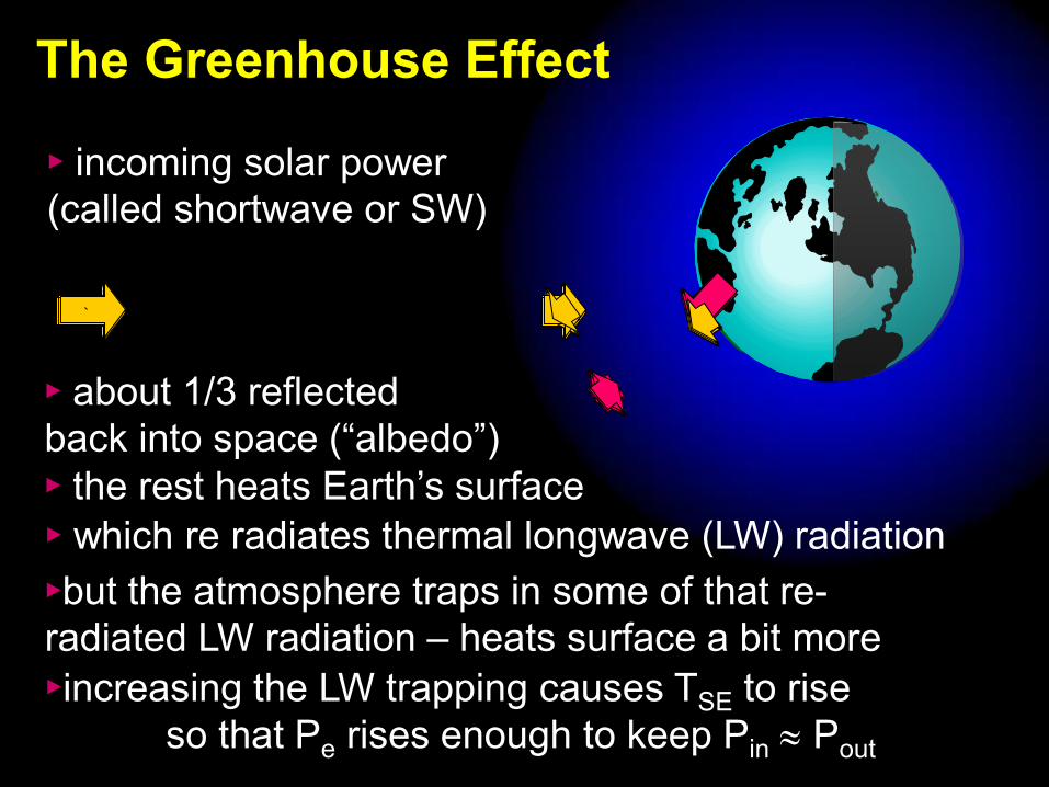
The Greenhouse Effect

► incoming solar power (called shortwave or SW)

► about 1/3 reflected back into space (“albedo”) ► the rest heats Earth’s surface ► which re radiates thermal longwave (LW) radiation ►but the atmosphere traps in some of that re-radiated LW radiation – heats surface a bit more ►increasing the LW trapping causes TSE to rise so that Pe rises enough to keep Pin Pout

(a) Bending mode

(c) asymmetric stretch

(b) symmetric stretch

Carbon

Oxygen

CO2

a CO2 molecule

Carbon Oxygen SW Photon

a CO2 molecule

Carbon Oxygen LW Photon

a CO2 molecule

a CO2 gas


a CO2 gas


Shortwave Longwave (TSUN)

(TSUN)

(TSE)

(TSE)

(TA)

(TA)

OLR spectrum looking down from h = 0 km

how does the Greenhouse effect work? Modtran 3 v1.3 imulations with U.S. Standard Atmosphere









OLR spectrum looking down from h = 8 km OLR spectrum looking down from h = 16 km


OLR spectrum looking down from h = 0 km OLR spectrum looking down from h = 1 km OLR spectrum looking down from h = 2 km OLR spectrum looking down from h = 4 km OLR spectrum looking down from h = 8 km OLR spectrum looking down from h = 16 km OLR spectrum looking down from h = 32 km


Modtran 3 v1.3 upward OLR flux at h = 20 km, U.S. Standard Atmosphere

300 ppm CO2, F = 260.12 Wm-2

600 ppm CO2, F = 256.72 Wm-2

“Radiative forcing” F = 3.39 Wm-2

Wavenumber (cm-1)

Spec

tral i

rrad

ianc

e ( W

cm

-2 c

m)

300 K 280 K 260 K 240 K 220 K

Negative greenhouse effect (observed to sometimes happen in Antarctica when atmosphere at 20-30 km is warmer than at surface) NB. Plotted against wavelength, not wavenumber, k = 1/, so main CO2 line around k = 675 cm-1 appears at = 15 m

(Schmithüsen et al, GRL, 2015)

Altitude Variations (observed and modelled zonal mean trends in latitude-altitude plots for 1979-2012) (Santer et al., 2013)

Observed (RSS and UAH analysis of satellite data)

Modelled. Forcings: ANT = anthropogenic NAT = natural VOL = Volcanic SOL = Solar ALL = ANT+NAT NAT =VOL+SOL

Babies and Bathwater

What? solar variability has NO

effects on global or regional climates?

Solar Outputs

Global Effects

Regional & Seasonal Effects

Solar Variability: Effects on Climate?

Solar Variability

The Future

Solar Outputs

Global Effects



Solar Variability

The Future

Solar Outputs

weakly modulated (~0.1%) by magnetic field in photosphere

Visible/IR

UV modulated (~1%) by magnetic fields threading the lowest solar atmosphere (chromosphere)

EUV strongly modulated (~50%) by magnetic fields in the solar atmosphere (corona)

X-Rays fully dependent on (modulated ~90%) by magnetic fields in the solar atmosphere (corona)

Solar wind ~65% modulated over the solar magnetic cycle Cosmic Rays ~20% - 40% modulated (at 10 - 1GeV) by solar

magnetic field irregularities in heliosphere SEPs ~100% modulated by transient magnetic fields in solar

flares & ahead of interplanetary coronal mass ejections

Earth’s atmosphere

10-6

10-5

10-4

10-3

10-2

10-1

1

density (kg m-3)

100

80

60

40

20

0 -100 -80 -60 -40 -20 0 20 40 60

10-3

10-2

10-1

1

10

102

103

tropopause

stratopause

mesopause

stratosphere

mesosphere

thermosphere

altitude (km) pressure

(mbar)

temperature (C)

O3

a

turbopause i winter pole

summer pole

O3 = ozone layer a = aerosols js = jet stream c = cloud i = ionosphere

troposphere c js

Electromagnetic solar inputs

10-6

10-5

10-4

10-3

10-2

10-1

1

density (kg m-3)

100

80

60

40

20

0 -100 -80 -60 -40 -20 0 20 40 60

10-3

10-2

10-1

1

10

102

103

tropopause

stratopause

mesopause

stratosphere

mesosphere

thermosphere


(mbar)

temperature (C)

O3

a

turbopause

winter pole

summer pole


troposphere

Visible/IR UV EUV X-Rays

i

c js

The Sun’s e-m radiation spectrum

Close to a 5770K blackbody radiator

Emitted flux F = Tsun

4

1 and surface temperature of Sun TS = 5770K

Implications of high CZ mass

0

log ( T / TC ) TC = T(r = 0)

-4

CZ

RZ

core

CZ contains ~31028kg (M

/60) thermal timescale of the CZ as a whole = timescale for its warming or cooling, 105 yr Switch off source at base of CZ and in t = 100 yr, Tsun changes by 1- exp(t/) = 0.001 F = Tsun

4 so that F/F = (Tsun/Tsun)4 = 0.9994 = 0.996 i.e. F changes by just 0.4%

3Mm (0.004R

)

R

Corpuscular solar inputs

10-6

10-5

10-4

10-3

10-2

10-1

1

density (kg m-3)

100

80

60

40

20

0 -100 -80 -60 -40 -20 0 20 40 60

10-3

10-2

10-1

1

10

102

103

tropopause

stratopause

mesopause

stratosphere

mesosphere

thermosphere


(mbar)

temperature (C)

O3

a

turbopause

winter pole

summer pole


troposphere

Cosmic Rays SEPs Solar wind

i

c js

Start of the Story: the associated flare CME hit Earth on 14th July 2000

The Bastille Day Storm Flare and SEPs Solar Terrestrial Physics

Summer School

“Halo” (Earthbound)

form most easily seen in C2 difference

movie ►

The Bastille Day Storm CME seen by SoHO/Lasco C2 and C3 Coronographs

Tomographic reconstruction from interplanetary scintillations

The Bastille Day Storm CMEs seen by IPS

Ground-level enhancement (GLE) of solar energetic particles seen between Forbush decreases of galactic cosmic rays caused by shielding by the two CMEs

Here seen at stations in both poles (McMurdo and Thule)

Neutron Monitor counts

Forbush decrease caused by 1st CME

GLE Forbush decrease caused by

CME associated with GLE

nm

cou

nts

The Bastille Day Storm GCRs and SEPs

The Bastille Day Storm SEP Proton Aurora – seen by Image FUV-SI12

Polar Cap NO From SEP event of April 2002

► Northern hemisphere ► Southern hemisphere

TIMED observations of 5.3 m NO radiative fluxes (Wm2) (Mlynczak et al., 2003)

Storm Event – SEP Ozone Depletion

The Bastille Day Storm Ozone Depletion (TOMS )

Energetic Particles Galactic Cosmic Rays

Generated at the shock fronts ahead of supernovae

Protons up to iron ions, travelling at close to speed of light

Three shields protect us on Earth’s surface:

The heliospheric field Earth’s magnetic field Earth’s atmosphere

Galactic Cosmic Ray Spectra

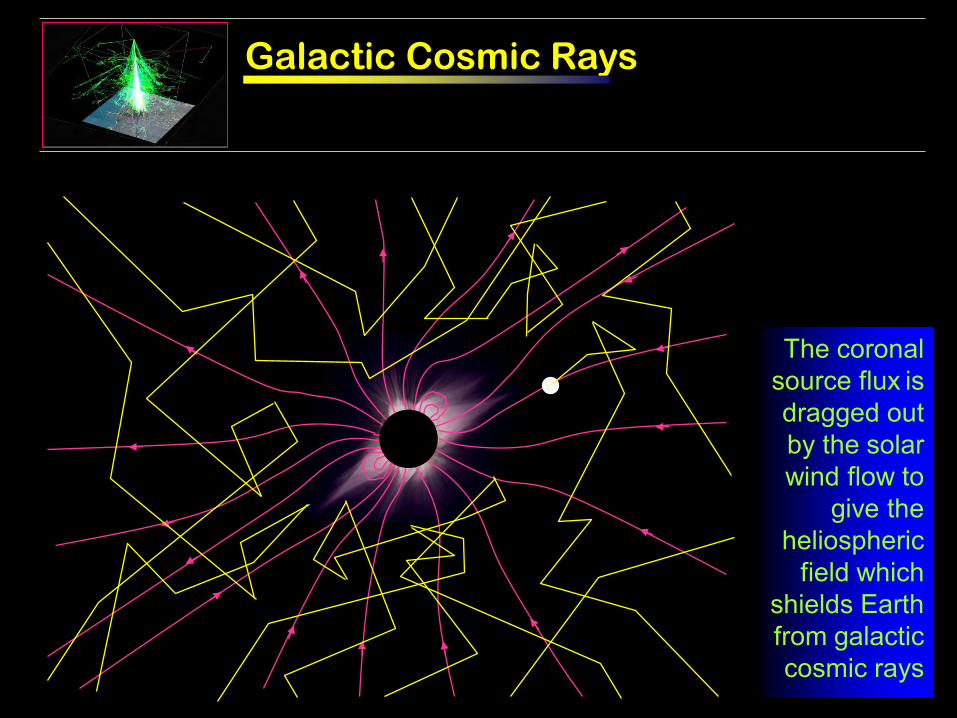
Galactic Cosmic Rays

The coronal source flux is dragged out by the solar wind flow to

give the heliospheric

field which shields Earth from galactic cosmic rays

Cosmic Rays Anticorrelation with sunspot numbers

Sunspot Number

Huancauyo – Hawaii neutron monitor counts

(>13GV)

Climax neutron monitor counts

(>3GV)

CMEs, CIRs, GCRs and SEPs

Both CME fronts and CIRs shield Earth from Galactic Cosmic Rays by scattering

Both CME fronts and CIRs generate SEPs

Both CMEs and CIRs are more common and more extensive at sunspot maximum

CME

CIR

Geomagnetic Shielding of GCRs (Cut-off rigidity)

low rigidity (e.g. 1 GV)

high rigidity (e.g. 13GV)

Rigidity is a measure of the extent to which cosmic rays maintain their direction of motion

It is measured in GV (v c, nGV rigidity energy nGeV)

Higher rigidity GCRs can penetrate to lower geomagnetic latitudes

minimum rigidity that can be seen at a magnetic latitude called the “rigidity cut-off” (e.g.) for Hawaii and Huancayo 13GV for Climax (Boulder) 3GV

At highest latitudes rigidity cut-off set by atmosphere at 1GV

Cosmic ray tracks in a bubble chamber

Solar Output Signals in Troposphere

at most, very small “bottom up” signals reported in troposphere

Visible/IR

UV clear heating effects in statosphere (ozone layer) – may have subtle “top down” effects on troposphere

EUV dominates thermosphere, no evidence nor credible mechanism for coupling to the troposphere

X-Rays major effects in thermosphere, no evidence or credible mechanism for for coupling to the troposphere

Solar wind same as for EUV and X-rays Cosmic Rays proposed modulation of cloud cover: effect on surface

temperatures depends critically on cloud height SEPs destroy ozone so may have similar effects to UV

Solar Outputs

Global Effects



Solar Variability

The Future

Total Solar Irradiance Observations Systematic errors and drifts due to instrument degradation

Tota

l Sol

ar Ir

radi

ance

(Wm

-2)

1980 1984 1988 1992 1996 2000 2004 2008

ORIGINAL DATA

0.3%

1374

1370

1358

1366

1362

Solar Irradiance Composites Errors and drifts corrected by intercalibration

Tota

l Sol

ar Ir

radi

ance

(Wm

-2)

PMOD Composite

ACRIM Composite

IRMB Composite

1980 1984 1988 1992 1996 2000 2004 2008

Total solar irradiance changes and magnetic field emergence

Dark sunspots and bright faculae are where magnetic field threads the solar surface

Enhanced field B blocks upward heat flux F

Gives temperatures:

Sunspot Darkening

B

Heat Flux F

Quiet Bright Spot Bright Quiet Sun Ring P U P Ring Sun

Quiet Sun TQS 6050K Bright ring TBR 6065K Penumbra TP 5680K Umbra TU 4240K

Photosphere

Convection Zone

Enhanced field raises magnetic pressure and depresses thermal pressure NkBT

Facular Brightening The Bright Wall Model

N falls & the O = 2/3 contour is depressed by z 50 km

flux tube small enough for radiation from walls to maintain internal temperature T

bright walls most visible at small for which Tf 6200 K

z

B B

F

< 250 km

Sunspot Darkening & Facular Brightening

Photospheric magnetic field magnetogram data

3-component TSI model using magnetogram data

Use model contrasts of umbrae, penumbrae and faculae CU, CP, and CF (>0 for brightenings) as a function of position on disc and wavelength (w.r.t quiet Sun, so CQS(,) = 0)

Contrasts independent of time t – the time dependence is all due to that in the filling factors which are functions of and t, but not .

Every pixel in the magnetogram for time t that falls on the visible disc is then classified as either umbra, penumbra, facula or quiet Sun to derive U, P, F. Limb darkening function is LD(,) and the quiet-Sun intensity (free of all magnetic features) of the disc centre is IO

ITS(,t = (Rs2 / R1

2) IO LD(,) [ P(,t){CP(,)+1} +

U(,t){CU(,)+1} + F(,t){CF(,)+1} + {1-P(,t)-U(,t)-P(,t)} ]d

1

0

penumbrae

umbrae faculae quiet Sun

4-component model (Solanki et al., 2003)

Total Solar Irradiance reconstructions using 4 component model (“SATIRE”) with magnetograms for 1996-2002 from the MDI satellite, compared with SoHO TSI data

Stellar Analogues: The use of the S index

► S index is a measure of stellar flux in the Ca I H and

K lines (chromospheric emissions associated with

magnetic field threading the solar surface)

► related to facular brightening term in TSI by Lean et

al. (1992)

Stellar Analogues: The distribution of S index values

150

100

50

0 0.10 0.12 0.14 0.16 0.18 0.20 0.22

average S index, < S > ►

num

ber o

f occ

urre

nces

►

1/3 non-cyclic stars Sun’s Maunder minimum?

2/3 cyclic stars present-day Sun?

► Baliunas & Jastrow (1990). Data from the Mt. Wilson survey of Sun-like stars. ► 74 “solar-type” stars with B - V

colours in range 0.60–0.76 (0.95-1.10 MS).

← from 13 of the 74 (so a third is just 4)

Active dynamo

Dormant dynamo

Hoyt and Schatten used solar cycle length, L, Lean et al. and Lean used a combination of sunspot number R and R11, Solanki and Flkigge use a combination of R and L, Lockwood and Stamper used Fs. All use stellar analogue except Lockwood and Stamper

TSI Reconstructions

1600 1700 1800 1900 2000

Lean, 2000

Lean et al., 1995

1368

1366

1364

1362 Hoyt & Schatten, 1993

Solanki & Fligge 1999

Tota

l S

olar

Irra

dian

ce (

Wm

-2)

Stellar Analogues: Recent re-evaluation of distribution

100

0 0.13 0.15 0.17 0.19 0.21 0.23 0.25

S Index ►

150

50 num

ber o

f occ

urre

nces

►

1/3 non-cyclic stars

(not bimodal)

2/3 cyclic stars

► Hall and Lockwood (2004) Lowell survey of 300 stars with colours in the same range as adopted by B&J (0.60 B-V 0.76)

Analogy: the spacing of birds on a wire!

Open Solar Flux, FS

(allowing for longitudinal structure in solar wind)

from geomagnetic data (Lockwood et al., 2009) model (Vieira & Solanki, 2010) from IMF data

► use both range and hourly mean geomagnetic data ► model emergence from sunspot number with two time constants for decay of open flux

TSI Reconstructions To

tal

Sol

ar Ir

radi

ance

ITS

(W

m-2

)

1600 1700 1800 1900 2000

1368

1366

1364

1362

Lockwood and Stamper, 1999

Hoyt & Schatten, 1993

Solanki & Fligge 1999

Foster, Lockwood, 2004

Lean, 2000

Lean et al., 1995

Wang et al., 2005

Krivova et al., 2007

I TS

Most recent best estimates are ITS 1 Wm-2 since MM

Outgoing Longwave (LW) Radiation ► infra-red (Longwave, LW) emmission = heat ► Earth is close to a “Blackbody” radiator of effective temperature TE ► emitted power by unit area of Earth = TE

4 where is the Stefan – Boltzmann constant

► surface area of 4RE2 , so total LW power ouput,

► Define TE4 = (1-g)TS

4, where g is the greenhouse term

Pout = 4RE2 TE

4 = 4RE2 (1 – g)TS

4

Incoming short wave (SW) radiation

► of the incident power a fraction A is reflected back into space, where A is called Earth’s “albedo”

► power density in sunlight = ITS (W m-2) ► called the “total solar irradiance” (TSI) ► the area of target presented by Earth = RE

2 (m2) where RE is the mean Earth radius

► of the incident power a fraction (1-A) is not reflected back into space, ► Input SW Power Pin = ITS RE

2 (1 – A)

RE

Terrestrial Energy Budget

Input SW Power Pin = ITS RE2 (1 – A)

Output LW Power Pout = 4RE2 TE

4 = 4RE2 (1 – g)TS

4

= Stefan-Boltzmann constant TE

= effective temperature of Earth / atmosphere 255K TS

= surface temperature of Earth g = normalised greenhouse effect Also need to consider power q (per unit area) surface gives to sub-surface layers (particularly the deep oceans)

Pin = Pout + 4RE2q

ITS(1 – A)/4 = (1 – g)TS4 + q


ITS(1 – A)/4 – TS4 + gTS

4 – q = 0 ITS(1 – A)/4 – TS

4 + G – q = 0

Differentiate w.r.t. time TS = [ITS/4 – ITSA/4 + G – q] / (4TS

3 )

= Stefan-Boltzmann constant TE

= effective temperature of Earth / atmosphere 255K TS

= surface temperature of Earth g = normalised greenhouse effect, N.B., g = G / (TS

4 ) G = greenhouse radiative forcing (in Wm-2)

Gives the concept of “radiative forcing” where we can add together the changes in the powers per unit surface area due to different effects in the term in square brackets

A little greenhouse gas is a good thing!

TS = ITS (1 – A) – 4q 1/4

4 (1 – g)

If no greenhouse gases, g = 0 and surface in equilibrium with oceans (q = 0): ITS = 1366.5 Wm-2 , Albedo, A = 1/3 = 5.669 10-8 W m-2 K-4

(if g = 0 TE

= TS )

Gives TS = 251.8 K = -21.2 C

TOO COLD FOR ALMOST ALL LIFEFORMS!


TS = ITS (1 – A) – 4q 1/4

4 (1 – g)

Typical values ITS = 1366.5 Wm-2 , Albedo, A = 1/3, q = 1 Wm-2 (Hansen et al., Science, 2005)

= 5.669 10-8 W m-2 K-4

TE = effective temperature of Earth & its atmos. 253K

g = 1 – (TE / TS

)4 Above eqn. for g = 0.410 gives TS = 286.9 K = 13.9 C

Increase g to 0.416 (a 1.5% rise & the value or 2000 ) gives TS = 14.7 C i.e. it gives a rise in Ts of Ts = 0.8 C


Typical values from before:

● g = 0.410 gives TS = 286.9 K ( = 13.2 C) corresponds to G = g TS

4 = 157.5 Wm-2

● Increasing g to 0.416 ( value for 2000) gives

TS = 287.7 K ( = 14.7 C) (the observed rise in Ts, Ts = 0.8 C) corresponds to G = g TS

4 = 161.6 Wm-2

● Thus a radiative forcing anomaly of G = 4.1 Wm-2

gives a surface temperature rise Ts = 0.8 K ●The “climate sensitivity” = Ts / G 0.2 K W-1 m2

Do greenhouse gases alone explain the observed warming?

(from before) for 1900-2000:

● radiative forcing anomaly of G = 4 Wm-2 gives a surface temperature rise Ts = 0.8 K

ppmv G (Wm-2) G (Wm-2)

1700 1900 2000 1900 2000 1900-2000 CO2 278 295.2 362.5 0.3 1.4 1.1 NH4 700 898 1800 0.2 0.5 0.3 Others 0.1 0.5 0.4 Total 0.6 2.4 1.8 ● direct effects not enough: but there are feedback effects

Solar radiative forcing

► Input SW Power Pin = ITS RE2 (1 – A)

RE

► SW Power per unit surface area of earth PSW = ITS RE

2 (1 – A) / (4 RE2) = ITS (1 – A) / 4

Solar radiative forcing = PSW = ITS (1 – A) / 4 Since pre-industrial times ITS 1 Wm-2

Gives PSW 1/6 = 0. 167 Wm-2 (for A = 1/3) = a tenth of greenhouse gas radiative forcing 1. 8 Wm-2 And remember total radiative forcing needed to explain GMAST rise (with feedbacks) = G 4 Wm-2 24 PSW

The sun seen is Visible and UV light 3rd February 2002

► white light, = 400-700 nm ► Ultraviolet, = 30.4 nm

The Sun’s e-m radiation spectrum

Variability is low in parts of spectrum power is greatest

Variability is highest in UV which is absorbed in the stratosphere

Solar UV data intercalibration (Lockwood, JGR, 2011)

► e.g. = 164.5nm ► data from different satellite and instruments ► note the “SOLSTICE gap” between the end of UARS/SOLSTICE data and start of SORCE/SOLSTICE data.

► UARS/SUSIM data not reliable at >205nm

Solar Outputs

Global Effects



Solar Variability

The Future

Greenhouse

LW SW Albedo

Clouds

Climate

Cosmic Rays & Clouds

Low cloud: Albedo effect exceeds greenhouse trapping effect

High Cloud: greenhouse trapping effect exceeds albedo effect

GCR fluxes fell over 1900-1985 so to contribute to warming Earth, they would have to generate low altitude cloud (so reduced albedo exceeds reduced greenhouse trapping)

% g

loba

l clo

ud c

over

ano

mal

y

Global Cloud Cover Variation

3

2

1

0

-1

-2

-3

1985 1990 1995 2000 2005

(Svensmark, 1998)

ISCCP D2 low-altitude cloud anomaly

N.B. 1- error in D2 dataset is about 2%

% g

loba

l clo

ud c

over

ano

mal

y


3

2

1

0

-1

-2

-3

1985 1990 1995 2000 2005

(Marsh & Svensmark, 2003) offset?

% g

loba

l clo

ud c

over

ano

mal

y


(Gray et al., 2010) 3

2

1

0

-1

-2

-3

1985 1990 1995 2000 2005

New Evidence: Diffuse Fraction (DF)

► Intensity in direct sunlight = IDI ► Intensity in shade = ISH ► Diffuse fraction, DF = ISH / IDI

► Measured at a number of sites since the 1950s

Idi

Ish Idi

CLOUD

CLEAR SKY ISH 0 DF = ISH / IDI 0

CLOUDY SKY (and/or aerosols) ISH IDI DF = ISH / IDI 1

Ish

detector

shield

0.65 0.70 0.75 0.80 0.85

Mean DF for C < 36 105 hr -1

Aberporth Aldergrove Beaufort Park Camborne Cambridge Eskdalemuir Jersey Kew Lerwick Stornaway

0.85

0.80

0.75

0.70

0.65

Mea

n D

F fo

r C ≥

36

105 h

r -1

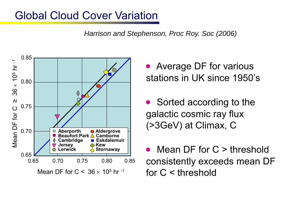
Global Cloud Cover Variation Harrison and Stephenson, Proc Roy. Soc (2006)

Average DF for various stations in UK since 1950’s Sorted according to the galactic cosmic ray flux (>3GeV) at Climax, C Mean DF for C > threshold consistently exceeds mean DF for C < threshold

Global Electric Circuit

IONOSPHERE

GROUND Conductivity H

eigh

t

Air ions generated by GCRs

Air ions generated by radon release

~ +130kV

free electrons & ions generated by solar EUV

+

+ + +

+ +

+ +

- - - - - -

-

fair weather

positive ion

flux

negative ion

flux

atmospheric

aerosol

sprites, elves etc.

lightning + - + - + -

Clouds

Climate

Climate System

Volcanoes Man-Made

Cryosphere

Ocean

Permafrost Sea Level

Sun

Biosphere

El Niño

Albedo

Greenhouse

LW SW Albedo

Greenhouse

LW SW Albedo

Clouds

Climate

Volcanoes Man-Made

Cryosphere

Ocean


Sun

Biosphere

El Niño

Albedo

Geological Effects

Greenhouse

LW SW Albedo

Clouds

Climate

Volcanoes Man-Made

Cryosphere

Ocean


Sun

Biosphere

El Niño

Albedo

Anthropogenic Effects

Greenhouse

LW SW Albedo

Clouds

Climate

Volcanoes Man-Made

Cryosphere

Ocean


Sun

Biosphere

El Niño

Albedo

Solar Influence

Greenhouse

LW SW Albedo

Clouds

Climate

Volcanoes Man-Made

Cryosphere

Ocean


Sun

Biosphere

El Niño

Albedo

Short-Timescale Ocean Energy Exchange

Observed Global Surface Air

Temperature Anomaly, TOBS

ENS0 N3.4 index Anomaly, E

Mean Optical

Depth (AOD) at 550 nm, V

Cosmic Ray Counts at Climax, C

Anthropogenic forcing, A,

(greenhouse gases, aerosols,& land use change)

fit to observed GMAST anomaly obtained using the Nelder-Mead simplex (direct search) method

(Lockwood, 2008)

1955 1965 1975 1985 1995 2005

Global Mean Air Surface Temperature

Observed, TOBS Fitted, TFIT

when a fit has too many degrees of freedom can start to fit to the noise in the training subset, which is not robust throughout the data (fit has no predictive power) recognised pitfall when quasi-chaotic behaviours give large internal noise such as in climate science1 and population growth2 often not recognised in space physics where systems tend to be somewhat more deterministic with lower internal variability.

DANGER ! BEWARE

OVERFITTING 1 e.g. Knutti et al. (2006) J. Climate, DOI: 10.1175/JCLI3865.1 2 e.g. Knape and de Valpine (2011) Proc. Roy. Soc. London B, DOI: 10.1098/rspb.2010.1333

Weighted contributions to best fit variation, Tp

(uses Climax GCR counts to quantify solar effect)

(updated from Lockwood, 2008)

Solar El Nino Volcanoes Anthro Total

20

15

10

5

0

-5

Tem

pera

ture

Tre

nd (1

0-3 K

yr -

1 )

1987-present

using GCRs (C), r = 0.89

(Lockwood, 2008)

Detection-Attribution

Use models to avoid over-fitting problem The idea is that models, started from slightly different initial conditions, can reproduce the internal variability of the climate system Produce an ensemble of many model runs for set inputs and then compare mean or median with observations Runs with no anthropogenic effect differ from observed GMAST rise by more than the internal noise level

Solar Outputs

Global Effects



Solar Variability

The Future

Regional Analysis (Lean and Rind, 2008)

solar UV

heated equatorial stratosphere

jet stream

mild westerlies blocked

cold north- easterlies

eddy refraction and/or polar vortex changes

“Top-down” Solar Modulation

Atlantic blocking events (Plelly and Hoskins, 2003)

► blocking events are large long-lived anticyclones which disrupt easterly flow of storms, bifurcating the jet stream and, in winter, causing cold winds from the east over Europe

Example at 12UT, 21 Sept, 1998: on the potential vorticity PV=2 surface (a) 250-hPa geopotential height (b) potential temperature (K)

Blocking Intensity Indices

► Lejenäs and Økland (1983) required a region of easterly winds and used Z(, o+/2)Z(, o/2) where Z is a constant height geopotential, is the longitude and the latitude ► Barriopedro et al. (2006,2008) used BI = 100 {[Z(o, o)/RC]1} where RC = {Z(o+, o) Z(o, o)} / 2

► Pelly and Hoskins (2006,2008) used mean potential temperature in the red and green areas of the plot B =

(2/) d (2/) d

o+/2

o o

o/2

ERA-40 Analysis of Blocking Index (change of terciles relative to whole set)

► sorted using open solar flux FS High/Low solar activity gives reduced/enhanced (up to 8%) blocking over east Atlantic and Europe (symmetric effect) Consistent and localised effect Grey area shows significance from Monte-Carlo technique > 95%

(Woollings et al, GRL.,2010)

ERA-40 Analysis of DJF temperatures & circulation (difference of high and low tercile subsets)

► sorted using open solar flux FS Low solar activity gives lower surface temperatures in central England Effect much stronger in central Europe Analysis shows a distinct system to NAO

(Woollings et al, GRL.,2010; see also Barriopedro et al., JGR, 2008)

Modelled solar maximum-solar minimum temperatures

► Heating effect only (no [O3] change)

(Ineson et al, Nature Geosci., 2011)

► HADGEM3rev1.1 GCM, 85 atmos and 42 ocean levels. ► Uses the SORCE max-min UV spectrum SS() ► Increased meridional temperature gradient increase in westerly flow

Modelled solar maximum-solar minimum zonal wind speed

► Modelled downward and northward propagation of easterly wind anomaly (by Eliassen-Palm flux divergence)

(Ineson et al, Nature Geosci., 2011)

► seen in ERA40+ data

► c.f. Kodera and Kuroda, 2002; Matthes et al.,2006

January 2010

Maunder Minimum & the “Little Ice Age”

a). Sunspot Number

b). Open Solar Flux

c). Reconstructed Northern Hemisphere Temperatures

MM

MM

LIA 1.0

0.5

0

-0.5 1700 1800 1900 2000

T N

H

(C

)

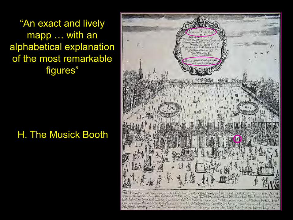
January 1683

A Frost Fair on the Thames in London. The river froze in central London relatively frequently during the Maunder Minimum of sunspot activity

“An exact and lively mapp … with an

alphabetical explanation of the most remarkable

figures”



figures”

H. The Musick Booth



figures”

I. The Printing Booth



figures”

E. The Roast Beefe Booth



figures”

N. The Boat drawne with a Hors



figures”

Q. The Bull Baiting



figures”

C. The Tory Booth



figures”

Z. London Bridge



Solar Outputs

Global Effects



Solar Variability

The Future

Predictions for the future

“It is not important to predict the future, but it is important to be prepared for it” Pericles, Athenian orator, statesman and general c. 495 – 429 BC

“It is not important to know the future, but to shape it” Antoine de Saint Exupéry, French writer and aviator 1900 - 1944

“Prediction is very hard — especially when it’s about the future”

Niels Bohr Danish Physicist 1885 – 1962 “Never make predictions — especially about the future”

Lawrence Peter (Yogi) Berra American Baseball Player, coach and author 1925 – Who also said “I never said half the things I really said."

"It ain't over ‘till it's over" "When you come to a fork in the road, take it."

"It's like déjà vu all over again" "Always go to other peoples' funerals, otherwise they won't come to yours."

“I don’t have nightmares about my team – you’ve got to be able to sleep before you can have nightmares”

Millennial Variation composite (25-year means) from cosmogenic isotopes by Steinhilber et al. (2008)

Year AD

Sola

r Mod

ulat

ion

Para

met

er, (

MV)

-6000 -4000 -2000 0 2000

1000

800

600

400

200

0

composite from Solanki et al., 2004; Vonmoos et al., 2006 & Muscheler et al., 2007

we are still within recent grand maximum

Superposed epoch study of the end of grand maxima

time after end of grand maximum (yrs)

800

600

400

200

0

end of grand solar maximum

-80 -40 0 40 80

(24 events in 9000 yrs)

Sola

r Mod

ulat

ion

Para

met

er, (

MV)

Future TSI Variation?

using the relationship of TSI and GCRs

& relationship between solar cycle amplitude and the mean

(Jones, Lockwood and Stott, JGR 2011)

Lean (2000)

Krivova et al. (2007)

Lean (2009) Maximum 1 Mean -1 Minimum

GMAST Predictions – EBM tuned to HadCM3

(Jones, Lockwood and Stott, JGR in press, 2011)

Lean (2000)

Krivova et al. (2007)

Lean (2009)

use B2 SRES emissions scenario

no future volcanic forcing

solar responses have been scaled to match a maximum possible solar cycle amplitude of 0.1K.

Maximum 1 Mean -1 Minimum

Temperature Commitment Climate Sensitivity 2.8°C

zero emissions

constant radiative forcing

example feasible scenario (here B2-400-MES-WBGU)

constant emissions

1850 1900 1950 2000 2050 2100 2150

2.5

2.0

1.5

1.0

0.5

0

-0.5

GM

AS

T A

nom

aly

( w.r.

t. 18

61-1

890)

Global Mean Air Surface Temperature

pre-industrial level

(Hare & Meinshausen, 2006)

Handling Uncertainty - For IPCC lognormal pdf of climate sensitivity

1900 2100 2300 1900 2100 2300 1900 2100 2300

GM

SAT

Ano

mal

y ( w

.r.t.

1861

-189

0) 5

4

3

2

1

0

Global Mean Air Surface Temperatures for Constant emissions Present forcing Zero Emissions

Best estimate 90% confidence 1-99 percentile 10-90 percentile 33-66 percentile

(Hare & Meinshausen, 2006)

Tipping Points (Lenton et al., 2007)

System State 1 System State 2

► Melt of the Greenland Ice Sheet ► Arctic sea ice loss ► Arctic sea Not necessarily irreversible ….



► Melt of the Greenland Ice Sheet ► Arctic sea ice loss ► Arctic sea



► Melt of the Greenland Ice Sheet ► Arctic sea ice loss ► Arctic sea

►Atlantic themohaline circulation disruption ►Indian monsoon chaotic multistability ►West African monsson latitude shift ►Change in ENSO frequency and/or amplitude ►West Antarctic ice sheet instability ►Changes in Antarctic bottom water formation

►Arctic sea ice loss ►Greenland ice sheet melting ►Boreal forest dieback ►Loss of permafrost and tundra ►Sahara greening ►Amazon rainforest dieback

Potential tipping points between climate states are:

time to…

STOP!!!

but questions most welcome, now, over dinner, or down the pub after

Long-term solar change and solar influences on global and ...

Documents