ABSTRACT Title of Dissertation: SOIL-PILE INTERACTION UNDER VERTICAL DYNAMIC LOADING Ghassan Sutaih, Doctor of Philosophy, 2018 Dissertation directed by: Professor M. Sherif Aggour (Chair/Advisor), Department of Civil and Environmental Engineering. Improper foundation designs for machine vibrations can result in machine failure, severe discomfort to workers around the machine or excessive settlement. The goal of foundation design for machine vibrations is to minimize vibration amplitude. In poor soil conditions, pile foundations are used to support the machine. Soil-pile stiffness and damping must be known at the level of the pile head. Since piles are used mostly in a group, it is also necessary to determine the interaction of the piles within the group. This study uses a 3D finite element method to study the response of pile foundations subjected to vertical dynamic loading. It uses Lysmer’s analog where the pile is replaced by a single degree of freedom dynamic system that provides frequency independent parameters. A parametric study is performed to obtain the value of the stiffness and the damping of a single pile for different soil properties and for both homogeneous and

Welcome message from author
This document is posted to help you gain knowledge. Please leave a comment to let me know what you think about it! Share it to your friends and learn new things together.
Transcript
ABSTRACT
Title of Dissertation: SOIL-PILE INTERACTION UNDER
VERTICAL DYNAMIC LOADING
Ghassan Sutaih, Doctor of Philosophy, 2018
Dissertation directed by: Professor M. Sherif Aggour (Chair/Advisor),
Department of Civil and Environmental
Engineering.
Improper foundation designs for machine vibrations can result in machine
failure, severe discomfort to workers around the machine or excessive settlement. The
goal of foundation design for machine vibrations is to minimize vibration amplitude.
In poor soil conditions, pile foundations are used to support the machine. Soil-pile
stiffness and damping must be known at the level of the pile head. Since piles are used
mostly in a group, it is also necessary to determine the interaction of the piles within
the group. This study uses a 3D finite element method to study the response of pile
foundations subjected to vertical dynamic loading. It uses Lysmer’s analog where the
pile is replaced by a single degree of freedom dynamic system that provides frequency
independent parameters.
A parametric study is performed to obtain the value of the stiffness and the
damping of a single pile for different soil properties and for both homogeneous and
nonhomogeneous soils. Floating and end-bearing piles were also studied. Pile group
response is influenced by the soil-pile-soil interaction. The interaction is obtained by
varying both the spacing and the soil properties around the pile. Interaction between
the piles causes reduction in the stiffness and damping of the soil-pile system compared
to an isolated pile. The study provided the interaction factors as a function of pile
spacing and properties of the soil. Using the interaction factors, the response of a group
of piles can be determined from the response of a single pile.
SOIL-PILE INTERACTION UNDER VERTICAL DYNAMIC LOADING
By
Ghassan Hassan Sutaih
Dissertation submitted to the Faculty of the Graduate School of the
University of Maryland, College Park, in partial fulfillment
of the requirements for the degree of
Doctor of Philosophy
2018
Advisory Committee:
Professor M. Sherif Aggour, Chair
Professor Amde M. Amde
Professor Chung C. Fu
Professor Dimitrios G. Goulias
Professor Amr Baz

© Copyright by
Ghassan Sutaih
2018

ii
Dedication
To my mother and my sisters for their contineous support during my graduates studies.
To the government of Saudi Arabia represented by Kng Abdul Aziz University for their
financial support and giving me this opputrtuinity to pursue a graduate degree.

iii
Acknowledgements
I would like to thanks Professor M.S. Aggour who supervised my research. I would
like to thank him for his contneous support and guidance during my graduate studies. I
would like to thank Professors Amde M. Amde, Chung Fu, Dimitrios G. Goulias and
Amr Baz for kindly serving on my thesis committee. I would like to thanks the
government of Saudi Arabia represented by Kng Abdul Aziz University for their
financial support and giving me this opputrtuinity to pursue a graduate degree.
iv
Table of Contents
Dedication ..................................................................................................................... ii
Acknowledgements ...................................................................................................... iii
Table of Contents ......................................................................................................... iv
List of Tables ............................................................................................................... vi
List of Figures ............................................................................................................ viii
1. Introduction ............................................................................................................... 1
1.1. Limitations in current design methods ............................................................... 5
1.2. The need for research ......................................................................................... 6
1.3. Problem Statement and Objectives .................................................................... 8
1.4. Thesis Organization ......................................................................................... 11
2. Literature Review.................................................................................................... 13
2.1. Machines and machine vibration ..................................................................... 13
2.2. Closed form solutions for single pile subjected to dynamic loading ............... 15
2.2.1. Richart (1970) solution for single pile resting on rock ............................. 15
2.2.2. Novak (1974) Solution for a single pile under dynamic loading .............. 19
2.2.3. Chowdhury & Dasgupta (2008) analytical solution for single pile .......... 24
2.3. Finite Element solution for Pile subjected to dynamic loading ....................... 25
2.3.1. One-dimensional finite element approach ................................................ 26
2.3.2. 3D Finite element modeling...................................................................... 30
2.4. Design of pile groups and pile to pile interaction ............................................ 30
2.4.1. Poulos (1968) static interaction factors..................................................... 31
2.4.2. Studies on dynamic interaction factors ..................................................... 35
3. The Finite element method, an introduction ........................................................... 38
3.1. Mathematical preliminaries for the finite element method .............................. 39
3.2. Axisymmetric elements ................................................................................... 40
3.3. Solution of the static equilibrium Equations .................................................... 48
3.3.1. Direct solution of the static equilibrium Equation in linear analysis ........ 49
3.3.2. Iterative solution of the static equilibrium Equation in linear analysis .... 51
3.4. Dynamic Analysis ............................................................................................ 51
3.4.1.Mass matrix of an axisymmetric element .................................................. 51
3.4.2. Integration of dynamic Equation of equilibrium in time .......................... 52
4. Modeling and finite element method implementation ............................................ 58
4.1. Research assumptions ...................................................................................... 59
4.2. Geometry Modeling ......................................................................................... 59
4.2.1. Additional geometry modeling considerations ......................................... 60
4.3. Finite element solution parameters .................................................................. 62
4.3.1. Element size .............................................................................................. 62
4.3.2. Time step ................................................................................................... 63
4.3.3. Boundary conditions ................................................................................. 64
4.4. Analysis, obtaining results and interpretation procedure ................................. 70
4.5. Verification of the modeling process for dynamic analysis ............................. 78
5. Results and Discussion ........................................................................................... 80
5.1. Floating pile in homogeneous soil ................................................................... 81
5.1.1. Results commentary and analysis ............................................................. 87
v
5.1.2. Comparison of finite element solution results with literature ................... 90
5.1.2.1. Comparison of stiffness ......................................................................... 90
5.1.2.2. Comparison of damping ......................................................................... 98
5.2. Floating pile in nonhomogeneous soil ........................................................... 106
5.2.1. Results commentary and analysis ........................................................... 112
5.2.2. Comparison of finite element solution results with literature ................. 117
5.2.2.1. Comparison of stiffness ....................................................................... 118
5.2.2.2. Comparison of damping ....................................................................... 121
5.3. End-bearing pile in homogeneous soil ........................................................... 123
5.3.1. Results commentary and analysis ........................................................... 128
5.3.2. Comparison of finite element solution results with literature ................. 131
5.3.2.1. Comparison of stiffness ....................................................................... 131
5.3.2.2. Comparison of damping ....................................................................... 136
5.4. End-bearing pile in nonhomogeneous soil ..................................................... 139
5.4.1. Results commentary and and analysis .................................................... 144
5.4.2. Comparison with 1D finite element method ........................................... 148
5.5. Pile-to-pile interaction in homogeneous soil ................................................. 150
5.5.1. Results commentary and analysis ........................................................... 159
5.5.2. Comparison of interaction factors with Poulos (1968) ........................... 161
5.6. Frequency independence of the stiffness and damping ................................. 163
5.7. A discussion on design applications ............................................................. 171
5.7.1. Design of a pile in homogeneous soil ..................................................... 171
5.7.2.Design of a pile group .............................................................................. 177
6. Design Charts and Conclusion .............................................................................. 182
6.1. Design Charts ............................................................................................. 182
6.2. Conclusion ................................................................................................. 188
6.3. Summary .................................................................................................... 192
Appendices ................................................................................................................ 194
A. An Introduction To Soil Dynamics .............................................................. 194
B. A program for static and dynamic analysis of single piles subjected to vertical
loading............................................................................................................... 231
Bibiliography ............................................................................................................ 246
vi
List of Tables
Table 4.1: Sample results for static and dynamic analysis ........................................ 73
Table 4.2: calculated Dynamic Displacement/Static Displacement using assumed D
value ............................................................................................................................ 74
Table 4.3: Table generated after solving for D that would minimize the sum of errors
..................................................................................................................................... 75
Table 4.4: results of verification study ....................................................................... 78
Table 5.1: Values for variables and constants for study of floating pile in homogeneous
soil ............................................................................................................................... 82
Table 5.2: Parameters used in study of pile in nonhomogeneous soil ...................... 108
Table 5.3: Numerical results for comparison between 3D and 1D FEM for a floating
pile in nonhomogeneous soil .................................................................................... 123
Table 5.4: Values for variables and constants for study of end-bearing pile in
homogeneous soil...................................................................................................... 125
Table 5.5: Values for variables and constants for study of end-bearing pile in
nonhomogenous soil ................................................................................................. 141
Table 5.6: Numerical results for Comparison of stiffness and damping calculated by
3D and 1D FEM for an end-bearing pile in nonhomogeneous soil and 𝐷𝑐/𝐿𝑝 = 1 149
Table 5.7: Variables and constants for study of pile to pile interaction ................... 151
Table 5.8: Parameters values for sample calculation of stiffness and damping in a 2 pile
system ....................................................................................................................... 154
Table 5.9: results of dynamic displacement for sample calculation of stiffness and
damping of 2 pile system .......................................................................................... 155
vii
Table 5.10:Summary of soil and pile parameters for example of design of pile grou
................................................................................................................................... 178
Table 5.11: Values of interaction factors for pile group design example ................ 180
viii
List of Figures
Figure 1.1: Criterion for Foundation Vibration after Richart F.E. et al. (1970) .......... 2
Figure 1.2: Criterion for foundation vibration after Baxter & Bernhard (1967) .......... 2
Figure 1.3: Simplified single degree of freedom problem for Different Types of
Foundations subjected to Vertical Dynamic Loading ................................................... 4
Figure 1.4: Typical variation of soil shear wave velocity with depth after Stokoe &
Woods (1972)................................................................................................................ 8
Figure 1.5: Graphical Representation of studied cases ............................................... 10
Figure 2.1: Model for pile resting on rock (a) Pile resting on rock base supporting
weight on top. (b) Simplified model as a fixed-free rod with a mass at the free end
Richart, F. E. et al. (1970). .......................................................................................... 16
Figure 2.2: plot of 𝜔𝑛 𝐿𝑝/𝑣𝑐 against 𝐴𝑝𝐿𝑝𝛾𝑝 /𝑊 after Richart, F.E. et al ( 1970). 18
Figure 2.3: Natural frequency for different pile materials after Richart, F. E. et al.
(1970) .......................................................................................................................... 19
Figure 2.4: Plot of 𝑓𝑧1 values for friction piles .......................................................... 20
Figure 2.5: Plot of 𝑓𝑧2 for friction piles ..................................................................... 21
Figure 2.6: Plot of 𝑓𝑧1 for end bearing piles .............................................................. 21
Figure 2.7: Plot of 𝑓𝑧2 for end bearing piles .............................................................. 22
Figure 2.8: Model for soil-pile interaction .................................................................. 26
Figure 2.9 Idealized t-z and q-z curves and value of 𝑘𝑠and 𝑘𝑏 .................................. 27
Figure 2.10 Model to account for material damping for side and base Soil ............... 29
Figure 2.11: Interaction factors between two piles after Poulos (1968) .................... 33
Figure 2.12: layout of 4 pile group ............................................................................. 34
ix
Figure 2.13 Interaction factors for 2, 3 and 4 symmetrical pile groups after Poulos
(1968) .......................................................................................................................... 34
Figure 2.14 Comparison between pile group and footing under vertical dynamic
loading after Novak (1974) ......................................................................................... 36
Figure 3.1: Axisymmetric element used to model solids of revolution. ..................... 42
Figure 3.2 Triangular axisymmetric element .............................................................. 43
Figure 3.3 Example of surface forces acting on an axisymmetric element (Logan, 2007)
..................................................................................................................................... 47
Figure 4.1: Pile subjected to vertical dynamic loading ............................................... 59
Figure 4.2: Details of geometry modeling. 2D axisymmetric model (top) ................. 61
Figure 4.3: Additonal modeling considerations .......................................................... 62
Figure 4.4: Definition of element length for a) Autodesk Simulation Axisymmetric
element and b) Autodesk Simulation 3D tetrahedron ................................................. 63
Figure 4.5: 2D axisymmetric model (meshed) with fixed boundaries placed far from
the pile ......................................................................................................................... 66
Figure 4.6: 3D model with dashpots as absorbing boundaries ................................... 67
Figure 4.7: Amplitude of dynamic displacement near side boundary (green) compared
to amplitude of dynamic displacement at pile(blue) ................................................... 68
Figure 4.8: Amplitude of dynamic displacement near bottom boundary (green)
compared to amplitude of dynamic displacement at pile(blue) .................................. 69
Figure 4.9: Example of applied Load-Time curve ..................................................... 71
Figure 4.10: Example of pile response curve under different frequencies ................. 72
x
Figure 4.11: Plot of finite element results and that predicted using calculated 𝐷 value
..................................................................................................................................... 75
Figure 4.12: Flowchart summarizing research process............................................... 77
Figure 4.13: Plot of verification study results ............................................................. 79
Figure 5.1: Floating pile in an elastic homogeneous soil ............................................ 83
Figure 5.2: Variation of stiffness, 𝑘 with soil modulus of elasticity, 𝐸𝑠 for a floating
pile in homogeneous soil ............................................................................................ 84
Figure 5.3: Variation of geometric damping, 𝐷 with soil modulus of elasticity, 𝐸𝑠 for
a floating pile in homogeneous soil ............................................................................ 85
Figure 5.4: Variation of critical damping, 𝑐𝑐𝑟 with soil modulus of elasticity, 𝐸𝑠 for a
floating pile in homogeneous soil ............................................................................... 85
Figure 5.5: Variation of damping, 𝑐 with soil modulus of elasticity, 𝐸𝑠 for a floating
pile in homogeneous soil ............................................................................................ 86
Figure 5.6: Variation of dimensionless Natural frequency, 𝑎0𝑛 with soil modulus of
elasticity, 𝐸𝑠 for a floating pile in homogeneous soil ................................................. 86
Figure 5.7: Variation of vertical dynamic displacement, 𝑢𝑑 at resonance with soil
modulus of elasticity, 𝐸𝑠 for a floating pile in homogeneous soil .............................. 88
Figure 5.8: Variation of dynamic amplification at resonance with soil modulus of
elasticity, 𝐸𝑠 for a floating pile in homogeneous soil ................................................. 88
Figure 5.9: Variation of natural frequency, 𝑓𝑛 with soil shear wave velocity, 𝑣𝑠 for a
floating pile in homogeneous soil ............................................................................... 89
Figure 5.10: Comparison of stiffness,𝑘 obtained by finite elemnt method with Novak
(1974) for a floating pile in homogeneous soil ........................................................... 90
xi
Figure 5.11: Relative Difference of stiffness between 3D FEM and Novak (1974) for
a floating pile in homogeneous soil ............................................................................ 91
Figure 5.12: problem layout as studied by G. Gazetas & Mylonakis (1998) ............. 94
Figure 5.13 Comparison of stiffness,𝑘 obtained by finite element method with Gazetas
& Mylonakis (1998) for a floating pile in homogeneous soil ..................................... 94
Figure 5.14: Relative difference of stiffness between 3D FEM and Gazetas &
Mylonakis (1998) for a floating pile in homogeneous soil ......................................... 95
Figure 5.15: Comparison of stiffness obtained by finite element method with work of
Chowdhury & Dasgupta (2008) for a floating pile in homogeneous soil ................... 97
Figure 5.16: Relative difference of stiffness between 3D FEM and Chowdhury &
Dasgupta (2008) for a floating pile in homogeneous soil ........................................... 97
Figure 5.17: Comparison between damping ratio, 𝐷 results Obtained by Finite element
method and Novak (1974) for a floating pile in homogeneous soil .......................... 99
Figure 5.18: Relative difference between Damping ratio, 𝐷 obtained by FEM and by
Novak (1974) for a floating pile in homogeneous soil ............................................... 99
Figure 5.19: Comparison between critical damping results Obtained by FEM and
Novak (1974) for a floating pile in homogeneous soil ............................................. 100
Figure 5.20: Relative difference between critical damping, 𝑐𝑐𝑟 obtained by FEM and
by Novak (1974) for a floating pile in homogeneous soil ........................................ 101
Figure 5.21, Comparison of Predicted dynamic displacement values, 𝑢𝑑 obtained by
finite element method and Novak (1974) for a floating pile in homogeneous soil .. 102
Figure 5.22: Relative difference of dynamic displacement values predicted by finite
element method and Novak (1974) for a floating pile in homogeneous soil ........... 103
xii
Figure 5.23 Comparison of damping ratio, 𝐷 results Obtained by FEM and Chowdhury
& Dasgupta (2008) for a floating pile in homogeneous soil ..................................... 104
Figure 5.24: Showing great difference between damping and critical damping obtained
by Chowdhury & Dasgupta (2008) for a floating pile in homogeneous soil ............ 104
Figure 5.25: Comparison of damping, 𝑐 obtained by FEM and Dobry (2014) for a
floating pile in homogeneous soil ............................................................................. 105
Figure 5.26: Floating pile in nonhomogeneous soil.................................................. 107
Figure 5.27: Variation of stiffness, 𝑘 with soil’s rate of increase in elastic modulus,
𝑆𝐸𝑆 for a floating pile in nonhomogeneous soil ...................................................... 109
Figure 5.28: Variation of stiffness, 𝑘 with 𝐷𝐶/𝐿 for a floating pile in nonhomogeneous
soil ............................................................................................................................. 110
Figure 5.29: Variation of Damping Ratio, 𝐷 with soil’s rate of increase in elastic
modulus, 𝑆𝐸𝑆 for a floating pile in nonhomogeneous soil ...................................... 110
Figure 5.30: Variation of Damping, 𝐷 Ratio with𝐷𝑐/𝐿 for a floating pile in
nonhomogeneous soil................................................................................................ 111
Figure 5.31: Variation of critical damping, 𝑐𝑐𝑟 with soil rate of increase in elastic
modulus, 𝑆𝐸𝑆 for a floating pile in nonhomogeneous soil ...................................... 111
Figure 5.32: Variation of damping, c with soil rate of elastic modulus for a floating
pile in nonhomogeneous soil .................................................................................... 112
Figure 5.33: Variation of dynamic Displacement, 𝑢𝑑 at natural frequency with 𝑆𝐸𝑠
for a floating pile in nonhomogeneous soil............................................................... 113
Figure 5.34: Variation of dynamic amplification 𝑢𝑑/𝑢𝑠 at natural frequency with 𝑆𝐸𝑠
for a floating pile in nonhomogeneous soil............................................................... 114
xiii
Figure 5.35:Variation of natural frequency, 𝑓𝑛 with 𝑆𝐸𝑠 for a floating pile in
nonhomogeneous soil................................................................................................ 115
Figure 5.36: Effect of inhomogeneity on stiffness for a floating pile in a
nonhomogeneous soil. Note: 𝐷𝑐/𝐿𝑝 = 0 means pile in homogeneous soil ............. 116
Figure 5.37: Effect of inhomogeneity on stiffness for a floating pile in a
nonhomogeneous soil. Note: 𝐷𝑐/𝐿𝑝= 0 means pile in homogeneous soil ............... 116
Figure 5.38: Pile modeled as beam segments and soil modeled as springs and dampers
................................................................................................................................... 118
Figure 5.39: Comparison of stiffness for a floating pile in nonhomogeneous soil
calculated by 3D FEM and 1D FEM for 𝐷𝑐/𝐿𝑝 = 1 .............................................. 119
Figure 5.40: Comparison of stiffness for a floating pile in nonhomogeneous soil
calculated by 3D FEM and 1D FEM for 𝐷𝑐/𝐿𝑝 = 0.8 .......................................... 119
Figure 5.41: Comparison of stiffness for a floating pile in nonhomogeneous soil
calculated by 3D FEM and 1D FEM for 𝐷𝑐/𝐿𝑝 = 0.6 ......................................... 120
Figure 5.42:Comparison of stiffness for a floating pile in nonhomogeneous soil
calculated by 3D FEM and 1D FEM for 𝐷𝑐/𝐿𝑝 = 0.4 ......................................... 120
Figure 5.43: Comparison of damping ratio for a floating pile in nonhomogeneous soil
calculated by 3D FEM and 1D FEM for 𝐷𝑐/𝐿𝑝 = 1 ............................................... 121
Figure 5.44: Comparison of damping ratio for a floating pile in nonhomogeneous soil
calculated by 3D FEM and 1D FEM for 𝐷𝑐/𝐿𝑝 = 0.8 ......................................... 121
Figure 5.45: Comparison of damping ratio for a floating pile in nonhomogeneous soil
calculated by 3D FEM and 1D FEM for 𝐷𝑐/𝐿𝑝 = 0.6 .......................................... 122
xiv
Figure 5.46: Comparison of geometric damping for a floating pile in nonhomogeneous
soil calculated by 3D FEM and 1D FEM for 𝐷𝑐/𝐿𝑝 = 0.4 ................................... 122
Figure 5.47: End-bearing pile in an elastic homogeneous soil ................................. 124
Figure 5.48: Variation of stiffness, 𝑘 with soil modulus of elasticity, 𝐸𝑠 for an end-
bearing pile in homogeneous soil ............................................................................. 126
Figure 5.49: Variation of damping ratio, 𝐷 with soil modulus of elasticity, 𝐸𝑠 for an
end-bearing pile in homogeneous soil ...................................................................... 126
Figure 5.50: Variation of critical damping, 𝑐𝑐𝑟 with soil modulus of elasticity 𝐸𝑠 for
an end-bearing pile in homogeneous soil.................................................................. 127
Figure 5.51: variation of damping, 𝑐 with soil modulus of elasticity, 𝐸𝑠 for an end-
bearing pile in homogeneous soil ............................................................................. 127
Figure 5.52: Variation of natural dimensionless frequency, 𝑎0𝑛 with soil modulus of
elasticity, 𝐸𝑠 for an end-bearing pile in homogeneous soil ...................................... 128
Figure 5.53: variation of dynamic displacement, 𝑢𝑑 at resonance with soil modulus of
elasticity, 𝐸𝑠 for an end-bearing pile in homogeneous soil ...................................... 129
Figure 5.54: Variation of dynamic amplification of static displacement, 𝑢𝑑/𝑢𝑠 at
resonance with variation of soil modulus of elasticity, 𝐸𝑠 for an end-bearing pile in
homogeneous soil...................................................................................................... 129
Figure 5.55: Variation of natural frequency, 𝑓𝑛 with soil modulus of elasticity, 𝐸𝑠 for
an end-bearing pile in homogeneous soil.................................................................. 131
Figure 5.56: Comparison of stiffness calculated using 3D FEM and Novak (1974) for
an end-bearing pile in a homogeneous soil ............................................................... 132
xv
Figure 5.57: Relative difference in stiffness between 3D FEM and Novak (1974) for an
end-bearing pile in a homogeneous soil.................................................................... 132
Figure 5.58: Comparison of stiffness, 𝑘 obtained by finite element method with
Gazetas & Mylonakis (1998) for an end-bearing pile in homogeneous soil ............ 133
Figure 5.59: Relative difference of stiffness between 3D FEM and Gazetas &
Mylonakis (1998), for an end-bearing pile in homogeneous soil ............................. 134
Figure 5.60: Comparison of stiffness obtained by 3D FEM with work of Chowdhury &
Dasgupta (2008) for an end-bearing pile in a homogeneous soil ............................. 135
Figure 5.61: Relative Difference of stiffness between 3D FEM and Chowdhury &
Dasgupta (2008) for an end-bearing pile in a homogeneous soil ............................. 135
Figure 5.62: Comparison of Damping ratio between finite element method and Novak
(1974) for an end-bearing pile in a homogeneous soil ............................................. 136
Figure 5.63: Relative Difference of stiffness between 3D FEM and Novak (1974) for
an end-bearing pile in a homogeneous soil ............................................................... 137
Figure 5.64: Comparison of critical damping between finite element method and Novak
(1974) for an end-bearing pile in a homogeneous soil ............................................. 138
Figure 5.65: Relative Difference of stiffness between 3D FEM and Novak (1974) for
an end-bearing pile in a homogeneous soil ............................................................... 138
Figure 5.66: Comparison of Damping ratio between finite element method and
Chowdhury & Dasgupta (2008) for an end-bearing pile in a homogeneous soil ..... 139
Figure 5.67: End-bearing pile in nonhomogeneous soil ........................................... 140
Figure 5.68: Variation of stiffness with 𝑆𝐸𝑠 for an end-bearing pile in nonhomogeneous
soil ............................................................................................................................. 142
xvi
Figure 5.69: Variation of geometric damping ratio with 𝑆𝐸𝑠 for an end-bearing pile in
nonhomogeneous soil................................................................................................ 142
Figure 5.70: Variation of critical damping with 𝑆𝐸𝑠 for an end-bearing pile in
nonhomogeneous soil................................................................................................ 143
Figure 5.71: Variation of damping with 𝑆𝐸𝑠 for an end-bearing pile in
nonhomogeneous soil................................................................................................ 143
Figure 5.72: Variation of dynamic displacement at resonance with 𝑆𝐸𝑠 for an end
bearing pile in nonhomogeneous soil ....................................................................... 144
Figure 5.73: Variation of 𝑢𝑑/𝑢𝑠 at resonance with 𝑆𝐸𝑠 for an end bearing pile in
nonhomogeneous soil................................................................................................ 145
Figure 5.74: variation of natural frequency with 𝑆𝐸𝑠 for an end bearing pile in
nonhomogeneous soil................................................................................................ 146
Figure 5.75: Variation of stiffness with inhomogeneity ratio for an end bearing pile
................................................................................................................................... 147
Figure 5.76: Variation of the stiffness with inhomogeneity ratio for an end bearing pile
................................................................................................................................... 147
Figure 5.77: Comparison of stiffness calculated by 3D FEM and 1D FEM for an end-
bearing pile in nonhomogeneous soil and 𝐷𝑐/𝐿𝑝 = 1 ............................................. 148
Figure 5.78: Comparison of geometric damping ratio calculated by 3D FEM and 1D
FEM for an end-bearing pile in nonhomogeneous soil and 𝐷𝑐/𝐿𝑝 = 1 .................. 149
Figure 5.79: 2 Floating piles in homogeneous soil ................................................... 150
Figure 5.80: Variation of stiffness interaction factors with 𝑠/𝑑𝑝 for 2 piles ........... 157
Figure 5.81: Variation of damping interaction factors with 𝑠/𝑑𝑝 for 2 piles .......... 157
xvii
Figure 5.82: Variation of stiffness of a pile in a 2 pile group compared with a single
isolated pile ............................................................................................................... 158
Figure 5.83: Variation of damping of a pile in a 2 pile group compared with a single
isolated pile ............................................................................................................... 158
Figure 5.84: Damping of a 2 pile group in homogeneous soil.................................. 159
Figure 5.85: Average fitted line for stiffness interaction factor ................................ 160
Figure 5.86: Average fitted line for dynamic interaction factor ............................... 161
Figure 5.87: Comparison of average stiffness interaction factors with static interaction
factors given by Poulos (1968) ................................................................................. 162
Figure 5.88: Comparison of average damping interaction factors with static interaction
factors given by Poulos (1968) ................................................................................. 163
Figure 5.89: Dynamic displacement results plotted using Equation 5.32 (solid line) and
finite element results (dots) ....................................................................................... 166
Figure 5.90: Dynamic displacement results plotted using Equation 5.32 (solid line) and
finite element results (dots) ....................................................................................... 167
Figure 5.91: (a) to (d): Examples of time history analysis for FEM and SDOF...... 169
Figure 5.92: Comparison of dynamic displacement at different frequencies. .......... 172
Figure 5.93:Comparison of dynamic displacement at different frequency. .............. 174
Figure 5.94: Comparison of Damping ratio between FEM and Novak (1974) after
adjusting stiffness for a floating pile ......................................................................... 176
Figure 5.95: Comparison of Damping ratio between FEM and Novak (1974) after
adjusting stiffness for an end-bearing pile ................................................................ 176
Figure 5.96: Outline of pile group for design example. ............................................ 179
xviii
Figure 5.97: response of pile group in design example ............................................ 181
Figure 6.1: Reduction in stiffness of a floating pile due to inhomogeneity of soil profile.
................................................................................................................................... 183
Figure 6.2: Reduction in damping of a floating pile due to inhomogeneity of soil profile.
................................................................................................................................... 184
Figure 6.3: Reduction in stiffness of an end bearing pile due to inhomogeneity of soil
profile. ....................................................................................................................... 185
Figure 6.4: Reduction in Damping of an end bearing pile due to inhomogeneity of soil
profile ........................................................................................................................ 186
Figure 6.5: Stiffness and damping interaction factors .............................................. 187
1
1. Introduction
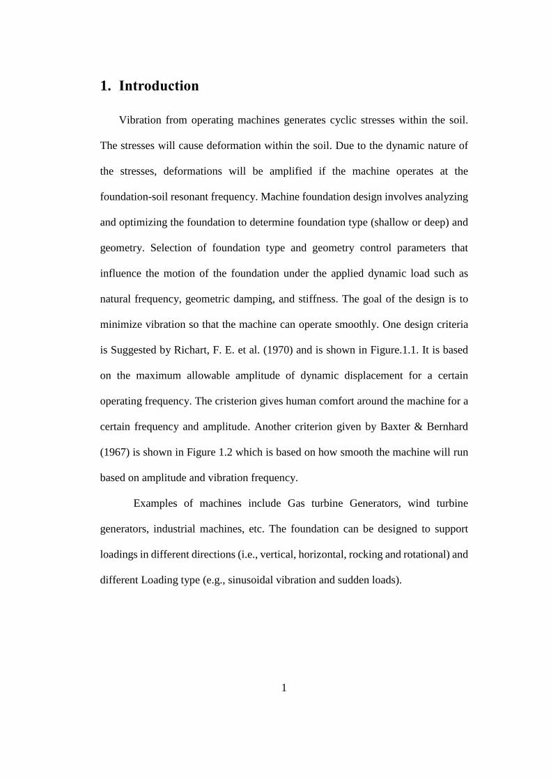
Vibration from operating machines generates cyclic stresses within the soil.
The stresses will cause deformation within the soil. Due to the dynamic nature of
the stresses, deformations will be amplified if the machine operates at the
foundation-soil resonant frequency. Machine foundation design involves analyzing
and optimizing the foundation to determine foundation type (shallow or deep) and
geometry. Selection of foundation type and geometry control parameters that
influence the motion of the foundation under the applied dynamic load such as
natural frequency, geometric damping, and stiffness. The goal of the design is to
minimize vibration so that the machine can operate smoothly. One design criteria
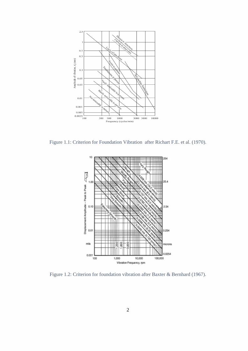
is Suggested by Richart, F. E. et al. (1970) and is shown in Figure.1.1. It is based
on the maximum allowable amplitude of dynamic displacement for a certain
operating frequency. The cristerion gives human comfort around the machine for a
certain frequency and amplitude. Another criterion given by Baxter & Bernhard
(1967) is shown in Figure 1.2 which is based on how smooth the machine will run
based on amplitude and vibration frequency.
Examples of machines include Gas turbine Generators, wind turbine
generators, industrial machines, etc. The foundation can be designed to support
loadings in different directions (i.e., vertical, horizontal, rocking and rotational) and
different Loading type (e.g., sinusoidal vibration and sudden loads).
2
Figure 1.1: Criterion for Foundation Vibration after Richart F.E. et al. (1970).
Figure 1.2: Criterion for foundation vibration after Baxter & Bernhard (1967).
3
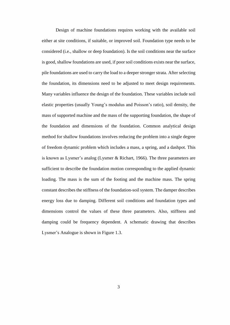
Design of machine foundations requires working with the available soil
either at site conditions, if suitable, or improved soil. Foundation type needs to be
considered (i.e., shallow or deep foundation). Is the soil conditions near the surface
is good, shallow foundations are used, if poor soil conditions exists near the surface,
pile foundations are used to carry the load to a deeper stronger strata. After selecting
the foundation, its dimensions need to be adjusted to meet design requirements.
Many variables influence the design of the foundation. These variables include soil
elastic properties (usually Young’s modulus and Poisson’s ratio), soil density, the
mass of supported machine and the mass of the supporting foundation, the shape of
the foundation and dimensions of the foundation. Common analytical design
method for shallow foundations involves reducing the problem into a single degree
of freedom dynamic problem which includes a mass, a spring, and a dashpot. This
is known as Lysmer’s analog (Lysmer & Richart, 1966). The three parameters are
sufficient to describe the foundation motion corresponding to the applied dynamic
loading. The mass is the sum of the footing and the machine mass. The spring
constant describes the stiffness of the foundation-soil system. The damper describes
energy loss due to damping. Different soil conditions and foundation types and
dimensions control the values of these three parameters. Also, stiffness and
damping could be frequency dependent. A schematic drawing that describes
Lysmer’s Analogue is shown in Figure 1.3.
4
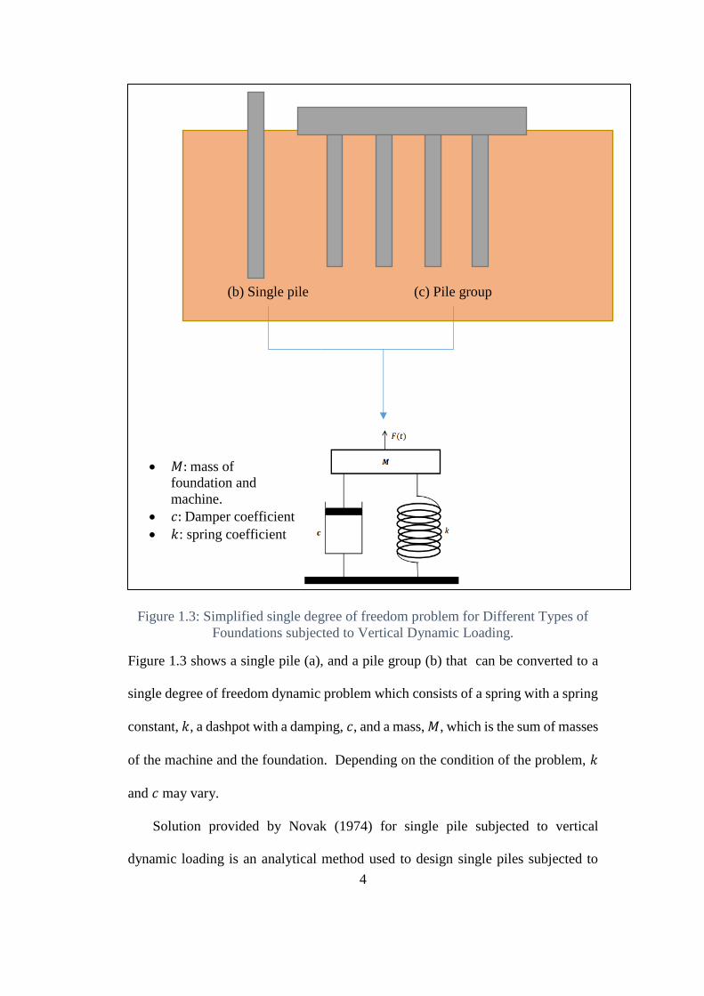
Figure 1.3: Simplified single degree of freedom problem for Different Types of
Foundations subjected to Vertical Dynamic Loading.
Figure 1.3 shows a single pile (a), and a pile group (b) that can be converted to a
single degree of freedom dynamic problem which consists of a spring with a spring
constant, 𝑘, a dashpot with a damping, 𝑐, and a mass, 𝑀, which is the sum of masses
of the machine and the foundation. Depending on the condition of the problem, 𝑘
and 𝑐 may vary.
Solution provided by Novak (1974) for single pile subjected to vertical
dynamic loading is an analytical method used to design single piles subjected to
(b) Single pile (c) Pile group
𝑀: mass of
foundation and
machine.
𝑐: Damper coefficient
𝑘: spring coefficient
5
dynamic loading. It gives the spring and damper coefficients that describe the
motion at the top of the pile. Another approach in design of piles subjected to
dynamic loading is a one dimensional finite element approach where the pile is
modeled as a bar element divided into segments. Side soil is modeled as a discrete
set of springs and dampers. Soil at the base is also modeled using a spring and
damper. This approach is approximate and better in modeling pile embedded in
layered soil profiles.
Since piles are used in groups, the values of the stiffness and damping of the
group are needed. Pile groups subjected to dynamic loading are designed by using
interaction factors. A single pile stiffness and damping are obtained analytically
using Novak’s solution. After obtaining stiffness and damping of a single pile, the
values of the stiffness and damping of the single piles are adjusted for group
behavior using interaction factors provided by Poulos (1968).
1.1. Limitations in current design methods
Current available analytical solution regarding pile subjected to vertical
dynamic load is the one provided by Novak (1974) and is accurate at α certain
value of dimensionless frequency, 𝑎0 = 0.3. where 𝑎0 = 𝜔 𝑟𝑝/𝑣𝑠. 𝜔 is the
frequency of the load in radians per seconds, 𝑟𝑝 is the pile radius and 𝑣𝑠 is the
shear wave velocity of the soil.
Novak’s (1974) Solution is also limited to homogeneous soil profiles (i.e.,
constant soil elastic modulus with depth). This means that if inhomogeneous
soil exists in the field, properties must be averaged for the engineer to be able
to design the foundation using Novak’s Solutions. Averaging soil properties
6
might yield an erroneous design that would require a high factor of safety. This
would render the design to be inefficient and costly.
One dimensional finite element approach is fast compared to 3D continuum
finite element modeling. However, the approach ignores the continuity of the
problem due to the soil being modeled as discrete separate sets of springs and
dampers. Piles interact with surrounding soil as continuum. Layers of soil
around the pile interact with each other and reflection, and refraction between
layers will alter the behavior of the soil around the pile. Discrete springs and
dampers might not represent real layered soil behavior.
Another limitation in current design methods is that static interaction factors
provided by Poulos (1968) are the ones used in design for pile groups subjected
to dynamic loading. The interaction factors are applied to both, stiffness and
damping of the group.
1.2. The need for research
Currently, available codes for machine foundation lack provisions for machine
foundation supported on piles. These codes include ACI 351.3R-04:
Foundations for Dynamic Equipment, 2004, DIN 4024: Machine Foundations,
1955, SAES-Q-007: Foundations and Supporting Structures for Heavy
Machinery, 2009s. An extensive review of codes provision for machine
foundations is given by Bharathi, Dhiraj, & Dubey (2014).
Novak accuracy is limited to dimensionless frequency, 𝑎0 = 0.3. studying
piles subjected to dynamic loading at dimensionless frequencies far from 0.3
is needed.
7
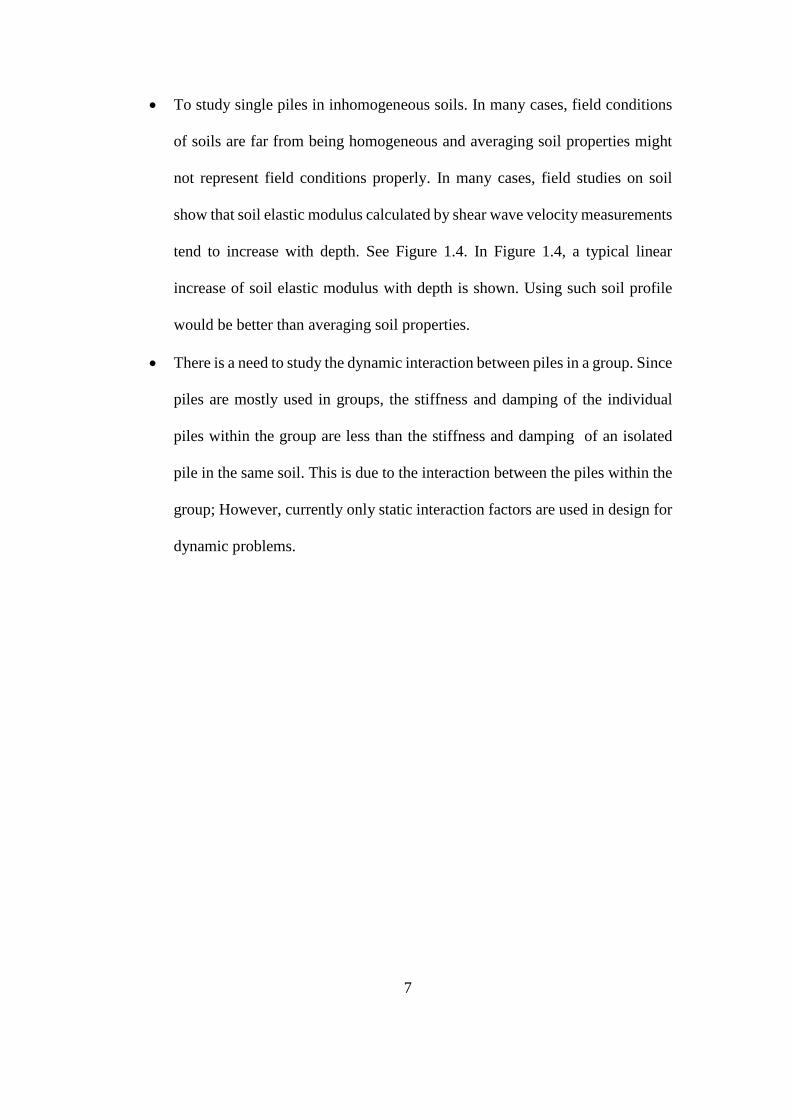
To study single piles in inhomogeneous soils. In many cases, field conditions
of soils are far from being homogeneous and averaging soil properties might
not represent field conditions properly. In many cases, field studies on soil
show that soil elastic modulus calculated by shear wave velocity measurements
tend to increase with depth. See Figure 1.4. In Figure 1.4, a typical linear
increase of soil elastic modulus with depth is shown. Using such soil profile
would be better than averaging soil properties.
There is a need to study the dynamic interaction between piles in a group. Since
piles are mostly used in groups, the stiffness and damping of the individual
piles within the group are less than the stiffness and damping of an isolated
pile in the same soil. This is due to the interaction between the piles within the
group; However, currently only static interaction factors are used in design for
dynamic problems.
8
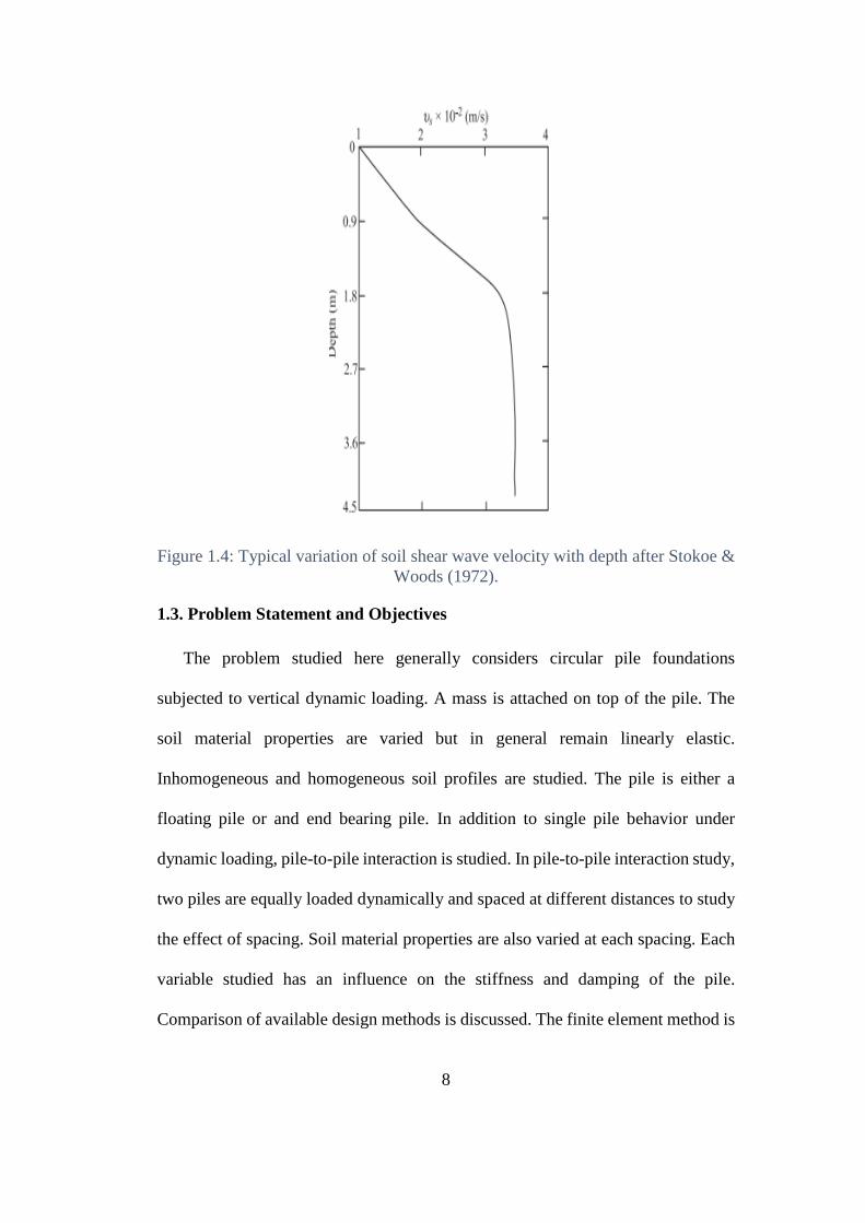
Figure 1.4: Typical variation of soil shear wave velocity with depth after Stokoe &
Woods (1972).
1.3. Problem Statement and Objectives
The problem studied here generally considers circular pile foundations
subjected to vertical dynamic loading. A mass is attached on top of the pile. The
soil material properties are varied but in general remain linearly elastic.
Inhomogeneous and homogeneous soil profiles are studied. The pile is either a
floating pile or and end bearing pile. In addition to single pile behavior under
dynamic loading, pile-to-pile interaction is studied. In pile-to-pile interaction study,
two piles are equally loaded dynamically and spaced at different distances to study
the effect of spacing. Soil material properties are also varied at each spacing. Each
variable studied has an influence on the stiffness and damping of the pile.
Comparison of available design methods is discussed. The finite element method is
9
used to determine the stiffness and damping of the pile for the different cases. Figure
1.4 shows a graphical representation of the cases considered.
In summary, the cases to be studied are
1- Study of a single pile foundation (floating and end bearing piles) subjected
to vertical dynamic loading in a homogeneous soil.
2- Study of a single pile foundation (floating and end bearing pile) subjected
to vertical dynamic loading in an inhomogeneous soil.
3- Study of pile-to-pile interaction at different spacing in a homogeneous soil.
10
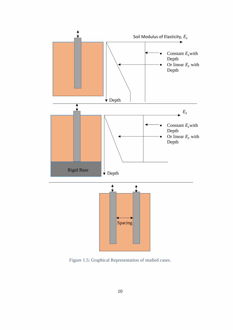
Figure 1.5: Graphical Representation of studied cases.
Soil Modulus of Elasticity, 𝐸𝑠
Depth
𝐸𝑠
Depth
Spacing
Constant 𝐸𝑠with
Depth
Or linear 𝐸𝑠 with
Depth
Constant 𝐸𝑠with
Depth
Or linear 𝐸𝑠 with
Depth
Rigid Base
11
In Figure 1.5, a floating pile in a homogeneous or an inhomogeneous soil
is shown (top). An end bearing pile in homogeneous or inhomogeneous soil is
shown (middle). Finally, pile-to-pile interaction is shown at the bottom.
1.4.Thesis Organization
The thesis is divided into 6 chapters (including this one). Starting from chapter 2
these chapters are:
Chapter 2: Literature Review. This chapter gives an introduction to
available design methods for single pile foundations. Both analytical and
numerical methods are discussed. A discussion of the design of pile groups
subjected to vertical dynamic loading is also provided.
Chapter 3: Introduction to the Finite Element Method. The chapter gives an
introduction to the finite element method and its application in dynamic
problems. A discussion of the math involved in finite element analysis is
provided. Discussion of element matrices formulation, assembly of global
matrices is provided. Static and dynamic solvers are discussed.
Chapter 4: Modeling and Finite Element Method Implementation. The
chapter describes how the finite element method is applied to current
research. It also discusses the research procedure from modeling the
geometry, performing the analysis to obtaining and interpreting the results.
Chapter 5: Results and Discussion. This chapter presents the results of this
research and discuss their interpretation. It also compares research results
with the work of others when applicable.

12
Chapter 6: Design Charts and Conclusion. The chapter summarizes the
research work, its results, and outcomes. Practical design recommendations
are provided based on outcomes of this research.
13
2. Literature Review
This chapter covers previous studies on piles under dynamic vertical loads.
It covers design methods and research related to pile dynamics. Several studies are
undertaken on piles subjected to vertical dynamic loading. These studies vary
greatly in their approach to the problem. Some studies provide a closed-form
solution to the differential Equations that describe the behavior of piles. This type
of study is limited to 1) the case considered in describing the problem. 2) the
assumptions made to simplify the problem in order to obtain the solution. Other
studies provide a simplified 1-Dimensional numerical solution to the problem.
These studies are limited due to the inherent error in using 1-Dimensional solution
to a 3D problem. Advancements have been made for these studies to account for
this error. Other studies provide the use of finite element method and varying the
variables that affect the response of the pile to the applied load. This chapter
provides a summary on these studies from the closed-form solutions to the
numerical analysis.
2.1. Machines and machine vibration
Proper machine foundation design is an integral part of machine operation.
The machines discussed are those related to industrial machines and power plants
machines. These machines operate at a certain frequency, and they generate
vibratory loads. The vibration can be amplified if the machine operate at the soil-
foundation resonance frequency. Amplification of machine vibration can hinder the
machine productivity, be very uncomfortable to people working next to the
14
machine, and in severe cases might break the machine or cause failure in the
systems connected to that machine.
Based on the frequency of operations, machines can be classified to 4
classes: 1) very low-speed machines that operate at 500 cycles per minute or less,
2) low-speed machines which operate at frequencies between 500 and 1500 cycles
per minute. 3) medium speed machines which operate at frequencies between 1500
and 3000 cycles per minute and 4) high-speed machines that operate at frequencies
higher than 3000 cycles per minute. Examples of machines include wind turbines,
printing machines, steam mills, boiler feed pumps, small fans used in power
industry and turbomachines such as gas turbines and compressors.
The goal of the design is to limit vibration. The design involves working
with existing field or improved soil condition and selecting the optimal foundation
type suitable for those conditions. From this definition, the variables of the design
are soil profile and soil properties (mainly elastic modulus, density and Poisson’s
ratio), foundation type: shallow or deep foundations and foundation Geometry
(shape, dimensions, and mass). The foundation serves two purposes: static stability
which means that foundation should carry the weight of the machine at acceptable
settlement and dynamical stability which means low vibration amplitude so that the
machine can operate smoothly.
This dissertation covers pile foundations, which are categorized as deep
foundations. This type of foundation is used when shallow foundations are not an
option due to poor soil conditions near the surface. The piles are used then to carry
the load into deeper more stronger soil strata or to rock base. Using piles increases
the value of the natural frequency of the system, and decreases the geometric
15
damping of the system. Design of piles for machine foundation also means working
with pile groups since piles are mostly used in groups. Piles in a group interact with
each other. This means that the stiffness and damping of a pile group is not simply
the sum of the stiffness and damping of individual piles within the group. It is less
than the sum due to the interaction between piles in the group. The following
sections in this chapter discuss pile foundation design and analysis techniques with
more detail. For more on machines and machine foundation the reader is referred
to Chowdhury & Dasgupta, (2008), Das & Ramana, (2010) and Richart, F.E. et al.,
(1970).
2.2. Closed form solutions for single pile subjected to dynamic loading
Closed form solutions simplify the problem into a mathematical model
consisting of differential Equations. A solution to these Equations is then provided.
Assumptions are made on the original problem to simplify the complexity of the
differential Equations to be solved.
2.2.1. Richart (1970) solution for single pile resting on rock
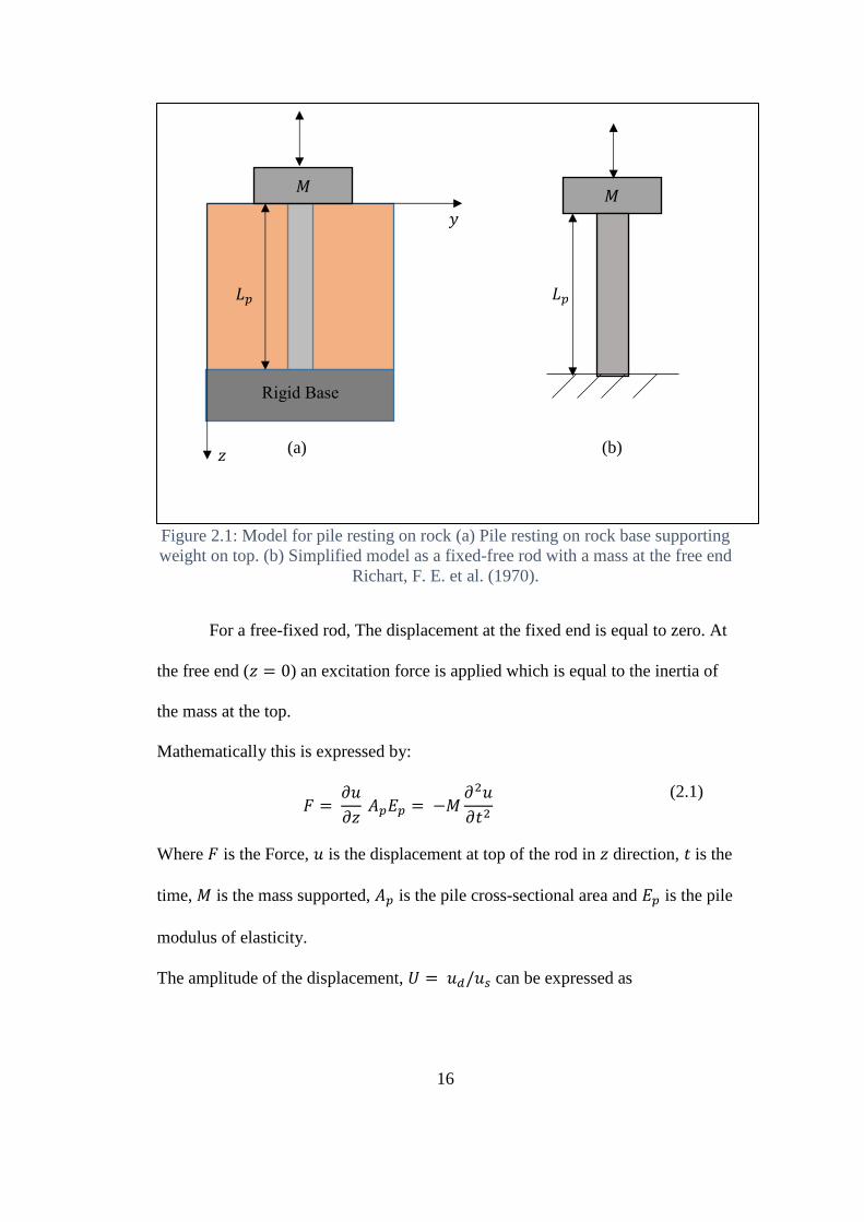
Richart, F. E. et al., (1970) presented a closed form solution for a pile resting
on a rock base. The pile supports a weight at its top. The problem is simplified into
a fixed free rod with a mass attached at the free end. See Figure 2.1 for illustration
of the actual problem and the corresponding simplified model.
16
Figure 2.1: Model for pile resting on rock (a) Pile resting on rock base supporting
weight on top. (b) Simplified model as a fixed-free rod with a mass at the free end
Richart, F. E. et al. (1970).
For a free-fixed rod, The displacement at the fixed end is equal to zero. At
the free end (𝑧 = 0) an excitation force is applied which is equal to the inertia of
the mass at the top.
Mathematically this is expressed by:
𝐹 = 𝜕𝑢
𝜕𝑧 𝐴𝑝𝐸𝑝 = −𝑀
𝜕2𝑢
𝜕𝑡2
(2.1)
Where 𝐹 is the Force, 𝑢 is the displacement at top of the rod in 𝑧 direction, 𝑡 is the
time, 𝑀 is the mass supported, 𝐴𝑝 is the pile cross-sectional area and 𝐸𝑝 is the pile
modulus of elasticity.
The amplitude of the displacement, 𝑈 = 𝑢𝑑/𝑢𝑠 can be expressed as
𝑀
𝐿𝑝
Rigid Base
𝐿𝑝
𝑀
(a) (b)
𝑦
𝑧
17
𝑈 = 𝑢𝑑
𝑢𝑠= 𝐶4 𝑠𝑖𝑛 (
𝜔𝑛 𝑧
𝑣𝑐)
(2.2)
Where 𝑢𝑑 is the dynamic displacement at a certain frequency, 𝑢𝑠 is the static
displacement if the load applied was static, 𝐶4 is a constant, 𝜔𝑛 is the natural
frequency in 𝑟𝑎𝑑𝑖𝑎𝑛𝑠/𝑠𝑒𝑐𝑜𝑛𝑑 and 𝑣𝑐 is the compressional wave velocity of the
pile. At the fixed end (𝑧 = 𝐿𝑝), the following Equations apply
𝜕𝑢
𝜕𝑧=
𝜕𝑈
𝜕𝑧 (𝐶1 𝑐𝑜𝑠(𝜔𝑛 𝑡) + 𝐶2 sin(𝜔𝑛 𝑡))
(2.3)
𝜕2𝑢
𝜕𝑡2= − 𝜔𝑛
2 𝑈 (𝐶1 𝑐𝑜𝑠(𝜔𝑛 𝑡) + 𝐶2 sin(𝜔𝑛 𝑡) (2.4)
Substituting Equation 2.3 and 2.4 in Equation 2.1 gives the following expression
𝐴𝑝 𝐸𝑝 𝜕𝑈
𝜕𝑧= 𝑀 𝜔𝑛
2 𝑈 (2.5)
Also substituting Equation 2.2 in Equation 2.5 gives
𝐴𝑝𝐸𝑝
𝜔𝑛
𝑉𝑐cos(
𝜔𝑛 𝐿𝑝
𝑉𝑐) = 𝑚 𝜔𝑛
2 𝑈 sin(𝜔𝑛 𝐿𝑝
𝑉𝑐)
(2.6)
Equation 2.6 can be rearranged to become
𝐴 𝐿𝑝 𝛾𝑝
𝑊=
𝜔𝑛 𝐿𝑝
𝑉𝑐 tan (
𝜔𝑛 𝐿𝑝
𝑉𝑐)
(2.7)
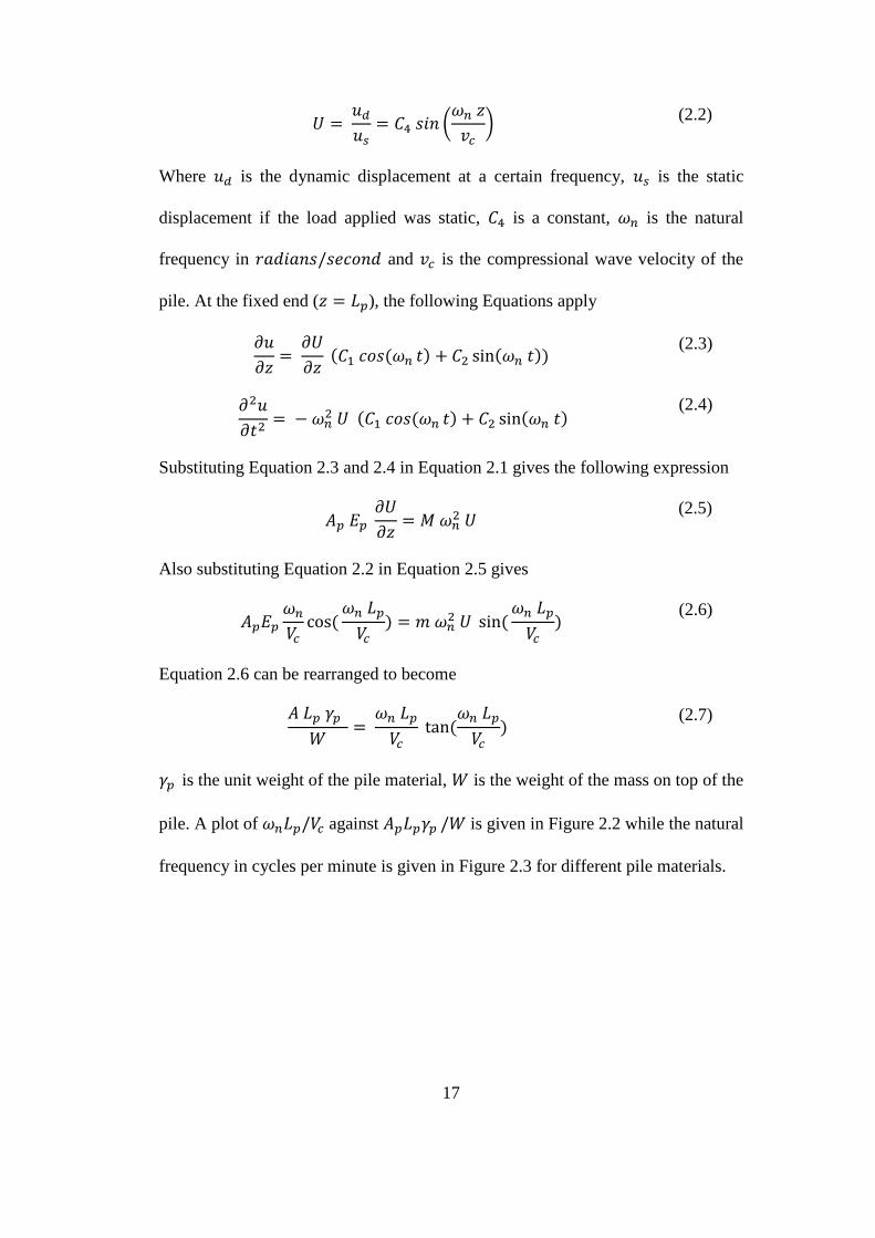
𝛾𝑝 is the unit weight of the pile material, 𝑊 is the weight of the mass on top of the
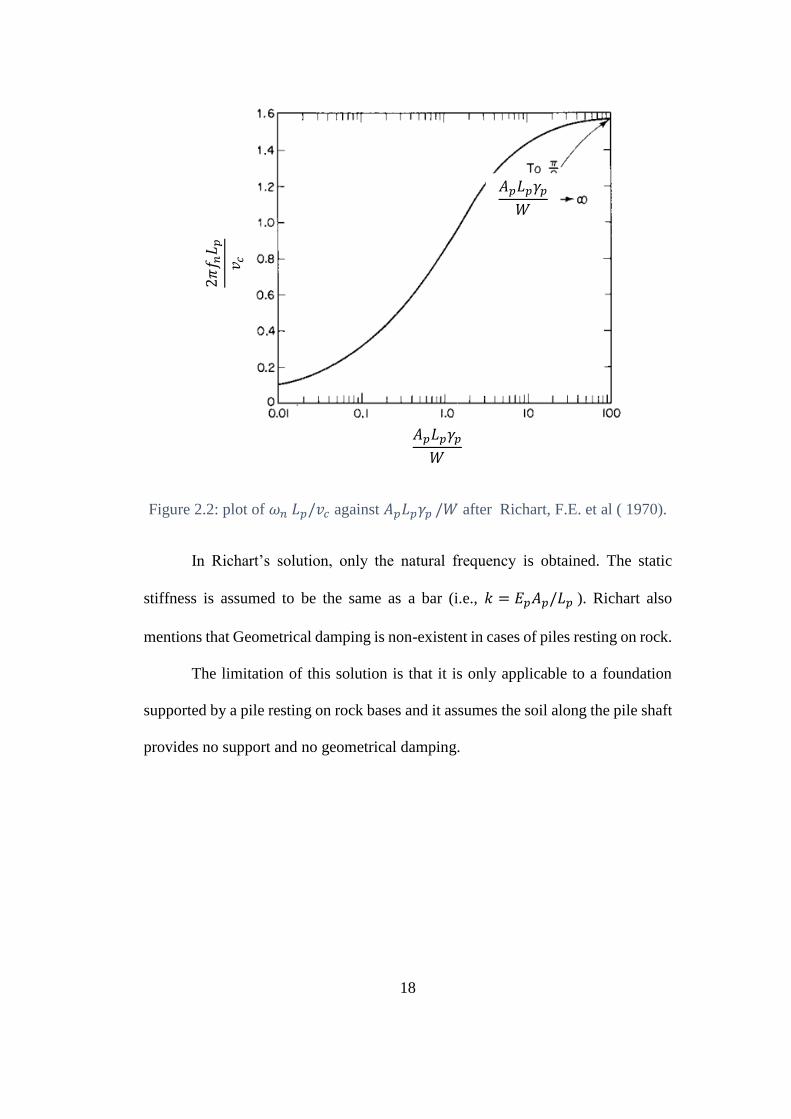
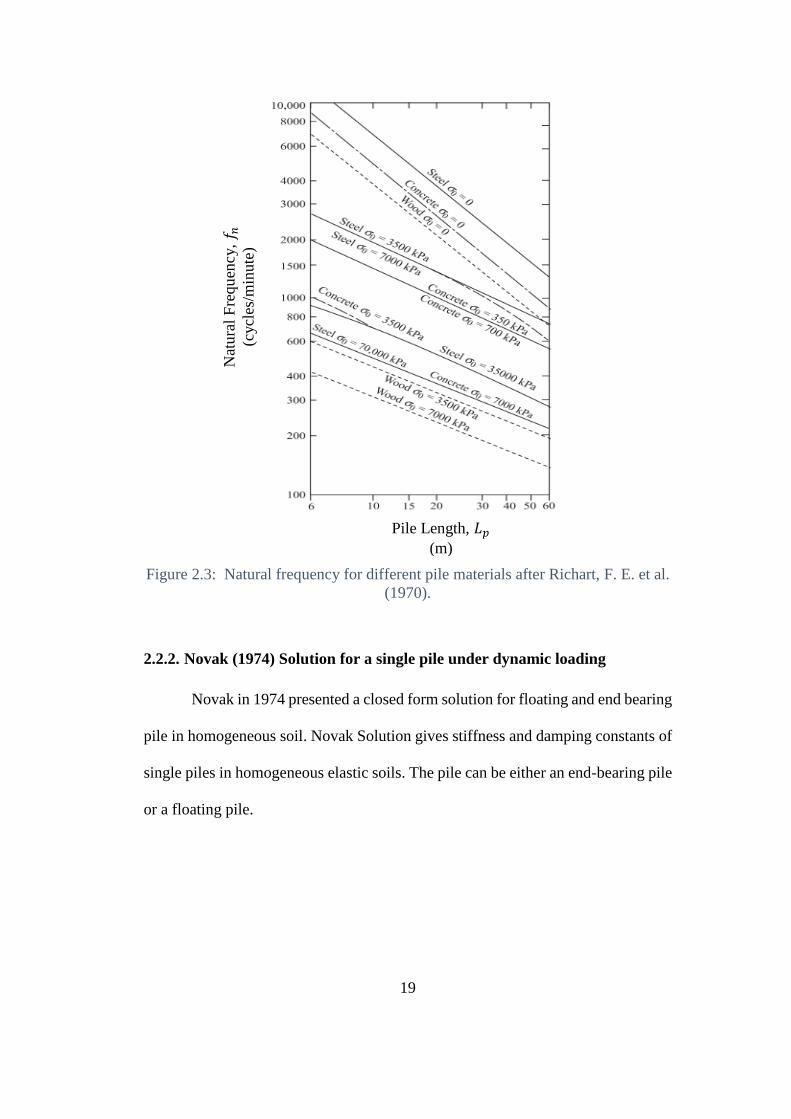
pile. A plot of 𝜔𝑛𝐿𝑝/𝑉𝑐 against 𝐴𝑝𝐿𝑝𝛾𝑝 /𝑊 is given in Figure 2.2 while the natural
frequency in cycles per minute is given in Figure 2.3 for different pile materials.
18
Figure 2.2: plot of 𝜔𝑛 𝐿𝑝/𝑣𝑐 against 𝐴𝑝𝐿𝑝𝛾𝑝 /𝑊 after Richart, F.E. et al ( 1970).
In Richart’s solution, only the natural frequency is obtained. The static
stiffness is assumed to be the same as a bar (i.e., 𝑘 = 𝐸𝑝𝐴𝑝/𝐿𝑝 ). Richart also
mentions that Geometrical damping is non-existent in cases of piles resting on rock.
The limitation of this solution is that it is only applicable to a foundation
supported by a pile resting on rock bases and it assumes the soil along the pile shaft
provides no support and no geometrical damping.
2𝜋𝑓 𝑛𝐿𝑝
𝑣 𝑐
𝐴𝑝𝐿𝑝𝛾𝑝
𝑊
𝐴𝑝𝐿𝑝𝛾𝑝
𝑊
19
Figure 2.3: Natural frequency for different pile materials after Richart, F. E. et al.
(1970).
2.2.2. Novak (1974) Solution for a single pile under dynamic loading
Novak in 1974 presented a closed form solution for floating and end bearing
pile in homogeneous soil. Novak Solution gives stiffness and damping constants of
single piles in homogeneous elastic soils. The pile can be either an end-bearing pile
or a floating pile.
Pile Length, 𝐿𝑝
(m)
Nat
ura
l F
requ
ency, 𝑓 𝑛
(cycl
es/m
inute
)
20
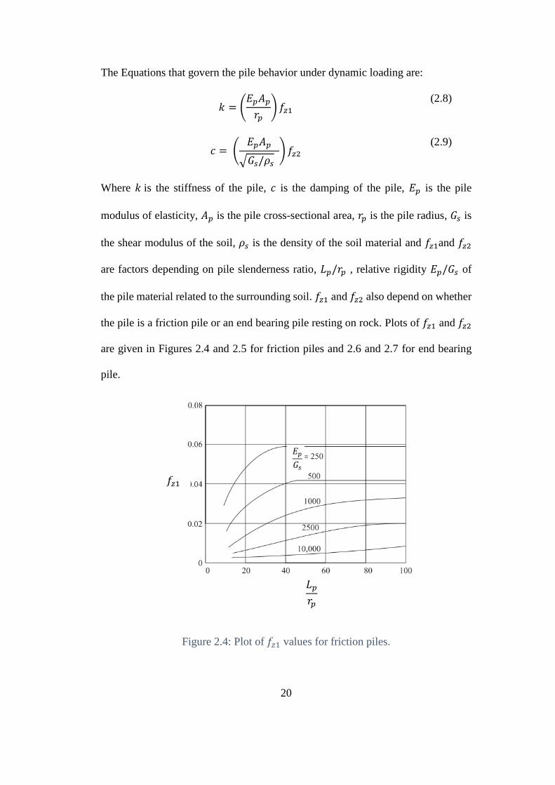
The Equations that govern the pile behavior under dynamic loading are:
𝑘 = (𝐸𝑝𝐴𝑝
𝑟𝑝)𝑓𝑧1
(2.8)
𝑐 = (𝐸𝑝𝐴𝑝
√𝐺𝑠/𝜌𝑠 ) 𝑓𝑧2
(2.9)
Where 𝑘 is the stiffness of the pile, 𝑐 is the damping of the pile, 𝐸𝑝 is the pile
modulus of elasticity, 𝐴𝑝 is the pile cross-sectional area, 𝑟𝑝 is the pile radius, 𝐺𝑠 is
the shear modulus of the soil, 𝜌𝑠 is the density of the soil material and 𝑓𝑧1and 𝑓𝑧2
are factors depending on pile slenderness ratio, 𝐿𝑝/𝑟𝑝 , relative rigidity 𝐸𝑝/𝐺𝑠 of
the pile material related to the surrounding soil. 𝑓𝑧1 and 𝑓𝑧2 also depend on whether
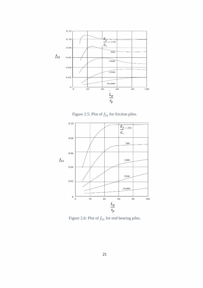
the pile is a friction pile or an end bearing pile resting on rock. Plots of 𝑓𝑧1 and 𝑓𝑧2
are given in Figures 2.4 and 2.5 for friction piles and 2.6 and 2.7 for end bearing
pile.
Figure 2.4: Plot of 𝑓𝑧1 values for friction piles.
𝐿𝑝
𝑟𝑝
𝑓𝑧1
𝐸𝑝
𝐺𝑠
21
Figure 2.5: Plot of 𝑓𝑧2 for friction piles.
Figure 2.6: Plot of 𝑓𝑧1 for end bearing piles.
𝐿𝑝
𝑟𝑝
𝑓𝑧2
𝐸𝑝
𝐺𝑠
𝐿𝑝
𝑟𝑝
𝑓𝑧1
𝐸𝑝
𝐺𝑠
22
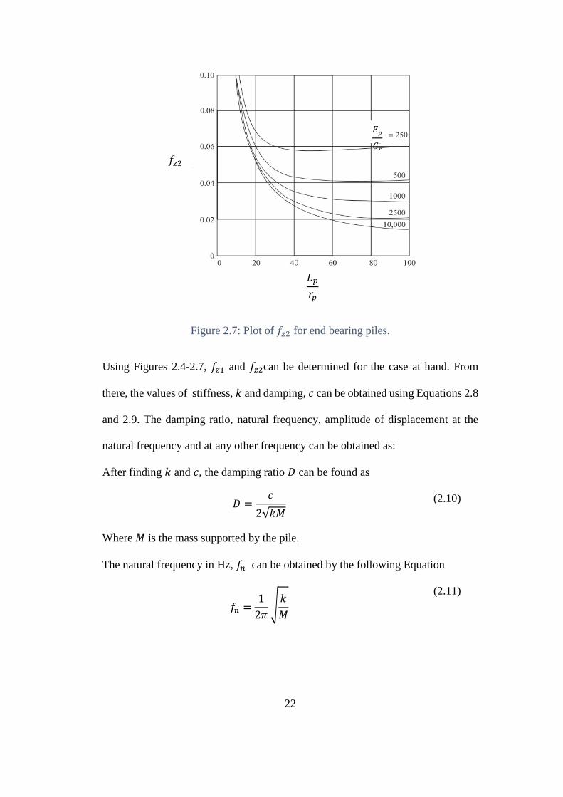
Figure 2.7: Plot of 𝑓𝑧2 for end bearing piles.
Using Figures 2.4-2.7, 𝑓𝑧1 and 𝑓𝑧2can be determined for the case at hand. From
there, the values of stiffness, 𝑘 and damping, 𝑐 can be obtained using Equations 2.8
and 2.9. The damping ratio, natural frequency, amplitude of displacement at the
natural frequency and at any other frequency can be obtained as:
After finding 𝑘 and 𝑐, the damping ratio 𝐷 can be found as
𝐷 =𝑐
2√𝑘𝑀
(2.10)
Where 𝑀 is the mass supported by the pile.
The natural frequency in Hz, 𝑓𝑛 can be obtained by the following Equation
𝑓𝑛 =1
2𝜋√𝑘
𝑀
(2.11)
𝐿𝑝
𝑟𝑝
𝑓𝑧2
𝐸𝑝
𝐺𝑠
23
The static displacement, 𝑢𝑠 is obtained by dividing the applied force, 𝐹 over the
static stiffness, 𝑘
𝑢𝑠 =𝐹
𝑘
(2.12)
the amplitude of displacement, 𝑈 = 𝑢𝑑/𝑢𝑠 can be found using the following
Equation
𝑈 =𝑢𝑑
𝑢𝑠=
1
√(1 −𝑓2
𝑓𝑛2)2
+ 4𝐷2 𝑓2
𝑓𝑛2
(2.13)
𝑢𝑑is the dynamic displacement, 𝑢𝑠 is the static displacement, 𝑓 is the frequency in
𝐻𝑧 and 𝑓𝑛 is the natural frequency in 𝐻𝑧 and 𝐷is the damping ratio. Once 𝑈 is
found, 𝑢𝑑 can be found as 𝑢𝑑 = 𝑈 𝑢𝑠.
It is worth mentioning that Novak’s solution is only accurate at
dimensionless frequency, 𝑎0 = 0.3. where 𝑎0 = 𝜔𝑟𝑝/𝑣𝑠. Where 𝜔 is the frequency
in radians/sec, 𝑟𝑝 is the pile radius and 𝑣𝑠 is the shear wave velocity of the soil.
Novak’s Solution provides an easy and a fast method for the analysis and
design of pile foundations under vertical dynamic load. This solution is subject to
certain assumptions and limitations. Assumptions include linearity of the problem,
the pile and soil being in perfect contact (no slippage at the pile-soil interface), the
pile is circular, vertical and elastic. Finally the soil at the side of the pile is assumed
to behave as very thin independent layers (Plane strain condition).
Comparisons with field tests by Novak (1977) found good agreement with
theory in cases where shear wave velocity at an end bearing pile base is twice that
at the side of the pile. In other cases, the theory overestimates the response of the
pile.
24
Elkasabgy & El Naggar (2013) compared Novak (1974) with the response
of helical and driven steel piles. It was found that theory gives highly overestimated
predictions while incorporating soil nonlinearity in the analysis provided better
predictions with field tests.
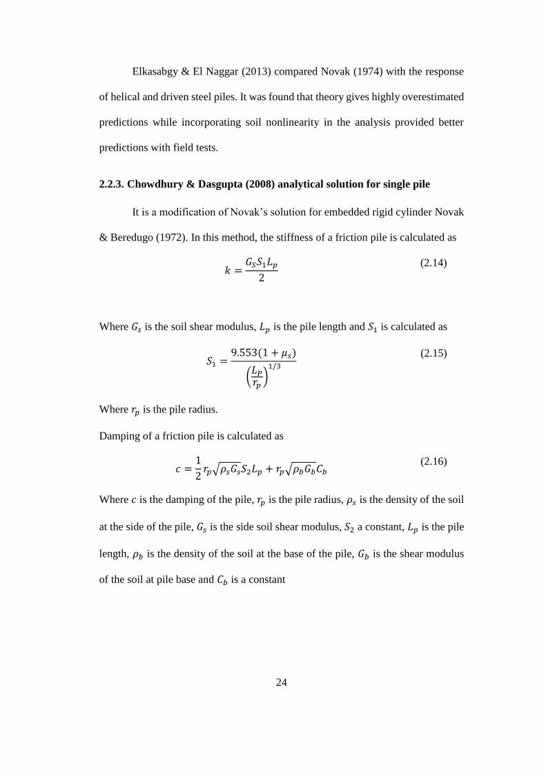
2.2.3. Chowdhury & Dasgupta (2008) analytical solution for single pile
It is a modification of Novak’s solution for embedded rigid cylinder Novak
& Beredugo (1972). In this method, the stiffness of a friction pile is calculated as
𝑘 =𝐺𝑆𝑆1𝐿𝑝
2
(2.14)
Where 𝐺𝑠 is the soil shear modulus, 𝐿𝑝 is the pile length and 𝑆1 is calculated as
𝑆1 =9.553(1 + 𝜇𝑠)
(𝐿𝑃𝑟𝑝)1/3
(2.15)
Where 𝑟𝑝 is the pile radius.
Damping of a friction pile is calculated as
𝑐 =1
2𝑟𝑝√𝜌𝑠𝐺𝑠𝑆2𝐿𝑝 + 𝑟𝑝√𝜌𝑏𝐺𝑏𝐶𝑏
(2.16)
Where 𝑐 is the damping of the pile, 𝑟𝑝 is the pile radius, 𝜌𝑠 is the density of the soil
at the side of the pile, 𝐺𝑠 is the side soil shear modulus, 𝑆2 a constant, 𝐿𝑝 is the pile
length, 𝜌𝑏 is the density of the soil at the base of the pile, 𝐺𝑏 is the shear modulus
of the soil at pile base and 𝐶𝑏 is a constant
25
In the case of an end bearing pile the static stiffness and damping are
calculated using the following Equation respectively:
𝑘 =𝐸𝑝𝐴𝑝
8𝐿𝑝+𝐺𝑠𝑆1𝐿𝑝
2
(2.17)
𝑐 =1
2𝑟𝑝√𝜌𝑠𝐺𝑠𝑆2𝐿𝑝
(2.18)
2.3. Finite Element solution for Pile subjected to dynamic loading
The finite element method is a numerical method used to solve differential
Equations. For more on the general finite element method, see Bathe (2006).
References specifically oriented towards geotechnical engineering include Potts &
Zdravkovic (1999, 2001) and Desai & Zaman (2013). A brief introduction is also
given in chapter 3 while application to the finite element method to current research
is covered in chapter 4. Usage of the finite element method in geotechnical
engineering is becoming the norm. This is due to the finite element method
reliability to get accurate results and its ability to connect lab and field tests to
computer simulations through material modeling. However, this accuracy is highly
dependable on the accuracy of the user input. Another limitation of the finite
element method is the need for high computing power and time to get results. This
is true in 3D geotechnical problems which involve non-linearity or dynamic
problems. Geotechnical problems also require large geometry and require fine
mesh. Another limitation is the absence of guidelines and codes that govern
modeling in geotechnical engineering. This makes the modeling process different
from a user to another and makes modeling subject to individual judgment.
Improvement on these limitations has been undertaken and as a result, it is a widely
26
used method in geotechnical engineering research and practice in different areas.
Current and future improvement in computer processors and parallel computing
will make it even easier, faster and more accurate.
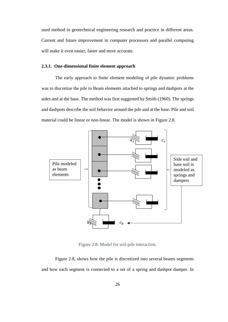
2.3.1. One-dimensional finite element approach
The early approach to finite element modeling of pile dynamic problems
was to discretize the pile to Beam elements attached to springs and dashpots at the
sides and at the base. The method was first suggested by Smith (1960). The springs
and dashpots describe the soil behavior around the pile and at the base. Pile and soil
material could be linear or non-linear. The model is shown in Figure 2.8.
Figure 2.8: Model for soil-pile interaction.
Figure 2.8, shows how the pile is discretized into several beams segments
and how each segment is connected to a set of a spring and dashpot damper. In
𝑘𝑠 𝑐𝑠
𝑘𝑏 𝑐𝑏
Pile modeled
as beam
elements
Side soil and
base soil is
modeled as
springs and
dampers
27
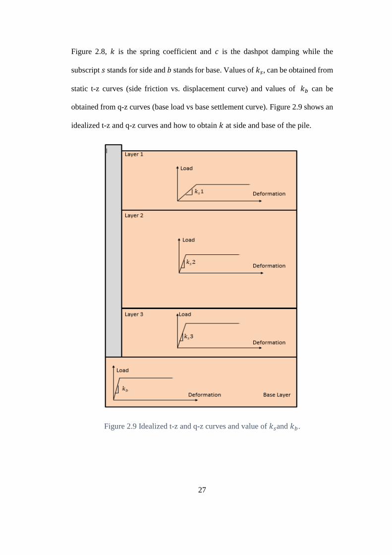
Figure 2.8, 𝑘 is the spring coefficient and 𝑐 is the dashpot damping while the
subscript 𝑠 stands for side and 𝑏 stands for base. Values of 𝑘𝑠, can be obtained from
static t-z curves (side friction vs. displacement curve) and values of 𝑘𝑏 can be
obtained from q-z curves (base load vs base settlement curve). Figure 2.9 shows an
idealized t-z and q-z curves and how to obtain 𝑘 at side and base of the pile.
Figure 2.9 Idealized t-z and q-z curves and value of 𝑘𝑠and 𝑘𝑏.
28
Values of side damping can be taken as 0.5 𝑠𝑒𝑐/𝑓𝑡 for sand while clay
should have 0.2 𝑠𝑒𝑐/𝑓𝑡. For base damper 𝑐𝑏 should be taken as 0.15 𝑠𝑒𝑐/𝑓𝑡 for
sand and 0.01 𝑠𝑒𝑐/𝑓𝑡 for clay (Coyle, Lowery, & Hirsch , 1977).
Randolph & Simons, (1986) suggested the following Equations for side
spring, 𝑘𝑠 and side damper, 𝑐𝑠
𝑘𝑠 = 1.375𝐺𝑠
𝜋𝑟𝑝
(2.19)
𝑐𝑠 =𝐺𝑠
𝑣𝑠
(2.20)
Where 𝐺𝑠 is soil shear modulus at the spring location, 𝑟𝑝 is the pile radius and 𝑣𝑠 is
the soil shear wave velocity at the spring location.
Lysmer & Richart (1966) proposed a static stiffness and dampings at of a
circularly loaded area on a surface of an elastic half-space. Based on this model the
values of the stiffness and dampings at the base of a circular area are given by the
following Equations respectively:
𝑘𝑏 =4𝐺𝑠𝑟𝑝
1 − 𝜇𝑠
(2.21)
𝑐𝑏 =3.4𝑟𝑝
2
1 − 𝜇𝑠√𝐺𝑠𝜌𝑠
(2.22)
In the previous Equations, 𝐺𝑠 is the soil shear modulus, 𝑟𝑝 is the pile radius, 𝜇𝑠 is
soil Poisson’s ratio and 𝜌𝑠 is the soil mass density.
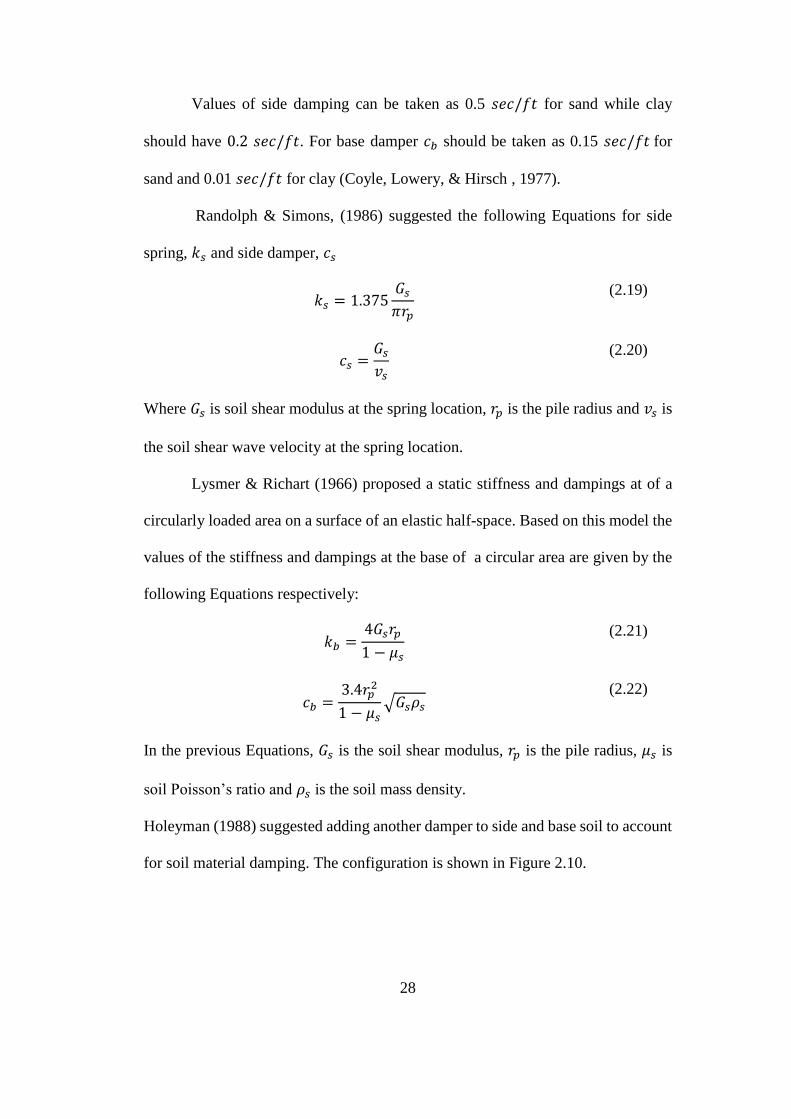
Holeyman (1988) suggested adding another damper to side and base soil to account
for soil material damping. The configuration is shown in Figure 2.10.
29
Figure 2.10 Model to account for material damping for side and base Soil.
. The method is further modified and refined by researchers to account for
shortcomings, to produce more accurate results and to expand applicability to
different cases. Kagawa (1991) proposed a nonlinear model that doesn’t use
dampers. The model relies only on the nonlinear behavior of the soil using dynamic
t-z (shaft resistance vs. displacement) and q-z curves (base resistance vs.
displacement). Seidel & Coronel (2011) formulated a model that takes into account
the degradation resulting from cyclic loading to predict long-term response of piles
The method described here (one-dimensional soil pile interaction) is
advantageous over analytical method as it is better in modeling layering of the soil
profile since the set of dashpots and springs around the pile can have different
coefficients. Care should be taken when choosing values of spring and dashpot
coefficients for the soil beneath the pile and the soil surrounding the pile. The values
should resemble field conditions and are obtained through field testing or available
literature. This model is flawed in that it ignores the continuity of the problem.
Reflections and interaction between soil layers cannot be accounted for. There is
also difficulty in choosing appropriate and reliable spring and damping values for
the soil.
spring
Radiation
damper Material
damper
30
2.3.2. 3D Finite element modeling
In this approach the soil is modeled as solid elements, the pile is modeled as
solid elements or beams with interface elements that connect the pile to the soil.
The method accuracy depends on the selected element size, time step and boundary
of the problem. The method is very time consuming and requires great
computational power due to a large number of elements. Several general purpose
computer programs are created for finite element simulation. Some programs are
more tailored to geotechnical engineering applications.
Ali, O. (2015) implemented 3D finite element method to study end bearing
piles subjected to a vertical dynamic load. The study calculated the dynamic
stiffness and damping of the pile. The soil along the pile shaft was homogeneous
and elastic. At the base, the soil shear modulus was 100 times that of the soil along
the pile shaft. In addition, a group of 3 by 3 piles are studied at different spacing.
2.4. Design of pile groups and pile to pile interaction
Piles are mostly used in groups. Groups of piles consist of a cap that
connects the piles together. This cap could be flexible or rigid. The difference
between rigid and flexible caps is that flexible caps allow for deformation of the
cap and thus the load is distributed unequally on the piles within the group. This
means that displacement is different between the piles. Rigid caps however
distribute the loads on the piles equally and displacement is uniform across the piles
in the group.
In static and dynamic problems, the stiffness and dampings of a single pile
don’t translate simply into a group of piles. Group stiffness and damping is not
31
simply the sum of the stiffness and damping of individual piles. The interaction
between the piles results in a reduction in the stiffness and dampings of individual
piles. Mathematically this is described by the following Equations
𝑘𝐺 =∑ 𝑘𝑖
𝑛𝑖=1
∑ 𝛼𝑖𝑛𝑖=1
(2.23)
𝑐𝐺 =∑ 𝑐𝑖
𝑛𝑖=1
∑ 𝛼𝑖𝑛𝑖=1
(2.24)
Where 𝑘𝐺is the group stiffness, 𝑘𝑖is the stiffness of a pile 𝑖 in the group, 𝛼𝑖is the
interaction factor of pile 𝑖 with a reference pile within the group. The interaction
factor is defined as the increase of settlement of a pile 𝑖 due to loading on an adjacent
pile 𝑗 over the settlement of pile 𝑖 if it were isolated.
Mathematically this is written as:
𝛼 =𝑢𝑖𝑗 − 𝑢𝑖
𝑢𝑖
(2.25)
Where 𝑢𝑖𝑗 is the total settlement of pile 𝑖 (settlement because of its own load and
added settlement due to loading on an closely spaced pile), 𝑢𝑖 is the settlement of
pile 𝑖 due to its own loading and if it were isolated. The interaction factor,𝛼 is a
function of pile dimensions (i.e. length and diameter), its stiffness, soil properties
around the piles and spacing between the piles in the group.
2.4.1. Poulos (1968) static interaction factors
In this study, two piles of the same characteristics embedded in an elastic
half-space are analyzed. The analysis is based on Elasticity theory. Equal loads are
applied on each pile. The increase of settlement on the piles due to the interaction
between them is calculated. This system despite having two piles, it is considered a
pile group by definition (The simplest form of a pile group). The analysis assumes
32
incompressibility of the piles and that the piles and the soil are perfectly contacted
and move together with no slippage at the pile-soil interface. This limits the solution
to cases where the stresses in the soil are within the elastic capacity of the soil and
not have reached yield strength of the soil. This doesn’t limit the solution from being
applicable to design since the investigation of pile groups load-settlement behavior
shows that the group settles linearly up to one third or one-half of its maximum load
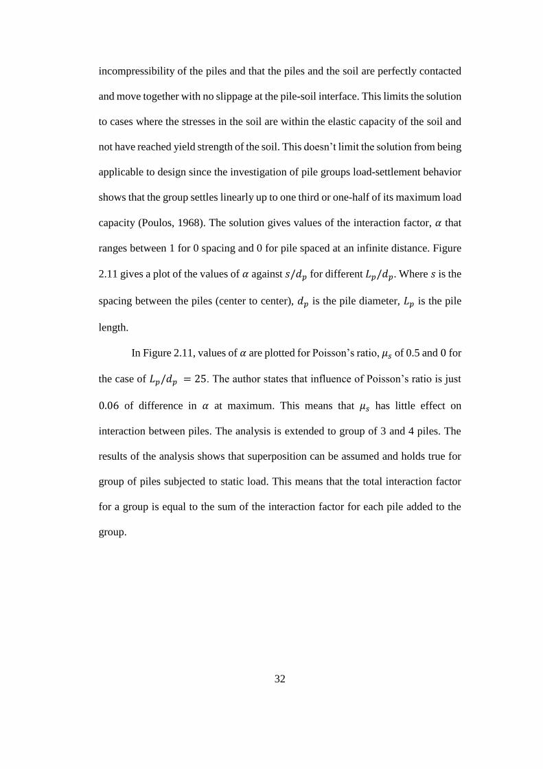
capacity (Poulos, 1968). The solution gives values of the interaction factor, 𝛼 that
ranges between 1 for 0 spacing and 0 for pile spaced at an infinite distance. Figure
2.11 gives a plot of the values of 𝛼 against 𝑠/𝑑𝑝 for different 𝐿𝑝/𝑑𝑝. Where 𝑠 is the
spacing between the piles (center to center), 𝑑𝑝 is the pile diameter, 𝐿𝑝 is the pile
length.
In Figure 2.11, values of 𝛼 are plotted fοr Poisson’s ratio, 𝜇𝑠 of 0.5 and 0 for
the case of 𝐿𝑝/𝑑𝑝 = 25. The author states that influence of Poisson’s ratio is just
0.06 of difference in 𝛼 at maximum. This means that 𝜇𝑠 has little effect on
interaction between piles. The analysis is extended to group of 3 and 4 piles. The
results of the analysis shows that superposition can be assumed and holds true for
group of piles subjected to static load. This means that the total interaction factor
for a group is equal to the sum of the interaction factor for each pile added to the
group.
33
Figure 2.11: Interaction factors between two piles after Poulos (1968).
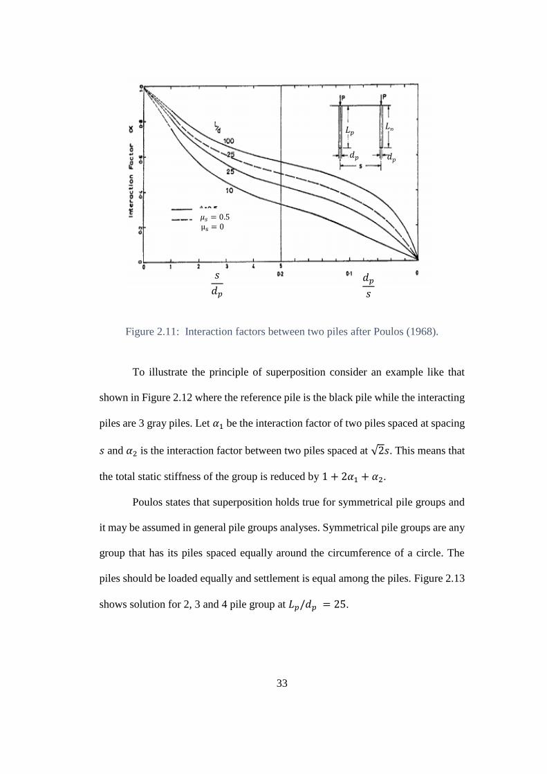
To illustrate the principle of superposition consider an example like that
shown in Figure 2.12 where the reference pile is the black pile while the interacting
piles are 3 gray piles. Let 𝛼1 be the interaction factor of two piles spaced at spacing
𝑠 and 𝛼2 is the interaction factor between two piles spaced at √2𝑠. This means that
the total static stiffness of the group is reduced by 1 + 2𝛼1 + 𝛼2.
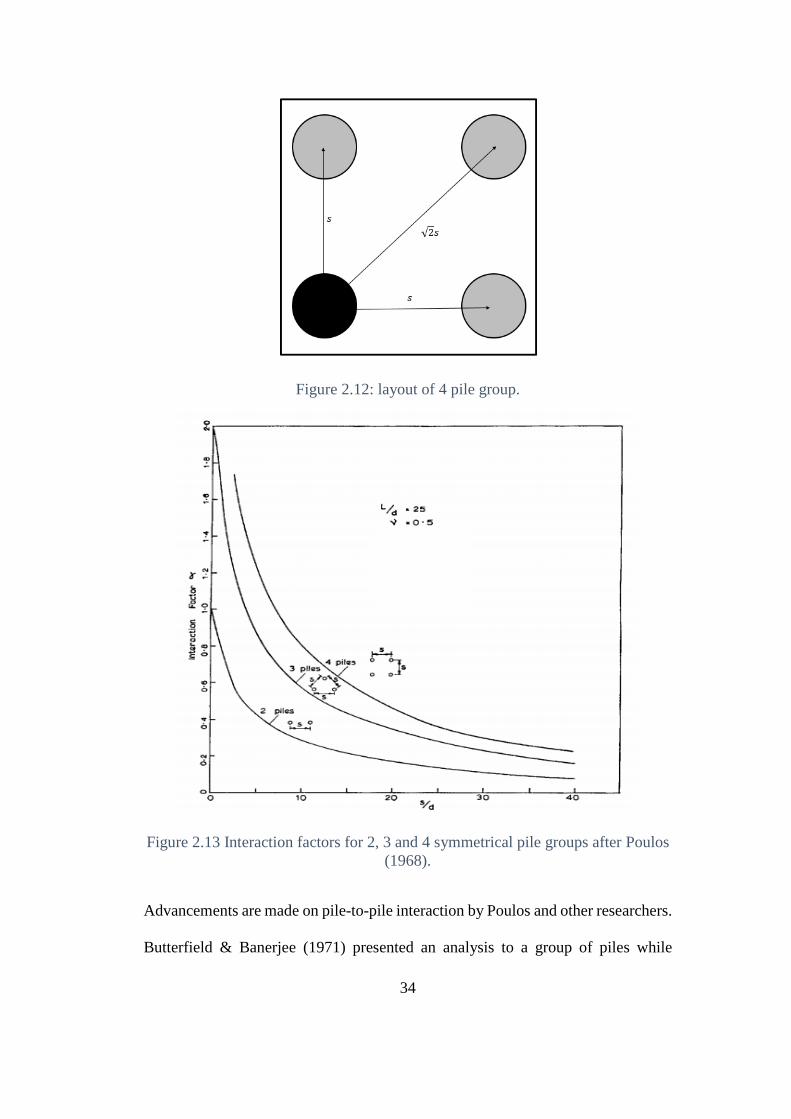
Poulos states that superposition holds true for symmetrical pile groups and
it may be assumed in general pile groups analyses. Symmetrical pile groups are any
group that has its piles spaced equally around the circumference of a circle. The
piles should be loaded equally and settlement is equal among the piles. Figure 2.13
shows solution for 2, 3 and 4 pile group at 𝐿𝑝/𝑑𝑝 = 25.
𝑠
𝑑𝑝
𝑑𝑝
𝑠
𝐿𝑝 𝐿𝑝
𝑑𝑝 𝑑𝑝
𝜇𝑠 = 0.5 μs = 0
34
Figure 2.12: layout of 4 pile group.
Figure 2.13 Interaction factors for 2, 3 and 4 symmetrical pile groups after Poulos
(1968).
Advancements are made on pile-to-pile interaction by Poulos and other researchers.
Butterfield & Banerjee (1971) presented an analysis to a group of piles while
35
considering the cap of the group being in contact with the ground. The results of the
analysis demonstrated that a contacting cap increased the stiffness of the pile group
by 5-15%. This increase in stiffness depends on the group size and spacing between
the piles. The portion of the load carried by the piles is different from that of a group
with a non-contacting cap. The range of difference is between 20% and 60%. The
larger the group, the higher the difference is. Chow & Teh (1992) studied groups in
a nonhomogeneous elastic soil where the soil’s Young's modulus increases linearly
with depth till it reaches rock base. They found that using homogeneous soil profile
underestimates the stiffness of the pile group. They provided field case studies in
which results are in agreement with their studies. In these case studies, the soil was
of clayey nature and the cap of the group was in contact with the ground. More
research in this area is being conducted to account for more cases and different soil
conditions.
2.4.2. Studies on dynamic interaction factors
Novak (1974) provided a comparison of pile groups against footing under
dynamic loading. The response is given in Figure 2.14. From Figure 2.14, Novak
concluded that due to increased stiffness of the pile group, the natural frequency
increases. The pile group had more amplitude of displacement at the natural
frequency which means that it is less damped than shallow block foundations. A
footing might have a higher amplitude at lower frequencies than a group of piles.
This is apparent at frequencies between 0 and 60 radians per seconds. Embedment
of the cap increased damping of the pile group so did embedment of the footing. In
this comparison interaction between the piles was considered by applying
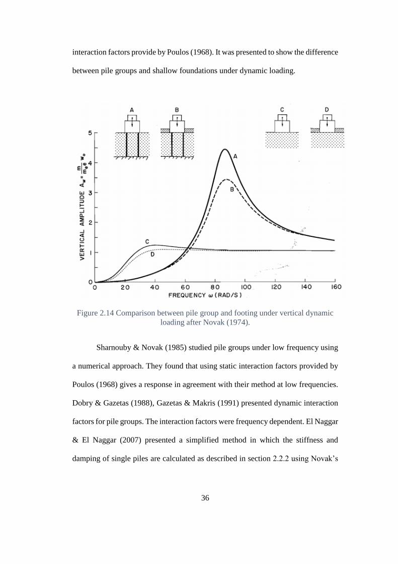
36
interaction factors provide by Poulos (1968). It was presented to show the difference
between pile groups and shallow foundations under dynamic loading.
Figure 2.14 Comparison between pile group and footing under vertical dynamic
loading after Novak (1974).
Sharnouby & Novak (1985) studied pile groups under low frequency using
a numerical approach. They found that using static interaction factors provided by
Poulos (1968) gives a response in agreement with their method at low frequencies.
Dobry & Gazetas (1988), Gazetas & Makris (1991) presented dynamic interaction
factors for pile groups. The interaction factors were frequency dependent. El Naggar
& El Naggar (2007) presented a simplified method in which the stiffness and
damping of single piles are calculated as described in section 2.2.2 using Novak’s
37
solution. The next step is to obtain interaction factor for a group that has been solved
for in the paper (2 by 2, 3 by 3, and 4 by 4 up to 9 by 9).
The presented studies in this section give some insight into the interaction
factor of dynamic loading on pile groups. Due to lack of analytical solutions on the
dynamic pile to pile interaction, references of soil dynamics refer to interaction
factors given by Poulos (1968) for dynamic analysis and it is the one used in design
for pile groups subjected to dynamic loading. See Prakash & Puri (1988) and Das
& Ramana ( 2010).
38
3. The Finite element method, an introduction
The finite element method (might be referred to as FEM or FEA throughout
the rest of this text) is a numerical method that discretizes a continuum into small
finite sub-structures. The sub-structure element is mathematically defined in how it
transports a certain quantity (e.g., stress, temperature, or fluid) to the adjacent
element. Boundary conditions and material models are to be defined in order for the
solution of the differential Equations to be solved. Basically, FEM is a numerical
method used to solve differential Equations of field problems. The field problem
can be one, two or three dimensional of any shape and configuration.
In this research, the finite element method is used to study the dynamic behavior
of pile foundations under vertical dynamic loading. Five different studies are
performed. 4 of those studies are on single piles. Since the piles in these studies
have circular cross sections, axisymmetric finite elements are used to discretize the
problem. Use of axisymmetric element is time efficient when simulating solids of
revolution. These solids are formed by revolving a planar shape around an axis. The
method would yield the same results as a full 3D simulation but with significantly
less number of elements. A smaller number of elements means a smaller stiffness
matrix and much less amount of time to solve the system of Equations. This is of
great importance in this research since the analysis is dynamic. Dynamic analysis
requires the system of linear Equations to be solved at each time step of the analysis.
The fifth study, however, is on the pile-to-pile interaction. This study requires a full
3D model to be set up for the analysis in order to properly capture the behavior of
the two piles. This means that full 3D analysis is run on this case and the analysis
time is very high compared to 2D analysis.
39
This chapter serves as an introduction to the finite element method based on
Bathe, (2006) and Logan (2007). In this chapter, 2D axisymmetric elements and 3D
tetrahedron elements are briefly introduced. The process of obtaining the stiffness
matrix and other matrices for each type of element is covered. A solution of linear
Equations systems is discussed. In particular, the sparse and iterative solvers are
discussed. Integration schemes in time for dynamic analysis are discussed.
3.1. Mathematical preliminaries for the finite element method
In a linear elastic material, the stress-strain relationship is defined by
{𝜎} = [𝐶]{휀} (3.1)
Where {𝜎} is the stress matrix, [𝐶] is a constitutive matrix that relates the stress to
the strain and {휀} is the strain matrix.
From the constitutive matrix, a local elemental stiffness matrix [𝑘] can be calculated
as
{𝑘} = ∫[𝐵]𝑇[𝐶][𝐵]𝑑𝑉 (3.2)
The matrix [𝐵] depends on the geometry and coordinates of the finite element and
is defined by
[𝐵] = {𝜕}[𝑁] (3.3)
In 3.3, {𝜕}is a differential operator of the shape functions matrix [𝑁].
The final equilibrium Equation for a static problem is
{𝐹} = [𝐾]{𝐷} (3.4)
40
Where [𝐹] is the global nodal forces matrix and [𝑈] is the global nodal displacement
matrix. They are defined by
{𝐹} = ∑𝑓𝑖
𝑛
𝑖=0
(3.5)
{𝐷} = ∑𝑑𝑖
𝑛
𝑖=0
(3.6)
𝑓𝑖 and 𝑢𝑖 are the force and displacement at node 𝑖 respectively. 𝑛 is the total number
of nodes in the problem.
[𝐾] is the global stiffness matrix and is obtained by
{𝐾} = ∑∑𝑘𝑖𝑗
𝑛
𝑖=0
𝑛
𝑗=0
(3.7)
{𝐹} and {𝑈} depends on the boundary conditions of the problem (i.e. applied loads
and prescribed displacements). After defining all the required matrices Equation 3.4
can be solved to obtain unknown forces or displacements at any node in the
continuum. All the above Equations depend on the problem at hand.
3.2. Axisymmetric elements
An axisymmetric element is a finite element used to model a three-
dimensional body that is symmetrical around an axis in regards to geometry and
boundary conditions. Due to symmetry around the z-axis, as shown in Figure 3.1,
the stresses and strains are independent of the value of 𝜃. The stresses are
dependent on the coordinates of the plane 𝑧 − 𝑟. The following is a derivation of
41
the matrices required to solve a finite element problem with a triangular
axisymmetric element. See Figure 3.2 for the triangular element with
vertices 𝑖, 𝑗, 𝑎𝑛𝑑 𝑚; each has the coordinates (𝑧, 𝑟). The element has two degrees of
freedom per node (𝑢 𝑎𝑛𝑑 𝑤). Let the element have the following displacement
functions
𝑢(𝑟, 𝑧) = 𝑎1 + 𝑎2𝑟 + 𝑎3𝑧 (3.8)
𝑤(𝑟, 𝑧) = 𝑎4 + 𝑎5𝑟 + 𝑎6𝑧 (3.9)
Note that the total number of the coefficients 𝑎 is the same as the number of the
degrees of freedom. (6 𝑎𝑖′𝑠 for 6 degrees of freedom).
The nodal displacement matrix is
{𝑑} = {
𝑑𝑖
𝑑𝑗
𝑑𝑚
} =
{
𝑢𝑖
𝑤𝑖
𝑢𝑗𝑤𝑗
𝑢𝑚
𝑤𝑚}
(3.10)
At any node 𝑖, 𝑢 and 𝑤 are evaluated as
𝑢(𝑟𝑖, 𝑧𝑖) = 𝑎1 + 𝑎2𝑟𝑖 + 𝑎3𝑧𝑖 (3.11)
𝑤(𝑟𝑖, 𝑧𝑖) = 𝑎4 + 𝑎5𝑟𝑖 + 𝑎6𝑧𝑖 (3.12)
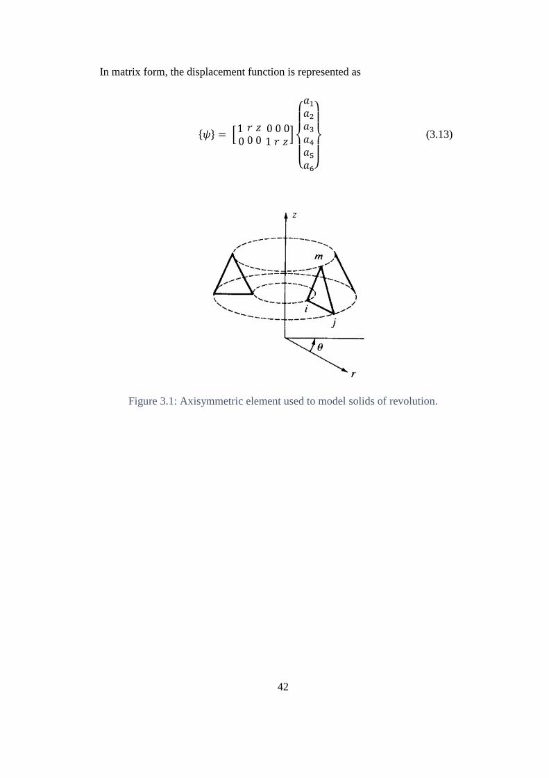
42
In matrix form, the displacement function is represented as
{𝜓} = [1 0
𝑟 0 𝑧 0 0 1 0𝑟 0𝑧]
{
𝑎1𝑎2𝑎3𝑎4𝑎5𝑎6}
(3.13)
Figure 3.1: Axisymmetric element used to model solids of revolution.
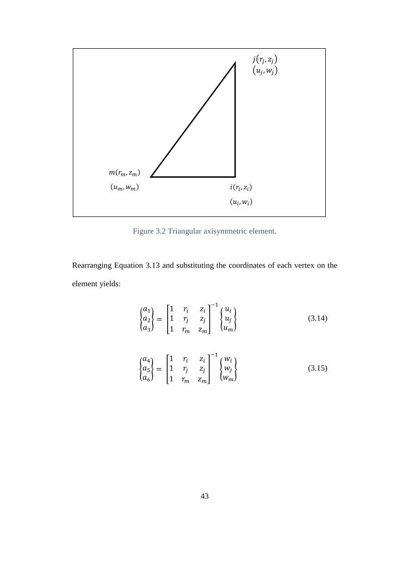
43
Figure 3.2 Triangular axisymmetric element.
Rearranging Equation 3.13 and substituting the coordinates of each vertex on the
element yields:
{
𝑎1𝑎2𝑎3
} = [
1 𝑟𝑖 𝑧𝑖1 𝑟𝑗 𝑧𝑗1 𝑟𝑚 𝑧𝑚
]
−1
{
𝑢𝑖
𝑢𝑗𝑢𝑚
} (3.14)
{
𝑎4𝑎5𝑎6
} = [
1 𝑟𝑖 𝑧𝑖1 𝑟𝑗 𝑧𝑗1 𝑟𝑚 𝑧𝑚
]
−1
{
𝑤𝑖
𝑤𝑗
𝑤𝑚
} (3.15)
𝑗 𝑟𝑗 , 𝑧𝑗
𝑢𝑗 , 𝑤𝑗
𝑖(𝑟𝑖, 𝑧𝑖)
(𝑢𝑖, 𝑤𝑖)
𝑚(𝑟𝑚, 𝑧𝑚)
(𝑢𝑚, 𝑤𝑚)
44
After performing the inversion in Equations 3.14 and 3.15, they become
{
𝑎1𝑎2𝑎3
} =1
2𝐴 [
𝛼𝜄 𝛼𝑗 𝑎𝑚𝛽𝜄 𝛽𝑗 𝛽𝑚𝛾𝑖 𝛾𝑗 𝛾𝑚
] {
𝑢𝑖
𝑢𝑗𝑢𝑚
} (3.16)
{
𝑎4𝑎5𝑎6
} = 1
2𝐴 [
𝛼𝜄 𝛼𝑗 𝑎𝑚𝛽𝜄 𝛽𝑗 𝛽𝑚𝛾𝑖 𝛾𝑗 𝛾𝑚
] {
𝑤𝑖
𝑤𝑗
𝑤𝑚
} (3.17)
Where:
𝛼𝜄 = 𝑟𝑗𝑧𝑚 − 𝑧𝑗𝑟𝑚 𝛼𝑗 = 𝑟𝑚𝑧𝑖 − 𝑧𝑚𝑟𝑖 𝛼𝑚 = 𝑟𝑖𝑧𝑗 − 𝑧𝑖𝑟𝑗
(3.18) 𝛽𝑖 = 𝑧𝑗 − 𝑧𝑚 𝛽𝑗 = 𝑧𝑚 − 𝑧𝑖 𝛽𝑚 = 𝑧𝑖 − 𝑧𝑗
𝛾𝑖 = 𝑟𝑚 − 𝑟𝑗 𝛾𝑗 = 𝑟𝑖 − 𝑟𝑚 𝛾𝑚 = 𝑟𝑗 − 𝑟𝑖
The shape functions are then defined as:
𝑁𝑖 =1
2𝐴(𝛼𝑖 + 𝛽𝑖𝑟 + 𝛾𝑖𝑧) (3.19)
𝑁𝑗 =1
2𝐴(𝛼𝑗 + 𝛽𝑗𝑟 + 𝛾𝑗𝑧) (3.20)
𝑁𝑚 =1
2𝐴(𝛼𝑚 + 𝛽𝑚𝑟 + 𝛾𝑚𝑧) (3.21)
The displacement matrix of the element is:
{𝑢(𝑧, 𝑟)
𝑤(𝑧, 𝑟)} = [
𝑁𝑖
0
0 𝑁𝑖
𝑁𝑗0 0𝑁𝑗 𝑁𝑚
0 0𝑁𝑚
]
{
𝑢𝑖
𝑤𝑖
𝑢𝑗𝑤𝑗
𝑢𝑚
𝑤𝑚}
(3.22)
45
From continuum mechanics and elasticity the strains can be defined as
휀𝑟 = 𝜕𝑢
𝜕𝑟 휀𝜃 =
𝑢
𝑟 휀𝑧 =
𝜕𝑤
𝜕𝑧 𝛾𝑟𝑧 =
𝜕𝑢
𝜕𝑧+
𝜕𝑤
𝜕𝑟 (3.23)
Using Equations 3.8 and 3.9 with 3.23 the following is obtained
{휀} =
{
𝑎2𝑎6
𝑎1𝑟+ 𝑎2 +
𝑎3𝑧
𝑟𝑎3 + 𝑎5 }
(3.24)
Equation 3.24 can be rewritten as
{
휀𝑟휀𝑧휀𝜃𝛾𝑟𝑧
} =
[ 001
𝑟0
1010
00𝑧
𝑟1
0000
0001
0100]
{
𝑎1𝑎2𝑎3𝑎4𝑎5𝑎6}
(3.25)
Substituting Equations 3.16 and 3.17 in 3.25 with simplification, the following
Equation is obtained
{휀} =
1
2𝐴
[
𝛽𝑖0
𝛼𝑖
𝑟+ 𝛽𝑖 +
𝛾𝑖𝑧
𝑟𝛾𝑖
0𝛾𝑖0𝛽𝑖
𝛽𝑗0
𝛼𝑗
𝑟+ 𝛽𝑗 +
𝛾𝑗𝑧
𝑟𝛾𝑗
0𝛾𝑗0𝛽𝑗
𝛽𝑚0
𝛼𝑚
𝑟+ 𝛽𝑚 +
𝛾𝑚𝑧
𝑟𝛾𝑚
0𝛾𝑚0𝛽𝑚]
{
𝑢𝑖
𝑤𝑖
𝑢𝑗𝑤𝑗
𝑢𝑚
𝑤𝑚}
(3.26
)
[𝐵]
46
The stresses are given by Equation 3.1 where the constitutive matrix [𝐶] is
according to the following Equation
[𝐶] =𝐸
(1 + 𝜇)(1 − 2𝜇)
[ 1 − 𝜇
𝜇𝜇0
𝜇1 − 𝜇𝜇0
𝜇𝜇
1 − 𝜇0
000
1 − 2𝜇
2 ]
(3.27)
The axisymmetric element stiffness matrix is calculated according to the volume
integral in Equation 3.2 and in the cylindrical coordinates Equation 3.2 becomes
[𝑘] = 2𝜋 ∬[𝐵]𝑇[𝐶][𝐵] 𝑟 𝑑𝑟 𝑑𝑧 (3.28)
So far the element stiffness matrix of an axisymmetric element is derived.
Boundary conditions (i.e., nodal forces and prescribed displacements) are applied
on each node and placed in the proper location in the forces and displacement
matrices. In the case of surface forces (i.e., surface traction and/or pressure), the
process is more involved in obtaining equivalent nodal forces. The process is
explained with the aid of Figure3.3. In Figure 3.3, an axisymmetric element is
presented with forces acting on the surface of the element. One force is a pressure
force and the other is a surface traction force. In general, surface forces can be found
by
{𝑓𝑠} = ∬[𝑁𝑠]𝑇{𝑇} 𝑑𝑆 (3.29)
Where {𝑓𝑠} is the element forces matrix and [𝑁𝑠] is the shape function matrix
evaluated along the surface where the surface forces are applied. In the case of the
element presented in Figure 3.3, Equation 3.29 becomes
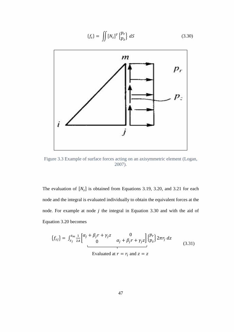
47
{𝑓𝑠} = ∬[𝑁𝑠]𝑇 {
𝑝𝑟𝑝𝑧} 𝑑𝑆 (3.30)
Figure 3.3 Example of surface forces acting on an axisymmetric element (Logan,
2007).
The evaluation of [𝑁𝑠] is obtained from Equations 3.19, 3.20, and 3.21 for each
node and the integral is evaluated individually to obtain the equivalent forces at the
node. For example at node 𝑗 the integral in Equation 3.30 and with the aid of
Equation 3.20 becomes
{𝑓𝑠𝑗} = ∫1
2𝐴[𝛼𝑗 + 𝛽𝑗𝑟 + 𝛾𝑗𝑧
0
0𝛼𝑗 + 𝛽𝑗𝑟 + 𝛾𝑗𝑧
]𝑧𝑚
𝑧𝑗{𝑝𝑟𝑝𝑧} 2𝜋𝑟𝑗 𝑑𝑧
(3.31)
Evaluated at 𝑟 = 𝑟𝑗 and 𝑧 = 𝑧
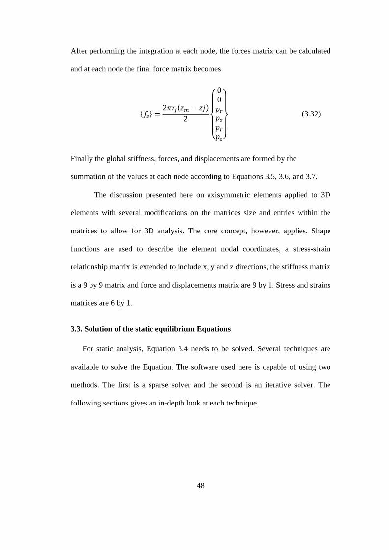
48
After performing the integration at each node, the forces matrix can be calculated
and at each node the final force matrix becomes
{𝑓𝑠} =2𝜋𝑟𝑗(𝑧𝑚 − 𝑧𝑗)
2
{
00𝑝𝑟𝑝𝑧𝑝𝑟𝑝𝑧}
(3.32)
Finally the global stiffness, forces, and displacements are formed by the
summation of the values at each node according to Equations 3.5, 3.6, and 3.7.
The discussion presented here on axisymmetric elements applied to 3D
elements with several modifications on the matrices size and entries within the
matrices to allow for 3D analysis. The core concept, however, applies. Shape
functions are used to describe the element nodal coordinates, a stress-strain
relationship matrix is extended to include x, y and z directions, the stiffness matrix
is a 9 by 9 matrix and force and displacements matrix are 9 by 1. Stress and strains
matrices are 6 by 1.
3.3. Solution of the static equilibrium Equations
For static analysis, Equation 3.4 needs to be solved. Several techniques are
available to solve the Equation. The software used here is capable of using two
methods. The first is a sparse solver and the second is an iterative solver. The
following sections gives an in-depth look at each technique.
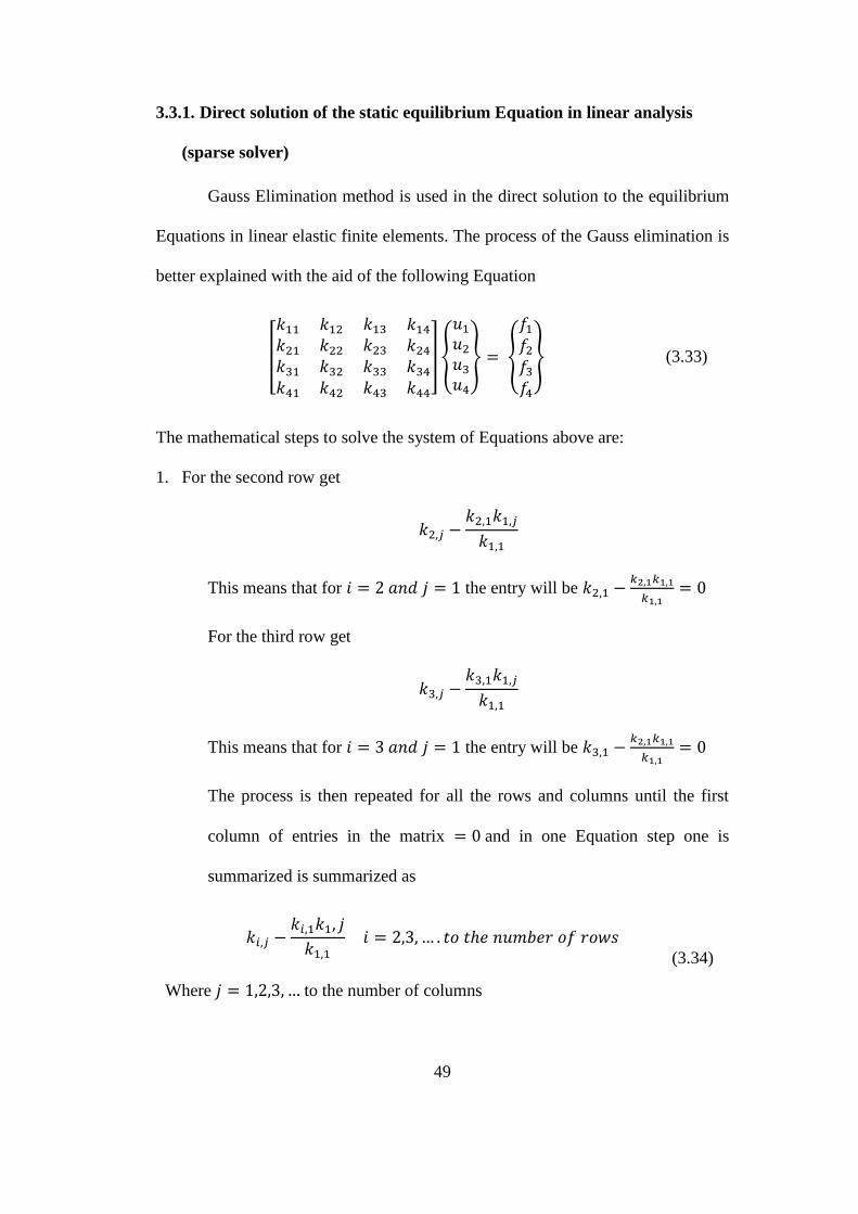
49
3.3.1. Direct solution of the static equilibrium Equation in linear analysis
(sparse solver)
Gauss Elimination method is used in the direct solution to the equilibrium
Equations in linear elastic finite elements. The process of the Gauss elimination is
better explained with the aid of the following Equation
[
𝑘11𝑘21𝑘31𝑘41
𝑘12𝑘22𝑘32𝑘42
𝑘13𝑘23𝑘33𝑘43
𝑘14𝑘24𝑘34𝑘44
] {
𝑢1𝑢2
𝑢3
𝑢4
} = {
𝑓1𝑓2𝑓3𝑓4
} (3.33)
The mathematical steps to solve the system of Equations above are:
1. For the second row get
𝑘2,𝑗 −𝑘2,1𝑘1,𝑗
𝑘1,1
This means that for 𝑖 = 2 𝑎𝑛𝑑 𝑗 = 1 the entry will be 𝑘2,1 −𝑘2,1𝑘1,1
𝑘1,1= 0
For the third row get
𝑘3,𝑗 −𝑘3,1𝑘1,𝑗
𝑘1,1
This means that for 𝑖 = 3 𝑎𝑛𝑑 𝑗 = 1 the entry will be 𝑘3,1 −𝑘2,1𝑘1,1
𝑘1,1= 0
The process is then repeated for all the rows and columns until the first
column of entries in the matrix = 0 and in one Equation step one is
summarized is summarized as
𝑘𝑖,𝑗 −𝑘𝑖,1𝑘1, 𝑗
𝑘1,1 𝑖 = 2,3, … . 𝑡𝑜 𝑡ℎ𝑒 𝑛𝑢𝑚𝑏𝑒𝑟 𝑜𝑓 𝑟𝑜𝑤𝑠
Where 𝑗 = 1,2,3, … to the number of columns
(3.34)
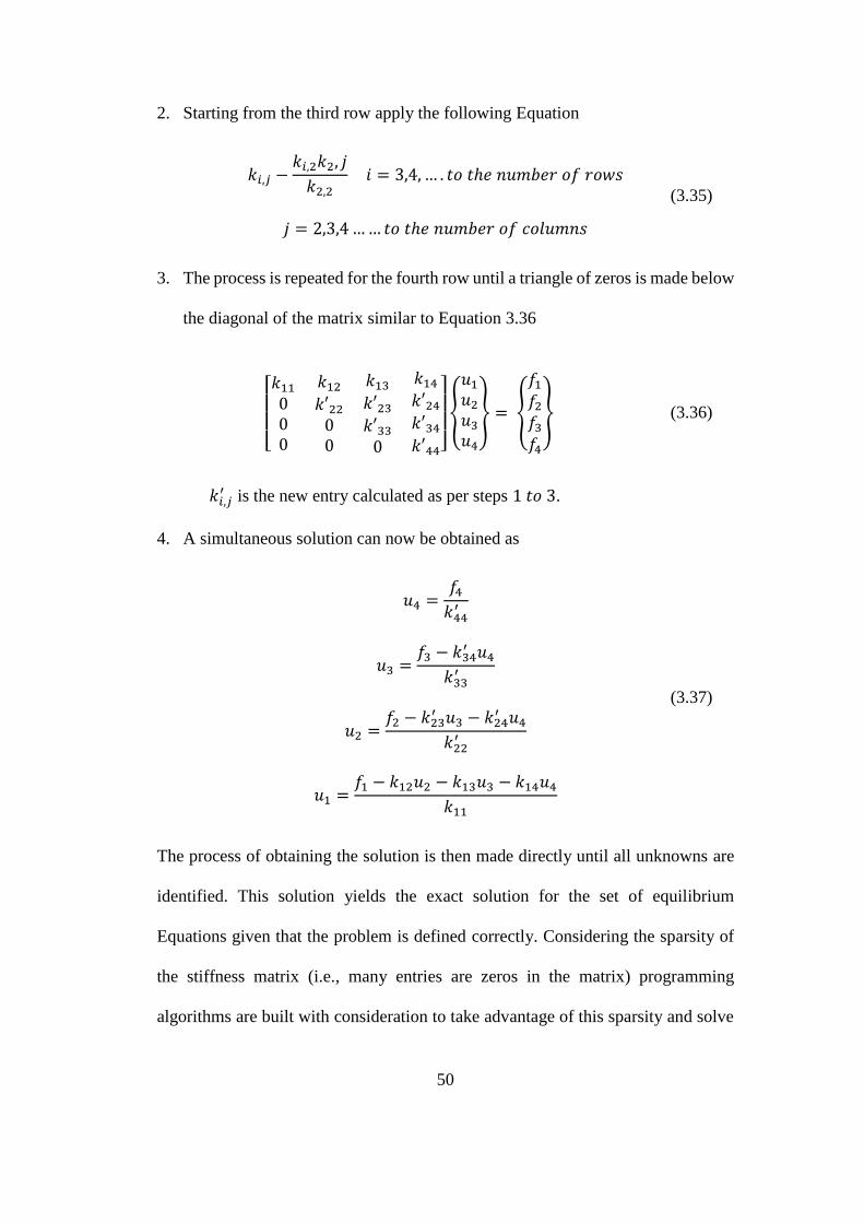
50
2. Starting from the third row apply the following Equation
𝑘𝑖,𝑗 −𝑘𝑖,2𝑘2, 𝑗
𝑘2,2 𝑖 = 3,4, … . 𝑡𝑜 𝑡ℎ𝑒 𝑛𝑢𝑚𝑏𝑒𝑟 𝑜𝑓 𝑟𝑜𝑤𝑠
𝑗 = 2,3,4…… 𝑡𝑜 𝑡ℎ𝑒 𝑛𝑢𝑚𝑏𝑒𝑟 𝑜𝑓 𝑐𝑜𝑙𝑢𝑚𝑛𝑠
(3.35)
3. The process is repeated for the fourth row until a triangle of zeros is made below
the diagonal of the matrix similar to Equation 3.36
[ 𝑘11000
𝑘12𝑘′2200
𝑘13𝑘′23𝑘′330
𝑘14𝑘′24𝑘′34𝑘′44]
{
𝑢1𝑢2
𝑢3
𝑢4
} = {
𝑓1𝑓2𝑓3𝑓4
} (3.36)
𝑘𝑖,𝑗′ is the new entry calculated as per steps 1 𝑡𝑜 3.
4. A simultaneous solution can now be obtained as
𝑢4 =𝑓4𝑘44′
𝑢3 =𝑓3 − 𝑘34
′ 𝑢4
𝑘33′
𝑢2 =𝑓2 − 𝑘23
′ 𝑢3 − 𝑘24′ 𝑢4
𝑘22′
𝑢1 =𝑓1 − 𝑘12𝑢2 − 𝑘13𝑢3 − 𝑘14𝑢4
𝑘11
(3.37)
The process of obtaining the solution is then made directly until all unknowns are
identified. This solution yields the exact solution for the set of equilibrium
Equations given that the problem is defined correctly. Considering the sparsity of
the stiffness matrix (i.e., many entries are zeros in the matrix) programming
algorithms are built with consideration to take advantage of this sparsity and solve
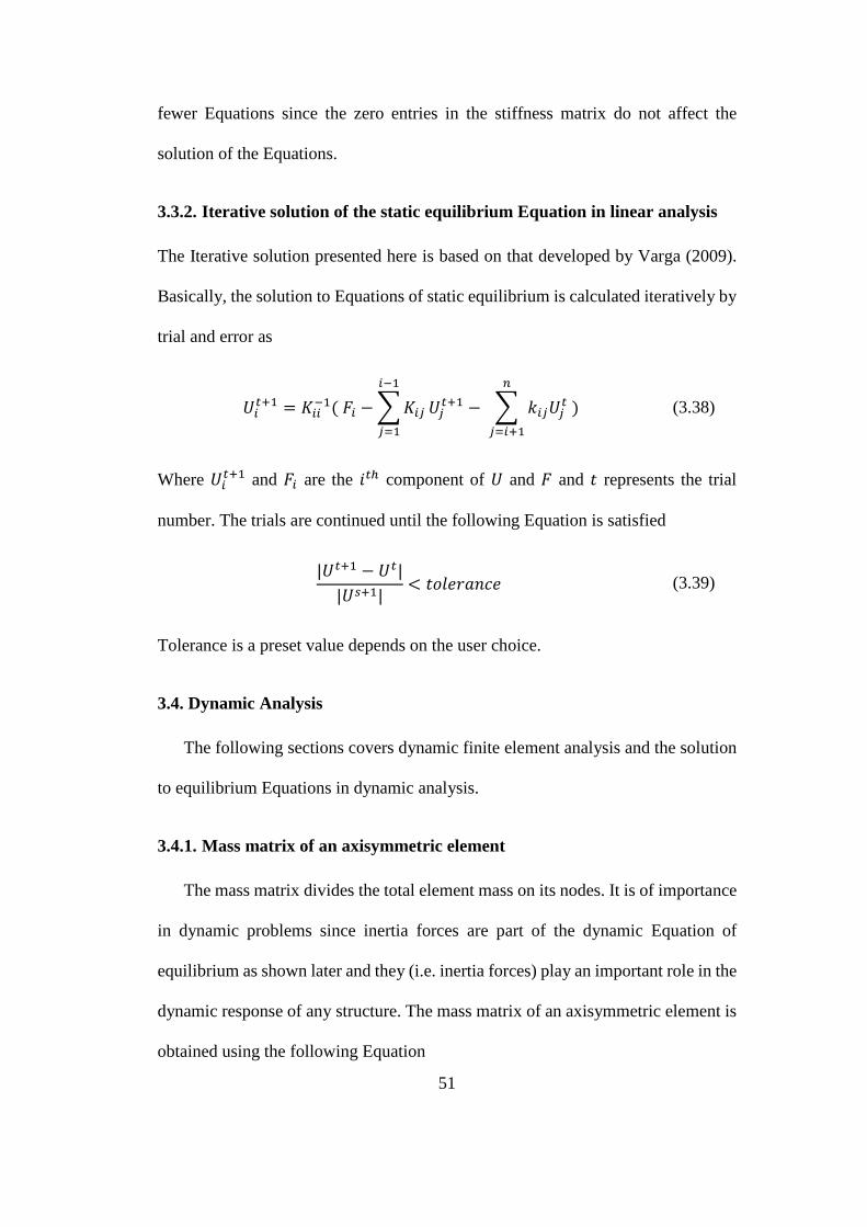
51
fewer Equations since the zero entries in the stiffness matrix do not affect the
solution of the Equations.
3.3.2. Iterative solution of the static equilibrium Equation in linear analysis
The Iterative solution presented here is based on that developed by Varga (2009).
Basically, the solution to Equations of static equilibrium is calculated iteratively by
trial and error as
𝑈𝑖𝑡+1 = 𝐾𝑖𝑖
−1( 𝐹𝑖 −∑𝐾𝑖𝑗
𝑖−1
𝑗=1
𝑈𝑗𝑡+1 − ∑ 𝑘𝑖𝑗𝑈𝑗
𝑡
𝑛
𝑗=𝑖+1
) (3.38)
Where 𝑈𝑖𝑡+1 and 𝐹𝑖 are the 𝑖𝑡ℎ component of 𝑈 and 𝐹 and 𝑡 represents the trial
number. The trials are continued until the following Equation is satisfied
|𝑈𝑡+1 − 𝑈𝑡|
|𝑈𝑠+1|< 𝑡𝑜𝑙𝑒𝑟𝑎𝑛𝑐𝑒 (3.39)
Tolerance is a preset value depends on the user choice.
3.4. Dynamic Analysis
The following sections covers dynamic finite element analysis and the solution
to equilibrium Equations in dynamic analysis.
3.4.1. Mass matrix of an axisymmetric element
The mass matrix divides the total element mass on its nodes. It is of importance
in dynamic problems since inertia forces are part of the dynamic Equation of
equilibrium as shown later and they (i.e. inertia forces) play an important role in the
dynamic response of any structure. The mass matrix of an axisymmetric element is
obtained using the following Equation
52
[𝑀] = ∭𝜌[𝑁]𝑇[𝑁]𝑑𝑉 (3.40)
This mass matrix is called the consistent mass matrix, and it is a full and symmetric
matrix. By using the shape functions given in Equations 3.19, 3.20 and 3.21, the
mass matrix can be obtained for the axisymmetric element. The same concept
applies to a 3D elements and the shape functions used are related to the 3D element.
3.4.2. Integration of dynamic Equation of equilibrium in time
The following integration schemes are summarized from Bathe (2006) and
Logan (2007) textbooks.
If no viscous damping is applied, the Equation of equilibrium in dynamics is
{𝐹(𝑡)} = {𝐾}{𝑑} + [𝑀]{��} (3.41)
In 3.41, the force is transient and is a function of time, [𝑀] is the global mass matrix
and {��} is the acceleration. The acceleration is defined as the second derivative of
the displacement over time. Several methods are used to integrate Equation 3.41
over time. The methods are called direct integration methods and under the direct
integration method there is the explicit method which is known as the central
difference method and there are the implicit methods such as Newmark-Beta (to be
referred to as Newmark’s method) and the Wilson-Theta method (to be referred to
as Wilson’s method). Each method has its advantages and disadvantages. A brief
description is given in the upcoming sections.
53
3.4.2.1 The central difference method
The finite difference Equations for velocity is
{��𝑖} ={𝑑𝑖+1} − {𝑑𝑖−1}
2(𝛥𝜏) (3.42)
And for acceleration
{��} ={��𝑖+1} − {��𝑖−1}
2(𝛥𝑡) (3.43)
In 3.43 and 3.42 the subscripts indicate the current time step for a time
increment 𝛥𝑡. This means that 𝑑{(𝑡)} = {𝑑𝑖} and {𝑑(𝑡 + 𝛥𝑡)}.
With 3.42 and 3.43 an Equation that relates the displacement with the acceleration
can be obtained as
{��} ={𝑑𝑖+1} − 2{𝑑𝑖} + {𝑑𝑖−1}
(𝛥𝑡)2 (3.44)
Given those previous two Equations, the procedure for the solution is
1- To start solving, {𝑑0}, {��𝑖}, {��}, and {𝐹𝑖(𝑡)} must be known
2- If {��} is not known, it should be calculated by rearranging Equation 3.41 as
{��0} = [𝑀]−1({𝐹0} − [𝐾]{𝑑0}) (3.45)
3- After obtaining {��0}, {𝑑−1} is calculated as
{𝑑−1} = {𝑑0} − (𝛥𝑡){𝑑0} +(𝛥𝑡)2
2{��0} (3.46)
4- {𝑑1} is now needed to be calculated as
54
{𝑑1} = [𝑀]−1{ (𝛥𝑡)2{𝐹0} + [2[𝑀] − (𝛥𝑡)2[𝐾]]{𝑑0} − [𝑀]{𝑑−1 } } (3.47)
5- {𝑑2} can now be calculated as
{𝑑2} = [𝑀]−1{ (𝛥𝑡)2{𝐹1} + [2[𝑀] − (𝛥𝑡)2[𝐾]]{𝑑1} − [𝑀]{𝑑0} } (3.48)
6- {��1} is calculated as
{��1} = [𝑀]−1({𝐹1} − [𝐾]{𝑑1}) (3.49)
7- The velocity is calculated as
{��1} ={𝑑2} − {𝑑0}
2(𝛥𝑡) (3.50)
Repeating steps 5 to 7 for all other time steps while increasing the subscripts in
Equations 3.48, 3.49, and 4.50 by 1 to complete the integration in time.
3.4.2.2 Newmark’s method
Newmark’s Equations that are used to solve finite element problems in dynamics
are
{��𝑖+1 } = {��𝑖} + (𝛥𝑡)[(1 − 𝛾){��𝑖} + 𝛾{��𝑖+1}] (3.51)
And
{𝑑𝑖+1} = {𝑑𝑖} + (𝛥𝑡){��𝑖} + (𝛥𝑡)2[(1
2− 𝛽) {��𝑖} + 𝛽{��𝑖+1}] (3.52)
In Newmark’s Equations the parameters 𝛾 and 𝛽 are selected by the analyzer. The
steps to solve a dynamic problem using Newmark’s method are:
55
1- With the load varying in time and known at every time step, proceed to
calculate the displacements, velocity, and acceleration for every time step.
2- Initially at 𝑡 = 0, {𝑑0} and {𝑑0} are know from the boundary conditions.
3- The initial acceleration {��0}; unless it is also know; is calculated as
{��0} = [𝑀]−1({𝐹0} − [𝐾]{𝑑0}) (3.53)
4- Using {𝑑0}, {��0}, and {𝑑0}, {𝑑1} is calculated as
[𝐾′]{𝑑1} = {𝐹1′} (3.54)
Where
[𝐾′] = [𝐾] +1
𝛽(𝛥𝑡)2[𝑀] (3.55)
And
{𝐹1′} = {𝐹1} +
[𝑀]
𝛽(𝛥𝑡)2[ {𝑑0} + (𝛥𝑡){��0} + (
1
2− 𝛽) (𝛥𝑡)2{𝑑0} ] (3.56)
5- {��1} is calculated by rearranging Equation 3.52 as
{𝑑1} =1
𝛽(𝛥𝑡)2[ {𝑑1} − {𝑑0} − (𝛥𝑡){𝑑0} − (𝛥𝑡)2 (
1
2− 𝛽) {��0}]
(3.57)
6- The velocity at 𝑖 = 1, is calculated from Equation 3.51
With the results from steps 5 and 6, the steps are repeated starting from step 4
while increasing the subscript 𝑖 by a 1.
56
3.4.2.3 Wilson’s method
Wilson Equations that are used are
{��𝑖+1} = {��𝑖} +𝜃(𝛥𝑡)
2 ({��𝑖+1 } + {��𝑖}) (3.58)
And
{𝑑𝑖+1} = {𝑑𝑖} + 𝜃(𝛥𝑡){��𝑖} +𝜃2(𝛥𝑡)2
6 ({��𝑖+1 } + 2{��𝑖}) (3.59)
The steps for integration in time using Wilson’s method are
1- From initial boundary and velocity conditions at time 𝑡 = 0, the
displacement {𝑑0} and the velocity {��} are known.
2- If the initial acceleration {��0} is not known, it is calculated as
{��0} = [𝑀]−1({𝐹0} − [𝐾]{𝑑0}) (3.60)
3- {𝑑1} is calculated a s
[𝐾′]{𝑑1} = {𝐹1′} (3.61)
Where
[𝐾′] = [𝐾] +6
(𝜃𝛥𝑡)2[𝑀] (3.62)
57
And
{𝐹1′} = {𝐹1
′} +[𝑀]
(𝜃𝛥𝑡)2[6{𝑑0} + 6𝜃(𝛥𝑡){��1} + 2(𝜃𝛥𝑡)2{��0}] (3.63)
4- {��1} is calculated as
{��1} =6
𝜃2(𝛥𝑡)2({𝑑1} − {𝑑0}) −
6
𝜃(𝛥𝑡){��0} − 2{��0} (3.64)
5- {��1} is calculated as
{��1} =3
𝜃(𝛥𝑡)({𝑑1} − {𝑑0}) − 2{��0} −
𝜃(𝛥𝑡)
2{��0} (3.65)
6- Steps 3 to 5 are repeated with the subscript increased by one each time a
repetition is made.
Notes on Dynamic analysis solvers
Solving the dynamic finite element is more involved than solving static
problems. The time step size is essential to the accuracy of the results and in case
of using Newmark’s method, the variables 𝛽 and 𝛾 affect the solution accuracy and
stability. Usually, 𝛽 is selected from between 0 and 1
4; while 𝛾 is selected as
1
2. If 𝛽
is set as 0 and 𝛾 is set as 1
2 , Newmark’s Equations 3.51 and 3.52 become similar to
the central difference Equations. Similarly, If Wilson’s method is used; the choice
of the variable 𝜃 also has an impact on the accuracy of the solution. Bathe (2006)
gives a discussion about the stability and the accuracy of the integration schemes
discussed in the previous sections.
58
4. Modeling and finite element method implementation
In this chapter, the process of modeling the geometry of the problem, its
boundary conditions, time step choice, element size are discussed. In order to verify
proper modeling of the problem and proper choice of modeling parameters, a
verification study is performed on the model. The verification study compares the
model of a single pile in homogeneous linear elastic soil with the analytical solution
of Novak (1974) at 𝑎0 = 0.3. His solution is given in more details in chapter 2.
The problem of a pile under a vibrating vertical load is shown in Figure 4.1.
the pile is considered a floating pile in this case (or friction pile). The black part on
top of the pile represents the mass the pile is carrying. A force 𝑄 is acting on top of
the pile. 𝑄 varies with time in a sinusoidal manner. The force applied (sinusoidal
load) has an amplitude of 22000 𝑁 therefore, 𝑄(𝑡) = 22000 𝑆𝑖𝑛(𝜔𝑡). Where 𝜔 is
the frequency of the load in 𝑟𝑎𝑑𝑖𝑎𝑛𝑠/𝑠𝑒𝑐, 𝑡 is the time in seconds.
Finite element modeling of this problem utilizes axisymmetric elements for
discretizing the model. The solution parameters need to be optimized for accuracy
include mesh size, time step, and boundary conditions. Choice of these parameters
is based on recommendations from the literature. Once these parameters are set, a
verification study is performed to verify that the modeling process is applicable to
the modeling of the research cases.
Although most of the discussion here is limited to the 2D axisymmetric
modeling of a single pile, the concepts and assumptions can be extended to the 3D
modeling of two piles for the dynamic interaction study.
Autodesk simulation was used in this research. It has the capability to
perform the linear static and dynamic finite element analysis required by this
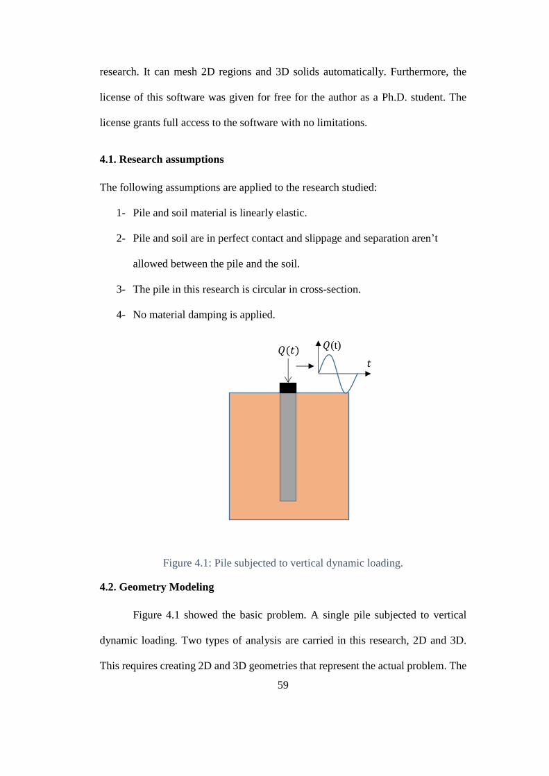
59
research. It can mesh 2D regions and 3D solids automatically. Furthermore, the
license of this software was given for free for the author as a Ph.D. student. The
license grants full access to the software with no limitations.
4.1. Research assumptions
The following assumptions are applied to the research studied:
1- Pile and soil material is linearly elastic.
2- Pile and soil are in perfect contact and slippage and separation aren’t
allowed between the pile and the soil.
3- The pile in this research is circular in cross-section.
4- No material damping is applied.
Figure 4.1: Pile subjected to vertical dynamic loading.
4.2. Geometry Modeling
Figure 4.1 showed the basic problem. A single pile subjected to vertical
dynamic loading. Two types of analysis are carried in this research, 2D and 3D.
This requires creating 2D and 3D geometries that represent the actual problem. The
𝑄(𝑡) 𝑄(t)
𝑡
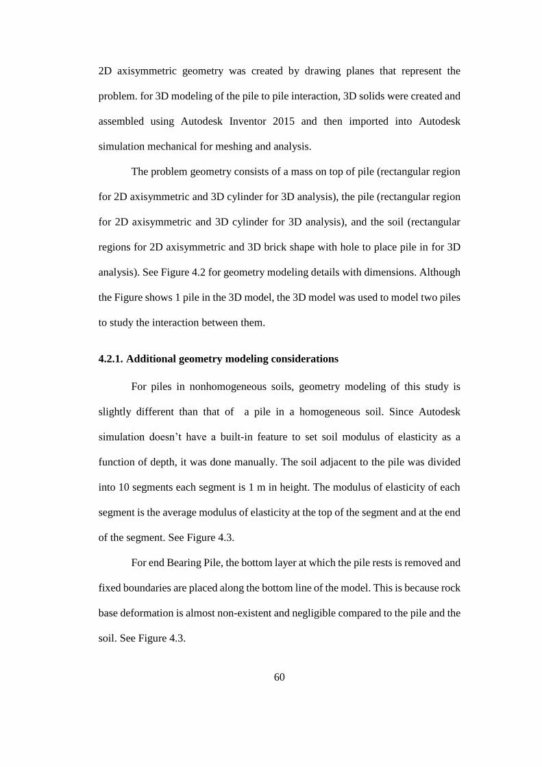
60
2D axisymmetric geometry was created by drawing planes that represent the
problem. for 3D modeling of the pile to pile interaction, 3D solids were created and
assembled using Autodesk Inventor 2015 and then imported into Autodesk
simulation mechanical for meshing and analysis.
The problem geometry consists of a mass on top of pile (rectangular region
for 2D axisymmetric and 3D cylinder for 3D analysis), the pile (rectangular region
for 2D axisymmetric and 3D cylinder for 3D analysis), and the soil (rectangular
regions for 2D axisymmetric and 3D brick shape with hole to place pile in for 3D
analysis). See Figure 4.2 for geometry modeling details with dimensions. Although
the Figure shows 1 pile in the 3D model, the 3D model was used to model two piles
to study the interaction between them.
4.2.1. Additional geometry modeling considerations
For piles in nonhomogeneous soils, geometry modeling of this study is
slightly different than that of a pile in a homogeneous soil. Since Autodesk
simulation doesn’t have a built-in feature to set soil modulus of elasticity as a
function of depth, it was done manually. The soil adjacent to the pile was divided
into 10 segments each segment is 1 m in height. The modulus of elasticity of each
segment is the average modulus of elasticity at the top of the segment and at the end
of the segment. See Figure 4.3.
For end Bearing Pile, the bottom layer at which the pile rests is removed and
fixed boundaries are placed along the bottom line of the model. This is because rock
base deformation is almost non-existent and negligible compared to the pile and the
soil. See Figure 4.3.
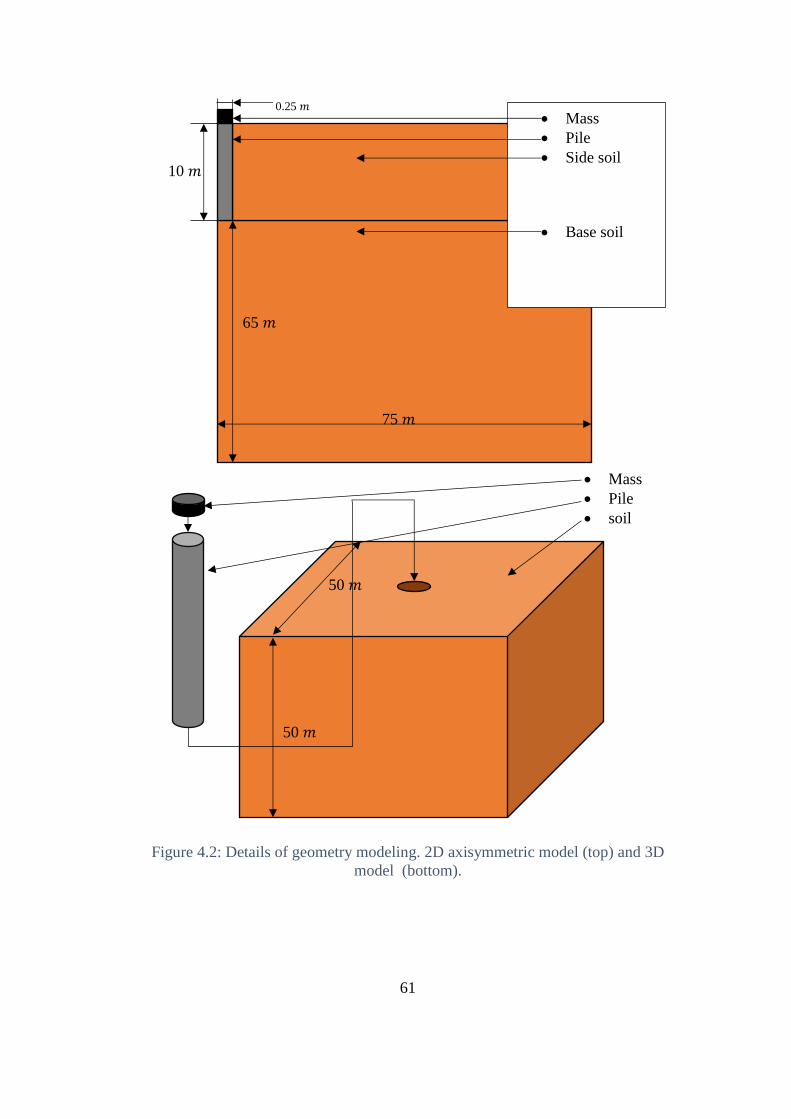
61
Figure 4.2: Details of geometry modeling. 2D axisymmetric model (top) and 3D
model (bottom).
Mass
Pile
Side soil
Base soil
65 𝑚
10 𝑚
Mass
Pile
soil
50 𝑚
50 𝑚
75 𝑚
0.25 𝑚
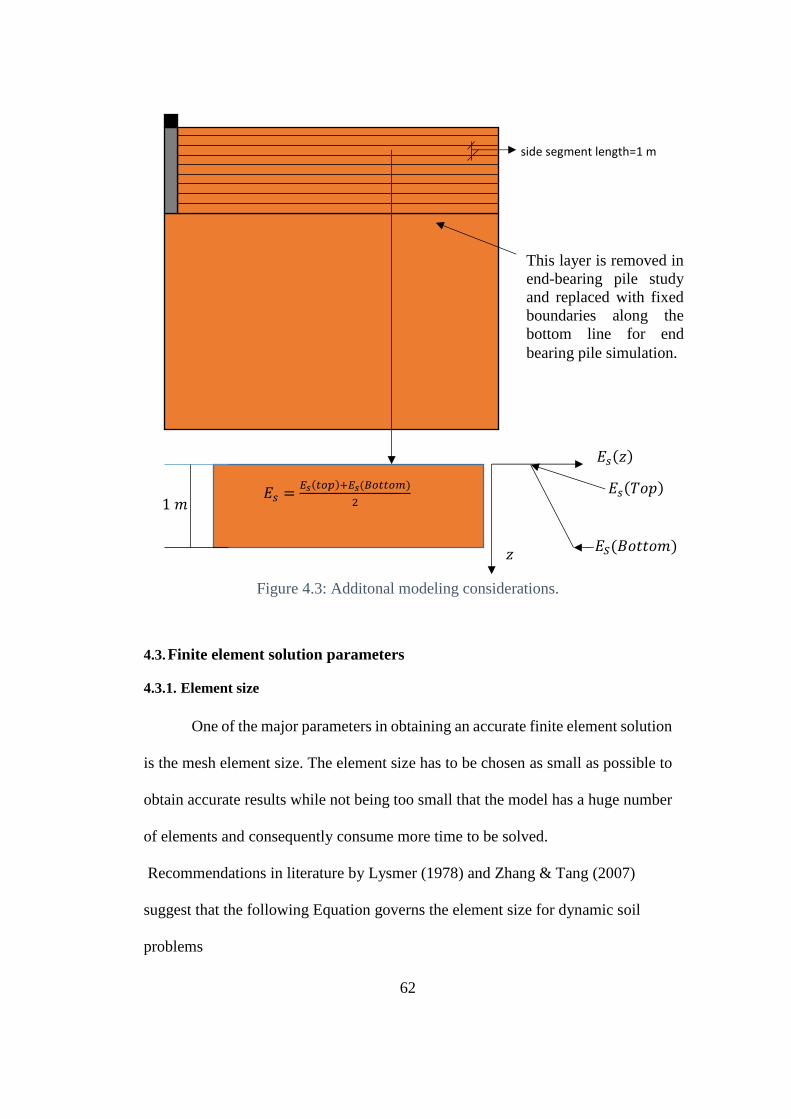
62
Figure 4.3: Additonal modeling considerations.
4.3. Finite element solution parameters
4.3.1. Element size
One of the major parameters in obtaining an accurate finite element solution
is the mesh element size. The element size has to be chosen as small as possible to
obtain accurate results while not being too small that the model has a huge number
of elements and consequently consume more time to be solved.
Recommendations in literature by Lysmer (1978) and Zhang & Tang (2007)
suggest that the following Equation governs the element size for dynamic soil
problems
side segment length=1 m
1 𝑚
𝐸𝑠(𝑧)
𝑧
𝐸𝑠(𝑇𝑜𝑝) 𝐸𝑆(𝐵𝑜𝑡𝑡𝑜𝑚)
𝐸𝑠 =𝐸𝑠(𝑡𝑜𝑝)+𝐸𝑠(𝐵𝑜𝑡𝑡𝑜𝑚)
2
This layer is removed in
end-bearing pile study
and replaced with fixed
boundaries along the
bottom line for end
bearing pile simulation.
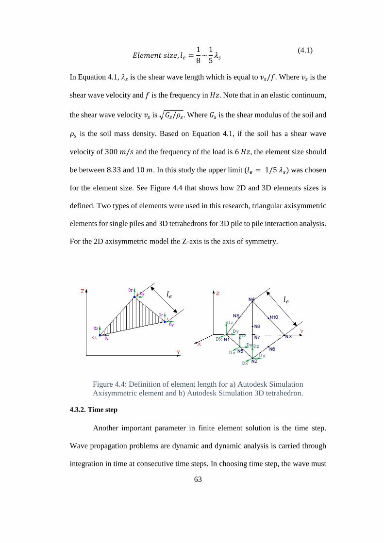
63
𝐸𝑙𝑒𝑚𝑒𝑛𝑡 𝑠𝑖𝑧𝑒, 𝑙𝑒 =1
8~1
5𝜆𝑠
(4.1)
In Equation 4.1, 𝜆𝑠 is the shear wave length which is equal to 𝑣𝑠/𝑓. Where 𝑣𝑠 is the
shear wave velocity and 𝑓 is the frequency in 𝐻𝑧. Note that in an elastic continuum,
the shear wave velocity 𝑣𝑠 is √𝐺𝑠/𝜌𝑠. Where 𝐺𝑠 is the shear modulus of the soil and
𝜌𝑠 is the soil mass density. Based on Equation 4.1, if the soil has a shear wave
velocity of 300 𝑚/𝑠 and the frequency of the load is 6 𝐻𝑧, the element size should
be between 8.33 and 10 𝑚. In this study the upper limit (𝑙𝑒 = 1/5 𝜆𝑠) was chosen
for the element size. See Figure 4.4 that shows how 2D and 3D elements sizes is
defined. Two types of elements were used in this research, triangular axisymmetric
elements for single piles and 3D tetrahedrons for 3D pile to pile interaction analysis.
For the 2D axisymmetric model the Z-axis is the axis of symmetry.
Figure 4.4: Definition of element length for a) Autodesk Simulation
Axisymmetric element and b) Autodesk Simulation 3D tetrahedron.
4.3.2. Time step
Another important parameter in finite element solution is the time step.
Wave propagation problems are dynamic and dynamic analysis is carried through
integration in time at consecutive time steps. In choosing time step, the wave must
𝑙𝑒 𝑙𝑒
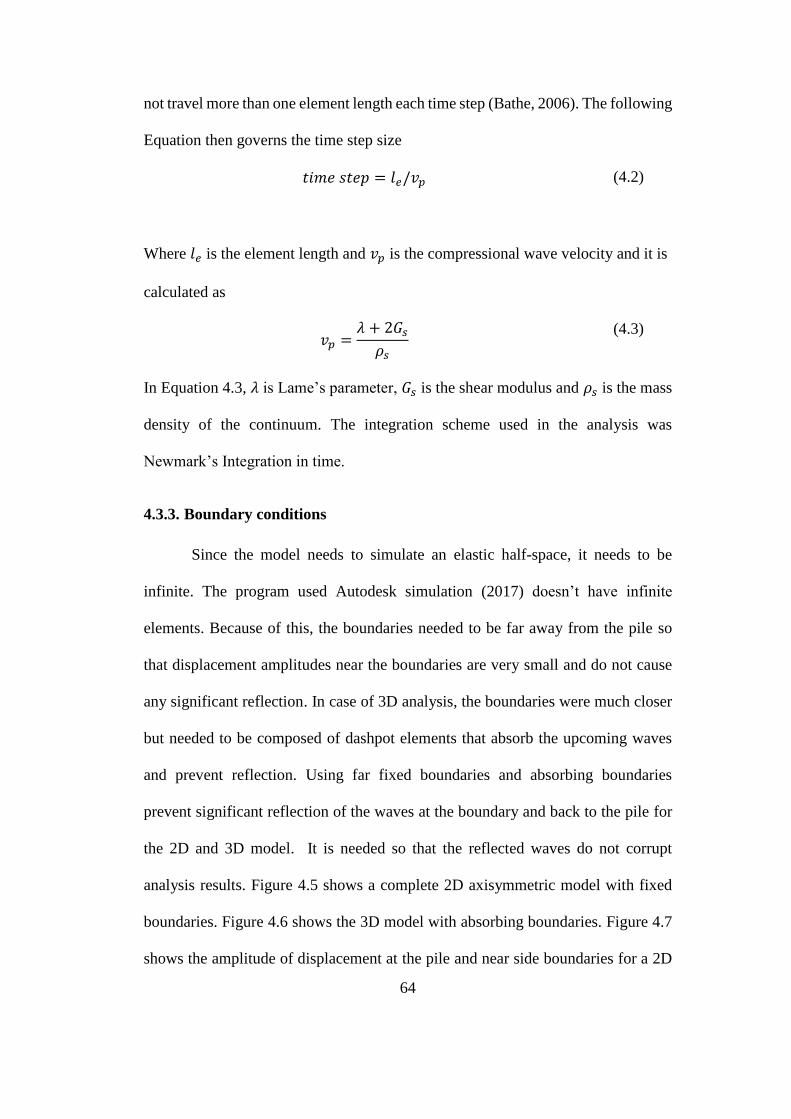
64
not travel more than one element length each time step (Bathe, 2006). The following
Equation then governs the time step size
𝑡𝑖𝑚𝑒 𝑠𝑡𝑒𝑝 = 𝑙𝑒/𝑣𝑝 (4.2)
Where 𝑙𝑒 is the element length and 𝑣𝑝 is the compressional wave velocity and it is
calculated as
𝑣𝑝 =𝜆 + 2𝐺𝑠
𝜌𝑠
(4.3)
In Equation 4.3, 𝜆 is Lame’s parameter, 𝐺𝑠 is the shear modulus and 𝜌𝑠 is the mass
density of the continuum. The integration scheme used in the analysis was
Newmark’s Integration in time.
4.3.3. Boundary conditions
Since the model needs to simulate an elastic half-space, it needs to be
infinite. The program used Autodesk simulation (2017) doesn’t have infinite
elements. Because of this, the boundaries needed to be far away from the pile so
that displacement amplitudes near the boundaries are very small and do not cause
any significant reflection. In case of 3D analysis, the boundaries were much closer
but needed to be composed of dashpot elements that absorb the upcoming waves
and prevent reflection. Using far fixed boundaries and absorbing boundaries
prevent significant reflection of the waves at the boundary and back to the pile for
the 2D and 3D model. It is needed so that the reflected waves do not corrupt
analysis results. Figure 4.5 shows a complete 2D axisymmetric model with fixed
boundaries. Figure 4.6 shows the 3D model with absorbing boundaries. Figure 4.7
shows the amplitude of displacement at the pile and near side boundaries for a 2D
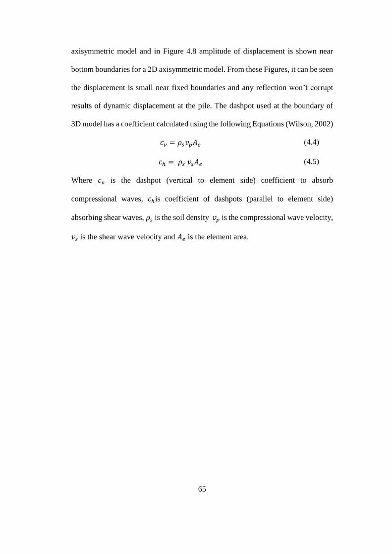
65
axisymmetric model and in Figure 4.8 amplitude of displacement is shown near
bottom boundaries for a 2D axisymmetric model. From these Figures, it can be seen
the displacement is small near fixed boundaries and any reflection won’t corrupt
results of dynamic displacement at the pile. The dashpot used at the boundary of
3D model has a coefficient calculated using the following Equations (Wilson, 2002)
𝑐𝑣 = 𝜌𝑠𝑣𝑝𝐴𝑒 (4.4)
𝑐ℎ = 𝜌𝑠 𝑣𝑠𝐴𝑒 (4.5)
Where 𝑐𝑣 is the dashpot (vertical to element side) coefficient to absorb
compressional waves, 𝑐ℎis coefficient of dashpots (parallel to element side)
absorbing shear waves, 𝜌𝑠 is the soil density 𝑣𝑝 is the compressional wave velocity,
𝑣𝑠 is the shear wave velocity and 𝐴𝑒 is the element area.
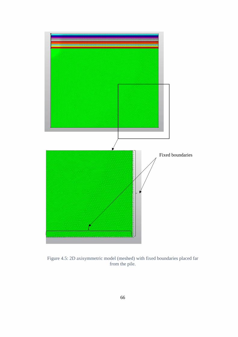
66
Figure 4.5: 2D axisymmetric model (meshed) with fixed boundaries placed far
from the pile.
Fixed boundaries
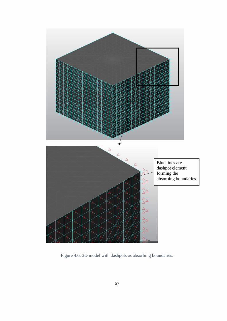
67
Figure 4.6: 3D model with dashpots as absorbing boundaries.
Blue lines are
dashpot element
forming the
absorbing boundaries
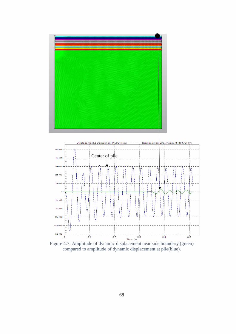
68
Figure 4.7: Amplitude of dynamic displacement near side boundary (green)
compared to amplitude of dynamic displacement at pile(blue).
Center of pile
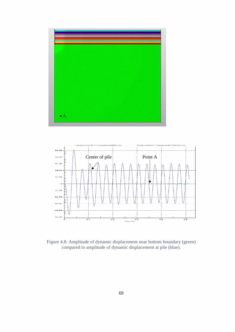
69
Figure 4.8: Amplitude of dynamic displacement near bottom boundary (green)
compared to amplitude of dynamic displacement at pile (blue).
Center of pile Point A
A
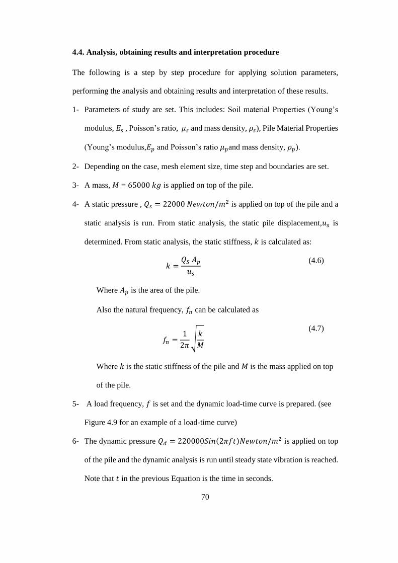
70
4.4. Analysis, obtaining results and interpretation procedure
The following is a step by step procedure for applying solution parameters,
performing the analysis and obtaining results and interpretation of these results.
1- Parameters of study are set. This includes: Soil material Properties (Young’s
modulus, 𝐸𝑠 , Poisson’s ratio, 𝜇𝑠 and mass density, 𝜌𝑠), Pile Material Properties
(Young’s modulus,𝐸𝑝 and Poisson’s ratio 𝜇𝑝and mass density, 𝜌𝑝).
2- Depending on the case, mesh element size, time step and boundaries are set.
3- A mass, 𝑀 = 65000 𝑘𝑔 is applied on top of the pile.
4- A static pressure , 𝑄𝑠 = 22000 𝑁𝑒𝑤𝑡𝑜𝑛/𝑚2 is applied on top of the pile and a
static analysis is run. From static analysis, the static pile displacement,𝑢𝑠 is
determined. From static analysis, the static stiffness, 𝑘 is calculated as:
𝑘 =𝑄𝑆 𝐴𝑝
𝑢𝑠
(4.6)
Where 𝐴𝑝 is the area of the pile.
Also the natural frequency, 𝑓𝑛 can be calculated as
𝑓𝑛 =1
2𝜋√𝑘
𝑀
(4.7)
Where 𝑘 is the static stiffness of the pile and 𝑀 is the mass applied on top
of the pile.
5- A load frequency, 𝑓 is set and the dynamic load-time curve is prepared. (see
Figure 4.9 for an example of a load-time curve)
6- The dynamic pressure 𝑄𝑑 = 220000𝑆𝑖𝑛(2𝜋𝑓𝑡)𝑁𝑒𝑤𝑡𝑜𝑛/𝑚2 is applied on top
of the pile and the dynamic analysis is run until steady state vibration is reached.
Note that 𝑡 in the previous Equation is the time in seconds.
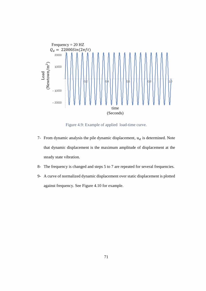
71
Figure 4.9: Example of applied load-time curve.
7- From dynamic analysis the pile dynamic displacement, 𝑢𝑑 is determined. Note
that dynamic displacement is the maximum amplitude of displacement at the
steady state vibration.
8- The frequency is changed and steps 5 to 7 are repeated for several frequencies.
9- A curve of normalized dynamic displacement over static displacement is plotted
against frequency. See Figure 4.10 for example.
0.2 0.4 0.6 0.8 1.0
20000
10000
10000
20000
Load
(N
ewtown/m
2)
time
(Seconds)
Frequency = 20 HZ
𝑄𝑑 = 22000𝑆𝑖𝑛(2𝜋𝑓𝑡)
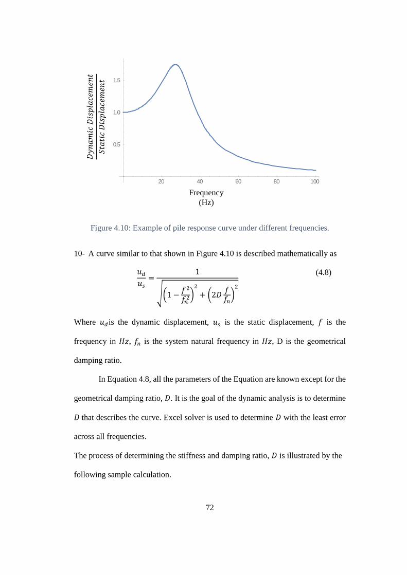
72
Figure 4.10: Example of pile response curve under different frequencies.
10- A curve similar to that shown in Figure 4.10 is described mathematically as
𝑢𝑑
𝑢𝑠=
1
√(1 −𝑓2
𝑓𝑛2)
2
+ (2𝐷𝑓𝑓𝑛)2
(4.8)
Where 𝑢𝑑is the dynamic displacement, 𝑢𝑠 is the static displacement, 𝑓 is the
frequency in 𝐻𝑧, 𝑓𝑛 is the system natural frequency in 𝐻𝑧, D is the geometrical
damping ratio.
In Equation 4.8, all the parameters of the Equation are known except for the
geometrical damping ratio, 𝐷. It is the goal of the dynamic analysis is to determine
𝐷 that describes the curve. Excel solver is used to determine 𝐷 with the least error
across all frequencies.
The process of determining the stiffness and damping ratio, 𝐷 is illustrated by the
following sample calculation.
20 40 60 80 100
0.5
1.0
1.5
𝐷𝑦𝑛𝑎𝑚𝑖𝑐 𝐷𝑖𝑠𝑝𝑙𝑎𝑐𝑒𝑚𝑒𝑛𝑡
𝑆𝑡𝑎𝑡𝑖𝑐 𝐷𝑖𝑠𝑝𝑙𝑎𝑐𝑒𝑚𝑒𝑛
𝑡
Frequency
(Hz)
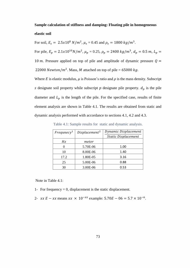
73
Sample calculation of stiffness and damping: Floating pile in homogeneous
elastic soil
For soil, 𝐸𝑠 = 2.5𝑥108 𝑁/𝑚2, 𝜇𝑠 = 0.45 and 𝜌𝑠 = 1800 𝑘𝑔/𝑚3.
For pile, 𝐸𝑝 = 2.1𝑥1010𝑁/𝑚2, 𝜇𝑝 = 0.25, 𝜌𝑝 = 2400 𝑘𝑔/𝑚3, 𝑑𝑝 = 0.5 𝑚, 𝐿𝑝 =
10 𝑚. Pressure applied on top of pile and amplitude of dynamic pressure 𝑄 =
22000 𝑁𝑒𝑤𝑡𝑜𝑛/𝑚2. Mass, 𝑀 attached on top of pile = 65000 𝑘𝑔.
Where 𝐸 is elastic modulus, 𝜇 is Poisson’s ratio and 𝜌 is the mass density. Subscript
𝑠 designate soil property while subscript 𝑝 designate pile property. 𝑑𝑝 is the pile
diameter and 𝐿𝑝 is the length of the pile. For the specified case, results of finite
element analysis are shown in Table 4.1. The results are obtained from static and
dynamic analysis performed with accordance to sections 4.1, 4.2 and 4.3.
Table 4.1: Sample results for static and dynamic analysis.
𝐹𝑟𝑒𝑞𝑢𝑛𝑒𝑐𝑦1
𝐷𝑖𝑠𝑝𝑙𝑎𝑐𝑒𝑚𝑒𝑛𝑡2
𝐷𝑦𝑛𝑎𝑚𝑖𝑐 𝐷𝑖𝑠𝑝𝑙𝑎𝑐𝑒𝑚𝑒𝑛𝑡
𝑆𝑡𝑎𝑡𝑖𝑐 𝐷𝑖𝑠𝑝𝑙𝑎𝑐𝑒𝑚𝑒𝑛𝑡
𝐻𝑧 𝑚𝑒𝑡𝑒𝑟
0 5.70E-06 1.00
10 8.00E-06 1.40
17.2 1.80E-05 3.16
25 5.00E-06 0.88
30 3.00E-06 0.53
Note in Table 4.1:
1- For frequency = 0, displacement is the static displacement.
2- 𝑥𝑥 𝐸 − 𝑥𝑥 means 𝑥𝑥 × 10−𝑥𝑥 example: 5.70𝐸 − 06 = 5.7 × 10⁻⁶.
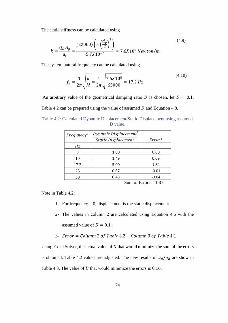
74
The static stiffness can be calculated using
𝑘 =𝑄𝑆 𝐴𝑝
𝑢𝑠=
(22000) (𝜋 (𝑑𝑝
2 )2
)
5.7𝑋10−6= 7.6𝑋108 𝑁𝑒𝑤𝑡𝑜𝑛/𝑚
(4.9)
The system natural frequency can be calculated using
𝑓𝑛 =1
2𝜋√𝑘
𝑀=
1
2𝜋√7.6𝑋108
65000= 17.2 𝐻𝑧
(4.10)
An arbitrary value of the geometrical damping ratio 𝐷 is chosen, let 𝐷 = 0.1.
Table 4.2 can be prepared using the value of assumed 𝐷 and Equation 4.8.
Table 4.2: Calculated Dynamic Displacement/Static Displacement using assumed
D value.
𝐹𝑟𝑒𝑞𝑢𝑛𝑒𝑐𝑦1
𝐷𝑦𝑛𝑎𝑚𝑖𝑐 𝐷𝑖𝑠𝑝𝑙𝑎𝑐𝑒𝑚𝑒𝑛𝑡
𝑆𝑡𝑎𝑡𝑖𝑐 𝐷𝑖𝑠𝑝𝑙𝑎𝑐𝑒𝑚𝑒𝑛𝑡
2
𝐸𝑟𝑟𝑜𝑟3
𝐻𝑧
0 1.00 0.00
10 1.49 0.09
17.2 5.00 1.84
25 0.87 -0.01
30 0.48 -0.04
Sum of Errors = 1.87
Note in Table 4.2:
1- For frequency = 0, displacement is the static displacement.
2- The values in column 2 are calculated using Equation 4.6 with the
assumed value of 𝐷 = 0.1.
3- 𝐸𝑟𝑟𝑜𝑟 = 𝐶𝑜𝑙𝑢𝑚𝑛 2 𝑜𝑓 𝑇𝑎𝑏𝑙𝑒 4.2 − 𝐶𝑜𝑙𝑢𝑚𝑛 3 𝑜𝑓 𝑇𝑎𝑏𝑙𝑒 4.1
Using Excel Solver, the actual value of 𝐷 that would minimize the sum of the errors
is obtained. Table 4.2 values are adjusted. The new results of 𝑢𝑑/𝑢𝑑 are show in
Table 4.3. The value of 𝐷 that would minimize the errors is 0.16.
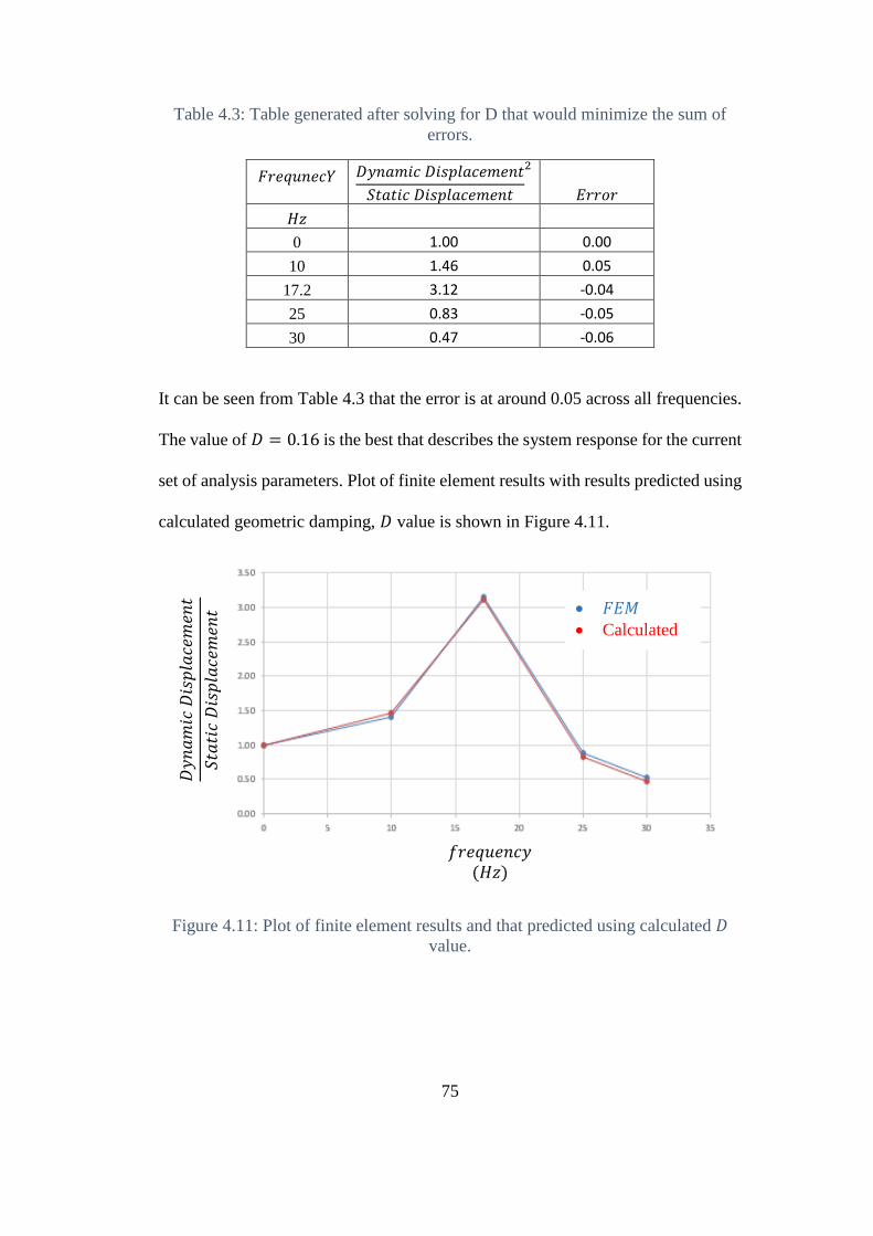
75
Table 4.3: Table generated after solving for D that would minimize the sum of
errors.
𝐹𝑟𝑒𝑞𝑢𝑛𝑒𝑐𝑌
𝐷𝑦𝑛𝑎𝑚𝑖𝑐 𝐷𝑖𝑠𝑝𝑙𝑎𝑐𝑒𝑚𝑒𝑛𝑡
𝑆𝑡𝑎𝑡𝑖𝑐 𝐷𝑖𝑠𝑝𝑙𝑎𝑐𝑒𝑚𝑒𝑛𝑡
2
𝐸𝑟𝑟𝑜𝑟
𝐻𝑧
0 1.00 0.00
10 1.46 0.05
17.2 3.12 -0.04
25 0.83 -0.05
30 0.47 -0.06
It can be seen from Table 4.3 that the error is at around 0.05 across all frequencies.
The value of 𝐷 = 0.16 is the best that describes the system response for the current
set of analysis parameters. Plot of finite element results with results predicted using
calculated geometric damping, 𝐷 value is shown in Figure 4.11.
Figure 4.11: Plot of finite element results and that predicted using calculated 𝐷
value.
𝐹𝐸𝑀
Calculated
𝑓𝑟𝑒𝑞𝑢𝑒𝑛𝑐𝑦 (𝐻𝑧)
𝐷𝑦𝑛𝑎𝑚𝑖𝑐 𝐷𝑖𝑠𝑝𝑙𝑎𝑐𝑒𝑚𝑒𝑛
𝑡
𝑆𝑡𝑎𝑡𝑖𝑐 𝐷𝑖𝑠𝑝𝑙𝑎𝑐𝑒𝑚𝑒𝑛
𝑡
76
After interpreting results for a certain case, the studied variables are adjusted
and steps outlined in sections 4.3 and 4.4 are repeated for the new set of variables.
After varying parameters, plots of the studied variable against static stiffness and
damping are generated. These plots show how the variation in a certain studied
variable affects the dynamic response of the system.
In summary, this chapter gives an insight of how data is collected and how
the results are interpreted to come up with static stiffness, 𝑘, natural frequency, 𝑓𝑛
and geometrical damping ratio, 𝐷. A flow chart is created to summarize the general
study procedure followed throughout this research. It is shown in Figure 4.12.
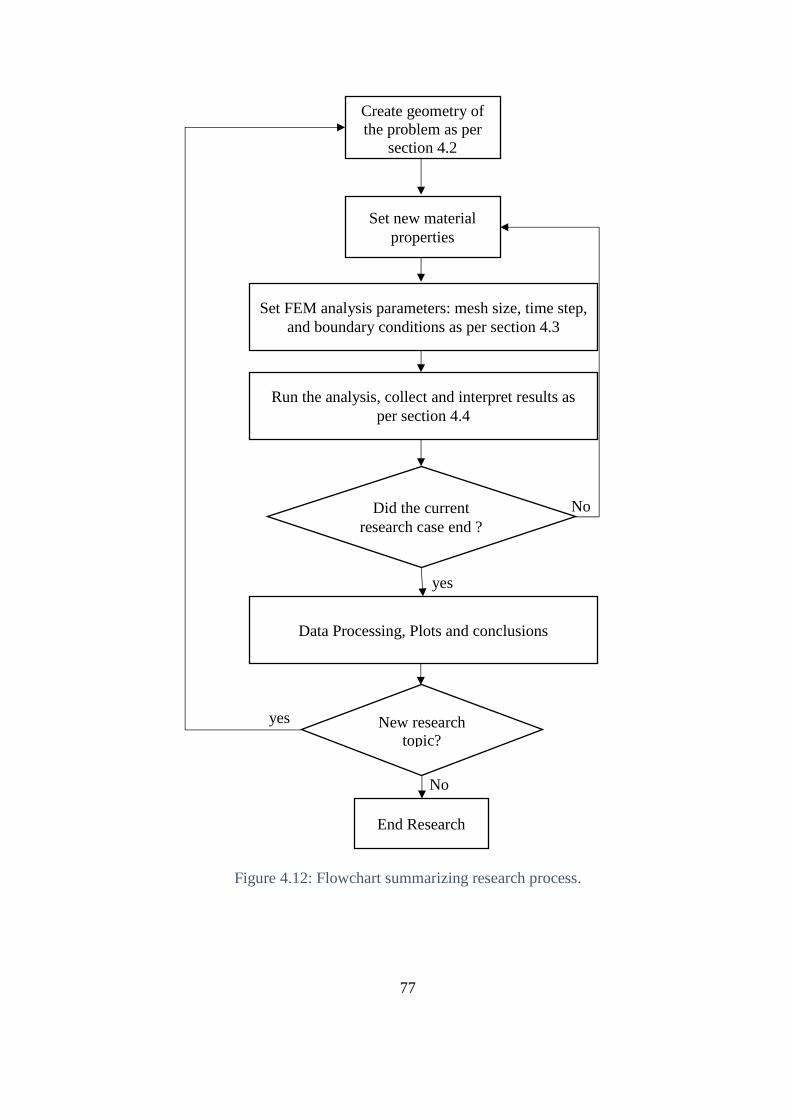
77
Figure 4.12: Flowchart summarizing research process.
Create geometry of
the problem as per
section 4.2
Set new material
properties
Set FEM analysis parameters: mesh size, time step,
and boundary conditions as per section 4.3
Run the analysis, collect and interpret results as
per section 4.4
Did the current
research case end ?
New research
topic?
yes
No
Data Processing, Plots and conclusions
yes
End Research
No
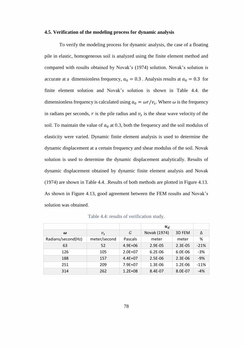
78
4.5. Verification of the modeling process for dynamic analysis
To verify the modeling process for dynamic analysis, the case of a floating
pile in elastic, homogeneous soil is analyzed using the finite element method and
compared with results obtained by Novak’s (1974) solution. Novak’s solution is
accurate at a dimensionless frequency, 𝑎0 = 0.3 . Analysis results at 𝑎0 = 0.3 for
finite element solution and Novak’s solution is shown in Table 4.4. the
dimensionless frequency is calculated using 𝑎0 = 𝜔𝑟/𝑣𝑠. Where 𝜔 is the frequency
in radians per seconds, 𝑟 is the pile radius and 𝑣𝑠 is the shear wave velocity of the
soil. To maintain the value of 𝑎0 at 0.3, both the frequency and the soil modulus of
elasticity were varied. Dynamic finite element analysis is used to determine the
dynamic displacement at a certain frequency and shear modulus of the soil. Novak
solution is used to determine the dynamic displacement analytically. Results of
dynamic displacement obtained by dynamic finite element analysis and Novak
(1974) are shown in Table 4.4. .Results of both methods are plotted in Figure 4.13.
As shown in Figure 4.13, good agreement between the FEM results and Novak’s
solution was obtained.
Table 4.4: results of verification study.
𝒖𝒅
𝝎 𝑣𝑠 𝐺 Novak (1974) 3D FEM Δ
Radians/second(Hz) meter/second Pascals meter meter %
63 52 4.9E+06 2.9E-05 2.3E-05 -21%
126 105 2.0E+07 6.2E-06 6.0E-06 -3%
188 157 4.4E+07 2.5E-06 2.3E-06 -9%
251 209 7.9E+07 1.3E-06 1.2E-06 -11%
314 262 1.2E+08 8.4E-07 8.0E-07 -4%
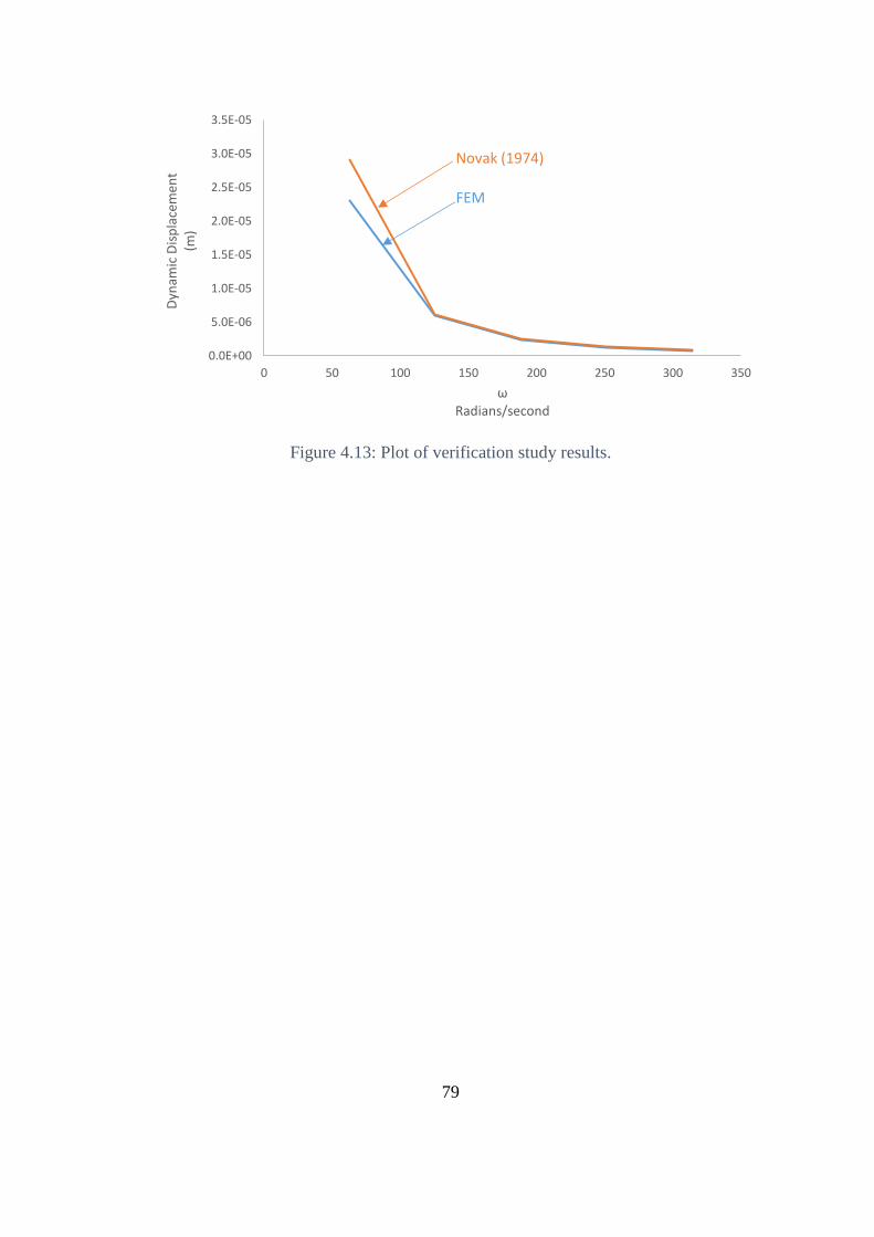
79
Figure 4.13: Plot of verification study results.
0.0E+00
5.0E-06
1.0E-05
1.5E-05
2.0E-05
2.5E-05
3.0E-05
3.5E-05
0 50 100 150 200 250 300 350
Dyn
amic
Dis
pla
cem
ent
(m)
ωRadians/second
Novak (1974)
FEM
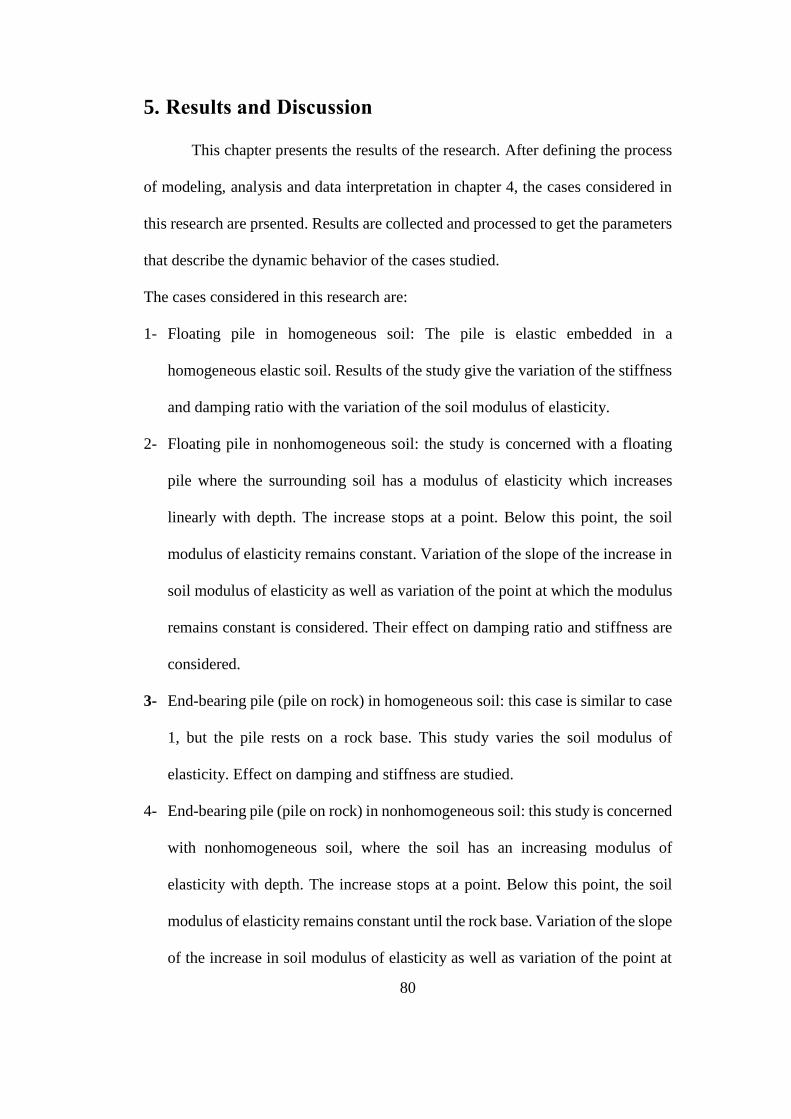
80
5. Results and Discussion
This chapter presents the results of the research. After defining the process
of modeling, analysis and data interpretation in chapter 4, the cases considered in
this research are prsented. Results are collected and processed to get the parameters
that describe the dynamic behavior of the cases studied.
The cases considered in this research are:
1- Floating pile in homogeneous soil: The pile is elastic embedded in a
homogeneous elastic soil. Results of the study give the variation of the stiffness
and damping ratio with the variation of the soil modulus of elasticity.
2- Floating pile in nonhomogeneous soil: the study is concerned with a floating
pile where the surrounding soil has a modulus of elasticity which increases
linearly with depth. The increase stops at a point. Below this point, the soil
modulus of elasticity remains constant. Variation of the slope of the increase in
soil modulus of elasticity as well as variation of the point at which the modulus
remains constant is considered. Their effect on damping ratio and stiffness are
considered.
3- End-bearing pile (pile on rock) in homogeneous soil: this case is similar to case
1, but the pile rests on a rock base. This study varies the soil modulus of
elasticity. Effect on damping and stiffness are studied.
4- End-bearing pile (pile on rock) in nonhomogeneous soil: this study is concerned
with nonhomogeneous soil, where the soil has an increasing modulus of
elasticity with depth. The increase stops at a point. Below this point, the soil
modulus of elasticity remains constant until the rock base. Variation of the slope
of the increase in soil modulus of elasticity as well as variation of the point at
81
which modulus remains constant is considered. Their effect on damping ratio
and stiffness are considered.
5- The pile-to-pile interaction: this study is concerned with the dynamic and static
interaction of piles. The simplest case of a pile group (2 piles) is studied in a
manner similar to Poulos (1968). Soil modulus of elasticity and pile spacing is
also varied. Effect of interaction between the piles is studied. Application to pile
groups is discussed.
5.1. Floating pile in homogeneous soil
In this study, an elastic pile in an elastic homogeneous soil is studied via
finite element method. An axisymmetric model is used to analyze this problem. Pile
modulus of elasticity, 𝐸𝑝 is fixed at 2.1 × 10¹⁰ 𝑁/𝑚 (pre-stressed concrete pile)
and its Poisson’s ratio, 𝜇𝑝 is fixed at 0.25. Pile diameter, 𝑑𝑝 = 0.5 𝑚 and its length,
𝐿𝑝 is 10 𝑚. The pile mass density, 𝜌𝑝 is 2500 𝐾𝑔/𝑚3. Soil modulus of elasticity,𝐸𝑠
is varied from 5 × 10⁶ 𝑡𝑜 8.34 × 10⁸ 𝑁/𝑚. The soil Poisson’s ratio, 𝜇𝑠 is fixed at
0.45. Soil density, 𝜌𝑠 is 1800 𝑘𝑔/𝑚3. Frequency is varied in the dynamic analysis
to capture dynamic response of the pile. Frequency variation depends on the soil
material. The variation is chosen to best capture the dynamic behavior by choosing
frequencies around the resonance area. In general, frequency was between 2.5 and
30 Hz. See Figure 5.1 for a general graphical description of the problem. See Table
5.1 for a summary of values of constants and range of values for varied parameters.
The study captured the effect of the varied variables on the stiffness and damping
of the pile.
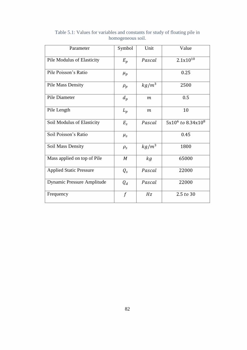
82
Table 5.1: Values for variables and constants for study of floating pile in
homogeneous soil.
Parameter Symbol Unit Value
Pile Modulus of Elasticity 𝐸𝑝 𝑃𝑎𝑠𝑐𝑎𝑙 2.1x10¹⁰
Pile Poisson’s Ratio 𝜇𝑝 0.25
Pile Mass Density 𝜌𝑝 𝑘𝑔/𝑚3 2500
Pile Diameter 𝑑𝑝 𝑚 0.5
Pile Length 𝐿𝑝 𝑚 10
Soil Modulus of Elasticity 𝐸𝑠 𝑃𝑎𝑠𝑐𝑎𝑙 5x10⁶ 𝑡𝑜 8.34x10⁸
Soil Poisson’s Ratio 𝜇𝑠 0.45
Soil Mass Density 𝜌𝑠 𝑘𝑔/𝑚3 1800
Mass applied on top of Pile 𝑀 𝑘𝑔 65000
Applied Static Pressure 𝑄𝑠 𝑃𝑎𝑠𝑐𝑎𝑙 22000
Dynamic Pressure Amplitude 𝑄𝑑 𝑃𝑎𝑠𝑐𝑎𝑙 22000
Frequency 𝑓 𝐻𝑧 2.5 𝑡𝑜 30
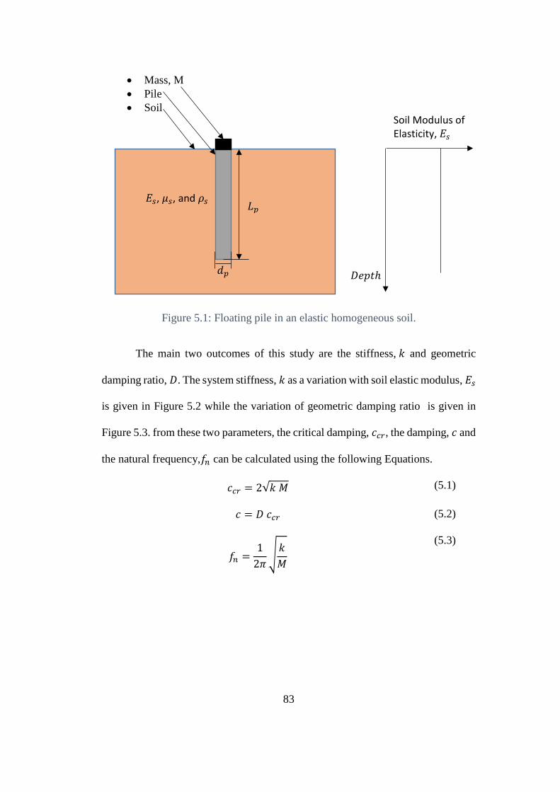
83
Figure 5.1: Floating pile in an elastic homogeneous soil.
The main two outcomes of this study are the stiffness, 𝑘 and geometric
damping ratio, 𝐷. The system stiffness, 𝑘 as a variation with soil elastic modulus, 𝐸𝑠
is given in Figure 5.2 while the variation of geometric damping ratio is given in
Figure 5.3. from these two parameters, the critical damping, 𝑐𝑐𝑟, the damping, 𝑐 and
the natural frequency,𝑓𝑛 can be calculated using the following Equations.
𝑐𝑐𝑟 = 2√𝑘 𝑀 (5.1)
𝑐 = 𝐷 𝑐𝑐𝑟 (5.2)
𝑓𝑛 =1
2𝜋√𝑘
𝑀
(5.3)
Soil Modulus of Elasticity, 𝐸𝑠
𝐷𝑒𝑝𝑡ℎ
Mass, M
Pile
Soil
𝑑𝑝
𝐿𝑝 𝐸𝑠, 𝜇𝑠, and 𝜌𝑠
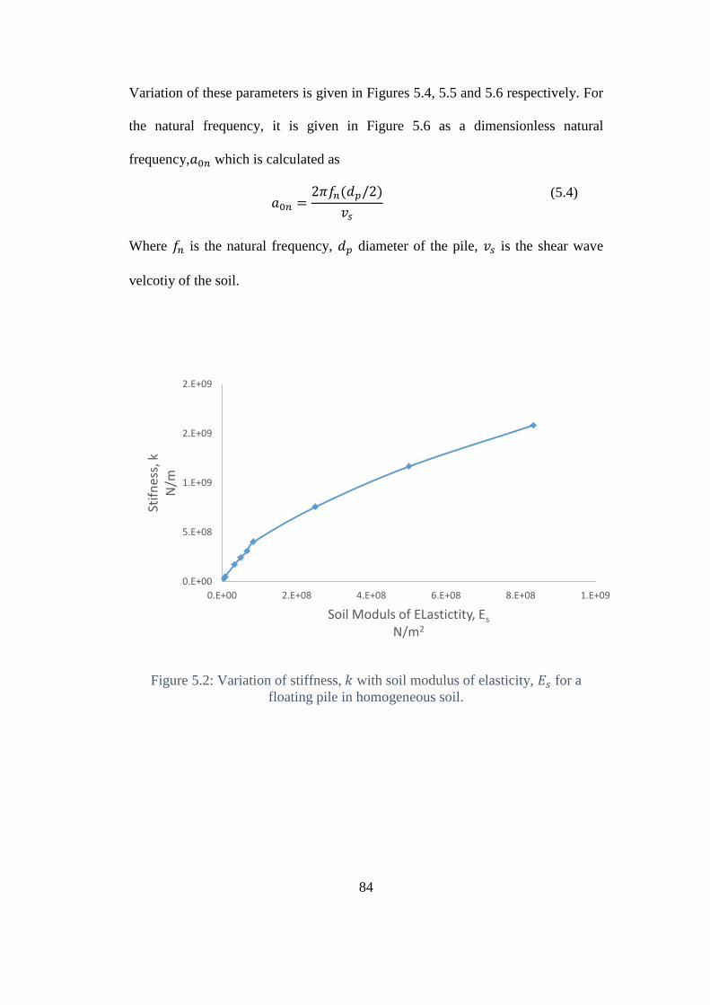
84
Variation of these parameters is given in Figures 5.4, 5.5 and 5.6 respectively. For
the natural frequency, it is given in Figure 5.6 as a dimensionless natural
frequency,𝑎0𝑛 which is calculated as
𝑎0𝑛 =2𝜋𝑓𝑛(𝑑𝑝/2)
𝑣𝑠
(5.4)
Where 𝑓𝑛 is the natural frequency, 𝑑𝑝 diameter of the pile, 𝑣𝑠 is the shear wave
velcotiy of the soil.
Figure 5.2: Variation of stiffness, 𝑘 with soil modulus of elasticity, 𝐸𝑠 for a
floating pile in homogeneous soil.
0.E+00
5.E+08
1.E+09
2.E+09
2.E+09
0.E+00 2.E+08 4.E+08 6.E+08 8.E+08 1.E+09
Stif
nes
s, k
N/m
Soil Moduls of ELastictity, Es
N/m2
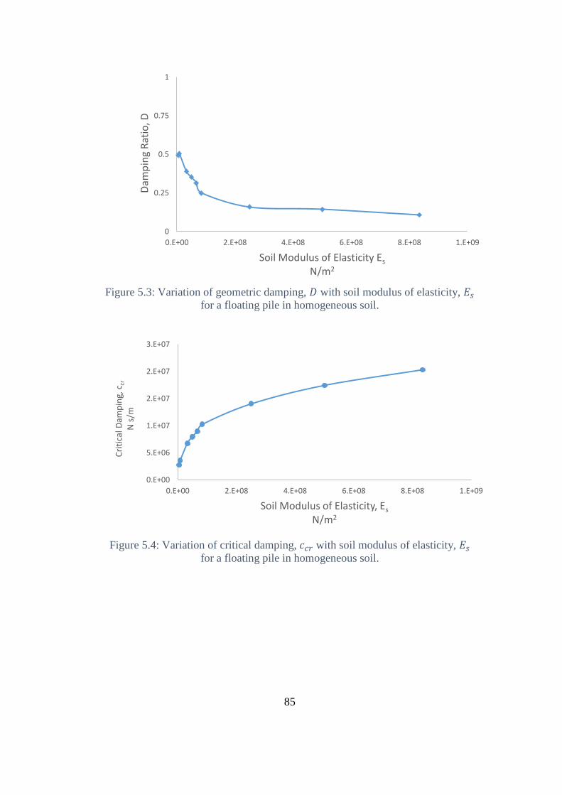
85
Figure 5.3: Variation of geometric damping, 𝐷 with soil modulus of elasticity, 𝐸𝑠
for a floating pile in homogeneous soil.
Figure 5.4: Variation of critical damping, 𝑐𝑐𝑟 with soil modulus of elasticity, 𝐸𝑠
for a floating pile in homogeneous soil.
0
0.25
0.5
0.75
1
0.E+00 2.E+08 4.E+08 6.E+08 8.E+08 1.E+09
Dam
pin
g R
atio
, D
Soil Modulus of Elasticity Es
N/m2
0.E+00
5.E+06
1.E+07
2.E+07
2.E+07
3.E+07
0.E+00 2.E+08 4.E+08 6.E+08 8.E+08 1.E+09
Cri
tica
l Dam
pin
g, c
cr
N s
/m
Soil Modulus of Elasticity, Es
N/m2
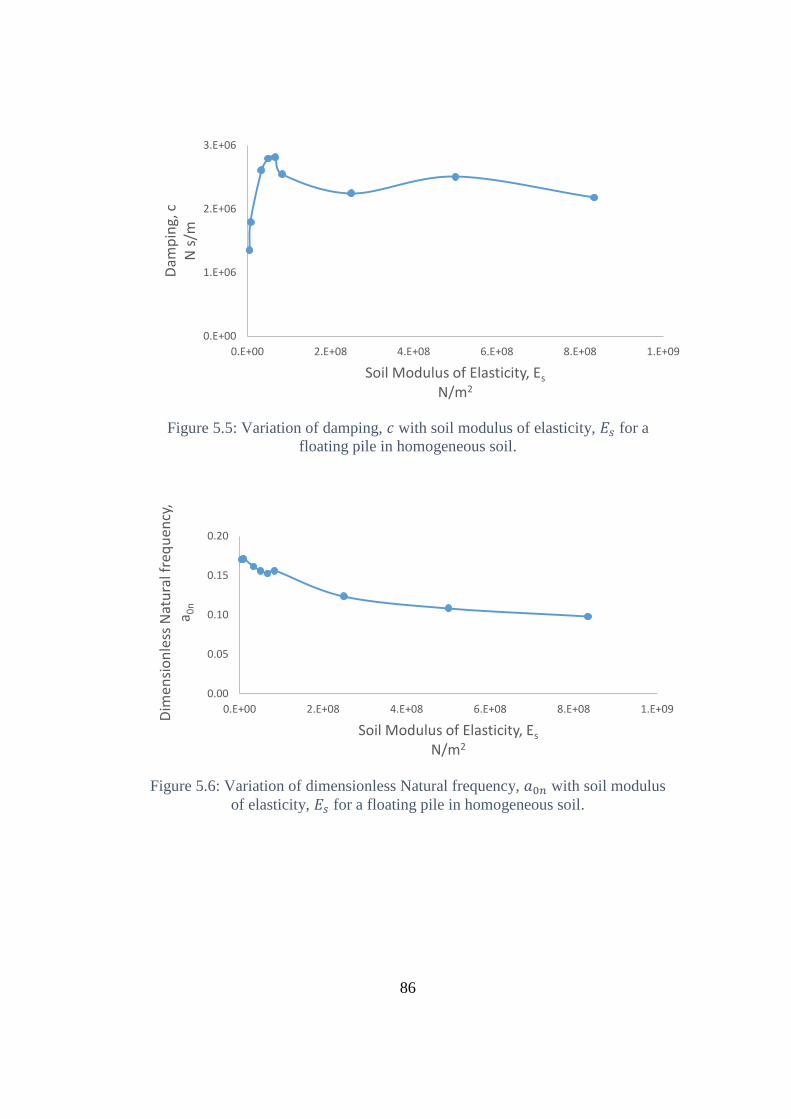
86
Figure 5.5: Variation of damping, 𝑐 with soil modulus of elasticity, 𝐸𝑠 for a
floating pile in homogeneous soil.
Figure 5.6: Variation of dimensionless Natural frequency, 𝑎0𝑛 with soil modulus
of elasticity, 𝐸𝑠 for a floating pile in homogeneous soil.
0.E+00
1.E+06
2.E+06
3.E+06
0.E+00 2.E+08 4.E+08 6.E+08 8.E+08 1.E+09
Dam
pin
g, c
N s
/m
Soil Modulus of Elasticity, Es
N/m2
0.00
0.05
0.10
0.15
0.20
0.E+00 2.E+08 4.E+08 6.E+08 8.E+08 1.E+09
Dim
ensi
on
less
Nat
ura
l fre
qu
ency
, a 0
n
Soil Modulus of Elasticity, Es
N/m2
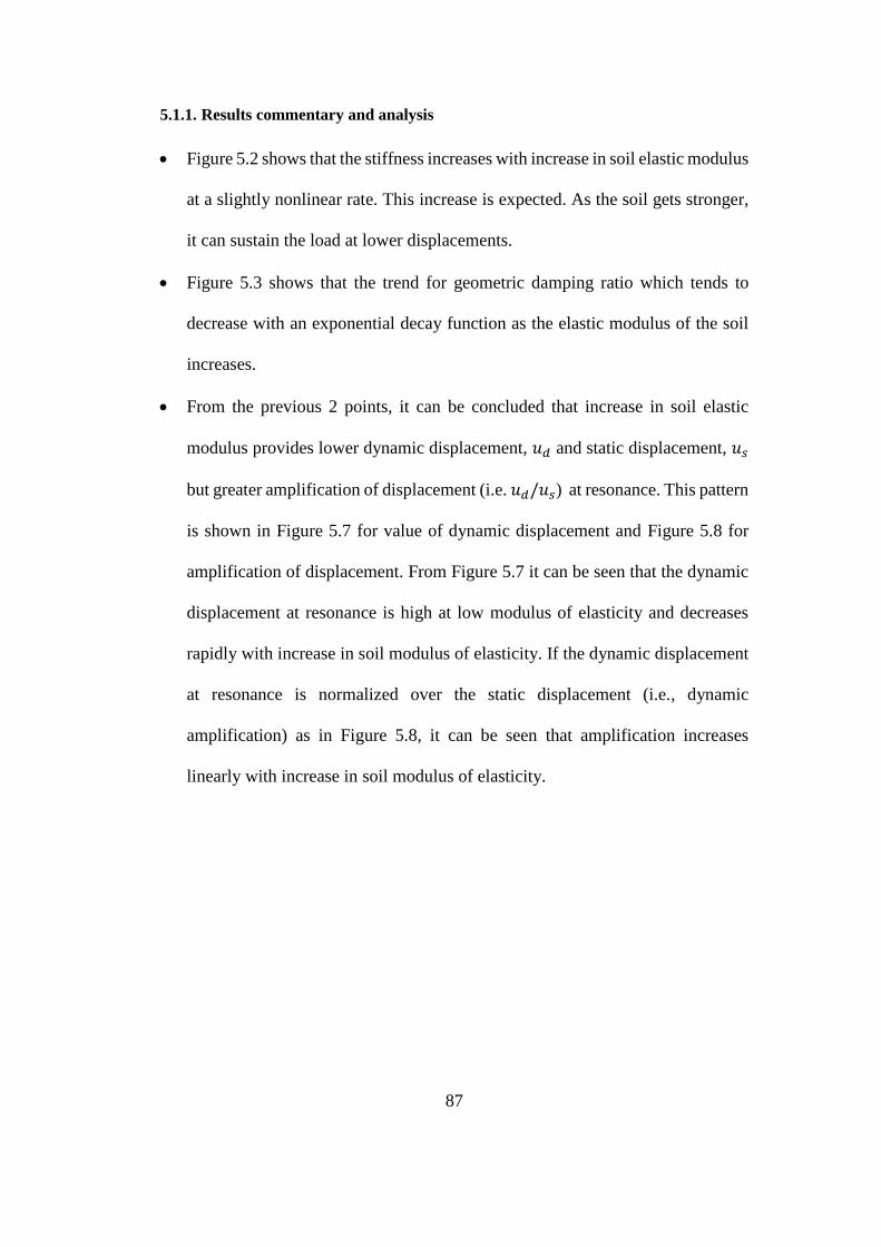
87
5.1.1. Results commentary and analysis
Figure 5.2 shows that the stiffness increases with increase in soil elastic modulus
at a slightly nonlinear rate. This increase is expected. As the soil gets stronger,
it can sustain the load at lower displacements.
Figure 5.3 shows that the trend for geometric damping ratio which tends to
decrease with an exponential decay function as the elastic modulus of the soil
increases.
From the previous 2 points, it can be concluded that increase in soil elastic
modulus provides lower dynamic displacement, 𝑢𝑑 and static displacement, 𝑢𝑠
but greater amplification of displacement (i.e. 𝑢𝑑/𝑢𝑠) at resonance. This pattern
is shown in Figure 5.7 for value of dynamic displacement and Figure 5.8 for
amplification of displacement. From Figure 5.7 it can be seen that the dynamic
displacement at resonance is high at low modulus of elasticity and decreases
rapidly with increase in soil modulus of elasticity. If the dynamic displacement
at resonance is normalized over the static displacement (i.e., dynamic
amplification) as in Figure 5.8, it can be seen that amplification increases
linearly with increase in soil modulus of elasticity.
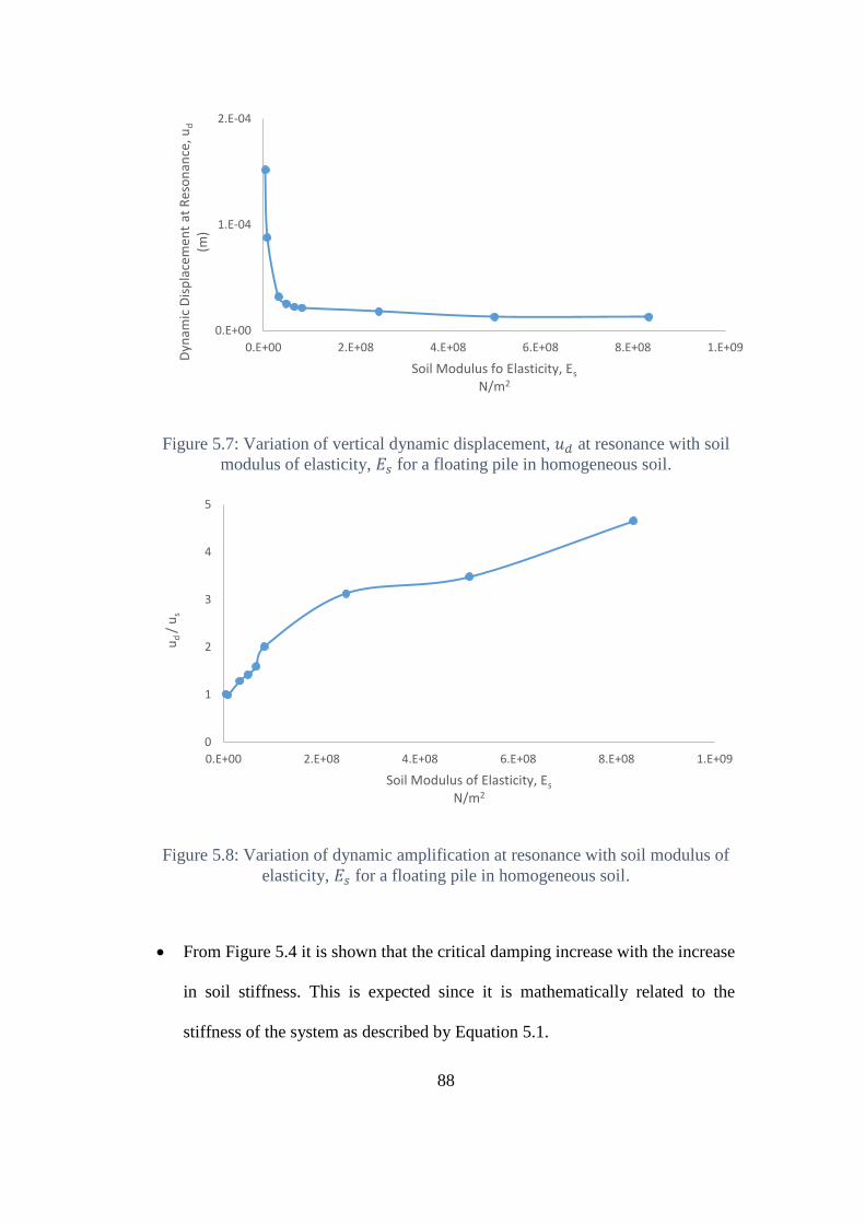
88
Figure 5.7: Variation of vertical dynamic displacement, 𝑢𝑑 at resonance with soil
modulus of elasticity, 𝐸𝑠 for a floating pile in homogeneous soil.
Figure 5.8: Variation of dynamic amplification at resonance with soil modulus of
elasticity, 𝐸𝑠 for a floating pile in homogeneous soil.
From Figure 5.4 it is shown that the critical damping increase with the increase
in soil stiffness. This is expected since it is mathematically related to the
stiffness of the system as described by Equation 5.1.
0.E+00
1.E-04
2.E-04
0.E+00 2.E+08 4.E+08 6.E+08 8.E+08 1.E+09
Dyn
amic
Dis
pla
cem
ent
at R
eso
nan
ce, u
d
(m)
Soil Modulus fo Elasticity, Es
N/m2
0
1
2
3
4
5
0.E+00 2.E+08 4.E+08 6.E+08 8.E+08 1.E+09
ud
/ u
s
Soil Modulus of Elasticity, Es
N/m2
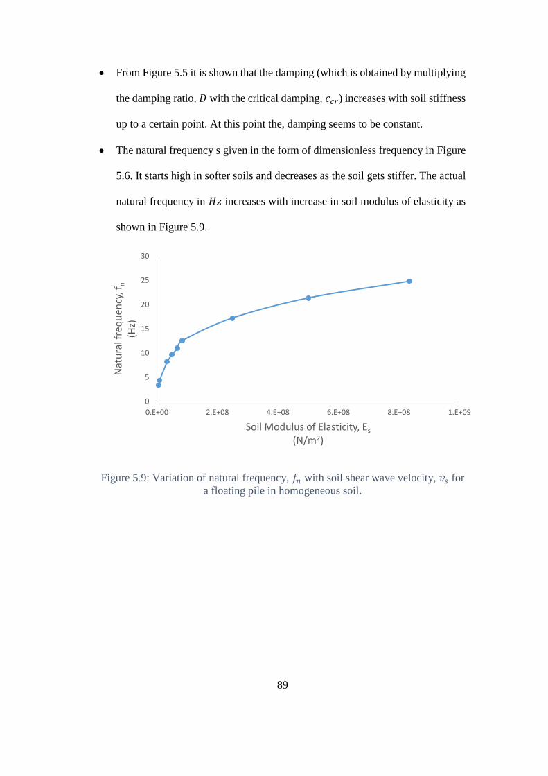
89
From Figure 5.5 it is shown that the damping (which is obtained by multiplying
the damping ratio, 𝐷 with the critical damping, 𝑐𝑐𝑟) increases with soil stiffness
up to a certain point. At this point the, damping seems to be constant.
The natural frequency s given in the form of dimensionless frequency in Figure
5.6. It starts high in softer soils and decreases as the soil gets stiffer. The actual
natural frequency in 𝐻𝑧 increases with increase in soil modulus of elasticity as
shown in Figure 5.9.
Figure 5.9: Variation of natural frequency, 𝑓𝑛 with soil shear wave velocity, 𝑣𝑠 for
a floating pile in homogeneous soil.
0
5
10
15
20
25
30
0.E+00 2.E+08 4.E+08 6.E+08 8.E+08 1.E+09
Nat
ura
l fre
qu
ency
, fn
(Hz)
Soil Modulus of Elasticity, Es
(N/m2)
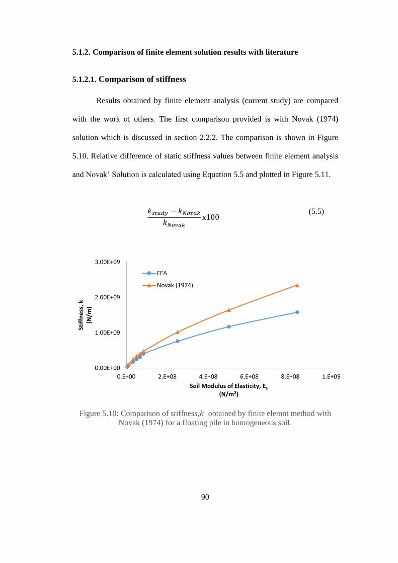
90
5.1.2. Comparison of finite element solution results with literature
5.1.2.1. Comparison of stiffness
Results obtained by finite element analysis (current study) are compared
with the work of others. The first comparison provided is with Novak (1974)
solution which is discussed in section 2.2.2. The comparison is shown in Figure
5.10. Relative difference of static stiffness values between finite element analysis
and Novak’ Solution is calculated using Equation 5.5 and plotted in Figure 5.11.
𝑘𝑠𝑡𝑢𝑑𝑦 − 𝑘𝑁𝑜𝑣𝑎𝑘
𝑘𝑁𝑜𝑣𝑎𝑘x100
(5.5)
Figure 5.10: Comparison of stiffness,𝑘 obtained by finite elemnt method with
Novak (1974) for a floating pile in homogeneous soil.
0.00E+00
1.00E+09
2.00E+09
3.00E+09
0.E+00 2.E+08 4.E+08 6.E+08 8.E+08 1.E+09
Stif
fne
ss,
k(N
/m)
Soil Modulus of Elasticity, Es
(N/m2)
FEA
Novak (1974)
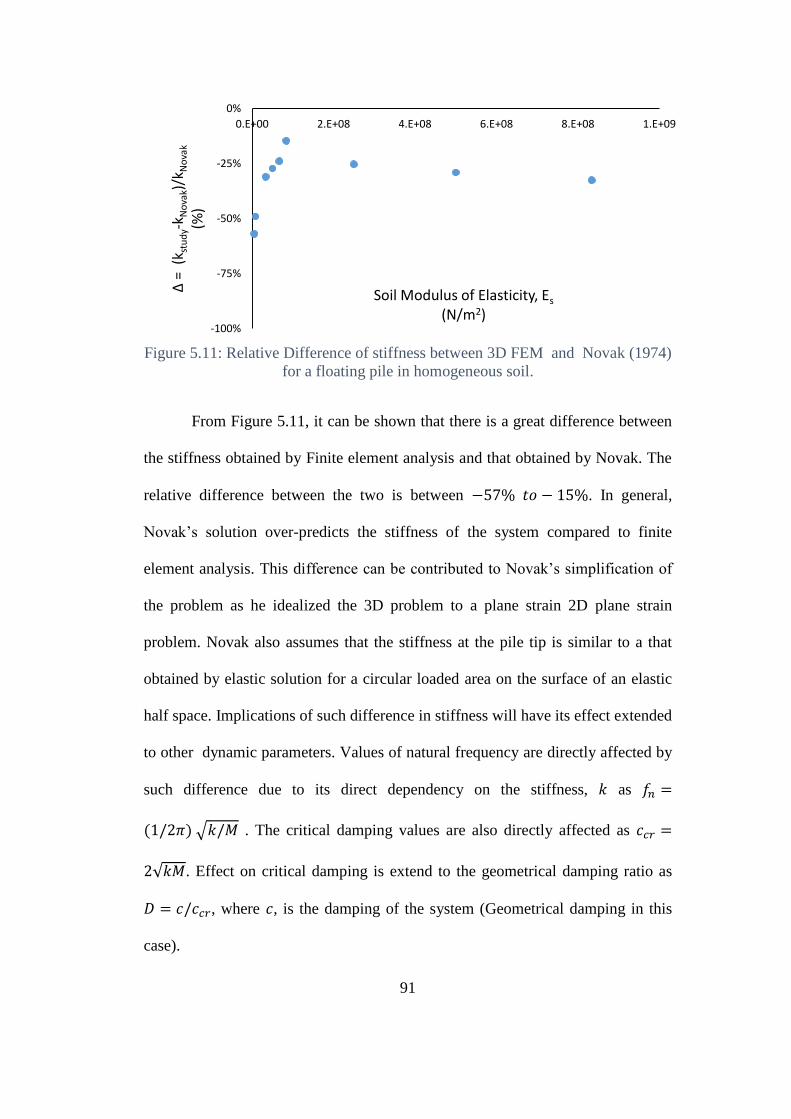
91
Figure 5.11: Relative Difference of stiffness between 3D FEM and Novak (1974)
for a floating pile in homogeneous soil.
From Figure 5.11, it can be shown that there is a great difference between
the stiffness obtained by Finite element analysis and that obtained by Novak. The
relative difference between the two is between −57% 𝑡𝑜 − 15%. In general,
Novak’s solution over-predicts the stiffness of the system compared to finite
element analysis. This difference can be contributed to Novak’s simplification of
the problem as he idealized the 3D problem to a plane strain 2D plane strain
problem. Novak also assumes that the stiffness at the pile tip is similar to a that
obtained by elastic solution for a circular loaded area on the surface of an elastic
half space. Implications of such difference in stiffness will have its effect extended
to other dynamic parameters. Values of natural frequency are directly affected by
such difference due to its direct dependency on the stiffness, 𝑘 as 𝑓𝑛 =
(1/2𝜋) √𝑘/𝑀 . The critical damping values are also directly affected as 𝑐𝑐𝑟 =
2√𝑘𝑀. Effect on critical damping is extend to the geometrical damping ratio as
𝐷 = 𝑐/𝑐𝑐𝑟, where 𝑐, is the damping of the system (Geometrical damping in this
case).
-100%
-75%
-50%
-25%
0%
0.E+00 2.E+08 4.E+08 6.E+08 8.E+08 1.E+09
Δ=
(k s
tud
y-k N
ova
k)/k
No
vak
(%)
Soil Modulus of Elasticity, Es
(N/m2)
92
Another comparison of the stiffness is provided against the work of Gazetas
& Mylonakis (1998). The stiffness of a pile in homogeneous elastic soil given is
calculated as follows:
𝑘 = 𝐸𝑝𝐴𝑝𝜆𝛺 + tanh (𝐿𝑝𝜆)
1 + 𝛺 tanh (𝐿𝑝𝜆)
(5.6)
Where 𝜆 is calculated using
𝜆 = √𝛿𝐺𝑠
𝐸𝑝𝐴𝑝
(5.7)
𝛺 is calculated using the following Equation
𝛺 =𝑘𝑏
𝐸𝑝𝐴𝑝𝜆
(5.8)
𝛿 is calculated as
𝛿 =2𝜋
ln (2𝑟𝑚𝑑𝑝
)
(5.9)
Where 𝑟𝑚 is
𝑟𝑚 = 2.5𝐿𝑝(1 − 𝜇𝑠) (5.10)
And 𝑘𝑏 is calculated as
𝑘𝑏 =𝑑𝐸𝑠
1 − 𝜇𝑠(1 + 0.65
𝑑𝑝
ℎ𝑏)
(5.11)
In Equations 5.6 to 5.11, the following notations apply:
𝐸𝑝: Pile modulus of elasticity.
𝐴𝑝: Pile cross sectional area.
𝜆: a parameter calculated using 5.7.
𝛺: a parameter calculated using 5.8.
93
𝐿𝑝: Pile length.
𝑘𝑏; stiffness at pile base given by Randolph & Wroth (1978).
𝐺𝑠: soil shear modulus.
𝐸𝑠: soil modulus of elasticity.
𝑑𝑝: pile diameter.
ℎ𝑏: depth to bed rock from pile tip (ℎ𝑏 = ∞, if far away and has no effect).
𝜇𝑠: soil Poisson’s ratio.
𝑟𝑚: radius at which soil settlement is negligible.
Using the Equations defined by Gazetas & Mylonakis (1998), the stiffness was
calculated. The problem as defined by Gazetas & Mylonakis (1998) is shown in
Figure 5.12. A comparison between this approach and the finite element solution is
provided in Figure 5.13 while relative difference (𝑘𝑠𝑡𝑢𝑑𝑦 − 𝑘𝐺𝑎𝑧𝑒𝑡𝑎𝑠)/𝑘𝐺𝑎𝑧𝑒𝑡𝑎𝑠 is
given in Figure 5.14.
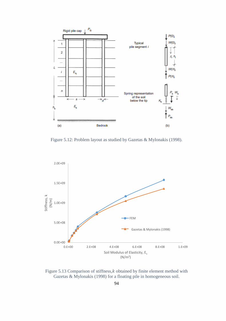
94
Figure 5.12: Problem layout as studied by Gazetas & Mylonakis (1998).
Figure 5.13 Comparison of stiffness,𝑘 obtained by finite element method with
Gazetas & Mylonakis (1998) for a floating pile in homogeneous soil.
0.0E+00
5.0E+08
1.0E+09
1.5E+09
2.0E+09
0.E+00 2.E+08 4.E+08 6.E+08 8.E+08 1.E+09
Stif
fnes
s, k
(N/m
)
Soil Modulus of Elasticity, Es
(N/m2)
FEM
Mylonakis, G. & Gazetas, G.(1998).
Gazetas & Mylonakis (1998)
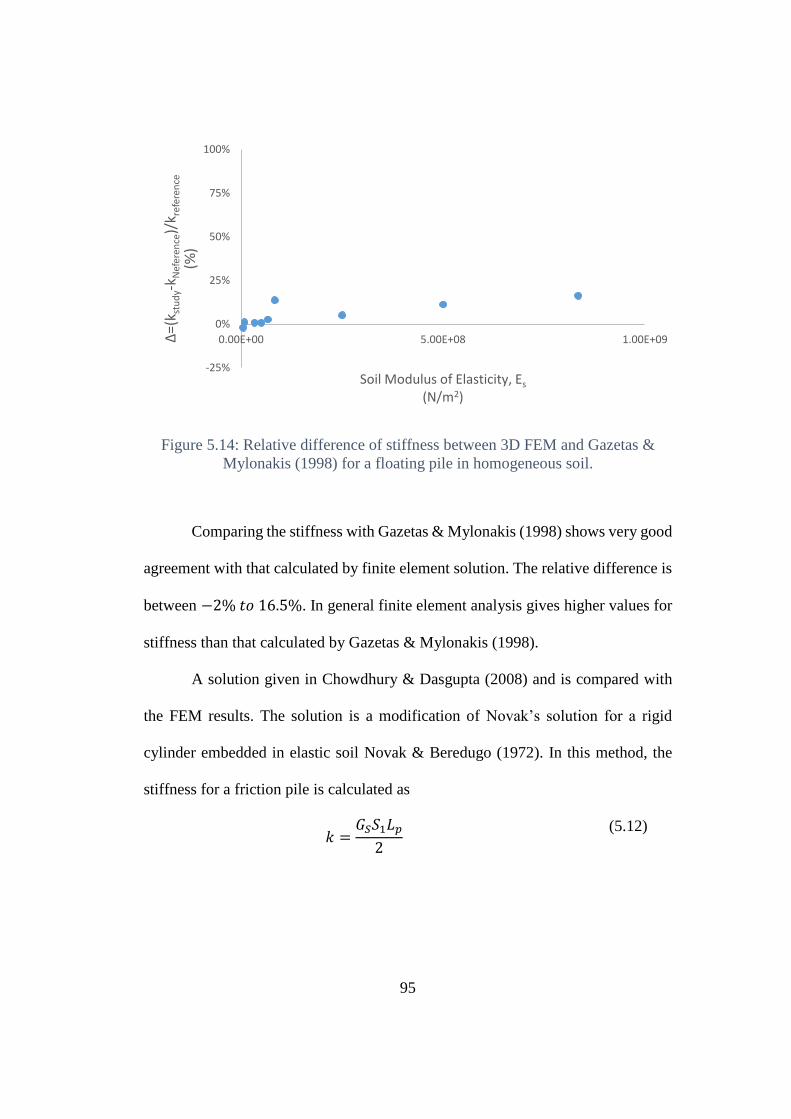
95
Figure 5.14: Relative difference of stiffness between 3D FEM and Gazetas &
Mylonakis (1998) for a floating pile in homogeneous soil.
Comparing the stiffness with Gazetas & Mylonakis (1998) shows very good
agreement with that calculated by finite element solution. The relative difference is
between −2% 𝑡𝑜 16.5%. In general finite element analysis gives higher values for
stiffness than that calculated by Gazetas & Mylonakis (1998).
A solution given in Chowdhury & Dasgupta (2008) and is compared with
the FEM results. The solution is a modification of Novak’s solution for a rigid
cylinder embedded in elastic soil Novak & Beredugo (1972). In this method, the
stiffness for a friction pile is calculated as
𝑘 =𝐺𝑆𝑆1𝐿𝑝
2
(5.12)
-25%
0%
25%
50%
75%
100%
0.00E+00 5.00E+08 1.00E+09Δ=(
k stu
dy-
k Nef
eren
ce)/
k ref
eren
ce
(%)
Soil Modulus of Elasticity, Es
(N/m2)
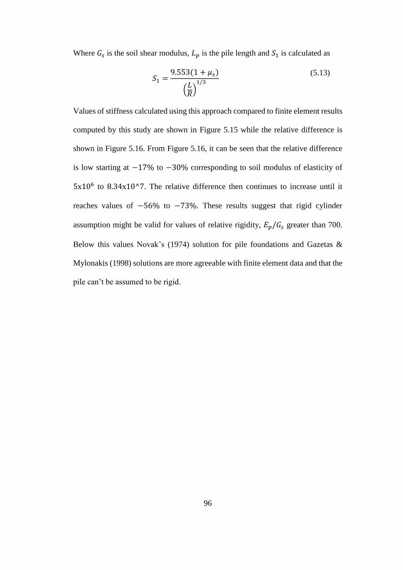
96
Where 𝐺𝑠 is the soil shear modulus, 𝐿𝑝 is the pile length and 𝑆1 is calculated as
𝑆1 =9.553(1 + 𝜇𝑠)
(𝐿𝑅)
1/3
(5.13)
Values of stiffness calculated using this approach compared to finite element results
computed by this study are shown in Figure 5.15 while the relative difference is
shown in Figure 5.16. From Figure 5.16, it can be seen that the relative difference
is low starting at −17% to −30% corresponding to soil modulus of elasticity of
5x10⁶ to 8.34x10^7. The relative difference then continues to increase until it
reaches values of −56% to −73%. These results suggest that rigid cylinder
assumption might be valid for values of relative rigidity, 𝐸𝑝/𝐺𝑠 greater than 700.
Below this values Novak’s (1974) solution for pile foundations and Gazetas &
Mylonakis (1998) solutions are more agreeable with finite element data and that the
pile can’t be assumed to be rigid.
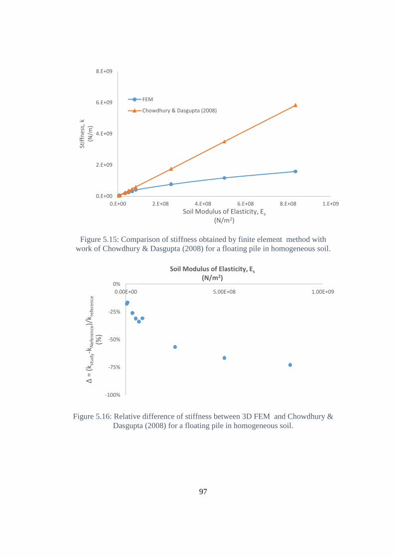
97
Figure 5.15: Comparison of stiffness obtained by finite element method with
work of Chowdhury & Dasgupta (2008) for a floating pile in homogeneous soil.
Figure 5.16: Relative difference of stiffness between 3D FEM and Chowdhury &
Dasgupta (2008) for a floating pile in homogeneous soil.
0.E+00
2.E+09
4.E+09
6.E+09
8.E+09
0.E+00 2.E+08 4.E+08 6.E+08 8.E+08 1.E+09
Stif
fnes
s, k
(N/m
)
Soil Modulus of Elasticity, Es
(N/m2)
FEM
Chowdhury & Dasgupta (2008)
-100%
-75%
-50%
-25%
0%
0.00E+00 5.00E+08 1.00E+09
Δ=
(kst
ud
y-k N
efer
ence
)/k r
efer
ence
(%)
Soil Modulus of Elasticity, Es
(N/m2)
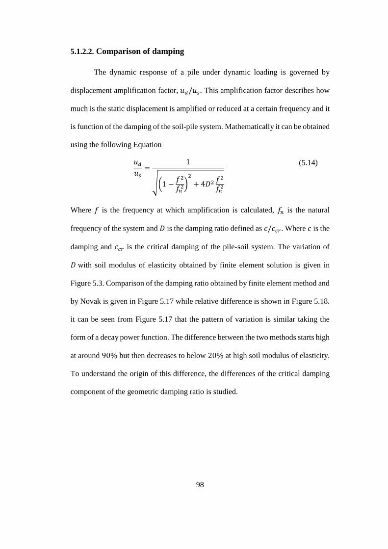
98
5.1.2.2. Comparison of damping
The dynamic response of a pile under dynamic loading is governed by
displacement amplification factor, 𝑢𝑑/𝑢𝑠. This amplification factor describes how
much is the static displacement is amplified or reduced at a certain frequency and it
is function of the damping of the soil-pile system. Mathematically it can be obtained
using the following Equation
𝑢𝑑
𝑢𝑠=
1
√(1 −𝑓2
𝑓𝑛2)2
+ 4𝐷2 𝑓2
𝑓𝑛2
(5.14)
Where 𝑓 is the frequency at which amplification is calculated, 𝑓𝑛 is the natural
frequency of the system and 𝐷 is the damping ratio defined as 𝑐/𝑐𝑐𝑟. Where 𝑐 is the
damping and 𝑐𝑐𝑟 is the critical damping of the pile-soil system. The variation of
𝐷 with soil modulus of elasticity obtained by finite element solution is given in
Figure 5.3. Comparison of the damping ratio obtained by finite element method and
by Novak is given in Figure 5.17 while relative difference is shown in Figure 5.18.
it can be seen from Figure 5.17 that the pattern of variation is similar taking the
form of a decay power function. The difference between the two methods starts high
at around 90% but then decreases to below 20% at high soil modulus of elasticity.
To understand the origin of this difference, the differences of the critical damping
component of the geometric damping ratio is studied.
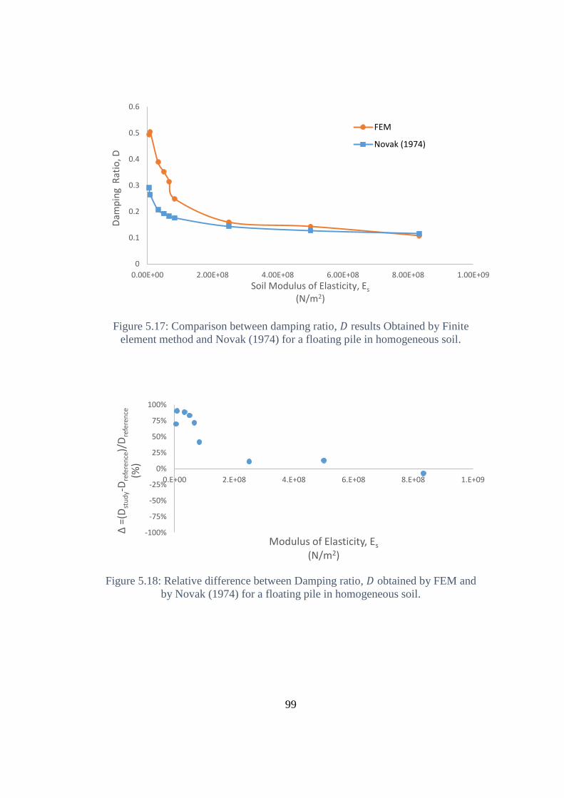
99
Figure 5.17: Comparison between damping ratio, 𝐷 results Obtained by Finite
element method and Novak (1974) for a floating pile in homogeneous soil.
Figure 5.18: Relative difference between Damping ratio, 𝐷 obtained by FEM and
by Novak (1974) for a floating pile in homogeneous soil.
0
0.1
0.2
0.3
0.4
0.5
0.6
0.00E+00 2.00E+08 4.00E+08 6.00E+08 8.00E+08 1.00E+09
Dam
pin
g R
atio
, D
Soil Modulus of Elasticity, Es
(N/m2)
FEM
Novak (1974)
-100%
-75%
-50%
-25%
0%
25%
50%
75%
100%
0.E+00 2.E+08 4.E+08 6.E+08 8.E+08 1.E+09
Δ=(
Dst
ud
y-D
refe
ren
ce)/
Dre
fere
nce
(%)
Modulus of Elasticity, Es
(N/m2)
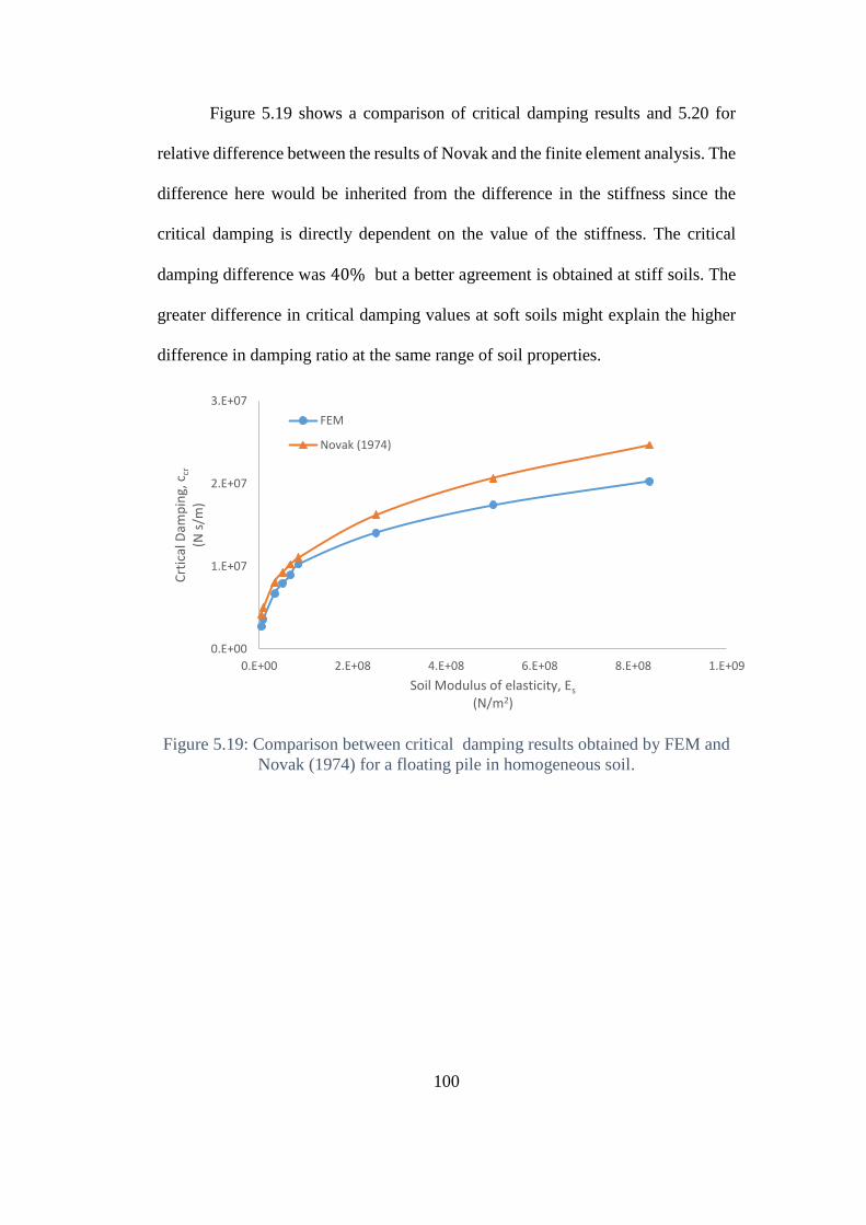
100
Figure 5.19 shows a comparison of critical damping results and 5.20 for
relative difference between the results of Novak and the finite element analysis. The
difference here would be inherited from the difference in the stiffness since the
critical damping is directly dependent on the value of the stiffness. The critical
damping difference was 40% but a better agreement is obtained at stiff soils. The
greater difference in critical damping values at soft soils might explain the higher
difference in damping ratio at the same range of soil properties.
Figure 5.19: Comparison between critical damping results obtained by FEM and
Novak (1974) for a floating pile in homogeneous soil.
0.E+00
1.E+07
2.E+07
3.E+07
0.E+00 2.E+08 4.E+08 6.E+08 8.E+08 1.E+09
Crt
ical
Dam
pin
g, c
cr
(N s
/m)
Soil Modulus of elasticity, Es
(N/m2)
FEM
Novak (1974)
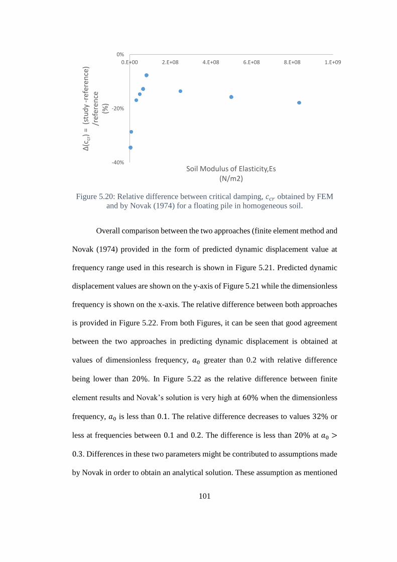
101
Figure 5.20: Relative difference between critical damping, 𝑐𝑐𝑟 obtained by FEM
and by Novak (1974) for a floating pile in homogeneous soil.
Overall comparison between the two approaches (finite element method and
Novak (1974) provided in the form of predicted dynamic displacement value at
frequency range used in this research is shown in Figure 5.21. Predicted dynamic
displacement values are shown on the y-axis of Figure 5.21 while the dimensionless
frequency is shown on the x-axis. The relative difference between both approaches
is provided in Figure 5.22. From both Figures, it can be seen that good agreement
between the two approaches in predicting dynamic displacement is obtained at
values of dimensionless frequency, 𝑎0 greater than 0.2 with relative difference
being lower than 20%. In Figure 5.22 as the relative difference between finite
element results and Novak’s solution is very high at 60% when the dimensionless
frequency, 𝑎0 is less than 0.1. The relative difference decreases to values 32% or
less at frequencies between 0.1 and 0.2. The difference is less than 20% at 𝑎0 >
0.3. Differences in these two parameters might be contributed to assumptions made
by Novak in order to obtain an analytical solution. These assumption as mentioned
-40%
-20%
0%
0.E+00 2.E+08 4.E+08 6.E+08 8.E+08 1.E+09
Δ(c
cr)
= (
stu
dy
-ref
eren
ce)
/ref
eren
ce(%
)
Soil Modulus of Elasticity,Es(N/m2)
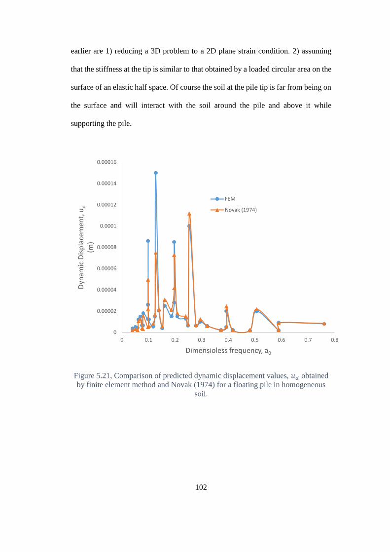
102
earlier are 1) reducing a 3D problem to a 2D plane strain condition. 2) assuming
that the stiffness at the tip is similar to that obtained by a loaded circular area on the
surface of an elastic half space. Of course the soil at the pile tip is far from being on
the surface and will interact with the soil around the pile and above it while
supporting the pile.
Figure 5.21, Comparison of predicted dynamic displacement values, 𝑢𝑑 obtained
by finite element method and Novak (1974) for a floating pile in homogeneous
soil.
0
0.00002
0.00004
0.00006
0.00008
0.0001
0.00012
0.00014
0.00016
0 0.1 0.2 0.3 0.4 0.5 0.6 0.7 0.8
Dyn
amic
Dis
pla
cem
ent,
ud
(m)
Dimensioless frequency, a0
FEM
Novak (1974)
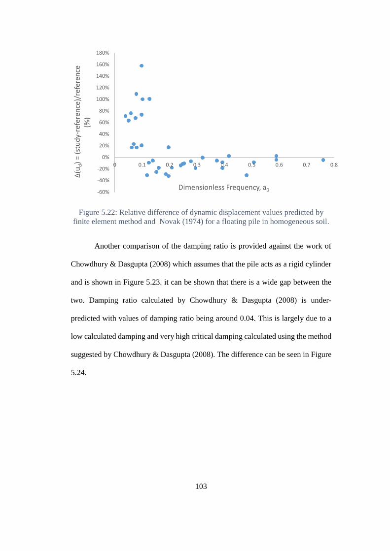
103
Figure 5.22: Relative difference of dynamic displacement values predicted by
finite element method and Novak (1974) for a floating pile in homogeneous soil.
Another comparison of the damping ratio is provided against the work of
Chowdhury & Dasgupta (2008) which assumes that the pile acts as a rigid cylinder
and is shown in Figure 5.23. it can be shown that there is a wide gap between the
two. Damping ratio calculated by Chowdhury & Dasgupta (2008) is under-
predicted with values of damping ratio being around 0.04. This is largely due to a
low calculated damping and very high critical damping calculated using the method
suggested by Chowdhury & Dasgupta (2008). The difference can be seen in Figure
5.24.
-60%
-40%
-20%
0%
20%
40%
60%
80%
100%
120%
140%
160%
180%
0 0.1 0.2 0.3 0.4 0.5 0.6 0.7 0.8
Δ(u
d)
= (s
tud
y-re
fere
nce
)/re
fere
nce
(%)
Dimensionless Frequency, a0
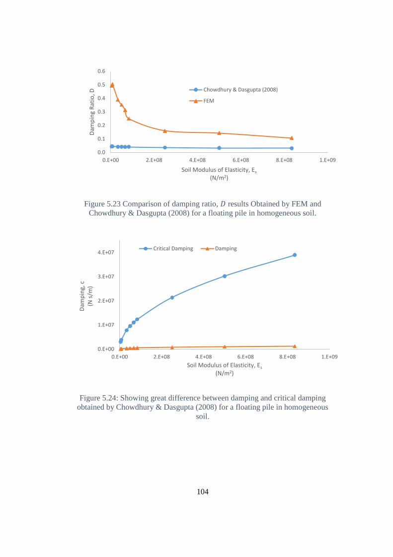
104
Figure 5.23 Comparison of damping ratio, 𝐷 results Obtained by FEM and
Chowdhury & Dasgupta (2008) for a floating pile in homogeneous soil.
Figure 5.24: Showing great difference between damping and critical damping
obtained by Chowdhury & Dasgupta (2008) for a floating pile in homogeneous
soil.
0.0
0.1
0.2
0.3
0.4
0.5
0.6
0.E+00 2.E+08 4.E+08 6.E+08 8.E+08 1.E+09
Dam
pin
g R
atio
, D
Soil Modulus of Elasticity, Es
(N/m2)
Chowdhury & Dasgupta (2008)
FEM
0.E+00
1.E+07
2.E+07
3.E+07
4.E+07
0.E+00 2.E+08 4.E+08 6.E+08 8.E+08 1.E+09
Dam
pin
g, c
(N
s/m
)
Soil Modulus of Elasticity, Es
(N/m2)
Critical Damping Damping
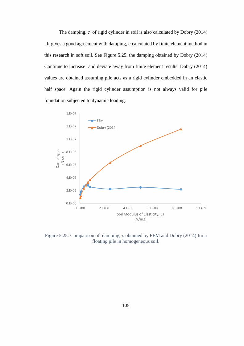
105
The damping, 𝑐 of rigid cylinder in soil is also calculated by Dobry (2014)
. It gives a good agreement with damping, 𝑐 calculated by finite element method in
this research in soft soil. See Figure 5.25. the damping obtained by Dobry (2014)
Continue to increase and deviate away from finite element results. Dobry (2014)
values are obtained assuming pile acts as a rigid cylinder embedded in an elastic
half space. Again the rigid cylinder assumption is not always valid for pile
foundation subjected to dynamic loading.
Figure 5.25: Comparison of damping, 𝑐 obtained by FEM and Dobry (2014) for a
floating pile in homogeneous soil.
0.E+00
2.E+06
4.E+06
6.E+06
8.E+06
1.E+07
1.E+07
1.E+07
0.E+00 2.E+08 4.E+08 6.E+08 8.E+08 1.E+09
Dam
pin
g , c
(N s
/m)
Soil Modulus of Elasticity, Es(N/m2)
FEM
Dobry (2014)
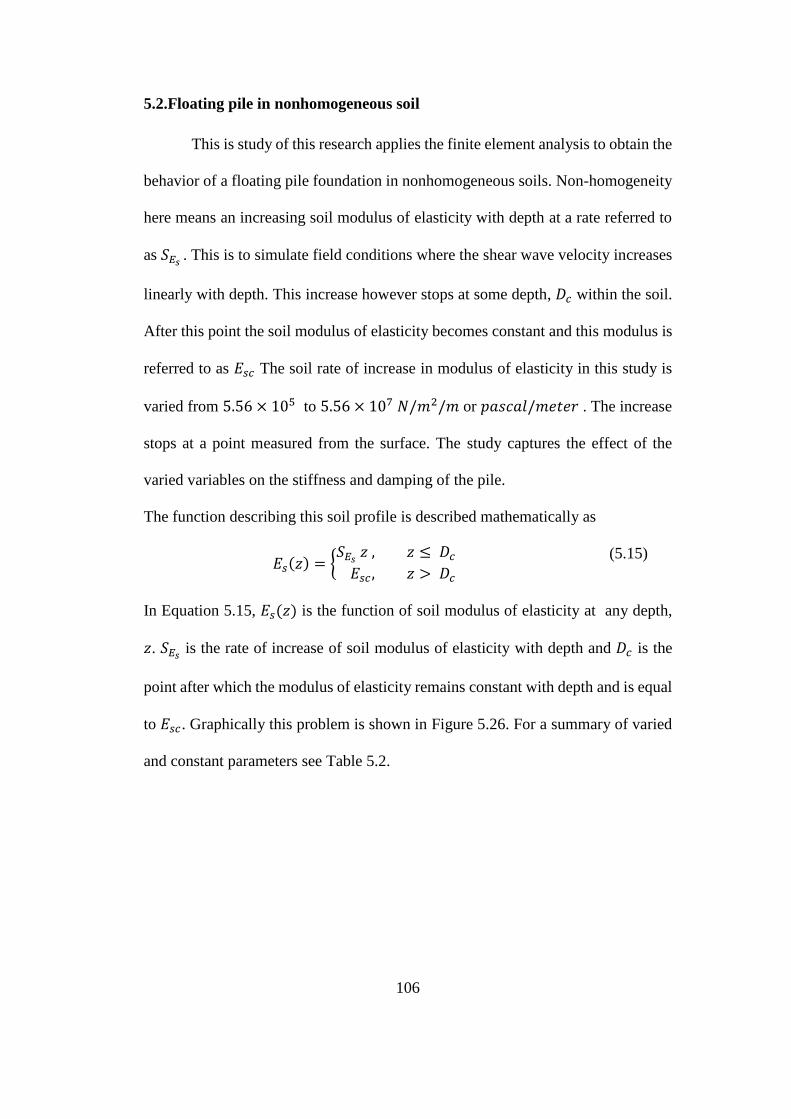
106
5.2.Floating pile in nonhomogeneous soil
This is study of this research applies the finite element analysis to obtain the
behavior of a floating pile foundation in nonhomogeneous soils. Non-homogeneity
here means an increasing soil modulus of elasticity with depth at a rate referred to
as 𝑆𝐸𝑠 . This is to simulate field conditions where the shear wave velocity increases
linearly with depth. This increase however stops at some depth, 𝐷𝑐 within the soil.
After this point the soil modulus of elasticity becomes constant and this modulus is
referred to as 𝐸𝑠𝑐 The soil rate of increase in modulus of elasticity in this study is
varied from 5.56 × 10⁵ to 5.56 × 10⁷ 𝑁/𝑚2/𝑚 or 𝑝𝑎𝑠𝑐𝑎𝑙/𝑚𝑒𝑡𝑒𝑟 . The increase
stops at a point measured from the surface. The study captures the effect of the
varied variables on the stiffness and damping of the pile.
The function describing this soil profile is described mathematically as
𝐸𝑠(𝑧) = {𝑆𝐸𝑠 𝑧 , 𝑧 ≤ 𝐷𝑐
𝐸𝑠𝑐 , 𝑧 > 𝐷𝑐
(5.15)
In Equation 5.15, 𝐸𝑠(𝑧) is the function of soil modulus of elasticity at any depth,
𝑧. 𝑆𝐸𝑠 is the rate of increase of soil modulus of elasticity with depth and 𝐷𝑐 is the
point after which the modulus of elasticity remains constant with depth and is equal
to 𝐸𝑠𝑐. Graphically this problem is shown in Figure 5.26. For a summary of varied
and constant parameters see Table 5.2.
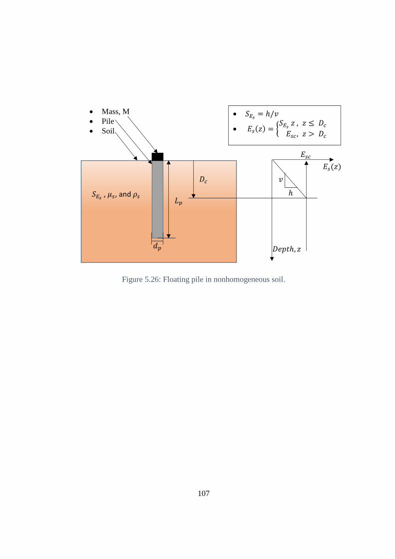
107
Figure 5.26: Floating pile in nonhomogeneous soil.
𝐸𝑠(𝑧)
𝐷𝑒𝑝𝑡ℎ, 𝑧
Mass, M
Pile
Soil
𝑑𝑝
𝐿𝑝 𝑆𝐸𝑠 , 𝜇𝑠, and 𝜌𝑠
𝐷𝑐
𝐸𝑠𝑐
ℎ
𝑣
𝑆𝐸𝑠 = ℎ/𝑣
𝐸𝑠(𝑧) = {𝑆𝐸𝑠 𝑧 , 𝑧 ≤ 𝐷𝑐
𝐸𝑠𝑐, 𝑧 > 𝐷𝑐
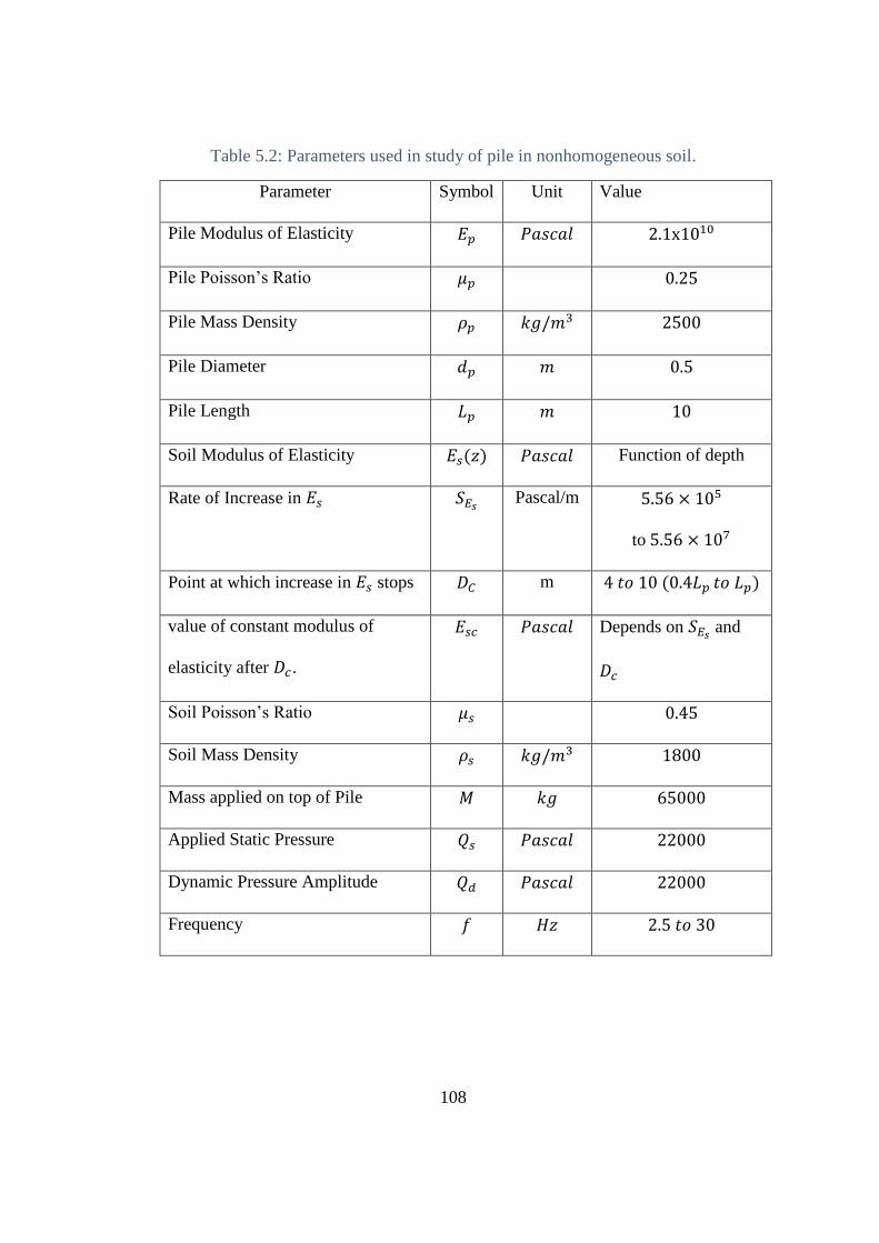
108
Table 5.2: Parameters used in study of pile in nonhomogeneous soil.
Parameter Symbol Unit Value
Pile Modulus of Elasticity 𝐸𝑝 𝑃𝑎𝑠𝑐𝑎𝑙 2.1x10¹⁰
Pile Poisson’s Ratio 𝜇𝑝 0.25
Pile Mass Density 𝜌𝑝 𝑘𝑔/𝑚3 2500
Pile Diameter 𝑑𝑝 𝑚 0.5
Pile Length 𝐿𝑝 𝑚 10
Soil Modulus of Elasticity 𝐸𝑠(𝑧) 𝑃𝑎𝑠𝑐𝑎𝑙 Function of depth
Rate of Increase in 𝐸𝑠 𝑆𝐸𝑠 Pascal/m 5.56 × 10⁵
to 5.56 × 10⁷
Point at which increase in 𝐸𝑠 stops 𝐷𝐶 m 4 𝑡𝑜 10 (0.4𝐿𝑝 𝑡𝑜 𝐿𝑝)
value of constant modulus of
elasticity after 𝐷𝑐.
𝐸𝑠𝑐 𝑃𝑎𝑠𝑐𝑎𝑙 Depends on 𝑆𝐸𝑠 and
𝐷𝑐
Soil Poisson’s Ratio 𝜇𝑠 0.45
Soil Mass Density 𝜌𝑠 𝑘𝑔/𝑚3 1800
Mass applied on top of Pile 𝑀 𝑘𝑔 65000
Applied Static Pressure 𝑄𝑠 𝑃𝑎𝑠𝑐𝑎𝑙 22000
Dynamic Pressure Amplitude 𝑄𝑑 𝑃𝑎𝑠𝑐𝑎𝑙 22000
Frequency 𝑓 𝐻𝑧 2.5 𝑡𝑜 30
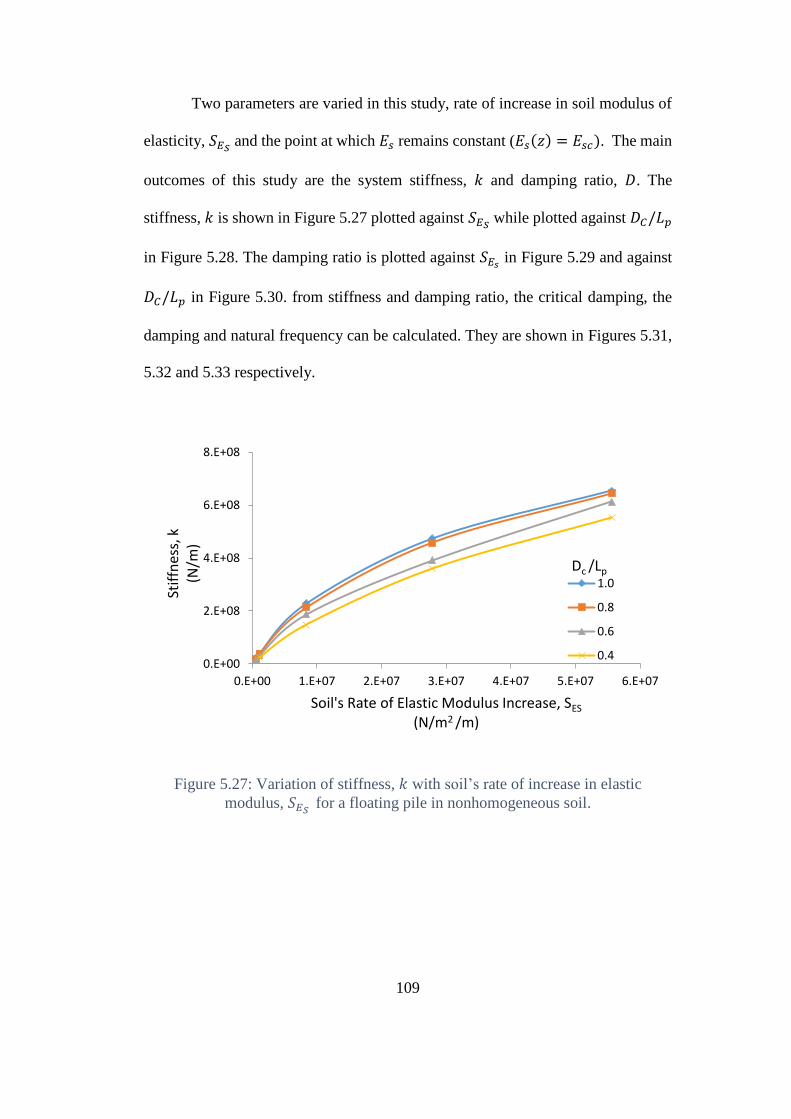
109
Two parameters are varied in this study, rate of increase in soil modulus of
elasticity, 𝑆𝐸𝑆 and the point at which 𝐸𝑠 remains constant (𝐸𝑠(𝑧) = 𝐸𝑠𝑐). The main
outcomes of this study are the system stiffness, 𝑘 and damping ratio, 𝐷. The
stiffness, 𝑘 is shown in Figure 5.27 plotted against 𝑆𝐸𝑆 while plotted against 𝐷𝐶/𝐿𝑝
in Figure 5.28. The damping ratio is plotted against 𝑆𝐸𝑠 in Figure 5.29 and against
𝐷𝐶/𝐿𝑝 in Figure 5.30. from stiffness and damping ratio, the critical damping, the
damping and natural frequency can be calculated. They are shown in Figures 5.31,
5.32 and 5.33 respectively.
Figure 5.27: Variation of stiffness, 𝑘 with soil’s rate of increase in elastic
modulus, 𝑆𝐸𝑆 for a floating pile in nonhomogeneous soil.
0.E+00
2.E+08
4.E+08
6.E+08
8.E+08
0.E+00 1.E+07 2.E+07 3.E+07 4.E+07 5.E+07 6.E+07
Stif
fnes
s, k
(N/m
)
Soil's Rate of Elastic Modulus Increase, SES
(N/m2 /m)
1.0
0.8
0.6
0.4
Dc /Lp
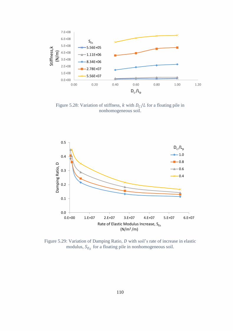
110
Figure 5.28: Variation of stiffness, 𝑘 with 𝐷𝐶/𝐿 for a floating pile in
nonhomogeneous soil.
Figure 5.29: Variation of Damping Ratio, 𝐷 with soil’s rate of increase in elastic
modulus, 𝑆𝐸𝑆 for a floating pile in nonhomogeneous soil.
0.E+00
1.E+08
2.E+08
3.E+08
4.E+08
5.E+08
6.E+08
7.E+08
0.00 0.20 0.40 0.60 0.80 1.00 1.20
Stif
fnes
s,k
(N/m
)
Dc /Lp
5.56E+05
1.11E+06
8.34E+06
2.78E+07
5.56E+07
SEs
0.0
0.1
0.2
0.3
0.4
0.5
0.E+00 1.E+07 2.E+07 3.E+07 4.E+07 5.E+07 6.E+07
Dam
pin
g R
atio
, D
Rate of Elastic Modulus Increase, SEs
(N/m2 /m)
1.0
0.8
0.6
0.4
Dc /Lp
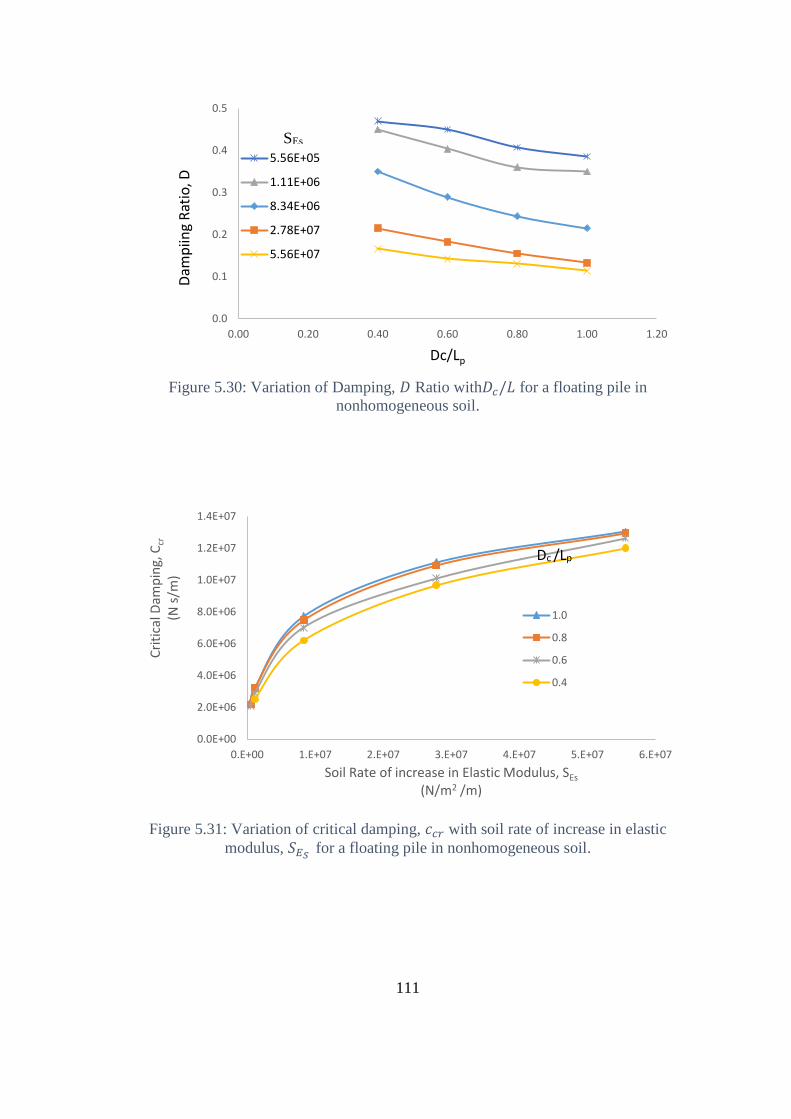
111
Figure 5.30: Variation of Damping, 𝐷 Ratio with𝐷𝑐/𝐿 for a floating pile in
nonhomogeneous soil.
Figure 5.31: Variation of critical damping, 𝑐𝑐𝑟 with soil rate of increase in elastic
modulus, 𝑆𝐸𝑆 for a floating pile in nonhomogeneous soil.
0.0
0.1
0.2
0.3
0.4
0.5
0.00 0.20 0.40 0.60 0.80 1.00 1.20
Dam
piin
g R
atio
, D
Dc/Lp
5.56E+05
1.11E+06
8.34E+06
2.78E+07
5.56E+07
0.0E+00
2.0E+06
4.0E+06
6.0E+06
8.0E+06
1.0E+07
1.2E+07
1.4E+07
0.E+00 1.E+07 2.E+07 3.E+07 4.E+07 5.E+07 6.E+07
Cri
tica
l Dam
pin
g, C
cr
(N s
/m)
Soil Rate of increase in Elastic Modulus, SEs
(N/m2 /m)
1.0
0.8
0.6
0.4
Dc /Lp
SEs
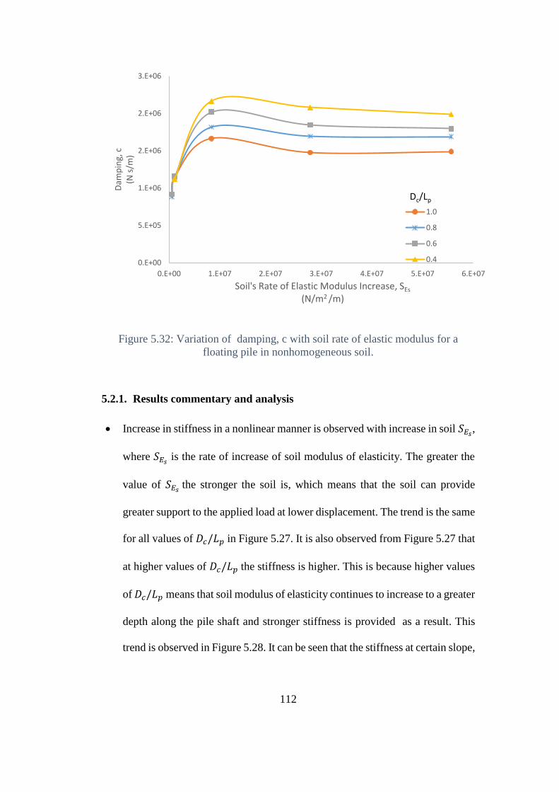
112
Figure 5.32: Variation of damping, c with soil rate of elastic modulus for a
floating pile in nonhomogeneous soil.
5.2.1. Results commentary and analysis
Increase in stiffness in a nonlinear manner is observed with increase in soil 𝑆𝐸𝑠,
where 𝑆𝐸𝑠 is the rate of increase of soil modulus of elasticity. The greater the
value of 𝑆𝐸𝑠 the stronger the soil is, which means that the soil can provide
greater support to the applied load at lower displacement. The trend is the same
for all values of 𝐷𝑐/𝐿𝑝 in Figure 5.27. It is also observed from Figure 5.27 that
at higher values of 𝐷𝑐/𝐿𝑝 the stiffness is higher. This is because higher values
of 𝐷𝑐/𝐿𝑝 means that soil modulus of elasticity continues to increase to a greater
depth along the pile shaft and stronger stiffness is provided as a result. This
trend is observed in Figure 5.28. It can be seen that the stiffness at certain slope,
0.E+00
5.E+05
1.E+06
2.E+06
2.E+06
3.E+06
0.E+00 1.E+07 2.E+07 3.E+07 4.E+07 5.E+07 6.E+07
Dam
pin
g, c
(N s
/m)
Soil's Rate of Elastic Modulus Increase, SEs
(N/m2 /m)
1.0
0.8
0.6
0.4
Dc/Lp
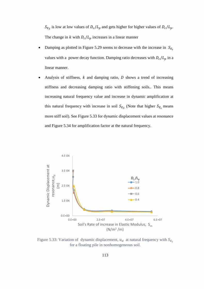
113
𝑆𝐸𝑆 is low at low values of 𝐷𝑐/𝐿𝑝 and gets higher for higher values of 𝐷𝑐/𝐿𝑝.
The change in 𝑘 with 𝐷𝑐/𝐿𝑝 increases in a linear manner
Damping as plotted in Figure 5.29 seems to decrease with the increase in 𝑆𝐸𝑠
values with a power decay function. Damping ratio decreases with 𝐷𝑐/𝐿𝑝 in a
linear manner.
Analysis of stiffness, 𝑘 and damping ratio, 𝐷 shows a trend of increasing
stiffness and decreasing damping ratio with stiffening soils.. This means
increasing natural frequency value and increase in dynamic amplification at
this natural frequency with increase in soil 𝑆𝐸𝑆 (Note that higher 𝑆𝐸𝑠 means
more stiff soil). See Figure 5.33 for dynamic displacement values at resonance
and Figure 5.34 for amplification factor at the natural frequency.
Figure 5.33: Variation of dynamic displacement, 𝑢𝑑 at natural frequency with 𝑆𝐸𝑠
for a floating pile in nonhomogeneous soil.
0.E+00
1.E-04
2.E-04
3.E-04
4.E-04
0.E+00 2.E+07 4.E+07 6.E+07
Dyn
amic
Dis
pla
cem
ent
at
reso
nan
ce,u
d
(m)
Soil's Rate of increase in Elastic Modulus, Svs
(N/m2 /m)
1.0
0.8
0.6
0.4
Dc /Lp
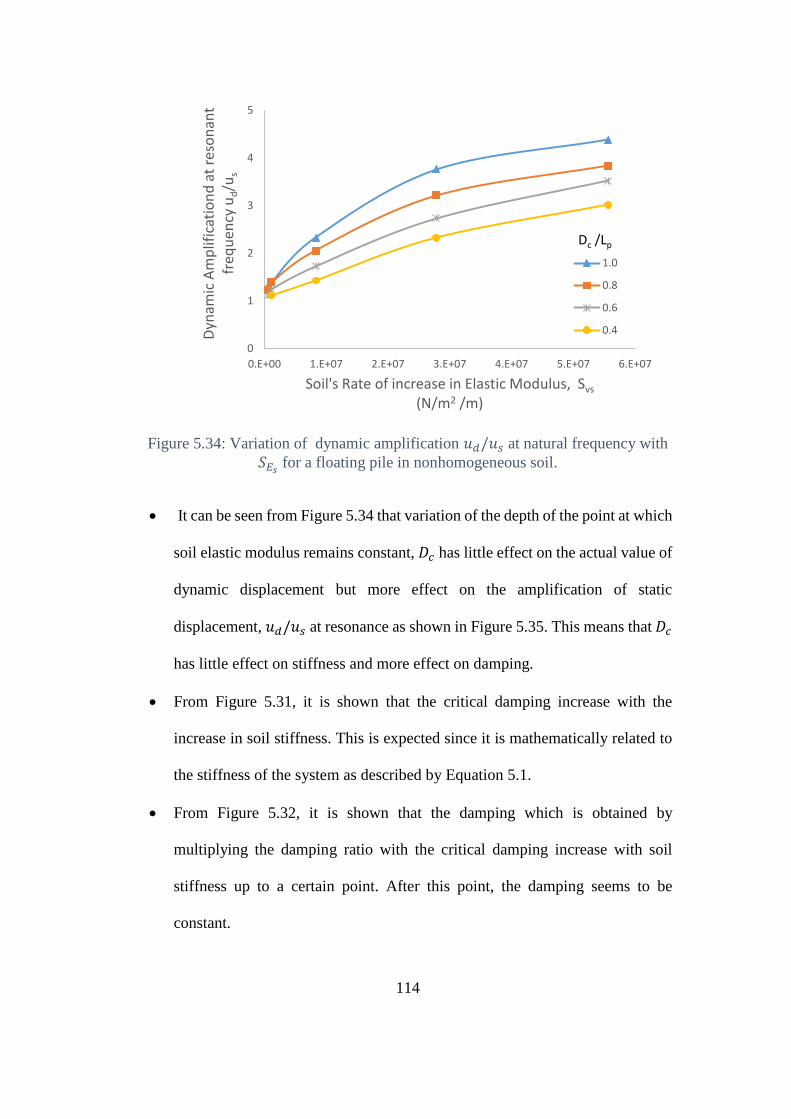
114
Figure 5.34: Variation of dynamic amplification 𝑢𝑑/𝑢𝑠 at natural frequency with
𝑆𝐸𝑠 for a floating pile in nonhomogeneous soil.
It can be seen from Figure 5.34 that variation of the depth of the point at which
soil elastic modulus remains constant, 𝐷𝑐 has little effect on the actual value of
dynamic displacement but more effect on the amplification of static
displacement, 𝑢𝑑/𝑢𝑠 at resonance as shown in Figure 5.35. This means that 𝐷𝑐
has little effect on stiffness and more effect on damping.
From Figure 5.31, it is shown that the critical damping increase with the
increase in soil stiffness. This is expected since it is mathematically related to
the stiffness of the system as described by Equation 5.1.
From Figure 5.32, it is shown that the damping which is obtained by
multiplying the damping ratio with the critical damping increase with soil
stiffness up to a certain point. After this point, the damping seems to be
constant.
0
1
2
3
4
5
0.E+00 1.E+07 2.E+07 3.E+07 4.E+07 5.E+07 6.E+07
Dyn
amic
Am
plif
icat
ion
d a
t re
son
ant
freq
uen
cy u
d/u
s
Soil's Rate of increase in Elastic Modulus, Svs
(N/m2 /m)
1.0
0.8
0.6
0.4
Dc /Lp
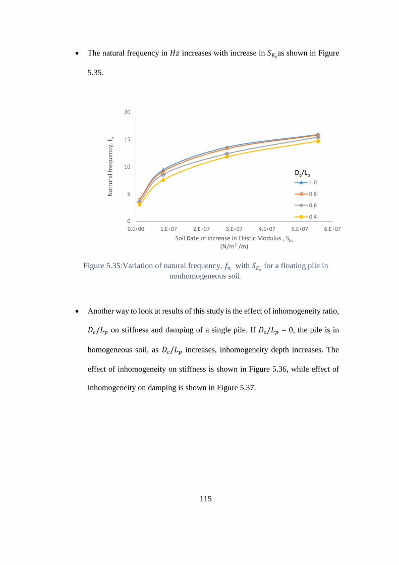
115
The natural frequency in 𝐻𝑧 increases with increase in 𝑆𝐸𝑠as shown in Figure
5.35.
Figure 5.35:Variation of natural frequency, 𝑓𝑛 with 𝑆𝐸𝑠 for a floating pile in
nonhomogeneous soil.
Another way to look at results of this study is the effect of inhomogeneity ratio,
𝐷𝑐/𝐿𝑝 on stiffness and damping of a single pile. If 𝐷𝑐/𝐿𝑝 = 0, the pile is in
homogeneous soil, as 𝐷𝑐/𝐿𝑝 increases, inhomogeneity depth increases. The
effect of inhomogeneity on stiffness is shown in Figure 5.36, while effect of
inhomogeneity on damping is shown in Figure 5.37.
0
5
10
15
20
0.E+00 1.E+07 2.E+07 3.E+07 4.E+07 5.E+07 6.E+07
Nat
rura
l fre
qu
ency
, fn
Soil Rate of increase in Elastic Modulus , SEs
(N/m2 /m)
1.0
0.8
0.6
0.4
Dc/Lp
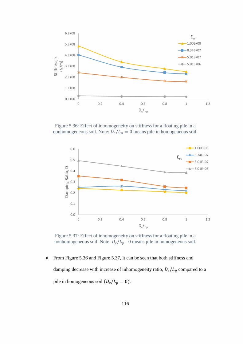
116
Figure 5.36: Effect of inhomogeneity on stiffness for a floating pile in a
nonhomogeneous soil. Note: 𝐷𝑐/𝐿𝑝 = 0 means pile in homogeneous soil.
Figure 5.37: Effect of inhomogeneity on stiffness for a floating pile in a
nonhomogeneous soil. Note: 𝐷𝑐/𝐿𝑝= 0 means pile in homogeneous soil.
From Figure 5.36 and Figure 5.37, it can be seen that both stiffness and
damping decrease with increase of inhomogeneity ratio, 𝐷𝑐/𝐿𝑝 compared to a
pile in homogeneous soil (𝐷𝑐/𝐿𝑝 = 0).
0.E+00
1.E+08
2.E+08
3.E+08
4.E+08
5.E+08
6.E+08
0 0.2 0.4 0.6 0.8 1 1.2
Stif
fnes
s, k
(N/m
)
Dc/Lp
1.00E+08
8.34E+07
5.01E+07
5.01E+06
Esc
0.0
0.1
0.2
0.3
0.4
0.5
0.6
0 0.2 0.4 0.6 0.8 1 1.2
Dam
pin
g R
atio
, D
Dc/Lp
1.00E+08
8.34E+07
5.01E+07
5.01E+06
Esc
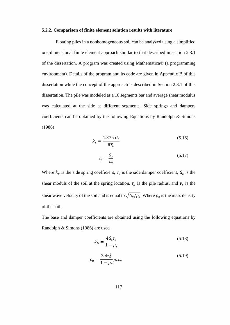
117
5.2.2. Comparison of finite element solution results with literature
Floating piles in a nonhomogeneous soil can be analyzed using a simplified
one-dimensional finite element approach similar to that described in section 2.3.1
of the dissertation. A program was created using Mathematica® (a programming
environment). Details of the program and its code are given in Appendix B of this
dissertation while the concept of the approach is described in Section 2.3.1 of this
dissertation. The pile was modeled as a 10 segments bar and average shear modulus
was calculated at the side at different segments. Side springs and dampers
coefficients can be obtained by the following Equations by Randolph & Simons
(1986)
𝑘𝑠 =1.375 𝐺𝑠
𝜋𝑟𝑝
(5.16)
𝑐𝑠 =𝐺𝑠
𝑣𝑠
(5.17)
Where 𝑘𝑠 is the side spring coefficient, 𝑐𝑠 is the side damper coefficient, 𝐺𝑠 is the
shear moduls of the soil at the spring location, 𝑟𝑝 is the pile radius, and 𝑣𝑠 is the
shear wave velocity of the soil and is equal to √𝐺𝑠/𝜌𝑠. Where 𝜌𝑠 is the mass density
of the soil.
The base and damper coefficients are obtained using the following equations by
Randolph & Simons (1986) are used
𝑘𝑏 =4𝐺𝑠𝑟𝑝
1 − 𝜇𝑠
(5.18)
𝑐𝑏 =3.4𝑟𝑝
2
1 − 𝜇𝑠𝜌𝑠𝑣𝑠
(5.19)
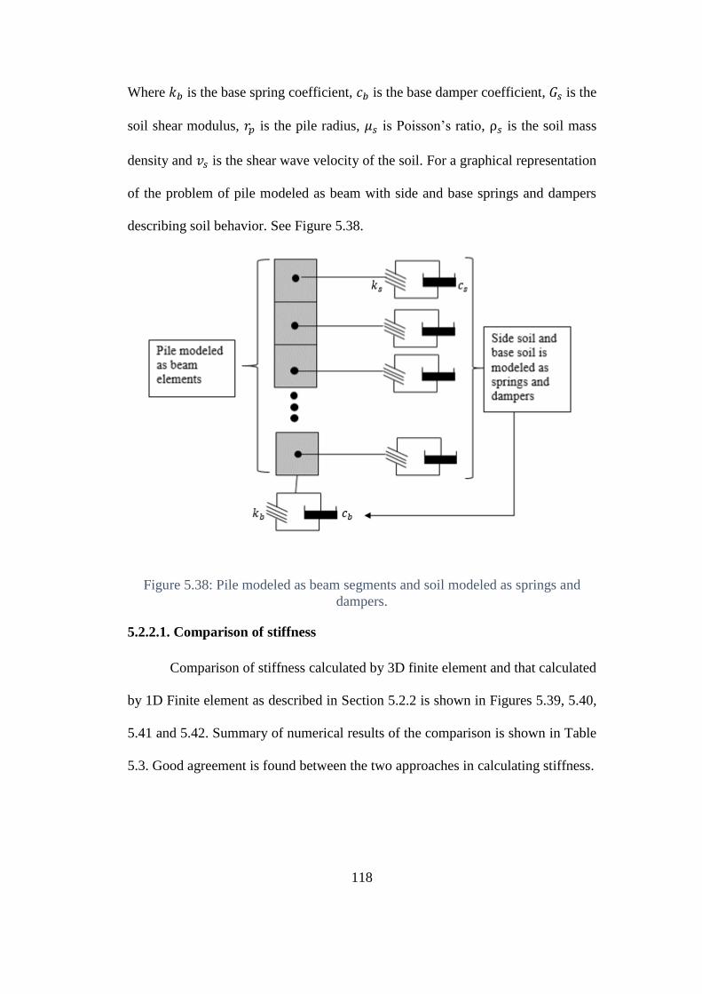
118
Where 𝑘𝑏 is the base spring coefficient, 𝑐𝑏 is the base damper coefficient, 𝐺𝑠 is the
soil shear modulus, 𝑟𝑝 is the pile radius, 𝜇𝑠 is Poisson’s ratio, ρ𝑠 is the soil mass
density and 𝑣𝑠 is the shear wave velocity of the soil. For a graphical representation
of the problem of pile modeled as beam with side and base springs and dampers
describing soil behavior. See Figure 5.38.
Figure 5.38: Pile modeled as beam segments and soil modeled as springs and
dampers.
5.2.2.1. Comparison of stiffness
Comparison of stiffness calculated by 3D finite element and that calculated
by 1D Finite element as described in Section 5.2.2 is shown in Figures 5.39, 5.40,
5.41 and 5.42. Summary of numerical results of the comparison is shown in Table
5.3. Good agreement is found between the two approaches in calculating stiffness.
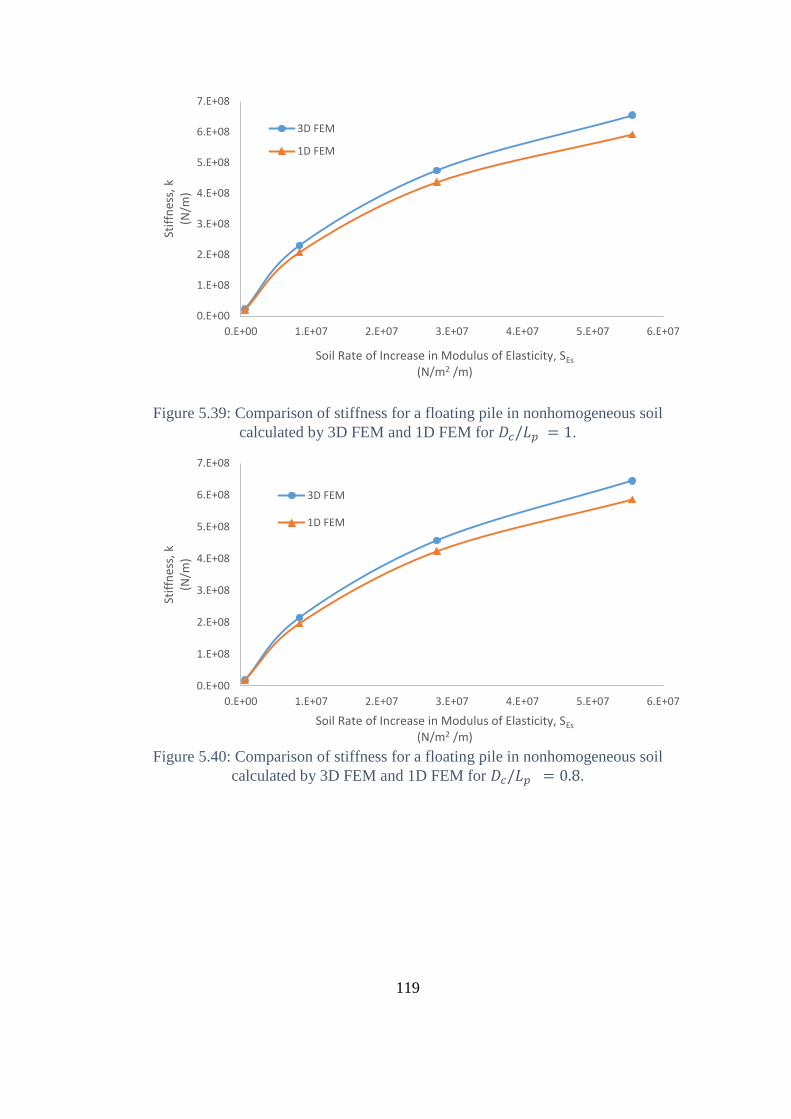
119
Figure 5.39: Comparison of stiffness for a floating pile in nonhomogeneous soil
calculated by 3D FEM and 1D FEM for 𝐷𝑐/𝐿𝑝 = 1.
Figure 5.40: Comparison of stiffness for a floating pile in nonhomogeneous soil
calculated by 3D FEM and 1D FEM for 𝐷𝑐/𝐿𝑝 = 0.8.
0.E+00
1.E+08
2.E+08
3.E+08
4.E+08
5.E+08
6.E+08
7.E+08
0.E+00 1.E+07 2.E+07 3.E+07 4.E+07 5.E+07 6.E+07
Stif
fnes
s, k
(N/m
)
Soil Rate of Increase in Modulus of Elasticity, SEs
(N/m2 /m)
3D FEM
1D FEM
0.E+00
1.E+08
2.E+08
3.E+08
4.E+08
5.E+08
6.E+08
7.E+08
0.E+00 1.E+07 2.E+07 3.E+07 4.E+07 5.E+07 6.E+07
Stif
fnes
s, k
(N/m
)
Soil Rate of Increase in Modulus of Elasticity, SEs
(N/m2 /m)
3D FEM
1D FEM
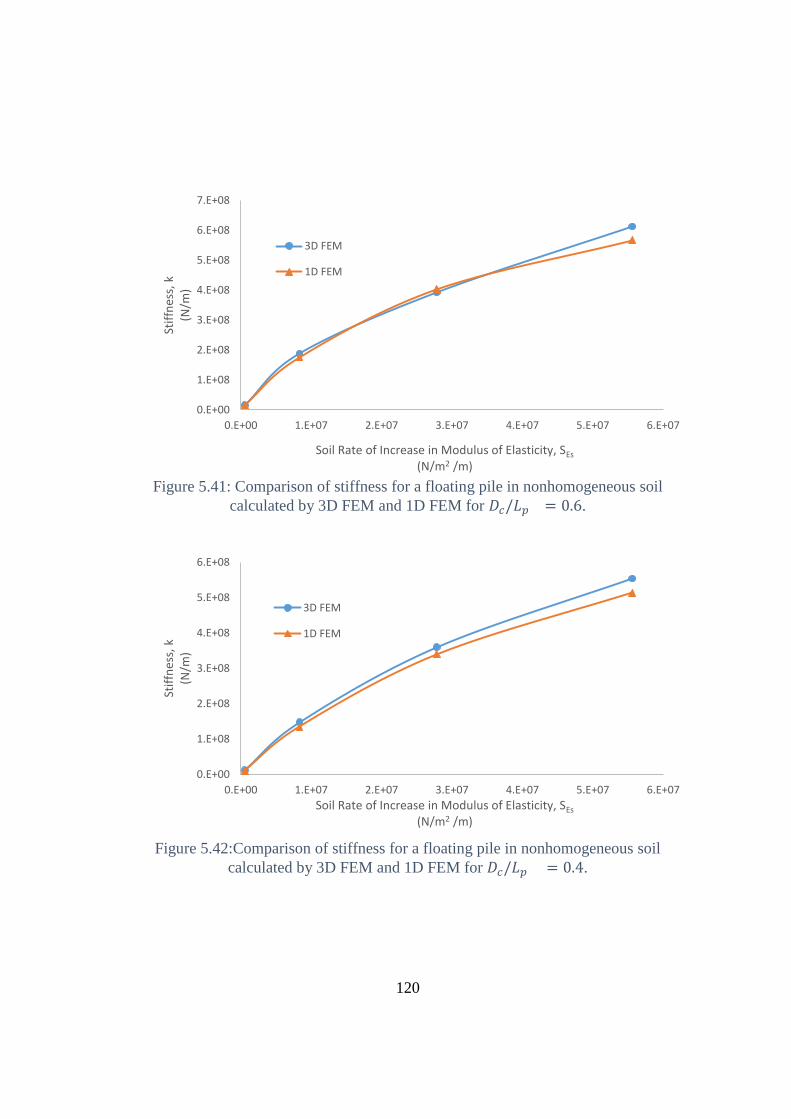
120
Figure 5.41: Comparison of stiffness for a floating pile in nonhomogeneous soil
calculated by 3D FEM and 1D FEM for 𝐷𝑐/𝐿𝑝 = 0.6.
Figure 5.42:Comparison of stiffness for a floating pile in nonhomogeneous soil
calculated by 3D FEM and 1D FEM for 𝐷𝑐/𝐿𝑝 = 0.4.
0.E+00
1.E+08
2.E+08
3.E+08
4.E+08
5.E+08
6.E+08
7.E+08
0.E+00 1.E+07 2.E+07 3.E+07 4.E+07 5.E+07 6.E+07
Stif
fnes
s, k
(N/m
)
Soil Rate of Increase in Modulus of Elasticity, SEs
(N/m2 /m)
3D FEM
1D FEM
0.E+00
1.E+08
2.E+08
3.E+08
4.E+08
5.E+08
6.E+08
0.E+00 1.E+07 2.E+07 3.E+07 4.E+07 5.E+07 6.E+07
Stif
fnes
s, k
(N/m
)
Soil Rate of Increase in Modulus of Elasticity, SEs
(N/m2 /m)
3D FEM
1D FEM
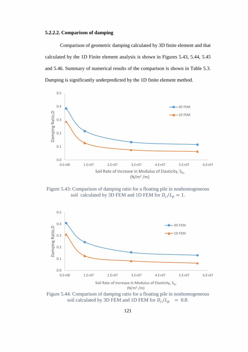
121
5.2.2.2. Comparison of damping
Comparison of geometric damping calculated by 3D finite element and that
calculated by the 1D Finite element analysis is shown in Figures 5.43, 5.44, 5.45
and 5.46. Summary of numerical results of the comparison is shown in Table 5.3.
Damping is significantly underpredicted by the 1D finite element method.
Figure 5.43: Comparison of damping ratio for a floating pile in nonhomogeneous
soil calculated by 3D FEM and 1D FEM for 𝐷𝑐/𝐿𝑝 = 1.
Figure 5.44: Comparison of damping ratio for a floating pile in nonhomogeneous
soil calculated by 3D FEM and 1D FEM for 𝐷𝑐/𝐿𝑝 = 0.8.
0.0
0.1
0.2
0.3
0.4
0.5
0.E+00 1.E+07 2.E+07 3.E+07 4.E+07 5.E+07 6.E+07
Dam
pin
g R
atio
,D
Soil Rate of Increase in Modulus of Elasticity, SEs
(N/m2 /m)
3D FEM
1D FEM
0.0
0.1
0.2
0.3
0.4
0.5
0.E+00 1.E+07 2.E+07 3.E+07 4.E+07 5.E+07 6.E+07
Dam
pin
g R
atio
,D
Soil Rate of Increase in Modulus of Elasticity, SEs
(N/m2 /m)
3D FEM
1D FEM
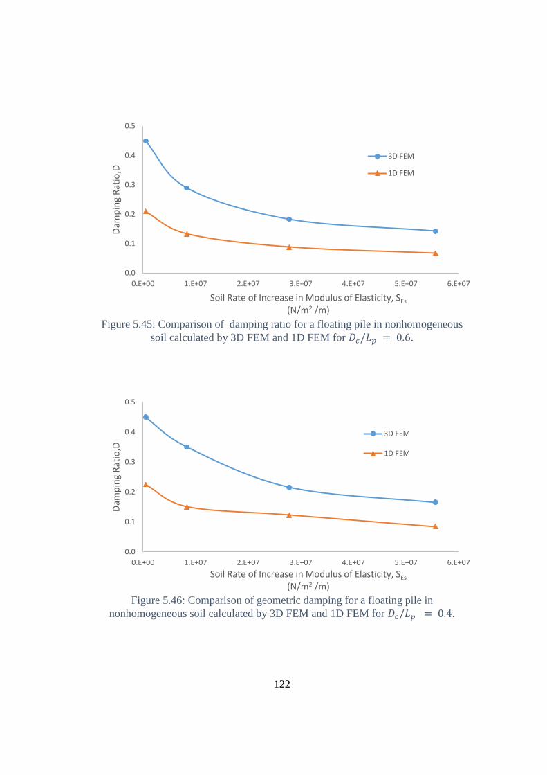
122
Figure 5.45: Comparison of damping ratio for a floating pile in nonhomogeneous
soil calculated by 3D FEM and 1D FEM for 𝐷𝑐/𝐿𝑝 = 0.6.
Figure 5.46: Comparison of geometric damping for a floating pile in
nonhomogeneous soil calculated by 3D FEM and 1D FEM for 𝐷𝑐/𝐿𝑝 = 0.4.
0.0
0.1
0.2
0.3
0.4
0.5
0.E+00 1.E+07 2.E+07 3.E+07 4.E+07 5.E+07 6.E+07
Dam
pin
g R
atio
,D
Soil Rate of Increase in Modulus of Elasticity, SEs
(N/m2 /m)
3D FEM
1D FEM
0.0
0.1
0.2
0.3
0.4
0.5
0.E+00 1.E+07 2.E+07 3.E+07 4.E+07 5.E+07 6.E+07
Dam
pin
g R
atio
,D
Soil Rate of Increase in Modulus of Elasticity, SEs
(N/m2 /m)
3D FEM
1D FEM
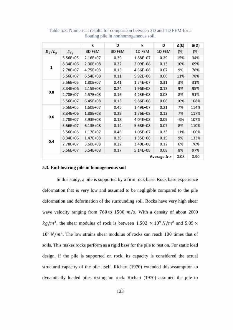
123
Table 5.3: Numerical results for comparison between 3D and 1D FEM for a
floating pile in nonhomogeneous soil.
k D k D Δ(k) Δ(D)
𝑫𝑪/𝑳𝒑 𝑆𝐸𝑆 3D FEM 3D FEM 1D FEM 1D FEM (%) (%)
1
5.56E+05 2.16E+07 0.39 1.88E+07 0.29 15% 34%
8.34E+06 2.30E+08 0.22 2.09E+08 0.13 10% 69%
2.78E+07 4.75E+08 0.13 4.36E+08 0.07 9% 78%
5.56E+07 6.54E+08 0.11 5.92E+08 0.06 11% 78%
0.8
5.56E+05 1.80E+07 0.41 1.74E+07 0.31 3% 31%
8.34E+06 2.15E+08 0.24 1.96E+08 0.13 9% 95%
2.78E+07 4.57E+08 0.16 4.23E+08 0.08 8% 91%
5.56E+07 6.45E+08 0.13 5.86E+08 0.06 10% 108%
0.6
5.56E+05 1.60E+07 0.45 1.49E+07 0.21 7% 114%
8.34E+06 1.88E+08 0.29 1.76E+08 0.13 7% 117%
2.78E+07 3.93E+08 0.18 4.04E+08 0.09 -3% 107%
5.56E+07 6.13E+08 0.14 5.68E+08 0.07 8% 110%
0.4
5.56E+05 1.17E+07 0.45 1.05E+07 0.23 11% 100%
8.34E+06 1.47E+08 0.35 1.35E+08 0.15 9% 133%
2.78E+07 3.60E+08 0.22 3.40E+08 0.12 6% 76%
5.56E+07 5.54E+08 0.17 5.14E+08 0.08 8% 97%
Average Δ-> 0.08 0.90
5.3. End-bearing pile in homogeneous soil
In this study, a pile is supported by a firm rock base. Rock base experience
deformation that is very low and assumed to be negligible compared to the pile
deformation and deformation of the surrounding soil. Rocks have very high shear
wave velocity ranging from 760 to 1500 𝑚/𝑠. With a density of about 2600
𝑘𝑔/𝑚3, the shear modulus of rock is between 1.502 × 10⁹ 𝑁/𝑚2 and 5.85 ×
109 𝑁/𝑚2. The low strains shear modulus of rocks can reach 100 times that of
soils. This makes rocks perform as a rigid base for the pile to rest on. For static load
design, if the pile is supported on rock, its capacity is considered the actual
structural capacity of the pile itself. Richart (1970) extended this assumption to
dynamically loaded piles resting on rock. Richart (1970) assumed the pile to
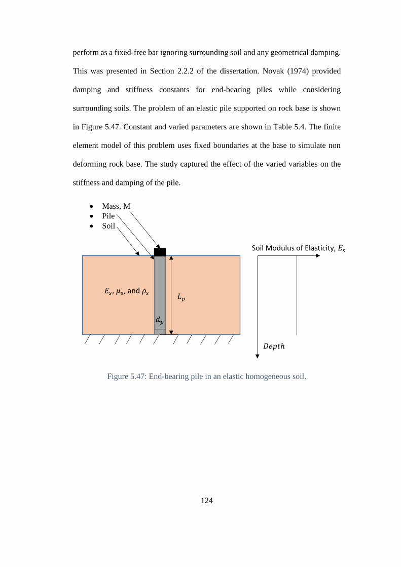
124
perform as a fixed-free bar ignoring surrounding soil and any geometrical damping.
This was presented in Section 2.2.2 of the dissertation. Novak (1974) provided
damping and stiffness constants for end-bearing piles while considering
surrounding soils. The problem of an elastic pile supported on rock base is shown
in Figure 5.47. Constant and varied parameters are shown in Table 5.4. The finite
element model of this problem uses fixed boundaries at the base to simulate non
deforming rock base. The study captured the effect of the varied variables on the
stiffness and damping of the pile.
Figure 5.47: End-bearing pile in an elastic homogeneous soil.
Soil Modulus of Elasticity, 𝐸𝑠
𝐷𝑒𝑝𝑡ℎ
Mass, M
Pile
Soil
𝑑𝑝
𝐿𝑝 𝐸𝑠, 𝜇𝑠, and 𝜌𝑠
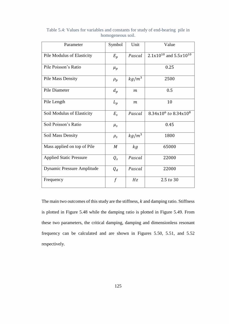
125
Table 5.4: Values for variables and constants for study of end-bearing pile in
homogeneous soil.
Parameter Symbol Unit Value
Pile Modulus of Elasticity 𝐸𝑝 𝑃𝑎𝑠𝑐𝑎𝑙 2.1x10¹⁰ and 5.5𝑥1010
Pile Poisson’s Ratio 𝜇𝑝 0.25
Pile Mass Density 𝜌𝑝 𝑘𝑔/𝑚3 2500
Pile Diameter 𝑑𝑝 𝑚 0.5
Pile Length 𝐿𝑝 𝑚 10
Soil Modulus of Elasticity 𝐸𝑠 𝑃𝑎𝑠𝑐𝑎𝑙 8.34x10⁶ 𝑡𝑜 8.34x10⁸
Soil Poisson’s Ratio 𝜇𝑠 0.45
Soil Mass Density 𝜌𝑠 𝑘𝑔/𝑚3 1800
Mass applied on top of Pile 𝑀 𝑘𝑔 65000
Applied Static Pressure 𝑄𝑠 𝑃𝑎𝑠𝑐𝑎𝑙 22000
Dynamic Pressure Amplitude 𝑄𝑑 𝑃𝑎𝑠𝑐𝑎𝑙 22000
Frequency 𝑓 𝐻𝑧 2.5 𝑡𝑜 30
The main two outcomes of this study are the stiffness, 𝑘 and damping ratio. Stiffness
is plotted in Figure 5.48 while the damping ratio is plotted in Figure 5.49. From
these two parameters, the critical damping, damping and dimensionless resonant
frequency can be calculated and are shown in Figures 5.50, 5.51, and 5.52
respectively.
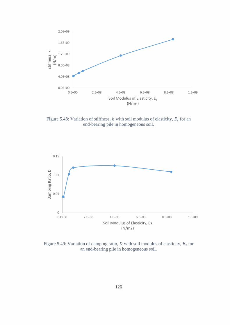
126
Figure 5.48: Variation of stiffness, 𝑘 with soil modulus of elasticity, 𝐸𝑠 for an
end-bearing pile in homogeneous soil.
Figure 5.49: Variation of damping ratio, 𝐷 with soil modulus of elasticity, 𝐸𝑠 for
an end-bearing pile in homogeneous soil.
0.0E+00
4.0E+08
8.0E+08
1.2E+09
1.6E+09
2.0E+09
0.E+00 2.E+08 4.E+08 6.E+08 8.E+08 1.E+09
stif
fnes
s, k
(N/m
)
Soil Modulus of Elasticity, Es
(N/m2)
0
0.05
0.1
0.15
0.E+00 2.E+08 4.E+08 6.E+08 8.E+08 1.E+09
Dam
pin
g R
atio
, D
Soil Modulus of Elasticity, Es(N/m2)
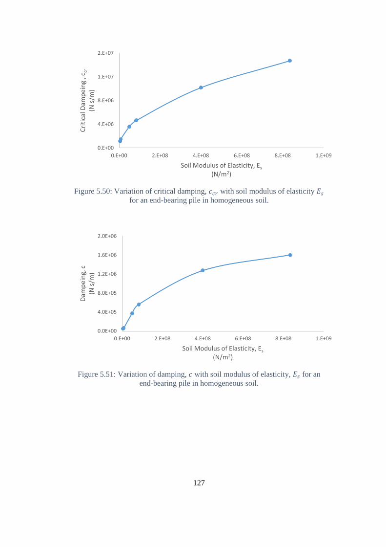
127
Figure 5.50: Variation of critical damping, 𝑐𝑐𝑟 with soil modulus of elasticity 𝐸𝑠
for an end-bearing pile in homogeneous soil.
Figure 5.51: Variation of damping, 𝑐 with soil modulus of elasticity, 𝐸𝑠 for an
end-bearing pile in homogeneous soil.
0.E+00
4.E+06
8.E+06
1.E+07
2.E+07
0.E+00 2.E+08 4.E+08 6.E+08 8.E+08 1.E+09
Cri
tica
l Dam
pei
ng
, ccr
(N s
/m)
Soil Modulus of Elasticity, Es
(N/m2)
0.0E+00
4.0E+05
8.0E+05
1.2E+06
1.6E+06
2.0E+06
0.E+00 2.E+08 4.E+08 6.E+08 8.E+08 1.E+09
Dam
pei
ng,
c(N
s/m
)
Soil Modulus of Elasticity, Es
(N/m2)
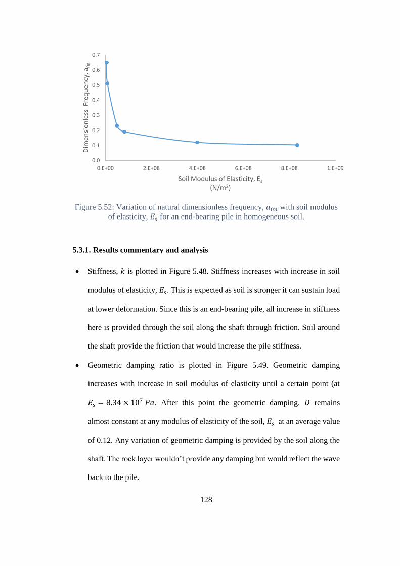
128
Figure 5.52: Variation of natural dimensionless frequency, 𝑎0𝑛 with soil modulus
of elasticity, 𝐸𝑠 for an end-bearing pile in homogeneous soil.
5.3.1. Results commentary and analysis
Stiffness, 𝑘 is plotted in Figure 5.48. Stiffness increases with increase in soil
modulus of elasticity, 𝐸𝑠. This is expected as soil is stronger it can sustain load
at lower deformation. Since this is an end-bearing pile, all increase in stiffness
here is provided through the soil along the shaft through friction. Soil around
the shaft provide the friction that would increase the pile stiffness.
Geometric damping ratio is plotted in Figure 5.49. Geometric damping
increases with increase in soil modulus of elasticity until a certain point (at
𝐸𝑠 = 8.34 × 10⁷ 𝑃𝑎. After this point the geometric damping, 𝐷 remains
almost constant at any modulus of elasticity of the soil, 𝐸𝑠 at an average value
of 0.12. Any variation of geometric damping is provided by the soil along the
shaft. The rock layer wouldn’t provide any damping but would reflect the wave
back to the pile.
0.0
0.1
0.2
0.3
0.4
0.5
0.6
0.7
0.E+00 2.E+08 4.E+08 6.E+08 8.E+08 1.E+09
Dim
ensi
on
less
Fre
qu
ency
, a0
n
Soil Modulus of Elasticity, Es
(N/m2)
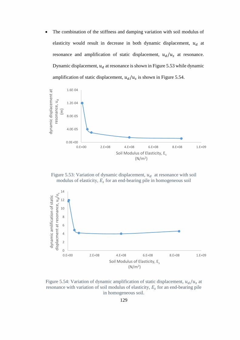
129
The combination of the stiffness and damping variation with soil modulus of
elasticity would result in decrease in both dynamic displacement, 𝑢𝑑 at
resonance and amplification of static displacement, 𝑢𝑑/𝑢𝑠 at resonance.
Dynamic displacement, 𝑢𝑑 at resonance is shown in Figure 5.53 while dynamic
amplification of static displacement, 𝑢𝑑/𝑢𝑠 is shown in Figure 5.54.
Figure 5.53: Variation of dynamic displacement, 𝑢𝑑 at resonance with soil
modulus of elasticity, 𝐸𝑠 for an end-bearing pile in homogeneous soil
Figure 5.54: Variation of dynamic amplification of static displacement, 𝑢𝑑/𝑢𝑠 at
resonance with variation of soil modulus of elasticity, 𝐸𝑠 for an end-bearing pile
in homogeneous soil.
0.0E+00
4.0E-05
8.0E-05
1.2E-04
1.6E-04
0.E+00 2.E+08 4.E+08 6.E+08 8.E+08 1.E+09
dyn
amic
dis
pla
cem
ent
at
reso
nan
ce, u
d
(m)
Soil Modulus of Elasticity, Es
(N/m2)
0
2
4
6
8
10
12
14
0.E+00 2.E+08 4.E+08 6.E+08 8.E+08 1.E+09
dyn
amic
am
lific
atio
n o
f st
atic
d
isp
lacm
ent
at r
eso
nan
ce, u
d/u
s
Soil Modulus of Elasticity, Es
(N/m2)
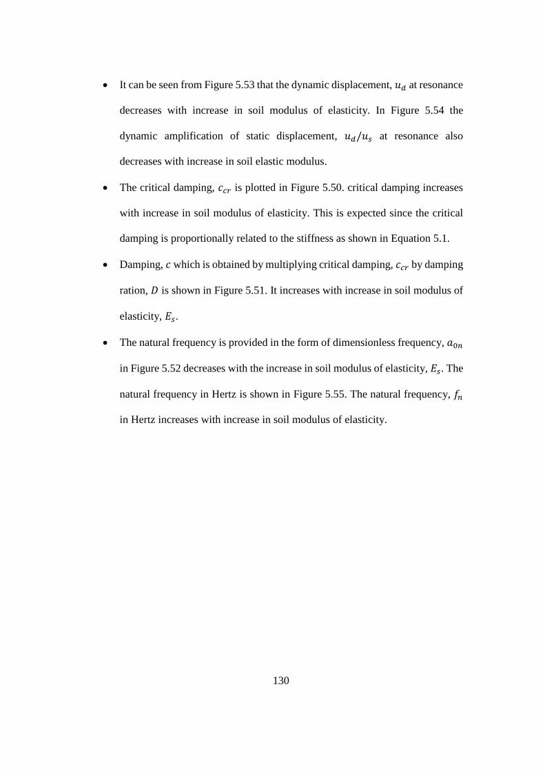
130
It can be seen from Figure 5.53 that the dynamic displacement, 𝑢𝑑 at resonance
decreases with increase in soil modulus of elasticity. In Figure 5.54 the
dynamic amplification of static displacement, 𝑢𝑑/𝑢𝑠 at resonance also
decreases with increase in soil elastic modulus.
The critical damping, 𝑐𝑐𝑟 is plotted in Figure 5.50. critical damping increases
with increase in soil modulus of elasticity. This is expected since the critical
damping is proportionally related to the stiffness as shown in Equation 5.1.
Damping, 𝑐 which is obtained by multiplying critical damping, 𝑐𝑐𝑟 by damping
ration, 𝐷 is shown in Figure 5.51. It increases with increase in soil modulus of
elasticity, 𝐸𝑠.
The natural frequency is provided in the form of dimensionless frequency, 𝑎0𝑛
in Figure 5.52 decreases with the increase in soil modulus of elasticity, 𝐸𝑠. The
natural frequency in Hertz is shown in Figure 5.55. The natural frequency, 𝑓𝑛
in Hertz increases with increase in soil modulus of elasticity.
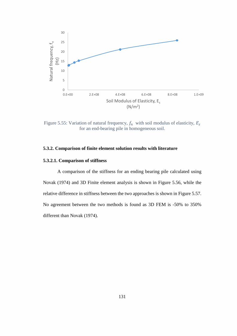
131
Figure 5.55: Variation of natural frequency, 𝑓𝑛 with soil modulus of elasticity, 𝐸𝑠
for an end-bearing pile in homogeneous soil.
5.3.2. Comparison of finite element solution results with literature
5.3.2.1. Comparison of stiffness
A comparison of the stiffness for an ending bearing pile calculated using
Novak (1974) and 3D Finite element analysis is shown in Figure 5.56, while the
relative difference in stiffness between the two approaches is shown in Figure 5.57.
No agreement between the two methods is found as 3D FEM is -50% to 350%
different than Novak (1974).
0
5
10
15
20
25
30
0.E+00 2.E+08 4.E+08 6.E+08 8.E+08 1.E+09
Nat
ura
l fre
qu
ency
, fn
(Hz)
Soil Modulus of Elasticity, Es
(N/m2)
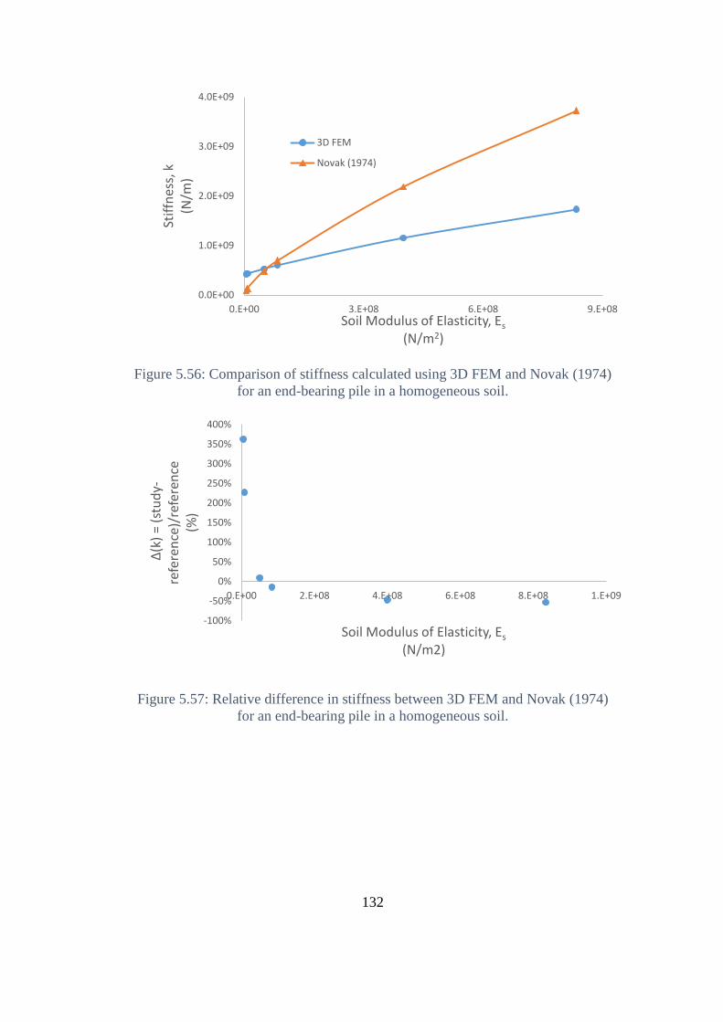
132
Figure 5.56: Comparison of stiffness calculated using 3D FEM and Novak (1974)
for an end-bearing pile in a homogeneous soil.
Figure 5.57: Relative difference in stiffness between 3D FEM and Novak (1974)
for an end-bearing pile in a homogeneous soil.
0.0E+00
1.0E+09
2.0E+09
3.0E+09
4.0E+09
0.E+00 3.E+08 6.E+08 9.E+08
Stif
fnes
s, k
(N/m
)
Soil Modulus of Elasticity, Es
(N/m2)
3D FEM
Novak (1974)
-100%
-50%
0%
50%
100%
150%
200%
250%
300%
350%
400%
0.E+00 2.E+08 4.E+08 6.E+08 8.E+08 1.E+09
Δ(k
) =
(stu
dy-
refe
ren
ce)/
refe
ren
ce(%
)
Soil Modulus of Elasticity, Es
(N/m2)
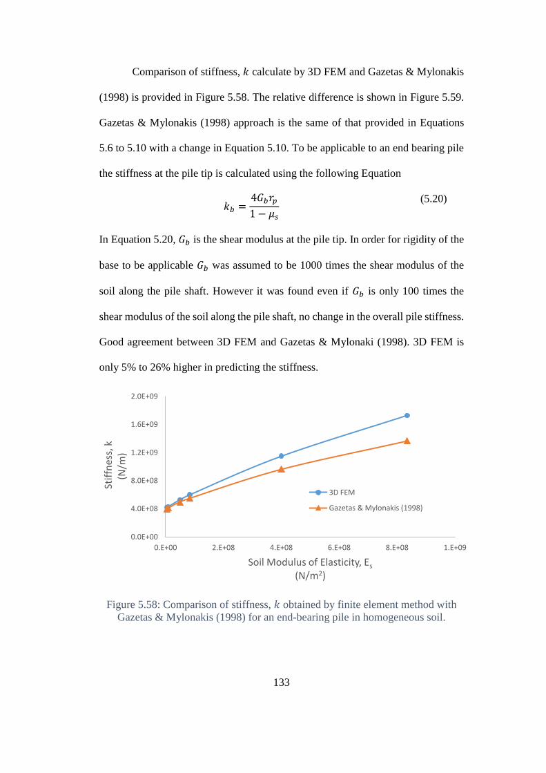
133
Comparison of stiffness, 𝑘 calculate by 3D FEM and Gazetas & Mylonakis
(1998) is provided in Figure 5.58. The relative difference is shown in Figure 5.59.
Gazetas & Mylonakis (1998) approach is the same of that provided in Equations
5.6 to 5.10 with a change in Equation 5.10. To be applicable to an end bearing pile
the stiffness at the pile tip is calculated using the following Equation
𝑘𝑏 =4𝐺𝑏𝑟𝑝
1 − 𝜇𝑠
(5.20)
In Equation 5.20, 𝐺𝑏 is the shear modulus at the pile tip. In order for rigidity of the
base to be applicable 𝐺𝑏 was assumed to be 1000 times the shear modulus of the
soil along the pile shaft. However it was found even if 𝐺𝑏 is only 100 times the
shear modulus of the soil along the pile shaft, no change in the overall pile stiffness.
Good agreement between 3D FEM and Gazetas & Mylonaki (1998). 3D FEM is
only 5% to 26% higher in predicting the stiffness.
Figure 5.58: Comparison of stiffness, 𝑘 obtained by finite element method with
Gazetas & Mylonakis (1998) for an end-bearing pile in homogeneous soil.
0.0E+00
4.0E+08
8.0E+08
1.2E+09
1.6E+09
2.0E+09
0.E+00 2.E+08 4.E+08 6.E+08 8.E+08 1.E+09
Stif
fnes
s, k
(N/m
)
Soil Modulus of Elasticity, Es
(N/m2)
3D FEM
Gazetas & Mylonakis (1998)
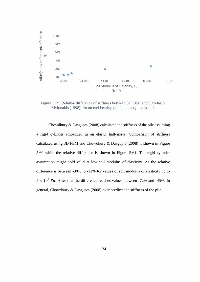
134
Figure 5.59: Relative difference of stiffness between 3D FEM and Gazetas &
Mylonakis (1998), for an end-bearing pile in homogeneous soil.
Chowdhury & Dasgupta (2008) calculated the stiffness of the pile assuming
a rigid cylinder embedded in an elastic half-space. Comparison of stiffness
calculated using 3D FEM and Chowdhury & Dasgupta (2008) is shown in Figure
5.60 while the relative difference is shown in Figure 5.61. The rigid cylinder
assumption might hold valid at low soil modulus of elasticity. As the relative
difference is between -38% to -22% for values of soil modulus of elasticity up to
5 × 10⁷ 𝑃𝑎. After that the difference reaches values between -72% and -45%. In
general, Chowdhury & Dasgupta (2008) over predicts the stiffness of the pile.
0%
20%
40%
60%
80%
100%
0.E+00 2.E+08 4.E+08 6.E+08 8.E+08 1.E+09Δ(k
)=(s
tud
y-re
fere
nce
)/re
fere
nce
(%)
Soil Modulus of Elasticity, Es
(N/m2)
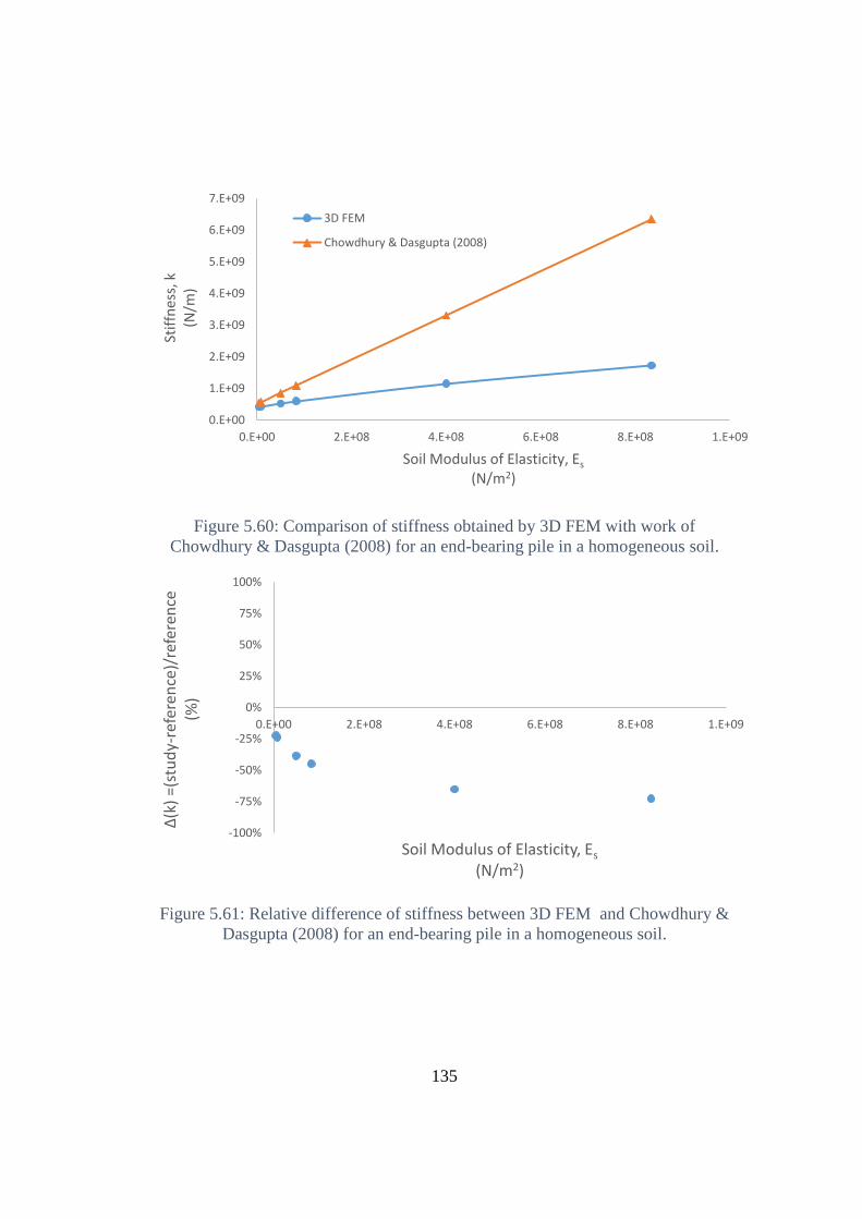
135
Figure 5.60: Comparison of stiffness obtained by 3D FEM with work of
Chowdhury & Dasgupta (2008) for an end-bearing pile in a homogeneous soil.
Figure 5.61: Relative difference of stiffness between 3D FEM and Chowdhury &
Dasgupta (2008) for an end-bearing pile in a homogeneous soil.
0.E+00
1.E+09
2.E+09
3.E+09
4.E+09
5.E+09
6.E+09
7.E+09
0.E+00 2.E+08 4.E+08 6.E+08 8.E+08 1.E+09
Stif
fnes
s, k
(N/m
)
Soil Modulus of Elasticity, Es
(N/m2)
3D FEM
Chowdhury & Dasgupta (2008)
-100%
-75%
-50%
-25%
0%
25%
50%
75%
100%
0.E+00 2.E+08 4.E+08 6.E+08 8.E+08 1.E+09
Δ(k
) =(
stu
dy-
refe
ren
ce)/
refe
ren
ce(%
)
Soil Modulus of Elasticity, Es
(N/m2)
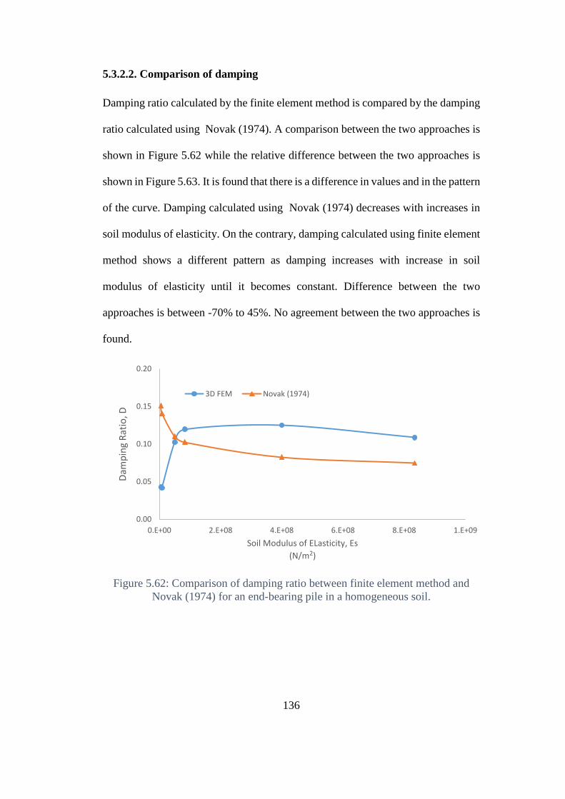
136
5.3.2.2. Comparison of damping
Damping ratio calculated by the finite element method is compared by the damping
ratio calculated using Novak (1974). A comparison between the two approaches is
shown in Figure 5.62 while the relative difference between the two approaches is
shown in Figure 5.63. It is found that there is a difference in values and in the pattern
of the curve. Damping calculated using Novak (1974) decreases with increases in
soil modulus of elasticity. On the contrary, damping calculated using finite element
method shows a different pattern as damping increases with increase in soil
modulus of elasticity until it becomes constant. Difference between the two
approaches is between -70% to 45%. No agreement between the two approaches is
found.
Figure 5.62: Comparison of damping ratio between finite element method and
Novak (1974) for an end-bearing pile in a homogeneous soil.
0.00
0.05
0.10
0.15
0.20
0.E+00 2.E+08 4.E+08 6.E+08 8.E+08 1.E+09
Dam
pin
g R
atio
, D
Soil Modulus of ELasticity, Es
(N/m2)
3D FEM Novak (1974)
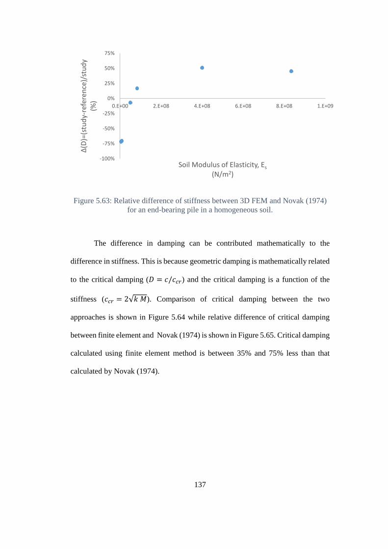
137
Figure 5.63: Relative difference of stiffness between 3D FEM and Novak (1974)
for an end-bearing pile in a homogeneous soil.
The difference in damping can be contributed mathematically to the
difference in stiffness. This is because geometric damping is mathematically related
to the critical damping (𝐷 = 𝑐/𝑐𝑐𝑟) and the critical damping is a function of the
stiffness (𝑐𝑐𝑟 = 2√𝑘 𝑀). Comparison of critical damping between the two
approaches is shown in Figure 5.64 while relative difference of critical damping
between finite element and Novak (1974) is shown in Figure 5.65. Critical damping
calculated using finite element method is between 35% and 75% less than that
calculated by Novak (1974).
-100%
-75%
-50%
-25%
0%
25%
50%
75%
0.E+00 2.E+08 4.E+08 6.E+08 8.E+08 1.E+09
Δ(D
)=(s
tud
y-re
fere
nce
)/st
ud
y(%
)
Soil Modulus of Elasticity, Es
(N/m2)
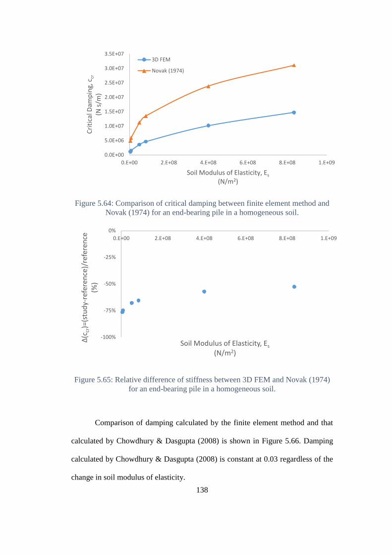
138
Figure 5.64: Comparison of critical damping between finite element method and
Novak (1974) for an end-bearing pile in a homogeneous soil.
Figure 5.65: Relative difference of stiffness between 3D FEM and Novak (1974)
for an end-bearing pile in a homogeneous soil.
Comparison of damping calculated by the finite element method and that
calculated by Chowdhury & Dasgupta (2008) is shown in Figure 5.66. Damping
calculated by Chowdhury & Dasgupta (2008) is constant at 0.03 regardless of the
change in soil modulus of elasticity.
0.0E+00
5.0E+06
1.0E+07
1.5E+07
2.0E+07
2.5E+07
3.0E+07
3.5E+07
0.E+00 2.E+08 4.E+08 6.E+08 8.E+08 1.E+09
Cri
tica
l Dam
pin
g, c
cr
(N s
/m)
Soil Modulus of Elasticity, Es
(N/m2)
3D FEM
Novak (1974)
-100%
-75%
-50%
-25%
0%
0.E+00 2.E+08 4.E+08 6.E+08 8.E+08 1.E+09
Δ(c
cr)=
(stu
dy-
refe
ren
ce)/
refe
ren
ce(%
)
Soil Modulus of Elasticity, Es
(N/m2)
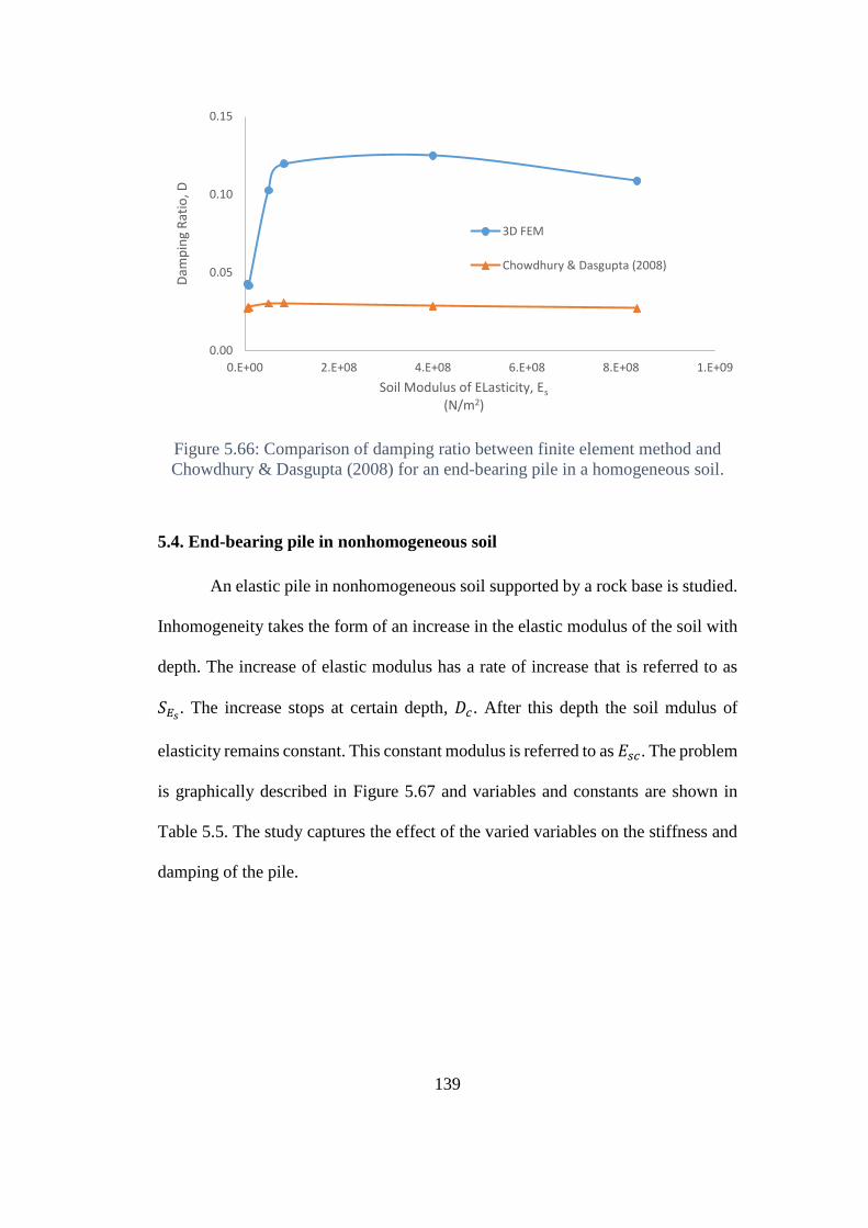
139
Figure 5.66: Comparison of damping ratio between finite element method and
Chowdhury & Dasgupta (2008) for an end-bearing pile in a homogeneous soil.
5.4. End-bearing pile in nonhomogeneous soil
An elastic pile in nonhomogeneous soil supported by a rock base is studied.
Inhomogeneity takes the form of an increase in the elastic modulus of the soil with
depth. The increase of elastic modulus has a rate of increase that is referred to as
𝑆𝐸𝑠. The increase stops at certain depth, 𝐷𝑐. After this depth the soil mdulus of
elasticity remains constant. This constant modulus is referred to as 𝐸𝑠𝑐. The problem
is graphically described in Figure 5.67 and variables and constants are shown in
Table 5.5. The study captures the effect of the varied variables on the stiffness and
damping of the pile.
0.00
0.05
0.10
0.15
0.E+00 2.E+08 4.E+08 6.E+08 8.E+08 1.E+09
Dam
pin
g R
atio
, D
Soil Modulus of ELasticity, Es
(N/m2)
3D FEM
Chowdhury & Dasgupta (2008)
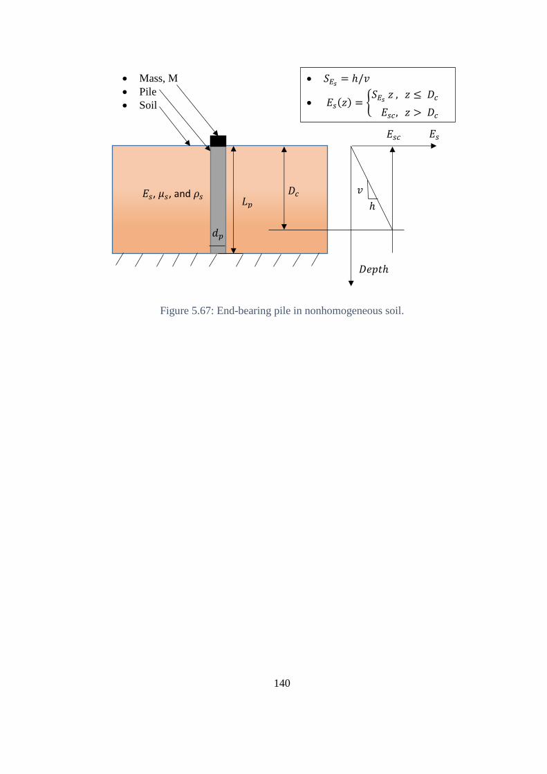
140
Figure 5.67: End-bearing pile in nonhomogeneous soil.
𝐸𝑠
𝐷𝑒𝑝𝑡ℎ
Mass, M
Pile
Soil
𝑑𝑝
𝐿𝑝 𝐸𝑠, 𝜇𝑠, and 𝜌𝑠 𝐷𝑐
𝐸𝑠𝑐
𝑆𝐸𝑠 = ℎ/𝑣
𝐸𝑠(𝑧) = 𝑆𝐸𝑠 𝑧 , 𝑧 ≤ 𝐷𝑐
𝐸𝑠𝑐, 𝑧 > 𝐷𝑐
𝑣
ℎ
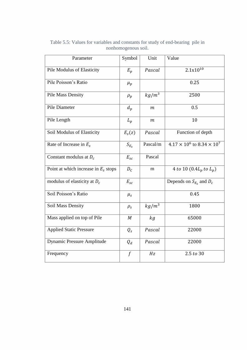
141
Table 5.5: Values for variables and constants for study of end-bearing pile in
nonhomogenous soil.
Parameter Symbol Unit Value
Pile Modulus of Elasticity 𝐸𝑝 𝑃𝑎𝑠𝑐𝑎𝑙 2.1x10¹⁰
Pile Poisson’s Ratio 𝜇𝑝 0.25
Pile Mass Density 𝜌𝑝 𝑘𝑔/𝑚3 2500
Pile Diameter 𝑑𝑝 𝑚 0.5
Pile Length 𝐿𝑝 𝑚 10
Soil Modulus of Elasticity 𝐸𝑠(𝑧) 𝑃𝑎𝑠𝑐𝑎𝑙 Function of depth
Rate of Increase in 𝐸𝑠 𝑆𝐸𝑠 Pascal/m 4.17 × 10⁶ to 8.34 × 10⁷
Constant modulus at 𝐷𝑐 𝐸𝑠𝑐 Pascal
Point at which increase in 𝐸𝑠 stops 𝐷𝐶 m 4 𝑡𝑜 10 (0.4𝐿𝑝 𝑡𝑜 𝐿𝑝)
modulus of elasticity at 𝐷𝑐 𝐸𝑠𝑐 Depends on 𝑆𝐸𝑠 and 𝐷𝑐
Soil Poisson’s Ratio 𝜇𝑠 0.45
Soil Mass Density 𝜌𝑠 𝑘𝑔/𝑚3 1800
Mass applied on top of Pile 𝑀 𝑘𝑔 65000
Applied Static Pressure 𝑄𝑠 𝑃𝑎𝑠𝑐𝑎𝑙 22000
Dynamic Pressure Amplitude 𝑄𝑑 𝑃𝑎𝑠𝑐𝑎𝑙 22000
Frequency 𝑓 𝐻𝑧 2.5 𝑡𝑜 30
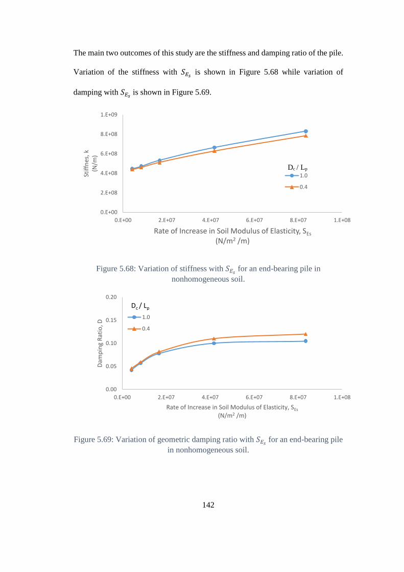
142
The main two outcomes of this study are the stiffness and damping ratio of the pile.
Variation of the stiffness with 𝑆𝐸𝑠 is shown in Figure 5.68 while variation of
damping with 𝑆𝐸𝑠 is shown in Figure 5.69.
Figure 5.68: Variation of stiffness with 𝑆𝐸𝑠 for an end-bearing pile in
nonhomogeneous soil.
Figure 5.69: Variation of geometric damping ratio with 𝑆𝐸𝑠 for an end-bearing pile
in nonhomogeneous soil.
0.E+00
2.E+08
4.E+08
6.E+08
8.E+08
1.E+09
0.E+00 2.E+07 4.E+07 6.E+07 8.E+07 1.E+08
Stif
fnes
, k
(N/m
)
Rate of Increase in Soil Modulus of Elasticity, SEs
(N/m2 /m)
1.0
0.4
0.00
0.05
0.10
0.15
0.20
0.E+00 2.E+07 4.E+07 6.E+07 8.E+07 1.E+08
Dam
pin
g R
atio
, D
Rate of Increase in Soil Modulus of Elasticity, SEs
(N/m2 /m)
1.0
0.4
Dc / Lp
Dc / Lp
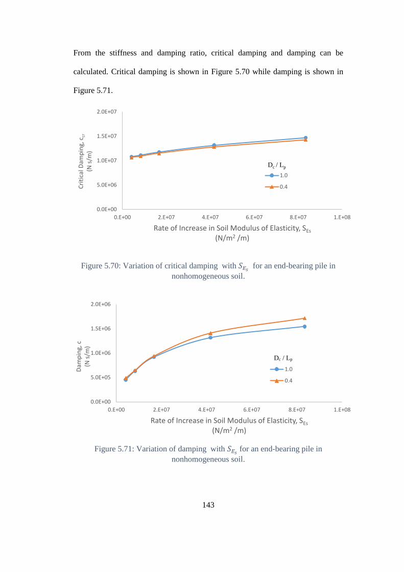
143
From the stiffness and damping ratio, critical damping and damping can be
calculated. Critical damping is shown in Figure 5.70 while damping is shown in
Figure 5.71.
Figure 5.70: Variation of critical damping with 𝑆𝐸𝑠 for an end-bearing pile in
nonhomogeneous soil.
Figure 5.71: Variation of damping with 𝑆𝐸𝑠 for an end-bearing pile in
nonhomogeneous soil.
0.0E+00
5.0E+06
1.0E+07
1.5E+07
2.0E+07
0.E+00 2.E+07 4.E+07 6.E+07 8.E+07 1.E+08
Cri
tica
l Dam
pin
g, c
cr
(N s
/m)
Rate of Increase in Soil Modulus of Elasticity, SEs
(N/m2 /m)
1.0
0.4
Dc / Lp
0.0E+00
5.0E+05
1.0E+06
1.5E+06
2.0E+06
0.E+00 2.E+07 4.E+07 6.E+07 8.E+07 1.E+08
Dam
pin
g, c
(N s
/m)
Rate of Increase in Soil Modulus of Elasticity, SEs
(N/m2 /m)
1.0
0.4
Dc / Lp
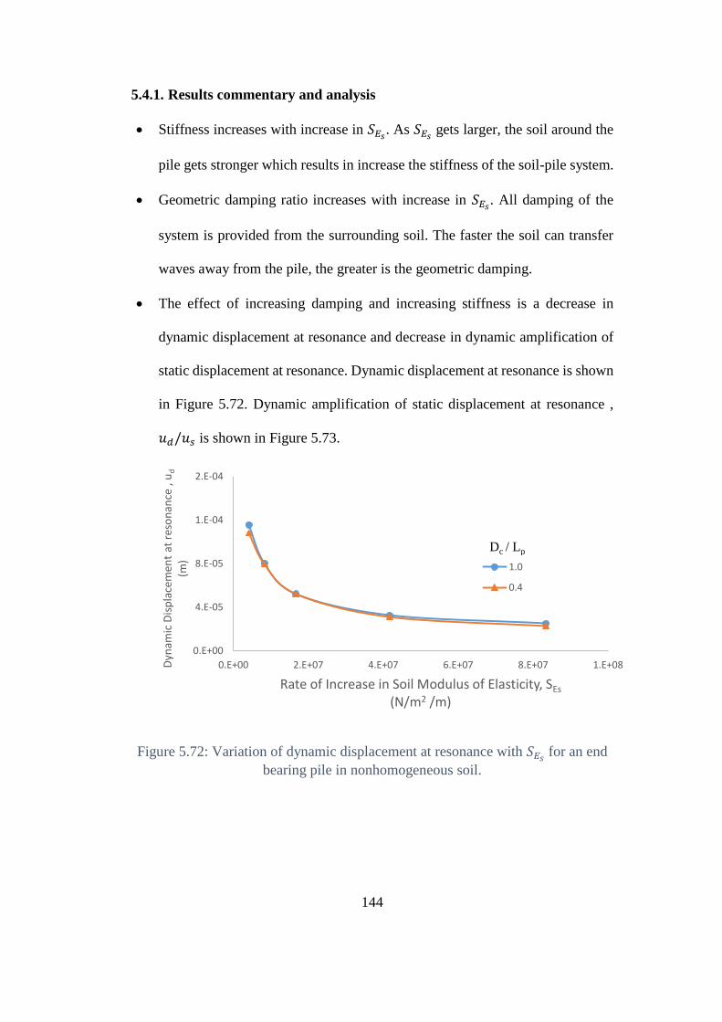
144
5.4.1. Results commentary and analysis
Stiffness increases with increase in 𝑆𝐸𝑠. As 𝑆𝐸𝑠 gets larger, the soil around the
pile gets stronger which results in increase the stiffness of the soil-pile system.
Geometric damping ratio increases with increase in 𝑆𝐸𝑠. All damping of the
system is provided from the surrounding soil. The faster the soil can transfer
waves away from the pile, the greater is the geometric damping.
The effect of increasing damping and increasing stiffness is a decrease in
dynamic displacement at resonance and decrease in dynamic amplification of
static displacement at resonance. Dynamic displacement at resonance is shown
in Figure 5.72. Dynamic amplification of static displacement at resonance ,
𝑢𝑑/𝑢𝑠 is shown in Figure 5.73.
Figure 5.72: Variation of dynamic displacement at resonance with 𝑆𝐸𝑠 for an end
bearing pile in nonhomogeneous soil.
0.E+00
4.E-05
8.E-05
1.E-04
2.E-04
0.E+00 2.E+07 4.E+07 6.E+07 8.E+07 1.E+08Dyn
amic
Dis
pla
cem
ent
at r
eso
nan
ce ,
ud
(m)
Rate of Increase in Soil Modulus of Elasticity, SEs
(N/m2 /m)
1.0
0.4
Dc / Lp
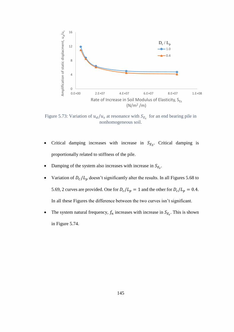
145
Figure 5.73: Variation of 𝑢𝑑/𝑢𝑠 at resonance with 𝑆𝐸𝑠 for an end bearing pile in
nonhomogeneous soil.
Critical damping increases with increase in 𝑆𝐸𝑆. Critical damping is
proportionally related to stiffness of the pile.
Damping of the system also increases with increase in 𝑆𝐸𝑠.
Variation of 𝐷𝐶/𝐿𝑝 doesn’t significantly alter the results. In all Figures 5.68 to
5.69, 2 curves are provided. One for 𝐷𝑐/𝐿𝑝 = 1 and the other for 𝐷𝑐/𝐿𝑝 = 0.4.
In all these Figures the difference between the two curves isn’t significant.
The system natural frequency, 𝑓𝑛 increases with increase in 𝑆𝐸𝑠. This is shown
in Figure 5.74.
0
4
8
12
16
0.E+00 2.E+07 4.E+07 6.E+07 8.E+07 1.E+08Am
plif
icat
ion
of
stat
ic d
isp
lacm
ent,
ud/u
s
Rate of Increase in Soil Modulus of Elasticity, SEs
(N/m2 /m)
1.0
0.4
Dc / Lp
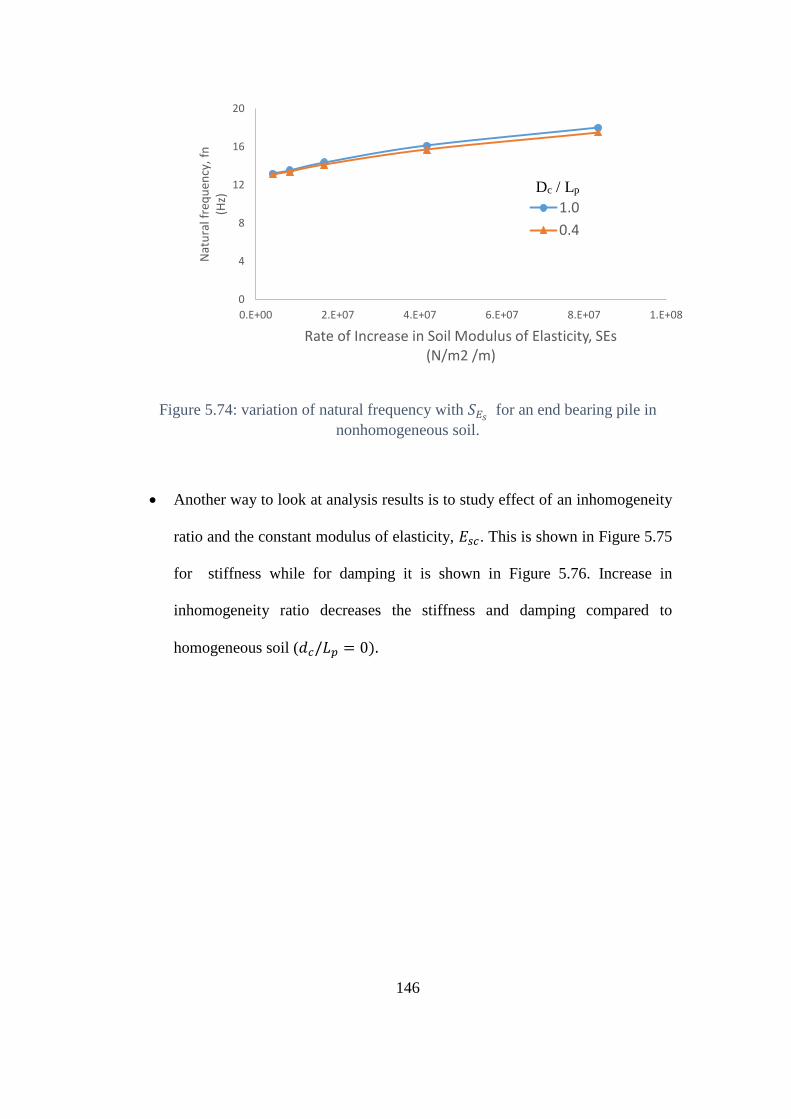
146
Figure 5.74: variation of natural frequency with 𝑆𝐸𝑠 for an end bearing pile in
nonhomogeneous soil.
Another way to look at analysis results is to study effect of an inhomogeneity
ratio and the constant modulus of elasticity, 𝐸𝑠𝑐. This is shown in Figure 5.75
for stiffness while for damping it is shown in Figure 5.76. Increase in
inhomogeneity ratio decreases the stiffness and damping compared to
homogeneous soil (𝑑𝑐/𝐿𝑝 = 0).
0
4
8
12
16
20
0.E+00 2.E+07 4.E+07 6.E+07 8.E+07 1.E+08
Nat
ura
l fre
qu
ency
, fn
(Hz)
Rate of Increase in Soil Modulus of Elasticity, SEs(N/m2 /m)
1.0
0.4
Dc / Lp
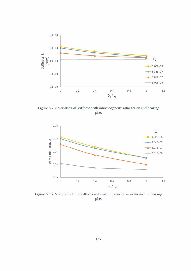
147
Figure 5.75: Variation of stiffness with inhomogeneity ratio for an end bearing
pile.
Figure 5.76: Variation of the stiffness with inhomogeneity ratio for an end bearing
pile.
0.E+00
2.E+08
4.E+08
6.E+08
8.E+08
0 0.2 0.4 0.6 0.8 1 1.2
Stif
fnes
s, k
(N/m
)
Dc / Lp
1.00E+08
8.34E+07
5.01E+07
5.01E+06
Esc
0.00
0.04
0.08
0.12
0.16
0 0.2 0.4 0.6 0.8 1 1.2
Dam
pin
g R
atio
, D
Dc / Lp
1.00E+08
8.34E+07
5.01E+07
5.01E+06
Esc
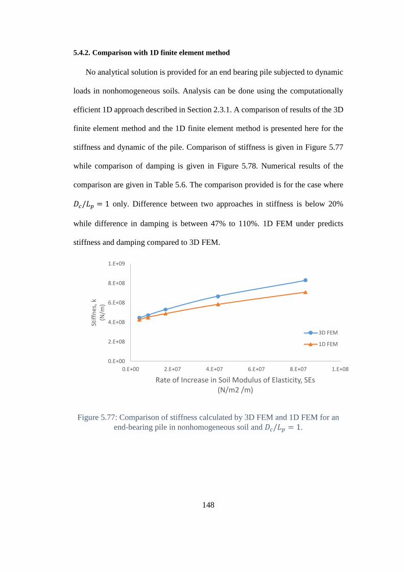
148
5.4.2. Comparison with 1D finite element method
No analytical solution is provided for an end bearing pile subjected to dynamic
loads in nonhomogeneous soils. Analysis can be done using the computationally
efficient 1D approach described in Section 2.3.1. A comparison of results of the 3D
finite element method and the 1D finite element method is presented here for the
stiffness and dynamic of the pile. Comparison of stiffness is given in Figure 5.77
while comparison of damping is given in Figure 5.78. Numerical results of the
comparison are given in Table 5.6. The comparison provided is for the case where
𝐷𝑐/𝐿𝑝 = 1 only. Difference between two approaches in stiffness is below 20%
while difference in damping is between 47% to 110%. 1D FEM under predicts
stiffness and damping compared to 3D FEM.
Figure 5.77: Comparison of stiffness calculated by 3D FEM and 1D FEM for an
end-bearing pile in nonhomogeneous soil and 𝐷𝑐/𝐿𝑝 = 1.
0.E+00
2.E+08
4.E+08
6.E+08
8.E+08
1.E+09
0.E+00 2.E+07 4.E+07 6.E+07 8.E+07 1.E+08
Stif
fnes
, k
(N/m
)
Rate of Increase in Soil Modulus of Elasticity, SEs(N/m2 /m)
3D FEM
1D FEM
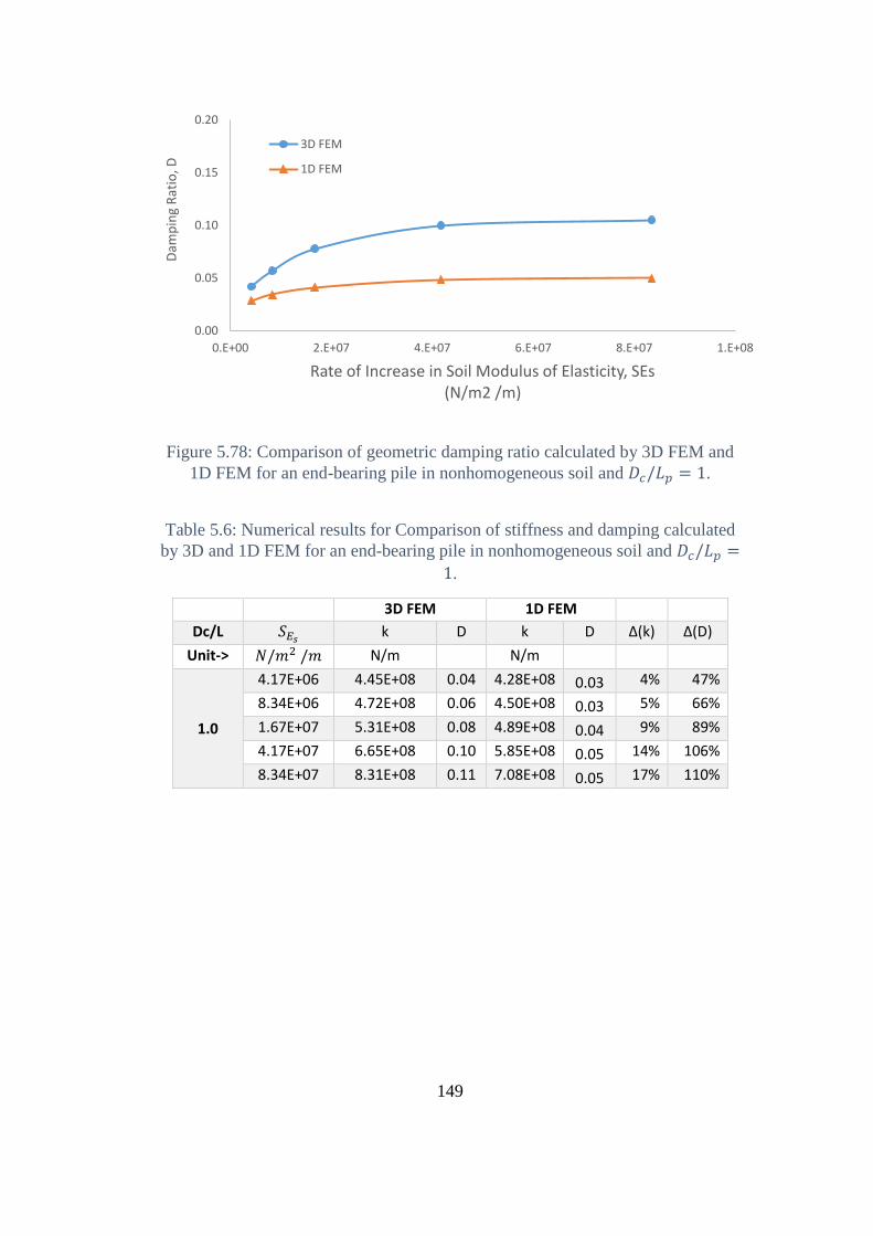
149
Figure 5.78: Comparison of geometric damping ratio calculated by 3D FEM and
1D FEM for an end-bearing pile in nonhomogeneous soil and 𝐷𝑐/𝐿𝑝 = 1.
Table 5.6: Numerical results for Comparison of stiffness and damping calculated
by 3D and 1D FEM for an end-bearing pile in nonhomogeneous soil and 𝐷𝑐/𝐿𝑝 =
1.
3D FEM 1D FEM
Dc/L 𝑆𝐸𝑠 k D k D Δ(k) Δ(D)
Unit-> 𝑁/𝑚2 /𝑚 N/m N/m
1.0
4.17E+06 4.45E+08 0.04 4.28E+08 0.03 4% 47%
8.34E+06 4.72E+08 0.06 4.50E+08 0.03 5% 66%
1.67E+07 5.31E+08 0.08 4.89E+08 0.04 9% 89%
4.17E+07 6.65E+08 0.10 5.85E+08 0.05 14% 106%
8.34E+07 8.31E+08 0.11 7.08E+08 0.05 17% 110%
0.00
0.05
0.10
0.15
0.20
0.E+00 2.E+07 4.E+07 6.E+07 8.E+07 1.E+08
Dam
pin
g R
atio
, D
Rate of Increase in Soil Modulus of Elasticity, SEs(N/m2 /m)
3D FEM
1D FEM
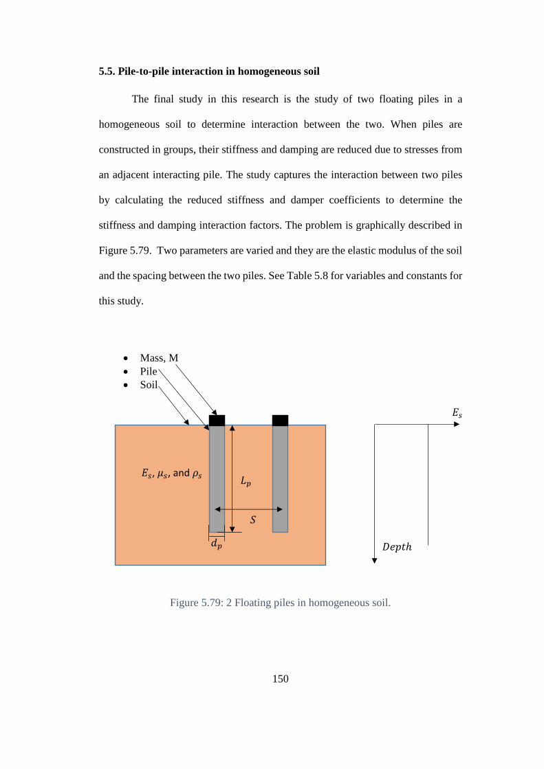
150
5.5. Pile-to-pile interaction in homogeneous soil
The final study in this research is the study of two floating piles in a
homogeneous soil to determine interaction between the two. When piles are
constructed in groups, their stiffness and damping are reduced due to stresses from
an adjacent interacting pile. The study captures the interaction between two piles
by calculating the reduced stiffness and damper coefficients to determine the
stiffness and damping interaction factors. The problem is graphically described in
Figure 5.79. Two parameters are varied and they are the elastic modulus of the soil
and the spacing between the two piles. See Table 5.8 for variables and constants for
this study.
Figure 5.79: 2 Floating piles in homogeneous soil.
𝐸𝑠
𝐷𝑒𝑝𝑡ℎ
Mass, M
Pile
Soil
𝑑𝑝
𝐿𝑝 𝐸𝑠, 𝜇𝑠, and 𝜌𝑠
𝑆
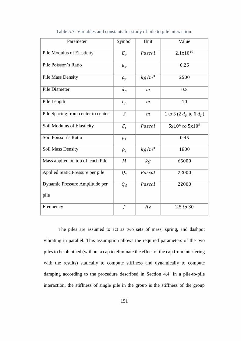
151
Table 5.7: Variables and constants for study of pile to pile interaction.
Parameter Symbol Unit Value
Pile Modulus of Elasticity 𝐸𝑝 𝑃𝑎𝑠𝑐𝑎𝑙 2.1x10¹⁰
Pile Poisson’s Ratio 𝜇𝑝 0.25
Pile Mass Density 𝜌𝑝 𝑘𝑔/𝑚3 2500
Pile Diameter 𝑑𝑝 𝑚 0.5
Pile Length 𝐿𝑝 𝑚 10
Pile Spacing from center to center 𝑆 𝑚 1 to 3 (2 𝑑𝑝 to 6 𝑑𝑝)
Soil Modulus of Elasticity 𝐸𝑠 𝑃𝑎𝑠𝑐𝑎𝑙 5x10⁶ 𝑡𝑜 5x10⁸
Soil Poisson’s Ratio 𝜇𝑠 0.45
Soil Mass Density 𝜌𝑠 𝑘𝑔/𝑚3 1800
Mass applied on top of each Pile 𝑀 𝑘𝑔 65000
Applied Static Pressure per pile 𝑄𝑠 𝑃𝑎𝑠𝑐𝑎𝑙 22000
Dynamic Pressure Amplitude per
pile
𝑄𝑑 𝑃𝑎𝑠𝑐𝑎𝑙 22000
Frequency 𝑓 𝐻𝑧 2.5 𝑡𝑜 30
The piles are assumed to act as two sets of mass, spring, and dashpot
vibrating in parallel. This assumption allows the required parameters of the two
piles to be obtained (without a cap to eliminate the effect of the cap from interfering
with the results) statically to compute stiffness and dynamically to compute
damping according to the procedure described in Section 4.4. In a pile-to-pile
interaction, the stiffness of single pile in the group is the stiffness of the group
152
divided by 2. Similarly, damping ratio of a single pile in the group is damping of
the group divided by two. The stiffness and damping of a single pile in the group
are always less than that a single isolated pile. Interaction is calculated based on this
reduction in stiffness and damping as described below.
Since a 2 pile system is the simplest form of a group, the following Equations apply:
𝑘𝐺 =∑ 𝑘𝑖
𝑛𝑖=1
∑ 𝛼𝑘𝑖𝑛𝑖=1
(5.21)
𝑐𝐺 =∑ 𝑐𝑖
𝑛𝑖=1
∑ 𝛼𝑐𝑖𝑛𝑖=1
(5.22)
Where 𝑘𝐺 is the group stiffness, 𝑘𝑖 stiffness calculated for an isolated pile, 𝑐𝐺 is the
group damping, 𝑐𝑖 is the damping calculated for an isolated pile, 𝑎𝑘𝑖 is stiffness
interaction factor and 𝛼𝑐𝑖 is the damping interaction factor. Finite element analysis
is used to calculate 𝑘𝐺 and 𝑐𝐺 of the 2 pile system. From the study on a single pile
in a homogeneous soil, 𝑘𝑖 and 𝑐𝑖 are calculated. The only remaining factors are
∑ 𝛼𝑘𝑖𝑛𝑖=1 and ∑ 𝛼𝑐𝑖
𝑛𝑖=1 . Since this is a 2 pile group, ∑ 𝑘𝑖
𝑛𝑖=1 = 2 𝑘 and ∑ 𝑐𝑖
𝑛𝑖=1 = 2 𝑐
where 𝑘 and 𝑐 indicates stiffness an damping of an isolated pile. Αlso, ∑ 𝛼𝑘𝑖𝑛𝑖=1 =
𝛼𝑘1 + 𝛼𝑘2 where 𝛼𝑘1 = 1. Similarly, ∑ 𝛼𝑐𝑖 =𝑛𝑖=1 𝛼𝑐1 + 𝛼𝑐2 and 𝛼𝑐1 = 1. The value
of 1 for 𝛼𝑘1 and 𝛼𝑐1 represent interaction of the pile with itself which are always be
1. Since no cap was used in the study, the value of geometric damping, 𝐷 calculated
using the procedure described in section 4.4 yields the geometric damping of the
group. This damping is the sum of the geometric damping coming from each pile
after being modified for group action.
The following Equation then applies,
𝐷𝐺 = 𝐷1′ +𝐷2
′ (5.23)
153
From 5.23, it can be said that
𝐷𝐺 =𝑐1′
2√𝑘1′𝑀1
+𝑐2′
2√𝑘2′𝑀2
(5.24)
The superscript ′ means modification of the isolated pile stiffness and damping for
the group. The stiffness of the group is 𝐾𝐺 = 𝑘1′ + 𝑘2
′ and damping is 𝑐𝐺 = 𝑐1′ +
𝑐2′ . Since each pile is identical to the other and is subjected to same mass and load,
it can be said that 𝑘1′ = 𝑘2
′ = 𝑘′ and 𝑐1′ = 𝑐2
′ = 𝑐′. Then the group stiffness
calculated from finite element, 𝑘𝐺 = 2𝑘′ and damping is 𝑐𝐺 = 2𝑐′. Equations 5.21
and 5.22 become:
2𝑘′ =2𝑘
1 + 𝛼𝑘2
(5.24)
2𝑐′ =2𝑐
1 + 𝛼𝑐2
(5.25)
Determining 𝛼𝑘2 and 𝛼𝑐2 is the goal of this study. In Equations 5.24 and 5.25, all
parameters are calculated using finite element method and 𝛼𝑘2 and 𝛼𝑐2 can be
obtained.
The following is a sample calculation of values of 𝛼𝑘2 and 𝛼𝑐2 using the described
procedure for the set of parameters described in Table 5.9.
1- A static load, 𝑄 is applied on each pile.
2- The static displacement of each pile can be determined from static analysis and
the stiffness of a pile in a 2 pile system,
𝑘′ can be calculated as
𝑘′ =𝑄
𝑢𝑠=
22000
7.23 × 10−6= 5.97 × 10⁸ 𝑁/𝑚
(5.26)
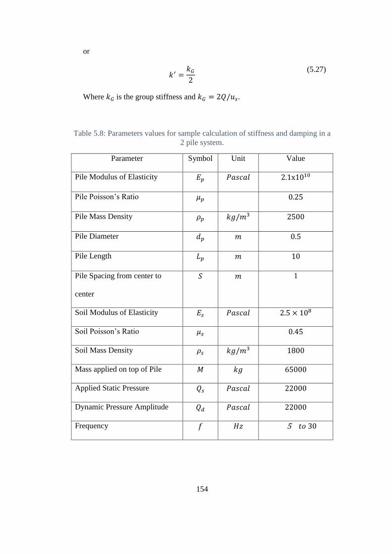
154
or
𝑘′ =𝑘𝐺2
(5.27)
Where 𝑘𝐺 is the group stiffness and 𝑘𝐺 = 2𝑄/𝑢𝑠.
Table 5.8: Parameters values for sample calculation of stiffness and damping in a
2 pile system.
Parameter Symbol Unit Value
Pile Modulus of Elasticity 𝐸𝑝 𝑃𝑎𝑠𝑐𝑎𝑙 2.1x10¹⁰
Pile Poisson’s Ratio 𝜇𝑝 0.25
Pile Mass Density 𝜌𝑝 𝑘𝑔/𝑚3 2500
Pile Diameter 𝑑𝑝 𝑚 0.5
Pile Length 𝐿𝑝 𝑚 10
Pile Spacing from center to
center
𝑆 𝑚 1
Soil Modulus of Elasticity 𝐸𝑠 𝑃𝑎𝑠𝑐𝑎𝑙 2.5 × 10⁸
Soil Poisson’s Ratio 𝜇𝑠 0.45
Soil Mass Density 𝜌𝑠 𝑘𝑔/𝑚3 1800
Mass applied on top of Pile 𝑀 𝑘𝑔 65000
Applied Static Pressure 𝑄𝑠 𝑃𝑎𝑠𝑐𝑎𝑙 22000
Dynamic Pressure Amplitude 𝑄𝑑 𝑃𝑎𝑠𝑐𝑎𝑙 22000
Frequency 𝑓 𝐻𝑧 5 𝑡𝑜 30
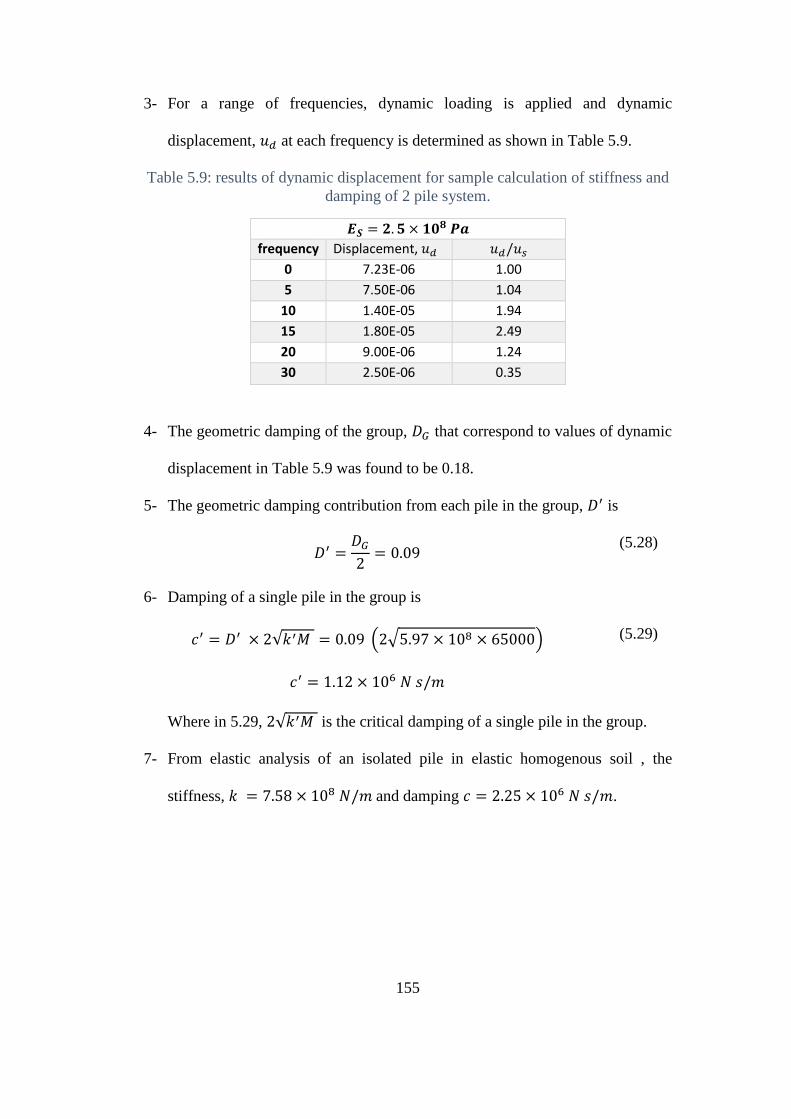
155
3- For a range of frequencies, dynamic loading is applied and dynamic
displacement, 𝑢𝑑 at each frequency is determined as shown in Table 5.9.
Table 5.9: results of dynamic displacement for sample calculation of stiffness and
damping of 2 pile system.
𝑬𝑺 = 𝟐. 𝟓 × 𝟏𝟎𝟖 𝑷𝒂
frequency Displacement, 𝑢𝑑 𝑢𝑑/𝑢𝑠
0 7.23E-06 1.00
5 7.50E-06 1.04
10 1.40E-05 1.94
15 1.80E-05 2.49
20 9.00E-06 1.24
30 2.50E-06 0.35
4- The geometric damping of the group, 𝐷𝐺 that correspond to values of dynamic
displacement in Table 5.9 was found to be 0.18.
5- The geometric damping contribution from each pile in the group, 𝐷′ is
𝐷′ =𝐷𝐺
2= 0.09
(5.28)
6- Damping of a single pile in the group is
𝑐′ = 𝐷′ × 2√𝑘′𝑀 = 0.09 (2√5.97 × 108 × 65000)
𝑐′ = 1.12 × 10⁶ 𝑁 𝑠/𝑚
(5.29)
Where in 5.29, 2√𝑘′𝑀 is the critical damping of a single pile in the group.
7- From elastic analysis of an isolated pile in elastic homogenous soil , the
stiffness, 𝑘 = 7.58 × 10⁸ 𝑁/𝑚 and damping 𝑐 = 2.25 × 10⁶ 𝑁 𝑠/𝑚.
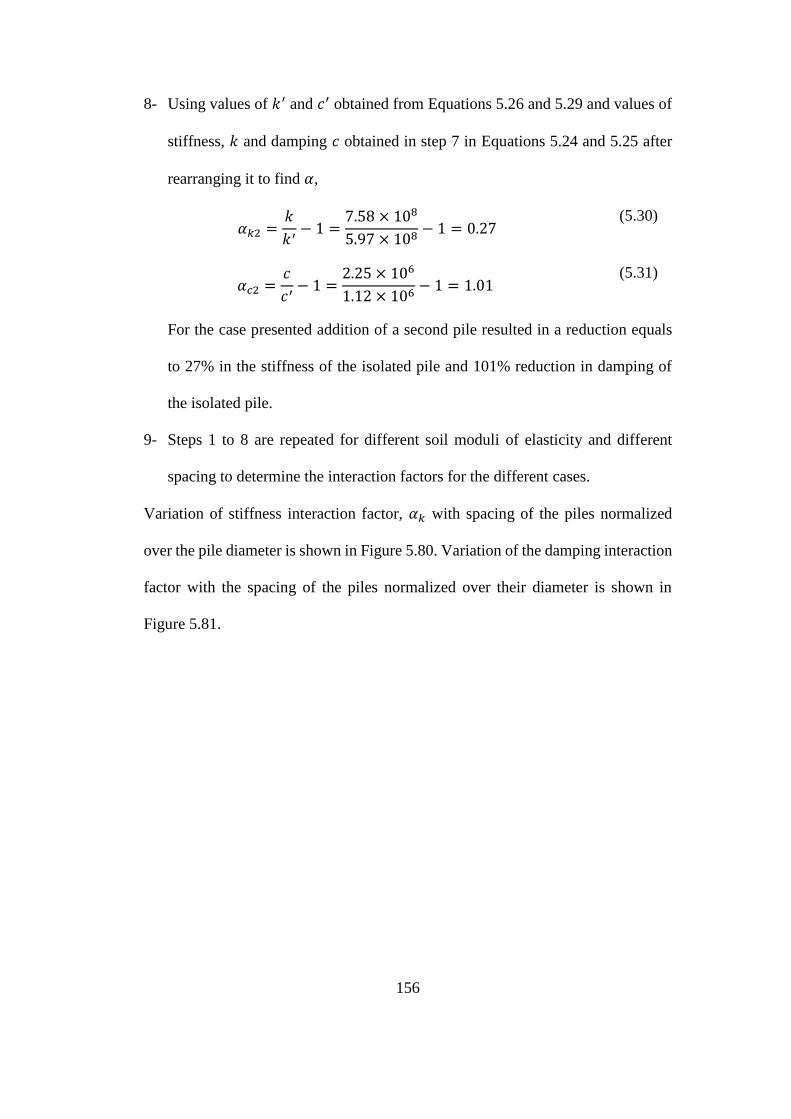
156
8- Using values of 𝑘′ and 𝑐′ obtained from Equations 5.26 and 5.29 and values of
stiffness, 𝑘 and damping 𝑐 obtained in step 7 in Equations 5.24 and 5.25 after
rearranging it to find 𝛼,
𝛼𝑘2 =𝑘
𝑘′− 1 =
7.58 × 10⁸
5.97 × 10⁸− 1 = 0.27
(5.30)
𝛼𝑐2 =𝑐
𝑐′− 1 =
2.25 × 10⁶
1.12 × 10⁶− 1 = 1.01
(5.31)
For the case presented addition of a second pile resulted in a reduction equals
to 27% in the stiffness of the isolated pile and 101% reduction in damping of
the isolated pile.
9- Steps 1 to 8 are repeated for different soil moduli of elasticity and different
spacing to determine the interaction factors for the different cases.
Variation of stiffness interaction factor, 𝛼𝑘 with spacing of the piles normalized
over the pile diameter is shown in Figure 5.80. Variation of the damping interaction
factor with the spacing of the piles normalized over their diameter is shown in
Figure 5.81.
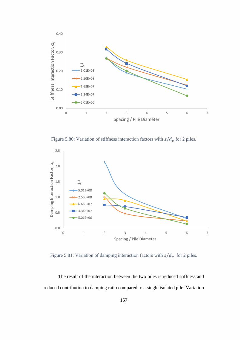
157
Figure 5.80: Variation of stiffness interaction factors with 𝑠/𝑑𝑝 for 2 piles.
Figure 5.81: Variation of damping interaction factors with 𝑠/𝑑𝑝 for 2 piles.
The result of the interaction between the two piles is reduced stiffness and
reduced contribution to damping ratio compared to a single isolated pile. Variation
0.00
0.10
0.20
0.30
0.40
0 1 2 3 4 5 6 7
Stif
fnes
s In
tera
ctio
n F
acto
r, α
k
Spacing / Pile Diameter
5.01E+08
2.50E+08
6.68E+07
3.34E+07
5.01E+06
0.0
0.5
1.0
1.5
2.0
2.5
0 1 2 3 4 5 6 7
Dam
pin
g In
tera
ctio
n F
acto
r, α
c
Spacing / Pile Diameter
5.01E+08
2.50E+08
6.68E+07
3.34E+07
5.01E+06
Es
Es
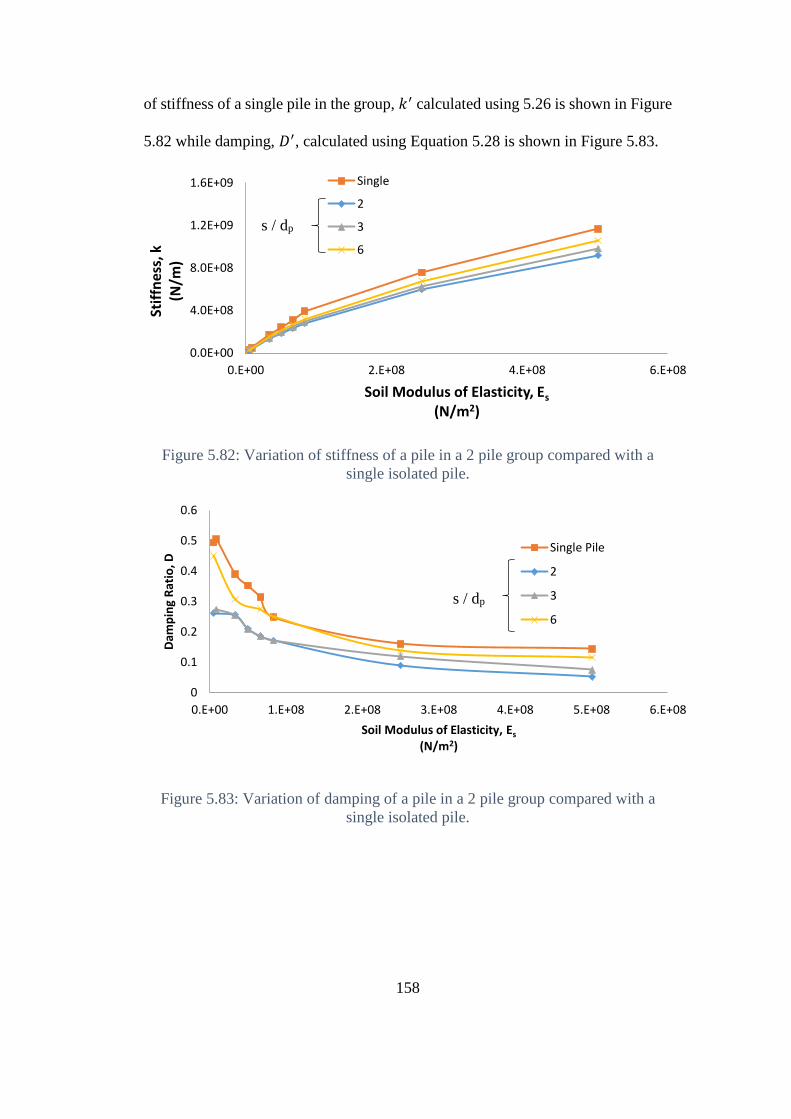
158
of stiffness of a single pile in the group, 𝑘′ calculated using 5.26 is shown in Figure
5.82 while damping, 𝐷′, calculated using Equation 5.28 is shown in Figure 5.83.
Figure 5.82: Variation of stiffness of a pile in a 2 pile group compared with a
single isolated pile.
Figure 5.83: Variation of damping of a pile in a 2 pile group compared with a
single isolated pile.
0.0E+00
4.0E+08
8.0E+08
1.2E+09
1.6E+09
0.E+00 2.E+08 4.E+08 6.E+08
Stif
fnes
s, k
(N/m
)
Soil Modulus of Elasticity, Es
(N/m2)
Single
2
3
6
0
0.1
0.2
0.3
0.4
0.5
0.6
0.E+00 1.E+08 2.E+08 3.E+08 4.E+08 5.E+08 6.E+08
Dam
pin
g R
atio
, D
Soil Modulus of Elasticity, Es
(N/m2)
Single Pile
2
3
6
s / dp
s / dp
159
Damping of a pile in a 2 pile group calculated as per Equation 5.29 is shown in
Figure 5.84.
Figure 5.84: Damping of a 2 pile group in homogeneous soil.
5.5.1. Results commentary and analysis
Results of stiffness interaction factor are plotted in Figure 5.80 for different
values of soil modulus of elasticity against the normalized spacing. All curves
show that interaction is reduced with increased spacing. This is even more
evident in Figure 5.82 that shows that stiffness for different spacing values.
The more the spacing is between the pile, the less is the interaction (Figure
5.80). The more the spacing the closer the stiffness curve is to that of a single
pile in the same soil (Figure 5.82).
The interaction means that the spring stiffness that describes the behavior the
top of the pile as obtained in Section 5.1 specifically in Figure 5.2 should be
reduced if the pile is used in a group. The amount of reduction in the stiffness
that should be applied is the interaction factor shown in Figure 5.80.
0.E+00
5.E+05
1.E+06
2.E+06
2.E+06
3.E+06
3.E+06
0.E+00 2.E+08 4.E+08 6.E+08
Dam
pin
g, c
(N s
/m)
Soil Modulus of Elasticity, Es(N/m)
Single
2
3
6
s / dp
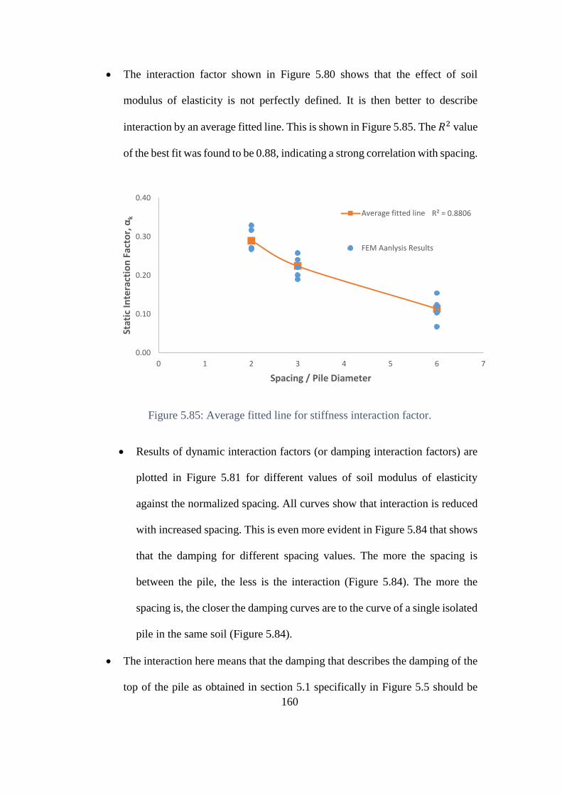
160
The interaction factor shown in Figure 5.80 shows that the effect of soil
modulus of elasticity is not perfectly defined. It is then better to describe
interaction by an average fitted line. This is shown in Figure 5.85. The 𝑅2 value
of the best fit was found to be 0.88, indicating a strong correlation with spacing.
Figure 5.85: Average fitted line for stiffness interaction factor.
Results of dynamic interaction factors (or damping interaction factors) are
plotted in Figure 5.81 for different values of soil modulus of elasticity
against the normalized spacing. All curves show that interaction is reduced
with increased spacing. This is even more evident in Figure 5.84 that shows
that the damping for different spacing values. The more the spacing is
between the pile, the less is the interaction (Figure 5.84). The more the
spacing is, the closer the damping curves are to the curve of a single isolated
pile in the same soil (Figure 5.84).
The interaction here means that the damping that describes the damping of the
top of the pile as obtained in section 5.1 specifically in Figure 5.5 should be
R² = 0.8806
0.00
0.10
0.20
0.30
0.40
0 1 2 3 4 5 6 7
Stat
ic In
tera
ctio
n F
acto
r, α
k
Spacing / Pile Diameter
Average fitted line
FEM Aanlysis Results
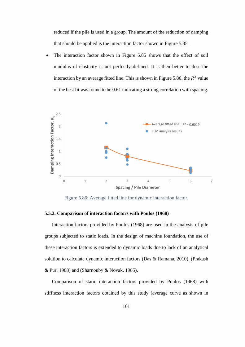
161
reduced if the pile is used in a group. The amount of the reduction of damping
that should be applied is the interaction factor shown in Figure 5.85.
The interaction factor shown in Figure 5.85 shows that the effect of soil
modulus of elasticity is not perfectly defined. It is then better to describe
interaction by an average fitted line. This is shown in Figure 5.86. the 𝑅2 value
of the best fit was found to be 0.61 indicating a strong correlation with spacing.
Figure 5.86: Average fitted line for dynamic interaction factor.
5.5.2. Comparison of interaction factors with Poulos (1968)
Interaction factors provided by Poulos (1968) are used in the analysis of pile
groups subjected to static loads. In the design of machine foundation, the use of
these interaction factors is extended to dynamic loads due to lack of an analytical
solution to calculate dynamic interaction factors (Das & Ramana, 2010), (Prakash
& Puri 1988) and (Sharnouby & Novak, 1985).
Comparison of static interaction factors provided by Poulos (1968) with
stiffness interaction factors obtained by this study (average curve as shown in
R² = 0.6019
0
0.5
1
1.5
2
2.5
0 1 2 3 4 5 6 7
Dam
pin
g In
tera
ctio
n F
acto
r, α
c
Spacing / Pile Diameter
Average fitted line
FEM analysis results
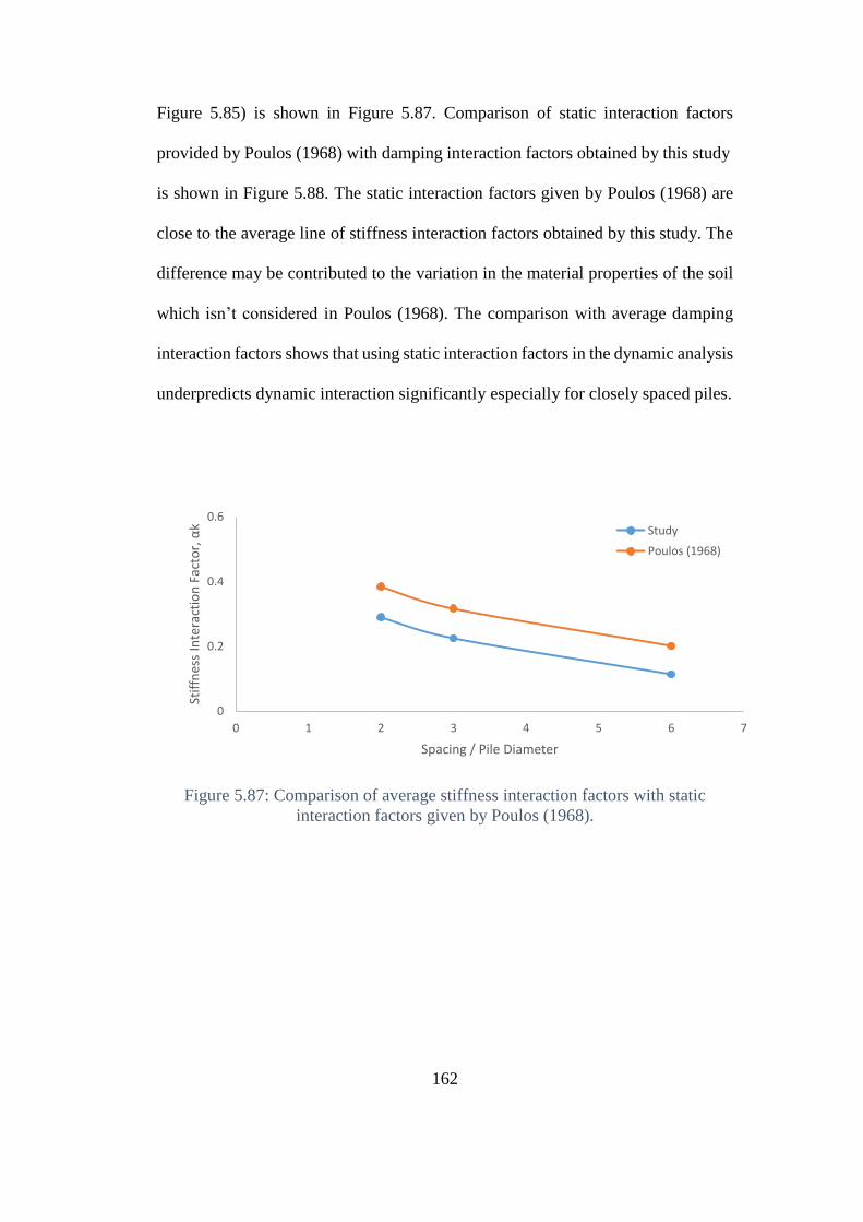
162
Figure 5.85) is shown in Figure 5.87. Comparison of static interaction factors
provided by Poulos (1968) with damping interaction factors obtained by this study
is shown in Figure 5.88. The static interaction factors given by Poulos (1968) are
close to the average line of stiffness interaction factors obtained by this study. The
difference may be contributed to the variation in the material properties of the soil
which isn’t considered in Poulos (1968). The comparison with average damping
interaction factors shows that using static interaction factors in the dynamic analysis
underpredicts dynamic interaction significantly especially for closely spaced piles.
Figure 5.87: Comparison of average stiffness interaction factors with static
interaction factors given by Poulos (1968).
0
0.2
0.4
0.6
0 1 2 3 4 5 6 7
Stif
fnes
s In
tera
ctio
n F
acto
r, α
k
Spacing / Pile Diameter
Study
Poulos (1968)
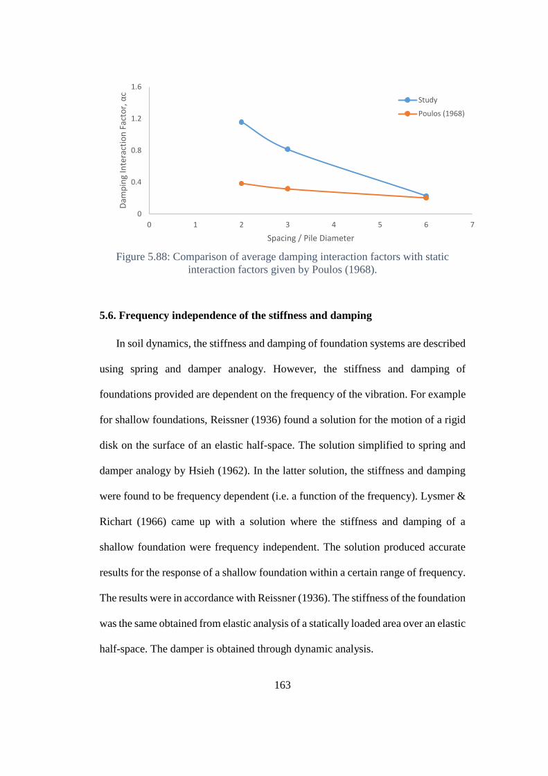
163
Figure 5.88: Comparison of average damping interaction factors with static
interaction factors given by Poulos (1968).
5.6. Frequency independence of the stiffness and damping
In soil dynamics, the stiffness and damping of foundation systems are described
using spring and damper analogy. However, the stiffness and damping of
foundations provided are dependent on the frequency of the vibration. For example
for shallow foundations, Reissner (1936) found a solution for the motion of a rigid
disk on the surface of an elastic half-space. The solution simplified to spring and
damper analogy by Hsieh (1962). In the latter solution, the stiffness and damping
were found to be frequency dependent (i.e. a function of the frequency). Lysmer &
Richart (1966) came up with a solution where the stiffness and damping of a
shallow foundation were frequency independent. The solution produced accurate
results for the response of a shallow foundation within a certain range of frequency.
The results were in accordance with Reissner (1936). The stiffness of the foundation
was the same obtained from elastic analysis of a statically loaded area over an elastic
half-space. The damper is obtained through dynamic analysis.
0
0.4
0.8
1.2
1.6
0 1 2 3 4 5 6 7
Dam
pin
g In
tera
ctio
n F
acto
r, α
c
Spacing / Pile Diameter
Study
Poulos (1968)
164
Novak (1974) solved the Equation of motion for a floating pile foundation.
The stiffness and damping of the of the pile were found to be function of the
frequency, however at dimensionless frequency, 𝑎0 = 0.3, stiffness and damping
were found stationary and independent of the frequency. Novak (1974) presented
Equations for stiffness and damping independent of the frequency while
compromising accuracy at other values of 𝑎0.
A system consisting of a mass, a spring and a dashpot can describe the motion
of the pile top when subjected to vertical loading. The mass is the mass supported
by the pile; the spring has a spring constant that is equal to the static stiffness of the
pile and dashpot that has a coefficient that represents energy loss in the soil-pile
system due to radiation damping. A procedure is described in section 4.4 of this
thesis of how these parameters were obtained. The concept is extended to different
cases of piles in non-homogeneous soils and friction and end bearing pile. The
concept is also extended to the case of the pile-to-pile interaction, where the piles
are assumed to act as two sets of mass, spring and dashpot vibrating in parallel. This
assumption allows the required parameters of the two piles to be obtained by
analyzing a group (without a cap to eliminate the effect of the cap from interfering
with the results) statically to compute stiffness and dynamically to compute
damping using the procedure described in section 4.4. In the pile-to-pile interaction
study the stiffness of a single pile in the group is the stiffness of the group divided
by 2. Similarly, damping of a single pile in the group is damping of the group
divided by 2. The stiffness and damping of a single pile in the group are always less
than that of a single isolated pile. Interaction is calculated based on the reduction in
stiffness and damping of a pile in a group compared to that of an isolated pile. The
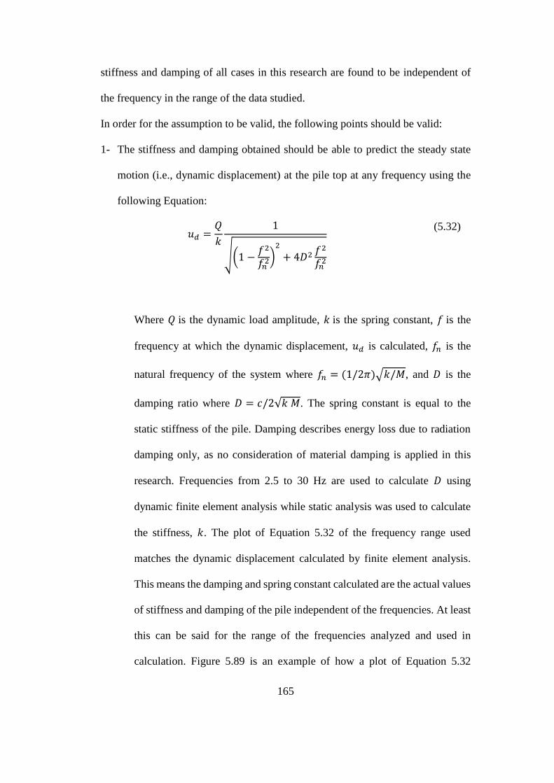
165
stiffness and damping of all cases in this research are found to be independent of
the frequency in the range of the data studied.
In order for the assumption to be valid, the following points should be valid:
1- The stiffness and damping obtained should be able to predict the steady state
motion (i.e., dynamic displacement) at the pile top at any frequency using the
following Equation:
𝑢𝑑 =𝑄
𝑘
1
√(1 −𝑓2
𝑓𝑛2)2
+ 4𝐷2 𝑓2
𝑓𝑛2
(5.32)
Where 𝑄 is the dynamic load amplitude, 𝑘 is the spring constant, 𝑓 is the
frequency at which the dynamic displacement, 𝑢𝑑 is calculated, 𝑓𝑛 is the
natural frequency of the system where 𝑓𝑛 = (1/2𝜋)√𝑘/𝑀, and 𝐷 is the
damping ratio where 𝐷 = 𝑐/2√𝑘 𝑀. The spring constant is equal to the
static stiffness of the pile. Damping describes energy loss due to radiation
damping only, as no consideration of material damping is applied in this
research. Frequencies from 2.5 to 30 Hz are used to calculate 𝐷 using
dynamic finite element analysis while static analysis was used to calculate
the stiffness, 𝑘. The plot of Equation 5.32 of the frequency range used
matches the dynamic displacement calculated by finite element analysis.
This means the damping and spring constant calculated are the actual values
of stiffness and damping of the pile independent of the frequencies. At least
this can be said for the range of the frequencies analyzed and used in
calculation. Figure 5.89 is an example of how a plot of Equation 5.32
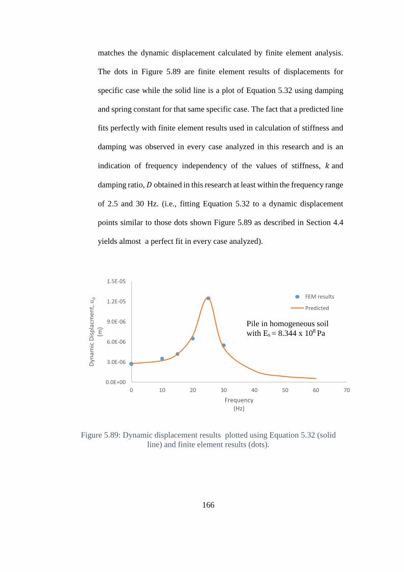
166
matches the dynamic displacement calculated by finite element analysis.
The dots in Figure 5.89 are finite element results of displacements for
specific case while the solid line is a plot of Equation 5.32 using damping
and spring constant for that same specific case. The fact that a predicted line
fits perfectly with finite element results used in calculation of stiffness and
damping was observed in every case analyzed in this research and is an
indication of frequency independency of the values of stiffness, 𝑘 and
damping ratio, 𝐷 obtained in this research at least within the frequency range
of 2.5 and 30 Hz. (i.e., fitting Equation 5.32 to a dynamic displacement
points similar to those dots shown Figure 5.89 as described in Section 4.4
yields almost a perfect fit in every case analyzed).
Figure 5.89: Dynamic displacement results plotted using Equation 5.32 (solid
line) and finite element results (dots).
0.0E+00
3.0E-06
6.0E-06
9.0E-06
1.2E-05
1.5E-05
0 10 20 30 40 50 60 70
Dyn
amic
Dis
pla
cmen
t, u
d
(m)
Frequency(Hz)
FEM results
Predicted
Pile in homogeneous soil
with Es = 8.344 x 10⁸ Pa
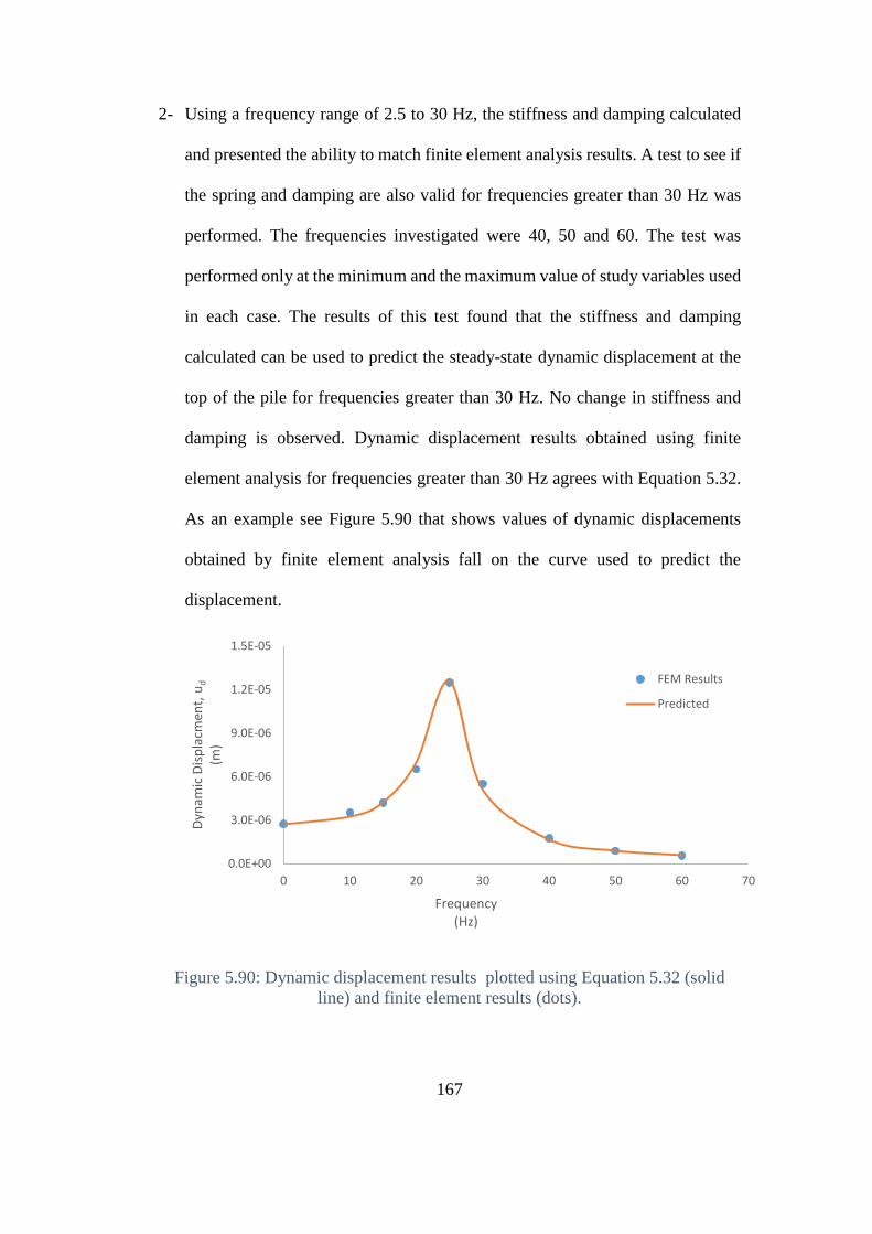
167
2- Using a frequency range of 2.5 to 30 Hz, the stiffness and damping calculated
and presented the ability to match finite element analysis results. A test to see if
the spring and damping are also valid for frequencies greater than 30 Hz was
performed. The frequencies investigated were 40, 50 and 60. The test was
performed only at the minimum and the maximum value of study variables used
in each case. The results of this test found that the stiffness and damping
calculated can be used to predict the steady-state dynamic displacement at the
top of the pile for frequencies greater than 30 Hz. No change in stiffness and
damping is observed. Dynamic displacement results obtained using finite
element analysis for frequencies greater than 30 Hz agrees with Equation 5.32.
As an example see Figure 5.90 that shows values of dynamic displacements
obtained by finite element analysis fall on the curve used to predict the
displacement.
Figure 5.90: Dynamic displacement results plotted using Equation 5.32 (solid
line) and finite element results (dots).
0.0E+00
3.0E-06
6.0E-06
9.0E-06
1.2E-05
1.5E-05
0 10 20 30 40 50 60 70
Dyn
amic
Dis
pla
cmen
t, u
d
(m)
Frequency(Hz)
FEM Results
Predicted
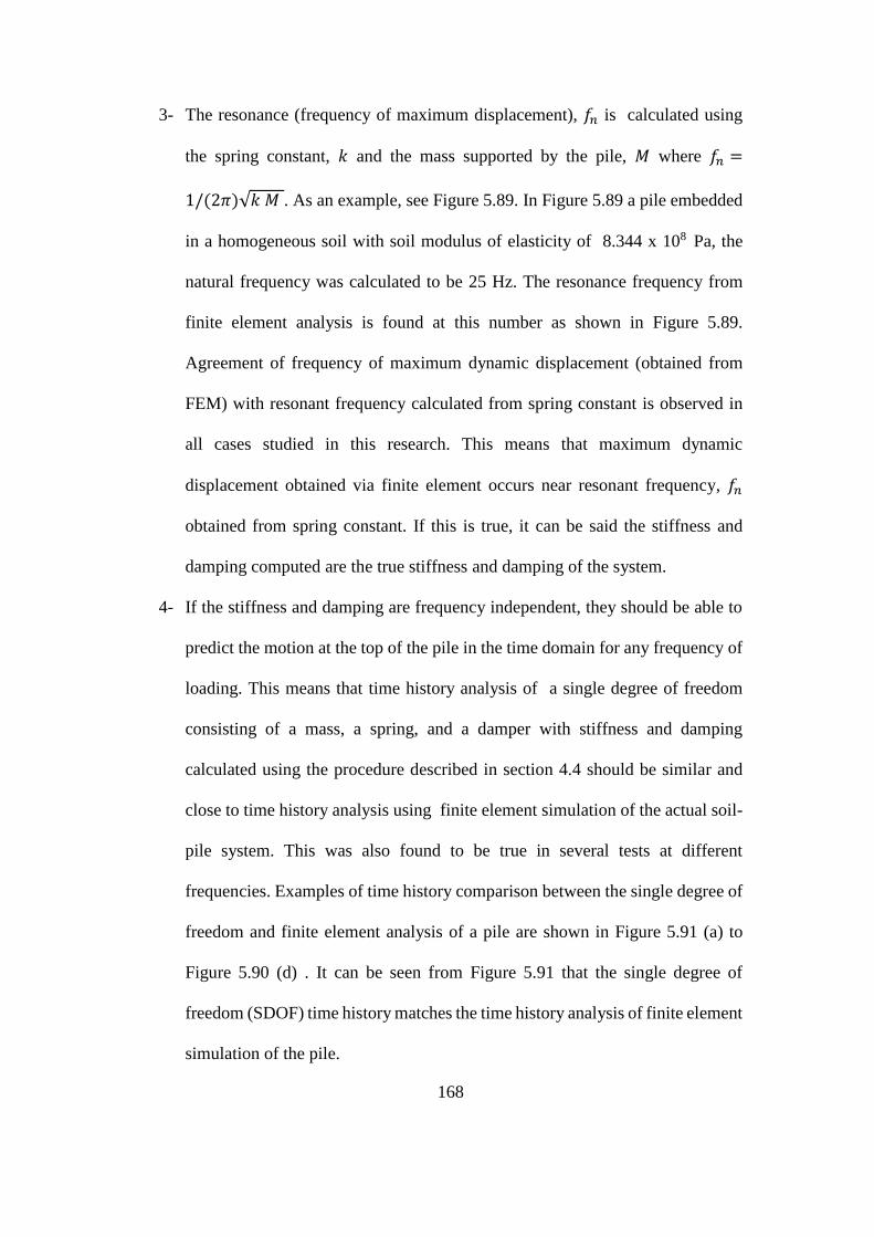
168
3- The resonance (frequency of maximum displacement), 𝑓𝑛 is calculated using
the spring constant, 𝑘 and the mass supported by the pile, 𝑀 where 𝑓𝑛 =
1/(2𝜋)√𝑘 𝑀 . As an example, see Figure 5.89. In Figure 5.89 a pile embedded
in a homogeneous soil with soil modulus of elasticity of 8.344 x 10⁸ Pa, the
natural frequency was calculated to be 25 Hz. The resonance frequency from
finite element analysis is found at this number as shown in Figure 5.89.
Agreement of frequency of maximum dynamic displacement (obtained from
FEM) with resonant frequency calculated from spring constant is observed in
all cases studied in this research. This means that maximum dynamic
displacement obtained via finite element occurs near resonant frequency, 𝑓𝑛
obtained from spring constant. If this is true, it can be said the stiffness and
damping computed are the true stiffness and damping of the system.
4- If the stiffness and damping are frequency independent, they should be able to
predict the motion at the top of the pile in the time domain for any frequency of
loading. This means that time history analysis of a single degree of freedom
consisting of a mass, a spring, and a damper with stiffness and damping
calculated using the procedure described in section 4.4 should be similar and
close to time history analysis using finite element simulation of the actual soil-
pile system. This was also found to be true in several tests at different
frequencies. Examples of time history comparison between the single degree of
freedom and finite element analysis of a pile are shown in Figure 5.91 (a) to
Figure 5.90 (d) . It can be seen from Figure 5.91 that the single degree of
freedom (SDOF) time history matches the time history analysis of finite element
simulation of the pile.
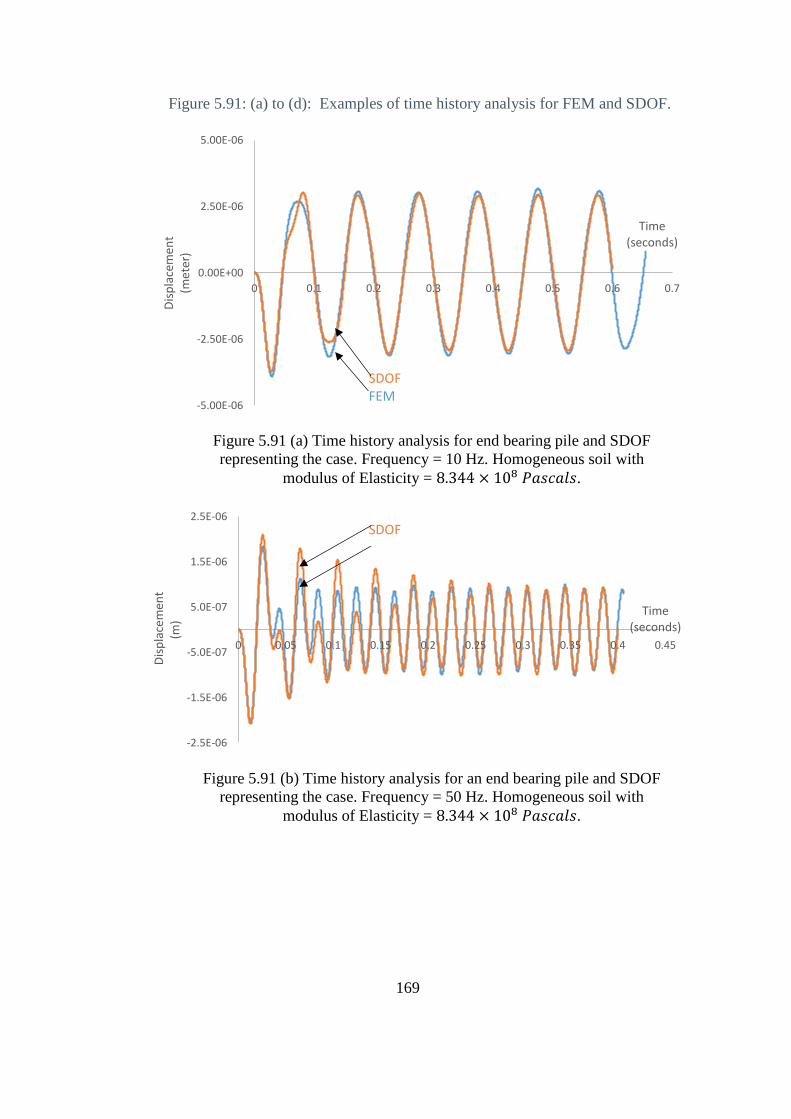
169
Figure 5.91: (a) to (d): Examples of time history analysis for FEM and SDOF.
Figure 5.91 (a) Time history analysis for end bearing pile and SDOF
representing the case. Frequency = 10 Hz. Homogeneous soil with
modulus of Elasticity = 8.344 × 10⁸ 𝑃𝑎𝑠𝑐𝑎𝑙𝑠.
Figure 5.91 (b) Time history analysis for an end bearing pile and SDOF
representing the case. Frequency = 50 Hz. Homogeneous soil with
modulus of Elasticity = 8.344 × 10⁸ 𝑃𝑎𝑠𝑐𝑎𝑙𝑠.
-5.00E-06
-2.50E-06
0.00E+00
2.50E-06
5.00E-06
0 0.1 0.2 0.3 0.4 0.5 0.6 0.7
Dis
pla
cem
ent
(met
er)
Time(seconds)
SDOFFEM
-2.5E-06
-1.5E-06
-5.0E-07
5.0E-07
1.5E-06
2.5E-06
0 0.05 0.1 0.15 0.2 0.25 0.3 0.35 0.4 0.45
Dis
pla
cem
ent
(m)
Time(seconds)
SDOF
170
Figure 5.91 (c) Time history analysis for a floating pile and SDOF
representing the case. Frequency = 10 Hz. Homogeneous soil with
modulus of Elasticity = 8.344 × 10⁸ 𝑃𝑎𝑠𝑐𝑎𝑙𝑠.
Figure 5.91 (d) Time history analysis for a floating pile and SDOF
representing the case. Frequency = 40 Hz. Homogeneous soil with
modulus of Elasticity = 8.344 × 10⁸ 𝑃𝑎𝑠𝑐𝑎𝑙𝑠.
-6.E-06
-4.E-06
-2.E-06
0.E+00
2.E-06
4.E-06
0 0.05 0.1 0.15 0.2 0.25 0.3 0.35
Dis
pla
cem
ent
(m)
Time(seonds)
-8.E-06
-6.E-06
-4.E-06
-2.E-06
0.E+00
2.E-06
4.E-06
0 0.1 0.2 0.3 0.4 0.5 0.6 0.7
Dis
pla
cmen
t(m
)
Time(seconds)
FEMSDOF
171
5.7. A discussion on design applications
5.7.1. Design of a pile in homogenous soil
Comparison of stiffness obtained by this study with Novak (1974) shows a great
difference in stiffness and damping. Comparison of stiffness and damping with
Chowdhury & Dasgupta (2008) shows good agreement of stiffness only at a low
modulus of elasticity of the soil. However, comparison of damping ratio shows no
agreement as damping ratio calculated by Chowdhury & Dasgupta (2008) was
constant at any value of the soil modulus of elasticity. To show how analyzing a
pile subjected to vertical dynamic load using stiffness and damping obtained by
Novak (1974) and Chowdhury & Dasgupta (2008) differ from finite element
analysis, see Figure 5.92. The graph shows differences in resonance frequency and
displacement at resonance. The displacements values are agreeable after resonant
frequency. Pile properties in this examples are the same used in this research.
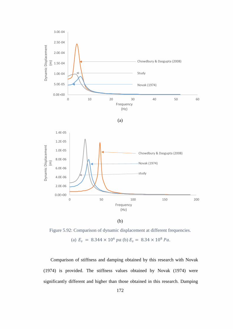
172
(a)
(b)
Figure 5.92: Comparison of dynamic displacement at different frequencies.
(a) 𝐸𝑠 = 8.344 × 10⁶ 𝑝𝑎 (b) 𝐸𝑠 = 8.34 × 10⁸ 𝑃𝑎.
Comparison of stiffness and damping obtained by this research with Novak
(1974) is provided. The stiffness values obtained by Novak (1974) were
significantly different and higher than those obtained in this research. Damping
0.0E+00
5.0E-05
1.0E-04
1.5E-04
2.0E-04
2.5E-04
3.0E-04
0 10 20 30 40 50 60
Dyn
amic
Dis
pla
cem
ent
(m)
Frequency(Hz)
Chowdbury & Dasgupta (2008)
Study
Novak (1974)
0.0E+00
2.0E-06
4.0E-06
6.0E-06
8.0E-06
1.0E-05
1.2E-05
1.4E-05
0 50 100 150 200
Dyn
amic
Dis
pla
cem
ent
(m)
Frequency(Hz)
Chowdbury & Dasgupta (2008)
Novak (1974)
study
173
ratio decreases with increase in soil elastic modulus if obtained by Novak (1974).
Damping ratios calculated by this research were found to be increasing with the
increase in soil modulus of elasticity. Comparison of stiffness and damping
obtained by Chowdhury & Dasgupta (2008) and those obtained by this research
found no agreement. Stiffness obtained by Chowdhury & Dasgupta (2008) was
significantly higher than that obtained in this research. Figure 5.93 shows how
using stiffness and damping obtained by Novak (1974) and Chowdhury &
Dasgupta (2008) compare with those obtained by this study in predicting dynamic
displacement at any frequency. The methods differ in predicting resonance
frequency and displacement at resonance. After resonance, both methods show
agreement in predicting dynamic displacements.
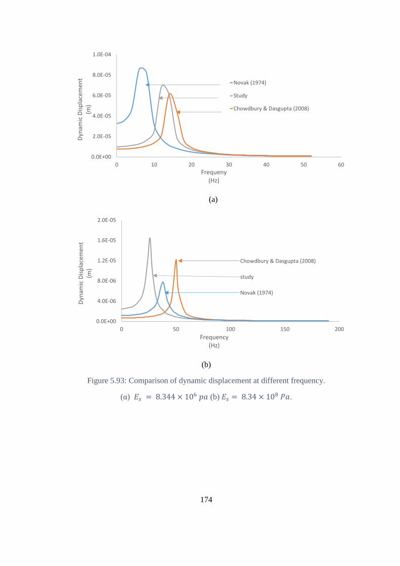
174
(a)
(b)
Figure 5.93: Comparison of dynamic displacement at different frequency.
(α) 𝐸𝑠 = 8.344 × 10⁶ 𝑝𝑎 (b) 𝐸𝑠 = 8.34 × 10⁸ 𝑃𝑎.
0.0E+00
2.0E-05
4.0E-05
6.0E-05
8.0E-05
1.0E-04
0 10 20 30 40 50 60
Dyn
amic
Dis
pla
cem
ent
(m)
Frequeny(Hz)
Novak (1974)
Study
Chowdbury & Dasgupta (2008)
0.0E+00
4.0E-06
8.0E-06
1.2E-05
1.6E-05
2.0E-05
0 50 100 150 200
Dyn
amic
Dis
pla
cem
ent
(m)
Frequency(Hz)
Chowdbury & Dasgupta (2008)
study
Novak (1974)
175
In the case of designing a floating or an end-bearing pile in a homogeneous
soil, comparison of stiffness obtained by finite element analysis with Novak (1974)
found that stiffness obtained by Novak (1974) is overestimated. This overestimation
in stiffness lead to overestimation in critical damping,𝑐𝑐𝑟 , and the damping ratio
which is equal to 𝑐/𝑐𝑐𝑟. It also affects the value of the natural frequency. However,
calculating damping, 𝑐 using Novak (1974) is more agreeable with finite element
results. As a result, ιt is suggested to use an analytical solution based on static elastic
analysis of piles to obtain stiffness of the pile. One method was presented earlier in
section 5.1.2.1 by Gazetas & Mylonakis (1998). In fact using such a method for
stiffness makes Novak solution more agreeable with finite element data in
determining dynamic displacement at any frequency as well as determining
resonant frequency. This is because adjusting the stiffness automatically adjusts the
value of the damping ratio, 𝐷 as shown in Figure 5.94 for damping of a floating pile
and 5.95 for damping of an end bearing pile. It can be seen from Figures 5.94 and
5.95 that using a static stiffness reduces the difference in damping between finite
element and Novak (1974). In fact, using a stiffness computed by static analysis
makes the damping ratio curve obtained by Novak (1974) agreeable with finite
element results not only in values but also in the pattern (i.e. increasing with
increase in soil modulus of elasticity) for the case of an end bearing pile.
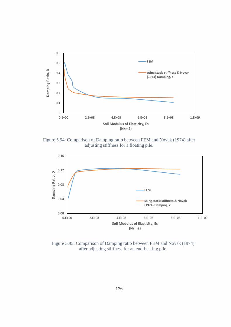
176
Figure 5.94: Comparison of Damping ratio between FEM and Novak (1974) after
adjusting stiffness for a floating pile.
Figure 5.95: Comparison of Damping ratio between FEM and Novak (1974)
after adjusting stiffness for an end-bearing pile.
0
0.1
0.2
0.3
0.4
0.5
0.6
0.E+00 2.E+08 4.E+08 6.E+08 8.E+08 1.E+09
Dam
pin
g R
atio
, D
Soil Modulus of Elasticity, Es(N/m2)
FEM
using static stiffness & Novak(1974) Damping, c
0.00
0.04
0.08
0.12
0.16
0.E+00 2.E+08 4.E+08 6.E+08 8.E+08 1.E+09
Dam
pin
g R
atio
, D
Soil Modulus of Elasticity, Es(N/m2)
FEM
using static stiffness & Novak(1974) Damping, c
177
5.7.2. Design of a pile group
An example is provided to show how interaction factors are used in designing a
pile group using static and dynamic interaction factors. The example considers 2
approaches: (1) the currently used one where Poulos (1968) interaction factors are
applied to both stiffness and damping and (2) The new interaction factors obtained
by FEM are applied to stiffness of the group and damping interaction factors are
applied to damping of the group. The parameters of the soil and the pile are
summarized in Table 5.10. The problem is shown graphically in Figure 5.9
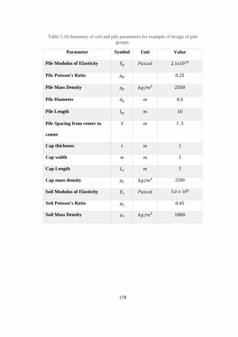
178
Table 5.10:Summary of soil and pile parameters for example of design of pile
groups.
Parameter Symbol Unit Value
Pile Modulus of Elasticity 𝐸𝑝 𝑃𝑎𝑠𝑐𝑎𝑙 2.1x10¹⁰
Pile Poisson’s Ratio 𝜇𝑝 0.25
Pile Mass Density 𝜌𝑝 𝑘𝑔/𝑚3 2500
Pile Diameter 𝑑𝑝 𝑚 0.5
Pile Length 𝐿𝑝 𝑚 10
Pile Spacing from center to
center
𝑆 𝑚 1 .5
Cap thickness 𝑡 𝑚 1
Cap width 𝑤 𝑚 5
Cap Length 𝐿𝐶 𝑚 5
Cap mass density 𝜌𝐶 𝑘𝑔/𝑚3 2500
Soil Modulus of Elasticity 𝐸𝑠 𝑃𝑎𝑠𝑐𝑎𝑙 5.0 × 10⁸
Soil Poisson’s Ratio 𝜇𝑠 0.45
Soil Mass Density 𝜌𝑠 𝑘𝑔/𝑚3 1800
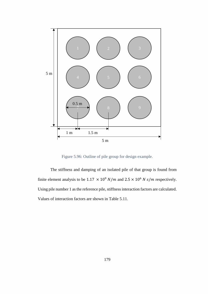
179
Figure 5.96: Outline of pile group for design example.
The stiffness and damping of an isolated pile of that group is found from
finite element analysis to be 1.17 × 10⁹ 𝑁/𝑚 and 2.5 × 10⁶ 𝑁 𝑠/𝑚 respectively.
Using pile number 1 as the reference pile, stiffness interaction factors are calculated.
Values of interaction factors are shown in Table 5.11.
1 2 3
4 5 6
7 8 9
1 m 1.5 m
0.5 m
5 m
5 m
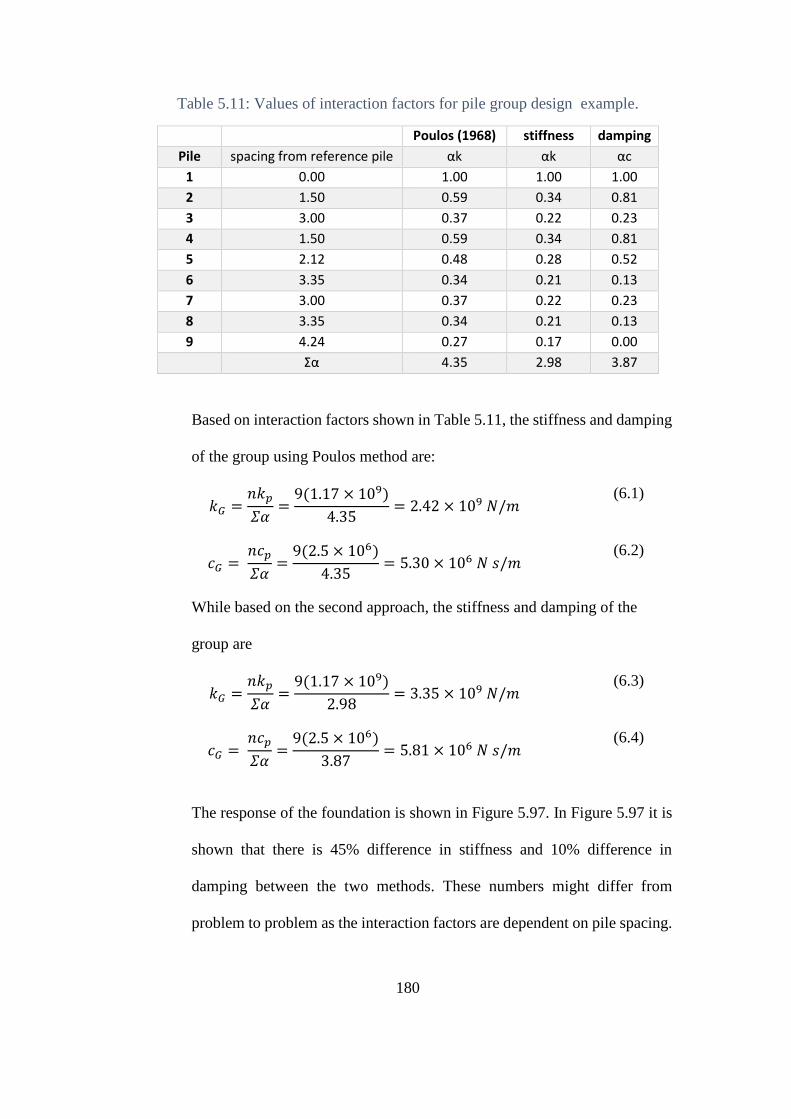
180
Table 5.11: Values of interaction factors for pile group design example.
Poulos (1968) stiffness damping
Pile spacing from reference pile αk αk αc
1 0.00 1.00 1.00 1.00
2 1.50 0.59 0.34 0.81
3 3.00 0.37 0.22 0.23
4 1.50 0.59 0.34 0.81
5 2.12 0.48 0.28 0.52
6 3.35 0.34 0.21 0.13
7 3.00 0.37 0.22 0.23
8 3.35 0.34 0.21 0.13
9 4.24 0.27 0.17 0.00 Σα 4.35 2.98 3.87
Based on interaction factors shown in Table 5.11, the stiffness and damping
of the group using Poulos method are:
𝑘𝐺 =𝑛𝑘𝑝
𝛴𝛼=
9(1.17 × 10⁹)
4.35= 2.42 × 10⁹ 𝑁/𝑚
(6.1)
𝑐𝐺 = 𝑛𝑐𝑝
𝛴𝛼=
9(2.5 × 10⁶)
4.35= 5.30 × 10⁶ 𝑁 𝑠/𝑚
(6.2)
While based on the second approach, the stiffness and damping of the
group are
𝑘𝐺 =𝑛𝑘𝑝
𝛴𝛼=
9(1.17 × 10⁹)
2.98= 3.35 × 10⁹ 𝑁/𝑚
(6.3)
𝑐𝐺 = 𝑛𝑐𝑝
𝛴𝛼=
9(2.5 × 10⁶)
3.87= 5.81 × 10⁶ 𝑁 𝑠/𝑚
(6.4)
The response of the foundation is shown in Figure 5.97. In Figure 5.97 it is
shown that there is 45% difference in stiffness and 10% difference in
damping between the two methods. These numbers might differ from
problem to problem as the interaction factors are dependent on pile spacing.
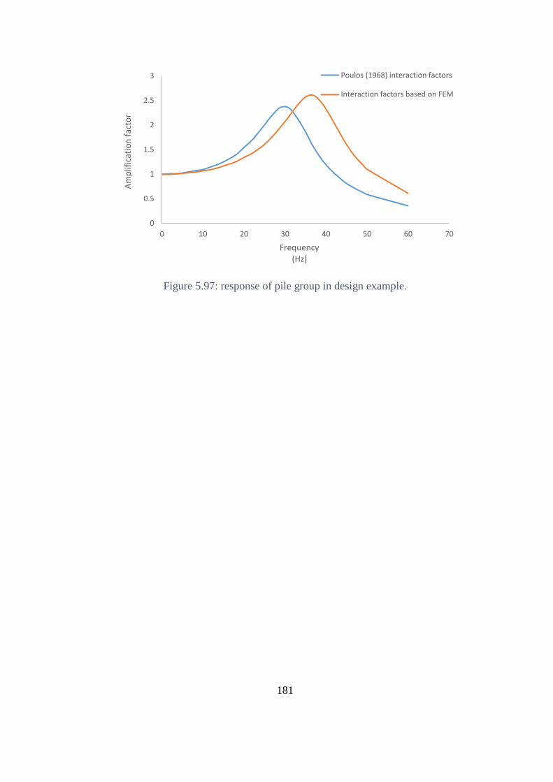
181
Figure 5.97: response of pile group in design example.
0
0.5
1
1.5
2
2.5
3
0 10 20 30 40 50 60 70
Am
plif
icat
ion
fac
tor
Frequency(Hz)
Poulos (1968) interaction factors
Interaction factors based on FEM
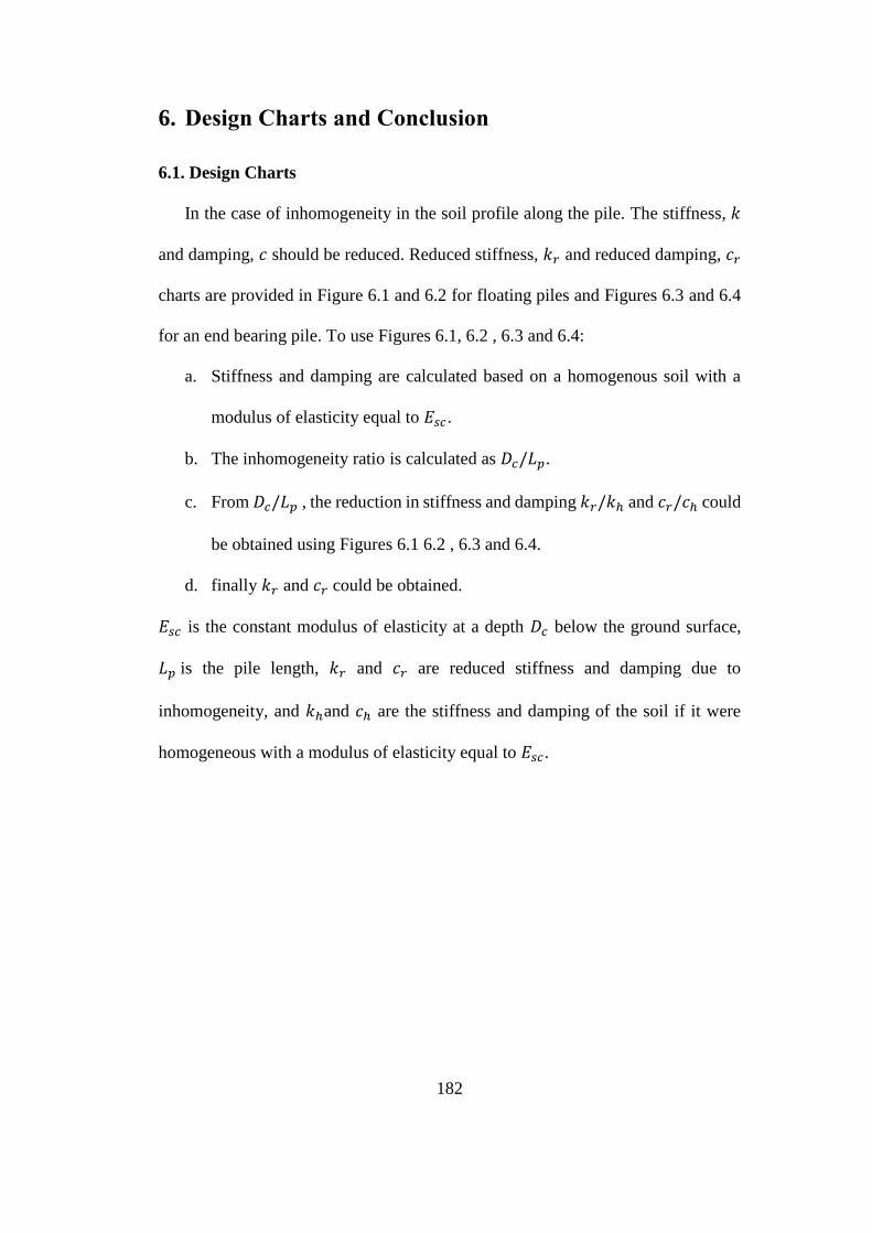
182
6. Design Charts and Conclusion
6.1. Design Charts
In the case of inhomogeneity in the soil profile along the pile. The stiffness, 𝑘
and damping, 𝑐 should be reduced. Reduced stiffness, 𝑘𝑟 and reduced damping, 𝑐𝑟
charts are provided in Figure 6.1 and 6.2 for floating piles and Figures 6.3 and 6.4
for an end bearing pile. To use Figures 6.1, 6.2 , 6.3 and 6.4:
a. Stiffness and damping are calculated based on a homogenous soil with a
modulus of elasticity equal to 𝐸𝑠𝑐.
b. The inhomogeneity ratio is calculated as 𝐷𝑐/𝐿𝑝.
c. From 𝐷𝑐/𝐿𝑝 , the reduction in stiffness and damping 𝑘𝑟/𝑘ℎ and 𝑐𝑟/𝑐ℎ could
be obtained using Figures 6.1 6.2 , 6.3 and 6.4.
d. finally 𝑘𝑟 and 𝑐𝑟 could be obtained.
𝐸𝑠𝑐 is the constant modulus of elasticity at a depth 𝐷𝑐 below the ground surface,
𝐿𝑝 is the pile length, 𝑘𝑟 and 𝑐𝑟 are reduced stiffness and damping due to
inhomogeneity, and 𝑘ℎand 𝑐ℎ are the stiffness and damping of the soil if it were
homogeneous with a modulus of elasticity equal to 𝐸𝑠𝑐.
183
Figure 6.1: Reduction in stiffness of a floating pile due to inhomogeneity of soil
profile.
0.4
0.5
0.6
0.7
0.8
0.9
1
0 0.2 0.4 0.6 0.8 1
Red
uce
d s
tiff
nes
s d
ue
to in
ho
mo
gen
eity
/ s
tiff
nes
s o
f h
om
ogn
eou
s ca
se, k
r/
k h
Inhomogeneity ratio Dc / Lp
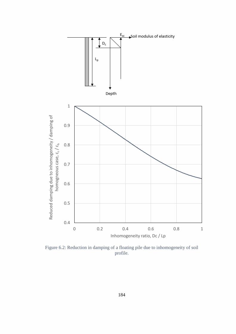
184
Figure 6.2: Reduction in damping of a floating pile due to inhomogeneity of soil
profile.
0.4
0.5
0.6
0.7
0.8
0.9
1
0 0.2 0.4 0.6 0.8 1
Red
uce
d d
amp
ing
du
e to
inh
om
oge
nei
ty /
dam
pin
g o
f h
om
ogn
eou
s ca
se,c
r/
c h
Inhomogeneity ratio, Dc / Lp
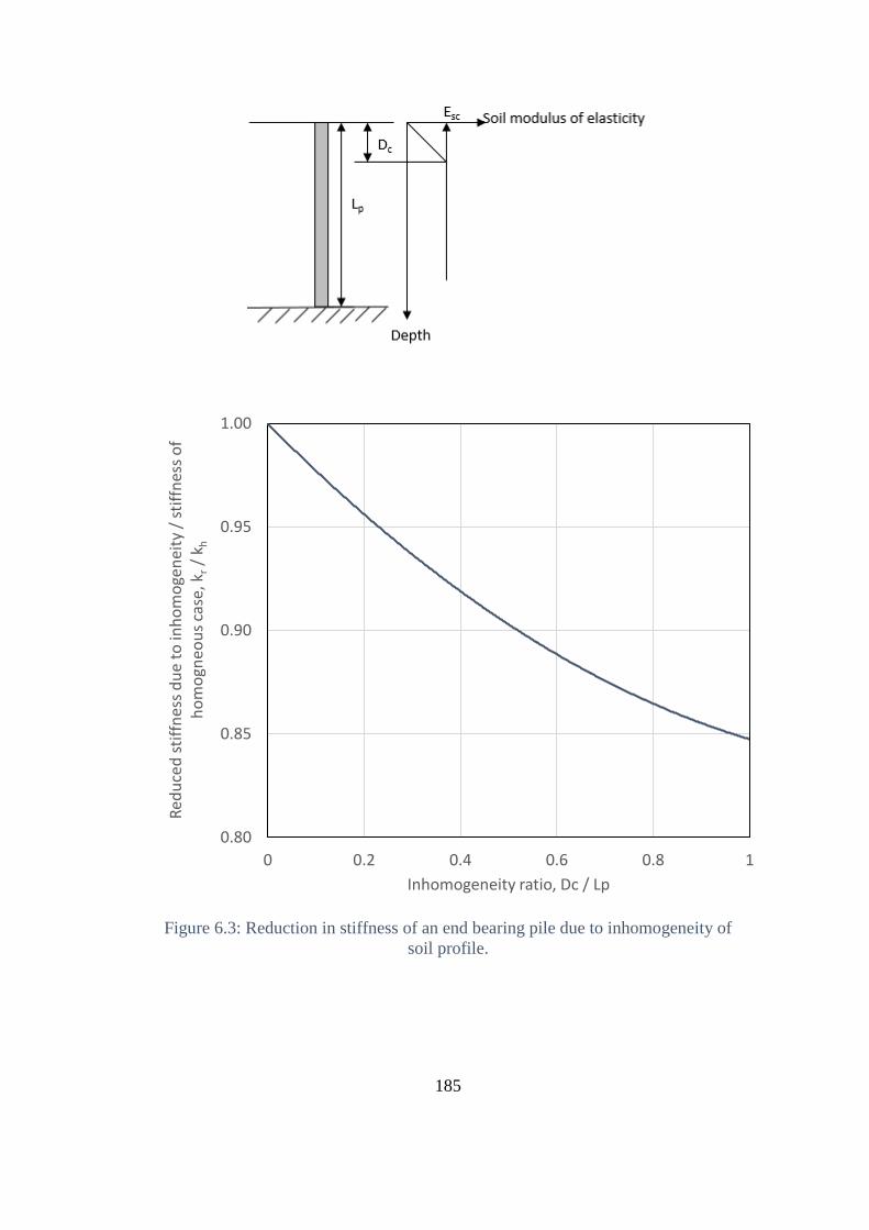
185
Figure 6.3: Reduction in stiffness of an end bearing pile due to inhomogeneity of
soil profile.
0.80
0.85
0.90
0.95
1.00
0 0.2 0.4 0.6 0.8 1
Red
uce
d s
tiff
nes
s d
ue
to in
ho
mo
gen
eity
/ s
tiff
nes
s o
f h
om
ogn
eou
s ca
se, k
r/
k h
Inhomogeneity ratio, Dc / Lp
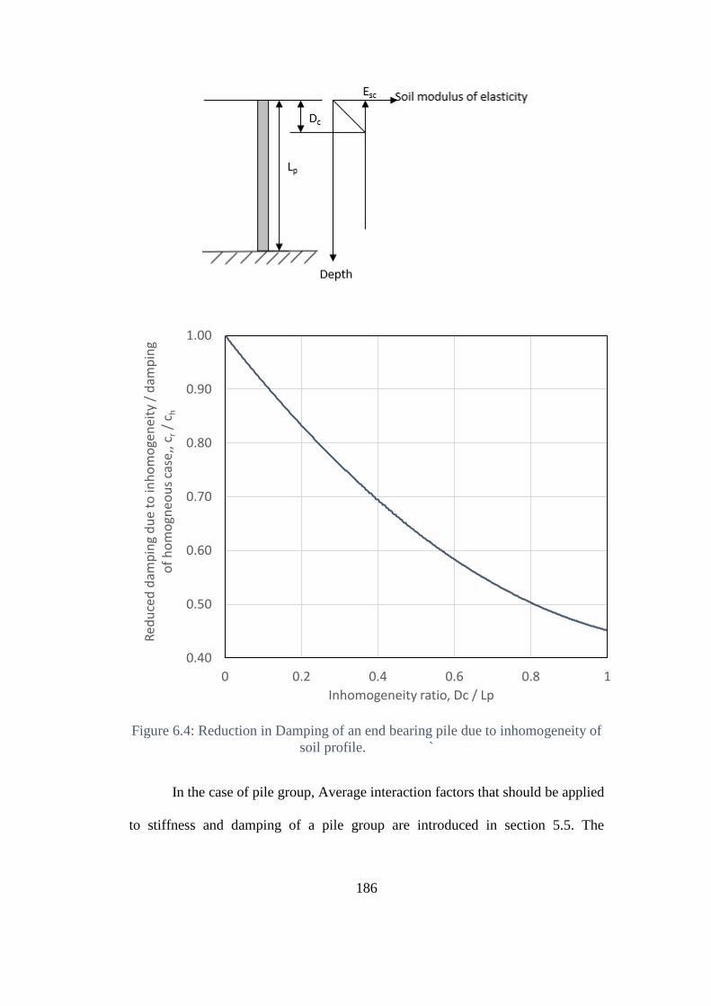
186
Figure 6.4: Reduction in Damping of an end bearing pile due to inhomogeneity of
soil profile. `
In the case of pile group, Average interaction factors that should be applied
to stiffness and damping of a pile group are introduced in section 5.5. The
0.40
0.50
0.60
0.70
0.80
0.90
1.00
0 0.2 0.4 0.6 0.8 1
Red
uce
d d
amp
ing
du
e to
inh
om
oge
nei
ty /
dam
pin
g o
f h
om
ogn
eou
s ca
se,,
c r/
c h
Inhomogeneity ratio, Dc / Lp
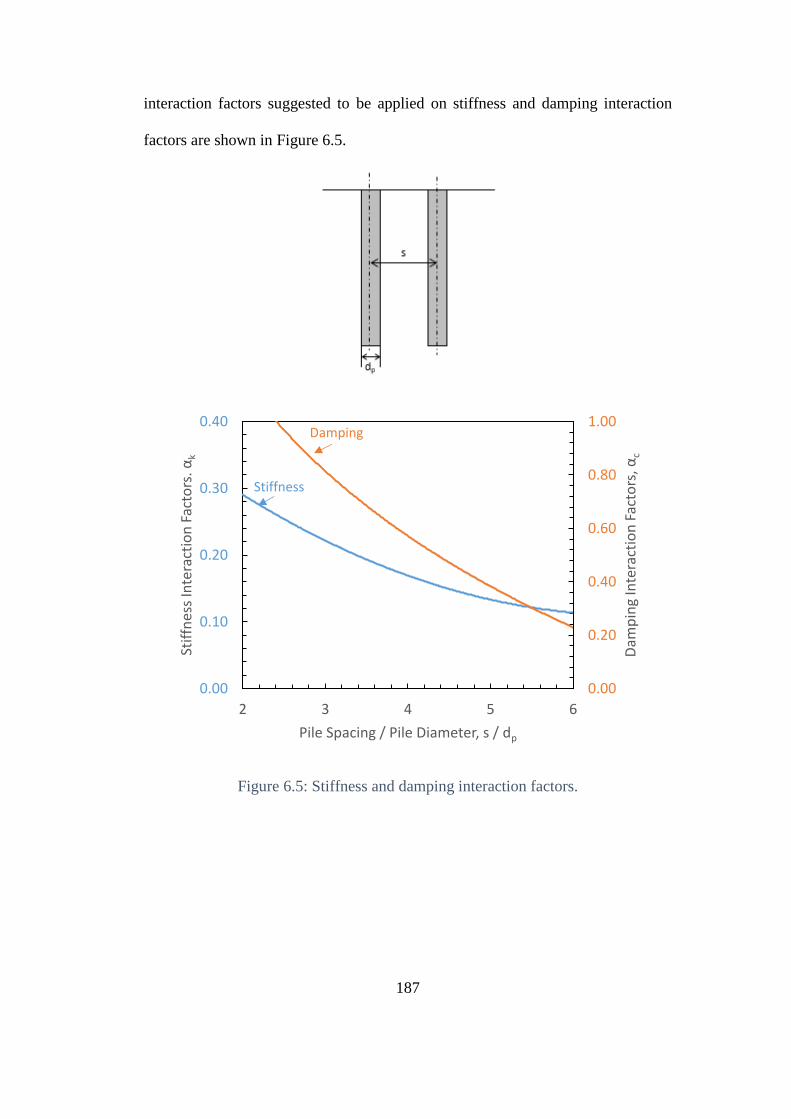
187
interaction factors suggested to be applied on stiffness and damping interaction
factors are shown in Figure 6.5.
Figure 6.5: Stiffness and damping interaction factors.
0.00
0.20
0.40
0.60
0.80
1.00
0.00
0.10
0.20
0.30
0.40
2 3 4 5 6
Dam
pin
g In
tera
ctio
n F
acto
rs, α
c
Stif
fnes
s In
tera
ctio
n F
acto
rs. α
k
Pile Spacing / Pile Diameter, s / dp
Damping
Stiffness
188
6.2. Conclusion
The stiffness and damping of a pile top when subjected to vertical vibration are
needed for the design of a pile subjected to dynamic loading.
Piles are mostly used in groups. The stiffness and damping of individual piles
within a pile group are less than that of an isolated pile due to pile-to-pile
interaction. The interaction between piles is accounted for in design by using
interaction factors. The process of designing a pile group begins by designing an
individual pile and then modify the design to account for interaction using
interaction factors. Interaction factors that are currently in use are the ones provided
by Poulos (1968). However, these interaction factors are based on static analysis of
pile to pile interaction.
This research focuses on variation in the conditions of the soil surrounding the
pile and the soil at the pile tip. The research studies floating and end bearing piles
in homogeneous and nonhomogeneous soils. The research also studies pile to pile
interaction in homogeneous soils. In all the cases studied, the response at the top of
the pile can be represented by a single degree of freedom system consisting of a
mass, a spring, and a damper. The spring stiffness is the same as the stiffness of the
pile and the damper represents energy loss due to radiation damping. The mass
represents the mass supported by the pile. A method described in section 4.4 of this
dissertation was used to obtain the stiffness and damping of the pile-soil system.
Charts of the variation of stiffness and damping with variation in soil conditions are
provided for each case studied in this research.
The concept of replacing the pile with a mass, spring and damper system is
extended to the study of the pile-to-pile interaction. The two piles are replaced by 2
189
parallel sets of spring and damper. The piles interact with each other which results
in a reduction in stiffness and damping compared to an isolated pile. The interaction
factor between the two pile is based on this reduction of stiffness and damping. A
stiffness interaction factor is introduced to represent the reduction in stiffness and a
damping interaction factor represents the reduction in damper coefficient.
The main outcomes of this research is as follows:
1- Floating pile in homogeneous soil
The stiffness, 𝑘 of a single pile increases with increase in soil modulus of
elasticity.
The geometric damping ratio, 𝐷 decreases with increase in soil modulus of
elasticity.
A change in soil modulus of elasticity from 8 × 10⁶ to 8 × 10⁸ Pascal (i.e., a
100-fold increase) results in 32-fold increase in stiffness and 5 fold decrease in
damping.
Critical damping, 𝑐𝑐𝑟 increases with increase in soil modulus of elasticity.
Damper coefficient increases until it reaches a point where it remains
practically constant.
The natural frequency of the soil-pile system increases with increase in soil
modulus of elasticity.
190
2- End bearing pile in homogeneous soil
For an end bearing pile, the stiffness of the pile system increase with an
increase in soil modulus of elasticity.
Geometrical damping ratio was found to increase until a certain value of the
soil modulus of elasticity. After this value, the geometric damping remains
almost constant.
Critical damping increases with increase in soil modulus of elasticity.
Damping increases with increase in soil modulus of elasticity.
Natural frequency increases with increase in soil modulus of elasticity.
An increase in soil modulus of elasticity from 8 × 10⁶ Pascal to 8 × 10⁸
Pascal will increase the stiffness by 400 % while the damping ratio increased
by 200%.
3- Comparison Between End-Bearing Piles and Floating Piles in
Homogeneous Soil
In weak soils, the stiffness of end-bearing piles is 1300% greater than the
stiffness of floating piles. However, damping of floating piles is 1000% higher
than damping of end-bearing piles.
In strong soils, similar values of stiffness and damping are obtained for both
floating and end-bearing piles.
4- Floating pile in nonhomogeneous soil
An increase in top weak soil layer results in reduction in stiffness, damping
ratio, damper coefficient and natural frequency.
191
5- If the top weak soil layer increases in thickness to become equal to the pile
length (i.e. 100% inhomogeneity), both the stiffness and damping are reduced
by 40%.
6- End bearing pile in nonhomogeneous soil
An increase in the thickness of the top weak soil layer reduces stiffness and
damping of the soil-pile system.
If the top weak soil layer increases in thickness to become equal to the pile
length (i.e. 100% inhomogeneity), the stiffness is reduced by 20% while
damping is reduced by 60%.
7- Pile to Pile Interaction
The stiffness and damping interaction factors were found to be dependent on
the spacing between the piles. The greater the spacing, the less is the value of
the interaction factor. This is because when piles are placed far from each other,
the transferred stresses between the two piles is reduced.
The values of damping interaction factors found to be different than static
interaction factors.
Damping interaction can be greater than one. This was found in cases of piles
placed at 0.5 meters away from each other.
Dynamic stiffness interaction factors are lower than the static interaction
factors currently used in practice.
Damping interaction factors are higher than the static interaction factors.
192
6.3. Summary
For design of a pile supported machine, the stiffness and damping of the
soil-pile system at the level of the pile head are needed. The research provides a
methodology to determine both the stiffness and damping for a wide range of
variables, both in material and geometry.
Floating Pile in Homogeneous Soil
• Increase in soil modulus of elasticity results in increase in stiffness, decrease in
damping ratio, increase in damping and increase in natural frequency.
• An increase in soil modulus of elasticity from 8 × 10⁶ Pascal to 8 × 10⁸ Pascal
will increase the stiffness by 3200 % while the damping ratio decreases by 500%.
End-Bearing Pile in Homogeneous Soil
• Increase in soil modulus of elasticity results in increase in stiffness, increase in
damping ratio, increase in damping and increase in natural frequency.
• An increase in soil modulus of elasticity from 8 × 10⁶ Pascal to 8 × 10⁸ Pascal
will increase the stiffness by 400 % while the damping ratio increased by 200%.
Comparison Between End-Bearing Piles and Floating Piles in Homogeneous Soil
• In weak soils, the stiffness of end-bearing piles is 1300% greater than the stiffness
of floating piles. However, damping of floating piles is 1000% greater than
damping of end-bearing piles.
• In strong soils, similar values of stiffness and damping are obtained for both
floating and end-bearing piles.
193
Floating Pile in Non-Homogeneous Soil
• An increase in the thickness of the top weak soil layer will reduce the stiffness and
damping of the soil-pile system.
• If the top weak soil layer increases in thickness to become equal to the pile length,
both the stiffness and damping are reduced by 40%.
End-Bearing Pile in Non-Homogeneous Soil
• An increase in the thickness of the top weak soil layer reduces stiffness and
damping of the soil-pile system.
• If the top weak soil layer increases in thickness to become equal to the pile length,
the stiffness is reduced by 20% while damping is reduced by 60%.
Pile to Pile Interaction Factors
• As spacing between piles increases, the interaction factor decreases.
• Dynamic stiffness interaction factors are lower than the static interaction factors
currently used in practice.
• Damping interaction factors are higher than the static interaction factors.
Design Charts
• Design charts are provided to account for inhomogeneity in the soil profile for
both floating and end-bearing piles.
• Stiffness and damping interactions factors are provided to account for dynamic
pile to pile interaction.
194
Appendices
A. An Introduction To Soil Dynamics
A.1. Vibrating systems
Consider a system of a single degree of freedom system as shown in
Figure A.1. Such system consists of a rigid mass, a supporting elastic spring and
viscous dashpot damper. Applying a force F to the system; in which F is dynamic
in nature that varies with time t. In such a system the inertia takes effect and
Newton’s second Equation of motion applies to the system. The following
differential Equation can be used
Md2u
dt2= F(t) (A.1)
In Equation A.1, M is the mass and u is the displacement. In said system, the spring
will respond to the displacement caused by the force while the damper will respond
to the velocity. Equation A.1 is now adjusted to include the spring and damper
reactions to becomes
Md2u
dt2+ c
du
dt+ ku = F(t) (A.2)
Where c is the damper viscosity coefficient and k is the spring constant.
Understanding such a system is critical in Machine foundation and soil dynamics
in general. In many cases, the soil response to an applied dynamic load is reduced
to an analogous spring and a viscous dashpot damper. This makes the problem easy
to solve. The engineers only need to conduct experiments to determine 𝑐 and 𝑘
values and solve the problem.
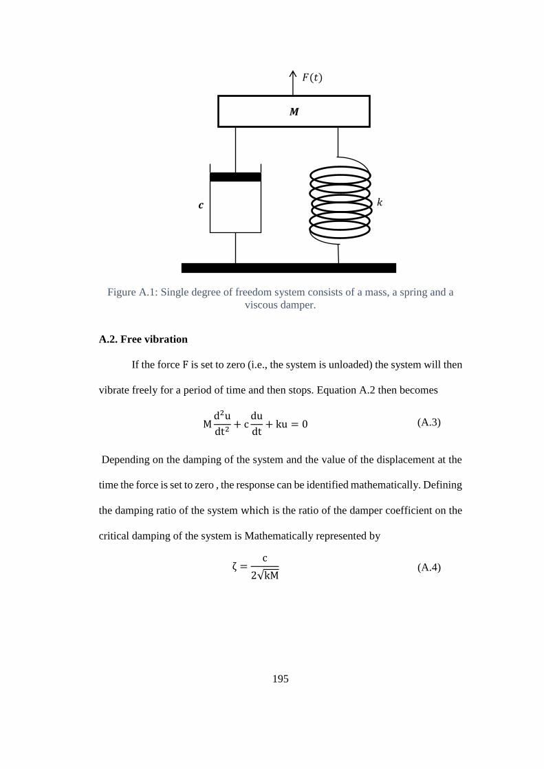
195
Figure A.1: Single degree of freedom system consists of a mass, a spring and a
viscous damper.
A.2. Free vibration
If the force F is set to zero (i.e., the system is unloaded) the system will then
vibrate freely for a period of time and then stops. Equation A.2 then becomes
Md2u
dt2+ c
du
dt+ ku = 0 (A.3)
Depending on the damping of the system and the value of the displacement at the
time the force is set to zero , the response can be identified mathematically. Defining
the damping ratio of the system which is the ratio of the damper coefficient on the
critical damping of the system is Mathematically represented by
ζ =c
2√kM (A.4)
𝑴
𝒄 𝑘
𝐹(𝑡)
196
Where the denominator is the value of the critical damping of the system. Also the
natural frequency 𝜔0 of such a system can be written as
ω0 =𝑓𝑛2𝜋
(𝑟𝑎𝑑𝑖𝑎𝑛𝑠
𝑠𝑒𝑐𝑜𝑛𝑑) 𝑤ℎ𝑒𝑟𝑒 𝑓𝑛 = √
κ
Μ(𝐻𝑧) (A.5)
The response of the system can be characterized by using the response time tr also
called the relaxation time which is defined as
tr = c/k (A.6)
The value of tr defines the response time of the system. At any time less than the
response time, the system is considered stiff and the response depends on the
damper. The system response depends more on the spring when the time is greater
than the response time. From Equations A.4, A.5 and A.6 the damping can be
related to the damping ratio and the natural frequency of the system as c = 2ζω0.
Using c = 2ζω0 into Equation A.3, gives the following
Md2u
dt2+ 2ζω0
du
dt+ ω0
2u = 0 (A.7)
Equation A.7 represents a differential Equation in which the solution can be
assumed to take the form
u = Aeat (A.8)
Where A is a constant related to the initial value of the displacement when F was
set to zero. and a is an unknown value.
197
Substituting Equation A.8 in Equation A.7 will give
𝑎2 + 2ζω0a + ω02 = 0 (A.9)
a now can be found by finding the roots of Equation 2.9. The solution might be real
or complex, and it takes the form
a1,2 = −ζω0 ±ω0√ζ2 − 1 (A.10)
It is clear from Equation 2.10 that the response of the system depends on the value
of the damping ratio ζ. In general, three outcomes can be obtained as shown in the
upcoming sections.
A.2.1. when the damping ratio, 𝛇 is less than 1
When the damping ratio ζ is less than 1(ζ < 1), the solution of Equation A.10 takes
the form complex roots.
α1,2 = −ζω0 ± iω0√1 − ζ2 (A.11)
Where i is the imaginary part of the complex number and( i = √−1). The dynamic
displacement u can be obtained as
u = Α1 eiω1t e−ζω0t + A2 e
iω1t e−ζω0t (A.12)
And ω1is defined as the damped natural frequency where ω1 = ω0√1 − ζ2. eiω1t
Can be rewritten as cos(ω1t) + i sin(ω1t). Equation 2.12 then becomes
ud = C1 cos(ω1t) e−ζω0t + C2 sin(ω1t) e
−ζω0t
(A.13)
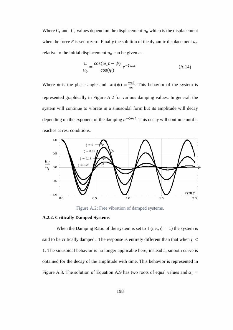
198
Where C1 and C2 values depend on the displacement 𝑢0 which is the displacement
when the force 𝐹 is set to zero. Finally the solution of the dynamic displacement 𝑢𝑑
relative to the initial displacement 𝑢0 can be given as
𝑢
𝑢0=
cos (𝜔1𝑡 − 𝜓)
cos (𝜓) 𝑒−𝜁𝜔0𝑡 (A.14)
Where 𝜓 is the phase angle and tan(𝜓) =𝜔0𝜁
𝜔1. This behavior of the system is
represented graphically in Figure A.2 for various damping values. In general, the
system will continue to vibrate in a sinusoidal form but its amplitude will decay
depending on the exponent of the damping 𝑒−𝜁𝜔0𝑡. This decay will continue until it
reaches at rest conditions.
Figure A.2: Free vibration of damped systems.
A.2.2. Critically Damped Systems
When the Damping Ratio of the system is set to 1 (i.e., 휁 = 1) the system is
said to be critically damped. The response is entirely different than that when 휁 <
1. The sinusoidal behavior is no longer applicable here; instead a, smooth curve is
obtained for the decay of the amplitude with time. This behavior is represented in
Figure A.3. The solution of Equation A.9 has two roots of equal values and 𝛼1 =
0.0 0.5 1.0 1.5 2.0
1.0
0.5
0.0
0.5
1.0
휁 = 0
휁 = 0.05
휁 = 0.15
휁 = 0.25 𝑢𝑑
𝑢𝑖
𝑡𝑖𝑚𝑒
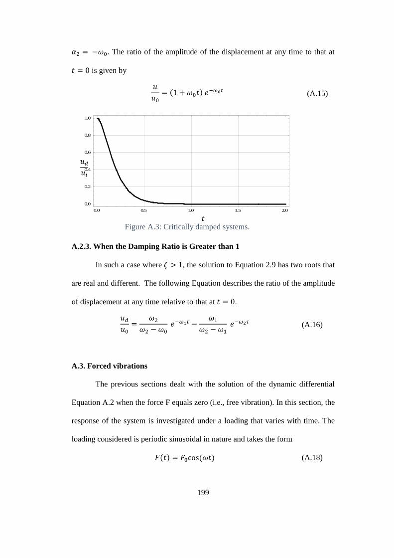
199
𝛼2 = −𝜔0. The ratio of the amplitude of the displacement at any time to that at
𝑡 = 0 is given by
𝑢
𝑢0= (1 + 𝜔0𝑡) 𝑒
−𝜔0𝑡 (A.15)
Figure A.3: Critically damped systems.
A.2.3. When the Damping Ratio is Greater than 1
In such a case where 휁 > 1, the solution to Equation 2.9 has two roots that
are real and different. The following Equation describes the ratio of the amplitude
of displacement at any time relative to that at 𝑡 = 0.
𝑢𝑑
𝑢0=
𝜔2
𝜔2 − 𝜔0 𝑒−𝜔1𝑡 −
𝜔1
𝜔2 − 𝜔1 𝑒−𝜔2𝜏 (A.16)
A.3. Forced vibrations
The previous sections dealt with the solution of the dynamic differential
Equation A.2 when the force F equals zero (i.e., free vibration). In this section, the
response of the system is investigated under a loading that varies with time. The
loading considered is periodic sinusoidal in nature and takes the form
𝐹(𝑡) = 𝐹0cos (𝜔𝑡) (A.18)
0.0 0.5 1.0 1.5 2.0
0.0
0.2
0.4
0.6
0.8
1.0
𝑢𝑑
𝑢𝑖
𝑡
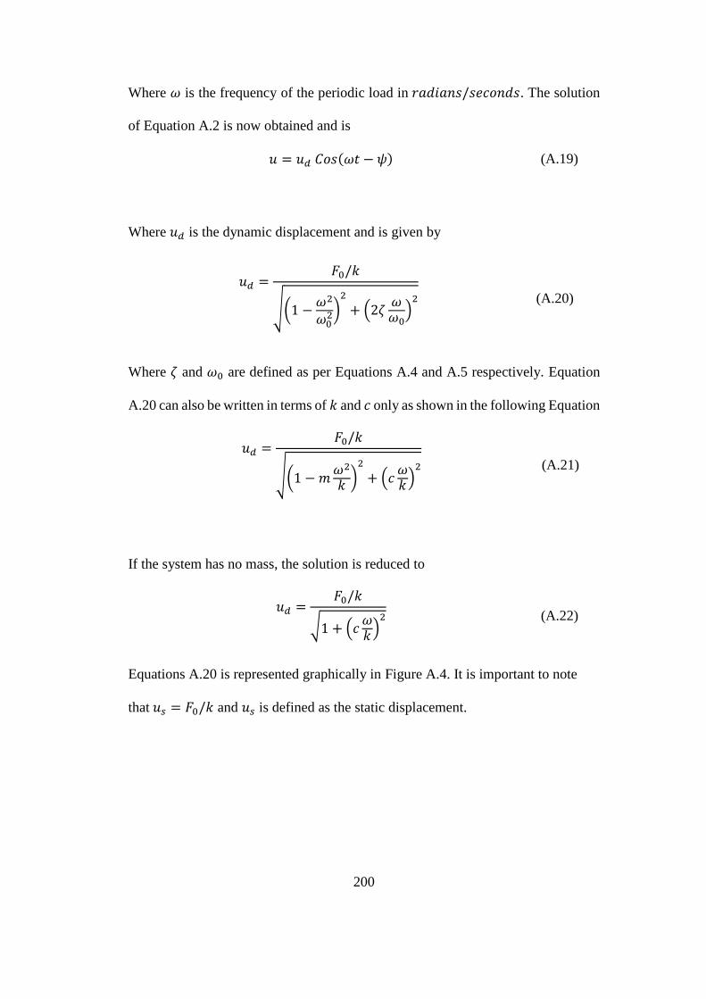
200
Where 𝜔 is the frequency of the periodic load in 𝑟𝑎𝑑𝑖𝑎𝑛𝑠/𝑠𝑒𝑐𝑜𝑛𝑑𝑠. The solution
of Equation A.2 is now obtained and is
𝑢 = 𝑢𝑑 𝐶𝑜𝑠(𝜔𝑡 − 𝜓) (A.19)
Where 𝑢𝑑 is the dynamic displacement and is given by
𝑢𝑑 =𝐹0/𝑘
√(1 −𝜔2
𝜔02)
2
+ (2휁𝜔𝜔0
)2
(A.20)
Where 휁 and 𝜔0 are defined as per Equations A.4 and A.5 respectively. Equation
A.20 can also be written in terms of 𝑘 and 𝑐 only as shown in the following Equation
𝑢𝑑 =𝐹0/𝑘
√(1 −𝑚𝜔2
𝑘)2
+ (𝑐𝜔𝑘)2
(A.21)
If the system has no mass, the solution is reduced to
𝑢𝑑 =𝐹0/𝑘
√1 + (𝑐𝜔𝑘)2
(A.22)
Equations A.20 is represented graphically in Figure A.4. It is important to note
that 𝑢𝑠 = 𝐹0/𝑘 and 𝑢𝑠 is defined as the static displacement.
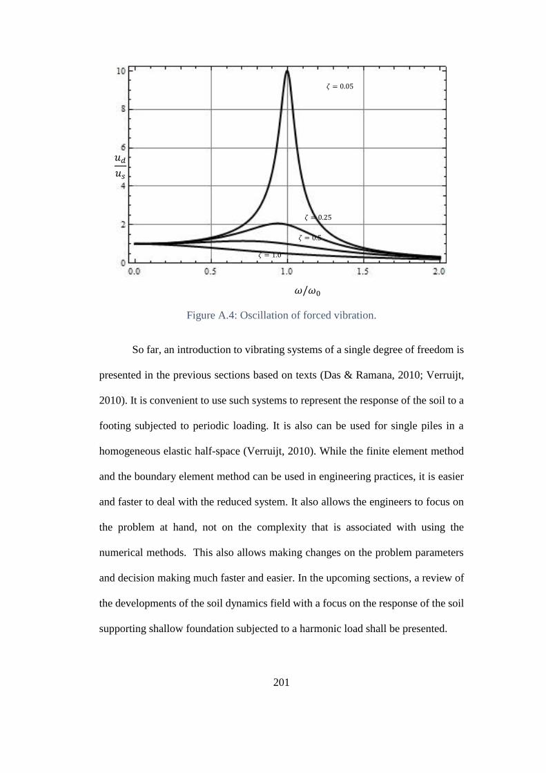
201
Figure A.4: Oscillation of forced vibration.
So far, an introduction to vibrating systems of a single degree of freedom is
presented in the previous sections based on texts (Das & Ramana, 2010; Verruijt,
2010). It is convenient to use such systems to represent the response of the soil to a
footing subjected to periodic loading. It is also can be used for single piles in a
homogeneous elastic half-space (Verruijt, 2010). While the finite element method
and the boundary element method can be used in engineering practices, it is easier
and faster to deal with the reduced system. It also allows the engineers to focus on
the problem at hand, not on the complexity that is associated with using the
numerical methods. This also allows making changes on the problem parameters
and decision making much faster and easier. In the upcoming sections, a review of
the developments of the soil dynamics field with a focus on the response of the soil
supporting shallow foundation subjected to a harmonic load shall be presented.
𝑢𝑑
𝑢𝑠
𝜔/𝜔0
휁 = 1.0
휁 = 0.5
휁 = 0.25
휁 = 0.05
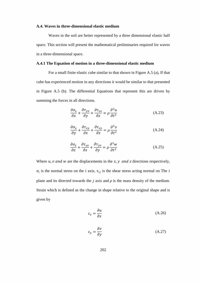
202
A.4. Waves in three-dimensional elastic medium
Waves in the soil are better represented by a three dimensional elastic half
space. This section will present the mathematical preliminaries required for waves
in a three-dimensional space.
A.4.1 The Equation of motion in a three-dimensional elastic medium
For a small finite elastic cube similar to that shown in Figure A.5 (a), If that
cube has experienced motion in any directions it would be similar to that presented
in Figure A.5 (b). The differential Equations that represent this are driven by
summing the forces in all directions.
𝜕𝜎𝑥𝜕𝑥
+𝜕𝜏𝑦𝑥
𝜕𝑦+𝜕𝜏𝑧𝑥𝜕𝑧
= 𝜌𝜕2𝑢
𝜕𝑡2 (A.23)
𝜕𝜎𝑦
𝜕𝑦+𝜕𝜏𝑥𝑦
𝜕𝑥+𝜕𝜏𝑧𝑦
𝜕𝑧= 𝜌
𝜕2𝑣
𝜕𝑡2 (A.24)
𝜕𝜎𝑧𝜕𝑧
+𝜕𝜏𝑥𝑧𝜕𝑥
+𝜕𝜏𝑦𝑧
𝜕𝑦= 𝜌
𝜕2𝑤
𝜕𝑡2 (A.25)
Where 𝑢, 𝑣 𝑎𝑛𝑑 𝑤 are the displacements in the 𝑥, 𝑦 𝑎𝑛𝑑 𝑧 directions respectively,
𝜎𝑖 is the normal stress on the 𝑖 axis, 𝜏𝑖𝑗 is the shear stress acting normal on The 𝑖
plane and its directed towards the 𝑗 axis and 𝜌 is the mass density of the medium.
Strain which is defined as the change in shape relative to the original shape and is
given by
휀𝑥 =𝜕𝑢
𝜕𝑥 (A.26)
휀𝑦 =𝜕𝑣
𝜕𝑦 (A.27)
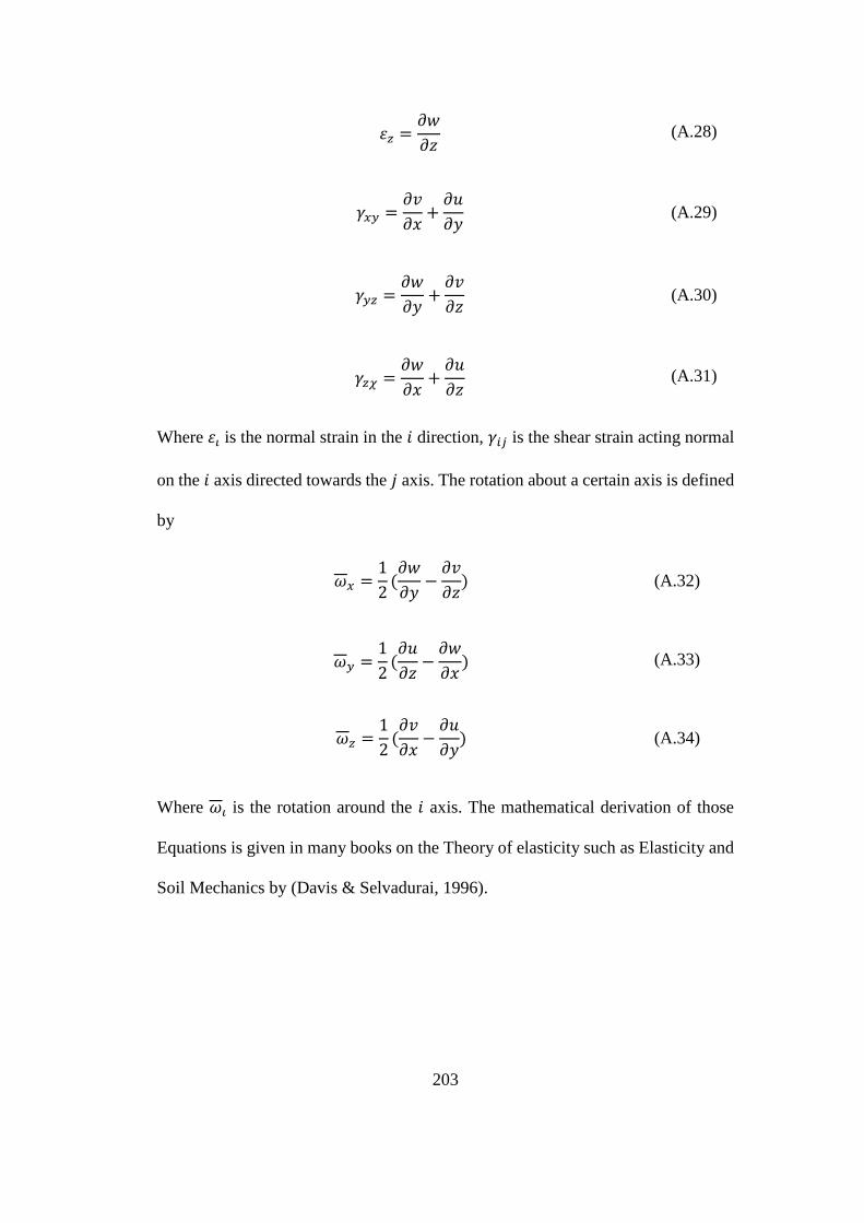
203
휀𝑧 =𝜕𝑤
𝜕𝑧 (A.28)
𝛾𝑥𝑦 =𝜕𝑣
𝜕𝑥+𝜕𝑢
𝜕𝑦 (A.29)
𝛾𝑦𝑧 =𝜕𝑤
𝜕𝑦+𝜕𝑣
𝜕𝑧 (A.30)
𝛾𝑧𝜒 =𝜕𝑤
𝜕𝑥+𝜕𝑢
𝜕𝑧 (A.31)
Where 휀𝜄 is the normal strain in the 𝑖 direction, 𝛾𝑖𝑗 is the shear strain acting normal
on the 𝑖 axis directed towards the 𝑗 axis. The rotation about a certain axis is defined
by
𝜔𝑥 =1
2(𝜕𝑤
𝜕𝑦−𝜕𝑣
𝜕𝑧) (A.32)
𝜔𝑦 =1
2(𝜕𝑢
𝜕𝑧−𝜕𝑤
𝜕𝑥) (A.33)
𝜔𝑧 =1
2(𝜕𝑣
𝜕𝑥−𝜕𝑢
𝜕𝑦) (A.34)
Where 𝜔𝜄 is the rotation around the 𝑖 axis. The mathematical derivation of those
Equations is given in many books on the Theory of elasticity such as Elasticity and
Soil Mechanics by (Davis & Selvadurai, 1996).
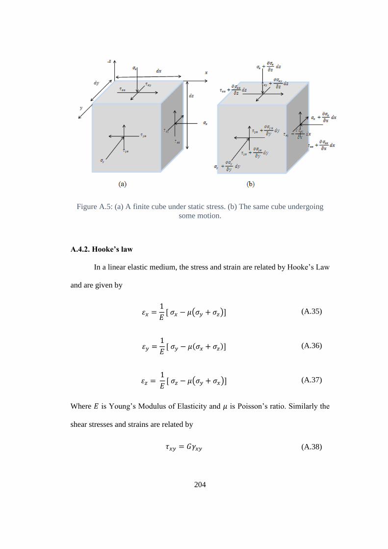
204
Figure A.5: (a) A finite cube under static stress. (b) The same cube undergoing
some motion.
A.4.2. Hooke’s law
In a linear elastic medium, the stress and strain are related by Hooke’s Law
and are given by
휀𝑥 =1
𝐸[ 𝜎𝑥 − 𝜇 𝜎𝑦 + 𝜎𝑧 ] (A.35)
휀𝑦 =1
𝐸[ 𝜎𝑦 − 𝜇(𝜎𝑥 + 𝜎𝑧)] (A.36)
휀𝑧 = 1
𝐸[ 𝜎𝑧 − 𝜇 𝜎𝑦 + 𝜎𝑥 ] (A.37)
Where 𝐸 is Young’s Modulus of Elasticity and 𝜇 is Poisson’s ratio. Similarly the
shear stresses and strains are related by
𝜏𝑥𝑦 = 𝐺𝛾𝑥𝑦 (A.38)
205
𝜏𝑦𝑧 = 𝐺𝛾𝑦𝑧 (A.39)
𝜏𝑧𝑥 = 𝐺𝛾𝑧𝑥 (A.40)
𝐺 is the shear modulus and is related the Young’s Modulus Poisson’s ratio by
𝐺 =1
2 𝐸 (1 + 𝜇) (A.41)
The solution to Equations A.35 to A.37 that relates the normal stresses to the normal
strains is
𝜎𝑥 = 𝜆휀 + 2𝐺휀𝑥 (A.42)
𝜎𝑦 = 𝜆휀 + 2𝐺휀𝑦 (A.43)
𝜎𝑧 = 𝜆휀 + 2𝐺휀𝑧 (A.44)
Where
𝜆 = 𝜇𝐸/[(1 + 𝜇)(1 − 2𝜇)] (A.45)
휀 = 휀𝑥 + 휀𝑦 + 휀𝑧 (A.46)
206
A.4.3. Equations for compression stress waves in an infinite elastic medium
Equation A.23 can be rewritten using Equations A.38, A.40 and A.42 to become
𝜌𝜕2𝑢
𝜕𝑡2=
𝜕
𝜕𝑥(𝜆휀 + 2𝐺휀𝑥) +
𝜕
𝜕𝑦 𝐺𝛾𝑥𝑦 +
𝜕
𝜕𝑧(𝐺𝛾𝑥𝑧) (A.47)
The values of 휀𝑥, 𝛾𝑥𝑦 and 𝛾𝑥𝑧 can be substituted using Equations A.26, A.29 and
A.31 so that Equation A.47 becomes
𝜌𝜕2𝑢
𝜕𝑡2=
𝜕
𝜕𝑥(𝜆휀 + 2𝐺휀𝑥) + 𝐺
𝜕
𝜕𝑦(𝜕𝑣
𝜕𝑥+𝜕𝑢
𝜕𝑦) + 𝐺
𝜕
𝜕𝑧(𝜕𝑤
𝜕𝑥+𝜕𝑢
𝜕𝑧) (A.48)
The previous Equation can be rearranged so that it becomes
𝜌𝜕2𝑢
𝜕𝑡2= 𝜆
𝜕𝑒
𝜕𝑥+ 𝐺(
𝜕2𝑢
𝜕𝑥2+
𝜕2𝑣
𝜕𝑥𝜕𝑦+
𝜕2𝑤
𝜕𝑥𝜕𝑧+𝜕2𝑢
𝜕𝑥2+𝜕2𝑢
𝜕𝑦2 +
𝜕2𝑢
2𝜕𝑧2 ) (A.49)
Yet 휀 = 휀𝑥 + 휀𝑦 + 휀𝑧 which values can be taken from Equations A.26, A.27 and
A.28 so that
𝜕2𝑢
𝜕𝑥2+
𝜕2𝑣
𝜕𝑥𝜕𝑦+
𝜕2𝑤
𝜕𝑥𝜕𝑧
can be rewritten as 𝜕𝜀
𝜕𝑥 . Using the previous derivation, Equation A.49 is simplified
to be
𝜌𝜕2𝑢
𝜕𝑡2= (𝜆 + 𝐺)
𝜕휀
𝜕𝑥+ 𝐺∇2𝑢 (A.50)
Where
∇2=𝜕2
𝜕𝑥2+
𝜕2
𝜕𝑦2+
𝜕2
𝜕𝑧2 (A.51)
207
Similarly in the 𝑦 and 𝑧 directions
𝜌𝜕2𝑣
𝜕𝑡2= (𝜆 + 𝐺)
𝜕휀
𝜕𝑦+ 𝐺∇2𝑣 (A.52)
𝜌𝜕2𝑤
𝜕𝑡2= (𝜆 + 𝐺)
𝜕휀
𝜕𝑧+ 𝐺∇2𝑤 (A.53)
By differentiating Equations A.50, A.52 and A.53 with respect to 𝑥, 𝑦 and
𝑧 respectively and then summing the Equations all together, the result would be
𝜌𝜕2휀
𝜕𝑡2= (𝜆 + 2𝐺)(∇2𝑒) (A.54)
By dividing both sides on 𝜌
𝜕2휀
𝜕𝑡2=
(𝜆 + 2𝐺)
𝜌∇2휀 = 𝑣𝑝∇
2휀 (A.55)
Where 𝑣𝑝is defined as the compressional wave velocity and is given by
𝑣𝑝 =𝜆 + 2𝐺
𝜌 (A.56)
For the rest of this text, Compression waves can be referred to as Primary waves or
P-waves.
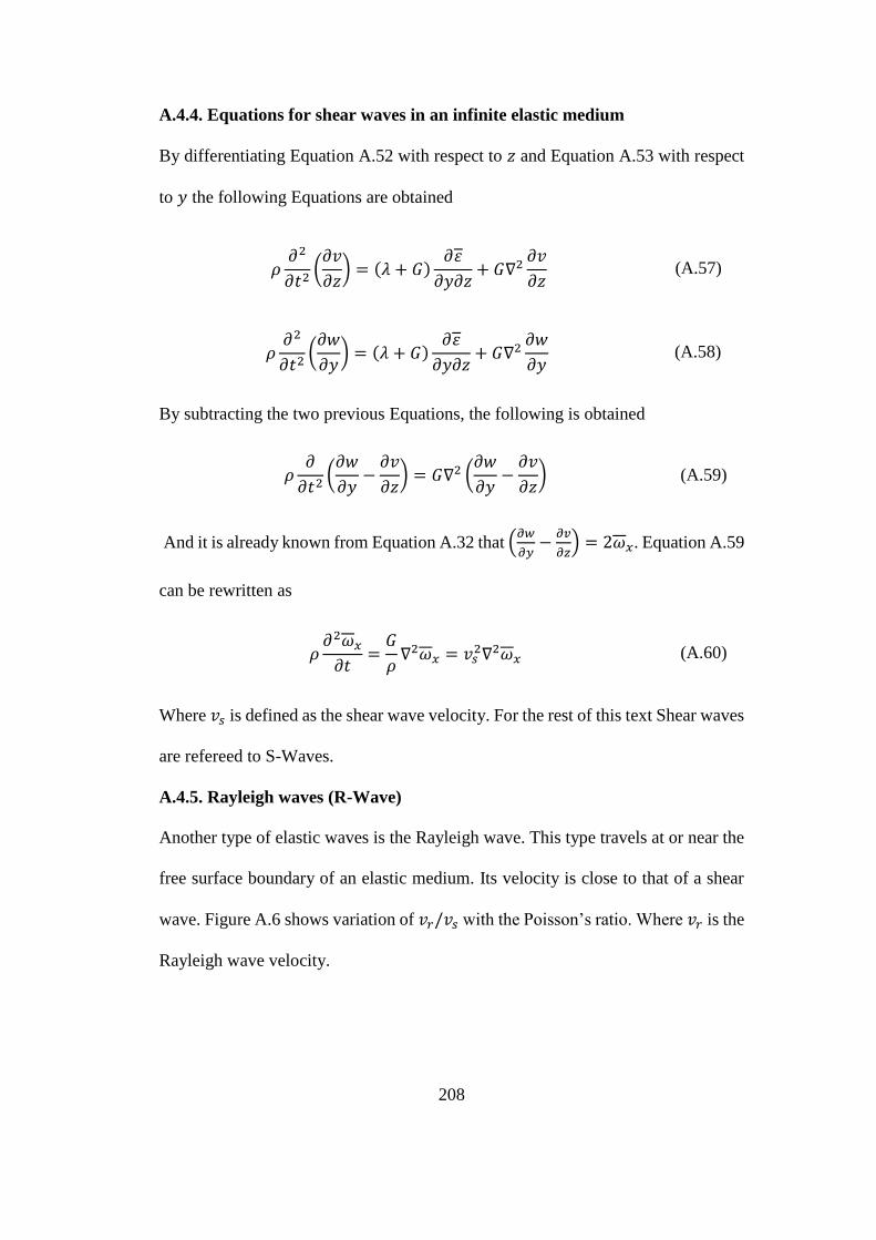
208
A.4.4. Equations for shear waves in an infinite elastic medium
By differentiating Equation A.52 with respect to 𝑧 and Equation A.53 with respect
to 𝑦 the following Equations are obtained
𝜌𝜕2
𝜕𝑡2(𝜕𝑣
𝜕𝑧) = (𝜆 + 𝐺)
𝜕휀
𝜕𝑦𝜕𝑧+ 𝐺∇2
𝜕𝑣
𝜕𝑧 (A.57)
𝜌𝜕2
𝜕𝑡2(𝜕𝑤
𝜕𝑦) = (𝜆 + 𝐺)
𝜕휀
𝜕𝑦𝜕𝑧+ 𝐺∇2
𝜕𝑤
𝜕𝑦 (A.58)
By subtracting the two previous Equations, the following is obtained
𝜌𝜕
𝜕𝑡2(𝜕𝑤
𝜕𝑦−𝜕𝑣
𝜕𝑧) = 𝐺∇2 (
𝜕𝑤
𝜕𝑦−𝜕𝑣
𝜕𝑧) (A.59)
And it is already known from Equation A.32 that (𝜕𝑤
𝜕𝑦−
𝜕𝑣
𝜕𝑧) = 2𝜔𝑥. Equation A.59
can be rewritten as
𝜌𝜕2𝜔𝑥
𝜕𝑡=
𝐺
𝜌∇2𝜔𝑥 = 𝑣𝑠
2∇2𝜔𝑥 (A.60)
Where 𝑣𝑠 is defined as the shear wave velocity. For the rest of this text Shear waves
are refereed to S-Waves.
A.4.5. Rayleigh waves (R-Wave)
Another type of elastic waves is the Rayleigh wave. This type travels at or near the
free surface boundary of an elastic medium. Its velocity is close to that of a shear
wave. Figure A.6 shows variation of 𝑣𝑟/𝑣𝑠 with the Poisson’s ratio. Where 𝑣𝑟 is the
Rayleigh wave velocity.
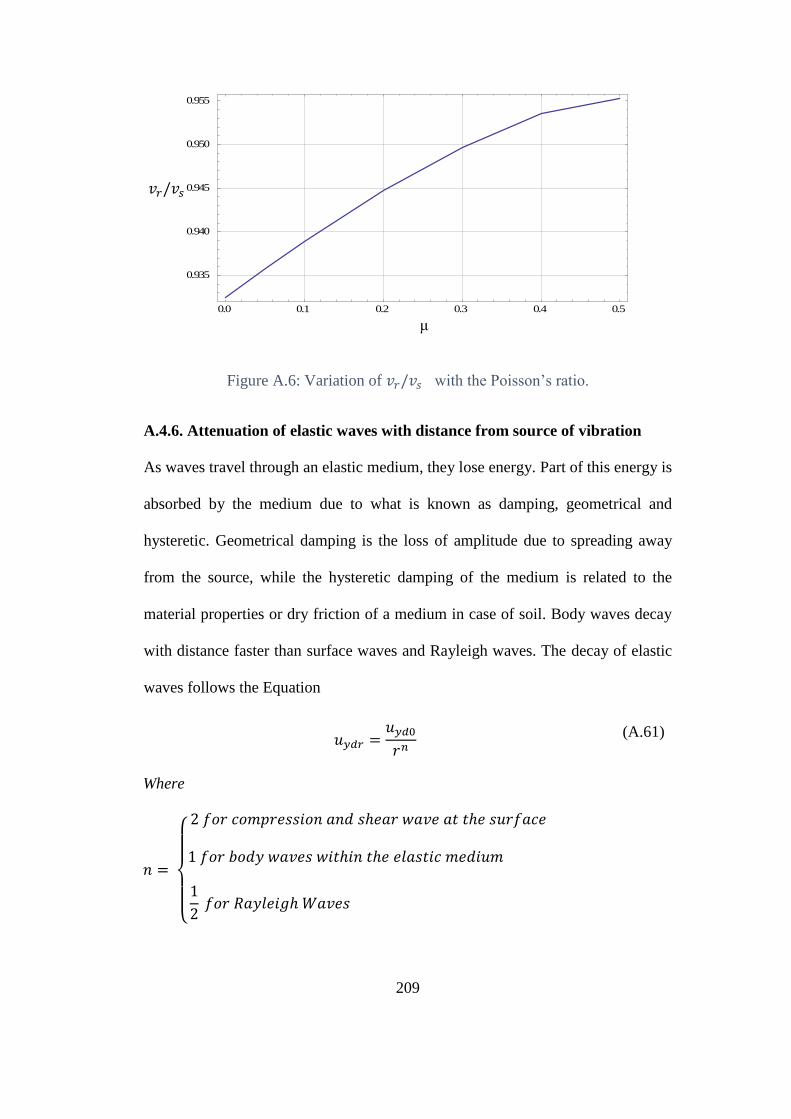
209
Figure A.6: Variation of 𝑣𝑟/𝑣𝑠 with the Poisson’s ratio.
A.4.6. Attenuation of elastic waves with distance from source of vibration
As waves travel through an elastic medium, they lose energy. Part of this energy is
absorbed by the medium due to what is known as damping, geometrical and
hysteretic. Geometrical damping is the loss of amplitude due to spreading away
from the source, while the hysteretic damping of the medium is related to the
material properties or dry friction of a medium in case of soil. Body waves decay
with distance faster than surface waves and Rayleigh waves. The decay of elastic
waves follows the Equation
𝑢𝑦𝑑𝑟 =𝑢𝑦𝑑0
𝑟𝑛
Where
𝑛 =
{
2 𝑓𝑜𝑟 𝑐𝑜𝑚𝑝𝑟𝑒𝑠𝑠𝑖𝑜𝑛 𝑎𝑛𝑑 𝑠ℎ𝑒𝑎𝑟 𝑤𝑎𝑣𝑒 𝑎𝑡 𝑡ℎ𝑒 𝑠𝑢𝑟𝑓𝑎𝑐𝑒
1 𝑓𝑜𝑟 𝑏𝑜𝑑𝑦 𝑤𝑎𝑣𝑒𝑠 𝑤𝑖𝑡ℎ𝑖𝑛 𝑡ℎ𝑒 𝑒𝑙𝑎𝑠𝑡𝑖𝑐 𝑚𝑒𝑑𝑖𝑢𝑚
1
2 𝑓𝑜𝑟 𝑅𝑎𝑦𝑙𝑒𝑖𝑔ℎ 𝑊𝑎𝑣𝑒𝑠
(A.61)
0.0 0.1 0.2 0.3 0.4 0.5
0.935
0.940
0.945
0.950
0.955
𝑣𝑟/𝑣𝑠
μ
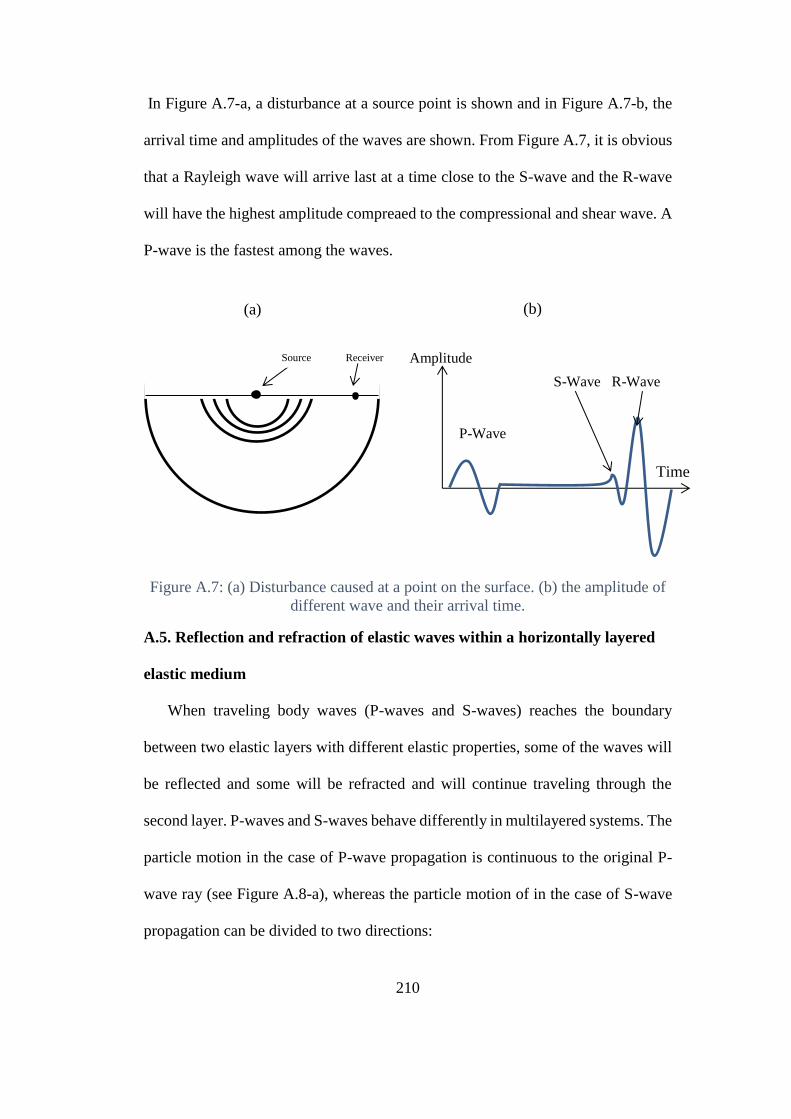
210
In Figure A.7-a, a disturbance at a source point is shown and in Figure A.7-b, the
arrival time and amplitudes of the waves are shown. From Figure A.7, it is obvious
that a Rayleigh wave will arrive last at a time close to the S-wave and the R-wave
will have the highest amplitude compreaed to the compressional and shear wave. A
P-wave is the fastest among the waves.
Figure A.7: (a) Disturbance caused at a point on the surface. (b) the amplitude of
different wave and their arrival time.
A.5. Reflection and refraction of elastic waves within a horizontally layered
elastic medium
When traveling body waves (P-waves and S-waves) reaches the boundary
between two elastic layers with different elastic properties, some of the waves will
be reflected and some will be refracted and will continue traveling through the
second layer. P-waves and S-waves behave differently in multilayered systems. The
particle motion in the case of P-wave propagation is continuous to the original P-
wave ray (see Figure A.8-a), whereas the particle motion of in the case of S-wave
propagation can be divided to two directions:
Source Receiver
Time
Amplitude
P-Wave
S-Wave R-Wave
(a) (b)
211
1- SH-waves which cause the particles to move in the plane of propagation as
presented in Figure A.8-b.
2- SV-waves that cause the particles to move in a direction that is perpendicular to
the plane of propagation as shown in Figure A.8-c.
In the case of a P-wave at the interface of two layers, there will be two
reflected waves and two refracted waves. The first of the reflected waves will be of
the same nature of the source wave, a P-wave, while the second one will be of the
nature of an SV-wave. As for the refracted waves, the same applies; a P-wave and
SV-wave will be generated (see Figure A.8-a).
For the first type of an S-wave which is an SH-wave, there would be a
reflected SH-wave and a refracted SH-wave as result of facing a new elastic layer.
See Figure A.8-b.
As for SV-waves, the result of facing a new layer would be two reflected
waves which are a P-wave and an SV-wave and two refracted waves, a P-wave and
an SV-wave as shown in Figure A.8-c.
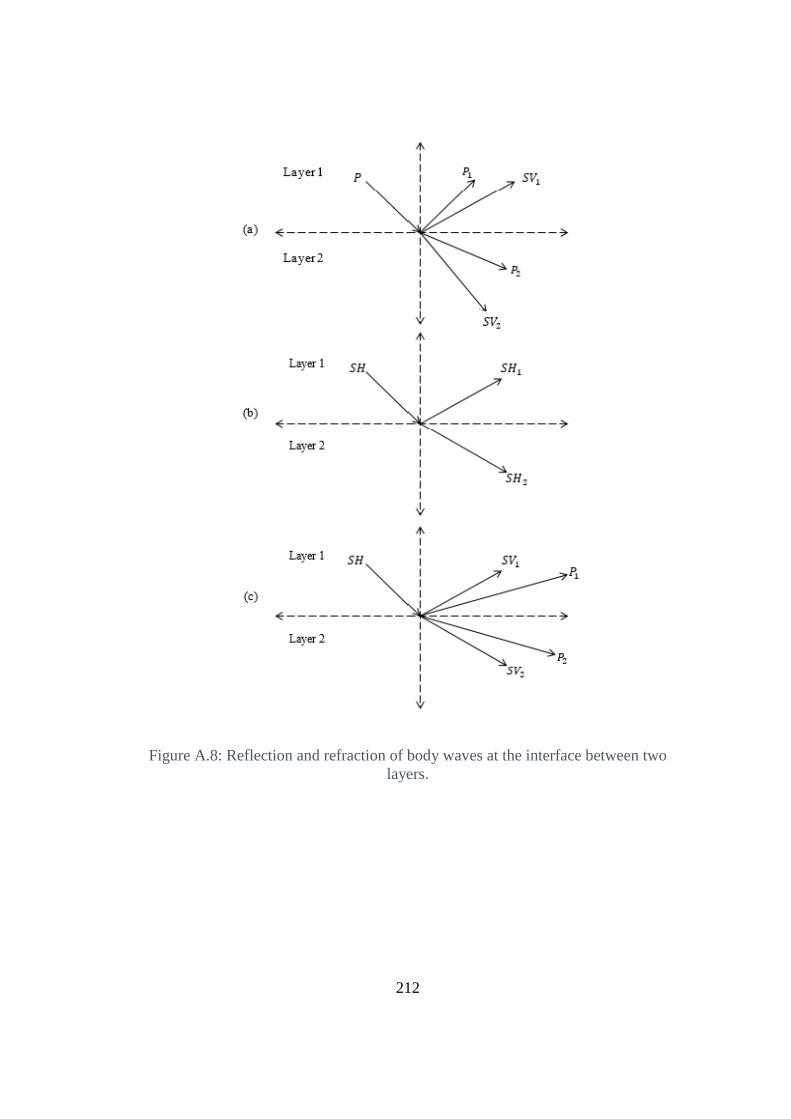
212
Figure A.8: Reflection and refraction of body waves at the interface between two
layers.
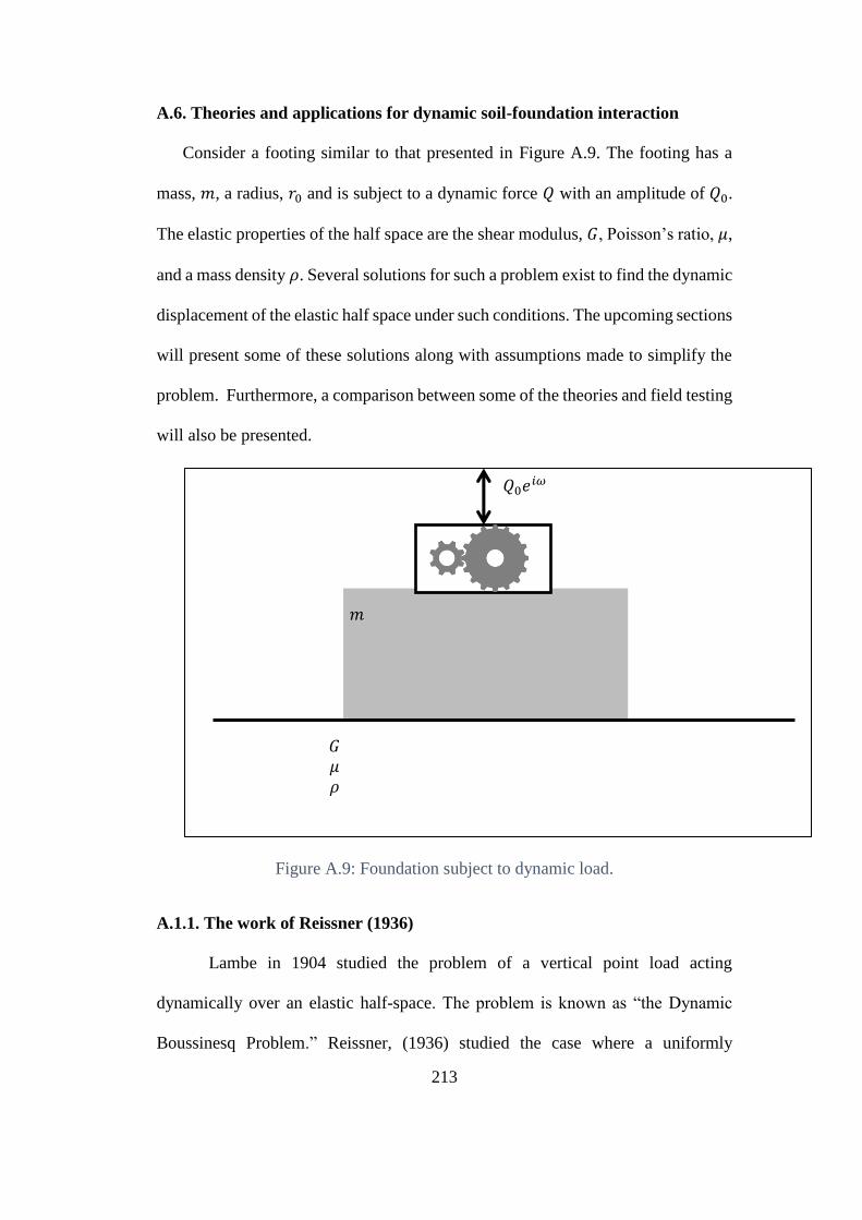
213
A.6. Theories and applications for dynamic soil-foundation interaction
Consider a footing similar to that presented in Figure A.9. The footing has a
mass, 𝑚, a radius, 𝑟0 and is subject to a dynamic force 𝑄 with an amplitude of 𝑄0.
The elastic properties of the half space are the shear modulus, 𝐺, Poisson’s ratio, 𝜇,
and a mass density 𝜌. Several solutions for such a problem exist to find the dynamic
displacement of the elastic half space under such conditions. The upcoming sections
will present some of these solutions along with assumptions made to simplify the
problem. Furthermore, a comparison between some of the theories and field testing
will also be presented.
Figure A.9: Foundation subject to dynamic load.
A.1.1. The work of Reissner (1936)
Lambe in 1904 studied the problem of a vertical point load acting
dynamically over an elastic half-space. The problem is known as “the Dynamic
Boussinesq Problem.” Reissner, (1936) studied the case where a uniformly
𝐺
𝜇
𝜌
𝑚
𝑄0𝑒𝑖𝜔𝑡
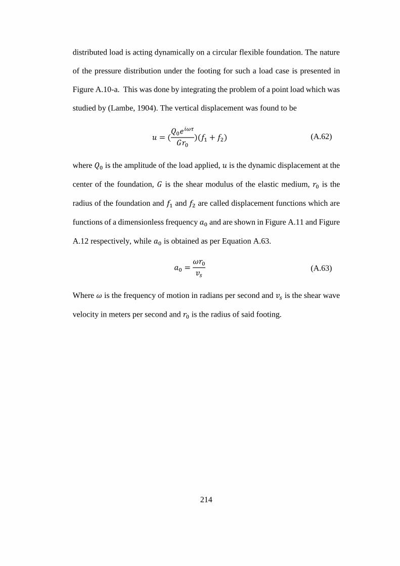
214
distributed load is acting dynamically on a circular flexible foundation. The nature
of the pressure distribution under the footing for such a load case is presented in
Figure A.10-a. This was done by integrating the problem of a point load which was
studied by (Lambe, 1904). The vertical displacement was found to be
𝑢 = (𝑄0𝑒
𝑖𝜔𝜏
𝐺𝑟0)(𝑓1 + 𝑓2) (A.62)
where 𝑄0 is the amplitude of the load applied, 𝑢 is the dynamic displacement at the
center of the foundation, 𝐺 is the shear modulus of the elastic medium, 𝑟0 is the
radius of the foundation and 𝑓1 and 𝑓2 are called displacement functions which are
functions of a dimensionless frequency 𝑎0 and are shown in Figure A.11 and Figure
A.12 respectively, while 𝑎0 is obtained as per Equation A.63.
𝑎0 =𝜔𝑟0𝑣𝑠
(A.63)
Where 𝜔 is the frequency of motion in radians per second and 𝑣𝑠 is the shear wave
velocity in meters per second and 𝑟0 is the radius of said footing.
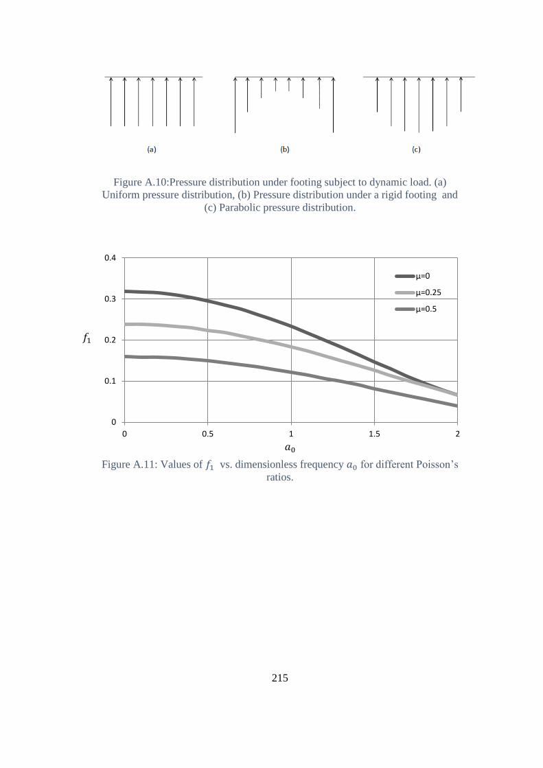
215
Figure A.10:Pressure distribution under footing subject to dynamic load. (a)
Uniform pressure distribution, (b) Pressure distribution under a rigid footing and
(c) Parabolic pressure distribution.
Figure A.11: Values of 𝑓1 vs. dimensionless frequency 𝑎0 for different Poisson’s
ratios.
0
0.1
0.2
0.3
0.4
0 0.5 1 1.5 2
μ=0
μ=0.25
μ=0.5
𝑓1
𝑎0
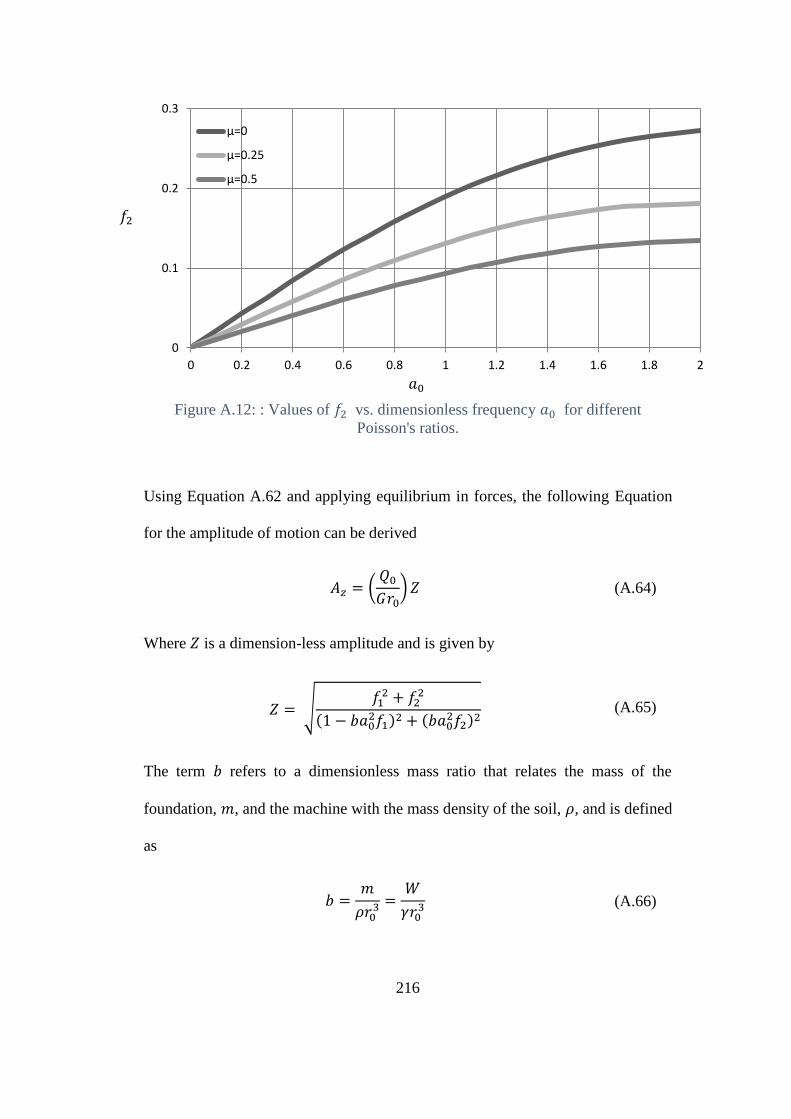
216
Figure A.12: : Values of 𝑓2 vs. dimensionless frequency 𝑎0 for different
Poisson's ratios.
Using Equation A.62 and applying equilibrium in forces, the following Equation
for the amplitude of motion can be derived
𝐴𝑧 = (𝑄0
𝐺𝑟0)𝑍 (A.64)
Where 𝑍 is a dimension-less amplitude and is given by
𝑍 = √𝑓12 + 𝑓2
2
(1 − 𝑏𝑎02𝑓1)2 + (𝑏𝑎0
2𝑓2)2 (A.65)
The term 𝑏 refers to a dimensionless mass ratio that relates the mass of the
foundation, 𝑚, and the machine with the mass density of the soil, 𝜌, and is defined
as
𝑏 =𝑚
𝜌𝑟03 =
𝑊
𝛾𝑟03 (A.66)
0
0.1
0.2
0.3
0 0.2 0.4 0.6 0.8 1 1.2 1.4 1.6 1.8 2
μ=0
μ=0.25
μ=0.5
𝑎0
𝑓2
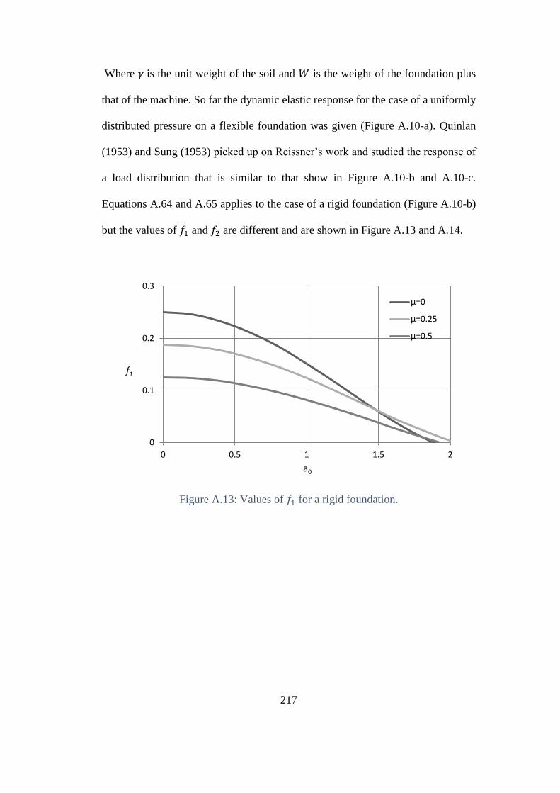
217
Where 𝛾 is the unit weight of the soil and 𝑊 is the weight of the foundation plus
that of the machine. So far the dynamic elastic response for the case of a uniformly
distributed pressure on a flexible foundation was given (Figure A.10-a). Quinlan
(1953) and Sung (1953) picked up on Reissner’s work and studied the response of
a load distribution that is similar to that show in Figure A.10-b and A.10-c.
Equations A.64 and A.65 applies to the case of a rigid foundation (Figure A.10-b)
but the values of 𝑓1 and 𝑓2 are different and are shown in Figure A.13 and A.14.
Figure A.13: Values of 𝑓1 for a rigid foundation.
0
0.1
0.2
0.3
0 0.5 1 1.5 2
μ=0
μ=0.25
μ=0.5
a0
f1
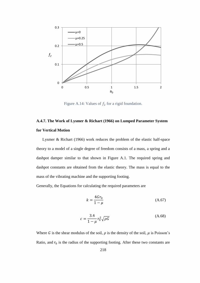
218
Figure A.14: Values of 𝑓2 for a rigid foundation.
A.4.7. The Work of Lysmer & Richart (1966) on Lumped Parameter System
for Vertical Motion
Lysmer & Richart (1966) work reduces the problem of the elastic half-space
theory to a model of a single degree of freedom consists of a mass, a spring and a
dashpot damper similar to that shown in Figure A.1. The required spring and
dashpot constants are obtained from the elastic theory. The mass is equal to the
mass of the vibrating machine and the supporting footing.
Generally, the Equations for calculating the required parameters are
𝑘 =4𝐺𝑟01 − 𝜇
(A.67)
𝑐 =3.4
1 − 𝜇𝑟02√𝜌𝐺
(A.68)
Where 𝐺 is the shear modulus of the soil, 𝜌 is the density of the soil, 𝜇 is Poisson’s
Ratio, and 𝑟0 is the radius of the supporting footing. After these two constants are
0
0.1
0.2
0.3
0 0.5 1 1.5 2
μ=0
μ=0.25
μ=0.5
f2
a0
219
calculated, the response of the soil can be obtained using the procedure presented
in sections A.1-A.3 to calculate the response of the single degree of freedom system.
Lysmer and Richart work is of importance because of its simplicity.
Moreover, his work showed that any elastic dynamic system could be reduced to a
single degree of freedom at the point of interest by identifying the equivalent spring
and dashpot constants. Since then development in the area of machine vibrations
has continued with different loading settings (e.g., horizontal and rocking
vibrations) different ground conditions (e.g., rock base). The mass ratio 𝐵, spring
constant 𝑘, and damping ratio 𝐷 for a rigid foundation under different types of
loading are in shown Table A.1. The Equations in Table A.1 are based on
continuation of Lysmer Solution.
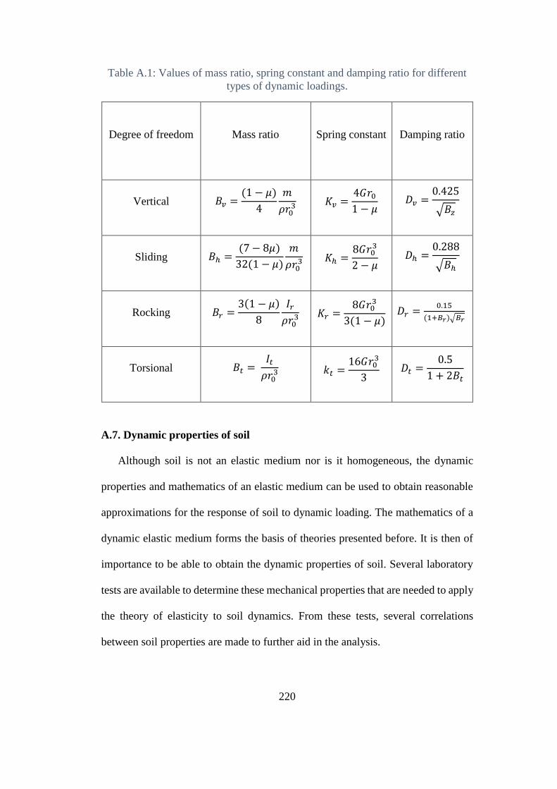
220
Table A.1: Values of mass ratio, spring constant and damping ratio for different
types of dynamic loadings.
Degree of freedom Mass ratio
Spring constant
Damping ratio
Vertical 𝐵𝑣 =(1 − 𝜇)
4
𝑚
𝜌𝑟03 𝐾𝑣 =
4𝐺𝑟01 − 𝜇
𝐷𝑣 =0.425
√𝐵𝑧
Sliding 𝛣ℎ =(7 − 8𝜇)
32(1 − 𝜇)
𝑚
𝜌𝑟03 𝐾ℎ =
8𝐺𝑟03
2 − 𝜇 𝐷ℎ =
0.288
√𝐵ℎ
Rocking 𝐵𝑟 =3(1 − 𝜇)
8
𝛪𝑟
𝜌𝑟03 𝐾𝑟 =
8𝐺𝑟03
3(1 − 𝜇) 𝐷𝑟 =
0.15
(1+𝐵𝑟)√𝐵𝑟
Torsional 𝐵𝑡 = 𝐼𝑡
𝜌𝑟03 𝑘𝑡 =
16𝐺𝑟03
3 𝐷𝑡 =
0.5
1 + 2𝐵𝑡
A.7. Dynamic properties of soil
Although soil is not an elastic medium nor is it homogeneous, the dynamic
properties and mathematics of an elastic medium can be used to obtain reasonable
approximations for the response of soil to dynamic loading. The mathematics of a
dynamic elastic medium forms the basis of theories presented before. It is then of
importance to be able to obtain the dynamic properties of soil. Several laboratory
tests are available to determine these mechanical properties that are needed to apply
the theory of elasticity to soil dynamics. From these tests, several correlations
between soil properties are made to further aid in the analysis.
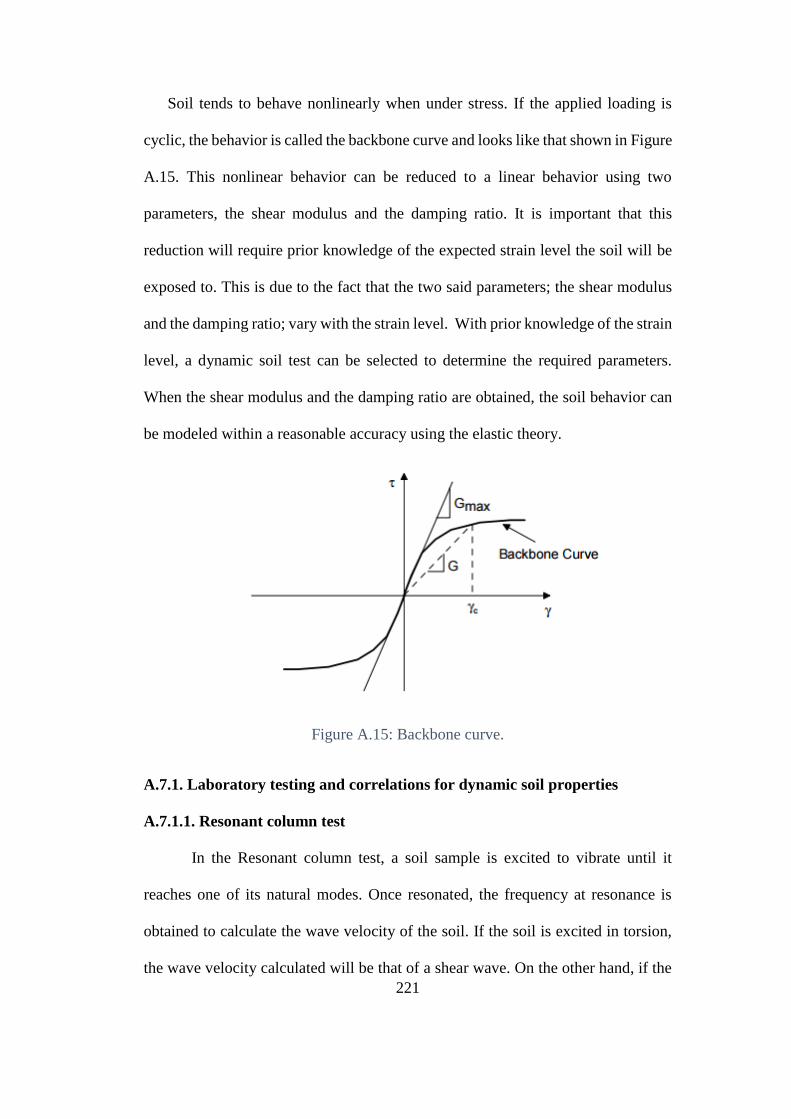
221
Soil tends to behave nonlinearly when under stress. If the applied loading is
cyclic, the behavior is called the backbone curve and looks like that shown in Figure
A.15. This nonlinear behavior can be reduced to a linear behavior using two
parameters, the shear modulus and the damping ratio. It is important that this
reduction will require prior knowledge of the expected strain level the soil will be
exposed to. This is due to the fact that the two said parameters; the shear modulus
and the damping ratio; vary with the strain level. With prior knowledge of the strain
level, a dynamic soil test can be selected to determine the required parameters.
When the shear modulus and the damping ratio are obtained, the soil behavior can
be modeled within a reasonable accuracy using the elastic theory.
Figure A.15: Backbone curve.
A.7.1. Laboratory testing and correlations for dynamic soil properties
A.7.1.1. Resonant column test
In the Resonant column test, a soil sample is excited to vibrate until it
reaches one of its natural modes. Once resonated, the frequency at resonance is
obtained to calculate the wave velocity of the soil. If the soil is excited in torsion,
the wave velocity calculated will be that of a shear wave. On the other hand, if the
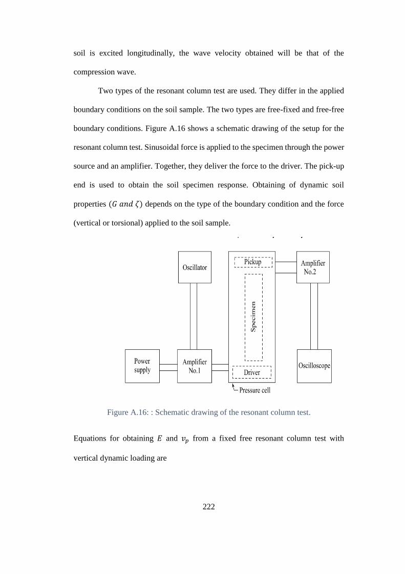
222
soil is excited longitudinally, the wave velocity obtained will be that of the
compression wave.
Two types of the resonant column test are used. They differ in the applied
boundary conditions on the soil sample. The two types are free-fixed and free-free
boundary conditions. Figure A.16 shows a schematic drawing of the setup for the
resonant column test. Sinusoidal force is applied to the specimen through the power
source and an amplifier. Together, they deliver the force to the driver. The pick-up
end is used to obtain the soil specimen response. Obtaining of dynamic soil
properties (𝐺 𝑎𝑛𝑑 휁) depends on the type of the boundary condition and the force
(vertical or torsional) applied to the soil sample.
Figure A.16: : Schematic drawing of the resonant column test.
Equations for obtaining 𝐸 and 𝑣𝑝 from a fixed free resonant column test with
vertical dynamic loading are
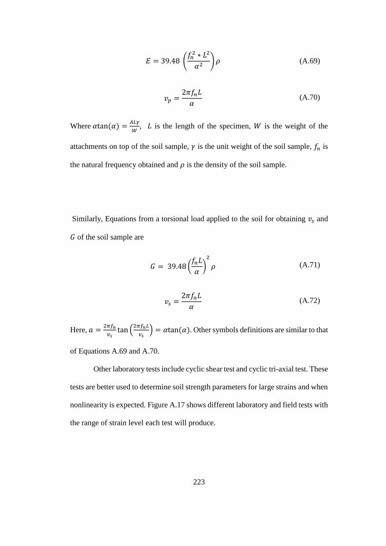
223
𝐸 = 39.48 (𝑓𝑛2 ∗ 𝐿2
𝛼2)𝜌 (A.69)
𝑣𝑝 =2𝜋𝑓𝑛𝐿
𝛼 (A.70)
Where 𝛼tan (𝛼) =𝐴𝐿𝛾
𝑊, 𝐿 is the length of the specimen, 𝑊 is the weight of the
attachments on top of the soil sample, 𝛾 is the unit weight of the soil sample, 𝑓𝑛 is
the natural frequency obtained and 𝜌 is the density of the soil sample.
Similarly, Equations from a torsional load applied to the soil for obtaining 𝑣𝑠 and
𝐺 of the soil sample are
𝐺 = 39.48 (𝑓𝑛𝐿
𝛼)2
𝜌 (A.71)
𝑣𝑠 =2𝜋𝑓𝑛𝐿
𝛼 (A.72)
Here, 𝑎 =2𝜋𝑓𝑛
𝑣𝑠tan (
2𝜋𝑓𝑛𝐿
𝑣𝑠) = 𝛼tan (𝛼). Other symbols definitions are similar to that
of Equations A.69 and A.70.
Other laboratory tests include cyclic shear test and cyclic tri-axial test. These
tests are better used to determine soil strength parameters for large strains and when
nonlinearity is expected. Figure A.17 shows different laboratory and field tests with
the range of strain level each test will produce.
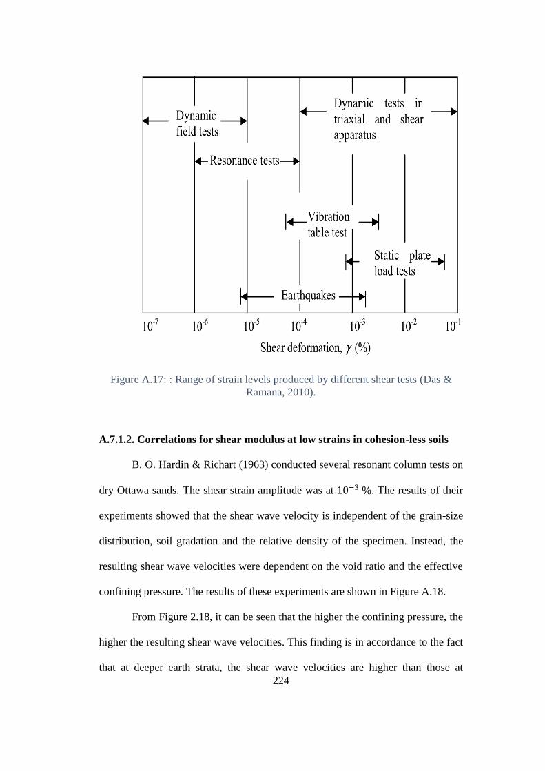
224
Figure A.17: : Range of strain levels produced by different shear tests (Das &
Ramana, 2010).
A.7.1.2. Correlations for shear modulus at low strains in cohesion-less soils
B. O. Hardin & Richart (1963) conducted several resonant column tests on
dry Ottawa sands. The shear strain amplitude was at 10−3 %. The results of their
experiments showed that the shear wave velocity is independent of the grain-size
distribution, soil gradation and the relative density of the specimen. Instead, the
resulting shear wave velocities were dependent on the void ratio and the effective
confining pressure. The results of these experiments are shown in Figure A.18.
From Figure 2.18, it can be seen that the higher the confining pressure, the
higher the resulting shear wave velocities. This finding is in accordance to the fact
that at deeper earth strata, the shear wave velocities are higher than those at
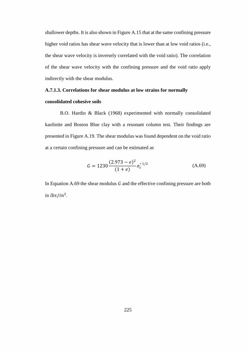
225
shallower depths. It is also shown in Figure A.15 that at the same confining pressure
higher void ratios has shear wave velocity that is lower than at low void ratios (i.e.,
the shear wave velocity is inversely correlated with the void ratio). The correlation
of the shear wave velocity with the confining pressure and the void ratio apply
indirectly with the shear modulus.
A.7.1.3. Correlations for shear modulus at low strains for normally
consolidated cohesive soils
B.O. Hardin & Black (1968) experimented with normally consolidated
kaolinite and Boston Blue clay with a resonant column test. Their findings are
presented in Figure A.19. The shear modulus was found dependent on the void ratio
at a certain confining pressure and can be estimated as
𝐺 = 1230(2.973 − 𝑒)2
(1 + 𝑒)𝜎𝑐′ 1/2
(A.69)
In Equation A.69 the shear modulus 𝐺 and the effective confining pressure are both
in 𝑙𝑏𝑠/𝑖𝑛2.
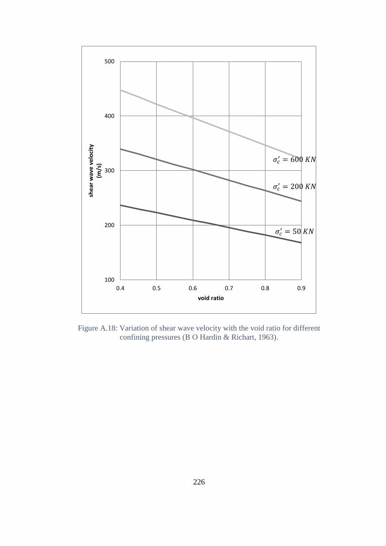
226
Figure A.18: Variation of shear wave velocity with the void ratio for different
confining pressures (B O Hardin & Richart, 1963).
100
200
300
400
500
0.4 0.5 0.6 0.7 0.8 0.9
she
ar w
ave
ve
loci
ty(m
/s)
void ratio
𝜎𝑐′ = 600 𝐾𝑁
𝜎𝑐′ = 200 𝐾𝑁
𝜎𝑐′ = 50 𝐾𝑁
227
Figure A.19: Correlation of shear modulus with void ratio for normally
consolidated clays (B. O. Hardin & Black, 1968).
A.7.1.4. Correlations for shear modulus at low strains for overly consolidated
cohesive soils
B. O. Hardin & Black (1968) consolidated some specimens before testing
to see how pre-consolidation pressure might affect the correlation between shear
modulus and void ratio. Equation A.69 will be modified so that the shear modulus
will be calculated as
𝐺 = 1230(2.973 − 𝑒)2
(1 + 𝑒)(𝑂𝐶𝑅)𝑘𝜎𝑐
′ 1/2 (A.70)
In (A.70) the term 𝑘 depends on the plasticity index of the clay specimen. This
variation is shown in Figure A.20.
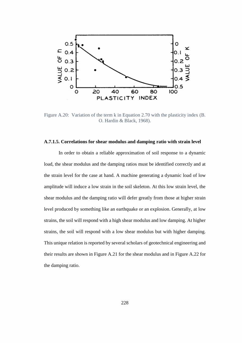
228
Figure A.20: Variation of the term k in Equation 2.70 with the plasticity index (B.
O. Hardin & Black, 1968).
A.7.1.5. Correlations for shear modulus and damping ratio with strain level
In order to obtain a reliable approximation of soil response to a dynamic
load, the shear modulus and the damping ratios must be identified correctly and at
the strain level for the case at hand. A machine generating a dynamic load of low
amplitude will induce a low strain in the soil skeleton. At this low strain level, the
shear modulus and the damping ratio will defer greatly from those at higher strain
level produced by something like an earthquake or an explosion. Generally, at low
strains, the soil will respond with a high shear modulus and low damping. At higher
strains, the soil will respond with a low shear modulus but with higher damping.
This unique relation is reported by several scholars of geotechnical engineering and
their results are shown in Figure A.21 for the shear modulus and in Figure A.22 for
the damping ratio.
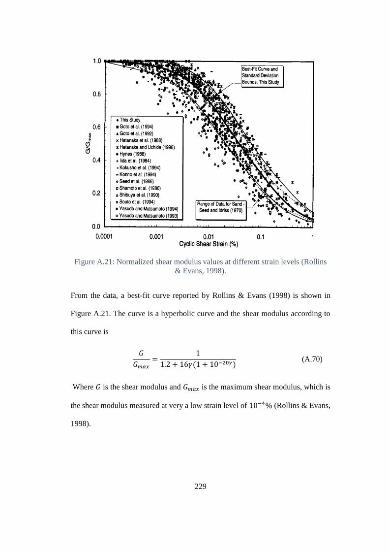
229
Figure A.21: Normalized shear modulus values at different strain levels (Rollins
& Evans, 1998).
From the data, a best-fit curve reported by Rollins & Evans (1998) is shown in
Figure A.21. The curve is a hyperbolic curve and the shear modulus according to
this curve is
𝐺
𝐺𝑚𝑎𝑥=
1
1.2 + 16𝛾(1 + 10−20𝛾) (A.70)
Where 𝐺 is the shear modulus and 𝐺𝑚𝑎𝑥 is the maximum shear modulus, which is
the shear modulus measured at very a low strain level of 10−4% (Rollins & Evans,
1998).
230
A similar correlation for the damping ratio with the shear strain is reported
by Rollins & Evans (1998). The damping is correlated with shear strain as
𝐷 = 0.8 + 18(1 + 0.15𝛾−0.9)−0.75 (A.71)
These relations are important to accurately and easily model a dynamic problem. If
the expected strain level is known, the non-linear soil stress-strain curve can be
reduced to an equivalent shear modulus and damping ratio. This correlation will
also help aid in selecting the proper dynamic soil testing method as some testing
methods produce higher strains than others which will yield a higher damping ratio
while the shear modulus will be lower than a low strain inducing laboratory test.
231
B. A program for static and dynamic analysis of single piles subjected to
vertical loading
A program that analyzes piles subjected to vertical loading is created using
1-dimensional finite element approach such as that described in section 2.3.1 of this
thesis. The purpose of the program is to use it in comparing results with the 3D
finite element method used in this research in cases where no analytical solution is
available. The following will discuss the math behind the program. A step by step
discussion on how the program is created is provided and the full code is provided
afterward. The program was created in Mathematica®. Mathematica is
computational language that can be used in programming engineering applications.
A graphical representation of the problem is shown in Figure B.1. In Figure B.1, it
is shown that the pile is divided into segments. Each segment represents a bar
element. Each element is then connected to a spring and a damper along the shaft.
These springs and dampers represent soil behavior along the pile shaft. The spring
represent friction provided by the soil and the damper will represent geometrical
damping of the soil at the side. At the base, the bar is connected to a spring and a
damper both at the side and from beneath. The bottom spring and damper attached
to the bottom segment represent soil behavior at the tip of the pile.
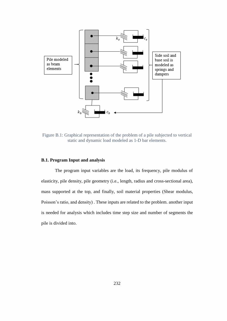
232
Figure B.1: Graphical representation of the problem of a pile subjected to vertical
static and dynamic load modeled as 1-D bar elements.
B.1. Program Input and analysis
The program input variables are the load, its frequency, pile modulus of
elasticity, pile density, pile geometry (i.e., length, radius and cross-sectional area),
mass supported at the top, and finally, soil material properties (Shear modulus,
Poisson’s ratio, and density) . These inputs are related to the problem. another input
is needed for analysis which includes time step size and number of segments the
pile is divided into.
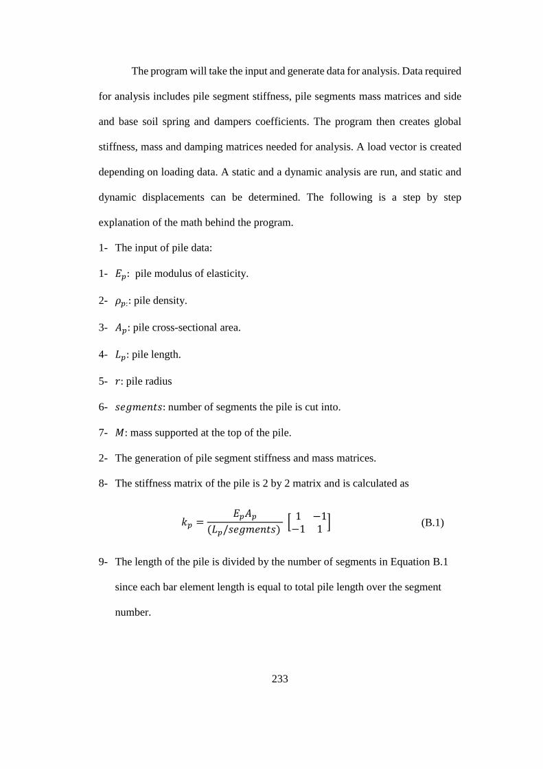
233
The program will take the input and generate data for analysis. Data required
for analysis includes pile segment stiffness, pile segments mass matrices and side
and base soil spring and dampers coefficients. The program then creates global
stiffness, mass and damping matrices needed for analysis. A load vector is created
depending on loading data. A static and a dynamic analysis are run, and static and
dynamic displacements can be determined. The following is a step by step
explanation of the math behind the program.
1- The input of pile data:
1- 𝐸𝑝: pile modulus of elasticity.
2- 𝜌𝑝:: pile density.
3- 𝐴𝑝: pile cross-sectional area.
4- 𝐿𝑝: pile length.
5- 𝑟: pile radius
6- 𝑠𝑒𝑔𝑚𝑒𝑛𝑡𝑠: number of segments the pile is cut into.
7- 𝑀: mass supported at the top of the pile.
2- The generation of pile segment stiffness and mass matrices.
8- The stiffness matrix of the pile is 2 by 2 matrix and is calculated as
𝑘𝑝 =𝐸𝑝𝐴𝑝
(𝐿𝑝/𝑠𝑒𝑔𝑚𝑒𝑛𝑡𝑠) [
1−1
−11] (B.1)
9- The length of the pile is divided by the number of segments in Equation B.1
since each bar element length is equal to total pile length over the segment
number.
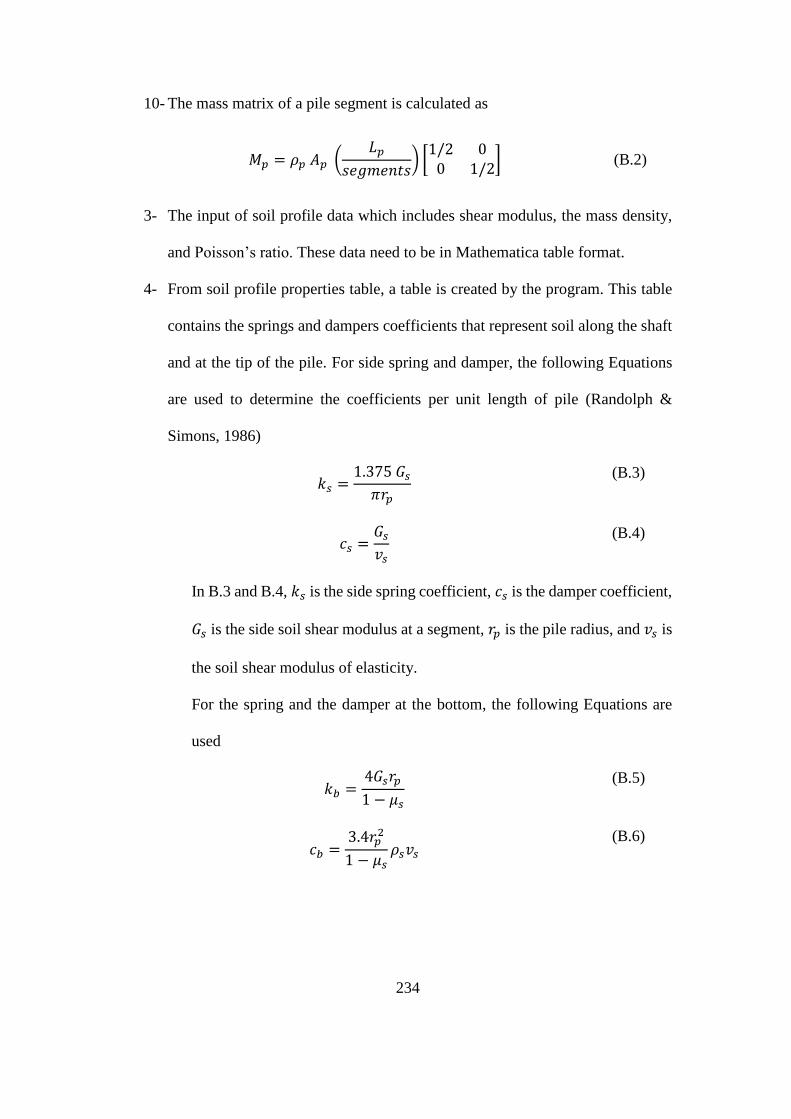
234
10- The mass matrix of a pile segment is calculated as
𝑀𝑝 = 𝜌𝑝 𝐴𝑝 (𝐿𝑝
𝑠𝑒𝑔𝑚𝑒𝑛𝑡𝑠) [
1/2 00 1/2
] (B.2)
3- The input of soil profile data which includes shear modulus, the mass density,
and Poisson’s ratio. These data need to be in Mathematica table format.
4- From soil profile properties table, a table is created by the program. This table
contains the springs and dampers coefficients that represent soil along the shaft
and at the tip of the pile. For side spring and damper, the following Equations
are used to determine the coefficients per unit length of pile (Randolph &
Simons, 1986)
𝑘𝑠 =1.375 𝐺𝑠
𝜋𝑟𝑝
(B.3)
𝑐𝑠 =𝐺𝑠
𝑣𝑠
(B.4)
In B.3 and B.4, 𝑘𝑠 is the side spring coefficient, 𝑐𝑠 is the damper coefficient,
𝐺𝑠 is the side soil shear modulus at a segment, 𝑟𝑝 is the pile radius, and 𝑣𝑠 is
the soil shear modulus of elasticity.
For the spring and the damper at the bottom, the following Equations are
used
𝑘𝑏 =4𝐺𝑠𝑟𝑝
1 − 𝜇𝑠
(B.5)
𝑐𝑏 =3.4𝑟𝑝
2
1 − 𝜇𝑠𝜌𝑠𝑣𝑠
(B.6)
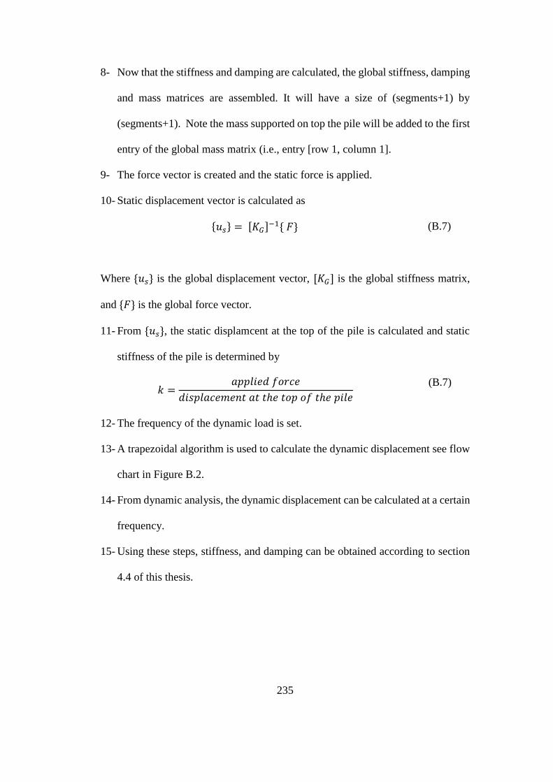
235
8- Now that the stiffness and damping are calculated, the global stiffness, damping
and mass matrices are assembled. It will have a size of (segments+1) by
(segments+1). Note the mass supported on top the pile will be added to the first
entry of the global mass matrix (i.e., entry [row 1, column 1].
9- The force vector is created and the static force is applied.
10- Static displacement vector is calculated as
{𝑢𝑠} = [𝐾𝐺]−1{ 𝐹} (B.7)
Where {𝑢𝑠} is the global displacement vector, [𝐾𝐺] is the global stiffness matrix,
and {𝐹} is the global force vector.
11- From {𝑢𝑠}, the static displamcent at the top of the pile is calculated and static
stiffness of the pile is determined by
𝑘 =𝑎𝑝𝑝𝑙𝑖𝑒𝑑 𝑓𝑜𝑟𝑐𝑒
𝑑𝑖𝑠𝑝𝑙𝑎𝑐𝑒𝑚𝑒𝑛𝑡 𝑎𝑡 𝑡ℎ𝑒 𝑡𝑜𝑝 𝑜𝑓 𝑡ℎ𝑒 𝑝𝑖𝑙𝑒
(B.7)
12- The frequency of the dynamic load is set.
13- A trapezoidal algorithm is used to calculate the dynamic displacement see flow
chart in Figure B.2.
14- From dynamic analysis, the dynamic displacement can be calculated at a certain
frequency.
15- Using these steps, stiffness, and damping can be obtained according to section
4.4 of this thesis.
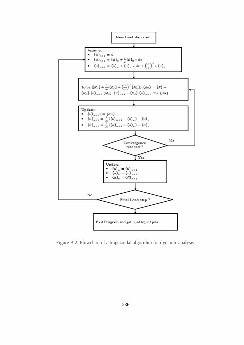
236
Figure B.2: Flowchart of a trapezoidal algorithm for dynamic analysis.
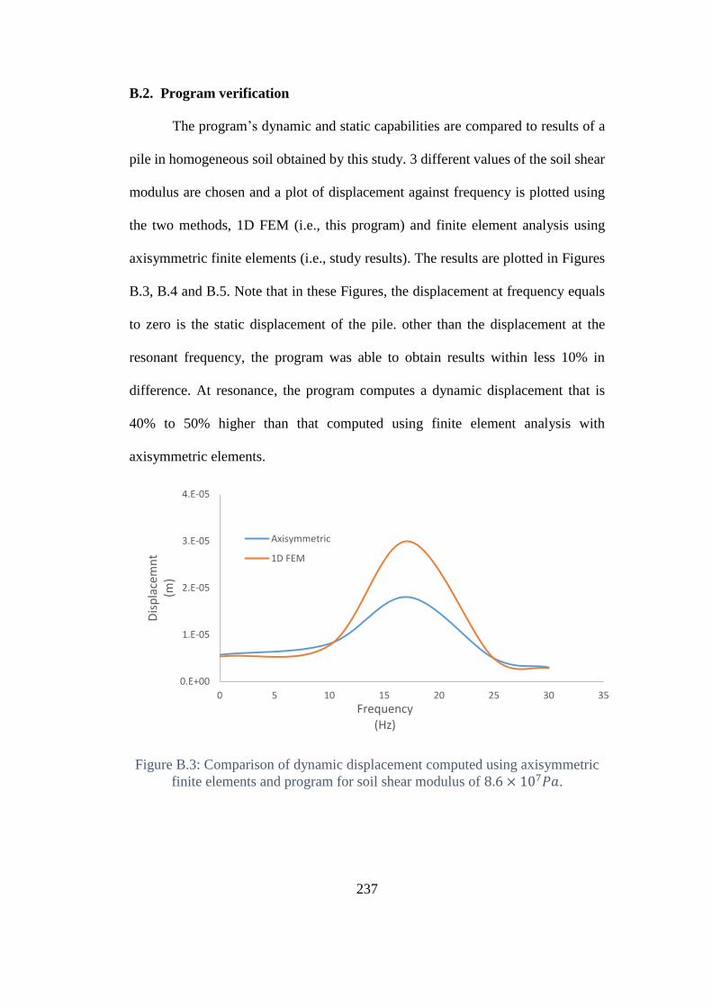
237
B.2. Program verification
The program’s dynamic and static capabilities are compared to results of a
pile in homogeneous soil obtained by this study. 3 different values of the soil shear
modulus are chosen and a plot of displacement against frequency is plotted using
the two methods, 1D FEM (i.e., this program) and finite element analysis using
axisymmetric finite elements (i.e., study results). The results are plotted in Figures
B.3, B.4 and B.5. Note that in these Figures, the displacement at frequency equals
to zero is the static displacement of the pile. other than the displacement at the
resonant frequency, the program was able to obtain results within less 10% in
difference. At resonance, the program computes a dynamic displacement that is
40% to 50% higher than that computed using finite element analysis with
axisymmetric elements.
Figure B.3: Comparison of dynamic displacement computed using axisymmetric
finite elements and program for soil shear modulus of 8.6 × 10⁷𝑃𝑎.
0.E+00
1.E-05
2.E-05
3.E-05
4.E-05
0 5 10 15 20 25 30 35
Dis
pla
cem
nt
(m)
Frequency(Hz)
Axisymmetric
1D FEM
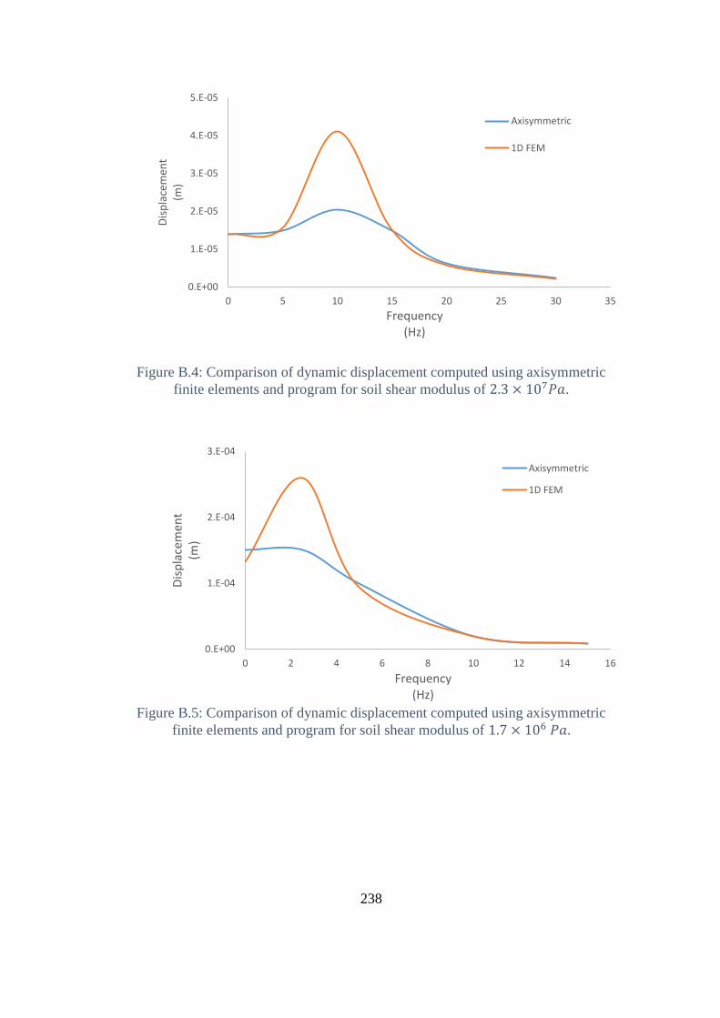
238
Figure B.4: Comparison of dynamic displacement computed using axisymmetric
finite elements and program for soil shear modulus of 2.3 × 10⁷𝑃𝑎.
Figure B.5: Comparison of dynamic displacement computed using axisymmetric
finite elements and program for soil shear modulus of 1.7 × 10⁶ 𝑃𝑎.
0.E+00
1.E-05
2.E-05
3.E-05
4.E-05
5.E-05
0 5 10 15 20 25 30 35
Dis
pla
cem
ent
(m)
Frequency(Hz)
Axisymmetric
1D FEM
0.E+00
1.E-04
2.E-04
3.E-04
0 2 4 6 8 10 12 14 16
Dis
pla
cem
ent
(m)
Frequency(Hz)
Axisymmetric
1D FEM
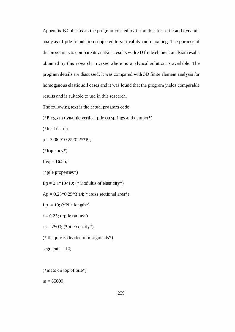
239
Appendix B.2 discusses the program created by the author for static and dynamic
analysis of pile foundation subjected to vertical dynamic loading. The purpose of
the program is to compare its analysis results with 3D finite element analysis results
obtained by this research in cases where no analytical solution is available. The
program details are discussed. It was compared with 3D finite element analysis for
homogenous elastic soil cases and it was found that the program yields comparable
results and is suitable to use in this research.
The following text is the actual program code:
(*Program dynamic vertical pile on springs and damper*)
(*load data*)
p = 22000*0.25*0.25*Pi;
(*frquency*)
freq = 16.35;
(*pile properties*)
Ep = 2.1*10^10; (*Modulus of elasticity*)
Ap = 0.25*0.25*3.14;(*cross sectional area*)
Lp = 10; (*Pile length*)
r = 0.25; (*pile radius*)
rp = 2500; (*pile density*)
(* the pile is divided into segments*)
segments = 10;
(*mass on top of pile*)
m = 65000;
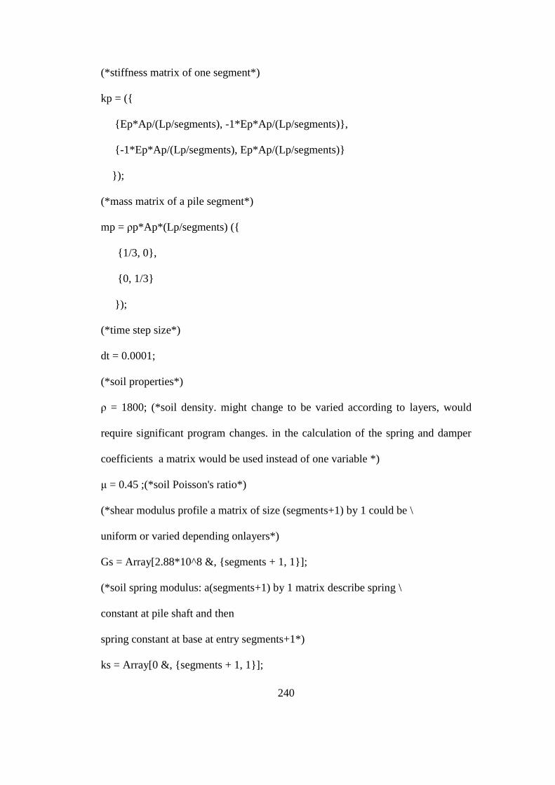
240
(*stiffness matrix of one segment*)
kp = ({
{Ep*Ap/(Lp/segments), -1*Ep*Ap/(Lp/segments)},
{-1*Ep*Ap/(Lp/segments), Ep*Ap/(Lp/segments)}
});
(*mass matrix of a pile segment*)
mp = ρp*Ap*(Lp/segments) ({
{1/3, 0},
{0, 1/3}
});
(*time step size*)
dt = 0.0001;
(*soil properties*)
ρ = 1800; (*soil density. might change to be varied according to layers, would
require significant program changes. in the calculation of the spring and damper
coefficients a matrix would be used instead of one variable *)
μ = 0.45 ;(*soil Poisson's ratio*)
(*shear modulus profile a matrix of size (segments+1) by 1 could be \
uniform or varied depending onlayers*)
Gs = Array[2.88*10^8 &, {segments + 1, 1}];
(*soil spring modulus: a(segments+1) by 1 matrix describe spring \
constant at pile shaft and then
spring constant at base at entry segments+1*)
ks = Array[0 &, {segments + 1, 1}];
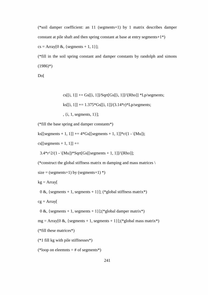
241
(*soil damper coefficient: an 11 (segments+1) by 1 matrix describes damper
constant at pile shaft and then spring constant at base at entry segments+1*)
cs = Array[0 &, {segments + 1, 1}];
(*fill in the soil spring constant and damper constants by randolph and simons
(1986)*)
Do[
cs[[i, 1]] += Gs[[i, 1]]/Sqrt[Gs[[i, 1]]/\[Rho]] *Lp/segments;
ks[[i, 1]] += 1.375*Gs[[i, 1]]/(3.14*r)*Lp/segments;
, {i, 1, segments, 1}];
(*fill the base spring and damper constants*)
ks[[segments + 1, 1]] += 4*Gs[[segments + 1, 1]]*r/(1 - \[Mu]);
cs[[segments + 1, 1]] +=
3.4*r^2/(1 - \[Mu])*Sqrt[Gs[[segments + 1, 1]]/\[Rho]];
(*construct the global stiffness matrix m damping and mass matrices \
size = (segments+1) by (segments+1) *)
kg = Array[
0 &, {segments + 1, segments + 1}]; (*global stiffness matrix*)
cg = Array[
0 &, {segments + 1, segments + 1}];(*global damper matrix*)
mg = Array[0 &, {segments + 1, segments + 1}];(*global mass matrix*)
(*fill these matrices*)
(*1 fill kg with pile stiffnesses*)
(*loop on eleemnts = # of segments*)
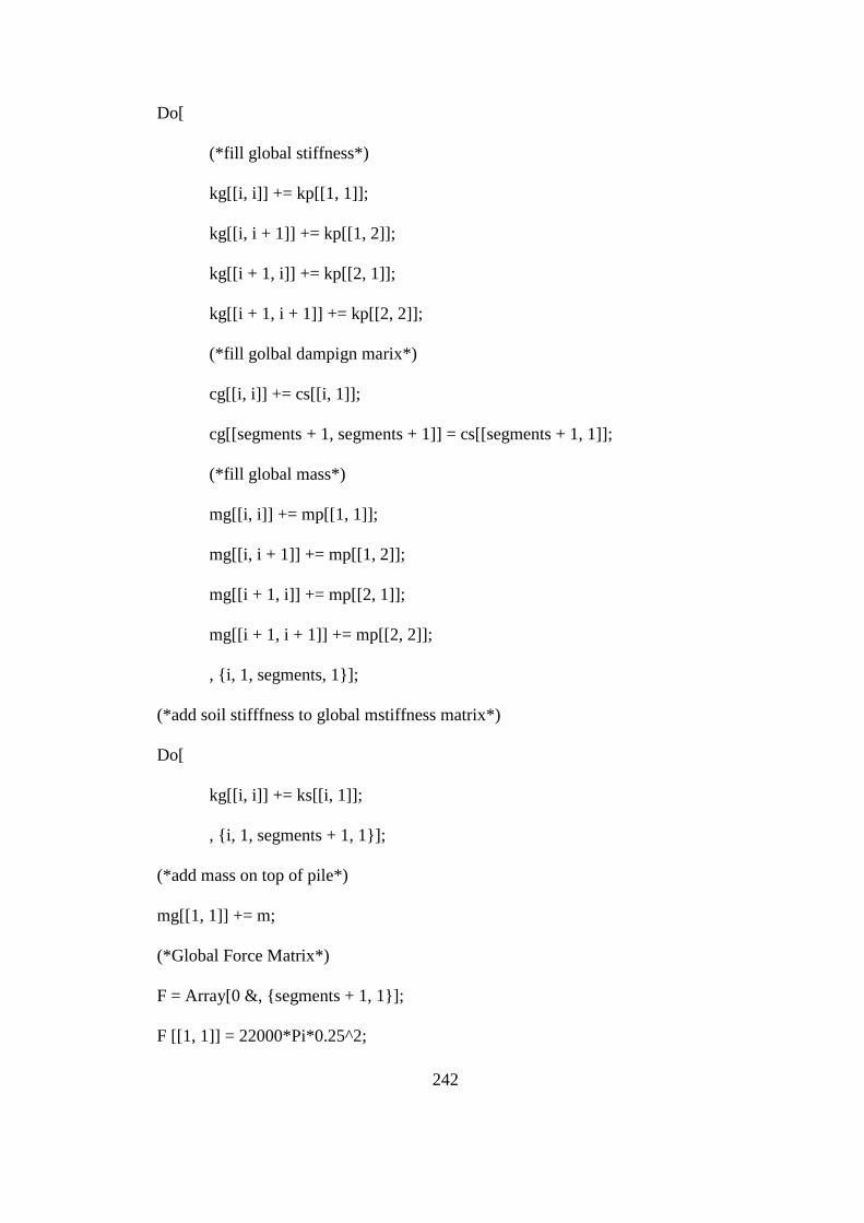
242
Do[
(*fill global stiffness*)
kg[[i, i]] += kp[[1, 1]];
kg[[i, i + 1]] += kp[[1, 2]];
kg[[i + 1, i]] += kp[[2, 1]];
kg[[i + 1, i + 1]] += kp[[2, 2]];
(*fill golbal dampign marix*)
cg[[i, i]] += cs[[i, 1]];
cg[[segments + 1, segments + 1]] = cs[[segments + 1, 1]];
(*fill global mass*)
mg[[i, i]] += mp[[1, 1]];
mg[[i, i + 1]] += mp[[1, 2]];
mg[[i + 1, i]] += mp[[2, 1]];
mg[[i + 1, i + 1]] += mp[[2, 2]];
, {i, 1, segments, 1}];
(*add soil stifffness to global mstiffness matrix*)
Do[
kg[[i, i]] += ks[[i, 1]];
, {i, 1, segments + 1, 1}];
(*add mass on top of pile*)
mg[[1, 1]] += m;
(*Global Force Matrix*)
F = Array[0 &, {segments + 1, 1}];
F [[1, 1]] = 22000*Pi*0.25^2;
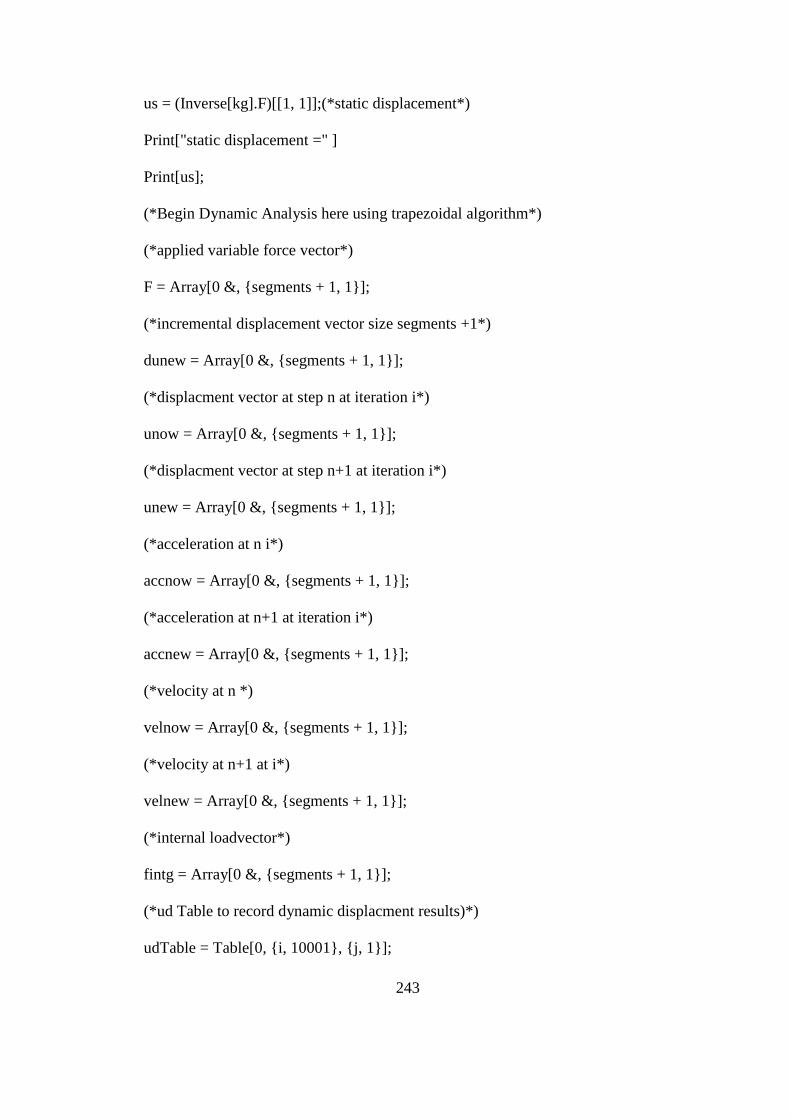
243
us = (Inverse[kg].F)[[1, 1]];(*static displacement*)
Print["static displacement =" ]
Print[us];
(*Begin Dynamic Analysis here using trapezoidal algorithm*)
(*applied variable force vector*)
F = Array[0 &, {segments + 1, 1}];
(*incremental displacement vector size segments +1*)
dunew = Array[0 &, {segments + 1, 1}];
(*displacment vector at step n at iteration i*)
unow = Array[0 &, {segments + 1, 1}];
(*displacment vector at step n+1 at iteration i*)
unew = Array[0 &, {segments + 1, 1}];
(*acceleration at n i*)
accnow = Array[0 &, {segments + 1, 1}];
(*acceleration at n+1 at iteration i*)
accnew = Array[0 &, {segments + 1, 1}];
(*velocity at n *)
velnow = Array[0 &, {segments + 1, 1}];
(*velocity at n+1 at i*)
velnew = Array[0 &, {segments + 1, 1}];
(*internal loadvector*)
fintg = Array[0 &, {segments + 1, 1}];
(*ud Table to record dynamic displacment results)*)
udTable = Table[0, {i, 10001}, {j, 1}];
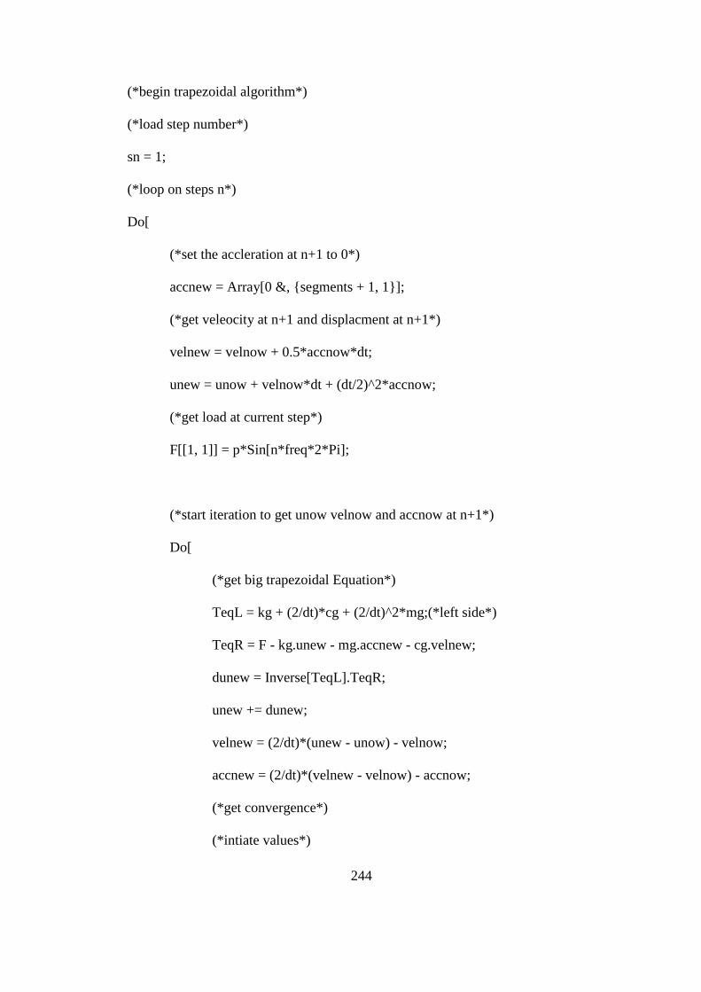
244
(*begin trapezoidal algorithm*)
(*load step number*)
sn = 1;
(*loop on steps n*)
Do[
(*set the accleration at n+1 to 0*)
accnew = Array[0 &, {segments + 1, 1}];
(*get veleocity at n+1 and displacment at n+1*)
velnew = velnow + 0.5*accnow*dt;
unew = unow + velnow*dt + (dt/2)^2*accnow;
(*get load at current step*)
F[[1, 1]] = p*Sin[n*freq*2*Pi];
(*start iteration to get unow velnow and accnow at n+1*)
Do[
(*get big trapezoidal Equation*)
TeqL = kg + (2/dt)*cg + (2/dt)^2*mg;(*left side*)
TeqR = F - kg.unew - mg.accnew - cg.velnew;
dunew = Inverse[TeqL].TeqR;
unew += dunew;
velnew = (2/dt)*(unew - unow) - velnow;
accnew = (2/dt)*(velnew - velnow) - accnow;
(*get convergence*)
(*intiate values*)
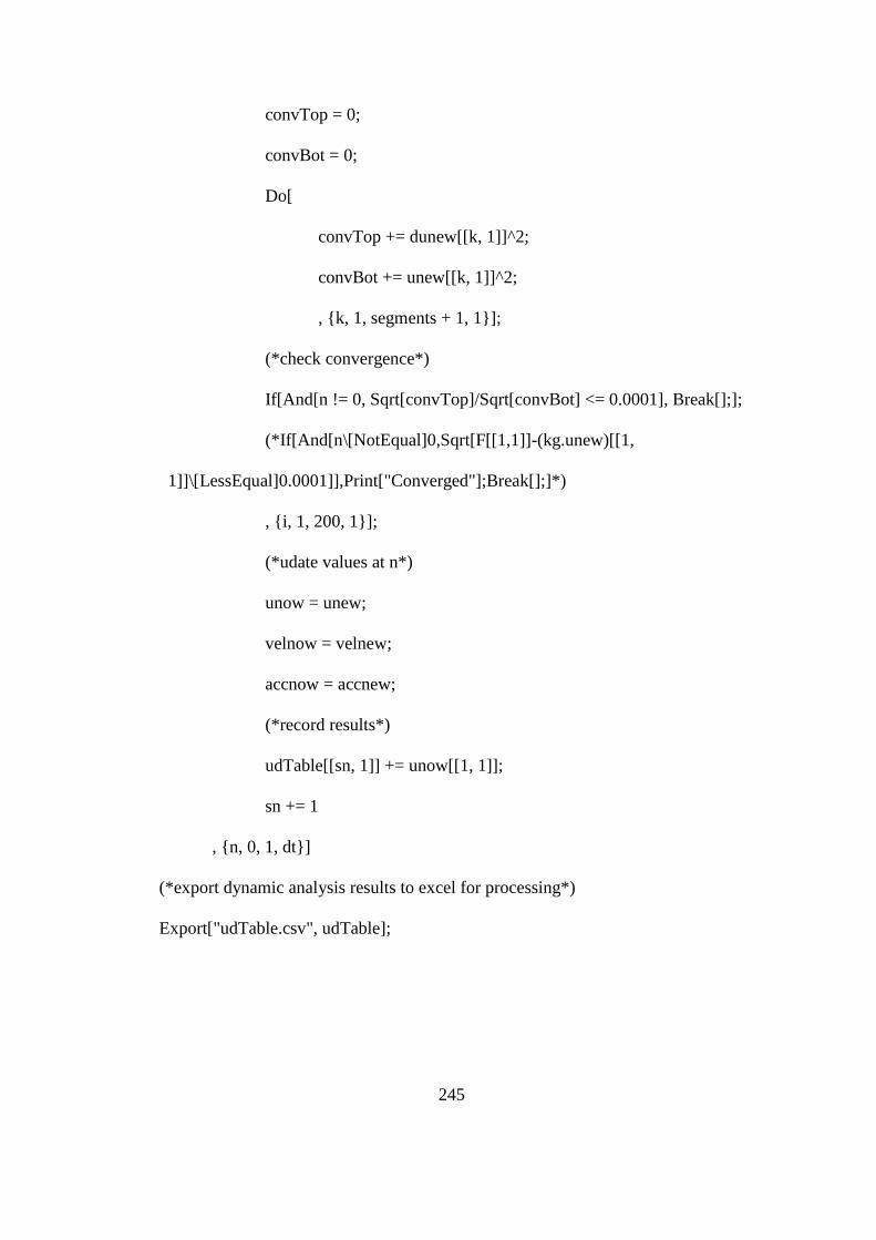
245
convTop = 0;
convBot = 0;
Do[
convTop += dunew[[k, 1]]^2;
convBot += unew[[k, 1]]^2;
, {k, 1, segments + 1, 1}];
(*check convergence*)
If[And[n != 0, Sqrt[convTop]/Sqrt[convBot] <= 0.0001], Break[];];
(*If[And[n\[NotEqual]0,Sqrt[F[[1,1]]-(kg.unew)[[1,
1]]\[LessEqual]0.0001]],Print["Converged"];Break[];]*)
, {i, 1, 200, 1}];
(*udate values at n*)
unow = unew;
velnow = velnew;
accnow = accnew;
(*record results*)
udTable[[sn, 1]] += unow[[1, 1]];
sn += 1
, {n, 0, 1, dt}]
(*export dynamic analysis results to excel for processing*)
Export["udTable.csv", udTable];
246
Bibliography
1- ACI 351 (2004). Foundations for Dynamic Equipment, American Concrete
Institute, 351.34, Farmington Hill, MI.
2- Ali, Osama (2015). Vertical Dynamic Soil-Pile Interaction for Machine
Foundations. University of Maryland, College Park, MD, U.S.A.
3- Autodesk Simulation Mechanical 2014-2017, Autodesk. Retrieved from:
https://www.autodesk.com/education/free-software/simulation-mechanical.
4- Bathe, K. J. (2006). Finite element procedures. Klaus-Jurgen Bathe. Retrieved
from: http://web.mit.edu/kjb/www/Books/FEP_2nd_Edition_4th_Printing.pdf
5- Baxter, R. L. & Bernhard, D. L. (1967, January). Vibration Tolerances for
Industry. ASME-American Society of Mechanical Engineers. Vol. 89(7).
6- Bharathi, M. Raj, D. & Dubey, D.R. (2014). Codal Provisions for Design of
Machine Foundations–A Review. International Symposium Geohazards:
Science: Engineering and Management, Kathmandu, Nepal, November, pp. 20-
21.
7- Butterfield R. & Banerjee, P. K. (1971). The problem of pile group–pile cap
interaction. Geotechnique, Vol. 21(2), pp. 135-142.
8- Chow, Y.K. & Teh, C.I. (1991). Pile-Cap-Pile-Group Interaction in
Nonhomogeneous Soil. Journal of Geotechnical Engineering, Vol. 117(11), pp.
1655-1668.
9- Chowdhury, I. & Dasgupta, S.P. (2006). Dynamic Response of Piles Under
Vertical Loads. Indian Geotechnical Journal, Vol. 115(143).
10- Chowdhury, I. & Dasgupta, S. P. (2008). Dynamics of Structure and
Foundation-A Unified Approach: 1. Fundamentals (Vol. 1). CRC Press.
247
11- Coyle, H. M. Lowery, L. L. & Hirsch, T. J. (1977). Wave Equation Analysis of
Piling Behavior. Numerical Methods in Geotechnical Engineering, pp. 272–
296. Mcgraw-Hill.
12- Das, B. & Ramana, G.V. (2010). Principles of Soil Dynamics. Cengage
Learning.
13- Davis, R.O. & Selvadurai, A.P.S. (1996). Elasticity and Geomechanics.
Cambridge University Press.
14- Desai, C.S. & Zaman, M. (2013). Advanced Geotechnical Engineering: Soil-
Structure Interaction using Computer and Material Models. CRC Press.
15- DIN 4024: Machine Foundations. (1955).
16- Dobry, R. (2014). Simplified Methods in Soil Dynamics. Soil Dynamics and
Earthquake Engineering, Vol. 61, pp. 246-268.
17- Dobry, R. & Gazetas, G. (1988). Simple Method for Dynamic Stiffness and
Damping of Floating Pile Groups. Geotechnique, Vol. 38(4), pp. 557-574.
18- El Naggar, H. & El Naggar, M.H. (2007). Simplified Approximate Approach to
Group Effect in Pile Dynamics. Fourth International Conference on Earthquake
Geotechnical Engineering, Greece, 1325.
19- Elkasabgy, M. & El Naggar, M.H. (2013). Dynamic Response of Vertically
Loaded Helical and Driven Steel Piles. Canadian Geotechnical Journal, Vol.
50(5), pp. 521-535.
20- Gazetas, G. & Makris, N. (1991). Dynamic Pile‐Soil‐pile Interaction. Part I:
Analysis of Axial Vibration. Earthquake Engineering & Structural
Dynamics, Vol. 20(2), pp. 115-132.
248
21- Gazetas, G. & Mylonakis, G. (1998). Settlement and Additional Internal Forces
of Grouped Piles in Layered Soil. Géotechnique, Vol. 48(1), pp. 55–72.
22- Hardin, B.O. & Black, W.L. (1968). Vibration Modulus of Normally
Consolidated Clay. Journal of the Soil Mechanics and Foundations Division,
Vol. 94, pp. 353–370.
23- Hardin, B.O. & Richart, J.F.E. (1963). Elastic Wave Velocities in Granular
Soils. ASCE Proceedings Journal of the Soil Mechanics and Foundations
Division, Vol. 89, pp. 33–65.
24- Holeyman, A.E. (1988). Modelling of Dynamic Behavior at the Pile Base.
Proceedings of the 3rd International Conference on the Application of Stress-
Wave Theory to Piles, pp. 174–185.
25- Hsieh, T.K. (1962), Foundation Vibrations, Proceedings, Institute of Civil
Engineers, London, Vol. 22, pp. 211-226.
26- Kagawa, B.T. (1991). Dynamic Soil Reaction to Axially Loaded Piles. Journal
of Geotechnical Engineering, Vol. 117(7), pp. 1001–1020.
27- Lambe, H. (1904). On the Propagation of Tremors Over the Surface of an
Elastic Solid. Philosophical Transactions of the Royal Society of London, Vol.
203, pp. 1–42.
28- Logan, D. L. (2011). A first course in the finite element method. Cengage
Learning.
29- Lysmer, J. (1978). Finite Element Analysis of Soil-Structure Interaction. Report
No. UCB/EERC-78/29, University of California, Berkeley, CA.
249
30- Lysmer, J. and Richart, F. E. (1966). Dynamic Response of Footings to Vertical
Loading. Journal of the Soil Mechanics and Foundations Division. ASCE, Vol.
92(1), pp. 65-91.
31- Mathematica 10. Wolfram Alpha. Retrieved from:
http://www.wolfram.com/mathematica/?source=nav.
32- Novak, M. (1974). Dynamic Stiffness and Damping of Piles. Faculty of
Engineering Science, University of Western Ontario, London, Ontario.
33- Novak, M. (1977). Vertical Vibration of Floating Piles. Journal of the
Engineering Mechanics Division, Vol. 103(1), pp. 153–168.
34- Novak, M. & Beredugo, Y.O. (1972). Vertical Vibration of Embedded
Footings, Journal of the Soil Mechanics and Foundations Division, ASCE, Vol.
98 (SM12), pp. 1291-1310.
35- Potts, D. M. & Zdravkovic, L. (1999). Finite Element Analysis in Geotechnical
Engineering: Theory. Thomas Telford.
36- Potts, D. M. & Zdravkovic, L. (2001). Finite Element Analysis in Geotechnical
Engineering: Application. Thomas Telford.
37- Poulos, H. G. (1968). Analysis of Settlement of Pile Groups, Geotechnique,
Vol. 18(4), pp. 449-471.
38- Prakash, S. & Puri, V.k. (1988). Foundations for Machines. John Wiley and
Sons.
39- Quinlan, P. (1953). The Elastic Theory of Soil Dynamics. ASTM Special
Technical Publication.
250
40- Randolph, M.F. and Simons, H.A. (1986). An Improved Soil Model for One
Dimensional Pile Driving Analysis. Proceedings of the 3rd International
Conference of Numerical Methods in Offshore Piling, pp. 3-17.
41- Randolph, M.F. & Wroth, P. (1978). Analysis of Deformation of Vertically
Loaded Piles. Journal of the Geotechnical Engineering Division, Vol. 104(12),
pp. 1465–1488.
42- Reissner, E. (1936). Stationäre, axialsymmetrische, durch eine schüttelnde
Masse erregte Schwingungen eines homogenen elastischen Halbraumes.
Ingenieur-Archiv, Vol. 7(6), pp. 381–396.
43- Richart, F.E. Hall, J.R., and Woods, R.D. (1970). Vibration of Soils and
Foundations. Prentice-Hall, Inc., Englewood Cliffs, NJ.
44- Rollins, K. & Evans, M. (1998). Shear Modulus and Damping Relationships for
Gravels. Journal of Geotechnical Engineering Vol. 124(5)
45- SAES-Q-007: Foundations and Supporting Structures for Heavy Machinery.
(2009), Saudi Aramco, SA
46- Seidel, M. & Coronel, M.C. (2011). A New Approach for Assessing Offshore
Piles Subjected to Cyclic Axial Loading. Geotechnik, Vol. 34(4), pp. 276–284.
47- Sharnouby, B. & Novak, M. (1985). Static and Low-Frequency Response of
Pile Groups. Canadian Geotechnical Journal, Vol. 22(1), pp. 79–94.
48- Smith, E.A.L. (1960). Pile-Driving Analysis by the Wave Equation. Journal of
Soil Mechanics and Foundations Division, Vol. 86(EM 4), pp. 35-61.
49- Stokoe, K. & Woods, R. (1972). In Situ Shear Wave Velocity by Cross-Hole
Method. Journal of the Soil Mechanics and Foundations Division, Vol.
98(SM5), pp. 443–457.
251
50- Sung, T. (1954). Vibrations in Semi-Infinite Solids due to Periodic Surface
Loading. In Symposium on Dynamic Testing of Soils. ASTM International.
51- Varga, R. S. (2009). Matrix Iterative Analysis. Springer Science & Business
Media.
52- Verruijt, A. (2010). An Introduction to Soil Dynamics. Springer Science &
Business Media.
53- Wilson, E.L. (2002). Three-Dimensional Static and Dynamic Analysis of
Structures, Computers and Structures, Inc.
54- Zhang, J. & Tang, Y. (2007). Radiation Damping of Shallow Foundations on
Nonlinear Soil Medium, 4th International Conference on Earthquake
Geotechnical Engineering.
Related Documents