SMS Tutorials SMS Overview v. 12smstutorials-12.2.aquaveo.com/SMS_Overview.pdfThe Edit Window appears below the menus at the top of the application. It is used to show and/or change

SMS Tutorials SMS Overview

Page 1 of 24 © Aquaveo 2017 Page

SMS 12.2 Tutorial Overview

Objectives

This tutorial describes the major components of the SMS interface and gives a brief introduction to the

different SMS modules. Ideally, this tutorial should be completed before any other tutorial. All files for

this tutorial are found in the “data files” folder within the “SMS_Overview” folder.

Prerequisites

None

Requirements

Generic 2D Mesh

Mesh Module

Scatter Module

Map Module

Time

45–60 minutes

v. 12.2



1 Getting Started

Before beginning this tutorial, SMS should have been installed. If SMS has not yet been

installed, please do so before continuing.

Each section of this tutorial document demonstrates the use of a specific component of

SMS. If not all modules of SMS have been purchased, or if evaluating the software, run

SMS in Demo Mode to complete this tutorial.

When using Demo Mode, it will not be possible to save files. For this reason, all files that

are to be saved have been included in the output subdirectory under the tutorial\

SMS_Overview\data files directory. When asked to save a file, instead open the file from

this output directory.

To start SMS, do the following:

1. Open the Start menu.

2. Go to All Programs.

3. Click on the “ SMS 12.2” folder.

1 Getting Started ...................................................................................................................... 2 2 Requirements ......................................................................................................................... 3 3 The SMS Screen .................................................................................................................... 3

3.1 The Main Graphics Window .......................................................................................... 4 3.2 The Toolbars .................................................................................................................. 4 3.3 The Project Explorer ...................................................................................................... 5 3.4 Time Steps Window ....................................................................................................... 6 3.5 The Edit Window ........................................................................................................... 6 3.6 The Menu Bar ................................................................................................................. 7 3.7 The Status Bars ............................................................................................................... 7

4 Using a Background Image .................................................................................................. 7 4.1 Opening the Image ......................................................................................................... 7

5 Using Feature Objects .......................................................................................................... 8 6 Creating Feature Arcs .......................................................................................................... 9 7 Manipulating Coverages ..................................................................................................... 11 8 Redistributing Vertices ....................................................................................................... 11 9 Defining Polygons ................................................................................................................ 12 10 Assigning Meshing Parameters .......................................................................................... 13

10.1 Creating a Refine Point for Paving ............................................................................... 13 10.2 Defining a Coons Patch ................................................................................................ 14

11 Assigning Materials............................................................................................................. 16 11.1 Assigning Materials to Polygons .................................................................................. 17 11.2 Displaying Material Types ........................................................................................... 17

12 Converting Feature Objects to a Mesh ............................................................................. 18 13 Editing the Generated Mesh .............................................................................................. 19 14 Interpolating to the Mesh ................................................................................................... 19 15 Converting Feature Objects to a 2D Grid ......................................................................... 20

15.1 Creating a Grid Frame .................................................................................................. 20 15.2 Editing the Grid Frame ................................................................................................. 21 15.3 Creating a New Dataset ................................................................................................ 22 15.4 Generating a Cartesian Grid ......................................................................................... 22

16 Saving a Project File ........................................................................................................... 24 17 Conclusion ........................................................................................................................... 24



4. Click on SMS 12.2.

5. Alternatively, a shortcut icon may already be on the desktop if that option was

selected during installation. If so, simply click on that icon.

2 Requirements

In order to complete this tutorial, the Mesh and Grid modules must be available under the

current SMS license. To check if these modules are enabled:

1. Click on the Help menu in SMS and select Register to open the Register dialog.

2. A list of components and the status of each are displayed in the dialog that

appears.

3. Turn off Show only enabled modules to show both enabled and disabled

components.

4. If desired, change the registration according to the project needs by clicking on

the Change Registration to bring up the Registration Wizard.

5. Complete the steps in the Registration Wizard dialog to change the registered

components.

6. Click Close in the Register dialog when done.

In general, purchasing any version of SMS should have these modules enabled.

3 The SMS Screen

The SMS screen is divided into six main sections: the Main Graphics Window, the

Project Explorer (this may also be referred to as the Tree Window), the Toolbars, the Edit

Window, the Menu Bar and the Status Bars, as shown in Figure 1. Normally the Main

Graphics Window fills the majority of the screen. However, plot windows can also be

opened in this space to display 2D plots of various data.



Figure 1 The SMS screen

3.1 The Main Graphics Window

The Main Graphics Window, or just Graphics Window, is the biggest part of the SMS

screen. Most of the data manipulation is done in this window. This will be used with each

tutorial chapter.

3.2 The Toolbars

Toolbars are dockable. By default, they are positioned at various locations on the left side

of the application, but can be positioned around the interface as desired. The macro

toolbars that appear at startup are set in the Preferences dialog under the Toolbars tab

(Edit | Preferences command or right-click in the Project Explorer and select

Preferences).

The toolbars include the following:

Modules

This image shows the current SMS Modules. As described in the SMS Online Help,

these icons control what menu commands and tools are available at any given time while

operating in SMS. Each module corresponds to a specific type of data. For example, one

icon corresponds to finite element meshes, one to Cartesian grids, and one to

scattered data. If the scattered data module is active, the commands that operate on

scattered data are available. Change modules by selecting the icon for the module, by

http://www.xmswiki.com/wiki/SMS:SMS



selecting an entity in the Project Explorer, or by right-clicking in the Project Explorer and

selecting Switch Module from the pop-up menu. The module toolbar is displayed by

default at the bottom left of the application.

Static Tools

This toolbar contains a set of tools that do not change for different modules. These tools

are used for manipulating the display. By default they appear vertically at the top left of

the display, between the Project Explorer and the Graphics Window.

Dynamic Tools

These tools change according to the selected module and the active model. They are used

for creating and editing entities specific to the module. By default, the toolbar appear

between the Project Explorer and the Graphics Window below the Static Tools.

Macros There are three separate Macro Toolbars. These are shortcuts for menu commands. By

default, the standard macros and the file toolbar appear above the Project Explorer when

displayed, and the Optional Macros appear between the Project Explorer and the

Graphics Window below the Dynamic Tools.

Macros File Toolbar Optional Macros

3.3 The Project Explorer

The Project Explorer allows viewing all the data that makes up a part of a project. It

appears by default on the left side of the screen, but can be docked on either side, or

viewed as a separate window.

It is used to switch modules, select a coverage to work with, select a dataset to be active,

and set display settings of the various entities in the active coverage. By right-clicking on

various entities in the Project Explorer, it is possible to also transform, copy, or

manipulate the entity.



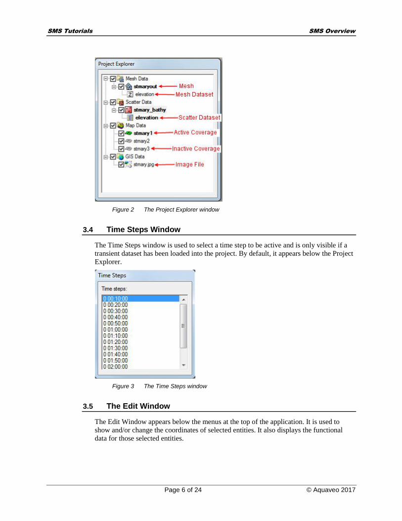
Figure 2 The Project Explorer window

3.4 Time Steps Window

The Time Steps window is used to select a time step to be active and is only visible if a

transient dataset has been loaded into the project. By default, it appears below the Project

Explorer.

Figure 3 The Time Steps window

3.5 The Edit Window

The Edit Window appears below the menus at the top of the application. It is used to

show and/or change the coordinates of selected entities. It also displays the functional

data for those selected entities.



Figure 4 The Edit Window

3.6 The Menu Bar

The Menu Bar contains commands that are available for data manipulation. The menus

shown in the Menu Bar depend on the active module and numerical model.

3.7 The Status Bars

There are two status bars: one at the bottom of the SMS application window and a second

attached to the Main Graphics Window. The status bar attached to the bottom of the main

application window shows help messages when the mouse hovers over a tool or an item

in a dialog box. At times, it also may display a message in red text to prompt for specific

actions, such as that shown in the figure below.

Figure 5 Status bar showing prompt

The second status bar, attached to the Main Graphics Window, is split into two separate

panes. The left shows the mouse coordinates when the model is in plan view. The right

pane shows information for selected entities.

Figure 6 Status bar showing information for a selected entity

4 Using a Background Image

A good way to visualize the model is to import a digital image of the site. For this

tutorial, an image was created by scanning a portion of a USGS quadrangle map and

saving the scanned image as a JPEG file. SMS can open most common image formats

including TIFF, JPEG, and Mr.Sid images. Once the image is inside SMS, it is displayed

in plan view behind all other data, or it can be mapped as a texture onto a finite element

mesh or triangulated scatter point surface.

4.1 Opening the Image

Do the following to open the JPEG image in this example:

1. Select File | Open. This will bring up the Open dialog.

2. Select the file “stmary.jpg” from the “data files” folder in the “SMS_Overview”

folder.

3. Click Open. SMS opens the file and searches for image georeferencing data.

Georeferencing data define the world locations (x, y) that correspond to each point

in an image. It is usually contained inside a world file or sometimes the image



itself. A world file could have the extension “.wld,” “.tfw,” “.jpgw,” and so on. If

SMS finds georeferencing data, the image will be opened and displayed. If not,

define this mapping using the Register Image dialog. This is not required in this tutorial.

4. Depending on the preference settings, SMS may ask whether to build image

pyramids or not. This improves image quality at various resolutions, but uses

more memory. If asked, click Yes to generate the pyramids.

Notice that an entry is added to the Project Explorer as the image is read in under “GIS

Data.”

5 Using Feature Objects

A conceptual model consists of a simplistic representation of the situation being modeled.

This includes the geometric attributes of the situation (such as domain extents), the forces

acting on the domain (such as inflow or water level boundary conditions), and the

physical characteristics (such as roughness or friction). It does not include numerical

details like elements. This model is constructed over a background image using feature

objects in the Map module.

Figure 7 Feature Objects

Feature objects in SMS include points, nodes, arcs, and polygons, as shown in Figure 7.

Feature objects are grouped into sets called “coverages.” Only one coverage can be active

at a time.

A feature point defines an (x, y) location that is not attached to an arc. Points are used to

define the location of a measured field value or a specific location of interest such as a

velocity gauge. SMS can extract data from a numerical model at such a location, or force

the creation of a mesh node at the specific location.

A feature node is the same as a feature point, except that it is attached to at least one arc.



A feature arc is a sequence of line segments grouped together as a polyline entity. Arcs

can form polygons or represent linear features such as channel edges. The two end points

of an arc are called “feature nodes,” and the intermediate points are called “feature

vertices.”

A feature polygon is defined by a closed loop of feature arcs. A feature polygon can

consist of a single feature arc or multiple feature arcs, as long as a closed loop is formed.

It may also include holes.

The conceptual model in this tutorial will consist of a single coverage in which the river

regions and the flood bank will be defined. While going through this tutorial, new

coverages will be created over the existing coverage. The new coverage will become

active and the old coverage will become inactive.

6 Creating Feature Arcs

A set of feature objects can be created to show topographically important features such as

river channels and material region boundaries. Feature objects can be digitized directly

inside SMS, converted from an existing CAD file (such as DXF or DWG), or they can be

extracted from survey data. For this example, the feature objects will be digitized inside

SMS using the registered JPEG image as a reference. To create the feature arcs by

digitizing:

1. Click on the “Area Property” coverage to make it active.

2. Choose the Create Feature Arc tool from the dynamic toolbox.

3. Click out the left riverbank, as shown in Figure 8 (if necessary, use the Zoom

tool to get a closer view). While creating the arc, if a mistake happens and there

is a need to back up, press the Backspace key. If there is a need to abort the arc

and start over, press the Esc key.

4. Double-click the last point to end the arc.

Figure 8 Creation of the first feature arc



A feature arc has defined the general shape of the left riverbank. Three more arcs are

required to define the right riverbank and the upstream and downstream river cross

sections. Together, these arcs will be used to create a polygon that defines the study area.

Do the following to create the remaining arcs:

1. In the same manner just described, create the remaining three arcs, as shown in

Figure 9.

2. Remember to double-click to terminate an arc unless terminating at an existing

node.

Figure 9 All feature arcs have been created

There is now a defined main river channel. When creating other models, normally

proceed to create other arcs, split the existing arcs to define material zones, and locate

specific model features such as hard points on the river. To save time, a conceptual model

with this all done has been saved in a file.

Do as follows to open the file:

1. Select File | Open to bring up the Open dialog.

2. Select the file “stmary1.map” from the data files folder for this tutorial.

3. Click Open. A new coverage is created from the data in the file.

Notice that coverage is called “stmary1” is under the “Area Property” coverage. If the

“Area Property” coverage was empty SMS would have replaced it with the “stmary1”

coverage.

4. To hide the coverage, uncheck the box next to its name (“stmary1”) in the Project

Explorer. Notice how the data in the Graphics Window disappears.

5. Check the box next to “stmary1” to the data can be seen in the Graphics Window.

The display should look something like Figure 10.



Figure 10 The stmary1.map feature object data

7 Manipulating Coverages

As stated at the beginning of this tutorial, feature objects are grouped into coverages.

When a set of feature objects is opened from a file, one or more new coverages are

created. The last coverage in the file becomes active. Any creation or editing of feature

objects occurs in the active coverage. Inactive coverages are drawn in a blue-gray color

by default or not displayed at all depending on the display option settings.

Each coverage is also represented by an entry on the Project Explorer. A project

commonly includes many coverages defining various options in a design or various

historical conditions.

When there are many coverages being drawn, the display can become cluttered.

Individual coverages may be turned off by unchecking the box next to the coverage name

in the Project Explorer. If a coverage is no longer desired, delete it by right-clicking on

the coverage in the Project Explorer and selecting the Delete option.

Coverages can also be organized in folders by right-clicking on the Map Data item and

selecting the New Folder command. Coverages can be clicked and dragged under folder

items in the Project Explorer. The folders can then be turned on or off to show or hide all

coverages in that folder.

8 Redistributing Vertices

To create the feature arcs, a line of points were simply clicked out over the image. The

spacing of the vertices along the arc may not have been noticed. The final element

density in a mesh created from feature objects matches the density of vertices along the

feature arcs, so it is desirable to have a more uniform node distribution. The vertices in a

feature arc can be redistributed at a desired spacing.

To redistribute vertices, follow these steps:



1. Choose the Select Feature Arc tool from the toolbox.

2. Click on the arc that follows the left of the river bank, labeled Arc #1 in Figure 9

above.

3. The addition of the conceptual model split Arc #1 into four segments; hold the

Shift key down to select all four segments.

4. Select Feature Objects | Redistribute Vertices. The Redistribute Vertices

dialog shows information about the feature arc segments and vertex spacing.

5. Make sure the “Specified spacing” option is selected for Specify and enter a value

of “200” for Average. This tells SMS to create vertices 200 ft apart from each

other (or 200 m apart if working in metric units).

6. Click OK to redistribute the vertices along the arc.

Figure 11 Redistribution of vertices along arcs

After using the Redistribute Vertices dialog, the display will refresh, showing the

specified vertex distribution. The arc will still be highlighted, because it is still selected.

7. Click somewhere else on the display. The selection is cleared and the effect of

the command can be more clearly seen.

When creating conceptual models, this redistribution would be done for each arc until

there is the vertex spacing that is wanted in all areas. If the spacing is the same for

multiple arcs, multiple arcs can be selected and redistributed at the same time. When

planning to use arcs in a patch, a better patch is created if opposite arcs have an equal

number of vertices. In this case, it’s best to use the “Number of Segments” option rather

than the “Specified Spacing” option so that the exact number of vertices can be specified

along each arc.

9 Defining Polygons

Open another map file, which has the vertices redistributed on all the arcs.




2. Select the file “stmary2.map” from the data files folder and click Open.

3. Turn off the display of the “stmary1” coverage.

Before proceeding with defining polygons, the coverage type must be changed to a 2D

Mesh:

4. Right-click on the coverage “stmary2” in the Project Explorer.

5. From the menu, choose Type | Generic| Mesh Generator.

Polygons are created from a group of arcs that form a closed loop. Each polygon is used

to define a specific material zone. Polygons can be created one by one, but it is more

reliable to have SMS create them automatically. To have SMS build polygons out of the

arcs, do the following:

6. Make sure no arcs are selected by clicking in the Graphics Window away from

any arcs.

7. Select Feature Objects | Clean to bring up the Clean Options dialog.

8. Click OK in the Clean Options dialog. This will make sure there are no problems

with the feature objects that were created.

9. Select Feature Objects | Build Polygons.

Although nothing appears to have changed in the display, polygons have been built from

the arcs. The one evidence of this is that the Select Polygon tool becomes available

(un-dimed). The polygons in this example are for defining the material zones as well as

aiding in creating a better quality mesh.

10 Assigning Meshing Parameters

With polygons, arcs, and points created, meshing parameters can be assigned. These

meshing parameters define which automatic mesh generation method will be used to

create finite elements inside the polygon. For each method, a corner node of a finite

element mesh will be created at each vertex on the feature arc. The difference comes in

how internal nodes are created and how those nodes are connected to form elements.

SMS has various mesh generation methods. The most commonly applied include patch,

paving, and scalar paving density. These methods are described in the SMS Online Help

(http://www.xmswiki.com/wiki/SMS:SMS), so they will not be described in detail here.

As an overview, paving is the default technique because it works for all polygon shapes.

Patches require either three or four polygonal sides. Density meshing options require

scattered datasets to define the mesh density.

10.1 Creating a Refine Point for Paving

When using the default paving method, some control can be maintained over how

elements are created. A “refine point” is a feature point that is created inside the

boundary of a polygon and assigned a size value. When the finite element mesh is

created, a corner node will be created at the location of the refine point and all element

http://www.xmswiki.com/wiki/SMS:SMS



edges that touch the node will be the exact length specified by the refine point size value.

Do the following to create a refine point:

1. Choose the Select Feature Point tool from the Toolbox.

2. Double-click on the point inside the left polygon, labeled in Figure 12. This will

bring up the Refine Attributes dialog.

3. Make sure the Refine Point option is checked.

4. Enter an Element size of “75.0” (ft).

5. Accept the default for other options and click the OK button to accept the refine

point. Depending on the display setting, the refine point will be distinguished

with a different color than nodes, as shown in Figure 12.

When the finite element mesh is generated, a mesh corner node will be created at the

refine point’s location, and all attached element edges will be 75.0 feet in length. A refine

point is useful when a node needs to be placed at a specific feature, such as at a high or

low elevation point.

Figure 12 The location of the refine point

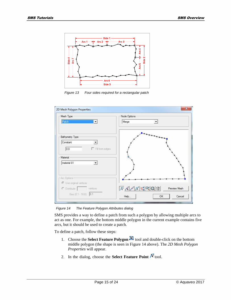
10.2 Defining a Coons Patch

The Coons Patch mesh generation method requires three or four sides to be created.

However, it is not uncommon to use the patching technique to fill a polygon defined by

more than four arcs. Figure 13 shows an example of a rectangular patch made up of four

sides. Note that Side 1 and Side 2 are both made from multiple feature arcs.



Figure 13 Four sides required for a rectangular patch

Figure 14 The Feature Polygon Attributes dialog

SMS provides a way to define a patch from such a polygon by allowing multiple arcs to

act as one. For example, the bottom middle polygon in the current example contains five

arcs, but it should be used to create a patch.

To define a patch, follow these steps:

1. Choose the Select Feature Polygon tool and double-click on the bottom

middle polygon (the shape is seen in Figure 14 above). The 2D Mesh Polygon

Properties will appear.

2. In the dialog, choose the Select Feature Point tool.



3. Click on the node at the center of the left side, as seen in Figure 9.

4. Select the “Merge” option from the Node Options drop down list. This makes

the two arcs on the left side be treated as a single arc.

5. Select the “Patch” option from the Mesh Type drop down list. (If assigning the

meshing type to be “Patch” before merging the node, SMS pops up a message

box indicating that three or four sides need to exist for a patch.) If wanting to

preview the patch, click the Preview Mesh button.

6. Click the OK button to close the 2D Mesh Polygon Attributes dialog.

11 Assigning Materials

When creating models, it's necessary to set up the desired polygon attributes for each

feature polygon in the model. For this tutorial, the rest of the polygons have been set up

and saved to a map file.

Do the following to import this data:

1. Select the File | Open command to bring up the Open dialog.

2. Select the file “stmary3.map” from the data files folder for this tutorial and click

Open to import the file.


4. From the menu, choose Type | Generic| Area Property.

In the coverage that opens, all polygon attributes have been assigned. The four main

channel polygons are assigned as patches, while the other polygons are assigned as

paving.

Each polygon is assigned a material type. All elements generated inside the polygon are

assigned the material type defined in the polygon. In order to assign the materials, new

materials must be specified:

1. Click on Edit | Materials Data to bring up the Materials Data dialog.

2. Select the New button. This creates a new material named “material 02”.

3. Select New again to create “material 03”.

4. Double-click on “material 01” and rename it “Left Bank”.

5. Double-click on “material 02” and rename it “Main Channel”.

6. Double-click on “material 03” and rename it “Right Bank”.

7. If desired, change the colors/patterns for all three materials by using the Pattern

drop-down menu to the right of each material.

8. Click OK to close the Materials Data dialog.



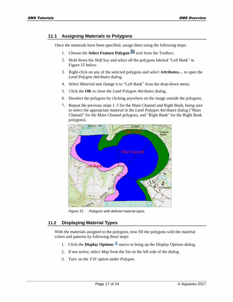
11.1 Assigning Materials to Polygons

Once the materials have been specified, assign them using the following steps:

1. Choose the Select Feature Polygon tool from the Toolbox.

2. Hold down the Shift key and select all the polygons labeled “Left Bank” in

Figure 15 below.

3. Right-click on any of the selected polygons and select Attributes… to open the

Land Polygon Attributes dialog.

4. Select Material and change it to “Left Bank” from the drop-down menu.

5. Click the OK to close the Land Polygon Attributes dialog.

6. Deselect the polygons by clicking anywhere on the image outside the polygons.

7. Repeat the previous steps 1–5 for the Main Channel and Right Bank, being sure

to select the appropriate material in the Land Polygon Attributes dialog ("Main

Channel" for the Main Channel polygons, and "Right Bank" for the Right Bank

polygons).

Figure 15 Polygons with defined material types

11.2 Displaying Material Types

With the materials assigned to the polygons, now fill the polygons with the material

colors and patterns by following these steps:

1. Click the Display Options macro to bring up the Display Options dialog.

2. If not active, select Map from the list on the left side of the dialog.

3. Turn on the Fill option under Polygon.



4. Make sure the Fill with materials option is selected.

5. Click the OK button to close the Display Options dialog.

6. After viewing the materials, repeat the previous steps to turn off the Fill option

before continuing with the tutorial.

The display will refresh, filling each polygon with the material color and pattern.

12 Converting Feature Objects to a Mesh

With the meshing techniques chosen, boundary conditions assigned, and materials

assigned, the next process it to generate the finite element mesh.

Start with a new map file that has everything set up to generate the mesh. Import this file

by doing the following:

1. Select the File | Open command to bring up the Open dialog.

2. Select the file “stmary4.map” from the data files folder for this tutorial and click

Open to import the file.


4. From the menu, choose Type | Generic| Mesh Generator.

To generate the mesh follow these steps:

1. Make sure no objects are selected by clicking in the Graphics Window away

from the river channel.

2. Select Feature Objects | Map →2D Mesh to open the 2D Mesh Options dialog.

3. Accept all default options and click the OK button to start the meshing process.

4. In the Mesh Name dialog, accept the default name by clicking OK.

After a few moments, the display will refresh to show the finite element mesh that was

generated according to the preset conditions. With the mesh created, it is often desirable

to hide the feature arcs and the image. To hide the feature objects, do as follows:

1. To hide the feature objects, uncheck the toggle box next to the Map Data folder

in the Project Explorer.

2. To hide the image, uncheck the toggle box next to the “stmary” image icon under

the “GIS Data” folder in the Project Explorer.

3. Frame the image by selecting Display | Frame Image or clicking on the Frame

Image macro in the Toolbar.

The display will refresh to show the finite element mesh, as shown in Figure 16. With the

feature objects and image hidden, the mesh can be manipulated without interference, but

they are still available if mesh reconstruction is desired.



Figure 16 The generated finite element mesh

13 Editing the Generated Mesh

When a finite element mesh is generated from feature objects, it sometimes has aspects

that need adjustment. An easy way to edit the mesh is to change the meshing parameters

in the conceptual model, such as the distribution of vertices on feature arcs or the mesh

generation parameters. Then the mesh can be regenerated according to the new

parameters. If there are only a few changes desired, they can be edited manually using

tools in the mesh module. These tools are described in SMS Help in the section on the

Mesh module.

14 Interpolating to the Mesh

The finite element mesh generated from the feature objects in this case only defined the

(x, y) coordinates for the nodes. This is because the bathymetric data had not been read in

before generating the mesh. Normally, read in the survey data, and associate it with the

polygons to assign bathymetry to the model. However, to illustrate how to update

bathymetry for an existing mesh, this section is included.

Bathymetric survey data, saved as scatter points, can be interpolated onto the finite

element mesh.

To open the scattered data, do the following:


2. Locate the file “stmary_bathy.h5” in the data file folder and click Open.



The screen will refresh, showing a set of scattered data points. Each point represents a

survey measurement. Scatter points are used to interpolate bathymetric (or other) data

onto a finite element mesh. Although this next step requires manually interpolating the

scattered data, this interpolation can be set up to automatically take place during the

meshing process.

To interpolate the scattered data onto the mesh:

3. Make sure the “stmary_bathy” scatter module is active.

4. Select Scatter | Interpolate to Mesh to open the Interpolation dialog.

5. Make sure “Linear” is selected from the Interpolation drop down list. (For more

information on SMS interpolation options, see SMS Online Help.)

6. Turn on the Map Z option at the lower left area of the dialog under Other

Options.

7. Click the OK button to perform the interpolation.

8. After this is completed, a new dataset, “elevation_interp”, will appear under the

“stmary3 Mesh” item in the “Mesh Data” folder in the Project Explorer.

The scattered data is triangulated when it is read into SMS and an interpolated value is

assigned to each node in the mesh. The Map Z option causes the newly interpolated value

to be used as the nodal Z-coordinate.

As with the feature objects, the scattered data will no longer be needed and may be

hidden or deleted. To hide the scatter point data uncheck the box next to the scatter set

named “stmary_bathy” in the Project Explorer.

So see if the scatter data was correctly interpolated to the mesh, do the following:

9. Select the Rotate tool then click and drag in the Graphics Window to view

how the elevation data was interpolated to the mesh.

10. Click on the Plan View macro when done rotating the mesh.

15 Converting Feature Objects to a 2D Grid

The process of creating a grid feature objects is similar to the process of creating a finite

element mesh. A grid can be created using any coverage that works with a grid model.

15.1 Creating a Grid Frame

Before features objects can be converted to a 2D grid, the area of the grid needs to be

defined. The grid area is determined using a grid frame created in a map coverage. This is

done using a grid frame.

Start by doing the following:

1. Turn on the toggle box next to the Map Data folder and turn off the box next to

the Mesh Data folder in the Project Explorer



2. Select File | Open to bring up the Open dialog

3. Select the “stmary5.map” file and click Open to import the file.

4. In the Project Explorer, select the “stmary5” item to make it active then right-

click and select Type | Generic | CGrid Generator.

The Create 2D Grid Frame tool is now active and can be used. A grid frame is

created by clicking in three locations in the Graphics Window. Each location will become

a corner of the grid frame. SMS will automatically calculate the fourth corner based on

the location of the other three corners.

5. Select the Create 2D Grid Frame tool and click in location 1 as shown in

Figure 17.

6. Click on location 2 then click on location 3 to complete the grid frame.

Figure 17 Grid frame locations

15.2 Editing the Grid Frame

The grid frame can be edited by using the Select 2D Grid Frame tool. This tool is

active when a grid frame exists in a coverage. It can be used to manually resize the grid

frame.

1. Select the Select 2D Grid Frame tool then click and drag the right side of the

grid frame to resize it.

2. Click on the circle in the lower right corner of the grid frame then click and drag

to rotate it.

Manual resizing of the grid frame is useful, but not very precise. A more accurate way to

edit the grid frame is by using the Grid Frame Properties dialog.

3. Using the Select 2D Grid Frame tool, double-click on the grid frame. The

Grid Frame Properties dialog will appear.



4. Enter the following parameters to make the grid frame consistent:

Origin X: 4400

Origin Y: 765

Angle: 30

I size: 2500

J size: 1800

5. For the Cell size, enter “100” in both locations. This will be used when

generating the 2D grid.

6. When done, click OK to close the Grid Frame Properties dialog.

The grid frame should now appear similar to Figure 17. The grid frame has now been

resized and is nearly ready for conversion.

15.3 Creating a New Dataset

The mesh created earlier in this tutorial used bathymetric survey data which was

interpolated to the mesh after the mesh was generated. This data is not useable for the

Cartesian grid. However, the data can be used to generate a more acceptable dataset using

the Dataset Toolbox.

The Dataset Toolbox holds a number of tools that are used to generate new datasets from

existing data.

1. Select the “stmary_bathy” dataset to make the Scatter module active.

2. Select the Data | Dataset Toolbox command to bring up the Dataset Toolbox

dialog.

3. Under Tools, select the Data Calculator option.

4. Under Datasets, select “d1.elevation” and click the Add to Expression button.

In the Calculator field, the number “d1” is shown. This represents the elevation dataset.

5. Click on the multiplication * button then type “-1” in the Calculator field to

make the final equation read “d1*-1”.

6. In the Output dataset name field enter “depth”.

7. When done, click the Compute button. A new dataset will be generated inverting

the elevation values so they can be used as depth values.

8. Click Done to close the Dataset Toolbox calculator.

There is now a new scatter set that can be used when generating the 2D grid.

15.4 Generating a Cartesian Grid

With the grid frame defined and depth dataset ready, now convert the feature objects to a

Cartesian grid.



1. Right-click on the “stmary5” coverage in the Project Explorer and select the

Convert | Map→2D Grid command. This will bring up the Map→2D Grid

dialog.

Most of the options in the Map→2D Grid dialog were set earlier in the Grid Frame

Properties dialog. Had these options not been specified then, the grid frame dimension

and options could be specified now.

When the mesh was created earlier in this tutorial, the elevation was interpolated to the

mesh after the mesh was generated. The Cartesian grid generation process allows datasets

to be assigned during the generation process using the Map→2D Grid dialog.

2. Under Depth Options, change the Source to “Scatter Set” then click the Select

button to bring up the Interpolation dialog.

3. Select the “depth” dataset under the Scatter Set To Interpolate From section.

4. Leave the other options with the default settings and click OK to close the

Interpolation dialog.

5. Click OK to close the Map→2D Grid dialog and generate the grid.

A Cartesian grid has now been generated. To better view the Cartesian grid, complete the

following:

6. Hide all Scatter Data, Map Data, GIS Data, and Mesh Data by unchecking the

box next to each item.

7. Select Display | Display Options to bring up the Display Options dialog.

8. Select Cartesian Grid from the list on the left.

9. Click the All Off button then turn on the Contours option.

10. Under the Contours tab, change the Contour method to “Color Fill”

11. Click OK to close the Display Options dialog.

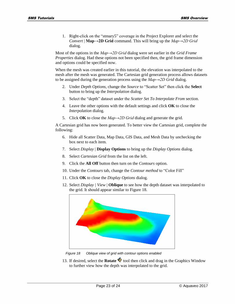
12. Select Display | View | Oblique to see how the depth dataset was interpolated to

the grid. It should appear similar to Figure 18.

Figure 18 Oblique view of grid with contour options enabled

13. If desired, select the Rotate tool then click and drag in the Graphics Window

to further view how the depth was interpolated to the grid.



14. Click on the Plan View macro when done rotating the grid.

16 Saving a Project File

Much data has been opened and changed, but nothing has been saved yet. The data can

all be saved in a project file. When a project file is saved, separate files are created for the

map, scatter data, and mesh data. The project file is a text file that references the

individual data files.

To save all this data for use in a later session:

1. Select File | Save New Project. This will bring up a Save dialog.

2. Enter a File name of “stmaryout.sms” then click the Save button to save the

files.

17 Conclusion

This concludes the “SMS Overview” tutorial. Topics covered in this tutorial included:

An overview of the SMS layout and interface

Using a background image

Using feature objects

Manipulating coverages

Assigning mesh parameters

Assigning materials

Basic mesh generation

Basic dataset creation

Basic grid generation

Saving a project file

Continue to experiment with the SMS interface or quit the program.

SMS Tutorials SMS Overview v. 12smstutorials-12.2.aquaveo.com/SMS_Overview.pdfThe Edit Window appears below the menus at the top of the application. It is used to show and/or change

Documents