U NIVERSITY OF L IÈGE DOCTORAL T HESIS Smart Regulation for Distribution Networks – Modelling New Local Electricity Markets and Regulatory Frameworks for the Integration of Distributed Electricity Generation Resources Author: Miguel MANUEL DE VILLENA MILLÁN Supervisor: Prof. Damien ERNST A thesis submitted in fulfilment of the requirements for the degree of Doctor of Philosophy in the Montefiore Institute Department of Electrical Engineering and Computer Science

Welcome message from author
This document is posted to help you gain knowledge. Please leave a comment to let me know what you think about it! Share it to your friends and learn new things together.
Transcript

UNIVERSITY OF LIÈGE
DOCTORAL THESIS
Smart Regulation for DistributionNetworks – Modelling New LocalElectricity Markets and RegulatoryFrameworks for the Integration ofDistributed Electricity Generation
Resources
Author:Miguel MANUEL DE VILLENA
MILLÁN
Supervisor:Prof. Damien ERNST
A thesis submitted in fulfilment of the requirementsfor the degree of Doctor of Philosophy
in the
Montefiore InstituteDepartment of Electrical Engineering and Computer Science

ii
March, 2 2021

iii
“If I have seen further than others, it is by standing upon the shoulders of giants.”
Sir Isaac Newton


v
Abstract
Growing awareness of the effects of man-made global warming is leading societiesworldwide to re-evaluate our seemingly ever-increasing energy requirements. Theneed to understand and mitigate the issues brought about by our current use of theworld’s resources has thus become a pivotal element in the political agendas of mostregions. Accordingly, curbing anthropogenic greenhouse gas emissions has been thegoal of many of the political decisions of the past decade. In this context, the elec-tricity sector is undergoing deep structural changes to accommodate intermittentrenewable electricity generation resources into a system originally designed to relyon dispatchable power plants to supply our energy needs. One of the main changesconsists of a decentralisation of the sector, bringing the generation assets closer tothe place of final consumption. This creates regulatory challenges that may jeop-ardise the integration of distributed renewable energy resources (DER). This PhDdissertation presents several research contributions dealing with these challenges.
In the first part of our work, we have created a simulation-based approach tostudy the effects of different regulatory frameworks on the deployment of DER in-stallations. DER deployment, in turn, is shown to have a notable impact on therevenue of the distribution system operator (DSO), which is also assessed with oursimulator. Our approach is designed so as to offer a tool for policy makers and regu-lators to discriminate between different regulatory frameworks depending on theirimpact on the distribution network, before implementing them in real life.
The second part of our dissertation models different decentralised electricitymarkets where consumers may exchange electricity, focusing on the concept of re-newable energy communities (REC). We have designed a model of interaction thatsimulates an REC where its members can offer flexibility services by means of acentralised agent such as the REC manager. In addition, we analyse the allocationof local electricity generation among the REC members, and propose an algorithmbased on repartition keys to minimise the total electricity costs of the REC.
The modelling tools developed in this thesis highlight a trade-off between pro-moting the integration of DER and containing their impact on the DSO revenue. Inaddition, they show that creating RECs may help maximise the use of local produc-tion and, therefore, lower the electricity costs of these communities.
Despite having been studied for a few decades now, the promotion of DER is stillvery much in the political agenda in many regions. Unstable policies concerningthese technologies, along with an insufficient understanding of the challenges theypose to the traditional electricity system, have hindered their natural integration intothe electricity networks. These problems, though deeply studied in this thesis, callfor further research to fight man-made global warming.


vii
AcknowledgementsLooking back at the past four years, it becomes apparent that this work would
never have been finished, were it not for the immense support, help, and guidanceof a number of people. These lines, which I write with my most sincere gratitude,are dedicated to all of them.
First and foremost, I want to express my deepest appreciation to Damien Ernst,for giving me the opportunity of working in a supportive and stimulating environ-ment and helping me discover the world of research. This work is, in no small part,the result of his constant support throughout these years.
I would like to extend my sincere gratitude to Axel Gautier, whose kind sugges-tions, support, and advice along these four years have exceedingly contributed tothis thesis.
My warmest thanks also go Julien Jacqmin, his immense help and guidance havegreatly contributed to the present work, and his friendliness has helped me navigatethrough my first years of research.
I want to thank especially Raphaël Fonteneau for his constant work and supportduring these years. The present work exists mostly due to his endless patience, hissharp and accurate remarks and, most importantly, his kindness and friendship.
I also want to thank Sébastien Mathieu for his patience, help, and advice duringthe last part of this work.
I would like to acknowledge the funding received from the Walloon region ofBelgium in the context of the TECR project, in particular, I want to thank Gilles Ti-hon from the Public Service of Wallonia for his collaboration in this project. I amdeeply grateful, too, for the funding received from haulogy and, in particular, manythanks to Eric Vermeulen and Philippe Drugmand for their interest and the numer-ous exchanges we had during the last years.
Many thanks also to the members of the jury –Louis Wehenkel, Axel Gautier,Damien Ernst, Raphaël Fonteneau, Stéphane Renier, Jean-Michel Glachant, TomásGómez San Román, and Dimitrios Papadaskalopoulos– who took their time to care-fully read this dissertation and provide advice to improve it.
I would like to thank my colleagues from the Montefiore Institute and the Uni-versity of Liège who have all contributed to creating a fantastic working environ-ment. In particular, I want to thank all the people with whom I had the chance tointeract: Frédéric, Samy, Michael, Quentin, and Julien. I would also like to thank mytwo French teachers, Catherine and Samia, who have gone the extra mile to help myintegration in Belgium.
I want to warmly thank some of my colleagues and friends who have particularlycontributed to making these four years a great experience. Daniele, Efthimios, andMathias thank you all for these four years. Many thanks especially to Bernardo, whofirst suggested that I should do a PhD; to David, who not only is the best office mateone can hope for, but also a superb friend; to Sergio, who is an amazing scientist and

viii
one of my favourite people in the world; and, of course, to my dear Ioannis, who hasfollowed a (sometimes eerily) similar journey and with whom I have shared manyups and downs along the road.
I would like to thank all the friends I made in Liège who helped make my lifeeasier: Gustavo, Celia, Carlos, Hector, Ariel, Fernando, Bea, Queralt, Pamela, Hugo,and many more. Among them there are a few that became my family in Liège (theSclessin family): Alessio and Javi thanks a lot for everything.
I would also like to thank Javi, Dani, and Ángel for their friendship and theiradvice which have also contributed to this work. My warmest gratitude to Jaime,who is always there.
Finally, I want to express my deepest gratitude to all my family and my family-in-law for their unconditional love and support, which they never failed to showdespite the distance. This work has been possible only thanks to the support of myparents, MJ, Rocío, and very especially, my sister Bea, during and before these lastfour years.

ix
To you Melisa, my lovebird, thank you for being there, believing in me, and working with meday and night. There are no words to express how grateful I am, thank you for everything.


xi
Contents
Abstract v
Acknowledgements vii
Introduction and contributions 3
1 Introduction 31.1 The decentralisation of the power sector . . . . . . . . . . . . . . . . . . 4
1.1.1 Definition of decentralised generation units . . . . . . . . . . . . 51.1.2 Drivers for the integration of decentralised generation . . . . . 6
1.2 Challenges posed by integrating decentralised generation . . . . . . . . 71.2.1 Technical challenges . . . . . . . . . . . . . . . . . . . . . . . . . 71.2.2 Regulatory challenges . . . . . . . . . . . . . . . . . . . . . . . . 8
Distribution network tariff design and metering technology . . 9New local electricity markets . . . . . . . . . . . . . . . . . . . . 12
1.3 Objectives of this thesis . . . . . . . . . . . . . . . . . . . . . . . . . . . . 13
2 Contributions 152.1 Structure of the thesis . . . . . . . . . . . . . . . . . . . . . . . . . . . . . 152.2 List of publications . . . . . . . . . . . . . . . . . . . . . . . . . . . . . . 16
I Modelling regulatory frameworks for distribution networks 19
3 The impact of the metering technology 213.1 Introduction . . . . . . . . . . . . . . . . . . . . . . . . . . . . . . . . . . 223.2 Related works . . . . . . . . . . . . . . . . . . . . . . . . . . . . . . . . . 23
3.2.1 Distribution tariff design and metering technology . . . . . . . 243.2.2 Incentive mechanisms . . . . . . . . . . . . . . . . . . . . . . . . 253.2.3 Modelling . . . . . . . . . . . . . . . . . . . . . . . . . . . . . . . 263.2.4 Motivation . . . . . . . . . . . . . . . . . . . . . . . . . . . . . . . 26
3.3 Simulator . . . . . . . . . . . . . . . . . . . . . . . . . . . . . . . . . . . . 273.3.1 Environment representation . . . . . . . . . . . . . . . . . . . . . 273.3.2 Actions of the agents . . . . . . . . . . . . . . . . . . . . . . . . . 273.3.3 Discrete time dynamical system . . . . . . . . . . . . . . . . . . 28
3.4 Modelling the regulatory framework . . . . . . . . . . . . . . . . . . . . 30

xii
3.4.1 Metering technology . . . . . . . . . . . . . . . . . . . . . . . . . 30Net-metering . . . . . . . . . . . . . . . . . . . . . . . . . . . . . 30Net-billing . . . . . . . . . . . . . . . . . . . . . . . . . . . . . . . 30
3.4.2 Tariff design . . . . . . . . . . . . . . . . . . . . . . . . . . . . . . 303.4.3 Distribution tariff update . . . . . . . . . . . . . . . . . . . . . . 31
3.5 Case study . . . . . . . . . . . . . . . . . . . . . . . . . . . . . . . . . . . 313.5.1 Results . . . . . . . . . . . . . . . . . . . . . . . . . . . . . . . . . 33
Tariff designs (E1 - E4) . . . . . . . . . . . . . . . . . . . . . . . . 33Incentive mechanisms (E5 - E9) . . . . . . . . . . . . . . . . . . . 34
3.5.2 Discussion . . . . . . . . . . . . . . . . . . . . . . . . . . . . . . . 36Tariff designs (E1 - E4) . . . . . . . . . . . . . . . . . . . . . . . . 36Incentive mechanisms (E5 - E9) . . . . . . . . . . . . . . . . . . . 36
3.6 Conclusion . . . . . . . . . . . . . . . . . . . . . . . . . . . . . . . . . . . 37
4 The impact of the distribution network tariff design 394.1 Introduction . . . . . . . . . . . . . . . . . . . . . . . . . . . . . . . . . . 424.2 Contributions . . . . . . . . . . . . . . . . . . . . . . . . . . . . . . . . . 454.3 Simulation configuration . . . . . . . . . . . . . . . . . . . . . . . . . . . 474.4 Modelling and problem formalisation . . . . . . . . . . . . . . . . . . . 48
4.4.1 Rules defining the technical and regulatory frameworks . . . . 48Tariff design . . . . . . . . . . . . . . . . . . . . . . . . . . . . . . 48Technology costs . . . . . . . . . . . . . . . . . . . . . . . . . . . 48
4.4.2 Users . . . . . . . . . . . . . . . . . . . . . . . . . . . . . . . . . . 494.4.3 Optimisation framework formalisation . . . . . . . . . . . . . . 504.4.4 Expanding the optimisation framework to multiple time-steps
and prosumers . . . . . . . . . . . . . . . . . . . . . . . . . . . . 534.4.5 Investment decision process . . . . . . . . . . . . . . . . . . . . . 534.4.6 Distribution system operator’s remuneration mechanism . . . . 554.4.7 User’s electricity bill . . . . . . . . . . . . . . . . . . . . . . . . . 56
4.5 Test case: simulator demonstration . . . . . . . . . . . . . . . . . . . . . 574.5.1 Simulation-based approach capabilities . . . . . . . . . . . . . . 58
Results . . . . . . . . . . . . . . . . . . . . . . . . . . . . . . . . . 59Discussion . . . . . . . . . . . . . . . . . . . . . . . . . . . . . . . 62
4.5.2 Sensitivity Analyses . . . . . . . . . . . . . . . . . . . . . . . . . 64Sensitivity to α . . . . . . . . . . . . . . . . . . . . . . . . . . . . 64Sensitivity to the selling price . . . . . . . . . . . . . . . . . . . . 65Sensitivity to the technology price . . . . . . . . . . . . . . . . . 66
4.6 Conclusion . . . . . . . . . . . . . . . . . . . . . . . . . . . . . . . . . . . 67
5 Regulatory challenges in distribution networks: policy recommendations 695.1 Introduction . . . . . . . . . . . . . . . . . . . . . . . . . . . . . . . . . . 705.2 Literature review . . . . . . . . . . . . . . . . . . . . . . . . . . . . . . . 71

xiii
5.3 Distribution network tariff and the integration of residential solar PVin Wallonia . . . . . . . . . . . . . . . . . . . . . . . . . . . . . . . . . . . 73
5.4 Tariff simulator . . . . . . . . . . . . . . . . . . . . . . . . . . . . . . . . 745.4.1 Model description . . . . . . . . . . . . . . . . . . . . . . . . . . 74
Consumers and Prosumers . . . . . . . . . . . . . . . . . . . . . 75DSO . . . . . . . . . . . . . . . . . . . . . . . . . . . . . . . . . . 76
5.4.2 Main assumptions . . . . . . . . . . . . . . . . . . . . . . . . . . 765.4.3 Simulated scenarios . . . . . . . . . . . . . . . . . . . . . . . . . 78
5.5 Benchmark and short-term reforms . . . . . . . . . . . . . . . . . . . . 785.6 Long-term reforms . . . . . . . . . . . . . . . . . . . . . . . . . . . . . . 81
5.6.1 Net-metering system with a capacity component . . . . . . . . . 825.6.2 Net-purchasing system . . . . . . . . . . . . . . . . . . . . . . . 835.6.3 Self-consumption and power exchanges with the grid . . . . . . 85
5.7 Conclusion and policy implications . . . . . . . . . . . . . . . . . . . . . 875.7.1 Policy implications . . . . . . . . . . . . . . . . . . . . . . . . . . 885.7.2 Limitations and future research . . . . . . . . . . . . . . . . . . . 89
II Decentralised electricity markets 91
6 Model of interaction for renewable energy communities 936.1 Introduction . . . . . . . . . . . . . . . . . . . . . . . . . . . . . . . . . . 946.2 Literature review . . . . . . . . . . . . . . . . . . . . . . . . . . . . . . . 956.3 Proposed interaction model . . . . . . . . . . . . . . . . . . . . . . . . . 966.4 Baseline and updates . . . . . . . . . . . . . . . . . . . . . . . . . . . . . 976.5 Flexibility bids . . . . . . . . . . . . . . . . . . . . . . . . . . . . . . . . . 996.6 Deviation mechanism . . . . . . . . . . . . . . . . . . . . . . . . . . . . . 1016.7 Conclusion . . . . . . . . . . . . . . . . . . . . . . . . . . . . . . . . . . . 102
7 Introducing demand response into renewable energy communities 1037.1 Introduction . . . . . . . . . . . . . . . . . . . . . . . . . . . . . . . . . . 1047.2 Simulator . . . . . . . . . . . . . . . . . . . . . . . . . . . . . . . . . . . . 105
7.2.1 Agents . . . . . . . . . . . . . . . . . . . . . . . . . . . . . . . . . 106Day-ahead market operator . . . . . . . . . . . . . . . . . . . . . 106Flexible consumers . . . . . . . . . . . . . . . . . . . . . . . . . . 106Non-flexible consumers . . . . . . . . . . . . . . . . . . . . . . . 107Generation assets . . . . . . . . . . . . . . . . . . . . . . . . . . . 107ECM . . . . . . . . . . . . . . . . . . . . . . . . . . . . . . . . . . 108
7.3 Day-ahead Flexibility activation . . . . . . . . . . . . . . . . . . . . . . . 1087.4 Test case . . . . . . . . . . . . . . . . . . . . . . . . . . . . . . . . . . . . 110
7.4.1 Cost analysis . . . . . . . . . . . . . . . . . . . . . . . . . . . . . 1117.4.2 Performance analysis . . . . . . . . . . . . . . . . . . . . . . . . . 112
7.5 Conclusions . . . . . . . . . . . . . . . . . . . . . . . . . . . . . . . . . . 113

xiv
8 How to allocate local generation in renewable energy communities 1158.1 Introduction . . . . . . . . . . . . . . . . . . . . . . . . . . . . . . . . . . 1178.2 Literature review . . . . . . . . . . . . . . . . . . . . . . . . . . . . . . . 1188.3 Problem statement . . . . . . . . . . . . . . . . . . . . . . . . . . . . . . 1208.4 Problem formulation . . . . . . . . . . . . . . . . . . . . . . . . . . . . . 1238.5 Results . . . . . . . . . . . . . . . . . . . . . . . . . . . . . . . . . . . . . 124
8.5.1 Test case 1: performance on a simplified example . . . . . . . . 1258.5.2 Test case 2: performance on a realistic example . . . . . . . . . . 1268.5.3 Test case 3: minimum SSR . . . . . . . . . . . . . . . . . . . . . . 1278.5.4 Test case 4: impact of initial repartition keys . . . . . . . . . . . 1298.5.5 Complexity analysis . . . . . . . . . . . . . . . . . . . . . . . . . 131
8.6 Conclusion . . . . . . . . . . . . . . . . . . . . . . . . . . . . . . . . . . . 132
Conclusions and future work 137
9 Conclusion 1379.1 Part I . . . . . . . . . . . . . . . . . . . . . . . . . . . . . . . . . . . . . . 1379.2 Part II . . . . . . . . . . . . . . . . . . . . . . . . . . . . . . . . . . . . . . 1399.3 Limitations and future research . . . . . . . . . . . . . . . . . . . . . . . 141
Appendix 145
A A multi-agent system approach to model the interaction between distributedgeneration deployment and the grid 145A.1 Introduction . . . . . . . . . . . . . . . . . . . . . . . . . . . . . . . . . . 145A.2 Methodology . . . . . . . . . . . . . . . . . . . . . . . . . . . . . . . . . 146
A.2.1 Optimisation of DRE units . . . . . . . . . . . . . . . . . . . . . 147A.2.2 Investment decision process . . . . . . . . . . . . . . . . . . . . . 148A.2.3 Computation of the distribution tariff . . . . . . . . . . . . . . . 148
A.3 Test Case . . . . . . . . . . . . . . . . . . . . . . . . . . . . . . . . . . . . 149A.4 Conclusion . . . . . . . . . . . . . . . . . . . . . . . . . . . . . . . . . . . 152
B Exploring Regulation Policies in Distribution Networks through a Multi-Agent Simulator 153B.1 Introduction . . . . . . . . . . . . . . . . . . . . . . . . . . . . . . . . . . 153B.2 Methodology . . . . . . . . . . . . . . . . . . . . . . . . . . . . . . . . . 155
B.2.1 Interactions . . . . . . . . . . . . . . . . . . . . . . . . . . . . . . 155B.2.2 Environments . . . . . . . . . . . . . . . . . . . . . . . . . . . . . 155B.2.3 Agents of the system . . . . . . . . . . . . . . . . . . . . . . . . . 158
DRE owners . . . . . . . . . . . . . . . . . . . . . . . . . . . . . . 159non-DRE owners . . . . . . . . . . . . . . . . . . . . . . . . . . . 159DSO . . . . . . . . . . . . . . . . . . . . . . . . . . . . . . . . . . 159

xv
B.3 LP Formalisation . . . . . . . . . . . . . . . . . . . . . . . . . . . . . . . 160B.4 Test case . . . . . . . . . . . . . . . . . . . . . . . . . . . . . . . . . . . . 162B.5 Conclusion . . . . . . . . . . . . . . . . . . . . . . . . . . . . . . . . . . . 164
Bibliography 167


xvii
List of Figures
1.1 Distribution network set-up. . . . . . . . . . . . . . . . . . . . . . . . . . 81.2 Feedback loop also known as the “death spiral” of the utility. Pro-
sumers deploying DER installations exert an impact on the level ofrevenue of the DSO, which, in turn, increases the distribution tariff.A feedback then emerges as higher distribution rates spur further de-ployment of DER installations. . . . . . . . . . . . . . . . . . . . . . . . 11
3.1 Time-line of the discrete time dynamical system. The simulation startsby assuming a distribution tariff Π(dis)
n . Then, at every time step, thereis a transition from consumer to prosumer leading to a change in theaggregated apparent consumption Ξn. This change induces an adjust-ment of the distribution tariff Π(dis)
n . . . . . . . . . . . . . . . . . . . . . 283.2 Flow diagram of the proposed multi-agent simulator. The flow of ac-
tions occurs from left to right. The distribution network consumersundergo individual MILP optimisations to minimise their LCOEs. Atransition from consumer to prosumer is computed (investment deci-sion tab (yellow) on the Figure), and finally the DSO adjusts the dis-tribution tariff. . . . . . . . . . . . . . . . . . . . . . . . . . . . . . . . . . 29
3.3 Evolution of Π(dis)n (upper two figures) and of the DER adoption (lower
two figures) across the discrete time dynamical system, for the evalu-ation of tariff designs E1 - E4 (left hand side figures), and of the incen-tive mechanisms E5 - E9 (right hand side figures). . . . . . . . . . . . . 33
3.4 Cumulative sum of the size of the deployed DER installations (includ-ing PV and batteries), over the discrete time dynamical system. Theupper figure corresponds to the evaluation of tariff designs, whereasthe lower one corresponds to the evaluation of the incentive mecha-nisms. . . . . . . . . . . . . . . . . . . . . . . . . . . . . . . . . . . . . . . 34
3.5 Gaussian kernel density estimation of the installed capacity of PV (up-per plot), and of batteries (lower plot). These figures represent theprobability density function for the kernel density estimation of PVand battery capacities, for every environment (E1 - E9). This proba-bility is computed based on the calculated DER installation size of theset I . . . . . . . . . . . . . . . . . . . . . . . . . . . . . . . . . . . . . . . 35
3.6 Levelized cost of electricity of the prosumers in set I , for every envi-ronment (E1 - E9). . . . . . . . . . . . . . . . . . . . . . . . . . . . . . . . 35

xviii
4.1 Evolution of the DER penetration and the electricity prices for con-sumers over the simulation period. . . . . . . . . . . . . . . . . . . . . . 60
4.2 Total capacity of installed PV capacity (blue), total capacity of installedbattery (red), total imports from the distribution network (green), andtotal exports to the distribution network (yellow) at the end of thesimulation period. . . . . . . . . . . . . . . . . . . . . . . . . . . . . . . . 61
4.3 Sensitivity to α. . . . . . . . . . . . . . . . . . . . . . . . . . . . . . . . . 644.4 Sensitivity to the selling price (sp). . . . . . . . . . . . . . . . . . . . . . 654.5 Sensitivity to the technology price (tp). . . . . . . . . . . . . . . . . . . . 66
5.1 Multi-agent interaction model with the feedback loop created by thedeployment of residential PV panels and by the DSO’s remunerationmechanism. . . . . . . . . . . . . . . . . . . . . . . . . . . . . . . . . . . 75
5.2 Evolution of the share of prosumers among potential prosumers. . . . 795.3 Evolution of the installed capacity of PV installations. . . . . . . . . . . 795.4 Evolution of the total tariff bill of a consumer . . . . . . . . . . . . . . . 805.5 Evolution of the LVOE of PV installations. . . . . . . . . . . . . . . . . . 815.6 Evolution of the share of households with a PV installation. . . . . . . 835.7 Evolution of the installed capacity of PV installations. . . . . . . . . . . 835.8 Evolution of the deployment of batteries. . . . . . . . . . . . . . . . . . 845.9 Evolution of the LVOE of PV installations. . . . . . . . . . . . . . . . . . 855.10 Evolution of the total tariff bill of a consumer . . . . . . . . . . . . . . . 85
6.1 Flow of interactions between a client and its retailer. A baseline iscomputed for each client. Then the retailer allows, or not, the pro-vision of flexibility of the client. If it is not accepted, the client fallsunder a classic retailing contract. If accepted, the client notifies its ca-pability to provide flexibility. If the retailer contracts the flexibility, theschedule of the client is modified accordingly. This schedule may bemodified upon notification of the client. The client is invoiced basedon the final schedule and the metered energy. . . . . . . . . . . . . . . . 95
6.2 Case of a schedule update that cancels out already sold flexibility. . . . 986.3 Example of upward modulation with three payback periods. . . . . . . 996.4 Evolution of flexibility bid statuses. . . . . . . . . . . . . . . . . . . . . . 100
7.1 Flexibility bids’ structure with three elements: the initial flexibility, anidle time, and the rebound. . . . . . . . . . . . . . . . . . . . . . . . . . 108
7.2 Initial demand (in red) vs demand after using flexibility (in blue). ThePV production is displayed in yellow. Detail of 13 days in March 2017. 113
8.1 Costs of the REC members. . . . . . . . . . . . . . . . . . . . . . . . . . 1278.2 SSR of the consumers after the repartition keys optimisation. . . . . . . 1278.3 Difference in the REC members costs, with and without enforcing any
minimum SSR of 42%. . . . . . . . . . . . . . . . . . . . . . . . . . . . . 128

xix
8.4 Total locally sold and globally sold production for a range of maxi-mum key deviations (Xt,i). . . . . . . . . . . . . . . . . . . . . . . . . . . 130
8.5 Costs of the members for a range of maximum key deviations (Xt,i)relative to the costs when Xt,i = 0. . . . . . . . . . . . . . . . . . . . . . 131
8.6 Allocated production of the REC members for a range of maximumkey deviations (Xt,i) relative to the allocated production when Xt,i = 0. 132
A.1 Data flow diagram of the proposed multi-agent system. The flow ofactions occurs from top to bottom. The individual users of group A,characterised by their load, undergo an optimisation. The optimisa-tion requires the technology costs, the tariff design, and the retail elec-tricity tariff, as well as the user load. The individual results of the opti-misation are used by the investment decision model, which comparesthe LCOE of the individually optimised installations with the retailtariff, yielding a positive or negative investment decision for each po-tential installation. Finally, the revenues derived from the aggregatednet consumption of all users of group A and of group B are comparedwith the (fixed) DSO costs, and the distribution cost is updated. . . . . 150
A.2 Evolution of the distribution tariff (left axis) and evolution of DREdeployment (right axis). The deployment of DRE units induces anincrease in the distribution tariff. Such an increase features a differ-ent extent depending on the environment (composed of tariff design,incentive scheme, and technology cost). . . . . . . . . . . . . . . . . . . 151
B.1 Cumulative PV and battery capacities of the deployed DRE, over thepresented discrete-time dynamical system. The economically optimalsize of the deployed DRE installations is influenced in a large extentby the environment. In this figure, we observe these different usersbehaviours under four distinct environments. . . . . . . . . . . . . . . . 164
B.2 Evolution of the distribution tariff. The deployment of DRE units in-duces an increase in the distribution tariff. Such an increase featuresa different extent depending on the environment. . . . . . . . . . . . . 165


xxi
List of Tables
4.1 Construction of the different scenarios . . . . . . . . . . . . . . . . . . . 594.2 General inputs of the multi-agent model . . . . . . . . . . . . . . . . . . 594.3 Annual electricity costs for an average consumer and an average ac-
tual prosumer at the end of the simulated period. . . . . . . . . . . . . 614.4 Sensitivity of PV- and battery-installed capacity to α. . . . . . . . . . . . 644.5 Sensitivity of PV- and battery-installed capacity to the selling price (sp). 654.6 Sensitivity of PV- and battery-installed capacity to the technology price
(tp). Note that the shown percentages are relative to the prices usedfor the first simulation. . . . . . . . . . . . . . . . . . . . . . . . . . . . . 67
5.1 Key parameters of the model . . . . . . . . . . . . . . . . . . . . . . . . 775.2 Simulated scenarios . . . . . . . . . . . . . . . . . . . . . . . . . . . . . 785.3 Self-consumption and aggregate power exchanges . . . . . . . . . . . . 875.4 Summary of the results (evolution compared to the baseline scenario) . 88
6.1 Influence of the correlation of the clients’ production on the total pro-duction of the retailer, as a function of the number of clients k and thecorrelation of their production ρ. . . . . . . . . . . . . . . . . . . . . . . 102
7.1 Notation. . . . . . . . . . . . . . . . . . . . . . . . . . . . . . . . . . . . . 1117.2 List of prices in the simulations (e/MWh). . . . . . . . . . . . . . . . . 1117.3 Costs for the three different cases and percentage of difference with
respect to the reference (first column). . . . . . . . . . . . . . . . . . . . 1127.4 Results of the analysis of flexibility use. . . . . . . . . . . . . . . . . . . 113
8.1 Price signals in e/MWh. . . . . . . . . . . . . . . . . . . . . . . . . . . . 1258.2 Test case 1 – inputs. . . . . . . . . . . . . . . . . . . . . . . . . . . . . . . 1258.3 Test case1 – outputs. . . . . . . . . . . . . . . . . . . . . . . . . . . . . . 1268.4 Allocated production for the different initial keys. . . . . . . . . . . . . 1298.5 Running times of the proposed algorithm. . . . . . . . . . . . . . . . . . 132
B.1 Notation . . . . . . . . . . . . . . . . . . . . . . . . . . . . . . . . . . . . 158


xxiii
List of Abbreviations
DER Distributed Electricity generation ResourcesDG Distributed GenerationDSO Distribution System OperatorECM Energy Community ManagerLCOE Levelised Cost Of ElectricityLVOE Levelised Value Of ElectricityLP Linear ProgramMILP Mixed Integer Linear ProgramPV PhotoVoltaicREC Renewable Energy CommunitySCR Self Consumption RateSSR Self-Sufficiency Rate


1
Introduction and contributions


3
Chapter 1
Introduction
Worldwide, the energy sector is undergoing a revolution – in fact, this revolutionhas been ongoing for over a decade now. Whilst in the past the most worrisomeprospect for society was to run out of fossil fuels to power our lives, the threat ofclimate change, caused by anthropogenic greenhouse gas emissions, has rearrangedthe priorities. Today, the most worrisome prospect is not gaining independence fromfossil fuels fast enough. For this reason, over the past decades, researchers and policymakers all around the globe have been trying to work out solutions to the challengesposed by climate change.
In December 2015, during the United Nations Climate Change Conference, theParis Agreement was adopted [1]. This agreement aims at holding global warm-ing below 2 degrees Celsius, with the ambition of limiting it to 1.5 degrees Celsiusabove pre-industrial levels. In compliance with this agreement, signing countrieshave had to outline their post-2020 climate actions in the form of intended nationallydetermined contributions. These climate actions, nonetheless, have been deemedinsufficient, according to some scientific publications, to curb greenhouse gas emis-sions to keep global warming below 2 degrees Celsius [2, 3]. Some researchers evenquestioned, back in 2016, whether the goal of 2 degrees Celsius is enough to attainthese targets [4]. Raising a similar concern, the authors in [5] claim that some tip-ping points (points-of-no-return which if surpassed would lock the world into a newdynamics) have come so close that, even if all man-made greenhouse gas emissionswere to stop today (2021), we are already past some of these points-of-no-return.Their results show a sustained melting of the permafrost for hundreds of years af-ter the emissions are halted. In this context, the intergovernmental panel on climatechange (IPCC)1 published in 2018 a report analysing the risks associated to a 1.5 - 2degrees Celsius global warming with respect to pre-industrial levels [7]. Such risks,reported for numerous areas of human development, provide a grim overview ofwhat might come about, should actions towards climate change mitigation not takeplace in short order.
In the European context, the European Union (EU) established in 2015 the EUEnergy Union [8] to provide EU consumers with secure, sustainable, competitive
1The IPCC was established in 1988 with the mission of assessing climate change based on the latestscience [6].

4 Chapter 1. Introduction
and affordable energy. Central to this Energy Union is the Clean Energy for all Eu-ropeans Package [9]. This package represents an update of the EU’s energy policyframework towards delivering the EU’s commitments in the Paris Agreement. Oneof the directives brought forward by this package is the recast of the 2009 Europeanrenewable energy directive, published in 2018 [10, 11]. This document establishes anew binding renewable energy target for the EU for 2030 of, at least, 32% in grossfinal energy consumption. However, no fixed path exists at the European level, andMember States may use different strategies toward meeting these targets. In thisregard, three possible scenarios are analysed in the last ten-year network develop-ment plan (TYNDP) of the European network of transmission system operators forelectricity (ENTSO-E) and for gas (ENTSOG). These three scenarios are compiledin two documents: [12] and [13]. The first scenario –National Trends– reflects thecommitment of each Member State to meet the EU targets for 2030 - 2050, whilstthe other two aim to reach the target set by the Paris Agreement (i.e. a warming of1.5 degrees Celsius below pre-industrial levels). Of the latter two scenarios, the firstone –Global Ambition– looks at a possible future that is led by developments in cen-tralised generation, and the other one –Distributed Energy– is specifically designedto embrace a decentralised approach to the energy transition. In this context, theterms centralised and decentralised refer to the manner the electricity is generated:the former indicates that the electricity is generated mostly in central power plants,whereas the latter implies that electricity production partially takes place where itis consumed, by means of smaller generation devices owned sometimes by the con-sumers. A substantial amount of research has been produced over the last few yearson how a decentralised electricity system may work. In this regard, technologicaladvances in electricity generation from renewable sources, notably including solarphotovoltaic (PV), have a natural market in private investments –such as householdsthat deploy these technologies on their rooftops– in a decentralised fashion.
This thesis revolves around this decentralisation of the power sector as a way ofachieving renewable energy targets such as the Paris Agreement. In particular, thiswork focuses on some of the regulatory challenges posed by such a decentralisation,proposing a mathematical description to them as well as modelling solutions.
1.1 The decentralisation of the power sector
The idea of decentralising the electricity sector is not new. One of the first worksmentioning the possibility of taking a decentralised energy path, as opposed to thebusiness as usual centralised policy, dates back to 1976 [14]. In this work the au-thor argues that this path would lead to social, economic, and geopolitical advan-tages2. Another early work on this topic is the essay “Power Systems ‘2000’: hier-archical control strategies”, written in 1978 by Fred C. Schweppe [15]. In his vision,
2Geopolitical advantages relate mostly to curbing the nuclear proliferation which, at that time, wasa very relevant objective. In our work however, we abstract from this type of arguments.

1.1. The decentralisation of the power sector 5
Schweppe elaborated upon the importance of demand-side procurement of electric-ity services, mostly combined heat and power, owing to the limitations of the time.
1.1.1 Definition of decentralised generation units
Despite the existence of some pioneers in the field, it was not until many years laterthat the scientific literature on the decentralisation of the power sector and, in partic-ular, on the integration of distributed generation, gained momentum. Two scientificpapers from 1995 and 1996 elaborate, probably for the first time, on the technicalaspects of integrating what the author calls embedded generation into the distributionnetworks [16, 17]. In these two papers the author suggests that embedded gen-eration –what is now understood as distributed energy resources (DER)– can pro-vide only energy and not capacity to the electricity system3. These two works claimthat some institutional arrangements would be needed to integrate great amountsof DER in the system. Back then, however, this type of technology was yet to be for-mally defined. The first work addressing this definition was published in 2001 [18].This scientific paper provides the first formal description of distributed generationas electric power generation within distribution networks or on the customer side ofthe network. Dealing with the same problem, the authors in [19] define distributedgeneration as small generation units of 30 MW or less which are located at or nearcustomer sites to meet their specific needs. The definition of distributed generation(or embedded or decentralised generation) is further addressed in two other earlyworks describing these technologies and discussing their benefits and issues [20, 21].These two works list a collection of definitions provided by different authors in theprevious literature, highlighting that all the definitions include small-scale genera-tion devices connected to the distribution grid. Some works, however, also includein this definition larger-scale cogeneration units or large wind farms connected tothe transmission network. Finally, in the European context, the trends for distributedgeneration integration are addressed in [22]. In this paper, the authors highlight agap in the literature to formally agree on what constitutes distributed generation,suggesting the importance of coming up with a universal definition. They, nev-ertheless, agree on some common characteristics seen across the existing researchworks: DER are small-scale generation units that are connected to the distributionnetwork. Using this broad definition, one of the first works focusing on the emer-gent DER technologies was published as a white paper in 2002. In this paper, theauthors consider DER as a way to supply, in an efficient fashion, the growing elec-tricity needs of customers, suggesting the concept of microgrids to organise theseresources [23]. Finally, the previous definition of DER is used in [24], another early
3When talking about procurement of electricity we can distinguish between energy procurementwhich refers to the ability to meet the overall energy consumption of the system, and capacity procure-ment which refers to the ability to meet instantaneous loads.

6 Chapter 1. Introduction
work which proposes a virtual power plant approach where several DER installa-tions are aggregated. This provides the distribution system operator (DSO) withenhanced visibility and control.
In this thesis we adhere to the use of the definition of DER proposed in [22],considering as distributed generation any small scale electricity generation deviceslocated at or near the consumer end at the distribution level. In particular, we focuson solar PV installations deployed by traditional consumers –who therefore turninto prosumers– or by small companies connected to the distribution network.
1.1.2 Drivers for the integration of decentralised generation
A number of drivers can explain the explosion of the adoption of DER technolo-gies such as rooftop solar PV. These drivers are studied in [25], where the authorsestablish two distinct categories classifying them:
1. Commercial drivers, which comprise the uncertainty of electricity marketsand the enhanced power quality they provide.
2. Regulatory drivers, among which the most relevant are the incentives to di-versify energy sources in order to improve energy security, or the support forcompetition that increase the amount of players in the market by introducingeconomically beneficial policies for DER. The latter, though, requires that DERowners trade in the electricity markets, which in turns necessitates appropriateframeworks, as it is discussed later in this introduction.
A consistent decrease of technology prices (including solar PV and batteries) can beadded to the list of these drivers [26]. In addition to them, the authors in [25] lista series of challenges brought about by the integration of DER. Examples of thesechallenges are, according to this work, steering clear of over-voltages, ensuring thepower quality, the protection of DER equipments, stability issues in the distributionnetwork, and regulatory issues, which are largely discussed in this document. Thispaper highlights the importance of moving away from the traditional fit-and-forgetapproach used to manage the distribution networks. Some other works have fo-cused on the integration of DER, pinpointing challenges and benefits, often from atechnical standpoint, as seen in [27]. In this line, the report entitled “The Utility ofthe Future” deals with challenges and opportunities stemming from the integrationof DER, focusing on the evolution of the power system for the coming decades [28].While this report aims to provide a thorough framework for the cost-efficient inte-gration of both centralised and distributed (decentralised) resources, the importanceof DER is remarked throughout the whole document. One of its key messages is thatthe electricity sector is shifting from a paradigm where large power plants, far fromthe consumption of electricity, are operated according to the plan of a central author-ity, to a decentralised fashion of electricity generation by which small generators aredeployed close to the loads. The drivers for such a paradigm shift are mainly three:

1.2. Challenges posed by integrating decentralised generation 7
(i) technological advances leading to substantial cost reduction for DER technolo-gies; (ii) policies related to the deployment of renewable energy technologies andthe de-carbonisation of the power sector; and (iii) consumer choices and preferencesby which passive consumers are able to express their preferences through decisionsconcerning their provision of electricity services.
This review on the evolution of the power sector is not intended to be exhaustivebut rather to provide the reader with an overview of the trends in the electricitysector over the last decades as well as the outlook to the future. Among these trends,a very prominent one consists in the decentralisation of the electricity generation.Such a decentralisation has been heralded by researchers for many decades, but onlyover the last few years has become a reality. This is why a large body of literaturehas been devoted to address new challenges and problems brought about by theintegration of these technologies.
1.2 Challenges posed by integrating decentralised generation
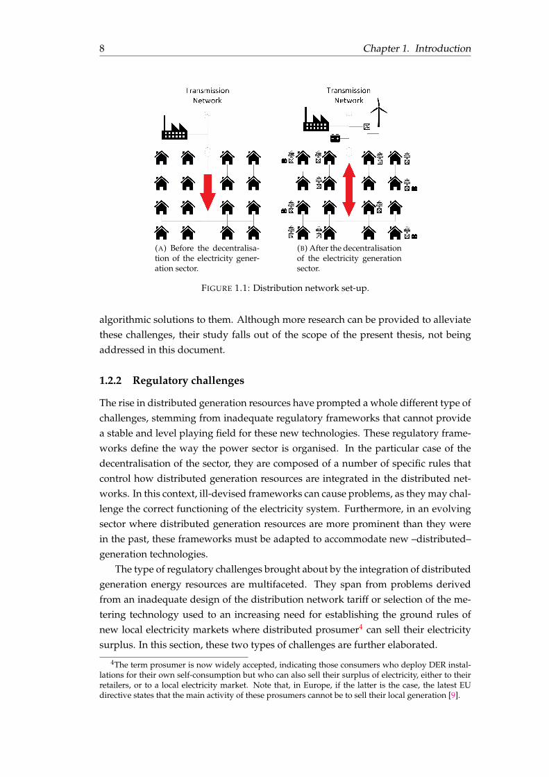
By now, it is clear that the revolution in new generation technologies, in combinationwith policies and regulations worldwide, have pushed the adoption of distributedgeneration. This integration of distributed generation has become pivotal to thede-carbonisation of the electricity sector, since a very significant proportion of thenew DER installations consist of renewable technologies such as solar photovoltaic(PV). However, this distributed renewable integration does not come free of prob-lems and, albeit it offers promising benefits for the future of the power systems, itmay also bring about several problems for this system which must be carefully stud-ied. Accordingly, since the electricity distribution networks were designed decadesago when multi-directional electricity flows were rare, they were not engineered toabsorb and re-distribute large amounts of distributed generation. Figure 1.1 presentsa schematic of how the electricity flows in a distribution network, before and afterthe decentralisation of the power sector.
Because of this decentralisation, the integration of renewable electricity genera-tion resources into the electricity distribution networks poses a number of challengesand uncertainties that may jeopardise the adequate operation of the distribution net-works. These challenges can be broadly divided, depending on their nature, intotechnical and regulatory.
1.2.1 Technical challenges
This type of challenges are well known since the beginning of the decentralisationand, therefore, have been studied extensively over the years. They typically rangefrom unbalances on the three phases due to power withdrawals or injections, tounder- and over-voltages in the low-voltage distribution networks [25]. A detailedanalysis of these problems can be found in [26], where the author proposes several
8 Chapter 1. Introduction
(A) Before the decentralisa-tion of the electricity gener-ation sector.
(B) After the decentralisationof the electricity generationsector.
FIGURE 1.1: Distribution network set-up.
algorithmic solutions to them. Although more research can be provided to alleviatethese challenges, their study falls out of the scope of the present thesis, not beingaddressed in this document.
1.2.2 Regulatory challenges
The rise in distributed generation resources have prompted a whole different type ofchallenges, stemming from inadequate regulatory frameworks that cannot providea stable and level playing field for these new technologies. These regulatory frame-works define the way the power sector is organised. In the particular case of thedecentralisation of the sector, they are composed of a number of specific rules thatcontrol how distributed generation resources are integrated in the distributed net-works. In this context, ill-devised frameworks can cause problems, as they may chal-lenge the correct functioning of the electricity system. Furthermore, in an evolvingsector where distributed generation resources are more prominent than they werein the past, these frameworks must be adapted to accommodate new –distributed–generation technologies.
The type of regulatory challenges brought about by the integration of distributedgeneration energy resources are multifaceted. They span from problems derivedfrom an inadequate design of the distribution network tariff or selection of the me-tering technology used to an increasing need for establishing the ground rules ofnew local electricity markets where distributed prosumer4 can sell their electricitysurplus. In this section, these two types of challenges are further elaborated.
4The term prosumer is now widely accepted, indicating those consumers who deploy DER instal-lations for their own self-consumption but who can also sell their surplus of electricity, either to theirretailers, or to a local electricity market. Note that, in Europe, if the latter is the case, the latest EUdirective states that the main activity of these prosumers cannot be to sell their local generation [9].

1.2. Challenges posed by integrating decentralised generation 9
Distribution network tariff design and metering technology
One of the first works discussing this type of regulatory challenge dates back to 2002,where the authors mention, possibly for the first time, that distribution network tar-iff structures might need to be revisited in the presence of a significant amount ofDER [29]. The authors of this paper highlight that, should distributed generationbecome widely spread, the distribution network will undergo a long-term trans-formation where communities and microgrids will naturally emerge. The researchon this topic continued over the years in a rather prolific fashion. Consequently,researchers worldwide have been able to pinpoint some of the most prominent chal-lenges stemming from an inadequate design of distribution network tariffs, in thecontext of an increasing integration of distributed generation into the distributionnetworks. Two of these challenges stand out: (i) the collapse of the economic sus-tainability of DSOs, illustrated by the “death spiral” of the utility (see Figure 1.2);and (ii) the cross-subsidies among final customers of the distribution network. Thesetwo challenges may be further aggravated depending on the metering technology.
The economic (un)sustainability of DSO: The design of the distribution tariff hasa strong impact on the DSO remuneration mechanism. This mechanism works bycollecting revenue from final customers connected to the distribution network, andcomparing it with the DSO costs. The way revenue are collected depends on thedistribution network tariff design and on the metering technology in place. Typ-ically, this tariff may be based on (i) energy charges in e per kWh consumed –commonly known as volumetric charges–, (ii) power charges in e per kWp with-drawn –commonly known as capacity charges–, or (iii) fixed charges in e per con-nection point. In addition, variations can be introduced to these charges, such asthe time-of-use (ToU) fees in which different levels of energy or power charges areapplied depending on the time of consumption [30]. Furthermore, the meteringtechnology in place strongly impacts on the way the electricity consumption is mea-sured on the prosumers end. Note that the metering technology is only relevant forprosumers, since it alters the way the electricity exchanges between the prosumersand the grid are measured – for regular consumers the metering is either a mechani-cal meter that measures energy consumption, or a smart meter that measures powerand energy consumption. There are two main metering technologies for prosumers,both addressed in this thesis: net-metering, and net-billing (sometimes referred toas net-purchasing) [30].
• Net-metering consists of one single mechanical meter that records importsfrom the grid by adding units of energy, and exports to the grid by subtractingunits of energy. Both types of exchange are assigned with the same monetaryvalue, namely the retail electricity tariff. With this metering system, if the ex-ports exceed the imports, the excess is not remunerated to the prosumer.

10 Chapter 1. Introduction
• Net-billing consists of two independent mechanical meters, or a smart meterthat can measure imports and export separately. In this setting, imports arecharged at retail price, and exports are compensated at a selling price. Nolimit exists, in principle, to the amount of exports allowed.
Regarding the costs of the DSO, they typically depend on the physical infrastructureof the distribution network, as well as on the level of use of such an infrastructure.Both costs are known to the DSO [31, 32]. The comparison between costs and rev-enue may yield an imbalance where either one is greater than the other. In suchcases, the DSO must increase or decrease the distribution tariff to ensure a level ofrevenue that is sufficient to break even5. On this basis, a non-negligible proportionof final customers deploying DER installations and turning into prosumers may leadto a drop in the revenue of the DSO, since prosumers consume less electricity fromthe DSO (be it in the form of energy or power) and, thereby, pay less in distributionfees6. This drop in the revenue will be multiplied if a net-metering system is in place,since prosumers will see their imports reduced when they export electricity, heav-ily eroding the revenue collected by the DSO7. Such a revenue drop may, in turn,create a feedback loop leading to an increase in distribution rates. This increase canpositively contribute to improve the business case of prosumers, thereby having thepotential to spur even more DER deployment, and further erode the DSO revenue[33]. This feedback loop is what some authors have termed the “death spiral” of theutility [34, 35]. Figure 1.2 illustrates this feedback loop.
Cross-subsidisation among final customers: This is one of the most studied chal-lenges arising from an inadequate distribution network tariff design [30, 35, 36, 37,38, 39, 40, 41]. As with the previous challenge, it all starts with an economic imbal-ance of the DSO. Then, the DSO, through the remuneration mechanism, adjusts (typ-ically increases) the distribution tariff – be it based on energy or power consumed. Inthis situation, depending on the distribution tariff design and the metering technol-ogy in place, some final customers may be more affected than others by the increasein the distribution tariff. Accordingly, those final customers relying on the DSO tocover the totality of their electricity (i.e. traditional consumers) are more exposed tothese changes in tariff than prosumers, who can partially self-consume their electric-ity needs. In these cases, consumers may wind up bearing most of the costs related tothe distribution of electricity, cross-subsidising prosumers. This cross-subsidisationstems from an over compensation to DER owners (i.e. final customers who own a
5In this context, a positive imbalance, meaning that the revenues collected by the DSO are greaterthan the costs, must be met by a reduction of the distribution tariff. Conversely, a negative imbalance,meaning that the revenues collected by the DSO are lower than the costs, will lead to increased ratesin the distribution tariff. Note that, depending on the country or region, the increase or decrease in thetariff is computed directly by the DSO, or by the regulatory authority.
6This will only occur under volumetric or capacity tariffs, since fixed fees are independent of thelevel of use of the distribution network.
7This will only occur under volumetric fees, since capacity and fixed fees are independent of theenergy consumed.

1.2. Challenges posed by integrating decentralised generation 11
Deployment of DER
DSO costs are sunk
DSO income increases/decreases
DSO increases/decreases
dist. tariff
Feedback
Feedback loop
FIGURE 1.2: Feedback loop also known as the “death spiral” of theutility. Prosumers deploying DER installations exert an impact on thelevel of revenue of the DSO, which, in turn, increases the distribu-tion tariff. A feedback then emerges as higher distribution rates spurfurther deployment of DER installations.
DER installation, typically in the form of PV and/or batteries) who, sometimes, endup free-riding on the electricity distribution costs [42, 33, 43]. It is worth noting thatthis effect is highly contingent on the tariff design and on the metering technology.Volumetric and capacity tariffs have the potential to lead to cross-subsidies, whereasthis is not true for fixed charges. Likewise, the potential of net-metering to lead tocross-subsidies is higher than such of net-billing [33, 30, 44]
From these challenges it can be pointed up –as many authors have highlighted–that the design of the distribution tariff is of paramount importance for the adequateoperation of the distribution network. If these challenges are not tackled in a timelyfashion, they may create severe economic strain to the DSO. However, most of thesechallenges have solely been studied from a qualitative standpoint and, therefore,there is a limited body of literature on their quantitative impact. Furthermore, thesechallenges present a dynamic aspect that has not been addressed in the prevailingliterature, where the impact of prosumers on distribution tariffs and of distributiontariffs on prosumers can be assessed over time, estimating how these two elementsevolve and influence each other over time.
In this thesis, the regulatory challenges related to an inadequate distribution tar-iff design are studied from a modelling standpoint. Thanks to this approach, both aqualitative analysis of the main drivers of these problems and a quantitative evalu-ation of the dynamics of distribution networks is made possible. The latter providesthe action–reaction feedback effect of the relation between prosumers and distribu-tion network prices, allowing for predicting the impact a given distribution network

12 Chapter 1. Introduction
tariff design will have on both the adoption level of prosumers and distribution net-work rates.
New local electricity markets
The large penetration of DER has also prompted a need to create new frameworksthat allow for electricity trading in a decentralised manner. Indeed, despite the em-powerment of final customers observed as part of the decentralisation of the powersector, the rules by which these customers interact with the rest of the network arenot yet up to date with their capabilities. This means that DER owners have limi-tations in the way they can use their installations. In fact, to date, usually the onlymechanism available for them is to use as much of the energy produced by theirinstallations as possible, exporting the surplus to the distribution network by meansof either a net-metering or a net-billing system8 [33, 43]. To fill this gap in the regula-tion, some authors have proposed solutions based on central entities managing thecommunications between several final customers, some of whom are also DER own-ers, with the goal of maximising the usage of locally generated electricity [45, 46].Most of the literature, however, has focused on peer-to-peer electricity exchanges,where DER owners trade their electricity surplus without any central entity actingas intermediary [47, 48, 49]. Another popular concept over the last years, concern-ing the cooperation between final customers, is the renewable energy community(REC). The European Commission, in the 2018 recast of the 2009 European renew-able energy directive [11], introduced in Article 22 the RECs as communities of finalcustomers who may also be prosumers (i.e. DER owners) and who may share therenewable energy produced by their generation units or the units owned by theREC. In addition, access to the electricity markets must be ensured in the context ofRECs, either directly or through an aggregator. Since this is a rather new concept,the literature on the topic is scarce, and the rules that apply to RECs in some of theexisting works [50, 51], are not consistent with new regulations. In the first of thesetwo works, the authors present an energy community where the energy commu-nity manager (ECM) acts as the interface between the community members and themarket. In addition, the ECM has the ability of computing and offering electricityprices to the REC members. In the second work, a benevolent planner maximisesthe welfare of the community redistributing revenue and costs among REC mem-bers so that all of them are better-off after the REC is established. This problem iscast as a bi-level optimisation where the lower level solves the clearing problem ofthe REC whereas the upper level shares the profits among the entities. Besides thesetwo works, the practical implementation of RECs is, to date, not well studied.
This thesis aims to fill this gap in the literature, notably by addressing the prob-lem of creating stable frameworks for RECs. This problem is studied from two an-gles. On the one hand, this thesis analyses the regular operation of an REC with a
8Other metering systems exists as, for instance a set-up with three meters sometimes used in Ger-many, these systems are, however, far less common and are not specifically studied in this work.

1.3. Objectives of this thesis 13
unique retailer that must perform the demand provisioning in the day-ahead mar-ket, accounting for the local consumption and production from the REC membersas well as for flexible load in the form of flexibility bids provided by flexible con-sumers [46]. On the other hand, the problem of allocation of local production inthe REC context is examined, providing a solution based on an ex-post settlementwhere the financial exchanges of an REC are optimised aiming to maximise the self-sufficiency rate of the community, that is, the proportion of REC electricity demandcovered by local generation [52].
1.3 Objectives of this thesis
The aforementioned challenges, posed by the integration of decentralised electricitygeneration units, lead to one broad research question: how to create adequate mech-anisms for the integration of DER that do not disrupt the adequate functioning of thedistribution networks and facilitate a seamless decentralisation of the power sector?This question can be decomposed in two parts, focusing on particular aspects of theDER integration:
1. what are the qualitative as well as the quantitative impacts of the deploymentof DERs on the economic sustainability of distribution networks, and whatroles do the design of the distribution network tariff and the metering tech-nology play in these dynamics?
2. how should new consumer-centric electricity markets be designed and imple-mented, in particular facing the new regulations concerning RECs?
This thesis sets out to provide answers to these two questions. To that end, dif-ferent aspects of these questions are addressed in separate chapters which focus onsome of the elements described in this introduction: (i) the metering system, (ii) thedistribution tariff structure, (iii) the simulation of an REC, and (iv) the allocation oflocal electricity generation within RECs.


15
Chapter 2
Contributions
This dissertation is based on different contributions in the domain of regulation fordistribution networks, addressing in particular the modelling of new local electric-ity markets and regulatory frameworks for the integration of distributed electricitygeneration resources. Each of these contributions deals with one particular aspect ofthis general topic. Consequently, this document is organised two parts, each of themcomprising several chapters.
2.1 Structure of the thesis
After the first part introducing the thesis, consisting of Chapters 1 and 2, the remain-der of this manuscript is organised as follows:
The study of the relevance of the regulatory framework fixing the metering tech-nology as well as the distribution network tariff design is addressed in Part I. Inparticular, the impact of the different metering technologies available is studied inChapter 3, where the modelling of these technologies is presented, showcasing pre-liminary results of their effects on final customers and DSO. Then, Chapter 4 intro-duces the mathematical formalisation of an agent based simulation-based approachin which the final customers of a distribution network are modelled as individualagents who can elect to deploy DER installations composed of PV panels and/orstorage devices in the form of batteries. In addition, this simulation-based approachencapsulates several salient characteristics of the distribution network tariff design,enabling the simulation of tariffs based on aggregated energy (volumetric), peakpower (capacity), or fixed fees. The feedback loop known as “the death spiral ofthe utility” is simulated through this approach, where the actions of the final cus-tomers (i.e. deploy DER installations) show an impact on the DSO, and the DSO, inturn, reacts by adjusting the distribution networks rates. Finally, the impact of thesedifferent metering systems and distribution network tariff designs on the distribu-tion network is shown in Chapter 5. In this chapter, all the previously developedmodelling tools are used to simulate a real-life case. Using the most representativefeatures of the distribution networks in Wallonia (southern region of Belgium), a vir-tual distribution network is simulated, mimicking the real network as accurately aspossible. This virtual distribution network permits analysing the impact of using

16 Chapter 2. Contributions
different combinations of metering systems and tariff designs on electricity pricesand DER integration.
Part II of this manuscript deals with new models for local electricity markets thatmay enable a seamless integration of distributed electricity generation resources.This second part consists of three chapters. In Chapter 6, the model of interaction ofthe members of an REC is presented. This model of interaction mimics the electricityand financial exchanges within an REC, and creates the basis for a complex analysison the rules regulating its functioning. The advantages of using flexible consump-tion in this context are evaluated in Chapter 7. In this chapter, flexible consumersoffer flexibility bids that increase or decrease their instantaneous consumption, atthe expense of a rebound a few time-steps later. The retailer of the community maymake use of these flexibility bids to reduce the total costs of performing the de-mand provisioning in the wholesale electricity markets such as the day-ahead mar-ket. Lastly, Chapter 8 presents a novel framework to allocate the local electricitygenerated within an REC among its members. This framework, based on the con-cept of repartition keys, allows for different objectives such as the maximisation ofthe self-sufficiency rates (proportion of demand covered by local electricity) of theREC members or the minimisation of total electricity costs.
Finally, in the last part of this thesis, Chapter 9 presents the overall conclusionand final remarks as well as the outlook and future work.
In addition, two publications are collected in the appendix. Appendix A shows apreliminary study concerning the differences between net-metering and net-billing.Appendix B presents a first approach to introduce fixed fees for the distributionnetwork.
2.2 List of publications
The research papers published in the context of this thesis are:
• Chapter 3 is based on [43]:
Manuel de Villena, Miguel; Fonteneau, Raphael; Gautier, Axel; Ernst,Damien. “Evaluating the evolution of distribution networks under dif-ferent regulatory frameworks with multi-agent modelling”. In: Ener-gies. 2019; 12(7): 1203.
• Chapter 4 is based on [30]:
Manuel de Villena, Miguel; Gautier, Axel; Ernst, Damien; Glavic,Mevludin; Fonteneau, Raphael. “Modelling and assessing the impactof the DSO remuneration strategy on its interaction with electricityusers”. In: International Journal of Electrical Power & Energy Systems.2021; 126: p. 106585.

2.2. List of publications 17
• Chapter 5 is based on [44]:
Manuel de Villena, Miguel; Jacqmin, Julien; Fonteneau, Raphael; Gau-tier, Axel; Ernst, Damien. “Network tariffs and the integration of pro-sumers: the Case of Wallonia”. In: Energy Policy. 2021; 150, 112065.
• Chapter 6 is based on [45]:
Mathieu, Sébastien; Manuel de Villena, Miguel; Vermeulen, Eric; Ernst,Damien. “Harnessing the flexibility of energy management systems: aretailer perspective”. In: Proceedings IEEE PowerTech Milan. 2019.
• Chapter 7 is based on [46]:
Manuel de Villena, Miguel; Boukas, Ioannis; Mathieu, Sébastien; Ver-meulen, Eric; Ernst, Damien. “A Framework to Integrate FlexibilityBids into Energy Communities to Improve Self-Consumption”. In: Pro-ceedings IEEE General Meeting Montreal. 2020.
• Chapter 8 is based on [52]:
Manuel de Villena, Miguel; Mathieu, Sébastien; Vermeulen, Eric; Ernst,Damien. “Allocation of locally generated electricity in renewable en-ergy communities”. In: Submitted for publication. 2021.
• Appendix A is based on [42]:
Manuel de Villena, Miguel; Gautier, Axel; Fonteneau, Raphael; Ernst,Damien. “A multi-agent system approach to model the interaction be-tween distributed generation deployment and the grid”. In: CIREDWorkshop Ljubljana. 2018.
• Appendix B is based on [53]:
Manuel de Villena, Miguel; Fonteneau, Raphael; Gautier, Axel; Ernst,Damien. “Exploring Regulation Policies in Distribution Networksthrough a Multi-Agent Simulator”. In: IEEE YRS Benelux. 2018.
Additionally, research work in the context of this thesis has led to several publi-cations which are not included in this manuscript:
Dumas, Jonathan; Boukas, Ioannis; Manuel de Villena, Miguel; Math-ieu, Sébastien; Cornélusse, Bertrand. “Probabilistic Forecasting of Im-balance Prices in the Belgian Context”. In: International Conference onthe European Energy Market (EEM). 2019.
Shinde, Priyanka; Boukas, Ioannis; Radu, David; Manuel de Villena,Miguel; Amelin, Mikael. “Analyzing Trade in Continuous intra-dayElectricity Market: An Agent-based Modeling Approach”. In: Submit-ted for publication. 2020.


19
Part I
Modelling regulatory frameworksfor distribution networks


21
Chapter 3
The impact of the meteringtechnology
This chapter introduces the first elements of a simulation-based approach that mod-els a distribution network and computes, among other variables, the electricity ex-changes taking place within it. These exchanges include the energy imported bytraditional consumers from the distribution network as well as the energy importedand exported by prosumers from and to the distribution network, respectively. Themethodology presented in this chapter is based on a multi-agent discrete-time dy-namical system where traditional consumers have the ability to deploy distributedelectricity generation resources (DER) composed of solar photovoltaic (PV) panelsand (or) batteries. Consequently, the cardinality of traditional consumers and pro-sumers is not fixed but can rather evolve dynamically over time, and therefore theelectricity exchanges computed by our simulation-based approach are not static andtheir evolution can be determined. From these exchanges, the simulator then calcu-lates the level of revenue of the distribution system operator (DSO), and determinesany necessary adjustments to the distribution tariff (part of the overall retail electric-ity price that finances this entity) to ensure that the DSO breaks even. Those tariffadjustments may impact on the investing decision of traditional consumers, which isreflected in the simulator by means of an investment decision process. This processis further developed in Chapter 4 and, by means of a cost comparison of potentialprosumers with and without DER installation, steer the investment decision of con-sumers. Our simulation-based approach can thereby compute the evolution of thedistribution tariff and of the changes in the final customer’s composition (cardinal-ity of consumers and prosumers) – these variables show an impact on one another,leading to a dynamically evolving distribution network.
The main idea behind this simulation-based approach is, by taking advantage ofits capability to compute the evolution of DER penetration (final customer’s compo-sition) and of distribution tariff level, to compute different trajectories of evolutionscorresponding to different regulatory frameworks. These frameworks comprise theset of rules, such as the metering technology or the distribution tariff design, thatcontrol different aspects of the distribution and have a notable impact on the DSO

22 Chapter 3. The impact of the metering technology
revenue and the investment decision of consumers. To simulate different frame-works, their salient features (including the metering technology and the design ofthe distribution tariff) must be modelled and introduced into the simulator. Thischapter focuses on the choice of metering technology, modelling two different me-tering systems, net-metering and net-billing, and integrating them into the differentelements of the simulation-based approach. To test these metering systems we as-sume a tariff design based on volumetric fees is used, in which a gradually increas-ing proportion of the costs are covered by means of fixed fees.
3.1 Introduction
One of the primary enablers of the energy transition is the widespread growth inthe integration of DER into the electricity mix [54]. For this reason, distributed gen-erating technologies as, for example, PV, have been (and are being) globally stim-ulated by means of policies and directives in order to foster their deployment (seefor instance the European Parliament Directive 2009/28/EC [10]). These policies areusually translated into different incentive mechanisms, such as feed-in tariffs (FiT),feed-in premiums (FiP), or other monetary aids which help improve the businessmodels of DER as generating technologies. Along with the incentive mechanisms,there are several indirect key drivers of DER deployment. Two such drivers arethe distribution tariff design (which for simplicity will be called tariff design in thischapter), and the technology costs. Regarding the former, they are typically regu-lated by the incumbent regulatory authority, which can be regional (e.g. in Belgiumthe tariffs are regulated by three different regulatory authorities depending on theregion, namely, Brussels, Flanders, and Wallonia) or national (e.g. in Germany thetariff design is regulated at a national level). As for the technology costs, over thelast few years these have been decreasing, and according to the projections, theymay still progressively decrease during the coming decade, owing to economy ofscales and technological maturity [55]. All these factors combined and, in particu-lar, the widespread use of incentive mechanisms, have contributed to a substantialdeployment of DER; however, such a DER integration might conceal the potentialto create both technical problems (e.g. under- and over-voltages or increased energylosses) [25] and regulatory challenges (e.g. cross-subsidisation amongst electricityconsumers) [33, 37, 56].
These regulatory challenges are multifaceted, and notably comprise, amongstothers: (i) cross-subsidies amongst the consumers of the distribution networks cre-ated by an unfair allocation of the electricity distribution costs [37]; (ii) the potentialfailure of the DSOs remuneration mechanisms [33]; or (iii) a generalised increase inthe distribution tariff, i.e. the distribution component of the overall retail electricityprice, the price end consumers are exposed to, which is composed of energy costs,transmission costs, distribution costs, taxes, and the retailer margin [34].

3.2. Related works 23
The scope of this chapter is to quantitatively assess the nature and extent of theseregulatory challenges, making use of a simulation environment to evaluate how thedeployment of substantial amounts of DER may alter the remuneration mechanismsof DSOs and how this, in turn, may have an impact on the distribution tariffs. Inparticular, we introduce the first elements of a methodology to compute the impactof different regulatory frameworks on the agents of a distribution network. Thismethodology allows for dynamically evaluating such impacts, moving beyond thestatic assessments which are usually performed. In a static analysis, the variablesof the system (e.g. deployed DER or distribution tariff level) are computed once(i.e. DER are deployed reacting to increased network tariffs). In a dynamical systemapproach, each variable evolves over time, rendering different states of the systemat every evaluated time-step (i.e. the reaction of DER is evaluated at several pointsin time). In this context, the complete evolution of the system can be computed byfixing the set of rules (i.e. the regulatory framework) controlling the interactions be-tween the variables. The regulatory framework describes the distribution tariff de-sign (including the metering technology), the remuneration mechanism of the DSO,the incentive mechanisms, and the technology costs. Finally, this methodology en-ables employing different regulatory frameworks, allowing for testing the short tomiddle run effects of distinct regulatory practices on the distribution networks andtheir agents.
For the remainder of this chapter, Section 3.2 documents previous works deal-ing with the regulatory challenges posed by a large integration of DER. Section 3.3introduces a high level description of the simulator. Section 3.4 explains how theregulatory framework (including the metering technology) is modelled. Section 3.5exhibits a case study in which we make use of the developed simulator. Finally,Section 3.6 concludes and exposes the limitations of our approach.
3.2 Related works
Studying the regulatory challenges existing in distribution networks has been thesubject of debate over the last decades, as the available literature reveals. In one ofthe first research papers on this topic [57], the authors identify two main elements toregulate: setting the distribution tariff allocating the total costs among all the users,and establishing an adequate remuneration mechanism for the DSO. Moreover, theypropose a remuneration mechanism based on a revenue limitation scheme, as previ-ously described in [58]. The two first documents dealing with the issue of distributedgeneration (DG) in distribution networks are [59] and [60]. The former focuses onthe impact of DG on the power systems, while the latter discusses the effects of reg-ulation on the deployment of DG. The concept of DG as generating technologies,generally of reduced installed capacity, and connected to the distribution networksis introduced in [20], where the authors showcase different DG technologies andtheir different costs. As mentioned in the introduction, the foremost drivers of DG

24 Chapter 3. The impact of the metering technology
integration (in which DER are included) are identified. Two of them are the distribu-tion tariff design on the one hand, and the use of incentive mechanisms on the otherhand. The existing literature can be divided accordingly.
3.2.1 Distribution tariff design and metering technology
Concerning distribution tariff design, most of the existing literature focuses on ex-ploring how distribution costs should be charged to end consumers. A series ofrules for the design of distribution tariffs can be found in [61], as well as in theCEER report [62]. According to these works, the design of a tariff should accountfor the choice of remuneration mechanisms, the tariff structure, and the allocationof allowed costs. Furthermore, the key regulatory principles to design a tariff areidentified, e.g. sustainability, non-discriminatory access, efficiency, transparency, ortariff additivity. These principles are, by and large, shared in [63, 64], where relevantregulatory principles are listed. In [36], the authors recommend that DG (both DERand combined heat and power) pay regulated shallow connection costs in order tofacilitate the integration of these generation resources. The discussion shallow vis-à-vis deep connection costs is also addressed in [56, 65, 66, 67, 39, 68], where diversemethodologies are assessed. In short, deep connection costs comprise the connec-tion cost itself as well as the costs derived from reinforcing the network, and shallowconnection costs consist only of the connection cost whereas the potential costs of re-inforcing the network are socialised via the distribution tariff. Some of the existingworks experiment with different distribution tariff designs, looking into their im-pact on DG and on the DSO ability to recover its costs. In this regard, the authors in[69] explore designs based on the cost-causality principle, claiming that such tariffsfunction better than average cost distribution tariffs to recover fixed network costs.In [63], the authors suggest a method to assign costs according to the same prin-ciple, based on peak demand, overall energy demand, and geographical location.Moreover, in this work it is highlighted that, since consumers may react to the tar-iffs, setting an adequate tariff might be an iterative process. In [70], the researcherspropose a way of taking into consideration the impact of DG on the cost-causalitycriterion used to design and compute distribution tariffs. In these studies, differentmetering technologies are mentioned for measuring the energy consumption andproduction of the DER installation, namely net-metering and net-billing.
• Net-metering (NM): consists of one meter that records imports (DER← Grid)by running forwards, and exports (DER to Grid) by running backwards. There-fore, both directions are assigned with the same monetary value, namely theretail electricity tariff. Additionally, if the exports exceed the imports, the ex-cess is not remunerated.
• Net-billing (NB), also called net purchase and sale: consists of two indepen-dent meters for imports and exports, in this setting imports are charged at re-tail price, and exports are compensated at a selling price. There is, in principle,

3.2. Related works 25
no limit to the amount of exports allowed.
Several authors have discussed the impact of these two systems. In [71], a modelto evaluate the impact of NM policies in introduced, concluding that this system isextremely beneficial for consumers owners of a DER installation (prosumers), butmay create macroeconomic problems such as the increase of the distribution tariff.Similar analyses are conducted in [33, 72] where the authors compare NM with NB,claiming that NM may lead to both cross-subsidies amongst the users of a distribu-tion network and an uncontrolled increase in distribution prices, also known as thedeath spiral of the utility [34, 72]. Analogous conclusions are drawn by [37], wherethe authors state that NM presents a trade-off between incentivising DG and secur-ing the financial stability of the DSO. In [73, 74], NM in the United States is analysed,these papers suggest that NM enhances the value of behind-the-meter devices andclaim that the potential feedback created by NM (i.e. the utility death spiral) is rathermodest.
Another way of spurring the deployment of DER installations is by introducingchanges in the method used to charge consumers and prosumers for their electric-ity consumption. Various methods have been explored in all the previous works,e.g. capacity or demand tariffs (e/kW), volumetric tariffs (e/kWh), fixed tariffs(e/connection), or time-of-use (ToU) tariffs. In this regard, the analysis in [75] showsthat when applying volumetric distribution charges, in a setting where NM is inplace, an increase in the distribution tariff leads to household PV deployment. In[35], the author demonstrates that a peak demand capacity tariff is more efficientand cost-reflective than its volumetric counterpart.
3.2.2 Incentive mechanisms
Concerning incentive mechanisms (or support schemes), several authors have ex-amined the effect of FiTs. In [76] FiTs are compared with traditional schemes suchas renewable obligations, proposing a two-part FiT with capacity and energy pay-ments which the authors claim to be a more effective framework for fostering thedeployment of DER than the existing alternatives. The authors in [77] review theregulatory and policy frameworks of FiT schemes, laying stress on how these haveaffected the solar PV market. They highlight that, due to generous tariffs the marketbloomed in 2008, nevertheless, FiTs have failed to continue supporting PV integra-tion since they tend to distort the electricity prices leading to economic instability.On the same topic, [78] shows that FiTs are likely to work better than quantity-basedsystems (e.g. quota-obligation) when it comes to fostering DER.
In addition, a few works can be found assessing the use of incentive mechanismsto promote the deployment of DER, for a range of different tariff designs. For exam-ple, in [79, 80] the authors analyse the use of FiTs in combination with NM and withNB. However, the results of these studies are inconclusive insofar as they greatly de-pend on the initial conditions (e.g. level of DER penetration, or distribution prices).

26 Chapter 3. The impact of the metering technology
3.2.3 Modelling
To date, the level of modelling in all these analyses is rather limited owing to thecomplexity of representing abstract regulatory principles in an exact manner. Fur-thermore, modelling the behaviour of prosumers is complex since they may not actrationally (see for instance [81]). For these reasons, in most of the existing literature,the penetration of DER as well as the distribution prices are considered parametersto study with little or no interaction between them. There are some works, nonethe-less, where this is addressed. In [82], the authors highlight the importance of de-signing efficient distribution charges in the context of increasing DER integration,claiming that the network peak is the main driver of network investment. A modelis introduced in this paper in which users can react to distribution charges by de-ploying fix-sized DER installations in order to overcome high distribution charges.Moreover, in [42], a model of interaction between prosumers and DSO is proposedcomparing NM with NB; in this model, prosumers react to distribution prices bydeploying optimally sized DER installations, the tariff is then updated by the DSO,responding to a change in energy consumption. In [40] a model including capacitycharges and injection fees is proposed, concluding that transitioning to rate struc-tures including capacity charges will not disrupt the adoption of PV and will lowerthe costs of consumers. Finally, in [31] a game-theoretical model is proposed to as-sess volumetric and capacity tariffs, their impact on the potential prosumers, andthe consequences for the consumers.
3.2.4 Motivation
As we can see, some of the questions proposed in this chapter have been to someextent studied in the previous literature, although from a purely qualitative stand-point. Only a few works exist tackling this issue from a more quantitative perspec-tive, using mathematical tools to simulate the behaviour of end-users in a distribu-tion network and, although with limitations, to estimate the repercussions of suchbehaviours for the distribution networks and, in particular, for the distribution tar-iff. This chapter proposes a methodology to quantify the development of distribu-tion networks across time, as a function of the DER deployment and the distributiontariff evolution. Furthermore, an interaction between DER deployment and distri-bution rates is modelled by which they impact one another and evolve over time,attaining –or not– an equilibrium after the simulation is completed (the horizon isreached). Our work includes notably the analysis of different metering technologiesin a simulation environment in which the actors are the residential consumers someof which may become prosumers, and the DSO.

3.3. Simulator 27
3.3 Simulator
The simulator introduced in this section relies on multi-agent modelling. It allowsmodelling every consumer/prosumer of the distribution network as a rational agent,who may deploy an optimally sized DER installation if it is cost-efficient comparedto the retail prices. Furthermore, the DSO is also modelled as an agent that can ad-just the distribution tariff to recover its costs of providing the distribution service.To assess the evolution of the distribution network, we introduce a discrete time dy-namical system that enables computing the actions of the agents at every time step.Finally, to compare different regulatory frameworks, we introduce the concept ofenvironment, which includes all of the rules characterising them. In our simulator,the agents interact (perform actions) within a particular environment. By modifyingthe environment, we also modify the actions of the agents, allowing the assessmentof the distribution network evolution under different regulatory frameworks.
3.3.1 Environment representation
Every environment is built with three distinct elements: (i) tariff design, (ii) incentivemechanism, and (iii) technology costs (assumed linearly decreasing over time). Notethat in our work, we consider the metering technology as an incentive mechanism.
We introduce distinct tariffs based on different proportions of volumetric fees,paid in e/kWh, and fixed fees, paid in e/connection. Furthermore, we includetwo different incentive mechanisms for the consumers to deploy DER, NM and NB,which have previously been explained.
3.3.2 Actions of the agents
There are two types of agents:
• Consumers: at the beginning of the simulation they simply draw electricityfrom the distribution network. However, as the simulation proceeds over thediscrete time dynamical system, they take actions to gradually deploy opti-mally sized DER installations, becoming prosumers. The prosumers may draw(import) and inject (export) electricity to the distribution network. To modelthe planning and operation of these agents, i.e. the computation of their elec-tricity trades (imports and exports), and the transition consumer to prosumer(DER deployment), we resort to an optimisation framework instantiated as amixed integer linear program (MILP). This MILP is loosely based on the LPfound in [83], and aims at minimising the levelized cost of electricity (LCOE)of the DER installation. The potential investment allowed for the consumersconsists of an optimally sized PV installation with or without batteries (de-pending on the optimisation).
• DSO: the actions of this agent consist in adjusting the distribution tariff ac-cording to the environment in place. For example, after collecting revenues,

28 Chapter 3. The impact of the metering technology
this agent may increase or decrease the distribution tariff, under the assump-tion that it must break-even (here it is assumed that if the DSO collects the totalamount of allowed revenues, it will completely cover its costs). The DSO can-not modify the tariff design, since this is imposed by the environment. Hence,if the tariff design set by the environment consists of a fully volumetric dis-tribution tariff, the DSO will be able to adjust the price per kWh, but it willnot be able to recover costs by applying extra charges to the distribution net-work consumers. The operation of this agent is modelled with its remunera-tion mechanism.
3.3.3 Discrete time dynamical system
The actions of the agents lead to the evolution of the distribution network. The con-sumers, by deploying DER, reduce their dependency on the distribution network,lowering their apparent consumption, which refers to the energy recorded by themeter at the end of the billing period. In response to the consumers actions, the DSOwill adjust the distribution tariff according to its remuneration mechanism. Thus, wecan compute the distribution network evolution as a function of the agents actions,by evaluating them at every time step of a discrete time dynamical system.
Let n ∈ N denote the time index of the discrete time dynamical system, withN = 0, . . . , N− 1. At every time step n, our simulator computes the actions of theagents, controlling the transition from n to n+ 1. This computation follows a specificorder: (1) the transition from consumer to prosumer is calculated, determining theirapparent consumption Ξn; (2) the DSO adjusts the distribution tariff Π(dis)
n . In Figure3.1, a time-line of the discrete time dynamical system can be found.
n = 0
n
Π(dis)n
n + 1
Ξn+1
Π(dis)n+1
n + 2
Ξn+2
Π(dis)n+2
n + 3
Ξn+3
Π(dis)n+3
n + 4
Ξn+4
Π(dis)n+4
. . .
FIGURE 3.1: Time-line of the discrete time dynamical system. Thesimulation starts by assuming a distribution tariff Π(dis)
n . Then, at ev-ery time step, there is a transition from consumer to prosumer leadingto a change in the aggregated apparent consumption Ξn. This changeinduces an adjustment of the distribution tariff Π(dis)
n .
The first billing period is necessary so that the consumers can observe their elec-tricity bill under the initial conditions. Then, the transition from consumer to pro-sumer can be computed, and from it, we determine the total apparent consumptionΞn+1 (which corresponds to the period n+ 1 to n+ 2). Since the consumption duringthe period n to n + 1 and the consumption under the initial conditions are the same,

3.3. Simulator 29
the distribution tariff does not change (Π(dis)n ≡ Π(dis)
n+1 ). However, once Ξn+1 is com-puted, it induces a change in the distribution tariff for the following period Π(dis)
n+2
(after the DSO observation of its revenue during the period n + 1 to n + 2). We as-sume that the consumers can react immediately to this distribution tariff adjustmentsince they already have knowledge regarding their consumption. Then, the aggre-gated apparent consumption Ξn+2 can be calculated. The discrete time dynamicalsystem continues in this fashion until no more consumers can turn into prosumers,or until the stopping criteria are met: when reaching the finite time horizon N, orwhen the DER are not economically profitable .
Every time step of the discrete time dynamical system, except for the first one,is computed with one run of our simulator. Thus, the developed simulator is runrecursively to simulate the complete dynamical system. The end of one run will beused as starting point for the next one. The flow diagram representing an outline ofone run of the simulator can be found in Figure 3.2.
FIGURE 3.2: Flow diagram of the proposed multi-agent simulator.The flow of actions occurs from left to right. The distribution networkconsumers undergo individual MILP optimisations to minimise theirLCOEs. A transition from consumer to prosumer is computed (in-vestment decision tab (yellow) on the Figure), and finally the DSOadjusts the distribution tariff.
The simulation starts with a pool of consumers who may become prosumers atany point of our discrete time dynamical system. These agents, characterised bytheir load, are modelled through an MILP to plan and operate a DER installationminimising their LCOEs. Such an optimisation requires the retail electricity price ateach time step, as well as the demand profile of the consumers. After the optimisa-tion, a transition consumer to prosumer is computed by comparing the costs of theconsumers with and without DER installation. The aggregated apparent consump-tion Ξn is then calculated and added to the residual demand of the system (thoseconsumers of the distribution network who cannot deploy DER due to technical oreconomic constraints). Finally, the DSO revenues are computed, and, assuming con-stant costs across the discrete time dynamical system, the distribution tariff Π(dis)
n forthe following time step is determined so as to fully recover those costs.

30 Chapter 3. The impact of the metering technology
3.4 Modelling the regulatory framework
In this simulator we introduce the concept of environment as the container of theset of rules that characterise the distribution network, namely the tariff design, theincentive mechanism, and the technology costs. Hence, to model the agents actions,we must take into account the distinct possible environments. Every single agenttake individual actions, therefore, we need to introduce the set I = 1, . . . , I repre-senting the consumers/prosumers, where I is the number of consumers/prosumers.In the following, we present the differences in the simulator, depending on meteringtechnology and the the tariff design.
3.4.1 Metering technology
We may use net-metering or net-billing. This choice impacts the individual apparentconsumption, and as such, the aggregated one.
Net-metering
The individual apparent consumption of the consumers/prosumers is given by:
∀i, n ∈ I ×N ξi,n = max
0,(
ρ(−)i,n − ρ
(+)i,n
)(3.1)
where ρ(−)i,n and ρ
(+)i,n are, respectively, the imports and exports of the ith prosumer at
the nth time step.
Net-billing
In this case, the exports do not affect the apparent consumption, thus:
∀i, n ∈ I ×N ξi,n = ρ(−)i,n (3.2)
3.4.2 Tariff design
In this chapter we use the most commonly adopted design, based on volumetriccharges. In addition, we introduce a gradually increasing fixed term to cover part ofthe tariff.
Under this setting, the individual electricity costs ψi,n of the agents in I are cal-culated as follows:
∀i, n ∈ I ×N ψi,n = ξi,n ·(
Π(dis)n + Π(en)
)(3.3)
where ξi,n represents the individual apparent consumption of the ith prosumer at thenth time step, Π(dis)
n is the distribution tariff set by the DSO, and Π(en) represents thecosts of energy, transmission and taxes, held constant across the simulation.

3.5. Case study 31
The DSO revenues are calculated as:
∀n ∈ N Rn = Π(dis)n · (Ω + Ξn) (3.4)
with Ω being the residual demand of the system (held constant), and Ξn is the ag-gregated apparent consumption of the consumers/prosumers, which is calculatedas Ξn = ∑I
i=1 ξi,n
To introduce a fixed fee into the tariff, we introduce a fixed term in the calcula-tions. The electricity costs of the consumers/prosumers are calculated as follows:
∀i, n ∈ I ×N ψi,n = ξi,n ·(
Π(dis)n + Π(en)
)+ ci (3.5)
where the term ci is set at the beginning of the simulation (see equation (3.8)) andkept constant. As for the DSO, its revenues are computed as follows:
∀n ∈ N Rn = Π(dis)n · (Ω + Ξn) + C (3.6)
where C = ∑(I+J)i=1 ci, with J being the amount of consumers who make up the resid-
ual demand Ω.
3.4.3 Distribution tariff update
For every option of tariff design and incentive mechanism, the distribution tariff isupdated at every time-step according to the following equation:
∀n ∈ N Π(dis)n+1 =
Θ + ∆n − CΩ + Ξn
(3.7)
where Θ are the costs of the DSO, which are calculated as the revenues of the firsttime step R0, and held constant across the dynamical system. The imbalance fromthe previous period is introduced with the difference ∆n = Θ− Rn. In other words,Θ represents the costs of the DSO, ∆n represents the “missing money” from the pre-vious period, and C represents the money recovered through fix charges, the sumof these parameters thus represents a quantity in e. Then, Ω represents the residualdemand of the system (only consumers), and Ξn represents the demand of the pro-sumers, the sum of these parameters is therefore a quantity in kWh. The mechanismworks in a way the the tariff Π(dis)
n+1 is updated according to costs divided by demand.
3.5 Case study
To assess the impact of different environments on the distribution network evolu-tion, we introduce a case study in which we compare nine different environments(regulatory frameworks). The simulator necessitates a set of consumers/prosumers

32 Chapter 3. The impact of the metering technology
to work. Each consumer/prosumer is characterised by a demand profile and a pro-duction profile. Once we have produced the set of consumers/prosumers we evalu-ate: (i) four distinct designs with decreasing proportions of costs recovered throughvolumetric charges being replaced by fixed ones (where the incentive mechanismis kept fixed for all of them), and (ii) five different incentive mechanisms (where theproportion of volumetric charges is kept fixed for all of them). The different assessedenvironments are presented next.
• Different proportions of volumetric and fixed charges:
– E1: environment with 100% volumetric charges. NB is used as incentivemechanism with a selling price of 0.04e.
– E2: environment with 75% volumetric charges and 25% fixed charges. NBis used as incentive mechanism with a selling price of 0.04e.
– E3: environment with 50% volumetric charges and 50% fixed charges. NBis used as incentive mechanism with a selling price of 0.04e.
– E4: environment with 25% volumetric charges and 75% fixed charges. NBis used as incentive mechanism with a selling price of 0.04e.
• Different incentive mechanisms:
– E5: environment with NM as incentive mechanism and with 100% volu-metric charges.
– E6: environment with NB as incentive mechanism, a selling price of 0.04e andwith 100% volumetric charges. Note that this is the same as E1, but forthe sake of clarity in the plots, it is used with the two names.
– E7: environment with NB as incentive mechanism, a selling price of 0.04e andwith 100% volumetric charges.
– E8: environment with NB as incentive mechanism, a selling price of 0.04e andwith 100% volumetric charges.
– E9: environment with NB as incentive mechanism, a selling price of 0.04e andwith 100% volumetric charges.
For all of the environments we set the value of Π(en) to 0.132e/kWh. Further-more, we assume an initial distribution tariff Π(dis)
n of 0.088e/kWh (making anequivalent retail price of 0.22e/kWh). To determine two-part tariffs (E2 - E4), wecompute:
∀i ∈ I ci =(Ω + Ξn) ·
(Π(dis)
n · η)
I + J· γi (3.8)
where η is the percentage of volumetric charges, and γi,n is an adjustment factorapplied depending on the peak demand of the consumer/prosumer, which is usefulto charge users fixed costs depending on their power consumption. In this casestudy γi is assumed equal to 1 for all prosumers.

3.5. Case study 33
3.5.1 Results
To represent the distribution network evolution for each environment we rely onfour metrics: (i) the evolution of the variable (volumetric) term of the distributiontariff, (ii) the penetration of DER relative to the maximum potential I, (iii) the actualdeployed PV and battery capacity (in kWp and kWh), and (iv) the LCOE of thedeployed DER installations (in e/kWh).
0 2 4 6 8 100
5
10
15
20
25
30
Evol
utio
n of
the
varia
ble
term
[%]
E1.E2.E3.E4.
0 2 4 6 8 100
5
10
15
20
25
30E5.E6.E7.E8.E9.
0 2 4 6 8 10Billing periods [n]
0
20
40
60
80
100
Pene
tratio
n of
DER
[%]
E1.E2.E3.E4.
0 2 4 6 8 10Billing periods [n]
0
20
40
60
80
100
E5.E6.E7.E8.E9.
FIGURE 3.3: Evolution of Π(dis)n (upper two figures) and of the DER
adoption (lower two figures) across the discrete time dynamical sys-tem, for the evaluation of tariff designs E1 - E4 (left hand side figures),and of the incentive mechanisms E5 - E9 (right hand side figures).
Tariff designs (E1 - E4)
According to Figure 3.3, upper-left subfigure, the variable (volumetric) term of thedistribution tariff increases in a quicker fashion when the share of this term in thetwo-part tariff design is large. Likewise, the deployment of DER over time (Figure3.3, lower-left subfigure), and the actual DER deployed capacity (Figure 3.4, uppersubfigure) which represents the counterpart to the growth of the distribution tariff,increase in environments where the variable term in the two-part design is more

34 Chapter 3. The impact of the metering technology
FIGURE 3.4: Cumulative sum of the size of the deployed DER instal-lations (including PV and batteries), over the discrete time dynami-cal system. The upper figure corresponds to the evaluation of tariffdesigns, whereas the lower one corresponds to the evaluation of theincentive mechanisms.
prominent. In Figure 3.5, we can observe that the probability density functions ofenvironments E1 - E4 exhibit larger installation sizes for E1 (note that E1 and E6represent the same environment) than E2, E3, and E4. Finally, regarding the LCOEof the DER installations, the four cases costs are similar to the equivalent retail price.Note that higher volume shares (E1) results in lower LCOEs. Finally, in Figure 3.6the resulting LCOE of the prosumers is showcased. The red, dotted line indicate theelectricity price (at the initialisation conditions) in e/kWh, without DER installation(i.e. for consumers).
Incentive mechanisms (E5 - E9)
Figure 3.3, upper-right subfigure, shows two different trends, one for the NM envi-ronment (E5), and another for the rest. E5 variable term outgrows the other four byat least 5%, followed by E8, E7, E9, and E6 at the end (n=10) of the simulation. Thesame trends are observed in Figure 3.3, lower-right subfigure, which represents thetotal DER penetration. However, examining the total capacities of deployed DER(Figure 3.4, lower subfigure, and Figure 3.5), it is visible that, despite the larger DER

3.5. Case study 35
2 0 2 4 6 8 10 12PV size [kWp]
0.0
0.2
0.4
0.6
0.8
1.0
Dens
ity
E1.E2.E3.E4.E5.E6.E7.E8.E9.
2 0 2 4 6 8 10 12Battery size [kWh]
0.0
0.2
0.4
0.6
0.8
1.0
Dens
ity
E1.E2.E3.E4.E5.E6.E7.E8.E9.
FIGURE 3.5: Gaussian kernel density estimation of the installed ca-pacity of PV (upper plot), and of batteries (lower plot). These figuresrepresent the probability density function for the kernel density esti-mation of PV and battery capacities, for every environment (E1 - E9).This probability is computed based on the calculated DER installationsize of the set I .
E1. E2. E3. E4. E5. E6. E7. E8. E9.Environments
0.06
0.08
0.10
0.12
0.14
0.16
0.18
0.20
0.22
Leve
lized
cos
t of e
lect
ricity
[/k
Wh]
Equivalent Retail Price
FIGURE 3.6: Levelized cost of electricity of the prosumers in set I , forevery environment (E1 - E9).
penetration, E5 results in lower total capacity of deployed PV and batteries. Regard-ing the LCOE, E5 displays a considerably lower LCOE than the rest of the environ-ments. Figure 3.6 displays the resulting LCOE of the prosumers for scenarios E5 toE9, as well as for the previous ones.

36 Chapter 3. The impact of the metering technology
3.5.2 Discussion
Tariff designs (E1 - E4)
We observe that by increasing the share of the variable term in the distribution tariff,the business case to deploy DER installations improves, thus facilitating the transi-tion from consumer to prosumer. This, in turn, causes the distribution tariff to growfurther in the environments with higher share of variable term, indicating a largerpotential death spiral behaviour for those environments. Hence, introducing a two-part design reduces the instability of the system, as already highlighted in [35]. Ifwe observe the total amount of PV and battery deployed (Figure 3.4), we can de-duce that relying on distribution tariffs which are predominantly volumetric resultsin larger deployed DER capacities. This suggests a trade-off between DER pene-tration and total capacity installed, and a distribution price spiral. Such a trade-offmust be addressed by policy makers in order to decide the desired trend. Finally,since the incentive mechanism in place (NB with a selling price of 0.04e/kWh) doesnot significantly improve the DER business case, the four LCOEs are similar to theequivalent retail price, as can be seen in Figure 3.6. The lowest LCOE correspondsto E1, which is consistent with Figures 3.4 and 3.5.
Incentive mechanisms (E5 - E9)
The different trends observed for NM and NB are a consequence of the distinct be-haviour of prosumers they induce. With NM there is no incentive to make a businesscase selling electricity or becoming self-sufficient. NM offers the perfect scenario forthe prosumers to adjust their production so that they import and export equivalentamounts of energy (ξi,n = 0). For this reason, the variable term in E5 (Figure 3.3),outgrows the other four environments, since the apparent consumption with E5 isclose to zero, and the DSO needs to adjust the distribution tariff in a larger extent.We may also note that, under NM, no batteries are deployed (Figure 3.5). This iscompatible with the findings in [33], where the authors observe that, with this sys-tem, batteries and imports are perfect substitutes. In Figure 3.6, we can the LCOEof these environments. The low LCOE of E5 is also consequence of the extremelylow apparent consumption of the prosumers under NM. In the other four environ-ments, the prosumers tend to deploy more PV and battery capacity to reduce theirimports. Interestingly, when the selling price is high (E9), the prosumers rely onselling electricity as a business case, not reducing their apparent consumption in thesame extent as E7 or E8. Hence, the increase in the distribution tariff is not so promi-nent in E9. A new trade-off appears between selling price and a distribution pricespiral, where both imply an extra burden for the community.

3.6. Conclusion 37
3.6 Conclusion
In the context of increasing decentralised electricity generation, this chapter has eval-uated the effects of different regulatory frameworks and, in particular, different me-tering technologies, on the evolution of distribution networks. A multi-agent modelis used to simulate the behaviour of the agents of a distribution network. The actionsof the agents are evaluated at several time-steps, leading to the evolution of the dis-tribution network. Electricity consumers interacting with a single distribution net-work are modelled as rational agents that may invest in optimally sized distributedenergy installations composed of PV and/or batteries. Finally, the distribution tariffis adapted according to the remuneration mechanism of the DSO.
We have designed and simulated several examples based on the metering tech-nology, on the selling price of electricity applied when net-billing is used, and ongradually decreasing the proportion of volumetric charges switching them by fixedones. The results are presented according to four distinct metrics: (i) the evolutionof the volumetric term of the distribution tariff, (ii) the penetration of DER instal-lations, (iii) the amount of deployed PV and batteries, and (iv) the LCOE of thedeployed DER installations.
The results show that using net-metering creates a potential spiral of the distri-bution tariff, with no integration of battery capacity in the system. When net-billingis used instead, the spiral of prices may be more easily contained by controlling theelectricity selling prices. Furthermore, replacing volumetric charges with fixed onesimpairs the economic business case of the consumers willing to deploy DER in thesystem. In general, we observe a trade-off between spiralling electricity prices andthe desired penetration of PV and batteries. Such trade-off may be tuned by pol-icy makers by adjusting key parameters such as the level of fixed charges, or theselling price of electricity when net-billing is utilised, the latter being possible onlydepending on the retailers’ offers.


39
Chapter 4
The impact of the distributionnetwork tariff design
This chapter elaborates upon the ideas introduced in Chapter 3, expanding the scopeof the previously introduced simulation-based approach, enhancing its capabilities,and accurately formalising its various elements. On the one hand, this chapter pro-vides the mathematical formalisation of all the elements of this simulation-basedapproach. On the other hand, it completes such an approach by improving the mod-elling of certain constraints such as the investment costs, and by introducing newelements as, for example, a redesigned investment decision process to control thetransition from traditional consumer to prosumer. However, the most relevant fea-ture added in this chapter is the possibility of simulating several types of distributiontariff design. Accordingly, four types of tariff designs are modelled in this chapter,based on: energy consumed (volumetric), power consumed (capacity), fixed con-nection fees, and time-dependent rates that are contingent on the time of energy orpower consumption (time-of-use or ToU fees). Among these four types of tariff de-sign, the capacity and the ToU fees require smart meters to work. Consequently, themethodology presented in this chapter assumes a full roll out of smart meters, inaddition to accounting for the uncertainties posed by the integration of distributedelectricity generation resources. All these new capabilities enable our simulation-based approach to perform more realistic simulations that take into account differ-ent types of metering technologies (as explained in the previous chapter) as well asseveral types of distribution tariff design.
This redesigned simulation-based approach can simulate the dynamics of the in-teractions between the different final customers of a distribution network and thedistribution system operator (DSO). In this context, traditional consumers have thepossibility to deploy distributed electricity generation resources (DER) in the formof solar photovoltaic (PV) and batteries. This is modelled through an optimisationframework and an investment decision process that gradually deploys householdPV installations depending on their profitability and the electricity charges, includ-ing the distribution rates. The electricity exchanges taking place within the distribu-tion network heavily depend on the proportion of consumers and prosumers, sinceprosumers are less reliant on the network to cover their electricity needs. Finally,

40 Chapter 4. The impact of the distribution network tariff design
these exchanges dictate the level of revenue of the DSO and, eventually, the need foradjusting the tariff if such a level is not sufficient for this entity to break even. Thisis measured by an accurate modelling of the remuneration mechanism of the DSO,which can adapt to various distribution tariff designs.
All the previously described dynamics occurring within a distribution networkare greatly affected by the regulatory framework in place. For this reason, the pre-sented approach allows for modelling the salient features of a regulatory framework,assessing then their impact on the final customers and the DSO. This assessment iscarried out over a discrete-time dynamical system, computing the evolution of dif-ferent variables, such as the level of penetration of DER or the distribution tarifflevel. Lastly, since different regulatory frameworks lead to different interactions,several frameworks may be analysed and compared with the presented approach.
Our methodology is illustrated in a broad range of examples of distribution tar-iffs including traditional –based on energy consumption or on per-connection fixedfees– as well as novel –based on power consumption or time-of use fees– designs.Finally, we provide a comprehensive sensitivity analysis of the proposed simulationenvironment to the main parameters of the methodology.
Notation
Sets of the MILPT Set of time-steps comprising each year of the optimisation with t ∈ 0, . . . , T − 1Y Set of years comprising the optimisation horizon with y ∈ 0, . . . , Y− 1
Parameters of the MILPQ(pv) Deployment costs of PVQ(bat) Deployment costs of batteryP(pv) Scaling costs of PV per kWp installedP(bat) Scaling costs of battery per kWh installedΠot Sum of energy and transmission costs, and taxes in e/kWhΠsp Selling price of electricity surplus for prosumers e/kWhΠvol Volumetric term of the distribution tariff e/kWhΠcap Power (capacity) term of the distribution tariff e/kWpΠ f ix Fixed term of the distribution tariff e/consumerη(−) Battery charge efficiencyη(+) Battery discharge efficiencyF(−) Battery maximum charge rateF(+) Battery maximum discharge rateB Battery lifetime in years
U(c)t Time-series of consumption
U(p)t Time-series of production
p Maximum PV potential per prosumer

Chapter 4. The impact of the distribution network tariff design 41
b Maximum battery potential per prosumerr Discount rate
Decision variables of the MILPp PV capacity deployed in kWpb Battery capacity deployed in kWhχ Investment costs of a single DER installation
ρ(−)t Imports of energy of a prosumer
ρ(+)t Exports of energy of a prosumer
ξy Yearly energy consumption of a prosumer in kWhγ Peak demand of a prosumer in kWpυy Yearly distribution costsψy Yearly transmission and taxes costsmy Yearly operation and maintenance costsφy Total yearly costskt PV output of a prosumer in kW
j(−)t Energy flow into the battery
j(+)t Energy flow out of the battery
vt State of charge of the batteryζy Revenue of a prosumer from electricity surplus sales
Auxiliary variables of the MILPτ(pv) Binary variable enforcing the deployment costs of PVτ(bat) Binary variable enforcing the deployment costs of batteryσt Binary variable controlling the status –charging or discharging– of the battery
Additional setsI Set of potential prosumers with i ∈ 1, . . . , IN Set of time-steps of the dynamical system with n ∈ 0, . . . , N − 1Jn Set potential prosumers at time n where Jn ⊆ I
Additional parametersα Continuous [0,1] bias of Bernoulli distributionΩ Residual demand of the system made of consumers
Additional variablesA∗ Optimal sizing configuration of a prosumerLVOE Levelised value of electricity of a prosumerΛ Levelised costs of an actual prosumer as though there was no DERΓ Price ratio between LVOE and ΛΞ Aggregated consumption of prosumers in set IR Revenue of the DSO

42 Chapter 4. The impact of the distribution network tariff design
∆ Economic imbalance of the DSOΘ Costs of the DSO
4.1 Introduction
One of the central objectives of the energy transition process is to progressivelyshift from fossil fuel-based power generation to low-carbon, renewable alternatives[84]. The integration of DER has been deemed a key enabler of a successful energytransition and thereby, DERs are typically promoted by means of various incentivemechanisms, which vary from region to region [85]. These incentive mechanisms,nonetheless, may sometimes have unforeseen and harmful effects on the electricitydistribution sector, which are difficult to identify a priori. Indeed, since the distri-bution networks are not technically and administratively designed to absorb largeamounts of distributed generation [86], the incorporation of DER may cause both se-vere technical disruption [25] and regulatory challenges [36]. This paper proposes amethodology to test novel regulatory frameworks promoting the integration of res-idential DER, usually composed of solar PV panels and/or batteries, evaluate theireffectiveness, and identify their shortcomings. More precisely, assuming that a con-stant part of the DSO costs must be recovered through the distribution charges todistribution network users, we investigate how business models exploiting behind-the-meter devices to reduce electricity bills may impact on the remuneration mech-anisms of DSOs.
Previous studies on the topic suggest that the integration of DERs into the dis-tribution networks induce changes in the way in which the distribution network isused, challenging its normal operation. Such changes, according to [87], are regionindependent, therefore representing a worldwide dilemma, and raise the questionof how to distribute the costs in these new distribution systems. The authors of thisreport review the distribution tariff structures of several countries/regions1, andsimulate their effects through notional households. The authors introduce severalnotions of fairness, highlighting the importance of finding the right scheme to deteran unfair allocation of distribution costs among final customers, and stressing thatthe fairness of the scheme depends on the interpretation of this concept. Another re-port, this time centred in Australia, discusses distribution tariff reforms in Victoria’sdistribution network [88]. The authors outline different tariff options toward distinctobjectives, making use of the principles of simplicity, efficiency, adaptability, afford-ability, and equity. Similar principles are suggested in other research articles such
1This report ([87]) analyses four European Union Member States: Italy, Portugal, Romania, andThe Netherlands; one European Economic Area State: Norway, and one state outside European juris-diction: the State of California in the US. The distribution tariff schemes in each of these examples isdifferent: Italy – energy, power, and fixed components, with an increasing block tariff; Portugal – en-ergy and power components, with a time-of-use basis; Romania – energy component; The Netherlands– power and fixed components; Norway – energy and fixed components; California – energy and fixedcomponents, with an increasing block tariff and a time-of-use basis.

4.1. Introduction 43
as [89, 82]. The works presented in [37, 33] indicate that, under certain regulatoryframeworks designing the DSO remuneration strategies, the deployment of DER,such as household PV units, may be responsible for a non-negligible increase in thedistribution component of the overall retail price of electricity (the latter typically in-cluding energy generation costs, transmission costs, distribution costs, and taxes). Inparticular, [37] suggests reviewing tariff designs based on volumetric charges withsingle metering, arguing that these designs are not cost reflective and potentiallylead to cross-subsidies, proposing bi-directional metering as an alternative. To addto the previous, the authors in [33] make the comparison of a single metering mech-anism (net-metering) with a dual one (net-purchasing), advocating the use of thelatter in order to create more accurate price signals to synchronise consumption andproduction and to avoid cross-subsidisation from consumers to prosumers. Further-more, the authors in [75] show, with empirical data, that in a setting where the distri-bution charges to the consumers are predominantly volumetric (i.e. in e/kWh), anincrease in the distribution tariff leads to a corresponding increase in household PVdeployment. The combination of these effects can result in a potentially disruptingphenomenon known as the death spiral of the utility.
This concept is introduced in [34], where it is analysed in depth and tentativesolutions from the DSO stand point are proposed to mitigate its potentially harm-ing effects (e.g., approval of new rate-making practices or support for new businessmodels). In another work, [35], the author states that an inadequate flat-rate tariffdesign in Queensland, Australia has led to network price increases of 112% owing toa death-spiral-related problem. The death spiral takes place in two stages: (1) distri-bution tariffs increase due to the deployment of DER (DSOs struggle to recover theircosts and must increase the distribution tariffs), and (2) higher distribution tariffs in-duce the proliferation of DER installations (or other types of response from final cus-tomers to mitigate on their end the tariff increase). Should this phenomenon proceedunchecked for some time, an uncontrolled increase in distribution tariffs may occur,in which the extra financial burden resulting from higher tariffs is mostly met by theusers who have not deployed DER, and who are thus more exposed to price fluctua-tions, as shown in [33, 42]. The latter work proposes a stylised framework assessingthe costs for consumers and prosumers after the deployment of DER installations, ina setting where net-metering is employed, quantifying the difference in costs. Thisdifference in costs may result in cross-subsidies from traditional consumers to DERowners, as shown in [37, 41]. In [41], the authors suggest a connection betweenthe self-consumption rate (i.e., the proportion of a prosumer’s consumption coveredby their own DER installation) and the level of cross-subsidies from consumers toprosumers, in a study focused on France. A similar observation is made across theAtlantic in [90], where different distribution tariff designs in Texas, US, are assessed,reporting on their impact on the distribution network as a function of the level ofcross-subsidisation –proxy for unfairness according to the authors– they induce.
To cope with these problems, several DSO remuneration strategies have been

44 Chapter 4. The impact of the distribution network tariff design
proposed and analysed – strategies that better reflect the costs of the electricity dis-tribution, and induce electricity rates that serve as efficient signals for the users of thedistribution network, as explained and recommended in [28, 64]. The challenges cre-ated by the integration of DER are qualitatively analysed in [67], where the authorsrecommend regulatory improvements on the remuneration mechanism of DSOs,taking into account the cost-reflectivity principle. In particular, they recommend theuse of incentive regulation based on price or revenue caps rather than rate of returnregulation, where DSOs are allowed to keep any efficiency gains from efficient DERintegration. Other cost-reflective strategies are analysed in [69], where the transitionfrom a distribution tariff based on average costs to a cost-causation tariff that looksinto time and location to determine the costs (via e.g., coincident peak) is analysed.The authors ultimately show the importance of breaking down the different effects achange in distribution tariff may induce, to quantitatively understand their foresee-able impacts. Hence, quantitatively assessing the effectiveness and potential pitfallsof novel DSO remuneration strategies is essential, and simulation-based techniquescan be invoked to test them in various technological and regulatory settings.
We can find several examples in the literature where the authors have made useof different simulation-based techniques to attain similar goals. The authors in [57]develop an framework to establish the remuneration mechanisms of DSOs. Such aframework lays out a global remuneration scheme to compute the distribution tar-iff, which is based on a revenue-limitation scheme that considers initial distributioncosts, annual market increases, and efficiency gains. Several works have made useof agent-based modelling to analyse this type of problem. For instance, in [91], asimulation approach based on multi-agent modelling is developed to analyse theimpact of the integration of renewable resources (wind in this case) on the efficientuse of the transmission system in Québec, Canada. Similarly, in [92], a multi-agent-based model is developed and applied to study the integration of distributed gen-eration units where the agents are the DER installations. This tool is employed tohelp ensure the power system balance control in Hungary. The previous two worksfocus on control problems but show the suitability of these frameworks to modelrenewables resources and, in particular, DER integration. In [93], a quantitative ap-proach is presented to assess distribution network performances when presentedwith incentive-based regulation. These performances are measured with and with-out DERs, and serve to guide DSO investments as well as to quantify the impact ofincentive regulation on these investments. This topic is also dealt with in [94], wherea method for regulators to find the right incentive scheme for distributed genera-tion is exposed. The proposed method is based on a multi-objective optimisationproblem that provides pareto-optimal solutions to the decision to invest in DERsfrom the investor (maximisation of the net present value) and the DSO (maximisa-tion of the net present value derived from the provided incentives) perspectives. In[95], an active distribution network is simulated by means of multi-agent system-based modelling, using cooperative agents representing different loading scenarios.

4.2. Contributions 45
A non-cooperative game is proposed in [31], where different tariff structures areevaluated, and their impacts on the electricity users are studied. This work is fur-ther developed in [32], where the authors introduce three types of fee to design thedistribution tariff: energy, power and fixed; considering prospective, in additional tosunk costs, to set the tariff level. In [82], the design of cost-reflective distribution tar-iffs is addressed, introducing a model in which users can react to high distributioncharges by deploying fix-sized DER installations in order to reduce their electricitybills. The impact of regulation on the willingness of DSOs to integrate distributedgeneration is addressed in [96], where a method is proposed and applied to differentcase studies. Finally, [43] introduces a stylised set-up where two different meteringsystems (net-metering and net-billing) are analysed in their ability to promote thedeployment of DER. In the latter work, the impact of such metering systems onthe consumers in the distribution network and on the electricity prices is studied,concluding that the death spiral of the utility might be a potential issue, in partic-ular in the net-metering case which can be considered as an incentive mechanismon its own. All these works deal with simulation-based analysis of the relation be-tween DSO remuneration strategies, DER integration, and impact on distributionnetworks.
Building upon the existing literature, the presented paper introduces a simulation-based computational tool that enables the modelling and study of the multi-agentsystem dynamics resulting from interactions between the agents of a distributionnetwork, namely the distribution network users and the DSO. At every time-step,agents may either stay idle or perform a pre-defined action: the distribution networkusers can deploy optimally sized PV installations with or without batteries aiming atminimising their electricity bills, whereas the DSO can adjust the distribution tariffin order to collect sufficient revenue so as to break even. Hence, the present paperadds to the literature by explicitly modelling the action-reaction dynamics of agentsunder various tariff structures, thereby allowing to represent the system evolutionover time and estimate the short-to-middle-run effects of specific pieces of regulationon aforementioned distribution network attributes.
In the remainder of this paper, Section 4.2 establishes the concrete contributionsof our work. Section 4.3 provides an introductory overview of the simulation-basedapproach. Section 4.4 details the underpinning mathematical models. Section 4.5illustrates the methodology considering various regulatory frameworks and DSOremuneration strategies, and tests the limits of the simulation-based computationaltool by introducing an extensive sensitivity analysis of the main parameters of themodel. Finally, Section 4.6 concludes the paper.
4.2 Contributions
Our approach adds to the previous works (notably including [43]) by:

46 Chapter 4. The impact of the distribution network tariff design
• Mathematically formalising a sizing tool which is used to optimally size DERinstallations.
• Mathematically formalising an investment decision process for modelling theadoption and deployment of DER installations based on the cost-efficiency andprofitability of the installation.
• Modelling, in a realistic fashion, the non-linear investment costs of deploy-ing DER installations by making use of a continuous piecewise approximationwhich is more accurate than the traditional approach whilst being computa-tionally efficient.
• Mathematically formalising the remuneration mechanism of DSOs that deter-mines the economic balance (or imbalance) of the DSO, which depends on thedistribution tariff and the DSO costs – this mechanism must take into accountall possible distribution tariff structures (i.e. based on units of energy con-sumed, units of power consumed, or type of access point to the distributionnetwork).
• Introducing the concept of levelised value of electricity (LVOE) as an extensionof the traditional levelised cost of electricity (LCOE) to take into account notonly the costs of DER installations, but also potential revenue via electricitysales – the LVOE is then used both as the objective function of a minimisationproblem and as a metric on which to report.
The simulation environment presented in our work requires a tariff design asinput, which is typically set by the regulator. In previous works (such as [43]), thesedesigns were limited to mechanical meters, therefore only volumetric and fixed feeswere possible. In this paper we assume full roll out of smart meters, opening thedoor to new tariff designs. Thus, in addition to the previous, we expand the currentliterature by introducing:
• Capacity fees by which the DSO charges the users depending on the powerthey draw from the distribution network.
• Time-of-use (ToU) fees that are time varying, i.e. the costs for the users dependon the time of the day.
We thus provide one single simulation environment which can assess, in a realis-tic fashion, the impact of all the different tariff designs (volume, capacity, fixed, ToU)on a detailed investment decision process where prosumers are accurately modelledthrough an optimisation framework, taking into account a coherent representationof the DSO remuneration mechanism.
4.3. Simulation configuration 47
4.3 Simulation configuration
The proposed methodology relies on a multi-agent system formalisation in whichthe agents (i.e. consumers, potential prosumers, actual prosumers, and the DSO)interact with each other within a given set of rules characterising a technical and aregulatory framework. Through the agent’s interactions over time, the topology ofthe distribution network changes, and so does the distribution tariff and, by trackingthe actions of agents across a provided simulation horizon, we can determine trajec-tories of topologies and prices over such a horizon. By using this principle utilisingvarious starting conditions, we may estimate the different topology changes thosestarting conditions induce.
Each type of agent interacts in a different way:
• Consumers are passive agents who simply consume electricity from the distri-bution network according to their demand profiles. They cannot become pro-sumers owing to technical or economic constraints and are modelled throughtheir electricity demand.
• Potential prosumers are agents who may deploy an optimally sized DER in-stallation, turning into actual prosumers; the decision to deploy such an instal-lation depends on its cost-efficiency when compared to the retail price of elec-tricity. After the comparison is computed, a probabilistic investment decisionprocess is laid out to determine whether a given potential prosumer becomesan actual prosumer.
• Actual prosumers are passive agents who consume and produce electricityfrom the distribution network according to their demand and production pro-files. Such profiles are established only when potential prosumers become ac-tual prosumers, therefore reflecting the after-the-meter consumption or pro-duction accounting for the deployed DER installations.
• The DSO manages the distribution network, incurring certain costs in this role.Through its remuneration mechanism, the DSO collects charges for the useof the distribution network by the three types of user (consumers, potentialprosumers, and actual prosumers), and is entitled to adjust the distributiontariff so that it recovers the totality of its costs, breaking-even.
Through the agent’s interactions over time, it is possible to determine the evolu-tion of the proportions of consumers, potential prosumers, and actual prosumers, aswell as the evolution of distribution tariff and electricity exchanges over a providedsimulation horizon. The simulation starts with a pool of potential prosumers whomay become actual prosumers during the simulation, relying less on the distributionnetwork. The DSO, expecting to collect a certain level of charges from these poten-tial prosumers, in fact collects a different level since the consumption behaviour ofactual prosumers is different to that of potential prosumers. As a result, the DSO

48 Chapter 4. The impact of the distribution network tariff design
may adjust the distribution tariff to adapt to the new situation. The full modelling ofthese agents as well as the simulation procedure is detailed in the following section.
4.4 Modelling and problem formalisation
In this section, we present the models used in our simulation-based computationaltool. We start by describing the set of rules defining the technical and regulatoryframeworks and then, we formalise the different agents and their interaction mech-anisms.
4.4.1 Rules defining the technical and regulatory frameworks
These rules define the playing field for agents to interact. A real-life playing fieldincludes many rules, which may not all be relevant to our modelling. Against thisbackdrop, we identified and selected a sub-set of rules capturing key drivers forDER deployment: tariff design and technology costs.
Tariff design
This sub-set of rules defines the structure of the distribution costs charged to theusers of the distribution network. In our work we consider that the distribution tariffmight be based on volume of energy drawn from the grid charged ine/kWh, powerdrawn charged in e/kWp, or connection point charged in e/user. The amount ofmoney charged by the DSO for its services over a given billing period is obtained asa weighted sum of those fees, whose respective proportions are regulated. To designa tariff, it is possible to use any combination of these fees.
In addition, in our simulation-based approach we introduce ToU tariffs by settingdifferent time-dependent price levels. Those levels can be applied both to volumefees and/or to capacity fees. Accordingly, under a ToU tariff, the volume and/or thecapacity fee of the distribution tariff will comprise several sub-fees, depending onthe time of consumption.
Technology costs
This sub-set of rules has an impact on the investment costs of prosumers. In ourwork, we divide these costs in two.
• Deployment costs are charges that depend on whether the DER installationis deployed or not. They represent the costs of installation, including the PV,inverter, and (if any) batteries.
• Scaling costs are the charges depending on the scale of the installation. We as-sume these costs to be linearly dependent on the size of the installation, there-fore on the total deployed capacity of PV and battery.

4.4. Modelling and problem formalisation 49
These are therefore non-linear costs that we model using a piecewise linear approxi-mation where the two terms are introduced (see 4.4.3 for more details). Furthermore,we assume these two components will linearly decrease over time. This means thatthe technology will be more expensive at the beginning of the simulated period thanat the end. In this sense, prosumers who deploy DER later in time will pay less fortheir installations.
4.4.2 Users
Users are divided into three groups: (i) consumers, (ii) potential prosumers, and(iii) actual prosumers. The consumers group comprises users who will not deploya DER installation due to economic or technical constraints. Their aggregated de-mand (also known as the residual demand of the distribution network) is used inthe simulation. We define potential prosumers as all the users who may deploy aDER installation, provided that the conditions are favourable. Potential prosumersare, initially, consumers importing electricity from the grid to cover their demand.Then, as the simulation proceeds over time, the number of potential prosumers maydecrease as they elect to invest in and progressively deploy optimally-sized DER in-stallations, effectively turning into actual prosumers. Finally, actual prosumers areable to import and export electricity from and into the distribution network.
To model the interactions of potential and actual prosumers, we make use of anoptimisation framework. We formulate this optimisation as a mixed integer linearproblem (MILP) aimed at minimising the levelised value of electricity (LVOE) of aDER installation. We introduce the concept of LVOE –whose formulation can befound in Section 4.4.3– as an extension of the traditional levelised cost of electricity(LCOE). The difference between these two concepts is that whilst the LCOE can onlyaccount for the costs incurred by the DER installation, the LVOE can take into consid-eration both costs and revenue (for instance revenue obtained from electricity sold).Adding the dimension of revenue was not needed in the past, where net-meteringwas predominant, since, with this system, the revenue are implicitly taken into ac-count. However, with the introduction of other mechanisms such as net-billing,where imports and exports are measured separately, the concept of LCOE falls shortin accurately describing the dynamics of prosumers, being necessary to introducethe LVOE to explicitly integrate the revenue. The LCOE is therefore computed ascosts divided by demand, whereas the LVOE is expressed as costs minus revenuedivided by demand (in all cases an annual discount rate is applied to costs, revenue,and demand). Hence, the LVOE provides an indication of the net economic gain ofpotential prosumers, should they become actual prosumers. Moreover, by compar-ing the LVOE with the electricity costs without DER we can compute the probabilis-tic investment decision process of potential prosumers becoming actual prosumers.Both the MILP and the investment decision process are presented in the remainderof this section.

50 Chapter 4. The impact of the distribution network tariff design
4.4.3 Optimisation framework formalisation
For every individual potential prosumer, this optimisation program is used to com-pute the electricity trades (imports and exports), the minimised LVOE, and the op-timal sizing configuration of the DER installation leading to the minimum LVOE.Hence, both sizing and operation are optimised under a perfect forecast assump-tion. The optimisation horizon is set to Y ∈ N years, where Y = 0, . . . , Y − 1(not to be confused with the simulation horizon, which will be presented later inSection 4.4.4). Each year is divided into T time-steps. Let T = 0, . . . , T− 1, whereT = 8760 represents a time discretisation of one year in hours. The MILP requiresseveral parameters as inputs; these parameters are constant over the simulation hori-zon Y since they do not evolve from year to year of the optimisation (note that someof them will evolve over the simulation horizon, see Section 4.4.4). Let G denote a4-tuple gathering these inputs:
G = (P, Π, H, U) ∈ G, with
G ⊂(
R4+
)×(R5
+
)×(R5
+
)×(R2
+
)T
where:
• P =(
Q(pv), Q(bat), P(pv), P(bat))
represent the deployment costs of PV (Q(pv))
and batteries (Q(bat)), as well as the scaling costs of PV per kWp (P(pv)) andbatteries per kWh (P(bat)). See Section 4.4.1 for a reminder on deployment andscaling costs.
• Π =(
Π(ot), Π(sp), Π(vol), Π(cap), Π( f ix))
are price signals. Π(ot) is the aggre-
gation of energy costs, transmission costs, and taxes, in e/kWh. Π(sp) corre-sponds to the price at which prosumers sell the electricity in e/kWh. Π(vol)
is the volumetric term of the distribution tariff in e/kWh. Π(cap) representsthe capacity term of the distribution tariff in e/kWp. Π( f ix) represents a fixedcharge to be paid by every user connected to the distribution network, in e.In the case of ToU tariffs, Π(vol) and/or Π(cap) will present different levels de-pending on the time of consumption.
• H =(
η(−), η(+), F(−), F(+), B)
defines the battery parameters. η(−) is the
charge efficiency. η(+) is the discharge efficiency. F(−) represents the maxi-mum charge rate. F(+) stands for the maximum discharge rate. Finally B is thebattery lifetime in years (B > 0).
• U =(
U(c)t , U(p)
t
)T−1
t=0is a time-series of pairs representing the potential
prosumer consumption profile(
U(c)t
)t=0...T−1
(in terms of hourly energy con-
sumption), and the solar load factor(
U(p)t
)t=0...T−1
(in %), respectively.

4.4. Modelling and problem formalisation 51
Let A =(p, b) |p ∈ [0, p] ; b ∈ [0, b]
denote the space of sizing variables con-
taining: PV size (p) in kWp, battery size (b) in kWh; with p, and b being parametersdenoting the upper bounds on PV and battery capacities, respectively. Furthermore,let τ(pv) and τ(bat) denote binary variables enforcing the deployment costs when ei-ther PV or batteries are installed. Finally, let χ represent the investment costs of PVand batteries, which are linearised by means of a piecewise affine function, and aredependent on the sizing variables A ∈ A.
χ = p · P(pv) +YB· b · P(bat) + τ(pv) ·Q(pv) + τ(bat) ·Q(bat) (4.1)
where the control of the binary variables τ(pv) and τ(bat) is given by:
p ≤ p · τ(pv) (4.2)
b ≤ b · τ(bat) (4.3)
The yearly costs incurred by a prosumer are represented by φy, and computedby means of the following equation:
φy = υy + ψy + my, ∀y ∈ Y (4.4)
where υy represents the yearly electricity distribution costs, computed according toEquation (4.5). ψy stands for the yearly costs of electricity not related to distributioncosts, i.e. transmission and energy costs, computed using Equation (4.6). my are thecosts of operating and maintaining the DER installation; these costs are computedas in [97], following Equation (4.7).
υy = ξy ·Π(vol) + γ ·Π(cap) + Π( f ix), ∀y ∈ Y (4.5)
ψy = ξy ·Π(ot), ∀y ∈ Y (4.6)
my =1
200· p +
1100· b, ∀y ∈ Y (4.7)
in these equations, ξy and γ represent the yearly consumption and the peak demandof a prosumer, respectively. They are computed as follows:
ξy =T−1
∑t=0
ρ(−)t , ∀y ∈ Y (4.8)
γ = max
ρ(−)t |t = 0, . . . , T − 1
(4.9)
where ρ(−)t are the hourly imports of a prosumer. To define the energy balance we
need to define: the exports of electricity ρ(+)t , the PV output of each DER kt (Equation
4.10), and the energy flows into and out of the battery j(−)t and j(+)t respectively

52 Chapter 4. The impact of the distribution network tariff design
(Equations 4.11 to 4.14).
kt = p ·U(p)t , ∀t ∈ T (4.10)
j(−)t ≤ b · 1F(−) , ∀t ∈ T (4.11)
j(+)t ≤ b · 1
F(+), ∀t ∈ T (4.12)
j(−)t ≤ b · σt, ∀t ∈ T (4.13)
j(+)t ≤ b · (1− σt), ∀t ∈ T (4.14)
In these equations, σt is a binary variable taking a value of 1 when the battery ischarging, and 0 if it is discharging. Then, the energy balance is given by:
U(c)t + ρ
(+)t + j(+)
t = kt + ρ(−)t + j(−)t , ∀t ∈ T (4.15)
The last variable of our model is the state of charge of the battery, vt.
vt ≤ b, ∀t ∈ T (4.16)
vt =
vt−1 −j(+)t
η(+)+ j(−)t · η(−), ∀t ∈ T \ 0
0 if t = 0(4.17)
Finally, let LVOE denote the general objective function of the MILP that repre-sents the levelised value of electricity. This function will be minimised when theMILP is instantiated and solved, it is a mapping from (G ×A) to R. For a given pair(G, A) ∈ (G,A), LVOE (G, A) is defined as follows:
LVOE (G, A) =
χ + ∑Y−1y=0
φy − ζy
(1 + r)y
∑Y−1y=0
∑T−1t=0 U(c)
t(1 + r)y
(4.18)
where ζy is the revenue of the prosumer from electricity sales, and r is the discountrate. By subtracting ζy from the operational costs φy, we compute the actual valueoffered by the DER installation (LVOE), instead of simply its levelised cost. This termdepends on the total amount of energy exported to the grid and on the selling priceof electricity at which the prosumers can sell the electricity to the grid, as expressedin eq. (4.19).
ζy =T−1
∑t=0
ρ(+)t ·Π(sp), ∀y ∈ Y (4.19)
From this MILP we extract the values of several variables to be used later on,they are the optimal sizing variables p and b; the yearly consumption ξy the yearlypeak demand γ.
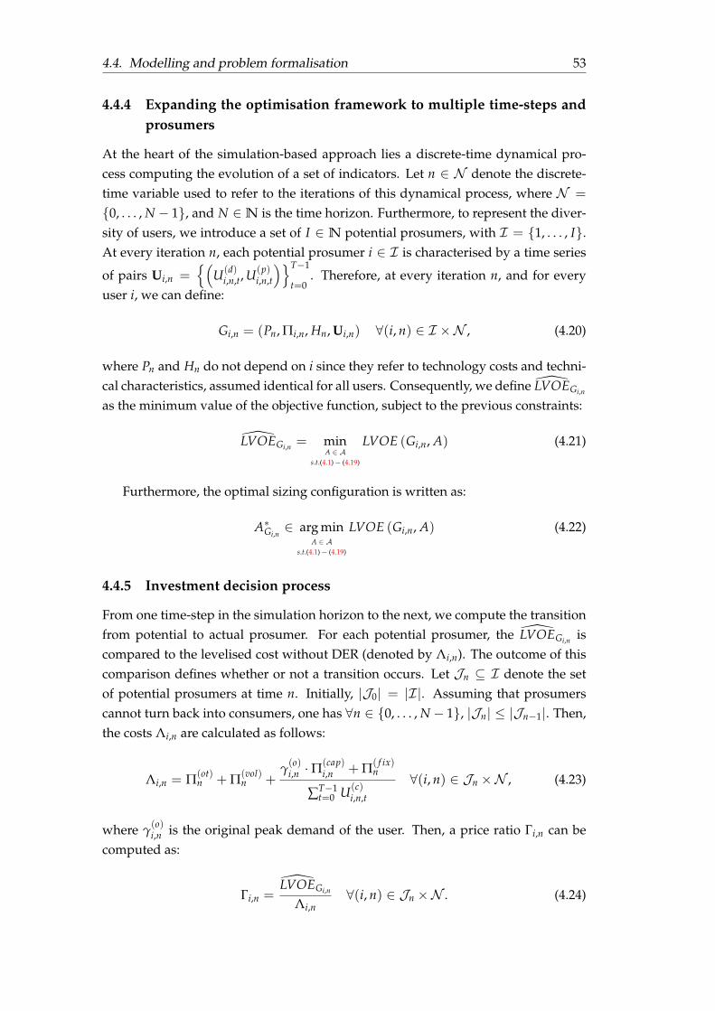
4.4. Modelling and problem formalisation 53
4.4.4 Expanding the optimisation framework to multiple time-steps andprosumers
At the heart of the simulation-based approach lies a discrete-time dynamical pro-cess computing the evolution of a set of indicators. Let n ∈ N denote the discrete-time variable used to refer to the iterations of this dynamical process, where N =
0, . . . , N − 1, and N ∈N is the time horizon. Furthermore, to represent the diver-sity of users, we introduce a set of I ∈ N potential prosumers, with I = 1, . . . , I.At every iteration n, each potential prosumer i ∈ I is characterised by a time series
of pairs Ui,n =(
U(d)i,n,t, U(p)
i,n,t
)T−1
t=0. Therefore, at every iteration n, and for every
user i, we can define:
Gi,n = (Pn, Πi,n, Hn, Ui,n) ∀(i, n) ∈ I ×N , (4.20)
where Pn and Hn do not depend on i since they refer to technology costs and techni-cal characteristics, assumed identical for all users. Consequently, we define LVOEGi,n
as the minimum value of the objective function, subject to the previous constraints:
LVOEGi,n = minA ∈ A
s.t.(4.1)− (4.19)
LVOE (Gi,n, A) (4.21)
Furthermore, the optimal sizing configuration is written as:
A∗Gi,n∈ arg min
A ∈ As.t.(4.1)− (4.19)
LVOE (Gi,n, A) (4.22)
4.4.5 Investment decision process
From one time-step in the simulation horizon to the next, we compute the transitionfrom potential to actual prosumer. For each potential prosumer, the LVOEGi,n iscompared to the levelised cost without DER (denoted by Λi,n). The outcome of thiscomparison defines whether or not a transition occurs. Let Jn ⊆ I denote the setof potential prosumers at time n. Initially, |J0| = |I|. Assuming that prosumerscannot turn back into consumers, one has ∀n ∈ 0, . . . , N − 1, |Jn| ≤ |Jn−1|. Then,the costs Λi,n are calculated as follows:
Λi,n = Π(ot)n + Π(vol)
n +γ(o)i,n ·Π
(cap)i,n + Π( f ix)
n
∑T−1t=0 U(c)
i,n,t
∀(i, n) ∈ Jn ×N , (4.23)
where γ(o)i,n is the original peak demand of the user. Then, a price ratio Γi,n can be
computed as:
Γi,n =LVOEGi,n
Λi,n∀(i, n) ∈ Jn ×N . (4.24)
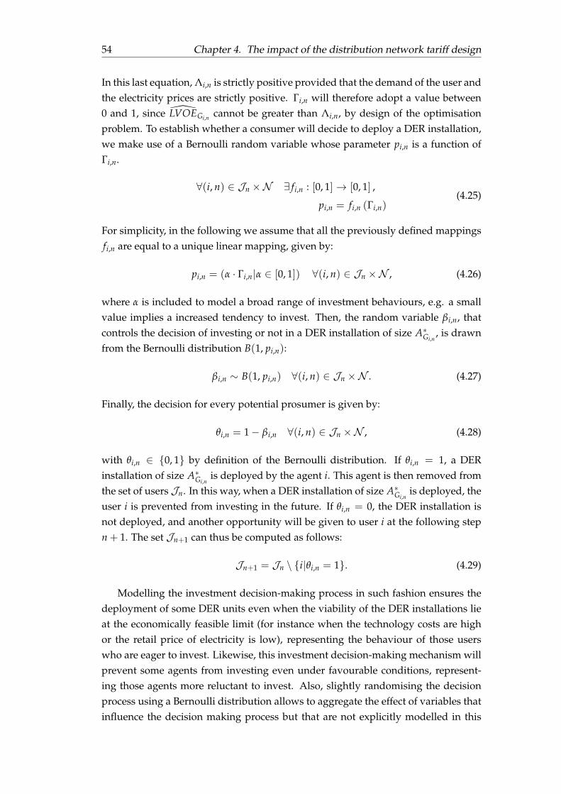
54 Chapter 4. The impact of the distribution network tariff design
In this last equation, Λi,n is strictly positive provided that the demand of the user andthe electricity prices are strictly positive. Γi,n will therefore adopt a value between0 and 1, since LVOEGi,n cannot be greater than Λi,n, by design of the optimisationproblem. To establish whether a consumer will decide to deploy a DER installation,we make use of a Bernoulli random variable whose parameter pi,n is a function ofΓi,n.
∀(i, n) ∈ Jn ×N ∃ fi,n : [0, 1]→ [0, 1] ,
pi,n = fi,n (Γi,n)(4.25)
For simplicity, in the following we assume that all the previously defined mappingsfi,n are equal to a unique linear mapping, given by:
pi,n = (α · Γi,n|α ∈ [0, 1]) ∀(i, n) ∈ Jn ×N , (4.26)
where α is included to model a broad range of investment behaviours, e.g. a smallvalue implies a increased tendency to invest. Then, the random variable βi,n, thatcontrols the decision of investing or not in a DER installation of size A∗Gi,n
, is drawnfrom the Bernoulli distribution B(1, pi,n):
βi,n ∼ B(1, pi,n) ∀(i, n) ∈ Jn ×N . (4.27)
Finally, the decision for every potential prosumer is given by:
θi,n = 1− βi,n ∀(i, n) ∈ Jn ×N , (4.28)
with θi,n ∈ 0, 1 by definition of the Bernoulli distribution. If θi,n = 1, a DERinstallation of size A∗Gi,n
is deployed by the agent i. This agent is then removed fromthe set of users Jn. In this way, when a DER installation of size A∗Gi,n
is deployed, theuser i is prevented from investing in the future. If θi,n = 0, the DER installation isnot deployed, and another opportunity will be given to user i at the following stepn + 1. The set Jn+1 can thus be computed as follows:
Jn+1 = Jn \ i|θi,n = 1. (4.29)
Modelling the investment decision-making process in such fashion ensures thedeployment of some DER units even when the viability of the DER installations lieat the economically feasible limit (for instance when the technology costs are highor the retail price of electricity is low), representing the behaviour of those userswho are eager to invest. Likewise, this investment decision-making mechanism willprevent some agents from investing even under favourable conditions, represent-ing those agents more reluctant to invest. Also, slightly randomising the decisionprocess using a Bernoulli distribution allows to aggregate the effect of variables thatinfluence the decision making process but that are not explicitly modelled in this

4.4. Modelling and problem formalisation 55
article, such as the access to capital for investing in DER, or the interest in renewableenergy.
4.4.6 Distribution system operator’s remuneration mechanism
The DSO distributes electricity to the users of the distribution network, charging adistribution fee for the service. This fee must be sufficiently large so as to collect therevenue that allows the DSO to break-even financially. Hence, assigning an adequatelevel of a distribution fee is a delicate process. An under-estimated fee may lead toinsufficient remuneration, creating an economic imbalance that must eventually besocialised via higher rates. On the other hand, an inflated tariff may place excessiveeconomic strain on users. Both deviations from the optimum are symptoms of aninefficient DSO remuneration strategy. To model the interactions of the DSO, werepresent its remuneration mechanism, which includes the adjustment of the distri-bution fee when needed. Note that the tariff design cannot be modified by the DSOsince it is controlled by the incumbent regulatory authority, and it is thereby out ofthe scope of our work.
The remuneration mechanism computes the distribution fee by comparing thecosts (Θn) and the revenue (Rn) of the DSO in the previous tariff period and comput-ing its difference ∆n = Θn − Rn. If ∆n = 0, it means that the distribution tariff levelis adequate. However, if ∆n > 0 or ∆n < 0, it indicates an under- or over-estimationof the distribution fee, respectively. It is important to note that the applied fee is al-ways an estimation of the real one, based on forecasts of consumption. In our work,we assume that the forecast used by the DSO is a continuation of the last observedstate of the system. Furthermore, we assume that at the initial state, the system iseconomically balanced, i.e. ∆−1 = 0 and therefore Θ−1 = R−1. Hence, the initialcosts of the system can be calculated by determining the initial revenue. The generalexpression to compute the DSO revenue is:
Rn =[Π(vol)
n · (Ω + Ξn)]+
[Π(cap)
n ·(I+I0)
∑i=1
γi,n
]+[Π( f ix)
n · (I + I0)]∀n ∈ N ,
(4.30)
where Π(vol)n , Π(cap)
n , and Π( f ix)n represent the volumetric, capacity, and fixed fees,
respectively, at the nth time-step. I0 stands for the number of consumers who makeup the residual demand (i.e. non prosumers). γi,n represents the optimised peakdemand of the ith user, output of the MILP. Ω represents the residual demand ofthe system, which is an input of the simulation and is held constant throughout theentire simulation process. Finally, Ξn represents the aggregated consumption of theagents in I , computed as:
Ξn =I
∑i=1
ρ(−)i,n ∀n ∈ N , (4.31)

56 Chapter 4. The impact of the distribution network tariff design
where ρ(−)i,n represents the optimised imports of the ith potential or actual prosumer
at the nth time-step, which is an output of the MILP.To begin the simulation we need the initial costs (Θ−1). These are, as previously
explained, equal to the initial revenue (R−1). The latter can be easily computed bymeans of Equation (4.30), since the demand profiles of the potential prosumers andthe residual demand are known. Once the initial revenue (and therefore the initialcosts) of the DSO are computed, the remuneration mechanism can distribute themacross the different types of fees: volumetric, capacity, or fixed, thus obtaining threedifferent fees which are applied to the final customers’ electricity bills (note that ToUfees are a particular case of volumetric fees). The same distribution mechanism isused for computing the initial fees and to update them in subsequent time-steps ofour discrete-time dynamical system. Such a computation is given by the followingexpressions:
Π(vol)n+1 =
[Θn + ∆n
Ω + Ξn
]· µ1 ∀n ∈ N , (4.32)
Π(cap)n+1 =
[Θn + ∆n
∑(I+I0)i=0 γi,n
]· µ2 ∀n ∈ N , (4.33)
Π( f ix)n+1 =
[Θn + ∆n
I + I0
]· µ3 ∀n ∈ N . (4.34)
In these equations, µ1, µ2, and µ3 represent the share of the volumetric, capac-ity, and fixed fee, respectively, imposed by the DSO remuneration strategy, andthereby by the regulatory framework set by the regulator. These shares comply with
∑3j=1 µj = 1.
To compute the fees for time-step n = 0, we know Θ−1 as it equals the revenueat this time-step. Furthermore, we know that ∆−1 = 0. The rest of the elements inEquations (4.32), (4.33), and (4.34) are given by the profiles of the users, which areknown. Once the simulation starts, at every time-step n, some potential prosumersmay turn into actual prosumers, impacting the revenue of the DSO and, in particular,Ξn and γi,n. The DSO, in turn, reacts by updating the different components of thedistribution tariff. Finally, since we work under the assumption that the DSO uses itslast observed state of the system as forecast for the following tariff period, the costsat a given period will be the same as the revenue at the previous one Θn = Rn−1.
4.4.7 User’s electricity bill
The electricity bills of the distribution network’s final customers depend on theirimports and their exports (if any) of electricity. In this paper, we assume a full roll outof smart meters, therefore these two electricity flows are registered independently bythe metering device, and have two different price signals associated.

4.5. Test case: simulator demonstration 57
Imports of electricity This is the overall price of electricity the final customers(consumers and potential and actual prosumers) pay to use the network and con-sume electricity from it. This price includes commodity, transmission, distributionand others. In this work we are interested in the distribution part, therefore, all theother elements making up the electricity price are grouped in one element, Π(ot), in-troduced in eq. (4.6) and set in e/kWh. As for the distribution fee, the smart metersallow us to split the distribution component of the electricity bill into its constituents:Π(vol), Π(cap), and Π( f ix), as in (4.5). The contribution of each element is given by µj
(see eqs. (4.32) - (4.34)) and depends on the DSO remuneration mechanism.
Exports of electricity This is the selling price of the actual prosumers when export-ing electricity to the grid. It is introduced by Π(sp) in eq. (4.19) and set in e/kWh.
4.5 Test case: simulator demonstration
To test and illustrate the proposed simulation-based approach, this section presentsan extensive range of tests showcasing the potential of the presented methodologyto flexibly simulate a wide range of scenarios. To create these scenarios, we need: (i)a set of users, and (ii) a set of rules representing a regulatory framework (designingthe DSO remuneration strategy). Then, by using the same set of users for differentremuneration strategies, we can analyse the impact of the latter on different featuresinherent to distribution networks, notably the distribution network prices and thelevel of penetration of distributed generation in the distribution network.
Set of users:Users are characterised by individual demand and production profiles. A bottom-
up approach, the CREST model [98], was used to generate demand profiles. Usingthe CREST model we produced a range of daily profiles representing weekends andweekdays and then, by means of a randomisation process, different demand pro-files spanning one year and with a resolution of one hour, were generated. As forthe production profiles, they were generated with the same time span and resolution(one year and one hour, respectively), representing the potential for PV generationof prosumers. To do so, the Python library PVLIB [99] was used. The profiles thusproduced are based on solar radiation historical data, obtained through typical me-teorological years (tmy), which were downloaded from the Joint Research Centre ofthe European Commission2. From a range of different tmy, and making variationson the tilt and orientation of the PV panels (parameters of PVLIB), different profileswere generated. These profiles represent the load factor, i.e. percentage of the totalinstalled capacity that is produced at each time-step.
In total, 1,000 demand and production profiles were generated, to represent 1,000potential prosumers. In addition to them, 5,000 consumers were created for whom
2Joint Research Centre photovoltaic geographical information system https://re.jrc.ec.europa.eu/pvg_tools/en/tools.html#TMY.

58 Chapter 4. The impact of the distribution network tariff design
only the aggregated yearly demand and the peak demand is needed as they make upwhat we call residual demand of the system. Both groups of customers (consumersand prosumers) have been created according to the Belgian reality, that is, the pro-files are consistent with electricity consumption and solar radiation in Belgium. Theproportion prosumers/consumers is selected so as to reflect the real-life situation inBelgium, as described in footnote 7 of [44].
Set of rules of a regulatory frameworkTwo groups of scenarios are proposed:
• Simulation-based approach capabilities: First we generate several scenar-ios showcasing the capabilities of the proposed simulation-based approach tocompute a prediction of the evolution of distribution network features (distri-bution prices and penetration of DER). These scenarios represent various DSOremuneration strategies.
• Sensitivity analyses: Then, the sensitivity of our approach to several parame-ters is tested, reporting on the impacts these parameters have on the simulation-based approach capabilities to predict the distribution network development.
4.5.1 Simulation-based approach capabilities
In this part of the simulation results, we test seven scenarios mimicking differentinitial conditions set by the regulator. Accordingly, we can introduce different val-ues of µj for each scenario. These values will impact on the evolution of the dif-ferent elements of the distribution tariff, as described by Equations (4.32), (4.33),and (4.34). In these equations, all the variables are known. Therefore, to start thesimulations we only need an initial state, i.e. the initial costs of the system (byassumption equal to the initial revenue Θ−1 = R−1). To compute the initial rev-enue, in this example we use the current situation in Belgium, where the distributionfee is based on a volumetric tariff which, on average, amounts to 0.08 e/kWh (i.e.Π(vol)−1 = 0.08, Π(cap)
−1 = 0, Π( f ix)−1 = 0) and determine R−1 as expressed in Equation
(4.30). Since this initial revenue must be the same regardless of the scenario we wantto test, we can break it down for different initial states representing different distri-butions of volume, capacity, and fixed fees (i.e. different scenarios), using Equations(4.32), (4.33), and (4.34). Using this procedure, we have built seven scenarios, show-casing a range of different possible tariff designs. Along with these, one additionalscenario has been created to test the impact of ToU distribution tariffs based on vol-umetric fees. All these scenarios are listed in Table 4.1.
Finally, Table 4.2 lists the rest of the inputs used to run the scenarios. To assesseach scenario, we use three metrics: (i) the penetration of actual prosumers relativeto the maximum potential; (ii) the evolution of the electricity costs for consumersand prosumers; and (iii) the actual deployed PV and battery capacities (in kWp andkWh respectively).

4.5. Test case: simulator demonstration 59
TABLE 4.1: Construction of the different scenarios
Scenario Description µ1 µ2 µ3
VOL Based on fully volumetric distribution fees 1 0 0CAP Based on fully capacity distribution fees 0 1 0FIX Based on fully fixed fees, per connection point 0 0 1
VOL_CAP Based 50% on volume and 50% on capacity fees 1/2 1/2 0VOL_FIX Based 50% on volume and 50% on fixed fees 1/2 0 1/2CAP_FIX Based 50% on capacity and 50% on fixed fees 0 1/2 1/2EVEN Based on a even distribution of the weights 1/3 1/3 1/3TOU Time-of-use tariff* 1 0 0
* The ToU distribution tariff is created by using a fully volumetric fee such as VOL, where differ-ent levels of the fee are applied depending on the time of the day. In our particular example,three different levels are applied corresponding to peak rates, off-peak rates, and shoulderrates: Peak rates (+10%): 07:00–08:00 & 11:00–12:00 & 17:00–19:00. Off-peak rates (–): 06:00–07:00 & 08:00–11:00 & 12:00–17:00 & 19:00–22:00. Shoulder rates (-10%): 22:00–06:00.
TABLE 4.2: General inputs of the multi-agent model
Parameter Value Units
P(pv)* 1200 [e/kWp]Q(pv)* 500 [e]P(bat)* 200 [e/kWh]Q(bat)* 200 [e]Π(ot)
n 0.132 [e/kWh]η(−) 0.95 [%]η(+) 0.95 [%]F(−) 2.5 [-]F(+) 4 [-]
B 8 [years]p 10 [kWp]b 30 [kWh]α 1 [-]Y 20 [years]r 2 [%]Ω 85% of total load [kWh]I 1000 [#]
* Prices at time n = 0, they linearly decrease overtime by 5% each tariff period.
Results
To quantitatively show the evolution of the penetration of actual prosumers overtime, Figure 4.1a presents the percentage of actual prosumers with respect to themaximum potential, for each time-step of the dynamical system. Furthermore, toshow the evolution of the distribution tariff, driven by Equations (4.32), (4.33), and(4.34), we compute the total costs for consumers, which depict the same evolution asonly the distribution component of the overall retail electricity tariff can change over

60 Chapter 4. The impact of the distribution network tariff design
time3. We compute these costs at each time-step and normalise them by the initialcosts t = 0, displaying the evolution in Figure 4.1b.
0 2 4 6 8 10Time [n]
0
20
40
60
80
100
Pro
por
tion
ofac
tual
pro
sum
ers
[%]
VOL
CAP
FIX
VOL CAP
VOL FIX
CAP FIX
EVEN
TOU
(A) Penetration of DER inthe distribution network asa proportion of the totalpotential penetration overtime.
0 2 4 6 8 10Time [n]
0
5
10
15
20
25
Ele
ctri
city
cost
sgr
owth
[%]
VOL
CAP
FIX
VOL CAP
VOL FIX
CAP FIX
EVEN
TOU
(B) Growth of the over-all electricity cost for con-sumers over time.
FIGURE 4.1: Evolution of the DER penetration and the electricityprices for consumers over the simulation period.
On the one hand these plots show the effectiveness of each scenario to stimulatethe adoption of PV and batteries (i.e. prosumers), and on the other hand the reper-cussions of such a deployment in terms of electricity costs for the regular consumersof the distribution network. In these examples, all the scenarios with the exceptionof the one based on only fixed fees (FIX), lead to increased electricity costs. However,the information in these plots is incomplete, since they do not provide any detailson how the actual amount of PV and batteries deployed by prosumers. Figure 4.2shows the total accumulated installed capacity of PV and batteries for each scenario.This information adds to that previously provided by including details of the com-position of the prosumers’ installations.
Finally, Table 4.3 shows the annual electricity costs for an average consumer andan average prosumer at the end of the simulated period (i.e., at time-step 10). Thisprovides the actual value in EUR consumers and prosumers pay to cover their elec-tricity needs for each scenario.
We can extract a few general remarks from Figures 4.1a, 4.1b and 4.2, and fromTable 4.3.
• Tariff structures prominently based on volumetric fees induce a large deploy-ment of PV panels and batteries (mainly the former) as well as rapid transitionfrom potential to actual prosumer. This deployment is followed by an alsolarge growth of the overall electricity costs for consumers. Moreover, these
3Note that for this calculation only consumers are used and not prosumers. The reason for this isthat the electricity costs of prosumers depend on their DER installations as well as on the distributiontariff, and consequently the evolution described by these costs is not equal to the one described bythe distribution tariff alone. Therefore, as our only interest is to show the evolution of the distributiontariff, prosumers can be left out from this computation.

4.5. Test case: simulator demonstration 61
VOL CAP FIX VOL CAP VOL FIX CAP FIX EVEN TOU0
1000
2000
3000
4000
5000
6000
7000
8000
Tot
alC
apac
ity
[PV
–kW
p;
BA
T–
kW
h]
PV [kWp]
BAT [kWh]
Imports [GWh]
Exports [GWh]
0.0
0.5
1.0
1.5
2.0
2.5
3.0
3.5
Tot
alim
por
ts&
exp
orts
[GW
h]
FIGURE 4.2: Total capacity of installed PV capacity (blue), total ca-pacity of installed battery (red), total imports from the distributionnetwork (green), and total exports to the distribution network (yel-low) at the end of the simulation period.
TABLE 4.3: Annual electricity costs for an average consumer and anaverage actual prosumer at the end of the simulated period.
Scenario Annual consumer costs [e] Annual prosumer costs [e]
VOL 1514.52 1063.21CAP 1491.59 1008.10FIX 1317.79 1235.72VOL_CAP 1487.72 1043.81VOL_FIX 1378.31 1149.53CAP_FIX 1384.60 1139.22EVEN 1415.09 1112.93TOU 1624.50 1085.86
tariffs lead to substantial exports from prosumers’ DER installations to the dis-tribution network, owing to larger PV capacities. In addition, these tariff struc-tures lead to substantial inequalities in the electricity costs, in particular whenno other component is added to the tariff (i.e., fully volumetric structures suchas VOL and TOU); in these cases the economic burden of maintaining the DSO ismostly carried by consumers.
• When the tariff design is weighted toward capacity fees, the deployment ofPV panels and batteries is also spurred, although to a lesser extent and inclinesthe balance toward more batteries this time. However, the induced increase inelectricity costs is larger than in the previous case. The bias of these scenariostoward using batteries is explained by the ability of actual prosumers to shavetheir peaks (γi in Equation (4.5)) thus paying less in capacity fees. This is con-sistent with the findings in [100]. Moreover, tariffs based on these fees tendto import more electricity than export it – this electricity is stored in the largerbatteries to shave the peak demand. Regarding the cost distribution shown inTable 4.3, these types of tariff result in highly unequal distributions, similar tothose observed with volumetric fees, where the financial burden of the DSO is

62 Chapter 4. The impact of the distribution network tariff design
born by consumers.
• Adding a fixed term helps reduce the impact on the electricity costs for con-sumers in either volumetric or capacity fees. However, using purely fixed feesdoes not seem to promote the deployment of PV panels and batteries, in par-ticular the latter. Balancing several part tariffs results in a trade-off that mustbe carefully studied (as exposed by P. Simshauser in [35]), falling outwith thescope of our work.
• Using ToU tariffs creates the more extreme outcome – the quickest transitionfrom potential to actual prosumers among all assessed scenarios is only fol-lowed by the largest increase in electricity costs for consumers. The incentiveto install PV panels is the second largest (after VOL), whereas the incentive toinstall batteries is the largest one. These results are explained by the possibilityof actual prosumers benefiting from both PV panels to limit their exposure tothe volumetric fees and batteries to shift load from peak and off-peak to shoul-der hours (ρ(−)t in Equation (4.8)). In a similar way as with volumetric fees,ToU fees lead to more exports than imports. However, in this case, the spreadbetween both is smaller, since the electricity surplus with ToU tariffs can bestored in the batteries to shift demand.
Discussion
These analyses show that different initial conditions, notably including various tariffstructures, induce vastly different outputs that can be quantitatively assessed. Thepresented simulation environment can be used to discriminate between the possibleoutcomes of employing distinct tariff structures. It may therefore be valuable forassessing a distribution tariff structure before putting it in force.
Extracting meaningful conclusions with this tool necessitates a previous tun-ing phase where the various parameters of the simulation-based approach (e.g., α,prices, bounds p and b) must be adapted to the particular context that one wants tosimulate. In this regard, in [44] this simulation-based approach is employed to sim-ulate a generic distribution network with the characteristics inherent to the Walloonregion of Belgium, providing policy recommendations for this particular case.
Although the example provided in this section does not correspond to any par-ticular context (i.e., no previous tuning phase has been performed to adapt thesimulation-based approach to any particular case), there are a few general obser-vations that can be drawn. In particular, these observations are based on the prin-ciples for distribution tariff design, as presented in the CEER report [89] and by I.Abdelmotteleb in [82].
• Distribution tariff designs based on volumetric fees (totally or partially) pro-mote the largest adoptions of PV panels and batteries; however, they lead tothe largest inequalities between consumers and prosumers. On the one hand,

4.5. Test case: simulator demonstration 63
their implementation is straight forward, complying with the principles oftransparency, simplicity, and predictability. On the other hand, they distortthe decisions concerning the use of the network, they are not cost reflective (infact prosumers, who use the network more, end up paying significantly lessthan consumers), resulting in discrimination among the users where not all ofthem pay the same for the same service.
• Capacity charges lead to high battery deployment and relatively high PV paneladoption. However, as with volumetric charges, the economic inequalitiesbetween consumers and prosumers are substantial. In terms of the tariff de-sign principles, capacity charges are not as predictable, transparent and simpleas volumetric ones, and moreover they induce distortion and discriminationamong the network users. Finally their cost-reflectivity in already developeddistribution networks is questionable, as typically network costs are sunk.
• Fixed fees comply with most of the principles of tariff design (non-distorting,non-discriminatory, transparent, predictable and simple). However, they donot promote the adoption of DER installations, which has been a high-levelgoal of all energy policies over the last few years (see for instance the Europeanrenewable directive [11]).
• Applying ToU charges on top of volumetric ones results in the largest batterydeployment and the second-largest PV panel deployment leading to the high-est cost different between consumers and prosumers where the former paysubstantially more than the latter for their network use. This type of chargesis transparent, predictable and relatively simple, although, as volumetric ones,they are not cost-reflective and they distort and discriminate among users.
• Tariffs based on a mix between different types of charge result in a trade-offbetween promoting PV panels and battery adoption, distributing the costsamong the users in a more equal fashion, and complying with the principlesof distribution tariff design.
These remarks confirm that selecting the tariff design is not a trivial process,where no perfect tariff exists. In general, applying fully volumetric, capacity, orfixed fees does not seem to yield the most adequate results where either DERs arenot promoted, or they are promoted but the costs for it are mostly born by con-sumers instead of prosumers (who generate them). A solution could be to resort todesigns where all these components are present. In these cases, a middle-groundtarget can be achieved, promoting some DER adoption whilst maintaining a relativelevel playing field for consumers and prosumers. Overall, promoting DER has a costassociated, and it is the decision of regulators and policy makers to choose how tocover it.

64 Chapter 4. The impact of the distribution network tariff design
4.5.2 Sensitivity Analyses
In this section, the sensitivity of the proposed simulation-based approach to severalparameters is tested. In particular, we perform sensitivity analyses on the α parame-ter, the selling price of electricity for prosumers (sp), and the prices of PV panels andbatteries (tp). For these analyses we use the same basic data listed in Table 4.2, onlymodifying the parameter we wish to study.
Sensitivity to α
The first of the analyses presented in this section corresponds to the sensitivity tothe α parameter, as shown in Figure 4.3 and Table 4.4. As explained in Section 4.4.5,this parameter controls the speed at which the DERs are deployed by potential pro-sumers. It works by biasing the p parameter of a Bernoulli random variable (i.e.the probability of drawing a 0 or a 1). The p parameter is typically computed asthe difference between the LVOE of a DER installation and the electricity costs thepotential prosumer would otherwise face without the DER installation. We furtherdevelop this definition introducing the α parameter multiplied by the cost difference(see Equation (4.26)). Since the investment decision is inverted (see Equation (4.28)),a low value of α fosters the deployment of DER whilst a high value should limit it.
0 2 4 6 8 10
Time [n]
0
20
40
60
80
100
Pen
etra
tion
ofD
ER
[%]
0.6
0.7
0.8
0.9
1.0
1.1
1.2
1.3
1.4
(A) Sensitivity of DER de-ployment.
0 2 4 6 8 10
Time [n]
0
2
4
6
8
10
12
14
Cos
tgr
owth
[%]
0.6
0.7
0.8
0.9
1.0
1.1
1.2
1.3
1.4
(B) Sensitivity of electricitycosts for consumers.
FIGURE 4.3: Sensitivity to α.
TABLE 4.4: Sensitivity of PV- and battery-installed capacity to α.
α=0.6 α=0.7 α=0.8 α=0.9 α=1.0 α=1.1 α=1.2 α=1.3 α=1.4
Total PV capacity [kWp] 6,071.4 6,374.6 6,738.7 7,124.9 7,673.1 7,456.1 6,506.9 4,688.2 2,460.0Total battery [kWh] 6,379.8 6,571.9 6,828.7 7,009.1 7,295.6 6,833.6 5,713.4 4,061.8 2,161.2
As we can observe in these figures, the lower the α, the greater the deployment ofDER. This greater DER penetration, in turn, results in a higher increase of the over-all electricity cost of traditional consumers. When looking at the total PV capacity

4.5. Test case: simulator demonstration 65
and battery capacity deployed, it can be noted that for low values of α the result-ing total capacity is lower than for values close to 1. This is explained by the factthat, since the DER installations need to be more profitable when α = 1 than whenα = 0.6 to be deployed (i.e to draw a 0 in the Bernoulli random variable), only largeand profitable installations will be deployed. This behaviour results apparent whenα > 1. However, since in those cases the simulator does not reach 100% of DERdeployment, the total DER capacity at the end of the simulation horizon is lowerthan for α = 1. A longer simulation horizon will prove those scenarios to presentthe largest total deployment of PV panels and batteries. This parameter presentsan enormous variability in the outcome; this is why, before making use of the pro-posed simulation-based approach, it is key to tune this parameter to adapt it to theconditions of the distribution network it aims to simulate, as done in [44].
Sensitivity to the selling price
The second analysis tests the sensitivity of the model to the selling price of elec-tricity of prosumers, as shown in Figure 4.4 and Table 4.5. These users primarilyuse their local electricity production to meet their demand, however, when thereis more production than demand, they can sell this surplus to the distribution net-work. Modifying the selling price has therefore the potential to affect the behaviourof those users as the value associated to their electricity exports changes.
0 2 4 6 8 10
Time [n]
0
20
40
60
80
100
Pen
etra
tion
ofD
ER
[%]
4.0
5.0
6.0
7.0
8.0
9.0
1.0
(A) Sensitivity of DER de-ployment.
0 2 4 6 8 10
Time [n]
0.0
2.5
5.0
7.5
10.0
12.5
15.0
Cos
tgr
owth
[%]
4.0
5.0
6.0
7.0
8.0
9.0
1.0
(B) Sensitivity of electricitycosts for consumers.
FIGURE 4.4: Sensitivity to the selling price (sp).
TABLE 4.5: Sensitivity of PV- and battery-installed capacity to the sell-ing price (sp).
sp=0.04 sp=0.05 sp=0.06 sp=0.07 sp=0.08 sp=0.09 sp=0.10
Total PV capacity [kWp] 7,712.4 8,961.0 9,748.5 9,928.5 9,970.0 9,970.0 9,970.0Total battery [kWh] 7,339.0 7,484.4 7,442.9 7,384.4 7,293.4 7,217.9 7,204.4

66 Chapter 4. The impact of the distribution network tariff design
From Figure 4.4a we can observe that higher selling prices leads greater DERadoption and, in turn, to an overall increase in electricity costs, as shown in Fig-ure 4.4b. From the total deployed capacity of PV and batteries (Table 4.5), it canbe deduced that the greater the selling price, the larger the PV installation. Thisrelation, nonetheless, is the opposite in the case of batteries, where a higher sell-ing price leads to lower battery adoption. These effects are a result of the businessmodel of these two behind-the-meter devices. A greater PV capacity results in alarger production surplus that can be sold to the network and, therefore, a higherselling price will spur larger PV installations with substantial production surpluses.Larger PV installations will in turn require fewer batteries to operate, since they willproduce sufficient electricity to cover the prosumers’ demand, even at times wherethere is a limited solar availability. Even though the selling price clearly imposessome changes in the adoption rate of PV and batteries, these changes are less signifi-cant than in our first analysis. The selection of this parameter is easier than the othertwo (α and technology price) for it should reflect the regulation in place.
Sensitivity to the technology price
The last of the introduced analyses deals with the sensitivity to the technology price.To carry out this assessment, as the starting point we take the technology costs (PVand battery) listed in Table 4.2. We then multiply them by a factor to increase ordecrease the initial technology costs, analysing the sensitivity to different factors(costs). Note that these are the initial technology costs, which then decrease by 5%every year. The results of this sensitivity analysis is presented in Figures 4.5 andTable 4.6.
0 2 4 6 8 10
Time [n]
0
20
40
60
80
100
Pen
etra
tion
ofD
ER
[%]
0.7
0.8
0.9
1.0
1.1
1.2
1.3
(A) Sensitivity of DER de-ployment.
0 2 4 6 8 10
Time [n]
0.0
2.5
5.0
7.5
10.0
12.5
15.0
17.5
Cos
tgr
owth
[%]
0.7
0.8
0.9
1.0
1.1
1.2
1.3
(B) Sensitivity of electricitycosts for consumers.
FIGURE 4.5: Sensitivity to the technology price (tp).
A linear relation can be seen between technology price and adoption rate of PVand batteries. Unsurprisingly, the higher the price the lower the penetration of actualprosumers and, as such, the lower the impact on overall electricity costs. On theother hand, the lower the technology price, the faster and larger the deployment of

4.6. Conclusion 67
TABLE 4.6: Sensitivity of PV- and battery-installed capacity to thetechnology price (tp). Note that the shown percentages are relative
to the prices used for the first simulation.
tp=70% tp=80% tp=90% tp=100% tp=110% tp=120% tp=130%
Total PV capacity [kWp] 9,942.0 9,436.6 8,502.8 7,541.1 6,584.7 5,751.9 4,225.1Total battery [kWh] 8,857.0 8,383.7 7,847.4 7,187.2 6,409.5 5,417.4 3,925.5
DER installations. As expected, this parameter has a strong influence on the shapeof the trend curves – it is therefore crucial to find the right level of technology prices.
4.6 Conclusion
This paper formalises and builds a framework based on a simulation-based ap-proach to assess the impact of a wide range of DSO remuneration strategies on theeconomic sustainability of the distribution network. The potential of this simulation-based approach lies in its ability to accurately discriminate between the possible out-comes of employing distinct remuneration strategies in order to provide sound argu-ments that underpin the selection of one of them. It therefore serves as guidance forpolicy makers and regulators to build new remuneration strategies for DSOs, aim-ing to achieve certain specific objectives (e.g. promote the adoption of renewabledistributed generation). By means of this simulation-based tool they can comparethe strengths and drawbacks of distinct options before applying them in real life.The proposed simulation environment contributes to the existing literature by:
• Providing the mathematical formalisation of a simulation-based approach basedon a dynamical system and on an optimisation framework that progressivelydeploys DER installations over time and, as a result, adapt the distributionnetwork charges to make sure any imbalance of the DSO is corrected.
• Encapsulating all the most commonly used DSO remuneration strategies –(i)volumetric fees based on energy consumed, (ii) capacity fees based on powerwithdrawn, (iii) fixed fees based on the availability of a connection point, and(iv) time-of-use fees that depend on the time of energy consumption– in thedeveloped mathematical formalisation of the simulation-based approach.
• Providing a computational tool encoding such a mathematical formalisation tohelp policy makers and regulators decide which DSO remuneration strategy toemploy according to a specific target.
The simulation-based approach presented in this paper is written to be sufficientlygeneric so that it can adapt to any context (i.e. distribution network) with ease bytuning certain parameters as, for instance, the Bernoulli bias α, or the technologycosts. This means that before being used, this tool must be tuned so as to match thedistribution network where the experiments are to be run.

68 Chapter 4. The impact of the distribution network tariff design
The presented approach has been extensively tested with a case study featur-ing eight different scenarios which illustrate the various options of the proposedsimulation environment to guide future developments in distribution network tariffstructures. This test case shows how prosumers’ choices vary from one remuner-ation strategy to another, suggesting that it is valuable to check by simulation thata remuneration strategy yields the desired outcome. Although this test case doesnot intend to offer insights regarding any particular distribution network (i.e. theparameters are set by default), it does provide some guidance on how to design theremuneration strategy of a DSO:
• Strategies based on volumetric fees (including time-of-use) offer the best in-centive for PV unit and battery deployment. However, this leads to the highestinequalities between consumers and prosumers in terms of electricity costs.
• Strategies based on capacity fees promote the integration of storage devicesas they take action to limit the peak of consumption of prosumers, leadingonce again to a cost distribution between consumers and prosumers where theformer bear most of the network costs.
• Strategies based on fixed fees significantly limit the incentives for DER deploy-ment (PV or battery), therefore they hardly show any impact on the distribu-tion of grid costs.
Furthermore, the sensitivity of the model to several input parameters –the Bernoullibias α, the selling price of electricity for prosumers, and the technology price– hasbeen reported, showing that the trends remain constant when applying differentvalues to the parameters, only changing in the rate at which DER installations aredeployed and electricity prices increase.

69
Chapter 5
Regulatory challenges indistribution networks: policyrecommendations
In this chapter, the third and last of Part I, we make use of the tool developed inthe previous two chapters to simulate a real life distribution network based on aspecific region – Wallonia, Belgium’s southern region. To that end, we calibrate thesimulation-based approach introduced in Chapters 3 and 4 to the specific desiredregional context. This simulator enables us to highlight how the emergence of pro-sumers featuring solar photovoltaic (PV) installations impacts the distribution net-work tariff and how this tariff, in turn, affects the gradual deployment of distributedelectricity generation resources (DER) by prosumers.
In Wallonia, the distribution component of the overall electricity retail tariff isessentially volumetric, i.e. based on the final customers’ energy consumption (ine/kWh). Residential prosumers, moreover, are connected to the grid via a net-metering system. In this context, our simulation-based approach permits the eval-uation of several tariff reforms currently under discussion in this region: the intro-duction of a prosumer fee, the introduction of a capacity component into the dis-tribution tariff, and a switch to a net-billing metering technology (also known asnet-purchasing). Some of these reforms, however, require the use of smart meters,which is infeasible in Wallonia in the short run. Short run reforms, therefore, canonly test the prosumer fee, which consists of a fee paid by all prosumers dependingon the total installed PV capacity (in e/kWp), as well as adding a fixed term to thetariff. In the long run, the roll out of smart meters enables the introduction of a net-purchasing system and of a distribution tariff with a capacity component. In thischapter we simulate both short and long run reforms using the simulation-basedapproach introduced in previous chapters. Our analysis highlights one key addedvalue of smart meters: they allow network tariffs that are fairer and sustainable.

70Chapter 5. Regulatory challenges in distribution networks: policy
recommendations
5.1 Introduction
Distributed electricity generation based on renewable energy sources has boomedglobally in recent years. The deployment of this type of decentralised generationhelps decarbonise the energy system. However, since distributed generation unitsare connected to the distribution network –traditionally designed to unidirectionallydistribute electricity from the transmission network to residential areas– they inducechallenges to the operation of the electricity system. In particular, they change thenature of energy exchanges within the distribution network, which are now bidirec-tional as households deploying solar photovoltaic panels on their rooftop not onlyimport but can also export electricity. In light of this paradigm change, regulatoryinterventions related to how these flows are measured and priced are key in theemergence of a more sustainable energy system. For that reason, reforms of the dis-tribution tariffs are on the agenda in many jurisdictions.
The situation of Wallonia, Belgium’s southern region, is particularly interestingin many respects. Households have made substantial investments in decentralisedenergy production sources over the last few years. By the end of 2019, despite a rela-tively low solar irradiance, over 10% of the households had installed solar PV panelsand became prosumers. This large adoption of PV installations can be explained bytwo main factors: (i) subsidies and (ii) network regulations. First, generous up-front investment subsidies (either in the form of direct financial support or in taxcuts) as well as production subsidies, mainly via a green certificate system [101],were granted by various jurisdiction levels. Second, favorable network regulationsfor prosumers helped substantially decrease the electricity bills of PV owners at thehousehold level. According to these network regulations, distribution tariffs in Bel-gium were (and still are) predominantly based on units of energy consumed, that is,volumetric fees typically in e/kWh. In addition, prosumers are integrated into thegrid via a net-metering system, where the exports of electricity are registered by sub-tracting from the meter the units of energy injected into the grid (which in practicemeans that the solar production is valued at retail price). In such a context, investingin PV panels substantially decreased the prosumers’ electricity bills, as their metersreadings, and thereby their electricity bills, could be greatly reduced.
This high take-up rate of PV adoption led to a tense debate in the public and po-litical arena. From 2016 to 2019, 40 out of the 93 Energy Commissions of the WalloonParliament discussed issues related to prosumers. Since 2018, all forms of subsidieshave been phased out for new PV installations. However, the current network reg-ulations have barely changed. One key issue facing the regulator is that Walloniais lagging behind other European regions in terms of smart meter adoption [102]:as yet, albeit there is a regional target coverage of 80% of households by 2030, fewsmart meters have been installed [103]. This is 10 years behind the goal set by the2009 Electricity Directive set at the European Union level. Hence, the mechanical sin-gle meters, i.e. the technology in place, limit the way distribution costs can be billed

5.2. Literature review 71
to the grid-connected users, and only the structure of the tariffs can be changed, e.g.by relying more on fixed fees rather than on volumetric ones. Fixed fees can be ap-plied to all users or to prosumers only. The switch to new bi-directional meters forprosumers (mechanical or smart) will make it possible to consider a different pricefor electricity imported from and exported to the grid, via a net-purchasing system.The roll-out of smart meters will in addition facilitate the introduction of capacityfees (based on units of power withdrawn from the grid, typically in e/kW). Fac-ing a similar policy context in Flanders, Belgium’s northern region, The VREG, theenergy regulator, decided to switch towards capacity-based starting from 2022 on[104].
This chapter analyzes how different distribution tariff regulations impact theconsumption, production, and (possibly) storage behaviors of residential house-holds. For this purpose, we rely on a tariff simulator developed by [30] and weuse regional-specific load and solar irradiance profile curves to apply the model tothe case of Wallonia. Compared with other simulators used in [105] or [31] to studya related research question, we use an agent-based modelling approach incorporat-ing the region-specific consumption and production profiles of several thousands ofheterogeneous households. This simulator enables us to evaluate the impact of vari-ous changes in regulation with respect to PV and battery investments, the evolutionof distribution network tariffs, the levelised value of electricity (LVOE) of prosumersand non-prosumers, as well as the formers’ rate of self-consumption, and the peakpower withdrawals and injections. Our work highlights the importance of consid-ering both the distribution tariff design and the technology connecting all electricityusers to the network, as only a subset of tariff regulations can be implemented inthe absence of smart meters. And, even if our simulations are computed to repre-sent the specific situation of one region, our policy conclusions carry further away toother legislations that want to adapt their distribution tariff to integrate distributedgeneration.
This chapter is organised as follows. In Section 5.2, we review the literature onthe integration of distributed generation into the grid. In Section 5.3, we describethe current distribution network regulations in place in Wallonia. The tariff simula-tor is presented in Section 5.4. Section 5.5 analyzes the regulatory scenarios imple-mentable with the metering technology in place. Section 5.6 describes the regulatoryreforms and their impact that can be set in the long run with a change of meters. Sec-tion 5.7 concludes our work.
5.2 Literature review
Our work relates to the literature focusing on the relationship between the emer-gence of decentralised generation units and the financing of the distribution system,in the context of an unbundled energy system. In the face of decreasing volumesof the electricity sales owing to the presence of prosumers, the distribution system

72Chapter 5. Regulatory challenges in distribution networks: policy
recommendations
operator (DSO) requires a higher distribution tariff level in order to break-even [37].However, as expounded by [106] and [33], such a reform, in a context of largely volu-metrically based tariffs, makes PV investments even more profitable, further leadingto inefficiently large investments in solar PV. This unsustainable financing of the gridis often referred to as the utility death spiral [35].
Our numerical model follows up on the works focusing on this feedback loopto analyze different distribution network regulations. While our conclusions aresimilar to the works previously done on this topic, we contribute to this literatureby better fitting our model with respect to the policy context studied, the WalloonRegion, on three different levels.
First, compared to [31] and [32], we use an agent-based modelling approach thatconsiders a large amount of residential households. The energy consumption andproduction profiles of 6000 heterogeneous households are considered. Thanks to thisapproach, we are able to make more realistic predictions regarding the decision toinvest in PV panels and batteries, including regarding the size of these investments.Similar to the work of [105], our simulator allows us to discuss how tariff regulationsimpact self-consumption and peak power withdrawals. In addition, we also analyzehow peak power injections, a key cost driver for a DSO, are influenced by networkregulations.
Second, the policy setting is greatly influenced by the metering technology inplace. The issue of death spiral is particularly important when a net-metering sys-tem is in place, as the energy exported to the grid is sold at the attractive retail price.This is the current metering technology in Wallonia1. Hence, the simulator used inthis chapter is closely related to the ones developed in [74, 108, 109] to analyze net-work regulations in respectively California, Colombia and New South Wales Aus-tralia 2. Compared to these works, we differentiate the implementable regulationsin the short and long run, depending on the available metering technology. In theshort run, only the tariff structure can be changed, for all on only a subset of energyusers. In the long run, a net-purchasing system can replace the net-metering systemto set different prices for the electricity imported from or exported to the grid. Inaddition, smart meters, will allow complex tariff structures such as capacity-basedone. Hence, we believe that it is important to differentiate short run, second best,regulations from long run ones that can take advantage of the technological featuresof more evolved meters than those currently in place that record flows only with asingle meter.
Third, we calibrate our simulator to the context of Wallonia, though not just withrespect to the solar irradiance and the typical production profile, as traditionally
1Note that a net-metering system is also in place in a majority of U.S. states, in European countrieslike Denmark, Netherlands, Greece, Hungary or Latvia as well as in various lesser developed countrieslike India or Brazil (see [107]).
2In comparison, the following papers [110, 111, 112] present a simulator suited respectively forQueensland Australia, Portugal, UK and Germany where a net-purchasing system, coupled with afeed-in tariff, is currently in place.

5.3. Distribution network tariff and the integration of residential solar PV inWallonia
73
done in the literature. In this regard, our simulator is parameterised in such a waythat the impact of a distribution tariff increase on the decision to invest in a PV instal-lation be similar to the one measured in [75] using PV installation data in Wallonia.
We trust that these three key aspects allow robust policy conclusions.
5.3 Distribution network tariff and the integration of resi-dential solar PV in Wallonia
Distribution tariffs in Wallonia have been regulated by the regional regulator (CWaPE)since 2014. The regulator uses a cost-plus methodology to fix the distribution tariff.There are 7 DSOs and 13 tariff zones, where the distribution tariff levels vary sub-stantially between zones. The tariff structure, however, is similar in all zones, witha distribution tariff that is essentially volumetric (in e/kWh), and which includesvery small fixed fees (around 20e per household per year, covering the rental ofthe meter). The other components of the electricity bills (transmission, energy, taxesand other levies) are also based on the consumption level in kWh. Some retailersalso include a relatively small fixed fee in their contracts. In 2018, the volumetricpart of the distribution tariff ranged from 7.3 ce/kWh to 14.9 ce/kWh, with an av-erage tariff equal to 11 ce/kWh. In Wallonia, the distribution tariff represents 36%of the consumer’s final electricity bill, including VAT [113]; this relatively large sharecan be explained, at least partially, by the large public service obligations imposedto the DSOs, which include public lighting, social energy tariffs, and the promotionof renewable energy integration.
In Wallonia, almost all meters are mechanical and PV adopters connect their PVinstallation to the existing meter. Prosumers then have a single meter that runs for-ward when electricity is imported from the grid, and backward when it is suppliedto the grid. To switch to net-purchasing with a different price for power injectionsand withdrawals, prosumers need to change their metering technology. They caneither install a second mechanical meter to register power injection or a smart meter.Smart meters can measure power in addition to energy, thus enabling the introduc-tion of more sophisticated tariff designs such as adding a capacity-based componentto the tariff.3
Over the current regulatory period (2018-2022), the regulator introduced a pro-sumer fee in October 2020 [114]. This fee is to be paid by the prosumers in contribu-tion to the network costs. Such a fee is based on the PV capacity of each prosumer,
3Smart meters still have other advantages that we do not consider here, e.g. the possibility of havingtime-of-use tariffs. As consumption is recorded almost instantaneously, the tariff can be adapted tofollow the trends of the wholesale market price. Our scenarios do not consider such a pricing butonly time-independent distribution network fees and electricity prices. For the time being, metersmeasure net consumption on a yearly basis. Negative meters could also be reset to zero on a weeklyor monthly basis. Our main reason for not discussing these changes is that, to our knowledge, thereis no discussion to date of implementing such tariffs in Wallonia. This standpoint might change ina foreseeable future as the Electricity Directive [11] requires Member States to implement dynamicelectricity price contract whenever smart meters are installed.

74Chapter 5. Regulatory challenges in distribution networks: policy
recommendations
and is computed to compensate the avoided distribution network fees assuminga self-consumption rate of 37.76%. Its level depends on the tariff zones, but is onaverage equal to 85e/kWp per year. Prosumers have the option to opt-out and in-stall a dual meter (net-purchasing) and pay the regular distribution tariff for theirelectricity imports.4 However, while it is useful to measure the concomitance of de-centralised production and consumption, the roll-out of smart meters has been slowcompared to the targets set at the EU level and the adoption rates of other MemberStates. The goal is to have 80% of users of the energy network equipped by 2030. 5
5.4 Tariff simulator
We rely on a multi-agent model to simulate the impact of distribution tariffs on res-idential consumers’ investments in PV modules and batteries. The model is intro-duced in [43] and described in further details in [30]. We present the main ingredi-ents of this model in Section 5.4.1, and the main assumptions on which it relies inSection 5.4.2. We describe the simulated scenarios in Section 5.4.3.
5.4.1 Model description
This simulation-based approach relies on a discrete time dynamical system with twotypes of agents, the users and the Distribution System Operator (DSO), which inter-act with each other for a given regulatory environment. Users are classified intothree categories of agents: consumers, potential prosumers, and prosumers. Theinteraction between the different categories is represented in Figure 5.1.
The model is composed of several modules: an individual optimisation module(OPT) that for each potential prosumer computes the levelised value of electricity(LVOE), given their consumption and production profiles and the regulatory envi-ronment in place. The LVOE differs from the traditional levelised cost of electricity(LCOE) in that the LCOE only accounts for costs (i.e. it is computed as discountedcosts divided by discounted aggregated demand), whereas the LVOE accounts forcosts and revenues (i.e. it is computed as discounted costs minus discounted rev-enue divided by discounted aggregated demand). The second module models theinvestment decision process (IDP), where the comparison between the LVOE of each
4There is currently a disagreement between the regulator and the regional government on this pro-sumer fee. For political reasons, the latter wants to compensate the prosumers for the introduction ofthe fee. As of today, it is not clear how the government plans to do so, except that it wants correctivemeasures to encourage self-consumption.
5There are two other regions in Belgium. The situation in Flanders is very similar to the one inWallonia where a prosumer fee has already been implemented since 2015 [115]. One key difference isthat the roll-out of smart meters will soon be completed and that capacity tariffs, similar to the onesdiscussed here, will be implemented from 2022 on [104]. However, note that, in the energy decreemodified in 2019, the Flemish government has committed to maintain the net-metering system as away to value energy flows, for at least 15 years starting from the date of the PV installation. In Brussels,a densely populated region with mostly shared rooftops, PV investments have been scarcer and a net-purchasing system is in place where the import price of electricity is slightly higher than the exportprice.

5.4. Tariff simulator 75
individual potential prosumer and the retail electricity price determines the proba-bility that they invest and become actual prosumers. The last module representsthe remuneration mechanism (RM) of the DSO – it computes the adjustment of thedistribution network tariff performed by the DSO as a consequence of PV (and/orbattery) investment. In this regard, the tariff is adjusted so as to cover the costs ofthe DSO.
FIGURE 5.1: Multi-agent interaction model with the feedback loopcreated by the deployment of residential PV panels and by the DSO’sremuneration mechanism.
Consumers and Prosumers
At the start of the simulation, there are no prosumers and all users draw electricityfrom the distribution network. However, as the simulation proceeds over the dis-crete time dynamical system, a subset of users, i.e. potential prosumers, take actionto gradually deploy optimally sized PV installations and batteries, thus becomingprosumers. A potential prosumer turns into an actual prosumer depending on thedifference between the LVOE and the actual electricity costs without PV installationand on an exogenous probability. We use the results of Gautier and Jacqmin (2020)to calibrate this probability. On the basis of data from residential prosumers in Wal-lonia, these authors estimate, by means of an econometric analysis, the elasticity ofinvestment in solar PV due to an increase in the volume-based tariff and, therefore,of the electricity price. They estimate that a 1 ce increase in the price of electricityincreases the probability of investment in a PV installation by 8%. We then created ascenario mimicking the conditions observed in [75], called baseline. In this scenario,an increase of 1 ce in the price of electricity for the initial period leads to an increasein PV investment by 8%. Then from the second period on, this probability evenly
76Chapter 5. Regulatory challenges in distribution networks: policy
recommendations
decreases as the deployment of PV installations converges to 100% of the potentialprosumers (see benchmark in Section 5.5). Once a user has invested, thus becominga prosumer, this agent is removed from the subset of potential prosumers and addedto the subset of prosumers, which prevents further investment from this particularuser.
DSO
The DSO is a regulated entity. The distribution tariff is set by the regulator and com-puted to a sufficient level so as to cover the costs deriving from the provision ofthe electricity distribution service. In our model, there is no explicit cost modellingfor the DSO. We consider the distribution costs to be constant over time and equalto their historical value. Hence, we model the financing of the DSO as a zero-sumgame: the fixed cost of the DSO must be covered and the different grid tariffs willallocate relatively more or less of this cost to a category of consumers or another.Prosumers’ investments in PV installations then change the revenues of the DSO,since these are less reliant on the imports of electricity from the distribution net-work, but they do not change the grid costs6. At every time step of the discrete timedynamical system, the DSO then is allowed to adjust the distribution tariff in orderto cover its cost (i.e the DSO must break even and the regulator allows it to increasethe tariff to this purpose). The DSO, however, is constrained by the tariff structure,which cannot be changed. Tariff changes then impact electricity costs by typicallyincreasing them, and hence the incentives to invest. Thus, there emerges a feedbackloop between the prosumers and the DSO, which is illustrated in Figure 5.1.
5.4.2 Main assumptions
Table 5.1 reports the main parameters used for running our simulations. The param-eters are calibrated to represent the tariff and electricity prices in Wallonia as well asreasonable estimates of PV and battery prices and their evolution. In addition, weuse solar irradiance data from Wallonia and standard consumption profile curves forrepresentative consumers for the region. These load profiles have been generated bydetailing a household’s list of electric appliances and other characteristics. In total,we generated 1000 load profiles, corresponding to different configurations of elec-tric appliances and inhabitants per household using the CREST Demand Model [98].These profiles represent 1000 potential prosumers. In addition, 5000 consumers areintroduced by using an average yearly load of consumers in Wallonia. Thus, thetotal population size is 6000 (5000 consumers and 1000 potential prosumers). Whilepotential prosumers may become prosumers over the time of the simulation, the5000 usual consumers are regarded as the residual load of the distribution network,representing those users who cannot become actual prosumers due to technical or
6In practice, the deployment of solar PV modifies the power injections and withdrawals on the gridand thereby impact the grid cost. We discuss further this issue in Section 5.6.3.

5.4. Tariff simulator 77
economic constraints. The set of potential prosumers and its size depend on thecharacteristics of both the habitations (apartment vs. houses, rooftop size and orien-tation) and the households (renters vs. owners, income, etc.).
In Wallonia, around 40% of the houses are detached and 66% of the householdsare owners. There is, however, a lack of reliable data for PV adoption in Walloniabecause all subsidies for solar PV installations have been phased out only recently(July 2018) and previous adoptions were massively subsidised. Hence it is difficult tobenchmark it with historical data. The comparison with Flanders, a region that bearsmany institutional similarities with Wallonia, makes us confident that our modelprovides a good approximation. There, subsidies were suppressed earlier and weobserved that, on average, 0.8% of the households installed PV each year, duringthe period 2016-2018. This adoption rate was slightly increasing over the periodand was 1.07% in 2018. If this rate is kept constant over 10 years, we would havethat 10.7% of the households representing 64.2% of the potential prosumers turn toprosumers at the end of the estimation period. As Flanders applies a prosumer fee,the closest scenario to represent the situation in Flanders is the net-metering systemwith a prosumer fee (NM f ee in the subsequent analysis). In our estimations, we findthat around 90% of the potential prosumers turned to prosumers in this scenario.This makes us believe that the potential prosumer set is not undersized and thediffusion of PV investments approximates well historical data.
The simulation-based approach is run for 10 periods, each of which correspondsto one year. At the end of each period, the simulation-based approach retrieves theamount of potential prosumers and of prosumers, the capacity of deployed PV pan-els and batteries, and the distribution tariff level, among other parameters (see Table5.1 for a detailed list of the parameters). Then, the simulator starts the simulation of anew period using as starting conditions, our exogenous parameters set initially andthe endogenous parameters retrieved from the previous period. Table 5.1 indicatesthe initial conditions used for the first step of the simulation.
TABLE 5.1: Key parameters of the model
Commodity price (e/kWh) 0.132Initial distribution tariff (e/kWh) 0.088Selling price (NP) (e/kWh) 0.040Population size 6000Potential prosumers 1000Initial PV Price (e/kWp) 1500Initial battery price (e/kWh) 300Yearly change PV price (%) -5Yearly change battery price (%) -5PV lifetime (years) 20Battery lifetime (years) 8Charging rate (in C.) 4Discharging rate (in C.) 2.5Interest rate (%) 2

78Chapter 5. Regulatory challenges in distribution networks: policy
recommendations
5.4.3 Simulated scenarios
We use the simulator to generate six different scenarios, four with the net-metering(NM) system and two with the net-purchasing (NP) system. We consider differenttariff structures, mixing fixed (Fix), volumetric (Vol), and capacity (Cap) elementsfor the distribution tariff. The selected scenarios discuss the most likely reforms ofthe tariff structure that are being considered in Wallonia. These scenarios are sum-marised in Table 5.2. The first three scenarios can be implemented with the currentsingle meters whereas the other three require a change in the metering technology.Scenario 5 can be implemented by installing an additional mechanical meter to theone currently in place or a smart meter. In addition, smart meters also allow theimplementation of scenario 4 and 6 with the inclusion of a capacity component inthe tariff.
For each scenario, we report the following elements: (i) the percentage of poten-tial prosumers who invested in solar PV and/or batteries, thus becoming prosumers;(ii) the installed capacity of solar PV (in kWp); (iii) the installed capacity of batter-ies (in kWh); (iv) the mean LVOE of the prosumers; (v) the percentage increase inthe electricity costs for the traditional consumers, calculated as the mean percentageincrease among the traditional consumers; (vi) the percentage of self-consumptioni.e. the share of electricity produced by the PV installations that is consumed on siteby prosumers; the peak demand withdrawn from the network; and (vii) the peakproduction injected into the network.
TABLE 5.2: Simulated scenarios
Number Scenarios NM/NP Tariff structure
#1 Baseline NM Vol (100%)#2 NM f ee NM Vol(100%) + prosumer fee (85 e/kWp )#3 NM f ix NM Vol (70%), Fix (30%)#4 NMcap NM Vol (50%), Cap (50%)#5 NPvol NP Vol (100%)#6 NPcap NP Vol (50%), Cap (50%)
5.5 Benchmark and short-term reforms
We set out considering three basic scenarios that can be easily implemented in theshort-term, without a change in the metering technology. The current net-meteringtechnology in place exclusively and mechanically registers the yearly energy net con-sumption. In this context, few reforms are possible. The simplest ones consist in re-balancing the structure of the distribution tariff bill to decrease the volumetric part,and as compensation, adding a fixed fee, either applied exclusively to prosumers orapplied to all consumers.

5.5. Benchmark and short-term reforms 79
We consider the scenario baseline as a benchmark. This scenario simulates thecurrent situation in Wallonia. We then consider two scenarios where, in addition,non-volumetric fees are introduced.7 In the first, prosumers pay a fee linked to theinstalled power of their PV installation (scenario NM f ee). This reform is appliedsince October 2020 on with an average prosumer fee of 85e per kWp of PV installed.In the second scenario, there is a fixed fee imposed to all users, prosumers and con-sumers (scenario NM f ix) alike. In this case, we consider that the fixed fee must cover30% of the distribution network costs, the remainder being covered by a volumetrictariff. This threshold has been defined to match the average tariff structure currentlyapplied in Europe [117].
0 2 4 6 8 10Time [n]
0
20
40
60
80
100
Prop
ortio
n of
act
ual p
rosu
mer
s [%
]
BASELINENM_FEENM_FIX
FIGURE 5.2: Evolu-tion of the share ofprosumers among po-tential prosumers.
0 2 4 6 8 10Time [n]
0
2000
4000
6000
8000
10000
Tota
l dep
loym
ent o
f PV
[kW
p]
BASELINENM_FEENM_FIX
FIGURE 5.3: Evolu-tion of the installedcapacity of PV instal-lations.
As shown in Figure 5.2, the baseline scenario is the more favorable one for PV in-vestments given that the electricity generated by the PV panels is valued at the retailtariff, which includes the price of the commodity as well as the distribution/transmissionfees and taxes. Unsurprisingly then, by the 5th of the 10 periods considered, nearlyall potential prosumers had already deployed a PV installation. Figure 5.3 showsthat this scenario is the fastest one to reach the full potential deployment of PV ca-pacity.
The large and rapid deployment of solar PV panels reduces the total consump-tion registered by the DSO (as the meter runs backward for prosumers) and, to coverthe DSO costs, the volumetric fee, as well as the fixed fee for scenario 3 must beincreased by the regulator. Figure 5.4 shows that the overall cost of electricity in-creases by around 30% at the end of the 10 periods for traditional consumers. Theseconsumers have to bear a larger proportion of the grid costs. As this upward change
7We will focus on distributional issues between prosumers and traditional energy users. However,as, on average, low income consumers tend to consume less electricity, increasing the fixed part of thebill can be detrimental to low income consumers, who are also less likely to invest PV as they are typ-ically tenants and face a binding financial constraint. This other dimension of the distributional issuecan be problematic especially in the scenario NM f ix. However, as discussed in [116], it is possible todesign fixed charges based on demand characteristics or income to mitigate the regressiveness relatedto fixed charges.

80Chapter 5. Regulatory challenges in distribution networks: policy
recommendations
in tariff makes investing in a PV installation even more favorable to potential pro-sumers, the financing of the DSO is not sustainable and we can observe what istraditionally referred to as the utility death spiral.
0 2 4 6 8 10Time [n]
0
5
10
15
20
25
30Co
st g
rowt
h [%
]
BASELINENM_FEENM_FIX
FIGURE 5.4: Evolution of the total tariff bill of a consumer
Introducing either a prosumer or a uniform fixed fee aims at decreasing the vol-umetric component of the distribution tariff, and hence the benefit of net-metering.Consequently, solar PV installations are less attractive and the rate of investment is,by and large, lower, as seen in Figure 5.2. In Figure 5.3, a similar trend is observedfor the installed capacity of PV. In the NM f ee scenario, the fee does not apply to thehistorical installations but only to the new ones, which implies that the initial tariff isequal to the tariff in the baseline scenario. In this case, the distribution tariff increasesless compared to the benchmark (see Figure 5.4) because, on the one hand, there arefewer PV installations, and, on the other, prosumers pay a fixed fee that partiallycompensates the loss of revenue of the DSO due to the meter rolling backward.
The prosumer fee reduces the rate of investment by prosumers. In the baselinescenario, over 80% of the potential prosumers have invested after two periods whilein the NM f ee scenario, less than 30% have made such an investment. By the end ofthe simulation horizon, in the NM f ee scenario, 90% of the potential prosumers haveinvested. This value, although similar to that of the baseline scenario, requires aboutsix or seven periods more than the baseline scenario. Note that with an increasein potential prosumer population, the final values for both scenarios would tend todiffer more. Finally, the introduction of a uniform fixed fee (NM f ix) hardly has animpact on the deployment of PV installations and simply serves as a re-distributivetool to share the grid costs between prosumers and traditional consumers differently.
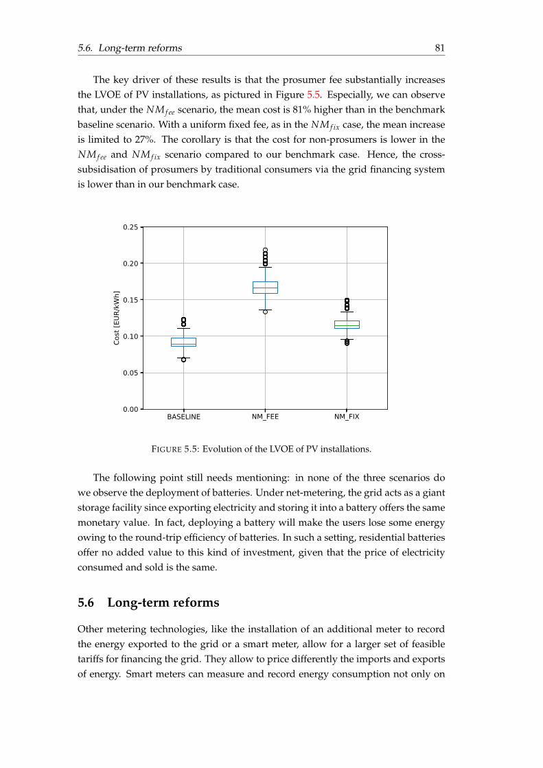
5.6. Long-term reforms 81
The key driver of these results is that the prosumer fee substantially increasesthe LVOE of PV installations, as pictured in Figure 5.5. Especially, we can observethat, under the NM f ee scenario, the mean cost is 81% higher than in the benchmarkbaseline scenario. With a uniform fixed fee, as in the NM f ix case, the mean increaseis limited to 27%. The corollary is that the cost for non-prosumers is lower in theNM f ee and NM f ix scenario compared to our benchmark case. Hence, the cross-subsidisation of prosumers by traditional consumers via the grid financing systemis lower than in our benchmark case.
BASELINE NM_FEE NM_FIX0.00
0.05
0.10
0.15
0.20
0.25
Cost
[EUR
/kW
h]
FIGURE 5.5: Evolution of the LVOE of PV installations.
The following point still needs mentioning: in none of the three scenarios dowe observe the deployment of batteries. Under net-metering, the grid acts as a giantstorage facility since exporting electricity and storing it into a battery offers the samemonetary value. In fact, deploying a battery will make the users lose some energyowing to the round-trip efficiency of batteries. In such a setting, residential batteriesoffer no added value to this kind of investment, given that the price of electricityconsumed and sold is the same.
5.6 Long-term reforms
Other metering technologies, like the installation of an additional meter to recordthe energy exported to the grid or a smart meter, allow for a larger set of feasibletariffs for financing the grid. They allow to price differently the imports and exportsof energy. Smart meters can measure and record energy consumption not only on

82Chapter 5. Regulatory challenges in distribution networks: policy
recommendations
a yearly basis but also in short intervals, such as every 15 minutes, and be remote-controlled. As a consequence, they can record the peak consumption over the shortinterval measured (the shorter the interval, the more accurate the measurement).
We consider two kinds of structural regulation taking advantage of these meter-ing technologies. The first one looks into changing the tariff structure and allowingfor capacity fees in addition to the traditional fixed and volumetric distribution tarifffees. The second one looks into the possibility of switching from a net-metering to anet-purchasing system.
With net-metering, imports and exports of electricity are not differentiated interms of prices. Hence, there is no monetary incentive to self-consume and, as shownabove, prosumers do not invest in residential batteries. By measuring electricity im-ports and exports separately, a net-purchasing system makes it possible to differ-entiate the prices of the two flows. This, in turn, changes the incentives to investboth in solar PV and storage systems. Furthermore, consumers may adapt their be-havior to increase their self-consumption, e.g. by shifting demand to synchroniseconsumption and production.
In the net-purchasing case, we consider that the price of exported electricity isequal to the average of the wholesale electricity price (around 40e/MWh) and thereis no distribution fee collected on exported electricity8. The electricity imported byprosumers is charged at the same price as for traditional consumers.
5.6.1 Net-metering system with a capacity component
In the NMcap scenario, the distribution tariff is half composed of a volumetric feeand half of a capacity fee. The capacity fee is based on the peak consumption (inkWp) recorded during the billing period. With a capacity fee, a battery can be usedto shave the peak consumption by displacing consumption from peak to off-peakhours. This investment may drastically reduce the prosumers’ bills. In this scenario,prosumers are still connected to the grid via the net-metering technology.
As shown in Figures 5.6 and 5.7, the change in the tariff structure only slightlycurbs the deployment of solar PV compared to the fully volumetric case presentedin our benchmark baseline scenario. A major difference is that we now observe thedeployment of batteries (see Figure 5.8). This evolution, however, is rather limitedin size and is only observed from period five on (due to lower technology costs andincreasing volumetric charges). While the presence of a net-metering system pro-vides no incentive to invest in batteries, we observe that batteries enable prosumersto shave their peak production, i.e. to decrease their electricity bill, which is partiallycapacity based.
8Increasing the purchasing price of electricity above the wholesale price increases the incentives toinvest in a PV installation, but decreases the incentives to invest in a battery. With a purchasing priceequal to the retail price, the net-purchasing scenario would be equivalent to the baseline scenario. Atleast, this would be so provided that the amount of electricity that can be exported is capped to thelevel of electricity consumed on a yearly basis.

5.6. Long-term reforms 83
Compared to our benchmark, the capacity fee scenario (NMcap) increases theLVOE for prosumers, but to a relatively lesser extent than when a prosumer fee isimplemented, as considered under the NM f ee scenario (see Figures 5.5 and 5.9). InFigure 5.10, the electricity tariff paid by traditional consumers increases almost inthe same proportion as in the baseline scenario. This can be explained by the factthat non-prosumers do not have the possibility to displace their peak production byusing batteries. Therefore we observe, as in the benchmark, that a larger fraction ofthe grid costs are paid by non-prosumers.
5.6.2 Net-purchasing system
A net-purchasing system can be implemented by the installation of an extra mechan-ical meter or of a smart meter. We consider two scenarios: a fully volumetric distri-bution tariff (NPvol), and a tariff combining capacity and volumetric terms (NPcap)with an equal contribution of the two components to the grid costs. The latter isonly possible in the presence of a smart meter. Thus, the tariff structure of NPvol isthe same as in the baseline scenario and the one of NPcap is the same as in scenarioNMcap.
0 2 4 6 8 10Time [n]
0
20
40
60
80
100
Prop
ortio
n of
act
ual p
rosu
mer
s [%
]
BASELINENM_CAPNP_VOLNP_CAP
FIGURE 5.6: Evolu-tion of the share ofhouseholds with a PVinstallation.
0 2 4 6 8 10Time [n]
0
2000
4000
6000
8000
10000
Tota
l dep
loym
ent o
f PV
[kW
p]
BASELINENM_CAPNP_VOLNP_CAP
FIGURE 5.7: Evolu-tion of the installedcapacity of PV instal-lations.
In figures 5.6 and 5.7, we observe that the two net-purchasing scenarios lead toa lower number of PV installations than under any net-metering system. At the endof the 10 periods considered, we find that 79% and 85% of the potential prosumershave become actual prosumers under the NPvol and NPcap scenarios, respectively.The growth trend of the investments made is constant and similar across the 10 pe-riods considered. In terms of deployed PV capacity, both scenarios display a similartotal installed capacity. This is because a volumetric tariff induces a larger averageinstallation size but fewer installations.
The high deployment of batteries is another key difference between the net-metering and the net-purchasing scenarios, as Figure 5.8 shows. Under the NPvol
scenario, over 3000 kWh of batteries are installed, while under the NPcap scenario
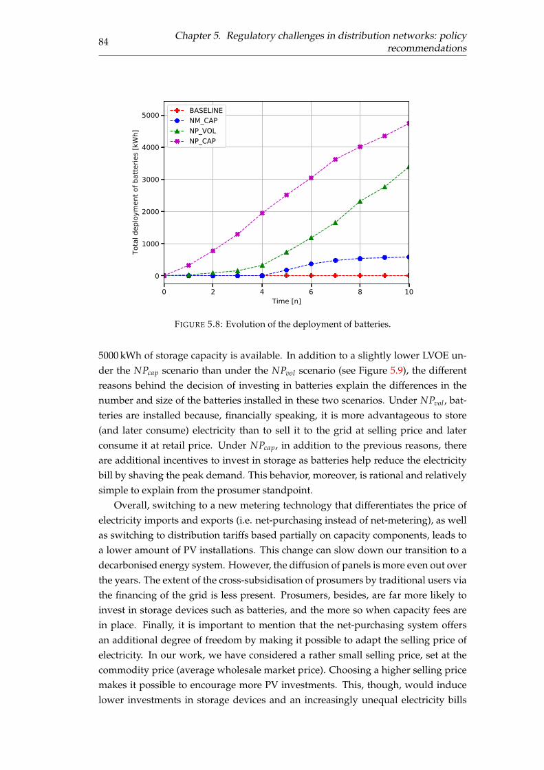
84Chapter 5. Regulatory challenges in distribution networks: policy
recommendations
0 2 4 6 8 10Time [n]
0
1000
2000
3000
4000
5000
Tota
l dep
loym
ent o
f bat
terie
s [kW
h]
BASELINENM_CAPNP_VOLNP_CAP
FIGURE 5.8: Evolution of the deployment of batteries.
5000 kWh of storage capacity is available. In addition to a slightly lower LVOE un-der the NPcap scenario than under the NPvol scenario (see Figure 5.9), the differentreasons behind the decision of investing in batteries explain the differences in thenumber and size of the batteries installed in these two scenarios. Under NPvol , bat-teries are installed because, financially speaking, it is more advantageous to store(and later consume) electricity than to sell it to the grid at selling price and laterconsume it at retail price. Under NPcap, in addition to the previous reasons, thereare additional incentives to invest in storage as batteries help reduce the electricitybill by shaving the peak demand. This behavior, moreover, is rational and relativelysimple to explain from the prosumer standpoint.
Overall, switching to a new metering technology that differentiates the price ofelectricity imports and exports (i.e. net-purchasing instead of net-metering), as wellas switching to distribution tariffs based partially on capacity components, leads toa lower amount of PV installations. This change can slow down our transition to adecarbonised energy system. However, the diffusion of panels is more even out overthe years. The extent of the cross-subsidisation of prosumers by traditional users viathe financing of the grid is less present. Prosumers, besides, are far more likely toinvest in storage devices such as batteries, and the more so when capacity fees arein place. Finally, it is important to mention that the net-purchasing system offersan additional degree of freedom by making it possible to adapt the selling price ofelectricity. In our work, we have considered a rather small selling price, set at thecommodity price (average wholesale market price). Choosing a higher selling pricemakes it possible to encourage more PV investments. This, though, would inducelower investments in storage devices and an increasingly unequal electricity bills

5.6. Long-term reforms 85
BASELINE NM_CAP NP_VOL NP_CAP0.00
0.05
0.10
0.15
0.20
0.25Co
st [E
UR/k
Wh]
FIGURE 5.9: Evolution of the LVOE of PV installations.
0 2 4 6 8 10Time [n]
0
5
10
15
20
25
30
Cost
gro
wth
[%]
BASELINENM_CAPNP_VOLNP_CAP
FIGURE 5.10: Evolution of the total tariff bill of a consumer
between prosumers and consumers.
5.6.3 Self-consumption and power exchanges with the grid
Finally, for each scenario, we compute the average self-consumption rate. The shareof self-consumed electricity corresponds to the total consumption minus the imports

86Chapter 5. Regulatory challenges in distribution networks: policy
recommendations
from the grid divided by the total consumption. By increasing self-consumption,peak consumption from the centralised energy system can decrease, which is knownas being one of the main drivers of the grid costs [118]. Promoting self-consumptionis also important because power injections to the distribution network might becostly. Indeed, as production is correlated locally, there may be large power injec-tions made by several prosumers at the same time in the same low-voltage feeder,e.g. at noon on a holiday weekend, when decentralised production is high and con-sumption low. These power injections may cause over-voltages on the local distribu-tion network, and the inverters to disconnect the solar PV from the network, induc-ing a loss for the prosumers. Furthermore, owing to prosumers’ excessive electricityinjection, the DSOs might need to reinforce the distribution network, in which con-text self-consumption reduces the overall costs of the DSO. These investments mightrequire new on-load tap changers, booster transformers, and static volt ampere re-active control compensator [107]. Hence, while self-consumption is not necessarilya goal in itself, it can be beneficial for the grid by decreasing peak consumption fromthe grid and peak injection to the grid.
The self-consumption rate is usually lower for residential households than forcommercial activities [41]. Moreover, there is a high discrepancy in Wallonia be-tween production and consumption: in the summer months, production is the high-est and consumption the lowest and conversely in the winter months. Despite thelack of financial incentives, around 40% of prosumers claim to take actions to syn-chronise their consumption and production. According to [119], this is mainly truefor those who tend to spend more time during daytime at home as, for instance,retired people.
We do not explicitly model the impact of self-consumption, via a change in ag-gregated peak consumption and injection, on the grid costs. Nevertheless, we com-pute the self-consumption rate for each of the six scenarios and the correspondingpeak power withdrawals and injections. Focusing only on prosumers, we measurethese two variables as the maximum aggregated amount of electricity withdrawn orinjected over a one hour period among the yearly profile. Table 5.3 presents the fig-ures. It shows that the net-metering system does not promote self-consumption; allthree net-metering scenarios present a self-consumption rate close to 30%. Aggre-gated peak power withdrawals and injections are marginally differing, except forthe NMcap where lower peak power withdrawals are observed due to the capacitycomponent (peak shaving behaviors).
A switch to the net-purchasing system implies an increase in the self-consumptionrate from 30% to 46-50%, which can easily be explained by the presence of bat-teries. As a consequence of promoting self-consumption, aggregate peak powerwithdrawals and injections are also decreasing. Under the NPvol scenario, the twopeaks decrease by respectively 0.76% and 4.62% compared with the baseline sce-nario. When coupled with a capacity component, a net-purchasing system is ableto decrease the peaks more substantially by 64.2% and 18.95% (withdrawals and

5.7. Conclusion and policy implications 87
injection, respectively).Hence, a net-purchasing system with capacity-based tariffs can substantially de-
crease the grid costs by shaving the import and export peaks. Compared to thebaseline scenario, the peak demand and the peak injection decrease by respectively60% and 19%. In the present chapter these metrics can be measured only from aphysical standpoint, with no associated monetary value of the reduction in the gridcosts. Note, however, that these gains are possible thanks to private investmentsinto batteries rather than a collective effort from the DSO. Those cost reduction forthe DSO could be passed through consumers under the form of a lower grid tariff.Under this NPcap scenario, these financial investments made by prosumers are esti-mated at around one million euros. If this figure from our model is extrapolated tothe size of Wallonia, we have that households’ investments in batteries will amountto 600 million euros to reduce grid costs. Overall, to judge the efficiency of the tar-iffs we would need to balance more precisely these private investments made byprosumers into batteries and the reduction in grid costs they create.
TABLE 5.3: Self-consumption and aggregate power exchanges
Absolute Self-consumption Peak Power Peak PowerScenarios value rate withdrawals injections
baseline 1,776.89 kWh 29.67% 2,806.90 kW 4,975.55 kWNM f ix 1,780.35 kWh 29.72% 2,805.65 kW 4,975.55 kWNM f ee 1,775.98 kWh 29.65% 2,808.54 kW 4,975.55 kWNMcap 1,623.91 kWh 27.11% 2,682.68 kW 4,967.99 kWNPvol 2,809.44 kWh 46.91% 2,784.24 kW 4,745.83 kWNPcap 2,997.92 kWh 50.05% 1,004.53 kW 4,032.66 kW
5.7 Conclusion and policy implications
This study has aimed to assess the impact of various tariff regulations and meteringtechnologies on the evolution of the electricity system and, in particular, the elec-tricity distribution network in a case study applied to Wallonia, the southern regionof Belgium. Findings expressed in comparison to the baseline scenario (describingthe current situation in Wallonia) are summarised in Table 5.4. They suggest thatchoosing between a net-metering and a net-purchasing technology to measure theimports and exports of electricity from/to the distribution network is critical. Thenet-metering system highly enhances the adoption of PV installations, which is oneof the primary energy targets in the European Union, compared to the other sce-narios. However, this comes at a cost. Regardless of the distribution network tariffstructure considered, net-metering does not incentivise investments in battery in-stallations at all and, therefore, does not encourage self-consumption. Peak powerwithdrawals and injections are decreased under a net-purchasing system, in par-ticular when capacity-based fees are applied. Net-purchasing and capacity-based

88Chapter 5. Regulatory challenges in distribution networks: policy
recommendations
tariffs tend to strongly complement each other. Moreover, the net-metering tech-nology leads to largely differing electricity bills for prosumers and non-prosumers,where non-prosumers end-up bearing most of the costs of the DSO. This issue canpotentially impair the acceptance of electricity generation technologies coming fromrenewable energy.
TABLE 5.4: Summary of the results (evolution compared to the base-line scenario)
NM f ix NM f ee NMcap NPvol NPcap
PV adoption = - - - - - -Battery installations = = + ++ ++Energy cost for non-prosumers - - - - - - - - -Peak power withdrawals / injections = = - - - -
5.7.1 Policy implications
The CWaPE, the energy regulator in Wallonia, pursues various objectives relatingto: (i) economic efficiency, (ii) equity, and (iii) the stability of the revenues of theDSO; moreover, the CWaPE aims at (iv) designing distribution tariffs that pave theway for the energy transition. Where the net-metering technology is in place, onlythe latter objective is partially fulfilled as it encourages large investments in PV pro-duction sources. This situation, however, is unsustainable as the network costs arefinanced by non-prosumers who see their electricity bills increase. The goal of theregulator is not to financially support investments in renewable production sourcesbut to facilitate the energy transition via regulations targeting the DSO. As othertariff regulations only marginally change these results, our analysis leads us to con-clude that a net-purchasing system should be adopted. If, in addition, a capacitycomponent is introduced in the tariff, less investments would be required to rein-force the grid as such a system substantially decreases peak power withdrawals andinjections. As these changes would require smart meters, we highlight the need todeploy this technology more urgently than currently planned by the regulator. Thiswould shorten the gap between short and long run policies, the latter of which en-ables the implementation of more adequate regulations.
One reason for the relatively high electricity bills in Wallonia is that they do notonly cover the costs of the commodity and the distribution network. The bills alsocharge users for various public policies, such as subsidies for investments in renew-able energy production sources, reduced energy prices for precarious households,for the financing of public lighting, or the costs of the planned nuclear phase-out[113]. As distribution tariffs are computed on a volumetric basis, considering theseadditional costs to compute the electricity bills makes the system even less sustain-able financially and prone to un-even allocation of those additional costs where pro-sumers may end up not paying for public services such as lighting. All these public

5.7. Conclusion and policy implications 89
policies should be financed by the public finance system. This, in addition, would bea much more transparent and democratic procedure as they would fall under parlia-mentary oversight. Changing the financing sources of these policies would decreasethe pressing concerns of a utility death spiral and equity issues between prosumersand traditional consumers.
Finally, this analysis shows the importance of designing holistic policies support-ing PV adoption and regulating the electricity distribution network, both concerningtariffs and metering technology, so as to facilitate a sustainable energy transition.
5.7.2 Limitations and future research
Our model relies on various assumptions relating to prosumers and the grid, whichcould influence some of our results. Yet, we believe that extending the model to con-sider these assumptions would lead to qualitatively similar results. To fully examinethem, future research will be needed.
In our model, potential prosumers are presumed to choose to invest in a PV in-stallation or in both a PV and a battery installation. As a consequence, early PVadopters do not have the opportunity to later invest in an additional battery sys-tem. Allowing for this possibility would not impact the scenarios considered in theshort run, i.e. where a net-metering system is in place, as anyway no investment inbatteries is done. However, in the net-purchasing cases considered in the long run,both investments in PV and in batteries would increase. Changing this assumptionwould further strengthen the main conclusion of our analysis.
Our model considers a wide, yet for simplicity’s sake, fixed variety of consump-tion load profiles. It is unlikely, though, that they will not evolve over time. For ex-ample, owing to the deployment of electric vehicles, consumption profiles are likelyto change. While electric vehicles increase consumption, they also act as a storagedevice potentially enabling peak shaving. As the functionalities of their batteries aresimilar to those of an ordinary battery, considering evolving load profiles would leadto lower investments in batteries in the long run scenario with a net-purchasing sys-tem or a net-metering system with tariffs with a capacity component. The ensuinghigher consumption levels would lead to a greater deployment of PV installationsalong with even larger rebates on the energy bill. Overall, taking these aspects intoconsideration would not qualitatively impact the key insights of the current simula-tor.
One final limitation deserves to be mentioned. In this chapter, we model the fi-nancing of the network grid as a zero-sum game. Further, we have shown that somegrid regulations, and especially capacity tariffs coupled to a net-purchasing system,lead to a decrease in peak power imports and exports. These collective benefits canbe translated into lower grid costs that are possible thanks to the private investmentsinto batteries by prosumers. We hope that further research will allow a more precisequantification and comparison of these aspects.

91
Part II
Decentralised electricity markets


93
Chapter 6
Model of interaction for renewableenergy communities
This chapter introduces Part II of the thesis, which deals with the integration of dis-tributed energy generation resources (DER) by means of new frameworks for (local)decentralised electricity markets, such as the renewable energy community (REC).As the business of electricity retailing changes following the current evolution of theelectricity system, new opportunities arise for emerging technologies. An exampleof this evolution is the increasing number of final customers installing sophisticatedenergy management systems (EMSs) – these systems can control the production orconsumption of a large variety of devices such as solar photovoltaic (PV) panels withstorage solutions. EMSs provide prosumers with an agile and flexible way of man-aging their DER installations. Additionally, they offer a seamless communicationchannel between those prosumers and their retailers. This communication channelopens the door to new products and services, such as the provision of flexibilityfrom prosumers to retailers, role that in the context of RECs can be adopted by theREC manager (ECM). The the retailer (or the ECM) may then use this flexibility inthe wholesale electricity markets and imbalance settlement mechanisms, or trade itwith other balance responsible parties (BRP). Using these ideas, Chapters 6 and 7explore the potential of REC members to offer flexibility bids to their ECM1.
The first step toward exploring this potential, and the one introduced in thischapter, consists of building a model of interaction between the different agents in-volved in our system. In the case of an REC, the agents whose interactions are mod-elled are the ECM and the REC members. These interactions comprise forecastingthe electricity demand of consumers and prosumers as well as forecasting the localproduction of prosumers. If flexible consumption is offered by the REC members,it is also part of these interactions. This model of interaction relies on smart me-ters to register the electricity exchanges and requires no modification of the currentrules and regulations of the European electricity system. Both the model of interac-tion and a numerical example are provided in this chapter. Note that, to produce
1The model developed in this chapter can also work with other entities aggregating a portfolio offinal customers, such as aggregators or retailers.
94 Chapter 6. Model of interaction for renewable energy communities
a generic framework, we use the term retailer throughout the chapter – this retailercan be an aggregator or, as explained above, the ECM of an REC.
6.1 Introduction
The role of a traditional electricity retailer comprises acting as an intermediary be-tween its clients and the rest of the electricity system. In its role, a retailer purchaseselectricity for its clients based on consumption forecasts, acts as BRP for the trans-mission system operator (TSO), and invoices its clients. The interaction between theretailer and its clients works one way: the client benefits from the system but doesnot contribute to it. To be able to manage this interaction efficiently, an increasingnumber of clients are installing (or upgrading) sophisticated EMS to save energy in acost-efficient manner [120]. An EMS is an automated energy controller using a com-puter as a central processor. The capabilities of the EMS may vary widely dependingon the selected model. Nonetheless, its basic capabilities are almost universal, andnotably comprise the scheduling of the electricity flows, fixing the set-points of thebatteries, alarms and safety measurements, and basic system monitoring.
An EMS can manage the production or consumption of a large variety of devices,such as photovoltaic panels, storage solutions (e.g. batteries), and flexible loads (e.g.demand-flexible boilers). The nature of the constraints of these different devicesthus requires dedicated management, for instance, one EMS may be designed tocontrol the appliances of a house, as described in [121], whilst another one couldbe designed to control a microgrid with several companies, photovoltaic panels, arun-on-the-river generator, and a storage system, as detailed in [122]. Furthermore,there might be cases where an EMS simply controls demand response devices. Fromthe standpoint of a retailer, an EMS represents a higher-level manager of all thesedevices (i.e. generation, storage, or flexible demand) to provide flexibility. The flex-ibility thus provided by the clients’ EMSs is then forwarded by the retailer to theday-ahead and intraday electricity markets. Alternatively, it can be exchanged withother BRPs, or be used by the retailer to participate in balancing mechanisms. In thisregard, the retailer can be interpreted as a smart BRP providing single generic accessto various flexibility products, aggregating this flexibility to meet minimum vol-ume constraints, simplifying accounting, and managing the flexibility of its clients.This chapter aims at defining an interaction model between a retailer and severalclients (through the clients’ EMSs) to exchange flexibility. The interactions are basedon a generic interface with the EMS, ensuring the scalability of the method, whichshould be simple for the most basic EMS, yet able to include the constraints of thecontrolled devices and, in particular, rebound effects [123]. In this context, flexibletrading should be an addition to traditional electricity retailing. If no flexibility istraded, the contract between the client and the retailer corresponds to a classic re-tailing contract. The scientific literature covers most of the components required

6.2. Literature review 95
to define such an interaction model. However, to date, there is no implementationcovering all the requirements together.
For the remainder of this chapter: the next section reviews the relevant literature.This review is followed by an outline of the proposed interaction model. Specificcomponents of the model are detailed in dedicated sections: the baseline and itsupdate, the flexibility bids, and the deviation mechanism. Finally, the last sectionconcludes the chapter and identifies the potential future prospective work.
FIGURE 6.1: Flow of interactions between a client and its retailer. Abaseline is computed for each client. Then the retailer allows, or not,the provision of flexibility of the client. If it is not accepted, the clientfalls under a classic retailing contract. If accepted, the client notifiesits capability to provide flexibility. If the retailer contracts the flexibil-ity, the schedule of the client is modified accordingly. This schedulemay be modified upon notification of the client. The client is invoicedbased on the final schedule and the metered energy.
6.2 Literature review
The existing literature regarding the use of demand response to provide flexibilityis abundant, see for instance reviews [124] and [125]. The latter was conducted in2018 and presents the results of 60 works. Furthermore, many projects on this topichave been conducted over recent years. ADDRESS started in 2008 and is one ofthe earliest European projects dedicated to demand response [126]. BRIDGE is aEuropean Commission initiative that unites Horizon 2020 Smart Grid and EnergyStorage Projects [127]. The BRIDGE project recommends implementing the WinterPackage directives into the market system regulation based on dedicated recommen-dations related to specific dimensions: demand response access to markets, serviceproviders’ access to markets, product requirements, measurement and verification,payments, and penalties [127]. To enable flexibility services, the authors in [126]highlight the importance of introducing minor modifications in existing markets,
96 Chapter 6. Model of interaction for renewable energy communities
rather than creating new ones. In this process, the retailer is well-placed to act as afacilitator.
The interaction model proposed in this chapter is a market-based approach. Otherexamples of such approaches for flexibility aggregation can be found in the Flexi-ciency [128] and PowerMatcher [129] projects. The former details a European marketplace facilitating interaction between agents with advanced monitoring, local energycontrol, and flexibility of aggregated customers. Flexibility services are very genericand must define various parameters such as the payment model, preconditions forservice, or detailed description of service delivery. Concerning PowerMatcher, thisproject represents a practical implementation of market-based aggregation; it oper-ates as a smart grid coordination mechanism balancing distributed energy resources(such as renewable ones) and flexible demand. First, different devices send bids de-tailing their willingness to consume energy, and then the aggregator sends back aprice signal so that they can determine its consumption volume at this price.
The mentioned projects interact with various types of devices, either using genericbut complex models, or several specific ones. The authors in [125] claim that, to cre-ate a well-functioning interaction model, it is necessary to formulate standardizedbut simple definitions of flexibility products, accounting for energy-constrained re-sources, flexibility capacity shortage situations, and including the rebound effect.One step toward the definition of such flexibility products is proposed in [130],where a solution is tailored to harness the flexibility from heat pumps. The flexibil-ity product introduced in the latter work is used as the base block of the interactionmodel proposed in this chapter.
6.3 Proposed interaction model
The proposed interaction model between a client willing to provide flexibility andits retailer complies with the following outline: a client provides a baseline, basedon its own consumption forecasts and additional forecasts if needed. If the EMS ofthe client has no forecasting capabilities, a reference is built from historical values.The retailer accepts or declines the participation of the client in its flexibility pool.Once accepted, the EMS of the client computes its capability to provide flexibilityand communicates it to the retailer. The retailer processes all flexibility offers com-ing from the different clients’ EMSs, taking into account the current status of theenergy markets and its requirements as a BRP. If the retailer contracts flexibility, theschedule of the relevant clients are modified accordingly. Simultaneously, forecastupdates may be requested by the client. The retailer checks if the new baseline isvalid and does not impair the provision of previously accepted flexibility. Finally,the client is invoiced based on the final schedule and the metered energy. Devia-tions from the reference, with a specified tolerance, are penalized by the retailer. Theflow of interactions is illustrated in Figure 6.1. This interaction model relies on smartmetering and requires no modification of the current electricity market.
6.4. Baseline and updates 97
6.4 Baseline and updates
A baseline is necessary to define the flexibility provided at a resolution of a mini-mum 15 minutes, for its use in most electricity markets. Such a baseline is a specificrequirement of this kind of client-retailer interaction. For classic retailing contracts,the baseline of a client is not compulsory. The retailer assumes the role of BRP for theclients it represents. In this setting, the TSO computes the potential imbalance of theretailer with respect to its net position. The computation of the net position of theretailer is based on its electricity purchases, which are in turn based on the forecastsof its clients. Large consumers may be requested to provide baselines to the retailer.In that instance, a communication of the baseline will be imposed by the retailer’scontract (i.e. as an agreement between the client and the retailer). Hence, the TSOmay not be aware of the baseline of the client and only has information concerningthe schedule of the retailer’s portfolio.
If flexibility is sold to the TSO, the baseline may be defined by the TSO itself[131, 132]. Taking another reference would create a mismatch between the flexibilityremunerated by the TSO and the flexibility provided by the client. In this case, theretailer communicates to the client the reference taken by the TSO, or the method ifthe necessary data are not available in advance.
If flexibility is sold only as a result of a change in the retailer’s net position, thedefinition of the client baseline is only an agreement between the client and the re-tailer. Since it is technically challenging to predict the state of an EMS without thedetails of the underlying devices, the EMS should provide its planned schedule tothe retailer. According to [133], baseline and flexibility should be computed by theEMS to ensure end-user privacy and comfort. However, a concern regarding theself-computation of the baseline and flexibility is that customers might attempt topurposely manipulate their baseline in order to maximize their profits. The typicalway of “gaming” the baseline is that customers may declare a higher consumptionthan their needs during their peak demand to sell flexibility in the form of a ficti-tious reduction of consumption. However, such abuses may not be intentional. Anyoptimization-based controller naturally exploits the flaws of a deficient interactionmodel. To prevent these problems, a retailer can compare the information providedby the client with its own forecasts. This check is essential to detect anomalies andcan be used to avoid abuses of the flexibility mechanism. One method to preventsuch potential abuses is to check the similarity of the communicated baseline withhistorical measurements, applying a tolerance.
The baseline must not only cover the period in which the client is willing to pro-vide flexibility, but also some periods before and after flexibility delivery, to considerthe rebound effect. The length of these periods depends, among other factors, on thestorage capacity behind the EMS controller. The order of magnitude of residentialthermal storage, for instance, is one and a half hours [130], whereas exploring the op-posite extreme, a microgrid storage system may shift consumption by several hours.

98 Chapter 6. Model of interaction for renewable energy communities
Considering these orders of magnitude, a baseline window of one day around aflexibility window is considered for the present chapter.
A baseline should be defined before the clearing of the day-ahead energy marketso that the retailer has sufficient time to compute and issue its offers. This baselineshould therefore be computed based on day-ahead forecasts. Typically, more accu-rate forecasts can be obtained closer to real-time, leading to the need for baselineupdates. However, an update may not always be accepted, since it could compen-sate for previously sold flexibility or an unspecified rebound effect. Thus, two ver-ification points are suggested: (i) a maximum relative deviation with respect to theinitial baseline, and (ii) prevention of baseline modification in the opposite directionto the provision of flexibility services. Figure 6.2 shows a schedule update whichcancels out already sold flexibility: (a) assuming a client with a flat baseline; (b) theclient sells flexibility and the schedule is modified accordingly; (c) the client requestsa schedule update in the opposite direction to its sold flexibility. If this update is ac-cepted, the client is paid for a flexibility it does not provide. To avoid such potentialabuses, the retailer should not accept a baseline update of an opposing sign than thesold flexibility. In practice, a small tolerance corresponding to acceptable forecasterrors should be considered.
FIGURE 6.2: Case of a schedule update that cancels out already soldflexibility.

6.5. Flexibility bids 99
6.5 Flexibility bids
A client communicates its flexibility by means of bids. This flexibility product isinspired by proposals of articles [130] and [134]. It consists of an offer coveringmultiple market periods in which signs may vary. This product generalises the caseof a single period offer. A bid communicates the flexibility over multiple time-stepsand includes the following information:
• Energy volume for each time step;
• Type: partial/binary acceptance;
• Cost of the bid; and
• Expiration time.
A graphical representation of such a bid is provided in Figure 6.3. The retailerselects interesting bids, either to directly use them, or to be sold (aggregated or not)to other BRPs or to the intraday market. As for the market clearing process, manyimplementations can be investigated. In any case, the clearing procedure should beadequate to exchange flexibility close to real-time as, for example, in the real-timebalancing settlement. The latter encourages the use of continuous clearings.
Time
(A) Modulation signal.
Time
Pow
er
(B) Modulation added to thebaseline.
FIGURE 6.3: Example of upward modulation with three payback pe-riods.
By default, a bid allows partial acceptance of the offered flexibility volumes. Theaccepted flexibility volume at each time-step is given by the offered volume multi-plied by the acceptance ratio. The client can prevent the possibility of partial accep-tance for any bid, imposing the complete acceptance or rejection condition, namely,using the binary bids.
The response of the retailer to the bid submission is the status of the bid, whichcan take the following values:

100 Chapter 6. Model of interaction for renewable energy communities
• FREE: Bid submitted and free to be revoked by the client.
• REVOKED: Bid revoked by the client.
• PENDING: The retailer is processing the flexibility bid and it cannot be re-voked.
• EXPIRED: The bid reached its expiration time without being accepted or re-jected.
• REJECTED: Bid rejected by the retailer.
• RESERVED: The bid is reserved and waits for its acceptance by its future ben-eficiary.
• ACCEPTED: The bid is accepted and an acceptance ratio is communicated.
FIGURE 6.4: Evolution of flexibility bid statuses.
Figure 6.4 illustrates the evolution of bid statuses. Clients submit their offers tothe retailers, which are initially in a free state. They are always free to revoke anoffer if it has not been processed. Periodically, the retailer processes the current freeoffers. During the processing phase, the statuses of the concerned offers is set aspending. The retailer first filters offers that have expired due to a time-out. Next, itselects offers to be submitted to the markets or proposed to the TSO or other BRPs.These offers are then set to a reserved status, waiting for acceptance, while the rest ofthem are switched back to the free status. The retailer could implement a wide rangeof strategies to process bids. A basic one would be to forward the bids directly tothe markets, in order of profitability, discarding the ones not suitable for participa-tion (e.g. the ones which will not generate profits). A more advanced strategy couldconsist of building a market offer by aggregating a collection of flexibility bids, how-ever, the definition of this kind of algorithm is out of the scope of this document. Thealgorithm proposed in this chapter is assumed to send offers to the market, commu-nicating back to the retailer the provided flexibility. The retailer then dispatches thisflexibility to the reserved offers and sets their status as accepted. Concerning the restof the offers, they are switched back to the free status for the next selection process.
6.6. Deviation mechanism 101
Once a flexibility bid is accepted, the schedule of the corresponding client is mod-ified accordingly. Note that following this principle, a client has an alternative to thebaseline update mechanism to modify its schedule. The client could bid the expectedschedule update at an appealing price with respect to the one of the intraday mar-ket. Thus, the retailer could buy or sell the corresponding energy on the market andupdate the schedule of the client accordingly.
6.6 Deviation mechanism
A deviation is given by the difference between the measured consumption and thebaseline (i.e. the foreseen consumption plus the provided flexibility). Nonetheless,these deviations are not considered an imbalance in this document since the clientsare not BRPs.
The retailer benefits from averaging its portfolio of clients to mitigate the vari-ability of its forecasts and deviations. The client cannot benefit from this averagingeffect owing to its small size and limited flexibility. Before pricing a deviation, a re-tailer may therefore grant a tolerance to its clients for deviations with respect to theirschedules. Beyond this tolerance, a price needs to be associated with this deviation.The imbalance price is a good candidate since it corresponds to the cost faced by theretailer. Furthermore, exposing the client to imbalance prices might encourage themto enroll in a flexibility program. The retailer could reduce the deviation price by afactor corresponding to the reduction of the risk resulting from the aggregation ofthe clients. This reduction can be computed as follows. Considering a retailer with kidentical clients with forecast errors following Gaussian distributions correlated bya factor ρ. The production of the ith client is given by pi,t, whereas its productionforecast is pi,t. Then, the covariance of a pair of clients i, j is given by ρσiσj. The sumof correlated Gaussian random variables is studied in paper [135]. In this paper,the authors prove that the sum of correlated normally distributed random variablesis equal to one single random variable following a normal distribution of varianceσZ = σ2
i ∑ki=1 ∑k
j=1 ρi,j where ρi,j is the covariance.Using this finding, the aggregated forecast error is given by the sum of the indi-
vidual distributions. Let Pt and Pt denote the production and the estimated produc-tion of the retailer, which corresponds to the sum of the production and estimatedproduction of its clients.
E[Pt − Pt
]= N
(0, σ2
i
k
∑i=1
k
∑j=1
ρi,j
)
= N
(0, σ2
i
k
∑i=1
(1 + (k− 1) ρ)
)= N
(0, σ2
i k (1 + (k− 1) ρ))

102 Chapter 6. Model of interaction for renewable energy communities
The relative standard deviation of the error C is given by:
C =E[Pt − Pt
]E [Pt]
=
√k + k (k− 1) ρ
kci
where ci is the relative standard deviation of the client’s error. We can define thefactor φ, representing the influence of the correlation of the client’s production onthe total production of the retailer as:
φ =Cci
=
√k + k (k− 1) ρ
k
The computation of φ for different numbers of clients k and for different correlationcoefficients ρ is showcased in Table 6.1. This table shows that for a sufficient numberof clients, with a realistic correlation of 0.2, the relative forecast error of the retaileris 45% of the one an individual client would obtain. Thus, 45% could be used as apotential discount on the imbalance price to define the deviation price of the client.
TABLE 6.1: Influence of the correlation of the clients’ production onthe total production of the retailer, as a function of the number of
clients k and the correlation of their production ρ.
k / ρ 0 0.1 0.2 0.3 0.4 0.51 100% 100% 100% 100% 100% 100%2 71% 74% 77% 81% 84% 87%3 58% 63% 68% 73% 77% 82%5 45% 53% 60% 66% 72% 77%10 32% 44% 53% 61% 68% 74%100 10% 33% 46% 55% 64% 71%1000 3% 32% 45% 55% 63% 71%10000 1% 32% 45% 55% 63% 71%
6.7 Conclusion
This chapter presents an interaction model allowing a set of clients equipped EMSsto provide flexibility services to the electrical system through their retailer. The scopeof this interaction model covers energy exchanges spanning from the day-ahead toreal-time. These exchanges may be simple for the most basic EMSs, while allow-ing clients with device constraints such as rebound effects to include them in suchexchanges. The trading of flexibility is an addition to traditional retailing. If noflexibility is traded, the contract between the client and the retailer corresponds to aclassical one.

103
Chapter 7
Introducing demand response intorenewable energy communities
The potential of final customers to offer flexibility based on the idea of renewableenergy communities (RECs) is further elaborated in this chapter. Making use ofthe interaction model developed in the Chapter 6, we design an REC where part ofthe REC members are flexible consumers who can post flexibility bids upon requestfrom the energy community manager (ECM). These bids, if accepted by the ECM,will change the demand profile of the (flexible) members and, as such, of the REC.The decision of activating flexibility bids may respond to different criteria – thischapter presents a flexibility activation decision mechanism based on a cost minimi-sation criterion.
To perform this cost minimisation, we assume that the only retailer of the RECis the ECM1. Thus, the ECM, as provider of electricity for the REC, can trade in thewholesale electricity market, in this case the day-ahead market, to purchase the elec-tricity needs of the community. When performing a typical demand provisioning,the ECM or the retailer must use forecasts of load, production within the communityand electricity prices. In addition, in this chapter we introduce one extra element theECM must account for: flexible consumption by flexible consumers equipped withenergy management systems (EMSs) in the form of flexibility bids spanning severaltime-steps. Taking all these elements into consideration, the ECM performs the de-mand provisioning in the day-ahead market, aiming to minimise the electricity costsof the REC. To that end, a strategy must be developed to decide which flexibility bidsto activate. Owing to the complexity of flexibility bids, comprised of three elements:initial activation of flexibility, idle time, and rebound (detailed later in the chapter),the strategy for bid activation is not straightforward. In this chapter we propose anoptimisation framework at the core of such an activation strategy – one that not onlyaccounts for the initial activation, but also for the idle time and the rebound of thebid, which may take place several time-steps after the initial activation.
1As per current European regulations, the ECM does not need to have the role of the retailer of thecommunity. However, in this paper we assume this is the case to avoid the extra layer of communica-tion with the retailer. The model presented in this chapter can work equally assuming the standpointof a retailer instead of an ECM.

104 Chapter 7. Introducing demand response into renewable energy communities
Our results show that creating an REC can significantly reduce the electricitycosts of the REC members. Furthermore, we show that introducing flexibility bidsfurther reduces the total system costs thanks to a better matching of local supply anddemand.
7.1 Introduction
Electricity retailing is rapidly evolving in response to the emergence of new tech-nologies such as smart meters or EMSs. These new technologies enable new formsof decentralised electricity trading [125]. In this regard, the European Parliament inits 2018/2001 directive has introduced the concept of RECs [11]. RECs are usuallycomposed of consumers and local renewable generators which are connected to thesame low voltage feeder. When an REC is established, their users may benefit fromlower electricity bills owing to: i) a greater synchronisation between renewable elec-tricity production and consumption; and ii) a potential discount on the distributionfee offered by the distribution system operator for all locally consumed electricity.RECs are managed by an ECM, in charge of billing the users and ensuring the ad-equate functioning of the REC. The role of the ECM then, includes managing thegeneration assets within the REC in order to maximise the global self-consumptionof the REC, and creating an adequate business model where the financial balance ispositive.
To maximise the REC self-consumption, the ECM needs to synchronise supplyand demand. However, when relying on renewable resources such as solar photo-voltaic (PV), the generation output cannot be controlled. A solution might involvethe deployment of storage devices such as batteries, yet their limited capacity as wellas their price make them an impractical solution for large scale implementations.Hence, another potential way of boosting the supply and demand synchronisationis the use of demand response (DR) or other flexibility services provided by theusers. In this regard, this chapter focuses on the development of a novel method todeal with DR in the context of an REC with generation assets in the form of solar PV,owned by an investor (for instance the ECM). This REC is composed of non-flexibleconsumers who simply consume electricity, flexible consumers who consume elec-tricity and offer DR, and generation assets that can sell the electricity either to theREC or to the main network.
In this set-up, flexibility bids can be offered by the REC’s flexible consumers oneday before physical delivery. Every day at noon, the flexible consumers can posttheir flexibility bids for every quarter of the following day. The ECM must then se-lect the bids according to the best interest of the system (e.g. self-consumption max-imisation). To that end, the ECM makes use of forecasts of consumption, production,and day-ahead market prices. It is important to note that network constraints of theREC are not considered during this process.
7.2. Simulator 105
Several works in the existing literature have tackled the issue of flexibility. In[136], the authors present an optimisation model to study the participation of a DRaggregator with a portfolio of DR resources in the wholesale market, highlightingthe cost opportunity offered to the aggregator, and the possibility of transferringsuch a gain to promote the participation of end-users in DR programs. In [137],several “smart” buildings are modeled to provide flexible consumption as fast reg-ulation reserve to the grid, reporting a reduction in operating costs. The authors in[138] study the provision of reserve with DR and stress the importance of account-ing for the rebound effect when using flexibility bids. In [139], the authors createa framework in which flexible consumers can provide flexibility bids while an ag-gregator supervises the flexibility transactions, suggesting the need for interactionbetween the different agents. In [140], three different market designs are proposedfor the activation of flexibility services within distribution networks. This paperfocuses on the coordination between retailer, transmission system operation, anddistribution system operation (DSO). Another work, [141], proposes the use of hier-archical agent-based modelling for the study of the impact of DR on the day-aheadmarket, showcasing a cost reduction on the user end while profits are maximised forthe retailer.
To date, no work has addressed the issue of introducing flexibility services inthe context of an REC. Although there exists literature on peer-to-peer trading, thismechanism is based on a decentralised planner. In this chapter, we take the stand-point of a centralised one, where the novelty lies on the introduction of flexibilitytrading where consumers can submit their willingness to offer flexibility services inthe context of European RECs as they have been laid out by the European Commis-sion. Furthermore, no comprehensive interaction model can be found in the litera-ture where flexibility bids coming from consumers’ EMSs can be offered in an RECmanaged by an ECM. Our work aims at filling this gap, introducing a novel multi-agent model capable of simulating the operation of an REC composed of differentagents: flexible consumers, non-flexible consumers, generation assets, and ECM. Inaddition to the regular operation of the REC, a strategy for activating flexibility bidsfrom flexible consumers, based on an optimisation problem is proposed and tested.
After this introduction, in Section 7.2, we detail the functioning of the proposedthe multi-agent the simulator. Section 7.3 presents the mathematical formulationof the optimisation problem written to select the flexibility bids. In Section 7.4, weintroduce a test case showcasing and discussing the capabilities of the simulator.Finally, in Section 7.5 we provide the conclusion of this work.
7.2 Simulator
In this section, we present an overview of the proposed simulator, establishing theinteractions between the agents of the REC. Moreover, the flow of information in ourmulti-agent computational tool is explained in detail.

106 Chapter 7. Introducing demand response into renewable energy communities
As explained in the introduction, the goal of the developed simulator is the de-tailed representation of the activities of an ECM and the REC it manages. The RECis composed of a portfolio of flexibility providers among its consumers, namely theflexible consumers. To maximise the self-consumption of the REC (or its welfareas we will see later on the document), the ECM can use the flexibility provided byflexible consumers when purchasing energy in the European day-ahead market.
In the developed simulator, the demand of the REC is introduced by means ofseveral consumers (flexible and non-flexible) that are modeled through their de-mand profiles. The generation needed to supply such a demand comes from thegeneration assets of the REC or, if needed, from the main network (outside the REC).
In this work, the ECM produces forecasts of the day-ahead market prices and thedemand of the non-flexible consumers. Then, the flexible consumers and the renew-able generation assets provide their individual demand forecasts to ECM, who addsthem to the forecast of the non-flexible consumers. With all the demand forecasts(flexible and non-flexible), an initial baseline is computed and the flexible consumersare scheduled.
In addition, the ECM receives flexibility bids from the flexible consumers, andactivates these bids in order to increase or reduce the demand at certain periods. TheECM will choose the bids that maximise the welfare of the REC which, in the casepresented, also maximises the self-consumption of the system (i.e. the part of thedemand met by local generation). A detailed explanation of the role of each agent isprovided in this section. The selection process of the flexibility bids is presented inSection 7.3.
7.2.1 Agents
In the following, the different agents of the multi-agent simulator are presented,highlighting the interactions between them and their impact on the simulation. Theagents of the proposed model are the day-ahead market operator, the flexible con-sumers, the non-flexible consumers, the generation assets, and the ECM. They allhave different roles and ways of interacting.
Day-ahead market operator
this agent is meant to provide the history of day-ahead market prices to the ECM sothat the it can produce forecasts. In addition, once the day-ahead market has beencleared and the prices are fixed (not forecasts), this agent provides the actual pricesthat will be charged to the ECM for its day-ahead provisioning.
Flexible consumers
this group of agents is composed of electricity consumers that can offer demand re-sponse (flexibility). Upon request of the ECM, these agents will compute and offer aflexibility bid upward or downward. This flexibility offer states that, if activated, the

7.2. Simulator 107
flexible consumer is obliged to increase or decrease its consumption at a given pointin time. This offer also states that, at a later moment in time, the same amount of en-ergy will be returned to the flexible consumer, decreasing or increasing its demandaccordingly (rebound). Each flexibility bid is offered at a fixed price. In principle,each flexible consumer should design this price according to their own utility func-tion through a bidding process. In this chapter, however, for the sake of simplicitywe consider the same price per unit of energy for all flexibility bids.
Flexible consumers have a baseline and a schedule, and while the baseline repre-sents their consumption without flexibility, the schedule can be adjusted dependingon the flexibility bids accepted by the ECM. The EMS of each agent is responsible forthe computation of the flexibility bids and for communicating them to the ECM.
The flexibility bids are composed of three elements:
• Initial flexibility: this is the initial change in schedule offered by the flexibleconsumer, it can be positive or negative and is instantaneous (i.e. it will beactivated at the appointed time for the appointed duration). The magnitude ofthe initial flexibility depends on the baseline of the flexible consumer (it cannotbe greater than the baseline itself).
• Idle time: this is the time between the flexibility offered and the start of therebound, during this time the flexibility bid follows the original schedule.
• Rebound: this is the amount of energy the flexible consumer must recover forthe flexibility offered. It may span over several time-steps and its magnitudeis equal to the initial flexibility offered, multiplied by a factor (typically greaterthan 1 in order to account for losses). We assume that the energy is equallydistributed over all rebound time-steps.
In Figure 7.1, an illustration of a possible flexibility bid is provided. Note that, inthe simulation, all three parameters: magnitude of initial flexibility, duration of idletime, and duration of rebound, can be adjusted.
Non-flexible consumers
this group of agents contains all electricity consumers with non-flexible baselines.These consumers do not offer flexibility bids to the ECM. In this case, the forecastsof these agents’ consumption profiles are computed by the ECM and, therefore, de-viations between forecast and actual consumption will not be charged to the agents.
Generation assets
in addition to the users, the REC contains generation assets, usually owned by aninvestor that can be the ECM, one of the consumers, or another entity. These gener-ation assets locally produce electricity, which can be used to meet the demand of theREC, or be sold to the main network. In this work, we assume that solar PV is the

108 Chapter 7. Introducing demand response into renewable energy communities
Original
Flexible
Initial f exibility of ered
Idle time Rebound
time (t)
energ
y (
kWh)
FIGURE 7.1: Flexibility bids’ structure with three elements: the initialflexibility, an idle time, and the rebound.
only available generation technology within the REC and that the locally generatedelectricity will be sold primarily within the REC. However, this last assumption willdepend on the optimisation problem. The generation assets forecast their produc-tion and submit it to the ECM.
ECM
the last agent of the simulator is the energy community manager. The role of thisagent is to receive i) price signals from DAM, ii) forecasts from flexible consumers,and iii) forecasts from generation assets. Additionally, it must forecast the consump-tion of the non-flexible consumers. With all this information, the ECM decides thedemand provisioning of the REC, and the flexibility bids to accept. Regarding thedemand provisioning, the ECM will act so as to maximise the self-consumption (orwelfare as presented in section 7.3) of the REC according to the optimisation problemlaid out in section 7.3, taking into account the flexibility bids. The objective of theoptimisation is to maximise the matching of demand with PV production. Finally,the ECM will try to maximise the local electricity exchanges within the REC.
7.3 Day-ahead Flexibility activation
In this section, the optimisation problem that defines the flexibility activation andthe day-ahead schedule is formulated. The objective function of this problem aimsat maximising the welfare of the REC and, as a result, its self-consumption.
The proposed REC is composed of consumers (flexible or not), and generationassets. This means that the system will have generation and demand profiles and,as such, its consumption can be divided into:

7.3. Day-ahead Flexibility activation 109
1. Local consumption: corresponds to the self-consumption of the system, i.e. thepart of the demand covered with the local PV generation;
2. Global consumption: corresponds to the imports from the main network (out-side the REC), and typically covers the consumption not met by the local gen-eration.
In an ideal REC, the total demand should be covered by the local production and,only if it is not sufficient, should the system resort to imports. The rationale behindthis is that, when a high-enough percentage of the production of an REC is locallyconsumed and, under the new European directive, the distribution system operatorserving the REC will offer certain discount on all exchanges taking place inside thecommunity. Thus, the ECM can select flexibility bids to increase or decrease theinstantaneous demand, taking into account the idle time and the rebound of eachbid so as to maximise self-consumption (minimise imports from the main network).To account for the potential negative effect of activating bids due to their reboundeffect, a comprehensive bid activation strategy must be developed. One that not onlylooks at the flexibility offered to match instantaneously demand and local supply,but also takes into account the adverse –or not– effects of the rebound taking placeseveral time-steps later.
For this reason, in this work we propose a framework to perform the flexibilitybid activation according to the output of an optimisation problem. The problem isdefined as following. Let T = 1, . . . , T represent the time discretisation of thehorizon T, where t ∈ T represents the time-steps (the resolution will depend on theused data set). In addition, we can define a set U = 1, . . . , U of users. In the pro-posed framework, Du,t and Pu,t denote the demand and the production forecasts ofeach user u respectively; Πl−
t is the local energy price (without distribution, trans-mission, or taxes); Πdl is the local distribution price (which contains also transmis-sion and taxes); Πg−
t is the global energy price (without distribution, transmission,or taxes), this is the price of the energy imported; and Πdg is the global distributioncosts (including transmission and taxes).
Additionally, we must define all the parameters related to the flexibility bids. LetB = 1, . . . , B denote the set of flexibility bids offered by the flexible consumers.Then, we can define the set Ib = 1, . . . , Ib representing the discretisation of theflexibility bid duration in time-steps, where Ib is the length of the idle time plusthe rebound effect of bid b ∈ B. In this context, every bid b ∈ B can be definedas b = (Fi,b ∀i ∈ Ib), where Fi,b denote the volume of flexibility offered at the ith
time-step by bid b. The activation time of a bid b ∈ B is given by τb. Finally, wecan define the subset B(t) ⊆ B denoting the set of flexibility bids which are activeat time-step t, thus B(t) = b ∈ B | t− Ib ≤ τb ≤ t , ∀t ∈ T . Table 7.1 contains adetailed overview of the notation used.

110 Chapter 7. Introducing demand response into renewable energy communities
min ∑t∈T
ρg−t ·
(Πg−
t + Πdg + Πo)
+ ρl−t ·
(Πl−
t + Πdl + Πo)
+ ∑b∈B
xb · Cb
− ρg+t ·Π
g+t
− ρl+t ·Πl+
t
, (7.1)
Subject to, ∀t ∈ T :
∑u∈U
Du,t + ∑b∈B(t)
xb · Ft,b − ∑u∈U
Pu,t = ρg−t − ρ
g+t , (7.2)
ρl−t = ∑
u∈UDu,t − ρ
g−t + ∑
b∈B(t)xb · Ft,b , (7.3)
ρl+t = ∑
u∈UPu,t − ρ
g+t . (7.4)
With:
ρg−t , ρ
g+t , ρl−
t , ρl+t ∈ R+ ∀t ∈ T , (7.5)
xb ∈ [0, 1] ∀b ∈ B . (7.6)
The goal of this problem is the selection of flexibility bids offered by the flex-ible consumers so as to maximise the self-consumption of the REC. The objectivefunction (Equation (7.1)) minimises the costs subtracting the revenues of the REC.Equation (7.2) ensures the energy balance at all time-steps. Equation (7.3) computesthe local consumption ρl−
t . Equation (7.4) computes the share of locally generatedenergy that is sold locally ρl+
t (i.e. never leaves the REC). Finally, xb ∈ [0, 1] is acontinuous variable used to activate each bid b if its effect (activation and rebound)contributes positively to the increase of the welfare.
7.4 Test case
In this section, we illustrate the use of the proposed framework and its main fea-tures by providing an example for the case of an REC in Belgium with the followingcharacteristics:
• the simulation’s resolution is 15 minutes;
• 20 flexible consumers whose demand profiles come from data from real usersin Belgium;
• 10 non-flexible consumers whose demand profiles come from data from realusers Belgium;

7.4. Test case 111
TABLE 7.1: Notation.
Symbol Meaning Units
Πg−t Global energy price e/MWh
Πl−t Local energy price e/MWh
Πdg Global distribution price e/MWhΠdl Local distribution price e/MWhΠg+
t Global selling price of energy e/MWhΠl+
t Local selling price of energy e/MWhΠo Cost of transmission and taxes e/MWhDu,t Demand of user u MWhPu,t Production of user u MWhρ
g−t Total imports of the REC from the grid MWh
ρg+t Total exports of the REC to the grid MWh
ρl−t Total local consumption of the REC MWh
ρl+t Total production locally consumed by the REC MWh
Ft,b Flexibility volume offered MWhxb Acceptance ratio of the bid %Cb Cost of the bid e
TABLE 7.2: List of prices in the simulations (e/MWh).
Πg+t Πg−
t Πl+t Πl−
t Πdgt Πdl
t Πo
40 60 55 56 85 67.15 75
• 1 solar PV installation of 48 MW whose production profile is computed usingthe python library PVLIB [99], calibrating the model for a location in Belgium;
• the idle time of the flexibility bids is 120 minutes;
• the payback duration of the flexibility bids is 60 minutes.
The values of the different price components used for the simulations are listedin Table 7.2. Note that, in the proposed test case, the imports from the main gridare charged at retail price. Thus, the ECM has an incentive to reduce the overallconsumption by matching PV generation with demand, using the flexibility bidsfrom flexible consumers.
7.4.1 Cost analysis
The costs of the REC (CREC) are given by equation (7.7). Results of the cost analysisare reported in Table 7.3. Three different cases are considered for the computation ofthe costs:
1. no REC is established: consumers and producers simply buy and sell the elec-tricity from the outside market;

112 Chapter 7. Introducing demand response into renewable energy communities
2. the REC is established, but no flexibility is used: consumers and producersbenefit from certain discount on the distribution tariff;
3. the REC is established and flexibility is used: consumers and producers benefitfrom certain discount on the distribution tariff and from flexibility bids.
Furthermore, we provide results for simulations corresponding to 1 day (January 2,2017), 1 week (second week of 2017), 1 month (January 2017), and 1 year of operation(2017). Note that January is selected to showcase the results of the costs analysisunder the worst possible case.
C = ∑t∈T
ρg−t ·
(Πg−
t + Πdg + Πo)+
∑t∈T
ρl−t ·
(Πl−
t + Πdl + Πo)−
∑t∈T
(ρ
g+t ·Π
g+t + ρl+
t ·Πl+t
).
(7.7)
TABLE 7.3: Costs for the three different cases and percentage of dif-ference with respect to the reference (first column).
Case NO REC (%) REC NO FLEX (%) REC FLEX (%)
1 day 262 ke (-) 260.6 ke (-0.006) 260.6 ke (-0.006)1 week 1,785 ke(-) 1,730 ke (-3.1) 1,726 ke (-3.3)1 month 7,054 ke (-) 6,863 ke (-2.7) 6,850 ke (-2.9)1 year 65,455 ke (-) 61,303 ke (-6.3) 61,019 ke (-6.8)
From these results, we can observe how the aggregated effect over the entire yearleads to significant reductions in the total operation costs when an REC is set in place(6.3%). And an additional reduction of 0.5% is achieved by introducing flexibility.
7.4.2 Performance analysis
To further evaluate the value of RECs and the use of flexibility, we compute the self-sufficiency rate (SSR) and the self-consumption rate (SCR):
SSR =∑t∈T ρl+
t + ∑b∈B(t) xb · Ft,b
∑t,u∈T ×U Du,t, (7.8)
SCR =∑t∈T ρl+
t + ∑b∈B(t) xb · Ft,b
∑t,u∈T ×U Pu,t. (7.9)
The available flexibility can be used to improve the matching between supplyand demand, as illustrated in Figure 7.2. The demand shift of the system (beforeand after flexibility) is shown by comparing the initial with the flexible demand. InFigure 7.2, we can observe that, in times of high local production, upward flexibility

7.5. Conclusions 113
is activated in order to increase the self-consumption of the REC and vice-versa,when there is scarcity of production, the flexible demand decreases as a result ofdownward bid activation. In Table 7.4, these findings are summarised for the yearlyoperation of an REC. A substantial increase in the utilisation of local production isachieved when flexibility is considered (+8.1%). Subsequently, the SCR is improvedin the REC by 5.01%. A similar trend can be observed for the SSR, which increasesby 2.92% when introducing flexibility. It is important to note that these results aresensitive to the amount of offered flexibility and to the REC configuration.
2017-03-01 2017-03-03 2017-03-05 2017-03-07 2017-03-09 2017-03-11 2017-03-13
0
5
10
15
20
25
30
35demand
flexible demand
production
Date [-]
Energ
y [
MW
h]
FIGURE 7.2: Initial demand (in red) vs demand after using flexibility(in blue). The PV production is displayed in yellow. Detail of 13 daysin March 2017.
TABLE 7.4: Results of the analysis of flexibility use.
Parameter With no flexibility With flexibility Difference
SSR 33.80% 36.72% +2.92%SCR 57.22% 62.23% +5.01%Total demand 333,325 MWh 333,688 MWh ∼ sameProduction 196,918 MWh 196,918 MWh sameLocal production 112,679 MWh 122,546 MWh +8.1%Global production 84,239 MWh 74,372 MWh -13.27%
7.5 Conclusions
In this chapter a modelling framework is proposed for analysing the benefits of cre-ating an REC with flexible and non-flexible consumers, and with PV generation as-sets. In this framework, an ECM is responsible for managing the REC and its par-ticipation in the European day-ahead market. Results show a 6.3% yearly reductionof total costs when an REC is created. A discount on the distribution tariff offered

114 Chapter 7. Introducing demand response into renewable energy communities
by the DSO when energy is produced and consumed locally has a key role on thiscost reduction. Furthermore, we account for flexibility offered by the flexible con-sumers of the REC. We propose a bid acceptance algorithm according to which theECM can optimise the amount of flexibility activated in the REC while accountingfor the rebound effect. The incorporation of flexibility in the REC is shown to furtherreduce the total system cost by 6.8%. The importance of the instantaneous matchingof supply and demand is showcased by an increase of the SSR and SCR of the RECwhen flexibility is introduced.

115
Chapter 8
How to allocate local generation inrenewable energy communities
In the previous two chapters, we simulate a renewable energy community (REC)by means of a model of interaction (see Chapter 6), introducing flexible loads intoit and formulating an activation strategy for this flexibility (see Chapter 7). Thesemodels rely on forecasts of demand and electricity prices to schedule the electricityexchanges among the REC members and between them and the energy communitymanager (ECM). However, when implementing a real-life REC, models relying onforecasts may lead to suboptimal schedules due to inevitable forecasting errors. Tocope with these problems, this chapter (Chapter 8) proposes a novel methodologyto allocate the locally generated electricity among the REC members, one that relieson real measurements of demand and production. This methodology consists of anex-post optimisation of repartition keys, which represent the proportion of total localproduction allocated to every REC member.
This optimisation of repartition keys takes place after physical delivery of elec-tricity and, in consequence, the actual electricity exchanges cannot be modified atthis point. However, according to the latest European regulation, the DSO allows formodifying the meter readings even after physical delivery. Accordingly, an ex-postallocation of local production, where the financial exchanges of the REC are opti-mised taking into account real measurements, is possible. This ex-post allocation iswhat we call the settlement phase, as opposed to the scheduling phase addressed inprevious chapters. The settlement phase is modelled through an optimisation frame-work which (i) minimises the sum of electricity costs of the REC members, and (ii)can enforce minimum self-sufficiency rates (SSRs) on them. We use the concept ofSSR, defined as the proportion of electricity demand covered by local production,to introduce the ability to ensure minimum SSRs to the members of the community.The SSR can be computed per REC member or at the REC level – while the formercan be maximised for some members at the expense of others, the latter is derivedfrom the load and production profiles of the REC. Imposing minimum SSRs on theREC members (or on a subset of them), is useful to provide all members with receiveenough economic incentives to participate in the REC, since higher SSRs are linkedto lower electricity prices, assuming that the local electricity prices are lower than

116 Chapter 8. How to allocate local generation in renewable energy communities
purchasing from a retailer.The presented framework is designed so as to provide a practical approach that is
ready to use by ECMs. It is also compliant with current legislation on decentralisedelectricity markets. This framework computes a set of optimal repartition keys permetering period and per member – these keys are computed based on an initial setof keys provided in the simulation, which are typically contractual i.e. agreed uponbetween the member and the manager the REC. Note that in this chapter we employthe term metering period to denote the resolution of the meters.
Finally, we provide a comprehensive range of scenarios where we test the pre-sented methodology, illustrating its ability to optimise the electricity costs of an REC.
Notation
SetsT Set of market periods 1, . . . , TI Set of REC members 1, . . . , I
ParametersAt,i Initial allocation of productionCt,i ConsumptionCn
t,i Netted consumptionKt,i Initial repartition keysPt,i ProductionPn
t,i Netted productionSSRmin
i Minimum self-sufficiency rateXt,i Maximum allowed key deviationξb
i Purchasing price importsξs
i Selling price exportsξ l−
i Local price importsξ l+
i Local price exportsξd
i Price of deviations from At,i
Decision variablesat,i Optimised allocated productiona+t Positive deviation from At,i
a−t Negative deviation from At,i
kt,i Optimised repartition keysssri Coverage ratevt,i Verified allocated productionyt,i Locally sold production

8.1. Introduction 117
8.1 Introduction
One of the most widely accepted trends in the path toward the de-carbonisation ofthe electricity sector is the decentralisation of electricity generation assets. This trendchallenges common practices in power system operations, where consumer-centricelectricity markets now play a key role [142]. Among these new potential marketsis the energy community, naturally stemming from the empowerment of final con-sumers which, according to [143], have made community energy an effective andcost-efficient way to meet the energy needs of citizens. An energy community isa consumer-centric electricity market where several community members may ex-change, among themselves, electricity produced from their own generation assets.According to some authors, the main barrier to developing these communities is thelack of sufficient legislation ensuring their viability [144, 145]. Aware of this issue,regional, national, and supra-national authorities are creating new legislations andframeworks that enable the emergence of these energy communities. The EuropeanParliament, in the 2018/2001 directive [11], introduced a series of legal notions suchas the renewables self-consumer (or prosumer), and the REC. According to this di-rective, all customers are eligible to participate in an REC while maintaining theirprevious status as final customers in a liberalised market, meaning that they are freeto choose their retailer. Since any customer is, according to this directive, entitled tobecome prosumer, RECs may be composed of consumers, prosumers, or generationassets owned by the REC. In this context, RECs are managed by a central entity: theECM.
Following the latest regulation developments on RECs, the main role of ECMs isto compute the allocation of locally generated production among the REC members,and to communicate it to the distribution system operator (DSO) ex-post, i.e., afterphysical delivery of electricity. This allocation of local generation is computed bythe ECM by means of what is known as repartition keys. These keys represent theproportion of available local electricity production –after-the-meter– that is allocatedto each of the REC members. After computing these keys, the ECM communicatesthem to the DSO, which modifies the meter readings of the REC members accord-ingly. The electricity flows of each member are thus divided into two. The first onecorresponds to the local production associated to each member, which is used bythe ECM to produce the local electricity bill. The second one corresponds to the de-mand that is not covered by local production, which is sent to the members’ retailersto process the rest of the billing. Such a concept is used by the French [146] and Wal-loon (region of Belgium) regulation [147]. The French regulation makes use of such aconcept [146] and, a similar legislative body exists in the Walloon region of Belgium,although without specifically mentioning the repartition keys [147]. Moreover, otherEuropean countries are adopting similar legislative decisions [148].
Using repartition keys to modify the meter readings of REC members affects

118 Chapter 8. How to allocate local generation in renewable energy communities
their SSRs. In this context, SSR represents the proportion of total consumption cov-ered by local production, for each member. The fraction of the total consumption notcovered by local production must be supplied by retailer contracts. The proportionsof consumption supplied locally (SSR) and by the retailer (100% - SSR) have differentprices associated. Both retailer and local REC price comprise commodity, distribu-tion, transmission and taxes, however, as per current European regulations, the DSOmay offer a discount on the distribution component of the local REC price. This iswhy maximising the use of local production, that is, the SSR of the REC members,is economically beneficial for them. Hence, computing the SSRs of the members iscrucial since it directly relates to their economic gains for participating in an REC.
According to regulation, a contract between the ECM and each REC membermust be set, depending on which, the repartition keys are computed. This compu-tation is a two-step process. First, an initial set of repartition keys are agreed uponbetween both parties, by signing a contract. These initial keys may be proportionalto the investments of the members on generation assets. Second, the actual reparti-tion keys are computed with some general objective, for instance the minimisation ofthe electricity bills of REC members. The deviations of the actual keys from the ini-tial ones can be limited by contract i.e., the actual keys might be forced to be aroundthe initial ones with a tolerance, for example, of 10%. If no initial keys are set bythe contract, or if the maximum tolerance is 100%, the set of actual keys behave asthough no initial keys were set, simply optimising the general objective.
The main contribution of this chapter is to provide a methodology to computeactual repartition keys based on a set of initial ones, allocating the local electricitygeneration of an REC among its members, accordingly. This methodology relies onan optimisation framework targeting a cost minimisation which is ready to use byECMs, offering the necessary flexibility to be compliant with current regulations. Inthe rest of the chapter the actual keys are referred to as optimised keys.
Following this introduction, the remainder of the chapter is structured as follows:Section 8.2 presents a review of the existing literature on the topic and expounds thetheoretical gap this chapter aims to fill. Section 8.3 describes the problem faced byan REC to allocate the locally generated electricity. Section 8.4 presents the problemformulation. Section 8.5 introduces a broad range of case studies. Finally, Section 8.6concludes the chapter.
8.2 Literature review
The current literature dealing with decentralised, consumer-centric electricity trad-ing can be broadly divided into two groups: trading in a peer-to-peer fashion andtrading through a central entity.
In [149], the authors present an approach for a service management frameworkto control and monitor decentralised energy consumers, storages, and generators

8.2. Literature review 119
where algorithms for automated control of these consumers are based on P2P trad-ing. On this topic, [150] proposes a P2P algorithm based on multi-bilateral trad-ing and product differentiation where the problem is implemented by means of adistributed relaxed consensus and innovation approach. Another P2P framework,based on game theory is presented in [151], where real-time energy trading is pro-posed. In the latter work, a community of prosumers is simulated through theirnet-demands, meaning that prosumers can either be net-sellers or net-buyers, de-pending on their position. An overview of the application of blockchain technologyto P2P prosumer trades is introduced in [152], showcasing a case study of a realcommunity. Another literature review, this time on P2P approaches for energy man-agement using game theory, is presented [48]. The authors in this work claim thereexists plenty of research on this topic, and provide a comprehensive overview of theimportance of game theory and its potential to be applied to P2P energy trading. In[47], the authors observe a P2P market relying on a consumer-centric and a bottom-up perspective. In their work, they provide consumers with the opportunity to freelychoose how to buy their electricity needs. This paper presents an overview of thesenew P2P markets, exposing their motivation, challenges, market designs, and po-tential future developments in this field, providing recommendations. A detailedreview of market proposals is provided, concluding that there are certain conditionswhere P2P markets may co-exist with existing market structures. In this paper, threetypes of P2P markets are presented: full P2P, community-based P2P, and a hybrid ofthe two. According to the authors, the most suitable one is the hybrid in terms ofscalability. A more recent work, [49], presents an analysis where the behaviours ofprosumers and prosumers are assessed under a P2P paradigm.
With regards to trading through a central planner, the literature is significantlyless abundant and detailed, in particular when it comes to describing consumer-centric markets such as RECs. In [50], the authors present a community based ap-proach to future electricity markets. An energy community is presented where theECM acts as the interface between community member and the market. In this com-munity, members do not interact with their retailers but rather with the ECM, whohas the ability of computing and offering electricity prices to them. Another ap-proach based on central planning is presented in [51] where a benevolent plannermaximises the welfare of the community, redistributing revenues and costs amongstthe members of the REC so that none of them is penalised as a result of being in acommunity. This problem is cast as a bi-level optimisation where the lower levelsolves the clearing problem of the community and the upper level shares the profitsamongst the entities. In [46], flexibility bids from flexible consumers in a REC areoffered to the ECM, who then selects and activates them to increase the welfare ofthe community. An approach based on game theory is presented in [142], wherethe authors present an analysis on the viability of RECs. This paper stresses the im-portance of allocating correctly the costs and benefits among the participants. Theypropose to base the sharing rule of the gains stemming from local production and

120 Chapter 8. How to allocate local generation in renewable energy communities
consumption, as opposed to only production as it is usually done. The authors in[145] claim that benefits within REC may come from reductions on the network costas well reductions on retailer costs, highlighting that proper price schemes may leadto substantial savings.
Whilst these papers offer different approaches to managing an REC, they all ad-dress the problem of scheduling the electricity exchanges within the REC, and be-tween the REC and the grid, disregarding the settlement phase occurring after phys-ical delivery. This chapter proposes to fill this gap, completing the already existingmethods. Note that the settlement proposed in this chapter considers that the cus-tomers maintain their contracts with their retailers, whereas in the existing literaturethe ECM often provides all market interactions, therefore acting as a retailer. Cur-rent regulation, however, dictates for ECM to be a mere facilitator of the internalelectricity exchanges of an REC without being a retailer.
8.3 Problem statement
To allocate the available local production injected into the grid among the REC mem-bers, the presented methodology must compute one repartition key per member andmetering period. The metering period is defined as the meter’s resolution, e.g., 15minutes. Repartition keys are computed with this resolution. These keys representthe proportion of local production injected into the grid from which each membercan benefit, directly impacting on their SSRs. In addition to the metering period,a reporting period can be defined, comprising several metering periods. The pre-sented methodology therefore computes repartition keys for all metering periods inone reporting period. Let T = 1, . . . , T denote the set of all metering periods ina reporting period where T is the reporting period duration. Accordingly, the me-tering period is defined by the intervals (t, t + 1] contained in the reporting periodT .
In addition, a set of I REC members is defined as I = 1, . . . , I. These membersare characterised by their total production (if any) and consumption profiles, givenas time-series with a resolution equal to the metering period, and spanning the re-porting period. Since REC members may be prosumers, that is, they may consumeor produce electricity along the reporting period, their consumption per meteringperiod must be netted. This is done to subtract the behind-the-meter production ofthese members. The consumption and net consumption are denoted by Ct,i and Cn
t,i,respectively. Similarly, the production must be netted to account for any behind-the-meter consumption. The production and net production are denoted by Pt,i and Pn
t,i,respectively.
Cnt,i = max 0, Ct,i − Pt,i ∀(t, i) ∈ T × I , (8.1)
Pnt,i = max 0, Pt,i − Ct,i ∀(t, i) ∈ T × I . (8.2)
8.3. Problem statement 121
Commonly, producers sell part of their netted production to the community,which may not be able to consume it all. The local production sold by REC memberi at metering period (t, t + 1] is denoted as yt,i and bounded by Pn
t,i: yt,i ≤ Pnt,i.
As stated in the introduction, the challenge of computing repartition keys in-volves using a set of initial keys agreed upon between the REC members and theECM. These initial keys are given by Kt,i, and represent the initial allocation of theavailable local production (whatever it is). They are set depending on the REC andthe different agreements between ECM and REC members. For instance, in the caseof an REC where the generation units are deployed thanks to an initial investmentof all REC members, the initial keys could be set as the share of each member ofthe total investment of the REC. If, on the other hand, there is no initial investment,the initial keys may indicate the initial quantity of local production promised by theECM to the REC members.
In this context, this chapter introduces a methodology to compute an optimal setof repartition keys, represented by kt,i, which are based on the initial ones. This com-putation of optimal keys aims at minimising the sum of individual billing electricitycosts of the REC members, which are determined by their electricity bill, expressedas:
Bt,i =ξbi ·(Cn
t,i − vt,i)+ ξ l−
i · vt,i−ξ l+
i · yt,i − ξsi ·(
Pnt,i − yt,i
) ∀(t, i) ∈ T × I , (8.3)
where ξbi is the overall price for electricity including distribution, transmission, en-
ergy price, and taxes for member i; and ξsi is the price at which member i sells any
electricity surplus to the retailer. Similarly, ξ l−i is the electricity price inside the REC,
including taxes, local distribution (which may also include a fee for the transmissionsystem operator), and energy price; and ξ l+
i is the selling price of electricity whenit is sold within the REC. Finally, vt,i represents the verified allocated production,which is discussed later in this section, and is computed simultaneously with theoptimal set of repartition keys.
To compute the optimal set of keys that leads to the minimisation of Equation(8.3), the methodology takes into account three sets of constraints. The first set re-lates to the maximum allowed deviation of kt,i with respect to Kt,i. Indeed, a toler-ance around the initial set of contractual keys Kt,i may be enforced, beyond whichthe optimal set of keys kt,i cannot deviate. Such a tolerance is given by Xt,i:
Xt,i = |kt,i − Kt,i| ∀(t, i) ∈ T × I . (8.4)
The second set of constraints defines the meter readings associated to the optimalkeys. First, with the initial keys and the optimal ones, an initial allocation of avail-able production and an optimal allocation of available production are computed,

122 Chapter 8. How to allocate local generation in renewable energy communities
represented by At,i and at,i, respectively:
At,i = Kt,i ·∑i∈I
Pnt,i ∀t ∈ T , (8.5)
at,i = kt,i ·∑i∈I
Pnt,i ∀t ∈ T . (8.6)
The allocated production, however, is not necessarily the one accepted by the DSOto correct the meter readings. For instance, if the total net production (Pn
t,i) is greaterthan the total net consumption (Cn
t,i), Equation (8.6) may lead to allocations (at,i) thatare, in fact, larger than the total net consumption. To avoid such situations, a finalcheck computes the verified allocated production vt,i, which takes the value of theoptimal allocated production or the net consumption depending on which one issmaller. In addition, the sum of verified allocated production must be equal to thesum of local production sold over the set I , for each metering period:
vt,i = min
at,i, Cnt,i∀ (t, i) ∈ T × I , (8.7)
∑i∈I
vt,i = ∑i∈I
yt,i ∀t ∈ T . (8.8)
The final set of constraints is related to the SSRs of the REC members, i.e. thefraction of the member’s net consumption that is covered by local production. Thatis, covered consumption divided by total consumption. The covered consumptionof member i is equal to the local production allocated to this member, which is cal-culated as Pt,i − yt,i + vt,i. However, since the allocated production may be greaterthan the total consumption Ct,i, the covered consumption must be expressed asmin Pt,i − yt,i + vt,i, Ct,i. In this last expression, if yt,i is positive, then Pt,i − yt,i +
vt,i is greater or equal than Ct,i, and therefore the expression can be simplified asmin Pt,i + vt,i, Ct,i. Consequently, the SSR of member i is given by:
ssri =∑t∈T min Pt,i + vt,i, Ct,i
∑t∈T Ct,i∀i ∈ I . (8.9)
Furthermore, a minimum SSR may be enforced so that the ssri is increased forsome REC members, enhancing their economic gains. This constraint, nonetheless,can potentially increase the sum of the electricity bills of the members. An SSRmin
i isthereby defined so that:
SSRmini ≤ ssri ∀i ∈ I . (8.10)
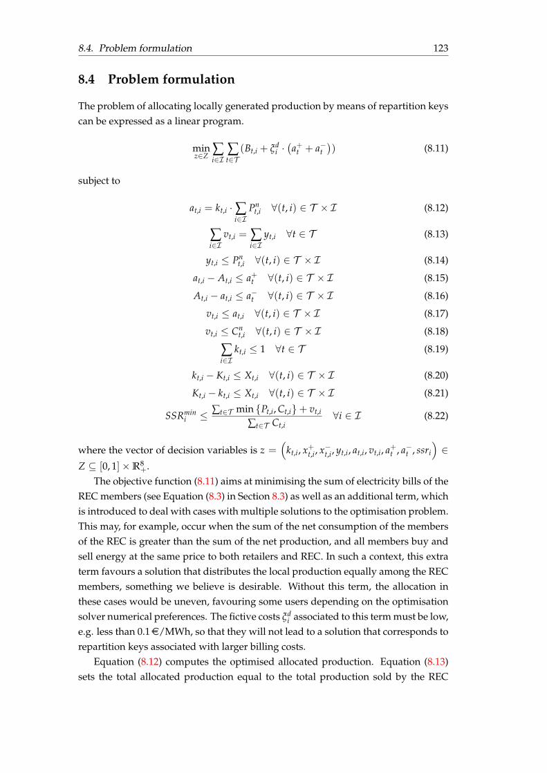
8.4. Problem formulation 123
8.4 Problem formulation
The problem of allocating locally generated production by means of repartition keyscan be expressed as a linear program.
minz∈Z
∑i∈I
∑t∈T
(Bt,i + ξdi ·(a+t + a−t
)) (8.11)
subject to
at,i = kt,i ·∑i∈I
Pnt,i ∀(t, i) ∈ T × I (8.12)
∑i∈I
vt,i = ∑i∈I
yt,i ∀t ∈ T (8.13)
yt,i ≤ Pnt,i ∀(t, i) ∈ T × I (8.14)
at,i − At,i ≤ a+t ∀(t, i) ∈ T × I (8.15)
At,i − at,i ≤ a−t ∀(t, i) ∈ T × I (8.16)
vt,i ≤ at,i ∀(t, i) ∈ T × I (8.17)
vt,i ≤ Cnt,i ∀(t, i) ∈ T × I (8.18)
∑i∈I
kt,i ≤ 1 ∀t ∈ T (8.19)
kt,i − Kt,i ≤ Xt,i ∀(t, i) ∈ T × I (8.20)
Kt,i − kt,i ≤ Xt,i ∀(t, i) ∈ T × I (8.21)
SSRmini ≤ ∑t∈T min Pt,i, Ct,i+ vt,i
∑t∈T Ct,i∀i ∈ I (8.22)
where the vector of decision variables is z =(
kt,i, x+t,i, x−t,i, yt,i, at,i, vt,i, a+t , a−t , ssri
)∈
Z ⊆ [0, 1]×R8+.
The objective function (8.11) aims at minimising the sum of electricity bills of theREC members (see Equation (8.3) in Section 8.3) as well as an additional term, whichis introduced to deal with cases with multiple solutions to the optimisation problem.This may, for example, occur when the sum of the net consumption of the membersof the REC is greater than the sum of the net production, and all members buy andsell energy at the same price to both retailers and REC. In such a context, this extraterm favours a solution that distributes the local production equally among the RECmembers, something we believe is desirable. Without this term, the allocation inthese cases would be uneven, favouring some users depending on the optimisationsolver numerical preferences. The fictive costs ξd
i associated to this term must be low,e.g. less than 0.1e/MWh, so that they will not lead to a solution that corresponds torepartition keys associated with larger billing costs.
Equation (8.12) computes the optimised allocated production. Equation (8.13)sets the total allocated production equal to the total production sold by the REC

124 Chapter 8. How to allocate local generation in renewable energy communities
members. Equation (8.14) limits the production sold to the total available produc-tion. Equations (8.15) and (8.16) compute the positive and negative deviations ofallocated production, respectively. Equations (8.17) and (8.18) limit the verified al-located production to the smaller value between allocated production and demand.Equation (8.19) limits the sum of the repartition keys of the REC members to 100%.Equations (8.20) and (8.21) compute the repartition key deviations. Finally, Equa-tion (8.22) computes the self-sufficiency rate of every member and enforces a min-imum self-sufficiency rate. This last equation may lead to infeasible solutions (byenforcing an unattainable SSRmin
i ), in which case new SSRmini need to be defined by
the ECM.Note that the numerator of Equation (8.22) is a linear form of the numerator of
Equation (8.9). The two versions can be shown to be equivalent. Focusing on thenumerator in Equations (8.9) and (8.22): If Pt,i > Ct,i, the net consumption Cn
t,i isnull, and thereby vt,i = 0 as per Equation (8.18). In this case, the two numeratorsbecome equal to min Pt,i, Ct,i. If Pt,i ≤ Ct,i, the net consumption Cn
t,i is not null,more precisely Cn
t,i ≥ 0, and thereby vt,i ≥ 0. Then, by definition of vt,i:
vt,i ≤ Cnt,i = Ct,i − Pt,i (8.23)
Pt,i + vt,i ≤ Pt,i + Cnt,i = Ct,i. (8.24)
As Pt,i + vt,i ≤ Ct,i, the numerator in Equation (8.9) becomes:
min Pt,i + vt,i, Ct,i = Pt,i + vt,i. (8.25)
which is equal to min Pt,i, Ct,i+ vt,i since Pt,i ≤ Ct,i.
8.5 Results
This section introduces four different test cases as well as a complexity analysis. Thefirst and second test cases illustrate the functioning of the methodology for differ-ent time horizons and number of REC members. The third one elaborates on thepossibility to enforce a minimum SSR for the REC members. The proposed method-ology requires an initial set of repartition keys from which an initial allocation ofproduction is determined. How to compute these initial keys is the subject of de-bate, therefore, the last test case (iv) analyses the impact of using different initialrepartition keys. Furthermore, it also tests the constraint enforcing maximum repar-tition key deviations (Xt,i). In all test cases except for the last one, the initial keysconsist of a pro rata attribution according to each member’s average consumption,as shown in [142, 153]. In addition to the initial keys, a set of price signals is neededfor the optimisation, listed in Table 8.1.

8.5. Results 125
TABLE 8.1: Price signals in e/MWh.
ξbi ξs
i ξ l−i ξ l+
i ξdi
220 60 100 98 1
8.5.1 Test case 1: performance on a simplified example
The first test case provides a simplified example to acquaint the reader with themost important features of the tool. This example features an REC with two pureconsumers (User1 and User2, in red), one pure producer (User3, in green) and oneprosumer (User4, in orange). The optimisation horizon is two metering periods, thefirst one with more production than consumption, and the second with more con-sumption than production. Table 8.2 presents the inputs used for this simulationincluding: (i) consumption which is positive for consumption and negative for pro-duction; (ii) initial keys; and (iii) initial allocated production. Note that the units inthis example are kWh. All these parameters are computed as a pre-process of theoptimisation problem. By comparing the consumption and initial allocated produc-tion in Table 8.2, it can be seen that the initial allocation of production is suboptimal.For metering period one, albeit there is more total production than total consump-tion not all the REC members see their electricity demand met, whereas for meteringperiod two, the distribution of the local production leads to spillage in User4 and tounder-supply in User1 and User2.
TABLE 8.2: Test case 1 – inputs.
Metering period User1 User2 User3 User4
Consumption
2017-03-01 00:00 0.17 0.21 -0.50 0.082017-03-01 00:15 0.21 0.23 -0.30 -0.02
Initial repartition keys
2017-03-01 00:00 0.42 0.49 0.00 0.0892017-03-01 00:15 0.42 0.49 0.00 0.089
Initial allocated production
2017-03-01 00:00 0.21 0.24 0.00 0.042017-03-01 00:15 0.13 0.16 0.00 0.03
This initial situation is then used by the optimisation problem to recompute thekeys. The results of this optimisation are presented in Table 8.3 which lists theconsumption-related and production-related outputs. In this table, an overall re-arrangement of the keys with respect to the initial ones can be observed. At meteringperiod one, the keys for User1 and User2 are decreased, whereas the key of User4 isincreased. Conversely, at metering period two, the inverse flow occurs. The new setof keys leads to an optimal allocation of the production among the REC members by

126 Chapter 8. How to allocate local generation in renewable energy communities
which any deficit of local production is supplied by the retailers, whereas any excessis sold to them.
TABLE 8.3: Test case1 – outputs.
Metering period User1 User2 User3 User4
Optimised repartition keys
2017-03-01 00:00 0.39 0.45 0.00 0.162017-03-01 00:15 0.47 0.53 0.00 0.00
Optimised verified allocated production
2017-03-01 00:00 0.17 0.21 0.00 0.082017-03-01 00:15 0.15 0.17 0.00 0.00
Production sold locally to the REC
2017-03-01 00:00 0.00 0.00 0.46 0.002017-03-01 00:15 0.00 0.00 0.30 0.02
Production sold to the main network
2017-03-01 00:00 0.00 0.00 0.04 0.002017-03-01 00:15 0.00 0.00 0.00 0.00
Additionally, Table 8.3 shows the distribution of local production: local sales (en-ergy delivered to REC members) and global sales (energy sold to the retailer). In thefirst metering period, local sales amount to 0.46, which is the total demand of thesystem. The production surplus (0.04), is sold to the retailer as global sales. In thesecond metering period, local sales are 0.30 + 0.02, which corresponds to the totalavailable production. Since, at this metering period, there is greater demand thansupply, there are no global sales. The maximisation of global sales observed in theseresults depends on the price signals imposed in the simulation. In this case, sincethe selling price is the same for all producers, the optimisation cannot discriminatebetween them when allocating local and global sales, and provides one of the possi-ble solutions. However, this parameter can be adjusted in the optimisation (i.e. oneprice signal per producer), leading to a ranking of producers.
8.5.2 Test case 2: performance on a realistic example
This second analysis introduces a more realistic set-up where an REC with 23 netconsumers and 1 net producer is simulated over one year of operation. Input con-sumption data corresponds to real measurements of small- and medium-volumeelectricity consumers in Belgium. The initial repartition keys fed to the optimisationare based on a proportionality principle of the annual consumption of the memberswith respect to the total accumulated consumption of the REC. The maximum keydeviation Xt,i allowed is not bounded.
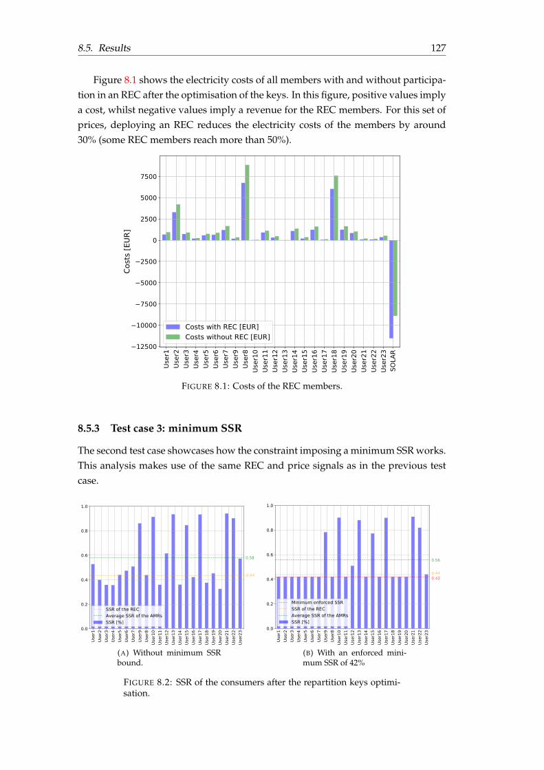
8.5. Results 127
Figure 8.1 shows the electricity costs of all members with and without participa-tion in an REC after the optimisation of the keys. In this figure, positive values implya cost, whilst negative values imply a revenue for the REC members. For this set ofprices, deploying an REC reduces the electricity costs of the members by around30% (some REC members reach more than 50%).
FIGURE 8.1: Costs of the REC members.
8.5.3 Test case 3: minimum SSR
The second test case showcases how the constraint imposing a minimum SSR works.This analysis makes use of the same REC and price signals as in the previous testcase.
(A) Without minimum SSRbound.
(B) With an enforced mini-mum SSR of 42%
FIGURE 8.2: SSR of the consumers after the repartition keys optimi-sation.

128 Chapter 8. How to allocate local generation in renewable energy communities
Figure 8.2 shows the SSR of the members of the REC, after running the optimi-sation with SSRmin
i = 0% and SSRmini = 42%. In this figure when no bound on
the SSRmini is imposed, the SSR of the members ssri is freely selected to minimise
the global costs of the REC. The values of ssri span from 32.5% for User20 to 94.1%for User21 (see Figure 8.2a). As the problem is progressively tightened by enforc-ing more restrictive values of SSRmin
i for all the REC members, a transfer from themembers with highest levels of ssri to those with lower levels takes place. Uponreaching the maximum feasible value of SSRmin
i = 42%, a more uniform ssri for allREC members can be seen (see Figure 8.2b). Note that for this example, enforcingan SSRmin
i greater than 42% leads to an infeasible problem where the system doesnot generate sufficient local electricity to keep increasing it. Tightening the optimi-sation problem may decrease the average SSR of all members, since some membersare forced to give up part of their ssri to increase other members’ SSRs. In this par-ticular example, the consequence is that the average SSR of the all REC members iseroded, decreasing from 58% to 56%. However, the same does not apply to the SSRof the REC, as this SSR only depends on the total local production, and this does notchange by enforcing tighter values of SSRmin
i .Enforcing a minimum SSR has an impact on the electricity costs of the REC
members. Figure 8.3 illustrates the difference in costs caused by the enforcementof SSRmin
i = 42% compared to the case where it is left free (0.0%). This figure showsthat members who are forced to give up their ssri when enforcing an SSRmin
i , incurhigher costs than before enforcing any SSRmin
i and conversely for the others. In par-ticular, the gains of REC members range from 0.25% for User16 to 9.5% for User23,whereas the losses range from −1.5% for User2 to −6.5% for User20.
FIGURE 8.3: Difference in the REC members costs, with and withoutenforcing any minimum SSR of 42%.

8.5. Results 129
8.5.4 Test case 4: impact of initial repartition keys
The last test case presented in this chapter illustrates the impact of employing dif-ferent initial repartition keys. Moreover, it also showcases the functioning of theconstraint imposing a maximum key deviation. In this context, key deviations arerepresented by the difference between optimised and initial repartition keys of eachREC member (kt,i − Kt,i). To perform this analysis, a smaller REC is selected, com-posed of six members: five net consumers (User1 – User5) and one net producer(User6). The simulation horizon is reduced to one month (April) because of the highnumber of runs required to perform the following analyses.
This example tests different types of initial repartition keys:
• Uniform: evenly distributed among the REC members – all members with pos-itive net demand receive the same percentage of the local production.
• Proportional static: Each member obtains a percentage of the local productionwhich is proportional to their average demand over the simulated period –each member receives a different initial key, constant over time.
• Proportional dynamic: Each member obtains a percentage of the available lo-cal production which is proportional to their instantaneous demand – eachmember receives a different initial key per metering period of the simulation.
Table 8.4 lists the total consumption and production of the system and total allo-cated production achieved with the three types of initial keys. With the proportionaldynamic keys, the local production is used up to 76% more than with uniform keys,and 29% more than with proportional static keys.
TABLE 8.4: Allocated production for the different initial keys.
Total demand 37.50 MWhTotal local production 11.35 MWhAllocated production with uniform keys 5.02 MWhAllocated production with proportional static keys 6.85 MWhAllocated production with proportional dynamic keys 8.87 MWh
In the following, the evolution of several parameters over a range of maximumallowed key deviations Xt,i given as parameters, is shown. The allowed deviationsspan from 0%, meaning that the optimised keys cannot deviate from the initial keys,to 100%, meaning that the optimised keys may deviate as much as needed, takingany value in [0, 1]. Since dynamic keys lead to the most optimal distribution betweenlocal and global sales as long as the price ξb
i is the same for all members (i.e., sameretailer contract), the sales do not change for different values of Xt,i when these keysare implemented. For this reason, the different parameter evolutions shown in therest of this section do not contain the impact of using dynamic keys. This also indi-cates that dynamic keys are a suitable solution when no other constraint is required,and purchasing prices ξb
i are similar across REC members.

130 Chapter 8. How to allocate local generation in renewable energy communities
The first of the parameters studied is the spread between local sales (yt,i) andglobal sales (Pn
t,i − yt,i). This spread is strictly positive if local sales are greater thanglobal sales. Figure 8.4 shows that for both sets of initial keys, allowing free keydeviations (Xt,i = 100%) leads to the same spread between local and global sales.However, they differ when Xt,i < 100%. When applying proportional static initialkeys, the spread is always positive and increases with the value of Xt,i. On the otherhand, applying uniform initial keys leads to negative spreads when Xt,i < 5%. Thisanalysis shows that when no limitation on the maximum key deviation is imposed,the optimisation finds the same solution regardless of the initial key. However, whenthis constraint is tight (Xt,i < 100%), the selection of initial keys has a notable impacton the results.
FIGURE 8.4: Total locally sold and globally sold production for arange of maximum key deviations (Xt,i).
The individual costs of the REC members, for a range of Xt,i from 0% to 100%, areshown in Figure 8.5. All net consumers (User1 – User5) see their costs reduced as themaximum key deviation allowed becomes less restrictive. The net producer (User6)electricity revenue increases as the costs of the consumers decrease. In this case,positive values indicate negative costs (or revenue), which increase by the givenpercentage. The variation in member’s costs in response to a relaxation of the max-imum key deviation allowed results in similar trends when using either uniform orproportional static initial keys. The extent of these variations is different though,being one order of magnitude larger for uniform keys. The savings of User1 – User5for uniform keys span from 1% to 8%, whereas for proportional static they span from0.5% to 4%. The increase in gains of User6 is 16% with uniform keys and 8% withstatic keys. These differences prove that uniform initial keys lead to a highly subop-timal solution compared to proportional static ones. This remark highlights the ideathat creating keys that are proportional to the demand of the REC members seemsto be a good practice, which concurs with current practices [153].
A final analysis is presented in Figure 8.6, showing the difference in allocatedlocal production for different initial keys and for a range of maximum allowed key

8.5. Results 131
10
5
0
5
10
15
Cost
evo
lutio
n [%
] Uniform initial keysUser1User2User3User4User5User6
0 1 3 5 10 20 30 50 100Maximum key deviation allowed [%]
10
5
0
5
10
15
Cost
evo
lutio
n [%
] Proportional static initial keysUser1User2User3User4User5User6
FIGURE 8.5: Costs of the members for a range of maximum key devi-ations (Xt,i) relative to the costs when Xt,i = 0.
deviations, relative to the initial situation when no deviation is allowed. In this lastfigure, the effect of relaxing the maximum allowed key deviation is not shown forproportional dynamic keys since, as in Figure 8.5, the changes are negligible. Thetrends followed by the members’ allocated production is similar for uniform andstatic keys. In both cases this trend is upward when relaxing the value of maxi-mum allowed key deviation. However, the extent is different, and the membersinvolved too: while in the uniform keys case the allocated production increases forUser1 and User4 to in excess of 100%, for static keys it only reaches 70% for User3.The difference in these results stems from the different demand profiles of the RECmembers. For User3, the average electricity demand is, on average, lower than forthe rest. Thus, when applying uniform keys, the allocated production is sufficient tocover the demand of this member, since the percentage of allocation is the same forall of them. However, when applying proportional static keys, the initial allocatedproduction given to User3 is low – it depends on average demand (which indeedis relatively low), but it has to cover instantaneous demand (which might be high).For this reason, the initial solution does not provide enough supply to User3 withstatic keys, and therefore the methodology must increase the optimised keys for thisparticular REC member.
8.5.5 Complexity analysis
In the final section of the results, we present an analysis of the complexity of themethodology proposed. The number of constraints of the optimisation is Ncons =
9|T ||U |+ |T |+ |U | and the number of variables Nvar = 17|T ||U |+ 2|T |+ |U |. Table8.5 introduces the running times for different complexities, ranging from 15 dayswith 10 REC members to one month with 100 members. The optimisation problemis implemented with Pyomo in Python 3.8 and solved with the open source solverCBC. Simulations are performed on a GNU/Linux machine with an Intel® Core™i7-8665U and 16 Gb of RAM.

132 Chapter 8. How to allocate local generation in renewable energy communities
0
20
40
60
80
100
Allo
c. p
rod.
[%] Uniform initial keys
User1User2User3User4User5User6
0 1 3 5 10 20 30 50 100Maximum key deviation allowed [%]
0
20
40
60
80
100Al
loc.
pro
d. [%
] Proportional static initial keysUser1User2User3User4User5User6
FIGURE 8.6: Allocated production of the REC members for a rangeof maximum key deviations (Xt,i) relative to the allocated productionwhen Xt,i = 0.
TABLE 8.5: Running times of the proposed algorithm.
|T | |U | Ncons Nvar Build time [s] Solve time [s]
1,440 10 131,050 247,690 5.01 5.962,880 10 262,090 495,370 9.71 12.231,440 50 649,490 1,226,930 20.36 27.722,880 50 1,298,930 2,453,810 43.55 56.551,440 100 1,297,540 2,450,980 39.67 58.932,880 100 2,594,980 4,901,860 85.92 133.93
8.6 Conclusion
This chapter proposes a methodology to deal with the settlement phase of an RECto optimise the sum of electricity bills and to enforce minimum SSRs in some of theREC members – a methodology that is compliant with current regulations and readyto use by an ECM. After physical delivery of electricity, the DSO permits modifyingthe meter readings. This implies that the financial flows of the REC members canbe determined in a settlement phase that changes the meter readings, and that splitsthese flows into two: one directed to the ECM corresponding to electricity consump-tion within the REC; and another sent to the retailers corresponding to the electricityconsumption covered by a traditional retailing process. To modify the meter read-ings, this chapter makes use of repartition keys, which represent the percentage oftotal local production provided to each member. The methodology presented in thischapter computes an ex-post allocation of local production in an REC by using thesekeys. The repartition keys are optimally computed by a linear program that min-imises the sum of individual electricity costs of the REC members, and that mayuse an initial set of keys as starting point. This methodology enables, by adding theright constraints, the control of some parameters such as the self-sufficiency rate ofthe REC members, or the deviations between optimised repartition keys and initial

8.6. Conclusion 133
ones. These keys can be optimally computed based on another set of –initial– keysthat is an input of the simulation.
Various test cases illustrate this methodology, testing the functioning of the opti-misation framework as well as its parameters. Such tests show that this methodol-ogy results in an allocation of local production that leads to lower operational coststhan when no REC is established. Moreover, this approach can be used to enforceminimum self-sufficiency rates on the REC members, enhancing the economic gainsof some of them that might, otherwise, be left without sufficient allocated produc-tion by a traditional global welfare optimisation. Finally, simulation results indicatethat using initial keys consisting of a pro rata attribution of each REC member in-stantaneous consumption is a good practice when the retail electricity price of all ofthem is similar. The methodology presented in this chapter has been tested and iscurrently being implemented by industrial partners in different REC managed bythem.


135
Conclusions and future work


137
Chapter 9
Conclusion
The unstoppable rise of distributed renewable electricity generation resources (DER),driven over the last decades by commercial and regulatory factors (as seen in Chap-ter 1) has brought about several challenges for the adequate functioning of the elec-tricity distribution network. Such challenges can be broadly divided into technicaland regulatory – this thesis has focused on the latter, exploring this type of chal-lenges from a modelling standpoint. In particular, this research has unfolded in twomain directions: (i) the study of regulatory frameworks consisting of the meteringtechnology, the distribution tariff design, and other incentive mechanisms; and (ii)the development of new frameworks for the integration of DER based on decen-tralised electricity markets. Accordingly, this manuscript has been divided in twomain parts that address the two main elements of this research.
9.1 Part I
In the first part of the thesis we have formalised and built a simulation-based ap-proach to assess the impact of a wide range of regulatory frameworks on the penetra-tion of DER and the economic sustainability of the distribution network. Such an ap-proach is based on agent-based modelling where the agents are the final customersof a distribution network and the distribution system operator (DSO). These agentstake actions over a discrete-time dynamical system, making the system evolve.
On the one hand, final customers’ actions consist in deploying DER installationscomposed of solar photovoltaic (PV) panels and/or batteries to reduce their elec-tricity costs. This is controlled through an optimisation framework followed by aninvestment decision process. The optimisation framework is instantiated in the formof a mixed integer linear problem that computes, for each agent, the optimal capac-ity of PV panels (in kWp) and batteries (in kWh) to be deployed to minimise theirlevelised value of electricity (LVOE)1. As for the investment decision process, it com-pares, for every customer the LVOE with the LCOE resulting if no DER installation
1The LVOE is computed as levelised annual costs (electricity imports from the grid) minus revenue(electricity exports to the grid) divided by levelised annual demand. The difference between the LVOEand the more traditional levelised cost of electricity (LCOE) is that whilst the former accounts forcosts and revenue of the prosumers, the latter can only account for costs, therefore not presenting thecomplete picture of the economic benefit of deploying DER installations since it can only show theavoided costs but not the revenue.

138 Chapter 9. Conclusion
is deployed. The result of this comparison is filtered through a Bernoulli distributionthat determines whether the optimally sized DER installation is deployed.
On the other hand, the DSO has the ability to adjust the distribution fee to en-sure its economic sustainability. This is controlled through an accurate modellingof its remuneration strategy, which depends on the regulatory framework. In par-ticular, our approach enables the simulation of two different metering technologies,net-metering and net-billing, as well as four different types of distribution fee whichdepend on energy consumption (volumetric), power consumption (capacity), avail-ability of an access point to the grid (fixed), and time of energy or power consump-tion (ToU). Additionally it is also possible to introduce any combination of thesemetering technologies and fees.
The evaluation of these actions at each time-step of the discrete-time dynam-ical system results in a trajectory of actions from which the evolution of severalvariables can be extracted: DER adoption, PV panel and battery capacities, elec-tricity imports and exports from and to the grid, and distribution tariff. Finally, us-ing this simulation-based approach with different regulatory frameworks facilitatestheir comparison based, on the different set of trajectories they induce. The poten-tial of this approach thus lies in its ability to accurately discriminate between thepossible outcomes of employing distinct regulatory frameworks in order to providesound arguments that underpin the selection of one of them. This tool can serve asguidance for policy makers and regulators to build new combinations of meteringtechnology and distribution tariff design, aiming to achieve certain specific objec-tives (e.g. promoting the adoption of DER). By means of this simulation-based tool,they can compare the strengths and drawbacks of distinct options before applyingthem in real life.
Concerning the design of this tool, the contributions of this thesis are:
• The mathematical formalisation of the simulation-based approach, which en-capsulates the salient features of all the most commonly used metering tech-nologies and distribution tariff designs.
• A computational tool encoding such a mathematical formalisation to help pol-icy makers and regulators design regulatory frameworks.
Furthermore, in the context of this thesis, we have extensively tested this simulation-based approach with a broad range of regulatory frameworks, covering all theirmost common features. Our findings offer insights on the impact of (i) the meteringtechnology, and (ii) the distribution tariff design.
Regarding the metering technology, we observe that regulatory frameworks basedon net-metering provide enormous incentives for potential prosumers to deployDER installations. In particular, this technology highly boosts the adoption of PVinstallations. However, it does not incentivise the deployment of batteries underany distribution tariff design. Furthermore, this large DER deployment comes at ahigh cost: net-metering creates very significant electricity cost differences between

9.2. Part II 139
consumers and prosumers, where consumers bear most of the distribution costs.This leads to substantial cross-subsidies from consumers to prosumers, and jeop-ardises the economic sustainability of the DSO. In addition, this metering technol-ogy may lead to a “death spiral” where the distribution tariff increases dramatically– the DSO looses revenue due to prosumers reduced contributions and must ad-just the tariff upward to compensate (see Figure 1.1). In contrast, employing net-purchasing as metering technology help reduce, though not eliminate, the risks ofcross-subsidisation incurred by net-metering. Moreover, this technology reducespeak power withdrawals and injections, in particular when capacity-based fees areapplied, suggesting that these two elements strongly complement each other. Thissystem may also lead to a “death spiral”, especially if it is associated to a fully volu-metric distribution fee.
As for the distribution tariff design, our results suggest that regulatory frame-works based on volumetric fees (including ToU) offer the best incentive for PV paneland battery deployment. These frameworks, though, lead to the highest inequalitiesbetween consumers and prosumers in terms of electricity costs. When applyingmostly capacity fees, the integration of storage devices is promoted, as these devicescan limit the peak of consumption of prosumers. However, these fees lead (as theprevious ones did) to a cost distribution between consumers and prosumers wherethe former bear most of the network costs. Frameworks based on fixed fees sig-nificantly limit the incentives for DER deployment, therefore they hardly show anyimpact on the distribution of grid costs. Finally, frameworks based on a combinationof these fees lead to various different outcomes which, to a greater or a lesser extent,induce “death spiral” behaviours and the promotion of DER installations.
An overall conclusion of our analysis is that, whilst the regulatory framework inplace plays a major role in the way the distribution network is expected to evolve,all of them lead, to some extent, to an increase in distribution rates as a result of DERdeployment (with the exception of fully fixed fees). This indicates that, consideringcurrent legislations where the DSO is financed through distribution fees to the finalcustomers, a trade-off will always emerge between promoting the adoption of DERtechnologies and containing the distribution rates – one is not possible without theother. Designing holistic policies supporting DER adoption and regulating the elec-tricity distribution network is, therefore, key to facilitate a seamless and sustainableenergy transition.
9.2 Part II
The second part of this thesis has studied new frameworks to promote the inte-gration of DER based on decentralised electricity trading and, in particular, on re-newable energy communities (RECs). According to the latest European regulations,RECs are communities of final customers (consumers or prosumers) who may bene-fit from renewable electricity produced locally. These communities are managed by

140 Chapter 9. Conclusion
a central entity: the REC manager (ECM). Since RECs are a rather new concept, theexisting literature in this topic is scarce. Aiming to fill this gap, we have proposingseveral modelling solutions for RECs, focusing on their economic viability.
The first step toward modelling RECs has been the design of a generic modelof interaction, based on agent-based modelling where the generic agents are: con-sumers and prosumers, retailer and ECM, wholesale market, and transmission sys-tem operator. This approach enables simulating different decentralised electricitymarkets, such as aggregator models or RECs. In addition, our model allows for theintroduction of flexible consumers. Since this is a generic model, it is necessary toadapt it to the desired context by selecting the agents to be used in the simulation.
Once designed, the model of interaction has been instantiated to simulate thescheduling of electricity exchanges within an REC. This instance is built so that theconsumers and prosumers represent the REC members, and the ECM and the re-tailer are the same entity. The ECM is therefore responsible for managing the RECand for its participation in the European day-ahead market, acting as the unique re-tailer of the REC. Flexibility bids are introduced with flexible consumers, and theireconomic impact is assessed by means of a bid acceptance algorithm. This algo-rithm is formulated as an optimisation framework that takes into account forecastsof demand and production within the REC, forecasts of day-ahead prices, and flex-ibility bids from flexible consumers. With these inputs, the optimisation frameworkdetermines the flexibility bids to be accepted by the ECM in order to minimise thecosts of performing the demand provisioning in the day-ahead market. If the bidscan be partially accepted, the optimisation framework can be instantiated as a lin-ear problem. Otherwise it is instantiated as a mixed integer linear problem. A testcase running this minimisation problem shows a significant yearly reduction of totalcosts when an REC is created, compared to the case where the final customers resortto classical retailing contracts. This cost reduction can be attributed to a discount onthe distribution tariff, offered by the DSO when energy is produced and consumedlocally. Furthermore, our analysis suggests that further cost reductions are possi-ble when flexibility bids are introduced in the simulation, owing, mainly, to a bettermatching of supply and demand within the REC.
After studying the scheduling of RECs, where the electricity exchanges are com-puted based on forecasts of demand, production, and electricity prices, we haveanalysed a settlement phase. Due to forecasting errors, the scheduling phase leads,inevitably, to suboptimal solutions. To overcome this problem, we have created anovel algorithm that allocates locally generated electricity among the REC membersin an ex-post phase where the actual production and demand are known. This iswhat we call the settlement phase. This phase takes place after physical delivery ofelectricity and, therefore, the electricity flows cannot be modified at this point. How-ever, since the financial exchanges depend on the meter readings and these can bemodified after physical delivery according to the latest regulations, an algorithm canbe laid out to optimise the financial flows of the REC members. At the core of this

9.3. Limitations and future research 141
algorithm is the concept of repartition keys, which represent the percentage of total lo-cal production allocated to each member. Each REC member is assigned one key permetering period (the resolution of the meter) and thus the production is allocated. Inaddition, an initial set of keys can be assigned, so that the algorithm can re-allocatean initial distribution of local production. The keys are optimised so as to minimisethe sum of individual electricity costs of the REC members. This optimisation isinstantiated in the form of a linear program that, in addition to minimise the elec-tricity costs, can enforce minimum levels of self-sufficiency rates (SSRs) on the RECmembers. This allows for increasing their incentive to participate in the REC since,without a sufficiently high SSR, some REC members may be better-off with classicalretailer contracts. This methodology represents a ready-to-be-used approach whichis compliant with current regulations. We have extensively tested this methodol-ogy, with and without initial repartition keys, demonstrating its ability to lower theoperational costs of a group of consumers, when an REC is established.
In this second part of the thesis we have provided the following contributions:
• A generic model of interaction which employs agent-based modelling to sim-ulate RECs accounting for flexible demand.
• An optimisation framework to control the activation of flexibility, aiming tominimise the sum of electricity costs of the REC members.
• An optimisation framework that optimises the financial flows of REC mem-bers, using the concept of repartition keys.
Assuming that the electricity exchanges within the REC are associated to a lowerprice than the retail tariff, the overall conclusion is that creating an REC to replacetraditional retailing contracts can result in lower electricity costs for the REC mem-bers. If, in addition to a regular REC, flexible consumption is allowed, the electricitycosts of the REC members can be further reduced. Finally, optimising repartitionkeys to determine the allocation of local production after physical delivery is shownto be a practical way of steering clear of forecasting errors whilst minimising elec-tricity costs thanks to the ex-post modification of the meter readings.
9.3 Limitations and future research
The models developed in the context of this research present some limitations. Themost relevant ones are discussed in this section.
Concerning the simulation-based approach presented in the first part of thismanuscript, the investment decision of prosumers is limited to a one-off deploymentof DER installations. This means that, once prosumers deploy a DER installation, ourapproach prevents them from reinvesting, and early adopters cannot expand theirinstallations even if the conditions are favourable. Enabling prosumers to reinvestis a potential improvement of our simulation-based approach. In addition, only a
142 Chapter 9. Conclusion
fixed variety of consumption profiles are considered, which cannot evolve over time.Real customers, nonetheless, are likely to change their consumption patterns by, forinstance, purchasing an electric vehicle, which is currently not considered in our ap-proach. Our approach relies on several parameters that must be precisely tuned inorder to perform real-life simulations, this tuning phase can be challenging since itrequires a substantial amount of data and work. Finally, our simulation-based ap-proach models the distribution network as a zero-sum game where the DSO costsare constant over time. However, certain distribution tariff designs may result in col-lective benefits such as peak power withdrawn or injected reductions that are onlypossible owing to private investments from prosumers. Quantifying these aspects,allowing for evolving DSO costs can potentially extend the scope of analysis.
As for the limitations of our approach to model decentralised electricity marketssuch as RECs, the interaction model created to deal with the scheduling phase ofRECs is designed so that the ECM activates and benefits from flexibility based solelyon energy. However, this approach could be extended by defining capacity prod-ucts. This capacity would be activated depending on the needs – a flexibility bid ofcapacity should include a reservation and an activation cost. In our framework, flex-ibility bids offered by flexible consumers are independent from the actual needs ofthe ECM, and flexible consumers post these bids based on their own consumption.An alternative option could be for the ECM to notify flexible consumers of a flexibil-ity need, and only then would they post flexibility bids. Moreover, the schedulingphase of the REC only takes into account one market floor: the day-ahead market.An additional optimisation step, closer to physical delivery, might further reduce theelectricity costs of the REC due to improved forecasts. As for the settlement, whenthis phase is simulated, our approach does not consider the real time control of theelectricity exchanges, only using the final consumption and production profiles ofthe REC members. A mixed approach where both electricity (through a control al-gorithm) and financial exchanges (through the algorithm presented in this thesis)are optimised may help reduce the electricity costs of the REC. Finally, electricitycharges based on peak power consumption that better reflect the costs of withdraw-ing electricity from the distribution network might be included in this phase. Thesecharges can help reduce not only the REC costs, but also relieve potential congestionin the distribution network.
In addition to these limitations and potential for improvement, some additionalresearch directions can be considered. Modelling the physical constraints inducedby the integration of DER, such as over-voltages, may provide a broader view of thelimits of our approach. In addition, considering the option of changing the topologyof the network, aiming to model future investments in infrastructure depending onthe DER penetration, can help better evaluate the DSO costs. Finally, restrictions onthe imports and exports of prosumers might be introduced. These restrictions mayrepresent some of the physical limits of the installations, offering a more realisticscenario which potentially deteriorates the business case of prosumers.

143
Appendix


145
Appendix A
A multi-agent system approach tomodel the interaction betweendistributed generation deploymentand the grid
This paper introduces a multi-agent dynamical system of the interaction betweenelectricity consumers, the electricity distribution system operator, and the technolog-ical (generation, storage) and regulatory (tariff design, incentive schemes) environ-ments. For any type of environment, our dynamical system simulates the evolutionof the deployment of distributed electricity generation, as well as the evolution ofthe cost of distribution. The system relies on the assumption that individual electric-ity consumers behave statistically as rational agents, who may invest in optimiseddistributed renewable energy installations, if they are cost-efficient compared to theretail electricity tariff. The deployment of these installations induces a change in theaggregated net consumption and generation of the users of a distribution network.By modelling the cost recovery mechanism of the distribution system operator, thesystem simulates the evolution of the retail electricity tariff in response to such achange in the aggregated consumption and production.
A.1 Introduction
The integration of distributed electricity generation technologies (DRE), such as so-lar photovoltaic panels (PV), into the distribution networks (DN) has been madepossible by the use of incentive schemes, as these technologies used to be less eco-nomically competitive than conventional ones [154]. The inclusion of a sizeableamount of DRE installations, nonetheless, may cause severe strain on the distribu-tion systems, since they are not engineered to absorb large amounts of distributedgeneration (DG) [86]. The nature of the strain imposed on the system can be multi-faceted, and may stem from technical problems such as over-voltages in the low volt-age distribution system [25], or regulatory problems including the over-compensation
146Appendix A. A multi-agent system approach to model the interaction between
distributed generation deployment and the grid
of DRE owners and the potential failure of the cost recovery mechanisms of the dis-tribution system operators (DSO) [36].
In our work, we aim at creating a methodology for testing the impact of any reg-ulatory and technological environments on the deployment of DRE installations andon the distribution component of the retail electricity tariff (simply distribution tarifffrom now on). The methodology we describe in this paper is based on a multi-agentdiscrete-time dynamical system formalisation, in which the agents interact with anenvironment. On the one hand, the agents of such a system are the DRE owners,the non-DRE owners, and a (unique) DSO. On the other hand, the environment (theDN), is composed of a set of rules including the aforementioned incentive schemes,the tariff design of the DN (e.g. volumetric tariffs or capacity tariffs), and the cost ofdistributed generation and storage technologies.
The purpose of this paper is to describe and test this methodology. In particular,our main contributions are the following:
• We provide a description of our multi-agent discrete-time dynamical systemformalisation, used to simulate the evolution of an electricity distribution sys-tem by modelling the interactions of individual agents (DRE owners, non-DREowners, and DSO), with the environment. This is presented in the Methodol-ogy section.
• We introduce a test case in which we compare different incentive schemes. Inparticular we compare two distinct compensation mechanisms (net-meteringand net-purchasing) as described in [33]. This is explained in detail in the TestCase section.
A.2 Methodology
In this section we elaborate on the modelling of our multi-agent discrete-time dy-namical system. The purpose of such a system is to evaluate, over a given timehorizon, and for any environment,
1. the impact of the environment on the rate of adoption of DRE installations;and
2. the impact of the penetration of a significant amount of DRE installations onthe distribution tariff.
The result of the first evaluation impacts the second one, which in turn also influ-ences the first evaluation at the subsequent time step, through a feedback mecha-nism.
In the proposed approach, electricity consumers, interacting with a unique DN,are modelled as rational agents that may invest in optimally sized grid-tied DREinstallations if these are cost-efficient compared to the retail electricity tariff. More-over, the distribution tariff is adapted according to the evolution of DRE generation

A.2. Methodology 147
within the DN. In this framework, three distinct components defining the behaviourof the agents: (i) the optimisation of DRE units, (ii) the investment decision process, and(iii) the computation of the distribution tariff. As a reminder, the agents are the DSOand the users of the DN. There are two distinct groups of users: group A which de-notes the users who may deploy a DRE installation, and group B, which comprisesthe users who cannot invest in a DRE installation due to technical or economic con-straints. The latter is therefore left out of the two first components (optimisation andinvestment decision), since these two, as discussed below, assign the optimal sizingconfiguration and the investment decision on DRE installations.
Our multi-agent discrete-time dynamical system works as follows. At the initial-isation of the system, we assume zero installed DRE capacity for all users. Then, atevery time-step, and assuming a tariff design based on volumes of energy traded, thesystem updates the proportion of consumers who have deployed a DRE installation,as well as the distribution tariff. The detailed work flow of the model is representedby a data flow diagram in Figure A.1, and the full description of this multi-agent sys-tem, including the code, can be found in [155]. The three components are describedin the following.
A.2.1 Optimisation of DRE units
As represented in Figure A.1, all potential DRE installations (group A) are optimisedfollowing the first component of the multi-agent system. Assuming that the storagedynamics and the investment costs of the DRE can be described by linear mappings,we formalise this optimisation problem as a linear program (LP). The inputs of thisLP comprise the consumption and the potential production profiles of each individ-ual agent, as well as several parameters that are user-independent (i.e. the same forall the users). These parameters are the prices of PV and battery, the retail electricitytariff at every time-step, and the efficiency, the depth of discharge and the lifetime ofthe batteries. The potential DRE installations are optimised so as to minimise theirlevelised cost of electricity (LCOE). Thus, the resolution of this optimisation prob-lem outputs the optimal sizing configuration (PV and battery capacities) that leadsto a minimised LCOE, as well as the LCOE, which is the objective function. We use astandard definition of the LCOE in this model: the average total cost to deploy andoperate a DRE installation, divided by the total energy consumed by the user overthe project lifetime. The LCOE is formulated according to equation (A.1):
LCOE =
i0 + ∑Y−1y=0
ξy
(1 + r)y
∑Y−1y=0
dy
(1 + r)y
(A.1)
where the capex are represented by i0, the yearly opex at year y are ξy, the yearlydemand at year y is defined as dy, and r represents the discount rate. Finally, thelifetime of the DRE installations (i.e. the optimisation horizon of this LP) is set to Y

148Appendix A. A multi-agent system approach to model the interaction between
distributed generation deployment and the grid
years. Note that this horizon is not the same as the horizon over which the evolutionof the multi-agent discrete-time dynamical system is studied.
A.2.2 Investment decision process
This component is used to decide, for each individual agent in group A, whether todeploy a DRE installation with the optimised sizing configuration indicated by theDRE optimisation. To model such a decision making process, we make use of a priceratio between the optimised LCOE of each agent, and the retail electricity tariff at ev-ery time-step of the dynamical system. Such a price ratio, denoted by Γ, will adopta value in [0, 1], since the LCOE of the DRE installations cannot be greater than theretail electricity tariff due to optimality constraints (since the DRE installations aregrid-tied, the feasible region of the optimisation problem is upper bounded by the re-tail electricity tariff). Then, by using a Bernoulli distribution in which the probabilityp is a linear function of the computed Γ, the investment decision can be controlledby a random variable β drawn from the distribution B (1, p), where β ∈ 0, 1 bydefinition of the Bernoulli distribution. According to such a linear function, low val-ues of Γ (i.e. when the LCOE of the optimised DRE unit is of reduced proportionscompared to the retail tariff) result in high probability p of drawing a variable β = 1,which indicates a positive investment decision. Similarly, when Γ is high, the prob-ability of drawing a variable β = 0 will be high, suggesting a negative investmentdecision for the agent. Finally, when all of the possible investment decisions havebeen computed for all of the individual agents, those agents whose investment deci-sion is positive are prevented from investing in the subsequent time-steps. Hence, inour simulator, the possibility of expanding an installation after its initial deploymentis not permitted.
Modelling the investment decision-making process in such fashion ensures thedeployment of some DRE units even when the viability of the DRE installations lie atthe economically feasible limit (for instance when the PV prices are high or the retailelectricity tariff is low), representing the behaviour of those users who are eager toinvest. Likewise, this investment decision-making mechanism will prevent someagents from investing even under favourable conditions, representing those agentsmore reluctant to invest.
A.2.3 Computation of the distribution tariff
Finally, in our multi-agent system, an overall demand reduction in the DN mightoccur as a result of the progressive deployment of DRE units, which self-consumepart of their electricity needs. Assuming that the revenues obtained by the DSO arecomputed as a monotonically non-decreasing function of the energy charged to theusers, this overall demand reduction will cause a loss in revenue, inducing a needfor adjusting the distribution tariff to offset the losses.

A.3. Test Case 149
To adjust the distribution tariff, the following inputs are required: the net con-sumption of all the agents of the DN (groups A and B), and the retail electricity tariffat every time-step of the dynamical system. Then, we represent the cost recoveryscheme of the DSO at every time-step by computing the potential economic imbal-ances created by the DRE installations deployed within the DN. If the revenue ofthe DSO at a particular time t does not match its incurred costs (assumed constantover the simulation horizon), an economic imbalance appears (which can be posi-tive or negative). Thus, the adjustment of the distribution tariff must account forboth the potential imbalance and the gradual aggregated net demand reduction inthe system, this is calculated according to equation (A.2):
Π(dis)t+1 =
C + ∆t
Dt+1∀t ∈ 1, . . . , T (A.2)
where Π(dis)t+1 is the distribution tariff of the next period, C are the incurred costs of
the DSO, ∆t represents the imbalance between costs and revenues at period t, andDt+1 is the expected aggregated demand (kWh) of the next period.
A.3 Test Case
To illustrate the functioning of our multi-agent system, an example inspired by thecurrent regulation policy in the Walloon region of Belgium is presented in this sec-tion. Hence, a tariff design based on volumes of energy traded (paid in e/kWh) isconsidered. Moreover, to test different environments, we use three distinct incentiveschemes, based on the choice of compensation mechanism (the manner electricitytraded between the DRE and the grid is recorded). The compensation mechanismsconsidered are: (a) net-metering (NM): this system consists of one meter that recordsimports (DRE← Grid) by running forwards, and exports (DRE→ Grid) by runningbackwards, therefore, this means that both directions are assigned with the samemonetary value, namely the retail electricity tariff; and (b) net-purchasing (NP): thisoption consists of two independent meters for imports and exports, in this settingimports are paid for at retail electricity tariff, and exports are paid at a selling price(SP). With NM the total exports are upper bounded by the total imports, however,with NP there is no upper limit. The three evaluated cases are: (i) NM, (ii) NPSP=0.04e, and (iii) NP SP=0.08e. In the three cases the retail electricity tariff isinitially set to 0.22e.
At every time-step of the multi-agent system simulation, we keep track of thedeployed DRE units, and of the distribution tariff adjustment. Thus, we can computethe evolution of the system in terms of rate of DRE deployment and distributiontariff evolution. The results of the testing of the multi-agent system with the threedifferent environments are summarised in Figure A.2.

150Appendix A. A multi-agent system approach to model the interaction between
distributed generation deployment and the grid
FIGURE A.1: Data flow diagram of the proposed multi-agent system.The flow of actions occurs from top to bottom. The individual usersof group A, characterised by their load, undergo an optimisation. Theoptimisation requires the technology costs, the tariff design, and theretail electricity tariff, as well as the user load. The individual resultsof the optimisation are used by the investment decision model, whichcompares the LCOE of the individually optimised installations withthe retail tariff, yielding a positive or negative investment decisionfor each potential installation. Finally, the revenues derived from theaggregated net consumption of all users of group A and of group Bare compared with the (fixed) DSO costs, and the distribution cost isupdated.
This figure depicts the two metrics considered: evolution of distribution tariff(left axis) and evolution of DRE deployment (right axis), for the three cases. Regard-ing the distribution tariff, we observe a similar 0.02e increase for cases (i) and (ii)after 10 years, due to the loss of revenue of the DSO in both cases, derived from

A.3. Test Case 151
FIGURE A.2: Evolution of the distribution tariff (left axis) and evolu-tion of DRE deployment (right axis). The deployment of DRE unitsinduces an increase in the distribution tariff. Such an increase fea-tures a different extent depending on the environment (composed oftariff design, incentive scheme, and technology cost).
the DRE deployment. This indicates that both cases are more inefficient distributingthe DSO costs than case (iii). As for the DRE deployment, we can observe a greaterdeployment for cases (i) and (iii) both in the trend and in the final outcome after thesimulated period, than for case (ii). This suggests that case (ii) is outperformed interms of DRE deployment fostering by cases (i) and (iii). These distinct behaviourscan be explained, case by case, by the optimal solution identified by the optimisationof DRE units component of the multi-agent discrete-time dynamical system:
• Case (i): with this environment, it results optimal to import and export thesame volume of electricity so that the electricity bill is reduced (netting 0 kWhconsumed). This leads to installations without batteries (since storage and gridare perfect substitutes). Eventually with this setting the DRE owners will notcompensate the DSO for their grid use.
• Case (ii): with this environment, imports must be reduced to decrease thebill, leading to highly autonomous installations (large PV + battery capacities).Eventually with this setting the DRE units will become completely indepen-dent.
• Case (iii): by increasing the SP with respect to the previous case, the DRE own-ers business case is to become electricity producers, selling it to offset theirelectricity bills. This leads to installations with large PV capacites as well assome storage. With this setting the DRE owners still pay the DSO for their griduse, since they rely on it during periods with low PV production.

152Appendix A. A multi-agent system approach to model the interaction between
distributed generation deployment and the grid
A.4 Conclusion
This paper has presented a multi-agent discrete-time dynamical system to describethe interaction between the distribution networks and the consumers. In such asystem: (i) electricity consumers interacting with a single distribution network aremodelled as rational agents that may invest in optimised distributed renewable en-ergy installations; and (ii) the distribution tariff is adapted according to the evolutionof the DSO’s revenues, depending on the distributed renewable energy that is pro-duced and consumed in the distribution network.
To illustrate the performance of the multi-agent system, we have designed andsimulated three different scenarios, starting with the current regulation in the Wal-loon region of Belgium, and further exploring other incentive schemes. The simu-lator allows to illustrate the impact of the regulation policies on many aspects: (i)the evolution of the electricity distribution tariff, and with it, the evolution of theretail electricity tariff; (ii) the evolution of DRE deployment; and (iii) the optimisedconfigurations of distributed renewable energy installations in terms of productionand storage capacities.

153
Appendix B
Exploring Regulation Policies inDistribution Networks through aMulti-Agent Simulator
This paper presents a multi-agent simulator that describes the interactions betweenthe agents of a distribution network (DN), and an environment. The agents are theusers of the DN and the electricity distribution system operator. The environmentis the set of rules (tariff design, technology costs, or incentive schemes) that impactsthe agents interactions. For a given environment, we can simulate the evolutionof the agents and the environment itself. We assume the electricity consumers arerational agents that may deploy distributed renewable energy installations if theyare cost-efficient compared to the retail electricity tariff. The deployment of suchinstallations may alter the cost recovery scheme of the distribution system operator,by inducing a change in the way the user use of the grid. By modelling the costrecovery mechanism of the distribution system operator, the system simulates theevolution of the retail electricity tariff in response to such a change in the aggregatedconsumption and production.
B.1 Introduction
Over the last few decades, proactive policy making has supported a major paradigmshift in the power generation sector, resulting in a progressive energy transition fromfossil fuels to renewable energy sources [156]. Such an energy transition is shapingthe future of the electricity system: in this context, numerous incentive mechanismsare fostering a notable integration of distributed renewable electricity (DRE) gen-eration technologies, such as solar photovoltaic panels (PV), into the distributionnetworks (DN). However, those incentive mechanisms might have been used with-out the adequate understanding of the underlying problems they may entail: sinceDN are not engineered to absorb large amounts of distributed electricity generation[86], the inclusion of a vast volume of DRE may cause severe technical problems [25].Additionally, regulatory problems may appear also as a result of DRE adoption [36].In our work we focus on the latter, which range from the over-compensation of DRE

154Appendix B. Exploring Regulation Policies in Distribution Networks through a
Multi-Agent Simulator
owners to the potential failure of the cost recovery mechanisms of the distributionsystem operators (DSO) [33].
This paper aims at presenting a methodology for assessing the potential regu-latory problems stemming from a set of regulation rules (including the incentivemechanisms) that stimulates a heavy DRE adoption. Thus, with this methodologywe may take any set of regulation rules as inputs, and compute their impact on aDN. Such an impact is measured with two metrics: (i) the evolution of the retailelectricity price (simply retail price from now on) over time, and (ii) the evolution ofthe proportion of DRE-owners and non-DRE owners in the DN over time. The set ofrules that drives these evolutions is known as an environment, and consists of threeelements, as explained in [42]:
• tariff design: this consists of the type of charges applied to the customers fortheir grid use (e.g. volumetric tariffs, or capacity tariffs);
• technology costs evolution: this includes the prices for generation and storagetechnologies; and
• incentive mechanism: this is the combination of technologies and/or supportschemes that help DRE become economically competitive, (e.g. a monetaryaid awarded to the DRE owners over the lifetime of the DRE).
To simulate the impact of a given environment on a DN, we need to introduce a setof agents who will interact with it, over a finite time horizon. There are three typesof agents:
• DRE owners: users of the DN that own a DRE installation (also known as pro-sumers);
• non-DRE owners: users of the DN that do not own a DRE installation (alsoknown as consumers); and
• distribution system operator (DSO): operator of the DN.
As a result of the agents interactions with the environment, the DN will evolve ina dynamical system. At every time step of this system, the two mentioned metricswill be computed, enabling the observation of such an evolution.
The methodology presented in this paper is based on a multi-agent discrete-timedynamical system formalisation that models the interactions of a some agents withan environment, and computes the resulting evolution of the DN. From this evolu-tion, we may compare different environments. Our main contributions are:
• We provide a description of our multi-agent discrete-time dynamical systemformalisation. Such a formalisation allows us to test different environments,in particular we introduce (i) two tariff designs, and (ii) two incentive mecha-nisms. This is detailed in Section B.2.
• We show the simulator functioning by testing different environments. This ispresented in Section B.4.

B.2. Methodology 155
B.2 Methodology
In our multi-agent discrete-time dynamical system, we model the electricity users asrational agents who are —in principle— exposed to retail prices, and that may investin optimally sized DRE installations, provided that these are cost-efficient comparedto the retail price. As a result of users deploying DRE installations, the DSO costrecovery mechanism may be altered, inducing a change in the distribution compo-nent of the retail price (distribution tariff from now on) for the subsequent time-stepof the dynamical system. These two effects (DRE adoption and distribution tariffevolution), are computed at every time-step of a discrete-time dynamical system inwhich the interactions of the agents with the environment will drive the evolution ofthe DN. Thus, in this methodology we: (A) start by explaining how the interactionsbetween the agents and the environment occur, (B) elaborating then on the differentintroduced environments, and (C) and finalising by providing a description of theagents modelling.
B.2.1 Interactions
The interactions between the agents and the environment are computed at everytime-step of our dynamical system. These interactions depend on the nature of theagent, namely:
• the DRE owners interact by trading electricity with the DN. These trades occurin the form of imports: DN→ user, and/or exports: DN← user;
• the non-DRE owners interact also by trading electricity with the DN. In thiscase these trades occur only in the form of imports: DN→ user.
• the DSO interacts by computing a distribution tariff that allows it to break-even.
Through these interactions, the agents incur costs and collect revenues. The relationbetween costs and revenues will drive the evolution of the DN. Computing theseinteractions, at every time-step, involves calculating: (1) the yearly electricity costsof the users, (2) the yearly electricity revenues of the users (if any), and (3) the newdistribution tariff determined by the DSO according to its cost recovery mechanism.These calculations depend on the environments, which are defined next.
B.2.2 Environments
In the presented multi-agent system, we introduce a number of options to build anenvironment:Depending on the tariff design:
• a1 - Volumetric: electricity trades are paid for/collected according to volumesof energy [e/kWh].

156Appendix B. Exploring Regulation Policies in Distribution Networks through a
Multi-Agent Simulator
• a2 - Volumetric and capacity: two terms, the first one is volumetric [e/kWh],and the second one is based on a fixed charge per capacity contracted by theuser [e/kWp].
Depending on the technology costs:
• b1 - Linearly decreasing trend over time.
Depending on the incentive mechanism: in particular we focus on the compensationmechanism. By compensation mechanism we refer to the manner the electricitytrades between the users and the DN are recorded [73]. We consider two distinctcompensation mechanisms, as described in [33]:
• c1 - Net-metering (NM): system consisting of one meter that records the im-ports by running forwards, and the exports by running backwards, this entailsthat both directions be assigned with the same monetary value, namely theretail tariff. Furthermore, the total exports are upper bounded by the total im-ports for a determined billing period, per user.
• c2 - Net-purchasing (NP): system consisting of two separate meters for theimports and the exports respectively, this implies that the imports are paid forat retail tariff, whereas the exports are paid at a selling price.
Constructing an environment necessitates choosing one element per option. Con-sequently, with these settings we can create four different families of environments:
• e1 = a1+b1+c1
• e2 = a1+b1+c2
• e3 = a2+b1+c1
• e4 = a2+b1+c2
Each of these families depends on the retail price, the capacity price, and/or theselling price. Consequently, it is possible to create any number of environments bysetting different values of these three prices.
The three calculations introduced in subsection B.2.1 (costs of the users, revenuesof the users, and cost recovery mechanism of the DSO) depend on the family ofenvironments. LetN = 1, . . . , N denote the set with the time-steps of our discrete-time dynamical system. And let I = 1, . . . , I denote the users of the DN.
Family of environments e1 the electricity costs of the users are computed accord-ing to equation (B.1). The revenues of the users are φi,n = 0 for this environment,since under net-metering the produced electricity is not sold to the grid. Finally the

B.2. Methodology 157
DSO computation of the new distribution tariff for the following time-step is com-puted according to equation (B.2).
ψi,n = max
0,(
ρ(−)i,n − ρ
(+)i,n
)·Π(in)
n
∀i, n ∈ I ×N (B.1)
Π(dis)n =
Ω(d)n + ∆(d)
n−1
Dn∀n ∈ N (B.2)
with ∆(d)n−1 = R(d)
n − R(d)n , where R(d)
n are the actual measured revenues, and R(d)n are
the expected revenues computed (before the period) according to equation (B.3).
R(d)n = Π(dis)
n ·I
∑i=1
ρ(−)i,n ∀n ∈ N (B.3)
Family of environments e2 the electricity costs and the revenues of the users arecomputed according to equations (B.4) and (B.5) respectively. The DSO computationof the following distribution tariff is performed as in environment e1 (see equations(B.2) and (B.3)).
ψi,n = ρ(−)i,n ·Π
(in)n ∀i, n ∈ I ×N (B.4)
φi,n = ρ(+)i,n ·Π
(sp)n ∀i, n ∈ I ×N (B.5)
Family of environments e3 the electricity costs of the users are computed by meansof equation (B.6). The users revenues are φi,n = 0 (same rationale as before). TheDSO computation of the distribution tariff follows equation (B.7). Furthermore, inthis case there is a capacity tariff which the DSO may adjust at every time-step (seeequation (B.8)).
ψi,n =max
0,(
ρ(−)i,n − ρ
(+)i,n
)·Π(in)
n
+ Π(cap)
n
∀i, n ∈ I ×N(B.6)
Π(dis)n =
Ω(d)n + ∆(d)
n−1
Dn∀n ∈ N (B.7)
Π(cap)n =
Ω(c)n + ∆(c)
n−1
Cn∀n ∈ N (B.8)
with ∆(c)n−1 = R(c)
n − R(c)n and ∆(d)
n−1 = R(d)n − R(d)
n , where R(c)n and R(d)
n are measuredonce the period is completed, R(c)
n is determined by means of equation (B.9), andR(d)
n is computed as in the family of environments e1 (see equation (B.3)).
R(c)n = Π(cap)
n · I ∀n ∈ N (B.9)

158Appendix B. Exploring Regulation Policies in Distribution Networks through a
Multi-Agent Simulator
Family of environments e4 the electricity costs of the users are computed withequation (B.10). The revenues of the users are computed as in the family of environ-ments e2 (equation (B.5)). The distribution tariff is computed as in environment e3(see equations (B.3), (B.7), (B.8), and (B.9)).
ψi,n =(
ρ(−)i,n ·Π
(in)n
)+ Π(cap)
n ∀i, n ∈ I ×N (B.10)
TABLE B.1: Notation
ρ(−)i,n total imports of user i at period n
ρ(+)i,n total exports of user i at period n
ψi,n electricity costs of user i at period nφi,n revenues of user i at period nΩ
(d)n costs of the DSO (volumetric) at period n
Ω(c)n costs of the DSO (capacity) at period n
∆(d)n−1 imbalance of the DSO (volumetric) of period n− 1
∆(c)n−1 imbalance of the DSO (capacity) of period n− 1
R(d)n expected revenues of the DSO (volumetric) at period n
R(c)n expected revenues of the DSO (capacity) at period n
R(d)n actual revenues of the DSO (volumetric) at period n
R(c)n actual revenues of the DSO (capacity) at period n
Dn expected demand of the users at period nCn expected peak demand of the users at period nΠ(sp)
n users selling price at period nΠ(cap)
n capacity price at period nΠ(in)
n retail price at period n *
Π(dis)n distribution tariff at period n *
λn costs of energy, transmission, and taxes *
* The relation between Π(in)n and Π(dis)
n follows this equation: Π(in)n = Π(dis)
n +λn ∀n ∈ N .
All of the presented equations depend on different parameters: ρ(−)i,n , ρ
(+)i,n , Ω
(d)n ,
Ω(c)n , Dn, and Cn. These parameters are computed when modelling the agents of the
system. The other parameters in table B.1 (Π(sp)n , and λn) are inputs of the model.
The rest of table B.1 are variables whose computations have been presented in thissection (ψi,n, φi,n, ∆(d)
n−1, ∆(c)n−1, R(d)
n , R(c)n , and Π(in)
n ).
B.2.3 Agents of the system
Once we have introduced the different environments, and how the interactions withthese occur, we can describe how the agents are modelled. In our system we havethree types of agents: DRE owners, non-DRE owners, and DSO. The first two are theusers of the DN, whereas the third one is the operator of the DN.

B.2. Methodology 159
DRE owners
these users are modelled relying on an optimisation framework instantiated in theform of a linear program (LP). This LP minimises the levelised cost of electricity(LCOE) of the DRE installation. The LCOE is the average total cost to deploy andoperate a DRE installation, divided by the total energy consumed by the user overthe project lifetime. With this LP we can extract, at every time-step, the values ofρ(−)i,n and ρ
(+)i,n . The LP formalisation is presented in the next section (Section B.3).
non-DRE owners
at the initialisation of the system, we assume zero installed DRE capacity for allthe users (i.e. all users are non-DRE owners). Then at every time-step, the systemupdates the proportion of users who have deployed a DRE installation. Thus, wedefine two groups of non-DRE owners: group A: denoting the users who may deploya DRE installation, and group B: comprising the users who cannot invest in a DREinstallation due to technical or economic constraints. We model these two groupsdifferently:
Group A we resort to the same LP we use to model the DRE owners. However,in this case we use it to extract the LCOE of the potential DRE installation a user ofthis group could deploy. By comparing this LCOE with the retail price, a gradient-like driver is created: if the LCOE is lower than the retail price, the user will havea probability p > 0 of actually deploying the DRE installation that leads to such anLCOE. Once a user from group A deploys a DRE installation, it is modelled as aDRE owner until the end of the simulation. If a user group A does not deploy a DREinstallation at a particular time-step, it is modelled in the same fashion as group Busers, for this particular time-step. However, at the subsequent time-steps, this userwill have a new opportunity of deploying a DRE installation.
Group B we compute the yearly electricity demand of every user, which is coveredentirely by the DN.
DSO
the last of the agents is modelled by computing, at every time-step, its cost recoverymechanism, as introduced previously. Then, the DSO will calculate a new distribu-tion tariff for the subsequent time-step that allows it to break-even. To compute thiscost recovery mechanism, the following parameters are required: Ω
(d)n , Ω
(c)n , Dn, and
Cn.
Ω(d)n costs of the DSO related with the volume of energy distributed to the users of
the grid. At the initialisation of the system, we assume a balanced system where thecosts of the DSO are fully recovered by its revenue. Thus, we assume the initial costs

160Appendix B. Exploring Regulation Policies in Distribution Networks through a
Multi-Agent Simulator
equal to the initial revenues (aggregated demand of all users times the distributiontariff). At every time step the revenues may decrease due to the DRE deployment.Hence, we measure the total actual revenues of the DSO (R(d)
n ). Assuming that thecost recovery mechanism recovers all the previous economic imbalances, we usethese revenues as costs of the DSO for the subsequent time-step (R(d)
n−1 = Ω(d)n ).
Ω(c)n costs of the DSO related with the capacity required by the users of the grid.
Similarly to the previous case, we assume a balanced initial state where the costsof the DSO are fully recovered by its revenue. Thus, we assume the initial costsequal to the initial revenues (aggregated capacity fees of the users). At every timestep, the DRE deployment may cause the fees to vary, altering the actual revenuesfrom capacity fees (R(c)
n ). These revenues are used as DSO costs for the subsequenttime-step (R(c)
n−1 = Ω(c)n ).
Dn expected volume of energy distributed at every time-step. It is computed be-fore the initialisation of the period, and corresponds to the last observed aggregateddemand (Dn−1) of the users, thus Dn−1 = Dn. Hence, this does not take into accountthe DRE installations that may have been deployed from n− 1 to n.
Cn expected aggregated peak demand of the users at every time-step. As in theprevious case, it is computed before the initialisation of the period, and correspondsto the last observed aggregated peak demand (Cn−1) of the users, thus Cn−1 = Cn.The DRE installations potentially deployed at the previous period are not taken intoaccount.
B.3 LP Formalisation
In this section we formalise the optimisation framework in the form of an LP, usedto model the DRE owners and the group A of the non-DRE owners. On the onehand, the DRE owners are modelled to compute their electricity trades, which wereintroduced in the previous section as imports and exports. On the other hand, thenon-DRE owners of group A are modelled to determine their minimised LCOE, ob-tained for an optimally sized DRE installation.
The optimisation horizon is set to Y ∈ N years which are divided into 8760time-steps (Y × 8760). Let T = 0, . . . , T − 1, with T = 8760, represent a timediscretisation of one year (in hours). Moreover let Y = 0, . . . , Y − 1, representthe years of the optimisation. All of the parameters and variables presented in thissection depend on N . Furthermore, this LP runs for every individual user in set I .
Let χ represent the investment costs as a linear function of technology prices andsizing configuration. These costs are computed according to the following equation:
χ = p · P(pv) +YB· b · P(bat) (B.11)

B.3. LP Formalisation 161
where p represents the optimal PV size in kWp, b is the optimal battery size in kWh,P(pv) and P(bat) are the technology prices (PV and battery respectively), and B islifetime of the battery.
The yearly costs of operation are represented by ξy, and computed by means ofthe following equation.
ξy = µy + my + ζy ∀y ∈ Y (B.12)
where µy are the yearly electricity costs, my represents the yearly costs of operationand maintenance, and ζy stands for the recovered costs. The electricity costs dependon the family of environments: for family e1 we use equation (B.13), for e2 we useequation (B.14), for e3 we use equation (B.15), and for the family of environments e4we make use of equation (B.16):
µy = max
0,
T−1
∑t=0
(ρ(−)t − ρ
(+)t
)·Π(in)
∀y ∈ Y (B.13)
µy =T−1
∑t=0
ρ(−)t ·Π(in) ∀y ∈ Y (B.14)
µy =max
0,
T−1
∑t=0
(ρ(−)t − ρ
(+)t
)·Π(in)
+ Π(cap)
∀y ∈ Y(B.15)
µy =
(T−1
∑t=0
ρ(−)t ·Π(in)
)+ Π(cap) ∀y ∈ Y (B.16)
where ρ(−)t are the hourly imports, and ρ
(+)t represents the hourly exports. Π(in)
and Π(cap) are the retail and the capacity price. These prices are fixed across theentire LP horizon, and correspond to the nth prices determined by the discrete-timedynamical system. The operation and maintenance costs my are computed accordingto equation (B.17) [97].
my =1
200· p +
1100· b ∀y ∈ Y (B.17)
Finally, the recovered costs are also environment dependent. In light of this, fami-lies of environments e1 and e3 have ζy = 0, whereas for families e2 and e4 we useequation (B.18).
ζy = −(
T
∑t=1
ρ(+)t ·Π(sp)
)∀y ∈ Y (B.18)
The energy balance of the system depends on the imports ρ(−)t , exports ρ
(+)t ,
the electricity produced by the PV array kt, the hourly demand U(d)t , the maximum
hourly production U(p)t , the energy flow into the battery j(−)t , the energy flow out of
162Appendix B. Exploring Regulation Policies in Distribution Networks through a
Multi-Agent Simulator
the battery j(+)t , the efficiency of charge ηc and discharge ηd the batteries, and the
depth of discharge of the batteries dod. The energy flows into and out of the batteryalso depend on the variation of the state of charge (soc) between t− 1 and t. Thus,the following equations control the energy balance, taking into account the state ofcharge of the batteries:
ρ(+)t − ρ
(−)t = kt −U(d)
t − j(−)t + j(+)t ∀t ∈ T , (B.19)
with:
kt = p ·U(p)t ∀t ∈ T (B.20)
j(−)t ≤ b · F(−) ∀t ∈ T (B.21)
j(+)t ≤ b · F(+) ∀t ∈ T (B.22)
b · dod ≤ soct ≤ b ∀t ∈ T (B.23)
soct =
soct−1 −j(+)t
η(d)+ j(−)t · η(c) ∀t ∈ T \ 0
soc0 ∈ [b · dod, b] for t = 0(B.24)
Finally, let LCOE denote the general objective function that represents the lev-elised cost of electricity. This objective function is minimised in this optimisation.
LCOE =
i0 + ∑Y−1y=0
ξy
(1 + r)y
∑Y−1y=0
dy
(1 + r)y
(B.25)
where the yearly demand of the system is defined as dy = ∑T−1t=0 U(d)
t , and r repre-sents the discount rate.
B.4 Test case
To illustrate our multi-agent discrete-time dynamical system, an example is pre-sented. In this example, we simulate one environment of each family of environ-ments. Thus, we create four environments, according to the four described families:
• Env. A: corresponds to the family of environments e1. We propose a volumetrictariff with a compensation mechanism consisting of net-metering. In this case,the distribution tariff is initially set to Π(dis)
0 = 0.09e/kWh.
• Env. B: corresponds to the family of environments e2. This case is based on avolumetric tariff with a compensation mechanism consisting of net-purchasing.As in the previous case, the distribution tariff is initially set to Π(dis)
0 = 0.09e/kWh.The selling price is fixed to Π(sp)
n = 0.08e/kWh (constant over the simulation).

B.4. Test case 163
• Env. C: corresponds to the family of environments e3. We create this casewith a distribution tariff with two components: volume and capacity. The firstcomponent represented with a volumetric fee conveyed to the users by meansa distribution tariff which is initially set to Π(dis)
0 = 0.045e/kWh. The secondcomponent is a capacity fee, set initially to Π(cap)
0 = 223e for installations upto 10 kWp, this term will not evolve in our simulation, since we do not let theusers adjust their peak demand.
• Env. D: corresponds to the family of environments e4. As in the previous case,there are two terms. The capacity term is the same as case C (Π(cap)
0 = 223e forinstallations up to 10 kWp which cannot evolve in our simulations). The dis-tribution tariff term is initially set to Π(dis)
0 = 0.045e/kWh. Furthermore, theselling price is fixed to Π(sp)
n = 0.08e/kWh.
The value of λn is fixed to 0.13e/kWh for all cases. The technology costs areinitially set to P(pv) = 1500e/kWp and P(bat) = 300e/kWh; they are assumed toevenly decrease at every period n by 0.07%. The optimisation horizon Y is set to 20years. The efficiencies are set fixed to η(c) = 0.95 and η(d) = 0.95. Finally the dod isfixed to 10%.
At the initialisation of the system, all the users are non-DRE owners. Hence,to represent every agent in the proposed multi-agent tool, the model includes twogroups of medium size residential users (peak demand of around 3 kW). Group A:modelling the heterogeneity of DN users involves the representation of every useras an individual agent. To introduce them in the simulation, the multi-agent modelnecessitates their electricity demand profile and their production profile. In the anal-ysed test case, we create different synthetic demand profiles with the help of theCREST model [98]. As for the production profile, we count on real PV measure-ments expressed in kW/kWp. Group B: the remaining customers of the DN must bemodelled only in terms of net energy off-take.
At every time-step of the multi-agent system simulation, we keep track of thedeployed DRE units, as well as of the distribution tariff adjustment. Thus, we candetermine the evolution of the deployed capacities of PV and battery. Moreover, it ispossible to compute the evolution of the distribution tariff for each case. Two figuresdepict the two metrics considered: the evolution of DRE deployment and optimalsize: Figure B.1; and the evolution of the distribution tariff: Figure B.2, for the fourdistinct environments.
Regarding the size of the installations, we observe two different behaviours ofthe four environments:
• A and C do not deploy batteries, these two environments rely on NM as in-centive mechanism, therefore not deploying batteries since, with this system,batteries and imports are perfect substitutes. Since there is no incentive to sellelectricity (see equations (B.13) and (B.15)), the PV capacity is adjusted to sim-ply cover their peak demand.

164Appendix B. Exploring Regulation Policies in Distribution Networks through a
Multi-Agent Simulator
FIGURE B.1: Cumulative PV and battery capacities of the deployedDRE, over the presented discrete-time dynamical system. The eco-nomically optimal size of the deployed DRE installations is influ-enced in a large extent by the environment. In this figure, we observethese different users behaviours under four distinct environments.
• B and D deploy some batteries to become more self-sufficient, reducing theimports. PV deployment results 2.5 times larger than in the other two envi-ronments, since there exists an incentive to sell electricity (see equations (B.14)and (B.16)). The difference between B and D lies in the fixed capacity term,which makes difficult the recovery of the installation costs for case D.
Regarding the distribution tariff, the upper sub-figure in Figure B.2 indicates thatintroducing a capacity term (Env. C and D) will considerably reduce the effect ofan increasing distribution tariff, induced by the DRE deployment. However, wheninspecting the lower sub-figure in Figure B.2 (change in distribution tariff relativeto the initial state), we can observe that the increase in the distribution tariff occurspredominantly in those environments with NM as incentive mechanism (Env. A andC), demonstrating the unfitness of this compensation mechanism to cope with DREdeployment.
B.5 Conclusion
This paper has presented a multi-agent simulator to describe the interaction betweendistribution networks and consumers, for any regulatory technical environment. Inthis system, electricity consumers interacting with a single distribution network are

B.5. Conclusion 165
FIGURE B.2: Evolution of the distribution tariff. The deployment ofDRE units induces an increase in the distribution tariff. Such an in-crease features a different extent depending on the environment.
modelled as rational agents that may invest in optimised distributed renewable en-ergy installations. The distribution tariff is adapted according to cost recovery mech-anism of the DSO (must break-even), that depends on the distributed renewableenergy that is produced and consumed in the distribution network.
To illustrate the performance of the multi-agent system, we have designed andsimulated four different examples based on the four families of environments intro-duced in this paper. The simulator allows to illustrate the impact of the regulationpolicies on many aspects: (i) the evolution of the electricity distribution tariff; (ii) theevolution of DRE deployment; and (iii) the optimised configurations of distributedrenewable energy installations (production and storage capacities).
Preliminary results show a more volatile distribution tariff when net-meteringis chosen as incentive mechanism, as a result of the deployment of distributed re-newable energy units. This remains true also when a capacity term is added to thedistribution costs. These results can be further explored in a future work, by scalingup the simulator introducing a larger user diversity.


167
Bibliography
[1] United Nations Framework Convention on Climate Change (UNFCCC). Adop-tion of the Paris Agreement – Report No. FCCC/CP/2015/L.9/Rev.1. 2015. URL:http://unfccc.int/resource/docs/2015/cop21/eng/l09r01.pdf.
[2] Joeri Rogelj et al. “Paris Agreement climate proposals need a boost to keepwarming well below 2 C”. In: Nature 534.7609 (2016), pp. 631–639.
[3] Mike Hulme. “1.5 C and climate research after the Paris Agreement”. In: Na-ture Climate Change 6.3 (2016), pp. 222–224.
[4] Reto Knutti et al. “A scientific critique of the two-degree climate change tar-get”. In: Nature Geoscience 9.1 (2016), p. 13.
[5] Jorgen Randers and Ulrich Goluke. “An earth system model shows self-sustainedmelting of permafrost even if all man-made GHG emissions stop in 2020”. In:Scientific Reports 10.1 (2020), pp. 1–9.
[6] Intergovernmental Panel on Climate Change (IPCC). URL: https://www.ipcc.ch/.
[7] Valérie Masson-Delmotte et al. Global Warming of 1.5 OC: An IPCC Special Re-port on the Impacts of Global Warming of 1.5° C Above Pre-industrial Levels andRelated Global Greenhouse Gas Emission Pathways, in the Context of Strengthen-ing the Global Response to the Threat of Climate Change, Sustainable Development,and Efforts to Eradicate Poverty. World Meteorological Organization Geneva,Switzerland, 2018.
[8] European Commission. “Energy Union Package: A Framework Strategy fora Resilient Energy Union with a Forward-Looking Climate Change Policy”.In: Communication from the commission to the European parliament, the council,the European Economic and social committee, the committee of the regions and theEuropean Investment bank. Energy Union (2015).
[9] European Commission. “Clean energy for all Europeans”. In: European Com-mission Publications (2019).
[10] European Commission. “Directive 2009/28/EC of the European Parliamentand of the Council of 23 April 2009”. In: Official Journal of the European Union(2009). URL: https://eur-lex.europa.eu/legal-content/EN/TXT/PDF/?uri=OJ:L:2009:140:FULL&from=EN.

168 Bibliography
[11] European Commission. “Directive 2018/2001 of the European Parliamentand of the Council of 11 December 2018”. In: Official Journal of the EuropeanUnion (2018). URL: https://eur-lex.europa.eu/legal-content/EN/TXT/PDF/?uri=OJ:L:2018:328:FULL&from=EN.
[12] ENTSO-E & ENTSOG. Ten-Year Network Development Plan (TYNDP) 2020. 2020.URL: https://www.entsos-tyndp2020-scenarios.eu/wp-content/uploads/2020/06/TYNDP_2020_Joint_ScenarioReport_final.pdf.
[13] ENTSO-E & ENTSOG. Ten-Year Network Development Plan (TYNDP) 2020. 2020.URL: https://www.entsos-tyndp2020-scenarios.eu/wp-content/uploads/2020/06/TYNDP_2020_Scenario_Building_Guidelines_Final_Report.pdf.
[14] Amory B Lovins. “Energy strategy: the road not taken”. In: Foreign Aff. 55(1976), p. 65.
[15] Fred C Schweppe. “Power systems2000’: hierarchical control strategies”. In:IEEE spectrum 15.7 (1978), pp. 42–47.
[16] Nicholas Jenkins. “Embedded generation”. In: Power engineering journal 9.3(1995), pp. 145–150.
[17] N Jenkins. “Embedded generation. Part 2”. In: Power Engineering Journal 10.5(1996), pp. 233–239.
[18] Thomas Ackermann, Göran Andersson, and Lennart Söder. “Distributed gen-eration: a definition”. In: Electric power systems research 57.3 (2001), pp. 195–204.
[19] Ann Chambers, Barry Schnoor, and Stephanie Hamilton. Distributed genera-tion: a nontechnical guide. PennWell Books, 2001.
[20] Guido Pepermans et al. “Distributed generation: definition, benefits and is-sues”. In: Energy policy 33.6 (2005), pp. 787–798.
[21] Johan Driesen and Ronnie Belmans. “Distributed generation: challenges andpossible solutions”. In: 2006 IEEE Power Engineering Society General Meeting.IEEE. 2006, 8–pp.
[22] K Purchala et al. “Distributed generation and the grid integration issues”. In:KULeuven, Imperial College London (2006), p. 9.
[23] Robert Lasseter et al. Integration of distributed energy resources. The CERTS Mi-crogrid Concept. Tech. rep. Lawrence Berkeley National Lab.(LBNL), Berkeley,CA (United States), 2002.
[24] Danny Pudjianto, Charlotte Ramsay, and Goran Strbac. “Virtual power plantand system integration of distributed energy resources”. In: IET Renewablepower generation 1.1 (2007), pp. 10–16.
[25] JA Pecas Lopes et al. “Integrating distributed generation into electric powersystems: A review of drivers, challenges and opportunities”. In: Electric powersystems research 77.9 (2007), pp. 1189–1203.

Bibliography 169
[26] F. Olivier. “Solutions for Integrating Photovoltaic Panels Into Low-voltageDistribution Networks”. PhD thesis. 2018.
[27] Math HJ Bollen and Fainan Hassan. Integration of distributed generation in thepower system. Vol. 80. John wiley & sons, 2011.
[28] Ignacio Pérez-Arriaga, Christopher Knittel, et al. “Utility of the future”. In:(2016).
[29] Peter Dondi et al. “Network integration of distributed power generation”. In:Journal of power sources 106.1-2 (2002), pp. 1–9.
[30] Miguel Manuel de Villena et al. “Modelling and assessing the impact of theDSO remuneration strategy on its interaction with electricity users”. In: In-ternational Journal of Electrical Power & Energy Systems 126 (2021), p. 106585.
[31] Tim Schittekatte, Ilan Momber, and Leonardo Meeus. “Future-proof tariff de-sign: recovering sunk grid costs in a world where consumers are pushingback”. In: Energy Economics 70 (2018), pp. 484–498.
[32] Tim Schittekatte and Leonardo Meeus. “Least-cost distribution network tariffdesign in theory and practice”. In: The Energy Journal 41 (2020).
[33] Axel Gautier, Julien Jacqmin, and Jean-Christophe Poudou. “The prosumersand the grid”. In: Journal of Regulatory Economics 53.1 (2018), pp. 100–126.
[34] Kenneth W Costello and Ross C Hemphill. “Electric utilities’‘death spiral’:hyperbole or reality?” In: The Electricity Journal 27.10 (2014), pp. 7–26.
[35] Paul Simshauser. “Distribution network prices and solar PV: Resolving rateinstability and wealth transfers through demand tariffs”. In: Energy Economics54 (2016), pp. 108–122.
[36] R. Cossent, T. Gómez, and P. Frías. “Towards a future with large penetrationof distributed generation: Is the current regulation of electricity distributionready? Regulatory recommendations under a European perspective”. In: En-ergy Policy 37.3 (2009), pp. 1145–1155.
[37] Cherrelle Eid et al. “The economic effect of electricity net-metering with so-lar PV: Consequences for network cost recovery, cross subsidies and policyobjectives”. In: Energy Policy 75 (2014), pp. 244–254.
[38] Carlos Mateo et al. “Impact of solar PV self-consumption policies on distri-bution networks and regulatory implications”. In: Solar Energy 176 (2018),pp. 62–72.
[39] Laura Antonia Faerber, Nazmiye Balta-Ozkan, and Peter M Connor. “Innova-tive network pricing to support the transition to a smart grid in a low-carboneconomy”. In: Energy Policy 116 (2018), pp. 210–219.
[40] Ricardo Prata and Pedro MS Carvalho. “Self-supply and regulated tariffs: Dy-namic equilibria between photovoltaic market evolution and rate structuresto ensure network sustainability”. In: Utilities Policy 50 (2018), pp. 111–123.

170 Bibliography
[41] Cédric Clastres et al. “Cross subsidies across electricity network users fromrenewable self-consumption”. In: Utilities Policy 59 (2019), p. 100925.
[42] Miguel Manuel de Villena Millan et al. “A multi-agent system approach tomodel the interaction between distributed generation deployment and thegrid”. In: CIRED Workshop Ljubljana. AIM, 2018.
[43] Miguel Manuel de Villena et al. “Evaluating the Evolution of DistributionNetworks under Different Regulatory Frameworks with Multi-Agent Mod-elling”. In: Energies 12.7 (2019), p. 1203.
[44] Miguel Manuel de Villena et al. “Network tariffs and the integration of pro-sumers: The case of Wallonia”. In: Energy Policy 150 (2021), p. 112065.
[45] Sébastien Mathieu et al. “Harnessing the flexibility of energy managementsystems: a retailer perspective”. In: 2019 IEEE Milan PowerTech. IEEE. 2019,pp. 1–6.
[46] Miguel Manuel de Villena et al. “A Framework to Integrate Flexibility Bidsinto Energy Communities to Improve Self-Consumption”. In: 2020 IEEE Gen-eral Meeting. IEEE. 2020, pp. 1–5.
[47] Tiago Sousa et al. “Peer-to-peer and community-based markets: A compre-hensive review”. In: Renewable and Sustainable Energy Reviews 104 (2019), pp. 367–378.
[48] Wayes Tushar et al. “Transforming energy networks via peer-to-peer energytrading: The potential of game-theoretic approaches”. In: IEEE Signal Process-ing Magazine 35.4 (2018), pp. 90–111.
[49] Ulf JJ Hahnel et al. “Becoming prosumer: Revealing trading preferences anddecision-making strategies in peer-to-peer energy communities”. In: EnergyPolicy 137 (2020), p. 111098.
[50] Fabio Moret and Pierre Pinson. “Energy collectives: a community and fair-ness based approach to future electricity markets”. In: IEEE Transactions onPower Systems 34.5 (2018), pp. 3994–4004.
[51] Bertrand Cornélusse et al. “A community microgrid architecture with an in-ternal local market”. In: Applied Energy 242 (2019), pp. 547–560.
[52] Miguel Manuel de Villena et al. “Allocation of locally generated electricity inrenewable energy communities”. In: arXiv preprint arXiv:2009.05411 (2020).
[53] Miguel Manuel de Villena Millan et al. “Exploring Regulation Policies inDistribution Networks through a Multi-Agent Simulator”. In: Proceedings ofYRS2018 (2018).
[54] “Study on the effective integration of demand energy recourses for providingflexibility to the electricity system”. In: Final report to The European CommissionApril (2015), p. 179.

Bibliography 171
[55] Chiara Candelise, Mark Winskel, and Robert JK Gross. “The dynamics of so-lar PV costs and prices as a challenge for technology forecasting”. In: Renew-able and Sustainable Energy Reviews 26 (2013), pp. 96–107.
[56] Johannes Jargstorf and Ronnie Belmans. “Multi-objective low voltage gridtariff setting”. In: IET Generation, Transmission & Distribution 9.15 (2015), pp. 2328–2336.
[57] J Román et al. “Regulation of distribution network business”. In: IEEE Trans-actions on Power delivery 14.2 (1999), pp. 662–669.
[58] G Alan Comnes. “Review of Performance-Based Ratemaking Plans for USGas Distribution Companies”. In: (1994). URL: https://cloudfront.escholarship.org/dist/prd/content/qt0pm4731k/qt0pm4731k.pdf.
[59] Philip P Barker and Robert W De Mello. “Determining the impact of dis-tributed generation on power systems. I. Radial distribution systems”. In:Power Engineering Society Summer Meeting, 2000. IEEE. Vol. 3. IEEE. 2000,pp. 1645–1656.
[60] Thomas Ackermann, Goran Andersson, and Lennart Soder. “Electricity mar-ket regulations and their impact on distributed generation”. In: Electric UtilityDeregulation and Restructuring and Power Technologies, 2000. Proceedings. DRPT2000. International Conference on. IEEE. 2000, pp. 608–613.
[61] Javier Reneses and María Pía Rodríguez Ortega. “Distribution pricing: theo-retical principles and practical approaches”. In: IET Generation, Transmission& Distribution 8.10 (2014), pp. 1645–1655.
[62] Council of European Energy Regulators. Electricity Distribution Network Tar-iffsCEER Guidelines of Good Practice. Tech. rep. 2017. URL: https://www.ceer.eu/documents/104400/-/-/1bdc6307-7f9a-c6de-6950-f19873959413.
[63] Maria Pia Rodriguez Ortega et al. “Distribution network tariffs: A closedquestion?” In: Energy Policy 36.5 (2008), pp. 1712–1725.
[64] Ignacio J Pérez-Arriaga, Jesse D Jenkins, Carlos Batlle, et al. “A regulatoryframework for an evolving electricity sector: Highlights of the MIT utility ofthe future study”. In: Economics of Energy & Environmental Policy 6.1 (2017),pp. 71–92.
[65] DG Energy for the European Commission. Study on tariff design for distributionsystems. Tech. rep. 2015. URL: https://ec.europa.eu/energy/sites/ener/files/documents/20150313%20Tariff%20report%20fina_revREF-E.PDF.
[66] J De Joode et al. “Increasing penetration of renewable and distributed elec-tricity generation and the need for different network regulation”. In: EnergyPolicy 37.8 (2009), pp. 2907–2915.
172 Bibliography
[67] P Frías et al. “Improvements in current European network regulation to fa-cilitate the integration of distributed generation”. In: International Journal ofElectrical Power & Energy Systems 31.9 (2009), pp. 445–451.
[68] Angela Picciariello et al. “Distributed generation and distribution pricing:Why do we need new tariff design methodologies?” In: Electric power systemsresearch 119 (2015), pp. 370–376.
[69] Paul M Sotkiewicz and J Mario Vignolo. “Towards a cost causation-based tar-iff for distribution networks with DG”. In: IEEE Transactions on Power Systems22.3 (2007), pp. 1051–1060.
[70] Alezeia González and T Gomez. “Use of system tariffs for distributed gener-ators”. In: 16th Power Systems Computation Conference. 2008.
[71] Georgios Christoforidis et al. “A model for the assessment of different net-metering policies”. In: Energies 9.4 (2016), p. 262.
[72] Nicholas D Laws et al. “On the utility death spiral and the impact of utilityrate structures on the adoption of residential solar photovoltaics and energystorage”. In: Applied energy 185 (2017), pp. 627–641.
[73] Naïm R Darghouth, Galen Barbose, and Ryan H Wiser. “Customer-economicsof residential photovoltaic systems (Part 1): The impact of high renewableenergy penetrations on electricity bill savings with net metering”. In: EnergyPolicy 67 (2014), pp. 290–300.
[74] Naïm R Darghouth et al. “Net metering and market feedback loops: Explor-ing the impact of retail rate design on distributed PV deployment”. In: AppliedEnergy 162 (2016), pp. 713–722.
[75] Axel Gautier and Julien Jacqmin. “PV adoption: the role of distribution tariffsunder net metering”. In: Journal of Regulatory Economics 57.1 (2020), pp. 53–73.
[76] Jonathan A Lesser and Xuejuan Su. “Design of an economically efficient feed-in tariff structure for renewable energy development”. In: Energy policy 36.3(2008), pp. 981–990.
[77] Andri Pyrgou, Angeliki Kylili, and Paris A Fokaides. “The future of the Feed-in Tariff (FiT) scheme in Europe: The case of photovoltaics”. In: Energy Policy95 (2016), pp. 94–102.
[78] Ramteen Sioshansi. “Retail electricity tariff and mechanism design to incen-tivize distributed renewable generation”. In: Energy Policy 95 (2016), pp. 498–508.
[79] Yoshihiro Yamamoto. “Pricing electricity from residential photovoltaic sys-tems: A comparison of feed-in tariffs, net metering, and net purchase andsale”. In: Solar Energy 86.9 (2012), pp. 2678–2685.

Bibliography 173
[80] Gilbert Fridgen et al. “One rate does not fit all: An empirical analysis ofelectricity tariffs for residential microgrids”. In: Applied Energy 210 (2018),pp. 800–814.
[81] Yilun Shang. “Hybrid consensus for averager–copier–voter networks withnon-rational agents”. In: Chaos, Solitons & Fractals 110 (2018), pp. 244–251.
[82] Ibtihal Abdelmotteleb et al. “Designing efficient distribution network chargesin the context of active customers”. In: Applied Energy 210 (2018), pp. 815–826.
[83] M. Manuel de Villena et al. “Exploring Regulation Policies in DistributionNetworks through a Multi-Agent Simulator”. In: Proceedings YRS. 2018. URL:http://hdl.handle.net/2268/223745.
[84] Sven Teske. Achieving the Paris climate agreement goals. Springer, 2019.
[85] Andreas Goldthau. “Rethinking the governance of energy infrastructure: Scale,decentralization and polycentrism”. In: Energy Research & Social Science 1 (2014),pp. 134–140.
[86] D. Connolly, H. Lund, and B.V. Mathiesen. “Smart Energy Europe: The tech-nical and economic impact of one potential 100% renewable energy scenariofor the European Union”. In: Renewable and Sustainable Energy Reviews 60(2016), pp. 1634–1653.
[87] L Lu and C Waddams Price. Designing distribution network tariffs that are fairfor different consumer groups. Tech. rep. University of East Anglia, Centre forCompetition Policy, UK, 2018.
[88] T Brown, A Faruqui, and N Lessem. Electricity Distribution Network Tariffs:Principles and analysis of options. Tech. rep. 2018.
[89] Council of European Energy Regulators. “Electricity Distribution NetworkTariffs – CEER Guidelines of Good Practice”. In: C16-DS-27-03 (2017).
[90] Mohammad Ansarin et al. “The economic consequences of electricity tariffdesign in a renewable energy era”. In: Applied Energy 275 (2020), p. 115317.
[91] Martin de Montigny et al. “Multiagent stochastic simulation of minute-to-minute grid operations and control to integrate wind generation under ACpower flow constraints”. In: IEEE Transactions on Sustainable Energy 4.3 (2013),pp. 619–629.
[92] Dániel Divényi and András M Dán. “Agent-based modeling of distributedgeneration in power system control”. In: IEEE Transactions on Sustainable En-ergy 4.4 (2013), pp. 886–893.
[93] Yalin Huang and Lennart Söder. “Assessing the impact of incentive regula-tion on distribution network investment considering distributed generationintegration”. In: International Journal of Electrical Power & Energy Systems 89(2017), pp. 126–135.
174 Bibliography
[94] Pierluigi Siano. “Assessing the impact of incentive regulation for innova-tion on RES integration”. In: IEEE Transactions on Power Systems 29.5 (2014),pp. 2499–2508.
[95] Merkebu Z Degefa et al. “MAS-based modeling of active distribution net-work: the simulation of emerging behaviors”. In: IEEE Transactions on SmartGrid 7.6 (2016), pp. 2615–2623.
[96] Angela Picciariello, Karin Alvehag, and Lennart Söder. “Impact of networkregulation on the incentive for DG integration for the DSO: opportunitiesfor a transition toward a smart grid”. In: IEEE Transactions on Smart Grid 6.4(2015), pp. 1730–1739.
[97] Sylvain Quoilin et al. “Quantifying self-consumption linked to solar homebattery systems: Statistical analysis and economic assessment”. In: AppliedEnergy 182 (2016), pp. 58–67.
[98] NREL. CREST Cost of Energy Models. URL: https://financere.nrel.gov/finance/content/crest-cost-energy-models.
[99] Joshua S Stein. “The photovoltaic performance modeling collaborative (PVPMC)”.In: 2012 38th IEEE Photovoltaic Specialists Conference. IEEE. 2012, pp. 003048–003052.
[100] Cajsa Bartusch et al. “Introducing a demand-based electricity distribution tar-iff in the residential sector: Demand response and customer perception”. In:Energy Policy 39.9 (2011), pp. 5008–5025.
[101] Nicolas Boccard and Axel Gautier. “Le coût de l’énergie verte en Wallonie,2003-2012”. In: Reflets et perspectives de la vie économique 54.1 (2015), pp. 71–85.
[102] Agency for the Cooperation of Energy Regulators (ACER) and Council ofEuropean Energy Regulators (CEER). ACER Market Monitoring Report 2018 –Electricity and Gas Retail Markets Volume. Tech. rep. 2018.
[103] Service Public de Wallonie. Décret modifiant les décrets du 12 avril 2001 relatifl’organisation du marché régional de l’électricité et du 19 janvier 2017 relatif à laméthodologie tarifaire applicable aux gestionnaires de réseau de distribution de gazet d’ électricité en vue du déploiement des compteurs intelligents et de la flexibilité.Tech. rep. 2018.
[104] Vlaamse Regulator van de Elektriciteits-en Gasmarkt (VREG. Tariefmethod-ologie voor distributie elektriciteit en aardgas gedurende de reguleringsperiode 2021-2024. Tech. rep. 2020.
[105] Merla Kubli. “Squaring the sunny circle? On balancing distributive justice ofpower grid costs and incentives for solar prosumers”. In: Energy Policy 114(2018), pp. 173–188.

Bibliography 175
[106] David P Brown and David EM Sappington. “Designing compensation fordistributed solar generation: Is net metering ever optimal?” In: The EnergyJournal 38.3 (2017).
[107] International Energy Agency Photovoltaic Power Systems Programme (IEA-PVPS). Net metering and PV self-consumption in emerging countries. Tech. rep.2018.
[108] Monica Castaneda et al. “Myths and facts of the utility death spiral”. In: En-ergy Policy 110 (2017), pp. 105–116.
[109] Sharon Young, Anna Bruce, and Iain MacGill. “Potential impacts of residen-tial PV and battery storage on Australia’s electricity networks under differenttariffs”. In: Energy policy 128 (2019), pp. 616–627.
[110] Nigel Martin and John Rice. “Solar Feed-In Tariffs: Examining fair and rea-sonable retail rates using cost avoidance estimates”. In: Energy Policy 112(2018), pp. 19–28.
[111] Sinan Küfeoglu and Michael G Pollitt. “The impact of PVs and EVs on domes-tic electricity network charges: A case study from Great Britain”. In: Energypolicy 127 (2019), pp. 412–424.
[112] Claudia Günther, Wolf-Peter Schill, and Alexander Zerrahn. “Prosumage ofsolar electricity: tariff design, capacity investments, and power system ef-fects”. In: arXiv preprint arXiv:1907.09855 (2019).
[113] Commission wallonne pour l’énergie (CWaPE. L’analyse des prix de l’électricitéet du gaz naturel en Wallonie (clients résidentiels sur la période de janvier 2007 àjuin 2019. Tech. rep. 2020.
[114] Commission wallonne pour l’énergie (CWaPE. Tarif prosumer. Tech. rep. 2019.URL: https://www.cwape.be/docs/?doc=3098.
[115] Olivier De Groote and Frank Verboven. “Subsidies and time discounting innew technology adoption: Evidence from solar photovoltaic systems”. In:American Economic Review 109.6 (2019), pp. 2137–72.
[116] Scott P Burger et al. “The efficiency and distributional effects of alternativeresidential electricity rate designs”. In: The Energy Journal 41.1 (2020).
[117] European Commission. Study on tariff design for distribution systems. Tech. rep.2015.
[118] Robert Passey et al. “Designing more cost reflective electricity network tariffswith demand charges”. In: Energy Policy 109 (2017), pp. 642–649.
[119] Axel Gautier et al. “Self-consumption choice of residential PV owners undernet-metering”. In: Energy Policy 127 (2018), pp. 647–653.
[120] K Stum, R Mosier, and T Haasl. “Energy Management Systems-a PracticalGuide”. In: Portland Energy Conservation Inc.(PECI), USA (1997), p. 116.

176 Bibliography
[121] Rim Missaoui et al. “Managing energy smart homes according to energyprices: analysis of a building energy management system”. In: Energy andBuildings 71 (2014), pp. 155–167.
[122] Bertrand Cornélusse et al. “Efficient management of a connected microgrid inBelgium”. In: CIRED-Open Access Proceedings Journal 2017.1 (2017), pp. 1729–1732.
[123] Sébastien Mathieu. “Flexibility services in the electrical system”. PhD thesis.University of Liège, Belgium, 2016.
[124] Ricardo J Bessa and Manuel A Matos. “Economic and technical managementof an aggregation agent for electric vehicles: a literature survey”. In: Europeantransactions on electrical power 22.3 (2012), pp. 334–350.
[125] José Villar, Ricardo Bessa, and Manuel Matos. “Flexibility products and mar-kets: Literature review”. In: Electric Power Systems Research 154 (2018), pp. 329–340.
[126] A Losi et al. “ADDRESS Recommendations for standard committees, regula-tors, stakeholders groups, future R&D”. In: Brussels, Belgium (2013).
[127] Bridge Horizon 2020. Bridge Business Models Working Group, Second Report:Business Models Issues. Apr. 2018. URL: https://www.h2020-bridge.eu.
[128] FLEXICIENCY. Deliverable D2.1: Definition of services and use cases description.Jan. 2016.
[129] JKAHPJ Kok. “The powermatcher: Smart coordination for the smart electric-ity grid”. In: (2013).
[130] Emeline Georges et al. “Residential heat pump as flexible load for direct con-trol service with parametrized duration and rebound effect”. In: Applied En-ergy 187 (2017), pp. 140–153.
[131] RTE. Règles pour la valorisation des effacements de consommation sur les marchésde l’énergie NEBEF 3.1. 2018.
[132] ELIA. Règles organisant le Transfert d’énergie. 2018.
[133] Miguel Luis Delgado Heleno. “Provision of advanced ancillary services throughdemand side integration”. In: (2016).
[134] Jonathan A Schachter and Pierluigi Mancarella. “Demand response contractsas real options: a probabilistic evaluation framework under short-term andlong-term uncertainties”. In: IEEE Transactions on Smart Grid 7.2 (2016), pp. 868–878.
[135] J.W. Fowler. Density Function for the Sum of Correlated Random Variables. 2011.
[136] Rodrigo Henríquez et al. “Participation of demand response aggregators inelectricity markets: Optimal portfolio management”. In: IEEE Transactions onSmart Grid 9.5 (2017), pp. 4861–4871.

Bibliography 177
[137] Weijie Mai and CY Chung. “Economic MPC of aggregating commercial build-ings for providing flexible power reserve”. In: IEEE Transactions on Power Sys-tems 30.5 (2014), pp. 2685–2694.
[138] Efthymios Karangelos and François Bouffard. “Towards full integration ofdemand-side resources in joint forward energy/reserve electricity markets”.In: IEEE Transactions on Power Systems 27.1 (2011), pp. 280–289.
[139] Pol Olivella-Rosell et al. “Local flexibility market design for aggregators pro-viding multiple flexibility services at distribution network level”. In: Energies11.4 (2018), p. 822.
[140] Alejandro Vicente-Pastor et al. “Evaluation of Flexibility Markets for Retailer–DSO–TSO Coordination”. In: IEEE Transactions on Power Systems 34.3 (2018),pp. 2003–2012.
[141] Kaveh Dehghanpour et al. “Agent-based modeling of retail electrical energymarkets with demand response”. In: IEEE Transactions on Smart Grid 9.4 (2016),pp. 3465–3475.
[142] Ibrahim Abada, Andreas Ehrenmann, and Xavier Lambin. “On the viabilityof energy communities”. In: The Energy Journal 41.1 (2020).
[143] Maciej M Sokołowski. “European law on the energy communities: A longway to a direct legal framework”. In: European Energy and Environmental LawReview 27.2 (2018), pp. 60–70.
[144] Eimear Heaslip, Gabriel J Costello, and John Lohan. “Assessing good-practiceframeworks for the development of sustainable energy communities in Eu-rope: Lessons from Denmark and Ireland”. In: Journal of Sustainable Develop-ment of Energy, Water and Environment Systems 4.3 (2016), pp. 307–319.
[145] Victor MJJ Reijnders, Marten D van der Laan, and Roelof Dijkstra. “Energycommunities: a Dutch case study”. In: Behind and Beyond the Meter. Elsevier,2020, pp. 137–155.
[146] Code de l’énergie Français. Article D315-6, créé par Décret 2017-676 du 28 avril2017 - art. 2. 2017.
[147] Service public de Wallonie. Mai 2019 – Décret modifiant les décrets des 12 avril2001 relatif à l’organisation du marché régional de l’électricité, du 19 décembre 2002.May 2019.
[148] Sara Torabi Moghadam et al. “Mainstreaming Energy Communities in theTransition to a Low-Carbon Future: A Methodological Approach”. In: Ener-gies 13.7 (2020), p. 1597.
[149] Michael Steinheimer, Ulrich Trick, and Patrick Ruhrig. “Energy communi-ties in Smart Markets for optimisation of peer-to-peer interconnected SmartHomes”. In: 2012 8th International Symposium on Communication Systems, Net-works & Digital Signal Processing (CSNDSP). IEEE. 2012, pp. 1–6.

178 Bibliography
[150] Etienne Sorin, Lucien Bobo, and Pierre Pinson. “Consensus-based approachto peer-to-peer electricity markets with product differentiation”. In: IEEE Trans-actions on Power Systems 34.2 (2018), pp. 994–1004.
[151] Amrit Paudel et al. “Peer-to-peer energy trading in a prosumer-based com-munity microgrid: A game-theoretic model”. In: IEEE Transactions on Indus-trial Electronics 66.8 (2018), pp. 6087–6097.
[152] Esther Mengelkamp et al. “Designing microgrid energy markets: A case study:The Brooklyn Microgrid”. In: Applied Energy 210 (2018), pp. 870–880.
[153] Dorian Frieden, Josh Roberts, and Andrej F Gubina. “Overview of emergingregulatory frameworks on collective self-consumption and energy commu-nities in Europe”. In: 2019 16th International Conference on the European EnergyMarket (EEM). IEEE. 2019, pp. 1–6.
[154] S.M. Moosavian et al. “Energy policy to promote photovoltaic generation”.In: Renewable and Sustainable Energy Reviews 25 (2013), pp. 44–58.
[155] M. Manuel de Villena et al. “Multi-agent discrete-time dynamical system tosimulate distribution networks evolution”. In: (). URL: https://github.com/manueldevillena/tariff_simulator.
[156] Bert JM De Vries, Detlef P Van Vuuren, and Monique M Hoogwijk. “Renew-able energy sources: Their global potential for the first-half of the 21st cen-tury at a global level: An integrated approach”. In: Energy policy 35.4 (2007),pp. 2590–2610.
Related Documents