Modelling Financial and Social Networks D I S S E R T A T I O N zur Erlangung des akademischen Grades doctor rerum politicarum (Doktor der Wirtschaftswissenschaft) eingereicht an der Wirtschaftswissenschaftlichen Fakultät der Humboldt-Universität zu Berlin von Yegor Klochkov Präsidentin der Humboldt-Universität zu Berlin: Prof. Dr.-Ing. Dr. Sabine Kunst Dekan der Wirtschaftswissenschaftlichen Fakultät: Prof. Dr. Daniel Klapper Gutachter/Gutachterin: 1. Prof. Dr. Wolfgang Karl Härdle 2. Prof. Dr. Vladimir Spokoiny Tag des Kolloquiums: 1. August 2019

Welcome message from author
This document is posted to help you gain knowledge. Please leave a comment to let me know what you think about it! Share it to your friends and learn new things together.
Transcript

Modelling Financial and Social Networks
D I S S E R T A T I O N
zur Erlangung des akademischen Grades
doctor rerum politicarum
(Doktor der Wirtschaftswissenschaft)
eingereicht an der
Wirtschaftswissenschaftlichen Fakultät
der Humboldt-Universität zu Berlin
von
Yegor Klochkov
Präsidentin der Humboldt-Universität zu Berlin:
Prof. Dr.-Ing. Dr. Sabine Kunst
Dekan der Wirtschaftswissenschaftlichen Fakultät:
Prof. Dr. Daniel Klapper
Gutachter/Gutachterin: 1. Prof. Dr. Wolfgang Karl Härdle
2. Prof. Dr. Vladimir Spokoiny
Tag des Kolloquiums: 1. August 2019


Acknowledgements
I am grateful for the opportunity to pursue my Doctor of Economics degree at Humboldt-Universität zu Berlin, one of the oldest universities in the world. Firstly, I would liketo express my deepest gratitude to my supervisor Professor Wolfgang Karl Härdle, formotivating to do research on various interesting topics, constant encouragement, and helpfuladvise that goes beyond the research.
Further, I am extremely grateful to my second supervisor Professor Vladimir Spokoinyfor bringing me into the academia and for having the patience to teach me advanced theoryfrom Parametric Statistics and Multiplier Bootstrap. I would also like to thank my co-authorsCathy Chen and Xiu Xu.
During the last years of my studies I was lucky to work with Nikita Zhivotovsky, a verysmart guy, I learn a lot every time I talk to him or look through his instagram stories.
It was a great joy to work at the Chair of Statistics at Humboldt-Universität zu Berlin,among the most interesting, charming, and easy-going colleagues. I want to thank AllaPetukhina and Petra Burdejova who are always happy to help and explain whatever problemyou have, both professionally and as a friend. Many thanks to Leslie Udvarhelyi for consistenthelp with the paperwork, setting a light mood in the office, and, of course, all the Song of theDay emails. Special thanks to the guy who knows all the rules, Raphael Reule. Thank you,Awdesh Melzer, Ya Qian, Alona Zharova, Xinwen Ni, Marius Sterling, and everyone else.
I am grateful to the former and current members of Research Group 6 in WIAS Berlin,especially Andzhey Koziuk and Nazar Buzun.
Most of all I am grateful to my parents and family members who always believe in meand support me and keep me aware of the things that are most important.
Finally, the financial support from the Deutsche Forschungsgemeinschaft via IRTG1792 “High Dimensional Non-Stationary Time Series”, Humboldt-Universität zu Berlin, isgratefully acknowledged.

Abstract
In this work we explore some ways of studying financial and social networks, a topic thathas recently received tremendous amount of attention in the Econometric literature.
Chapter 2 studies risk spillover effect via Multivariate Conditional Autoregressive Valueat Risk model introduced in White et al. (2015). We are particularly interested in applicationto non-stationary time series and develop a sequential test procedure that chooses the largestavailable interval of homogeneity. This allows to balance between bias that appears due toparameter shifts, when the estimation sample is too large, and the variance. Our approachis based on change point test statistics and we use a novel Multiplier Bootstrap approachfor the evaluation of critical values. The properties of the estimator are successfully studiedtheoretically and through simulations. Applying the method to certain market indices westudy the risk dependencies between the financial markets.
In Chapter 3 we aim at social networks. We model interactions between users through avector autoregressive model, following Zhu et al. (2017). To cope with high dimensionalitywe consider a network that is driven by influencers on one side, and communities on theother, which helps us to estimate the autoregressive operator even when the number of activeparameters is smaller than the sample size. The estimation procedure is based on combinationof a greedy clustering algorithm and Lasso. With application to daily sentiment weightsextracted from a microblogging platform StockTwits we are able to identify the importantusers.
Chapter 4 is devoted to technical tools related to covariance cross-covariance estimation.We derive uniform versions of the Hanson-Wright inequality for a random vector withindependent subgaussian components. The core technique is based on the entropy methodcombined with truncations of both gradients of functions of interest and of the coordinatesitself. The results recover, in particular, the classic uniform bound of Talagrand (1996) forRademacher chaoses and a more recent uniform result of Adamczak (2015), which holdsunder certain rather strong assumptions on the distribution. We provide several applicationsof our techniques: we establish a version of the standard Hanson-Wright inequality, whichis tighter in some regimes. Extending our results we show a version of the dimension-freematrix Bernstein inequality that holds for random matrices with a subexponential spectralnorm. We apply the derived inequality to the problem of covariance estimation with missingobservations and prove an improved high probability version of the recent result of Lounici(2014).
iv

Keywords: conditional quantile autoregression, local parametric approach, change pointdetection, multiplier bootstrap, social media, network autoregression, influencer, community,sentiment analysis, StockTwits, concentration inequalities, modified logarithmic Sobolevinequalities, uniform Hanson-Wright inequalities, matrix Bernstein inequality
v

Zusammenfassung
In dieser Arbeit untersuchen wir einige Möglichkeiten, financial und soziale Netzwerke zuanalysieren, ein Thema, das in letzter Zeit in der ökonometrischen Literatur große Beachtunggefunden hat.
Kapitel 2 untersucht den Risiko-Spillover-Effekt über das in White et al. (2015) einge-führte multivariate bedingtes autoregressives Value-at-Risk-Modell. Wir sind besonders ander Anwendung auf nicht stationäre Zeitreihen interessiert und entwickeln einen sequentiel-len statistischen Test, welcher das größte verfügbare Homogenitätsintervall auswählt. Diesermöglicht einen Kompromiss zwischen einer Verzerrung, die aufgrund von der Parame-teränderung, wenn die Stichprobegröße zu großist auftritt, und der Varianz. Unser Ansatzbasiert auf der Changepoint-Teststatistik und wir verwenden einen neuartigen MultiplierBootstrap Ansatz zur Bewertung der kritischen Werte. Die Eigenschaften des Schätzerswurden theoretisch und durch Simulationen erfolgreich untersucht. Unter Anwendung derMethode auf bestimmte Marktindizes untersuchen wir die Risikoabhängigkeiten zwischenden Finanzmärkten.
In Kapitel 3 konzentrieren wir uns auf soziale Netzwerke. Wir modellieren Interaktio-nen zwischen Benutzern durch ein Vektor-Autoregressivmodell, das Zhu et al. (2017) folgt.Um für die hohe Dimensionalität kontrollieren, betrachten wir ein Netzwerk, das einerseitsvon Influencers und Andererseits von Communities gesteuert wird, was uns hilft, den au-toregressiven Operator selbst dann abzuschätzen, wenn die Anzahl der aktiven Parameterkleiner als die Stichprobengrße ist. Das Schätzverfahren basiert auf der Kombination einesGreedy-Clustering-Algorithmus und Lasso. Mit der Anwendung auf die täglichen SentimentGewichte, die von einer Microblogging-Plattform StockTwits extrahiert wurden, sind wir inder Lage, die wichtigen Benutzer zu identifizieren.
Kapitel 4 befasst sich mit technischen Tools für die Schätzung des Kovarianzmatrixund Kreuzkovarianzmatrix. Wir entwickeln eine neue Version von der Hanson-Wright-Ungleichung für einen Zufallsvektor mit subgaußschen Komponenten. Die Kerntechnikbasiert auf der Entropiemethode in Kombination mit Kürzungen sowohl der Gradienten derinteressierenden Funktionen als auch der Koordinaten selbst. Die Ergebnisse stützen sich ins-besondere auf die klassische Uniformgrenze von Talagrand (1996) für Rademacher-Chaosenund ein neues Uniformergebnis von Adamczak (2015) das unter bestimmten ziemlich starkenVoraussetzungen für die Verteilung gilt. Wir bieten verschiedene Anwendungen unsererTechniken an: Wir stellen eine Version der Standard-Hanson-Wright-Ungleichung auf, die ineinigen Regimen besser ist. Ausgehend von unseren Ergebnissen zeigen wir eine Version derdimensionslosen Bernstein-Ungleichung, die für Zufallsmatrizen mit einer subexponentiel-
vi

len Spektralnorm gilt. Wir wenden diese Ungleichung auf das Problem der Schätzung derKovarianzmatrix mit fehlenden Beobachtungen an und beweisen eine verbesserte Versiondes früheren Ergebnisses von (Lounici 2014).
Schlagwörter: bedingtes autoregressives Value-at-Risk-Modell, lokaler parametrischer An-satz, Changepoint-Test, Multiplier Bootstrap, social media, Netzwerk Autoregressivmo-dell, Influencer, Community, Sentiment Analysis, StockTwits, Konzetrationsungleichingen,modified-logarithmic-Sobolev-Ungleichungen, Uniform-Hanson-Wright-Ungleichungen,Matrix-Bernstein-Ungleichung
vii


Contents
List of Figures xiii
List of Tables xv
1 Introduction 1
2 Localizing MV-CAViaR 3
2.1 Model . . . . . . . . . . . . . . . . . . . . . . . . . . . . . . . . . . . . . 5
2.1.1 Assumptions . . . . . . . . . . . . . . . . . . . . . . . . . . . . . 7
2.1.2 Consistency of the estimator . . . . . . . . . . . . . . . . . . . . . 8
2.1.3 Local quadratic expansion . . . . . . . . . . . . . . . . . . . . . . 9
2.2 Homogeneity testing via local change point detection . . . . . . . . . . . . 10
2.2.1 Multiplier bootstrap . . . . . . . . . . . . . . . . . . . . . . . . . 11
2.3 Localizing Multivariate CAViaR . . . . . . . . . . . . . . . . . . . . . . . 13
2.4 Simulation . . . . . . . . . . . . . . . . . . . . . . . . . . . . . . . . . . . 15
2.5 Application . . . . . . . . . . . . . . . . . . . . . . . . . . . . . . . . . . 17
2.5.1 Data and Parameter Dynamics . . . . . . . . . . . . . . . . . . . . 17
2.5.2 Results . . . . . . . . . . . . . . . . . . . . . . . . . . . . . . . . 21
2.6 Conclusion . . . . . . . . . . . . . . . . . . . . . . . . . . . . . . . . . . 28
2.7 Proofs . . . . . . . . . . . . . . . . . . . . . . . . . . . . . . . . . . . . . 28
2.7.1 Proof of Lemma 2.1 . . . . . . . . . . . . . . . . . . . . . . . . . 28

Contents
2.7.2 Proof of Proposition 2.1 . . . . . . . . . . . . . . . . . . . . . . . 30
2.7.3 Proof of Proposition 2.2 . . . . . . . . . . . . . . . . . . . . . . . 32
2.7.4 Proof of Proposition 2.3 . . . . . . . . . . . . . . . . . . . . . . . 32
2.7.5 Proof of Theorem 2.1 . . . . . . . . . . . . . . . . . . . . . . . . . 34
2.7.6 Proof of Lemma 2.3 . . . . . . . . . . . . . . . . . . . . . . . . . 36
2.7.7 Proof of Corollary 2.1 . . . . . . . . . . . . . . . . . . . . . . . . 37
3 Influencers and Communities in Social Networks 39
3.1 StockTwits . . . . . . . . . . . . . . . . . . . . . . . . . . . . . . . . . . 42
3.1.1 Quantifying message content . . . . . . . . . . . . . . . . . . . . . 43
3.2 Main results . . . . . . . . . . . . . . . . . . . . . . . . . . . . . . . . . . 47
3.2.1 Clusters of nodes and influencers . . . . . . . . . . . . . . . . . . 47
3.2.2 Model with missing observations . . . . . . . . . . . . . . . . . . 49
3.2.3 Alternating minimization algorithm . . . . . . . . . . . . . . . . . 52
3.2.4 Local consistency result . . . . . . . . . . . . . . . . . . . . . . . 55
3.3 Simulation study . . . . . . . . . . . . . . . . . . . . . . . . . . . . . . . 59
3.4 Application to StockTwits sentiment . . . . . . . . . . . . . . . . . . . . . 59
3.5 Proof of main result . . . . . . . . . . . . . . . . . . . . . . . . . . . . . . 63
3.5.1 Preliminary lemmas . . . . . . . . . . . . . . . . . . . . . . . . . 63
3.5.2 Proof of Theorem 3.3 . . . . . . . . . . . . . . . . . . . . . . . . . 68
3.6 Proof of Theorems 3.1 and 3.2 . . . . . . . . . . . . . . . . . . . . . . . . 79
4 Uniform Hanson-Wright inequality with subgaussian entries 91
4.1 Some applications and discussions . . . . . . . . . . . . . . . . . . . . . . 97
4.2 Proof of Theorem 4.1 . . . . . . . . . . . . . . . . . . . . . . . . . . . . . 105
4.2.1 Truncation for unbounded variables . . . . . . . . . . . . . . . . . 111
4.2.2 Proof of Proposition 4.1 . . . . . . . . . . . . . . . . . . . . . . . 115
4.3 Matrix Bernstein inequality in the subexponential case . . . . . . . . . . . 116
x

Contents
4.4 Approximation argument for non-smooth functions . . . . . . . . . . . . . 127
Appendix A Technical tools 131
A.1 Lasso and missing observations . . . . . . . . . . . . . . . . . . . . . . . . 131
A.2 Gaussian approximation for change point statistic . . . . . . . . . . . . . . 137
Bibliography 141
xi


List of Figures
2.1 Selected length of homogeneous intervals for timepoints 80 to 500 with step20. . . . . . . . . . . . . . . . . . . . . . . . . . . . . . . . . . . . . . . . 16
2.2 LMCR’s predicted quantile one step ahead (red), actual quantile (yellow)and the original simulated time series (green) for i = 1 in (2.10). . . . . . . 16
2.3 LMCR’s predicted quantile one step ahead (red), actual quantile (yellow)and the original simulated time series (green) for i = 2 in (2.10). . . . . . . 17
2.4 Selected index return time series from 3 January 2005 to 29 December 2017(3390 trading days). . . . . . . . . . . . . . . . . . . . . . . . . . . . . . 18
2.5 Estimated parameters β11, β12, β21, β22 at quantile level τ = 0.05 for theselected two stock markets from 1 January 2007 to 29 December 2017, with60 (upper panel) and 500 (lower panel) observations used in the rollingwindow exercises. . . . . . . . . . . . . . . . . . . . . . . . . . . . . . . . 19
2.6 Estimated parameters β11, β12, β21, β22 at quantile level τ = 0.01 for theselected two stock markets from 1 January 2007 to 29 December 2017, with60 (upper panel) and 500 (lower panel) observations used in the rollingwindow exercises. . . . . . . . . . . . . . . . . . . . . . . . . . . . . . . . 20
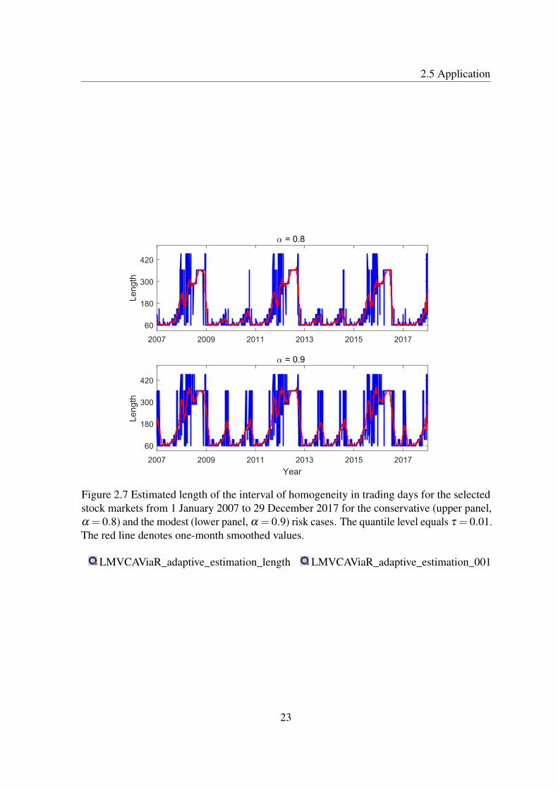
2.7 Estimated length of the interval of homogeneity in trading days for theselected stock markets from 1 January 2007 to 29 December 2017 for theconservative (upper panel, α = 0.8) and the modest (lower panel, α = 0.9)risk cases. The quantile level equals τ = 0.01. The red line denotes one-month smoothed values. . . . . . . . . . . . . . . . . . . . . . . . . . . . 23
xiii

List of Figures
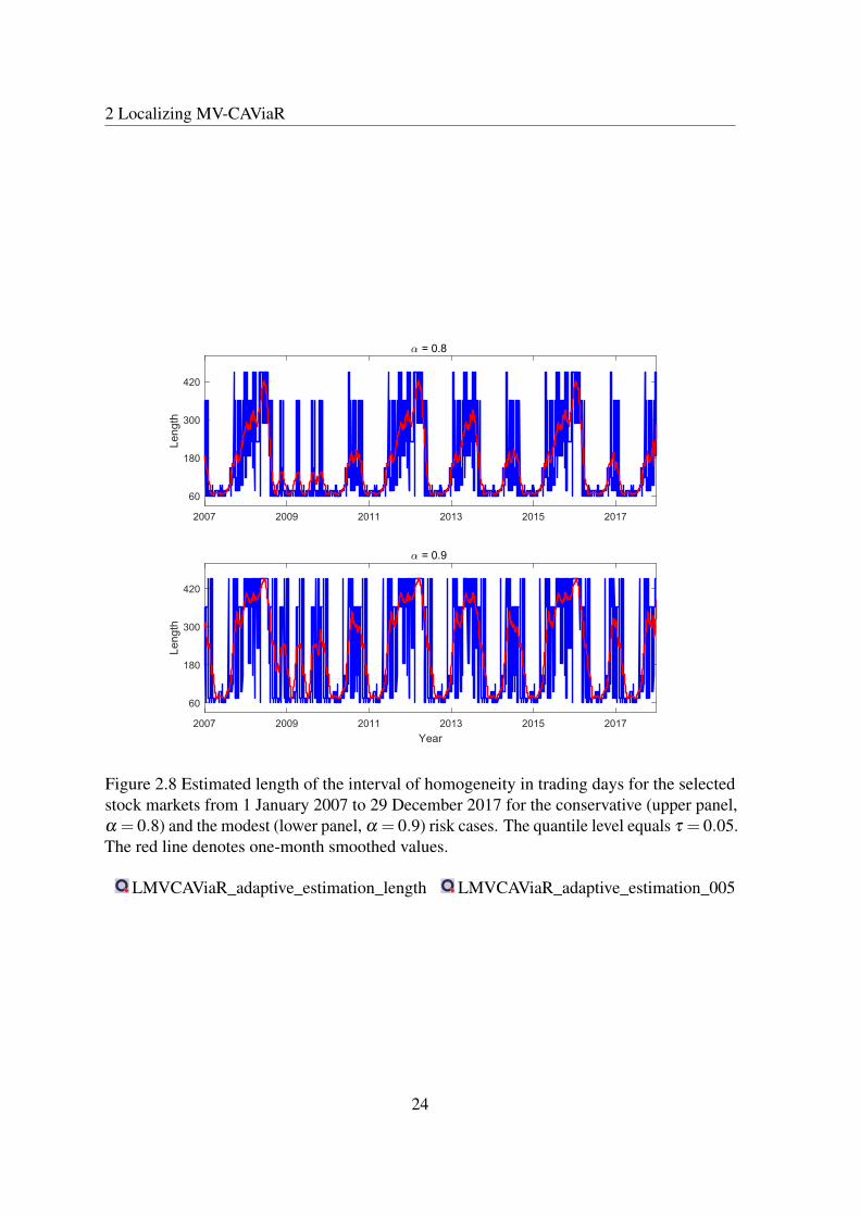
2.8 Estimated length of the interval of homogeneity in trading days for theselected stock markets from 1 January 2007 to 29 December 2017 for theconservative (upper panel, α = 0.8) and the modest (lower panel, α = 0.9)risk cases. The quantile level equals τ = 0.05. The red line denotes one-month smoothed values. . . . . . . . . . . . . . . . . . . . . . . . . . . . 24
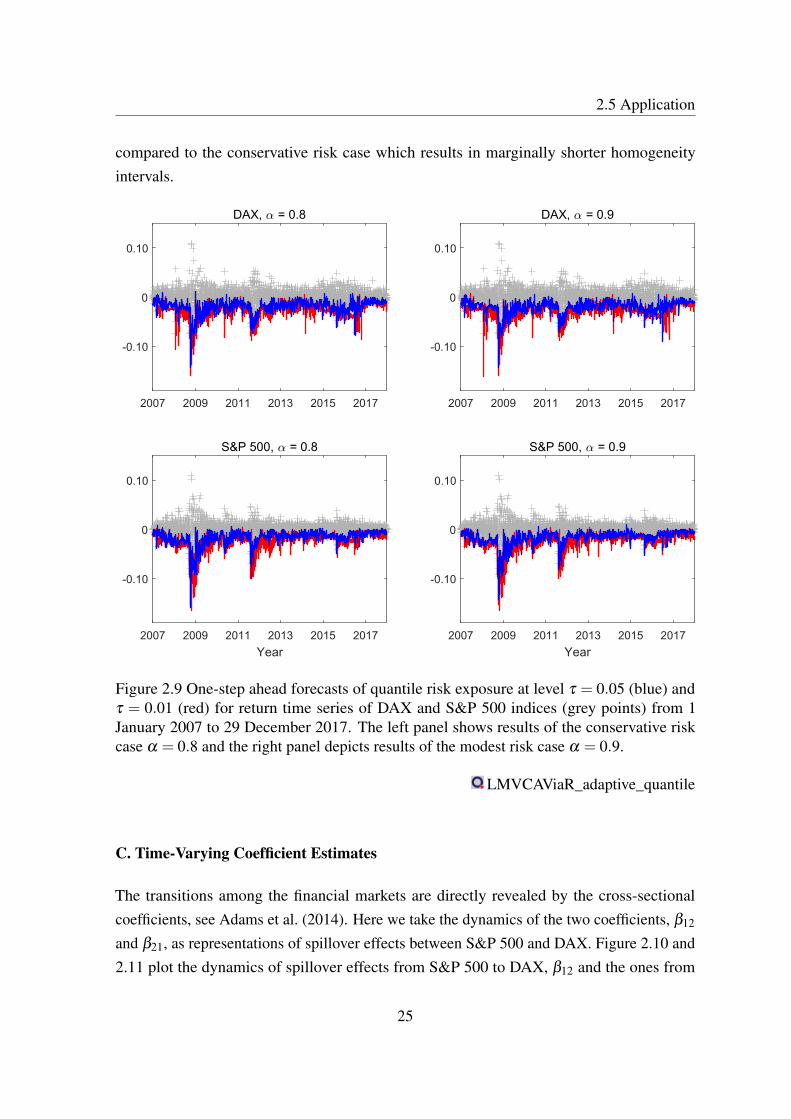
2.9 One-step ahead forecasts of quantile risk exposure at level τ = 0.05 (blue)and τ = 0.01 (red) for return time series of DAX and S&P 500 indices (greypoints) from 1 January 2007 to 29 December 2017. The left panel showsresults of the conservative risk case α = 0.8 and the right panel depictsresults of the modest risk case α = 0.9. . . . . . . . . . . . . . . . . . . . 25
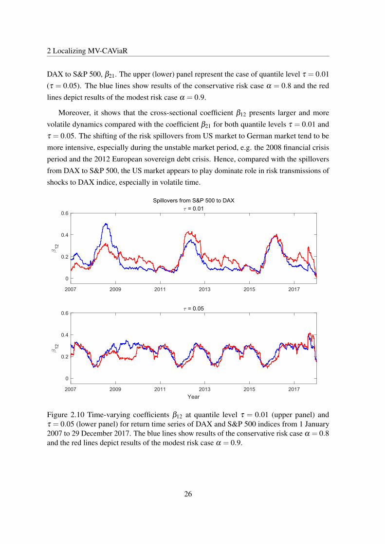
2.10 Time-varying coefficients β12 at quantile level τ = 0.01 (upper panel) andτ = 0.05 (lower panel) for return time series of DAX and S&P 500 indicesfrom 1 January 2007 to 29 December 2017. The blue lines show resultsof the conservative risk case α = 0.8 and the red lines depict results of themodest risk case α = 0.9. . . . . . . . . . . . . . . . . . . . . . . . . . . 26
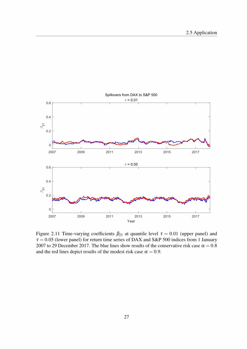
2.11 Time-varying coefficients β21 at quantile level τ = 0.01 (upper panel) andτ = 0.05 (lower panel) for return time series of DAX and S&P 500 indicesfrom 1 January 2007 to 29 December 2017. The blue lines show resultsof the conservative risk case α = 0.8 and the red lines depict results of themodest risk case α = 0.9. . . . . . . . . . . . . . . . . . . . . . . . . . . 27
3.1 Social media users’ sentiment over time . . . . . . . . . . . . . . . . . . . 46
3.2 Example of a network with influencers. . . . . . . . . . . . . . . . . . . . 49
3.3 Simulation results for N = T = 100 and s = 1. . . . . . . . . . . . . . . . . 60
3.4 Estimated Θ for AAPL and BTC datasets. The axes correspond to user id’sand are rearranged with respect to the estimated clusterings. . . . . . . . . 62
xiv

List of Tables
2.1 Descriptive statistics for the selected index return time series from 3 January2005 to 29 December 2017 (3390 trading days): mean, median, minimum(Min), maximum (Max), standard deviation (Std), skewness (Skew.) andkurtosis (Kurt.). . . . . . . . . . . . . . . . . . . . . . . . . . . . . . . . 19
2.2 Mean value of the adaptively selected intervals. Note: the average numberof trading days of the adaptive interval length is provided for the DAX andS&P 500 market indices at quantile levels, τ = 0.05 and τ = 0.01, and theconservative (α = 0.80) and the modest (α = 0.90) risk case. . . . . . . . 22
3.1 Summary statistics of social media messages . . . . . . . . . . . . . . . . 43
xv


Chapter 1
Introduction
Risk dependence within financial networks and the mechanism of risk spillover amonginternational equity markets has attracted increasing attention among theorists, empiricalresearchers and practitioners. A risk contagion is generated through dependence betweenextreme negative shocks across financial markets. It is well-known that large downsidemarket movements occurring in one country would unavoidably have substantial effectson other international equity markets. Moreover, financial risk scenarios tend to transmitthemselves among different markets, which consequently intensifies a global risk contagionleading to an international economic crisis. Identifying sensitivity of financial institutions toshocks to the whole system is a vital task in controlling stability of financial markets. Forthis purpose White et al. (2015) introduces Multivariate Conditional Autoregressive Valueat Risk (MV-CAViaR) model, which is typically applied pairwise between institutions andfinancial market indices. However, empirical studies suggest that interdependence of the tailrisk contagion is unstable and time-varying, (Baele and Inghelbrecht, 2010; Elyasiani et al.,2007). The model, therefore, asks for a procedure that would balance between long-termbiasness and short-term high variance of the estimator. In Chapter 2 we introduce anddevelop such procedure. Based on the idea of sequential testing from Spokoiny (2009), wepick a time interval that passes homogeneity test with a predefined confidence level. Thehomogeneity test is based on a multiscale change point test statistics. The latter requiressimulation of critical values, since pivotal distribution is typically not given, plus we wantas well to account for possible misspecification of a model. A novel approach based onMultiplier Bootstrap is used, Spokoiny and Zhilova (2015). We analyse the properties of thistest both theoretically and through simulation study and apply it to a simultaneous CAViaRmodel of stock market indices DAX and S&P 500.
1
1 Introduction
Social media is another type of networks that receives plenty of attention in the recentEconometric literature. It represents an ideal platform where users can easily communicatewith each other, exchange information and share opinions. An increasing popularity in socialmedia is a clear evidence of such demand for exchanging options and information amonggranular users in the cyber world. Econometric analysis of social media data encounters thechallenges from the granularity of users, complexity of interaction and a variety of opinions.On the other hand, these challenges bear the chances to augment econometric analysis viathe massive availability of social media data. In Chapter 3 we model interactions in a socialnetwork through a vector autoregressive model, following a line of work Zhu and Pan (2017);Zhu et al. (2017, 2016). Such a model naturally suffers from curse of dimensionality, as thenumber of connection within a typical network is often larger that the available data sample,due to either limited data or time-variation of the model parameter. To cope with this problemwe take into account two major aspects of social networks. The first one relies on the fact thatin a typical social network only a small portion of users produce significant influence on thenetwork, whom we call influencers. Secondly, each user in a social network represents a largegroup of users called community, who together share opinions and exhibit similar behaviour.This motivates us to introduce a new model called Social Network with Influencers andCommunities (SoNIC), bringing the two aspects together. In theoretical and simulationanalysis we show that it allows consistent estimation even when the number of users issmaller than the available time period. We focus on the application to sentiment extractedfrom StockTwits, a microblogging platform dedicated to discussion of stock market assetsfor traders and financial analysts. Apart from the estimation of the network connections, weidentify the influencers — important users whose opinion matters the most.
We additionally provide several theoretical extensions and improvements. In Chapter 2 weshow a Bahadur-type expansion for quantile estimation with exponentially high probabilitiesin the finite sample regime. In the appendix in Section A.1 we extend the results of Tropp(2006) for the exact Lasso recovery in the case of missing observations. Finally, in Chapter 4we prove a new version of Bernstein Matrix inequality that works for unbounded matrices. Asan application we improve the tail bound of Lounici (2014) for the covariance estimator undermissing observations. Using a similar trick we extend uniform Hanson-Wright inequality togeneral unbounded subgaussian variable, a problem closely related to covariance estimation.
2

Chapter 2
Localizing Multivariate ConditionalAutoregressive Value at Risk
There exists a wide-spread consensus in the empirical literature that the dependence betweenthe returns of financial assets is non Gaussian with asymmetric marginals, nonlinear featuresand time-varying (Longin and Solnik, 2001; Okimoto, 2008). In order to address theseproperties Engle and Manganelli (2004) propose a conditional autoregressive value at risk(CAViaR) model to specify the evolution of conditional quantile over time for univariatetime series. Further, White et al. (2015) built up a multivariate framework for multiple timeseries as well as various quantile levels, which can be considered as a vector autoregressive(VAR) extension to quantile models with the underlying value at risk processes not onlyautocorrelated but also cross-sectionally intertwined. When applying CAViaR to financialinstitutions, it presents valuable results in capturing the sensitivity of financial entities toinstitutional specific and market-wide shocks of the system. It does however not copewith time-variation. We therefore propose a feasible extension towards a local multivariateCAViaR to estimate and forecast the dynamics of financial risk dependence.
The majority of existing literature use volatility as the risk measure and investigatethe volatility risk contagions (e.g. Bauwens et al. (2006); Engle (2002, 2004); Pelletier(2006)). Although volatility is a crucial instrument to measure the risk movement, it has beencommonly criticized as only capturing the properties of second moments of the return timeseries and ignoring extreme market events structure (Han et al., 2016; Hong et al., 2009). Inaddition, the volatility risk measure is symmetric and equally values the gains and losses,which contradicts the facts that investors tends to be more sensitive to the negative returns and
3
2 Localizing MV-CAViaR
especially for large downside risk, e.g. financial crisis. Therefore volatility risk measure is notenough to evaluate the financial risk interdependence. On the contrary, Value at Risk (VaR)is commonly utilized to measure the asymmetric risk due to the straightforward implications,i.e., evaluate the loss given a predetermined probability of extreme events. Although nota perfect risk measure, it has been accepted as a standard for financial regulations, e.g. acriterion by the Basel committee on banking supervision, Franke et al. (2019).
The interdependence of financial risk and especially the tail risk contagion is typicallyfeatured as unstable and time-varying by empirical studies (Baele and Inghelbrecht, 2010;Elyasiani et al., 2007). The risk contagion is caused by dependence between extreme negativeshocks across international financial markets. A parametric model over a long-run time seriesis at limit to portray almost certainly existed properties of non-stationarity. Gerlach et al.(2011) propose a time-varying quantile model using a Bayesian approach for univariate timeseries. In this paper, we focus on time-varying parameter properties of multivariate quantilemodelling. We propose a framework for localizing multivariate autoregressive conditionalquantiles by exploiting a local parametric approach, denoted as LMCR model for simplicity.The advantages of our strategy are at least twofold: (1) we consider the extreme tail riskspillover among financial markets and (2) we examine interdependence pattern of the tailrisk contagion, both in a dynamic time-varying context.
The local parametric approach (LPA) utilizes a parametric model over an adaptivelychosen interval of homogeneity. The essential idea of LPA is to find — backwards looking —the longest interval that guarantees a relatively small modelling bias, see e.g. Spokoiny (1998,2009). A great advantage of this modelling approach is the search of balance between themodelling bias and parameter variability, see e.g. Chen et al. (2010); Chen and Niu (2014);Härdle et al. (2015); Niu et al. (2017); Xu et al. (2018). Recent advances in multipliersbootstrap (MBS) allow to construct data-driven critical values for homogeneity tests based onchange point detection, see Suvorikova and Spokoiny (2017) and the references therein. TheMBS only relies on the autoregressive equation for conditional quantiles and has no particularassumption about the distribution of the innovations. In our research, we extend LPA toquantile regression and develop LMCR. In Section 2.1 we extend the asymptotic results ofWhite et al. (2015) to finite samples. In particular, we establish a Bahadur-type expansionbased on uniform exponential inequality Lemma 2.1, which may as well be of independentinterest. We then compare it with the multiplier bootstrap counterpart by utilizing the resultsof Chernozhukov et al. (2013).
4
2.1 Model
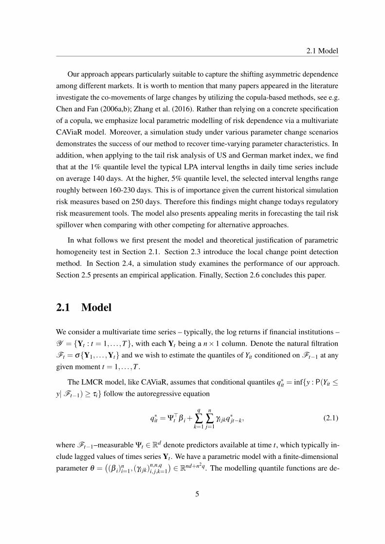
Our approach appears particularly suitable to capture the shifting asymmetric dependenceamong different markets. It is worth to mention that many papers appeared in the literatureinvestigate the co-movements of large changes by utilizing the copula-based methods, see e.g.Chen and Fan (2006a,b); Zhang et al. (2016). Rather than relying on a concrete specificationof a copula, we emphasize local parametric modelling of risk dependence via a multivariateCAViaR model. Moreover, a simulation study under various parameter change scenariosdemonstrates the success of our method to recover time-varying parameter characteristics. Inaddition, when applying to the tail risk analysis of US and German market index, we findthat at the 1% quantile level the typical LPA interval lengths in daily time series includeon average 140 days. At the higher, 5% quantile level, the selected interval lengths rangeroughly between 160-230 days. This is of importance given the current historical simulationrisk measures based on 250 days. Therefore this findings might change todays regulatoryrisk measurement tools. The model also presents appealing merits in forecasting the tail riskspillover when comparing with other competing for alternative approaches.
In what follows we first present the model and theoretical justification of parametrichomogeneity test in Section 2.1. Section 2.3 introduce the local change point detectionmethod. In Section 2.4, a simulation study examines the performance of our approach.Section 2.5 presents an empirical application. Finally, Section 2.6 concludes this paper.
2.1 Model
We consider a multivariate time series – typically, the log returns if financial institutions –Y = Yt : t = 1, . . . ,T, with each Yt being a n×1 column. Denote the natural filtrationFt = σY1, . . . ,Yt and we wish to estimate the quantiles of Yit conditioned on Ft−1 at anygiven moment t = 1, . . . ,T .
The LMCR model, like CAViaR, assumes that conditional quantiles q∗it = infy : P(Yit ≤y|Ft−1)≥ τi follow the autoregressive equation
q∗it = Ψ>t β i +
q
∑k=1
n
∑j=1
γi jkq∗jt−k, (2.1)
where Ft−1–measurable Ψt ∈ Rd denote predictors available at time t, which typically in-clude lagged values of times series Yt . We have a parametric model with a finite-dimensionalparameter θ =
((β i)
ni=1,(γi jk)
n,n,qi, j,k=1
)∈ Rnd+n2q. The modelling quantile functions are de-
5

2 Localizing MV-CAViaR
fined recursively,
qit(θ ,Y ) = Ψ>t β i +
q
∑k=1
n
∑j=1
γi jkq jt−k(θ ,Y ). (2.2)
For any interval I = [a,b]⊂ 0, . . . ,T we will write
(Yit ,Ψt)t∈I ∼ LMCR(θ),
if the equation (2.1) is fulfilled on this interval with parameter θ .
The parameter can be estimated via the quantile regression quasi-Maximum LikelihoodEstimator (qMLE). For a given quantile level of interest τ ∈ (0,1) denote the check functionρτ(x) = x(τ− I[1≤ τ]) and set
`t(θ) =−n
∑i=1
ρτYit−qit(θ ,Y ),
— quasi log-probability of t’s observation. The log-likelihood based on the interval I ⊂1, . . . ,T of observations for a fixed τ reads as
LI (θ) = ∑t∈I
`t(θ)
and the estimator based on this set of observations as
θI = arg maxθ∈Θ0
LI (θ). (2.3)
The paper White et al. (2015) deals with the estimator that uses the whole data set I =
1, . . . ,T and provides consistency and asymptotic normality of the estimator when T tendsto infinity.
Remark 2.1. The value −LI (θ) is usually referred to as risk or contrast and the corre-
sponding estimator as risk minimizer or contrast estimator. We, however, prefer the terms
quasi likelihood and quasi maximum likelihood estimator, as we work with LRTs, Spokoiny
and Zhilova (2015).
The main objective of the present work is to provide a practical technique that choosesappropriate intervals I . Roughly speaking, the longer the interval the less is the variance ofthe estimator, while choosing the interval too large we can bring in bias due to time-varying
6

2.1 Model
parameter. We say that the model is homogeneous at the time interval I , if the followingassumption holds.
Assumption 2.1. There exists a “true” parameter θ∗ ∈ Θ0 such that q∗it = qit(θ
∗,Y ) for
each i = 1, . . . ,n and t ∈I .
Obviously, such an assumption ensures that θ∗ = argmaxE`t(θ) for each t ∈I , and,
therefore, θ∗ = argmaxELI (θ), which falls into the general framework of maximum likeli-
hood estimators, see e.g. Huber (1967), White (1996) and Spokoiny (2017).
Here though we study LMCR, a non-stationary CAViaR model, that follows the local
parametric assumption, meaning that for each time point t there exists a historical interval[t−m; t] where the model is nearly homogeneous, we also derive the theoretical propertiesof LMCR under general mixing conditions which might be of interest by itself for a deeperstochastic analysis.
2.1.1 Assumptions
We first impose the following assumptions on the LMCR model, in particular, we say thatthe model is “homogeneous” on an interval I if it satisfies the assumptions of this section.
The first one ensures the identification of the model and is akin to Assumption 4 of Whiteet al. (2015). The second one controls the values and derivatives of the quantile regressionfunctions.
Assumption 2.2. There is a set of indices J ⊂ 1, . . . ,n such that for any ε > 0 there exists
δ = δ (ε)> 0 such that whenever ‖θ −θ∗‖ ≥ ε ,
P(∪ni=1 |qit(θ)−qit(θ
∗)| ≥ δ)≥ δ , t ∈I . (2.4)
Assumption 2.3. (i) For s = 0,1,2 there are constants Ds > 0 such that for each i, t and for
each θ ∈ Θ0 it holds pointwise |qit(θ , ·)| ≤ D0, ‖∇qit(θ , ·)‖ ≤ D1 and ‖∇2qit(θ , ·)‖ ≤ D2.
(ii) Conditional density of innovations εit are bounded from above fit(x)≤ f0 for each i, t and
x ∈ R. (iii) Additionally, conditional density of innovations satisfies fit(x)≥ f for |t| ≤ δ0.
Furthermore, we impose the following assumptions on the given time series. Let usfirst recall the definition of the mixing coefficients. For any sub σ -fields A1,A2 of same
7

2 Localizing MV-CAViaR
probability space (Ω,F ,P) define,
α(A1,A2) = supA∈A1,B∈A2
|P(A∩B)−P(A)P(B)| ,
β (A1,A2) = sup(Ai)⊂A1,(Bi)⊂A2
∑i, j
∣∣P(Ai∩B j)−P(Ai)P(B j)∣∣ ,
where in the latter the supremum is taken over all finite partitions (Ai)⊂A1 and (B j)⊂A2
of Ω. Then, the coefficients
ak((Xt)) =supt
α(σ(X1, . . . ,Xt),σ(Xt+k, . . . ,XT )),
bk((Xt)) =supt
β (σ(X1, . . . ,Xt),σ(Xt+k, . . . ,XT ))
and denote α– and β–mixing coefficients of the process (Xt)t≤T , respectively.
Assumption 2.4. (i) Suppose, that the sequence of vectors (q·t(θ),∇q·t(θ)) is α–mixing
with α(m)≤ exp(−γm) for some constant γ > 0; (ii) The sequence of vectors ∇q·t(θ ∗,Y )
is β–mixing with coefficients β (m)≤ m−δ , δ > 1; (iii) for each i = 1, . . . ,n the innovations
εit for t ∈I are i.i.d. and satisfy P(εit < 0) = τ .
Finally, we introduce the assumptions concerning information matrix as well as varianceof the score, which corresponds to Assumption 6 of White et al. (2015).
Assumption 2.5. The vector (q∗t ,∇qt(θ∗),ε t) is a stationary process for t ∈I . Additionally,
the matrices
Q2 = E fit(0)∇qit(θ∗)[∇qit(θ
∗)]>, V 2 = Vargt(θ∗)
are strictly positive definite.
2.1.2 Consistency of the estimator
Here we present the results for consistency of the estimator θ as the length of the interval|I | tends to infinity. Unlike White et al. (2015), who show convergence in probability or insquare mean, we provide bounds with exponentially large probabilities, which allows us totake into consideration growing amount of intervals simultaneously.
One of the main tools in providing convergence and asymptotic normality for M-estimators is uniform deviation bounds for the score, see e.g. White (1996), Spokoiny
8

2.1 Model
(2017) and the references therein. The score of the likelihood is ∇LI (θ) = ∑t∈I ∇`t(θ) =
∑t∈I gt(θ), where we denote gt(θ) = ∇`t(θ). By definition of the log-likelihood, wehave gt(θ) = ∑i ∇qit(θ , ·)ψτYit−qit(θ , ·). We also introduce the expectation of the latterλt(θ) = Egt(θ). The following bound provides exponential in probability uniform deviationbound.
Lemma 2.1. Assume 2.3 and 2.4 hold on an interval I . Then,
supθ∈Θ0(r)
1|I |1/2
∥∥∥∥∥∑t∈I
gt(θ)−λ t(θ)−gt(θ∗)+λ t(θ
∗)
∥∥∥∥∥≤♦(|I |,r,x),with probability at least 1− e−x, where
♦(T ′,r,x) =C1
r√x+r1/2
√x+ logT ′+T ′−1/2(logT ′)2(rx+x+ logT ′)
with some C1 that does not depend on T ′,r,x.
Remark 2.2. Here the error term with r1/2 comes from the fact that gt(θ , ·) contains non-
differentiable generalized errors ψτ(Yit−qit(θ)), which being Bernoulli random variables,
can not be handled by chaining alone, unlike the case of smooth score, see e.g. Spokoiny
et al. (2017).
Given the result above we can bound the score uniformly over all parameter set. Thisallow us to have the following consistency result.
Proposition 2.1. Let assumptions 2.1–2.5 hold on the interval I . It holds with probability
≥ 1−6e−x,
‖θI −θ∗‖ ≤C0
√x+ log |I ||I |
.
2.1.3 Local quadratic expansion
The next step in providing asymptotic normality of the estimator θ is a local Fisher expansion.The main tool is linear approximation of the gradient of the likelihood, which can be done bymeans of Proposition 2.1.
It is shown in White et al. (2015) (see formula (24)), that for each θ ∈Θ,∥∥∥∥∥∑t∈I
λ t(θ)− ∑t∈I
λ t(θ∗)+ |I |Q2(θ −θ
∗)
∥∥∥∥∥≤C2|I |‖θ −θ∗‖2, (2.5)
9

2 Localizing MV-CAViaR
with some C2 that does not depend on the length of the interval. Finally, we present the mainresult of this section, that serves as a non-asymptotic adaptation of Theorem 2 of White et al.(2015). We postpone the proof to Section 2.7.3.
Proposition 2.2. Suppose, on some interval I ⊂ [0,T ] the Assumptions 2.1–2.5 hold. Then,
for any x≤ |I |, it holds with probability at least 1−3e−x,
∥∥∥√|I |Q(θI −θ∗)−ξ I
∥∥∥≤C(x+ log |I |)3/4
|I |1/4 ,∣∣∣L(θI )−L(θ ∗)−‖ξ I ‖2/2∣∣∣≤C
(x+ log |I |)3/4
|I |1/4 ,
(2.6)
where ξ I = 1√|I |∑t∈I Q−1gt(θ
∗) and C does not depend on |I | and x.
Remark 2.3. This result serves as a non-asymptotic version of central limit theorem (CLT)
for the estimator, Theorem 2 in White et al. (2015). This follows from the fact that the sequence
(Q−1gt(θ∗))t≤T satisfies CLT as a martingale difference sequence, see also Theorem 5.24 in
White (2014).
2.2 Homogeneity testing via local change point detection
Suppose, we have an interval I = [a,b]⊂ 1, . . . ,T of observations and we want to testwhether there is a change in the parameter, that generates the data on this interval throughthe model (2.1). An alternative would be that there exist a break point s ∈ (a,b) such that onthe left part As = [a,s] the data generating process is described by one parameter and on theright part Bs = [s+1,b] it is described by a different parameter. This means that we want totest a null hypothesis
H0(I ) : (Yit ,Ψt)t∈I ∼ LMCR(θ ∗I ), θ∗I ∈Θ0,
against the alternative
H1(I ) : (Yit ,Ψt)t∈I ∼ LMCR(θ ∗As),
(Yit ,Ψt)t∈I ∼ LMCR(θ ∗Bs) with some θ
∗As6= θ
∗Bs.
10

2.2 Homogeneity testing via local change point detection
To construct the test statistics consider a set of candidates for a break point S (I )⊂ (a,b)
and for each such candidate s ∈S (I ) introduce the test,
TI ,s = LAI ,s(θ AI ,s)+LBI ,s(θ BI ,s)−LI (θI ),
where AI ,s = [a,s] represents observations to the left from break point and BI ,s = [s+1,b]are the observations to the right from the break point candidate s ∈I . The existence of thebreak point among the candidates is tested using statistic
TI = maxs∈S (I )
TI ,s.
Given a certain confidence level α we want to construct a critical value zI ,α such that underthe null hypothesis it holds
P(TI > zI ,α
)= α,
which stands for the false alarm rate. Evaluating such critical values is a crucial question inhypothesis testing.
Spokoiny et al. (2013) and Xu et al. (2018) use a propogation approach for constructingthe critical values. The approach is based on generation the distribution of test statistics,assuming that the distribution of the data is known precisely up to the parameter. For instance,the latter paper assumes normal distribution for the innovations in the conditional expectilesprocess. In the next section, in order to account for arbitrary distribution of the innovations,we construct data-driven critical values zI ,α(Y ) that use the corresponding data interval foreach test based on multiplier bootstrap.
2.2.1 Multiplier bootstrap
The idea is to simulate the unknown distribution of the original log-likelihood by introducingMBS with each term reweighted
LI (θ) = ∑t∈I
wt`t(θ),
where (wt)t≤T is a given random sequence of i.i.d. weights independent of the sample. Forsake of simplicity we additionally assume, that they have sub-Gaussian tails.
11

2 Localizing MV-CAViaR
Assumption 2.6. The weights wt are independent with Ewt = 1 and Var(wt) = 1. Addition-
ally, there is Cw such that for each t it holds Eexp(wt/Cw)2 ≤ 2.
Denote the corresponding bootstrap estimator
θI = argmaxLI (θ),
while the expectation of bootstrap log-likelihood with respect to the simulated weights isobviously maximized by the original estimator,
θI = argmaxELI (θ) = argmaxLI (θ),
where E[·] = E[·| Y ] denotes expectation in the “bootstrap world”. The paper Spokoiny andZhilova (2015) shows that with high probability the distribution of the simulated likelihoodratio LI (θ
I )−LI (θI ) in the “bootstrap world” mimics the distribution of the original
likelihood ratio LI (θI )−LI (θ ∗) up to some error that decreases with growing sample.We adapt their theory for the case of regression quantiles.
Proposition 2.3. Suppose, Assumptions 2.1–2.5 and 2.6 hold on the interval I . Then, there
is T0 > 0 such that if T ≥ T0 and x≤ T , on the event of probability at least 1− e−x, it holds
with probability at least 1− e−x conditioned on the data, that
∥∥∥√|I |Q(θI − θI )−ξ
I
∥∥∥≤C(x+ logT )3/4
T 1/4 ,∣∣∣LI (θI )−LI (θI )−‖ξ I ‖2/2
∣∣∣≤C(x+ logT )3/4
T 1/4 ,
where ξI = 1√
T ∑t∈I wtQ−1gt(θ∗) and C does not depend on T and x.
The papers Suvorikova and Spokoiny (2017) and Avanesov and Buzun (2016) apply theapproach for change point detection. Following them, introduce the bootstrap test for changepoint s on the interval I ,
T I ,s =LAs(θAs)+LBs
(θBs)− supLAs
(θ)+LBs(θ + θ Bs− θ As),
T I = maxs∈S (I )
TI ,s.
Note, that here the shift θ Bs− θ As is devoted to compensate the biases of the estimators θAs
and θBs
in the bootstrap world, which is not required in the original test. This test can further
12

2.3 Localizing Multivariate CAViaR
be used to simulate the critical values, since it’s distribution conditioned on the data mimicsthe distribution of the original test TI with high probability, as the following theorem states.
Theorem 2.1. Suppose, that on an interval I ⊂ 0, . . . ,T the model satisfies 2.2-2.5 and
2.6. Suppose, that the set of break points satisfies for some α0 > 0
maxs∈S (I )
(|AI ,s|, |BI ,s|)≥ α0|I |. (2.7)
Then, there are C,c > 0 that does not depend on |I |, such that it holds with probability at
least 1−1/|I |,supz∈R|P(TI > z)−P(T I > z)|.C|I |−c.
The theorem justifies that the distribution of the bootstrap statistics T I mimics theunknown distribution of the original statistics TI , so we can construct critical values for thechange point test by simulating the bootstrap statistics:
zI (α) = zI (α;Y) = infz : P(T I > z)≤ α, (2.8)
is totally data-dependent and can be estimated via Monte-Carlo simulations with arbitraryprecision (see Sections 5 for details). Given the theorem above, we can use these data-dependent critical values for the original test on the same data interval.
Corollary 2.1. Under the assumptions of Theorem 2.1, we have
|P(TI > zI (α))−α| ≤C|I |−c,
where C,c > 0 do not depend on the interval length.
2.3 Localizing Multivariate CAViaR
Although time series should not be (globally) fitted by a parametric model with constantparameter, we assume that at each time point t = 1, . . . ,T , there exists a historical interval[t−m, t], over which the data process follows a parametric model, in our case equation (2.1).This local parametric assumption enables us to apply well-developed parametric estimationtechniques in time series analysis. What is more, such an assumption includes the followingscenarios as special cases: (i) the parameters are time-varying as the interval length changes
13

2 Localizing MV-CAViaR
over time and simultaneously (ii) our approach accounts for possible discontinuities andjumps in parameter coefficients as a function of time.
The essential idea of the proposed LMCR framework is to find the longest time seriesdata interval over which the LMCR model can be “well” approximated by the parametricmodel. Therefore, the estimation procedure consists of two steps:
• for a time point of interest (usually latest available) select a historical interval thatpasses the homogeneity test described in the previous section;
• use the selected data interval for parameter estimation.
Interval Selection
The common way of selecting the homogeneous interval is as follows. To alleviate thecomputational burden, choose (K +1) nested intervals of length nk = |Ik|, k = 0, . . . ,K, i.e.,I0 ⊂I1 ⊂ ·· · ⊂IK . Interval lengths are usually taken to be geometrically increasing withnk = dn0cke, where c > 1 is slightly greater than one, so that in the worst case one onlyneglects a small proportion of unknown homogeneous interval. We assume that the initialinterval I0 is small enough, so that the model parameters are constant within this interval.
Further, we conduct a sequential testing procedure. For each k = 1, . . . ,K we want to testthe homogeneity of the parameter over interval Ik against the alternative of homogeneityover interval Ik−1. By our assumption I0 is homogeneous. The resulting interval ofhomogeneity would then be the last before the first one rejected. Therefore, for each suchk = 1, . . . ,K we choose a set of breaking points Sk = Ik \Ik−1 outside of the interval thatwe already tested. Using the testing procedure from Section 2.2 we reject the kth interval, if
maxs∈Sk
Ts > zIk(α),
where zIk(α) is generated through multiplier bootstrap (2.8). Observe that if the model is
homogeneous on a historical interval [t− n∗, t], then due to Corollary 2.1 we will accepthomogeneity of each interval Ik = [t−nk, t] with nk ≤ n∗ with high probability. If an intervalIk remains homogeneous, the estimator θIk has small bias, while the variance decreases withgrowing number of observations, according to Theorem 2.2. The least variance, therefore,corresponds to the largest found interval of homogeneity, and the final estimator reads as
θ = θIκ, κ = maxk : Ik is not rejected against Ik−1.
14

2.4 Simulation
This finishes the second step of our LMCR estimator. In the next two sections we analyse theproposed procedure numerically.
2.4 Simulation
In this section we study the effectiveness of our adaptive approach in detecting the structurebreaks in numerical analysis. Following the setup of WKM and the simulation study inGerlach et al. (2011) and Hong et al. (2009), we generate the data time series using atwo-variate GARCH process:
σ1t = β11σ1t−1 + β12σ2t−1 + γ11|y1t−1|+ γ12|y2t−1|+ c1 (2.9)
σ2t = β21σ1t−1 + β22σ2t−1 + γ21|y1t−1|+ γ22|y2t−1|+ c2
Yit = σitεit , εit ∼ N(0,1) i.i.d. i = 1,2
Denote the parameter set θ = (βi j, γi j, ci) where i, j = 1,2.
Note that at a given quantile level τ , the quantile process qit(τ) = Quantτ(Yit |Ft−1)
satisfies qit(τ) = Φ−1(τ)σit , where Φ−1(τ) is the quantile function of the standard normaldistribution. Therefore, the following recurrent equation takes place
q1t(τ) = β11q1t−1(τ)+β12q2t−1(τ)+ γ11|y1t−1|+ γ12|y2t−1|+ c1 (2.10)
q2t(τ) = β21q1t−1(τ)+β22q2t−1(τ)+ γ21|y1t−1|+ γ22|y2t−1|+ c2,
where the parameter θτ = (βi j,γi j,ci)i, j=1,2 consists of ten coefficients βi j = βi j and γi j =
Φ−1(τ)γi j, ci = Φ−1(τ)ci for i, j = 1,2.
For simulations we consider a time series (Yit)500t=1 with the initial variances σi1 = 1 and
parameters
θ le f t =(0.5,0,0,0.5,0,0.2,0.2,0,0.5,0.5),
θ right =(−0.5,0,0,0.5,0,0.2,0.2,0,0.5,0.5),
so that before the break t ≤ s = 250 the time series satisfies (2.9) with the parameter θ le f t
and after the break with θ right . For each time point with step 20 (i.e. 500, 480, 460, andso on) we test a nested sequence of intervals I0 ⊂ I1 ⊂ ·· · ⊂ IK with lengths nk = dck|I0|e,which we take with K = 9, |I0|= 60 and c = 1.25. The considered lengths of intervals are
15
2 Localizing MV-CAViaR
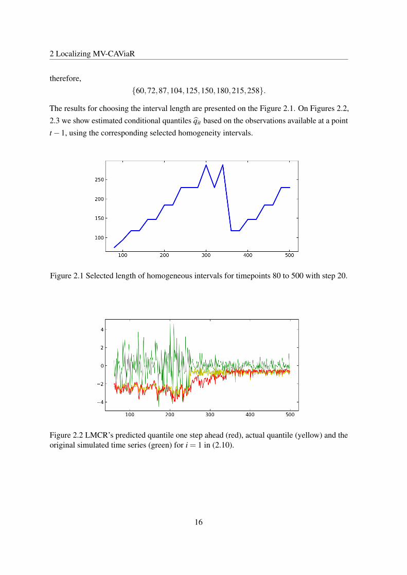
therefore,60,72,87,104,125,150,180,215,258.
The results for choosing the interval length are presented on the Figure 2.1. On Figures 2.2,2.3 we show estimated conditional quantiles qit based on the observations available at a pointt−1, using the corresponding selected homogeneity intervals.
Figure 2.1 Selected length of homogeneous intervals for timepoints 80 to 500 with step 20.
Figure 2.2 LMCR’s predicted quantile one step ahead (red), actual quantile (yellow) and theoriginal simulated time series (green) for i = 1 in (2.10).
16
2.5 Application
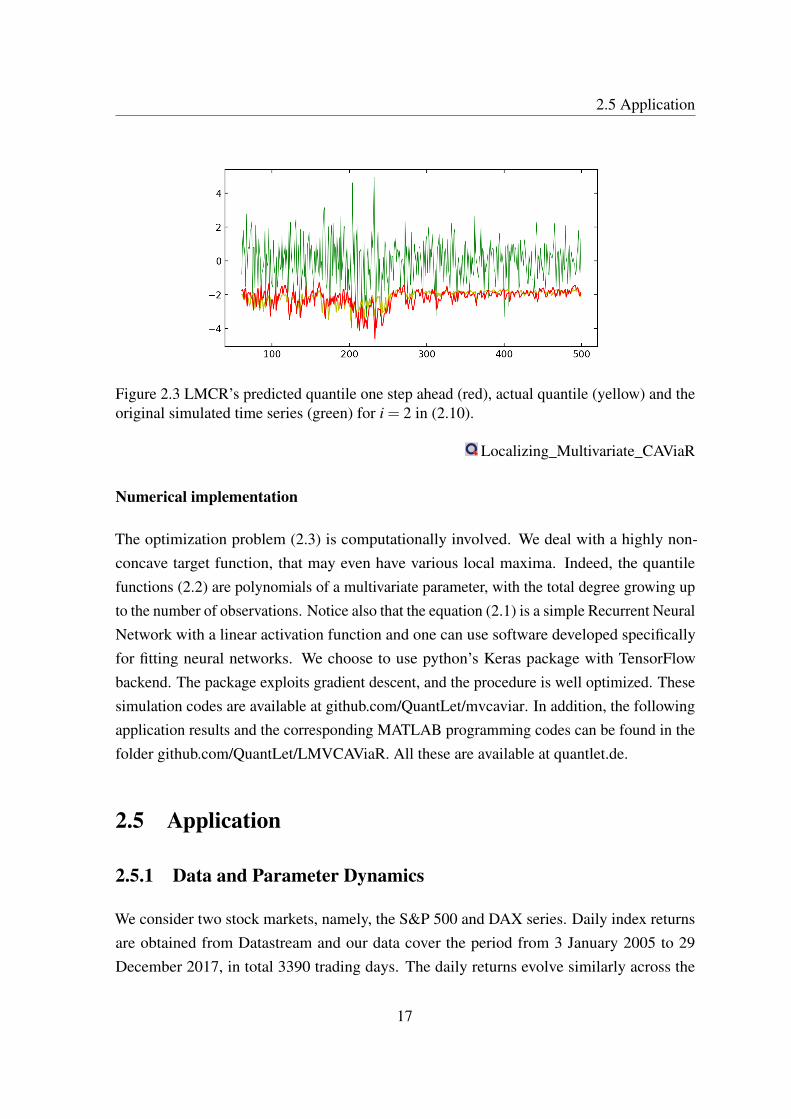
Figure 2.3 LMCR’s predicted quantile one step ahead (red), actual quantile (yellow) and theoriginal simulated time series (green) for i = 2 in (2.10).
Localizing_Multivariate_CAViaR
Numerical implementation
The optimization problem (2.3) is computationally involved. We deal with a highly non-concave target function, that may even have various local maxima. Indeed, the quantilefunctions (2.2) are polynomials of a multivariate parameter, with the total degree growing upto the number of observations. Notice also that the equation (2.1) is a simple Recurrent NeuralNetwork with a linear activation function and one can use software developed specificallyfor fitting neural networks. We choose to use python’s Keras package with TensorFlowbackend. The package exploits gradient descent, and the procedure is well optimized. Thesesimulation codes are available at github.com/QuantLet/mvcaviar. In addition, the followingapplication results and the corresponding MATLAB programming codes can be found in thefolder github.com/QuantLet/LMVCAViaR. All these are available at quantlet.de.
2.5 Application
2.5.1 Data and Parameter Dynamics
We consider two stock markets, namely, the S&P 500 and DAX series. Daily index returnsare obtained from Datastream and our data cover the period from 3 January 2005 to 29December 2017, in total 3390 trading days. The daily returns evolve similarly across the
17

2 Localizing MV-CAViaR
selected markets and all present relatively large variations during the financial crisis periodfrom 2008–2010, see Figure 2.4. Although the return time series exhibit nearly zero-meanwith slightly pronounced skewness values, all present comparatively high kurtosis, see Table2.1 that collects the summary statistics.
2005 2007 2009 2011 2013 2015 2017-0.10
-0.05
0
0.05
0.10
DAX
2005 2007 2009 2011 2013 2015 2017Time
-0.10
-0.05
0
0.05
0.10
S&P 500
Figure 2.4 Selected index return time series from 3 January 2005 to 29 December 2017 (3390trading days).
LMVCAViaR_return_plot
We utilize model (2.10) in the study of the selected (daily) stock market indices. Wefirstly consider different interval lengths (e.g., 60 and 500 observations) and analyze thecorresponding estimates. One may observe a relatively large variability of the estimatedparameters while fitting the model over short data intervals and vice versa. The time-variationof the parameter are presented here via two quantile levels, namely τ = 0.01 and τ = 0.05.
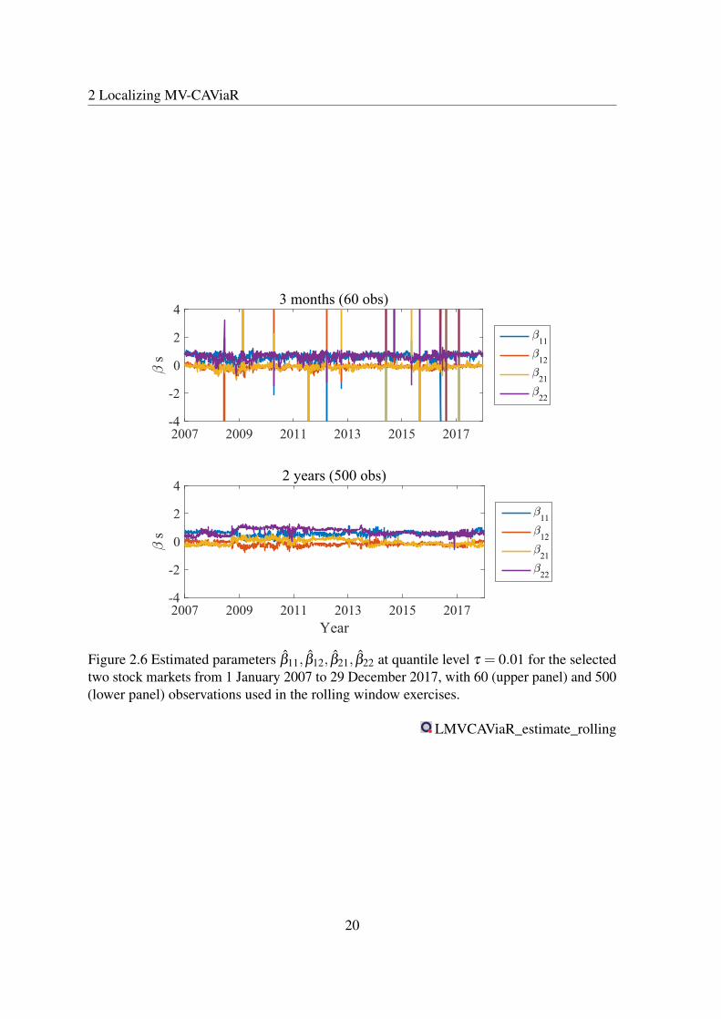
Parameter estimates are indeed more volatile when fitting the MV-CAViaR over shorterintervals (60 days), see e.g. Figures 2.5 and 2.6. More precisely, we display the estimatedMV-CAViaR parameters β11, β12, β21, β22 in model (2.10) in rolling window exercises from1 January 2007 to 29 December 2017. The upper (lower) panel at each figure shows theestimated parameter values if 60 (500) observations are included in the respective window.
18
2.5 Application
Index Mean Median Min Max Std Skew. Kurt.S&P 500 0.0002 0.0003 -0.0947 0.1096 0.0121 -0.3403 14.6949DAX 0.0003 0.0007 -0.0743 0.1080 0.0137 -0.0406 9.2297
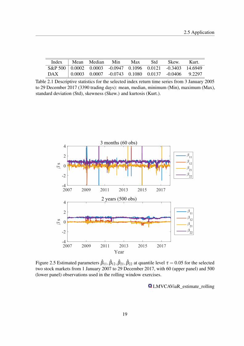
Table 2.1 Descriptive statistics for the selected index return time series from 3 January 2005to 29 December 2017 (3390 trading days): mean, median, minimum (Min), maximum (Max),standard deviation (Std), skewness (Skew.) and kurtosis (Kurt.).
2007 2009 2011 2013 2015 2017-4
-2
0
2
4
- s
3 months (60 obs)
-11-
12-
21-
22
2007 2009 2011 2013 2015 2017Year
-4
-2
0
2
4
- s
2 years (500 obs)
-11-
12-
21-
22
Figure 2.5 Estimated parameters β11, β12, β21, β22 at quantile level τ = 0.05 for the selectedtwo stock markets from 1 January 2007 to 29 December 2017, with 60 (upper panel) and 500(lower panel) observations used in the rolling window exercises.
LMVCAViaR_estimate_rolling
19
2 Localizing MV-CAViaR
2007 2009 2011 2013 2015 2017-4
-2
0
2
4
- s
3 months (60 obs)
-11-
12-
21-
22
2007 2009 2011 2013 2015 2017Year
-4
-2
0
2
4
- s
2 years (500 obs)
-11-
12-
21-
22
Figure 2.6 Estimated parameters β11, β12, β21, β22 at quantile level τ = 0.01 for the selectedtwo stock markets from 1 January 2007 to 29 December 2017, with 60 (upper panel) and 500(lower panel) observations used in the rolling window exercises.
LMVCAViaR_estimate_rolling
20
2.5 Application
Key empirical results from the presented fixed rolling window exercise can be summarizedas follows: (a) there exists a trade-off between the modeling bias and parameter variabilityacross different estimation setups, (b) the characteristics of the time series of estimatedparameter values as well as the estimation quality results demand the application of anadaptive method that successfully accommodates time-varying parameters, (c) data intervalscovering 60 to 500 observations may provide a good balance between the bias and variability.Motivated by these findings, we now turn to LMCR.
We exactly follow the steps as described in Section 2.2 to implement LMCR in theapplication. In line with the aforementioned empirical results, we select (K +1) = 13intervals, starting with 60 observations (three months) and ending with 500 observations(two trading years), i.e., we consider the set
60,75,94,118,148,185,231,289,361,451,500
with the coefficient c = 1.25 in accordance with the literature. In addition, we assume themodel parameters are constant within the initial interval I0 = 60.
Meanwhile, we use the initial two-year time series, i.e. from 3 January 2005 to 30December 2006, as the training sample to simulate the critical values. We exactly followthe procedure described in Section 2.2.1 to operate the simulation. We set two cases of thetuning parameter: the conservative case α = 0.8 and the modest case α = 0.9 to choose thecritical values. We present the empirical results in the next section.
2.5.2 Results
LMCR accommodates and reacts to structural changes. From the fixed rolling windowexercise in subsection 2.5.1 one observes time-varying parameter characteristics while facingthe trade-off between parameter variability and the modelling bias. How to account for theeffects of potential market changes on the tail risk based on the intervals of homogeneity? Inthe application, we employ LMCR to estimate the tail risk exposure as well as to analyze thecross-sectional spillover effects between the two selected stock markets. Using the time seriesof the adaptively selected interval length, one can trace out the dynamic tail risk spilloversand identify the distinct roles in risk transmissions.
21

2 Localizing MV-CAViaR
A. Homogeneous Intervals
The interval of homogeneity in tail quantile dynamics is obtained here by the LMCR frame-work for the time series of DAX and S&P 500 returns. Using the sequential local changepoint detection test, the optimal interval length is considered at two quantile levels, namely,τ = 0.01 and τ = 0.05, see Figure 2.8 and 2.7. All figures present the estimated lengths ofthe interval of homogeneity in trading days using the selected stock market indices from1 January 2007 to 29 December 2017. The upper panel depicts the conservative risk caseα = 0.8, whereas the lower panel denotes the modest risk case α = 0.9.
In a similar way, the intervals of homogeneity are slightly shorter in the conservativerisk case α = 0.8, as compared to the modest risk case α = 0.9. The average daily selectedoptimal interval length supports this, see, e.g., Table 2.2. The results are presented for theselected quantile levels at the conservative and modest risk cases, α = 0.8 and α = 0.9,respectively. In general the average lengths of selected intervals range between 7-10 monthsof daily observations across different markets. At quantile levels τ = 0.05, the intervals ofhomogeneity are slightly larger than the intervals at τ = 0.01.
α = 0.8 α = 0.9τ = 0.05 159 231τ = 0.01 143 171
Table 2.2 Mean value of the adaptively selected intervals. Note: the average number oftrading days of the adaptive interval length is provided for the DAX and S&P 500 marketindices at quantile levels, τ = 0.05 and τ = 0.01, and the conservative (α = 0.80) and themodest (α = 0.90) risk case.
LMVCAViaR_adaptive_estimation_length
B. One-Step-Ahead Forecasts of Tail Risk Exposure
Based on LMCR, one may directly estimate dynamic tail risk exposure. The tail risk atsmaller quantile level is relatively lower than risk at higher levels, see, e.g., Figure 2.9. Herethe estimated quantile risk exposure for the two stock market indices from 1 January 2007to 29 December 2017 is displayed for two quantile levels, τ = 0.01 and τ = 0.05. The leftpanel represents the conservative risk case α = 0.8 results, whereas the right panel considersthe modest risk case α = 0.9. The latter leads on average to slightly lower variability, as
22
2.5 Application
2007 2009 2011 2013 2015 2017
60
180
300
420
Leng
th
, = 0.8
2007 2009 2011 2013 2015 2017Year
60
180
300
420
Leng
th
, = 0.9
Figure 2.7 Estimated length of the interval of homogeneity in trading days for the selectedstock markets from 1 January 2007 to 29 December 2017 for the conservative (upper panel,α = 0.8) and the modest (lower panel, α = 0.9) risk cases. The quantile level equals τ = 0.01.The red line denotes one-month smoothed values.
LMVCAViaR_adaptive_estimation_length LMVCAViaR_adaptive_estimation_001
23
2 Localizing MV-CAViaR
2007 2009 2011 2013 2015 2017
60
180
300
420
Leng
th
, = 0.8
2007 2009 2011 2013 2015 2017Year
60
180
300
420
Leng
th
, = 0.9
Figure 2.8 Estimated length of the interval of homogeneity in trading days for the selectedstock markets from 1 January 2007 to 29 December 2017 for the conservative (upper panel,α = 0.8) and the modest (lower panel, α = 0.9) risk cases. The quantile level equals τ = 0.05.The red line denotes one-month smoothed values.
LMVCAViaR_adaptive_estimation_length LMVCAViaR_adaptive_estimation_005
24
2.5 Application
compared to the conservative risk case which results in marginally shorter homogeneityintervals.
2007 2009 2011 2013 2015 2017
-0.10
0
0.10
DAX, , = 0.8
2007 2009 2011 2013 2015 2017
-0.10
0
0.10
DAX, , = 0.9
2007 2009 2011 2013 2015 2017Year
-0.10
0
0.10
S&P 500, , = 0.8
2007 2009 2011 2013 2015 2017Year
-0.10
0
0.10
S&P 500, , = 0.9
Figure 2.9 One-step ahead forecasts of quantile risk exposure at level τ = 0.05 (blue) andτ = 0.01 (red) for return time series of DAX and S&P 500 indices (grey points) from 1January 2007 to 29 December 2017. The left panel shows results of the conservative riskcase α = 0.8 and the right panel depicts results of the modest risk case α = 0.9.
LMVCAViaR_adaptive_quantile
C. Time-Varying Coefficient Estimates
The transitions among the financial markets are directly revealed by the cross-sectionalcoefficients, see Adams et al. (2014). Here we take the dynamics of the two coefficients, β12
and β21, as representations of spillover effects between S&P 500 and DAX. Figure 2.10 and2.11 plot the dynamics of spillover effects from S&P 500 to DAX, β12 and the ones from
25
2 Localizing MV-CAViaR
DAX to S&P 500, β21. The upper (lower) panel represent the case of quantile level τ = 0.01(τ = 0.05). The blue lines show results of the conservative risk case α = 0.8 and the redlines depict results of the modest risk case α = 0.9.
Moreover, it shows that the cross-sectional coefficient β12 presents larger and morevolatile dynamics compared with the coefficient β21 for both quantile levels τ = 0.01 andτ = 0.05. The shifting of the risk spillovers from US market to German market tend to bemore intensive, especially during the unstable market period, e.g. the 2008 financial crisisperiod and the 2012 European sovereign debt crisis. Hence, compared with the spilloversfrom DAX to S&P 500, the US market appears to play dominate role in risk transmissions ofshocks to DAX indice, especially in volatile time.
2007 2009 2011 2013 2015 2017
0
0.2
0.4
0.6
12
Spillovers from S&P 500 to DAX = 0.01
2007 2009 2011 2013 2015 2017Year
0
0.2
0.4
0.6
12
= 0.05
Figure 2.10 Time-varying coefficients β12 at quantile level τ = 0.01 (upper panel) andτ = 0.05 (lower panel) for return time series of DAX and S&P 500 indices from 1 January2007 to 29 December 2017. The blue lines show results of the conservative risk case α = 0.8and the red lines depict results of the modest risk case α = 0.9.
26
2.5 Application
2007 2009 2011 2013 2015 2017
0
0.2
0.4
0.6
21
Spillovers from DAX to S&P 500 = 0.01
2007 2009 2011 2013 2015 2017Year
0
0.2
0.4
0.6
21
= 0.05
Figure 2.11 Time-varying coefficients β21 at quantile level τ = 0.01 (upper panel) andτ = 0.05 (lower panel) for return time series of DAX and S&P 500 indices from 1 January2007 to 29 December 2017. The blue lines show results of the conservative risk case α = 0.8and the red lines depict results of the modest risk case α = 0.9.
27
2 Localizing MV-CAViaR
2.6 Conclusion
The cross-sectional tail risk dependence among financial markets are time-varying and LMCRis constructed to cope with this challenge in evaluating the risk contagion. A local adaptiveapproach assumes that at any given point of time there is a historical interval of observationsover which the time series follows a parametric model. By utilizing a local change pointdetection procedure, one can sequentially determine the interval of homogeneity over whichthe time series behavior can be approximated described by a fixed parameter. LMCRadaptively estimates the tail risk transmission by relying on the longest detected intervalof homogeneity. The corresponding statistical properties of this method are successfullyderived.
A comprehensive simulation study supports the effectiveness of our approach in detectingstructural changes in multivariate tail risk estimation. When setting the quantile levels atτ = 0.05 and τ = 0.01 in a application of stock market indices DAX and S&P 500, thedynamic tail risk measures are successfully obtained. In addition, the developed approachpermits a delineation of the shifting tail risk spillover effects. We find that the US markettends to play prominent role in risk transmissions of shocks to German market, especially involatile times.
2.7 Proofs
Without loss of generality in Sections 2.7.1–2.7.4 we assume, that the interval of interest isthe whole observed data set, i.e. I = 0, . . . ,T. For this reason we neglect the index “I ”where applies, for instance, L(θ) instead of LI (θI ).
2.7.1 Proof of Lemma 2.1
Denote,gt(θ) = gt(θ)−∑
i∇qit(θ
∗)Ic[Yit ≤ qit(θ)],
where for Ft−1–measurable Z we set Ic[Yit ≤ Z] = I[Yit ≤ Z]−P(Yit ≤ Z|Ft−1). Since qit(θ)
are Ft−1–measurable, we obviously have Egt(θ) = λ t(θ). For any two θ ,θ ′ ∈ Θ consider
28

2.7 Proofs
the decomposition,
gt(θ)−gt(θ′) =∑
i∇qit(θ)−∇qit(θ
′)ψτi(Yit−qit(θ))
+∑i
∇qit(θ∗)P[Yit ≤ qit(θ)|Fit ]−P[Yit ≤ qit(θ
′)|Fit ]
+∑i
∇qit(θ∗)
Ic[Yit ≤ qit(θ)]− Ic[Yit ≤ qit(θ′)],
and, similarly, the difference gt(θ)− gt(θ∗) has only two first terms in this decomposition.
In the proof of Theorem 2 of White et al. (2015) it is shown, that with Assumption 2.3
‖gt(θ)− gt(θ′)‖ ≤ D2(np+ f0D1)‖θ −θ
′‖.
Let us fix some unit γ ∈ Rp and apply Theorem 1 of Merlevède et al. (2009) to thesum ∑t γ>gt(θ)− gt(θ
′). Since by Assumption 2.4 it holds α(k)≤ exp(−ck), we have aHoeffding-type inequality for each x≥ 0,
γ>
∑t
gt(θ)−λ t(θ)− gt(θ′)+λ t(θ
′)>C1‖θ −θ
′‖(√xT +x log2 T ) (2.11)
with probability ≥ 1−C2e−x, where C1 and C2 only depend on γ . Further we apply Theo-rem 2.2.27 of Talagrand (2014a) to get for any x≥ 0
P
(sup
θ∈Θ : ‖θ−θ∗‖≤r
∥∥∥∥∑t
gt(θ)−λ t(θ)− gt(θ′)+λ t(θ
′)
∥∥∥∥> LA(r,x)
)≤ LC2e−x,
where A(r,x) =√
T γ2(rB1,‖ · ‖)√x+(log2 T )γ1(rB1,‖ · ‖)x, with L being a generic con-
stant, B1 is a unit ball in Rp, and γ1,2(T,‖ · ‖) are Talagrand gamma-functionals, precisely,see Definition 2.2.18 in Talagrand (2014a). In the case of finite dimensional space, we haveγ1,2(rB1(0),‖ · ‖)≤ rC, where C =C(p) only depends on the dimension. We therefore canrewrite the above inequality,
P
(sup
θ∈Θ : ‖θ−θ∗‖≤r
∥∥∥∥∑t
gt(θ)−λ t(θ)− gt(θ′)+λ t(θ
′)
∥∥∥∥>Cr(√xT +x log2 T )
)≤ e−x,
where C only depends on n and γ , and x≥ 1.
Consider a δ -net θ 1, . . . ,θ N of the set Θ0(r), so that for each θ ∈ Θ0(r) there isj = 1..N with ‖θ − θ j‖ ≤ δ . It is known, that there is such a set with logN ≤ Cp log r
δ
29

2 Localizing MV-CAViaR
elements. By Bernstein-type inequality, Theorem 2 in Merlevède et al. (2009), it holds∥∥∥∥∥∑t∑
i∇qit(θ
∗)(Ic[Yit ≤ qit(θ k)]− Ic[Yit ≤ qit(θ∗)])
∥∥∥∥∥≤C√rT√x+ logN
+(logT )2(x+ logN),
uniformly for all k = 1, . . . ,N with probability at least 1− e−x, and the constant only dependon n,γ . Here we use the fact that the terms Ic[Yit ≤ qit(θ)] are centred conditioned on Ft−1,while ∇qit(θ) are Ft measurable.
Furthermore, taking into account part (iii) of Assumption 2.4 we can use Theorem 5.2from Boucheron et al. (2005a) to get that for any i = 1, . . . ,n
|t : εit ∈ [a,b]| ≤ T f0(b−a)+C√
T f0(b−a)x+Cx
with probability at least 1−4e−x uniformly over all intervals, with some universal constantC. By definition, for any θ ∈ Θ0(r) there is some k such that |git(θ)−git(θ k)| ≤ D1δ foreach i, t. Therefore, the amount of indices i, t, for which the values of I[Yit − qit(θ)] andI[Yit − qit(θ k)] differ is bounded by C(T δ +
√T δx+ x), constant C does not depend on
T,x,r and δ . We come to the conclusion, that choosing δ = rT−1/2, on the intersection ofthe events listed above it holds,∥∥∥∥∥∑t
∑i
∇qit(θ∗)I[Yit ≤ qit(θ)]− I[Yit ≤ qit(θ k)]
∥∥∥∥∥. T 1/2r+√
T 1/2rx+x.
Putting the inequalities together we get the result.
2.7.2 Proof of Proposition 2.1
The claim follows directly from a slightly flexible version, that we are using for the consis-tency of bootstrap estimator as well.
Lemma 2.2. Let assumptions 2.1–2.5 hold on the interval I . Then there are T0,a0 > 0such that whenever |I | ≥ T0, a≤ a0 and x≤ |I | the following implication takes place with
probability ≥ 1−6e−x. Each θ ∈Θ that satisfies,
LI (θ)−LI (θ ∗)≥−|I |a
30

2.7 Proofs
satisfies as well
‖θ −θ∗‖ ≤
√a/b+C0
√x+ log |I ||I |
,
where b,C0 do not depend on |I | and x.
First, we present a uniform bound for the score. Similar to (2.11) it holds ‖∇ζ (θ ∗)‖ ≤C(√xT +x log2 T ) with probability≥ 1−e−x, while by Lemma 2.1 we have with probability
≥ 1− e−x, that
supθ∈Θ0
‖∇ζ (θ)−∇ζ (θ ∗)‖ ≤C(√
T√x+ logT +x log2 T ),
using the fact that the set Θ0 is bounded. Using a simple triangle inequality we have,
‖∇ζI (θ)‖ ≤C(√
T√x+ logT +x log2 T ) (2.12)
with probability ≥ 1−2e−x uniformly for each θ ∈Θ0, with C not depending on T,x.
Next we present a technical lemma, that shows quadratic deviation of the expectation oflog-likelihood in the neighbourhood of true parameter. The resulting inequality is akin tocondition (Lr) of Spokoiny (2017).
Lemma 2.3. Suppose, 2.1–2.3 and 2.5 hold. Then, there are r0,b > 0 that do not depend
on |I |, such that for each θ ∈ Θ satisfying ‖θ −θ∗‖ ≥ r it holds ELI (θ)−ELI (θ ∗) ≤
−b|I |(r2∧r20).
The proof of this lemma is postponed to Section 2.7.6.
Proof of Lemma 2.2. By (2.12) we have for x≤ |I |,
1|I |
ELI (θ)− 1|I |
ELI (θ ∗)≥LI (θ)−LI (θ ∗)−‖θ −θ∗‖ sup
θ∈Θ
‖∇ζI (θ)‖
≥−a−C2‖θ −θ∗‖|I |−1/2
√x+ log |I |
≥−a0−C2R|I |−1/2√x+ log |I |
with probability at least 1−2e−x. By Lemma 2.3 this implies,
b‖θ −θ∗‖2 ≤ a+C2‖θ −θ
∗‖|I |−1/2√x+ log |I |,
31

2 Localizing MV-CAViaR
and it is left to notice that x2 ≤ α +βx implies x ≤√
α +β . Additionally, L(θ) ≥ L(θ ∗)
pointwise, thus the deviation bound for the estimator takes place.
2.7.3 Proof of Proposition 2.2
First of all, by Proposition 2.1 it holds with probability ≥ 1−7e−x, that ‖θ −θ∗‖ ≤ r0 =
C0√
T−1(x+ logT ). Applying Lemma 2.1 with this radius, we get that with probability≥ 1−13e−x additionally this holds for each θ ∈Θ0(r0):
1√T
∥∥∥∥∑t
gt(θ)−λ t(θ)−gt(θ∗)+λ t(θ
∗)
∥∥∥∥. δT,x =(x+ logT )3/4
T 1/4 . (2.13)
With θ = θ and using ∑t gt(θ) = 0, ∑t λ t(θ∗) = 0 we get,∥∥∥∥√T Q(θ −θ
∗)− 1√T ∑
tgt(θ
∗)
∥∥∥∥. δT,x.
Similar to the proof of Theorem 2.3 in Spokoiny (2017), introducing the error of quadraticapproximation of log-likelihood near the true parameter and provided (2.5) and (2.13), onecan show that the square root of log-likelihood ratio is approximated with the same rate, i.e.∣∣∣√2L(θ)−2L(θ ∗)−‖ξ‖
∣∣∣≤ δT,x. Scaling x← x+ log13 provides the result.
2.7.4 Proof of Proposition 2.3
Similar to the original likelihood,
ζ(θ) = L(θ)−EL(θ) = ∑
t(wt−1)`t(θ)
denotes the stochastic part of the likelihood in the bootstrap world.
Lemma 2.4. Suppose 2.2, 2.3 and 2.6. For each x≥ 1 with probability ≥ 1−4e−x w.r.t. to
the data, the probability of
supθ∈Θ(r)
1T 1/2
∥∥∥∥∑t(wt−1)gt(θ)−gt(θ
∗)∥∥∥∥≤♦[(T,r,x)
32

2.7 Proofs
conditioned on the data is at least 1−3e−x, where
♦[(T,r,x) =C3
(r∨√r+T−1/4(rx)1/2∨ (rx)1/4+T−1/2x
)√x+ logT ,
with C3 not depending on T,r,x.
Proof. The proof is similar to that of Lemma 2.1.
Corollary 2.2. For x≤√
T it holds with probability at least 1−6e−x,
P(
supθ∈Θ
‖∇ζ(θ)‖ ≤C5T 1/2
√x+ logT
)≤ 1−5e−x,
where C5 does not depend on T,x.
Now we are ready to state the global concentration result for the bootstrap estimator.
Proposition 2.4. Assume 2.2-2.5 and 2.6. Then, on a set of probability at least 1−12e−x it
holds with probability at least 1−5e−x conditioned on the data,
‖θ−θ
∗‖ ≤C
√x+ logT
T.
Proof. Denote r = ‖θ−θ‖. Using Corollary 2.2 and the fact that L(θ
) ≥ L(θ ∗), we
have on the event of probability at least 1−6e−x w.r.t. data, with probability at least 1−5e−x
conditioned on the data, that
L(θ)−L(θ ∗)≥L(θ)−L(θ ∗)−‖θ
−θ
∗‖× sup‖∇ζ(θ)‖
≥−C5T 1/2r√x+ logT .
Using Proposition 2.1, we have that, additionally, on the other event of probability 1−6e−x
it holds r .
√r√
x+log TT +
√x+log T
T , which yields the result.
The rest can be accomplished using linear approximation of the score. Similar to theoriginal likelihood, with r0 = ‖θ −θ
∗‖∨‖θ−θ
∗‖ it follows from (2.5),∥∥∥∥∑t
λ t(θ)−∑
tλ t(θ)+T Q2(θ
− θ)
∥∥∥∥≤ 2C2Tr20.
33

2 Localizing MV-CAViaR
Here, ∑t λ t(θ) stands for the expectation of gradient of the likelihood. With help ofProposition 2.1 we first replace it with just the gradient, then, using Lemma 2.4 we replace itwith the gradient of bootstrap likelihood. This finally leads to the proof of the proposition.
2.7.5 Proof of Theorem 2.1
W.l.o.g. we have an interval I = 1, . . . ,T and a set of break points S (I ) ⊂ I to beconsidered. Let us denote T = α0T with α0 > 0 from the conditions of the theorem. Wehave by Proposition 2.2, that with probability at least 1− e−x it holds for each s ∈S (I ),∣∣∣LAI ,s(θ AI ,s)−LAI ,s(θ
∗)−‖ξ AI ,s‖2/2
∣∣∣≤♦, ∣∣∣LBI ,s(θ BI ,s)−LBI ,s(θ∗)−‖ξ BI ,s
‖2/2∣∣∣≤♦,∣∣∣LI (θI )−LI (θ ∗)−‖ξ AI
‖2/2∣∣∣≤♦,
where ♦=CT−1/4(x+ logT + log(1+2|S (I )|))3/4, implying∣∣∣LAI ,s(θ AI ,s)+LBI ,s(θ BI ,s)−LI (θI )− (‖ξ AI ,s‖2 +‖ξ BI ,s
‖2−‖ξ I ‖2)/2∣∣∣≤ 3♦.
By definition, |I |1/2ξ I = |AI ,s|1/2
ξ AI ,s+ |BI ,s|1/2
ξ BI ,s, therefore for α = |AI ,s|/|I |
and β = |BI ,s|/|I |= 1−α we have,
‖ξ AI ,s‖2 +‖ξ BI ,s
‖2−‖ξ I ‖2 =‖ξ AI ,s‖2 +‖ξ BI ,s
‖2−‖α1/2ξ AI ,s
+β1/2
ξ BI ,s‖2
=β‖ξ AI ,s‖2 +α‖ξ BI ,s
‖2−2α1/2
β1/2
ξ>AI ,s
ξ BI ,s
=‖β 1/2ξ AI ,s
−α1/2
ξ BI ,s‖2
Obviously, similar expansion holds for the bootstrap counterpart, so that denoting
SI ,s =1√|I |
[√|BI ,s||AI ,s| ∑
t∈AI ,s
Q−1gt(θ∗)−
√|AI ,s||BI ,s| ∑
t∈BI ,s
Q−1gt(θ∗)
],
SI ,s =1√|I |
[√|BI ,s||AI ,s| ∑
t∈AI ,s
Q−1wtgt(θ∗)−
√|AI ,s||BI ,s| ∑
t∈BI ,s
Q−1wtgt(θ∗)
],
we have∣∣∣maxs
TI ,s−maxs‖SI ,s‖2
∣∣∣≤ 3♦,∣∣∣max
sT I ,s−max
s‖SI ,s‖2
∣∣∣≤ 3♦. (2.14)
34

2.7 Proofs
For a single break point s ∈S (I ) by Azuma-Hoeffding inequality for all x> 0 it holds,
P(‖SI ,s‖. 1+
√x)≥ 1− e−x,
so that it holds with probability ≥ 1− e−x,
maxs‖SI ,s‖.
√logT +
√x, max
s‖SI ,s‖.
√logT +
√x.
Additionally, for each A⊂I the covariance
Var(ξ A) =1|A|∑t∈A
Q−1gt(θ∗)gt(θ
∗)>Q−1.
is concentrated near Σ = Var(Q−1g1(θ∗)) = Q−1V 2Q−1, e.g. by Azuma-Hoeffding
P
(‖Var(ξ A)−Σ‖.
√1+x
|A|
)≥ 1− e−x,
so that taking into account (2.7), it holds with probability ≥ 1− e−x, that for each A = AI ,s
or A = BI ,s with s ∈S (I ),
‖Var(ξ A)−Σ‖.√
logT +x
T. (2.15)
Now we want to use Lemma A.4 with n = T . Since δ > 1 by Assumption 2.4, we canchoose c2,c′ > 0 such that (1+δ )/2− (1+2δ )c2 > 1+c′. Then, we can have a,ε > 0 suchthat a+ ε < 1
2 −2c2 and c2 +(1+δ )a > 1+ c′. Setting b = a+ γ + ε , we have that
1−b− γa <−c′, b <12− c2, b−a > c2.
This means, that taking q = dT ae and r = dT be and Dn .√
logn by Assumption 2.6, theconditions of Lemma A.4 are satisfied. Moreover, by (2.15) we have ∆ .
√logT/T with
probability ≥ 1−1/(2T ), so that for each t,y ∈ R∣∣∣P(maxs‖SI ,s‖> t)−P(max
s‖SI ,s‖> t + y)
∣∣∣. T−c∧c′+ |y| log1/2 T. (2.16)
35

2 Localizing MV-CAViaR
Thus, for |y| ≤ 6♦ taken for x=C logT , we have for each t,y ∈ R
supt
∣∣∣P(maxs
TI ,s > t + y)−P(maxs
T I ,s > t)∣∣∣. T−c∧c′+ |y| log1/2 T
with probability ≥ 1−1/T .
2.7.6 Proof of Lemma 2.3
Note, that integrating the inequality (2.5) with Q = ∑ni=1E fit(0)∇qit(θ
∗)[∇qit(θ∗)]>, we get
second-order approximation in the neighbourhood of θ∗,∣∣∣∣ 1
TEL(θ)− 1
TEL(θ ∗)+‖Q(θ −θ
∗)‖2/2∣∣∣∣≤C‖θ −θ
∗‖3,
therefore we get that for ‖θ −θ∗‖> r and r≤ r0 = λmin(Q2)/(4C) we have
1TEL(θ)− 1
TEL(θ ∗)<−blocr
2, bloc = λmin(Q2)/4.
Next, notice that if a r.v. Z has τ quantile 0, then for δ > 0
Eρτ(Z +δ )−Eρτ(Z) =E(Z +δ )(τ− I[Z +δ ≤ 0])−EZ(τ− I[Z ≤ 0])
=δE(τ− I(Z ≤ δ )+ I[Z ∈ (−δ ,0)])+EZ I(Z ∈ (−δ ,0))
=E(Z +δ )I(Z ∈ (−δ ;0))
≥δ/2EI(Z ∈ (−δ/2;0))
≥f δ
2
(δ
2∧δ0
),
and by analogy same bound takes place for Eρτ(Z−δ )−Eρτ(Z). Therefore,
E`t(θ)−E`t(θ∗)≤ E
n
∑i=1
f |qit−q∗it |2
(|qit−q∗it |
2∧δ0
),
where due to (2.4), the right-hand side is bounded by f δ (δ ∧δ0)/4 with δ = δ (r0). Settingbglob = f δ (δ ∧δ0)/(4r2
0), we get that the required inequality is satisfied with b = bloc∧bglob.
36

2.7 Proofs
2.7.7 Proof of Corollary 2.1
Let z(α) denotes (1−α)-quantile of the test T , and z(α) is that of T with respect to thebootstrap probability (here for convenience we write the confidence level in the brackets).Since P(X +Y > a+b)≤ P(X > a)+P(Y ≥ b) for arbitrary random variables X ,Y and realnumbers a,b, we have for each δ ∈ (0;α)
P(T > z(α))≤P(T > z(α +δ ))+P(z(α)≤ z(α +δ ))
=α +δ +P(z(α)≤ z(α +δ )),
P(T > z(α))≥P(T > z(α−δ ))−P(z(α)≥ z(α−δ ))
=α−δ −P(z(α)≥ z(α−δ )).
(2.17)
Furthermore,
P(z(α)≥ z(α−δ )) =PP(T > z(α−δ ))≥ α ,
P(z(α)≤ z(α +δ )) =PP(T > z(α +δ ))≤ α .
By Theorem 2.1 we have on a set of probability ≥ 1−1/T , that
supt|P(T > t)−P(T > t)| ≤CT−c.
Taking δ = 2CT−c and t = z(α−δ ) we have,
P(T > z(α−δ ))≤ α−δ +CT−c < α
and in a similar way,
P(T > z(α +δ ))≥ α +δ −CT−c > α.
Thus, with this choice of δ it holds,
P(z(α)≤ z(α +δ ))≤ 1/T, P(z(α)≥ z(α−δ ))≤ 1/T,
which via (2.17) concludes the proof.
37


Chapter 3
Influencers and Communities in SocialNetworks
Financial and social networks are often analysed through vector autoregression model, forinstance, in Härdle et al. (2019). Consider a network that produces a time series Yt ∈ RN ,t = 1, . . . ,T and dependencies between it’s elements are modeled through the equation
Yt = ΘYt−1 +Wt , (3.1)
where Wt are innovations that satisfy E[Wt |Ft−1] = 0, Ft = σYt−1,Yt−2, . . ., so that theinteractions between the nodes are described by an autoregression operator Θ ∈ RN×N . Interms of the network connections we say that a node i is connected tothe node j if
Θi j 6= 0,
so that the adjacency matrix of such network is represented by nonzero coefficients and thesparsity of Θ represents number of the edges. For large-scale time series one encountersthe curse of dimension, as estimating the matrix-parameter Θ with N2 elements requiressignificantly large number of observations T .
Several attempts to reduce the dimensionality have been made in the past literature.Assuming that the elements of a time series form a connected network, Zhu et al. (2017)introduces a Network Autoregression model (NAR) with Θi j = βAi j/∑
Nk=1 Aik, provided that
the adjacency matrix A ∈ RN×N is known. Here, the regression operator, defined up to asingle parameter β , which called a network effect, can be estimated through a simple least
39
3 Influencers and Communities in Social Networks
squares. Zhu et al. (2016) also extend this model for conditional quantiles. Furthermore,Zhu and Pan (2017) argue that a single network parameter may not be satisfactory as ittreats all nodes of the network homogeneously. In particular, the NAR model implies thateach node is affected by it’s neighbours in the same extent, while in reality we may havefinancial institutions that are affected less than the others, thus more secure and risk-free.They then propose to detect communities in the network based on the given adjacency matrixand suggest that the nodes in each community share a separate network effect parameter.A somewhat opposite direction is taken by Gudmundsson and Brownlees (2018): theirBlockBuster algorithm determines the communities through the estimated autoregressivemodel, which, however, does not solve the dimensionality problem. Apart from this lineof work, sparse regularisations have been extensively used, see Fan et al. (2009); Han et al.(2015); Melnyk and Banerjee (2016).
To sum up we want to address the following problems, which one encounters dealingwith vector autoregression:
• as already mentioned above, in VAR the parameter dimension is particularly large andrequires even larger time intervals for consistent estimation. Even if one can affordsuch data set, in the long run, autoregressive parametric models tend to be violated,see e.g. Cížek et al. (2009). Naturally, we want to impose some structural assumptionson the operator Θ, so that it can be estimated by means of moderate sample sizes.
• The NAR model assumes that the adjacency matrix is given. In particular, this is justi-fied for social networks with a natural friendship/follower-followee relationship. For anetwork of financial institutions, there is no explicitly defined adjacency matrix andone has to heuristically evaluate it using additional information (identical shareholders,trading volumes, etc.) or through analysing correlations and lagged cross-correlationsbetween returns or risk profile, see Diebold and Yılmaz (2014) and Chen et al. (2019b).However, there is no rigorous reason to believe that the operator in (3.1) dependsexplicitly on such adjacency matrix, see also Cha et al. (2010).
Motivated by two aspects of social networks we construct a new Social Network autore-
gression with Influencers and Communities model (SoNIC). Based on a user experienceon platforms like facebook, twitter, etc., one can assume that there are some users thatare followed significantly more than the others. Take, for example, celebrities, sportsmen,politicians, or instagram divas. These nodes of a network have much more influence overthe others, than the rest of the nodes. We call such nodes influencers. In the notation of
40

autoregressive parameter, a node j is called an influencer, if there is a significant amount ofother nodes i such that Θi j 6= 0. Assuming that the number of influencers is limited, we cansay that only few columns of matrix Θ are important. This allows us to take into accountonly the connections to the influencers, significantly reducing the number of parameters tobe estimated. A similar idea is used in Chen et al. (2018), with a group-lasso regularisationimposed, so that they find a solution with few active columns. Notice, however, that onlyrelying on sparsity still requires T > N, see e.g. Chernozhukov et al. (2018); Fan et al.(2009).
It is also widely known that social networks consist of smaller communities, with thenodes exhibiting higher connection density or similar behaviour inside the communities. Zhuand Pan (2017) makes one step to extend the NAR model from Zhu et al. (2017) into a morerealistic set-up by saying that instead of a single network effect parameter, there are separateparameters for each community. For us the behaviour of a node i is characterized by thecoefficients Θi1, . . . ,ΘiN , i.e. the nodes it depends on and to what extent. We assume thatthe nodes are separated into few clusters such that the nodes from the same cluster have thesame dependencies. This brings a bigger picture into the view: instead of saying that twonodes from the same cluster are more likely to be connected, we say that they are connectedto the same influencers.
Our main focus is application to sentiment extracted from a microblogging platformdedicated to stock trading, StockTwits1. For each user one can extract average sentimentweight over the messages he posts during the day. Analysing the resulting time series we areable to identify, on one hand, influencers — the users whose opinion is most important, andon the other, different communities. Another problem that we want to address is the presenceof missing observation in the data set, since on some days some users do not leave anymessages. We treat this as follows: the there is an underlying opinion process that followsautoregressive equation (3.1), while the users decide whether to express it or not during eachday.
The rest of the chapter is organized as follows. Section 3.1 introduces the reader toStockTwits platform, describes in detail the available data set and the process of sentimentweights extraction. In Section 3.2 first introduces our SoNIC model, then describes theestimation procedure and provides a consistency result. In Section 3.3 we provide simulationresults that partially confirm the theoretical properties of our estimator. Next, in Section 3.4we present and discuss the results of application of our model to some data sets extracted
1https://stocktiwts.com
41
3 Influencers and Communities in Social Networks
from the StockTwits. Section 3.5, as well as Sections 3.6, A.1 in the appendix, are dedicatedto the proofs.
3.1 StockTwits
Among social media platforms, we particularly are interested in StockTwits2 for a number ofreasons. Firstly, it becomes predominantly popular and stands for a leading social network forinvestors and traders. Secondly, it is similar to Twitter, but dedicated to financial discussion.One of features leads to its popularity is a well-designed reference between the messagecontent and the referring stock symbols. Conversations are organized around ‘cashtags’ (e.g.‘$AAPL’ for APPLE; ‘$BTC.X’ for BITCOIN) that allow to narrow streams down to specificassets. Thirdly and most importantly, users can also express their sentiment/opinions bylabeling their messages as ‘Bearish’ (negative) or ‘Bullish’ (positive) via a toggle button.These are so-called self-report sentiment. Indeed, the user generated messages and self-reported sentiment attract the researchers for sentiment analysis. The available labeleddata benefits an advance on textual analysis that typically relies on the available trainingdataset. We use this convention and StockTwits Application Programming Interface (API) todownload all messages containing the preferred cashtages. StockTwits API also providesfor each message its user’s unique identifier, the time it was posted at with a one-secondprecision, and the sentiment associated by the user (‘Bullish’, ‘Bearish’ or unclassified).
Among over thousand tickers/symbols, we particularly pick up two selective symbols,$AAPL for APPLE; $BTC.X for BITCOIN, which represents the most popular security andcryptocurrency, respectively. We conjecture that due to the fact they attract investors/userswith very distinct risk preference, the resulting opinion networks and its dynamics mayexhibit diverse structures. In Table 3.1 we summarize the messages’ statistics with respect toAAPL and bitcoin. Even though we exclusively consider these two symbols, the messagevolume and number of users associated with these two symbols are tremendous. A glimpseof table shows different profiles between two symbols. Firstly, the users who interest in BTCtend to disclose their sentiment, evident by 44% of labelled messages, while in AAPL only28% of messages are labelled. It may lead to a better training accuracy in the case of BTCmessages relative to the training model based on AAPL. Secondly, there is a clear imbalancebetween the numbers of positive and negative messages, showing that online investors areoptimistic on average, as previously found by Kim and Kim (2014) or Avery et al. (2016). It
2https://stocktwits.com/
42

3.1 StockTwits
seems that the imbalance is more evident in the case of AAPL. Through the reported averagemessage volume per day, there is no doubt that AAPL is more able to attract attentions frompotential investors than BTC could.
Symbols AAPL BTCmessage volume 449,761 644,597number of distinct users 26,521 25,492number of bullish messages 133,316 196,555number of bearish messages 48,186 90,677percentage of bullish messages 20.6% 30.4%percentage of bearish messages 7.4% 14.0%percentage of labeled messages 28.0% 44.4%size of positive training dataset 99,985 147,759size of negative training dataset 36,100 67,752message volume per day 730 305number of positive terms in lexicon 4,000 3,775number of negative terms in lexicon 4,000 3,759sample period 2017-05-22 2013-03-21
2019-01-27 2018-12-27
Table 3.1 Summary statistics of social media messages
3.1.1 Quantifying message content
In order to study the sentiment interaction of users and the dynamics of interaction, oneneeds to quantify the messages from the selected users and subsequently model the quantifiedtexts from ultra high-dimensional users. In practice, converting text data into a quantitativesentiment variable can been done by two techniques, namely dictionary-based and machinelearning-based analysis. Although a machine learning technique has many advantages com-pared to a dictionary-based approach, a dictionary-based approach offers better transparency,explication and less computational burden. Loughran and McDonald (2016) recommend thatalternative complex methods (machine learning) should be considered only when they addsubstantive value beyond simpler and more transparent approaches such as bag-of word. Wetherefore opt for the lexicon approach in the task of sentiment quantification.
A dictionary, or lexicon, is a list of words labeled as positive, negative or neutral. As-suming such a list, the classic bag-of-words approach consists of counting the number ofpositive and negative words in a document in order to assign it a sentiment value or tone. For
43
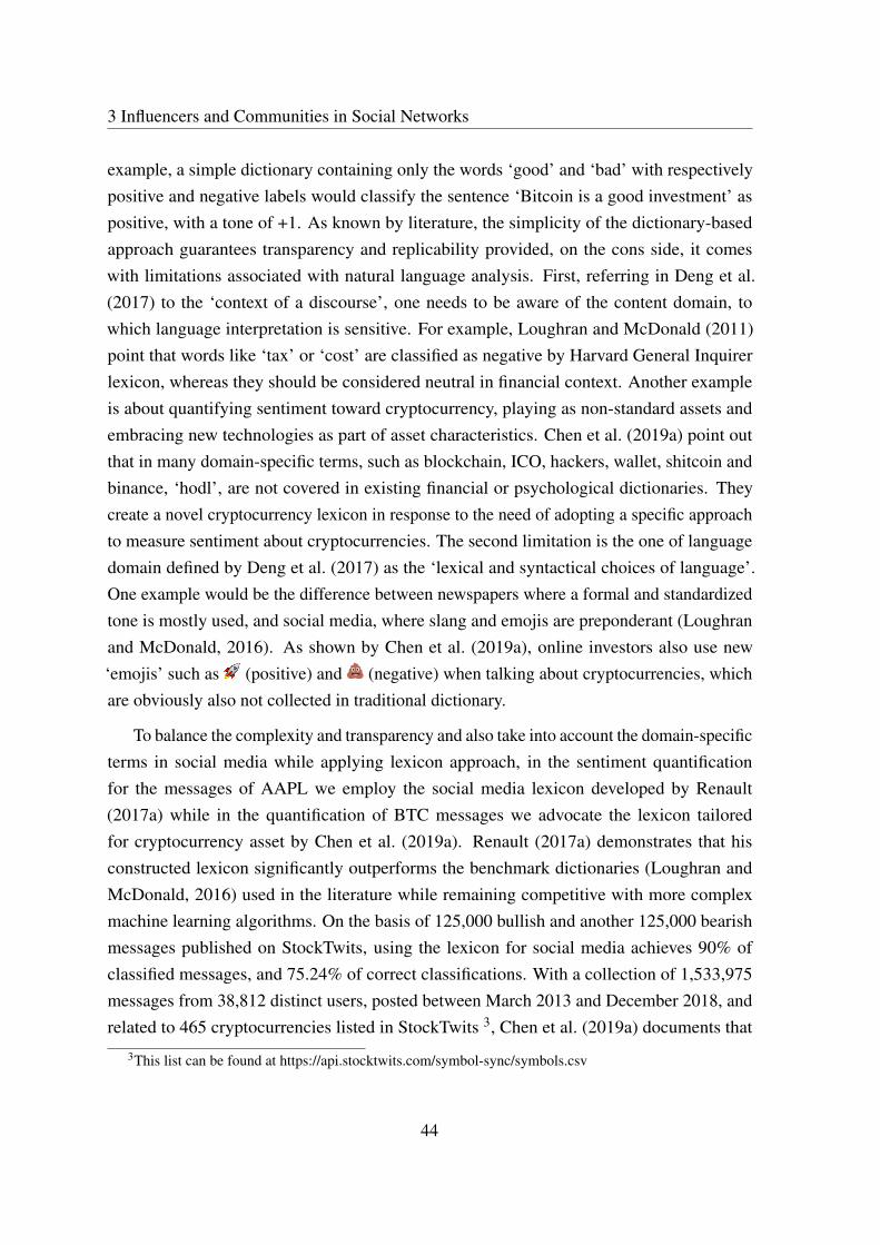
3 Influencers and Communities in Social Networks
example, a simple dictionary containing only the words ‘good’ and ‘bad’ with respectivelypositive and negative labels would classify the sentence ‘Bitcoin is a good investment’ aspositive, with a tone of +1. As known by literature, the simplicity of the dictionary-basedapproach guarantees transparency and replicability provided, on the cons side, it comeswith limitations associated with natural language analysis. First, referring in Deng et al.(2017) to the ‘context of a discourse’, one needs to be aware of the content domain, towhich language interpretation is sensitive. For example, Loughran and McDonald (2011)point that words like ‘tax’ or ‘cost’ are classified as negative by Harvard General Inquirerlexicon, whereas they should be considered neutral in financial context. Another exampleis about quantifying sentiment toward cryptocurrency, playing as non-standard assets andembracing new technologies as part of asset characteristics. Chen et al. (2019a) point outthat in many domain-specific terms, such as blockchain, ICO, hackers, wallet, shitcoin andbinance, ‘hodl’, are not covered in existing financial or psychological dictionaries. Theycreate a novel cryptocurrency lexicon in response to the need of adopting a specific approachto measure sentiment about cryptocurrencies. The second limitation is the one of languagedomain defined by Deng et al. (2017) as the ‘lexical and syntactical choices of language’.One example would be the difference between newspapers where a formal and standardizedtone is mostly used, and social media, where slang and emojis are preponderant (Loughranand McDonald, 2016). As shown by Chen et al. (2019a), online investors also use new‘emojis’ such as (positive) and (negative) when talking about cryptocurrencies, whichare obviously also not collected in traditional dictionary.
To balance the complexity and transparency and also take into account the domain-specificterms in social media while applying lexicon approach, in the sentiment quantificationfor the messages of AAPL we employ the social media lexicon developed by Renault(2017a) while in the quantification of BTC messages we advocate the lexicon tailoredfor cryptocurrency asset by Chen et al. (2019a). Renault (2017a) demonstrates that hisconstructed lexicon significantly outperforms the benchmark dictionaries (Loughran andMcDonald, 2016) used in the literature while remaining competitive with more complexmachine learning algorithms. On the basis of 125,000 bullish and another 125,000 bearishmessages published on StockTwits, using the lexicon for social media achieves 90% ofclassified messages, and 75.24% of correct classifications. With a collection of 1,533,975messages from 38,812 distinct users, posted between March 2013 and December 2018, andrelated to 465 cryptocurrencies listed in StockTwits 3, Chen et al. (2019a) documents that
3This list can be found at https://api.stocktwits.com/symbol-sync/symbols.csv
44
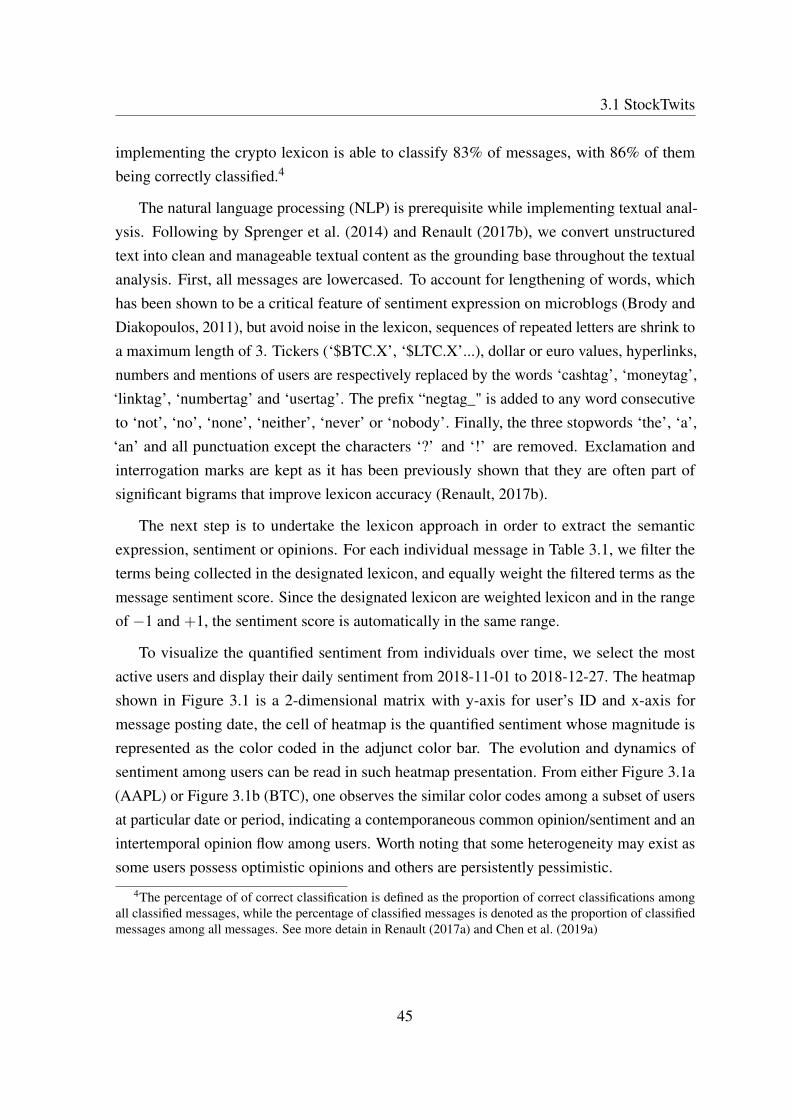
3.1 StockTwits
implementing the crypto lexicon is able to classify 83% of messages, with 86% of thembeing correctly classified.4
The natural language processing (NLP) is prerequisite while implementing textual anal-ysis. Following by Sprenger et al. (2014) and Renault (2017b), we convert unstructuredtext into clean and manageable textual content as the grounding base throughout the textualanalysis. First, all messages are lowercased. To account for lengthening of words, whichhas been shown to be a critical feature of sentiment expression on microblogs (Brody andDiakopoulos, 2011), but avoid noise in the lexicon, sequences of repeated letters are shrink toa maximum length of 3. Tickers (‘$BTC.X’, ‘$LTC.X’...), dollar or euro values, hyperlinks,numbers and mentions of users are respectively replaced by the words ‘cashtag’, ‘moneytag’,‘linktag’, ‘numbertag’ and ‘usertag’. The prefix “negtag_" is added to any word consecutiveto ‘not’, ‘no’, ‘none’, ‘neither’, ‘never’ or ‘nobody’. Finally, the three stopwords ‘the’, ‘a’,‘an’ and all punctuation except the characters ‘?’ and ‘!’ are removed. Exclamation andinterrogation marks are kept as it has been previously shown that they are often part ofsignificant bigrams that improve lexicon accuracy (Renault, 2017b).
The next step is to undertake the lexicon approach in order to extract the semanticexpression, sentiment or opinions. For each individual message in Table 3.1, we filter theterms being collected in the designated lexicon, and equally weight the filtered terms as themessage sentiment score. Since the designated lexicon are weighted lexicon and in the rangeof −1 and +1, the sentiment score is automatically in the same range.
To visualize the quantified sentiment from individuals over time, we select the mostactive users and display their daily sentiment from 2018-11-01 to 2018-12-27. The heatmapshown in Figure 3.1 is a 2-dimensional matrix with y-axis for user’s ID and x-axis formessage posting date, the cell of heatmap is the quantified sentiment whose magnitude isrepresented as the color coded in the adjunct color bar. The evolution and dynamics ofsentiment among users can be read in such heatmap presentation. From either Figure 3.1a(AAPL) or Figure 3.1b (BTC), one observes the similar color codes among a subset of usersat particular date or period, indicating a contemporaneous common opinion/sentiment and anintertemporal opinion flow among users. Worth noting that some heterogeneity may exist assome users possess optimistic opinions and others are persistently pessimistic.
4The percentage of of correct classification is defined as the proportion of correct classifications amongall classified messages, while the percentage of classified messages is denoted as the proportion of classifiedmessages among all messages. See more detain in Renault (2017a) and Chen et al. (2019a)
45
3 Influencers and Communities in Social Networks
(a) AAPL users
(b) BTC users
Figure 3.1 Social media users’ sentiment over timey-axis is the user’s id, while x-axis is time stamp from 2018-11-01 —a 2018-12-27.
46

3.2 Main results
3.2 Main results
3.2.1 Clusters of nodes and influencers
In our set-up the behaviour of each node i∈ [N] is characterized by the coefficients Θi1, . . . ,ΘiN ,and when we group the nodes using their characteristics the notion of community is mergedwith the notion of cluster. We assume that the nodes are separated into clusters, such thatthese coefficients remain the same for the nodes within each cluster. Let us first give a precisedefinition of a clustering.
Definition 3.1. A K-clustering of the set of the nodes [N] is called a sequence C =(C1, . . . ,CK)
of K subsets of [N], such that
• any two subsets are disjoint Ci∩C j = /0 for i 6= j;
• the union of subsets C j gives all nodes,
C1∪·· ·∪CK = 1, . . . ,N.
Two clusterings C and C ′ are equivalent, if there is a permutation π on 1, . . . ,K, such that
the clusters are equal with respect to relabelling, i.e. C j =C′π( j) for each j = 1, . . . ,K.
Furthermore, denote a distance between two clusterings is defined as
d(C ,C ′) = minπ
K
∑j=1|C j \C′
π( j)|.
Remark 3.1. The distance between clusterings is in fact the minimal amount of node transfers
from one cluster to another, that is required to make the clusterings equivalent. To see this,
notice that each clustering can be defined as a sequence (l1, . . . , lN) of N labels taking values
in 1, . . . ,K, so that each cluster defines as C j = i : li = j. Then, if the clustering C ′
corresponds to the labels l′1, . . . , l′N , it is not hard to see, that the distance between them
equals to
d(C ,C ′) = minπ
N
∑i=1
I(li 6= π(l′i)).
We specify our model by putting structural assumptions which are motivated by both thecommunities and presence of the influencers.
47

3 Influencers and Communities in Social Networks
Definition 3.2. We say that Θ ∈ SoNIC(s,K) (Social Network with Influencers and Commu-
nities) if
• each user is influenced by at most s influencers, i.e.
maxi
N
∑j=1
I(Θi j 6= 0)≤ s;
• there is a K-clustering C = (C1, . . . ,CK) such that
Θi j = Θi′ j, j = 1, . . . ,N
whenever i, i′ are from the same cluster Cl , l = 1, . . . ,K.
We will also say that Θ has clustering C .
Once Θ ∈ SoNIC(s,K) has clustering C = (C1, . . . ,CK), the following factor representa-tion takes place
Θ = ZCV>, (3.2)
where ZC ,V are N×K matrices such that
• ZC = [zC1 , . . . ,zCK ] is a normalized index matrix of clustering C , where for any C⊂ [N]
we denotezC =
1√|C|
(I(1 ∈C), . . . ,I(N ∈C)) ∈ RN
— a normalized index vector for the cluster C;
• V = [v1, . . . ,vK] has sparse columns,
‖v j‖0 ≤ s.
A schematic picture of what we expect is shown in Figure 3.2. Here, the nodes from thesame clusters depend on the same influencers (the grey nodes may be in any of the clusters),which also coincides with the idea of Rohe et al. (2016), who look for the right-hand sidesingular vectors of the Lagrangian in a directed network, grouping the nodes who tend to beaffected by the same group of nodes.
48

3.2 Main results
Figure 3.2 Example of a network with influencers.
The equation (3.2) is akin to bilinear factor models, which appear in Econometric modelswith factor loadings, see e.g. Moon and Weidner (2018) and the references therein. It is alsoa popular machine learning technique for low rank approximation, see a thorough review inUdell et al. (2016). Chen and Schienle (2019) use sparse factors for a closely related model.
3.2.2 Model with missing observations
A network of size N represents a multivariate time series Yt = (Y1t , . . . ,YNt) ∈RN , where Yit
is the response of a node i = 1, . . . ,N at a time t = 1, . . . ,T , that follows the autoregressiveequation
Yt = Θ∗Yt−1 +Wt ,
with E[Wt | Ft−1] = 0 for Ft−1 = σ(Wt−1,Wt−2, . . .). Once |||Θ∗|||op < 1 the process existsas a converging series
Yt = ∑k≥0
(Θ∗)kWt−k, (3.3)
and if the covariance of the innovations is S = Var(Wt), then the covariance of the processreads as
Σ = Var(Yt) = ∑k≥0
(Θ∗)kS(Θ∗)k.
For simplicity we consider subgaussian vectors Wt , as it allows to have deviation bounds forcovariance estimation with exponential probabilities. Recall the following definition, see e.g.Vershynin (2018).
49
3 Influencers and Communities in Social Networks
Definition 3.3. A random vector W ∈ Rd is called L-subgaussian if for arbitrary u ∈ Rd it
holds
‖u>W‖ψ2 ≤ L‖u>X‖L2 ,
where for a random variable X ∈ R we denote
‖X‖ψ2 = infC > 0 : Ee(|X |C
)2
≤ 2,
‖X‖L2 = E1/2|X |2.
Additionally, we adopt the framework of Lounici (2014) for vectors with missing ob-servations, assuming that each variable Yit is either observed or not independently and withsome probability. Formally speaking, instead of having a realisation of the whole vector Yt
we only have access to the vectors of form
Zt = (δ1tY1t , . . . ,δNtYNt)>, t = 1, . . . ,T, (3.4)
where δit ∼ Be(pi) are independent Bernoulli random variables for each i = 1, . . . ,N andt = 1, . . . ,T and some pi ∈ (0,1]. This means that each variable Yit is only observed withprobability pi independently from the other variables, with δit = 1 corresponding to observedYit and δit = 0 to missing Yit , so instead we simply receive zero. Obviously, the case pi = 1for each i = 1, . . . ,N corresponds to the process without missing observations, therefore thenew problem serves as a generalisation and the results for the missing observations modelcan be applied in the regular case as well.
Remark 3.2. In terms of the StockTwits sentiment we interpret the process Yt as unobserved
underlying opinion process. During each day the users decide whether to express their
opinion or not by posting a message on their page, which results in a masked process
Zt . Since some users are more active than the others, we need to account for different
probabilities pi.
Suppose, that the probabilities pi are given (otherwise they can easily be estimated)and set p = (p1, . . . , pN)
>. Due to Lounici (2014), set the observed empirical covarianceΣ∗ = 1
T ∑Tt=1 ZtZ>t and consider the following covariance estimator,
Σ = diagp−1 Diag(Σ∗)+diagp−1 Off(Σ∗)diagp−1.
50

3.2 Main results
It is straightforward to calculate that this is an unbiased estimator, i.e.
EΣ = Σ.
The following lemma provides deviation bounds restricted to a subspace of a dimensionlower than the process itself.
Theorem 3.1. Assume the vectors Wt are independent L-subgaussian and also
|||Θ|||op ≤ γ < 1, pi ≥ pmin > 0.
Let P,Q ∈ RN×N be two arbitrary orthogonal projectors of rank M1,M2, respectively. Then,
for any u≥ 1it holds with probability at least 1− e−u,
|||P(Σ−Σ)P|||op ≤C|||S|||op
(√M1∨M2(logN +u)
T p2min
∨√M1M2(logN +u) logTT p2
min
),
where C =C(γ,L) only depends on L and γ .
See proof of this result in Section 3.6.
Additionally, we are interested in estimating lag-1 cross-covariance under the samescenario. Namely, based on the sample Z1, . . . ,ZT and given the probabilities p1, . . . , pN wewish to estimate the matrix A = EYtY>t+1 . Since E[Yt+1|Ft ] = ΘYt for the linear process(3.19), the corresponding cross-covariance reads as
A = ΣΘ.
Consider the following estimator
A = diagp−1A∗T diagp−1,
where A∗ is the observed empirical cross-covariance
A∗ =1
T −1
T−1
∑t=1
ZtZ>t+1.
For this estimator we provide an upper-bound, again with a restriction to some low-dimensionalsubspaces.
51

3 Influencers and Communities in Social Networks
Theorem 3.2. Let P,Q be two projectors of rank M1 and M2, respectively. Assume the
vectors Wt independent are L-subgaussian and also
|||Θ|||op ≤ γ < 1, pi ≥ pmin > 0.
Then, for any u≥ 1 it holds with probability at least 1− e−u
|||P(A−A)Q|||op ≤C|||S|||op
(√(M1∨M2)(logN +u)
T p2min
∨√M1M2(logN +u) logTT p2
min
),
where C =C(γ,L) only depends on γ and L.
The proof is postponed to Section 3.6.
3.2.3 Alternating minimization algorithm
In order to estimate the matrix Θ = ZCV> we need to estimate both C and V simultaneously.Suppose, we have some clustering C at hand and we want to estimate the corresponding V .The mean squared loss from the fully observed sample would like as follows,
R∗C (V ) =1
2(T −1)
T−1
∑t=1‖Yt+1−ZCV>Yt‖2
=12
tr(V>ΣV )− tr(V>AZC )+1
2(T −1)
T−1
∑t=1‖Yt+1‖2,
where we used the fact that Z>C ZC = IK and the trace of matrix product is invariant withrespect to transition tr(AB) = tr(BA). Here, we also denote
Σ =1
T −1
T−1
∑t=1
YtY>t , A =1
T −1
T−1
∑t=1
YtY>t+1,
to be empirical covariance and empirical lag-1 covariance built on a sample Y1, . . . ,YT , whichwe do not fully observe. Instead, since we only have access to the missing observationestimators Σ and A, consider the loss function (notice that the star has disappeared)
RC (V ) =12
tr(V>ΣV )− tr(V>AZC ).
52

3.2 Main results
As we are searching for a sparse matrix V , we additionally put a lasso regularization, so weend up with the following program,
VC ,λ = argminRC ,λ (V ), RC ,λ (V ) =RC (V )+λ‖V‖1,1
=12
tr(V>ΣV )− tr(V>AZC )+λ‖V‖1,1,
where ‖V‖1,1 = ∑i j |Vi j|, and λ > 0 somehow depends on the dimension N and number ofobservations T . Concerning this minimization problem we have the following observations:
• the problem reduces to a simple quadratic programming and therefore can be efficientlysolved;
• since ‖V‖1,1 = ∑Kj=1 ‖v j‖1 we can rewrite
Rλ ,C (V ) =12
tr(
V>ΣV)− tr
(V>AZ
)+λ‖V‖1,1
=K
∑j=1
12
v>j Σv j−v>j Az j +λ‖v j‖1,
therefore we need to solve K independent problems of size N, which reduces computa-tional complexity and may also be implemented in parallel.
Ideally, we want to solve the following problem (note that the number of clusters K and thetuning parameter λ are fixed here)
Fλ (C )→minC
, Fλ (C ) = minV
Rλ ,C (V ).
We can employ a simple greedy procedure. In the beginning we initialize C (0) = (l1, . . . , lN)
randomly, each label takes values 1, . . . ,K. Then, at a step t we try to change one label of anode that reduces the risk the most. This means that we try all the clusterings in the nearestvicinity of a current solution C (t), i.e.
C (t+1) = arg mind(C ,C (t))≤1
Fλ (C ).
At each such step we would need to calculate Fλ (C ) for O(N(K−1)) different candidates.
Remark 3.3. In general, it is impossible to optimize arbitrary function f (C ) with respect
to a clustering. For instance, there it is known that K-means is general NP-hard, however
53

3 Influencers and Communities in Social Networks
different solutions are widely used in practice, see Shindler et al. (2011) and Likas et al.
(2003).
To speed up the trials at of greedy procedure we utilize alternating minimization strategy.Suppose, at the beginning we initialize the clustering by C (0) and compute the lasso solutionV (0) =VC (0),t . When we want to update the clustering, we fix the matrix V =V (t) and solvethe problem
RC ,λ (V ) =12
tr(V>ΣV )− tr(V>AZC )+λ‖V‖1,1→minC
,
where only the term − tr(V>AZC ) depends on C . Minimizing by conducting a few steps ofthe greedy procedure we obtain the next clustering update C (t+1). Then, we again update theV -factor by setting V (t+1) =VC (t+1),λ . We continue so until the clustering does not change orthe number of iterations exceeds a certain limit. The pseudo code in Algorithm 1 summarizesthis procedure.
Result: a pair (C ,V )
initialize C (0) = (l(0)1 , . . . , l(0)N ) randomly;t← 0;while t < max_iter do
update V (t)← argminRC (t),λ (V );
for i = 1, . . . ,N dofor l = 1, . . . ,N do
consider candidate C ′ = (l(t)1 , . . . , l(t)i−1, l, l(t)i+1, . . . , l
(t)N );
ril ←− tr(V (t)AZC ′);
endend(i∗, l∗) = argminril;
update C (t+1)← (l(t)1 , . . . , l(t)i∗−1, l∗, l(t)i∗+1, . . . , l
(t)N );
if C (t+1) = C (t) thenreturn (C (t),V (t));
elset← t +1;
endend
Algorithm 1: Alternating greedy clustering procedure.
54

3.2 Main results
3.2.4 Local consistency result
In this section we show the existence of a locally optimal solution in the neighbourhood ofthe true parameter with high probability. We call a clustering solution C locally optimal, ifthe functional Fλ (·) has the minimum value at the point C among it’s nearest neighboursd(C , C )≤ 1. In particular, Algorithm 1 obviously stops at such a solution. We first introducesome notation.
Notation
For a real vector x ∈ Rd and q≥ 1 or q = ∞ denote `q-norm ‖x‖q = (|x1|q + · · ·+ |xd|q)1/q;for q = 2 we ignore the index, i.e. ‖x‖ = ‖x‖2; we also denote a pseudo-norm ‖x‖0 =
∑i I(xi 6= 0). For a real matrix A denote ‖A‖F = tr1/2(A>A) is Frobenius norm. For A ∈Rd1×d2 denote σ1(A)≥ σ2(A)≥ ·· · ≥ σmin(d1,d2)(A) as it’s non-trivial singular values. Wewill also refer to σmin(A) as the least nontrivial eigenvalue, i.e. σmin(A) = σmin(d1,d2)(A).Furthermore, we write |||A|||op = max j σ j(A) for spectral norm and |||A|||F = tr1/2(A>A) =(
∑min(p,q)j=1 σ j(A)2
)1/2for Frobenius norm. Additionally, we introduce element-wise norms
‖A‖p,q for p,q≥ 1 (including ∞) denotes `q norm of a vector composed of `p norms of rows
of A, i.e. ‖A‖p,q =(
∑i(∑ j |Ai j|p
)q/p)1/q
. Notice that ‖A‖2,2 = |||A|||F.
Conditions
Here we describe the conditions that we need for the consistency result. The first conditionconcludes the requirements of Theorems 3.1 and 3.2.
Assumption 3.1. There is some Θ∗ ∈ RN×N such that |||Θ∗|||op ≤ γ for some γ < 1 and
the time series Yt follows (3.3). The innovations Wt are independent with EWt = 0 and
Var(Wt) = S. Moreover, each Wt is L-subgaussian.
Furthermore, we impose structural assumptions onto the true parameter Θ∗ described inSection 3.2.1.
Assumption 3.2. The true VAR operator admits decomposition with K-clustering C ∗
Θ∗ = ZC ∗V ∗,
and meets the following conditions:
55

3 Influencers and Communities in Social Networks
1. |||Θ∗|||op = |||V ∗|||op ≤ γ < 1;
2. cluster separation
σmin([V ∗]>ΣV ∗)≥ a0; (3.5)
3. sparsity: for each j = 1, . . . ,K the active set Λ j = supp(v∗j) satisfies
|Λ j| ≤ s;
4. significant active coefficients:
|v∗i j| ≥ τ0s−1/2, i ∈ Λ j, j = 1, . . . ,K . (3.6)
Here each ‖v∗j‖ ≤ 1 has (at most) s nonzero values, hence the normalization;
5. significant cluster sizes:
min j |C∗j |max j |C∗j |
≥ α, 0 < α ≤ 1.
Notice that the condition (3.5) requires that the clusters appropriately separated, since itmeans in particular that each v∗j is far enough from a linear combination of the rest. Anotherassumption is concerned with the population covariance Σ.
Assumption 3.3. The covariance of Yt reads as
Σ =∞
∑k=0
(Θ∗)kS[(Θ∗)k]>,
where S = Var(Wt). We impose the following assumptions onto this matrix.
1. bounded operator norm
|||Σ|||op ≤ σmax;
2. restricted least eigenvalue
σmin(ΣΛ j,Λ j)≥ σmin, j = 1, . . . ,K .
56

3.2 Main results
3. bounded (1,1)-norm
‖Σ−1Λ j,Λ j‖1,1 ≤M, j = 1, . . . ,K. (3.7)
Remark 3.4. Note, that we do not assume that the smallest eigenvalue of Σ is bounded away
from zero, but only those corresponding to the small subsets of indices are. For sake of
simplicity we additionally assume that the ratio
σmax
σmin≤ κ,
is bounded by some constant κ ≥ 1.
Note also, that the bias term of the lasso term usually reads as Σ−1Λ j,Λ j
g with some
‖g‖∞ ≤ 1, see Lemma A.1. We need (3.7) to control the sup-norm of this bias.
Finally, we present the assumption that allows to control exact recovery of sparsitypatterns for the lasso estimator.
Assumption 3.4. For each j = 1, . . . ,K it holds
‖ΣΛcj,Λ jΣ
−1Λ j,Λ j‖1,∞ ≤
14,
Remark 3.5. The inequality ‖ΣΛcj,Λ jΣ
−1Λ j,Λ j‖1,∞ < 1 allows to derive exact recovery of the
sparsity pattern at the LASSO procedure-step described above. In Section A.1 we show
a straightforward extension of results from Tropp (2006) to the case with the presence of
missing observations.
Theorem 3.3. Suppose, Assumptions 3.1-3.4 hold. There are constants c,C > 0 that depend
on L,γ such that the following holds. Suppose,√sn∗ logN
T p2min
∨√s logN log2 TT p2
min≤ c, (3.8)
where n∗ = max j≤K |C∗j | and, additionally, N ≥ (Cα2∨κ)K. Then, with probability at least
1−1/N for any λ satisfying
Cσmax
√logNT p2
min≤ λ ≤ c
(κ−4(a2
0/σmax)K−2s−1∧
σminτ0s−1),
57

3 Influencers and Communities in Social Networks
and, additionally, λ ≥Cα2K/N, there is a locally optimal solution C satisfying
|||ZC V>C ,λ−Θ
∗|||F ≤
(3σ−1min
√Ks+
Cγ
a0
(σmax
σmin
)2
K√
s
)λ .
Remark 3.6. It also follows from the proof that under the assumptions of the theorem,
the sparsity pattern of each vector is recovered precisely, i.e. we correctly identified the
influencers for each cluster.
Let us take a closer look at the condition (3.8). Under the cluster size restriction fromAssumption 3.2 we have that all clusters have the size of order N/K, since
αNK≤ |C∗j | ≤ α
−1 NK, j = 1, . . . ,K.
This means that, say if we ignore the missing observations, we only need
(sN/K) logNT
≤ c(α)
to hold, to be able to estimate the parameter. This means that once K is large enough theestimator works with the corresponding error. Notice that the `1-regularisation alone requiresthe number of the observations must be at least the number of edges times logN, see Fanet al. (2009). In our setting the number of connections is up to Ns, so the condition reads as√
sN logNT
≤ 1,
therefore our SoNIC model is an improvement in this regards.
According to the model, say if N/K ≥√
T , the best available choice of tuning parameteris
λ∗ =Cσmax
√logNT p2
min,
in which case the error of the estimator reads as
|||Θλ ∗−Θ∗|||F . K
√s logNT p2
min,
which suggests some kind of tradeoff between small and large K.
58

3.3 Simulation study
3.3 Simulation study
Take N = T = 100 and s = 1, while K will be changing in a range 2..30. We are particularlyinteresting in capturing this effect that larger amount of clusters allows better estimation. Foreach K = 2, . . . ,30 we contruct the following matrix Θ∗,
• pick clusters C∗j having approximately the same size NK ±1;
• for each j = 1, . . . ,K set
v∗j = 0.5e j = (0, . . . ,0.5, . . . ,0)>,
with a single nonzero value at the place j, so that s = 1.
• by construction we have,
|||Θ∗|||op = |||V ∗|||op = 0.5, |||Θ∗|||F = |||V ∗|||F = 0.5√
K.
Furthermore we generate i.i.d. W−19,W−18, . . . ,WT ∼ N(0, I) and set
Yt =20
∑k=0
(Θ∗)kWt−k, t = 1, . . .T,
where due to 0.5−20 ≈ 10−6 the terms for k > 20 can easily be neglected. On Figure 3.3awe show the relative error E|||Θ−Θ∗|||F/|||Θ∗|||F along regularization paths for differentchoices of K. Picking the best λ we show the relative error against the number of clusters onFigure 3.3b. We also show the clustering error Ed(C ,C ∗) on Figure 3.3c depending on K.All expectations are estimated based on 20 simulations.
We conclude that the simulations confirm the following theoretical property of ourestimator: the smaller the size of largest cluster, the better, while the total size of the networkcan be even as large as the number of observations.
3.4 Application to StockTwits sentiment
Here we present the results of experiment with two datasets described in Section 3.1. Thefirst one contains daily average sentiment weights constructed from the messages containing
59
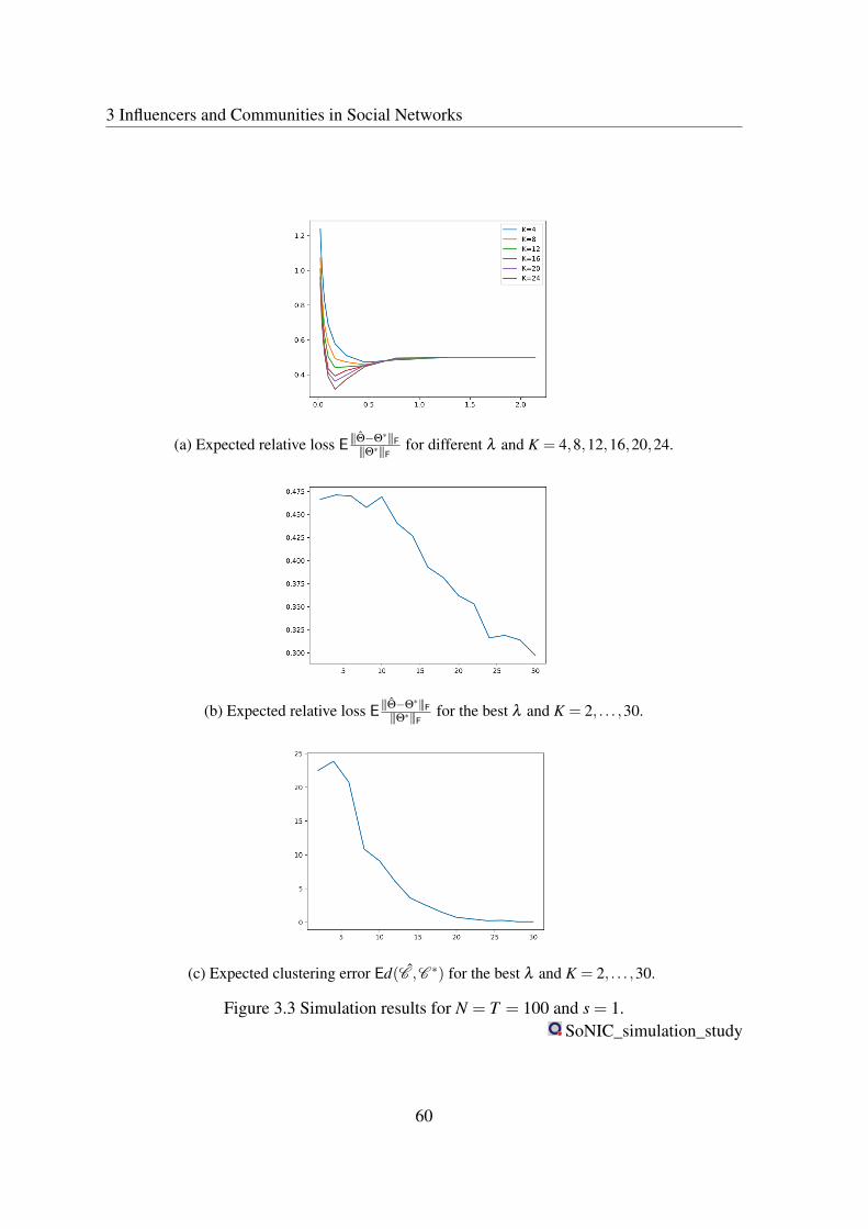
3 Influencers and Communities in Social Networks
(a) Expected relative loss E |||Θ−Θ∗|||F|||Θ∗|||F for different λ and K = 4,8,12,16,20,24.
(b) Expected relative loss E |||Θ−Θ∗|||F|||Θ∗|||F for the best λ and K = 2, . . . ,30.
(c) Expected clustering error Ed(C ,C ∗) for the best λ and K = 2, . . . ,30.
Figure 3.3 Simulation results for N = T = 100 and s = 1.SoNIC_simulation_study
60

3.4 Application to StockTwits sentiment
the cashtag ‘$AAPL’ (Apple) and the second one from those containing the cashtag ‘$BTC.X’(Bitcoin.)
The missing observation model presented in Section 3.2.2 relies on persistent observationfrequency with the same probability pi over a time period under consideration. Moreover,since in Theorems 3.1 and 3.2 the amount of observations scales with the factor p2
min, we needto avoid the users whose pi is too little. Based on these remarks we suggest the followingpreprocessing steps:
1. pick users with estimated probability pi ≥ 0.5;
2. for each user left after step 1, pick the longest historical interval over which the userexhibits persistent probability of observation. One can look at a moving averageestimation and ensure that for each window it remains within appropriate confidenceinterval;
3. take only users for whom the historical interval from step 2 is at least 50 days.
For AAPL dataset we are left with 46 users and 72 days, while for BTC we have 68 usersand 52 days. The two datasets are visualized using heatmap in Figure 3.1.
We apply our SoNIC model to AAPL dataset with λ = 0.05 and K = 6. A heatmap visu-alisation for estimated matrix Θ is presented in Figure 3.4a. From here we can identify thatthe most important users have identification number 47688, 619769, 850976 and 14382875.For the BTC dataset we use λ = 0.05 and K = 5, the results presented in Figure 3.4b. Theinfluencers are 1171931 and 1254166.
Remark 3.7. Choosing the tuning parameter λ and the number of clusters K remains beyond
the scope of this work. For this experiment we picked both numbers graphically: for λ based
on the number of active columns with relatively small values, while for K we picked the
smallest one for which there is no clusters that are much smaller than the others, as well as
no clusters that are split into two or more. Development of a statistically-backed selection is
left for further research.
Let us point out some observations based on the results of this experiment. The first oneis that for the Apple dataset we end up with users who have lots of followers, while fromthe Bitcoin dataset we have found two accounts that have moderate amount of followers and
5To access the page type https://stocktwits.com/user_id in the address line of a web browser.
61
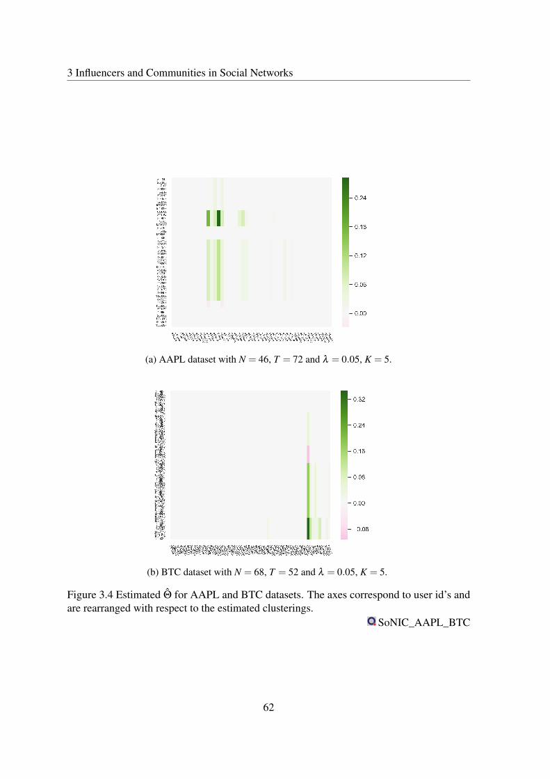
3 Influencers and Communities in Social Networks
(a) AAPL dataset with N = 46, T = 72 and λ = 0.05, K = 5.
(b) BTC dataset with N = 68, T = 52 and λ = 0.05, K = 5.
Figure 3.4 Estimated Θ for AAPL and BTC datasets. The axes correspond to user id’s andare rearranged with respect to the estimated clusterings.
SoNIC_AAPL_BTC
62

3.5 Proof of main result
as it seems belong to companies that provide analytical tools for traders. We assume thatit highlights the difference between two assets of different nature — a classical one and acryptocurrency. Secondly, in both cases the “heaviest” users fall into the same cluster, thoughwe do not provide any interpretation for this fact.
3.5 Proof of main result
This section is devoted to the proof of Theorem 3.3. We start with some preliminary lemmasand then proceed with the proof that consists of several steps. Following the ideas inGribonval et al. (2015), the proof is based on explicit representation of the loss function.
We exploit the following simplified notation. Denote, z∗j = zC∗j to be the columnsof Z∗ = ZC ∗ and we also denote n∗j = |C∗j | for each j = 1, . . . ,K. When the clusteringC = (C1, . . . ,CK) is clear from the context we will also write Z for ZC , z j for zC j , andn j = |C j| for each j = 1, . . . ,K. A vector e j ∈ Rd denotes a jth standard basis vector, i.e. jthelement equal to one and the rest are zeros.
3.5.1 Preliminary lemmas
Lemma 3.1. Suppose that C j is such that ‖zC j − z∗j‖ ≤ 0.3. Then,
11.1|C∗j | ≤ |C j| ≤ 1.1|C∗j |.
Proof. Suppose, n j = |C j|> n∗j = |C∗j |, then
r2 = ‖z j− z∗j‖2 = 2− 2√n jn∗j|C j∩C∗j | ≥ 2−2
√n∗jn j,
since |C j ∩C∗j | ≤ n∗j . Thus, √n j −√
n∗j ≤ (r2/2)√n j, which due to r ≤ 0.3 implies byrearranging and taking square n j ≤ 1.1n∗j .
If n j < n∗j we have,
r2 ≥ ‖z j− z∗j‖2 = 2−2|C j∩C′j|√
n jn∗j≥ 2−2
√n j
n∗j,
63

3 Influencers and Communities in Social Networks
and the fact that r ≤ 0.3 implies n∗j ≤ 1.1n j.
Lemma 3.2. Let ‖zC1− zC2‖ ≤ 0.3. Then,
‖zC1− zC2‖1 ≤ 1.55√
N1‖zC1− zC2‖2 .
Proof. Let N j = |C j| and a = |C1 ∩C2|, b = |C1 \C2|, c = |C2 \C1|, so that N1 = a+ b,N2 = a+ c, and |C14C2|= b+ c. We have,
‖zC1− zC2‖2 =
(1√N1− 1√
N2
)2
a+b
N1+
cN2≥ b
N1+
cN2
.
On the other hand,
‖zC1− zC2‖1 =
∣∣∣∣ 1√N1− 1√
N2
∣∣∣∣a+ b√N1
+c√N2
≤∣∣∣∣ 1√
N1− 1√
N2
∣∣∣∣a+√N1∨N2‖zC1− zC2‖2 .
Since |N1−N2| ≤ b+ c we obviously have,∣∣∣∣ 1√N1− 1√
N2
∣∣∣∣a =|N1−N2|a√
(a+b)(a+ c)(√
a+b+√
a+ c)
≤ (b+ c)a√N1∨N2
√a(2√
a)
≤√
N1∧N2‖zC1− zC2‖2/2,
and it is left to apply Lemma 3.1.
Lemma 3.3. Suppose,min j n∗jmax j n∗j
≥α for some α ∈ (0,1] and let ‖z j−z∗j‖≤ r. Suppose, r≤ 0.3.
Then,
‖[Z∗]>(z j− z∗j)‖1 ≤ 3.05α−1/2r2.
Proof. 1) We first consider the case |C j|= n∗j . It holds then
[z∗j ]>(z∗j − z j) =
1n∗j
(n∗j −|C j∩C∗j |) =1n∗j|C∗j \C j|.
64

3.5 Proof of main result
Moreover, for each k 6= j it holds
|[z∗k ]>(z∗j − z j)|= |[z∗k ]>z j|=1√n∗kn∗j|C∗k ∩C j| ≤
α−1/2
n∗j|C∗k ∩C j|.
Summing up, we get
‖[Z∗]>(z j− z∗j)‖1 ≤α−1/2
n∗j
(|C∗j \C j|+ ∑
k 6= j|C∗k ∩C j|
)
≤ α−1/2
n∗j
(|C∗j \C j|+ |C j \C∗j |
)=
α−1/2
n∗j|C j4C∗j |.
It is left to notice that in the case |C j|= |C∗j |= n∗j we have exactly ‖z j− z∗j‖2 = 1n∗j|C j4C∗j |.
2) Suppose, n j = |C j|> n∗j . Obviously, we can decompose C j =C′j∪B such that |C′j|= n∗jand B∩C∗j = /0. Setting z′j = zC′j
we get by the above derivations that ‖[Z∗]>(z′j− z∗j)‖1 ≤α−1/2‖z′j− z∗j‖2. Since C′j∩C∗j =C j∩C∗j we can compare the distances
‖z j− z∗j‖2 = 2− 2√n jn∗j|C j∩C∗j |> 2− 2
n∗j|C j∩C∗j |= ‖z′j− z∗j‖2.
Taking the remainder b = z j− z′j we have that
bi =
n j−1/2− (n∗j)
−1/2, i ∈C′j,
n j−1/2, i ∈ B,
0 otherwise.
65

3 Influencers and Communities in Social Networks
Setting d = n j−n∗j = |B| it is easy to obtain |n j−1/2− (n∗j)
−1/2| ≤ dn j
1√n∗j
. Thus, we get
K
∑k=1|[z∗k ]>b| ≤
k
∑i=1
1√n∗k
dn j
1√n∗j|C′j∩C∗k |+ |B∩C∗k |
1√n j
≤ α−1/2d
n∗jn j|C′j|+
α−1/2√n∗jn j
d
<2α−1/2d√
n jn∗j.
We show that the latter is at most 2.05α−1/2r2. Indeed, it is not hard to show that fromn j ≤ 1.1n∗j (see Lemma 3.1) it follows
n j−n∗j√n jn∗j
≤ 2.05
1−n∗j√n jn∗j
≤ 2.05× r2
2,
thus ‖[Z∗]>(z j− z∗j)‖1 ≤ 3.05α−1/2r2 and the result follows.
3) The case n j < n∗j can be resolved similarly to the previous one. Since |C∗j \C j| ≥ n∗j−n j
we can pick a subset B⊂C∗j \C j of size d = n∗j −n j and set C′j = B∪C j with |C′j|= n∗j ; setalso z′j = zC′j
. Then, we have
‖z′j− z∗j‖2 = 2−2|C′j∩C∗j |
n∗j≤ 2−
2|C j∩C′j|√n jn∗j
= ‖z j− z∗j‖2,
and it is not hard to derive that ‖z′j−z∗j‖2 ≤ ‖z j−z∗j‖2. Thus, by the first part of this proof itholds ‖[Z∗]>(z′j− z∗j)‖1 ≤ α−1/2r2 . Setting b = z′j− z j we have,
bi =
(n∗j)
−1/2−n j−1/2, i ∈C j,
n∗j−1/2, i ∈ B,
0 otherwise.
66

3.5 Proof of main result
Since |n j−1/2− (n∗j)
−1/2| ≤ dn∗j
1√n jwe obtain,
K
∑k=1|[z∗k ]>b| ≤
k
∑i=1
1√n∗k
dn∗j
1√n j|C j∩C∗k |+ |B∩C∗k |
1√n∗j
≤ α−1/2d
(n∗j)3/2n1/2
j
|C j|+α−1/2
n∗jd
<2α−1/2d
n∗j.
It is left to notice that
r2 ≥ 2−2n j√n jn∗j
=2(√
n∗j −√n j)
√n j=
2(n∗j −n j)
n∗j +√
n jn∗j≥ 2d
2n∗j,
therefore ‖[Z∗]>b‖1 ≤ 2α−1/2r2, thus ‖[Z∗]>(z j− z∗j)‖1 ≤ 3α−1/2r2.
Lemma 3.4. Let r = |||ZC −Z∗|||F and suppose that r ≤ 0.3. Then |||PC −PC ∗ |||2F ≥ 2r2(1−10α−1r2).
Proof. Denote z j = zC j and r j = ‖z j− z∗j‖. It holds,
|||PC −PC ∗ |||2F = 2K−2tr(PC PC ∗) = 2K−∑j,k(z>j z∗k)
2.
Notice, that 2z>j z∗j = 2−‖z j‖2−‖z∗j‖2 +2z>j z∗j = 2−‖z j− z∗j‖2, i.e. z>j z∗j = 1− r2j/2. In
particular, 1− (z>j z∗j)2 = r2j − r4
j/4, whereas ([z∗j ]>(z j−z∗j))2 = r4j/4. Since we additionally
have [z∗k ]>(z j− z∗j) = [z∗k ]
>z j for k 6= j, it holds
2K−2∑j,k(z>j z∗k)
2 = 2∑j
r2j − r4
j/4−2∑j
∑k 6= j
([z∗k ]>(z j− z∗j)
)2
= 2r2−2∑j,k
([z∗k ]>(z j− z∗j)
)2
= 2r2−2∑j‖[Z∗]>(z j− z∗j)‖2
By Lemma 3.3 we have for each j = 1, . . . ,K
‖[Z∗]>(z j− z∗j)‖ ≤ ‖[Z∗]>(z j− z∗j)‖1 ≤ 3.05α−1/2r2
j ,
67

3 Influencers and Communities in Social Networks
therefore
∑j‖[Z∗]>(z j− z∗j)‖2 ≤ 10α
−1∑
jr4
j ≤ 10α−1r4,
thus inequality follows.
Lemma 3.5. Let C,C′ be such that |C4C′|= 1. Then ‖zC− zC′‖2 ≤ 2|C|∨|C′| .
Proof. Suppose, |C′|> |C| then C′ =C∪a and denoting n = |C| we have
‖zC− zC′‖2 =n
(√1
n+1−√
1n
)2
+1
n+1=
(√
n+1−√
n)2 +1n+1
≤ 2n+1
.
3.5.2 Proof of Theorem 3.3
The proof consists of several steps, each represented by a separate lemma.
Lemma 3.6. Suppose, Assumption 3.1 holds and let N ≥ 2. There is a constant C =C(γ,L),
so that ifs logN log2 T
T p2min
≤ 13,
then with probability at least 1−1/N and for with ∆1 =Cσmax
√log NT p2
minthe following inequal-
ities take place for each j = 1, . . . ,K
•
‖A−A‖∞,∞ ≤ ∆1, ‖Σ−1Λ j,Λ j
(AΛ j,·−AΛ j,·)‖∞,∞ ≤ σ−1min∆1; (3.9)
•
‖(A−A)z∗j‖∞ ≤ ∆1, ‖Σ−1Λ j,Λ j
(AΛ j,·−AΛ j,·)z∗j‖∞ ≤ σ
−1min∆1; (3.10)
•
‖Σ−Σ‖∞,∞ ≤ ∆1, ‖(ΣΛ j,·−ΣΛ j,·)v∗j‖∞ ≤ ∆1; (3.11)
•
‖Σ−1Λ j,Λ j
(ΣΛ j,·−ΣΛ j,·)v∗j‖∞ ≤ σ
−1min∆1; (3.12)
•
|||ΣΛ j,Λ j −ΣΛ j,Λ j |||op ≤√
s∆1. (3.13)
68

3.5 Proof of main result
Proof. By Theorem 3.2 it holds for any pair a,b ∈ RN with ‖a‖ ≤ 1, ‖b‖ ≤ 1 it holdsprobability ≥ 1−N−m,
|a>(A−A)b| ≤Cσmax
(√(m+1) logN
T p2min
∨ (m+1) logN logTT p2
min
).
Suppose for a moment that m is such that√(m+1)s logN
T p2min
logT ≤ 1, (3.14)
so that we can neglect the second term. Set,
A0 = (ei,ei′) : i, i′ ≤ N, B0 = (ei,z∗l ) : i≤ N, l ≤ K,
as well as for each j = 1, . . . ,K
A j = (σminΣ−1Λ j,Λ j
ei,ei′) : i ∈ Λ j, i′ ≤ N,
B j = (σminΣ−1Λ j,Λ j
ei,z∗l ) : i ∈ Λ j, l ≤ K.
Obviously we have |A0| ≤ N2, |B0| ≤ NK and |A j| ≤ sN, |B j| ≤ sK for j = 1, . . . ,N, so sinces,K ≤ N together they have not more than 4N3 pairs of vectors (a,b), each having normbounded by one. Taking a union bound, we have that the inequalities (3.9) and (3.10) holdwith probability at least 1−4N3−m. By analogy, we can show that (3.11) and (3.12) holdwith probability at least 1−4N3−m.
As for the last inequality, for each j = 1, . . . ,K pick Pj = ∑i∈Λ j eie>i , i.e. projectors ontothe subspace of vectors supported on Λ j. Then by Theorem 3.1 it holds with probability atleast 1−KN−m for each j = 1, . . . ,K (taking into account (3.14))
|||ΣΛ j,Λ j −ΣΛ j,Λ j |||op = |||Pj(Σ−Σ)Pj|||op ≤Cσmax
√s(m+1) logN
T p2min
.
The total probability will be at least 1−8N3−m−KN−m, which is at least 1−1/N wheneverm≥ 7 and N ≥ 2.
69

3 Influencers and Communities in Social Networks
In the following we apply technique from Gribonval et al. (2015). Suppose, that the lassosolution v j for a given clustering C is not only supported exactly on Λ j, but the signs arematching those of the true v∗j . Then, ‖v j‖1 = s>j (v j)Λ j . Therefore, we can write
(v j)Λ j = arg minv∈RΛ j
12
v>ΣΛ j,Λ jv−v>AΛ j,·z j +λ s>j v
= Σ−1Λ j,Λ j
(AΛ j,·z j−λ s j),
and plugging this solution into the risk function we get that Fλ (C ) = Φλ (C ), where thelatter is defined explicitly
Φλ (C ) =−12
K
∑j=1
(AΛ j,·z j−λ s j)>
Σ−1Λ j,Λ j
(AΛ j,·z j−λ s j).
Lemma 3.7. Suppose, the inequalities (3.9)–(3.13) take place. Assume,
s∆1 ≤ 1/16, 12∆1 ≤ λ ≤ σmin
4τ0s−1. (3.15)
Then, for each C = (C1, . . . ,CK) satisfying
maxj‖zC j − zC∗j ‖ ≤ 0.3∧0.22
√(2σmaxα−1/2 +
√n∗∆1
)−1λ (3.16)
it holds
|||Vλ ,C −V ∗|||F ≤ 3σ−1min
√Ksλ ,
and the equality Fλ (C ) = Φλ (C ) takes place.
Proof. Taking into account Z>Z = IK , it holds
Rλ ,C (V ) =12
tr(
V>ΣV)− tr
(V>AZ
)+λ‖V‖1,1
=K
∑j=1
12
v>j Σv j−v>j Az j +λ‖v j‖1,
so that the optimization problem separates into K independent subproblems. Solving each ofthe problems
12
v>j Σv j−v>j Az j +λ‖v j‖1→minv j
70

3.5 Proof of main result
corresponds to Corollary A.1 with D = Σ and c = Az j, whereas the “true” version of theproblem corresponds to D = Σ and c = Az∗j = Σ(Θ∗)>z∗j = Σv∗j . We need to control thedifferences between c and c, and between D and D. It holds,
‖Az j−Az∗j‖∞ ≤‖A(z j− z∗j)‖∞ +‖(A−A)z∗j‖∞ +‖(A−A)(z j− z∗j)‖∞ .
Since A = ΣV ∗[Z∗]>, we bound the first term using Lemma 3.3
‖A(z j− z∗j)‖∞ ≤ ‖ΣV ∗‖∞,∞‖[Z∗]>(z j− z∗j)‖1 ≤ 3.05α−1/2‖ΣV ∗‖∞,∞r2
j .
The second term is bounded by ∆1, whereas the fourth term satisfies
‖(A−A)(z j− z∗j)‖∞ ≤ ‖A−A‖∞,∞‖z j− z∗j‖1 ≤ 1.55∆1√
n∗r2j ,
where we also used Lemma 3.2. Summing up we get,
‖c− c‖∞ ≤ 1.55(2σmaxα−1/2 +
√n∗j∆1)r2
j +∆1 .
Similarly, we bound ‖ΣΛ j,Λ j(cΛ j − cΛ j)‖∞ as follows
‖Σ−1Λ j,Λ j
(AΛ j,·z j−AΛ j,·z∗j)‖∞ ≤‖Σ−1
Λ j,Λ jA(z j− z∗j)‖∞ +‖Σ−1
Λ j,Λ j(AΛ j,·−AΛ j,·)z
∗j‖∞
+‖Σ−1Λ j,Λ j
(AΛ j,·−AΛ j,·)(z j− z∗j)‖∞
≤‖Σ−1Λ j,Λ j
A(z j− z∗j)‖∞ +1.55σ−1min∆1
√n∗r2
j +σ−1min∆1
≤1.55σ−1min(2σmaxα
−1/2 +√
n∗j∆1)r2j +σ
−1min∆1
To sum up, Corollary A.1 is applied with
δc =1.55(2σmaxα−1/2 +
√n∗∆1)r2
j +∆1,
δ′c =1.55σ
−1min(2σmaxα
−1/2 +√
n∗∆1)r2j +σ
−1min∆1
δD =∆1, δ′D = ∆1, δ
′′D = σ
−1min∆1.
It requires the conditions,
3(1.55(2σmaxα−1/2 +
√n∗∆1)r2
j +2∆1)≤ λ , s∆1 ≤1
16,
71

3 Influencers and Communities in Social Networks
and due to the fact that ‖D−1Λ j,Λ j‖1,∞ ≤
√s|||D−1
Λ j,Λ j|||op and Assumption 3.6,
2σ−1min(1.55(2σmaxα
−1/2 +√
n∗∆1)r2j +2∆1 +
√sλ )< τ0s−1/2,
which are not hard to derive from the given inequalities. All this that v j is supported on Λ j
and the solution satisfies
(v j)Λ j = Σ−1Λ j,Λ j
(AΛ j,·z j−λ s∗j
),
and the corresponding minimum is equal to
12
v>j Σv>j − v>j Az j +λ (v j)>Λ j
s∗j =−12(AΛ j,·z j−λ s∗j
)>Σ−1Λ j,Λ j
(AΛ j,·z j−λ s∗j
).
Summing up we get the corresponding expression for Fλ (C ). Moreover, we have
‖v j−v∗j‖ ≤2√
s
2∆1 +1.55(2σmaxα−1 +
√n∗∆1)r2
j +λ
≤2σ
−1min√
s(
λ
6+
1.55λ
20+λ
)≤3σ
−1min√
sλ ,
and together it provides a bound on |||Vλ ,C −V ∗|||F.
Consider the function,
Φλ (C ) =−12
k
∑j=1
(AΛ j,·z j−λ s∗j
)>Σ−1Λ j,Λ j
(AΛ j,·z j−λ s∗j
).
The growth of this function as C recedes from the true clustering C ∗ is controlled by thefollowing lemma.
Lemma 3.8. Suppose, C is some clustering such that r = |||ZC −Z∗|||F ≤ 0.3. Then,
Φλ (C )− Φλ (C∗)≥ a0
2r2(1−10α
−1r2)−λ√
Ks|||V ∗|||Fr.
72

3.5 Proof of main result
Proof. Denoting Φ0(C ) =−12 ∑
kj=1 z>j A>
Λ j,·Σ−1Λ j,Λ j
AΛ j,·z j (which indeed corresponds to λ =
0), we have the decomposition
Φλ (C )− Φλ (C∗) = Φ0(C )− Φ0(C
∗)−λ
K
∑j=1
[s∗j ]>
Σ−1Λ j,Λ j
AΛ j,·(z j− z∗j).
Let us first deal with the term Φ0(C )− Φ0(C∗). Note that since [v∗j ]Λ j = Σ
−1Λ j,Λ j
AΛ j,·z∗j , we
have
Φ0(C∗) =−1
2
K
∑j=1
[v∗j ]>
Σv∗j =−12
tr([V ∗]>ΣV ∗) =−12
tr(Θ∗Σ[Θ∗]>).
whereasΦ0(C ) = min
V=[v1,...,vk]
12
tr(V>ΣV )− tr(V>AZ)
where the minimum is taken s.t. the restrictions supp(v j)⊂ Λ j. Dropping the restrictions weget,
Φ0(C )− Φ0(C∗)≥min
V
12
tr(V>ΣV )− tr(V>AZ)+12
tr(Θ∗Σ[Θ∗]>)
= minV
12|||ZV>Σ
1/2|||2F− tr(ZV>Σ[Θ∗]>)+ |||Θ∗Σ1/2|||2F
= minV
12|||(ZV>−Θ
∗)Σ1/2|||2F.
It is not hard to calculate that the minimum is attained for V = [Θ∗]>Z and therefore
Φ0(C )− Φ0(C∗)≥ 1
2|||(ZZ>− I)Θ∗Σ1/2|||2F ≥
a0
2|||(ZZ>− I)Z∗|||2F,
where the latter follows using Θ∗ = Z∗[V ∗]> and from the fact that λmin([V ∗]>ΣV ∗) ≥ σ0.Moreover,
|||(ZZ>− I)Z∗|||2F = tr((PC − I)PC ∗(PC − I)) = tr(PC ∗)− tr(PC PC ∗)
=12|||PC −PC ∗ |||2F,
where we used the fact that tr(PC ) = tr(PC ∗) = K. It is left to recall the result of Lemma 3.4,so that we get
Φ0(C )− Φ0(C∗)≥ a0r2
2(1−10α
−1r2).
73

3 Influencers and Communities in Social Networks
As for the linear term, it holds(K
∑j=1
[s∗j ]>
Σ−1Λ j,Λ j
AΛ j,·(z j− z∗j)
)2
≤
(K
∑j=1‖[s∗j ]>Σ
−1Λ j,Λ j
AΛ j,·‖2
)r2
Since A = Σ[Θ∗]>, we have A>Λ j,·Σ
−1Λ j,Λ j
s∗j = Θ∗Σ·,Λ jΣ−1Λ j,Λ j
s∗j . Denote, x = Σ·,Λ jΣ−1Λ j,Λ j
s∗j , thenwe have xΛ j = s j and ‖xΛ j‖∞ = 1. Moreover, by the ERC property
‖xΛcj‖∞ = ‖ΣΛc
j,Λ jΣ−1Λ j,Λ j
s j‖∞ ≤ ‖ΣΛcj,Λ jΣ
−1Λ j,Λ j‖1,∞ ≤ 1/2.
We have
‖A>Λ j,·Σ−1Λ j,Λ j
s∗j‖2 = ‖∑z∗j [v∗j ]>x‖2 =
K
∑k=1|[v∗k ]>x|2,
where, since v∗k is supported on Λk of size at most s,
|[v∗k ]>x| ≤ ‖v∗k‖1‖x‖∞ ≤√
s‖v∗k‖.
Summing up we get ‖A>Λ j,·Σ
−1Λ j,Λ j
s∗j‖2 ≤ s|||V ∗|||2F, so that
∣∣∣∣∣ K
∑j=1
[s∗j ]>
Σ−1Λ j,Λ j
AΛ j,·(z j− z∗j)
∣∣∣∣∣≤√Ks|||V ∗|||Fr.
The lemma now follows from the two terms put together.
The next step is to bound the difference Φλ (C )−Φλ (C ) uniformly in the neighbourhoodof C ∗.
Lemma 3.9. Suppose that the inequalities (3.9)–(3.13) hold and let
∆1 ≤ σmin/(2√
s)∨ λ
12, σmax/σmin ≤ n∗, λ ≤ σmins−1
Let some r ≤ 0.3 satisfies√
sn∗∆1r2 ≤ σmax. Then,
sup|||Z−Z∗|||F≤r
|Φλ (C )− Φλ (C )−Φλ (C∗)+ Φλ (C
∗)|
≤4
((σmax
σmin
)2√s|||V ∗|||F+
σmax
σmin
√K
)∆1r+15
σmax
σmin
√sn∗∆1r2.
74

3.5 Proof of main result
Proof. Denote,
Φλ (C ) =−12
K
∑j=1
(AΛ j,·z j−λ s∗j
)>Σ−1Λ j,Λ j
(AΛ j,·z j−λ s∗j
),
so that we have
|Φλ (C )− Φλ (C )− Φλ (C∗)+ Φλ (C
∗)|
≤ 12
K
∑j=1
∣∣∣(AΛ j,·(z j + z∗j)−2λ s∗j)>
(Σ−1Λ j,Λ j
−Σ−1Λ j,Λ j
)AΛ j,·(z j− z∗j)∣∣∣
First of all, due to (3.13) it holds,
|||Σ−1Λ j,Λ j
−Σ−1Λ j,Λ j|||op ≤
σ−2min√
s∆1
1−σ−1min√
s∆1≤ 2σ
−2min√
s∆1.
Since A = Σ[Θ∗]>, we have
‖AΛ j,·(z j− z∗j)‖ ≤ σmaxr j
‖AΛ j,·(z j + z∗j)−2λ s∗j‖ ≤ σmax(2‖v∗j‖+ r j)+2λ√
s.
Then by Cauchy-Schwartz,
|Φλ (C )− Φλ (C )− Φλ (C∗)+ Φλ (C
∗)| ≤σ−2min√
s∆1
(K
∑j=1
σmaxr j
σmax(2‖v j‖+ r j)+2λ√
s)
≤2(
σmax
σmin
)2√s|||V ∗|||F∆1r+2
σmax
σ2min
λ s√
K∆1r
+
(σmax
σmin
)2√s∆1r2.
Going further,
Φλ (C )− Φλ (C ) =−12
K
∑j=1
((AΛ j,·+ AΛ j,·)z j−2λ s∗j
)>Σ−1Λ j,Λ j
(AΛ j,·−AΛ j,·)z j,
75

3 Influencers and Communities in Social Networks
which implies that
|Φλ (C )− Φλ (C )−Φλ (C∗)+ Φλ (C
∗)|
≤ 12
K
∑j=1
∣∣∣((AΛ j,·+ AΛ j,·)(z j− z∗j))>
Σ−1Λ j,Λ j
(AΛ j,·−AΛ j,·)z j
∣∣∣≤1
2
K
∑j=1
∣∣∣((AΛ j,·+ AΛ j,·)z∗j −2λ s∗j
)>Σ−1Λ j,Λ j
(AΛ j,·−AΛ j,·)(z j− z∗j)∣∣∣
(3.17)
First notice, that due to Lemma 3.2 and (3.9) it holds,
‖(AΛ j,·−AΛ j,·)(z j− z∗j)‖ ≤√
s‖AΛ j,·−AΛ j,·‖∞,∞‖z j− z∗j‖1
≤ 1.55√
sn∗∆1r2j .
Therefore, it follows
‖(AΛ j,·+AΛ j,·)(z j− z∗j)‖ ≤ 2σmaxr j +1.55√
sn∗∆1r2j .
Moreover, using (3.10) we get
‖(AΛ j,·−AΛ j,·)z j‖ ≤ ∆1 +1.55√
sn∗∆1r2j
‖(AΛ j,·+AΛ j,·)z∗j −2λ s∗j‖ ≤ 2σmax‖v j‖+∆1 +2λ
√s.
and we also have |||Σ−1Λ j,Λ j|||op ≤ 2σ
−1min due to the condition σ
−1min√
s∆1 ≤ 1/2. Thus we getthat the first sum of (3.17) is bounded by
σ−1min
K
∑j=1
(2σmaxr j +1.55
√sn∗∆1r2
j
)(∆1 +1.55
√sn∗∆1r2
j
)≤ 2
σmax
σmin∆1√
Kr+1.55σ−1min
√sn∗∆2
1r2 +3.1σmax
σmin
√sn∗∆1r3 +2.5σ
−1minsn∗∆2
1r4,
while the second sum is bounded by
σ−1min
K
∑j=1
(2σmax‖v∗j‖+∆1 +2λ
√s)(
1.55√
sn∗∆1r2j
)≤ 1.55
σmin
(σmax√
sn∗+√
sn∗∆1 +2λ s√
n∗)
∆1r2
≤ 5σmin
(σmax√
sn∗+λ s√
n∗)
∆1r2
76

3.5 Proof of main result
where we used the fact that max j ‖v∗j‖ ≤ |||V ∗|||op = |||Θ∗|||op < 1 together with the condition∆1 ≤ σmax. Combining all the bounds we get
|Φλ (C )− Φλ (C )−Φλ (C∗)+ Φλ (C
∗)|
≤2
((σmax
σmin
)2√s|||V ∗|||F+2
σmax
σ2min
λ s√
K +2σmax
σmin
√K
)∆1r
+
(5
σmax
σmin
√sn∗+5σ
−1minλ s
√n∗+1.55σ
−1min
√sn∗∆1 +
(σmax
σmin
)2√s
)∆1r2
+3.1σmax
σmin
√sn∗∆1r3
+2.5σ−1minsn∗∆2
1r4,
where by r ≤ 0.3 and√
sn∗∆1 ≤ σmax we can neglect the third and the fourth power, respec-tively, and thus the required bound follows.
Lemma 3.10. There are numerical constant c,C > 0 such that the following holds. Suppose,
the inequalities take place:√sn∗ logN
T p2min
≤ ca0σmin
σ2max
, n∗ ≥ σmax/σmin. (3.18)
Let Cσmax
√log NT p2
min≤ λ ≤ cσminτ0s−1, and set
r = 0.3∧0.18√
α ∧0.22
√(2σmaxα−1/2 +
√n∗∆1
)−1λ .
Then under the inequalities (3.9)–(3.13) the clustering
C = arg min|||ZC−Z∗|||F≤rmax
Fλ (C )
satisfies
|||ZC −Z∗|||F ≤Ca0
(σmax
σmin
)2
λK√
s .
Proof. It is not hard to see that for ∆1 =√
log NT p2
minthe inequalities required by Lemmas 3.7–3.9
are satisfied for r ≤ r due to (3.18) and conditions on λ and r. Since obviously C satisfies
77

3 Influencers and Communities in Social Networks
Fλ (C )≤ Fλ (C∗), we have for r = |||ZC −ZC ∗ |||F ≤ rmax
Fλ (C )−Fλ (C∗)≥Φλ (C )− Φλ (C )−|Fλ (C )− Φλ (C )−Fλ (C
∗)+ Φλ (C∗)|
≥a0r2
2(1−10α
−1r2)−λ√
Ks|||V ∗|||Fr
−4
((σmax
σmin
)2√s|||V ∗|||F+
σmax
σmin
√K
)∆1r−15
σmax
σmin
√sn∗∆1r2
=a0r2
2
(1−10α
−1r2− 30a0
σmax
σmin
√sn∗∆1
)−λ√
Ks|||V ∗|||Fr−4
((σmax
σmin
)2√s|||V ∗|||F+
σmax
σmin
√K
)∆1r .
Since r ≤ 0.2√
α implies 10α−1r2 ≤ 13 , it holds by (3.18)
1−10α−1r2− 30
a0
σmax
σmin
√sn∗∆1 ≥
12.
Therefore, after dividing by r, we get that such optimal clustering must satisfy
a0
4r ≤ λ
√Ks|||V ∗|||F+4
((σmax
σmin
)2√s|||V ∗|||F+
σmax
σmin
√K
)∆1.
Recalling that |||V ∗|||F ≤√
K, ∆1 =Cσmax
√log NT p2
minand ∆2 =C
√s log NT p2
minyields the result.
Now we are ready to finalize the proof of Theorem 3.3. Firstly, we need to show that theclustering C from the lemma above is locally optimal. By Lemma 3.5, any neighbouring toit clustering C ′ satisfies |||ZC ′−ZC |||F ≤
2√αN/K
. Therefore,
|||ZC ′−ZC ∗ |||F ≤Ca0
(σmax
σmin
)2
λK√
s+2α−1/2
√KN,
78

3.6 Proof of Theorems 3.1 and 3.2
and it is enough to check that this value is at most r. We check that each of the terms is atmost r/2. For the first one it is enough to have,
Ca0
(σmax
σmin
)2
α−1/2
λK√
s≤ 0.09,
C2
a20
(σmax
σmin
)4
λ
(2σmaxα
−1/2 +√
n∗∆1
)K2s≤ 0.012,
and both are satisfied due to the upper bound λ ≤ cκ−4(a20/σmax)K−2s−1 and the requirement√
sn∗ log NT p2
min≤ c. For the second term we need
α−1 K
N≤ 0.008α, α
−1(
2σmaxα−1/2 +
√n∗∆1
) KN≤ λ ,
both are satisfied once N ≥Cα2K and λ ≥Cσmaxα−3/2 KN .
Moreover, by Lemma 3.7 we have for Θ = ZC VC ,λ
|||Θ−Θ∗|||F ≤ |||ZC (VC ,λ −V ∗)>|||F+ |||(ZC −Z∗)V ∗|||F
≤ 3σ−1min
√Ksλ +
Ca0
(σmax
σmin
)2
γK√
sλ ,
which finishes the proof.
3.6 Proof of Theorems 3.1 and 3.2
Recall that we have a time series,
Yt = ∑k≥0
ΘkWt−k, t ∈ Z, (3.19)
where Wt ∈ RN , t ∈ Z are independent vectors with EWt = 0 and Var(Wt) = S. We also havethat |||Θ|||op ≤ γ for some γ < 1 and the covariance Σ = Var(Yt) reads as
Σ = ∑k≥0
ΘkS[Θk]>.
79

3 Influencers and Communities in Social Networks
We have the observations
Zt = (δ1tY1t , . . . ,δNtYNt)>, t = 1, . . . ,T, (3.20)
where δit ∼ Be(pi) are independent Bernoulli random variables for each i = 1, . . . ,N andt = 1, . . . ,T and some pi ∈ (0,1].
The proofs of both statements are based on a version of Bernstein matrix inequalitypresented in Chapter 4, Proposition 4.3.
Theorem 3.4 (Klochkov and Zhivotovskiy (2018), Proposition 4.1). Suppose, the matrices At
for t = 1, . . . ,T are independent and let M = maxt∥∥|||At |||op
∥∥ψ1
is finite. Then, ST = ∑Tt=1 At
satisfies for any u≥ 1
P
(|||ST −EST |||op >C
(√σ2(logN +u)+M logT (logN +u)
))≤ e−u,
where σ2 = |||∑Tt=1EA>t At |||op∨|||∑T
t=1EAtA>t |||op and C is an absolute constant.
Let δ t = (δt1, . . . ,δtN)> denotes the vector with Bernoilli variables from above corre-
sponding to the time point t. In what follows we consider the following matrices,
Ak, jt,t ′ = diagδ tΘkWt−kW>t ′− j[Θ
j]> diagδ t ′,
so that since Zt = ∑k≥0 diagδ tΘkWt−k, we have
ZtZ>t = ∑k, j≥0
diagδ tΘkWt−kW>t− j[Θj]> diagδ t= ∑
k, j≥0Ak, j
t,t .
Therefore, the decomposition takes place
Σ∗ = ∑
k, j≥0Sk, j, Sk, j =
1T
T
∑t=1
Ak, jt,t , (3.21)
and we shall analyze the sum for each pair of k, j ≥ 0 separately. We first introduce twotechnical lemmas. In what follows we assume w.l.o.g. that |||S|||op = 1, since if we scale it,all the covariances and estimators scale correspondingly.
80

3.6 Proof of Theorems 3.1 and 3.2
Lemma 3.11. Under the assumptions of Proposition 3.1 it holds,
‖|||Pdiagp−1 Diag(Ak, jt,t ′)Q|||op‖ψ1 ≤Cp−1
min√
M1M2γk+ j,
‖|||Pdiagp−1 Off(Ak, jt,t ′)diagp−1Q|||op‖ψ1 ≤Cp−2
min√
M1M2γk+ j,
with some C =C(L)> 0.
Proof. Denote for simplicity x = ΘkWt−k, y = Θ jWt ′− j, as well as xδ = diagδ tx, yδ =
diagδ ty, such that Ak, jt,t ′ = xδ [yδ ]>. Since Wt are subgaussian and |||ΘkSΘk|||op ≤ γ2k, we
have for each u ∈ RN thatlogEexp(u>x)≤C′γ2k‖u‖2, (3.22)
and since δt takes values in [0,1]N , same takes place for xδ . By Theorem 2.1 in Hsu et al.(2012) it holds for any matrix A and vector u ∈ RN ,
‖‖Axδ‖‖ψ2 ≤C′′γk|||A|||F, ‖u>xδ‖ψ2 ≤C′′γk‖u‖, (3.23)
and, similarly,
‖‖Ayδ‖‖ψ2 ≤C′′γ j|||A|||F, ‖u>yδ‖ψ2 ≤C′′γ j‖u‖.
We first deal with the diagonal term. Let P = ∑M1i=1 u ju>j be its eigen-decomposition with
‖u j‖= 1, then
‖|||Pdiag(xδ )|||op‖2ψ2
=‖|||diag(xδ )Pdiag(xδ )|||op‖ψ1 ≤M1
∑j=1‖|||diag(xδ )u ju>j diag(xδ )|||op‖ψ1
=M1
∑j=1‖‖diag(u j)xδ‖‖2
ψ2,
where each term in the latter is bounded by γ2k due the fact that |||diag(u j)|||F = 1. Summingup and taking square root we arrive at
∥∥|||Pdiag(xδ )|||op∥∥
ψ2≤√
C′′M1γk. Taking into accountsimilar bound for Qdiag(yδ ), we have by Hölder inequality
‖|||Pdiagδ−1 diag(xδ )diag(yδ )Q|||op‖ψ1 ≤p−1min‖|||Pdiag(xδ )|||op
∥∥ψ2‖|||Qdiag(yδ )|||op‖ψ2
≤C′′√
M1M2γk+ j,
81

3 Influencers and Communities in Social Networks
which yields the bound for the diagonal. As for the off-diagonal, consider first the wholematrix,
‖|||Pxδ [yδ ]>Q|||op‖ψ1 ≤ ‖‖Pxδ‖‖ψ2‖‖Qyδ‖‖ψ2 ≤ (C′′)2√M1M2γj+k,
and since Off(A j,kt,t ′) =A j,k
t,t ′−Diag(A j,kt,t ′), the bound follows from the triangular inequality.
The following technical lemma will help us to upper-bound σ2 in Theorem 3.4.
Lemma 3.12. Let δ1, . . . ,δN consists of independent Bernoilli components with probabilities
of success p1, . . . , pN and set pmin = mini≤N pi. Let a,b ∈ RN be two arbitrary vectors. It
holds,
E
(∑
i
δi
piaibi
)2
≤p−1min‖a‖
2‖b‖2,
E
(∑i6= j
δiδ j
pi p jaib j
)2
≤32p−2min‖a‖
2‖b‖2 +4
(∑
iai
)2(∑
ibi
)2
.
Additionally, if δ ′1, . . . ,δ′N are independent copies of δ1, . . . ,δN , it holds
E
(∑i, j
δiδ′j
pi p jaib j
)2
≤ 4p−2min‖a‖
2‖b‖2 +4
(∑
iai
)2(∑
ibi
)2
.
Proof. It holds,
E
(∑
i
δi
piaibi
)2
=∑i, j
Eδiδ j
pi p jaibia jb j = ∑
i, j1+ I(i = j)(p−1
i −1)aibia jb j
≤
(∑
iaibi
)2
+(p−1min−1)∑
ia2
i b2i
≤‖a‖2‖b‖2 +(p−1min−1)‖a‖2‖b‖2.
82

3.6 Proof of Theorems 3.1 and 3.2
To show the second inequality we use decoupling (Theorem 6.1.1 in Vershynin (2018))and the trivial inequality (x+ y)2 ≤ 2x2 +2y2,
E
(∑i6= j
δiδ j
pi p jaib j
)2
≤2
(∑i6= j
aib j
)2
+2E
(∑i6= j
(δi− pi)(δ j− p j)
pi p jaib j
)2
≤2
(∑i6= j
aib j
)2
+32E
(∑i6= j
(δi− pi)(δ′j− p j)
pi p jaib j
)2
.
(3.24)
Denote for simplicity δ i = δi− pi and δ′i = δ ′i − pi. Since the latter are centred we have,
E
(∑i6= j
δ iδ′j
pi p jaib j
)2
= ∑i6= jk 6=l
Eδ iδ k
pi pk
Eδ′jδ′l
p j p jaiakb jbl (3.25)
note that the expectation Eδ iδ k is only non-vanishing when i = k, in which case it holdsEδ
2i = pi− p2
i . Taking into account similar property of Eδ′jδ′l we have that the sum above is
equal to
∑i6= j
(pi− p2i )(p j− p2
j)
p2i p2
ja2
i b2j ≤ (p−1
min−1)2∑i, j
a2i b2
j ≤ (p−1min−1)2‖a‖2‖b‖2.
It is left to notice that(∑i6= j
aib j
)2
≤ 2
(∑i, j
aib j
)2
+2
(∑
iaib j
)2
≤ 2
(∑
iai
)2(∑
ibi
)2
+2‖a‖2‖b‖2,
which recalling (3.24) and noting that 32(p−1min−1)2+4≤ 32p−2
min for pmin ∈ [0,1], completesthe proof.
Similarly to (3.25) we can show the third inequality.
Now we apply Bernstein matrix inequality to the sum Sk j defined in (3.21), dealing sepa-rately with diagonal and off-diagonal parts. After that we present the proof of Proposition 3.1.
83

3 Influencers and Communities in Social Networks
Lemma 3.13. Under the assumptions of Proposition 3.1 for each u≥ 1 it holds with proba-
bility at least 1− e−u
|||Pdiagp−1(Diag(Sk, j)−EDiag(Sk, j))Q|||op
≤Cγk+ j
(√M1∨M2(logN +u)
T pmin
∨√M1M2(logN +u)T pmin
)
where C =C(K) only depends on K.
Proof. Note that,
Pdiagp−1 Diag(Sk j)Q = T−1T
∑t=1
At , At = Pdiagp−1 Diag(Ak, jt,t )Q.
By Lemma 3.11 we have ‖|||At |||op‖ψ1 ≤Cp−1min√
M1M2γk+ j. Moreover, using decompositionQ = ∑
M2j=1 u ju j, we have
|||EAtA>t |||op ≤|||Ediagp−1 Diag(Ak, jt,t )QDiag(Ak, j
t,t )diagp−1|||op
≤M2
∑j=1|||Ediagp−1 Diag(Ak, j
t,t )u ju>j Diag(Ak, jt,t )diagp−1|||op
≤M2
∑j=1
sup‖γ‖=1
E(γ> diagp−1 Diag(Ak, jt,t )u j)
2
By definition, Diag(Ak, jt,t ) = diagδtixiyiN
i=1 for x = ΘkWt−k, y = Θ jWt− j. Let Eδ denotesthe expectation w.r.t. the Bernoulli variables and conditioned on everything else. Setting a =
(x1γ1, . . . ,xNγN)>) and b= (y1u1, . . . ,yNuN)
>, we have by the first inequality of Lemma 3.12,
E(γ> diagp−1 Diag(Ak, jt,t )u j)
2 = EEδ
(∑
iγixi
δti
piyiui
)2
≤ p−1minE‖a‖
2‖b‖2
≤ p−1minE
1/2‖a‖4E1/4‖b‖4.
Observe that,‖a‖2 = ∑
iγ
2i x2
i = x> diagγ2x,
84

3.6 Proof of Theorems 3.1 and 3.2
so since tr(diagγ2) = 1 and due to (3.22) and by Theorem 2.1 Hsu et al. (2012) it holdsE1/2‖a‖4 ≤ ‖‖a‖2‖ψ1 ≤C′γ2k. Similarly, it holds E1/2‖a‖4 ≤C′γ2 j, which together implies
|||EAtA>t |||op∨|||EA>t A>t |||op ≤C′′M2∨M1γ2k+2 j.
Now notice that At is not necessary an independent sequence, as At depends directlyon (Wt−k,Wt− j,δ t), which might intersect with e.g. t ′ = t + | j− k|. However, if we take aset I ⊂ [1,T ] such that any two t, t ′ ∈ I satisfy |t ′− t| 6= | j− k| then obviously the sequence(At)t∈I is independent. We separate the whole interval [1,T ] into two such independent sets,
I1 =t ∈ [1,T ] : dt/| j− k|e is odd ,
I2 =t ∈ [1,T ] : dt/| j− k|e is even
=[1,T ]\ I1.
(3.26)
Indeed, if for t, t ′ ∈ I1 then dt/| j−k|e and dt ′/| j−k|e are either equal or differ in at least two,so that in the first case we have |t− t ′|< | j−k| and in the second |t− t ′|> | j−k|. Since bothintervals have, very roughly, at most T elements, it holds by Theorem 3.4 with probability atleast 1− e−u for both j,
|||∑t∈I j
At−EAt |||op
≤Cγj+k(√
p−1min(M1∨M2)T (logN +u)∨ p−1
min√
M1M2(logN +u) logT),
so summing up the two and dividing by T we get the result.
Lemma 3.14. Under the assumptions of Proposition 3.1 for each u≥ 1 it holds with proba-
bility at least 1− e−u
|||Pdiagp−1(Off(Sk, j)−EOff(Sk, j))diagp−1Q|||op
≤Cγk+ j
(√M1∨M2(logN +u)
T p2min
∨√M1M2(logN +u) logTT p2
min
)
where C =C(K) only depends on K.
85

3 Influencers and Communities in Social Networks
Proof. It holds,
Pdiagp−1 Off(Sk j)diagp−1Q = T−1T
∑t=1
Bt , Bt = Pdiagp−1 Off(Ak, jt,t )diagp−1Q.
By Lemma 3.11 we have ‖|||Bt |||op‖ψ1 ≤ Cp−2min√
M1M2γk+ j. Using decomposition Q =
∑M2j=1 u ju j with ‖u j‖= 1 we get that
|||EBtB>t |||op ≤|||Ediagp−1 Off(Ak, jt,t )diagp−1Qdiagp−1 Off(Ak, j
t,t )diagp−1|||op
≤M2
∑j=1|||Ediagp−1 Off(Ak, j
t,t )diagp−1u ju>j diagp−1 Off(Ak, jt,t )diagp−1|||op
≤M2
∑j=1
sup‖γ‖=1
E(γ> diagp−1 Off(Ak, jt,t )diagp−1u j)
2
Again, using the notation x = ΘkWt−k, y = Θ jWt− j and a = diagγx, b = diaguy, wehave that Off(A j,k
t,t ) = Off(xy>), therefore by Lemma 3.12
E(γ> diagp−1 Off(Ak, jt,t )diagp−1u j)
2 =EEδ
(∑i6= j
γiδit
pixiy j
δ jt
δ ju j
)2
=EEδ
(∑i6= j
δit
pi
δ jt
δ jaib j
)2
≤32p−2minE‖a‖
2‖b‖2 +4E
(∑
iai
)2(∑
ibi
)2
.
From the proof of Lemma 3.14 we know that E‖a‖2‖b‖2 ≤C′γ2k+2 j. Moreover, we have
∑i ai = γ>x and ∑i bi = u>y. Thus, by (3.23) it holds E1/4‖γ>x‖4 ≤ ‖γ>x‖ψ2 ≤C′γ j and,similarly, E1/4‖u>y‖4 ≤C′γk. Putting those bounds together and applying Cauchy-Schwarzinequality, we have
|||EBtB>t |||op ≤C′′p−2minM2γ
2k+2 j.
By analogy, we have
|||EBtB>t |||op∨|||EB>t Bt |||op ≤C′′p−2minM1∨M2γ
2k+2 j.
86

3.6 Proof of Theorems 3.1 and 3.2
Applying the same sample splitting (3.26) we obtain the bound
|||∑t
At−EAt |||op ≤Cγj+k(√
p−2min(M1∨M2)T (logN +u)∨ p−2
min√
M1M2(logN +u)),
which divided by T provides the result.
Proof of Theorem 3.1. Set,
Sδk, j = diagp−1 Diag(Sk, j)−diagδ−1 Off(Sk, j)diagδ−1,
so that by the union of bounds in Lemmas 3.14, 3.13 for each u≥ 1
|||P(Sδk, j−ESδ
k, j)Q|||op >Cγk+ j
(√M1∨M2(logN +u)
T p2min
∨√M1M2(logN +u)T p2
min
)
holds with probability at least 1− e−u. Take a union of those bounds for each k, j withu = uk, j = k+ j+1+u′. The total probability of complementary event is at most
∑k, j≥0
e−k− j−1−u = e−1−u
(∑k≥0
e−k
)2
= e−u/(e−1)< e−u.
On such event it holds
|||P(Σ−EΣ)Q|||op ≤ ∑k, j≥0|||P(Sδ
k, j−ESδk, j)Q|||op
≤C ∑k, j≥0
γk+ j
(√M1∨M2(logN +uk, j)
T p2min
∨√M1M2(logN +uk, j)
T p2min
)
≤C′[
∑k, j≥0
γk+ j
](√(M1∨M2) logN
T p2min
∨√M1M2 logNT p2
min
)
+C
[∑k, j(k+ j)γk+ j
](√(M1∨M2)u
T p2min
∨√M1M2uT p2
min
),
87

3 Influencers and Communities in Social Networks
which completes the proof due to the equalities
∑k, j≥0
γk+ j =
(∑k≥0
γk
)2
=1
(1− γ)2
∑k, j≥0
(k+ j)γk+ j =2 ∑k, j≥0
kγk+ j =
2(1− γ) ∑
k≥0kγ
k =2
(1− γ)3 .
Proof of Theorem 3.2. Recall the definition,
Ak, jt,t ′ = diagδ tΘkWt−kW>t ′− j[Θ
j]> diagδ t ′.
Then, it holds
ZtZ>t+1 = ∑k, j≥0
diagδ tΘkWt−kW>t+1− j[Θj]> diagδ t+1= ∑
k, j≥0Ak, j
t,t+1,
and the decomposition takes place,
A∗ = ∑k, j≥0
Sk, j, Sk, j =1
T −1
T−1
∑t=1
Ak, jt,t+1.
We first apply Bernstein matrix for each Sk, j separately. Observe that
Pdiagp−1Sk, j diagp−1Q =1
T −1
T−1
∑t=1
Bt , Bt = Pdiagp−1Ak, jt,t+1 diagp−1Q.
By Lemma 3.11 each term satisfies,
maxt‖|||Bt |||op‖ψ1 ≤C
√M1M2γ
k+ j.
Furthermore, let Q = ∑M2j=1 u ju>j with unit vectors u j. Also, denoting x = ΘkWt−k and
y = ΘkWt+1−k it holds Ak, jt,t+1 = diagδ txy> diagδ t+1. Then, we have for each unit
88

3.6 Proof of Theorems 3.1 and 3.2
γ ∈ RN and using Lemma 3.12,
E(γ> diagp−1Ak, jt,t+1 diagp−1u j)
2
=EEδ
(∑i, j
γixiδti
pi
δt+1, j
p jy ju j
)2
≤p−2minE‖diagγx‖2‖diaguy‖2 +E(γ>x)(u>y)2,
which due to the subgaussianity of x and y yields,
E‖diagγx‖2‖diaguy‖2 ≤E1/2‖diagγx‖4E1/2‖diaguy‖4
≤C′γ2k+2 j
E(γ>x)(u>y)2 ≤E1/2(γ>x)4E1/2(u>y)4
≤C′γ2k+2 j.
Therefore, we get that
|||EBtB>t |||op = sup‖γ‖=1
M2
∑j=1
E(
γ> diagp−1Ak, j
t,t+1 diagp−1u j
)2≤C′′p−2
minM2γ2k+2 j.
Taking similar derivations we can arrive at
σ2 = |||EBtB>t |||op∨|||EB>t Bt |||op ≤C′′p−2
min(M1∨M2)γ2k+2 j.
Now we separate the indices t = 1, . . . ,T into four subsets, such that each correspondsto a set of independent matrices Bt . Since each Bt is generated by (Wt−k,Wt+1− j,δ t), andδ t+1, we simply need to ensure that none of the pair of indices t, t ′ from the same subsetsatisfies |t− t ′|= |k− j+1| nor |t− t ′|= 1. This can be satisfied by the following separation.First, we separate the indices into two subsets with odd and even indices, respectively, sothat none of the subsets contains two indices with |t− t ′| = 1. Then, both of the subsetsneed to be separated into two others according to the scheme (3.26), so that the assertion|t− t ′|= |k− j+1| is avoided within each subset. Therefore, applying Bernstein inequality,Theorem 3.4, to each sum separately and then summing up, we get that for each u≥ 1 with
89

3 Influencers and Communities in Social Networks
probability at least 1− e−u,
|||Pdiagδ−1(Sk, j−ESk, j)diagδ−1Q|||op
≤C(√
p−2min(M1∨M2)T (logN +u)
∨√M1M2(logN +u) logT
).
Similarly to the proof of Proposition 3.1 we take the union of those bounds for each i, j withu = j+ k+u′ and then the result follows.
90

Chapter 4
Uniform Hanson-Wright inequality withsubgaussian entries
The concentration properties of quadratic forms of random variables is a classic topic inprobability. The well-known result is due to Hanson and Wright (we refer to the form ofthis inequality presented in Rudelson and Vershynin (2013)) which claims that if A is ann×n real matrix and X = (X1, . . . ,Xn) is a random vector in Rn with independent centeredcoordinates satisfying maxi ‖Xi‖ψ2 ≤ K (we will recall the definition of ‖ · ‖ψ2 below) thenfor all t ≥ 0
P(|X>AX−EX>AX | ≥ t)≤ 2exp(−cmin
t2
K4‖A‖2HS
,t
K2‖A‖
), (4.1)
for some absolute c > 0 and ‖A‖HS =√
∑i, j A2i, j defines the Hilbert-Schmidt norm and ‖A‖
is an operator norm of A. An important extension of these results is when instead of just onematrix A we have a family of matrices A and want to understand the behaviour of randomquadratic forms simultaneously for all matrices in the family. As a concrete example weconsider an order-2 Rademacher chaos: given a family A ⊂ Rn×n of n×n real symmetricmatrices with zero diagonal, that is for all A ∈A we have Aii = 0 for all i = 1, . . . ,n, onewants to study the following random variable
Z = supA∈A
n
∑i, j=1
Ai jεiε j = supA∈A
ε>Aε,
91
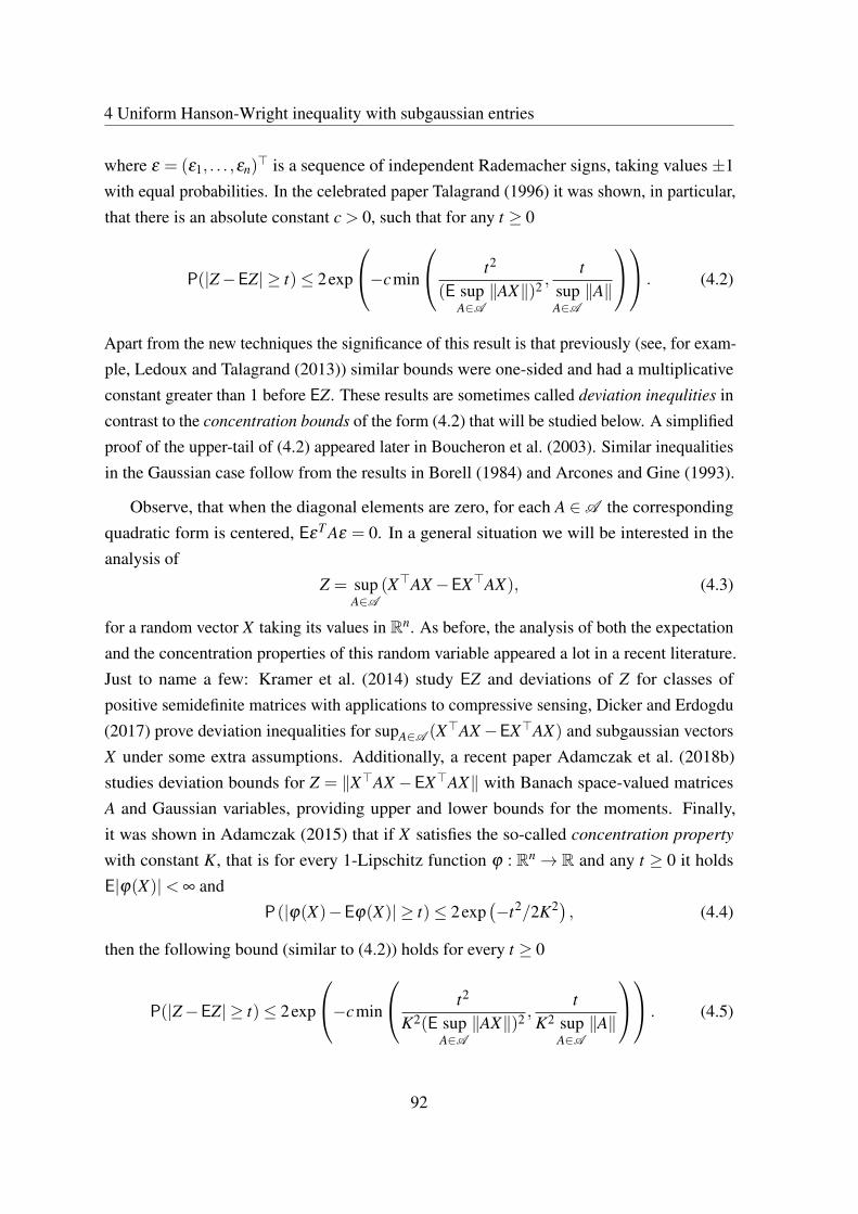
4 Uniform Hanson-Wright inequality with subgaussian entries
where ε = (ε1, . . . ,εn)> is a sequence of independent Rademacher signs, taking values ±1
with equal probabilities. In the celebrated paper Talagrand (1996) it was shown, in particular,that there is an absolute constant c > 0, such that for any t ≥ 0
P(|Z−EZ| ≥ t)≤ 2exp
−cmin
t2
(E supA∈A‖AX‖)2 ,
tsupA∈A‖A‖
. (4.2)
Apart from the new techniques the significance of this result is that previously (see, for exam-ple, Ledoux and Talagrand (2013)) similar bounds were one-sided and had a multiplicativeconstant greater than 1 before EZ. These results are sometimes called deviation inequlities incontrast to the concentration bounds of the form (4.2) that will be studied below. A simplifiedproof of the upper-tail of (4.2) appeared later in Boucheron et al. (2003). Similar inequalitiesin the Gaussian case follow from the results in Borell (1984) and Arcones and Gine (1993).
Observe, that when the diagonal elements are zero, for each A ∈A the correspondingquadratic form is centered, EεT Aε = 0. In a general situation we will be interested in theanalysis of
Z = supA∈A
(X>AX−EX>AX), (4.3)
for a random vector X taking its values in Rn. As before, the analysis of both the expectationand the concentration properties of this random variable appeared a lot in a recent literature.Just to name a few: Kramer et al. (2014) study EZ and deviations of Z for classes ofpositive semidefinite matrices with applications to compressive sensing, Dicker and Erdogdu(2017) prove deviation inequalities for supA∈A (X>AX−EX>AX) and subgaussian vectorsX under some extra assumptions. Additionally, a recent paper Adamczak et al. (2018b)studies deviation bounds for Z = ‖X>AX −EX>AX‖ with Banach space-valued matricesA and Gaussian variables, providing upper and lower bounds for the moments. Finally,it was shown in Adamczak (2015) that if X satisfies the so-called concentration property
with constant K, that is for every 1-Lipschitz function ϕ : Rn→ R and any t ≥ 0 it holdsE|ϕ(X)|< ∞ and
P(|ϕ(X)−Eϕ(X)| ≥ t)≤ 2exp(−t2/2K2) , (4.4)
then the following bound (similar to (4.2)) holds for every t ≥ 0
P(|Z−EZ| ≥ t)≤ 2exp
−cmin
t2
K2(E supA∈A‖AX‖)2 ,
tK2 sup
A∈A‖A‖
. (4.5)
92

This result has an application in the covariance estimation and recovers another recentconcentration result of Koltchinskii and Lounici (2017); we will discuss this in what follows.The drawback of (4.5) is that the concentration property is quite restrictive: it works when X
has standard Gaussian distribution, for some log-concave distributions (see Ledoux (2001)),but at the same time does not hold for general subgaussian entries and even in the simplestcase of Rademacher random vector ε .
We extend the mentioned results in two directions. On one hand we revisit the resultof Boucheron et al. (2003) for bounded variables allowing non-zero diagonal values of thematrices, and on the other we allow unbounded subgaussian variables Xi. First, let us recallthe following definition. For α > 0 denote the ψα -norm of a random variable Y by
‖Y‖ψα= inf
t ≥ 0 : Eexp
(|Y |α
tα
)≤ 2,
which is a proper norm whenever α ≥ 1. A random variable Y with ‖Y‖ψ1 < ∞ will berefereed to as subexponential and ‖Y‖ψ2 < ∞ will be refereed to as subgaussian and thecorresponding norm is usually named a subgaussian norm. We also use the Lp(P) norm. Forp≥ 1 we set ‖Y‖Lp = (E|Y |p)
1p . One of our main contributions is the following upper-tail
bound.
Theorem 4.1. Suppose that components of X = (X1, . . . ,Xn) are independent centered
random variables and A is a finite family of n× n real symmetric matrices. Denote
M =∥∥maxi |Xi|
∥∥ψ2
. Then, for any t ≥maxMEsup‖AX‖,M2 supA ‖A‖ it holds
P(Z−EZ ≥ t)≤ exp
−cmin
t2
M2(E supA∈A‖AX‖)2 ,
tM2 sup
A∈A‖A‖
,
where c > 0 is an absolute constant and Z is defined by (4.3).
Remark 4.1. In Theorem 4.1 and below we assume that all A ∈A is symmetric. This was
done only for the convenience of presentation and in fact, the analysis may be performed
for general square matrixes. The only difference will be that in many places A should be
replaced by 12(A+AT ).
In particular, Theorem 4.1 recovers the right-tail of the result of Talagrand (4.2) up toabsolute constants, since in this case we obviously have
∥∥maxi |εi|∥∥
ψ2. 1. Furthermore,
the result of Theorem 4.1 works without the assumption used in Talagrand (1996) and
93

4 Uniform Hanson-Wright inequality with subgaussian entries
Boucheron et al. (2003) that diagonals of all matrices in A are zero. Moreover, it is alsoapplicable in some situations when the concentration property (4.4) holds: indeed, if X isa standard normal vector in Rn then it is well known (see Ledoux and Talagrand (2013))that M =
∥∥maxi |Xi|∥∥
ψ2∼√
logn and at the same time if the identity matrix In ∈ A thenEsupA∈A ‖AX‖ ≥ E‖X‖ &
√n. Therefore, in this case the factor M is only of at most
logarithmic order when compared to EsupA∈A ‖AX‖.
In a special case when A consists of just one matrix our bound recovers the boundwhich is similar to the original Hanson-Wright inequality. On the one hand our bound mayhave an extra logarithmic factor that depends on the dimension n. On the other hand theoriginal term maxi ‖Xi‖ψ2‖A‖HS is replaced by the better term E‖AX‖. We will discuss thisphenomenon below. The core of the proof of the Hanson-Wright inequality in Rudelsonand Vershynin (2013) is based on the decoupling technique which may be used (at leastin a straightforward way) to prove the deviation, but not the concentration inequality forsupA∈A (X>AX−EX>AX) in the case when A consists of more than one matrix.
A natural question to ask is whether one may improve Theorem 4.1 and replace M =∥∥maxi |Xi|∥∥
ψ2by K = maxi
∥∥Xi∥∥
ψ2. In what follows we discuss that in the deviation version
of Theorem 4.1 this replacement is not possible in some cases. This is quite unexpected inlight of the fact that
∥∥maxi |Xi|∥∥
ψ2does not appear in the original Hanson-Wright inequality.
Therefore, we believe that the form of our result is close to optimal. We also provide thefollowing extension of Theorem 4.1, which may be better in some cases.
Proposition 4.1. Suppose that components of X = (X1, . . . ,Xn) are independent centered
random variables. Suppose also, that the variables Xi have symmetric distribution (Xi has
the same distribution as −Xi). Let A be a finite family of n× n real symmetric matrices.
Denote M =∥∥maxi |Xi|
∥∥ψ2
and K = maxi∥∥Xi∥∥
ψ2and let g be a standard Gaussian vector in
Rn. Then, for any t ≥maxMKEsup‖AG‖,MK supA ‖A‖ it holds
P(Z−EZ ≥ t)≤ exp
−cmin
t2
M2K2(E supA∈A‖AG‖)2 ,
tMK sup
A∈A‖A‖
,
where c > 0 are absolute constants and Z is defined by (4.3).
Remark 4.2. Proposition 4.1 is closer to the standard Hanson-Wright inequality (4.1).Indeed, in the case when A = A we have E‖AG‖ ∼ ‖A‖HS. The difference is that K4 and
K2 are replaced by M2K2 and MK respectively.
94

We proceed with some notations that will be used below. For a non-negative randomvariable Y , define its entropy as
Ent(Y ) = EY logY −EY logEY.
Instead of the concentration property (4.4) we also discuss the following property:
Assumption 4.1. We say that the random vector X taking its values in Rn satisfies the
logarithmic Sobolev inequality with constant K > 0 if for any continuously differentiable
function f : Rn→ R it holds
Ent( f 2)≤ 2K2E‖∇ f (X)‖2, (4.6)
whenever both sides of the inequality are not infinite.
To show that logarithmic Sobolev property is closely related to the concentration propertywe remind (Theorem 5.3 Ledoux (2001)) that Assumption 4.1 implies the concentrationproperty (4.4) and the proof of this fact is based essentially on taking f (X) = exp(λ (ϕ(X)−Eϕ(X))/2) for λ > 0 which implies
Ent(exp(λ (ϕ(X)−Eϕ(X))))≤ K2λ 2
2Eexp(λ (ϕ(X)−Eϕ(X))).
This is known to imply (4.4) through Herbst argument, see Boucheron et al. (2013). Moreover,the last inequality is equivalent to concentration property. Indeed, from the concentrationproperty we know that ‖ϕ(X)−Eϕ(X)‖ψ2 . K and this implies (see van Handel (2016))that for all λ ∈ R
Ent(exp(λ (ϕ(X)−Eϕ(X)))). K2λ
2Eexp(λ (ϕ(X)−Eϕ(X))).
One of our technical contributions is that we use a similar scheme to prove Theorem4.1 and to recover (4.5) under the logarithmic Sobolev Assumption 4.1. The applicationof logarithmic Sobolev inequalities requires computation of the gradient of the function ofinterest, that is in our case the gradient of f (X) = supA∈A (XT AX −EXT AX). It appearsthat in the analysis we need to control the behaviour of ∇ f (X) (or its analogs) and, as inBoucheron et al. (2003) and Adamczak (2015), we will use a truncation argument to doso. However, in both cases our proofs will pass through the entropy variational formula
of Boucheron et al. (2013), that states that for random variables Y,W with Eexp(W )< ∞ it
95

4 Uniform Hanson-Wright inequality with subgaussian entries
holdsE(W exp(λY ))≤ Eexp(λY ) log(Eexp(W ))+Ent(exp(λY )). (4.7)
This will allow us to shorten the proofs and avoid some technicalities appearing in previouspapers. Finally, to prove Theorem 4.1 we use a second truncation argument: that will bebased on Hoffman-Jørgensen inequality (see Ledoux and Talagrand (2013)). We also presenttwo lemmas, which will be used several times in the text. Both results have short proofs andmay be of independent interest.
Lemma 4.1. Suppose, that for random variables Z,W and any λ > 0 it holds
Ent(eλZ)≤ λ2EWeλZ and P(W > L+θ t)≤ e−t , (4.8)
where θ ,L are positive constants. Then, the following concentration result holds
P(Z−EZ > t)≤ exp(−cmin
t2
L+θ,
t√θ
), (4.9)
where c > 0 is an absolute constant. Moreover, if (4.8) holds as well for λ ≤ 0, we have
P(|Z−EZ|> t)≤ 2exp(−cmin
t2
L+θ,
t√θ
).
The second technical result is a version of the convex concentration inequality of Tala-grand (1996), which does not require the boundedness of components of X .
Lemma 4.2. Let f : Rn→ R be a convex, L-Lipschitz function with respect to Euclidian
norm in Rn and X = (X1, . . . ,Xn) be a random vector with independent components. Then, it
holds for any t ≥CL‖maxi |Xi|‖ψ2
P(| f (X)−E f (X)|> t)≤ exp
(−c
t2
L2 ‖maxi |Xi|‖2ψ2
),
where c,C > 0 are absolute constants.
We discuss the optimality of this result in what follows. Finally, we sum up the structureof the rest of this chapter and outline the main contributions:
• Section 4.1 is devoted to applications and discussions and consists of several parts.At first, we give a simple proof of the uniform bound of Adamczak (2015) under the
96
4.1 Some applications and discussions
logarithmic Sobolev assumption. The second paragraph is devoted to improvementsin the non-uniform Hanson-Wright inequality (4.1) in the subgaussian regime. Fur-thermore, we apply our techniques to obtain a uniform concentration result similarto Theorem 4.1 in a particular case of non-independent components. We considerthe Ising model under Dobrushin’s condition that caught some attention recently (seeAdamczak et al. (2018a) and Götze et al. (2018)). The question we study was raisedby Marton (2003) in a closely related scenario. Finally, we show that it is not possiblein general to replace ‖maxi |Xi|‖ψ2 with maxi ‖Xi‖ψ2 in Theorem 4.1 by providing anappropriate counterexample.
• In Section 4.2 we present the proof of Theorem 4.1. Between the lines, we proveLemma 4.8 and Lemma 4.2. Finally, we give a proof of Proposition 4.1.
• In Section 4.3 we prove a dimension-free matrix Bernstein inequality that holds forrandom matrices with the subexponential spectral norm. The proof is based on thesame truncation approach as in the proof of Theorem 4.1. We demonstrate how ourBernstein inequality can be used in the context of covariance estimation for subgaussianobservations, improving the state-of-the-art result of Lounici (2014) for covarianceestimation with missing observations.
4.1 Some applications and discussions
We begin with some notation that will be used below. For a random vector X taking itsvalues in Rn let X1, . . . ,Xn denote its components. In the case when all the componentsof X are independent let X ′i denote the independent copy of the component Xi. Symbol ∼denotes equivalence up to absolute constants and . denotes an inequality up to some absoluteconstant. The numbers C,c > 0 denote absolute constants, which also may change from lineto line.
A uniform Hanson-Wright inequality under the logarithmic Sobolev condition
In this paragraph we recover the result of Adamczak (2015) under the Assumption 4.1.Consider a random variables Z defined by (4.3) as a function of X , that satisfies logarithmicSobolev assumption (4.6).
97

4 Uniform Hanson-Wright inequality with subgaussian entries
Following Adamczak (2015) we assume without the loss of generality, that A is a finiteset of matrices, then Z is Lebesgue-a.e. differentiable and
‖∇Z(X)‖ ≤ 2supA‖AX‖,
bounded by a Lipschitz function of X with good concentration properties.
Remark 4.3. Note, that Assumption 4.1 applies only for smooth functions, so that a standard
smoothing argument should be used (see e.g. Ledoux (2001)). For sake of completeness we
recover this argument in Section 4.4. In what follows in this section we assume that none of
these potential technical problems appear.
In particular, since X satisfies log-Sobolev condition with constant K, we have (Theorem5.3 in Ledoux (2001))
P
(sup
A‖AX‖ ≥ Esup
A‖AX‖+K
√t sup
A‖A‖
)≤ e−t .
Taking square and using (a+b)2 ≤ 2a2 +2b2, we get
P
(sup
A‖AX‖2 ≥ 2
(Esup
A‖AX‖
)2
+2K2 supA‖A‖2t
)≤ e−t .
Furthermore, the logarithmic Sobolev condition implies for any λ ∈ R
Ent(eλZ)≤ 4K2λ
2EsupA‖AX‖2eλZ.
Therefore, by Lemma 4.1 it holds for any t ≥ 1,
P
(|Z−EZ|>C
(KEsup
A‖AX‖
√t +K2 sup
A‖A‖t
))≤ 2e−t ,
which coincides with (4.5) for K-concentrated vectors up to absolute constant factors.
Remark 4.4. This result may be used directly to prove the concentration for ‖Σ−Σ‖, where
Σ is the sample covariance defined as Σ= 1N ∑
Ni=1 XiX>i and X1, . . . ,XN are centered Gaussian
vectors with the covariance matrix Σ (see Theorem 4.1 in Adamczak (2015)). We return to
the covariance estimation problem in Section 4.3.
98

4.1 Some applications and discussions
Improving Hanson-Wright inequality in the subgaussian regime
Our analysis implies, in particular, an improved version of Hanson-Wright inequality (4.1)in some cases. We consider a centered random vector X = (X1, . . . ,Xn) with independentsubgaussian components and set K = maxi ‖Xi‖ψ2 , M = ‖maxi |Xi|‖ψ2 . In this case (4.1)implies that with probability at least 1−2e−t it holds
X>AX−EX>AX . K2 (‖A‖HS√
t +‖A‖t). (4.10)
At the same time, Theorem 4.1 for a single matrix A = A implies with the same probability
X>AX−EX>AX . ME‖AX‖√
t +M2‖A‖t. (4.11)
Observe that when |Xi| ≤ L almost surely for each i ≤ n, we have M . minK√
logn,L.The following example illustrates the difference between these two bounds.
Example 4.1. Assume, δ = (δ1, . . . ,δn) is a sequence of independent Bernoulli random
variables with the mean δ and let δ ≤ 14 . For X = (δ1−δ , . . . ,δn−δ ) we easily get
E‖AX‖ ≤√EXT A2X ≤
√δ‖A‖HS.
On the other hand, for δ ≤ 14 it holds
‖X1‖2ψ2
= ‖δ1−δ‖2ψ2∼ sup
λ∈R
log(Eexp(λ (δ1−δ )))
λ 2
= supλ∈R
log(δ exp(λ (1−δ ))+(1−δ )exp(−λδ ))
λ 2 =1−2δ
4log((1−δ )/δ )∼ 1| logδ |
,
where the last line follows directly from Theorem 1.1 in Schlemm (2016). Therefore, the
standard Hanson-Wright inequality implies that with probability at least 1− e−t it holds,
X>AX−EX>AX .1
| logδ |(‖A‖HS
√t +‖A‖t
),
while (4.11) and M . minK√
logn,1 imply that for t ≥ 1 and δ ≤ 14 it holds with proba-
bility at least 1−2e−t
X>AX−EX>AX . min
√δ logn| logδ |
,√
δ
‖A‖HS
√t +min
logn| logδ |
,1‖A‖t. (4.12)
99

4 Uniform Hanson-Wright inequality with subgaussian entries
It is easy to verify that limδ→0+
√δ | logδ |= 0, thus the inequality (4.12) is better than Hanson-
Wright inequality for this X in the subgaussian regime (when the t-term is dominated by the√
t-term).
Uniform concentration results in the Ising model
Suppose, we have a discrete random vector σ ∈ −1,1n with the distribution defined by
π(σ) =1Z′
exp
(n
∑i, j=1
Ji jσiσ j−n
∑i=1
hiσi
),
where Z′ is a normalizing factor. This distribution defines the Ising model with parametersJ = (Ji j)
ni, j=1 and h = (hi)
ni=1.
For an arbitrary function f on −1,1n denote a difference operator,
|d f |2(σ) =12
n
∑i=1
( f (σ)− f (Tiσ))2π(−σi | σ1, . . . ,σi−1,σi+1, . . .),
where the operator Tiσ = (σ1, . . . ,σi−1,−σi,σi+1, . . .) flips the sign of the ith coordinate,and π(· | σ1, . . . ,σi−1,σi+1, . . .) is conditional distribution of the ith coordinate, given therest of the elements. The following recent result provides log-Sobolev inequality for vectorσ under Dobrushin-type conditions.
Theorem 4.2 (Proposition 1.1, Götze et al. (2018)). Suppose, ‖h‖∞ ≤ α and J satisfies
Jii = 0 and
‖J‖17→1 = maxi=1,...,n
n
∑j=1|Ji j| ≤ 1−ρ (4.13)
There is a constant C =C(α,ρ), such that for an arbitrary function f on −1,1n it holds,
Ent( f 2)≤ 2CE|d f |2.
Remark 4.5. Following Götze et al. (2018) the condition (4.13) will be called Dobrushin’scondition.
We may obtain the following uniform concentration result which is a simple outcome ofour Lemma 4.1 and Theorem 4.2.
100

4.1 Some applications and discussions
Proposition 4.2. Let A be a finite set of symmetric matrices with zero diagonal. It holds in
the Ising model under Dobrushin’s condition and ‖h‖∞ ≤ α that for any t ≥ 0
P
(supA∈A
σ>Aσ −E sup
A∈Aσ>Aσ ≥ t
)≤ exp
−cmin
t2
(E supA∈A‖Aσ‖+ supA∈A ‖A‖)2 ,
tsupA∈A‖A‖
,
(4.14)where C depends only on α,ρ .
Proof. Let σ ′(i) = (σ1, . . . ,σi−1,σ′i ,σi+1, . . .) given all but the i-th element, the variables
σi and σ ′i are independent and are distributed according to π(· | σ1, . . . ,σi−1,σi+1, . . .).Obviously, we may have all σ1, . . . ,σi and σ ′1, . . . ,σ
′n defined on the same discrete probability
space, and thus we will use the notation π(·) and π(· | ·) for the distribution and the conditionaldistribution. Then, we have
E|d f |2(σ) =12
n
∑i=1
E( f (σ)− f (Tiσ))2π(−σi | σ1, . . . ,σi−1,σi+1, . . .)
=n
∑i=1
∑σ∈−1,1n
π(σ) ∑σ ′i∈−1,1
( f (σ)− f (σ ′(i)))2+π(σ ′i | σ1, . . . ,σi−1,σi+1, . . .)
where we switched from 12( f (σ)− f (σ ′(i)))
2 to ( f (σ)− f (σ ′(i)))2+ due to the symmetry
between σi and σ ′i .
Observe, that denoting for short σ−i = (σ1, . . . ,σi−1,σi+1, . . . ,σn) and using the inde-pendence of σi and σ ′i given σ−i, we have π(σi,σ
′i | σ−i) = π(σi | σ−i)π(σ ′i | σ−i), and
therefore by the chain rule,
π(σ)π(σ ′i | σ1, . . . ,σi−1,σi+1, . . .) = π(σ−i)π(σi | σ−i)π(σ ′i | σ−i)
= π(σ−i)π(σi,σ′i | σ−i) = π(σ ′i ,σi,σ
−i).
Finally, we get
E|d f |2(σ) =n
∑i=1
∑(σ ,σ ′i )∈−1,1n+1
( f (σ)− f (σ ′(i)))2+π(σ ,σ ′i ) =
n
∑i=1
E( f (σ)− f (σ ′(i)))2+ .
Now we want to consider the function
Z = supA∈A
σ>Aσ , (4.15)
101

4 Uniform Hanson-Wright inequality with subgaussian entries
where A is a given set of symmetric matrices with zero diagonal (the diagonal is notimportant here, since σ2
i = 1). Applying Theorem 4.2 to f = eλZ/2, we have
E|d f |2(σ) = En
∑i=1
( f (σ)− f (σ ′(i)))2+ = EeλZ
n
∑i=1
(1− eλ (Z(σ)−Z(σ ′(i)))/2)2+
≤ λ 2
4EeλZ
n
∑i=1
(Z−Z(σ ′(i)))2+,
where for A being maximizer of (4.15) we have,
n
∑i=1
(Z−Z(σ ′(i)))2+ ≤
n
∑i=1
(σ>Aσ − [σ ′(i)]
>Aσ′(i)
)2
+=
n
∑i=1
(2(σi−σ
′i )
n
∑j=1
Ai jσ j
)2
+
≤ 16 supA∈A‖Aσ‖2.
Note, that concentration for supA∈A ‖Aσ‖ is implied by the same result. Indeed, we have
n
∑i=1
(sup
A∈A ,γ∈Sn−1γ>Aσ − sup
A∈A ,γ∈Sn−1γ>Aσ
′(i)
)2
+
≤n
∑i=1
(w>σ − w>σ′(i))
2+
=n
∑i=1
(wi(σi−σ′i ))
2+ ≤ 4sup
A‖A‖,
where w> = γ>A is such that supA ‖Aσ‖ = w>σ . Thus, the expectation of correspondingdifference operator is bounded by 4supA ‖A‖, so that due to standard Herbst argument,Theorem 4.2 implies
P
(supA∈A‖Aσ‖> E sup
A∈A‖Aσ‖+C sup‖A‖
√t)≤ e−t .
To sum up, by Theorem 4.2 it holds,
Ent(eλZ)≤ λ2E(4 sup
A∈A‖Aσ‖)eλZ.
It is left to apply Lemma 4.1, which brings us to a uniform Hanson-Wright-type concentrationbound for the Ising model
P
(sup
Aσ>Aσ −Esup
Aσ>Aσ >C(
√tEsup
A‖Aσ‖+(
√t + t)sup
A‖A‖)
)≥ 1− e−t , (4.16)
102

4.1 Some applications and discussions
where C only depends on α,ρ from Theorem 4.2. The claim follows.
Remark 4.6. In the case when A = A our result implies the upper tail of the recent
concentration inequality proved in Adamczak et al. (2018a) (see Theorem 2.2 and Example
2.5). To show this fact (denoting σ = σ −Eσ ) we observe that
E‖Aσ‖ ≤ E‖Aσ‖+‖AEσ‖= E‖Aσ‖+( n
∑i=1
(n
∑j=1
Ai, jEσ j)2) 1
2 .
Now, it is well known that Ent( f 2)≤ 2cE|d f |2 implies Poincaré’s inequlity Var( f )≤ cE|d f |2
and therefore,
‖Eσ σ>‖= sup
u∈Sn−1Var(uT
σ)≤ (c(α,ρ)/2) supu∈Sn−1
4‖u‖2 = 2c(α,ρ).
This implies,
E‖Aσ‖2 = E tr(A2σ σ
>)≤ ‖A‖2HS‖Eσ σ
T‖ ≤ 2c(ρ,α)‖A‖2HS,
where we used that tr(BD)≤ tr(B)‖D‖, which holds for any symmetric and nonnegative B,D.
Finally,
‖Aσ‖ ≤C(ρ,α)‖A‖HS +( n
∑i=1
(n
∑j=1
Ai, jEσ j)2) 1
2 .
The right-hand side term appears instead of ‖Aσ‖ in Example 2.5 mentioned above.
Replacing ‖maxi |Xi|‖ψ2 with maxi ‖Xi‖ψ2 in Theorem 4.1
Here we show that it is essentially not possible in general to substitute ‖maxi |Xi|‖ψ2 withmaxi ‖Xi‖ψ2 in Theorem 4.1 by presenting a concrete counterexample, which was kindlysuggested by Radosław Adamczak. Suppose the opposite, that there is an absolute constantC > 0 such that for any set of matrices A and any subgaussian random variables X1, . . . ,Xn
it holds with probability at least 1− e−t ,
Z ≤C(EZ +max
i‖Xi‖ψ2
√tEsup
A‖AX‖+max
i‖Xi‖2
ψ2sup
A‖A‖t
), (4.17)
103

4 Uniform Hanson-Wright inequality with subgaussian entries
which implies with some other constant C′ > 0
E1/2Z2 ≤C′(EZ +max
i‖Xi‖ψ2Esup
A‖AX‖+max
i‖Xi‖2
ψ2sup
A‖A‖
).
Notice, that here we also allow a constant in front of the expectation.
Let us take A = A(1), . . . ,A(n) with A(i) having only one nonzero element A(i)ii = 1. For
simplicity take i.i.d. X1, . . . ,Xn with EX2i = 1, so that
Z = maxi≤n
(X2i −1), sup
A‖AX‖= max
i≤n|Xi|, sup
A‖A‖= 1.
Then, assuming, say ‖X1‖ψ2 ≤ 4 we have
∥∥maxi
X2i −1
∥∥L2≤C′
(Emax
i(X2
i −1)+4Emaxi|Xi|+16
),
which since ‖maxi X2i ‖L1 ≥ ‖Xi‖L2 = 1 implies
∥∥maxi
X2i ‖L2 ≤ 1+C′(‖max
iX2
i ‖L1 +4Emaxi|Xi|+15)≤ (1+20C′)‖max
iX2
i ‖L1 .
Note, that this inequality also holds if we rescale X ′i =αXi for an arbitrary α > 0. Therefore, ifwe have a moment equivalence ‖X1‖ψ2 ≤ 4‖X1‖L2 , we can always rescale to have ‖X1‖L2 = 1and ‖X1‖ψ2 ≤ 4, so that the above inequality holds.
Taking the latter into account, we conclude that there is a constant D > 0, such that if acentred random X1 satisfies ‖X1‖ψ2 ≤ 4‖X1‖L2 , then for any n≥ 1 the following holds,
∥∥maxi≤n
X2i∥∥
L2≤ D‖max
i≤nX2
i ‖L1 . (4.18)
It is known that such hypercontractivity of maxima implies certain regularity of tails ofthe distribution of X2
1 . In this case by Theorem 4.6 in Hitczenko et al. (1998) for any ρ,ε > 0there is another constant A = A(D,ρ,ε)> 1 such that for all t ≥ t0 = ρ‖X1‖L1 it holds,
AqP(X21 > At)≤ εP(X2
1 > t),
so that in our case of p = 2 and q = 1 and taking ρ = ε = 1, there is A = A(D)> 1 such thatfor all t ≥ ‖X1‖L1 it holds
P(X21 > At)≤ 1
AP(X2
1 > t). (4.19)
104

4.2 Proof of Theorem 4.1
The latter does not have to hold for any subgaussian random variable X1. For instance, takinga symmetric random variable X1 with P(|X1| = 1) = 1− e−r and P(|X1| =
√r) = e−r for
r ≥ 4 > 4log2 we have Eexp(|X1|2
2
)= e
12 (1−e−r)+e−r+ r
2 ≤ e12 +e−
r2 ≤ 2, which implies
‖X1‖ψ2 ≤ 2. Moreover, for r≥ 4 we also have EX21 ≥ 1−e−
r2 ≥ 1
2 , thus ‖X1‖L2 ≥ 1/√
2 andthe conditions of (4.18) are satisfied. But for large enough r > At for t = t0, we have
P(X2
1 > At)= P(X2
1 > t) = e−r,
therefore breaking the tail regularity (4.19). Thus, it is impossible to establish inequality ofform (4.17). We also note that it is also possible to prove that (4.18) may not hold for X1
defined above via some direct computations.
By the same reason it is not possible to replace ‖maxi≤n |Xi|‖ψ2 with maxi≤n ‖Xi‖ψ2 inLemma 4.2. Indeed, suppose for any convex L-Lipschitz function f it holds,
P
(f (X)≤C(E f (X)+Lmax
i≤n‖Xi‖ψ2
√t))≤ e−t .
Then, taking f (X) = maxi≤n |Xi|, which is convex and 1-Lipschitz, we get
∥∥maxi≤n
X2i∥∥
L2=∥∥max
i≤n|Xi|∥∥
L4≤C′
(Emax
i|Xi|+max
i‖Xi‖ψ2
),
which for the same random variable X1 as before implies (4.18) and leads to a contradiction.
4.2 Proof of Theorem 4.1
In this section we assume that all components of X are independent. We recall that X ′idenotes an independent copy of the component Xi. The main tool of the proof is the modifiedlogarithmic Sobolev inequality (see Theorem 2 in Boucheron et al. (2003) or Theorem 6.15in Boucheron et al. (2013)). Set,
Z′i = Z(X1, . . . ,Xi−1,X ′i ,Xi, . . . ,Xn).
Then, by symmetrised version of the inequality we have for any λ ,
Ent(eλZ)≤n
∑i=1
EeλZτ(−λ (Z−Z′i)+),
105

4 Uniform Hanson-Wright inequality with subgaussian entries
where τ(x) = x(ex−1). Since τ(x)≤ x2 for x≤ 0, we have for all λ ≥ 0,
Ent(eλZ)≤ λ2EV+eλZ, V+ := E′
n
∑i=1
(Z−Z′i)2+.
The right-hand side of the inequality can be “decoupled” by variational entropy formula(4.7), as it is done in the proof of Lemma 4.1, that we presented in the introduction.
Proof of Lemma 4.1. We have
Ent(eλZ)≤ λ2LeλZ +λ
2E(W −L)+eλZ.
Due to the deviation bound for W it holds for some absolute constant C > 0,
Eexp((W −L)+
Cθ
)≤ e.
Therefore, by (4.7) we have,
E(W −L)+/(Cθ)eλZ ≤ EeλZ +Ent(eλZ),
which implies(1−Cθλ
2)Ent(eλZ)≤ λ2(L+Cθ)EeλZ.
By the Herbst argument (see e.g., Proposition 6.1 in Boucheron et al. (2013)) we have foreach 0 < λ ≤ (Cθ)−1/2,
logEexp(λ (Z−EZ))≤ 2(L+Cθ)λ 2,
therefore (Z−EZ) is subexponential and the right-hand concentration bound follows. If (4.8)holds for all λ ∈ R, the two sided inequality can be derived in the same way.
Remark 4.7. Note, there is as well a moment version of the modified log-Sobolev inequality,
see Theorem 2 in Boucheron et al. (2005b). By the theorem it holds, for all q≥ 2
‖(Z−EZ)+‖Lq ≤√
2κq‖√
V+‖Lq ,
106
4.2 Proof of Theorem 4.1
where κ < 2 is an absolute constant. Then, if we have a condition for V+ in the form
‖√
V+‖Lq ≤√
L+√
θq, ∀q≥ 2, (4.20)
which is equivalent to the second inequality in (4.8) up to constants, then it simply holds for
each q≥ 2‖(Z−EZ)+‖Lq ≤
√4Lq+
√4θq,
which as well implies (4.9) up to constants. We note that similar moment computations
where used in Boucheron et al. (2005b) to analyze the Rademacher chaos. Similarly, one can
introduce the moment analog of logarithmic Sobolev inequality (see equation 3 in Adamczak
and Wolff (2015)):
‖Z(X)−EZ(X)‖Lq ≤ K√
q‖|∇Z(X)|‖Lq ,
where K > 0 is a constant, | · | stands for the standard Euclidian norm and q≥ 2. Now, if it
holds (which may be in some cases derived by the second application of the moment analog
of logarithmic Sobolev inequalities)
‖|∇Z(X)|‖Lq ≤ E|∇Z(X)|+‖|∇Z(X)|−E|∇Z(X)|‖Lq ≤√
L+K√
θq, ∀q≥ 2
then
‖Z−EZ‖Lq ≤ K(√
Lq+K√
θq),
which implies the bound similar to (4.5).
Now we establish a version of our result that does not require neither centered Xi northat they have variance one. In this case it might happen that EX>AX 6= tr(A), but in factthe value we subtract does not really affect the concentration properties. In general we canconsider,
Z = supA∈A
(X>AX−g(A)), (4.21)
where g : Rn×n→ R is an arbitrary function.
Lemma 4.3. Suppose, |Xi| ≤ K almost surely, are independent, but not necessary centred.
Then, for Z defined by (4.21) and for any t ≥ 1
Z−EZ ≤C(
K(EsupA‖AX‖+Esup
A‖Diag(A)X‖)
√t +K2 sup
A‖A‖t
),
with probability at least 1− e−t where C is an absolute constant.
107

4 Uniform Hanson-Wright inequality with subgaussian entries
Proof. Let A be the matrix on which the maximum is achieved for the original sample. Wehave,
∑i≤n
(Z−Zi)2+ ≤∑
i≤n
(2(Xi−X ′i )∑
j 6=iai jX j + aii(X2
i −X ′2i )
)2
= ∑i≤n
(Xi−X ′i )2
(2 ∑
j 6=iai jX j + aii(Xi +X ′i )
)2
≤ (2K)2∑i≤n
(2∑
jai jX j + aii(X ′i +Xi)
)2
,
where the last line follows from |Xi−X ′i | ≤ 2K. Applying the triangle inequality we get
V+ = E′∑i≤n
(Z−Zi)2+ ≤ (2K)2E′ sup
A(2‖AX‖+‖Diag(A)X‖+‖Diag(A)X ′‖)2,
where the expectation is taken with respect to the copy sample. Thus,
E′V+ ≤ 12K2(
supA‖AX‖2 + sup
A‖Diag(A)X‖2 +Esup
A‖Diag(A)X‖2
).
Since |Xi| ≤ K, we have by convex concentration for Lipshitz functions (see e.g. Theo-rem 6.10 in Boucheron et al. (2013))
P
(sup
A‖AX‖> Esup
A‖AX‖+2
√2K sup
A‖A‖√
t)≤ e−t . (4.22)
Using (a+ b)2 ≤ 2a2 + 2b2 we have, that for L ∼ (KEsup‖AX‖+KEsup‖Diag(A)X‖)2
and θ ∼ (K sup‖A‖)2 it holds
P(V+ > L+θ t)≤ e−t ,
so that due to the modified log-Sobolev inequality (4.2) we can use Lemma 4.1. This providesus with the inequality
P(Z−EZ >C(√
L+θ√
t +√
θ t))≤ e−t ,
where we can neglect the θ in front of√
t when t ≥ 1.
108

4.2 Proof of Theorem 4.1
Note, that here we have the term EsupA ‖Diag(A)X‖, which can be avoided in the caseof centered variables Xi, therefore matching the previous bounds (4.5) and (4.2).
Corollary 4.1. Suppose, |Xi| ≤ K almost surely and EXi = 0. Then, for any t > 0
Z−EZ . KEsupA‖AX‖
√t +K2 sup
A‖A‖t,
with probability at least 1−2e−t .
In the next two lemmas we show how to get rid of the diagonal term, which finishes theproof of the corollary above.
Lemma 4.4. Suppose, Y ∈ Rn has i.i.d. coordinates with symmetric distribution, and let B
be a set of n×n positive-definite symmetric matrices. Then,
E supB∈B
Y>Diag(B)Y ≤ E supB∈B
Y>BY.
Proof. Given the vector x ∈Rn let Diag(x) denote a diagonal n×n matrix with x on diagonal.Since Y d
= Diag(ε)Y for an independent Rademacher vector ε ∈ 1,−1n, we have byJensen’s inequality
E supB∈B
Y>BY = EEε supB∈B
Y> diag(ε)Bdiag(ε)Y
≥ E supB∈B
EεY> diag(ε)Bdiag(ε)Y
= E supB∈B
Y>Diag(B)Y,
where Eε denotes expectation conditioned on Y .
Lemma 4.5. For a random X with independent mean zero coordinates it holds,
E supA∈A‖Diag(A)X‖ ≤CE sup
A∈A‖AX‖,
where C > 0 is an absolute constant.
Proof. Setting X ′ as an independent copy of X , we have a standard symmetrisation argument,i.e. applying first Jensen’s and then the triangle inequality we have,
E supA∈A‖AX‖ ≤ E sup
A∈A‖A(X−X ′)‖ ≤ 2E sup
A∈A‖AX‖. (4.23)
109

4 Uniform Hanson-Wright inequality with subgaussian entries
Observe that X−X ′ d= (X−X ′)diag(ε) = diag(X−X ′)ε , where ε ∈ 1,−1n is an indepen-
dent Rademacher vector. Therefore, we have
E supA∈A‖A(X−X ′)‖= EEε sup
A∈A‖Adiag(X−X ′)ε‖,
where Eε denotes the expectation with respect to ε . Conditionally on (X−X ′) set AX ,X ′ =
Adiag(X −X ′) : A ∈ A . Let a1, . . . ,an be columns of a matrix A. Notice, that for anymatrix A we have Diag(A>A) = diag(‖a1‖2, . . . ,‖an‖2) diag(A2
11, . . . ,A2nn) = Diag(A)2.
Therefore, by Lemma 4.4
Eε supA∈AX ,X ′
‖Diag(A)ε‖2 ≤ Eε supA∈AX ,X ′
‖Aε‖2. (4.24)
We now want to get rid of the squares in the inequality above which is possible dueto concentration. Let us fix some matrix B ∈ B, where B is a set of matrixes. Then,E‖Bε‖2 = ‖B‖2
HS and by Khinchin’s inequality it holds
E‖Bε‖ ≥ 1√2‖B‖HS,
with the optimal constant due to Szarek (1976). Thus, we have
E supB∈B‖Bε‖ ≥ sup
B∈BE‖Bε‖ ≥ 1√
2supB∈B‖B‖.
Note furthermore, that by the convex Poincare inequality (Theorem 3.17, Boucheron et al.(2013)) it holds,
Var( supB∈B‖Bε‖) = E sup
B∈B‖Bε‖2−
(E sup
B∈B‖Bε‖
)2
≤ 4 supB∈B‖B‖2.
Therefore, it holds EsupB ‖Bε‖2 ≤ (EsupB∈B ‖Bε‖)2 + 4supB ‖B‖2 ≤ 9(EsupB∈B ‖Bε‖)2
and we get(E sup
B∈B‖Bε‖)2 ≤ E sup
B∈B‖Bε‖2 ≤ 9(E sup
B∈B‖Bε‖)2.
The last inequality combined with (4.24) implies
Eε supA∈AX ,X ′
‖Diag(A)ε‖ ≤
(Eε sup
A∈AX ,X ′‖Diag(A)ε‖2
) 12
≤ 3Eε supA∈AX ,X ′
‖Aε‖.
110

4.2 Proof of Theorem 4.1
Now, taking an expectation with respect to X ,X ′ and applying (4.23) again we finish theproof.
4.2.1 Truncation for unbounded variables
In this section we finish the proof of Theorem 4.1. In order to apply the bounded version, wewant to truncate each variable Xi, which can be done by the approach from Adamczak (2008)(see reference therein for more details on the applications of this method), where it was usedin the context of Talagrand’s concentration inequality. Suppose, ‖maxi |Xi|‖ψ2 < ∞ and set
Yi = Xi I(|Xi| ≤M), Wi = Xi−Yi, (4.25)
with M = 8Emax |Xi|. We have,
Z = supA(Y>AY −EX>AX +W>AX +W>AY )
≤ supA(Y>AY −EX>AX)+ sup
A|W>AX |+ sup
A|W>AY |
≤ supA(Y>AY −EX>AX)+‖W‖sup
A‖AX‖+‖W‖sup
A‖AY‖. (4.26)
Now that the variables Yi are bounded by the value M pointwise, the first term of the last linecan be carried out by Lemma 4.3.
To bound the rest we need to control the deviations of ‖W‖. We have, ‖W‖2 = W 21 +
· · ·+W 2n is a sum of independent variables with bounded ψ1-norm, so we can control it’s
expectation via Hoffman-Jørgensen inequality. Due to the choice of the cut-off, we have byMarkov inequality,
P
(max
iW 2
i > 0)= P
(max
i|Xi|> M
)≤ Emaxi |Xi|
M≤ 1
8.
Denoting Sk =W 21 + · · ·+W 2
k we have ‖W‖2 = Sn. Then,
P(maxk≤n|Sk|> 0)≤ P(max
i≤nW 2
i > 0)≤ 18.
Therefore, by Proposition 6.8 in Ledoux and Talagrand (2013) it holds,
E‖W‖2 = ESn ≤ 8Emaxi≤n
W 2i . ‖max
i≤n|Xi|‖2
ψ2,
111

4 Uniform Hanson-Wright inequality with subgaussian entries
where the latter holds since ‖maxi≤nW 2i ‖ψ1 ≤ ‖maxi |Xi|‖2
ψ2. Furthermore, by Theorem 6.21
in Ledoux and Talagrand (2013) it holds with some absolute constant K1,∥∥∥∥∥ n
∑i=1
W 2i −EW 2
i
∥∥∥∥∥ψ1
≤ K1
(E∣∣‖W‖2−E‖W‖2∣∣+∥∥max
i|W 2
i −EW 2i |∥∥
ψ1
)≤ 2K1
(E‖W‖2 +
∥∥maxi
W 2i∥∥
ψ1
). ‖max
i|Xi|‖2
ψ2,
and given the bound on the expectation of ‖W‖2 it implies,
∥∥‖W‖∥∥ψ2
.∥∥max
i|Xi|∥∥
ψ2.
Hence we obtain the deviation bound for any t > 0,
P
(‖W‖ ≥C
√t‖max
i|Xi|‖ψ2
)≤ 2e−t . (4.27)
Now we apply Lemma 4.3 to the bounded variables Y . Notice, that the theorem doesnot require the variables to be centered, we only use it in the Corollary 4.1. Taking this intoaccount, the lemma applies to the variables Y in the following form. Set g(A) = EX>AX andZ(Y ) = supA(Y
>AY −g(A)), then by Lemma 4.3 it holds,
Z(Y )−EZ(Y ). M√
t(EsupA‖AY‖+Esup
A‖Diag(A)Y‖)+M2t sup
A‖A‖ (4.28)
with probability at least 1−e−t . Next all we need to do is to carefully replace the expectationsEZ(Y ), EsupA ‖AY‖ and EsupA ‖Diag(A)Y‖ in (4.28) by those, taken with respect to X , asin the original formulation of the result.
First we want to provide a concentration bound for the convex function supA ‖AX‖, thataccounts for unbounded variables. As a matter of fact we prove the following Lemma whichis even slightly stronger than Lemma 4.2.
Lemma 4.6. Let f : Rn→ R be separately convex1 L-Lipschitz with respect to Euclidian
norm in Rn and X = (X1, . . . ,Xn) be a random vector with independent components. Then, it
1This means that for every i = 1, ...,n it is a convex function of i-th variable if the rest of the variables arefixed. Any convex function is separately convex.
112

4.2 Proof of Theorem 4.1
holds for t ≥ 1
P
(f (X)> E f (X)+C
∥∥maxi|Xi|∥∥
ψ2L√
t)≤ e−t ,
where C > 0 is an absolute constant. Additionally, if f is convex L-Lipschitz, then for any
t > 0P
(| f (X)−E f (X)|>C
∥∥maxi|Xi|∥∥
ψ2L√
t)≤ 4e−t .
Proof. By the convex concentration (Theorem 6.10 in Boucheron et al. (2013)) for boundedYi defined by (4.25) it holds for any t > 0
P
(f (Y )> E f (Y )+C‖max
i|Xi|‖ψ2L
√t)≤ e−t .
Moreover, due to the Lipschitz assumption and (4.27) we have
| f (X)− f (Y )| ≤ L‖W‖. L‖maxi|Xi|‖ψ2
√1+ t,
where the latter holds with probability at least 1− e−t . Integrating these two bounds we alsoget
|E f (X)−E f (Y )|. L‖maxi|Xi|‖ψ2 , (4.29)
which together implies that with probability at least 1− e−t it holds
f (X)−E f (X)≤ f (Y )−E f (Y )+ | f (X)− f (Y )|+ |E f (X)−E f (Y )|
. L‖maxi|Xi|‖ψ2
√t.
The proof of the lower tail bound follows from Theorem 7.12 in Boucheron et al. (2013) andthe standard relation between median and the expectation, which holds in our case.
From the lemma it follows due to the fact that supA ‖AX‖ if supA ‖A‖-Lipschitz we have
P
(sup
A‖AX‖> Esup
A‖AX‖+C
∥∥maxi|Xi|∥∥
ψ2sup
A‖A‖√
t)≤ 2e−t . (4.30)
Moreover, similar to (4.29) it holds∣∣∣∣EsupA‖AY‖−Esup
A‖AX‖
∣∣∣∣.C‖maxi|Xi|‖ψ2 sup
A‖A‖. (4.31)
Next, we bound the difference between EZ(X) and EZ(Y ).
113

4 Uniform Hanson-Wright inequality with subgaussian entries
Lemma 4.7. It holds
|EZ(Y )−EZ(X)|. ‖maxi|Xi|‖ψ2Esup
A‖AX‖+‖max
i|Xi|‖2
ψ2sup
A‖A‖.
Proof. Similarly to (4.26),
|EZ(Y )−EZ(X)| ≤ E‖W‖supA‖AX‖+E‖W‖sup
A‖AY‖
≤ E1/2‖W‖2(E1/2 supA‖AX‖2 +E1/2 sup
A‖AY‖2), (4.32)
where by (4.27) E1/2‖W‖2 . ‖maxi |Xi|‖ψ2 and by (4.30),
EsupA‖AX‖2 .
(Esup
A‖AX‖
)2
+‖maxi|Xi|‖2
ψ2sup
A‖A‖2,
which taking square root turns into,
E1/2 supA‖AX‖2 . Esup
A‖AX‖+‖max
i|Xi|‖ψ2 sup
A‖A‖.
Similarly and using (4.31) we have,
E1/2 supA‖AY‖2 . Esup
A‖AY‖+‖max
i|Xi|‖ψ2 sup
A‖A‖
. EsupA‖AX‖+‖max
i|Xi|‖ψ2 sup
A‖A‖.
Plugging it in (4.32) we get the required inequality.
Therefore, in (4.28) we can replace by the lemma above
EZ(Y )≤ EZ(X)+C(‖max
i|Xi|‖ψ2Esup
A‖AX‖+‖max
i|Xi|‖2
ψ2sup
A‖A‖
), (4.33)
and by Lemma 4.31 (neglecting the diagonal term for centred X due to Lemma 4.5)
EsupA‖AY‖+Esup
A‖Diag(A)Y‖ ≤C
(Esup
A‖AX‖+‖max
i|Xi|‖ψ2 sup
A‖A‖
). (4.34)
114

4.2 Proof of Theorem 4.1
Finally, with probability at least 1− e−t for t ≥ 1 we have from (4.26), (4.31) and (4.30)
|Z(X)−Z(Y )| ≤ ‖W‖supA‖AY‖+‖W‖sup
A‖AX‖
. ‖W‖EsupA‖AX‖+‖W‖‖max
i|Xi|‖ψ2 sup
A‖A‖√
t,
which using (4.27) turns into
|Z(X)−Z(Y )|. ‖maxi|Xi|‖ψ2Esup
A‖AX‖
√t +‖max
i|Xi|‖2
ψ2sup
A‖A‖t.
Putting this together with (4.33) and (4.34) we finish the proof of Theorem 4.1.
4.2.2 Proof of Proposition 4.1
The proof is essentially based on the application of the next standard deviation bound insteadof the concentration bound of (4.30) in the proof of Theorem 4.1. Since we did not find anexact reference we derive it here.
Lemma 4.8. Suppose, X1, . . . ,Xn are independent centered random variables and A is a
finite set of symmetric matrices. Let g be a standard normal vector in Rn. Then, it holds with
probability at least 1−Ce−t that
supA∈A‖AX‖. max
i
∥∥Xi∥∥
ψ2
(E sup
A∈A‖Ag‖+ sup
A‖A‖√
t),
where C > 0 is an absolute constant.
Proof. At first we observe that supA∈A ‖AX‖ = supA∈A ,γ∈Sn−1
γT AX . Consider the metric ρ
defined by ρ(a,b) = ‖a−b‖maxi‖Xi‖ψ2 for any a,b ∈ Rn. By Theorem 2.2.26 in Talagrand
(2014b) it holds for t ≥ 0 and an absolute constant C > 0 that with probability at least1−C exp(−t)
supA∈A ,γ∈Sn−1
γT AX . diam(A Sn−1,ρ)
√t + γ2(A Sn−1,ρ),
where diam(A Sn−1) = supx,y∈A Sn−1
‖x− y‖maxi‖Xi‖ψ2 ≤ 2 sup
A∈A‖A‖maxi
∥∥Xi∥∥
ψ2and the func-
tional γ2 is also defined in Talagrand (2014b). For the sake of brevity, we will not introduce
115

4 Uniform Hanson-Wright inequality with subgaussian entries
its definition here. Finally, applying Talagrand’s majorizing measure theorem (Theorem 2.4.1in Talagrand (2014b)) we have
γ2(A Sn−1,ρ). maxi
∥∥Xi∥∥
ψ2E sup
x∈A Sn−1xT G = max
i
∥∥Xi∥∥
ψ2E sup
A∈A‖AG‖.
The claim follows.
Setting M = 8Emaxi |Xi| and K = maxi ‖Xi‖ψ2 consider the truncation scheme just like in(4.25). Due to the assumption that Xi have symmetric distribution, we have EYi = 0, thereforethe lemma above applies in the following form,
P
(supA∈A‖AY‖>CK(E sup
A∈A‖Ag‖+ sup
A‖A‖√
t))≤ e−t ,
which can be used instead of the convex concentration inequality (4.22) when dealing withmodified log-Sobolev inequality, see proof of Lemma 4.3. Following this proof and usingthe fact that maxi |Yi| ≤M almost surely, we end up with the following concentration bound
Z(Y )−EZ(Y ). MK(E sup
A∈A‖Ag‖
√t + sup
A‖A‖t
)with probability at least 1− e−t for any t > 1. Furthermore, we can slightly modify thederivations of the previous section, again, using Lemma 4.8 instead of (4.30). In particular,we get with probability at least 1− e−t for any t > 1,
|Z(X)−Z(Y )|. MK(EsupA‖AG‖
√t + sup
A‖A‖t),
and taking expectation we also get |EZ(X)−EZ(Y )| . MKEsupA ‖AG‖. The claim thenfollows from (4.26).
4.3 Matrix Bernstein inequality in the subexponential case
As we mentioned above, one of the prominent applications of the uniform Hanson-Wrightinequalities is the recent concentration result in the Gaussian covariance estimation problem.It is known that covariance estimation problems may be alternatively approached by thematrix Bernstein inequality. Following the truncation approach, which was taken above weprovide a version of matrix Bernstein inequality, that does not require uniformly bounded
116
4.3 Matrix Bernstein inequality in the subexponential case
matrices. The standard version of the inequality (see Tropp (2012) and reference therein)may be formulated as follows: consider random independent matrices X1, . . . ,XN ∈ Rn×n,such that almost surely maxi ‖Xi‖ ≤ L. It holds
P
(∥∥∥∥∥ N
∑i=1
Xi−EXi
∥∥∥∥∥> u
)≤ nexp
(−c(
u2
σ2
∧ uL
)),
where c is an absolute constant and σ2 =∥∥E∑
Ni=1(Xi−EXi)
2∥∥. The first problem with this
result is that it does not hold in general cases when maxi ‖Xi‖ψ1 or maxi ‖Xi‖ψ2 are bounded.The second problem is the dependence on the dimension n, which does not allow applyingit to operators in Hilbert spaces. For a positive definite real square matrix A we define theeffective rank as r(A) = tr(A)
‖A‖ . We show the following bound.
Proposition 4.3. Suppose, we have random independent symmetric matrices X1, . . . ,XN ∈Rn×n, each satisfying
∥∥‖Xi‖∥∥
ψ1< ∞. Set M =
∥∥maxi≤N ‖Xi‖∥∥
ψ1and let positive-definite
matrix R be such that E∑Ni=1 X2
i R. Finally, set σ2 = ‖R‖. There are absolute constants
c,C,c1 > 0 such that for any u≥ c1 maxM,σ it holds
P
(∥∥∥∥∥ N
∑i=1
Xi−EXi
∥∥∥∥∥> u
)≤Cr(R)exp
(−c(
u2
σ2
∧ uM
)).
Remark 4.8. Using the well known bound for the maximum of subexponential random
variables (see Ledoux and Talagrand (2013)) we have
∥∥maxi≤N‖Xi‖
∥∥ψ1
. logN maxi≤N
∥∥‖Xi‖∥∥
ψ1,
and so, up to constant factors. we may state the same bound for M = logN maxi≤N∥∥‖Xi‖
∥∥ψ1
.
When n = 1 the effective rank plays no role and our bound recovers the version of classical
Bernstein inequality which is due to Adamczak (2008). In this paper, it is also shown that the
logN factor cannot be removed in general, meaning that M =∥∥maxi≤N ‖Xi‖
∥∥ψ1
cannot be
replaced by maxi≤N∥∥‖Xi‖
∥∥ψ1
in general.
Proof. Fix U > 0 and consider the decomposition
Xi = Yi +Zi, Yi = Xi I(‖Xi‖ ≤U), Zi = Xi I(‖Xi‖>U),
117

4 Uniform Hanson-Wright inequality with subgaussian entries
so that the matrices Yi are uniformly bounded by U in operator norm. By the triangleinequality and the union bound,
P
(∥∥∥∥∥ N
∑i=1
Xi−EXi
∥∥∥∥∥> 2u
)≤ P
(∥∥∥∥∥ N
∑i=1
Yi−EYi
∥∥∥∥∥> u
)+P
(∥∥∥∥∥ N
∑i=1
Zi−EZi
∥∥∥∥∥> u
),
so the two parts can be treated separately. Throughout the proof c > 0 is an absoluteconstant which may change from line to line. It is known that uniformly bounded randommatrices satisfy Bernstein-type inequality (see Theorem 3.1 in Minsker (2017)) for u ≥16(U +
√U2 +36σ2)
P
(∥∥∥∥∥ N
∑i=1
Yi−EYi
∥∥∥∥∥> u
)≤ 14r
(E
N
∑i=1
(Yi−EYi)2
)exp
− cu2∥∥∥∥ N∑
i=1(Yi−EYi)2
∥∥∥∥+Uu
,
where we used ‖Yi‖ ≤U . However, since we want to present this bound in terms of Xi andnot Yi, we need the following modification of the proof of Minsker’s theorem. Using thenotation of his proof, it follows from Lemma 3.1 in Minsker (2017):
logEexp(θ(Yi−EYi))φ(θU)
U2 E(Yi−EYi)2 φ(θU)
U2 2EY 2i
φ(θU)
U2 2EX2i .
Now, using the same lines of the proof, instead of formula (3.4) we have
E trφ
(θ
N
∑i=1
(Yi−EYi)
)≤ tr
(exp
(φ(θU)
U2 2N
∑i=1
EX2i
)− Id
),
and lines (3.5) with the condition ∑ni=1EX2
i R imply
exp
(φ(θU)
U2 2N
∑i=1
EX2i
)− Id exp
(2φ(θU)
U2 R)− Id
Rσ2 exp
(2φ(θU)
U2 σ2),
where σ2 = ‖R‖. Following last lines of the proof of Theorem 3.1 we finally have
P
(∥∥∥∥∥ N
∑i=1
Yi−EYi
∥∥∥∥∥> u
)≤ 14r(R)exp
(− cu2
σ2 +Uu
), (4.35)
for u≥C maxU,σ.
118

4.3 Matrix Bernstein inequality in the subexponential case
We proceed with the analysis of Zi. Set U = 8Emaxi≤n‖Xi‖, then we have by Markov
inequality
P
(maxk≤n
∥∥∥∥∥ k
∑i=1
Zi
∥∥∥∥∥> 0
)≤ P
(maxi≤n‖Zi‖> 0
)= P
(max
i‖Xi‖>U
)≤ 1/8.
Thus, we can apply Proposition 6.8 from Ledoux and Talagrand (2013) to Zi taking valuesthe Banach space (Rn×n,‖ · ‖) equipped with the spectral norm. We have,
E
∥∥∥∥∥ N
∑i=1
Zi
∥∥∥∥∥≤ 8Emaxi≤n‖Zi‖,
which implies with some constant K > 0,
E
∥∥∥∥∥ N
∑i=1
Zi−EZi
∥∥∥∥∥≤ 2E
∥∥∥∥∥ N
∑i=1
Zi
∥∥∥∥∥≤ 16Emaxi≤N‖Zi‖ ≤ K
∥∥maxi≤N‖Zi‖
∥∥ψ1.
Using Theorem 6.21 from Ledoux and Talagrand (2013) in (Rn×n,‖ · ‖) we have,∥∥∥∥∥∥∥∥∥∥ N
∑i=1
Zi−EZi
∥∥∥∥∥∥∥∥∥∥
ψ1
≤ K1
(E
∥∥∥∥∥ N
∑i=1
Zi−EZi
∥∥∥∥∥+∥∥maxi≤N‖Zi‖
∥∥ψ1
)≤ K2
∥∥maxi≤N‖Zi‖
∥∥ψ1,
with some constants K1,K2 > 0. This implies a deviation bound for u≥∥∥maxi≤N ‖Zi‖
∥∥ψ1
,
P
(∥∥∥∥∥ N
∑i=1
Zi−EZi
∥∥∥∥∥> u
)≤ exp
(− cu∥∥maxi≤N ‖Zi‖
∥∥ψ1
),
where c > 0 is an absolute constant. Combining it with (4.35), and that for some absoluteC > 0 we have U ≤C
∥∥maxi≤N ‖Xi‖∥∥
ψ1and
∥∥maxi≤N ‖Zi‖∥∥
ψ1≤∥∥maxi≤N ‖Xi‖
∥∥ψ1
, we provethe claim.
To the best of our knowledge, the Proposition 4.3 is the first to combine two importantproperties: it simultaneously captures the effective rank instead of the dimension n and isvalid for matrices with subexponential operator norm (previously matrix Bernstein inequalityin the unbounded case was granted under the so-called Bernstein moment condition; werefer to Tropp (2012) and the references therein). We should also compare our results with
119

4 Uniform Hanson-Wright inequality with subgaussian entries
Proposition 2 of Koltchinskii (2011), which has the same form as our bound, but instead ofthe effective rank, the original dimension n is used and M =
∥∥maxi≤n ‖Xi‖∥∥
ψ1is replaced by
maxi≤N∥∥‖Xi‖
∥∥ψ1
log(
N(
maxi≤N∥∥‖Xi‖
∥∥ψ1
)2/σ2
).
Application to covariance estimation with missing observations
Now we turn to the problem studied in Koltchinskii and Lounici (2017) and Lounici (2014).Suppose, we want to estimate the covariance structure of a centered random subgaussianvector X ∈ Rn (which will be assumed centered) based on N i.i.d. observations X1, . . . ,XN .For the sake of brevity, we work with the finite-dimensional case, while as in Koltchinskiiand Lounici (2017) our results will not depend explicitly on the dimension n. Recall, that acentered random vector X ∈ Rn is subgaussian if for all u ∈ Rn it holds
‖〈X ,u〉‖ψ2 . (E〈X ,u〉2)12 , (4.36)
which does not require any independence of components of X .
In what follows we discuss a more general framework suggested by Lounici (2014). Letδi, j, i≤ N, j ≤ n be independent Bernoulli random variables with the mean δ . We assumethat instead of observing X1, . . . ,XN we observe vectors Y1, . . . ,YN , which are defined asY j
i = δi, jXj
i . This means that some components of vectors X1, . . . ,XN are missing (replacedby zero) each with probability 1−δ . Since δ can be easily estimated we assume that it isknown. Following Lounici (2014), denote
Σ(δ ) =
1N
N
∑i=1
YiY>i .
It can be easily shown that the estimator
Σ = (δ−1−δ−2)Diag(Σ(δ ))+δ
−2Σ(δ )
is an unbiased estimator of Σ = EXiX>i . In particular,
Σ = (δ−1−δ−2)Diag(EYiY>i )+δ
−2EYiY>i . (4.37)
120

4.3 Matrix Bernstein inequality in the subexponential case
Theorem 4.3. Under the assumptions defined above, it holds with probability at least 1−e−t
for t ≥ 1
‖Σ−Σ‖. ‖Σ‖max
(√r(Σ) log r(Σ)
Nδ 2 ,
√t
Nδ 2 ,r(Σ)(log r(Σ)+ t) logN
Nδ 2
).
Remark 4.9. The upper-bound above provides an important improvement upon Proposition
3 in Lounici (2014), which is
‖Σ−Σ‖. ‖Σ‖max
(√r(Σ) logn
Nδ 2 ,
√r(Σ)tNδ 2 ,
r(Σ)(logn+ t)(logN + t)Nδ 2
)(4.38)
The bound (4.38) depends on n and therefore is not applicable in the infinite dimensional
scenarios. It also contains a term proportional to t2, which appears due to a straightforward
truncation of each observation. Moreover, this result has an unnecessary factor r(Σ) in the
term√
r(Σ)tNδ 2 . Finally, when δ = 1 tighter results may be obtained using high probability
generic chaining bounds for quadratic processes. In particular, Theorem 9 in Koltchinskii
and Lounici (2017) implies
‖Σ−Σ‖. ‖Σ‖max
(√r(Σ)
N,
√tN,r(Σ)
N,
tN
)(4.39)
Unfortunately, this analysis may not be implied for δ < 1 in general, since the assumption
(4.36) will not hold for the vector Y , defined by Y ji = δi, jX
ji . Therefore, our technique is
a reasonable alternative which works for general δ and is almost as tight as (4.39) when
δ = 1.
To prove Theorem 4.3 we need the following technical Lemma, parts of which may aswell be found in Lounici (2014). For a matrix A let Diag(A) denote its diagonal part anddefine Off(A) = A−Diag(A).
Lemma 4.9. Let X ∈ Rn satisfy (4.36) with covariance matrix Σ any Y = (δ1X1, . . . ,δnXn),
where δi, i≤ n are independent Bernoulli random variables with the mean δ . Then, it holds
∥∥‖Diag(YY>)‖∥∥
ψ1. r(Σ)‖Σ‖,
∥∥‖Off(YY>)‖∥∥
ψ1. r(Σ)‖Σ‖.
121

4 Uniform Hanson-Wright inequality with subgaussian entries
Additionally, it holds for some absolute constant C > 0
EOff(YY>)2 Cδ2 tr(Σ)(Σ+Diag(Σ)), and EDiag(YY>)2 .Cδ tr(Σ)Diag(Σ).
(4.40)
Proof. Observe, that ‖Diag(YY>)‖ ≤ ‖Y‖2 and ‖Off(YY>)‖ ≤ ‖YY>‖+‖Diag(YY>)‖ ≤2‖Y‖2. Therefore, ∥∥∥‖Off(YY>)‖
∥∥∥ψ1≤ 2‖‖Y‖‖2
ψ2≤ 2‖‖X‖‖2
ψ2. tr(Σ),
and the same bound holds for∥∥‖Diag(YY>)‖
∥∥ψ1
.
Let A be an arbitrary symmetric matrix and let us calculate E(A δδ>)2, where
denotes Hadamard product and δ = (δ1, . . . ,δn) is a vector with independent componentshaving Bernoulli distribution with the mean δ . We have,[
E(Aδδ>)2]
ii= E∑
kAikδiδkAkiδiδk = ∑
kAikAikEδ
2i δ
2k = δ
2[A2]ii +(δ −δ2)A2
ii.
For the element at the position i j with i 6= j we have,[E(Aδδ
>)2]
i j= E∑
kAikδiδkAk jδ jδk = ∑
kAikAk jEδiδ jδ
2k
= δ3[A2]i j +(δ 2−δ
3)(AiiAi j +Ai jA j j).
This can be put together in the following expression,
E(δδ>A)2 = δ
3A2 +(δ 2−δ3)[Diag(A2)+Off(A)Diag(A)+Diag(A)Off(A)
]+(δ −δ
2)Diag(A)2.
Note, that all of these matrices are positive definite, apart from the term Off(A)Diag(A)+Diag(A)Off(A), which we can obviously bound by 1
2(Off(A)+Diag(A))2 = A2/2. Takinginto account δ ≤ 1, we have a simple bound
E(δδ>A)2 1
2(δ 3 +δ
2)A2 +(δ 2−δ3)Diag(A2)+(δ −δ
2)Diag(A)2
δ2(A2 +Diag(A2))+δ Diag(A)2.
122

4.3 Matrix Bernstein inequality in the subexponential case
Now recall that Y = diag(δ )X , therefore Off(YY>) = δδ>Off(XX>). Since the latter has
zero diagonal, the term with δ in the formula above disappears. Therefore,
EOff(YY>)2 δ2[EOff(XX>)2 +Diag
(EOff(XX>)2
)]. (4.41)
It holds EOff(XXT )2 2E(XX>)2+2EDiag(XXT )2, and we also have from Lounici (2014)that E(XX>)2 C tr(Σ)Σ. Additionally, due to subgaussianity (4.36) we have EX4
i . Σ2ii.
Finally, the following bound holds
EDiag(XX>)2 C Diag(Σ)2 C tr(Σ)Diag(Σ).
Plugging this bounds into (4.41) we get the second inequality.
As for the diagonal, we have for A = Diag(XX>),
EDiag(YY>) 3δEDiag(XX>)2 Cδ tr(Σ)Diag(Σ).
Lemma 4.10. For Y as in Lemma 4.9 and any unit u ∈ Rn it holds,
‖u>Off(YY>)u‖L2 . δ2‖Σ‖, ‖u>Diag(YY>)u‖L2 . δ‖Σ‖.
Proof. Let v ∈ Rn be as well arbitrary unit vector. First we want to check, that
‖u>Diag(XX>)v‖L4 . ‖Σ‖, ‖u>Off(XX>)v‖L4 . ‖Σ‖. (4.42)
Obviously, ‖u>XX>v‖L4 ≤ ‖u>X‖L8‖v>X‖L8 . ‖Σ‖, so it is enough to check just for thediagonal. Let us apply simmetrization argument. Suppose, ε = (ε1, . . . ,εd)
> are independentRademacher variables, then
u>Diag(XX>)v = Eεε> diag(u)XX> diag(v)ε = EεuεXX>vε ,
where uε = (u1ε1, . . . ,udεd)> and Eε denotes expectation conditioned on X . Then, by Jensen
and Hölder inequalities,
E(
u>Diag(XX>)u)4≤ E
(u>ε XX>uε
)4= EεE
1/2[(u>ε X)8 | ε]E1/2[(v>ε X)8 | ε]. ‖Σ‖4,
thus implying (4.42).
123

4 Uniform Hanson-Wright inequality with subgaussian entries
Next, let us consider a zero diagonal symmetric matrix B. We have,
E(δ>Bδ )2 = ∑i6= j
Bi j ∑k 6=l
BklEδiδ jδkδl
Given i 6= j and k 6= l we have,
Eδiδ jδkδl = δ4 +(δ 3−δ
4)I(i = l)+ I( j = l)+ I(i = k)+ I( j = k)
+(δ 2−2δ3 +δ
4)I((i, j) = (k, l))+ I((i, j) = (l,k)).
Therefore, due to the fact that B is symmetric we have
E(δ>Bδ )2 = δ4
(∑i j
Bi j
)2
+4(δ 3−δ4)∑
i jkBi jB jk +2(δ 2−2δ
3 +δ4)∑
i jB2
i j
Denoting S (A) = ∑i j Ai j, we have(∑i j Bi j
)2= S (B)2 and ∑i jk Bi jB jk = S (B2). Thus,
E(δ>Bδ )2 . δ4S (B)2 +δ
3S (B2)+δ2‖B‖2
HS
Since u>Off(YY>)u= δ> diag(u)Off(XX>)diag(u)δ we have for B= diag(u)Off(XX>)diag(u),
ES (B)2 = E(
u>Off(YY>)v)2≤ ‖u>Off(YY>)v‖L4 . ‖Σ‖
2,
ES(B2) = ∑i
u2i E(
u>Off(XX>)ei
)2. ‖Σ‖2,
Finally,
E‖B‖2HS = tr(B2) = ∑
ie>i diag(u)Off(XX>)diag(u)2 Off(XX>)diag(u)ei
= ∑i
u2i e>i diag(u)Off(XX>)
[∑
ju2
je je>j
]Off(XX>)diag(u)ei
= ∑i j
u2i u2
j
(e>i Off(XX>)e j
)2. ‖Σ‖2
Therefore, we conclude that
E(
u>Off(YY>)u)2
. δ2‖Σ‖2.
124

4.3 Matrix Bernstein inequality in the subexponential case
As for the diagonal, we have
E(
u>Diag(YY>)u)2
= E
(∑
iδ
iu2i X2
i
)= δ
2E(
u>Diag(XX>)u)2
+(δ −δ2)∑
iu4
i EX4i
. δ2‖Σ‖2 +(δ −δ
2)maxi
EX4i ∑
iu2
i . δ‖Σ‖2.
Before we start with the proof of deviation bound let us present the following versionof Talagrand’s concentration inequality for the empirical processes, which will help us tocapture the tail behavior in the subgaussian regime. Remarkably, the following result can beproven using very similar techniques: at first one may use the modified logarithmic Sobolevinequality to prove a version of Talagrand’s concentration inequality in the bounded case andthen use the truncation as in the proof of Theorem 4.1 to get the result in the unbounded case.
Theorem 4.4 (Theorem 4 in Adamczak (2008)). Let X1, . . . ,XN ∈X be independent sample
and F is a countable class of measurable functions X 7→R such that sup f∈F ‖ f (Xi)‖ψ1 <∞.
Set,
Z = supf∈F
∣∣∣∣∣ N
∑i=1
f (Xi)−E f (Xi)
∣∣∣∣∣ (4.43)
and σ2 = sup f∈F ∑Ni=1E f 2(Xi). Then, there is an absolute constant C > 0 such that
P(Z > 2EZ + t)≤ exp(− t2
4σ2
)+3exp
(− t
C‖maxi sup f | f (Xi)|‖ψ1
).
Proof of Theorem 4.3. At first, using (4.37) we have
‖Σ−Σ‖. δ−1∥∥∥Diag(Σ(δ ))−EDiag(Σ(δ ))
∥∥∥+δ−2∥∥∥Off(Σ(δ ))−EOff(Σ(δ ))
∥∥∥ ,Let us apply our version of matrix Bernstein inequality to N Off(Σ(δ )) = ∑
Ni=1 Off(YiY>i ) with
R =CNδ2 tr(Σ)(Σ+Diag(Σ)).
125

4 Uniform Hanson-Wright inequality with subgaussian entries
We have r(R)≤ 2r(Σ) and ‖R‖. Nδ 2 tr(Σ)‖Σ‖. Therefore, with probability at least 1− e−t
‖Off(Σ(δ ))−EOff(Σ(δ ))‖. max
(√δ 2 tr(Σ)‖Σ‖(logr(Σ)+ t)
N,tr(Σ)(logr(Σ)+ t) logN
N
)
= ‖Σ‖max
(√δ 2r(Σ)(logr(Σ)+ t)
N,r(Σ)(logr(Σ)+ t) logN
N
).
(4.44)
Integrating this bound (see e.g. Theorem 2.3 in Boucheron et al. (2013)) we easily get
E‖Off(Σ(δ ))−EOff(Σ(δ ))‖. ‖Σ‖max
(√δ 2r(Σ) logr(Σ)
N,r(Σ) logr(Σ) logN
N
).
Now we apply Theorem 4.4 to the set of functions indexed by γ ∈ Sn−1,
fγ(Xi) = γ>Off(YiY>i )γ,
so that Z = N‖Off(Σ(δ ))−EOff(Σ(δ ))‖ in (4.43). Then, by Lemma 4.10 we have σ2 .
δ 2N‖Σ‖2 and by Lemma 4.9 ‖maxi sup f | f (Xi)|‖ψ1 = ‖maxi ‖Off(YiY>i )‖‖ψ1 . r(Σ)‖Σ‖ logN,so that with probability 1− e−t for t ≥ 1
‖Off(Σ(δ ))−EOff(Σ(δ ))‖ ≤ 2E‖Off(Σ(δ ))−EOff(Σ(δ ))‖+δ‖Σ‖√
tN+‖Σ‖ r(Σ)t logN
N
. ‖Σ‖max
(√δ 2r(Σ) logr(Σ)
N,
√δ 2tN
,r(Σ)(logr(Σ)+ t) logN
N
).
We proceed with the diagonal term. Applying Proposition 4.3 to the sum N Diag(Σ(δ )) =
∑Ni=1 Diag(YiY>i ) with R =CNδ tr(Σ)Diag(Σ) we have r(R). r(Σ) and ‖R‖. Nδ tr(Σ)‖Σ‖.
Thus, with probability at least 1− e−t we get,
‖Diag(Σ(δ ))−EDiag(Σ(δ ))‖. ‖Σ‖max
(√δr(Σ)(logr(Σ)+ t)
N,r(Σ)(logr(Σ)+ t) logN
N
).
(4.45)Again, integrating this inequality we get a bound for the expectation,
E‖Diag(Σ(δ ))−EDiag(Σ(δ ))‖. ‖Σ‖max
(√δr(Σ) logr(Σ)
N,r(Σ) logr(Σ) logN
N
).
126

4.4 Approximation argument for non-smooth functions
We have ‖u>Diag(YiY>i )u‖2L2
. δ‖Σ‖2 and ‖maxi ‖Off(YiY>i )‖‖ψ1 . r(Σ)‖Σ‖ logN byLemma 4.10 and Lemma 4.9. By Theorem 4.4 we have with probability at least 1− e−t ,
‖Diag(Σ(δ ))−EDiag(Σ(δ ))‖ ≤ 2E‖Diag(Σ(δ ))−EDiag(Σ(δ ))‖+‖Σ‖√
δ tN
+‖Σ‖ r(Σ)t logNN
. ‖Σ‖max
(√δr(Σ) logr(Σ)
N,
√δ tN,r(Σ)(logr(Σ)+ t) logN
N
).
It is left to combine the off-diagonal and diagonal bounds,
‖Σ−Σ‖ ≤ δ−2‖Off(Σ(δ ))−EOff(Σ(δ ))‖+δ
−1‖Diag(Σ(δ ))−EDiag(Σ(δ ))‖ .
4.4 Approximation argument for non-smooth functions
In this section we explain how one can apply the Sobolev inequality for functions that arenot everywhere diffirentiable rigorously. In order to use the Assumption (4.6), we need totake smooth approximations of the function
Z(X) = supA(X>AX−EX>AX).
Notice, that we have
|Z(X)−Z(Y )| ≤ ‖X −Y‖(
supA‖AX‖+ sup
A‖AY‖
).
The following simple lemma shows how to apply the logarithmic Sobolev inequality tonon-differentiable functions that satisfy such inequality.
Lemma 4.11. Suppose, a random vector X satisfies Assumption 4.1. Let f : Rn→R be such
that
| f (x)− f (y)| ≤ |x− y|max(L(x),L(y)),
for some continuous L(x) ≥ 0. Then, for some absolute constant C > 0 and any λ ∈ R it
holds,
Ent(eλ f )≤CK2λ
2EL(x)2eλ f
127

4 Uniform Hanson-Wright inequality with subgaussian entries
Proof. Set h(x) = x2(1− x)2+ and consider a smoothing kernel supported on unit ball,
φ(u) =1Zh
h(‖u‖2), Zh =∫
h(‖u‖2)du = Sn−1
∫∞
0h(r2)dr,
where Sn−1 is a surface area of the unit sphere in Rn. Note, that since φ is radial, ∇φ(u) =
−∇φ(−u) and also,
∫‖u‖‖∇φ(u)‖du =
2Sn−1
Zh
∫∞
0r2|g′(r)|dr =
2∫
∞
0 r2|h′(r)|dr∫∞
0 h(r2)dr=Ch.
Setting φm(u) = m−1φ(u/m) we have ∇φm(u) = m−2(∇φ)(u/m), therefore∫‖u‖‖∇φm(u)‖du =
∫ ∥∥∥ um
∥∥∥∥∥∥(∇φ)( u
m
)∥∥∥dum
=Ch.
Take F(x) = eλ f (x)/2 and let us consider a sequence of smooth approximations Fm(x) =∫φm (x−u)F(u)du, so that Fm(x) tends to F pointwise due to the fact that F is continuous.
Moreover, we have due to the symmetry
∇Fm(x) =∫(∇φm)(x−u)F(u)du =
∫(∇φm)(u)F(x−u)du
=12
∫(∇φm)(u)[F(x−u)−F(x+u)]du.
Since φm(u) vanishes for ‖u‖ ≥ 1/m, we have
‖∇Fm(x)‖ ≤12
sup‖u‖≤m−1
|F(x−u)−F(x+u)|‖u‖
∫‖u‖‖∇φm(u)‖du
≤Cg sup‖u‖≤m−1
|F(x−u)−F(x+u)|2‖u‖
.
It is easy to see that
|F(x)−F(y)|= |eλ f (x)/2− eλ f (y)/2| ≤ ‖x− y‖max(eλ f (x)/2,eλ f (y)/2)max(L(x),L(y)),
therefore‖∇Fm(x)‖ ≤CgFm(x)×Lm(x),
where we set Lm(x) = supy :‖x−y‖≤m−1 L(y) and Fm(x) = sup‖x−y‖≤m−1 eλ f (y)/2, tend point-wise to L(x) and F(x), respectively, as m→ ∞. Since each fm is smooth, we have by the
128

4.4 Approximation argument for non-smooth functions
Assumption 1,Ent(F2
m)≤ K2E‖∇Fm(x)‖2 ≤ 2CgK2EL2m(x)Fm(x)2,
and taking limit m→ ∞ gives the required inequality.
129


Appendix A
Technical tools
A.1 Lasso and missing observations
Suppose, we observe a signal y ∈ Rn of the form
y = Φb∗+ ε,
where Φ = [φ 1, . . . ,φ p] ∈ Rn×p is a dictionary of words φ j ∈ Rn and b∗ is some sparseparameter with a support Λ⊂ 1, . . . , p. We want to recover exact sparse representation bysolving quadratic program
12‖y−Φb‖2 + γ‖b‖1→ min
b∈Rp. (A.1)
Denote by RΛ the set of vectors with elements indexed by Λ, for b ∈ Rn let xΛ ∈ RΛ bethe result of taking only elements indexed by Λ. With some abuse of notation we will alsoassociate each vector xΛ ∈ RΛ with a vector x from Rn that has same coefficients on Λ andzeros elsewhere. Let us also ΦΛ = [φ j] j∈Λ be a subdictionary composed of words indexedby Λ and PΛ is the projector onto the corresponding subspace.
The following sufficient conditions for the global minimizer of (A.1) to be supported onΛ are due to Tropp (2006), who uses the notion of exact recovery coefficient,
ERCΦ(Λ) = 1−maxj/∈Λ
‖Φ+Λ
φ j‖1,
131

A Technical tools
The results are summarized in the next theorem.
Theorem A.1 (Tropp (2006)). Let b be a solution to (A.1). Suppose, that ‖Φ>ε‖∞ ≤γERC(Λ). Then,
• the support of b is contained in Λ;
• the distance between b and optimal (non-penalized) parameter satisfies,
‖b−b∗‖∞ ≤ ‖Φ+Λ
ε‖∞ + γ‖(ΦΛΦ>Λ)−1‖1,∞,
‖ΦΛ(b−b∗)−PΛε‖2 ≤ γ‖(Φ+Λ)>‖2,∞;
In what follows we want to extend this result for the possibility of using missing observa-tions model. Observe that the program (A.1) is equivalent to
12
b>[Φ>Φ]b−b>[Φ>y]+ γ‖b‖1→ minb∈Rp
,
so that for the minimization procedure only knowing D = Φ>Φ and c = Φ>y is required.Suppose, that instead we have only access to some estimators D ≥ 0 and c that are closeenough to the original matrix and vector, which may come e.g. from missing observationsmodel. Then, we can solve instead the following problem,
12
b>Db−b>c+ γ‖b‖1→ minb∈Rp
. (A.2)
In what follows we provide a slight extension of Tropp’s result towards missing observations,the proof mainly follows the same steps.
Further, for a matrix D and two sets of indices A,B we denote the submatrix on thoseindices as DA,B and for a vector c, the corresponding subvector is cA.
Lemma A.1. Suppose, that
‖DΛc,ΛD−1Λ,ΛcΛ− cΛc‖∞ ≤ γ(1−‖DΛc,ΛD−1
Λ,Λ‖1,∞).
Then, the solution b to (A.2) is supported on Λ.
Proof. Let b be the solution to (A.2) with the restriction supp(b)⊂ Λ. Since D≥ 0 this is aconvex problem and therefore the solution is unique and satisfy,
DΛ,Λb− cΛ + γg = 0, g ∈ ∂‖b‖1,
132

A.1 Lasso and missing observations
where ∂ f (b) denotes subdifferential of a convex function f at a point b, in the case of `1
norm we have ‖g‖∞ ≤ 1. Thus,
b = D−1Λ,ΛcΛ− γD−1
Λ,Λg. (A.3)
Next, we want to check that b is a global minimizer. To do so, let us compare the objectivefunction at a point b = b+δe j for arbitrary index j /∈ Λ. Since ‖b‖1 = ‖b‖1 + |δ |, we have
L(b)−L(b) =12
b>Db− 12
b>Db− c>(b−b)− γ|δ |
=δ 2
2e>j De j + |δ |γ−δe>j Db+δ c j
> |δ |γ−δe>j Db+δ c j,
where the latter comes from the fact that D is positively definite. Applying the equality (A.3)yields,
e>j Db = D j,ΛD−1Λ,ΛcΛ− γD j,ΛD−1
Λ,Λg,
therefore, taking into account ‖g‖∞ ≤ 1 we have,
L(b)−L(b)> |δ |[γ(1−‖DΛc,ΛD−1
Λ,Λ‖1,∞)−∣∣D j,ΛD−1
Λ,ΛcΛ− c j∣∣] ,
where the right-hand side is nonnegative by the condition of the lemma. Since j /∈ Λ isarbitrary, b is a global solution as well.
Remark A.1. It is not hard to see that in the exact case D=Φ>Φ and c=Φ>y the condition
of the lemma above turns into the condition ‖Φ>ΛcPΛε‖∞ ≤ γERC(Λ) of Theorem A.1.
Since we are particularly interested in an application to time series, the features matrix Φ
should in fact be random, thus stating a ERC-like condition onto it might result in additionalunnecessary technical difficulties. Instead, let us assume that there is some other matrix D,potentially the expectation of Φ>Φ, such that it is close enough to D (with some probability,but we are stating all the results deterministically in this section), and the value that controlsthe exact recovery looks like
ERC(Λ; D) = 1−‖DΛc,ΛD−1Λ,Λ‖1,∞.
133

A Technical tools
Additionally, we set c = Db∗ = D·,Λb∗Λ
— the vector that c is intended to approximate. Notethat in this case we have DΛc,ΛD−1
Λ,ΛcΛ− cΛc = DΛc,Λb∗Λ− cΛc = 0, thus the conditions of
Lemma A.1 hold for D, c once ERC(Λ; D) and γ are nonnegative. In what follows we controlthe values appearing in the lemma for D and c through the differences between c, D and c, D,respectively, thus allowing the exact recovery of the sparsity pattern. Lemma 3.7
Corollary A.1. Let D and c be such that c = Db∗. Assume that
‖c− c‖∞ ≤ δc, ‖D−1Λ,Λ(cΛ− cΛ)‖∞ ≤ δ
′c, ‖D−1
Λ,Λ(DΛ,·− DΛ,·)‖∞,∞ ≤ δD,
‖(D·,Λ− D·,Λ)b∗Λ‖∞ ≤ δ′D, ‖D−1
Λ,Λ(DΛ,Λ− DΛ,Λ)b∗Λ‖∞ ≤ δ′′D.
Suppose, ERC(Λ)≥ 3/4 and
3δc +3δ′D ≤ γ, sδD ≤
116
,
where |Λ|= s. Then, the solution to (A.2) is supported on Λ and satisfies
bΛ = D−1Λ,ΛcΛ− γD−1
Λ,Λg, (A.4)
with some g ∈ Rs satisfying ‖gΛ‖∞ ≤ 1 and the max-norm error satisfies
‖b−b∗‖∞ ≤ 2(δ ′′D +δ′c + γ‖D−1
Λ,Λ‖1,∞),
while the `2-norm error satisfies
‖b−b∗‖ ≤ 2√
s(δ ′′D +δ′c + γσ
−1min).
If additionally 2(δ ′′D +δ ′c + γ‖D−1Λ,Λ‖1,∞)≤min j∈Λ |b∗j |, then we have the exact recovery,
so that the following equality takes place
bΛ = D−1Λ,Λcλ − γD−1
Λ,ΛsΛ,
where s = sign(b∗).
134

A.1 Lasso and missing observations
Proof. First observe that DΛc,ΛD−1Λ,ΛcΛ−cΛc =Φ>
Λc(Φ+Λ
y−y)=Φ>Λc(PΛ−I)ε . By Lemma A.2
we have,
‖DΛc,ΛD−1Λ,Λ‖1,∞ ≤ ‖DΛc,ΛD−1
Λ,Λ‖1,∞ +4sδD ≤ 1/2,
while since cΛc = DΛc,Λb∗Λ= DΛc,ΛD−1
Λ,ΛcΛ,
‖DΛc,ΛD−1Λ,ΛcΛ− cΛc‖∞ ≤ ‖DΛc,ΛD−1
Λ,ΛcΛ− DΛc,ΛD−1Λ,ΛcΛ‖∞ +‖cΛc− cΛc‖∞
≤ ‖DΛc,ΛD−1Λ,Λ(cΛ− cΛ)‖∞ +‖DΛc,Λ(D−1
Λ,Λ− D−1Λ,Λ)cΛ‖∞
+‖(DΛc,Λ− DΛc,Λ)D−1Λ,ΛcΛ‖∞ +δc
≤ ‖DΛc,ΛD−1Λ,Λ(cΛ− cΛ)‖∞ +‖DΛc,Λ(D−1
Λ,Λ− D−1Λ,Λ)cΛ‖∞ +δ
′D +δc.
Here, ‖DΛc,ΛD−1Λ,Λ(cΛ− cΛ)‖∞ ≤ δc/2 due to ‖DΛc,ΛD−1
Λ,Λ‖1,∞ ≤ 1/2. Moreover, we have
‖DΛc,Λ(D−1Λ,Λ− D−1
Λ,Λ)cΛ‖∞ = ‖DΛc,ΛD−1Λ,Λ(DΛ,Λ− DΛ,Λ)D−1
Λ,ΛcΛ‖∞
≤ ‖DΛc,ΛD−1Λ,Λ‖1,∞‖(DΛ,Λ− DΛ,Λ)D−1
Λ,ΛcΛ‖∞
≤ δ′D/2.
Using the condition on γ , we get that
‖DΛc,ΛD−1Λ,ΛcΛ− cΛc‖∞ ≤
32(δ ′D +δc)≤
γ
2≤ γ(1−‖DΛc,ΛD−1
Λ,Λ‖1,∞),
so that the conditions of Lemma A.1 are satisfied and (A.4) takes place. This allows us towrite
bΛ−b∗Λ = D−1Λ,ΛcΛ− D−1
Λ,ΛcΛ− γD−1Λ,Λg,
= D−1Λ,Λ(DΛ,Λ− DΛ,Λ)D−1
Λ,ΛcΛ + D−1Λ,Λ(cΛ− cΛ)− γD−1
Λ,Λg
= D−1Λ,Λ(DΛ,Λ− DΛ,Λ)b∗Λ + D−1
Λ,Λ(cΛ− cΛ)− γD−1Λ,Λg
= D−1Λ,ΛDΛ,Λ
(D−1
Λ,Λ(DΛ,Λ− DΛ,Λ)b∗Λ + D−1Λ,Λ(cΛ− cΛ)− γD−1
Λ,Λg)
By Lemma A.2 we have ‖D−1Λ,ΛDΛ,Λ‖∞7→∞ ≤ 2 so that
‖bΛ−b∗Λ‖∞ ≤ 2‖D−1Λ,Λ(DΛ,Λ− DΛ,Λ)b∗Λ‖∞ +2‖D−1
Λ,Λ(cΛ− cΛ)‖∞ +2γ‖D−1Λ,Λ‖1,∞ .
135

A Technical tools
and since we also have |||D−1Λ,ΛDΛ,Λ|||op ≤ 2 and ‖g‖ ≤
√s, it holds
‖bΛ−b∗Λ‖ ≤ 2√
s(‖D−1
Λ,Λ(DΛ,Λ− DΛ,Λ)b∗Λ‖∞ +‖D−1Λ,Λ(cΛ− cΛ)‖∞ + γ|||D−1
Λ,Λ|||op).
Before we proceed with the proof of this corollary, we present a technical lemma thatcollects some trivial inequalities.
Lemma A.2. Set δc = ‖c− c‖∞, δD = ‖(DΛc,Λ−DΛc,Λ)D−1Λ,Λ‖∞,∞. Suppose, ‖DΛcΛD−1
ΛΛ‖1,∞≤
1 and sδD ≤ 1/2. It holds,
• for each q≥ 1
‖DΛ,ΛD−1Λ,Λ‖q→q ≤ 2, ‖D−1
Λ,ΛDΛ,Λ‖q→q ≤ 2;
•
‖DΛc,ΛD−1Λ,Λ−DΛc,ΛD−1
Λ,Λ‖1,∞ ≤ 4sδD.
Proof. First, we have
‖DΛ,ΛD−1Λ,Λ‖q→q = ‖I +(DΛ,Λ− DΛ,Λ)D−1
Λ,Λ‖q→q
≤ 1+‖(DΛ,Λ− DΛ,Λ)D−1Λ,Λ‖q→q‖DΛ,ΛD−1
Λ,Λ‖q→q
≤ 1+ sδD‖DΛ,ΛD−1Λ,Λ‖q→q,
which solving the inequality and since sδD ≤ 1/2 turns into
‖DΛ,ΛD−1Λ,Λ‖q→q ≤
11− sδD
≤ 2.
Similarly, ‖D−1Λ,ΛDΛ,Λ‖q→q ≤ 2.
Furthermore,
‖(DΛc,Λ−DΛc,Λ)D−1Λ,Λ‖1,∞ ≤ ‖(DΛc,Λ−DΛc,Λ)D−1
Λ,Λ‖1,∞‖DΛ,ΛD−1Λ,Λ‖1→1
≤ 2sδD.
136

A.2 Gaussian approximation for change point statistic
and
‖DΛc,Λ(D−1Λ,Λ− D−1
Λ,Λ)‖1,∞ ≤‖DΛ,ΛcD−1Λ,Λ‖1,∞‖D−1
Λ,Λ(DΛ,Λ−DΛ,Λ)‖1→1
≤‖DΛ,ΛcD−1Λ,Λ‖1,∞‖D−1
Λ,ΛDΛ,Λ‖1→1‖D−1Λ,Λ(D−D)‖1→1
≤2‖DΛ,ΛcD−1Λ,Λ‖1,∞sδD,
which together give us the second inequality.
A.2 Gaussian approximation for change point statistic
Let X1, . . . ,Xn ∈ Rd be a martingale difference sequence (MDS) with coefficients bk, and set
σ2(q) = max
j=1,...,dmax
IVar
(q−1/2
∑i∈I
Xi j
),
σ2(q) = min
j=1,...,dmin
IVar
(q−1/2
∑i∈I
Xi j
),
where maxI,minI are taken with respect to the subsets I⊂1, . . . ,n of form I = i+1, . . . , i+q. Let additionally, with probability one
|Xi j| ≤ Dn, 1≤ i≤ n;1≤ j ≤ p.
Denote the statistics,
T = maxj=1,...,d
n−1/2n
∑i=1
Xi j, (A.5)
and let Y =(Y1, . . . ,Yd)> be normal with zero mean and covariance EYY>=Σ := 1
n ∑ni=1EXiX>i .
Theorem A.2 (Chernozhukov et al. (2013), Theorem B.1). Suppose, positive r,q be such
that r+q≤ n/2 and for some c1,C1 > 0 and 0 < c2 < 1/4, c1 ≤ σ(q)≤ σ(q)∨σ(r)≤C1
for each i = 1, . . . ,n, j = 1, . . . ,d, (r/q) log2 d ≤C1n−c2 and,
max
qDn log1/2 d,rDn log3/2 d,√
qDn log7/2 d≤C1n1/2−c2 .
Then, there are c,C > 0 that only exist on c1,c2,C1, such that
supt
∣∣∣∣P(T < t)−P(maxj≤d
Yj < t)∣∣∣∣≤Cn−c +2(n/q−1)br.
137

A Technical tools
Suppose we have another MDS X ′1, . . . ,X′n, from which we construct a similar to (A.5)
statistic T ′. Suppose, the sequence has β -mixing coefficients bounded by the same valuesbk and the values of the vectors bounded a.s. by the same Dn. Finally, let us set Σ′ =1n ∑
ni=1EXiX>i . Combining the result above with Gaussian comparison and anti-concentration
we get the following corollary.
Lemma A.3. Suppose, there are positive q,r such that q+ r < n/2 and there are c1,C1 > 0and 0 < c2 < 1/4 such that c1 ≤ σ(q) ≤ σ(q)∨σ(r) ≤C1 holds for both (Xi), (X ′i ). Let
|Σ jk−Σ′jk| ≤ ∆ for each j,k = 1, . . . ,d. Then, under conditions of Theorem A.2 it holds for
each t,δ ∈ R,
∣∣P(T > t +δ )−P(T ′ > t)∣∣≤C∆
1/3 log2/3 p+C|δ | log1/2 p+Cn−c +2(n/q−1)br,
where c,C > 0 only depend on c1,c2,C1.
Proof. Simply apply Theorem A.2, together with Theorem 2 of Chernozhukov et al. (2015)and Theorem 1 of Chernozhukov et al. (2017).
Let now X1, . . . ,Xn ∈Rp be a martingale difference sequence, with β -mixing coefficientsbk and Var(Xi) =V . We need to bring the statistics
T = maxs∈S
1√n
∥∥∥∥∥√
n− ss
s
∑i=1
Xi−√
sn− s
n
∑i=s+1
Xi
∥∥∥∥∥into the above form. Following Zhilova (2015) we consider the following approximation.Let Gε be an ε-net of the unit sphere in Rp, such that for each a ∈ Rp it holds,
(1− ε)‖a‖ ≤ maxγ∈Gε
γ>a≤ (1+ ε)‖a‖.
Let Gε = γ1, . . . ,γ |Gε | be fixed and set,
[X ]Gε= (γ>1 X , . . . ,γ>|Gε |X) ∈ R|Gε |,
138

A.2 Gaussian approximation for change point statistic
and having S = s1 < s2 < · · ·< s|S | set for each i = 1, . . . ,n a stacked vector,
Xi =(
αn,s1(i)[Xi]>Gε, . . . ,αn,s|S|(i)[Xi]
>Gε
)>∈ R|S|×|Gε |,
αn,s(i) =sign(s− i+1/2)(
n− ss
)sign(s−i+1/2)/2
,
which implies that
(1− ε)T ≤maxj
1√n
n
∑i=1
Xi j ≤ (1+ ε)T .
For sake of simplicity assume, a−1 ≤ s/(n− s)≤ a for each s ∈S . Note, that for each j and|I|= q it holds for some γ that,
Var
(q−1/2
∑i∈I
Xi j
)= Var
(q−1/2
∑i∈I
γ>Xi
)∈ [σmin(V ),σmax(V )].
Suppose, there is another MDS X ′1, . . . ,X′n with same mixing properties and set for each
interval I of observations,
V ′I =1q ∑
i∈IEX ′i [X
′i ]>, |I|= q,
and assume that for each such I it holds,
‖V ′I −V‖ ≤ ∆I, ∆q = max|I|=q
∆I.
Denote by analogy the test statistics T ′ and the vectors X ′i . In what follows we assume thatthe dimension p is constant and the size of S is growing with n. Moreover, assume that|Xi j|, |X ′i j| ≤ Dn for each i, j and that T , T ′ ≤ An, all with probability ≥ 1−1/n.
Lemma A.4. Suppose, positive r,q be such that r+ q ≤ n/2 and for some c1,C1 > 0 and
0< c2 < 1/4, c1≤σmin(V )≤σmax(V )≤C1 for each i= 1, . . . ,n, j = 1, . . . ,d, (r/q) log2 n≤C1n−c2 and,
max
qDn log1/2 n,rDn log3/2 n,√
qDn log7/2 n≤C1n1/2−c2 .
139

A Technical tools
Moreover, assume ∆r,∆q ≤ c1/2. Then, for any C2 > 0 there are c,C > 0 that only depend
on c1,c2,C1,C2, such that for each t,δ ∈ R it holds,
∣∣P(T > t +δ )−P(T ′ > t)∣∣≤C∆
1/3 log2/3 n+C(Ann−C2 + |δ |) log1/2 n
+Cn−c +2(n/q−1)br,
where ∆ = maxs∈S ∆[1,s],∆(s,n],∆n.
Proof. Take ε = n−C2 , then we can have log |Gε | . logn, so that if d is dimension of X ,then log p . logn. In order to apply Lemma A.3 with δ = εAn + δ , it is left to bound thecovariance difference ∆. We have, that (assuming s1 ≤ s2)
1n ∑
i=1nEXi jXik =
1n
n
∑i=1
as1,n(i)as2,n(i)γ>1 EXiX>i γ2
=γ>1
[s1
n−s1s1
n−s2s2− (s2− s1)
s1n−s1
n−s2s2
+(n− s2)s1
n−s1
s2n−s2
nV
]γ2,
while
1n ∑
i=1nEX ′i jX
′ik =
1n
n
∑i=1
sign(s1− i+1/2)sign(s2− i+1/2)γ>1 EX ′i [X′i ]>
γ2
=γ>1
[s1
n−s1s1
n−s2s2
V[1,s1]− (s2− s1)s1
n−s1
n−s2s2
V(s1,s2]
n
+(n− s2)
s1n−s1
s2n−s2
V(s2,n]
n
]γ2.
Observe, that (s2− s1)V(s1,s2] = nV[1,n]− s1V[1,s1]− (n− s2)V(s2,n]. Therefore, the differencebetween two is bounded by,
|Σ jk−Σ′jk| ≤
a2s1
n‖V[1,s1]−V‖+ a2(n− s2)
n‖V(s2,n]−V‖+a2‖V[1,n]−V‖
≤2a2 maxs∈S∆[1,s],∆(s,n],∆n,
thus the statement follows.
140
Bibliography
Adamczak, R. (2008). A tail inequality for suprema of unbounded empirical processes withapplications to markov chains. Electronic Journal of Probability.
Adamczak, R. (2015). A note on the Hanson-Wright inequality for random vectors withdependencies. Electronic Communications in Probability.
Adamczak, R., Kotowski, M., Polaczyk, B., and Strzelecki, M. (2018a). A note on concen-tration for polynomials in the Ising model. arxiv.org/abs/1809.03187.
Adamczak, R., Latała, R., and Meller, R. (2018b). Hanson-Wright inequality in Banachspaces. arXiv preprint arXiv:1811.00353.
Adamczak, R. and Wolff, P. (2015). Concentration inequalities for non-lipschitz functionswith bounded derivatives of higher order. Probab. Theory Relat. Fields.
Adams, Z., Füss, R., and Gropp, R. (2014). Spillover effects among financial institutions: Astate-dependent sensitivity value-at-risk approach. Journal of Financial and QuantitativeAnalysis, 49(3):575–598.
Arcones, M. and Gine, E. (1993). On decoupling, series expansions, and tail behavior ofchaos processes. Journal of Theoretical Probability.
Avanesov, V. and Buzun, N. (2016). Change-point detection in high-dimensional covariancestructure. arXiv preprint arXiv:1610.03783.
Avery, C. N., Chevalier, J. A., and Zeckhauser, R. J. (2016). The “CAPS” Prediction Systemand Stock Market Returns. Review of Finance, 20(4):1363–1381.
Baele, L. and Inghelbrecht, K. (2010). Time-varying integration, interdependence andcontagion. Journal of International Money and Finance, 29(5):791–818.
Bauwens, L., Laurent, S., and Rombouts, J. V. (2006). Multivariate GARCH models: asurvey. Journal of Applied Econometrics, 21(1):79–109.
Borell, C. (1984). On the taylor series of a wiener polynomial. Seminar Notes on multiplestochastic integration, polynomial chaos and their integration. Case Western ReserveUniv., Cleveland.
Boucheron, S., Bousquet, O., and Lugosi, G. (2005a). Theory of classification: A survey ofsome recent advances. ESAIM: probability and statistics, 9:323–375.
141
Bibliography
Boucheron, S., Bousquet, O., Lugosi, G., and Massart, P. (2005b). Moment inequalities forfunctions of independent random variables. The Annals of Probability.
Boucheron, S., Lugosi, G., and Massart, P. (2003). Concentration inequalities using theentropy method. The Annals of Probability.
Boucheron, S., Lugosi, G., and Massart, P. (2013). Concentration inequalities: A nonasymp-totic theory of independence. Oxford university press.
Brody, S. and Diakopoulos, N. (2011). Cooooooooooooooollllllllllllll!!!!!!!!!!!!!!: Usingword lengthening to detect sentiment in microblogs. In Proceedings of the Conferenceon Empirical Methods in Natural Language Processing, EMNLP ’11, pages 562–570,Stroudsburg, PA, USA. Association for Computational Linguistics.
Cha, M., Haddadi, H., Benevenuto, F., and Gummadi, K. P. (2010). Measuring user influencein twitter: The million follower fallacy. In fourth international AAAI conference onweblogs and social media.
Chen, C. Y., Després, R., Guo, L., and Renault, T. (2019a). What makes cryptocurrenciesspecial? Investor sentiment and price predictability during the bubble. working paper.
Chen, C. Y.-H., Härdle, W. K., and Okhrin, Y. (2019b). Tail event driven networks of SIFIs.Journal of Econometrics, 208(1):282–298.
Chen, S. and Schienle, M. (2019). Pre-screening and reduced rank regression for high-dimensional cointegration. KIT working paper.
Chen, X. and Fan, Y. (2006a). Estimation and model selection of semiparametric copula-based multivariate dynamic models under copula misspecification. Journal of Economet-rics, 135(1-2):125–154.
Chen, X. and Fan, Y. (2006b). Estimation of copula-based semiparametric time series models.Journal of Econometrics, 130(2):307–335.
Chen, Y., Härdle, W. K., and Pigorsch, U. (2010). Localized realized volatility modeling.Journal of the American Statistical Association, 105(492):1376–1393.
Chen, Y. and Niu, L. (2014). Adaptive dynamic Nelson–Siegel term structure model withapplications. Journal of Econometrics, 180(1):98–115.
Chen, Y., Trimborn, S., and Zhang, J. (2018). Discover regional and size effects in globalbitcoin blockchain via sparse-group network autoregressive modeling. Available at SSRN3245031.
Chernozhukov, V., Chetverikov, D., and Kato, K. (2013). Testing many moment inequalities.arXiv preprint arXiv:1312.7614.
Chernozhukov, V., Chetverikov, D., and Kato, K. (2015). Comparison and anti-concentrationbounds for maxima of gaussian random vectors. Probability Theory and Related Fields,162(1-2):47–70.
Chernozhukov, V., Chetverikov, D., and Kato, K. (2017). Detailed proof of Nazarov’sinequality. arXiv preprint arXiv:1711.10696.
142
Bibliography
Chernozhukov, V., Härdle, W. K., Huang, C., and Wang, W. (2018). Lasso-driven inferencein time and space. arXiv preprint arXiv:1806.05081.
Cížek, P., Härdle, W., and Spokoiny, V. (2009). Adaptive pointwise estimation in time-inhomogeneous conditional heteroscedasticity models. The Econometrics Journal,12(2):248–271.
Deng, S., Sinha, A. P., and Zhao, H. (2017). Adapting sentiment lexicons to domain-specificsocial media texts. Decision Support Systems, 94:65 – 76.
Dicker, L. H. and Erdogdu, M. (2017). Flexible results for quadratic forms with applicationsto variance components estimation. The Annals of Statistics.
Diebold, F. X. and Yılmaz, K. (2014). On the network topology of variance decompositions:Measuring the connectedness of financial firms. Journal of Econometrics, 182(1):119–134.
Elyasiani, E., Mansur, I., and Pagano, M. S. (2007). Convergence and risk-return linkagesacross financial service firms. Journal of Banking & Finance, 31(4):1167–1190.
Engle, R. (2002). Dynamic conditional correlation: A simple class of multivariate generalizedautoregressive conditional heteroskedasticity models. Journal of Business & EconomicStatistics, 20(3):339–350.
Engle, R. (2004). Risk and volatility: Econometric models and financial practice. Americaneconomic review, 94(3):405–420.
Engle, R. F. and Manganelli, S. (2004). CAViaR: Conditional autoregressive value at risk byregression quantiles. Journal of Business & Economic Statistics, 22(4):367–381.
Fan, J., Feng, Y., and Wu, Y. (2009). Network exploration via the adaptive LASSO andSCAD penalties. The annals of applied statistics, 3(2):521.
Franke, J., Härdle, W. K., and Hafner, C. M. (2019). Statistics of Financial Markets: AnIntroduction. Springer, Fifth edition.
Gerlach, R. H., Chen, C. W., and Chan, N. Y. (2011). Bayesian time-varying quantile fore-casting for value-at-risk in financial markets. Journal of Business & Economic Statistics,29(4):481–492.
Götze, F., Sambale, H., and Sinulis, A. (2018). Higher order concentration for functions ofweakly dependent random variables. arxiv.org/abs/1801.06348.
Gribonval, R., Jenatton, R., and Bach, F. (2015). Sparse and spurious: dictionary learningwith noise and outliers. IEEE Transactions on Information Theory, 61(11):6298–6319.
Gudmundsson, G. and Brownlees, C. T. (2018). Community Detection in Large VectorAutoregressions. Available at SSRN 3072985.
Han, F., Lu, H., and Liu, H. (2015). A direct estimation of high dimensional stationary vectorautoregressions. The Journal of Machine Learning Research, 16(1):3115–3150.
143

Bibliography
Han, H., Linton, O., Oka, T., and Whang, Y.-J. (2016). The cross-quantilogram: measuringquantile dependence and testing directional predictability between time series. Journal ofEconometrics, 193(1):251–270.
Härdle, K. W., Chen, C. Y.-H., and Althof, M. (2019). Financial Risk Meter. EmpiricalEconomics, to appear.
Härdle, W. K., Hautsch, N., and Mihoci, A. (2015). Local Adpative Multiplicative ErrorModels for High-Frequency Forecasts. Journal of Applied Econometrics, 30(4):529–550.
Hitczenko, P., Kwapien, S., Li, W., Schechtman, G., Schlumprecht, T., and Zinn, J. (1998).Hypercontractivity and Comparison of Moments of Iterated Maxima and Minima ofIndependent Random Variables. Electronic Journal of Probability.
Hong, Y., Liu, Y., and Wang, S. (2009). Granger causality in risk and detection of extremerisk spillover between financial markets. Journal of Econometrics, 150(2):271–287.
Hsu, D., Kakade, S., and Zhang, T. (2012). A tail inequality for quadratic forms of subgaus-sian random vectors. Electronic Communications in Probability, 17.
Huber, P. J. (1967). The behavior of maximum likelihood estimates under nonstandardconditions. In Proceedings of the fifth Berkeley symposium on mathematical statistics andprobability, volume 1, pages 221–233. Berkeley, CA.
Kim, S.-H. and Kim, D. (2014). Investor sentiment from internet message postings and thepredictability of stock returns. Journal of Economic Behavior & Organization, 107:708 –729. Empirical Behavioral Finance.
Klochkov, Y. and Zhivotovskiy, N. (2018). Uniform Hanson-Wright type concentration in-equalities for unbounded entries via the entropy method. arXiv preprint arXiv:1812.03548.
Koltchinskii, V. (2011). Von neumann entropy penalization and low-rank matrix estimation.Annals of Statistics.
Koltchinskii, V. and Lounici, K. (2017). Concentration inequalities and moment bounds forsample covariance operators. Bernoulli.
Kramer, F., Mendelson, S., and Rauhut., H. (2014). Suprema of chaos processes and therestricted isometry property. Communications in pure and applied mathematics.
Ledoux, M. (2001). The concentration of measure phenomenon. AMS.
Ledoux, M. and Talagrand, M. (2013). Probability in Banach Spaces: isoperimetry andprocesses. Springer Science & Business Media.
Likas, A., Vlassis, N., and Verbeek, J. J. (2003). The global k-means clustering algorithm.Pattern recognition, 36(2):451–461.
Longin, F. and Solnik, B. (2001). Extreme correlation of international equity markets. TheJournal of Finance, 56(2):649–676.
Loughran, T. and McDonald, B. (2011). When is a liability not a liability? textual analysis,dictionaries, and 10-ks. The Journal of Finance, 66(1):35–65.
144

Bibliography
Loughran, T. and McDonald, B. (2016). Textual analysis in accounting and finance: A survey.Journal of Accounting Research, 54(4):1187–1230.
Lounici, K. (2014). High-dimensional covariance matrix estimation with missing observa-tions. Bernoulli.
Marton, K. (2003). Measure concentration and strong mixing. Studia scientiarum mathe-maticarum hungarica, pages 95 – 113.
Melnyk, I. and Banerjee, A. (2016). Estimating structured vector autoregressive models. InInternational Conference on Machine Learning, pages 830–839.
Merlevède, F., Peligrad, M., Rio, E., et al. (2009). Bernstein inequality and moderatedeviations under strong mixing conditions. In High dimensional probability V: the Luminyvolume, pages 273–292. Institute of Mathematical Statistics.
Minsker, S. (2017). On Some Extensions of Bernstein’s Inequality for Self-adjoint Operators.Statistics and Probability Letters.
Moon, H. R. and Weidner, M. (2018). Nuclear norm regularized estimation of panelregression models. arXiv preprint arXiv:1810.10987.
Niu, L., Xu, X., and Chen, Y. (2017). An adaptive approach to forecasting three keymacroeconomic variables for transitional China. Economic Modelling, 66:201–213.
Okimoto, T. (2008). New evidence of asymmetric dependence structures in internationalequity markets. Journal of financial and quantitative analysis, 43(3):787–815.
Pelletier, D. (2006). Regime switching for dynamic correlations. Journal of Econometrics,131(1-2):445–473.
Renault, T. (2017a). Intraday online investor sentiment and return patterns in the us stockmarket. Journal of Banking & Finance, 84:25–40.
Renault, T. (2017b). Intraday online investor sentiment and return patterns in the u.s. stockmarket. Journal of Banking & Finance, 84:25 – 40.
Rohe, K., Qin, T., and Yu, B. (2016). Co-clustering directed graphs to discover asymme-tries and directional communities. Proceedings of the National Academy of Sciences,113(45):12679–12684.
Rudelson, M. and Vershynin, R. (2013). Hanson-wright inequality and sub-gaussian concen-tration. Electron. Commun. Probab.
Schlemm, E. (2016). The kearns–saul inequality for bernoulli and poisson-binomial distribu-tions. Journal of Theoretical Probability.
Shindler, M., Wong, A., and Meyerson, A. W. (2011). Fast and accurate k-means for largedatasets. In Advances in neural information processing systems, pages 2375–2383.
Spokoiny, V. (1998). Estimation of a function with discontinuities via local polynomial fitwith an adaptive window choice. The Annals of Statistics, 26(4):1356–1378.
145
Bibliography
Spokoiny, V. (2009). Multiscale local change point detection with applications to value-at-risk. The Annals of Statistics, pages 1405–1436.
Spokoiny, V. (2017). Penalized maximum likelihood estimation and effective dimension.In Annales de l’Institut Henri Poincaré, Probabilités et Statistiques, volume 53, pages389–429. Institut Henri Poincaré.
Spokoiny, V. et al. (2017). Penalized maximum likelihood estimation and effective dimension.In Annales de l’Institut Henri Poincaré, Probabilités et Statistiques, volume 53, pages389–429. Institut Henri Poincaré.
Spokoiny, V., Wang, W., and Härdle, W. K. (2013). Local quantile regression (with discus-sion). Journal of Statistical Planning and Inference, 143(7):1109–1129.
Spokoiny, V. and Zhilova, M. (2015). Bootstrap confidence sets under model misspecification.The Annals of Statistics, 43(6):2653–2675.
Sprenger, T. O., Tumasjan, A., Sandner, P. G., and Welpe, I. M. (2014). Tweets andtrades: the information content of stock microblogs. European Financial Management,20(5):926–957.
Suvorikova, A. and Spokoiny, V. (2017). Multiscale change point detection. Theory ofProbability & Its Applications, 61(4):665–691.
Szarek, S. (1976). On the best constants in the khinchin inequality. Studia Mathematica,58(2):197–208.
Talagrand, M. (1996). New concentration inequalities in product spaces. Inventionesmathematicae.
Talagrand, M. (2014a). Upper and lower bounds for stochastic processes: modern methodsand classical problems, volume 60. Springer Science & Business Media.
Talagrand, M. (2014b). Upper and lower bounds for stochastic processes: modern methodsand classical problems, volume 60. Springer Science & Business Media.
Tropp, J. (2012). User-friendly tail bounds for sums of random matrices. Foundations ofComputational Mathematics.
Tropp, J. A. (2006). Just relax: Convex programming methods for identifying sparse signalsin noise. IEEE transactions on information theory, 52(3):1030–1051.
Udell, M., Horn, C., Zadeh, R., and Boyd, S. (2016). Generalized low rank models. Founda-tions and Trends® in Machine Learning, 9(1):1–118.
van Handel, R. (2016). Probability in high dimension. Lecture Notes Princeton University.
Vershynin, R. (2018). High-dimensional probability: An introduction with applications indata science, volume 47. Cambridge University Press.
White, H. (1996). Estimation, inference and specification analysis. Number 22. Cambridgeuniversity press.
146

Bibliography
White, H. (2014). Asymptotic theory for econometricians. Academic press.
White, H., Kim, T.-H., and Manganelli, S. (2015). VAR for VaR: Measuring tail dependenceusing multivariate regression quantiles. Journal of Econometrics, 187(1):169–188.
Xu, X., Mihoci, A., and Härdle, W. K. (2018). lCARE-localizing Conditional AutoregressiveExpectiles. Journal of Empirical Finance, 48:198–220.
Zhang, S., Okhrin, O., Zhou, Q. M., and Song, P. X.-K. (2016). Goodness-of-fit test forspecification of semiparametric copula dependence models. Journal of Econometrics,193(1):215–233.
Zhilova, M. (2015). Simultaneous likelihood-based bootstrap confidence sets for a largenumber of models. arXiv preprint arXiv:1506.05779.
Zhu, X. and Pan, R. (2017). Grouped Network Vector Autoregression. Statistica Sinca.
Zhu, X., Pan, R., Li, G., Liu, Y., and Wang, H. (2017). Network vector autoregression. TheAnnals of Statistics, 45(3):1096–1123.
Zhu, X., Wang, W., Wang, H., and Härdle, W. K. (2016). Network quantile autoregression.The Journal of Machine Learning Research, in print.
147


Declaration
I hereby declare that I completed this work without any improper help from a third partyand without using any aids other than those cited. All ideas derived directly or indirectlyfrom other sources are identified as such. The results of Chapter 2 are based on joint workwith Wolfgang Härdle and Xiu Xu. The results of Chapter 3 are based on joint work withWolfgang Härdle and Cathy Chen. Finally, the results of Chapter 4 are based on joint paperwith Nikita Zhivotovsky.
I testify through my signature that all information that I have provided about resourcesused in the writing of my doctoral thesis, about the resources and support provided to me aswell as in earlier assessments of my doctoral thesis correspond in every aspect to the truth.
Berlin, den September 17, 2019 Yegor Klochkov
149
Related Documents