Date: 8 th June 2012 Author: Dr Bachir Belloul Document Ref.: REDW_OPS_2012044 Version 1.1 Smart Meter RF Surveys - Final Report

Welcome message from author
This document is posted to help you gain knowledge. Please leave a comment to let me know what you think about it! Share it to your friends and learn new things together.
Transcript
Date: 8th June 2012
Author: Dr Bachir Belloul
Document Ref.: REDW_OPS_2012044 Version 1.1
Smart Meter RF Surveys
-
Final Report

Smart Meter RF Surveys – Final Report (version 1.1) REDW_OPS_2012044
© 2012 | Red-M 2 Company Confidential
Document Control Page:
Prepared for: Department of Energy and Climate Change
Author(s): Bachir Belloul
Checked by: Steve Wooff
Report Initiated: 24th April 2012
Doc. No.: REDW_OPS_2012044
Version No.: 1.1
Contact Details: Graylands, Langhurstwood Road, Warnham,
West Sussex. RH12 4QD
E: [email protected] tel: 01403 211100
Version History
Version Date Comments
0.1 24-April-2012 Report created
0.3 11-May-2012 Draft issued for comments
1.0 01-Jun-2012 Final version issued
1.1 08-Jun-2012 Minor amendments
Disclaimer Red-M Wireless Limited, Red-Predict, MbP (Measurement-based Prediction) and the Red-M name, Red-M logo, Total Airspace Management (TAM) logo and tagline ‘when wireless matters’ are trademarks or registered trademarks of Red-M Wireless Limited. All other trademarks are registered to their respective owners. Copyright © 2012 Red-M Wireless Limited. All rights reserved. Information in this document is subject to change without notice. Red-M assumes no responsibility for any errors that may appear in this document. This document and any information contained therein is intended for the use of DECC and other participants of the SMIP programme. No part of this document may be reproduced or transmitted to a third party in any form or means without the prior written consent of DECC. The information or statements provided in this document concerning the suitability, capability or performance of the mentioned hardware or software products cannot be considered binding upon Red-M. Red-M will not be responsible for errors in this document or for any damages, incidental or consequential, including any monetary losses that might arise from the use of this document or reliance upon information contained within it. Whilst Red-M use best-in-class methodologies and practices to ensure accurate gathering of all wireless systems present on the bands of interest within the environment, the principles of radio propagation and technology protocols mean that in certain circumstances wireless elements may not be detected as part of any measurements. These measurements are only true and accurate for the conditions encountered at the time of any survey. Red-M therefore accepts no liabilities for any omissions. Red-M requires customer sign off against any design works and any subsequent implementation works will be against the agreed design. This may involve some compromises against the original requirements where some requirements may be mutually exclusive. All drawings shown in this report are indicative and are not necessarily to scale. They should not be used as the basis for system installation. Scaled CAD drawings can be requested where installation is required.

Smart Meter RF Surveys – Final Report (version 1.1) REDW_OPS_2012044
© 2012 | Red-M 3 Company Confidential
List of Abbreviations
Abbreviation Description
CDF Cumulative Density Function
CW Continuous Wave
dBm Decibel referenced to 1 milliwatt
dBW Decibel referenced to 1 Watt
DECC Department of Energy and Climate Change
EHS English Housing Survey
EM Electric Meter
GM Gas Meter
HAN Home Area Network
IHD In-Home Display
MAPL Maximum allowed pathloss
MEG Mean effective gain (of an antenna)
RF Radio Frequency
VM Virtual Meter
WJ Watkins-Johnson – scanning receiver
Smart Meter RF Surveys – Final Report (version 1.1) REDW_OPS_2012044
© 2012 | Red-M 4 Company Confidential
Table of Contents
Executive Summary ............................................................. 6
1. Introduction............................................................. 7
2. Measurements Profile .............................................. 9
2.1 Distribution of links by type ................................................. 9
2.2 Distribution of properties by type ....................................... 10
2.3 Distribution of properties by age ........................................ 12
3. Delivered data/reports .......................................... 13
3.1 Property reports ............................................................... 13
3.2 Methodology document ..................................................... 13
3.3 Calibration of the antennas and the feeder cables ................. 13
3.4 Pathloss summary table .................................................... 14
4. Pathloss Model ....................................................... 15
4.1 Existing indoor models ...................................................... 15
4.2 Proposed model ............................................................... 16
4.3 Additional loss for semi-concealed meters ........................... 19
4.4 Open-street model at 869MHz ............................................ 19
5. Availability of service for the UK housing stock ..... 22
5.1 Maximum Pathloss Requirements ....................................... 22
5.2 Proposed Approach ........................................................... 23
5.3 Assumptions/Observations ................................................ 27
5.4 Results ............................................................................ 32
Appendix A Test Methodology ........................................ 34
A.1 Testing Procedure ............................................................. 35
A.1.1 Arrival on site .................................................................. 36
A.1.2 Walk around the property .................................................. 37
A.1.3 Identifying Test Location ................................................... 37
A.1.4 Interference Measurements ............................................... 39
A.1.5 Test Frequencies to be used .............................................. 40
A.1.6 Weather Reporting ........................................................... 41
A.2 Producing the Floor Plan .................................................... 41
A.3 Making the pathloss measurements .................................... 43
Smart Meter RF Surveys – Final Report (version 1.1) REDW_OPS_2012044
© 2012 | Red-M 5 Company Confidential
A.3.1 Selecting the test locations ................................................ 43
A.3.2 Setting up TX at Virtual Meter locations ............................... 43
A.3.3 Setting up TX at the Actual Meter location ........................... 44
A.3.4 Test Procedure for the engineer handling the TX .................. 45
A.3.5 Setting up the receiver ...................................................... 45
A.3.6 Test Procedure for the engineer handling the RX .................. 46
A.4 Antenna Height ................................................................ 47
A.5 Special Cases ................................................................... 48
A.5.1 Semi-concealed Meters ..................................................... 48
A.5.2 TX and RX on separate floors ............................................. 50
A.5.3 Testing on a rainy/wet day ................................................ 51
A.6 Definition of Locations in a Non-flat .................................... 52
A.7 Definition of Locations in a Flat .......................................... 53
Appendix B Definition of Energy Meter Locations and Proportion of links ............................................................. 54
B.1 Location Categories .......................................................... 54
B.2 Proportions of links between various property locations ......... 55
Appendix C Probability density functions of model
prediction errors ................................................................ 56
C.1 Non-flat Models ................................................................ 56
C.2 Flat Models ...................................................................... 57
Appendix D Estimating the Local Mean Pathloss and the
fade margin from the HAN survey data .............................. 60
D.1 Median to Mean conversion ................................................ 61
D.2 Fast fading margin............................................................ 62
D.2.1 Theoretical estimate of Rayleigh fading ............................... 63
D.2.2 The Valenzuela et al. measurement results .......................... 64
D.2.3 HAN measurement campaign ............................................. 65
D.2.4 Using CDF50% to estimate fast fading margins .................... 66
D.2.5 Recommended fade margin ............................................... 67
D.3 References ...................................................................... 68

Smart Meter RF Surveys – Final Report (version 1.1) REDW_OPS_2012044
© 2012 | Red-M 6 Company Confidential
Executive Summary
This report presents the results of a measurement campaign aimed at providing a detailed understanding of how radio waves propagate in and around UK properties. This campaign was commissioned by DECC and forms part of the Smart Metering Program. Red-M has completed the surveying of 120 properties of different types and ages across the UK. Each property was surveyed at a number of locations, some of them being actual energy meter locations, but most being virtual locations. The surveys, referred to in this report as the HAN surveys for Home Area Network, were spread over a 2 ½ month period between the 23rd of January and the 10th of April 2012. An average of 6.5 links were tested at each property using 4 separate frequency bands: 169MHz, 433MHz, 869MHz and 2.4GHz. This report provides a detailed account of the types of properties surveyed and the types of links measured. The report also describes propagation pathloss prediction models derived from the data gathered during this campaign using industry-accepted models. The models take into account some key parameters such as frequency or the number of external walls or floors along the direct path. And finally, the reports looks at how the results of the campaign could be used to predict how many UK homes would be covered by each frequency band.
Smart Meter RF Surveys – Final Report (version 1.1) REDW_OPS_2012044
© 2012 | Red-M 7 Company Confidential
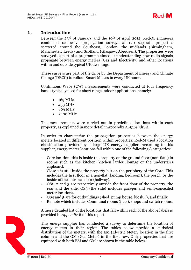
1. Introduction
Between the 23rd of January and the 10th of April 2012, Red-M engineers conducted radiowave propagation surveys at 120 separate properties scattered around the Southeast, London, the midlands (Birmingham, Manchester, Leeds) and Scotland (Glasgow, Aberdeen). The properties were surveyed as part of a programme aimed at understanding how radio signals propagate between energy meters (Gas and Electricity) and other locations within and outside typical UK dwellings. These surveys are part of the drive by the Department of Energy and Climate Change (DECC) to rollout Smart Meters in every UK home. Continuous Wave (CW) measurements were conducted at four frequency bands typically used for short range indoor applications, namely:
169 MHz
433 MHz
869 MHz
2400 MHz The measurements were carried out in predefined locations within each property, as explained in more detail inAppendix A Appendix A. In order to characterise the propagation properties between the energy meters located in different position within properties, Red-M used a location classification provided by a large UK energy supplier. According to this supplier, energy meter locations fall within one of the following 8 categories: - Core location: this is inside the property on the ground floor (non-flats) in
rooms such as the kitchen, kitchen larder, lounge or the understairs cupboard.
- Close 1 is still inside the property but on the periphery of the Core. This includes the first floor in a non-flat (landing, bedroom), the porch, or the inside of the entrance door (hallway).
- OS1, 2 and 3 are respectively outside the front door of the property, the rear and the side. OS3 (the side) includes garages and semi-concealed meter locations.
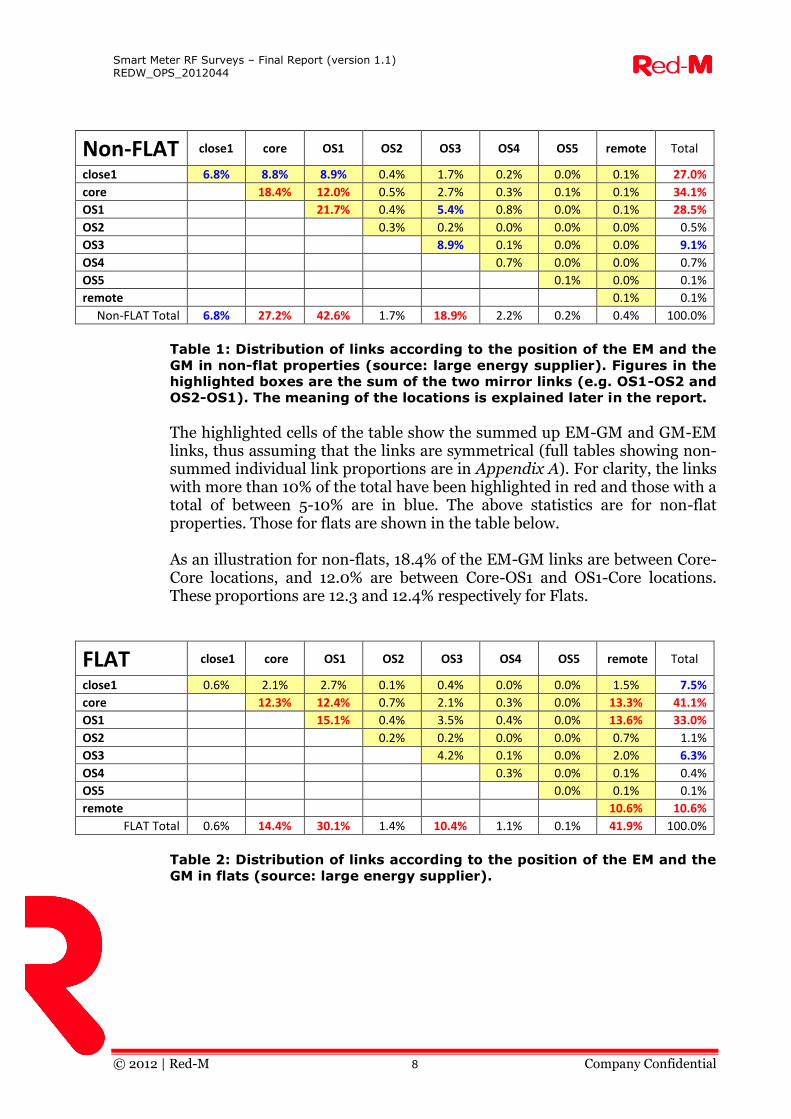
- OS4 and 5 are for outbuildings (shed, pump house, kiosk…), and finally - Remote which includes Communal rooms (flats), shops and switch rooms. A more detailed list of the locations that fall within each of the above labels is provided in Appendix B of this report. This energy supplier has conducted a survey to determine the location of energy meters in their region. The tables below provide a statistical distribution of the meters, with the EM (Electric Meter) location in the first column and the GM (Gas Meter) in the first row. Only properties that are equipped with both EM and GM are shown in the table below.
Smart Meter RF Surveys – Final Report (version 1.1) REDW_OPS_2012044
© 2012 | Red-M 8 Company Confidential
Non-FLAT close1 core OS1 OS2 OS3 OS4 OS5 remote Total
close1 6.8% 8.8% 8.9% 0.4% 1.7% 0.2% 0.0% 0.1% 27.0%
core 1.9% 18.4% 12.0% 0.5% 2.7% 0.3% 0.1% 0.1% 34.1%
OS1 1.1% 2.3% 21.7% 0.4% 5.4% 0.8% 0.0% 0.1% 28.5%
OS2 0.0% 0.1% 0.2% 0.3% 0.2% 0.0% 0.0% 0.0% 0.5%
OS3 0.3% 0.8% 2.9% 0.1% 8.9% 0.1% 0.0% 0.0% 9.1%
OS4 0.0% 0.1% 0.4% 0.0% 0.0% 0.7% 0.0% 0.0% 0.7%
OS5 0.0% 0.0% 0.0% 0.0% 0.0% 0.0% 0.1% 0.0% 0.1%
remote 0.0% 0.1% 0.1% 0.0% 0.0% 0.0% 0.0% 0.1% 0.1%
Non-FLAT Total 6.8% 27.2% 42.6% 1.7% 18.9% 2.2% 0.2% 0.4% 100.0%
Table 1: Distribution of links according to the position of the EM and the
GM in non-flat properties (source: large energy supplier). Figures in the
highlighted boxes are the sum of the two mirror links (e.g. OS1-OS2 and
OS2-OS1). The meaning of the locations is explained later in the report.
The highlighted cells of the table show the summed up EM-GM and GM-EM links, thus assuming that the links are symmetrical (full tables showing non-summed individual link proportions are in Appendix A). For clarity, the links with more than 10% of the total have been highlighted in red and those with a total of between 5-10% are in blue. The above statistics are for non-flat properties. Those for flats are shown in the table below. As an illustration for non-flats, 18.4% of the EM-GM links are between Core-Core locations, and 12.0% are between Core-OS1 and OS1-Core locations. These proportions are 12.3 and 12.4% respectively for Flats.
FLAT close1 core OS1 OS2 OS3 OS4 OS5 remote Total
close1 0.6% 2.1% 2.7% 0.1% 0.4% 0.0% 0.0% 1.5% 7.5%
core 0.4% 12.3% 12.4% 0.7% 2.1% 0.3% 0.0% 13.3% 41.1%
OS1 0.1% 2.9% 15.1% 0.4% 3.5% 0.4% 0.0% 13.6% 33.0%
OS2 0.0% 0.0% 0.1% 0.2% 0.2% 0.0% 0.0% 0.7% 1.1%
OS3 0.0% 0.7% 2.3% 0.1% 4.2% 0.1% 0.0% 2.0% 6.3%
OS4 0.0% 0.1% 0.2% 0.0% 0.0% 0.3% 0.0% 0.1% 0.4%
OS5 0.0% 0.0% 0.0% 0.0% 0.0% 0.0% 0.0% 0.1% 0.1%
remote 0.5% 10.2% 12.4% 0.7% 1.7% 0.1% 0.0% 10.6% 10.6%
FLAT Total 0.6% 14.4% 30.1% 1.4% 10.4% 1.1% 0.1% 41.9% 100.0%
Table 2: Distribution of links according to the position of the EM and the
GM in flats (source: large energy supplier).
Smart Meter RF Surveys – Final Report (version 1.1) REDW_OPS_2012044
© 2012 | Red-M 9 Company Confidential
2. Measurements Profile
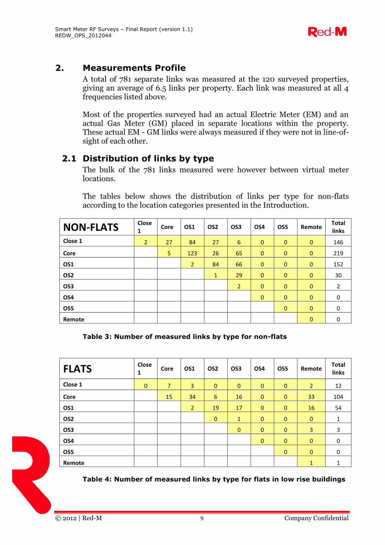
A total of 781 separate links was measured at the 120 surveyed properties, giving an average of 6.5 links per property. Each link was measured at all 4 frequencies listed above. Most of the properties surveyed had an actual Electric Meter (EM) and an actual Gas Meter (GM) placed in separate locations within the property. These actual EM - GM links were always measured if they were not in line-of-sight of each other.
2.1 Distribution of links by type
The bulk of the 781 links measured were however between virtual meter locations. The tables below shows the distribution of links per type for non-flats according to the location categories presented in the Introduction.
NON-FLATS Close 1
Core OS1 OS2 OS3 OS4 OS5 Remote Total links
Close 1 2 27 84 27 6 0 0 0 146
Core 5 123 26 65 0 0 0 219
OS1 2 84 66 0 0 0 152
OS2 1 29 0 0 0 30
OS3 2 0 0 0 2
OS4 0 0 0 0
OS5 0 0 0
Remote 0 0
Table 3: Number of measured links by type for non-flats
FLATS Close 1
Core OS1 OS2 OS3 OS4 OS5 Remote Total links
Close 1 0 7 3 0 0 0 0 2 12
Core 15 34 6 16 0 0 33 104
OS1 2 19 17 0 0 16 54
OS2 0 1 0 0 0 1
OS3 0 0 0 3 3
OS4 0 0 0 0
OS5 0 0 0
Remote 1 1
Table 4: Number of measured links by type for flats in low rise buildings
Smart Meter RF Surveys – Final Report (version 1.1) REDW_OPS_2012044
© 2012 | Red-M 10 Company Confidential
HIGH-RISE Close 1
Core OS1 OS2 OS3 OS4 OS5 Remote Total links
Close 1 0 24 0 0 0 0 0 0 24
Core 5 5 3 3 0 0 10 26
OS1 0 4 3 0 0 0 7
OS2 0 0 0 0 0 0
OS3 0 0 0 0 0
OS4 0 0 0 0
OS5 0 0 0
Remote 0 0
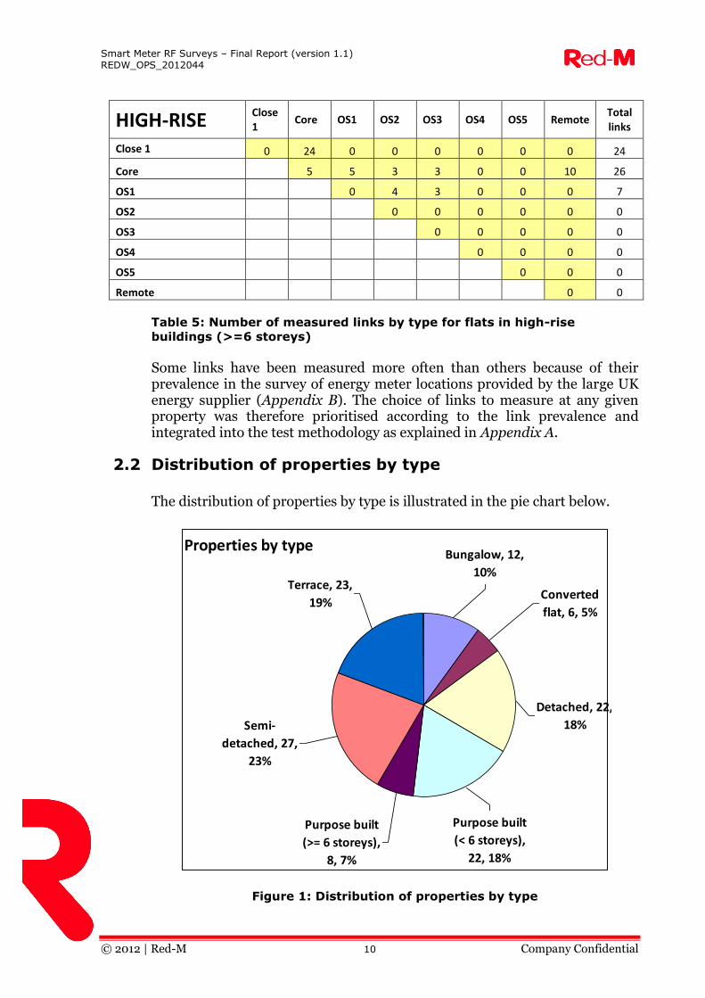
Table 5: Number of measured links by type for flats in high-rise
buildings (>=6 storeys)
Some links have been measured more often than others because of their prevalence in the survey of energy meter locations provided by the large UK energy supplier (Appendix B). The choice of links to measure at any given property was therefore prioritised according to the link prevalence and integrated into the test methodology as explained in Appendix A.
2.2 Distribution of properties by type
The distribution of properties by type is illustrated in the pie chart below.
Properties by type
Terrace, 23,
19%
Semi-
detached, 27,
23%
Detached, 22,
18%
Purpose built
(< 6 storeys),
22, 18%
Purpose built
(>= 6 storeys),
8, 7%
Converted
flat, 6, 5%
Bungalow, 12,
10%
Figure 1: Distribution of properties by type

Smart Meter RF Surveys – Final Report (version 1.1) REDW_OPS_2012044
© 2012 | Red-M 11 Company Confidential
The profile of the distribution of properties types compares well with that of the English Housing Survey (EHS) in the entire UK as shown in the bar chart below, except maybe for the high-rise buildings (Purpose built >= 6 storeys). This property type has been over-represented in the HAN surveys and will therefore be treated separately in most of the analyses that follow.
0%
5%
10%
15%
20%
25%
30%
35%
Bungalow
Convert
ed flat
Detach
ed
Purpose
built
(< 6
store
ys)
Purpose
built
(>= 6
store
ys)
Semi-d
etach
ed
Terrace
HAN survey
EHS
Figure 2- Comparison between the property type profile of the HAN
surveys (120) and that of the EHS for the entire UK housing stock

Smart Meter RF Surveys – Final Report (version 1.1) REDW_OPS_2012044
© 2012 | Red-M 12 Company Confidential
2.3 Distribution of properties by age
Properties by age
Pre 1919, 40,
33%
1945-64, 25,
21%
Post 1990,
20, 17%
1965-80, 16,
13%
1981-90, 4,
3%
1919-44, 15,
13%
Figure 3: Distribution of properties by age
A large proportion of the properties pre-dates 1919 (40 out of 120), followed by Post-1990 (20). The smallest sample of properties was recorded from the period 1981-90 (4/120). Again, comparing the age profiles of the HAN surveyed properties with that of the EHS, the 1981-1990 period is under-represented in the HAN properties whilst the Pre-1919 period is over-represented UK. Otherwise, the two profiles correlate well as shown in the bar chart below.
0%
5%
10%
15%
20%
25%
30%
35%
Pre 1919 1919-44 1945-64 1965-80 1981-90 Post 1990
HAN survey
EHS
Figure 4- Comparison between the age profiles of the HAN surveys and
the EHS
Smart Meter RF Surveys – Final Report (version 1.1) REDW_OPS_2012044
© 2012 | Red-M 13 Company Confidential
3. Delivered data/reports
3.1 Property reports
Individual reports for each of the 120 properties were submitted as part of the project. Typical content of each report consisted of: 1. A description of the property surveyed (type, age, construction…) 2. An outline of the test methodology 3. A floor plan with individual test locations and dimensions marked 4. Results of an interference test at all 4 frequencies to determine the quiet
spots 5. Results of the RF tests in terms of pathloss between the transmitter and
the receiver derived from a measure of the signal level 6. Auxiliary information such as weather and origin of interference sources
(if determined)
3.2 Methodology document
In the build-up to the campaign, Red-M, in association with DECC employees, have defined the methodology for carrying out the tests. The methodology document1 was fine-tuned at the early stages of the tests in order to account for a number of cases that have appeared to require special treatment. Large extracts of this document are reproduced in Appendix A of this report.
3.3 Calibration of the antennas and the feeder cables
Calibration of the antennas used during the tests was performed in an anechoic chamber at the start of the campaign. This was done in order to verify the radiation patterns and the gain of the trial antennas and thus remove any inaccuracies in determining pathloss from the measured signal strengths. Free-space field tests have also been carried out by Red-M at the start and half-way through the campaign at their offices in Horsham with a view to validating the links at all 4 frequencies in a free-space environment. And finally, the RF equipment was validated at the start, halfway through and at the end of the campaign in order to characterise the losses through the
1 DECC/Red-M – Smart Meter RF Survey Methodology, Reference REDW_OPS_2012001-v1.2, Issued 9th Feb 2012

Smart Meter RF Surveys – Final Report (version 1.1) REDW_OPS_2012044
© 2012 | Red-M 14 Company Confidential
feeders/connectors by injecting signals of known level and measuring the loss/offset using the test equipment. Red-M has submitted a separate report2 on the calibration containing the findings from the validation/calibration tests and the resulting offsets applied to the measured field strength measurements to derive the pathloss values for each link.
3.4 Pathloss summary table
A table containing the measured pathloss values for each link/frequency/property was also delivered to DECC. The table contained other auxiliary information as listed in Table 6, and was used to refine the pathloss models derived from the measurements.
Field Description
Property ID Unique property identifier
Property Type Uses the EHS classification
TX ID No Test Location identifier for TX as used on the property report
RX ID No Test Location identifier for RX - as used on the property report
TX LOC Descriptor of the TX test location - see Location types worksheet
RX LOC Descriptor of the TX test location - see Location types worksheet
TX-RX Link name Link name combining the names of both link-ends
TX SSE Code TX location descriptor using the Code (Core, Close1, OS1/2/3/4/5, Remote)
RX LOC RX location descriptor using the Code (Core, Close1, OS1/2/3/4/5, Remote)
TX-RX Link name Link name combining the Code Names of both link-ends
yDiff Intermediate step cell - ignore
xDiff Intermediate step cell - ignore
Horizontal Distance Horizontal distance between TX and RX (assuming they are on the same plane
TX height Height of TX relative to ground reference
RX height Height of RX relative to ground reference
Vertical Distance Vertical separation between TX and RX
3D distance Distance estimated from the Horizontal and the Vertical distances above
log_dist Log10 of the above
No Ext Walls Nb of external walls between TX and RX
No Solid Int walls Nb of internal solid walls between TX and RX
No Partition Int walls Nb of partition walls between TX and RX
Nb of Doors Nb of doors (incl external doors) between TX and RX
No of Windows Nb of windows (incl glass patio doors) between TX and RX
No of Floors Diff Nb of floors between TX and RX
169MHz [50%] 50% pathloss at 169MHz
433MHz [50%] 50% pathloss at 433MHz
869MHz [50%] 50% pathloss at 869MHz
2.4GHz [50%] 50% pathloss at 2.4GHz
169MHz [90%] 950% pathloss at 169MHz
433MHz [90%] 90% pathloss at 433MHz
869MHz [90%] 90% pathloss at 869MHz
2.4GHz [90%] 90% pathloss at 2.4GHz
Table 6: list of key parameters included in the pathloss summary table
2 Smart Meter RF Surveys - RF System Calibration Report, Doc No.: REDW_OPS_2012023, 16/03/2012 by Bachir Belloul
Smart Meter RF Surveys – Final Report (version 1.1) REDW_OPS_2012044
© 2012 | Red-M 15 Company Confidential
4. Pathloss Model
The initial step in the analysis consisted of deriving a propagation pathloss model based on the collected data. There are many such models in the open literature and we have reviewed below a couple that we believe are relevant to this study.
4.1 Existing indoor models
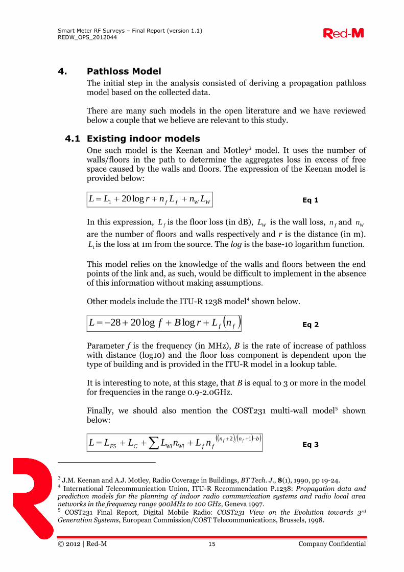
One such model is the Keenan and Motley3 model. It uses the number of walls/floors in the path to determine the aggregates loss in excess of free space caused by the walls and floors. The expression of the Keenan model is provided below:
WWff LnLnrLL log201 Eq 1
In this expression, fL is the floor loss (in dB), WL is the wall loss, fn and Wn
are the number of floors and walls respectively and r is the distance (in m).
1L is the loss at 1m from the source. The log is the base-10 logarithm function.
This model relies on the knowledge of the walls and floors between the end points of the link and, as such, would be difficult to implement in the absence of this information without making assumptions. Other models include the ITU-R 1238 model4 shown below.
ff nLrBfL loglog2028 Eq 2
Parameter f is the frequency (in MHz), B is the rate of increase of pathloss with distance (log10) and the floor loss component is dependent upon the type of building and is provided in the ITU-R model in a lookup table. It is interesting to note, at this stage, that B is equal to 3 or more in the model for frequencies in the range 0.9-2.0GHz. Finally, we should also mention the COST231 multi-wall model5 shown below:
bnn
ffWiWiCFSffnLnLLLL
12 Eq 3
3 J.M. Keenan and A.J. Motley, Radio Coverage in Buildings, BT Tech. J., 8(1), 1990, pp 19-24. 4 International Telecommunication Union, ITU-R Recommendation P.1238: Propagation data and prediction models for the planning of indoor radio communication systems and radio local area networks in the frequency range 900MHz to 100 GHz, Geneva 1997. 5 COST231 Final Report, Digital Mobile Radio: COST231 View on the Evolution towards 3rd Generation Systems, European Commission/COST Telecommunications, Brussels, 1998.
Smart Meter RF Surveys – Final Report (version 1.1) REDW_OPS_2012044
© 2012 | Red-M 16 Company Confidential
In this expression, FSL represents free-space loss. cL and b are adjustable
parameters that can be derived from the measurements. The wall loss component of the equation is a summation over all wall types in the direct path. Note also that in this model, the individual contributions from floors in a multi-floor building diminishes with the number of floors as the radio waves find ways of propagating around obstacles (staircase, lift shaft, windows…).
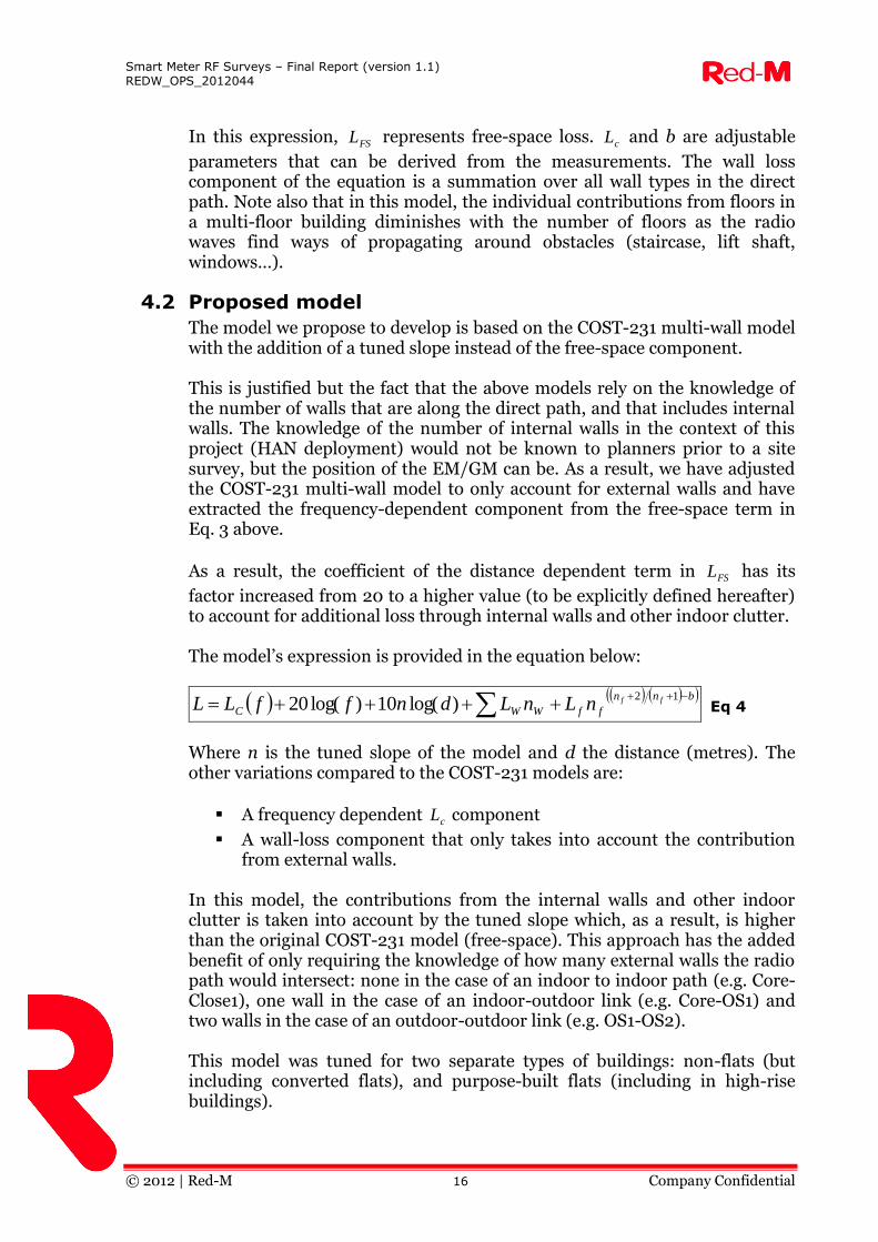
4.2 Proposed model
The model we propose to develop is based on the COST-231 multi-wall model with the addition of a tuned slope instead of the free-space component. This is justified but the fact that the above models rely on the knowledge of the number of walls that are along the direct path, and that includes internal walls. The knowledge of the number of internal walls in the context of this project (HAN deployment) would not be known to planners prior to a site survey, but the position of the EM/GM can be. As a result, we have adjusted the COST-231 multi-wall model to only account for external walls and have extracted the frequency-dependent component from the free-space term in Eq. 3 above.
As a result, the coefficient of the distance dependent term in FSL has its
factor increased from 20 to a higher value (to be explicitly defined hereafter) to account for additional loss through internal walls and other indoor clutter. The model’s expression is provided in the equation below:
bnn
ffWWCffnLnLdnffLL
12)log(10)log(20 Eq 4
Where n is the tuned slope of the model and d the distance (metres). The other variations compared to the COST-231 models are:
A frequency dependent cL component
A wall-loss component that only takes into account the contribution from external walls.
In this model, the contributions from the internal walls and other indoor clutter is taken into account by the tuned slope which, as a result, is higher than the original COST-231 model (free-space). This approach has the added benefit of only requiring the knowledge of how many external walls the radio path would intersect: none in the case of an indoor to indoor path (e.g. Core-Close1), one wall in the case of an indoor-outdoor link (e.g. Core-OS1) and two walls in the case of an outdoor-outdoor link (e.g. OS1-OS2). This model was tuned for two separate types of buildings: non-flats (but including converted flats), and purpose-built flats (including in high-rise buildings).

Smart Meter RF Surveys – Final Report (version 1.1) REDW_OPS_2012044
© 2012 | Red-M 17 Company Confidential
The key difference between the two categories, in addition to the number of floors, is that the non-flats category dwellings tend to have wooden floors and largely partition walls. In the case of the latter, the floors would most certainly be of concrete, with the walls also likely to be of a solid material such as bricks or concrete. The following tables provide the parameters obtained by tuning the model to the collected data. The first table shows the parameters that are common to both non-flats and flats (high-rise).
Parameter Value Units
B 0.46 -
Lw 3.65 dB
Lf 5.5 dB
Table 7: Value of parameters that are common to both the non-flats and
the high-rise (purpose-built flats) models
The next table shows the values of the model parameters specific to the non-flat model.
Parameter 169MHz 433MHz 869MHz 2400MHz
n 3.8 3.8 3.8 3.8
Lc -21.4 -21.3 -26.7 -19.4
Table 8: Model parameters for non-flats
And finally, the table below shows the parameters for the purpose-built flats (high-rise).
Parameter 169MHz 433MHz 869MHz 2400MHz
n 3.5 3.5 3.5 3.5
Lc -21.4 -21.9 -24.9 -17.4
Table 9: Model parameters for purpose-built flats
The standard deviation of the model error at each frequency/building category is provided in the table below. Note that the mean of the prediction error was tuned to be zero.

Smart Meter RF Surveys – Final Report (version 1.1) REDW_OPS_2012044
© 2012 | Red-M 18 Company Confidential
Standard deviation of model error, dB
169MHz 433MHz 869MHz 2400MHz
Purpose-built flats 11.5 10.3 10.8 11.3
Non-flats 9.2 8.5 8.7 9.1
Table 10: Standard deviation of the proposed models’ prediction error
These models are aggregated across all the measured links and regardless of whether the direct TX/RX paths crossed internal walls (solid/partition), doors or windows. It is interesting to note the non-flat model’s ability to better track the measured data than the purpose-built model (lower standard deviation). This is clearly due to lower variability in the field strength in smaller dwellings possibly due to the higher likelihood of an available direct path through “RF-transparent” walls. The probability density function (PDF) shown below is for the 2.4GHz non-flat model. It shows the distribution of the prediction error (Predicted – Measured pathloss) for this model.
Figure 5: Probability density function of the prediction error for the
2.4GHz non-flat model. The red curve is a theoretical PDF obtained using
the same standard deviation as the model
Smart Meter RF Surveys – Final Report (version 1.1) REDW_OPS_2012044
© 2012 | Red-M 19 Company Confidential
The PDF of the error compares well with that of a normal distribution (in red), suggesting the measured values are normally distributed around the model. The PDF for the other models/frequencies bands are provided in Appendix C.
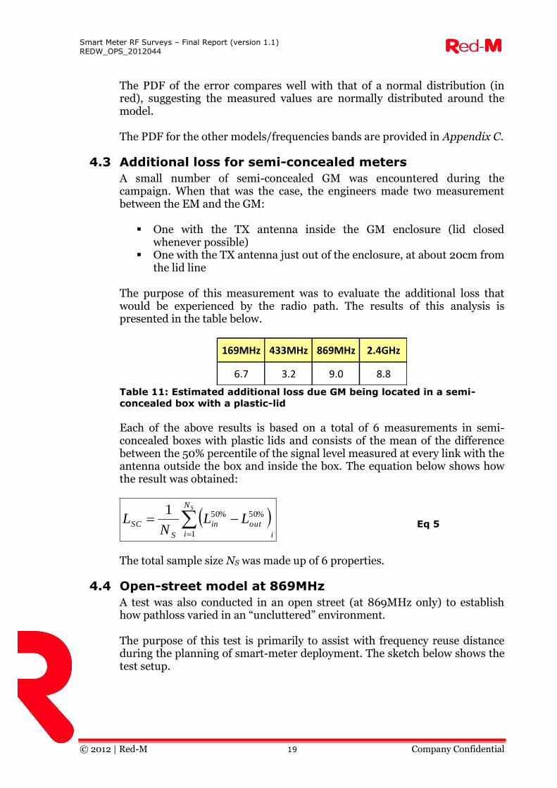
4.3 Additional loss for semi-concealed meters
A small number of semi-concealed GM was encountered during the campaign. When that was the case, the engineers made two measurement between the EM and the GM:
One with the TX antenna inside the GM enclosure (lid closed whenever possible)
One with the TX antenna just out of the enclosure, at about 20cm from the lid line
The purpose of this measurement was to evaluate the additional loss that would be experienced by the radio path. The results of this analysis is presented in the table below.
169MHz 433MHz 869MHz 2.4GHz
6.7 3.2 9.0 8.8
Table 11: Estimated additional loss due GM being located in a semi-
concealed box with a plastic-lid
Each of the above results is based on a total of 6 measurements in semi-concealed boxes with plastic lids and consists of the mean of the difference between the 50% percentile of the signal level measured at every link with the antenna outside the box and inside the box. The equation below shows how the result was obtained:
i
N
i
outin
S
SC
S
LLN
L
1
%50%501 Eq 5
The total sample size NS was made up of 6 properties.
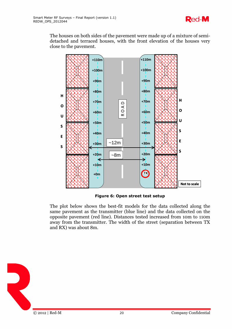
4.4 Open-street model at 869MHz
A test was also conducted in an open street (at 869MHz only) to establish how pathloss varied in an “uncluttered” environment. The purpose of this test is primarily to assist with frequency reuse distance during the planning of smart-meter deployment. The sketch below shows the test setup.
Smart Meter RF Surveys – Final Report (version 1.1) REDW_OPS_2012044
© 2012 | Red-M 20 Company Confidential
The houses on both sides of the pavement were made up of a mixture of semi-detached and terraced houses, with the front elevation of the houses very close to the pavement.
+10m
+20m
+30m
+40m
+50m
+60m
+70m
+80m
+90m
+100m
+110m
+10m
+20m
+30m
+40m
+50m
+60m
+70m
+80m
+90m
+100m
+110m
+0m TX
R O
A D
H
O
U
S
E
S
H
O
U
S
E
S~8m
~12m
Not to scale
+10m
+20m
+30m
+40m
+50m
+60m
+70m
+80m
+90m
+100m
+110m
+10m
+20m
+30m
+40m
+50m
+60m
+70m
+80m
+90m
+100m
+110m
+0m TX
R O
A D
H
O
U
S
E
S
H
O
U
S
E
S~8m
~12m
Not to scale
Figure 6: Open street test setup
The plot below shows the best-fit models for the data collected along the same pavement as the transmitter (blue line) and the data collected on the opposite pavement (red line). Distances tested increased from 10m to 110m away from the transmitter. The width of the street (separation between TX and RX) was about 8m.

Smart Meter RF Surveys – Final Report (version 1.1) REDW_OPS_2012044
© 2012 | Red-M 21 Company Confidential
Open-street pathloss - 869MHz
y = 0.27x + 54.96
y = 0.29x + 59.46
0
20
40
60
80
100
120
0 20 40 60 80 100 120
TX-RX distance, m
Path
loss, d
B
Opposite pavement
Same pavement
The results show a decrease of between 2.7 and 2.9dB per 10m and a model intercept (when d=0) of ~55dB for the opposite pavement and ~59.5dB for the opposite pavement. The lower pathloss on the opposite pavement can be explained by the availability of clearer paths between the TX and RX even though it is more likely to be blocked (by cars for example). The same pavement propagation path on the other hand is more likely to have a larger proportion of its Fresnel zone infringed, thus leading to less power being carried forward by the radio waves. For planning purposes, we would therefore recommend to use the most favourable of the two models (i.e. the opposite pavement) as it would restrict the frequency reuse to larger repeat-channel distances.
Smart Meter RF Surveys – Final Report (version 1.1) REDW_OPS_2012044
© 2012 | Red-M 22 Company Confidential
5. Availability of service for the UK housing stock
In this section, we make some suggestions as to how the measurements could be used to estimate how many GB properties would be served at the four tested frequencies. This section is speculative and is based on a number of assumptions that will be clearly laid out as the discussion progresses. This analysis considers the results of the campaign in terms of how pathloss increases with distance and per link type, and combines the resulting models with the distribution of link types in the UK housing stock (information provided by the energy suppliers to DECC) and the performance of the equipment considered for deployment at each of the tested frequencies.
5.1 Maximum Pathloss Requirements
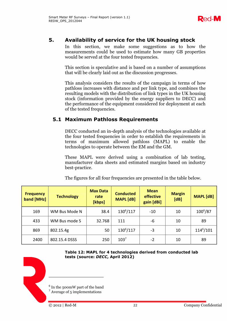
DECC conducted an in-depth analysis of the technologies available at the four tested frequencies in order to establish the requirements in terms of maximum allowed pathloss (MAPL) to enable the technologies to operate between the EM and the GM. These MAPL were derived using a combination of lab testing, manufacturer data sheets and estimated margins based on industry best-practice. The figures for all four frequencies are presented in the table below.
Frequency band [MHz]
Technology Max Data
rate [kbps]
Conducted MAPL [dB]
Mean effective gain [dBi]
Margin [dB]
MAPL [dB]
169 WM Bus Mode N 38.4 1306/117 -10 10 1006/87
433 WM Bus mode S 32.768 111 -6 10 89
869 802.15.4g 50 1306/117 -3 10 1146/101
2400 802.15.4 DSSS 250 1037 -2 10 89
Table 12: MAPL for 4 technologies derived from conducted lab
tests (source: DECC, April 2012)
6 In the 500mW part of the band 7 Average of 5 implementations
Smart Meter RF Surveys – Final Report (version 1.1) REDW_OPS_2012044
© 2012 | Red-M 23 Company Confidential
The mean effective gains values above are an average of the gain of the antenna over the 360º horizontal plane around the antenna axis. The above values of MEG are typical of small-sized antennas generally found in 0ff-the-shelf products for the mentioned bands. They assume slightly less efficient radiating elements than those of the antennas used in the trials and measured during the anechoic and open field tests conducted by Red-M/DECC as part of the validation procedure of the test system (by 1-2dB in the worst-case).
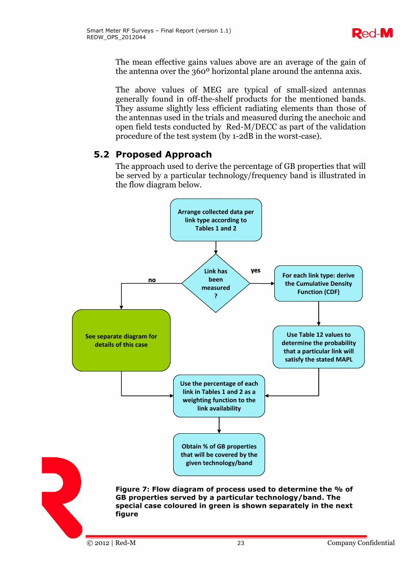
5.2 Proposed Approach
The approach used to derive the percentage of GB properties that will be served by a particular technology/frequency band is illustrated in the flow diagram below.
For each link type: derive the Cumulative Density
Function (CDF)
Arrange collected data per link type according to
Tables 1 and 2
Use Table 12 values to determine the probability that a particular link will satisfy the stated MAPL
Link has been
measured ?
Use the percentage of each link in Tables 1 and 2 as a weighting function to the
link availability
Obtain % of GB properties that will be covered by the
given technology/band
See separate diagram for details of this case
yes
noFor each link type: derive the Cumulative Density
Function (CDF)
Arrange collected data per link type according to
Tables 1 and 2
Use Table 12 values to determine the probability that a particular link will satisfy the stated MAPL
Link has been
measured ?
Use the percentage of each link in Tables 1 and 2 as a weighting function to the
link availability
Obtain % of GB properties that will be covered by the
given technology/band
See separate diagram for details of this case
yes
no
Figure 7: Flow diagram of process used to determine the % of
GB properties served by a particular technology/band. The
special case coloured in green is shown separately in the next
figure
Smart Meter RF Surveys – Final Report (version 1.1) REDW_OPS_2012044
© 2012 | Red-M 24 Company Confidential
Link has been
measured ?
Use the percentage of each link in Tables 1 and 2 as a weighting function to the
link availability
Aggregate all links per end-of-link type (e.g. all links that start or end in OS1)
andGenerate one CDF per end-
of-link type
no
Is there an “aggregated” CDF for the
link
Produce a CDF will all the data aggregated into one set
From the CDF, determine the probability that the
link will satisfy the MAPL
no
yes
Is the link listed on the left ?
Core-CoreClose1-Close1OS1-OS1OS2-OS2OS3-OS3
Assume 100% of the link is served
no
Determine the probability that the link will satisfy the MAPL
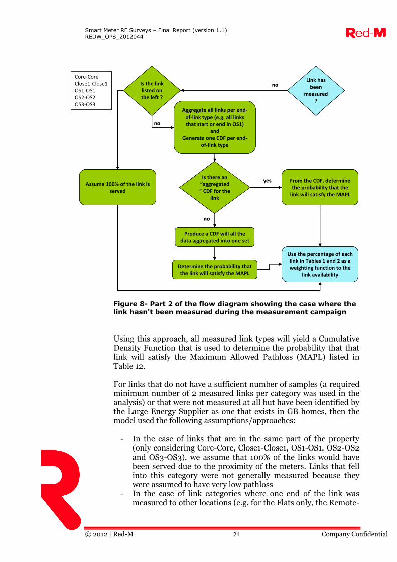
Figure 8- Part 2 of the flow diagram showing the case where the
link hasn't been measured during the measurement campaign
Using this approach, all measured link types will yield a Cumulative Density Function that is used to determine the probability that that link will satisfy the Maximum Allowed Pathloss (MAPL) listed in Table 12. For links that do not have a sufficient number of samples (a required minimum number of 2 measured links per category was used in the analysis) or that were not measured at all but have been identified by the Large Energy Supplier as one that exists in GB homes, then the model used the following assumptions/approaches:
- In the case of links that are in the same part of the property (only considering Core-Core, Close1-Close1, OS1-OS1, OS2-OS2 and OS3-OS3), we assume that 100% of the links would have been served due to the proximity of the meters. Links that fell into this category were not generally measured because they were assumed to have very low pathloss
- In the case of link categories where one end of the link was measured to other locations (e.g. for the Flats only, the Remote-
Smart Meter RF Surveys – Final Report (version 1.1) REDW_OPS_2012044
© 2012 | Red-M 25 Company Confidential
Remote link was only measured once, but Remote was measured to 54 other locations such as Core, Close1, OS1 and OS3), Red-M produced an aggregated CDF of all the data that have that link end measured at.
- For the other link categories (e.g. all links that have OS4 or OS5 at one end), Red-M produced an aggregated CDF that used all of the data collected during the campaign. It should be stressed that the total number of these latter links represents only a very small percentage of the total links identified by the Large Energy Supplier.
The figure overleaf illustrates for example the family of CDF curves obtained from the data for the 2.4GHz band for non-flats.

Smart Meter RF Surveys – Final Report (version 1.1) REDW_OPS_2012044
© 2012 | Red-M 26 Company Confidential
Figure 9: Typical set of CDF curves derived from the data. The curves
use the 50% pathloss measured at each location and are aggregated
based on the end-points shown in the key. This example is for the
2.4GHz non-flats data set.
Smart Meter RF Surveys – Final Report (version 1.1) REDW_OPS_2012044
© 2012 | Red-M 27 Company Confidential
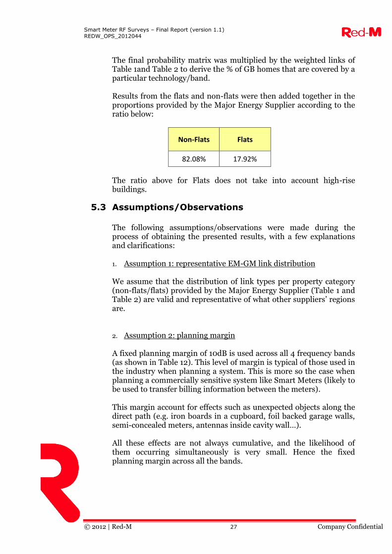
The final probability matrix was multiplied by the weighted links of Table 1and Table 2 to derive the % of GB homes that are covered by a particular technology/band. Results from the flats and non-flats were then added together in the proportions provided by the Major Energy Supplier according to the ratio below:
Non-Flats Flats
82.08% 17.92%
The ratio above for Flats does not take into account high-rise buildings.
5.3 Assumptions/Observations
The following assumptions/observations were made during the process of obtaining the presented results, with a few explanations and clarifications: 1. Assumption 1: representative EM-GM link distribution We assume that the distribution of link types per property category (non-flats/flats) provided by the Major Energy Supplier (Table 1 and Table 2) are valid and representative of what other suppliers’ regions are. 2. Assumption 2: planning margin A fixed planning margin of 10dB is used across all 4 frequency bands (as shown in Table 12). This level of margin is typical of those used in the industry when planning a system. This is more so the case when planning a commercially sensitive system like Smart Meters (likely to be used to transfer billing information between the meters). This margin account for effects such as unexpected objects along the direct path (e.g. iron boards in a cupboard, foil backed garage walls, semi-concealed meters, antennas inside cavity wall…). All these effects are not always cumulative, and the likelihood of them occurring simultaneously is very small. Hence the fixed planning margin across all the bands.
Smart Meter RF Surveys – Final Report (version 1.1) REDW_OPS_2012044
© 2012 | Red-M 28 Company Confidential
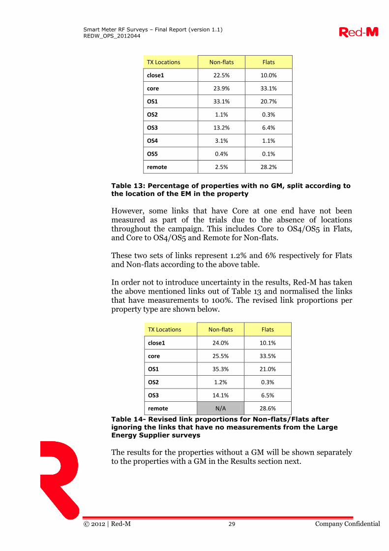
3. Assumption 3: fast-fading margin In addition to the planning margin, the analysis also considers a fast-fading margin that is not included in the 10dB planning margin. The fast-fading margin is due to multipath propagation between the EM-GM which, when combined in a destructive way, can lead to deep fades in the signal. These deep fades were observed throughout the measurement campaign, hence the method used which consisted of placing the RX antenna on a rotating arm of 50cm radius and of moving the antenna around the rotation point during the 30sec measurement period at each location/frequency. A detailed discussion about the fast-fading margin is provided in Appendix D. Theoretical estimates of the fast-fading margin show that the standard deviation is between 3-6dB. This was of the same order of magnitude than the average difference between the 90th percentile and the 50th percentile of the pathloss that was derived from the full set of measurement. For the analysis results shown further below, Red-M used a range of fast-fading margins (in the range 0-3-6-9dB) to illustrate the sensitivity of the final results on this parameter. 4. Observation 1: what about properties without a GM Properties without a Gas Meter have been accounted for in the process by assuming that one end of the link will be the Electric Meter and the other end would be an IHD. For the properties which had an EM but no GM, the Large Energy Supplier split the EM locations into the 8 categories identified earlier and the results of their survey is shown in Table 13. In this case, Red-M assumed that the IHD was always located in the Core of the property and consequently derived the CDF using all data which had Core at one end of the link.
Smart Meter RF Surveys – Final Report (version 1.1) REDW_OPS_2012044
© 2012 | Red-M 29 Company Confidential
TX Locations Non-flats Flats
close1 22.5% 10.0%
core 23.9% 33.1%
OS1 33.1% 20.7%
OS2 1.1% 0.3%
OS3 13.2% 6.4%
OS4 3.1% 1.1%
OS5 0.4% 0.1%
remote 2.5% 28.2%
Table 13: Percentage of properties with no GM, split according to
the location of the EM in the property
However, some links that have Core at one end have not been measured as part of the trials due to the absence of locations throughout the campaign. This includes Core to OS4/OS5 in Flats, and Core to OS4/OS5 and Remote for Non-flats. These two sets of links represent 1.2% and 6% respectively for Flats and Non-flats according to the above table. In order not to introduce uncertainty in the results, Red-M has taken the above mentioned links out of Table 13 and normalised the links that have measurements to 100%. The revised link proportions per property type are shown below.
TX Locations Non-flats Flats
close1 24.0% 10.1%
core 25.5% 33.5%
OS1 35.3% 21.0%
OS2 1.2% 0.3%
OS3 14.1% 6.5%
remote N/A 28.6%
Table 14- Revised link proportions for Non-flats/Flats after
ignoring the links that have no measurements from the Large
Energy Supplier surveys
The results for the properties without a GM will be shown separately to the properties with a GM in the Results section next.

Smart Meter RF Surveys – Final Report (version 1.1) REDW_OPS_2012044
© 2012 | Red-M 30 Company Confidential
5. Observation 2: how does the property type profile compare with the English Housing Survey
Red-M compared the housing profile (per property type) in the UK produced by the EHS with the profile of properties tested during this campaign and found that, although not perfectly aligned, the two were sufficiently similar to assume that there is no bias towards a particular type of properties in the data collected. The data collected also includes measurements from a range of property sizes (from small studio flats to large mansion houses and flats in converted properties and in purpose-built buildings). Red-M however collected a large number of samples in high-rise buildings (6+ levels). Since high-rise buildings have a lower overall percentage in the EHS, Red-M simply ignored the data from this category of properties (8 out of 120). The other argument for leaving this category out is that, given the high density of meters likely to co-exist in high-rise buildings, it is Red-M’s view that this category should be treated separately from the rest of the properties as high-rise buildings might require a specific solution. 6. Observation 3: use of the 50th percentile pathloss in the model Throughout this analysis, Red-M used the 50th percentile of the pathloss value (or Median) derived from the 30s test duration (whilst the antenna was being moved around its rotation point). The Median is a probabilistic measure, giving the 50% probability of the pathloss at the test location. In opposition, the local mean pathloss (generally used in radio planning) is an average value across all the measurements (in Watts). In the latter case, if a deep fade was measured, the probability of the antenna being in the deep fade is very small, but its effect on the average value would be overestimated. As a result, and when comparison to the Local Mean Pathloss was required, Red-M used a conversion offset to turn Median to Mean using the following values derived from a sample of 70 links from the total data set.
169MHz 433MHz 869MHz 2.4GHz
MEAN [dB] 0.5 0.9 0.8 0.8
STDEV [dB] 1.2 1.1 1.0 0.8 Table 15- Mean and standard deviation of the difference between
the Local Mean and the Median values (Mean – Median) of the
received signal strength using 70 independent links
Smart Meter RF Surveys – Final Report (version 1.1) REDW_OPS_2012044
© 2012 | Red-M 31 Company Confidential
Note that the Mean were obtained by averaging the signal strength in Watts. These values compare well with the theoretical conversion in the case of a pure Rayleigh distribution which gives a 1.6dB value. IN the case of the HAN surveys, the distribution of the fades is not a pure Rayleigh.
Smart Meter RF Surveys – Final Report (version 1.1) REDW_OPS_2012044
© 2012 | Red-M 32 Company Confidential
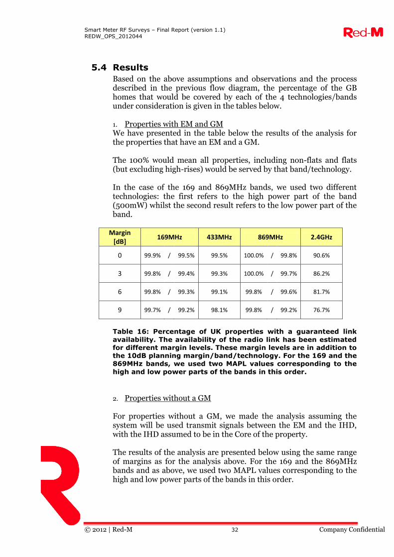
5.4 Results
Based on the above assumptions and observations and the process described in the previous flow diagram, the percentage of the GB homes that would be covered by each of the 4 technologies/bands under consideration is given in the tables below. 1. Properties with EM and GM We have presented in the table below the results of the analysis for the properties that have an EM and a GM. The 100% would mean all properties, including non-flats and flats (but excluding high-rises) would be served by that band/technology. In the case of the 169 and 869MHz bands, we used two different technologies: the first refers to the high power part of the band (500mW) whilst the second result refers to the low power part of the band.
Margin [dB]
169MHz 433MHz 869MHz 2.4GHz
0 99.9% / 99.5% 99.5% 100.0% / 99.8% 90.6%
3 99.8% / 99.4% 99.3% 100.0% / 99.7% 86.2%
6 99.8% / 99.3% 99.1% 99.8% / 99.6% 81.7%
9 99.7% / 99.2% 98.1% 99.8% / 99.2% 76.7%
Table 16: Percentage of UK properties with a guaranteed link
availability. The availability of the radio link has been estimated
for different margin levels. These margin levels are in addition to
the 10dB planning margin/band/technology. For the 169 and the
869MHz bands, we used two MAPL values corresponding to the
high and low power parts of the bands in this order.
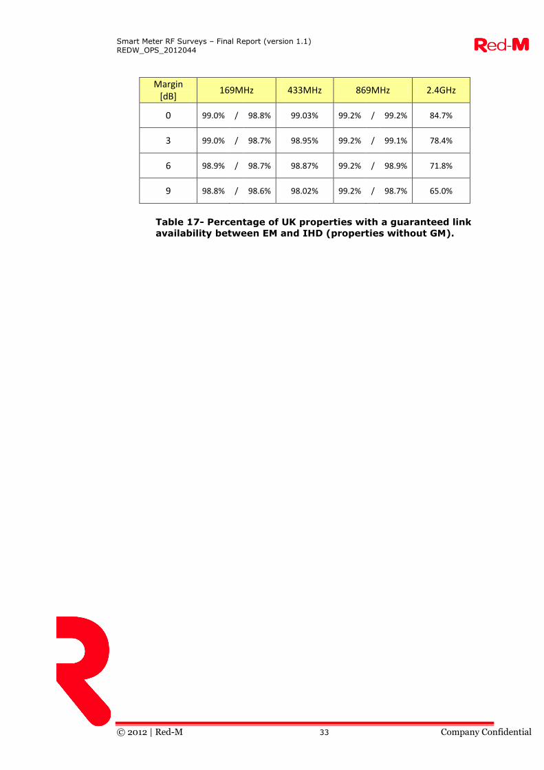
2. Properties without a GM For properties without a GM, we made the analysis assuming the system will be used transmit signals between the EM and the IHD, with the IHD assumed to be in the Core of the property. The results of the analysis are presented below using the same range of margins as for the analysis above. For the 169 and the 869MHz bands and as above, we used two MAPL values corresponding to the high and low power parts of the bands in this order.
Smart Meter RF Surveys – Final Report (version 1.1) REDW_OPS_2012044
© 2012 | Red-M 33 Company Confidential
Margin [dB]
169MHz 433MHz 869MHz 2.4GHz
0 99.0% / 98.8% 99.03% 99.2% / 99.2% 84.7%
3 99.0% / 98.7% 98.95% 99.2% / 99.1% 78.4%
6 98.9% / 98.7% 98.87% 99.2% / 98.9% 71.8%
9 98.8% / 98.6% 98.02% 99.2% / 98.7% 65.0%
Table 17- Percentage of UK properties with a guaranteed link
availability between EM and IHD (properties without GM).
Smart Meter RF Surveys – Final Report (version 1.1) REDW_OPS_2012044
© 2012 | Red-M 34 Company Confidential
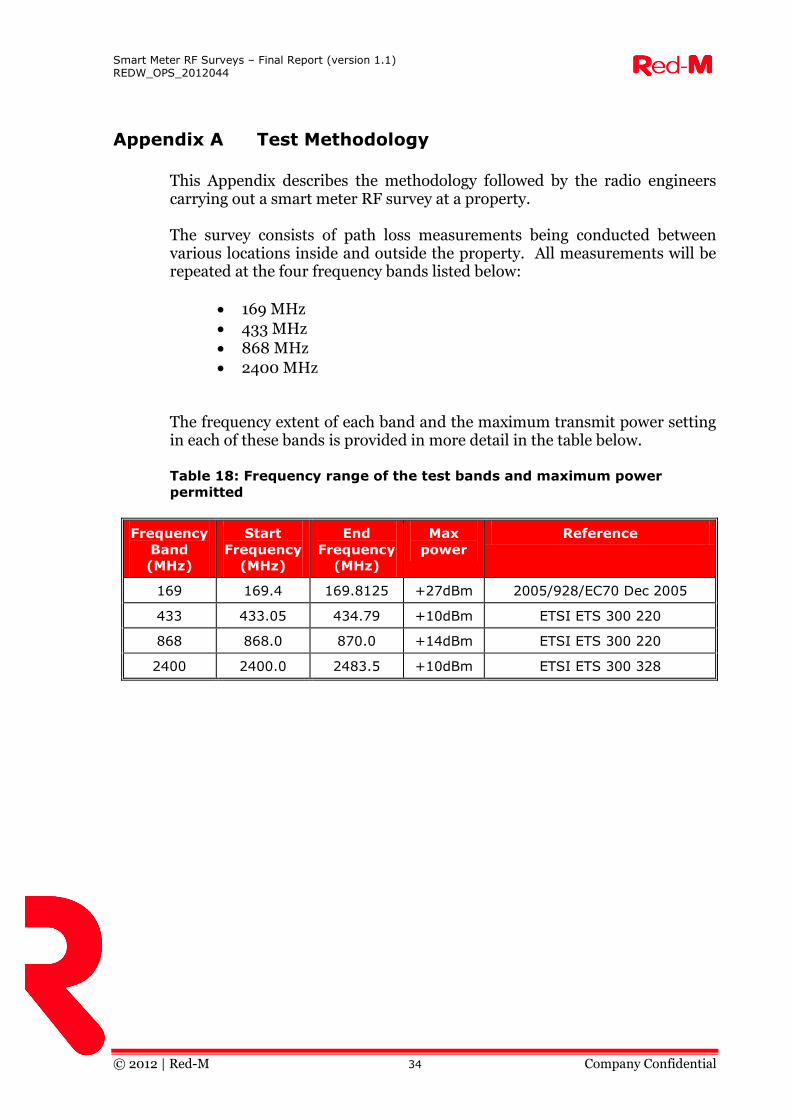
Appendix A Test Methodology
This Appendix describes the methodology followed by the radio engineers carrying out a smart meter RF survey at a property. The survey consists of path loss measurements being conducted between various locations inside and outside the property. All measurements will be repeated at the four frequency bands listed below:
169 MHz
433 MHz
868 MHz
2400 MHz The frequency extent of each band and the maximum transmit power setting in each of these bands is provided in more detail in the table below. Table 18: Frequency range of the test bands and maximum power
permitted
Frequency
Band
(MHz)
Start
Frequency
(MHz)
End
Frequency
(MHz)
Max
power
Reference
169 169.4 169.8125 +27dBm 2005/928/EC70 Dec 2005
433 433.05 434.79 +10dBm ETSI ETS 300 220
868 868.0 870.0 +14dBm ETSI ETS 300 220
2400 2400.0 2483.5 +10dBm ETSI ETS 300 328

Smart Meter RF Surveys – Final Report (version 1.1) REDW_OPS_2012044
© 2012 | Red-M 35 Company Confidential
A.1 Testing Procedure
The following sections provides details of the methodology for carrying out path loss measurements at a property. Figure 10 shows the order in which the processes was carried out while on site. The survey was carried out by 2 engineers and took about 2.5 to 3 hours to complete.
Introduction, describe work, and look over building, identify test locations
Carry out Interference Measurements Draw floor plan and measure distances
Check interference and decide exact test frequencies
Make Pathloss Measurements
Pack up Equipment, Get Photos Approved by Property Owner, Leave site
10-15min
~20min
5-10min
~1hr20min
10-15min
Figure 10: Process to follow on site
The rest of this section provides details and the methodology on how to carry out each of the processes as shown above.

Smart Meter RF Surveys – Final Report (version 1.1) REDW_OPS_2012044
© 2012 | Red-M 36 Company Confidential
A.1.1 Arrival on site
On arrival at the site, the engineers would introduce themselves to the property occupier and give a brief overview of what they intend to do and where about they intend to work. A list of the points the occupier is told about is shown below.
Informing the householder: My name is … and I am an employee of Red-M, Here is my ID card
We are working on behalf of the Department of Energy and Climate Change, doing house survey to characterise radiowave propagation in homes as part of the Smart Metering project. These are non-intrusive tests and do not require making any alterations to the property
We will be here for about 2.5 -3 hours and will be respectful of your home and belongings.
Are you aware of any sources of radio interference such as Wifi routers, baby alarms, clip on smart meters and their locations in the property?
We would like a short tour of the property to get an idea about the layout and also where we will be potentially setting up our equipment.
I will be producing a plan sketch of the ground floor and would like to use a distance measuring device to obtain measurements of rooms. At this stage, the engineer can also ask if the householder has a sketch of the building in-hand that he could use for the purpose of the survey.
I would like to identify a number of locations inside and outside where RF equipment will be setup to conduct the measurements. This will be the bulk of the survey time.
We would like to use some electric power to run our equipment. Do you mind if we plug an extension lead to one of your power outlets.
We would like to take a few pictures inside and outside the house to show the general characteristics of the property and the locations of the tests. We will show you all the photos on the camera for your approval before we leave the property. They will only be used for the project.
We would like to place equipment just inside the cupboard in the central hall area; I hope this is ok with you.
We will ask you to stand out of certain rooms whilst measurements are taking place so as not to interfere with the test.
We will ask you to keep the doors closed whilst the measurements are taking place
We would also like to know what types of walls are in the area we are surveying. We might give your walls a few knocks to try to identify what they are or use a device.
If requested by the occupier, Red M engineers will take their shoes off when entering the property.
Before leaving the property, the lead engineer will ask the household if everything is fine.
Was it what you expected the survey team to do in the property
Did they think the survey team overstayed
Smart Meter RF Surveys – Final Report (version 1.1) REDW_OPS_2012044
© 2012 | Red-M 37 Company Confidential
Have the engineers left the property in the same state as it was before they came in
What else we could have done better so that we can consider it for next visits…
A.1.2 Walk around the property
The engineers will ask the property owner to give them a tour of the property so the floor layout can be understood. During this tour, the property owner can identify any hazards or risks they may be aware of and also inform of any issues that may affect the survey work. The engineers will be looking to identify the test locations for the path loss measurements and sources of radio interference. The locations will be pointed out to the property owner and they can give approval of these places or highlight any problems they have with putting equipment in or by the locations. The engineers will also ask the owner for permission to “knock” on the walls using their hand in order to identify the type of wall (solid or partition) in the floor area where the measurements are taking place. These wall types will then be indicated on the sketch of the floor that will be produced on site by the engineer. The types of internal walls need to be selected from the following list: 1. Solid brick – single skin 2. Partition: lath and plaster 3. Partition: Plasterboard stud 4. Partition: dry lining
For external walls we need to record whether they are cavity walls or not and their construction needs to be selected from the following list
1. Masonry 2. Concrete 3. Timber 4. Metal 5. Other (please specify) (e.g. Granite)
The in the case of flats, the engineers will record which floor of the block the flat is on.
A.1.3 Identifying Test Location
The test locations will be identified from a list of priority links (TX to RX) provided by the DECC and will depend on the availability of the locations in the property as the engineers run down the priority list. A maximum of 7 links will be measured, or 6 if there is no GM in the property or the actual EM-GM link is the same as one of the chosen virtual links.
Smart Meter RF Surveys – Final Report (version 1.1) REDW_OPS_2012044
© 2012 | Red-M 38 Company Confidential
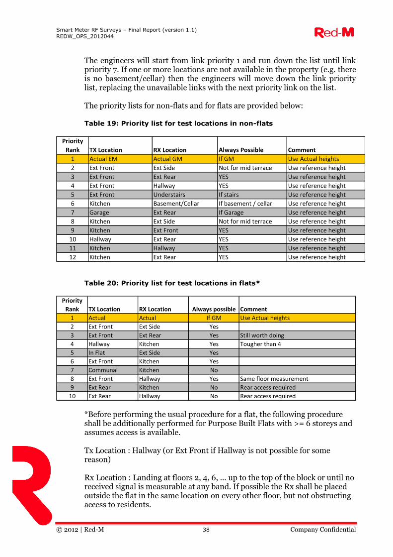
The engineers will start from link priority 1 and run down the list until link priority 7. If one or more locations are not available in the property (e.g. there is no basement/cellar) then the engineers will move down the link priority list, replacing the unavailable links with the next priority link on the list. The priority lists for non-flats and for flats are provided below: Table 19: Priority list for test locations in non-flats
Priority
Rank TX Location RX Location Always Possible Comment
1 Actual EM Actual GM If GM Use Actual heights
2 Ext Front Ext Side Not for mid terrace Use reference height
3 Ext Front Ext Rear YES Use reference height
4 Ext Front Hallway YES Use reference height
5 Ext Front Understairs If stairs Use reference height
6 Kitchen Basement/Cellar If basement / cellar Use reference height
7 Garage Ext Rear If Garage Use reference height
8 Kitchen Ext Side Not for mid terrace Use reference height
9 Kitchen Ext Front YES Use reference height
10 Hallway Ext Rear YES Use reference height
11 Kitchen Hallway YES Use reference height
12 Kitchen Ext Rear YES Use reference height
Table 20: Priority list for test locations in flats*
Priority
Rank TX Location RX Location Always possible Comment
1 Actual Actual If GM Use Actual heights
2 Ext Front Ext Side Yes
3 Ext Front Ext Rear Yes Still worth doing
4 Hallway Kitchen Yes Tougher than 4
5 In Flat Ext Side Yes
6 Ext Front Kitchen Yes
7 Communal Kitchen No
8 Ext Front Hallway Yes Same floor measurement
9 Ext Rear Kitchen No Rear access required
10 Ext Rear Hallway No Rear access required *Before performing the usual procedure for a flat, the following procedure shall be additionally performed for Purpose Built Flats with >= 6 storeys and assumes access is available. Tx Location : Hallway (or Ext Front if Hallway is not possible for some reason) Rx Location : Landing at floors 2, 4, 6, … up to the top of the block or until no received signal is measurable at any band. If possible the Rx shall be placed outside the flat in the same location on every other floor, but not obstructing access to residents.

Smart Meter RF Surveys – Final Report (version 1.1) REDW_OPS_2012044
© 2012 | Red-M 39 Company Confidential
A definition of what each location means for flats and non-flats can be found in Appendix A of this report. There will be slight variations depending upon the type of property and the way it is laid out. The exact test locations will be marked down on a floor plan sketch of the property. This is explained in section A.2. Engineers will mark down approximate positions of windows and doors on the floor plan. A mention will also be added to indicate single/double glazed windows. Engineers will mark down any split-levels on the map, with approximate height difference. In high rise blocks or flats higher than ground level, the floor heights will be measured/estimated by the engineer in order to determine the height difference between the TX and RX locations.
A.1.4 Interference Measurements
This will require the use of the FSH6 Spectrum analyser and a set of the test antennas. The engineer will set up the instrument in a central location of the property such as the kitchen and mark the position on the floor plan. The engineer will then slowly walk to the front of the property and then to the back of the property before returning to the start position. Where possible source of interference shall be identified and confirmed by bringing the FSH6 up close to them and their positions marked on the plan The instrument will then be placed on a table/worktop in the kitchen in order to complete the 5min required capture time for this type of measurement. The settings for the spectrum analyser to be used for each measurement are shown below. Table 21: FSH6 Configuration Settings
Frequency
Band
(MHz)
Start
Frequency
(MHz)
End
Frequency
(MHz)
RBW
(KHz)
Sweep
Time
Trace Internal
Pre-amp
169 169.4 169.8125 10 10s Max hold On
433 433.05 434.79 10 10s Max hold On
868 868.0 870.0 10 10s Max hold On
2400 2400.0 2483.5 10 10s Max hold On
The following procedure should be followed for each of the 4 frequency bands.
1. Place correct antenna onto FSH6 (note that some antennas will need adaptors as FSH 6 has an N-type connector)

Smart Meter RF Surveys – Final Report (version 1.1) REDW_OPS_2012044
© 2012 | Red-M 40 Company Confidential
2. Load pre-recorded configuration settings as per Table 21 3. Chose trace> max hold 4. Start FSH6 scan 5. Walk with the FSH6 towards the front of the property (but remaining
indoors) 6. Walk towards the back of the property 7. Walk back towards the start point of the measurement (as in step 4
above) 8. Complete the measurement for 4-5 minutes 9. Save trace under appropriate name 10. Write down file name and location for records 11. Change antenna to the next frequency band 12. Repeat parts 2-10 with new antennas
At the end of this process, the engineer should have identified some “quiet” spots at each of the 4 frequency bands for carrying out the tests. A quiet spot is defined as a part of the spectrum where the interference measurement just registers the noise floor as recorded by the instrument. Exact test frequencies can be identified directly on the FSH6 by using the Marker function of the instrument. This is particularly useful in highly occupied bands such as the 2.4GHz WiFi band.
A.1.5 Test Frequencies to be used
For each of the 4 frequency bands, a test frequency is required for use during the path loss measurements. The frequency range of each of the test bands is specified in Table 18. The interference measurements taken with the FSH6 (see section A.1.4) will have identified one or more frequencies in a quiet spot of the band. The 169, 433 and 869 MHz bands are expected to be quiet as usage within these bands is sporadic and intermittent, unlike the 2400MHz band which hosts the very popular WiFi technology. For the 2400MHz band, the exact frequency of 2400.000MHz is suggested as this sits at the start of the whole band and is less likely to exhibit interference. Alternative frequencies also include 2427.000MHz, 2457.000MHz and 2483.5MHz. These frequencies are the furthest away from the heavily used WiFi channels 1, 7 and 13.
Figure 11 below provides an overview of the channel allocation in the 802.11b/g band.

Smart Meter RF Surveys – Final Report (version 1.1) REDW_OPS_2012044
© 2012 | Red-M 41 Company Confidential
2412 2414 2416 2418 2420 2422 2424 2426 2428 2430 2432 2434 2436 2438 2440 2442 2444 2446 2448 2450 2452 2454 2456 2458 2460 2462 2464 2466 2468 2470 2472
1 2 3 4 5 6 7 8 9 10 11 12 13
802.11b/g channel allocation
Figure 11 - WiFi band channel allocation (802.11b/g)
A.1.6 Weather Reporting
It has been reported that high humidity / rain adversely affects propagation at 2.4 GHz. Engineers should note the weather sunny / overcast / raining at the time of their visit.
A.2 Producing the Floor Plan
To analyse the results in a scientific manner, a suitable floor plan of the building needs to be produced that defines structures such as doors, wall types and location and windows. The engineer will make best effort to draw the floor plan of the property as accurately as possible. The dimensions of the rooms will be recorded and noted on the drawing. This will be done using a laser measuring device. This sketch can then be used to mark the test locations for the survey and also record important information by placing crosses/symbols and labelling the locations. An example floor plan is shown Figure 12 below.

Smart Meter RF Surveys – Final Report (version 1.1) REDW_OPS_2012044
© 2012 | Red-M 42 Company Confidential
Porch
Patio
Kitchen/dining
Living
Adjacent
property
In the understairs
cupboard
EM
1/2/3/4
3
8
5
EM
Solid wall
External wall
Partition
Window
Door
Electric/Gas
meter locations
Test locations
Key:
Garage door - GRP
2 GM
GM
6
7
345 x 450321 x 450120 x 520
Garage
220 x 520
340 x 280
Porch
Patio
Kitchen/dining
Living
Adjacent
property
In the understairs
cupboard
EM
1/2/3/4
3
8
5
EM
Solid wall
External wall
Partition
Window
Door
Electric/Gas
meter locations
Test locations
Key:
Garage door - GRP
2 GM
GM
6
7
345 x 450321 x 450120 x 520
Garage
220 x 520
340 x 280
Figure 12: Example floor plan showing dimensions of room (in cm), test
locations, window/door locations and wall types
The information captured on the plans will consist of:
General layout of the floor
Room dimensions
Actual locations of EM and GM (if available)
Test locations, marked and numbered
Wall types (as described in section A.1.2)
Position of doors and windows
Additional information such as where the adjacent property wall is (if any), type of garage door (if any), porch/patio areas (if any), understairs cupboard/cellar/basement…
Any identified source of in band interference and it’s location.
Smart Meter RF Surveys – Final Report (version 1.1) REDW_OPS_2012044
© 2012 | Red-M 43 Company Confidential
A.3 Making the pathloss measurements
The engineers will perform pathloss measurements on a maximum of 7 links (6 if there is no GM at the property).
A.3.1 Selecting the test locations
Refer to section A.1.3 on how to identify the test locations. The path loss measurements are only to be carried out in one direction and only where both locations in the listed link are available to measure from or to.
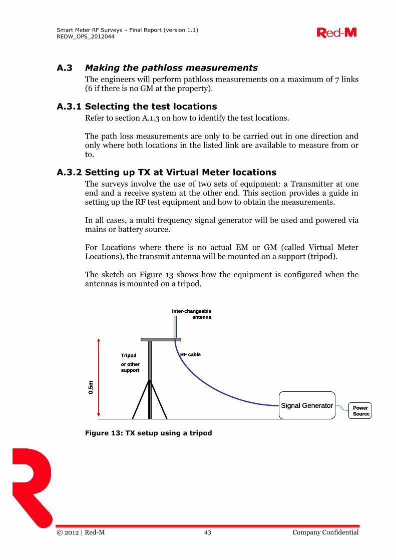
A.3.2 Setting up TX at Virtual Meter locations
The surveys involve the use of two sets of equipment: a Transmitter at one end and a receive system at the other end. This section provides a guide in setting up the RF test equipment and how to obtain the measurements. In all cases, a multi frequency signal generator will be used and powered via mains or battery source. For Locations where there is no actual EM or GM (called Virtual Meter Locations), the transmit antenna will be mounted on a support (tripod). The sketch on Figure 13 shows how the equipment is configured when the antennas is mounted on a tripod.
Signal Generator
RF cableTripod
or other
support
Power
Source
0.5
m
Inter-changeable
antenna
Signal Generator
RF cableTripod
or other
support
Power
Source
0.5
m
Inter-changeable
antenna
Figure 13: TX setup using a tripod
Smart Meter RF Surveys – Final Report (version 1.1) REDW_OPS_2012044
© 2012 | Red-M 44 Company Confidential
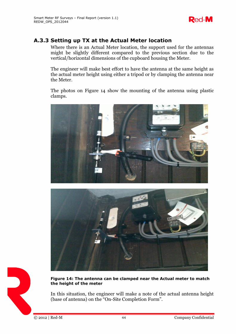
A.3.3 Setting up TX at the Actual Meter location
Where there is an Actual Meter location, the support used for the antennas might be slightly different compared to the previous section due to the vertical/horizontal dimensions of the cupboard housing the Meter. The engineer will make best effort to have the antenna at the same height as the actual meter height using either a tripod or by clamping the antenna near the Meter. The photos on Figure 14 show the mounting of the antenna using plastic clamps.
Figure 14: The antenna can be clamped near the Actual meter to match
the height of the meter
In this situation, the engineer will make a note of the actual antenna height (base of antenna) on the “On-Site Completion Form”.
Smart Meter RF Surveys – Final Report (version 1.1) REDW_OPS_2012044
© 2012 | Red-M 45 Company Confidential
A.3.4 Test Procedure for the engineer handling the TX
The procedure to be followed by the engineer at the transmit location is as follows:
1. Switch the signal generator on 2. Mount the 169 MHz antenna on the tripod/clamp 3. Connect the signal generator to the 169 MHz antenna bulkhead using
the RF cable. 4. Set the signal generator to the pre-selected test frequency and make
sure the power is set to +10dBm output. 5. Turn RF ON on the signal generator 6. Wait for ½ minute until the measurement is complete at the receive
end of the link. 7. Get confirmation from engineer handling the RX that the
measurement is completed 8. Turn RF OFF on the signal generator 9. Dismount the 169 MHz antenna from the support using the easy-screw
nut. 10. Mount the 433MHz antenna on the tripod. 11. Repeat steps 4-8 but at 433MHz – output power = +10dBm 12. Dismount 433 MHz antenna from tripod 13. Mount the 869MHz antenna on the tripod. 14. Repeat steps 4-8 but at 869MHz – output power = +10dBm 15. Dismount 869 antenna from tripod 16. Mount the 2400MHz antenna on the tripod. 17. Repeat steps 4-8 but at 2400MHz – output power = +10dBm 18. Collect all equipment and move to the next planned test location (if
applicable) When TX and RX are on separate floors, see adjustments to procedure described in section 5.4.
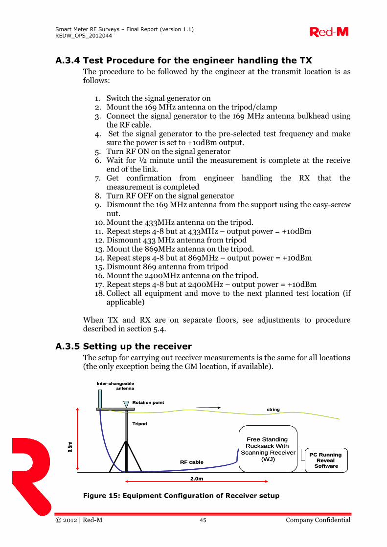
A.3.5 Setting up the receiver
The setup for carrying out receiver measurements is the same for all locations (the only exception being the GM location, if available).
Free Standing
Rucksack With
Scanning Receiver
(WJ)RF cable
PC Running
Reveal
Software
string
2.0m
Inter-changeable
antenna
0.5
m
Tripod
Rotation point
Free Standing
Rucksack With
Scanning Receiver
(WJ)RF cable
PC Running
Reveal
Software
string
2.0m
Inter-changeable
antenna
0.5
m
Tripod
Rotation point
Figure 15: Equipment Configuration of Receiver setup
Smart Meter RF Surveys – Final Report (version 1.1) REDW_OPS_2012044
© 2012 | Red-M 46 Company Confidential
A Watkins Johnson Miniceptor 8607 fast scanning receiver will be used to measure the receive signal from the transmit source. The receiver will be setup to measure the transmitted signal using that band’s antenna. The scanner will be configured to measure using a 12.5 KHz bandwidth. The data will be collected on a laptop running a proprietary Red-M software (Reveal) and will record data for one minute. For the purpose of limiting the effect of body loss on the total path loss, the engineers will stand back at least 2m from the receive antenna whilst the test is being performed. Any Doors between Tx and Rx should be closed. During the ½ minute measurement period, it is important that the receive antenna is not static and needs to move to account for signal fading. To produce movement of the antenna, the mount on top of the tripod has the ability to move and the engineer will use a string to pull the mount and make it rotate slowly over the test period. The test will be repeated for the other frequency bands in association with the TX site being configured with the same frequency setup.
A.3.6 Test Procedure for the engineer handling the RX
The procedure to be followed by the engineer at the receiver location is as follows:
1. Switch on the control laptop and the WJ receiver 2. Mount the 169 MHz antenna on the RX tripod 3. Connect the WJ receiver to the 169 MHz antenna bulkhead using the
RF cable. Make sure that the TX is on and correctly configured 4. Set the WJ to the 169MHz band test frequency 5. Check with the engineer handling the TX site that the signal generator
is set at the correct frequency/power and that the power is on 6. Start the measurement 7. Gently and slowly pull the string to enable the antenna to move
around the rotation point of the tripod whilst measuring the signal on the receive equipment for ½ minute.
8. Stop the measurement from the control laptop using the relevant button on the control software
9. Save the data using a filename that contains location, frequency and location ID. An example would be: Property0023_Loc1to4_169MHz.txt
10. Dismount the 169 MHz antenna from the support using the easy-screw nut.
11. Mount the 433MHz antenna on the RX tripod. 12. Rotate the antenna arm back to its original position 13. Set the WJ to the 433MHz band test frequency 14. Start the measurement from the control laptop using the relevant
button on the control software
Smart Meter RF Surveys – Final Report (version 1.1) REDW_OPS_2012044
© 2012 | Red-M 47 Company Confidential
15. Repeat steps 5-9 but with the TX set at 433MHz – output power = 10dBm
16. Dismount 433 antenna from tripod 17. Mount the 869MHz antenna on the tripod. 18. Rotate antenna arm back to its original position 19. Set WJ at the 869MHz band test frequency 20. Repeat steps 5-9 but with the TX set at 869MHz – output power =
10dBm 21. Dismount 869 antenna from tripod 22. Mount the 2400MHz antenna on the tripod. 23. Rotate antenna arm back to its original position 24. Set WJ at the 2400MHz band test frequency 25. Repeat steps 5-9 but with the TX set at 2400MHz – output power =
10dBm 26. Dismount 2400 MHz antenna from tripod 27. Stop measurement 28. Collect all equipment and move to next test location (if applicable)
A.4 Antenna Height
At virtual meter locations, antennas will be mounted on a support structure at a nominal 0.5m (at base of antenna) from the ground. This height will be used as a reference height and will allow the analysis of the results to be provided in a general context by removing the height factor and looking at the impact of the build environment. Where measurements are made between locations having different local ground levels e.g. on different floors a measurement of the difference in heights shall be made. At the actual EM and GM locations, the engineers will make best effort to mount the antenna at the actual height of the metre using non-conductive clamps at the EM location and the tripod at the GM location. In areas where the antennas cannot be mounted at the same height as the Meter because of dimensions of cupboards, the engineers will adapt the height to fit with the space available. All test heights will be reported on the On-Site Survey Form for subsequent analysis.
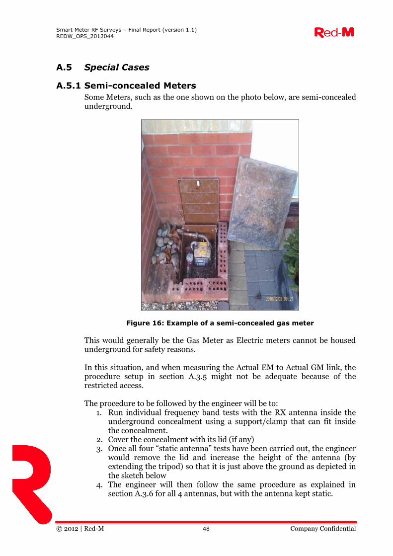
Smart Meter RF Surveys – Final Report (version 1.1) REDW_OPS_2012044
© 2012 | Red-M 48 Company Confidential
A.5 Special Cases
A.5.1 Semi-concealed Meters
Some Meters, such as the one shown on the photo below, are semi-concealed underground.
Figure 16: Example of a semi-concealed gas meter
This would generally be the Gas Meter as Electric meters cannot be housed underground for safety reasons. In this situation, and when measuring the Actual EM to Actual GM link, the procedure setup in section A.3.5 might not be adequate because of the restricted access. The procedure to be followed by the engineer will be to:
1. Run individual frequency band tests with the RX antenna inside the underground concealment using a support/clamp that can fit inside the concealment.
2. Cover the concealment with its lid (if any) 3. Once all four “static antenna” tests have been carried out, the engineer
would remove the lid and increase the height of the antenna (by extending the tripod) so that it is just above the ground as depicted in the sketch below
4. The engineer will then follow the same procedure as explained in section A.3.6 for all 4 antennas, but with the antenna kept static.

Smart Meter RF Surveys – Final Report (version 1.1) REDW_OPS_2012044
© 2012 | Red-M 49 Company Confidential
Scanning Receiver
(WJ)
Laptop with
Control
Software
Inter-changeable antenna
GM
Ground level
Scanning Receiver
(WJ)
Laptop with
Control
Software
Inter-changeable antenna
GM
Ground level
Scanning Receiver
(WJ)
Laptop with
Control
Software
Inter-changeable antenna
GM
Ground level
Scanning Receiver
(WJ)
Laptop with
Control
Software
Inter-changeable antenna
GM
Ground level
Figure 17 : Receiver setup in the case of a semi-concealed Meter. The
antenna is first tested inside the pit (top) with the lid on, and then
outside the pit (bottom) in a static configuration
This test should be conducted preferably with the TX antenna not too far away from the RX antenna, if there is a pre-defined location already. This procedure will allow for the characterisation of the link loss between the actual RX meter location (pit) and the TX location and also provide a measure of the loss caused by the lid/concealment. For clarity this measurement should be performed in addition to any measurements with the Rx at the GM location where the antenna is moved as usual.
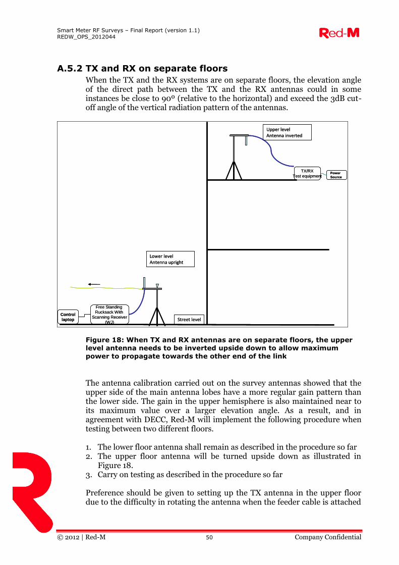
Smart Meter RF Surveys – Final Report (version 1.1) REDW_OPS_2012044
© 2012 | Red-M 50 Company Confidential
A.5.2 TX and RX on separate floors
When the TX and the RX systems are on separate floors, the elevation angle of the direct path between the TX and the RX antennas could in some instances be close to 90º (relative to the horizontal) and exceed the 3dB cut-off angle of the vertical radiation pattern of the antennas.
Free Standing
Rucksack With
Scanning Receiver
(WJ)
Control
laptop
TX/RX
Test equipmentPower
Source
Street level
Upper levelAntenna inverted
Lower levelAntenna upright
Free Standing
Rucksack With
Scanning Receiver
(WJ)
Control
laptop
TX/RX
Test equipmentPower
Source
Street level
Upper levelAntenna inverted
Lower levelAntenna upright
Figure 18: When TX and RX antennas are on separate floors, the upper
level antenna needs to be inverted upside down to allow maximum
power to propagate towards the other end of the link
The antenna calibration carried out on the survey antennas showed that the upper side of the main antenna lobes have a more regular gain pattern than the lower side. The gain in the upper hemisphere is also maintained near to its maximum value over a larger elevation angle. As a result, and in agreement with DECC, Red-M will implement the following procedure when testing between two different floors. 1. The lower floor antenna shall remain as described in the procedure so far 2. The upper floor antenna will be turned upside down as illustrated in
Figure 18. 3. Carry on testing as described in the procedure so far
Preference should be given to setting up the TX antenna in the upper floor due to the difficulty in rotating the antenna when the feeder cable is attached
Smart Meter RF Surveys – Final Report (version 1.1) REDW_OPS_2012044
© 2012 | Red-M 51 Company Confidential
at the top (risk of snapping the cable from its connecting socket due to the weight of the cable). If testing in a rainy day (see next section) and on separate floors and that the RX cannot be placed downstairs outdoors (e.g. testing on the side of the property in the rain), then the TX should be placed downstairs using the long feeder as explained in the next section, and the RX should be placed upstairs (as explained in this section) with the addition of a 90º bend pad at the base of the bulkhead between the RX antenna and the feeder to the WJ. This setup should relieve the stress on the antenna connector and allow a better movement of the rotating arm during the test This change in procedure helps to maintain the methodology implemented so far in the testing and also preserves the orientation and the polarisation of the antennas. Care should be taken when working with inverted antennas not to get the RF Cable in the way of the broad direction of the other end of the link.
A.5.3 Testing on a rainy/wet day
In order to reduce disruptions to the project, the approach described in this document requires a slight modification when surveying in rainy conditions. The key changes to the procedure are provided below:
1. Indoor to indoor path links should remain as described in this procedure (e.g. Hallway to Kitchen, or EM to GM when both are indoors)
2. When one of the path ends is outdoors (e.g. External Front/Side/Rear), the engineers will endeavour to place the TX equipment outdoors whilst keeping the RX equipment indoors
3. The engineer will use a longer feeder cable than the standard 3m cable between the signal generator and the TX antenna stand, allowing all electrical equipment to be kept indoors whilst the test is going on.
4. The engineer handling the TX equipment will still be required to shuttle between the indoor signal generator (to change the frequency/power settings) and the outdoor antenna stand (to change antennas).
5. If measurements require that both the Tx and Rx antennas be outside then the Rx antenna tripod will need to be weighted down so that the string can be pulled from indoors without the risk of turning over the tripod.
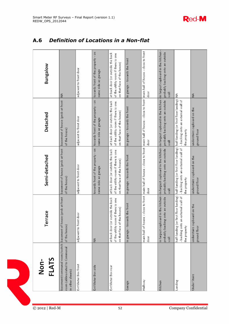
Smart Meter RF Surveys – Final Report (version 1.1) REDW_OPS_2012044
© 2012 | Red-M 52 Company Confidential
A.6 Definition of Locations in a Non-flat

Smart Meter RF Surveys – Final Report (version 1.1) REDW_OPS_2012044
© 2012 | Red-M 53 Company Confidential
A.7 Definition of Locations in a Flat

Smart Meter RF Surveys – Final Report (version 1.1) REDW_OPS_2012044
© 2012 | Red-M 54 Company Confidential
Appendix B Definition of Energy Meter Locations and Proportion of links
B.1 Location Categories
The table below lists the locations that fall within each of the categories that a large Energy Supplier defined for Flats and Non-flats and that were used throughout this report.
Meter Locations Non-flats Flats
IN FLAT core core
KITCHEN core core
LARDER core core
LOUNGE core core
UNDER SINK core core
UNDER STAIRS core core
ABOVE DOOR HEIGHT core core
EXCESSIVE HEIGHT core core
BEDROOM close1 close1
LANDING close1 close1
BASEMENT close1 remote
HALLWAY close1 remote
PORCH close1 remote
COMMUNAL ROOM remote remote
PLANT ROOM remote remote
SHOP remote remote
SWITCH ROOM remote remote
EXT. METER BOX OS1 OS1
EXT MTR BOX REAR OS2 OS2
EXT MTR BOX SIDE OS3 OS3
GARAGE OS3 OS3
OUTSIDE CUPBOARD OS3 OS3
PERMALI BOX OS3 OS3
SEMICONCEALED BOX OS3 OS3
IN SHED OS4 OS4
KIOSK OS4 OS4
PUMP HOUSE OS4 OS4
OUTBUILDING OS5 OS5

Smart Meter RF Surveys – Final Report (version 1.1) REDW_OPS_2012044
© 2012 | Red-M 55 Company Confidential
B.2 Proportions of links between various property locations
The tables below show what proportions of links were recorded by the Large Energy Supplier during their survey of 2.5 million homes in their region. The tables are split into non-flats and flats. Note that properties without a GM have been excluded from the totals.
Non-FLAT close1 core OS1 OS2 OS3 OS4 OS5 remote Total
close1 6.8% 7.0% 7.8% 0.4% 1.4% 0.2% 0.0% 0.0% 23.6%
core 1.9% 18.4% 9.7% 0.5% 1.9% 0.2% 0.0% 0.0% 32.6%
OS1 1.1% 2.3% 21.7% 0.2% 2.5% 0.4% 0.0% 0.0% 28.2%
OS2 0.0% 0.1% 0.2% 0.3% 0.1% 0.0% 0.0% 0.0% 0.7%
OS3 0.3% 0.8% 2.9% 0.1% 8.9% 0.1% 0.0% 0.0% 13.1%
OS4 0.0% 0.1% 0.4% 0.0% 0.0% 0.7% 0.0% 0.0% 1.3%
OS5 0.0% 0.0% 0.0% 0.0% 0.0% 0.0% 0.1% 0.0% 0.1%
remote 0.0% 0.1% 0.1% 0.0% 0.0% 0.0% 0.0% 0.1% 0.3%
Non-FLAT Total 10.2% 28.7% 42.9% 1.5% 14.9% 1.6% 0.2% 0.1% 100.0%
FLAT close1 core OS1 OS2 OS3 OS4 OS5 remote Total
close1 0.6% 1.8% 2.6% 0.1% 0.4% 0.0% 0.0% 1.1% 6.6%
core 0.4% 12.3% 9.5% 0.7% 1.4% 0.2% 0.0% 3.2% 27.6%
OS1 0.1% 2.9% 15.1% 0.3% 1.2% 0.2% 0.0% 1.2% 20.9%
OS2 0.0% 0.0% 0.1% 0.2% 0.1% 0.0% 0.0% 0.0% 0.4%
OS3 0.0% 0.7% 2.3% 0.1% 4.2% 0.0% 0.0% 0.2% 7.6%
OS4 0.0% 0.1% 0.2% 0.0% 0.0% 0.3% 0.0% 0.0% 0.7%
OS5 0.0% 0.0% 0.0% 0.0% 0.0% 0.0% 0.0% 0.0% 0.1%
remote 0.5% 10.2% 12.4% 0.7% 1.7% 0.1% 0.0% 10.6% 36.1%
FLAT Total 1.6% 27.9% 42.2% 2.0% 9.1% 0.8% 0.1% 16.3% 100.0%
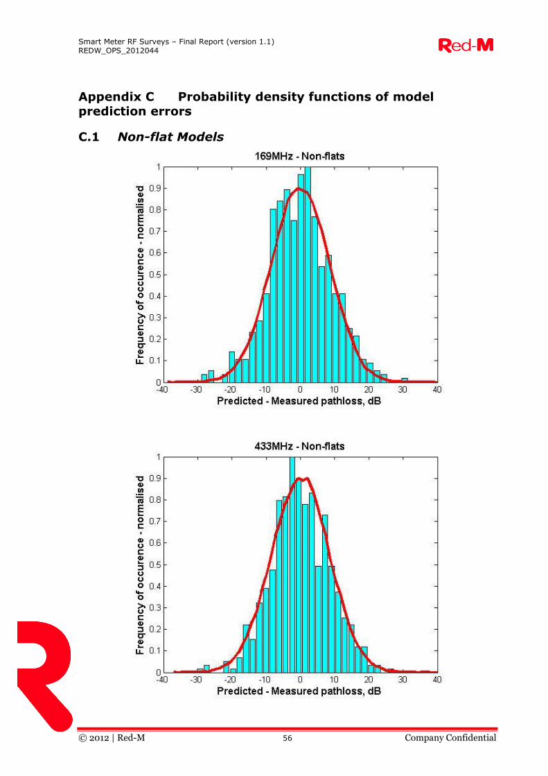
Smart Meter RF Surveys – Final Report (version 1.1) REDW_OPS_2012044
© 2012 | Red-M 56 Company Confidential
Appendix C Probability density functions of model prediction errors
C.1 Non-flat Models
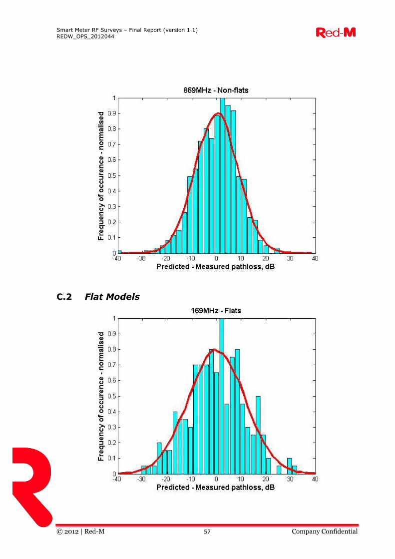
Smart Meter RF Surveys – Final Report (version 1.1) REDW_OPS_2012044
© 2012 | Red-M 57 Company Confidential
C.2 Flat Models
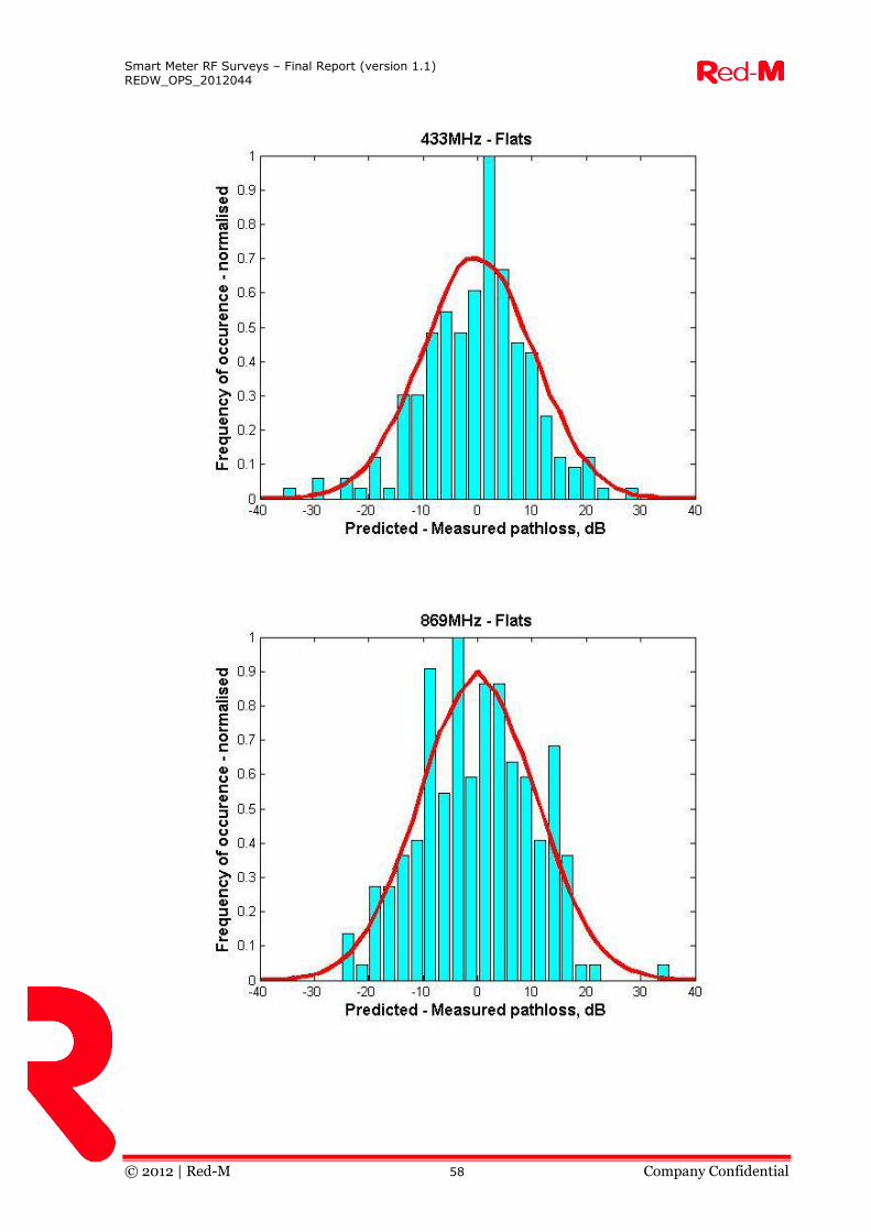
Smart Meter RF Surveys – Final Report (version 1.1) REDW_OPS_2012044
© 2012 | Red-M 58 Company Confidential
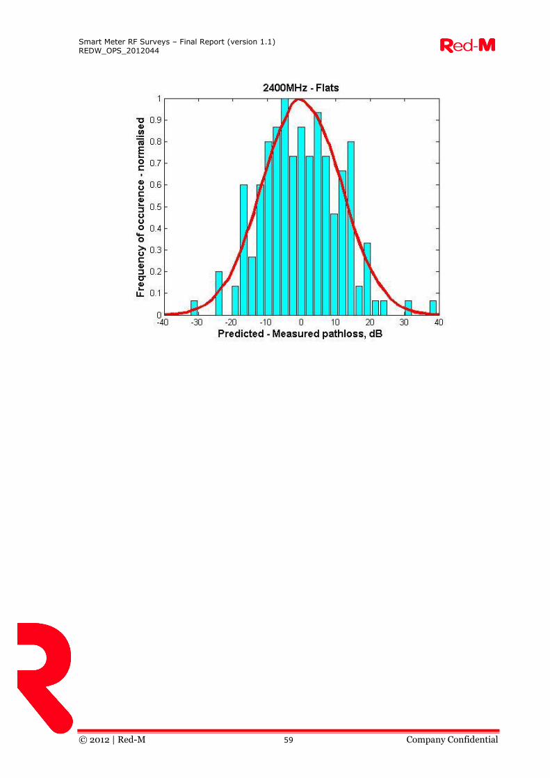
Smart Meter RF Surveys – Final Report (version 1.1) REDW_OPS_2012044
© 2012 | Red-M 59 Company Confidential

60
Appendix D Estimating the Local Mean Pathloss and the fade margin from the HAN survey data
The data collected during the HAN surveys consists of un-averaged, high sample rate (100 samples/sec) received signal strength data of a CW signal collected over a 30sec period. During the 30sec measuring period, the TX was kept stationary whilst the RX was moved over a circular, horizontal area of radius approximately equal to 50cm. The purpose of moving the RX was to capture a sufficient sample size with the local variability built-in to enable the Local Mean Signal Strength (LMSS) to be estimated from the data. Each link consisting of a TX-RX pair at a given frequency would therefore be made up of approximately 3000 individual sample points, from which a LMSS value is estimated, leading to an estimate of the mean pathloss and of the fade statistics for that link. According to the literature, the preferred method that yields maximum accuracy in the estimation of the LMSS is when both transmitter and receiver are moved over a circular, horizontal region several wavelengths across centred at the TX and RX [see Ref.3 ]. This method allows the capture of the local variability at both ends of the link, thus enabling the fast fading (multipath variability) to be well resolved. Implementing the above method (both TX/RX moving) is quite complex as requires both ends of the link to be motorised, with a slow and a fast movement in order to capture all possible combinations of the link. Furthermore, in the context of the HAN trial, the tests were conducted in confined locations on a large number of links (e.g. understairs cupboard) making the rotation at one end very difficult to achieve.
MeanMedian (50%)90th percentile
MeanMedian (50%)90th percentile
Figure 19- The signal collected at each link contains fast fading resulting
from multipath captured by the measurement system
61
Out of the ~3000 samples per link collected by Red-M two statistical metrics were computed: the Median value (or 50th percentile of the distribution of signal levels or pathloss – also referred to as CDF50% hereafter) and the 90th percentile of signal level (or 10th percentile of the pathloss –also referred to as CDF90% or CDF10% depending on the variable). To illustrate the relationship between the Median, the Mean and the CDF90%, we have plotted all three values (of the signal strength) obtained for a typical link in the figure above (BG11, OS1-OS2, 869MHz). The Median and the 90% values were then used throughout the analyses presented in the main report compiled at the end of the campaign. From the above discussion, two questions need looking into in the context of the model and the subsequent analyses provided in the final report:
1. What is the impact of using the Local Median in lieu of the Local Mean
and can this be quantified?
2. What is the impact of moving only the RX on the ability of the data
collection system to capture the full extent of the fast fading and how do
we determine the level of fast-fading to apply for our analysis?
We will attempt to answer these two questions in this short note.
D.1 Median to Mean conversion
According to the literature [e.g. Ref. 3-4], radio signals transmitted between a fixed and a mobile terminal will experience two types of local effects: a slow fading effect due to large obstacles such as apertures in walls, furniture, walls; and fast fading effects due to the combination of constructive and destructive summation of signals following different radio paths between the transmitter and the receiver (multipath). One effect (slow fading) takes place over a large number of wavelengths whilst the second effect takes place within distances of one or a few wavelengths. In the HAN trials situation (indoor propagation), the RX was only moved locally over an area of a few wavelengths at most (depending on the frequency band). It is therefore fair to assume that the signal would only experience fast fading under this test setup. The slow fading would therefore be captured by testing over a large number of links of similar types and lengths in order for the radio link to “experience” different types and scales of obstacles. The probability density function of a complex Gaussian variable follows the distribution of a Rayleigh function. In the case of indoor multipath, it is a well established fact that the multipath-generated fast fading follows a Rician distribution that tends towards a Rayleigh distribution in cases of severe obstruction in one extreme case. Where there is a strong dominant direct path between the terminals (high k-factor), the distribution becomes
62
symmetrical and resembles a Gaussian distribution. In this latter case (in the same way as for the Gaussian distribution), the Mean and the Median values are the same thing (distribution is symmetrical around the mean). If the envelope has a Rayleigh distribution, the ratio of the mean to the median of the exponential distribution is just ln(2) or 0.69. The median is higher than the mean. So the mean power will be lower than the reported median by- 10log10(ln2) = 1.6dB. Since the distribution is not exactly Rayleigh due to the availability in general of a dominant path (even though no LOS was ever measured due to their triviality), we have looked at a large number of samples (a total of 70 links) and compared the difference between the Mean and the Median values, and found the following results:
169MHz 433MHz 869MHz 2.4GHz
MEAN [dB] 0.5 0.9 0.8 0.8
STDEV [dB] 1.2 1.1 1.0 0.8
Table 22- Mean and standard deviation of the difference between the
Local Mean and the Median values (Mean – Median) of the received
signal strength using 70 independent links
Note that in the above table, the Mean is obtained by averaging the Watts values. For the Median, it doesn’t matter if dB or Watts values are used. According to the results above and as expected, the mean difference between Mean and Median lies between the 0dB (zero) of a Gaussian distribution and the 1.6dB of a Rayleigh distribution. The low standard deviation of the difference suggests that the results are quite consistent across the samples used in this analysis. For the HAN data, we recommend therefore the use of the values in
Table 22 to convert the Median values presented in the final report into LMSS and Mean pathloss.
D.2 Fast fading margin
The fast fading margin is the margin needed to be taken into account in order to overcome deep fades in the signal due to the antenna of the smart meter being located in a destructive interference spot (as a result of multipaths). In an ideal world, Red-M would have measured a sufficiently large number of properties for each link-type (e.g. Core-Close1) and used the raw data from each link-type to determine the Cumulative Density Functions (CDF’s) of the pathloss (the raw data will contain the fast-fading due to the moving of the TX/RX). For each technology, applying the MAPL value to the CDF of the pathloss would then yield the probability that the link-type is served.
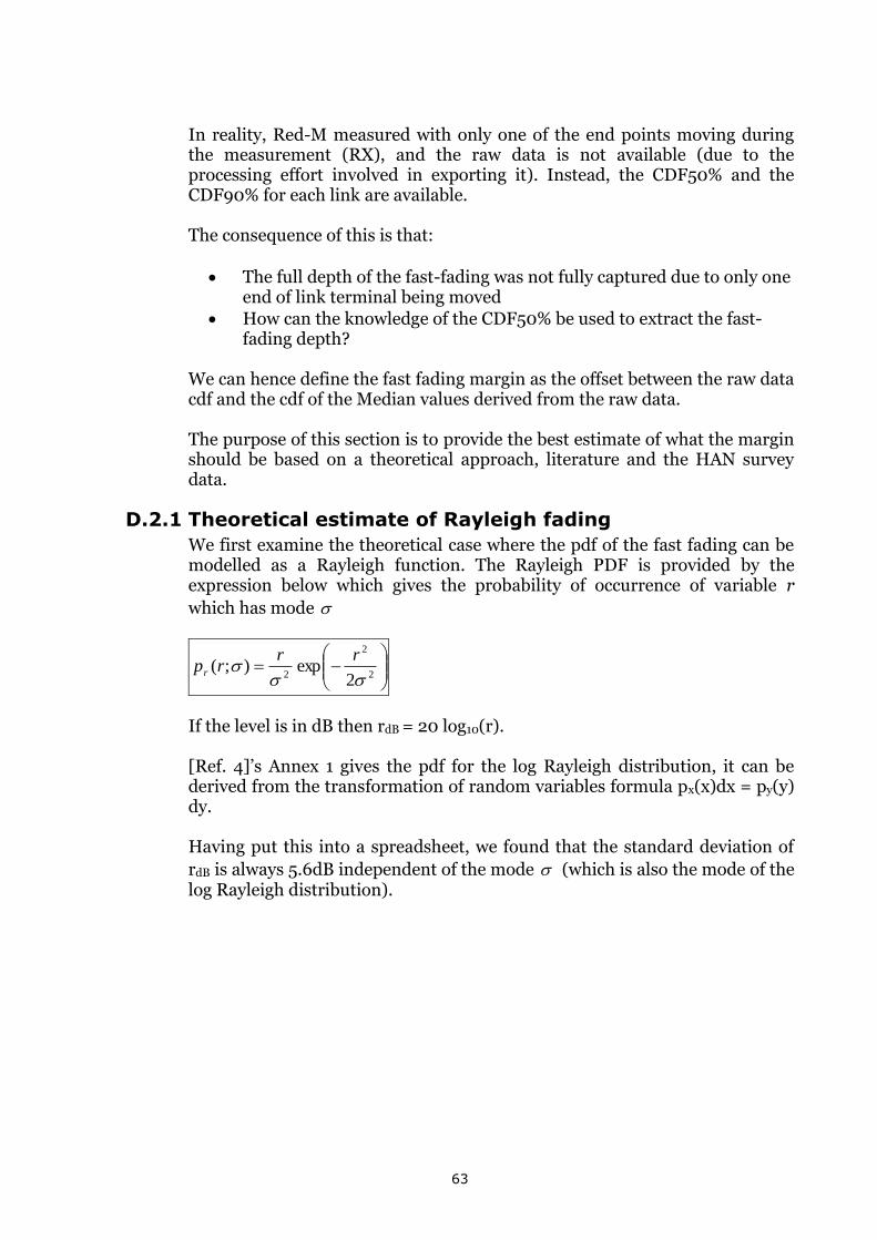
63
In reality, Red-M measured with only one of the end points moving during the measurement (RX), and the raw data is not available (due to the processing effort involved in exporting it). Instead, the CDF50% and the CDF90% for each link are available. The consequence of this is that:
The full depth of the fast-fading was not fully captured due to only one end of link terminal being moved
How can the knowledge of the CDF50% be used to extract the fast-fading depth?
We can hence define the fast fading margin as the offset between the raw data cdf and the cdf of the Median values derived from the raw data. The purpose of this section is to provide the best estimate of what the margin should be based on a theoretical approach, literature and the HAN survey data.
D.2.1 Theoretical estimate of Rayleigh fading
We first examine the theoretical case where the pdf of the fast fading can be modelled as a Rayleigh function. The Rayleigh PDF is provided by the expression below which gives the probability of occurrence of variable r
which has mode
2
2
2 2exp);(
rrrpr
If the level is in dB then rdB = 20 log10(r). [Ref. 4]’s Annex 1 gives the pdf for the log Rayleigh distribution, it can be derived from the transformation of random variables formula px(x)dx = py(y) dy. Having put this into a spreadsheet, we found that the standard deviation of
rdB is always 5.6dB independent of the mode (which is also the mode of the log Rayleigh distribution).
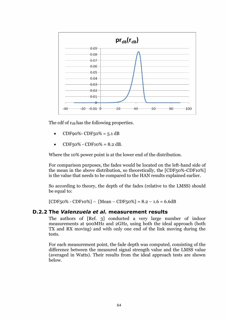
64
The cdf of rdB has the following properties.
CDF90%- CDF50% = 5.1 dB
CDF50% - CDF10% = 8.2 dB. Where the 10% power point is at the lower end of the distribution. For comparison purposes, the fades would be located on the left-hand side of the mean in the above distribution, so theoretically, the [CDF50%-CDF10%] is the value that needs to be compared to the HAN results explained earlier. So according to theory, the depth of the fades (relative to the LMSS) should be equal to: [CDF50% - CDF10%] – [Mean – CDF50%] = 8.2 – 1.6 = 6.6dB
D.2.2 The Valenzuela et al. measurement results
The authors of [Ref. 3] conducted a very large number of indoor measurements at 900MHz and 2GHz, using both the ideal approach (both TX and RX moving) and with only one end of the link moving during the tests. For each measurement point, the fade depth was computed, consisting of the difference between the measured signal strength value and the LMSS value (averaged in Watts). Their results from the ideal approach tests are shown below.
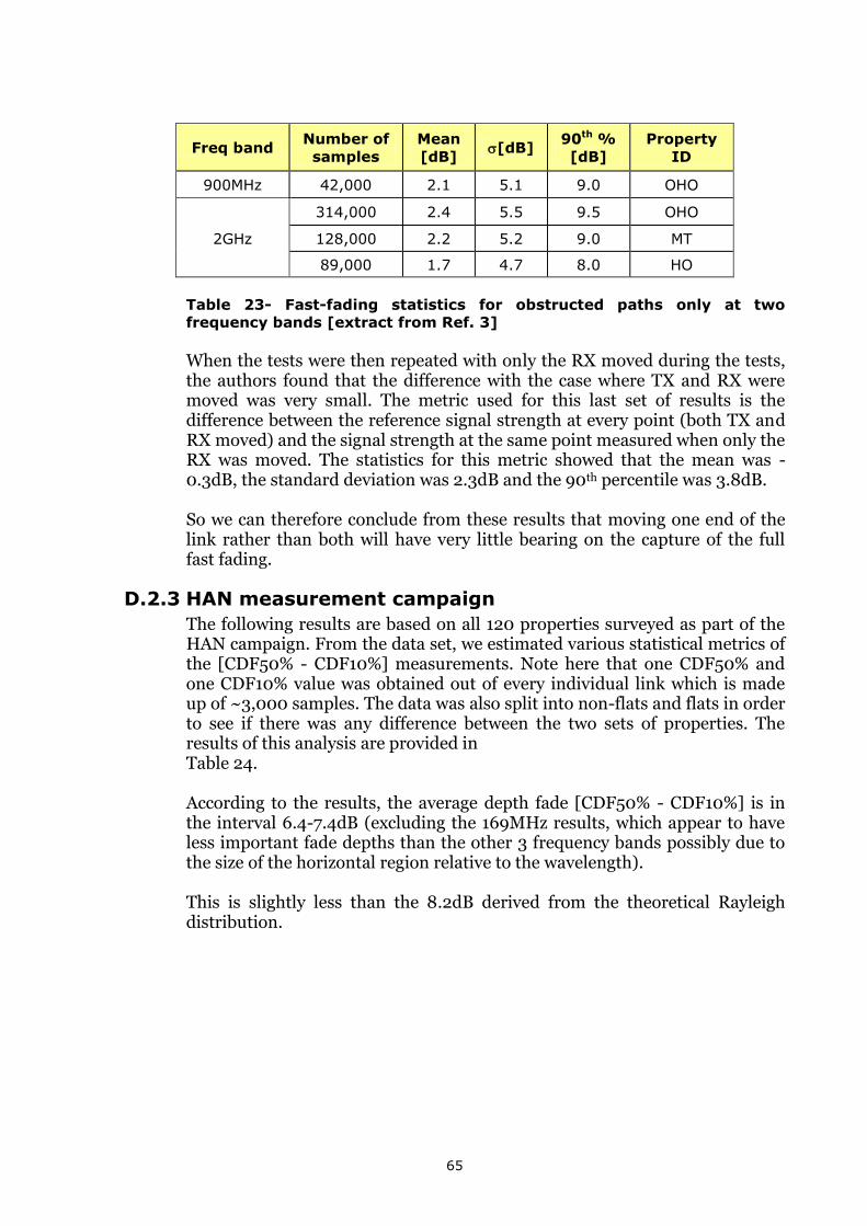
65
Freq band Number of
samples
Mean
[dB] [dB]
90th %
[dB]
Property
ID
900MHz 42,000 2.1 5.1 9.0 OHO
314,000 2.4 5.5 9.5 OHO
2GHz 128,000 2.2 5.2 9.0 MT
89,000 1.7 4.7 8.0 HO
Table 23- Fast-fading statistics for obstructed paths only at two
frequency bands [extract from Ref. 3]
When the tests were then repeated with only the RX moved during the tests, the authors found that the difference with the case where TX and RX were moved was very small. The metric used for this last set of results is the difference between the reference signal strength at every point (both TX and RX moved) and the signal strength at the same point measured when only the RX was moved. The statistics for this metric showed that the mean was -0.3dB, the standard deviation was 2.3dB and the 90th percentile was 3.8dB. So we can therefore conclude from these results that moving one end of the link rather than both will have very little bearing on the capture of the full fast fading.
D.2.3 HAN measurement campaign
The following results are based on all 120 properties surveyed as part of the HAN campaign. From the data set, we estimated various statistical metrics of the [CDF50% - CDF10%] measurements. Note here that one CDF50% and one CDF10% value was obtained out of every individual link which is made up of ~3,000 samples. The data was also split into non-flats and flats in order to see if there was any difference between the two sets of properties. The results of this analysis are provided in Table 24. According to the results, the average depth fade [CDF50% - CDF10%] is in the interval 6.4-7.4dB (excluding the 169MHz results, which appear to have less important fade depths than the other 3 frequency bands possibly due to the size of the horizontal region relative to the wavelength). This is slightly less than the 8.2dB derived from the theoretical Rayleigh distribution.
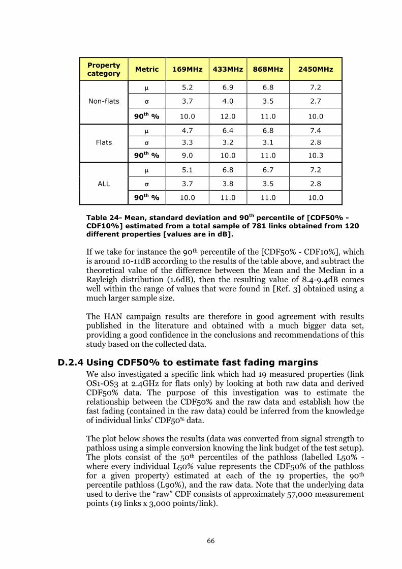
66
Property
category Metric 169MHz 433MHz 868MHz 2450MHz
5.2 6.9 6.8 7.2
Non-flats 3.7 4.0 3.5 2.7
90th % 10.0 12.0 11.0 10.0
4.7 6.4 6.8 7.4
Flats 3.3 3.2 3.1 2.8
90th % 9.0 10.0 11.0 10.3
5.1 6.8 6.7 7.2
ALL 3.7 3.8 3.5 2.8
90th % 10.0 11.0 11.0 10.0
Table 24- Mean, standard deviation and 90th percentile of [CDF50% -
CDF10%] estimated from a total sample of 781 links obtained from 120
different properties [values are in dB].
If we take for instance the 90th percentile of the [CDF50% - CDF10%], which is around 10-11dB according to the results of the table above, and subtract the theoretical value of the difference between the Mean and the Median in a Rayleigh distribution (1.6dB), then the resulting value of 8.4-9.4dB comes well within the range of values that were found in [Ref. 3] obtained using a much larger sample size. The HAN campaign results are therefore in good agreement with results published in the literature and obtained with a much bigger data set, providing a good confidence in the conclusions and recommendations of this study based on the collected data.
D.2.4 Using CDF50% to estimate fast fading margins
We also investigated a specific link which had 19 measured properties (link OS1-OS3 at 2.4GHz for flats only) by looking at both raw data and derived CDF50% data. The purpose of this investigation was to estimate the relationship between the CDF50% and the raw data and establish how the fast fading (contained in the raw data) could be inferred from the knowledge of individual links’ CDF50% data. The plot below shows the results (data was converted from signal strength to pathloss using a simple conversion knowing the link budget of the test setup). The plots consist of the 50th percentiles of the pathloss (labelled L50% - where every individual L50% value represents the CDF50% of the pathloss for a given property) estimated at each of the 19 properties, the 90th percentile pathloss (L90%), and the raw data. Note that the underlying data used to derive the “raw” CDF consists of approximately 57,000 measurement points (19 links x 3,000 points/link).

67
We are interested in a particular value of pathloss (Maximum Allowed Pathloss of 89dB).
Figure 20- Comparing the CDFs obtained using the raw pathloss data,
the L50% and the L90% data - 2.4GHz OS1-OS3 Flats only
For an MAPL value of 89dB, the raw data CDF returns a probability of 39%. In order for the CDF of the L50% to produce the same probability, the MAPL needs to be reduced (i.e. a fade margin) by 3.2dB. This represents the margin by which the MAPL would have needed to be reduced in order to account for the fast fading that is inherent to the raw data. Now this example is specific to this link type/property type and cannot be used to infer the margin for all the other link types. But this value is within the range of values published in Table 24 for this frequency band.
D.2.5 Recommended fade margin
The difficulty in defining the exact value of fade margin to apply to our model resides in the fact that the margin in itself depends on the quality of the link (from a radio propagation point of view) and on the distance between the terminals. For this study, it is more appropriate to use a blanket fade margin and allow for a tolerance interval to analyse how sensitive the final results are to the level of fade margin to be applied. In the majority of cases, the fade margin would not have any effects on the final outcome of the analysis because there is sufficient margin in the system to overcome the fast fading (an example is the link category Close1-OS1 shown in Figure 9 where all the data collected was well within the MAPL). However, in a few cases (e.g. the OS1-OS2 links which are the links between

68
the front and that back of the properties) and in the high frequency bands, there is a case to have a closer look at the results to determine more accurately the impact of the fade margin level. So for this analysis, we recommend using a fast fading margin of typically 3-6dB but extend the interval for the sensitivity analysis to 0-9dB to account for extreme cases and cases of little to no fast fading.
D.3 References
1. Analysis of HAN Trial Pathloss Statistics, W. Harrold, Ref. WBH/DECC/02, 28 Feb
2012
2. DECC – Red-M Smart Meter RF Survey Methodology by D. Simpson, B. Belloul, W.
Harrold, P. Morgan January 2012 REDW_OPS_2012001-v1.0
3. Estimating Local Mean Signal Strength of Indoor Multipath Propagation, R.
Valenzuela, O. Ladron and D.L Jacobs, IEEE Trans Vehicular Technology Vol 46 No.
1, February 1997.
4. The Mobile Radio Propagation Channel, J.D. Parsons, 2nd Edition, 2000
Related Documents