LOCAL ADAPTIVE SLICING FOR LAYERED MANUFACTURING Justin T. Tyberg Thesis submitted to the Faculty of the Virginia Polytechnic Institute and State University in partial fulfillment of the requirements for the degree of Master of Science in Mechanical Engineering Jan Helge Bøhn, Chair Arvid Myklebust Ronald Kander February 16, 1998 Blacksburg, Virginia Keywords: Adaptive Slicing, Calibration, Contour Matching, Fused Deposition Modeler (FDM) Copyright 1998, Justin Tyberg

Welcome message from author
This document is posted to help you gain knowledge. Please leave a comment to let me know what you think about it! Share it to your friends and learn new things together.
Transcript
8/13/2019 Slicing Layers
http://slidepdf.com/reader/full/slicing-layers 1/83
LOCAL ADAPTIVE SLICING FOR LAYERED MANUFACTURING
Justin T. Tyberg
Thesis submitted to the Faculty of the Virginia Polytechnic Institute and State University in partial
fulfillment of the requirements for the degree of
Master of Science
in
Mechanical Engineering
Jan Helge Bøhn, Chair
Arvid Myklebust
Ronald Kander
February 16, 1998
Blacksburg, Virginia
Keywords: Adaptive Slicing, Calibration, Contour Matching, Fused Deposition Modeler (FDM)
Copyright 1998, Justin Tyberg

8/13/2019 Slicing Layers
http://slidepdf.com/reader/full/slicing-layers 2/83
LOCAL ADAPTIVE SLICING FOR LAYERED MANUFACTURING
by
Justin Tyberg
Jan Helge Bøhn, Chairman
Department of Mechanical Engineering
ABSTRACTExisting layered manufacturing systems fabricate parts using a constant build layer thickness.
Hence, operators must compromise between rapid production with large surface inaccuracies, and
slow production with high precision, by choosing between thick and thin build layers,
respectively. Adaptive layered manufacturing methods alleviate this decision by automatically
adjusting the build layer thickness to accommodate surface geometry, thereby potentially enabling
part fabrication in significantly less time. Unfortunately, conventional adaptive layered
manufacturing techniques are often unable to realize this potential when transitioning from the
laboratory to an industrial setting. The problem is that they apply the variable build layer
thickness uniformly across each horizontal build plane, applying the same build layer thickness to
all parts and part features across that plane even though they have different build layer thickness
needs. When this happens, the advantage of using adaptive build layer thicknesses is lost. This
thesis demonstrates how to minimize fabrication times when implementing adaptive layered
manufacturing. Specifically, it presents a new method in which each part or individual part
feature is assigned a distinct, independent build layer thickness according to its particular surface
geometry. Additionally, this thesis presents a calibration procedure for the Fused Deposition
Modeler (FDM) rapid prototyping system that enables accurate, adaptively sliced parts to be physically realizable. Experimental software has been developed and sample parts have been
fabricated to demonstrate both aspects of this work.

8/13/2019 Slicing Layers
http://slidepdf.com/reader/full/slicing-layers 3/83
iii
ACKNOWLEDGEMENTS
I would like to extend thanks to the people whose contributions helped to make this thesis possible. In particular, I would like to thank:
• Dr. Jan Helge Bøhn, my advisor, for introducing me to the world of rapid prototyping, and for
helping me discover the tools I needed to complete my research.
• Dr. Arvid Myklebust, committee member and Director of the Virginia Tech CAD Lab, for
introducing me to the world of CAD/CAM, for making the mathematics of geometric curves
and surfaces so interesting, and most of all, for providing me with a great experience as a
CAD lab teaching assistant.• Dr. Ron Kander, committee member, for explaining to me the fundamentals of the
characteristics of polymer materials, and for being so flexible in scheduling.
• Darrell Early, Manager of the Virginia Tech CAD Lab, for his ability to remedy the seemingly
abundant hardware and software problems so quickly.
• The Virginia Tech Department of Mechanical Engineering for funding me throughout my
graduate career, and for providing ample computing resources.
• Stratasys, Inc., Eden Prairie, Minnesota for providing the Virginia Tech Rapid PrototypingLab with outstanding service of its FDM 1600 rapid prototyping system.
• Bjarne Stroustrup and David R. Musser, for developing the C++ programming language and
the Standard Template Library, respectively.
Finally, I would like to thank my fiancé, Christy, for her unending support through every stage of
this work.
8/13/2019 Slicing Layers
http://slidepdf.com/reader/full/slicing-layers 4/83
iv
TABLE OF CONTENTS
ABSTRACT ............................................................................................................................... ii
ACKNOWLEDGEMENTS........................................................................................................ iii
TABLE OF CONTENTS........................................................................................................... iv
LIST OF FIGURES................................................................................................................... vi
LIST OF TABLES......................................................................................................................x
CHAPTER 1 INTRODUCTION............................................................................................... 1
1.1 PROBLEM STATEMENT AND OBJECTIVES..........................................................4
1.2 SOLUTION OUTLINE................................................................................................ 5
1.3 THESIS ORGANIZATION.......................................................................................... 8
CHAPTER 2 LITERATURE REVIEW.....................................................................................9
2.1 TOPOLOGY, DEFINITIONS, AND CONVENTIONS............................................... 9
2.1.1 Use of Topology ................................................................................................9
2.1.2 Brief Definitions ............................................................................................. 10
2.1.3 Contour Orientation Convention .....................................................................11
2.2 FILE FORMATS........................................................................................................ 12
2.2.1 .STL ................................................................................................................ 12
2.2.2 Other File Formats ......................................................................................... 13
2.3 EFFICIENT SLICING ............................................................................................... 14
2.4 DIRECT CAD MODEL SLICING.............................................................................17
2.5 ADAPTIVE SLICING ............................................................................................... 19

8/13/2019 Slicing Layers
http://slidepdf.com/reader/full/slicing-layers 5/83
v
2.6 SLOPED LAYERS....................................................................................................27
2.7 OBSERVATIONS...................................................................................................... 31
CHAPTER 3 LOCAL ADAPTIVE SLICING ......................................................................... 32
3.1 THICK SLAB GENERATION................................................................................... 32
3.2 CONTOUR MATCHING........................................................................................... 33
3.3 SUB-SLAB DIVISION.............................................................................................. 39
3.4 RESULTS.................................................................................................................. 40
CHAPTER 4 CALIBRATING FDM RAPID PROTOTYPING SYSTEMS FOR ADAPTIVE
BUILD LAYER THICKNESSES...................................................................... 46
4.1 FDM SOFTWARE .....................................................................................................47
4.2 FDM 1600 HARDWARE........................................................................................... 47
4.3 CALIBRATION EXPERIMENTS.............................................................................50
4.3.1 Determining Road Width vs. Flow Rate ........................................................... 50
4.3.2 Assessing Effects of Build Parameters on Overall Part Quality ....................... 53
4.4 RESULTS.................................................................................................................. 54
4.4.1 Road Width Calibration .................................................................................. 54
4.4.2 Effects of Numerical Round Off ...................................................................... 55
4.4.3 Overall Part Quality ....................................................................................... 56
CHAPTER 5 CONCLUSIONS AND CONTRIBUTIONS...................................................... 59
5.1 CONCLUDING REMARKS...................................................................................... 59
5.2 CONTRIBUTIONS....................................................................................................60
5.3 RECOMMENDATIONS FOR FUTURE WORK....................................................... 61
REFERENCES......................................................................................................................... 62
APPENDIX A: GEOMETRIC PROOFS................................................................................. 67
VITA........................................................................................................................................ 73
8/13/2019 Slicing Layers
http://slidepdf.com/reader/full/slicing-layers 6/83
vi
LIST OF FIGURES
FIGURE 1.1: Comparison of stair-steppin g inaccuracies due to thick and thin build layers. (a)Thick build layers poorly approximate complex surfaces; (b) thin layers better
approximate these surfaces; [Sabourin96a] [Sabourin97]. ................................ .. 3
FIGURE 1.2: The potential savings of adaptive slicing is lost by conventional adaptive slicing
methods, which slice all parts of a given build with the same resolution,
regardless of their dissimilar surface characteristics. This results in unnecessary
build layers for the simpler geometries. In the case shown here, the thin layers
necessary for the sphere are imposed unnecessarily on the block. ....................... 4FIGURE 1.3: The effects of uniform slicing. (a) Original model; (b) fabricated part;
[Dolenc94]........................................................................................................5
FIGURE 1.4: Individual parts are fabricated independently with distinct layer resolutions
applied locally as necessary ................................................................................ 6
FIGURE 1.5: Lower contours L 1 and L 2 are matched with upper contours U 1 and U 2 to form
sub-slabs 1 and 2 respectively. Sub-slab 1 can then be divided into m thinner
layers, while sub-slab 2 is divided into n layers, with m > n. ............................... 7
FIGURE 2.1: Contour orientation convention. Interior contours are directed clockwise, while
exterior contours are directed counterclockwise. ............................................. 11
FIGURE 2.2: Faceted representation of a sphere. .................................................................. 12
FIGURE 2.3: A facet that intersects the slice plane has two intersecting edges. Once the
intersection of the initial edge is found, the marching direction is determined by Z
x N . ................................................................................................................. 15
FIGURE 2.4: Given an initial facet F A with intersecting edge E 12 , the next intersecting edge is
determined by the relative position of the vertex V 3. In this case, since V 3 is
below the slice plane, the next edge to be intersected is E 13. The corresponding
facet F 13 is then used to determine the ensuing edge. ................................ ........ 16

8/13/2019 Slicing Layers
http://slidepdf.com/reader/full/slicing-layers 7/83
vii
FIGURE 2.5: The maximum deviation between the ideal surface and the surface of the
fabricated part is given by the cusp height. The cusp height is measured in the
direction normal to the ideal surface. ............................................................... 19
FIGURE 2.6: The effects of uniform slicing. (a) Original model; (b) uniformly sliced part; (c)
adaptively sliced part; [Dolenc94]. ................................................................... 20
FIGURE 2.7: Determining the build layer thickness from the cusp vector C , and the vertical
component of the unit normal to the surface; [Dolenc94]. ................................ 20
FIGURE 2.8: Approximation of the local surface curvature with a sphere to obtain an
appropriate build layer thickness d ; [Suh94]. ................................................... 21
FIGURE 2.9: Determining the location of sampling points along a given contour. From a
sampling point P i, the location of the next sampling point P i+1 is dependent upon
the radius of curvature of the contour ρ and the cusp height δ; [Suh94]...........22
FIGURE 2.10: Four possible configurations that may be encountered when using the build layer
thickness approximation method developed by Kulkarni and Dutta; (a) convex
curvature on upper hemisphere; (b) concave curvature on upper hemisphere; (c)
convex curvature on lower hemisphere; and (d) concave curvature on lower
hemisphere; [Kulkarni96] ................................................................................ 23
FIGURE 2.11: The overall fabrication time is reduced by increasing the throughput of material
deposition of the thick interior layers while the surface quality is maintained with
thin exterior layers; [Sabourin96a] [Sabourin97]. ................................ ............. 26
FIGURE 2.12: An example of interior and exterior segregation due to contour offsetting. (a) A
thick slice; (b) the same slice segregated into interior and exterior regions;
[Sabourin96a] [Sabourin97] ............................................................................ 26
FIGURE 2.13: Comparison of errors produced by 2½D and sloped (ruled) layers; [de Jager97]
. ...................................................................................................................... 28FIGURE 2.14: The Stereolithography Apparatus (SLA) creates each build layer by curing the
surface of a vat of photopolymer resin with an ultraviolet laser. ....................... 30
FIGURE 2.15: Curing the meniscus regions decreases the surface roughness. ......................... 30

8/13/2019 Slicing Layers
http://slidepdf.com/reader/full/slicing-layers 8/83
viii
FIGURE 3.1: Lower contours L 1 and L 2 are paired with upper contours U 1 and U 2 to form
sub-slabs 1 and 2 respectively. Sub-slab 1 can then be divided into m thinner
layers, while sub-slab 2 is divided into n layers, with m > n .............................. 33
FIGURE 3.2: Checking for vertical connectivity between two contours located on adjacent
slices ............................................................................................................... 34
FIGURE 3.3: A shared facet establishes connectivity between two contours C L and C U, located
on adjacent slices P L and P U, respectively......................................................... 35
FIGURE 3.4: Adjacent facets can establish connectivity between two contours C L and C U,
located on adjacent slices P L and P U, respectively.............................................36
FIGURE 3.5: Instances when a virtual connection would be established. (a) Connection is
correctly made; (b) rare occurrence where two features establish a false
connection....................................................................................................... 37
FIGURE 3.6: Branching occurs when a single contour at one thick slice plane can be matched
with multiple contours from the next highest slice plane. ................................ .. 37
FIGURE 3.7: Interior and exterior contours in the same slice plane must be appropriately
matched to ensure that the material between them is deposited with a single layer
thickness. Each interior contour is matched with the smallest exterior contour
that encloses it. ................................................................................................ 39
FIGURE 3.8: Feature tops and bottoms can be identified by contours that do not connect to
any contour in the slice plane above and below them, respectively. .................. 40
FIGURE 3.9: The maximum c usp height for a 45° sloped surface. .........................................41
FIGURE 3.10: Sample builds using CAD models that have been adaptively sliced using
conventional methods. (a) Build 1 consists of part A; (b) build 2 consists of part
B; and (c) build 3 consists of both parts A and B. ............................................ 42
FIGURE 3.11: Sample builds using CAD models that have been adaptively sliced using the newapproach to adaptive slicing. (a) Build 1 consists of part A; (b) build 2 consists
of part B; and (c) build 3 consists of both parts A and B. ................................ . 43
8/13/2019 Slicing Layers
http://slidepdf.com/reader/full/slicing-layers 9/83
ix
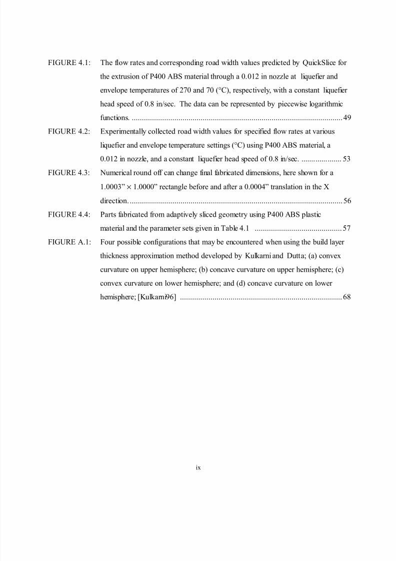
FIGURE 4.1: The flow rates and corresponding road width values predicted by QuickSlice for
the extrusion of P400 ABS material through a 0.012 in nozzle at liquefier and
envelope temperatures of 270 and 70 (°C), respectively, with a constant liquefier
head speed of 0.8 in/sec. The data can be represented by piecewise logarithmic
functions. ........................................................................................................ 49
FIGURE 4.2: Experimentally collected road width values for specified flow rates at various
liquefier and envelope temperature settings (°C) using P400 ABS material, a
0.012 in nozzle, and a constant liquefier head speed of 0.8 in/sec. .................... 53
FIGURE 4.3: Numerical round off can change final fabricated dimensions, here shown for a
1.0003” × 1.0000” rectangle before and after a 0.0004” translation in the X
direction. ......................................................................................................... 56
FIGURE 4.4: Parts fabricated from adaptively sliced geometry using P400 ABS plastic
material and the parameter sets given in Table 4.1 ........................................... 57
FIGURE A.1: Four possible configurations that may be encountered when using the build layer
thickness approximation method developed by Kulkarni and Dutta; (a) convex
curvature on upper hemisphere; (b) concave curvature on upper hemisphere; (c)
convex curvature on lower hemisphere; and (d) concave curvature on lower
hemisphere; [Kulkarni96] ................................................................................ 68

8/13/2019 Slicing Layers
http://slidepdf.com/reader/full/slicing-layers 10/83
x
LIST OF TABLES
TABLE 3.1: Fabrication times of sample builds processed with various slicing methods. ...... 44TABLE 4.1: Build parameter sets used for experimental builds. ........................................... 54

8/13/2019 Slicing Layers
http://slidepdf.com/reader/full/slicing-layers 11/83
1
CHAPTER 1
INTRODUCTION
Rapid prototyping refers to a family of modern technologies in which three-dimensional, solid
objects are fabricated under computer control. There are several advantages that these automated
processes have which are absent from manual fabrication and molding processes. The most
important is known as Solid WYSIWYG (“What-you-see-is-what-you-get”). Essentially this is the
result of removing human interpretation, or error, from the manufacturing process. The object is
designed and fabricated solely from computer data. Rapid prototyping also enables fast andfrequent design iterations. Designers are able to fabricate physical prototypes that aid them in
eliminating potential design flaws early in a product’s development stages, leading to reduced
production costs. Finally, rapid prototyping processes enable fabrication of parts with a high
degree of accuracy.
Rapid prototyping processes fall into three categories: subtractive, formative, and additive.
Subtractive processes achieve the desired shape of an object by successively removing material
from an initial block of solid material. Examples of automated subtractive processes includecomputer numerical control (CNC) milling and wire-type electrical discharge machining (EDM).
Formative processes apply mechanical forces to material to form it into a desired shape.
Examples of this type of process are stamping, bending and forging. Additive processes build
objects by adding successive layers of raw material to create a solid volume. Subtractive and
formative processes are well established and understood. Additive processes, on the other hand,
have emerged more recently. 3D Systems, Inc. introduced the first commercially available
system, the Stereolithography Apparatus (SLA), in 1987. Since then, a myriad of additive
processes has been introduced, including Fused Deposition Modeling (FDM), which was made
available by Stratasys, Inc. in 1992 [Burns93].
The term layered manufacturing (LM) is commonly used to describe the family of modern
additive processes. In these processes, the geometry of the object to be manufactured can be

8/13/2019 Slicing Layers
http://slidepdf.com/reader/full/slicing-layers 12/83
2
obtained from computer aided design (CAD) model data, an existing object (through reverse
engineering), or mathematical data (e.g., surface equations) [Burns93]. Regardless of the source,
the geometry must be processed. First it is converted into a series of horizontal layers, whose
thickness is often specified by the user. This is generally known as the slicing process. These
layers are then used to generate the numerical control (NC) code required by the fabricator to
build the corresponding physical layers. Most all LM fabrication systems accept CAD model data
described in an intermediate file format called the .STL format. This file format approximates the
original CAD model geometry by a series of triangular facets whose information can be easily
processed by the LM hardware. A slicing procedure is then applied to the tessellated model. In
this process, the model is intersected with a set of horizontal planes to create a series of cross
sections, or slices, comprised of contours that represent the material boundaries of the part to be
generated. The contours are subsequently used to generate the NC tool paths for the LM
hardware.
Fabricating a freeform sculptured 3D geometry by a series of 2½D layers will inherently
produce an approximate representation of the original surface geometry. This is commonly
referred to as the stair-stepping effect, and it affects all non-horizontal surfaces. Figure 1.1
illustrates how the inaccuracies caused by the stair-stepping effect are considerably larger with
thicker build layers. Conversely, the use of thinner build layers tends to provide smoother, more
precise surfaces. Hence, the surface quality of a part can be improved by simply decreasing the
build layer thickness. However, because both thick and thin layers have similar build times,
reducing the build layer thickness will result in an increase in fabrication time. Herein lies the
dilemma that is currently facing the rapid prototyping industry. Operators must choose a build
layer thickness that will produce a part with an acceptable level of accuracy in an acceptable
amount of time.

8/13/2019 Slicing Layers
http://slidepdf.com/reader/full/slicing-layers 13/83
3
(a) (b)
Figure 1.1: Comparison of stair-stepping inaccuracies due to thick and thin build layers. (a)Thick build layers poorly approximate complex surfaces; (b) thin layers better approximatethese surfaces; [Sabourin96a] [Sabourin97].
Consequently, research in the rapid prototyping industry is focused on enhancing part
accuracy and reducing fabrication time simultaneously. One technique that has originated from
these efforts is adaptive slicing, which minimizes the stair-stepping inaccuracies by adapting the
thickness of each build layer to better match the part surface geometry. Several methods have
been introduced which survey the surface geometry at each layer to determine an appropriate
thickness for that layer. With these methods, vertical and near-vertical surfaces are built with
relatively thick layers, while flat and near-flat surfaces are built with thinner layers. Hence, the
layer resolution is increased where the geometry would tend to produce more significant errors
due to stair-stepping.
However, conventional adaptive slicing routines are limited in that they are one-dimensional,
only varying the build layer thicknesses with a change in vertical position (height). As a
consequence, these methods are ill suited for an industrial setting in which the build envelope is
typically filled with parts and part features at the same horizontal levels having vastly dissimilar
surface characteristics. In such situations, too many of these parts and features are fabricated
with needlessly thin layers only to satisfy the needs of some remote part or feature elsewhere in
the build envelope at that particular height (Figure 1.2).

8/13/2019 Slicing Layers
http://slidepdf.com/reader/full/slicing-layers 14/83
4
x
y
z
Part with complex surface Part with simple surfaces
Figure 1.2: The potential savings of adaptive slicing is lost by conventional adaptive slicing
methods, which slice all parts of a given build with the same resolution, regardless of theirdissimilar surface characteristics. This results in unnecessary build layers for the simplergeometries. In the case shown here, the thin layers necessary for the sphere are imposedunnecessarily on the block.
Furthermore, the literature addressing these conventional adaptive slicing methods has thus far
been limited to the theoretical control of build layer thicknesses. Indeed, adaptive slicing has not
been implemented on commercial layered manufacturing systems primarily because fabrication
with adaptive build layer thicknesses is not well supported. For example, reducing adaptive slicing
to practice using a FDM 1600 rapid prototyping system often produces surface discontinuities
that are particularly apparent when transitioning from one layer thickness to another. Hence,
using this system to fabricate adaptively sliced parts requires that it be calibrated for multiple build
layer thicknesses simultaneously.
1.1 PROBLEM STATEMENT AND OBJECTIVES
Conventional adaptive slicing routines slice all parts of a given build with the same resolution,
regardless of their dissimilar surface characteristics. Consequently, these methods are unable to
realize the full potential of adaptive slicing (to reduce fabrication times) due to the fabrication of
unnecessary build layers. Furthermore, commercial layered manufacturing systems do not support
fabrication with adaptive build layer thicknesses.

8/13/2019 Slicing Layers
http://slidepdf.com/reader/full/slicing-layers 15/83
5
Therefore, this thesis has two objectives. The first objective is to develop a new approach to
adaptive slicing that applies adaptive slicing techniques locally across part geometries such that
individual parts and part features are fabricated independently of one another with respect to build
layer thicknesses. This new approach will effectively eliminate unnecessary build layers and
thereby minimize fabrication times. The second objective is to reduce adaptive slicing to practice
by fabricating high quality, adaptively sliced parts using a FDM rapid prototyping system. In
particular, this objective involves the calibration of adaptive build layer thicknesses relative to one
another to reduce surface discontinuities at transitions between build layers with dissimilar
thicknesses.
1.2 SOLUTION OUTLINE
The simplest, most widely practiced slicing method employed by the LM industry produces
horizontal layers of equal thickness throughout the CAD model. This is called uniform slicing.
With uniform slicing, details of the geometric data supplied by the CAD model are often ignored.
Minor changes in geometry of the model surfaces are frequently not accounted for [Dolenc94],
and inaccuracies like those illustrated in Figure 1.3 are introduced. Adaptive slicing methods
improve the overall part accuracy by adjusting the build layer thicknesses to accommodate surface
geometry.
(b)(a)
Figure 1.3: The effects of uniform slicing. (a) Original model; (b) fabricated part;[Dolenc94].

8/13/2019 Slicing Layers
http://slidepdf.com/reader/full/slicing-layers 16/83
6
This thesis presents a new adaptive slicing method that minimizes the fabrication time required
when employing adaptive slicing principles by slicing and fabricating each part and individual part
feature independently of one another within the build envelope. This new method ensures that
thin build layers are used only where necessary and thicker build layers are used elsewhere (Figure
1.4).
x
yz
Sphere is fabricated with thinlayers where needed
Block only requires thick layers
Figure 1.4: Individual parts are fabricated independently with distinct layer resolutionsapplied locally as necessary.
To accomplish this task, the model is first sliced into thick slabs with the maximum thicknessallowed by the fabricator. The resulting contours belonging to a slab’s top and bottom slices are
then matched using topological information to form a set of sub-slabs (Figure 1.5). Finally,
adaptive slicing is performed by sub-dividing each thick sub-slab into a distinct number of thinner
layers based on the vertical slope of its surface, measured along the contours that define it.

8/13/2019 Slicing Layers
http://slidepdf.com/reader/full/slicing-layers 17/83
7
Contour L 2Contour L 1
Contour U 1 Contour U 2
Sub-slab 1Sub-slab 2
Figure 1.5: Lower contours L 1 and L 2 are matched with upper contours U 1 and U 2 to formsub-slabs 1 and 2 respectively. Sub-slab 1 can then be divided into m thinner layers, whilesub-slab 2 is divided into n layers, with m > n .
The advantage of implementing this new approach to local adaptive slicing over conventional
adaptive slicing and uniform slicing methods is controversial at best if the parts fabricated with the
new approach exhibit poor surface quality. Therefore, a calibration method for a FDM rapid
prototyping system that enables robust fabrication with adaptive build layer thicknesses is
provided. In particular, the specific build parameters that are associated with this system and
contribute to surface discontinuities are identified. Then, a simple procedure to ensure that the
system is calibrated for use with multiple build layer thicknesses is detailed. Finally, observations
made from experimental builds are used to recommend specific build parameter values that willsupport robust fabrication with this system.

8/13/2019 Slicing Layers
http://slidepdf.com/reader/full/slicing-layers 18/83
8
1.3 THESIS ORGANIZATION
The remainder of this thesis details the new approach to local adaptive slicing as well as the
calibration procedure that enables fabrication with adaptive build layer thicknesses using the FDMrapid prototyping system. It consists of the following:
Chapter 2 provides background material that is necessary to obtain a better understanding of
layered manufacturing as it pertains to this thesis. It also presents a survey of recent work that
has been done in the field of layered manufacturing. Specifically, methods to improve slicing
efficiency and surface smoothness are addressed.
Chapter 3 details the methodology of the new approach to local adaptive slicing, which is used
to minimize the occurrence of unnecessarily thin build layers, thereby minimizing fabrication
times.
Chapter 4 outlines the new calibration procedure that has been successfully implemented for
the FDM rapid prototyping system.
Chapter 5 presents concluding remarks, outlines contributions, and gives recommendations for
future work.

8/13/2019 Slicing Layers
http://slidepdf.com/reader/full/slicing-layers 19/83
9
CHAPTER 2
LITERATURE REVIEW
Layered manufacturing (LM) technologies have secured a position in modern design processes by
enabling fast and frequent design iterations. Designers are able to produce prototype parts that
assist them in eliminating potential design flaws early in a product’s development cycle.
However, a major limitation of LM systems is their inability to achieve acceptable part surface
quality within an acceptable amount of time. To overcome this limitation, ongoing research is
exploring advances in software, hardware and materials. This chapter provides important background information related to LM processes and the methods presented in this thesis. It then
reviews current research, focusing on efficient CAD model processing, efficient software
controlled fabrication strategies, and advanced hardware solutions.
2.1 TOPOLOGY, DEFINITIONS, AND CONVENTIONS
This section presents a definition of topology as it is used in the context of this thesis. It also
provides brief definitions that are used throughout this thesis to describe entities that are
commonly associated with LM processes. These definitions are not generic, but merely describe
how this thesis refers to each entity. Finally, this section details the contour orientation
convention as it applies to the LM industry.
2.1.1 Use of Topology
One aspect of topology is the connectivity information that relates the components of a composite
entity. In particular, each component may be related to its sub-components, or the components
that contain it as a sub-component. In addition, a component may also be related to its
neighboring components. In this thesis, the composite entity of interest is a solid described in the
.STL file format. This format describes the boundary representation of 3D geometry with a series

8/13/2019 Slicing Layers
http://slidepdf.com/reader/full/slicing-layers 20/83
10
of interconnected triangular facets that are defined by three edges. Each edge, in turn, is defined
by two vertices. Therefore, the term topology in this thesis will refer to the information that
describes the connectivity between each facet, edge and vertex that comprise the surface of a
solid. Specifically, this thesis assumes that each facet at minimum includes references to its three
edges, as well as its neighboring facets; and that each edge contains references to its two vertices.
2.1.2 Brief Definitions
Vertex A vertex is a zero-dimensional topological entity. Its geometric representation is a
point, which in 3D space is described with three spatial coordinates.
Edge An edge is a one-dimensional topological entity that connects two vertices. An edge
typically has a direction. In this case, one of its vertices is denoted its head, and the
other, its tail. In this thesis, the term edge will also be used to denote a linear line
segment in 3D space.
Facet A facet is a planar geometric entity. In this thesis, the term facet will be used to
denote a triangular planar entity that is defined by an ordered list of three edges.
These edges are implied by an ordered list of three vertices. A facet has a directed
normal that is perpendicular to the facet plane, and is oriented according to the “right
hand rule” applied to the ordered list of vertices.
Solid A solid is a collection of interconnected facets. They must form a closed, oriented,
and topologically two-manifold shell. This implies that its facet normals must all be
directed away from the material.
Feature A feature is a partial volume of a solid. It is a unique geometric entity that emanates
from a solid, such as a protrusion.
Slice A slice is a two-dimensional plane that describes a horizontal cross section of a solid.
Contour The term contour in this thesis denotes a two-dimensional entity comprised of a
collection of directed edges. It bounds the material regions of a given slice. It is
closed and oriented.

8/13/2019 Slicing Layers
http://slidepdf.com/reader/full/slicing-layers 21/83
11
Layer A layer is a partial volume of a solid. It represents the material bounded by two
adjacent slices.
Slab A slab is a thick layer corresponding to the maximum layer thickness with which a
particular LM system is capable of fabricating.
Sub-slab A sub-slab is defined by two or more contours from the slices that bound a slab. The
contours must be derived from the same feature. This can be established using
topological information.
2.1.3 Contour Ori entation Convention
On a given slice, the material regions are circumscribed by a set of contours. By convention,
these contours are directed such that the material lies to the left of the contours, as viewed in the
direction of the contour. Therefore, external contours are directed counterclockwise (CCW), and
internal contours are directed clockwise (CW). This is illustrated in Figure 2.1.
Exterior contour
Material region
Contour direction
Interior contour
Figure 2.1: Contour orientation convention. Interior contours are directed clockwise, whileexterior contours are directed counterclockwise.

8/13/2019 Slicing Layers
http://slidepdf.com/reader/full/slicing-layers 22/83
12
2.2 FILE FORMATS
All current commercial LM systems require that the geometry to be fabricated be described in the
.STL file format. Once in this format, the geometry is sliced to obtain the horizontal cross-sections. These cross-sections are then used to generate the NC toolpaths required by the
fabricator.
2.2.1 .STL
The .STL file format [Burns93] consists of an unordered list of triangular facets that approximate
the actual surfaces of an original CAD model. It is a boundary representation of 3D geometry.
Figure 2.2 illustrates a faceted representation of a sphere.
Figure 2.2: Faceted representation of a sphere.
The .STL file format has become the de facto industry standard for describing CAD models to
LM processes for two reasons. First, 3D Systems, Inc. introduced the format three years prior to
any other for use with their Stereolithography Apparatus (SLA). Second, its extremely simplistic
format for describing CAD models minimizes the cost of providing one-way translation. As a

8/13/2019 Slicing Layers
http://slidepdf.com/reader/full/slicing-layers 23/83
13
result, most CAD vendors have developed software that is capable of translating data to this
format.
However, the .STL file format contains minimal topological information. Specifically, it
contains a list of possibly unconnected triangular facets. Hence, there is no guarantee that a .STL
model is closed and properly oriented. A model that is not closed and properly oriented cannot be
fabricated because it does not describe a rigid solid. Therefore, it must first be repaired before it
can be sliced. Furthermore, without topology, it is much more difficult to check a faceted model
for closure and orientation before the slicing process is implemented.
The lack of topological information in the .STL file format is also a source of unnecessarily
large files containing redundant and possibly inconsistent data. In the .STL file format, each facet
is represented by three vertices whose coordinates are explicitly described. This causes
considerable redundancy since each vertex is described once each time it is used, which is at a
minimum three times, and often ten times or more. The .STL format also explicitly describes the
surface normal for each facet, in addition to defining it implicitly by the order of the facet’s
vertices using the right hand rule. These duplications are sources of inflated file sizes and possible
inconsistencies.
2.2.2 Other F ile F ormats
As a result of the deficiencies of the .STL file format, Rock and Wozny [Rock91a] developed a
new file format that makes use of indexed lists to represent vertices, edges and facets in a manner
similar to that of the IGES file format [USPro96]. In this file format, each facet references the
appropriate vertices via indices into a vertex list instead of storing nine explicit entries
corresponding to the three vertices’ 3D coordinates. This establishes topological information,
eliminates redundant vertex definitions, reduces the likelihood of inconsistencies, and significantly
reduces the required file size.
The new file format is called the .RPI file format, and it can be derived from the .STL file
format at some computational cost. Specifically, the cost emerges from inferring topology using
the topology reconstruction algorithm outlined in [Rock92]. This algorithm incorporates three

8/13/2019 Slicing Layers
http://slidepdf.com/reader/full/slicing-layers 24/83
14
sequential stages: vertex merging, edge and facet creation, and the determination of the
relationships between these edges and facets. Upon completion of the last stage, each facet
references its three edges as well as its neighboring facets. Each edge, in turn, references its two
vertices and the two facets that define it.
Several other file formats have been developed for use with LM technologies. The Standard
Triangles Hinted (.STH) file format also employs indexed lists to describe a 3D model which may
be comprised of ruled surfaces, polygons, bounded planes, or a collection of triangular facets
[Brock91]. The Common Layer Interface (.CLI) file format describes the cross-sectional data of
a model using polygonal contours [CLI98]. This file format originated primarily from the need to
describe computed tomography (CT) scan data to LM technologies being used in the medical
industry. The .CLI format is also used by some to store the cross-sectional data obtained from
slicing models directly with CAD software [Jamieson95] [Krause97]. The Layered File Format
(.LFF) is being developed by Zheng and Newman for use with their CAM-LEM process
[Zheng97]. This format is also used with direct CAD model slicing, and supports edges,
polylines, elliptic arcs and B-splines. Finally, the Virtual Reality Modeling Language (VRML)
format can be used in a virtual environment that allows users to manipulate vertices to modify
triangles [Fadel96].
2.3 EFFICIENT SLICING
The lack of topological information in the .STL file format makes model slicing expensive since
each facet must first be checked to determine if it intersects a given slice plane, and then all the
edges obtained from these intersections must be sorted to form closed contours. To overcome
this problem, Rock and Wozny [Rock91b] developed a method that greatly enhances the speed
and efficiency with which a given model is sliced. This method, known as the marching algorithm
for slicing, makes use of topological information while intersecting the facets with slice planes.
Their algorithm eliminates the requirement to sort the edges obtained by intersecting facets with
slice planes in the contour generation process. Instead, contours are ordered as they are

8/13/2019 Slicing Layers
http://slidepdf.com/reader/full/slicing-layers 25/83
15
constructed by ‘marching’ from facet to neighboring facet. The result is a faster, more efficient
slicing procedure.
Rock and Wozny observed that each intersecting facet has two intersecting edges, as shown in
Figure 2.3. The intersection of these two edges defines a contour edge. The adjacent contour
edges, in turn, are defined by the intersection of the two adjacent intersecting facets. Adding
topology enables each facet to reference the facets that share its edges. With this connectivity
known, an ordered contour can be constructed by ‘marching’ from facet to neighboring facet
given an initial facet that intersects the slice plane. Hence, the requirement to sort the edges
obtained by intersecting the facets with a given slice plane is eliminated.
Slice plane
Initial edge
Initial facetV2
V1
V3
Z Subsequent facet
Contour orientation
Z x N
Contour edge
Intersection point
Figure 2.3: A facet that intersects the slice plane has two intersecting edges. Once theintersection of the initial edge is found, the marching direction is determined by Z x N .
Once the intersection of the initial facet edge is performed, the direction of the march must be
established to properly define the orientation of each contour. This direction is given by Z x N ,
where Z is the vertical vector and N is the facet’s surface normal. Rock and Wozny [Rock91b]
deduce this direction by determining the relative position, with respect to the slice plane, of the
facet vertex that lies opposite the initial edge. For instance, in Figure 2.4, if edge E 12 of facet
FA(V 1, V 2, V 3) is the initial edge, with vertex V 1 lying above the slice plane and vertex V 2 below

8/13/2019 Slicing Layers
http://slidepdf.com/reader/full/slicing-layers 26/83
16
it, then the next edge to be intersected will be E 13 if vertex V 3 lies below the plane, or E 23 if V 3
lies above the plane. The corresponding adjacent facets would be F 13 and F 23, respectively. The
algorithm continues traversing subsequent facets until the initial edge is reached, at which point
the contour is complete.
Slice plane
V3
V2
V1
FA
F12 F13
F23
Initial edge E 12
V3 lies belowthe slice plane
Edge E 13 also intersectsthe slice plane, and isshared by F 13
FA: current facetF12, F 13, F 23: adjacent facets
Figure 2.4: Given an initial facet F A with intersecting edge E 12 , the next intersecting edge isdetermined by the relative position of the vertex V 3. In this case, since V 3 is below the sliceplane, the next edge to be intersected is E 13 . The corresponding facet F 13 is then used todetermine the ensuing edge.
The extensive number of edge/plane intersections in the overall slicing process requires that
the calculation used to obtain these intersections be fast and efficient. Recognizing this, Rock and
Wozny [Rock91b] developed the following procedure for obtaining the intersection of an edge
and a plane. This method has been optimized such that the computational expense, in particular,
the number of floating point operations (FLOPS) is minimum.
The planes used to slice a solid are horizontal. Therefore, each plane can be represented, in
the Cartesian coordinate system in Euclidian 3-space, by the equation
z = h (2.1)

8/13/2019 Slicing Layers
http://slidepdf.com/reader/full/slicing-layers 27/83
17
where h is the height of the plane. In addition, an edge defined by two vertices p = ( x p, y p, z p) and
q = ( xq, yq, z q) can be described in parametric form by
P (t) = p + t ( q - p ) (2.2)
with t [0,1]. Rock and Wozny show that if one of these points lies above the slice plane, and the
other lies below it, then the edge/plane intersection resides at
th z
z z p
q p
= −
− (2.3)
Assuming one FLOP for each addition, subtraction, and multiplication, and five FLOPS for each
division [Bøhn89], t can be computed in seven FLOPS. The x and y coordinates of the
intersection point can then be computed in an additional six FLOPS using equation (2.2). Hence,
the total number of FLOPS required for the entire calculation is 13 FLOPS.
Rather than address the problems directly associated with the .STL file format, Kirschman and
Alamonte [Kirschman92] proposed parallel processing as a means to reduce slice times. They
implemented a parallel slicing algorithm in which 2,4,8,16 and 32 concurrent processors were
used to carry out the slicing procedure. Theoretically, fabrication times can be reduced by
93.75% and 96.875% when using 16 and 32 processors, respectively, as compared to a single
processor implementation.
2.4 DIRECT CAD MODEL SLICING
Direct CAD model slicing originated from the desire to provide LM fabricators with a CAD
model description that was more accurate than that provided by the .STL file format. A model
description in the .STL file format can only approximate the curved surfaces of a CAD model
from which the .STL file is derived. Furthermore, the cross-sections resulting from slicing
tessellated models are comprised of polygonal contours that can only approximate the true cross-
sections of higher order surfaces such as spheres or Non-Uniform Rational B-splines (NURBS).
In addition, the translation of CAD models to the .STL file format often produces errors such as
missing and intersecting facets, and repairing these models is an expensive and imperfect task.

8/13/2019 Slicing Layers
http://slidepdf.com/reader/full/slicing-layers 28/83
18
One approach to resolve these issues is to slice the CAD model directly. The primary benefits
of direct CAD model slicing are increased model accuracy and smaller file sizes. Researchers
contend that, by slicing the model within the CAD software, exact contours can be derived from
the model’s true surfaces [Guduri92] [Zheng97]. In addition, storing the cross-sectional data
requires less space than a tessellated model would require [Vuyyuru94] [Jamieson95]
[Beaman97]. Also, the need for model repair and a conventional slicing process is eliminated.
As a result, many research groups have implemented direct CAD model slicing. Guduri et al .
[Guduri92] developed an interface to LM processes based on constructive solid geometry (CSG).
In their work, a part to be fabricated is represented by CSG primitives. Each primitive is sliced
individually to generate a set of independent contours. Boolean operations are then performed at
the intersections of these contours to produce each slice. Hope et al. [Hope97a] [Hope97b] also
developed their own CAD model slicing software, TruSurf, which makes use of the IGES file
format [USPro96] (supported by most commercial CAD systems) to translate CAD models.
Several research groups have also made use of existing commercial CAD systems to perform
model slicing. Vuyyuru et al. [Vuyyuru94] sliced a solid model using SDRC’s I-DEAS CAD
package to obtain contours represented by NURBS. Jamieson and Hacker [Jamieson95] used
Parasolid, the solid modeling kernel provided by EDS Unigraphics, to output slice curves in the
.CLI file format [CLI98], and Zheng and Newman [Zheng97] utilize ACIS, the 3D geometric
modeler from Spatial Technology, to produce slice data described in their .LFF file format.
Despite the benefits of direct CAD model slicing, commercial LM systems continue to
primarily support the .STL file format for several reasons. The main advantage of the .STL
description is the simplicity of the intersection calculations (detailed in the previous Section)
required for slicing [Beaman97]. Slicing high-degree polynomial surfaces (NURBS), on the other
hand, is non-trivial [Guduri92] and prone to round-off errors [Beaman97]. Furthermore, there is
currently no standard higher-order geometric description available to exchange geometric datafrom a particular CAD system to a specified LM fabricator.

8/13/2019 Slicing Layers
http://slidepdf.com/reader/full/slicing-layers 29/83
19
2.5 ADAPTIVE SLICING
The most significant development in LM technology, in terms of improved part accuracy, has
been adaptive slicing. The basic principle of adaptive slicing is to evaluate local surfacegeometries to determine the maximum build layer thickness that can be used while maintaining a
user-defined surface tolerance, usually measured by the cusp height. The cusp height represents
the maximum deviation of the part surface from the true surface. As shown in Figure 2.5, it is
measured in the direction normal to the true surface. The layer thicknesses are usually distinct
values bound by [ Lmin, Lmax] which are pre-determined by the user and which are limited by the
fabrication capabilities of the specific LM process. Existing methods typically incorporate
mathematical expressions that predict the cusp height at discrete locations along a given slice.
These expressions are then used to determine the optimal thickness for each layer based on the
part surface curvature. Dolenc and Mäkelä [Dolenc94], Suh and Wozny [Suh94], Kulkarni and
Dutta [Kulkarni95] [Kulkarni96], Sabourin et al. [Sabourin96a] [Sabourin96b] [Sabourin97], and
Krause et al. [Krause97] have all developed methods that employ these techniques.
Depositedmaterial
Ideal surface
Cusp height
Figure 2.5: The maximum deviation between the ideal surface and the surface of thefabricated part is given by the cusp height. The cusp height is measured in the directionnormal to the ideal surface.
Dolenc and Mäkelä [Dolenc94] demonstrate the important advantage of using adaptive slicing
techniques rather than uniform slicing. Figure 2.6 [Dolenc94] illustrates the possible effects of
fabricating a part that has been uniformly sliced. When using this method, flat areas and peak
features of a part may not be accounted for. However, with adaptive slicing, it is possible to place

8/13/2019 Slicing Layers
http://slidepdf.com/reader/full/slicing-layers 30/83
20
slice heights at locations that coincide with these key features, thereby eliminating significant
errors.
(b)(a) (c)
Figure 2.6: The effects of uniform slicing. (a) Original model; (b) uniformly sliced part; (b)adaptively sliced part; [Dolenc94].
In addressing the stair-stepping problem, Dolenc and Mäkelä focus on polyhedral models such as
those described in the .STL file format. They observe that the layer thickness required to satisfy
the specified surface tolerance, C max, in the vicinity of a point P on the part surface is dependent
upon n z , the vertical component of n which is the unit surface normal at P . Specifically, they
observe that the cusp height c is maintained below C max if C cn= satisfies C c C = ≤ max
(Figure 2.7).
P
l P
n
n
Cus vector C = cn
P
Part surface
Build layer
Figure 2.7: Determining the build layer thickness from the cusp vector C, and the verticalcomponent of the unit normal to the surface; [Dolenc94].

8/13/2019 Slicing Layers
http://slidepdf.com/reader/full/slicing-layers 31/83
21
Given C max, the optimal layer thickness at P is therefore
l L C n P z = min{ , / }max max (2.4)
A layer thickness is determined for several discrete points P i along a given slice and the minimum
is used to fabricate the layer above it, provided that it is larger than the minimum thickness
available:
l L l slice P i= max{ ,min{ }}min (2.5)
Suh and Wozny [Suh94] divide each model into sub-regions whose vertical boundaries are
defined by the model's peak features. With the peak features accounted for, each sub-region is
then adaptively sliced. The thickness of each layer, d , is calculated by first sampling the surface
geometry at several points along the previous slice. The minimum of these calculated values is
then considered the optimal layer thickness. Suh and Wozny determine the thickness at a sample
point P by approximating the part surface geometry using a sphere of radius r , based on the part
surface curvature at that point. The thickness is then computed from equations that are derived
from the geometry shown in Figure 2.8 for points on upward and downward facing surfaces,
respectively.
ρ
ρ
θ
δ d d
ρ
θδρ
Approximate
surface
(a) (b)
Figure 2.8: Approximation of the local surface curvature with a sphere to obtain anappropriate build layer thickness d ; [Suh94].
The sampling points, P i, along each slice are determined by approximating the contour curves by arcs, as shown in Figure 2.9. From a given sampling point, the location of the next sampling
point is calculated from equation (2.6).

8/13/2019 Slicing Layers
http://slidepdf.com/reader/full/slicing-layers 32/83
22
Pi
ρ
Pi+1δ
Arc length: l
θSampling point
Contour approximation
Figure 2.9: Determining the location of sampling points along a given contour. From asampling point P i , the location of the next sampling point P i+1 is dependent upon the radiusof curvature of the contour ρ and the cusp height ; [Suh94].
arc length l
if
otherwise=
∞ =
− −
ρ
ρδρ
0
2 11cos ( ) (2.6)
Kulkarni and Dutta [Kulkarni95] [Kulkarni96] correct and expand upon the method
developed by Suh and Wozny by identifying all possible configurations that could arise during the
calculation of a given build layer thickness (Figure 2.10). While Suh and Wozny only differentiate
between upward and downward facing surfaces in their calculations, Kulkarni and Dutta also
consider the differences in curvature for both of these situations. As a result, they recognized
four unique configurations (Figure 2.10) as opposed to just the two identified by Suh and Wozny,
and derived expressions for each to determine the curvature at a given point. Equations 2.7, 2.8,
2.9 and 2.10 correspond to the cases shown in Figures 2.10a-d, respectively. Their derivations
are shown in Appendix A.
222 2sinsin δρδθρθρ −++−=d (2.7)
222
2sinsin δρδθρθρ +++−=d (2.8)222 2sinsin δρδθρθρ +−−=d (2.9)
222 2sinsin δρδθρθρ −−−=d (2.10)

8/13/2019 Slicing Layers
http://slidepdf.com/reader/full/slicing-layers 33/83
23
Furthermore, Kulkarni and Dutta limit their geometry to parametric surfaces represented by
algebraic equations. They are therefore able to extract the exact expression for the surface
curvature in the vertical direction along each slice level. The curvatures computed by Suh and
Wozny, on the other hand, contain a level of uncertainty because each is obtained by sampling
discrete points along each level.
δρ
NP
d
θθ
δρ N
P
d
(a) (b)
θ
δ
ρ
N
P
dδ
ρ
N
P
d
θ
(c) (d)
P: a point on the part surface
N: the surface normal at P
θ: the angle that N makes to the horizontal
ρ: the radius of curvature at P
δ: the allowed cusp height
d: the layer thickness to be computed
Figure 2.10: Four possible configurations that may be encountered when using the buildlayer thickness approximation method developed by Kulkarni and Dutta; (a) convexcurvature on upper hemisphere; (b) concave curvature on upper hemisphere; (c) convexcurvature on lower hemisphere; and (d) concave curvature on lower hemisphere;[Kulkarni96]

8/13/2019 Slicing Layers
http://slidepdf.com/reader/full/slicing-layers 34/83
24
The methods introduced by Suh and Wozny [Suh94] and Kulkarni and Dutta [Kulkarni95]
[Kulkarni96] were developed using non-polyhedral surface representations. As a consequence,
neither method is suitable for faceted models such as those described in the .STL file format.
Sabourin et al. [Sabourin96a] [Sabourin96b] offer an alternative approach to adaptive slicing
that does apply to the .STL file format. In what they term stepwise uniform refinement , each
model is first sliced into thick, uniform, horizontal slabs. Each slab has a thickness corresponding
to the maximum layer thickness that can be fabricated. These slabs are then uniformly sub-divided
individually, as needed, to satisfy the cusp height requirement developed by Dolenc and Mäkelä
[Dolenc94]. However, unlike the previous methods, this method applies the measure
l C n P z = max / to both the top and bottom slices that define each slab rather than to the bottom
slice only. Furthermore, Sabourin et al. perform adaptive slicing by determining the optimal
integer number of uniform thickness slice layers that a particular slab is to be subdivided into:
=
=
min
maxmaxmax
max
max
int],[
}max{int
L
L1,
,nnC
L
slab
bottom z top z slab
ααα
α
(2.11)
where { }n z topand { }n z bottom
are the sets of unit normal z components for the points P i along the
top and bottom slices of a particular slab, respectively. This ensures that every point P along the
pair of slices is considered in the calculation of the optimal layer thickness within that slab. This
thickness is then given by
slabmax Ll α/= (2.12)
By evaluating the surface characteristics at every point along both the top and bottom slice levels,
this method is less likely to miss regions of extreme curvature during the slicing process
[Sabourin96a] [Sabourin96b].

8/13/2019 Slicing Layers
http://slidepdf.com/reader/full/slicing-layers 35/83
25
Suh and Wozny [Suh94], Kulkarni and Dutta [Kulkarni95] [Kulkarni96], and Sabourin et al.
[Sabourin96a] [Sabourin96b] each report an increase in fabrication speed when comparing parts
sliced using their respective methods with the identical uniformly sliced parts. Each group
attributes this speedup to the lesser number of layers required to produce an adaptively sliced
part. Suh and Wozny [Suh94] generated a 10 inch (254 mm) diameter sphere using both uniform
and adaptive slicing techniques. The adaptively sliced version required 909 layers that ranged in
thickness from 0.001 inch (0.03 mm) to 0.020 inches (0.51 mm). A layer thickness of 0.006
inches (0.15 mm) was used for the uniformly sliced version, which required 1667 layers. The
cusp height was maintained below 0.006 inches (0.15 mm) in both cases. Kulkarni and Dutta
[Kulkarni95] [Kulkarni96] reported an 18 per cent reduction in fabrication time when comparing
an ellipsoid that was adaptively sliced to a uniformly sliced version. The former required just 82
layers, while 146 were required for the uniformly sliced model. Finally, Sabourin et al.
[Sabourin96a] [Sabourin96b] built a part using uniform 0.005 inch (0.13 mm) thick layers, and
then again with adaptive slicing using discrete layer thicknesses of 0.0050, 0.0075 and 0.0150
inches (0.13, 0.19 and 0.38 mm) as needed. The result was a 52 per cent reduction in measured
build time, while going from 79 to 41 layers.
In an effort to further reduce build times, Sabourin et al. [Sabourin96a] [Sabourin97]
developed a unique method that combines the use of thick and thin build layers. The approach
involves separating the model space into interior and exterior regions as illustrated in Figure 2.11
[Sabourin96a] [Sabourin97]. After slicing the model space into thick slabs [Sabourin96b], they
offset the external contours of the subsequent slices into the model (Figure 2.12) [Sabourin96a]
[Sabourin97]. The offset curves mark the boundary between the interior and exterior regions.
The latter are then re-sliced using stepwise uniform refinement [Sabourin96b] to enhance the
quality of the part surfaces, while the interior regions are built with thick layers to increase the
fabrication speed. By increasing the throughput of the material deposition in the interior regions,they were able to realize an additional approximate 50 per cent reduction in fabrication times
[Sabourin96a] [Sabourin97].

8/13/2019 Slicing Layers
http://slidepdf.com/reader/full/slicing-layers 36/83
26
Thick interior layersimprove fabrication speed
Thin exterior layersmaintain surface accuracy
Figure 2.11: The overall fabrication time is reduced by increasing the throughput of material deposition of the thick interior layers while the surface quality is maintained withthin exterior layers; [Sabourin96a] [Sabourin97]
(a) (b)
Figure 2.12: An example of interior and exterior segregation due to contour offsetting. (a) Athick slice; (b) the same slice segregated into interior and exterior regions; [Sabourin96a]
[Sabourin97]
All of the above adaptive slicing procedures determine a given build layer thickness by
evaluating the surface curvature along the slice levels that define it. With these methods, the
minimum build layer thickness computed along each slice level is used to fabricate all parts and
individual part features existing at that height across the build envelope. This produces
unnecessary build layers whenever any of these parts or features do not require this minimum
layer thickness to meet the overall surface tolerance. The result is a needlessly inefficient build
process.
Recognizing this flaw, Krause et al. [Krause97] have introduced an approach that uses a
feature recognition algorithm to divide each CAD model into a set of arbitrary partial volumes, or
segments, based on their unique geometries. Each segment of the part is then sliced
8/13/2019 Slicing Layers
http://slidepdf.com/reader/full/slicing-layers 37/83

8/13/2019 Slicing Layers
http://slidepdf.com/reader/full/slicing-layers 38/83
28
their vertical surfaces to achieve the sloped shape, and stack them using a sintering [Zheng97] or
gluing process [Hope97a]. The Shape Deposition Manufacturing (SDM) process, on the other
hand, deposits droplets of molten metal to achieve each layer, and machines the surfaces
afterwards using a 3 or 5-axis mill [Merz94] [Klingbeil97].
Contour at height z i
Contour at height z i+1
Contour at height i
Contour at height z i+1
error error
2.5D layer sloped layer
Figure 2.13: Comparison of errors produced by 2½D and sloped (ruled) layers; [deJager97].
As with 2½D layers, the creation of each sloped layer requires the establishment of the
contours that define it. However, sloped layers that are machined require further computations to
produce an approximate surface between these two contours, and an accurate cutting vector
along this surface. The process of establishing an approximate surface between two contours is
not new. Keppel [Keppel75] joined points along neighboring contours to form a surface that was
approximated by triangular planar elements. Most current researchers simplify this by
approximating the layer surfaces with ruled surfaces [Thomas96] [de Jager97] [Zheng97]. These
are obtained by connecting points along adjacent contours with a series of straight-line segments.
Both de Jager et al. [de Jager97] and Zheng and Newman [Zheng97] perform direct CAD
model slicing to obtain the slice contours. They use ruled surfaces to define the outer surface of
each layer. This enables tangent-cutting of each layer by at least a four axis system that employs
line visibility [de Jager97] [Zheng97]. The Shapemaker II process [Thomas96] also makes use of ruled surfaces to define the layer surfaces. Hope et al. [Hope97a] [Hope97b] create the
appropriate contours using their own software, and obtain the cutting direction at discrete points

8/13/2019 Slicing Layers
http://slidepdf.com/reader/full/slicing-layers 39/83
29
along the surface of a given layer by computing the cross product of the surface normal and the
tangent vector at each.
The greatest disadvantage shared by these sloped layer methods is that they require a system
with a minimum of four degrees of freedom (translations in the x-y plane and two rotational) to
manufacture a given part. Adequate processes include wire EDM, hot-wire cutting, laser cutting,
water-jet cutting, and CNC side milling, among others [de Jager97]. These systems are
significantly more expensive and difficult to program than current 2½D rapid prototyping systems.
Furthermore, although these methods significantly reduce stair-stepping, errors will persist for
surfaces with double curvature [Hope97a].
Various other processes do not employ a machining stage to produce sloped layer surfaces,
but simulate sloped layers instead. In the 3D Printing (3DP) process, layers are formed by
spraying a binder onto a powder bed using inkjet technology. These binder droplets can be
deflected during deposition to reduce the stair-stepping effect (further details have not been
provided) [Sachs97].
Reeves et al . [Reeves97] simulate sloped layers using the Stereolithography Apparatus (SLA)
by performing additional laser scanning sequences to cure meniscus regions between previously
cured 2½D layers (Figures 2.14 and 2.15). The SLA fabricator employs an ultraviolet laser to
selectively scan the surface of a vat of photopolymer resin. The scanned regions of the resin
surface cure (or solidify) upon exposure to the laser beam to produce each build layer. Upon
completion of each scanning sequence, a platform which supports the previously cured layers
descends into the vat a distance equal to the subsequent build layer thickness (Figure 2.14). Time
is allotted to allow the resin to settle above the top layer, and the scanning process is repeated.
Reeves et al . employ additional scanning sequences to decrease the surface roughness of the part.
Specifically, after completing each layer using the conventional process, they raise the build
platform such that the most recently fabricated layer lies just above the resin surface. The resins’typically high surface tension causes a meniscus to form between the current layer and the one
below it. This meniscus is then cured using additional scanning sequences (Figure 2.15) to reduce
the stair-stepping error.

8/13/2019 Slicing Layers
http://slidepdf.com/reader/full/slicing-layers 40/83
30
Photopolymer resin
UV laser beam
Platform
Build layersSupports
Figure 2.14: The Stereolithography Apparatus (SLA) creates each build layer by curing thesurface of a vat of photopolymer resin with an ultraviolet laser.
UV laser beam
Build layers
Meniscusregion
Figure 2.15: Curing the meniscus regions decreases the surface roughness.

8/13/2019 Slicing Layers
http://slidepdf.com/reader/full/slicing-layers 41/83
31
2.7 OBSERVATIONS
With regard to manufacturing accurate parts in the minimum fabrication time using LM processes,
the literature suggests the following:(a) Although the .STL file format is the de facto industry standard, it suffers from a lack of
topological information [Rock91a] [Rock92].
(b) Topology (connectivity) must be added to the facets, edges and vertices that comprise a solid
to enable fast and efficient slicing processes [Rock91b].
(c) Adaptive slicing has been proven to reduce fabrication times while manufacturing parts with
enhanced surface quality [Suh94] [Kulkarni95] [Kulkarni96] [Sabourin96a] [Sabourin96b]
[Sabourin97].
(d) Employing stepwise uniform refinement, and specifically, evaluating the surface characteristics
at every point along both the top and bottom slice levels of a given slab, makes it less likely to
miss regions of extreme curvature during the slicing process [Sabourin96a] [Sabourin96b].
(e) Most conventional adaptive slicing procedures result in a needlessly inefficient build process.
Specifically, the minimum build layer thickness computed along each slice level is used to
fabricate all parts and individual part features existing at that height throughout the build
envelope. This produces unnecessary build layers whenever any of these parts or features do
not require this minimum layer thickness to meet the overall surface tolerance [Krause97].

8/13/2019 Slicing Layers
http://slidepdf.com/reader/full/slicing-layers 42/83
32
CHAPTER 3
LOCAL ADAPTIVE SLICING
The new approach to local adaptive slicing minimizes the fabrication time required by adaptive
layered manufacturing processes by identifying the individual parts and part features of a
particular build and then determining an appropriate build layer thickness for each of them
separately. The basic strategy employed by this local adaptive slicing technique incorporates three
stages: (1) the generation of thick slabs, (2) the division of each thick slab into sub-slabs, and (3)
the division of each sub-slab into a distinct number of thinner layers. The first and final stages arecarried out similarly to the methods described in [Sabourin96a] [Sabourin96b] [Sabourin97]. The
division of each thick slab into sub-slabs is accomplished by a contour matching algorithm that
identifies contours from adjacent thick slices whose physical connectivity can be established using
topology.
This chapter presents the methods upon which local adaptive slicing is based. Specifically, it
briefly describes the thick slab generation process, details the contour matching algorithm, and
revisits the stepwise uniform refinement method used to sub-divide each sub-slab. Finally, thischapter presents a comparison of the fabrication times resulting from the implementation of
uniform slicing, conventional adaptive slicing, and local adaptive slicing techniques on several
parts that were then fabricated on a FDM 1600 rapid prototyping system.
3.1 THICK SLAB GENERATION
This stage is comprised of several specific tasks. The first of these tasks involves loading a CAD
model described in the .STL file format into memory. This task relies on the software librariesdeveloped by Bøhn [Bøhn93b] to generate the needed topological information (using the
topology reconstruction algorithm described in [Rock92]), and to ensure that the models are
closed and properly oriented. The .STL file is then intersected with a series of horizontal planes,

8/13/2019 Slicing Layers
http://slidepdf.com/reader/full/slicing-layers 43/83

8/13/2019 Slicing Layers
http://slidepdf.com/reader/full/slicing-layers 44/83
34
and fast to check if they have the same orientation. The test for different solids is trivial and fast if
shell membership is recorded with each facet during topology generation [Bøhn93a] [Bøhn93b];
simply compare the names of the shells that are pointed to by any of the facets associated with the
contours in question.
ENDYES
NO
NO
Vertical connectivitim ossible
No verticalconnectivit
Vertical connectivitestablished
NO
YES
YES
YES
NO
BEGIN
Direct test:Do CL and CU share an facet?
Orientation test :Do CL and CU have the
same orientation?
Multi le art test:Do CL and CU belon to
the same art?
Proximit test: Are CL and CU within a
reasonable horizontal roximit ?
Indirect test:Is there a strictl increasinhei ht ath from CL to CU?
Virtual test:Do CL and CU intersect within
some to lerance?
Vertical connectivitim robable
NO
YES
NO
Vertical connectivitrobableYES
Vertical connectivitcertain
Figure 3.2: Checking for vertical connectivity between two contours located on adjacent slices.
The third test (or proximity test) is used to determine whether a vertical connection betweenthe contours in question is probable. This test implies that it is unlikely for the contours to be
vertically connected if they are separated by a horizontal distance (within the build volume) that is
greater than a user-specified tolerance. A typical value for this tolerance is 1.0 inch (25.4 mm)
when used with a slab thickness of 0.030 inches (0.76 mm).

8/13/2019 Slicing Layers
http://slidepdf.com/reader/full/slicing-layers 45/83
35
The next two tests seek to establish definite topological contour connections in the vertical
direction. In the direct test, each contour on the lower slice is searched for any facet that is also a
member of a contour on the above adjacent slice. If such a facet exists, then the two contours in
question both belong to the same sub-slab. For instance, in Figure 3.3, the contours C L and C U
both belong to the same sub-slab. The direct test is fairly fast and will identify the majority of
connections that exist since the probability of sharing at least one facet across the 0.030-inch
(0.76 mm) slabs is high. In the minority of cases where the direct test fails to identify an existing
connection, a computationally more expensive indirect test is applied. In particular, a steepest
gradient climb upwards from each of the facets on the lower contours is performed in an attempt
to reach the upper contours (Figure 3.4); if a connecting, strictly increasing ascent exists
anywhere along the two contours, then they belong to the same sub-slab.
PL: slice plane at height z i
PU: slice plane at height z i+1
Upper contour C U
Lower contour C L
Facet F
Figure 3.3: A shared facet F establishes connectivity between the two contours C L and C U
located on the adjacent slices P L and P U, respectively.

8/13/2019 Slicing Layers
http://slidepdf.com/reader/full/slicing-layers 46/83
36
PL: slice plane at height z i
PU: slice plane at height z i+1
Upper contour C U
Lower contour C L
Starting facet F L
Ending facet F U
Figure 3.4: Adjacent facets can establish connectivity between the two contours C L and C U
located on the adjacent slices PL
and PU
, respectively.
The final test seeks to resolve an uncertain, rare situation; namely when two contours are
vertically connected without there being a single strictly increasing ascent between them (Figure
3.5). This situation is rare because the vertical difference between the slices is only 0.030 inches
(0.76 mm), which is significantly smaller than most facets found in an .STL file. It is therefore
improbable for .STL facets to describe a complex geometry within this space. Resolving this
situation with certainty is computationally expensive. A conservative, but far less expensive
solution is to consider that two contours belong to the same sub-slab if their projections onto a
common horizontal plane intersect within some tolerance. In essence, a virtual connection is
made between the two contours. This test is therefore referred to as the virtual test. This test
will identify several special cases of vertical connectivity, and it may identify connectivities where
none exist. When the latter happens, the fabrication will not fail, but will only cause the sub-slab
to be fabricated with possibly thinner build layers than what is necessary to meet the specified
surface tolerance.

8/13/2019 Slicing Layers
http://slidepdf.com/reader/full/slicing-layers 47/83
37
a
0.03 in (0.76 mm)
PL: slice plane at height z i
PU: slice plane at height z i+1
Upper contours
Lower contours b
Figure 3.5: Instances when a virtual connection would be established. (a) Connection iscorrectly made; (b) rare occurrence where two features establish a false connection.
Once this suite of tests has been applied to each contour on a lower slice level with every
contour on the adjacent slice level above it, the contours are organized into sub-slabs, each of
which represent a many-to-many contour matching. This matching automatically accounts for
branching and merging geometries, an example of which is shown in Figure 3.6. In this situation,
all three contours (A, B and C) will comprise the given sub-slab and contribute to the calculation
of an appropriate build layer thickness within that sub-slab. These contour matchings are all
based on identifying two-manifold connectivity along the part surfaces.
CB
A
part
slice planes
Figure 3.6: Branching occurs when a single contour at one thick slice plane is matched withmultiple contours from the next highest slice plane.

8/13/2019 Slicing Layers
http://slidepdf.com/reader/full/slicing-layers 48/83
38
In addition to establishing all vertical connections during the formation of sub-slabs, it is
necessary to merge the sub-slabs within each thick slab based on their horizontal connectivity
through solid material. In other words, each interior sub-slab must be matched with the
appropriate exterior sub-slab on the same thick slab. To illustrate why these intra-slab
connections are needed, consider the fabrication of an open, hollow, vertical cylinder. At each
slice level there will be two contours, one for the outside surface and one for the inside surface.
The contour matching algorithm presented thus far will connect the outer and inner contours into
two separate sub-slabs, each of which would be refined separately. This, however, is
incompatible with most layered manufacturing systems since they require that any area subject to
material deposition fabrication (such as the material bound by these contours) be of constant
thickness. Since the inner and outer sub-slabs formed by these contours are originally
unconnected, there is no guarantee that their respective subsequent layer thicknesses will be
identical. Fortunately, this can be remedied by merging the outer and inner sub-slabs based on the
orientation of the contours on their lower slice levels. In the case of the cylinder, both sub-slabs
would then be divided into the same number of uniform thickness build layers. Hence, the general
solution is to match clockwise (CW) oriented inner contours with counterclockwise (CCW)
oriented outer contours on the same slice level. This will effectively merge their respective sub-
slabs (if different). Figure 3.7 illustrates this concept. The contours A, D, and F are each outer
contours (CCW), while the contours B, C, and E are inner contours (CW). They will therefore be
matched to form at most three sub-slabs containing {A,B,C}, {D,E}, and {F}, respectively.

8/13/2019 Slicing Layers
http://slidepdf.com/reader/full/slicing-layers 49/83
39
A
B
C
E
F
D
Figure 3.7: Interior and exterior contours in the same slice plane must be appropriatelymatched to ensure that the material between them is deposited with a single layer thickness.Each interior contour is matched with the smallest exterior contour that encloses it.
3.3 SUB-SLAB DIVISION
Once all sub-slabs have been defined, each sub-slab is subdivided independently into an integer
number of uniform thickness build layers using the stepwise uniform refinement technique
presented in [Sabourin96a] [Sabourin96b]. This number of thinner layers, α sub−slab , is computed
using the z-component of the unit surface normals at each point along the contours that make up
the sub-slab:
α α α α sub slab z sub slab LC
n L L
− −=
=
int max{ } [ , ] intmax
maxmax max
max
min
1 (3.1)
where Lmin and Lmax are the minimum and maximum build layer thicknesses available, respectively;
C max is the maximum permissible surface error; and {n z } is the set of unit normal z-components for
all the points along all the contours in the sub-slab. The build layer thickness used to fabricate this
sub-slab therefore becomes:
l L
sub slabmax
sub slab
−
−
=α
(3.2)
With its build layer thickness determined, the sub-slab is efficiently sliced using the marching
algorithm described in Section 2.3. Furthermore, the existence of sub-slabs eliminates the need
for an extensive starting point search since suitable starting points are located along the sub-slab
contours and, subsequently, along the vertical ascent up towards the top of the sub-slab. This will

8/13/2019 Slicing Layers
http://slidepdf.com/reader/full/slicing-layers 50/83
40
suffice for those sub-slabs that were formed by either the direct or indirect test. However, for
those that were formed by the virtual test, it is necessary to migrate the slicing both upward from
the lower contours and downward from the upper contours since these might not actually be
vertically connected. Likewise, feature tops and bottoms (Figure 3.8) only have contours on one
side of the sub-slab. These will therefore have their build layer thicknesses extrapolated from the
points along their contours on the one slice level only, and will only migrate the slicing away from
that slice level.
feature tops
feature bottoms
Figure 3.8: Feature tops and bottoms are identified as contours that do not connect to anycontour in the slice plane above and below them, respectively.
3.4 RESULTS
The new approach to local adaptive slicing was implemented for the Stratasys, Inc. FDM 1600
rapid prototyping system. Software was written in C++ and compiled on an IBM RISC/6000
workstation using the xlC compiler under AIX 4.2. The program will slice any CAD model
represented in the .STL file format. It currently generates the resulting slice contours in the .SSL
file format for use with QuickSlice 5.0, the software provided by Stratasys, Inc. for generating
NC code for their FDM systems.
The thickness used to generate the thick slabs was Lmax = 0.030 inches (0.76 mm),
corresponding to the maximum thickness permitted by the FDM 1600 rapid prototyping system.

8/13/2019 Slicing Layers
http://slidepdf.com/reader/full/slicing-layers 51/83
41
The minimum layer thickness Lmin was set to 0.005 inches (0.13 mm) which corresponds to an
upper limit of 6 on α sub−slab . In addition, the maximum cusp height C max was set to
00052 2 0 00354
. ".= inches (0.09 mm) (3.5)
which corresponds to the cusp height generated by a 0.005 inch (0.13 mm) thick build layer
modeling a 45° sloped surface (Figure 3.9).
Cusp height
45°
Figure 3.9: The maximum cusp height for a 45° sloped surface.
The software was configured for use with P400 ABS material with a 0.012 inch (0.30 mm)
nozzle. Discrete layer thicknesses of 0.0050, 0.0075 and 0.0150 inches (0.13, 0.19 and 0.38 mm,
respectively) were pre-defined for the thin layers into which the sub-slabs (0.03 inch or 0.76 mm)
were sub-divided. Hence, each sub-slab was divided into either 6, 4 or 2 thinner layers havinguniform thickness. In addition, the FDM 1600 system was calibrated according to the procedure
outlined in the next Chapter. This was necessary to maximize the quality of parts fabricated using
multiple build layer thicknesses simultaneously.
The new approach to local adaptive slicing realizes the most time savings when fabricating
several complex and simple parts simultaneously. To illustrate this point, three configurations
were fabricated using conventional adaptive slicing methods and, then again, using the new
approach. The resulting sliced geometries for each of these builds are shown in Figures 3.10 and3.11, respectively.

8/13/2019 Slicing Layers
http://slidepdf.com/reader/full/slicing-layers 52/83
42
(a) (b)
(c)
Figure 3.10: Sample builds using CAD models that were adaptively sliced usingconventional methods. (a) Build 1 consists of part A; (b) build 2 consists of part B; and (c)build 3 consists of both parts A and B.
0.0050 inch (0.13 mm) layers
0.0075 inch (0.19 mm) layers
0.0150 inch (0.38 mm) layers
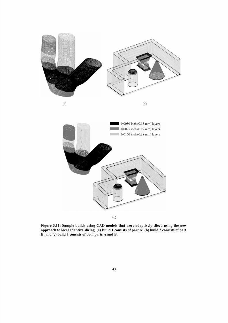
8/13/2019 Slicing Layers
http://slidepdf.com/reader/full/slicing-layers 53/83
43
(a) (b)
(c)
Figure 3.11: Sample builds using CAD models that were adaptively sliced using the newapproach to local adaptive slicing. (a) Build 1 consists of part A; (b) build 2 consists of partB; and (c) build 3 consists of both parts A and B.
0.0050 inch (0.13 mm) layers
0.0075 inch (0.19 mm) layers
0.0150 inch (0.38 mm) layers
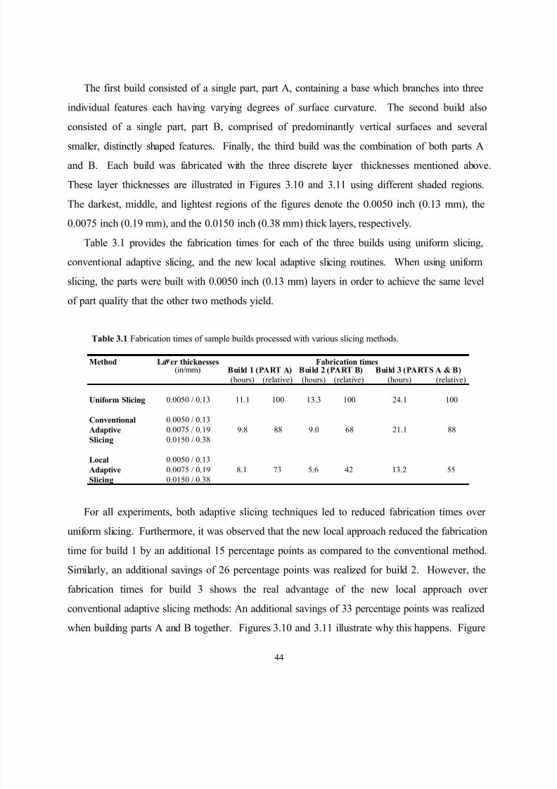
8/13/2019 Slicing Layers
http://slidepdf.com/reader/full/slicing-layers 54/83
44
The first build consisted of a single part, part A, containing a base which branches into three
individual features each having varying degrees of surface curvature. The second build also
consisted of a single part, part B, comprised of predominantly vertical surfaces and several
smaller, distinctly shaped features. Finally, the third build was the combination of both parts A
and B. Each build was fabricated with the three discrete layer thicknesses mentioned above.
These layer thicknesses are illustrated in Figures 3.10 and 3.11 using different shaded regions.
The darkest, middle, and lightest regions of the figures denote the 0.0050 inch (0.13 mm), the
0.0075 inch (0.19 mm), and the 0.0150 inch (0.38 mm) thick layers, respectively.
Table 3.1 provides the fabrication times for each of the three builds using uniform slicing,
conventional adaptive slicing, and the new local adaptive slicing routines. When using uniform
slicing, the parts were built with 0.0050 inch (0.13 mm) layers in order to achieve the same level
of part quality that the other two methods yield.
Table 3.1 Fabrication times of sample builds processed with various slicing methods.
Method La er thicknesses Fabrication times(in/mm) Build 1 (PART A) Build 2 (PART B) Build 3 (PARTS A & B)
(hours) (relative) (hours) (relative) (hours) (relative)
Uniform Slicing 0.0050 / 0.13 11.1 100 13.3 100 24.1 100
Conventional 0.0050 / 0.13Adaptive 0.0075 / 0.19 9.8 88 9.0 68 21.1 88Slicing 0.0150 / 0.38
Local 0.0050 / 0.13Adaptive 0.0075 / 0.19 8.1 73 5.6 42 13.2 55Slicing 0.0150 / 0.38
For all experiments, both adaptive slicing techniques led to reduced fabrication times over
uniform slicing. Furthermore, it was observed that the new local approach reduced the fabrication
time for build 1 by an additional 15 percentage points as compared to the conventional method.Similarly, an additional savings of 26 percentage points was realized for build 2. However, the
fabrication times for build 3 shows the real advantage of the new local approach over
conventional adaptive slicing methods: An additional savings of 33 percentage points was realized
when building parts A and B together. Figures 3.10 and 3.11 illustrate why this happens. Figure

8/13/2019 Slicing Layers
http://slidepdf.com/reader/full/slicing-layers 55/83
45
3.10c, in particular, shows what happens when fabricating multiple parts using conventional
adaptive slicing routines; the complex surfaces of part A cause nearly all of part B to be sliced
with thinner layers than what Figure 3.11b indicates is necessary. On the other hand, the new
local approach slices each part and feature of build 3 independently of the others, so each of the
parts is sliced in exactly the same manner as when it was processed alone (Figure 3.11).

8/13/2019 Slicing Layers
http://slidepdf.com/reader/full/slicing-layers 56/83
46
CHAPTER 4
CALIBRATION OF FUSED DEPOSITION RAPIDPROTOTYPING SYSTEMS FOR FABRICATION WITH
ADAPTIVE BUILD LAYER THICKNESSES
Commercial layered manufacturing (LM) systems have not been designed to accommodate either
adaptive slicing or fabrication with adaptive build layer thicknesses. Most LM systems onlysupport fabrication with uniform build layer thicknesses throughout a given build. Among these
systems is the fused deposition modeler (FDM) rapid prototyping system developed by Stratasys,
Inc., (Eden Prairie, Minnesota). For this system in particular, the standard calibrations of build
parameters for different build layer thicknesses (provided by Stratasys) are out of alignment
relative to one another.
This chapter considers calibration issues for existing FDM rapid prototyping systems. Both
software and hardware issues are discussed. Specifically, t his chapter briefly addresses the
process required to implement adaptive slicing methods using this system. It then provides
background information pertaining to FDM hardware, which includes an overview of initial
attempts to fabricate with adaptive build layer thicknesses, and discusses the resulting poor part
quality that prompted this study. This chapter then outlines experiments used to calibrate a FDM
1600 for fabrication of parts using adaptive build layer thicknesses. Finally, it provides data
obtained from these experiments, and recommends specific build parameter values, based on these
data, that help ensure robust fabrication with this system.

8/13/2019 Slicing Layers
http://slidepdf.com/reader/full/slicing-layers 57/83
47
4.1 FDM SOFTWARE
QuickSlice, the postprocessor provided by Stratasys, Inc. for use with their FDM rapid
prototyping systems, only supports uniform slicing routines; that is, it is only capable of slicing aCAD model with a single build layer thickness throughout. To take advantage of adaptive slicing
techniques with this system, the user must implement independent adaptive slicing routines to
generate the slices from a .STL file, and then output the results in the Stratasys slice file format
(.SSL). Files in this format can then be imported by QuickSlice, which uses the slice data solely
to generate the toolpaths necessary to drive the FDM hardware.
4.2 FDM 1600 HARDWARELayered manufacturing systems fabricate three-dimensional parts by adding layer upon layer of
build material, beginning with the bottom of the part. The FDM rapid prototyping systems, in
particular, achieve this by extruding molten wax or thermoplastic material through a small nozzle
to form a thin bead or “road” that is deposited in a pre-determined pattern to complete each build
layer, bonding the extrudate to adjacent and previously deposited roads. The motion of the
extrusion system operates under three-dimensional computer numerical control (CNC). The
extrusion system consists of a small ram extruder in which the spooled filament feedstock pushesmolten material through the liquefier with low shear. The feedstock is driven into the extruder by
counter rotating rollers as needed under CNC, where it is heated to a manually set temperature,
T L. The extrudate is deposited within a build chamber holding a manually set temperature, T C . In
the case of the FDM 1600 rapid prototyping system, T L and T C can be up to 300°C and 70°C,
respectively.
The cross section of a FDM road has the shape of a flattened ellipsoid that can be
approximated as a rectangle. Its height is given by the layer thickness, i.e., the height of the
nozzle above previously deposited material. With this height being constant, the road width is
controlled by the volumetric flow rate of the material through the liquefier and the speed of the
liquefier (head) XY motion [Argawala96]. This flow rate is primarily dependent upon the ram
speed, the material viscosity, and the nozzle tip dimensions [Comb94]; which can be manipulated

8/13/2019 Slicing Layers
http://slidepdf.com/reader/full/slicing-layers 58/83
48
by varying the roller speed under CNC, by manually varying T L, or by manually changing to a
different nozzle size, respectively. Hence, for a constant material, nozzle, T L and T C combination,
the road width can be determined by CNC of (1) the feed roller speed, (2) the build layer
thickness, and (3) the head travel speed. This control can be pre-computed using QuickSlice
[Stratasys97]. To manage these three parameters, QuickSlice uses look-up tables that are each
based on a constant material, nozzle, T L and T C combination. For instance, given a liquefier head
speed and build layer thickness, QuickSlice will use the lookup table calibrated for a specific
material, nozzle, T L and T C combination, to determine the roller speed (flow rate) that most closely
matches the user-requested road width. This function is shown in Figure 4.1 for the P400 ABS
material ( Stratasys, Inc.) on a FDM 1600 with a T L of 270°C, a T C of 70°C, a 0.012” (0.30 mm)
nozzle, a head speed of 0.800 in/sec (20.3 mm/s), and build layer thicknesses of 0.0050”, 0.0075”,
0.0100”, and 0.0150” (0.13 mm, 0.19 mm, 0.25 mm, and 0.38 mm), respectively.
Stratasys recommends using distinct nozzle diameters, liquefier temperatures T L, and chamber
temperatures T C for various build layer thicknesses [Stratasys97]. However, these
recommendations cannot be adhered to when building with multiple build layer thicknesses
simultaneously, since these parameters cannot be varied under computer control during a given
build. As a result, initial attempts to fabricate adaptively sliced parts while using the default
parameters provided in Figure 4.1 produced (1) delamination, which occurs when consecutive
build layers fail to bond to one another; (2) curling, which can be attributed to residual stresses in
deposited material; (3) surface discontinuities that were particularly apparent when transitioning
between adjacent build layers with dissimilar thicknesses; and (4) surface inaccuracies due to
numerical round off.

8/13/2019 Slicing Layers
http://slidepdf.com/reader/full/slicing-layers 59/83
49
0
20
40
60
80
100
120
140
160
180
200
0.0000 0.0050 0.0100 0.0150 0.0200 0.0250 0.0300 0.0350 0.0400
Road Widths (inches)
F l o w
( R P M / i n / s e c
)
Layer thickness = 0.0150 in
Layer thickness = 0.0100 in
Layer thickness = 0.0075 in
Layer thickness = 0.0050 in
Figure 4.1: The flow rates and corresponding road width values predicted by QuickSlice forthe extrusion of P400 ABS material through a 0.012 inch nozzle at liquefier and envelopetemperatures of 270 and 70 (°C), respectively, with a constant liquefier head speed of 0.8in/sec. The data can be represented by piecewise logarithmic functions.
Several factors contributed to the overall poor quality of these initial parts. Figure 4.1
explains one reason why the surface discontinuities occur. Ideally, the functions relating the flow
rate to the road width should be continuous, both along a curve (reflecting a change in road width
for a given build layer thickness) and from one curve to another (reflecting the transition from one
build layer thickness to another). This, however, is clearly not the case for the QuickSlice lookup
tables (Figure 4.1) which effectively describe a set of piecewise logarithmic curves (solid curves).
One would expect, as is the case, that road widths calculated from these discontinuous build layer
curves will be slightly off target. Furthermore, experiments (described in the next Section)
indicate that, for a given nozzle diameter, the liquefier and chamber temperature settings have a
significant effect on the road width values obtained using particular flow rates and build layer
thicknesses. Indeed, these effects must be accounted for if the build layer thicknesses are to be

8/13/2019 Slicing Layers
http://slidepdf.com/reader/full/slicing-layers 60/83
50
properly calibrated with respect to one another. Finally, the issue of conflicting build parameters
for different build layer thicknesses must be resolved in order to fabricate high quality parts when
using these thicknesses simultaneously.
Past work in FDM calibration has not addressed these particular issues, probably because
researchers have not been concerned with fabricating with multiple build layer thicknesses
simultaneously. Comb et al . [Comb94] discuss various control and material selection parameters
that affect the overall FDM process; Agarwala et al . [Argawala96] address the internal and
surface defects that lead to poor structural quality of parts produced by fused deposition systems;
while Yardimici et al . [Yardimici97] present a thermal analysis of the extrusion process of FDM
systems and the effect of liquefier and nozzle designs on these systems.
4.3 CALIBRATION EXPERIMENTS
Two sets of experiments were conducted using a FDM 1600 rapid prototyping system loaded
with P400 ABS material. The first was designed to gather accurate data pertaining to the
relationship between various feed roller speeds (flow rates) and their resulting road widths for
various build layer thicknesses. The second was designed to assess the effect of T L and T C
combinations, build style, and flow rate values on the overall part quality.
4.3.1 Determi ning Road Width vs. Flow Rate
Road width measurements were obtained by building several series of vertical walls. Each wall
was 2.0” (50 mm) long, 0.25” (6.4 mm) tall, had the width of a single bead, and was assigned a
flow rate value being an even number between 2 and 254 (RPM/inch/sec) [Stratasys97]. Each
series contained up to 21 parallel walls that were given sequentially increasing flow rates, and that
were located about 0.4” (10 mm) apart on a single support material base. This base was placed in
the center of the build chamber, and its walls were oriented in the direction of the heated airflow
in the build chamber, to provide near uniform material cooling.
12 series of walls were fabricated using a nozzle tip diameter of 0.012” (0.30 mm); T L / T C
settings of 270°C / 70°C, 290°C / 70°C, and 290°C / 50°C; and build layer thicknesses of
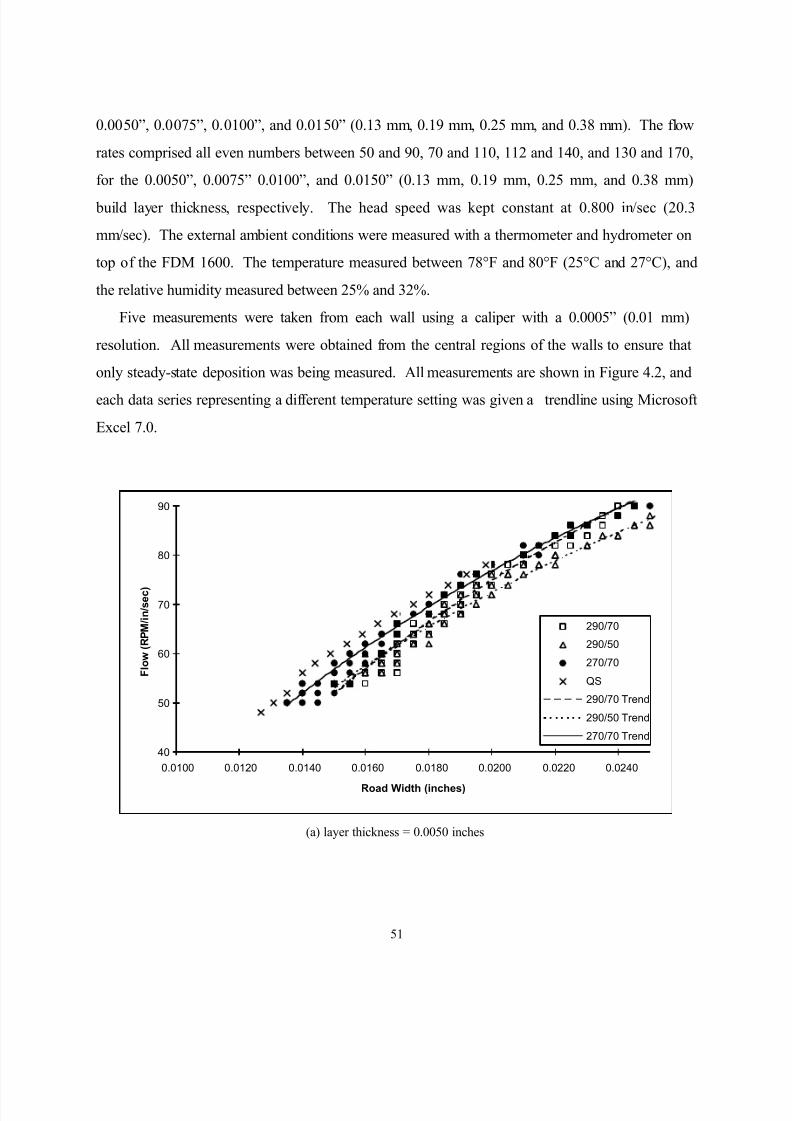
8/13/2019 Slicing Layers
http://slidepdf.com/reader/full/slicing-layers 61/83

8/13/2019 Slicing Layers
http://slidepdf.com/reader/full/slicing-layers 62/83
52
60
70
80
90
100
110
0.0120 0.0140 0.0160 0.0180 0.0200 0.0220 0.0240 0.0260
Road Width (inches)
F l o w
( R P M / i n / s e c
)
290/70
290/50
270/70
QS
290/70 Trend
290/50 Trend
270/70 Trend
(b) layer thickness = 0.0075 inches
100
110
120
130
140
150
0.0160 0.0180 0.0200 0.0220 0.0240 0.0260 0.0280 0.0300
Road Width (inches)
F l o w
( R P M / i n / s e c
)
290/70
290/50
270/70
QS
290/80 Trend
290/50 Trend
270/70 Trend
(c) layer thickness = 0.0100 inches

8/13/2019 Slicing Layers
http://slidepdf.com/reader/full/slicing-layers 63/83
53
120
130
140
150
160
170
0.0170 0.0190 0.0210 0.0230 0.0250 0.0270 0.0290 0.0310
Road Width (inches)
F l o w
( R P M / i n / s e c
)
290/70
290/50
270/70
QS
290/70 Trend
290/50 Trend
270/70 Trend
(d) layer thickness = 0.0150 inches
Figure 4.2: Experimentally collected road width values for specified flow rates at variousliquefier and envelope temperature settings (°C) using P400 ABS material, a 0.012 inchnozzle, and a constant liquefier head speed of 0.8 in/sec.
4.3.2 Assessing Eff ects of Bui ld Parameters on Overal l Par t Quali ty
A solid 1.0” × 1.0” × 0.72” (25 mm × 25 mm × 18 mm) test block consisting of 36, 24, 18, and
12 0.0050”, 0.0075”, 0.0100”, and 0.0150” (0.13 mm, 0.19 mm, 0.25 mm, and 0.38 mm) build
layers, respectively, was fabricated repeatedly to assess the specific build parameters T L, T C , build
style, and flow rate, on the overall part quality. Five samples of this block were built using a
0.012” (0.30 mm) nozzle, 0.800 in/sec (20.3 mm/sec) head speed, and the respective parameters
listed in Table 4.1. The T L / T C were set at 270°C / 70°C and 290°C / 50°C since Stratasys, Inc.
recommends these values for fabricating with 0.0100” (0.25 mm) and 0.0070” (0.18 mm) build
layer thicknesses, respectively [Stratasys97]. The build styles tested were contour, where the
roads were deposited first at the perimeter and then progressively in towards the center for each
layer, and raster patterns. Each of the five parts was built in the same location and orientation in

8/13/2019 Slicing Layers
http://slidepdf.com/reader/full/slicing-layers 64/83
54
the center of the build chamber to minimize the possible effects of non-uniform transverse
cooling.
Table 4.1: Build parameter sets used for experimental builds.
Liquefier/Envelope Flow Rate/Road Width (in) ValuesPart Build Style Temp. Settings (°C) 0.0050 0.0075 0.0100 0.015 A contour (Out-In) 270/70 56/0.014 78/0.014 118/0.020 140/0.020B contour (Out-In) 270/70 76/0.020 102/0.020 118/0.020 140/0.020C Raster 270/70 76/0.020 102/0.020 118/0.020 140/0.020D Raster 290/50 56/0.014 78/0.014 118/0.020 140/0.020E Raster 290/50 76/0.020 102/0.020 118/0.020 140/0.020
4.4 RESULTS
4.4.1 Road Width Cali bration
Figure 4.2 shows that discrepancies exist between the experimental road width data and the
default data used by QuickSlice. The most significant discrepancies are due to changes in the T L
and T C settings. However, for the 0.0050” (0.13 mm) and 0.0150” (0.38 mm) build layer
thicknesses, the QuickSlice data are inconsistent with any temperature setting (Figures 4.2a and
4.2d); in the first case with the QuickSlice estimated road width being less than the measured road
width, while in the latter case it being opposite. Furthermore, Figure 4.2c shows that the
QuickSlice road width estimates perfectly match the experimental data for the 0.012” (0.30 mm)
nozzle, 0.010” (0.25 mm) build layer thickness, 0.020” (0.51 mm) road width, and T L / T C of
270°C / 70°C combination; which is the standard build parameter combination recommended by
Stratasys, Inc. [Stratasys97]. These results explain (1) why Stratasys, Inc. prefers that customers
consistently use the standard parameter combination, and (2) why current QuickSlice flow rates
and road widths perform poorly when used in adaptive slicing.
Figure 4.2 shows that a 20°C increase in liquefier temperature T L from 270°C to 290°C
reduces the measured road width by about 0.001” (0.025 mm) in the cases of 0.0100” (0.25 mm)and 0.0150” (0.38 mm) build layer thicknesses, while it has only an insignificant effect in the cases
of 0.0050” (0.13 mm) and 0.0075” (0.19 mm) build layer thicknesses. It also shows that a 20°C
decrease in build chamber temperature T C from 70°C to 50°C increases the measured road width

8/13/2019 Slicing Layers
http://slidepdf.com/reader/full/slicing-layers 65/83
55
by nearly 0.001” (0.025 mm) in the cases of 0.0050” (0.13 mm) and 0.0075” (0.19 mm) build
layer thicknesses, while it has only an insignificant effect in the cases of 0.0100” (0.25 mm) and
0.0150” (0.38 mm) build layer thicknesses. Finally, Figure 4.2 shows that when combining these
changes in T L and T C the measured road width increased by about 0.001” (0.025 mm) in the cases
of 0.0050” (0.13 mm) and 0.0075” (0.19 mm) build layer thicknesses, and decreased by about the
same amount in the cases of 0.0100” (0.25 mm) and 0.0150” (0.38 mm) build layer thicknesses.
Increasing T L will, for thick roads, add heat to the extrudate, and thus increase the time during
which the material experiences significant shrinkage. Thick roads will therefore shrink as T L
increases. Thin roads, on the other hand, will continue to cool down too fast to significantly
increase shrinkage, and they will therefore not experience a change in measured road width.
Decreasing T C will, for thin roads, prevent the extrudate from heating up existing material to
above the softening point (105°C). The existing material will therefore not yield to the pressure
exerted by the extrudate, which causes the extrudate to escape outwards to create a wider road.
Thick roads, on the other hand, contain sufficient heat so the extrudate can continue to bring
existing material to above the softening point. This causes the existing material to continue to
yield to the extrudate pressure, and hence there is no change in measured road width.
4.4.2 Eff ects of Numeri cal Round Off
Imperfect surface transitions between adjacent build layers of dissimilar thicknesses can also be
caused by numerical round off. The flow rates selected represent discrete road widths at given
build layer thicknesses. These road widths can be carried through the road path calculations as
high resolution floating point numbers, and up until this point, any numerical round off would be
insignificant. However, these floating point values need, in the case of current FDM equipment,
to be rounded off to the closest 0.001” (0.025 mm) XY coordinate to reflect the programming
resolution of the FDM’s XY controller. This round off can easily cause a 0.001” (0.025 mm)
mismatch within any two build layers. This mismatch will in general be particularly noticeable
between two adjacent build layers of dissimilar thicknesses since the round off error adds to errors

8/13/2019 Slicing Layers
http://slidepdf.com/reader/full/slicing-layers 66/83
56
in the road width estimation function (however small they might be, they will most likely be
present). Figure 4.3 illustrates this problem.
( 0.000, 1.000) ( 1.000, 1.000)
. , . . , .
(0.000, 1.000) ( 1.001, 1.000)
. , . . , .
1.0003 in 1.0003 in
1.0000 in 1.0000 in+ 0.0004
Figure 4.3: Numerical round off can change final fabricated dimensions, here shown for a1.0003” × 1.0000” rectangle before and after a 0.0004” translation in the X direction.
Consider a rectangular cylinder measuring 1.0003” × 1.0000” (25.408 mm × 25.400 mm).
Due to numerical round off, it will be manufactured as a perfect 1.000” × 1.000” (25.400 mm ×25.400 mm) square. Now move the original cylinder 0.0004” (0.010 mm) in the positive X
direction. This would simulate the change in road path offset due to a slight change in road
width, which invariably occurs as one transitions from one build layer thickness to another. The
size of the virtual cylinder will thus remain the same; however, the new manufactured cylinder will
now measure 1.001” × 1.000” (25.425 mm × 25.400 mm) and will no longer be perfectly square.
The build layer thickness transitional errors appeared to being limited to not much more than
that which arises from numerical round off. This was in part determined by using a sheet of paper
(0.0035”, 0.09 mm) to gauge the relative magnitude of the build layer thickness transitional
surface discontinuities.
4.4.3 Overall Part Quality
As described in the previous Section, a 1.0” x 1.0” x 0.72” test block was fabricated five times.
Each test block consisted of 36 0.0050” (0.13 mm), 24 0.0075” (0.19 mm), 18 0.0100” 0.25
mm), and 12 0.015” (0.38 mm) layers, with the layer thicknesses increasing in the vertical (z)
direction. Each build implemented a set of parameters given in Table 4.1. Profiles of the resulting
parts, a through e, are shown in Figures 4.4a-e, respectively. By comparing these individual

8/13/2019 Slicing Layers
http://slidepdf.com/reader/full/slicing-layers 67/83
57
parts, it can be concluded that the highest part quality is obtained using a raster build style with T L
= 290°C (Figures 4.4d,e). It was also found that part quality improved if the build chamber
temperature T C simultaneously was reduced to 50°C, which is in accordance with the
recommendations provided by Stratasys, Inc. for fabricating with 0.007” (0.18 mm) build layers
[Stratasys97]. In addition, a thicker road width seems better suited for the 0.0050” and 0.0075”
(0.13 and 0.19 mm) layer thicknesses when using the 0.0120” (0.30 mm) tip. Hence, the flow
rates for these layers must be adjusted because they are originally set by Stratasys to produce road
widths of 0.014” (0.36 mm).
a b c d e
Figure 4.4: Parts fabricated from adaptively sliced geometry using P400 ABS plasticmaterial and the parameter sets given in Table 4.1.
It should be noted that the 0.0050” and 0.0075” (0.13 and 0.19 mm) layers contributed most
to the poor quality of each part, especially at the lower liquefier temperature (Figures 4.4a-c).
This is likely the result of increased viscoelastic stresses in the deposited material of these thinner layers. Fortunately, the curling and delamination effects are virtually eliminated when increasing
the liquefier temperature (Figures 4.4d,e).
Sperling [Sperling92] presents the viscosity of polymer material as
η = Ae E a RT (4.1)
where A is a material specific constant, E a is the activation energy of the polymer, R is the
universal gas constant, and T is the absolute temperature of the material. Furthermore, he
expresses the relaxation time of polymers as
τ η=
E (4.2)
where E is Young’s modulus. Finally, the viscoelastic behavior of the material can be modeled as
x
z

8/13/2019 Slicing Layers
http://slidepdf.com/reader/full/slicing-layers 68/83
58
σ σ τ= −o
t
e (4.3)
where σ represents the mechanical stresses in the material, and t represents time.
From these equations, it can be observed that increasing the temperature of the extrudate
decreases its viscosity, thereby reducing the relaxation time of the polymer, which subsequently
reduces its mechanical stresses. Hence, the curling and delamination that was present in parts a , b
and c is significantly reduced for parts d and e, which were built at the higher liquefier
temperature. Thus, it is recommended that the liquefier temperature be increased when
fabricating with multiple build layer thicknesses simultaneously in order to accommodate the
higher viscoelastic stresses of the thinner layers used.
8/13/2019 Slicing Layers
http://slidepdf.com/reader/full/slicing-layers 69/83
59
CHAPTER 5
CONCLUSIONS AND CONTRIBUTIONS
This thesis has presented a new method that significantly reduces the fabrication time associated
with conventional adaptive slicing procedures. It has also presented a calibration procedure for
the Fused Deposition Modeler rapid prototyping system that facilitates the fabrication of accurate,
adaptively sliced parts by improving the dimensional accuracy of the transitions between different
layer thicknesses, and by identifying build parameters that help ensure high part quality. Actual
parts have been produced to demonstrate both aspects of this work. This research representsimportant steps toward the realization of a truly fast and accurate layered manufacturing process.
5.1 CONCLUDING REMARKS
The new approach to adaptive slicing, presented in this thesis, is limited to polyhedral CAD
models such as those described in the .STL file format. The .STL format, however, is the de
facto industry standard and is supported by all commercial layered manufacturing systems.
Therefore, the new approach could be implemented in any of these LM processes, provided that
the software is modified to output the slice data in the appropriate format. Currently, the
software generates slice data for the FDM rapid prototyping system only.
The potential advantage that can be realized by this new method is critical to the layered
manufacturing industry. In particular, users of FDM systems may benefit from enormous savings
in fabrication time. The potential for savings is directly proportional to the number of individual
parts and/or part features in a given build, and their respective differences in geometry. Hence,
this new method is ideal for users in industry who typically optimize fabrication by buildingmultiple parts simultaneously.

8/13/2019 Slicing Layers
http://slidepdf.com/reader/full/slicing-layers 70/83
60
5.2 CONTRIBUTIONS
This thesis addresses the inefficiencies of current adaptive slicing procedures, as well as the issue
of reducing these procedures to practice. Specifically, this thesis has made the followingcontributions:
Efficient adaptive layered manufacturing : The feasibility and advantage of adaptively slicing
individual parts and part features independently of one another has been demonstrated. This new
method overcomes the limitations of conventional adaptive slicing routines by accounting for
differences in surface geometry in three dimensions. Rather than consider only the differences in
surface geometry from one height to the next, the new procedure utilizes topology-based feature
extraction to separate individual surfaces at each build height so that they may be treated
independently. The result is the elimination of unnecessary layers and, hence, reduced fabrication
times.
FDM calibration for adaptive build layer thicknesses : The ability to manufacture accurate,
adaptively sliced parts using the FDM system has been demonstrated. In particular, a calibration
procedure has been presented that reduces the inaccuracies that occur when transitioning between
dissimilar build layer thicknesses. Prior to this work, commercial layered manufacturing systems
have not supported multiple build layer thicknesses concurrently. Consequently, little concern has
been given to the variations in calibration accuracy when transitioning from one layer thickness to
another. This thesis has demonstrated that this variation in calibration should be of concern, and
it has demonstrated how these problems can be overcome. Specifically, experiments have been
conducted to determine the effects of critical FDM build parameters, including the flow rate, and
the liquefier and chamber temperatures, on the quality of fabricated parts. These observations
were then used to recommend parameter values that will consistently produce highly accurate
parts.

8/13/2019 Slicing Layers
http://slidepdf.com/reader/full/slicing-layers 71/83
61
5.3 RECOMMENDATIONS FOR FUTURE WORK
This thesis presents important contributions to the layered manufacturing industry; however,
several aspects must be properly completed to ensure its acceptance. The following should beinvestigated:
Support generation : Fabrication of overhang structures requires that temporary support structures
be built. At present, the new local adaptive slicing procedure does not have a companion support
generation procedure that is capable of generating support structures for locally adaptive parts.
Developing such a support generation procedure is non-trivial. Consider, for example, the
merging of two features that require support structures, and whose surfaces call for different build
layer thicknesses. Such an occurrence would cause support layers of different thicknesses to
merge as well. At a minimum, a method that possesses the ability to adequately handle this and
other situations when generating support structures must be developed before parts that require
them can be manufactured.
Incorporation with existing methods : Several adaptive slicing methods have been introduced
which enhance the speed and accuracy of layered manufacturing processes. Some of these make
good candidates for integration with the approach developed in this thesis. Specifically, the
incorporation of the high-precision exterior, high-speed interior layered manufacturing process
developed by Sabourin et al . [Sabourin96a] [Sabourin97] would produce a truly efficient
fabrication process.
8/13/2019 Slicing Layers
http://slidepdf.com/reader/full/slicing-layers 72/83
62
REFERENCES
[Argawala96] Argawala, M. K., Jamalabad, V. R., Langrana, N. A., Safari, A., Whalen, P. J.,and Danforth, S. C., “Structural Quality of Parts Processed by Fused
Deposition,” Rapid Prototyping Journal , vol. 2, no. 4, 1996, pp. 4-19.
[Beaman97] Beaman, J. J., Barlow, J. W., Bourell, D. L., Crawford, R. H., Marcus, H. L.,
and McAlea, K. P., Solid Freeform Fabrication: A New Direction in
Manufacturing , Klewar Academic Publishers, Norwell, Massachusetts, USA,
1997.
[Bøhn89] Bøhn, J. H., “Computing the Unit Normal for NURBS Surfaces,” M.S. Thesis,Rensselaer Polytechnic Institute, Troy, New York, USA, December, 1989.
[Bøhn93a] Bøhn, J. H., and Wozny, M. J., “A Topology-Based Approach for Shell-
Closure,” in: Wilson, P. R., et al ., eds., Geometric Modeling for Product
Realization , IFIP Transactions B-8, Elsevier Science Publishers B. V. (North-
Holland), Amsterdam, 1993, pp. 297-319.
[Bøhn93b] Bøhn, J. H., Automatic CAD Model Repair , Ph.D. thesis, Rensselaer Polytechnic
Institute, Troy, New York, USA, August 1993.
[Brock91] STH File Format , Brock Rooney and Associates, Inc., Birmingham, Michigan,
USA, 1991.
[Burns93] Burns, M., Automated Fabrication; Improving Productivity in Manufacturing ,
PTR Prentice Hall, Englewood Cliffs, New Jersey, USA, 1993.
[CLI98] Common Layer Interface (CLI), version 2.0, Available:
http://www.cranfield.ac.uk/coa/rapid/cli/cli_v20.html [January 22, 1998].
[Comb94] Comb, J. W., Priedeman, W. R., and Turley, P. W., “FDM Technology Process
Improvements,” Proceedings, Solid Freeform Fabrication Symposium , Marcus,
H. L., et al., eds., University of Texas at Austin, Austin, Texas, USA, August
8-10, 1994, pp. 42-49.

8/13/2019 Slicing Layers
http://slidepdf.com/reader/full/slicing-layers 73/83
63
[de Jager97] de Jager, P. J., Broek, J. J., and Vergeest, J. S. M., “Using Adaptive Ruled
Layers for Rapid Prototyping: Principles and First Results,” Proceedings, Solid
Freeform Fabrication Symposium , Bourell, D. L., et al ., eds., University of
Texas at Austin, Austin, Texas, USA, August 11-13, 1997, pp. 585-592.
[Dolenc94] Dolenc, A. and Mäkelä, I., “Slicing Procedures for Layered Manufacturing
Techniques,” Computer-Aided Design , vol. 26, no. 2, February 1994, pp. 119-
126.
[Fadel96] Fadel, G. M., and Kirschman, C., “Accuracy Issues in CAD to RP Translation,”
Rapid Prototyping Journal , vol. 2, no. 2, 1996, pp. 4-17.
[Guduri92] Guduri, S., Crawford, R. H., and Beaman, J. J., “A Method to Generate Exact
Contour Files for Solid Freeform Fabrication,” Proceedings, Solid Freeform
Fabrication Symposium , Marcus, H. L., et al ., eds., University of Texas at
Austin, Austin, Texas, USA, August 3-5, 1992, pp. 95-101.
[Hope97a] Hope, R. L., Jacobs, P. A., and Roth, R. N., “Rapid Prototyping with Sloping
Surfaces,” Rapid Prototyping Journal , vol. 3, no. 1, 1997, pp. 12-19.
[Hope97b] Hope, R. L., Jacobs, P. A., and Roth, R. N., “Adaptive Slicing with Sloping
Layer Surfaces,” Rapid Prototyping Journal , vol. 3, no. 3, 1997, pp. 89-98.
[Jamieson95] Jamieson, R., and Hacker, H., “Direct Slicing of CAD Models for Rapid
Prototyping,” Rapid Prototyping Journal , vol. 1, no. 2, 1995, pp. 4-12.
[Keppel75] Keppel, E., “Approximating Complex Surfaces by Triangulation of Contour
Lines,” IBM Journal of Research and Development , vol. 19, no. 1, pp. 2-11.
[Kirschman92] Kirschman, C. F., and Jara-Almonte, C. C., “A Parallel Slicing Algorithm for
Solid Freeform Fabrication Processes,” Proceedings, Solid Freeform
Fabrication Symposium , Marcus, H. L., et al ., eds., University of Texas at
Austin, Austin, Texas, USA, August 3-5, 1992, pp. 26-33.[Klingbeil97] Klingbeil, N. W., Zinn, J. W., and Beuth, J. L., “Measurement of Residual Stress
in Parts Created by Shape Deposition Manufacturing,” Proceedings, Solid

8/13/2019 Slicing Layers
http://slidepdf.com/reader/full/slicing-layers 74/83
64
Freeform Fabrication Symposium , Bourell, D. L., et al ., eds., University of
Texas at Austin, Austin, Texas, USA, August 11-13, 1997, pp. 125-132.
[Krause97] Krause, F. L., Ulbrich, A., Ciesla, M., Klocke, F., and Wirtz, H., “Improving
Rapid Prototyping Processing Speeds by Adaptive Slicing,” Proceedings, Sixth
European Conference on Rapid Prototyping and Manufacturing , Dickens, P.
M., ed., Nottingham, UK, July 1-3, 1997, pp. 31-36.
[Kulkarni95] Kulkarni, P., and Dutta, D., “Adaptive Sli cing for Parameterizable Surfaces for
Layered Manufacturing,” Proceedings, ASME Design Engineering Technical
Conference , Azarm, S., et al ., eds., Boston, Massachusetts, USA, September
17-20, 1995, DE-Vol. 82-1, pp.211-217.
[Kulkarni96] Kulkarni, P., and Dutta, D., “An Accurate Slicing Procedure for Layered
Manufacturing,” Computer-Aided Design , vol. 28, no. 9, September 1996, pp.
683-697.
[Merz94] Merz, R., Prinz, F. B., Ramaswami, K., Terk, M., and Weiss, L. E., “Shape
Deposition Manufacturing,” Proceedings, Solid Freeform Fabrication
Symposium , Marcus, H. L., et al ., eds., University of Texas at Austin, Austin,
Texas, USA, August 8-10, 1994, pp. 1-8.
[O’Rourke94] O’Rourke, J., Computational Geometry in C , Cambridge University Press, 1994.
[Reeves97] Reeves, P. E., Dickens, P. M., Davey, N., and Cobb, R. C., “Surface Roughness
of Stereolithography Models Using an Alternative Build Strategy,” Proceedings,
Sixth European Conference on Rapid Prototyping and Manufacturing , Dickens,
P. M., ed., Nottingham, UK, July 1-3, 1997, pp. 85-94.
[Rock91a] Rock, S. J., and Wozny, M. J., “A Flexible File Format for Solid Freeform
Fabrication,” Proceedings, Solid Freeform Fabrication Symposium , Marcus, H.
L., et al., eds., University of Texas at Austin, Austin, Texas, USA, August 12-14, 1991, pp. 1-11.
[Rock91b] Rock, S. J., and Wozny, M. J., “Utilizing Topological Information to Increase
Scan Vector Generation Efficiency,” Proceedings, Solid Freeform Fabrication

8/13/2019 Slicing Layers
http://slidepdf.com/reader/full/slicing-layers 75/83
65
Symposium , Marcus, H. L., et al ., eds., University of Texas at Austin, Austin,
Texas, USA, August 12-14, 1991, pp. 28-36.
[Rock92] Rock, S. J., and Wozny, M. J., “Generating Topological Information from a
Bucket of Facets,” Proceedings, Solid Freeform Fabrication Symposium ,
Marcus, H. L., et al ., eds., University of Texas at Austin, Austin, Texas, USA,
August 3-5, 1992, pp. 251-258.
[Sabourin96a] Sabourin, E., “Adaptive High-Precision Exterior, High-Speed Interior, Layered
Manufacturing,” M.S. Thesis, Virginia Polytechnic Institute and State
University, Blacksburg, Virginia, USA, February, 1996.
[Sabourin96b] Sabourin, E., Houser, S. A., and Bøhn, J. H., “Adaptive Slicing Using Stepwise
Uniform Refinement,” Rapid Prototyping Journal , vol. 2, no. 4, 1996, pp. 20-
26.
[Sabourin97] Sabourin, E., Houser, S. A., and Bøhn, J. H., “Accurate Exterior, Fast Interior
Layered Manufacturing,” Rapid Prototyping Journal , vol. 3, no. 2, 1997, pp.
44-52.
[Sachs97] Sachs, E., Allen, A., Honglin, G., Banos, J., Cima, M., Serdy, J., and Brancazio,
D., “Progress on Tooling by 3D Printing; Conformal Cooling, Dimensional
Control, Surface Finish and Hardness,” Proceedings, Solid Freeform
Fabrication Symposium , Bourell, D. L., et al ., eds., University of Texas at
Austin, Austin, Texas, USA, August 11-13, 1997, pp. 115-123.
[Sperling92] Sperling, L. H., Introduction to Physical Polymer Science, 2 nd Edition , John
Wiley and Sons, Inc., 1992, pp. 467-487.
[Stratasys97] QuickSlice 5.0, Stratasys, Inc., Eden Prairie, Minnesota, USA, 1997.
[Suh94] Suh, Y. S., and Wozny, M. J., “Adaptive Slicing of Solid Freeform Fabrication
Processes,” Proceedings, Solid Freeform Fabrication Symposium , Marcus, H.L., et al ., eds., University of Texas at Austin, Austin, Texas, USA, August. 8-10,
1994, pp. 404-411.

8/13/2019 Slicing Layers
http://slidepdf.com/reader/full/slicing-layers 76/83
66
[Thomas96] Thomas, C. L., Gaffney, T. M., Kaza, S., and Lee, C. H., “Rapid Prototyping of
Large Scale Aerospace Structures,” Proceedings, 1996 IEEE Aerospace
Applications Conference, Profet, R., chair, Aspen, Colorado, USA, February 4-
11, 1996, Vol. 4, pp. 219-230.
[USPro96] US Product Data Association, Initial Graphics Exchange Specification (IGES) ,
version 5.3, IGES/PDES Organization, 1996.
[Vuyyuru94] Vuyyuru, P., Kirschman, C. F., Fadel, G., Baghi, A., and Jara-Almonte, C. C.,
“A NURBS-Based Approach for Rapid Product Realization,” Proceedings, Fifth
International Conference on Rapid Prototyping , Chartoff, R. P., et al ., eds.,
University of Dayton, Dayton, Ohio, USA, June 12-15, 1994, pp. 229-240.
[Yardimici97] Yardimici, M. A., Hattori, T., Guceri, S.I., and Danforth, S.C., “Thermal
Analysis of Fused Deposition,” Proceedings, Solid Freeform Fabrication
Symposium , Bourell, D. L., et al ., eds., University of Texas at Austin, Austin,
Texas, USA, August 11-13, 1997, pp. 689-698.
[Zheng97] Zheng, Y., and Newman, W. S., “Software Design Challenges for Computer-
Aided Manufacturing of Laminated Engineering Materials (CAM-LEM),”
Proceedings, Sixth European Conference on Rapid Prototyping and
Manufacturing , Dickens, P. M., ed., Nottingham, UK, July 1-3, 1997, pp. 21-30.

8/13/2019 Slicing Layers
http://slidepdf.com/reader/full/slicing-layers 77/83
67
APPENDIX A: GEOMETRIC PROOFS
As described in Section 2.5, Kulkarni and Dutta [Kulkarni95] [Kulkarni96] compute adaptive
build layer thickness values to match the vertical surface curvature at a point P by assuming that
the surface at P can be approximated by a sphere whose radius is equivalent to the vertical
curvature at that point. Specifically, they site four possible configurations that must be handled
when using this method (Figure A.1). This appendix provides derivations for the four
independent expressions that were developed using the geometry shown in each of these
configurations. These derivations were not presented in [Kulkarni95] [Kulkarni96].

8/13/2019 Slicing Layers
http://slidepdf.com/reader/full/slicing-layers 78/83
68
ρ
NP
d
θδρ N
P
d
α
δ
θ
(a) (b)
θ
δ
ρ
N
P
d
ρ
N
P
d
θ
α
δ
(c) (d)
P: a point on the part surface
N: the surface normal at P
θ: the angle that N makes to the horizontal
ρ: the radius of curvature at P
δ: the allowed cusp height
d: the layer thickness to be computed
Figure A.1: Four possible configurations that may be encountered when using the buildlayer thickness approximation method developed by Kulkarni and Dutta; (a) convexcurvature on upper hemisphere; (b) concave curvature on upper hemisphere; (c) convexcurvature on lower hemisphere; and (d) concave curvature on lower hemisphere;[Kulkarni96]

8/13/2019 Slicing Layers
http://slidepdf.com/reader/full/slicing-layers 79/83
69
Configuration (a):
By applying the law of cosines to the shaded triangle in Figure A.1a, equation (A.1) is produced,
)90cos(2)( 222 αρρδρ −−+=− d d (A.1)
where (90 - α ) is the included angle between sides ρ and d . Using the definitioncos(90 - α ) = sin α , (A.1) reduces to
αρρδρδρ sin22 2222 d d −+=+−
which can be further simplified to obtain
0)2(sin2 22 =−+− δρδαρd d (A.2)
It is clear thatθραρ sinsin +=d (A.3)
By substituting (A.3) into (A.2) and simplifying, it can be shown that
0)2()sin2( 22 =−−+ δρδθρ d d (A.4)
The build layer thickness d can now be determined using the quadratic equation:
2)2(4sin4sin2
222
δρδθρθρ −++−=d
Finally, after simplifying,
222 2sinsin δρδθρθρ −++−=d (A.5)

8/13/2019 Slicing Layers
http://slidepdf.com/reader/full/slicing-layers 80/83
70
Configuration (b):
By applying the law of cosines to the shaded triangle in Figure A.1b, equation (A.6) is produced,
)90cos(2)( 222 θρρδρ +−+=+ d d (A.6)
where (90 + θ) is the included angle between sides ρ and d . Using the definitioncos(90 + θ) = -sin θ, (A.6) reduces to
θρρδρδρ sin22 2222 d d ++=++
which can be further simplified to obtain
0)2()sin2( 22 =+−+ δρδθρ d d (A.7)
The build layer thickness d can now be determined using the quadratic equation:
2
)2(4sin4sin2 222 δρδθρθρ +++−=d
Finally, after simplifying,
222 2sinsin δρδθρθρ +++−=d (A.8)

8/13/2019 Slicing Layers
http://slidepdf.com/reader/full/slicing-layers 81/83
71
Configuration (c):
By applying the law of cosines to the shaded triangle in Figure A.1c, equation (A.9) is produced,
)90cos(2)( 222 θρρδρ −−+=− d d (A.9)
where (90 - θ) is the included angle between sides ρ and d . Using the definitioncos(90 - θ) = sin θ, (A.9) reduces to
θρρδρδρ sin22 2222 d d −+=+−
which can be further simplified to obtain
0)2()sin2( 22 =−+− δρδθρ d d (A.10)
The build layer thickness d can now be determined using the quadratic equation:
2
)2(4sin4sin2 222 δρδθρθρ −−−=d
Finally, after simplifying,
222 2sinsin δρδθρθρ +−−=d (A.11)

8/13/2019 Slicing Layers
http://slidepdf.com/reader/full/slicing-layers 82/83
72
Configuration (d):
By applying the law of cosines to the shaded triangle in Figure A.1d, equation (A.12) is produced,
)90cos(2)( 222 αρρδρ +−+=+ d d (A.12)
where (90 + α ) is the included angle between sides ρ and d . Using the definitioncos(90 + α ) = -sin α , (A.12) reduces to
αρρδρδρ sin22 2222 d d ++=++
which can be further simplified to obtain
0)2(sin2 22 =+−+ δρδαρd d (A.13)
It is clear thatd −= θραρ sinsin (A.14)
By substituting (A.14) into (A.13) and simplifying, it can be shown that
0)2()sin2( 22 =++− δρδθρ d d (A.15)
The build layer thickness d can now be determined using the quadratic equation:
2)2(4sin4sin2
222
δρδθρθρ +−−=d
Finally, after simplifying,
222 2sinsin δρδθρθρ −−−=d (A.16)

8/13/2019 Slicing Layers
http://slidepdf.com/reader/full/slicing-layers 83/83
VITA
My older twin sister and I were born in Washington, DC, on May 8, 1973. My parents saw to itthat I would become independent (and stubborn) by conceiving two more daughters. When I
wasn’t sequestering myself in my room, doing homework, I was usually out playing on the soccer
field or running around a large oval track. Through my schooling and athletics, I learned
dedication and perseverance. I spent most of my childhood in Southeastern NY (Peekskill), but
attended high school in the outskirts of Philadelphia, PA. I decided to matriculate at Virginia
Tech because of its outstanding reputation in engineering, and because it was a seven hour drive
from my parents. After earning a bachelor’s degree in Aerospace Engineering, and gainingvaluable work experience while building submarines at General Dynamics, Electric Boat Division
in Groton, CT, I decided to pursue a Master’s degree in Mechanical Engineering. Not wanting to
leave Blacksburg, I remained at Virginia Tech where I was introduced to the world of CAD/CAM
and rapid prototyping. I spent the summer of 1997 in Plantation, FL where I worked as an intern
at Motorola, Land Mobile Products Center. Through my experiences I have discovered an
appreciation for programming, and I plan to develop my skills in this area in my future endeavors.
Related Documents