7.1 SKEWNESS The literally meaning of 'skewness' is 'lack of symmetry' . Skewness is opposite to symmetry and its presence tells us that a particular distribution is not symmetrical. A distribution is said to be symmetrical when mean, median and mode are identical or coincide. A symmetrical distribution when plotted on a graph give a perfectly bell-shaped curve as shown in the figure. A distribution said to be skewed if its frequency curve is not symmetrical but it is stretched more on one side than of skewness to the other side. Mean = Mode = Median Fig. 7.1 : Symmetrical curve 7.2 DEFINITION OF SKEWNESS Various statisticians defined skewness in the following various ways : .. "Skewness is the lack of symmetry. When a frequency distribution is plotted on a chart, skewness present in the series tends to be dispersed more on one side of the mean than on the other". - Riggleman and Frisbee "Skewness or asymmetry is the attribute of a frequency distribution that extends further on one side of the class with the highest frequency that on the other". - Simpson and Kafka "When a series is not symmetrical it is said to be asymmetrical or skewed". - Croxton and Cowden 131 Arora, P.N., and P.K. Malhan. Biostatistics, Global Media, 2009. ProQuest Ebook Central, http://ebookcentral.proquest.com/lib/ugmartyrsu-ebooks/detail.action?docID=3011262. Created from ugmartyrsu-ebooks on 2021-10-13 19:11:48. Copyright © 2009. Global Media. All rights reserved.

Welcome message from author
This document is posted to help you gain knowledge. Please leave a comment to let me know what you think about it! Share it to your friends and learn new things together.
Transcript

7.1 SKEWNESS The literally meaning of 'skewness' is 'lack of symmetry' . Skewness is opposite to symmetry
and its presence tells us that a particular distribution is not symmetrical.
A distribution is said to be symmetrical when mean, median and mode are identical or coincide.
A symmetrical distribution when plotted on a graph give a perfectly bell-shaped curve as shown in the figure. A distribution said to be skewed if its frequency curve is not symmetrical but it is stretched more on one side than of skewness to the other side.
Mean = Mode = Median
Fig. 7.1 : Symmetrical curve
7.2 DEFINITION OF SKEWNESS Various statisticians defined skewness in the following various ways :
.. ~. "Skewness is the lack of symmetry. When a frequency distribution is plotted on a chart,
skewness present in the series tends to be dispersed more on one side of the mean than on the other". - Riggleman and Frisbee
"Skewness or asymmetry is the attribute of a frequency distribution that extends further on one side of the class with the highest frequency that on the other". - Simpson and Kafka
"When a series is not symmetrical it is said to be asymmetrical or skewed". - Croxton and Cowden
131
Arora, P.N., and P.K. Malhan. Biostatistics, Global Media, 2009. ProQuest Ebook Central, http://ebookcentral.proquest.com/lib/ugmartyrsu-ebooks/detail.action?docID=3011262.Created from ugmartyrsu-ebooks on 2021-10-13 19:11:48.
Cop
yrig
ht ©
200
9. G
loba
l Med
ia. A
ll rig
hts
rese
rved
.
132 Biostatistics
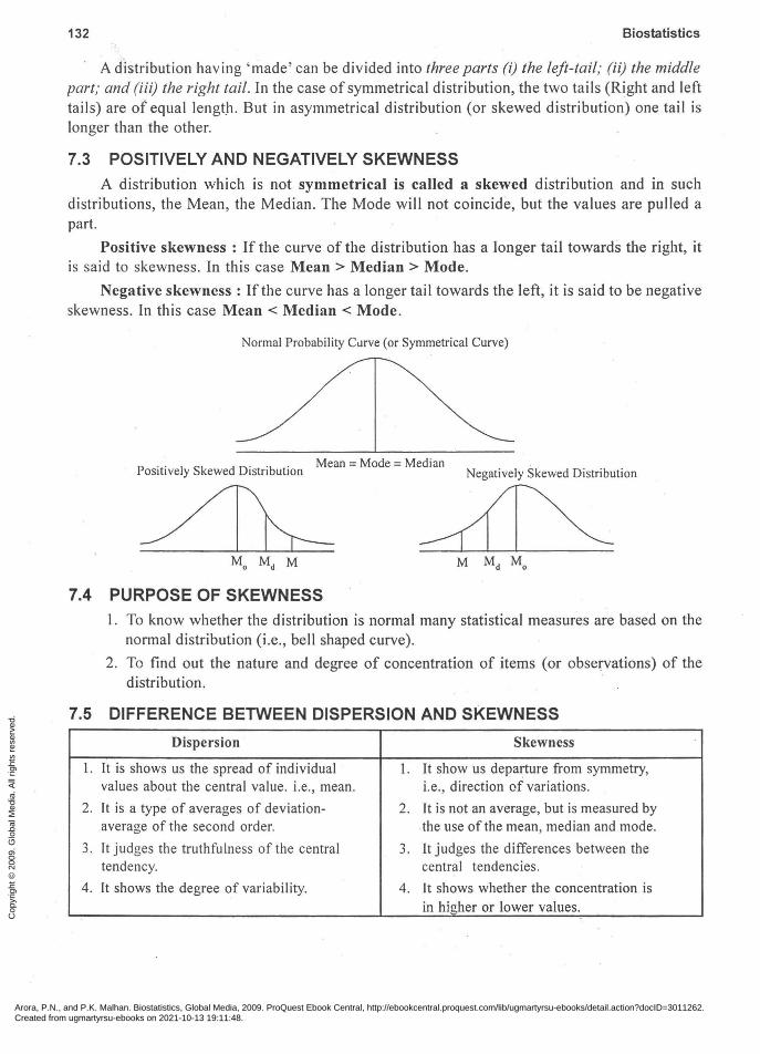
A distribution having 'made' can be divided into three parts (i) the left-tail; (ii) the middle part; and (iii) the right tail. In the case of symmetrical distribution, the two tails (Right and left tails) are of equal length. But in asymmetrical distribution (or skewed distribution) one tail is longer than the other.
7.3 POSITIVELY AND NEGATIVELY SKEWNESS
A distribution which is not symmetrical is called a skewed distribution and in such distributions, the Mean, the Median. The Mode will not coincide, but the values are pulled a part.
Positive skewness: If the curve of the distribution has a longer tail towards the right, it is said to skewness. In this case Mean> Median> Mode.
Negative skewness: If the curve has a longer tail towards the left, it is said to be negative skewness. In this case Mean < Median < Mode.
Normal Probability ClIrve (or Symmetrical Curve)
P .. I Sk d ' 'b' Mean = Mode = Median oSltIve y ewe Dlstn utJOn Negatively Skewed Distribution
~~ 7.4 PURPOSE OF SKEWNESS
I. To know whether the distribution is normal many statistical measures are based on the normal distribution (i.e., bell shaped curve).
2. To find out the nature and degree of concentration of items (or observations) of the distribution.
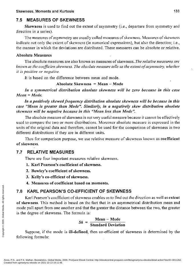
7.5 DIFFERENCE BETWEEN DISPERSION AND SKEWNESS
Dispersion Skewness
1. It is shows us the spread of individual 1. It show us departure from symmetry, values about the central value. i.e., mean. i.e., direction of variations.
2. It is a type of averages of deviation- 2. It is not an average, but is measured by average of the second order. the use of the mean, median and mode.
3. It judges the truthfulness of the central 3. It judges the differences between the tendency. central tendencies.
4. It shows the degree of variability. 4. It shows whether the concentration is in higher or lower values.
Arora, P.N., and P.K. Malhan. Biostatistics, Global Media, 2009. ProQuest Ebook Central, http://ebookcentral.proquest.com/lib/ugmartyrsu-ebooks/detail.action?docID=3011262.Created from ugmartyrsu-ebooks on 2021-10-13 19:11:48.
Cop
yrig
ht ©
200
9. G
loba
l Med
ia. A
ll rig
hts
rese
rved
.
Skewness, Moments and Kurtosis 133
7.5 MEASURES OF SKEWNESS Skewness is used to find out the extent of asymmetry (i.e., departure from symmetry and
direction in a series).
The measures of asymmetry are usually called measures of skewness. Measures of skewness indicate not only the extent of skewness (in numerical expressions), but also the direction; i.e., the manner in which the deviations are distributed. These measures can be absolute or relative.
Absolute Measures
The absolute measures are also known as measures of skewness. The relative measures are known as the coefficien skewness. The absolute measure tells us the extent of asymmetry, whether it is positive or negative.
It is based on the difference between mean and mode.
Absolute Skewness = Mean - Mode
In a flynllnetrical distribution absolute skewness will be zero because in this case Mean = Mode.
In a positively skewed frequency distribution absolute skewness will be because in tltis case "Mean is greater than Mode". Similarly, in a negatively skew distribution absolute skewness will be negative because in this "Mean less than Mode".
The absolute measure of skewness is not very useful measure because it cannot be effectively used to compare the two or more distributions. Moreover absolute measure is expressed in the units of the original data and therefore, cannot be used for the comparison of skewness in two different distributions if they are in different units.
Thus for comparison purpose, we use relative measure of skewness known as coefficient of skewness.
7.7 RELATIVE MEASURES There are four important measures relative skewness.
1. Karl Pearson's coefficient of skewness.
2. Bowley's coefficient of skewness.
3. Kelly's co-efficient of skewness.
4. Measures of coefficient based on moments.
7.8 KARL PEARSON'S CO-EFFICIENT OF SKEWNESS Karl Pearson's coefficient of skewness enables us to find out the direction as well as extent
of skewness. This method is based on the fact that in an asymmetrical distribution mean and mode pull apart from one another and that the greater the distance between the two, the greater is the degree of skewness. The formula is:
Mean - Mode Sk = S d d D .. tan ar eVlatlOn
Suppose, if the mode is ill-defined, then co-efficient of skewness is determined by the following formula:
Arora, P.N., and P.K. Malhan. Biostatistics, Global Media, 2009. ProQuest Ebook Central, http://ebookcentral.proquest.com/lib/ugmartyrsu-ebooks/detail.action?docID=3011262.Created from ugmartyrsu-ebooks on 2021-10-13 19:11:48.
Cop
yrig
ht ©
200
9. G
loba
l Med
ia. A
ll rig
hts
rese
rved
.

134
3 (Mean - Median) Sk = ----'---------'-
Standard Deviation
Properties of Karl Pearson's coefficient of skewness I. [t's value usually lies between ± 1.
Biostatistics
2. When it's value is zero, there is no skewness, i.e., the distribution is symmetrical.
3. When its value is negative, the distribution is negatively skewed.
4. When its value is positive, the distribution is positively skewed.
Example 1 : Calculate Karl Pearson s coefficient of skewness for the following data on the number of red flowers on a plant 12, 18, 35, 22 and 18.
Solution:
Calculation of Mean and Standard Deviation
SI.No. No. of Red flowers (X) (X- X) X
1 12 -9 81
2 18 > -3 9
3 35 14 196
4 22 1 1
5 18 -3 9
N=5 IX = 105 IX2 = 296
:EX 105 X= N =5 =21
J1X1 ~296 cr = IV = -5- = .J59.2 = 7.7
Mode = 18, because it occurs maximum number of times in the series.
21- 18 3 Coefficient of skewness = Mean - Mode
= 7.7 = 7.7 = 0.4. Standard deviation
Example 2 : 120 patients were tested their blood for total cholesterol from two pathology laboratories A and B. The following results were obtained in mg/dl).
Solution:
Laboratory A : Mean = 46.83 ; Mode = 51.67; S.D. = 14.8
Mean = 47.83 ; Mode = 47.U7; S.D. = 14.8.
Determine the results of which laboratory is more skewed.
Laboratory A : Sk = A
Mean - Mode
cr
46.83 - 51.67 - 484 14.8 = 14.-~- = -0.327
Arora, P.N., and P.K. Malhan. Biostatistics, Global Media, 2009. ProQuest Ebook Central, http://ebookcentral.proquest.com/lib/ugmartyrsu-ebooks/detail.action?docID=3011262.Created from ugmartyrsu-ebooks on 2021-10-13 19:11:48.
Cop
yrig
ht ©
200
9. G
loba
l Med
ia. A
ll rig
hts
rese
rved
.

Skewness, Moments and Kurtosis 135
Mean - Mode 47.83 - 47.07 0.76 14.8 = 14.8 = 0.0514. Laboratory B : Sk =-----
B 0-
Thus we find that ISk AI = 0.327 is greater than ISkBI = 0.0514, so the results of the pathology laboratory A are more skewed.
Example 3 : Consider the following distribution of blood test for fasting sugar of 1 00 persons in two pathology laboratory.
Laboratory A Laboratory B
Mean 100 90
Median 90 80
Standard Deviation 10 10
Both the results have the same degrees of skewness. True/False?
Solution: Karl Pearson's co-efficient of skewness is:
3 (Mean - Median)
Sk = Standard Deviation
Skewness for the laboratories A and B.
3 (100 - 90) Laboratory A : Coefficient of skewness: Sk(A) = 10 =3
3 (90 - 80) Laboratory B : Coefficient of skewness : Sk(B) = 10 = 3
Since Sk(A) and Sk(B) = 3, the statement that both the laboratories have the same degree of skewness is true.
Exam pie 4 : From a moderately skewed distribution of retail prices for men s shoes, it is found that the mean price is Rs. 20 and the median price is Rs. 17. If the coefficient of variation is 20%, find the Pearson ian coefficient of skewness of the distribution.
Solution : We are given that:
Mean = 20 and Median = 17. To find the coefficient of skewness, we need standard deviation.
or
Standard deviation x 100 C.V. =
Mean
0-20 = - x 100 => Sa = 20 or a = 4.
20
3 (Mean - Median) 3 (20 - 18) 3 x3 Sk = = =- =2.25.
Standard Deviation 4 4
Example 5 : From the following data find out Karl Pearson s coefficient of skewness:
Measurement : 10 11 12 13 14 15 Frequency: 2 4 10 8 5 1
(Guru Nanak Dev. Uni. B. Com. II. Sept, 1982)
Arora, P.N., and P.K. Malhan. Biostatistics, Global Media, 2009. ProQuest Ebook Central, http://ebookcentral.proquest.com/lib/ugmartyrsu-ebooks/detail.action?docID=3011262.Created from ugmartyrsu-ebooks on 2021-10-13 19:11:48.
Cop
yrig
ht ©
200
9. G
loba
l Med
ia. A
ll rig
hts
rese
rved
.
136 Biostatistics
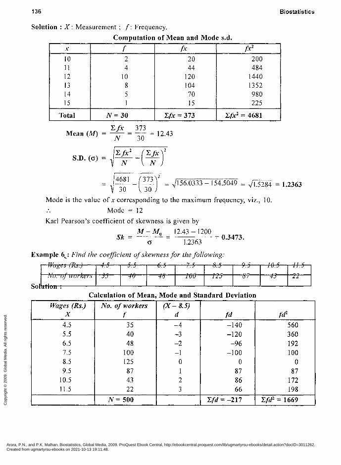
Solution: X: Measurement; f: Frequency.
Computation of Mean and Mode s.d.
x f fx f.\:2
10 2 20 200 11 4 44 484 12 10 120 1440 13 8 104 1352 14 5 70 980 15 I 15 225
Total N= 30 r.fx = 373 r.(x2 = 4681
"Lf\: 373 Mean (M) = N = 30 = 12.43
S.D. (0") = "L/x
2 _ (r./X)2 ]V ]V
-- - - = ~]56.0333 -154.5049 = .J1.5284 = 12363 468] (373)2 30 30 .
Mode is the value of x corresponding to the maximum frequency, viz., 10.
.. Mode = 12
Karl Pearson's coefficient of skewness is given by
111- Mo ]2.43 - 1200 Sk = = 0.3473.
0" 1.2363
Example 6._: Find the coefficient of skewness for the following:
~ :;; :~"" I:: I~: I ~: I : I ;: I :: I ';;S I ;;5 I Solnt .
Calculation of Mean, Mode and Standard Deviation
Wages (Rs.) No. 0/ workers (X - 8.5) X ( d (d ((f-
4.5 35 -4 -140 560 5.5 40 -3 -120 360 6.5 48 -2 -96 192 7.5 100 -I -100 100 8.5 125 0 0 0 9.5 87 1 87 87
1 0.5 43 2 86 172 11.5 22 3 66 198
N= 500 r.(d = -217 r.((p = 1669
Arora, P.N., and P.K. Malhan. Biostatistics, Global Media, 2009. ProQuest Ebook Central, http://ebookcentral.proquest.com/lib/ugmartyrsu-ebooks/detail.action?docID=3011262.Created from ugmartyrsu-ebooks on 2021-10-13 19:11:48.
Cop
yrig
ht ©
200
9. G
loba
l Med
ia. A
ll rig
hts
rese
rved
.

Skewness, Moments and Kurtosis
- Lfd -217 X = A + N = 8.5 + 500 = 8.5 - 0.43 = 8.07
a = "Lfi/2 _ (Lfd )2 N N
1669 _ (-217)1 = ")3.34 _ 0.l9 = .)3.l5 = 1.77 500 500
Mode = 8.5, because it occurs maximum no. of times.
. X - Mode Coefficient of skewness = ---
a
8.07 - 8.5 -.43 l.77 = l.77 = - 0.24.
7.9 BOWLEY'S COEFFICIENT OF SKEWNESS
137
Prof. A.L. Bowley's coefficient of skewness is based on the quartiles and is given by
Q3 - Q\ - 2 Median Bowley's coefficient of skewness: Sk = Q
3 - Q
1 •
where, Q\ = First quartile, Q3 = Third quartile
Limits for Bowley'S coefficient of skewness: It ranges from -1 to 1
I.e., -1 $; Sk (Bowley) $; 1. . Example 7: A distribution had Qj = 31.3, median = 35, and Q
3 = 36.4. Calculate the coefficient
of skewness.
Solution: Here Q3 = 36.4 ; Q1 = 31.3; med = 35.
or
Q3 - Q\ - 2 Median Co-eff. skewness = -=..::-~-----
Q3-QI
Sk __ 36.4 + 31.3 - 2 x 35 -2.3 -------= -- = - 0.43.
36.6 - 31.3 5.3
Hence the distribution is negatively skewed.
7.10 KELLY'S MEASURE OF SKEWNESS
Bowley's co-efficient of skewness ignores 50% of the data towards the extremes. This can partially removed by taking two deciles or percentiles equidistant from the median values. This refinement was suggested by Kelly. Kelly has suggested the following formula for measuring skewness upon 10th and 90th percentiles.
P.o + Ito - 2 median Kelly's coefficient of skewness = ---.:..:'-------=:..:'-------
Ito - P.o DI + D9 - 2 median
Kelly's coefficient of skewness = D9 -D1
Remark: This method is primarily of theoretical importance only and is seldom used in practice.
Arora, P.N., and P.K. Malhan. Biostatistics, Global Media, 2009. ProQuest Ebook Central, http://ebookcentral.proquest.com/lib/ugmartyrsu-ebooks/detail.action?docID=3011262.Created from ugmartyrsu-ebooks on 2021-10-13 19:11:48.
Cop
yrig
ht ©
200
9. G
loba
l Med
ia. A
ll rig
hts
rese
rved
.

138 Biostatistics
Example 8 : Calculate percentile co-efficient of skewness from the following positional measures given below: .
P90
= 101; PIO
= 58.12; P50 = 79.06.
Solution:
~o + ~o - 2 median Kelly's coefficient of skewness = p. _ P.
90 10
or Sk (kell ) == 101 + 58.12 - 2 (79.06) = 159.12 -158.12 = _1_ = 0.02 y 101 - 58.12 42.88 42.88
Hence the distribution is positively skewed.
7.11 CO-EFFICIENT OF SKEWNESS BASED ON MOMENTS
The term 'moment' in mechanics refers to the turning or the rotating effect of a force. In statistics, it is used to describe the peculiarities of a frequency distribution. Using moments, we can measure the central tendency of set of observations, their scatter, asymmetry and the peakedness of the curve. Deviations of items are taken from the arithmetic mean ofthe distribution. The arithmetic mean of the various powers of the deviations will give the required moments of the distribution. The moments about the actual mean is denoted by the Greek letter Il(mu).
rth order moment about the mean:
(XI - X) + (X2 - X) + .... + (XII - X) L (X - X) ll,= = N N
where X = is the mean of items XI' X2, •••• , XII and
LX X ==-
N
The first four moments about arithmetic mean are called central moments and are given by the following formulae.
Momellts Individual Series Discrete Series
First moment: III L(X-X) Lf(X-X)
N N
Second moment : 112 L(X_X)2 Lf(X-X)2
N N
Third moment: 113 L(X-X)3 Lf(X-X)3
N N
Fourth moment: 114 L(X-Xt Lf(X-X)4
N N
Where N = "Lf
Arora, P.N., and P.K. Malhan. Biostatistics, Global Media, 2009. ProQuest Ebook Central, http://ebookcentral.proquest.com/lib/ugmartyrsu-ebooks/detail.action?docID=3011262.Created from ugmartyrsu-ebooks on 2021-10-13 19:11:48.
Cop
yrig
ht ©
200
9. G
loba
l Med
ia. A
ll rig
hts
rese
rved
.
Skewness, Moments and Kurtosis 139
7.12 ROLE OF MOMENTS
1. The first moment (/-1) of a frequency distribution is always zero, i.e., /-ll = O. It measures
mean of the distribution, i.e., /-ll = X = o. 2. The second moment (/-l2) of a frequency distribution about the mean is the variance of the
distribution, i.e., /-l2 = 0'2. It measures variance i.e., the spread of the different terms in a distribution.
3. The third moment (/-l3) gives an idea about the degree of skewness present in a series.
4. The fourth moment (/-l4) throws light on the height of a frequency distribution, i.e., whether it is more peaked or more flat topped than the normal curve. It measures Kurtosis.
2
5. Co-efficient of skewness is given by ~1' where ~l = /-l~ . J.l2
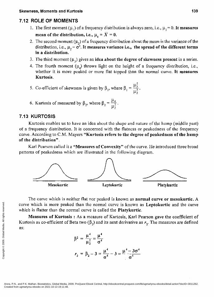
6. Kurtosis of measured by ~2' where ~2 = ~i . 7.13 KURTOSIS
Kurtosis enables us to have an idea about the shape and nature of the hump (middle past) of a frequency distribution. It is concerned with the flatness or peakedness of the frequency curve. According to C.M. Mayers "Kurtosis refers to the degree of peakedness of the hump of the distribution".
Karl Pearson called it a "Measures of Convexity" of the curve. He introduced three broad patterns of peakedness which are illustrated in the following diagram.
Mesokurtic Leptokurtic Platykurtic
The curve which is neither flat nor peaked is known as normal curve or mesokurtic. A curve which is more peaked than the normal curve is known as Leptokurtic and the curve which is flatter than the normal curve is called the Platykurtic.
Measures of Kurtosis : As a measure of Kurtosis, Karl Pearson gave the coefficient of Kurtosis as co-efficient of Beta two (~2) and its next derivative as r2• The measures are defined as:
Arora, P.N., and P.K. Malhan. Biostatistics, Global Media, 2009. ProQuest Ebook Central, http://ebookcentral.proquest.com/lib/ugmartyrsu-ebooks/detail.action?docID=3011262.Created from ugmartyrsu-ebooks on 2021-10-13 19:11:48.
Cop
yrig
ht ©
200
9. G
loba
l Med
ia. A
ll rig
hts
rese
rved
.

140 Biostatistics
When the value of ~2 > 3, it is a leptokurtic.
Leptokurtic curve
Mean
I. When the value of ~2 < 3, it is a platykurtic.
II. When the value of ~2 = 3, it is a mesokurtic.
Example 9: The number of bacteria in 1 ml of blood from 5 persons are 2,3, 7,8,10. Calculate the first, second, third and fourth moments about the mean.
Also find skewness and Kurtosis.
Solution:
x
2
3
7
8
10
N=5
:EX ~I=N
o ~I = 5" = 0;
Table: Calculation of moments
(X-X) (X - X)2 (X - X)3 X x2 xl -4 16 -64
-3 9 -27
1 1 1
2 4 8
4 16 64
LX = 0 Lx2 = 46 Lx3 = -18
:EX2 ~2=N
46 ~ =-=92 2 5 .
~; ~;
:EX3
~3=N
-18 ~3 = -5- = -3.6
12.96 778.688 = 0.0166.
~4 ~ Kurtosis (~2) = ~; = (9.2)2 = 1.4.
(X - X)4 X4
256
81
1
16
256
Lx4 = 610
:EX' ~4=N
610 ~4 = -5- = 122.
As the Kurtosis is less than 3, i.e., 1.4, the distribution is platykurtic.
Arora, P.N., and P.K. Malhan. Biostatistics, Global Media, 2009. ProQuest Ebook Central, http://ebookcentral.proquest.com/lib/ugmartyrsu-ebooks/detail.action?docID=3011262.Created from ugmartyrsu-ebooks on 2021-10-13 19:11:48.
Cop
yrig
ht ©
200
9. G
loba
l Med
ia. A
ll rig
hts
rese
rved
.
Skewness, Moments and Kurtosis 141
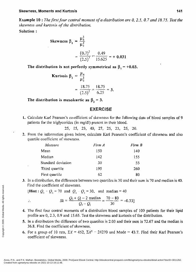
Example 10 : Thefirstfour central moment of a distribution are 0,2.5, 0.7 and 18. 75. Test the skewness and kurtosis of the distribution.
Solution:
Skewness ~1
(0.7)2 0.49 (2.5)3 = 15.625 = + 0.031
The distribution is not perfectly symmetrical as ~1 = +0.03.
J.l4 Kurtosis ~2 = J.l;
18.75 18.75 -( )" = 6 ?5 = 3. 2.5 - .-
The distribution is mesokurtic as ~2 = 3.
EXERCISE
1. Calculate Karl Pearson's co-efficient of skewness for the following data of blood samples of 9 patients for the triglycerides (in mg/dl) present in their blood.
25, 15, 23, 4~ 2~ 25, 23, 25, 20.
2. From the information given below, calculate Karl Pearson's coefficient of skewness and also quartile coefficient of skewness.
Measure FirmA Firm B
Mean 150 140
Median 142 155
Standard deviation 30 55
Third quartile 195 260
First quartile 62 80
3. In a distribution, the difference between two quartiles is 30 and their sum is 70 and median is 40. Find the coefficient of skewness.
[Hint: Q1
+ Q3 = 70 and Q3
- Q1 = 30, and median = 40
.. Sk = Q3 + QI - 2 median = 70 - 80 = -0.33] Q3 - QI 30
4. The first four central moments of a distribution blood samples of 100 patients for their lipid profile are 0, 2.3, 0.9 and 15.65. Test the skewness and kurtosis of the distribution.
5. In a distribution the difference of two quartiles is 2.03 and their sum is 72.67 and the median is 36.8. Find the coefficient of skewness.
6. For a group of 10 rats, LX = 452, L,{'2 = 24270 and Mode = 43.7. Find their Karl Pearson's coefficient of skewness.
Arora, P.N., and P.K. Malhan. Biostatistics, Global Media, 2009. ProQuest Ebook Central, http://ebookcentral.proquest.com/lib/ugmartyrsu-ebooks/detail.action?docID=3011262.Created from ugmartyrsu-ebooks on 2021-10-13 19:11:48.
Cop
yrig
ht ©
200
9. G
loba
l Med
ia. A
ll rig
hts
rese
rved
.
142 Biostatistics
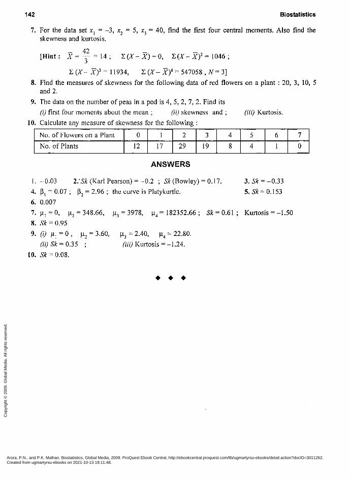
7. For the data set Xl = -3, x2 = 5, X3 = 40, find the first four central moments. Also find the skewness and kurtosis.
_ 42 _ _ [Hint: X = 3 = 14 ; L (X - X) = 0, L (X - X? = 1046 ;
L (X - X)3 = 11934, L (X - X)4 = 547058 , N = 3]
8. Find the measures of skewness for the following data of red flowers on a plant: 20, 3, 10, 5 and 2.
9. The data on the number of peas in a pod is 4, 5, 2, 7, 2. Find its
(i) first four moments about the mean; (iO skewness and; (iii) Kurtosis.
10. Calculate any measure of skewness for the following:
No. of Flowers on a Plant 0 1 2 3 4 5 6 7
No. of Plants 12 17 29 19 8 4 1 0
ANSWERS
I. - 0.03 2: Sk (Karl Pearson) = -0.2 ; Sk (Bowley) = 0.17. 3. Sk = -0.33
4. ~l = 0.07; ~2 = 2.96; the curve is Platykurtic. 5. Sk= 0.153
6. 0.007
7. III = 0, 112 = 348.66, 113 = 3978, 114 = 182352.66; Sk = 0.61; Kurtosis = -1.50
8. Sk = 0.95
9. (i) III = 0, 112 = 3.60, 113 = 2.40, 114 = 22.80.
(ii) Sk = 0.35 (iii) Kurtosis = -1.24.
10. Sk = 0.08.
• • •
Arora, P.N., and P.K. Malhan. Biostatistics, Global Media, 2009. ProQuest Ebook Central, http://ebookcentral.proquest.com/lib/ugmartyrsu-ebooks/detail.action?docID=3011262.Created from ugmartyrsu-ebooks on 2021-10-13 19:11:48.
Cop
yrig
ht ©
200
9. G
loba
l Med
ia. A
ll rig
hts
rese
rved
.
Related Documents