Singular potentials and limit cycles

arX

iv:q

uant

-ph/

0010

073v

2 6

Apr

200

1

NT@UW-00-023DOE/ER/411332-102-INT00

RBRC-140KRL MAP-271

Singular Potentials and Limit Cycles

S.R. Beanea,1, P.F. Bedaqueb,2, L. Childressa,3,A. Kryjevskib,4, J. McGuireb,5, and U. van Kolckc,d,e,6

aDepartment of Physics and bInstitute for Nuclear Theory,University of Washington,

Seattle, WA 98195

c Department of Physics,University of Arizona,

Tucson, AZ 85721

d RIKEN-BNL Research Center,Brookhaven National Laboratory,

Upton, NY 11973

e Kellogg Radiation Laboratory, 106-38,California Institute of Technology,

Pasadena, CA 91125

Abstract

We show that a central 1/rn singular potential (with n ≥ 2) is renormalizedby a one-parameter square-well counterterm; low-energy observables are made in-dependent of the square-well width by adjusting the square-well strength. We finda closed form expression for the renormalization-group evolution of the square-wellcounterterm.

[email protected]@[email protected]@[email protected]@krl.caltech.edu

1 Introduction

The study of singular potentials in quantum mechanics is almost as old as quantum me-chanics itself [1]. Physically, singular potentials pose problems because the force betweentwo particles, represented by the potential, does not uniquely determine the scatteringproblem [2]. Here we will focus on singular potentials of 1/rn type, with n ≥ 2. Classi-cally, particles subject to such a force fall to the origin with an infinite velocity. In thequantum theory, the wavefunction oscillates indefinitely on the way to the origin, allow-ing no way of specifying a linear combination of solutions [2]. Of course, in any physicalsituation described by a singular potential, the potential is intended as a description oflong-range behavior, so there is a sense in which the pathologies which occur near theorigin are irrelevant to the physical problem. This should remind the reader of the infini-ties encountered in quantum field theory which are cured through renormalization. Thisanalogy with field theory has provided an important motivation for the study of singularpotentials [3].

If a singular potential itself is not sufficient to determine the scattering problem, onemight be tempted to classify the singular potentials as nonrenormalizable and abandon allhope. This point of view is now outdated. In the modern version of the renormalizationparadigm a low-energy system with a clear-cut separation of scales can be describedby an effective field theory (EFT) involving explicitly only the long-wavelength degreesof freedom, and organized as an expansion in powers of momenta [4]. The short-rangedynamics can always be treated as a set of local operators. In the present context, the 1/rn

potential represents the long-distance part of the potential. Local operators in momentumspace correspond to delta-function interactions in coordinate space. The essential point ofEFT is that the details of the short-distance physics are not of importance to low-energyscattering. Hence one can simulate the delta function in an infinite number of ways. Thesimplest choice of a “smeared out” delta function is a simple square well. With a singularpotential representing a given long-distance force, and a square well representing unknownshort-distance physics, an interesting question is whether one can obtain an EFT withwell defined low-energy scattering observables, which are to a specified degree of accuracyinsensitive to the short-distance physics encoded by the square well. It is the purposeof this paper to explore this issue. Note that we do not attempt to renormalize thecoupling strength of the singular potential itself [5]. In the physical problems of interest,the coupling strength is completely determined by the long-distance physics so there isno freedom to renormalize this parameter.

By way of physical motivation we note that the singular potentials of 1/rn type areof great current physical interest. The special case n = 2 is relevant to the three-bodyproblem in nuclear physics [6][7][8]. This case is also relevant to point-dipole interactionsin molecular physics [9]. The case n = 3 corresponds to the tensor force between nucleonsand is at the heart of nuclear physics. The issue of the proper renormalization of thispotential is an essential ingredient of the intense ongoing effort to develop a perturbativetheory of nuclear interactions [10]. The interaction between a charge and an induceddipole is of type n = 4 [11]. The case n = 5 is a perturbative correction to the tensor

1

force in the nuclear potential [10]. Both n = 6 and n = 7 correspond to van der Waalsforces, of London [12] and Casimir-Polder [13] type, respectively.

This paper is organized as follows. In section 2 we set up the quantum mechanicalscattering problem of two particles subject to a 1/rn potential with a square well. Insection 3 we consider the marginal n = 2 case in some detail. The pure singular potentialsn ≥ 3 are considered at zero energy in section 4. In section 5 we make use of theWKB approximation to generalize our results to non-zero energy and to estimate theerrors associated with the renormalization procedure. We discuss the applicability of aperturbative expansion for singular potentials in section 6. Our numerical analysis, forthe case n = 4, is discussed in section 7. We discuss and conclude in section 8.

2 The 1/rn potential with a Square Well

We consider two particles of reduced mass M interacting in the S wave with a singularpotential that goes as 1/rn, n ≥ 2. This potential has a scale that sets its curvature,r0; this is the characteristic scale of the long-distance physics. The strength of the long-distance potential is governed by a parameter λL/2Mr2

0. To obtain well-defined solutions,we need to regulate the potential by introducing a cutoff procedure. Since we are posingthe problem in coordinate space, we do this through a cutoff radius R ≡ Rr0, R<∼ 1.We expect that the solutions will depend sensitively on R, that is, on the short-rangephysics. We simulate a short-range delta-function interaction by a square well of thisradius and with depth λS/2Mr2

0. The problem will be correctly renormalized once weare able to vary R (inasmuch as R<∼ 1) and simultaneously λS in such a way as tokeep observables (say phase shifts) invariant. The corresponding constraint λS = λS(R)represents the renormalization-group flow of the contact interaction 7. We will see thatthis short-distance physics is represented by the running coupling

Hn(R) ≡√

λS(R)R. (1)

We thus take as our potential

V (r) =1

2Mr20

(

−λSθ(R − r) − λLf(r/r0)

(r/r0)nθ(r − R)

)

, (2)

where f(x) is a regular function of x near the origin with f(0) = 1, f(1) = O(1). Noticethat λS, λL > 0 correspond to purely attractive potentials. In terms of x = r/r0, theSchrodinger equation for the wavefunction u(r)/r at an energy E = k2/2M = η2/2Mr2

0

is

{

u′′(x) + (η2 + λS)u(x) = 0 x < Ru′′(x) + (η2 + λL

f(x)xn )u(x) = 0 x > R.

(3)

7Here we mean that there is a “group” of transformations on the cutoff R which leaves observablesinvariant.

2

We will consider the simplified case f(x) = 1 until section 5.There is a very simple argument for classifying singular potentials which we will repeat

here [12]. In the vicinity of the origin the uncertainty principle dictates that the kineticenergy scales like x−2. Therefore in a system described by an attractive singular potentialalone, the Hamiltonian of the system is given by the sum of the kinetic energy and thepotential energy, −λLx−n. Note that for a Coulomb potential, n = 1, and for a sufficientlyweak n = 2 potential, the Hamiltonian is bounded and therefore the Schrodinger equationhas a unique regular solution. Clearly for n = 2 and λL sufficiently strong, the Hamiltonianis unbounded from below. Furthermore, when n ≥ 3 the Hamiltonian is always unboundedfrom below. Hence, an attractive singular potential alone is meaningless in the vicinity ofthe origin; the unboundedness of the Hamiltonian represents the onset of short-distancephysics whose effect must be included in the potential.

3 The Marginal Case: n = 2

3.1 The k = 0 Solution

Consider first the zero-energy solution u(x; 0). The Schrodinger equation for x > R is

u′′(x; 0) +λL

x2u(x; 0) = 0 (4)

and the general solution is

u(x; 0) = Ax1

2+γ + Bx

1

2−γ (5)

where γ =√

1/4 − λL. For λL < 1/4 the solution is well known [12] and will not be

further considered in this paper. On the other hand, for λL > 1/4 we can define γ ≡ iν,and the general solution is

u(x; 0) =√

x cos (ν log (x) + φ2) (6)

where ν =√

λL − 1/4, φ2 = (log A/B)/2i and we ignore the overall normalization. Both

of the linearly independent solutions of Eq. (5) vanish as x → 0, and oscillate indefinitelyon the way there. There is no obvious way to determine a unique linear combinationof solutions; i.e. fix φ2. This is the fundamental problem with singular potentials inquantum mechanics. Renormalization theory tells us that this sickness is to be expectedand arises from probing arbitrarily short-distance scales, where the true potential nolonger has the form 1/x2. The cure is to cut off the long-distance potential at a radiusR and introduce a simple parametrization of the unknown short-distance physics, sincelow-energy observables cannot distinguish between the schematic, parametrized potentialand the true potential at short distances. We choose a square well for simplicity, but weemphasize that any choice of function is equally valid.

3

3.2 Matching to the Square Well

The solution in the interior region, x < R, is straightforward. It is sufficient to consideran attractive square-well potential, λS > 0. Matching logarithmic derivatives at theboundary x = R gives

√

λS cot√

λSR =1

R

{

1

2− ν tan (ν log (R) + φ2)

}

. (7)

If we vary R and λS(R) as given here, the zero-energy phase φ2 will not be affected. Eq. (7)is transcendental and therefore rather cumbersome. However there are two regimes wherean analytical expression can be found. The first is when cot

√λSR is large. This is the

generic situation as R → 0 since the the right-hand side of this equation blows up, exceptwhere ν tan(ν log (R) + φ2) = 0. We can then find an approximate solution by writing√

λSR = mπ+ǫ where m is an integer and ǫ is a small number. Inserting this into Eq. (7)and keeping the leading order in ǫ we find

H2(R) = mπ

sin(

ν log (R) + φ2 − arctan 12ν

)

sin(

ν log (R) + φ2 + arctan 12ν

)

. (8)

Close to the zeroes of the right-hand side of this equation we can write instead√

λSR =(m + 1/2)π + ǫ and following the same procedure we find, to leading order in ǫ,

H2(R) = (m + 1/2)π − 1

(m + 1/2)π

{

1

2− ν tan (ν log (R) + φ2)

}

. (9)

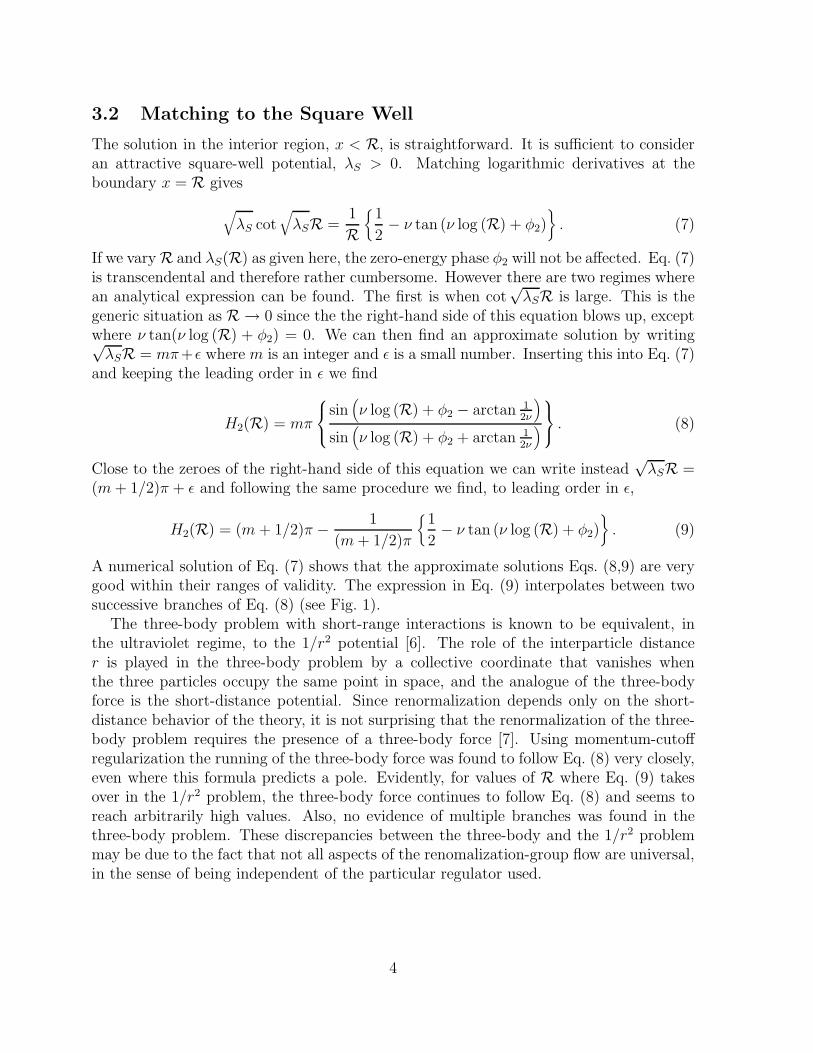
A numerical solution of Eq. (7) shows that the approximate solutions Eqs. (8,9) are verygood within their ranges of validity. The expression in Eq. (9) interpolates between twosuccessive branches of Eq. (8) (see Fig. 1).

The three-body problem with short-range interactions is known to be equivalent, inthe ultraviolet regime, to the 1/r2 potential [6]. The role of the interparticle distancer is played in the three-body problem by a collective coordinate that vanishes whenthe three particles occupy the same point in space, and the analogue of the three-bodyforce is the short-distance potential. Since renormalization depends only on the short-distance behavior of the theory, it is not surprising that the renormalization of the three-body problem requires the presence of a three-body force [7]. Using momentum-cutoffregularization the running of the three-body force was found to follow Eq. (8) very closely,even where this formula predicts a pole. Evidently, for values of R where Eq. (9) takesover in the 1/r2 problem, the three-body force continues to follow Eq. (8) and seems toreach arbitrarily high values. Also, no evidence of multiple branches was found in thethree-body problem. These discrepancies between the three-body and the 1/r2 problemmay be due to the fact that not all aspects of the renomalization-group flow are universal,in the sense of being independent of the particular regulator used.

4

-1 0 1

0

10

H 2

Log(R)

Figure 1: The running coupling for the n = 2 singular potential. The solid lines are givenby Eq. (8) and the dashed lines are given by Eq. (9). The bold lines are a numericalsolution of Eq. (7).

3.3 The Full Solution

In the case n = 2, the Schrodinger equation can be solved exactly for all energies. Thesolution is

u(x; η) =√

x [exp (iα)Jiν(ηx) + exp (−iα)J−iν(ηx)] (10)

where the J±iν are Bessel functions, and α is to be fixed by a boundary condition. Forsmall x we find

u(x; η) =√

x cos (ν log (xη/2) + α − Im log Γ(1 + iν)). (11)

Matching to Eq. (6) gives

φ2 = α + ν log η/2 − Im log Γ(1 + iν). (12)

Since φ2 is, by construction, energy independent, α is energy dependent.We can now look for solutions with η = iκ which fall off exponentially at large x. It

follows from Eq. (10) that

u(x; κ) → 1

2exp (i

π

4) cos(α + i

νπ

2) exp (κx) + C exp (−κx) (13)

where C is an energy-dependent coefficient. The bound-state solutions then correspondto α(η) = (m + 1/2)π − iνπ/2, with m an integer. Comparing with Eq. (12) gives thebound-state spectrum

5

Em = − 2

Mr20

exp

(

2φ2 + Im log Γ(1 + iν) − (m + 1/2)π

ν

)

. (14)

Once φ2 is fixed by a single bound-state energy, all other energies are predicted [2].Adjacent bound-state energies are related by

κm+1

κm= exp (−π

ν). (15)

Hence we see that the periodicity in the running coupling H2(R) is associated with theaccumulation or dissipation of bound states near the origin.

One can also fix φ2 to a scattering observable, like the scattering length or the phaseshift at a given energy. Unfortunately, as for the Coulomb potential, the n = 2, 3 singularpotentials suffer infrared problems at low energies, and therefore scattering lengths canbe defined only if an infrared cutoff is imposed [3].

4 Pure Singular Potentials: n ≥ 3

4.1 The k = 0 Solution

The exact zero-energy solution for n ≥ 3 is well known [3]. Defining z =√

λLx1−n/2/|1−n/2| and φ(z) = u(x; 0)/

√x, for x > R Eq. (3) becomes an ordinary Bessel equation:

φ′′(z) +1

zφ′(z) +

(

1 − 1

(n − 2)2z2

)

φ(z) = 0. (16)

The solution is

u(x; 0) =√

x

[

AnJ1/(n−2)

( √λL

1 − n/2x1−n/2

)

+ BnJ−1/(n−2)

( √λL

1 − n/2x1−n/2

)]

, (17)

which is a linear combination of Bessel functions. For small x we can write8

u(x; 0) = xn/4 cos

( √λL

n/2 − 1x1−n/2 + φn

)

[

1 + O(xn/2−1)]

, (18)

where we have set the constant prefactor to unity and

φn = −nπ

4

1

(n − 2)+ i log

(

1 +Bn

An

exp

(

− iπ

(n − 2)

))

. (19)

This solution exhibits precisely the same pathologies as Eq. (6).

8In the case n = 4, the Bessel functions are of half-integral order and Eq. (18) is exact for all x.

6

4.2 Matching to the Square Well

We proceed as in the case n = 2. Again we have a square well in the interior region.Matching logarithmic derivatives at the boundary x = R gives

√

λS cot√

λSR =n

4R −(

λL

Rn

)1/2

tan

( √λL

n/2 − 1R1−n/2 + φn

)

(20)

where we have neglected O(Rn/2−1) corrections to the wavefunction at x > R. The phaseφn is physical and can be traded for the scattering length (for n > 3), as will be seenbelow. If we vary R and λS(R) as given here, the phase φn will not be affected. Weproceed as we did before in the n = 2 case and find, in the regions where the right-handside of Eq. (20) is large

Hn(R) = mπ

1 − 1

1 − n/4 +√

λLR1−n/2 tan(

2√

λL

n−2R1−n/2 + φn

)

. (21)

In the other regime, where the right-hand side is close to a zero, we have

Hn(R) = (m +1

2)π − 1

(m + 12)π

(

n/4 −√

λLR1−n/2 tan

(

2√

λL

n − 2R1−n/2 + φn

))

. (22)

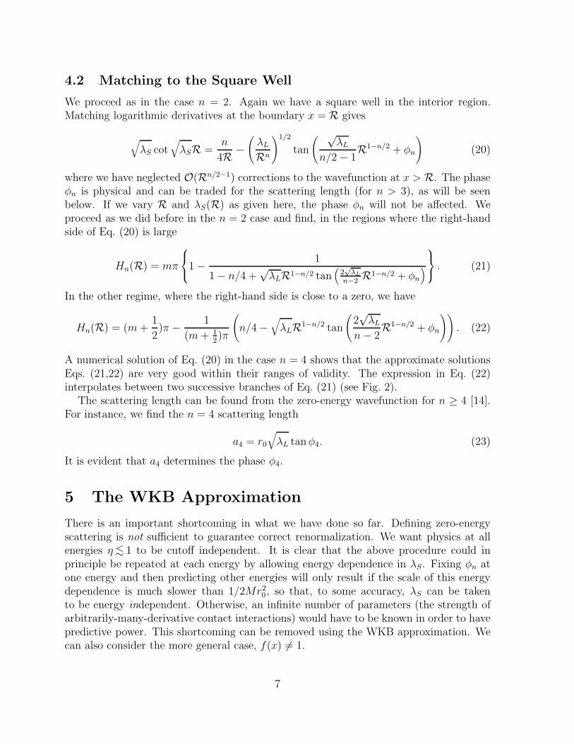
A numerical solution of Eq. (20) in the case n = 4 shows that the approximate solutionsEqs. (21,22) are very good within their ranges of validity. The expression in Eq. (22)interpolates between two successive branches of Eq. (21) (see Fig. 2).

The scattering length can be found from the zero-energy wavefunction for n ≥ 4 [14].For instance, we find the n = 4 scattering length

a4 = r0

√

λL tan φ4. (23)

It is evident that a4 determines the phase φ4.

5 The WKB Approximation

There is an important shortcoming in what we have done so far. Defining zero-energyscattering is not sufficient to guarantee correct renormalization. We want physics at allenergies η <∼ 1 to be cutoff independent. It is clear that the above procedure could inprinciple be repeated at each energy by allowing energy dependence in λS. Fixing φn atone energy and then predicting other energies will only result if the scale of this energydependence is much slower than 1/2Mr2

0, so that, to some accuracy, λS can be takento be energy independent. Otherwise, an infinite number of parameters (the strength ofarbitrarily-many-derivative contact interactions) would have to be known in order to havepredictive power. This shortcoming can be removed using the WKB approximation. Wecan also consider the more general case, f(x) 6= 1.

7

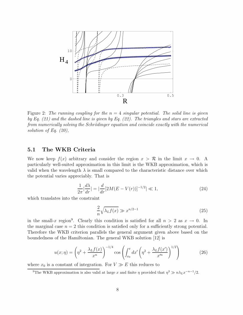
0.3 0.5

0

10

H 4

R

Figure 2: The running coupling for the n = 4 singular potential. The solid line is givenby Eq. (21) and the dashed line is given by Eq. (22). The triangles and stars are extractedfrom numerically solving the Schrodinger equation and coincide exactly with the numericalsolution of Eq. (20),

5.1 The WKB Criteria

We now keep f(x) arbitrary and consider the region x > R in the limit x → 0. Aparticularly well-suited approximation in this limit is the WKB approximation, which isvalid when the wavelength λ is small compared to the characteristic distance over whichthe potential varies appreciably. That is

1

2π|dλ

dr| = | d

dr[2M(E − V (r))]−1/2| ≪ 1, (24)

which translates into the constraint

2

n

√

λLf(x) ≫ xn/2−1 (25)

in the small-x region9. Clearly this condition is satisfied for all n > 2 as x → 0. Inthe marginal case n = 2 this condition is satisfied only for a sufficiently strong potential.Therefore the WKB criterion parallels the general argument given above based on theboundedness of the Hamiltonian. The general WKB solution [12] is

u(x; η) =

(

η2 +λLf(x)

xn

)−1/4

cos

∫ x

x0

dx′(

η2 +λLf(x′)

x′n

)1/2

(26)

where x0 is a constant of integration. For V ≫ E this reduces to

9The WKB approximation is also valid at large x and finite η provided that η3 ≫ nλLx−n−1/2.

8

u(x; 0) = xn/4f−1/4(x) cos(

√

λL

∫ x

x0

dx′x′−n/2f 1/2(x′))

. (27)

In the limit R < x ≪ 1, we can set f(x) = 1 (keep the leading term in a power series inx). We then recover, for n > 2,

u(x; 0) = xn/4 cos

( √λL

n/2 − 1x1−n/2 + φn

)

(28)

where φn = −√

λLx0−n/2+1/(1 − n/2). The case n = 2 is also recovered if one takes

λL → λL − 1/4. Therefore, we expect our conclusions about the renormalization of thesingular potentials to be valid for the more general case f(x) 6= 1.

5.2 The Leading Energy Dependence

We now show that the zero-energy solution is in fact sufficient to remove cutoff dependenceat all other low energies. The crucial point is that, in the intermediate region R < x ≪ 1,for the energies of interest, the potential energy is much larger than the total energy, andwe recover the zero-energy case. This can be made more precise using WKB again [2].We write the wavefunction for any x ≥ R as

u(x; η) = A(x; η)u(x; 0). (29)

Then A(x; η) obeys

d2A(x)

dx2+ 2

d lnu(x; 0)

dx

dA(x)

dx+ η2A(x) = 0 (30)

which depends only on the zero energy wavefunction. Now, since for R < x ≪ 1,

∣

∣

∣

∣

∣

d lnu(x; 0)

dx

∣

∣

∣

∣

∣

≫ 1, (31)

A(x) can be written

A(x) = A(0)(x) + A(1)(x) + . . . , (32)

where

dA(0)

dx= 0;

dA(1)

dx= −1

2

u(x; 0)

u′(x; 0)η2A(0); . . . (33)

We then find the leading energy corrections

A(x; η) = A(0)

{

1 − η2

2

∫ x

0dx′ u(x′; 0)

u′(x′; 0)+ . . .

}

(34)

9

We see that, in the intermediate region, the energy dependence of the wavefunction (29)is determined by the zero-energy wavefunction u(x; 0). If the phase of u(x; 0) has beenfixed, the phase of u(x; η) is fixed, and scattering observables can be predicted at lowenergies.

5.3 Error Estimates

The fact remains that our arguments are all at short distances where the WKB approxi-mation is valid. This is, of course, the opposite of the EFT limit which interests us. Onemay wonder whether cutoff effects can be amplified when propagating the wavefunctionfrom short to long distances. We will see now that this cannot occur and in turn findan estimate of the cutoff error associated with the scattering phase shift. Usually, inperturbative EFT, the error is a power law in R. Here we will find a more complicatedfunctional dependence.

By adjusting Hn(R) as in Eqs. (21,22) we guarantee that two zero-energy solutionsuR(x; 0), uR′(x; 0) corresponding to two different cutoffs R,R′ ≪ 1 ∼ 1/η are identical.At finite values of η, solutions obtained with different cutoffs will no longer be equal,but their difference can be easily estimated. Taking R′ < R, the Schrodinger equationssatisfied by uR(x; η) and uR′(x; η) are the same in the x > R region so their Wronskian,

W [uR, uR′](x; η) = uR(x; η)u′R′(x; η) − u′

R(x; η)uR′(x; η) (35)

is independent of x. At large distances (r ≫ (λL/k2)(1/n)), where the solutions are planewaves, W [uR, uR′] is related to the phase shifts δR, δR′ obtained with the cutoffs R andR′ by

W [uR, uR′](r ≫ (λL/k2)(1/n); η) = ARAR′η sin(δR − δR′), (36)

where AR, AR′ are the amplitudes at large distances. These prefactors are easily estimatedfrom the general WKB solution, Eq. (26), in the region r ≫ (λL/k2)(1/n), where theWKB solution maps to the asymptotic plane-wave solution (see Footnote 9). We findAR , AR′ ∼ η−1/2.

On the other hand, at the cutoff distance x = R, W [uR, uR′] is estimated using ourWKB formula, Eq. (34). We find

W [uR, uR′](R; η) = W [uR, uR′](R; 0) − η2

2E(R; 0) + . . . (37)

where

W [uR, uR′](R; 0) = uR(R; 0)uR′(R; 0)

[

u′R′(R; 0)

uR′(R; 0)− u′

R(R; 0)

uR(R; 0)+ O

(

Rn/2−1 u′R(R)

uR(R)

)]

(38)and

10

E(R; 0) ≡ uR(R; 0)uR′(R; 0)

[

uR′(R; 0)

u′R′(R; 0)

− uR(R; 0)

u′R(R; 0)

+ O(

Rn/2−1 uR(R)

u′R(R)

)]

+ W [uR, uR′](R; 0)∫ R

0dx′

[

uR′(x′; 0)

u′R′(x′; 0)

+uR(x′; 0)

u′R(x′; 0)

+ O(

x′n/2−1 uR(x′)

u′R(x′)

)]

.(39)

We have included the error due to keeping only the leading zero-energy wavefunctionin Eq. (18). Recall that we choose our fitting procedure to be energy independent, forexample, by comparing the zero-energy wavefunction to the scattering length. It thenfollows that W [uR, uR′](R; 0) = 0, by construction, for the full wavefunction, and fromEq. (38) we have

u′R′(R; 0)

uR′(R; 0)− u′

R(R; 0)

uR(R; 0)= O

(

Rn/2−1 u′R(R)

uR(R)

)

. (40)

Using these constraints it is straightforward to find

E(R; 0) = O(

Rn/2−1 (uR(R))3

u′R(R)

)

. (41)

If we assume that all oscillating functions of R are of order unity for values of R at whichwe fit observables, then E(R; 0) = O(R3n/2−1), which is small for all n ≥ 2. Matchingthe Wronskians at large (r ≫ (λL/k2)(1/n)) and short (x = R) distances then yields anestimate for the error in the phase shift:

δR − δR′ ∼ η2 E(R; 0) (42)

where E(R; 0) is a function of R whose complicated parametric cutoff dependence is givenby Eq. (41). This shows that the renormalization procedure described here produces cutoffindependent phase shifts, accurate up to order η2 E(R; 0).

6 The Weak Coupling Limit

It might seem odd that the explicit dependence on the coupling constant is nonanalyticin the formula for the n = 4 scattering length, Eq. (23). Naively it would appear thatnonperturbative effects are important at arbitrarily weak coupling.

However, we know that this cannot be the case, since for weak coupling the scatteringlength should go smoothly to its square-well value. We would expect a perturbativedescription in the singular potential to be valid when the potential energy, −λLx−n, ismuch smaller than the kinetic energy, x−2. This leads to the condition

r ≫ r0λ1

n−2

L , or k ≪ r−10 λ

− 1

n−2

L . (43)

In effect, taking φ4 from Eq. (20) we find, for λL/R2 ≪ 1,

11

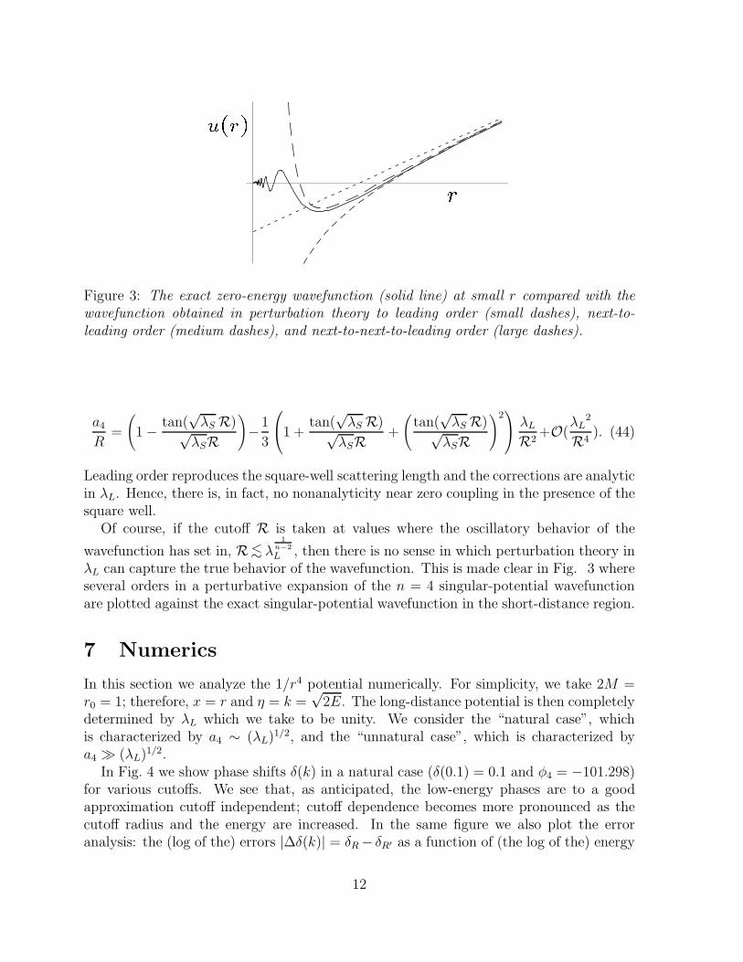
ru(r)Figure 3: The exact zero-energy wavefunction (solid line) at small r compared with thewavefunction obtained in perturbation theory to leading order (small dashes), next-to-leading order (medium dashes), and next-to-next-to-leading order (large dashes).

a4

R=

(

1 − tan(√

λS R)√λSR

)

−1

3

1 +tan(

√λS R)√

λSR+

(

tan(√

λS R)√λSR

)2

λL

R2+O(

λL2

R4). (44)

Leading order reproduces the square-well scattering length and the corrections are analyticin λL. Hence, there is, in fact, no nonanalyticity near zero coupling in the presence of thesquare well.

Of course, if the cutoff R is taken at values where the oscillatory behavior of the

wavefunction has set in, R<∼ λ1

n−2

L , then there is no sense in which perturbation theory inλL can capture the true behavior of the wavefunction. This is made clear in Fig. 3 whereseveral orders in a perturbative expansion of the n = 4 singular-potential wavefunctionare plotted against the exact singular-potential wavefunction in the short-distance region.

7 Numerics

In this section we analyze the 1/r4 potential numerically. For simplicity, we take 2M =r0 = 1; therefore, x = r and η = k =

√2E. The long-distance potential is then completely

determined by λL which we take to be unity. We consider the “natural case”, whichis characterized by a4 ∼ (λL)1/2, and the “unnatural case”, which is characterized bya4 ≫ (λL)1/2.

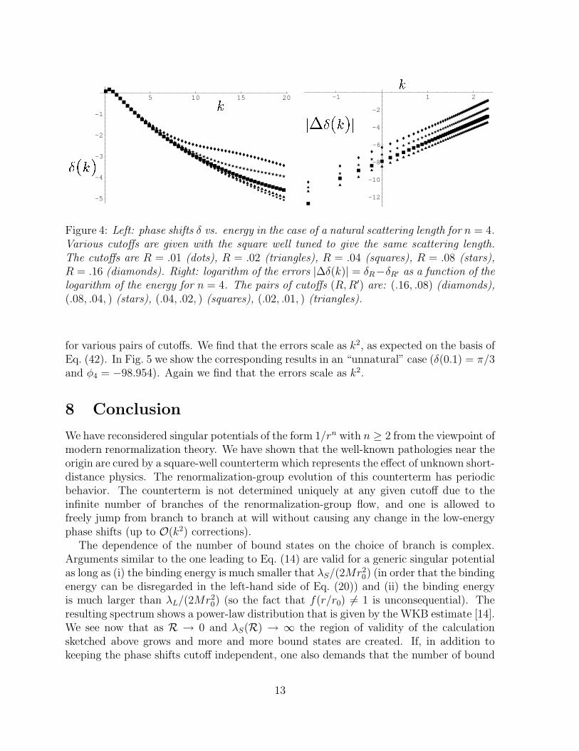
In Fig. 4 we show phase shifts δ(k) in a natural case (δ(0.1) = 0.1 and φ4 = −101.298)for various cutoffs. We see that, as anticipated, the low-energy phases are to a goodapproximation cutoff independent; cutoff dependence becomes more pronounced as thecutoff radius and the energy are increased. In the same figure we also plot the erroranalysis: the (log of the) errors |∆δ(k)| = δR − δR′ as a function of (the log of the) energy

12

5 10 15 20

-5

-4

-3

-2

-1k�(k)

-1 1 2

-12

-10

-8

-6

-4

-2

kj��(k)jFigure 4: Left: phase shifts δ vs. energy in the case of a natural scattering length for n = 4.Various cutoffs are given with the square well tuned to give the same scattering length.The cutoffs are R = .01 (dots), R = .02 (triangles), R = .04 (squares), R = .08 (stars),R = .16 (diamonds). Right: logarithm of the errors |∆δ(k)| = δR−δR′ as a function of thelogarithm of the energy for n = 4. The pairs of cutoffs (R, R′) are: (.16, .08) (diamonds),(.08, .04, ) (stars), (.04, .02, ) (squares), (.02, .01, ) (triangles).

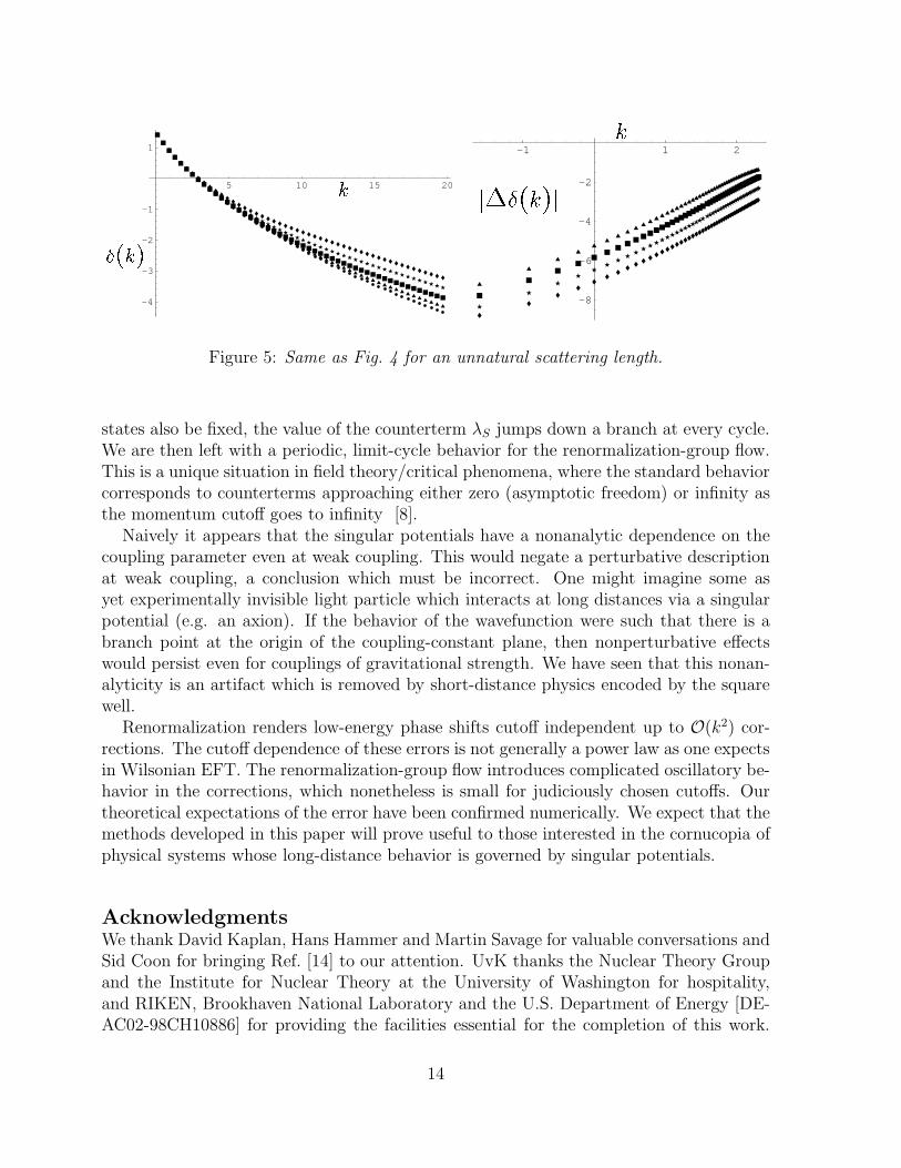
for various pairs of cutoffs. We find that the errors scale as k2, as expected on the basis ofEq. (42). In Fig. 5 we show the corresponding results in an “unnatural” case (δ(0.1) = π/3and φ4 = −98.954). Again we find that the errors scale as k2.

8 Conclusion

We have reconsidered singular potentials of the form 1/rn with n ≥ 2 from the viewpoint ofmodern renormalization theory. We have shown that the well-known pathologies near theorigin are cured by a square-well counterterm which represents the effect of unknown short-distance physics. The renormalization-group evolution of this counterterm has periodicbehavior. The counterterm is not determined uniquely at any given cutoff due to theinfinite number of branches of the renormalization-group flow, and one is allowed tofreely jump from branch to branch at will without causing any change in the low-energyphase shifts (up to O(k2) corrections).

The dependence of the number of bound states on the choice of branch is complex.Arguments similar to the one leading to Eq. (14) are valid for a generic singular potentialas long as (i) the binding energy is much smaller that λS/(2Mr2

0) (in order that the bindingenergy can be disregarded in the left-hand side of Eq. (20)) and (ii) the binding energyis much larger than λL/(2Mr2

0) (so the fact that f(r/r0) 6= 1 is unconsequential). Theresulting spectrum shows a power-law distribution that is given by the WKB estimate [14].We see now that as R → 0 and λS(R) → ∞ the region of validity of the calculationsketched above grows and more and more bound states are created. If, in addition tokeeping the phase shifts cutoff independent, one also demands that the number of bound

13

5 10 15 20

-4

-3

-2

-1

1

�(k) k -1 1 2

-8

-6

-4

-2j��(k)j kFigure 5: Same as Fig. 4 for an unnatural scattering length.

states also be fixed, the value of the counterterm λS jumps down a branch at every cycle.We are then left with a periodic, limit-cycle behavior for the renormalization-group flow.This is a unique situation in field theory/critical phenomena, where the standard behaviorcorresponds to counterterms approaching either zero (asymptotic freedom) or infinity asthe momentum cutoff goes to infinity [8].

Naively it appears that the singular potentials have a nonanalytic dependence on thecoupling parameter even at weak coupling. This would negate a perturbative descriptionat weak coupling, a conclusion which must be incorrect. One might imagine some asyet experimentally invisible light particle which interacts at long distances via a singularpotential (e.g. an axion). If the behavior of the wavefunction were such that there is abranch point at the origin of the coupling-constant plane, then nonperturbative effectswould persist even for couplings of gravitational strength. We have seen that this nonan-alyticity is an artifact which is removed by short-distance physics encoded by the squarewell.

Renormalization renders low-energy phase shifts cutoff independent up to O(k2) cor-rections. The cutoff dependence of these errors is not generally a power law as one expectsin Wilsonian EFT. The renormalization-group flow introduces complicated oscillatory be-havior in the corrections, which nonetheless is small for judiciously chosen cutoffs. Ourtheoretical expectations of the error have been confirmed numerically. We expect that themethods developed in this paper will prove useful to those interested in the cornucopia ofphysical systems whose long-distance behavior is governed by singular potentials.

AcknowledgmentsWe thank David Kaplan, Hans Hammer and Martin Savage for valuable conversations andSid Coon for bringing Ref. [14] to our attention. UvK thanks the Nuclear Theory Groupand the Institute for Nuclear Theory at the University of Washington for hospitality,and RIKEN, Brookhaven National Laboratory and the U.S. Department of Energy [DE-AC02-98CH10886] for providing the facilities essential for the completion of this work.

14

This research was supported in part by the DOE grants DE-FG03-97ER41014 (SRB) andDOE-ER-40561 (PFB), and by NSF grant PHY 94-20470 (UvK). LC and JMc are gratefulto the University of Washington REU program of the NSF for support.

References

[1] M. Plesset, Phys. Rev. 41, 278 (1932).

[2] K.M. Case, Phys. Rev. 80, 797 (1950).

[3] For a comprehensive review, see W.M. Frank, D.J. Land and R.M. Spector, Rev.Mod. Phys. 43, 36 (1971).

[4] For reviews, see D.B. Kaplan, nucl-th/9506035; P. Lepage, nucl-th/9706029.

[5] H.E. Camblong et. al., Phys. Rev. Lett. 85, 1590 (2000), hep-th/0003014; hep-th/0003255; hep-th/0003267.

[6] V.N. Efimov, Sov. J. Nucl. Phys. 12, 589 (1971).

[7] P.F. Bedaque, H.-W. Hammer, and U. van Kolck, Nucl. Phys. A646, 444 (1999),nucl-th/9811046; P.F. Bedaque, H.-W. Hammer, and U. van Kolck, Phys. Rev. Lett.82, 463 (1999), nucl-th/9809025.

[8] K. Wilson, A Limit Cycle for Three-Body Short Range Forces, talk presented at theInstitute for Nuclear Theory, University of Washington, 2000.

[9] J-M. Levy-Leblond, Phys. Rev. 153, 1 (1967); O.H. Crawford, Proc. Phys. Soc. 91,279 (1967).

[10] See, for instance, U. van Kolck, Prog. Part. Nucl. Phys. 43, 409 (1999); S.R. Beaneet. al., nucl-th/0008064.

[11] E. Vogt and H. Wannier, Phys. Rev. 95, 1190 (1954).

[12] L.D. Landau and E.M. Lifshitz, Quantum Mechanics, (Pergamon Press, London,1965).

[13] See, for instance, C. Itzykson and J-B. Zuber, Quantum Field Theory, (McGraw-Hill,New York, 1980).

[14] A.M. Perelomov and V.S. Popov, Teor. Mat. Fiz. 4, 664 (1970).

15