COMMUTATION METHODS FOR SCHR ¨ ODINGER OPERATORS WITH STRONGLY SINGULAR POTENTIALS ALEKSEY KOSTENKO, ALEXANDER SAKHNOVICH, AND GERALD TESCHL Abstract. We explore the connections between singular Weyl–Titchmarsh theory and the single and double commutation methods. In particular, we compute the singular Weyl function of the commuted operators in terms of the original operator. We apply the results to spherical Schr¨odinger operators (also known as Bessel operators). We also investigate the connections with the generalized B¨acklund–Darboux transformation. 1. Introduction The present paper is concerned with spectral theory for one-dimensional Schr¨ o- dinger operators (1.1) H = - d 2 dx 2 + q(x), x ∈ (a, b), on the Hilbert space L 2 (a, b) with a real-valued potential q ∈ L 1 loc (a, b). It has been shown recently by Gesztesy and Zinchenko [23], Fulton and Langer [14], [15], Kurasov and Luger [33] that, for a large class of singularities at a, it is still possible to define a singular Weyl function at the basepoint a. Furthermore, in previous work we have shown that this singular Weyl function shares many properties with the classical Weyl function [30] and established the connection with super singular perturbations for the special case of spherical Schr¨ odinger operators (1.2) H = - d 2 dx 2 + l(l + 1) x 2 + q(x), x ∈ (0, ∞), (also known as Bessel operators) [28]. On the other hand, commutation methods have played an important role in the theory of one-dimensional Schr¨ odinger operators both as a method for inserting eigenvalues as well as for constructing solutions of the (modified) Korteweg–de Vries equation (see, e.g., [18] and the references therein). Historically, these methods of inserting eigenvalues go back to Jacobi [26] and Darboux [8] with decisive later contributions by Crum [7], Krein [31], Schmincke [39], and Deift [9]. Two particular methods turned out to be of special importance: The single commutation method, also called the Crum–Darboux method [7], [8] (actually going back at least to Jacobi [26]) and the double commutation method, to be found, e.g., in the seminal work of Gel’fand and Levitan [16]. For recent extensions of these methods we refer to [17], [20], [21], [40]. 2010 Mathematics Subject Classification. Primary 34B20, 34L05; Secondary 34B24, 47A10. Key words and phrases. Schr¨odinger operators, spectral theory, commutation methods, strongly singular potentials. Math. Nachr. 285, 392–410 (2012). Research supported by the Austrian Science Fund (FWF) under Grant No. Y330. 1

Welcome message from author
This document is posted to help you gain knowledge. Please leave a comment to let me know what you think about it! Share it to your friends and learn new things together.
Transcript
COMMUTATION METHODS FOR SCHRODINGER OPERATORS
WITH STRONGLY SINGULAR POTENTIALS
ALEKSEY KOSTENKO, ALEXANDER SAKHNOVICH, AND GERALD TESCHL
Abstract. We explore the connections between singular Weyl–Titchmarsh
theory and the single and double commutation methods. In particular, wecompute the singular Weyl function of the commuted operators in terms of
the original operator. We apply the results to spherical Schrodinger operators
(also known as Bessel operators). We also investigate the connections with thegeneralized Backlund–Darboux transformation.
1. Introduction
The present paper is concerned with spectral theory for one-dimensional Schro-dinger operators
(1.1) H = − d2
dx2+ q(x), x ∈ (a, b),
on the Hilbert space L2(a, b) with a real-valued potential q ∈ L1loc(a, b). It has
been shown recently by Gesztesy and Zinchenko [23], Fulton and Langer [14], [15],Kurasov and Luger [33] that, for a large class of singularities at a, it is still possibleto define a singular Weyl function at the basepoint a. Furthermore, in previouswork we have shown that this singular Weyl function shares many properties withthe classical Weyl function [30] and established the connection with super singularperturbations for the special case of spherical Schrodinger operators
(1.2) H = − d2
dx2+l(l + 1)
x2+ q(x), x ∈ (0,∞),
(also known as Bessel operators) [28].On the other hand, commutation methods have played an important role in the
theory of one-dimensional Schrodinger operators both as a method for insertingeigenvalues as well as for constructing solutions of the (modified) Korteweg–de Vriesequation (see, e.g., [18] and the references therein). Historically, these methodsof inserting eigenvalues go back to Jacobi [26] and Darboux [8] with decisive latercontributions by Crum [7], Krein [31], Schmincke [39], and Deift [9]. Two particularmethods turned out to be of special importance: The single commutation method,also called the Crum–Darboux method [7], [8] (actually going back at least to Jacobi[26]) and the double commutation method, to be found, e.g., in the seminal workof Gel’fand and Levitan [16]. For recent extensions of these methods we refer to[17], [20], [21], [40].
2010 Mathematics Subject Classification. Primary 34B20, 34L05; Secondary 34B24, 47A10.Key words and phrases. Schrodinger operators, spectral theory, commutation methods,
strongly singular potentials.Math. Nachr. 285, 392–410 (2012).
Research supported by the Austrian Science Fund (FWF) under Grant No. Y330.1
2 A. KOSTENKO, A. SAKHNOVICH, AND G. TESCHL
Krein [31] was the first to realize the connection between inverse spectral prob-lems and Crum’s results. Namely, in [31], the connection between the spectralmeasures of the original and transformed operators was established and then ex-ploited to characterize the spectral measures of Bessel operators in the case l ∈ N(see also [13]). This idea has been subsequently used by many authors: see, forinstance, [2, 5, 9, 13, 24] and references therein.
The purpose of our present paper is to continue the work of Krein and estab-lish the connection between the singular Weyl functions (and hence between thespectral measures) of the original and transformed operators for both the singleand double commutation method. In particular, we will obtain an independentproof for the fact that the singular Weyl function of perturbed Bessel operatorsis a generalized Nevanlinna function. In addition, we investigate the connectionswith the generalized Backlund–Darboux transformation (GBDT) for a particularexample. This method is a generalization of the double commutation method whichit contains as a special case (cf. Subsection 5.1).
2. Singular Weyl–Titchmash theory
We begin by recalling a few facts from [30]. To set the stage, we will considerone-dimensional Schrodinger operators on L2(a, b) with −∞ ≤ a < b ≤ ∞ of theform
(2.1) τ = − d2
dx2+ q,
where the potential q is real-valued and satisfies
(2.2) q ∈ L1loc(a, b).
We will use τ to denote the formal differential expression and H to denote a corre-sponding self-adjoint operator given by τ with separated boundary conditions at aand/or b.
If a (resp. b) is finite and q is in addition integrable near a (resp. b), we will saya (resp. b) is a regular endpoint. We will say τ , respectively H, is regular if both aand b are regular.
We will choose a point c ∈ (a, b) and also consider the operators HD(a,c), H
D(c,b)
which are obtained by restricting H to (a, c), (c, b) with a Dirichlet boundary con-dition at c, respectively. The corresponding operators with a Neumann boundarycondition will be denoted by HN
(a,c) and HN(c,b).
Moreover, let c(z, x), s(z, x) be the solutions of τu = z u corresponding to theinitial conditions c(z, c) = 1, c′(z, c) = 0 and s(z, c) = 0, s′(z, c) = 1.
Define the Weyl m-functions (corresponding to the base point c) such that
u−(z, x) = c(z, x)−m−(z)s(z, x), z ∈ C \ σ(HD(a,c)),
u+(z, x) = c(z, x) +m+(z)s(z, x), z ∈ C \ σ(HD(c,b)),(2.3)
are square integrable on (a, c), (c, b) and satisfy the boundary condition of H at a,b (if any), respectively. The solutions u±(z, x) (as well as their multiples) are calledWeyl solutions at a, b. For further background we refer to [42, Chap. 9] or [43].
To define an analogous singular Weyl m-function at the, in general singular,endpoint a we will first need an analog of the system of solutions c(z, x) and s(z, x).Hence our first goal is to find a system of real entire solutions θ(z, x) and φ(z, x)such that φ(z, x) lies in the domain of H near a and such that the Wronskian
COMMUTATION METHODS FOR STRONGLY SINGULAR POTENTIALS 3
W (θ(z), φ(z)) = 1. By a real entire function we mean an entire function which isreal-valued on the real line. To this end we start with a hypothesis which will turnout necessary and sufficient for such a system of solutions to exist.
Hypothesis 2.1. Suppose that the spectrum of HD(a,c) is purely discrete for one
(and hence for all) c ∈ (a, b).
Note that this hypothesis is for example satisfied if q(x) → +∞ as x → a (cf.Problem 9.7 in [42]).
Lemma 2.2 ([30]). Suppose Hypothesis 2.1 holds. Then there exists a fundamentalsystem of solutions φ(z, x) and θ(z, x) of τu = zu which are real entire with respectto z such that
(2.4) W (θ(z), φ(z)) = 1
and φ(z, .) is in the domain of H near a. Here Wx(u, v) = u(x)v′(x)−u′(x)v(x) isthe usual Wronski determinant.
It is important to point out that such a system is not unique and any other suchsytem is given by
θ(z, x) = e−g(z)θ(z, x)− f(z)φ(z, x), φ(z, x) = eg(z)φ(z, x),
where g(z), f(z) are real entire functions.Given a system of real entire solutions φ(z, x) and θ(z, x) as in the above lemma
we can define the singular Weyl function
(2.5) M(z) = −W (θ(z), u+(z))
W (φ(z), u+(z))
such that the solution which is in the domain of H near b (cf. (2.3)) is given by
(2.6) u+(z, x) = a(z)(θ(z, x) +M(z)φ(z, x)
),
where a(z) = −W (φ(z), u+(z)) = β(z) − m+(z)α(z). By construction we obtainthat the singular Weyl function M(z) is analytic in C\R and satisfies M(z) =M(z∗)∗. Rather than u+(z, x) we will use
(2.7) ψ(z, x) = θ(z, x) +M(z)φ(z, x).
Recall also from [30, Lem. 3.2] that associated with M(z) is a correspondingspectral measure
(2.8)1
2
(ρ((x0, x1)
)+ ρ([x0, x1]
))= lim
ε↓0
1
π
∫ x1
x0
Im(M(x+ iε)
)dx.
3. Connection with the single commutation method
3.1. Preliminary basic results. We begin by recalling a few basic facts from thesingle commutation method. Let A be a densely defined closed operator and recallthat H = A∗A is a self-adjoint operator with ker(H) = ker(A). Similarly, H = AA∗
is a self-adjoint operator with ker(H) = ker(A∗). Then the key observation is thefollowing well-known result (see e.g. [42, Thm. 8.6] for a short proof):
Theorem 3.1 ([9]). Let A be a densely defined closed operator and introduce
H = A∗A, H = AA∗. Then the operators H∣∣ker(H)⊥
and H∣∣ker(H)⊥
are unitar-
ily equivalent.
4 A. KOSTENKO, A. SAKHNOVICH, AND G. TESCHL
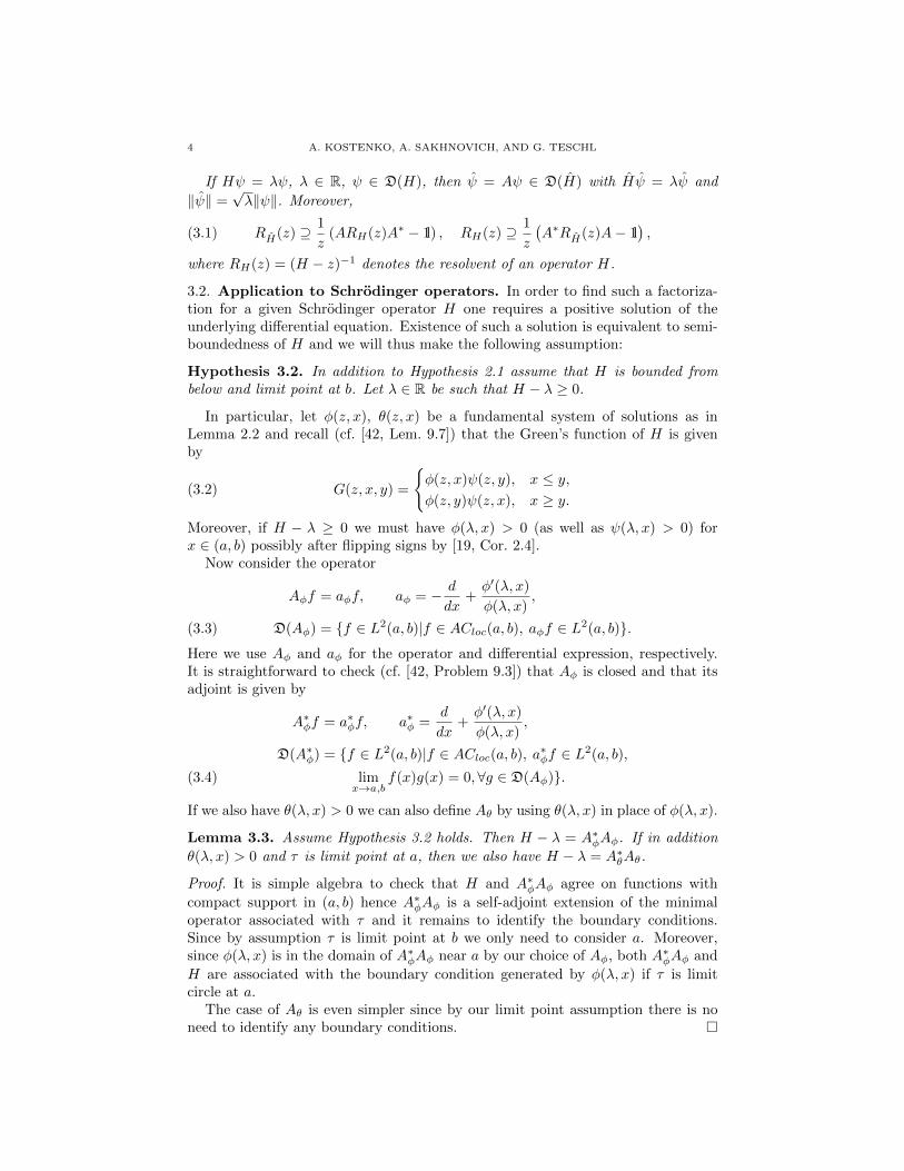
If Hψ = λψ, λ ∈ R, ψ ∈ D(H), then ψ = Aψ ∈ D(H) with Hψ = λψ and
‖ψ‖ =√λ‖ψ‖. Moreover,
(3.1) RH(z) ⊇ 1
z(ARH(z)A∗ − 1l) , RH(z) ⊇ 1
z
(A∗RH(z)A− 1l
),
where RH(z) = (H − z)−1 denotes the resolvent of an operator H.
3.2. Application to Schrodinger operators. In order to find such a factoriza-tion for a given Schrodinger operator H one requires a positive solution of theunderlying differential equation. Existence of such a solution is equivalent to semi-boundedness of H and we will thus make the following assumption:
Hypothesis 3.2. In addition to Hypothesis 2.1 assume that H is bounded frombelow and limit point at b. Let λ ∈ R be such that H − λ ≥ 0.
In particular, let φ(z, x), θ(z, x) be a fundamental system of solutions as inLemma 2.2 and recall (cf. [42, Lem. 9.7]) that the Green’s function of H is givenby
(3.2) G(z, x, y) =
φ(z, x)ψ(z, y), x ≤ y,φ(z, y)ψ(z, x), x ≥ y.
Moreover, if H − λ ≥ 0 we must have φ(λ, x) > 0 (as well as ψ(λ, x) > 0) forx ∈ (a, b) possibly after flipping signs by [19, Cor. 2.4].
Now consider the operator
Aφf = aφf, aφ = − d
dx+φ′(λ, x)
φ(λ, x),
D(Aφ) = f ∈ L2(a, b)|f ∈ ACloc(a, b), aφf ∈ L2(a, b).(3.3)
Here we use Aφ and aφ for the operator and differential expression, respectively.It is straightforward to check (cf. [42, Problem 9.3]) that Aφ is closed and that itsadjoint is given by
A∗φf = a∗φf, a∗φ =d
dx+φ′(λ, x)
φ(λ, x),
D(A∗φ) = f ∈ L2(a, b)|f ∈ ACloc(a, b), a∗φf ∈ L2(a, b),
limx→a,b
f(x)g(x) = 0,∀g ∈ D(Aφ).(3.4)
If we also have θ(λ, x) > 0 we can also define Aθ by using θ(λ, x) in place of φ(λ, x).
Lemma 3.3. Assume Hypothesis 3.2 holds. Then H − λ = A∗φAφ. If in addition
θ(λ, x) > 0 and τ is limit point at a, then we also have H − λ = A∗θAθ.
Proof. It is simple algebra to check that H and A∗φAφ agree on functions with
compact support in (a, b) hence A∗φAφ is a self-adjoint extension of the minimaloperator associated with τ and it remains to identify the boundary conditions.Since by assumption τ is limit point at b we only need to consider a. Moreover,since φ(λ, x) is in the domain of A∗φAφ near a by our choice of Aφ, both A∗φAφ and
H are associated with the boundary condition generated by φ(λ, x) if τ is limitcircle at a.
The case of Aθ is even simpler since by our limit point assumption there is noneed to identify any boundary conditions.
COMMUTATION METHODS FOR STRONGLY SINGULAR POTENTIALS 5
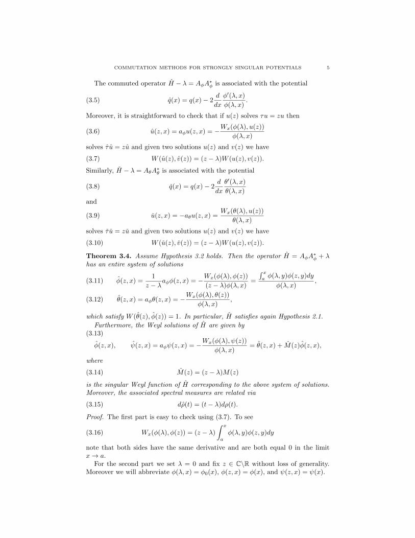
The commuted operator H − λ = AφA∗φ is associated with the potential
(3.5) q(x) = q(x)− 2d
dx
φ′(λ, x)
φ(λ, x).
Moreover, it is straightforward to check that if u(z) solves τu = zu then
(3.6) u(z, x) = aφu(z, x) = −Wx(φ(λ), u(z))
φ(λ, x)
solves τ u = zu and given two solutions u(z) and v(z) we have
(3.7) W (u(z), v(z)) = (z − λ)W (u(z), v(z)).
Similarly, H − λ = AθA∗θ is associated with the potential
(3.8) q(x) = q(x)− 2d
dx
θ′(λ, x)
θ(λ, x)
and
(3.9) u(z, x) = −aθu(z, x) =Wx(θ(λ), u(z))
θ(λ, x)
solves τ u = zu and given two solutions u(z) and v(z) we have
(3.10) W (u(z), v(z)) = (z − λ)W (u(z), v(z)).
Theorem 3.4. Assume Hypothesis 3.2 holds. Then the operator H = AφA∗φ + λ
has an entire system of solutions
φ(z, x) =1
z − λaφφ(z, x) = −Wx(φ(λ), φ(z))
(z − λ)φ(λ, x)=
∫ xaφ(λ, y)φ(z, y)dy
φ(λ, x),(3.11)
θ(z, x) = aφθ(z, x) = −Wx(φ(λ), θ(z))
φ(λ, x),(3.12)
which satisfy W (θ(z), φ(z)) = 1. In particular, H satisfies again Hypothesis 2.1.
Furthermore, the Weyl solutions of H are given by(3.13)
φ(z, x), ψ(z, x) = aφψ(z, x) = −Wx(φ(λ), ψ(z))
φ(λ, x)= θ(z, x) + M(z)φ(z, x),
where
(3.14) M(z) = (z − λ)M(z)
is the singular Weyl function of H corresponding to the above system of solutions.Moreover, the associated spectral measures are related via
(3.15) dρ(t) = (t− λ)dρ(t).
Proof. The first part is easy to check using (3.7). To see
(3.16) Wx(φ(λ), φ(z)) = (z − λ)
∫ x
a
φ(λ, y)φ(z, y)dy
note that both sides have the same derivative and are both equal 0 in the limitx→ a.
For the second part we set λ = 0 and fix z ∈ C\R without loss of generality.Moreover we will abbreviate φ(λ, x) = φ0(x), φ(z, x) = φ(x), and ψ(z, x) = ψ(x).
6 A. KOSTENKO, A. SAKHNOVICH, AND G. TESCHL
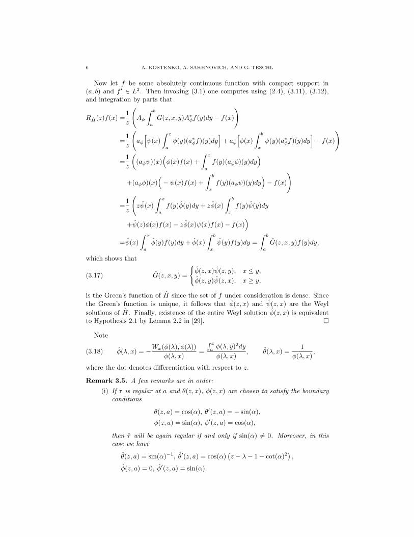
Now let f be some absolutely continuous function with compact support in(a, b) and f ′ ∈ L2. Then invoking (3.1) one computes using (2.4), (3.11), (3.12),and integration by parts that
RH(z)f(x) =1
z
(Aφ
∫ b
a
G(z, x, y)A∗φf(y)dy − f(x)
)
=1
z
(aφ
[ψ(x)
∫ x
a
φ(y)(a∗φf)(y)dy]
+ aφ
[φ(x)
∫ b
x
ψ(y)(a∗φf)(y)dy]− f(x)
)
=1
z
((aφψ)(x)
(φ(x)f(x) +
∫ x
a
f(y)(aφφ)(y)dy)
+(aφφ)(x)(− ψ(x)f(x) +
∫ b
x
f(y)(aφψ)(y)dy)− f(x)
)
=1
z
(zψ(x)
∫ x
a
f(y)φ(y)dy + zφ(x)
∫ b
x
f(y)ψ(y)dy
+ψ(z)φ(x)f(x)− zφ(x)ψ(x)f(x)− f(x))
=ψ(x)
∫ x
a
φ(y)f(y)dy + φ(x)
∫ b
x
ψ(y)f(y)dy =
∫ b
a
G(z, x, y)f(y)dy,
which shows that
(3.17) G(z, x, y) =
φ(z, x)ψ(z, y), x ≤ y,φ(z, y)ψ(z, x), x ≥ y,
is the Green’s function of H since the set of f under consideration is dense. Since
the Green’s function is unique, it follows that φ(z, x) and ψ(z, x) are the Weyl
solutions of H. Finally, existence of the entire Weyl solution φ(z, x) is equivalentto Hypothesis 2.1 by Lemma 2.2 in [29].
Note
(3.18) φ(λ, x) = −Wx(φ(λ), φ(λ))
φ(λ, x)=
∫ xaφ(λ, y)2dy
φ(λ, x), θ(λ, x) =
1
φ(λ, x),
where the dot denotes differentiation with respect to z.
Remark 3.5. A few remarks are in order:
(i) If τ is regular at a and θ(z, x), φ(z, x) are chosen to satisfy the boundaryconditions
θ(z, a) = cos(α), θ′(z, a) = − sin(α),
φ(z, a) = sin(α), φ′(z, a) = cos(α),
then τ will be again regular if and only if sin(α) 6= 0. Moreover, in thiscase we have
θ(z, a) = sin(α)−1, θ′(z, a) = cos(α)(z − λ− 1− cot(α)2
),
φ(z, a) = 0, φ′(z, a) = sin(α).
COMMUTATION METHODS FOR STRONGLY SINGULAR POTENTIALS 7
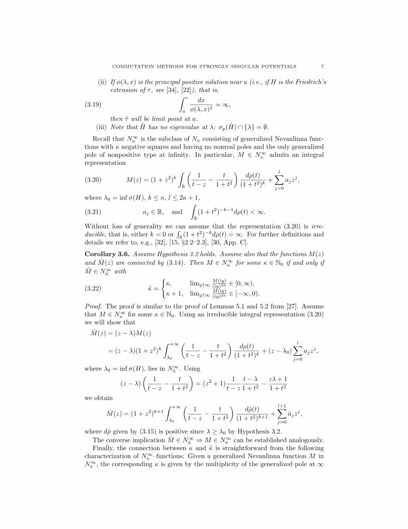
(ii) If φ(λ, x) is the principal positive solution near a (i.e., if H is the Friedrich’sextension of τ , see [34], [22]), that is,
(3.19)
∫ c
a
dx
φ(λ, x)2=∞,
then τ will be limit point at a.(iii) Note that H has no eigenvalue at λ: σp(H) ∩ λ = ∅.
Recall that N∞κ is the subclass of Nκ consisting of generalized Nevanlinna func-tions with κ negative squares and having no nonreal poles and the only generalizedpole of nonpositive type at infinity. In particular, M ∈ N∞κ admits an integralrepresentation
(3.20) M(z) = (1 + z2)k∫R
(1
t− z− t
1 + t2
)dρ(t)
(1 + t2)k+
l∑j=0
ajzj ,
where λ0 = inf σ(H), k ≤ κ, l ≤ 2κ+ 1,
(3.21) aj ∈ R, and
∫R
(1 + t2)−k−1dρ(t) <∞.
Without loss of generality we can assume that the representation (3.20) is irre-ducible, that is, either k = 0 or
∫R(1 + t2)−kdρ(t) =∞. For further definitions and
details we refer to, e.g., [32], [15, §2.2–2.3], [30, App. C].
Corollary 3.6. Assume Hypothesis 3.2 holds. Assume also that the functions M(z)
and M(z) are connected by (3.14). Then M ∈ N∞κ for some κ ∈ N0 if and only if
M ∈ N∞κ with
(3.22) κ =
κ, limy↑∞
M(iy)(iy)2κ ∈ [0,∞),
κ+ 1, limy↑∞M(iy)(iy)2κ ∈ [−∞, 0).
Proof. The proof is similar to the proof of Lemmas 5.1 and 5.2 from [27]. Assumethat M ∈ N∞κ for some κ ∈ N0. Using an irreducible integral representation (3.20)we will show that
M(z) = (z − λ)M(z)
= (z − λ)(1 + z2)k∫ +∞
λ0
(1
t− z− t
1 + t2
)dρ(t)
(1 + t2)k+ (z − λ0)
l∑j=0
ajzj ,
where λ0 = inf σ(H), lies in N∞κ . Using
(z − λ)
(1
t− z− t
1 + t2
)= (z2 + 1)
1
t− zt− λ1 + t2
− zλ+ 1
1 + t2
we obtain
M(z) = (1 + z2)k+1
∫ +∞
λ0
(1
t− z− t
1 + t2
)dρ(t)
(1 + t2)k+1+
l+1∑j=0
ajzj ,
where dρ given by (3.15) is positive since λ ≥ λ0 by Hypothesis 3.2.
The converse implication M ∈ N∞κ ⇒M ∈ N∞κ can be established analogously.Finally, the connection between κ and κ is straightforward from the following
characterization of N∞κ –functions: Given a generalized Nevanlinna function M inN∞κ , the corresponding κ is given by the multiplicity of the generalized pole at ∞

8 A. KOSTENKO, A. SAKHNOVICH, AND G. TESCHL
which is determined by the facts that the following limits exist and take values asindicated:
limy↑∞− M(iy)
(iy)2κ−1∈ (0,∞], lim
y↑∞
M(iy)
(iy)2κ+1∈ [0,∞).
Similarly, we obtain
Theorem 3.7. Assume Hypothesis 3.2, τ is limit point at a, and let θ(λ, x) > 0.The operator H = AθA
∗θ − λ has an entire system of solutions
φ(z, x) = −aθφ(z, x) =Wx(θ(λ), φ(z))
θ(λ, x),(3.23)
θ(z, x) = − 1
z − λaθθ(z, x) =
Wx(θ(λ), θ(z))
(z − λ)θ(λ, x),(3.24)
which satisfy W (θ(z), φ(z)) = 1. In particular, H satisfies again Hypothesis 2.1.Furthermore, the Weyl solutions of H are given by
(3.25)
φ(z, x), ψ(z, x) = −aθψ(z, x) =Wx(θ(λ), ψ(z))
(z − λ)θ(λ, x)= θ(z, x) + M(z)φ(z, x),
where
(3.26) M(z) = (z − λ)−1M(z)
is the singular Weyl function of H. The associated spectral measures are relatedvia
(3.27) dρ(t) = (t− λ)−1dρ(t)−M(λ)dΘ(t− λ),
where Θ(t) = 0 for t < 0 and Θ(t) = 1 for t ≥ 0 is the usual step function. HereM(λ) = limε↓0M(λ− ε).
Note
(3.28) φ(λ, x) =1
θ(λ, x), θ(λ, x) =
Wx(θ(λ), θ(λ))
θ(λ, x).
Remark 3.8. Again a few remarks are in order:
(i) If θ(λ, x) is the principal positive solution near b, that is,
(3.29)
∫ b
c
dx
θ(λ, x)2=∞,
then τ will be limit point at b. (Note that the principal positive solutionnear a is φ(λ, x) since we assumed the limit point case at a.)
(ii) Note that H has an eigenvalue at λ unless θ(λ, x) is the principal positivesolution near b.
(iii) Note that factorizing H using θ(λ, x) = φ(λ, x)−1 will transform H back
into H. In particular,ˇφ(z, x) = φ(z, x) and
ˇθ(z, x) = θ(z, x).
(iv) Clearly this procedure can be iterated and we refer (e.g.) to Appendix A of[20] for the well-known formulas.
COMMUTATION METHODS FOR STRONGLY SINGULAR POTENTIALS 9
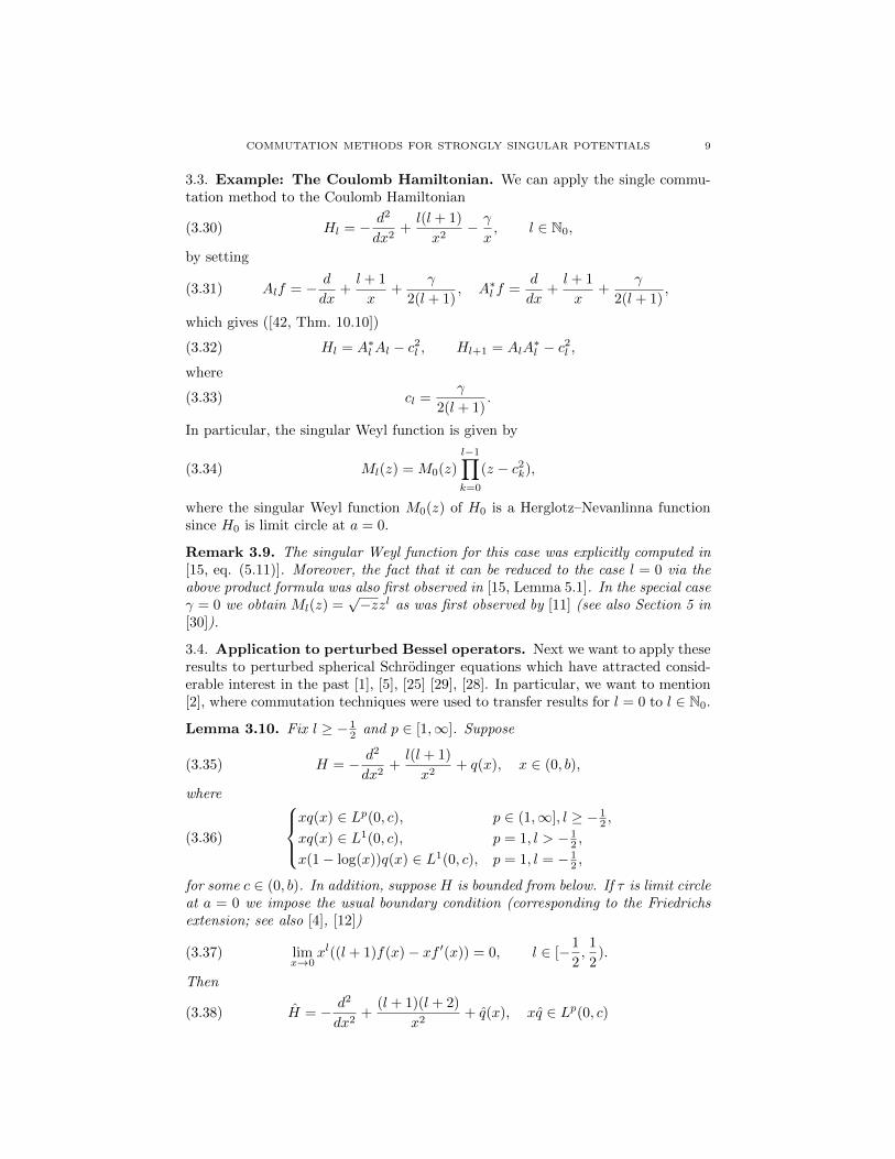
3.3. Example: The Coulomb Hamiltonian. We can apply the single commu-tation method to the Coulomb Hamiltonian
(3.30) Hl = − d2
dx2+l(l + 1)
x2− γ
x, l ∈ N0,
by setting
(3.31) Alf = − d
dx+l + 1
x+
γ
2(l + 1), A∗l f =
d
dx+l + 1
x+
γ
2(l + 1),
which gives ([42, Thm. 10.10])
(3.32) Hl = A∗lAl − c2l , Hl+1 = AlA∗l − c2l ,
where
(3.33) cl =γ
2(l + 1).
In particular, the singular Weyl function is given by
(3.34) Ml(z) = M0(z)
l−1∏k=0
(z − c2k),
where the singular Weyl function M0(z) of H0 is a Herglotz–Nevanlinna functionsince H0 is limit circle at a = 0.
Remark 3.9. The singular Weyl function for this case was explicitly computed in[15, eq. (5.11)]. Moreover, the fact that it can be reduced to the case l = 0 via theabove product formula was also first observed in [15, Lemma 5.1]. In the special caseγ = 0 we obtain Ml(z) =
√−zzl as was first observed by [11] (see also Section 5 in
[30]).
3.4. Application to perturbed Bessel operators. Next we want to apply theseresults to perturbed spherical Schrodinger equations which have attracted consid-erable interest in the past [1], [5], [25] [29], [28]. In particular, we want to mention[2], where commutation techniques were used to transfer results for l = 0 to l ∈ N0.
Lemma 3.10. Fix l ≥ − 12 and p ∈ [1,∞]. Suppose
(3.35) H = − d2
dx2+l(l + 1)
x2+ q(x), x ∈ (0, b),
where
(3.36)
xq(x) ∈ Lp(0, c), p ∈ (1,∞], l ≥ − 1
2 ,
xq(x) ∈ L1(0, c), p = 1, l > − 12 ,
x(1− log(x))q(x) ∈ L1(0, c), p = 1, l = − 12 ,
for some c ∈ (0, b). In addition, suppose H is bounded from below. If τ is limit circleat a = 0 we impose the usual boundary condition (corresponding to the Friedrichsextension; see also [4], [12])
(3.37) limx→0
xl((l + 1)f(x)− xf ′(x)) = 0, l ∈ [−1
2,
1
2).
Then
(3.38) H = − d2
dx2+
(l + 1)(l + 2)
x2+ q(x), xq ∈ Lp(0, c)
10 A. KOSTENKO, A. SAKHNOVICH, AND G. TESCHL
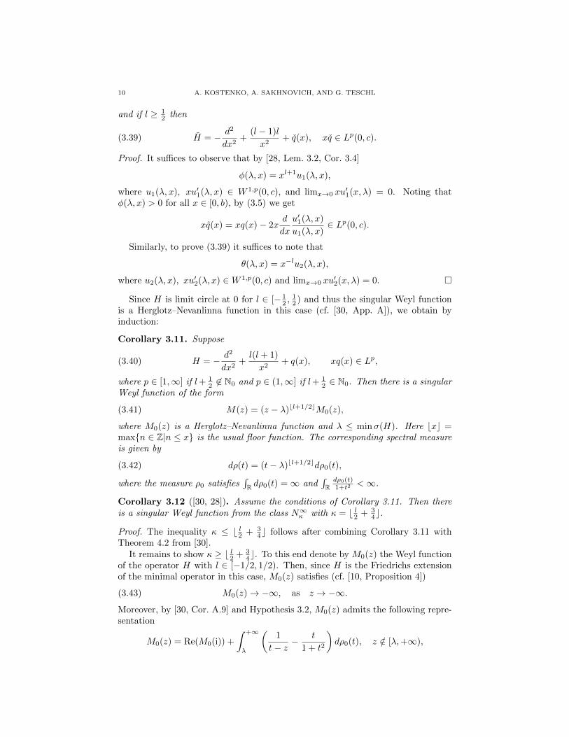
and if l ≥ 12 then
(3.39) H = − d2
dx2+
(l − 1)l
x2+ q(x), xq ∈ Lp(0, c).
Proof. It suffices to observe that by [28, Lem. 3.2, Cor. 3.4]
φ(λ, x) = xl+1u1(λ, x),
where u1(λ, x), xu′1(λ, x) ∈ W 1,p(0, c), and limx→0 xu′1(x, λ) = 0. Noting that
φ(λ, x) > 0 for all x ∈ [0, b), by (3.5) we get
xq(x) = xq(x)− 2xd
dx
u′1(λ, x)
u1(λ, x)∈ Lp(0, c).
Similarly, to prove (3.39) it suffices to note that
θ(λ, x) = x−lu2(λ, x),
where u2(λ, x), xu′2(λ, x) ∈W 1,p(0, c) and limx→0 xu′2(x, λ) = 0.
Since H is limit circle at 0 for l ∈ [− 12 ,
12 ) and thus the singular Weyl function
is a Herglotz–Nevanlinna function in this case (cf. [30, App. A]), we obtain byinduction:
Corollary 3.11. Suppose
(3.40) H = − d2
dx2+l(l + 1)
x2+ q(x), xq(x) ∈ Lp,
where p ∈ [1,∞] if l+ 12 6∈ N0 and p ∈ (1,∞] if l+ 1
2 ∈ N0. Then there is a singularWeyl function of the form
(3.41) M(z) = (z − λ)bl+1/2cM0(z),
where M0(z) is a Herglotz–Nevanlinna function and λ ≤ minσ(H). Here bxc =maxn ∈ Z|n ≤ x is the usual floor function. The corresponding spectral measureis given by
(3.42) dρ(t) = (t− λ)bl+1/2cdρ0(t),
where the measure ρ0 satisfies∫R dρ0(t) =∞ and
∫Rdρ0(t)1+t2 <∞.
Corollary 3.12 ([30, 28]). Assume the conditions of Corollary 3.11. Then thereis a singular Weyl function from the class N∞κ with κ = b l2 + 3
4c.
Proof. The inequality κ ≤ b l2 + 34c follows after combining Corollary 3.11 with
Theorem 4.2 from [30].It remains to show κ ≥ b l2 + 3
4c. To this end denote by M0(z) the Weyl functionof the operator H with l ∈ [−1/2, 1/2). Then, since H is the Friedrichs extensionof the minimal operator in this case, M0(z) satisfies (cf. [10, Proposition 4])
(3.43) M0(z)→ −∞, as z → −∞.
Moreover, by [30, Cor. A.9] and Hypothesis 3.2, M0(z) admits the following repre-sentation
M0(z) = Re(M0(i)) +
∫ +∞
λ
(1
t− z− t
1 + t2
)dρ0(t), z /∈ [λ,+∞),
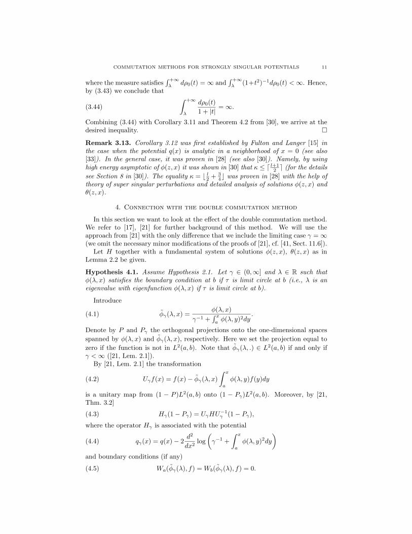
COMMUTATION METHODS FOR STRONGLY SINGULAR POTENTIALS 11
where the measure satisfies∫ +∞λ
dρ0(t) =∞ and∫ +∞λ
(1+t2)−1dρ0(t) <∞. Hence,by (3.43) we conclude that
(3.44)
∫ +∞
λ
dρ0(t)
1 + |t|=∞.
Combining (3.44) with Corollary 3.11 and Theorem 4.2 from [30], we arrive at thedesired inequality.
Remark 3.13. Corollary 3.12 was first established by Fulton and Langer [15] inthe case when the potential q(x) is analytic in a neighborhood of x = 0 (see also[33]). In the general case, it was proven in [28] (see also [30]). Namely, by usinghigh energy asymptotic of φ(z, x) it was shown in [30] that κ ≤ d l+1
2 e (for the details
see Section 8 in [30]). The equality κ = b l2 + 34c was proven in [28] with the help of
theory of super singular perturbations and detailed analysis of solutions φ(z, x) andθ(z, x).
4. Connection with the double commutation method
In this section we want to look at the effect of the double commutation method.We refer to [17], [21] for further background of this method. We will use theapproach from [21] with the only difference that we include the limiting case γ =∞(we omit the necessary minor modifications of the proofs of [21], cf. [41, Sect. 11.6]).
Let H together with a fundamental system of solutions φ(z, x), θ(z, x) as inLemma 2.2 be given.
Hypothesis 4.1. Assume Hypothesis 2.1. Let γ ∈ (0,∞] and λ ∈ R such thatφ(λ, x) satisfies the boundary condition at b if τ is limit circle at b (i.e., λ is aneigenvalue with eigenfunction φ(λ, x) if τ is limit circle at b).
Introduce
(4.1) φγ(λ, x) =φ(λ, x)
γ−1 +∫ xaφ(λ, y)2dy
.
Denote by P and Pγ the orthogonal projections onto the one-dimensional spaces
spanned by φ(λ, x) and φγ(λ, x), respectively. Here we set the projection equal to
zero if the function is not in L2(a, b). Note that φγ(λ, .) ∈ L2(a, b) if and only ifγ <∞ ([21, Lem. 2.1]).
By [21, Lem. 2.1] the transformation
(4.2) Uγf(x) = f(x)− φγ(λ, x)
∫ x
a
φ(λ, y)f(y)dy
is a unitary map from (1 − P )L2(a, b) onto (1 − Pγ)L2(a, b). Moreover, by [21,Thm. 3.2]
(4.3) Hγ(1− Pγ) = UγHU−1γ (1− Pγ),
where the operator Hγ is associated with the potential
(4.4) qγ(x) = q(x)− 2d2
dx2log
(γ−1 +
∫ x
a
φ(λ, y)2dy
)and boundary conditions (if any)
(4.5) Wa(φγ(λ), f) = Wb(φγ(λ), f) = 0.
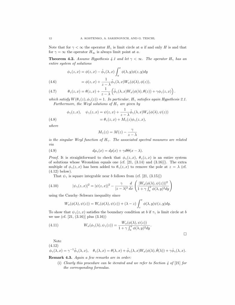
12 A. KOSTENKO, A. SAKHNOVICH, AND G. TESCHL
Note that for γ <∞ the operator Hγ is limit circle at a if and only H is and thatfor γ =∞ the operator H∞ is always limit point at a.
Theorem 4.2. Assume Hypothesis 4.1 and let γ < ∞. The operator Hγ has anentire system of solutions
φγ(z, x) = φ(z, x)− φγ(λ, x)
∫ x
a
φ(λ, y)φ(z, y)dy
= φ(z, x) +1
z − λφγ(λ, x)Wx(φ(λ), φ(z)),(4.6)
θγ(z, x) = θ(z, x) +1
z − λ
(φγ(λ, x)Wx(φ(λ), θ(z)) + γφγ(z, x)
).(4.7)
which satisfy W (θγ(z), φγ(z)) = 1. In particular, Hγ satisfies again Hypothesis 2.1.Furthermore, the Weyl solutions of Hγ are given by
φγ(z, x), ψγ(z, x) = ψ(z, x) +1
z − λφγ(λ, x)Wx(φ(λ), ψ(z))
= θγ(z, x) +Mγ(z)φγ(z, x),(4.8)
where
Mγ(z) = M(z)− γ
z − λis the singular Weyl function of Hγ . The associated spectral measures are relatedvia
(4.9) dργ(x) = dρ(x) + γdΘ(x− λ).
Proof. It is straightforward to check that φγ(z, x), θγ(z, x) is an entire systemof solutions whose Wronskian equals one (cf. [21, (3.14) and (3.16)]). The extramultiple of φγ(z, x) has been added to θγ(z, x) to remove the pole at z = λ (cf.(4.12) below).
That ψγ is square integrable near b follows from (cf. [21, (3.15)])
(4.10) |ψγ(z, x)|2 = |ψ(z, x)|2 − γ
|z − λ|2d
dx
(|Wx(φ(λ), ψ(z))|2
1 + γ∫ xaφ(λ, y)2dy
)using the Cauchy–Schwarz inequality since
Wx(φ(λ), ψ(z)) = Wc(φ(λ), ψ(z)) + (λ− z)∫ x
c
φ(λ, y)ψ(z, y)dy.
To show that ψγ(z, x) satisfies the boundary condition at b if τγ is limit circle at bwe use (cf. [21, (3.16)] plus (3.16))
(4.11) Wx(φγ(λ), ψγ(z)) =Wx(φ(λ), ψ(z))
1 + γ∫ xaφ(λ, y)2dy
.
Note(4.12)
φγ(λ, x) = γ−1φγ(λ, x), θγ(λ, x) = θ(λ, x) + φγ(λ, x)Wx(φ(λ), θ(λ)) + γφγ(λ, x).
Remark 4.3. Again a few remarks are in order:
(i) Clearly this procedure can be iterated and we refer to Section 4 of [21] forthe corresponding formulas.

COMMUTATION METHODS FOR STRONGLY SINGULAR POTENTIALS 13
(ii) If λ is an eigenvalue, one could even admit γ ∈ [−‖φ(λ)‖−2,∞).(iii) This procedure leaves operators of the type (3.35) invariant. In particular,
it does not change l.
Theorem 4.4. Assume Hypothesis 4.1 and let γ = ∞. The operator H∞ has anentire system of solutions
φ∞(z, x) =1
z − λ
(φ(z, x)− φ∞(λ, x)
∫ x
a
φ(λ, y)φ(z, y)dy
)(4.13)
θ∞(z, x) = (z − λ)θ(z, x) + φ∞(λ, x)Wx(φ(λ), θ(z)),(4.14)
which satisfy W (θ∞(z), φ∞(z)) = 1. In particular, H∞ satisfies again Hypothe-sis 2.1.
Furthermore, the Weyl solutions of H∞ are given by
φ∞(z, x), ψ∞(z, x) = (z − λ)ψ(z, x) + φ∞(λ, x)Wx(φ(λ), ψ(z))
= θ∞(z, x) +M∞(z)φ∞(z, x),(4.15)
where
(4.16) M∞(z) = (z − λ)2M(z)
is the singular Weyl function of H∞. The associated spectral measures are relatedvia
(4.17) dρ∞(t) = (t− λ)2dρ(t).
Proof. In the limiting case γ → ∞ the definition (4.6) from the previous theoremwould give φ∞(λ, x) = 0 and we simply need to remove this zero. The rest followsas in the previous theorem.
Note(4.18)
φ∞(λ, x) = φ(λ, x)− φ∞(λ, x)
∫ x
a
φ(λ, y)φ(λ, y)dy, θ∞(λ, x) = −φ∞(λ, x)
Remark 4.5. (i) Again this procedure can be iterated and we refer to Sec-tion 4 of [21] for the corresponding formulas.
(ii) For operators of the type (3.35) this procedure changes l to l + 2.
5. Examples based on the generalized Backlund–Darbouxtransformation
In this section we want to look at connections with the generalized Backlund–Darboux transformation (GBDT) approach (see [35, 37] and the references therein).This approach contains the double commutation method as a special case as we willshow below and there are close relations with the binary Darboux transform (see,e.g., the comparative discussion in [6, Section 7.2]). Here we will use the GBDTto construct an explicit example with a generalized Weyl function which is rationalwith respect to
√z and which has non-real zeros.
More specific, we want to apply the GBDT to the Schrodinger equation
τu = zu, x ∈ (0,∞).(5.1)
This case was treated in Proposition 2.2 [36], see also [35].
14 A. KOSTENKO, A. SAKHNOVICH, AND G. TESCHL
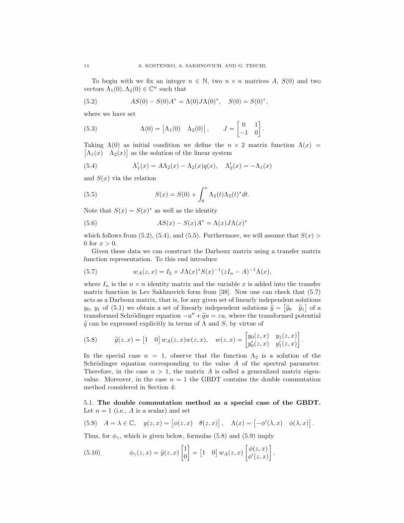
To begin with we fix an integer n ∈ N, two n × n matrices A, S(0) and twovectors Λ1(0),Λ2(0) ∈ Cn such that
(5.2) AS(0)− S(0)A∗ = Λ(0)JΛ(0)∗, S(0) = S(0)∗,
where we have set
(5.3) Λ(0) =[Λ1(0) Λ2(0)
], J =
[0 1−1 0
].
Taking Λ(0) as initial condition we define the n × 2 matrix function Λ(x) =[Λ1(x) Λ2(x)
]as the solution of the linear system
(5.4) Λ′1(x) = AΛ2(x)− Λ2(x)q(x), Λ′2(x) = −Λ1(x)
and S(x) via the relation
S(x) = S(0) +
∫ x
0
Λ2(t)Λ2(t)∗dt.(5.5)
Note that S(x) = S(x)∗ as well as the identity
(5.6) AS(x)− S(x)A∗ = Λ(x)JΛ(x)∗
which follows from (5.2), (5.4), and (5.5). Furthermore, we will assume that S(x) >0 for x > 0.
Given these data we can construct the Darboux matrix using a transfer matrixfunction representation. To this end introduce
(5.7) wA(z, x) = I2 + JΛ(x)∗S(x)−1(zIn −A)−1Λ(x),
where In is the n× n identity matrix and the variable x is added into the transfermatrix function in Lev Sakhnovich form from [38]. Now one can check that (5.7)acts as a Darboux matrix, that is, for any given set of linearly independent solutionsy0, y1 of (5.1) we obtain a set of linearly independent solutions y =
[y0 y1
]of a
transformed Schrodinger equation −u′′+ qu = zu, where the transformed potentialq can be expressed explicitly in terms of Λ and S, by virtue of
(5.8) y(z, x) =[1 0
]wA(z, x)w(z, x), w(z, x) =
[y0(z, x) y1(z, x)y′0(z, x) y′1(z, x)
].
In the special case n = 1, observe that the function Λ2 is a solution of theSchrodinger equation corresponding to the value A of the spectral parameter.Therefore, in the case n > 1, the matrix A is called a generalized matrix eigen-value. Moreover, in the case n = 1 the GBDT contains the double commutationmethod considered in Section 4:
5.1. The double commutation method as a special case of the GBDT.Let n = 1 (i.e., A is a scalar) and set
A = λ ∈ C, y(z, x) =[φ(z, x) θ(z, x)
], Λ(x) =
[−φ′(λ, x) φ(λ, x)
].(5.9)
Thus, for φγ , which is given below, formulas (5.8) and (5.9) imply
φγ(z, x) = y(z, x)
[10
]=[1 0
]wA(z, x)
[φ(z, x)φ′(z, x)
].(5.10)
COMMUTATION METHODS FOR STRONGLY SINGULAR POTENTIALS 15
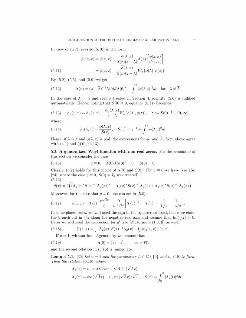
In view of (5.7), rewrite (5.10) in the form
φγ(z, x) = φ(z, x) +φ(λ, x)
S(x)(z − λ)Λ(x)
[φ(z, x)φ′(z, x)
]= φ(z, x) +
φ(λ, x)
S(x)(z − λ)Wx
(φ(λ), φ(z)
).(5.11)
By (5.2), (5.5), and (5.9) we get
S(x) = (λ− λ)−1Λ(0)JΛ(0)∗ +
∫ x
0
|φ(λ, t)|2dt for λ 6= λ.(5.12)
In the case of λ = λ and real φ treated in Section 4, identity (5.6) is fulfilledautomatically. Hence, noting that S(0) ≥ 0, equality (5.11) becomes
φγ(z, x) = φγ(z, x) +φγ(λ, x)
z − λWx(φ(λ), φ(z)), γ := S(0)−1 ∈ (0, ∞],(5.13)
where
φγ(λ, x) =φ(λ, x)
S(x), S(x) = γ−1 +
∫ x
0
φ(λ, t)2dt.(5.14)
Hence, if λ = λ and φ(λ, x) is real, the expressions for φγ and φγ from above agreewith (4.1) and (4.6), (4.13).
5.2. A generalized Weyl function with non-real zeros. For the remainder ofthis section we consider the case
q ≡ 0, Λ(0)JΛ(0)∗ = 0, S(0) = 0.(5.15)
Clearly, (5.2) holds for this choice of Λ(0) and S(0). For q ≡ 0 we have (see also[24], where the case q ≡ 0, S(0) = In was treated):(5.16)
q(x) = 2((
Λ2(x)∗S(x)−1Λ2(x))2
+ Λ1(x)∗S(x)−1Λ2(x) + Λ2(x)∗S(x)−1Λ1(x)).
Moreover, for the case that q ≡ 0, one can set in (5.8):
(5.17) w(z, x) = T (z)
[ei√zx 0
0 e−i√zx
]T (z)−1, T (z) =
[1 1
i√z −i
√z
].
In some places below we will need the sign in the square root fixed, hence we chosethe branch cut in
√z along the negative real axis and assume that Im(
√z) > 0.
Later we will need the expression for y′ (see [24, formula (1.30)]) as well:
(5.18) y′(z, x) =[−Λ2(x)∗S(x)−1Λ2(x) 1
]wA(z, x)w(z, x).
If n = 1, without loss of generality we assume that
(5.19) Λ(0) =[v1 1
], υ1 = υ1,
and the second relation in (5.15) is immediate.
Lemma 5.1. [30] Let n = 1 and the parameters A ∈ C \ 0 and υ1 ∈ R be fixed.Then the relation (5.16), where
Λ1(x) = υ1 cos(√Ax) +
√A sin(
√Ax),
Λ2(x) = cos(√Ax)− υ1 sin(
√Ax)/
√A, S(x) =
∫ x
0
|Λ2(t)|2dt,
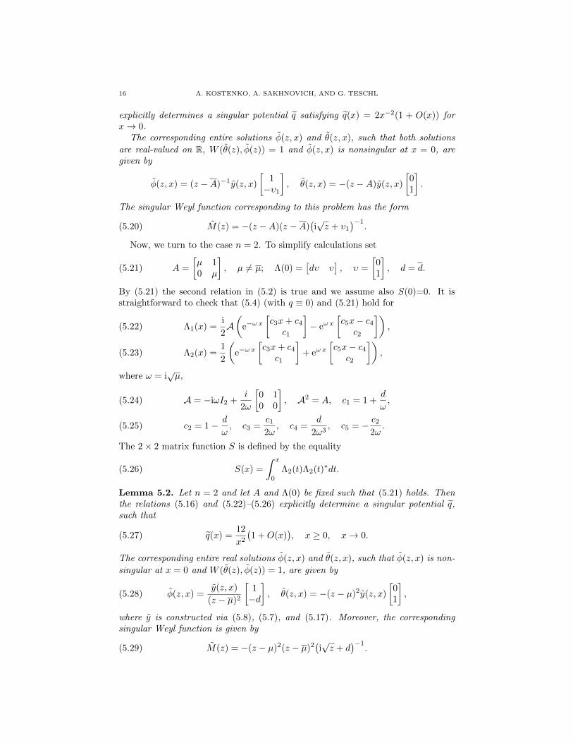
16 A. KOSTENKO, A. SAKHNOVICH, AND G. TESCHL
explicitly determines a singular potential q satisfying q(x) = 2x−2(1 + O(x)) forx→ 0.
The corresponding entire solutions φ(z, x) and θ(z, x), such that both solutions
are real-valued on R, W (θ(z), φ(z)) = 1 and φ(z, x) is nonsingular at x = 0, aregiven by
φ(z, x) = (z −A)−1y(z, x)
[1−υ1
], θ(z, x) = −(z −A)y(z, x)
[01
].
The singular Weyl function corresponding to this problem has the form
M(z) = −(z −A)(z −A)(i√z + υ1
)−1.(5.20)
Now, we turn to the case n = 2. To simplify calculations set
(5.21) A =
[µ 10 µ
], µ 6= µ; Λ(0) =
[dυ υ
], υ =
[01
], d = d.
By (5.21) the second relation in (5.2) is true and we assume also S(0)=0. It isstraightforward to check that (5.4) (with q ≡ 0) and (5.21) hold for
Λ1(x) =i
2A(
e−ω x[c3x+ c4
c1
]− eω x
[c5x− c4
c2
]),(5.22)
Λ2(x) =1
2
(e−ω x
[c3x+ c4
c1
]+ eω x
[c5x− c4
c2
]),(5.23)
where ω = i√µ,
A = −iωI2 +i
2ω
[0 10 0
], A2 = A, c1 = 1 +
d
ω,(5.24)
c2 = 1− d
ω, c3 =
c12ω, c4 =
d
2ω3, c5 = − c2
2ω.(5.25)
The 2× 2 matrix function S is defined by the equality
(5.26) S(x) =
∫ x
0
Λ2(t)Λ2(t)∗dt.
Lemma 5.2. Let n = 2 and let A and Λ(0) be fixed such that (5.21) holds. Thenthe relations (5.16) and (5.22)–(5.26) explicitly determine a singular potential q,such that
q(x) =12
x2(1 +O(x)
), x ≥ 0, x→ 0.(5.27)
The corresponding entire real solutions φ(z, x) and θ(z, x), such that φ(z, x) is non-
singular at x = 0 and W (θ(z), φ(z)) = 1, are given by
φ(z, x) =y(z, x)
(z − µ)2
[1−d
], θ(z, x) = −(z − µ)2y(z, x)
[01
],(5.28)
where y is constructed via (5.8), (5.7), and (5.17). Moreover, the correspondingsingular Weyl function is given by
M(z) = −(z − µ)2(z − µ)2(i√z + d
)−1.(5.29)
COMMUTATION METHODS FOR STRONGLY SINGULAR POTENTIALS 17
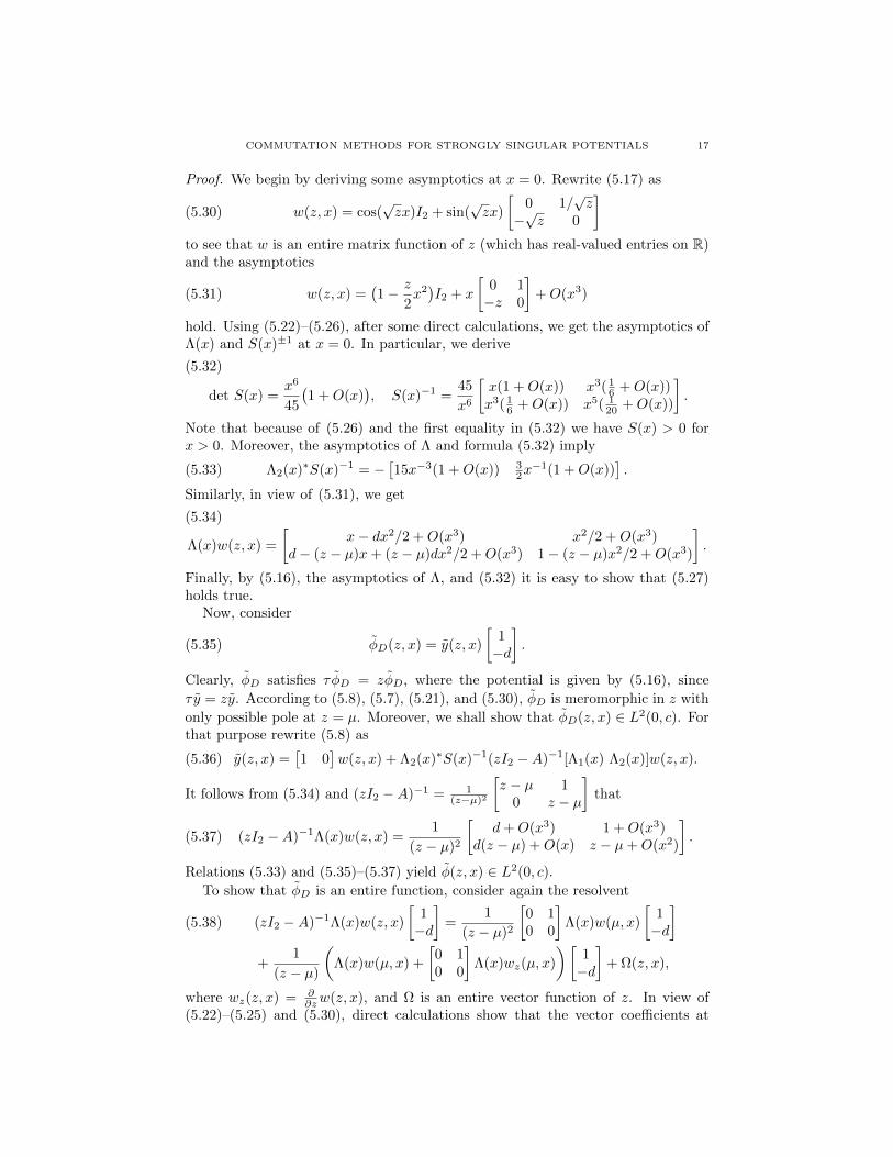
Proof. We begin by deriving some asymptotics at x = 0. Rewrite (5.17) as
(5.30) w(z, x) = cos(√zx)I2 + sin(
√zx)
[0 1/
√z
−√z 0
]to see that w is an entire matrix function of z (which has real-valued entries on R)and the asymptotics
(5.31) w(z, x) =(1− z
2x2)I2 + x
[0 1−z 0
]+O(x3)
hold. Using (5.22)–(5.26), after some direct calculations, we get the asymptotics ofΛ(x) and S(x)±1 at x = 0. In particular, we derive
det S(x) =x6
45
(1 +O(x)
), S(x)−1 =
45
x6
[x(1 +O(x)) x3( 1
6 +O(x))x3( 1
6 +O(x)) x5( 120 +O(x))
].
(5.32)
Note that because of (5.26) and the first equality in (5.32) we have S(x) > 0 forx > 0. Moreover, the asymptotics of Λ and formula (5.32) imply
Λ2(x)∗S(x)−1 = −[15x−3(1 +O(x)) 3
2x−1(1 +O(x))
].(5.33)
Similarly, in view of (5.31), we get
Λ(x)w(z, x) =
[x− dx2/2 +O(x3) x2/2 +O(x3)
d− (z − µ)x+ (z − µ)dx2/2 +O(x3) 1− (z − µ)x2/2 +O(x3)
].
(5.34)
Finally, by (5.16), the asymptotics of Λ, and (5.32) it is easy to show that (5.27)holds true.
Now, consider
(5.35) φD(z, x) = y(z, x)
[1−d
].
Clearly, φD satisfies τ φD = zφD, where the potential is given by (5.16), since
τ y = zy. According to (5.8), (5.7), (5.21), and (5.30), φD is meromorphic in z with
only possible pole at z = µ. Moreover, we shall show that φD(z, x) ∈ L2(0, c). Forthat purpose rewrite (5.8) as
y(z, x) =[1 0
]w(z, x) + Λ2(x)∗S(x)−1(zI2 −A)−1[Λ1(x) Λ2(x)]w(z, x).(5.36)
It follows from (5.34) and (zI2 −A)−1 = 1(z−µ)2
[z − µ 1
0 z − µ
]that
(zI2 −A)−1Λ(x)w(z, x) =1
(z − µ)2
[d+O(x3) 1 +O(x3)
d(z − µ) +O(x) z − µ+O(x2)
].(5.37)
Relations (5.33) and (5.35)–(5.37) yield φ(z, x) ∈ L2(0, c).
To show that φD is an entire function, consider again the resolvent
(zI2 −A)−1Λ(x)w(z, x)
[1−d
]=
1
(z − µ)2
[0 10 0
]Λ(x)w(µ, x)
[1−d
](5.38)
+1
(z − µ)
(Λ(x)w(µ, x) +
[0 10 0
]Λ(x)wz(µ, x)
)[1−d
]+ Ω(z, x),
where wz(z, x) = ∂∂zw(z, x), and Ω is an entire vector function of z. In view of
(5.22)–(5.25) and (5.30), direct calculations show that the vector coefficients at
18 A. KOSTENKO, A. SAKHNOVICH, AND G. TESCHL
(z − µ)−2 and (z − µ)−1 on the right-hand side of (5.38) equal zero, that is, theleft-hand side of (5.38) is an entire vector function. Therefore, by (5.35) and (5.36)
one can see that φD(z, x) is an entire function too.Let us consider another solution
θD(z, x) = y(z, x)
[01
].(5.39)
According to (5.8), (5.17), (5.18), and (5.35) we have
W(θD(z), φD(z)
)= −detwA(z, x).(5.40)
Thus, detwA(z, x) does not depend on x. Moreover, using (5.7) and (5.6) we get
wA(z, x)∗JwA(z, x) = J,(5.41)
that is, |detwA(z, x)| = 1. Taking into account the fact that wA(z, x) is a rationalfunction of z with the only possible pole at z = µ (of order no greater than 2) andrecalling that the relations µ 6= µ,
|detwA(z, x)| = 1, limz→∞
detwA(z, x) = 1
hold, we derive: detwA(z, x) = (z−µ)k(z−µ)−k (0 ≤ k ≤ 4). Further calculationsshow that k = 2:
detwA(z, x) = (z − µ)2(z − µ)−2.(5.42)
To prove that φ and θ are entire and real, rewrite (5.41) as wA(z, x)∗ = JwA(z, x)−1J∗.In view of (5.42) the last equality yields[
w11(z, x) w21(z, x)w12(z, x) w22(z, x)
]= (z − µ)2(z − µ)−2
[w11(z, x) w21(z, x)w12(z, x) w22(z, x)
],
where wA =: wij2i,j=1. In other words, we get
(z − µ)−2wA(z, x) = (z − µ)−2wA(z, x).(5.43)
Recall that w(z, x) = w(z, x), that is, w is real. Thus, by (5.8) and (5.43) the
vector function (z − µ)−2y(z, x) is real for µ 6= µ. So, the functions φ and θ, whichare given by (5.28), are real. Definitions (5.28), (5.35), and (5.39) yield also
φ(z, x) = (z − µ)−2φD(z, x), θ(z, x) = −(z − µ)2θD(z, x).(5.44)
Since φD is an entire function, it follows from (5.44) that the real function φ may
have only one pole at z = µ (µ 6= µ). Therefore, φ is an entire function. It follows
from (5.44) that θ is an entire function too. Finally, (5.40), (5.42), and (5.44) imply
that W(θ(z), φ(z)
)= 1. Thus, the statements of our lemma regarding φ and θ are
proved.Now, using φ and θ we can construct explicitly a singular Weyl function M .
Observe that (5.17) yields
w(z, x)
[1
i√z
]=
[ei√zx
i√zei√zx
].(5.45)
In view of (5.23) and (5.26) we calculate that
detS(x) ∼ |c2c5|2(4Re(ω))−4e4Re(ω)x (x→ +∞),
COMMUTATION METHODS FOR STRONGLY SINGULAR POTENTIALS 19
and so the transfer function wA(z, x) given by (5.7) behaves like O(x4). Hence, itfollows from (5.8) and (5.45) that
ψD(z, x) = y(x, z)
[1
i√z
]=[1 0
]wA(z, x)
[ei√zx
i√zei√zx
]∈ L2(c,∞).(5.46)
Therefore, by (5.28), (5.29), and (5.46) we get
ψ(z, x) = θ(z, x) + M(z)φ(z, x) ∈ L2(c,∞),
that is, M(z) given by (5.29) is a singular Weyl function of our system.
Remark 5.3. According to (5.27), the GBDT generated by a 2×2 matrix A of theform (5.21) transforms a Schrodinger operator with l = 0 into one with l = 3.
Acknowledgments. A.K. acknowledges the hospitality and financial support ofthe Erwin Schrodinger Institute and financial support from the IRCSET PostDoc-toral Fellowship Program. In addition, we are indebted to two anonymous refereesfor valuable suggestions improving the presentation of the material.
References
[1] S. Albeverio, R. Hryniv, and Ya. Mykytyuk, Inverse spectral problems for Sturm–Liouville operators in impedance form, J. Funct. Anal. 222, 143–177 (2005).
[2] S. Albeverio, R. Hryniv, and Ya. Mykytyuk, Inverse spectral problems for Bessel opera-tors, J. Diff. Eqs. 241, 130–159 (2007).
[3] C. Bennewitz and W. N. Everitt, The Titchmarsh–Weyl eigenfunction expansion the-
orem for Sturm–Liouville differential equations, in Sturm-Liouville Theory: Past andPresent, 137–171, Birkhauser, Basel, 2005.
[4] W. Bulla and F. Gesztesy, Deficiency indices and singular boundary conditions in quan-
tum mechanics, J. Math. Phys. 26:10, 2520–2528 (1985).[5] R. Carlson, Inverse spectral theory for some singular Sturm–Liouville problems, J. Diff.
Eqs. 106, 121–140 (1993).
[6] J. L. Cieslinski, Algebraic construction of the Darboux matrix revisited, J. Phys. A 42,404003, 40 pp (2009).
[7] M. M. Crum, Associated Sturm–Liouville systems, Quart. J. Math. Oxford (2) 6, 121–
127 (1955).[8] G. Darboux, Sur une proposition relative aux equations lineaires, C. R. Acad. Sci. (Paris)
94, 1456–1459 (1882).[9] P. A. Deift, Applications of a commutation formula, Duke Math. J. 45, 267–310 (1978).
[10] V. A. Derkach and M. M. Malamud, Generalised resolvents and the boundary value
problems for Hermitian operators with gaps, J. Funct. Anal. 95, 1–95 (1991).[11] A. Dijksma and Yu. Shondin, Singular point-like perturbations of the Bessel operator in
a Pontryagin space, J. Diff. Eqs. 164, 49–91 (2000).[12] W. N. Everitt and H. Kalf, The Bessel differential equation and the Hankel transform,
J. Comput. Appl. Math. 208, 3–19 (2007).[13] L. Faddeev, The inverse problem in quantum scattering theory, J. Math. Phys. 4, 72–104
(1963).[14] C. Fulton, Titchmarsh–Weyl m-functions for second order Sturm-Liouville problems,
Math. Nachr. 281, 1417–1475 (2008).[15] C. Fulton and H. Langer, Sturm-Liouville operators with singularities and generalized
Nevanlinna functions, Complex Anal. Oper. Theory 4, 179–243 (2010).[16] I. M. Gel’fand and B. M. Levitan, On the determination of a differential equation from
its spectral function, Amer. Math. Soc. Transl. Ser 2, 1, 253–304 (1955).[17] F. Gesztesy, A complete spectral characterization of the double commutation method, J.
Funct. Anal. 117, 401–446 (1993).[18] F. Gesztesy, W. Schweiger, and B. Simon, Commutation methods applied to the mKdV-
equation, Trans. Amer. Math. Soc. 324, 465–525 (1991).

20 A. KOSTENKO, A. SAKHNOVICH, AND G. TESCHL
[19] F. Gesztesy, B. Simon, and G. Teschl, Zeros of the Wronskian and renormalized oscil-
lation theory, Am. J. Math. 118, 571–594 (1996).
[20] F. Gesztesy, B. Simon, and G. Teschl, Spectral deformations of one-dimensionalSchrodinger operators, J. d’Analyse Math. 70, 267–324 (1996).
[21] F. Gesztesy and G. Teschl, On the double commutation method, Proc. Amer. Math. Soc.
124, 1831–1840 (1996).[22] F. Gesztesy and Z. Zhao, On critical and subcritical Sturm–Liouville operators, J. Funct.
Anal. 98, 311-345 (1991).
[23] F. Gesztesy and M. Zinchenko, On spectral theory for Schrodinger operators with stronglysingular potentials, Math. Nachr. 279, 1041–1082 (2006).
[24] I. Gohberg, M. A. Kaashoek and A. L. Sakhnovich, Sturm–Liouville systems with rational
Weyl functions: explicit formulas and applications, Integral Equations Operator Theory30, 338–377 (1998).
[25] J.-C. Guillot and J. V. Ralston, Inverse spectral theory for a singular Sturm–Liouvilleoperator on [0, 1], J. Diff. Eqs. 76, 353–373 (1988).
[26] C. G. J. Jacobi, Zur Theorie der Variationsrechnung und der Differentialgleichungen,
J. Reine Angew. Math. 17, 68–82 (1837).[27] I. S. Kac and M. G. Krein, R-functions — analytic functions mapping the upper halfplane
into itself, in Amer. Math. Soc. Transl. Ser. (2), 103, 1–19 (1974).
[28] A. Kostenko and G. Teschl, On the singular Weyl–Titchmarsh function of perturbedspherical Schrodinger operators, J. Diff. Eq. 250, 3701–3739 (2011).
[29] A. Kostenko, A. Sakhnovich, and G. Teschl, Inverse eigenvalue problems for perturbed
spherical Schrodinger operators, Inverse Problems 26, 105013, 14pp (2010).[30] A. Kostenko, A. Sakhnovich, and G. Teschl, Weyl–Titchmarsh theory for Schrodinger
operators with strongly singular potentials, Int. Math. Res. Not. 2011, Art. ID rnr065,
49pp (2011).[31] M. G. Krein, On a continual analogue of a Christoffel formula from the theory of or-
thogonal polynomials, Dokl. Akad. Nauk SSSR (N.S.) 113, 970–973 (1957). [Russian]
[32] M. G. Krein and H. Langer, Uber einige Fortsetzungsprobleme, die eng mit der Theorie
hermitescher Operatoren im Raume Πκ zusammenhangen. Teil I: Einige Funktionen-
klassen und ihre Darstellungen, Math. Nachr. 77, 187–236 (1977).[33] P. Kurasov and A. Luger, An operator theoretic interpretation of the generalized
Titchmarsh–Weyl coefficient for a singular Sturm–Liouville problem, Math. Phys. Anal.
Geom. 14, 115–151 (2011).[34] R. Rosenberger, A new characterization of the Friedrichs extension of semibounded
Sturm–Liouville equations, J. London Math. Soc. 31, 501–510 (1985).[35] A. L. Sakhnovich, Generalized Backlund-Darboux transformation: spectral properties
and nonlinear equations, J. Math. Anal. Appl. 262, 274–306 (2001).
[36] A. L. Sakhnovich, Non-Hermitian matrix Schrodinger equation: Backlund-Darbouxtransformation, Weyl functions, and PT symmetry, J. Phys. A 36, 7789–7802 (2003).
[37] A. L. Sakhnovich, On the GBDT version of the Backlund-Darboux transformation and
its applications to the linear and nonlinear equations and spectral theory, MathematicalModelling of Natural Phenomena 5:4, 340–389 (2010).
[38] L. A. Sakhnovich, On the factorization of the transfer matrix function, Soviet Math.
Dokl. 17, 203–207 (1976).[39] U.-W. Schmincke, On Schrodinger’s factorization method for Sturm–Liouville operators,
Proc. Roy. Soc. Edinburgh 80A, 67–84 (1978).[40] U.-W. Schmincke, On a paper by Gesztesy, Simon, and Teschl concerning isospectral
deformations of ordinary Schrodinger operators, J. Math. Anal. Appl. 277, 51–78 (2003).
[41] G. Teschl, Jacobi Operators and Completely Integrable Nonlinear Lattices, Math. Surv.
and Mon. 72, Amer. Math. Soc., Rhode Island, 2000.[42] G. Teschl, Mathematical Methods in Quantum Mechanics; With Applications to
Schrodinger Operators, Graduate Studies in Mathematics, Amer. Math. Soc., RhodeIsland, 2009.
[43] J. Weidmann, Spectral Theory of Ordinary Differential Operators, Lecture Notes in
Mathematics, 1258, Springer, Berlin, 1987.
COMMUTATION METHODS FOR STRONGLY SINGULAR POTENTIALS 21
Institute of Applied Mathematics and Mechanics, NAS of Ukraine, R. Luxemburg str.
74, Donetsk 83114, Ukraine, and School of Mathematical Sciences, Dublin Institute of
Technology, Kevin Street, Dublin 8, IrelandE-mail address: [email protected]
Faculty of Mathematics, University of Vienna, Nordbergstrasse 15, 1090 Wien, Aus-tria
E-mail address: [email protected]
URL: http://www.mat.univie.ac.at/~sakhnov/
Faculty of Mathematics, University of Vienna, Nordbergstrasse 15, 1090 Wien, Aus-
tria, and International Erwin Schrodinger Institute for Mathematical Physics, Boltz-
manngasse 9, 1090 Wien, AustriaE-mail address: [email protected]
URL: http://www.mat.univie.ac.at/~gerald/
Related Documents