Simultaneous Perturbation Stochastic Approximation-Based Localization Algorithms for Mobile Devices

Ocean DynamicsDOI 10.1007/s10236-011-0387-6

Simultaneous perturbation stochastic approximationfor tidal models

Muhammad Umer Altaf · Arnold W. Heemink ·Martin Verlaan · Ibrahim Hoteit

Received: 3 November 2010 / Accepted: 7 February 2011© The Author(s) 2011. This article is published with open access at Springerlink.com

Abstract The Dutch continental shelf model (DCSM)is a shallow sea model of entire continental shelf whichis used operationally in the Netherlands to forecastthe storm surges in the North Sea. The forecasts arenecessary to support the decision of the timely closureof the moveable storm surge barriers to protect theland. In this study, an automated model calibrationmethod, simultaneous perturbation stochastic approx-imation (SPSA) is implemented for tidal calibration ofthe DCSM. The method uses objective function evalu-ations to obtain the gradient approximations. The gra-dient approximation for the central difference methoduses only two objective function evaluation indepen-dent of the number of parameters being optimized.The calibration parameter in this study is the modelbathymetry. A number of calibration experiments isperformed. The effectiveness of the algorithm is eval-uated in terms of the accuracy of the final results aswell as the computational costs required to producethese results. In doing so, comparison is made witha traditional steepest descent method and also witha newly developed proper orthogonal decomposition-based calibration method. The main findings are: (1)

Responsible Editor: Phil Peter Dyke

This article is part of the Topical Collection on Joint NumericalSea Modelling Group Workshop 2010

M. U. Altaf (B) · A. W. Heemink · M. VerlaanDelft University of Technology, Mekelweg 4,2628 CD, Delft, Netherlandse-mail: [email protected], [email protected]

I. HoteitKing Abdullah University of Science and Technology,25955-690, Thuwal, Saudi Arabia

The SPSA method gives comparable results to steepestdescent method with little computational cost. (2) TheSPSA method with little computational cost can beused to estimate large number of parameters.

Keywords Numerical tidal modeling ·Parameter estimation · Simultaneous perturbation ·Stochastic approximation

1 Introduction

Accurate sea water level forecasting is crucial in theNetherlands. This is mainly because large areas of theland lie below sea level. Forecasts are made to supportthe storm surge flood warning system. Timely waterlevel forecasts are necessary to support the decisionfor closure of the movable storm surge barriers in theEastern Scheldt and the New Waterway. Moreover,forecasting is also important for harbor management,as the size of some ships have become so large that theycan only enter the harbor during high water period. Thestorm surge warning service (SVSD) in close coopera-tion with the Royal Netherlands meteorological insti-tute is responsible for these forecasts. The surge is pre-dicted by using a numerical hydrodynamic model, theDutch continental shelf model (DCSM) (see Stelling1984; Verboom et al. 1992). The performance of theDCSM regarding the storm surges is influenced byits performance in forecasting the astronomical tides.Using inverse modeling techniques, these tidal data canbe used to improve the model results.

Most efficient optimization algorithms require a gra-dient of the objective function. This usually requiresthe implementation of the adjoint code for the com-

Ocean Dynamics

putation of the gradient of the objective function. Theadjoint method aims at adjusting a number of unknowncontrol parameters on the basis of given data. Thecontrol parameters might be model initial conditions ormodel parameters (Thacker and Long 1988). A sizeableamount of research on adjoint parameter estimationwas carried out in the last 30 years in fields such as me-teorology, petroleum reservoirs, and oceanography forinstance by Seinfeld and Kravaris (1982), Bennet andMcintosh (1982), Ulman and Wilson (1998), Courtierand Talagrand (1990), Lardner et al. (1993) andHeemink et al. (2002). A detailed description of theapplication of the adjoint method in atmosphere andocean problems can be found in Navon (1998).

One of the drawbacks of the adjoint method is theprogramming effort required for the implementationof the adjoint model. Research has recently been car-ried out on automatic generation of computer code forthe adjoint, and adjoint compilers have now becomeavailable (see Kaminski et al. 2003). Even with the useof these adjoint compilers, this is a huge programmingeffort that hampers new applications of the method.Courtier et al. (1994) had proposed an incrementalapproach, in which the forward solution of the nonlin-ear model is replaced by a low resolution approximatemodel. Reduced order modeling can also be used toobtain an efficient low-order approximate linear model(Hoteit 2008; Lawless et al. 2008).

This paper focuses on a method referred to asthe simultaneous perturbation stochastic approxima-tion (SPSA) method. This method can be easily com-bined with any numerical model to do automaticcalibration. For the calibration of numerical tidalmodel, the SPSA algorithm would require only thewater level data predicted from the given model. SPSAis stochastic offspring of the Keifer–Wolfowitz Algo-rithm (Kiefer and Wolfowitz 1952) commonly referredas finite difference stochastic approximation (FDSA)method. This algorithm uses objective function eval-uations to obtain the gradient approximations. Eachindividual model parameter is perturbed one at a timeand the partial derivatives of the objective functionwith respect to the each parameter is estimated by adivided difference based on the standard Taylor seriesapproximation of a partial derivative. This approxima-tion of each partial derivative involved in the gradientof the objective function requires at least one newevaluation of the objective function, thus this methodis not feasible for automated calibration when we havelarge number of parameters.

The SPSA method uses stochastic simultaneous per-turbation of all model parameters to generate a searchat each iteration. SPSA is based on a highly efficient

and easily implemented simultaneous perturbation ap-proximation to the gradient. This gradient approxima-tion for the central difference method uses only two ob-jective function evaluation independent of the numberof parameters being optimized. The SPSA algorithmhas gathered a great deal of interest over the lastdecade and has been used for a variety of applications(Hutchison and Hill 1997; Spall 1998, 2000; Gerencseret al. 2001; Gao and Reynolds 2007). As a result of thestochastic perturbation, the calculated gradient is alsostochastic, however the expectation of the stochasticgradient is the true gradient (Gao and Reynolds 2007).So one would expect that the performance of the basicSPSA algorithm to be similar to the performance ofsteepest descent.

The gradient-based algorithms are faster to convergethan any objective function-based gradient approxima-tions such as SPSA algorithm when speed is measurein terms of the number of iterations. The total costto achieve effective convergence depends not only onthe number of iterations required, but also on the costneeded to perform these iterations, which is typicallygreater in gradient-based algorithms. This cost mayinclude greater computational burden and resources,additional human effort required for determining andcoding gradients.

Vermeulen and Heemink (2006) proposed a methodbased on proper orthogonal decomposition (POD)which shifts the minimization into lower dimensionalspace and avoids the implementation of the adjointof the tangent linear approximation of the originalnonlinear model. Recently, Altaf et al. (2011) appliedthis POD-based calibration method for the estimationof depth values and bottom friction coefficients for avery large-scale tidal model. The method has also beenapplied in petroleum engineering by Kaleta et al. (2011)for history matching problems. One drawback of thePOD-based calibration method is its dependence onthe number of parameters.

In this paper the SPSA algorithm is applied for theestimation of depth values in the tidal model DCSMof the entire European continental shelf. A number ofcalibration experiments is performed both simulatedand real data. The effectiveness of the algorithm isevaluated in terms of the accuracy of the final resultsas well as the computational costs required to producethese results. In doing so, comparison is made witha traditional steepest descent method and also with anewly developed POD-based calibration method.

The paper is organized as follows. Section 2 describesthe SPSA algorithm. This section also briefly discussesthe POD-based calibration approach which is usedhere as comparison with SPSA method. The following

Ocean Dynamics

section briefly explains the DCSM model used in thisstudy. Section 4 contains results from experiments withthe model DCSM, to estimate the water depth. Thepaper concludes in Section 5 by discussing the results.

2 Parameter estimation using SPSA

Consider a data assimilation problem for a general non-linear dynamical system. The discrete system equationfor the state vectors X(ti+1) ∈ �n is given by;

X(ti+1) = Mi[X(ti), γ ], (1)

where Mi is nonlinear and deterministic dynamics oper-ator that includes inputs and propagates the state fromtime ti to time ti+1, γ is vector of uncertain parameterswhich needs to be determined. Suppose now that wehave imperfect observations Y(ti) ∈ �q of the dynami-cal system (1) that are related to model state at time tithrough

Y(ti) = HX(ti) + η(ti), (2)

where H : �n → �nqis linear observation operator that

maps the model fields on observation space and η(ti)is unbiased random Gaussian error vector with covari-ance matrix Ri.

We assume that the difference between data andsimulation results is only due to measurement er-rors and incorrectly prescribed model parameters. Theproblem of the estimation is then solved by directlyminimizing the objective function J

J(γ ) =∑

i

[Y(ti) − H(X(ti))]T R−1i [Y(ti) − H(X(ti))]

(3)

with respect to the parameters γ satisfying the discretenonlinear forecast model (1).

In the SPSA algorithm, we minimize the objectivefunction J(γ ) using the iteration procedure

γ l+1 = γ l − al gl(γl), (4)

where gl(γl) is a stochastic approximation of ∇ J(γ l),

which denotes the gradient of the objective functionwith respect to γ evaluated at the old iterate, γ l. if gl(γ

l)

is replaced by ∇ J(γ l), then Eq. 4 represents the steepestdescent algorithm.

The stochastic gradient gl(γl) is SPSA algorithm is

calculated by the following procedure.

1. Define the np dimensional column vector �l by

�l = [�l,1, �l,2, · · · , �l,np]T , (5)

and

�−1l = [�−1

l,1 , �−1l,2 , · · · , �−1

l,np]T , (6)

where �l,i, i = 1, 2, · · · , np represents independentsamples from the symmetric ±1 Bernoulli distribu-tion. This means that +1 or −1 are the only possiblevalues that can be obtained for each �l,i. It alsomeans that

�−1l,i = �l,i, (7)

and

E[�−1l,i ] = E[�l,1] = 0, (8)

where E denotes the expectation.2. Define a positive coefficient cl and obtain two eval-

uations of the objective function J(γ ) based on thesimultaneous perturbation around the current γ l:J(γ l + cl�l) and J(γ l − cl�l).

3. A realization of the stochastic gradient is then cal-culated by using central difference approximationas

gl(γl) = J(γ l + cl�l) − J(γ l − cl�l)

2cl�−1

l (9)

Since �l is a random vector, gl is also randomvector. So by generating a sample of �l, we gen-erate a specific sample of gl. The FDSA algorithminvolves computation of each component of ∇ J byperturbing one model parameter at a time. If onedoes a one-sided approximation for each partialderivative involved in ∇ J(γ l), then computation ofthe gradient requires np + 1 evaluations of J foreach iteration of the steepest descent algorithm. Incontrast, the SPSA requires only two evaluations ofthe objective function J(γ l + cl�l) and J(γ l + cl�l)

at each iteration.

2.1 Choice of al and cl

Returning to Eqs. 4 and 9, we see that we have left tospecify with al and cl. These are specified here accord-ing to the guidelines given by Spall (1998). The relevantformulas for al and cl are given by

al = a(A + l + 1)α

, (10)

and

cl = c

(l + 1)β, (11)

where a, c, A, α and β are positive real numberssuch that 0 < α ≤ 1, α − β < 0.5 and α > 2β. Thegiven choices for α, β will ensure that the algorithm,

Ocean Dynamics

Eq. 4 converges to a minimum of J in a stochastic sense(almost surely). The choice of a, c, A, α and β is tosome extent case dependent and it may require someexperimentation to determine good values of these pa-rameters. Although the asymptotically optimal valuesof α and β are 1.0 and 1/6, respectively (Chin 1997), butchoosing smaller values, e.g., α = 0.602 and β = 0.101(Spall 1998) appear to be more effective in practice.One recommendation for A is to set A equal to 10%of the maximum number of iterations allowed.

The value of constant c should be chosen so that c isequal to the standard deviation of the noise in objectivefunction J. If one has perfect objective function, then cshould be chosen as small positive number.

2.2 Average stochastic gradient

One of the motivations for SPSA is that for a quadraticobjective function such as J, the expectation of the sto-chastic gradient is the true gradient (Gao and Reynolds2007), i.e.,

E[gl(γl)] = gl(γ l) = ∇ J(γ l), (12)

where gl(γ l) is defined as

gl(γ l) = 1

N

N∑

i=1

gl(γl), (13)

with each gl(γl) is obtained from Eq. 9 using N different

samples of �l. Due to the relationship given in Eq. 12,one would hope that SPSA would have convergenceproperties similar to those of steepest descent in termsof the number of iterations required to reduce theobjective function J to a certain level. In this case,SPSA could be much more efficient than the steepestdescent algorithm.

2.3 POD-based calibration method

Vermeulen and Heemink (2006) proposed a methodbased on POD which shifts the minimization into lowerdimensional space and avoids the implementation ofthe adjoint of the tangent linear approximation of theoriginal nonlinear model. Due to the linear characterof the POD-based reduced model its adjoint can beimplemented easily and the minimization problem issolved completely in reduced space with very low com-putational cost.

The linearization of nonlinear high-order model (1)using the first order Taylor’s formula around the back-ground parameter γ b

k gives

�X(ti+1) = ∂ Mi[Xb (ti), γ b ]∂ Xb (ti)

�X(ti)

+∑

k

∂ Mi[Xb (ti), γ b ]∂γk

�γk (14)

where X is linearized state vector, Xb is the back-ground state vector with the prior estimated parametersvector γ b and �X is a deviation of the model frombackground trajectory.

A model can be reduced if the incremental state�X(ti+1) can be written as linear combination:

�X(ti) = Pξ(ti+1) (15)

where P = {p1, p2, · · · , pr} is a projection matrix suchthat PT P = I and ξ is a reduced state vector given by:(

ξ(ti+1)

�γ

)=

(Mi Mγ

i0 I

) (ξ(ti)�γ

)(16)

Here, �γ is the control parameter vector, Mi and Mγ

iare simplified dynamics operators which approximatethe full Jacobians ∂Mi

∂ Xb and ∂Mi∂γk

, respectively:

Mi = PT ∂ Mi

∂ Xb (ti)P (17)

Mγ

i = PT(

∂ Mi

∂γ1, · · · ,

∂ Mi

∂γnp

)(18)

The dimension on which the reduced model operatesis (r + np) × (r + np) with np being the number of esti-mated parameters.

2.3.1 Collection of the snapshots and POD basis

The POD method is used here to obtain an approx-imate low-order formulation of the original tangentlinear model. POD is an optimal technique of findinga basis which spans an ensemble of data (snapshots)collected from an experiment or a numerical simulationof a dynamical system. The reduced model used here isto estimate uncertain parameters, the snapshots shouldbe able to represent the behavior of the system forthese parameters. Therefore the snapshot vectors ei ∈�s are obtained from the perturbations ∂Mi

∂γkalong each

estimated parameter γk to get a matrix

E = {e1, · · · , es}; i = {1, 2, · · · , s}. (19)

The dimension of this ensemble matrix E is s = np × ns,where ns is the number of snapshot collected for each

Ocean Dynamics

individual parameter γk. The covariance matrix Q canbe constructed from the ensemble E of the snapshotsby taking the outer product

Q = EET (20)

This covariance matrix is usually huge as in the currentapplication with state vector of dimension ∼ 3 × 106, sodirect solution of eigenvalue problem is not feasible.To shorten the calculation time necessary for solvingthe eigenvalue problem for this high-dimensional co-variance matrix, we define a covariance matrix G as aninner product

G = Et E (21)

In the method of snapshots (Sirovich 1987), one thensolves the s × s eigenvalue problem

Gzi = Et Ezi = λizi, i ∈ {1, 2, · · · , s} (22)

where λi are the eigenvalues of the above eigenvalueproblem. The eigenvectors zi may be chosen to beorthonormal and the POD modes P are then given by:

pi = Ezi/√

λi (23)

We define a measure ψi for the relative informationto choose a low dimensional basis by neglecting modescorresponding to the small eigenvalues:

ψi = λi∑sl=1 λl

100%, i = {1, 2, · · · , s} (24)

We collect pr (r < s) modes such that ψ1 > ψ2 > . . . >

ψr and they totally explain at least the required varianceψe,

ψe =r∑

l=1

ψl (25)

The total number of eigenmodes r in the POD basisP depends on the required accuracy of the reducedmodel.

2.3.2 Approximate objective function and its adjoint

In POD-based approach, we look for an optimal so-lution of Eq. 1 to minimize the approximate objectivefunction ( J) in an incremental way:

J(�γ ) =∑

i

[{Y(ti) − H(Xb (ti))} − Hξ(ti, �γ )]T

× R−1i [{Y(ti) − H(Xb (ti))} − Hξ(ti, �γ )] (26)

The value of the approximate objective function Jis obtained by correcting the observations Y(ti) for

background state Xb (ti) which is mapped on the obser-vational space through a mapping H and to the reducedmodel state ξ(ti, �γ ) which is mapped to the observa-tional space through mapping H, with H = H P.

Since the reduced model has linear characteristics, itis easy to build an approximate adjoint model for thecomputation of gradient of the approximate objectivefunction (26). The gradient of J with respect to �γ isgiven by:

∂ J∂(�γ )

=∑

i

−[ν(ti+1)]T ∂ξ(ti+1)

∂(�γ )(27)

where ν(ti+1) is the reduced adjoint state variable(Vermeulen and Heemink 2006). Once the gradient hasbeen computed, the process of minimizing the approxi-mate objective function J is done along the direction ofthe gradient vector in the reduced space.

Recently, Altaf et al. (2011) applied this POD-basedcalibration method for the estimation of depth valuesand bottom friction coefficients for a very large-scaletidal model. The method has also been recently appliedin petroleum engineering by Kaleta et al. (2011) forhistory matching problems. One drawback of the POD-based calibration method is its dependence on the num-ber of parameters.

3 The Dutch Continental Shelf Model

The DCSM is an operational storm surge model, usedin the Netherlands for real-time storm surge predictionin North sea. Accurate predictions of the storm surgesare of vital importance to the Netherlands since largeareas of the land lie below sea level. Accurate fore-casts at least six hours ahead are needed for properclosure of the movable storm surge barriers in EasternScheldt and the New Waterway. The governing equa-tions used in DCSM are the nonlinear 2D shallow waterequations. The shallow water equations, which describelarge-scale water motions, are used to calculate themovements of the water in the area under considera-tion. These equations are

∂u∂t

+ u∂u∂x

+ v∂u∂y

+ g∂h∂x

− fv + gu√

u2 + v2

HC22D

= 1

ρw

τx

H− 1

ρw

∂pa

∂x, (28)

Ocean Dynamics

∂v

∂t+ u

∂v

∂x+ v

∂v

∂y+ g

∂h∂y

+ f u + gv√

u2 + v2

HC22D

= 1

ρw

τy

H− 1

ρw

∂pa

∂y, (29)

∂h∂t

+ ∂ Hu∂x

+ ∂ Hv

∂y= 0, (30)

where

x, y Cartesian coordinates in horizontal planet time coordinate

u, v depth-averaged current in x and y direction,respectively

h water level above reference planeD water depth below the reference planeH total water depth (D + h)f coefficient for the Coriolis force

C2D Chezy coefficientτx, τy wind stress in x and y direction, respectively

ρw density of sea waterpa atmospheric pressureg acceleration of gravity

These equations are descretized using an alternatingdirections implicit (ADI) method and the staggeredgrid that is based on the method by Leendertse (1967)and improved by Stelling (1984). In the implementa-tion, the spherical grid is used instead of rectangular(see e.g. Verboom et al. 1992). Boundary conditions areapplied at both closed and open boundaries. At closedboundaries, the velocity normal to the boundary iszero. So no inflow and outflow can occur through theseboundaries. At the open boundaries, the water level isdescribed in terms of different harmonic componentsas follows:

h(t) = h0 +10∑

j=1

f jH j cos(ω jt − θ j) (31)

where

h0 mean water levelH total water depth

f jH j amplitude of harmonic constituent jω j angular velocity of jθ j phase of j

All the open boundaries of the model are located indeep water (more than 200 m), see Fig. 1. This is done inorder to explicitly model the nonlinearities of the surgetide interaction. A uniform initial water level of 0 mmean sea level has been used. For the initial velocityzero flow conditions have been prescribed. The timezone of the model is GMT.

3.1 Estimation of depth

The bathymetry for a model is usually from nauti-cal maps. These maps usually give details of shallowrather than deep-water areas. If we use these maps toprescribe the water depth, it is reasonable to assumethat this prescription of the bathymetry is erroneous.So depth can be a parameter on which model can becalibrated. In the early years of the developments ofthe DCSM, the changes to bathymetry were made man-ually. Later automated calibration procedures basedon variational data assimilation were developed (Ten-Brummelhuis et al. 1993; Mouthaan et al. 1994). Thecomplete description on the development of these cali-brated procedures for DCSM can be found in Verlaanet al. (2005).

4 Numerical experiment

4.1 Experiment 1

The DCSM model used in this experiment covers anarea in the north-east European continental shelf, i.e.,12◦W to 13◦E and 48◦N to 62◦N, as shown in Fig. 1. Theresolution of the spherical grid is 1/8◦ × 1/12◦, whichis approximately 8 × 8 km. With this configurationthere are 201 × 173 grid with 19,809 computational gridpoints. The time step is �t = 10 min.

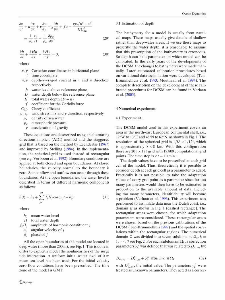
The depth values have to be prescribed at each gridcell of the model. Thus, theoretically it is possible toconsider depth at each grid cell as a parameter to adapt.Practically it is not possible to take the adaptationvalues of every grid point as a parameter since far toomany parameters would then have to be estimated inproportion to the available amount of data. Includ-ing too many parameters, identifiability will becomea problem (Verlaan et al. 1996). This experiment wasperformed to assimilate data near the Dutch coast, i.e.,domain � as shown in Fig. 1 (dashed rectangle). Therectangular areas were chosen, for which adaptationparameters were considered. These rectangular areaswere chosen based on the previous calibrations of theDCSM (Ten-Brummelhuis 1992) and the spatial corre-lations within the rectangular regions. The numericaldomain � was divided into seven subdomains �k, k =1, · · · , 7 see Fig. 2. For each subdomain �k, a correctionparameters γ b

k was defined that was related to Dn1,n2 by:

Dn1,n2 = Dbn1,n2

+ γ bk ; if(n1, n2) ∈ �k (32)

with Dbn1,n2

, the initial value. The parameters γ bk were

treated as unknown parameters. They acted as a correc-

Ocean Dynamics

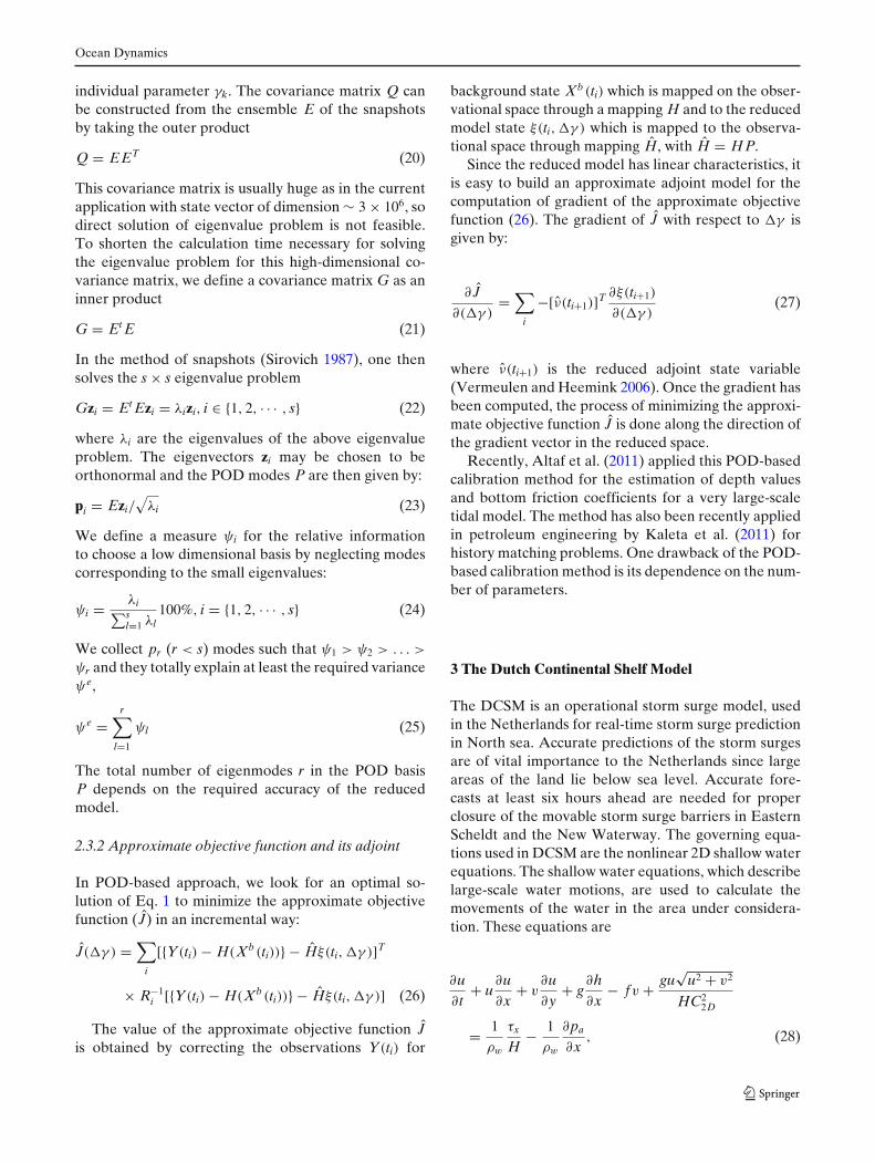
Fig. 1 DCSM area withcalibration stations: 1 N51,2 Southend, 3 Innerdowsing,4 Oostende, 5 H.v.Holland,6 Den Helder, and 7 N4. Thedashed rectangle shows thedomain �

longitude (¡W/E)

latit

ude

(¡N

)

2

317

45

6

200

200

200

200

200

-10 -5 0 5 10

50

52

54

56

58

60

62

tion for the mean level of the Dn1,n2 in a subdomain �k

and leave the spatial dependence inside �k unaltered.Seven observation points were included in the assim-

ilation, two of which are located along the east coastof the UK, two along the Dutch coast and one at theBelgium coast (see Fig. 1). The truth model was runfor a period of 15 days from 13 December 1997 00:00to 27 December 1997 24:00 with the specification ofwater depth Db

n1,n2as used in the operational DCSM

to generate artificial data at the assimilation stations.The first 2 days were used to properly initialize the sim-ulations and set of observations Y of computed waterlevels h were collected for last 13 days at an intervalof every ten minutes in seven selected assimilation gridpoints, which coincide with the points where data areobserved in reality. The observations were assumed tobe perfect. This assumption was made to see how closethe estimate is to the truth; 5 m was added in Db

n1,n2

at all the grid points in domain � to get the initialadjustments γ b

k .For the SPSA optimization algorithm, two methods

were applied to calculate the stochastic gradient. In the

first method, the stochastic gradient gl(γl) was com-

puted according to Eq. 9. In the second method, thegradient was computed by Eq. 13 referred as average

0 5 10

50

52

54

longitude (o W/E)

latit

ude

(o N) Ω

1

Ω 2

Ω 3

Ω4

Ω5

Ω 6

Ω 7

Fig. 2 Shows the subdomains �1, �2, �3, �4, �5, �6, and �7

Ocean Dynamics

SPSA where expectation is taken over two independentstochastic gradients.

The values of a, c, A, α, and β were obtained accord-ing to the guidelines given in section 2.1. These valueswere determined as best from several forward modelsimulations. The iteration cycle for the SPSA algorithmwas aborted when the value of the objective functionJ did not change for the last three iterations of theminimization process (Wang et al. 2009).

Figure 3 shows a plot of the objective function J ver-sus number of iterations β for the two implementationsof the SPSA algorithms compared with the steepestdescent and the POD-based calibration method. Notethat the gradient used in the steepest descent algorithmis obtained from the finite difference method using one-sided perturbation. The graph shows that both SPSAand average SPSA gave comparable results, althoughfor average SPSA the decrease in the objective func-tion J is more at early iterations. Also, the rate ofconvergence of average SPSA is slightly better thanthe SPSA. However, both SPSA and average SPSAare less efficient than steepest descent method. Thesteepest descent algorithm converged in ten iterationsas compared to 20 and 15 iterations in SPSA and av-erage SPSA, respectively. However, the cost of singleiteration in SPSA algorithm is far less than the steepestdescent algorithm.

For all the algorithms, there was a significant im-provements in parameters for regions coinciding withthe UK, Dutch and Belgian coast, but there was notmuch improvement in deep water regions �1 and �7.Since the subdomains containing deep areas are lesssensitive as compared the subdomains containing shal-low areas, so it is much difficult to estimate γk in regions�1 and �7.

0 5 10 15

0

100

200

300

400

500

600

700

Iterations (β)

Ob

ject

ive

Fu

nct

ion

(J)

PODSPSAAverage SPSASteepest descent

Fig. 3 Successive iterations β of the minimization process

Table 1 Comparison of estimated parameters to true parametersfor the twin experiment

ζ SPSA Average Steepest(%) SPSA (%) descent (%)

All parameters 35.11 29.27 21.02Sensitive parameters 9.95 6.29 6.49

Table 1 lists the measure (ζ ) between the updatedestimated parameters γ up obtained after calibrationwith different optimization algorithms and the true pa-rameter estimate γ t. The measure is defined as the twonorm of the difference between estimated parametersγ up obtained after optimization and the true parameterestimate γ t divided by the norm of the true parameterestimate γ t (Gao and Reynolds 2007).

ζ = || γ up − γ t ||2|| γ t ||2 (33)

By this measure, steepest descent (21%) performedthe best followed by average SPSA (29%) and SPSA(35%). Since the stochastic gradient in the SPSA algo-rithm is based on two perturbations of the independentrandom samples, it is more likely that the SPSA algo-rithm improves more sensitive areas. The table also liststhe same measure for shallow regions. In this case, allthe algorithms steepest descent (6.49%), average SPSA(6.29%) and SPSA (9.95%) performed very well. Here,average SPSA matched the performance of the steepestdescent algorithm. In average SPSA, the gradient wasthe average of only two independent stochastic gra-dients. One would expect better performance by theinclusion of more stochastic gradients in average SPSA.The Dutch continental shelf model (Table 2) presentsthe RMSE between estimated parameters (γ up) andthe true parameters (γ t) after iterations β = 5, β = 10,β = 15 and β = 20 of SPSA algorithm for calibrationstations and compares it with average SPSA and steep-est descent algorithms. The RMSE for SPSA algorithmafter iteration β = 5 is 9.95 compared to 8.92 and 6.05 inaverage SPSA and steepest descent algorithm, respec-tively. So SPSA and average SPSA are comparable atthis point. The RMSE for SPSA after ten iterations is

Table 2 RMSE results for the minimization process after 5th,10th, 15th, and 20th iterations

SPSA Average Steepest(cm) SPSA (cm) descent (cm)

Initial 22.80 22.80 22.80β = 5 9.95 8.92 6.05β = 10 5.63 4.09 2.91β = 15 4.10 3.27 –β = 20 3.55 – –

Ocean Dynamics

comparable to the RMSE of steepest descent methodafter only five iterations. Since the cost of one iter-ation of steepest descent is eight model simulationscompared to two model simulations in SPSA algorithm,SPSA is two times more efficient than steepest descentat this point and one would expect SPSA to be moreefficient if we have large number of parameters.

The RMSE with SPSA after β = 15 and averageSPSA after β = 10 is similar. At this point the compu-tational costs of both SPSA and average SPSA are alsocomparable. It is also clear from the Table 2 that thesmallest RMSE value is achieved by steepest descentmethod in ten iterations.

Figure 4 presents water levels h at the two tidegauge stations Den Helder and Southend along theDutch and English coasts, respectively for the periodfrom 18 December 1997 00:00 to 18 December 199724:00. These time series refer to water levels obtainedfrom true values of the parameters, the initial values

of the parameters and the estimated values of the pa-rameters using SPSA algorithm, respectively. Figure 4demonstrates that the estimation methods significantlyreduces the differences between time series obtainedfrom initial parameters and the true parameters as com-pared with the differences between time series obtainedfrom the estimated parameters and true parameters.

4.2 Experiment 2

The DCSM model used in this experiment is a newlydesigned spherical grid model. This newly developedDCSM covers an area in the north-east European con-tinental shelf, i.e., 15◦ W to 13◦ E, and 43◦ to 64◦ N,as shown in Fig. 5. The spherical grid has a uniformcell size of 1/40◦ in east-west direction and 1/60◦ innorth-south direction which corresponds to a grid cellsize of about ∼ 2 × 2 km. With this configuration thereare 1,120 grid cells in east-west direction and 1,260 grid

Fig. 4 Water level time seriesfor the period from 18December 1997 00:00 to 18December 1997 24:00obtained from truth model,deterministic model withinitial values of the estimatedparameters and deterministicmodel after calibration,respectively, at the two tidegauge stations a Den Helderand b Southend

6 12 18 242

1.5

1

0.5

0

0.5

1

1.5

2

Time [Hours]

Wat

er L

evel

[m

]

Truth Initial SPSA

6 12 18 243

2

1

0

1

2

3

Time [Hours]

Wat

er L

evel

[m

]

Truth Initial SPSA

Ocean Dynamics

Fig. 5 Newly developed hydrodynamic DCSM area. The dashedline represents the area of the operational DCSM extent

cells in north-south direction. The grid cells that includeland are excluded form the model by the enclosures andthe model contains 869,544 computational grid points.The grid resolution of the spherical grid is factor fivefiner then the DCSM model grid used in the previousexperiment. The idea is to perform numerical experi-ment with a very large-scale model and with real datausing SPSA algorithm.

The bathymetry of the model here is based on aNOOS gridded data set and for some areas in themodel, ETOPO2 bathymetry data is interpolated onthe computational grid (Ray 1999). The model bathym-etry is presented in Fig. 6. The dashed line in Fig. 5shows the comparison of the newly developed DCSMmodel area with the old DCSM. The model area ofthe newly developed DCSM is extended significantly inorder to ensure that the open boundary conditions arelocated further away in deep water. A computationaltime step of 2 min has been applied. So to complete a1 year model run on eight 3.6 MHz CPUs takes morethan 2 days.

The model performance can be assessed by compar-ing it to the measured (observed) dataset. The availabledata used in this research consisted of two datasets ofthe tide gauge stations, namely,

1. water level measurement data from the DutchDONAR database and

longitude (oW/E)

latit

ude

(o N)

-15 -10 -5 0 5 10

62.5

60

57.5

55

52.5

50

47.5

45

0

200

400

600

800

1000

1200

1400

1600

1800

2000

Fig. 6 DCSM model bathymetry in meters. The bathymetrygreater than 2,000 m is shown as 2,000 m

2. British Oceanographic Data Center offshore waterlevel measurement data.

For the calibration, 50 water level locations are se-lected (see Fig. 7). Observations obtained by the har-monic analysis from these 50 stations at every fifth timestep (10 min) were used for the calibration experiments.The calibration runs were performed for the periodfrom 28 December 2006 to 30 January 2007 (34 days).The first 3 days were used to properly initialize thesimulation. The measurement data were used for theremaining 30 days. This period was selected such thattwo spring neap-tide cycles are simulated. We haveassumed that the observations Y of the computed wa-ter levels h contain an error described by white noiseprocess with standard deviation σm = 0.10 (m).

The experiment was performed to estimate depthvalues using SPSA algorithm in this large-scale tidalmodel. The numerical domain � was divided intothe 12 subdomains �k, k = 1, . . . , 12 (see Fig. 8). Theinfluence of the depth adjustments is quite significantspecially in shallow regions. Thus, the subdivision ofmodel area was made such that both deep and shallowareas were separated (see Fig. 8). The data observationpoints are concentrated in the English Channel, so thisregion was divided into five subdomains to improve theresults by considering the local effects of the depth ineach subdomain �k, k = 3, · · · , 7, in this area.

Figure 9 shows a plot of the objective function Jversus number of iterations β for the SPSA algorithm

Ocean Dynamics

Fig. 7 DCSM area withstations included in the modelcalibration

compared with the POD-based calibration method.The SPSA method is compared here with POD-basedcalibration method for practical reasons. One reasonis we have seen in the previous experiment that thePOD-based calibration method efficiently estimatedthe depth values with the fastest convergence rate ascompared to SPSA and steepest descent algorithms.Secondly, its not worthwhile to compute gradient byfinite differences in this large-scale model. The graphshows that both the calibration methods give compara-ble results in terms of reduction in the objective func-tion J. Though the rate of convergence of the POD-based calibration method is far better than the SPSA.

The POD-based calibration method converged inonly two iterations as compared to 14 iterations withthe SPSA, respectively. However, the cost of singleiteration in the POD-based calibration method is muchhigher and is dependent on the number of parame-

ters np and the POD modes r used to construct thereduced model (Altaf et al. 2009). So for this exper-iment one iteration of the POD method required 13initial simulations of the original nonlinear model toget the ensemble and then additional simulations of theoriginal model to construct the POD reduced model ineach iteration β of the optimization process. The SPSAmethod on the other hand required only two objectivefunction evaluations to compute the gradient in eachiteration β of the optimization procedure. For this ap-plication, the POD method is also fast since it is notneeded to use a full simulations of the original modelfor the generation of the ensemble (Altaf et al. 2011).One disadvantage of POD-based calibration method isif the number of parameters is large the size of ensem-ble becomes large too and to construct a good reducedmodel is usually difficult with large ensemble size. Forboth the experiments performed the SPSA algorithm

Ocean Dynamics

−15 −10 −5 0 5 10

45

50

55

60

12

3

4 5

6

7

910

11

12

8

Longitude [oW/E]

Latit

ude

[oN

]

Fig. 8 The 12 subdomains �k of the DCSM used in Experiment2

converged in almost similar iterations although thenumber of parameters were different. So, it is expectedthat the SPSA algorithm will work even with moreparameters as the SPSA algorithm is independent ofthe number of the estimated parameters.

0 5 101500

2000

2500

3000

3500

4000

Iterations (β)

Ob

ject

ive

Fu

nct

ion

(J)

POD

SPSA

Fig. 9 Successive iterations β of the minimization process

5 Conclusions

In the absence of the adjoint model, the gradient isusually obtained by objective function evaluations toobtain the gradient approximations. Each individualmodel parameter is perturbed one at a time and the par-tial derivatives of the objective function with respect tothe each parameter is estimated. This method is not fea-sible for automated calibration when large number ofparameters are estimated. Simultaneous perturbationstochastic approximation (SPSA) method uses stochas-tic simultaneous perturbation of all model parametersto generate a search at each iteration. SPSA is based ona highly efficient and easily implemented simultaneousperturbation approximation to the gradient. This gra-dient approximation for the central difference methoduses only two objective function evaluation indepen-dent of the number of parameters being optimized.

SPSA algorithm is applied to calibrate the modelDCSM. The DCSM is an operational storm surgemodel, used in the Netherlands for real-time stormsurge prediction in North sea. A number of calibrationexperiments was performed both with simulated andreal data. The results from twin experiment showedthat SPSA has a lower convergence rate than the steep-est descent and POD-based calibration methods. Thesteepest descent algorithm converged in ten iterationsas compared to 20 and 15 iterations in SPSA and av-erage SPSA, respectively. However, the computationalcost of single iteration in the steepest descent and thePOD-based calibration methods is much higher and isdependent on the number of parameters np. Althoughboth SPSA and steepest descent methods converged tosimilar value of the objective function, none of the op-timization algorithms achieved the expected reductionin the objective function.

The results from a very large-scale tidal modeland with real data showed that SPSA algorithm givescomparable results to POD-based calibration method.The POD-based calibration method converged in onlytwo iterations as compared to 14 iterations withthe SPSA, respectively. The POD-based calibrationmethod though required 13 initial simulations of theoriginal model to get the ensemble and then extrasimulations to construct the POD reduced model ineach iteration β of the optimization process. The SPSAmethod on the other hand required only two objectivefunction evaluations to compute an approximation ofthe gradient in each iteration β of the optimization pro-cedure independent of the number of estimated para-meters. Thus, SPSA algorithm proved to be a promisingoptimization algorithm for model calibration for cases

Ocean Dynamics

where adjoint code is not available for computing thegradient of the objective function.

Open Access This article is distributed under the terms of theCreative Commons Attribution Noncommercial License whichpermits any noncommercial use, distribution, and reproductionin any medium, provided the original author(s) and source arecredited.

References

Altaf MU, Heemink AW, Verlaan M (2009) Inverse shallow-water flow modelling using model reduction. Int J MultiscaleCom Eng 7:577–596

Altaf MU, Verlaan M, Heemink AW (2011) Efficient iden-tification of uncertain parameters in a large scale tidal modelof European continental shelf by proper orthogonal decom-position. Int J Numer Methods Fluids. doi:10.1002/fld.2511

Bennet AF, Mcintosh PC (1982) Open ocean modeling as aninverse problem: tidal theory. J Phys Oceanogr 12:1004–1018

Chin DC (1997) Comparative study of stochastic algorithms forsystem optimization based on gradient approximation. IEEETrans Syst Man Cybern 27:244–249

Courtier P, Talagrand O (1990) Variational assimilation of me-teorological observations with the direct and adjoint shallowwater equations. Tellus 42:531

Courtier P, Thepaut JN, Hollingsworth A (1994) A strategy foroperational implementation of 4d-var, using an incrementalapproach. Q J R Meteorol Soc 120:1367–1387

Gao G, Reynolds AC (2007) A stochastic algorithm for auto-matic history matching. SPE J 12:196–208

Gerencser L, Hill SD, Vagoo Z (2001) Discrete optimization viaspsa. In: Proc. of American control conference, USA

Heemink AW, Mouthaan EEA, Roest MRT (2002) Inverse 3Dshallow water flow modeling of the continental shelf. ContShelf Res 22:465–484

Hoteit I (2008) A reduced-order simulated annealing approachfor four-dimensional variational data assimilation in mete-orology and oceanography. Int J Numer Methods Fluids58:1181–1199. doi:10.1002/fld.1794

Hutchison DW, Hill SD (1997) Simulation optimization of airlinedelay with constraints. In: Proc. 36th IEEE conference ondecision and control, San Diego, USA

Kaleta MP, Henea RG, Jansen JD, Heemink AW (2011) Model-reduced gradient-based history matching. Comput Geosci15:135–153

Kaminski T, Giering R, Scholze M (2003) An example of an auto-matic differentiation-based modeling system. Lect NotesComput Sci 2668:5–104

Kiefer J, Wolfowitz J (1952) Stochastic estimation of a regressionfunction. Ann Math Statist 23:462–466

Lardner RW, Al-Rabeh AH, Gunay N (1993) Optimal estima-tion of parameters for a two dimensional hydrodynamicalmodel of the arabian gulf. J Geophys Res Oceans 98:229–242

Lawless AS, Nichols NC, Boess C, Bunse-Gerstner A (2008)Using model reduction methods within incremental 4dvar.Mon Weather Rev 136:1511–1522

Leendertse J (1967) Aspects of a computational model for long-period water wave propagation. Ph.D. thesis, Rand Corpo-ration, Memorandom RM-5294-PR, Santa Monica

Mouthaan EEA, Heemink AW, Robaczewska KB (1994) As-similation of ERS-1 altimeter data in a tidal model of thecontinental shelf. Dtsch Hydrogr Z 36(4):285–319

Navon IM (1998) Practical and theoratical aspects of adjointparameter estimation and identifiability in meteorology andoceanography. Dyn Atmos Oceans (Special issue in honor ofRichard Pfeffer) 27:55–79

Ray RD (1999) A global ocean tide model from topex/poseidonaltimetry: Got99.2. NASA Technical Memorandum 209478

Seinfeld JH, Kravaris C (1982) Distributed parameter iden-tification in geophysics-petroleum reservoirs and aquifers.In: Tzafestas, SG (ed) Distributed parameter control sys-tems. Pergamon, Oxford. pp 367–390

Sirovich L (1987) Choatic dynamics of coherent structures. Phys-ica D 37:126–145

Spall JC (1998) Implementation of the simultaneous perturbationalgorithm for stochastic optimization. IEEE Trans AerospElectron Syst 34:817–823

Spall JC (2000) Adaptive stochastic approximation by the simul-taneous perturbation method. IEEE Trans Automat Contr45:1839–1853

Stelling GS (1984) On the construction of computational meth-ods for shallow water flow problem. PhD thesis, Rijkswater-staat Communications 35, Rijkswaterstaat

Ten-Brummelhuis PGJ (1992) Parameter estimation in tidal flowmodels with uncertain boundary conditions. Ph.D. thesis,Twente University, The Netherlands

Ten-Brummelhuis PGJ, Heemink AW, van den Boogard HFP(1993) Identification of shallow sea models. Int J NumerMethods Fluids 17:637–665

Thacker WC, Long RB (1988) Fitting models to inadequate databy enforcing spatial and temporal smoothness. J GeophysRes 93:10655–10664

Ulman DS, Wilson RE (1998) Model parameter estimation fordata assimilation modeling: temporal and spatial variabil-ity of the bottom drag coefficient. J Geophys Res Oceans103:5531–5549

Verboom GK, de Ronde JG, van Dijk RP (1992) A fine grid tidalflow and storm surge model of the north sea. Cont Shelf Res12:213–233

Verlaan M, Mouthaan EEA, Kuijper EVL, Philippart ME (1996)Parameter estimation tools for shallow water flow models.Hydroinformatis 96:341–348

Verlaan M, Zijderveld A, Vries H, Kroos J (2005) Operationalstorm surge forcasting in the Netherlands: developments inlast decade. Philos Trans R Soc A 363:1441–1453

Vermeulen PTM, Heemink AW (2006) Model-reduced vari-ational data assimilation. Mon Weather Rev 134:2888–2899

Wang C, Gaoming L, Reynolds AC (2009) Production optimiza-tion in closed-loop reservoir management. SPE J 14:506–523