Simultaneous Perturbation Stochastic Approximation Algorithm for Solving Stochastic Problems of Transportation Network Analysis: Performance Evaluation

Performance Evaluation of Simultaneous Perturbation Stochastic Approximation

Algorithm for Solving Stochastic Transportation Network Analysis Problems

Eren Erman Ozguven, M.Sc. (Corresponding Author)

Graduate Research Assistant,

Department of Civil and Environmental Engineering,

Rutgers, The State University of New Jersey,

623 Bowser Road, Piscataway, NJ 08854 USA,

Tel: (732) 445-4092

Fax: (732) 445-0577

e-mail: [email protected]

Kaan Ozbay, Ph.D.

Associate Professor,

Department of Civil and Environmental Engineering,

Rutgers, The State University of New Jersey,

623 Bowser Road, Piscataway, NJ 08854 USA,

Tel: (732) 445-0579 / 127

Fax: (732) 445-0577

e-mail: [email protected]

Word count: 5999 + 2 Figures + 4 Tables = 7499

Abstract: 250

Submission Date: April 1, 2008

Paper Accepted for Publication in the

Transportation Research Record, Journal of Transportation Research Board after being

presented at the Transportation Research Board’s 87th Annual Meeting, Washington,

D.C., 2008

Ozguven E. E., Ozbay K.

2

ABSTRACT

Stochastic optimization has become one of the important modeling approaches in the

transportation network analysis. For example, for traffic assignment problems based on

stochastic simulation, it is necessary to use a mathematical algorithm that iteratively

seeks out the optimal and/or suboptimal solution because an analytical (closed-form)

objective function is not available. Therefore, there is a need for efficient stochastic

approximation algorithms that can find optimal and/or suboptimal solutions to these

problems. Method of Successive Averages (MSA), a well-known algorithm, is used to

solve both deterministic and stochastic equilibrium assignment problems. As stated in

previous studies, MSA has questionable convergence characteristics, especially when

number of iterations is not sufficiently large. In fact, stochastic approximation algorithm

is of little practical use if the number of iterations to reduce the errors to within

reasonable bounds is arbitrarily large. An efficient method to solve stochastic

approximation problems is the Simultaneous Perturbation Stochastic Approximation

(SPSA), which can be a viable alternative to MSA due to its proven power to converge to

suboptimal solutions in the presence of stochasticities and its ease of implementation. In

this paper, we compare the performance of MSA and SPSA algorithms for solving traffic

assignment problem with varying levels of stochasticities on a small network. The

outmost importance is given to comparison of the convergence characteristics of two

algorithms as well as the computational times. A worst case scenario is also studied to

check the efficiency and practicality of both algorithms in terms of computational times

and accuracy of results.

Ozguven E. E., Ozbay K.

3

INTRODUCTION

A problem of great practical importance in transportation engineering field is the

problem of stochastic optimization and approximation. Many problems in this field can

be expressed as finding the setting of certain adjustable parameters so as to minimize an

objective function. Most of the real world problems of this kind have to be considered as

stochastic optimization problems to capture random nature of real-world occurrences. To

make this discussion more concrete, consider the problem of setting traffic light timing

schedules to minimize the total time spent by vehicles in that area waiting at intersections

during rush hour (1). Typically, the aim is to minimize the objective function, like the

average total delay time in signal timing problem (2).

Stochastic optimization and approximation techniques are discussed by Spall (3),

and Gelfand and Mitter (4) where a survey of several important algorithms is given. Early

work in this field begins with the pioneering papers of Robbins and Monro (5), and

Kiefer and Wolfowitz (6) in the context of root-finding and statistical regression. The

certain conditions and assumptions made by Robbins and Monro are studied by

Wolfowitz (7). Blum provides the conditions for convergence of the approximation

methods in (8) and (9). Andradottir (10), proposes a new algorithm, and shows that it has

efficient convergence properties compared with classical optimization algorithms.

Furthermore, he presents a review of methods for optimizing stochastic systems using

simulation (11).

In the field of transportation, Sheffi and Powell (12) describe an algorithmic

approach called "Method of Successive Averages (MSA)" for the equilibrium assignment

problems. They apply MSA to equilibrium assignment problems with “random link

times” and give numerical examples in (13). They also show that MSA converges to an

optimum value for the proposed objective function under certain regularity conditions

(14). (see Sheffi (15) for details). MSA algorithm has since been widely used in solving

traffic equilibrium problems, and has been included in many popular transportation

planning software packages such as TransCAD (16), EMME 3 (17), and TP+ (18).

MSA has been applied for O/D matrix estimation using traffic counts on

congested networks by Cascetta and Postorino (19). Proposing different fixed-point

algorithms, namely, functional iteration, MSA, and MSA with decreasing reinitialisation,

they compare the performances on a test network with 15 nodes and 54 links, and verify

that all algorithms converge to the same solution, though with different speeds. Bar-Gera

and Boyce (20) propose a solution of a non-convex combined travel forecasting model

where MSA with constant step sizes is employed. Boyce and Florian (21) give

explanations for solving traffic assignment problems with equilibrium methods and show

real world examples using algorithms including MSA. Cominetti and Baillon (22) work

on a Markovian traffic equilibrium model and give the proof of the global convergence of

MSA algorithm with respect to this model. Walker et al. (23) compare MSA and Evans

Algorithm for a regional travel demand model. In all their tests except one, they observe

that the Evans algorithm performs better than MSA both for convergence error and

computational times. They conclude that this is consistent with the mathematical theory

because Evans algorithm uses gradient search to determine iteration weighting factors

where MSA depends on predetermined step sizes.

Ozguven E. E., Ozbay K.

4

Mahmassani and Peeta use MSA for dynamic traffic assignment problems. In one

of their papers (24), they discuss the details of system optimal and user equilibrium time-

dependent traffic assignment models in congested networks solved using MSA algorithm.

By applying MSA, Mahmassani and Peeta (25) study the implications of network

performance under system optimal and user equilibrium dynamic assignments for

advanced traveler information systems. Sbayti et al. (26) describe efficient

implementations of MSA for large-scale network problems. More recently the FHWA

Dynamic Traffic Assignment project has supported the development of DYNASMART

(Mahmassani et al., (27)) and DYNAMIT (Ben-Akiva et al., (28)), in which MSA

algorithm is effectively implemented. Mahut et al. (29), give a detailed report about the

simulation-based traffic assignment methods where MSA is used as the main solution

approach. MSA algorithms have also been used in route guidance related problems.

Bottom et al. (30), using MSA, have focused on the identification of effective and

efficient algorithms by considering route guidance generation as a fixed point problem.

Similarly, Crittin and Bierlaire (31) work on new algorithmic approaches for the

anticipatory route guidance generation problem using MSA. Dong et al. (32) present a

theoretical analysis and simulation-based approach using MSA to generate consistent

anticipatory route guidance information.

It is clear that MSA has been widely and successfully used to solve a number of

transportation optimization problems. In a recent paper, Sbayti et al. (26) identify a

number of problems related to MSA in the context of large scale dynamic traffic

assignment problems. They state the inconclusive convergence properties of MSA in

real-life networks. According to Sbayti et al. (26), there are two main reasons for this

problem. First, simulation-based models are typically “not well-behaved

mathematically, and therefore their solution properties are not guaranteed”.

Second, “pre-determined step sizes do not exploit local information in searching for

a solution, and therefore tend to have sluggish performance properties”. Hence,

there is definitely a need for the introduction and testing of novel and efficient stochastic

approximation algorithms to solve various stochastic optimization problems faced in the

transportation engineering field.

In this paper, a new and efficient method for stochastic approximation called

"Simultaneous Perturbation Stochastic Approximation (SPSA)" developed by Spall (33)

is introduced as an alternative to MSA for solving highly stochastic traffic assignment

problems. Some implementations of SPSA have been discussed in (34), and (35). Maryak

and Chin (36) study the efficiency of SPSA, and show that SPSA will converge to a

global optimum with effectively introducing noise. Whitney et al. (37) compare SPSA

with simulated annealing algorithms for the constrained optimization of discrete non-

separable functions. Hutchison and Spall (38) give a criterion for stopping stochastic

approximation.

Some of SPSA applications in different fields are given in (39), (40), and (41).

SPSA has also been used in neural network applications. Chin and Smith (42) make a

neural network application in signal timing control using SPSA whereas Srinavasan et al.

and Choy et al. study the use of SPSA in neural networks for real-time traffic signal

control and online learning in (43) and (44), respectively.

In this paper, MSA and SPSA algorithms are tested to perform a traffic

assignment on a small network where there is considerable amount of noise in the link

Ozguven E. E., Ozbay K.

5

travel times. Next section gives the mathematical background for MSA and SPSA

algorithms, and a numerical study is presented with comparative results of the analysis in

the case study section.

STOCHASTIC APPROXIMATION

In many practical non-linear, high-dimensional deterministic and stochastic

optimization problems, the objective function may not be easily presented in a closed,

analytical form. Then, an iterative, numerical technique must be applied to find the

optimal solution. Stochastic approximation algorithms are designed to solve these

problems involving functions that cannot be evaluated analytically, but whose values

have to be estimated or measured. The problem of great practical importance is stated as

the problem of finding the minimum point,��� � ��, of a real-valued objective function���� in the presence of noise. Then, our problem is

�� ��� ��� (1)

where ���possibly vector-valued stochastic system parameters, ���set of possible values of �, �����expected system performance (� � �).

Then, the optimization problem can be translated into the classical mathematical

formulation which leads to finding the minimizing ��� such that����� � �. It is assumed

that measurements of ����are available at various values of��. These measurements may

or may not include noise.

Basic Iterative Approximation Approach (45)

Let ��� denote the estimate for � at the ��� iteration so that the stochastic optimization algorithm has the standard recursive form of

����� � ��� � �������� (2)

where the gain sequence ��� �satisfies certain well-known conditions: ! �� � "#

�$�! ��% & "#

�$�

Here, ������ is either the gradient itself at ��� �or the estimate of the gradient

��� � ���� �at the iterate�����based on the measurements of the objective function. In

particular, the sequence is taken as ��� � �����because it is the sequence with the largest

elements satisfying the criteria given for Equation (2) and�� ' ��� ' (. Intuitively, the

Ozguven E. E., Ozbay K.

6

minus sign in Equation (2) indicates that the algorithm is moving in the gradient descent

direction.

A number of iterative stochastic approximation algorithms are proposed to solve

the problem in Equation (1) (3). In this paper, MSA and SPSA algorithms are

implemented to solve Equation (1) on a small network for traffic assignment, where the

idea is to mimic what happens in stochastic simulations:

)*+,�-./01,-.20�.3,456�.275�89:.2/:�;�<=1535(>��?@ABC�D@EBE@F�ED�EG@HAIJBKI�EG@A�@CK�IK@KHLEGED@EB�MNAO�P�NJKD���D��� Q GAEDK>���R>��SCKHKMAHKT @H�PKN�@ELK�UKBALKD���MJGB@EAG�AM�IK@KHLEGED@EB�MNAO��GI�GAEDKT

��� � M�IK@KHLEGED@EB�MNAOT GAEDK>

(3)

Method of Successive Averages (MSA)

MSA, for transportation related problems, is basically a version of

aforementioned classical stochastic approximation method with predetermined step sizes

(See Sheffi, 1985 (15)). The convergence of this algorithm under certain conditions and

fairly mild restrictions has been proven by Powell and Sheffi (14). This method has been

used for the equilibrium assignment problems since the early papers of Sheffi and Powell

(13), and (14). Satisfying the gain sequence conditions for Equation (2) and

taking���� � ���, MSA uses the step size and gradient as follows:

����� � ��� Q �� ��V���W � ��� Q �

� VXY� � ���W � Z( � ��[ ��� Q �

� XY� (4)

Here, ��V���W � VXY� � ���W�is the search direction at iteration��, and XY�� is the auxiliary path assignments obtained by all-or-nothing assignment method in iteration��. With MSA, careful choice of the initial point and step size can lead the analyzer to a

global optimum point. However, it may get stuck at a certain point and therefore may

never reach the global optima.

Simultaneous Perturbation Stochastic Approximation (SPSA)

SPSA, which is an approximate-gradient stochastic approximation algorithm that

uses the standard algorithm form shown in Equation (2) as well as the special form of

gradient approximation called the "Simultaneous Perturbation Gradient Approximation",

which was developed by Spall (33). Consider the finite difference method, a standard

approach to approximating the gradients, where the�E�� component of the gradient

approximation is computed as

\� �]^_`\� `]^_

%] (5)

where F�a�is the actual, possibly noisy, measurement of ��a�; Kb� is a vector with a one in the �E�� component and zero in all the other components; and B is a small positive

Ozguven E. E., Ozbay K.

7

number. Using this gradient approximation in Equation (2) results in an approximate

gradient in which the �E���component of the gradient approximation is

��_V���W � \V cd�]d^_W`\V cd`]d^_W%]d (6)

where �B� �is usually chosen to be a decreasing sequence of small positive numbers. In

SPSA, the �E�� component of the gradient approximation is computed as

\� �]e`\� `]e

%]e_ (7)

Here, e is a vector having the same size as � and contains elements randomly generated

according to the specifications given in (34), and eb is the�E�� component of�e. The�eb�are usually (but not necessarily) generated from the Bernoulli (±1) distribution. Uniformly or

normally distributed perturbations are not allowed by the conditions given in (1).

Substituting the gradient approximation into Equation (5) gives

�Y�_V���W � \V cd�]dedW`\V cd`]dedW%]ded_

(8)

where e��is the vector of random elements generated at iteration �, and e�_ is the �E�� component of e�. Then, SPSA gradient vector is obtained as

��� �

\� �]e`\� `]e%]ef\� �]e`\� `]e%]egh\� �]e`\� `]e%]ei

(9)

where � is assumed to be a p-dimension vector.

The choice of gain sequences is extremely important for SPSA. The gain

sequence in Equation (2) is obtained as��� � j�k����l� and the one in Equation (8) is

given as�B� � ]����m�. Here, the coefficients �T nT BT oT �GI�p�may be determined based on

the practical guidelines in Spall (35). With this information, SPSA algorithm can be

presented as follows (Spall, 1998 (35)):

• Initialization: Define the number of iterations��q. Determine the initial guess and

coefficients for SPSA gain sequences.

• Generation of Simultaneous Perturbation Vector: Generate by Monte Carlo

simulation a p-dimensional random perturbation vector�e� �, where each of the r�components of��e���are independently generated from a zero-mean probability

distribution satisfying the conditions in Spall (1).

Ozguven E. E., Ozbay K.

8

• Objective Function Evaluations: Obtain two measurements of the objective

function ��a based on the simultaneous perturbation around the current ���:

sUtKB@EPK�uJGB@EAGD � F���� Q B�e�FV��� � B�e�W (10)

• Gradient Approximation: Generate the simultaneous perturbation

approximation to the unknown gradient �V���W as

�Y�_V���W � \V cd�]dedW`\V cd`]dedW%]d

vwwwxe�f

`�e�g

`�he�i`�yz

zz{ (11)

• Updating the Estimate: Update the estimate using Equation (2).

• Stopping Criterion: Check the convergence criteria, and stop if it is reached. The

convergence criteria can be selected as either reaching the maximum allowable

number of iterations, or checking the relative difference between the consecutive

iterates obtained. That is,

o � & q, or o |����� � ���| & }, where }�is a small predefined number.

NUMERICAL STUDY: SPSA VERSUS MSA

The performance of stochastic optimization algorithms is highly dependent on the

specific properties of the problem to be solved. Worst case analysis typically includes a

substantial amount of noise in the measurements. Therefore, we need to compare the

performance of our implementations by introducing various levels of noise into the

system to evaluate the performance of SPSA and MSA when applied to the traffic

assignment problem.

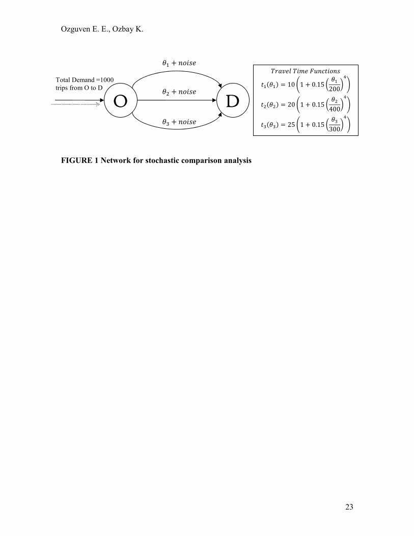
The network shown in FIGURE 1 (46) will be used for MSA and SPSA

performance comparison analysis. It consists of three links between the nodes O (origin)

and D (destination) with the travel time functions and demand shown (Volume-delay

curves are taken as BPR functions for the sake of simplicity).

[Insert FIGURE 1 here]

This network was chosen for three main reasons:

1. The deterministic optimal solution is known. (�� � ~���T ���T (����with an objective function value of (����). This makes it possible to compare MSA

and SPSA using the objective function values.

2. It is an efficient way of testing MSA and SPSA with any link performances

(volume-delay) including BPR functions and different level of stochasticities

Ozguven E. E., Ozbay K.

9

due to not only measurement but also modeling errors. The modeling errors,

for example, can appear while using a dynamic traffic assignment model for

real-time traffic routing model applications where BPR functions does not

necessarily reflect real travel times.

3. Our major goal in selecting this network is to isolate the impact of

stochasticities from other issues such as network size, path flows, etc.,

discussed in a 2007 paper by Sbayti et al. (26), where they proposed ways to

improve MSA algorithm to address these problems. We focus on a different

aspect of this problem namely, the impact of high noise levels on the

performance of MSA and therefore choose to employ a network without the

complexities associated with the size and topology of the network described in

(26).

Considering the network in FIGURE 1, the optimization problem that will achieve

the user equilibrium without the addition of stochasticity can be written as (Sheffi, 1985

(15)): LEG ���DJUtKB@�@A��( Q �R Q �� � (����(T �RT �� � ��

(12)

Here, the objective function for the equilibrium assignment to find the optimum

link flows can be represented as the sum of the integrals of the link performances:

��� � � @(�O�(� IO Q � @R�O�R� IO Q � @��O��� IO (13)

The stochasticity in the decision parameters (flows in each link) directly adds the

noise into the objective function. Therefore, the random terms in the travel time

calculations complicate the problem to a point where it can no longer be effectively

solved as a regular deterministic optimization problem. Thus, we must employ a

stochastic approximation algorithm such as MSA or SPSA. The penalty function

approach should be used to apply SPSA. Pflug (47) present and analyze a stochastic

approximation algorithm based on the penalty function method for stochastic

optimization of a convex function with convex inequality constraints and show that

stochastic approximation using penalty functions converges almost surely. Wang and

Spall (48), and (49) have extended this result to SPSA. They show that with the careful

selection and application of the penalty function, the average relative error for the

objective function can be reduced up-to 5%. This penalty function technique is a

Sequential Penalty Transformation approach which is the oldest and most commonly

used penalty method (50). With this information, the penalty function for the equality

constraint given in Equation (12) is selected as H��� where���� � ��( Q �R Q �� �(���%. Fiacco and McCormick (50) show that choosing H big enough will lead to the optimal solution. Therefore, our objective function for SPSA becomes

Ozguven E. E., Ozbay K.

10

����� Q �H���OCKHK

��� � � @��O f� IO Q � @%�O g� IO Q � @��O �� IO��� � ��� Q �% Q �� � (���%��T �%T �� � ��

(14)

By selecting a sufficiently high�H, the H����component of the objective function

becomes relatively large compared with����. Thus, the non-negativity constraints for ��T �%T ���are always satisfied, and these constraints become redundant. Then,

selecting�H � R�, the optimization problem given in Equation (14) reduces to: ����� Q �R� � ���

OCKHK��� � � @��O f� IO Q � @%�O g� IO Q � @��O �� IO

��� � ��� Q �% Q �� � (���% (15)

Implementation and Results

In this section, we present several case studies to compare the performance of

MSA and SPSA. The computational time of our MATLAB implementation on a 3.00

GHz Pentium (R) D PC is presented for each case.

The performance of basic SPSA is analyzed using the parameters ��� � j�k����l�

and�B� � ]����m�, with��n � R�T � � �>�R�T B � (T o �T �>��RT��and��p � �>(�(��selected

using the guidelines given in Spall (35). The initial point is taken as �� � ~�T �T �� for both algorithms and the perturbation vector (e�) choices for SPSA are varied randomly.

A maximum number of iterations (q�j�) is determined before the analysis, and

then the difference of two consecutive objective function values is checked as the

stopping criterion. If the stopping criterion is not achieved when q�j� is reached, the algorithm stops automatically. Therefore, no runs after q�j� are allowed. At every iteration, |����� � ���| & } � �>(��is checked for stopping. For any particular application, this may or may not be an appropriate stopping rule, but is only used here for purposes of

comparison.

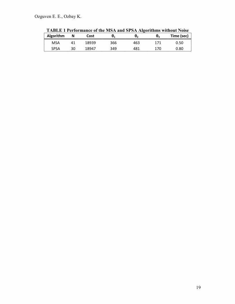
Firstly, algorithms are run without injecting noise into the decision parameters,

therefore not disturbing the performance. The resulting values are given in TABLE 1

where represents the number of iterations. Here, an average of 100 evaluations with

different random perturbations (e�) is given for SPSA. Note that randomly generated

simultaneous perturbations are needed for SPSA to find the gradient direction (35). The

results indicate that both algorithms show similar behaviors. They converge to a certain

point in a fast manner showing no significant difference (The deterministic optimal

solution is 18933). Since MSA has a lower objective function value, it works better than

SPSA in the absence of link stochasticity. However, in the case of simulation-based or

high-noise systems, deterministic link travel times are not applicable or even present.

[Insert TABLE 1 here]

Ozguven E. E., Ozbay K.

11

Then, a normally introduced random noise, expected in the simulation-based

assignment models, is introduced into the system, and both optimization algorithms are

run once more. Three cases are studied with 10 evaluations (runs) for each case. For the

first, second, and third (worst) cases, noise is selected between [-10, 10], [-25, 25], and [-

40, 40], respectively. For each case, number of runs, number of iterations in each run,

objective function and decision parameter values, and computational times (wall-clock

times) are reported.

The results of the first scenario are given in TABLE 2. q�j� is selected as 500 for each evaluation. In this case, both MSA and SPSA algorithms work efficiently in terms

of reaching the optimum solution; however, MSA is better than SPSA considering

relatively shorter time it takes to find the suboptimal solution as compared with the

deterministic solution.

[Insert TABLE 2 here]

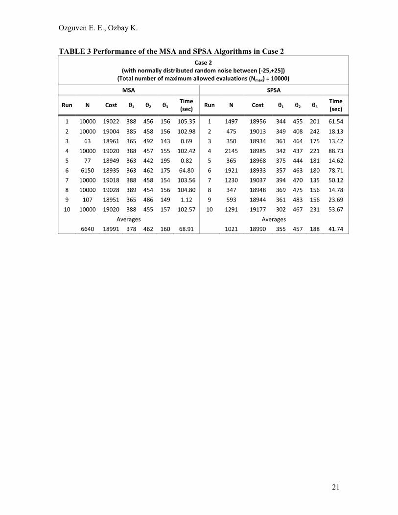
Case 2 results are given in TABLE 3. q�j���is 10000 for each evaluation. As the noise is increased, the performance of MSA decreases. In four of the ten cases, it reaches

a suboptimal solution. For the other runs, it remains far away from the optimum solution

even after q�j� is reached. On the other hand, as the noise increases, SPSA still has the good performance of finding the solution in less number of iterations. The algorithm

stops far before q�j� is reached for SPSA. The average cost and time values are very

close for both algorithms.

[Insert TABLE 3 here]

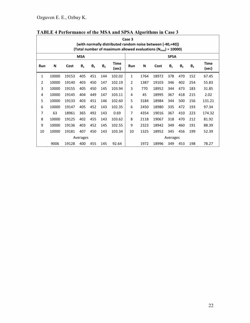
Third case results are given in TABLE 4. q�j� is 10000 for each evaluation. This case includes the highest stochasticity on the flows among the three cases. As MSA

already moves away from the vicinity of the deterministic optimal solution, the case with

the highest stochasticity is considered as the worst case scenario. As observed, the

performance of MSA is not satisfactory. Only one out of ten runs gives an acceptable

objective function value. SPSA, on the other hand, gives better objective function and

time values. The algorithm stops before q�j� is reached for SPSA. This indicates that SPSA works more efficiently as the noise increases in the system.

[Insert TABLE 4 here]

Discussions

The analysis and comparison of MSA and SPSA algorithms provide useful

insights into the development of solution techniques for traffic assignment models that

can be highly stochastic. The performance comparison of these two algorithms is based

on the analysis of the objective functions and the overall computational times. The

number of iterations is not used for comparison due to the fact that the computation time

of a single iteration for each algorithm is different. That is, it is not possible to make a

clear distinction by using the number of iterations. Rather, analysis of the individual

computation times is used as the main comparison method.

Ozguven E. E., Ozbay K.

12

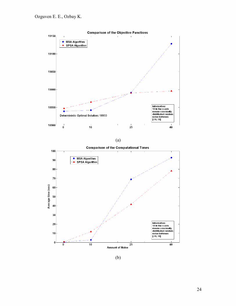
The results of this numerical study (see FIGURE 2) suggest that the performance

of the basic SPSA can improve the optimal solution as the amount of system stochasticity

is increased. Note that high levels of stochasticities are most likely to be encountered in

the simulation-based traffic assignment models.

[Insert FIGURE 2 here]

There are a few significant points about these results. Firstly, we apply the t-test

to assess whether the means (averages) of the objective functions and computational

times for MSA and SPSA algorithms are statistically different from each other. A t-test is

used when statistical comparison of optimization algorithms is needed (Maryak and Chin

(2) and Spall (51)). The first step is to specify the null hypothesis and alternative

hypothesis. The null hypothesis in this study is that the difference between means is zero.

Then, the null and alternative hypotheses are:

��� �� � �% � ���� �� � �% � � (16)

Using Equation (16), the difference between the two average values of

computation time shown in TABLE 4 appears to be statistically significant (T-test @

95%) for all cases. This indicates that we cannot accept the null hypothesis and two

averages are statistically different for the worst case. Considering the average values of

objective functions, the differences appear to be statistically significant for Cases 1 and 3,

whereas there is no statistical difference for Case 2 (T-test @ 95%).

Second, for the noise-free case and Case 1, MSA performs better than SPSA for

both in terms of objective function values and computational times as seen clearly from

FIGURE 2a. For the last two cases where noisy measurements are high, on the other

hand, the performance of SPSA is obviously better. It reaches a better solution than MSA

in less amount of computation time. Of course, the choice of gain sequences is the

significant point for SPSA as they define the search direction for the objective function.

They must be selected separately for every network using the guidelines given in Spall

(35).

Third, from FIGURE 2b, it is observed that the computation time for MSA

increases rapidly as the stochasticity is increased. As stated in (13), the stochastic

approximation algorithm is of little practical use if the number of iterations required to

reduce the errors to within reasonable bounds is arbitrarily large. This happens for MSA

in the worst case scenario (Case 3). SPSA, on the other hand, stays under a reasonable

amount of computational time and requires acceptable number of iterations (an average

of 1972) to reduce the errors to within reasonable bounds in the worst case scenario.

Finally, a natural question is whether the stochastic approximation is converging

to a global optimal solution. As the stochasticity of the system is increased, MSA tends to

converge to a certain point and becomes stuck there whereas SPSA reaches better

objective function values than MSA (see TABLE 3 and TABLE 4). Therefore, it can be

stated that SPSA algorithm exhibits a better performance in terms of converging to a

possible global optimum than MSA in the presence of high levels of stochasticities.

Ozguven E. E., Ozbay K.

13

CONCLUSIONS AND FUTURE RESEARCH

In this paper, we have conducted experiments on a network with 2 nodes and 3

links to compare the performance of the two stochastic approximation algorithms,

namely, -well-known and widely adopted as the standard-, Method of Successive

Averages (MSA) and relatively new Simultaneous Perturbation Stochastic

Approximation (SPSA). The optimization model includes noisy measurements on the

decision parameters (flows at each link). The algorithms are applied to optimally assign

the total flow on links with BPR travel time functions both injecting and not injecting the

noise to the decision parameters. In a recent study by Sbayti et al. (26), the authors stated

that “the convergence properties of MSA in real-life networks have been inconclusive

due to the unguaranteed solution properties of simulation-based models and the sluggish

performance of the pre-determined step size approach”. In this study, we have focused on

a different aspect of MSA algorithm namely, the impact of high noise levels on its

performance and have chosen to employ a network that will not have the complexities

described in Sbayti et al. (26).

Numerical results and comparisons between MSA and SPSA algorithms show

that MSA gives better results for the noise-free case and when the stochasticity is low.

However, the performance of MSA degrades with increasing stochasticity whereas SPSA

still continues to perform well. We observed that number of iterations gets very large for

MSA in the worst case scenario. In fact, for nine out of ten cases, MSA cannot reach a

suboptimal solution. As stated in (13), “stochastic approximation algorithm is of little

practical use if the number of iterations required to reduce the errors to within reasonable

bounds is arbitrarily large”. Furthermore, it is observed that MSA tends to converge to a

local minimum while SPSA reaches better objective function values as the noise in the

measurements is increased.

Throughout the analysis, well known BPR functions are used for the volume

delay calculations. The decrease in the performance of MSA algorithm with BPR

functions as the noise is increased reveal the fact that MSA may perform worse if more

complex objective functions, such as simulation-based functions, are used. SPSA, on the

other hand, has been shown in the literature to be a good optimizer even with complex

functions having many local minima (2).

The goal of global optimization of the stochastic approximation algorithms for

traffic assignment models is still an active area of research; however it is valuable to see

that SPSA method can be efficient in approaching to a global minimum especially when

stochasticities are considerably high. This conclusion has obvious consequences for the

transportation field. MSA is commonly used for traffic assignment models for mostly

large and complex networks. However, it has questionable convergence characteristics

under noisy measurements even with the small network studied in this paper. Therefore,

as another option, SPSA can be easily and successfully applied to the problems of

transportation and traffic engineering fields. Further research is required in this area. For

instance, application to a large network will be an important step towards better

understanding the performance of SPSA when applied to large-scale optimization

problems.

It is our hope that this analysis and comparison will not only provide a better

understanding of both algorithms—MSA and SPSA—but will also serve to point at the

Ozguven E. E., Ozbay K.

14

needs for further algorithm improvement and extension, especially for real world

stochastic traffic optimization problems.

REFERENCES

1. Spall, J. C., “An Overview of the Simultaneous Perturbation Method for Efficient

Optimization”, Johns Hopkins APL Technical Digest, pp. 482-492, Volume 19, No.

4, 1998.

2. Maryak, J. L., and Chin, D. C., “Global Random Optimization by Simultaneous

Perturbation Stochastic Approximation”, Johns Hopkins APL Technical Digest, pp.

91-100, Volume 25, No. 2, 2004.

3. Spall, J. C., “Stochastic Optimization, Stochastic Approximation and Simulated

Annealing”, Wiley Encyclopedia of Electrical and Electronics Engineering, pp. 529-

542, Volume 20, John Wiley & Sons, Inc., 1999.

4. Gelfand, S. B., and Mitter, S. K., “Recursive Stochastic Algorithms for Global

Optimization in Rd”, Proceedings of the 29th Conference on Decision and Control,

pp. 220-221, 1990.

5. Robbins, H. and Monro, S., “A Stochastic Approximation Method”, Annals of

Mathematical Statistics, pp. 400-407, Volume 22, No. 3, 1951.

6. Kiefer, J., and Wolfowitz, J., “Stochastic Estimation of the Maximum of a Regression

Function”, The Annals of Mathematical Statistics, pp. 462-466, Volume 23, No. 3,

1952.

7. Wolfowitz, J., “On the Stochastic Approximation Method of Robbins and Monro”,

Annals of Mathematical Statistics, pp. 457-461, Volume 23, No. 3, 1952.

8. Blum, J. R., “Multidimensional Stochastic Approximation Methods”, The Annals of

Mathematical Statistics, pp. 737-744, Volume 25, No. 4, 1954.

9. Blum, J. R., “Approximation Methods which Converge with Probability one”, The

Annals of Mathematical Statistics, pp. 382-386, Volume 25, No. 2, 1954.

10. Andradottir, S., “A New Algorithm for Stochastic Optimization”, Proceedings of the

1990 Winter Simulation Conference, pp. 151-158, 1990.

11. Andradottir, S., “A Review of Simulation Optimization Techniques”, Proceedings of

the 1998 Winter Simulation Conference, 1998.

12. Sheffi, Y., and Powell W., “A Comparison of Stochastic and Deterministic Traffic

Assignment over Congested Networks”, Transportation Research Part B, Volume 15,

pp. 53-64, 1981.

13. Sheffi, Y., and Powell, W. B., “An Algorithm for the Equilibrium Assignment

Problem with Random Link Times”, Networks, pp. 191-207, Volume 12, 1982.

14. Powell, W. B., and Sheffi, Y., “The Convergence of Equilibrium Algorithms with

Predetermined Step Sizes”, Transportation Science, pp. 45-55, Volume 16, No. 1,

1982.

15. Sheffi, Y., Urban Transportation Networks: Equilibrium Analysis with Mathematical

Programming Methods, Prentice-Hall Inc., 1985.

16. TransCAD, Transportation Planning GIS Software, http://www.caliper.com/.

17. EMME 3, Travel Forecasting Software, http://www.inro.ca/.

18. Transportation Planning Plus (TP+), Transportation Planning Software,

http://www.citilabs.com/tpplus/.

Ozguven E. E., Ozbay K.

15

19. Cascetta, E., and Postorino, M. N., “Fixed Point Approaches to the Estimation of O/D

Matrices Using Traffic Counts on Congested Networks”, Transportation Science, pp.

134-147, Volume 35, No. 2, 2001.

20. Bar-Gera, H., and Boyce, D., “Solving a Non-Convex Combined Travel Forecasting

Model by the Method of Successive Averages with Constant Step Sizes”,

Transportation Research Part B, pp. 351-367, Volume 40, 2006.

21. Boyce, D, and Florian, M., “Workshop on Traffic Assignment with Equilibrium

Models”, 2005.

22. Cominetti, R., and Baillon, J-B., “Stochastic Equilibrium in Traffic Networks”, VII

French-Latin American Congress on Applied Mathematics, 2005.

23. Walker, W. T., Rossi T. F., and Islam N., “Method of Successive Averages Versus

Evans Algorithm Iterating a Regional Travel Simulation Model to the User

Equilibrium Solution”, Transportation Research Record No. 1645, pp. 32–40, 1998.

24. Peeta, S., and Mahmassani, H. S., “System Optimal and User Equilibrium Time-

dependent Traffic Assignment in Congested Networks”, Annals of Operations

Research, Volume 60, pp. 81-113, 1995.

25. Mahmassani, H. S., and Peeta, S., “Network Performance under System Optimal and

User Equilibrium Dynamic Assignments: Implications for Advanced Traveler

Information Systems”, Transportation Research Record No. 1408, pp. 83–93, 1993.

26. Sbayti, H., Lu, C., and Mahmassani, H. S., “Efficient Implementations of the Method

of Successive Averages in Simulation-Based DTA Models for Large-Scale Network

Applications”, Presented in the 86th Annual Meeting of Transportation Research

Board, 2007.

27. Mahmassani, H.S., Abdelghany, A.F., Huynh, N., Zhou, X., Chiu, Y.-C. and

Abdelghany, K.F., DYNASMART-P (version 0.926) User’s Guide, Technical Report

STO67-85-PIII, Center for Transportation Research, University of Texas at Austin,

2001.

28. Ben-Akiva, M., Koutsopoulos, H. N., and Mishalani, R., “DynaMIT: A Simulation-

Based System for Traffic Prediction”, Paper presented at the DACCORD Short Term

Forecasting Workshop, 1998.

29. Mahut, M., Florian, M., and Tremblay, N., “Comparison of Assignment Methods for

Simulation-Based Dynamic Equilibrium Traffic Assignment”, Presented in 6th

Triennial Symposium on Transportation Analysis, 2007.

30. Bottom, J., Ben-Akiva, M., Bierlaire M., Chabini I., Koutsopoulos H., and Yang Q.,

“Investigation of Route Guidance Generation Issues by Simulation with DYNAMIT”,

Proceedings of the 14th International Symposium on Transportation and Traffic

Theory, 1999.

31. Crittin, F., and Bierlaire, M., “New Algorithmic Approaches for the Anticipatory

Route Guidance Generation Issues”, 1st Swiss Transport Research Conference, 2001.

32. Dong J., Mahmassani, H. S., and Lu, C., “How Reliable is the Route? Predictive

Travel Time and Reliability for Anticipatory Traveler Information Systems”,

Transportation Research Record No. 1980, pp. 117–125, 2006.

33. Spall, J. C., “A Stochastic Approximation Technique for Generating Maximum

Likelihood Parameters”, Proceedings of the American Control Conference, pp. 1161-

1167, 1987.

Ozguven E. E., Ozbay K.

16

34. Spall, J. C., “Multivariate Stochastic Approximation Using a Simultaneous

Perturbation Gradient Approximation”, IEEE Transactions on Automatic Control, pp.

332-341, Volume 37, No. 3, 1992.

35. Spall, J. C., “Implementation of the Simultaneous Perturbation Algorithm for

Stochastic Optimization”, IEEE Transactions on Aerospace and Electronic Systems,

pp. 817-823, Volume 34, No. 3, 1998.

36. Maryak, J. L., and Chin, D. C., “Efficient Global Optimization Using SPSA”,

Proceedings of the American Control Conference, pp. 890-894, 1999.

37. Whitney, J. E., Wairia, D., Hill, S. D., and Bahari, F., “Comparison of the SPSA and

Simulated Annealing Algorithms for the Constrained Optimization of Discrete Non-

seperable Functions”, Proceedings of the American Control Conference, pp. 3260-

3262, 2003.

38. Hutchison, D. W., and Spall, J. C., “Stopping Stochastic Approximation”,

Proceedings of the PerMIS Workshop, 2003.

39. Kleinman, N. L., Hill, S. D., and Ilenda, V. A., “SPSA/SIMMOD Optimization of Air

Traffic Delay Cost”, Proceedings of the American Control Conference, pp. 1121-

1125, Volume 2, 1997.

40. Gerencser, L., Kozmann, G., Vago, Z., and Haraszti, K., “The Use of the SPSA

Method in ECG Analysis”, IEEE Transactions on Biomedical Engineering, pp. 1094-

1101, Volume 49, No. 10, 2002.

41. Xing, X. Q., and Damodaran, M., “Application of Simultaneous Perturbation

Stochastic Approximation Method for Aerodynamic Shape Design Optimization”,

AIAA Journal, pp. 284-294, Volume 43, No. 2, 2005.

42. Chin, D. C., and Smith, R. H., “A Neural Network Application in Signal Timing

Control”, IEEE International Conference on Neural Networks, pp.2010-2106, 1996.

43. Srinivasan, D., Choy, M. C., and Cheu, R. L., “Neural Networks for Real-Time

Traffic Signal Control”, IEEE Transactions on Intelligent Transportation Systems, pp.

261-272, Volume 7, No. 3, 2006.

44. Choy, M. C., Srinivasan, D., and Cheu, R. L., “Simultaneous Perturbation Stochastic

Approximation Based Neural Networks for Online Learning”, IEEE Intelligent

Transportation Systems Conference, pp. 1038-1044, 2004.

45. Kushner H. J., and Yin G. G., “Stochastic Approximation Algorithms and

Applications”, Springer-Verlak New York Inc., 1997.

46. EMME2 Resources Web Center, www.emme2.spiess.ch/e2news/news02/node3.html

47. Pflug, G. C., “On the Convergence of a Penalty-type Stochastic Optimization

Procedure”, Journal of Information and Optimization Sciences, Volume 2, pp. 249-

258, 1981.

48. Wang, I., Spall, J. C., “A Constrained Simultaneous Perturbation Stochastic

Approximation Algorithm Based on Penalty Functions”, Proceedings of the IEEE

ISIC/CIRA/ISAS Joint Conference, pp. 452-458, 1998.

49. Wang, I., Spall, J. C., “Stochastic Optimization with Inequality Constraints Using

Simultaneous Perturbations and Penalty Functions”, Proceedings of the 42nd IEEE

Conference on Decision and Control, pp. 3808-3813, 2003.

50. Fiacco, A. V., and McCormick G. P., Nonlinear Programming: Sequential

Unconstrained Minimization Techniques, John Wiley & Sons Inc., 1968.

Ozguven E. E., Ozbay K.

17

51. Spall, J. C., Introduction to Stochastic Search and Optimization: Estimation,

Simulation and Control, Wiley-Interscience Series in Discrete Mathematics and

Optimization, 2005.

Ozguven E. E., Ozbay K.

18

LIST OF TABLES

TABLE 1 Performance of the MSA and SPSA Algorithms without Noise

TABLE 2 Performance of the MSA and SPSA Algorithms in Case 1

TABLE 3 Performance of the MSA and SPSA Algorithms in Case 2

TABLE 4 Performance of the MSA and SPSA Algorithms in Case 3

LIST OF FIGURES

FIGURE 1 Network for stochastic comparison analysis

FIGURE 2 Comparison of the performance of MSA and SPSA algorithms (Figure 2a)

comparison of the objective Functions (Figure 2b) comparison of the computational times

Ozguven E. E., Ozbay K.

19

TABLE 1 Performance of the MSA and SPSA Algorithms without Noise

Algorithm N Cost θ1 θ2 θ3 Time (sec)

MSA 41 18939 366 463 171 0.50

SPSA 30 18947 349 481 170 0.80

Ozguven E. E., Ozbay K.

20

TABLE 2 Performance of the MSA and SPSA Algorithms in Case 1

Case 1

(with normally distributed random noise between [-10,+10])

(Total number of maximum allowed evaluations (Nmax) = 500)

MSA SPSA

Run N Cost θ1 θ2 θ3 Time

(sec) Run N Cost θ1 θ2 θ3

Time

(sec)

1 74 18940 365 473 162 0.80 1 171 18957 341 471 188 7.49

2 500 18959 374 452 174 5.16 2 500 19010 336 512 151 4.68

3 54 18937 352 462 186 0.60 3 103 18943 348 468 184 21.42

4 500 18971 378 454 168 5.16 4 281 18952 356 490 154 12.11

5 186 18936 360 473 167 1.98 5 113 19015 328 483 189 5.09

6 222 18936 360 473 167 2.39 6 179 18966 339 474 187 7.98

7 500 18942 368 460 172 5.26 7 500 18950 345 473 182 21.32

8 208 18934 361 467 172 2.18 8 304 18934 360 469 171 13.11

9 150 18934 360 460 180 1.60 9 329 18945 368 473 159 13.99

10 305 18933 358 465 177 3.20 10 239 18977 336 476 188 10.73

Averages Averages

270 18942 364 464 173 2.83 272 18965 346 479 175 11.79

Ozguven E. E., Ozbay K.

21

TABLE 3 Performance of the MSA and SPSA Algorithms in Case 2

Case 2

(with normally distributed random noise between [-25,+25])

(Total number of maximum allowed evaluations (Nmax) = 10000)

MSA SPSA

Run N Cost θ1 θ2 θ3 Time

(sec) Run N Cost θ1 θ2 θ3

Time

(sec)

1 10000 19022 388 456 156 105.35 1 1497 18956 344 455 201 61.54

2 10000 19004 385 458 156 102.98 2 475 19013 349 408 242 18.13

3 63 18961 365 492 143 0.69 3 350 18934 361 464 175 13.42

4 10000 19020 388 457 155 102.42 4 2145 18985 342 437 221 88.73

5 77 18949 363 442 195 0.82 5 365 18968 375 444 181 14.62

6 6150 18935 363 462 175 64.80 6 1921 18933 357 463 180 78.71

7 10000 19018 388 458 154 103.56 7 1230 19037 394 470 135 50.12

8 10000 19028 389 454 156 104.80 8 347 18948 369 475 156 14.78

9 107 18951 365 486 149 1.12 9 593 18944 361 483 156 23.69

10 10000 19020 388 455 157 102.57 10 1291 19177 302 467 231 53.67

Averages Averages

6640 18991 378 462 160 68.91 1021 18990 355 457 188 41.74

Ozguven E. E., Ozbay K.

22

TABLE 4 Performance of the MSA and SPSA Algorithms in Case 3

Case 3

(with normally distributed random noise between [-40,+40])

(Total number of maximum allowed evaluations (Nmax) = 10000)

MSA SPSA

Run N Cost θ1 θ2 θ3 Time

(sec) Run N Cost θ1 θ2 θ3

Time

(sec)

1 10000 19153 405 451 144 102.02 1 1764 18972 378 470 152 67.45

2 10000 19140 403 450 147 102.19 2 1387 19103 346 402 254 55.83

3 10000 19155 405 450 145 103.94 3 770 18952 344 473 183 31.85

4 10000 19145 404 449 147 103.11 4 45 18995 367 418 215 2.02

5 10000 19133 403 451 146 102.60 5 3184 18984 344 500 156 131.21

6 10000 19147 405 452 143 102.35 6 2450 18980 335 472 193 97.34

7 63 18961 365 492 143 0.69 7 4354 19016 367 410 223 174.32

8 10000 19125 402 455 143 103.62 8 2118 19067 318 470 212 81.92

9 10000 19136 403 452 145 102.55 9 2323 18942 349 460 191 88.39

10 10000 19181 407 450 143 103.34 10 1325 18952 345 456 199 52.39

Averages Averages

9006 19128 400 455 145 92.64 1972 18996 349 453 198 78.27

Ozguven E. E., Ozbay K.

23

FIGURE 1 Network for stochastic comparison analysis

O D

Total Demand =1000

trips from O to D

SH�PKN�SELK�uJGB@EAGD@���� � (� �( Q �>(� � ��R���

��@%��% � R� �( Q �>(� � �%����

��@���� � R��( Q �>(� � ������

��

�� Q GAEDK

�% Q GAEDK

�� Q GAEDK

Ozguven E. E., Ozbay K.

24

(a)

(b)

Ozguven E. E., Ozbay K.

25

FIGURE 2 Comparison of the performance of MSA and SPSA algorithms (Figure

2a) comparison of the objective Functions (Figure 2b) comparison of the

computational times