Similarity Searching: Indexing, Nearest Neighbor Finding, Dimensionality Reduction, and Embedding Methods, for Applications in Multimedia Databases Hanan Samet * [email protected] Department of Computer Science University of Maryland College Park, MD 20742, USA Based on joint work with Gisli R. Hjaltason. * Currently a Science Foundation of Ireland (SFI) Walton Fellow at the Centre for Geocomputation at the National University of Ireland at Maynooth (NUIM) Copyright 2009: Hanan Samet Similarity Searching for Multimedia Databases Applications – p.1/114

Welcome message from author
This document is posted to help you gain knowledge. Please leave a comment to let me know what you think about it! Share it to your friends and learn new things together.
Transcript

Similarity Searching:
Indexing, Nearest Neighbor Finding, DimensionalityReduction, and Embedding Methods, for Applications in
Multimedia Databases
Hanan Samet∗
Department of Computer Science
University of Maryland
College Park, MD 20742, USA
Based on joint work with Gisli R. Hjaltason.
∗Currently a Science Foundation of Ireland (SFI) Walton Fellow at the Centre for Geocomputation at the National University of
Ireland at Maynooth (NUIM)
Copyright 2009: Hanan Samet Similarity Searching for Multimedia Databases Applications – p.1/114
Outline
1. Similarity Searching
2. Distance-based indexing
3. Dimension reduction
4. Embedding methods
5. Nearest neighbor finding
Copyright 2009: Hanan Samet Similarity Searching for Multimedia Databases Applications – p.2/114

Similarity Searching
Important task when trying to find patterns in applications involving miningdifferent types of data such as images, video, time series, text documents,DNA sequences, etc.
Similarity searching module is a central component of content-basedretrieval in multimedia databases
Problem: finding objects in a data set S that are similar to a query object qbased on some distance measure d which is usually a distance metric
Sample queries:1. point: objects having particular feature values2. range: objects whose feature values fall within a given range or where
the distance from some query object falls into a certain range3. nearest neighbor: objects whose features have values similar to those
of a given query object or set of query objects4. closest pairs: pairs of objects from the same set or different sets which
are sufficiently similar to each other (variant of spatial join)
Responses invariably use some variant of nearest neighbor finding
Copyright 2009: Hanan Samet Similarity Searching for Multimedia Databases Applications – p.3/114

Voronoi DiagramsApparently straightforward solution:
1. Partition space into regions where allpoints in the region are closer to theregion’s data point than to any otherdata point
2. Locate the Voronoi region corre-sponding to the query point
Problem: storage and construction cost for N d-dimensional points is Θ(N d/2)
Impractical unless resort to some high-dimensional approximation of a Voronoidiagram (e.g., OS-tree) which results in approximate nearest neighbors
Exponential factor corresponding to the dimension d of the underlying space inthe complexity bounds when using approximations of Voronoi diagrams (e.g.,(t, ε)-AVD) is shifted to be in terms of the error threshold ε rather than in termsof the number of objects N in the underlying space
1. (1, ε)-AVD: O(N/εd−1) space and O(log(N/εd−1)) time for nearest neigh-bor query
2. (1/ε(d−1)2, ε)-AVD: O(N) space and O(t + log N) time for nearest neigh-bor query
Copyright 2009: Hanan Samet Similarity Searching for Multimedia Databases Applications – p.4/114

Approximate Voronoi Diagrams (AVD)
Example partitions of space induced by ε neighbor sets
Darkness of shading indicates cardinality of nearest neighbor sets withwhite corresponding to 1
(ε = 0.10) (ε = 0.30) (ε = 0.50)
Copyright 2009: Hanan Samet Similarity Searching for Multimedia Databases Applications – p.5/114

Approximate Voronoi Diagrams (AVD) Representations
GI
C
BA
D
H
E
FG
I
C
BA
D
H
EADD
CFI
GH
AD
A AB BC BC
GHG H HI
I
ADE
ABE
ADE
BEF
EF
E
HI
EGH
HDG
FHI
CFI
BCF
AEG
DEG
G
EFH
F
Partition underlying domain so thatfor ε ≥ 0, every block b is asso-ciated with some element rb in Ssuch that rb is an ε-nearest neigh-bor for all of the points in b (e.g.,AVD or (1,0.25)-AVD)
Allow up to t ≥ 1 elements rib(1 ≤i ≤ t) of S to be associated witheach block b for a given ε, whereeach point in b has one of the rib asits ε-nearest neighbor (e.g., (3,0)-AVD)
Copyright 2009: Hanan Samet Similarity Searching for Multimedia Databases Applications – p.6/114

Problem: Curse of Dimensionality
Number of samples needed to estimate an arbitrary function with a givenlevel of accuracy grows exponentially with the number of variables (i.e.,dimensions) that comprise it (Bellman)
For similarity searching, curse means that the number of points in the dataset that need to be examined in deriving the estimate (≡ nearest neighbor)grows exponentially with the underlying dimension
Effect on nearest neighbor finding is that the process may not bemeaningful in high dimensions
When ratio of variance of distances and expected distances, between tworandom points p and q drawn from the data and query distributions,converges to zero as dimension d gets very large (Beyer et al.)
limd→∞Variance[dist(p,q)]Expected[dist(p,q)]
= 0
1. distance to the nearest neighbor and distance to the farthest neighbortend to converge as the dimension increases
2. implies that nearest neighbor searching is inefficient as difficult todifferentiate nearest neighbor from other objects
3. assumes uniformly distributed data
Partly alleviated by fact that real-world data is rarely uniformly-distributedCopyright 2009: Hanan Samet Similarity Searching for Multimedia Databases Applications – p.7/114

Alternative View of Curse of Dimensionality
Probability density function (analogous to histogram) of the distances ofthe objects is more concentrated and has a larger mean value
Implies similarity search algorithms need to do more work
Worst case when d(x, x) = 0 and d(x, y) = 1 for all y 6= x
Implies must compare every object with every other object1. can’t always use triangle inequality to prune objects from consideration2. triangle inequality (i.e., d(q, p) ≤d(p, x) + d(q, x)) implies that any x
such that |d(q, p)− d(p, x)| > ε cannot be at a distance of ε or less fromq as d(q, x) ≥ d(q, p)− d(p, x) > ε
3. when ε is small while probability density function is large at d(p, q),then probability of eliminating an object from consideration via use oftriangle inequality is remaining area under curve which is small (seeleft) in contrast to case when distances are more uniform (see right)
d(p,q) d(p,q)d(p,x) d(p,x)
prob
abili
ty d
ensi
ty
prob
abili
ty d
ensi
ty
ε ε22(a) (b)
Copyright 2009: Hanan Samet Similarity Searching for Multimedia Databases Applications – p.8/114
Other Problems
Point and range queries are less complex than nearest neighbor queries1. easy to do with multi-dimensional index as just need comparison tests2. nearest neighbor require computation of distance
Euclidean distance needs d multiplications and d− 1 additions
Often we don’t know features describing the objects and thus need aid ofdomain experts to identify them
Copyright 2009: Hanan Samet Similarity Searching for Multimedia Databases Applications – p.9/114

Solutions Based on Indexing
1. Map objects to a low-dimensional vector space which is then indexedusing one of a number of different data structures such as k-d trees,R-trees, quadtrees, etc.
use dimensionality reduction: representative points, SVD, DFT, etc.
2. Directly index the objects based on distances from a subset of the objectsmaking use of data structures such as the vp-tree, M-tree, etc.
useful when only have a distance function indicating similarity (ordis-similarity) between all pairs of N objectsif change distance metric, then need to rebuild index — not so formultidimensional index
3. If only have distance information available, then embed the data objects ina vector space so that the distances of the embedded objects asmeasured by the distance metric in the embedding space approximate theactual distances
commonly known embedding methods include multidimensionalscaling (MDS), Lipschitz embeddings, FastMap, etc.once a satisfactory embedding has been obtained, the actual searchis facilitated by making use of conventional indexing methods, perhapscoupled with dimensionality reduction
Copyright 2009: Hanan Samet Similarity Searching for Multimedia Databases Applications – p.10/114

Outline
1. Indexing low and high dimensional spaces
2. Distance-based indexing
3. Dimensionality reduction
4. Embedding methods
5. Nearest neighbor searching
Copyright 2009: Hanan Samet Similarity Searching for Multimedia Databases Applications – p.11/114

Part 1: Indexing Low and High Dimensional Spaces
1. Quadtree variants
2. k-d tree
3. R-tree
4. Bounding sphere methods
5. Hybrid tree
6. Avoiding overlapping all of the leaf blocks
7. Pyramid technique
8. Methods based on a sequential scan
Copyright 2009: Hanan Samet Similarity Searching for Multimedia Databases Applications – p.12/114

Simple Non-Hierarchical Data Structures
Sequential list Inverted List
Name X YChicago 35 42Mobile 52 10Toronto 62 77Buffalo 82 65Denver 5 45Omaha 27 35Atlanta 85 15Miami 90 5
X YDenver MiamiOmaha MobileChicago AtlantaMobile OmahaToronto ChicagoBuffalo DenverAtlanta BuffaloMiami Toronto
Inverted lists:1. 2 sorted lists2. data is pointers3. enables pruning the search with respect to one key
Copyright 2009: Hanan Samet Similarity Searching for Multimedia Databases Applications – p.13/114

Grid Method
Divide space into squares of width equal to the search region
Each cell contains a list of all points within it
Assume L∞ distance metric (i.e., Chessboard)
Assume C = uniform distribution of points per cell
Average search time for k-dimensional space is O(F · 2k)
F = number of records found = C, since query region has the width ofa cell2k = number of cells examined
(0,100) (100,100)
(100,0)(0,0)
y
x
(5,45)Denver (35,42)
Chicago
(27,35)Omaha
(52,10)Mobile
(62,77)Toronto (82,65)
Buffalo
(85,15)Atlanta
(90,5)Miami
Copyright 2009: Hanan Samet Similarity Searching for Multimedia Databases Applications – p.14/114

Point Quadtree (Finkel/Bentley)
Marriage between uniform grid and a binary search tree
(0,100) (100,100)
(100,0)(0,0)
(35,42)Chicago
(52,10)Mobile
(62,77)Toronto
(82,65)Buffalo
(5,45)Denver
(27,35)Omaha
(85,15)Atlanta
(90,5)Miami
Chicago
MobileToronto
MiamiAtlantaBuffalo
OmahaDenver
Copyright 2009: Hanan Samet Similarity Searching for Multimedia Databases Applications – p.15/114

PR Quadtree
1. Regular decomposition point representation
2. Decompose whenever a block contains more than one point
3. Maximum level of decomposition depends on minimum point separationif two points are very close, then decomposition can be very deepcan be overcome by viewing blocks as buckets with capacity c andonly decomposing a block when it contains more than c points
A
B
D F
Toronto
C E
Buffalo Denver
Chicago Omaha Atlanta Miami
Mobile
(0,100) (100,100)
(100,0)(0,0)
(35,42)Chicago
(52,10)Mobile
(62,77)Toronto
(82,65)Buffalo
(5,45)Denver
(27,35)Omaha
(85,15)Atlanta
(90,5)Miami
Copyright 2009: Hanan Samet Similarity Searching for Multimedia Databases Applications – p.16/114

Region Search
Ex: Find all points within radius r of point A
A
r
1 2 39 10
13
1211
45
876
Use of quadtree results in pruning the search space
If a quadrant subdivision point p lies in a region l, then search thequadrants of p specified by l
1. SE 5. SW, NW 9. All but NW 13. All2. SE, SW 6. NE 10. All but NE3. SW 7. NE, NW 11. All but SW4. SE, NE 8. NW 12. All but SE
Copyright 2009: Hanan Samet Similarity Searching for Multimedia Databases Applications – p.17/114

Finding Nearest Object
Ex: find the nearest object to P
Assume PR quadtree for points (i.e., atmost one point per block)
Search neighbors of block 1 incounterclockwise order
Points are sorted with respect to the spacethey occupy which enables pruning thesearch space
P
12 8 7 6
13 9 1 4 5
2 3
10 11
D
E C
F
A
B
new F
Algorithm:1. start at block 2 and compute distance to P from A2. ignore block 3, even if nonempty, as A is closer to P than any point in 33. examine block 4 as distance to SW corner is shorter than the distance
from P to A; however, reject B as it is further from P than A4. ignore blocks 6, 7, 8, 9, and 10 as the minimum distance to them from
P is greater than the distance from P to A5. examine block 11 as the distance from P to the S border of 1 is shorter
than distance from P to A; but, reject F as it is further from P than AIf F was moved, a better order would have started with block 11, thesouthern neighbor of 1, as it is closest to the new F
Copyright 2009: Hanan Samet Similarity Searching for Multimedia Databases Applications – p.18/114

k-d tree (Bentley)
Test one attribute at a time instead of all simultaneously as in the pointquadtree
Usually cycle through all the attributes
Shape of the tree depends on the order in which the data is encountered
(90,5)Miami
(27,35)Omaha
(5,45)Denver
(82,65)Buffalo
(62,77)Toronto
(52,10)Mobile
(0,100) (100,100)
(100,0)(0,0)
(35,42)Chicago
(85,15)Atlanta
Atlanta
y test
Omaha
Denver
Buffalo
x testToronto
y testMobile
x testChicago
Miami
Copyright 2009: Hanan Samet Similarity Searching for Multimedia Databases Applications – p.19/114

Adaptive k-d tree
Data is only stored in terminal nodes
An interior node contains the median of the set as the discriminator
The discriminator key is the one for which the spread of the values of thekey is a maximum
(0,100) (100,100)
(100,0)(0,0)
(5,45)Denver (35,42)
Chicago
(27,35)Omaha
(52,10)Mobile
(62,77)Toronto
(82,65)Buffalo
(85,15)Atlanta
(90,5)Miami
72,X
BuffaloTorontoAtlantaMiami
10,Y10,Y
40,Y
26,Y
ChicagoMobile
16,X
OmahaDenver
31,X
57,X
Copyright 2009: Hanan Samet Similarity Searching for Multimedia Databases Applications – p.20/114

Minimum Bounding Rectangles: R-tree (Guttman)Objects grouped into hierarchies, stored in a structure similar to a B-tree
Object has single bounding rectangle, yet area that it spans may beincluded in several bounding rectangles
Drawback: not a disjoint decomposition of space (e.g., Chicago in R1+R2)
Order (m, M) R-tree1. between m ≤M/2 and M entries in each node except root2. at least 2 entries in root unless a leaf node
X-tree (Berchtold/Keim/Kriegel): if split creates too much overlap, then in-stead of splitting, create a supernode
R0
R0 R1 R2
R3
(0,100) (100,100)
(100,0)(0,0)
y
(5,45)Denver (35,42)
Chicago(27,35)Omaha
(52,10)Mobile
(62,77)Toronto
(85,15)Atlanta
(90,5)Miami
R5 R6
R4(82,65)Buffalo
OmahaDenverR3 TorontoBuffaloR4 MobileChicagoR5 Atlanta MiamiR6
x
R2
R3 R4R1 R5 R6R2
R3
Copyright 2009: Hanan Samet Similarity Searching for Multimedia Databases Applications – p.21/114

R*-tree (Beckmann et al.)
Goal: minimize overlap for leaf nodes and area increase for nonleaf nodes
Changes from R-tree:1. insert into leaf node p for which resulting bounding box has minimum
increase in overlap with bounding boxes of p’s brotherscompare with R-tree where insert into leaf node for which increasein area is a minimum (minimizes coverage)
2. in case of overflow in p, instead of splitting p as in R-tree, reinsert afraction of objects in p (e.g., farthest from centroid)
known as ‘forced reinsertion’ and similar to ‘deferred splitting’ or‘rotation’ in B-trees
3. in case of true overflow, use a two-stage process (goal: low coverage)determine axis along which the split takes placea. sort bounding boxes for each axis on low/high edge to get 2d
lists for d-dimensional datab. choose axis yielding lowest sum of perimeters for splits based on
sorted ordersdetermine position of splita. position where overlap between two nodes is minimizedb. resolve ties by minimizing total area of bounding boxes
Works very well but takes time due to forced reinsertionCopyright 2009: Hanan Samet Similarity Searching for Multimedia Databases Applications – p.22/114

Minimum Bounding HyperspheresSS-tree (White/Jain)1. make use of hierarchy of minimum bounding
hyperspheres2. based on observation that hierarchy of
minimum bounding hyperspheres is moresuitable for hyperspherical query regions
3. specifying a minimum bounding hypersphererequires slightly over one half the storage for aminimum bounding hyperrectangle
enables greater fanout at each noderesulting in shallower trees
4. drawback over minimum boundinghyperrectangles is that it is impossible coverspace with minimum bounding hypersphereswithout some overlap
(5,45)Denver
(35,42)Chicago
(27,35)Omaha
(52,10)Mobile
(62,77)Toronto
(82,65)Buffalo
(85,15)Atlanta
(90,5)Miami
(0,100) (100,100)
(100,0)(0,0)
y
S1
S3
S2
R0
S4x
SR-tree (Katayama/Satoh)1. bounding region is intersection of minimum bounding
hyperrectangle and minimum bounding hypersphere2. motivated by desire to improve performance of SS-tree
by reducing volume of minimum bounding boxes
SR-tree (Katayama/Satoh)1. bounding region is intersection of minimum bounding
hyperrectangle and minimum bounding hypersphere2. motivated by desire to improve performance of SS-tree
by reducing volume of minimum bounding boxes
SR-tree (Katayama/Satoh)1. bounding region is intersection of minimum bounding
hyperrectangle and minimum bounding hypersphere2. motivated by desire to improve performance of SS-tree
by reducing volume of minimum bounding boxesCopyright 2009: Hanan Samet Similarity Searching for Multimedia Databases Applications – p.23/114

K-D-B-tree (Robinson)
Rectangular embedding space is hierarchically decomposed into disjointrectangular regions
No dead space in the sense that at any level of the tree, entire embeddingspace is covered by one of the nodes
Aggregate blocks of k-d tree partition of space into nodes of finite capacity
When a node overflows, it is split along one of the axes
Originally developed to store points but may be extended to non-pointobjects represented by their minimum bounding boxes
Drawback: to get area covered by object, must retrieve all cells it occupies
(0,100) (100,100)
(100,0)(0,0)
y
x
A
BJ
C
D
GH
I
E
F
x=50
Copyright 2009: Hanan Samet Similarity Searching for Multimedia Databases Applications – p.24/114

Hybrid tree (Chakrabarti/Mehrotra)
1. Variant of k-d-B-tree that avoids splittingthe region and point pages that intersecta partition line l along partition axis a withvalue v by slightly relaxing the disjointnessrequirement
2. Add two partition lines at x = 70 for regionlow and x = 50 for region high
a. A, B, C, D, and G with region low
b. E, F, H, I, and J with region high
(0,100) (100,100)
(100,0)(0,0)
y
x
A
BJ
C
D
GH
I
E
F
x=70x=50
3. Associating two partition lines with each partition region is analogous toassociating a bounding box with each region (also spatial k-d tree)
similar to bounding box in R-tree but not minimum bounding boxstore approximation of bounding box by quantizing coordinate valuealong each dimension to b bits for a total of 2bd bits for each boxthereby reducing fanout of each node (Henrich)
Copyright 2009: Hanan Samet Similarity Searching for Multimedia Databases Applications – p.25/114

Avoiding Overlapping All of the Leaf BlocksAssume uniformly-distributed data1. most data points lie near the boundary of the space that is being split
Ex: for d = 20, 98.5% of the points lie within 10% of the surfaceEx: for d = 100, 98.3% of the points lie within 2% of the surface
2. rarely will all of the dimensions be split even onceEx: assuming at least M/2 points per leaf node blocks, and at leastone split along each dimension, then total number of points N mustbe at least 2dM/2
if d = 20 and M = 10, then N must be at least 5 million to splitalong all dimensions once
3. if each region is split at most once, and without loss of generality, splitis in half, then query region usually intersects all the leaf node blocks
query selectivity of 0.01% for d = 20 leads to ‘side length of queryregion’=0.63 which means that it intersects all the leaf node blocksimplies a range query will visit each leaf node block
One solution: use a 3-way split along each dimension into three parts ofproportion r, 1− 2r, and r
Sequential scan may be cheaper than using an index due to highdimensions
We assume our data is not of such high dimensionality!Copyright 2009: Hanan Samet Similarity Searching for Multimedia Databases Applications – p.26/114

Pyramid Technique (Berchtold/Böhm/Kriegel)Subdivide data space as if it is an onion by peeling off hypervolumes thatare close to the boundary
Subdivide hypercube into 2d pyramids having the center of the data spaceas the tip of their cones
Each of the pyramids has one of the faces of the hypercube as its base
Each pyramid is decomposed into slices parallel to its base
Useful when query region side length is greater than half the width of thedata space as won’t have to visit all leaf node blocks
q
q
Pyramid containing q is the one corresponding to the coordinate i whosedistance from the center point of the space is greater than all others
Analogous to iMinMax method (Ooi/Tan/Yu/Bressan) with exception that iM-inMax associates a point with its closest surface but the result is still a de-composition of the underlying space into 2d pyramids
Copyright 2009: Hanan Samet Similarity Searching for Multimedia Databases Applications – p.27/114

Methods Based on a Sequential Scan
1. If neighbor finding in high dimensions must access every disk page atrandom, then a linear scan may be more efficient
advantage of sequential scan over hierarchical indexing methods isthat actual I/O cost is reduced by being able to scan the datasequentially instead of at random as only need one disk seek
2. VA-file (Weber et al.)use bi bits per feature i to approximate feature
impose a d dimensional grid with b =Pd
i=1 bi grid cells
sequentially scan all grid cells as a filter step to determine possiblecandidates which are then checked in their entirety via a disk accessVA-file is an additional representation in the form of a grid which isimposed on the original data
3. Other methods apply more intelligent quantization processesVA+-file (Ferhatosmanoglu et al): decorrelate the data with KLTyielding new features and vary number of bits as well as use clusteringto determine the region partitionsIQ-tree (Berchtold et al): hierarchical like an R-tree with unorderedminimum bounding rectangles
Copyright 2009: Hanan Samet Similarity Searching for Multimedia Databases Applications – p.28/114
Part 2: Distance-Based Indexing
1. Basic definitions
2. Properties for pruning the search
3. Ball partitioning methodsa. vp-treeb. mvp-tree
4. General hyperplane partitioning methodsa. gh-treeb. GNATc. Bisector trees and mb-trees
5. M-tree
6. sa-tree
7. Distance matrix methodsa. AESAb. LAESA
Copyright 2009: Hanan Samet Similarity Searching for Multimedia Databases Applications – p.29/114

Basic Definitions
1. Often only information available is a distance function indicating degree ofsimilarity (or dis-similarity) between all pairs of N data objects
2. Distance metric d: objects must reside in finite metric space (S, d) wherefor o1, o2, o3 in S, d must satisfy
d(o1, o2) = d(o2, o1) (symmetry)
d(o1, o2) ≥ 0, d(o1, o2) = 0 iff o1 = o2 (non-negativity)d(o1, o3) ≤ d(o1, o2) + d(o2, o3) (triangle inequality)
3. Triangle inequality is a key property for pruning search spaceComputing distance is expensive
4. Non-negativity property enables ignoring negative values in derivations
Copyright 2009: Hanan Samet Similarity Searching for Multimedia Databases Applications – p.30/114

PivotsIdentify a distinguished object or subset of the objects termed pivots orvantage points1. sort remaining objects based on
a. distances from the pivots, orb. which pivot is the closest
2. and build index3. use index to achieve pruning of other objects during search
Given pivot p ∈ S, for all objects o ∈ S′ ⊆ S, we know:1. exact value of d(p, o),2. d(p, o) lies within range [rlo, rhi] of values (ball partitioning) (ball
partitioning) ordrawback is asymmetry of partition as outer shell is usually narrow
3. o is closer to p than to some other object p2 ∈ S (generalized hyperplanepartitioning)(generalized hyperplane partitioning)
Distances from pivots are useful in pruning the search
S1
p r
S2
p
p2
Copyright 2009: Hanan Samet Similarity Searching for Multimedia Databases Applications – p.31/114

Pruning: Two Distances
Lemma 1: Knowing distance d(p, q) from p to q and distance d(p, o) from p to o
enables bounding the distance d(q, o) from q to o:
|d(q, p)− d(p, o)| ≤ d(q, o) ≤ d(q, p) + d(p, o)
p
o
qd(q,p)+d(p,o)
d(q,o)p
o
q|d(q,p)–d(p,o)|
d(q,o)
Copyright 2009: Hanan Samet Similarity Searching for Multimedia Databases Applications – p.32/114

Pruning: One Distance and One Range
Lemma 2: Knowing distance d(p, q) from p to q and that distance d(p, o) from p
to o is in the range [rlo, rhi] enables bounding the distance d(q, o) from q to o:
maxd(q, p)− rhi, rlo − d(q, p), 0 ≤ d(q, o) ≤ d(q, p) + rhi
d(q2,p)+rhi
p
orlorhi
q1
q2
q3rhi-d(q1,p)
d(q2,p)-rlo
Copyright 2009: Hanan Samet Similarity Searching for Multimedia Databases Applications – p.33/114

Pruning: Two Ranges
Lemma 3: Knowing that the distance d(p, q) from p to q is in the range [slo, shi]
and and that distance d(p, o) from p to o is in the range [rlo, rhi] enablesbounding the distance d(q, o) from q to o:
maxslo − rhi, rlo − shi, 0 ≤ d(q, o) ≤ rhi + shi
p o
q
[slo,shi]
qo p
slo-rhi
rhi+shi
[rlo,rhi][slo,shi]
[rlo,rhi]
Copyright 2009: Hanan Samet Similarity Searching for Multimedia Databases Applications – p.34/114

Pruning: Two Objects and Identity of Closest
Lemma 4: Knowing the distance d(q, p1) and d(q, p2) from q to pivot objects p1
and p2 and that o is closer to p1 than to p2 (or equidistant from both — i.e.,d(p1, o) ≤ d(p2, o)) enables a lower bound on the distance d(q, o) from q to o:
max
d(q, p1)− d(q, p2)
2, 0
ff
≤ d(q, o)
p2p1 q
o
(d(q,p1)-d(q,p2))/2
Lower bound is attained when q is anywhere on the line from p1 to p2
Lower bound decreases as q is moved off the line
No upper bound as objects can be arbitrarily far from p1 and p2
Copyright 2009: Hanan Samet Similarity Searching for Multimedia Databases Applications – p.35/114

vp-tree (Metric tree; Uhlmann|Yianilos)
Ball partitioning method
Pick p from S and let r be median of distances of other objects from p
Partition S into two sets S1 and S2 where:
S1 = o ∈ S \ p | d(p, o) < rS2 = o ∈ S \ p | d(p, o) ≥ r
Apply recursively, yielding a binary tree with pivot and radius values atinternal nodes
Choosing pivots1. simplest is to pick at random2. choose a random sample and then select median
S1
p r
S2p
S1 S2
<r ≥r
Copyright 2009: Hanan Samet Similarity Searching for Multimedia Databases Applications – p.36/114

vp-tree Example
e
t
k
u lv
m
b
n
f
ds
j
r
i
a
h
q
c
p
o
g
n f
bv
we
c
g k
o
m
h
a q
j
d r
s
t u
p
i
Copyright 2009: Hanan Samet Similarity Searching for Multimedia Databases Applications – p.37/114

Range Searching with vp-tree
Find all objects o such that d(q, o) ≤ ε
S1
p r
S2
qε
p r
q
εmust also
visit “inside”
pr
q
ε
must alsovisit “outside”
Use Lemma 2 as know distance from pivot and bounds on the ranges inthe two subtrees
maxd(q, p)− rhi, rlo − d(q, p), 0 ≤ d(q, o) ≤ d(q, p) + rhi
1. visit left subtree iff d(q, p)− r ≤ ε⇒ d(q, p) ≤ r + ε
rlo = 0 and rhi = r
2. visit right subtree iff r − d(q, p) ≤ ε⇒ d(q, p) ≥ r − ε
rlo = r and rhi =∞
Copyright 2009: Hanan Samet Similarity Searching for Multimedia Databases Applications – p.38/114

Increasing Fanout in vp-tree
Fanout of a node in vp-tree is lowOptions
1. increase fanout by splitting S into m equal-sized subsets based on m + 1 boundingvalues r0, . . . , rm or even let r0 = 0 andrm =∞
2. mvp-tree
each node is equivalent to collapsingnodes at several levels of vp-treeuse same pivot for each subtree at a levelalthough the ball radius values differrationale: only need one distancecomputation per level to visit all nodes atthe level (useful when search backtracks)a. first pivot i partitions into ball of
radius r1
b. second pivot p partitions inside of theball for i into subsets S1 and S2 , andoutside of the ball for i into subsetsS3 and S4
i
p
S2
r2
S3
S1
r1
ir1
P r2
S1 S1 =a,h,q,t
S2
r3
S3
S2 =d,j,s
S3 =c,g,k,m,o,t
S1
r
ah
q d
s jg
t
k
m
c
p
o r3
S4e
uv
f
nb
w
S4
S4 =b,e,f,n,u,v,wCopyright 2009: Hanan Samet Similarity Searching for Multimedia Databases Applications – p.39/114

gh-tree (Metric tree; Uhlmann)
Generalized hyperplane partitioning method
Pick p1 and p2 from S and partition S into two sets S1 and S2 where:
S1 = o ∈ S \ p1, p2 | d(p1, o) ≤ d(p2, o)S2 = o ∈ S \ p1, p2 | d(p2, o) < d(p1, o)
Objects in S1 are closer to p1 than to p2 (or equidistant from both), andobjects in S2 are closer to p2 than to p1
hyperplane corresponds to all points o satisfying d(p1, o) = d(p2, o)
can also “move” hyperplane, by using d(p1, o) = d(p2, o) + m
Apply recursively, yielding a binary tree with two pivots at internal nodes
p1
p2
S1 S2
p1 p2
Copyright 2009: Hanan Samet Similarity Searching for Multimedia Databases Applications – p.40/114

gh-tree Example
(a) (b)
b
a
d
c
k
l
ji
e
f
h
gm
n
t
u
v
s
r
qpo
o,p q r s t u v
g h i j k l m n
e fc d
a b
Copyright 2009: Hanan Samet Similarity Searching for Multimedia Databases Applications – p.41/114

Range Searching with gh-tree
Find all objects o such that d(q, o) ≤ ε
p1
p2
q
ε
p2p1 qε
o
p2p1 qε
o
Lower bound on d(q, o) is distance to hyperplane (or zero)
can only use directly in Euclidean spaces
otherwise, no direct representation of the “generalized hyperplane”
But, can use Lemma 4 with distance from pivots
max
d(q, p1)− d(q, p2)
2, 0
ff
≤ d(q, o)
1. visit left subtree iff d(q,p1)−d(q,p2)2 ≤ ε⇒ d(q, p1) ≤ d(q, p2) + 2ε
2. visit right subtree iff d(q,p2)−d(q,p1)2 ≤ ε⇒ d(q, p2) ≤ d(q, p1) + 2ε
Copyright 2009: Hanan Samet Similarity Searching for Multimedia Databases Applications – p.42/114
Increasing Fanout in gh-tree
Fanout of a node in gh-tree is low
Geometric Near-neighbor Access tree (GNAT; Brin)1. increase fanout by adding m pivots P = p1, . . . , pm to split S into
S1, . . . , Sm based on which of the objects in P is the closest2. for any object o ∈ S \ P , o is a member of Si if d(pi, o) ≤ d(pj , o) for all
j = 1, . . . , m
3. store information about ranges of distances between pivots andobjects in the subtrees to facilitate pruning search
Copyright 2009: Hanan Samet Similarity Searching for Multimedia Databases Applications – p.43/114

Bisector tree (bs-tree) (Kalantari/McDonald)
1. gh-trees with covering balls
2. Drawback: radius of covering ball of a node is sometimes smaller than theradii of the covering balls of its descendants (termed eccentric)
3. Drawback: radius of covering ball of a node is sometimes smaller than theradii of the covering balls of its descendants (termed eccentric)
4. Drawback: radius of covering ball of a node is sometimes smaller than theradii of the covering balls of its descendants (termed eccentric)
5. Bad for pruning as ideally we want radii of covering balls to decrease assearch descends
x
y
-10 10
-10
10
pa
p1o1
o2
p2
Copyright 2009: Hanan Samet Similarity Searching for Multimedia Databases Applications – p.44/114

mb-tree (Dehne/Noltemeier)
1. Inherit one pivot from ancestor node
2. Fewer pivots and fewer distance computations but perhaps deeper tree
3. Like bucket (k) PR k-d tree as split whenever region has k > 1 objects butregion partitions are implicit (defined by pivot objects) instead of explicit
(a) (b)
e b
e
tk
u l
vm
b
n
f
ds
j
r
i
ah
q
c p
og
a b
b
a
c a
a
c
eb
o cc
o
a dd
a
e u
eu
b v
v
b
g,q p h,i j,r,s k m,t n f,l
Copyright 2009: Hanan Samet Similarity Searching for Multimedia Databases Applications – p.45/114

Comparison of mb-tree (BSP tree) and PR k-d tree
(100,100)(0,100)
y
(0,0) x (100,0)
(35,42)Chicago
Mobile(52,10)
(62,77)Toronto
(82,65)Buffalo
Toronto BuffaloDenver(5,45) Denver
Omaha(27,35)
ChicagoOmaha
AtlantaMobile
(85,15)Atlanta
Mobile
-Atlanta
Atlanta
(85,15)Atlanta
Omaha -
Omaha Chicago
(27,35)Omaha BuffaloToronto
-Buffalo
(82,65)Buffalo
-Denver
Denver Chicago
(5,45)Denver
(62,77)Toronto
Toronto
Toronto
Chicago
-Mobile
Chicago - Mobile
(52,10)Mobile
(35,42)Chicago
Chicago
(0,100) (100,100)
(100,0)(0,0)
y
x
Partition ofunderlyingspaceanalogousto that ofBSP treefor points
PR k-d tree
BSP tree
Copyright 2009: Hanan Samet Similarity Searching for Multimedia Databases Applications – p.46/114

PR k-d tree
1. Regular decomposition point representation
2. Decompose whenever a block contains more than one point, while cyclingthrough attributes
3. Maximum level of decomposition depends on minimum point separationif two points are very close, then decomposition can be very deepcan be overcome by viewing blocks as buckets with capacity c andonly decomposing a block when it contains more than c points
(100,100)(0,100)
y
(0,0) x (100,0)
(35,42)Chicago
Mobile(52,10)
(62,77)Toronto
(82,65)Buffalo
Toronto BuffaloDenver(5,45) Denver
Omaha(27,35)
ChicagoOmaha
AtlantaMobile
(85,15)Atlanta
Copyright 2009: Hanan Samet Similarity Searching for Multimedia Databases Applications – p.47/114

M-tree (Ciaccia et al.)
Dynamic structure based on R-tree(actually SS-tree)
All objects in leaf nodes
Balls around “routing” objects (like piv-ots) play same role as minimum boundingboxes
p1
p3
p2
o
Pivots play similar role as in GNAT, but:1. all objects are stored in the leaf nodes and an object may be
referenced several times in the M-tree as it could be a routing object inmore than one nonleaf node
2. for an object o in a subtree of node n, the subtree’s pivot p is notalways the one closest to o among all pivots in n
3. object o can be inserted into subtrees of several pivots: a choice
Each nonleaf node n contains up to c entries of format (p, r, D, T )
1. p is the pivot (i.e., routing object)2. r is the covering radius
3. D is distance from p to its parent pivot p′
4. T points to the subtreeCopyright 2009: Hanan Samet Similarity Searching for Multimedia Databases Applications – p.48/114

Delaunay GraphDefinition1. each object is a node and two nodes have an edge between them if their
Voronoi cells have a common boundary2. explicit representation of neighbor relations that are implicitly represented
in a Voronoi diagram
equivalent to an index or access structure for the Voronoi diagram
3. search for a nearest neighbor of q starts with an arbitrary object and thenproceeds to a neighboring object closer to q as long as this is possible
Unfortunately we cannot construct Voronoi cells explicitly if only haveinterobject distances
Spatial Approximation tree (sa-tree): approximation of the Delaunay graph
ad
bc
qo
p rg i
h
f
e
kl
n
jm
qhi
go
r
acd
b
e
mn
l
k f
j
p
Point Set Delaunay graphCopyright 2009: Hanan Samet Similarity Searching for Multimedia Databases Applications – p.49/114

sa-tree (Navarro)
Definition:1. choose arbitrary object a as root of tree2. find N(a), smallest possible set of neighbors of a, so that any neighbor
is closer to a than to any other object in N(a)i.e., x is in N(a) iff for all y ∈ N(a)− x, d(x, a) < d(x, y)
all objects in S \N(a) are closer to some object in N(a) than to a
3. objects in N(a) become children of a
4. associate remaining objects in S with closest child of a, andrecursively define subtrees for each child of a
bh
i
j
m
q
v
w
r
fg
k
l
n
o
s
a
b
c
d
e
fg
h
i
j
k
lm
n
o
q
r
s
t u v
w
c
d
e
a
ut
1. a is root2. N(a)=b,c,d,e3. second level4. h 6∈ N(a) and N(b) as h
closer to F than to b or a5. fourth level
Use heuristics to construct sa-tree as N(a) is used in the definition whichmakes it circular, and thus resulting tree is not necessarily minimal and notunique
Copyright 2009: Hanan Samet Similarity Searching for Multimedia Databases Applications – p.50/114

Range Searching with sa-tree
Search algorithms make use of Lemma 4 which provides a lower bound ondistances1. know that for c in a ∪N(a), b in N(a), and o in tree rooted at b, then o
is closer to b than to ctherefore,(d(q, b)− d(q, c))/2 ≤ d(q, o) from Lemma 4
2. want to avoid visiting as many children of a as possiblemust visit any object o for which d(q, o) ≤ ε
must visit any object o in b if lower bound (d(q, b)− d(q, c))/2 ≤ ε
no need to visit any objects o in b for which there exist c ina ∪N(a) so that (d(q, b)− d(q, c))/2 > ε
higher lower bound implies less likely to visitd(q, o) is maximized when d(q, c) is minimizedc is object in a ∪N(a) which is closest to q
3. choose c so that lower bound (d(q, b)− d(q, c))/2 on d(q, o) ismaximized
c is object in a ∪N(a) closest to q
Once find c, traverse each child b ∈ N(a) except those for which
(d(q, b)− d(q, c))/2 > ε
Copyright 2009: Hanan Samet Similarity Searching for Multimedia Databases Applications – p.51/114

kNN Graphs (Sebastian/Kimia)1. Each vertex has an edge to each of its k nearest neighbors
ad
bc
qo
p rg i
h
f
e
kl
n
jm
ad
bc
o
p rq
gh
i
f
em
nj
l
k
ad
bc
o
p r
qg
hi
f
em
n
jl
kl
q
ad
bc
i
h
f
e
k
mn
j
p r
o g
f
el
mn
j
krp
o
h
ig
q
cb
da
X
Point Set 1NN graph 2NN graph 3NN graph 4NN graph2. Problems
graph is not necessarily connectedeven if increase k so graph is connected, search may halt at object p
which is closer to q than any of the k nearest neighbors of p but notcloser than all of the objects in p’s neighbor set (e.g., the k + 1st
nearest neighbor)Ex: search for nearest neighbor of X in 4NN graph starting at anyone of e,f,j,k,l,m,n will return k instead of r
overcome by extending size of search neighborhood as in approximatenearest neighbor searchuse several starting points for search (i.e., seeds)
3. Does not require triangle inequality and thus works for arbitrary distancesCopyright 2009: Hanan Samet Similarity Searching for Multimedia Databases Applications – p.52/114

Alternative Approximations of the Delaunay Graph
1. Other approximation graphs of the Delaunay graph are connected byvirtue of being supersets of the minimal spanning tree (MST) of the vertices
2. Relative neighborhood graph (RNG): an edge between vertices u and v iffor all vertices p, u is closer to v than is p or v is closer to u than is p — thatis, d(u, v) ≤ Maxd(p, u), d(p, v)
3. Gabriel graph (GG): an edge between vertices u and v if for all othervertices p we have that d(u, p)2 + d(v, p)2 ≥ d(u, v)2
4. RNG and GG are not restricted to Euclidean plane or Minkowski metrics
5. MST(E) ⊂RNG(E) ⊂GG(E) ⊂DT(E) in Euclidean plane with edges E
6. MST(E) ⊂RNG(E) ⊂GG(E) in any metric space as DT is only defined forthe two-dimensional Euclidean plane
ad
bc
qo
p rg i
h
f
e
kl
n
jm
ad
bc
o
p rg
h
i
f
ej
nm
l
k
q
ad
bc
qo
p
gh
i
f
em
n
l
k
j
r
cb
da
g h
i
f
em
n
kj
l
p
o
r
q qhi
go
r
acd
b
e
mn
l
k f
j
p
Point Set MST RNG GG Delaunay Graph (DT)Copyright 2009: Hanan Samet Similarity Searching for Multimedia Databases Applications – p.53/114

Use of Delaunay Graph Approximations
1. Unless approximation graph is a superset of Delaunay graph (which it isnot), to be useful in nearest neighbor searching, we need to be able toforce the algorithm to move to other neighbors of current object p even ifthey are farther from q than p
2. Examples:kNN graph: use extended neighborhoodsa-tree: prune search when can show (with aid of triangle inequality)that it is impossible to reach the nearest neighbor via a transition tonearest neighbor or set of neighborsRNG and GG have advantage that are always connected and don’tneed seedsadvantage of kNN graph is that k nearest neighbors are precomputed
Copyright 2009: Hanan Samet Similarity Searching for Multimedia Databases Applications – p.54/114

Spatial Approximation Sample Hierarchy (SASH)(Houle)Hierarchy of random samples of set of objects S of size S/2, S/4, S/8, . . . , 1
Makes use of approximate nearest neighbors
Has similar properties as the kNN graph
1. both do not require that the triangle inequality be satisfied2. both are indexes
O(N2) time to build kNN graph as no existing indexSASH is built incrementally level by level starting at root with samples ofincreasing size making use of index already built for existing levelsthereby taking O(N log N) timeeach level of SASH is a kNN tree with maximum k = c
Key to approximation is to treat the “nearest neighbor relation” as an“equivalence relation” even though this is not generally true
1. assumption of “equivalence” relation is the analog of ε
2. no symmetry: x being approximate nearest neighbor of x′ does not meanthat x′ must be an approximate nearest neighbor of x
3. no transitivity: x being approximate nearest neighbor of q and x′ beingapproximate nearest neighbor of x does not mean that x′ must be anapproximate nearest neighbor of q
4. construction of SASH is analog of UNION operation5. finding approximate nearest neighbor is analog of FIND operation
Copyright 2009: Hanan Samet Similarity Searching for Multimedia Databases Applications – p.55/114

SASH vis-a-vis Triangle Inequality
Triangle inequality is analogous to transitivity with ≤ corresponding to“approximate nearest neighbor” relation
Appeal to triangle inequality, d(x′, q) ≤ d(q, x) + d(x′, x), regardless ofwhether or not it holds1. to establish links to objects likely to be neighbors of query object q,
when d(q, x) and d(x′, x) are both very small, then d(q, x′) is alsovery small (analogous to “nearest”)implies if x ∈ S \ S′ is a highly ranked neighbor of both q andx′ ∈ S′ among objects in S \ S′, then x′ is also likely to be a highlyranked neighbor of q among objects in S ′
x′ is a highly ranked neighbor of x (symmetry)AND x is a highly ranked neighbor of q
RESULT: x′ is a highly ranked neighbor of q (transitivity)2. INSTEAD of to eliminate objects that are guaranteed not to be
neighbors
Copyright 2009: Hanan Samet Similarity Searching for Multimedia Databases Applications – p.56/114

Mechanics of SASHSASH construction (UNION of UNION-FIND)1. form hierarchy of samples
2. assume SASHi has been built and process sample S ′
know that x in SASHi\SASHi−1 is one of p approximate nearestneighbors of x′ ∈ S′ and use SASHi to determine x
infer that x′ is one of c > p approximate nearest neighbors in S ′ of x
(symmetry)3. special handling to ensure that every object at level i + 1 is an
approximate nearest neighbor of at least one object at level i (i.e., noorphan objects)
Finding k approximate nearest neighbors of q (FIND of UNION-FIND)1. follow links from level i− 1 of SASH to level i retaining in Ui the ki
approximate nearest neighbors of q at level i of the SASH2. determine k approximate nearest neighbors of q from the union of Ui
over all levels of the SASH3. know that x in Ui is an approximate nearest neighbor of q
4. know that x′ in Ui+1 is an approximate nearest neighbor of x in Ui
5. infer that x′ in Ui+1 is an approximate nearest neighbor of q
(transitivity)Copyright 2009: Hanan Samet Similarity Searching for Multimedia Databases Applications – p.57/114
Example of SASH construction
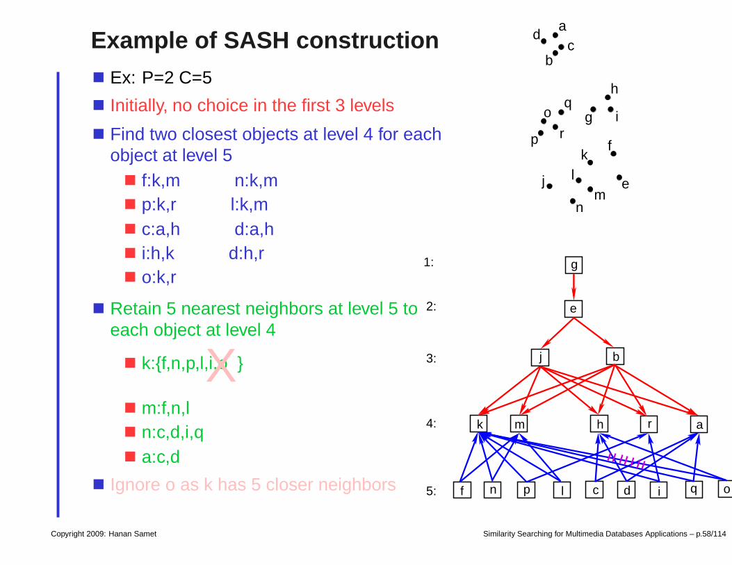
Ex: P=2 C=5
Initially, no choice in the first 3 levels
Find two closest objects at level 4 for eachobject at level 5
f:k,m n:k,mp:k,r l:k,mc:a,h d:a,hi:h,k d:h,ro:k,r
Retain 5 nearest neighbors at level 5 toeach object at level 4
k:f,n,p,l,i,oX
m:f,n,ln:c,d,i,qa:c,d
Ignore o as k has 5 closer neighbors
ad
bc
qo
p rg i
h
f
e
kl
n
jm
e
g
r ahmk
n p l c d i q o
bj
f
4:
3:
1:
2:
5:
Copyright 2009: Hanan Samet Similarity Searching for Multimedia Databases Applications – p.58/114

Example SASH Approximate k Nearest Neighbor Finding
Ex: k = 3 and query object c
Let f(k, i) = ki = k1−(h−i)/ log2
N yielding ki = (1, 1, 2, 2, 3)
U1 = root g of SASH
U2 = objects reachable from U1 which is e
U3 = objects reachable form U2 which is b and j which are retained ask3 = 2
U4 objects reachable from U3 which is a,h,k,m,r and we retain just a andh in U4 as k4 = 2
U5 = objects reachable form U4 which is c,d,i,q, and we retain just c, d,and q in U5 as k5 = 3
Take union of U1, U2, U3, U4, U5 which is the set a,b,c,d,e,g,h,i,j,k,m,q,r,and the closest three neighbors to query object c are a, b, and d
Copyright 2009: Hanan Samet Similarity Searching for Multimedia Databases Applications – p.59/114
Drawback of SASH
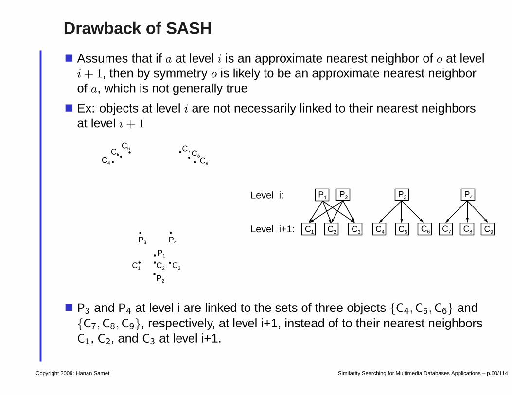
Assumes that if a at level i is an approximate nearest neighbor of o at leveli + 1, then by symmetry o is likely to be an approximate nearest neighborof a, which is not generally true
Ex: objects at level i are not necessarily linked to their nearest neighborsat level i + 1
P1
C1 C2 C3
P2
C6C5
C4
C7 C8
P3 P4
C9
P1 P2 P3 P4
C1 C2 C3 C4 C5 C6 C7 C8 C9Level i+1:
Level i:
P3 and P4 at level i are linked to the sets of three objects C4,C5, C6 andC7,C8, C9, respectively, at level i+1, instead of to their nearest neighborsC1, C2, and C3 at level i+1.
Copyright 2009: Hanan Samet Similarity Searching for Multimedia Databases Applications – p.60/114

AESA (Vidal Ruiz)
Precomputes O(N2) interobject distances between all N objects in S andstores them in a distance matrix
Distance matrix is used to provide lower bounds on distances from queryobject q to objects whose distances have not yet been computed
Only useful if static set of objects and number of queries N as otherwisecan use brute force to find nearest neighbor with N distance computations
Algorithm for range search:Su: objects whose distance from q has not been computed and thathave not been pruned, initially S
dlo(q, o): lower bound on d(q, o) for o ∈ Su, initially zero
1. remove from Su the object p with lowest value dlo(q, p)
terminate if Su is empty or if dlo(q, p) > ε
2. compute d(q, p), adding p to result if d(q, p) ≤ ε
3. for all o ∈ Su, update dlo(q, o) if possibledlo(q, o)← maxdlo(q, o), |d(q, p)− d(p, o)|lower bound property by Lemma 1: |d(q, p)− d(p, o)| ≤ d(q, o)
4. go to step 1
Other heuristic possible for choosing next object: random, highest dlo, etc.Copyright 2009: Hanan Samet Similarity Searching for Multimedia Databases Applications – p.61/114

LAESA (Micó et al.)
AESA is costly as treats all N objects as pivots
Choose a fixed number M of pivots
Similar approach to searching as in AESA but1. non-pivot objects in Sc do not help in tightening lower bound distances
of the objects in Su
2. eliminating pivot objects in Su may hurt later in tightening the distancebounds
Differences:1. selecting a pivot object in Su over any non-pivot object, and2. eliminating pivot objects from Su only after a certain fraction f of the
pivot objects have been selected into Sc (f can range from 0 to 100%if f = 100% then pivots are never eliminated from Su
Copyright 2009: Hanan Samet Similarity Searching for Multimedia Databases Applications – p.62/114

Classifying Distance-Based Indexing Methods
1. Pivot-based methods:pivots, assuming k of them, can be viewed as coordinates in ak-dimensional space and the result of the distance computation forobject x is equivalent to a mapping of x to a point (x0, x1, . . . , xk−1)
where coordinate value xi is the distance d(x, pi) of x from pivot pi
result is similar to embedding methodsalso includes distance matrix methods which contain precomputeddistances between some (e.g., LAESA) or all (e.g., AESA) objects
difference from ball partitioning as no hierarchical partitioning ofdata set
2. Clustering-based methods:partition data into spatial-like zones based on proximity todistinguished object called the cluster centereach object associated with closest cluster centeralso includes sa-tree which records subset of Delaunay graph of thedata set which is a graph whose vertices are the Voronoi cellsdifferent from pivot-based methods where an object o is associatedwith a pivot p on the basis of o’s distance from p rather than because pis the closest pivot to o
Copyright 2009: Hanan Samet Similarity Searching for Multimedia Databases Applications – p.63/114

Pivot-Based vs: Clustering-Based Indexing Methods
1. Both achieve a partitioning of the underlying data set into spatial-like zones
2. Difference:pivot-based: boundaries of zones are more well-defined as they canbe expressed explicitly using a small number of objects and a knowndistance valueclustering-based methods: boundaries of zones are usually expressedimplicitly in terms of the cluster centers, instead of explicitly, whichmay require quite a bit of computation to determine
in fact, very often, the boundaries cannot be expressed explicitly as,for example, in the case of an arbitrary metric space (in contrast toa Euclidean space) where we do not have a direct representation ofthe ‘generalized hyperplane’ that separates the two partitions
Copyright 2009: Hanan Samet Similarity Searching for Multimedia Databases Applications – p.64/114

Distance-Based vs: Multidimension Indexing
1. Distance computations are used to build index in distance-based indexing,but once index has been built, similarity queries can often be performedwith significantly fewer distance computations than a sequential scan ofentire dataset
2. Drawback is that if we want to use a different distance metric, then need tobuild a separate index for each metric in distance-based indexing
not the case for multidimensional indexing methods which can supportarbitrary distance metrics when performing a query, once the indexhas been builthowever, multidimensional indexing is not very useful if don’t have afeature value and only know relative interobject distances (e.g., DNAsequences)
Copyright 2009: Hanan Samet Similarity Searching for Multimedia Databases Applications – p.65/114

Part 3: Dimension Reduction
1. Motivationovercoming curse of dimensionalitywant to use traditional indexing methods (e.g., R-tree and quadtreevariants) which lose effectiveness in higher dimensions
2. Searching in a dimensionally-reduced space
3. Using only one dimension
4. Representative point methods
5. Singular value decomposition (SVD, PCA, KLT)
6. Discrete Fourier transform (DFT)
Copyright 2009: Hanan Samet Similarity Searching for Multimedia Databases Applications – p.66/114

Searching in a Dimensionally-Reduced Space
Want a mapping f so that d(v, u) ≈ d′(f(v), f(u)) where d′ is the distancein the transformed space
Range searching1. reduce query radius
implies more precision as reduce false hits2. increase query radius
implies more recall as reduce false dismissals
3. d′(f(a), f(b)) ≤ d(a, b) for any pair of objects a and b
mapping f is contractive and 100% recall
Copyright 2009: Hanan Samet Similarity Searching for Multimedia Databases Applications – p.67/114

Nearest Neighbors in a Dimensionally-Reduced Space
1. Ideally d(a, b) ≤ d(a, c) implies d′(f(a), f(b)) ≤ d′(f(a), f(c)), for anyobjects a, b, and c
proximity preserving propertyimplies that nearest neighbor queries can be performed directly in thetransformed spacerarely holdsa. holds for translation and scaling with any Minkowski metricb. holds for rotation when using Euclidean metric in both original and
transformed space
2. Use “filter-and-refine” algorithm with no false dismissals (i.e., 100% recall)as long as f is contractive
if o is nearest neighbor of q, contractiveness ensures that ‘filter’ stepfinds all candidate objects o′ such that d′(f(q), f(o′)) ≤ d(q, o)
‘refine’ step calculates actual distance to determine actual nearestneighbor
Copyright 2009: Hanan Samet Similarity Searching for Multimedia Databases Applications – p.68/114
Using only One Dimension
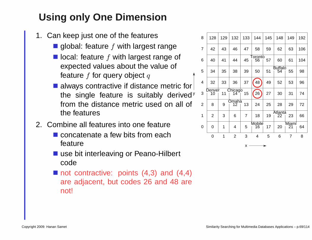
1. Can keep just one of the featuresglobal: feature f with largest rangelocal: feature f with largest range ofexpected values about the value offeature f for query object q
always contractive if distance metric forthe single feature is suitably derivedfrom the distance metric used on all ofthe features
2. Combine all features into one featureconcatenate a few bits from eachfeatureuse bit interleaving or Peano-Hilbertcodenot contractive: points (4,3) and (4,4)are adjacent, but codes 26 and 48 arenot!
y
x
0 1 2 3 4 5 6 7 8
0
1
2
3
4
5
6
7
8
0 1 4 5 17
25
64
2 3 6 7 18 19
26 27
66
8 9 13
20
28 29 72
11 15
23
30 31 74
32 33 36 37 48 49 52 53 96
34 35 38 39 50 51 55 98
40 41 44 45 57 60 61 104
42 43 46 47 58 59 62 63 106
128 129 132 133 144 145 148 149 192
24
Chicago
Mobile
Toronto
Buffalo
Denver
Omaha
Atlanta
Miami16
12
21
10 14
22
54
56
Copyright 2009: Hanan Samet Similarity Searching for Multimedia Databases Applications – p.69/114

Representative Points
Often, objects with spatial extent are represented by a representative pointsuch as a sphere by its radius and the coordinate values of its center
Really a transformation into a point in a higher dimensional space andthus not a dimensional reduction
Transformation is usually not contractive as distance between thetransformed objects is greater than the distance between the originalobjects
Copyright 2009: Hanan Samet Similarity Searching for Multimedia Databases Applications – p.70/114

Transformation into a Different and Smaller Feature Set
A D
C
B
A D
C
B
(a) (b)
yy
xx
y’
x’
Rotate x, y axes to obtain x′, y′ axes
x′ is dominant axis and can even drop axis y′
Copyright 2009: Hanan Samet Similarity Searching for Multimedia Databases Applications – p.71/114

SVD (KLT, PCA)
Method of finding a linear transformation of n-dimensional feature vectorsthat yields good dimensionality reduction1. after transformation, project feature vectors on “first” k axes, yielding
k-dimensional vectors (k ≤ n)2. projection minimizes the sum of the squares of the Euclidean
distances between the set of n-dimensional feature vectors and theircorresponding k-dimensional feature vectors
Letting F denote the original feature vectors, calculate V , the SVDtransform matrix, and obtain transformed feature vectors T so that FV = T
F = UΣV T and retain the k most discriminating values in Σ (i.e., thelargest ones and zeroing the remaining ones)
Start with m n-dimensional points
Drawback is the need to know all of the data in advance which means thatneed to recompute if any of the data values change
Transformation preserves Euclidean distance and thus projection iscontractive
Copyright 2009: Hanan Samet Similarity Searching for Multimedia Databases Applications – p.72/114

Discrete Fourier Transform (DFT)
Drawback of SVD: need to recompute when one feature vector is modified
DFT is a transformation from time domain to frequency domain or viceversa
DFT of a feature vector has same number of components (termedcoefficients) as original feature vector
DFT results in the replacement of a sequence of values at differentinstances of time by a sequence of an equal number of coefficients in thefrequency domain
Analogous to a mapping from a high-dimensional space to another spaceof equal dimension
Provides insight into time-varying data by looking into the dependence ofthe variation on time as well as its repeatability, rather than just looking atthe strength of the signal (i.e., the amplitude) as can be seen from theconventional representation of the signal in the time domain
Copyright 2009: Hanan Samet Similarity Searching for Multimedia Databases Applications – p.73/114

Invertibility of DFT
Ex: decomposition of real-valued five-dimensional feature vector ~x =(1.2,1.4,0.65,-0.25,-0.75)
−1 0 1 2 3 4 5−1
−0.5
0
0.5
1
1.5
feature vector component ( t )
feat
ure
vect
or c
ompo
nent
val
ue (
xt )
Cosine basis functions are solid
Sine basis functions are broken
Solid circle shows original feature vector
Copyright 2009: Hanan Samet Similarity Searching for Multimedia Databases Applications – p.74/114

Use of DFT for Similarity Searching
Euclidean distance norm of feature vector and its DFT are equal
Can apply a form of dimension reduction by eliminating some of theFourier coefficients
Zeroth coefficient is average of components of feature vector
Hard to decide which coefficients to retain1. choose just the first k coefficients2. find dominant coefficients (i.e., highest magnitude, mean, variance,
etc.)requires knowing all of the data and not so dynamic
Copyright 2009: Hanan Samet Similarity Searching for Multimedia Databases Applications – p.75/114

Part 4: Embedding Methods
1. Problem statement
2. Lipschitz embeddings
3. SparseMap
4. FastMap
5. MetricMap
Copyright 2009: Hanan Samet Similarity Searching for Multimedia Databases Applications – p.76/114
Overview of Embedding Methods
1. Given a finite set of N objects and a distance metric d indicating distancebetween them
2. Find function F that maps N objects into a vector space of dimension k
using a distance function d′ in this spaceideally, k is low: k N
computing F should be fast — O(N) or O(N log N)
avoid examining all O(N2) inter-object distance pairs
fast way of obtaining F (o) given o
3. Problem setting also includes situation where the N original objects aredescribed by an n-dimensional feature vector
4. Ideally, the distances between the objects are preserved exactly by themapping F
exact preservation means that (S, d) and (F (S), d′) are isometric
possible when d and d′ are both Euclidean, in which case it is alwaystrue when k = N − 1
difficult in general for arbitrary combinations of d and d′ regardless ofvalue of k
Copyright 2009: Hanan Samet Similarity Searching for Multimedia Databases Applications – p.77/114

Exact Distance Preservation May Be Impossible
Ex: 4 objects a, b, c, e
1. d(a, b) = d(b, c) = d(a, c) = 2 and d(e, a) = d(e, b) = d(e, c) = 1.1
d satisfies triangle inequality
Cannot embed objects into a 3-d Euclidean space — that is, with d′ asthe Euclidean distance while preserving d
2. Can embed if distance between e and a, b, and c is at least 2/√
3
place a, b, and c in plane p and place e on line perpendicular to p thatpasses through the centroid of the triangle in p formed by a, b, and c
3. Also possible if use City Block distance metric dA (L1)place a, b, and c at (0,0,0), (2,0,0), and (1,1,0), respectively, and e at(1,0,0.1)
Copyright 2009: Hanan Samet Similarity Searching for Multimedia Databases Applications – p.78/114

Exact Distance Preservation Always Possible with
Chessboard Distance
One dimension for each object
Map object o into vector d(o, o1), d(o, o2), . . . , d(o, oN )For any pair of objects oi and oj ,
d′(F (oi), F (oj)) = dM (F (oi), F (oj)) = maxl|d(oi, ol)− d(oj , ol)|
For any l, |d(oi, ol)− d(oj , ol)| ≤ d(oi, oj) by the triangle inequality
|d(oi, ol)− d(oj , ol)| = d(oi, oj) for l = i and l = j in which cased′(F (oi), F (oj)) = d(oi, oj)
Therefore, distances are preserved by F when using the Chessboardmetric dM (L∞)
Number of dimensions here is high: k = N
At times, define F in terms of a subset of the objects
Copyright 2009: Hanan Samet Similarity Searching for Multimedia Databases Applications – p.79/114

Properties of Embeddings1. Contractiveness:
d′(F (a), F (b)) ≤ d(a, b)
alternative to exact distance preservationensures 100% recall when use the same search radius in both the originaland embedding space as no correct responses are missedbut precision may be less than 100% due to false candidates
2. Distortion: measures how much larger or smaller the distances in the embed-ding space d′(F (o1), F (o2)) are than the corresponding distances d(o1, o2) inthe original space
defined as c1c2 where 1c1· d(o1, o2) ≤ d′(F (o1), F (o2)) ≤ c2 · d(o1, o2) for
all object pairs o1 and o2 where c1, c2 ≥ 1
similar effect to contractiveness
3. SVD is optimal way of linearly transforming n-dimensional points to k-dimensional points (k ≤ n)
ranks features by importancedrawbacks:a. can’t be applied if only know distance between objectsb. slow: O(N ·m2) where m is dimension of original spacec. only works if d and d′ are the Euclidean distance
Copyright 2009: Hanan Samet Similarity Searching for Multimedia Databases Applications – p.80/114

Lipschitz Embeddings (Linial et al.)
Based on defining a coordinate space where each axis corresponds to areference set which is a subset of the objects
Definition1. set R of subsets of S, R = A1, A2, . . . , Ak2. d(o, A) = minx∈Ad(o, x) for A ⊂ S
3. F (o) = (d(o, A1), d(o, A2), . . . , d(o, Ak))
coordinate values of o are distances from o to the closest elementin each of Ai
saw one such embedding earlier using L∞ where R is all singletonsubsets of S — that is, R = o1, o2, . . . , oN
Copyright 2009: Hanan Samet Similarity Searching for Multimedia Databases Applications – p.81/114

Motivation for Lipschitz Embeddings
If x is an arbitrary object, can obtain some information about d(o1, o2) forarbitrary objects o1 and o2 by comparing d(o1, x) and d(o2, x) — that is,|d(o1, x)− d(o2, x)||d(o1, x)− d(o2, x)| ≤ d(o1, o2) by Lemma 1
Extend to subset A so that |d(o1, A)− d(o2, A)| ≤ d(o1, o2)
Proof:1. let x1, x2 ∈ A be such that d(o1, A) = d(o1, x1) and d(o2, A) = d(o2, x2)
2. d(o1, x1) ≤ d(o1, x2) and d(o2, x2) ≤ d(o2, x1) implies|d(o1, A)− d(o2, A)| = |d(o1, x1)− d(o2, x2)|
3. d(o1, x1)− d(o2, x2) can be positive, while a negative value implies|d(o1, x1)−d(o2, x2)| ≤ max|d(o1, x1)−d(o2, x1)|, |d(o1, x2)−d(o2, x2)|
4. from triangle inequality,max|d(o1, x2)− d(o2, x2)|, |d(o1, x1)− d(o2, x1)| ≤ d(o1, o2)
5. therefore, |d(o1, A)− d(o2, A)| ≤ d(o1, o2) as|d(o1, A)− d(o2, A)| = |d(o1, x1)− d(o2, x2)|
By using R of the subsets, we increase likelihood that d(o1, o2) is capturedby d′(F (o1), F (o2))
Copyright 2009: Hanan Samet Similarity Searching for Multimedia Databases Applications – p.82/114

Mechanics of Lipschitz Embeddings
Linial et al. let R be O(log2 N) randomly selected subsets of S
For d′ = Lp, define F so that
F (o) = (d(o, A1)/q, d(o, A2)/q, . . . , d(o, Ak)/q), where q = k1/p
F satisfies cblog
2Nc· d(o1, o2) ≤ d′(F (o1), F (o2)) ≤ d(o1, o2)
Distortion of O(log N) is large and may make F ineffective at preservingrelative distances as want to use distance value in original space
Since sets Ai are chosen at random, proof is probabilistic and c is aconstant with high probability
Embedding is impractical1. large number and sizes of subsets in R mean that there is a high
probability that all N objects appear in a subset of Rimplies need to compute distance between query object q and allobjects in S
2. number of coordinates is blog2 Nc2, which is relatively largeN = 100 yields k = 36 which is too high
Copyright 2009: Hanan Samet Similarity Searching for Multimedia Databases Applications – p.83/114

SparseMap (Hristescu/Farach-Colton)
Attempts to overcome high cost of computing Lipschitz embedding ofLinial in terms of number of distance computations and dimensions
Uses regular Lipschitz embedding instead of Linial et al. embedding
1. does not divide the distances d(o, Ai) by k1/p
2. uses Euclidean distance metric
Two heuristics1. reduce number of distance computations by calculating an upper
bound d(o, Ai) instead of the exact value d(o, Ai)
only calculate a fixed number of distance values for each object asopposed to |Ai| distance values
2. reduce number of dimensions by using a “high quality” subset of R
instead of the entire setuse greedy resampling to reduce number of dimensions byeliminating poor reference sets
Heuristics do not lead to a contractive embedding but can be madecontractive (Hjaltason and Samet)1. modify first heuristic to compute actual value d(o, Ai), not upper bound
2. use dM (L∞) as d′ instead of dE (L2)
Copyright 2009: Hanan Samet Similarity Searching for Multimedia Databases Applications – p.84/114

FastMap (Faloutsos/Lin)
Inspired by dimension reduction methods for Euclidean space based onlinear transformations such as SVD, KLT, PCA
Claimed to be general but assumes that d is Euclidean as is d′ and only forthese cases is it contractive
Objects are assumed to be points
Copyright 2009: Hanan Samet Similarity Searching for Multimedia Databases Applications – p.85/114

Mechanics of FastMap
Obtain coordinate values for points by projecting them on k mutuallyorthogonal coordinate axes
Compute projections using the given distance function d
Construct coordinate axes one-by-one1. choose two objects (pivots) at each iteration2. draw a line between them that serves as the coordinate axis3. determine coordinate value along this axis for each object o by
mapping (i.e., projecting) o onto this line
Prepare for next iteration1. determine the (m− 1)-dimensional hyperplane H perpendicular to the
line that forms the previous coordinate axis2. project all of the objects onto H
perform projection by defining a new distance function dH
measuring distance between projections of objects on H
dH is derived from original distance function d and coordinate axesdetermined so far
3. recur on original problem with m and k reduced by one, and a newdistance function dH
continue process until have enough coordinate axesCopyright 2009: Hanan Samet Similarity Searching for Multimedia Databases Applications – p.86/114

Choosing Pivot Objects
Pivot objects serve to anchor the line that forms the newly-formedcoordinate axis
Ideally want a large spread of the projected values on the line between thepivot objects1. greater spread generally means that more distance information can be
extracted from the projected valuesfor objects a and b, more likely that |xa − xb| is large, therebyproviding more information
2. similar to principle in KLT but different as spread is weaker notion thanvariance which is used in KLT
large spread can be caused by a few outliers while large variancemeans values are really scattered over a wide range
Use an O(N) heuristic instead of O(N2) process for finding approximationof farthest pair1. arbitrarily choose one of the objects a
2. find object r which is farthest from a
3. find object s which is farthest from r
could iterate more times to obtain a better estimate of farthest pair
Copyright 2009: Hanan Samet Similarity Searching for Multimedia Databases Applications – p.87/114

Deriving First Coordinate Value
1. Two possible positions for projection of object for first coordinatea
r sxa
d(r,s)
d(r,a) d(s,a)
a
sxa d(r,s)
d(r,a)d(s,a)
r
xa obtained by solving d(r, a)2 − x2a = d(s, a)2 − (d(r, s)− xa)2
Expanding and rearranging yields xa =d(r,a)2+d(r,s)2−d(s,a)2
2d(r,s)
2. Used Pythagorean Theorem which is only applicable to Euclidean spaceimplicit assumption that d is Euclidean distanceequation is only a heuristic when used for general metric spacesimplies embedding may not be contractive
3. Observations about xa
can show |xa| ≤ d(r, s)
maximum spread between arbitrary a and b is 2d(r, s)
bounds may not hold if d is not Euclidean as then the distance functionused in subsequent iterations may possibly not satisfy triangleinequality
Copyright 2009: Hanan Samet Similarity Searching for Multimedia Databases Applications – p.88/114

Projected Distance
u
rs
|xt-xu|
t
xt
u’
t’
b’
a’ya
yb
H
C
AB
xu
Ex: 3-d space and just before determining second coordinate
dH : distance function for the distances betweenobjects when projected onto the hyperplane H
perpendicular to the first coordinate axis(through pivots r and s)
Determining dH(t, u) for some objects t and u:
1. let t′ and u′ be their projections on H
dH(t, u) equals distance between t′ and u′
also know: d(t′, u′) = d(C, u)
2. angle at C in triangle tuC is 90, so can apply Pythagorean theorem:
d(t, u)2 = d(t, C)2 + d(C, u)2 = (xt − xu)2 + d(t′, u′)2
3. rearranging and dH(t, u) = d(t′, u′) yields
dH(t, u)2 = d(t, u)2 − (xt − xu)2
Implicit assumption that d is Euclidean distance
Copyright 2009: Hanan Samet Similarity Searching for Multimedia Databases Applications – p.89/114

Side-Effects of Non-Euclidean Distance d
1. dH can fail to satisfy triangle inequalityproduce coordinate values that lead to non-contractiveness
2. Non-contractiveness may cause negative values of dH(a, b)2
complicates search for pivot objectsproblem: square root of negative number is a complex number whichmeans that a and b (really their projections) cannot serve as pivotobjects
Copyright 2009: Hanan Samet Similarity Searching for Multimedia Databases Applications – p.90/114

Subsequent Iterations
Distance function at iteration i is the distance function dH from previousiteration
Notation:1. xi
o: ith coordinate value obtained for object o
2. Fi(o) = x1o, x2
o, . . . , xio: first i coordinate values of F (o)
3. di: distance function used in iteration i
4. pi1 and pi
2: two pivot objects chosen in iteration i
pi2 is the farthest object from pi
1
xio =
di(pi
1,o)2+di(p
i
1,pi
2)2−di(p
i
2,o)2
2di(pi
1,pi
2)
Recursive distance function:
d1(a, b) = d(a, b)
di(a, b)2 = di−1(a, b)2 − (xi−1a − xi−1
b )2
= d(a, b)2 − dE(Fi−1(a), Fi−1(b))2
Copyright 2009: Hanan Samet Similarity Searching for Multimedia Databases Applications – p.91/114

Computational Complexity
1. O(k ·N) distance computations to map N objects to k-dimensional spaceO(N) distance computations at each iteration
2. O(k ·N) space to record the k coordinate values of each of the pointscorresponding to the N objects
3. 2× k array to record identities of k pairs of pivot objects, as thisinformation is needed to process queries
4. Query objects are transformed to k-dimensional points by applying samealgorithm used to construct points corresponding to original objects,except that we use existing pivot objects
O(k) process as o(k) distance computations
5. Can also record distance between pivot objects so no need to recompute
Copyright 2009: Hanan Samet Similarity Searching for Multimedia Databases Applications – p.92/114

Properties of FastMap
1. Contractivenessyes as long as d and d′ are both Euclideana. no if d is Euclidean and d′ is not
Ex: use city block distance dA (L1) for d′ as dA((0, 0), (3, 4)) = 7
while dE((0, 0), (3, 4)) = 5
b. no if d is not Euclidean regardless of d′
Ex: four objects, a through e, with distances d(a, b) = 10,d(a, c) = 4, d(a, e) = 5, d(b, c) = 8, d(b, e) = 7, and d(c, e) = 1
letting a and b be pivots in the first iterations, results inxe − xc = 6/5 = 1.2 < 1 = d(c, e)
if d non-Euclidean, then eventually non-contractive if enough iterations
2. With Euclidean distances, distance can preserved given enough iterationsminm, N − 1 for m-dimensional space and N points
3. Distance expansion can be very large if non-contractive
4. If d is not Euclidean, then dH could violate triangle inequalityEx: four objects, a through e, with distances d(a, b) = d(c, e) = 6,d(a, c) = 5, d(a, e) = d(b, e) = 4, and d(b, c) = 3
letting a and b be pivots, yields dH(a, c) + dH(a, e) ≈ 5.141 <
5.850 ≈ dH(c, e), violating triangle inequalityCopyright 2009: Hanan Samet Similarity Searching for Multimedia Databases Applications – p.93/114

Implications of Non-Contractiveness of FastMap
1. Not guaranteed to to be able to determine k coordinate axeslimits extent of distance preservationfailure to determine more coordinate axes does not necessarily implythat relative distances among the objects are effectively preserved
2. Distance distortion can be very large
3. Presence of many non-positive, or very small positive, distance values(which can cause large distortion) in the intermediate distance functions(i.e., those used to determine the second and subsequent coordinateaxes) may cause FastMap to no longer satisfy the claimed O(N) bound onthe number of distance computations in each iteration
finding a legal pivot pair may, in the worst case, require examining thedistances between a significant fraction of all possible pairs of objects,or Ω(N2) distance computations
Copyright 2009: Hanan Samet Similarity Searching for Multimedia Databases Applications – p.94/114

MetricMap (Wang et al.)
1. Similar to SVD, FastMap, and a special class of Lipschitz embeddingsin Euclidean spaces, equivalent to applying SVD for dimensionreductionbased on an analogy to rotation and projection in Euclidean spaces
2. Differs from FastMap as embedding space is pseudo-Euclideansome coordinate axes make a negative contribution to “distances”between the points
3. Makes use of 2k reference objects which form a coordinate space in a(2k − 1)-dimensional space
one reference object is mapped to origin and rest are mapped to unitvectors in the (2k − 1)-dimensional space
forms a matrix that preserves distance between reference objects
4. Mapping each object is less expensive than in FastMaponly need k + 1 distance computations
5. Employs different strategy to handle non-Euclidean metricsmaps into a pseudo-Euclidean space, which may result in lessdistortion in the distancesmay possibly not be contractive
Copyright 2009: Hanan Samet Similarity Searching for Multimedia Databases Applications – p.95/114

Part 5: Nearest Neighbor Finding
1. Classical methods such as branch and bound
2. K nearest neighbors
3. Incremental nearest neighbor findinga. general methodb. permitting duplicate instances of objects
4. Approximate nearest neighbor finding
5. Probably approximately correct (PAC) nearest neighbor finding
Copyright 2009: Hanan Samet Similarity Searching for Multimedia Databases Applications – p.96/114

Branch and Bound Algorithm (Fukunaga/Narendra)
1. Visit elements in hierarchy using a depth-first traversalmaintain a list L of current candidate k nearest neighbors
2. Dk: distance between q and the farthest object in L
Dk = maxo∈Ld(q, o)), or∞ if L contains fewer than k objects
Dk is monotonically non-increasing over the course of the searchtraversal, and eventually reaches the distance of the kth nearestneighbor of q
3. If element et being visited represents an object o (i.e., t = 0), then insert o
into L, removing farthest if |L| > k
4. Otherwise, et (t ≥ 1) is not an objectconstruct an active list A(et) of child elements of et, ordered by“distance” from q
recursively visit the elements in A(et) in order, backtracking whena. all elements have been visited, orb. reaching an element et′ ∈ A(et) with dt′(q, et′) > Dk
condition ensures that all objects at distance of kth nearestneighbor are reportedif sufficient to report k objects, then use dt′(q, et′) ≥ Dk
Copyright 2009: Hanan Samet Similarity Searching for Multimedia Databases Applications – p.97/114

Branch and Bound Enhancements
Process elements of active list in an order more closely correlated withfinding the k nearest neighbors1. process elements that are more likely to contain the k nearest
neighbors before those that are less likely to do so2. possibly prune elements from further consideration by virtue of being
farther away from the query object than any of the members of list L ofthe current candidate k nearest neighbors
in case of distance-based indexes for metric space searching,prune with aid of triangle inequality
Can use cost estimate functions1. MinDistObject(q, n) is least possible distance from query object q to
an object in tree rooted at n
2. MaxDistObject(q, n) is greatest possible distance between q and anobject in tree rooted at n
When use a spatial index with bounding box hierarchies, then order onbasis of minimum distance to the bounding box associated with eachelement
Copyright 2009: Hanan Samet Similarity Searching for Multimedia Databases Applications – p.98/114

Incremental Nearest Neighbors (Hjaltason/Samet)
Motivation1. often don’t know in advance how many neighbors will need2. e.g., want nearest city to Chicago with population > 1 million
Several approaches1. guess some area range around Chicago and check populations of
cities in rangeif find a city with population > 1 million, must make sure that thereare no other cities that are closer with population > 1 millioninefficient as have to guess size of area to searchproblem with guessing is we may choose too small a region or toolarge a region
a. if size too small, area may not contain any cities with rightpopulation and need to expand the search region
b. if size too large, may be examining many cities needlessly
2. sort all the cities by distance from Chicagoimpractical as we need to re-sort them each time pose a similarquery with respect to another cityalso sorting is overkill when only need first few neighbors
3. find k closest neighbors and check population condition
Copyright 2009: Hanan Samet Similarity Searching for Multimedia Databases Applications – p.99/114

Mechanics of Incremental Nearest Neighbor Algorithm
Make use of a search hierarchy (e.g., tree) where1. objects at lowest level2. object approximations are at next level (e.g., bounding boxes in an
R-tree)3. nonleaf nodes in a tree-based index
Traverse search hierarchy in a “best-first” manner similar to A*-algorithminstead of more traditional depth-first or breadth-first manners1. at each step, visit element with smallest distance from query object
among all unvisited elements in the search hierarchyi.e., all unvisited elements whose parents have been visited
2. use a global list of elements, organized by their distance from queryobject
use a priority queue as it supports necessary insert and deleteminimum operationsties in distance: priority to lower type numbersif still tied, priority to elements deeper in search hierarchy
Copyright 2009: Hanan Samet Similarity Searching for Multimedia Databases Applications – p.100/114

Incremental Nearest Neighbor Algorithm
Algorithm:
INCNEAREST(q, S, T )
1 Q← NEWPRIORITYQUEUE()2 et← root of the search hierarchy induced by q, S, and T3 ENQUEUE(Q, et, 0)4 while not ISEMPTY(Q) do5 et← DEQUEUE(Q)6 if t = 0 then /* et is an object */7 Report et as the next nearest object8 else9 for each child element et′ of et do
10 ENQUEUE(Q, et′ , dt′(q, et′))
1. Lines 1-3 initialize priority queue with root
2. In main loop take element et closest to q off the queuereport et as next nearest object if et is an objectotherwise, insert child elements of et into priority queue
Copyright 2009: Hanan Samet Similarity Searching for Multimedia Databases Applications – p.101/114

Example of INCNEAREST
Initially, algorithm descends tree to leaf node containing qexpand nexpand n1
Start growing search regionexpand n3
report e as nearest neighbor
n
ga
q
e
d
c
bi
f
h
nn1
n2n3
n
n1 n2
n3
queue
front
expand
n
ga
q
e
d
c
bi
f
h
nn1
n2n3
n
n1 n2
n3
queue
front
expand
n2
n3
n1front
expand
n
ga
q
e
d
c
bi
f
h
nn1
n2n3
n
n1 n2
n3
queue
front
expand
n2
n3
n1front
expand
cadn2
n3front
expand
n
ga
q
e
d
c
bi
f
h
nn1
n2n3
n
n1 n2
n3
queue
front
expand
n2
n3
n1front
expand
cadn2
n3front
expand
hbcadn2
e front
Copyright 2009: Hanan Samet Similarity Searching for Multimedia Databases Applications – p.102/114

VASCO Spatial Applet
http://www.cs.umd.edu/ hjs/quadtree/index.html
Copyright 2009: Hanan Samet Similarity Searching for Multimedia Databases Applications – p.103/114

Complexity Analysis
Algorithm is I/O optimalno nodes outside search region are accessedbetter pruning than branch and bound algorithm
Observations for finding k nearest neighbors for uniformly-distributedtwo-dimensional points
expected # of points on priority queue: c ·√
k
expected # of leaf nodes intersecting search region: c · (k +√
k)
In worst case, priority queue will be as large as entire data set
e.g., when data objects are all nearlyequidistant from query objectprobability of worst case very low, as itdepends on a particular configuration ofboth the data objects and the query object(but: curse of dimensionality!)
Copyright 2009: Hanan Samet Similarity Searching for Multimedia Databases Applications – p.104/114

Duplicate Instances of Objects
Objects with extent such as lines, rectangles, regions, etc. are indexed bymethods that associate the objects with the different blocks that theyoccupy
Indexes employ a disjoint decomposition of space in contrast tonon-disjoint as is the case for bounding box hierarchies (e.g., R-tree)
Search hierarchies will contain multiple references to some objects
Adapting incremental nearest neighbor algorithm:1. make sure to detect all duplicate instances that are currently in priority
queue2. avoid inserting duplicate instances of an object that has already been
reported
Copyright 2009: Hanan Samet Similarity Searching for Multimedia Databases Applications – p.105/114

Duplicate Instances Algorithm
INCNEARESTDUP(q, S, T )
1 Q← NEWPRIORITYQUEUE()2 et← root of the search hierarchy induced by q, S, and T3 ENQUEUE(Q, et, 0)4 while not ISEMPTY(Q) do5 et← DEQUEUE(Q)6 if t = 0 then /* et is an object */7 while et = FIRST(Q) do8 DELETEFIRST(Q)9 Report et as the next nearest object
10 else /* et is not an object */11 for each child element et′ of et do
12 if t′ > 0 or dt′(q, et′) ≥ dt(q, et) then
13 ENQUEUE(Q, et′ , dt′(q, et′))
Copyright 2009: Hanan Samet Similarity Searching for Multimedia Databases Applications – p.106/114

Differences from INCNEAREST
1. Object o (et′ ) is enqueued only if o has not yet been reportedcheck if o’s distance from q is less than distance from et to q (line 12)if yes, then o must have been encountered in an element et′′ whichwas closer to q and hence already been reported
2. Check for multiple instances of object o and report only once (lines 7–9)
3. Order objects in queue by identity when at same distance
4. Retrieve all nodes in the queue before objects at same distanceimportant because an object can have several ancestor nodes of thesame typeinteresting as unlike INCNEAREST where want to report neighbors assoon as possible so break ties by giving priority to elements with lowertype numbers
Copyright 2009: Hanan Samet Similarity Searching for Multimedia Databases Applications – p.107/114

VASCO Spatial Applet
http://www.cs.umd.edu/ hjs/quadtree/index.html
Copyright 2009: Hanan Samet Similarity Searching for Multimedia Databases Applications – p.108/114
INCNEAREST Extensions
1. Incremental range query
2. Incremental retrieval of k nearest neighborsneed an extra queue to keep track of k neighbors found so far and canuse distance dk from q of the kth candidate nearest neighbor ok toreduce number of priority queue operations
3. Farthest neighbor
4. Pairs of objectsdistance joindistance semi-join
Copyright 2009: Hanan Samet Similarity Searching for Multimedia Databases Applications – p.109/114

Approximate Nearest Neighbors
1. Often, obtaining exact results is not critical and willing to trade off accuracyfor improved performance
2. Let ε denote the approximation error tolerancecommon criterion is that the distance between q and the resultingcandidate nearest neighbor o′ is within a factor of 1 + ε of the distanceto the actual nearest neighbor o
i.e., d(q, o′) ≤ (1 + ε)d(q, o)
Copyright 2009: Hanan Samet Similarity Searching for Multimedia Databases Applications – p.110/114

Approximate Nearest Neighbors with INCNEAREST
1. Modify INCNEAREST by multiplying the key values for non-object elementson the priority queue by 1 + ε
in a practical sense, non-object element et is enqueued with a largerdistance value — that is, by a factor of (1 + ε)
implies that we delay its processing, thereby allowing objects to bereported ‘before their time’e.g., once et is finally processed, all objects o satisfyingd(q, o) ≤ (1 + ε)dt(q, et) (which is greater than dt(q, et) if ε > 0) wouldhave already been reportedthus an object c in et with a distance d(q, c) ≤ d(q, o) could exist, yet o
is reported before c
algorithm does not necessarily report the resulting objects in strictlyincreasing order of their distance from q
2. Different from Arya/Mount algorithm which cannot be incremental aspriority queue only contains non-object elements
shrinks distance r from q to the closest object o by a factor of 1 + ε andonly inserts a non-object element e into the priority queue if thedistance d(b, q) of e’s corresponding block b from q is less than theshrunken distance
Copyright 2009: Hanan Samet Similarity Searching for Multimedia Databases Applications – p.111/114

Probably Approximately Correct (PAC) Nearest
Neighbors (Ciaccia/Patella)Relax approximate nearest neighbor condition by stipulating a maximumprobability δ for tolerating failure, thereby enabling the decision process tohalt sooner at the risk δ of being wrong
Object o′ is considered a PAC-nearest neighbor of q if the probability thatd(q, o′) ≤ (1 + ε) · d(q, o) is at least 1− δ, where o is actual nearest neighbor
Alternatively, given ε and δ, 1− δ is the minimum probability that o′ is the(1 + ε)-approximate nearest neighbor of q
Ciaccia and Patella use information about the distances between q and thedata objects to derive an upper bound s on the distance between q and aPAC-nearest neighbor o′
Distance bound s is used during the actual nearest neighbor search as apre-established halting condition — that is, the search can be halted oncelocating an object o′ with d(q, o′) ≤ s
Method is analogous to executing a variant of a range query, where therange is defined by the distance bound s, which halts on the first object inthe range
Difficulty is determining a relationship between δ and the distance bound sCopyright 2009: Hanan Samet Similarity Searching for Multimedia Databases Applications – p.112/114

Concluding Remarks
1. Similarity search is a broad area of research
2. Much relation to geometry; geometric setting is usually missing
3. Progress is heavily influenced by applications
4. Need to look at old literature to be able to evaluate current research results
5. Much is left to do as difficult to say what is best solution
Copyright 2009: Hanan Samet Similarity Searching for Multimedia Databases Applications – p.113/114

Selected Overview ReferencesH. Samet. Applications of Spatial Data Structures: Computer Graphics,Image Processing, and GIS. Addison-Wesley, Reading, MA, 1990.
H. Samet. The Design and Analysis of Spatial Data Structures,Addison-Wesley, Reading, MA, 1990.
V. Gaede and O. Günther. Multidimensional access methods. ACMComputer Surveys, 20(2):170–231, June 1998.
C. Böhm, S. Berchtold, and D. A. Keim. Searching in high-dimensionalspaces: Index structures for improving the performance of multimediadatabases. ACM Computing Surveys, 33(3):322–373, Sept. 2001.
E. Chávez, G. Navarro, R. Baeza-Yates, and J. Marroquín. Searching inmetric spaces. ACM Computing Surveys, 33(3):273–322, Sept. 2001.
G. R. Hjaltason and H. Samet. Properties of embedding methods forsimilarity searching in metric spaces. IEEE Transactions on PatternAnalysis and Machine Intelligence, 25(5):530–549, May 2003. AlsoUniversity of Maryland Computer Science TR-4102.
G. R. Hjaltason and H. Samet. Index-driven similarity search in metricspaces. ACM Transactions on Database Systems, 28(4):517–580, Dec.2003.H. Samet. Foundations of Multidimensional and Metric Data Structures,Morgan-Kaufmann, San Francisco, CA, 2006.
Copyright 2009: Hanan Samet Similarity Searching for Multimedia Databases Applications – p.114/114
Related Documents