Sibling Correlations and Social Mobility in Latin America

Inter-American Development Bank

Banco Interamericano de Desarrollo (BID)

Office of the Chief Economist

Oficina del Economista Jefe

Working Paper # 395

Sibling Correlations and Social Mobility

in Latin America

byMomi DahanBank of Israel

Research DepartmentKaplan 1

Jerusalem 91007, [email protected]

Alejandro Gaviria∗

Inter-American Development BankResearch Department

1300 New York Avenue, N.W.Washington, D.C. 20577

[email protected]

Inter-American Development Bank

Washington, D.C. 20577

February 1999

∗ Corresponding author. This paper was written when Dahan was working for the Research Department atthe IDB. We thank Ugo Panizza and Miguel Szekely and seminar participants at the IDB and the 1999Latin American Meetings of the Econometric Society for helpful comments.

2

Abstract

This paper uses sibling correlations in schooling to measure differences in

intergenerational mobility for 16 Latin American countries. The results indicate that there

are substantial differences in mobility within Latin America. On the whole, social

mobility increases with mean schooling and income per capita, but is only mildly

associated with public expenditures in education.

JEL codes: J62 and O54.

© 1999Inter-American Development Bank1300 New York Avenue, N.W.Washington, D.C. 20577

The views and interpretations in this document are those of the authors andshould not be attributed to the Inter-American Development Bank, or to anyindividual acting on its behalf.

For a complete list of publications, visit our Web Site at:http:\\www.iadb.org\oce

3

1. Introduction

In life, there is not a fresh start for each generation. Quite the opposite, life, one might

say, is akin to a relay race in which parents hand the baton to their children. If we

approach social justice problems from this perspective, we must accept at least two

important implications. First, we must accept that policy interventions in this realm

should aim at “leveling the playing field” rather than at redistributing resources from

winners to losers. And second, we must accept that social mobility is a much more

accurate measure of social justice than inequality--the latter, after all, focuses only on the

finish line, ignoring what happens in the middle of the race.

Interestingly, the debate about social justice in developing countries (and especially in

Latin America) has been mainly concerned with inequality. This is important because we

can argue that had it been otherwise (i.e., had social mobility been given more

preeminence), policies would have been different: perhaps more concerned with the

availability of opportunities and less concerned with compensating the losers (IDB,

1998). The neglect of social mobility is not entirely a matter of principle, however. Social

mobility, to be sure, is much more difficult to measure than income distribution. At least

two reasons can be mentioned as to why. First, there is not an obvious way to measure

social mobility and, second, most measures require information for at least two

generations of the same family (usually in the form of long panels). These difficulties

may, of course, go a long way towards explaining why social mobility has often been set

aside in the debates about social justice in developing countries.

In this paper, we measure social mobility by looking at the extent to which family

background determines socioeconomic success. Roughly speaking, social mobility can be

measured by means of two distinct types of correlations: intergenerational correlations

and sibling correlations.1 Both measures rely on a simple premise. If family background

1 Solon (1998) provides a comprehensive summary of the empirical research on sibling andintergenerational correlations.

4

does matter, we should observe some connection between the fates of parents and

children on the one hand and the fates of siblings on the other. These two measures differ

greatly in terms of data requirements. While computing intergenerational correlations

often requires repeated observations of the same family over long periods of time,

computing sibling correlations is possible on the basis of cross-sectional data sets.

In this paper, we propose an index of social mobility for developing countries based on

the correlation of schooling outcomes between siblings. Our index measures the extent to

which schooling outcomes can be explained by family background. If there were perfect

social mobility, family background wouldn’t matter, siblings wouldn’t be more alike than

two people taken at random, and our index would be close to zero. If there were little

mobility, family background would matter very much, siblings would be very similar and

our index would be close to one.

The main advantage of our index is that it can be computed on the basis of the

information found in most household surveys. Our index is based on the assumption that

those children who by their late teens have fallen behind in terms of schooling will have

the worst socioeconomic outcomes later in life. Computing our index involves two main

steps. First, we have to identify those children who have been irremediably left behind.

Then we have to determine the extent to which family background explains their poor

performance. To this end, we compute first what we call a leading indicator of

socioeconomic failure, and then we compute the correlation among siblings of this

indicator. We interpret this correlation as an index of social mobility.

We apply our index to a sample of 16 Latin American countries (we also include the

United States as a benchmark). We find that social mobility is highly correlated with

average country-wide education levels. Countries with more schooling and less inequality

of schooling allow greater mobility. We also find that social mobility is uncorrelated with

public expenditures in education as a percentage of GDP, and tenuously correlated with

GDP per capita.

5

There have been a few recent studies looking at the connection between family

background and schooling in developing countries. Thus, Behrman, Birdsall, and SzJkely

(1998) study the connection between parental attributes (income and education) and

children outcomes. They measure social mobility as the proportion of the children’s

differences in schooling due to observable parental attributes. Filmer and Pritchet (1998)

study the connection between levels of education and family wealth. They compute, for a

large sample of developing countries, median schooling differences of teenagers coming

from rich and poor households. Both studies find a strong connection between education

levels and mobility; that is, countries with higher levels of education exhibit higher

intergenerational mobility.

Other studies have examined social mobility within specific countries. These studies

include that of Lam and Schoeni (1993) on family background and the returns to

education in Brazil and that of Woodruff and Binder (1999) on the intergenerational

transmission of schooling in Mexico, among others. Because these studies use different

methodologies and dissimilar data sets, few general conclusions can be drawn. One point

remains clear, however. Social mobility seems to increase steadily with income both

across countries and over time within the same country.

Finally, we also study in this paper the connection between assortative mating and

inequality. We find a strong connection between the overall level of inequality and the

degree of sorting in marriage markets (measured by the correlation of spouses’

schooling). Although definitive interpretations are difficult, this result is consistent with a

wealth of recent studies that underscore the role sorting and segregation in the creation of

inequality.

The organization of this paper is as follows. Section 2 describes the main data sources;

Section 3 presents the empirical strategy; Section 4 presents our mobility results along

with some exploratory correlations; Section 5 presents the evidence on assortative

mating; and Section 6 concludes.

6

2. Data

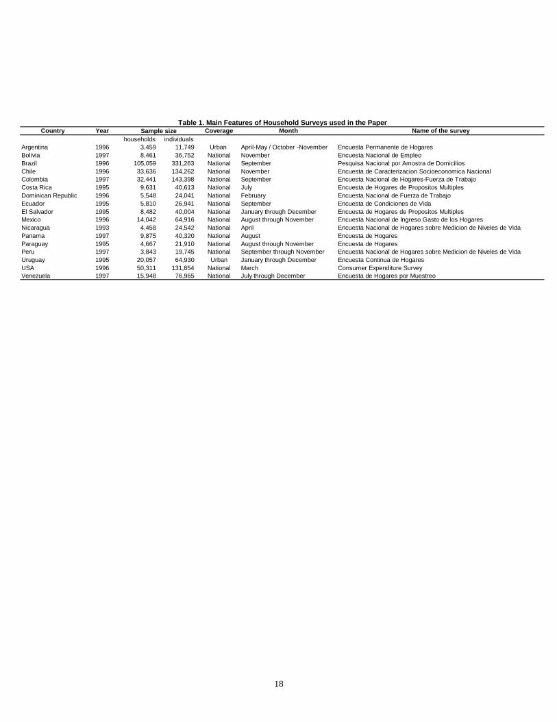
Most of the data used in this paper comes from household surveys. A description of the

surveys, including names, coverage and sample sizes, is presented in Table 1. All the

surveys are for the late 1990s and all are representative of each country’s population with

the exceptions of Argentina and Uruguay, where only urban data is available. The sample

sizes differ widely across countries. They are very large in Brazil, Chile and Colombia,

and much smaller in Argentina, Nicaragua, and Peru.

Although the surveys use different sampling methodologies and include different

questions, they allow meaningful cross-country comparisons, at least in terms of income

and education outcomes. The same set of surveys have been used before to study the

levels and sources of inequality (IDB, 1998), and the interplay between labor supply and

demographics (Duryea and Szekely, 1998).

3. Empirical strategy

In this paper we propose an index of intergenerational mobility for developing countries

that, unlike the standard measures of social mobility, can be computed on the basis of the

information found in most household surveys. In this way, we are able to circumvent, at

least to some degree, the lack of panel information that have hitherto hindered the study

of intergenerational mobility in all but a few developed countries.

At first glance, we can learn very little about intergenerational relations from household

surveys. Not only do we observe parents and children at very different ages, but also we

observe children so early in their lives that little can be inferred about their

socioeconomic performance later in life. Put it differently, household surveys provide a

snapshot so early in the race for socioeconomic success that little can be said about what

will happen at the finish line.

7

The previous problem notwithstanding, there is a group of children for whom a prediction

regarding future socioeconomic outcomes can be made on the basis of the education

levels reported by all household surveys--those who have fallen so far behind that any

hope of catching up seems impossible. So even though the race for socioeconomic status

is long and unsteady, and even though our vantage point into the race is far from the

finish line, we can safely identify the losers as those who have been largely outdistanced

right from the beginning. Once we have identified them, we can examine the extent to

which family background determines their bad outcomes, and hence compare the degree

of mobility among the countries under scrutiny.

Thus, the main hypothesis of this paper (the hypothesis that allows us to use household

surveys to study intergenerational mobility) is predicated on a simple premise. In life, as

in sports, we don’t have to wait until the end of the race to identify who will arrive last--

or very close to last, for that matter. We certainly have to wait until the end to know who

will win, but if we are interested only in those who will arrive last, a glimpse early on in

the race may suffice.

The problem is, of course, how to identify the losers--those who have fallen so far behind

that their socioeconomic fate is, as it were, sealed. We deal with this problem as follows.

We first compute the median schooling for each cohort (we define cohorts on the basis of

age and gender), and then we use these values to define the relevant thresholds. We

assign a value of one to those children whose schooling is greater than the median minus

one (those whose fate is still uncertain), and we assign a value of zero to all the others

(those who have fallen so far behind that socioeconomic success is improbable).2

By following the procedure sketched above, we compute a leading indicator of

socioeconomic failure. Note that our indicator is very conservative. We venture to make a

guess about future outcomes only for those children who have fallen behind the median

levels of education. Figure 1 illustrates our methodology. The figure shows the

2 We will show later that the results of the paper are robust to changes on the arbitrary thresholds used toidentify those who, in our view, have fallen behind beyond redemption.

8

distribution of years of schooling for 18-year-old Brazilian males along with our leading

indicator of socioeconomic failure. Those with six or more years of schooling are given a

value of one, and those with five or fewer years of schooling are given a value of zero.

We impose two sample restrictions in our analysis. First, we restrict all samples to

children between 16 and 20 years of age. This restriction reflects a compromise between

two opposing factors: narrow age groups reduce sample sizes, on the one hand, but allow

more meaningful comparisons of schooling outcomes, on the other (ideally, we should

compare only those children making the same marginal schooling decisions). And

second, we restrict the samples to those households with two or more children in the

specified age range.

It is important to emphasize that our indicator of socioeconomic failure is based on the

median of schooling within specific age and gender categories. We do not compare males

against females. Nor do we compare children of different ages. This is important not only

because schooling varies with age as children move from one grade to the next, but also

because schooling may also vary with gender. If we don’t take these variations into

account, we may misjudge the importance of family background in important ways. For

example, a society in which girls get much more education than boys will appear more

mobile than it actually is if we don’t control for gender differences. Similarly, a society in

which most people don’t leave schooling until they are well into their twenties will

appear more mobile if we don’t control for age.

In this paper we compare countries that differ substantially in terms of average education

levels. While in some countries almost the entire population finishes high school and

many go to college, in other countries most of the population does not finish high school

and only a minority goes to college. So while in the former case we will observe children

too early to appreciate substantial differences in schooling, in the latter case we will

observe children late enough to elucidate most of the schooling differences. We assume

9

throughout that we are able to identify those who have fallen behind irrespective of the

average educational attainment of the country in question.3

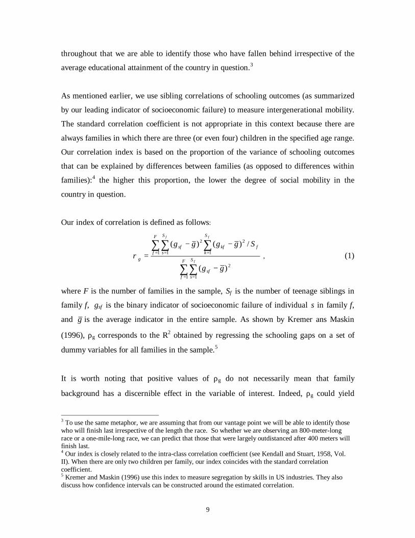
As mentioned earlier, we use sibling correlations of schooling outcomes (as summarized

by our leading indicator of socioeconomic failure) to measure intergenerational mobility.

The standard correlation coefficient is not appropriate in this context because there are

always families in which there are three (or even four) children in the specified age range.

Our correlation index is based on the proportion of the variance of schooling outcomes

that can be explained by differences between families (as opposed to differences within

families):4 the higher this proportion, the lower the degree of social mobility in the

country in question.

Our index of correlation is defined as follows:

∑ ∑

∑ ∑∑

= =

= ==

−

−−=

F

f

S

ssf

F

f

S

kfkf

S

ssf

g f

ff

gg

Sgggg

1 1

2

1 1

2

1

2

)(

/)()(ρ , (1)

where F is the number of families in the sample, Sf is the number of teenage siblings in

family f, gsf is the binary indicator of socioeconomic failure of individual s in family f,

and g is the average indicator in the entire sample. As shown by Kremer ans Maskin

(1996), ρg corresponds to the R2 obtained by regressing the schooling gaps on a set of

dummy variables for all families in the sample.5

It is worth noting that positive values of ρg do not necessarily mean that family

background has a discernible effect in the variable of interest. Indeed, ρg could yield

3 To use the same metaphor, we are assuming that from our vantage point we will be able to identify thosewho will finish last irrespective of the length the race. So whether we are observing an 800-meter-longrace or a one-mile-long race, we can predict that those that were largely outdistanced after 400 meters willfinish last.4 Our index is closely related to the intra-class correlation coefficient (see Kendall and Stuart, 1958, Vol.II). When there are only two children per family, our index coincides with the standard correlationcoefficient.5 Kremer and Maskin (1996) use this index to measure segregation by skills in US industries. They alsodiscuss how confidence intervals can be constructed around the estimated correlation.

10

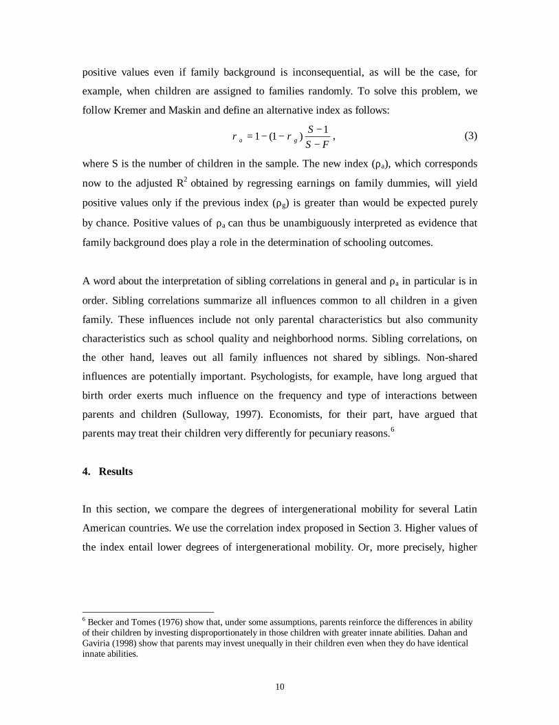
positive values even if family background is inconsequential, as will be the case, for

example, when children are assigned to families randomly. To solve this problem, we

follow Kremer and Maskin and define an alternative index as follows:

FSS

ga −−−−= 1

)1(1 ρρ , (3)

where S is the number of children in the sample. The new index (ρa), which corresponds

now to the adjusted R2 obtained by regressing earnings on family dummies, will yield

positive values only if the previous index (ρg) is greater than would be expected purely

by chance. Positive values of ρa can thus be unambiguously interpreted as evidence that

family background does play a role in the determination of schooling outcomes.

A word about the interpretation of sibling correlations in general and ρa in particular is in

order. Sibling correlations summarize all influences common to all children in a given

family. These influences include not only parental characteristics but also community

characteristics such as school quality and neighborhood norms. Sibling correlations, on

the other hand, leaves out all family influences not shared by siblings. Non-shared

influences are potentially important. Psychologists, for example, have long argued that

birth order exerts much influence on the frequency and type of interactions between

parents and children (Sulloway, 1997). Economists, for their part, have argued that

parents may treat their children very differently for pecuniary reasons.6

4. Results

In this section, we compare the degrees of intergenerational mobility for several Latin

American countries. We use the correlation index proposed in Section 3. Higher values of

the index entail lower degrees of intergenerational mobility. Or, more precisely, higher

6 Becker and Tomes (1976) show that, under some assumptions, parents reinforce the differences in abilityof their children by investing disproportionately in those children with greater innate abilities. Dahan andGaviria (1998) show that parents may invest unequally in their children even when they do have identicalinnate abilities.

11

values allow a higher fraction of the differences in socioeconomic performance among

children to be explained by family background. 7

Figure 2 displays the values of our index for 16 Latin American countries and the United

States. As shown, mobility is the highest in the United States and Costa Rica, and the

lowest in Colombia, Mexico and El Salvador. Mobility is also relatively high in Peru and

relatively low in Nicaragua and Ecuador. For most Latin American countries, up to 50

percent of the differences in socioeconomic performance (as measured here) can be

accounted merely to family background.

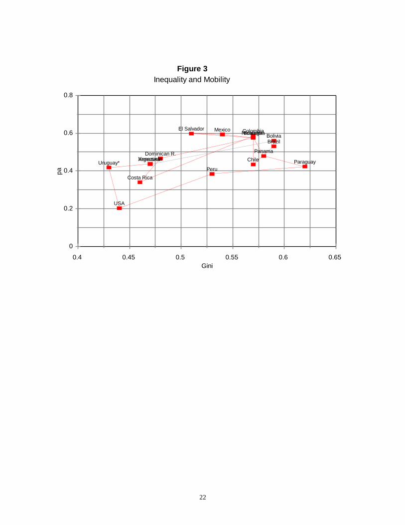
Figure 3 compares intergenerational mobility and income inequality for the same sample

of countries.8 Most Latin American countries exhibit high inequality of income and low

levels of intergenerational mobility (at least in comparison to the United States).9 The

exceptions are Uruguay, which have low inequality and moderate levels of mobility, and

Costa Rica, which has low inequality and relatively high mobility.

How robust are these results to small changes in the methodology? This question is

important because, as explained earlier, our index is based on arbitrary thresholds in the

distribution of schooling: we assume that those children whose education is above the

median education minus one year are fine, and that those below that threshold are

doomed. Needless to say, if the results change drastically when we marginally change the

thresholds, the credibility of our index will come into question.

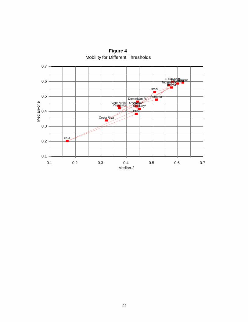
Figure 4 shows the association between two indices that use different thresholds. One

uses the median minus one year of schooling and the other the median minus two years.

As shown, the two indices yield very similar results (the correlation coefficient between

the two is greater than 0.96). The ranking of countries is identical at the extremes, only in

7 Sample sizes and descriptive statistics are presented in Tables A.1 in the appendix.8 Gini coefficients are used to measure income inequality. The same surveys used to compute the indices ofmobility are used to compute the Ginis.9 This result is also consistent with a few cross-country studies that show a positive connection betweenincome distribution and earnings mobility (see, for example, Erikson and Goldthorpe, 1991 and Bjorklundand Jantti, 1997).

12

the middle where the differences are tiny to begin with, the ranking can change

depending on what index is used. Similar results are obtained for other cutoffs, dispelling

most doubts about the fragility of our index to small changes in arbitrary definitions.

The previous results make it clear that there are sizable differences in intergenerational

mobility from one Latin American country to another. This raises the question as to what

country-wide variables are associated with these differences. At a basic level, one should

expect at least some association between educational attainment and mobility--education,

after all, has long been regarded as the foremost instrument of social ascension.

Figure 5 shows the relationship between social mobility and average schooling gaps.

Schooling gaps are defined as the difference between the years of schooling that a child

would have completed had she entered school at age six and advanced one grade each

year and her actual years of schooling. The average gap is computed over all children

between 16 and 20 years of age in the country in question. Higher average gaps are, of

course, indicative of faulty or insufficient educational systems. As shown, there is a

positive association between schooling gaps and our correlation index (or, put differently,

between country-wide schooling averages and intergenerational mobility).10 The

association is linear and strong for most countries. Brazil, Nicaragua, El Salvador and

Paraguay exhibit, however, higher degrees of mobility than would be expected given

their relative backwardness in terms of education.

Figure 7 shows the association between the coefficient of variation of schooling and our

correlation index.11 A strong positive association between these two variables is apparent,

meaning that countries with high schooling inequality also tend to be less mobile. Given

the previously uncovered association between inequality of schooling and average

schooling, Figure 6 just reiterates a point already made; namely, social mobility increases

as education becomes the right of many, not simply the privilege of few.

10 The correlation coefficient is 0.62 and is significant at the one-percent level.11 The correlation coefficient is 0.67 and is also significant at the one-percent level.

13

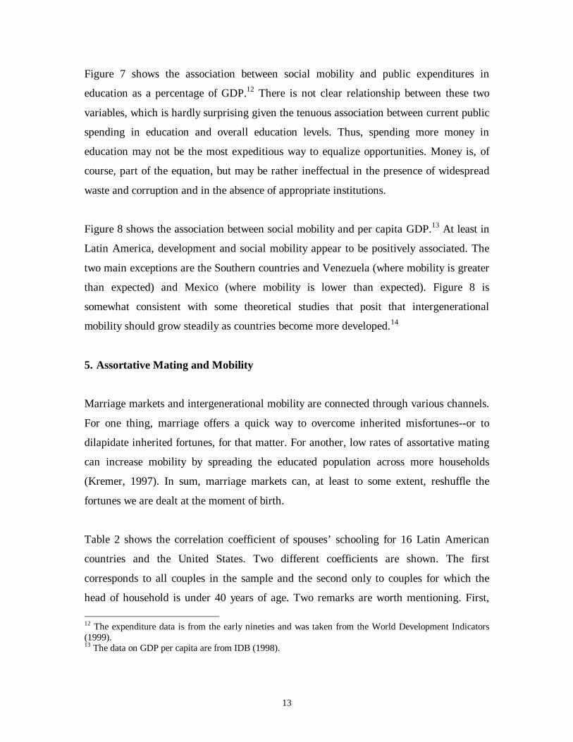
Figure 7 shows the association between social mobility and public expenditures in

education as a percentage of GDP.12 There is not clear relationship between these two

variables, which is hardly surprising given the tenuous association between current public

spending in education and overall education levels. Thus, spending more money in

education may not be the most expeditious way to equalize opportunities. Money is, of

course, part of the equation, but may be rather ineffectual in the presence of widespread

waste and corruption and in the absence of appropriate institutions.

Figure 8 shows the association between social mobility and per capita GDP.13 At least in

Latin America, development and social mobility appear to be positively associated. The

two main exceptions are the Southern countries and Venezuela (where mobility is greater

than expected) and Mexico (where mobility is lower than expected). Figure 8 is

somewhat consistent with some theoretical studies that posit that intergenerational

mobility should grow steadily as countries become more developed.14

5. Assortative Mating and Mobility

Marriage markets and intergenerational mobility are connected through various channels.

For one thing, marriage offers a quick way to overcome inherited misfortunes--or to

dilapidate inherited fortunes, for that matter. For another, low rates of assortative mating

can increase mobility by spreading the educated population across more households

(Kremer, 1997). In sum, marriage markets can, at least to some extent, reshuffle the

fortunes we are dealt at the moment of birth.

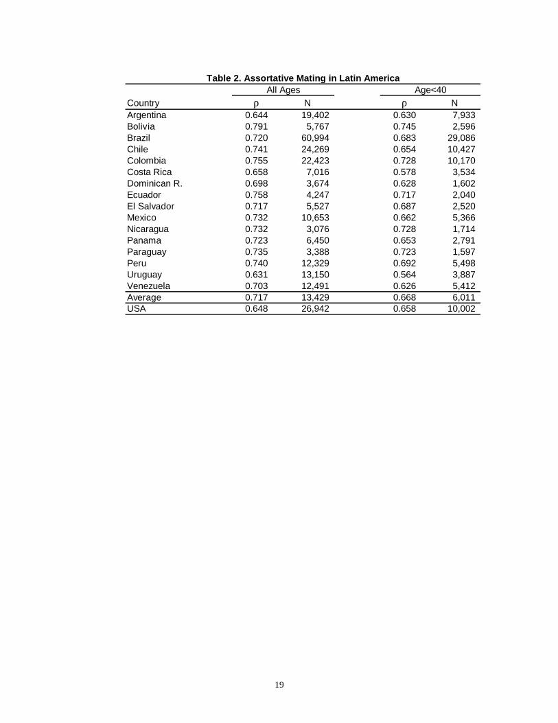
Table 2 shows the correlation coefficient of spouses’ schooling for 16 Latin American

countries and the United States. Two different coefficients are shown. The first

corresponds to all couples in the sample and the second only to couples for which the

head of household is under 40 years of age. Two remarks are worth mentioning. First, 12 The expenditure data is from the early nineties and was taken from the World Development Indicators(1999).13 The data on GDP per capita are from IDB (1998).

14

assortative mating varies much less across countries than intergenerational mobility: the

ratio between the two polar countries is 1.3 in the former case and 3.7 in the latter case.

And second, sorting by education in marriage markets has declined in Latin America, at

least in light of the differences between young and old couples implied by the differences

between columns (2) and (3) of the table.

Figure 9 shows the association between assortative mating and mobility and between

assortative mating and inequality.15 While the connection between the first two variables

is noticeable but not overwhelming (the correlation coefficient is 0.60), the connection

between the last two variables is very high (the correlation coefficient is 0.81). Thus,

sorting by education in marriage markets seems to be increase sharply with inequality,

which suggests that either more unequal societies will tend to be more stratified (perhaps

due to the presence of spatial segregation and discrimination) or, alternative, that more

stratified societies will tend to accentuate inequalities (perhaps due to the presence of

externalities in the transmission of human capital between generations).16

6. Conclusions

We argue in this paper that by comparing sibling correlations of schooling, we can learn

about the differences in the degrees of social mobility among countries (that is, we can

learn about the extent to which family background determines socioeconomic success in

different countries). Our analysis is limited for obvious reasons. First, schooling is an

imperfect measure of child outcomes. School quality, for example, is conspicuously

absent from our analysis, as are differences in parental investments. Second, schooling

doesn’t capture all possible channels through which family background affects

socioeconomic success. Family connections, for example, can make all the difference

when children enter the labor force. Parental wealth also can make a big difference later

in life. Both factors, however, have been left out of our analysis. 14 The relationship between GDP growth and social mobility has been studied by Galor and Tsiddon (1997)and Maoz and Moav (1998), among others.15 The rates of assortative mating are for the younger households.

15

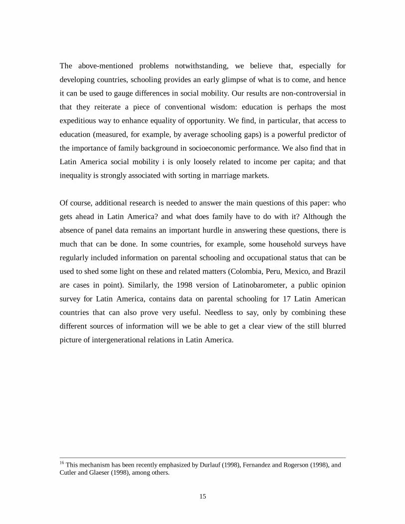
The above-mentioned problems notwithstanding, we believe that, especially for

developing countries, schooling provides an early glimpse of what is to come, and hence

it can be used to gauge differences in social mobility. Our results are non-controversial in

that they reiterate a piece of conventional wisdom: education is perhaps the most

expeditious way to enhance equality of opportunity. We find, in particular, that access to

education (measured, for example, by average schooling gaps) is a powerful predictor of

the importance of family background in socioeconomic performance. We also find that in

Latin America social mobility i is only loosely related to income per capita; and that

inequality is strongly associated with sorting in marriage markets.

Of course, additional research is needed to answer the main questions of this paper: who

gets ahead in Latin America? and what does family have to do with it? Although the

absence of panel data remains an important hurdle in answering these questions, there is

much that can be done. In some countries, for example, some household surveys have

regularly included information on parental schooling and occupational status that can be

used to shed some light on these and related matters (Colombia, Peru, Mexico, and Brazil

are cases in point). Similarly, the 1998 version of Latinobarometer, a public opinion

survey for Latin America, contains data on parental schooling for 17 Latin American

countries that can also prove very useful. Needless to say, only by combining these

different sources of information will we be able to get a clear view of the still blurred

picture of intergenerational relations in Latin America.

16 This mechanism has been recently emphasized by Durlauf (1998), Fernandez and Rogerson (1998), andCutler and Glaeser (1998), among others.

16

References

Becker, Gary S. and Nigel Tomes, 1976, “Child Endowments and the Quantity andQuality of Children,” Journal of Political Economy, 84, 143-62.

Behrman, Jere R., Nancy Birdsall and Miguel SzJkely, Miguel, 1998, “IntergenerationalSchooling Mobility and Macro Conditions and Schooling Policies in Latin America,”Inter-American Development Bank, Office of the Chief Economist, Working Paper #386.

Bjorklund, Anders and Markus Jantti, 1997, “Intergenerational Income Mobility inSweden Compared to the United States,” American Economic Review, 87, 1009-18.

Cutler, David M. and Edward L. Glaeser, 1997, “Are Ghettos Good or Bad?”Quarterly Journal of Economics 112, 827-72.

Erikson, Robert and John Goldthorpe, 1991, The Constant Flux: A Study of ClassMobility in Industrial Societies, Oxford: Clarendon Press.

Dahan, Momi and Alejandro Gaviria, 1998, “Parental Action and Siblings’ Inequality,”Inter-American Development Bank, Office of the Chief Economist, Working Paper #389.

Durlauf, Steve, 1997, “The Membership Theory of Inequality: Theory and Applications.”Santa Fe Institute WP # 97-05-47.

Duryea, Suzanne, and Miguel SzJkely, 1998, “Labor Markets in Latin America: ASupply Side Story,” Inter-American Development Bank, Office of the Chief Economist,Working Paper # 374.

Fernandez, Raquel and Richard Rogerson, 1992, “Income Distribution, Communities andThe Quality of Public Education: a Policy Analysis,” NBER Working Paper # 4158.

Filmer, Deon and Lant Pritchett, 1998, “The Effects of Household Wealth on EducationalAttainment Around the World. Demographic and Health Survey Evidence,” World Bank,Mimeo.

Galor, Oder and Daniel Tsiddon, 1997, “Technological Progress, Mobility and EconomicGrowth,” American Economic Review, 87, 363-82.

Inter-American Development Bank (IDB), 1998, Facing up to Inequality in LatinAmerica, Washington D.C.: John Hopkins University Press.

Kendall, Maurice G. and Alan Stuart, 1958, The Advanced Theory of Statistics. 3 Vols.,New York: Hafner.

17

Kremer, Michael, 1997, “How Much Does Sorting Increase Inequality?” QuarterlyJournal of Economics 12, 15-39.

Kremer, Michael and Eric Maskin, 1996, “Wage Inequality and Segregation by Skill,”NBER Working Paper # 5718, August.

Lam, David and Robert F. Schoeni, 1993, “Effects of Family Background on Earningsand Returns to Schooling: Evidence from Brazil,” Journal of Political Economy, 101,710-40.

Maoz, Yishay and Omer Moav, 1998, “Intergenerational Mobility and the Process ofDevelopment,” Hebrew University, Mimeo.

Solon, Gary, 1998, “Intergenerational Mobility in the Labor Market,” Mimeo,Forthcoming in the Handbook of Labor Economics.

Sulloway, Frank J., 1997, Born to Rebel: Birth Order, Family Dynamics, and CreativeLives, Vintage Books.

Woodruff, C. and Melissa Binder, 1999, "Intergenerational Mobility in EducationalAttainment in Mexico,” Unpublished Manuscript.

18

Country Year Coverage Month Name of the surveyhouseholds individuals

Argentina 1996 3,459 11,749 Urban April-May / October -November Encuesta Permanente de HogaresBolivia 1997 8,461 36,752 National November Encuesta Nacional de EmpleoBrazil 1996 105,059 331,263 National September Pesquisa Nacional por Amostra de DomiciliosChile 1996 33,636 134,262 National November Encuesta de Caracterizacion Socioeconomica NacionalColombia 1997 32,441 143,398 National September Encuesta Nacional de Hogares-Fuerza de TrabajoCosta Rica 1995 9,631 40,613 National July Encuesta de Hogares de Propositos MultiplesDominican Republic 1996 5,548 24,041 National February Encuesta Nacional de Fuerza de TrabajoEcuador 1995 5,810 26,941 National September Encuesta de Condiciones de VidaEl Salvador 1995 8,482 40,004 National January through December Encuesta de Hogares de Propositos MultiplesMexico 1996 14,042 64,916 National August through November Encuesta Nacional de Ingreso Gasto de los HogaresNicaragua 1993 4,458 24,542 National April Encuesta Nacional de Hogares sobre Medicion de Niveles de VidaPanama 1997 9,875 40,320 National August Encuesta de HogaresParaguay 1995 4,667 21,910 National August through November Encuesta de HogaresPeru 1997 3,843 19,745 National September through November Encuesta Nacional de Hogares sobre Medicion de Niveles de VidaUruguay 1995 20,057 64,930 Urban January through December Encuesta Continua de HogaresUSA 1996 50,311 131,854 National March Consumer Expenditure SurveyVenezuela 1997 15,948 76,965 National July through December Encuesta de Hogares por Muestreo

Sample sizeTable 1. Main Features of Household Surveys used in the Paper

19

Country ρ N ρ NArgentina 0.644 19,402 0.630 7,933 Bolivia 0.791 5,767 0.745 2,596 Brazil 0.720 60,994 0.683 29,086 Chile 0.741 24,269 0.654 10,427 Colombia 0.755 22,423 0.728 10,170 Costa Rica 0.658 7,016 0.578 3,534 Dominican R. 0.698 3,674 0.628 1,602 Ecuador 0.758 4,247 0.717 2,040 El Salvador 0.717 5,527 0.687 2,520 Mexico 0.732 10,653 0.662 5,366 Nicaragua 0.732 3,076 0.728 1,714 Panama 0.723 6,450 0.653 2,791 Paraguay 0.735 3,388 0.723 1,597 Peru 0.740 12,329 0.692 5,498 Uruguay 0.631 13,150 0.564 3,887 Venezuela 0.703 12,491 0.626 5,412 Average 0.717 13,429 0.668 6,011 USA 0.648 26,942 0.658 10,002

All Ages Age<40Table 2. Assortative Mating in Latin America

20

Figure 1. Distribution of Schooling and Index of Socioeconomic FailureBrazil, 18-year-old Males

0

0.05

0.1

0.15

0 1 2 3 4 5 6 7 8 9 10 11 12 13Years of Schooling

%

0

0.25

0.5

0.75

1

21

Figure 2. Social Mobility in the Americas

0.00 0.10 0.20 0.30 0.40 0.50 0.60 0.70

El Salvador

Mexico

Colombia

Ecuador

Nicaragua

Bolivia

Brazil

Panama

Dominican R.

Venezuela

Argentina *

Chile

Paraguay

Uruguay *

Peru

Costa Rica

USA

22

0

0.2

0.4

0.6

0.8

pa

0.4 0.45 0.5 0.55 0.6 0.65 Gini

Argentina*

BoliviaBrazil

Chile

Colombia

Costa Rica

Dominican R.

EcuadorEl Salvador Mexico

Nicaragua

Panama

ParaguayPeru

USA

Uruguay*Venezuela

Figure 3Inequality and Mobility

23

0.1

0.2

0.3

0.4

0.5

0.6

0.7

Med

ian-

one

0.1 0.2 0.3 0.4 0.5 0.6 0.7 Median-2

Argentina*

BoliviaBrazil

Chile

Colombia

Costa Rica

Dominican R.

El SalvadorMexicoNicaragua

Panama

Paraguay

Peru

USA

Uruguay*Venezuela

Figure 4Mobility for Different Thresholds

24

0

0.2

0.4

0.6

0.8

pa

0 1 2 3 4 5 6 7 Gap

Argentina*

BoliviaBrazil

Chile

Colombia

Costa Rica

Dominican R.

EcuadorEl SalvadorMexico

Nicaragua

Panama

ParaguayPeru

USA

Uruguay*Venezuela

Figure 5Schooling Gaps and Mobility

25

0

0.2

0.4

0.6

0.8

pa

0.1 0.2 0.3 0.4 0.5 0.6 0.7 Coefficient of Variation

Argentina*

BoliviaBrazil

Chile

Colombia

Costa Rica

Dominican R.

EcuadorEl SalvadorMexico

Nicaragua

Panama

ParaguayPeru

USA

Uruguay*Venezuela

Figure 6Inequality of Schooling and Mobility

26

0

0.2

0.4

0.6

0.8

pa

1 2 3 4 5 6 Spending in Education/GDP

Argentina*

BoliviaBrazil

Chile

Colombia

Costa Rica

Dominican R.

EcuadorEl Salvador Mexico

Nicaragua

Panama

Paraguay

USA

Uruguay*Venezuela

Figure 7Spending in Education and Mobility

27

0.2

0.3

0.4

0.5

0.6

0.7

pa

1000 2000 3000 4000 5000 6000 7000 GDP per Capita

Argentina*

Bolivia

Brazil

Chile

Colombia

Costa Rica

Dominican R.

EcuadorEl Salvador Mexico

Nicaragua

Panama

Paraguay

Peru

Uruguay*Venezuela

Figure 8GDP per capita and Mobility

28

0.2

0.4

0.6 pa

0.5 0.55 0.6 0.65 0.7 0.75 Assortative Mating

Argentina*

Bolivia

Brazil

Chile

Colombia

Costa Rica

Dominican R.

EcuadorEl SalvadorMexico

Nicaragua

Panama

Paraguay

Peru

USA

Uruguay*Venezuela

Figure 9 (a)Mobility and Assortative Mating

0.4

0.45

0.5

0.55

0.6

0.65

Gin

i

0.55 0.6 0.65 0.7 0.75 Assortative Mating

Argentina*

BoliviaBrazil

Chile Colombia

Costa Rica

Dominican R.

Ecuador

El Salvador

Mexico

NicaraguaPanama

Paraguay

Peru

USAUruguay*

Venezuela

Figure 9 (b)Inequality and Assortative Mating

29

Appendix

Average Number of Gap Average InequalityCountry Year ρa kids per families (years of years of of

family schooling) schooling schoolingArgentina * 1996 0.437 2.18 2,098 2.1 10.0 0.26Bolivia 1997 0.561 2.14 647 3.1 8.6 0.35Brazil 1996 0.531 2.20 5,906 5.3 6.4 0.49Chile 1996 0.435 2.12 1,801 2.3 9.6 0.25Colombia 1997 0.587 2.18 2,426 3.7 8.1 0.38Costa Rica 1995 0.340 2.18 679 4.1 7.7 0.36Dominican R. 1996 0.466 2.19 439 3.2 8.7 0.37Ecuador 1995 0.577 2.19 506 3.4 8.4 0.35Mexico 1996 0.594 2.21 1,352 3.5 8.4 0.38Nicaragua 1993 0.576 2.23 442 6.3 5.5 0.66Panama 1997 0.480 2.18 565 3.0 8.9 0.32Peru 1997 0.385 2.17 377 2.6 9.3 0.271Paraguay 1995 0.423 2.13 279 4.4 7.4 0.41El Salvador 1995 0.599 2.17 791 4.9 6.9 0.55Uruguay * 1995 0.418 2.15 863 2.3 9.7 0.25Venezuela 1995 0.438 2.20 1,737 3.3 8.6 0.32Average 0.490 2.18 1,307 3.6 8.3 0.37USA 1996 0.203 2.10 1,214 0.8 11.0 0.17Children between 16 and 20 years of age were used in the computations.

Table A1. Sibling Correlations of Schooling Outcomes: Latin America and the U.S.