Shortest Paths II: Bellman- Ford, Topological Sort, DAG Shortest Paths, Linear Programming, Difference Constraints Lecture 15

Welcome message from author
This document is posted to help you gain knowledge. Please leave a comment to let me know what you think about it! Share it to your friends and learn new things together.
Transcript

Shortest Paths II: Bellman-Ford, Topological Sort, DAG Shortest Paths, Linear Programming, Difference Constraints
Lecture 15

L15.2
Negative-weight cycles
Recall: If a graph G = (V, E) contains a negative-weight cycle, then some shortest paths may not exist.
Example:
u v
…
< 0
Bellman-Ford algorithm: Finds all shortest-path lengths from a source s V to all v V or determines that a negative-weight cycle exists.

L15.3
Bellman-Ford algorithm
d[s] 0 for each v V – {s}
do d[v]
for i 1 to | V | – 1
do for each edge (u, v) E do if d[v] > d[u] + w(u, v)
then d[v] d[u] + w(u, v)
for each edge (u, v) E do if d[v] > d[u] + w(u, v)
then report that a negative-weight cycle exists
initialization
At the end, d[v] = d(s, v). Time = O(V E).
relaxation step

L15.4
Example of Bellman-Ford
A
B
E
C D
–1
4
1 2
–3
2
5
3
A B C D E
0
0

L15.5
–1
0 –1
Example of Bellman-Ford
A
B
E
C D
–1
4
1 2
–3
2
5
3
A B C D E
0
0

L15.6
–1
0 –1
Example of Bellman-Ford
A
B
E
C D
–1
4
1 2
–3
2
5
3
A B C D E
0
0
4
0 –1 4
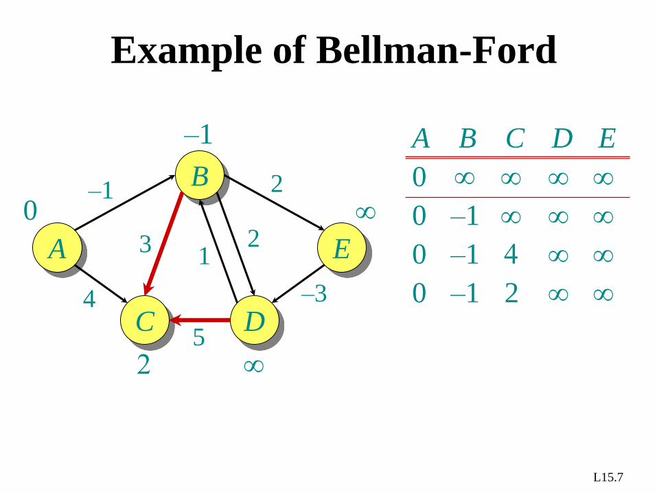
L15.7
4
0 –1 2
2
–1
0 –1
Example of Bellman-Ford
A
B
E
C D
–1
4
1 2
–3
2
5
3
A B C D E
0
0
0 –1 4

L15.8
–1
Example of Bellman-Ford
A
B
E
C D
–1
4
1 2
–3
2
5
3
0
2
0 –1 2
0 –1
A B C D E
0
0 –1 4

L15.9
–1
Example of Bellman-Ford
A
B
E
C D
–1
4
1 2
–3
2
5
3
0
2
0 –1 2
0 –1
A B C D E
0
0 –1 4
1
0 –1 2 1

L15.10
0 –1 2 1 1 1
–1
Example of Bellman-Ford
A
B
E
C D
–1
4
1 2
–3
2
5
3
0
2
0 –1 2
0 –1
A B C D E
0
0 –1 4
1
0 –1 2 1
L15.11
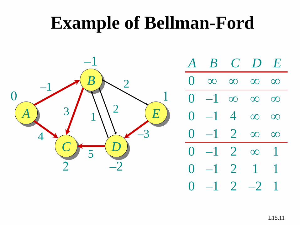
1
0 –1 2 –2 1
–2 0 –1 2 1 1
–1
Example of Bellman-Ford
A
B
E
C D
–1
4
1 2
–3
2
5
3
0
2
0 –1 2
0 –1
A B C D E
0
0 –1 4
1
0 –1 2 1

L15.12
1
0 –1 2 –2 1
–2 0 –1 2 1 1
–1
Example of Bellman-Ford
A
B
E
C D
–1
4
1 2
–3
2
5
3
0
2
0 –1 2
0 –1
A B C D E
0
0 –1 4
1
0 –1 2 1
Note: Values decrease monotonically.

L15.13
Correctness
Theorem. If G = (V, E) contains no negative-weight cycles, then after the Bellman-Ford algorithm executes, d[v] = d(s, v) for all v V. Proof. Let v V be any vertex, and consider a shortest path p from s to v with the minimum number of edges.
v1 v
2
v3
vk v0
…
s v
p:
Since p is a shortest path, we have
d(s, vi) = d(s, vi–1) + w(vi–1, vi) .

L15.14
Correctness (continued)
v1 v
2
v3
vk v0
…
s v
p:
Initially, d[v0] = 0 = d(s, v0), and d[s] is unchanged by subsequent relaxations (because of the lemma from Lecture 17 that d[v] d(s, v)).
• After 1 pass through E, we have d[v1] = d(s, v1).• After 2 passes through E, we have d[v2] = d(s, v2).
M• After k passes through E, we have d[vk] = d(s, vk).
Since G contains no negative-weight cycles, p is simple. Longest simple path has | V | – 1 edges.
L15.15
Detection of negative-weight cycles
Corollary. If a value d[v] fails to converge after | V | – 1 passes, there exists a negative-weight cycle in G reachable from s.

L15.16
DAG shortest paths
If the graph is a directed acyclic graph (DAG), we first topologically sort the vertices.
Walk through the vertices u V in this order, relaxing the edges in Adj[u], thereby obtaining the shortest paths from s in a total of O(V + E) time.
• Determine f : V {1, 2, …, | V |} such that (u, v) E
f (u) < f (v).
• O(V + E) time using depth-first search.
3 5 6
4
2 s
7
9
8 1

L15.17
Linear programming
Let A be an mn matrix, b be an m-vector, and c be an n-vector. Find an n-vector x that maximizes cTx subject to Ax b, or determine that no such solution exists.
. . maximizing m
n
A x b cT x

L15.18
Linear-programming algorithms
Algorithms for the general problem
• Simplex methods — practical, but worst-caseexponential time.
• Ellipsoid algorithm — polynomial time, butslow in practice.
• Interior-point methods — polynomial time andcompetes with simplex.
Feasibility problem: No optimization criterion. Just find x such that Ax b. • In general, just as hard as ordinary LP.

L15.19
Solving a system of difference constraints
Linear programming where each row of A contains exactly one 1, one –1, and the rest 0’s.
Example:
x1 – x2 3 x2 – x3 –2 x1 – x3 2
xj – xi wij
Solution:
x1 = 3 x2 = 0 x3 = 2
Constraint graph:
vjvixj – xi wij
wij
(The “A” matrix has dimensions |E | |V |.)

L15.20
Unsatisfiable constraints
Theorem. If the constraint graph contains a negative-weight cycle, then the system of differences is unsatisfiable. Proof. Suppose that the negative-weight cycle is v1 v2 L vk v1. Then, we have
x2 – x1 w12
x3 – x2 w23M
xk – xk–1 wk–1, k
x1 – xk wk1
Therefore, no values for the xi can satisfy the constraints.
0 weight of cycle < 0

7 L15.21
Satisfying the constraints
Theorem. Suppose no negative-weight cycle exists in the constraint graph. Then, the constraints are satisfiable. Proof. Add a new vertex s to V with a 0-weight edge to each vertex vi V.
v1
v4
v
v9
v3
s
0 Note: No negative-weight cycles introduced shortest paths exist.

L15.22
The triangle inequality gives us d(s,vj) d(s, vi) + wij. Since xi = d(s, vi) and xj = d(s, vj), the constraint xj – xi wij is satisfied.
Proof (continued)
Claim: The assignment xi = d(s, vi) solves the constraints.
s
vj
vi
d(s, vi)
d(s, vj) wij
Consider any constraint xj – xi wij, and consider the shortest paths from s to vj and vi:
L15.23
Bellman-Ford and linear programming
Corollary. The Bellman-Ford algorithm can solve a system of m difference constraints on n variables in O(m n) time.
Single-source shortest paths is a simple LP problem.
In fact, Bellman-Ford maximizes x1 + x2 + L + xn
subject to the constraints xj – xi wij and xi 0 (exercise).
Bellman-Ford also minimizes maxi{xi} – mini{xi} (exercise).
Related Documents


![4.4 BELLMAN-FORD DEMOxiaojuan/algo16/slides/7DemoBellmanFor… · Repeat V times: relax all E edges. Bellman-Ford algorithm demo 3 4 7 1 3 5 2 6 initialize 0 v distTo[] edgeTo[] 0](https://static.cupdf.com/doc/110x72/600ad23c9473ea2d4c6d5ff8/44-bellman-ford-demo-xiaojuanalgo16slides7demobellmanfor-repeat-v-times-relax.jpg)


![A Potential-Based Variant of the Bellman-Ford …ceur-ws.org/Vol-2504/paper15.pdfThe Bellman-Ford algorithm [Bel58,For56] maintains a FIFO queue of la-beled nodes. A node that becomes](https://static.cupdf.com/doc/110x72/5e73c240896a6715033aba0e/a-potential-based-variant-of-the-bellman-ford-ceur-wsorgvol-2504-the-bellman-ford.jpg)


