Outline Shortest path Dijkstra Bellman-Ford All-pairs Floyd Shortest Paths Dijkstra Bellman-Ford Floyd All-pairs paths Lecturer: Georgy Gimel’farb COMPSCI 220 Algorithms and Data Structures 1 / 69

Welcome message from author
This document is posted to help you gain knowledge. Please leave a comment to let me know what you think about it! Share it to your friends and learn new things together.
Transcript

Outline Shortest path Dijkstra Bellman-Ford All-pairs Floyd
Shortest PathsDijkstra Bellman-Ford Floyd All-pairs paths
Lecturer: Georgy Gimel’farb
COMPSCI 220 Algorithms and Data Structures
1 / 69

Outline Shortest path Dijkstra Bellman-Ford All-pairs Floyd
1 Single-source shortest path
2 Dijkstra’s algorithm
3 Bellman-Ford algorithm
4 All-pairs shortest path problem
5 Floyd’s algorithm
2 / 69

Outline Shortest path Dijkstra Bellman-Ford All-pairs Floyd
Paths and Distances Revisited
Cost of a walk / path v0, v1, . . . , vk in a digraph G = (V,E) withedge weights {c(u, v) | (u, v) ∈ E}:
cost(v0, v1, . . . , vk) =
k−1∑i=0
c(vi, vi+1)
Distance d(u, v) between two vertices u and v of V (G): theminimum cost of a path between u and v.
Eccentricity of a node u ∈ V : ec[u] = maxv∈V
d(u, v).
Radius of G: the minimum eccentricity of u ∈ V : minu∈V
ec[u].
Diameter of G: the maximum eccentricity of u ∈ V : maxu∈V
ec[u].
Note: there are analogous definitions for graphs.
3 / 69

Outline Shortest path Dijkstra Bellman-Ford All-pairs Floyd
Unweighted / Weighted Graphs: Shortest Paths
The shortest path from the vertex A to the vertex D:
A B
C D
E
F
min{2A,C,D, 3A,C,E,D, 3A,B,F,D}
A B
C D
E
F1
4
3
38
2 3
min{9A,C,D, 6A,C,E,D, 10A,B,F,D}
4 / 69

Outline Shortest path Dijkstra Bellman-Ford All-pairs Floyd
Single-source Shortest Path (SSSP) in G = (V,E, c)
Given a source node v, find the shortest (minimum weight) path toeach other node.
• Weight of a path: the sum of weights (costs) on the arcs.
• BFS works only if all weights c(u, v); (u, v) ∈ E, are equal.
• Dijkstra’s algorithm – one of the known solutions.
• A greedy algorithm: each locally best choice is globallybest.
• Works only if all weights are non-negative.• Initial paths: one-arc paths from s to v of weight
cost(s, v).• Each step compares the shortest paths with and without
each new node.
5 / 69

Outline Shortest path Dijkstra Bellman-Ford All-pairs Floyd
Single-source Shortest Path (SSSP) in G = (V,E, c)
1 Build a list S of visited nodes (say, using a priority queue).
2 Iterative propagation of the shortest paths:
1 Choose the closest unvisited node u being on a path withinternal nodes in S.
2 If adding the node u has established shorter paths,update distances of remaining unvisited nodes v from thesource s.
Complexity depends on data structures used.
• For a priority queue, such as a binary heap, running timeO((m+ n) log n) is possible.• If every node is reachable from the source: O(m log n).
• More sophisticated Fibonacci heaps lead to the bestcomplexity of O(m+ n log n).
6 / 69

Outline Shortest path Dijkstra Bellman-Ford All-pairs Floyd
Dijkstra’s Algorithm
algorithm Dijkstra( weighted digraph (G, c), node s ∈ V (G) )array colour[n] = {WHITE, . . . ,WHITE}array dist[n] = {c[s, 0], . . . , c[s, n− 1]}colour[s]← BLACKwhile there is a WHITE node do
pick a WHITE node u, such that dist[u] is minimumcolour[u]← BLACKfor each x adjacent to u do
if colour[x] = WHITE thendist[x]← min
{dist[x], dist[u] + c[u, x]
}end if
end forend whilereturn dist
end7 / 69

Outline Shortest path Dijkstra Bellman-Ford All-pairs Floyd
Dijkstra’s Algorithm: Example 1
a
b
c
d
e
3
8
1
2
2
2
7
3
2
5
BLACK dist[x]List S a b c d e
a 0 3 8 ∞ ∞a b 0 3 8 5 ∞a b d 0 3 7 5 10a b c d 0 3 7 5 9a b c d e 0 3 7 5 9
8 / 69

Outline Shortest path Dijkstra Bellman-Ford All-pairs Floyd
Dijkstra’s Algorithm: Example 1
a
b
c
d
e
3
8
1
2
2
2
7
3
2
5
BLACK dist[x]List S a b c d e
a 0 3 8 ∞ ∞a b 0 3 8 5 ∞a b d 0 3 7 5 10a b c d 0 3 7 5 9a b c d e 0 3 7 5 9
8 / 69

Outline Shortest path Dijkstra Bellman-Ford All-pairs Floyd
Dijkstra’s Algorithm: Example 1
a
b
c
d
e
3
8
1
2
2
2
7
3
2
5
BLACK dist[x]List S a b c d e
a 0 3 8 ∞ ∞a b 0 3 8 5 ∞a b d 0 3 7 5 10a b c d 0 3 7 5 9a b c d e 0 3 7 5 9
8 / 69

Outline Shortest path Dijkstra Bellman-Ford All-pairs Floyd
Dijkstra’s Algorithm: Example 1
a
b
c
d
e
3
8
1
2
2
2
7
3
2
5
BLACK dist[x]List S a b c d e
a 0 3 8 ∞ ∞a b 0 3 8 5 ∞a b d 0 3 7 5 10a b c d 0 3 7 5 9a b c d e 0 3 7 5 9
8 / 69

Outline Shortest path Dijkstra Bellman-Ford All-pairs Floyd
Dijkstra’s Algorithm: Example 1
a
b
c
d
e
3
8
1
2
2
2
7
3
2
5
BLACK dist[x]List S a b c d e
a 0 3 8 ∞ ∞a b 0 3 8 5 ∞a b d 0 3 7 5 10a b c d 0 3 7 5 9a b c d e 0 3 7 5 9
8 / 69

Outline Shortest path Dijkstra Bellman-Ford All-pairs Floyd
Why Does Dijkstra’s Algorithm Work?
Let an S-path be a path startingat node s and ending at node xwith all the intermediate nodescoloured BLACK, i.e., from thelist S, except possibly x.
x
u
Ss
y·
·
Theorem 6.8: Suppose that all arc weights are nonnegative.
Then these two properties hold at the top of while-loop:
P1: If x ∈ V (G), then dist[x] is the minimum cost of an S-pathfrom s to x.
P2: If colour[w] = BLACK (i.e., w ∈ S), then dist[w] is theminimum cost of a path from s to w.
Once a node u is added to S and dist[u] is updated, dist[u] never changes insubsequent steps. After S = V , dist holds the goal shortest distances.
9 / 69
Outline Shortest path Dijkstra Bellman-Ford All-pairs Floyd
Proving Why Dijkstra’s Algorithm Works
The update rule: dist[x]← min{dist[x], dist[u] + c[u, x]
}.
dist[x] is the length of some path froms to x at every step.
• If x ∈ S, then it is an S-path.
• Updated dist[v] never increases.
To prove P1 and P2: induction on thenumber of times k of going through thewhile-loop (Sk; S0 = {s}; dist[s] = 0).
x
u
Ss
y·
·
• k = 0: P1 and P2 hold as dist[s] = 0.
• Inductive hypothesis: P1 and P2 hold for k ≥ 0; Sk+1 = Sk⋃{u}.
• Inductive steps for P2 and P1:
• Consider any s-to-w Sk+1-path γ = (s, . . . , y, u) of the weight|γ|.
• If w ∈ Sk, consider the hypothesis.• If w /∈ Sk, γ extends some s-to-y Sk-path γ1 = (s, . . . , y).
10 / 69

Outline Shortest path Dijkstra Bellman-Ford All-pairs Floyd
Proving Why Dijkstra’s Algorithm Works
Inductive step for P2:
• For w ∈ Sk+1 and w 6= u, P2 holds by inductive hypothesis.
• For w = u, P2 holds, too, because any Sk+1-path γ = (s, . . . , y, u)of weight |γ| extends some Sk-path γ1 = (s, . . . , y) of weight |γ1|:• By the inductive hypothesis, dist[y] ≤ |γ1|.• By the update rule, dist[u] ≤ dist[y] + c(y, u).• Therefore, dist[u] ≤ |γ| = |γ1|+ c(y, u).
u
Sk
γ1
s
y
11 / 69

Outline Shortest path Dijkstra Bellman-Ford All-pairs Floyd
Proving Why Dijkstra’s Algorithm Works
Inductive step for P1: x ∈ V (G); γ – any s-to-x Sk+1-path;Sk+1 = Sk
⋃{u}:
• u /∈ γ: γ is an Sk-path and |γ| ≤ dist[x] by the inductive hypothesis.
• u ∈ γ =( γ1︷ ︸︸ ︷s, . . . , u, x
): by the update rule, |γ| = |γ1|+ c(u, x) ≥ dist[x].
• u ∈ γ = (
γ1︷ ︸︸ ︷s, . . . , u, . . . .y, x
), returning to Sk after u: by the update rule,
|γ| = |γ1|+ c(y, x) ≥ |β|+ c(y, x) ≥ dist[y] + c(y, x) ≥ dist[x]
where |β| is the min weight of an s-to-y Sk-path.
x
u
Sks
y·
·
12 / 69
Outline Shortest path Dijkstra Bellman-Ford All-pairs Floyd
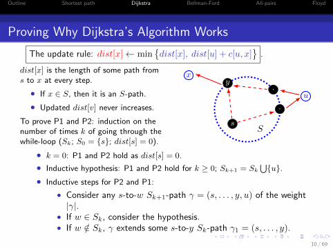
Dijksra’s Algorithm: Example 2
7
9
14
10
15
112
9 6
A B
C
F E D Node u A B C D E F
0 7 9 ∞ ∞ 14A 0 7 9 ∞ ∞ 14A B 0 7 9 22 ∞ 14A B C 0 7 9 20 ∞ 11A B C F 0 7 9 20 20 11A B C D F 0 7 9 20 20 11A B C D E F 0 7 9 20 20 11
for u ∈ V (G) dist[u]← c[A, u]
13 / 69

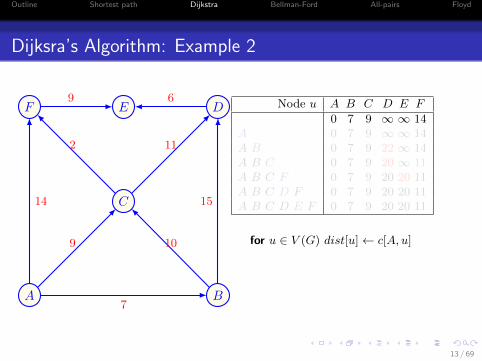
Outline Shortest path Dijkstra Bellman-Ford All-pairs Floyd
Dijksra’s Algorithm: Example 2
7
9
14
10
15
112
9 6
A B
C
F E D
A
Node u A B C D E F
0 7 9 ∞ ∞ 14A 0 7 9 ∞ ∞ 14A B 0 7 9 22 ∞ 14A B C 0 7 9 20 ∞ 11A B C F 0 7 9 20 20 11A B C D F 0 7 9 20 20 11A B C D E F 0 7 9 20 20 11
colour[A]← BLACK; dist[A]← 0
13 / 69

Outline Shortest path Dijkstra Bellman-Ford All-pairs Floyd
Dijksra’s Algorithm: Example 2
7
9
14
10
15
112
9 6
A B
C
F E D
A B
Node u A B C D E F
0 7 9 ∞ ∞ 14A 0 7 9 ∞ ∞ 14A B 0 7 9 22 ∞ 14A B C 0 7 9 20 ∞ 11A B C F 0 7 9 20 20 11A B C D F 0 7 9 20 20 11A B C D E F 0 7 9 20 20 11
while-loop:WHITE B,C,D,E, F : min dist[B]colour[B]← BLACKfor x ∈ V (G)
dist[x]←min
{dist[x], dist[B] + c[B, x]
}
13 / 69

Outline Shortest path Dijkstra Bellman-Ford All-pairs Floyd
Dijksra’s Algorithm: Example 2
7
9
14
10
15
112
9 6
A B
C
F E D
A B
C
Node u A B C D E F
0 7 9 ∞ ∞ 14A 0 7 9 ∞ ∞ 14A B 0 7 9 22 ∞ 14A B C 0 7 9 20 ∞ 11A B C F 0 7 9 20 20 11A B C D F 0 7 9 20 20 11A B C D E F 0 7 9 20 20 11
while-loop:WHITE C,D,E, F : min dist[C]colour[C]← BLACK;for x ∈ V (G)
dist[x]←min
{dist[x], dist[C] + c[C, x]
}
13 / 69

Outline Shortest path Dijkstra Bellman-Ford All-pairs Floyd
Dijksra’s Algorithm: Example 2
7
9
14
10
15
112
9 6
A B
C
F E D
A B
C
FNode u A B C D E F
0 7 9 ∞ ∞ 14A 0 7 9 ∞ ∞ 14A B 0 7 9 22 ∞ 14A B C 0 7 9 20 ∞ 11A B C F 0 7 9 20 20 11A B C D F 0 7 9 20 20 11A B C D E F 0 7 9 20 20 11
while-loop:WHITE D,E, F : min dist[F ]colour[F ]← BLACK;for x ∈ V (G)
dist[x]←min
{dist[x], dist[F ] + c[F, x]
}
13 / 69
Outline Shortest path Dijkstra Bellman-Ford All-pairs Floyd
Dijksra’s Algorithm: Example 2
7
9
14
10
15
112
9 6
A B
C
F E D
A B
C
F DNode u A B C D E F
0 7 9 ∞ ∞ 14A 0 7 9 ∞ ∞ 14A B 0 7 9 22 ∞ 14A B C 0 7 9 20 ∞ 11A B C F 0 7 9 20 20 11A B C D F 0 7 9 20 20 11A B C D E F 0 7 9 20 20 11
while-loop:WHITE D,E: min dist[D]colour[D]← BLACK;for x ∈ V (G)
dist[x]←min
{dist[x], dist[D] + c[D,x]
}
13 / 69

Outline Shortest path Dijkstra Bellman-Ford All-pairs Floyd
Dijksra’s Algorithm: Example 2
7
9
14
10
15
112
9 6
A B
C
F E D
A B
C
F DENode u A B C D E F
0 7 9 ∞ ∞ 14A 0 7 9 ∞ ∞ 14A B 0 7 9 22 ∞ 14A B C 0 7 9 20 ∞ 11A B C F 0 7 9 20 20 11A B C D F 0 7 9 20 20 11A B C D E F 0 7 9 20 20 11
while-loop:WHITE E: min dist[E]colour[E]← BLACK;for x ∈ V (G)
dist[x]←min
{dist[x], dist[E] + c[E, x]
}
13 / 69

Outline Shortest path Dijkstra Bellman-Ford All-pairs Floyd
Dijksta’s Algorithm: PFS Version
Input: weighted digraph (G, c); source node s ∈ V (G);priority queue Q; arrays dist[0..n− 1]; colour[0..n− 1]
for u ∈ V (G) do:colour[u]←WHITE
colour[s]← GREYQ.insert(s, keys = 0)
Q.is empty()? return distyes
no
Q.delete() u← Q.peek()τ ← Q.getKey(u)
for each x adjacent to u do:
t← τ + c(u, x)
colour[x] = WHITE?yes
colour[x]← GREYQ.insert(x, t)
no
colour[x] = GREY?yes
Q.getKey(x) > t?yes
Q.decreaseKey(x, t)
nono
14 / 69
Outline Shortest path Dijkstra Bellman-Ford All-pairs Floyd
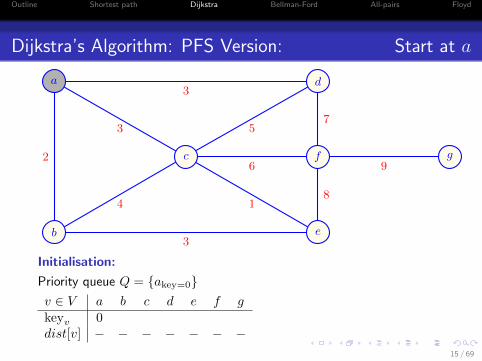
Dijkstra’s Algorithm: PFS Version: Start at a
2
4
3
3 5
6
1
7
8
9
3
b
a
c
e
f
d
g
Initialisation:
Priority queue Q = {akey=0}v ∈ V a b c d e f gkeyv 0dist[v] − − − − − − −
15 / 69

Outline Shortest path Dijkstra Bellman-Ford All-pairs Floyd
Dijkstra’s Algorithm: PFS Version: Steps 1 – 2
2
4
3
3 5
6
1
7
8
9
3
b
a
c
e
f
d
g
u← a; t1 ← keya = 0; x ∈ {b, c, d}x← b: t2 = t1 + cost(a, b) = 2; Q = {a0, b2}v ∈ V a b c d e f gkeyv 0 2dist[v] − − − − − − −
16 / 69

Outline Shortest path Dijkstra Bellman-Ford All-pairs Floyd
Dijkstra’s Algorithm: PFS Version: Step 3
2
4
3
3 5
6
1
7
8
9
3
b
a
c
e
f
d
g
u = a; t1 = keya = 0; x ∈ {b, c, d}x← c: t2 = t1 + cost(a, c) = 3; Q = {a0, b2, c3}v ∈ V a b c d e f gkeyv 0 2 3dist[v] − − − − − − −
17 / 69

Outline Shortest path Dijkstra Bellman-Ford All-pairs Floyd
Dijkstra’s Algorithm: PFS Version: Step 4
2
4
3
3 5
6
1
7
8
9
3
b
a
c
e
f
d
g
u = a; t1 = keya = 0; x ∈ {b, c, d}x← d: t2 = t1 + cost(a, d) = 3; Q = {a0, b2, c3, d3}v ∈ V a b c d e f gkeyv 0 2 3 3dist[v] − − − − − − −
18 / 69

Outline Shortest path Dijkstra Bellman-Ford All-pairs Floyd
Dijkstra’s Algorithm: PFS Version: Step 5
2
4
3
3 5
6
1
7
8
9
3
b
a
c
e
f
d
g
Completing the while-loop for u = a
dist[a]← t1 = 0; Q = {b2, c3, d3}v ∈ V a b c d e f gkeyv 0 2 3 3dist[v] 0 − − − − − −
19 / 69

Outline Shortest path Dijkstra Bellman-Ford All-pairs Floyd
Dijkstra’s Algorithm: PFS Version: Steps 6 – 7
2
4
3
3 5
6
1
7
8
9
3
b
a
c
e
f
d
g
u← b; t1 ← keyb = 2; x ∈ {c, e}x← c: t2 = t1 + cost(b, c) = 2 + 4 = 6; keyc = 3 < t2 = 6
v ∈ V a b c d e f gkeyv 0 2 3 3dist[v] 0 − − − − − −
20 / 69

Outline Shortest path Dijkstra Bellman-Ford All-pairs Floyd
Dijkstra’s Algorithm: PFS Version: Step 8
2
4
3
3 5
6
1
7
8
9
3
b
a
c
e
f
d
g
u = b; t1 = keyb = 2; x ∈ {c, e}x← e: t2 = t1 + cost(b, e) = 2 + 3 = 5; Q = {b2, c3, d3, e5}v ∈ V a b c d e f gkeyv 0 2 3 3 5dist[v] 0 − − − − − −
21 / 69

Outline Shortest path Dijkstra Bellman-Ford All-pairs Floyd
Dijkstra’s Algorithm: PFS Version: Step 9
2
4
3
3 5
6
1
7
8
9
3
b
a
c
e
f
d
g
Completing the while-loop for u = b
dist[b]← t1 = 2; Q = {c3, d3, e5}v ∈ V a b c d e f gkeyv 0 2 3 3 5dist[v] 0 2 − − − − −
22 / 69

Outline Shortest path Dijkstra Bellman-Ford All-pairs Floyd
Dijkstra’s Algorithm: PFS Version: Steps 10 – 11
2
4
3
3 5
6
1
7
8
9
3
b
a
c
e
f
d
g
u← c; t1 ← keyc = 3; x ∈ {d, e, f}x← d: t2 = t1 + cost(c, d) = 3 + 5 = 8; keyd = 3 < t2 = 8
v ∈ V a b c d e f gkeyv 0 2 3 3 5dist[v] 0 2 − − − − −
23 / 69

Outline Shortest path Dijkstra Bellman-Ford All-pairs Floyd
Dijkstra’s Algorithm: PFS Version: Step 12
2
4
3
3 5
6
1
7
8
9
3
b
a
c
e
f
d
g
u = c; t1 = keyc = 3; x ∈ {d, e, f}x← e: t2 = t1 + cost(c, d) = 3 + 1 = 4; keye = 5 < t2 = 4; keye ← 4
v ∈ V a b c d e f gkeyv 0 2 3 3 4dist[v] 0 2 − − − − −
24 / 69

Outline Shortest path Dijkstra Bellman-Ford All-pairs Floyd
Dijkstra’s Algorithm: PFS Version: Step 13
2
4
3
3 5
6
1
7
8
9
3
b
a
c
e
f
d
g
u = c; t1 = keyc = 3; x ∈ {d, e, f}x← f : t2 = t1 + cost(c, f) = 3 + 6 = 9; Q = {c3, d3, e4, f9}v ∈ V a b c d e f gkeyv 0 2 3 3 4 9dist[v] 0 2 − − − − −
25 / 69

Outline Shortest path Dijkstra Bellman-Ford All-pairs Floyd
Dijkstra’s Algorithm: PFS Version: Step 14
2
4
3
3 5
6
1
7
8
9
3
b
a
c
e
f
d
g
Completing the while-loop for u = c
dist[c]← t1 = 3; Q = {d3, e4, f9}v ∈ V a b c d e f gkeyv 0 2 3 3 4 9dist[v] 0 2 3 − − − −
26 / 69

Outline Shortest path Dijkstra Bellman-Ford All-pairs Floyd
Dijkstra’s Algorithm: PFS Version: Steps 15 – 16
2
4
3
3 5
6
1
7
8
9
3
b
a
c
e
f
d
g
u← d; t1 ← keyd = 3; x ∈ {f}x← f : t2 = t1 + cost(d, f) = 3 + 7 = 10; keyf = 9 < t2 = 10
v ∈ V a b c d e f gkeyv 0 2 3 3 4 9dist[v] 0 2 3 − − − −
27 / 69

Outline Shortest path Dijkstra Bellman-Ford All-pairs Floyd
Dijkstra’s Algorithm: PFS Version: Step 17
2
4
3
3 5
6
1
7
8
9
3
b
a
c
e
f
d
g
Completing the while-loop for u = d
dist[d]← t1 = 3; Q = {e4, f9}v ∈ V a b c d e f gkeyv 0 2 3 3 4 9dist[v] 0 2 3 3 − − −
28 / 69

Outline Shortest path Dijkstra Bellman-Ford All-pairs Floyd
Dijkstra’s Algorithm: PFS Version: Steps 18 – 19
2
4
3
3 5
6
1
7
8
9
3
b
a
c
e
f
d
g
u← e; t1 ← keye = 4; x ∈ {f}x← f : t2 = t1 + cost(e, f) = 4 + 8 = 12; keyf = 9 < t2 = 12
v ∈ V a b c d e f gkeyv 0 2 3 3 4 9dist[v] 0 2 3 3 − − −
29 / 69
Outline Shortest path Dijkstra Bellman-Ford All-pairs Floyd
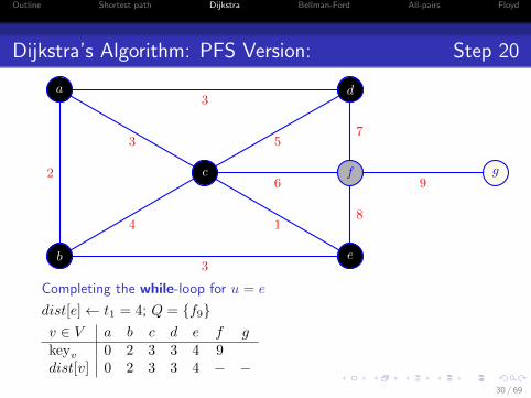
Dijkstra’s Algorithm: PFS Version: Step 20
2
4
3
3 5
6
1
7
8
9
3
b
a
c
e
f
d
g
Completing the while-loop for u = e
dist[e]← t1 = 4; Q = {f9}v ∈ V a b c d e f gkeyv 0 2 3 3 4 9dist[v] 0 2 3 3 4 − −
30 / 69

Outline Shortest path Dijkstra Bellman-Ford All-pairs Floyd
Dijkstra’s Algorithm: PFS Version: Steps 21 – 22
2
4
3
3 5
6
1
7
8
9
3
b
a
c
e
f
d
g
u← f ; t1 ← keyf = 9; x ∈ {g}x← g: t2 = t1 + cost(f, g) = 9 + 9 = 18; Q = {f9, g18}v ∈ V a b c d e f gkeyv 0 2 3 3 4 9 18dist[v] 0 2 3 3 4 − −
31 / 69

Outline Shortest path Dijkstra Bellman-Ford All-pairs Floyd
Dijkstra’s Algorithm: PFS Version: Step 23
2
4
3
3 5
6
1
7
8
9
3
b
a
c
e
f
d
g
Completing the while-loop for u = f
dist[f ]← t1 = 9; Q = {g18}v ∈ V a b c d e f gkeyv 0 2 3 3 4 9 18dist[v] 0 2 3 3 4 9 −
32 / 69

Outline Shortest path Dijkstra Bellman-Ford All-pairs Floyd
Dijkstra’s Algorithm: PFS Version: Steps 24 – 25
2
4
3
3 5
6
1
7
8
9
3
b
a
c
e
f
d
g
Completing the while-loop for u = g
dist[g]← t1 = 18; no adjacent verices for g; empty Q = {}v ∈ V a b c d e f gkeyv 0 2 3 3 4 9 18dist[v] 0 2 3 3 4 9 18
33 / 69
Outline Shortest path Dijkstra Bellman-Ford All-pairs Floyd
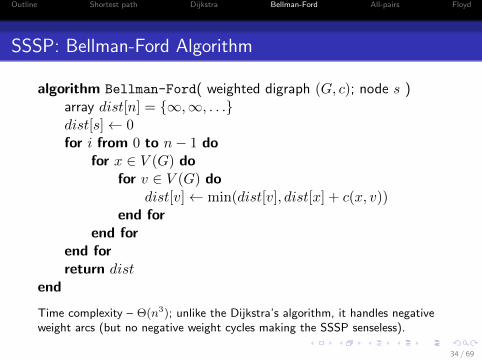
SSSP: Bellman-Ford Algorithm
algorithm Bellman-Ford( weighted digraph (G, c); node s )array dist[n] = {∞,∞, . . .}dist[s]← 0for i from 0 to n− 1 do
for x ∈ V (G) dofor v ∈ V (G) do
dist[v]← min(dist[v], dist[x] + c(x, v))end for
end forend forreturn dist
end
Time complexity – Θ(n3); unlike the Dijkstra’s algorithm, it handles negativeweight arcs (but no negative weight cycles making the SSSP senseless).
34 / 69
Outline Shortest path Dijkstra Bellman-Ford All-pairs Floyd
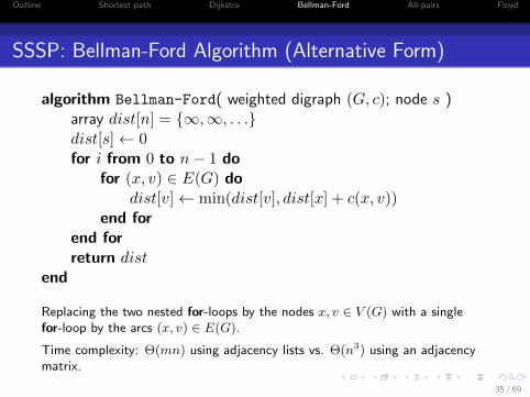
SSSP: Bellman-Ford Algorithm (Alternative Form)
algorithm Bellman-Ford( weighted digraph (G, c); node s )array dist[n] = {∞,∞, . . .}dist[s]← 0for i from 0 to n− 1 do
for (x, v) ∈ E(G) dodist[v]← min(dist[v], dist[x] + c(x, v))
end forend forreturn dist
end
Replacing the two nested for-loops by the nodes x, v ∈ V (G) with a singlefor-loop by the arcs (x, v) ∈ E(G).
Time complexity: Θ(mn) using adjacency lists vs. Θ(n3) using an adjacencymatrix.
35 / 69
Outline Shortest path Dijkstra Bellman-Ford All-pairs Floyd
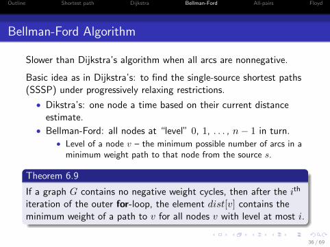
Bellman-Ford Algorithm
Slower than Dijkstra’s algorithm when all arcs are nonnegative.
Basic idea as in Dijkstra’s: to find the single-source shortest paths(SSSP) under progressively relaxing restrictions.
• Dikstra’s: one node a time based on their current distanceestimate.
• Bellman-Ford: all nodes at “level” 0, 1, . . . , n− 1 in turn.• Level of a node v – the minimum possible number of arcs in a
minimum weight path to that node from the source s.
Theorem 6.9
If a graph G contains no negative weight cycles, then after the ith
iteration of the outer for-loop, the element dist[v] contains theminimum weight of a path to v for all nodes v with level at most i.
36 / 69

Outline Shortest path Dijkstra Bellman-Ford All-pairs Floyd
Proving Why Bellman-Ford Algorithm Works
Just as for Dijkstra’s, the update ensures dist[v] never increases.
Induction by the level i of the nodes:
• Base case: i = 0; the result is true due to initialisation:dist[s] = 0; dist[v] =∞; v ∈ V \s.
• Induction hypothesis: dist[v]; v ∈ V , are true for i− 1.• Induction step for a node v at level i:
• Due to no negative weight cycles, a min-weight s-to-v path, γ,has i arcs.
• If y is the last node before v and γ1 the subpath to y, thendist[y] ≤ |γ1| by the induction hypothesis.
• Thus by the update rule:
dist[v] ≤ dist[y] + c(y, v) ≤ |γ1|+ c(y, v) ≤ |γ|
as required at level i.
37 / 69

Outline Shortest path Dijkstra Bellman-Ford All-pairs Floyd
Illustrating Bellman-Ford Algorithm
a
b
c
d
e
3
-1
1
2
2
2
4
-2
6
-3
i dist[x]a b c d e
0 0 ∞ ∞ ∞ ∞1 0 3 −1 ∞ ∞2 0 0 −1 3 53 0 0 −1 2 04 0 0 −1 2 −1
38 / 69

Outline Shortest path Dijkstra Bellman-Ford All-pairs Floyd
Illustrating Bellman-Ford Algorithm
a
b
c
d
e
3
-1
1
2
2
2
4
-2
6
-3
3
-1
∞
∞
i dist[x]a b c d e
0 0 ∞ ∞ ∞ ∞1 0 3 −1 ∞ ∞2 0 0 −1 3 53 0 0 −1 2 04 0 0 −1 2 −1
38 / 69

Outline Shortest path Dijkstra Bellman-Ford All-pairs Floyd
Illustrating Bellman-Ford Algorithm
a
b
c
d
e
3
-1
1
2
2
2
4
-2
6
-3
0
-1
3
5
i dist[x]a b c d e
0 0 ∞ ∞ ∞ ∞1 0 3 −1 ∞ ∞2 0 0 −1 3 53 0 0 −1 2 04 0 0 −1 2 −1
38 / 69

Outline Shortest path Dijkstra Bellman-Ford All-pairs Floyd
Illustrating Bellman-Ford Algorithm
a
b
c
d
e
3
-1
1
2
2
2
4
-2
6
-3
0
-1
2
-1
i dist[x]a b c d e
0 0 ∞ ∞ ∞ ∞1 0 3 −1 ∞ ∞2 0 0 −1 3 53 0 0 −1 2 04 0 0 −1 2 −1
38 / 69

Outline Shortest path Dijkstra Bellman-Ford All-pairs Floyd
Illustrating Bellman-Ford Algorithm
a
b
c
d
e
3
-1
1
2
2
2
4
-2
6
-3
0
-1
2
-1
i dist[x]a b c d e
0 0 ∞ ∞ ∞ ∞1 0 3 −1 ∞ ∞2 0 0 −1 3 53 0 0 −1 2 04 0 0 −1 2 −1
38 / 69
Outline Shortest path Dijkstra Bellman-Ford All-pairs Floyd
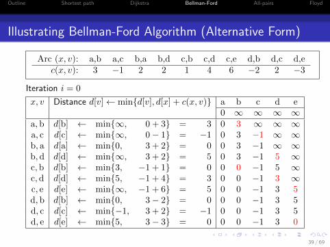
Illustrating Bellman-Ford Algorithm (Alternative Form)
Arc (x, v): a,b a,c b,a b,d c,b c,d c,e d,b d,c d,ec(x, v): 3 −1 2 2 1 4 6 −2 2 −3
Iteration i = 0
x, v Distance d[v]← min{d[v], d[x] + c(x, v)} a b c d e0 ∞ ∞ ∞ ∞
a,b d[b] ← min{∞, 0 + 3} = 3 0 3 ∞ ∞ ∞a, c d[c] ← min{∞, 0− 1} = −1 0 3 −1 ∞ ∞b, a d[a] ← min{0, 3 + 2} = 0 0 3 −1 ∞ ∞b,d d[d] ← min{∞, 3 + 2} = 5 0 3 −1 5 ∞c,b d[b] ← min{3, −1 + 1} = 0 0 0 −1 5 ∞c,d d[d] ← min{5, −1 + 4} = 3 0 0 −1 3 ∞c, e d[e] ← min{∞, −1 + 6} = 5 0 0 −1 3 5d,b d[b] ← min{0, 3− 2} = 0 0 0 −1 3 5d, c d[c] ← min{−1, 3 + 2} = −1 0 0 −1 3 5d, e d[e] ← min{5, 3− 3} = 0 0 0 −1 3 0
39 / 69
Outline Shortest path Dijkstra Bellman-Ford All-pairs Floyd
Illustrating Bellman-Ford Algorithm (Alternative Form)
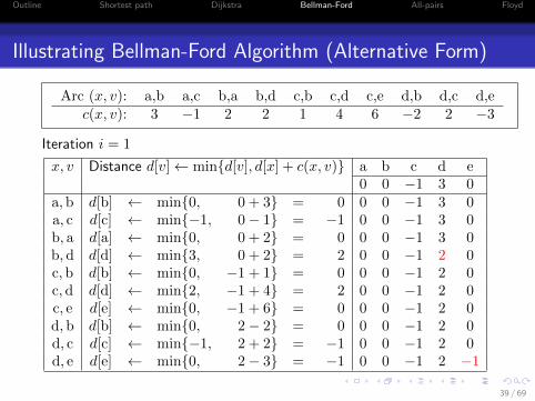
Arc (x, v): a,b a,c b,a b,d c,b c,d c,e d,b d,c d,ec(x, v): 3 −1 2 2 1 4 6 −2 2 −3
Iteration i = 1
x, v Distance d[v]← min{d[v], d[x] + c(x, v)} a b c d e0 0 −1 3 0
a,b d[b] ← min{0, 0 + 3} = 0 0 0 −1 3 0a, c d[c] ← min{−1, 0− 1} = −1 0 0 −1 3 0b, a d[a] ← min{0, 0 + 2} = 0 0 0 −1 3 0b,d d[d] ← min{3, 0 + 2} = 2 0 0 −1 2 0c,b d[b] ← min{0, −1 + 1} = 0 0 0 −1 2 0c,d d[d] ← min{2, −1 + 4} = 2 0 0 −1 2 0c, e d[e] ← min{0, −1 + 6} = 0 0 0 −1 2 0d,b d[b] ← min{0, 2− 2} = 0 0 0 −1 2 0d, c d[c] ← min{−1, 2 + 2} = −1 0 0 −1 2 0d, e d[e] ← min{0, 2− 3} = −1 0 0 −1 2 −1
39 / 69

Outline Shortest path Dijkstra Bellman-Ford All-pairs Floyd
Illustrating Bellman-Ford Algorithm (Alternative Form)
Arc (x, v): a,b a,c b,a b,d c,b c,d c,e d,b d,c d,ec(x, v): 3 −1 2 2 1 4 6 −2 2 −3
Iteration i = 2..4
x, v Distance d[v]← min{d[v], d[x] + c(x, v)} a b c d e0 0 −1 2 −1
a,b d[b] ← min{0, 0 + 3} = 0 0 0 −1 2 −1a, c d[c] ← min{−1, 0− 1} = −1 0 0 −1 2 −1b, a d[a] ← min{0, 0 + 2} = 0 0 0 −1 2 −1b,d d[d] ← min{2, 0 + 2} = 2 0 0 −1 2 −1c,b d[b] ← min{0, −1 + 1} = 0 0 0 −1 2 −1c,d d[d] ← min{2, −1 + 4} = 2 0 0 −1 2 −1c, e d[e] ← min{−1, −1 + 6} = −1 0 0 −1 2 −1d,b d[b] ← min{0, 3− 2} = 0 0 0 −1 2 −1d, c d[c] ← min{−1, 3 + 2} = −1 0 0 −1 2 −1d, e d[e] ← min{−1, 3− 3} = −1 0 0 −1 2 −1
39 / 69

Outline Shortest path Dijkstra Bellman-Ford All-pairs Floyd
Comments on Bellman-Ford Algorithm
• This (non-greedy) algorithm handles negative weight arcs, butnot negative weight cycles.
• Running time with the two innermost nested for-loops:O(n3).• Runs slower than the Dijkstra’s algorithm since considers all
nodes at “level” i = 0, 1, . . . , n− 1, in turn.
• The alternative form where the two inner-most for-loops arereplaced with: for (u, v) ∈ E(V ) runs in time O(nm).• The outer for-loop (by i) in this case can be terminated after
no distance changes during the iteration (e.g., after i = 2 inthe example on Slide 39).
• Bellman-Ford algorithm can be modified to detect negativeweight cycle (see Textbook, Exercise 6.3.4)
40 / 69

Outline Shortest path Dijkstra Bellman-Ford All-pairs Floyd
All Pairs Shortest Path (APSP) Problem
Given a weighted digraph (G, c), determine for each pair of nodesu, v ∈ V (G) (the length of) a minimum weight path from u to v.
Convenient output: a distance matrix D =[D[u, v]
]u,v∈V (G)
• Time complexity Θ(nAn,m) of computing the matrix D byfinding the single-source shortest paths (SSSP) from eachnode as the source in turn.• An=|V (G)|,m=|E(G)| – the complexity of the SSSP algorithm.
• The APSP complexity Θ(n3) for the adjacency matrix versionof the Dijkstra’s SSSP algorithm: An,m = n2.
• The APSP complexity Θ(n2m) for the Bellman-Ford SSSPalgorithm: An,m = mn.
41 / 69
Outline Shortest path Dijkstra Bellman-Ford All-pairs Floyd
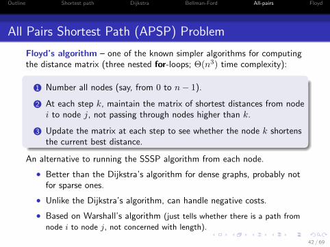
All Pairs Shortest Path (APSP) Problem
Floyd’s algorithm – one of the known simpler algorithms for computingthe distance matrix (three nested for-loops; Θ(n3) time complexity):
1 Number all nodes (say, from 0 to n− 1).
2 At each step k, maintain the matrix of shortest distances from nodei to node j, not passing through nodes higher than k.
3 Update the matrix at each step to see whether the node k shortensthe current best distance.
An alternative to running the SSSP algorithm from each node.
• Better than the Dijkstra’s algorithm for dense graphs, probably notfor sparse ones.
• Unlike the Dijkstra’s algorithm, can handle negative costs.
• Based on Warshall’s algorithm (just tells whether there is a path from
node i to node j, not concerned with length).
42 / 69

Outline Shortest path Dijkstra Bellman-Ford All-pairs Floyd
Floyd’s Algorithm
algorithm Floyd( weighted digraph (G, c) )Initialisation: for u, v ∈ V (G) do D[u, v]← c(u, v) end forfor x ∈ V (G) do
for u ∈ V (G) dofor v ∈ V (G) do
D[u, v]← min{D[u, v], D[u, x] +D[x, v]}end for
end forend for
This algorithm is based on dynamic programming principles.
At the bottom of the outer for-x-loop, D[u, v] for each u, v ∈ V (G) isthe length of the shortest path from u to v passing through intermediatenodes x having been seen in that loop.
43 / 69

Outline Shortest path Dijkstra Bellman-Ford All-pairs Floyd
Illustrating Floyd’s Algorithm
3
-1
1
2
2
2
4
-2
6
-3
0
1
2
3
4
0 3 −1 ∞ ∞2 0 ∞ 2 ∞∞ 1 0 4 6∞ −2 2 0 −3∞ ∞ ∞ ∞ 0
Adjacency/cost matrix c[u, v]
0
0
1
1
2
2
3
3
4
4
0
0
0
0
44 / 69
Outline Shortest path Dijkstra Bellman-Ford All-pairs Floyd
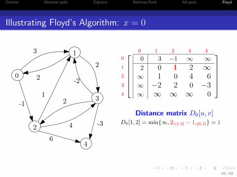
Illustrating Floyd’s Algorithm: x = 0
3
-1
1
2
2
2
4
-2
6
-3
0
1
2
3
4
0 3 −1 ∞ ∞2 0 1 2 ∞∞ 1 0 4 6∞ −2 2 0 −3∞ ∞ ∞ ∞ 0
Distance matrix D0[u, v]
0
0
1
1
2
2
3
3
4
4
D0[1, 2] = min{∞, 2c[1,0] − 1c[0,1]} = 1
0
0
0
45 / 69

Outline Shortest path Dijkstra Bellman-Ford All-pairs Floyd
Illustrating Floyd’s Algorithm: x = 1
3
-1
1
2
2
2
4
-2
6
-3
0
1
2
3
4
0 3 −1 5 ∞2 0 1 2 ∞3 1 0 3 60 −2 −1 0 −3∞ ∞ ∞ ∞ 0
Distance matrix D1[u, v]
0
0
1
1
2
2
3
3
4
4
D1[0, 3] = min{∞, 3D0[0,1] + 2D0[1,3]} = 5
D1[2, 3] = min{4, 1D0[2,1] + 2D0[1,3]} = 3
D1[3, 2] = min{2,−2D0[3,1] + 1D0[1,2]} = −1
0
46 / 69

Outline Shortest path Dijkstra Bellman-Ford All-pairs Floyd
Illustrating Floyd’s Algorithm: x = 2
3
-1
1
2
2
2
4
-2
6
-3
0
1
2
3
4
0 0 −1 2 52 0 1 2 73 1 0 3 6
0 −2 −1 0 −3∞ ∞ ∞ ∞ 0
Distance matrix D2[u, v]
0
0
1
1
2
2
3
3
4
4
D2[0, 1] = min{3,−1D1[0,2] + 1D1[2,1]} = 0
D2[0, 3] = min{5,−1D1[0,2] + 3D1[2,3]} = 2
D2[0, 4] = min{∞,−1D1[0,2] + 6D1[2,4]} = 5
D2[1, 4] = min{∞, 1D1[1,2] + 6D1[2,4]} = 7
47 / 69

Outline Shortest path Dijkstra Bellman-Ford All-pairs Floyd
Illustrating Floyd’s Algorithm: x = 3
3
-1
1
2
2
2
4
-2
6
-3
0
1
2
3
4
0 0 −1 2 −12 0 1 2 −13 1 0 3 00 −2 −1 0 −3
∞ ∞ ∞ ∞ 0
Distance matrix D3[u, v]
0
0
1
1
2
2
3
3
4
4
D3[0, 4] = min{5, 2D2[0,3] − 3D2[3,4]} = −1
D3[1, 4] = min{7, 2D1[1,3] − 3D1[3,4]} = −1
D3[2, 4] = min{6, 3D1[2,3] − 3D1[3,4]} = 0
0
48 / 69

Outline Shortest path Dijkstra Bellman-Ford All-pairs Floyd
Illustrating Floyd’s Algorithm: x = 4
3
-1
1
2
2
2
4
-2
6
-3
0
1
2
3
4
0 0 −1 2 −12 0 1 2 −13 1 0 3 00 −2 −1 0 −3∞ ∞ ∞ ∞ 0
Final distance matrix D ≡ D4[u, v]
0
0
1
1
2
2
3
3
4
4
0
0
0
0
49 / 69

Outline Shortest path Dijkstra Bellman-Ford All-pairs Floyd
Proving Why Floyd’s Algorithm Works
Theorem 6.12: At the bottom of the outer for-loop, for all nodes u and v,
D[u, v] contains the minimum length of all paths from u to v that arerestricted to using only intermediate nodes that have been seen in theouter for-loop.
When algorithm terminates, all nodes have been seen and D[u, v] is the lengthof the shortest u-to-v path.
Notation: Sk – the set of nodes seen after k passes through this loop; Sk-path
– one with all intermediate nodes in Sk; Dk – the corresponding value of D.
Induction on the outer for-loop:
• Base case: k = 0; S0 = ∅, and the result holds.
• Induction hypothesis: It holds after k ≥ 0 times through the loop.
• Inductive step: To show that Dk+1[u, v] after k + 1 passesthrough this loop is the minimum length of an u-to-v Sk+1-path.
50 / 69

Outline Shortest path Dijkstra Bellman-Ford All-pairs Floyd
Proving Why Floyd’s Algorithm Works
Inductive step:Suppose that x is the last node seen in the loop, so Sk+1 = Sk
⋃{x}.• Fix an arbitrary pair of nodes u, v ∈ V (G) and let L be the
min-length of an u-to-v Sk+1-path, so that obviouslyL ≤ Dk+1[u, v].
• To show that also Dk+1[u, v] ≤ L, choose an u-to-v Sk+1-path γ oflength L. If x /∈ γ, the result follows from the induction hypothesis.
• If x ∈ γ, let γ1 and γ2 be, respectively, the u-to-x and x-to-vsubpaths. Then γ1 and γ2 are Sk-paths and by the inductivehypothesis,
L ≥ |γ1|+ |γ2| ≥ Dk[u, x] +Dk[x, v] ≥ Dk+1[u, v]
Non-negativity of the weights is not used in the proof, and Floyd’s algorithmworks for negative weights (but negative weight cycles should not be present).
51 / 69

Outline Shortest path Dijkstra Bellman-Ford All-pairs Floyd
Floyd’s Algorithm: Example 2
2
4
3
3 5
6
1
7
8
9
3
b
a
c
e
f
d
g
Computing all-pairs shortest paths
52 / 69

Outline Shortest path Dijkstra Bellman-Ford All-pairs Floyd
Floyd’s Algorithm: Example 2 Initialisation
[D[u, v]
]u,v∈V (G)
←
Initialisation: c(u,v)]︷ ︸︸ ︷
0 2 3 3 ∞ ∞ ∞2 0 4 ∞ 3 ∞ ∞3 4 0 5 1 6 ∞3 ∞ 5 0 ∞ 7 ∞∞ 3 1 ∞ 0 8 ∞∞ ∞ 6 7 8 0 9∞ ∞ ∞ ∞ ∞ 9 0
a
b
c
d
e
f
ga b c d e f g
for x ∈ V = {a, b, c, d, e, f, g} dofor u ∈ V = {a, b, c, d, e, f, g} do
for v ∈ V = {a, b, c, d, e, f, g} doD[u, v]← min {D[u, v], D[u, x] +D[x, v]}
end forend for
end for
53 / 69

Outline Shortest path Dijkstra Bellman-Ford All-pairs Floyd
Floyd’s Algorithm: Example 2 x← a
a
a
b
c
d
e
f
g
a
b
c
d
e
f
g
0 2 3 3 ∞ ∞ ∞2 0 4 5 3 ∞ ∞3 4 0 5 1 6 ∞3 5 5 0 ∞ 7 ∞∞ 3 1 ∞ 0 8 ∞∞ ∞ 6 7 8 0 9∞ ∞ ∞ ∞ ∞ 9 0
︸ ︷︷ ︸
D[u, v]← min {D[u, v], D[u, a] +D[a, v]} ;(u, v) ∈ V 2
a
b
c
d
e
f
g
a b c d e f g
E.g.,
D[b, d] ← min{D[b, d], D[b, a] +D[a, d]}= min{∞, 2 + 3} = 5
54 / 69
Outline Shortest path Dijkstra Bellman-Ford All-pairs Floyd
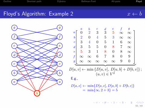
Floyd’s Algorithm: Example 2 x← b
b
a
b
c
d
e
f
g
a
b
c
d
e
f
g
0 2 3 3 5 ∞ ∞2 0 4 5 3 ∞ ∞3 4 0 5 1 6 ∞3 5 5 0 8 7 ∞5 3 1 8 0 8 ∞∞ ∞ 6 7 8 0 9∞ ∞ ∞ ∞ ∞ 9 0
︸ ︷︷ ︸
D[u, v]← min {D[u, v], D[u, b] +D[b, v]} ;(u, v) ∈ V 2
a
b
c
d
e
f
g
a b c d e f g
E.g.,
D[a, e] ← min{D[a, e], D[a, b] +D[b, e]}= min{∞, 2 + 3} = 5
55 / 69

Outline Shortest path Dijkstra Bellman-Ford All-pairs Floyd
Floyd’s Algorithm: Example 2 x← c
c
a
b
c
d
e
f
g
a
b
c
d
e
f
g
0 2 3 3 4 9 ∞2 0 4 5 3 10 ∞3 4 0 5 1 6 ∞3 5 5 0 6 7 ∞4 3 1 6 0 7 ∞9 10 6 7 7 0 9∞ ∞ ∞ ∞ ∞ 9 0
︸ ︷︷ ︸
D[u, v]← min {D[u, v], D[u, c] +D[c, v]} ;(u, v) ∈ V 2
a
b
c
d
e
f
g
a b c d e f g
E.g.,
D[a, f ] ← min{D[a, f ], D[a, c] +D[c, f ]}= min{∞, 3 + 6} = 9
56 / 69

Outline Shortest path Dijkstra Bellman-Ford All-pairs Floyd
Floyd’s Algorithm: Example 2 x← d
d
a
b
c
d
e
f
g
a
b
c
d
e
f
g
0 2 3 3 4 9 ∞2 0 4 5 3 10 ∞3 4 0 5 1 6 ∞3 5 5 0 8 7 ∞4 3 1 8 0 7 ∞9 10 6 7 7 0 9∞ ∞ ∞ ∞ ∞ 9 0
︸ ︷︷ ︸
D[u, v]← min {D[u, v], D[u, d] +D[d, v]} ;(u, v) ∈ V 2
a
b
c
d
e
f
g
a b c d e f g
E.g.,
D[a, f ] ← min{D[a, f ], D[a, d] +D[d, f ]}= min{9, 3 + 7} = 9
57 / 69

Outline Shortest path Dijkstra Bellman-Ford All-pairs Floyd
Floyd’s Algorithm: Example 2 x← e
e
a
b
c
d
e
f
g
a
b
c
d
e
f
g
0 2 3 3 4 9 ∞2 0 4 5 3 10 ∞3 4 0 5 1 6 ∞3 5 5 0 8 7 ∞4 3 1 8 0 7 ∞9 10 6 7 7 0 9∞ ∞ ∞ ∞ ∞ 9 0
︸ ︷︷ ︸
D[u, v]← min {D[u, v], D[u, e] +D[e, v]} ;(u, v) ∈ V 2
a
b
c
d
e
f
g
a b c d e f g
E.g.,
D[b, f ] ← min{D[b, f ], D[b, e] +D[e, f ]}= min{9, 3 + 7} = 9
58 / 69

Outline Shortest path Dijkstra Bellman-Ford All-pairs Floyd
Floyd’s Algorithm: Example 2 x← f
f
a
b
c
d
e
f
g
a
b
c
d
e
f
g
0 2 3 3 4 9 182 0 4 5 3 10 193 4 0 5 1 6 153 5 5 0 8 7 164 3 1 8 0 7 169 10 6 7 7 0 918 19 15 16 16 9 0
︸ ︷︷ ︸
D[u, v]← min {D[u, v], D[u, f ] +D[f, v]} ;(u, v) ∈ V 2
a
b
c
d
e
f
g
a b c d e f g
E.g.,
D[a, g] ← min{D[a, g], D[a, f ] +D[f, g]}= min{∞, 9 + 9} = 18
59 / 69
Outline Shortest path Dijkstra Bellman-Ford All-pairs Floyd
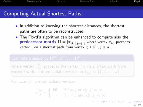
Computing Actual Shortest Paths
• In addition to knowing the shortest distances, the shortestpaths are often to be reconstructed.
• The Floyd’s algorithm can be enhanced to compute also thepredecessor matrix Π = [πij ]
n,ni,j=1,1 where vertex πi,j precedes
vertex j on a shortest path from vertex i; 1 ≤ i, j ≤ n.
Compute a sequence Π(0),Π(1), . . .Π(n),
where vertex π(k)i,j precedes the vertex j on a shortest path from
vertex i with all intermediate vertices in V(k) = {1, 2, . . . , k}.
For case of no intermediate vertices:
π(0)i,j =
{NIL if i = j or c[i, j] =∞i if i 6= j and c[i, j] <∞
60 / 69

Outline Shortest path Dijkstra Bellman-Ford All-pairs Floyd
Floyd’s Algorithm with Predecessors
algorithm FloydPred( weighted digraph (G, c) )
D ← c Create initial distance matrix from weights.
Π← Π(0) Initialize predecessors from c as in Slide 60.
for k from 1 to n dofor i from 1 to n do
for j from 1 to n doif D[i, j] > D[i, k] +D[k, j] then
D[i, j]← D[i, k] +D[k, j]; Π[i, j]← Π[k, j]end if
end forend for
end for
61 / 69

Outline Shortest path Dijkstra Bellman-Ford All-pairs Floyd
Illustrating Floyd’s Algorithm with Predecessors
5 4
1 3
2
3
8
−4
7 14
−5
2
6
D(0) =
0 3 8 ∞ −4∞ 0 ∞ 1 7∞ 4 0 ∞ ∞2 ∞ −5 0 ∞∞ ∞ ∞ 6 0
1
1
2
2
3
3
4
4
5
5
Π(0) =
NIL 1 1 NIL 1NIL NIL NIL 2 2NIL 3 NIL NIL NIL
4 NIL 4 NIL NIL
NIL NIL NIL 5 NIL
1
1
2
2
3
3
4
4
5
5
62 / 69
Outline Shortest path Dijkstra Bellman-Ford All-pairs Floyd
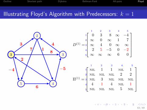
Illustrating Floyd’s Algorithm with Predecessors: k = 1
5 4
1 3
2
1
3
8
−4
7 14
−5
2
6
D(1) =
0 3 8 ∞ −4∞ 0 ∞ 1 7∞ 4 0 ∞ ∞2 5 −5 0 −2∞ ∞ ∞ 6 0
1
1
2
2
3
3
4
4
5
5
Π(1) =
NIL 1 1 NIL 1NIL NIL NIL 2 2NIL 3 NIL NIL NIL
4 1 4 NIL 1NIL NIL NIL 5 NIL
1
1
2
2
3
3
4
4
5
5
63 / 69

Outline Shortest path Dijkstra Bellman-Ford All-pairs Floyd
Illustrating Floyd’s Algorithm with Predecessors: k = 2
5 4
1 3
22
3
8
−4
7 14
−5
2
6
D(2) =
0 3 8 4 −4∞ 0 ∞ 1 7∞ 4 0 5 112 5 −5 0 −2∞ ∞ ∞ 6 0
1
1
2
2
3
3
4
4
5
5
Π(2) =
NIL 1 1 2 1NIL NIL NIL 2 2NIL 3 NIL 2 24 1 4 NIL 1
NIL NIL NIL 5 NIL
1
1
2
2
3
3
4
4
5
5
64 / 69

Outline Shortest path Dijkstra Bellman-Ford All-pairs Floyd
Illustrating Floyd’s Algorithm with Predecessors: k = 3
5 4
1 3
2
3
3
8
−4
7 14
−5
2
6
D(3) =
0 3 8 4 −4∞ 0 ∞ 1 7∞ 4 0 5 112 −1 −5 0 −2∞ ∞ ∞ 6 0
1
1
2
2
3
3
4
4
5
5
Π(3) =
NIL 1 1 2 1NIL NIL NIL 2 2NIL 3 NIL 2 24 3 4 NIL 1
NIL NIL NIL 5 NIL
1
1
2
2
3
3
4
4
5
5
65 / 69

Outline Shortest path Dijkstra Bellman-Ford All-pairs Floyd
Illustrating Floyd’s Algorithm with Predecessors: k = 4
5 4
1 3
2
4
3
8
−4
7 14
−5
2
6
D(4) =
0 3 −1 4 −43 0 −4 1 −17 4 0 5 32 −1 −5 0 −28 5 1 6 0
1
1
2
2
3
3
4
4
5
5
Π(4) =
NIL 1 4 2 14 NIL 4 2 14 3 NIL 2 14 3 4 NIL 14 3 4 5 NIL
1
1
2
2
3
3
4
4
5
5
66 / 69

Outline Shortest path Dijkstra Bellman-Ford All-pairs Floyd
Illustrating Floyd’s Algorithm with Predecessors: k = 5
5 4
1 3
2
5
3
8
−4
7 14
−5
2
6
D(5) =
0 1 −3 2 −43 0 −4 1 −17 4 0 5 32 −1 −5 0 −28 5 1 6 0
1
1
2
2
3
3
4
4
5
5
Π(5) =
NIL 3 4 5 14 NIL 4 2 14 3 NIL 2 14 3 4 NIL 14 3 4 5 NIL
1
1
2
2
3
3
4
4
5
5
67 / 69

Outline Shortest path Dijkstra Bellman-Ford All-pairs Floyd
Getting Shortest Paths from Π Matrix
The recursive algorithm using the predecessor matrix Π = Π(n) toprint the shortest path between vertices i and j:
algorithm PrintPath( Π, i, j )
if i = j then print ielse
if πi,j = NIL then print “no path from i to j”else
PrintPath( Π, i, πi,j )print j
end ifend if
68 / 69

Outline Shortest path Dijkstra Bellman-Ford All-pairs Floyd
Illustrating PrintPath Algorithm
Π(5) =
NIL 3 4 5 14 NIL 4 2 14 3 NIL 2 14 3 4 NIL 14 3 4 5 NIL
1
1
2
2
3
3
4
4
5
5
PrintPath( Π(5), 5, 3 )
→ PrintPath( Π(5), 5, π5,3 = 4)
→ PrintPath( Π(5), 5, π5,4 = 5)print 5
print 4print 3
PrintPath( Π(5), 1, 2 )
→ PrintPath( Π(5), 1, π1,2 = 3)
→ PrintPath( Π(5), 1, π1,3 = 4)
→ PrintPath( Π(5), 1, π1,4 = 5)
→ PrintPath( Π(5), 1, π1,5 = 1)print 1
print 5print 4
print 3print 2
69 / 69
Related Documents


![Antony and Cleopatra [James F. Bellman, Kathryn Bellman]](https://static.cupdf.com/doc/110x72/55cf9761550346d03391502a/antony-and-cleopatra-james-f-bellman-kathryn-bellman.jpg)