Shape changing (intensity redistribution) collisions of solitons in mixed coupled nonlinear Schr{\"o}dinger equations

$Page 1: Shape changing (intensity redistribution) collisions of solitons in mixed coupled nonlinear Schr{\"o}dinger equations$
arX

iv:n

lin/0

5110

34v1

[nl

in.S

I] 1

7 N

ov 2

005

Shape changing (intensity redistribution) collisions of solitons in

mixed coupled nonlinear Schrodinger equations

T. Kanna∗,1 M. Lakshmanan,2 P. Tchofo Dinda,1 and Nail Akhmediev3

1Laboratoire de Physique de l’Universite de Bourgogne, UMR CNRS No 5027,

Av. A Savary, BP47 870, 21078 Dijon Cedex, France

2Centre for Nonlinear Dynamics, Department of Physics,

Bharathidasan University, Tiruchirapalli-620 024, India

3 Optical Sciences Group, Research School of Physical Sciences and Engineering,

The Australian National University, Canberra, ACT 0200, Australia

Abstract

A novel kind of shape changing (intensity redistribution) collision with potential application to

signal amplification is identified in the integrable N -coupled nonlinear Schrodinger (CNLS) equa-

tions with mixed signs of focusing and defocusing type nonlinearity coefficients. The corresponding

soliton solutions for N = 2 case are obtained by using Hirota’s bilinearization method. The dis-

tinguishing feature of the mixed sign CNLS equations is that the soliton solutions can both be

singular and regular. Although the general soliton solution admits singularities we present para-

metric conditions for which non-singular soliton propagation can occur. The multisoliton solutions

and a generalization of the results to multicomponent case with arbitrary N are also presented.

An appealing feature of soliton collision in the present case is that all the components of a soliton

can simultaneously enhance their amplitudes, which can lead to new kind of amplification process

without induced noise.

PACS numbers: 02.30IK, 42.81Dp, 42.65Tg

∗ corresponding author, e-mail: [email protected]

1

http://arxiv.org/abs/nlin/0511034v1

I. INTRODUCTION

It was suggested a long time ago that solitons could be used to carry data at very

high bit rate in optical communication systems, because of their ability to overcome the

dispersion limitation through a balance between the self-phase modulation and dispersion

effects [1]. In fact soliton pulses are known to have many other desirable properties, such

as their robustness against small changes in the pulse shape or amplitude around the exact

soliton profile leads to treat such changes only as small perturbations on soliton propagation

[2, 3, 4]. Strictly speaking, the soliton properties can exit only in an ideal fiber. Indeed, in

a standard telecommunication fiber, the propagation of light pulses gives rise to a host of

perturbing effects which inhibit the desirable properties of solitons [5]. One of the strongly

perturbing effects that comes inevitably into play is the linear attenuation of light along

the fiber (which is of the order of 0.2dB/km at carrier wavelength 1.55µm), which does not

permit to keep a constant balance between the self-phase modulation and the group-velocity

dispersion [5]. Although the fundamental soliton propagation cannot be obtained in standard

fibers, pulse propagation over relatively long distances (and even transoceanic distances) can

still be obtained through an appropriate combination of dispersion management and optical

amplification (now mostly based on Er-doped fiber amplifiers and Raman amplifiers) [6, 7, 8].

All the existing amplification processes involve three major ingredients: The first one is a

pump wave, which serves as a photon reservoir. The second one is an amplification medium,

that is, a special material in which the pump wave is mixed with the signal. The third

ingredient is a physical mechanism that can cause a transfer of photons from the pump to

the signal. Only three types of physical mechanisms have been exploited so far in optical

amplifiers, namely the laser process used in laser optical amplifiers (e.g. Er-doped fiber

amplifiers, semi-conductor optical amplifiers) [9], the stimulated Raman scattering (used in

Raman amplifiers) [5, 8] and parametric wave mixing (used in parametric amplifiers) [5, 8].

Such optical amplifiers do permit to fully compensate the fiber losses, but the amplification

process is unavoidably accompanied by an undesirable effect of noise generation which is

commonly referred to as the ”amplified spontaneous emission” (ASE) [10, 11, 12]. Hence,

one of the most important characteristic parameters of the optical amplifiers developed so

far is the so-called ”noise figure”, which serves as a measure of the amount of noise generated

during the amplification process [13]. The ASE increases with the amplifier gain, and there

2

exists an unavoidable amount of noise, known as the amplifier noise figure limit of 3 dB

[13, 14, 15]. The ASE is one of the major effects that severely degrades the transmission

quality of ultra-short light pulses over long distances [5, 7, 16]. To radically resolve the

problem of ASE limitation in high-speed long-distance transmission systems, it is clear that

the conceptual approach of optical amplification based on the three ingredients mentioned

above needs to be partially or totally reformulated.

In the present work, we examine shape changing (intensity redistribution) collisions of

vector solitons in mixed coupled nonlinear Schrodinger (CNLS) equations, and report some

results that suggest the possibility of constructing a novel approach of signal amplification.

The novelty lies in viewing the collision process of solitons as a fundamental physical mech-

anism for transferring energy from the pump to the signal. The collision involves two vector

solitons. One of the two solitons, say S1, is chosen, to be the signal, while the other soliton

(S2) serves as the energy reservoir (pump wave). The major virtue of this type of collision-

based amplification process is that it does not induce any noise, as it does not make use of

any external amplification medium.

0n the other hand, the study of physical and mathematical aspects of CNLS equations is of

considerable current interest as these equations arise in diverse areas of science like nonlinear

optics, optical communication, bio-physics, Bose-Einstein condensates, and plasma physics

[3, 4, 17, 18, 19]. The fundamental integrable N -CNLS system is given by the following set

of equations

iqj,z + qj,tt + 2µ

(

N∑

l=1

σl|ql|2

)

qj = 0, j = 1, 2, ..., N, (1a)

where qj , j = 1, 2, . . . , N , is the complex amplitude of the j-th component, the subscripts

z and t denote the partial derivatives with respect to normalized distance and retarded

time, respectively, µ represents the strength of nonlinearity (µ > 0) and the coefficients

σl’s define the sign of the nonlinearity. System (1a) can be classified into three classes as

focusing, defocusing and mixed types depending on the signs of the nonlinearity coefficients

σl’s. The focusing case arises where all σl’s are equal to 1 and the corresponding system

admits bright soliton solutions [20, 21, 22, 23, 24, 25]. These bright solitons are found to

undergo fascinating shape changing (intensity redistribution) collisions [21, 23, 24] (for other

details see for example Refs. [26, 27, 28]) and such collision properties are not observed in

systems with defocusing nonlinearity which arises for all σl = −1 in (1a). The latter system

3

possesses either dark solitons in all the components or dark-bright solitons which undergo

standard elastic collision [25, 29, 30]. Also special analytic solutions for the focusing and

defocusing types are given in Refs. [31, 32]. The third case arises for mixed signs of σl’s

(that is, +1 or −1). For convenience, we define σl’s for this mixed case as

σl = 1 for l = 1, 2, . . . , n,

= −1 for l = n+ 1, n+ 2, . . . , N. (1b)

Here onwards we refer to Eq. (1) with the above choice of σl’s as mixed CNLS equations.

From a physical point of view, system (1) with N = 2 corresponds to the modified

Hubbard model in one dimension [33]. Similar equation, for N = 2, is observed in the

context of electromagnetic pulse propagation in left handed materials [34]. The above set

of equations (1) is found to be completely integrable [33, 35, 36] and the corresponding Lax

pair was obtained in [33]. In their pioneering works Makhankov et al. [33, 35] have shown

that Eq. (1), for N = 2, admits particular bright-bright, bright-dark, dark-dark type one

soliton solutions depending upon the asymptotic behaviour of the complex amplitudes qj,

j = 1, 2. Since then very few works have appeared in the literature to analyse the problem

further [25, 29, 37, 38, 39] (for a detailed review of existing results one can refer to [38]).

Particularly, in a recent work [38], Kanna et al. have obtained stationary solutions of

mixed CNLS equations with singularities by following an algebraic approach [22, 40, 41]. It

was observed that despite the points of singularities the solutions behave smoothly in finite

region of the temporal domain. Then the natural question arises as to whether multisoliton

solutions exhibiting regular behaviour over the entire space-time regions exist and, if so,

what is the nature of soliton interactions?

Being motivated by the above fundamental and intriguing aspects, in the present paper

we perform a detailed study on the bright soliton collision dynamics arising in the mixed

CNLS system. In particular, we point out that bright solitons of regular type do exist,

provided the soliton parameters satisfy certain conditions and that the underlying solitons

undergo novel shape changing/intensity redistribution collisions. The singular solutions turn

out to be special cases (with specific parametric choices) of the general soliton solutions. An

important new feature which we identify in the collision process of regular solitons in the

mixed CNLS case is that after collision a soliton can gain energy in all its components, while

the opposite takes place in the other soliton.

4

This paper is organized as follows. Section II contains the details of Hirota’s bilineariza-

tion procedure [42] for the CNLS equations to obtain soliton solutions. Though the solutions

obtained in this paper admit both singular and non-singular behaviours, we call them as

soliton solutions ascribing to their soliton nature in some specific region. In section III, we

obtain the one and two soliton solutions. Section IV is devoted to a detailed analysis of

shape changing (intensity redistribution) collisions exhibited by these soliton solutions. The

procedure to obtain one and two soliton solutions is extended to multisoliton solutions in

section V. The results of two component case are generalized in a systematic way to the

multicomponent case with arbitrary number of components following the lines of Ref. [24].

Final section is allotted for conclusion. In Appendix A we present the singular station-

ary three soliton solution for mixed 3-CNLS equations. The multicomponent multisoliton

solutions of mixed N -CNLS equations, for arbitrary N , is given in Appendix B.

II. BILINEARIZATION OF MIXED CNLS EQUATIONS

The set of equations (1) has been shown to be completely integrable [33, 36], admitting

certain types of single soliton solutions [33, 35], for the N = 2 case, as mentioned in

the Introduction. Here we are concerned with bright-bright multisoliton solutions whose

intensity profiles vanish asymptotically and with the nature of soliton interactions.

Let us apply the bilinearizing transformation [42]

qj =g(j)

f, j = 1, 2, ..., N, (2)

to Eq. (1) similar to the focusing case σl = 1, l = 1, 2, .., N [24]. This results in the following

set of bilinear equations,

(iDz +D2t )g

(j).f = 0, j = 1, 2, ..., N, (3a)

D2t (f.f) = 2µ

N∑

l=1

σlg(l)g(l)∗, (3b)

where σl is given by Eq. (1b), ∗ denotes the complex conjugate, g(j)’s are complex functions,

while f(z, t) is a real function and the Hirota’s bilinear operators Dz and Dt are defined by

DnzD

mt (a.b) =

(

∂

∂z−

∂

∂z′

)n(∂

∂t−

∂

∂t′

)m

a(z, t)b(z′, t′)∣

∣

∣

(z=z′,t=t′). (3c)

5

FIG. 1: Intensity plots of singular one soliton solution of Eq. (1) for N = 2: (a) for the case

|α(1)1 | = |α

(2)1 |, (b) for the case |α

(1)1 | < |α

(2)1 |.

The above set of equations can be solved by introducing the following power series expansions

for g(j)’s and f :

g(j) = χg(j)1 + χ3g

(j)3 + ..., j = 1, 2, ..., N, (4a)

f = 1 + χ2f2 + χ4f4 + ..., (4b)

where χ is the formal expansion parameter. The resulting set of equations, after collecting

the terms with the same power in χ, can be solved recursively to obtain the forms of g(j)’s

and f .

III. SOLITON SOLUTIONS FOR N=2 CASE

The mixed system (1) with N = 2 and σ1 = 1, σ2 = −1 is of special physical interest.

To start with, we consider this particular case.

A. One soliton solution

In order to write down the one soliton solution we restrict the power series (4) to the

lowest order

g(j) = χg(j)1 , j = 1, 2, f = 1 + χ2f2. (5)

Then by solving the resulting set of linear partial differential equations recursively, one can

write down the explicit one soliton solution as

q1

q2

=

α(1)1

α(2)1

eη1

1 + eη1+η∗

1+R(6a)

=

A1

A2

k1R sech

(

η1R +R

2

)

eiη1I , (6b)

6

FIG. 2: Intensity plots of regular one soliton solution of Eq. (1) for N = 2 case.

where

η1 = k1(t+ ik1z) = η1R + iη1I , Aj =α

(j)1

[

µ(

σ1|α(1)1 |2 + σ2|α

(2)1 |2

)]1/2, j = 1, 2, (6c)

eR =µ(

σ1|α(1)1 |2 + σ2|α

(2)1 |2

)

(k1 + k∗1)2

, σ1 = −σ2 = 1. (6d)

Note that this one soliton solution is characterized by three arbitrary complex parameters

α(1)1 , α

(2)1 , and k1 = k1R + ik1I , where the suffices R and I represent the real and imaginary

parts, respectively. The quantities k1RA1 and k1RA2, give the amplitude of the soliton in

components q1 and q2, respectively, subject to the condition

σ1|A1|2 + σ2|A2|

2 =1

µ, (6e)

and the soliton velocity in each component is given by 2k1I . The position of the soliton is

found to be

R

2k1R=

1

2k1Rln

µ(

σ1|α(1)1 |2 + σ2|α

(2)1 |2

)

(k1 + k∗1)2

. (6f)

From Eq. (6b), it is clear that singular solutions start occurring when |α(1)1 | = |α

(2)1 |. In this

case, one can easily observe from Eq. (6d) that the quantity eR becomes 0, and one gets the

solution

q1

q2

=

α(1)1

α(2)1

eη1 (7)

which is unbounded. Such an unbounded solution is depicted in Fig. ??(a) for k1 = 1 + i,

α(1)1 = α

(2)1 = 1, and µ = 1.

When |α(1)1 | < |α

(2)1 |, eR becomes negative (so R becomes complex). In this case, singu-

larity occurs, whenever

1 − |eR|e2η1R = 0, (8a)

or

η1R =1

2ln

(

1

|eR|

)

. (8b)

7

Again a singular solution in this case is plotted in Fig. ??(b) for k1 = 1 + i, α(1)1 = 0.8,

α(2)1 = 1, and µ = 1.

However the bright soliton solution is always regular as long as the condition |α(1)1 | >

|α(2)1 | is valid in which case eR is always real and positive, as the denominator

(

1 + eη1+η∗

1+R)

in Eq. (6a) is always positive definite (as η1R is real) for this choice. This regular one soliton

solution is shown in Fig. 2 for k1 = 1 + i, α(1)1 = 1, α

(2)1 = 0.2, and µ = 1.

It is also interesting to note here that the polarization vector evolves in a hyperboloid

defined by the surface |A1|2 − |A2|

2 = 1µ

[33], whereas in the Manakov case it is a sphere

(that is |A1|2 + |A2|

2 = 1µ)[24] . This allows Eq. (1) to admit a rich variety of singular

and non-singular solutions and makes significant difference in the collision scenario of bright

solitons arising in the two systems as we will see in the following sections.

B. Two soliton solution

To obtain the two soliton solution the power series expansion (4) is terminated at the

higher order terms

g(j) = χg(j)1 + χ3g

(j)3 , j = 1, 2, (9a)

f = 1 + χ2f2 + χ4f4. (9b)

Then by solving the resultant linear partial differential equations recursively, we can write

the explicit form of the solution as

qj =α

(j)1 eη1 + α

(j)2 eη2 + eη1+η∗

1+η2+δ1j + eη1+η2+η∗

2+δ2j

D, j = 1, 2, (10a)

where

D = 1 + eη1+η∗

1+R1 + eη1+η∗

2+δ0 + eη∗

1+η2+δ∗0 + eη2+η∗

2+R2 + eη1+η∗

1+η2+η∗

2+R3 .

(10b)

Various quantities found in Eq. (10), are defined as below:

ηi = ki(t+ ikiz), eδ0 =κ12

k1 + k∗2, eR1 =

κ11

k1 + k∗1, eR2 =

κ22

k2 + k∗2,

eδ1j =(k1 − k2)(α

(j)1 κ21 − α

(j)2 κ11)

(k1 + k∗1)(k∗1 + k2)

, eδ2j =(k2 − k1)(α

(j)2 κ12 − α

(j)1 κ22)

(k2 + k∗2)(k1 + k∗2),

eR3 =|k1 − k2|

2

(k1 + k∗1)(k2 + k∗2)|k1 + k∗2|2(κ11κ22 − κ12κ21), (10c)

8

and

κij =µ(

σ1α(1)i α

(1)∗j + σ2α

(2)i α

(2)∗j

)

(

ki + k∗j) , i, j = 1, 2, (10d)

where σ1 = 1 and σ2 = −1. This solution is characterized by six arbitrary complex param-

eters α(1)1 , α

(2)1 , α

(1)2 , α

(2)2 , k1, and k2. Note that the form of the above two soliton solution

remains the same as that of the Manakov case (where σ1 = +1, σ2 = +1) [21, 24], except

for the crucial difference that in the expressions for the parameters κij in Eq. (10d) σ1 = +1

and σ2 = −1.

It can also be easily verified that the singular stationary solution for the N = 2 case given

by Eq. (17) in Ref. [38] can be obtained for the specific parametric choice

α(1)1 = −eη10 , α

(2)2 = eη20 , α

(2)1 = 0, α

(1)2 = 0, k1I = k2I = 0, µ = 1, (11)

where η10 and η20 are two arbitrary real parameters. For this choice of parameters, Eq. (10)

reduces to the form

q1 =1

D

(

−eη1 +(k1R − k2R)eη1+η2+η∗

2

4k22R(k1R + k2R)

)

, (12a)

q2 =1

D

(

eη2 −(k1R − k2R)eη1+η∗

1+η2

4k21R(k1R + k2R)

)

, (12b)

where

D = 1 +

[

eη1+η∗

1

4k21R

−eη2+η∗

2

4k22R

]

−(k1R − k2R)2eη1+η∗

1+η2+η∗

2

16k21Rk

22R(k1R + k2R)2

, (12c)

and ηj is redefined as

ηj = kjR(t+ ikjRz) + ηj0, j = 1, 2, (12d)

where ηj0’s are arbitrary real parameters. The above equation (12) can be expressed in

terms of hyperbolic functions as

q1 =2k1R

D

√

k1R + k2R

k1R − k2Rsinh

(

k2Rt+ η20 +1

2ln

[

k1R − k2R

4k22R(k1R + k2R)

])

eik21R

z, (13a)

q2 = −2k2R

D

√

k1R + k2R

k1R − k2Rsinh

(

k1Rt+ η10 +1

2ln

[

k1R − k2R

4k21R(k1R + k2R)

])

eik22R

z, (13b)

where

D = −sinh

(

k1Rt+ k2Rt+ η10 + η20 + ln

[

k1R − k2R

2k1Rk2R(k1R + k2R)

])

+

(

k1R + k2R

k1R − k2R

)

sinh

(

k1Rt− k2Rt+ η10 − η20 + ln

[

k2R

k1R

])

. (13c)

9

FIG. 3: Stationary singular two soliton solution for N = 2 case.

One can check that Eq. (17) given in Ref. [38] can be re-expressed in terms of hyperbolic

functions in a form similar to Eq. (13). Figure 3 represents the stationary singular two

soliton solution at z = 0 for k1R = 0.2, k2R = −0.25, α(1)1 = −α

(2)2 = −1, α

(2)1 = α

(1)2 = 0,

and µ = 1.

Now from the expression (10) it can be observed that the denominator can become zero

for finite values of z and t leading to singular solutions. However, in the case of the general

two soliton solution (10), it is possible to make the denominator (D in Eq. (10b)) to be

non-zero for any value of t and z for suitable choice of kj and α(l)j ’s, j, l = 1, 2. In order to

do so we rewrite the denominator D (see Eq. (10b)) as

D = 2eη1R+η2R{

e(R1+R2)/2cosh (η1R − η2R + (R1 − R2)/2)

+eδ0Rcos (η1I − η2I + δ0I)

+eR3/2cosh (η1R + η2R +R3/2)}

, (14a)

where the suffices R and I denote the real and imaginary parts, respectively. Then the

solution is regular if the above expression is positive for all values of z and t. For this purpose,

a definite set of criteria can be identified as follows. As in the case of one soliton solution

in Sec. IIIA, if we choose the parameters α(j)i , i, j = 1, 2, such that |α

(1)i |2 > |α

(2)i |2, i = 1, 2,

k1R > 0 and k2R > 0 then

κ11 > 0, κ22 > 0. (14b)

Correspondingly, from Eqs. (10c) we note that eR1 > 0 and eR2 > 0, so that eR1+R2 > 0.

Then, e(R1+R2)/2cosh (η1R − η2R + (R1 − R2)/2) > 0. There is also the other possibility

κ11 < 0, κ22 < 0. But it will not lead to regular solution as in this case eR1 and eR2 become

negative thereby making R1 and R2 complex.

The term eR3/2 becomes greater than zero if

κ11κ22 − |κ12|2 > 0. (14c)

Then for this choice eR3/2cosh (η1R + η2R +R3/2) is always greater than zero.

However, the term cos (η1I − η2I + δ0I) oscillates between −1 and 1. So in order that the

middle term does not compensate the other two terms at any point in space/time resulting

10

FIG. 4: Shape changing (intensity redistribution) collision of two solitons in the mixed CNLS

system for N = 2 case.

in D being equal to zero, we should have

e(R1+R2)/2 + eR3/2 > eδ0R . (14d)

Consequently using the expressions (10c) in (14d) one may deduce the condition

1

2

√

κ11κ22

k1Rk2R+

|k1 − k2|

2|k1 + k∗2|

√

κ11κ22 − |κ12|2

k1Rk2R>

|κ12|

|k1 + k∗2|. (14e)

Note that the conditions (14b) and (14c) are necessary conditions to obtain regular solution

as their falsity will always result in singular solution. Condition (14e) is a sufficient one as

its validity confirms that the solution is always regular. We are unable to prove whether

condition (14e) is also necessary or not due to the complicated form of the function D as

a function of the variables t and z given by Eq. (10b) or (14a). It appears that the latter

can only be checked numerically for given soliton parameter values. In terms of soliton

parameters the conditions (14b) and (14c) read as

|α(1)1 |2 − |α

(2)1 |2 > 0, (15a)

|α(1)2 |2 − |α

(2)2 |2 > 0, (15b)

while (14e) becomes

(|α(1)1 |2 − |α

(2)1 |2)(|α

(1)2 |2 − |α

(2)2 |2)

|α(1)1 α

(1)∗2 − α

(2)1 α

(2)∗2 |2

>16k2

1Rk22R

(k1R + k2R)2 + (k1I − k2I)2.

(15c)

Thus the two soliton solution satisfying these conditions represent the interaction of two finite

amplitude bright solitons with definite velocities and their collision behaviour is analysed in

the follwing section.

For illustrative purpose we consider the case k1R > 0, k2R > 0, µ = 1, α(1)1 = cosh(θ1)e

iφ1 ,

α(1)2 = cosh(θ2)e

iφ1 , α(2)1 = sinh(θ1)e

iφ2 , and α(2)2 = sinh(θ2)e

iφ2 , for some arbitrary θ1, θ2, φ1,

11

and φ2. Then, the conditions (14b), (14c), and (14e) become

κ11 =1

2k1R

, κ22 =1

2k2R

,

|k1 + k∗2|2 − 4k1Rk2Rcosh2 (θ12) > 0,

1

4k1Rk2R+

|k1 − k2|√

|k1 + k∗2|2 − 4k1Rk2Rcosh2 (θ12)

4k1Rk2R|k1 + k∗2|2

>cosh (θ12)

|k1 + k∗2|, (16)

where θ12 = θ1 − θ2. A two soliton collision process corresponding to the condition (16) is

shown in Fig. 4 for the parameter choice k1 = 1.0+ i, k2 = 1.1− i, θ1 = 0.8, θ2 = 0.2, φ1 = 1

and φ2 = 0.3. This collision behaviour is analysed in detail in the following section.

IV. SHAPE CHANGING (INTENSITY REDISTRIBUTION) COLLISIONS OF

SOLITONS

Now it is of interest to understand the collision behaviour, shown in Fig. 4, of the regular

two soliton solution. Figure 4 shows the interaction of two solitons S1 and S2 which are

well separated before and after collision, in the q1 and q2 components. This figure shows

that after collision, the first soliton S1 in the component q1 gets enhanced in its amplitude

while the soliton S2 is suppressed. Interestingly, the same kind of changes are observed in

the second component q2 as well. This collision scenario is entirely different from the one

observed in the Manakov system where one soliton gets suppressed in one component and

is enhanced in the other component with commensurate changes in the other soliton.

On the other hand, conceptually, the collision scenario shown in Fig. 4 may be viewed as

an amplification process in which the soliton S1 represents a signal (or data carrier) while

the soliton S2 represents an energy reservoir (pump). The main virtue of this amplification

process is that it does not require any external amplification medium and therefore the

amplification of S1 does not induce any noise.

The understanding of this fascinating collision process can be facilitated by making an

asymptotic analysis of the two soliton solution as in the Manakov case [21, 24, 43]. We

perform the analysis for the choice k1R, k2R > 0 and k1I > k2I . For any other choice the

analysis is similar. The study shows that due to collision, the amplitudes of the colliding

solitons S1 and S2 change from (A1−1 k1R, A

1−2 k1R) and (A2−

1 k2R, A2−2 k2R) to (A1+

1 k1R, A1+2 k1R)

and (A2+1 k2R, A

2+2 k2R), respectively. Here the superscripts in Aj

i ’s denote the solitons (num-

ber(1,2)), the subscripts represent the components (number(1,2)) and ’±’ signs stand for

12

FIG. 5: Elastic collision of two solitons in the mixed CNLS system for N = 2 case.

’z → ±∞’. They are defined as

A1−1

A1−2

=

α(1)1

α(2)1

e−R1/2

(k1 + k∗1), (17a)

A2−1

A2−2

=

eδ11

eδ12

e−(R1+R3)/2

(k2 + k∗2), (17b)

A1+1

A1+2

=

eδ21

eδ22

e−(R2+R3)/2

(k1 + k∗1), (17c)

A2+1

A2+2

=

α(1)2

α(2)2

e−R2/2

(k2 + k∗2). (17d)

All the quantities in the above expressions are given in Eq. (10) [21, 24, 43]. The analysis

reveals the fact that, for the non-singular two soliton solution, the colliding solitons change

their amplitudes in each component according to the conservation equation

|Aj−1 |2 − |Aj−

2 |2 = |Aj+1 |2 − |Aj+

2 |2 =1

µ, j = 1, 2. (18)

This can be easily verified from the actual expressions given in Eq. (17).

This condition allows the given soliton to experience the same effect in each component

during collision, which may find potential applications in some physical situations like noise-

less amplification of a pulse. It can be easily observed from the conservation relation (18)

that each component of a given soliton experiences the same kind of energy switching dur-

ing collision process. The other soliton (say S2 ) experiences an opposite kind of energy

switching due to the conservation law

∫ ∞

−∞

|qj |2dt = constant, j = 1, 2, (19)

as required from Eq. (1).

The asymptotic analysis also results in the following expression relating the intensities of

solitons S1 and S2 in q1 and q2 components before and after interaction (see Eq. (17)),

|Al+j |2 = |T l

j |2|Al−

j |2, j, l = 1, 2, (20)

13

where the superscripts l± represent the solitons designated as S1 and S2 at z → ±∞. The

transition intensities are defined as

|T 1j |

2 =|1 − λ2(α

(j)2 /α

(j)1 )|2

|1 − λ1λ2|, (21a)

|T 2j |

2 =|1 − λ1λ2|

|1 − λ1(α(j)1 /α

(j)2 )|2

, j = 1, 2, (21b)

λ1 =κ21

κ11, λ2 =

κ12

κ22. (21c)

In fact, this way of energy (amplitude) redistribution can also be expressed in terms of

linear fractional transformations (LFTs) as in the CNLS system with focusing nonlinearities

[24, 44, 45]. For example, one can identify from the asymptotic expressions (17) that the

state of S1 after interaction (say ρ1+1,2 =

A1+1

A1+2

) is related to its state before interaction (say

ρ1−1,2 =

A1−1

A1−2

) through the following LFT,

ρ1+1,2 =

A1+1

A1+2

=C

(1)11 ρ

1−1,2 + C

(1)12

C(1)21 ρ

1−1,2 + C

(1)22

, (22a)

where

C(1)11 = α

(1)2 α

(1)∗2 (k2 − k1) + α

(2)2 α

(2)∗2 (k1 + k∗2),

C(1)12 = −α

(1)2 α

(2)∗2 (k2 + k∗2),

C(1)21 = α

(2)2 α

(1)∗2 (k2 + k∗2),

C(1)22 = α

(2)2 α

(2)∗2 (k1 − k2) − α

(1)2 α

(1)∗2 (k1 + k∗2). (22b)

A similar expression can be obtained for soliton S2 also. The analysis of such state trans-

formations preserving the difference of intensities among the components, during collision,

in the context of optical computing and their advantage in constructing logic gates is kept

for future study.

For the standard elastic collision property ascribed to the scalar solitons to occur here

we need the magnitudes of the transition intensities to be unity which is possible for the

specific choice

α(1)1

α(1)2

=α

(2)1

α(2)2

. (23)

As an example in Fig. 5 we present the elastic collision for θ1 = θ2 = 0.2, φ1 = φ2 = 0.3 (see

Eq. (16)), with kj’s unaltered, j = 1, 2, (Note that this choice satisfies the above condition

14

(23)). For all other values of α(j)i ’s, the soliton energies get exchanged between the solitons

in both the components as in Fig. 4.

The other quantities characterizing this collision process, along with this energy redistri-

bution, are the amplitude dependent phase shifts and change in relative separation distances.

Their explicit forms can be obtained as in the case of the Manakov model [21, 24]. Explicit

expressions for the phase shifts Φ1 and Φ2 of solitons S1 and S2, respectively, during the

collision are obtained from the asymptotic analysis as

Φ1 = −Φ2 =(R3 −R1 − R2)

2, (24)

where R1, R2, and R3 are defined in Eq. (10).

Then, the change in relative separation distance between the solitons can be expressed

as

∆t12 = t−12 − t+12 =(k1R + k2R)

k1Rk2RΦ1, (25)

where t±12 = the position of S2 (at z → ±∞) minus position of S1 (at z → ±∞) .

V. GENERALIZATION OF THE RESULTS TO MULTISOLITON SOLUTIONS

AND MULTICOMPONENT CASE

Having discussed the nature of two soliton collision in the two component case (N = 2),

we now wish to study multisoliton collisions for the N = 2 as well as N > 2 cases. For this

purpose, we will consider first the three soliton collision scenario for the N = 2 case and

then extend the analysis to more general cases.

A. Multisoliton solutions

It is straightforward to extend the bilinearization procedure of obtaining one and two

soliton solutions to multisoliton solutions as was done in Ref. [24] for the integrable CNLS

equations with focusing nonlinearity coefficients. Below, we present the form of the three

15

soliton solution for the mixed CNLS equations (1) as

qj =α

(j)1 eη1 + α

(j)2 eη2 + α

(j)3 eη3 + eη1+η∗

1+η2+δ1j + eη1+η∗

1+η3+δ2j + eη2+η∗

2+η1+δ3j

D

+eη2+η∗

2+η3+δ4j + eη3+η∗

3+η1+δ5j + eη3+η∗

3+η2+δ6j + eη∗

1+η2+η3+δ7j + eη1+η∗

2+η3+δ8j

D

+eη1+η2+η∗

3+δ9j + eη1+η∗

1+η2+η∗

2+η3+τ1j + eη1+η∗

1+η3+η∗

3+η2+τ2j

D

+eη2+η∗

2+η3+η∗

3+η1+τ3j

D, j = 1, 2, (26a)

where

D = 1 + eη1+η∗

1+R1 + eη2+η∗

2+R2 + eη3+η∗

3+R3 + eη1+η∗

2+δ10 + eη∗

1+η2+δ∗10

+eη1+η∗

3+δ20 + eη∗

1+η3+δ∗20 + eη2+η∗

3+δ30 + eη∗

2+η3+δ∗30 + eη1+η∗

1+η2+η∗

2+R4

+eη1+η∗

1+η3+η∗

3+R5 + eη2+η∗

2+η3+η∗

3+R6 + eη1+η∗

1+η2+η∗

3+τ10 + eη1+η∗

1+η3+η∗

2+τ∗

10

+eη2+η∗

2+η1+η∗

3+τ20 + eη2+η∗

2+η∗

1+η3+τ∗

20 + eη3+η∗

3+η1+η∗

2+τ30 + eη3+η∗

3+η∗

1+η2+τ∗

30

+eη1+η∗

1+η2+η∗

2+η3+η∗

3+R7 . (26b)

16

Expressions for various quantities given in Eq. (26) have the following forms:

ηi = ki(t+ ikiz), i = 1, 2, 3, (27a)

eδ1j =(k1 − k2)(α

(j)1 κ21 − α

(j)2 κ11)

(k1 + k∗1)(k∗1 + k2)

, eδ2j =(k1 − k3)(α

(j)1 κ31 − α

(j)3 κ11)

(k1 + k∗1)(k∗1 + k3)

,

eδ3j =(k1 − k2)(α

(j)1 κ22 − α

(j)2 κ12)

(k1 + k∗2)(k2 + k∗2), eδ4j =

(k2 − k3)(α(j)2 κ32 − α

(j)3 κ22)

(k2 + k∗2)(k∗2 + k3)

,

eδ5j =(k1 − k3)(α

(j)1 κ33 − α

(j)3 κ13)

(k3 + k∗3)(k∗3 + k1)

, eδ6j =(k2 − k3)(α

(j)2 κ33 − α

(j)3 κ23)

(k∗3 + k2)(k∗3 + k3)

,

eδ7j =(k2 − k3)(α

(j)2 κ31 − α

(j)3 κ21)

(k∗1 + k2)(k∗1 + k3), eδ8j =

(k1 − k3)(α(j)1 κ32 − α

(j)3 κ12)

(k1 + k∗2)(k∗2 + k3)

,

eδ9j =(k1 − k2)(α

(j)1 κ23 − α

(j)2 κ13)

(k1 + k∗3)(k2 + k∗3),

eτ1j =(k2 − k1)(k3 − k1)(k3 − k2)(k

∗2 − k∗1)

(k∗1 + k1)(k∗1 + k2)(k∗1 + k3)(k∗2 + k1)(k∗2 + k2)(k∗2 + k3)

×[

α(j)1 (κ21κ32 − κ22κ31) + α

(j)2 (κ12κ31 − κ32κ11) + α

(j)3 (κ11κ22 − κ12κ21)

]

,

eτ2j =(k2 − k1)(k3 − k1)(k3 − k2)(k

∗3 − k∗1)

(k∗1 + k1)(k∗1 + k2)(k

∗1 + k3)(k

∗3 + k1)(k

∗3 + k2)(k

∗3 + k3)

×[

α(j)1 (κ33κ21 − κ31κ23) + α

(j)2 (κ31κ13 − κ11κ33) + α

(j)3 (κ23κ11 − κ13κ21)

]

,

eτ3j =(k2 − k1)(k3 − k1)(k3 − k2)(k

∗3 − k∗2)

(k∗2 + k1)(k∗2 + k2)(k

∗2 + k3)(k

∗3 + k1)(k

∗3 + k2)(k

∗3 + k3)

×[

α(j)1 (κ22κ33 − κ23κ32) + α

(j)2 (κ13κ32 − κ33κ12) + α

(j)3 (κ12κ23 − κ22κ13)

]

,

eRm =κmm

km + k∗m, m = 1, 2, 3, eδ10 =

κ12

k1 + k∗2, eδ20 =

κ13

k1 + k∗3, eδ30 =

κ23

k2 + k∗3,

eR4 =(k2 − k1)(k

∗2 − k∗1)

(k∗1 + k1)(k∗1 + k2)(k1 + k∗2)(k∗2 + k2)

[κ11κ22 − κ12κ21] ,

eR5 =(k3 − k1)(k

∗3 − k∗1)

(k∗1 + k1)(k∗1 + k3)(k∗3 + k1)(k∗3 + k3)[κ33κ11 − κ13κ31] ,

eR6 =(k3 − k2)(k

∗3 − k∗2)

(k∗2 + k2)(k∗2 + k3)(k∗3 + k2)(k3 + k∗3)[κ22κ33 − κ23κ32] ,

eτ10 =(k2 − k1)(k

∗3 − k∗1)

(k∗1 + k1)(k∗1 + k2)(k∗3 + k1)(k∗3 + k2)[κ11κ23 − κ21κ13] ,

eτ20 =(k1 − k2)(k

∗3 − k∗2)

(k∗2 + k1)(k∗2 + k2)(k

∗3 + k1)(k

∗3 + k2)

[κ22κ13 − κ12κ23] ,

eτ30 =(k3 − k1)(k

∗3 − k∗2)

(k∗2 + k1)(k∗2 + k3)(k∗3 + k1)(k∗3 + k3)[κ33κ12 − κ13κ32] , (27b)

17

eR7 =|k1 − k2|

2|k2 − k3|2|k3 − k1|

2

(k1 + k∗1)(k2 + k∗2)(k3 + k∗3)|k1 + k∗2|2|k2 + k∗3|

2|k3 + k∗1|2

× [(κ11κ22κ33 − κ11κ23κ32) + (κ12κ23κ31 − κ12κ21κ33)

+(κ21κ13κ32 − κ22κ13κ31)] , (27c)

and

κij =µ∑2

l=1 σlα(l)i α

(l)∗j

(

ki + k∗j) , i, j = 1, 2, 3, (27d)

where σ1 = 1 and σ2 = −1. Here α(j)1 , α

(j)2 and α

(j)3 , k1, k2 and k3, j = 1, 2, 3, are complex

parameters.

The solution (26) also features singular and non-singular behaviours, as in the case of

one and two soliton solutions depending upon the values of the soliton parameters. Though

the denominator D in the solution (26) is cumbersome, possible non-singular conditions can

be obtained with some effort. Eq. (26b) can be rewritten as

D = 2eη1R+η2R+η3R{

e(R1+R6)/2cosh (η1R − η2R − η3R + (R1 −R6)/2)

+e(R2+R5)/2cosh (η2R − η1R − η3R + (R2 −R5)/2)

+e(R3+R4)/2cosh (η3R − η1R − η2R + (R3 −R4)/2)

+2e(δ10R+τ30R)/2 (cosh(X1)cos(Y1)cos(Z1) − sinh(X1)sin(Y1)sin(Z1))



+eR7/2cosh (η1R + η2R + η3R +R7/2)}

, (28a)

where

X1 = −η3R +(δ10R − τ30R)

2, X2 = −η2R +

(δ20R − τ20R)

2,

X3 = −η1R +(δ30R − τ10R)

2, Y1 = η1I − η2I +

(δ10I + τ30I)

2,

Y2 = η1I − η3I +(δ20I + τ20I)

2, Y3 = η2I − η3I +

(δ30I + τ10I)

2,

Z1 =(δ10I − τ30I)

2, Z2 =

(δ20I − τ20I)

2, Z3 =

(δ30I − τ10I)

2. (28b)

Here the suffices R and I denote the real and imaginary parts, respectively. As in the case

of two soliton solution here also we find the following conditions need to be satisfied for the

18

FIG. 6: Shape changing (intensity redistribution) collision of three solitons in the mixed CNLS

system for N = 2 case.

FIG. 7: Elastic collision of three solitons in the mixed CNLS system for N = 2 case.

solution to be regular:

eRi > 0, i = 1, 2, ..., 7, (29a)

e(R1+R6)/2, e(R2+R5)/2, e(R3+R4)/2, eR7/2 > 4 max{

eδ10R+τ30R , eδ20R+τ20R , eδ30R+τ10R}

.

(29b)

Note that, the conditions given in (29a) are necessary as the falsity of any of them always

results in singular solution and the last condition (29b) is sufficient to ensure that the given

solution is regular. In fact these conditions can also be expressed in terms of soliton param-

eters, but due to their cumbersome nature we do not present them here. The appropriate

choice of parameters can be made by carefully looking at the explicit forms of eRi , eδj0 , and

eτj0 , i = 1, ..., 7, and j = 1, 2, 3.

Such a non-singular solution representing the shape changing (intensity redistribution)

collision of three solitons S1, S2, and S3 in the two components q1 and q2 is shown in Fig. 6

for the parameter choice k1 = 1 + i, k2 = 1.2 − 0.5i, k3 = 1 − i, µ = 1, α(1)1 = cosh(θ1)e

iφ1 ,

α(1)2 = cosh(θ2)e

iφ1 , α(1)3 = cosh(θ3)e

iφ1 , α(2)1 = sinh(θ1)e

iφ2 , α(2)2 = sinh(θ2)e

iφ2 , α(2)3 =

sinh(θ3)eiφ2 , where θ1 = 0.8, θ2 = 0.4, θ3 = 0.2, φ1 = 0.5, and φ2 = 1.0. From the figure we

observe that after collision solitons S1 and S2 are enhanced in their intensities while there

occurs suppression of intensity for soliton S3 in both the components q1 and q2. It can be

verified that before and after collision the conservation relation

|Aj−1 |2 − |Aj−

2 |2 = |Aj+1 |2 − |Aj+

2 |2 =1

µ, j = 1, 2, 3, (30)

is satisfied, so that the difference of intensities of the solitons between the components q1

and q2 is preserved before and after the collision process. The standard elastic collision can

be regained if α(1)1 : α

(1)2 : α

(1)3 = α

(1)2 : α

(2)2 : α

(2)3 . Fig. 7 illustrates such an elastic collision

for the choice θ1 = θ2 = θ3 = 0.4, φ1 = φ2 = 0.5, with same kj’s , j = 1, 2, 3, as in Fig. 6.

In a similar manner the four soliton solution can be deduced from Eq.(A2) given in Ref.

[24] by redefining κij as in Eq. (27d) with i, j running from 1 to 4. We do not present the

explicit form of it here because of its cumbersome nature.

19

B. Multicomponent case with N>2

The next step is to generalize the above results for the N = 2 case to arbitrary N with

N > 2. To do this we follow the earlier work of two of the authors (T.K. and M.L)[24] on

the focusing type CNLS equations with all σl = 1, l = 1, 2, ..., N . This study shows that the

solutions of mixed CNLS equations with N = 2 case can be generalized to arbitrary N case

just by allowing the number of components to run from 2 to N and redefining κij ’s suitably.

The procedure can be well understood by considering the example of writing down the

soliton solutions of Eq. (1) for the case N = 3.

1. One soliton solution

The one soliton solution of mixed 3-CNLS equations obtained by Hirota’s method can be

written as

q1

q2

q3

=

α(1)1

α(2)1

α(3)1

eη1

1 + eη1+η∗

1+R, (31a)

where

η1 = k1(t+ ik1z), eR =κ11

(k1 + k∗1), (31b)

in which κ11 =µ(

σ1|α(1)1 |2+σ2|α

(2)1 |2+σ3|α

(3)1 |2

)

(k1+k∗

1)and without loss of generality we assume either

σ1 = 1, σ2 = σ3 = −1 or σ1 = σ2 = 1, σ3 = −1. As in the case of N = 2, Sec. III A, the

solution is singular if σ1|α(1)1 |2 + σ2|α

(2)1 |2 + σ3|α

(3)1 |2 ≤ 0. Otherwise the solution is regular.

It can be noticed that for any other combination of σl’s also the above solution satisfies Eq.

(1), for N = 3.

2. Two soliton solution

The two soliton solution for the N = 3 case is found to possess the same form of Eq.

(10), with j = 1, 2, 3, and κij is given by

κij =µ(

σ1α(1)i α

(1)∗j + σ2α

(2)i α

(2)∗j + σ3α

(3)i α

(3)∗j

)

(

ki + k∗j) , i, j = 1, 2, (32)

20

FIG. 8: Stationary singular three soliton solution for N = 3 case.


system, for N = 3 case, exhibiting same kind of shape changes for a given soliton in all the three

components.

where σl’s, l = 1, 2, 3, can take the value either +1 or −1. Here also the non-singular solution

exists for the conditions (14b), (14c), and (14e) with the redefinition of κij ’s as in Eq. (32).

3. Three and multisoliton solutions

A similar analysis can be done for the multisoliton solutions of the multicomponent case

with arbitrary N . Particularly the three soliton solution of the mixed 3-CNLS equations

, Eq. (1) with N = 3, can be identified to have the form of three soliton solution for the

N = 2 case with j running from 1 to 3 (that is, now we have three components q1, q2, and

q3) and here κij is redefined as

κij =µ(

σ1α(1)i α

(1)∗j + σ2α

(2)i α

(2)∗j + σ3α

(3)i α

(3)∗j

)

(

ki + k∗j) , i, j = 1, 2, 3, (33)

where σl’s, l = 1, 2, 3, can take the value either +1 or −1 (see also Eq. (10) of Ref. [24]).

It can also be noticed that the stationary singular solution for N = 3 case given in Ref.

[38] results from the above mentioned three soliton solution for the choice

α(1)1 = −eη10 , α

(2)2 = eη20 , α

(3)3 = −eη30 , α

(j)i = 0, kjI = 0, µ = 1, i 6= j, i, j = 1, 2, 3, (34)

where ηj0’s, j = 1, 2, 3, are real parameters. The resulting limiting form reads in terms of

hyperbolic functions as given in Appendix A. This singular solution at z = 0 is shown in

Figure 8. The parameters are chosen as α(1)1 = −1, α

(2)2 = 1, α

(3)3 = −1, α

(j)i = 0, i 6=

j, i, j = 1, 2, 3, k1R = 0.8, k2R = 0.5, k3R = 0.4 , and µ = 1.

This procedure can be generalized further to obtain multisoliton solutions of the multi-

component case with arbitrary N . For completeness we present the determinant form of the

N -soliton solution of N -component case in Appendix B, following the lines of Ref. [46] for

the Manakov case.

21


system, for N = 3 case, exhibiting same kind of shape changes for a given soliton in the q1 and q3

components and an exactly opposite collision scenario in the q2 component.

C. Collision scenario in multicomponent cases

As we increase the number of components the collision behaviour becomes more interest-

ing. For example, we consider the collision of two solitons in three component (N = 3) mixed

CNLS system. We study the collision dynamics for the following two possible combinations

of σ’s. For illustration, we present two nontrivial scenarios with two different choices of σi’s.

Case (i): σ1 = 1, σ2 = σ3 = −1

For this case, one possible parametric choice for non-singular solution is given by k1 = 1.0+i,

k2 = 0.9 − i, α(1)1 = α

(1)2 = 1 + i, α

(2)1 = 0.2 + 0.4i, α

(2)2 = 0.7 + 0.2i, α

(3)1 = 0.1 + 0.3i,

α(3)2 = 0.4 + 0.1i, and µ = 1. We plot the two soliton solution corresponding to this

parameter choice in Fig. 9. The figure shows that after collision there is an enhancement

(suppression) of intensities (amplitudes) for a given soliton (say soliton S1 (S2)) in all the

three components. Here also one can verify that the difference of intensities is conserved

according to the conservation law

|Al∓1 |2 − |Al∓

2 |2 − |Al∓3 |2 =

1

µ, l = 1, 2. (35)

Case (ii): σ1 = σ2 = 1 σ3 = −1

Next we consider the above possible choice for σ’s. The nonsingular intensity plots of solitons

S1 and S2 are shown in Fig. 10. The parameters are chosen as k1 = 1.0 + i, k2 = 0.9 − i,

α(1)1 = 1 + i, α

(1)2 = 39−80i

89, α

(2)1 = 0.2 + 0.4i, α

(2)2 = 1, α

(3)1 = 39+80i

89, α

(3)2 = 0.3 + 0.2i

and µ = 1. This figure shows that after collision the intensity of soliton S1(S2) in the first

and third components gets enhanced (suppressed) while in the second component S1(S2) is

suppressed (enhanced) in its intensity. This is a consequence of the conservation given by

the relation

|Al−1 |2 + |Al−

2 |2 − |Al−3 |2 = |Al+

1 |2 + |Al+2 |2 − |Al+

3 |2 =1

µ, l = 1, 2. (36)

Thus for the two soliton solution of the N -component case the shape changing (intensity

22

redistribution) collision occurs according to the relation

N∑

l=1

σl|Aj−l |2 =

N∑

l=1

σl|Aj+l |2 =

1

µ, j = 1, 2. (37)

However the elastic collision occurs for the choice

α(1)1

α(1)2

=α

(2)1

α(2)2

= ... =α

(N)1

α(N)2

. (38)

One can also observe that multisoliton solutions for the case N > 2 also undergo the

above kind of shape changing (intensity redistribution) collisions but with more possible

ways of energy exchange.

VI. CONCLUSION

In this paper we have obtained the bright soliton type solutions of mixed CNLS Eq.

(1) by applying Hirota’s bilinear method. These solutions admit both singular and non-

singular behaviours depending upon the choice of the soliton parameters. The condition

for the existence of non-singular one and two soliton solutions for the N = 2 case are

identified first. Analysing the corresponding collision behaviour reveals the fact that the

solitons undergo fascinating shape changing (intensity redistribution) collisions with similar

changes occurring in both components, which is not possible in the well known Manakov

system. This shape changing (intensity redistribution) collision occurs with a redistribution

of intensities among the solitons, spread up in two components, in a particular fashion,

where the intensity difference of the solitons between the two components is preserved after

collision, and amplitude dependent phase-shifts as well as change in relative separation

distances also occur. We have extended this study to obtain multicomponent multisoliton

solutions. Numerical plottings of the solutions show that similar shape changing (intensity

redistribution) collision behaviour are also observed for the multicomponent case with N > 2

as in the case of N = 2 but with many possible ways of shape variation. Still it is an open

question to identify the regions in which system (1) admits bright-dark, dark-bright, dark-

dark soliton solutions. Our study gives an adequate understanding of collision of bright-

bright solitons arising in system (1) for mixed signs of nonlinearities. We believe that this

kind of study will be of interest in the description of magnetic excitations over an anti-

ferromagnetic vacuum, electromagnetic pulse propagation in left handed materials and so

23

on. In particular one of the most interesting properties of the bright solitons that we have

identified in the present work is that the two components of a soliton can be simultaneously

amplified during a collision process. Using this property, in principle it becomes possible to

promote the collision process to the rank of a highly efficient amplification process without

noise generation, in which the gain can be tuned over a relatively large range through a

careful choice of pre-collision parameters. However, there still remains a lot of work to be

done to make the fascinating concept of amplifiers with zero noise figure as practical device

for optical communication systems. For example, an important and challenging issue will

be to determine whether such amplification process can survive in the presence of strong

perturbations or in the presence of propagation instabilities.

Acknowledgments

T. K. acknowledges the Ministrie de l’ Education Nationale, de la Recherche et de la

Technology for offering a Research Associate fellowship. The work of M. L. is supported

by the Department of Science and Tecnology, Government of India, research project. N. A.

acknowledges support from the Australian Research Council.

APPENDIX A: SINGULAR STATIONARY THREE SOLITON SOLUTION FOR

N=3 CASE

In this appendix we present the singular stationary three soliton solutions of mixed 3-

CNLS equations. Considering the three soliton solution given by Eq. (26) but now the κij ’s

are defined as in Eq. (33), the limiting form for the specific choice of parameters given by

Eq. (34) can be deduced as

q1 =

−2k1R

√

(

(k1R+k2R)(k1R+k3R)(k2R−k1R)(k3R−k1R)

) [

cosh(A1) +∣

∣

∣

(k2R+k3R)(k2R−k3R)

∣

∣

∣cosh(B1)

]

eik21R

z

D, (A1a)

q2 =

2k2R

√

(


) [

cosh(A2) −∣

∣

∣


∣

∣

∣cosh(B2)

]

eik22Rz

D, (A1b)

q3 =

2k3R

√

(


) [

sinh(A3) +∣

∣

∣


∣

∣

∣sinh(B3)

]

eik23R

z

D, (A1c)

24

where

D = cosh(D1) +

∣

∣

∣

∣

(k1R + k2R)(k1R + k3R)

(k2R − k1R)(k3R − k1R)

∣

∣

∣

∣

cosh(D2)

−

∣

∣

∣

∣

(k1R + k2R)(k2R + k3R)

(k2R − k1R)(k2R − k3R)

∣

∣

∣

∣

cosh(D3) −

∣

∣

∣

∣

(k2R + k3R)(k1R + k3R)

(k2R − k3R)(k3R − k1R)

∣

∣

∣

∣

cosh(D4), (A1d)

A1 = (k2R + k3R)t+ η20 + η30 +1

2ln

[

(k2R − k1R)(k3R − k1R)(k3R − k2R)2

16k22Rk

23R(k1R + k2R)(k1R + k3R)(k2R + k3R)2

]

,

B1 = (k2R − k3R)t+ η20 − η30 +1

2ln

[

(k1R − k2R)(k1R + k3R)k23R

k22R(k1R + k2R)(k1R − k3R)

]

,

A2 = (k1R + k3R)t+ η10 + η30 +1

2ln

[

(k2R − k1R)(k3R − k1R)2(k3R − k2R)

16k21Rk

23R(k1R + k2R)(k1R + k3R)2(k2R + k3R)

]

,

B2 = (k1R − k3R)t+ η10 − η30 +1

2ln

[

(k1R − k2R)(k2R + k3R)k23R

k21R(k1R + k2R)(k2R − k3R)

]

,

A3 = (k1R + k2R)t+ η10 + η20 +1

2ln

[

(k3R − k1R)(k2R − k1R)2(k3R − k2R)

16k21Rk

22R(k1R + k2R)2(k1R + k3R)(k2R + k3R)

]

,

B3 = (k1R − k2R)t+ η10 − η20 +1

2ln

[

(k3R − k1R)(k2R + k3R)k22R

k21R(k1R + k3R)(k3R − k2R)

]

,

D1 = (k1R + k2R + k3R)t+ η10 + η20 + η30

+ln

[

(k1R − k2R)(k1R − k3R)(k2R − k3R)

8k1Rk2Rk3R(k1R + k2R)(k1R + k3R)(k2R + k3R)

]

,

D2 = (k1R − k2R − k3R)t+ η10 − η20 − η30 + ln

[

2(k2R + k3R)k2Rk3R

k1R(k2R − k3R)

]

,

D3 = (k1R − k2R + k3R)t+ η10 − η20 + η30 + ln

[

(k3R − k1R)k2R

2k1Rk3R(k1R + k3R)

]

,

D4 = (k1R + k2R − k3R)t+ η10 + η20 − η30 + ln

[

(k2R − k1R)k3R

2k1Rk2R(k1R + k2R)

]

. (A1e)

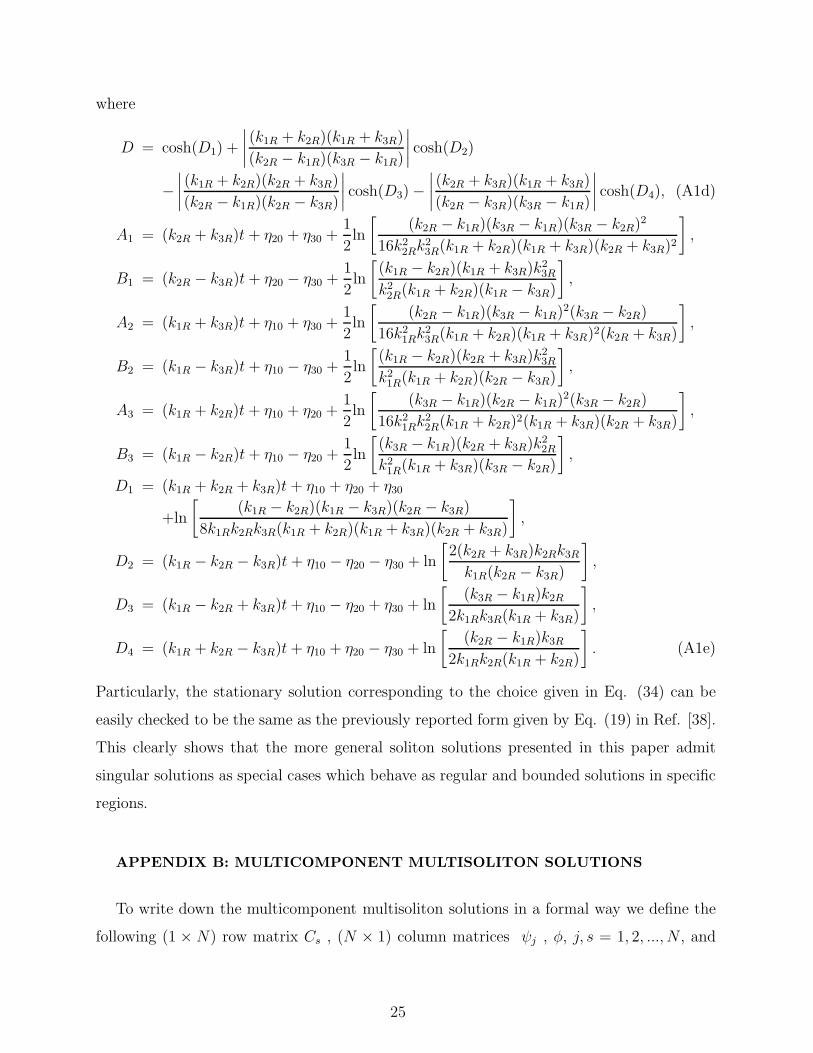
Particularly, the stationary solution corresponding to the choice given in Eq. (34) can be

easily checked to be the same as the previously reported form given by Eq. (19) in Ref. [38].

This clearly shows that the more general soliton solutions presented in this paper admit

singular solutions as special cases which behave as regular and bounded solutions in specific

regions.

APPENDIX B: MULTICOMPONENT MULTISOLITON SOLUTIONS

To write down the multicomponent multisoliton solutions in a formal way we define the

following (1 × N) row matrix Cs , (N × 1) column matrices ψj , φ, j, s = 1, 2, ..., N , and

25

the (N ×N) matrix σ:

Cs = −(

α(s)1 , α

(s)2 , ..., α

(s)N

)

, ψj =

α(1)j

α(2)j

...

α(N)j

, φ =

eη1

eη2

...

eηN

, j, s = 1, 2, ..., N,

σ =

σ1 0 ... 0

0 σ2 ... 0...

.... . .

...

0 0 ... σN

, (B1a)

where σj , j = 1, 2, ..., N , can take value either +1 or −1. Then the N -soliton solution of

N -CNLS system (1) with mixed signs of nonlinearities can be written as

qs =g(s)

D, s = 1, 2, 3, ..., N, (B1b)

where

g(s) =

∣

∣

∣

∣

∣

∣

∣

∣

∣

A I φ

−I B 0

0 Cs 0

∣

∣

∣

∣

∣

∣

∣

∣

∣

, D =

∣

∣

∣

∣

∣

∣

A I

−I B

∣

∣

∣

∣

∣

∣

, (B1c)

in which s denotes the component. Here I is (N×N) unit matrix and the (N×N) matrices

A and B are defined as

Ai,j =eηi+η∗

j

ki + k∗j, Bi,j = κji =

µ (ψi†σψj)

k∗i + kj

, i, j = 1, 2, ..., N, (B1d)

where ηi = ki(t+ ikiz), ki is complex, † represents the transpose conjugate. Here we remark

that though presenting the solutions in determinant form seems to be compact, one has to

explicitly write down the solutions as we have presented in Secs. II - V, for a complete

characterization and analysis of the solution. This way of expressing the solutions explicitly

is also useful to identify the particular parameter choice for which the singular stationary

N -soliton solution of N -component case results from the general solutions. In particular,

by generalizing the Eqs. (11) and (34) one can identify that the singular stationary N -

soliton solution of the N -component case results from the above solution (B1) for the choice

26

α(i)i = (−1)ieηi0 , i = 1, 2, ..., N , and α

(j)i = 0, kjI = 0, µ = 1, where i 6= j, i, j = 1, 2, 3, ..., N

and eηi0 ’s are arbitrary real parameters.

[1] A. Hasegawa and F. Tappert, Appl. Phys. Lett. 23, 142 (1973).

[2] M. Remoissenet, Waves called Solitons, 3rd Edition, ( Springer, Berlin, 1999).

[3] M. Lakshmanan and S. Rajasekar, Nonlinear Dynamics: Integrability, Chaos and Patterns,

(Springer-Verlag, Berlin, 2003).

[4] N. Akhmediev and A. Ankiewicz, Solitons: Nonlinear Pulses and Beams, (Chapman and Hall,

London, 1997).

[5] G. P. Agrawal, Nonlinear Fiber Optics, 2nd Edition, (Academic Press Inc., New York, 1995).

[6] L. F. Mollenauer and K. Smith, Opt. Lett. 23, 675 (1988).

[7] V. E. Zakharov and S. Wabnitz, Eds., Optical Solitons: Theoretical Challenges and Industrial

Perspectives, (Springer-Verlag, Berlin, 1998).

[8] I. P. Kaminow and T. L. Koch, Eds., Optical Fiber Communications III, (Academic Press,

New York, 1997).

[9] E. Desurvire, Erbium-doped fiber amplifiers: Principles and applications, (Wiley, New York,

1994).

[10] W. H. Louisell, A. Yariv, and A. E. Stegman, Phys. Rev. 124, 1646 (1961).

[11] H. A. Hauss and J. A. Mullen, Phys. Rev. 128, 2407 (1962).

[12] E. Desurvire, Appl. Opt. 29, 3118 (1990).

[13] E. Desurvire, Optical Fiber Technology 5, 40 (1999).

[14] C. M. Caves, Phys. Rev. 26, 1817 (1982).

[15] R. J. Stolen, Can. J. Phys. 78, 391 (2000).

[16] L. J. Richardson, W. Forysiak, and N. J. Doran, IEEE Photonics Technol. Lett. 13, 209

(2001).

[17] V. G. Makhankov, Soliton Phenomenology, (Kluwer Academic, London, 1990).

[18] See for example, several articles in the Focus Issue on “Optical Solitons - Perspectives and

Applications” in Chaos 10, No. 3 (2000).

[19] A. C. Scott, Phys. Scr. 29, 279 (1984).

[20] S. V. Manakov, Zh. Eksp. Teor. Fiz. 65, 505 (1973) [Sov. Phys. JETP 38, 248 (1974)].

27

[21] R. Radhakrishnan, M. Lakshmanan, and J. Hietarinta, Phys. Rev. E 56, 2213 (1997).

[22] N. Akhmediev, W. Krolikowski, and A. W. Snyder, Phys. Rev. Lett. 81, 4632 (1998).

[23] T. Kanna and M. Lakshmanan, Phys. Rev. Lett. 86, 5043 (2001) .

[24] T. Kanna and M. Lakshmanan, Phys. Rev. E 67 , 046617 (2003).

[25] Q. H. Park and H. J. Shin, Phys. Rev. E 61, 3093 (2000).

[26] M. J. Ablowitz, B. Prinari, and A. D. Trubatch, Inv. Probl. 20, 1217 (2004).

[27] T. Tsuchida, Progr. Theor. Phys. 111, 151 (2004).

[28] M. Soljacic, K. Steiglitz, S. M. Sears, M. Segev, M. H. Jakubowski, and R. Squier, Phys. Rev.

Lett. 90, 254102 (2003).

[29] R. Radhakrishnan and M. Lakshmanan, J. Phys. A: Math. Gen. 28, 2683 (1995).

[30] A. P. Sheppard and Y. S. Kivshar, Phys. Rev. E 55, 4773 (1997).

[31] F. T. Hioe, J. Math. Phys. 43, 6325 (2002).

[32] F. T. Hioe and T. S. Salter J. Phys. A: Math. Gen. 35, 8913 (2002).

[33] V. G. Makhankov, N. V. Makhaldiani, and O. K. Pashaev, Phys. Lett. 81A, 161 (1981) ; V.

G. Makhankov and O. K. Pashaev, Teor. Mat. Fiz. 53, 55 (1982).

[34] N. Lazarides and G. P. Tsironis, Phys. Rev. E 71, 036614 (2005).

[35] V. G. Makhankov, Phys. Lett. A 81, 156 (1981).

[36] V. E. Zakharov and E. I. Schulman, Physica D 4, 270 (1982).

[37] F. T. Hioe, Phys. Lett. A 304, 30 (2002).

[38] T. Kanna, E. N. Tsoy, and N. N. Akhmediev, Phys. Lett. A 330, 224 (2004).

[39] E. N. Tsoy and N. N. Akhmediev, Dynamics and interaction of pulses in the modified Manakov

model (submitted to Phys. Lett. A).

[40] Y. Nogami and C. S. Warke, Phys. Lett. A 59, 251 (1976).

[41] A. Ankiewicz, W. Krolikowski, and N. Akhmediev, Phys. Rev. E 59, 6079 (1999) .

[42] R. Hirota, J. Math. Phys. (N.Y.) 14, 805 (1973).

[43] M. Lakshmanan and T. Kanna, Pramana - J. of Phys. 57, 885 (2001).

[44] M. H. Jakubowski, K. Steiglitz, and R. Squier, Phys. Rev. E 58, 6752 (1998).

[45] K. Steiglitz, Phys. Rev. E 63, 016608 (2000).

[46] M. J. Ablowitz, Y. Ohta, and A. D. Trubatch , Phys. Lett. A 253, 287 (1999).

28

FIGURE CAPTIONS

Fig. 1: Singular one soliton solution of Eq. (1) for N = 2 case.

Fig. 2: Regular one soliton solution of Eq. (1) for N = 2 case.

Fig. 3: Stationary singular two soliton solution for N = 2 case.

Fig. 4: Shape changing (intensity redistribution) collision of two solitons in the mixed

CNLS system for N = 2 case.

Fig. 5: Elastic collision of two solitons in the mixed CNLS system for N = 2 case.

Fig. 6: Shape changing (intensity redistribution) collision of three solitons in the mixed

CNLS system for N = 2 case.

Fig. 7: Elastic collision of three solitons in the mixed CNLS system for the N = 2 case.

Fig. 8: Stationary singular three soliton solution for N = 3 case.


CNLS system, for N = 3 case, exhibiting same kind of shape changes for a given soliton in

all the three components.


CNLS system, for N = 3 case, exhibiting same kind of shape changes for a given soliton in

the q1 and q3 components and an exactly opposite collision scenario in the q2 component.

29

This figure "figure1.jpeg" is available in "jpeg" format from:

http://arxiv.org/ps/nlin/0511034v1





























Shape changing (intensity redistribution) collisions of solitons in mixed coupled nonlinear Schr{\"o}dinger equations

Documents