Shantanu Sinha. - UCSD Radiology Residency

Shantanu Sinha.

Department of Radiology

UCSD School of Medicine,

San Diego, CA-92103.

E-mail: [email protected]

Fundamentals of MR Imaging

Background

References:

R.B.Lufkin, “The MRI Manual”(2nd Edition).

Web: http://www.cis.rit.edu/htbooks/mri/

Donald G. Mitchell “MRI Principles”

Stark and Bradley.

A tiny little bit of history!

MRI as a Radiologic Imaging Modality.

http://www.cis.rit.edu/htbooks/mri/

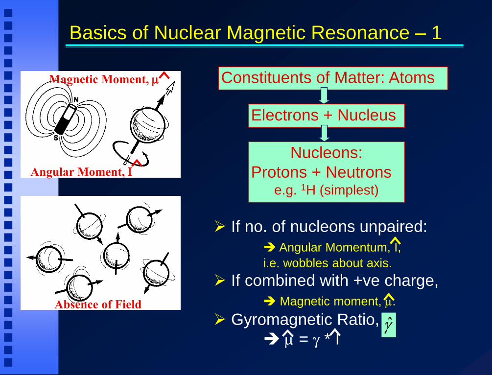
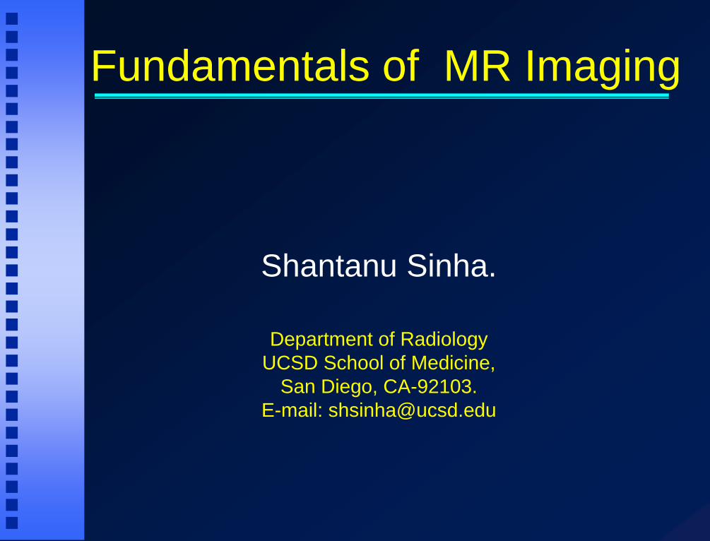
If no. of nucleons unpaired:

Angular Momentum, I,

i.e. wobbles about axis.

If combined with +ve charge,

Magnetic moment, m.

Gyromagnetic Ratio,

m = g * I

Basics of Nuclear Magnetic Resonance – 1

Magnetic Moment, m

Angular Moment, I

Absence of Field

Constituents of Matter: Atoms

Electrons + Nucleus

Nucleons:

Protons + Neutrons e.g. 1H (simplest)

g

Human body is made up of billions of these

tiny magnets (and others as well)

Randomly oriented in the absence of any field.


Nuclei Angular

Momentum, I

Isotopic

Abndnce

Freq.

At

10 KG

g Gyro-M

Ratio

Relative Sensitivity for

equal

# of Nuclei Overall

1H ½ 99.98 42.5 2.79 1.00 1.00

13C ½ 1.11 10.7 0.7 0.016 0.0001

14N 1 99.6 3.07 0.4 0.0011 0.0031

31P ½ 100 17.2 1.13 0.066 0.0014

I for: 23Na =3/2; 25Mg = 5/2; 43Ca = 7/2 There can be MR of the electron as well, EPR

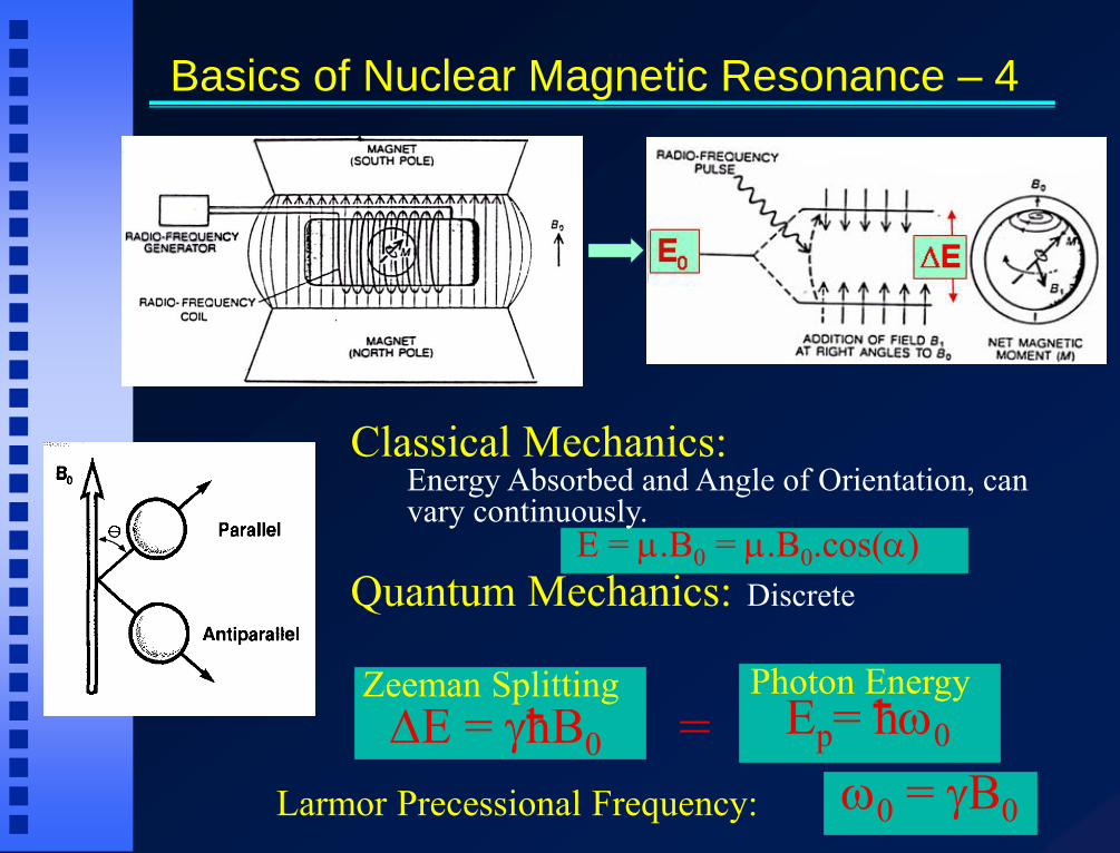
Classical Mechanics: Energy Absorbed and Angle of Orientation, can vary continuously. E = m.B0 = m.B0.cos(a)

Quantum Mechanics: Discrete


w0 = gB0 Larmor Precessional Frequency:

= DE = ghB0

Zeeman Splitting Photon Energy Ep= hw0

The Intrusion of Radio Frequency – 9

B1

Tipping the Spins:

a1 = wt1 = gB1t1

p/2 pulse a = 90o

p pulse a = 180o

B1

t1

RF pulse

Mz

+

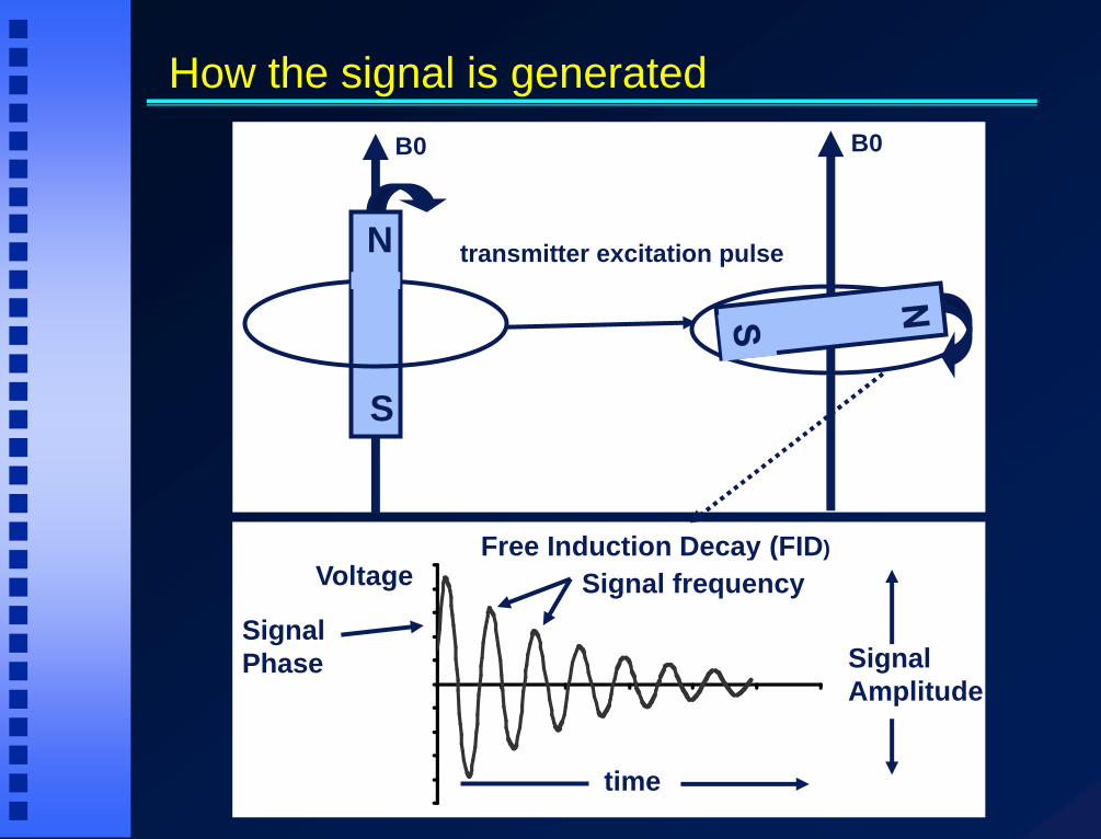
Voltage

Signal

Amplitude

Signal

Phase

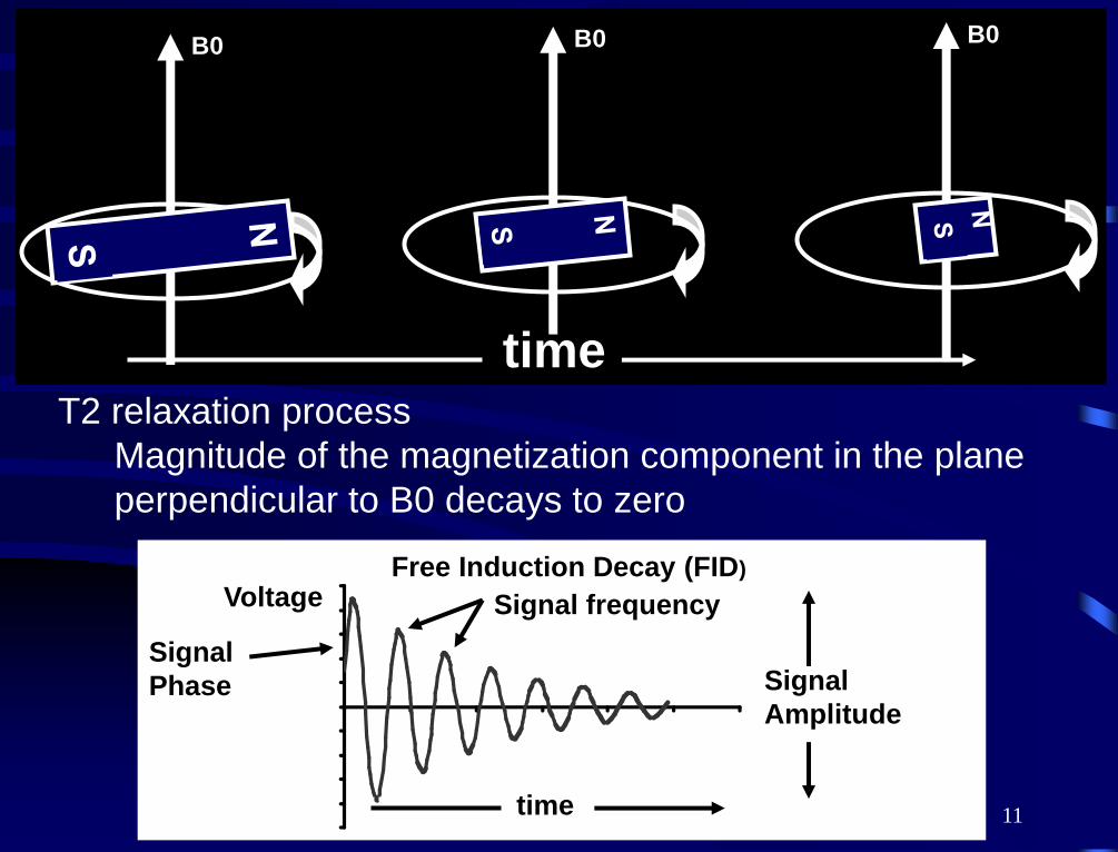
Free Induction Decay (FID)

Signal frequency

time

transmitter excitation pulse

B0 B0

N

S

How the signal is generated

Time

Vo

lta

ge

RF – p/2

Spin System

Detector Coil

B0

Detection of Signal After Tipping of Spin – 10

1. Most spins are

aligned along Z,

forming Mz. Since Mz

is in plane of detector

coil, no Voltage is

generated.

2. A 90o RF pulse tips Mz

to X-Y plane. Mz now

rotates in X-Y, transverse

plane, perpendicular to

plane of detector coil.

3. As it rotates in

transverse plane, Mx

produces an alternate,

sinu-soidal current in

coil in the X-Z plane.

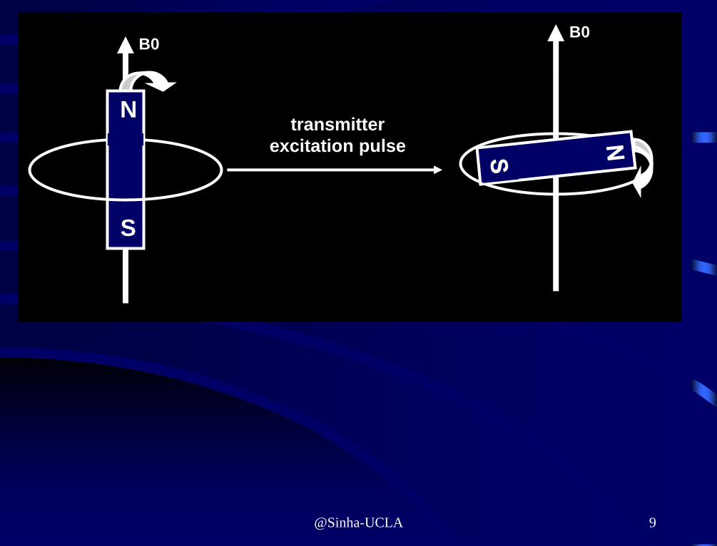
@Sinha-UCLA 9

transmitter

excitation pulse

B0 B0

N

S

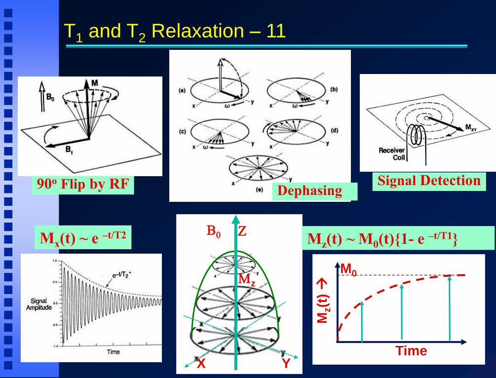
T1 and T2 Relaxation – 11

B0

Mz

Z

X Y

Mx(t) ~ e –t/T2 Mz(t) ~ M0(t){1- e –t/T1}

90o Flip by RF Signal Detection

Dephasing

Time

Mz(t

)

M0

@Sinha-UCLA 11

T2 relaxation process

Magnitude of the magnetization component in the plane

perpendicular to B0 decays to zero

B0 B0 B0

time

Voltage

Signal

Amplitude

Signal

Phase

Free Induction Decay (FID)

Signal frequency

time

@Sinha-UCLA 12

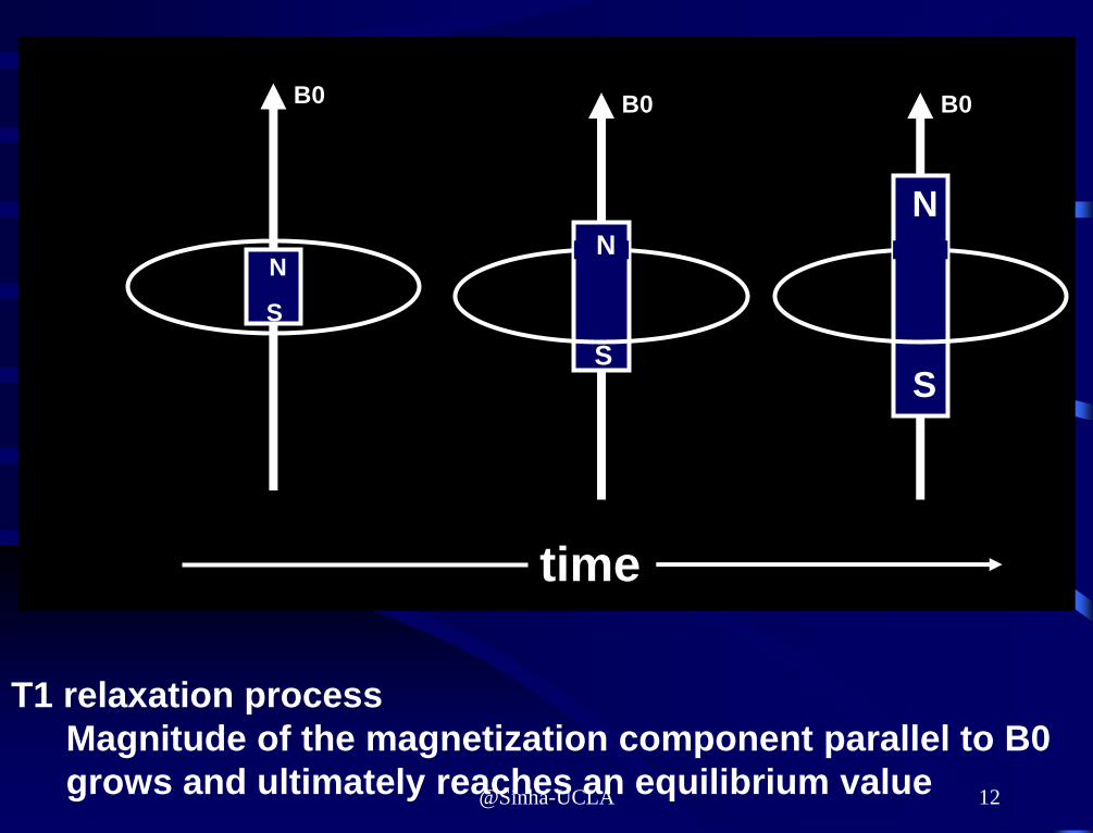
T1 relaxation process

Magnitude of the magnetization component parallel to B0

grows and ultimately reaches an equilibrium value

B0

N

S

B0

S

N

B0

S

N

time

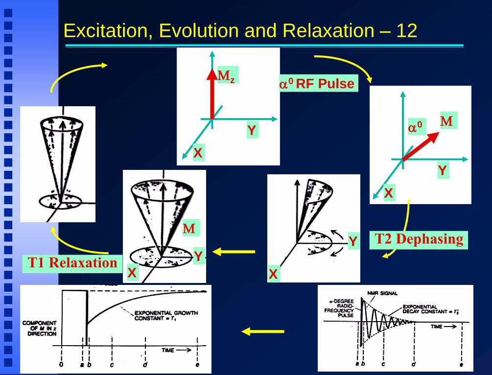
Excitation, Evolution and Relaxation – 12

Mz

X

Y

M

X

Y

a0

a0 RF Pulse

X

Y

X

Y

M T2 Dephasing

T1 Relaxation

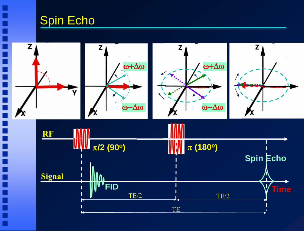
Spin Echo

w+Dw

w-Dw

w+Dw

w-Dw

p/2 (90o)

RF

p (180o)

FID

Spin Echo

Time

Signal

TE/2 TE/2

TE

T2, T2*, Multiple Echoes, Measurement of T2

T2*: • Due to inherent magnetic field inhomogeneities, dephasing occurs

much more rapidly than T2, much more rapid decay of T2

curve. 1

T2*

1

DH

1

T2

= + Multiple Echoes:

• Can create several echoes, by using repeated 180o RF pulses to

flip dephasing spins to the other side, and allowing them to

rephase.

• This is multiple echoes, (Double Echo, when only two).

Measurement of T2:

• Fitting the peaks to the

equation will yield T2.

• Individual Echoes decay

at T2*, much more

rapidly.

90o 180o 180o 180o

RF

Time

Mz(t) ~ M0(t)*e –t/T2 TE1 ~20ms

TE2 ~80ms

TE3 ~120ms

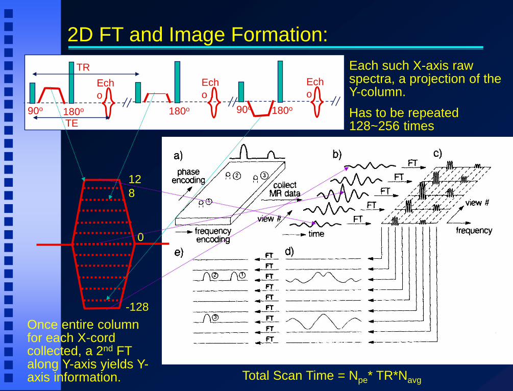
2D FT and Image Formation:

90o 180o

Ech

o

180o 90o 180o

Ech

o

Ech

o

TE

TR

12

8

-128

0

Each such X-axis raw spectra, a projection of the Y-column.

Has to be repeated 128~256 times

Once entire column for each X-cord collected, a 2nd FT along Y-axis yields Y-axis information. Total Scan Time = Npe* TR*Navg

17

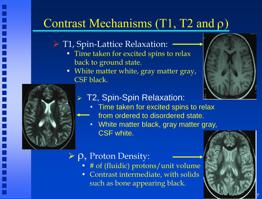
Contrast Mechanisms (T1, T2 and r)

T1, Spin-Lattice Relaxation: • Time taken for excited spins to relax

back to ground state. • White matter white, gray matter gray,

CSF black.

T2, Spin-Spin Relaxation: • Time taken for excited spins to relax

from ordered to disordered state.

• White matter black, gray matter gray,

CSF white.

r, Proton Density: • # of (fluidic) protons/unit volume • Contrast intermediate, with solids

such as bone appearing black.

18

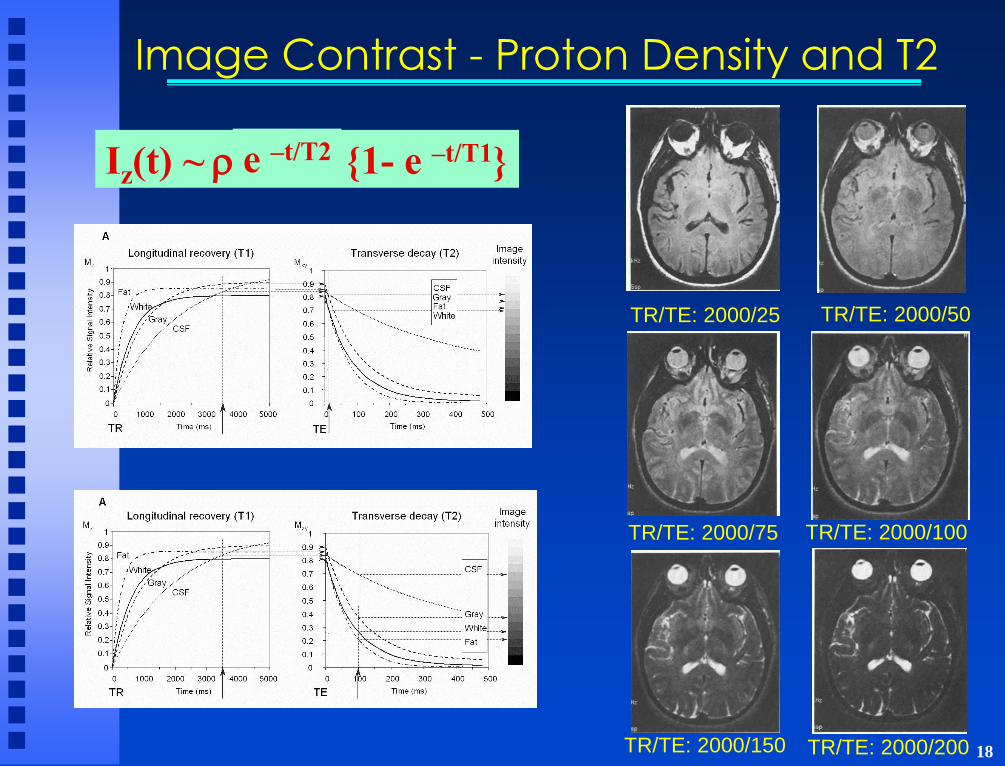
Image Contrast - Proton Density and T2

TR/TE: 2000/25 TR/TE: 2000/50

TR/TE: 2000/75 TR/TE: 2000/100

TR/TE: 2000/150 TR/TE: 2000/200

Iz(t) ~ r {1- e –t/T1} e –t/T2

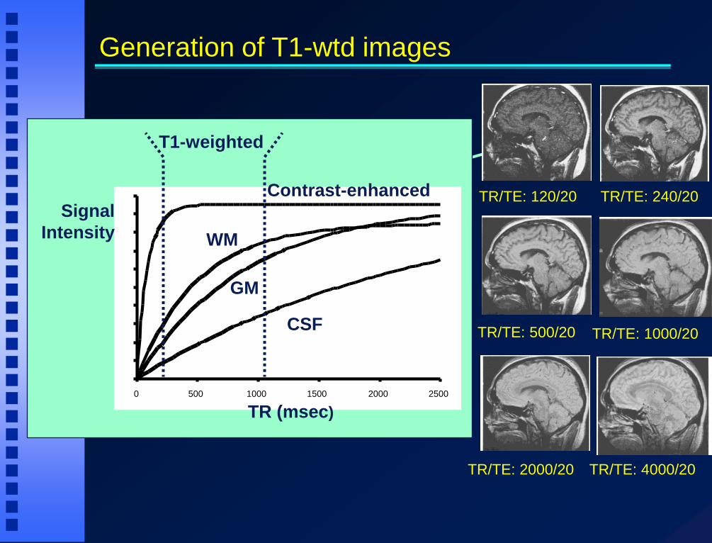
0 500 1000 1500 2000 2500

TR (msec)

CSF

GM

WM

Signal

Intensity

Contrast-enhanced

T1-weighted

Generation of T1-wtd images

TR/TE: 120/20 TR/TE: 240/20

TR/TE: 500/20 TR/TE: 1000/20

TR/TE: 2000/20 TR/TE: 4000/20

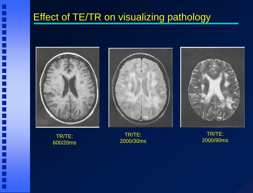
Effect of TE/TR on visualizing pathology

TR/TE:

600/20ms

TR/TE:

2000/30ms

TR/TE:

2000/90ms

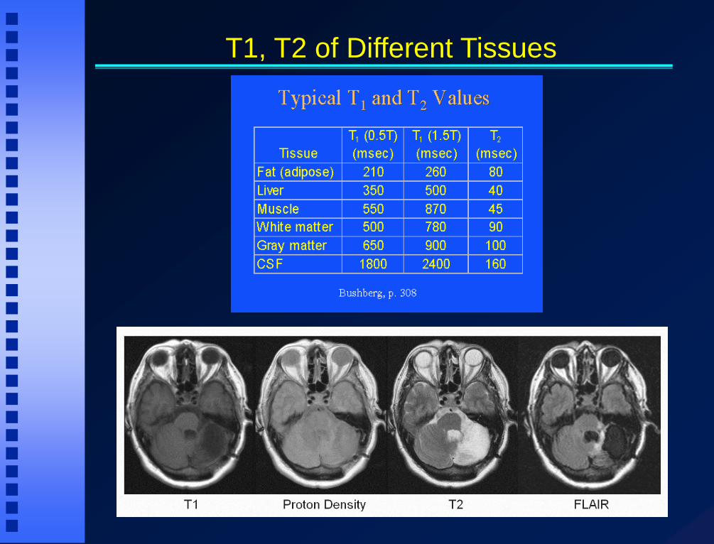
T1, T2 of Different Tissues

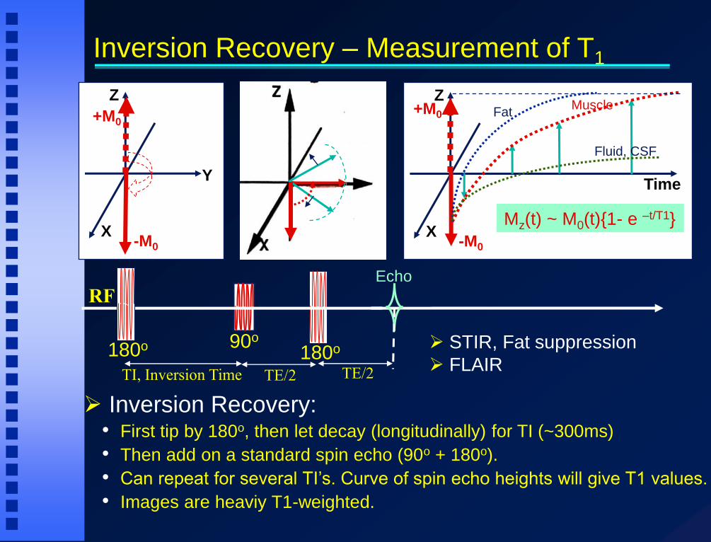
Inversion Recovery – Measurement of T1

Z

X

Y

+M0

-M0

Z

X

Time

-M0

Mz(t) ~ M0(t){1- e –t/T1}

+M0

90o

RF

180o

Echo

TE/2 TI, Inversion Time

180o TE/2

Inversion Recovery: • First tip by 180o, then let decay (longitudinally) for TI (~300ms)

• Then add on a standard spin echo (90o + 180o).

• Can repeat for several TI’s. Curve of spin echo heights will give T1 values.

• Images are heaviy T1-weighted.

Fat

Fluid, CSF

Muscle

STIR, Fat suppression

FLAIR

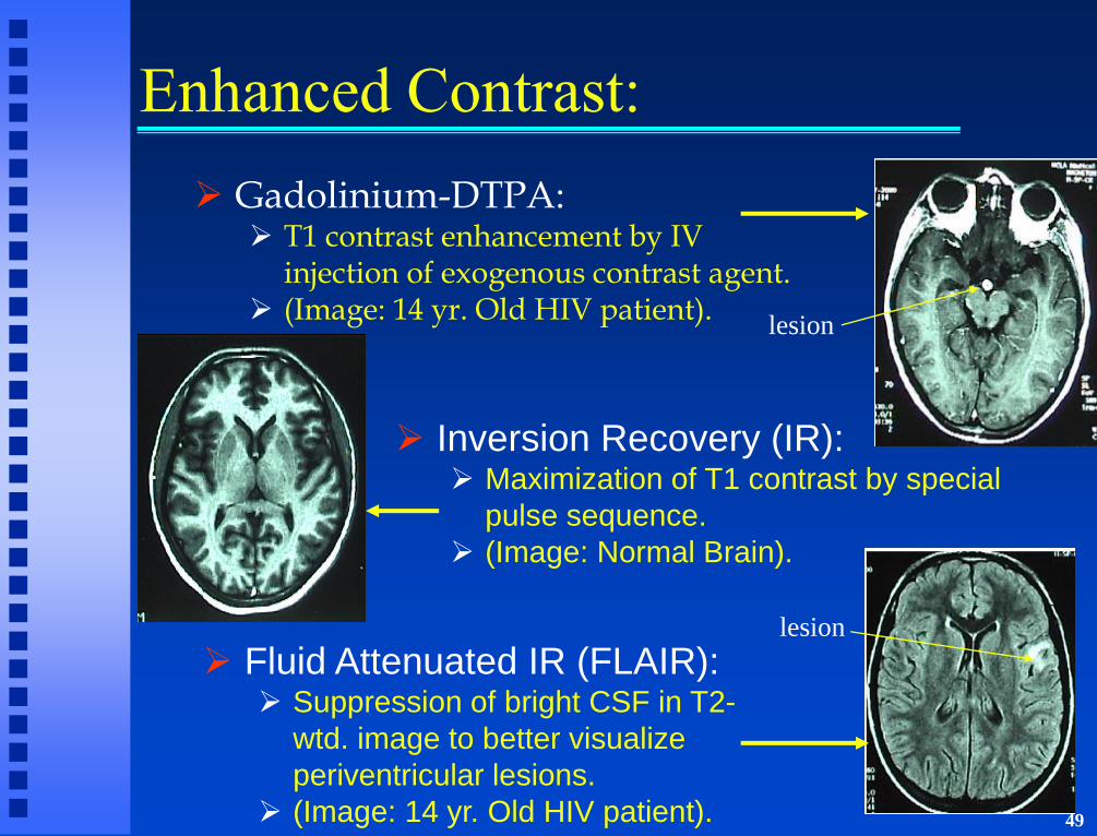
Enhanced Contrast:

Gadolinium-DTPA: T1 contrast enhancement by IV

injection of exogenous contrast agent.

(Image: 14 yr. Old HIV patient).

Inversion Recovery (IR): Maximization of T1 contrast by

special pulse sequence.

(Image: Normal Brain).

Fluid Attenuated IR (FLAIR): Suppression of bright CSF in T2-

wtd. image to better visualize

periventricular lesions.


lesion

lesion

Magnetic Field Gradients : • If the two vials are in same magnetic field,

B0, they both resonate at: w0 = g*B0

since they are in the same magnetic field

• They produce FID’s at the same frequency.

• If the magnetic field is made to vary linearly along the X-axis as: B(x) = B0 + (dB/dx)* x, and, in frequency, w(x) = g*{B0 +(dB/dx)*x} = w0 + g*(dB/dx)*x,

• Then frequency of spin becomes dependent on it’s X-spatial coordinate.

• Signal becomes spatially encoded, and one has mapping!

• The spins in the two vials produce FID’s at two different frequencies

since they are in different magnetic fields

• Similar gradients can be switched on each of the 3 physical axis's, to encode in all three directions.

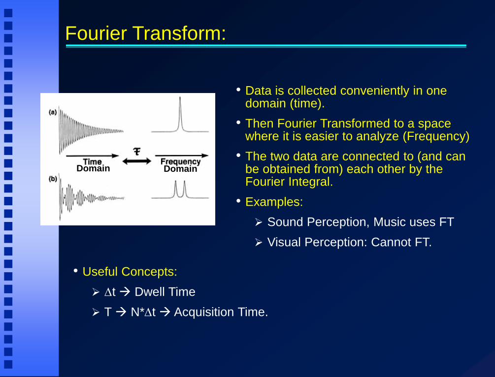
Fourier Transform:

Domain Domain

• Useful Concepts:

Dt Dwell Time

T N*Dt Acquisition Time.

• Data is collected conveniently in one domain (time).

• Then Fourier Transformed to a space where it is easier to analyze (Frequency)

• The two data are connected to (and can be obtained from) each other by the Fourier Integral.

• Examples:

Sound Perception, Music uses FT

Visual Perception: Cannot FT.

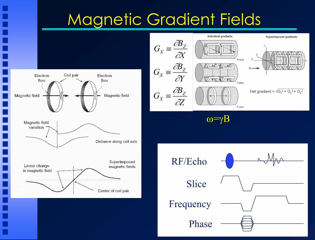
Magnetic Gradient Fields

GX BZX

GX BZY

GX BZZ

w=gB

Phase

Slice

RF/Echo

Frequency

Slice Selection – Gradients with RF on:

90o 180o

Slice Select Gradient

RF Pulses

Left Right

B0

p/2 (90o) Slice Select Gradient

Slice Selection: • Spins aligned along B0

• Superimpose Slice Select

gradient, dB/dx:

Linear variation of magnc field w/

one axis

• Switch on RF 900 pulse

• Spins only within a slice are

flipped by 900 to the X-Y plane

• SSG also switched on during

1800 pulse, so that same spins

are flipped over.

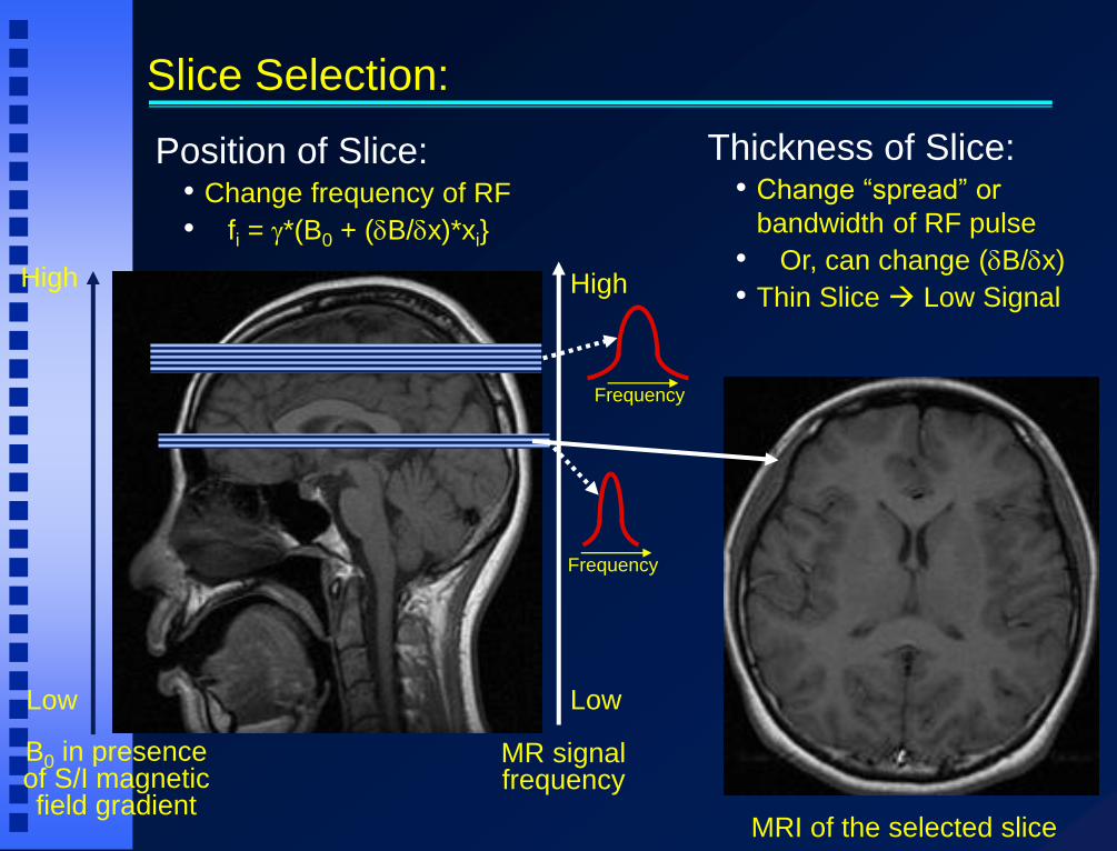
Slice Selection:

MRI of the selected slice

B0 in presence of S/I magnetic field gradient

Low

High

MR signal frequency

Low

High

Position of Slice: • Change frequency of RF

• fi = g*(B0 + (dB/dx)*xi}

Thickness of Slice: • Change “spread” or

bandwidth of RF pulse

• Or, can change (dB/dx)

• Thin Slice Low Signal

Frequency

Frequency

A few quick questions on Slice Selection:

Position of Slice: Thickness of Slice:

Slice Position (x)

Fre

qu

en

cy

Higher Gradient

Lower Gradient

Thicker Slice Thicker Slice

RF Pulse

Slice Position (x)

Fre

qu

en

cy

RF Pulse

F1

RF Pulse

F2

1) At 1.5T, if Slice Thickness 10 to 5 mm, Gradient Strength?

If Magnetic Field 1.5T 3T, for same change in Sl.Thk, Grad

Strength?

If Magnetic Field 1.5T 3T, how much will frequency need to be

changed if going from left ear to right?

For (i), what if changing from H nuclei to P?

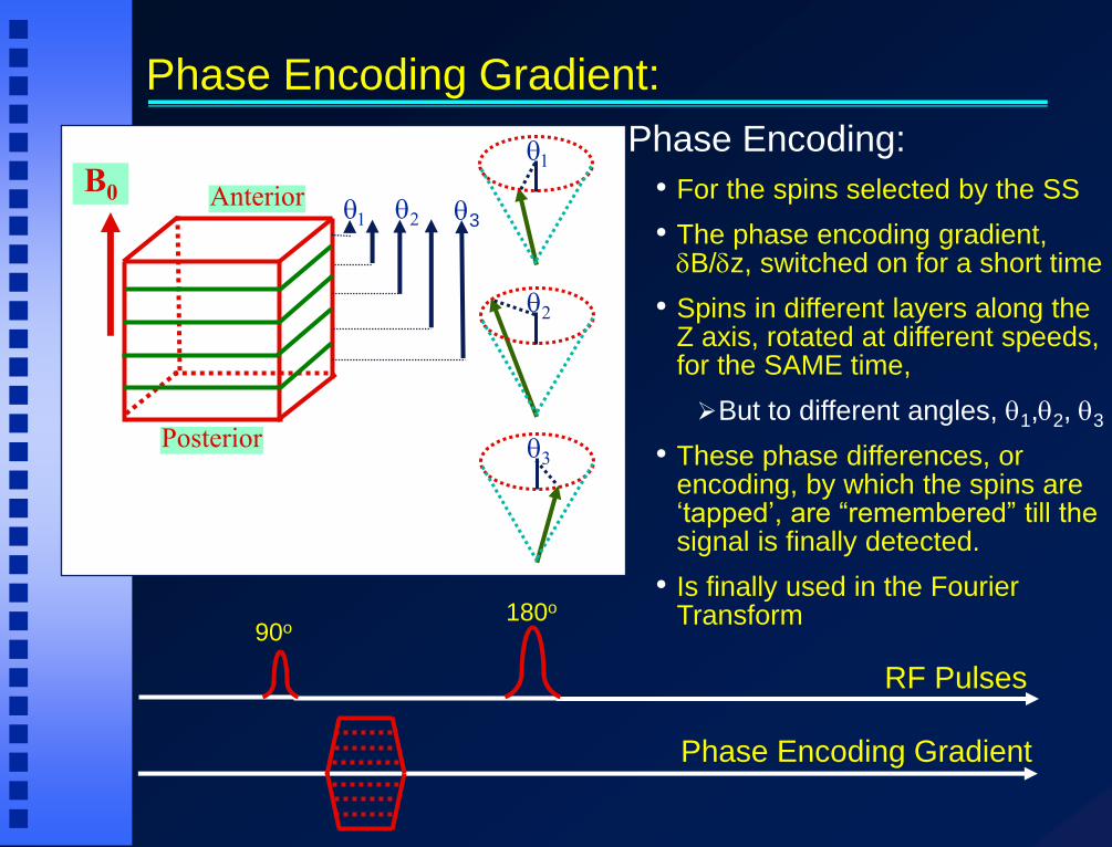
Phase Encoding Gradient:

q3 q2 q1

q1

q2

q3

B0 Anterior

Posterior

Phase Encoding Gradient

180o 90o

RF Pulses

Phase Encoding:

• For the spins selected by the SS

• The phase encoding gradient, dB/dz, switched on for a short time

• Spins in different layers along the Z axis, rotated at different speeds, for the SAME time,

But to different angles, q1,q2, q3

• These phase differences, or encoding, by which the spins are ‘tapped’, are “remembered” till the signal is finally detected.

• Is finally used in the Fourier Transform

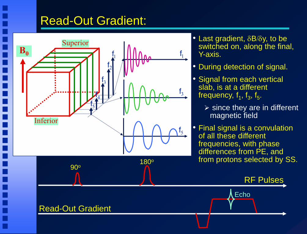
Read-Out Gradient:

B0

Superior

Inferior

f1

f2

f3

f4

f5

f1

f5

f3

Read-Out Gradient

180o 90o

RF Pulses

Echo

• Last gradient, dB/dy, to be switched on, along the final, Y-axis.

• During detection of signal.

• Signal from each vertical slab, is at a different frequency, f1, f3, f5.

since they are in different magnetic field

• Final signal is a convulation of all these different frequencies, with phase differences from PE, and from protons selected by SS.

2D FT and Image Formation:

90o 180o

Ech

o

180o 90o 180o

Ech

o

Ech

o

TE

TR

12

8

-128

0

Each such X-axis raw spectra, a projection of the Y-column.

Has to be repeated 128~256 times

Once entire column for each X-cord collected, a 2nd FT along Y-axis yields Y-axis information. Total Scan Time = Npe* TR*Navg

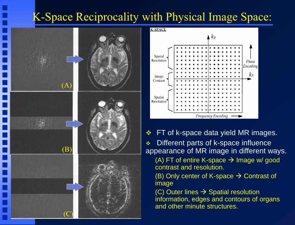
K-Space Reciprocality with Physical Image Space:

FT of k-space data yield MR images.

Different parts of k-space influence appearance of MR image in different ways.

(A) FT of entire K-space Image w/ good contrast and resolution.

(B) Only center of K-space Contrast of image

(C) Outer lines Spatial resolution information, edges and contours of organs and other minute structures.

(A)

(B)

(C)

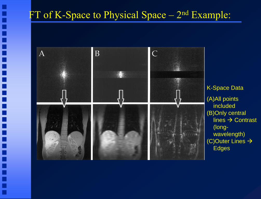
FT of K-Space to Physical Space – 2nd Example:

K-Space Data

(A)All points

included

(B)Only central

lines Contrast

(long-

wavelength)

(C)Outer Lines

Edges

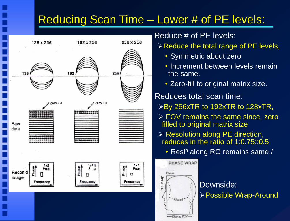
Reducing Scan Time – Lower # of PE levels: Reduce # of PE levels:

Reduce the total range of PE levels,

• Symmetric about zero

• Increment between levels remain the same.

• Zero-fill to original matrix size.

Reduces total scan time:

By 256xTR to 192xTR to 128xTR,

FOV remains the same since, zero filled to original matrix size

Resolution along PE direction, reduces in the ratio of 1:0.75::0.5

• Resln along RO remains same./

Downside:

Possible Wrap-Around

FAST Spin Echo

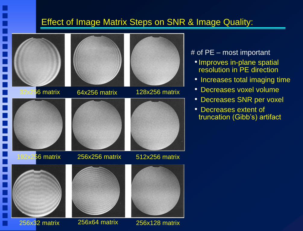
32x256 matrix 64x256 matrix 128x256 matrix



Effect of Image Matrix Steps on SNR & Image Quality:

# of PE – most important

• Improves in-plane spatial resolution in PE direction

• Increases total imaging time

• Decreases voxel volume

• Decreases SNR per voxel

• Decreases extent of truncation (Gibb’s) artifact

Wrap Around Artifact -- Phase Direction: Number of Phase Encoding Steps:

• Each PE step takes TR amount of time.

• Larger the number of PE steps, better the resolution in that direction

• But, increases the total scan time.

WRAP-AROUND ARTIFACT:

• If sufficient number of steps not acquired to cover range of anatomy along that direction

Can be eliminated by increasing # of PE steps,

Can change PE/RO directions to minimize effects.

No Wrap

Around

Wrap Around

Artifact

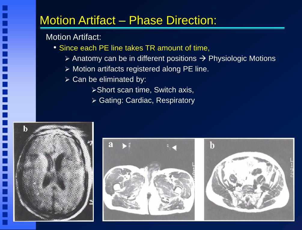
Motion Artifact – Phase Direction: Motion Artifact:

• Since each PE line takes TR amount of time,

Anatomy can be in different positions Physiologic Motions

Motion artifacts registered along PE line.

Can be eliminated by:

Short scan time, Switch axis,

Gating: Cardiac, Respiratory

T1W: SE 500/26 ms

# of PE – most important

• Improves in-plane spatial resolution in PE direction

• Increases total imaging time

• Decreases voxel volume

• Decreases SNR per voxel

• Decreases extent of truncation (Gibb’s) artifact

Effect of Phase Encoding Steps on SNR and Image Quality:

Npe = 32 Npe = 64 Npe = 128

Npe = 192 Npe = 256 Npe = 512

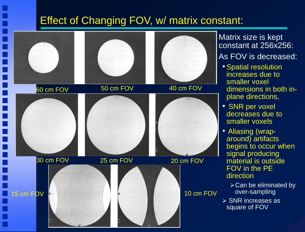
Effect of Changing FOV, w/ matrix constant:

60 cm FOV

Matrix size is kept constant at 256x256:

As FOV is decreased:

• Spatial resolution increases due to smaller voxel dimensions in both in-plane directions,

• SNR per voxel decreases due to smaller voxels

• Aliasing (wrap-around) artifacts begins to occur when signal producing material is outside FOV in the PE direction

Can be eliminated by over-sampling

SNR increases as square of FOV

50 cm FOV 40 cm FOV

30 cm FOV 25 cm FOV 20 cm FOV

10 cm FOV 15 cm FOV

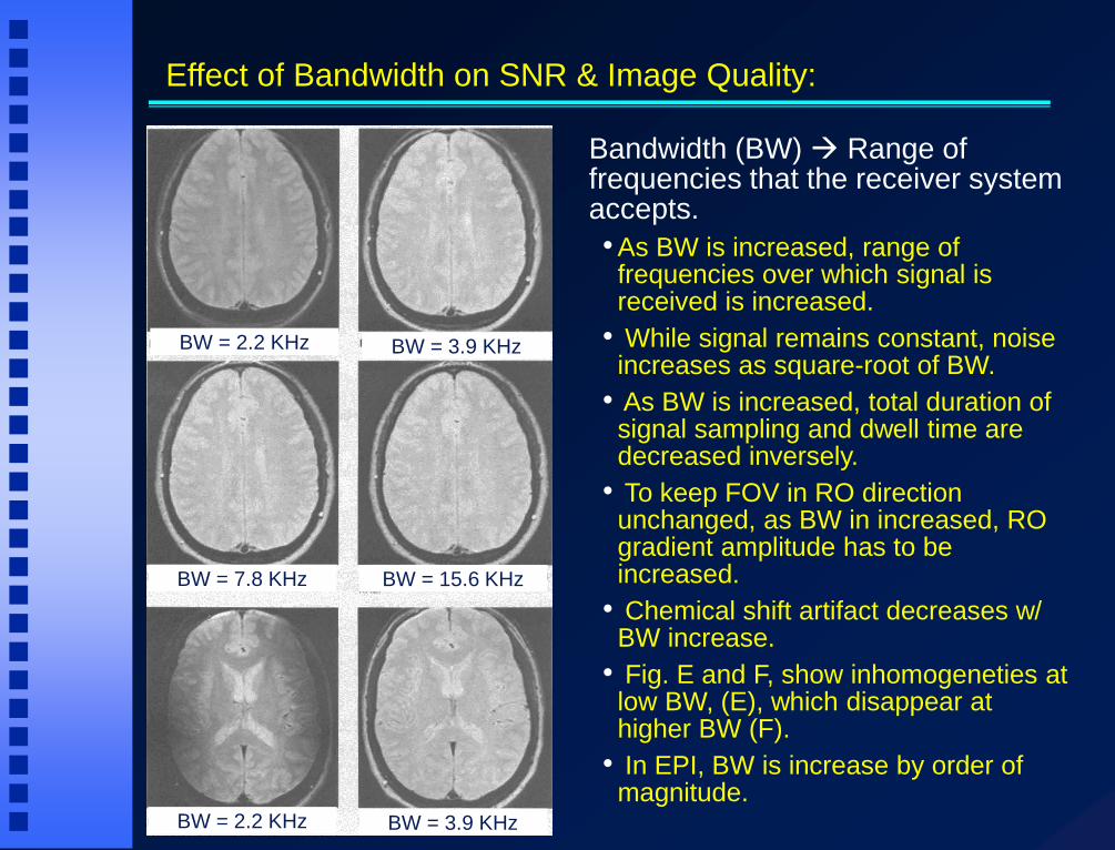
Bandwidth (BW) Range of frequencies that the receiver system accepts.

• As BW is increased, range of frequencies over which signal is received is increased.

• While signal remains constant, noise increases as square-root of BW.

• As BW is increased, total duration of signal sampling and dwell time are decreased inversely.

• To keep FOV in RO direction unchanged, as BW in increased, RO gradient amplitude has to be increased.

• Chemical shift artifact decreases w/ BW increase.

• Fig. E and F, show inhomogeneties at low BW, (E), which disappear at higher BW (F).

• In EPI, BW is increase by order of magnitude.

BW = 2.2 KHz BW = 3.9 KHz

BW = 7.8 KHz BW = 15.6 KHz

BW = 2.2 KHz BW = 3.9 KHz

Effect of Bandwidth on SNR & Image Quality:

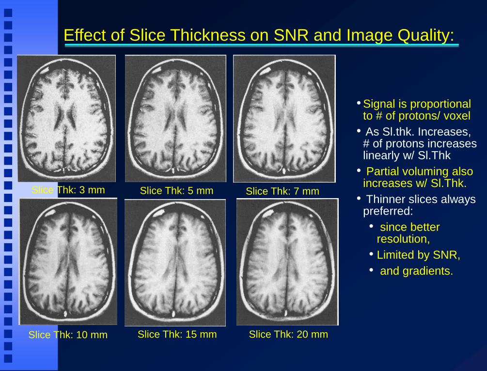
Slice Thk: 3 mm

Effect of Slice Thickness on SNR and Image Quality:

• Signal is proportional to # of protons/ voxel

• As Sl.thk. Increases, # of protons increases linearly w/ Sl.Thk

• Partial voluming also increases w/ Sl.Thk.

• Thinner slices always preferred:

• since better resolution,

• Limited by SNR,

• and gradients.

Slice Thk: 5 mm Slice Thk: 7 mm

Slice Thk: 10 mm Slice Thk: 15 mm Slice Thk: 20 mm

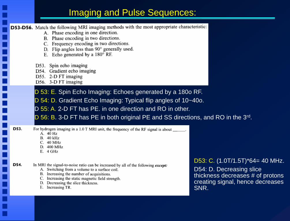
D 53: E. Spin Echo Imaging: Echoes generated by a 180o RF.

D 54: D. Gradient Echo Imaging: Typical flip angles of 10~40o.

D 55: A. 2-D FT has PE. in one direction and RO in other.

D 56: B. 3-D FT has PE in both original PE and SS directions, and RO in the 3rd.

Imaging and Pulse Sequences:

D53: C. (1.0T/1.5T)*64= 40 MHz.

D54: D. Decreasing slice thickness decreases # of protons creating signal, hence decreases SNR.

D51: C. Long T1 tends to saturate and short T2 decays the signal too rapidly. Higher signals are produced from short T1 and long T2.

D 52: D. T1 ~80 to 3000ms; T2 ~ 10 to 80ms. T2* is reduced from T2.

Contrast:

D55: E. Atomic number doesn’t play a part.

D 56: A. Pure water has a long T1 and long T2, same as CSF. Both can be shortened by

D57: C. Gradient fields are used to localize MR signal.

D 58: B. RF pulses are used to flip M thru desired angles.

D59: A. Shim coils are used to change magnetic fields locally and increase inhomogeneity of field.

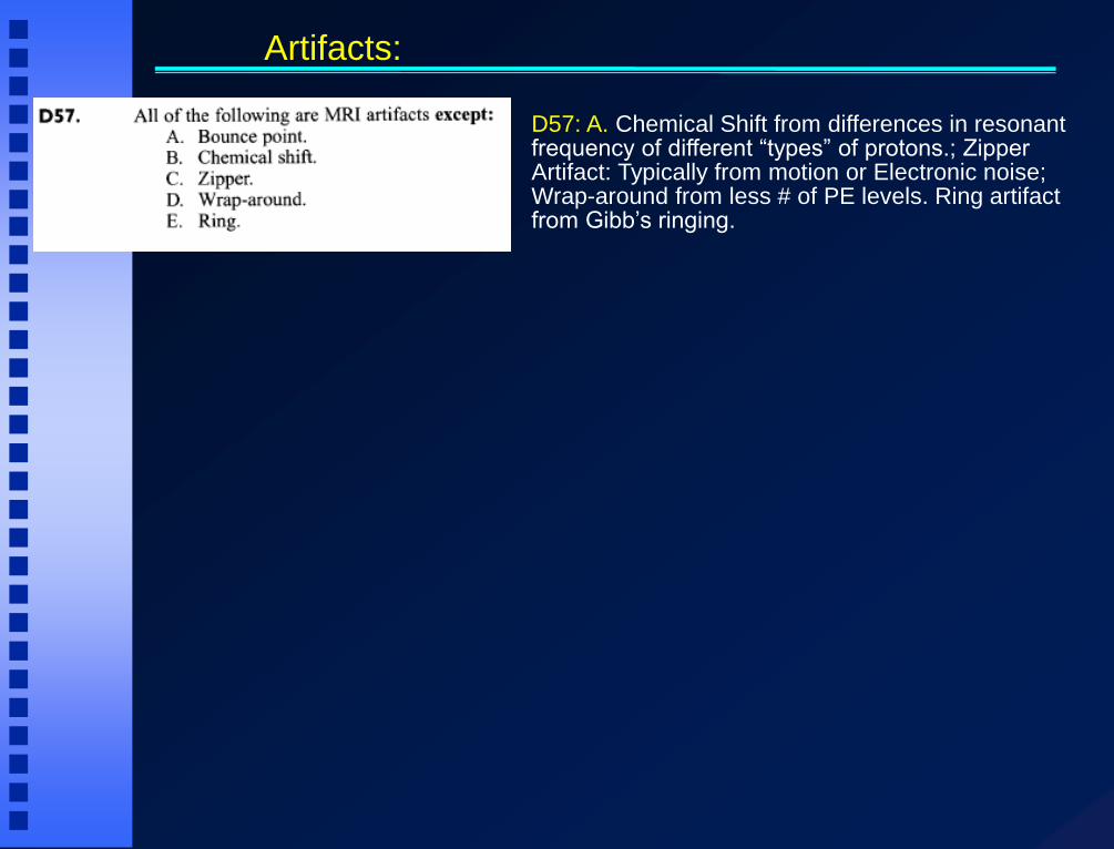
Artifacts:

D57: A. Chemical Shift from differences in resonant frequency of different “types” of protons.; Zipper Artifact: Typically from motion or Electronic noise; Wrap-around from less # of PE levels. Ring artifact from Gibb’s ringing.

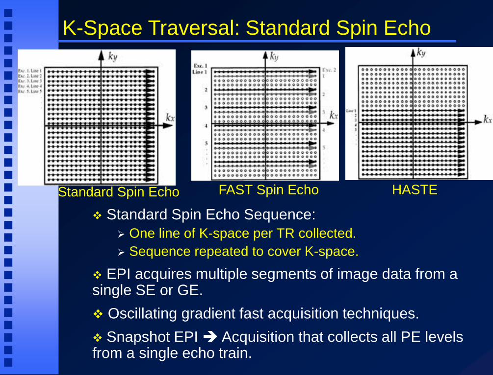
K-Space Traversal: Standard Spin Echo

Standard Spin Echo Sequence:

One line of K-space per TR collected.

Sequence repeated to cover K-space.

EPI acquires multiple segments of image data from a single SE or GE.

Oscillating gradient fast acquisition techniques.

Snapshot EPI Acquisition that collects all PE levels from a single echo train.

Standard Spin Echo FAST Spin Echo HASTE

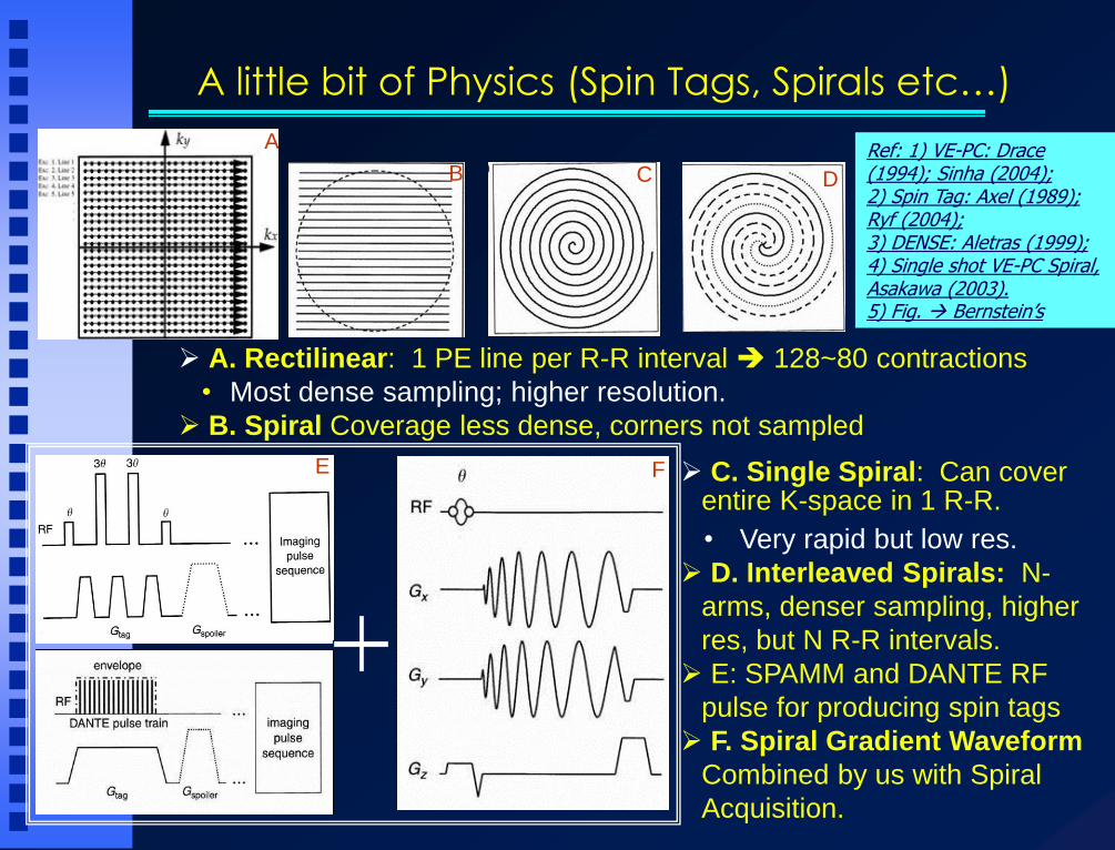
A little bit of Physics (Spin Tags, Spirals etc…)

A. Rectilinear: 1 PE line per R-R interval 128~80 contractions

• Most dense sampling; higher resolution.

B. Spiral Coverage less dense, corners not sampled

A

B C D

E F C. Single Spiral: Can cover entire K-space in 1 R-R.

• Very rapid but low res.

D. Interleaved Spirals: N-

arms, denser sampling, higher

res, but N R-R intervals.

E: SPAMM and DANTE RF

pulse for producing spin tags

F. Spiral Gradient Waveform

Combined by us with Spiral

Acquisition.

Ref: 1) VE-PC: Drace (1994); Sinha (2004); 2) Spin Tag: Axel (1989); Ryf (2004); 3) DENSE: Aletras (1999); 4) Single shot VE-PC Spiral, Asakawa (2003). 5) Fig. Bernstein’s

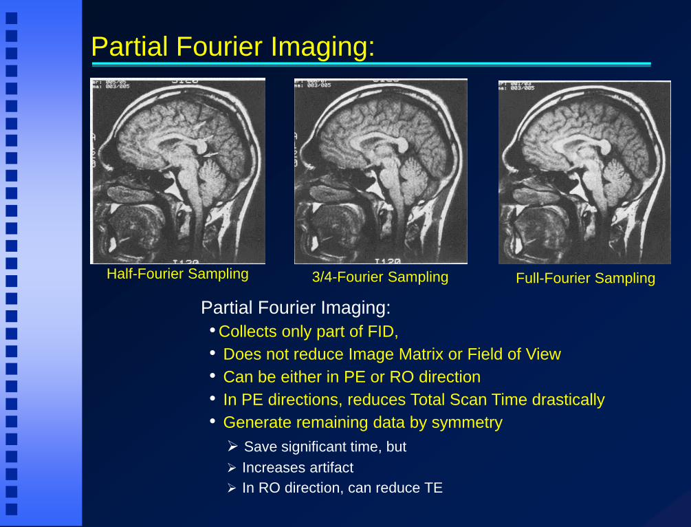
Partial Fourier Imaging:

Partial Fourier Imaging:

• Collects only part of FID,

• Does not reduce Image Matrix or Field of View

• Can be either in PE or RO direction

• In PE directions, reduces Total Scan Time drastically

• Generate remaining data by symmetry

Save significant time, but

Increases artifact

In RO direction, can reduce TE

Half-Fourier Sampling 3/4-Fourier Sampling Full-Fourier Sampling

49

Enhanced Contrast:

Gadolinium-DTPA: T1 contrast enhancement by IV

injection of exogenous contrast agent. (Image: 14 yr. Old HIV patient).

Inversion Recovery (IR): Maximization of T1 contrast by special

pulse sequence.

(Image: Normal Brain).

Fluid Attenuated IR (FLAIR): Suppression of bright CSF in T2-

wtd. image to better visualize

periventricular lesions.


lesion

lesion

50

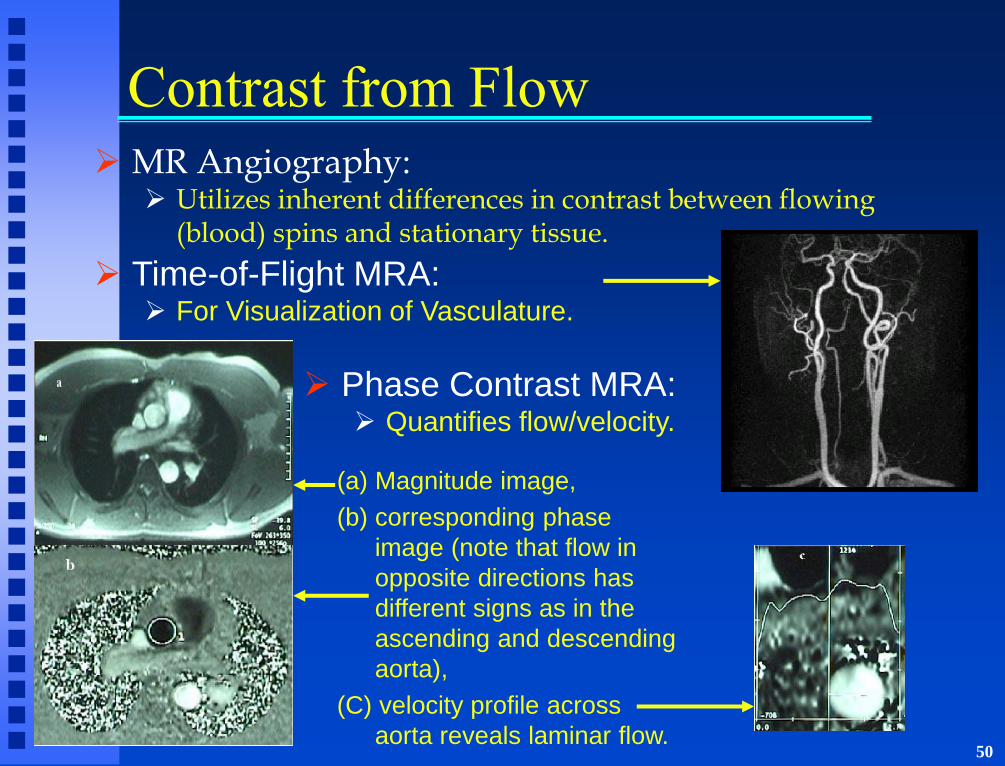
Contrast from Flow

MR Angiography: Utilizes inherent differences in contrast between flowing

(blood) spins and stationary tissue.

Time-of-Flight MRA: For Visualization of Vasculature.

Phase Contrast MRA: Quantifies flow/velocity.

(a) Magnitude image,

(b) corresponding phase

image (note that flow in

opposite directions has

different signs as in the

ascending and descending

aorta),

(C) velocity profile across

aorta reveals laminar flow.

51

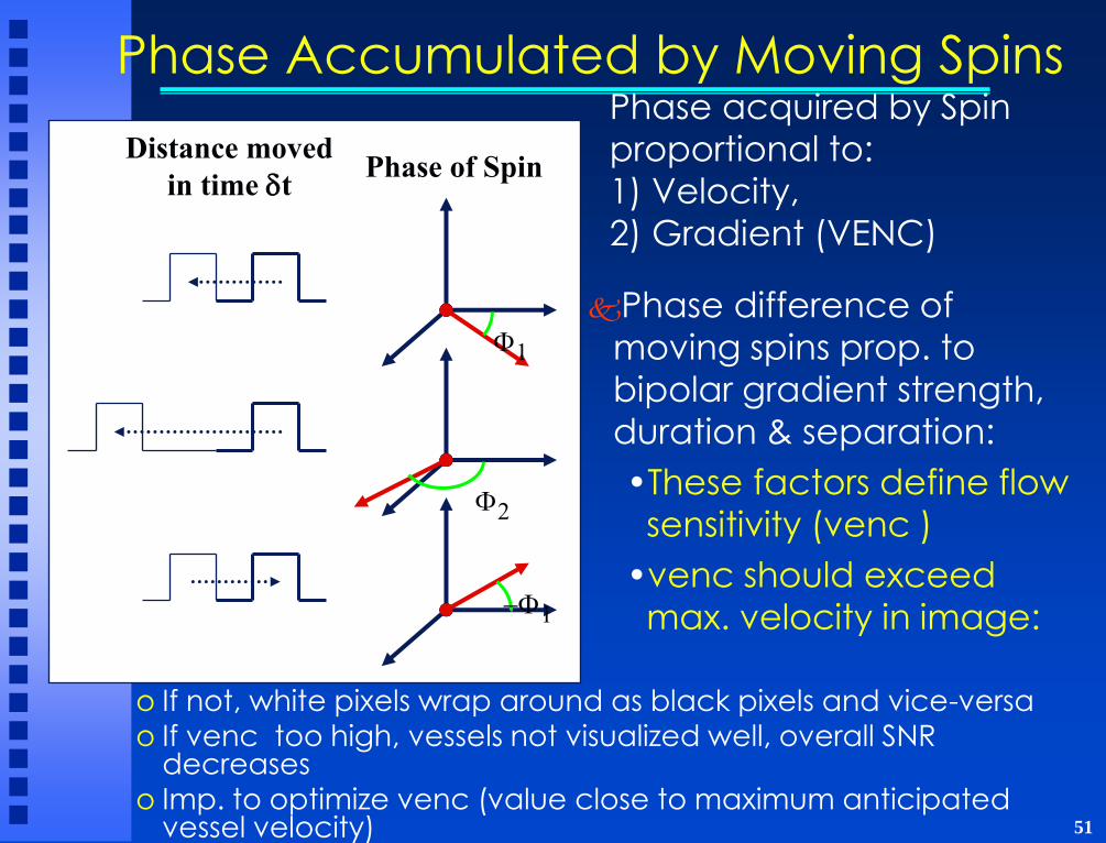
Phase Accumulated by Moving Spins Phase acquired by Spin

proportional to:

1) Velocity,

2) Gradient (VENC)

Distance moved

in time dt Phase of Spin

F1

F2

-F1

Phase difference of

moving spins prop. to

bipolar gradient strength,

duration & separation:

•These factors define flow

sensitivity (venc )

•venc should exceed

max. velocity in image:

o If not, white pixels wrap around as black pixels and vice-versa

o If venc too high, vessels not visualized well, overall SNR decreases

o Imp. to optimize venc (value close to maximum anticipated vessel velocity)

52

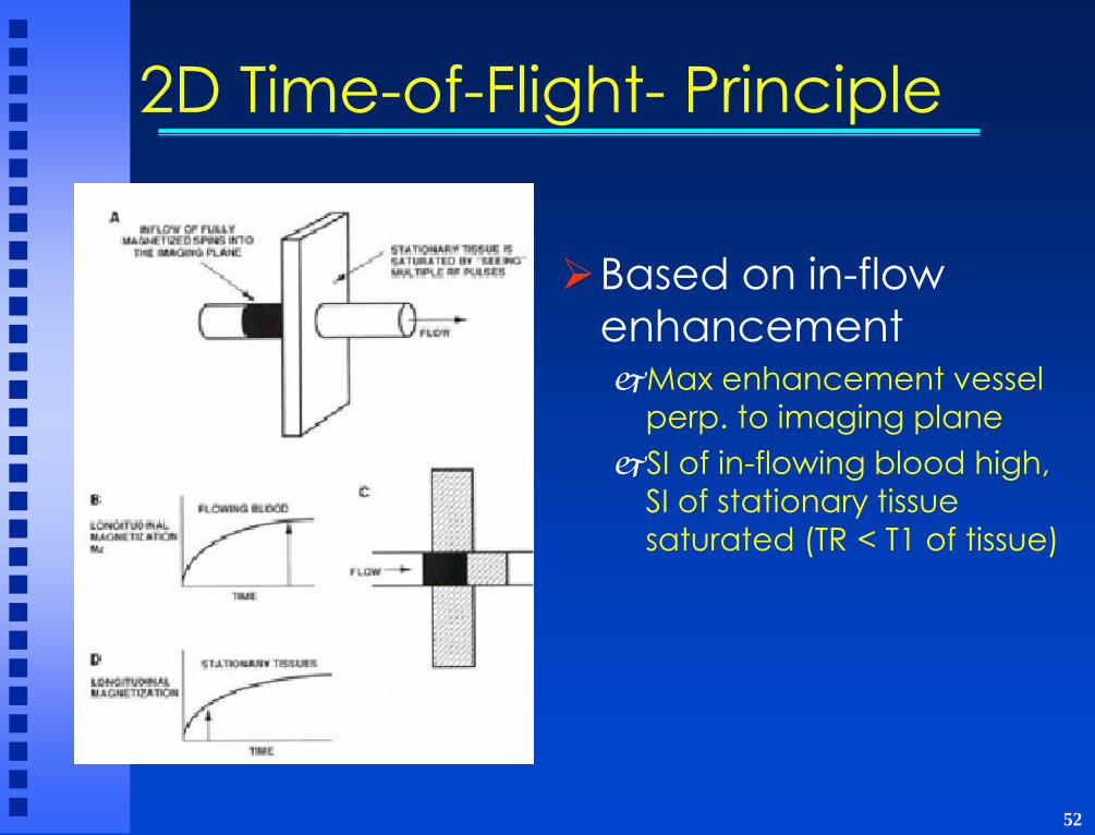
2D Time-of-Flight- Principle

Based on in-flow

enhancement Max enhancement vessel

perp. to imaging plane

SI of in-flowing blood high,

SI of stationary tissue

saturated (TR < T1 of tissue)

53

6 directly acquired images (out of 256) are shown

at the level of the carotids

Raw Data Set

54

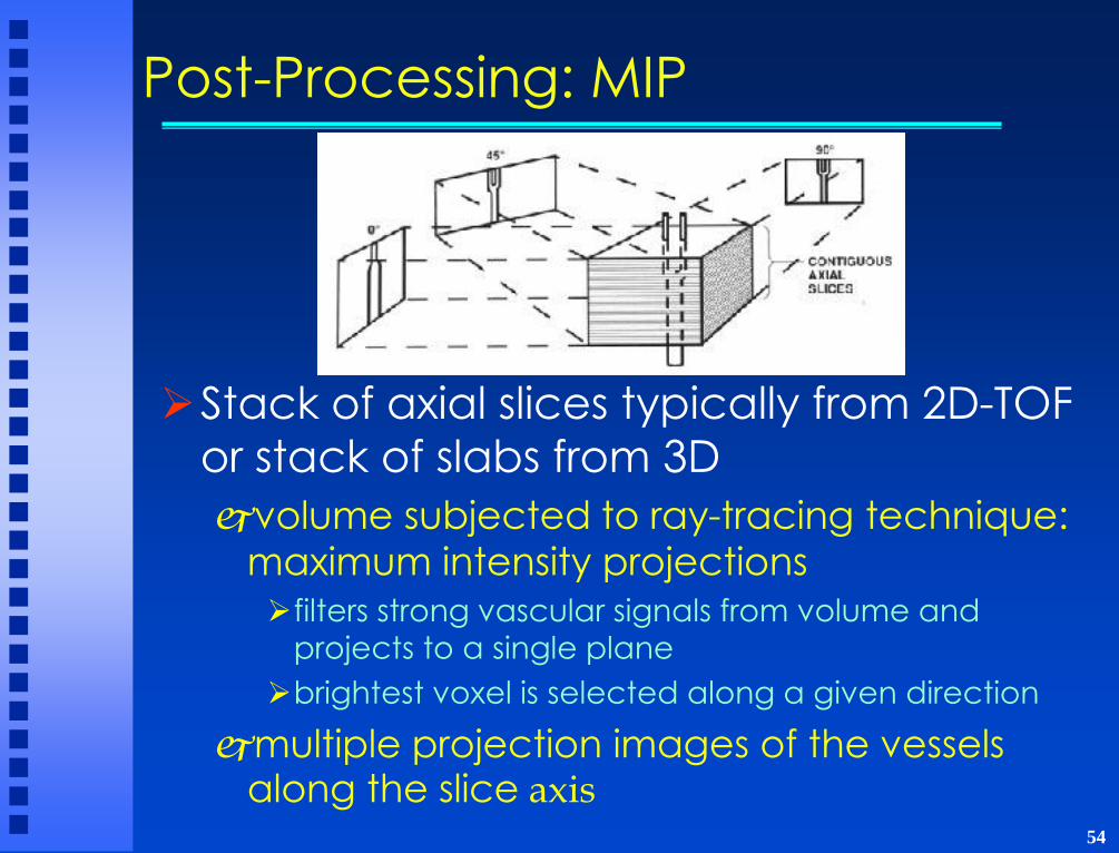
Post-Processing: MIP

Stack of axial slices typically from 2D-TOF

or stack of slabs from 3D

volume subjected to ray-tracing technique:

maximum intensity projections

filters strong vascular signals from volume and

projects to a single plane

brightest voxel is selected along a given direction

multiple projection images of the vessels along the slice axis

55

& After MIP

MIP images in different projections: axial (a),

sagittal (b) and coronal (c)

56

Phase Contrast MRA

RF

Gz

Gv

Gx

•One image without additional velocity encoding

•One image with additional velocity encoding

•Display phase difference between images

•Phase difference is directly proportional to velocity

•Phase difference subtracts out off-resonance and other phase effects

57

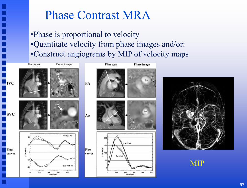
Phase Contrast MRA

•Phase is proportional to velocity

•Quantitate velocity from phase images and/or:

•Construct angiograms by MIP of velocity maps

MIP

Shantanu Sinha. - UCSD Radiology Residency

Documents