ABSTRACT VACHHANI, SHANTANU AVINASH. Computer Simulation and Analysis of Nanoparticle Delivery to the Olfactory Bulb for Direct Drug Migration to the Brain. (Under the direction of Dr. Clement Kleinstreuer). Central Nervous System (CNS) disorders are one of the major causes of fatalities in the world today. The ground zero for all these disorders is the brain; thus, it is essential to transport a considerable concentration of drugs to the brain for any treatment to be effective. Invasive strategies have been used (eg, neurosurgery) to achieve life-saving treatment, but not without major risks. Hence, research into non-invasive strategies (nebulizers, inhalers, etc.) have gained momentum. The main pathway for transport these drugs into the brain requires crossing the Blood- Brain Barrier (BBB) located along the olfactory region of the nasal cavity. An important caveat to this pathway is that the tight junctions of the BBB allow only particles of nano-scale to pass through. Advancements in bio manufacturing have led to the development of multifunctional nanoparticles that can be used to target the brain via the olfactory bulb and then the BBB. The nasal cavity is a highly complex structure with various undulating pathways; hence, in vivo studies offer the most realistic picture of the air-particle dynamics inside the nasal cavities. However, human trials for drug delivery targeting the brain are scarce due to the delicate nature of the organs. Computational Fluid-Particle Dynamics (CF-PD) studies offer a manageable, accurate and cost- effective solution to the problem. OpenFOAM was employed to conduct all the fluid-particle dynamics simulations. OpenFOAM is an open-source CFD toolbox, used cost-free by researchers across the fields of engineering and sciences. To establish the credibility of the numerical simulation approach, the present computer models for nanoparticle transport and deposition have been validated. The main objective of this study is to establish a novel and practical methodology to optimize the nanodrug deposition efficiency inside the olfactory region, using a representative

Welcome message from author
This document is posted to help you gain knowledge. Please leave a comment to let me know what you think about it! Share it to your friends and learn new things together.
Transcript
ABSTRACT
VACHHANI, SHANTANU AVINASH. Computer Simulation and Analysis of Nanoparticle
Delivery to the Olfactory Bulb for Direct Drug Migration to the Brain. (Under the direction of Dr.
Clement Kleinstreuer).
Central Nervous System (CNS) disorders are one of the major causes of fatalities in the world
today. The ground zero for all these disorders is the brain; thus, it is essential to transport a
considerable concentration of drugs to the brain for any treatment to be effective. Invasive
strategies have been used (eg, neurosurgery) to achieve life-saving treatment, but not without
major risks. Hence, research into non-invasive strategies (nebulizers, inhalers, etc.) have gained
momentum. The main pathway for transport these drugs into the brain requires crossing the Blood-
Brain Barrier (BBB) located along the olfactory region of the nasal cavity. An important caveat to
this pathway is that the tight junctions of the BBB allow only particles of nano-scale to pass
through. Advancements in bio manufacturing have led to the development of multifunctional
nanoparticles that can be used to target the brain via the olfactory bulb and then the BBB. The
nasal cavity is a highly complex structure with various undulating pathways; hence, in vivo studies
offer the most realistic picture of the air-particle dynamics inside the nasal cavities. However,
human trials for drug delivery targeting the brain are scarce due to the delicate nature of the organs.
Computational Fluid-Particle Dynamics (CF-PD) studies offer a manageable, accurate and cost-
effective solution to the problem. OpenFOAM was employed to conduct all the fluid-particle
dynamics simulations. OpenFOAM is an open-source CFD toolbox, used cost-free by researchers
across the fields of engineering and sciences. To establish the credibility of the numerical
simulation approach, the present computer models for nanoparticle transport and deposition have
been validated. The main objective of this study is to establish a novel and practical methodology
to optimize the nanodrug deposition efficiency inside the olfactory region, using a representative

human nasal cavity. The particle release map (PRM) approach was utilized to determine the best
injection position for a cannula connected to a nebulizer. For 10nm nanodrugs leaving the cannula
at 10m/s, 41% deposited in the olfactory region, while 20% deposited via targeting without the
cannula, and <1% at normal breathing condition, i.e., 20lpm.

© Copyright 2019 by Shantanu Avinash Vachhani
All Rights Reserved

Computer Simulation and Analysis of Nanoparticle Delivery to the Olfactory Bulb for Direct
Drug Migration to the brain
by
Shantanu Avinash Vachhani
A thesis submitted to the Graduate Faculty of
North Carolina State University
in partial fulfillment of the
requirements for the degree of
Master of Science
Mechanical Engineering
Raleigh, North Carolina
2019
APPROVED BY:
_______________________________ _______________________________
Dr. Gregory Buckner Dr. Pramod Subbareddy
_______________________________
Dr. Clement Kleinstreuer
Committee Chair

ii
DEDICATION
To my parents, sister and friends for their unconditional support
iii
BIOGRAPHY
Shantanu Vachhani was born on the 14th of May, 1995 to Mr. Avinash Vachhani and Mrs. Taruna
Vachhani in Mumbai, India. After completing his high school education he attained his Bachelors
of Engineering degree in the field of Mechanical engineering from Birla Institute of Technology
and Science (BITS) Pilani, K.K Birla Goa Campus, Goa, India. Subsequently he moved to Raleigh,
North Carolina in 2017 to pursue his graduate degree in Mechanical Engineering at North Carolina
State University. He has been conducting research for his master’s thesis under the guidance of
Dr. Clement Kleinstreuer in the Computational Multi-Physics Lab at NC State and will receiving
his master’s degree in Fall 2019.

iv
ACKNOWLEDGMENTS
First and foremost I would like to express my deepest gratitude to my academic advisor, Dr.
Clement Kleinstreuer for giving me the opportunity to be a part of his research group. His constant
guidance and support during this time has been invaluable to my research and has enabled me to
grow professionally as a student. Throughout all the roadblocks he was very patient and offered
valuable insight and suggestions that helped me overcome these hurdles. I would also like to thank
Dr. Gregory Buckner and Dr. Pramod Subbareddy for taking time out of their busy schedules to
be a part of my thesis committee. I would also like to thank all the members of the Computational
Multi-Physics lab, Sriram, Adithya, Nilay, Sujal and Karthik for creating an environment that
fosters discussion and innovation. The NCSU high performance computing services and support
were extremely helpful in providing assistance in running my numerical simulations. My friends
Chaitee, Shalini, Aamir , Utkarsh and Prasad have been a constant life support system and have
made my time here in NCSU extremely enjoyable and comfortable. Last but not the least my
family has been there for me during times of need and I would like this opportunity for their
unconditional love.

v
TABLE OF CONTENTS
LIST OF TABLES ....................................................................................................................... viii
LIST OF FIGURES ....................................................................................................................... ix
CHAPTER 1. INTRODUCTION AND RESEARCH OBJECTIVES ........................................... 1
1.1. Research Motivation ........................................................................................................ 1
1.2. Literature Review................................................................................................................. 2
1.2.1. Introduction ................................................................................................................... 2
1.2.2. Nasal Drug Delivery Devices ....................................................................................... 5
1.2.3. CFD studies ................................................................................................................. 10
CHAPTER 2. MATH MODEL DEVELOPMENT AND COMPUTER SIMULATIONS ......... 15
2.1. Introduction ........................................................................................................................ 15
2.2. Assumptions ....................................................................................................................... 15
2.3. Airflow Equations .............................................................................................................. 16
2.4. Particle Dynamics Equations ............................................................................................. 19
2.4.1. Drag Force .................................................................................................................. 21
2.4.2. Brownian Force ........................................................................................................... 22
2.4.3. Saffman Lift Force ...................................................................................................... 22
2.4.4. Gravitational Force ..................................................................................................... 23
2.5. Quantifying Particle Deposition ........................................................................................ 23
2.6. Quasi-Steady vs Transient particle dynamics .................................................................... 24
vi
CHAPTER 3. NUMERICAL METHOD USING OPENFOAM ................................................. 26
3.1 Introduction ......................................................................................................................... 26
3.2. Case Structure .................................................................................................................... 27
3.3. Case Set-up ........................................................................................................................ 34
3.4. Boundary Conditions ......................................................................................................... 36
3.5. Numerical Schemes ........................................................................................................... 39
3.6. Solution Control ................................................................................................................. 41
CHAPTER 4. MODEL VALIDATIONS ..................................................................................... 42
4.1. Introduction ........................................................................................................................ 42
4.2. Geometry and Mesh of the Representative Nasal Cavities ................................................ 43
4.3. Comparison with Calmet et al., 2018................................................................................. 48
4.3.1. Airflow Field Results .................................................................................................. 48
4.3.2. Particle Deposition Results ......................................................................................... 54
4.4. Comparison with Ingham (1975) ....................................................................................... 57
4.4.1. Geometry and Mesh .................................................................................................... 57
4.4.2. Results and Discussions .............................................................................................. 58
4.5. Comparison with Tian et al., 2019 ..................................................................................... 60
4.5.1. Airflow Field Results .................................................................................................. 62
4.5.2. Particle Deposition Results ......................................................................................... 66
CHAPTER 5. PARTICLE RELEASE MAP FOR OLFACTORY DRUG TARGETING .......... 73

vii
5.1 Introduction ......................................................................................................................... 73
5.2 Methodology ....................................................................................................................... 74
5.3. Results and Discussion ...................................................................................................... 76
5.3.1. Micron-size Particles .................................................................................................. 76
5.3.2. Nanoparticles .............................................................................................................. 85
CHAPTER 6. NASAL CANNULA FOR OLFACTORY DRUG TARGETING ....................... 95
6.1 Introduction ......................................................................................................................... 95
6.2. Results and Discussion ...................................................................................................... 97
CHAPTER 7. CONCLUSION AND FUTURE WORK ............................................................ 102
REFERENCES ........................................................................................................................... 106
viii
LIST OF TABLES
Table 2. 1. Boundary conditions for Particles. .............................................................................. 24
Table 3. 1 Boundary conditions for Velocity and Pressure. ......................................................... 36
Table 3. 2 Boundary conditions for Turbulent Kinetic Energy and Turbulence Dissipation ....... 37
Table 3. 3. Numerical Schemes used in simpleFoam. .............................................................. 40
Table 3. 4. Algebraic solvers used in simpleFoam. .................................................................. 41
Table 4. 1. Geometry features of the Nasal Cavity. ...................................................................... 45
Table 4. 2. Unstructured mesh characteristics. ............................................................................. 47
Table 4. 3. Comparison of particle deposition efficiencies. ......................................................... 54
Table 4. 4. Surface Area Comparison between G1 and G2 .......................................................... 62
Table 5. 1. Legend correlating the color to the specific region………………………………….75
Table 6. 1. Olfactory deposition efficiencies for Cannula Injection (SOI = 10 m/s) .................. 101
Table 6. 2. Olfactory deposition efficiencies for Cannula injection (SOI = 3.5 m/s) ................. 101
Table 7. 1. Olfactory deposition comparison between the injection methods………………….103

ix
LIST OF FIGURES
Figure 1. 1. Blood Brain Barrier (25). ............................................................................................ 5
Figure 1. 2. Anatomy of the Human Nasal Cavity (29). ................................................................. 6
Figure 1. 3. Schematics of a nasal spray (32). ................................................................................ 7
Figure 1. 4. Schematics of a nebulizer (34). ................................................................................... 8
Figure 2 .1.Workflow of Euler- Lagrange simulations..................................................................20
Figure 3. 1. OpenFOAM case structure. ....................................................................................... 28
Figure 3. 2. U file for the elbow case. ........................................................................................... 29
Figure 3. 3. boundary file in the polyMesh directory. .................................................................. 30
Figure 3. 4. transportProperties file in the constant directory.................................. 31
Figure 3. 5. controlDict file in the system directory.......................................................... 32
Figure 3. 6. fvSchemes file in the system directory. ............................................................ 32
Figure 3. 7. Workflow for conducting OpenFOAM simulations. ................................................. 33
Figure 3. 8. transportProperties file. ........................................................................... 34
Figure 3. 9. Snippet of the kinematicCloudProperties file. ........................................ 35
Figure 4. 1. Geometry of the nasal cavity. .................................................................................... 43
Figure 4. 2. Complete view of the Nasal Cavity Geometry. ......................................................... 44
Figure 4. 3. Isometric view of the unstructured mesh of the representative nasal cavity. ............ 46
Figure 4. 4. Mesh slice of the mid-section of the nasal cavity...................................................... 47
Figure 4. 5. Mesh slice of the nostrils. .......................................................................................... 48
Figure 4. 6. Slices 1-1’ to 6-6’ (left to right) of the nasal geometry. ............................................ 50
Figure 4. 7. Velocity contours (Slice 1-1’ and 2-2’). .................................................................... 50
Figure 4. 8. Velocity contours (Slice 3-3’ to Slice 6-6’). ............................................................. 51

x
Figure 4. 9. Wall Shear Stress contour of the nasal cavity for 20 lpm. ........................................ 51
Figure 4. 10. Turbulent kinetic energy contour of the nasal cavity for 20 lpm. ........................... 52
Figure 4. 11. Particle Deposition Pattern for 2, 10 and 20 µm particles ....................................... 55
Figure 4. 12. Sectional Deposition for 20 µm particles. ............................................................... 56
Figure 4. 13. Sectional Deposition for 10 µm particles. ............................................................... 56
Figure 4. 14. Cylindrical geometry. .............................................................................................. 57
Figure 4. 15. O grid meshing of the cylinder geometry. ............................................................... 58
Figure 4. 16. Deposition efficiency comparison for a flowrate of lpm......................................... 59
Figure 4. 17. Deposition efficiency comparison for a flowrate of 5pm. ....................................... 60
Figure 4. 18. Geometry G1. .......................................................................................................... 61
Figure 4. 19. Geometry G2. .......................................................................................................... 61
Figure 4. 20. Velocity contours along the nasal cavity for 5 lpm flowrate................................... 63
Figure 4. 21. Velocity contours along the nasal cavity for 10 lpm flowrate................................. 64
Figure 4. 22. Velocity streamlines across the nasal cavity. .......................................................... 65
Figure 4. 23. Velocity streamlines in the olfactory region. .......................................................... 65
Figure 4. 24. Recirculation regions in the nostrils……………………………………………….66
Figure 4. 25. Dean vortices in the nasopharynx ............................................................................ 66
Figure 4. 26. Deposition pattern for 10 lpm flowrate and 1nm diameter particle. ....................... 67
Figure 4. 27. TDE comparison for 5 lpm and 7 lpm flowrates. .................................................... 68
Figure 4. 28. NOP Independent study for Total Deposition (10 lpm). ......................................... 69
Figure 4. 29. ODE comparison for 5 lpm and 7 lpm flowrates. ................................................... 70
Figure 4. 30. NOP Independent study for Olfactory Deposition (10 lpm). .................................. 70
Figure 4. 31. Sectional Deposition of 1.1 nm,10 nm, 50 nm and 100 nm. ................................... 71

xi
Figure 5. 1. Nasal geometry with the specific regions that will be represented in the ................. 75
Figure 5. 2.1. PRM for an impaction parameter of 333.333 µm2cm3s − 1. ............................... 78
Figure 5. 2.2. Deposition efficiency comparison between normal and targeted injection. ........... 78
Figure 5. 3.1. PRM for an impaction parameter of 1333.333 µm2cm3s − 1. ............................. 79
Figure 5. 3.2. Deposition efficiency comparison between normal and targeted injection ............ 79
Figure 5. 4.1. PRM for an impaction parameter of 2083.333 µm2cm3s − 1. ............................. 80
Figure 5. 4.2. Deposition efficiency comparison between normal and targeted injection ............ 80
Figure 5. 5.1. PRM for an impaction parameter of 8333.3333 µm2cm3s − 1. ........................... 81
Figure 5. 5.2. Deposition efficiency comparison between normal and targeted injection ............ 81
Figure 5. 6.1. PRM for an impaction parameter of 33333.3333 µm2cm3s − 1. ......................... 82
Figure 5. 6.2. Deposition efficiency comparison between normal and targeted injection ............ 82
Figure 5. 7. Deposition Pattern due to normal injection ............................................................... 83
Figure 5. 8. Deposition Pattern due to targeted injection ............................................................ 83
Figure 5. 9. Deposition Pattern due to targeted injection. ............................................................ 84
Figure 5. 10. Deposition Pattern due to targeted injection .......................................................... 85
Figure 5. 11.1. PRM of 1 nm particles for the flowrate of 5 lpm. ................................................ 86
Figure 5. 11.2. Deposition efficiency comparison between normal and targeted injection .......... 86
Figure 5. 12.1. PRM of 10 nm particles for the flowrate of 5 lpm. .............................................. 87
Figure 5. 12.2. Deposition efficiency comparison between normal and targeted injection .......... 87
Figure 5. 13.1. PRM of 100 nm particles for the flowrate of 5 lpm. ............................................ 88
Figure 5. 13.2. Deposition efficiency comparison between normal and targeted injection .......... 88
Figure 5. 14.1. PRM of 1 nm particles for the flowrate of 20 lpm. .............................................. 90
Figure 5. 14.2. Deposition efficiency comparison between normal and targeted injection .......... 90
xii
Figure 5. 15.1. PRM of 10 nm particles for the flowrate of 20 lpm. ............................................ 91
Figure 5. 15.2. Deposition efficiency comparison between normal and targeted injection .......... 91
Figure 5. 16.1. PRM of 100 nm particles for the flowrate of 20 lpm. .......................................... 92
Figure 5. 16.2. Deposition efficiency comparison between normal and targeted injection .......... 92
Figure 5. 17. Deposition Pattern due to normal injection ............................................................. 93
Figure 5. 18. Deposition Pattern due to targeted injection ........................................................... 93
Figure 5. 19. Olfactory Deposition Efficiency trend due to targeted injection............................. 94
Figure 5. 20. Nasal Deposition Efficiency trend due to targeted injection. .................................. 94
Figure 6. 1. Streamlines to the olfactory region............................................................................ 95
Figure 6. 2. Schematic of aerosol delivery using HFNC with a nebulizer.. ................................. 96
Figure 6. 3. Position of the injection of particles from the cannula. ............................................. 96
Figure 6. 4.1. PRM of 2 µm particles for the flowrate of 20 lpm ................................................. 98
Figure 6. 4.2. Deposition pattern as a result of cannula injection ................................................. 98
Figure 6. 5.1. PRM of 10 nm particles for the flowrate of 20 lpm ............................................... 99
Figure 6. 5.2. Deposition pattern as a result of cannula injection ................................................. 99
Figure 6. 6.1. PRM of 50 nm particles for the flowrate of 20 lpm ............................................. 100
Figure 6. 6.2. Deposition pattern as a result of cannula injection ............................................... 100

1
CHAPTER 1. INTRODUCTION AND RESEARCH OBJECTIVES
1.1. Research Motivation
Brain tumors as well as Central Nervous System (CNS) disorders (Alzheimer’s,
Parkinson’s, Multiple Sclerosis etc.) are major causes of fatalities in the world today. Malignant
brain tumors have a survival prognosis of less than 15 months (1) despite the progress that has
been made. The most common brain cancer accounts for 80 % of all the malignant tumors (2).
According to the Parkinson’s Prevalence Project, nearly 1 million American’s over the age of 45
will be diagnosed with Parkinson’s by 2020 and this number is expected to increase to 1.24 million
by 2030. Alzheimer’s disease, according to the Alzheimer Association Report (2017), affects
nearly 5.5 million people and is the 6th leading cause of death in the USA. These statistics clearly
underline the gravity of the situation. Therefore treatment of these diseases has garnered a lot of
attention, and considerable efforts have been put into the treatment of these ailments.
The ground zero for all these disorders is the brain; hence, it is essential to transport drugs
to the brain for any treatment to be effective. The brain is a an extremely fragile organ that is
comprised of billions of nerve cells (neurons) that require regular supply of nutrients for proper
functioning of the central nervous system. Due to the fragile nature of the brain, it is protected by
the Blood Brain Barrier (BBB). This highly selective semipermeable membrane protects the brain
from the circulating blood. The high selectivity is due to the presence of tight junctions between
the adjacent endothelial cells that allow only very small compounds to pass through (3, 4).
Furthermore, the cerebral endothelial cells show a considerably less pinocytic activity than the
systemic endothelium (5). Pinocytic activity results in the transportation of substances across an
epithelium by material-uptake on one face of a coated vesicle that can then be transported from
the opposite face. Clearly, the reduction in the pinocytic activity further limits the drug

2
transportation across the BBB. The blood cerebrospinal fluid barrier (BCSFB) forms the second
layer that restricts the movement of drugs. This layer is located at the choroid plexus and separates
the blood and the cerebrospinal fluid. However this layer is slightly more permeable than the BBB.
The BBB surface area (120 sq ft) is roughly 5000 times the area of the BCSFB (6). Hence, BBB
layer is the dominant obstacle for the delivery of drugs to the brain. These membranes are there to
inhibit the passage of pathogens, antibodies, toxins etc. to the brain. In doing so they also restrict
the transport of therapeutic drugs in to the brain. In summary, drug delivery to the brain is difficult
to achieve at high enough efficiencies to counteract the toxins that are the root to the various CNS
disorders (7).
1.2. Literature Review
1.2.1. Introduction
To overcome the limitations associated with brain drug targeting, different strategies have
been or are in the process of being developed (4, 8, 9). These strategies can be broadly categorized
into invasive and non-invasive strategies. Invasive strategies understandably are not preferred
because of the complicated and delicate structure of the brain. Khan et al., 2017(8) described the
various conventional invasive strategies that have been employed for brain drug targeting. One
novel way to do this is using ultrasound waves to transiently open the BBB to facilitate drug
migration to the brain. It involves exerting pressure on the BBB by using microbubbles that are
injected in accordance with the acoustic energy principle. This results in the loosening of the
junctions between the endothelial cells; thus, increasing the permeability of BBB towards the
administered drugs. This methodology can increase the penetration of the BBB by as much as 340
% for glioblastoma treatment (10). A more direct way of drug targeting is intracerebral and
intraventricular injection. This is done through the scalp where the drug is infused into the brain
3
parenchyma. In addition to being dangerous, this methodology is rendered largely ineffective due
to the decreasing diffusive property inside the brain (11). With the progress in polymer technology,
use of microchips and polymeric wafers (12, 13) has gained a lot of popularity in relation to brain
drug targeting. These polymer wafers are based on polyanhydride and are placed in the tumor
specific area from where controlled doses of the drug are released. Lin and Kleinberg, 2008(14)
reviewed the pharmacokinetics of carmustine wafers as well as the efficacy of it in preclinical and
clinical studies. The preclinical study compared the effect of drug delivery via the polymer wafer
with systemic administered drugs in terms of the tumor growth delays. The former showed a 16.3
day delay as compared to a 9.3-11.2 day delay showing the potential of polymer wafers for
treatment. A chemotherapeutic agent called temozolomide (TMZ) is utilized to treat gliosarcoma.
Scott et al.,2011(15) conducted an in vivo rodent study that utilized a biocompatible microcapsule
device to deliver TMZ to the tumor-infected area and showed the effectiveness of these devices.
The microcapsule was implanted at day 0 and the median survival time was between 31-50 days,
while for orally administered drugs it was 25 days. Microchips are another novel technology that
has shown promising signs to achieve higher drug deposition efficiency in the olfactory region.
Microchips can be microelectromechanical systems (MEMS), a device that provides
programmable release of the drug at a specific target site (16). Drug is filled in a reservoir and the
release of the dug is achieved by dissolving the reservoir cover through applying voltage between
the anode and the cathode of the microchip. Since this a new technology and microfabrication of
the device is expensive, not many in vivo studies have been conducted to implement this
technology. According to one study (17) doses of 1,3-bis(2-chloroethyl)-1-nitrosourea (BCNU) (a
brain cancer chemotherapeutic) through a microchip inserted into the brain were administered. The

4
BCNU chip showed comparable efficacy to the BCNU polymerized wafer and further research
should pave way for an encouraging future of microchip technology.
As explained earlier, the Blood Brain Barrier (BBB) is a major obstacle for transporting
the drugs into the brain stem. The BBB allows only an extremely selective set of particles to pass
through it and hence it is essential to look into the physio-chemical characteristics of the drugs for
an effective drug targeting system for brain tumors and other CNS disorders. There are two
principle mechanisms by which molecules traverse through the barriers, ie, Active Transport and
Passive Diffusion. The passive diffusion route involves drugs accumulating near the BBB and
subsequently passing through it by means of diffusion. This route does not require any external
energy input. Alternatively, certain transport proteins at the brain endothelial surface can help
certain molecules bypass the BBB. This phenomenon is a form of active transport which can be
further classified into carrier-mediated transport and receptor-based transport. It involves active
efflux transporters (like P‐glycoprotein (P‐gp)) pumping out substrates in-between the brain and
blood (18). The tight junctions of the BBB (Figure 1.1) restrict the molecular weight of bypassing
molecules via passive diffusion and active transport to 500 Da and 600 Da, respectively (19).
Clearly, the size of the drug plays a pivotal role in efficiency and effectiveness of drug delivery
into the brain. Consequently Nanoparticles (particles with size ranging between 1-100nm) fit into
the tight window that is required for passing through the BBB. Several studies (20-22) have shown
that the lower the size of the particles, the higher is the deposition efficiency. Shape also plays a
role in nanoparticle transport. Specifically nanorods have shown to have a higher adhesive
property to the brain epithelium than the spherical nanoparticles (23, 24).

5
Figure 1. 1. Blood Brain Barrier (25).
1.2.2. Nasal Drug Delivery Devices
Drug delivery using the nasal route is a promising option and has been conventionally used
in the form of nebulizers, nasal dry powder inhalers, spray pumps, nasal pressurized metered-dose
inhalers, etc. Although the nose provides an accessible route to the olfactory region, there are
certain challenge to nasal direct drug delivery (26-28).
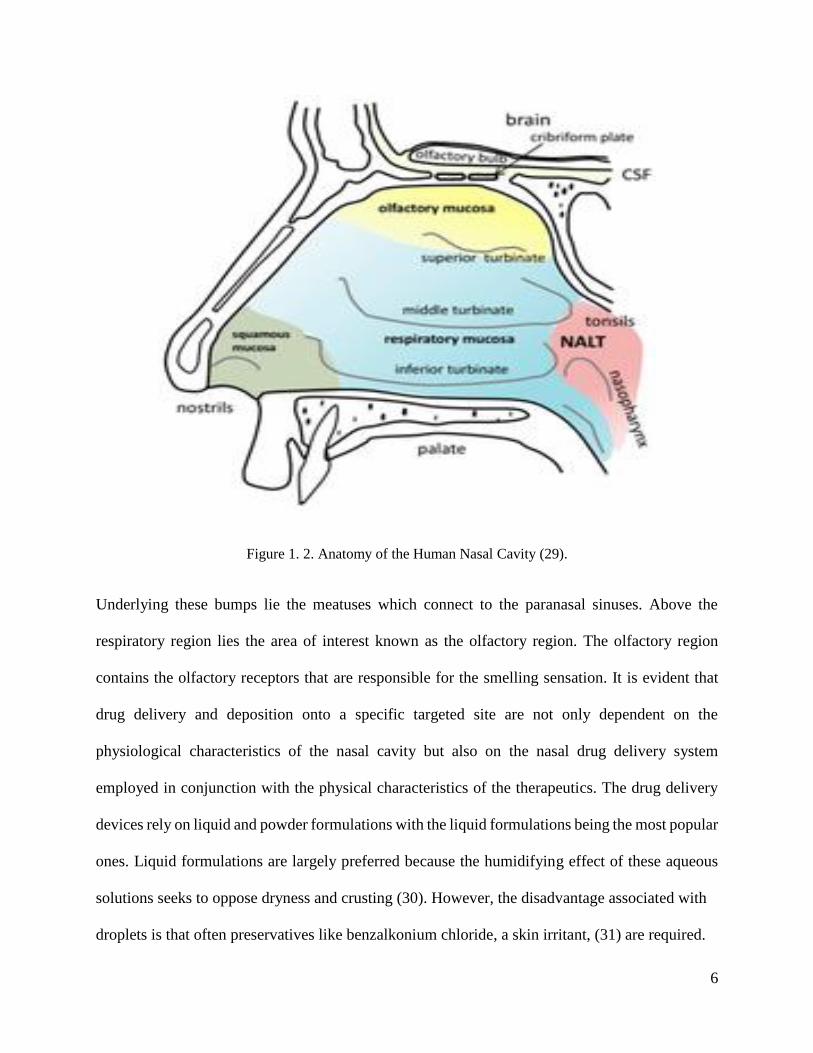
Figure 1.2 shows the anatomy of the human nasal cavity. The nasal cavity is lined up with
nasal mucosa which forms a part of the immune system. These barriers provide protection against
any infectious and allergenic pathogens. The structure of the human nasal cavity starts with the
nostril in the region known as the vestibule. This is followed by the respiratory section through
which air travels, encountering contain bumps (also known as conchae or turbinate bones).
6
Figure 1. 2. Anatomy of the Human Nasal Cavity (29).
Underlying these bumps lie the meatuses which connect to the paranasal sinuses. Above the
respiratory region lies the area of interest known as the olfactory region. The olfactory region
contains the olfactory receptors that are responsible for the smelling sensation. It is evident that
drug delivery and deposition onto a specific targeted site are not only dependent on the
physiological characteristics of the nasal cavity but also on the nasal drug delivery system
employed in conjunction with the physical characteristics of the therapeutics. The drug delivery
devices rely on liquid and powder formulations with the liquid formulations being the most popular
ones. Liquid formulations are largely preferred because the humidifying effect of these aqueous
solutions seeks to oppose dryness and crusting (30). However, the disadvantage associated with
droplets is that often preservatives like benzalkonium chloride, a skin irritant, (31) are required.

7
Figure 1. 3. Schematics of a nasal spray device (32).
Metered-dose spray pumps have dominated the nasal drug delivery market since their inception.
Figure 1.3 shows the schematics of a standard nasal spray. Standard spray pumps are associated
with dose volumes between 25 and 200 µl. The components of a metered-dose pump spray are a
container, the pump with a valve and an actuator. The dose spray characteristics like particle size
are dependent on the orifice of the actuator, pump properties and the force exerted. Another device
used for delivering nasal drugs is a nasal pressurized metered-dose inhaler (pMDI). A compressed
gas is suddenly expanded resulting in a high speed release of the drug particles. However these are
also associated with something called the “cold Freon” effect, characterized by discomfort and
dryness. Its name stems from the fact that conventionally the propellant used in these inhalers have
been ozone depleting chlorofurocarbons (CFC). However, recently hydrofluroalkanes (HFA) have
gained popularity as a propellant due to the negative environmental impact of the former. The HFA
based inhalers produce a relatively slower particle velocity (15 m/s) than CFC based inhalers (52

8
m/s) (33) decreasing the irritation caused by the ‘cold Freon” effect. Until now, these pMDIs have
not been used for nose-to-brain applications. A recent study is focused on developing a nitrogen-
based inhaler but further in vitro and in vivo studies are required for practical implementation.
Figure 1. 4. Schematics of a nebulizer (34).
Compressed air nebulizers (35) are also popular for nasal drug delivery. Figure 1.4 shows the
schematics of a nebulizer. These devices use either oxygen, compressed air, ultrasonic or
mechanical power to break up medical formulations into small aerosol droplets at comparatively
low speeds. The popular types of these devices in the market are jet nebulizers, ultrasonic and
vibrating-mesh nebulizers - distinguished by the droplet creation mechanism (36). With
nebulizers, droplets with diameters between 0.5 µm and 5 µm can be produced (37-41), well within

9
the respirable range. These nebulizers can also be used in conjunction with a high flow nasal
cannula (HFNC). The HFNC efficiency has been analyzed (42, 43) for the purposes of ventilation
and drug-delivery to lung sites. An in vitro study showed the maximum lung deposition efficiency
of 32 % using this approach (44). The impact of gas flow and humidity using the nasal cannula in
adults was studied by Alcoforado et al., 2019 (45). All the aforementioned studies have been
concentrated on pulmonary drug delivery. Studies of direct nanodrug delivery to the olfactory bulb,
using the cannula as an administering device, has not been published as the goal so far was to reach
specific sites in the lung. For example, Longest et al., 2019 (46) reviewed the various nebulization
technologies for delivering aerosols to the lungs and suggested secondary devices and technologies
to increase the delivery efficiency of particles in the lungs. These claims are substantiated by the
use of computational fluid dynamic simulations. Spence et al., 2019 (47) developed a new
combination device with separate mesh nebulizers for generating humidity and delivering the
medical aerosol. The device consists of a small volume mixing region where the aerosols are mixed
with ventilation gas flow followed by a heating channel which produces small size droplets that
are optimum for highly efficient nose-to-lung administration. Major utilization of these devices
have been to target the sinuses and not the olfactory region. In addition to these liquid formulations,
there are some powder formulations that are popular. These powder formulations are more stable
than the liquid counterparts thereby eliminating the use of preservatives. These formulations are
available in the market in three forms namely powder sprayers, powder inhalers and insufflators.
Powder sprayers create a plume of spray particles due to the pressure created by the compressible
compartment. Several studies (48-51) have been performed for testing the effectiveness of these
devices in the market. On the other hand, nasal powder inhalers uses the subject’s breath to inhale
the particles. Insufflators unlike these two have a more complicated mechanism. It consists of a
10
mouthpiece and a connected nosepiece. The subject exhales in to the mouthpiece, closing the
velum which enables the airflow to carry the particles into the nosepiece.
1.2.3. CFD studies
Previous studies on nasal deposition of inhaled nanoparticles include in vivo experiments
in healthy volunteers (52, 53) and in vitro experiments in nasal replica casts based on cadavers or
imaging of live subjects (53, 54). As explained earlier, the olfactory region serves as a promising
path for nanodrugs to reach the brain via translocation along the nerve cells into the brain (55, 56).
However, due to the complex structure of the nasal cavity, only a minuscule amount reaches the
olfactory region naturally. In vivo studies offer the most realistic picture of the fluid-particle
dynamics inside the nasal cavity; but, human trials are difficult to get approved owing to the
delicacy of the targeted organ. Alternatively, Computational Fluid Dynamics (CFD) studies allow
us to overcome this problem. CFD studies enable us to conduct “computer experiments” to predict
nanoparticle trajectories and the effect of the airflow for realistic inhalation conditions. Once, a
relatively high degree of confidence in the simulation accuracy is achieved and administering the
drug is deemed safe and effective, in vivo studies in humans can be performed. Hence, it is essential
to accurately model the interplay between airflow and particle dynamics. Historically micron
particles have been studied for drug delivery due to the ability of nasal delivery devices (eg,
nebulizers) to generate these micron-size droplets. Various CFD studies involved simulating the
airflow and micron-size particle deposition inside a representative human nasal cavity model.
Wang et al., 2009 (57) studied the influence of flowrate and the particle diameter on the deposition
patterns for both micron and submicron sized particles. The results showed that micron deposition
is dependent on the inertial parameter and Stokes number while deposition efficiency for
nanoparticles is diffusion dominant. Reports from rat models are extrapolated to humans for in

11
vivo studies and then with CFD studies for particle deposition comparisons. Shang et al., 2015 (58)
conducted such a study to establish a relationship between the depositions in rat and human nasal
cavity. The results highlighted the anatomical differences between the geometries. As a
consequence of this study, scaling factors were established for low, medium and high inertial
particles. The aforementioned studies have considered only the nasal cavity as the computational
domain. However, a more realistic picture of the flow and the deposition can be obtained by
considering the breathing zone outside the nostril as well. Shang et al., 2015 (59) studied the effect
of the breathing zone on the airflow patterns and consequently the particle deposition efficiencies.
They found that the existence of the breathing zone creates additional small vortices in the nostrils
and in the mid-section of the nasal cavities. This change in velocity contours significantly lowers
the particle deposition efficiencies for particle sizes ranging from 7.8 -20 µm. The maximum
decrease in particle deposition efficiency observed was 37.7 % for 12 µm particles. Hence the new
nasal cavity model along with the breathing zone offers a better picture of the actual fluid-particle
dynamics inside the nasal cavity. When it comes to nasal deposition patterns, subject variability is
an important topic. Nasal geometries are different for different people and hence a study is required
to establish a relationship between the particle deposition efficiencies and the geometrical
parameters. Calmet et al., 2018 (60) used three different nasal geometries to study the effect of the
different anatomical structures on deposition efficiencies. An interesting consequence of this study
is that total deposition efficiency curves for all the subjects collapsed into a single function for a
new Stokes-Reynolds number combination (𝑖𝑒, 𝑆𝑡𝑘1.23𝑅𝑒1.28). However, local deposition did
not follow such a trend,as only one of the subject geometries observed particle deposition in the
olfactory region.
12
One of the earliest CFD studies using a representative human nasal cavity model regarding
nanoparticle deposition in the olfactory region was performed by Shi et al.,2006 (61). They treated
airflow as laminar and incompressible while modeling nanoparticles as an Eulerian phase. Their
simulations showed that for normal breathing rate and a nanoparticle diameter of 1nm, the
olfactory deposition efficiency is about 0.5 % while the total deposition efficiency is about 75 %.
A similar study was conducted by Garcia and Kimbell, 2009 (62) using the CFD technique (63,
64) for a rat, considering nanoparticles with diameters ranging from 1 to 100 nm. They showed
that the total deposition efficiencies decreases with increasing diameter. This was in agreement to
previous studies (65-67) . Interestingly the highest olfactory deposition efficiency was
approximately between 6-9 % for 3-4 nm particles. This can be attributed to the fact that the
olfactory region occupies a greater percentage (about 5 times) of the area of the nasal cavity in
case of rats as compared to humans. Tian et al. (2017) conducted a numerical study for a human
nasal cavity (68) where the maximum olfactory deposition was 3.5% for nanoparticles of diameter
of 1.5 nm. They also did a comparison between the deposition fractions between the rat and human
nasal cavities (69). The study concluded that the major factors affecting the nasal and olfactory
nanoparticle depositions are particle diffusivity and the breathing airflow rate. As a consequence
they also developed certain correlations for olfactory and total nasal deposition efficiencies.
Another outcome of the study was that the olfactory deposition of nanoparticles in both rats and
humans is extremely low (< 3.5% and 8.1 %, respectively) due to the geometric and hence flow
features of the nasal cavities. As an extension of their work on rats, Garcia et al.,2015 (70)
compared the nanoparticle deposition inside the nasal cavities of humans for varying inhalation
rates (15 to 30 L/min) and varying nanoparticle diameters(<100 nm). They concluded that the
maximum olfactory deposition of the nanoparticles was around 1% for 1-2 nm particles.
13
The aforementioned studies involve steady-state simulations to have a qualitative and quantitative
relationship between the particle dynamics and the fluid flow. However, for real life applications
(inhalers, nebulizers, etc.) transient studies have to be done to accurately simulate the inhalation
phenomena while using these devices. Particle deposition in transient studies are highly sensitive
to the number of particles, injection timing and the position of the injection. Unlike the steady-
state simulations, transient CFD simulations are considerably time consuming due to stability
considerations. As mentioned earlier, one of the first transient studies conducted to compare the
deposition patterns for steady and transient flow was by Shi et al.,2006 (61). Nanoparticles were
treated as an Eulerian phase and the normal transient breathing profile was modeled using a
modified sine-function, divided into an acceleration and a deceleration phase. The differences
between particle transport in the accelerating and decelerating phase as well as the steady-state
simulation are due to the “kinematic particle accumulation effect”. The decelerating phase
generates a higher deposition efficiency while the accelerating phase results in the least. In addition
to that a matching steady-state inhalation profile was determined that resulted in the same total
deposition and to a certain degree the same sectional deposition that the transient breathing profile
generated. Again, the maximum olfactory deposition efficiency observed was around 0.5 %. A
similar study of micro-particles was done by Bahmanzadeh et al., 2016 (71). They observed that
the steady flow analysis over-predicted the cyclic flow analysis by relative errors in the range of
10-60 %. It also concluded that although steady flow simulations are computationally more
efficient, they do not accurately compare to transient simulations. Apart from the normal cyclic
inspiratory flow, other breathing profiles have also been analyzed. Jiang et al., 2010 (72) simulated
nanoparticle transport and deposition in a representative rat nasal cavity for restful breathing,
moderate sniffing, and strong sniffing conditions. They noted that the total and olfactory deposition
14
during cyclic flows is lower than for steady flows. Furthermore the quasi – steady state assumption
for transient flows is highly dependent on particle size, flowrate and breathing frequency. These
factors can be combined to from the particle Strouhal number (Strp). A similar sniffing study for
micron-sized particles was performed by Calmet et al., 2018 (73). The sniffing profile was dived
into three phases; namely acceleration, plateau and deceleration. The study provided a detailed
regional deposition pattern from the nostril to third generation of the airways. An interesting result
of this study is that olfactory deposition efficiency of 2.7% was observed for 10µm particle size.
If correct, this is an important result for olfactory drug targeting.

15
CHAPTER 2. MATH MODEL DEVELOPMENT AND COMPUTER SIMULATIONS
2.1. Introduction
To conduct an accurate and realistic study of particle deposition in the olfactory region, it
is essential to have the know-how of the underlying mathematical models to simulate the
deposition mechanisms. This chapter provides the necessary equations and computer simulation
approach in detail. The applicable conservation laws are difficult to implement, owing to the
system’s high degree of complexity. Hence, to conduct successful Computational Fluid-Particle
Dynamics (CF-PD) simulations, certain assumptions have to be made which are listed in Section
2.2. After considering these assumptions, the resulting mathematical equations become simpler to
solve. These equations are described in Section 2.3 along with the various particle transport forces
which determine the trajectories of the particles. Chapter 3 then provides a brief introduction to
the structure and working of OpenFOAM.
2.2. Assumptions
The air inside the nasal cavity is taken to be an incompressible medium, indicating that
there are no changes in the density of the air throughout the simulation. As the average
human inhalation flow rate is between 15-20 lpm at approximately constant relative
humidity, this is a reasonable assumption.
All fluid dynamics processes are under isothermal conditions. Although there is always a
certain temperature difference between the body and the incoming air, this study is only
concerned with the interplay of the flow-particle characteristics.
Two-phase particle fluid simulations are characterized by fluid-particle interactions (one–
way coupling), vice-versa (two-way coupling) and particle-particle interactions (four-way

16
coupling). However because this study assumes that the fluid as a dilute suspension with
volume fractions usually less than 10−3, only one –way coupling is considered.
For the purposes of this study, the monodisperse droplets (or solid particles) are spherical
in shape. In this study, both nano- and micron- size particles are considered.
Physiologically, the nasal cavity is lined with a mucus layer. The mucus layer is not
stationary and incorporation of this behavior into the simulation could be done by solving
another complex boundary condition equation. Consequently the particle transport and
deposition changes. However this is a very basic study and the effect of mucus layer will
be considered in future works.
In the case of droplets in the air, due to the heat transfer inside the nasal cavity resulting in
either evaporation or condensation, depending on the temperature difference. However
since the study assumes isothermal conditions, these phenomena are not taken into account.
2.3. Airflow Equations
For simulating particle deposition in the human olfactory bulb, it is essential to model the
fluid flow equations correctly. Since the values of the velocities in the fluid domain determine the
forces and consequently the trajectories of the particles, any mistake in modelling these equations
would result in inaccurate particle paths and deposition efficiencies. The airflow inside the nasal
cavity is characterized by the Navier-Stokes Equations (Eq. 2.1 and Eq. 2.2). For model validation
purposes, various (slow, medium and high) breathing rates are used. For medium to high breathing
rates, the flow lies in the transitional regime, requiring to incorporate certain turbulence equations.
Turbulence is modelled via Reynolds-Averaged Navier-Stokes (RANS) equations, and the
Reynolds stresses via the Boussinesq hypothesis (1877) along with eddy viscosity models. Eddy
viscosity is represented by the Shear Stress Transport k-omega (SST k-ω) model as it captures the
17
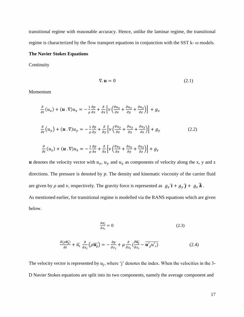
transitional regime with reasonable accuracy. Hence, unlike the laminar regime, the transitional
regime is characterized by the flow transport equations in conjunction with the SST k- ω models.
The Navier Stokes Equations
Continuity
∇. 𝒖 = 0 (2.1)
Momentum
𝜕
𝜕𝑡(𝑢𝑥) + (𝒖 . ∇)𝑢𝑥 = −
1
𝜌
𝜕𝑝
𝜕𝑥+
𝜕
𝜕𝑥[𝜈 (
𝜕𝑢𝑥
𝜕𝑥+
𝜕𝑢𝑥
𝜕𝑦+
𝜕𝑢𝑥
𝜕𝑧)] + 𝑔𝑥
𝜕
𝜕𝑡(𝑢𝑦) + (𝒖 . ∇)𝑢𝑦 = −
1
𝜌
𝜕𝑝
𝜕𝑦+
𝜕
𝜕𝑦[𝜈 (
𝜕𝑢𝑦
𝜕𝑥+
𝜕𝑢𝑦
𝜕𝑦+
𝜕𝑢𝑦
𝜕𝑧)] + 𝑔𝑦 (2.2)
𝜕
𝜕𝑡(𝑢𝑧) + (𝒖 . ∇)𝑢𝑧 = −
1
𝜌
𝜕𝑝
𝜕𝑧+
𝜕
𝜕𝑧[𝜈 (
𝜕𝑢𝑧
𝜕𝑥+
𝜕𝑢𝑧
𝜕𝑦+
𝜕𝑢𝑧
𝜕𝑧)] + 𝑔𝑧
𝒖 denotes the velocity vector with 𝑢𝑥, 𝑢𝑦 and 𝑢𝑧 as components of velocity along the x, y and z
directions. The pressure is denoted by 𝑝. The density and kinematic viscosity of the carrier fluid
are given by 𝜌 and 𝜈, respectively. The gravity force is represented as 𝑔𝑥 �� + 𝑔𝑦 �� + 𝑔𝑧 �� .
As mentioned earlier, for transitional regime is modelled via the RANS equations which are given
below.
𝜕𝑢𝑖
𝜕𝑥𝑖= 0 (2.3)
𝜕(𝜌𝒖𝒋 )
𝜕𝑡+ 𝑢��
𝜕
𝜕𝑥𝑖(𝜌𝒖𝒋 ) = −
𝜕𝑝
𝜕𝑥𝑗+ 𝜇
𝜕
𝜕𝑥𝑖(
𝜕𝒖𝒋
𝜕𝑥𝑖− 𝒖′𝒋
𝑢′𝑖) (2.4)
The velocity vector is represented by 𝑢𝑗 , where ‘j’ denotes the index. When the velocities in the 3-
D Navier Stokes equations are split into its two components, namely the average component and
18
the fluctuating component (Eq. 2.5), it results in the formation of the RANS equations.
𝒖𝒋 = 𝒖𝒋 + 𝒖′𝒋 (2.5)
Where,
𝑢�� = Average component of the velocity.
𝑢′𝑗 = Fluctuating component of the velocity.
When dealing with the RANS equations, it is extremely difficult to quantify the fluctuating
component of the velocities because of their nature of randomness. Hence the shear transport term
(𝒖′𝒋 𝑢′𝑖
) is modelled as shown in eq. This model formulation is based on the Boussinesq hypothesis
(1877).
𝒖′𝒋 𝑢′𝑖
= 𝑣𝑇 (𝜕𝒖𝒋
𝜕𝑥𝑖+
𝜕𝒖𝒊
𝜕𝑥𝑗) (2.6)
As a result of the aforementioned modelling, RANS equations are no longer dependant on the
fluctuating component of the velocity and hence solving the RANS equations is easier.To turn the
RANS equations into a closed system of non-linear differential equations and make them solvable,
it is necessary to obtain math models for 𝑣𝑇 (known as the eddy or turbulent viscosity). In the
current study, a SST-k- ω turbulence model is used to solve for the turbulent viscosity. This model
approximates the turbulent viscosity as a function of the ratio of turbulent kinetic energy (k) and
specific dissipation rate ω. This model is briefly explained below.
𝜕(𝜌𝑘)
𝜕𝑡+
𝜕
𝜕𝑥𝑗(𝜌𝑢𝑗𝑘) = 𝑃�� − 𝐷�� +
𝜕
𝜕𝑥𝑗((𝜇 +
𝜇𝑡
𝜎𝑘)
𝜕𝑘
𝜕𝑥𝑗) (2.7)
where 𝑃�� and 𝐷�� are the terms for production and destruction of turbulence kinetic energy,
respectively; 𝜇𝑡 is the turbulent viscosity and 𝜎𝑘 is the turbulent Prandtl number for k.
𝜕(𝜌𝜔)
𝜕𝑡+
𝜕
𝜕𝑥𝑗(𝜌𝑢𝑗𝜔) = 𝛼
𝑃𝑘
𝑣𝑡− 𝐷𝜔 + 𝑐𝑑𝜔 +
𝜕
𝜕𝑥𝑗((𝜇 +
𝜇𝑡
𝜎𝜔)
𝜕𝜔
𝜕𝑥𝑗) (2.8)
19
where 𝜔 is specific dissipation rate, 𝑣𝑡 is the turbulent eddy viscosity, and 𝑐𝑑𝜔 is the cross
diffusion term.
𝜕(𝜌𝛾)
𝜕𝑡+
𝜕
𝜕𝑥𝑗(𝜌𝑢𝑗𝛾) = 𝑃𝛾1 − 𝐸𝛾1 + 𝑃𝛾2 − 𝐸𝛾2 +
𝜕
𝜕𝑥𝑗((𝜇 +
𝜇𝑡
𝜎𝛾)
𝜕𝛾
𝜕𝑥𝑗) (2.9)
where 𝑃𝛾1 and 𝐸𝛾1 are transition source terms, 𝑃𝛾2 and 𝐸𝛾2 are destruction source terms and 𝛾 is
the intermittency coefficient. But since for calculating 𝑃𝛾1 we require critical Reynolds number
��𝑒𝜃𝑐, a transported scalar ��𝑒𝜃𝑡 is used in the transport equation to calculate ��𝑒𝜃𝑐
𝜕(𝜌��𝑒𝜃𝑡)
𝜕𝑡+
𝜕
𝜕𝑥𝑗(𝜌𝑢𝑗��𝑒𝜃𝑡) = 𝑃𝜃𝑡 +
𝜕
𝜕𝑥𝑗(𝜎𝜃𝑡(𝜇 + 𝜇𝑡)
𝜕��𝑒𝜃𝑡
𝜕𝑥𝑗) (2.10)
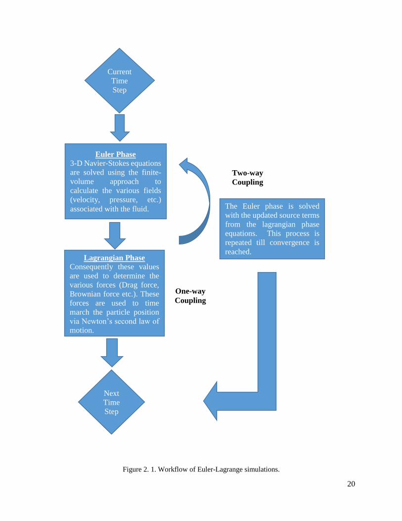
2.4. Particle Dynamics Equations
An Euler-Lagrange approach was used to solve for the fluid-particle dynamics. Euler (in
this case being the carrier fluid) refers to the fluid phase, being treated as a continuum, while the
Lagrangian phase is being treated as a discrete phase (the drug particles). The Lagrangian phase is
tracked individually along the particle path, where the particles are grouped together to form an
“element” with the aggregation of such similar elements creating a control volume. The finite
volume methodology utilizes the control volume approach to solve for the scalar, vector and tensor
fields associated with the carrier fluid. The particle transport equation for particles under
consideration (micron and nano-sized particles) takes the form of Newton’s second law of
motion.The workflow of equations solved in the Euler-Lagrangian approach in a particular time
step is shown in Figure 2.1.The trajectories of the particles are calculated by time-marching the
Ordinary Partial Differential Equations (ODEs) represented by Eq. (2.11).
𝑚𝑝𝜕(𝒗𝒑)
𝜕𝑡= ∑ 𝑭𝒑 (2.11)
Here the 𝒗𝒑 and 𝑚𝑝 denote the velocity and the mass of the particle, respectively; while ∑ 𝑭𝒑
20
Figure 2. 1. Workflow of Euler-Lagrange simulations.
Euler Phase 3-D Navier-Stokes equations
are solved using the finite-
volume approach to
calculate the various fields
(velocity, pressure, etc.)
associated with the fluid.
Lagrangian Phase Consequently these values
are used to determine the
various forces (Drag force,
Brownian force etc.). These
forces are used to time
march the particle position
via Newton’s second law of
motion.
The Euler phase is solved
with the updated source terms
from the lagrangian phase
equations. This process is
repeated till convergence is
reached.
Current
Time
Step
Next
Time
Step
One-way
Coupling
Two-way
Coupling
21
represents the summation of the various forces acting on the particle. The forces acting on the
particle are greatly dependant on the size of the particles. For example, gravity and drag forces
dominate the dynamics of micron particles while Brownian and lift forces play a major role in
determining the trajectories of nanoparticles.
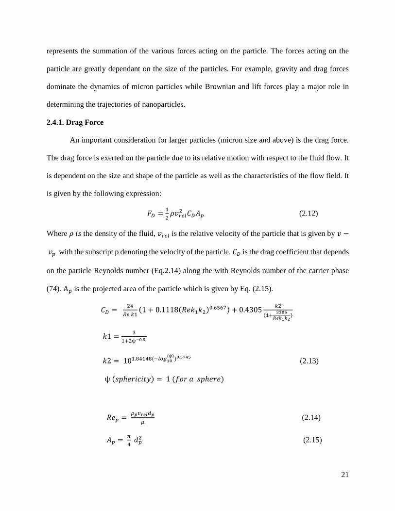
2.4.1. Drag Force
An important consideration for larger particles (micron size and above) is the drag force.
The drag force is exerted on the particle due to its relative motion with respect to the fluid flow. It
is dependent on the size and shape of the particle as well as the characteristics of the flow field. It
is given by the following expression:
𝐹𝐷 =1
2𝜌𝑣𝑟𝑒𝑙
2 𝐶𝐷𝐴𝑝 (2.12)
Where 𝜌 𝑖𝑠 the density of the fluid, 𝑣𝑟𝑒𝑙 is the relative velocity of the particle that is given by 𝑣 −
𝑣𝑝 with the subscript p denoting the velocity of the particle. 𝐶𝐷 is the drag coefficient that depends
on the particle Reynolds number (Eq.2.14) along the with Reynolds number of the carrier phase
(74). Ap is the projected area of the particle which is given by Eq. (2.15).
𝐶𝐷 = 24
𝑅𝑒 𝑘1(1 + 0.1118(𝑅𝑒𝑘1𝑘2)0.6567) + 0.4305
𝑘2
(1+3305
𝑅𝑒𝑘1𝑘2)
𝑘1 =3
1+2ѱ−0.5
𝑘2 = 101.84148(−𝑙𝑜𝑔10(ѱ)
)0.5745 (2.13)
ѱ (𝑠𝑝ℎ𝑒𝑟𝑖𝑐𝑖𝑡𝑦) = 1 (𝑓𝑜𝑟 𝑎 𝑠𝑝ℎ𝑒𝑟𝑒)
𝑅𝑒𝑝 = 𝜌𝑝𝑣𝑟𝑒𝑙𝑑𝑝
𝜇 (2.14)
𝐴𝑝 = 𝜋
4 𝑑𝑝
2 (2.15)
22
2.4.2. Brownian Force
For particles in the nano-scale domain, corresponding to the ultra-fine suspensions in this
study, the momentum is imparted to the particles by the fluid at random; unlike micron particles
where inertia is the major driving force. As a result, the particles move in a random path. As the
size of the nanoparticles increases, the influence of the Brownian force decreases. The Brownian
force is given by the following equation.
𝑭𝑩 = 𝜻√𝝅𝑺𝟎
𝚫𝒕 (2.16)
where 𝜁 is a zero-mean, unit-variance Gaussian random number , Δ𝑡 is the time-step size of
particle integration and 𝑆0 is the spectral intensity function defined as
𝑆0 = 216 𝜇 𝑘𝑏 𝑇
𝜋2𝑑𝑝5 𝜌𝑝
2 𝐶𝑐 (2.17)
𝑘𝑏 =𝑅
𝑁𝑎=
8.315 𝑋 103 𝐽
𝑘𝑚𝑜𝑙 .𝐾
6.022 𝑋 1026 𝑚𝑜𝑙𝑒𝑐𝑢𝑙𝑒
𝑘𝑚𝑜𝑙
1.38 𝑋 10−23 𝐽
𝑚𝑜𝑙𝑒𝑐𝑢𝑙𝑒 . 𝐾 (2.18)
here 𝜇 and 𝑇 is the dynamic viscosity and Temperature of the carrier phase respectively. 𝜇𝑝 and
𝑑𝑝 denote the dynamic viscosity and diameter of the particle respectively. 𝑘𝑏 (Eq. 2.18) is the
Boltzmann constant and 𝐶𝑐 is the Cunningham correction factor given by
𝐶𝑐 = 1 + 2𝜆
𝑑𝑝 (1.17 + 0.525 𝑒
−(0.78 𝑑𝑝
2𝜆)) (2.19)
𝜆 is the mean-free path of the carrier phase.
2.4.3. Saffman Lift Force
Small particles in a shear field experience a lift force perpendicular to the direction of
flow. It is as a result of inertia effects in a viscous flow.
23
𝐹𝐿 = 𝜋
6𝑑𝑝
3𝜌𝐶𝐿 ((�� − ��𝑝)Xcurl(��)) (2.20)
where
𝐶𝐿 = 3 𝐶𝑙𝑑
2𝜋 √𝜌|𝑐𝑢𝑟𝑙(��)| 𝑑𝑝
2
𝜇
(2.21)
𝐶𝑙𝑑 = 6.46 ∗ 0.0524 √0.5𝜌|𝑐𝑢𝑟𝑙(��)| 𝑑𝑝
2
𝜇 (2.22)
2.4.4. Gravitational Force
Gravitational force is experienced due to the earth’s gravitational force. However for
convenience Buoyancy forces are grouped with the gravitational forces. Buoyancy force is the
upward exerted on the particle submerged in the fluid. These forces directly impact particle
deposition due to sedimentation and hence for bigger particles it is essential to take these forces
into account. It is given by Eq.2.23. The subscripts p and f represent the particle and carrier phase
(fluid) respectively.
𝐹𝑔 = 𝑚𝑝𝑔 (1 −𝜌𝑓
𝜌𝑝) (2.23)
2.5. Quantifying Particle Deposition
For accurately determining the deposition efficiencies, it is essential to specify the various
boundary conditions for the particles. OpenFOAM has three basic options, namely REBOUND,
STICK and ESCAPE.
The particle is said to STICK when it is at the particle-radius distance from the wall.
REBOUND boundary condition makes the particle rebound from the particular patch
(Coefficient of Restitution = 1).
The ESCAPE boundary condition allows the particle to pass through the particular patch
and escape the geometry without sticking or rebounding.

24
Table 2. 1. Boundary conditions for Particles.
PART BOUNDARY CONDITIONS
NASALINLET REBOUND
NASAL STICK
OUT ESCAPE
For an Euler-Lagrange approach, Deposition Fraction (DF) is a parameter used to quantify the
percentage of deposition.
DFregion =Number of particles deposited in a specific region
Number of particles entering the region (2.24)
2.6. Quasi-Steady vs Transient particle dynamics
As mentioned above, drug deposition is the parameter used to measure the efficacy of drug
delivery. As far as practical application is considered, drug delivery is a transient phenomenon.
The various transient studies have been explained in Chapter 1. Drug deposition in transient studies
is highly sensitive to various parameters like time of injection, duration of injection, etc. However
while conducting studies that determine the effect of flowrate and particle injection, it is essential
to isolate only these parameters. Furthermore transient studies are more computationally expensive
and time consuming than quasi- steady state studies. Hence before conducting a transient
simulation that mimics the workings of an actual drug delivery system like an inhaler or a nasal
spray, particle deposition in a quasi-steady state flow is measured to determine the optimum
particle diameter and flowrate as well as the desired position of injection for maximum olfactory
deposition efficiency. In this study, all the simulations performed are under the assumption of
quasi-steady state conditions. According to the approach reported in previous studies (61, 75) , a

25
steady state inhalation value that results in the same deposition as that of a transient case is
calculated using the following formula :-
𝑄𝑚𝑎𝑡𝑐ℎ = 𝐶 (𝑄𝑚𝑒𝑎𝑛 + 𝑄𝑚𝑎𝑥 ) (2.22)
Where C ≈ 0.5 for all smooth inhalation forms.This result is an important one because it forms a
bridge between the steady and transient inhalation results. It furthermore shows that the steady and
transient results are similar in their qualitative distribution while differing in quantitative
deposition results. Hence the optimal particle injection position resulting from a quasi-steady state
flow assumption would also result in the highest olfactory deposition efficiency when using
transient flow with only the exact value being different.

26
CHAPTER 3. NUMERICAL METHOD USING OPENFOAM
3.1 Introduction
For the purpose of this study, an open source Computational Fluid Dynamics toolbox
named OpenFOAM (Open Field Operation and Manipulation) has been used
(https://www.openfoam.com). In addition to being cost-free, this toolbox has far-reaching
applications in engineering and scientific circles. Professionals from industry as well as academia
utilize this toolbox to perform all facets of thorough Computational Fluid Dynamics activities,
ranging from meshing (blockMesh and snappyHexMesh) to numerically solving 3-D
complex flow systems (electromagnetics, turbulence, heat transfer, chemical reactions, multiphase
flow, etc.). Owing to its open source nature, it facilitates the sharing of information and high level
mathematical models for the purposes of a collaborative study. OpenFOAM is also highly
compatible with various post-processing software (eg, ICEM, ParaView and Tecplot) and
therefore results can be analysed without any inconvenience. OpenFOAM is built on the principle
of Object Oriented Programming as it is written in C++. Therefore, all the models and
computational solvers are built based on classes and objects. Furthermore, all the advantageous
features of C++ (inheritance, encapsulation, data abstraction, etc.) are carried over into
OpenFOAM, thereby making it quite user-friendly. The code structure is easy to grasp and enables
the user to not only customize and extend the functionality of existing solvers but also to develop
new ones with great ease. When dealing with numerical computations, running time is an
important factor to be taken into consideration as certain computations may require months.
Running these simulations in “parallel” has been shown to have reduced running (or computing)
time considerably. In this method, the case geometry is decomposed into a number of sections and
each processor is responsible for the computation involving a particular section. In other words,
27
multiple processors are simultaneously carrying out computations and exchanging data as opposed
to only one processor solving necessary governing mathematical equations for the whole case
geometry. OpenFOAM has built-in provisions for decomposition of cases, running them in parallel
as well as reconstructing the decomposed fields for data analysing and post processing. It is
essential to gain understanding of the unique case structure of OpenFOAM to make use of its full
functionality. This structure is explained in the following section.
3.2. Case Structure
As mentioned earlier, OpenFOAM is a multi-purpose open source toolbox for carrying out
computational studies (especially Computational Fluid Dynamics). It has various in built-in
solvers with a sample case study associated with the solver. Each case directory in OpenFOAM
has three main subdirectories: time directories, constant, and system. The content of these
subdirectories varies from solver to solver. For example, the simplest solver in OpenFOAM is
icoFoam which solves the Navier-Stokes equations for an incompressible, isothermal system.
This case contains three subdirectories: 0, constant and system (Figure 3.1). The 0
folder is a time directory that holds the solution (in this case u and p for velocity and pressure,
respectively) during the start of the simulation. Basically the 0 folder is used to specify the initial
and the boundary conditions. These conditions can be very basic, such as a fixed value, to
complicated ones like specifying a time-varying sinusoidal wave at the boundary via swak4Foam
(Swiss Army Knife for FOAM). Like the 0 directory, there can be other time directories that stores
the values of the fields (p, T,u etc.) at those respective time values. These time directories are
used to post-process the simulation results in ParaView. The contents of these time subdirectories
differ from solver to solver. For cases that deal with heat transfer, the time directories will have T
(Temperature) as a field while for turbulence solvers, k and epsilon may be present as fields.

28
Figure 3. 1. OpenFOAM case structure.
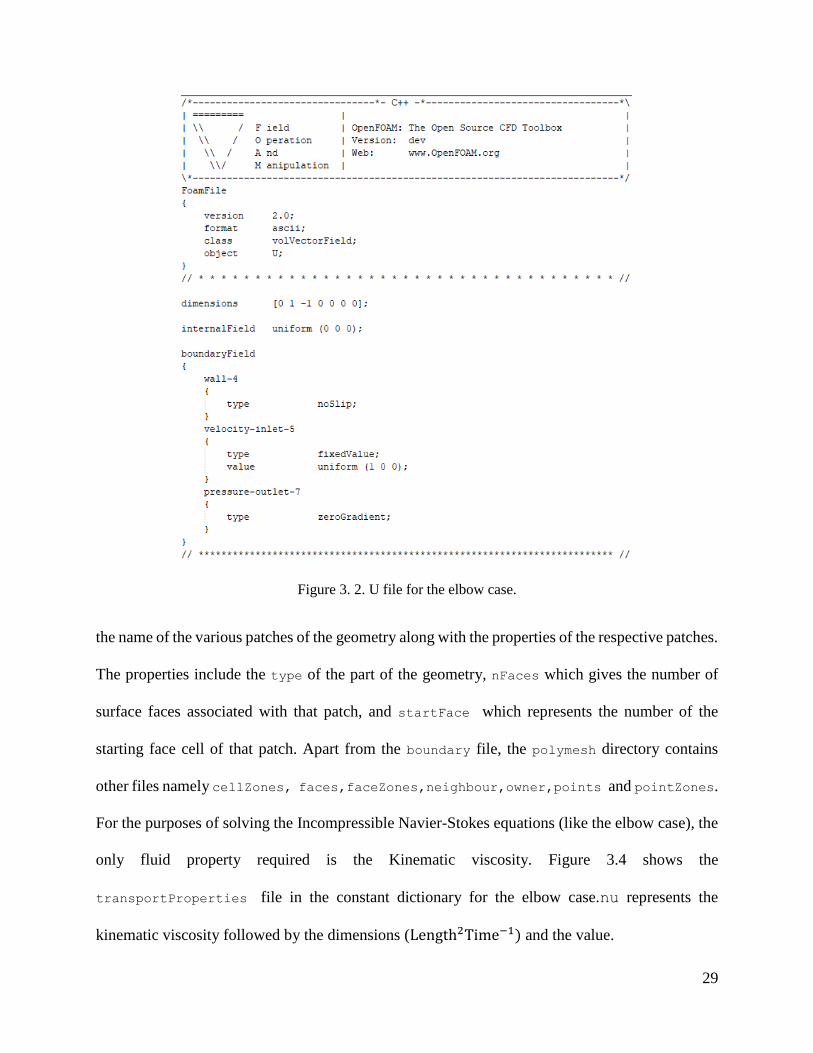
For example, the tutorial case in icoFoam is simulating flow inside an elbow. The 0 folder of the
elbow case requires the boundary conditions for pressure (p) and velocity (U). Figure 3.2 shows
the U file for the elbow case. The file consists of the dimensions of the field, the internalField
which has the information of the initial conditions of the velocity and the boundaryField through
which the boundary conditions are specified. In this case, the velocity magnitude is 0 throughout
the internal mesh. Through OpenFOAM this field can be either uniform or nonuniform; wall-
4, velocity-inlet-5 and pressure-outlet-7 are the names of the patches of the elbow
geometry. Here, noSlip and fixedValue are examples of the Dirchlet boundary condition, while
zeroGradient is a type of Neumann boundary condition.The constant subdirectory has a
polyMesh folder that contains the details of the mesh, ie, the number of points, boundary faces,
neighbouring elements, etc. The directory constant, as the name suggests, also has the values of
those properties that are not varying with time (eg, density, kinematic viscosity, etc.).
Figure 3.3 shows the boundary file in the polyMesh directory for the elbow case. It contains
29
Figure 3. 2. U file for the elbow case.
the name of the various patches of the geometry along with the properties of the respective patches.
The properties include the type of the part of the geometry, nFaces which gives the number of
surface faces associated with that patch, and startFace which represents the number of the
starting face cell of that patch. Apart from the boundary file, the polymesh directory contains
other files namely cellZones, faces,faceZones,neighbour,owner,points and pointZones.
For the purposes of solving the Incompressible Navier-Stokes equations (like the elbow case), the
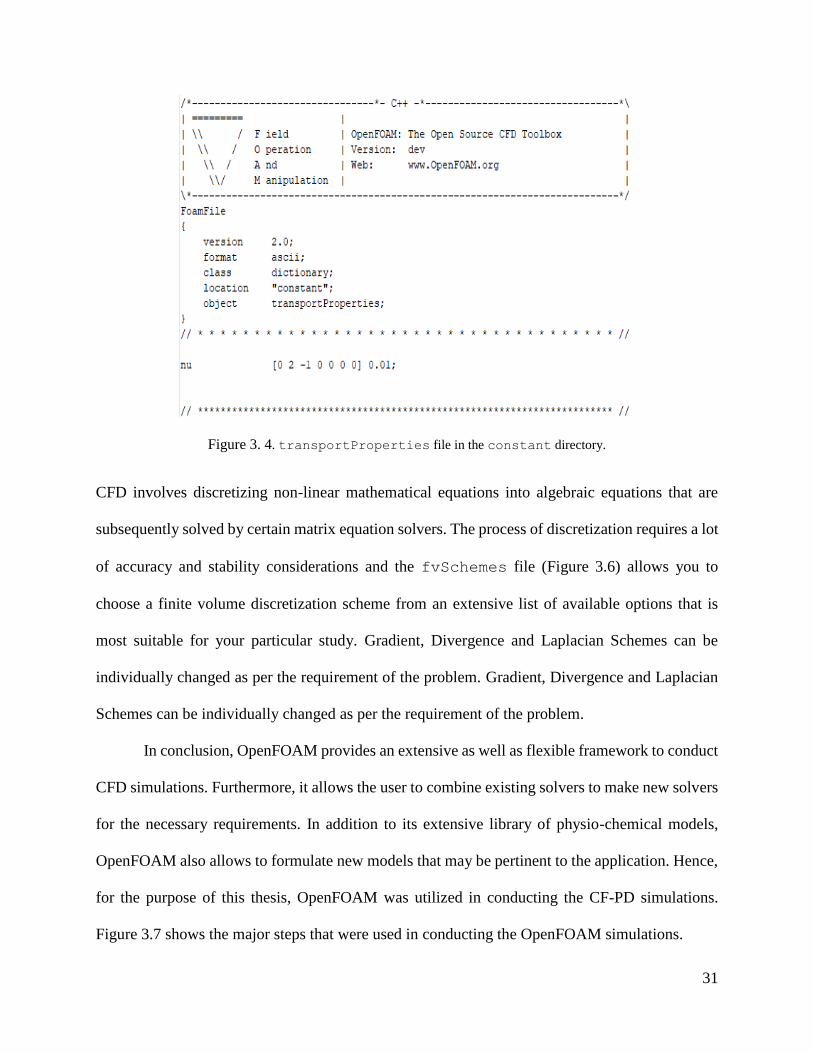
only fluid property required is the Kinematic viscosity. Figure 3.4 shows the
transportProperties file in the constant dictionary for the elbow case.nu represents the
kinematic viscosity followed by the dimensions (Length2Time−1) and the value.

30
Figure 3. 3. boundary file in the polyMesh directory.
While icoFoam is a simple solver, other complex solvers require properties other than the
kinematic viscosity. For nonNewtonianIcoFoam, the specific Non Newtonian Model
(Quemada, Carreau, etc.) along with the value of specific coefficients while for conducting
Computational Fluid-Particle Dynamics (CF-PD) simulations various parcel properties like parcel
injection rate, number of parcels and parcel diameter are to be specified in the constant
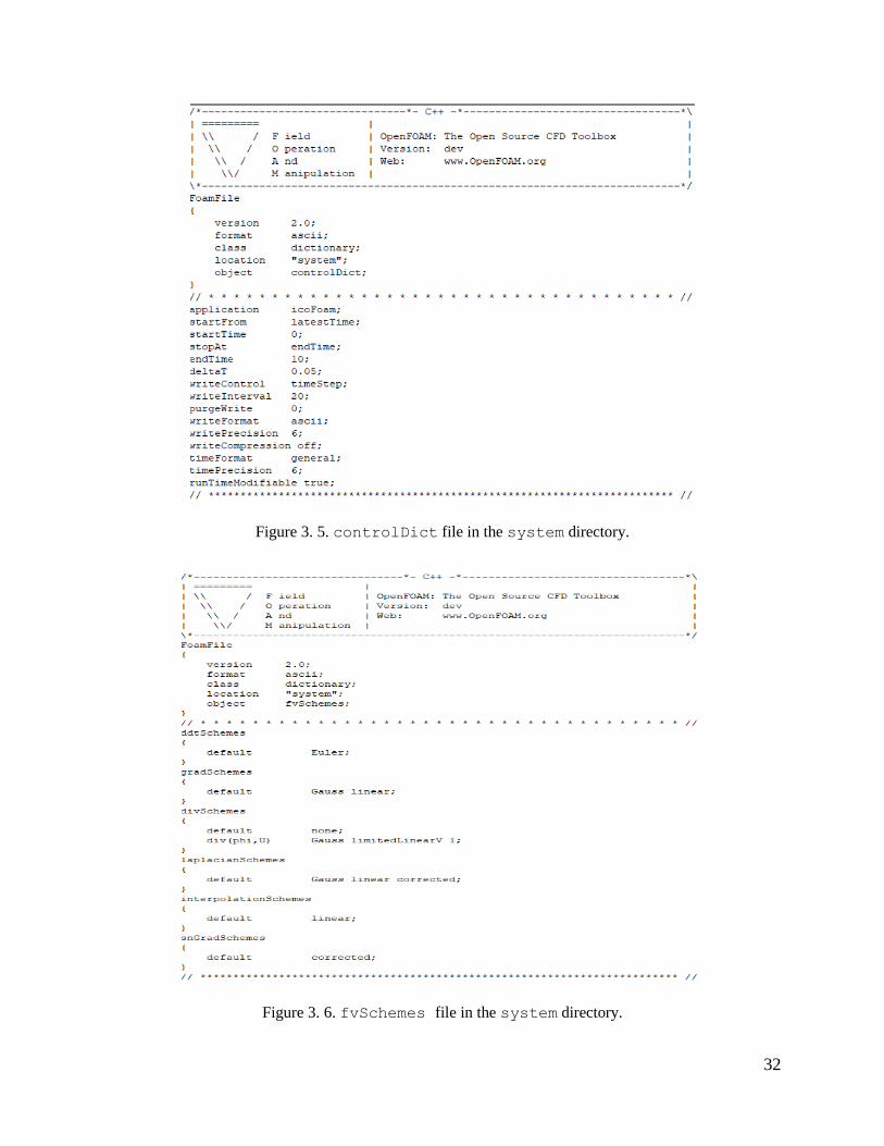
directory.The system directory is comprised of three basic files namely controlDict,
fvSchemes and fvSolutions. The controlDict file is responsible for the Solution Time
control of the simulation. The user specifies the start time, end time, write Interval and time step
of the simulation amongst other parameters in this file (Fig. 3.5).
31
Figure 3. 4. transportProperties file in the constant directory.
CFD involves discretizing non-linear mathematical equations into algebraic equations that are
subsequently solved by certain matrix equation solvers. The process of discretization requires a lot
of accuracy and stability considerations and the fvSchemes file (Figure 3.6) allows you to
choose a finite volume discretization scheme from an extensive list of available options that is
most suitable for your particular study. Gradient, Divergence and Laplacian Schemes can be
individually changed as per the requirement of the problem. Gradient, Divergence and Laplacian
Schemes can be individually changed as per the requirement of the problem.
In conclusion, OpenFOAM provides an extensive as well as flexible framework to conduct
CFD simulations. Furthermore, it allows the user to combine existing solvers to make new solvers
for the necessary requirements. In addition to its extensive library of physio-chemical models,
OpenFOAM also allows to formulate new models that may be pertinent to the application. Hence,
for the purpose of this thesis, OpenFOAM was utilized in conducting the CF-PD simulations.
Figure 3.7 shows the major steps that were used in conducting the OpenFOAM simulations.
32
Figure 3. 5. controlDict file in the system directory.
Figure 3. 6. fvSchemes file in the system directory.

33
Figure 3. 7. Workflow for conducting OpenFOAM simulations.
Mesh
•Create the mesh in ICEM CFD and convert it into the OpenFOAM format using the command: fluentMeshToFoam
•Apply checkMesh -allGeometry -allTopology to detect for any bad elements and any other mesh quality parameters.
•As a result of these commands, a polyMesh folder detailing the points,cells,faces etc of the mesh is created.
Initial and Boundary Conditions
•The initial as well as the boundary conditions of all the fields (p,T,U,k,etc) are specificed in the 0 directory.
Properties
•The different properties that govern the simulation are specified in the constant directory.
•transportProperties contains the density and viscosity of the fluid which are necessary for solving the Navier-Stokes equations.
•turbulenceProperties contains the specific turbulence model required to account for the turbulence effects.
•kinematicCloudProperties file enables to specify the injection position, the parcel properties,etc.
Solution Control
•The next step is to specify the time step, write interval, etc in the controlDict file present in the system directory.
•In addition to that the various finite volume schemes and the algebric solvers are specificed in the fvSchemes and fvSolutions files respectively in the same directory.
Running the Solver
•The final step includes running the respective solver. This can be done in two ways:-
•Serial - The simulation utilizes only one processor and hence is higher execution time. For e.g. running simpleFoam in serial processing is executed by the following command: simpleFoam.
•Parallel - OpenFOAM also has the option of running simulations using multiple processes. In this approach , the geometric mesh is decomposed into multiple parts where each processor is responsible for the computation of each part. The decomposition algorithm and the number of processors can be specified via the decomposeParDict file in the system directory. For e.g. running simpleFoam in parallel processing with 10 processors is executed by the following command: mpirun -n 10 simpleFoam -parallel
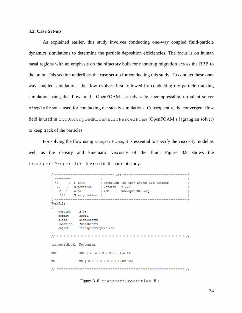
34
3.3. Case Set-up
As explained earlier, this study involves conducting one-way coupled fluid-particle
dynamics simulations to determine the particle deposition efficiencies. The focus is on human
nasal regions with an emphasis on the olfactory bulb for nanodrug migration across the BBB to
the brain. This section underlines the case set-up for conducting this study. To conduct these one-
way coupled simulations, the flow evolves first followed by conducting the particle tracking
simulation using that flow field. OpenFOAM’s steady state, incompressible, turbulent solver
simpleFoam is used for conducting the steady simulations. Consequently, the convergent flow
field is used in icoUncoupledKinematicParcelFoam (OpenFOAM’s lagrangian solver)
to keep track of the particles.
For solving the flow using simpleFoam, it is essential to specify the viscosity model as
well as the density and kinematic viscosity of the fluid. Figure 3.8 shows the
transportProperties file used in the current study.
Figure 3. 8. transportProperties file.

35
For icoUncoupledKinematicParcelFoam it is essential to determine the particle
properties will govern their trajectory. As mentioned these properties are specified using the
kinematicCloudProperties file. Figure 3.9 shows a snippet of the file to show the
syntax for providing information regarding the properties of particles, the forces acting on the
particles and the injection model to be specified.
Figure 3. 9. Snippet of the kinematicCloudProperties file.
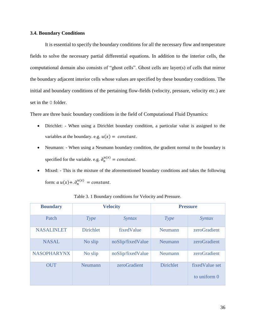
36
3.4. Boundary Conditions
It is essential to specify the boundary conditions for all the necessary flow and temperature
fields to solve the necessary partial differential equations. In addition to the interior cells, the
computational domain also consists of “ghost cells”. Ghost cells are layer(s) of cells that mirror
the boundary adjacent interior cells whose values are specified by these boundary conditions. The
initial and boundary conditions of the pertaining flow-fields (velocity, pressure, velocity etc.) are
set in the 0 folder.
There are three basic boundary conditions in the field of Computational Fluid Dynamics:
Dirichlet: - When using a Dirichlet boundary condition, a particular value is assigned to the
variables at the boundary. e.g. 𝑢(𝑥) = 𝑐𝑜𝑛𝑠𝑡𝑎𝑛𝑡.
Neumann: - When using a Neumann boundary condition, the gradient normal to the boundary is
specified for the variable. e.g. 𝜕𝑛𝑢(𝑥)
= 𝑐𝑜𝑛𝑠𝑡𝑎𝑛𝑡.
Mixed: - This is the mixture of the aforementioned boundary conditions and takes the following
form: 𝑎 𝑢(𝑥)+. 𝜕𝑛𝑢(𝑥)
= 𝑐𝑜𝑛𝑠𝑡𝑎𝑛𝑡.
Table 3. 1 Boundary conditions for Velocity and Pressure.
Boundary Velocity Pressure
Patch Type Syntax Type Syntax
NASALINLET Dirichlet fixedValue Neumann zeroGradient
NASAL No slip noSlip/fixedValue Neumann zeroGradient
NASOPHARYNX No slip noSlip/fixedValue Neumann zeroGradient
OUT Neumann zeroGradient Dirichlet fixedValue set
to uniform 0

37
Table 3. 2 Boundary conditions for Turbulent Kinetic Energy and Turbulence Dissipation
Frequency.
Boundary Turbulent Kinetic Energy Turbulence Dissipation
Frequency
Patch Type Syntax Type Syntax
NASALINLET Dirichlet fixedValue Dirichlet fixedValue
NASAL Dirichlet kqR
WallFunction
Dirichlet omega
WallFunction
NASOPHARYNX Dirichlet kqR
WallFunction
Dirichlet omega
WallFunction
OUT Neumann zeroGradient Neumann zeroGradient
For a given boundary, different types of boundary conditions can be used for different variables.
Table 3.1 shows the pressure and velocity boundary conditions while Table 3.2 shows the
boundary conditions for the turbulence parameters: Turbulence Kinetic Energy and Specific
Dissipation Frequency.The detailed description for the boundary conditions is given below:
<patchName>
{
type
<Boundary Condition Type>;
value
uniform <Specific Value>;
}
<patchName> is used to specify the name of the boundary patch as per the mesh.

38
type is used to specify the name of the boundary condition recognized by the solver.
value, as the name suggests denotes the specific value (scalar or vector) of the boundary
condition.
The type options used in this particular study are as follows:-
fixedValue:- This option maintains a particular value at the boundary patch. It is a type of
Dirchlet boundary condition. The value needs to be specified under the value option. E.g.
uniform (0 1 0) for a vector, uniform 2.0 for a scalar etc.
noSlip:- This is special type of fixedValue boundary condition whose value is 0.
zeroGradient:- This option indicates that the gradient of the variable normal to the boundary
is 0. It is a type of Neumann boundary condition.
𝛛𝐮
𝛛𝐧= 𝟎 (3.1)
u corresponds to the particular variable and n is the normal vector to the boundary patch.
As explained in Section 2.3, certain flowrates used for this study correspond to transitional regimes
and hence it is essential to model the effects of turbulence. The existence of turbulence creates
random fluctuations and as a result the velocity profile and wall effects are different from the
laminar regime. A non-dimensional number 𝑦+(Eq) is used to divide the region near the wall into
three parts: viscous sublayer, buffer layer and log-law region.
𝒚+ = 𝒖𝝉𝒚
𝝂 (3.2)
where 𝑢𝜏 (eq) is the shear velocity , 𝒚 is the distance from the wall and 𝜈 is the kinematic viscosity
of the fluid.
𝒖𝝉 = √𝝉𝒘
𝝆 (3.3)
𝜏𝑤 is the wall shear stress and 𝜌 is the density of the fluid.
39
Viscous Sublayer for y+ < 5
Buffer Layer for 5 < y+ < 30 (3.4)
Log − law layer for 30 < y+ < 200
𝑦+ value can be thought of as a local Reynolds number and shows the relative significance between
the turbulent and viscous stresses. Viscous Sublayer is the region closest to the wall where the
laminar stresses are dominant. In the buffer region the stresses are of the same order while the log-
law makes up >90% of the region where turbulence dominates. Due to its transitional nature, it is
difficult to capture the flow-field physics of the buffer layer unlike the other two other layers.
Hence there is a need for empirical wall functions; for example, kqRWallFunction and
omegaWallFunction are options for the turbulence kinetic energy (k) and turbulent
dissipation rate (𝜔), respectively. These two turbulence parameters are essential to form a closed
system of turbulence equations that are required to resolve the flow completely. kqRWallFunction
is a zeroGradient type of Neumann boundary condition. omegaFunction has a
functionality of changing the value based on the y+ value.
The syntax for the aforementioned wall functions is similar to that of that of pressure and
velocity. In addition to the initial and boundary conditions, the case set-up also requires the
numerical schemes that are being used to solve the partial differential equations.
3.5. Numerical Schemes
The Navier-Stokes equations are a set of non-linear partial differential equations that
govern the physics of the flow. These equations are not theoretically solvable and hence the need
for Computational Fluid Dynamics (CFD) studies. CFD involves converting these complex
equations into simple algebraic equations using certain numerical schemes. For the purposes of
stability, convergence and accuracy, it is important to select the appropriate numerical schemes.
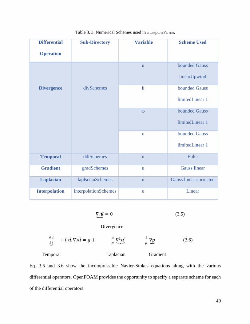
40
Table 3. 3. Numerical Schemes used in simpleFoam.
Differential
Operation
Sub-Directory Variable Scheme Used
Divergence
divSchemes
u bounded Gauss
linearUpwind
k bounded Gauss
limitedLinear 1
ω bounded Gauss
limitedLinear 1
ε bounded Gauss
limitedLinear 1
Temporal ddtSchemes u Euler
Gradient gradSchemes u Gauss linear
Laplacian laplscianSchemes u Gauss linear corrected
Interpolation interpolationSchemes u Linear
∇. ��⏟ = 0 (3.5)
Divergence
𝜕��
𝜕𝑡⏟ + ( ��. ∇)�� = 𝑔 + 𝜇
𝜌 ∇2𝒖 ⏟ −
1
𝜌 ∇𝑝⏟ (3.6)
Temporal Laplacian Gradient
Eq. 3.5 and 3.6 show the incompressible Navier-Stokes equations along with the various
differential operators. OpenFOAM provides the opportunity to specify a separate scheme for each
of the differential operators.

41
Table 3.3 shows the various numerical schemes used in the simpleFoam. These are mentioned
under the fvSchemes dictionary in the system directory. It also shows the sub-dictionaries
corresponding to the differential operators. The finite-volume method solves for the average value
of the system variables. However, the aforementioned numerical schemes require the values at the
boundary of each cell. Hence the need for the interpolationSchemes sub-dictionary. These
schemes can be adjusted as per the requirements of the problem.
3.6. Solution Control
Table 3. 4. Algebraic solvers used in simpleFoam.
Variable Solver Smoother
U smoothSolver GaussSeidel
P GAMG GaussSeidel
K smoothSolver GaussSeidel
Ω smoothSolver GaussSeidel
Once the differential equations are converted into algebraic equations by the appropriate numerical
schemes, certain algebraic solvers are used to get the values of the field variables at each time step.
The choice of the solvers affects the computational time and stability of the simulation. Table 3.4
shows the algebraic solvers used for the system variables. GAMG (Generalized geometric algebraic
multi-grid) solver is used for pressure while the smoothSolver is used for the rest of the
variables. GAMG is a multi-grid solver and is considerably faster than the standard methods. This
solver generates a quick solution for a coarser mesh, maps this solution onto the finer mesh and
using it as an initial guess. The smoothSolver uses a standard Gauss Seidel approach to
calculate the solution.
42
CHAPTER 4. MODEL VALIDATIONS
4.1. Introduction
Predictive computational fluid-particle dynamics (CF-PD) simulations are an essential tool
to analyze complex fluid systems that are otherwise too costly and intricate to evaluate in vitro. In
vivo studies of, say, the nasal cavity, are difficult to undertake due to the delicate nature of the
organs involved. Hence the need for conducting “computer experiments” that capture the physics
of the problem with reasonable realism and accuracy. These CF-PD simulations allow evaluating
the impact of significant parameters (e.g., system configuration, flowrate, particle diameter, etc.)
and eliminating extraneous factors. This chapter is divided into multiple sections based on different
case studies that have been validated. As explained earlier, these simulations are carried out using
an open source CF-PD toolbox named OpenFOAM®. These validations were necessary as they
confirm the validity of the solvers and models available in OpenFOAM. Section 4.3 compares the
Euler-Lagrange approach used for tracking micron-size particles inside the nasal cavity with the
results presented by Calmet et al., 2018(60). Section 4.4 discusses the legitimacy of the Lagrangian
approach for nanoparticle tracking. Numerical simulation results are compared with an analytical
solution presented by Ingham, 1975 (76). Section 4.4 compares the Euler-Lagrange approach used
for tracking nanoparticles inside the nasal cavity with the results presented by Tian et al., 2019(69).
As the thesis involves studying particle deposition, it is pivotal to mention the methodology behind
the Euler-Lagrange particle tracking solvers in OpenFOAM. For steady-state simulations of the
Eulerian phase, OpenFOAM uses the SIMPLE (Semi-Implicit Method for Pressure-Linked
Equations), while employing the PIMPLE algorithm for transient cases. The PIMPLE algorithm
is a combination of the PISO (Pressure Implicit with Splitting of Operator) and SIMPLE. In each
time step, the Eulerian variables (u, p, k, ω, etc.) were solved until residual convergence
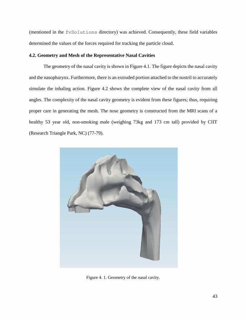
43
(mentioned in the fvSolutions directory) was achieved. Consequently, these field variables
determined the values of the forces required for tracking the particle cloud.
4.2. Geometry and Mesh of the Representative Nasal Cavities
The geometry of the nasal cavity is shown in Figure 4.1. The figure depicts the nasal cavity
and the nasopharynx. Furthermore, there is an extruded portion attached to the nostril to accurately
simulate the inhaling action. Figure 4.2 shows the complete view of the nasal cavity from all
angles. The complexity of the nasal cavity geometry is evident from these figures; thus, requiring
proper care in generating the mesh. The nose geometry is constructed from the MRI scans of a
healthy 53 year old, non-smoking male (weighing 73kg and 173 cm tall) provided by CIIT
(Research Triangle Park, NC) (77-79).
Figure 4. 1. Geometry of the nasal cavity.

44
Figure 4. 2. Complete view of the Nasal Cavity Geometry.
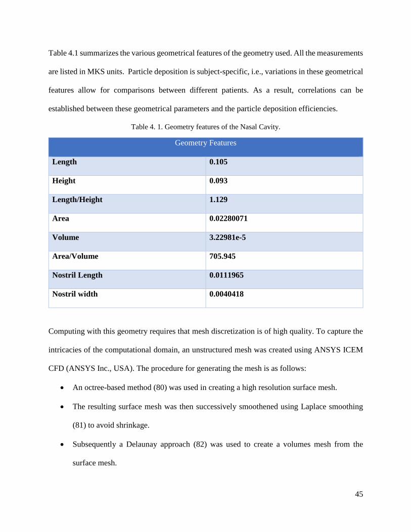
45
Table 4.1 summarizes the various geometrical features of the geometry used. All the measurements
are listed in MKS units. Particle deposition is subject-specific, i.e., variations in these geometrical
features allow for comparisons between different patients. As a result, correlations can be
established between these geometrical parameters and the particle deposition efficiencies.
Table 4. 1. Geometry features of the Nasal Cavity.
Geometry Features
Length 0.105
Height 0.093
Length/Height 1.129
Area 0.02280071
Volume 3.22981e-5
Area/Volume 705.945
Nostril Length 0.0111965
Nostril width 0.0040418
Computing with this geometry requires that mesh discretization is of high quality. To capture the
intricacies of the computational domain, an unstructured mesh was created using ANSYS ICEM
CFD (ANSYS Inc., USA). The procedure for generating the mesh is as follows:
An octree-based method (80) was used in creating a high resolution surface mesh.
The resulting surface mesh was then successively smoothened using Laplace smoothing
(81) to avoid shrinkage.
Subsequently a Delaunay approach (82) was used to create a volumes mesh from the
surface mesh.
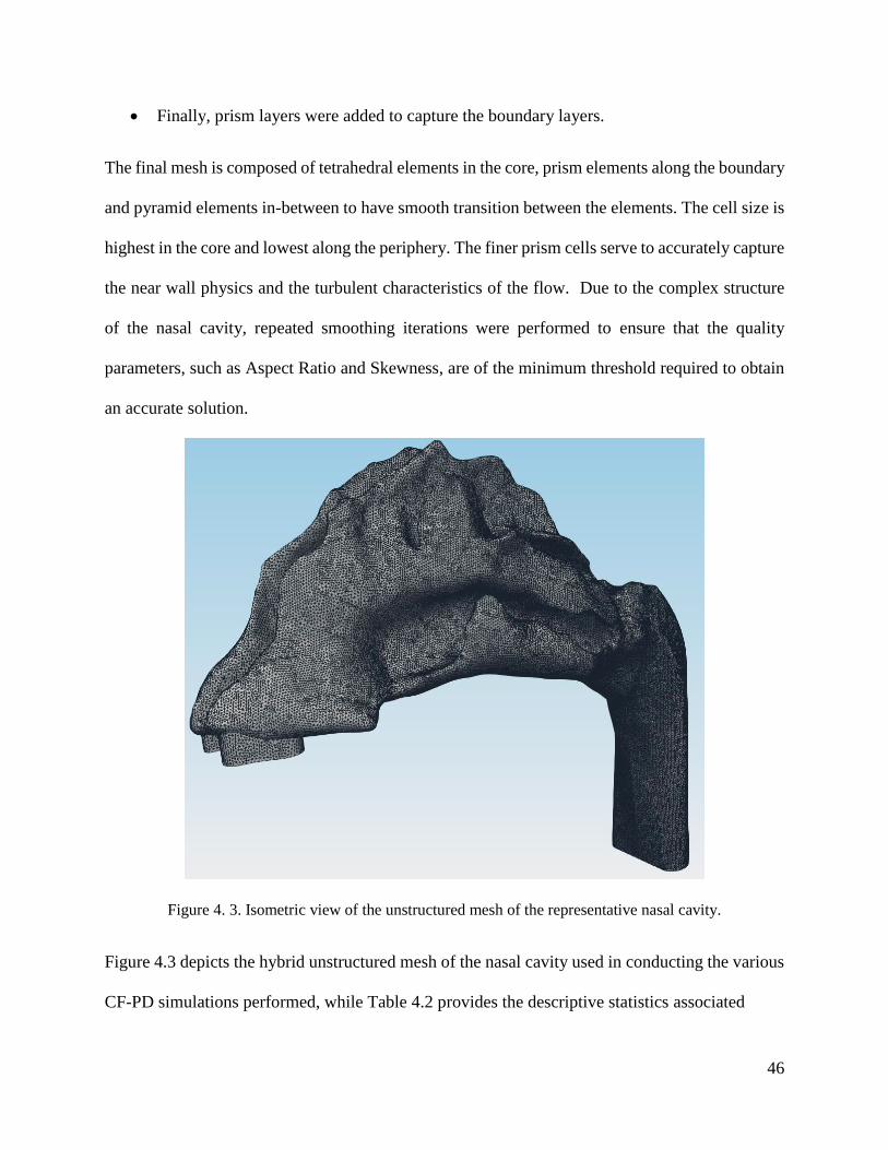
46
Finally, prism layers were added to capture the boundary layers.
The final mesh is composed of tetrahedral elements in the core, prism elements along the boundary
and pyramid elements in-between to have smooth transition between the elements. The cell size is
highest in the core and lowest along the periphery. The finer prism cells serve to accurately capture
the near wall physics and the turbulent characteristics of the flow. Due to the complex structure
of the nasal cavity, repeated smoothing iterations were performed to ensure that the quality
parameters, such as Aspect Ratio and Skewness, are of the minimum threshold required to obtain
an accurate solution.
Figure 4. 3. Isometric view of the unstructured mesh of the representative nasal cavity.
Figure 4.3 depicts the hybrid unstructured mesh of the nasal cavity used in conducting the various
CF-PD simulations performed, while Table 4.2 provides the descriptive statistics associated

47
with the aforementioned mesh.
Table 4. 2. Unstructured mesh characteristics.
Mesh Statistics
Number of Points 1071282
Number of Elements 4269286
Number of Faces 9106628
Number of prism elements 906380
Number of tetrahedral elements 3362856
Number of pyramid elements 50
Number of prism layers 4
Minimum edge length 3.08642e-06
Maximum edge length 0.00103895
Figure 4. 4. Mesh slice of the mid-section of the nasal cavity.

48
Figure 4. 5. Mesh slice of the nostrils.
4.3. Comparison with Calmet et al., 2018
For model validation, the present results were compared to airflow pattern and particle
deposition of Calmet et al., 2018 (60).This was done to confirm the validity of the Lagrangian
micron-particle tracking approach used in OpenFOAM®. The paper presents a detailed analysis
on the airflow and particle deposition efficiencies for varying flowrates (7.5lpm to 20lpm).
Furthermore, a subject-variability study compared the velocity contours and deposition fractions
between three different geometries. However, for the purposes of this thesis, only one
representative nasal geometry has been considered, namely Subject A which is being used in this
thesis.
4.3.1. Airflow Field Results
For the purposes of analyzing the flow field, six slices have been cut into the nasal
geometry. The location of these slices are shown in Figure 4.6. The flow is assumed to be steady

49
and the inlet flowrate is set to be at 20lpm. The velocity contours in each of these slices are given
in Figure 4.7, where these are dimensionless velocity contours (u/Uinlet) perpendicular to the plane.
Furthermore, the dimensionless velocities of the first two slices range until unity and the rest of
them range from 0 to 0.75. As it is evident from Slice 1-1’, higher velocities are observed in the
left nasal cavity because of the smaller cross sectional area for the same inflow rate. The presence
of these narrow, intricate pathways creates a jet- like flow. Slice 2-2’ shows the undulating
pathway inside the nasal cavity. It also indicates that the bulk velocity is located in the middle
where the superior portion receives zero flowrates.
Slices 3-3’ to 5-5’ in Figure 4.8 cover the region of the nasal cavity known as the meatuses.
These slices indicate that there is a near symmetric flow distribution in the left and right meatuses
with slight differences due to the unusual asymmetry in the middle-meatus region. Slice 6-6’
(Figure 4.8) marks the end of the nasal cavity and the start of the nasopharynx. It shows an
asymmetric velocity distribution with the posterior region with elevated flowrates due to the
presence of Dean Vortices. This is resulting from the geometry undergoing a 90° bend from the
nasal passages to the descending nasopharynx. In summary, the airflow entering through nostrils
undergoes a drastic change as it traverses through the complicated, undulating pathways of the
nasal cavity. Most of the air flows through the wider middle-to-lower portion of the cavity that are
free of obstacles. As the air passes, due to the no-slip condition boundary layer forms along the
boundary of the main meatuses and the main passageway. Finally, airflow from both the
passageways converge in the nasopharynx.Wall shear stress is an important factor representing the
resistance to the flow during respiration. Figure 4.9 shows the wall shear stress contour of the nasal
cavity for a flowrate of 20lpm. Through the figure it can be observed that the maximum wall shear
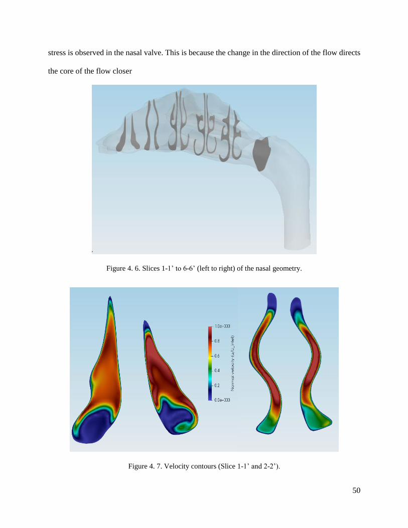
50
stress is observed in the nasal valve. This is because the change in the direction of the flow directs
the core of the flow closer
Figure 4. 6. Slices 1-1’ to 6-6’ (left to right) of the nasal geometry.
Figure 4. 7. Velocity contours (Slice 1-1’ and 2-2’).

51
Figure 4. 8. Velocity contours (Slice 3-3’ to Slice 6-6’).
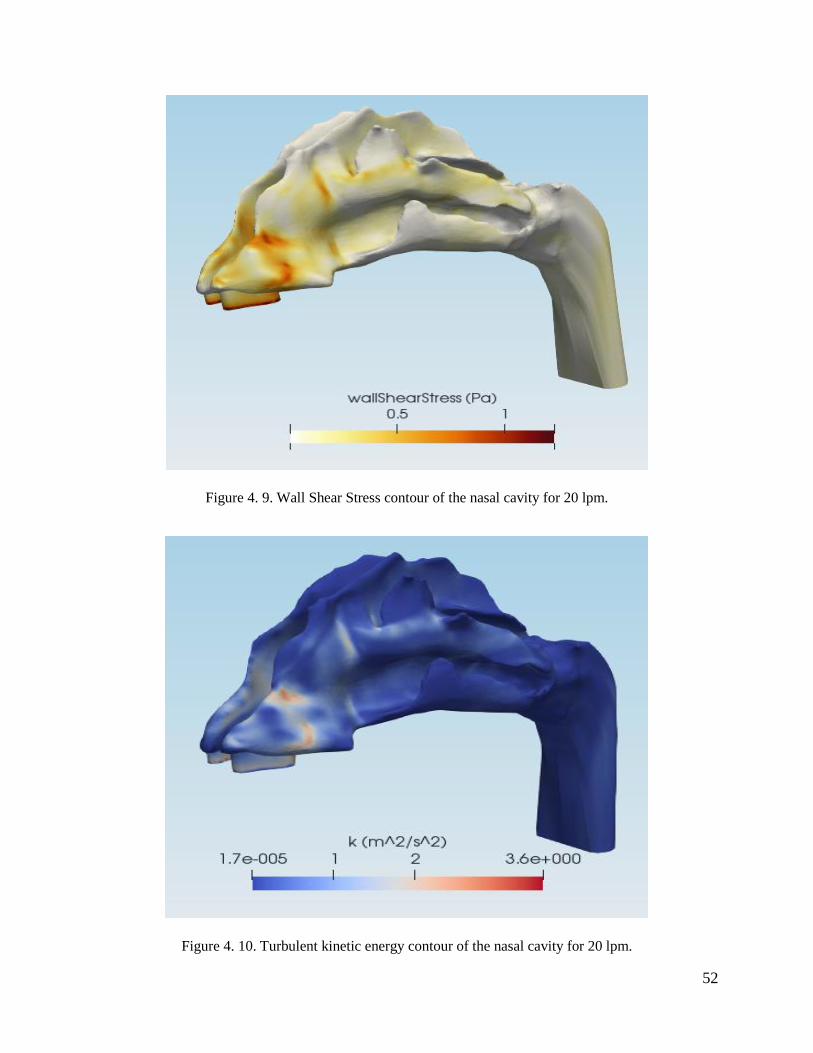
52
Figure 4. 9. Wall Shear Stress contour of the nasal cavity for 20 lpm.
Figure 4. 10. Turbulent kinetic energy contour of the nasal cavity for 20 lpm.
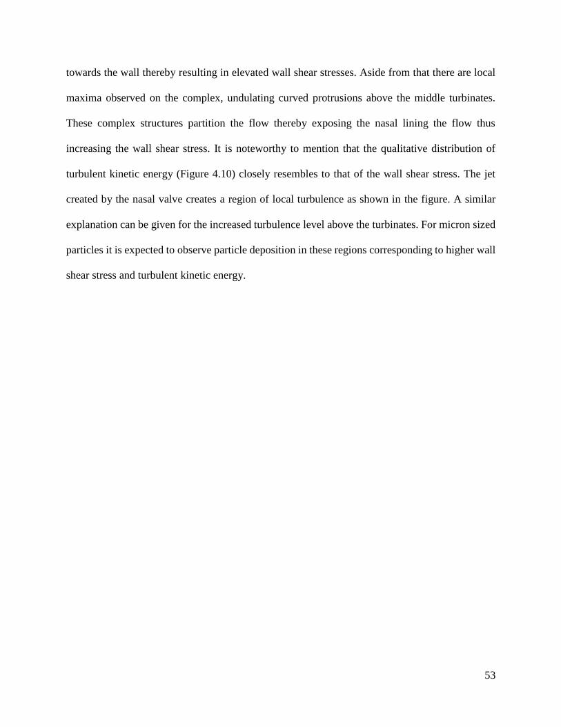
53
towards the wall thereby resulting in elevated wall shear stresses. Aside from that there are local
maxima observed on the complex, undulating curved protrusions above the middle turbinates.
These complex structures partition the flow thereby exposing the nasal lining the flow thus
increasing the wall shear stress. It is noteworthy to mention that the qualitative distribution of
turbulent kinetic energy (Figure 4.10) closely resembles to that of the wall shear stress. The jet
created by the nasal valve creates a region of local turbulence as shown in the figure. A similar
explanation can be given for the increased turbulence level above the turbinates. For micron sized
particles it is expected to observe particle deposition in these regions corresponding to higher wall
shear stress and turbulent kinetic energy.

54
4.3.2. Particle Deposition Results
4.3.2.1. Total Nasal Deposition
Figure 4.11 shows the particle deposition patterns for 2 µm, 10 µm and 20 µm spheres. As
evident from this graphs, the nasal deposition is highly dependent on the particle diameter. Small
particles follow somewhat the streamlines while larger microspheres with their inertia cross
streamlines, thereby resulting in higher depositions (see Table 4.3). The slight discrepancy in the
values may be due to the difference in the number of particles injected. The smaller particles go
with the flow and escape through the nasopharynx, while the larger particles deposit inside the
nasal cavity due to the dominating effects of inertia and secondary flows.
Table 4. 3. Comparison of particle deposition efficiencies.
Particle Diameter (µm) Total Deposition Efficiency %
Simulations
Total Deposition Efficiency %
Calmet et al. (2018)
20 98.5 97.9
10 53.37 55.65
2 3.32 3.12
4.3.2.2. Sectional Deposition
Next to determining the total deposition, it is also essential to find the spatial deposition in
the nasal cavity. Figures 4.12 and 4.13 depict the sectional deposition inside the nasal cavity for
20 µm and 10 µm particles, respectively. Here, 0 in the horizontal axis represents the nose tip and
7 represents the end of the nasopharynx, while 1 to 6 denote the slices shown in Figure 4.6. Hence,
the values in the vertical axis denote the particle deposition efficiencies in-between the consecutive
slices. In the aforementioned figures, the Sectional Deposition Efficiency is given as:
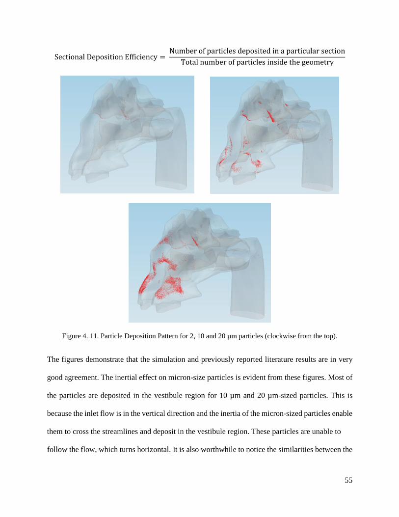
55
Sectional Deposition Efficiency = Number of particles deposited in a particular section
Total number of particles inside the geometry
Figure 4. 11. Particle Deposition Pattern for 2, 10 and 20 µm particles (clockwise from the top).
The figures demonstrate that the simulation and previously reported literature results are in very
good agreement. The inertial effect on micron-size particles is evident from these figures. Most of
the particles are deposited in the vestibule region for 10 µm and 20 µm-sized particles. This is
because the inlet flow is in the vertical direction and the inertia of the micron-sized particles enable
them to cross the streamlines and deposit in the vestibule region. These particles are unable to
follow the flow, which turns horizontal. It is also worthwhile to notice the similarities between the

56
It is also worthwhile to notice the similarities between the deposition pattern of 20 µm particles
and the wall shear stress contour in Figure 4.9. The particle hotspots reasonably matched the high
wall shear stress regions of the nasal cavity. Hence it can be concluded that for high inertial
particles, hotspots are to be anticipated in the regions of high wall shear stress.
Figure 4. 12. Sectional Deposition for 20 µm particles.
Figure 4. 13. Sectional Deposition for 10 µm particles.
0
10
20
30
40
50
60
70
80
0-1 1-2 2-3 3-4 4-5 5-6 6-7
Sect
ion
al D
ep
osi
tio
n
Effi
cie
ncy
Slice PositionEfficiency (Simu) Efficiency (Calmet.et.al.2006)
0
10
20
30
40
50
60
0-1 1-2 2-3 3-4 4-5 5-6 6-7
Sect
ion
al D
ep
osi
tio
n
Effi
cie
ncy
Slice PositionEfficiency(Simu) Efficiency (Calmet.et.al.2018)
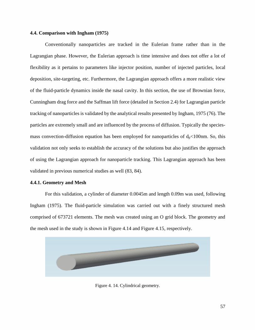
57
4.4. Comparison with Ingham (1975)
Conventionally nanoparticles are tracked in the Eulerian frame rather than in the
Lagrangian phase. However, the Eulerian approach is time intensive and does not offer a lot of
flexibility as it pertains to parameters like injector position, number of injected particles, local
deposition, site-targeting, etc. Furthermore, the Lagrangian approach offers a more realistic view
of the fluid-particle dynamics inside the nasal cavity. In this section, the use of Brownian force,
Cunningham drag force and the Saffman lift force (detailed in Section 2.4) for Lagrangian particle
tracking of nanoparticles is validated by the analytical results presented by Ingham, 1975 (76). The
particles are extremely small and are influenced by the process of diffusion. Typically the species-
mass convection-diffusion equation has been employed for nanoparticles of dp<100nm. So, this
validation not only seeks to establish the accuracy of the solutions but also justifies the approach
of using the Lagrangian approach for nanoparticle tracking. This Lagrangian approach has been
validated in previous numerical studies as well (83, 84).
4.4.1. Geometry and Mesh
For this validation, a cylinder of diameter 0.0045m and length 0.09m was used, following
Ingham (1975). The fluid-particle simulation was carried out with a finely structured mesh
comprised of 673721 elements. The mesh was created using an O grid block. The geometry and
the mesh used in the study is shown in Figure 4.14 and Figure 4.15, respectively.
Figure 4. 14. Cylindrical geometry.
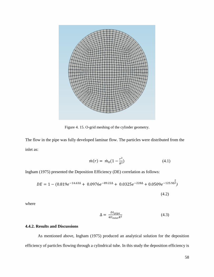
58
Figure 4. 15. O-grid meshing of the cylinder geometry.
The flow in the pipe was fully developed laminar flow. The particles were distributed from the
inlet as:
��(𝑟) = ��0(1 −𝑟2
𝑅2) (4.1)
Ingham (1975) presented the Deposition Efficiency (DE) correlation as follows:
𝐷𝐸 = 1 − (0.819𝑒−14.63∆ + 0.0976𝑒−89.22∆ + 0.0325𝑒−228∆ + 0.0509𝑒−125.9∆23)
(4.2)
where
∆ = 𝐷𝐿𝑝𝑖𝑝𝑒
4𝑈𝑖𝑛𝑙𝑒𝑡𝑅2 (4.3)
4.4.2. Results and Discussions
As mentioned above, Ingham (1975) produced an analytical solution for the deposition
efficiency of particles flowing through a cylindrical tube. In this study the deposition efficiency is
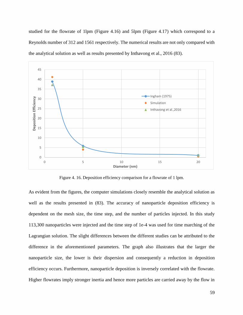
59
studied for the flowrate of 1lpm (Figure 4.16) and 5lpm (Figure 4.17) which correspond to a
Reynolds number of 312 and 1561 respectively. The numerical results are not only compared with
the analytical solution as well as results presented by Inthavong et al., 2016 (83).
Figure 4. 16. Deposition efficiency comparison for a flowrate of 1 lpm.
As evident from the figures, the computer simulations closely resemble the analytical solution as
well as the results presented in (83). The accuracy of nanoparticle deposition efficiency is
dependent on the mesh size, the time step, and the number of particles injected. In this study
113,300 nanoparticles were injected and the time step of 1e-4 was used for time marching of the
Lagrangian solution. The slight differences between the different studies can be attributed to the
difference in the aforementioned parameters. The graph also illustrates that the larger the
nanoparticle size, the lower is their dispersion and consequently a reduction in deposition
efficiency occurs. Furthermore, nanoparticle deposition is inversely correlated with the flowrate.
Higher flowrates imply stronger inertia and hence more particles are carried away by the flow in
0
5
10
15
20
25
30
35
40
45
0 5 10 15 20
De
po
siti
on
Eff
icie
ncy
Diameter (nm)
Ingham (1975)
Simulation
Inthavong et al.,2016
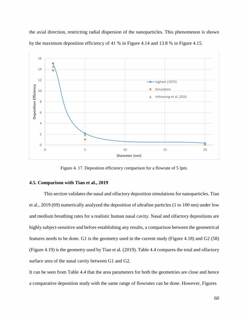
60
the axial direction, restricting radial dispersion of the nanoparticles. This phenomenon is shown
by the maximum deposition efficiency of 41 % in Figure 4.14 and 13.8 % in Figure 4.15.
Figure 4. 17. Deposition efficiency comparison for a flowrate of 5 lpm.
4.5. Comparison with Tian et al., 2019
This section validates the nasal and olfactory deposition simulations for nanoparticles. Tian
et al., 2019 (69) numerically analyzed the deposition of ultrafine particles (1 to 100 nm) under low
and medium breathing rates for a realistic human nasal cavity. Nasal and olfactory depositions are
highly subject-sensitive and before establishing any results, a comparison between the geometrical
features needs to be done. G1 is the geometry used in the current study (Figure 4.18) and G2 (58)
(Figure 4.19) is the geometry used by Tian et al. (2019). Table 4.4 compares the total and olfactory
surface area of the nasal cavity between G1 and G2.
It can be seen from Table 4.4 that the area parameters for both the geometries are close and hence
a comparative deposition study with the same range of flowrates can be done. However, Figures
0
2
4
6
8
10
12
14
16
0 5 10 15 20
De
po
siti
on
Eff
icie
ncy
Diameter (nm)
Ingham (1975)
Simulation
Inthavong et al.,2016
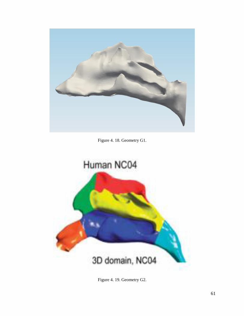
61
Figure 4. 18. Geometry G1.
Figure 4. 19. Geometry G2.

62
4.18 and 4.19 highlight the contrasting shape-features of these two nasal configurations. G1 has a
narrow vestibule region as compared to the G2 geometry. In addition, a distinctive feature
separating the two geometries is that G1 has a concave cavity separating the vestibule region and
the nasal passages while G2 is characterized by a smooth transition between the vestibule and the
airway passage. Apart from that, both the geometries have well-defined upper, middle and lower
passages.
Table 4. 4. Surface Area Comparison between G1 and G2 in MKS units.
G1 G2
Nasal Cavity Surface Area .0196563 .019882
Olfactory Region Surface Area .00208761 .00194583
% of Olfactory to Nasal Surface
Area
10.6 9.78
4.5.1. Airflow Field Results
Figures 4.20 and 4.21 show the sectional velocity contours for the in-house geometry,
considering the sedentary breathing rates of 5lpm and 10lpm, respectively. It can be seen that both
the flowrates have the same qualitative velocity contours. The air enters the nostrils in the vertical
direction before accelerating in the vestibule region followed by deceleration inside the nasal
cavity. Finally, due to the decrease in the size of the cross sectional area, the airflow accelerates
into the nasopharynx.
An important characteristic of the flow inside the nasal cavity is that the superior meatus
receives almost no airflow, which poses a hindrance in olfactory deposition. Hence, most of the
flow passes through the middle and inferior meatus; hence, it is to be expected that major
depositions occur in those areas.

63
Figure 4.22 provides the streamlines and the respective velocity magnitudes throughout the nasal
cavity. Since the study involves multiple flow rates (5, 7 and 10lpm) and all the flowrates lie in
the laminar regime, the magnitudes are normalized with the inlet velocities. Ambient air enters the
nostrils in the upward direction and turns 90 degrees entering the middle and inferior meatus before
finally turning 90 degrees again towards the nasopharynx. Air enters the nostrils at a high velocity
before decelerating inside the meatuses. It can also be seen that the olfactory region receives almost
no air which is a major problem when it pertains to olfactory drug targeting. This phenomenon can
be deduced from Figure 4.23.
Figure 4. 20. Velocity contours along the nasal cavity for 5 lpm flowrate.

64
After traversing through the meatuses, fluid accelerates into the nasopharynx due to the reduction
in the cross-sectional area. It is also noteworthy to see the formation of recirculation zone formed
around the nostrils (Figure 4.24). The nostrils are wider than the inlet that creates a low-pressure
region resulting in the formation of the recirculation zone. Hence, it is reasonable to anticipate
deposition of particles around the nostril region.
Figure 4. 21. Velocity contours along the nasal cavity for 10 lpm flowrate.
Another interesting phenomenon is the formation of Dean’s vortices at the start of the nasopharynx
(Figure 4.25). Due to the curved nature of the nasopharynx, an adverse pressure gradient is created
resulting in a decrease in the velocity close to the convex wall and the opposite close to the concave

65
wall. In summary, most of the air inside the nasal cavity passes through the middle and inferior
meatuses with very low velocities observed in the superior meatus closer to the olfactory region.
Figure 4. 22. Velocity streamlines across the nasal cavity.
Figure 4. 23. Velocity streamlines in the olfactory region.
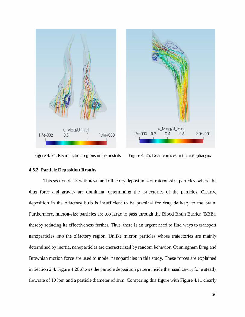
66
Figure 4. 24. Recirculation regions in the nostrils Figure 4. 25. Dean vortices in the nasopharynx
4.5.2. Particle Deposition Results
This section deals with nasal and olfactory depositions of micron-size particles, where the
drag force and gravity are dominant, determining the trajectories of the particles. Clearly,
deposition in the olfactory bulb is insufficient to be practical for drug delivery to the brain.
Furthermore, micron-size particles are too large to pass through the Blood Brain Barrier (BBB),
thereby reducing its effectiveness further. Thus, there is an urgent need to find ways to transport
nanoparticles into the olfactory region. Unlike micron particles whose trajectories are mainly
determined by inertia, nanoparticles are characterized by random behavior. Cunningham Drag and
Brownian motion force are used to model nanoparticles in this study. These forces are explained
in Section 2.4. Figure 4.26 shows the particle deposition pattern inside the nasal cavity for a steady
flowrate of 10 lpm and a particle diameter of 1nm. Comparing this figure with Figure 4.11 clearly

67
shows the difference in fluid-particle dynamics between nanoparticles and micron particles.
Micron-size particles show preferential deposition mainly in the vestibule region, thereby resulting
in certain deposition “hotspots”. This is because the motion of micron particles is determined by
the relatively high inertial forces which enable the particles to cross streamlines. For example in
the case of 20 µm, the particle inertia is carried by the vertical airflow through the nostrils and
deposited majorly in the vestibule region. On the other hand, nanoparticle deposition is dispersed
throughout the nasal cavity. Due to the considerably lower inertia of nanoparticles, they are carried
further into the nasal cavity rather than just depositing in the vestibule region by inertial impaction.
Figure 4.27 shows the comparison of the total deposition efficiencies (TDE) between the results
presented by Tian et al., 2019 and that of the present simulations. However, it is noteworthy to
mention that the simulation showed a higher deposition efficiency for a specific particle diameter.
This difference can be attributed to the difference in the shapes of the two nasal cavities. Most
pronounced, the geometry used in Tian et al., 2019 has a sudden circular bend after the nasal
vestibule (see Figure 4.19).
Figure 4. 26. Deposition pattern for 10 lpm flowrate and 1nm diameter particle.

68
Due to this the velocity streamlines are unable to immediately conform to the geometry surface.
Consequently low pressure and a region of recirculation are created around the circular bend. As
a result, the olfactory region receives less air, i.e., much lower flow to the olfactory region, thereby
restricting nanoparticles to reach the olfactory epithelium. On the other hand the nasal geometry
used in the simulation has a smooth transition from the vestibule to the meatuses. This enables a
higher concentration of streamlines through the olfactory region and as a result, more deposition
was observed in the simulation geometry. In addition, a higher flowrate results in lower total
deposition. This can be attributed to the fact that unlike micron particles, nanoparticles do not have
enough inertia to cross streamlines and they are easily carried away by the flow. At higher
flowrates, more particles exit through the nasopharynx.
Figure 4. 27. TDE comparisons for 5 lpm and 7 lpm flowrates.
While considering Lagrangian particle tracking simulations, the number of particles (NOP)
injected can skew the deposition efficiency values. Hence, to validate the force formulations and
0
10
20
30
40
50
60
70
80
90
100
1 10 100
Tota
l De
po
siti
on
Eff
icie
ncy
%
Diameter (nm)
5 lpm
7 lpm
5 lpm (Tian et al., 2019)
7 lpm (Tian et al., 2019)
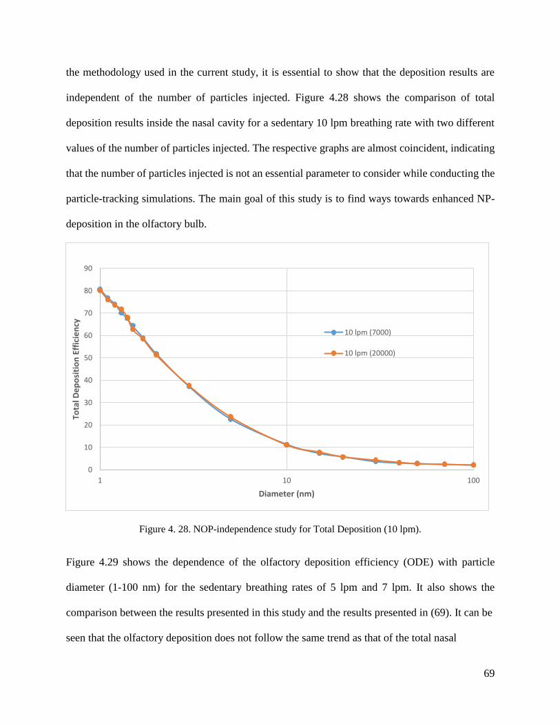
69
the methodology used in the current study, it is essential to show that the deposition results are
independent of the number of particles injected. Figure 4.28 shows the comparison of total
deposition results inside the nasal cavity for a sedentary 10 lpm breathing rate with two different
values of the number of particles injected. The respective graphs are almost coincident, indicating
that the number of particles injected is not an essential parameter to consider while conducting the
particle-tracking simulations. The main goal of this study is to find ways towards enhanced NP-
deposition in the olfactory bulb.
Figure 4. 28. NOP-independence study for Total Deposition (10 lpm).
Figure 4.29 shows the dependence of the olfactory deposition efficiency (ODE) with particle
diameter (1-100 nm) for the sedentary breathing rates of 5 lpm and 7 lpm. It also shows the
comparison between the results presented in this study and the results presented in (69). It can be
seen that the olfactory deposition does not follow the same trend as that of the total nasal
0
10
20
30
40
50
60
70
80
90
1 10 100
Tota
l De
po
siti
on
Eff
icie
ncy
Diameter (nm)
10 lpm (7000)
10 lpm (20000)

70
Figure 4. 29. ODE comparison for 5 lpm and 7 lpm flowrates.
Figure 4. 30. NOP Independent study for Olfactory Deposition (10 lpm).
0
0.5
1
1.5
2
2.5
3
3.5
1 10 100
Olf
acto
ry D
ep
osi
tio
n E
ffic
ien
cy %
Diameter(nm)
5 lpm
7 lpm
5 lpm (Tian et al., 2019)
7 lpm (Tian et al., 2019)
0
0.5
1
1.5
2
2.5
3
3.5
4
4.5
5
1 10 100
Olf
acto
ry D
ep
osi
tio
n E
ffic
ien
cy
Diameter (nm)
10 lpm (7000) 10 lpm (20000)

71
Figure 4. 31. Sectional Deposition for 1.1 nm, 10nm, 50 nm and 100 nm (clockwise from the bottom)
at a flowrate of 10 lpm.
deposition. There is a local maximum observed for the 2nm particle diameter. The unusual peak
can be explained as follows. 1 nm particles are highly diffusive in nature and their deposition is
completely dependent on the brownian dispersion force. 2 nm particles are slightly less diffusive
and are more susceptible to be carried away by the streamlines and hence more particles reach the
olfactory region. Most 1 nm particles on the other hand don’t reach the olfactory region due to
either being deposited in the vestibule region or passing through the middle passage. The
subsequent decrease in olfactory deposition with increase in the size of nanoparticles can be
0-121%
1-226%
2-35%
3-416%
4-522%
5-62%
6-78%
1.1 nm
0-115%
1-221%
2-38%
3-416%
4-523%
5-64%
6-713%
10 nm
0-117%
1-225%
2-324%
3-412%
4-515%
5-61%
6-76%
100 nm
0-115%
1-221%
2-38%3-4
16%
4-523%
5-64%
6-713%
50 nm

72
reasoned due to the less diffusive nature of the particles. So even if the particles travel to the
passage of the olfactory region, their low diffusivity inhibits them from being deposited .The
maximum olfactory deposition for 5 lpm and 7 lpm using the simulation is 3.1% and 3.2%,
respectively, which confirms published NP-deposition data.
Figure 4.30 shows that the olfactory results are independent of the number of particles
injected. It is also noteworthy to compare the sectional deposition for nanoparticles (Figure 4.31)
to that of micron particles (Figure 4.12 and Figure 4.13). While micron-size particles generate
“particle hotspots”, nanoparticles are distributed almost uniformly throughout the nasal cavity and
nasopharynx. This is due to the impact of Brownian motion that produces random, ie, diffusional,
changes in the trajectories of the nanoparticles. Furthermore, the size of the nanoparticles has a
miniscule effect on sectional deposition. This inidcates that local deposition for nanoparticles is
greatly governed by the shape of the nasal geometry. The shape of the nasal geometry determines
the flow distribution which subsequently is the driving force along with the Brownian force in
particle depsosition along the different sections of the geometry.
73
CHAPTER 5. PARTICLE RELEASE MAP FOR OLFACTORY DRUG TARGETING
5.1 Introduction
Targeted drug delivery is based on the idea that a specific diseased organ site is targeted
for drug delivery to produce a significant therapeutic efficiency. Drug administration can take
place through the mouth in the form of pills, through injection using a syringe (known as the
parenteral route), through the nasal route in the form of inhalers and so on and so forth. Usually
the parenteral and the oral routes result in the drug formulations reaching throughout the body via
the bloodstream. While most drugs are innocuous, some drug formulations might be toxic to
certain parts of the body and hence the need for targeted drug delivery. Furthermore targeted drug
delivery increases the efficiency of drug deposition on the targeted site significantly. Olfactory
drug targeting through the nasal route has gained a lot of priority in recent years. Since only
nanoparticles are small enough to successfully cross the Blood Brain Barrier (BBB), the progress
in the field of nanotechnology has further made this approach more feasible. Furthermore, recent
advances in nebulizer technologies have shown to produce aerosol particles and droplets in the
nanoparticle range (85-87). The aforementioned technologies in conjunction pave the way for
efficient drug targeting in the future. Results from Chapter 4 show that the maximum olfactory
deposition efficiency observed was 3-4 %. This deposition is not enough to be of clinical
significance. Hence the need for further research into improving the deposition. The approach for
olfactory drug deposition in Chapter 4 involved injecting particles randomly throughout the
nostrils and checking the drug deposition efficiency. It may be beneficial to utilize the Particle
Release Map (PRM) (88, 89) approach to decide the optimal injection area that results in maximum
olfactory deposition efficiency. The PRM approach involves injecting particles uniformly
throughout the nostrils and studying the regional deposition inside the nasal cavity. These
74
deposited particles are backtracked to their injection position and marked. Each area of deposition
is marked differently in the PRM. This methodology gives the position of the injection that would
majorly transport the particles to the specific region.
5.2 Methodology
In this study, Particle Release Maps (PRMs) are generated for nanoparticles and micron
sized particles under different flow conditions.The particle deposition is studied for low (5 lpm)
and medium (20 lpm). OpenFOAM generates an extensive data file showing the particle positions,
their ID’s, deposited particles and so on and so forth. This information is essential for creating the
Particle Release Map. The PRM is constructed via the following steps:-
1. Conducted a simpleFoam simulation to get a steady state flow field for a particular flowrate.
2. Using the flow field, conducted a CF-PD simulation using
icoUncoupledKinematicParcelFoam for lagrangian tracking of individual particles and
measuring the regional and total deposition efficiency. In this simulation the particles are uniformly
distributed throughout the nostrils and all of them are released initially all at once.
3. Tracked all of these particles until all of them are either deposited or escaped.
4. The initial and final position of the particles are then compared using the particle ID to determine
which particles are deposited in a specific region in the nasal cavity. This was done using a Matlab
script.
5. Marking each specific region deposited particles with a separate marker on the initial injection
position file gives the full-fledged particle release map.
The purpose of the PRM is to determine the optimal injection position for maximum regional
deposition to the specific area. In this study, once the PRM is constructed, another simulation is
conducted by injecting similar amount of particles from the position on the PRM that is suitable
for olfactory drug targeting. This is done so as to

75
Figure 5. 1. Nasal geometry with the specific regions that will be represented in the
Particle Release Map
Table 5. 1. Legend correlating the color to the specific region.
Colour Region
Blue Anterior
Red Olfactory
Yellow Middle Meatus
Green Interior Meatus
Magenta Nasopharynx
76
establish the effectiveness of the PRM approach. For each flowrate, both micron-sized particles (2
µm, 5 µm and 10 µm) and nanoparticles (1 nm, 10 nm and 100 nm) were considered. Figure 5.1
shows the nasal geometry with the different parts highlighted in specific color. These are the
regions that will be represented by the particle release map. Table 5.1 represents the legend
correlating the highlighted colors with the specific regions.
5.3. Results and Discussion
5.3.1. Micron-size Particles
The study is done for different flowrates and multiple particle diameters but it is easier to
combine the two parameters for analyzing the particle deposition for micron particles where inertia
is dominant. The parameter is called the Impaction Parameter (IP) which is given by:
IP = d2Q
Where d is the particle diameter and Q is the volumetric flowrate. These parameters represent the
cumulative effect of the size of the particle and the fluid inertia. Figures 5.2.1 – 5.6.1 show the
Particle Release Maps for various impaction parameter values. The specific color on the PRM
denote the region of the nasal geometry where the particles deposited as per Table 5.1. The particle
release maps clearly show the preferential sites of injection for olfactory deposition. These are
located at the narrower end of the nostrils. Using these PRMs, separate computer simulations are
conducted by injecting particles to target the olfactory region. Figures 5.2.2-5.6.2 show the
comparison of deposition efficiencies between normal and targeted injection. As the impaction
parameter increases, the total nasal deposition efficiency increases for normal injection. This is
primarily because of inertial impaction and most of the particles deposit in the vestibule region.
However, the trend for olfactory deposition is the opposite. This is because low inertia results in

77
more particles entering the nasal passage rather than getting stuck in the vestibule region. For the
same reason, nasopharynx deposition follows the same trend as that of olfactory deposition.
The olfactory deposition observed from normal injection is extremely low (<0.05 %). To improve
the deposition efficiency, a circular injector-nozzle of diameter 0.5mm was employed. The figures
indicate that targeted injection greatly increases the olfactory deposition efficiencies. The
maximum nasal and olfactory depositions observed are 54% and 11 % respectively in Figure 5.5.2.
Figures 5.7 and 5.8 illustrate the effect of the targeted injection on the deposition pattern inside the
nasal cavity. The phenomenon of targeted injection directs the micron particles to the olfactory
region. However, because of their ability to cross streamlines, a major fraction of these particles
deposit just before the olfactory region and consequently a maximum deposition of only 11 %
occurred.As shown in Figure 5.8, the olfactory as well as nasal deposition achieves a maximum
for an IP of 8333.333, caused by the gravitational effect. The higher impaction number generally
signifies higher particle diameters, amplified by the dependence on the square of the particle
diameter. So higher impaction parameter values with targeted injection results in pushing particles
upwards from the nostrils into the olfactory region. However, as the particle diameter increases,
the effect of gravity becomes more significant and the particles that were being pushed upwards
start going due to the middle and lower portion of the nasal passages. This phenomenon is called
the “sedimentation effect”. This can be observed by comparing Figures 5.8 and 5.9. Through the
comparison it can be observed that the higher impaction parameter yields lower nasal and olfactory
depositions.
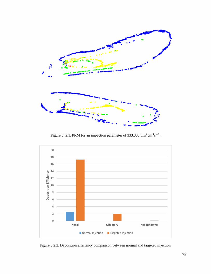
78
Figure 5. 2.1. PRM for an impaction parameter of 333.333 µm2cm3s−1.
Figure 5.2.2. Deposition efficiency comparison between normal and targeted injection.
0
2
4
6
8
10
12
14
16
18
20
Nasal Olfactory Nasopharynx
De
po
siti
on
Eff
icie
ncy
Normal Injection Targeted Injection

79
Figure 5. 3.1. PRM for an impaction parameter of 1333.333 µm2cm3s−1.
Figure 5.3.2. Deposition efficiency comparison between normal and targeted injection.
0
2
4
6
8
10
12
14
16
Nasal Olfactory Nasopharynx
De
po
siti
on
Eff
icie
ncy
Normal Injection Targeted Injection
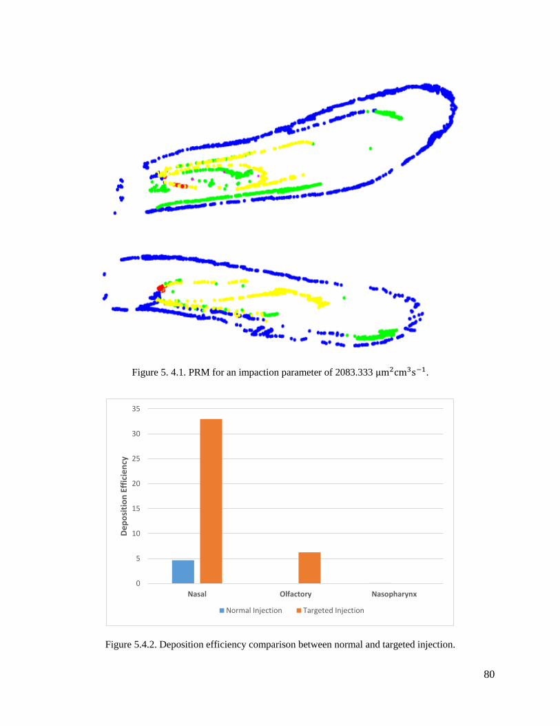
80
Figure 5. 4.1. PRM for an impaction parameter of 2083.333 µm2cm3s−1.
Figure 5.4.2. Deposition efficiency comparison between normal and targeted injection.
0
5
10
15
20
25
30
35
Nasal Olfactory Nasopharynx
De
po
siti
on
Eff
icie
ncy
Normal Injection Targeted Injection

81
Figure 5. 5.1. PRM for an impaction parameter of 8333.3333 µm2cm3s−1.
Figure 5.5.2. Deposition efficiency comparison between normal and targeted injection.
0
10
20
30
40
50
60
Nasal Olfactory Nasopharynx
De
po
siti
on
Eff
icie
ncy
Normal Injection Targeted Injection
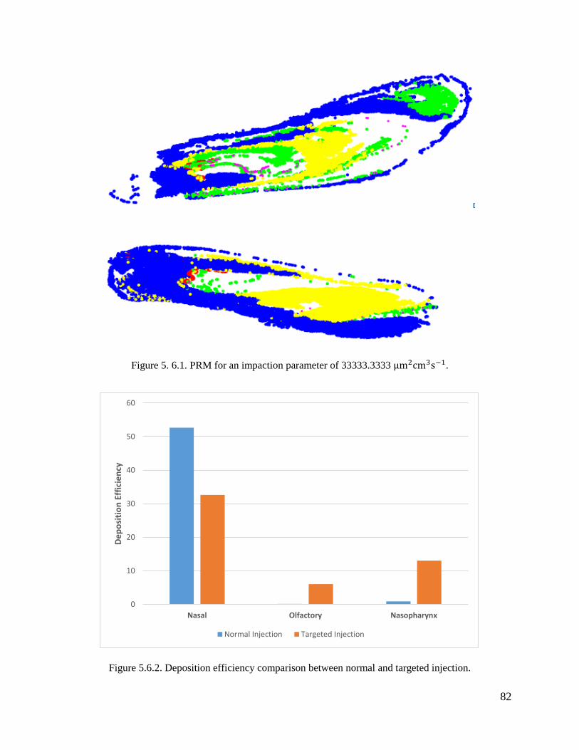
82
Figure 5. 6.1. PRM for an impaction parameter of 33333.3333 µm2cm3s−1.
Figure 5.6.2. Deposition efficiency comparison between normal and targeted injection.
0
10
20
30
40
50
60
Nasal Olfactory Nasopharynx
De
po
siti
on
Eff
icie
ncy
Normal Injection Targeted Injection
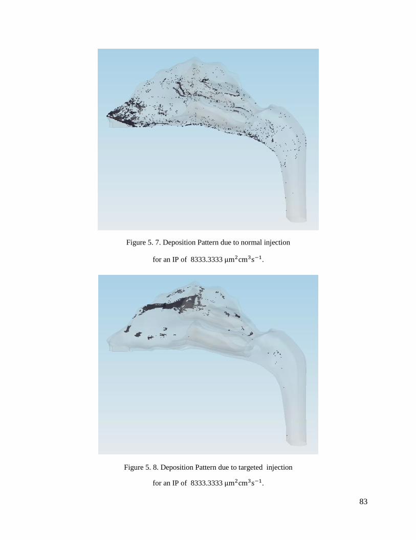
83
Figure 5. 7. Deposition Pattern due to normal injection
for an IP of 8333.3333 µm2cm3s−1.
Figure 5. 8. Deposition Pattern due to targeted injection
for an IP of 8333.3333 µm2cm3s−1.
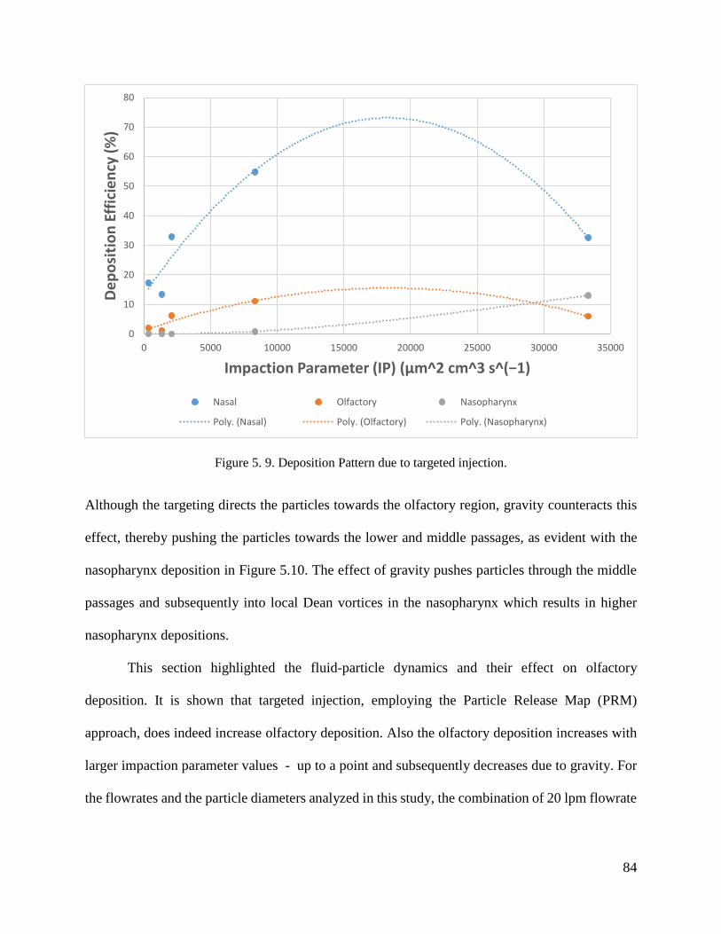
84
Figure 5. 9. Deposition Pattern due to targeted injection.
Although the targeting directs the particles towards the olfactory region, gravity counteracts this
effect, thereby pushing the particles towards the lower and middle passages, as evident with the
nasopharynx deposition in Figure 5.10. The effect of gravity pushes particles through the middle
passages and subsequently into local Dean vortices in the nasopharynx which results in higher
nasopharynx depositions.
This section highlighted the fluid-particle dynamics and their effect on olfactory
deposition. It is shown that targeted injection, employing the Particle Release Map (PRM)
approach, does indeed increase olfactory deposition. Also the olfactory deposition increases with
larger impaction parameter values - up to a point and subsequently decreases due to gravity. For
the flowrates and the particle diameters analyzed in this study, the combination of 20 lpm flowrate
0
10
20
30
40
50
60
70
80
0 5000 10000 15000 20000 25000 30000 35000
De
po
siti
on
Eff
icie
ncy
(%
)
Impaction Parameter (IP) (μm^2 cm^3 s^(−1)
Nasal Olfactory Nasopharynx
Poly. (Nasal) Poly. (Olfactory) Poly. (Nasopharynx)
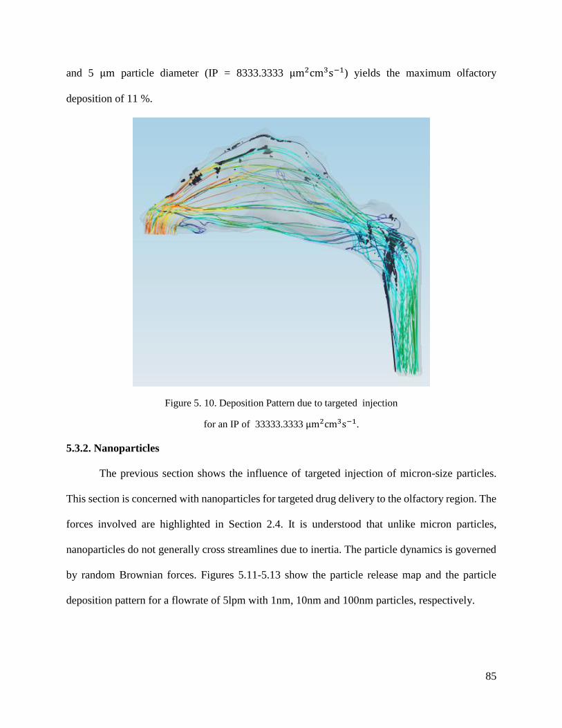
85
and 5 µm particle diameter (IP = 8333.3333 µm2cm3s−1) yields the maximum olfactory
deposition of 11 %.
Figure 5. 10. Deposition Pattern due to targeted injection
for an IP of 33333.3333 µm2cm3s−1.
5.3.2. Nanoparticles
The previous section shows the influence of targeted injection of micron-size particles.
This section is concerned with nanoparticles for targeted drug delivery to the olfactory region. The
forces involved are highlighted in Section 2.4. It is understood that unlike micron particles,
nanoparticles do not generally cross streamlines due to inertia. The particle dynamics is governed
by random Brownian forces. Figures 5.11-5.13 show the particle release map and the particle
deposition pattern for a flowrate of 5lpm with 1nm, 10nm and 100nm particles, respectively.

86
Figure 5. 11.1. PRM of 1 nm particles for the flowrate of 5 lpm.
Figure 5.11.2. Deposition efficiency comparison between normal and targeted injection.
0
10
20
30
40
50
60
70
80
90
100
Nasal Olfactory Nasopharynx
De
po
siti
on
Eff
icie
ncy
Normal Injection Targeted Injection

87
Figure 5. 12.1. PRM of 10 nm particles for the flowrate of 5 lpm.
Figure 5.12.2 Deposition efficiency comparison between normal and targeted injection.
0
2
4
6
8
10
12
14
16
Nasal Olfactory Nasopharynx
De
po
siti
on
Eff
icie
ncy
Normal Injection Targeted Injection

88
Figure 5. 13.1. PRM of 100 nm particles for the flowrate of 5 lpm.
Figure 5.13.2. Deposition efficiency comparison between normal and targeted injection.
0
5
10
15
20
25
Nasal Olfactory Nasopharynx
De
po
siti
on
Eff
icie
ncy
Normal Injection Targeted Injection

89
Figures 5.14-5.16 are for a flowrate of 20 lpm; where subsection 1 represents the particle release
map and subsection 2 shows the comparison between normal and targeted injections. As expected,
for small sized nanoparticles, targeted injection substantially increases the olfactory deposition
efficiency with the maximum increase from 1 to 50% (see Figure 5.14.2). However, drug-particle
sizes below 50nm are presently not available. The effect of targeted injection decreases with the
increase in particle size. This is because for very small nanoparticles there is a well-defined region
for olfactory deposition in the particle release map, whereas for 100nm particles there are only
distinct points on the particle release map corresponding to olfactory deposition. This results in
olfactory deposition efficiencies of 0.87% and 1.15% for Figures 5.13.2 and 5.16.2, respectively.
The deposition pattern of 10nm particles for a 20 lpm flowrate due to normal and targeted injection
is shown in Figure 5.17 and Figure 5.18 respectively. It shows that the targeted injection greatly
changes the deposition pattern inside the nasal geometry. Normal injection results in a uniformly
spread deposition pattern, while the targeted injection concentrates the particles in the upper region
of the nasal cavity closer to the olfactory region. The comparison between Figure 5.8 and Figure
5.18 highlight the differences in the behavior of micron particles and nanoparticles. The
phenomenon of targeted injection works on low sized nanoparticles due to the property of
nanoparticles to follow the streamlines. Micron particles on the other hand are carried away by
inertia and deposit in regions other than the intended target. The impact of targeted injection
decreases with the increase in the particle diameter size (Figure 5.19). Furthermore higher flowrate
generates higher olfactory deposition efficiency.
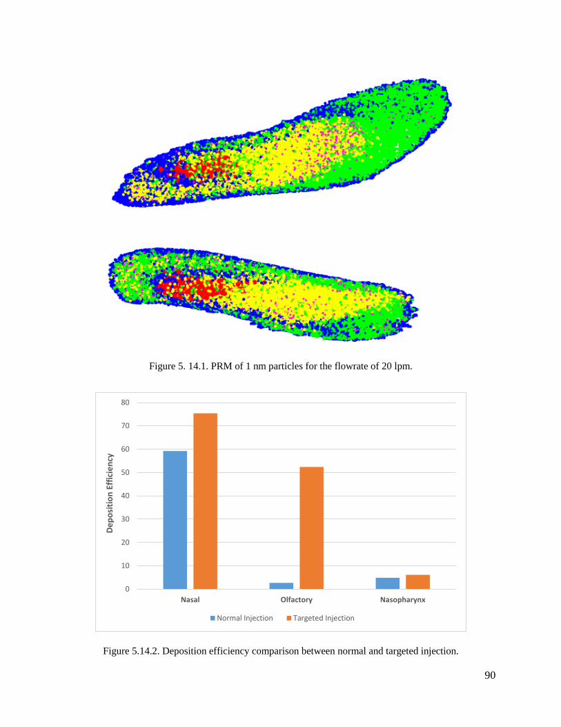
90
Figure 5. 14.1. PRM of 1 nm particles for the flowrate of 20 lpm.
Figure 5.14.2. Deposition efficiency comparison between normal and targeted injection.
0
10
20
30
40
50
60
70
80
Nasal Olfactory Nasopharynx
De
po
siti
on
Eff
icie
ncy
Normal Injection Targeted Injection

91
Figure 5. 15.1. PRM of 10 nm particles for the flowrate of 20 lpm.
Figure 5.15.2. Deposition efficiency comparison between normal and targeted injection.
0
5
10
15
20
25
30
35
40
Nasal Olfactory Nasopharynx
De
po
siti
on
Eff
icie
ncy
Normal Injection Targeted Injection

92
Figure 5. 16.1. PRM of 100 nm particles for the flowrate of 20 lpm.
Figure 5.16.2. Deposition efficiency comparison between normal and targeted injection.
0
5
10
15
20
25
Nasal Olfactory Nasopharynx
De
po
siti
on
Eff
icie
ncy
Normal Injection Targeted Injection
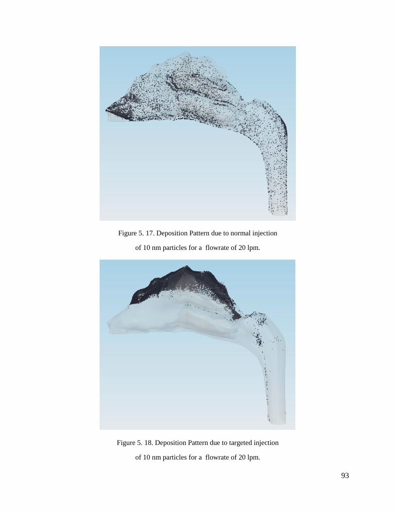
93
Figure 5. 17. Deposition Pattern due to normal injection
of 10 nm particles for a flowrate of 20 lpm.
Figure 5. 18. Deposition Pattern due to targeted injection
of 10 nm particles for a flowrate of 20 lpm.
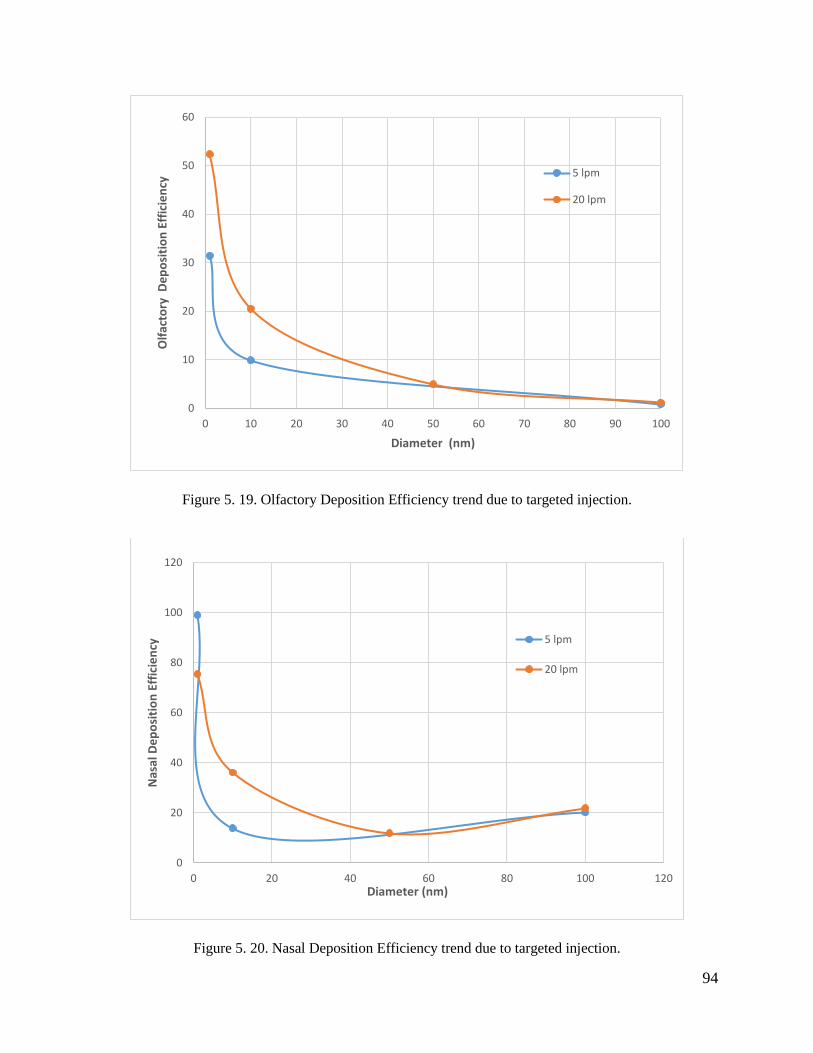
94
Figure 5. 19. Olfactory Deposition Efficiency trend due to targeted injection.
Figure 5. 20. Nasal Deposition Efficiency trend due to targeted injection.
0
10
20
30
40
50
60
0 10 20 30 40 50 60 70 80 90 100
Olf
acto
ry D
ep
osi
tio
n E
ffic
ien
cy
Diameter (nm)
5 lpm
20 lpm
0
20
40
60
80
100
120
0 20 40 60 80 100 120
Nas
al D
ep
osi
tio
n E
ffic
ien
cy
Diameter (nm)
5 lpm
20 lpm

95
CHAPTER 6. NASAL CANNULA FOR OLFACTORY DRUG TARGETING
6.1 Introduction
As indicated with the particle release maps (PRMs) for nanoparticles (as shown in Chapter
5) nanoparticles are unable to cross the streamlines owing to their low inertia. Hence, the most
effective way of transporting nanoparticles to the olfactory region is to introduce particles into the
streamlines that reach the desired site or region. From the PRMs, it is observed that the streamlines
close to the narrower section of the nostrils travel to the olfactory region and hence that would be
the optimal position of injection to achieve maximum olfactory deposition.
Figure 6. 1. Streamlines to the olfactory region.
Figure 6.1 shows the streamlines going to the olfactory region. The reason for the low olfactory
deposition efficiency is that the major amount of streamlines pass through the lower and middle
meatuses. This is the principle behind targeted injection in Chapter 5. In this chapter, computer
experiments are conducted to analyze the deposition of particles by employing a nebulizer (or
inhaler) with a cannula-type attachment to reach further inside the nasal cavity geometry. Cannulas
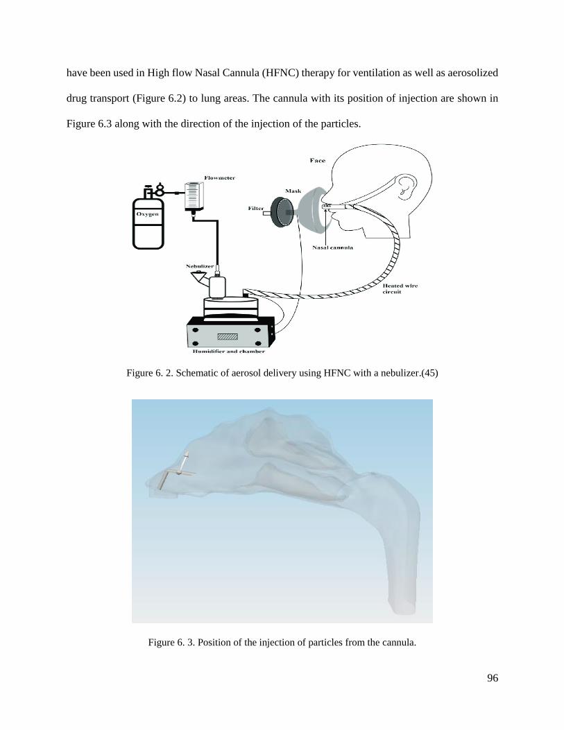
96
have been used in High flow Nasal Cannula (HFNC) therapy for ventilation as well as aerosolized
drug transport (Figure 6.2) to lung areas. The cannula with its position of injection are shown in
Figure 6.3 along with the direction of the injection of the particles.
Figure 6. 2. Schematic of aerosol delivery using HFNC with a nebulizer.(45)
Figure 6. 3. Position of the injection of particles from the cannula.
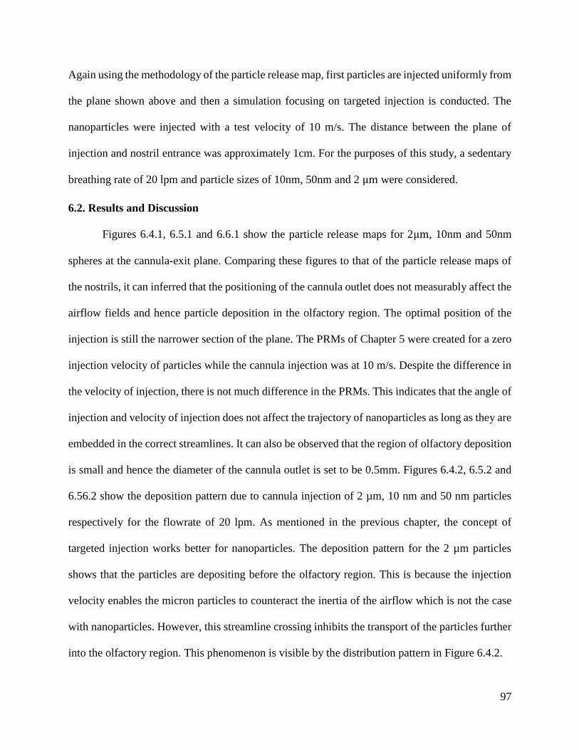
97
Again using the methodology of the particle release map, first particles are injected uniformly from
the plane shown above and then a simulation focusing on targeted injection is conducted. The
nanoparticles were injected with a test velocity of 10 m/s. The distance between the plane of
injection and nostril entrance was approximately 1cm. For the purposes of this study, a sedentary
breathing rate of 20 lpm and particle sizes of 10nm, 50nm and 2 µm were considered.
6.2. Results and Discussion
Figures 6.4.1, 6.5.1 and 6.6.1 show the particle release maps for 2µm, 10nm and 50nm
spheres at the cannula-exit plane. Comparing these figures to that of the particle release maps of
the nostrils, it can inferred that the positioning of the cannula outlet does not measurably affect the
airflow fields and hence particle deposition in the olfactory region. The optimal position of the
injection is still the narrower section of the plane. The PRMs of Chapter 5 were created for a zero
injection velocity of particles while the cannula injection was at 10 m/s. Despite the difference in
the velocity of injection, there is not much difference in the PRMs. This indicates that the angle of
injection and velocity of injection does not affect the trajectory of nanoparticles as long as they are
embedded in the correct streamlines. It can also be observed that the region of olfactory deposition
is small and hence the diameter of the cannula outlet is set to be 0.5mm. Figures 6.4.2, 6.5.2 and
6.56.2 show the deposition pattern due to cannula injection of 2 µm, 10 nm and 50 nm particles
respectively for the flowrate of 20 lpm. As mentioned in the previous chapter, the concept of
targeted injection works better for nanoparticles. The deposition pattern for the 2 µm particles
shows that the particles are depositing before the olfactory region. This is because the injection
velocity enables the micron particles to counteract the inertia of the airflow which is not the case
with nanoparticles. However, this streamline crossing inhibits the transport of the particles further
into the olfactory region. This phenomenon is visible by the distribution pattern in Figure 6.4.2.
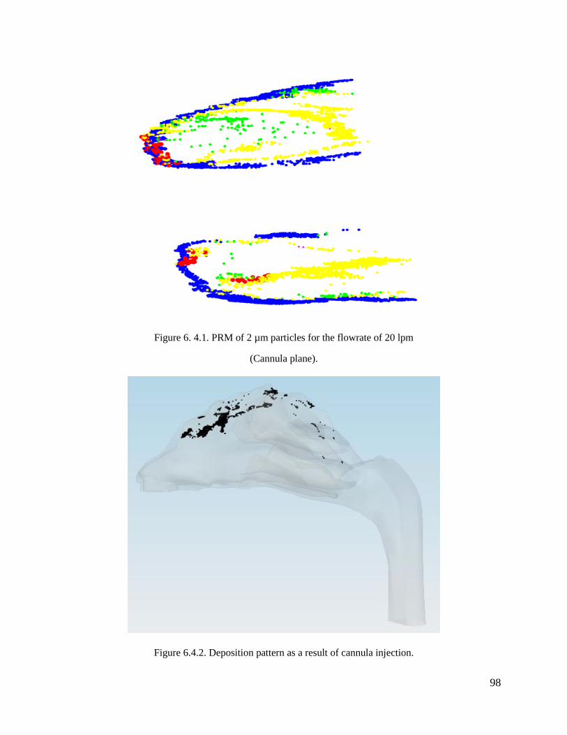
98
Figure 6. 4.1. PRM of 2 µm particles for the flowrate of 20 lpm
(Cannula plane).
Figure 6.4.2. Deposition pattern as a result of cannula injection.

99
Figure 6. 5.1. PRM of 10 nm particles for the flowrate of 20 lpm
(Cannula plane).
Figure 6.5.2. Deposition pattern as a result of cannula injection.
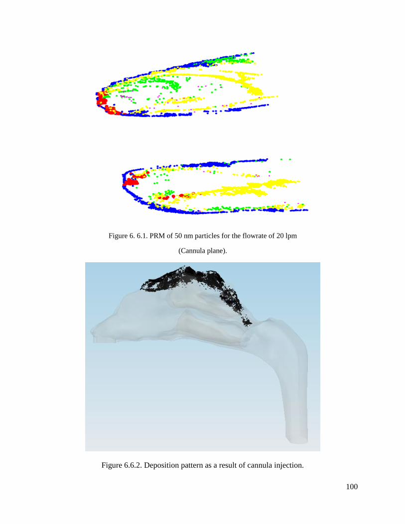
100
Figure 6. 6.1. PRM of 50 nm particles for the flowrate of 20 lpm
(Cannula plane).
Figure 6.6.2. Deposition pattern as a result of cannula injection.
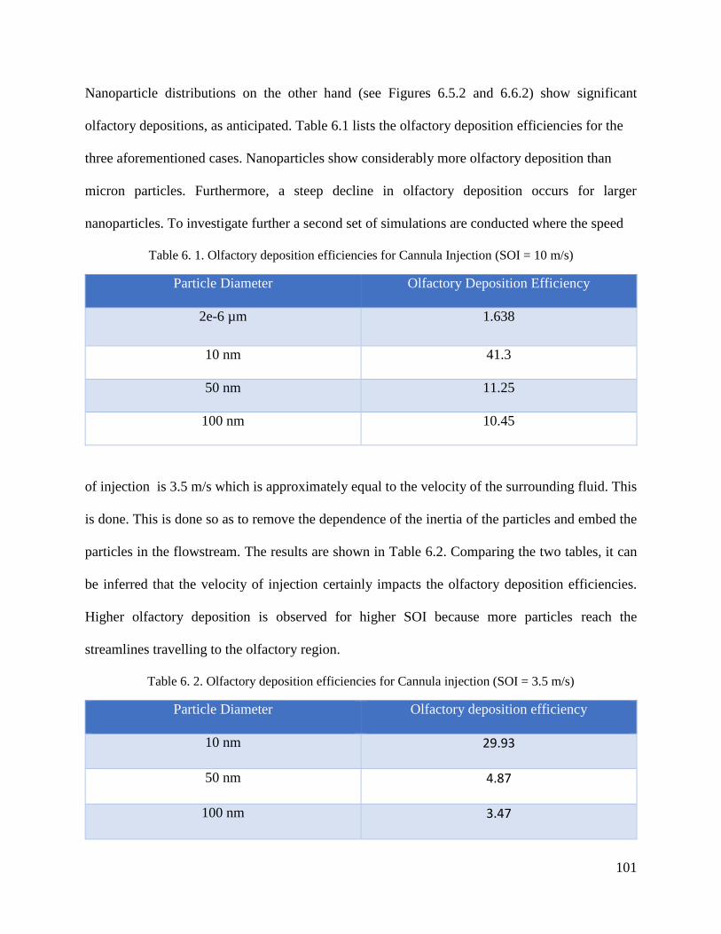
101
Nanoparticle distributions on the other hand (see Figures 6.5.2 and 6.6.2) show significant
olfactory depositions, as anticipated. Table 6.1 lists the olfactory deposition efficiencies for the
three aforementioned cases. Nanoparticles show considerably more olfactory deposition than
micron particles. Furthermore, a steep decline in olfactory deposition occurs for larger
nanoparticles. To investigate further a second set of simulations are conducted where the speed
Table 6. 1. Olfactory deposition efficiencies for Cannula Injection (SOI = 10 m/s)
Particle Diameter Olfactory Deposition Efficiency
2e-6 µm 1.638
10 nm 41.3
50 nm 11.25
100 nm 10.45
of injection is 3.5 m/s which is approximately equal to the velocity of the surrounding fluid. This
is done. This is done so as to remove the dependence of the inertia of the particles and embed the
particles in the flowstream. The results are shown in Table 6.2. Comparing the two tables, it can
be inferred that the velocity of injection certainly impacts the olfactory deposition efficiencies.
Higher olfactory deposition is observed for higher SOI because more particles reach the
streamlines travelling to the olfactory region.
Table 6. 2. Olfactory deposition efficiencies for Cannula injection (SOI = 3.5 m/s)
Particle Diameter Olfactory deposition efficiency
10 nm 29.93
50 nm 4.87
100 nm 3.47

102
CHAPTER 7. CONCLUSION AND FUTURE WORK
The olfactory region in the nasal cavity is an important gateway for transporting drug
particles into the brain for the treatment of various central nervous system disorders. Drug injection
via the nasal route serves as a promising non-invasive technique for drug delivery. However the
complex structure of the human nasal cavity inhibits the transport of the particles to the olfactory
region. Particle sizes ranging from 1-50nm are optimal for actively crossing the Blood Brain
Barrier via active or passive (ie, diffusional) processes. This study aims at increasing the deposition
of nanoparticles in the olfactory region.
Chapter 4 deals with validating the simulation approach of micron particles vs.
nanoparticles by comparing the deposition from previous studies. Through these studies it has been
found that micron particles show almost no olfactory deposition while nanoparticles show a
maximum deposition of 3-4% for particles of sizes between 1 and 2 nm. Particles above the size
of 10 nm show negligible deposition on the olfactory epithelium. Extremely small nanodrugs are
not possible to manufacture and/or generate with the current atomization technologies.
Chapter 5 employs the particle release map (PRM) approach to determine the optimal
position of injection for elevated olfactory deposition. The PMRs further illustrated the behavior
of particles in a sedentary flowrate of 20 lpm which corresponds to a normal breathing rate. The
optimal injection point for targeting the olfactory region lies in the narrower section of the nostrils.
Using the particle release maps, simulations were conducted to target the olfactory region and the
results are very promising. Targeted injection achieves an olfactory deposition of 52 % (Figure
5.14.2) for 1 nm particles, 20% (Figure 5.15.2) for 10 nm particles and 1.15 % (Figure 5.16.2) for
100 nm particles at a breathing rate of 20lpm. For micron particles, a relatively less prominent
effect of targeted injection has been observed. Normal injection resulted in a 2 % deposition for

103
2 µm, 11 % for 5 µm and 6 % for 10 µm particles for the same breathing rate. Through the targeted
injection approach, a substantial increase in olfactory deposition was observed. This approach can
be utilized for devices like nebulizers that inject drug particles through the nostrils.
A preliminary study to test the use of a cannula-type device was done in Chapter 6. The
cannula-exit plane was placed at approximately 1cm from the nostrils and the particles were
injected with a test velocity of 3.5 m/s (velocity of the flow) and 10 m/s. The idea behind this is
that the further the injection point from the nostril, the less the nanoparticles will diffuse before
the olfactory region. Table 7.1 shows the comparison between the various injection methods used
in this study. It can be seen that the cannula injection and targeted injection from the nostrils
successfully increase the olfactory deposition. A consistent increase in the olfactory deposition is
observed from normal injection to targeted injection and from targeted injection and cannula
injection. Hence the preliminary study for cannula injection along with the particle release map
approach should be further studied by incorporating realistic conditions for olfactory drug
targeting.
Table 7. 1. Olfactory deposition comparison between the injection methods.
Olfactory Deposition Efficiency
Particle Diameter Normal Injection Targeted
Injection
Cannula
Injection
(SOI = 3.5 m/s)
Cannula
Injection
(SOI = 10 m/s)
10 nm 0.24 20.49 29.93 41.31
50 nm 0.04 4.93 4.87 11.25
100 nm 0.03 1.16 3.47 10.43

104
Although this study has shown promising results in increasing nanoparticle deposition in the
olfactory bulb, it is subject to many assumptions. To implement this approach of targeted injection
more realistically, subsequent CF-PD studies have to be performed.
All the simulations have been conducted under the assumption of pseudo-steady state. This
was done so as to conduct a parametric study for the deposition of particles in the olfactory
region. However, for simulating realistic breathing cycles, this approach of targeted
injection has to be employed by conducting transient studies for normal breathing rates and
sniffing breathing rate profiles.
One-way coupling has been employed for the cannula study with micron particles.
However a more accurate depiction of the flow physics can be captured via two-way
coupling. The particle injection velocity from the cannula is approximately 10 m/s, which
disturbs the air around the particles and subsequently affects the drag computations. One –
way coupling over-predicts the drag value because it does not account for the change of
velocity around the particles. Hence two-way coupling is a more accurate option for
Lagrangian tracking of high inertia particles.
In this study the mucus layers of the nasal cavity is not considered. The presence of the
mucus dynamics quantitatively affects particle deposition.
The particles in this study were treated primarily as a solid. For liquid formulations
additional considerations have to be incorporated to model the physics completely. For
high inertia droplets, usually a breakup is observed when the drag force dominates over the
surface tension force. This breakup reduces the size of the droplets which may be beneficial
as injected micron particles turn into nanoparticles as they move through the nasal cavity
which might aid the transport to the olfactory region

105
The outcomes of this study reveal that targeted injection using the cannula significantly increases
the olfactory deposition efficiency and thereby this methodology can be utilized for effective
olfactory drug targeting. This study will be submitted in the form of following manuscripts.
• “Computer Simulation and Analysis of Nanoparticle Delivery to the Olfactory Bulb for
Direct Drug Migration to the Brain” in the Journal of Drug Delivery.
• “Computational study of the behavior of micron and nano particles in a representative
human cavity model” in the Journal of Aerosol Science.
• “The use of a nasal cannula in conjunction with a nebulizer for efficient olfactory drug
targeting” in the Journal of Drug Delivery Science and Technology.
106
REFERENCES
1. Lalatsa A, Leite DM, Figueiredo MF, O’Connor M. Nanotechnology in Brain Tumor
Targeting: Efficacy and Safety of Nanoenabled Carriers Undergoing Clinical Testing. In:
Nanotechnology-Based Targeted Drug Delivery Systems for Brain Tumors. Elsevier; 2018. p.
111-45.
2. Dolecek TA, Propp JM, Stroup NE, Kruchko C. CBTRUS statistical report: primary brain and
central nervous system tumors diagnosed in the United States in 2005–2009. Neuro-oncology.
2012;14(suppl_5):v1-v49.
3. Burgess A, Hynynen K. Noninvasive and targeted drug delivery to the brain using focused
ultrasound. ACS chemical neuroscience. 2013;4(4):519-26.
4. Azad TD, Pan J, Connolly ID, Remington A, Wilson CM, Grant GA. Therapeutic strategies to
improve drug delivery across the blood-brain barrier. Neurosurgical focus. 2015;38(3):E9.
5. Lesniak MS, Brem H. Targeted therapy for brain tumours. Nature reviews Dr ug discovery.
2004;3(6):499.
6. Pajouhesh H, Lenz GR. Medicinal chemical properties of successful central nervous system
drugs. NeuroRx. 2005;2(4):541-53.
7. Agrawal M, Saraf S, Saraf S, Antimisiaris SG, Chougule MB, Shoyele SA, et al. Nose-to-
brain drug delivery: An update on clinical challenges and progress towards approval of anti-
Alzheimer drugs. J Controlled Release. 2018;281:139-77.
107
8. Khan AR, Liu M, Khan MW, Zhai G. Progress in brain targeting drug delivery system by
nasal route. J Controlled Release. 2017;268:364-89.
9. Parrish KE, Sarkaria JN, Elmquist WF. Improving drug delivery to primary and metastatic
brain tumors: strategies to overcome the blood–brain barrier. Clinical Pharmacology &
Therapeutics. 2015;97(4):336-46.
10. Liu H, Hua M, Chen P, Chu P, Pan C, Yang H, et al. Blood-brain barrier disruption with
focused ultrasound enhances delivery of chemotherapeutic drugs for glioblastoma treatment.
Radiology. 2010;255(2):415-25.
11. Nicholson C, Syková E. Extracellular space structure revealed by diffusion analysis. Trends
Neurosci. 1998;21(5):207-15.
12. Nagpal S. The role of BCNU polymer wafers (Gliadel) in the treatment of malignant glioma.
Neurosurgery Clinics. 2012;23(2):289-95.
13. Brem H, Gabikian P. Biodegradable polymer implants to treat brain tumors. J Controlled
Release. 2001;74(1-3):63-7.
14. Lin SH, Kleinberg LR. Carmustine wafers: localized delivery of chemotherapeutic agents in
CNS malignancies. Expert review of anticancer therapy. 2008;8(3):343-59.
15. Scott AW, Tyler BM, Masi BC, Upadhyay UM, Patta YR, Grossman R, et al. Intracranial
microcapsule drug delivery device for the treatment of an experimental gliosarcoma model.
Biomaterials. 2011;32(10):2532-9.
108
16. Eltorai AE, Fox H, McGurrin E, Guang S. Microchips in medicine: current and future
applications. BioMed research international. 2016;2016.
17. Kim GY, Tyler BM, Tupper MM, Karp JM, Langer RS, Brem H, et al. Resorbable polymer
microchips releasing BCNU inhibit tumor growth in the rat 9L flank model. J Controlled
Release. 2007;123(2):172-8.
18. Malakoutikhah M, Teixidó M, Giralt E. Shuttle‐mediated drug delivery to the brain.
Angewandte Chemie International Edition. 2011;50(35):7998-8014.
19. Vieira DB, Gamarra LF. Multifunctional Nanoparticles for Successful Targeted Drug
Delivery across the Blood-Brain Barrier. In: Molecular Insight of Drug Design. IntechOpen;
2018.
20. Etame AB, Smith CA, Chan WC, Rutka JT. Design and potential application of PEGylated
gold nanoparticles with size-dependent permeation through brain microvasculature.
Nanomedicine: Nanotechnology, Biology and Medicine. 2011;7(6):992-1000.
21. Hanada S, Fujioka K, Inoue Y, Kanaya F, Manome Y, Yamamoto K. Cell-based in vitro
blood–brain barrier model can rapidly evaluate nanoparticles’ brain permeability in
association with particle size and surface modification. International journal of molecular
sciences. 2014;15(2):1812-25.
22. Sonavane G, Tomoda K, Makino K. Biodistribution of colloidal gold nanoparticles after
intravenous administration: effect of particle size. Colloids and Surfaces B: Biointerfaces.
2008;66(2):274-80.
109
23. Kolhar P, Anselmo AC, Gupta V, Pant K, Prabhakarpandian B, Ruoslahti E, et al. Using
shape effects to target antibody-coated nanoparticles to lung and brain endothelium.
Proceedings of the National Academy of Sciences. 2013;110(26):10753-8.
24. Decuzzi P, Godin B, Tanaka T, Lee S, Chiappini C, Liu X, et al. Size and shape effects in the
biodistribution of intravascularly injected particles. J Controlled Release. 2010;141(3):320-7.
25. Georgieva JV, Hoekstra D, Zuhorn IS. Smuggling drugs into the brain: an overview of
ligands targeting transcytosis for drug delivery across the blood–brain barrier. Pharmaceutics.
2014;6(4):557-83.
26. Moinuddin S, Razvi SH, Uddin MS, Fazil M, Shahidulla SM, Akmal MM. Nasal drug
delivery system: A innovative approach. Perception. 2019;15:16.
27. Hasan MM, Rahman MM, Kabir AK, Ghosh AK, Hasan M, Karim MS, et al. Contemporary
investigation on nasal spray drug delivery system. . 2016.
28. Rakesh N, Khan AB. Targeted drug delivery systems mediated through nasal delivery for
improved absorption: an update. RGUHS J Pharm Sci. 2015;5:4-20.
29. Gänger S, Schindowski K. Tailoring formulations for intranasal nose-to-brain delivery: A
review on architecture, physico-chemical characteristics and mucociliary clearance of the
nasal olfactory mucosa. Pharmaceutics. 2018;10(3):116.
30. Kublik H, Vidgren MT. Nasal delivery systems and their effect on deposition and absorption.
Adv Drug Deliv Rev. 1998;29(1-2):157-77.

110
31. Marple B, Roland P, Benninger M. Safety review of benzalkonium chloride used as a
preservative in intranasal solutions: an overview of conflicting data and opinions.
Otolaryngology-Head and Neck Surgery. 2004;130(1):131-41.
32. Chauhan H, Liu-Cordero SN, Liao L, Werbeck J. IMPACT OF ACTUATOR DESIGN ON
MULTI-DOSE NASAL SPRAY CHARACTERISTICS.
33. Djupesland PG, Messina JC, Mahmoud RA. The nasal approach to delivering treatment for
brain diseases: an anatomic, physiologic, and delivery technology overview. Therapeutic
delivery. 2014;5(6):709-33.
34. O'Callaghan C, Barry PW. The science of nebulised drug delivery. Thorax. 1997;52(Suppl
2):S31.
35. Knoch M, Finlay W. Nebulizer technologies. Drugs Pharm Sci. 2003;126:849-56.
36. Ruzycki CA, Javaheri E, Finlay WH. The use of computational fluid dynamics in inhaler
design. Expert opinion on drug delivery. 2013;10(3):307-23.
37. Djupesland PG. Nasal drug delivery devices: characteristics and performance in a clinical
perspective—a review. Drug delivery and translational research. 2013;3(1):42-62.
38. Xi J, Si XA. Numerical simulation and experimental testing to improve olfactory drug
delivery with electric field guidance of charged particles. Advanced Technology for
Delivering Therapeutics. 2017:89.
111
39. Katial RK, Reisner C, Buchmeier A, Bartelson BB, Nelson HS. Comparison of three
commercial ultrasonic nebulizers. Annals of Allergy, Asthma & Immunology.
2000;84(2):255-61.
40. Bauer A, McGlynn P, Bovet LL, Mims PL, Curry LA, Hanrahan JP. Output and aerosol
properties of 5 nebulizer/compressor systems with arformoterol inhalation solution. Respir
Care. 2009;54(10):1342-7.
41. Loffert DT, Ikle D, Nelson HS. A comparison of commercial jet nebulizers. Chest.
1994;106(6):1788-92.
42. Longest PW, Golshahi L, Hindle M. Improving pharmaceutical aerosol delivery during
noninvasive ventilation: effects of streamlined components. Ann Biomed Eng.
2013;41(6):1217-32.
43. Tian G, Hindle M, Longest PW. Targeted lung delivery of nasally administered aerosols.
Aerosol Science and Technology. 2014;48(4):434-49.
44. Wallin M, Tang P, Chang RYK, Yang M, Finlay WH, Chan H. Aerosol drug delivery to the
lungs during nasal high flow therapy: an in vitro study. BMC pulmonary medicine.
2019;19(1):42.
45. Alcoforado L, Ari A, Barcelar JdM, Brandão SCS, Fink JB, de Andrade AD. Impact of Gas
Flow and Humidity on Trans-Nasal Aerosol Deposition via Nasal Cannula in Adults: A
Randomized Cross-Over Study. Pharmaceutics. 2019;11(7):320.
112
46. Longest W, Spence B, Hindle M. Devices for Improved Delivery of Nebulized
Pharmaceutical Aerosols to the Lungs. Journal of aerosol medicine and pulmonary drug
delivery. 2019.
47. Spence BM, Longest W, Wei X, Dhapare S, Hindle M. Development of a High-Flow Nasal
Cannula and Pharmaceutical Aerosol Combination Device. Journal of aerosol medicine and
pulmonary drug delivery. 2019.
48. Haruta S, Tsutsui T. Meeting the needs for nasal delivery devices for powder formulations.
Drug Dev Deliv. 2012;12(5):22-7.
49. Kaye RS, Purewal TS, Alpar OH. Development and testing of particulate formulations for
the nasal delivery of antibodies. J Controlled Release. 2009;135(2):127-35.
50. Pringels E, Callens C, Vervaet C, Dumont F, Slegers G, Foreman P, et al. Influence of
deposition and spray pattern of nasal powders on insulin bioavailability. Int J Pharm.
2006;310(1-2):1-7.
51. Huang J, Garmise RJ, Crowder TM, Mar K, Hwang CR, Hickey AJ, et al. A novel dry
powder influenza vaccine and intranasal delivery technology: induction of systemic and
mucosal immune responses in rats. Vaccine. 2004;23(6):794-801.
52. Cheng K, Cheng Y, Yeh H, Guilmette RA, Simpson SQ, Yang Y, et al. In vivo
measurements of nasal airway dimensions and ultrafine aerosol deposition in the human
nasal and oral airways. J Aerosol Sci. 1996;27(5):785-801.
113
53. Cheng YS, Yeh HC, Guilmette RA, Simpson SQ, Cheng KH, Swift DL. Nasal deposition of
ultrafine particles in human volunteers and its relationship to airway geometry. Aerosol
Science and Technology. 1996;25(3):274-91.
54. Cheng Y, Smith SM, Yeh H, Kim D, Cheng K, Swift DL. Deposition of ultrafine aerosols
and thoron progeny in replicas of nasal airways of young children. Aerosol Science and
Technology. 1995;23(4):541-52.
55. Oberdörster G, Sharp Z, Atudorei V, Elder A, Gelein R, Kreyling W, et al. Translocation of
inhaled ultrafine particles to the brain. Inhal Toxicol. 2004;16(6-7):437-45.
56. Hopkins LE, Patchin ES, Chiu P, Brandenberger C, Smiley-Jewell S, Pinkerton KE. Nose-to-
brain transport of aerosolised quantum dots following acute exposure. Nanotoxicology.
2014;8(8):885-93.
57. Wang SM, Inthavong K, Wen J, Tu JY, Xue CL. Comparison of micron-and nanoparticle
deposition patterns in a realistic human nasal cavity. Respiratory physiology & neurobiology.
2009;166(3):142-51.
58. Shang Y, Dong J, Inthavong K, Tu J. Comparative numerical modeling of inhaled micron-
sized particle deposition in human and rat nasal cavities. Inhal Toxicol. 2015;27(13):694-
705.
59. Shang YD, Inthavong K, Tu JY. Detailed micro-particle deposition patterns in the human
nasal cavity influenced by the breathing zone. Comput Fluids. 2015;114:141-50.
114
60. Calmet H, Kleinstreuer C, Houzeaux G, Kolanjiyil AV, Lehmkuhl O, Olivares E, et al.
Subject-variability effects on micron particle deposition in human nasal cavities. J Aerosol
Sci. 2018;115:12-28.
61. Shi H, Kleinstreuer C, Zhang Z. Laminar airflow and nanoparticle or vapor deposition in a
human nasal cavity model. J Biomech Eng. 2006;128(5):697-706.
62. Garcia GJ, Kimbell JS. Deposition of inhaled nanoparticles in the rat nasal passages: dose to
the olfactory region. Inhal Toxicol. 2009;21(14):1165-75.
63. Kimbell JS, Gross EA, Joyner DR, Godo MN, Morgan KT. Application of computational
fluid dynamics to regional dosimetry of inhaled chemicals in the upper respiratory tract of the
rat. Toxicol Appl Pharmacol. 1993;121(2):253-63.
64. Kimbell JS, Godo MN, Gross EA, Joyner DR, Richardson RB, Morgan KT. Computer
simulation of inspiratory airflow in all regions of the F344 rat nasal passages. Toxicol Appl
Pharmacol. 1997;145(2):388-98.
65. Gerde P, Cheng YS, Medinsky MA. In vivo deposition of ultrafine aerosols in the nasal
airway of the rat. Toxicological Sciences. 1991;16(2):330-6.
66. Cheng YS, Hansen GK, Su YF, Yeh HC, Morgan KT. Deposition of ultrafine aerosols in rat
nasal molds. Toxicol Appl Pharmacol. 1990;106(2):222-33.
67. Wong BA, Tewksbury EW, Asgharian B. Nanoparticle deposition efficiency in rat and
human nasal replicas. Toxicologist. 2008;62:310.
115
68. Tian L, Shang Y, Dong J, Inthavong K, Tu J. Human nasal olfactory deposition of inhaled
nanoparticles at low to moderate breathing rate. J Aerosol Sci. 2017;113:189-200.
69. Tian L, Shang Y, Chen R, Bai R, Chen C, Inthavong K, et al. Correlation of regional
deposition dosage for inhaled nanoparticles in human and rat olfactory. Particle and fibre
toxicology. 2019;16(1):6.
70. Garcia GJ, Schroeter JD, Kimbell JS. Olfactory deposition of inhaled nanoparticles in
humans. Inhal Toxicol. 2015;27(8):394-403.
71. Bahmanzadeh H, Abouali O, Ahmadi G. Unsteady particle tracking of micro-particle
deposition in the human nasal cavity under cyclic inspiratory flow. J Aerosol Sci.
2016;101:86-103.
72. Jiang J, Zhao K. Airflow and nanoparticle deposition in rat nose under various breathing and
sniffing conditions—a computational evaluation of the unsteady and turbulent effect. J
Aerosol Sci. 2010;41(11):1030-43.
73. Calmet H, Houzeaux G, Vázquez M, Eguzkitza B, Gambaruto AM, Bates AJ, et al. Flow
features and micro-particle deposition in a human respiratory system during sniffing. J
Aerosol Sci. 2018;123:171-84.
74. Ganser GH. A rational approach to drag prediction of spherical and nonspherical particles.
Powder Technol. 1993;77(2):143-52.
75. Kleinstreuer C, Zhang Z. Laminar-to-turbulent fluid-particle flows in a human airway model.
Int J Multiphase Flow. 2003;29(2):271-89.

116
76. Ingham DB. Diffusion of aerosols from a stream flowing through a cylindrical tube. J
Aerosol Sci. 1975;6(2):125-32.
77. Kelly JT, Asgharian B, Kimbell JS, Wong BA. Particle deposition in human nasal airway
replicas manufactured by different methods. Part I: Inertial regime particles. Aerosol Science
and Technology. 2004;38(11):1063-71.
78. Shi H, Kleinstreuer C, Zhang Z. Dilute suspension flow with nanoparticle deposition in a
representative nasal airway model. Phys Fluids. 2008;20(1):013301.
79. Shi H, Kleinstreuer C, Zhang Z. Modeling of inertial particle transport and deposition in
human nasal cavities with wall roughness. J Aerosol Sci. 2007;38(4):398-419.
80. Baehmann PL, Wittchen SL, Shephard MS, Grice KR, Yerry MA. Robust, geometrically
based, automatic two‐dimensional mesh generation. Int J Numer Methods Eng.
1987;24(6):1043-78.
81. Field DA. Laplacian smoothing and Delaunay triangulations. Communications in applied
numerical methods. 1988;4(6):709-12.
82. Shewchuk JR. Engineering a 2D quality mesh generator and Delaunay triangulator., Applied
Computational Geometry: Towards Geometric Engineering. . 1996.
83. Inthavong K, Tian L, Tu J. Lagrangian particle modelling of spherical nanoparticle
dispersion and deposition in confined flows. J Aerosol Sci. 2016;96:56-68.

117
84. Shang Y, Tian L, Fan Y, Dong J, Inthavong K, Tu J. Effect of morphology on nanoparticle
transport and deposition in human upper tracheobronchial airways. The Journal of
Computational Multiphase Flows. 2018;10(2):83-96.
85. Sheehan MJ, Peters TM, Cena L, O'Shaughnessy PT, Gussman RA. Generation of
nanoparticles with a nebulizer-cyclone system. Aerosol Science and Technology.
2009;43(11):1091-8.
86. Dailey LA, Schmehl T, Gessler T, Wittmar M, Grimminger F, Seeger W, et al. Nebulization
of biodegradable nanoparticles: impact of nebulizer technology and nanoparticle
characteristics on aerosol features. J Controlled Release. 2003;86(1):131-44.
87. Ohata S, Moteki N, Schwarz J, Fahey D, Kondo Y. Evaluation of a method to measure black
carbon particles suspended in rainwater and snow samples. Aerosol Science and Technology.
2013;47(10):1073-82.
88. Xu Z, Kleinstreuer C. Direct nanodrug delivery for tumor targeting subject to shear-
augmented diffusion in blood flow. Med Biol Eng Comput. 2018;56(11):1949-58.
89. Childress EM, Kleinstreuer C. Computationally efficient particle release map determination
for direct tumor-targeting in a representative hepatic artery system. J Biomech Eng.
2014;136(1):011012.
Related Documents