Session 3: Characteristics of Instruments ITI104 - Instrumentación e Informática Industrial Curso 2013/2014 Grado en Ingeniería en Tecnologías Industriales

Welcome message from author
This document is posted to help you gain knowledge. Please leave a comment to let me know what you think about it! Share it to your friends and learn new things together.
Transcript
Session 3: Characteristics of
Instruments
ITI104 - Instrumentación e Informática Industrial
Curso 2013/2014
Grado en Ingeniería en Tecnologías Industriales
ITI104 - Session 3 2/28 Characteristics of Instruments
1. Introduction Understanding the performance characteristics of a measurement system is very critical to the process of selection, and to understanding how they operate. Performance characteristics can be divided into static characteristics and dynamic characteristics. Static characteristics apply when the input is not changing with time. Dynamic characteristics relate to the time changing nature of the input signal and how the measurement system responds to it. As discussed in the last Chapter, performance characteristics can be divided into static characteristics and dynamic characteristics. Static characteristics address the behaviour of the measurement system under steady state conditions, once all transients have died out and the output of the system has settled. In other words, static characteristics attempt to find the value of q(∞) as the output of the measurement system against the input p(∞).
2. Static Characteristics The following is a discussion of the static characteristics of a measurement instrument. Not all of them will apply in all cases and for all instruments, but they are listed for completeness. Some or all of those will be found on the data sheets of measuring instruments and also for sensors and transducers. Note that these characteristics are only valid when the environmental conditions stated in the datasheets are accurate.
2.1. Accuracy and Inaccuracy The accuracy of an instrument is a measure of how close the measured value of the instrument is to the true value. It is defined as the freedom from systematic errors1. It is more usual to quote the inaccuracy. It is important to select suitable range of an instrument for the application. If the range is not selected correctly, this can effectively increase the inaccuracy of a measurement system. For example, using a 0-10 V to measure a signal that will change only between 0 to 1 V will increase the inaccuracy tenfold.
ITI104 - Session 3 3/28 Characteristics of Instruments
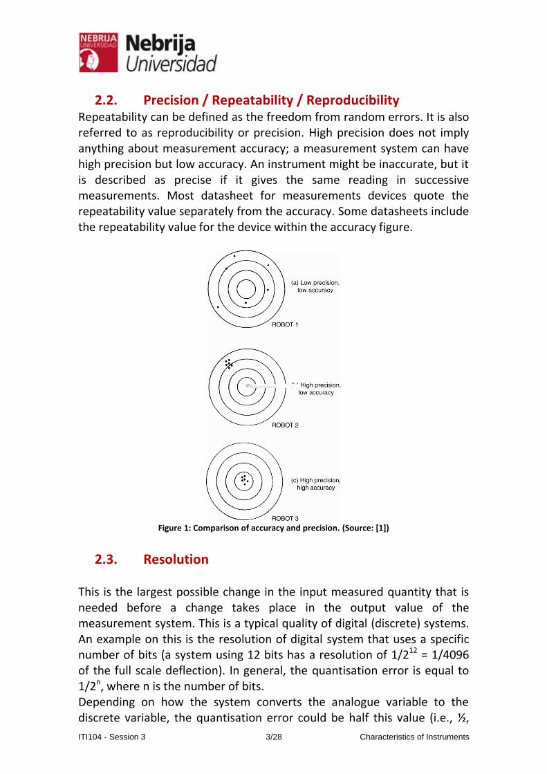
2.2. Precision / Repeatability / Reproducibility Repeatability can be defined as the freedom from random errors. It is also referred to as reproducibility or precision. High precision does not imply anything about measurement accuracy; a measurement system can have high precision but low accuracy. An instrument might be inaccurate, but it is described as precise if it gives the same reading in successive measurements. Most datasheet for measurements devices quote the repeatability value separately from the accuracy. Some datasheets include the repeatability value for the device within the accuracy figure.
Figure 1: Comparison of accuracy and precision. (Source: [1])
2.3. Resolution This is the largest possible change in the input measured quantity that is needed before a change takes place in the output value of the measurement system. This is a typical quality of digital (discrete) systems. An example on this is the resolution of digital system that uses a specific number of bits (a system using 12 bits has a resolution of 1/212 = 1/4096 of the full scale deflection). In general, the quantisation error is equal to 1/2n, where n is the number of bits. Depending on how the system converts the analogue variable to the discrete variable, the quantisation error could be half this value (i.e., ½,
ITI104 - Session 3 4/28 Characteristics of Instruments
1/2n). This formula could be used to decide the number of bits based on the acceptable quantisation error (e.g., a quantisation error of 0.1% will require a 10 bit system). Obviously the resolution of the system can be improved by increasing the number of bits, but this leads to extra cost and an increase in the conversion time of the A to D conversion process.
2.4. Range and span The range of an instrument defines the minimum and maximum values of a quantity that the instrument is designed to measure, and can be applied to both the input as well as the output of the measurement system. The range does not necessarily start at zero (e.g., thermometer that is used to measure body temperature might range from 30 ºC to 42 ºC). Span is the maximum variation in the input or output.
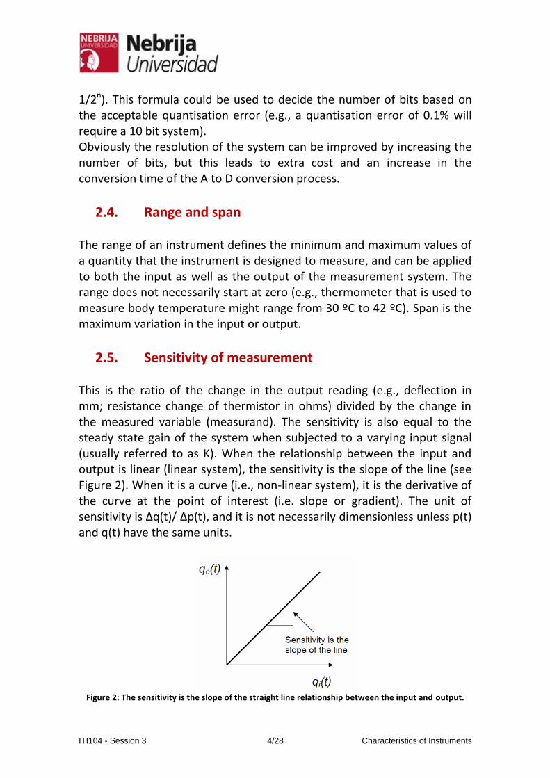
2.5. Sensitivity of measurement This is the ratio of the change in the output reading (e.g., deflection in mm; resistance change of thermistor in ohms) divided by the change in the measured variable (measurand). The sensitivity is also equal to the steady state gain of the system when subjected to a varying input signal (usually referred to as K). When the relationship between the input and output is linear (linear system), the sensitivity is the slope of the line (see Figure 2). When it is a curve (i.e., non-linear system), it is the derivative of the curve at the point of interest (i.e. slope or gradient). The unit of sensitivity is Δq(t)/ Δp(t), and it is not necessarily dimensionless unless p(t) and q(t) have the same units.
Figure 2: The sensitivity is the slope of the straight line relationship between the input and output.
ITI104 - Session 3 5/28 Characteristics of Instruments
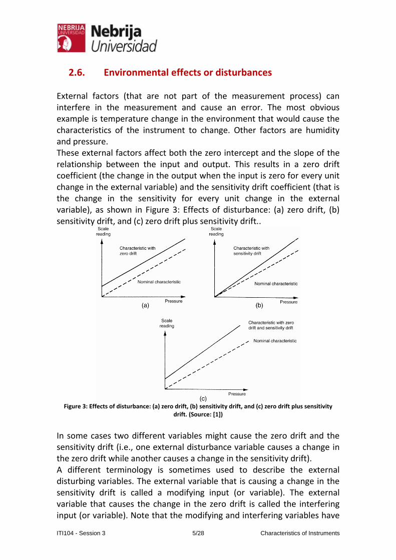
2.6. Environmental effects or disturbances External factors (that are not part of the measurement process) can interfere in the measurement and cause an error. The most obvious example is temperature change in the environment that would cause the characteristics of the instrument to change. Other factors are humidity and pressure. These external factors affect both the zero intercept and the slope of the relationship between the input and output. This results in a zero drift coefficient (the change in the output when the input is zero for every unit change in the external variable) and the sensitivity drift coefficient (that is the change in the sensitivity for every unit change in the external variable), as shown in Figure 3: Effects of disturbance: (a) zero drift, (b) sensitivity drift, and (c) zero drift plus sensitivity drift..
Figure 3: Effects of disturbance: (a) zero drift, (b) sensitivity drift, and (c) zero drift plus sensitivity
drift. (Source: [1])
In some cases two different variables might cause the zero drift and the sensitivity drift (i.e., one external disturbance variable causes a change in the zero drift while another causes a change in the sensitivity drift). A different terminology is sometimes used to describe the external disturbing variables. The external variable that is causing a change in the sensitivity drift is called a modifying input (or variable). The external variable that causes the change in the zero drift is called the interfering input (or variable). Note that the modifying and interfering variables have
ITI104 - Session 3 6/28 Characteristics of Instruments
become external variables because they are not an intentional part of the measurement process.
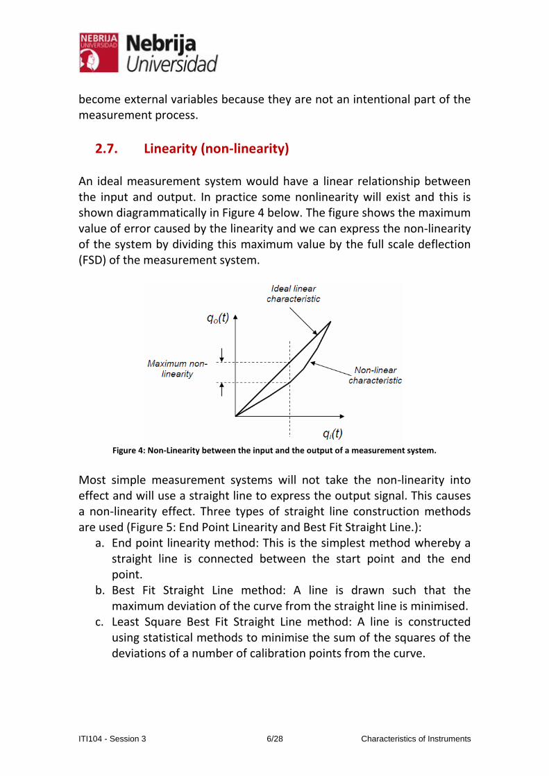
2.7. Linearity (non-linearity) An ideal measurement system would have a linear relationship between the input and output. In practice some nonlinearity will exist and this is shown diagrammatically in Figure 4 below. The figure shows the maximum value of error caused by the linearity and we can express the non-linearity of the system by dividing this maximum value by the full scale deflection (FSD) of the measurement system.
Figure 4: Non-Linearity between the input and the output of a measurement system.
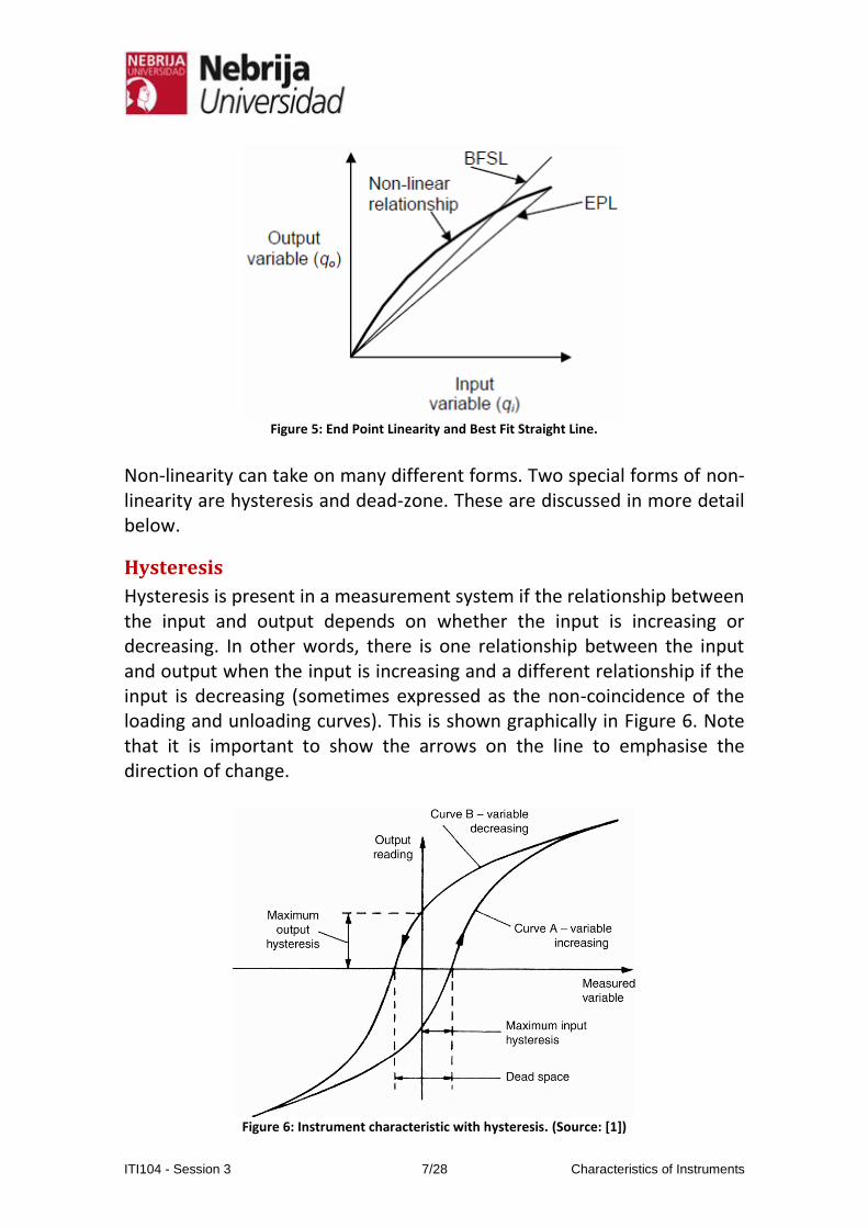
Most simple measurement systems will not take the non-linearity into effect and will use a straight line to express the output signal. This causes a non-linearity effect. Three types of straight line construction methods are used (Figure 5: End Point Linearity and Best Fit Straight Line.):
a. End point linearity method: This is the simplest method whereby a straight line is connected between the start point and the end point.
b. Best Fit Straight Line method: A line is drawn such that the maximum deviation of the curve from the straight line is minimised.
c. Least Square Best Fit Straight Line method: A line is constructed using statistical methods to minimise the sum of the squares of the deviations of a number of calibration points from the curve.
ITI104 - Session 3 7/28 Characteristics of Instruments
Figure 5: End Point Linearity and Best Fit Straight Line.
Non-linearity can take on many different forms. Two special forms of non-linearity are hysteresis and dead-zone. These are discussed in more detail below.
Hysteresis
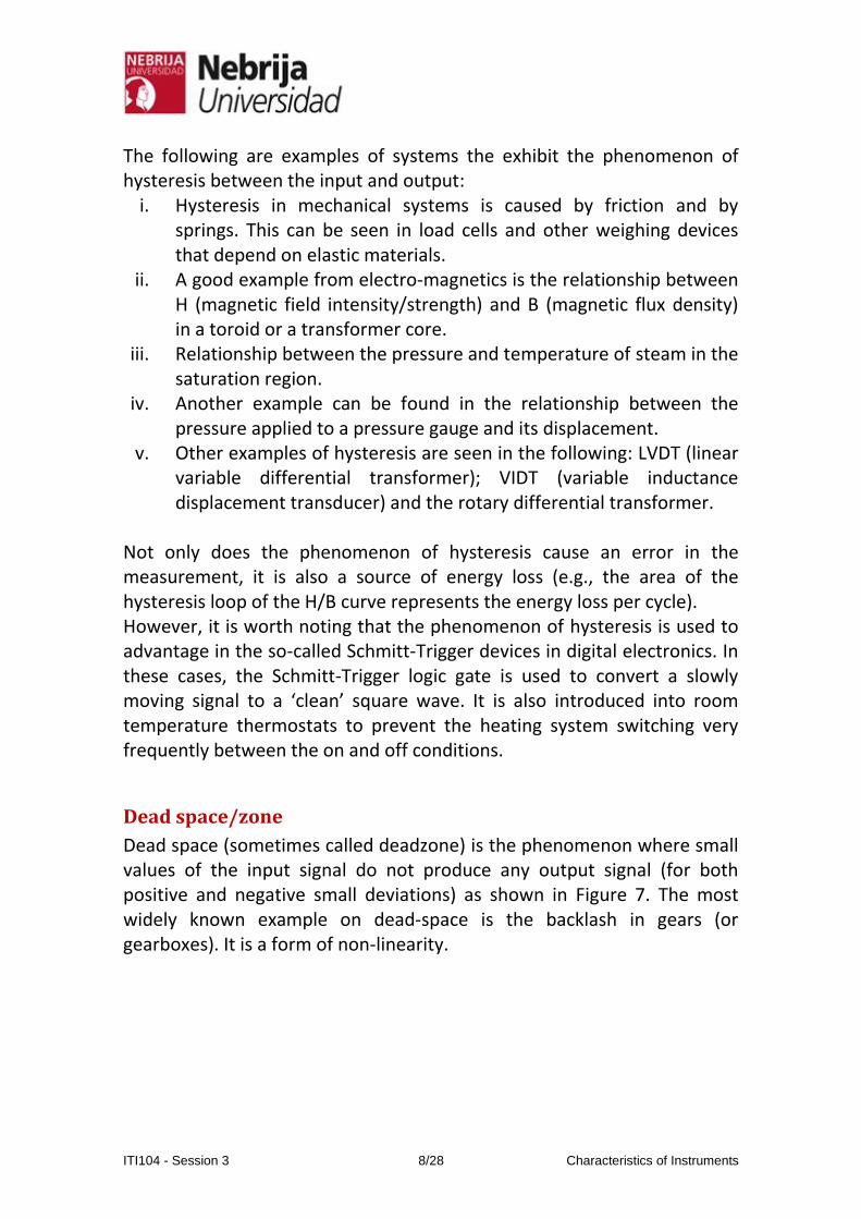
Hysteresis is present in a measurement system if the relationship between the input and output depends on whether the input is increasing or decreasing. In other words, there is one relationship between the input and output when the input is increasing and a different relationship if the input is decreasing (sometimes expressed as the non-coincidence of the loading and unloading curves). This is shown graphically in Figure 6. Note that it is important to show the arrows on the line to emphasise the direction of change.
Figure 6: Instrument characteristic with hysteresis. (Source: [1])
ITI104 - Session 3 8/28 Characteristics of Instruments
The following are examples of systems the exhibit the phenomenon of hysteresis between the input and output:
i. Hysteresis in mechanical systems is caused by friction and by springs. This can be seen in load cells and other weighing devices that depend on elastic materials.
ii. A good example from electro-magnetics is the relationship between H (magnetic field intensity/strength) and B (magnetic flux density) in a toroid or a transformer core.
iii. Relationship between the pressure and temperature of steam in the saturation region.
iv. Another example can be found in the relationship between the pressure applied to a pressure gauge and its displacement.
v. Other examples of hysteresis are seen in the following: LVDT (linear variable differential transformer); VIDT (variable inductance displacement transducer) and the rotary differential transformer.
Not only does the phenomenon of hysteresis cause an error in the measurement, it is also a source of energy loss (e.g., the area of the hysteresis loop of the H/B curve represents the energy loss per cycle). However, it is worth noting that the phenomenon of hysteresis is used to advantage in the so-called Schmitt-Trigger devices in digital electronics. In these cases, the Schmitt-Trigger logic gate is used to convert a slowly moving signal to a ‘clean’ square wave. It is also introduced into room temperature thermostats to prevent the heating system switching very frequently between the on and off conditions.
Dead space/zone
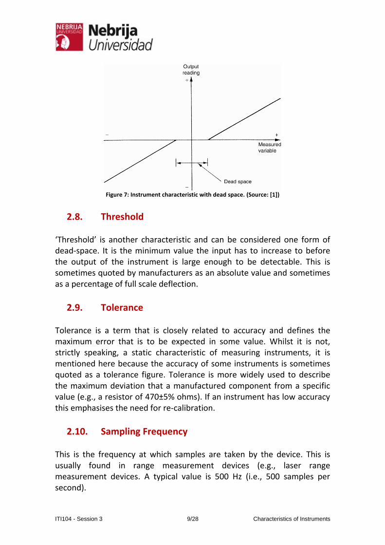
Dead space (sometimes called deadzone) is the phenomenon where small values of the input signal do not produce any output signal (for both positive and negative small deviations) as shown in Figure 7. The most widely known example on dead-space is the backlash in gears (or gearboxes). It is a form of non-linearity.
ITI104 - Session 3 9/28 Characteristics of Instruments
Figure 7: Instrument characteristic with dead space. (Source: [1])
2.8. Threshold ‘Threshold’ is another characteristic and can be considered one form of dead-space. It is the minimum value the input has to increase to before the output of the instrument is large enough to be detectable. This is sometimes quoted by manufacturers as an absolute value and sometimes as a percentage of full scale deflection.
2.9. Tolerance Tolerance is a term that is closely related to accuracy and defines the maximum error that is to be expected in some value. Whilst it is not, strictly speaking, a static characteristic of measuring instruments, it is mentioned here because the accuracy of some instruments is sometimes quoted as a tolerance figure. Tolerance is more widely used to describe the maximum deviation that a manufactured component from a specific value (e.g., a resistor of 470±5% ohms). If an instrument has low accuracy this emphasises the need for re-calibration.
2.10. Sampling Frequency This is the frequency at which samples are taken by the device. This is usually found in range measurement devices (e.g., laser range measurement devices. A typical value is 500 Hz (i.e., 500 samples per second).
ITI104 - Session 3 10/28 Characteristics of Instruments
2.11. Life Expectancy This is the expected design life of the measurement system.
2.12. Reliability The number of failures expected of the device in a certain period of time. It is usually expressed as MTBF (mean time between failures) for repairable items and quoted in years. This parameter is extremely important in order to calculate the overall reliability of a plant or factory within which the measurement system will be installed.
3. Dynamic Characteristics In the section we examine the dynamic characteristics of measurement systems. We are trying to understand the transient behavior of the output signal. This allows us to quantify the transient error in the measurement.
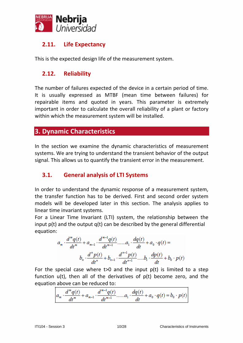
3.1. General analysis of LTI Systems In order to understand the dynamic response of a measurement system, the transfer function has to be derived. First and second order system models will be developed later in this section. The analysis applies to linear time invariant systems. For a Linear Time Invariant (LTI) system, the relationship between the input p(t) and the output q(t) can be described by the general differential equation:
For the special case where t>0 and the input p(t) is limited to a step function u(t), then all of the derivatives of p(t) become zero, and the equation above can be reduced to:
ITI104 - Session 3 11/28 Characteristics of Instruments
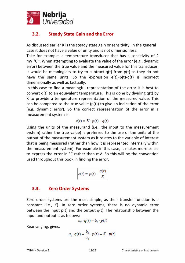
3.2. Steady State Gain and the Error As discussed earlier K is the steady state gain or sensitivity. In the general case it does not have a value of unity and is not dimensionless. Take for example, a temperature transducer that has a sensitivity of 2 mV·°C-1. When attempting to evaluate the value of the error (e.g., dynamic error) between the true value and the measured value for this transducer, It would be meaningless to try to subtract q(t) from p(t) as they do not have the same units. So the expression e(t)=p(t)-q(t) is incorrect dimensionally as well as factually. In this case to find a meaningful representation of the error it is best to convert q(t) to an equivalent temperature. This is done by dividing q(t) by K to provide a temperature representation of the measured value. This can be compared to the true value (p(t)) to give an indication of the error (e.g. dynamic error). So the correct representation of the error in a measurement system is:
Using the units of the measurand (i.e., the input to the measurement system) rather the true value) is preferred to the use of the units of the output of the measurement system as it relates to the variable of interest that is being measured (rather than how it is represented internally within the measurement system). For example in this case, it makes more sense to express the error in °C rather than mV. So this will be the convention used throughout this book in finding the error:
3.3. Zero Order Systems Zero order systems are the most simple, as their transfer function is a constant (i.e., K). In zero order systems, there is no dynamic error between the input p(t) and the output q(t). The relationship between the input and output is as follows:
Rearranging, gives:
ITI104 - Session 3 12/28 Characteristics of Instruments
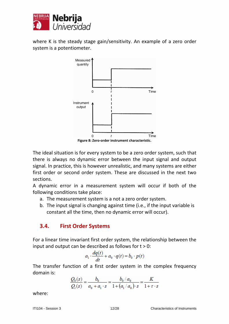
where K is the steady stage gain/sensitivity. An example of a zero order system is a potentiometer.
Figure 8: Zero-order instrument characteristic.
The ideal situation is for every system to be a zero order system, such that there is always no dynamic error between the input signal and output signal. In practice, this is however unrealistic, and many systems are either first order or second order system. These are discussed in the next two sections. A dynamic error in a measurement system will occur if both of the following conditions take place:
a. The measurement system is a not a zero order system. b. The input signal is changing against time (i.e., if the input variable is
constant all the time, then no dynamic error will occur).
3.4. First Order Systems For a linear time invariant first order system, the relationship between the input and output can be described as follows for t > 0:
The transfer function of a first order system in the complex frequency domain is:
where:
ITI104 - Session 3 13/28 Characteristics of Instruments
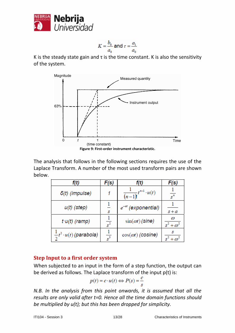
K is the steady state gain and τ is the time constant. K is also the sensitivity of the system.
Figure 9: First-order instrument characteristic.
The analysis that follows in the following sections requires the use of the Laplace Transform. A number of the most used transform pairs are shown below.
Step Input to a first order system
When subjected to an input in the form of a step function, the output can be derived as follows. The Laplace transform of the input p(t) is:
N.B. In the analysis from this point onwards, it is assumed that all the results are only valid after t=0. Hence all the time domain functions should be multiplied by u(t); but this has been dropped for simplicity.
ITI104 - Session 3 14/28 Characteristics of Instruments
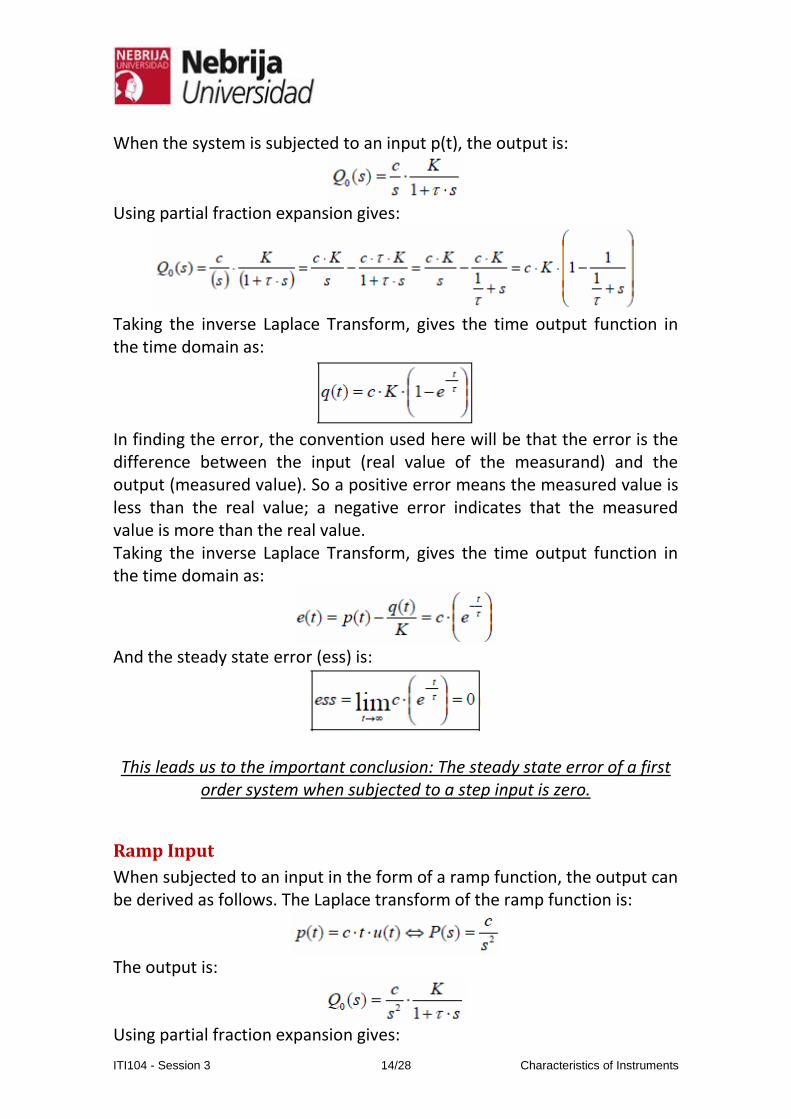
When the system is subjected to an input p(t), the output is:
Using partial fraction expansion gives:
Taking the inverse Laplace Transform, gives the time output function in the time domain as:
In finding the error, the convention used here will be that the error is the difference between the input (real value of the measurand) and the output (measured value). So a positive error means the measured value is less than the real value; a negative error indicates that the measured value is more than the real value. Taking the inverse Laplace Transform, gives the time output function in the time domain as:
And the steady state error (ess) is:
This leads us to the important conclusion: The steady state error of a first
order system when subjected to a step input is zero.
Ramp Input
When subjected to an input in the form of a ramp function, the output can be derived as follows. The Laplace transform of the ramp function is:
The output is:
Using partial fraction expansion gives:
ITI104 - Session 3 15/28 Characteristics of Instruments
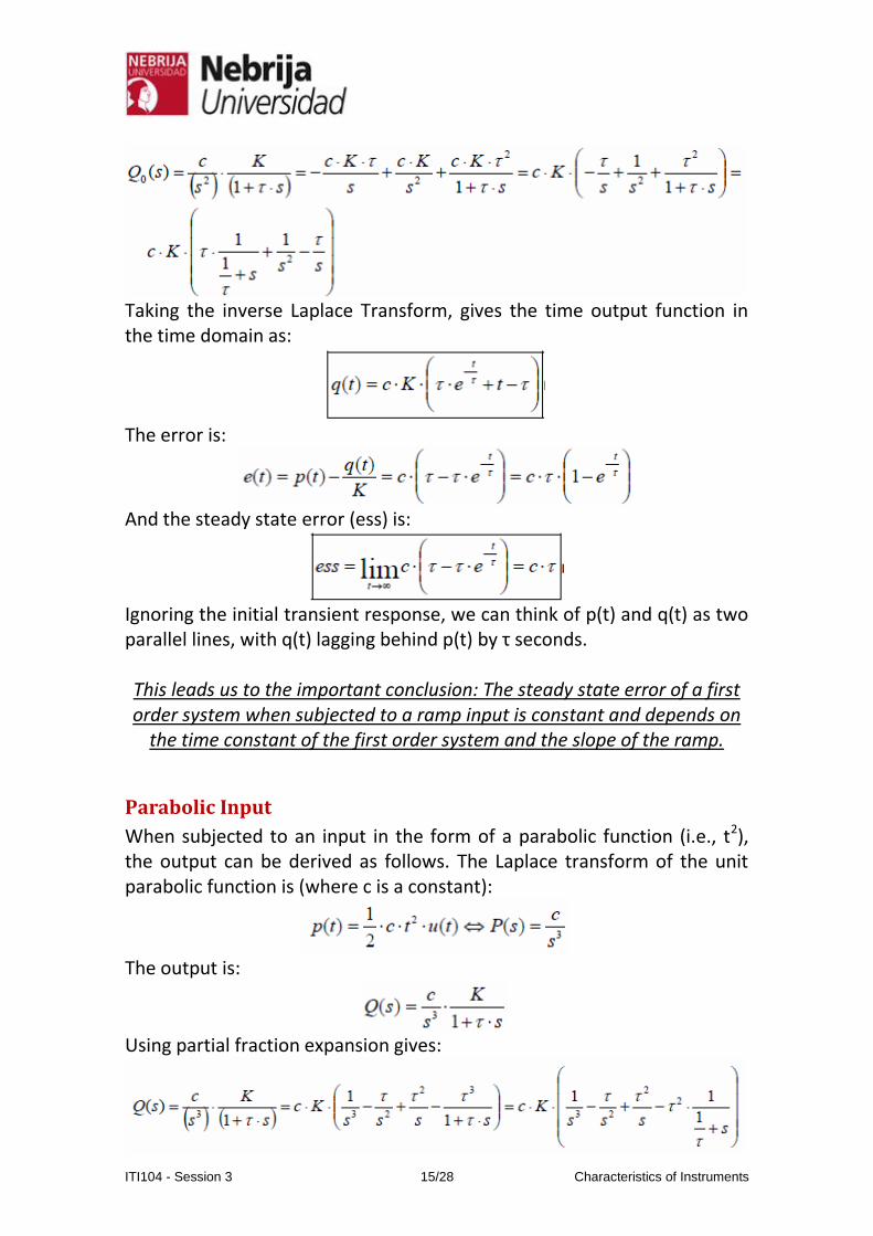
Taking the inverse Laplace Transform, gives the time output function in the time domain as:
The error is:
And the steady state error (ess) is:
Ignoring the initial transient response, we can think of p(t) and q(t) as two parallel lines, with q(t) lagging behind p(t) by τ seconds. This leads us to the important conclusion: The steady state error of a first order system when subjected to a ramp input is constant and depends on
the time constant of the first order system and the slope of the ramp.
Parabolic Input
When subjected to an input in the form of a parabolic function (i.e., t2), the output can be derived as follows. The Laplace transform of the unit parabolic function is (where c is a constant):
The output is:
Using partial fraction expansion gives:
ITI104 - Session 3 16/28 Characteristics of Instruments
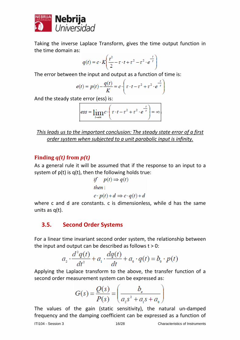
Taking the inverse Laplace Transform, gives the time output function in the time domain as:
The error between the input and output as a function of time is:
And the steady state error (ess) is:
This leads us to the important conclusion: The steady state error of a first
order system when subjected to a unit parabolic input is infinity.
Finding q(t) from p(t)
As a general rule it will be assumed that if the response to an input to a system of p(t) is q(t), then the following holds true:
where c and d are constants. c is dimensionless, while d has the same units as q(t).
3.5. Second Order Systems For a linear time invariant second order system, the relationship between the input and output can be described as follows t > 0:
Applying the Laplace transform to the above, the transfer function of a second order measurement system can be expressed as:
The values of the gain (static sensitivity), the natural un-damped frequency and the damping coefficient can be expressed as a function of
ITI104 - Session 3 17/28 Characteristics of Instruments
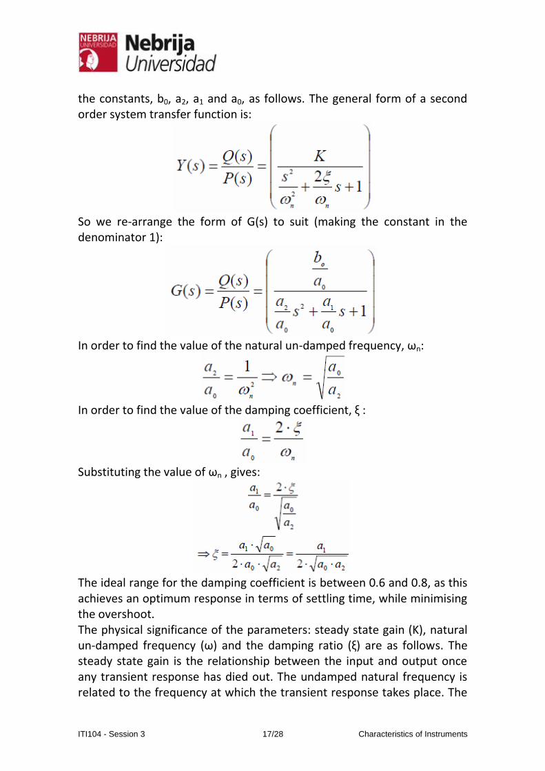
the constants, b0, a2, a1 and a0, as follows. The general form of a second order system transfer function is:
So we re-arrange the form of G(s) to suit (making the constant in the denominator 1):
In order to find the value of the natural un-damped frequency, ωn:
In order to find the value of the damping coefficient, ξ :
Substituting the value of ωn , gives:
The ideal range for the damping coefficient is between 0.6 and 0.8, as this achieves an optimum response in terms of settling time, while minimising the overshoot. The physical significance of the parameters: steady state gain (K), natural un-damped frequency (ω) and the damping ratio (ξ) are as follows. The steady state gain is the relationship between the input and output once any transient response has died out. The undamped natural frequency is related to the frequency at which the transient response takes place. The
ITI104 - Session 3 18/28 Characteristics of Instruments
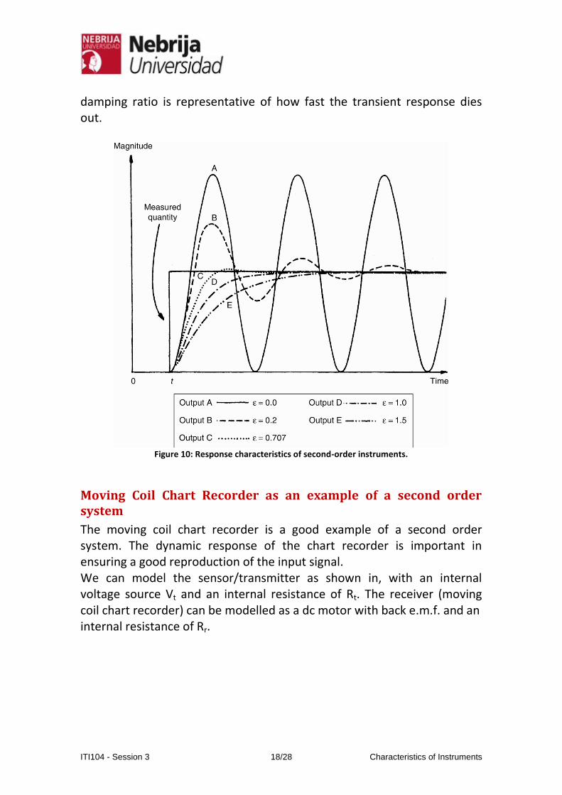
damping ratio is representative of how fast the transient response dies out.
Figure 10: Response characteristics of second-order instruments.
Moving Coil Chart Recorder as an example of a second order system
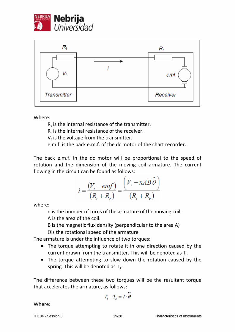
The moving coil chart recorder is a good example of a second order system. The dynamic response of the chart recorder is important in ensuring a good reproduction of the input signal. We can model the sensor/transmitter as shown in, with an internal voltage source Vt and an internal resistance of Rt. The receiver (moving coil chart recorder) can be modelled as a dc motor with back e.m.f. and an internal resistance of Rr.
ITI104 - Session 3 19/28 Characteristics of Instruments
Where:
Rt is the internal resistance of the transmitter. Rr is the internal resistance of the receiver. Vt is the voltage from the transmitter. e.m.f. is the back e.m.f. of the dc motor of the chart recorder.
The back e.m.f. in the dc motor will be proportional to the speed of rotation and the dimension of the moving coil armature. The current flowing in the circuit can be found as follows:
where:
n is the number of turns of the armature of the moving coil. A is the area of the coil. B is the magnetic flux density (perpendicular to the area A)
is the rotational speed of the armature The armature is under the influence of two torques:
The torque attempting to rotate it in one direction caused by the current drawn from the transmitter. This will be denoted as Ti.
The torque attempting to slow down the rotation caused by the spring. This will be denoted as Ts.
The difference between these two torques will be the resultant torque that accelerates the armature, as follows:
Where:
ITI104 - Session 3 20/28 Characteristics of Instruments
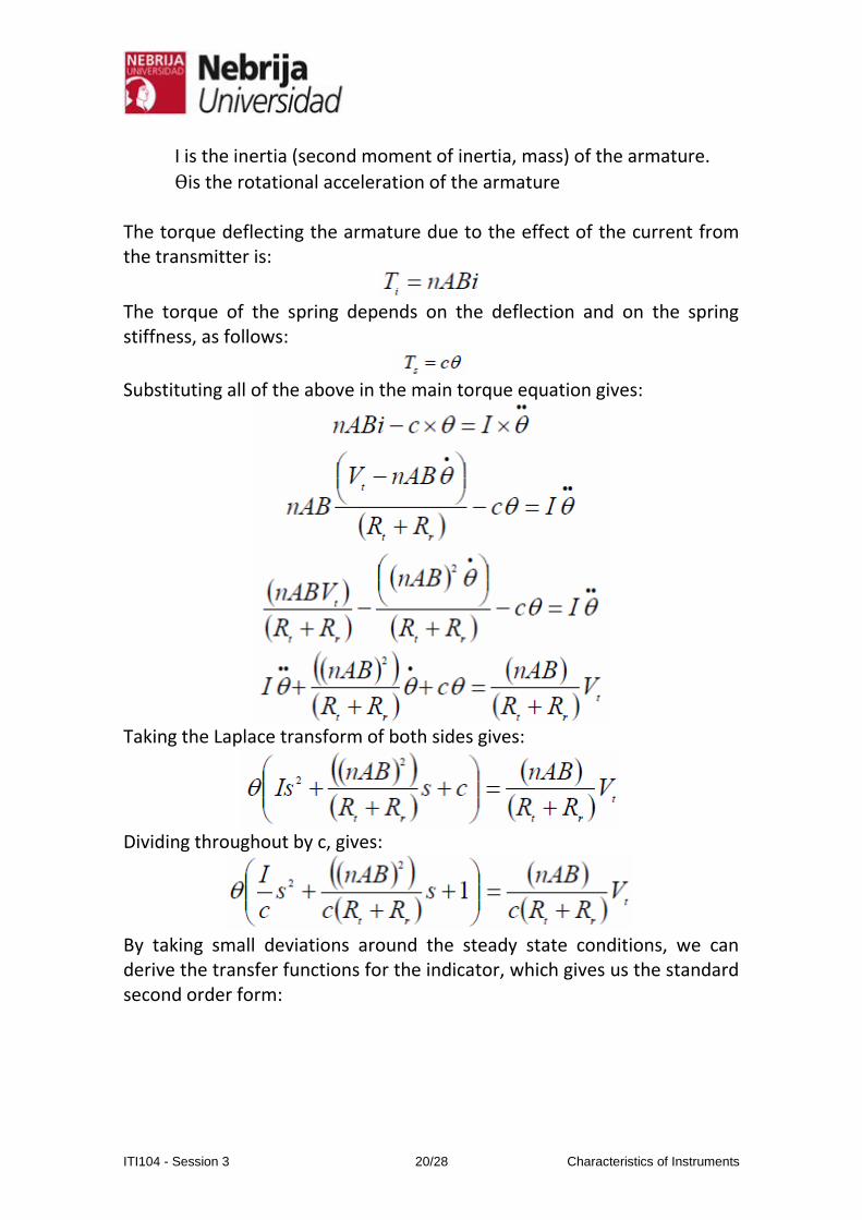
I is the inertia (second moment of inertia, mass) of the armature.
is the rotational acceleration of the armature The torque deflecting the armature due to the effect of the current from the transmitter is:
The torque of the spring depends on the deflection and on the spring stiffness, as follows:
Substituting all of the above in the main torque equation gives:
Taking the Laplace transform of both sides gives:
Dividing throughout by c, gives:
By taking small deviations around the steady state conditions, we can derive the transfer functions for the indicator, which gives us the standard second order form:
ITI104 - Session 3 21/28 Characteristics of Instruments
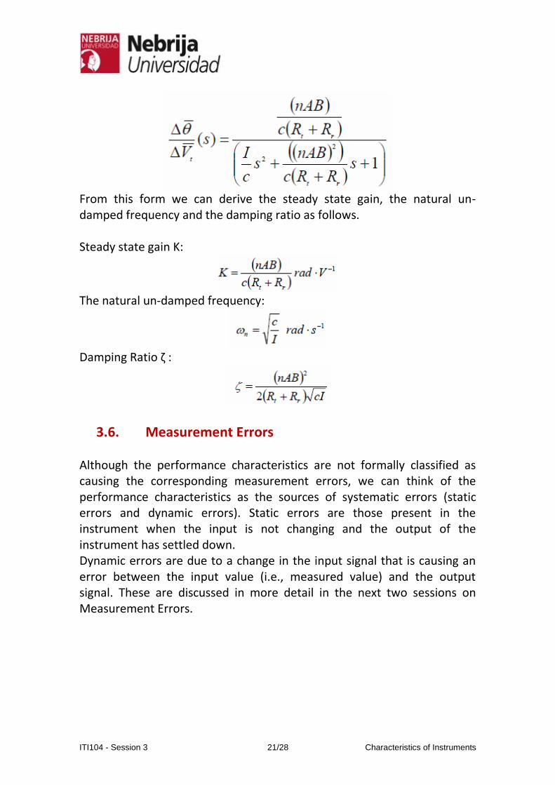
From this form we can derive the steady state gain, the natural un-damped frequency and the damping ratio as follows. Steady state gain K:
The natural un-damped frequency:
Damping Ratio ζ :
3.6. Measurement Errors Although the performance characteristics are not formally classified as causing the corresponding measurement errors, we can think of the performance characteristics as the sources of systematic errors (static errors and dynamic errors). Static errors are those present in the instrument when the input is not changing and the output of the instrument has settled down. Dynamic errors are due to a change in the input signal that is causing an error between the input value (i.e., measured value) and the output signal. These are discussed in more detail in the next two sessions on Measurement Errors.
ITI104 - Session 3 22/28 Characteristics of Instruments
4. Problems
1. A voltmeter uses 10 bits to express, store and display the measured voltage. Calculate its resolution as a percentage of the full scale.
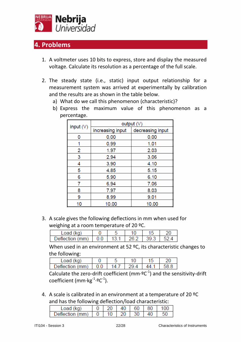
2. The steady state (i.e., static) input output relationship for a
measurement system was arrived at experimentally by calibration and the results are as shown in the table below.
a) What do we call this phenomenon (characteristic)? b) Express the maximum value of this phenomenon as a
percentage.
3. A scale gives the following deflections in mm when used for weighing at a room temperature of 20 ºC.
When used in an environment at 52 ºC, its characteristic changes to the following:
Calculate the zero-drift coefficient (mm·ºC-1) and the sensitivity-drift coefficient (mm·kg-1·ºC-1).
4. A scale is calibrated in an environment at a temperature of 20 ºC and has the following deflection/load characteristic:

ITI104 - Session 3 23/28 Characteristics of Instruments
When used in an environment at 40 ºC, its characteristic changes to the following:
Calculate the zero-drift coefficient and the sensitivity-drift coefficients.
5. A pressure transducer has an input range of 0 to 104 Pa that corresponds to an output range of 1.0 to 5.0 V at a standard temperature of 20 ºC. When the temperature changes to 30 ºC, the output range changes to 1.2 V to 5.2 V. Calculate the zero-drift coefficient and the sensitivity-drift coefficient. Ignore any non-linearity and assume a straight line relationship between the input and output at both temperatures (i.e., 20 ºC and 30 ºC).
6. A scale that is used to measure body weight has the following characteristics at 24 ºC: 0.0 kg 0.0 mm deflection 70 kg 35 mm deflection When used in an ambient temperature of 40 ºC, it has the following characteristics: 0.0 kg 4 mm deflection 70 kg 32 mm deflection Calculate the zero-drift coefficient and the sensitivity-drift coefficient. (Assume a linear relationship between the input and output, ignoring any nonlinearities).
7. Repeat the last problem for the same scale given the following: When used at a temperature of 24 ºC: 0.0 kg 0.0 mm deflection 70 kg 35 mm deflection When used in an ambient temperature of 40 ºC, it has the following characteristics: 0.0 kg -4.0 mm deflection 70 kg 38 mm deflection
8. An electric heater is used to heat a water tank where the water is initially at room temperature of 20 degrees ºC. The temperature of the water in the tank increases linearly with time at a rate of 0.25
ITI104 - Session 3 24/28 Characteristics of Instruments
degrees ºC per second. A glass mercury thermometer is used to measure the temperature, and has a time constant of 5 seconds.
• What will the temperature indicated by the thermometer after 5 seconds be (ºC)? (Ans. 20.46 ºC).
• What will the temperature indicated by the thermometer after 240 seconds be in (ºC)? (Ans. 78.75 ºC).
• What will the steady state error be between the actual temperature of the tank and the thermometer in ºC? (Ans. 1.25 ºC).
9. An electric pump is used to pump water to a residential storage
tank. The water level rises in the tank linearly with time at a rate of 2 mm/second. The initial water level in the tank is 200 mm. A water level measurement system is used to detect the water height in the tank and can be approximated as a first order system with a time constant of 2 seconds. Calculate the following:
• The water level indicated by the water level measurement system after 2 seconds (mm). (Ans. 201.5 mm).
• The water level indicated by the water level measurement system after 150 seconds (mm). (Ans. 496 mm).
• The steady state error between the actual level of the tank and that indicated (mm). (Ans. 4 mm).
10. The thermocouple described in the data-sheet in Attachment 1 is
fitted to a mobile instrument. The instrument is used to measure the temperature of a machine room, whereby the temperature varies between 5 ºC to 40 ºC. The instrument is brought in from an adjacent room in which the room temperature is 20 ºC to the machine room when the machine room temperature was 40 ºC. Note that the thermocouple has been grounded. a) What is the purpose of grounding the thermocouple? b) What is the temperature indicated by the instrument after:
0.5 second, 2.0 seconds.
c) What is the steady state error?
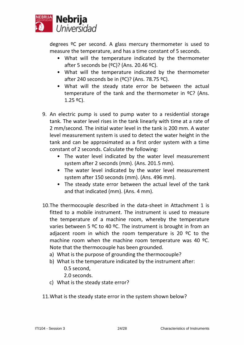
11. What is the steady state error in the system shown below?
ITI104 - Session 3 25/28 Characteristics of Instruments
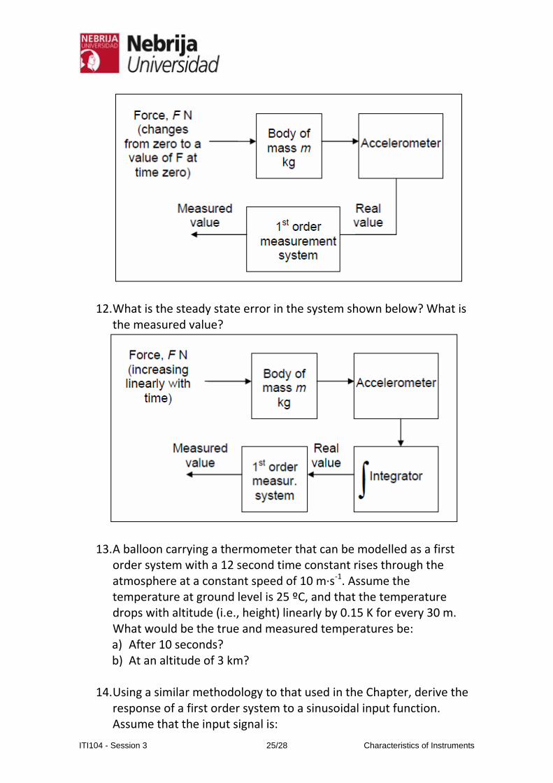
12. What is the steady state error in the system shown below? What is the measured value?
13. A balloon carrying a thermometer that can be modelled as a first order system with a 12 second time constant rises through the atmosphere at a constant speed of 10 m·s-1. Assume the temperature at ground level is 25 ºC, and that the temperature drops with altitude (i.e., height) linearly by 0.15 K for every 30 m. What would be the true and measured temperatures be: a) After 10 seconds? b) At an altitude of 3 km?
14. Using a similar methodology to that used in the Chapter, derive the
response of a first order system to a sinusoidal input function. Assume that the input signal is:
ITI104 - Session 3 26/28 Characteristics of Instruments
Find an expression for q(t). Assume that the steady state gain of the first order system is K (dimensionless) and that it has a time constant of τ seconds.
5. References [1] Alan S. Morris and R. Langari, “Measurement and Instrumentation.
Theory and Application”, Ed. Elsevier, 1st Edition, 2011. Some text is reproduced with authorization of Dr. Lufti Al-Sharif ([email protected])
6. Annex

ITI104 - Session 3 27/28 Characteristics of Instruments

ITI104 - Session 3 28/28 Characteristics of Instruments
Related Documents