Sensitivity of the Northern Hemisphere climate system to extreme changes in Holocene Arctic sea ice

Quaternary Science Reviews 22 (2003) 645–658

Sensitivity of the Northern Hemisphere climate system to extremechanges in Holocene Arctic sea ice

L. Micaela Smitha,*, Gifford H. Millera, Bette Otto-Bliesnerb, Sang-Ik Shinc

aDepartment of Geological Sciences and Institute of Arctic and Alpine Research (INSTAAR), University of Colorado, Boulder, Campus Box 450,

Boulder, CO 80309, USAbClimate Change Research, National Center for Atmospheric Research, P.O. Box 3000, Boulder, CO 80307, USA

cCenter for Climate Research, University of Wisconsin-Madison, 1225 W. Dayton St, Madison, WI, 53706-1695, USA

Received 12 February 2001; accepted 11 August 2002

Abstract

The extent of seasonal and perennial sea ice changed dramatically through the Late Quaternary and these changes influenced both

the ocean and atmosphere by controlling the exchange of energy, moisture and gases between them, and by altering the planetary

albedo. Reconstructing the changing patterns of sea ice distribution in the recent past remains one of the outstanding challenges to

the paleo-community. To evaluate the importance of these reconstructions we performed sensitivity tests using NCAR’s Community

Climate Model (CCM3), and a series of prescribed sea ice extents designed to capture the full range of Arctic sea ice variability under

interglacial (Holocene) and full glacial (Last Glacial Maximum) boundary conditions. Our simulations indicate that surface

temperatures and sea level pressures in winter (DJF) are most sensitive to changes in sea ice, and that these changes are propagated

over the surrounding land masses in the North Atlantic, but that equivalent changes in sea ice produce smaller corresponding

changes in temperature or sea level pressure in the North Pacific region. A comparison between CLIMAP (Map Chart Series MC-

36, Geological Society of America, Boulder, CO, 1981) and a more realistic assessment of LGM sea ice yields dramatic changes in

winter temperatures and precipitation patterns across Eurasia. These differences, forced only by changed sea ice conditions,

reinforce the need to develop accurate maps of past sea ice to correctly simulate Late Quaternary environments. Such

reconstructions also will be essential to validate the next generation of sea ice models.

r 2002 Elsevier Science Ltd. All rights reserved.

1. Introduction

Sea ice influences and is influenced by both theatmosphere and ocean, making it a sensitive butcomplex component of the climate system. Sea icemodulates the climate system through albedo, oceanstratification and dynamics, and the exchange of heat,moisture, and momentum between the atmosphere andocean. Both positive and negative feedbacks link sea iceto changes in albedo, cloud cover, atmospheric watervapor, and ocean thermohaline circulation that, in turn,influences climate and its sensitivity to external andinternal perturbations (Dickinson, 1985). Recent boxmodel experiments indicate that sea ice may be thetrigger of the glacial/interglacial switch by regulating the

hydrological cycle and moisture exchange between theland and ocean that controls snow accumulation onterrestrial ice sheets (Gildor and Tziperman, 2000,2001). Therefore, climate models should be sensitive tosea ice extent, and when modeling past climatescenarios, the sea ice reconstructions are an importantmodel component.Although sea ice margins are known to have changed

dramatically in the Late Quaternary, no reliable pan-Arctic synthesis is yet available for any particular timeslice. Sea ice leaves no obvious direct trace preserved inthe geologic record. Most sea ice reconstructions arebased on faunal and floral assemblage abundances thatcharacterize the marginal ice zone (e.g. Ko-c et al., 1993)or the duration of ice-free conditions (e.g. de Vernalet al., 2000), or changes in specific traits of the physicalsedimentology (reviewed in Miller et al., 2001). Moststudies of past sea ice changes have focused on thedifferences between glacial and Holocene, or recent, sea

*Corresponding author. Now at: BP America, 501 Westlake Blvd,

Houston, TX 77079, USA.

E-mail address: [email protected] (L.M. Smith).

0277-3791/03/$ - see front matter r 2002 Elsevier Science Ltd. All rights reserved.

PII: S 0 2 7 7 - 3 7 9 1 ( 0 2 ) 0 0 1 6 6 - X

ice distribution. The importance of incorporatingcorrect sea ice boundaries for Last Glacial Maximum(LGM) paleoclimate simulations is widely understood,although usually overlooked, and for ease, mostsimulations incorporate CLIMAP (1981) sea ice bound-aries.Recent observations showing large decreases in the

thickness of Arctic Ocean sea ice over the past severaldecades suggest additional effort may be warranted todefine the minimum limits of sea ice in the earlyHolocene, when the flux of warm Atlantic water to theArctic Ocean was at a maximum. Likewise, recentpaleoceanographic data reconstructions indicate less seaice cover than previously thought during deglaciationand the LGM, especially in the North Atlantic (Kocet al., 1993; Hebbeln et al., 1998; deVernal and Hillaire-Marcel, 2000; de Vernal et al., 2000).The purpose of this paper is to use an atmospheric

general circulation model to evaluate the sensitivity ofthe atmosphere to realistic minimum and maximum seaice configurations for the Holocene. No study has yetevaluated the sensitivity of the climate system during theHolocene to extreme changes in sea ice configurationsduring this period. The sensitivity of the climate systemto sea ice, as determined by this study, will define therequired accuracy of paleo-sea-ice—reconstructions. Asa benchmark, a similar sensitivity experiment wascarried out for the LGM using dramatically differentsea ice configurations: a maximum reconstructionCLIMAP (1981) and a restricted margin more consis-tent with recent literature. These sensitivity experimentsevaluate the sensitivity of climate to sea ice extent, butare not intended to be accurate predictors of past orfuture climates, because we have not used a fullycoupled GCM for these model experiments.

2. Previous work

Few modeling experiments have specifically analyzedthe sensitivity of the climate system to extremedifferences in both Holocene and LGM sea ice coverover the northern high latitudes. Most modelingexperiments focus on the LGM, while overlooking theextreme changes in Arctic sea ice throughout theHolocene. Pinot et al. (1999) modeled the sensitivity ofthe European LGM climate to different North Atlanticsea-surface temperatures (SST) and sea ice using theCLIMAP prescribed SST versus reduced LGM NorthAtlantic SST and sea ice based on recent publications.The model results simulate a hydrological cycle andtemperatures different from those reported by CLIMAP(1981) with regional impacts across Europe. ThePaleoclimate Model Intercomparison Project (PMIP)has also used CLIMAP (1981) SSTs in an atmosphericglobal circulation modeling effort, and obtained com-

puted SSTs with a coupled slab-ocean model (Kageya-ma et al., 2001). Marsiat and Valdes (2001) used bothPMIPs prescribed and computed SSTs to demonstratethe sensitivity of northern hemisphere climate to seasurface temperatures. But, differences between thePMIP model experiments and those presented in thispaper do not allow for adequate comparison of thesemodel results. Recently, both Shin et al. (in review) andKitoh et al. (2001) used NCAR and PMIPs coupledatmosphere-ocean global circulation models (AOGCM),respectively, with different boundary conditions for theLGM, and both model experiments resulted in sea icedistributions less than CLIMAP (1981). Thus, thereare both model and proxy record data indicating thatthe CLIMAP (1981) sea ice reconstructions may be tooextensive.There are fewer model experiments to evaluate

Holocene climate. Rind et al. (1986) used CLIMAPSST and sea ice extents to model the impact of cold,North Atlantic SST on climate as an analog for theYounger Dryas. Kerwin et al. (1999) evaluated theimportance of the prescribed ocean boundary conditionsin mid-Holocene (6 ka) climate modeling experiments.Alternatively, model experiments have focused on theclimate system response to complete removal of Arcticsea ice (Warsaw and Rapp, 1973; Raymo et al., 1990;Royer et al., 1990) as analogs for global warmingscenarios, but these simulations are not always suitablefor paleoclimate reconstructions when there is proxyrecord evidence for sea ice.

3. Methods

Sensitivity experiments allow us to investigate theclimate response to altering a specific boundary condi-tion within a model experiment, and then to understandthe boundary condition’s complex role within theclimate system (Bradley, 2000). We are investigatingthe role of sea ice by conducting experiments withprescribed maximum and minimum sea ice extents forthe Holocene, and a benchmark study of the LGM.Simulations for this study were conducted with the

NCAR Community Climate Model (CCM3) (Kiehlet al., 1998). CCM3, the atmospheric model of theNCAR Climate System Model (CSM), is a spectralmodel with 18 levels in the vertical and, for this study, ahorizontal grid spacing set at the T31 grid (B3.751). Theland surface model has specified vegetation types and acomprehensive treatment of surface processes (Bonan,1998). Atmospheric greenhouse gases, CO2, CH4, andN2O, were specified from ice core data at pre-Industrialvalues for the Holocene simulations and at LGM valuesfor the LGM simulations (Raynaud et al., 1993; Blunieret al., 1995; Fluckiger et al., 1999; Indermuhle et al.,1999) (Table 1). Insolation was set at 6 ka for all

L.M. Smith et al. / Quaternary Science Reviews 22 (2003) 645–658646

Holocene experiments and 21 ka for the LGM experi-ments. Modern land and ice sheet configurations areused in the Holocene model experiments, whereas LGMland and ice sheet configuration is based on Peltier(1994). The model was run with a fixed ocean where theseasonal sea ice extents and sea surface temperatureswere specified and did not change throughout the modelexperiment. This limits the predictive potential of ourexperiments, but provides a more accurate sensitivitytest, our primary objective.The experiments were run for 20 model years, but

only the last 15 model years were used in analysis andinterpretation. Differences between simulations areevaluated in terms of the natural interannual variabilityof the model. Standard deviations of the seasonalaverages for the individual years are used in conjunctionwith the Student t-test (Panofsky and Brier, 1965) toseparate signal from noise when comparing simulations(Chervin and Schneider, 1976). Only differences whichare greater than the 90% confidence interval areconsidered statistically different from the year-to-yearvariability, i.e. there is a 1 in 10 chance that suchdifferences could arise by chance.We designed a primary experiment for the Holocene

in which extreme values for maximum and minimum seaice are compared to a control run with modern sea ice,and a secondary benchmark experiment for the LGMcomparing CLIMAP and recently published less ex-tensive sea ice limits (Koc et al., 1993; Hebbeln et al.,1998; deVernal and Hillaire-Marcel, 2000; de Vernalet al., 2000). The Holocene and LGM limits of sea iceused in this study emphasize the maximum reasonabledifferences in sea ice limits based on published literaturecombined with our own interpretation. Our primary

emphasis is on assessing the sensitivity of the atmo-sphere to realistic differences in sea ice extents underinterglacial and glacial conditions.The prescribed limits of sea ice for both the Holocene

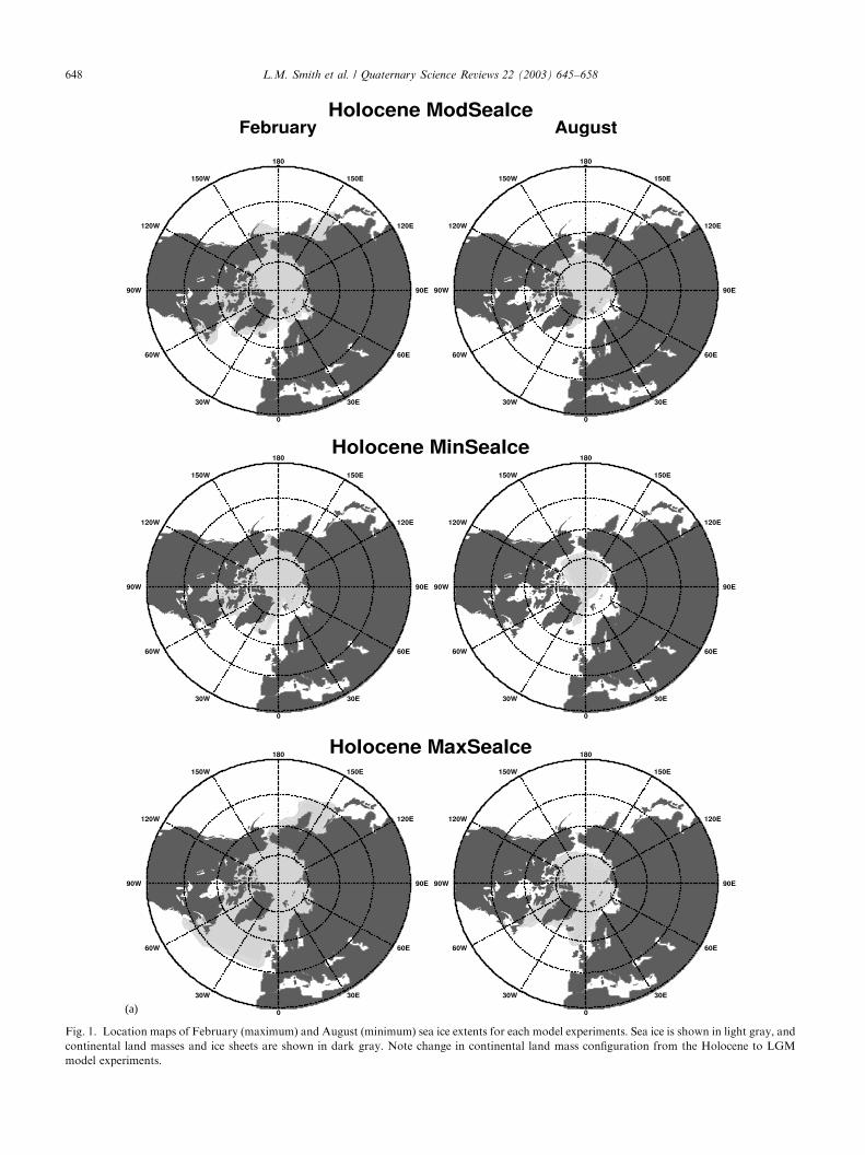
and LGM winter (February) and summer (August) areshown in Fig. 1, and the amount of ocean area coveredby maximum (February) and minimum (August) sea icein each model experiment is shown in Fig. 2. We definedFebruary, April, August, and October sea ice limits foreach experiment, and fit these four months with asinusoidal curve in order to define the sea limits for theremaining eight months. Although maximum andminimum sea ice limits usually occur in March andSeptember or October, respectively, we used Februaryand August because those were the months defined byCLIMAP as maximum and minimum sea ice, respec-tively.

3.1. Holocene

The Holocene minimum sea ice experiment (HoloceneMinSeaIce), analogous to the mid-Holocene Optimum(6 ka), has February and August sea ice conditions at25% and 50%, respectively, less than our Holocenecontrol (Holocene ModSeaIce) within the Arctic Oceanand no Atlantic or Pacific sea ice. We do prescribe asmall amount of sea ice along the East Greenland coast(Fig. 1) to simulate sea ice export through the FramStrait (Aagaard and Carmack, 1989). Sea ice conditionsfor the Holocene maximum sea ice experiment (Holo-cene MaxSeaIce) are based on CLIMAP’s LGMreconstruction (CLIMAP, 1981). Sea ice in the Holo-cene MaxSeaIce experiment is increased by 160% and120% in February and August, respectively, compared

Table 1

Input parameters for each modeling experiment

Model Sea ice extenta SST Insolation Atm

gasesbLand and ice

sheetsc

Holocene Modern Sea Ice

(ModSeaIce)

Present-day Modern 6 ka Pre-I Modern

Holocene Minimum Sea Ice

(MinSeaIce)

oPresent day Modern 6 ka Pre-I Modern

Holocene Maximum Sea Ice

(MaxSeaIce)

CLIMAP Modern, except >201N

(CLIMAP)d6 ka Pre-I Modern

LGM Minimum Sea Ice (MinSeaIce) CLIMAP, ice-free

Nordic SeaseCLIMAP except in

Nordic Sea

21 ka LGM LGM

LGM Maximum Sea Ice (MaxSeaIce) CLIMAP CLIMAP 21 ka LGM LGM

aSee Fig. 1 for winter and summer sea ice extents in each experiment.bValues for atmospheric gases (CO2, CH4, CFC, N2O) are based on ice core values from Blunier et al. (1995), Fluckiger et al. (1999), Indermuhle

et al. (1999), and Raynaud et al. (1993). Holocene values: CO2=280ppm, CH4=750ppb, CFC=0ppb, N2O=275ppb. LGM values:

CO2=200ppm, CH4=350ppb, CFC=0ppb, N2O=190ppb.cLand and ice sheet configuration for the LGM model experiments is based on CLIMAP (1981) and Peltier (1994).dSee methods for the determination of North Atlantic SST in the Holocene MaxSeaIce experiment.eThe reduced sea ice extent for the Nordic Seas was based on deVernal et al. (2000), deVernal and Hillaire-Marcel (2000), Hebbeln et al. (1998),

Koc (1993).

L.M. Smith et al. / Quaternary Science Reviews 22 (2003) 645–658 647

(a)

Fig. 1. Location maps of February (maximum) and August (minimum) sea ice extents for each model experiments. Sea ice is shown in light gray, and

continental land masses and ice sheets are shown in dark gray. Note change in continental land mass configuration from the Holocene to LGM

model experiments.


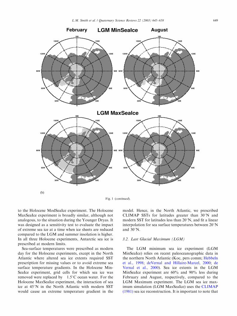
to the Holocene ModSeaIce experiment. The HoloceneMaxSeaIce experiment is broadly similar, although notanalogous, to the situation during the Younger Dryas. Itwas designed as a sensitivity test to evaluate the impactof extreme sea ice at a time when ice sheets are reducedcompared to the LGM and summer insolation is higher.In all three Holocene experiments, Antarctic sea ice isprescribed at modern limits.Sea-surface temperatures were prescribed as modern

day for the Holocene experiments, except in the NorthAtlantic where altered sea ice extents required SSTprescription for missing values or to avoid extreme seasurface temperature gradients. In the Holocene Min-SeaIce experiment, grid cells for which sea ice wasremoved were replaced by �1.51C ocean water. For theHolocene MaxSeaIce experiment, the interaction of seaice at 451N in the North Atlantic with modern SSTwould cause an extreme temperature gradient in the

model. Hence, in the North Atlantic, we prescribedCLIMAP SSTs for latitudes greater than 301N andmodern SST for latitudes less than 201N, and fit a linearinterpolation for sea surface temperatures between 201Nand 301N.

3.2. Last Glacial Maximum (LGM)

The LGM minimum sea ice experiment (LGMMinSeaIce) relies on recent paleoceanographic data inthe northern North Atlantic (Koc, pers comm; Hebbelnet al., 1998; deVernal and Hillaire-Marcel, 2000; deVernal et al., 2000). Sea ice extents in the LGMMinSeaIce experiment are 60% and 90% less duringFebruary and August, respectively, compared to theLGM Maximum experiment. The LGM sea ice max-imum simulation (LGM MaxSeaIce) uses the CLIMAP(1981) sea ice reconstruction. It is important to note that

(b)

Fig. 1 (continued).


although the Holocene and LGM MaxSeaIce experi-ments use the CLIMAP (1981) sea ice reconstruction,the change in land area from a glacial continentconfiguration with ice sheets and lowered sea level tomodern continents and sea level configuration results ina much larger areal distribution of sea ice in theHolocene MaxSeaIce experiment compared to theLGM MaxSeaIce experiment (Figs. 1 and 2), eventhough Hudson Bay and some coastal regions of theArctic Ocean were not filled with sea ice in the HoloceneMaxSeaIce experiment. CLIMAP (1981) sea ice limits inthe Antarctic were prescribed for both LGM experi-ments.Sea-surface temperatures were prescribed as CLI-

MAP SST for the LGM experiments. The grid cells inthe North Atlantic where LGM MinSeaIce limits arereduced compared to those in LGM MaxSeaIce werereplaced with �1.51C ocean water.

4. Model results—Holocene

4.1. Holocene Surface temperature

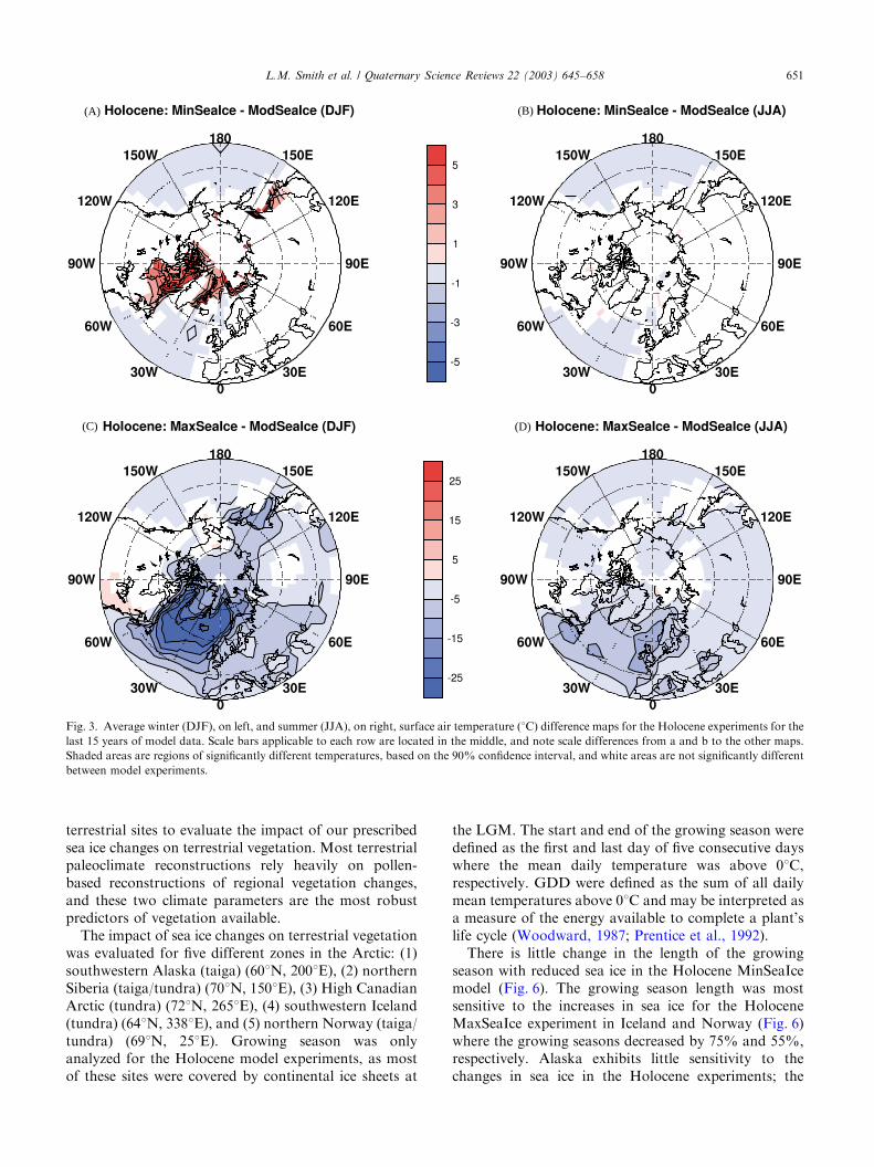
In the Holocene MinSeaIce simulation, the dominantatmospheric response occurs in winter, and is focused inthe western North Atlantic where there is up to a 51Cwarming over the Eastern Canadian Arctic and aroundGreenland with a restricted warming in eastern Asia

(Fig. 3a). With reduced sea ice through the CanadianArchipelago and the northern North Atlantic tempera-tures increase over the adjacent land areas. In contrast,the Pacific sector only exhibits winter temperaturechange in a small area in the western Sea of Okhotsk,despite equivalent reduction in sea ice as that ofthe North Atlantic. There is no significant temperaturechange in the summer months for the HoloceneMinSeaIce compared to the Holocene ModSeaIcesimulations (Fig. 3b).With maximum Holocene sea ice simulation, extreme

winter cooling over Greenland occurs (5–251C) extend-ing downstream from the North Atlantic region intoEurope and Asia (0–151C) (Fig. 3c). Summer cooling isalso modeled throughout the same region, although it isreduced to p101C (Fig. 3d).

4.2. Holocene sea level pressure

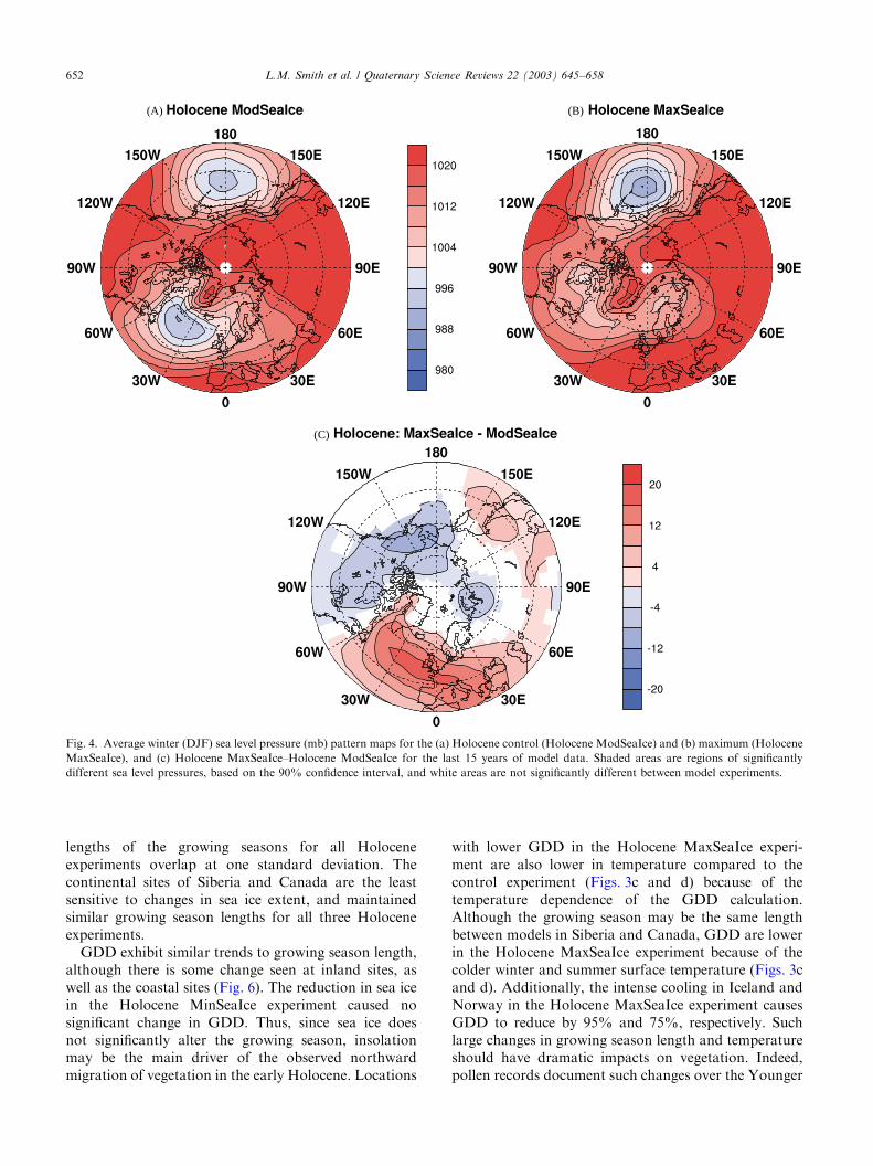
Sea level pressure changes are only significant in theHolocene MaxSeaIce–Holocene ModSeaIce comparison(Fig. 4). Reduced sea ice in the Holocene MinSeaIceexperiment does not produce any significant differencesin sea level pressure in any month compared with thecontrol experiment. For the Holocene MaxSeaIceexperiment, the sea level pressure changes are mostsignificant in the winter months, and are focused overthe North Atlantic (Fig. 4). In the North Atlantic, thereis a weakening of the Icelandic Low over the NorthAtlantic and into western Europe (Fig. 4c). In the NorthPacific, the pressure difference map of HoloceneMaxSeaIce–Holocene ModSeaIce indicates a slightdeepening of the Aleutian Low and a more extendedeffect over Alaska (Fig. 4c).

4.3. Holocene snowfall and storm track variability

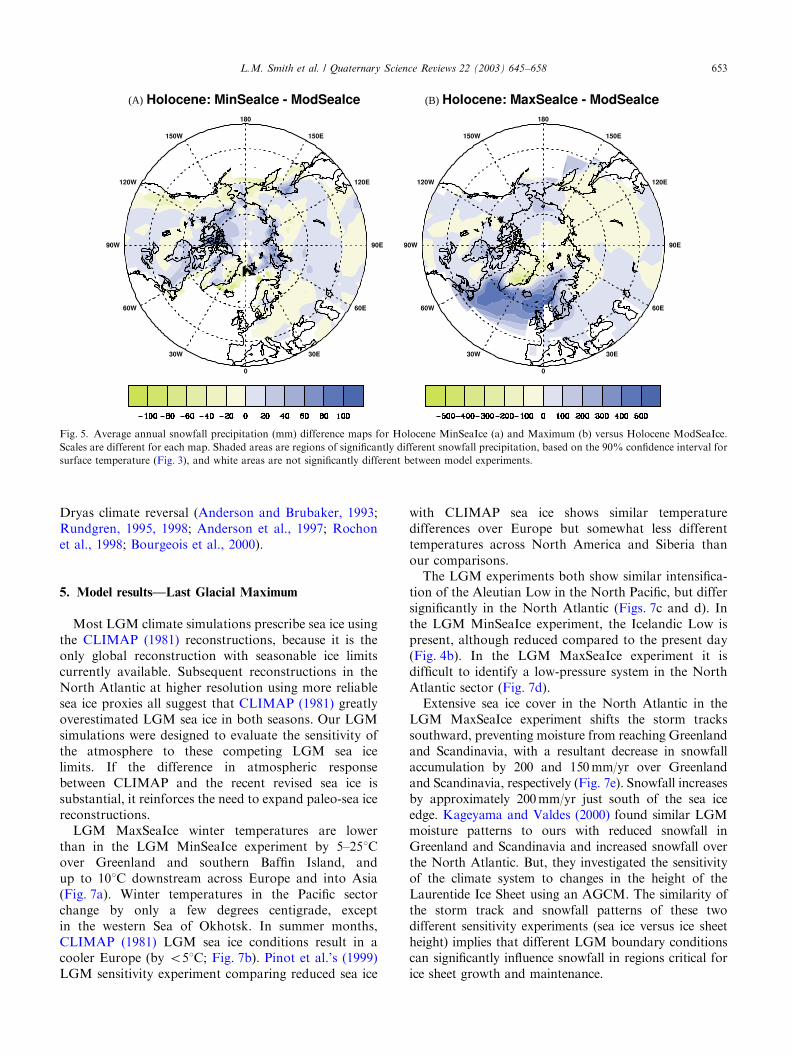
With reduced sea ice in the North Atlantic in theHolocene MinSeaIce experiment, moisture is carriedfarther north into the Arctic Ocean basin and causes anincrease in snowfall by 80–100mm/yr centered over theEastern Canadian Arctic and extending around theArctic Ocean, whereas northern Greenland, northernEurope, Siberia, and Canada generally experience drierconditions and a snowfall reduction (Fig. 5a).In the Holocene MaxSeaIce experiment with in-

creased sea ice in the North Atlantic, the storm tracksshift southward and snowfall increases up to 500mm/yrover the ice-covered Labrador Sea, Iceland, the NorthSea, and Scandinavia, whereas snowfall in Greenland isreduced by over 300mm/yr (Fig. 5b).

4.4. Holocene growing season

We compute changes in growing degree days (GDD)and the length of the growing season for several Arctic

0

0.5

1

1.5

2

2.5

August

February

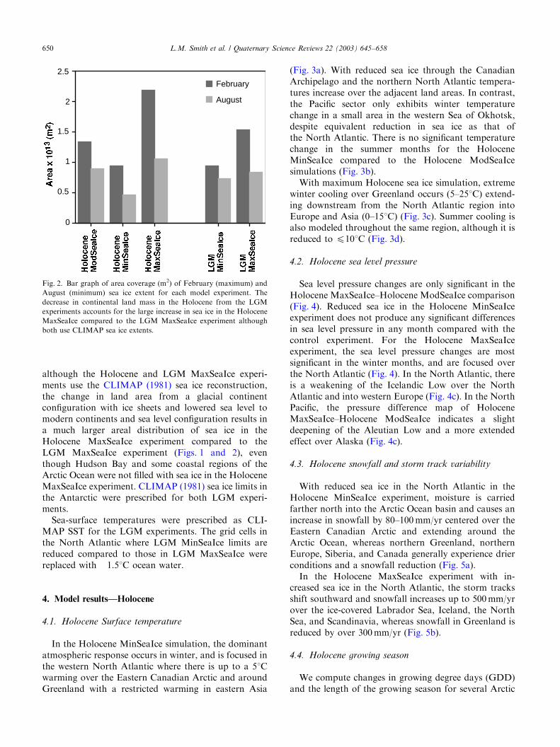
Fig. 2. Bar graph of area coverage (m2) of February (maximum) and

August (minimum) sea ice extent for each model experiment. The

decrease in continental land mass in the Holocene from the LGM

experiments accounts for the large increase in sea ice in the Holocene

MaxSeaIce compared to the LGM MaxSeaIce experiment although

both use CLIMAP sea ice extents.


terrestrial sites to evaluate the impact of our prescribedsea ice changes on terrestrial vegetation. Most terrestrialpaleoclimate reconstructions rely heavily on pollen-based reconstructions of regional vegetation changes,and these two climate parameters are the most robustpredictors of vegetation available.The impact of sea ice changes on terrestrial vegetation

was evaluated for five different zones in the Arctic: (1)southwestern Alaska (taiga) (601N, 2001E), (2) northernSiberia (taiga/tundra) (701N, 1501E), (3) High CanadianArctic (tundra) (721N, 2651E), (4) southwestern Iceland(tundra) (641N, 3381E), and (5) northern Norway (taiga/tundra) (691N, 251E). Growing season was onlyanalyzed for the Holocene model experiments, as mostof these sites were covered by continental ice sheets at

the LGM. The start and end of the growing season weredefined as the first and last day of five consecutive dayswhere the mean daily temperature was above 01C,respectively. GDD were defined as the sum of all dailymean temperatures above 01C and may be interpreted asa measure of the energy available to complete a plant’slife cycle (Woodward, 1987; Prentice et al., 1992).There is little change in the length of the growing

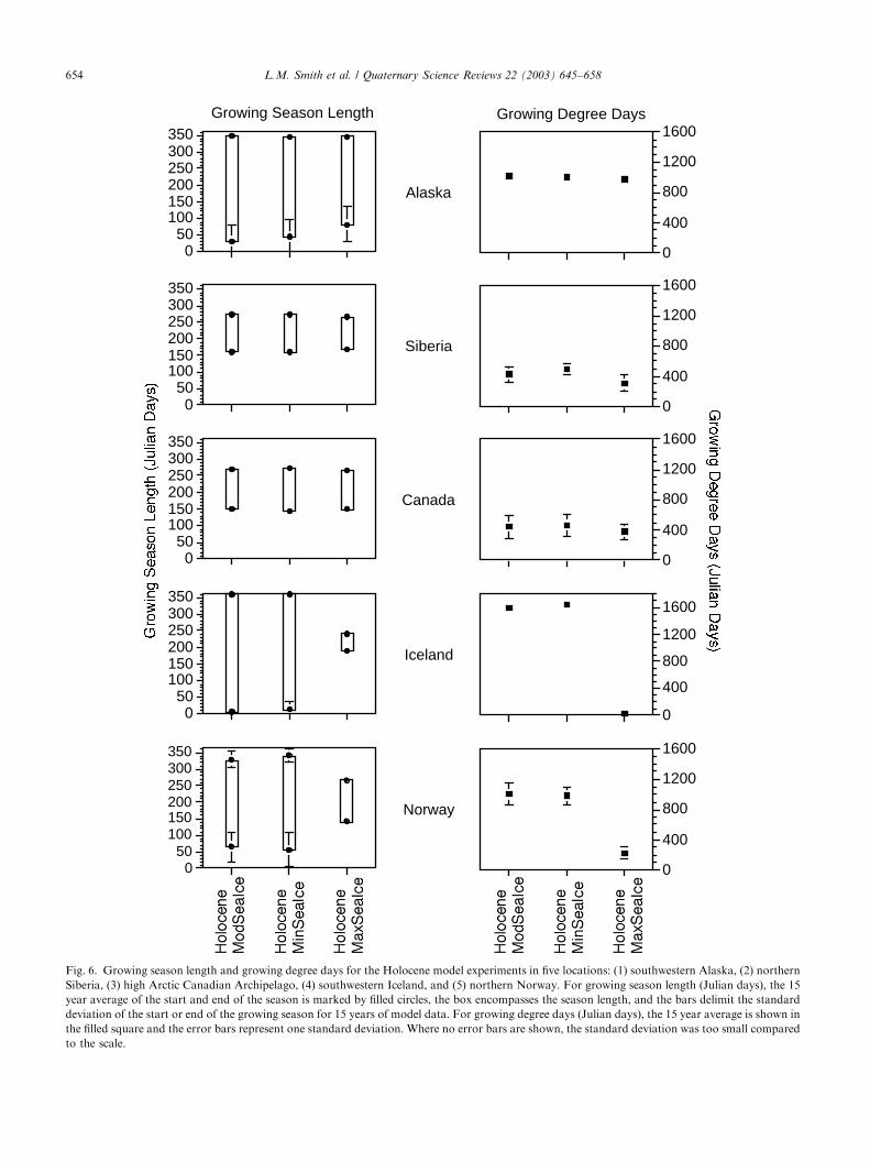
season with reduced sea ice in the Holocene MinSeaIcemodel (Fig. 6). The growing season length was mostsensitive to the increases in sea ice for the HoloceneMaxSeaIce experiment in Iceland and Norway (Fig. 6)where the growing seasons decreased by 75% and 55%,respectively. Alaska exhibits little sensitivity to thechanges in sea ice in the Holocene experiments; the

(B)

(C) (D)

(A)

Fig. 3. Average winter (DJF), on left, and summer (JJA), on right, surface air temperature (1C) difference maps for the Holocene experiments for the

last 15 years of model data. Scale bars applicable to each row are located in the middle, and note scale differences from a and b to the other maps.

Shaded areas are regions of significantly different temperatures, based on the 90% confidence interval, and white areas are not significantly different

between model experiments.


lengths of the growing seasons for all Holoceneexperiments overlap at one standard deviation. Thecontinental sites of Siberia and Canada are the leastsensitive to changes in sea ice extent, and maintainedsimilar growing season lengths for all three Holoceneexperiments.GDD exhibit similar trends to growing season length,

although there is some change seen at inland sites, aswell as the coastal sites (Fig. 6). The reduction in sea icein the Holocene MinSeaIce experiment caused nosignificant change in GDD. Thus, since sea ice doesnot significantly alter the growing season, insolationmay be the main driver of the observed northwardmigration of vegetation in the early Holocene. Locations

with lower GDD in the Holocene MaxSeaIce experi-ment are also lower in temperature compared to thecontrol experiment (Figs. 3c and d) because of thetemperature dependence of the GDD calculation.Although the growing season may be the same lengthbetween models in Siberia and Canada, GDD are lowerin the Holocene MaxSeaIce experiment because of thecolder winter and summer surface temperature (Figs. 3cand d). Additionally, the intense cooling in Iceland andNorway in the Holocene MaxSeaIce experiment causesGDD to reduce by 95% and 75%, respectively. Suchlarge changes in growing season length and temperatureshould have dramatic impacts on vegetation. Indeed,pollen records document such changes over the Younger

(A) (B)

(C)

Fig. 4. Average winter (DJF) sea level pressure (mb) pattern maps for the (a) Holocene control (Holocene ModSeaIce) and (b) maximum (Holocene

MaxSeaIce), and (c) Holocene MaxSeaIce–Holocene ModSeaIce for the last 15 years of model data. Shaded areas are regions of significantly

different sea level pressures, based on the 90% confidence interval, and white areas are not significantly different between model experiments.


Dryas climate reversal (Anderson and Brubaker, 1993;Rundgren, 1995, 1998; Anderson et al., 1997; Rochonet al., 1998; Bourgeois et al., 2000).

5. Model results—Last Glacial Maximum

Most LGM climate simulations prescribe sea ice usingthe CLIMAP (1981) reconstructions, because it is theonly global reconstruction with seasonable ice limitscurrently available. Subsequent reconstructions in theNorth Atlantic at higher resolution using more reliablesea ice proxies all suggest that CLIMAP (1981) greatlyoverestimated LGM sea ice in both seasons. Our LGMsimulations were designed to evaluate the sensitivity ofthe atmosphere to these competing LGM sea icelimits. If the difference in atmospheric responsebetween CLIMAP and the recent revised sea ice issubstantial, it reinforces the need to expand paleo-sea icereconstructions.LGM MaxSeaIce winter temperatures are lower

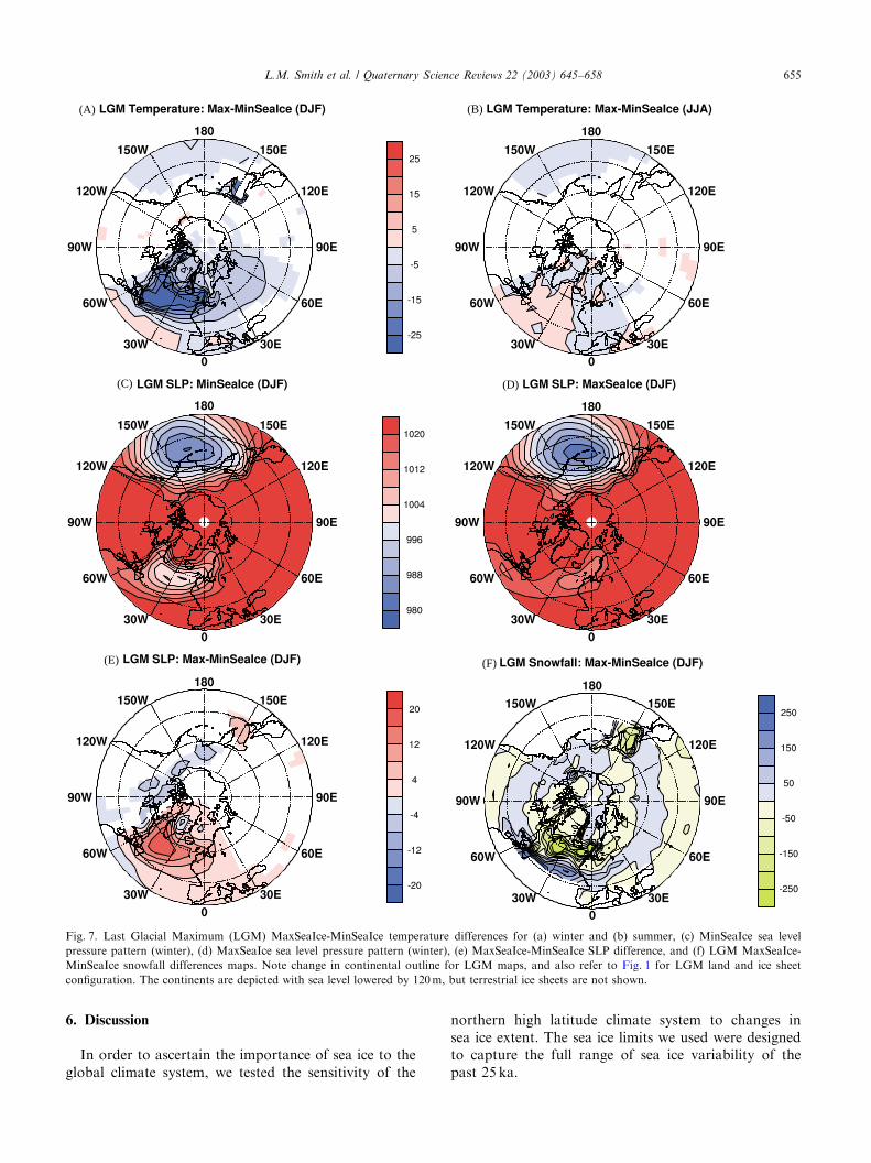
than in the LGM MinSeaIce experiment by 5–251Cover Greenland and southern Baffin Island, andup to 101C downstream across Europe and into Asia(Fig. 7a). Winter temperatures in the Pacific sectorchange by only a few degrees centigrade, exceptin the western Sea of Okhotsk. In summer months,CLIMAP (1981) LGM sea ice conditions result in acooler Europe (by o51C; Fig. 7b). Pinot et al.’s (1999)LGM sensitivity experiment comparing reduced sea ice

with CLIMAP sea ice shows similar temperaturedifferences over Europe but somewhat less differenttemperatures across North America and Siberia thanour comparisons.The LGM experiments both show similar intensifica-

tion of the Aleutian Low in the North Pacific, but differsignificantly in the North Atlantic (Figs. 7c and d). Inthe LGM MinSeaIce experiment, the Icelandic Low ispresent, although reduced compared to the present day(Fig. 4b). In the LGM MaxSeaIce experiment it isdifficult to identify a low-pressure system in the NorthAtlantic sector (Fig. 7d).Extensive sea ice cover in the North Atlantic in the

LGM MaxSeaIce experiment shifts the storm trackssouthward, preventing moisture from reaching Greenlandand Scandinavia, with a resultant decrease in snowfallaccumulation by 200 and 150mm/yr over Greenlandand Scandinavia, respectively (Fig. 7e). Snowfall increasesby approximately 200mm/yr just south of the sea iceedge. Kageyama and Valdes (2000) found similar LGMmoisture patterns to ours with reduced snowfall inGreenland and Scandinavia and increased snowfall overthe North Atlantic. But, they investigated the sensitivityof the climate system to changes in the height of theLaurentide Ice Sheet using an AGCM. The similarity ofthe storm track and snowfall patterns of these twodifferent sensitivity experiments (sea ice versus ice sheetheight) implies that different LGM boundary conditionscan significantly influence snowfall in regions critical forice sheet growth and maintenance.

(B)(A)

Fig. 5. Average annual snowfall precipitation (mm) difference maps for Holocene MinSeaIce (a) and Maximum (b) versus Holocene ModSeaIce.

Scales are different for each map. Shaded areas are regions of significantly different snowfall precipitation, based on the 90% confidence interval for

surface temperature (Fig. 3), and white areas are not significantly different between model experiments.


050

100150200250300350

0

400

800

1200

1600

0

400

800

1200

1600

0

400

800

1200

1600

0

400

800

1200

1600

0

400

800

1200

1600

050

100150200250300350

Growing Season Length

050

100150200250300350

050

100150200250300350

050

100150200250300350

Growing Degree Days

Alaska

Siberia

Canada

Iceland

Norway

Fig. 6. Growing season length and growing degree days for the Holocene model experiments in five locations: (1) southwestern Alaska, (2) northern

Siberia, (3) high Arctic Canadian Archipelago, (4) southwestern Iceland, and (5) northern Norway. For growing season length (Julian days), the 15

year average of the start and end of the season is marked by filled circles, the box encompasses the season length, and the bars delimit the standard

deviation of the start or end of the growing season for 15 years of model data. For growing degree days (Julian days), the 15 year average is shown in

the filled square and the error bars represent one standard deviation. Where no error bars are shown, the standard deviation was too small compared

to the scale.


6. Discussion

In order to ascertain the importance of sea ice to theglobal climate system, we tested the sensitivity of the

northern high latitude climate system to changes insea ice extent. The sea ice limits we used were designedto capture the full range of sea ice variability of thepast 25 ka.

(A) (B)

(C) (D)

(E) (F)

Fig. 7. Last Glacial Maximum (LGM) MaxSeaIce-MinSeaIce temperature differences for (a) winter and (b) summer, (c) MinSeaIce sea level

pressure pattern (winter), (d) MaxSeaIce sea level pressure pattern (winter), (e) MaxSeaIce-MinSeaIce SLP difference, and (f) LGM MaxSeaIce-

MinSeaIce snowfall differences maps. Note change in continental outline for LGM maps, and also refer to Fig. 1 for LGM land and ice sheet

configuration. The continents are depicted with sea level lowered by 120m, but terrestrial ice sheets are not shown.


The reduced sea ice in the Holocene MinSeaIceexperiment results in a localized effect adjacent tothe areas with greatest sea ice reduction, primarily in theNorth Atlantic (Fig. 1). Reduced Holocene sea icecauses a significant winter temperature increase andgreater snowfall over the Eastern Canadian Arcticwithout significant changes in sea level pressure or thegrowing season. Additionally, there is a small region ofsignificant winter warming and increased snowfall ineastern Asia adjacent to the Sea of Okhotsk caused bylocal sea ice removal.Extended sea ice in both the Holocene and LGM

MaxSeaIce experiments causes significant temperaturedecreases, sea level pressure changes, and a southwardshift in storm tracks and maximum snowfall. Addition-

ally, the growing season is colder and shorter at thecoastal locations of interest in the Holocene MaxSeaIceexperiment. These climate changes are the result ofexpanded sea ice in the North Atlantic and NorthPacific oceans that reduces the heat and moistureexchange, and creates an overall stabilization betweenthe ocean and atmosphere. This atmospheric stabiliza-tion is best illustrated by the increase in sea levelpressure with extended sea ice in both the Holocene andLGM MaxSeaIce experiments compared to the Holo-cene ModSeaIce and LGM MinSeaIce experiments,respectively (Figs. 4c and 7e).Our results allow an evaluation of the relative effects

of sea ice and continental ice sheets on climate becausesea ice is similarly prescribed in both the Holocene and

(B)(A)

(C)

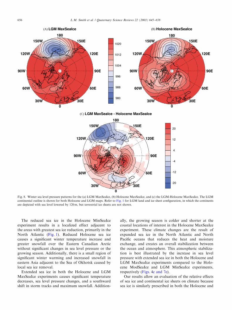
Fig. 8. Winter sea level pressure patterns for the (a) LGMMaxSeaIce, (b) Holocene MaxSeaIce, and (c) the LGM-Holocene MaxSeaIce. The LGM

continental outline is shown for both Holocene and LGM maps. Refer to Fig. 1 for LGM land and ice sheet configuration, in which the continents

are depicted with sea level lowered by 120m, but terrestrial ice sheets are not shown.


LGM MaxSeaIce experiments. Differences in climatebetween these two experiments may be best attributedto changes in ice sheet and land mass configuration,although we did not prescribe similar insolationand greenhouse gases values for these two experiments(Table 1). The only significant temperature changeis cooling over the North American and Eurasianice sheets in the LGM MaxSeaIce experiment (Figs. 7aand b) compared to the Holocene MaxSeaIce experi-ment (Figs. 3c and d). Sea level pressure significantlydiffers between these two experiments (Fig. 8) with asouthward shift and intensification of the AleutianLow in the LGM MaxSeaIce experiment and increasedsea level pressure over North America and Eurasia.The deepening and shifting of the Aleutian Low isattributed to the increased land mass configuration inthe Bering Sea and the presence of the Laurentide IceSheet downstream in North America. The increased sealevel pressure in North America and Eurasia isattributed to the Laurentide Ice Sheet that shifts theair flow south and reduces the westerlies acrossthe North Atlantic. This stabilization in air flow overthe North Atlantic and reduction in moisture transferbetween the ocean and atmosphere caused by extensivesea ice act together to create a reduction in the numberof storms and the amount of snowfall in the highlatitude region of the eastern North Atlantic at theLGM. The reduced snowfall with increased NorthAtlantic sea ice calls into question whether theScandinavian Ice Sheet could exist with the CLIMAP(1981) sea ice reconstruction.In all experiments presented herein, the North

Atlantic climate appears to be more sensitive to changesin sea ice than the North Pacific, although we havechanged sea ice similarly in both ocean basins. In termsof climate parameters, only sea level pressure withinthe North Pacific is sensitive, and temperature, snowfall,and the growing season are less sensitive. The reducedsensitivity of the North Pacific is not surprisinggiven that present-day North Pacific SST is lower thanthe North Atlantic SST at similar latitudes, and anysea ice expansion (reduction) in the North Pacificwould not significantly insulate (heat) the adjacentland area or decrease (increase) the moisture transferto the land as it would in the North Atlantic. Thechange in sea level pressure is surmised to be relatedto atmospheric changes, and not ocean processesbecause the ocean is fixed in these sensitivity experi-ments. The reduced sea level pressure in the NorthPacific is a result of compensation for cold airtemperatures coming off Siberian. Intensification ofthe Aleutian Low allows for a larger heat transferfrom the ocean to the atmosphere. Mikolajewiczet al. (1997) attributed similar changes in NorthPacific sea level pressure related to colder SST to cold,Siberian air.

7. Conclusions

Our sensitivity experiments demonstrate that there aresignificant changes in the climate system, primarily inwinter temperature, sea level pressure, and snowfall, as aresponse to extreme changes in Holocene, as well asLGM, Arctic sea ice extents. These climate changessubsequently affect the terrestrial growing season. Anyreduction in sea ice extent increases the period duringwhich the ocean and atmosphere can exchange energy,moisture, and gases.Overall, in both the Holocene and LGM experiments,

the North Atlantic region and downstream into Europeand Asia are more sensitive to changes in hemisphericsea ice extent than the North Pacific. Sea ice limits weremodified by a similar proportion in both the NorthAtlantic and North Pacific basins, but the majority ofthe climatic effects are found in the North Atlantic.Furthermore, because the ocean is fixed and does notchange in these experiments, the sensitivity of the NorthAtlantic region to sea ice cannot be attributed tothermohaline circulation, but is instead thought to becontrolled by the atmosphere.These model experiments demonstrate that the

climate system is sensitive to sea ice, and emphasizethe need for circum-Arctic sea ice reconstructions foruse in paleoclimate studies and modeling experiments.Our results reinforce the need to develop accurateHolocene and LGM sea ice reconstructions, andadditional sea ice proxies that will allow reconstructionsof Holocene and LGM sea ice limits throughout thecircum-Arctic and to ensure that the different sea iceproxies are intercalibrated (Miller et al., 2001).

Acknowledgements

Funding for this project was provided by the NationalScience Foundation through ATM-9708418 NSF toPaleoenvironmental ARCtic Sciences (PARCS). Thecomputer experiments were performed at the NationalCenter for Atmospheric Research (NCAR), which issupported by the NSF. We wish to thank C. Shields andC. Ammann for their help with generating the modelexperiments and figures. C. Ammann and S. Lehmancontributed constructive thoughts to these modelexperiments and analyses, and this manuscript benefitedfrom comments by two anonymous reviewers. PARCSContribution #160.

References

Aagaard, K., Carmack, E.C., 1989. The role of sea ice and other fresh

water in the Arctic Circulation. Journal of Geophysical Research

94 (C10), 14485–14498.


Anderson, P.M., Brubaker, L.B., 1993. Holocene vegetation and

climate histories of Alaska. In: Wright Jr., H.E., Kutzbach, J.E.,

Webb III, T., Ruddiman, W.F., Street-Perrott, F.A., Bartlein, P.J.

(Eds.), Global Climates since the Last Glacial Maximum.

University of Minnesota Press, Minneapolis, pp. 386–400.

Anderson, P.M., Lozhkin, A.V., Belaya, B.V., Glushkova, O.Y.,

Brubaker, L.B., 1997. A lacustrine pollen record from near

altitudinal forest limit, Upper Kolyma region, northeastern Siberia.

The Holocene 7 (3), 331–335.

Blunier, T., Raynaud, D., Chappellaz, J., Schwander, J., Stauffer, B.,

1995. Variations in atmospheric methane concentration during the

Holocene epoch. Nature 374, 46–49.

Bourgeois, J.C., Koerner, R.M., Gajewski, K., Fisher, D.A., 2000. A

Holocene ice-core pollen record from Ellesmere Island, Nunavut,

Canada. Quaternary Research 54, 275–283.

Chervin, R.M., Schneider, S.H., 1976. On determining the statistical

significance of climate experiments with general circulation models.

Journal of Atmospheric Sciences 33, 405–412.

CLIMAP, 1981. Seasonal reconstructions of the earth’s surface at the

Last Glacial Maximum. Map Chart Series MC-36, Geological

Society of America, Boulder, CO.

deVernal, A., Hillaire-Marcel, C., 2000. Sea-ice cover, sea-surface

salinity and halo-/thermocline structure of the northwest North

Atlantic: modern versus full glacial conditions. Quaternary Science

Reviews 19, 65–85.

de Vernal, A., Hillaire-Marcel, C., Turon, J.L., Matthiessen, J., 2000.

Reconstruction of sea-surface temperature, salinity, and sea-ice

cover in the northern North Atlantic during the last glacial

maximum based on dinocyst assemblages. Canadian Journal of

Earth Sciences 37 (5), 725–750.

Dickinson, R.E., 1985. Climate sensitivity. In: Manabe, S. (Ed.), Issues

in Atmospheric and Oceanic Modelling, Part A: Climate

Dynamics, Advances in Geophysics, Vol. 28. Academic Press,

Orlando, pp. 99–129.

Fluckiger, J., Stocker, T.F., Raynaud, D., Barnola, J.-M., Dallenbach,

A., Blunier, T., Stauffer, B., 1999. Variations in atmospheric

N2O concentration during abrupt climatic changes. Science 285,

227–230.

Gildor, H., Tziperman, E., 2000. Sea ice as the glacial cycles’ climate

switch: role of seasonal and orbital forcing. Paleoceanography 15

(6), 605–615.

Gildor, H., Tziperman, E., 2001. A sea ice climate switch mechanism

for the 100-kyr glacial cycles. Journal of Geophysical Research 106

(C5), 9117–9133.

Hebbeln, D., Henrich, R., Baumann, K.H., 1998. Paleoceanography of

the last interglacial/glacial cycle in the Polar North Atlantic.

Quaternary Science Reviews 17 (1–3), 125–153.

Indermuhle, A., Smith, H.J., Wahlen, M., Deck, B., Mastrolanni, D.,

Tschumi, J., Blunier, T., Meyer, R., Stauffer, B., Stocker, T.F.,

Joos, F., Fischer, H., 1999. Holocene carbon-cycle dynamics based

on CO2 trapped in ice at Taylor Dome, Antarctica. Nature 398,

121–126.

Kageyama, M., Valdes, P.J., 2000. Impact of the North American ice-

sheet orography on the Last Glacial Maximum eddies and

snowfall. Geophysical Research Letters 27 (10), 1515–1519.

Kageyama, M., Peyron, O., Pinto, S., Tarasov, P., Guiot, J.,

Joussaume, Ramstein, G., 2001. The Last Glacial Maximum

climate over Europe and western Siberia: a PMIP comparison

between models and data. Climate Dynamics 17, 23–43.

Kerwin, M.W., Overpeck, J.T., Webb, R.S., deVernal, A., Rind, D.H.,

Healy, R.J., 1999. The role of oceanic forcing in mid-Holocene

Northern Hemisphere climatic change. Paleoceanography 14 (2),

200–210.

Kiehl, J.T., Hack, J.J., Bonan, G.B., Boville, B.A., Williamson, D.L.,

Rasch, P.J., 1998. The National Center for Atmospheric Research

community climate model: CCM3. Journal of Climate 11,

1131–1149.

Kitoh, A., Murakami, S., Koide, H., 2001. A simulation of the Last

Glacial Maximum with a coupled atmospheric-ocean GCM.

Geophysical Research Letters 28 (11), 2221–2224.

Koc, N., Jansen, E., Haflidason, H., 1993. Paleoceanographic

reconstructions of surface ocean conditions in the Greenland,

Iceland, and Norwegian Seas through the last 14-ka based on

diatoms. Quaternary Science Reviews 12 (2), 115–140.

Marsiat, I., Valdes, P.J., 2001. Sensitivity of the Northern Hemisphere

climate of the Last Glacial Maximum to sea surface temperatures.

Climate Dynamics 17, 233–248.

Mikolajewicz, U., Crowley, T.J., Schiller, A., Voss, R., 1997.

Modelling teleconnections between the North Atlantic and North

Pacific during the Younger Dryas. Nature 387, 384–387.

Miller, G.H., Geirsdottir, A., Koerner, R.M., 2001. Sea Ice in the

Climate System: lessons from the North Atlantic Arctic, EOS

Transactions.

Panofsky, H.A.,Brier, G.W., 1965. Some Applications of Statistics to

Meteorology. The Pennsylvania State University, University Park,

224pp.

Peltier, W.R., 1994. Ice age paleotopography. Science 256, 195–201.

Pinot, S., Ramstein, G., Marsiat, I., deVernal, A., Peyron, O.,

Duplessy, J.-C., Weinelt, M., 1999. Sensitivity of the European

LGM climate to North Atlantic sea-surface temperature. Geophy-

sical Research Letters 26 (13), 1893–1896.

Prentice, I.C., Cramer, W., Harrison, S.P., Leemans, R., Monserud,

R.A., Solomon, A.M., 1992. A global biome model based on plant

physiology and dominance, soil properties and climate. Journal of

Biogeography 19, 117–134.

Raymo, M.E., Rind, D., Ruddiman, W.F., 1990. Climatic effects of

reduced Arctic sea ice limits in the GISS II general circulation

model. Paleoceanography 5, 367–382.

Raynaud, D., Delmas, R.J., Lorius, C., Jouzel, J., Barnola, J.M.,

Chappellaz, J., 1993. The ice record of greenhouse gases. Science

259, 926–934.

Rind, D., Peteet, D., Broecker, W., McIntyre, A., Ruddiman, W.,

1986. The impact of cold North Atlantic sea surface temperatures

on climate: implications for the Younger Dryas cooling (11-10 ka).

Climate Dynamics 1, 3–33.

Rochon, A., deVernal, A., Sejrup, H-P., Haflidason, H., 1998.

Palynological evidence of climatic and oceanographic changes in

the North Sea during the Last Deglaciation. Quaternary Research

49, 197–207.

Royer, J.F., Planton, S., Deque, M., 1990. A sensitivity experiment for

the removal of Arctic sea ice with the French spectral general

circulation model. Climate Dynamics 5, 1–17.

Rundgren, M., 1995. Biostratigraphic evidence of the Aller�d-YoungerDryas-Preboreal Oscillation in Northern Iceland. Quaternary

Research 44, 405–416.

Rundgren, M., 1998. Early holocene vegetation of northern Iceland:

pollen and plant macrofossil evidence from Skagi Peninsula. The

Holocene 8 (5), 553–564.

Shin, S.-I., Liu, Z., Otto-Bliesner, B., Brady, E.C., Kutzbach,

J.E.,Harrison, S.P., in review. A simulation of the Last Glacial

Maximum climate using NCAR-CCSM. Climate Dynamics,

in review.

Warshaw, M., Rapp, R.R., 1973. An experiment on the sensitivity of a global

circulation model. Journal of Applied Meteorology 12, 43–49.

Woodward, F.I., 1987. Climate and Plant Distribution. Cambridge

University Press, Cambridge, 174pp.


Sensitivity of the Northern Hemisphere climate system to extreme changes in Holocene Arctic sea ice

Documents