SELF-TEST PROBLEMS & SOLUTIONS

-1-

Chapter 2

Economic Optimization

SELF-TEST PROBLEMS & SOLUTIONS

ST2.1 Profit versus Revenue Maximization. Presto Products, Inc., manufactures smallelectrical appliances and has recently introduced an innovative new dessert maker forfrozen yogurt and fruit smoothies that has the clear potential to offset the weak pricingand sluggish volume growth experienced during recent periods.

Monthly demand and cost relations for Presto's frozen dessert maker are asfollows:

P = $60 - $0.005Q TC = $100,000 + $5Q + $0.0005Q2

MR = MTR/MQ = $60 - $0.01Q MC = MTC/MQ = $5 + $0.001Q

A. Set up a table or spreadsheet for Presto output (Q), price (P), total revenue (TR),marginal revenue (MR), total cost (TC), marginal cost (MC), total profit (π), andmarginal profit (Mπ). Establish a range for Q from 0 to 10,000 in increments of1,000 (i.e., 0, 1,000, 2,000, ..., 10,000).

B. Using the Presto table or spreadsheet, create a graph with TR, TC, and π asdependent variables, and units of output (Q) as the independent variable. At whatprice/output combination is total profit maximized? Why? At what price/outputcombination is total revenue maximized? Why?

C. Determine these profit-maximizing and revenue-maximizing price/outputcombinations analytically. In other words, use Presto's profit and revenueequations to confirm your answers to part B.

D. Compare the profit-maximizing and revenue-maximizing price/outputcombinations, and discuss any differences. When will short-run revenuemaximization lead to long-run profit maximization?

ST2.1 SOLUTION

A. A table or spreadsheet for Presto output (Q), price (P), total revenue (TR),marginal revenue (MR), total cost (TC), marginal cost (MC), total profit (π), andmarginal profit (Mπ) appears as follows:

-2-

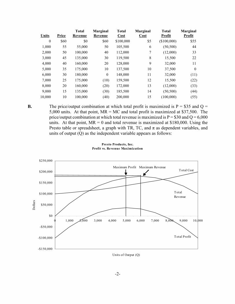
Presto Products, Inc.Profit vs. Revenue Maximization

-$150,000

-$100,000

-$50,000

$0

$50,000

$100,000

$150,000

$200,000

$250,000

0 1,000 2,000 3,000 4,000 5,000 6,000 7,000 8,000 9,000 10,000

Units of Output (Q)

Dol

lars

Total Revenue

Total Cost

Total Profit

Maximum RevenueMaximum Profit

Units PriceTotal

RevenueMarginalRevenue

TotalCost

MarginalCost

TotalProfit

MarginalProfit

0 $60 $0 $60 $100,000 $5 ($100,000) $55 1,000 55 55,000 50 105,500 6 (50,500) 44 2,000 50 100,000 40 112,000 7 (12,000) 33 3,000 45 135,000 30 119,500 8 15,500 22 4,000 40 160,000 20 128,000 9 32,000 11 5,000 35 175,000 10 137,500 10 37,500 0 6,000 30 180,000 0 148,000 11 32,000 (11)7,000 25 175,000 (10) 159,500 12 15,500 (22)8,000 20 160,000 (20) 172,000 13 (12,000) (33)9,000 15 135,000 (30) 185,500 14 (50,500) (44)

10,000 10 100,000 (40) 200,000 15 (100,000) (55)

B. The price/output combination at which total profit is maximized is P = $35 and Q =5,000 units. At that point, MR = MC and total profit is maximized at $37,500. Theprice/output combination at which total revenue is maximized is P = $30 and Q = 6,000units. At that point, MR = 0 and total revenue is maximized at $180,000. Using thePresto table or spreadsheet, a graph with TR, TC, and π as dependent variables, andunits of output (Q) as the independent variable appears as follows:

-3-

C. To find the profit-maximizing output level analytically, set MR = MC, or set Mπ = 0,and solve for Q. Because

MR = MC

$60 - $0.01Q = $5 + $0.001Q

0.011Q = 55

Q = 5,000

At Q = 5,000,

P = $60 - $0.005(5,000)

= $35

π = -$100,000 + $55(5,000) - $0.0055(5,0002)

= $37,500

(Note: M2π/MQ2 < 0, This is a profit maximum because total profit is falling for Q >5,000.)

To find the revenue-maximizing output level, set MR = 0, and solve for Q. Thus,

MR = $60 - $0.01Q = 0

0.01Q = 60

Q = 6,000

At Q = 6,000,

P = $60 - $0.005(6,000)

= $30

π = TR - TC

= ($60 - $0.005Q)Q - $100,000 - $5Q - $0.0005Q2

= -$100,000 + $55Q - $0.0055Q2

-4-

= -$100,000 + $55(6,000) - $0.0055(6,0002)

= $32,000

(Note: M2TR/MQ2 < 0, and this is a revenue maximum because total revenue isdecreasing for output beyond Q > 6,000.)

D. Given downward sloping demand and marginal revenue curves and positive marginalcosts, the profit-maximizing price/output combination is always at a higher price andlower production level than the revenue-maximizing price-output combination. Thisstems from the fact that profit is maximized when MR = MC, whereas revenue ismaximized when MR = 0. It follows that profits and revenue are only maximized at thesame price/output combination in the unlikely event that MC = 0.

In pursuing a short-run revenue rather than profit-maximizing strategy, Presto canexpect to gain a number of important advantages, including enhanced productawareness among consumers, increased customer loyalty, potential economies of scalein marketing and promotion, and possible limitations in competitor entry and growth.To be consistent with long-run profit maximization, these advantages of short-runrevenue maximization must be at least worth Presto's short-run sacrifice of $5,500 (=$37,500 - $32,000) in monthly profits.

ST2.2 Average Cost-Minimization. Pharmed Caplets, Inc., is an international manufacturerof bulk antibiotics for the animal feed market. Dr. Indiana Jones, head of marketing andresearch, seeks your advice on an appropriate pricing strategy for Pharmed Caplets,an antibiotic for sale to the veterinarian and feedlot-operator market. This product hasbeen successfully launched during the past few months in a number of test markets, andreliable data are now available for the first time.

The marketing and accounting departments have provided you with the followingmonthly total revenue and total cost information:

TR = $900Q - $0.1Q2 TC = $36,000 + $200Q + $0.4Q2

MR = MTR/MQ = $900 - $0.2Q MC = MTC/MQ = $200 + $0.8Q

A. Set up a table or spreadsheet for Pharmed Caplets output (Q), price (P), totalrevenue (TR), marginal revenue (MR), total cost (TC), marginal cost (MC),average cost (AC), total profit (π), and marginal profit (Mπ). Establish a rangefor Q from 0 to 1,000 in increments of 100 (i.e., 0, 100, 200, ..., 1,000).

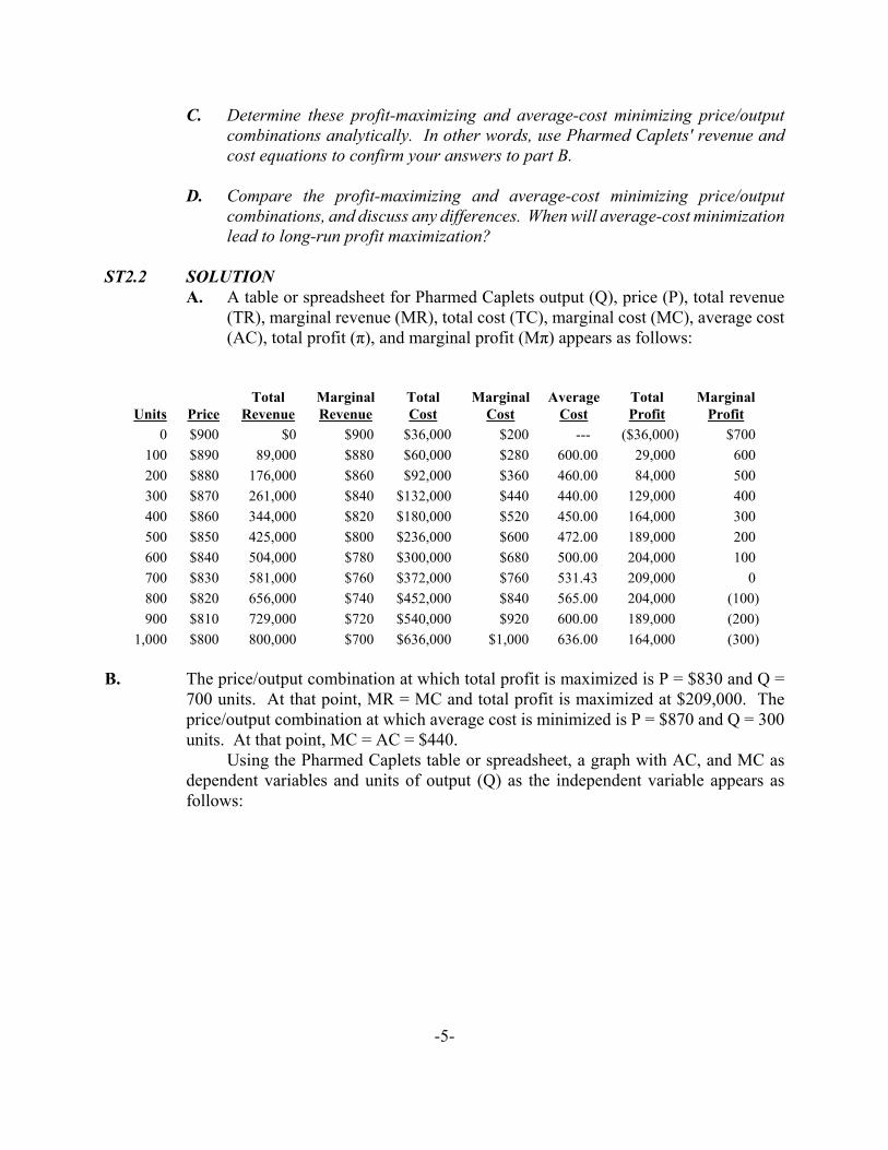
B. Using the Pharmed Caplets table or spreadsheet, create a graph with AC and MCas dependent variables and units of output (Q) as the independent variable. Atwhat price/output combination is total profit maximized? Why? At whatprice/output combination is average cost minimized? Why?

-5-

C. Determine these profit-maximizing and average-cost minimizing price/outputcombinations analytically. In other words, use Pharmed Caplets' revenue andcost equations to confirm your answers to part B.

D. Compare the profit-maximizing and average-cost minimizing price/outputcombinations, and discuss any differences. When will average-cost minimizationlead to long-run profit maximization?

ST2.2 SOLUTIONA. A table or spreadsheet for Pharmed Caplets output (Q), price (P), total revenue

(TR), marginal revenue (MR), total cost (TC), marginal cost (MC), average cost(AC), total profit (π), and marginal profit (Mπ) appears as follows:

Units PriceTotal

RevenueMarginalRevenue

TotalCost

MarginalCost

AverageCost

TotalProfit

MarginalProfit

0 $900 $0 $900 $36,000 $200 --- ($36,000) $700 100 $890 89,000 $880 $60,000 $280 600.00 29,000 600 200 $880 176,000 $860 $92,000 $360 460.00 84,000 500 300 $870 261,000 $840 $132,000 $440 440.00 129,000 400 400 $860 344,000 $820 $180,000 $520 450.00 164,000 300 500 $850 425,000 $800 $236,000 $600 472.00 189,000 200 600 $840 504,000 $780 $300,000 $680 500.00 204,000 100 700 $830 581,000 $760 $372,000 $760 531.43 209,000 0 800 $820 656,000 $740 $452,000 $840 565.00 204,000 (100)900 $810 729,000 $720 $540,000 $920 600.00 189,000 (200)

1,000 $800 800,000 $700 $636,000 $1,000 636.00 164,000 (300)

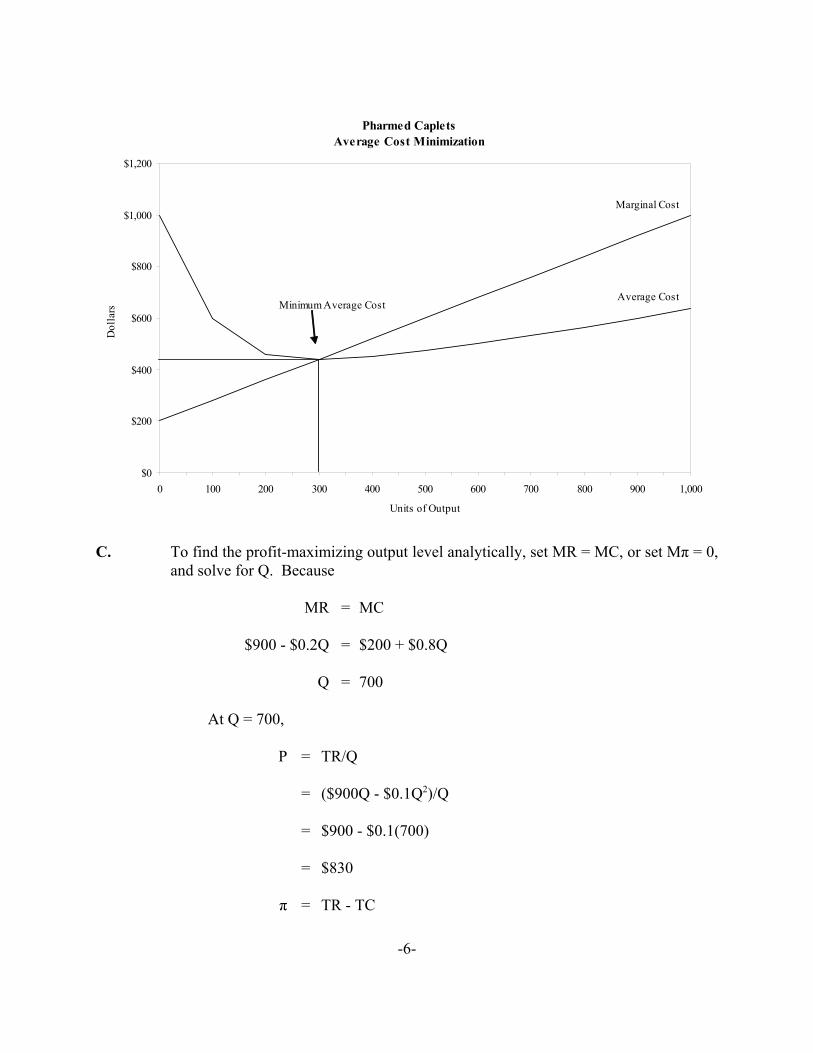
B. The price/output combination at which total profit is maximized is P = $830 and Q =700 units. At that point, MR = MC and total profit is maximized at $209,000. Theprice/output combination at which average cost is minimized is P = $870 and Q = 300units. At that point, MC = AC = $440.

Using the Pharmed Caplets table or spreadsheet, a graph with AC, and MC asdependent variables and units of output (Q) as the independent variable appears asfollows:

-6-

Pharmed CapletsAverage Cost Minimization

$0

$200

$400

$600

$800

$1,000

$1,200

0 100 200 300 400 500 600 700 800 900 1,000

Units of Output

Dol

lars

Average Cost

Marginal Cost

Minimum Average Cost

C. To find the profit-maximizing output level analytically, set MR = MC, or set Mπ = 0,and solve for Q. Because

MR = MC

$900 - $0.2Q = $200 + $0.8Q

Q = 700

At Q = 700,

P = TR/Q

= ($900Q - $0.1Q2)/Q

= $900 - $0.1(700)

= $830

π = TR - TC

-7-

= $900Q - $0.1Q2 - $36,000 - $200Q - $0.4Q2

= -$36,000 + $700(700) - $0.5(7002)

= $209,000

(Note: M2π/MQ2 < 0, and this is a profit maximum because profits are falling for Q >700.)

To find the average-cost minimizing output level, set MC = AC, and solve for Q.Because

AC = TC/Q

= ($36,000 + $200Q + $0.4Q2)/Q

= $36,000Q-1 + $200 + $0.4Q,

it follows that:

MC = AC

$200 + $0.8Q = $36,000Q-1 + $200 + $0.4Q

0.4Q = 36,000Q-1

0.4Q2 = 36,000

Q2 = 36,000/0.4

Q2 = 90,000

Q = 300

At Q = 300,

P = $900 - $0.1(300)

= $870

π = -$36,000 + $700(300) - $0.5(3002)

= $129,000

(Note: M2AC/MQ2 > 0, and this is an average-cost minimum because average cost is

-8-

rising for Q > 300.)

D. Given downward sloping demand and marginal revenue curves and a U-shaped, orquadratic, AC function, the profit-maximizing price/output combination will often beat a different price and production level than the average-cost minimizing price-outputcombination. This stems from the fact that profit is maximized when MR = MC,whereas average cost is minimized when MC = AC. Profits are maximized at the sameprice/output combination as where average costs are minimized in the unlikely eventthat MR = MC and MC = AC and, therefore, MR = MC = AC.

It is often true that the profit-maximizing output level differs from the averagecost-minimizing activity level. In this instance, expansion beyond Q = 300, the averagecost-minimizing activity level, can be justified because the added gain in revenue morethan compensates for the added costs. Note that total costs rise by $240,000, from$132,000 to $372,000 as output expands from Q = 300 to Q = 700, as average cost risesfrom $440 to $531.43. Nevertheless, profits rise by $80,000, from $129,000 to$209,000, because total revenue rises by $320,000, from $261,000 to $581,000. Theprofit-maximizing activity level can be less than, greater than, or equal to the average-cost minimizing activity level depending on the shape of relevant demand and costrelations.

-9-

Chapter 3

Demand and Supply


ST3.1 Demand and Supply Curves. The following relations describe demand and supplyconditions in the lumber/forest products industry

QD = 80,000 - 20,000P (Demand)

QS = -20,000 + 20,000P (Supply)

where Q is quantity measured in thousands of board feet (one square foot of lumber, oneinch thick) and P is price in dollars.

A. Set up a spreadsheet to illustrate the effect of price (P), on the quantity supplied(QS), quantity demanded (QD), and the resulting surplus (+) or shortage (-) asrepresented by the difference between the quantity supplied and the quantitydemanded at various price levels. Calculate the value for each respectivevariable based on a range for P from $1.00 to $3.50 in increments of 10¢ (i.e.,$1.00, $1.10, $1.20, . . . $3.50).

B. Using price (P) on the vertical or y-axis and quantity (Q) on the horizontal or x-axis, plot the demand and supply curves for the lumber/forest products industryover the range of prices indicated previously.

ST3.1 SOLUTION

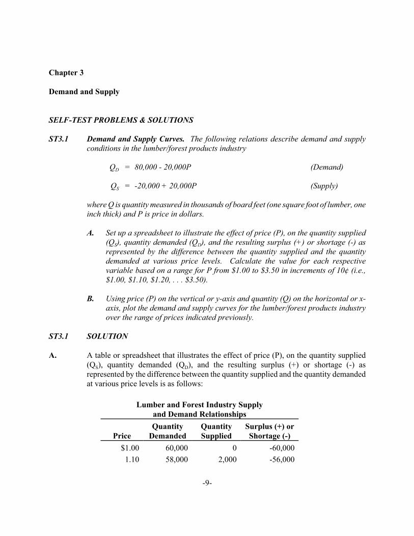
A. A table or spreadsheet that illustrates the effect of price (P), on the quantity supplied(QS), quantity demanded (QD), and the resulting surplus (+) or shortage (-) asrepresented by the difference between the quantity supplied and the quantity demandedat various price levels is as follows:

Lumber and Forest Industry Supplyand Demand Relationships

PriceQuantity

DemandedQuantitySupplied

Surplus (+) orShortage (-)

$1.00 60,000 0 -60,0001.10 58,000 2,000 -56,000

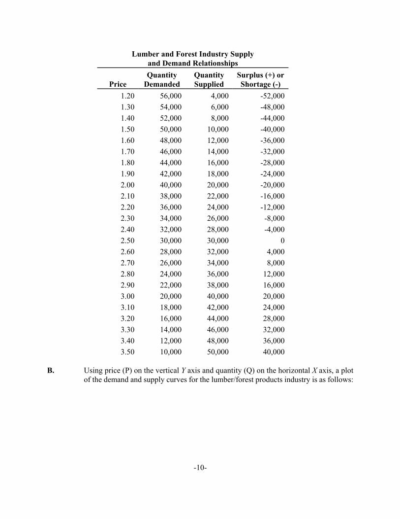
Lumber and Forest Industry Supplyand Demand Relationships

PriceQuantity

DemandedQuantitySupplied

Surplus (+) orShortage (-)

-10-

1.20 56,000 4,000 -52,0001.30 54,000 6,000 -48,0001.40 52,000 8,000 -44,0001.50 50,000 10,000 -40,0001.60 48,000 12,000 -36,0001.70 46,000 14,000 -32,0001.80 44,000 16,000 -28,0001.90 42,000 18,000 -24,0002.00 40,000 20,000 -20,0002.10 38,000 22,000 -16,0002.20 36,000 24,000 -12,0002.30 34,000 26,000 -8,0002.40 32,000 28,000 -4,0002.50 30,000 30,000 02.60 28,000 32,000 4,0002.70 26,000 34,000 8,0002.80 24,000 36,000 12,0002.90 22,000 38,000 16,0003.00 20,000 40,000 20,0003.10 18,000 42,000 24,0003.20 16,000 44,000 28,0003.30 14,000 46,000 32,0003.40 12,000 48,000 36,0003.50 10,000 50,000 40,000

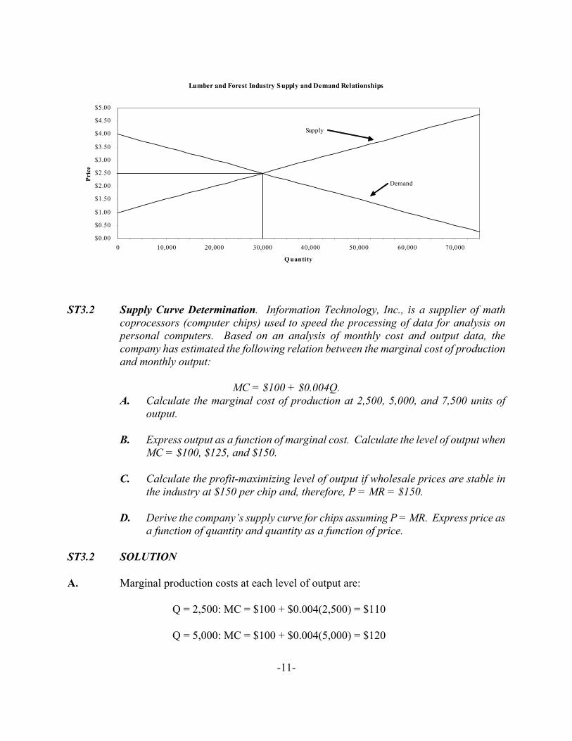
B. Using price (P) on the vertical Y axis and quantity (Q) on the horizontal X axis, a plotof the demand and supply curves for the lumber/forest products industry is as follows:

-11-

Lumber and Forest Industry Supply and Demand Relationships

$0.00

$0.50

$1.00

$1.50

$2.00

$2.50

$3.00

$3.50

$4.00

$4.50

$5.00

0 10,000 20,000 30,000 40,000 50,000 60,000 70,000

Q uantity

Pric

e

Demand

Supply

ST3.2 Supply Curve Determination. Information Technology, Inc., is a supplier of mathcoprocessors (computer chips) used to speed the processing of data for analysis onpersonal computers. Based on an analysis of monthly cost and output data, thecompany has estimated the following relation between the marginal cost of productionand monthly output:

MC = $100 + $0.004Q.A. Calculate the marginal cost of production at 2,500, 5,000, and 7,500 units of

output.

B. Express output as a function of marginal cost. Calculate the level of output whenMC = $100, $125, and $150.

C. Calculate the profit-maximizing level of output if wholesale prices are stable inthe industry at $150 per chip and, therefore, P = MR = $150.

D. Derive the company’s supply curve for chips assuming P = MR. Express price asa function of quantity and quantity as a function of price.

ST3.2 SOLUTION

A. Marginal production costs at each level of output are:

Q = 2,500: MC = $100 + $0.004(2,500) = $110

Q = 5,000: MC = $100 + $0.004(5,000) = $120

-12-

Q = 7,500: MC = $100 + $0.004(7,500) = $130

B. When output is expressed as a function of marginal cost:

MC = $100 + $0.004Q

0.004Q = -100 + MC

Q = -25,000 + 250MC

The level of output at each respective level of marginal cost is:

MC = $100: Q = -25,000 + 250($100) = 0

MC = $125: Q = -25,000 + 250($125) = 6,250

MC = $150: Q = -25,000 + 250($150) = 12,500

C. Note from part B that MC = $150 when Q = 12,500. Therefore, when MR = $150, Q= 12,500 will be the profit-maximizing level of output. More formally:

MR = MC

$150 = $100 + $0.004Q

0.004Q = 50

Q = 12,500

D. Because prices are stable in the industry, P = MR, this means that the company willsupply chips at the level of output where

MR = MC

and, therefore, that

P = $100 + $0.004Q

This is the supply curve for math chips, where price is expressed as a function ofquantity. When quantity is expressed as a function of price:

P = $100 + $0.004Q

0.004Q = -100 + P

-13-

Q = -25,000 + 250P

-14-

Chapter 4

Consumer Demand


ST4.1 Budget Allocation. Consider the following data:

Goods (G) Services (S)

Units Total Utility Units Total Utility

0 0 0 0

1 150 1 100

2 275 2 190

3 375 3 270

4 450 4 340

5 500 5 400

A. Construct a table showing the marginal utility derived from the consumption ofgoods and services. Also show the trend in marginal utility per dollar spent (theMU/P ratio) if PG = $25 and PS = $20.

B. If consumption of three units of goods is optimal, what level of servicesconsumption could also be justified?

C. If consumption of five units of services is optimal, what level of goodsconsumption could also be justified?

D. Calculate the optimal allocation of a $150 budget. Explain.

ST4.1 SOLUTION

A.

GOODS (G) SERVICES (S)

UnitsTotalUtility

MarginalUtility

MU/PG =MU/$25 Units

TotalUtility

MarginalUtility

MU/PS =MU/$20

-15-

0 0 -- -- 0 0 -- --

1 150 150 6.00 1 100 100 5.00

2 275 125 5.00 2 190 90 4.50

3 375 100 4.00 3 270 80 4.00

4 450 75 3.00 4 340 70 3.50

5 500 50 2.00 5 400 60 3.00

B. S = 3. When 3 units of goods are purchased, the last unit consumed generates 100 utilsof satisfaction at a rate of 4 utils per dollar. Consumption of 3 units of services couldalso be justified on the grounds that consumption at that level would also generate 4 utilsper dollar spent on services.

C. G = 4. When 5 units of services are purchased, the last unit consumed generated 60 utilsof satisfaction at a rate of 3 utils per dollar. Consumption of 4 units of goods could bejustified on the grounds that consumption at that level would also generate 3 utils perdollar spent on goods.

D. G = 3 and S = 3.75. The optimal allocation of a $100 budget involves spendingaccording to the highest marginal utility generated per dollar of expenditure. First, oneunit of goods would be purchased since it results in 6 utils per dollar spent. Then, oneunits of services and another unit of goods would be purchased, each yielding 5 utils perdollar. Then , a third unit of both goods and services would be purchased, thus yielding4 utils per dollar. With thee units of goods and three units of services, a total of $75dollars will have been spent on goods and $60 on services. This totals $135 inexpenditures, and leaves $15 unspent from a $150. budget. Assuming that partial unitscan be consumed, $15 is enough to buy an additional 0.75 units of services.

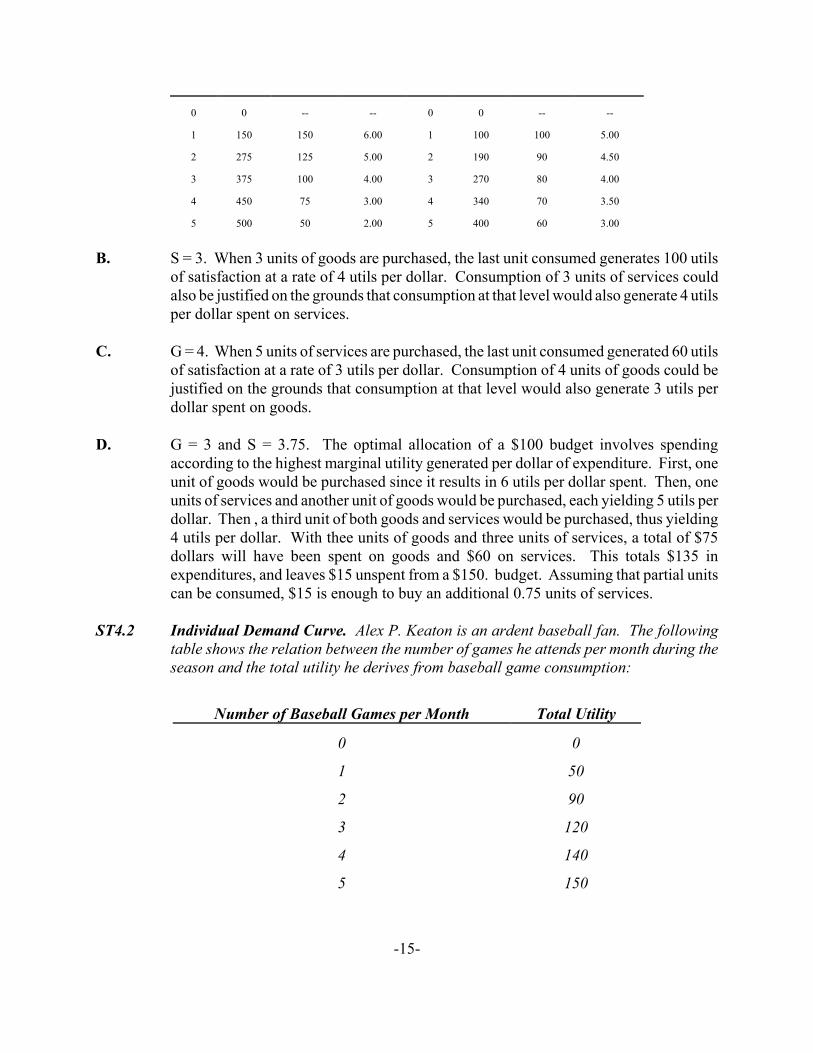
ST4.2 Individual Demand Curve. Alex P. Keaton is an ardent baseball fan. The followingtable shows the relation between the number of games he attends per month during theseason and the total utility he derives from baseball game consumption:

Number of Baseball Games per Month Total Utility

0 0

1 50

2 90

3 120

4 140

5 150

-16-

A. Construct a table showing Keaton's marginal utility derived from baseball gameconsumption.

B. At an average ticket price of $25, Keaton can justify attending only one game permonth. Calculate Keaton’s cost per unit of marginal utility derived from baseballgame consumption at this activity level.

C. If the cost/marginal utility trade-off found in part B represents the most Keatonis willing to pay for baseball game consumption, calculate the prices at which hewould attend two, three, four, and five games per month.

D. Plot Keaton's baseball game demand curve.

ST4.2 SOLUTION

A.

Number of BaseballGames Per Month

TotalUtility

MarginalUtility

0 0 --

1 50 50

2 90 40

3 120 30

4 140 20

5 150 10

B. At one baseball game per month, MU = 50. Thus, at a $25 price per baseball game, thecost per unit of marginal utility derived from baseball game consumption is P/MU =$25/50 = $0.50 or 50¢ per util.

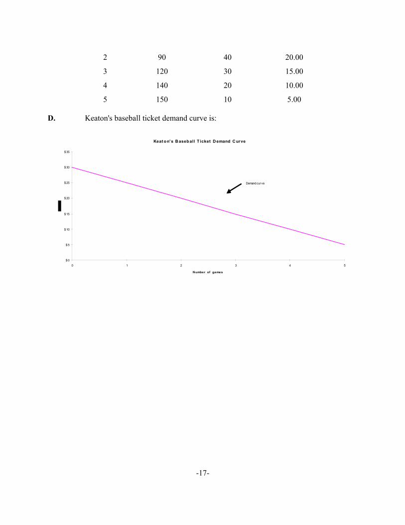
C. At a maximum acceptable price of 50¢ per util, Keaton's maximum acceptable price forbaseball game tickets varies according to the following schedule:

Numberof Games

Per Month Total Utility

MarginalUtility

MU = MU/MG

MaximumAcceptable

priceat 50¢ per MU

0 0 -- --

1 50 50 $25.00

-17-

2 90 40 20.00

3 120 30 15.00

4 140 20 10.00

5 150 10 5.00

D. Keaton's baseball ticket demand curve is:

Keat o n' s B aseb all T icket D emand C urve

$0

$5

$10

$15

$20

$25

$30

$35

0 1 2 3 4 5

Number of games

Demand cur ve

-18-

Chapter 5

Demand Analysis


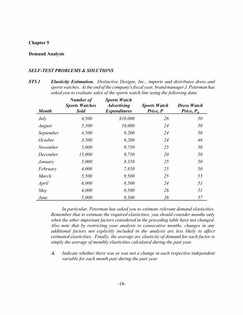
ST5.1 Elasticity Estimation. Distinctive Designs, Inc., imports and distributes dress andsports watches. At the end of the company's fiscal year, brand manager J. Peterman hasasked you to evaluate sales of the sports watch line using the following data:

Month

Number ofSports Watches

Sold

Sports WatchAdvertising

ExpendituresSports Watch

Price, PDress Watch

Price, PD

July 4,500 $10,000 26 50 August 5,500 10,000 24 50 September 4,500 9,200 24 50 October 3,500 9,200 24 46 November 5,000 9,750 25 50 December 15,000 9,750 20 50 January 5,000 8,350 25 50 February 4,000 7,850 25 50 March 5,500 9,500 25 55 April 6,000 8,500 24 51 May 4,000 8,500 26 51 June 5,000 8,500 26 57

In particular, Peterman has asked you to estimate relevant demand elasticities.Remember that to estimate the required elasticities, you should consider months onlywhen the other important factors considered in the preceding table have not changed.Also note that by restricting your analysis to consecutive months, changes in anyadditional factors not explicitly included in the analysis are less likely to affectestimated elasticities. Finally, the average arc elasticity of demand for each factor issimply the average of monthly elasticities calculated during the past year.

A. Indicate whether there was or was not a change in each respective independentvariable for each month pair during the past year.

-19-

Month-Pair


Expenditures, ASports Watch

Price, PDress Watch

Price, PD

July-August ____________ ____________ ____________August-September ____________ ____________ ____________September-October ____________ ____________ ____________October-November ____________ ____________ ____________November-December ____________ ____________ ____________December-January ____________ ____________ ____________January-February ____________ ____________ ____________February-March ____________ ____________ ____________March-April ____________ ____________ ____________April-May ____________ ____________ ____________May-June ____________ ____________ ____________

B. Calculate and interpret the average advertising arc elasticity of demand for sportswatches.

C. Calculate and interpret the average arc price elasticity of demand for sportswatches.

D. Calculate and interpret the average arc cross-price elasticity of demand betweensports and dress watches.

ST5.1 SOLUTION

A.

Month-Pair


Expenditures, ASports Watch

Price, PDress Watch

Price, PD

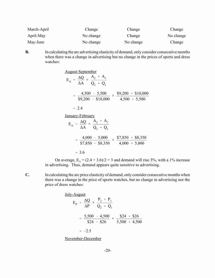
July-August No change Change No changeAugust-September Change No change No changeSeptember-October No change No change ChangeOctober-November Change Change ChangeNovember-December No change Change No changeDecember-January Change Change No changeJanuary-February Change No change No changeFebruary-March Change No change Change

-20-

EA '∆Q∆A

×A2 % A1

Q2 % Q1

'4,500 & 5,500

$9,200 & $10,000× $9,200 % $10,000

4,500 % 5,500

' 2.4

EA '∆Q∆A

×A2 % A1

Q2 % Q1

'4,000 & 5,000

$7,850 & $8,350× $7,850 % $8,350

4,000 % 5,000

' 3.6

EP '∆Q∆P

×P2 % P1

Q2 % Q1

'5,500 & 4,500

$24 & $26× $24 % $26

5,500 % 4,500

' &2.5

March-April Change Change ChangeApril-May No change Change No changeMay-June No change No change Change

B. In calculating the arc advertising elasticity of demand, only consider consecutive monthswhen there was a change in advertising but no change in the prices of sports and dresswatches:

August-September

January-February

On average, EA = (2.4 + 3.6)/2 = 3 and demand will rise 3%, with a 1% increasein advertising. Thus, demand appears quite sensitive to advertising.

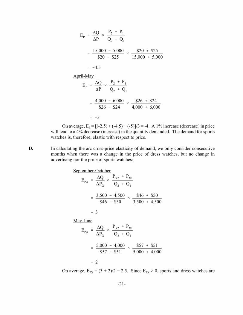
C. In calculating the arc price elasticity of demand, only consider consecutive months whenthere was a change in the price of sports watches, but no change in advertising nor theprice of dress watches:

July-August

November-December

-21-

EP '∆Q∆P

×P2 % P1

Q2 % Q1

'15,000 & 5,000

$20 & $25× $20 % $25

15,000 % 5,000

' &4.5

EP '∆Q∆P

×P2 % P1

Q2 % Q1

'4,000 & 6,000

$26 & $24× $26 % $24

4,000 % 6,000

' &5

EPX '∆Q∆PX

×PX2 % PX1

Q2 % Q1

'3,500 & 4,500

$46 & $50× $46 % $50

3,500 % 4,500

' 3

EPX '∆Q∆PX

×PX2 % PX1

Q2 % Q1

'5,000 & 4,000

$57 & $51× $57 % $51

5,000 % 4,000

' 2

April-May

On average, EP = [(-2.5) + (-4.5) + (-5)]/3 = -4. A 1% increase (decrease) in pricewill lead to a 4% decrease (increase) in the quantity demanded. The demand for sportswatches is, therefore, elastic with respect to price.

D. In calculating the arc cross-price elasticity of demand, we only consider consecutivemonths when there was a change in the price of dress watches, but no change inadvertising nor the price of sports watches:

September-October

May-June

On average, EPX = (3 + 2)/2 = 2.5. Since EPX > 0, sports and dress watches are

-22-

substitutes.

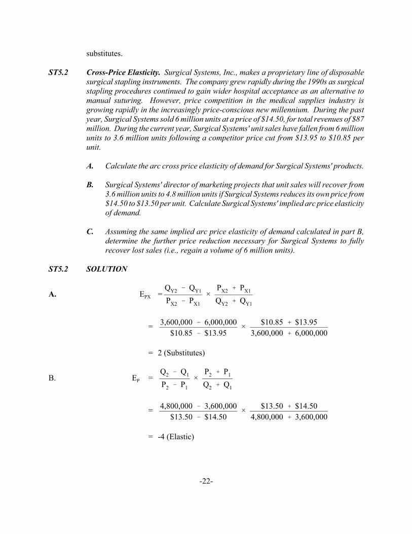
ST5.2 Cross-Price Elasticity. Surgical Systems, Inc., makes a proprietary line of disposablesurgical stapling instruments. The company grew rapidly during the 1990s as surgicalstapling procedures continued to gain wider hospital acceptance as an alternative tomanual suturing. However, price competition in the medical supplies industry isgrowing rapidly in the increasingly price-conscious new millennium. During the pastyear, Surgical Systems sold 6 million units at a price of $14.50, for total revenues of $87million. During the current year, Surgical Systems' unit sales have fallen from 6 millionunits to 3.6 million units following a competitor price cut from $13.95 to $10.85 perunit.

A. Calculate the arc cross price elasticity of demand for Surgical Systems' products.

B. Surgical Systems' director of marketing projects that unit sales will recover from3.6 million units to 4.8 million units if Surgical Systems reduces its own price from$14.50 to $13.50 per unit. Calculate Surgical Systems' implied arc price elasticityof demand.

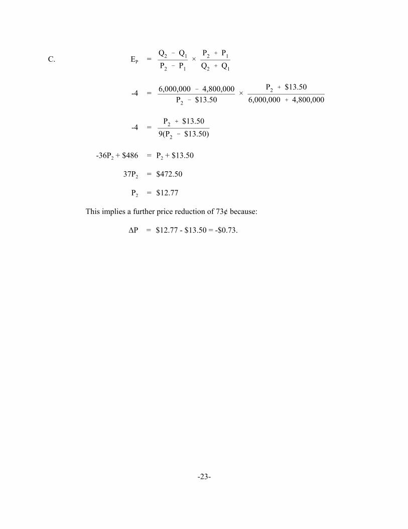
C. Assuming the same implied arc price elasticity of demand calculated in part B,determine the further price reduction necessary for Surgical Systems to fullyrecover lost sales (i.e., regain a volume of 6 million units).

ST5.2 SOLUTION

A. EPX =QY2 & QY1

PX2 & PX1

×PX2 % PX1

QY2 % QY1

= 3,600,000 & 6,000,000$10.85 & $13.95

× $10.85 % $13.953,600,000 % 6,000,000

= 2 (Substitutes)

B. EP =Q2 & Q1

P2 & P1

×P2 % P1

Q2 % Q1

= 4,800,000 & 3,600,000$13.50 & $14.50

× $13.50 % $14.504,800,000 % 3,600,000

= -4 (Elastic)

-23-

C. EP =Q2 & Q1

P2 & P1

×P2 % P1

Q2 % Q1

-4 = 6,000,000 & 4,800,000P2 & $13.50

×P2 % $13.50

6,000,000 % 4,800,000

-4 =P2 % $13.50

9(P2 & $13.50)

-36P2 + $486 = P2 + $13.50

37P2 = $472.50

P2 = $12.77

This implies a further price reduction of 73¢ because:

∆P = $12.77 - $13.50 = -$0.73.

-24-

Chapter 6

Demand Estimation


ST6.1 Linear Demand Curve Estimation. Women’s NCAA basketball has enjoyed growingpopularity across the country, and benefitted greatly from sophisticated sportsmarketing. Savvy institutions use time-tested means of promotion, especially whenmatch-ups against traditional rivals pique fan interest. As a case in point, fan interestis high whenever the Arizona State Sun Devils visit Tucson, Arizona, to play the ArizonaWildcats. To ensure a big fan turnout for this traditional rival, suppose the Universityof Arizona offered one-half off the $16 regular price of reserved seats, and sales jumpedfrom 1,750 to 2,750 tickets.

A. Calculate ticket revenues at each price level. Did the pricing promotion increaseor decrease ticket revenues?

B. Estimate the reserved seat demand curve, assuming that it is linear.

C. How should ticket prices be set to maximize total ticket revenue? Contrast thisanswer with your answer to part A.

ST6.1 SOLUTION

A. The total revenue function for the Arizona Wildcats is:

TR = P × Q

Then, total revenue at a price of $16 is:

TR = P × Q

= $16 × 1,750

= $28, 000

Total revenue at a price of $8 is:

TR = P × Q

-25-

= $8 × 2,750

= $22,000

The pricing promotion caused a decrease in ticket revenues.

B. When a linear demand curve is written as:

P = a + bQ

a is the intercept and b is the slope coefficient. From the data given previously, twopoints on this linear demand curve are identified. Given this information, it is possibleto exactly identify the linear demand curve by solving the system of two equations withtwo unknowns, a and b:

16 = a + b(1,750)minus 8 = a + b(2,250)

8 = -1,000 b

b = -0.008

By substitution, if b = -0.008, then:

16 = a + b(1,750)

16 = a - 0.008(1,750)

16 = a - 14

a = 30

Therefore, the reserved seat demand curve can be written:

P = $30 - $0.008Q

C. To find the revenue-maximizing output level, set MR = 0, and solve for Q. Because

TR = P × Q

= ($30 - $0.008Q)Q

= $30Q - $0.008Q2

MR = MTR/MQ

-26-

MR = $30 - $0.016Q = 0

0.016Q = 30

Q = 1,875

At Q = 1,875,

P = $30 - $0.008(1,875)

= $15

Total revenue at a price of $15 is:

TR = P × Q

= $15 × 1,875

= $28,125

(Note: M2TR/MQ2 < 0. This is a ticket-revenue maximizing output level because totalticket revenue is decreasing for output beyond Q > 1,875.)

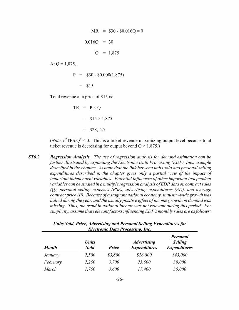
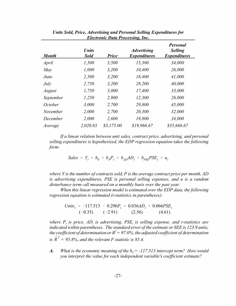
ST6.2 Regression Analysis. The use of regression analysis for demand estimation can befurther illustrated by expanding the Electronic Data Processing (EDP), Inc., exampledescribed in the chapter. Assume that the link between units sold and personal sellingexpenditures described in the chapter gives only a partial view of the impact ofimportant independent variables. Potential influences of other important independentvariables can be studied in a multiple regression analysis of EDP data on contract sales(Q), personal selling expenses (PSE), advertising expenditures (AD), and averagecontract price (P). Because of a stagnant national economy, industry-wide growth washalted during the year, and the usually positive effect of income growth on demand wasmissing. Thus, the trend in national income was not relevant during this period. Forsimplicity, assume that relevant factors influencing EDP's monthly sales are as follows:

Units Sold, Price, Advertising and Personal Selling Expenditures forElectronic Data Processing, Inc.

MonthUnitsSold Price

AdvertisingExpenditures

PersonalSelling

ExpendituresJanuary 2,500 $3,800 $26,800 $43,000February 2,250 3,700 23,500 39,000March 1,750 3,600 17,400 35,000

Units Sold, Price, Advertising and Personal Selling Expenditures forElectronic Data Processing, Inc.



PersonalSelling

Expenditures

-27-

Sales ' Yt ' b0 % bPPt % bADADt % bPSEPSEt % ut

Unitst ' &117.513 & 0.296Pt % 0.036ADt % 0.066PSEt(&0.35) (&2.91) (2.56) (4.61)

April 1,500 3,500 15,300 34,000May 1,000 3,200 10,400 26,000June 2,500 3,200 18,400 41,000July 2,750 3,200 28,200 40,000August 1,750 3,000 17,400 33,000September 1,250 2,900 12,300 26,000October 3,000 2,700 29,800 45,000November 2,000 2,700 20,300 32,000December 2,000 2,600 19,800 34,000Average 2,020.83 $3,175.00 $19,966.67 $35,666.67

If a linear relation between unit sales, contract price, advertising, and personalselling expenditures is hypothesized, the EDP regression equation takes the followingform:

where Y is the number of contracts sold, P is the average contract price per month, ADis advertising expenditures, PSE is personal selling expenses, and u is a randomdisturbance term--all measured on a monthly basis over the past year.

When this linear regression model is estimated over the EDP data, the followingregression equation is estimated (t-statistics in parentheses):

where Pt is price, ADt is advertising, PSEt is selling expense, and t-statistics areindicated within parentheses. The standard error of the estimate or SEE is 123.9 units,the coefficient of determination or R2 = 97.0%, the adjusted coefficient of determinationis = 95.8%, and the relevant F statistic is 85.4.R̄ 2

A. What is the economic meaning of the b0 = -117.513 intercept term? How wouldyou interpret the value for each independent variable's coefficient estimate?

1The t statistic for personal selling expenses exceeds 3.355, the precise critical t value for theα = 0.01 level and n - k = 12 - 4 = 8 degrees of freedom. The t statistic for price and advertisingexceeds 2.306, the critical t value for the α = 0.05 level and 8 degrees of freedom, meaning thatthere can be 95 percent confidence that price and advertising affect sales. Note also that F3,8 =85.40 > 7.58, the precise critical F value for the α = 0.01 significance level.

-28-

B. How is the standard error of the estimate (SEE) employed in demand estimation?

C. Describe the meaning of the coefficient of determination, R2, and the adjustedcoefficient of determination, R̄ 2.

D. Use the EDP regression model to estimate fitted values for units sold andunexplained residuals for each month during the year.

ST6.2 SOLUTION

A. The intercept term b0 = -117.513 has no clear economic meaning. Caution must alwaysbe exercised when interpreting points outside the range of observed data and thisintercept, like most, lies far from typical values. This intercept cannot be interpreted asthe expected level of unit sales at a zero price, assuming both advertising and personalselling expenses are completely eliminated. Similarly, it would be hazardous to use thisregression model to predict sales at prices, selling expenses, or advertising levels wellin excess of sample norms.

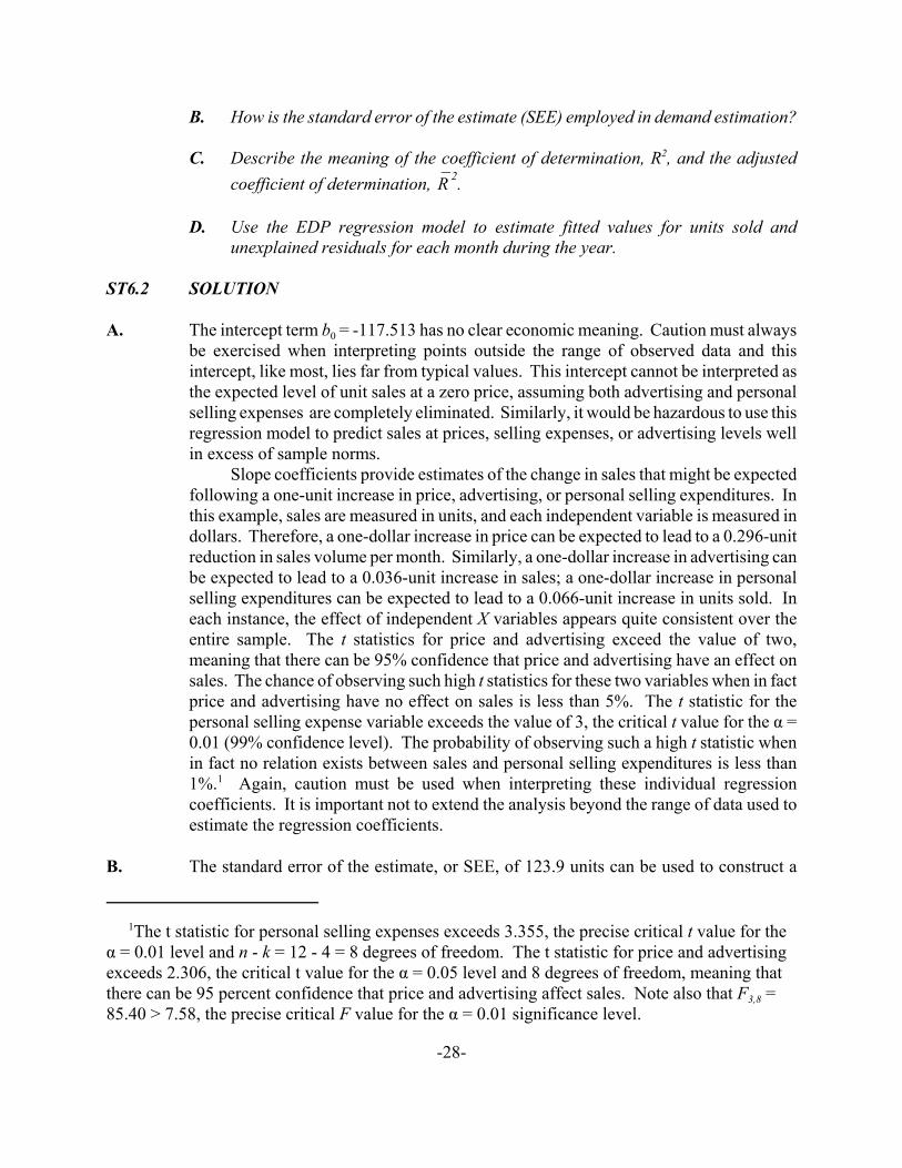
Slope coefficients provide estimates of the change in sales that might be expectedfollowing a one-unit increase in price, advertising, or personal selling expenditures. Inthis example, sales are measured in units, and each independent variable is measured indollars. Therefore, a one-dollar increase in price can be expected to lead to a 0.296-unitreduction in sales volume per month. Similarly, a one-dollar increase in advertising canbe expected to lead to a 0.036-unit increase in sales; a one-dollar increase in personalselling expenditures can be expected to lead to a 0.066-unit increase in units sold. Ineach instance, the effect of independent X variables appears quite consistent over theentire sample. The t statistics for price and advertising exceed the value of two,meaning that there can be 95% confidence that price and advertising have an effect onsales. The chance of observing such high t statistics for these two variables when in factprice and advertising have no effect on sales is less than 5%. The t statistic for thepersonal selling expense variable exceeds the value of 3, the critical t value for the α =0.01 (99% confidence level). The probability of observing such a high t statistic whenin fact no relation exists between sales and personal selling expenditures is less than1%.1 Again, caution must be used when interpreting these individual regressioncoefficients. It is important not to extend the analysis beyond the range of data used toestimate the regression coefficients.

B. The standard error of the estimate, or SEE, of 123.9 units can be used to construct a

-29-

confidence interval within which actual values are likely to be found based on the sizeof individual regression coefficients and various values for the X variables. Forexample, given this regression model and the values Pt = $3,800, ADt = $26,800, andPSEt = $43,000 for each respective independent X variable during the month of January;the fitted value ^Yt = 2,566.88 can be calculated (see part D). Given these values for theindependent X variables, 95% of the time actual observations for the month of Januarywill lie within roughly 2 standard errors of the estimate; 99% of the time actualobservations will lie within roughly 3 standard errors of the estimate. Thus,approximate bounds for the 95% confidence interval are given by the expression2,566.88 ± (2 × 123.9), or from 2,319.08 to 2,814.68 sales units. Approximate boundsfor the 99% confidence interval are given by the expression 2,566.88 ± (3 × 123.9), orfrom 2,195.18 to 2,938.58 sales units.

C. The coefficient of determination is R2 = 97.0%; it indicates that 97% of the variation inEDP demand is explained by the regression model. Only 3% is left unexplained.Moreover, the adjusted coefficient of determination is = 95.8%; this reflects only aR̄ 2

modest downward adjustment to R2 based upon the size of the sample analyzed relativeto the number of estimated coefficients. This suggests that the regression modelexplains a significant share of demand variation--a suggestion that is supported by theF statistic. F3,8 = 85.4 and is far greater than five, meaning that the hypothesis of norelation between sales and this group of independent X variables can be rejected with99% confidence. There is less than a 1% chance of encountering such a large F statisticwhen in fact there is no relation between sales and these X variables as a group.

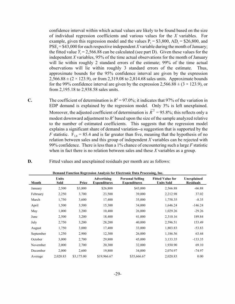
D. Fitted values and unexplained residuals per month are as follows:

Demand Function Regression Analysis for Electronic Data Processing, Inc.



Personal SellingExpenditures

Fitted Value forUnits Sold

UnexplainedResiduals

January 2,500 $3,800 $26,800 $43,000 2,566.88 -66.88

February 2,250 3,700 23,500 39,000 2,212.98 37.02

March 1,750 3,600 17,400 35,000 1,758.35 -8.35

April 1,500 3,500 15,300 34,000 1,646.24 -146.24 May 1,000 3,200 10,400 26,000 1,029.26 -29.26

June 2,500 3,200 18,400 41,000 2,310.16 189.84

July 2,750 3,200 28,200 40,000 2,596.51 153.49

August 1,750 3,000 17,400 33,000 1,803.83 -53.83

September 1,250 2,900 12,300 26,000 1,186.56 63.44 October 3,000 2,700 29,800 45,000 3,133.35 -133.35

November 2,000 2,700 20,300 32,000 1,930.90 69.10

December 2,000 2,600 19,800 34,000 2,074.97 -74.97

Average 2,020.83 $3,175.00 $19,966.67 $35,666.67 2,020.83 0.00

-30-

-31-

Chapter 7

Forecasting


ST7.1 Gross Domestic Product (GDP) is a measure of overall activity in the economy. It isdefined as the value at the final point of sale of all goods and services produced duringa given period by both domestic and foreign-owned enterprises. GDP data for the1950-2004 period shown in Figure 7.3 offer the basis to test the abilities of simpleconstant change and constant growth models to describe the trend in GDP over time.However, regression results generated over the entire 1950-2004 period cannot be usedto forecast GDP over any subpart of that period. To do so would be to overstate theforecast capability of the regression model because, by definition, the regression lineminimizes the sum of squared deviations over the estimation period. To test forecastreliability, it is necessary to test the predictive capability of a given regression modelover data that was not used to generate that very model. In the absence of GDP datafor future periods, say 2005-2010, the reliability of alternative forecast techniques canbe illustrated by arbitrarily dividing historical GDP data into two subsamples: a 1950-99 50-year test period, and a 2000-04 5-year forecast period. Regression modelsestimated over the 1950-99 test period can be used to “forecast” actual GDP over the2000-04 period. In other words, estimation results over the 1950-99 subperiod providea forecast model that can be used to evaluate the predictive reliability of the constantgrowth model over the 2000-04 forecast period.

A. Use the regression model approach to estimate the simple linear relation betweenthe natural logarithm of GDP and time (T) over the 1950-99 subperiod, where

ln GDPt = b0 + b1Tt + ut

and ln GDPt is the natural logarithm of GDP in year t, and T is a time trendvariable (where T1950 = 1, T1951 = 2, T1952 = 3, . . ., and T1999 = 50); and u is aresidual term. This is called a constant growth model because it is based on theassumption of a constant percentage growth in economic activity per year. Howwell does the constant growth model fit actual GDP data over this period?

B. Create a spreadsheet that shows constant growth model GDP forecasts over the2000-04 period alongside actual figures. Then, subtract forecast values fromactual figures to obtain annual estimates of forecast error, and squared forecasterror, for each year over the 2000-04 period.

Finally, compute the correlation coefficient between actual and forecast

-32-

values over the 2000-04 period. Also compute the sample average (or root meansquared) forecast error. Based upon these findings, how well does the constantgrowth model generated over the 1950-99 period forecast actual GDP data overthe 2000-04 period?

ST7.1 SOLUTION

A. The constant growth model estimated using the simple regression model techniqueillustrates the linear relation between the natural logarithm of GDP and time. A constantgrowth regression model estimated over the 1950-99 50-year period (t-statistic inparentheses), used to forecast GDP over the 2000-04 5-year period, is:

ln GDPt = 5.5026 + 0.0752t, R2 = 99.2% (188.66) (75.50)

The R2 = 99.2% and a highly significant t statistic for the time trend variable indicatethat the constant growth model closely describes the change in GDP over the 1950-99time frame. Nevertheless, even modest changes in the intercept term and slopecoefficient over the 2000-04 time frame can lead to large forecast errors.

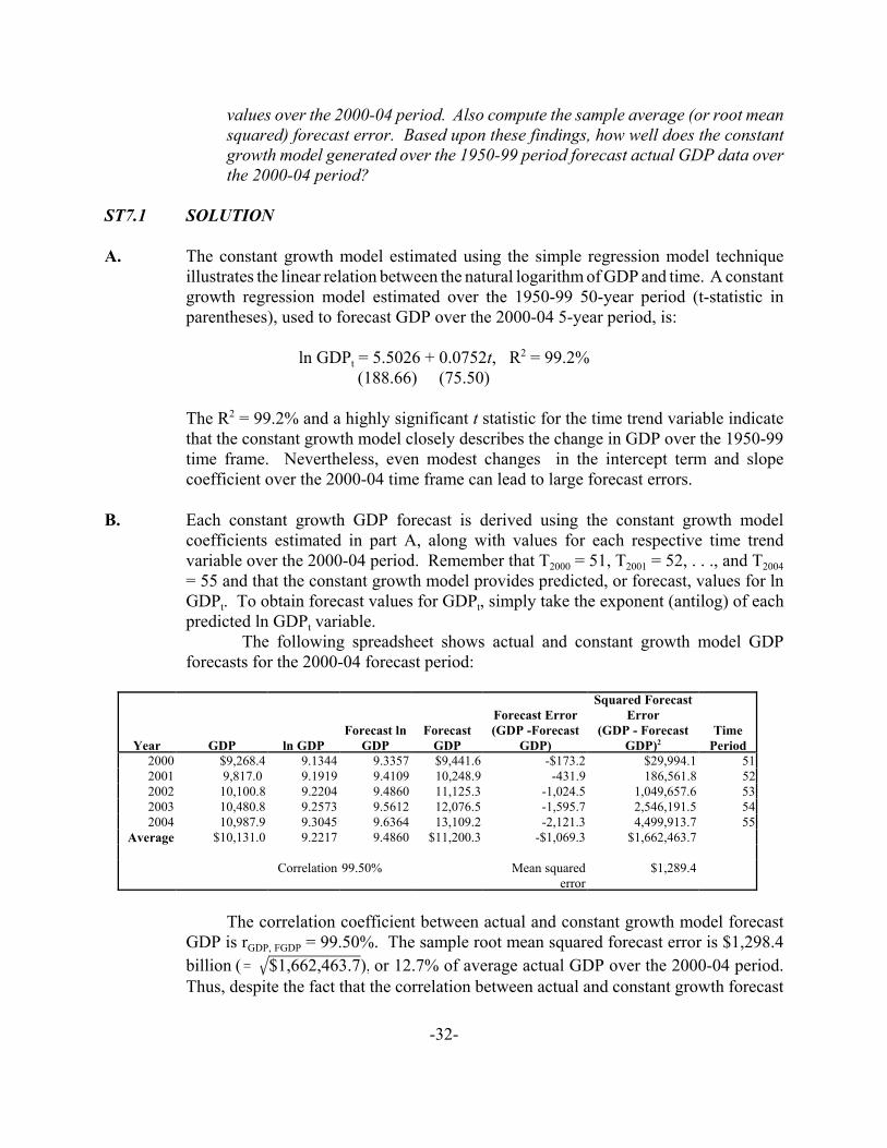
B. Each constant growth GDP forecast is derived using the constant growth modelcoefficients estimated in part A, along with values for each respective time trendvariable over the 2000-04 period. Remember that T2000 = 51, T2001 = 52, . . ., and T2004= 55 and that the constant growth model provides predicted, or forecast, values for lnGDPt. To obtain forecast values for GDPt, simply take the exponent (antilog) of eachpredicted ln GDPt variable.

The following spreadsheet shows actual and constant growth model GDPforecasts for the 2000-04 forecast period:

Year GDP ln GDPForecast ln

GDPForecast

GDP

Forecast Error(GDP -Forecast

GDP)

Squared ForecastError

(GDP - ForecastGDP)2

TimePeriod

2000 $9,268.4 9.1344 9.3357 $9,441.6 -$173.2 $29,994.1 512001 9,817.0 9.1919 9.4109 10,248.9 -431.9 186,561.8 522002 10,100.8 9.2204 9.4860 11,125.3 -1,024.5 1,049,657.6 532003 10,480.8 9.2573 9.5612 12,076.5 -1,595.7 2,546,191.5 542004 10,987.9 9.3045 9.6364 13,109.2 -2,121.3 4,499,913.7 55

Average $10,131.0 9.2217 9.4860 $11,200.3 -$1,069.3 $1,662,463.7

Correlation 99.50% Mean squarederror

$1,289.4

The correlation coefficient between actual and constant growth model forecastGDP is rGDP, FGDP = 99.50%. The sample root mean squared forecast error is $1,298.4billion or 12.7% of average actual GDP over the 2000-04 period.(' $1,662,463.7),Thus, despite the fact that the correlation between actual and constant growth forecast

-33-

model values is relatively high, forecast error is also very high. Unusually modesteconomic growth at the start of the new millennium leads to large forecast errors whenGDP data from more rapidly growing periods, like the 1950-99 period, are used toforecast economic growth.

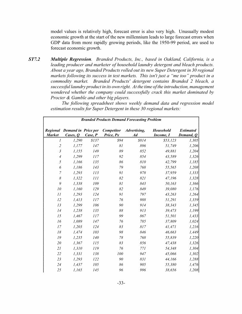
ST7.2 Multiple Regression. Branded Products, Inc., based in Oakland, California, is aleading producer and marketer of household laundry detergent and bleach products.About a year ago, Branded Products rolled out its new Super Detergent in 30 regionalmarkets following its success in test markets. This isn't just a “me too” product in acommodity market. Branded Products' detergent contains Branded 2 bleach, asuccessful laundry product in its own right. At the time of the introduction, managementwondered whether the company could successfully crack this market dominated byProcter & Gamble and other big players.

The following spreadsheet shows weekly demand data and regression modelestimation results for Super Detergent in these 30 regional markets:

Branded Products Demand Forecasting Problem

RegionalMarket

Demand inCases, Q

Price perCase, P

CompetitorPrice, Px

Advertising,Ad

HouseholdIncome, I

EstimatedDemand, Q

1 1,290 $137 $94 $814 $53,123 1,3052 1,177 147 81 896 51,749 1,2063 1,155 149 89 852 49,881 1,2044 1,299 117 92 854 43,589 1,3265 1,166 135 86 810 42,799 1,1856 1,186 143 79 768 55,565 1,2087 1,293 113 91 978 37,959 1,3338 1,322 111 82 821 47,196 1,3289 1,338 109 81 843 50,163 1,366

10 1,160 129 82 849 39,080 1,17611 1,293 124 91 797 43,263 1,26412 1,413 117 76 988 51,291 1,35913 1,299 106 90 914 38,343 1,34514 1,238 135 88 913 39,473 1,19915 1,467 117 99 867 51,501 1,43316 1,089 147 76 785 37,809 1,02417 1,203 124 83 817 41,471 1,21618 1,474 103 98 846 46,663 1,44919 1,235 140 78 768 55,839 1,22020 1,367 115 83 856 47,438 1,32621 1,310 119 76 771 54,348 1,30422 1,331 138 100 947 45,066 1,30223 1,293 122 90 831 44,166 1,28824 1,437 105 86 905 55,380 1,47625 1,165 145 96 996 38,656 1,208

RegionalMarket

Demand inCases, Q

Price perCase, P

CompetitorPrice, Px

Advertising,Ad

HouseholdIncome, I

EstimatedDemand, Q

-34-

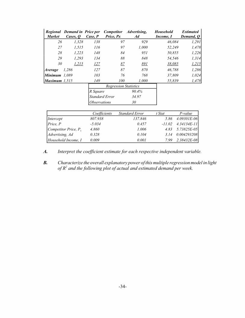
26 1,328 138 97 929 46,084 1,29127 1,515 116 97 1,000 52,249 1,47828 1,223 148 84 951 50,855 1,22629 1,293 134 88 848 54,546 1,31430 1,215 127 87 891 38,085 1,215

Average 1,286 127 87 870 46,788 1,286Minimum 1,089 103 76 768 37,809 1,024Maximum 1,515 149 100 1,000 55,839 1,478

Regression StatisticsR Square 90.4%Standard Error 34.97Observations 30

Coefficients Standard Error t Stat P-valueIntercept 807.938 137.846 5.86 4.09301E-06Price, P -5.034 0.457 -11.02 4.34134E-11Competitor Price, Px 4.860 1.006 4.83 5.73825E-05Advertising, Ad 0.328 0.104 3.14 0.004293208Household Income, I 0.009 0.001 7.99 2.38432E-08

A. Interpret the coefficient estimate for each respective independent variable.

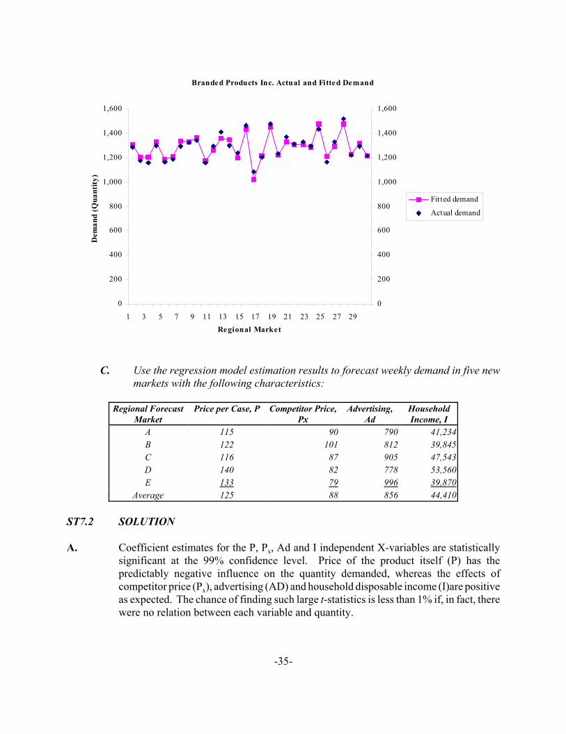
B. Characterize the overall explanatory power of this multiple regression model in lightof R2 and the following plot of actual and estimated demand per week.

-35-

Branded Products Inc. Actual and Fitted Demand

0

200

400

600

800

1,000

1,200

1,400

1,600

1 3 5 7 9 11 13 15 17 19 21 23 25 27 29Regional Market

Dem

and

(Qua

ntity

)

0

200

400

600

800

1,000

1,200

1,400

1,600

Fitted demand

Actual demand

C. Use the regression model estimation results to forecast weekly demand in five newmarkets with the following characteristics:

Regional ForecastMarket

Price per Case, P Competitor Price,Px

Advertising,Ad

HouseholdIncome, I

A 115 90 790 41,234B 122 101 812 39,845C 116 87 905 47,543D 140 82 778 53,560E 133 79 996 39,870

Average 125 88 856 44,410

ST7.2 SOLUTION

A. Coefficient estimates for the P, Px, Ad and I independent X-variables are statisticallysignificant at the 99% confidence level. Price of the product itself (P) has thepredictably negative influence on the quantity demanded, whereas the effects ofcompetitor price (Px), advertising (AD) and household disposable income (I)are positiveas expected. The chance of finding such large t-statistics is less than 1% if, in fact, therewere no relation between each variable and quantity.

-36-

B. The R2 = 90.4% obtained by the model means that 90.4% of demand variation isexplained by the underlying variation in all four independent variables. This is arelatively high level of explained variation and implies an attractive level of explanatorypower. Moreover, as shown in the graph of actual and fitted (estimated) demand, themultiple regression model closely tracks week-by-week changes in demand with noworrisome divergences between actual and estimated demand over time. This meansthat this regression model can be used to forecast demand in similar markets undersimilar conditions..

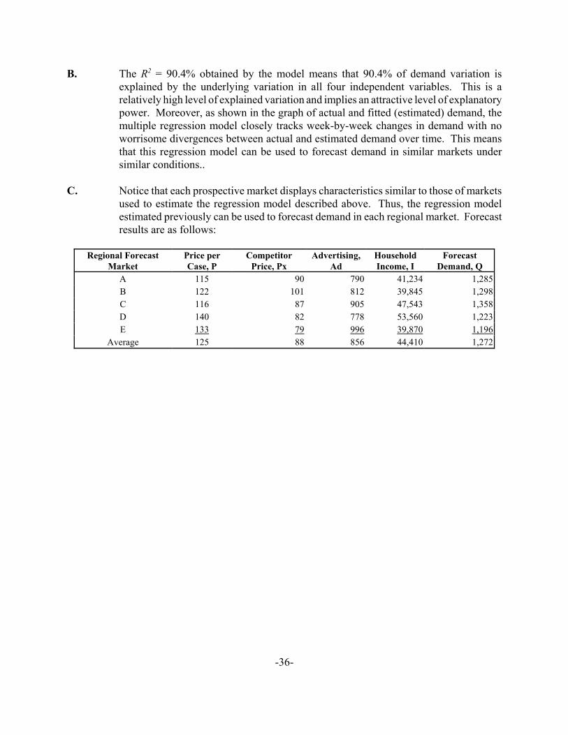
C. Notice that each prospective market displays characteristics similar to those of marketsused to estimate the regression model described above. Thus, the regression modelestimated previously can be used to forecast demand in each regional market. Forecastresults are as follows:

Regional ForecastMarket

Price perCase, P

CompetitorPrice, Px

Advertising,Ad

HouseholdIncome, I

ForecastDemand, Q

A 115 90 790 41,234 1,285B 122 101 812 39,845 1,298C 116 87 905 47,543 1,358D 140 82 778 53,560 1,223E 133 79 996 39,870 1,196

Average 125 88 856 44,410 1,272

-37-

MPT

PT

'MPA

PA

Chapter 8

Production Analysis and Compensation Policy


ST8.1 Optimal Input Usage. Medical Testing Labs, Inc., provides routine testing services forblood banks in the Los Angeles area. Tests are supervised by skilled technicians usingequipment produced by two leading competitors in the medical equipment industry.Records for the current year show an average of 27 tests per hour being performed onthe Testlogic-1 and 48 tests per hour on a new machine, the Accutest-3. The Testlogic-1is leased for $18,000 per month, and the Accutest-3 is leased at $32,000 per month. Onaverage, each machine is operated 25 eight-hour days per month.

A. Describe the logic of the rule used to determine an optimal mix of input usage.

B. Does Medical Testing Lab usage reflect an optimal mix of testing equipment?

C. Describe the logic of the rule used to determine an optimal level of input usage.

D. If tests are conducted at a price of $6 each while labor and all other costs arefixed, should the company lease more machines?

ST8.1 SOLUTION

A. The rule for an optimal combination of Testlogic-1 (T) and Accutest-3 (A) equipmentis

This rule means that an identical amount of additional output would be produced withan additional dollar expenditure on each input. Alternatively, an equal marginal cost ofoutput is incurred irrespective of which input is used to expand output. Of course,marginal products and equipment prices must both reflect the same relevant time frame,either hours or months.

B. On a per hour basis, the relevant question is

27$18,000/(25 × 8)

'? 48

$32,000/(25 × 8)

-38-

0.3 0.3'%

On a per month basis, the relevant question is

27 × (25 × 8)$18,000

'?

48 × (25 × 8)$32,000

0.3 '%

0.3

In both instances, the last dollar spent on each machine increased output by the same 0.3units, indicating an optimal mix of testing machines.

C. The rule for optimal input employment is

MRP = MP × MRQ = Input Price

This means that the level of input employment is optimal when the marginal salesrevenue derived from added input usage is equal to input price, or the marginalcost of employment.

D. For each machine hour, the relevant question is

Testlogic-1

MRPT = MPT × MRQ PT'?

27 × $6 $18,000/(25 × 8)'?

$162 > $90.

Accutest-3

MRPA = MPA × MRQ PA'?

48 × $6 $32,000/(25 × 8)'?

$288 > $160.

-39-

Q ' b0Lb1K b2E b3

Or, in per month terms:

Testlogic-1

MRPT = MPT × MRQ PT'?

27 × (25 × 8) × $6 $18,000'?

$32,400 > $18,000.

Accutest-3

MRPA = MPA × MRQ PA'?

48 × (25 × 8) × $6 $32,000'?

$57,600 > $32,000.

In both cases, each machine returns more than its marginal cost (price) of employment,and expansion would be profitable.

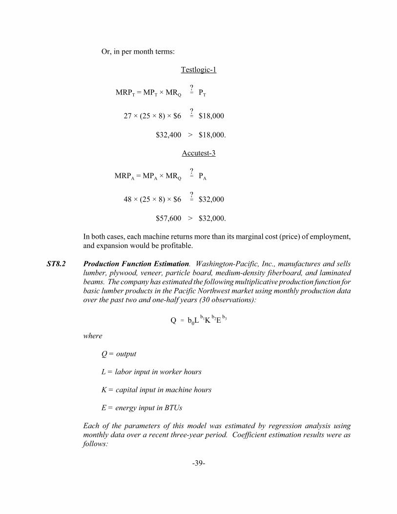
ST8.2 Production Function Estimation. Washington-Pacific, Inc., manufactures and sellslumber, plywood, veneer, particle board, medium-density fiberboard, and laminatedbeams. The company has estimated the following multiplicative production function forbasic lumber products in the Pacific Northwest market using monthly production dataover the past two and one-half years (30 observations):

where

Q = output

L = labor input in worker hours

K = capital input in machine hours

E = energy input in BTUs

Each of the parameters of this model was estimated by regression analysis usingmonthly data over a recent three-year period. Coefficient estimation results were asfollows:

-40-

MQ/QML/L

'MQML

× LQ

'(b0b1L

b1 & 1K b2E b3) × LQ

'b0b1L

b1 & 1 % 1K b2E b3

b0Lb1K b2E b3

' b1

= 0.9; = 0.4; = 0.4; and = 0.2b̂0 b̂1 b̂2 b̂3

The standard error estimates for each coefficient are:

= 0.6; = 0.1; = 0.2; = 0.1σb̂0σb̂1

σb̂2σb̂3

A. Estimate the effect on output of a 1% decline in worker hours (holding K and Econstant).

B. Estimate the effect on output of a 5% reduction in machine hours availabilityaccompanied by a 5% decline in energy input (holding L constant).

C. Estimate the returns to scale for this production system.

ST8.2 SOLUTION

A. For Cobb-Douglas production functions, calculations of the elasticity of output withrespect to individual inputs can be made by simply referring to the exponents of theproduction relation. Here a 1% decline in L, holding all else equal, will lead to a 0.4%decline in output. Notice that:

And because (MQ/Q)/(ML/L) is the percent change in Q due to a 1% change in L,

= b1MQ/QML/L

MQ/Q = b1 × ML/L

= 0.4(-0.01)

= -0.004 or -0.4%

-41-

Q ' b0Lb1K b2E b3

hQ ' b0(kL)b1(kK)b2(kE)b3

' k b1 % b2 % b3b0Lb1K b2E b3

' k b1 % b2 % b3Q

B. From part A it is obvious that:

MQ/Q = b2(MK/K) + b3(ME/E)

= 0.4(-0.05) + 0.2(-0.05)

= -0.03 or -3%

C. In the case of Cobb-Douglas production functions, returns to scale are determined bysimply summing exponents because:

Here b1 + b2 + b3 = 0.4 + 0.4 + 0.2 = 1 indicating constant returns to scale. This meansthat a 1% increase in all inputs will lead to a 1% increase in output, and average costswill remain constant as output increases.

-42-

Chapter 9

Cost Analysis and Estimation


ST9.1 Learning Curves. Modern Merchandise, Inc., makes and markets do-it-yourselfhardware, housewares, and industrial products. The company's new Aperture Miniblindis winning customers by virtue of its high quality and quick order turnaround time. Theproduct also benefits because its price point bridges the gap between ready-made vinylblinds and their high-priced custom counterpart. In addition, the company's expandingproduct line is sure to benefit from cross-selling across different lines. Given thesuccess of the Aperture Miniblind product, Modern Merchandise plans to open a newproduction facility near Beaufort, South Carolina. Based on information provided byits chief financial officer, the company estimates fixed costs for this product of $50,000per year and average variable costs of:

AVC = $0.5 + $0.0025Q,

where AVC is average variable cost (in dollars) and Q is output.

A. Estimate total cost and average total cost for the projected first-year volume of20,000 units.

B. An increase in worker productivity because of greater experience or learningduring the course of the year resulted in a substantial cost saving for thecompany. Estimate the effect of learning on average total cost if actual second-year total cost was $848,000 at an actual volume of 20,000 units.

ST9.1 SOLUTION

A. The total variable cost function for the first year is:

TVC = AVC × Q

= ($0.5 + $0.0025Q)Q

= $0.5Q + $0.0025Q2

At a volume of 20,000 units, estimated total cost is:

-43-

TC = TFC + TVC

= $50,000 + $0.5Q + $0.0025Q2

= $50,000 + $0.5(20,000) + $0.0025(20,0002)

= $1,060,000

Estimated average cost is:

AC = TC/Q

= $1,060,000/20,000

= $53 per case

B. If actual total costs were $848,000 at a volume of 20,000 units, actual average total costswere:

AC = TC/Q

= $848,000/20,000

= $42.40 per case

Therefore, greater experience or learning has resulted in an average cost saving of$10.60 per case since:

Learning effect = Actual AC - Estimated AC

= $42.40 - $53

= -$10.60 per case

Alternatively,

Learning rate = 1 &AC2

AC1

× 100

= 1 &$42.40

$53× 100

= 20%

-44-

ST9.2 Minimum Efficient Scale Estimation. Kanata Corporation is a leading manufacturerof telecommunications equipment based in Ontario, Canada. Its main product ismicro-processor controlled telephone switching equipment, called automatic privatebranch exchanges (PABXs), capable of handling 8 to 3,000 telephone extensions.Severe price cutting throughout the PABX industry continues to put pressure on salesand margins. To better compete against increasingly aggressive rivals, the company iscontemplating the construction of a new production facility capable of producing 1.5million units per year. Kanata's in-house engineering estimate of the total cost functionfor the new facility is:

TC = $3,000 + $1,000Q + $0.003Q2,

MC = MTC/MQ = $1,000 + $0.006Q

where TC = Total Costs in thousands of dollars, Q = Output in thousands of units, andMC = Marginal Costs in thousands of dollars.

A. Estimate minimum efficient scale in this industry.

B. In light of current PABX demand of 30 million units per year, how would youevaluate the future potential for competition in the industry?

ST9.2 SOLUTION

A. Minimum efficient scale is reached when average costs are first minimized. This occursat the point where MC = AC.

Average Costs = AC = TC/Q

= ($3,000 + $1,000Q + $0.003Q2)/Q

= + $1,000 + $0.003Q$3,000Q

Therefore,

MC = AC

$1,000 + $0.006Q = + $1,000 + $0.003Q$3,000Q

0.003Q = 3,000Q

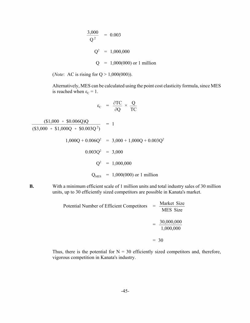
-45-

= 0.0033,000Q 2

Q2 = 1,000,000

Q = 1,000(000) or 1 million

(Note: AC is rising for Q > 1,000(000)).

Alternatively, MES can be calculated using the point cost elasticity formula, since MESis reached when εC = 1.

εC = MTCMQ

× QTC

= 1($1,000 % $0.006Q)Q($3,000 % $1,000Q % $0.003Q 2)

1,000Q + 0.006Q2 = 3,000 + 1,000Q + 0.003Q2

0.003Q2 = 3,000

Q2 = 1,000,000

QMES = 1,000(000) or 1 million

B. With a minimum efficient scale of 1 million units and total industry sales of 30 millionunits, up to 30 efficiently sized competitors are possible in Kanata's market.

Potential Number of Efficient Competitors = Market SizeMES Size

= 30,000,0001,000,000

= 30

Thus, there is the potential for N = 30 efficiently sized competitors and, therefore,vigorous competition in Kanata's industry.

-46-

Chapter 10

Competitive Markets


ST10.1 Market Supply. In some markets, cutthroat competition can exist even when the marketis dominated by a small handful of competitors. This usually happens when fixed costsare high, products are standardized, price information is readily available, and excesscapacity is present. Airline passenger service in large city-pair markets, and electroniccomponents manufacturing are good examples of industries where price competitionamong the few can be vigorous. Consider three competitors producing a standardizedproduct (Q) with the following marginal cost characteristics:

MC1 = $5 + $0.0004Q1 (Firm 1)

MC2 = $15 + $0.002Q2 (Firm 2)

MC3 = $1 + $0.0002Q3 (Firm 3)

A. Using each firm’s marginal cost curve, calculate the profit-maximizing short-runsupply from each firm at the competitive market prices indicated in the followingtable. For simplicity, assume price is greater than average variable cost in everyinstance.

Market Supply is the Sum of Firm Supply Across all Competitors

Firm One Supply Firm Two Supply Firm Three Supply Market Supply

PriceP = MC1= $5 + $0.0004Q1 and Q1 = -12,500 + 2,500P

P = MC2= $15 + $0.002Q2and Q2 = -7,500 + 500P

P = MC3= $1 + $0.0002Q3and Q3 = -5,000 + 5,000P

P = $3.125 + $0.000125Pand QI = -25,000 + 8,000P (QI = Q1 + Q2 + Q3)

$05

101520253035

-47-

404550556065707580

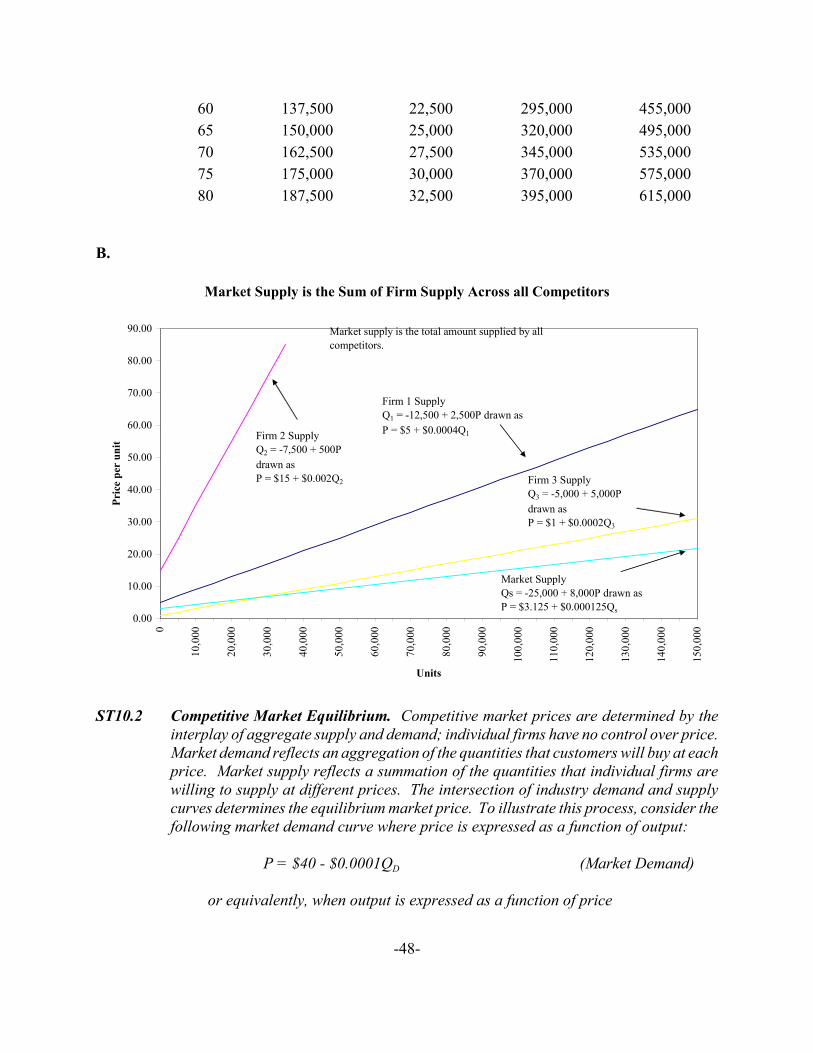
B. Use these data to plot short-run supply curves for each firm. Also plot the marketsupply curve.

ST10.1 SOLUTION

A. The marginal cost curve constitutes the short-run supply curve for firms in perfectlycompetitive markets so long as price is greater than average variable cost.


Firm OneSupply

Firm TwoSupply

Firm ThreeSupply Market Supply

Price

P = MC1= $5 + $0.0004Q1and Q1 = -12,500 +2,500P

P = MC2= $15 +$0.002Q2 and Q2 = -7,500 +500P

P = MC3= $1 +$0.0002Q3 and Q3 = -5,000 +5,000P

P = $3.125 +$0.000125P and QI = -25,000 +8,000P (QI = Q1+ Q2 + Q3)

$0 -12,500 -7,500 -5,000 -25,0005 0 -5,000 20,000 15,000

10 12,500 -2,500 45,000 55,00015 25,000 0 70,000 95,00020 37,500 2,500 95,000 135,00025 50,000 5,000 120,000 175,00030 62,500 7,500 145,000 215,00035 75,000 10,000 170,000 255,00040 87,500 12,500 195,000 295,00045 100,000 15,000 220,000 335,00050 112,500 17,500 245,000 375,00055 125,000 20,000 270,000 415,000

-48-


0.00

10.00

20.00

30.00

40.00

50.00

60.00

70.00

80.00

90.00

0

10,0

00

20,0

00

30,0

00

40,0

00

50,0

00

60,0

00

70,0

00

80,0

00

90,0

00

100,

000

110,

000

120,

000

130,

000

140,

000

150,

000

Units

Pric

e pe

r un

it

Firm 2 SupplyQ2 = -7,500 + 500P drawn asP = $15 + $0.002Q2

Firm 1 SupplyQ1 = -12,500 + 2,500P drawn asP = $5 + $0.0004Q1

Firm 3 SupplyQ3 = -5,000 + 5,000P drawn asP = $1 + $0.0002Q3

Market SupplyQs = -25,000 + 8,000P drawn asP = $3.125 + $0.000125Qs

Market supply is the total amount supplied by all competitors.

60 137,500 22,500 295,000 455,00065 150,000 25,000 320,000 495,00070 162,500 27,500 345,000 535,00075 175,000 30,000 370,000 575,00080 187,500 32,500 395,000 615,000

B.

ST10.2 Competitive Market Equilibrium. Competitive market prices are determined by theinterplay of aggregate supply and demand; individual firms have no control over price.Market demand reflects an aggregation of the quantities that customers will buy at eachprice. Market supply reflects a summation of the quantities that individual firms arewilling to supply at different prices. The intersection of industry demand and supplycurves determines the equilibrium market price. To illustrate this process, consider thefollowing market demand curve where price is expressed as a function of output:

P = $40 - $0.0001QD (Market Demand)

or equivalently, when output is expressed as a function of price

-49-

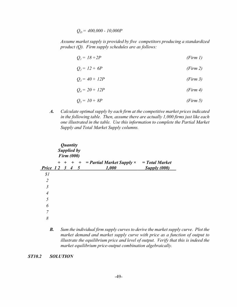
QD = 400,000 - 10,000P

Assume market supply is provided by five competitors producing a standardizedproduct (Q). Firm supply schedules are as follows:

Q1 = 18 +2P (Firm 1)

Q2 = 12 + 6P (Firm 2)

Q3 = 40 + 12P (Firm 3)

Q4 = 20 + 12P (Firm 4)

Q5 = 10 + 8P (Firm 5)

A. Calculate optimal supply by each firm at the competitive market prices indicatedin the following table. Then, assume there are actually 1,000 firms just like eachone illustrated in the table. Use this information to complete the Partial MarketSupply and Total Market Supply columns.

QuantitySupplied byFirm (000)

Price 1+2

+3

+4

+5

= Partial Market Supply ×1,000

= Total Market Supply (000)

$12345678

B. Sum the individual firm supply curves to derive the market supply curve. Plot themarket demand and market supply curve with price as a function of output toillustrate the equilibrium price and level of output. Verify that this is indeed themarket equilibrium price-output combination algebraically.

ST10.2 SOLUTION

-50-

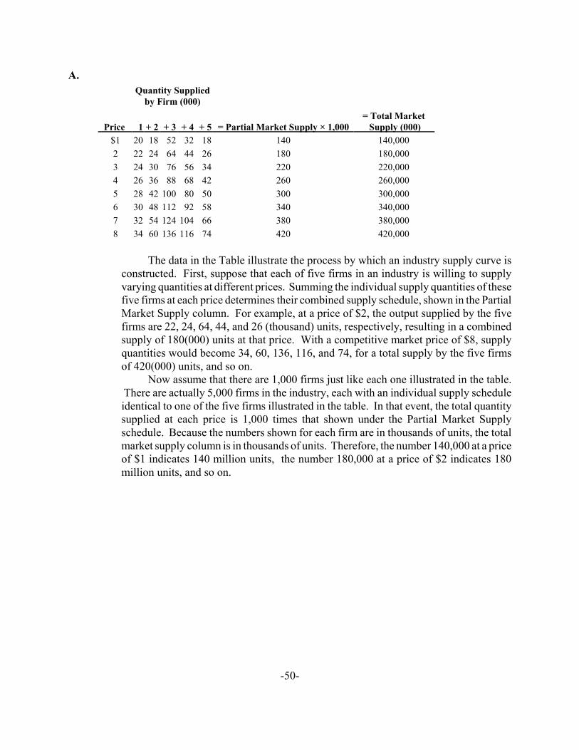
A.Quantity Supplied

by Firm (000)

Price 1 + 2 + 3 + 4 + 5 = Partial Market Supply × 1,000= Total Market Supply (000)

$1 20 18 52 32 18 140 140,0002 22 24 64 44 26 180 180,0003 24 30 76 56 34 220 220,0004 26 36 88 68 42 260 260,0005 28 42 100 80 50 300 300,0006 30 48 112 92 58 340 340,0007 32 54 124 104 66 380 380,0008 34 60 136 116 74 420 420,000

The data in the Table illustrate the process by which an industry supply curve isconstructed. First, suppose that each of five firms in an industry is willing to supplyvarying quantities at different prices. Summing the individual supply quantities of thesefive firms at each price determines their combined supply schedule, shown in the PartialMarket Supply column. For example, at a price of $2, the output supplied by the fivefirms are 22, 24, 64, 44, and 26 (thousand) units, respectively, resulting in a combinedsupply of 180(000) units at that price. With a competitive market price of $8, supplyquantities would become 34, 60, 136, 116, and 74, for a total supply by the five firmsof 420(000) units, and so on.

Now assume that there are 1,000 firms just like each one illustrated in the table. There are actually 5,000 firms in the industry, each with an individual supply scheduleidentical to one of the five firms illustrated in the table. In that event, the total quantitysupplied at each price is 1,000 times that shown under the Partial Market Supplyschedule. Because the numbers shown for each firm are in thousands of units, the totalmarket supply column is in thousands of units. Therefore, the number 140,000 at a priceof $1 indicates 140 million units, the number 180,000 at a price of $2 indicates 180million units, and so on.

-51-

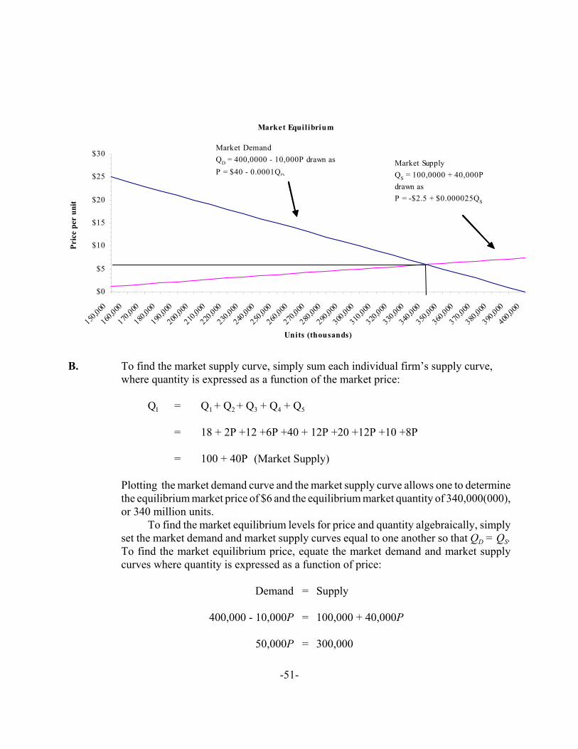
Market Equilibrium

$0

$5

$10

$15

$20

$25

$30

150,000

160,000

170,000

180,000

190,000

200,000

210,000

220,000

230,000

240,000

250,000

260,000

270,000

280,000

290,000

300,000

310,000

320,000

330,000

340,000

350,000

360,000

370,000

380,000

390,000

400,000

Units (thousands)

Pric

e pe

r un

it

Market DemandQD = 400,0000 - 10,000P drawn asP = $40 - 0.0001QD

Market SupplyQS = 100,0000 + 40,000P drawn asP = -$2.5 + $0.000025QS

B. To find the market supply curve, simply sum each individual firm’s supply curve,where quantity is expressed as a function of the market price:

QI = Q1 + Q2 + Q3 + Q4 + Q5

= 18 + 2P +12 +6P +40 + 12P +20 +12P +10 +8P

= 100 + 40P (Market Supply)

Plotting the market demand curve and the market supply curve allows one to determinethe equilibrium market price of $6 and the equilibrium market quantity of 340,000(000),or 340 million units.

To find the market equilibrium levels for price and quantity algebraically, simplyset the market demand and market supply curves equal to one another so that QD = QS.To find the market equilibrium price, equate the market demand and market supplycurves where quantity is expressed as a function of price:

Demand = Supply

400,000 - 10,000P = 100,000 + 40,000P

50,000P = 300,000

-52-

P = $6

To find the market equilibrium quantity, set equal the market demand and marketsupply curves where price is expressed as a function of quantity, and QD = QS:

Demand = Supply

$40 - $0.0001Q = -$2.5 + $0.000025Q

0.000125Q = 42.5

Q = 340,000(000)

Therefore, the equilibrium price-output combination is a market price of $6 with anequilibrium output of 340,000(000), or 340 million units.

-53-

Chapter 11

Performance and Strategy in Competitive Markets


ST11.1 Social Welfare. A number of domestic and foreign manufacturers produce replacementparts and components for personal computer systems. With exacting user specifications,products are standardized and price competition is brutal. To illustrate the net amountof social welfare generated in this hotly competitive market, assume that market supplyand demand conditions for replacement tower cases can be described as:

QS = -175+ 12.5P (Market Supply)

QD = 125 - 2.5P (Market Demand)

where Q is output in thousands of units and P is price per unit.

A. Graph and calculate the equilibrium price/output solution.

B. Use this graph to help you algebraically determine the amount of consumersurplus, producer surplus and net social welfare generated in this market.

ST11.1 SOLUTION

A. The market supply curve is given by the equation

QS = -175 + 12.5P

or, solving for price,

12.5P = 175 + QS

P = $14 + $0.08QS

The market demand curve is given by the equation

QD = 125 - 2.5P


-54-

2.5P = 125 - QD

P = $50 - $0.4QD

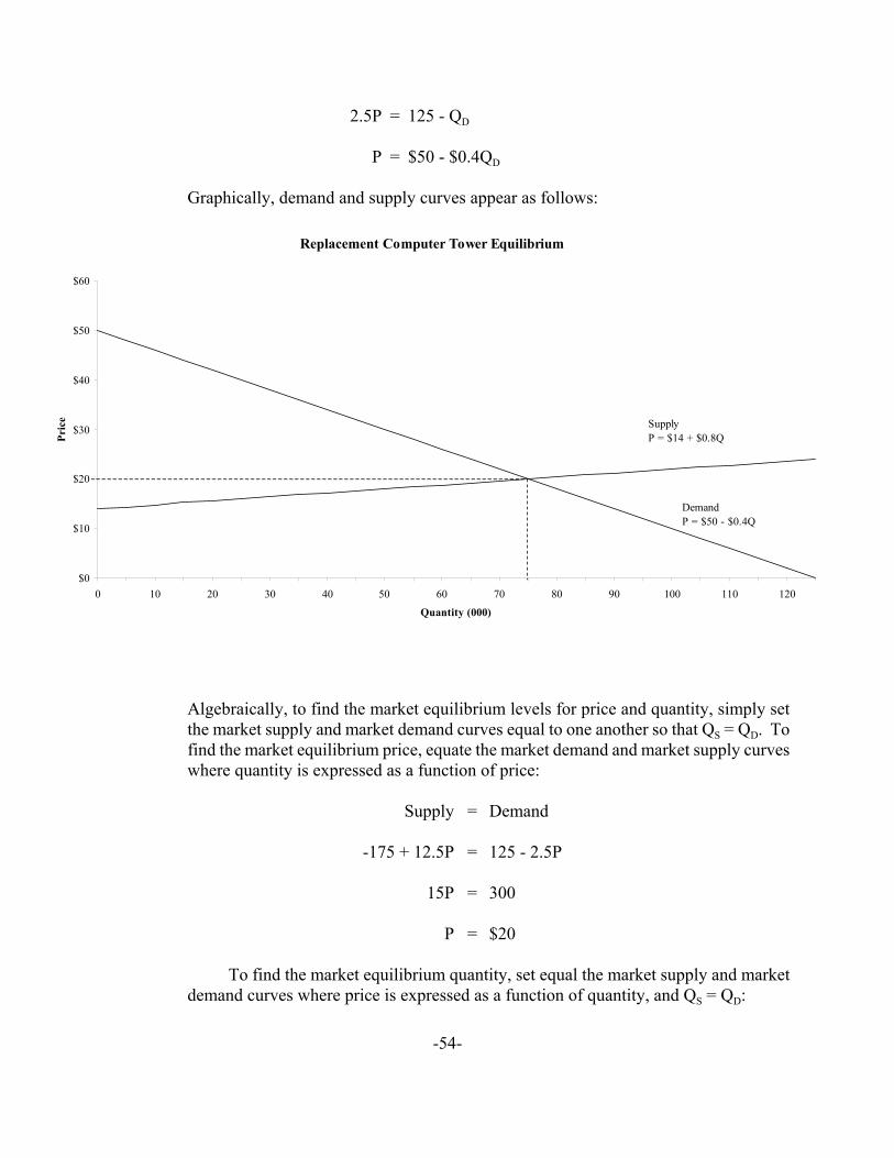
Graphically, demand and supply curves appear as follows:

Algebraically, to find the market equilibrium levels for price and quantity, simply setthe market supply and market demand curves equal to one another so that QS = QD. Tofind the market equilibrium price, equate the market demand and market supply curveswhere quantity is expressed as a function of price:

Supply = Demand

-175 + 12.5P = 125 - 2.5P

15P = 300

P = $20

To find the market equilibrium quantity, set equal the market supply and marketdemand curves where price is expressed as a function of quantity, and QS = QD:

Replacement Computer Tower Equilibrium

$0

$10

$20

$30

$40

$50

$60

0 10 20 30 40 50 60 70 80 90 100 110 120

Quantity (000)

Pric

e SupplyP = $14 + $0.8Q

DemandP = $50 - $0.4Q

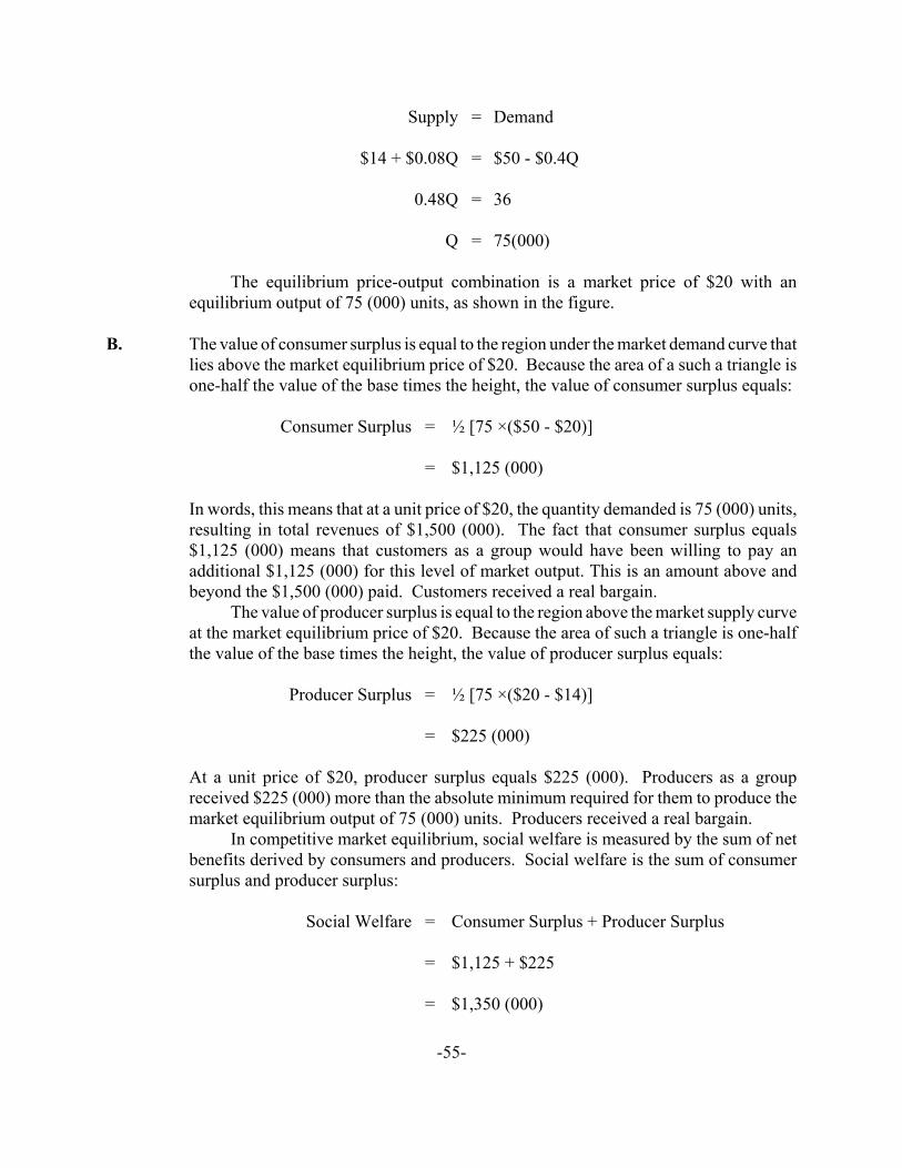
-55-

Supply = Demand

$14 + $0.08Q = $50 - $0.4Q

0.48Q = 36

Q = 75(000)

The equilibrium price-output combination is a market price of $20 with anequilibrium output of 75 (000) units, as shown in the figure.

B. The value of consumer surplus is equal to the region under the market demand curve thatlies above the market equilibrium price of $20. Because the area of a such a triangle isone-half the value of the base times the height, the value of consumer surplus equals:

Consumer Surplus = ½ [75 ×($50 - $20)]

= $1,125 (000)

In words, this means that at a unit price of $20, the quantity demanded is 75 (000) units,resulting in total revenues of $1,500 (000). The fact that consumer surplus equals$1,125 (000) means that customers as a group would have been willing to pay anadditional $1,125 (000) for this level of market output. This is an amount above andbeyond the $1,500 (000) paid. Customers received a real bargain.

The value of producer surplus is equal to the region above the market supply curveat the market equilibrium price of $20. Because the area of such a triangle is one-halfthe value of the base times the height, the value of producer surplus equals:

Producer Surplus = ½ [75 ×($20 - $14)]

= $225 (000)

At a unit price of $20, producer surplus equals $225 (000). Producers as a groupreceived $225 (000) more than the absolute minimum required for them to produce themarket equilibrium output of 75 (000) units. Producers received a real bargain.

In competitive market equilibrium, social welfare is measured by the sum of netbenefits derived by consumers and producers. Social welfare is the sum of consumersurplus and producer surplus:

Social Welfare = Consumer Surplus + Producer Surplus

= $1,125 + $225

= $1,350 (000)

-56-

ST11.2 Price Ceilings. The local government in a West Coast college town is concerned abouta recent explosion in apartment rental rates for students and other low-income renters.To combat the problem, a proposal has been made to institute rent control that wouldplace a $900 per month ceiling on apartment rental rates. Apartment supply anddemand conditions in the local market are:

QS = -400+ 2P (Market Supply)

QD = 5,600 - 4P (Market Demand)

where Q is the number of apartments and P is monthly rent.

A. Graph and calculate the equilibrium price/output solution. How muchconsumer surplus, producer surplus, and social welfare is produced at thisactivity level?

B. Use the graph to help you algebraically determine the quantity demanded,quantity supplied, and shortage with a $900 per month ceiling on apartmentrental rates.

C. Use the graph to help you algebraically determine the amount of consumerand producer surplus with rent control.

D. Use the graph to help you algebraically determine the change in socialwelfare and deadweight loss in consumer surplus due to rent control.

ST11.2 SOLUTION

A. The competitive market supply curve is given by the equation

QS = -400 + 2P


2P = 400 + QS

P = $200 + $0.5QS

The competitive market demand curve is given by the equation

QD = 5,600 - 4P


-57-

4P = 5,600 - QD

P = $1,400 - $0.25QD

To find the competitive market equilibrium price, equate the market demand andmarket supply curves where quantity is expressed as a function of price:

Supply = Demand

-400 + 2P = 5,600 - 4P

6P = 6,000

P = $1,000

To find the competitive market equilibrium quantity, set equal the market supplyand market demand curves where price is expressed as a function of quantity, and QS =QD:

Supply = Demand

$200 + $0.5Q = $1,400 - $0.25Q

0.75Q = 1,200

Q = 1,600

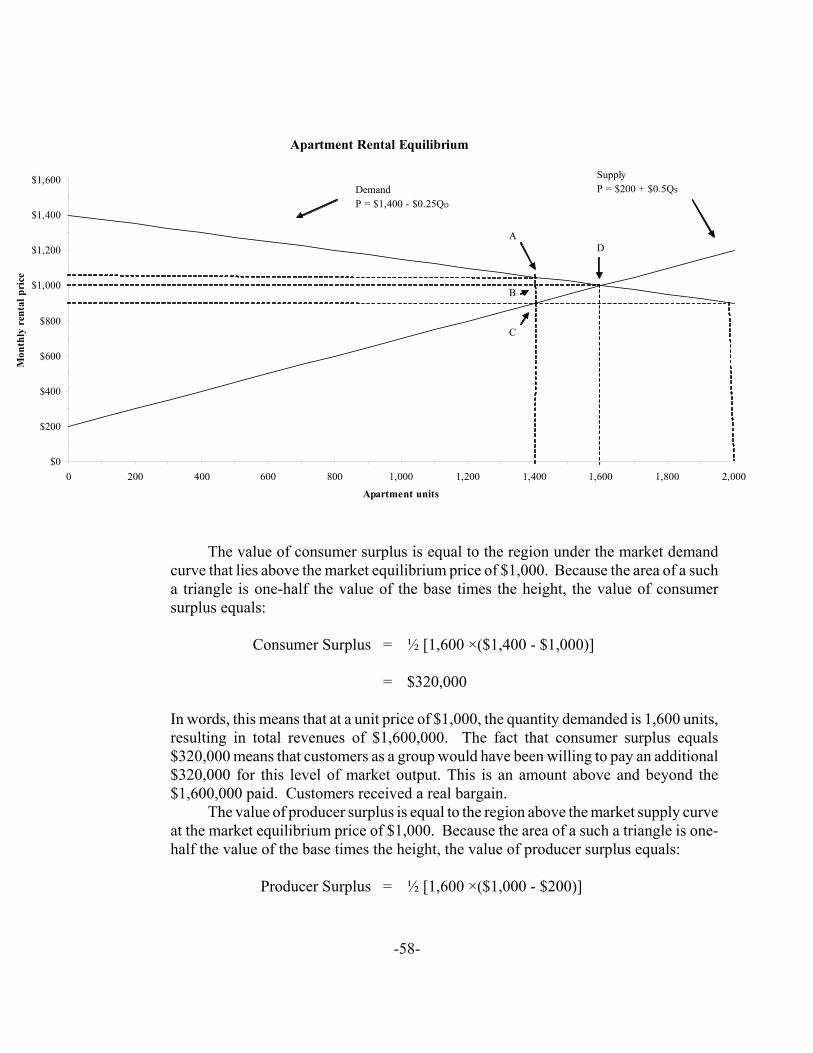
Therefore, the competitive market equilibrium price-output combination is amarket price of $1,000 with an equilibrium output of 1,600 units.

-58-

Apartment Rental Equilibrium

$0

$200

$400

$600

$800

$1,000

$1,200

$1,400

$1,600

0 200 400 600 800 1,000 1,200 1,400 1,600 1,800 2,000

Apartment units

Mon

thly

ren

tal p

rice

DemandP = $1,400 - $0.25QD

SupplyP = $200 + $0.5QS

A

B

C

D

The value of consumer surplus is equal to the region under the market demandcurve that lies above the market equilibrium price of $1,000. Because the area of a sucha triangle is one-half the value of the base times the height, the value of consumersurplus equals:

Consumer Surplus = ½ [1,600 ×($1,400 - $1,000)]

= $320,000

In words, this means that at a unit price of $1,000, the quantity demanded is 1,600 units,resulting in total revenues of $1,600,000. The fact that consumer surplus equals$320,000 means that customers as a group would have been willing to pay an additional$320,000 for this level of market output. This is an amount above and beyond the$1,600,000 paid. Customers received a real bargain.

The value of producer surplus is equal to the region above the market supply curveat the market equilibrium price of $1,000. Because the area of a such a triangle is one-half the value of the base times the height, the value of producer surplus equals:

Producer Surplus = ½ [1,600 ×($1,000 - $200)]

-59-

= $640,000

At a rental price of $1,000 per month, producer surplus equals $640,000. Producers asa group received $640,000 more than the absolute minimum required for them toproduce the market equilibrium output of 1,600 units. Producers received a real bargain.



= $320,000 + $640,000

= $960,000

B. The market demand at the $900 price ceiling is

QD = 5,600 - 4(900)

= 2,000 units

The market supply at the $900 price ceiling is

QS = -400 + 2(900)

= 1,400 units

The market shortage created by the $900 price ceiling is

Shortage = QD - QS

= 2,000 - 1,400

=600 units

C. Under rent control, the maximum amount of apartment supply that landlords are willingto offer at a rent of $900 per month is 1,400 units. From the market demand curve, itis clear that renters as a group are willing to pay as much as (or have a reservation priceof) $1,050 per month to rent 1,400 apartments:

P = $1,400 - $0.25(1,400)

= $1,050

-60-

Under rent control, the value of consumer surplus has two components. A firstcomponent of consumer surplus is equal to the region under the market demand curvethat lies above the price of $1,050 per month. This amount corresponds touncompensated value obtained by renters willing to pay above the market price all theway up to $1,400 per month. As in the case of an uncontrolled market, the area of sucha triangle is one-half the value of the base times the height. A second component ofconsumer surplus under rent control is the uncompensated value obtained by renterswilling to pay as much as $1,050 per month to rent 1,400 apartments, and who aredelighted to rent for the controlled price of $900 per month. This amount correspondsto the amount of revenue represented by the rectangle defined by the prices of $1,050and $900 and the quantity of 1,400 units. Notice that this second component ofconsumer surplus includes some value privately measured as producer surplus. Underrent control, the total amount of consumer surplus is:

Rent-Controlled Consumer Surplus = ½ [1,400 ×($1,400 - $1,050)]

+ [1,400 ×($1,050 - $900)]

= $245,000 + $210,000

= $455,000

In this case, consumer surplus rises from $320,000 to $455,000, a gain of $135,000 asa result of rent control.

The value of producer surplus is equal to the region above the market supply curveat the rent-controlled price of $900. Because the area of such a triangle is one-half thevalue of the base times the height, the value of producer surplus equals:

Producer Surplus = ½ [1,400 ×($900 - $200)]

= $490,000

At a rent-controlled price of $900 per month, producer surplus falls from $640,000 to$490,000, a loss of $150,000.

D. The change in social welfare caused by rent control is measured by the change in netbenefits derived by consumers and producers. The change in social welfare is thechange in the sum of consumer surplus and producer surplus:

Social Welfare Change = Consumer Surplus Change

+ Producer Surplus Change

= $135,000 - $150,000

-61-

= -$15,000 (a loss)

This $15,000 deadweight loss in social welfare due to rent control has twocomponents. First, there is a deadweight loss of consumer surplus from consumersunable to find a rent-controlled apartment but willing to pay upwards from the priormarket equilibrium price of $1,000 per month up to $1,050 per month. This amount isequal to the area shown in the graph as ABD. Because the area of such a triangle isone-half the value of the base times the height, the first component of deadweight lossin consumer surplus equals:

Deadweight Loss in Consumer Surplus = ½ [(1,600 -1,400) ×($1,050 - $1,000)]

= $5,000

Second, there is a deadweight loss of producer surplus from landlords forced to rent atthe rent-controlled price of $900 per month rather than the market equilibrium price of$1,000 per month. This amount is equal to the area shown in the graph as BCD.Because the area of such a triangle is one-half the value of the base times the height, thesecond component of deadweight loss in consumer surplus equals:

Deadweight Loss in Producer Surplus = ½ [(1,600 -1,400) ×($1,000 - $900)]

= $10,000

-62-

Chapter 12

Monopoly and Monopsony


ST12.1 Capture Problem. It remains a widely held belief that regulation is in the public interestand influences firm behavior toward socially desirable ends. However, in the early1970s, Nobel laureate George Stigler and his colleague Sam Peltzman at the Universityof Chicago introduced an alternative capture theory of economic regulation. Accordingto Stigler and Peltzman, the machinery and power of the state are a potential resourceto every industry. With its power to prohibit or compel, to take or give money, the statecan and does selectively help or hurt a vast number of industries. Because of this,regulation may be actively sought by industry. They contended that regulation istypically acquired by industry and is designed and operated primarily for industry'sbenefit.

Types of state favors commonly sought by regulated industries include directmoney subsidies, control over entry by new rivals, control over substitutes andcomplements, and price fixing. Domestic "air mail" subsidies, Federal DepositInsurance Corporation (FDIC) regulation that reduces the rate of entry into commercialbanking, suppression of margarine sales by butter producers, price fixing in motorcarrier (trucking) regulation, and American Medical Association control of medicaltraining and licensing can be interpreted as historical examples of control by regulatedindustries.

In summarizing their views on regulation, Stigler and Peltzman suggest thatregulators should be criticized for pro-industry policies no more than politicians forseeking popular support. Current methods of enacting and carrying out regulations onlymake the pro-industry stance of regulatory bodies more likely. The only way to getdifferent results from regulation is to change the political process of regulator selectionand to provide economic rewards to regulators who serve the public interest effectively.

Capture theory is in stark contrast to more traditional public interest theory, whichsees regulation as a government-imposed means of private-market control. Rather thanviewing regulation as a "good" to be obtained, controlled, and manipulated, publicinterest theory views regulation as a method for improving economic performance bylimiting the harmful effects of market failure. Public interest theory is silent on the needto provide regulators with economic incentives to improve regulatory performance.Unlike capture theory, a traditional view has been that the public can trust regulators tomake a good-faith effort to establish regulatory policy in the public interest.

A. The aim of antitrust and regulatory policy is to protect competition, not to protectcompetitors. Explain the difference.

-63-

B. Starting in the 1970s, growing dissatisfaction with traditional approaches togovernment regulation led to a global deregulation movement that spurredcompetition, lowered prices, and resulted in more efficient production. Explainhow this experience is consistent with the capture theory of regulation.

C. Discuss how regulatory efficiency could be improved by focusing on outputobjectives like low prices for cable or telephone services rather than productionmethods or rates of return.

ST12.1 SOLUTION

A. Entry and exit are common facts of life in competitive markets. Firms that efficientlyproduce goods and services that consumers crave are able to boost market share andenjoy growing revenues and profits. Firms that fail to measure up in the eyes ofconsumers will lose market share and suffer declining revenues and profits. Thedisciplining role of competitive markets can be swift and harsh, even for the largest andmost formidable corporations. For example, in August, 2000, Enron Corp. traded in thestock market at an all-time high and was ranked among the 10 most valuablecorporations in America. Nevertheless, Enron filed for bankruptcy just 16 months lateras evidence emerged of a failed diversification strategy, misguided energy trading, andfinancial corruption. Similarly, once powerful telecom giant WorldCom quicklystumbled into bankruptcy as evidence came to light concerning the company’s abuse ofaccounting rules and regulations. In both cases, once powerful corporations werebrought to their knees by competitive capital and product markets that simply refusedto tolerate inefficiency and corporate malfeasance.

In evaluating the effects of deregulation, and in gauging the competitiveimplications of market exit by previously regulated firms, it is important to rememberthat protecting competition is not the same as protecting competitors. Withoutregulation, it is inevitable that some competitors will fall by the wayside and thatconcentration will rise in some previously regulated markets. Although such trendsmust be watched closely for anti-competitive effects, they are characteristics of avigorously competitive environment. Bankruptcy and exit are the regrettable costs ofremedying economic dislocation in competitive markets. Though such costs areregrettable, experience shows that they are much less onerous than the costs ofindefinitely maintaining inefficient production methods in a tightly regulatedenvironment.

B. Although it is difficult to pinpoint a single catalyst for the deregulation movement, it ishard to overlook the role played by George Stigler, Sam Peltzman, Alfred E. Kahn, andother economists who documented how government regulation can sometimes harmconsumer interests. A study by the Brookings Institution documented important benefitsof deregulation in five major industries--natural gas, telecommunications, airlines,trucking, and railroads. It was found that prices fell 4-15% within the first two yearsafter deregulation; within 10 years, prices were 25-50% lower. Deregulation also leads

-64-

to service quality improvements. Crucial social goals like airline safety, reliability ofgas service, and reliability of the telecommunications network were maintained orimproved by deregulation. Regulatory reform also tends to confer benefits on mostconsumers. Although it is possible to find narrowly defined groups of customers inspecial circumstances who paid somewhat higher prices after deregulation, the gains tothe vast majority of consumers far outweighed negative effects on small groups. Finally,deregulation offers benefits in the sense of permitting greater customer choice.

Although many industries have felt the effects of changing state and localregulation, changing federal regulation has been most pronounced in the financial,telecommunications, and transportation sectors. Since 1975, for example, it has beenillegal for securities dealers to fix commission rates. This broke a 182-year traditionunder which the New York Stock Exchange (NYSE) set minimum rates for each 100-share ("round lot") purchase. Until 1975, everyone charged the minimum rate approvedby the NYSE. Purchase of 1,000 shares cost a commission of ten times the minimum,even though the overhead and work involved are roughly the same for small and largestock transactions. Following deregulation, commission rates tumbled, and, predictably,some of the least efficient brokerage firms merged or otherwise went out of business.Today, commission rates have fallen by 90% or more, and the industry is noteworthyfor increasing productivity and innovative new product introductions. It is also worthmentioning that since brokerage rates were deregulated, the number of sales offices inthe industry, trading volume, employment, and profits have skyrocketed. This has leadsome observers to conclude that deregulation can benefit consumers without causing anylasting damage to industry. In fact, a leaner, more efficient industry may be one of thegreatest benefits of deregulation.

In Canada, the deregulation movement led to privatization of government-ownedAir Canada. Trucking, historically a regulated industry, also was deregulated.Specialized telecommunications services industries were deregulated and thrown opento competition. In other areas where the government considered continued regulationdesirable and necessary, regulatory agencies were pressured to reform and improve theregulatory decision-making process to reduce inefficiencies, bureaucratic delays, andadministrative red tape.

C. A significant problem with regulation is that regulators seldom have the information orexpertise to specify, for example, the correct level of utility investment, minimumtransportation costs, or the optimum method of pollution control. Because technologychanges rapidly in most regulated industries, only industry personnel working at thefrontier of current technology have such specialized knowledge. One method fordealing with this technical expertise problem is to have regulators focus on the preferredoutcomes of regulatory processes, rather than on the technical means that industryadopts to achieve those ends. The FCC's decision to adopt downward-adjusting pricecaps for long-distance telephone service is an example of this developing trend towardincentive-based regulation. If providers of long-distance telephone service are able toreduce costs faster than the FCC-mandated decline in prices, they will enjoy an increasein profitability. By setting price caps that fall over time, the FCC ensures that

-65-

consumers share in expected cost savings while companies enjoy a positive incentiveto innovate. This approach to regulation focuses on the objectives of regulation whileallowing industry to meet those goals in new and unique ways. Tying regulator rewardsand regulated industry profits to objective, output-oriented performance criteria has thepotential to create a desirable win/win situation for regulators, utilities, and the generalpublic. For example, the public has a real interest in safe, reliable, and low-cost electricpower. State and federal regulators who oversee the operations of utilities could developobjective standards for measuring utility safety, reliability, and cost efficiency. Tyingfirm profit rates to such performance-oriented criteria could stimulate real improvementsin utility and regulator performance.

Although some think that there is simply a question of regulation versusderegulation, this is seldom the case. On grounds of economic and political feasibility,it is often most fruitful to consider approaches to improving existing methods ofregulation. Competitive forces provide a persistent and socially desirable constraininginfluence on firm behavior. When vigorous competition is absent, governmentregulation can be justified through both efficiency and equity criteria. When regulationis warranted, business, government, and the public must work together to ensure thatregulatory processes represent the public interest. The unnecessary costs of antiquatedregulations dictate that regulatory reform is likely to remain a significant social concern.

ST12.2 Deadweight Loss From Monopoly. The Las Vegas Valley Water District (LVVWD) isa not-for-profit agency that began providing water to the Las Vegas Valley in 1954. TheDistrict helped build the city's water delivery system and now provides water to morethan one million people in Southern Nevada. District water rates are regulated by lawand can cover only the costs of water delivery, maintenance, and facilities. Districtwater rates are based on a four-tier system to encourage conservation. The first tierrepresents indoor usage for most residential customers. Rate for remaining tiersbecomes increasingly higher with the amount of water usage.

To document the deadweight loss from monopoly problem, allow the monthlymarket supply and demand conditions for water in the Las Vegas Water District to be:

QS = 10P (Market Supply)

QD = 120 - 40P (Market Demand)

where Q is water and P is the market price of water. Water is sold in units of onethousand gallons, so a $2 price implies a user cost of 0 .2 cents per gallon. Waterdemand and supply relations are expressed in terms of millions of units.

A. Graph and calculate the equilibrium price/output solution. How much consumersurplus, producer surplus, and social welfare is produced at this activity level?

B. Use the graph to help you calculate the quantity demanded and quantity suppliedif the market is run by a profit-maximizing monopolist. (Note: If monopoly market

-66-

demand is P = $3 - $0.025Q, then the monopolist’s MR = $3 - $0.05Q)

C. Use the graph to help you determine the deadweight loss for consumers and theproducer if LVVWD is run as an unregulated profit-maximizing monopoly.

D. Use the graph to help you ascertain the amount of consumer surplus transferredto producers following a change from a competitive market to a monopoly market.How much is the net gain in producer surplus?

ST12.2 SOLUTION

A. The market supply curve is given by the equation

QS = 10P


P = 0.1QS

The market demand curve is given by the equation

QD = 120 - 40P


40P = 120 - QD

P = $3 - $0.025QD

To find the competitive market equilibrium price, equate the market demand andmarket supply curves where quantity is expressed as a function of price:

Supply = Demand

10P = 120 - 40P

50P = 120

P = $2.40

To find the competitive market equilibrium quantity, set equal the market supplyand market demand curves where price is expressed as a function of quantity, and QS =QD:

-67-

Supply = Demand

$0.1Q = $3 - $0.025Q

0.125Q = 3

Q = 24 (million) units per month

Therefore, the competitive market equilibrium price-output combination is amarket price of $2.40 with an equilibrium output of 24 (million) units.

The value of consumer surplus is equal to the region under the market demandcurve that lies above the market equilibrium price of $2.40. Because the area of sucha triangle is one-half the value of the base times the height, the value of consumersurplus equals:

Consumer Surplus = ½ [24 ×($3 - $2.40)]

= $7.2 (million) per month

In words, this means that at a unit price of $2.40, the quantity demanded is 24 (million),resulting in total revenues of $57.6 (million). The fact that consumer surplus equals$7.2 (million) means that customers as a group would have been willing to pay anadditional $7.2 (million) for this level of market output. This is an amount above andbeyond the $57.6 (million) paid. Customers received a real bargain.

The value of producer surplus is equal to the region above the market supply curveat the market equilibrium price of $2.40. Because the area of such a triangle is one-halfthe value of the base times the height, the value of producer surplus equals:

Producer Surplus = ½ [24 ×($2.40 - $0)]


At a water price of $2.40 per thousand gallons, producer surplus equals $28.8 (million).Producers as a group received $28.8 (million) more than the absolute minimum requiredfor them to produce the market equilibrium output of 24 (million) units of output.Producers received a real bargain.



= $7.2 (million) + $28.8 (million)

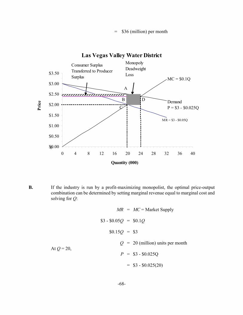
-68-

Las Vegas Valley Water District

$0.00

$0.50

$1.00

$1.50

$2.00

$2.50

$3.00

$3.50

0 4 8 12 16 20 24 28 32 36 40

Quantity (000)

Pric

e

MC = $0.1Q

DemandP = $3 - $0.025Q

D

C

B

A

MonopolyDeadweightLoss

MR = $3 - $0.05Q

0

Consumer Surplus Transferred to Producer Surplus

= $36 (million) per month

B. If the industry is run by a profit-maximizing monopolist, the optimal price-outputcombination can be determined by setting marginal revenue equal to marginal cost andsolving for Q:

MR = MC = Market Supply

$3 - $0.05Q = $0.1Q

$0.15Q = $3

Q = 20 (million) units per monthAt Q = 20,

P = $3 - $0.025Q

= $3 - $0.025(20)

-69-

= $2.50 per unit

C. Under monopoly, the amount supplied falls to 20 (million) units and the market pricejumps to $2.50 per thousand gallons of water. The amount of deadweight loss frommonopoly suffered by consumers is given by the triangle bounded by ABD in the figure.Because the area of such a triangle is one-half the value of the base times the height, thevalue of lost consumer surplus due to monopoly equals:

Consumer Deadweight Loss = ½ [(24 - 20) × ($2.50 - $2.40)]


The amount of deadweight loss from monopoly suffered by producers is given by thetriangle bounded by BCD. Because the area of a such a triangle is one-half the value ofthe base times the height, the value of lost producer surplus equals:

Producer Deadweight Loss = ½ [(24 - 20) × ($2.40 - $2)]


The total amount of deadweight loss from monopoly suffered by consumers andproducers is given by the triangle bounded by ACD. The area of a such a triangle issimply the amount of consumer deadweight loss plus producer deadweight loss:

Total Deadweight Loss = Consumer Loss + Producer Loss

= $0.2 (million) + $0.8 (million)


D. In addition to the deadweight loss from monopoly problem, there is a wealth transferproblem associated with monopoly. The creation of a monopoly results in a significanttransfer from consumer surplus to producer surplus. In the figure, this amount is shownas the area in the rectangle bordered by PCMPMAB:

Transfer to Producer Surplus = 20 × ($2.50 - $2.40)


Therefore, from the viewpoint of the producer, the change to monopoly results in a veryfavorable net increase in producer surplus:

Net Change in Producer Surplus = Producer Deadweight Loss + Transfer

-70-

= -$0.8 (million) + $2 (million)

= $1. 2 (million) per month

From the viewpoint of consumers, the problem with monopoly is twofold.Monopoly result in both a significant deadweight loss in consumer surplus ($0.2 millionper month), and monopoly causes a significant transfer of consumer surplus to producersurplus ($2 million per month). In this example, the cost of monopoly to consumers ismeasured by a total loss in consumer surplus of $2.2 million per month. The wealthtransfer problem associated with monopoly is seen as an issue of equity or fairnessbecause it involves the distribution of income or wealth in the economy. Althougheconomic profits serve the useful functions of providing incentives and helping allocateresources, it is difficult to justify monopoly profits that result from the raw exercise ofmarket power rather than from exceptional performance.

-71-

Chapter 13

Monopolistic Competition and Oligopoly


ST13.1 Price Leadership. Over the last century, The Boeing Co. has grown from buildingplanes in an old, red boathouse to become the largest aerospace company in the world.Boeing’s principal global competitor is Airbus, a French company jointly owned byEads (80%) and BAE Systems (20%). Airbus was established in 1970 as a Europeanconsortium of French, German and later, Spanish and U.K companies. In 2001, thirtyyears after its creation, Airbus became a single integrated company. Though dominatedby Boeing and Airbus, smaller firms have recently entered the commercial aircraftindustry. Notable among these is Embraer, a Brazilian aircraft manufacturer. Embraerhas become one of the largest aircraft manufacturers in the world by focusing onspecific market segments with high growth potential. As a niche manufacturer, Embraermakes aircraft that offer excellent reliability and cost effectiveness.

To illustrate the price leadership concept, assume that total and marginal costfunctions for Airbus (A) and Embraer (E) aircraft are as follows:

TCA = $10,000,000 + $35,000,000QA + $250,000QA2

MCA = $35,000,000 + $500,000QA

TCE = $200,000,000 + $20,000,000QE + $500,000QE2

MCE = $20,000,000 + $1,000,000QE

Boeing’s total and marginal cost relations are as follows:

TCB = $4,000,000,000 + $5,000,000QB + $62,500Q2B

MCB = MTCB/MQB = $5,000,000 + $125,000QB

The industry demand curve for this type of jet aircraft is

Q = 910 - 0.000017P

Assume throughout this problem that the Airbus and Embraer aircraft are perfectsubstitutes for Boeing’s Model 737-600, and that each total cost function includes arisk-adjusted normal rate of return on investment.

-72-

A. Determine the supply curves for Airbus and Embraer aircraft, assuming that thefirms operate as price takers.

B. What is the demand curve faced by Boeing?

C. Calculate Boeing’s profit-maximizing price and output levels. (Hint: Boeing’stotal and marginal revenue relations are TRB = $50,000,000QB - $50,000Q2

B, andMRB =MTRB/MQB = $50,000,000 - $100,000QB.)

D. Calculate profit-maximizing output levels for the Airbus and Embraer aircraft.

E. Is the market for aircraft from these three firms in short-run and in long-runequilibrium?

ST13.1 SOLUTION

A. Because price followers take prices as given, they operate where individual marginalcost equals price. Therefore, the supply curves for Airbus and Embraer aircraft are:

Airbus

PA = MCA = $35,000,000 + $500,000QA

500,000QA = -35,000,000 + PA

QA = -70 + 0.000002PA

Embraer

PE = MCE = $20,000,000 + $1,000,000QE

1,000,000QE = -20,000,000 + PE

QE = -20 + 0.000001PE

B. As the industry price leader, Boeing’s demand equals industry demand minus followingfirm supply. Remember that P = PB = PM = PE because Boeing is a price leader for theindustry:

QB = Q - QA - QE

= 910 - 0.000017P + 70 - $0.000002P

+ 20 - $0.000001P

-73-

= 1,000 - 0.00002PB

PB = $50,000,000 - $50,000QB

C. To find Boeing’s profit maximizing price and output level, set MRB = MCB and solvefor Q:

MRB = MCB

$50,000,000 - $100,000QB = $5,000,000 + $125,000QB

45,000,000 = 225,000QB

QB = 200 units

PB = $50,000,000 - $50,000(200)

= $40,000,000

D. Because Boeing is a price leader for the industry,

P = PB = PA = PE = $40,000,000

Optimal supply for Airbus and Embraer aircraft are:

QA = -70 + 0.000002PA

= -70 + 0.000002(40,000,000)

= 10

QE = -20 + 0.000001PE

= -20 + 0.000001(40,000,000)

= 20

E. Yes. The industry is in short-run equilibrium if the total quantity demanded is equal tototal supply. The total industry demand at a price of $40 million is:

QD = 910 - 0.000017P

= 910 - 0.000017(40,000,000)

-74-

= 230 units

The total industry supply is:

QS = QB + QA + QE

= 200 + 10 + 20

= 230 units

Thus, the industry is in short-run equilibrium. The industry is also in long-runequilibrium provided that each manufacturer is making at least a risk-adjusted normalrate of return on investment. To check profit levels for each manufacturer, note that:

πA = TRA - TCA

= $40,000,000(10) -$10,000,000 -$35,000,000(10)

- $250,000(102)

= $15,000,000

πE = TRE - TCE

= $40,000,000(20) -$200,000,000 -$20,000,000(20)

- $500,000(202)

= $0

πB = TRB - TCB

= $40,000,000(200) -$4,000,000,000 - $5,000,000(200)

- $62,500(2002)

= $500,000,000

Boeing and Airbus are both earning economic profits, whereas Embraer, themarginal entrant, is earning just a risk-adjusted normal rate of return. As such, theindustry is in long-rum equilibrium and there is no incentive to change.

ST13.2 Monopolistically Competitive Equilibrium. Soft Lens, Inc., has enjoyed rapid growthin sales and high operating profits on its innovative extended-wear soft contact lenses.

-75-

However, the company faces potentially fierce competition from a host of newcompetitors as some important basic patents expire during the coming year. Unless thecompany is able to thwart such competition, severe downward pressure on prices andprofit margins is anticipated.

A. Use Soft Lens’s current price, output, and total cost data to complete the table:

Price

($)

Monthly

Output

(million)

Total

Revenue

($million)

Marginal

Revenue

($million)

Total

Cost

($million)

Marginal

Cost

($million)

Average

Cost

($million)

Total

Profit

($million)

$20 0 $0

19 1 12

18 2 27

17 3 42

16 4 58

15 5 75

14 6 84

13 7 92

12 8 96

11 9 99

10 10 105

(Note: Total costs include a risk-adjusted normal rate of return.)

B. If cost conditions remain constant, what is the monopolistically competitive high-price/low-output long-run equilibrium in this industry? What are industryprofits?

C. Under these same cost conditions, what is the monopolistically competitive low-price/high-output equilibrium in this industry? What are industry profits?

D. Now assume that Soft Lens is able to enter into restrictive licensing agreementswith potential competitors and create an effective cartel in the industry. Ifdemand and cost conditions remain constant, what is the cartel price/output andprofit equilibrium?

ST13.2 SOLUTION

A.

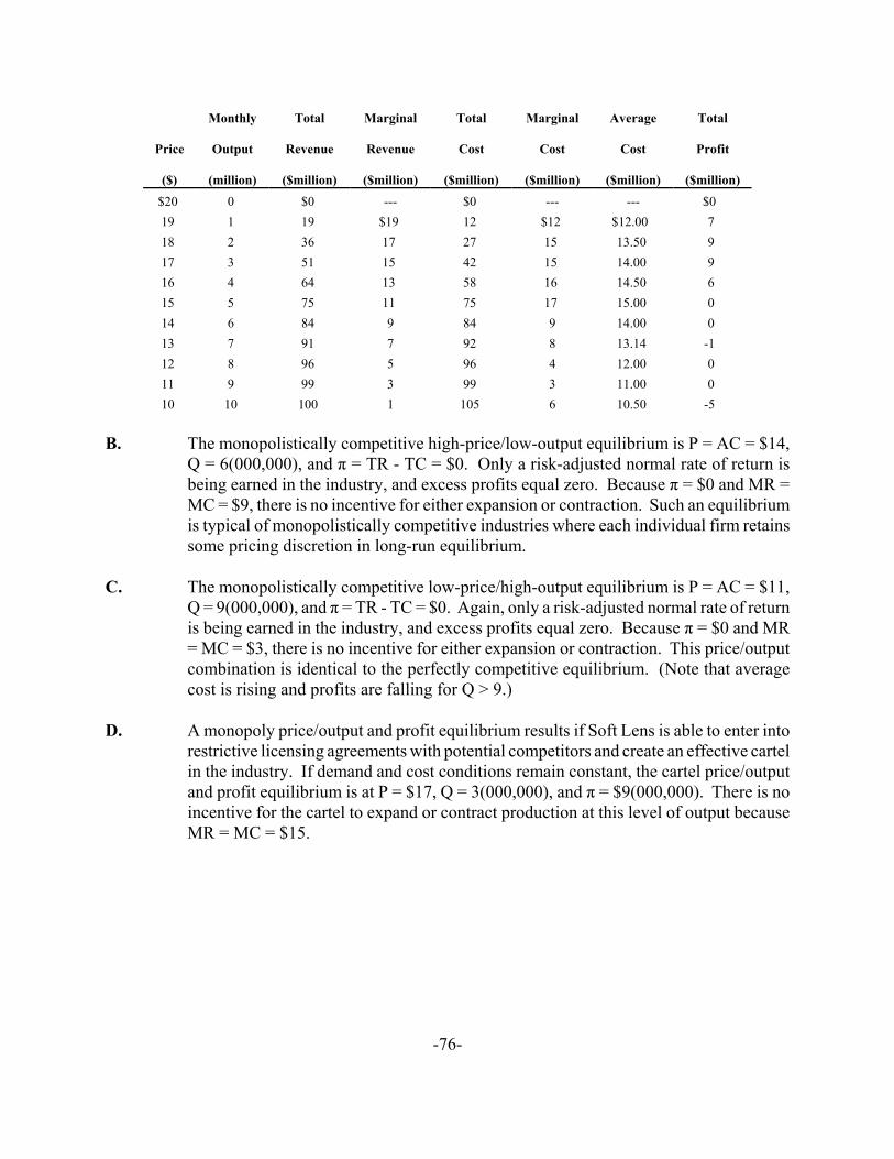
-76-

Price

($)

Monthly

Output

(million)

Total

Revenue

($million)

Marginal

Revenue

($million)

Total

Cost

($million)

Marginal

Cost

($million)

Average

Cost

($million)

Total

Profit

($million)$20 0 $0 --- $0 --- --- $0 19 1 19 $19 12 $12 $12.00 7 18 2 36 17 27 15 13.50 9 17 3 51 15 42 15 14.00 9 16 4 64 13 58 16 14.50 6 15 5 75 11 75 17 15.00 0 14 6 84 9 84 9 14.00 0 13 7 91 7 92 8 13.14 -1 12 8 96 5 96 4 12.00 0 11 9 99 3 99 3 11.00 0 10 10 100 1 105 6 10.50 -5

B. The monopolistically competitive high-price/low-output equilibrium is P = AC = $14,Q = 6(000,000), and π = TR - TC = $0. Only a risk-adjusted normal rate of return isbeing earned in the industry, and excess profits equal zero. Because π = $0 and MR =MC = $9, there is no incentive for either expansion or contraction. Such an equilibriumis typical of monopolistically competitive industries where each individual firm retainssome pricing discretion in long-run equilibrium.

C. The monopolistically competitive low-price/high-output equilibrium is P = AC = $11,Q = 9(000,000), and π = TR - TC = $0. Again, only a risk-adjusted normal rate of returnis being earned in the industry, and excess profits equal zero. Because π = $0 and MR= MC = $3, there is no incentive for either expansion or contraction. This price/outputcombination is identical to the perfectly competitive equilibrium. (Note that averagecost is rising and profits are falling for Q > 9.)

D. A monopoly price/output and profit equilibrium results if Soft Lens is able to enter intorestrictive licensing agreements with potential competitors and create an effective cartelin the industry. If demand and cost conditions remain constant, the cartel price/outputand profit equilibrium is at P = $17, Q = 3(000,000), and π = $9(000,000). There is noincentive for the cartel to expand or contract production at this level of output becauseMR = MC = $15.

-77-

Chapter 14

Game Theory and Competitive Strategy


ST14.1 Game Theory Strategies. Suppose two local suppliers are seeking to win the right toupgrade the communications capability of the internal “intranets” that link a numberof customers with their suppliers. The system quality decision facing each competitor,and potential profit payoffs, are illustrated in the table. The first number listed in eachcell is the profit earned by U.S. Equipment Supply; the second number indicates theprofit earned by Business Systems, Inc. For example, if both competitors, U.S.Equipment Supply and Business Systems, Inc., pursue a high-quality strategy, U.S.Equipment Supply will earn $25,000 and Business Systems, Inc., will earn $50,000. IfU.S. Equipment Supply pursues a high-quality strategy while Business Systems, Inc.,offers low-quality goods and services, U.S. Equipment Supply will earn $40,000;Business Systems, Inc.,will earn $22,000. If U.S. Equipment Supply offers low-qualitygoods while Business Systems, Inc., offers high-quality goods, U.S. Equipment Supplywill suffer a net loss of $25,000, and Business Systems, Inc., will earn $20,000. Finally,if U.S. Equipment Supply offers low-quality goods while Business Systems, Inc., offerslow-quality goods, both U.S. Equipment Supply and Business Systems, Inc., will earn$25,000.

Business Systems, Inc.

U.S. Equipment SupplyQuality Strategy High Quality Low Quality

High Quality $25,000, $50,000 $40,000, $22,000

Low Quality -$25,000, $20,000 $25,000, $25,000

A. Does U.S. Equipment Supply and/or Business Systems, Inc., have a dominantstrategy? If so, what is it?

B. Does U.S. Equipment Supply and/or Business Systems, Inc., have a securestrategy? If so, what is it?

C. What is the Nash equilibrium concept, and why is it useful? What is the Nashequilibrium for this problem?

ST14.1 SOLUTION

-78-

A. The dominant strategy for U.S. Equipment Supply is to provide high-quality goods.Irrespective of the quality strategy chosen by Business Systems, Inc., U.S. EquipmentSupply can do no better than to choose a high-quality strategy. To see this, note that ifBusiness Systems, Inc., chooses to produce high-quality goods, the best choice for U.S.Equipment Supply is to also provide high-quality goods because the $25,000 profit thenearned is better than the $25,000 loss that would be incurred if U.S. Equipment Supplychose a low-quality strategy. If Business Systems, Inc., chose a low-quality strategy,the best choice by U.S. Equipment Supply would again be to produce high-qualitygoods. U.S. Equipment Supply’s high-quality strategy profit of $40,000 dominates thelow-quality payoff for U.S. Equipment Supply of $25,000.

Business Systems, Inc., does not have a dominant strategy. To see this, note thatif U.S. Equipment Supply chooses to produce high-quality goods, the best choice forBusiness Systems, Inc., is to also provide high-quality goods because the $50,000 profitthen earned is better than the $22,000 profit if Business Systems, Inc., chose a low-quality strategy. If U.S. Equipment Supply chose a low-quality strategy, the best choiceby Business Systems, Inc., would be to produce low-quality goods and earn $25,000versus $20,000.

B. The secure strategy for U.S. Equipment Supply is to provide high-quality goods. Bychoosing to provide high-quality goods, U.S. Equipment Supply can be guaranteed aprofit payoff of at least $25,000. By pursuing a high-quality strategy, U.S. EquipmentSupply can eliminate the chance of losing $25,000, as would happen if U.S. EquipmentSupply chose a low-quality strategy while Business Systems, Inc., chose to producehigh-quality goods.

The secure strategy for Business Systems, Inc., is to provide low-quality goods.By choosing to provide high-quality goods, Business Systems, Inc., can guarantee aprofit payoff of only $20,000. Business Systems, Inc., can be assured of earning at least$22,000 with a low-quality strategy. Thus, the secure strategy for Business Systems,Inc., is to provide low-quality goods.

C. A set of strategies constitute a Nash equilibrium if, given the strategies of other players,no player can improve its payoff through a unilateral change in strategy. The conceptof Nash equilibrium is very important because it represents a situation where everyplayer is doing the best possible in light of what other players are doing.

Although useful, the notion of a secure strategy suffers from a seriousshortcoming. In the present example, suppose Business Systems, Inc., reasoned asfollows: “U.S. Equipment Supply will surely choose its high-quality dominant strategy.Therefore, I should not choose my secure low-quality strategy and earn $22,000. Ishould instead choose a high-quality strategy and earn $50,000.” A natural way offormalizing the “end result” of such a thought process is captured in the definition ofNash equilibrium.

In the present example, if U.S. Equipment Supply chooses a high-quality strategy,the Nash equilibrium strategy is for Business Systems, Inc., to also choose a high-qualitystrategy. Similarly, if Business Systems, Inc., chooses a high-quality strategy, the Nash

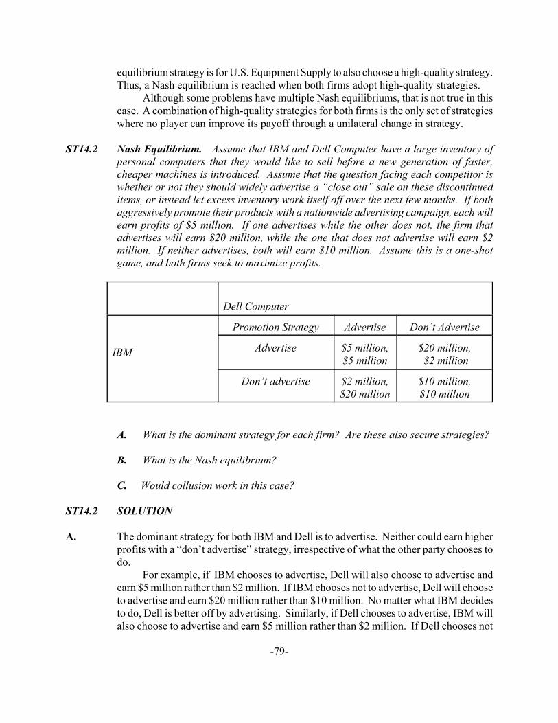
-79-

equilibrium strategy is for U.S. Equipment Supply to also choose a high-quality strategy.Thus, a Nash equilibrium is reached when both firms adopt high-quality strategies.

Although some problems have multiple Nash equilibriums, that is not true in thiscase. A combination of high-quality strategies for both firms is the only set of strategieswhere no player can improve its payoff through a unilateral change in strategy.

ST14.2 Nash Equilibrium. Assume that IBM and Dell Computer have a large inventory ofpersonal computers that they would like to sell before a new generation of faster,cheaper machines is introduced. Assume that the question facing each competitor iswhether or not they should widely advertise a “close out” sale on these discontinueditems, or instead let excess inventory work itself off over the next few months. If bothaggressively promote their products with a nationwide advertising campaign, each willearn profits of $5 million. If one advertises while the other does not, the firm thatadvertises will earn $20 million, while the one that does not advertise will earn $2million. If neither advertises, both will earn $10 million. Assume this is a one-shotgame, and both firms seek to maximize profits.

Dell Computer

IBM

Promotion Strategy Advertise Don’t Advertise

Advertise $5 million,$5 million

$20 million, $2 million

Don’t advertise $2 million,$20 million

$10 million,$10 million

A. What is the dominant strategy for each firm? Are these also secure strategies?

B. What is the Nash equilibrium?

C. Would collusion work in this case?

ST14.2 SOLUTION

A. The dominant strategy for both IBM and Dell is to advertise. Neither could earn higherprofits with a “don’t advertise” strategy, irrespective of what the other party chooses todo.

For example, if IBM chooses to advertise, Dell will also choose to advertise andearn $5 million rather than $2 million. If IBM chooses not to advertise, Dell will chooseto advertise and earn $20 million rather than $10 million. No matter what IBM decidesto do, Dell is better off by advertising. Similarly, if Dell chooses to advertise, IBM willalso choose to advertise and earn $5 million rather than $2 million. If Dell chooses not

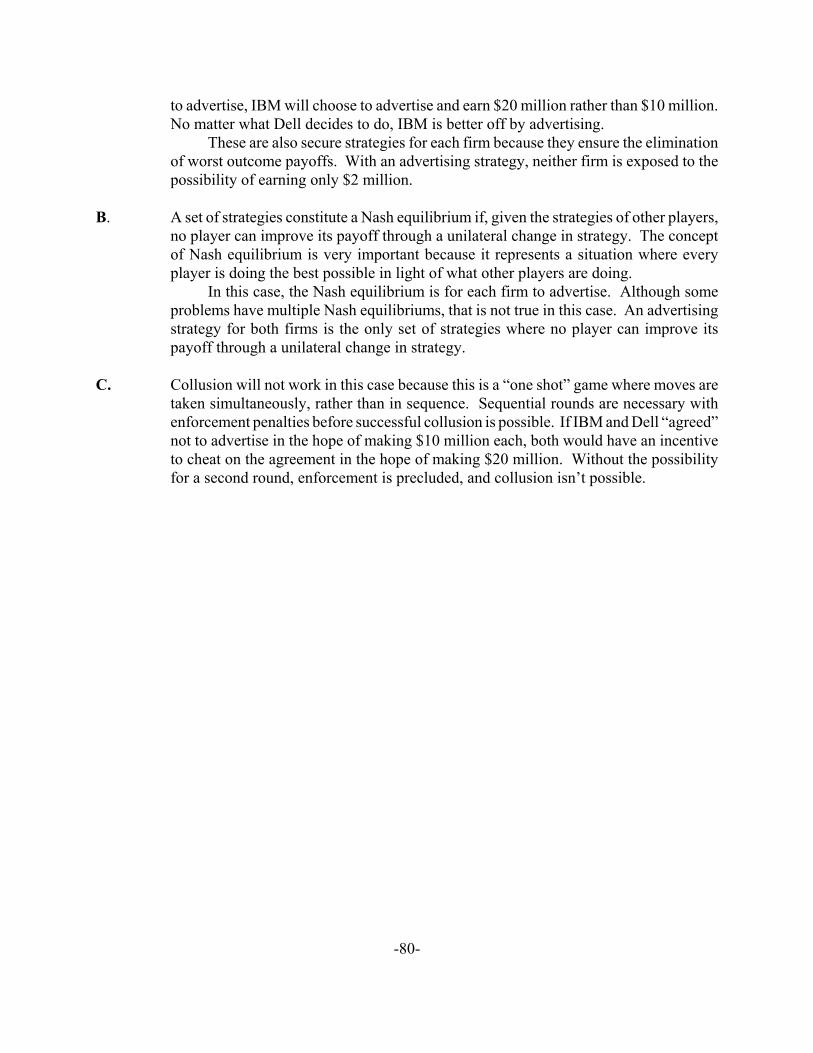
-80-

to advertise, IBM will choose to advertise and earn $20 million rather than $10 million.No matter what Dell decides to do, IBM is better off by advertising.

These are also secure strategies for each firm because they ensure the eliminationof worst outcome payoffs. With an advertising strategy, neither firm is exposed to thepossibility of earning only $2 million.

B. A set of strategies constitute a Nash equilibrium if, given the strategies of other players,no player can improve its payoff through a unilateral change in strategy. The conceptof Nash equilibrium is very important because it represents a situation where everyplayer is doing the best possible in light of what other players are doing.

In this case, the Nash equilibrium is for each firm to advertise. Although someproblems have multiple Nash equilibriums, that is not true in this case. An advertisingstrategy for both firms is the only set of strategies where no player can improve itspayoff through a unilateral change in strategy.

C. Collusion will not work in this case because this is a “one shot” game where moves aretaken simultaneously, rather than in sequence. Sequential rounds are necessary withenforcement penalties before successful collusion is possible. If IBM and Dell “agreed”not to advertise in the hope of making $10 million each, both would have an incentiveto cheat on the agreement in the hope of making $20 million. Without the possibilityfor a second round, enforcement is precluded, and collusion isn’t possible.

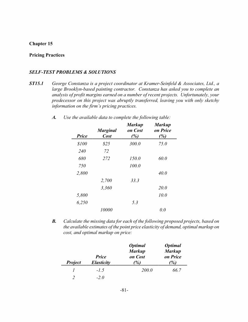
-81-

Chapter 15

Pricing Practices


ST15.1 George Constanza is a project coordinator at Kramer-Seinfeld & Associates, Ltd., alarge Brooklyn-based painting contractor. Constanza has asked you to complete ananalysis of profit margins earned on a number of recent projects. Unfortunately, yourpredecessor on this project was abruptly transferred, leaving you with only sketchyinformation on the firm’s pricing practices.

A. Use the available data to complete the following table:

PriceMarginal

Cost

Markupon Cost

(%)

Markupon Price

(%)$100 $25 300.0 75.0240 72 680 272 150.0 60.0750 100.0

2,800 40.02,700 33.33,360 20.0

5,800 10.06,250 5.3

10000 0.0

B. Calculate the missing data for each of the following proposed projects, based onthe available estimates of the point price elasticity of demand, optimal markup oncost, and optimal markup on price:

ProjectPrice

Elasticity

OptimalMarkupon Cost

(%)

OptimalMarkupon Price

(%)1 -1.5 200.0 66.72 -2.0

ProjectPrice

Elasticity


(%)


(%)

-82-

3 66.74 25.05 -5.0 25.06 11.1 10.07 -15.0 8 -20.0 5.09 4.0

10 -50.0 2.0

ST15.1 SOLUTION

A.

PriceMarginal

Cost

Markupon Cost

(%)

Markupon Price

(%)$100 $25 300.0 75.0240 72 233.3 70.0680 272 150.0 60.0750 375 100.0 50.0

2,800 1,680 66.7 40.03,600 2,700 33.3 25.04,200 3,360 25.0 20.05,800 5,220 11.1 10.06,250 5,938 5.3 5.010,000 10,000 0.0 0.0

B.

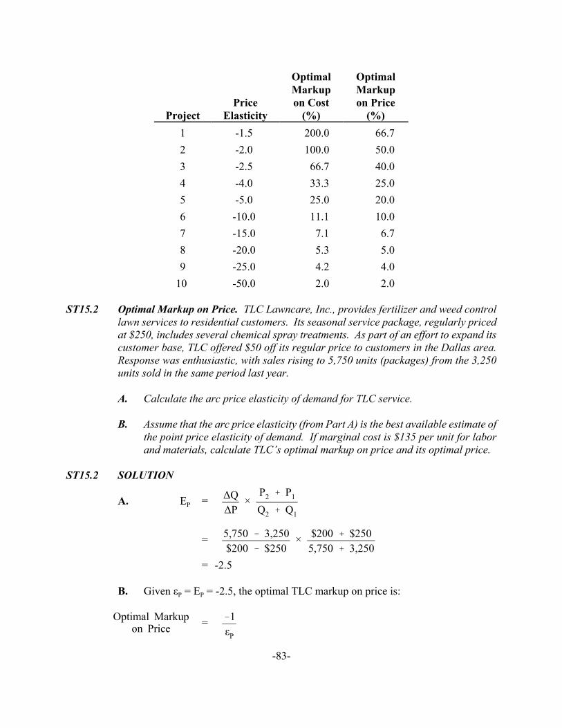
-83-

ProjectPrice

Elasticity


(%)


(%)1 -1.5 200.0 66.72 -2.0 100.0 50.03 -2.5 66.7 40.04 -4.0 33.3 25.05 -5.0 25.0 20.06 -10.0 11.1 10.07 -15.0 7.1 6.78 -20.0 5.3 5.09 -25.0 4.2 4.0

10 -50.0 2.0 2.0

ST15.2 Optimal Markup on Price. TLC Lawncare, Inc., provides fertilizer and weed controllawn services to residential customers. Its seasonal service package, regularly pricedat $250, includes several chemical spray treatments. As part of an effort to expand itscustomer base, TLC offered $50 off its regular price to customers in the Dallas area.Response was enthusiastic, with sales rising to 5,750 units (packages) from the 3,250units sold in the same period last year.

A. Calculate the arc price elasticity of demand for TLC service.

B. Assume that the arc price elasticity (from Part A) is the best available estimate ofthe point price elasticity of demand. If marginal cost is $135 per unit for laborand materials, calculate TLC’s optimal markup on price and its optimal price.

ST15.2 SOLUTION

A. EP = ∆Q∆P

×P2 % P1

Q2 % Q1

= 5,750 & 3,250$200 & $250

× $200 % $2505,750 % 3,250

= -2.5

B. Given εP = EP = -2.5, the optimal TLC markup on price is:

=Optimal Markupon Price

&1εP

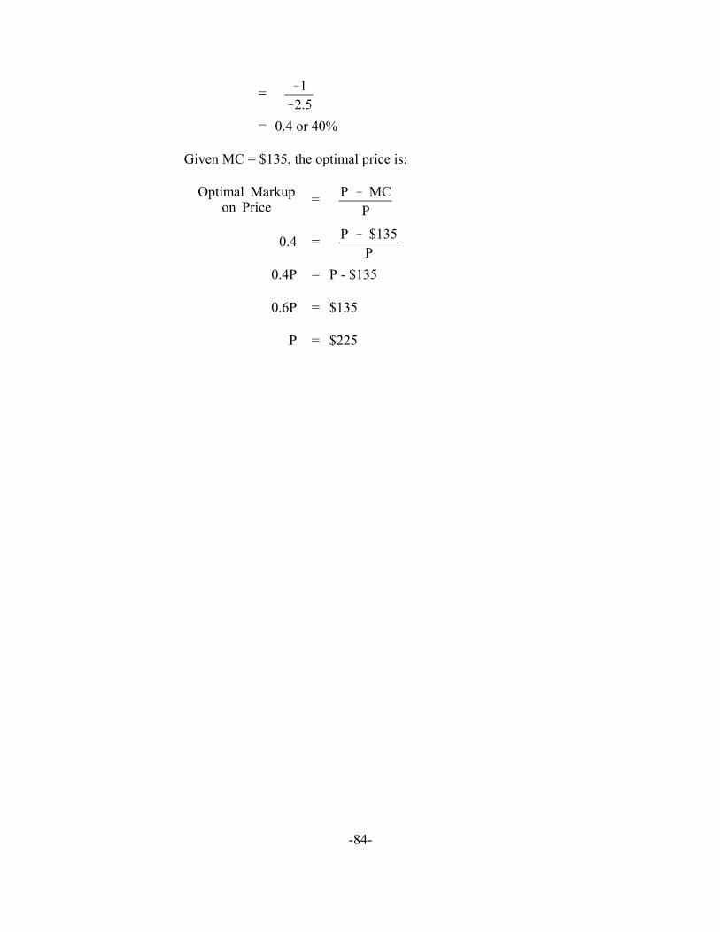
-84-

= &1&2.5

= 0.4 or 40%

Given MC = $135, the optimal price is:

=Optimal Markupon Price

P & MCP

0.4 = P & $135P

0.4P = P - $135

0.6P = $135

P = $225

-85-

Chapter 16

Markets for Labor and Other Inputs


ST16.1 Marginal Revenue Product. To better serve customers interested in buying cars overthe Internet, Smart Motors, Inc., hired Nora Jones to respond to customer inquiries,offer price quotes, and write orders for leads generated by the company’s Web site.During last year, Jones averaged 1.5 vehicle sales per week. On average, these vehiclessold for a retail price of $25,000 and brought the dealership a profit contribution of$1,000 each.

A. Estimate Jones’ annual (50 workweek) marginal revenue product.

B. Jones earns a base salary of $60,000 per year, and Smart Motors pays anadditional 28% of this base salary in taxes and various fringe benefits. Is Jonesa profitable employee?

ST16.1 SOLUTION

A. In the long run, Jones’ marginal revenue product is the maximum amount Smart Motorscould pay in base salary plus all fringe benefits. It is the amount of added revenue afterall other variable costs that Jones’ effort brings to the firm. In this case, Jones’ marginalrevenue product is determined by the number of cars sold and the profit contributionearned on each sale.

MRPL = MPL × MRQ

= (Car sales per year) × (Profit contribution per unit)

= (1.5 × 50) × ($1,000)

= $75,000

Because Jones is only engaged in the sales function, Jones does not produce cars. WhatJones does produce are car sales, and the added value to the employer of Jones’ saleseffort is what determines the amount the employer is willing and able to pay.

B. No. In addition to base salary, employers must pay additional taxes and fringe benefits.All of these costs must be justified by the amount of marginal revenue product generated

-86-

to justify employment. In this case, employment costs for Jones are $76,800 (= $60,000× 1.28). A comparison of marginal revenue product figures with these employment costdata suggests:

MRPL = $75,000 < $76,800 = PL

Therefore, Jones brings in $75,000 per year in additional profit contribution, but costsSmart Motors $76,800. This means that Jones brings in $1,800 per year less in netmarginal revenues than the marginal cost of employment. At the margin, Jones’semployment represents a marginal loss to Smart Motors. Jones is not a profitableemployee.

ST16.2 Monopsony Power. Safecard Corporation offers a unique service. The companynotifies credit card issuers after being informed that a subscriber's credit card has beenlost or stolen. The Safecard service is sold to card issuers on a one-year subscriptionbasis. Relevant revenue and cost relations for the service are as follows:

TR = $5Q - $0.00001Q2

MR = MTR/MQ = $5 - $0.00002Q

TC = $50,000 + $0.5Q + $0.000005Q2

MC = MTC/MQ = $0.5 + $0.00001Q

where TR is total revenue, Q is output measured in terms of the number of subscriptionsin force, MR is marginal revenue, TC is total cost, including a risk-adjusted normal rateof return on investment, and MC is marginal cost.

A. If Safecard has a monopoly in this market, calculate the profit-maximizingprice/output combination and optimal total profit.

B. Calculate Safecard's optimal price, output, and profits if credit card issuerseffectively exert monopsony power and force a competitive market equilibrium inthis market.

ST16.2 SOLUTION

A. The profit-maximizing monopoly price/output combination is found by setting MR =MC and solving for Q:

MR = MC

$5 - $0.00002Q = $0.5 + $0.00001Q,

-87-

0.00003Q = 4.5

Q = 150,000

P = TR/Q = $5 - $0.00001Q

= $5 - $0.00001(150,000)

= $3.50

π = TR - TC = -$0.000015(150,0002) + $4.5(150,000) - $50,000

= $287,500

(Note: Profit is falling for Q > 100,000.)

B. If credit card issuers effectively exert monopsony power and force a competitive marketequilibrium, P = MR and, therefore, P = MC at the average cost minimizing outputlevel. To find the output level where average cost is minimized, set MC = AC and solvefor Q:

MC = AC

$0.5 + $0.00001Q = ($50,000 + $0.5Q + $0.000005Q2)/Q

$0.5 + $0.00001Q = $50,000Q-1 + $0.5 + $0.000005Q

50,000Q-1 = 0.000005Q

50,000Q-2 = 0.000005

= 0.00000550,000Q 2

Q = 50,0000.000005

= 100,000

AC = $50,000/100,000 + $0.5 + $0.000005(100,000)

= $1.50

-88-

At the average-cost minimizing output level, MC = AC = $1.50. Because P = MR in acompetitive market at the profit-maximizing output level:

P = MR = MC = AC = $1.50

π = P × Q - TC

= $1.50(100,000) - $50,000 - $0.5(100,000) - $0.000005(100,0002)

= $0

(Note: Average cost is rising for Q > 150,000.)

-89-

Chapter 17

Risk Analysis


ST17.1 Certainty Equivalent Method. Courteney-Cox, Inc., is a Texas-based manufacturer anddistributor of components and replacement parts for the auto, machinery, farm, andconstruction equipment industries. The company is presently funding a program ofcapital investment that is necessary to reduce production costs and thereby meet anonslaught of competition from low-cost suppliers located in Mexico and throughoutLatin America. Courteney-Cox has a limited amount of capital available and mustcarefully weigh both the risks and potential rewards associated with alternativeinvestments. In particular, the company seeks to weigh the advantages anddisadvantages of a new investment project, project X, in light of two other recentlyadopted investment projects, project Y and project Z:

Expected Cash Flows After Tax (CFAT)Per Year

Year Project X Project Y Project Z2001 $10,000 $20,000 $02002 10,000 18,000 2,5002003 10,000 16,000 5,0002004 10,000 14,000 7,5002005 10,000 12,000 10,0002006 10,000 10,000 12,5002007 10,000 8,000 15,0002008 10,000 6,000 17,5002009 10,000 4,000 20,0002010 10,000 2,000 22,500

PV of Cash Flow @ 5% $91,131 $79,130InvestmentOutlay in 2000:

$60,000 $60,000 $50,000

A. Using a 5% risk-free rate, calculate the present value of expected cash flows aftertax (CFAT) for the ten-year life of project X.

-90-

B. Calculate the minimum certainty equivalent adjustment factor for each project’sCFAT that would justify investment in each project.

C. Assume that the management of Courteney-Cox is risk averse and uses thecertainty equivalent method in decision making. Is project X as attractive or moreattractive than projects Y and Z?

D. If the company would not have been willing to invest more than $60,000 in projectY nor more than $50,000 in project Z, should project X be undertaken?

ST17.1 SOLUTION

A. Using a 5% risk-free rate, the present value of expected cash flows after tax (CFAT) forthe ten-year life of Project X is $77,217, calculated as follows:

Expected Cash Flows After Tax (CFAT) Per Year

Year Project X

PV of $1

at 5%

PV of CFAT

at 5%2001 $10,000 0.9524 $9,5242002 10,000 0.9070 9,0702003 10,000 0.8638 8,6382004 10,000 0.8227 8,2272005 10,000 0.7835 7,8352006 10,000 0.7462 7,4622007 10,000 0.7107 7,1072008 10,000 0.6768 6,7682009 10,000 0.6446 6,4462010 10,000 0.6139 6,139

PV of Cash Flow @ 5% $77,217

B. To justify each investment alternative, the company must have a certainty equivalentadjustment factor of at least αX = 0.777 for project X, αY = 0.658 for project Y, and αZ= 0.632 for project Z, because:

α = Certain SumExpected Risky Sum

= Investment Outlay (Opportunity cost)Present Value CFAT

-91-

Project X

αX = $60,000$77,217

' 0.777

Project Y

αY = $60,000$91,131

' 0.658

Project Z

αZ = $50,000$79,130

' 0.632

In other words, each risky dollar of expected profit contribution from project X must be“worth” at least (valued as highly as) 77.7¢ in certain dollars to justify investment. Forproject Y, each risky dollar must be worth at least 65.8¢ in certain dollars; each riskydollar must be worth at least 63.2¢ to justify investment in project Z.

C. Given managerial risk aversion, project X is the least attractive investment because ithas the highest “price” on each risky dollar of expected CFAT. In adopting projects Yand Z, Courteney-Cox implicitly asserted that it is willing to pay between 63.2¢ (projectZ) and 65.8¢ (project Y) per each expected dollar of CFAT.

D. No. If the prices described previously represent the maximum price the company iswilling to pay for such risky returns, then project X should not be undertaken.

ST17.2 Project Valuation. The Central Perk Coffee House, Inc., is engaged in an aggressivestore refurbishing program and is contemplating expansion of its in-store bakingfacilities. This investment project is to be evaluated using the certainty equivalentadjustment factor method and the risk-adjusted discount rate method. If the project hasa positive value when both methods are employed, the project will be undertaken. Theproject will not be undertaken if either evaluation method suggests that the investmentwill fail to increase the value of the firm. Expected cash flow after tax (CFAT) valuesover the five-year life of the investment project and relevant certainty equivalentadjustment factor information are as follows:

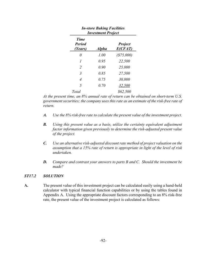
-92-

In-store Baking FacilitiesInvestment Project

TimePeriod(Years) Alpha

ProjectE(CFAT)

0 1.00 ($75,000)1 0.95 22,5002 0.90 25,0003 0.85 27,5004 0.75 30,0005 0.70 32,500

Total $62,500At the present time, an 8% annual rate of return can be obtained on short-term U.S.government securities; the company uses this rate as an estimate of the risk-free rate ofreturn.

A. Use the 8% risk-free rate to calculate the present value of the investment project.

B. Using this present value as a basis, utilize the certainty equivalent adjustmentfactor information given previously to determine the risk-adjusted present valueof the project.

C. Use an alternative risk-adjusted discount rate method of project valuation on theassumption that a 15% rate of return is appropriate in light of the level of riskundertaken.

D. Compare and contrast your answers to parts B and C. Should the investment bemade?

ST17.2 SOLUTION

A. The present value of this investment project can be calculated easily using a hand-heldcalculator with typical financial function capabilities or by using the tables found inAppendix A. Using the appropriate discount factors corresponding to an 8% risk-freerate, the present value of the investment project is calculated as follows:

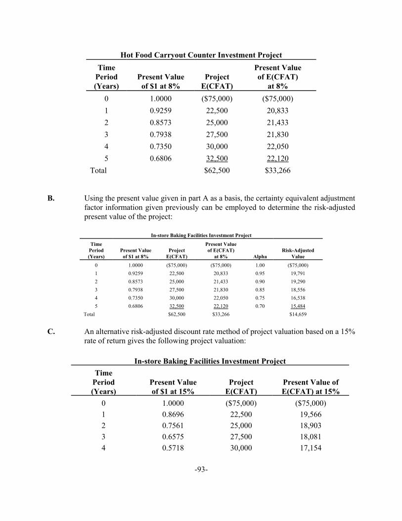
-93-

Hot Food Carryout Counter Investment ProjectTime

Period(Years)

Present Valueof $1 at 8%

ProjectE(CFAT)

Present Valueof E(CFAT)

at 8%0 1.0000 ($75,000) ($75,000)1 0.9259 22,500 20,8332 0.8573 25,000 21,4333 0.7938 27,500 21,8304 0.7350 30,000 22,0505 0.6806 32,500 22,120

Total $62,500 $33,266

B. Using the present value given in part A as a basis, the certainty equivalent adjustmentfactor information given previously can be employed to determine the risk-adjustedpresent value of the project:

In-store Baking Facilities Investment Project

TimePeriod(Years)


ProjectE(CFAT)

Present Valueof E(CFAT)

at 8% AlphaRisk-Adjusted

Value

0 1.0000 ($75,000) ($75,000) 1.00 ($75,000)1 0.9259 22,500 20,833 0.95 19,7912 0.8573 25,000 21,433 0.90 19,2903 0.7938 27,500 21,830 0.85 18,5564 0.7350 30,000 22,050 0.75 16,5385 0.6806 32,500 22,120 0.70 15,484

Total $62,500 $33,266 $14,659

C. An alternative risk-adjusted discount rate method of project valuation based on a 15%rate of return gives the following project valuation:

In-store Baking Facilities Investment ProjectTime

Period(Years)


ProjectE(CFAT)

Present Value ofE(CFAT) at 15%

0 1.0000 ($75,000) ($75,000)1 0.8696 22,500 19,5662 0.7561 25,000 18,9033 0.6575 27,500 18,0814 0.5718 30,000 17,154

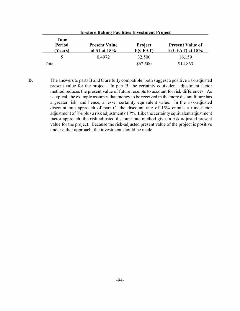
In-store Baking Facilities Investment ProjectTime

Period(Years)


ProjectE(CFAT)

Present Value ofE(CFAT) at 15%

-94-

5 0.4972 32,500 16,159Total $62,500 $14,863

D. The answers to parts B and C are fully compatible; both suggest a positive risk-adjustedpresent value for the project. In part B, the certainty equivalent adjustment factormethod reduces the present value of future receipts to account for risk differences. Asis typical, the example assumes that money to be received in the more distant future hasa greater risk, and hence, a lesser certainty equivalent value. In the risk-adjusteddiscount rate approach of part C, the discount rate of 15% entails a time-factoradjustment of 8% plus a risk adjustment of 7%. Like the certainty equivalent adjustmentfactor approach, the risk-adjusted discount rate method gives a risk-adjusted presentvalue for the project. Because the risk-adjusted present value of the project is positiveunder either approach, the investment should be made.

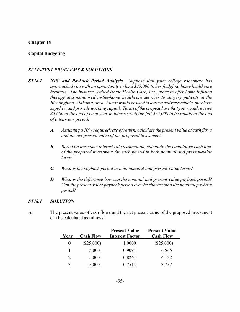
-95-

Chapter 18

Capital Budgeting


ST18.1 NPV and Payback Period Analysis. Suppose that your college roommate hasapproached you with an opportunity to lend $25,000 to her fledgling home healthcarebusiness. The business, called Home Health Care, Inc., plans to offer home infusiontherapy and monitored in-the-home healthcare services to surgery patients in theBirmingham, Alabama, area. Funds would be used to lease a delivery vehicle, purchasesupplies, and provide working capital. Terms of the proposal are that you would receive$5,000 at the end of each year in interest with the full $25,000 to be repaid at the endof a ten-year period.

A. Assuming a 10% required rate of return, calculate the present value of cash flowsand the net present value of the proposed investment.

B. Based on this same interest rate assumption, calculate the cumulative cash flowof the proposed investment for each period in both nominal and present-valueterms.

C. What is the payback period in both nominal and present-value terms?

D. What is the difference between the nominal and present-value payback period?Can the present-value payback period ever be shorter than the nominal paybackperiod?

ST18.1 SOLUTION

A. The present value of cash flows and the net present value of the proposed investmentcan be calculated as follows:

Year Cash FlowPresent ValueInterest Factor

Present ValueCash Flow

0 ($25,000) 1.0000 ($25,000) 1 5,000 0.9091 4,545 2 5,000 0.8264 4,132 3 5,000 0.7513 3,757

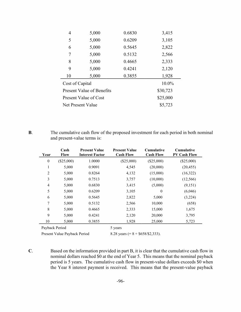
-96-

4 5,000 0.6830 3,415 5 5,000 0.6209 3,105 6 5,000 0.5645 2,822 7 5,000 0.5132 2,566 8 5,000 0.4665 2,333 9 5,000 0.4241 2,120

10 5,000 0.3855 1,928 Cost of Capital 10.0% Present Value of Benefits $30,723 Present Value of Cost $25,000 Net Present Value $5,723

B. The cumulative cash flow of the proposed investment for each period in both nominaland present-value terms is:

YearCashFlow

Present ValueInterest Factor

Present ValueCash Flow

CumulativeCash Flow

CumulativePV Cash Flow

0 ($25,000) 1.0000 ($25,000) ($25,000) ($25,000) 1 5,000 0.9091 4,545 (20,000) (20,455) 2 5,000 0.8264 4,132 (15,000) (16,322) 3 5,000 0.7513 3,757 (10,000) (12,566) 4 5,000 0.6830 3,415 (5,000) (9,151) 5 5,000 0.6209 3,105 0 (6,046) 6 5,000 0.5645 2,822 5,000 (3,224) 7 5,000 0.5132 2,566 10,000 (658) 8 5,000 0.4665 2,333 15,000 1,675 9 5,000 0.4241 2,120 20,000 3,795

10 5,000 0.3855 1,928 25,000 5,723 Payback Period 5 yearsPresent Value Payback Period 8.28 years (= 8 + $658/$2,333).

C. Based on the information provided in part B, it is clear that the cumulative cash flow innominal dollars reached $0 at the end of Year 5. This means that the nominal paybackperiod is 5 years. The cumulative cash flow in present-value dollars exceeds $0 whenthe Year 8 interest payment is received. This means that the present-value payback

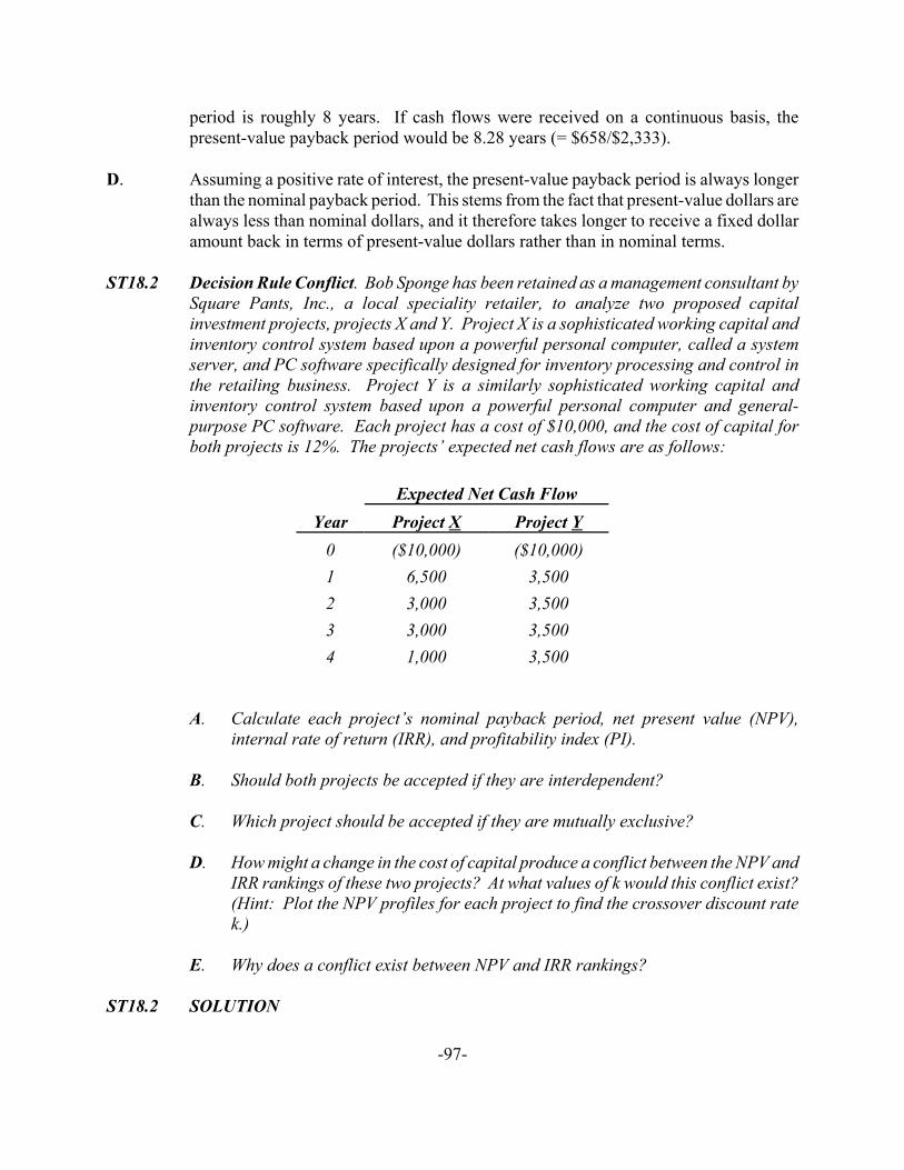
-97-

period is roughly 8 years. If cash flows were received on a continuous basis, thepresent-value payback period would be 8.28 years (= $658/$2,333).

D. Assuming a positive rate of interest, the present-value payback period is always longerthan the nominal payback period. This stems from the fact that present-value dollars arealways less than nominal dollars, and it therefore takes longer to receive a fixed dollaramount back in terms of present-value dollars rather than in nominal terms.

ST18.2 Decision Rule Conflict. Bob Sponge has been retained as a management consultant bySquare Pants, Inc., a local speciality retailer, to analyze two proposed capitalinvestment projects, projects X and Y. Project X is a sophisticated working capital andinventory control system based upon a powerful personal computer, called a systemserver, and PC software specifically designed for inventory processing and control inthe retailing business. Project Y is a similarly sophisticated working capital andinventory control system based upon a powerful personal computer and general-purpose PC software. Each project has a cost of $10,000, and the cost of capital forboth projects is 12%. The projects’ expected net cash flows are as follows:

Expected Net Cash FlowYear Project X Project Y

0 ($10,000) ($10,000)1 6,500 3,5002 3,000 3,5003 3,000 3,5004 1,000 3,500

A. Calculate each project’s nominal payback period, net present value (NPV),internal rate of return (IRR), and profitability index (PI).

B. Should both projects be accepted if they are interdependent?

C. Which project should be accepted if they are mutually exclusive?

D. How might a change in the cost of capital produce a conflict between the NPV andIRR rankings of these two projects? At what values of k would this conflict exist?(Hint: Plot the NPV profiles for each project to find the crossover discount ratek.)

E. Why does a conflict exist between NPV and IRR rankings?

ST18.2 SOLUTION

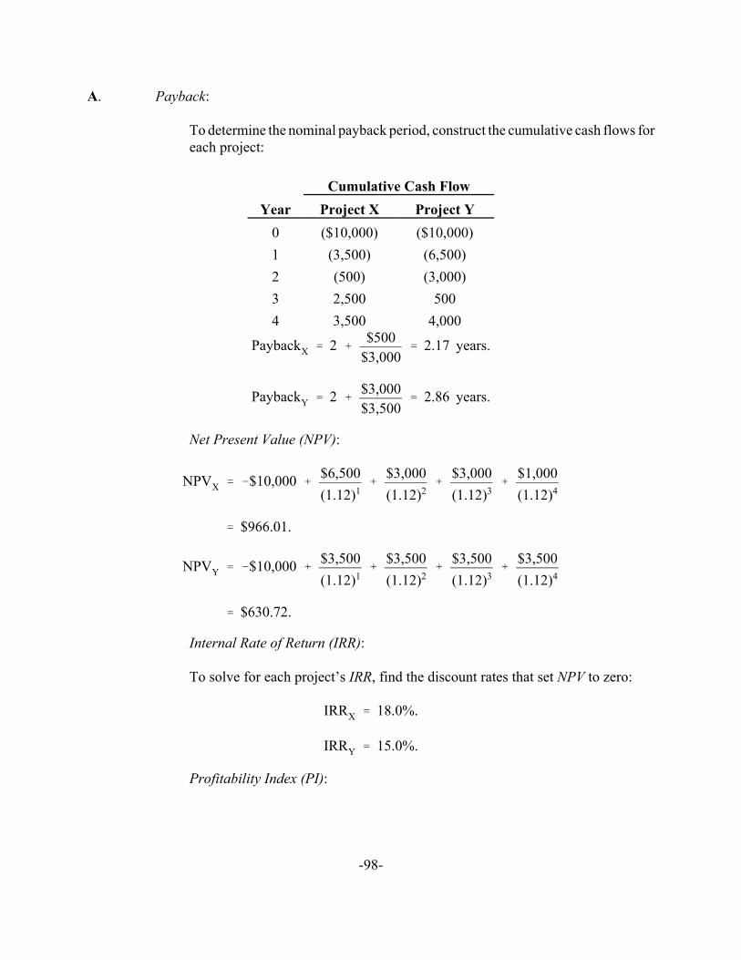
-98-

PaybackX ' 2 %$500

$3,000' 2.17 years.

PaybackY ' 2 %$3,000$3,500

' 2.86 years.

NPVX ' &$10,000 %$6,500(1.12)1

%$3,000(1.12)2

%$3,000(1.12)3

%$1,000(1.12)4

' $966.01.

NPVY ' &$10,000 %$3,500(1.12)1

%$3,500(1.12)2

%$3,500(1.12)3

%$3,500(1.12)4

' $630.72.

IRRX ' 18.0%.

IRRY ' 15.0%.

A. Payback:

To determine the nominal payback period, construct the cumulative cash flows foreach project:

Cumulative Cash FlowYear Project X Project Y

0 ($10,000) ($10,000)1 (3,500) (6,500)2 (500) (3,000)3 2,500 5004 3,500 4,000

Net Present Value (NPV):

Internal Rate of Return (IRR):

To solve for each project’s IRR, find the discount rates that set NPV to zero:

Profitability Index (PI):

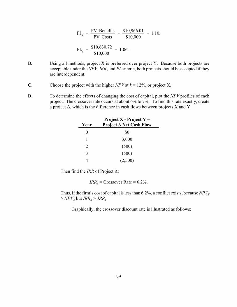
-99-

PIX 'PV Benefits

PV Costs'

$10,966.01$10,000

' 1.10.

PIY '$10,630.72

$10,000' 1.06.

B. Using all methods, project X is preferred over project Y. Because both projects areacceptable under the NPV, IRR, and PI criteria, both projects should be accepted if theyare interdependent.

C. Choose the project with the higher NPV at k = 12%, or project X.

D. To determine the effects of changing the cost of capital, plot the NPV profiles of eachproject. The crossover rate occurs at about 6% to 7%. To find this rate exactly, createa project ∆, which is the difference in cash flows between projects X and Y:

YearProject X - Project Y =

Project ∆ Net Cash Flow0 $01 3,0002 (500)3 (500)4 (2,500)

Then find the IRR of Project ∆:

IRR∆ = Crossover Rate = 6.2%.

Thus, if the firm’s cost of capital is less than 6.2%, a conflict exists, because NPVY> NPVX but IRRX > IRRY.

Graphically, the crossover discount rate is illustrated as follows:

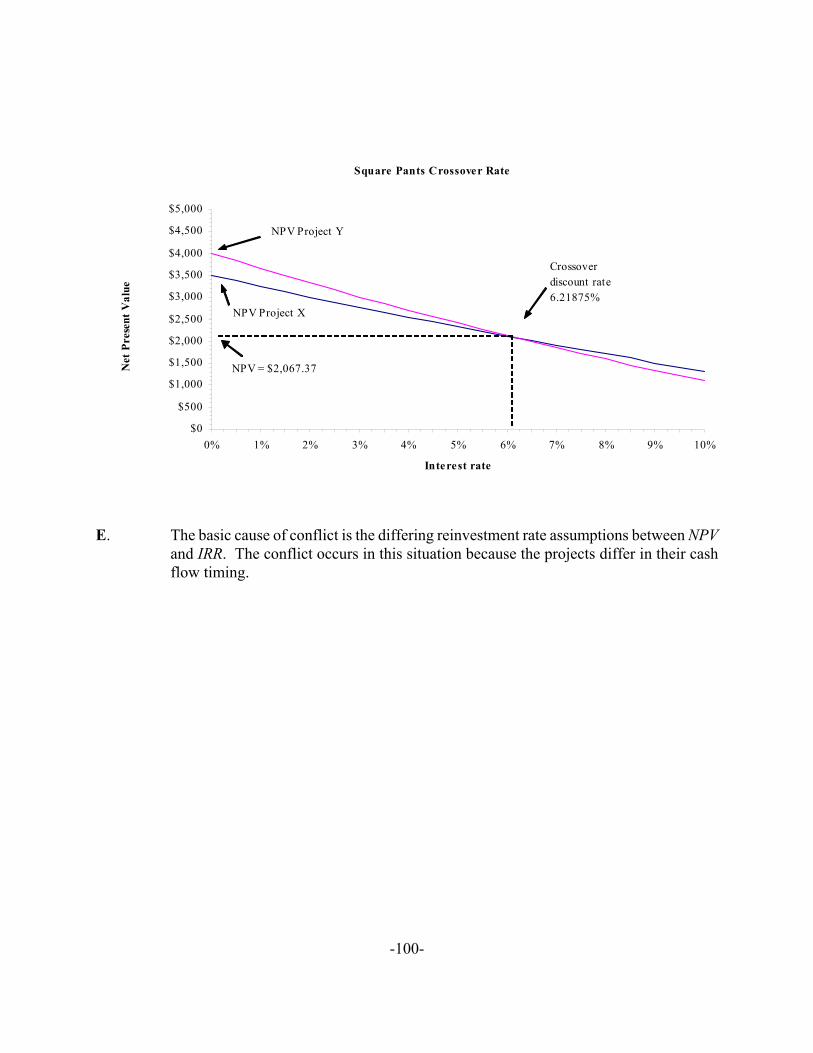
-100-

Square Pants Crossover Rate

$0

$500

$1,000

$1,500

$2,000

$2,500

$3,000

$3,500

$4,000

$4,500

$5,000

0% 1% 2% 3% 4% 5% 6% 7% 8% 9% 10%

Interest rate

Net

Pre

sent

Val

ue

NPV Project Y

NPV Project X

Crossover discount rate6.21875%

NPV = $2,067.37

E. The basic cause of conflict is the differing reinvestment rate assumptions between NPVand IRR. The conflict occurs in this situation because the projects differ in their cashflow timing.

-101-

Chapter 19

Organization Structure and Corporate Governance


ST19.1 Agency Problem. In the 1930s, economists Adolf A. Berle and Gardiner C. Meansexpressed concern that managers with relatively little ownership interest mightdemonstrate a suboptimal focus on transitory short-term profits rather than durablelong-run value. Berle and Means also voiced concern for value-reducing risk avoidanceon the part of management-controlled firms.

A. In general, describe the “agency problem” referred to by Berle and Means. Then,specifically describe how inefficient risk avoidance by top managers could be aproblem.

B. What corporate governance mechanisms are commonly employed to combat theagency problems feared by Berle and Means?

ST19.1 SOLUTION

A. So-called agency problems stem from the natural conflict that exists between ownersand managers. Given their ownership position, stockholders are the principals of thefirm. Managers and other employees without any ownership interest can be thought ofas hired hands, or agents of the stockholders. An agency problem is present to the extentthat unresolved material conflicts exist between the self-seeking goals of (agent)managers and the value maximization goal of (principal) stockholders. Agency costsare the explicit and implicit transaction costs necessary to overcome the naturaldivergence of interest between agent managers and principal stockholders. Agencycosts incurred by stockholders are reflected in expenses for managerial monitoring, theover consumption of perquisites by managers, lost opportunities due to excessive riskavoidance, and so on.

Managers have incentives for risk avoidance to the extent that spectacular short-run performance creates expectations that are difficult or impossible to satisfy and,therefore, leads to stockholder disappointment and sanctions. Incentives for managerialrisk avoidance are also present if stockholder risk aversion leads to an asymmetry ofmanagerial rewards and penalties following short-term “success” versus “failure.”

B. Although the potential for such a managerial risk-avoidance problem clearly exists,long-term performance plans are employed on a widespread basis to force a convergencebetween managerial and stockholder interests. Some of these plans tie executive and

-102-

employee pay to well-defined accounting performance measures, like the accountingreturn on equity, or return on assets over extended periods. Others tie managerialrewards to long-term stock performance over, say, 5 to 10-year time intervals. Finally,executive stock option or stock ownership plans are an effective means of tyingmanagerial incentives to the shareholder’s preferred value maximization objective.

ST19.2 Ownership Structure. Both General Electric and Microsoft Corp. feature charismaticand highly effective chief executive officers, display enviable records of serving growingmarkets with remarkable efficiency, and enjoy sterling accounting returns and stock-market valuations. GE and Microsoft are also huge organizations that rank near thetop in stock-market valuation among U.S. companies. Interestingly, both featuresignificant institutional ownership, but are starkly different in terms of the amount ofcommon stock held by insiders. At GE, insider holding total a mere 1 %, about averageamong industrial giants. At Microsoft, insiders hold an astounding 19.8 % of thecompany.

A. What economic differences in the products produced by GE and Microsoft couldbe used to explain such stark differences in ownership structure?

B. Legend has it that IBM turned down a chance to buy 50 % of Microsoft for $50million in the early 1980s. Was this a mistake on IBM’s part?

ST19.2 SOLUTION

A. GE is a widely diversified manufacturer that produces a extensive variety of productsin a broad array of industries. Many of GE’s products are well-known by long-satisfiedcustomers and produced at standard production facilities in the United States GE’soperating facilities have good loan collateral value, and the company uses extensivefinancial leverage. Many outside investors find it easy to assess the financialperformance and prospects of GE and have been eager to supply outside equityfinancing. As a result, it is easy to see why GE has been able to flourish despite havinglittle of its huge capital needs supplied by insiders.

In contrast, Microsoft produces PC software and services that are hard to fathomfor most customers, lenders, and outside suppliers of equity. Microsoft uses little in theway of traditional capital resources; most of the capital employed by Microsoft is humancapital, not physical plant and equipment. When intangible assets such as patents,copyrights, and trademarks form the preponderance of firm resources, outside investorstend to be reluctant to supply the bulk of firm financing. Without clear loan collateralvalue, lenders back away from extending significant amounts of credit. Because thevalue of patents, copyrights, and trademarks is often closely tied to managerialefficiency, outside investors can also be reluctant to supply equity financing. BecauseMicrosoft’s success depends upon the efficiency with which its human capital isexploited, both lenders and outside suppliers of equity demand that the company featurea significant amount of inside equity financing so that insiders have a strong incentive

-103-

to maximize the value of the firm.

B. With 20/20 hindsight, it is easy to say that IBM blew it by not purchasing 50 % ofMicrosoft for $50 million in the early 1980s. After all, with a total market capitalizationin excess of $200 billion for Microsoft today, IBM would have achieved an enormouswindfall from such an investment. (While we are on the subject, you and I also blew itby not buying MSFT stock when it first became publicly traded in 1982.)

However, it is not appropriate to evaluate this decision with the benefits of 20/20hindsight. Back in 1980, for example, it was not clear that bringing the graphical userinterface of the Apple Computer to IBM-compatible PCs would be such an amazingsuccess story. Before the fact, much of the unrealized value potential of Microsoft wastied up in the dreams and imagination of Bill Gates, Paul Allen and a cadre ofhardworking computer “geeks.” If IBM had purchased 50 % of Microsoft, would theyall have worked as hard to make Microsoft a success? Maybe, but perhaps not. In thecase of Microsoft, Coca-Cola, Intel and other companies with significant intangibleassets, investors and lenders require high levels of inside equity financing as a signal ofthe credible commitment by insiders to maximize the value of the firm.

-104-

Chapter 20

Government in the Market Economy


ST20.1 Pollution Control Costs. Anthony Soprano is head of Satriale Pork Producers, Inc., afamily-run pork producer with a hog-processing facility in Musconetcong, New Jersey.Each hog processed yields both pork and a render by-product in a fixed 1:1 ratio.Although the by-product is unfit for human consumption, some can be sold to a local petfood company for further processing. Relevant annual demand and cost relations areas follows:

PP = $110 - $0.00005QP,

(Demand for pork)

MRP = MTRP/MQP = $110 - $0.0001QP,

(Marginal revenue from pork)

PB = $10 - $0.0001QB,

(Demand for render by-product)

MRB = MTRB/MQB = $10 - $0.0002QB,

(Marginal revenue from render by-product)

TC = $10,000,000 + $60Q,

(Total cost)

MC = MTC/MQ = $60.

(Marginal cost)

Here, P is price in dollars, Q is the number of hogs processed (with an average weightof 100 pounds), and QP and QB are pork and render by-product per hog, respectively;both total and marginal costs are in dollars. Total costs include a risk-adjusted normalreturn of 15% on a $50 million investment in plant and equipment.

-105-

Currently, the city allows the company to dump excess by-product into its sewagetreatment facility at no charge, viewing the service as an attractive means of keeping avalued employer in the area. However, the sewage treatment facility is quicklyapproaching peak capacity and must be expanded at an expected operating cost of $3million per year. This is an impossible burden on an already strained city budget.

A. Calculate the profit-maximizing price/output combination and optimal total profitlevel for Satriale.

B. How much by-product will the company dump into the Musconetcong sewagetreatment facility at the profit-maximizing activity level?

C. Calculate output and total profits if the city imposes a $35 per unit charge on theamount of by-product Satriale dumps.

D. Calculate output and total profits if the city imposes a fixed $3-million-per-yeartax on Satriale to pay for the sewage treatment facility expansion.

E. Will either tax alternative permit Satriale to survive in the long run? In youropinion, what should the city of Musconetcong do about its sewage treatmentproblem?

ST20.1 SOLUTION

A. Solution to this problem requires that one look at several production and sales optionsavailable to the firm. One option is to produce and sell equal quantities of pork (P) andby-product (B). In this case, the firm sets relevant MC = MR.

MC = MRP + MRB = MR

$60 = $110 - $0.0001Q + $10 - $0.0002Q

0.0003Q = 60

Q = 200,000 hogs

Thus, the profit-maximizing output level for production and sale of equal quantities ofP and B would be 200,000 hogs. However, the marginal revenues of both products mustbe positive at this sales level for this to be an optimal activity level.

Evaluated at 200,000 hogs:

MRP = $110 - $0.0001(200,000)

-106-

= $90

MRB = $10 - $0.0002(200,000)

= -$30

Because the marginal revenue for B is negative, and Satriale can costlessly dump excessproduction, the sale of 200,000 units of B is suboptimal. This invalidates the entiresolution developed above because output of P is being held down by the negativemarginal revenue associated with B. The problem must be set up to recognize thatSatriale will stop selling B at the point where its marginal revenue becomes zerobecause, given production for P, the marginal cost of B is zero.

Set:

MRB = MCB

$10 - $0.0002QB = $0

0.0002QB = 10

QB = 50,000 units

Thus, 50,000 units of B are the maximum that would be sold. Any excess units will bedumped into the city’s sewage treatment facility. The price for B at 50,000 units is:

PB = $10 - $0.0001QB

= 10 - 0.0001(50,000)

= $5

To determine the optimal production of P (pork), set the marginal revenue of P equal tothe marginal cost of hog processing because pork production is the only motive forprocessing more than 50,000 units:

MRP = MCP = MCQ

$110 - $0.0001QP = $60

0.0001QP = 50

QP = 500,000 units

-107-

(Remember (QP = Q)

and

PP = $110 - $0.00005QP

= 110 - 0.00005(500,000)

= $85

Excess profits at the optimal activity level for Satriale are:

Excess profits = π = TRP + TRB - TC

= PP × QP + PB × QB - TCQ

= $85(500,000) + $5(50,000) - $10,000,000 - $60(500,000)

= $2,750,000

Because total costs include a normal return of 15% on $50 million in investment,

Total profits = Required return + Excess profits

= 0.15($50,000,000) + $2,750,000

= $10,250,000

B. With 500,000 hogs being processed, but only 50,000 units of B sold, dumping of B is:

Units B dumped = Units produced - Units sold

= 500,000 - 50,000

= 450,000 units

C. In part A, it is shown that if all P and B produced is sold, an activity level of Q =200,000 results in MRB = -$30. A dumping charge of $35 per unit of B will causeSatriale to prefer to sell the last unit of B produced (and lose $30) rather than pay a $35fine. Therefore, this fine, as does any fine greater than $30, will eliminate dumping andcause Satriale to reduce processing to 200,000 hogs per year. This fine structure wouldundoubtedly reduce or eliminate the need for a new sewage treatment facility.

Although eliminating dumping is obviously attractive in the sense of reducingsewage treatment costs, the $35 fine has the unfortunate consequence of cutting output

-108-

substantially. Pork prices rise to PP = $110 - $0.00005(200,000) = $100, and by productprices fall to PB = $10 - $0.0001(200,000) = -$10. This means Satriale will pay the petfood company $10 per unit to accept all of its by-product sludge. Employment willundoubtedly fall as well. In addition to these obvious short-run effects, long-runimplications may be especially serious. At Q = 200,000, Satriale’s excess profits are:

Excess profits = TRP + TRB - TC

= $110Q - $0.00005Q2 + $10Q - $0.0001Q2 - $10,000,000 - $60Q

= $110(200,000) - $0.00005(200,0002) + $10(200,000)

- $0.0001(200,0002) - $10,000,000 - $60(200,000)

= -$4,000,000 (a loss)

This means that total profits are:

Total profits = Required return + Excess profits

= 0.15($50,000,000) + (-$4,000,000)

= $3,500,000

This level of profit is insufficient to maintain investment. Although a $35 dumpingcharge will eliminate dumping, it is likely to cause the firm to close down or move tosome other location. The effect on employment in Musconetcong could be disastrous.

D. In the short run, a $3 million tax on Satriale has no effect on dumping, output oremployment. At the Q = 500,000 activity level, a $3 million tax would reduce Satriale’stotal profits to $7,250,000, or $250,000 below the required return on investment.However, following imposition of a $3 million tax, the firm’s survival and totalemployment would be imperiled in the long run.

E. No. Satriale is not able to bear the burden of either tax alternative. Obviously, there isno single best alternative here. The highest fixed tax the company can bear in the longrun is $2.75 million, the full amount of excess profits. If the city places an extremelyhigh priority on maintaining employment, perhaps a $2.75 million tax on Satriale plus$250,000 in general city tax revenues could be used to pay for the new sewage systemtreatment facility.

ST20.2 Benefit-cost Analysis Methodology. The benefit-cost approach is not new. The conceptfirst surfaced in France in 1844. In this century, benefit-cost analysis has been widelyused in the evaluation of river and harbor projects since as early as 1902. In the United

-109-

States, the 1936 Flood Control Act authorized federal assistance in developingflood-control programs “if the benefits to whomsoever they may accrue are in excessof the estimated costs.” By 1950, federal agency practice required the considerationof both direct and indirect benefits and costs and that unmeasured intangible influencesbe listed. Despite this long history of widespread use, it has only been since 1970 thatpublic-sector managers have sought to broadly apply the principles of benefit-costanalysis to the evaluation of agricultural programs, rapid transit projects, highwayconstruction, urban renewal projects, recreation facility construction, job trainingprograms, health-care reform, education, research and development projects, anddefense policies.

A. Briefly describe major similarities and differences between public-sectorbenefit-cost analysis and the private-sector capital budgeting process.

B. What major questions must be answered before meaningful benefit-cost analysisis possible?

C. Although the maximization of society’s wealth is the primary objective ofbenefit-cost analysis, it is important to recognize that constraints often limitgovernment’s ability to achieve certain objectives. Enumerate some of thecommon economic, political, and social constraints faced in public-sectorbenefit-cost analysis.

D. In light of these constraints, discuss some of the pluses and minuses associatedwith the use of benefit-cost analysis as the foundation for a general approach tothe allocation of government-entrusted resources.

ST20.2 SOLUTION

A. Benefit-cost analysis is a method for assessing the desirability of social programs andpublic-sector investment projects when it is necessary to take a long view of the publicand private repercussions of such expenditures. As in the case of private-sector capitalbudgeting, benefit-cost analysis is frequently used in cases where the economicconsequences of a program or project are likely to extend beyond 1 year in time. Unlikecapital budgeting, however, benefit-cost analysis seeks to measure both direct privateeffects and indirect social implications of public-sector investment decisions and policychanges.

B. Before meaningful benefit-cost analysis is possible, a number of important policyquestions must be answered. Among these policy questions are

P What is the social objective function that is to be maximized?

P What constraints are placed on the decision-making process?

-110-

P What marginal social benefits and marginal social costs are to be included,and how are they to be measured?

P What social investment criterion should be used?

P What is the appropriate social rate of discount?

C. A number of constraints impinge upon society’s ability to maximize the social benefitsderived from public expenditures. Among these constraints are

P Physical constraints. Program alternatives are limited by the available stateof technology and by current production possibilities. For example, it is notyet possible to cure AIDS. Therefore, major emphasis for public policy inthis area must be directed toward prevention, early detection and treatment,and research.

P Legal constraints. Domestic laws and international agreements place limitson property rights, the right of eminent domain, due process, constitutionallimits on a particular agency’s activities, and so on. These legal constraintsoften play an important role in shaping the realm of public policy.

P Administrative constraints. Effective programs require competentmanagement and execution. Qualified individuals must be available to carryout social objectives. Even the best-conceived program is doomed to failureunless managers and workers with the proper mix of technical andadministrative skill are available.

P Distributional constraints. Social programs and public-sector investmentprojects affect different groups in different ways. The “gainers” are seldomthe same as “losers.” When distributional impacts of public policy are ofparamount concern, the objective of benefit-cost analysis might maximizesubject to the constraint that equity considerations be met.

P Political constraints. That which is optimal may not be feasible because ofslowness and inefficiency in the political process. Often what is best istempered by what is possible, given the existence of strong competingspecial-interest groups.

P Budget constraints. Public agencies often work within the bounds of apredetermined budget. As a result, virtually all social programs andpublic-sector investment projects have some absolute financial ceiling abovewhich the program cannot be expanded, irrespective of social benefits.

P Social or religious constraints. Social or religious constraints may limit the

-111-

range of feasible program alternatives. It is futile to attempt to combat teenpregnancy with public support for family planning if religious constraintsprohibit the use of modern birth control methods.

D. An important potential use of benefit-cost analysis is as the structure for a generalphilosophy of government resource allocation. As such, the results of benefit-coststudies have the potential to serve as a guide for resource-allocation decisions within andamong government programs and investment projects in agriculture, defense, education,healthcare, welfare, and other areas. The objective of such a comprehensive benefit-costapproach to government would be to maximize the net present-value of the differencebetween the marginal social benefits and the marginal social costs derived from allsocial programs and public-sector investment projects.

Although a benefit-cost approach to evaluating all levels and forms of governmentis conceptually appealing on an efficiency basis, it suffers from a number of seriouspractical limitations. Perhaps most importantly, the measurement of marginal socialbenefits and marginal social costs for goods and services that are not or cannot beprovided by the private sector is often primitive, at best. Measurement systems have notbeen sufficiently refined or standardized to permit meaningful comparisons among thesocial net present-value of “Star Wars” defense systems, the guaranteed student loanprogram for college students, funding for AIDS research, Medicare, and Medicaid. Afurther problem arises because benefit-cost analysis is largely restricted to aconsideration of the efficiency objective; equity-related considerations are seldomaccorded full treatment in benefit-cost analysis. In addition, as discussed previously, anumber of important economic, political, and social constraints limit the effectivenessof benefit-cost analysis. As a result, significant problems arise when a given socialprogram or public-sector investment project is designed to meet efficiency andequity-related objectives.

For these reasons, benefit-cost analysis is traditionally viewed within the narrowcontext of a decision technique that is helpful in focusing interest on the economicconsequences of proposed social programs and public-sector investment projects. Itsgreatest use is in comparing programs and projects that are designed to achieve the sameor similar objectives and as a tool for focusing resources on the best use of resourcesintended to meet a given social objective.

SELF-TEST PROBLEMS & SOLUTIONS

Documents