Welcome message from author
This document is posted to help you gain knowledge. Please leave a comment to let me know what you think about it! Share it to your friends and learn new things together.
Transcript


Sensors and Electronic Instrumentation Advances:
Proceedings of the 7th International Conference
on Sensors and Electronic Instrumentation Advances
22-24 September 2021 Palma de Mallorca, Mallorca (Balearic Islands), Spain
Edited by Sergey Y. Yurish

Sergey Y. Yurish, Editor Sensors and Electronic Instrumentation Advances SEIA’ 2021 Conference Proceedings Copyright © 2021 by International Frequency Sensor Association (IFSA) Publishing, S. L.
E-mail (for orders and customer service enquires): [email protected]
Visit our Home Page on http://www.sensorsportal.com
All rights reserved. This work may not be translated or copied in whole or in part without the written permission of the publisher (IFSA Publishing, S. L., Barcelona, Spain).
Neither the authors nor International Frequency Sensor Association Publishing accept any responsibility or liability for loss or damage occasioned to any person or property through using the material, instructions, methods or ideas contained herein, or acting or refraining from acting as a result of such use.
The use in this publication of trade names, trademarks, service marks, and similar terms, even if they are not identifies as such, is not to be taken as an expression of opinion as to whether or not they are subject to proprietary rights.
ISBN: 978-84-09-33525-1 BN-20190915-XX BIC: TJFC

7th International Conference on Sensors Engineering and Electronics Instrumentation Advances (SEIA' 2021), 22-24 September 2021, Palma de Mallorca, Mallorca (Balearic Islands), Spain
3
Contents
Foreword ........................................................................................................................................................... 6 Giant Magnetoimpedance Effect of Magnetically Soft Microwires for Sensor Applications ..................... 7
A. Zhukov, P. Corte-Leon, M. Ipatov, J. M. Blanco A. Gonzalez and V. Zhukova
Assessing the Sensitivity of Site Index Models Developed Using Repeated Airborne Laser Scanning Data to Height Metrics and Plot Size ............................................................................................ 10
J. Socha and Luiza Tymińska-Czabańska
A Review of Energy Consumption Measurement Systems with Applications in Wireless Sensor Networks .......................................................................................................................................................... 16
F. Barišić and H. Hegeduš
Gravitational Search Algorithm-based Multi-hop Routing Scheme for Energy Efficient Heterogeneous Clustered Scheme.................................................................................................................. 23
T. Sood and K. Sharma
Temperature Sensing with Erbium-doped Multi-component Tellurite Glasses ....................................... 30 R. Yatskiv, P. Kostka, J. Grym, J. Zavadil
Static Calibration and Dynamic Verification of a 3-axis Accelerometer Using the Method of Variable Projection .................................................................................................................................... 33
E. Lang, M. Rollett, E. Theussl and P. O’Leary
Study of the Prospects for the Use of Ionic Liquids and Non-Aqueous Salt Solutions for Low-temperature Operation of Serial Electrochemical Geophysical Sensors .................................... 39
E. I. Egorov, D. L. Zaitsev and V. M. Agafonov
Quantification of Double Strand Methylated DNA, Using rGO and AuNPs Decorated Screen Printed Electrode ............................................................................................................................................ 44
Mina Safarzadeh and Genhua Pan
Role of Cobalt in Co-ZnO Nanoflower Gas Sensors for the Detection of Low Concentration VOCs ..... 46 Y. Luo, A. Ly, D. Lahem, C. Zhang and M. Debliquy
Sensor Technology and Corporate Social Responsibility: From “Sustainable Indicators” to “Sustainable Technology” .......................................................................................................................... 49
V. Potocan and S. Treven
Carbon Electrodes Modification for Epidermal Growth Factor Receptor Detection .............................. 52 I. Šišoláková, J. Shepa, M. Panigaj, V. Huntošová, D. Marcin Behunová, R. Oriňaková
Electrochemical Sensors for Epidermal Growth Factor Receptor Detection ............................................ 54 R. Gorejová, I. Šišoláková, J. Shepa, M. Panigaj and R. Oriňaková
The Application of Gas Sensor with Biohydroxyapatite to Study the Volatile Profile of Nasal Secretion ........................................................................................................................................... 56
T. A. Kuchmenko, R. U. Umarkhanov, A. A. Shuba, D. A. Menzhulina
Optimization of Epidermal Growth Factor Receptor Electrochemical Sensing Procedure .................... 62 R. Oriňaková, I. Šišoláková, J. Shepa and M. Panigaj
Fiber-optic Mach-Zehnder Interferometer for Refractive Index Measurement Based on MEMS Optofluidic Platform ....................................................................................................................................... 64
Z. Djinović, A. Kocsis and M. Tomić
Optimization of Impedance Based Microsensors for Biological Analysis .................................................. 69 J. Claudel, R. Benttenfeld, D. Kourtiche and M. Nadi
Electrical Properties Measurement of Graphene-based Composites using an Open-ended Coaxial Probe Technique ............................................................................................................................... 72
H. Bakli, M. Moualhi and M. Makhlouf
Numerical Studies of a Side-hole Optical Fiber with Modified Geometry as a Refractive Index Sensor .................................................................................................................................................... 76
M. Dudek, K. Köllő, P. Marć and L. R. Jaroszewicz
Multilayer Amorphous Lead Oxide-based X-ray Detector ......................................................................... 78 O. Grynko, E. Pineau, T. Thibault, G. DeCrescenzo and A. Reznik

7th International Conference on Sensors Engineering and Electronics Instrumentation Advances (SEIA' 2021), 22-24 September 2021, Palma de Mallorca, Mallorca (Balearic Islands), Spain
4
3-D Measurement of Abdomen by Moiré Analysis and Its Use for Abnormal Respiratory Conditions by Deep Learning ........................................................................................................................ 83
Y. Mochizuki and N. Tagawa
Comfort Prognosis by Microclimate Simulation and Measurement .......................................................... 88 Bernhard Kurz, Christoph Russ, Michael Kurz
Potential of Dual Energy X-ray Transmission on Food Safety ................................................................... 90 C. Bauer, R. Wagner and J. Leisner
Filter-free Measurements of Carbonaceous Particles Using Photoacoustic Spectroscopy (PAS) Operating at 880 nm ....................................................................................................................................... 94
G. Abichou, S. H. Ngagine, T. N. Ba, G. Wang, P. Flament, K. Deboudt, S. Dusanter, A. Tomas, M. W. Sigrist and W. Chen
Detecting Drifts and Offsets in Environmental Monitoring Networks ...................................................... 96 G. Jesus, A. Oliveira and A. Casimiro
Development of New Bioreceptors for Pesticides Detection ...................................................................... 101 F. Tortora, F. Febbraio, G. Manco and E. Porzio
Intelligent Sensor Network for Home Monitoring of Vital Parameters ................................................... 103 Ulrich H. P. Fischer, Jens-Uwe Just and Fabian Theuerkauf
Two-phase Flow Measurement Based on Wavelet Cross-correlation of Photonic Density Meter Signals ................................................................................................................................................. 107
L. Zarour, G. F. Malykhina and D. A. Tarkhov
A Small-scale Extensometer for Precise Strain Measurements of Thin Fibres with Millinewton Resolution ........................................................................................................................ 116
Ricardo Gridling, Alexander Spaett and Bernhard Zagar
Facile and Electrically Reliable Electroplated Gold Contacts to p-type InAsSb Bulk-like Epilayers ........................................................................................................................................................ 122
S. Zlotnik, J. Wróbel, J. Boguski, M. Nyga, M. Kojdecki and J. Wróbel
Fiber-optic Rotational Seismograph as Adequate Device for Recording Rotational Components Caused by Artificial Events ......................................................................................................................... 124
L. R. Jaroszewicz, A. T. Kurzych, M. Dudek and P. Marć
Comparison between RGB Images and Munsell Color Sheets to Determine the Status of Different Grass Species During the Leaf Flushing ..................................................................................................... 127
Pedro V. Mauri, Lorena Parra, Salima Yousfy, Barbara Stefanutti, Jaime Lloret, Jose F. Marin
Differential Eddy Current Sensor Probe Development for Solder Joint Inspection of Photovoltaic Modules ............................................................................................................................... 129
M. Lenzhofer, L. Neumaier and J. Kosel
Delay Impact in the Stability of the Digital GMI Sensor Operating in Closed-loop ............................... 131 P. S. Traore, M. I. Correa, C. A. B. Mbodji
Expanded-beam Fiber-optic Connector Based on Ball Lenses ................................................................. 135 V. Shapar, V. Lysenko, A. Savchuk
Strain Measurement Within Thin Fibers Based on Subjective Laser Speckle Patterns ........................ 137 A. Spaett, R. Gridling and B. G. Zagar
THz Sensor Array of Multi Sensor System for Thin Subsurface Layer Analysis ................................... 142 Janez Trontelj andrej Švigelj and Domen Višnar
Remote Sensing of Greenhouse Gases in the Atmospheric Column Using Laser Heterodyne Radiometers (LHR) ...................................................................................................................................... 146
Fengjiao Shen, Jingjing Wang, Gaoxuan Wang, Tu Tan, Zhensong Cao, Xiaoming Gao, Pascal Jeseck, Yao-Veng Te, Weidong Chen
Enantioanalysis – A Step Forward for Early Detection of Gastric Cancer ............................................. 148 R. I. Stefan-van Staden, R. M. Ilie-Mihai and D. C. Gheorghe
Stochastic Sensors for the Molecular Recognition and Determination of Heregulin-α in Biological Samples .................................................................................................................................... 150
C. Cioates Negut, R. I. Stefan-van Staden, S. S. Gheorghe and M. Badulescu

7th International Conference on Sensors Engineering and Electronics Instrumentation Advances (SEIA' 2021), 22-24 September 2021, Palma de Mallorca, Mallorca (Balearic Islands), Spain
5
Flexible Fiber-optic Temperature Sensor for a Laser Surgery ................................................................ 152 A. S. Novikov, I. Usenov, P. Caffier, B. Limmer, V. Artyushenko and H. J. Eichler
Regressing Relative Fine-Grained Change for Sub-Groups in Unreliable Heterogeneous Data through Deep Multi-Task Metric Learning ................................................................................................ 155
Niall O’ Mahony, Sean Campbell, Lenka Krpalkova, Joseph Walsh and Daniel Riordan
A Highly Sensitive Silver Film Based Surface Enhanced Fluorescence Imaging Sensor ....................... 161 Zhiyou Wang and Maojin Wang
Preparation and Characterization of β-Ga2O3-based Photo- detectors for UV Detection Applications ...................................................................................................................... 166
H. Ghorbel, L. Damé, M. Meftah, X. Arrateig, F. Bouyssou, I. Sidi-Boumeddine, P. Gilbert, P. Maso, D. Rogers, P. Bove, V. Sandana, F. Teherani
Performances and Calibrations of New Disruptive UVC Sensors for New Space Applications ............ 171 I. Sidi Boumeddine, F. Bouyssou, L. Damé, H. Ghorbel, X. Arrateig, M. Meftah, P. Gilbert, P. Maso, D. Rogers, P. Bove, V. Sandana and F. Teherani
Basic Study on Blood Coagulation Measurement in an Extracorporeal Circulation Circuit by LED Photoacoustic Method Using an Extracorporeal Circulation Device ........................................ 174
Takahiro Wabe, Ryo Suzuki, Akimitsu Fujii, Yohsuke Uchida, Kazuo Maruyama, Yasutaka Uchida
Novel Sensing Technique for Non-destructive Composites Monitoring .................................................. 178 V. Zhukova, P. Corte-Leon, A. Allue, K. Gondra, M. Ipatov, J. M. Blanco, J. Gonzalez and A. Zhukov
Optimization of Environmental Sensors Placement in Geophysical Research ....................................... 180 A. Sokolov, K. Karroum, H. Delbarre, Y. Ben Maissa and M. Elhaziti
Cognitive Measurements and Fuzzy Reasoning in Monitoring and Decision Support System for Bridge Maintenance ................................................................................................................................ 183
Sergei Koltunov and Maria Koroleva
Soft Sensors on the Basis of Bayesian Intelligent Technologies ................................................................ 188 S. V. Prokopchina
Methods and Measurement Tools Based on Smart Sensors ..................................................................... 193 S. S. Sergeev, M. D. Krysanov and S. V. Prokopchina
Digital Models of Smart Distributed Measuring Systems ......................................................................... 196 Vladimir V. Alekseev, Natalia V. Orlova and Anastasia A. Minina

7th International Conference on Sensors Engineering and Electronics Instrumentation Advances (SEIA' 2021), 22-24 September 2021, Palma de Mallorca, Mallorca (Balearic Islands), Spain
6
Foreword
On behalf of the Organizing Committees, we introduce with pleasure this proceedings with contributions from the 7th International Conference on Sensors and Electronic Instrumentation Advances (SEIA’ 2021) held in Palma de Mallorca, Mallorca (Balearic Islands), Spain. The conference is organized by the International Frequency Sensor Association (IFSA) - one of the major professional, non-profit association serving for sensor industry and academy more than 20 years in technical cooperation with IFSA Publishing, S.L. (Spain), and our media partners – journals ‘Soft Measurements and Computing’; MDPI Sensors, MDPI Biosensors and MDPI Chemosensors journals (Switzerland). The conference program provides an opportunity for researchers interested in various applications of sensing and measurement to discuss their latest results and exchange ideas on the new trends. The main objective of the conference is to encourage discussion on a broad range of related topics and to stimulate new collaborations among the participants. Extending the tradition that began in 2015 in Dubai, UAE, this conference attracts researchers and practitioners from around the world including 5 keynote speakers from a distinguished researchers of industry and academia from Canada, France, Russia and Spain who were invited to overview the progress in selected research trends. This year, we have got submissions from 29 countries (21 European and 8 non-European countries), from which 64 papers for 54 regular and 10 posters presentations were selected and included into Conference Programme covering theory, design, device technology, and applications of sensors and sensing systems. The proceedings contains all papers of both: oral and poster presentations (in-person and virtual) including the papers from Special Session on ‘Soft Sensors and Measurements’. We hope that these proceedings will give readers an excellent overview of important and diversity topics discussed at the SEIA’ 2021 Conference. We thank all authors for submitting their latest work, thus contributing to the excellent technical contents of the Conference. Especially, we would like to thank the individuals and organizations that worked together diligently to make this Conference a success, and to the members of the International Program Committee for the thorough and careful review of the papers. It is important to point out that the great majority of the efforts in organizing the technical program of the Conference came from volunteers. Prof., Dr. Sergey Y. Yurish, SEIA’ 2021 Conference Chairman

7th International Conference on Sensors Engineering and Electronics Instrumentation Advances (SEIA' 2021), 22-24 September 2021, Palma de Mallorca, Mallorca (Balearic Islands), Spain
7
(Keynote Presentation)
Giant Magnetoimpedance Effect of Magnetically Soft Microwires for Sensor Applications
A. Zhukov 1,2,3, P. Corte-Leon 1,2, M. Ipatov 1,2, J. M. Blanco 2 A. Gonzalez 1,2 and V. Zhukova 1,2
1 Dpto. Polímeros y Materiales Avanzados, University of Basque Country (UPV/EHU), Spain 2 Dpto. de Física Aplicada, EIG, University of Basque Country (UPV/EHU), San Sebastian, Spain
3 IKERBASQUE, Basque Foundation for Science, 48011 Bilbao, Spain Tel.: + 34943018611, fax: + 34043017130
E-mail: [email protected]
Summary: We provide the overview of the routes for development of magnetically soft thin wires for applications in magnetic sensors. The GMI effect and magnetic softness of microwires can be tailored either by controlling magnetoelastic anisotropy of as-prepared microwires or by controlling their internal stresses and structure with heat treatment. Excellent soft magnetic properties and GMI ratio up to 650 % have been obtained in properly processed low magnetostrictive Co-rich microwires. Although less expensive Fe-rich microwires exhibit rather high magnetostriction coefficient and consequently quite low GMI effect, magnetic softness and GMI effect can be substantially improved by appropriate processing. In both Fe and Co-rich microwires the maximum GMI ratio is observed for frequencies above 100 MHz. Keywords: Soft magnetic materials, Giant magnetoimpedance, Magnetoelastic anisotropy, Magnetostriction, Microwires.
1. Introduction
Studies of Giant magnetoimpedance, GMI, effect have attracted considerable attention in the last few years owing to its suitability for technological applications [1, 2]. The main features of the GMI effect have been successfully explained in terms of classical electrodynamics that consider the influence of a magnetic field on the penetration depth of AC current (MHz-GHz frequency range) flowing through the magnetically soft conductor.
The most common quantity for the characterization of the GMI effect is the GMI ratio, ΔZ/Z, defined as:
ΔZ/Z = [Z (H) - Z (Hmax)] / Z (Hmax), (1)
where Hmax is the axial DC-field with maximum value up to few kA/m.
Extremely high sensitivity of the GMI effect to even low magnetic field attracted great interest in the field of applied magnetism basically for applications in magnetic sensors and smart composites. Cylindrical shape and high circumferential permeability observed in amorphous wires are quite favorable for achievement of high GMI effect [1-4].
One of the tendencies in modern GMI sensors is the size reduction [5]. Recently developed magnetic sensors using the GMI effect allow achieving nT and pT magnetic field sensitivity with low noise [1, 4, 5].
The aim of this report is to provide recent results on the optimization of soft magnetic properties and the GMI effect in magnetic microwires.
2. Experimental Methods and Samples
We measured magnetic field dependences of impedance, Z, and GMI ratio, ΔZ/Z, of magnetic microwires using a specially designed micro-strip sample holder. The sample holder was placed inside a sufficiently long solenoid that creates a homogeneous magnetic field, H. The sample impedance Z was measured using vector network analyzer from reflection coefficient S11. More details on experimental technique can be found in refs. [1, 4]. 3. Routes for GMI Effect Optimization
As discussed elsewhere [1, 4], for amorphous materials characterized by the absence of magneto-crystalline anisotropy the main sources of magnetic anisotropy are the shape and magnetoelastic anisotropy, Kme. The latter is determined by the magnetostriction coefficient, λs, and the internal stresses, σi, by the relation [4]:
Kme = 3/2 λsσi, (2)
Nearly-zero λs –values can be achieved in Co1-xFex
alloys at x about 0.03 – 0.08 [4]. Accordingly, Co-rich microwires can present high GMI ratio. ΔZ/Z(H) dependencies measured at different frequencies in Co67Fe3.9Ni1.4B11.5Si14.5Mo1.6 (d = 10.8 μm, D = 13.8 μm) microwire are shown in Fig. 1a. This microwire presents high maximum GMI ratio, Z/Zm, (~530 %) at optimal frequency of about 700 MHz (see
7th International Conference on Sensors Engineering and Electronics Instrumentation Advances (SEIA' 2021), 22-24 September 2021, Palma de Mallorca, Mallorca (Balearic Islands), Spain
8
Fig. 1b). However, from ΔZ/Zm(f) dependence for Co67.7Fe4.3Ni1.6Si11.2B12.4C1.5Mo1.3 microwires with d = 10.8 μm and d = 25.6 μm we can appreciate that for Co67.7Fe4.3Ni1.6Si11.2B12.4C1.5Mo1.3 microwires with d = 25.6 μm the optimal frequency is about 300 MHz at which Z/Zm ≈560 % can be achieved. The observed behaviour reflects the relationship between the optimal frequency for the GMI performance and the wire diameter: to achieve the maximum GMI effect a trade-off between wire dimensions and frequency is required [6]. The diameter reduction must be Nearly-zero λs –values can be achieved in Co1-xFex alloys at x about 0.03 – 0.08 [4]. Accordingly, Co-rich microwires can present high GMI ratio. ΔZ/Z(H) dependencies measured at different frequencies in Co67Fe3.9Ni1.4B11.5Si14.5Mo1.6 (d = 10.8 μm, D = 13.8 μm) microwire are shown in Fig. 1a. This microwire presents high maximum GMI ratio, Z/Zm, (~530 %) at optimal frequency of about 700 MHz (see Fig. 1b). However, from ΔZ/Zm(f) dependence for Co67.7Fe4.3Ni1.6Si11.2B12.4C1.5Mo1.3 microwires with d = 10.8 μm and d = 25.6 μm we can appreciate that for Co67.7Fe4.3Ni1.6Si11.2B12.4C1.5Mo1.3 microwires with d = 25.6 μm the optimal frequency is about 300 MHz at which Z/Zm ≈560 % can be achieved. The observed behaviour reflects the relationship between the optimal frequency for the GMI performance and the wire diameter: to achieve the maximum GMI effect a trade-off between wire dimensions and frequency is required [6]. The diameter reduction must be associated with the increasing of the optimal GMI frequency range [6].
-2 -1 0 1 2
0
200
400
600
600 MHz 700 MHz 900 MHz
Z/Z
(%)
H(kA/m)
100 MHz 300 MHz 500 MHz
(a)
Fig. 1. ΔZ/Z(H) dependencies measured in Co67Fe3.9Ni1.4B11.5Si14.5Mo1.6 (d = 25.6 m, D = 26.6 m) microwires (a) and ΔZ/Zm(f) dependence for Co67.7Fe4.3Ni1.6Si11.2B12.4C1.5Mo1.3 with d = 10.8 μm, D = 13.8 μm and d = 25.6 m, D = 26.6 m microwires.
Usually, highly magnetostrictive Fe-rich microwires present poor GMI effect. However, from the viewpoint of the cost Fe-rich microwires are preferable. Recently, we identified that the magnetic softness and GMI effect of Fe-rich microwires can be substantially improved by stress-annealing (see Fig. 2): an order of magnitude Z/Zm improvement (see Fig. 2b) is explained by transverse character of induced by stress-annealing magnetic anisotropy (see Fig. 2a).
-400 -200 0 200 400
-1.0
-0.5
0.0
0.5
1.0
Stress-annealed
250oC, 790 MPa
M/M
0
H(A/m)
(a)
As-prepared
300oC, 790 MPa
-10 0 100
60
120 As-prepared
Z
/Z(%
)
H(kA/m)
Stress-annealed
250oC, 790 MPa
300oC, 790 MPa
(b)
Fig. 2. Hysteresis loops (a) and Z/Z(H) dependences measured at 300 MHz (b) of as-prepared and stress-
annealed Fe75B9Si12C4 microwires. 4. Conclusions
We studied the factors allowing optimization of GMI effect of magnetic microwires. Generally, low coercivity and high GMI effect have been observed in as-prepared Co-rich microwires. We identified a relationship between the optimal frequency for the GMI performance and the wire diameter: to achieve the maximum GMI effect a trade-off between wire dimensions and frequency is required. GMI ratio of Fe-rich microwires can be substantially improved by the adequate postprocessing. References [1]. A. Zhukov, V. Zhukova, Magnetic Sensors and
Applications Based on Thin Magnetically Soft Wires with Tunable Magnetic Properties, International Frequency Sensor Association Publishing, Barcelona, 2013.
[2]. M.-H. Phan, H.-X. Peng, Giant magnetoimpedance materials: Fundamentals and applications, Prog. Mater. Science, Vol. 53, 2008, pp. 323-420.
300 600 900
200
400
600
Z
/Zm(%
)
f (MHz)
25.6 m 10.8 m
(b)

7th International Conference on Sensors Engineering and Electronics Instrumentation Advances (SEIA' 2021), 22-24 September 2021, Palma de Mallorca, Mallorca (Balearic Islands), Spain
9
[3]. L. V. Panina, K. Mohri, Magneto-impedance effect in amorphous wires, Appl. Phys. Lett., Vol. 65, 1994, pp. 1189-1191.
[4]. A. Zhukov, M. Ipatov, V. Zhukova, Advances in giant magnetoimpedance of materials, Chapter 2, in Handbook of Magnetic Materials (K. H. J. Buschow, Ed.), Vol. 24, Elsevier, 2015, pp. 139-236.
[5]. K. Mohri, T. Uchiyama, L. V. Panina, M. Yamamoto, K. Bushida, Recent advances of amorphous wire
CMOS IC magneto-impedance sensors: Innovative high-performance micromagnetic sensor chip, J. Sens., Vol. 2015, 2015, 718069.
[6]. D. Ménard, M. Britel, P. Ciureanu, A. Yelon, Giant magnetoimpedance in a cylindrical conductor, J. Appl. Phys., Vol. 84, 1998, pp. 2805-2814.
7th International Conference on Sensors Engineering and Electronics Instrumentation Advances (SEIA' 2021), 22-24 September 2021, Palma de Mallorca, Mallorca (Balearic Islands), Spain
10
(001)
Assessing the Sensitivity of Site Index Models Developed Using Repeated Airborne Laser Scanning Data to Height Metrics and Plot Size
J. Socha 1 and Luiza Tymińska-Czabańska 1
1 University of Agriculture in Krakow, Faculty of Forestry, Department of Forest Resources Management, Al. Mickiewicza 21, 31-120 Krakow, Poland Tel.: + 48 12 6625011, fax: + 48 12 4119715
E-mail: [email protected] Summary: Site productivity and forest growth are critical inputs into projecting wood volume and biomass accumulation over time. Site productivity, which is determined most commonly using site index models is also the primary criterion to consider many forest management decisions. This study demonstrates how bi-temporal airborne laser scanning (ALS) data collected within the 8-year period can be used for the development of site index models for Scots pine. Four methods of estimating top height from ALS point clouds were evaluated: 95th, 99th and 100th percentiles of point clouds and an individual tree detection approach (ITD). The results indicate that bitemporal ALS data could substitute traditional methods that have been applied to date for stand growth modelling. It was found that top height increment can be estimated by using both ITD approach and the 100th percentile of point cloud giving an appropriate top height increment estimation. Keywords: ALS metrics, LiDAR, Tree segmentation, Height growth model, Forest productivity.
1. Introduction
Estimation of forest site productivity is necessary both for forest management decisions and environmental applications [1-3]. Site productivity and the growth of forests are the keys to projecting biomass accumulation over time, forecasting the impact of climate change, and for estimating key aspects of the terrestrial carbon cycle [1, 4]. Forest site productivity may be assessed with different methods, usually classified as either geocentric or phytocentric. Remote sensing is often used to assess forest productivity [5-9] and airborne laser scanning (ALS) data enable precise measurement of forest biometrical characteristics.
ALS have become an efficient and precise tool employed in forest inventories by providing the capability to accurately estimate the tree and stand height [10, 11]. Multitemporal ALS data were also used to measure forest height growth without statistically significant divergences between the field and ALS mean height increment measurement [12-14]. There are many studies showing that ALS (or image-derived) point clouds can be successfully used for estimation of site index [2, 4, 6, 7, 15-19].
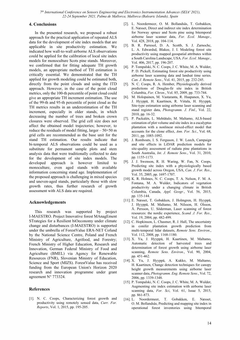
The objective of this study is to demonstrate how bitemporal ALS data can be used for the development of reliable site index models for Scots pine. We evaluated different methods of TH estimation based on ALS data and used these estimates as inputs for calibration of height growth models. TH was estimated based on segmentation of single tree crowns (ITD) and as the 100th, 99th and 95th percentiles of ALS point clouds. We also analysed the appropriateness of models developed with different plot size (0.01 ha, 0.09 ha and 0.25 ha). The accuracy of ALS-derived site index models was assessed by comparison to the
reference model developed based on the reconstruction of past height growth using stem analysis method (SA). We hypothesised that the method of the TH estimation from ALS data affects the obtained TH increment and therefore influence the height growth model trajectories. We assumed that a period of 8 years between subsequent ALS data acquisition is enough to acknowledge the interannual TH increment variability resulting from climate variations and other environmental factors; therefore the developed model would correctly express a height growth trajectories. 2. Methods 2.1. Acquisition and Pre-processing of the ALS Data
We used the repeated ALS point clouds from 2007 and 2015 for TH estimation. In both campaigns, ALS data were acquired in August after the end of height increment period. Technical specifications for the ALS sensor and data are presented in Table 1. A digital terrain model (DTM) with a spatial resolution of 0.5 m was generated in the TerraSolid software by the data provider. The DTM was used to normalize ALS point cloud heights to above ground level. Furthermore, a Canopy Height Model (CHM) with a spatial resolution of 0.5 m was generated using the PFSK method, where a pit-free CHM is the final product of the processing. 2.2. Calculation of TH from ALS Data
The calculation of TH from ALS data was made for the Scots pine stands composed of at least 90 % of stand volume by Scots pine. Each selected stand was
7th International Conference on Sensors Engineering and Electronics Instrumentation Advances (SEIA' 2021), 22-24 September 2021, Palma de Mallorca, Mallorca (Balearic Islands), Spain
11
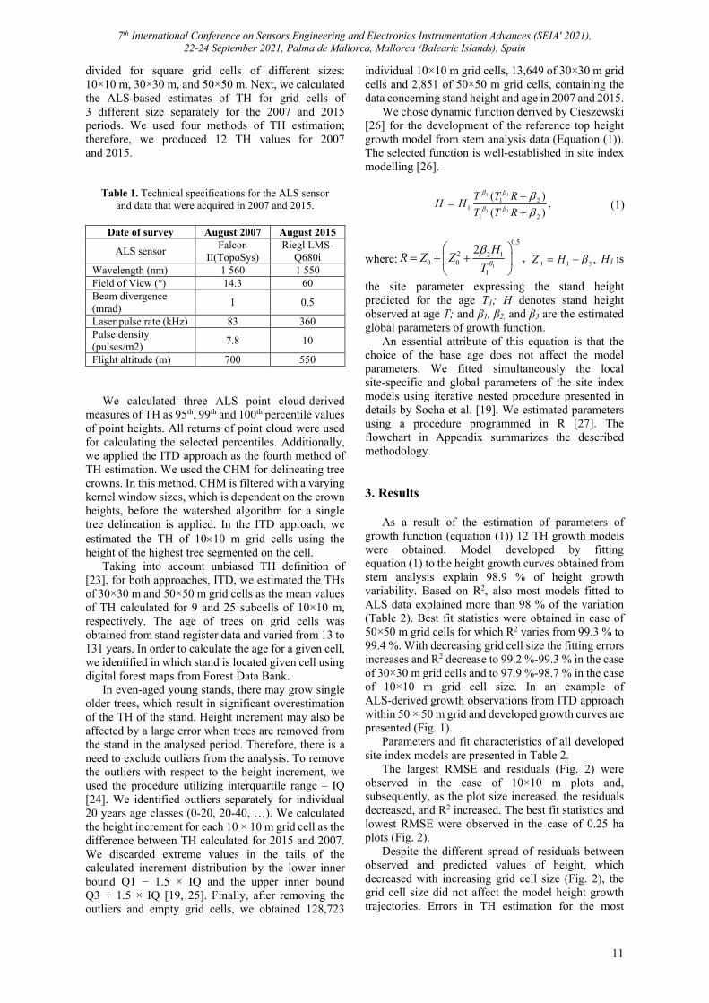
divided for square grid cells of different sizes: 10×10 m, 30×30 m, and 50×50 m. Next, we calculated the ALS-based estimates of TH for grid cells of 3 different size separately for the 2007 and 2015 periods. We used four methods of TH estimation; therefore, we produced 12 TH values for 2007 and 2015.
Table 1. Technical specifications for the ALS sensor and data that were acquired in 2007 and 2015.
Date of survey August 2007 August 2015
ALS sensor Falcon
II(TopoSys) Riegl LMS-
Q680i Wavelength (nm) 1 560 1 550 Field of View (°) 14.3 60 Beam divergence (mrad)
1 0.5
Laser pulse rate (kHz) 83 360 Pulse density (pulses/m2)
7.8 10
Flight altitude (m) 700 550
We calculated three ALS point cloud-derived measures of TH as 95th, 99th and 100th percentile values of point heights. All returns of point cloud were used for calculating the selected percentiles. Additionally, we applied the ITD approach as the fourth method of TH estimation. We used the CHM for delineating tree crowns. In this method, CHM is filtered with a varying kernel window sizes, which is dependent on the crown heights, before the watershed algorithm for a single tree delineation is applied. In the ITD approach, we estimated the TH of 1010 m grid cells using the height of the highest tree segmented on the cell.
Taking into account unbiased TH definition of [23], for both approaches, ITD, we estimated the THs of 30×30 m and 50×50 m grid cells as the mean values of TH calculated for 9 and 25 subcells of 10×10 m, respectively. The age of trees on grid cells was obtained from stand register data and varied from 13 to 131 years. In order to calculate the age for a given cell, we identified in which stand is located given cell using digital forest maps from Forest Data Bank.
In even-aged young stands, there may grow single older trees, which result in significant overestimation of the TH of the stand. Height increment may also be affected by a large error when trees are removed from the stand in the analysed period. Therefore, there is a need to exclude outliers from the analysis. To remove the outliers with respect to the height increment, we used the procedure utilizing interquartile range – IQ [24]. We identified outliers separately for individual 20 years age classes (0-20, 20-40, …). We calculated the height increment for each 10 × 10 m grid cell as the difference between TH calculated for 2015 and 2007. We discarded extreme values in the tails of the calculated increment distribution by the lower inner bound Q1 − 1.5 × IQ and the upper inner bound Q3 + 1.5 × IQ [19, 25]. Finally, after removing the outliers and empty grid cells, we obtained 128,723
individual 10×10 m grid cells, 13,649 of 30×30 m grid cells and 2,851 of 50×50 m grid cells, containing the data concerning stand height and age in 2007 and 2015.
We chose dynamic function derived by Cieszewski [26] for the development of the reference top height growth model from stem analysis data (Equation (1)). The selected function is well-established in site index modelling [26].
1 1
1 1
1 21
1 2
( ),
( )
T T RH H
T T R
(1)
where:1
0.5
2 2 10 0
1
2,
HR Z Z
T
0 1 3 ,Z H H1 is
the site parameter expressing the stand height predicted for the age T1; H denotes stand height observed at age T; and β1, β2, and β3 are the estimated global parameters of growth function.
An essential attribute of this equation is that the choice of the base age does not affect the model parameters. We fitted simultaneously the local site-specific and global parameters of the site index models using iterative nested procedure presented in details by Socha et al. [19]. We estimated parameters using a procedure programmed in R [27]. The flowchart in Appendix summarizes the described methodology. 3. Results
As a result of the estimation of parameters of growth function (equation (1)) 12 TH growth models were obtained. Model developed by fitting equation (1) to the height growth curves obtained from stem analysis explain 98.9 % of height growth variability. Based on R2, also most models fitted to ALS data explained more than 98 % of the variation (Table 2). Best fit statistics were obtained in case of 50×50 m grid cells for which R2 varies from 99.3 % to 99.4 %. With decreasing grid cell size the fitting errors increases and R2 decrease to 99.2 %-99.3 % in the case of 30×30 m grid cells and to 97.9 %-98.7 % in the case of 10×10 m grid cell size. In an example of ALS-derived growth observations from ITD approach within 50 × 50 m grid and developed growth curves are presented (Fig. 1).
Parameters and fit characteristics of all developed site index models are presented in Table 2.
The largest RMSE and residuals (Fig. 2) were observed in the case of 10×10 m plots and, subsequently, as the plot size increased, the residuals decreased, and R2 increased. The best fit statistics and lowest RMSE were observed in the case of 0.25 ha plots (Fig. 2).
Despite the different spread of residuals between observed and predicted values of height, which decreased with increasing grid cell size (Fig. 2), the grid cell size did not affect the model height growth trajectories. Errors in TH estimation for the most
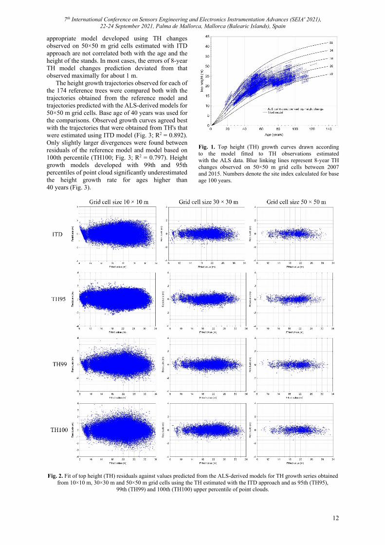
7th International Conference on Sensors Engineering and Electronics Instrumentation Advances (SEIA' 2021), 22-24 September 2021, Palma de Mallorca, Mallorca (Balearic Islands), Spain
12
appropriate model developed using TH changes observed on 50×50 m grid cells estimated with ITD approach are not correlated both with the age and the height of the stands. In most cases, the errors of 8-year TH model changes prediction deviated from that observed maximally for about 1 m.
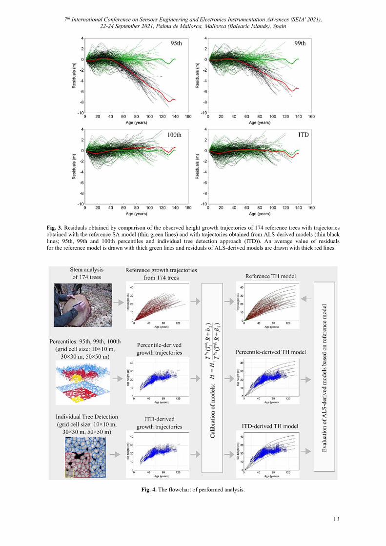
The height growth trajectories observed for each of the 174 reference trees were compared both with the trajectories obtained from the reference model and trajectories predicted with the ALS-derived models for 50×50 m grid cells. Base age of 40 years was used for the comparisons. Observed growth curves agreed best with the trajectories that were obtained from TH's that were estimated using ITD model (Fig. 3; R2 = 0.892). Only slightly larger divergences were found between residuals of the reference model and model based on 100th percentile (TH100; Fig. 3; R2 = 0.797). Height growth models developed with 99th and 95th percentiles of point cloud significantly underestimated the height growth rate for ages higher than 40 years (Fig. 3).
Fig. 1. Top height (TH) growth curves drawn according to the model fitted to TH observations estimated with the ALS data. Blue linking lines represent 8-year TH changes observed on 50×50 m grid cells between 2007 and 2015. Numbers denote the site index calculated for base age 100 years.
Fig. 2. Fit of top height (TH) residuals against values predicted from the ALS-derived models for TH growth series obtained from 10×10 m, 30×30 m and 50×50 m grid cells using the TH estimated with the ITD approach and as 95th (TH95),
99th (TH99) and 100th (TH100) upper percentile of point clouds.
7th International Conference on Sensors Engineering and Electronics Instrumentation Advances (SEIA' 2021), 22-24 September 2021, Palma de Mallorca, Mallorca (Balearic Islands), Spain
13
Fig. 3. Residuals obtained by comparison of the observed height growth trajectories of 174 reference trees with trajectories obtained with the reference SA model (thin green lines) and with trajectories obtained from ALS-derived models (thin black lines; 95th, 99th and 100th percentiles and individual tree detection approach (ITD)). An average value of residuals for the reference model is drawn with thick green lines and residuals of ALS-derived models are drawn with thick red lines.
Fig. 4. The flowchart of performed analysis.
7th International Conference on Sensors Engineering and Electronics Instrumentation Advances (SEIA' 2021), 22-24 September 2021, Palma de Mallorca, Mallorca (Balearic Islands), Spain
14
4. Conclusions
In the presented research, we proposed a robust approach for the practical application of repeated ALS data for the development of site index models that are applicable in site productivity estimation. We indicated how wall-to-wall airborne ALS observations could be applied for the calibration of local site index models for monoculture Scots pine stands. Moreover, we confirmed that for fitting adequate TH growth models, an appropriate method of TH estimation is critically essential. We demonstrated that the TH applied for growth modeling could be estimated both, directly from the point clouds and using the ITD approach. However, in the case of the point cloud metrics, only the 100-th percentile of point cloud could give an appropriate TH increment estimation. The use of the 99-th and 95-th percentile of point cloud as the TH metrics results in an underestimation of the TH increment, especially in older stands, in which decreasing the number of trees and broken crown closures were observed. The grid cell size does not affect the obtained model trajectories; however, to reduce the residuals of model fitting, larger – 50×50 m grid cells are recommended as the base unit for the stand TH estimation. Our results indicate that bi-temporal ALS observations could be used as a substitute for permanent sample plots and stem analysis data that were traditionally collected to date for the development of site index models. The developed approach is however limited to monoculture, even aged stands with available information concerning stand age. Implementation of the proposed approach is challenging in mixed species and uneven-aged stands, particularly those with slow growth rates, thus further research of growth assessment with ALS data are required.
Acknowledgements
This research was supported by project I-MAESTRO. Project Innovative forest MAnagEment STrategies for a Resilient biOeconomy under climate change and disturbances (I-MAESTRO) is supported under the umbrella of ForestValue ERA-NET Cofund by the National Science Centre, Poland and French Ministry of Agriculture, Agrifood, and Forestry; French Ministry of Higher Education, Research and Innovation, German Federal Ministry of Food and Agriculture (BMEL) via Agency for Renewable Resources (FNR), Slovenian Ministry of Education, Science and Sport (MIZS). ForestValue has received funding from the European Union's Horizon 2020 research and innovation programme under grant agreement N° 773324.
References [1]. N. C. Coops, Characterizing forest growth and
productivity using remotely sensed data, Curr. For. Reports, Vol. 1, 2015, pp. 195-205.
[2]. L. Noordermeer, O. M. Bollandsås, T. Gobakken, E. Næsset, Direct and indirect site index determination for Norway spruce and Scots pine using bitemporal airborne laser scanner data, For. Ecol. Manage., Vol. 428, 2018, pp. 104-114.
[3]. B. R. Parresol, D. A. Scottb, S. J. Zarnochc, L. A. Edwardsd, Blakee, J. I. Modeling forest site productivity using mapped geospatial attributes within a South Carolina Landscape, USA. For. Ecol. Manage., Vol. 406, 2017, pp. 196-207.
[4]. P. Tompalski, N. C. Coops, J. C. White, M. A. Wulder, P. D. Pickell, Estimating forest site productivity using airborne laser scanning data and landsat time series. Can. J. Remote Sens., Vol. 41, 2015, pp. 232-245.
[5]. N. C. Coops, R. A. Hember, Physiologically derived predictions of Douglas-fir site index in British Columbia, For. Chron., Vol. 85, 2009, pp. 733-744.
[6]. M. Holopainen, M. Vastaranta, R. Haapanen, X. Yu, J. Hyyppä, H. Kaartinen, R. Viitala, H. Hyyppä, Site-type estimation using airborne laser scanning and stand register data, Photogramm. J. Finl., Vol. 22, 2010, pp. 16-32.
[7]. P. Packalén, L. Mehtätalo, M. Maltamo, ALS-based estimation of plot volume and site index in a eucalyptus plantation with a nonlinear mixed-effect model that accounts for the clone effect, Ann. For. Sci., Vol. 68, 2011, pp. 1085-1092.
[8]. J. Rombouts, I. S. Ferguson, J. W. Leech, Campaign and site effects in LiDAR prediction models for site-quality assessment of radiata pine plantations in South Australia, Int. J. Remote Sens., Vol. 31, 2010, pp. 1155-1173.
[9]. J. J. Swenson, R. H. Waring, W. Fan, N. Coops, Predicting site index with a physiologically based growth model across Oregon, USA, Can. J. For. Res., Vol. 35, 2005, pp. 1697-1707.
[10]. K. R. Holmes, N. C. Coops, T. A. Nelson, F. M. A. Fontana, M. A. Wulder, Indicators of vegetation productivity under a changing climate in British Columbia, Canada, Appl. Geogr., Vol. 56, 2015, pp. 135-144.
[11]. E. Næsset, T. Gobakken, J. Holmgren, H. Hyyppä, J. Hyyppä, M. Maltamo, M. Nilsson, H. Olsson, Å. Persson, U. Söderman, Laser scanning of forest resources: the nordic experience, Scand. J. For. Res., Vol. 19, 2004, pp. 482-499.
[12]. C. Hopkinson, L. Chasmer, R. J. Hall, The uncertainty in conifer plantation growth prediction from multi-temporal lidar datasets, Remote Sens. Environ., Vol. 112, 2008, pp. 1168-1180.
[13]. X. Yu, J. Hyyppä, H. Kaartinen, M. Maltamo, Automatic detection of harvested trees and determination of forest growth using airborne laser scanning, Remote Sens. Environ., Vol. 90, 2004, pp. 451-462.
[14]. X. Yu, J. Hyyppä, A. Kukko, M. Maltamo, H. Kaartinen, Change detection techniques for canopy height growth measurements using airborne laser scanner data, Photogramm. Eng. Remote Sens., Vol. 72, 2006, pp. 1339-1348.
[15]. P. Tompalski, N. C. Coops, J. C. White, M. A. Wulder, Augmenting site index estimation with airborne laser scanning data, For. Sci, Vol. 61, Issue 5, 2015, pp. 861-873.
[16]. L. Noordermeer, T. Gobakken, E. Næsset, O. M. Bollandsås, Predicting and mapping site index in operational forest inventories using bitemporal
7th International Conference on Sensors Engineering and Electronics Instrumentation Advances (SEIA' 2021), 22-24 September 2021, Palma de Mallorca, Mallorca (Balearic Islands), Spain
15
airborne laser scanner data. For. Ecol. Manage., Vol. 457, 2020, 117768.
[17]. S. Solberg, H. Kvaalen, S. Puliti, Age-independent site index mapping with repeated single-tree airborne laser scanning, Scand. J. For. Res., Vol. 34, Issue, 2019, pp. 763-770.
[18]. C. Véga, B. St-Onge, Height growth reconstruction of a boreal forest canopy over a period of 58 years using a combination of photogrammetric and lidar models, Remote Sens. Environ., Vol. 112, 2008, pp. 1784-1794.
[19]. J. Socha, M. Pierzchalski, R. Bałazy, M. Ciesielski, Modelling top height growth and site index using repeated laser scanning data, For. Ecol. Manage., Vol. 406, 2017, pp. 307-3017.
[20]. Y. Erfanifard, K. Stereńczak, B. Kraszewski, A. Kamińska, Development of a robust canopy height model derived from ALS point clouds for predicting individual crown attributes at the species level, Int. J. Remote Sens., Vol. 39, 2018, pp. 1-22.
[21]. S. Miścicki, K. Stereńczak, A two-phase inventory method for calculating standing volume and tree-density of forest stands in central Poland based on
airborne laser-scanning data, For. Res. Pap., Vol. 74, 2013, pp. 127-136.
[22]. K. Stereńczak, B. Kraszewski, M. Mielcarek, Ż. Piasecka, Inventory of standing dead trees in the surroundings of communication routes – The contribution of remote sensing to potential risk assessments, For. Ecol. Manage., Vol. 402, 2017, pp. 76-91.
[23]. K. Rennolls, Top height: its definition and estimation, Commonw. For. Rev., Vol. 57, 1978, pp. 215-219.
[24]. J. W. Tukey, Exploratory Data Analysis, Addison-Wesley, 1977.
[25]. D. A. Antony, G. Singh, Model-based outlier detection system with statistical preprocessing model – based outlier detection system with, J. Mod. Appl. Stat. Methods, Vol. 15, 2016, 39.
[26]. C. J. Cieszewski, Three methods of deriving advanced dynamic site equations demonstrated on inland Douglas-fir site curves, Can. J. For. Res. For., Vol. 31, 2001, pp. 165-173.
[27]. R Core Team, R: A Language and Environment for Statistical Computing, http://www.R-project.org/
7th International Conference on Sensors Engineering and Electronics Instrumentation Advances (SEIA' 2021), 22-24 September 2021, Palma de Mallorca, Mallorca (Balearic Islands), Spain
16
(002)
A Review of Energy Consumption Measurement Systems with Applications in Wireless Sensor Networks
F. Barišić and H. Hegeduš
University of Zagreb, Faculty of Electrical Engineering and Computing, Unska 3, 10000 Zagreb, Croatia Tel.: + 385 91 72 480 72
E-mail: [email protected] Summary: Internet of Things (IoT), as a technology concept, is getting every year more attention and importance. Therefore, Wireless Sensor Network (WSN) as one of the key IoT’s technologies has become an important one for monitoring multiple values such as temperature, humidity, pressure, different sorts of gases, particles etc. In this paper area of energy consumption measurement systems with applications in Wireless Sensor Networks (WSNs) is covered in a way that most important parts of WSNs are mentioned, both commercial sensor nodes and data acquisition systems and their current drains. Also, various measurement setups presented in scientific papers are described and compared. Keywords: Wireless Sensor Networks, Measurement system, Energy consumption measurement, Wireless communication, Data transmission, Sensor node.
1. Introduction
Nowadays, Internet of Things (IoT), as a technology concept, is getting huge attention and importance. Wireless Sensor Network (WSN) as one of the key IoT’s technologies has become an important one for monitoring multiple values, especially in an area of environmental monitoring such as temperature, humidity, pressure, different sorts of gases, particles etc. [1-3]. Also, there are examples of WSN for monitoring other non-electrical values such as dynamic acceleration of infrastructure [4]. Many scientific papers considering this area are doing development of WSN in multiple occasions. Main goal of those developed systems is to measure physical values in real time.
However, biggest constraint for long term autonomous operation of WSN is energy consumption. To better estimate battery lifetime we need to be able to measure energy consumption of sensor nodes, microcontroller unit [2, 5]. There is also a case where we already have information about battery lifetime but we need to validate it, or we want some additional specific detail about the energy consumption of the whole WSN. Important to mention, under term energy consumption measurement we usually measure current consumption during some time interval or number of coulombs. In some papers term power consumption is used, but it is a synonym for energy consumption [6]. To make energy consumption measurement possible different measurement devices are used such as oscilloscopes [3, 7, 8], Digital Multi Meters (DMMs) [3, 10], current sensors [5] and shunts [3]. In most of papers considering energy consumption measurement of WSNs some typical actions were considered and their related energy consumptions. Some of them are data transmission and reception, wake-up from sleep state, measurement process and some papers made research about dependence between energy
consumption and different security algorithms applied in WSN [3, 9].
The remaining part of the paper is structured as follows. In Section 2 different sensor nodes and their parts, especially RF modules, are presented. For most of these sensor nodes and RF modules energy consumption values are mentioned. In Section 3 commercial energy consumption measurement systems are presented and in the second part various measurement system setups from various scientific papers are described. In last section, conclusion is written, recaption is made and future work is covered. 2. Sensor Nodes Energy Consumption
In this section various sensor nodes and their parts used in scientific research are presented and described. Usually, the aim of sensor node research, considering the area of energy consumption measurement, is to investigate how much energy they use in different mode of work, while using different communication protocols and how to integrate them efficiently as a part of a whole WSN. In papers typical mode of works that are investigated are sleep mode, idle state, wake up routine, data transmission and reception. Also, many correlations are presented considering energy consumption such as number of sensor nodes and cumulative energy consumption of the system, usage of different communication protocols for data transmission on the same sensor node and their comparison. Length of duty cycles depending on sleep time and their impact on energy consumption are also presented.
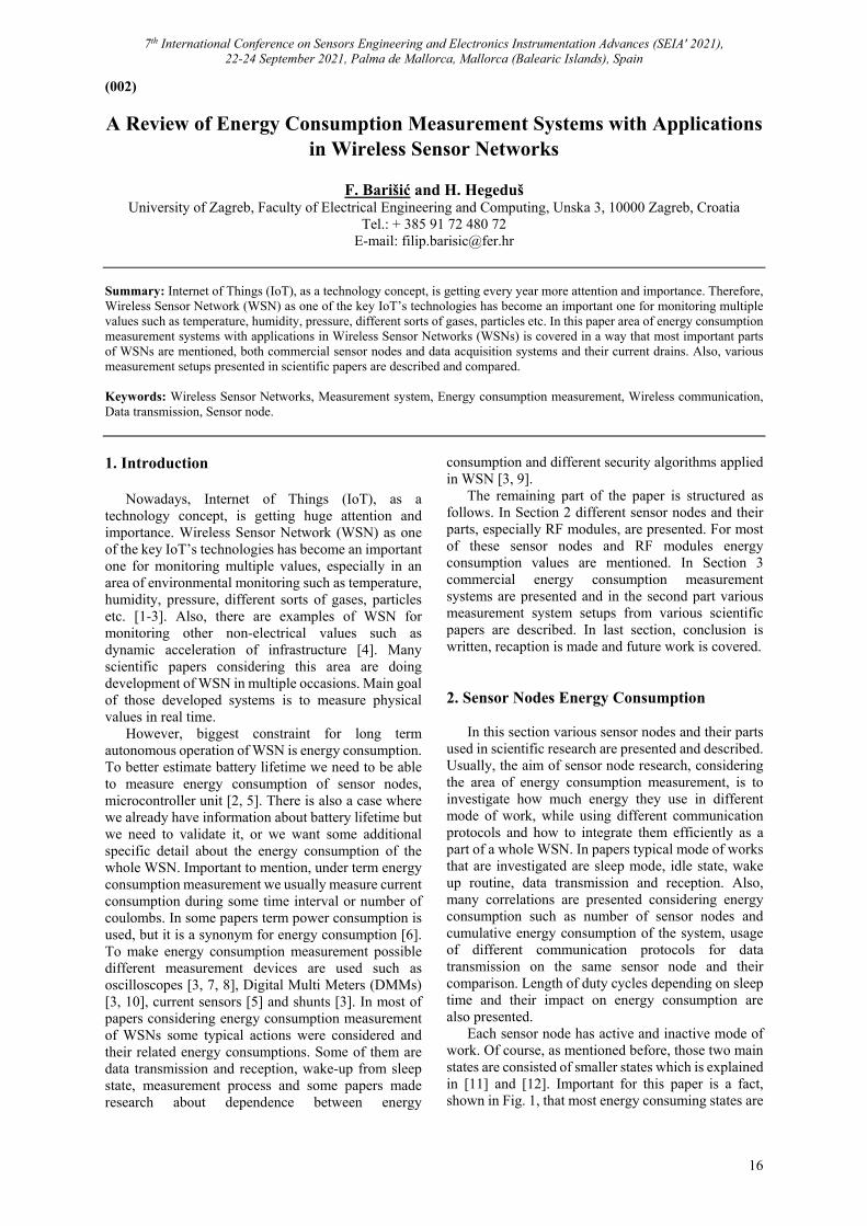
Each sensor node has active and inactive mode of work. Of course, as mentioned before, those two main states are consisted of smaller states which is explained in [11] and [12]. Important for this paper is a fact, shown in Fig. 1, that most energy consuming states are
7th International Conference on Sensors Engineering and Electronics Instrumentation Advances (SEIA' 2021), 22-24 September 2021, Palma de Mallorca, Mallorca (Balearic Islands), Spain
17
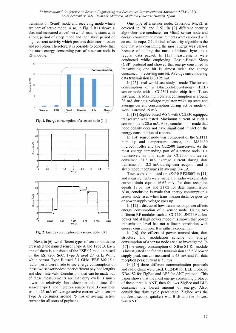
transmission (Send) mode and receiving mode which are part of active mode. Also, in Fig. 2 it is shown a classical measured waveform which usually starts with a long period of sleep mode and then short period of high-current activity which presents data transmission and reception. Therefore, it is possible to conclude that the most energy consuming part of a sensor node is RF module.
Fig. 1. Energy consumption of a sensor node [14].
Fig. 2. Energy consumption of a sensor node [24]. Next, in [6] two different types of sensor nodes are
presented and named sensor Type A and Type B. Each one of them is consisted of the ESP-07 module based on the ESP8266 SoC. Type A used 2.4 GHz WiFi, while sensor Type B used 2.4 GHz IEEE 802.15.4 radio. Tests were made to see energy consumption of these two sensor nodes under different payload lengths and sleep intervals. Conclusions that can be made out of these measurements are that duty cycle is much lower for relatively short sleep period of times for sensor Type B and therefore sensor Type B consumes around 25 mA of average active current while sensor Type A consumes around 75 mA of average active current for all sorts of payloads.
One type of a sensor node, Crossbow Mica2, is covered in [9] and [15]. In [9] different security algorithms are conducted on Mica2 sensor node and energy consumption measurements were captured with an oscilloscope. Of all kinds of security algorithms the one that was consuming the most energy was SHA-1 because of adding the most additional bytes to a regular data packet. In [15] measurements were conducted while employing Gossip-Based Sleep (GSP) protocol and showed that energy consumed in transmitting one bit is almost twice the energy consumed in receiving one bit. Average current during data transmission is 30.95 mA.
In [25] a real-world case study is made. The current consumption of a Bluetooth-Low-Energy (BLE) sensor node with a CC2541 radio chip from Texas Instruments. Maximum current consumption is around 26 mA during a voltage regulator wake up state and average current consumption during active mode of work is around 19 mA.
In [13] ZigBee-based WSN with CC2530 equipped transceiver was tested. Maximum current of such a sensor node is 20.6 mA. Also, conclusion is made that node density does not have significant impact on the energy consumption of routers.
In [14] sensor node was composed of the SHT11 humidity and temperature sensor, the MSP430 microcontroller and the CC2500 transceiver. As the most energy demanding part of a sensor node is a transceiver, in this case the CC2500 transceiver consumed 21.2 mA average current during data transmission, 12.8 mA during data reception and in sleep mode it consumes in average 0.4 µA.
Tests were conducted on eZ430-RF2500T in [11] and measurements were made. For radio wakeup state current drain equals 16.62 mA, for data reception equals 18.08 mA and 21.02 for data transmission. Also, conclusion is made that energy consumption a sensor node rises when transmission distance goes up or power supply voltage goes up.
In [12] is discussed how transmission power affects energy consumption of a sensor node. Using two different RF modules such as CC2420, JN5139 at low power and at high power mode it is shown that power transmission level has not a linear correlation with energy consumption. It is rather exponential.
It [16], the effects of power transmission, data structure and modulation scheme on energy consumption of a sensor node are also investigated. In [17] the energy consumption of XBee S1 RF module is investigated and for data transmission at 3.3 V power supply peak current measured is 45 mA and for data reception peak current is 50 mA.
In [10] three different communication protocols and radio chips were used. CC2450 for BLE protocol, XBee S2 for ZigBee and AP2 for ANT protocol. This paper shows that the most energy consuming protocol of these three is ANT, then follows ZigBee and BLE consumes the lowest amount of energy. Also, considering duty cycle percentage, ZigBee was the quickest, second quickest was BLE and the slowest was ANT.
7th International Conference on Sensors Engineering and Electronics Instrumentation Advances (SEIA' 2021), 22-24 September 2021, Palma de Mallorca, Mallorca (Balearic Islands), Spain
18
3. Energy Consumption Measurement Systems
In this section various energy consumption measurement systems are introduced. These systems help to optimize energy consumption, make better battery management system and make system work longer than it used to do. As it is mentioned in previous section, usual current values that are measured in WSNs are moving from a couple of dozen microamperes (µA) to a couple of hundred milliamperes (mA). Therefore, it is relevant for these systems to have a good precision, accuracy, resolution and measurement range. Eventually, it could be important to have information about its own energy consumption, especially if it is battery operated and part of autonomous WSN which is powered with 12 VDC battery.
In various scientific papers different setups are introduced for sensor node energy consumption measurement. Many of them are sensor node by itself. Mostly, the aim of those papers is to create an electric circuit with low cost and low energy consumption, capable of measuring energy consumption of a sensor node.
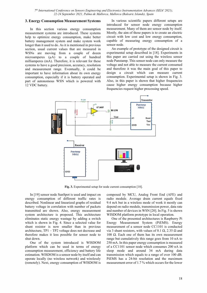
An example of prototype of the designed circuit is experimental setup described in [18]. Experiments in this paper are carried out using the wireless sensor node Panstamp. This sensor node can only measure the voltage and not able to measure the current consumed and therefore it was the main goal of this paper to design a circuit which can measure current consumption. Experimental setup is shown in Fig. 3. Also, in this paper is shown that higher frequencies cause higher energy consumption because higher frequencies request higher processing speed.
Fig. 3. Experimental setup for node current consumption [18]. In [19] sensor node SunSpot is used and impact on
energy consumption of different traffic rates is described. Nonlinear and linearized graphs of residual battery voltage in correlation with number of packets transmitted are shown. Also, energy measurement system architecture is proposed. This architecture eliminates static energy wastage by adding a switch which is shown in Fig. 4. Since a selected value for shunt resistor is now smaller than in previous architecture, TP1 – TP2 voltage does not decrease and therefore makes it less possible for sensor node to shut down.
One of the system introduced is WISDOM platform which can be used in terms of energy consumption measurement, efficiency and battery life estimation. WISDOM is a sensor node by itself and can operate locally (no wireless network) and wirelessly (remotely). Next, energy consumption of WISDOM is
composed by MCU, Analog Front End (AFE) and radio module. Average drain current equals fixed 9.4 mA but in a wireless mode of work it mostly can depend on radio module, transmission power, data rate and number of devices in WSN [20]. In Fig. 5 is shown WISDOM platform prototype in local operation.
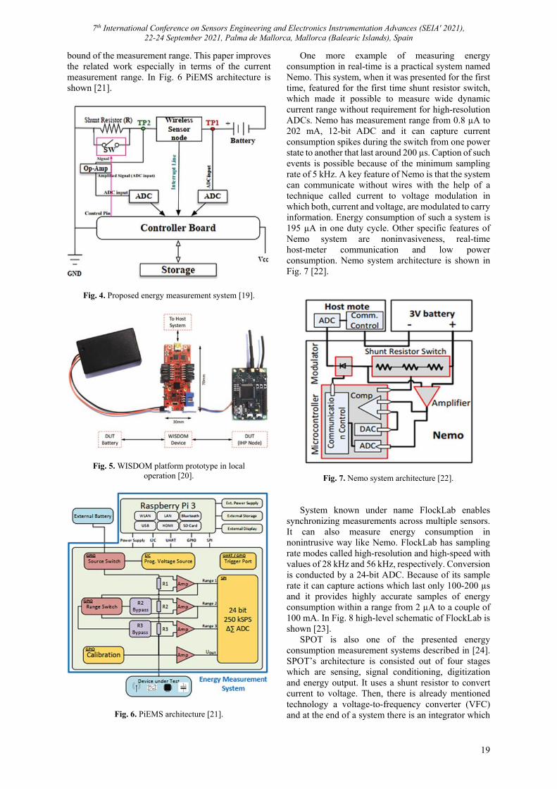
One of the presented architectures is Raspberry Pi Energy Measurement System (PiEMS). Energy measurement of a sensor node CC1101 is conducted via 3 shunt resistors, with values of 0.1 Ω, 2.35 Ω and 100 Ω. Each one of them has its own measurement range but cumulatively this range goes from 10 nA to 250 mA. In this paper energy consumption is measured of a CC1101 sensor node which consumes 200 nA in sleep mode and around 34 mA during data transmission which equals to a range of over 100 dB. PiEMS has a 24-bit resolution and the maximum measurement error of 1.7 % which occurs for the lower
7th International Conference on Sensors Engineering and Electronics Instrumentation Advances (SEIA' 2021), 22-24 September 2021, Palma de Mallorca, Mallorca (Balearic Islands), Spain
19
bound of the measurement range. This paper improves the related work especially in terms of the current measurement range. In Fig. 6 PiEMS architecture is shown [21].
Fig. 4. Proposed energy measurement system [19].
Fig. 5. WISDOM platform prototype in local operation [20].
Fig. 6. PiEMS architecture [21].
One more example of measuring energy consumption in real-time is a practical system named Nemo. This system, when it was presented for the first time, featured for the first time shunt resistor switch, which made it possible to measure wide dynamic current range without requirement for high-resolution ADCs. Nemo has measurement range from 0.8 µA to 202 mA, 12-bit ADC and it can capture current consumption spikes during the switch from one power state to another that last around 200 µs. Caption of such events is possible because of the minimum sampling rate of 5 kHz. A key feature of Nemo is that the system can communicate without wires with the help of a technique called current to voltage modulation in which both, current and voltage, are modulated to carry information. Energy consumption of such a system is 195 µA in one duty cycle. Other specific features of Nemo system are noninvasiveness, real-time host-meter communication and low power consumption. Nemo system architecture is shown in Fig. 7 [22].
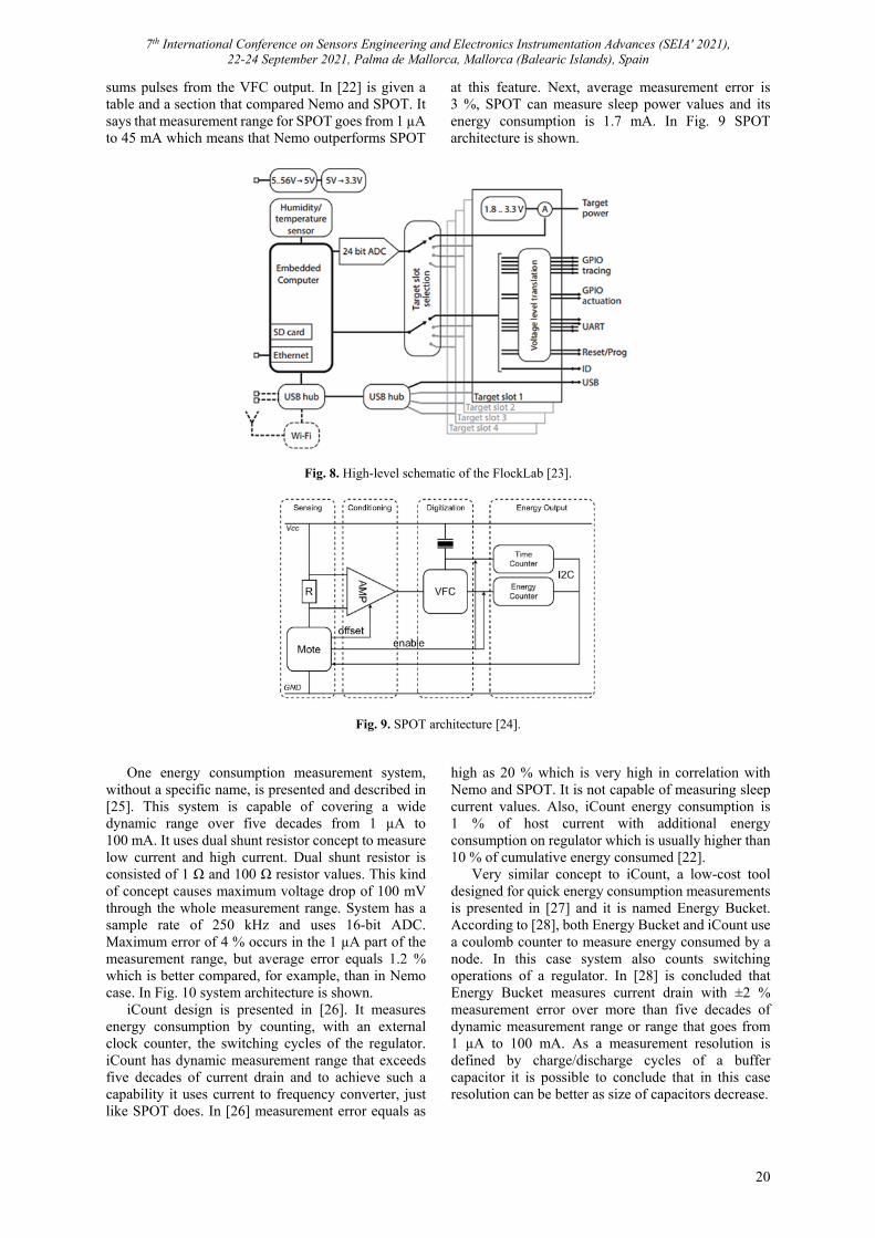
Fig. 7. Nemo system architecture [22]. System known under name FlockLab enables
synchronizing measurements across multiple sensors. It can also measure energy consumption in nonintrusive way like Nemo. FlockLab has sampling rate modes called high-resolution and high-speed with values of 28 kHz and 56 kHz, respectively. Conversion is conducted by a 24-bit ADC. Because of its sample rate it can capture actions which last only 100-200 µs and it provides highly accurate samples of energy consumption within a range from 2 µA to a couple of 100 mA. In Fig. 8 high-level schematic of FlockLab is shown [23].
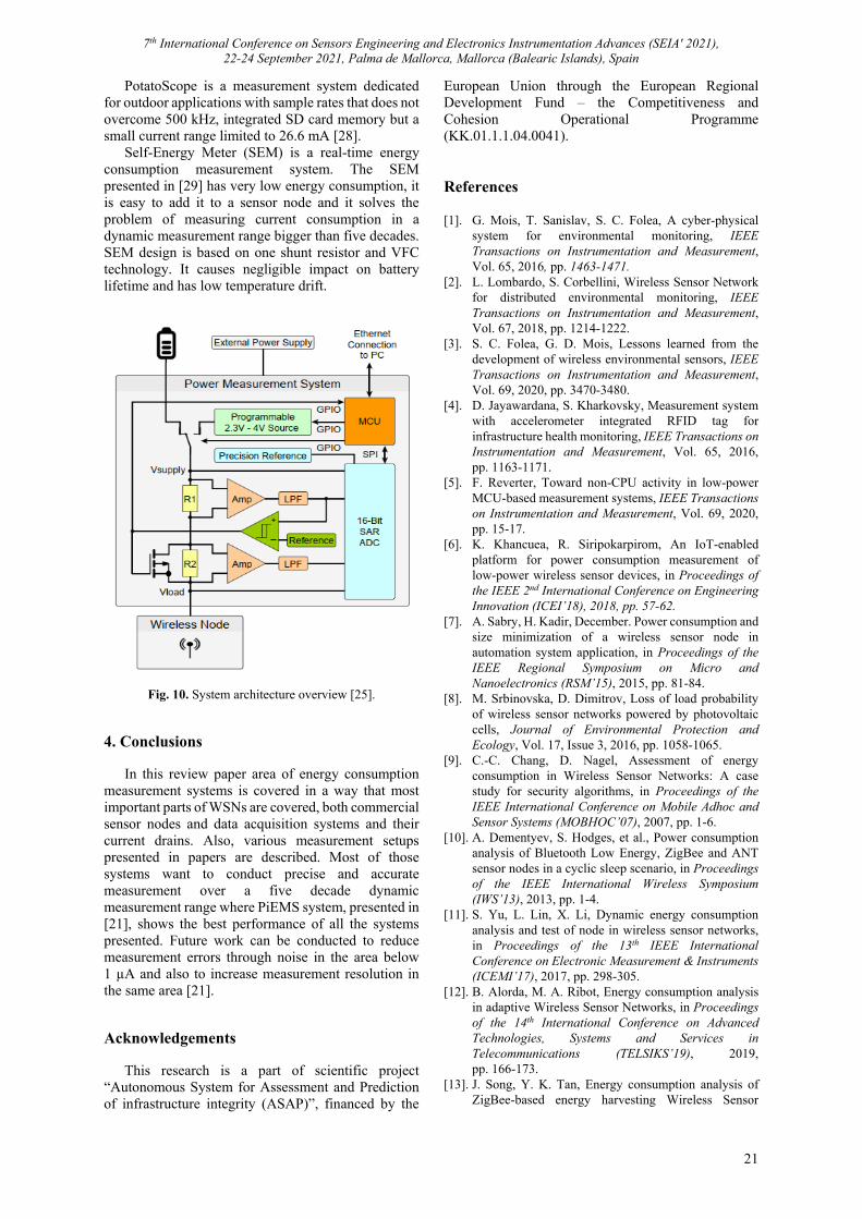
SPOT is also one of the presented energy consumption measurement systems described in [24]. SPOT’s architecture is consisted out of four stages which are sensing, signal conditioning, digitization and energy output. It uses a shunt resistor to convert current to voltage. Then, there is already mentioned technology a voltage-to-frequency converter (VFC) and at the end of a system there is an integrator which
7th International Conference on Sensors Engineering and Electronics Instrumentation Advances (SEIA' 2021), 22-24 September 2021, Palma de Mallorca, Mallorca (Balearic Islands), Spain
20
sums pulses from the VFC output. In [22] is given a table and a section that compared Nemo and SPOT. It says that measurement range for SPOT goes from 1 µA to 45 mA which means that Nemo outperforms SPOT
at this feature. Next, average measurement error is 3 %, SPOT can measure sleep power values and its energy consumption is 1.7 mA. In Fig. 9 SPOT architecture is shown.
Fig. 8. High-level schematic of the FlockLab [23].
Fig. 9. SPOT architecture [24]. One energy consumption measurement system,
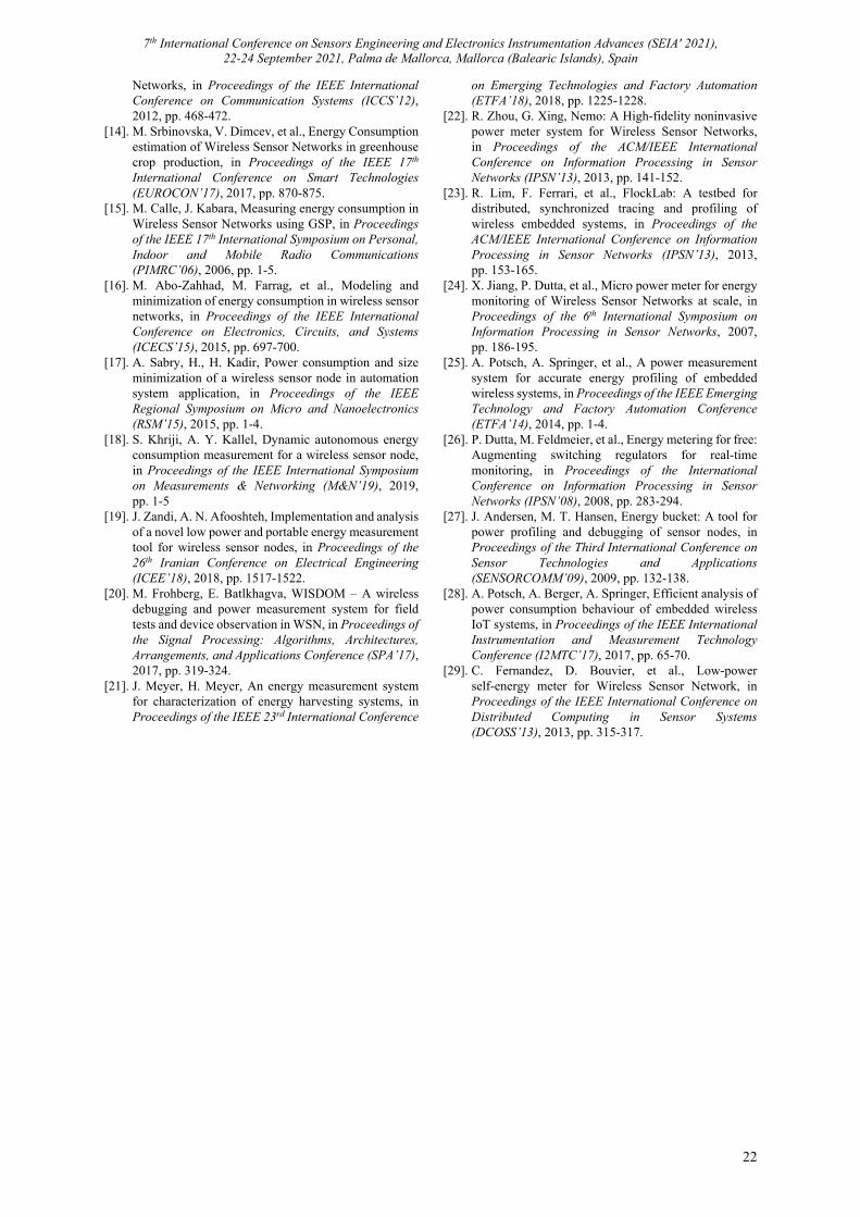
without a specific name, is presented and described in [25]. This system is capable of covering a wide dynamic range over five decades from 1 µA to 100 mA. It uses dual shunt resistor concept to measure low current and high current. Dual shunt resistor is consisted of 1 Ω and 100 Ω resistor values. This kind of concept causes maximum voltage drop of 100 mV through the whole measurement range. System has a sample rate of 250 kHz and uses 16-bit ADC. Maximum error of 4 % occurs in the 1 µA part of the measurement range, but average error equals 1.2 % which is better compared, for example, than in Nemo case. In Fig. 10 system architecture is shown.
iCount design is presented in [26]. It measures energy consumption by counting, with an external clock counter, the switching cycles of the regulator. iCount has dynamic measurement range that exceeds five decades of current drain and to achieve such a capability it uses current to frequency converter, just like SPOT does. In [26] measurement error equals as
high as 20 % which is very high in correlation with Nemo and SPOT. It is not capable of measuring sleep current values. Also, iCount energy consumption is 1 % of host current with additional energy consumption on regulator which is usually higher than 10 % of cumulative energy consumed [22].
Very similar concept to iCount, a low-cost tool designed for quick energy consumption measurements is presented in [27] and it is named Energy Bucket. According to [28], both Energy Bucket and iCount use a coulomb counter to measure energy consumed by a node. In this case system also counts switching operations of a regulator. In [28] is concluded that Energy Bucket measures current drain with ±2 % measurement error over more than five decades of dynamic measurement range or range that goes from 1 µA to 100 mA. As a measurement resolution is defined by charge/discharge cycles of a buffer capacitor it is possible to conclude that in this case resolution can be better as size of capacitors decrease.
7th International Conference on Sensors Engineering and Electronics Instrumentation Advances (SEIA' 2021), 22-24 September 2021, Palma de Mallorca, Mallorca (Balearic Islands), Spain
21
PotatoScope is a measurement system dedicated for outdoor applications with sample rates that does not overcome 500 kHz, integrated SD card memory but a small current range limited to 26.6 mA [28].
Self-Energy Meter (SEM) is a real-time energy consumption measurement system. The SEM presented in [29] has very low energy consumption, it is easy to add it to a sensor node and it solves the problem of measuring current consumption in a dynamic measurement range bigger than five decades. SEM design is based on one shunt resistor and VFC technology. It causes negligible impact on battery lifetime and has low temperature drift.
Fig. 10. System architecture overview [25].
4. Conclusions
In this review paper area of energy consumption measurement systems is covered in a way that most important parts of WSNs are covered, both commercial sensor nodes and data acquisition systems and their current drains. Also, various measurement setups presented in papers are described. Most of those systems want to conduct precise and accurate measurement over a five decade dynamic measurement range where PiEMS system, presented in [21], shows the best performance of all the systems presented. Future work can be conducted to reduce measurement errors through noise in the area below 1 µA and also to increase measurement resolution in the same area [21]. Acknowledgements
This research is a part of scientific project “Autonomous System for Assessment and Prediction of infrastructure integrity (ASAP)”, financed by the
European Union through the European Regional Development Fund – the Competitiveness and Cohesion Operational Programme (KK.01.1.1.04.0041). References [1]. G. Mois, T. Sanislav, S. C. Folea, A cyber-physical
system for environmental monitoring, IEEE Transactions on Instrumentation and Measurement, Vol. 65, 2016, pp. 1463-1471.
[2]. L. Lombardo, S. Corbellini, Wireless Sensor Network for distributed environmental monitoring, IEEE Transactions on Instrumentation and Measurement, Vol. 67, 2018, pp. 1214-1222.
[3]. S. C. Folea, G. D. Mois, Lessons learned from the development of wireless environmental sensors, IEEE Transactions on Instrumentation and Measurement, Vol. 69, 2020, pp. 3470-3480.
[4]. D. Jayawardana, S. Kharkovsky, Measurement system with accelerometer integrated RFID tag for infrastructure health monitoring, IEEE Transactions on Instrumentation and Measurement, Vol. 65, 2016, pp. 1163-1171.
[5]. F. Reverter, Toward non-CPU activity in low-power MCU-based measurement systems, IEEE Transactions on Instrumentation and Measurement, Vol. 69, 2020, pp. 15-17.
[6]. K. Khancuea, R. Siripokarpirom, An IoT-enabled platform for power consumption measurement of low-power wireless sensor devices, in Proceedings of the IEEE 2nd International Conference on Engineering Innovation (ICEI’18), 2018, pp. 57-62.
[7]. A. Sabry, H. Kadir, December. Power consumption and size minimization of a wireless sensor node in automation system application, in Proceedings of the IEEE Regional Symposium on Micro and Nanoelectronics (RSM’15), 2015, pp. 81-84.
[8]. M. Srbinovska, D. Dimitrov, Loss of load probability of wireless sensor networks powered by photovoltaic cells, Journal of Environmental Protection and Ecology, Vol. 17, Issue 3, 2016, pp. 1058-1065.
[9]. C.-C. Chang, D. Nagel, Assessment of energy consumption in Wireless Sensor Networks: A case study for security algorithms, in Proceedings of the IEEE International Conference on Mobile Adhoc and Sensor Systems (MOBHOC’07), 2007, pp. 1-6.
[10]. A. Dementyev, S. Hodges, et al., Power consumption analysis of Bluetooth Low Energy, ZigBee and ANT sensor nodes in a cyclic sleep scenario, in Proceedings of the IEEE International Wireless Symposium (IWS’13), 2013, pp. 1-4.
[11]. S. Yu, L. Lin, X. Li, Dynamic energy consumption analysis and test of node in wireless sensor networks, in Proceedings of the 13th IEEE International Conference on Electronic Measurement & Instruments (ICEMI’17), 2017, pp. 298-305.
[12]. B. Alorda, M. A. Ribot, Energy consumption analysis in adaptive Wireless Sensor Networks, in Proceedings of the 14th International Conference on Advanced Technologies, Systems and Services in Telecommunications (TELSIKS’19), 2019, pp. 166-173.
[13]. J. Song, Y. K. Tan, Energy consumption analysis of ZigBee-based energy harvesting Wireless Sensor
7th International Conference on Sensors Engineering and Electronics Instrumentation Advances (SEIA' 2021), 22-24 September 2021, Palma de Mallorca, Mallorca (Balearic Islands), Spain
22
Networks, in Proceedings of the IEEE International Conference on Communication Systems (ICCS’12), 2012, pp. 468-472.
[14]. M. Srbinovska, V. Dimcev, et al., Energy Consumption estimation of Wireless Sensor Networks in greenhouse crop production, in Proceedings of the IEEE 17th International Conference on Smart Technologies (EUROCON’17), 2017, pp. 870-875.
[15]. M. Calle, J. Kabara, Measuring energy consumption in Wireless Sensor Networks using GSP, in Proceedings of the IEEE 17th International Symposium on Personal, Indoor and Mobile Radio Communications (PIMRC’06), 2006, pp. 1-5.
[16]. M. Abo-Zahhad, M. Farrag, et al., Modeling and minimization of energy consumption in wireless sensor networks, in Proceedings of the IEEE International Conference on Electronics, Circuits, and Systems (ICECS’15), 2015, pp. 697-700.
[17]. A. Sabry, H., H. Kadir, Power consumption and size minimization of a wireless sensor node in automation system application, in Proceedings of the IEEE Regional Symposium on Micro and Nanoelectronics (RSM’15), 2015, pp. 1-4.
[18]. S. Khriji, A. Y. Kallel, Dynamic autonomous energy consumption measurement for a wireless sensor node, in Proceedings of the IEEE International Symposium on Measurements & Networking (M&N’19), 2019, pp. 1-5
[19]. J. Zandi, A. N. Afooshteh, Implementation and analysis of a novel low power and portable energy measurement tool for wireless sensor nodes, in Proceedings of the 26th Iranian Conference on Electrical Engineering (ICEE’18), 2018, pp. 1517-1522.
[20]. M. Frohberg, E. Batlkhagva, WISDOM – A wireless debugging and power measurement system for field tests and device observation in WSN, in Proceedings of the Signal Processing: Algorithms, Architectures, Arrangements, and Applications Conference (SPA’17), 2017, pp. 319-324.
[21]. J. Meyer, H. Meyer, An energy measurement system for characterization of energy harvesting systems, in Proceedings of the IEEE 23rd International Conference
on Emerging Technologies and Factory Automation (ETFA’18), 2018, pp. 1225-1228.
[22]. R. Zhou, G. Xing, Nemo: A High-fidelity noninvasive power meter system for Wireless Sensor Networks, in Proceedings of the ACM/IEEE International Conference on Information Processing in Sensor Networks (IPSN’13), 2013, pp. 141-152.
[23]. R. Lim, F. Ferrari, et al., FlockLab: A testbed for distributed, synchronized tracing and profiling of wireless embedded systems, in Proceedings of the ACM/IEEE International Conference on Information Processing in Sensor Networks (IPSN’13), 2013, pp. 153-165.
[24]. X. Jiang, P. Dutta, et al., Micro power meter for energy monitoring of Wireless Sensor Networks at scale, in Proceedings of the 6th International Symposium on Information Processing in Sensor Networks, 2007, pp. 186-195.
[25]. A. Potsch, A. Springer, et al., A power measurement system for accurate energy profiling of embedded wireless systems, in Proceedings of the IEEE Emerging Technology and Factory Automation Conference (ETFA’14), 2014, pp. 1-4.
[26]. P. Dutta, M. Feldmeier, et al., Energy metering for free: Augmenting switching regulators for real-time monitoring, in Proceedings of the International Conference on Information Processing in Sensor Networks (IPSN’08), 2008, pp. 283-294.
[27]. J. Andersen, M. T. Hansen, Energy bucket: A tool for power profiling and debugging of sensor nodes, in Proceedings of the Third International Conference on Sensor Technologies and Applications (SENSORCOMM’09), 2009, pp. 132-138.
[28]. A. Potsch, A. Berger, A. Springer, Efficient analysis of power consumption behaviour of embedded wireless IoT systems, in Proceedings of the IEEE International Instrumentation and Measurement Technology Conference (I2MTC’17), 2017, pp. 65-70.
[29]. C. Fernandez, D. Bouvier, et al., Low-power self-energy meter for Wireless Sensor Network, in Proceedings of the IEEE International Conference on Distributed Computing in Sensor Systems (DCOSS’13), 2013, pp. 315-317.
7th International Conference on Sensors Engineering and Electronics Instrumentation Advances (SEIA' 2021), 22-24 September 2021, Palma de Mallorca, Mallorca (Balearic Islands), Spain
23
(004)
Gravitational Search Algorithm-based Multi-hop Routing Scheme for Energy Efficient Heterogeneous Clustered Scheme
T. Sood and K. Sharma
Department of Electronics and Communication Engineering, NITTTR, 160019, Chandigarh, India Tel.: +91 7696889323
E-mail: [email protected] Summary: Restricted energy has always been a prime constraint in Wireless Sensor Network (WSN) which pose a threat to its operation. To efficiently utilize the attached energy resources over an elongated period, network can be partitioned into clusters. To further enhance the network routine, the proposed scheme targets the clustering rotation epoch and inter-cluster communication model between the upper tier of the network between the cluster head (CH) and the sink. In this paper, Gravitational Search Algorithm-based multi-hop routing scheme has been presented for a three-level energy heterogeneous WSN. The proposed scheme utilizes the gravitational search algorithm (GSA) to optimize the data route between the CH and the sink & additionally uses the conditional static rotation epoch. This scheme has been simulated using Network Simulator NS-2 and the results have been contrasted with the Energy Efficient Heterogeneous Clustering scheme (EEHC) to illustrate the advantages of the proposed work over the established work. Keywords: Wireless sensor network, Multi-hop routing, Heterogeneous, GSA, Optimization, Epoch.
1. Introduction
With wireless sensor network (WSN) becoming
one of the most interesting networking technologies, its communication infrastructure is of utmost importance with energy drainage being highest during data communication. WSN can be known as a network with nodes and a sink, where sink mainly serves as a gateway to some other networks or to the central monitoring system [1]. These nodes may either follow a direct communication path to the sink for packet transmission or have a multi-hop path to the sink. The direct communication with the sink causes every node in the network to have a one-hop communication with the sink. However, it has its own disadvantages.
Redundant data delivered at the sink of the network.
Exuberant network energy depletion. Shorter operative round iterations of the
network. However, to overcome these disadvantages,
Voronoi structure was introduced that utilized multi-hop communication model. Voronoi structure allows the nodes to be grouped into many clusters with each being governed by a similar node upholding the cluster head (CH) duty. This establishment helps reduce the redundancy at the sink while also manages the energy model of the network. However, multi-hop packet transmission from the source nodes to the sink introduces delay which formulates the need of research on optimizing the multi-hop channel route to the sink. An additional reason to assist the need of improvising the multi-hop route arises from the relation between the energy depletion during commutation (𝐸 .) and the commuting distance (𝑑) i.e., 𝐸 . 𝑓 𝑑 . Therefore, despite the introduction of a CH and its two-
hop model from the source nodes to the sink, it may require additional hops if the chosen CH is at a larger distance from the sink to avoid excess energy leakage during its CH-duty patrol. These additional hops should be chosen such that the energy efficiency also improves apart from the lifespan of the network. To achieve the aforementioned objectives, various heuristic methods have been opted that define the relay route for every CH for every round iteration. However, as the research further unfolded, apart from the heuristic approaches, many meta-heuristic approaches were also introduced that have been utilized in optimizing the route from the CH to the sink.
Many nature-inspired (physics/chemistry-based and bio-inspired) meta-heuristic algorithms like Genetic Algorithm (GA), Particle-Swarm Optimization (PSO), Ant-Colony Optimization (ACO), Gravitational Search Algorithm (GSA), Artificial Bee Colony (ABC), etc. have been proposed which have constantly been used for optimizing the multi-hop route from the CH to the sink. Optimization problems in WSN can be broadly classified into single and multi-objective optimization problems where single-objective optimization (SOO) problem-based techniques aim at minimizing or maximizing one objective while the latter simultaneously optimizes multiple objectives. With most real-world scenarios facing multi-objective optimization problems, multi-objective optimization (MOO) framework is known to be a challenging task for the researchers [2]. Lately, MOO technique uses the advantage of a SOO technique of reaching global optimum solution to the problem. The MOO technique assigns different weights to multiple objectives which are collectively directed to one figure of merit upon which SOO technique is applied as the last step.
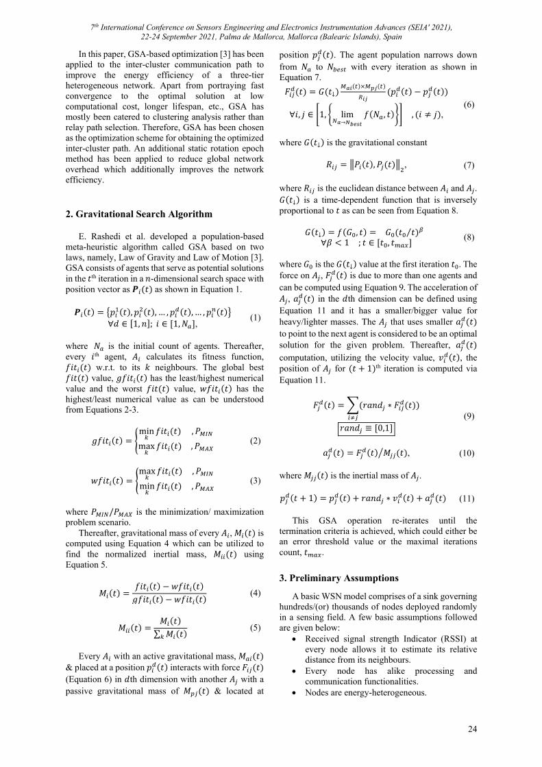
7th International Conference on Sensors Engineering and Electronics Instrumentation Advances (SEIA' 2021), 22-24 September 2021, Palma de Mallorca, Mallorca (Balearic Islands), Spain
24
In this paper, GSA-based optimization [3] has been applied to the inter-cluster communication path to improve the energy efficiency of a three-tier heterogeneous network. Apart from portraying fast convergence to the optimal solution at low computational cost, longer lifespan, etc., GSA has mostly been catered to clustering analysis rather than relay path selection. Therefore, GSA has been chosen as the optimization scheme for obtaining the optimized inter-cluster path. An additional static rotation epoch method has been applied to reduce global network overhead which additionally improves the network efficiency.
2. Gravitational Search Algorithm
E. Rashedi et al. developed a population-based meta-heuristic algorithm called GSA based on two laws, namely, Law of Gravity and Law of Motion [3]. GSA consists of agents that serve as potential solutions in the 𝑡th iteration in a 𝑛-dimensional search space with position vector as 𝑷 𝑡 as shown in Equation 1.
𝑷 𝑡 𝑝 𝑡 , 𝑝 𝑡 , … , 𝑝 𝑡 , … , 𝑝 𝑡
∀𝑑 ∈ 1, 𝑛 ; 𝑖 ∈ 1, 𝑁 , (1)
where 𝑁 is the initial count of agents. Thereafter, every 𝑖th agent, 𝐴 calculates its fitness function, 𝑓𝑖𝑡 𝑡 w.r.t. to its 𝑘 neighbours. The global best 𝑓𝑖𝑡 𝑡 value, 𝑔𝑓𝑖𝑡 𝑡 has the least/highest numerical value and the worst 𝑓𝑖𝑡 𝑡 value, 𝑤𝑓𝑖𝑡 𝑡 has the highest/least numerical value as can be understood from Equations 2-3.
𝑔𝑓𝑖𝑡 𝑡min 𝑓𝑖𝑡 𝑡 , 𝑃
max 𝑓𝑖𝑡 𝑡 , 𝑃 (2)
𝑤𝑓𝑖𝑡 𝑡max 𝑓𝑖𝑡 𝑡 , 𝑃
min 𝑓𝑖𝑡 𝑡 , 𝑃 (3)
where 𝑃 /𝑃 is the minimization/ maximization problem scenario.
Thereafter, gravitational mass of every 𝐴 , 𝑀 𝑡 is computed using Equation 4 which can be utilized to find the normalized inertial mass, 𝑀 𝑡 using Equation 5.
𝑀 𝑡𝑓𝑖𝑡 𝑡 𝑤𝑓𝑖𝑡 𝑡
𝑔𝑓𝑖𝑡 𝑡 𝑤𝑓𝑖𝑡 𝑡 (4)
𝑀 𝑡𝑀 𝑡
∑ 𝑀 𝑡 (5)
Every 𝐴 with an active gravitational mass, 𝑀 𝑡
& placed at a position 𝑝 𝑡 interacts with force 𝐹 𝑡 (Equation 6) in 𝑑th dimension with another 𝐴 with a passive gravitational mass of 𝑀 𝑡 & located at
position 𝑝 𝑡 . The agent population narrows down from 𝑁 to 𝑁 with every iteration as shown in Equation 7.
𝐹 𝑡 𝐺 𝑡↓ 𝑝 𝑡 𝑝 𝑡
∀𝑖, 𝑗 ∈ 1, lim→
𝑓 𝑁 , 𝑡 , 𝑖 𝑗 , (6)
where 𝐺 𝑡↓ is the gravitational constant
𝑅 𝑃 𝑡 , 𝑃 𝑡 , (7) where 𝑅 is the euclidean distance between 𝐴 and 𝐴 . 𝐺 𝑡↓ is a time-dependent function that is inversely proportional to 𝑡 as can be seen from Equation 8.
𝐺 𝑡↓ 𝑓 𝐺 , 𝑡 𝐺 𝑡 𝑡⁄ ∀𝛽 1 ; 𝑡 ∈ 𝑡 , 𝑡
(8)
where 𝐺 is the 𝐺 𝑡↓ value at the first iteration 𝑡 . The force on 𝐴 , 𝐹 𝑡 is due to more than one agents and can be computed using Equation 9. The acceleration of 𝐴 , 𝑎 𝑡 in the 𝑑th dimension can be defined using Equation 11 and it has a smaller/bigger value for heavy/lighter masses. The 𝐴 that uses smaller 𝑎 𝑡 to point to the next agent is considered to be an optimal solution for the given problem. Thereafter, 𝑎 𝑡
computation, utilizing the velocity value, 𝑣 𝑡 , the position of 𝐴 for 𝑡 1 th iteration is computed via Equation 11.
𝐹 𝑡 𝑟𝑎𝑛𝑑 ∗ 𝐹 𝑡
𝑟𝑎𝑛𝑑 ≡ 0,1 (9)
𝑎 𝑡 𝐹 𝑡 𝑀 𝑡 , (10)
where 𝑀 𝑡 is the inertial mass of 𝐴 . 𝑝 𝑡 1 𝑝 𝑡 𝑟𝑎𝑛𝑑 ∗ 𝑣 𝑡 𝑎 𝑡 (11)
This GSA operation re-iterates until the termination criteria is achieved, which could either be an error threshold value or the maximal iterations count, 𝑡 .
3. Preliminary Assumptions
A basic WSN model comprises of a sink governing hundreds/(or) thousands of nodes deployed randomly in a sensing field. A few basic assumptions followed are given below:
Received signal strength Indicator (RSSI) at every node allows it to estimate its relative distance from its neighbours.
Every node has alike processing and communication functionalities.
Nodes are energy-heterogeneous.

7th International Conference on Sensors Engineering and Electronics Instrumentation Advances (SEIA' 2021), 22-24 September 2021, Palma de Mallorca, Mallorca (Balearic Islands), Spain
25
The sink is static and is taken in the centre of the field. It does not face any memory, energy, or computation constraint.
Energy depletion has been considered as the only potential cause considered for a node’s failure.
All nodes are clock synchronized and all communication links are symmetric & wireless.
Single-hop transmissions are considered for intra-cluster communications.
3.1. Radio Energy Model
The radio energy consumption model of WSN as shown in Fig. 1 allows a WSN to compute the energy dissipated during its life. The energy dissipation is expected during sensing, aggregation, communication.
Fig. 1. Radio Energy Consumption Model (modified after [4]).
The energy consumed to amplify a signal, 𝐸 𝑑 varies with the channel model opted within a node & can be computed using Equation 12. The channel models (free-space model, 𝑓𝑠𝑚 & multi-path model, 𝑚𝑝𝑚) are a function of 𝑑 which is compared with a
threshold distance, 𝑑 𝐸 𝐸⁄ . Energy commuted via 𝑓𝑠𝑚/𝑚𝑝𝑚 channel over a unit distance is 𝐸 /𝐸 .
𝐸 𝑑𝐸 ∗ 𝑑 , 𝑖𝑓 𝑑 𝑑𝐸 ∗ 𝑑 , 𝑖𝑓 𝑑 𝑑
(12)
Energy usage for aggregation, 𝐸 𝑁 (Eq. 13) supports abridging redundancy in an 𝑖 node, 𝑁 serving as a CH to 𝐶 nodes. Total energy expended while segregating data from a single node can be denoted as 𝐸 .
𝐸 𝑁 𝐶 ∗ 𝐸 (13)
To achieve an acceptable range of SNR (signal to noise ratio) [5], energy expended within a node during 𝐿-bit data transmission is based on 𝑑 as can be seen from Equation 14 while it also emits some energy during the reception which is independent of 𝑑 as can be seen in Equation 15. 𝐸 is the energy expended in the electronic circuitry of a node.
𝐸Ƭ 𝐿, 𝑑 𝐿 ∗ 𝐸 𝐸 𝑑 (14)
𝐸ʀ 𝐿 𝐸 ∗ 𝐿 (15)
Network’s total energy consumption per round, 𝐸 can be computed as given in Equation 16.
𝐸 2 ∗ L ∗ 𝐸𝐸 𝑑 L 1𝐸 𝑁
(16)
3.2 Heterogeneous Network Model
The three-tier energy-heterogeneous model has been opted for the proposed work. The field contains 𝑁 number of haphazardly yet uniformly dispersed nodes with static positions. The heterogeneity hierarchy is defined as normal nodes 𝑛𝑟𝑚, advanced nodes 𝑎𝑑𝑣 and super-advanced nodes 𝑠𝑝𝑟. Assuming 𝐸 as the initial energy of an individual 𝑛𝑟𝑚, the rest parameters have been described as in Table 1.
Table 1. Node-Type Description Model.
Node-Type Initial Energy
Initial Population Count
𝑛𝑟𝑚 𝐸 1 𝑚 𝑚 𝑚 𝑁 𝑎𝑑𝑣 𝐸 1 𝑎 𝑚 𝑁 𝑠𝑝𝑟 𝐸 1 𝑠 𝑚 𝑚 𝑁
The total initial energy, 𝐸 can be calculated using Equation 17 by utilizing the data from Table 1.
𝐸 1 𝑎𝑚 𝑠𝑚 𝑚 ∗ 𝑁 ∗ 𝐸 (17)
4. GSA-based Multi-hop Routing Scheme for EEHC
This work proposes a GSA-based multi-hop routing scheme for Energy Efficient Heterogeneous Clustered scheme (EEHC) [1] and the scheme has been coined as GSA-EEHC. The basic operation of GSA-EEHC is as followed in EEHC with setup phase and steady state phase. However, GSA-EEHC introduces conditional static rotation epoch during CH selection and also optimizes the relay path between the CH and the sink.
4.1. Static Rotation Epoch based CH Selection
As observed in EEHC, a basic round iteration initialises with computation of weighted probability, 𝑃 𝑁 by every node 𝑁 , for their fair election for the CH role. The respective probabilities are computed using Equation 18. Every node type inputs its weighted probability value 𝑃 𝑁 to calculate its threshold value 𝑇 𝑁 using Equation 19. If the node has not been elected as a CH in the last 1 𝑃⁄ rounds, it obtains 𝑇 𝑁 0 and becomes a nominee for CH selection, while if, the node has been elected at least once in the last 1 𝑃⁄ rounds, its 𝑇 𝑁 is equated to zero. Every individual node may have a different output as every node has its unique value of rotating epoch.
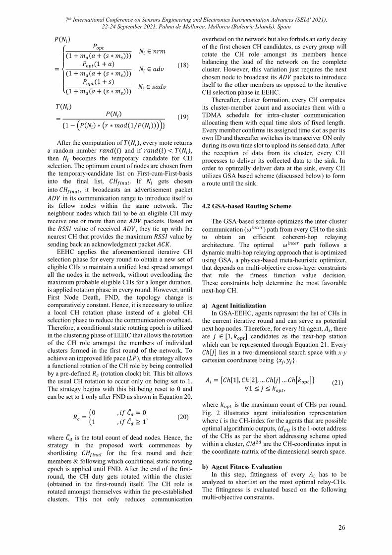
7th International Conference on Sensors Engineering and Electronics Instrumentation Advances (SEIA' 2021), 22-24 September 2021, Palma de Mallorca, Mallorca (Balearic Islands), Spain
26
𝑃 𝑁
⎩⎪⎪⎨
⎪⎪⎧
𝑃1 𝑚 𝑎 𝑠 ∗ 𝑚
𝑁 ∈ 𝑛𝑟𝑚
𝑃 1 𝑎1 𝑚 𝑎 𝑠 ∗ 𝑚
𝑁 ∈ 𝑎𝑑𝑣
𝑃 1 𝑠1 𝑚 𝑎 𝑠 ∗ 𝑚
𝑁 ∈ 𝑠𝑎𝑑𝑣
(18)
𝑇 𝑁
𝑃 𝑁
1 𝑃 𝑁 ∗ 𝑟 ∗ 𝑚𝑜𝑑 1 𝑃 𝑁⁄ (19)
After the computation of 𝑇 𝑁 , every mote returns
a random number 𝑟𝑎𝑛𝑑 𝑖 and if 𝑟𝑎𝑛𝑑 𝑖 𝑇 𝑁 , then 𝑁 becomes the temporary candidate for CH selection. The optimum count of nodes are chosen from the temporary-candidate list on First-cum-First-basis into the final list, 𝐶𝐻 . If 𝑁 gets chosen into 𝐶𝐻 , it broadcasts an advertisement packet 𝐴𝐷𝑉 in its communication range to introduce itself to its fellow nodes within the same network. The neighbour nodes which fail to be an eligible CH may receive one or more than one 𝐴𝐷𝑉 packets. Based on the 𝑅𝑆𝑆𝐼 value of received 𝐴𝐷𝑉, they tie up with the nearest CH that provides the maximum 𝑅𝑆𝑆𝐼 value by sending back an acknowledgment packet 𝐴𝐶𝐾.
EEHC applies the aforementioned iterative CH selection phase for every round to obtain a new set of eligible CHs to maintain a unified load spread amongst all the nodes in the network, without overloading the maximum probable eligible CHs for a longer duration. is applied rotation phase in every round. However, until First Node Death, FND, the topology change is comparatively constant. Hence, it is necessary to utilize a local CH rotation phase instead of a global CH selection phase to reduce the communication overhead. Therefore, a conditional static rotating epoch is utilized in the clustering phase of EEHC that allows the rotation of the CH role amongst the members of individual clusters formed in the first round of the network. To achieve an improved life pace (𝐿𝑃), this strategy allows a functional rotation of the CH role by being controlled by a pre-defined 𝑅 (rotation clock) bit. This bit allows the usual CH rotation to occur only on being set to 1. The strategy begins with this bit being reset to 0 and can be set to 1 only after FND as shown in Equation 20.
𝑅0 , 𝑖𝑓 𝐶 01 , 𝑖𝑓 𝐶 1
, (20)
where 𝐶 is the total count of dead nodes. Hence, the strategy in the proposed work commences by shortlisting 𝐶𝐻 for the first round and their members & following which conditional static rotating epoch is applied until FND. After the end of the first-round, the CH duty gets rotated within the cluster (obtained in the first-round) itself. The CH role is rotated amongst themselves within the pre-established clusters. This not only reduces communication
overhead on the network but also forbids an early decay of the first chosen CH candidates, as every group will rotate the CH role amongst its members hence balancing the load of the network on the complete cluster. However, this variation just requires the next chosen node to broadcast its 𝐴𝐷𝑉 packets to introduce itself to the other members as opposed to the iterative CH selection phase in EEHC.
Thereafter, cluster formation, every CH computes its cluster-member count and associates them with a TDMA schedule for intra-cluster communication allocating them with equal time slots of fixed length. Every member confirms its assigned time slot as per its own ID and thereafter switches its transceiver ON only during its own time slot to upload its sensed data. After the reception of data from its cluster, every CH processes to deliver its collected data to the sink. In order to optimally deliver data at the sink, every CH utilizes GSA based scheme (discussed below) to form a route until the sink. 4.2 GSA-based Routing Scheme
The GSA-based scheme optimizes the inter-cluster communication (𝜔 ) path from every CH to the sink to obtain an efficient coherent-hop relaying architecture. The optimal 𝜔 path follows a dynamic multi-hop relaying approach that is optimized using GSA, a physics-based meta-heuristic optimizer, that depends on multi-objective cross-layer constraints that rule the fitness function value decision. These constraints help determine the most favorable next-hop CH. a) Agent Initialization
In GSA-EEHC, agents represent the list of CHs in the current iterative round and can serve as potential next hop nodes. Therefore, for every 𝑖th agent, 𝐴 , there are 𝑗 ∈ 1, 𝑘 candidates as the next-hop station which can be represented through Equation 21. Every 𝐶ℎ 𝑗 lies in a two-dimensional search space with x-y cartesian coordinates being 𝑥 , 𝑦 .
𝐴 𝐶ℎ 1 , 𝐶ℎ 2 , … 𝐶ℎ 𝑗 … 𝐶ℎ 𝑘 ∀1 𝑗 𝑘 ,
(21)
where 𝑘 is the maximum count of CHs per round. Fig. 2 illustrates agent initialization representation where 𝑖 is the CH-index for the agents that are possible optimal algorithmic outputs, 𝑖𝑑 is the 1-octet address of the CHs as per the short addressing scheme opted within a cluster, 𝐶𝑀 are the CH-coordinates input in the coordinate-matrix of the dimensional search space. b) Agent Fitness Evaluation
In this step, fittingness of every 𝐴 has to be analyzed to shortlist on the most optimal relay-CHs. The fittingness is evaluated based on the following multi-objective constraints.

7th International Conference on Sensors Engineering and Electronics Instrumentation Advances (SEIA' 2021), 22-24 September 2021, Palma de Mallorca, Mallorca (Balearic Islands), Spain
27
Fig. 2. Agent Initialization representation
Channel Estimation, 𝐶𝑆 𝑡 Taking into consideration the complexity of the
transmission environment during fittest relay-CH exploration, node’s efficient capability to suffice channel’s estimate is based on 𝐶𝑆 𝑡 (Equation 25). 𝐶𝑆 𝑡 should be in maximum for 𝐴 in the current 𝑡 th iteration and its value is based on its 𝑅𝑆𝑆𝐼 Quality, 𝑅𝑆𝑆𝐼𝑞 𝑡 and Signal-to-Interference-plus-Noise Ratio, 𝑆𝐼𝑁𝑅 𝑡 showcased in Equations 22 & 24, respectively [6]. 𝐶ℎ 𝑗 of 𝐴 should have high 𝑅𝑆𝑆𝐼 (computed using Equation 23) in contrast to the threshold RSSI, 𝑅𝑆𝑆𝐼 .
𝑅𝑆𝑆𝐼𝑞 𝑡 𝑅𝑆𝑆𝐼 /𝑅𝑆𝑆𝐼 (22)
𝑅𝑆𝑆𝐼 𝑃 ∗ 𝐺𝑡 ∗ 𝐺𝑟 4𝜋 ∗ 𝑑 , (23) where 𝑃 is the transmission power (watts), 𝑑 is the commuting distance between 𝐴 and 𝐶ℎ 𝑗 (metres), 𝐺𝑡/𝐺𝑟 is the transmit/receipt antenna electric power gain (dB). A higher 𝑆𝐼𝑁𝑅 𝑡 is demanded at the anchor node 𝐴 whilst communication with 𝐶ℎ 𝑗 corresponding to lower interference and thereby, lower path loss of the data-signal. A higher 𝑆𝐼𝑁𝑅 𝑡 asymptotically approximates the fitness function value to a better solution.
𝑆𝐼𝑁𝑅 𝑡𝑃 ∗ 𝐺𝑡 ∗ 𝐺𝑟 4𝜋 ∗ 𝑅𝑆𝑆𝐼⁄ ∗ 𝑃 ∗ 𝑟 ,
(24)
where 𝑟 determines the random noise value to the signal. Therefore, 𝑅𝑆𝑆𝐼𝑞 𝑡 and 𝑆𝐼𝑁𝑅 𝑡 direct the algorithm to use physical layer characteristics to partly determine an optimal routing pattern following fittest 𝐴 based on Equation 25.
𝐹 𝑡 𝐶𝑆 𝑡 𝑅𝑆𝑆𝐼𝑞 𝑡 𝑆𝐼𝑁𝑅 𝑡 (25)
Energy Ratio, 𝐸𝑅 𝑡 Energy is an important constraint in relay-CH
selection criteria. An optimal relay-CH should be able to consume minimum energy to relay the data of another CH to the sink requiring it to hold greater energy. Every 𝐴 calculates 𝐸𝑅 𝑡 in the current 𝑡th iteration using Equation 26. Optimal set of relay-CHs, 𝐶ℎ 𝑗 ’s, will give maximum value for 𝐹 𝑡 . 𝐹 𝑡 𝐸𝑅 𝑡 𝐸 𝐴 / 𝐸 1 𝑎𝑚
𝑠𝑚 𝑚 , (26)
where 𝐸 𝐴 is the residual energy of 𝐴 .
End-to-End Latency, Ƚ 𝑡 Data dissemination from CHs to sink requires
energy cost subject to minimum end-to-end latency, Ƚ 𝑡 . Since usually, multi-hop model introduces greater latency compared to single-hop model, minimal delay route is a primary criteria for determining an optimal 𝐴 and can be obtained via Ƚ 𝑡 parameter which can be calculated using Equation 27. A delay-aware routing algorithm increases network’s reliability during critical situations which could otherwise hinder the probability to avoid fatal consequences.
𝐹Ƚ 𝑡 Ƚ 𝑡 𝜑 𝜑 , (27) where 𝜑 is the time stamp when data is received by sink and 𝜑 is the time stamp when data is sent by the CH.
Cluster Density, 𝜕 𝑡 Due to haphazard deployment, nodes at some
location may have a higher cluster density when grouped together under the supervision of the same CH. Therefore, characterizing cluster density, 𝜕 𝑡 for determining optimality of any 𝐴 is important as the CH heading a dense cluster may get deprived of more power as compared to the one governing a sparse cluster. 𝜕 𝑡 described in Equation 28 should be in minimum to guarantee that the chosen 𝐶ℎ 𝑗 has sufficient 𝐸 𝐶ℎ 𝑗 even after relaying data from its neighbor source-CH.
𝐹 𝑡 𝜕 𝑡 1 𝑑 𝐶 𝑁 , (28)
where 𝐶 is the member count for every 𝐴 , 𝑑 is the distance of 𝐴 from its member, 𝑁 is the initial node population. c) Fitness function for GSA-EEHC, 𝒇𝒊𝒕𝒊 𝒕
This GSA-based scheme takes into consideration the multi-objective constraints from parallel OSI layers (as mentioned in Equations 25-28) that help achieve the optimal relay route from the CH to the sink in the current 𝑡th iterative round. The fitness measure for the 𝑡th iterative round, 𝑓𝑖𝑡 𝑡 can be given as in Equation 29.
𝑓𝑖𝑡 𝑡 max 𝛼𝐹 𝑡 𝛽𝐹 𝑡𝜃𝐹Ƚ 𝑡 𝛾𝐹 𝑡 ,
(29)
where 𝛼 𝛽 𝜃 𝛾 1; 0 𝛼, 𝛽, 𝜃, 𝛾 1 d) Position computation of the fittest
Utilizing GSA algorithm computations [3] and 𝑓𝑖𝑡 𝑡 (Equation 29) of every 𝐶ℎ 𝑗 , quality of the agents can be verified and evaluated for the best-route identification. Since, the GSA-EEHC strategy rests upon 𝑃 , 𝑔𝑓𝑖𝑡 𝑡 with the highest numerical count and 𝑤𝑓𝑖𝑡 𝑡 with the lowest numerical count is computed amongst all the agents. These 𝑔𝑓𝑖𝑡 𝑡 and 𝑤𝑓𝑖𝑡 𝑡 values are used to compute 𝑀 𝑡 and 𝑀 𝑡
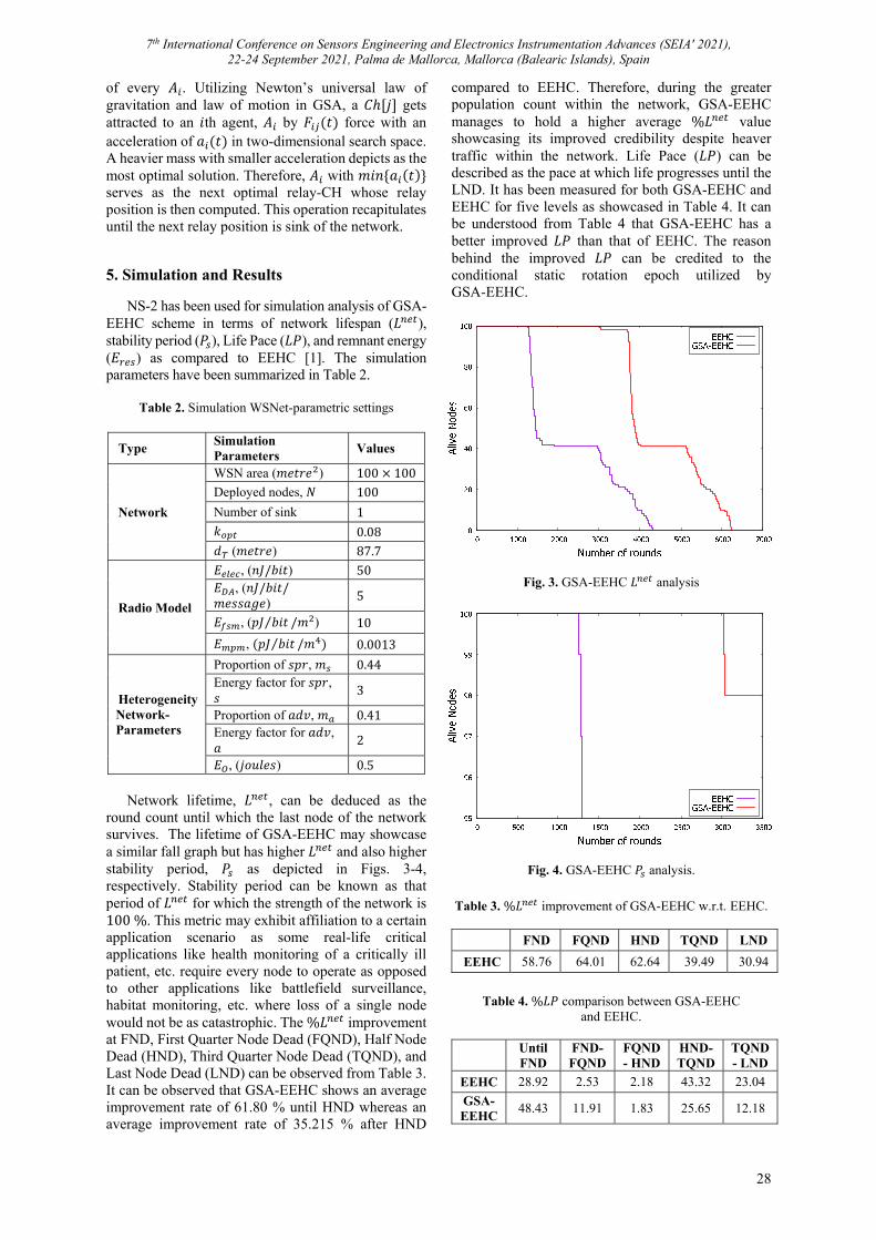
7th International Conference on Sensors Engineering and Electronics Instrumentation Advances (SEIA' 2021), 22-24 September 2021, Palma de Mallorca, Mallorca (Balearic Islands), Spain
28
of every 𝐴 . Utilizing Newton’s universal law of gravitation and law of motion in GSA, a 𝐶ℎ 𝑗 gets attracted to an 𝑖th agent, 𝐴 by 𝐹 𝑡 force with an acceleration of 𝑎 𝑡 in two-dimensional search space. A heavier mass with smaller acceleration depicts as the most optimal solution. Therefore, 𝐴 with 𝑚𝑖𝑛 𝑎 𝑡 serves as the next optimal relay-CH whose relay position is then computed. This operation recapitulates until the next relay position is sink of the network. 5. Simulation and Results
NS-2 has been used for simulation analysis of GSA-EEHC scheme in terms of network lifespan (𝐿 ), stability period (𝑃 ), Life Pace (𝐿𝑃), and remnant energy (𝐸 ) as compared to EEHC [1]. The simulation parameters have been summarized in Table 2.
Table 2. Simulation WSNet-parametric settings
Type Simulation Parameters
Values
Network
WSN area (𝑚𝑒𝑡𝑟𝑒 ) 100 100
Deployed nodes, 𝑁 100
Number of sink 1
𝑘 0.08
𝑑 (𝑚𝑒𝑡𝑟𝑒) 87.7
Radio Model
𝐸 , (𝑛𝐽/𝑏𝑖𝑡) 50 𝐸 , (𝑛𝐽/𝑏𝑖𝑡/𝑚𝑒𝑠𝑠𝑎𝑔𝑒)
5
𝐸 , (𝑝𝐽 𝑏𝑖𝑡⁄ /𝑚 ) 10
𝐸 , 𝑝𝐽 𝑏𝑖𝑡⁄ /𝑚 0.0013
Heterogeneity Network-Parameters
Proportion of 𝑠𝑝𝑟, 𝑚 0.44 Energy factor for 𝑠𝑝𝑟, 𝑠
3
Proportion of 𝑎𝑑𝑣, 𝑚 0.41 Energy factor for 𝑎𝑑𝑣, 𝑎
2
𝐸 , (𝑗𝑜𝑢𝑙𝑒𝑠) 0.5
Network lifetime, 𝐿 , can be deduced as the round count until which the last node of the network survives. The lifetime of GSA-EEHC may showcase a similar fall graph but has higher 𝐿 and also higher stability period, 𝑃 as depicted in Figs. 3-4, respectively. Stability period can be known as that period of 𝐿 for which the strength of the network is 100 %. This metric may exhibit affiliation to a certain application scenario as some real-life critical applications like health monitoring of a critically ill patient, etc. require every node to operate as opposed to other applications like battlefield surveillance, habitat monitoring, etc. where loss of a single node would not be as catastrophic. The %𝐿 improvement at FND, First Quarter Node Dead (FQND), Half Node Dead (HND), Third Quarter Node Dead (TQND), and Last Node Dead (LND) can be observed from Table 3. It can be observed that GSA-EEHC shows an average improvement rate of 61.80 % until HND whereas an average improvement rate of 35.215 % after HND
compared to EEHC. Therefore, during the greater population count within the network, GSA-EEHC manages to hold a higher average %𝐿 value showcasing its improved credibility despite heaver traffic within the network. Life Pace (𝐿𝑃) can be described as the pace at which life progresses until the LND. It has been measured for both GSA-EEHC and EEHC for five levels as showcased in Table 4. It can be understood from Table 4 that GSA-EEHC has a better improved 𝐿𝑃 than that of EEHC. The reason behind the improved 𝐿𝑃 can be credited to the conditional static rotation epoch utilized by GSA-EEHC.
Fig. 3. GSA-EEHC 𝐿 analysis
Fig. 4. GSA-EEHC 𝑃 analysis.
Table 3. %𝐿 improvement of GSA-EEHC w.r.t. EEHC.
FND FQND HND TQND LND
EEHC 58.76 64.01 62.64 39.49 30.94
Table 4. %𝐿𝑃 comparison between GSA-EEHC
and EEHC.
Until FND
FND- FQND
FQND- HND
HND- TQND
TQND- LND
EEHC 28.92 2.53 2.18 43.32 23.04
GSA-EEHC
48.43 11.91 1.83 25.65 12.18
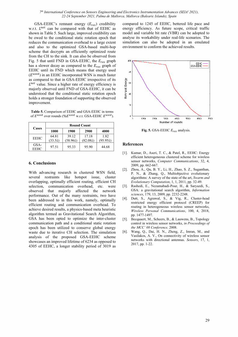
7th International Conference on Sensors Engineering and Electronics Instrumentation Advances (SEIA' 2021), 22-24 September 2021, Palma de Mallorca, Mallorca (Balearic Islands), Spain
29
GSA-EEHC’s remnant energy (𝐸 ) credibility w.r.t. 𝐿 can be compared with that of EEHC as shown in Table 5. Such large, improved credibility can be owed to the conditional static rotation epoch that reduces the communication overhead to a large extent and also to the optimized GSA-based multi-hop scheme that decrypts an efficiently optimized route from the CH to the sink. It can also be observed from Fig. 5 that until FND in GSA-EEHC, the 𝐸 graph has a slower decay as compared to the 𝐸 graph of EEHC until its FND which means that energy used (𝐸 ) in an EEHC incorporated WSN is much faster as compared to that in GSA-EEHC irrespective of its 𝐿 value. Since a higher rate of energy efficiency is majorly observed until FND of GSA-EEHC, it can be understood that the conditional static rotation epoch holds a stronger foundation of supporting the observed improvement.
Table 5. Comparison of EEHC and GSA-EEHC in terms of 𝐸 over rounds (%𝐸 w.r.t. GSA-EEHC 𝐸 ).
Cases Round Count
1000 1900 2900 4000
EEHC 64.81
(33.5↓) 39.12
(58.96↓) 17.18
(82.08↓) 1.82
(95.95↓) GSA-EEHC
97.51 95.33 95.90 44.68
6. Conclusions With advancing research in clustered WSN field, several restraints like hotspot issue, cluster overlapping, optimally efficient routing, efficient CH selection, communication overhead, etc. were observed that majorly affected the network performance. Out of the many restraints, two have been addressed to in this work, namely, optimally efficient routing and communication overhead. To achieve desired results, a physics-based meta heuristic algorithm termed as Gravitational Search Algorithm, GSA has been opted to optimize the inter-cluster communication path and a conditional static rotation epoch has been utilized to conserve global energy waste due to iterative CH selection. The simulation analysis of the proposed GSA-EEHC scheme showcases an improved lifetime of 6234 as opposed to 4305 of EEHC, a longer stability period of 3019 as
compared to 1245 of EEHC, bettered life pace and energy efficiency. As future scope, critical traffic model and variable bit rate (VBR) can be adopted to analyse its workability under real-life scenarios. The simulation can also be adopted in an emulated environment to conform the achieved results.
Fig. 5. GSA-EEHC 𝐸 analysis. References [1]. Kumar, D., Aseri, T. C., & Patel, R., EEHC: Energy
efficient heterogeneous clustered scheme for wireless sensor networks, Computer Communications, 32, 4, 2009, pp. 662-667.
[2]. Zhou, A., Qu, B. Y., Li, H., Zhao, S. Z., Suganthan, P. N., & Zhang, Q., Multiobjective evolutionary algorithms: A survey of the state of the art, Swarm and Evolutionary Computation, 1, 1, 2011, pp. 32-49.
[3]. Rashedi, E., Nezamabadi-Pour, H., & Saryazdi, S., GSA: a gravitational search algorithm, Information sciences, 179, 13, 2009, pp. 2232-2248.
[4]. Dutt, S., Agrawal, S., & Vig, R., Cluster-head restricted energy efficient protocol (CREEP) for routing in heterogeneous wireless sensor networks, Wireless Personal Communications, 100, 4, 2018, pp. 1477-1497.
[5]. Becquaert, M., Scheers, B., & Lauwens, B., Topology control in wireless sensor networks, in Proceedings of the MCC’ 08 Conference, 2008.
[6]. Wang, Q., Dai, H. N., Zheng, Z., Imran, M., and Vasilakos, A. V., On connectivity of wireless sensor networks with directional antennas. Sensors, 17, 1, 2017, pp. 1-22.
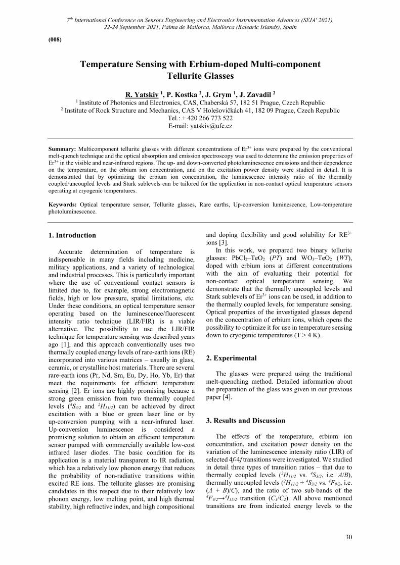
7th International Conference on Sensors Engineering and Electronics Instrumentation Advances (SEIA' 2021), 22-24 September 2021, Palma de Mallorca, Mallorca (Balearic Islands), Spain
30
(008)
Temperature Sensing with Erbium-doped Multi-component Tellurite Glasses
R. Yatskiv 1, P. Kostka 2, J. Grym 1, J. Zavadil 2
1 Institute of Photonics and Electronics, CAS, Chaberská 57, 182 51 Prague, Czech Republic 2 Institute of Rock Structure and Mechanics, CAS V Holešovičkách 41, 182 09 Prague, Czech Republic
Tel.: + 420 266 773 522 E-mail: [email protected]
Summary: Multicomponent tellurite glasses with different concentrations of Er3+ ions were prepared by the conventional melt-quench technique and the optical absorption and emission spectroscopy was used to determine the emission properties of Er3+ in the visible and near-infrared regions. The up- and down-converted photoluminescence emissions and their dependence on the temperature, on the erbium ion concentration, and on the excitation power density were studied in detail. It is demonstrated that by optimizing the erbium ion concentration, the luminescence intensity ratio of the thermally coupled/uncoupled levels and Stark sublevels can be tailored for the application in non-contact optical temperature sensors operating at cryogenic temperatures. Keywords: Optical temperature sensor, Tellurite glasses, Rare earths, Up-conversion luminescence, Low-temperature photoluminescence.
1. Introduction
Accurate determination of temperature is indispensable in many fields including medicine, military applications, and a variety of technological and industrial processes. This is particularly important where the use of conventional contact sensors is limited due to, for example, strong electromagnetic fields, high or low pressure, spatial limitations, etc. Under these conditions, an optical temperature sensor operating based on the luminescence/fluorescent intensity ratio technique (LIR/FIR) is a viable alternative. The possibility to use the LIR/FIR technique for temperature sensing was described years ago [1], and this approach conventionally uses two thermally coupled energy levels of rare-earth ions (RE) incorporated into various matrices – usually in glass, ceramic, or crystalline host materials. There are several rare-earth ions (Pr, Nd, Sm, Eu, Dy, Ho, Yb, Er) that meet the requirements for efficient temperature sensing [2]. Er ions are highly promising because a strong green emission from two thermally coupled levels (4S3/2 and 2H11/2) can be achieved by direct excitation with a blue or green laser line or by up-conversion pumping with a near-infrared laser. Up-conversion luminescence is considered a promising solution to obtain an efficient temperature sensor pumped with commercially available low-cost infrared laser diodes. The basic condition for its application is a material transparent to IR radiation, which has a relatively low phonon energy that reduces the probability of non-radiative transitions within excited RE ions. The tellurite glasses are promising candidates in this respect due to their relatively low phonon energy, low melting point, and high thermal stability, high refractive index, and high compositional
and doping flexibility and good solubility for RE3+ ions [3].
In this work, we prepared two binary tellurite glasses: PbCl2–TeO2 (PT) and WO3–TeO2 (WT), doped with erbium ions at different concentrations with the aim of evaluating their potential for non-contact optical temperature sensing. We demonstrate that the thermally uncoupled levels and Stark sublevels of Er3+ ions can be used, in addition to the thermally coupled levels, for temperature sensing. Optical properties of the investigated glasses depend on the concentration of erbium ions, which opens the possibility to optimize it for use in temperature sensing down to cryogenic temperatures (T > 4 K). 2. Experimental
The glasses were prepared using the traditional melt-quenching method. Detailed information about the preparation of the glass was given in our previous paper [4]. 3. Results and Discussion
The effects of the temperature, erbium ion
concentration, and excitation power density on the variation of the luminescence intensity ratio (LIR) of selected 4f-4f transitions were investigated. We studied in detail three types of transition ratios – that due to thermally coupled levels (2H11/2 vs. 4S3/2, i.e. A/B), thermally uncoupled levels (2H11/2 + 4S3/2 vs. 4F9/2, i.e. (A + B)/C), and the ratio of two sub-bands of the 4F9/2→4I15/2 transition (C1/C2). All above mentioned transitions are from indicated energy levels to the
7th International Conference on Sensors Engineering and Electronics Instrumentation Advances (SEIA' 2021), 22-24 September 2021, Palma de Mallorca, Mallorca (Balearic Islands), Spain
31
ground state 4I15/2. The sub-bands of the 4F9/2→4I15/2 transition (C1 and C2) are due to Stark levels splitting of the ground state 4I15/2. Using different excitation processes (direct absorption – 515 nm, and frequency up-conversion – 980 nm), we found that the LIR for all the above described emission bands did not depend on the excitation power density. In the case of the thermally coupled levels, a steeper LIR temperature dependence and higher sensitivity Sa were achieved for the glasses with low concentration of erbium ions. However, the luminescence for the 2H11/2→4I15/2 transition (A) was quenched already at ~100 K for both excitation processes. We also found that erbium ion concentration has only a negligible effect on intensity of the A band, so it cannot be enhanced in this way. These findings limit the use of thermally coupled levels for detection at temperatures below 100 K.
However, in the up-conversion emission spectra, the LIR of thermally uncoupled levels did not follow this behaviour. We observed a strong increase of the red band intensity and a decrease in the ratios of the green to red integral intensity when erbium concentration was increased. As a consequence, the temperature dependence of the corresponding LIR (A + B/C) appears to be sufficiently strong and exhibits a linear dependence (see Fig. 1a), which is a favourable property for potential application. Thus the up-conversion luminescence spectra for highly doped glasses could be used for temperature sensing down to 4 K, when for the LIR analysis are used integral intensities of green bands (A + B) and the red band C
that correspond to luminescence transitions from levels (4S3/2 + 2H11/2) and 4F9/2 to the ground state 4I15/2.
The sub-bands C1 and C2 of the emission band 4F9/24I15/2 that are observed due to the Stark levels splitting of the ground state 4I15/2 behave similarly. The corresponding LIR (C1/C2) exhibits sufficiently strong and linear temperature dependence (see Fig. 1b). Thus, the selected thermally uncoupled levels and sub-bands due to Stark levels splitting could be used for temperature sensing down to 4 K for both investigated tellurite PbCl2–TeO2 and WO3–TeO2 glasses for high doping Er concentrations. This leads us to the conclusion that the studied tellurite glasses are promising candidates for optical temperature sensing at cryogenic temperatures.
It turns out that the two binary glass systems, presented in this paper, offer similar extension of the temperature sensing range (down to 4 K) and sensitivity (by using the LIR technique) when exploiting the red band transitions, as previously studied ternary system of TeO2–PbCl2–WO3 [4]. In terms of maximizing the red (C) band intensity and the ratios associated with this band, a high PbCl2 concentration appears to be advantageous. It should be noted however, that increasing of PbCl2 concentration generates other disadvantages. All glasses presented in this paper show sufficient capability for use as temperature sensors starting from cryogenic temperatures (the limit of the presented data is due to limitation of the experimental setup at 4 K).
Fig. 1. Experimental luminescence intensity ratios (LIR) for PT and WT glasses doped with 2 mol% Er3+ are shown as a function of temperature in the range of 4–300 K. A, B, and C represent transitions from the excited Er3+ levels 2H11/2,
4S3/2, 4F9/2 to the ground state 4I15/2, respectively. C1 and C2 represent Stark sub-bands of the C transition. 4. Conclusions
We studied stable PT and WT glasses doped with different concentrations of Er3+ using transmission and
low-temperature photoluminescence spectroscopy. Samples excited by an infrared laser showed a strong frequency up-conversion in the visible and NIR spectral range. Temperature dependence of luminescence intensity ratio of the two strong green
0 25 50 75 100 125 150 175 200 225 250 275 3000.2
0.4
0.6
0.8
1.0
20 WO3 - 80 TeO2: ErO3/2
LIR
(C
1/C
2)
Temperature (K)
0 25 50 75 100 125 150 175 200 225 250 275 300
1
2
3
4
5
6
7
(b)
30 PbCl2 - 70TeO2: ErO3/2
30 PbCl2 - 70TeO2: ErO3/2
Exp. data
Linear Fit
20 WO3 - 80 TeO2: ErO3/2
LIR
(A
+B
/C
) 980nm; 2mol. % ErO3/2
(a)

7th International Conference on Sensors Engineering and Electronics Instrumentation Advances (SEIA' 2021), 22-24 September 2021, Palma de Mallorca, Mallorca (Balearic Islands), Spain
32
emission bands was studied, and its use for temperature sensing starting from 100 K was proposed. Moreover, the red band (4F9/24I11/2), for highly doped samples, was found to exhibit a strong temperature dependence down to even significantly lower temperatures. Thus, the intensity ratio of red and green bands (transitions due to thermally un-coupled levels) turns out to be usable for temperature sensing down to 4 K.
Acknowledgements
The work was supported by the Czech Science Foundation [Grant No. 19-07456S].
References [1]. H. Kusama, O. J. Sovers, T. Yoshioka, Line shift
method for phosphor temperature measurements, Jpn. J. Appl. Phys., Vol. 15, 1976, pp. 2349-2358.
[2]. V. K. Rai, Temperature sensors and optical sensors, Applied Physics B, Vol. 88, 2007, pp. 297-300.
[3]. R. A. H. El-Mallawany, Tellurite Glasses Handbook: Physical Properties and Data, CRC Press, 2018.
[4]. P. Kostka, R. Yatskiv, J. Grym, J. Zavadil, Luminescence, up-conversion and temperature sensing in Er-doped TeO2-PbCl2-WO3 glasses, J. Non-Cryst. Solids, Vol. 553, 2021, 120287.
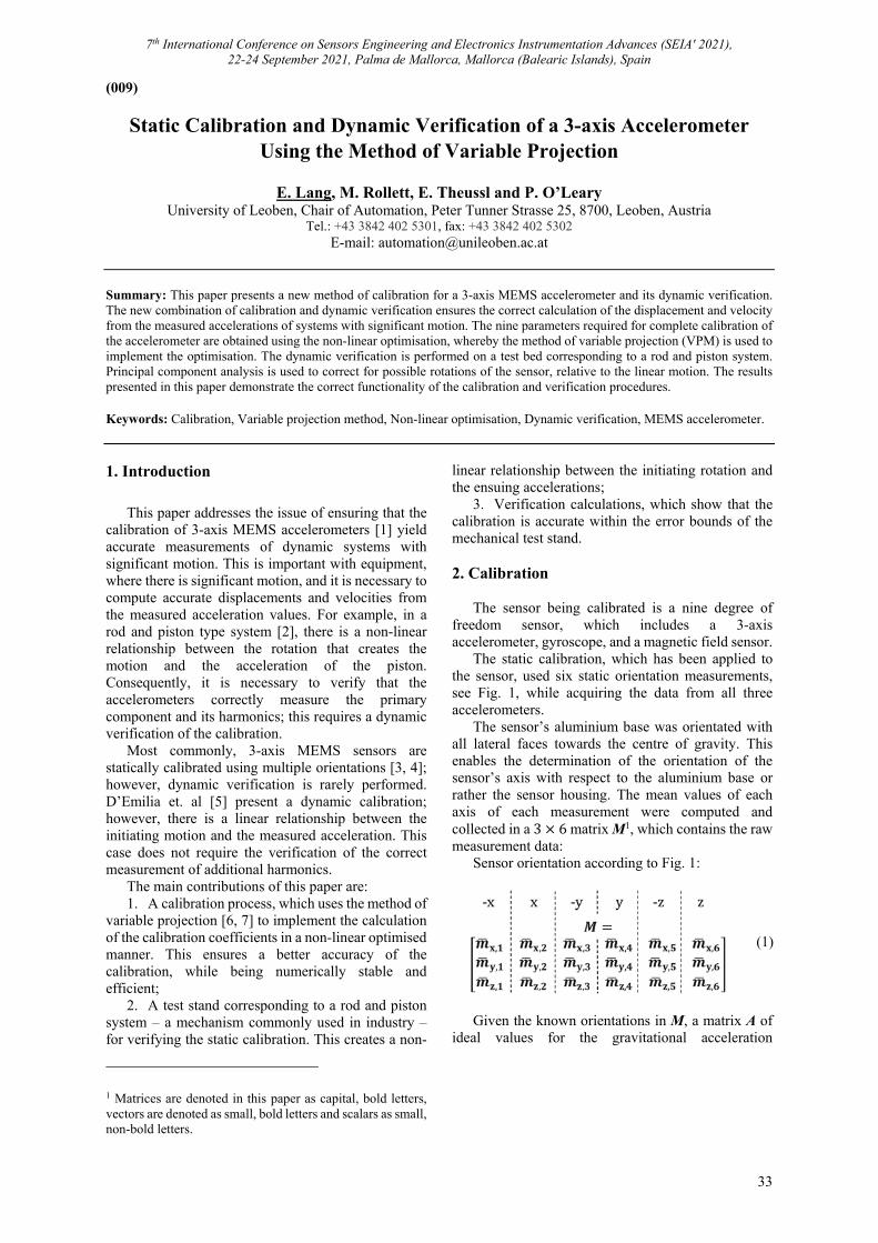
7th International Conference on Sensors Engineering and Electronics Instrumentation Advances (SEIA' 2021), 22-24 September 2021, Palma de Mallorca, Mallorca (Balearic Islands), Spain
33
(009)
Static Calibration and Dynamic Verification of a 3-axis Accelerometer Using the Method of Variable Projection
E. Lang, M. Rollett, E. Theussl and P. O’Leary
University of Leoben, Chair of Automation, Peter Tunner Strasse 25, 8700, Leoben, Austria Tel.: +43 3842 402 5301, fax: +43 3842 402 5302
E-mail: [email protected]
Summary: This paper presents a new method of calibration for a 3-axis MEMS accelerometer and its dynamic verification. The new combination of calibration and dynamic verification ensures the correct calculation of the displacement and velocity from the measured accelerations of systems with significant motion. The nine parameters required for complete calibration of the accelerometer are obtained using the non-linear optimisation, whereby the method of variable projection (VPM) is used to implement the optimisation. The dynamic verification is performed on a test bed corresponding to a rod and piston system. Principal component analysis is used to correct for possible rotations of the sensor, relative to the linear motion. The results presented in this paper demonstrate the correct functionality of the calibration and verification procedures.
Keywords: Calibration, Variable projection method, Non-linear optimisation, Dynamic verification, MEMS accelerometer.
1. Introduction
This paper addresses the issue of ensuring that the
calibration of 3-axis MEMS accelerometers [1] yield accurate measurements of dynamic systems with significant motion. This is important with equipment, where there is significant motion, and it is necessary to compute accurate displacements and velocities from the measured acceleration values. For example, in a rod and piston type system [2], there is a non-linear relationship between the rotation that creates the motion and the acceleration of the piston. Consequently, it is necessary to verify that the accelerometers correctly measure the primary component and its harmonics; this requires a dynamic verification of the calibration.
Most commonly, 3-axis MEMS sensors are statically calibrated using multiple orientations [3, 4]; however, dynamic verification is rarely performed. D’Emilia et. al [5] present a dynamic calibration; however, there is a linear relationship between the initiating motion and the measured acceleration. This case does not require the verification of the correct measurement of additional harmonics.
The main contributions of this paper are: 1. A calibration process, which uses the method of
variable projection [6, 7] to implement the calculation of the calibration coefficients in a non-linear optimised manner. This ensures a better accuracy of the calibration, while being numerically stable and efficient;
2. A test stand corresponding to a rod and piston system – a mechanism commonly used in industry – for verifying the static calibration. This creates a non-
1 Matrices are denoted in this paper as capital, bold letters, vectors are denoted as small, bold letters and scalars as small, non-bold letters.
linear relationship between the initiating rotation and the ensuing accelerations;
3. Verification calculations, which show that the calibration is accurate within the error bounds of the mechanical test stand.
2. Calibration
The sensor being calibrated is a nine degree of freedom sensor, which includes a 3-axis accelerometer, gyroscope, and a magnetic field sensor.
The static calibration, which has been applied to the sensor, used six static orientation measurements, see Fig. 1, while acquiring the data from all three accelerometers.
The sensor’s aluminium base was orientated with all lateral faces towards the centre of gravity. This enables the determination of the orientation of the sensor’s axis with respect to the aluminium base or rather the sensor housing. The mean values of each axis of each measurement were computed and collected in a 3 6 matrix M1, which contains the raw measurement data:
Sensor orientation according to Fig. 1:
(1)
Given the known orientations in M, a matrix A of
ideal values for the gravitational acceleration

7th International Conference on Sensors Engineering and Electronics Instrumentation Advances (SEIA' 2021), 22-24 September 2021, Palma de Mallorca, Mallorca (Balearic Islands), Spain
34
𝑔 9.81 , with the signs corresponding to the
orientations can be created
𝑨 𝑔 𝑔 0 0 0 0
0 0 𝑔 𝑔 0 00 0 0 0 𝑔 𝑔
(2)
Fig. 1. Six orthogonal orientation positions for calibration of the 3-axis accelerometer. At each orientation an axis (labeled as: -z, -y, -x, +z, +y, +x) pointed towards the aluminium base. As surface a levelled granite stone is used. A high precision water level was used to level the surface. The stone was encapsulated from the vibrating environment with speaker dampers.
Given 𝑨, 𝑴, a 3 3 rotational matrix 𝑹 Eq. (4), a
3 3 gain matrix 𝑮 Eq. (5) and a 3 6 offset matrix C Eq. (6), the calibration model, hence the relationship between the ideal values in A and the raw measurements in M, can be formulated as
𝑨 𝑮𝑹𝑴 𝑪 (3)
Hereby the rotational matrix
𝑹 ϕ 𝑹 𝜙 𝑹 𝜙 𝑹 𝜙
𝑐𝑜𝑠𝜙 𝑠𝑖𝑛𝜙 0𝑠𝑖𝑛𝜙 𝑐𝑜𝑠𝜙 0
0 0 1
𝑐𝑜𝑠𝜙 0 𝑠𝑖𝑛𝜙0 1 0
𝑠𝑖𝑛𝜙 0 𝑐𝑜𝑠𝜙
1 0 00 𝑐𝑜𝑠𝜙 𝑠𝑖𝑛𝜙0 𝑠𝑖𝑛𝜙 𝑐𝑜𝑠𝜙
(4)
compensates for any inaccuracies, in the orthogonal orientation of the three-sensing element axis to the sensor aluminium base of the sensor housing, due to assembly tolerances. Note, that 𝜙 denotes a 3D rotation. The diagonal matrix
𝑮 𝑔 0 00 𝑔 00 0 𝑔
(5)
compensates for the gain in each axis and the matrix
2 i is here a placeholder for the variables x, y or z standing for each measurement axis respectively.
𝑪𝑐 ⋯ 𝑐𝑐 ⋯ 𝑐𝑐 ⋯ 𝑐
(6)
compensates for the offset error in each axis. In sum, Eq. (3) is a system of nine-degree freedom.
The corrected measurements 𝑨𝒓 can then be formulated as
𝑨 𝑮𝑹𝑴 𝑪 (7)
The method of variable projection is used to solve the non-linear least squares problem for ϕ of the cost
ϵ 𝜙 𝑚𝑖𝑛‖𝑨 𝑨𝒓‖F, (8)
with a standard non-linear iteration process, to yield the optimised calibration parameters for the rotation, the offset, and the gain for each axis respectively.
2.1. Algorithm for Computing the Calibration Parameters
To yield the nine calibration parameters: the rotation in each axis 𝜙 , 𝜙 , 𝜙 ; the gain in each axis 𝑔 , 𝑔 , 𝑔 and the offset in each axis 𝑐 , 𝑐 , 𝑐 , the VPM is used. We consider for now the non-linear portion due to the rotation R 𝜙 applied on the measurement 𝑴, such that
𝑴𝒓 𝜙 𝑹 𝜙 𝑴 (9)
To solve for the measurements 𝑴𝒓 𝜙 the model in Eq. (3) is reformulated as
𝑨 𝑮𝑴𝒓 𝜙 𝑪 (10)
To solve for the linear parameters, we begin by subtracting C from A
𝑨 𝑪 𝑮𝑴𝒓 𝜙 (11) To determine the linear calibration parameters for
each axis, in the following the axis must be considered separately. When looking only at one axis i2, we can formulate for each axis i a rotated measurement vector
𝒎 , 𝜙 𝑚 , 𝑚 , ⋯ 𝑚 , , (12)
from M. From A an ideal vector 𝒂 is extracted
𝒂 𝑎 , 𝑎 , ⋯ 𝑎 , , (13)
and from C an offset vector 𝒄 of the dimension 6 1
𝒄 𝑐 𝑐 ⋯ 𝑐 (14)

7th International Conference on Sensors Engineering and Electronics Instrumentation Advances (SEIA' 2021), 22-24 September 2021, Palma de Mallorca, Mallorca (Balearic Islands), Spain
35
Formulating Eq. (11) for an axis i yields
𝒂 𝒄 𝑔 𝒎 , 𝜙 (15) Dividing by the scalar 𝑔 yields
𝟏
𝒂𝟏
𝒄 𝒎 , 𝜙 , (16)
where 𝑔 is the scalar element from G. Equation (16) can be reformulated into its matrix-vector form for each axis respectively which yields the model equation
𝒎 , 𝜙 𝑫 𝛂 , (17) where 𝑫 is the design matrix for the calibration model
𝑫 𝒂 𝟏 (18)
The matrix contains 𝒂 and a vector of ones 𝟏 of the dimension 6 1, which both built the basis for the calibration model, for the gain and offset in each axis respectively.
The coefficients for the offset and gain are comprised in the vector
𝛂 𝟏𝑔
𝟏𝑔
𝒄 (19)
Solving for the wanted coefficients 𝛂 given the
measurements for the i axis from the 6 orientations, hence 𝒎 , 𝜙 , the minimisation of the cost function
ϵ 𝜙 𝒎 , 𝜙 𝑫 𝛂 , (20)
a scalar value, wrt. 𝛟 yields
𝛂 𝑫 𝒎 , 𝜙 , (21) whereby 𝑫 denotes the Moore-Penrose pseudo inverse of 𝑫 .
After computing the coefficients for all axes i, the coefficients for the gain and offset can be collated in the gain matrix 𝑮 and the offset matrix 𝑪. Finally, the Frobenius norm in Eq. (8) can be computed.
2.2. Implementation of the Calibration Algorithm In the following MATLAB m-code is presented
which shows the implementation of the above-described algorithm for the computation of the calibration parameters. Listing 1 shows the determination of the coefficients for each axis in a for-loop which are later comprised as gain matrix G and an offset matrix 𝑪.
Listing 1 is wrapped by a non-linear solver to minimize the cost function wrt. the rotations 𝜙 , 𝜙 , 𝜙 as shown in Listing 2.
Listing 1. Cost function for solving the linear portion of the calibration model for a 3-axis accelerometer.
1 2 3 4 5 6 7 8 9 10 11 12 13 14 15 16 17 18 19 20 21 22 23 24 25 26 27 28 29 30
function cost = costCal(params,M,A) %% Extract the parameters xPhi = params(1); yPhi = params(2); zPhi = params(3); % Rotate the measurement data M R = rotz(zPhi) * roty(yPhi) * rotx( xPhi ); Mr = R*M; % % Solve the linear portion G = zeros(3); c = zeros(3,1); for k = 1:3 ak = A(k,:)'; D = [ak, ones(size(ak))]; mr = Mr(k,:)'; % cfs = D \ mr; % G(k,k) = 1/cfs(1); c(k) = – cfs(2)/cfs(1); end % Compute the corrected measurements Ar = (G * Mr + repmat(c,1,6)); % Compute the cost E = A – Ar; cost = norm( E, 'fro')/sqrt(18);
Listing 2. M-code wrapping the linear portion of Listing 1
with a non-linear solver.
1 2
fun = @(phis)costCal(phis, M, A); phis = fminsearch(fun, phisInit);
3. Dynamic Verification 3.1. Test System
In order to verify the above introduced calibration method with respect to its dynamic behaviour, dynamic measurements with significant motion are conducted at different frequencies. The test stand, see Fig. 2, provides a non-linear relationship between the rotational motion of the 24 V motor and the linear motion of the sensor. The test stand is comprised of a DC motor, a rod and piston system, which converts the rotational motion provided by the motor into a linear motion, a speed controller, and a linear guide. The speed controller enables adaptation of the rotational speed in units of percent of the maximum rotational speed of 800 rpm.
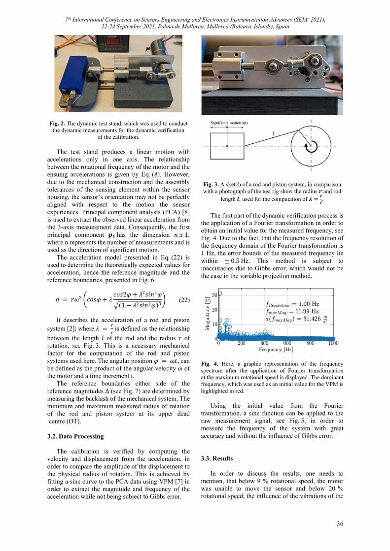
7th International Conference on Sensors Engineering and Electronics Instrumentation Advances (SEIA' 2021), 22-24 September 2021, Palma de Mallorca, Mallorca (Balearic Islands), Spain
36
Fig. 2. The dynamic test stand, which was used to conduct the dynamic measurements for the dynamic verification
of the calibration.
The test stand produces a linear motion with accelerations only in one axis. The relationship between the rotational frequency of the motor and the ensuing accelerations is given by Eq. (8). However, due to the mechanical construction and the assembly tolerances of the sensing element within the sensor housing, the sensor’s orientation may not be perfectly aligned with respect to the motion the sensor experiences. Principal component analysis (PCA) [8] is used to extract the observed linear acceleration from the 3-axis measurement data. Consequently, the first principal component 𝒑𝟏 has the dimension 𝑛 𝑥 1, where n represents the number of measurements and is used as the direction of significant motion.
The acceleration model presented in Eq. (22) is used to determine the theoretically expected values for acceleration, hence the reference magnitude and the reference boundaries, presented in Fig. 6.
𝑎 𝑟𝜔 𝑐𝑜𝑠𝜑 𝜆𝑐𝑜𝑠2𝜑 𝜆 𝑠𝑖𝑛 𝜑
1 𝜆 𝑠𝑖𝑛 𝜑 (22)
It describes the acceleration of a rod and piston
system [2]; where 𝜆 is defined as the relationship
between the length 𝑙 of the rod and the radius 𝑟 of rotation, see Fig. 3. This is a necessary mechanical factor for the computation of the rod and piston systems used here. The angular position 𝜑 𝜔𝑡, can be defined as the product of the angular velocity ω of the motor and a time increment t.
The reference boundaries either side of the reference magnitudes ∆ (see Fig. 7) are determined by measuring the backlash of the mechanical system. The minimum and maximum measured radius of rotation of the rod and piston system at its upper dead centre (OT).
3.2. Data Processing
The calibration is verified by computing the velocity and displacement from the acceleration, in order to compare the amplitude of the displacement to the physical radius of rotation. This is achieved by fitting a sine curve to the PCA data using VPM [7] in order to extract the magnitude and frequency of the acceleration while not being subject to Gibbs error.
Fig. 3. A sketch of a rod and piston system, in comparison with a photograph of the test rig show the radius 𝒓 and rod
length 𝒍, used for the computation of 𝝀𝒓
𝒍.
The first part of the dynamic verification process is
the application of a Fourier transformation in order to obtain an initial value for the measured frequency, see Fig. 4. Due to the fact, that the frequency resolution of the frequency domain of the Fourier transformation is 1 Hz, the error bounds of the measured frequency lie within 0.5 Hz. This method is subject to inaccuracies due to Gibbs error, which would not be the case in the variable projection method.
Fig. 4. Here, a graphic representation of the frequency spectrum after the application of Fourier transformation at the maximum rotational speed is displayed. The dominant frequency, which was used as an initial value for the VPM is highlighted in red.
Using the initial value from the Fourier
transformation, a sine function can be applied to the raw measurement signal, see Fig. 5, in order to measure the frequency of the system with great accuracy and without the influence of Gibbs error.
3.3. Results
In order to discuss the results, one needs to mention, that below 9 % rotational speed, the motor was unable to move the sensor and below 20 % rotational speed, the influence of the vibrations of the
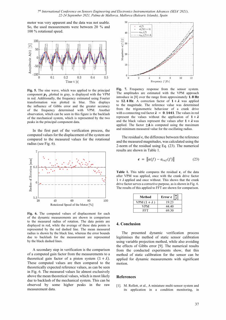
7th International Conference on Sensors Engineering and Electronics Instrumentation Advances (SEIA' 2021), 22-24 September 2021, Palma de Mallorca, Mallorca (Balearic Islands), Spain
37
motor was very apparent and the data was not usable. So, the used measurements were between 20 % and 100 % rotational speed.
Fig. 5. The sine wave, which was applied to the principal component 𝒑𝟏 ,plotted in gray, is displayed with the VPM in red. Additionally, the frequency estimated using Fourier transformation was plotted in blue. This displays the influence of Gibbs error and the greater accuracy of the frequency determined with VPM. Another observation, which can be seen in this figure is the backlash of the mechanical system, which is represented by the two peaks in the principal component data.
In the first part of the verification process, the
computed values for the displacement of the system are compared to the measured values for the rotational radius (see Fig. 6).
Fig. 6. The computed values of displacement for each of the dynamic measurements are shown in comparison to the measured radius of rotation. The data points are displayed in red, while the average of these data points is represented by the red dashed line. The mean measured radius is shown by the black line, whereas the error bounds due to backlash for the measurement are represented by the black dashed lines.
A secondary step in verification is the comparison
of a computed gain factor from the measurements to a theoretical gain factor of a piston system 1 𝜆 . These computed values are then compared to the theoretically expected reference values, as can be seen in Fig. 6. The measured values lie almost exclusively above the mean theoretical values, which is most likely due to backlash of the mechanical system. This can be observed by some higher peaks in the raw measurement data.
Fig. 7. Frequency response from the sensor system. The amplitudes are estimated with the VPM approach introduce in [8] over the range from approximately 𝟏. 𝟖 𝐇𝐳 to 𝟏𝟐. 𝟒 𝐇𝐳. A correction factor of 𝟏 𝝀 was applied to the magnitude. The reference value was determined from the trigonometric behaviour of a crank drive with a connecting rod factor 𝝀 𝟎. 𝟏𝟒𝟒𝟏. The values in red represent the values without the application of 𝟏 𝝀 and the black values represent the values after 𝟏 𝝀 was applied. The factor 𝚫 is computed using the maximum and minimum measured value for the oscillating radius.
The residual ϵ, the difference between the reference
and the measured magnitudes, was calculated using the 2-norm of the residual using Eq. (23). The numerical results are shown in Table 1.
𝝐 𝑎 𝑓 𝑎 𝑓 (23)
Table 1. This table compares the residual 𝛜, of the data after VPM was applied, once with the crank drive factor 1 𝜆 applied and once without. This shows that the crank drive factor serves a corrective purpose, as is shown in Fig. 6. The results of this applied to FFT are shown for comparison.
Method Error 𝝐 𝒎
𝒔𝟐
VPM (1 𝜆 ) 19.23 VPM 44.40 FFT 69.30
4. Conclusion
The presented dynamic verification process legitimises the method of static sensor calibration using variable projection method, while also avoiding the effects of Gibbs error [9]. The numerical results from the conducted experiments show, that this method of static calibration for the sensor can be applied for dynamic measurements with significant motion.
References
[1]. M. Rollett, et al., A miniature multi-sensor system and its application in a condition monitoring, in

7th International Conference on Sensors Engineering and Electronics Instrumentation Advances (SEIA' 2021), 22-24 September 2021, Palma de Mallorca, Mallorca (Balearic Islands), Spain
38
Proceedings of the 6th International Conference on Sensors Engineering and Electronics Instrumentation Advances (SEIA’ 2020), 23-25 September 2020, pp. 75-81.
[2]. B. Künne, Köhler/Rögnitz Maschinenteile 2, Springer Nature, 2008 (in German)
[3]. S.-h. P. Won, F. Golnaraghi, A triaxial accelerometer calibration method using a mathematical model, IEEE Transactions on Instrumentation and Measurement, Vol. 59, Issue 8, 2009, pp. 2144-2153.
[4]. F. Camps, S. Harasse, A. Monin, Numerical calibration for 3-axis accelerometers and magnetometers, in Proceedings of the IEEE International Conference on Electro/Information Technology (EIT’09), 2009, pp. 217-221.
[5]. G. D'Emilia, A. Gaspari, E. Natale, Dynamic calibration uncertainty of 3-axis low frequency
accelerometers, Acta IMEKO, Vol. 4, Issue 4, 2015, pp. 75-81.
[6]. D. O’Leary, B. Rust, Variable projection for nonlinear least squares problems, Computational Optimization and Applications, Vol. 54, Issue 2, 2013, pp. 579-593.
[7]. P. O’Leary, D. Ninevski, Estimating parameters of a sine wave by the method of variable projection, in Proceedings of the International Instrumentation and Measurement Technology Conference (I2MTC’21), May 2021, Glasgow, Scotland, pp. 1-6.
[8]. S. Wold, K. Esbensen, P. Geladi, Principal component analysis, Chemometrics and Intelligent Laboratory Systems, Vol. 2, Issues 1-3, 1987, pp. 37-52.
[9]. A. J. Jerri, The Gibbs Phenomenon in Fourier Analysis, Splines and Wavelet Approximations, Vol. 446, Springer Science & Business Media, 2013, pp. 12-32.
7th International Conference on Sensors Engineering and Electronics Instrumentation Advances (SEIA' 2021), 22-24 September 2021, Palma de Mallorca, Mallorca (Balearic Islands), Spain
39
(010)
Study of the Prospects for the Use of Ionic Liquids and Non-Aqueous Salt Solutions for Low-temperature Operation of Serial Electrochemical
Geophysical Sensors
E. I. Egorov, D. L. Zaitsev and V. M. Agafonov
Moscow Institute of Physics and Technology, 9 Institutsky Per., 141701 Dolgoprudny, Russia Tel.: + 74987446995, fax: + 74987446995
E-mail: [email protected] Summary: Electrochemical seismic sensors have recently been gaining popularity in the field of seismic exploration of minerals. With their obvious advantages such as operability in any orientation, the absence of complex mechanical structures, sensors have a number of limitations. In particular, aqueous electrolyte solutions are used as a working fluid, which, having a tabular freezing point of -48 °C, in practice undergo a phase transition in the range from -30 °C to -50 °C. This article examines electrolyte solutions as a working fluid of an electrochemical sensor based on new aqueous and non-aqueous solvents with the addition of an ionic liquid. It is shown that the selected samples of electrolytes have a freezing point obviously lower than -40 °C, the frequency response of sensitive elements is formed up to -40 °C, and seismic sensors based on these samples of electrolytes have acceptable output characteristics. Keywords: Molecular-electronic technology, Temperature dependence, Electrochemical сell.
1. Introduction
Seismic sensors based on molecular-electron transfer have proven well both in the field of studying the Earth's crust [1-3], its changes, as well as the search for natural resources [4-6]. The unique features are performance at any angle of deviation from the gravity vector and the absence of complex and precise mechanics. These properties are key for most areas of application, in particular, the search for natural resources, where rearrangement and transfer of equipment often occurs [7, 8].
Today, the development of resources and their control in hard-to-reach regions with difficult climate conditions is intensively going on [9]. For example, in the Arctic region, most of the work is carried out at low (down to -40 °C) and extremely low (-60 °C) temperatures, which increases the requirements for the characteristics of sensors when operating under those conditions [10]. This is necessary for the primary data to have the least distortion.
1.1. The Principle of Operation of an Electrochemical Seismic Sensor
The schematic diagram of the electrochemical seismic sensor is shown in Fig. 1, and the work is based on the following. The sensing element is a liquid-permeable four-electrode electrochemical cell located in a housing filled with a highly concentrated electrolyte solution 3. The ends of the housing are limited by flexible membranes 4. Magnet 5 and coil 6, shown in Fig. 3, form a mechanism for generating a feedback signal. The principle of operation is that the inertia forces associated with the ground vibrations set the fluid in motion. In turn, the flow of liquid through
the conversion element changes the electric current flowing between the electrodes. The current variations are converted into an output voltage with a transfer function W at the outputs, which controls the feedback mechanism via a separate electronic stage with a transfer function [11, 12].
Fig. 1. Schematic representation of an electrochemical sensor with an electromagnetic power feedback system: 1 – anodes; 2 – cathodes; 3 – electrolyte; 4 – membranes; 5 – magnet; 6 – electromagnetic coil.
The valid ranges of operating temperatures of such
sensors are determined by the electronic components in the electrical circuit, as well as by the properties of the used working fluid [13, 14]. The working fluid is an electrolyte solution with the addition of active molecules, which undergo a dissociation process on the electrodes and transfer a charge.
The main parameters of the electrolyte are: Coefficient of viscosity, which mainly affects the
mechanical subsystem of the sensing element; The diffusion coefficient determines the rate of
delivery of ions to the electrode, thereby
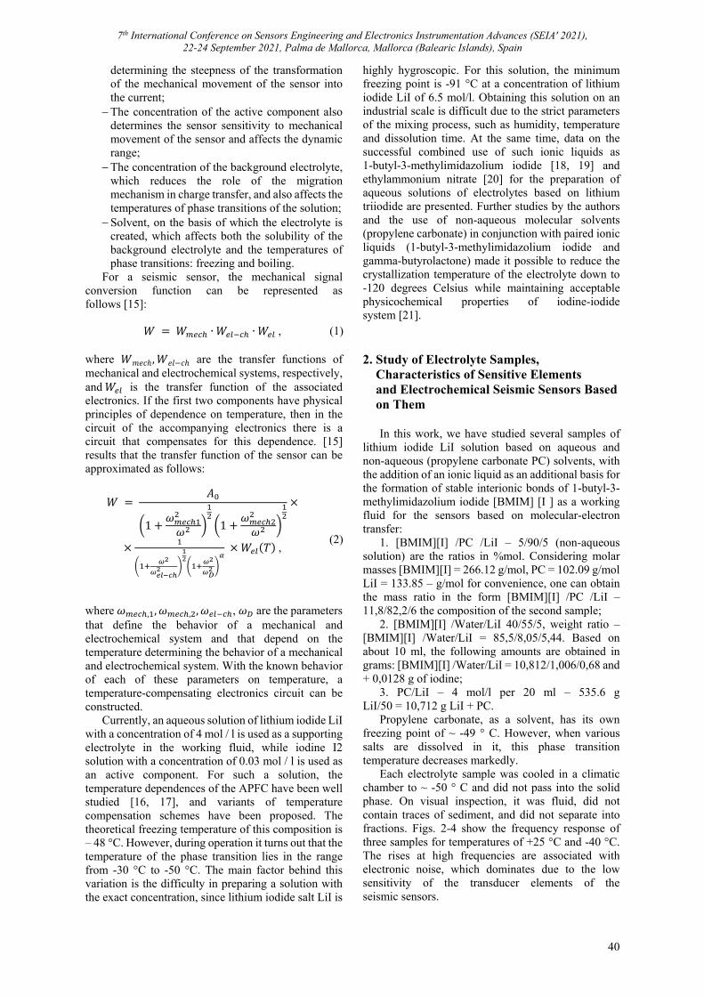
7th International Conference on Sensors Engineering and Electronics Instrumentation Advances (SEIA' 2021), 22-24 September 2021, Palma de Mallorca, Mallorca (Balearic Islands), Spain
40
determining the steepness of the transformation of the mechanical movement of the sensor into the current;
The concentration of the active component also determines the sensor sensitivity to mechanical movement of the sensor and affects the dynamic range;
The concentration of the background electrolyte, which reduces the role of the migration mechanism in charge transfer, and also affects the temperatures of phase transitions of the solution;
Solvent, on the basis of which the electrolyte is created, which affects both the solubility of the background electrolyte and the temperatures of phase transitions: freezing and boiling.
For a seismic sensor, the mechanical signal conversion function can be represented as follows [15]:
𝑊 𝑊 ∙ 𝑊 ∙ 𝑊 , (1)
where 𝑊𝑚𝑒𝑐ℎ, 𝑊𝑒𝑙 𝑐ℎ are the transfer functions of mechanical and electrochemical systems, respectively, and 𝑊 is the transfer function of the associated electronics. If the first two components have physical principles of dependence on temperature, then in the circuit of the accompanying electronics there is a circuit that compensates for this dependence. [15] results that the transfer function of the sensor can be approximated as follows:
𝑊 𝐴
1𝜔
𝜔 1𝜔
𝜔
𝑊 𝑇 , (2)
where 𝜔 , , 𝜔 , , 𝜔 , 𝜔 are the parameters that define the behavior of a mechanical and electrochemical system and that depend on the temperature determining the behavior of a mechanical and electrochemical system. With the known behavior of each of these parameters on temperature, a temperature-compensating electronics circuit can be constructed.
Currently, an aqueous solution of lithium iodide LiI with a concentration of 4 mol / l is used as a supporting electrolyte in the working fluid, while iodine I2 solution with a concentration of 0.03 mol / l is used as an active component. For such a solution, the temperature dependences of the APFC have been well studied [16, 17], and variants of temperature compensation schemes have been proposed. The theoretical freezing temperature of this composition is – 48 °C. However, during operation it turns out that the temperature of the phase transition lies in the range from -30 °C to -50 °C. The main factor behind this variation is the difficulty in preparing a solution with the exact concentration, since lithium iodide salt LiI is
highly hygroscopic. For this solution, the minimum freezing point is -91 °C at a concentration of lithium iodide LiI of 6.5 mol/l. Obtaining this solution on an industrial scale is difficult due to the strict parameters of the mixing process, such as humidity, temperature and dissolution time. At the same time, data on the successful combined use of such ionic liquids as 1-butyl-3-methylimidazolium iodide [18, 19] and ethylammonium nitrate [20] for the preparation of aqueous solutions of electrolytes based on lithium triiodide are presented. Further studies by the authors and the use of non-aqueous molecular solvents (propylene carbonate) in conjunction with paired ionic liquids (1-butyl-3-methylimidazolium iodide and gamma-butyrolactone) made it possible to reduce the crystallization temperature of the electrolyte down to -120 degrees Celsius while maintaining acceptable physicochemical properties of iodine-iodide system [21].
2. Study of Electrolyte Samples, Characteristics of Sensitive Elements and Electrochemical Seismic Sensors Based on Them
In this work, we have studied several samples of lithium iodide LiI solution based on aqueous and non-aqueous (propylene carbonate PC) solvents, with the addition of an ionic liquid as an additional basis for the formation of stable interionic bonds of 1-butyl-3-methylimidazolium iodide [BMIM] [I ] as a working fluid for the sensors based on molecular-electron transfer:
1. [BMIM][I] /PC /LiI – 5/90/5 (non-aqueous solution) are the ratios in %mol. Considering molar masses [BMIM][I] = 266.12 g/mol, PC = 102.09 g/mol LiI = 133.85 – g/mol for convenience, one can obtain the mass ratio in the form [BMIM][I] /PC /LiI – 11,8/82,2/6 the composition of the second sample;
2. [BMIM][I] /Water/LiI 40/55/5, weight ratio – [BMIM][I] /Water/LiI = 85,5/8,05/5,44. Based on about 10 ml, the following amounts are obtained in grams: [BMIM][I] /Water/LiI = 10,812/1,006/0,68 and + 0,0128 g of iodine;
3. PC/LiI – 4 mol/l per 20 ml – 535.6 g LiI/50 = 10,712 g LiI + PC.
Propylene carbonate, as a solvent, has its own freezing point of ~ -49 ° C. However, when various salts are dissolved in it, this phase transition temperature decreases markedly.
Each electrolyte sample was cooled in a climatic chamber to ~ -50 ° C and did not pass into the solid phase. On visual inspection, it was fluid, did not contain traces of sediment, and did not separate into fractions. Figs. 2-4 show the frequency response of three samples for temperatures of +25 °C and -40 °C. The rises at high frequencies are associated with electronic noise, which dominates due to the low sensitivity of the transducer elements of the seismic sensors.
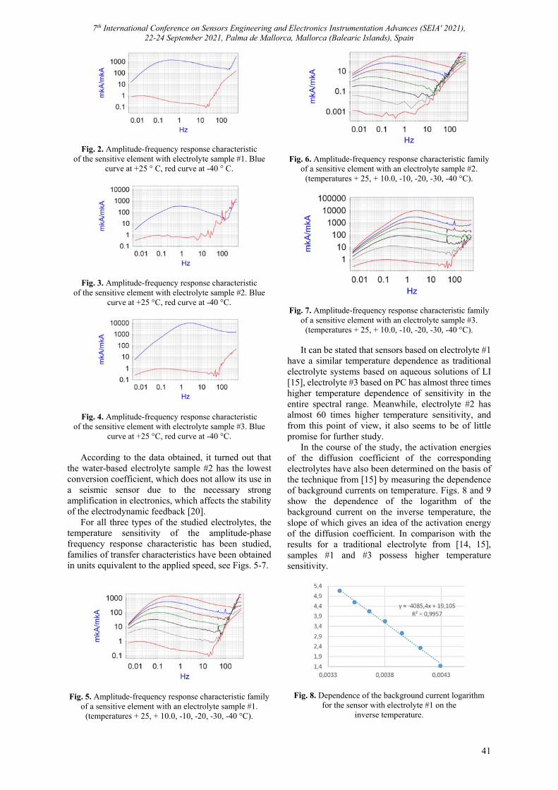
7th International Conference on Sensors Engineering and Electronics Instrumentation Advances (SEIA' 2021), 22-24 September 2021, Palma de Mallorca, Mallorca (Balearic Islands), Spain
41
Fig. 2. Amplitude-frequency response characteristic of the sensitive element with electrolyte sample #1. Blue
curve at +25 ° C, red curve at -40 ° C.
Fig. 3. Amplitude-frequency response characteristic of the sensitive element with electrolyte sample #2. Blue
curve at +25 °C, red curve at -40 °C.
Fig. 4. Amplitude-frequency response characteristic of the sensitive element with electrolyte sample #3. Blue
curve at +25 °C, red curve at -40 °C. According to the data obtained, it turned out that
the water-based electrolyte sample #2 has the lowest conversion coefficient, which does not allow its use in a seismic sensor due to the necessary strong amplification in electronics, which affects the stability of the electrodynamic feedback [20].
For all three types of the studied electrolytes, the temperature sensitivity of the amplitude-phase frequency response characteristic has been studied, families of transfer characteristics have been obtained in units equivalent to the applied speed, see Figs. 5-7.
Fig. 5. Amplitude-frequency response characteristic family of a sensitive element with an electrolyte sample #1.
(temperatures + 25, + 10.0, -10, -20, -30, -40 °C).
Fig. 6. Amplitude-frequency response characteristic family of a sensitive element with an electrolyte sample #2.
(temperatures + 25, + 10.0, -10, -20, -30, -40 °C).
Fig. 7. Amplitude-frequency response characteristic family of a sensitive element with an electrolyte sample #3.
(temperatures + 25, + 10.0, -10, -20, -30, -40 °C).
It can be stated that sensors based on electrolyte #1 have a similar temperature dependence as traditional electrolyte systems based on aqueous solutions of LI [15], electrolyte #3 based on PC has almost three times higher temperature dependence of sensitivity in the entire spectral range. Meanwhile, electrolyte #2 has almost 60 times higher temperature sensitivity, and from this point of view, it also seems to be of little promise for further study.
In the course of the study, the activation energies of the diffusion coefficient of the corresponding electrolytes have also been determined on the basis of the technique from [15] by measuring the dependence of background currents on temperature. Figs. 8 and 9 show the dependence of the logarithm of the background current on the inverse temperature, the slope of which gives an idea of the activation energy of the diffusion coefficient. In comparison with the results for a traditional electrolyte from [14, 15], samples #1 and #3 possess higher temperature sensitivity.
Fig. 8. Dependence of the background current logarithm for the sensor with electrolyte #1 on the
inverse temperature.
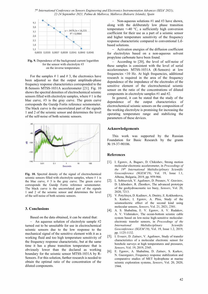
7th International Conference on Sensors Engineering and Electronics Instrumentation Advances (SEIA' 2021), 22-24 September 2021, Palma de Mallorca, Mallorca (Balearic Islands), Spain
42
Fig. 9. Dependence of the background current logarithm for the sensor with electrolyte #3
on the inverse temperature.
For the samples # 1 and # 3, the electronics have been adjusted so that the output amplitude-phase frequency response characteristics corresponded to the R-Sensors MTSS-1031A accelerometer [21]. Fig. 10 shows the spectral densities of electrochemical seismic sensors filled with electrolyte samples, where # 1 is the blue curve, #3 is the gray curve. The green curve corresponds the Guralp Fortis reference seismometer. The black curve is the uncorrelated part of the signals 1 and 2 of the seismic sensor and determines the level of the self-noise of both seismic sensors.
Fig. 10. Spectral density of the signal of electrochemical seismic sensors filled with electrolyte samples, where # 1 is the blue curve, # 3 is the gray curve. The green curve corresponds the Guralp Fortis reference seismometer. The black curve is the uncorrelated part of the signals 1 and 2 of the seismic sensor and determines the level of the self-noise of both seismic sensors.
3. Conclusions
Based on the data obtained, it can be stated that: An aqueous solution of electrolyte sample #2
turned out to be unsuitable for use in electrochemical seismic sensors due to the low response to the mechanical signal of the sensitive element with it as a working fluid and too high temperature sensitivity of the frequency response characteristic, but at the same time it has a phase transition temperature that is obviously lower than the declared as working boundary for the seismic sensor MTSS-1031A by R-Sensors. For this solution, further research is needed to obtain the optimal ratio of the concentration of the diluted components.
Non-aqueous solutions #1 and #3 have shown, along with the deliberately low phase transition temperature <-40 °C, a sufficiently high conversion coefficient for their use as a part of a seismic sensor and higher temperature sensitivity of the frequency response characteristic compared to conventional LiI-based solutions.
Activation energies of the diffusion coefficient for electrolytes based on a non-aqueous solvent propylene carbonate have been found.
According to [20], the level of self-noise of these samples is consistent with the level of serial accelerometers MTSS-1031A (R-Sensors) at low frequencies <10 Hz. At high frequencies, additional research is required in the area of the frequency dependence of the impedance of the electrodes of the sensitive element of the electrochemical seismic sensor on the ratio of the concentrations of diluted components in electrolyte samples #1 and #2.
In general, it can be stated that the study of the dependence of the output characteristics of electrochemical seismic sensors on the composition of the working electrolyte is promising for increasing the operating temperature range and stabilizing the parameters of these devices.
Acknowledgements
This work was supported by the Russian Foundation for Basic Research by the grants 19-37-90106.
References [1]. I. Egorov, A. Bugaev, D. Chikishev, Strong motion
molecular-electronic accelerometer, in Proceedings of the 19th International Multidisciplinary Scientific Geoconference (SGEM’19), Vol. 19, Issue 1.1, Albena, Bulgaria, 2019, pp. 959-966.
[2]. L. Sobisevich, V. Agafonov, D. Presnov, V. Gravirov, D. Likhodeev, R. Zhostkov, The advanced prototype of the geohydroacoustic ice buoy, Sensors, Vol. 20, 2020, 7213.
[3]. V. Potylitsyn, D. Kudinov, A. Dmitry, E. Kokhonkova, S. Kurkov, I. Egorov, A. Pliss, Study of the seismoelectric effect of the second kind using molecular sensors, Sensors, Vol. 21, 2021, 2301.
[4]. A. S. Shabalina, E. V. Egorov, A. V. Rudakov, A. V. Vishniakov, The ocean-bottom seismic cable system based on low-noise high-sensitive molecular-electronic transfer sensors, in Proceedings of the International Multidisciplinary Scientific Geoconference (SGEM’19), Vol. 19, Issue 1.2, 2019, pp. 1125-1132.
[5]. I. Evseev, D. Zaitsev, V. Agafonov, Study of transfer characteristics of a molecular electronic sensor for borehole surveys at high temperatures and pressures, Sensors, Vol. 19, 2019, 2545.
[6]. E. Egorov, A. Shabalina, D. Zaitsev, S. Kurkov, N. Gueorguiev, Frequency response stabilization and comparative studies of MET hydrophone at marine seismic exploration systems, Sensors, Vol. 20, 2020, 1944.

7th International Conference on Sensors Engineering and Electronics Instrumentation Advances (SEIA' 2021), 22-24 September 2021, Palma de Mallorca, Mallorca (Balearic Islands), Spain
43
[7]. T. Liang, et al., A MEMS based electrochemical angular accelerometer with a force-balanced negative feedback, IEEE Sensors Journal, Vol. 21, Issue 14, 2021, pp. 15972-15978.
[8]. D. Zaitsev, E. Egorov, A. Shabalina, High resolution miniature MET sensors for healthcare and sport applications, in Proceedings of the Twelfth International Conference on Sensing Technology (ICST’18), Limerick, Ireland, 4-6 December 2018, pp. 287-292.
[9]. D. L. Zaitsev, S. Yu. Avdyukhina, V. M. Agafonov, A. S. Bugaev, E. V. Egorov, A molecular-electronic hydrophone for low-frequency research of ambient noise in the world ocean, Doklady Earth Sciences, Vol. 483, Issue 6, Part 2, 2018, pp. 1579-1581.
[10]. A. Fokina, D. Zaitsev, E. Egorov, A simple and cheap method of met geophones and seismic accelerometers temperature sensitivity stabilization in a wide temperature band, in Proceedings of the 19th International Multidisciplinary Scientific Geoconference (SGEM’20), Vol. 2020-August, Issue 1.2, 2020, pp. 411-418.
[11]. M. Ryzhkov, V. Agafonov, Modeling of the MET sensitive element conversion factor on the intercathode distance, Sensors, Vol. 20, 2020, 5146.
[12]. V. M. Agafonov, Modeling the convective noise in an electrochemical motion transducer, International Journal of Electrochemical Science, Vol. 13, Issue 12, 2019, pp. 11432-11442.
[13]. V. Agafonov, A. Shabalina, V. Krishtop, Modeling and experimental study of convective noise inelectrochemical planar sensitive element of MET motion sensor, Sensors and Actuators A, Vol. 293, 2019, pp. 259-268.
[14]. D. L. Zaitsev, P. V. Dudkin, T. V. Krishtop, A. V. Neeshpapa, V. G. Popov, V. V. Uskov, V. G. Krishtop, Experimental studies of temperature dependence of transfer function of molecular electronic transducers at high frequencies, IEEE
Sensors Journal, Vol. 16, Issue 22, 2016, pp. 7864-7869.
[15]. D. A. Chikishev, D. L. Zaitsev, K. S. Belotelov, I. V. Egorov, The temperature dependence of amplitude- frequency response of the MET sensor of linear motion in a broad frequency range, IEEE Sensors Journal, Vol. 19, Issue 21, 2019, pp. 9653-9661
[16]. A. Fokina, I. Egorov, A. Shabalina, Method for ensuring temperature and time stability of parameters of molecular electronic geophysical sensors for oil and gas exploration systems, in Proceedings of the 20th International Multidisciplinary Scientific Geoconference: Science and Technologies in Geology, Exploration and Mining (SGEM’20), Vol. 2020, Issue 1.2, 18 August 2020 – 24 August 2020, pp. 719-726.
[17]. I. V. Egorov, N. C. Nguyen, T. S. Nguyen, et al., Simulation of the laminar-turbulent transition by applying dissipative numerical schemes, Comput. Math. and Math. Phys., Vol. 61, 2021, pp. 254-266.
[18]. Y. Xu, W. J. Lin, M. Gliege, R. Gunckel, Z. Zhao, H. Yu, L. L. Dai, A dual ionic liquid-based low-temperature electrolyte system, The Journal of Physical Chemistry B, Vol. 122, Issue 50, 2018, pp. 12077-12086.
[19]. W. J. Lin, Y. Xu, S. MacDonald, R. Gunckel, Z. Zhaob, L. L. Dai, Tailoring intermolecular interactions to develop a low-temperature electrolyte system consisting of 1-butyl-3-methylimidazolium iodide and organic solvents, RSC Adv., Vol. 9, 2019, pp. 36796-36807.
[20]. I. V. Egorov, A. S. Shabalina, V. M. Agafonov, Design and self-noise of MET closed-loop seismic accelerometers, IEEE Sens. J., Vol. 17, Issue 7, 2017, pp. 2008-2014.
[21]. R-sensors, Accelerometers, http://r-sensors.ru/ru/ products/accel/
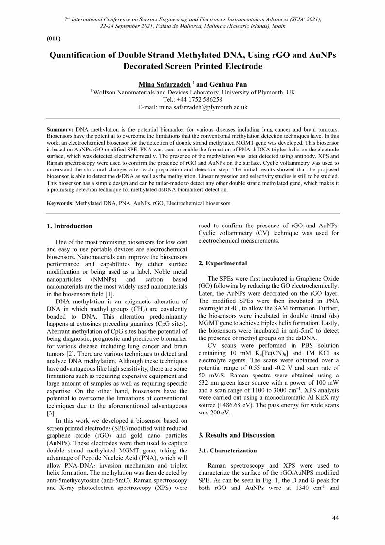
7th International Conference on Sensors Engineering and Electronics Instrumentation Advances (SEIA' 2021), 22-24 September 2021, Palma de Mallorca, Mallorca (Balearic Islands), Spain
44
(011)
Quantification of Double Strand Methylated DNA, Using rGO and AuNPs Decorated Screen Printed Electrode
Mina Safarzadeh 1 and Genhua Pan
1 Wolfson Nanomaterials and Devices Laboratory, University of Plymouth, UK Tel.: +44 1752 586258
E-mail: [email protected] Summary: DNA methylation is the potential biomarker for various diseases including lung cancer and brain tumours. Biosensors have the potential to overcome the limitations that the conventional methylation detection techniques have. In this work, an electrochemical biosensor for the detection of double strand methylated MGMT gene was developed. This biosensor is based on AuNPs/rGO modified SPE. PNA was used to enable the formation of PNA-dsDNA triplex helix on the electrode surface, which was detected electrochemically. The presence of the methylation was later detected using antibody. XPS and Raman spectroscopy were used to confirm the presence of rGO and AuNPs on the surface. Cyclic voltammetry was used to understand the structural changes after each preparation and detection step. The initial results showed that the proposed biosensor is able to detect the dsDNA as well as the methylation. Linear regression and selectivity studies is still to be studied. This biosensor has a simple design and can be tailor-made to detect any other double strand methylated gene, which makes it a promising detection technique for methylated dsDNA biomarkers detection. Keywords: Methylated DNA, PNA, AuNPs, rGO, Electrochemical biosensors.
1. Introduction
One of the most promising biosensors for low cost and easy to use portable devices are electrochemical biosensors. Nanomaterials can improve the biosensors performance and capabilities by either surface modification or being used as a label. Noble metal nanoparticles (NMNPs) and carbon based nanomaterials are the most widely used nanomaterials in the biosensors field [1].
DNA methylation is an epigenetic alteration of DNA in which methyl groups (CH3) are covalently bonded to DNA. This alteration predominantly happens at cytosines preceding guanines (CpG sites). Aberrant methylation of CpG sites has the potential of being diagnostic, prognostic and predictive biomarker for various disease including lung cancer and brain tumors [2]. There are various techniques to detect and analyze DNA methylation. Although these techniques have advantageous like high sensitivity, there are some limitations such as requiring expensive equipment and large amount of samples as well as requiring specific expertise. On the other hand, biosensors have the potential to overcome the limitations of conventional techniques due to the aforementioned advantageous [3].
In this work we developed a biosensor based on screen printed electrodes (SPE) modified with reduced graphene oxide (rGO) and gold nano particles (AuNPs). These electrodes were then used to capture double strand methylated MGMT gene, taking the advantage of Peptide Nucleic Acid (PNA), which will allow PNA-DNA2 invasion mechanism and triplex helix formation. The methylation was then detected by anti-5methycytosine (anti-5mC). Raman spectroscopy and X-ray photoelectron spectroscopy (XPS) were
used to confirm the presence of rGO and AuNPs. Cyclic voltammetry (CV) technique was used for electrochemical measurements.
2. Experimental
The SPEs were first incubated in Graphene Oxide (GO) following by reducing the GO electrochemically. Later, the AuNPs were decorated on the rGO layer. The modified SPEs were then incubated in PNA overnight at 4C, to allow the SAM formation. Further, the biosensors were incubated in double strand (ds) MGMT gene to achieve triplex helix formation. Lastly, the biosensors were incubated in anti-5mC to detect the presence of methyl groups on the dsDNA.
CV scans were performed in PBS solution containing 10 mM K3[Fe(CN)6] and 1M KCl as electrolyte agents. The scans were obtained over a potential range of 0.55 and -0.2 V and scan rate of 50 mV/S. Raman spectra were obtained using a 532 nm green laser source with a power of 100 mW and a scan range of 1100 to 3000 cm−1. XPS analysis were carried out using a monochromatic Al KαX-ray source (1486.68 eV). The pass energy for wide scans was 200 eV.
3. Results and Discussion 3.1. Characterization
Raman spectroscopy and XPS were used to characterize the surface of the rGO/AuNPS modified SPE. As can be seen in Fig. 1, the D and G peak for both rGO and AuNPs were at 1340 cm-1 and
7th International Conference on Sensors Engineering and Electronics Instrumentation Advances (SEIA' 2021), 22-24 September 2021, Palma de Mallorca, Mallorca (Balearic Islands), Spain
45
1570 cm-1 respectively. The intensity ratio (ID/IG) was 1.16 for rGO which decreased to 0.13 for rGO/AuNPs. This suggests that after introducing AuNPs, sp2 cluster number increased and more graphitic domains were formed [4].
Fig. 1. Raman spectra of rGO and AuNPS.
Fig. 2. XPS spectra of rGO and AuNPS.
Fig. 2 shows wide scan spectra of rGO and AuNPs modified SPEs. For the rGO electrode, the C and O peaks are observed at 286.33 eV and 533.33 eV respectively. Regarding the rGO/AuNPs modified electrodes, the C and O peak are observed at 298.99 eV and 551.00 eV, respectively. Also, five new peaks appeared at 16.23 eV, 68.33 eV, 94.99 eV, 351.14 eV and 370.08 eV confirming the presence of AuNPs on the rGO surface [5]. 3.1. Electrochemical Detection
After each preparation and incubation step, CV was performed to evaluate and understand the structural changes in the surface of the electrode. As observed in Fig. 3 the anodic peak current (ipa) for the GO was 1.39 V, where it increased to 127.18 V after its reduction, which is due to the high conductivity of the rGO layer. It then reduced slightly to 118.38 V for AuNPs where it further decreased to 80.40 V after being incubated in PNA confirming the attachment of PNA to the AuNPs. After incubating the PNA modified electrodes in the double strand gene, the peak current reduced to 78.57 V which confirms the presence of double strand DNA on the surface. The peak current rose slightly to 81 V after being incubated
in anti-5mC, which further confirmed the presence of antibody and thus detection of the presence of methyl groups on the double strand gene.
Fig. 3. Cyclic voltammograms of various steps of DNA preparation.
4. Conclusions
In this work, a potential biosensor for the detection of double strand methylated gene was reported. RGO and AuNPs were used to modify the SPE surface in order to increase the conductivity and reproducibility of the electrode. Their presence was confirmed by Raman and XPS spectra. Also, PNA was used to allow the formation of PNA-DNA2 triplex helix and the methylation was detected with antibody, which were both confirmed by voltammetry results. Linear regression and the selectivity of the biosensor will be further investigated. This biosensor has a simple design for cost-efficient production and can be tailor-made to detect any other double strand methylated gene. Acknowledgements
This research was funded by EU Horizon 2020 Marie Skłodowska-Curie Actions-ITN-ETN AiPBAND grant number 764281. References [1]. G. Maduraiveeran, Electrochemical sensor and
biosensor platforms based on advanced nanomaterials for biological and biomedical applications, Biosensors and Bioelectronic, Vol. 103, 2018, pp.113-129.
[2]. T. Mikeska, DNA methylation biomarkers: Cancer and beyond, Genes, Vol. 5, Issue, 2014, pp. 821-864.
[3]. S. Kurdyukov, DNA methylation analysis: choosing the right method, Biolog, Vol. 5, 2016, 3.
[4]. N. Shams, Electrochemical sensor based on gold nanoparticles/ethylenediamine-reduced graphene oxide for trace determination of fenitrothion in water, RSC Advances, Issue 92, 2016, pp. 89430-89439.
[5]. R. Kanagaraj, Highly selective and sensitive detection of Cr6+ ions using size-specific label-free gold nanoparticles, Sensors and Actuators B: Chemical, Vol. 251, 2017, pp. 683-691.
7th International Conference on Sensors Engineering and Electronics Instrumentation Advances (SEIA' 2021), 22-24 September 2021, Palma de Mallorca, Mallorca (Balearic Islands), Spain
46
(012)
Role of Cobalt in Co-ZnO Nanoflower Gas Sensors for the Detection of Low Concentration VOCs
Y. Luo 1, A. Ly 2, D. Lahem 2, C. Zhang 3 and M. Debliquy 2
1 Service de Science des Matériaux, Faculté Polytechnique, University of Mons, Mons 7000, Belgium 2 Material Science Department, Materia Nova ASBL, Mons 7000, Belgium
3 College of Mechanical Engineering, Yangzhou University, Yangzhou 225127, P. R. China Tel.: +32 465614284, fax: + 87654321
E-mail: [email protected] Summary: As a non-invasive detection method, breath analysis for the diagnosis of lung cancer has been a hotspot in the medical field. Using an e-nose to achieve the breath analysis is a popular choice. To prepare the sensors used in the e-nose for the detection of the volatile organic compounds which are considered as the biomarkers for lung cancers, cobalt doped ZnO sensors with high response to low concentration VOCs were fabricated. The Co-ZnO samples were synthesized via wet chemical method and drop coated onto the alumina substrates equipped with gold interdigitated electrodes after calcination. The as-synthesized materials were characterized by SEM, XRD, FT-IR and XPS to observe the microstructure, the crystal phase and the states of Co atom in the samples. The sensors were tested with various VOCs at different temperatures showing a strong influence of the different amounts of Co2+ addition on the sensing characteristics. The difference in the sensing performance could be explained by the different phases of Co in the sensing layers. Keywords: ZnO, Co doping, p-n heterojunctions, Gas sensor, VOCs, Lung cancer.
1. Introduction
In the medical field, developing non-invasive diagnosis methods for lung cancer has become a hotspot. Among them, breath analysis is an efficient method tracking gases, volatile organic compounds (VOCs), considered as biomarkers [1-3]. Traditionally, gas chromatography was used to study the components in breath analysis but the size and cost of the equipment and difficulties in data analysis made it hard to be used for doctors. Therefore e-nose can be good choice. Biomarkers in breath are at low concentrations, mostly in the ppb range and it becomes essential to develop sensors with high response to those biomarkers. Here we focused on isopropanol which seems to be an important biomarker for lung cancer. [4-5] Semiconductor gas sensors can be candidates due to their relative high response and low cost. However, pure metal oxide such as ZnO cannot fit the requirement of detecting ppb level concentration change of VOCs, so it is necessary to modify the metal oxide. Synthesizing nanostructures with high specific surface area, doping or building p-n heterojunctions between two different semiconductors are efficient methods to improve the response of semiconductor sensors. [6-8]. The operating mechanism of metal oxide semiconductor is the In this work, we synthesized cobalt assisted flower like zinc oxide (Co-ZnO) as sensing material. The ratio between Co and ZnO were adjusted and its influence on the sensing performances was studied.
2. Experiments
The Co-ZnO composites were synthesized via a chemical deposition method. First, x mmol Co(NO3)2•6H2O and 3-x mmol Zn(NO3)2•6H2O were dissolved in 55 ml of deionized (DI) water, which was marked as solution A. x was set as 0.3, 0.6, 0.9, 1.2 and 1.5 (10 at%, 20 at%, 30 at%, 30 at% and 50 at% Co respectively). The obtained samples are named as 10Co, 20Co 30Co 40Co and 50Co respectively. At the same time, 30 mmol of 2-Methylimidazole (MeIM) was dissolved in 50 mmol of DI water and magnetically stirred until the solution becomes clear. The solution was marked as solution B. Solution B was poured into solution A, then 15.5 ml of ammonia was immediately added into the solution. Afterwards, the purple solution was magnetically stirred at room temperature for 2 h. The purple precipitates were centrifugated and washed and dried at 80 oC overnight. To prepare the Co-ZnO, the as-prepared purple powders were calcinated at 500 oC for 2 h. For making the sensors, the as-prepared powders were drop coated on an alumina substrate with interdigitated gold electrodes. The gas sensing test was carried out in a homemade testing system. The testing system and the testing method are the same as introduced in ref. [9]. The response of n-type and p-type sensors is defined as:
𝑆 𝑅 𝑅 /𝑅
or 𝑆 𝑅 𝑅 /𝑅 , (1)
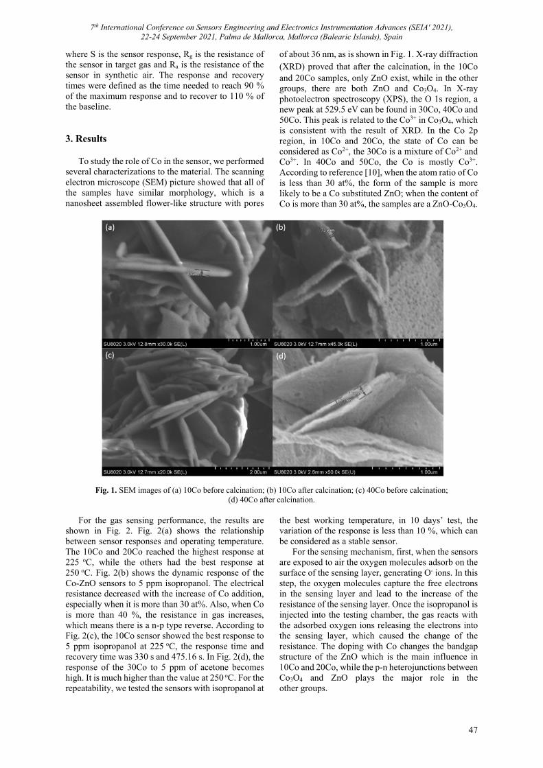
7th International Conference on Sensors Engineering and Electronics Instrumentation Advances (SEIA' 2021), 22-24 September 2021, Palma de Mallorca, Mallorca (Balearic Islands), Spain
47
where S is the sensor response, Rg is the resistance of the sensor in target gas and Ra is the resistance of the sensor in synthetic air. The response and recovery times were defined as the time needed to reach 90 % of the maximum response and to recover to 110 % of the baseline. 3. Results
To study the role of Co in the sensor, we performed several characterizations to the material. The scanning electron microscope (SEM) picture showed that all of the samples have similar morphology, which is a nanosheet assembled flower-like structure with pores
of about 36 nm, as is shown in Fig. 1. X-ray diffraction (XRD) proved that after the calcination, in the 10Co and 20Co samples, only ZnO exist, while in the other groups, there are both ZnO and Co3O4. In X-ray photoelectron spectroscopy (XPS), the O 1s region, a new peak at 529.5 eV can be found in 30Co, 40Co and 50Co. This peak is related to the Co3+ in Co3O4, which is consistent with the result of XRD. In the Co 2p region, in 10Co and 20Co, the state of Co can be considered as Co2+, the 30Co is a mixture of Co2+ and Co3+. In 40Co and 50Co, the Co is mostly Co3+. According to reference [10], when the atom ratio of Co is less than 30 at%, the form of the sample is more likely to be a Co substituted ZnO; when the content of Co is more than 30 at%, the samples are a ZnO-Co3O4.
Fig. 1. SEM images of (a) 10Co before calcination; (b) 10Co after calcination; (c) 40Co before calcination; (d) 40Co after calcination.
For the gas sensing performance, the results are
shown in Fig. 2. Fig. 2(a) shows the relationship between sensor responses and operating temperature. The 10Co and 20Co reached the highest response at 225 oC, while the others had the best response at 250 oC. Fig. 2(b) shows the dynamic response of the Co-ZnO sensors to 5 ppm isopropanol. The electrical resistance decreased with the increase of Co addition, especially when it is more than 30 at%. Also, when Co is more than 40 %, the resistance in gas increases, which means there is a n-p type reverse. According to Fig. 2(c), the 10Co sensor showed the best response to 5 ppm isopropanol at 225 oC, the response time and recovery time was 330 s and 475.16 s. In Fig. 2(d), the response of the 30Co to 5 ppm of acetone becomes high. It is much higher than the value at 250 oC. For the repeatability, we tested the sensors with isopropanol at
the best working temperature, in 10 days’ test, the variation of the response is less than 10 %, which can be considered as a stable sensor.
For the sensing mechanism, first, when the sensors are exposed to air the oxygen molecules adsorb on the surface of the sensing layer, generating O- ions. In this step, the oxygen molecules capture the free electrons in the sensing layer and lead to the increase of the resistance of the sensing layer. Once the isopropanol is injected into the testing chamber, the gas reacts with the adsorbed oxygen ions releasing the electrons into the sensing layer, which caused the change of the resistance. The doping with Co changes the bandgap structure of the ZnO which is the main influence in 10Co and 20Co, while the p-n heterojunctions between Co3O4 and ZnO plays the major role in the other groups.
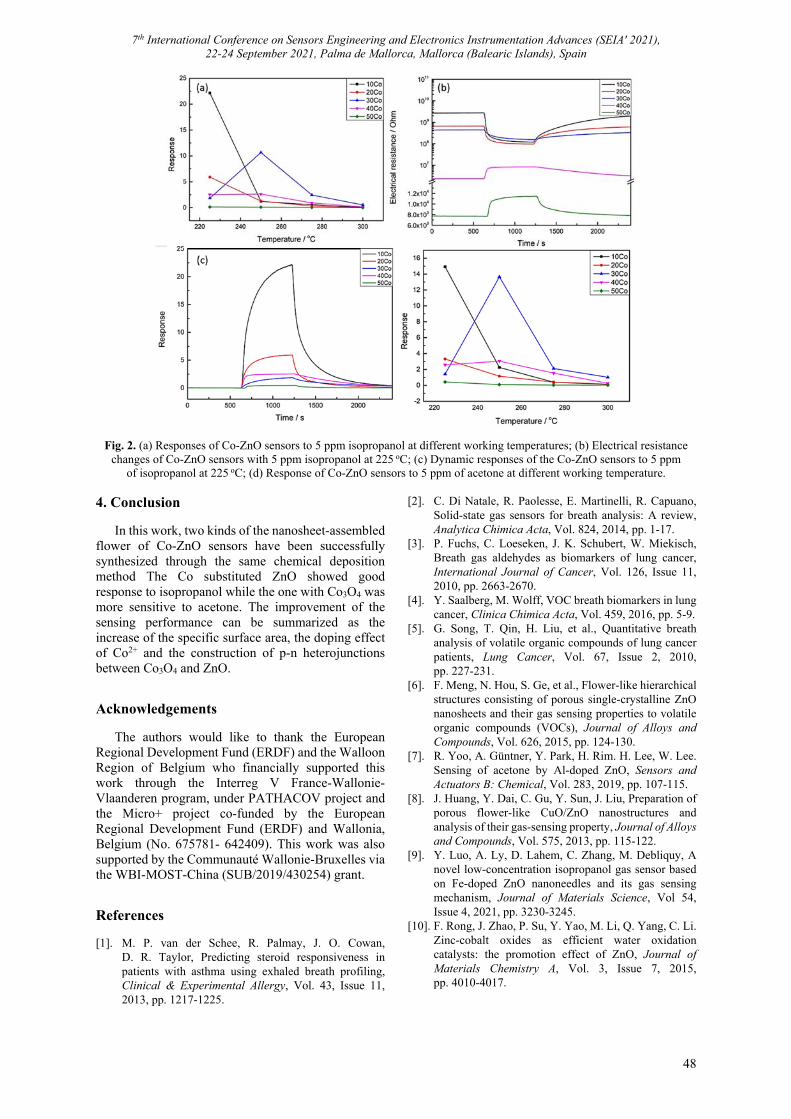
7th International Conference on Sensors Engineering and Electronics Instrumentation Advances (SEIA' 2021), 22-24 September 2021, Palma de Mallorca, Mallorca (Balearic Islands), Spain
48
Fig. 2. (a) Responses of Co-ZnO sensors to 5 ppm isopropanol at different working temperatures; (b) Electrical resistance changes of Co-ZnO sensors with 5 ppm isopropanol at 225 oC; (c) Dynamic responses of the Co-ZnO sensors to 5 ppm
of isopropanol at 225 oC; (d) Response of Co-ZnO sensors to 5 ppm of acetone at different working temperature. 4. Conclusion
In this work, two kinds of the nanosheet-assembled flower of Co-ZnO sensors have been successfully synthesized through the same chemical deposition method The Co substituted ZnO showed good response to isopropanol while the one with Co3O4 was more sensitive to acetone. The improvement of the sensing performance can be summarized as the increase of the specific surface area, the doping effect of Co2+ and the construction of p-n heterojunctions between Co3O4 and ZnO.
Acknowledgements
The authors would like to thank the European Regional Development Fund (ERDF) and the Walloon Region of Belgium who financially supported this work through the Interreg V France-Wallonie-Vlaanderen program, under PATHACOV project and the Micro+ project co-funded by the European Regional Development Fund (ERDF) and Wallonia, Belgium (No. 675781- 642409). This work was also supported by the Communauté Wallonie-Bruxelles via the WBI-MOST-China (SUB/2019/430254) grant.
References [1]. M. P. van der Schee, R. Palmay, J. O. Cowan,
D. R. Taylor, Predicting steroid responsiveness in patients with asthma using exhaled breath profiling, Clinical & Experimental Allergy, Vol. 43, Issue 11, 2013, pp. 1217-1225.
[2]. C. Di Natale, R. Paolesse, E. Martinelli, R. Capuano, Solid-state gas sensors for breath analysis: A review, Analytica Chimica Acta, Vol. 824, 2014, pp. 1-17.
[3]. P. Fuchs, C. Loeseken, J. K. Schubert, W. Miekisch, Breath gas aldehydes as biomarkers of lung cancer, International Journal of Cancer, Vol. 126, Issue 11, 2010, pp. 2663-2670.
[4]. Y. Saalberg, M. Wolff, VOC breath biomarkers in lung cancer, Clinica Chimica Acta, Vol. 459, 2016, pp. 5-9.
[5]. G. Song, T. Qin, H. Liu, et al., Quantitative breath analysis of volatile organic compounds of lung cancer patients, Lung Cancer, Vol. 67, Issue 2, 2010, pp. 227-231.
[6]. F. Meng, N. Hou, S. Ge, et al., Flower-like hierarchical structures consisting of porous single-crystalline ZnO nanosheets and their gas sensing properties to volatile organic compounds (VOCs), Journal of Alloys and Compounds, Vol. 626, 2015, pp. 124-130.
[7]. R. Yoo, A. Güntner, Y. Park, H. Rim. H. Lee, W. Lee. Sensing of acetone by Al-doped ZnO, Sensors and Actuators B: Chemical, Vol. 283, 2019, pp. 107-115.
[8]. J. Huang, Y. Dai, C. Gu, Y. Sun, J. Liu, Preparation of porous flower-like CuO/ZnO nanostructures and analysis of their gas-sensing property, Journal of Alloys and Compounds, Vol. 575, 2013, pp. 115-122.
[9]. Y. Luo, A. Ly, D. Lahem, C. Zhang, M. Debliquy, A novel low-concentration isopropanol gas sensor based on Fe-doped ZnO nanoneedles and its gas sensing mechanism, Journal of Materials Science, Vol 54, Issue 4, 2021, pp. 3230-3245.
[10]. F. Rong, J. Zhao, P. Su, Y. Yao, M. Li, Q. Yang, C. Li. Zinc-cobalt oxides as efficient water oxidation catalysts: the promotion effect of ZnO, Journal of Materials Chemistry A, Vol. 3, Issue 7, 2015, pp. 4010-4017.
7th International Conference on Sensors Engineering and Electronics Instrumentation Advances (SEIA' 2021), 22-24 September 2021, Palma de Mallorca, Mallorca (Balearic Islands), Spain
49
(013)
Sensor Technology and Corporate Social Responsibility: From “Sustainable Indicators” to “Sustainable Technology”
V. Potocan 1 and S. Treven 2
1 University of Maribor, Faculty of Economics and Business Razlagova 14, 2000 Maribor, Slovenia
Tel.: + 38622290255 E-mails: [email protected]
Summary: This paper highlights the significance of technology for advance of corporate social responsibility (CSR) in organizations. Drawing upon environmentalist and technological theories, we analyzing shift of organizations from only technologically oriented development to CSR oriented development, which includes sustainable technology. Technology decisively influences the development of humankind, but its treatment is traditionally separated from CSR in organizations. More comprehensive treatment of technology in CSR is enabled by newer technological visions, which presumed incorporation of new technologies in all industries and several social activities and solving problems related to economic development and social issues. Such an orientation is followed by the idea of the need and appropriateness of extending the CSR model with a technological dimension with interdisciplinary treatment of sustainable technology in this context. Also individual examples of good practices in an organization prove the usefulness of such understanding of technology and its important contribution to the development of CSR. Keywords: Sustainable development, Sustainable indicators, Technology, Indicators of technology, Sustainable technology.
1. Introduction
Media headlines on “questionable technological development” and “neglected societal influences of technology”, keep worsening public opinion about the contribution of technological development and new technologies to corporate social responsibility (CSR) and sustainable development of society [1].
Technology is traditionally considered separately from CSR issues and this leads the treatment of technology as an external factor or condition for the sustainable development of society [2]. Such an approach did not significantly contribute to the development of sustainable technologies and the researchers focused mainly on the development of individual and more comprehensive criteria for assessing the sustainability of developed technologies and their suitability for CSR achievement [1].
The emergence of the newest technological visions exposes the importance of technology itself for interdisciplinary consideration of the phenomena of organizational CSR, but researchers still do not consider technology as a content-related dimension in CSR [3].
These findings are leading our research about possibility to expand the concept of CSR with sustainable technology as a precondition for CSR. 2. Theoretical Framework
From the 1960s, multi-disciplinary studies of
environmentalism, management, and behavior formed conceptual and methodological frameworks for the utilization of CSR in organizations [4]. Later studies of
multi-functional modeling and care of organization for their natural, social, and economic environment have formed conceptual frameworks and methods for addressing the management, organization, and social challenges in CSR practices [5].
Despite some attempts to attain a more comprehensive understanding of the technology in terms of social issues - such as sociotechnical theory and systems theories [2], technology has traditionally been considered separately from CSR in organizations [1]. Thus, in the past, only individual studies on the suitability of available technologies for CSR development have been conducted, but still mainly from technological viewpoints [4].
The newest technological visions in the framework of the 5th phase of the industrial revolution incorporates interdisciplinary research of technology in terms of achieving responsible operating and behavior of organizations [3]. In doing so, the authors focus primarily on the sustainable use of available technologies and sustainable technological development [3]. 3. Technology and CSR 3.1. Sustainable Indicators of Technology
Humankind’s history is characterized by technologically based development, the mono-disciplinary nature of which characterized most previous discussions on the role of technology for CSR [1]. In addition, increasing was the pressure on organizations to align their technological development and functioning with social expectations regarding natural, social and economic impacts on society [5].
7th International Conference on Sensors Engineering and Electronics Instrumentation Advances (SEIA' 2021), 22-24 September 2021, Palma de Mallorca, Mallorca (Balearic Islands), Spain
50
Researchers and organizations have therefore focused on the search for sustainable solutions and, in this context, they first focused their attention on assessing the impacts of organizational technology on the environment and society [6].
The development of sustainable indicators of technology has been led by international organizations, but literature review states that most sustainable indicators for technology are still not consistently defined and suitable for use in different organizations [1; 5]. Consequently, literature notes several attempts to create more broadly valid systems of indicators, which authors classify mainly according to three dimensions of sustainability: (1) environmental care (emission, pollution, resource consumptions, and natural habitat conservation); (2) economic care – costs, profits, and investments; and (3) social care – employee, customers, and community. Additionally, researchers also developed aggregate indicators to measure the suitability of technological development, individual technologies, and the use of technology in organizations [1; 2].
Despite the importance of developing sustainable indicators of technology, such an approach does not encourage the content-related development of sustainable technologies itself and related technologies and technological solutions [1, 4].
3.2. “Sustainable Technology” for CSR Newer technological visions - such as Industry 4.0,
Industrial Internet scheme, and Society 5.0 include a substantive treatment of the sustainability of technological development and individual technologies [2, 3]. Despite the fact that most organizations prefer more sustainable technologies, they attend mainly the sustainable use of various technologies [1].
A more comprehensive understanding of CSR with the inclusion of the technological dimension is currently being developed only by individual technology-leading companies in the world [3; 7]. The basic purpose of such an interdisciplinary CSR is to define the necessary sustainable technologies that would enable high sustainability of operation, products, and services of organizations in the future [1, 3].
On the basis of determining sustainable technological needs, organizations additionally form the requirements for technology developers or determine their criteria for selecting available technologies for their operation [1, 3]. At the same time, organizations also formulate the needs and requirements for other stakeholders in society regarding the necessary development of technologies, infrastructure or conditions for the future use of envisaged sustainable technologies [2, 3].
A possible example is the development of autonomous car by Honda which can operate in self-driving mode based on the use of various sensors,
which provide and generate data needed to vehicle to see and sense everything on the road, collect the information needed in order to drive safely, form an appropriate path, share data between cars - connected through M2M technology and which to send the appropriate instructions to the controls of the car for steering, acceleration, and braking [7].
The majority of manufacturers use several sensors in autonomous vehicles such as cameras, radars, and lidars. Cameras and sensors enables vehicles to see and interpret the objects, maintaining a 360 ° view and the data about traffic. Radar (Radio Detection and Ranging) sensors – such as short range (24 GHz) and the long range (77 GHz) radars detects objects and gauge their distance and speed in relation to the vehicle. Lidar (Light Detection and Ranging) sensors use lasers for creating 3D images of the detected objects and for a full 360-degree map around the vehicle.
Vehicle sensors share their data with other road users and the environment. The future integration of data of all participants will enable the desired full driving automation of vehicles.
4. Conclusions
Technology remains the basic driver of society's development, but growing sustainable expectation in society place new demands for technology developers to provide responsible and sustainable technologies that will enable the surviving of humanity in the long run [1, 3]. Although currently sustainable oriented development of technology is only a potential opportunity, individual examples of good practices of technologically leading organizations in the world prove its justification and meaningfulness of including technology in the interdisciplinary treatment of CSR [4, 3]. References [1]. P. Weaver, L. Jansen, G. Grootveld, E. Spiegel,
P. Vergragt, Sustainable Technological Development, Routledge, London, 2017.
[2]. P. Savaget, M. Geissdoerfer, A. Kharrazi, S. Evans, The theoretical foundations of sociotechnical systems change for sustainability: A systematic literature review, Journal of Cleaner Production, Vol. 206, 2019, pp. 878-892.
[3]. Y. Shiroishi, K. Uchiyama, N. Suzuki, Society 5.0: For human security and well-being, Computer, Vol. 51, Issue 7, 2018, pp. 91-95.
[4]. H. Wang, L. Tong, R. Takeuchi, G. George, Corporate social responsibility: an overview and new research directions: Thematic issue on corporate social responsibility, Academy of Management Journal, Vol. 59, Issue 2, 2016, pp. 534-544.
[5]. A. Carroll, K. Shabana, The business case for corporate social responsibility: A review of concepts, research and practice, International Journal of Management Reviews, Vol. 12, Issue 1, 2010, pp. 85-105.

7th International Conference on Sensors Engineering and Electronics Instrumentation Advances (SEIA' 2021), 22-24 September 2021, Palma de Mallorca, Mallorca (Balearic Islands), Spain
51
[6]. C. Joung, J. Carrell, P. Sarkar, S. Feng, Categorization of indicators for sustainable manufacturing, Ecological Indicators, Vol. 24, 2013, pp. 148-157.
[7]. Techxplore Web Portal, Honda Wins World-First Approval for Level 3 Autonomous Car, https://
techxplore.com/news/2020-11-honda-world-first-autonomous-car.html
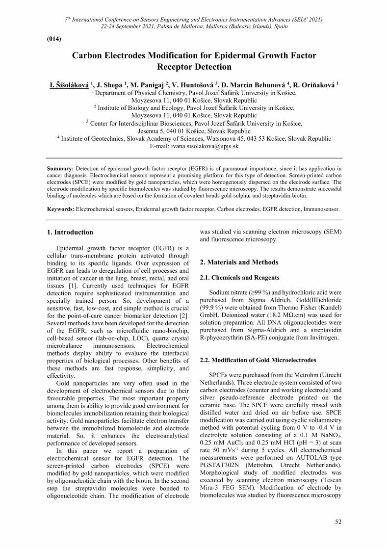
7th International Conference on Sensors Engineering and Electronics Instrumentation Advances (SEIA' 2021), 22-24 September 2021, Palma de Mallorca, Mallorca (Balearic Islands), Spain
52
(014)
Carbon Electrodes Modification for Epidermal Growth Factor Receptor Detection
I. Šišoláková 1, J. Shepa 1, M. Panigaj 2, V. Huntošová 3, D. Marcin Behunová 4, R. Oriňaková 1
1 Department of Physical Chemistry, Pavol Jozef Šafárik University in Košice, Moyzesova 11, 040 01 Košice, Slovak Republic
2 Institute of Biology and Ecology, Pavol Jozef Šafárik University in Košice, Moyzesova 11, 040 01 Košice, Slovak Republic
3 Center for Interdisciplinar Biosciences, Pavol Jozef Šafárik University in Košice, Jesenna 5, 040 01 Košice, Slovak Republic
4 Institute of Geotechnics, Slovak Academy of Sciences, Watsonova 45, 043 53 Košice, Slovak Republic E-mail: [email protected]
Summary: Detection of epidermal growth factor receptor (EGFR) is of paramount importance, since it has application in cancer diagnosis. Electrochemical sensors represent a promising platform for this type of detection. Screen-printed carbon electrodes (SPCE) were modified by gold nanoparticles, which were homogenously dispersed on the electrode surface. The electrode modification by specific biomolecules was studied by fluorescence microscopy. The results demonstrate successful binding of molecules which are based on the formation of covalent bonds gold-sulphur and streptavidin-biotin. Keywords: Electrochemical sensors, Epidermal growth factor receptor, Carbon electrodes, EGFR detection, Immunosensor.
1. Introduction
Epidermal growth factor receptor (EGFR) is a cellular trans-membrane protein activated through binding to its specific ligands. Over expression of EGFR can leads to deregulation of cell processes and initiation of cancer in the lung, breast, rectal, and oral tissues [1]. Currently used techniques for EGFR detection require sophisticated instrumentation and specially trained person. So, development of a sensitive, fast, low-cost, and simple method is crucial for the point-of-care cancer biomarker detection [2]. Several methods have been developed for the detection of the EGFR, such as microfluidic nano-biochip, cell-based sensor (lab-on-chip, LOC), quartz crystal microbalance immunosensors. Electrochemical methods display ability to evaluate the interfacial properties of biological processes. Other benefits of these methods are fast response, simplicity, and effectivity.
Gold nanoparticles are very often used in the development of electrochemical sensors due to their favourable properties. The most important property among them is ability to provide good environment for biomolecules immobilization retaining their biological activity. Gold nanoparticles facilitate electron transfer between the immobilized biomolecule and electrode material. So, it enhances the electroanalytical performance of developed sensors.
In this paper we report a preparation of electrochemical sensor for EGFR detection. The screen-printed carbon electrodes (SPCE) were modified by gold nanoparticles, which were modified by oligonucleotide chain with the biotin. In the second step the streptavidin molecules were bonded to oligonucleotide chain. The modification of electrode
was studied via scanning electron microscopy (SEM) and fluorescence microscopy. 2. Materials and Methods 2.1. Chemicals and Reagents
Sodium nitrate (≥99 %) and hydrochloric acid were purchased from Sigma Aldrich. Gold(III)chloride (99.9 %) were obtained from Thermo Fisher (Kandel) GmbH. Deionized water (18.2 MΩ.cm) was used for solution preparation. All DNA oligonucleotides were purchased from Sigma-Aldrich and a streptavidin R-phycoerythrin (SA-PE) conjugate from Invitrogen. 2.2. Modification of Gold Microelectrodes
SPCEs were purchased from the Metrohm (Utrecht Netherlands). Three electrode system consisted of two carbon electrodes (counter and working electrode) and silver pseudo-reference electrode printed on the ceramic base. The SPCE were carefully rinsed with distilled water and dried on air before use. SPCE modification was carried out using cyclic voltammetry method with potential cycling from 0 V to -0.4 V in electrolyte solution consisting of a 0.1 M NaNO3, 0.25 mM AuCl3 and 0.25 mM HCl (pH = 3) at scan rate 50 mVs-1 during 5 cycles. All electrochemical measurements were performed on AUTOLAB type PGSTAT302N (Metrohm, Utrecht Netherlands). Morphological study of modified electrodes was executed by scanning electron microscopy (Tescan Mira-3 FEG SEM). Modification of electrode by biomolecules was studied by fluorescence microscopy
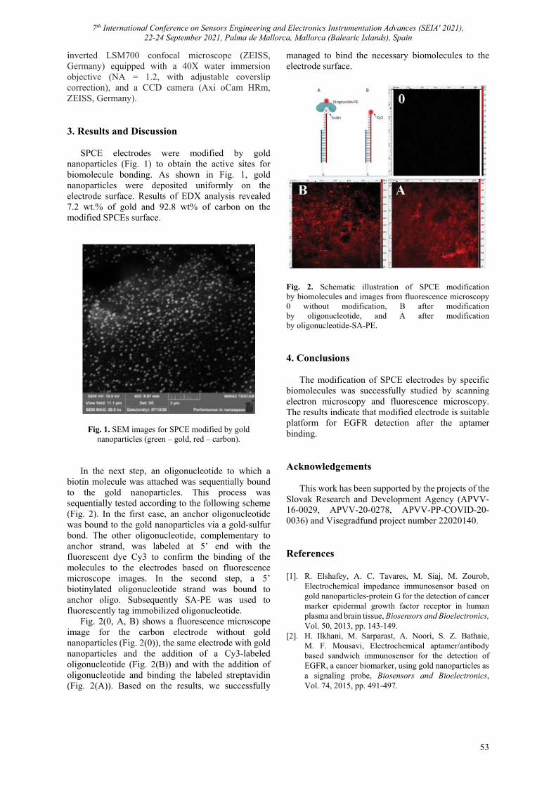
7th International Conference on Sensors Engineering and Electronics Instrumentation Advances (SEIA' 2021), 22-24 September 2021, Palma de Mallorca, Mallorca (Balearic Islands), Spain
53
inverted LSM700 confocal microscope (ZEISS, Germany) equipped with a 40X water immersion objective (NA = 1.2, with adjustable coverslip correction), and a CCD camera (Axi oCam HRm, ZEISS, Germany). 3. Results and Discussion
SPCE electrodes were modified by gold nanoparticles (Fig. 1) to obtain the active sites for biomolecule bonding. As shown in Fig. 1, gold nanoparticles were deposited uniformly on the electrode surface. Results of EDX analysis revealed 7.2 wt.% of gold and 92.8 wt% of carbon on the modified SPCEs surface.
Fig. 1. SEM images for SPCE modified by gold nanoparticles (green – gold, red – carbon).
In the next step, an oligonucleotide to which a
biotin molecule was attached was sequentially bound to the gold nanoparticles. This process was sequentially tested according to the following scheme (Fig. 2). In the first case, an anchor oligonucleotide was bound to the gold nanoparticles via a gold-sulfur bond. The other oligonucleotide, complementary to anchor strand, was labeled at 5’ end with the fluorescent dye Cy3 to confirm the binding of the molecules to the electrodes based on fluorescence microscope images. In the second step, a 5’ biotinylated oligonucleotide strand was bound to anchor oligo. Subsequently SA-PE was used to fluorescently tag immobilized oligonucleotide.
Fig. 2(0, A, B) shows a fluorescence microscope image for the carbon electrode without gold nanoparticles (Fig. 2(0)), the same electrode with gold nanoparticles and the addition of a Cy3-labeled oligonucleotide (Fig. 2(B)) and with the addition of oligonucleotide and binding the labeled streptavidin (Fig. 2(A)). Based on the results, we successfully
managed to bind the necessary biomolecules to the electrode surface.
Fig. 2. Schematic illustration of SPCE modification by biomolecules and images from fluorescence microscopy 0 without modification, B after modification by oligonucleotide, and A after modification by oligonucleotide-SA-PE. 4. Conclusions
The modification of SPCE electrodes by specific biomolecules was successfully studied by scanning electron microscopy and fluorescence microscopy. The results indicate that modified electrode is suitable platform for EGFR detection after the aptamer binding. Acknowledgements
This work has been supported by the projects of the Slovak Research and Development Agency (APVV-16-0029, APVV-20-0278, APVV-PP-COVID-20-0036) and Visegradfund project number 22020140. References [1]. R. Elshafey, A. C. Tavares, M. Siaj, M. Zourob,
Electrochemical impedance immunosensor based on gold nanoparticles-protein G for the detection of cancer marker epidermal growth factor receptor in human plasma and brain tissue, Biosensors and Bioelectronics, Vol. 50, 2013, pp. 143-149.
[2]. H. Ilkhani, M. Sarparast, A. Noori, S. Z. Bathaie, M. F. Mousavi, Electrochemical aptamer/antibody based sandwich immunosensor for the detection of EGFR, a cancer biomarker, using gold nanoparticles as a signaling probe, Biosensors and Bioelectronics, Vol. 74, 2015, pp. 491-497.
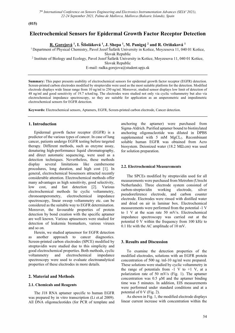
7th International Conference on Sensors Engineering and Electronics Instrumentation Advances (SEIA' 2021), 22-24 September 2021, Palma de Mallorca, Mallorca (Balearic Islands), Spain
54
(015)
Electrochemical Sensors for Epidermal Growth Factor Receptor Detection
R. Gorejová 1, I. Šišoláková 1, J. Shepa 1, M. Panigaj 2 and R. Oriňaková 1
1 Department of Physical Chemistry, Pavol Jozef Šafárik University in Košice, Moyzesova 11, 040 01 Košice, Slovak Republic
2 Institute of Biology and Ecology, Pavol Jozef Šafárik University in Košice, Moyzesova 11, 040 01 Košice, Slovak Republic
E-mail: [email protected] Summary: This paper presents usability of electrochemical sensors for epidermal growth factor receptor (EGFR) detection. Screen-printed carbon electrodes modified by streptavidin were used as the most suitable platform for the detection. Modified electrode displays wide linear range from 10 ng/ml to 250 ng/ml. Moreover, studied sensor displays low limit of detection of 48 ng/ml and good sensitivity of 19.7 nAml/ng. The electrodes were studied not only via cyclic voltammetry but also via electrochemical impedance spectroscopy, so they are suitable for application as an amperometric and impedimetric electrochemical sensors for EGFR detection. Keywords: Electrochemical sensors, Aptamers, EGFR, Screen-printed carbon electrode, Cancer detection.
1. Introduction
Epidermal growth factor receptor (EGFR) is a predictor of the various types of cancer. In case of lung cancer, patients undergo EGFR testing before targeted therapy. Different methods, such as enzyme assay, denaturing high-performance liquid chromatography, and direct automatic sequencing, were used as a detection techniques. Nevertheless, these methods display several limitations like cumbersome procedures, long duration, and high cost [1]. In general, electrochemical biosensors attracted recently considerable attention. Electrochemical methods offer many advantages as high sensitivity, good selectivity, low cost, and fast detection [2]. Various electrochemical methods lie cyclic voltammetry, chronoamperometry, electrochemical impedance spectroscopy, linear sweep voltammetry etc. can be considered as the suitable way to EGFR determination. Moreover, the favourable properties of protein detection by bond creation with the specific aptamer are well known. Various aptasensors were studied for detection of leukemia biomarkers, various viruses and so on.
Herein, we studied aptasensor for EGFR detection as another approach to cancer diagnostics. Screen-printed carbon electrodes (SPCE) modified by streptavidin were studied due to this simplicity and good electrochemical properties. Both methods, cyclic voltammetry and electrochemical impedance spectroscopy were used to evaluate electroanalytical properties of these electrodes in more details.
2. Material and Methods 2.1. Chemicals and Reagents
The J18 RNA aptamer specific to human EGFR was prepared by in vitro transcription (Li et.al 2009). All DNA oligonucleotides (for PCR of template and
anchoring the aptamer) were purchased from Sigma-Aldrich. Purified aptamer bound to biotinylated anchoring oligonucleotide was diluted in DPBS supplemented with 5 mM MgCL2. Recombinant soluble human EGFR was obtained from Acro biosystem. Deionized water (18.2 MΩ.cm) was used for solution preparation. 2.2. Electrochemical Measurements
The SPCEs modified by streptavidin used for all measurements were purchased from Metrohm (Utrecht Netherlands). Three electrode system consisted of carbon-streptavidin working electrode, silver pseudoreference electrode, and carbon counter electrode. Electrodes were rinsed with distilled water and dried on air in laminar box. Electrochemical measurements were performed from the potential -1 V to 1 V at the scan rate 50 mV/s. Electrochemical impedance spectroscopy was carried out at the potential 0 V within the frequency from 100 kHz to 0.1 Hz with the AC amplitude of 10 mV. 3. Results and Discussion
To examine the detection properties of the modified electrodes, solutions with an EGFR protein concentration of 500 ng /ml-10 ng/ml were prepared. These solutions were studied by cyclic voltammetry in the range of potentials from -1 V to +1 V, at a polarization rate of 50 mV/s (Fig. 1). The aptamer concentration was 0.5 μM and the aptamer binding time was 5 minutes. In addition, EIS measurements were performed under standard conditions and at a potential of 0 V (Fig. 2).
As shown in Fig. 1, the modified electrode displays linear current increase with concentration within the
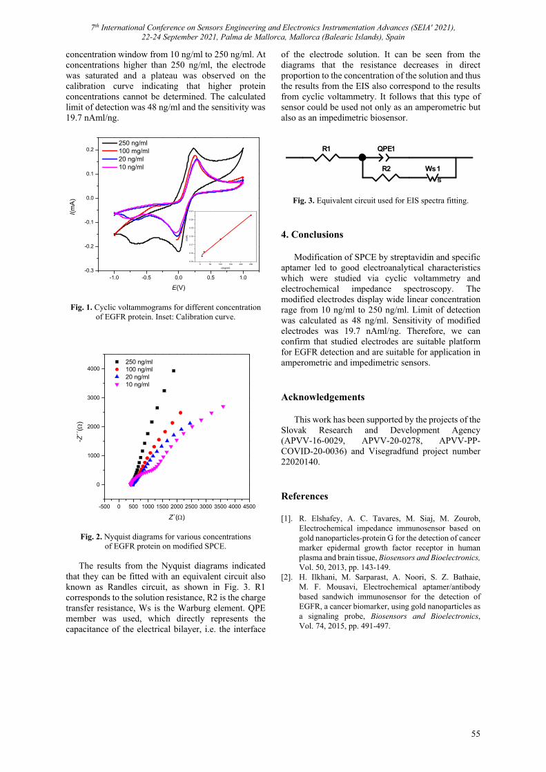
7th International Conference on Sensors Engineering and Electronics Instrumentation Advances (SEIA' 2021), 22-24 September 2021, Palma de Mallorca, Mallorca (Balearic Islands), Spain
55
concentration window from 10 ng/ml to 250 ng/ml. At concentrations higher than 250 ng/ml, the electrode was saturated and a plateau was observed on the calibration curve indicating that higher protein concentrations cannot be determined. The calculated limit of detection was 48 ng/ml and the sensitivity was 19.7 nAml/ng.
-1.0 -0.5 0.0 0.5 1.0-0.3
-0.2
-0.1
0.0
0.1
0.2
0 50 100 150 200 2500.15
0.16
0.17
0.18
0.19
0.20
0.21
I(m
A)
c(ng/ml)
I(m
A)
E(V)
250 ng/ml 100 mg/ml 20 ng/ml 10 ng/ml
Fig. 1. Cyclic voltammograms for different concentration of EGFR protein. Inset: Calibration curve.
-500 0 500 1000 1500 2000 2500 3000 3500 4000 4500
0
1000
2000
3000
4000 250 ng/ml 100 ng/ml 20 ng/ml 10 ng/ml
-Z´´
()
Z´()
Fig. 2. Nyquist diagrams for various concentrations of EGFR protein on modified SPCE.
The results from the Nyquist diagrams indicated
that they can be fitted with an equivalent circuit also known as Randles circuit, as shown in Fig. 3. R1 corresponds to the solution resistance, R2 is the charge transfer resistance, Ws is the Warburg element. QPE member was used, which directly represents the capacitance of the electrical bilayer, i.e. the interface
of the electrode solution. It can be seen from the diagrams that the resistance decreases in direct proportion to the concentration of the solution and thus the results from the EIS also correspond to the results from cyclic voltammetry. It follows that this type of sensor could be used not only as an amperometric but also as an impedimetric biosensor.
Fig. 3. Equivalent circuit used for EIS spectra fitting. 4. Conclusions
Modification of SPCE by streptavidin and specific aptamer led to good electroanalytical characteristics which were studied via cyclic voltammetry and electrochemical impedance spectroscopy. The modified electrodes display wide linear concentration rage from 10 ng/ml to 250 ng/ml. Limit of detection was calculated as 48 ng/ml. Sensitivity of modified electrodes was 19.7 nAml/ng. Therefore, we can confirm that studied electrodes are suitable platform for EGFR detection and are suitable for application in amperometric and impedimetric sensors. Acknowledgements
This work has been supported by the projects of the Slovak Research and Development Agency (APVV-16-0029, APVV-20-0278, APVV-PP-COVID-20-0036) and Visegradfund project number 22020140. References [1]. R. Elshafey, A. C. Tavares, M. Siaj, M. Zourob,
Electrochemical impedance immunosensor based on gold nanoparticles-protein G for the detection of cancer marker epidermal growth factor receptor in human plasma and brain tissue, Biosensors and Bioelectronics, Vol. 50, 2013, pp. 143-149.
[2]. H. Ilkhani, M. Sarparast, A. Noori, S. Z. Bathaie, M. F. Mousavi, Electrochemical aptamer/antibody based sandwich immunosensor for the detection of EGFR, a cancer biomarker, using gold nanoparticles as a signaling probe, Biosensors and Bioelectronics, Vol. 74, 2015, pp. 491-497.
R1 QPE1
R2 Ws1
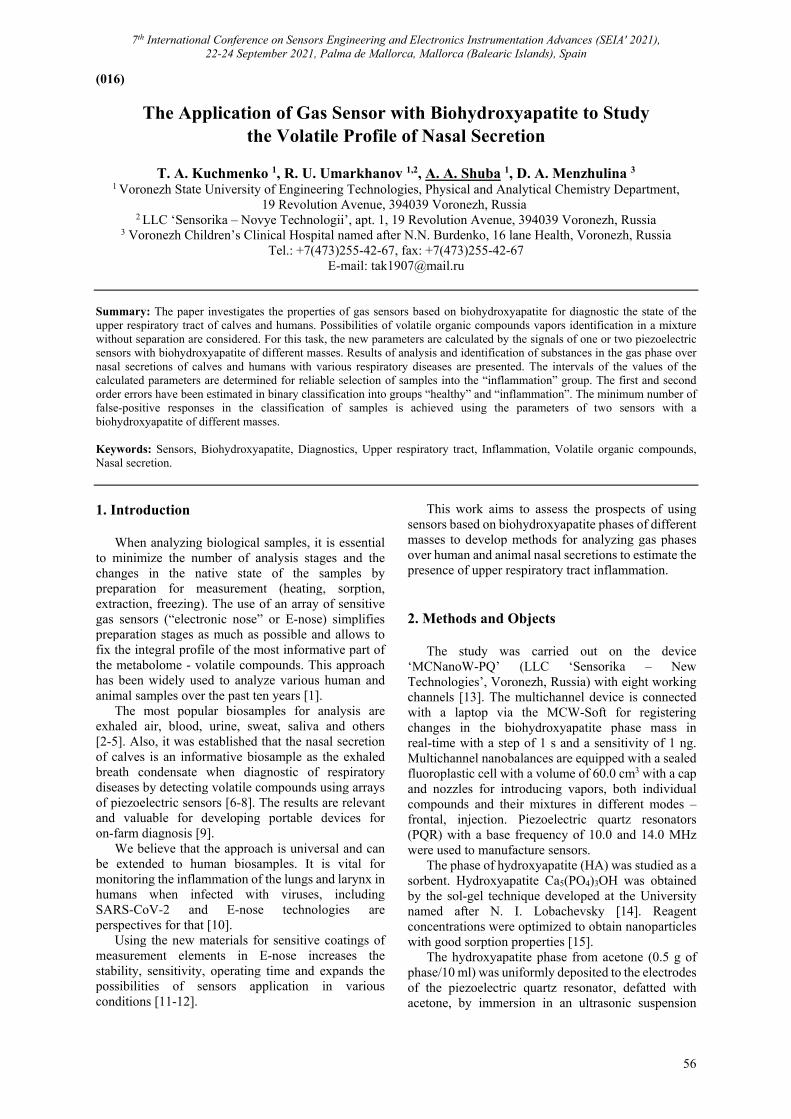
7th International Conference on Sensors Engineering and Electronics Instrumentation Advances (SEIA' 2021), 22-24 September 2021, Palma de Mallorca, Mallorca (Balearic Islands), Spain
56
(016)
The Application of Gas Sensor with Biohydroxyapatite to Study the Volatile Profile of Nasal Secretion
T. A. Kuchmenko 1, R. U. Umarkhanov 1,2, A. A. Shuba 1, D. A. Menzhulina 3
1 Voronezh State University of Engineering Technologies, Physical and Analytical Chemistry Department, 19 Revolution Avenue, 394039 Voronezh, Russia
2 LLC ‘Sensorika – Novye Technologii’, apt. 1, 19 Revolution Avenue, 394039 Voronezh, Russia 3 Voronezh Children’s Clinical Hospital named after N.N. Burdenko, 16 lane Health, Voronezh, Russia
Tel.: +7(473)255-42-67, fax: +7(473)255-42-67 E-mail: [email protected]
Summary: The paper investigates the properties of gas sensors based on biohydroxyapatite for diagnostic the state of the upper respiratory tract of calves and humans. Possibilities of volatile organic compounds vapors identification in a mixture without separation are considered. For this task, the new parameters are calculated by the signals of one or two piezoelectric sensors with biohydroxyapatite of different masses. Results of analysis and identification of substances in the gas phase over nasal secretions of calves and humans with various respiratory diseases are presented. The intervals of the values of the calculated parameters are determined for reliable selection of samples into the “inflammation” group. The first and second order errors have been estimated in binary classification into groups “healthy” and “inflammation”. The minimum number of false-positive responses in the classification of samples is achieved using the parameters of two sensors with a biohydroxyapatite of different masses. Keywords: Sensors, Biohydroxyapatite, Diagnostics, Upper respiratory tract, Inflammation, Volatile organic compounds, Nasal secretion.
1. Introduction
When analyzing biological samples, it is essential to minimize the number of analysis stages and the changes in the native state of the samples by preparation for measurement (heating, sorption, extraction, freezing). The use of an array of sensitive gas sensors (“electronic nose” or E-nose) simplifies preparation stages as much as possible and allows to fix the integral profile of the most informative part of the metabolome - volatile compounds. This approach has been widely used to analyze various human and animal samples over the past ten years [1].
The most popular biosamples for analysis are exhaled air, blood, urine, sweat, saliva and others [2-5]. Also, it was established that the nasal secretion of calves is an informative biosample as the exhaled breath condensate when diagnostic of respiratory diseases by detecting volatile compounds using arrays of piezoelectric sensors [6-8]. The results are relevant and valuable for developing portable devices for on-farm diagnosis [9].
We believe that the approach is universal and can be extended to human biosamples. It is vital for monitoring the inflammation of the lungs and larynx in humans when infected with viruses, including SARS-CoV-2 and E-nose technologies are perspectives for that [10].
Using the new materials for sensitive coatings of measurement elements in E-nose increases the stability, sensitivity, operating time and expands the possibilities of sensors application in various conditions [11-12].
This work aims to assess the prospects of using sensors based on biohydroxyapatite phases of different masses to develop methods for analyzing gas phases over human and animal nasal secretions to estimate the presence of upper respiratory tract inflammation.
2. Methods and Objects The study was carried out on the device
‘MCNanoW-PQ’ (LLC ‘Sensorika – New Technologies’, Voronezh, Russia) with eight working channels [13]. The multichannel device is connected with a laptop via the MCW-Soft for registering changes in the biohydroxyapatite phase mass in real-time with a step of 1 s and a sensitivity of 1 ng. Multichannel nanobalances are equipped with a sealed fluoroplastic cell with a volume of 60.0 cm3 with a cap and nozzles for introducing vapors, both individual compounds and their mixtures in different modes – frontal, injection. Piezoelectric quartz resonators (PQR) with a base frequency of 10.0 and 14.0 MHz were used to manufacture sensors.
The phase of hydroxyapatite (HA) was studied as a sorbent. Hydroxyapatite Ca5(PO4)3OH was obtained by the sol-gel technique developed at the University named after N. I. Lobachevsky [14]. Reagent concentrations were optimized to obtain nanoparticles with good sorption properties [15].
The hydroxyapatite phase from acetone (0.5 g of phase/10 ml) was uniformly deposited to the electrodes of the piezoelectric quartz resonator, defatted with acetone, by immersion in an ultrasonic suspension
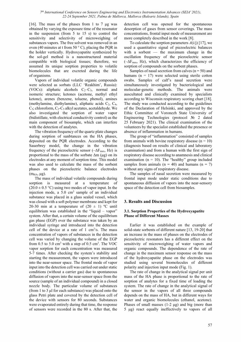
7th International Conference on Sensors Engineering and Electronics Instrumentation Advances (SEIA' 2021), 22-24 September 2021, Palma de Mallorca, Mallorca (Balearic Islands), Spain
57
[16]. The mass of the phases from 1 to 7 μg was obtained by varying the exposure time of the resonator in the suspension (from 5 to 15 s) to control the sensitivity and selectivity of microweighing of substances vapors. The free solvent was removed in an oven (40 minutes at t from 50 ° C), placing the PQR in the holder vertically. Hydroxyapatite synthesized by the sol-gel method is a nanostructured material compatible with biological tissues; therefore, we assumed its unique sorption properties to volatile biomolecules that are excreted during the life of organisms.
Vapors of individual volatile organic compounds were selected as sorbats (LLC ‘Reakhim’, Russia): (VOCs): aliphatic alcohols C2–C5, normal and isomeric structure; ketones (acetone, methyl ethyl ketone), arenes (benzene, toluene, phenol), amines (methylamine, diethylamine), aliphatic acids C2, C4, C5; chloroform, C2-C5 alkyl acetates, acetaldehyde. We also investigated the sorption of water vapor (bidistillate, with electrical conductivity control) as the main component of biosample, which can interfere with the detection of analytes.
The vibration frequency of the quartz plate changes during sorption of sunbtances on the HA phases, deposited on the PQR electrodes. According to the Sauerbrey model, the change in the vibration frequency of the piezoelectric sensor (–∆Fmax, Hz) is proportional to the mass of the sorbate Δm (μg) on its electrodes at any moment of sorption time. This model was also used to calculate the mass of the sorbent phases on the piezoelectric balance electrodes (mHA, μg).
The mass of individual volatile compounds during sorption is measured at a temperature of (20.0 ± 0.5 °C) using two modes of vapor input. In the injection mode, a 5.0 cm3 sample of an individual substance was placed in a glass sealed vessel, which was closed with a soft polymer membrane and kept for 20-30 min at a temperature of (20 ± 1) ºС until equilibrium was established in the “liquid – vapor” system. After that, a certain volume of the equilibrium gas phase (EGP) over the substance was taken by an individual syringe and introduced into the detection cell of the device at a rate of 1 cm3/s. The mass concentration of vapors of substances in the detection cell was varied by changing the volume of the EGP from 0.5 to 5.0 cm3 with a step of 0.5 cm3. The VOC vapor sorption for each concentration was measured 5-7 times. After checking the system’s stability and starting the measurement, the vapors were introduced into the near-sensor space. The frontal mode of vapor input into the detection cell was carried out under static conditions (without a carrier gas) due to spontaneous diffusion of vapors into the near-sensor space from the source (sample of an individual compound) in a closed nozzle body. The particular volume of substances (from 1 to 3 μl for each substance) was placed onto the glass Petri plate and covered by the detection cell of the device with sensors for 80 seconds. Substances were evaporated entirely during that time, the response of sensors were recorded in the 80 s. After that, the
detection cell was opened for the spontaneous desorption of gases from sensor coverings. The mass concentrations, frontal input mode of measurement are more completely described in the work [8].
To calculate the sorption parameters A(i/j) [17], we used a quantitative signal of piezoelectric balances with a sorbent — the maximum change in the oscillation frequency of the piezoelectric sensor (–∆Fmax, Hz), which characterizes the efficiency of sorption of compounds on the sorbent phases.
Samples of nasal secretion from calves (n = 50) and humans (n = 17) were selected using sterile cotton swabs. Samples of calf’s nasal secretion were simultaneously investigated by bacteriological and molecular-genetic methods. The animals were auscultated and clinically examined by specialists according to Wisconsin respiratory scoring chart [18]. The study was conducted according to the guidelines of the Declaration of Helsinki, and approved by the Ethic Committee of Voronezh State University of Engineering Technologies (protocol 2 dated 25 February 2021). The clinical examination of the volunteers by the specialist established the presence or absence of inflammation in humans.
The group of “inflammation” consisted of samples from animals with bovine respiratory disease (n = 10) (diagnosis based on results of clinical and laboratory examination) and from a human with the first sign of respiratory disease according to anamnesis and clinical examination (n = 10). The “healthy” group included samples from animals (n = 40) and humans (n = 7) without any signs of respiratory disease.
The samples of nasal secretion were measured by frontal input mode under static conditions due to spontaneous diffusion of vapors into the near-sensory space of the detection cell from biosamples.
3. Results and Discussion 3.1. Sorption Properties of the Hydroxyapatite Phase of Different Masses
Earlier it was established on the example of solid-state sorbents of different nature [13, 19-20] that an increase in the mass of phases on the electrodes of piezoelectric resonators has a different effect on the sensitivity of microweighing of water vapors and organic compounds. The dependence of the rate of change in the maximum sensor response on the mass of the hydroxyapatite phase on the electrodes was studied using several biomolecules of different polarity and injection input mode (Fig. 1).
The rate of change in the analytical signal per unit mass of the HA phase is proportional to the rate of sorption of analytes for a fixed time of loading the system. The rate of change in the analytical signal of the sensor in the vapors of all three compounds depends on the mass of HA, but in different ways for water and organic biomolecules (ethanol, acetone). Phases of small masses (1-2 μg) and big (more than 5 μg) react equally ineffectively to vapors of all
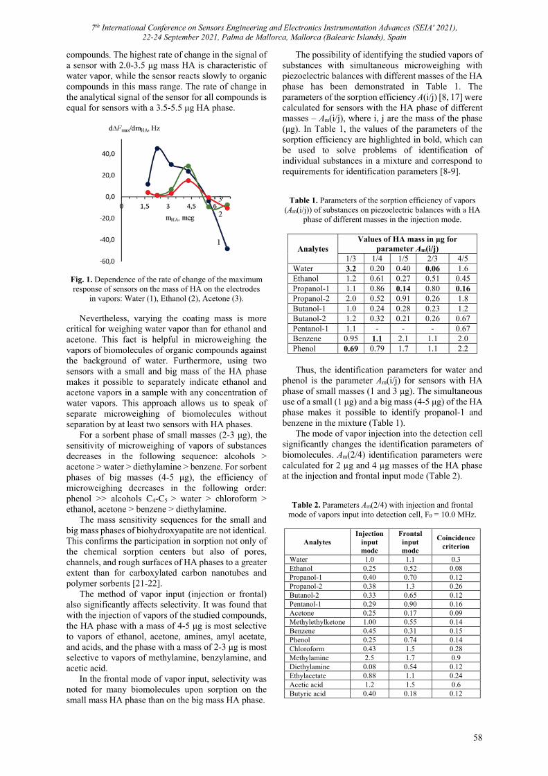
7th International Conference on Sensors Engineering and Electronics Instrumentation Advances (SEIA' 2021), 22-24 September 2021, Palma de Mallorca, Mallorca (Balearic Islands), Spain
58
compounds. The highest rate of change in the signal of a sensor with 2.0-3.5 μg mass HA is characteristic of water vapor, while the sensor reacts slowly to organic compounds in this mass range. The rate of change in the analytical signal of the sensor for all compounds is equal for sensors with a 3.5-5.5 μg HA phase.
Fig. 1. Dependence of the rate of change of the maximum response of sensors on the mass of HA on the electrodes
in vapors: Water (1), Ethanol (2), Acetone (3).
Nevertheless, varying the coating mass is more critical for weighing water vapor than for ethanol and acetone. This fact is helpful in microweighing the vapors of biomolecules of organic compounds against the background of water. Furthermore, using two sensors with a small and big mass of the HA phase makes it possible to separately indicate ethanol and acetone vapors in a sample with any concentration of water vapors. This approach allows us to speak of separate microweighing of biomolecules without separation by at least two sensors with HA phases.
For a sorbent phase of small masses (2-3 μg), the sensitivity of microweighing of vapors of substances decreases in the following sequence: alcohols > acetone > water > diethylamine > benzene. For sorbent phases of big masses (4-5 μg), the efficiency of microweighing decreases in the following order: phenol >> alcohols C4-C5 > water > chloroform > ethanol, acetone > benzene > diethylamine.
The mass sensitivity sequences for the small and big mass phases of biohydroxyapatite are not identical. This confirms the participation in sorption not only of the chemical sorption centers but also of pores, channels, and rough surfaces of HA phases to a greater extent than for carboxylated carbon nanotubes and polymer sorbents [21-22].
The method of vapor input (injection or frontal) also significantly affects selectivity. It was found that with the injection of vapors of the studied compounds, the HA phase with a mass of 4-5 μg is most selective to vapors of ethanol, acetone, amines, amyl acetate, and acids, and the phase with a mass of 2-3 μg is most selective to vapors of methylamine, benzylamine, and acetic acid.
In the frontal mode of vapor input, selectivity was noted for many biomolecules upon sorption on the small mass HA phase than on the big mass HA phase.
The possibility of identifying the studied vapors of substances with simultaneous microweighing with piezoelectric balances with different masses of the HA phase has been demonstrated in Table 1. The parameters of the sorption efficiency А(i/j) [8, 17] were calculated for sensors with the HA phase of different masses – Аm(i/j), where i, j are the mass of the phase (μg). In Table 1, the values of the parameters of the sorption efficiency are highlighted in bold, which can be used to solve problems of identification of individual substances in a mixture and correspond to requirements for identification parameters [8-9].
Table 1. Parameters of the sorption efficiency of vapors (Аm(i/j)) of substances on piezoelectric balances with a HA
phase of different masses in the injection mode.
Analytes Values of HA mass in μg for
parameter Аm(i/j) 1/3 1/4 1/5 2/3 4/5
Water 3.2 0.20 0.40 0.06 1.6 Ethanol 1.2 0.61 0.27 0.51 0.45 Propanol-1 1.1 0.86 0.14 0.80 0.16 Propanol-2 2.0 0.52 0.91 0.26 1.8 Butanol-1 1.0 0.24 0.28 0.23 1.2 Butanol-2 1.2 0.32 0.21 0.26 0.67 Pentanol-1 1.1 - - - 0.67 Benzene 0.95 1.1 2.1 1.1 2.0 Phenol 0.69 0.79 1.7 1.1 2.2
Thus, the identification parameters for water and
phenol is the parameter Аm(i/j) for sensors with HA phase of small masses (1 and 3 μg). The simultaneous use of a small (1 μg) and a big mass (4-5 μg) of the HA phase makes it possible to identify propanol-1 and benzene in the mixture (Table 1).
The mode of vapor injection into the detection cell significantly changes the identification parameters of biomolecules. Am(2/4) identification parameters were calculated for 2 µg and 4 µg masses of the HA phase at the injection and frontal input mode (Table 2).
Table 2. Parameters Аm(2/4) with injection and frontal mode of vapors input into detection cell, F0 = 10.0 MHz.
Analytes Injection
input mode
Frontal input mode
Coincidence criterion
Water 1.0 1.1 0.3 Ethanol 0.25 0.52 0.08 Propanol-1 0.40 0.70 0.12 Propanol-2 0.38 1.3 0.26 Butanol-2 0.33 0.65 0.12 Pentanol-1 0.29 0.90 0.16 Acetone 0.25 0.17 0.09 Methylethylketone 1.00 0.55 0.14 Benzene 0.45 0.31 0.15 Phenol 0.25 0.74 0.14 Chloroform 0.43 1.5 0.28 Methylamine 2.5 1.7 0.9 Diethylamine 0.08 0.54 0.12 Ethylacetate 0.88 1.1 0.24 Acetic acid 1.2 1.5 0.6 Butyric acid 0.40 0.18 0.12

7th International Conference on Sensors Engineering and Electronics Instrumentation Advances (SEIA' 2021), 22-24 September 2021, Palma de Mallorca, Mallorca (Balearic Islands), Spain
59
The overlap of the identification parameter values using the coincidence criterion [9, 17] at different modes of vapor input was established for water, acetone, benzene, methylamine, ethylacetate, and acetic acid (Table 2). The differences are significant for other compounds, and the identification parameters obtained under different sorption conditions cannot be applied. It is explained the different character of dependence of the sensor signal on the concentration of the analyte in the detection cell and near sensory space. Vapors of acetone, benzene, methylamine, ethyl acetate, acetic acid have a linear dependence of the sensor signal on the concentration of the substance in the studied range. For vapors with nonlinear dependence of the sensor signal on the concentration of the substance (alcohols, phenol, chloroform, diethylamine), the differences in the values of the parameters are significant.
The results correspond to the theoretical and practical foundations of sorption interactions. Therefore, an approach for identifying individual analytes in a mixture by comparing the identification parameters of standard test substances and calculated for analyzed samples obtained under identical experimental conditions is acceptable.
The frontal mode of vapors input allows identifying more substances in the mixture than the injection input. For the analysis of biosamples, comparison of their state, and assessment of changes in time, the most promising is the frontal input mode of highly volatile compounds, which significantly simplifies the experiment and practically eliminates sample preparation.
3.2. Nasal Secretion Analysis
Clinical examination and analysis of biological samples by laboratory methods made it possible to classify animals by the degree of damage to the respiratory organs [7, 9].
The used arrays included sensors with phases of biohydroxyapatite of different masses (4.0 μg and
2.0 μg). According to the measurement results, the values of the parameter Аm(2/4) were calculated for 50 samples of nasal secretions of calves and the informative values of this parameter for ranking into groups “healthy”, “inflammation” from the respiratory organs were found out (Table 3) with an assessment of classification errors for the systems with a binary response [23].
The numerical values of the calculated parameter Аm(2/4) for sensors with HA phases help to identify individual test substances in samples, the content of which is predominated, and divide them into groups (Tables 2, 3). It was found that only for one range of values of this parameter, the proportion of false-positive assignments of samples from the “healthy” group to the “inflammation” group is equal to zero.
For nasal secretion samples of the ”inflammation” group, volatile compounds were identified (amines, alcohols, ketones, arenas). These compounds are markers of inflammation and protein destruction [8].
The versatility of the approach to assessing the state of the upper respiratory tract using highly volatile compounds of human nasal secretion was tested on 17 samples. In this case, the ranking of the samples into the “inflammation” group was carried out according to the range of the parameter Am(2/4) = 0.60 – 0.67 (Table 4).
The proportion of correct ranking of human secretions samples in the “inflammation” group according to the selected numerical boundaries of the parameter Аm(2/4) is 0.91. The proportion of false attribution for the considered sample is 0.25 due to the small size of the sample. However, the high sensitivity of assigning samples to the “inflammation” group confirms the correctness and versatility of the approach. The first and second order errors have been estimated in binary classification based on sorption parameters for sensors with HA. The sensitivity and specificity of classification were 100 and 86 %, respectively.
Table 3. Parameter Аm(2/4) with the frontal mode of vapors input from nasal secretion samples of calves, F0 = 10 MHz.
Сalf stock number and diagnostic group
Range of parameter Аm(2/4) values
Identified compounds
Proportion of correct positive (false negative)
answers
Proportion of correct negative (false positive)
answers “Healthy”: 2663, 2661, 2655, 2432, 2657,
2650, 2438, 2671, 2670, 2669, 2666 “Inflammation”: 2646
0.77 – 0.9
No compounds dominating in concentration
- (0.1)
0.28
“Healthy”: 2428, 2659, 2658, 2661, 2675 2443, 2437, 2659, 2667, 2662, 2647, 2668, 2657, 2664, 2653, 2442, 2662, 2676, 2677,
2674, 2679, 2675, 2674, 2673 “Inflammation”: 2439, 2665, 2469
1.0 – 1.4 Propanol-2 - (0.3) 0.6
“Healthy”: 2652, 2430, 2653, 2652, 2679 “Inflammation”: 2672
1.5 – 1.8 Methylamine, acetic
acid - (0.1)
0.12
“Healthy”: - “Inflammation”: 2666, 2660, 2665, 2669, 2663
0.60-0.67
Diethylamine, ethanol, propanol-1, butanol-2,
phenol, methylethylketone
0.5
- (0)

7th International Conference on Sensors Engineering and Electronics Instrumentation Advances (SEIA' 2021), 22-24 September 2021, Palma de Mallorca, Mallorca (Balearic Islands), Spain
60
Table 4. Classification of human nasal secretion samples by parameter Am(i/j) for two sensors with 2 and 4 μg of HA.
Sample number
Value of parameter Am(2/4)
Assignment to the “inflammation” group according
to the values of the parameter Am(2/4)
Condition based on clinical examination
1 0.63 Yes Inflammation 2 0.63 Yes Healthy 3 0.59 Yes Inflammation 4 0.20 No Healthy 5 0.63 Yes Inflammation 6 0.67 Yes Inflammation 7 1.0 No Dry nose, secretion is almost absent 8 0.71 Yes Healthy 9 0.83 No Healthy 10 0.63 Yes Inflammation 11 0.63 Yes Inflammation 12 0.67 Yes Inflammation 13 0.63 Yes Inflammation 14 0.67 Yes Inflammation 15 0.63 Yes Inflammation 16 0.91 No Healthy 17 0.77 No Healthy – 0.77 – Water – 1.0 – Container
4. Conclusions
The study of the sorption of organic compounds and water vapors by phases of HA of different masses on the piezoelectric resonators is allowed to formulate a new approach to changing the selectivity of microweighing of VOCs and its identification in “electronic nose” systems or other devices based on them. Using one effective sorbent of different masses changes the response of piezoelectric sensors in vapors of the studied biomolecules and makes it possible to identify it in a mixture without separation. The frontal mode of vapors input creates conditions similar to gas chromatography to recognize components in a mixture with a much simpler and faster instrumental solution.
The proposed sorption parameters, which estimate the volatile profile of nasal secretions from animals and humans, could be applied to assess the inflammation presence in the upper respiratory tract rapidly. The correctness of the interpretation of the results was confirmed by the clinical examination and laboratory data of biosamples analysis. The success of applying the approach in the analysis of biological samples of animals and humans opens up new prospects for out-of-laboratory diagnostics.
Acknowledgments
The research was supported by Russian Science Foundation, grant number 18-76-10015.
References [1]. A. D. Wilson, noninvasive early disease diagnosis by
electronic-nose and related VOC-detection devices, Biosensors, Vol. 10, Issue 7, 2020, 73.
[2]. M. Fleischer, E. Simon, E. Rumpel, H. Ulmer, V. Harbeck, M. Wandel, C. Fietzek, U. Weimar, H. Meixner, Detection of volatile compounds correlated to human diseases through breath analysis with chemical sensors, Sensors and Actuators B: Chemical, 2002, Vol. 83, Issues 1-3, 2002. pp. 245-249.
[3]. M. Milanowski, P. Pomastowski, T. Ligor, B. Buszewski, Saliva – volatile biomarkers and profiles, Critical Reviews in Analytical Chemistry, Vol. 47, Issue 3, 2017, pp. 251-266.
[4]. M. Monteiro, N. Moreira, J. Pinto, A. S. Pires-Luis, R. Henrique, C. Jeronimo, M. D. Bastos, A. M. Gil, M. Carvalho, P. G. de Pinho, GC-MS metabolomics-based approach for the identification of a potential VOC-biomarker panel in the urine of renal cell carcinoma patients, Journal of Cellular and Molecular Medicine, Vol. 21, Issue 9, 2017, pp. 2092-2105.
[5]. R. Xue, L. Dong, S. Zhang, C. Deng, T. Liu, J. Wang, X. Shen, Investigation of volatile biomarkers in liver cancer blood using solid-phase microextraction and gas chromatography/mass spectrometry, Rapid Communications in Mass Spectrometry, Vol. 22, Issue 8, 2008, pp. 1181-1186.
[6]. T. A. Kuchmenko, A. A. Shuba, R. U. Umarkhanov, E. V. Drozdova, A. E. Chernitskii, Application of a piezoelectric nose to assessing the respiratory system in calves by volatile compounds, Journal of Analytical Chemistry, Vol. 75, Issue 5, 2020, pp. 645-652.
[7]. T. A. Kuchmenko, A. A. Shuba, R. U. Umarhanov, A. E. Chernickij, “Electronic nose” signals correlation evaluation for nasal mucus and exhaled breath condensate of calves with the clinical and laboratory indicators, Analitika i Kontrol' (Analytics and Control), Vol. 23, Issue 4, 2019, pp. 557-562.
[8]. T. Kuchmenko, A. Shuba, R. Umarkhanov, L. Lvova, The new approach to a pattern recognition of volatile compounds: The inflammation markers in nasal mucus swabs from calves using the gas sensor array, Chemosensors, Vol. 9, Issue 6, 2021, 116.
[9]. T. Kuchmenko, A. Shuba, R. Umarkhanov, A. Chernitskiy, portable electronic nose for analyzing the smell of nasal secretions in calves: Toward
7th International Conference on Sensors Engineering and Electronics Instrumentation Advances (SEIA' 2021), 22-24 September 2021, Palma de Mallorca, Mallorca (Balearic Islands), Spain
61
noninvasive diagnosis of infectious bronchopneumonia, Veterinary Sciences, Vol. 8, Issue 5, 2021, 74.
[10]. S. Dragonieri, G. Pennazza, P. Carratu, O. Resta, Electronic nose technology in respiratory diseases, Lung, Vol. 195, Issue 2, 2017, pp. 157-165.
[11]. D. Goyal, S. K. Mittal, A. Choudhary, R. K. Dang, Graphene: A two dimensional super material for sensor applications, Materials Today-Proceedings, Vol. 43, 2021, pp. 203-208.
[12]. T. Wasilewski, B. Szulczynski, M. Wojciechowski, W. Kamysz, J. Gebicki, Determination of long-chain aldehydes using a novel quartz crystal microbalance sensor based on a biomimetic peptide, Microchemical Journal, Vol. 154, 2020, 104509.
[13]. T. Kuchmenko, R. Umarkhanov. D. Menzhulina, Biohydroxiappatite – New phase for selective micro weighing of organic compounds – Inflammation markers. First communication: Sorption in model mixtures, Sorbtzionnye i Khromatograficheskie Protzessy (Sorption and chromatographic processes), Vol. 21, Issue 2, 2021, pp. 142-152.
[14]. E. N. Bulanov, Obtaining and Investigation of Nanostructured Biocompatible Materials Based on Hydroxyappatite, Nizhnii Novgorod University, 2012 (in Russian).
[15]. A. A. Shuba, T. A. Kuchmenko, R. U. Umarkhanov, A. E. Chernitskiy, Portable E-nose for diagnostic of inflammation and diverse variation in health status of humans and animals, in Proceedings of the Fifth International Conference On Advances In Sensors, Actuators, Metering And Sensing (ALLSENSORS’20), Valencia, Spain, 16-22 March 2020, pp. 56-62.
[16]. Ya. I. Korenman, Yu. E. Silina, T. A. Kuchmenkko, Method for Modifying the Electrodes of a Piezoquartz Resonator, Patent 2259007 RU, Russia, 29.01.2004.
[17]. T. Kuchmenko, А. Shuba, N. Belskich, The identification parameters of organic substances in multisensors piezoquartz microbalance, Analitika i Kontrol' (Analytics and Control), Vol. 16, Issue 2, 2012, pp. 151-161.
[18]. S. M. McGuirk, Disease management of dairy calves and heifers, Veterinary Clinics of North America: Food Animal Practice, Vol. 24, Issue. 1, 2008, pp. 139-153.
[19]. T. A. Kuchmenko, R. U. Umarkhanov, et al., Investigation of sorption properties of carboxilated nanotubes on piezoelectric microbalance BAW-type, Sorbtzionnye i Khromatograficheskie Protzessy (Sorption and Chromatographic Processes), Vol. 21, Issue 3, 2021, pp. 336-346.
[20]. T. A. Kuchmenko, Electronic nose based on nanoweights, expectation and reality, Pure and Applied Chemistry, Vol. 89, Issue 10, 2017, pp. 1587-1601.
[21]. Yu. Kh. Shogenov, T. A. Kuchmenko, S. S. Grazhulene, Features of sorption of alcohols mixtures of normal and isomeric structure on the carbon nanomaterials, Sorbtzionnye i Khromatograficheskie Protzessy (Sorption and Chromatographic Processes), Vol. 9, Issue 3, 2009, pp. 416-423.
[22]. T. A. Kuchmenko, R. U. Umarkhanov, Peculiarities of microweighing of trace quantities of alkylamines on polymer and solid-state thin films, Journal Of Analytical Chemistry, Vol. 68, Issue 4, 2013, pp. 368-375.
[23]. Yu. V. Kholin, N. A. Nikitina, A. V. Panteleimonov, Ye. A. Reshetnyak, A. A. Bugaevskii, L. P. Loginova, Metrological Characteristics of Binary Response Detection Techniques, Timchenko, 2008.

7th International Conference on Sensors Engineering and Electronics Instrumentation Advances (SEIA' 2021), 22-24 September 2021, Palma de Mallorca, Mallorca (Balearic Islands), Spain
62
(017)
Optimization of Epidermal Growth Factor Receptor Electrochemical Sensing Procedure
R. Oriňaková 1, I. Šišoláková 1, J. Shepa1 and M. Panigaj 2
1 Department of Physical Chemistry, Pavol Jozef Šafárik University in Košice, Moyzesova 11, 040 01 Košice, Slovak Republic
2 Institute of Biology and Ecology, Pavol Jozef Šafárik University in Košice, Moyzesova 11, 040 01 Košice, Slovak Republic
E-mail: [email protected] Summary: Fast, sensitive and effective cancer detection attracts a lot of attention of scientific community. Epidermal growth factor receptor (EGFR) is a protein directly associated with several types of cancer. Screen-printed carbon electrodes (SPCE) modified by streptavidin molecule were studied as a sensitive electrochemical sensing platform for cancer detection. SPCE-streptavidin electrodes were modified by specific aptamers during 5 minutes. The modified electrodes were able to detect EGFR protein via cyclic voltammetry and electrochemical impedance spectroscopy. Keywords: Epidermal growth factor receptor, Screen-printed carbon electrode, EGFR detection, Electrochemical sensing, Aptamer sensors.
1. Introduction
Epidermal growth factor receptor (EGFR) is cell trans-membrane protein, which is located at the cell surface. EGFR is overexpressed in many tumors, such as lung, breast, gastric, pancreatic, and ovarian cancers. So, this protein could be used as a target for antitumor strategies. Early detection of cancer can dramatically change treatment and improved prognosis. Therefore, fast, accurate and cheap way for cancer diagnosis is required. A number of techniques have been employed to detect EGFR as a cancer marker, i.e. immunohistochemistry, western blotting analysis, enzyme-linked immunosorbent assay (ELISA) and so on. However, mentioned techniques are time consuming, require multi-steps, or enzymatic tagging [1], while the electrochemical methods represent simple, low-cost, and sensitive techniques. Therefore, we focused on the development of electrochemical sensor for EGFR with low limit of detection, high sensitivity, and high specificity caused by usage of aptamer. Aptamers dissociation constants with their target protein displays high level of specificity, sensitivity, and repeatability [2]. Various electrochemical methods can be used for EGFR detection like cyclic voltammetry, linear sweep voltammetry, chronoamperometry, and electrochemical impedance spectroscopy (EIS). EIS have been used as a most suitable method for EGFR detection due to the high speed, simplicity, and high sensitivity.
Herein, the SPCE-streptavidin electrodes were modified by specific aptamer for EGFR detection. The kinetics of aptamer binding was studied via cyclic voltammetry. Moreover, required concentration of aptamer was studied and the best conditions were optimised for EGFR detection by means of EIS.
2. Materials and Methods 2.1. Chemicals and Reagents
The J18 RNA aptamer specific to human EGFR was prepared by in vitro transcription (Li et.al 2009). All DNA oligonucleotides (for PCR of template and anchoring the aptamer) were purchased from Sigma-Aldrich. Purified aptamer bound to biotinylated anchoring oligonucleotide was diluted in DPBS supplemented with 5 mM MgCL2. Deionized water (18.2 MΩ.cm) was used for solution preparation. 2.2. Modification of Screen-printed Carbon Electrodes
The SPCEs modified by streptavidin were purchased from Metrohm (Utrecht Netherlands). Three electrode system consisted of carbon-streptavidin working electrode, carbon counter electrode, and silver pseudoreference electrode was used. Streptavidin electrodes were rinsed with distilled water and dried on air in laminar box. Electrochemical measurements were performed within the potential window from -1 V to 1 V at the scan rate 50 mVs-1. Electrochemical impedance spectroscopy was carried out at the potential of 0 V within the frequency range from 100 kHz to 0.1 Hz with the AC amplitude of 10 mV. 3. Results and Discussion
The SPCE modification process was studied by binding the aptamer to the electrode surface for 60 minutes.
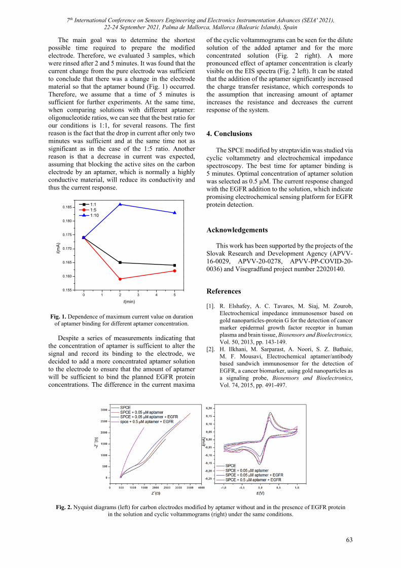
7th International Conference on Sensors Engineering and Electronics Instrumentation Advances (SEIA' 2021), 22-24 September 2021, Palma de Mallorca, Mallorca (Balearic Islands), Spain
63
The main goal was to determine the shortest possible time required to prepare the modified electrode. Therefore, we evaluated 3 samples, which were rinsed after 2 and 5 minutes. It was found that the current change from the pure electrode was sufficient to conclude that there was a change in the electrode material so that the aptamer bound (Fig. 1) occurred. Therefore, we assume that a time of 5 minutes is sufficient for further experiments. At the same time, when comparing solutions with different aptamer: oligonucleotide ratios, we can see that the best ratio for our conditions is 1:1, for several reasons. The first reason is the fact that the drop in current after only two minutes was sufficient and at the same time not as significant as in the case of the 1:5 ratio. Another reason is that a decrease in current was expected, assuming that blocking the active sites on the carbon electrode by an aptamer, which is normally a highly conductive material, will reduce its conductivity and thus the current response.
0 1 2 3 4 50.155
0.160
0.165
0.170
0.175
0.180
0.185
I(m
A)
t(min)
1:1 1:5 1:10
Fig. 1. Dependence of maximum current value on duration of aptamer binding for different aptamer concentration.
Despite a series of measurements indicating that
the concentration of aptamer is sufficient to alter the signal and record its binding to the electrode, we decided to add a more concentrated aptamer solution to the electrode to ensure that the amount of aptamer will be sufficient to bind the planned EGFR protein concentrations. The difference in the current maxima
of the cyclic voltammograms can be seen for the dilute solution of the added aptamer and for the more concentrated solution (Fig. 2 right). A more pronounced effect of aptamer concentration is clearly visible on the EIS spectra (Fig. 2 left). It can be stated that the addition of the aptamer significantly increased the charge transfer resistance, which corresponds to the assumption that increasing amount of aptamer increases the resistance and decreases the current response of the system. 4. Conclusions
The SPCE modified by streptavidin was studied via cyclic voltammetry and electrochemical impedance spectroscopy. The best time for aptamer binding is 5 minutes. Optimal concentration of aptamer solution was selected as 0.5 µM. The current response changed with the EGFR addition to the solution, which indicate promising electrochemical sensing platform for EGFR protein detection. Acknowledgements
This work has been supported by the projects of the Slovak Research and Development Agency (APVV-16-0029, APVV-20-0278, APVV-PP-COVID-20-0036) and Visegradfund project number 22020140. References [1]. R. Elshafey, A. C. Tavares, M. Siaj, M. Zourob,
Electrochemical impedance immunosensor based on gold nanoparticles-protein G for the detection of cancer marker epidermal growth factor receptor in human plasma and brain tissue, Biosensors and Bioelectronics, Vol. 50, 2013, pp. 143-149.
[2]. H. Ilkhani, M. Sarparast, A. Noori, S. Z. Bathaie, M. F. Mousavi, Electrochemical aptamer/antibody based sandwich immunosensor for the detection of EGFR, a cancer biomarker, using gold nanoparticles as a signaling probe, Biosensors and Bioelectronics, Vol. 74, 2015, pp. 491-497.
Fig. 2. Nyquist diagrams (left) for carbon electrodes modified by aptamer without and in the presence of EGFR protein in the solution and cyclic voltammograms (right) under the same conditions.
7th International Conference on Sensors Engineering and Electronics Instrumentation Advances (SEIA' 2021), 22-24 September 2021, Palma de Mallorca, Mallorca (Balearic Islands), Spain
64
(018)
Fiber-optic Mach-Zehnder Interferometer for Refractive Index Measurement Based on MEMS Optofluidic Platform
Z. Djinović 1, A. Kocsis 1 and M. Tomić 2
1 ACMIT Gmbh, 2 Viktor Kaplan str., 2700 Wiener Neustadt, Austria 2 Institute of Technical Sciences of SASA, 35 Knez Mihailova, 11000 Belgrade, Serbia
Tel.: + 436644669297 E-mail: [email protected]
Summary: We present a fiber-optic sensing configuration based on Mach-Zehnder interferometer (MZI) embedded into the MEMS optofluidic platform for measurement of index of refraction of liquids in dynamic regime. The sensing principle is based on the low-coherence interferometry, characterized by generation of Gaussian shape interferograms, which maximum position depends on the optical path difference (OPD) between the sensing and reference arm of the MZI. When liquid flows through the central microchannel of the optofluidic platform it crosses the light beam between the two optical fibers in the sensing arm causing the OPD change. An algorithm has been applied for calculation of index of refraction of liquids out of the raw interference signals. We obtained very good agreement between the experimental results and literature data of index of refraction of subjected fluids. The accuracy of index of refraction measurement is about 1 % that is predominantly determined by accuracy of reading the position of mechanical scanner. Keywords: Fiber-optic sensors, Index of refraction, Interferometry, Optofluidic, MEMS.
1. Introduction
Index of refraction is a frequently used physical parameter for material characterization in various scientific and industrial fields including life science, biomedicine, analytical chemistry and bio-chemistry, material science, etc. [1, 2]. Fiber-optic sensors for refractive index measurement have attracted attention of many research groups dealing with label-free biological and biochemical sensing since they provide high sensitivity, fast response, extremely small volume of test sample, remote sensing, immunity against electromagnetic radiation, etc. [3]. Among them fiber-optic interferometric sensors are the most sensitive and allow different designs [4, 5]. They are very convenient to combine with some other technologies such as micro-electro-mechanical-systems (MEMS) for making high throughput analytical devices such as Lab-on-a-Chips and micro total analyser system (m-TAS) [6]. These systems allow a number of advantages such as direct contactless detection, miniaturization and multiplexing.
In this paper, we present a sensing configuration for in-line measurement of index of refraction of liquid samples based on low-coherence Mach-Zehnder interferometer (MZI), embedded into the MEMS optofluidic platform. The MZI is built up of two 1×2 single-mode fiber-optic couplers. The optofluidic platform is composed of glass and silicon wafers, which are anodically bonded. The structure contains a central microchannels, which enable the flow of a liquid sample through the platform. In the down side of the platform there are V-grooves which holds the sensing optical fibers. The reference fiber is mechanically moved along its groove, changing the
optical path difference of MZI. We applied the centroid algorithm for finding out the center of the coherence zone in the low coherence interferogram. We measured index of refraction of five liquids and got a very good agreement between the experimental results and literature data. 2. Principle of Operation
Fig. 1 presents a sensing configuration based on single-mode @1310 nm “all-in-fiber” low-coherence Mach-Zehnder interferometer (MZI) integrated in an MEMS optofluidic platform.
This is a two beams interferometer, containing two beam splitters, with two completely separated paths. Intensity of light at the interferometer output is described by classical interferometric relation [7]:
𝐼 𝐼 𝐼
2 𝐼 𝐼 |𝛾 ∆𝐿 |𝑐𝑜𝑠 ∆𝐿 , (1)
where I1 and I2 are irradiances of light beams in the two interferometric arms; L12 = L1-L2 is the optical paths difference (OPD) of the two light beams; γ11(L12) is light source degree of coherence. Optical paths L1 and L2 are obtained by integration along two separated paths, from the first fiber optical coupler, throughout two fibers, till the second, combining optical coupler.
The principle of operation of MZI in a low coherence sensing application is as following. The lengths of two arms are made to be approximately equal, within several hundreds of micrometers. One of the interferometer arms, named the sensing arm, is exposed to the influence of a measurand. This measurand (and preferably only this one) changes, in
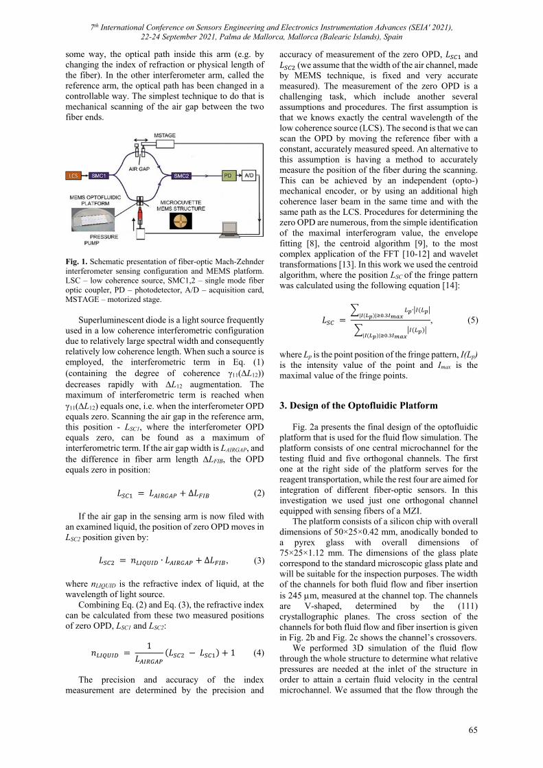
7th International Conference on Sensors Engineering and Electronics Instrumentation Advances (SEIA' 2021), 22-24 September 2021, Palma de Mallorca, Mallorca (Balearic Islands), Spain
65
some way, the optical path inside this arm (e.g. by changing the index of refraction or physical length of the fiber). In the other interferometer arm, called the reference arm, the optical path has been changed in a controllable way. The simplest technique to do that is mechanical scanning of the air gap between the two fiber ends.
Fig. 1. Schematic presentation of fiber-optic Mach-Zehnder interferometer sensing configuration and MEMS platform. LSC – low coherence source, SMC1,2 – single mode fiber optic coupler, PD – photodetector, A/D – acquisition card, MSTAGE – motorized stage.
Superluminescent diode is a light source frequently
used in a low coherence interferometric configuration due to relatively large spectral width and consequently relatively low coherence length. When such a source is employed, the interferometric term in Eq. (1) (containing the degree of coherence γ11(L12)) decreases rapidly with L12 augmentation. The maximum of interferometric term is reached when γ11(L12) equals one, i.e. when the interferometer OPD equals zero. Scanning the air gap in the reference arm, this position - LSC1, where the interferometer OPD equals zero, can be found as a maximum of interferometric term. If the air gap width is LAIRGAP, and the difference in fiber arm length LFIB, the OPD equals zero in position:
𝐿 𝐿 ∆𝐿 (2)
If the air gap in the sensing arm is now filed with
an examined liquid, the position of zero OPD moves in LSC2 position given by:
𝐿 𝑛 ∙ 𝐿 ∆𝐿 , (3)
where nLIQUID is the refractive index of liquid, at the wavelength of light source.
Combining Eq. (2) and Eq. (3), the refractive index can be calculated from these two measured positions of zero OPD, LSC1 and LSC2:
𝑛 1
𝐿𝐿 𝐿 1 (4)
The precision and accuracy of the index
measurement are determined by the precision and
accuracy of measurement of the zero OPD, 𝐿 and 𝐿 (we assume that the width of the air channel, made by MEMS technique, is fixed and very accurate measured). The measurement of the zero OPD is a challenging task, which include another several assumptions and procedures. The first assumption is that we knows exactly the central wavelength of the low coherence source (LCS). The second is that we can scan the OPD by moving the reference fiber with a constant, accurately measured speed. An alternative to this assumption is having a method to accurately measure the position of the fiber during the scanning. This can be achieved by an independent (opto-) mechanical encoder, or by using an additional high coherence laser beam in the same time and with the same path as the LCS. Procedures for determining the zero OPD are numerous, from the simple identification of the maximal interferogram value, the envelope fitting [8], the centroid algorithm [9], to the most complex application of the FFT [10-12] and wavelet transformations [13]. In this work we used the centroid algorithm, where the position LSC of the fringe pattern was calculated using the following equation [14]:
𝐿∙
| | .
| | .
, (5)
where Lp is the point position of the fringe pattern, I(Lp) is the intensity value of the point and Imax is the maximal value of the fringe points. 3. Design of the Optofluidic Platform
Fig. 2a presents the final design of the optofluidic platform that is used for the fluid flow simulation. The platform consists of one central microchannel for the testing fluid and five orthogonal channels. The first one at the right side of the platform serves for the reagent transportation, while the rest four are aimed for integration of different fiber-optic sensors. In this investigation we used just one orthogonal channel equipped with sensing fibers of a MZI.
The platform consists of a silicon chip with overall dimensions of 50×25×0.42 mm, anodically bonded to a pyrex glass with overall dimensions of 75×25×1.12 mm. The dimensions of the glass plate correspond to the standard microscopic glass plate and will be suitable for the inspection purposes. The width of the channels for both fluid flow and fiber insertion is 245 m, measured at the channel top. The channels are V-shaped, determined by the (111) crystallographic planes. The cross section of the channels for both fluid flow and fiber insertion is given in Fig. 2b and Fig. 2c shows the channel’s crossovers.
We performed 3D simulation of the fluid flow through the whole structure to determine what relative pressures are needed at the inlet of the structure in order to attain a certain fluid velocity in the central microchannel. We assumed that the flow through the
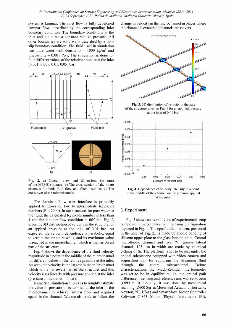
7th International Conference on Sensors Engineering and Electronics Instrumentation Advances (SEIA' 2021), 22-24 September 2021, Palma de Mallorca, Mallorca (Balearic Islands), Spain
66
system is laminar. The inlet flow is fully developed laminar flow, described by the corresponding inlet boundary condition. The boundary conditions at the inlet and outlet set a constant relative pressure. All other boundaries are solid walls described by a non-slip boundary condition. The fluid used in simulation was pure water with density ρ = 1000 kg/m3 and viscosity = 0.001 Pas. The simulation is done for four different values of the relative pressure at the inlet [0.001, 0.005, 0.01, 0.05] bar.
a)
b) c)
Fig. 2. a) Overall view and dimensions (in mm) of the MEMS structure; b) The cross-section of the micro channels for both fluid flow and fiber insertion; c) The cross-over of the microchannels.
The Laminar Flow user interface is primarily
applied to flows of low to intermediate Reynolds numbers (R < 2000). In our structure, for pure water as the fluid, the calculated Reynolds number is less than 1 and the laminar flow condition is fulfilled. Fig. 3 gives the 3D distribution of velocity in the structure for an applied pressure at the inlet of 0.01 bar. As expected, the velocity dependence is parabolic, equal to zero at the structure walls, and its maximum value is reached in the microchannel, which is the narrowest part of the structure.
Fig. 4 shows the dependence of the fluid velocity magnitude in a point in the middle of the microchannel for different values of the relative pressure at the inlet. As seen, the velocity is the largest in the microchannel which is the narrowest part of the structure, and this velocity rises linearly with pressure applied at the inlet (pressure at the outlet = 0 bar).
Numerical simulation allows us to roughly estimate the value of pressure to be applied at the inlet of the microchannel to achieve laminar flow and required speed in the channel. We are also able to follow the
change in velocity in the microchannel in places where the channel is extended (channels crossover).
Fig. 3. 3D distribution of velocity in the part of the structure given in Fig. 1 for an applied pressure
at the inlet of 0.01 bar.
Fig. 4. Dependence of velocity intensity in a point in the middle of the channel on the pressure applied
at the inlet. 3. Experiment
Fig. 5 shows an overall view of experimental setup composed in accordance with sensing configuration depicted in Fig. 1. The optofluidic platform, presented in the inset of Fig. 2., is made by anodic bonding of silicone upper plate to the glass bottom plate. Central microfluidic channel and five ”V” groove lateral channels 125 µm in width are made by chemical etching of Si. The platform is set to be just under the optical microscope equipped with video camera and acquisition unit for capturing the streaming fluid through the central microchannel. Before characterization, the Mach-Zehnder interferometer was set to be in equilibrium, i.e. the optical path difference in sensing and reference arm was set to zero (OPD = 0). Usually, it was done by mechanical scanning (Z600 Series Motorized Actuator, ThorLabs, Newton, NJ, USA) and SmartMove Motor Controller Software C-843 Motor (Physik Instrumente (PI),
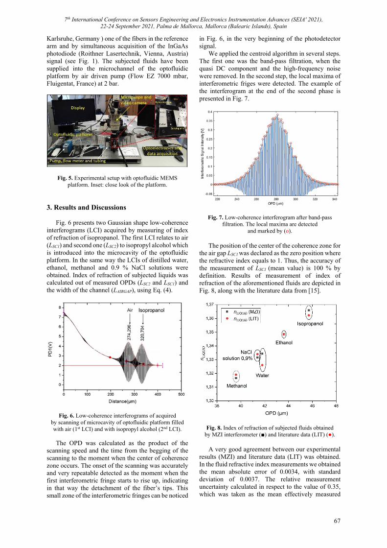
7th International Conference on Sensors Engineering and Electronics Instrumentation Advances (SEIA' 2021), 22-24 September 2021, Palma de Mallorca, Mallorca (Balearic Islands), Spain
67
Karlsruhe, Germany ) one of the fibers in the reference arm and by simultaneous acquisition of the InGaAs photodiode (Roithner Lasertechnik, Vienna, Austria) signal (see Fig. 1). The subjected fluids have been supplied into the microchannel of the optofluidic platform by air driven pump (Flow EZ 7000 mbar, Fluigentat, France) at 2 bar.
Fig. 5. Experimental setup with optofluidic MEMS platform. Inset: close look of the platform.
3. Results and Discussions
Fig. 6 presents two Gaussian shape low-coherence interferograms (LCI) acquired by measuring of index of refraction of isopropanol. The first LCI relates to air (LSC1) and second one (LSC2) to isopropyl alcohol which is introduced into the microcavity of the optofluidic platform. In the same way the LCIs of distilled water, ethanol, methanol and 0.9 % NaCl solutions were obtained. Index of refraction of subjected liquids was calculated out of measured OPDs (LSC2 and LSC1) and the width of the channel (LAIRGAP), using Eq. (4).
Fig. 6. Low-coherence interferograms of acquired by scanning of microcavity of optofluidic platform filled with air (1st LCI) and with isopropyl alcohol (2nd LCI).
The OPD was calculated as the product of the
scanning speed and the time from the begging of the scanning to the moment when the center of coherence zone occurs. The onset of the scanning was accurately and very repeatable detected as the moment when the first interferometric fringe starts to rise up, indicating in that way the detachment of the fiber’s tips. This small zone of the interferometric fringes can be noticed
in Fig. 6, in the very beginning of the photodetector signal.
We applied the centroid algorithm in several steps. The first one was the band-pass filtration, when the quasi DC component and the high-frequency noise were removed. In the second step, the local maxima of interferometric friges were detected. The example of the interferogram at the end of the second phase is presented in Fig. 7.
Fig. 7. Low-coherence interferogram after band-pass filtration. The local maxima are detected
and marked by (o).
The position of the center of the coherence zone for the air gap LSC1 was declared as the zero position where the refractive index equals to 1. Thus, the accuracy of the measurement of LSC1 (mean value) is 100 % by definition. Results of measurement of index of refraction of the aforementioned fluids are depicted in Fig. 8, along with the literature data from [15].
Fig. 8. Index of refraction of subjected fluids obtained by MZI interferometer () and literature data (LIT) ().
A very good agreement between our experimental
results (MZI) and literature data (LIT) was obtained. In the fluid refractive index measurements we obtained the mean absolute error of 0.0034, with standard deviation of 0.0037. The relative measurement uncertainty calculated in respect to the value of 0.35, which was taken as the mean effectively measured

7th International Conference on Sensors Engineering and Electronics Instrumentation Advances (SEIA' 2021), 22-24 September 2021, Palma de Mallorca, Mallorca (Balearic Islands), Spain
68
index value (1.35-1), was about 1 % (0.0034/0.35). One exception was the measurement of the distilled water, where we measured its refraction index with the absolute error of 0.0083 (2.5 %).
It is interesting to note that the standard deviations in 16 measurements performed with the air filled channel was only 0.0002 – one order of magnitude better than in the measurement with fluids. This result can lead to the conclusion that the precision and accuracy of measurement can be better than those of 1 %, which we found out in this measurement, using the same scanning mechanism and the centroid algorithm. 4. Conclusions
We presented a fiber-optic sensing technique capable to measure index of refraction of liquids in dynamic regime. The technique combines a Mach-Zehnder low-coherence interferometer embedded into the MEMS optofluidic platform. Five liquids were tested with index of refraction in the range of 1.32 to 1.38. A very high agreement between the experimental and literature data was obtained. The precision and accuracy of the index of refraction measurement was about 1 %. The proposed sensor is suitable for label-free sensing in biomedicine due to high precision and accuracy and small sample volume.
Acknowledgements
The authors thank to the NFB und ACMIT Gmbh, Austria, which sponsored this work in the frame of the LSC15-004 project “Immune-regulatory capacity of mesenchymal stem cells (MSCs)”. M.T. thanks to Ministry of Education, Science and Technological Development of Serbia to support him in this investigation, in the frame of the agreement 451-03-68/2020-14/200175 with ITS-SASA.
References [1]. J. A. Flores-Bravo, M. A. Illarramendi, J. Zubia,
J. Villatoro, Optical fiber interferometer for temperature-independent refractive index measuring over a broad range, Optics and Laser Technology, Vol. 139, 2021, 106977.
[2]. S. Samanta, S. Kalathimekkad, S. K. Selvaraja, Fluid sensing strategies adopted in photonic devices: A review, Optics and Laser Technology, Vol. 139, 2021, 106975.
[3]. J. T. Dong, C. H. Cheng, C. Wu, J. Li, B. O. Guan, Highly sensitive optofluidic refractive index sensor based on a seven-liquid-core Teflon-cladding fiber, Optics Express, Vol. 28, Issue 18, 2020, pp. 26218-26227.
[4]. J. Jiang, Y. Zhao, Y. Yang, Y. Wang, X. He, W. Yang, L. Li, All-fiber Fabry-Perot interferometer for liquid refractive index measurement, Journal of Russian Laser Research, Vol. 40, Issue 4, 2019, pp. 370-374.
[5]. H. Yu, L. Xiong, Z. Chen, Q. Li, X. Yi, Y. Ding, F. Wang, H. Lv, Y. Ding, Ultracompact and high sensitive refractive index sensor based on Mach-Zehnder interferometer, Optics and Lasers in Engineering, Vol. 56, 2014, pp. 50-53.
[6]. A. Rostamian, E. Madadi-Kandjani, H. Dalir, V. J. Sorger, R. T. Chen, Towards lab-on-chip ultrasensitive ethanol detection using photonic crystal waveguide operating in the mid-infrared, Nanophotonics, Vol. 10, Issue 6, 2021, pp. 1675-1682.
[7]. M. Francon, Optical Interferometry, Academic Press, 1966.
[8]. K. Larkin, Efficient nonlinear algorithm for envelope detection in white light interferometry, J. Opt. Soc. Am., Vol. 13, Issue 4, 1996, pp. 832-843.
[9]. C. Ai, E. L. Novak, Centroid Approach for Estimating Modulation Peak in Broad-Bandwidth Interferometry, U. S. Patent 5,633,715, USA, 27 May 1997.
[10]. S. Chim, G. Kino, Three-dimensional image realization in interference microscopy, Appl. Opt., Vol. 31, Issue 14, 1992, pp. 2550-2553.
[11]. Q. Vo, F. Fang, X. Zhang, H. Gao, Surface recovery algorithm in white light interferometry based on combined white light phase shifting and fast Fourier transform algorithms, Appl. Opt., Vol. 56, Issue 29, 2017, pp. 8174-8185.
[12]. Z. Yu, A. Wang, Fast White light interferometry demodulation algorithm for low-finesse Fabry-Pérot sensors, IEEE Photonics Technology Letters, Vol. 27, Issue 8, 2015, pp. 817-820.
[13]. P. Sandoz, Wavelet transform as a processing tool in white-light interferometry, Opt. Lett., Vol. 22, Issue 14, 1997, pp. 1065-1067.
[14]. C. Wang, X. Zhang, J. Jiang, K. Liu, S. Wang, Y. Li, T. Liu, A demodulation method of spatial domain for low-coherence interferometry with high accuracy and adaptability, IEEE Photonics Journal, Vol. 12, Issue 2, 2020, pp. 1-11.
[15]. Refractive Index Database, https://refractiveindex.info/
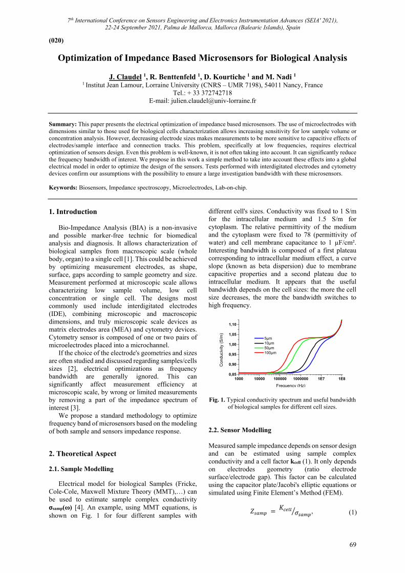
7th International Conference on Sensors Engineering and Electronics Instrumentation Advances (SEIA' 2021), 22-24 September 2021, Palma de Mallorca, Mallorca (Balearic Islands), Spain
69
(020)
Optimization of Impedance Based Microsensors for Biological Analysis
J. Claudel 1, R. Benttenfeld 1, D. Kourtiche 1 and M. Nadi 1
1 Institut Jean Lamour, Lorraine University (CNRS – UMR 7198), 54011 Nancy, France Tel.: + 33 372742718
E-mail: [email protected] Summary: This paper presents the electrical optimization of impedance based microsensors. The use of microelectrodes with dimensions similar to those used for biological cells characterization allows increasing sensitivity for low sample volume or concentration analysis. However, decreasing electrode sizes makes measurements to be more sensitive to capacitive effects of electrodes/sample interface and connection tracks. This problem, specifically at low frequencies, requires electrical optimization of sensors design. Even this problem is well-known, it is not often taking into account. It can significantly reduce the frequency bandwidth of interest. We propose in this work a simple method to take into account these effects into a global electrical model in order to optimize the design of the sensors. Tests performed with interdigitated electrodes and cytometry devices confirm our assumptions with the possibility to ensure a large investigation bandwidth with these microsensors. Keywords: Biosensors, Impedance spectroscopy, Microelectrodes, Lab-on-chip.
1. Introduction
Bio-Impedance Analysis (BIA) is a non-invasive and possible marker-free technic for biomedical analysis and diagnosis. It allows characterization of biological samples from macroscopic scale (whole body, organ) to a single cell [1]. This could be achieved by optimizing measurement electrodes, as shape, surface, gaps according to sample geometry and size. Measurement performed at microscopic scale allows characterizing low sample volume, low cell concentration or single cell. The designs most commonly used include interdigitated electrodes (IDE), combining microscopic and macroscopic dimensions, and truly microscopic scale devices as matrix electrodes area (MEA) and cytometry devices. Cytometry sensor is composed of one or two pairs of microelectrodes placed into a microchannel.
If the choice of the electrode's geometries and sizes are often studied and discussed regarding samples/cells sizes [2], electrical optimizations as frequency bandwidth are generally ignored. This can significantly affect measurement efficiency at microscopic scale, by wrong or limited measurements by removing a part of the impedance spectrum of interest [3].
We propose a standard methodology to optimize frequency band of microsensors based on the modeling of both sample and sensors impedance response.
2. Theoretical Aspect 2.1. Sample Modelling
Electrical model for biological Samples (Fricke, Cole-Cole, Maxwell Mixture Theory (MMT),…) can be used to estimate sample complex conductivity σsamp(ω) [4]. An example, using MMT equations, is shown on Fig. 1 for four different samples with
different cell's sizes. Conductivity was fixed to 1 S/m for the intracellular medium and 1.5 S/m for cytoplasm. The relative permittivity of the medium and the cytoplasm were fixed to 78 (permittivity of water) and cell membrane capacitance to 1 µF/cm². Interesting bandwidth is composed of a first plateau corresponding to intracellular medium effect, a curve slope (known as beta dispersion) due to membrane capacitive properties and a second plateau due to intracellular medium. It appears that the useful bandwidth depends on the cell sizes: the more the cell size decreases, the more the bandwidth switches to high frequency.
1000 10000 100000 1000000 1E7 1E80,85
0,90
0,95
1,00
1,05
1,10
Con
duci
vity
(S
/m)
Frequency (Hz)
5µm 10µm 50µm 100µm
Fig. 1. Typical conductivity spectrum and useful bandwidth of biological samples for different cell sizes.
2.2. Sensor Modelling Measured sample impedance depends on sensor design and can be estimated using sample complex conductivity and a cell factor kcell (1). It only depends on electrodes geometry (ratio electrode surface/electrode gap). This factor can be calculated using the capacitor plate/Jacobi's elliptic equations or simulated using Finite Element’s Method (FEM).
𝑍 𝐾𝜎 , (1)
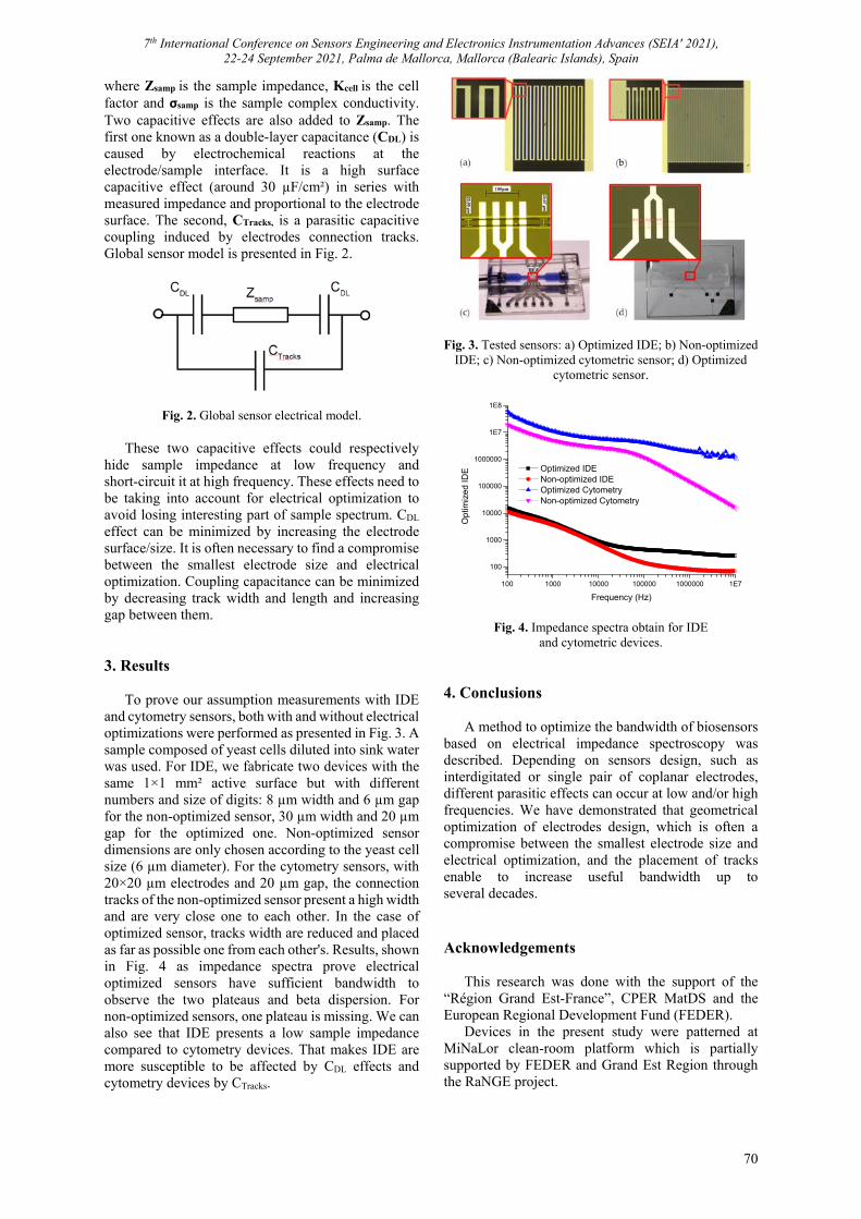
7th International Conference on Sensors Engineering and Electronics Instrumentation Advances (SEIA' 2021), 22-24 September 2021, Palma de Mallorca, Mallorca (Balearic Islands), Spain
70
where Zsamp is the sample impedance, Kcell is the cell factor and σsamp is the sample complex conductivity. Two capacitive effects are also added to Zsamp. The first one known as a double-layer capacitance (CDL) is caused by electrochemical reactions at the electrode/sample interface. It is a high surface capacitive effect (around 30 µF/cm²) in series with measured impedance and proportional to the electrode surface. The second, CTracks, is a parasitic capacitive coupling induced by electrodes connection tracks. Global sensor model is presented in Fig. 2.
Fig. 2. Global sensor electrical model.
These two capacitive effects could respectively hide sample impedance at low frequency and short-circuit it at high frequency. These effects need to be taking into account for electrical optimization to avoid losing interesting part of sample spectrum. CDL
effect can be minimized by increasing the electrode surface/size. It is often necessary to find a compromise between the smallest electrode size and electrical optimization. Coupling capacitance can be minimized by decreasing track width and length and increasing gap between them. 3. Results
To prove our assumption measurements with IDE and cytometry sensors, both with and without electrical optimizations were performed as presented in Fig. 3. A sample composed of yeast cells diluted into sink water was used. For IDE, we fabricate two devices with the same 1×1 mm² active surface but with different numbers and size of digits: 8 µm width and 6 µm gap for the non-optimized sensor, 30 µm width and 20 µm gap for the optimized one. Non-optimized sensor dimensions are only chosen according to the yeast cell size (6 µm diameter). For the cytometry sensors, with 20×20 µm electrodes and 20 µm gap, the connection tracks of the non-optimized sensor present a high width and are very close one to each other. In the case of optimized sensor, tracks width are reduced and placed as far as possible one from each other's. Results, shown in Fig. 4 as impedance spectra prove electrical optimized sensors have sufficient bandwidth to observe the two plateaus and beta dispersion. For non-optimized sensors, one plateau is missing. We can also see that IDE presents a low sample impedance compared to cytometry devices. That makes IDE are more susceptible to be affected by CDL effects and cytometry devices by CTracks.
Fig. 3. Tested sensors: a) Optimized IDE; b) Non-optimized IDE; c) Non-optimized cytometric sensor; d) Optimized
cytometric sensor.
100 1000 10000 100000 1000000 1E7
100
1000
10000
100000
1000000
1E7
1E8
Opt
imiz
ed ID
E
Frequency (Hz)
Optimized IDE Non-optimized IDE Optimized Cytometry Non-optimized Cytometry
Fig. 4. Impedance spectra obtain for IDE and cytometric devices.
4. Conclusions
A method to optimize the bandwidth of biosensors based on electrical impedance spectroscopy was described. Depending on sensors design, such as interdigitated or single pair of coplanar electrodes, different parasitic effects can occur at low and/or high frequencies. We have demonstrated that geometrical optimization of electrodes design, which is often a compromise between the smallest electrode size and electrical optimization, and the placement of tracks enable to increase useful bandwidth up to several decades. Acknowledgements
This research was done with the support of the “Région Grand Est-France”, CPER MatDS and the European Regional Development Fund (FEDER).
Devices in the present study were patterned at MiNaLor clean-room platform which is partially supported by FEDER and Grand Est Region through the RaNGE project.

7th International Conference on Sensors Engineering and Electronics Instrumentation Advances (SEIA' 2021), 22-24 September 2021, Palma de Mallorca, Mallorca (Balearic Islands), Spain
71
References [1]. C. Petchakup, K. H. H. Li, H. W. Hou, Advances in
single cell impedance cytometry for biomedical applications, Micromachines, Vol. 8, Issue 3, 2017, 87.
[2]. Y. Park, J. J. Cha, S. Seo, et al., Ex vivo characterization of age-associated impedance changes of single vascular endothelial cells using micro
electrical impedance spectroscopy with a cell trap, Biomicrofluidics, Vol. 10, Issue 1, 2016, 014114.
[3]. J. Claudel, T. T. Ngo, D. Kourtiche, et al., Interdigitated sensor optimization for blood sample analysis, Biosensors, Vol. 10, Issue 12, 2020, 208.
[4]. C. Gabriel, S. Gabriel, Y. E. Corthout, The dielectric properties of biological tissues: I. Literature survey, Physics in Medicine & Biology, Vol. 41, Issue 11, 1996, 2231.
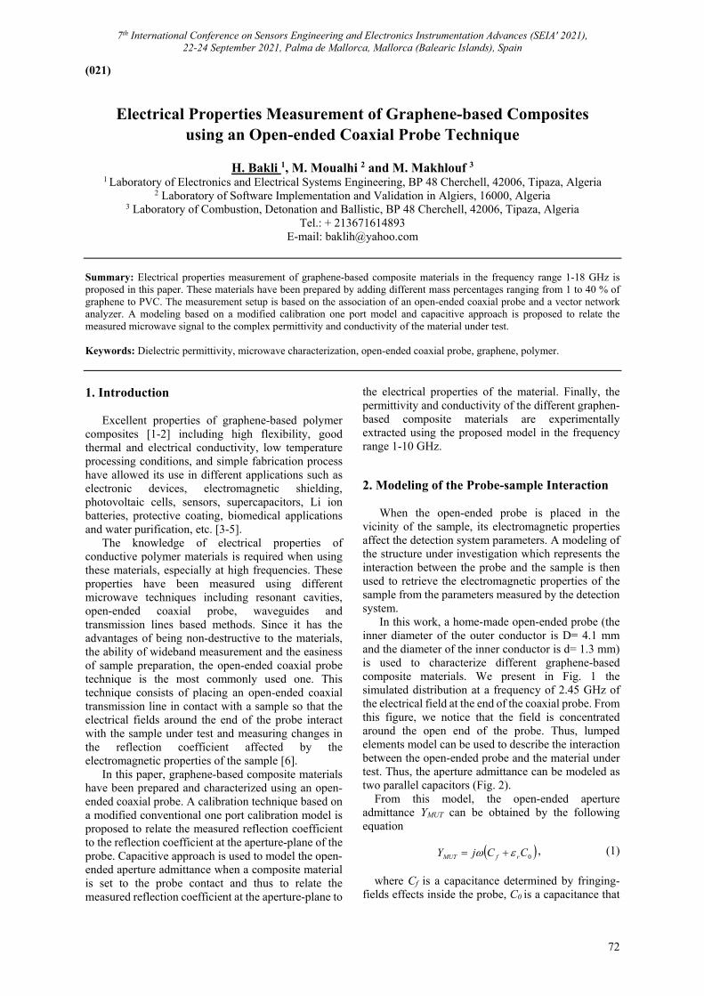
7th International Conference on Sensors Engineering and Electronics Instrumentation Advances (SEIA' 2021), 22-24 September 2021, Palma de Mallorca, Mallorca (Balearic Islands), Spain
72
(021)
Electrical Properties Measurement of Graphene-based Composites using an Open-ended Coaxial Probe Technique
H. Bakli 1, M. Moualhi 2 and M. Makhlouf 3
1 Laboratory of Electronics and Electrical Systems Engineering, BP 48 Cherchell, 42006, Tipaza, Algeria 2 Laboratory of Software Implementation and Validation in Algiers, 16000, Algeria
3 Laboratory of Combustion, Detonation and Ballistic, BP 48 Cherchell, 42006, Tipaza, Algeria Tel.: + 213671614893
E-mail: [email protected] Summary: Electrical properties measurement of graphene-based composite materials in the frequency range 1-18 GHz is proposed in this paper. These materials have been prepared by adding different mass percentages ranging from 1 to 40 % of graphene to PVC. The measurement setup is based on the association of an open-ended coaxial probe and a vector network analyzer. A modeling based on a modified calibration one port model and capacitive approach is proposed to relate the measured microwave signal to the complex permittivity and conductivity of the material under test. Keywords: Dielectric permittivity, microwave characterization, open-ended coaxial probe, graphene, polymer.
1. Introduction
Excellent properties of graphene-based polymer
composites [1-2] including high flexibility, good thermal and electrical conductivity, low temperature processing conditions, and simple fabrication process have allowed its use in different applications such as electronic devices, electromagnetic shielding, photovoltaic cells, sensors, supercapacitors, Li ion batteries, protective coating, biomedical applications and water purification, etc. [3-5].
The knowledge of electrical properties of conductive polymer materials is required when using these materials, especially at high frequencies. These properties have been measured using different microwave techniques including resonant cavities, open-ended coaxial probe, waveguides and transmission lines based methods. Since it has the advantages of being non-destructive to the materials, the ability of wideband measurement and the easiness of sample preparation, the open-ended coaxial probe technique is the most commonly used one. This technique consists of placing an open-ended coaxial transmission line in contact with a sample so that the electrical fields around the end of the probe interact with the sample under test and measuring changes in the reflection coefficient affected by the electromagnetic properties of the sample [6].
In this paper, graphene-based composite materials have been prepared and characterized using an open-ended coaxial probe. A calibration technique based on a modified conventional one port calibration model is proposed to relate the measured reflection coefficient to the reflection coefficient at the aperture-plane of the probe. Capacitive approach is used to model the open-ended aperture admittance when a composite material is set to the probe contact and thus to relate the measured reflection coefficient at the aperture-plane to
the electrical properties of the material. Finally, the permittivity and conductivity of the different graphen-based composite materials are experimentally extracted using the proposed model in the frequency range 1-10 GHz.
2. Modeling of the Probe-sample Interaction When the open-ended probe is placed in the
vicinity of the sample, its electromagnetic properties affect the detection system parameters. A modeling of the structure under investigation which represents the interaction between the probe and the sample is then used to retrieve the electromagnetic properties of the sample from the parameters measured by the detection system.
In this work, a home-made open-ended probe (the inner diameter of the outer conductor is D= 4.1 mm and the diameter of the inner conductor is d= 1.3 mm) is used to characterize different graphene-based composite materials. We present in Fig. 1 the simulated distribution at a frequency of 2.45 GHz of the electrical field at the end of the coaxial probe. From this figure, we notice that the field is concentrated around the open end of the probe. Thus, lumped elements model can be used to describe the interaction between the open-ended probe and the material under test. Thus, the aperture admittance can be modeled as two parallel capacitors (Fig. 2).
From this model, the open-ended aperture admittance YMUT can be obtained by the following equation
0CCjY rfMUT , (1)
where Cf is a capacitance determined by fringing-fields effects inside the probe, C0 is a capacitance that
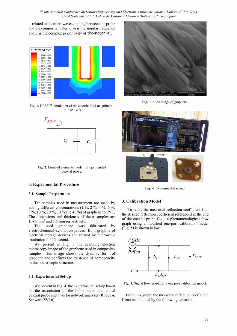
7th International Conference on Sensors Engineering and Electronics Instrumentation Advances (SEIA' 2021), 22-24 September 2021, Palma de Mallorca, Mallorca (Balearic Islands), Spain
73
is related to the microwave coupling between the probe and the composite material, ω is the angular frequency and εr is the complex permittivity of the material.
Fig. 1. HFSSTM simulation of the electric field magnitude - F = 2.45 GHz.
Fig. 2. Lumped elements model for open-ended coaxial probe.
3. Experimental Procedure 3.1. Sample Preparation
The samples used in measurement are made by
adding different concentrations (1 %, 2 %, 4 %, 6 %, 8 %, 10 %, 20 %, 30 % and 40 %) of graphene to PVC. The dimensions and thickness of these samples are 10x6 mm2 and 1.5 mm respectively.
The used graphene was fabricated by electrochemical exfoliation process from graphite of electrical storage devices and treated by microwave irradiation for 15 second.
We present in Fig. 3 the scanning electron microscopy image of the graphene used in composites samples. This image shows the dynamic form of graphene and confirms the existence of homogeneity in the microscopic structure. 3.2. Experimental Set-up
We present in Fig. 4, the experimental set-up based
on the association of the home-made open-ended coaxial probe and a vector network analyzer (Rhode & Schwarz ZVL6).
Fig. 3. SEM image of graphene.
Fig. 4. Experimental set-up. 3. Calibration Model
To relate the measured reflection coefficient Γ to the desired reflection coefficient referenced at the end of the coaxial probe ΓMUT, a phenomenological flow graph using a modified one-port calibration model (Fig. 5) is shown below
Fig. 5. Signal flow graph for a one port calibration model.
From this graph, the measured reflection coefficient Γ can be obtained by the following equation
CcCf
ΓГMUT
E12E21
E11
1
E22
Г
ГMUT
F GHz
P dBm~
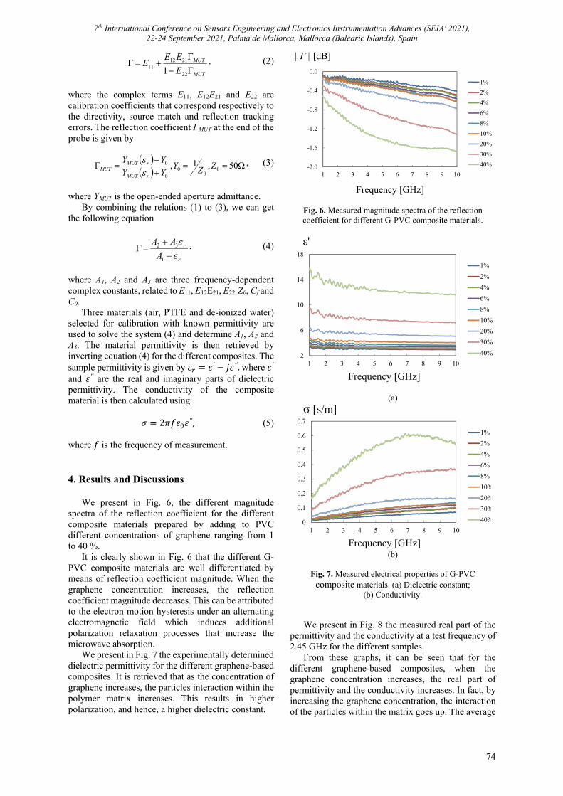
7th International Conference on Sensors Engineering and Electronics Instrumentation Advances (SEIA' 2021), 22-24 September 2021, Palma de Mallorca, Mallorca (Balearic Islands), Spain
74
MUT
MUT
E
EEE
22
211211 1
, (2)
where the complex terms E11, E12E21 and E22 are calibration coefficients that correspond respectively to the directivity, source match and reflection tracking errors. The reflection coefficient ΓMUT at the end of the probe is given by
50,1, 00
00
0 ZZYYY
YY
rMUT
rMUTMUT
, (3)
where YMUT is the open-ended aperture admittance.
By combining the relations (1) to (3), we can get the following equation
r
r
A
AA
1
32 , (4)
where A1, A2 and A3 are three frequency-dependent complex constants, related to E11, E12E21, E22, Z0, Cf and C0.
Three materials (air, PTFE and de-ionized water) selected for calibration with known permittivity are used to solve the system (4) and determine A1, A2 and A3. The material permittivity is then retrieved by inverting equation (4) for the different composites. The sample permittivity is given by 𝜀 𝜀 ′ 𝑗𝜀 ′′. where 𝜀 ′ and 𝜀 ′′ are the real and imaginary parts of dielectric permittivity. The conductivity of the composite material is then calculated using
𝜎 2𝜋𝑓 𝜀 𝜀 ′′, (5) where 𝑓 is the frequency of measurement. 4. Results and Discussions
We present in Fig. 6, the different magnitude
spectra of the reflection coefficient for the different composite materials prepared by adding to PVC different concentrations of graphene ranging from 1 to 40 %.
It is clearly shown in Fig. 6 that the different G-PVC composite materials are well differentiated by means of reflection coefficient magnitude. When the graphene concentration increases, the reflection coefficient magnitude decreases. This can be attributed to the electron motion hysteresis under an alternating electromagnetic field which induces additional polarization relaxation processes that increase the microwave absorption.
We present in Fig. 7 the experimentally determined dielectric permittivity for the different graphene-based composites. It is retrieved that as the concentration of graphene increases, the particles interaction within the polymer matrix increases. This results in higher polarization, and hence, a higher dielectric constant.
Fig. 6. Measured magnitude spectra of the reflection coefficient for different G-PVC composite materials.
(a)
(b)
Fig. 7. Measured electrical properties of G-PVC
composite materials. (a) Dielectric constant; (b) Conductivity.
We present in Fig. 8 the measured real part of the permittivity and the conductivity at a test frequency of 2.45 GHz for the different samples.
From these graphs, it can be seen that for the different graphene-based composites, when the graphene concentration increases, the real part of permittivity and the conductivity increases. In fact, by increasing the graphene concentration, the interaction of the particles within the matrix goes up. The average
-2.0
-1.6
-1.2
-0.8
-0.4
0.0
1 2 3 4 5 6 7 8 9 10
1%
2%
4%
6%
8%
10%
20%
30%
40%
| Γ | [dB]
Frequency [GHz]
2
6
10
14
18
1 2 3 4 5 6 7 8 9 10
1%
2%
4%
6%
8%
10%
20%
30%
40%
Frequency [GHz]
ε'
Frequency [GHz]
σ [s/m]
0
0.1
0.2
0.3
0.4
0.5
0.6
0.7
1 2 3 4 5 6 7 8 9 10
1%
2%
4%
6%
8%
10%
20%
30%
40%
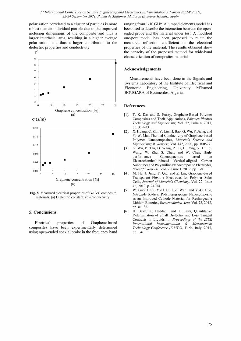
7th International Conference on Sensors Engineering and Electronics Instrumentation Advances (SEIA' 2021), 22-24 September 2021, Palma de Mallorca, Mallorca (Balearic Islands), Spain
75
polarization correlated to a cluster of particles is more robust than an individual particle due to the improved inclusion dimensions of the composite and thus a larger interfacial area, resulting in a higher average polarization, and thus a larger contribution to the dielectric properties and conductivity.
(a)
(b)
Fig. 8. Measured electrical properties of G-PVC composite
materials. (a) Dielectric constant; (b) Conductivity.
5. Conclusions Electrical properties of Graphene-based
composites have been experimentally determined using open-ended coaxial probe in the frequency band
ranging from 1-10 GHz. A lumped elements model has been used to describe the interaction between the open-ended probe and the material under test. A modified one-port model has been proposed to relate the measured reflection coefficient to the electrical properties of the material. The results obtained show the capacity of the proposed method for wide-band characterization of composites materials.
Acknowledgements
Measurements have been done in the Signals and Systems Laboratory of the Institute of Electrical and Electronic Engineering, University M’hamed BOUGARA of Boumerdes, Algeria.
References [1]. T. K. Das and S. Prusty, Graphene-Based Polymer
Composites and Their Applications, Polymer-Plastics Technology and Engineering, Vol. 52, Issue 4, 2013, pp. 319–331.
[2]. X. Huang, C. Zhi, Y. Lin, H. Bao, G. Wu, P. Jiang, and Y.-W. Mai, Thermal Conductivity of Graphene-based Polymer Nanocomposites, Materials Science and Engineering: R: Reports, Vol. 142, 2020, pp. 100577.
[3]. G. Wu, P. Tan, D. Wang, Z. Li, L. Peng, Y. Hu, C. Wang, W. Zhu, S. Chen, and W. Chen, High-performance Supercapacitors based on Electrochemical-induced Vertical-aligned Carbon Nanotubes and Polyaniline Nanocomposite Electrodes, Scientific Reports, Vol. 7, Issue 1, 2017, pp. 1-8.
[4]. M. He, J. Jung, F. Qiu, and Z. Lin, Graphene-based Transparent Flexible Electrodes for Polymer Solar Cells, Journal of Materials Chemistry, Vol. 22, Issue 46, 2012, p. 24254.
[5]. W. Guo, J. Su, Y.-H. Li, L.-J. Wan, and Y.-G. Guo, Nitroxide Radical Polymer/graphene Nanocomposite as an Improved Cathode Material for Rechargeable Lithium Batteries, Electrochimica Acta, Vol. 72, 2012, pp. 81–86.
[6]. H. Bakli, K. Haddadi, and T. Lasri, Quantitative Determination of Small Dielectric and Loss Tangent Contrasts in Liquids, in Proceedings of the IEEE International Instrumentation & Measurement Technology Conference (I2MTC), Turin, Italy, 2017, pp. 1-6.
ε'
Graphene concentration [%]
2
3
4
5
6
7
8
9
0 5 10 15 20 25 30
σ (s/m)
Graphene concentration [%]
0.00
0.04
0.08
0.12
0.16
0.20
0 5 10 15 20 25 30

7th International Conference on Sensors Engineering and Electronics Instrumentation Advances (SEIA' 2021), 22-24 September 2021, Palma de Mallorca, Mallorca (Balearic Islands), Spain
76
(022)
Numerical Studies of a Side-hole Optical Fiber with Modified Geometry as a Refractive Index Sensor
M. Dudek, K. Köllő, P. Marć and L. R. Jaroszewicz
Military University of Technology, Institute of Applied Physics, gen. Sylwestra Kaliskiego 2, 00-908 Warsaw, Poland
Tel.: +48 261839065, fax: +48 261839317 E-mail: [email protected]
Summary: In this work we present a preliminary results of a side-hole optical fiber (S-H OF) with modified geometry utilized as a refractive index sensor. We have considered a rectangular cut-out of the fiber cladding which has opened one of the two holes located symmetrically around its core. Due to this kind of modification the fundamental modes propagating in the core (TE and TM) can be perturbed by the change of the external refractive index (RI), and therefore their insertion losses are also changing. This provides a possibility to apply a simple polarization sensitive detection scheme in which the output optical power levels of orthogonal polarizations can be correlated with the RI of material inside the rectangular cavity. Based on the proposed modifications of the S-H OF’s geometry it is possible to propose a novel simple RI sensor for liquids. Keywords: Side-hole optical fiber, Refractive index, Optical fiber sensor, Insertion loss, Numerical modeling, FDTD method.
1. Introduction
With the increasing interest in the optical fibers, along with the telecommunication properties, the development of fiber optic sensors (FOSs) is also present. To cope with the constantly widening fields of their possible applications, the design of FOSs, as well as the technology to obtain them, had to improve [1]. In the midst of many possibilities of FOSs, the inline sensors with microcavities inside the fibers can be highlighted [2]. This kind of sensor allows to measure the desired physical parameter using for instance the change in the refractive index of the medium the sensor is placed in. The inline cavity sensing is an unusual method, since it requires change in the geometry of optical fiber’s core, which in normal conditions is inaccessible. This method however is associated with the need of micromachining of the optical fiber using for example a laser beam or chemical etching [3]. The geometry of the cavity itself can determine optical losses, which are one of the most important parameters in this kind of sensors, as they can be directly measured and translated into specific changes in the cavity’s environment – thus performing the role of a sensor.
2. Methodology
The presented study was conducted using the finite-difference time-domain (FDTD) method, which is a widely used full-wave technique for approximate description of propagation of electromagnetic waves, especially in systems in which the dimensions of studied structures are comparable to wavelengths used in the simulations [4]. In this work for numerical simulations we used the FDTD solver by ANSYS/Lumerical.
One of the most important factors determining the usability of inline FOSs are the insertion loss (IL), which may be calculated as follows:
𝐼𝐿 10 log , (1)
where PI is the power inserted into the system (input power) and PT is the power transmitted through the system (output power). 3. Results
The analyzed S-H OF was based on an actual fiber produced by the Optical Fiber Technology Laboratory, Maria Curie-Sklodowska University. The RI of the S-H OF (its model is presented in Fig. 1) cladding was set to 1.4425, while the RI of the core was set to 1.457. The radii of the elliptic core were 1 μm and 2.3 µm, the cladding radius was 62.5 µm, the holes were ellipses with radii set to 16 μm and 12 µm. The simulation region was 130×130×50 µm3 with uniform mesh step of 0.1 µm and source wavelength of 1.55 μm.
Fig. 1. Example of rectangular cut-out in S-H OF.
The simulations of rectangular cut-outs were performed for a cavity with the height of 10 μm and
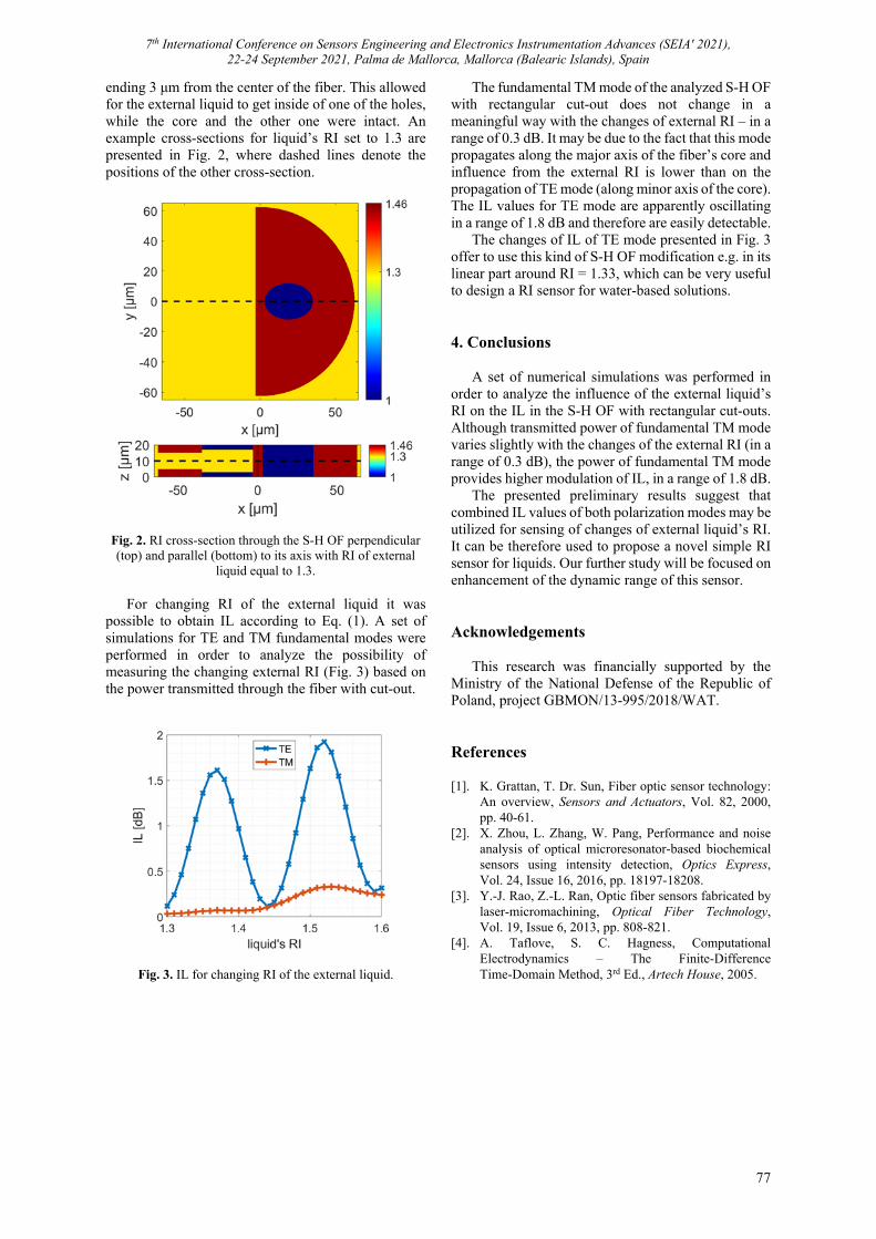
7th International Conference on Sensors Engineering and Electronics Instrumentation Advances (SEIA' 2021), 22-24 September 2021, Palma de Mallorca, Mallorca (Balearic Islands), Spain
77
ending 3 μm from the center of the fiber. This allowed for the external liquid to get inside of one of the holes, while the core and the other one were intact. An example cross-sections for liquid’s RI set to 1.3 are presented in Fig. 2, where dashed lines denote the positions of the other cross-section.
Fig. 2. RI cross-section through the S-H OF perpendicular (top) and parallel (bottom) to its axis with RI of external
liquid equal to 1.3.
For changing RI of the external liquid it was possible to obtain IL according to Eq. (1). A set of simulations for TE and TM fundamental modes were performed in order to analyze the possibility of measuring the changing external RI (Fig. 3) based on the power transmitted through the fiber with cut-out.
Fig. 3. IL for changing RI of the external liquid.
The fundamental TM mode of the analyzed S-H OF with rectangular cut-out does not change in a meaningful way with the changes of external RI – in a range of 0.3 dB. It may be due to the fact that this mode propagates along the major axis of the fiber’s core and influence from the external RI is lower than on the propagation of TE mode (along minor axis of the core). The IL values for TE mode are apparently oscillating in a range of 1.8 dB and therefore are easily detectable.
The changes of IL of TE mode presented in Fig. 3 offer to use this kind of S-H OF modification e.g. in its linear part around RI = 1.33, which can be very useful to design a RI sensor for water-based solutions. 4. Conclusions
A set of numerical simulations was performed in order to analyze the influence of the external liquid’s RI on the IL in the S-H OF with rectangular cut-outs. Although transmitted power of fundamental TM mode varies slightly with the changes of the external RI (in a range of 0.3 dB), the power of fundamental TM mode provides higher modulation of IL, in a range of 1.8 dB.
The presented preliminary results suggest that combined IL values of both polarization modes may be utilized for sensing of changes of external liquid’s RI. It can be therefore used to propose a novel simple RI sensor for liquids. Our further study will be focused on enhancement of the dynamic range of this sensor. Acknowledgements
This research was financially supported by the Ministry of the National Defense of the Republic of Poland, project GBMON/13-995/2018/WAT. References [1]. K. Grattan, T. Dr. Sun, Fiber optic sensor technology:
An overview, Sensors and Actuators, Vol. 82, 2000, pp. 40-61.
[2]. X. Zhou, L. Zhang, W. Pang, Performance and noise analysis of optical microresonator-based biochemical sensors using intensity detection, Optics Express, Vol. 24, Issue 16, 2016, pp. 18197-18208.
[3]. Y.-J. Rao, Z.-L. Ran, Optic fiber sensors fabricated by laser-micromachining, Optical Fiber Technology, Vol. 19, Issue 6, 2013, pp. 808-821.
[4]. A. Taflove, S. C. Hagness, Computational Electrodynamics – The Finite-Difference Time-Domain Method, 3rd Ed., Artech House, 2005.
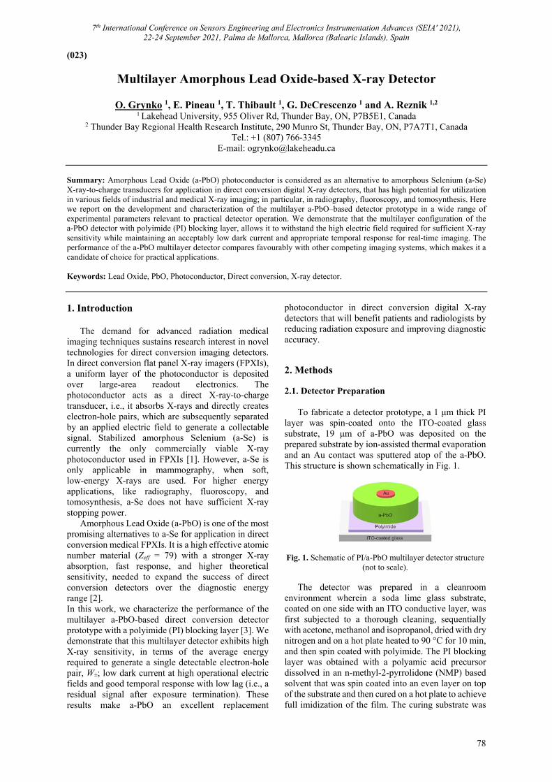
7th International Conference on Sensors Engineering and Electronics Instrumentation Advances (SEIA' 2021), 22-24 September 2021, Palma de Mallorca, Mallorca (Balearic Islands), Spain
78
(023)
Multilayer Amorphous Lead Oxide-based X-ray Detector
O. Grynko 1, E. Pineau 1, T. Thibault 1, G. DeCrescenzo 1 and A. Reznik 1,2
1 Lakehead University, 955 Oliver Rd, Thunder Bay, ON, P7B5E1, Canada 2 Thunder Bay Regional Health Research Institute, 290 Munro St, Thunder Bay, ON, P7A7T1, Canada
Tel.: +1 (807) 766-3345 E-mail: [email protected]
Summary: Amorphous Lead Oxide (a-PbO) photoconductor is considered as an alternative to amorphous Selenium (a-Se) X-ray-to-charge transducers for application in direct conversion digital X-ray detectors, that has high potential for utilization in various fields of industrial and medical X-ray imaging; in particular, in radiography, fluoroscopy, and tomosynthesis. Here we report on the development and characterization of the multilayer a-PbO–based detector prototype in a wide range of experimental parameters relevant to practical detector operation. We demonstrate that the multilayer configuration of the a-PbO detector with polyimide (PI) blocking layer, allows it to withstand the high electric field required for sufficient X-ray sensitivity while maintaining an acceptably low dark current and appropriate temporal response for real-time imaging. The performance of the a-PbO multilayer detector compares favourably with other competing imaging systems, which makes it a candidate of choice for practical applications. Keywords: Lead Oxide, PbO, Photoconductor, Direct conversion, X-ray detector. 1. Introduction
The demand for advanced radiation medical imaging techniques sustains research interest in novel technologies for direct conversion imaging detectors. In direct conversion flat panel X-ray imagers (FPXIs), a uniform layer of the photoconductor is deposited over large-area readout electronics. The photoconductor acts as a direct X-ray-to-charge transducer, i.e., it absorbs X-rays and directly creates electron-hole pairs, which are subsequently separated by an applied electric field to generate a collectable signal. Stabilized amorphous Selenium (a-Se) is currently the only commercially viable X-ray photoconductor used in FPXIs [1]. However, a-Se is only applicable in mammography, when soft, low-energy X-rays are used. For higher energy applications, like radiography, fluoroscopy, and tomosynthesis, a-Se does not have sufficient X-ray stopping power.
Amorphous Lead Oxide (a-PbO) is one of the most promising alternatives to a-Se for application in direct conversion medical FPXIs. It is a high effective atomic number material (Zeff = 79) with a stronger X-ray absorption, fast response, and higher theoretical sensitivity, needed to expand the success of direct conversion detectors over the diagnostic energy range [2]. In this work, we characterize the performance of the multilayer a-PbO-based direct conversion detector prototype with a polyimide (PI) blocking layer [3]. We demonstrate that this multilayer detector exhibits high X-ray sensitivity, in terms of the average energy required to generate a single detectable electron-hole pair, W±; low dark current at high operational electric fields and good temporal response with low lag (i.e., a residual signal after exposure termination). These results make a-PbO an excellent replacement
photoconductor in direct conversion digital X-ray detectors that will benefit patients and radiologists by reducing radiation exposure and improving diagnostic accuracy. 2. Methods 2.1. Detector Preparation
To fabricate a detector prototype, a 1 μm thick PI layer was spin-coated onto the ITO-coated glass substrate, 19 μm of a-PbO was deposited on the prepared substrate by ion-assisted thermal evaporation and an Au contact was sputtered atop of the a-PbO. This structure is shown schematically in Fig. 1.
Fig. 1. Schematic of PI/a-PbO multilayer detector structure (not to scale).
The detector was prepared in a cleanroom
environment wherein a soda lime glass substrate, coated on one side with an ITO conductive layer, was first subjected to a thorough cleaning, sequentially with acetone, methanol and isopropanol, dried with dry nitrogen and on a hot plate heated to 90 °C for 10 min, and then spin coated with polyimide. The PI blocking layer was obtained with a polyamic acid precursor dissolved in an n-methyl-2-pyrrolidone (NMP) based solvent that was spin coated into an even layer on top of the substrate and then cured on a hot plate to achieve full imidization of the film. The curing substrate was
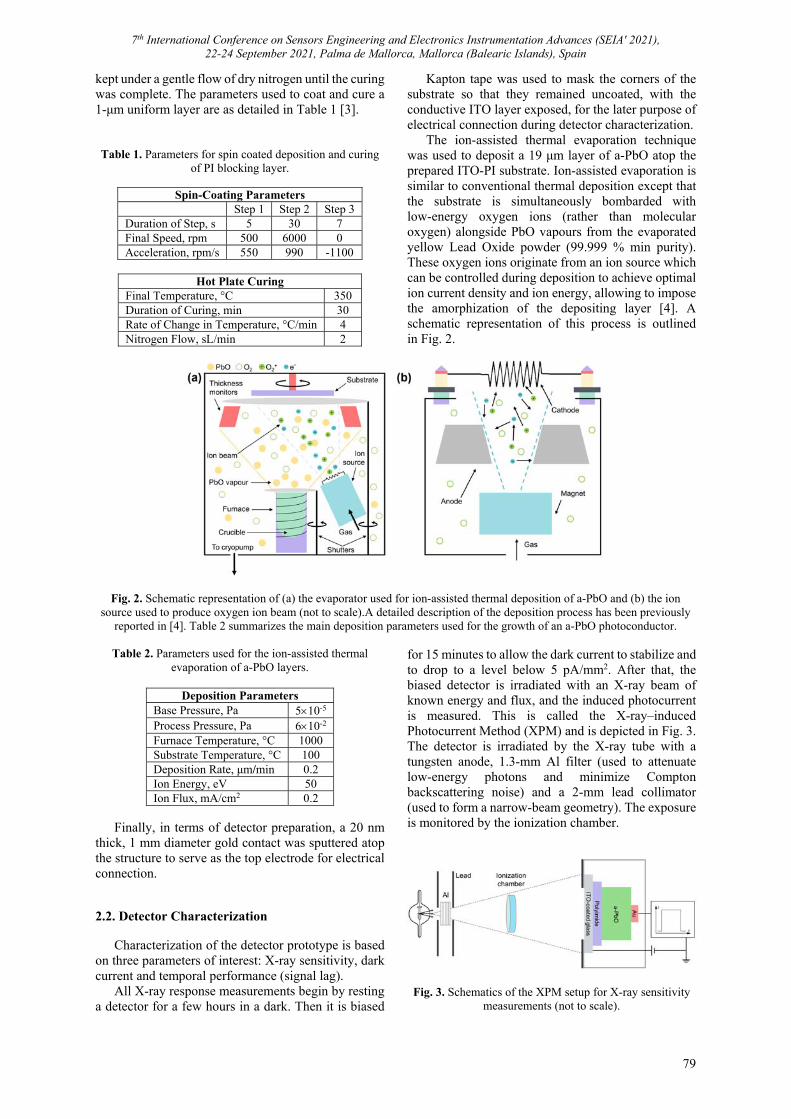
7th International Conference on Sensors Engineering and Electronics Instrumentation Advances (SEIA' 2021), 22-24 September 2021, Palma de Mallorca, Mallorca (Balearic Islands), Spain
79
kept under a gentle flow of dry nitrogen until the curing was complete. The parameters used to coat and cure a 1-μm uniform layer are as detailed in Table 1 [3].
Table 1. Parameters for spin coated deposition and curing of PI blocking layer.
Spin-Coating Parameters Step 1 Step 2 Step 3
Duration of Step, s 5 30 7 Final Speed, rpm 500 6000 0 Acceleration, rpm/s 550 990 -1100
Hot Plate Curing
Final Temperature, °C 350 Duration of Curing, min 30 Rate of Change in Temperature, °C/min 4 Nitrogen Flow, sL/min 2
Kapton tape was used to mask the corners of the substrate so that they remained uncoated, with the conductive ITO layer exposed, for the later purpose of electrical connection during detector characterization.
The ion-assisted thermal evaporation technique was used to deposit a 19 μm layer of a-PbO atop the prepared ITO-PI substrate. Ion-assisted evaporation is similar to conventional thermal deposition except that the substrate is simultaneously bombarded with low-energy oxygen ions (rather than molecular oxygen) alongside PbO vapours from the evaporated yellow Lead Oxide powder (99.999 % min purity). These oxygen ions originate from an ion source which can be controlled during deposition to achieve optimal ion current density and ion energy, allowing to impose the amorphization of the depositing layer [4]. A schematic representation of this process is outlined in Fig. 2.
Fig. 2. Schematic representation of (a) the evaporator used for ion-assisted thermal deposition of a-PbO and (b) the ion source used to produce oxygen ion beam (not to scale).A detailed description of the deposition process has been previously
reported in [4]. Table 2 summarizes the main deposition parameters used for the growth of an a-PbO photoconductor.
Table 2. Parameters used for the ion-assisted thermal evaporation of a-PbO layers.
Deposition Parameters
Base Pressure, Pa 510-5
Process Pressure, Pa 610-2
Furnace Temperature, °C 1000 Substrate Temperature, °C 100 Deposition Rate, μm/min 0.2 Ion Energy, eV 50 Ion Flux, mA/cm2 0.2
Finally, in terms of detector preparation, a 20 nm
thick, 1 mm diameter gold contact was sputtered atop the structure to serve as the top electrode for electrical connection.
2.2. Detector Characterization
Characterization of the detector prototype is based on three parameters of interest: X-ray sensitivity, dark current and temporal performance (signal lag).
All X-ray response measurements begin by resting a detector for a few hours in a dark. Then it is biased
for 15 minutes to allow the dark current to stabilize and to drop to a level below 5 pA/mm2. After that, the biased detector is irradiated with an X-ray beam of known energy and flux, and the induced photocurrent is measured. This is called the X-ray–induced Photocurrent Method (XPM) and is depicted in Fig. 3. The detector is irradiated by the X-ray tube with a tungsten anode, 1.3-mm Al filter (used to attenuate low-energy photons and minimize Compton backscattering noise) and a 2-mm lead collimator (used to form a narrow-beam geometry). The exposure is monitored by the ionization chamber.
Fig. 3. Schematics of the XPM setup for X-ray sensitivity
measurements (not to scale).
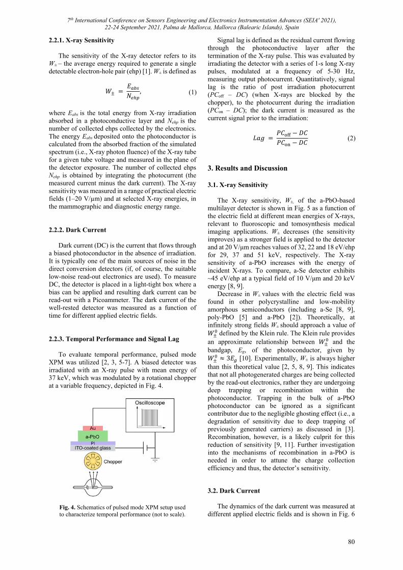
7th International Conference on Sensors Engineering and Electronics Instrumentation Advances (SEIA' 2021), 22-24 September 2021, Palma de Mallorca, Mallorca (Balearic Islands), Spain
80
2.2.1. X-ray Sensitivity
The sensitivity of the X-ray detector refers to its W± – the average energy required to generate a single detectable electron-hole pair (ehp) [1]. W± is defined as
𝑊
𝐸𝑁
, (1)
where Eabs is the total energy from X-ray irradiation absorbed in a photoconductive layer and Nehp is the number of collected ehps collected by the electronics. The energy Eabs deposited onto the photoconductor is calculated from the absorbed fraction of the simulated spectrum (i.e., X-ray photon fluence) of the X-ray tube for a given tube voltage and measured in the plane of the detector exposure. The number of collected ehps Nehp is obtained by integrating the photocurrent (the measured current minus the dark current). The X-ray sensitivity was measured in a range of practical electric fields (1–20 V/µm) and at selected X-ray energies, in the mammographic and diagnostic energy range. 2.2.2. Dark Current
Dark current (DC) is the current that flows through
a biased photoconductor in the absence of irradiation. It is typically one of the main sources of noise in the direct conversion detectors (if, of course, the suitable low-noise read-out electronics are used). To measure DC, the detector is placed in a light-tight box where a bias can be applied and resulting dark current can be read-out with a Picoammeter. The dark current of the well-rested detector was measured as a function of time for different applied electric fields. 2.2.3. Temporal Performance and Signal Lag
To evaluate temporal performance, pulsed mode
XPM was utilized [2, 3, 5-7]. A biased detector was irradiated with an X-ray pulse with mean energy of 37 keV, which was modulated by a rotational chopper at a variable frequency, depicted in Fig. 4.
Fig. 4. Schematics of pulsed mode XPM setup used to characterize temporal performance (not to scale).
Signal lag is defined as the residual current flowing through the photoconductive layer after the termination of the X-ray pulse. This was evaluated by irradiating the detector with a series of 1-s long X-ray pulses, modulated at a frequency of 5-30 Hz, measuring output photocurrent. Quantitatively, signal lag is the ratio of post irradiation photocurrent (PCoff – DC) (when X-rays are blocked by the chopper), to the photocurrent during the irradiation (PCon – DC); the dark current is measured as the current signal prior to the irradiation:
𝐿𝑎𝑔
𝑃𝐶 𝐷𝐶𝑃𝐶 𝐷𝐶
(2)
3. Results and Discussion 3.1. X-ray Sensitivity
The X-ray sensitivity, W±, of the a-PbO-based
multilayer detector is shown in Fig. 5 as a function of the electric field at different mean energies of X-rays, relevant to fluoroscopic and tomosynthesis medical imaging applications. W± decreases (the sensitivity improves) as a stronger field is applied to the detector and at 20 V/μm reaches values of 32, 22 and 18 eV/ehp for 29, 37 and 51 keV, respectively. The X-ray sensitivity of a-PbO increases with the energy of incident X-rays. To compare, a-Se detector exhibits ~45 eV/ehp at a typical field of 10 V/μm and 20 keV energy [8, 9].
Decrease in W± values with the electric field was found in other polycrystalline and low-mobility amorphous semiconductors (including a-Se [8, 9], poly-PbO [5] and a-PbO [2]). Theoretically, at infinitely strong fields W± should approach a value of 𝑊 defined by the Klein rule. The Klein rule provides an approximate relationship between 𝑊 and the bandgap, Eg, of the photoconductor, given by 𝑊 3𝐸 [10]. Experimentally, W± is always higher than this theoretical value [2, 5, 8, 9]. This indicates that not all photogenerated charges are being collected by the read-out electronics, rather they are undergoing deep trapping or recombination within the photoconductor. Trapping in the bulk of a-PbO photoconductor can be ignored as a significant contributor due to the negligible ghosting effect (i.e., a degradation of sensitivity due to deep trapping of previously generated carriers) as discussed in [3]. Recombination, however, is a likely culprit for this reduction of sensitivity [9, 11]. Further investigation into the mechanisms of recombination in a-PbO is needed in order to attune the charge collection efficiency and thus, the detector’s sensitivity. 3.2. Dark Current
The dynamics of the dark current was measured at different applied electric fields and is shown in Fig. 6
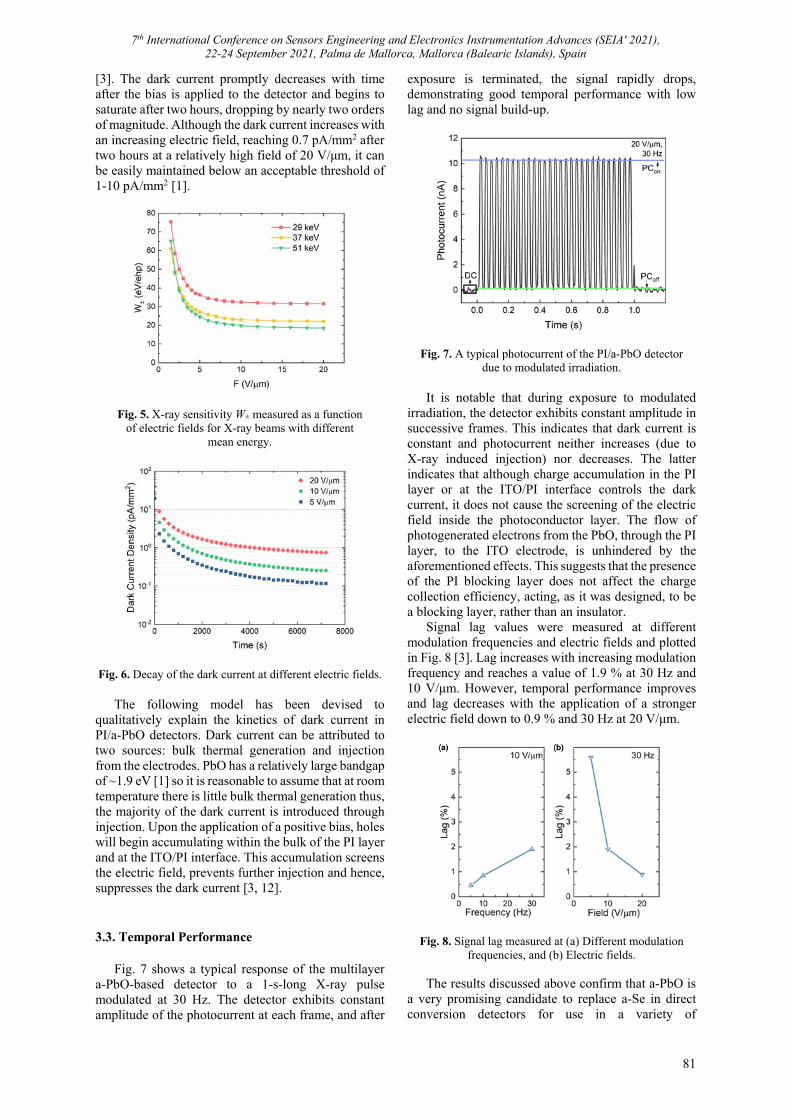
7th International Conference on Sensors Engineering and Electronics Instrumentation Advances (SEIA' 2021), 22-24 September 2021, Palma de Mallorca, Mallorca (Balearic Islands), Spain
81
[3]. The dark current promptly decreases with time after the bias is applied to the detector and begins to saturate after two hours, dropping by nearly two orders of magnitude. Although the dark current increases with an increasing electric field, reaching 0.7 pA/mm2 after two hours at a relatively high field of 20 V/μm, it can be easily maintained below an acceptable threshold of 1-10 pA/mm2 [1].
Fig. 5. X-ray sensitivity W± measured as a function of electric fields for X-ray beams with different
mean energy.
Fig. 6. Decay of the dark current at different electric fields.
The following model has been devised to qualitatively explain the kinetics of dark current in PI/a-PbO detectors. Dark current can be attributed to two sources: bulk thermal generation and injection from the electrodes. PbO has a relatively large bandgap of ~1.9 eV [1] so it is reasonable to assume that at room temperature there is little bulk thermal generation thus, the majority of the dark current is introduced through injection. Upon the application of a positive bias, holes will begin accumulating within the bulk of the PI layer and at the ITO/PI interface. This accumulation screens the electric field, prevents further injection and hence, suppresses the dark current [3, 12]. 3.3. Temporal Performance
Fig. 7 shows a typical response of the multilayer
a-PbO-based detector to a 1-s-long X-ray pulse modulated at 30 Hz. The detector exhibits constant amplitude of the photocurrent at each frame, and after
exposure is terminated, the signal rapidly drops, demonstrating good temporal performance with low lag and no signal build-up.
Fig. 7. A typical photocurrent of the PI/a-PbO detector due to modulated irradiation.
It is notable that during exposure to modulated
irradiation, the detector exhibits constant amplitude in successive frames. This indicates that dark current is constant and photocurrent neither increases (due to X-ray induced injection) nor decreases. The latter indicates that although charge accumulation in the PI layer or at the ITO/PI interface controls the dark current, it does not cause the screening of the electric field inside the photoconductor layer. The flow of photogenerated electrons from the PbO, through the PI layer, to the ITO electrode, is unhindered by the aforementioned effects. This suggests that the presence of the PI blocking layer does not affect the charge collection efficiency, acting, as it was designed, to be a blocking layer, rather than an insulator.
Signal lag values were measured at different modulation frequencies and electric fields and plotted in Fig. 8 [3]. Lag increases with increasing modulation frequency and reaches a value of 1.9 % at 30 Hz and 10 V/μm. However, temporal performance improves and lag decreases with the application of a stronger electric field down to 0.9 % and 30 Hz at 20 V/μm.
Fig. 8. Signal lag measured at (a) Different modulation frequencies, and (b) Electric fields.
The results discussed above confirm that a-PbO is
a very promising candidate to replace a-Se in direct conversion detectors for use in a variety of
7th International Conference on Sensors Engineering and Electronics Instrumentation Advances (SEIA' 2021), 22-24 September 2021, Palma de Mallorca, Mallorca (Balearic Islands), Spain
82
applications, from mammography tomosynthesis to fluoroscopy: it has higher stopping power, smaller W±
(i.e., better X-ray sensitivity) and adequate dark current at practical electric fields. Additionally, from a clinical perspective, the highly sensitive a-PbO detector would allow to maintain a high detectable photo-signal even at low radiation levels, adhering to the principle of ALARA (“As Low As Reasonably Achievable”) and reducing the radiation exposure to the patients and radiologists. The possibility to lower the X-ray flux is especially critical for image-guided interventions, where the continuous exposure is used for a prolonged time. The a-PbO photoconductor is also well-suited for real-time imaging due to its minimal signal lag. Indeed, it demonstrates the 0.9 % lag measured at 30 Hz and 20 V/µm, in contrary to a lag of ~1 % for a-Se detectors at similar experimental conditions [7]. As for other competitor materials, first frame lag values are reported to be 1.5–7 % for poly-PbO [5], 30–50 % for poly-PbI2 [13], 10–20 % for poly-HgI2 [13, 14], 30 % for poly-CdTe [15], which is too high to be utilized for real-time imaging in fluoroscopy where lag leads to deterioration of the image quality during subsequent frames. 4. Conclusions
The performance of a multilayer X-ray detector based on amorphous Lead Oxide photoconductor with a polyimide blocking layer was evaluated in terms of signal lag, dark current and X-ray sensitivity. The detector is capable of operation in real-time imaging mode with a high read-out rate of 30 frames per second with lag values as low as 0.9 %. The dark current can be maintained below 1 pA/mm2, which satisfies requirements for application in the direct conversion detectors. a-PbO multilayer detector demonstrates high X-ray sensitivity at practical electric fields, even at relatively high energy of incident X-rays. All these benefits make a-PbO-based multilayer detector a great candidate for various applications in medical and industrial X-ray imaging.
Acknowledgements
Financial support from Teledyne DALSA, the Natural Sciences and Engineering Research Council of Canada (NSERC) and Mitacs is gratefully acknowledged. References [1]. S. Kasap, J. Frey, G. Belev, O. Tousignant, H. Mani,
J. Greenspan, L. Laperriere, O. Bubon, A. Reznik, G. DeCrescenzo, K. Karim, J. Rowlands, Amorphous and polycrystalline photoconductors for direct conversion flat panel X-Ray image sensors, Sensors, Vol. 11, 2011, pp. 5112-5157.
[2]. O. Semeniuk, O. Grynko, G. Juska, A. Reznik, Amorphous lead oxide (a-PbO): Suppression of signal
lag via engineering of the layer structure, Scientific Reports, Vol. 7, 2017, 13272.
[3]. O. Grynko, T. Thibault, E. Pineau, A. Reznik, Engineering of a blocking layer structure for low-lag operation of the a-PbO-Based X-Ray detector, IEEE Transactions on Electron Devices, Vol. 68, 2021, pp. 2335-2341.
[4]. O. Semeniuk, A. Csik, S. Kökényesi, A. Reznik, Ion-assisted deposition of amorphous PbO layers, Jounral of Materials Science, Vol. 52, Issue 13, 2017, pp. 7937-7946.
[5]. O. Semeniuk, O. Grynko, G. Decrescenzo, G. Juska, K. Wang, A. Reznik, Characterization of polycrystalline lead oxide for application in direct conversion X-ray detectors, Scientific Reports, Vol. 7, 2017, 8659.
[6]. O. Grynko, T. Thibault, E. Pineau, G. Juska, A. Reznik, Bilayer lead oxide X‑ray photoconductor for lag‑free operation, Scientific Reports, Vol. 10, 2020, 20117.
[7]. S. Abbaszadeh, C. C. Scott, O. Bubon, A. Reznik, K. S. Karim, Enhanced detection efficiency of direct conversion X-ray detector using polyimide as hole-blocking layer, Scientific Reports, Vol. 3, 2013, 3360.
[8]. S. Kasap, J. B. Frey, G. Belev, O. Tousignant, H. Mani, L. Laperriere, A. Reznik, J. A. Rowlands, Amorphous selenium and its alloys from early xeroradiography to high resolution X-ray image detectors and ultrasensitive imaging tubes, Physica Status Solidi B, Vol. 246, Issue 8, 2009, pp. 1794-1805.
[9]. O. Bubon, K. Jandieri, S. D. Baranovskii, S. O. Kasap, A. Reznik, Columnar recombination for X-ray generated electron-holes in amorphous selenium and its significance in a-Se X-ray detectors, Journal of Applied Physics, Vol. 119, 2016, 124511.
[10]. C. A. Klein, Bandgap dependence and related features of radiation ionization energies in semiconductors, Journal of Applied Physics, Vol. 39, 1968, pp. 2029-2038.
[11]. N. Hijazi, D. Panneerselvam, M. Z. Kabir, Electron-hole pair creation energy in amorphous selenium for high energy photon excitation, Journal of Materials Science: Materials in Electronics, Vol. 29, 2018, pp. 486-490.
[12]. S. A. Mahmood, M. Z. Kabir, Dark current mechanisms in stabilized amorphous selenium based n-i detectors for X-ray imaging applications, Journal of Vacuum Science and Technology A: Vacuum, Surfaces and Films, Vol. 29, Issue 3, 2011, 031603.
[13]. R. A. Street, S. E. Ready, K. Van Schuylenbergh, J. Ho, J. B. Boyce, P. Nylen, K. Shah, L. Melekhov, H. Hermon, Comparison of PbI2 and HgI2 for direct detection active matrix x-ray image sensors, Journal of Applied Physics, Vol. 91, Issue 5, 2002, pp. 3345-3355.
[14]. H. Jiang, Q. Zhao, L. E. Antonuk, Y. El-Mohri, T. Gupta, Development of active matrix flat panel imagers incorporating thin layers of polycrystalline HgI2 for mammographic X-ray imaging, Physics in Medicine and Biology, Vol. 58, Issue 3, 2013, pp. 703-714.
[15]. S. Lee, J. S. Kim, K. R. Ko, G. H. Lee, D. J. Lee, D. W. Kim, J. E. Kim, H. K. Kim, D. W. Kim, S. Im, Direct thermal growth of large scale Cl-doped CdTe film for low voltage high resolution X-ray image sensor, Scientific Reports, Vol. 8, 2018, 14810.
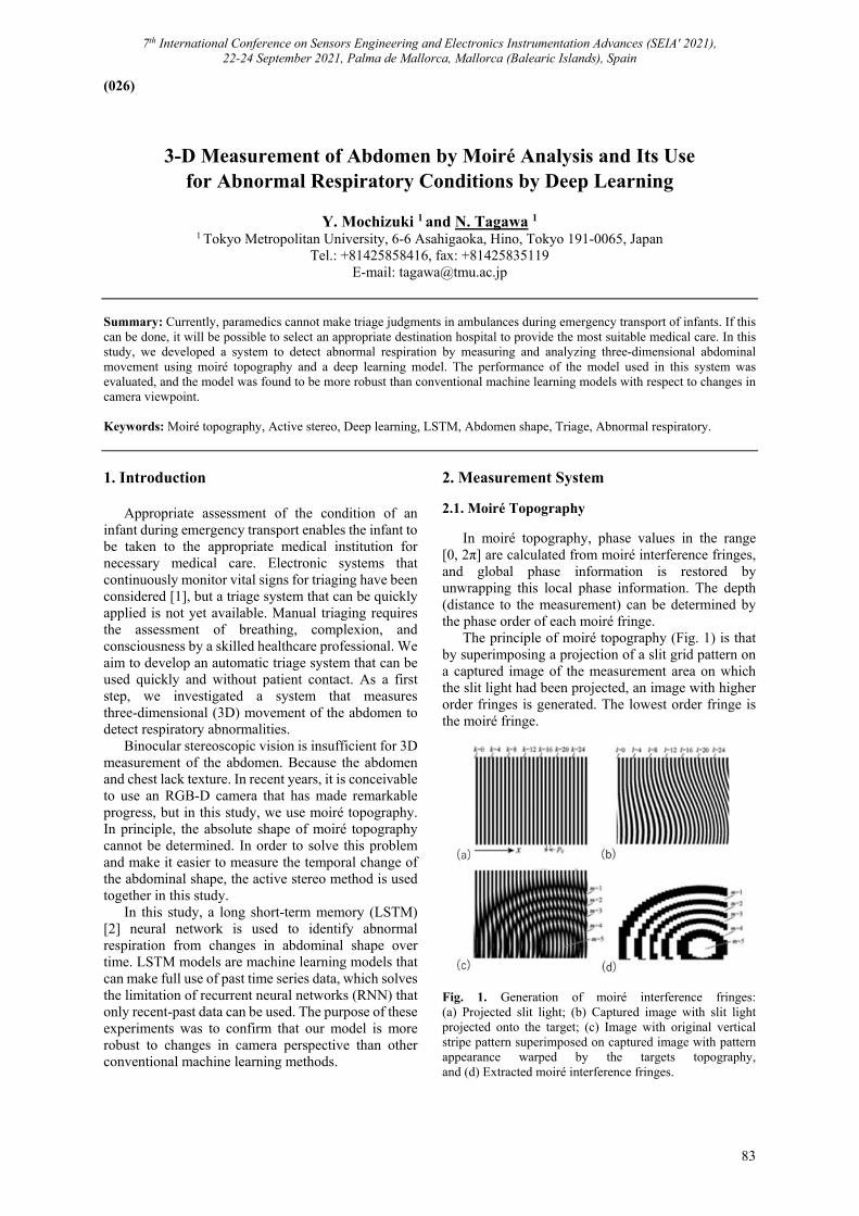
7th International Conference on Sensors Engineering and Electronics Instrumentation Advances (SEIA' 2021), 22-24 September 2021, Palma de Mallorca, Mallorca (Balearic Islands), Spain
83
(026)
3-D Measurement of Abdomen by Moiré Analysis and Its Use for Abnormal Respiratory Conditions by Deep Learning
Y. Mochizuki 1 and N. Tagawa 1
1 Tokyo Metropolitan University, 6-6 Asahigaoka, Hino, Tokyo 191-0065, Japan Tel.: +81425858416, fax: +81425835119
E-mail: [email protected] Summary: Currently, paramedics cannot make triage judgments in ambulances during emergency transport of infants. If this can be done, it will be possible to select an appropriate destination hospital to provide the most suitable medical care. In this study, we developed a system to detect abnormal respiration by measuring and analyzing three-dimensional abdominal movement using moiré topography and a deep learning model. The performance of the model used in this system was evaluated, and the model was found to be more robust than conventional machine learning models with respect to changes in camera viewpoint. Keywords: Moiré topography, Active stereo, Deep learning, LSTM, Abdomen shape, Triage, Abnormal respiratory.
1. Introduction
Appropriate assessment of the condition of an infant during emergency transport enables the infant to be taken to the appropriate medical institution for necessary medical care. Electronic systems that continuously monitor vital signs for triaging have been considered [1], but a triage system that can be quickly applied is not yet available. Manual triaging requires the assessment of breathing, complexion, and consciousness by a skilled healthcare professional. We aim to develop an automatic triage system that can be used quickly and without patient contact. As a first step, we investigated a system that measures three-dimensional (3D) movement of the abdomen to detect respiratory abnormalities.
Binocular stereoscopic vision is insufficient for 3D measurement of the abdomen. Because the abdomen and chest lack texture. In recent years, it is conceivable to use an RGB-D camera that has made remarkable progress, but in this study, we use moiré topography. In principle, the absolute shape of moiré topography cannot be determined. In order to solve this problem and make it easier to measure the temporal change of the abdominal shape, the active stereo method is used together in this study.
In this study, a long short-term memory (LSTM) [2] neural network is used to identify abnormal respiration from changes in abdominal shape over time. LSTM models are machine learning models that can make full use of past time series data, which solves the limitation of recurrent neural networks (RNN) that only recent-past data can be used. The purpose of these experiments was to confirm that our model is more robust to changes in camera perspective than other conventional machine learning methods.
2. Measurement System
2.1. Moiré Topography
In moiré topography, phase values in the range [0, 2π] are calculated from moiré interference fringes, and global phase information is restored by unwrapping this local phase information. The depth (distance to the measurement) can be determined by the phase order of each moiré fringe.
The principle of moiré topography (Fig. 1) is that by superimposing a projection of a slit grid pattern on a captured image of the measurement area on which the slit light had been projected, an image with higher order fringes is generated. The lowest order fringe is the moiré fringe.
Fig. 1. Generation of moiré interference fringes: (a) Projected slit light; (b) Captured image with slit light projected onto the target; (c) Image with original vertical stripe pattern superimposed on captured image with pattern appearance warped by the targets topography, and (d) Extracted moiré interference fringes.
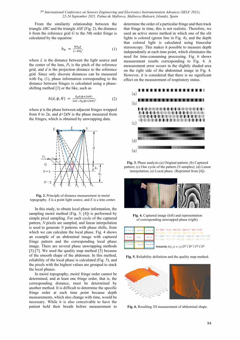
7th International Conference on Sensors Engineering and Electronics Instrumentation Advances (SEIA' 2021), 22-24 September 2021, Palma de Mallorca, Mallorca (Balearic Islands), Spain
84
From the similarity relationship between the triangle ABC and the triangle ASE (Fig. 2), the distance h from the reference grid G to the Nth order fringe is calculated by the equation:
ℎ , (1)
where L is the distance between the light source and the center of the lens, P0 is the pitch of the reference grid, and d is the projection distance to the reference grid. Since only discrete distances can be measured with Eq. (1), phase information corresponding to the distance between fringes is calculated using a phase-shifting method [3] or the like, such as
ℎ 𝑑, 𝜙, 𝑁 , (2)
where ϕ is the phase between adjacent fringes wrapped from 0 to 2π, and ϕ+2πN is the phase measured from the fringes, which is obtained by unwrapping data.
Fig. 2. Principle of distance measurement in moiré
topography. S is a point light source, and E is a lens center. In this study, to obtain local phase information, the
sampling moiré method (Fig. 3; [4]) is performed by simple pixel sampling. For each cycle of the captured pattern, N pixels are sampled, and linear interpolation is used to generate N patterns with phase shifts, from which we can calculate the local phase. Fig. 4 shows an example of an abdominal image with captured fringe pattern and the corresponding local phase image. There are several phase unwrapping methods [5]-[7]. We used the quality map method [5] because of the smooth shape of the abdomen. In this method, reliability of the local phase is calculated (Fig. 5), and the pixels with the highest values are grouped to stack the local phases.
In moiré topography, moiré fringe order cannot be determined, and at least one fringe order, that is, the corresponding distance, must be determined by another method. It is difficult to determine the specific fringe order at each time point because depth measurements, which also change with time, would be necessary. While it is also conceivable to have the patient hold their breath before measurement to
determine the order of a particular fringe and then track that fringe in time, this is not realistic. Therefore, we used an active stereo method in which one of the slit lights is colored (green line in Fig. 4), and the depth that colored light is calculated using binocular stereoscopy. This makes it possible to measure depth independently at each time point, which eliminates the need for time-consuming processing. Fig. 6 shows measurement results corresponding to Fig. 4. A measurement error occurs in the slightly shaded area on the right side of the abdominal image in Fig. 4. However, it is considered that there is no significant effect on the measurement of respiratory status.
Fig. 3. Phase analysis.(a) Original pattern; (b) Captured pattern; (c) One cycle of the pattern (N samples); (d) Linear
interpolation; (e) Local phase. (Reprinted from [4]).
Fig. 4. Captured image (left) and representation of corresponding unwrapped phase (right).
Fig. 5. Reliability definition and the quality map method.
Fig. 6. Resulting 3D measurement of abdominal shape.
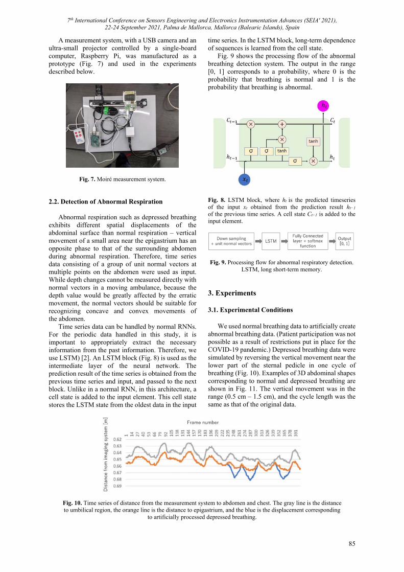
7th International Conference on Sensors Engineering and Electronics Instrumentation Advances (SEIA' 2021), 22-24 September 2021, Palma de Mallorca, Mallorca (Balearic Islands), Spain
85
A measurement system, with a USB camera and an ultra-small projector controlled by a single-board computer, Raspberry Pi, was manufactured as a prototype (Fig. 7) and used in the experiments described below.
Fig. 7. Moiré measurement system.
2.2. Detection of Abnormal Respiration
Abnormal respiration such as depressed breathing exhibits different spatial displacements of the abdominal surface than normal respiration – vertical movement of a small area near the epigastrium has an opposite phase to that of the surrounding abdomen during abnormal respiration. Therefore, time series data consisting of a group of unit normal vectors at multiple points on the abdomen were used as input. While depth changes cannot be measured directly with normal vectors in a moving ambulance, because the depth value would be greatly affected by the erratic movement, the normal vectors should be suitable for recognizing concave and convex movements of the abdomen.
Time series data can be handled by normal RNNs. For the periodic data handled in this study, it is important to appropriately extract the necessary information from the past information. Therefore, we use LSTM) [2]. An LSTM block (Fig. 8) is used as the intermediate layer of the neural network. The prediction result of the time series is obtained from the previous time series and input, and passed to the next block. Unlike in a normal RNN, in this architecture, a cell state is added to the input element. This cell state stores the LSTM state from the oldest data in the input
time series. In the LSTM block, long-term dependence of sequences is learned from the cell state.
Fig. 9 shows the processing flow of the abnormal breathing detection system. The output in the range [0, 1] corresponds to a probability, where 0 is the probability that breathing is normal and 1 is the probability that breathing is abnormal.
Fig. 8. LSTM block, where ht is the predicted timeseries of the input xt obtained from the prediction result ht−1 of the previous time series. A cell state Ct−1 is added to the input element.
Fig. 9. Processing flow for abnormal respiratory detection.
LSTM, long short-term memory.
3. Experiments 3.1. Experimental Conditions
We used normal breathing data to artificially create abnormal breathing data. (Patient participation was not possible as a result of restrictions put in place for the COVID-19 pandemic.) Depressed breathing data were simulated by reversing the vertical movement near the lower part of the sternal pedicle in one cycle of breathing (Fig. 10). Examples of 3D abdominal shapes corresponding to normal and depressed breathing are shown in Fig. 11. The vertical movement was in the range (0.5 cm – 1.5 cm), and the cycle length was the same as that of the original data.
Fig. 10. Time series of distance from the measurement system to abdomen and chest. The gray line is the distance to umbilical region, the orange line is the distance to epigastrium, and the blue is the displacement corresponding
to artificially processed depressed breathing.
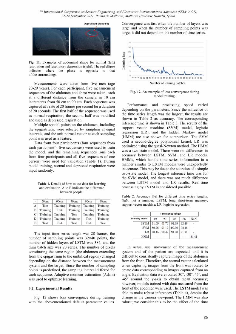
7th International Conference on Sensors Engineering and Electronics Instrumentation Advances (SEIA' 2021), 22-24 September 2021, Palma de Mallorca, Mallorca (Balearic Islands), Spain
86
Fig. 11. Examples of abdominal shape for normal (left) respiration and respiratory depression (right). The red ellipse indicates where the phase is opposite to that of the surroundings.
Measurements were taken from five men (age 20-29 years). For each participant, five measurement sequences of the abdomen and chest were taken, each at a different distance from the camera in 10 cm increments from 50 cm to 90 cm. Each sequence was captured at a rate of 20 frames per second for a duration of 20 seconds. The first half of the sequence was used as normal respiration; the second half was modified and used as depressed respiration.
Multiple spatial points on the abdomen, including the epigastrium, were selected by sampling at equal intervals, and the unit normal vector at each sampling point was used as a feature.
Data from four participants (four sequences from each participant’s five sequences) were used to train the model, and the remaining sequences (one each from four participants and all five sequences of one person) were used for validation (Table 1). During model training, normal and depressed respiration were input randomly.
Table 1. Details of how to use data for learning and evaluation. A to E indicate the difference
between people.
The input time series length was 28 frames, the
number of sampling points was 32×40 points, the number of hidden layers of LSTM was 384, and the mini batch size was 20 series. The number of pixels constituting the same region (the abdomen extending from the epigastrium to the umbilical region) changed depending on the distance between the measurement system and the target. Since the number of sampling points is predefined, the sampling interval differed for each sequence. Adaptive moment estimation (Adam) was used to optimize learning.
3.2. Experimental Results
Fig. 12 shows loss convergence during training with the abovementioned default parameter values.
Convergence was fast when the number of layers was large and when the number of sampling points was large; it did not depend on the number of time series.
Fig. 12. An example of loss convergence during model training.
Performance and processing speed varied
depending on the parameters. Since the influence of the time series length was the largest, the results are shown in Table 2 as accuracy. The corresponding inference time is shown in Table 3. The results of the support vector machine (SVM) model, logistic regression (LR), and the hidden Markov model (HMM) are also shown for comparison. The SVM used a second-degree polynomial kernel. LR was optimized using the quasi-Newton method. The HMM was a two-state model. There were no differences in accuracy between LSTM, SVM, and LR models. HMMs, which handle time series information in a manner similar to LSTM models were unexpectedly inaccurate. This may be due to the adoption of a simple two-state model. The longest inference time was for the SVM model, and there was not much difference between LSTM model and LR results. Real-time processing by LSTM is considered possible.
Table 2. Accuracy [%] for different time series lengths. NaN, not a number; LSTM, long short-term memory, support vector machine; LR, logistic regression.
In actual use, movement of the measurement
system and of the patient are expected, and it is difficult to consistently capture images of the abdomen from the front. Therefore, the normal vector calculated when capturing images from the front was rotated to create data corresponding to images captured from an angle. Evaluation data were rotated 30°, -30°, 45°, and -45° around the y-axis to obtain mean accuracy; however, models trained with data measured from the front of the abdomen were used. The LSTM model was able to make robust inferences (Table 4), despite the change in the camera viewpoint. The HMM was also robust; we consider this to be the effect of the time
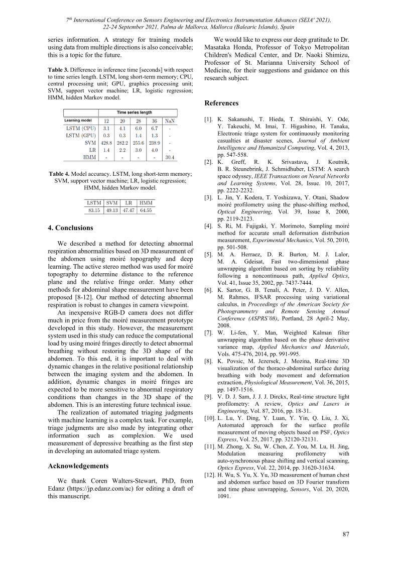
7th International Conference on Sensors Engineering and Electronics Instrumentation Advances (SEIA' 2021), 22-24 September 2021, Palma de Mallorca, Mallorca (Balearic Islands), Spain
87
series information. A strategy for training models using data from multiple directions is also conceivable; this is a topic for the future.
Table 3. Difference in inference time [seconds] with respect to time series length. LSTM, long short-term memory; CPU, central processing unit; GPU, graphics processing unit; SVM, support vector machine; LR, logistic regression; HMM, hidden Markov model.
Table 4. Model accuracy. LSTM, long short-term memory; SVM, support vector machine; LR, logistic regression;
HMM, hidden Markov model.
4. Conclusions
We described a method for detecting abnormal respiration abnormalities based on 3D measurement of the abdomen using moiré topography and deep learning. The active stereo method was used for moiré topography to determine distance to the reference plane and the relative fringe order. Many other methods for abdominal shape measurement have been proposed [8-12]. Our method of detecting abnormal respiration is robust to changes in camera viewpoint.
An inexpensive RGB-D camera does not differ much in price from the moiré measurement prototype developed in this study. However, the measurement system used in this study can reduce the computational load by using moiré fringes directly to detect abnormal breathing without restoring the 3D shape of the abdomen. To this end, it is important to deal with dynamic changes in the relative positional relationship between the imaging system and the abdomen. In addition, dynamic changes in moiré fringes are expected to be more sensitive to abnormal respiratory conditions than changes in the 3D shape of the abdomen. This is an interesting future technical issue.
The realization of automated triaging judgments with machine learning is a complex task. For example, triage judgments are also made by integrating other information such as complexion. We used measurement of depressive breathing as the first step in developing an automated triage system. Acknowledgements
We thank Coren Walters-Stewart, PhD, from Edanz (https://jp.edanz.com/ac) for editing a draft of this manuscript.
We would like to express our deep gratitude to Dr. Masataka Honda, Professor of Tokyo Metropolitan Children's Medical Center, and Dr. Naoki Shimizu, Professor of St. Marianna University School of Medicine, for their suggestions and guidance on this research subject. References [1]. K. Sakanushi, T. Hieda, T. Shiraishi, Y. Ode,
Y. Takeuchi, M. Imai, T. Higashino, H. Tanaka, Electronic triage system for continuously monitoring casualties at disaster scenes, Journal of Ambient Intelligence and Humanized Computing, Vol. 4, 2013, pp. 547-558.
[2]. K. Greff, R. K. Srivastava, J. Koutnik, B. R. Steunebrink, J. Schmidhuber, LSTM: A search space odyssey, IEEE Transactions on Neural Networks and Learning Systems, Vol. 28, Issue. 10, 2017, pp. 2222-2232.
[3]. L. Jin, Y. Kodera, T. Yoshizawa, Y. Otani, Shadow moiré profilometry using the phase-shifting method, Optical Engineering, Vol. 39, Issue 8, 2000, pp. 2119-2123.
[4]. S. Ri, M. Fujigaki, Y. Morimoto, Sampling moiré method for accurate small deformation distribution measurement, Experimental Mechanics, Vol. 50, 2010, pp. 501-508.
[5]. M. A. Herraez, D. R. Burton, M. J. Lalor, M. A. Gdeisat, Fast two-dimensional phase unwrapping algorithm based on sorting by reliability following a noncontinuous path, Applied Optics, Vol. 41, Issue 35, 2002, pp. 7437-7444.
[6]. K. Sartor, G. B. Tenali, A. Peter, J. D. V. Allen, M. Rahmes, IFSAR processing using variational calculus, in Proceedings of the American Society for Photogrammetry and Remote Sensing Annual Conference (ASPRS’08), Portland, 28 April-2 May, 2008.
[7]. W. Li-fen, Y. Man, Weighted Kalman filter unwrapping algorithm based on the phase derivative variance map, Applied Mechanics and Materials, Vols. 475-476, 2014, pp. 991-995.
[8]. K. Povsic, M. Jezersek, J. Mozina, Real-time 3D visualization of the thoraco-abdominal surface during breathing with body movement and deformation extraction, Physiological Measurement, Vol. 36, 2015, pp. 1497-1516.
[9]. V. D. J. Sam, J. J. J. Dirckx, Real-time structure light profilometry: A review, Optics and Lasers in Engineering, Vol. 87, 2016, pp. 18-31.
[10]. L. Lu, Y. Ding, Y. Luan, Y. Yin, Q. Liu, J. Xi, Automated approach for the surface profile measurement of moving objects based on PSF, Optics Express, Vol. 25, 2017, pp. 32120-32131.
[11]. M. Zhong, X. Su, W. Chen, Z. You, M. Lu, H. Jing, Modulation measuring profilometry with auto-synchronous phase shifting and vertical scanning, Optics Express, Vol. 22, 2014, pp. 31620-31634.
[12]. H. Wu, S. Yu, X. Yu, 3D measurement of human chest and abdomen surface based on 3D Fourier transform and time phase unwrapping, Sensors, Vol. 20, 2020, 1091.
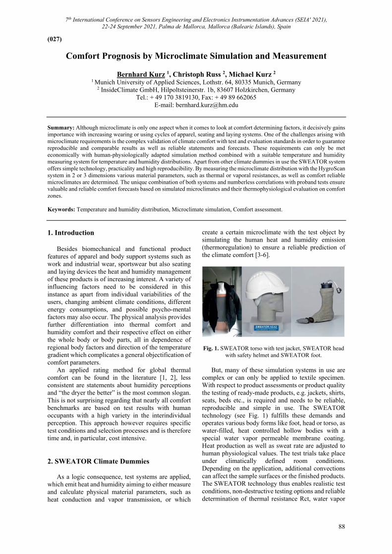
7th International Conference on Sensors Engineering and Electronics Instrumentation Advances (SEIA' 2021), 22-24 September 2021, Palma de Mallorca, Mallorca (Balearic Islands), Spain
88
(027)
Comfort Prognosis by Microclimate Simulation and Measurement
Bernhard Kurz 1, Christoph Russ 2, Michael Kurz 2
1 Munich University of Applied Sciences, Lothstr. 64, 80335 Munich, Germany 2 InsideClimate GmbH, Hilpoltsteinerstr. 1b, 83607 Holzkirchen, Germany
Tel.: + 49 170 3819130, Fax: + 49 89 662065 E-mail: [email protected]
Summary: Although microclimate is only one aspect when it comes to look at comfort determining factors, it decisively gains importance with increasing wearing or using cycles of apparel, seating and laying systems. One of the challenges arising with microclimate requirements is the complex validation of climate comfort with test and evaluation standards in order to guarantee reproducible and comparable results as well as reliable statements and forecasts. These requirements can only be met economically with human-physiologically adapted simulation method combined with a suitable temperature and humidity measuring system for temperature and humidity distributions. Apart from other climate dummies in use the SWEATOR system offers simple technology, practicality and high reproducibility. By measuring the microclimate distribution with the HygroScan system in 2 or 3 dimensions various material parameters, such as thermal or vaporal resistances, as well as comfort reliable microclimates are determined. The unique combination of both systems and numberless correlations with proband tests ensure valuable and reliable comfort forecasts based on simulated microclimates and their thermophysiological evaluation on comfort zones. Keywords: Temperature and humidity distribution, Microclimate simulation, Comfort assessment.
1. Introduction
Besides biomechanical and functional product features of apparel and body support systems such as work and industrial wear, sportswear but also seating and laying devices the heat and humidity management of these products is of increasing interest. A variety of influencing factors need to be considered in this instance as apart from individual variabilities of the users, changing ambient climate conditions, different energy consumptions, and possible psycho-mental factors may also occur. The physical analysis provides further differentiation into thermal comfort and humidity comfort and their respective effect on either the whole body or body parts, all in dependence of regional body factors and direction of the temperature gradient which complicates a general objectification of comfort parameters.
An applied rating method for global thermal comfort can be found in the literature [1, 2], less consistent are statements about humidity perceptions and “the dryer the better” is the most common slogan. This is not surprising regarding that nearly all comfort benchmarks are based on test results with human occupants with a high variety in the interindividual perception. This approach however requires specific test conditions and selection processes and is therefore time and, in particular, cost intensive.
2. SWEATOR Climate Dummies As a logic consequence, test systems are applied,
which emit heat and humidity aiming to either measure and calculate physical material parameters, such as heat conduction and vapor transmission, or which
create a certain microclimate with the test object by simulating the human heat and humidity emission (thermoregulation) to ensure a reliable prediction of the climate comfort [3-6].
Fig. 1. SWEATOR torso with test jacket, SWEATOR head with safety helmet and SWEATOR foot.
But, many of these simulation systems in use are
complex or can only be applied to textile specimen. With respect to product assessments or product quality the testing of ready-made products, e.g. jackets, shirts, seats, beds etc., is required and needs to be reliable, reproducible and simple in use. The SWEATOR technology (see Fig. 1) fulfills these demands and operates various body forms like foot, head or torso, as water-filled, heat controlled hollow bodies with a special water vapor permeable membrane coating. Heat production as well as sweat rate are adjusted to human physiological values. The test trials take place under climatically defined room conditions. Depending on the application, additional convections can affect the sample surfaces or the finished products. The SWEATOR technology thus enables realistic test conditions, non-destructive testing options and reliable determination of thermal resistance Rct, water vapor
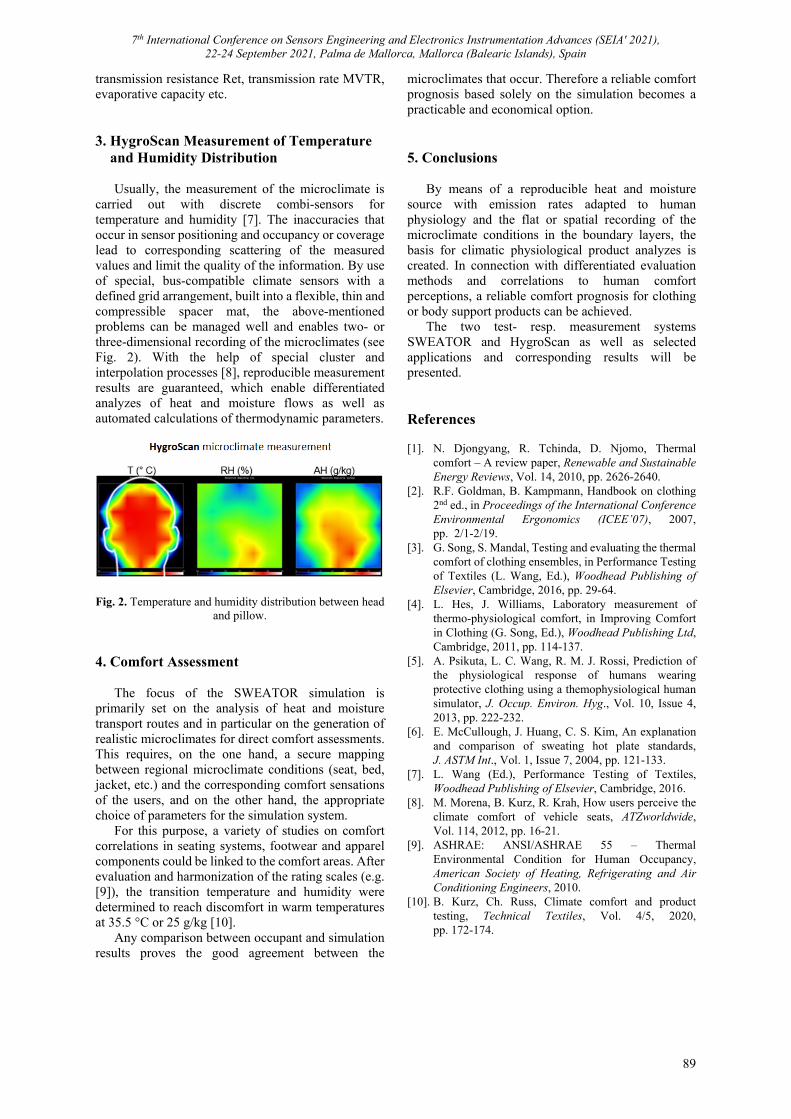
7th International Conference on Sensors Engineering and Electronics Instrumentation Advances (SEIA' 2021), 22-24 September 2021, Palma de Mallorca, Mallorca (Balearic Islands), Spain
89
transmission resistance Ret, transmission rate MVTR, evaporative capacity etc. 3. HygroScan Measurement of Temperature and Humidity Distribution
Usually, the measurement of the microclimate is carried out with discrete combi-sensors for temperature and humidity [7]. The inaccuracies that occur in sensor positioning and occupancy or coverage lead to corresponding scattering of the measured values and limit the quality of the information. By use of special, bus-compatible climate sensors with a defined grid arrangement, built into a flexible, thin and compressible spacer mat, the above-mentioned problems can be managed well and enables two- or three-dimensional recording of the microclimates (see Fig. 2). With the help of special cluster and interpolation processes [8], reproducible measurement results are guaranteed, which enable differentiated analyzes of heat and moisture flows as well as automated calculations of thermodynamic parameters.
Fig. 2. Temperature and humidity distribution between head and pillow.
4. Comfort Assessment
The focus of the SWEATOR simulation is primarily set on the analysis of heat and moisture transport routes and in particular on the generation of realistic microclimates for direct comfort assessments. This requires, on the one hand, a secure mapping between regional microclimate conditions (seat, bed, jacket, etc.) and the corresponding comfort sensations of the users, and on the other hand, the appropriate choice of parameters for the simulation system.
For this purpose, a variety of studies on comfort correlations in seating systems, footwear and apparel components could be linked to the comfort areas. After evaluation and harmonization of the rating scales (e.g. [9]), the transition temperature and humidity were determined to reach discomfort in warm temperatures at 35.5 °C or 25 g/kg [10].
Any comparison between occupant and simulation results proves the good agreement between the
microclimates that occur. Therefore a reliable comfort prognosis based solely on the simulation becomes a practicable and economical option.
5. Conclusions
By means of a reproducible heat and moisture source with emission rates adapted to human physiology and the flat or spatial recording of the microclimate conditions in the boundary layers, the basis for climatic physiological product analyzes is created. In connection with differentiated evaluation methods and correlations to human comfort perceptions, a reliable comfort prognosis for clothing or body support products can be achieved.
The two test- resp. measurement systems SWEATOR and HygroScan as well as selected applications and corresponding results will be presented. References [1]. N. Djongyang, R. Tchinda, D. Njomo, Thermal
comfort – A review paper, Renewable and Sustainable Energy Reviews, Vol. 14, 2010, pp. 2626-2640.
[2]. R.F. Goldman, B. Kampmann, Handbook on clothing 2nd ed., in Proceedings of the International Conference Environmental Ergonomics (ICEE’07), 2007, pp. 2/1-2/19.
[3]. G. Song, S. Mandal, Testing and evaluating the thermal comfort of clothing ensembles, in Performance Testing of Textiles (L. Wang, Ed.), Woodhead Publishing of Elsevier, Cambridge, 2016, pp. 29-64.
[4]. L. Hes, J. Williams, Laboratory measurement of thermo-physiological comfort, in Improving Comfort in Clothing (G. Song, Ed.), Woodhead Publishing Ltd, Cambridge, 2011, pp. 114-137.
[5]. A. Psikuta, L. C. Wang, R. M. J. Rossi, Prediction of the physiological response of humans wearing protective clothing using a themophysiological human simulator, J. Occup. Environ. Hyg., Vol. 10, Issue 4, 2013, pp. 222-232.
[6]. E. McCullough, J. Huang, C. S. Kim, An explanation and comparison of sweating hot plate standards, J. ASTM Int., Vol. 1, Issue 7, 2004, pp. 121-133.
[7]. L. Wang (Ed.), Performance Testing of Textiles, Woodhead Publishing of Elsevier, Cambridge, 2016.
[8]. M. Morena, B. Kurz, R. Krah, How users perceive the climate comfort of vehicle seats, ATZworldwide, Vol. 114, 2012, pp. 16-21.
[9]. ASHRAE: ANSI/ASHRAE 55 – Thermal Environmental Condition for Human Occupancy, American Society of Heating, Refrigerating and Air Conditioning Engineers, 2010.
[10]. B. Kurz, Ch. Russ, Climate comfort and product testing, Technical Textiles, Vol. 4/5, 2020, pp. 172-174.
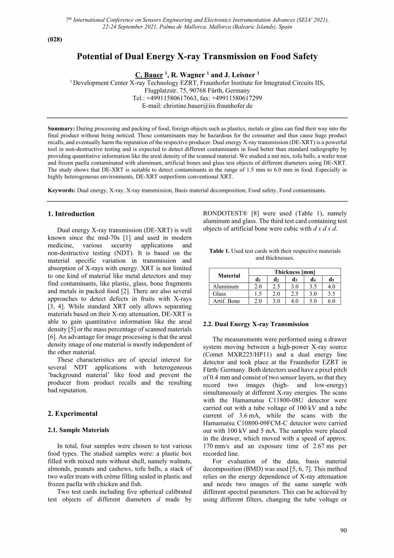
7th International Conference on Sensors Engineering and Electronics Instrumentation Advances (SEIA' 2021), 22-24 September 2021, Palma de Mallorca, Mallorca (Balearic Islands), Spain
90
(028)
Potential of Dual Energy X-ray Transmission on Food Safety
C. Bauer 1, R. Wagner 1 and J. Leisner 1
1 Development Center X-ray Technology EZRT, Fraunhofer Institute for Integrated Circuits IIS, Flugplatzstr. 75, 90768 Fürth, Germany
Tel.: +49911580617663, fax: +49911580617299 E-mail: [email protected]
Summary: During processing and packing of food, foreign objects such as plastics, metals or glass can find their way into the final product without being noticed. Those contaminants may be hazardous for the consumer and thus cause huge product recalls, and eventually harm the reputation of the respective producer. Dual energy X-ray transmission (DE-XRT) is a powerful tool in non-destructive testing and is expected to detect different contaminants in food better than standard radiography by providing quantitative information like the areal density of the scanned material. We studied a nut mix, tofu balls, a wafer treat and frozen paella contaminated with aluminum, artificial bones and glass test objects of different diameters using DE-XRT. The study shows that DE-XRT is suitable to detect contaminants in the range of 1.5 mm to 6.0 mm in food. Especially in highly heterogeneous environments, DE-XRT outperform conventional XRT. Keywords: Dual energy, X-ray, X-ray transmission, Basis material decomposition, Food safety, Food contaminants.
1. Introduction
Dual energy X-ray transmission (DE-XRT) is well known since the mid-70s [1] and used in modern medicine, various security applications and non-destructive testing (NDT). It is based on the material specific variation in transmission and absorption of X-rays with energy. XRT is not limited to one kind of material like metal detectors and may find contaminants, like plastic, glass, bone fragments and metals in packed food [2]. There are also several approaches to detect defects in fruits with X-rays [3, 4]. While standard XRT only allows separating materials based on their X-ray attenuation, DE-XRT is able to gain quantitative information like the areal density [5] or the mass percentage of scanned materials [6]. An advantage for image processing is that the areal density image of one material is mostly independent of the other material.
These characteristics are of special interest for several NDT applications with heterogeneous ’background material’ like food and prevent the producer from product recalls and the resulting bad reputation.
2. Experimental 2.1. Sample Materials
In total, four samples were chosen to test various food types. The studied samples were: a plastic box filled with mixed nuts without shell, namely walnuts, almonds, peanuts and cashews, tofu balls, a stack of two wafer treats with crème filling sealed in plastic and frozen paella with chicken and fish.
Two test cards including five spherical calibrated test objects of different diameters d made by
RONDOTEST® [8] were used (Table 1), namely aluminum and glass. The third test card containing test objects of artificial bone were cubic with d x d x d.
Table 1. Used test cards with their respective materials and thicknesses.
Material Thickness [mm]
d1 d2 d3 d4 d5 Aluminum 2.0 2.5 3.0 3.5 4.0 Glass 1.5 2.0 2.5 3.0 3.5 Artif. Bone 2.0 3.0 4.0 5.0 6.0
2.2. Dual Energy X-ray Transmission
The measurements were performed using a drawer system moving between a high-power X-ray source (Comet MXR225/HP11) and a dual energy line detector and took place at the Fraunhofer EZRT in Fürth/ Germany. Both detectors used have a pixel pitch of 0.4 mm and consist of two sensor layers, so that they record two images (high- and low-energy) simultaneously at different X-ray energies. The scans with the Hamamatsu C11800-08U detector were carried out with a tube voltage of 100 kV and a tube current of 3.6 mA, while the scans with the Hamamatsu C10800-09FCM-C detector were carried out with 100 kV and 5 mA. The samples were placed in the drawer, which moved with a speed of approx. 170 mm/s and an exposure time of 2.67 ms per recorded line.
For evaluation of the data, basis material decomposition (BMD) was used [5, 6, 7]. This method relies on the energy dependence of X-ray attenuation and needs two images of the same sample with different spectral parameters. This can be achieved by using different filters, changing the tube voltage or
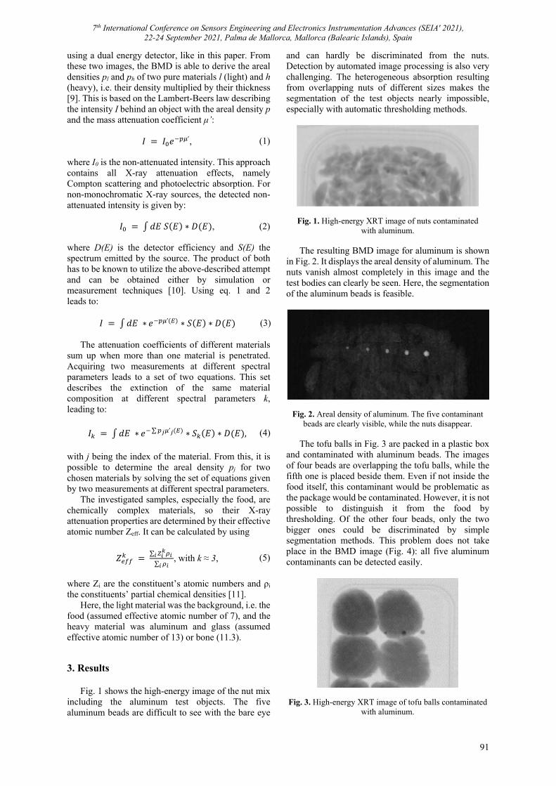
7th International Conference on Sensors Engineering and Electronics Instrumentation Advances (SEIA' 2021), 22-24 September 2021, Palma de Mallorca, Mallorca (Balearic Islands), Spain
91
using a dual energy detector, like in this paper. From these two images, the BMD is able to derive the areal densities pl and ph of two pure materials l (light) and h (heavy), i.e. their density multiplied by their thickness [9]. This is based on the Lambert-Beers law describing the intensity I behind an object with the areal density p and the mass attenuation coefficient μ’:
𝐼 𝐼 𝑒 ’, (1) where I0 is the non-attenuated intensity. This approach contains all X-ray attenuation effects, namely Compton scattering and photoelectric absorption. For non-monochromatic X-ray sources, the detected non-attenuated intensity is given by:
𝐼 𝑑𝐸 𝑆 𝐸 ∗ 𝐷 𝐸 , (2) where D(E) is the detector efficiency and S(E) the spectrum emitted by the source. The product of both has to be known to utilize the above-described attempt and can be obtained either by simulation or measurement techniques [10]. Using eq. 1 and 2 leads to:
𝐼 𝑑𝐸 ∗ 𝑒 ’ ∗ 𝑆 𝐸 ∗ 𝐷 𝐸 (3)
The attenuation coefficients of different materials sum up when more than one material is penetrated. Acquiring two measurements at different spectral parameters leads to a set of two equations. This set describes the extinction of the same material composition at different spectral parameters k, leading to:
𝐼 𝑑𝐸 ∗ 𝑒 ∑ ’ ∗ 𝑆 𝐸 ∗ 𝐷 𝐸 , (4)
with j being the index of the material. From this, it is possible to determine the areal density pj for two chosen materials by solving the set of equations given by two measurements at different spectral parameters.
The investigated samples, especially the food, are chemically complex materials, so their X-ray attenuation properties are determined by their effective atomic number Zeff. It can be calculated by using
𝑍 ∑
∑, with k ≈ 3, (5)
where Zi are the constituent’s atomic numbers and ρi the constituents’ partial chemical densities [11].
Here, the light material was the background, i.e. the food (assumed effective atomic number of 7), and the heavy material was aluminum and glass (assumed effective atomic number of 13) or bone (11.3). 3. Results
Fig. 1 shows the high-energy image of the nut mix including the aluminum test objects. The five aluminum beads are difficult to see with the bare eye
and can hardly be discriminated from the nuts. Detection by automated image processing is also very challenging. The heterogeneous absorption resulting from overlapping nuts of different sizes makes the segmentation of the test objects nearly impossible, especially with automatic thresholding methods.
Fig. 1. High-energy XRT image of nuts contaminated with aluminum.
The resulting BMD image for aluminum is shown
in Fig. 2. It displays the areal density of aluminum. The nuts vanish almost completely in this image and the test bodies can clearly be seen. Here, the segmentation of the aluminum beads is feasible.
Fig. 2. Areal density of aluminum. The five contaminant beads are clearly visible, while the nuts disappear.
The tofu balls in Fig. 3 are packed in a plastic box
and contaminated with aluminum beads. The images of four beads are overlapping the tofu balls, while the fifth one is placed beside them. Even if not inside the food itself, this contaminant would be problematic as the package would be contaminated. However, it is not possible to distinguish it from the food by thresholding. Of the other four beads, only the two bigger ones could be discriminated by simple segmentation methods. This problem does not take place in the BMD image (Fig. 4): all five aluminum contaminants can be detected easily.
Fig. 3. High-energy XRT image of tofu balls contaminated with aluminum.
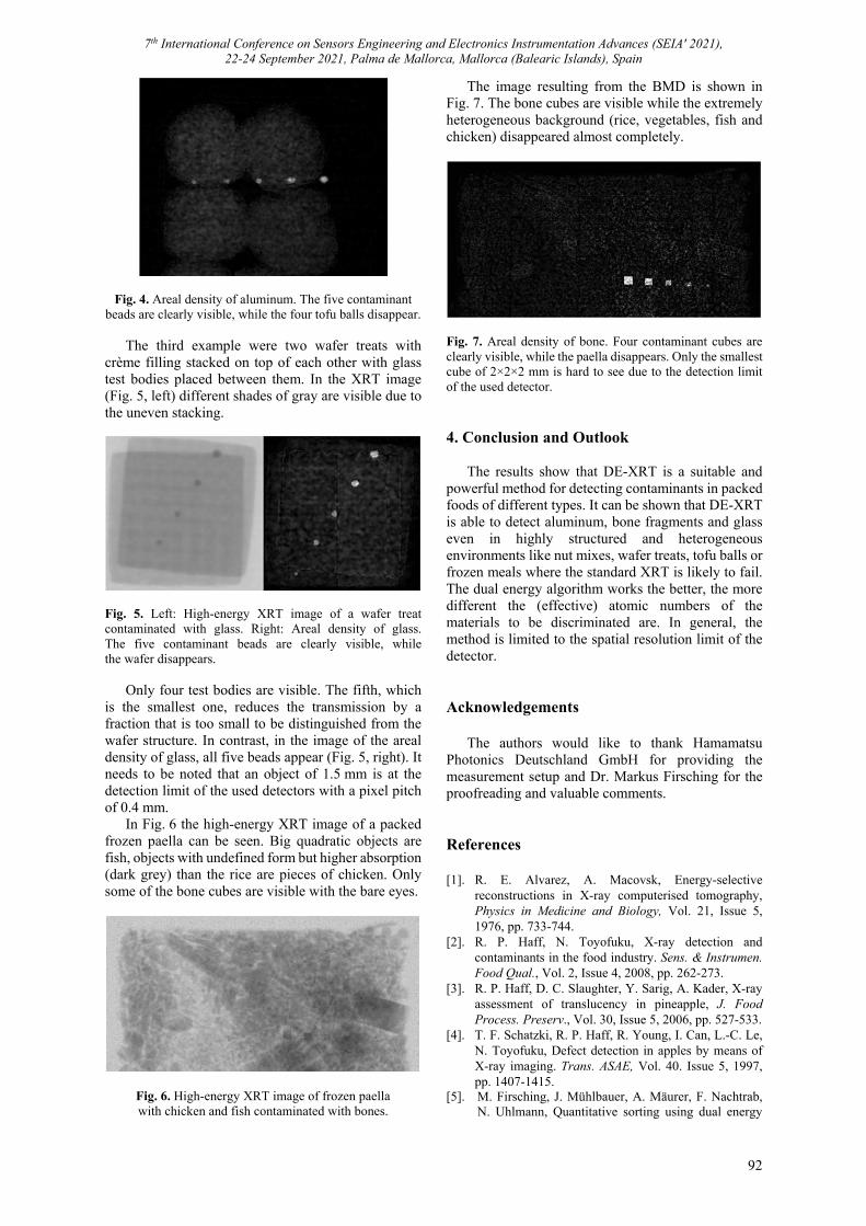
7th International Conference on Sensors Engineering and Electronics Instrumentation Advances (SEIA' 2021), 22-24 September 2021, Palma de Mallorca, Mallorca (Balearic Islands), Spain
92
Fig. 4. Areal density of aluminum. The five contaminant beads are clearly visible, while the four tofu balls disappear.
The third example were two wafer treats with crème filling stacked on top of each other with glass test bodies placed between them. In the XRT image (Fig. 5, left) different shades of gray are visible due to the uneven stacking.
Fig. 5. Left: High-energy XRT image of a wafer treat contaminated with glass. Right: Areal density of glass. The five contaminant beads are clearly visible, while the wafer disappears.
Only four test bodies are visible. The fifth, which
is the smallest one, reduces the transmission by a fraction that is too small to be distinguished from the wafer structure. In contrast, in the image of the areal density of glass, all five beads appear (Fig. 5, right). It needs to be noted that an object of 1.5 mm is at the detection limit of the used detectors with a pixel pitch of 0.4 mm.
In Fig. 6 the high-energy XRT image of a packed frozen paella can be seen. Big quadratic objects are fish, objects with undefined form but higher absorption (dark grey) than the rice are pieces of chicken. Only some of the bone cubes are visible with the bare eyes.
Fig. 6. High-energy XRT image of frozen paella with chicken and fish contaminated with bones.
The image resulting from the BMD is shown in Fig. 7. The bone cubes are visible while the extremely heterogeneous background (rice, vegetables, fish and chicken) disappeared almost completely.
Fig. 7. Areal density of bone. Four contaminant cubes are clearly visible, while the paella disappears. Only the smallest cube of 2×2×2 mm is hard to see due to the detection limit of the used detector. 4. Conclusion and Outlook
The results show that DE-XRT is a suitable and powerful method for detecting contaminants in packed foods of different types. It can be shown that DE-XRT is able to detect aluminum, bone fragments and glass even in highly structured and heterogeneous environments like nut mixes, wafer treats, tofu balls or frozen meals where the standard XRT is likely to fail. The dual energy algorithm works the better, the more different the (effective) atomic numbers of the materials to be discriminated are. In general, the method is limited to the spatial resolution limit of the detector. Acknowledgements
The authors would like to thank Hamamatsu Photonics Deutschland GmbH for providing the measurement setup and Dr. Markus Firsching for the proofreading and valuable comments. References [1]. R. E. Alvarez, A. Macovsk, Energy-selective
reconstructions in X-ray computerised tomography, Physics in Medicine and Biology, Vol. 21, Issue 5, 1976, pp. 733-744.
[2]. R. P. Haff, N. Toyofuku, X-ray detection and contaminants in the food industry. Sens. & Instrumen. Food Qual., Vol. 2, Issue 4, 2008, pp. 262-273.
[3]. R. P. Haff, D. C. Slaughter, Y. Sarig, A. Kader, X-ray assessment of translucency in pineapple, J. Food Process. Preserv., Vol. 30, Issue 5, 2006, pp. 527-533.
[4]. T. F. Schatzki, R. P. Haff, R. Young, I. Can, L.-C. Le, N. Toyofuku, Defect detection in apples by means of X-ray imaging. Trans. ASAE, Vol. 40. Issue 5, 1997, pp. 1407-1415.
[5]. M. Firsching, J. Mühlbauer, A. Mäurer, F. Nachtrab, N. Uhlmann, Quantitative sorting using dual energy

7th International Conference on Sensors Engineering and Electronics Instrumentation Advances (SEIA' 2021), 22-24 September 2021, Palma de Mallorca, Mallorca (Balearic Islands), Spain
93
X-ray transmission imaging, in Proceedings of the Optical Characterization of Materials Conference (OCM’13), Karlsruhe, Germany, 6-7 March 2013, pp. 259-264.
[6]. M. Firsching, J. Lucic, A. Ennen, N. Uhlmann, Concentration determination for sorting applications using dual energy X-ray transmission imaging, in Proceedings of the Optical Characterization of Materials-conference (OCM’17), Karlsruhe, Germany, 22-23 March 2017, pp. 65-74.
[7]. M. Firsching, F. Nachtrab, N. Uhlmann, R. Hanke, Multi‐energy X‐ray imaging as a quantitative method for materials characterization, Adv. Mater., Vol. 23, Issues 22‐23, 2011, pp. 2655-2656.
[8]. Rondotest Website, https://rondotest.de/
[9]. C. Bauer, R. Wagner, B. Orberger, M. Firsching, A. Ennen, C. Garcia Pina, C. Wagner, M. Honarmand, G. Nabatian, I. Monsef, Potential of dual and multi energy XRT and CT analyses on iron formations, MDPI Sensors, Vol. 21, Issue 7, 2021, 2455.
[10]. E. Y. Sidky, L. Yu, X. Pan, Y. Zou, M. Vannier, A robust method of X-ray source spectrum estimation from transmission measurements: Demonstrated in computer simulated, scatter-free transmission data, J. Appl. Phys., Vol. 97, Issue 12, 2005, 124701.
[11]. B. Heismann, J. Leppert, K. Stierstorfer, Density and atomic number measurements with spectral X-ray attenuation method, J. Appl. Phys., Vol. 94, Issue 3, 2003, pp. 2073-2079.
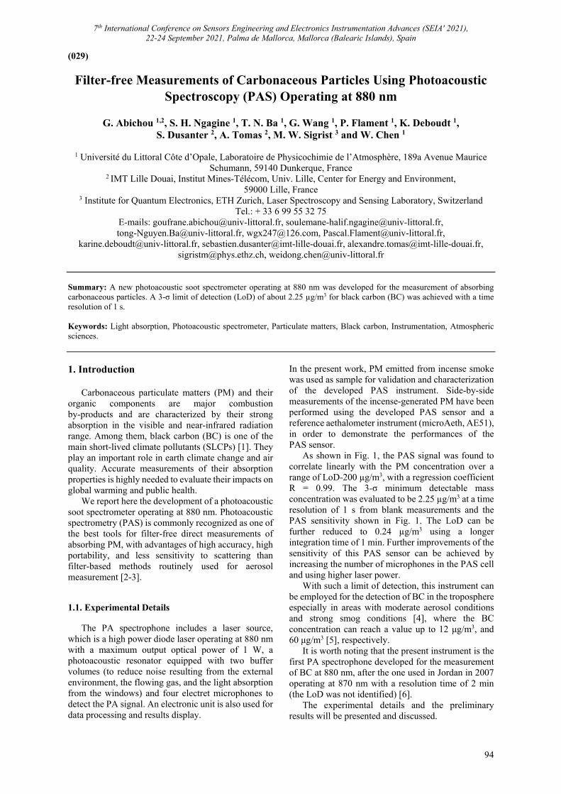
7th International Conference on Sensors Engineering and Electronics Instrumentation Advances (SEIA' 2021), 22-24 September 2021, Palma de Mallorca, Mallorca (Balearic Islands), Spain
94
(029)
Filter-free Measurements of Carbonaceous Particles Using Photoacoustic Spectroscopy (PAS) Operating at 880 nm
G. Abichou 1,2, S. H. Ngagine 1, T. N. Ba 1, G. Wang 1, P. Flament 1, K. Deboudt 1,
S. Dusanter 2, A. Tomas 2, M. W. Sigrist 3 and W. Chen 1
1 Université du Littoral Côte d’Opale, Laboratoire de Physicochimie de l’Atmosphère, 189a Avenue Maurice Schumann, 59140 Dunkerque, France
2 IMT Lille Douai, Institut Mines-Télécom, Univ. Lille, Center for Energy and Environment, 59000 Lille, France
3 Institute for Quantum Electronics, ETH Zurich, Laser Spectroscopy and Sensing Laboratory, Switzerland Tel.: + 33 6 99 55 32 75
E-mails: [email protected], [email protected], [email protected], [email protected], [email protected],
[email protected], [email protected], [email protected], [email protected], [email protected]
Summary: A new photoacoustic soot spectrometer operating at 880 nm was developed for the measurement of absorbing carbonaceous particles. A 3-σ limit of detection (LoD) of about 2.25 µg/m3 for black carbon (BC) was achieved with a time resolution of 1 s. Keywords: Light absorption, Photoacoustic spectrometer, Particulate matters, Black carbon, Instrumentation, Atmospheric sciences.
1. Introduction
Carbonaceous particulate matters (PM) and their organic components are major combustion by-products and are characterized by their strong absorption in the visible and near-infrared radiation range. Among them, black carbon (BC) is one of the main short-lived climate pollutants (SLCPs) [1]. They play an important role in earth climate change and air quality. Accurate measurements of their absorption properties is highly needed to evaluate their impacts on global warming and public health.
We report here the development of a photoacoustic soot spectrometer operating at 880 nm. Photoacoustic spectrometry (PAS) is commonly recognized as one of the best tools for filter-free direct measurements of absorbing PM, with advantages of high accuracy, high portability, and less sensitivity to scattering than filter-based methods routinely used for aerosol measurement [2-3]. 1.1. Experimental Details
The PA spectrophone includes a laser source, which is a high power diode laser operating at 880 nm with a maximum output optical power of 1 W, a photoacoustic resonator equipped with two buffer volumes (to reduce noise resulting from the external environment, the flowing gas, and the light absorption from the windows) and four electret microphones to detect the PA signal. An electronic unit is also used for data processing and results display.
In the present work, PM emitted from incense smoke was used as sample for validation and characterization of the developed PAS instrument. Side-by-side measurements of the incense-generated PM have been performed using the developed PAS sensor and a reference aethalometer instrument (microAeth, AE51), in order to demonstrate the performances of the PAS sensor.
As shown in Fig. 1, the PAS signal was found to correlate linearly with the PM concentration over a range of LoD-200 µg/m3, with a regression coefficient R = 0.99. The 3-σ minimum detectable mass concentration was evaluated to be 2.25 µg/m3 at a time resolution of 1 s from blank measurements and the PAS sensitivity shown in Fig. 1. The LoD can be further reduced to 0.24 µg/m3 using a longer integration time of 1 min. Further improvements of the sensitivity of this PAS sensor can be achieved by increasing the number of microphones in the PAS cell and using higher laser power.
With such a limit of detection, this instrument can be employed for the detection of BC in the troposphere especially in areas with moderate aerosol conditions and strong smog conditions [4], where the BC concentration can reach a value up to 12 μg/m3, and 60 μg/m3 [5], respectively.
It is worth noting that the present instrument is the first PA spectrophone developed for the measurement of BC at 880 nm, after the one used in Jordan in 2007 operating at 870 nm with a resolution time of 2 min (the LoD was not identified) [6].
The experimental details and the preliminary results will be presented and discussed.
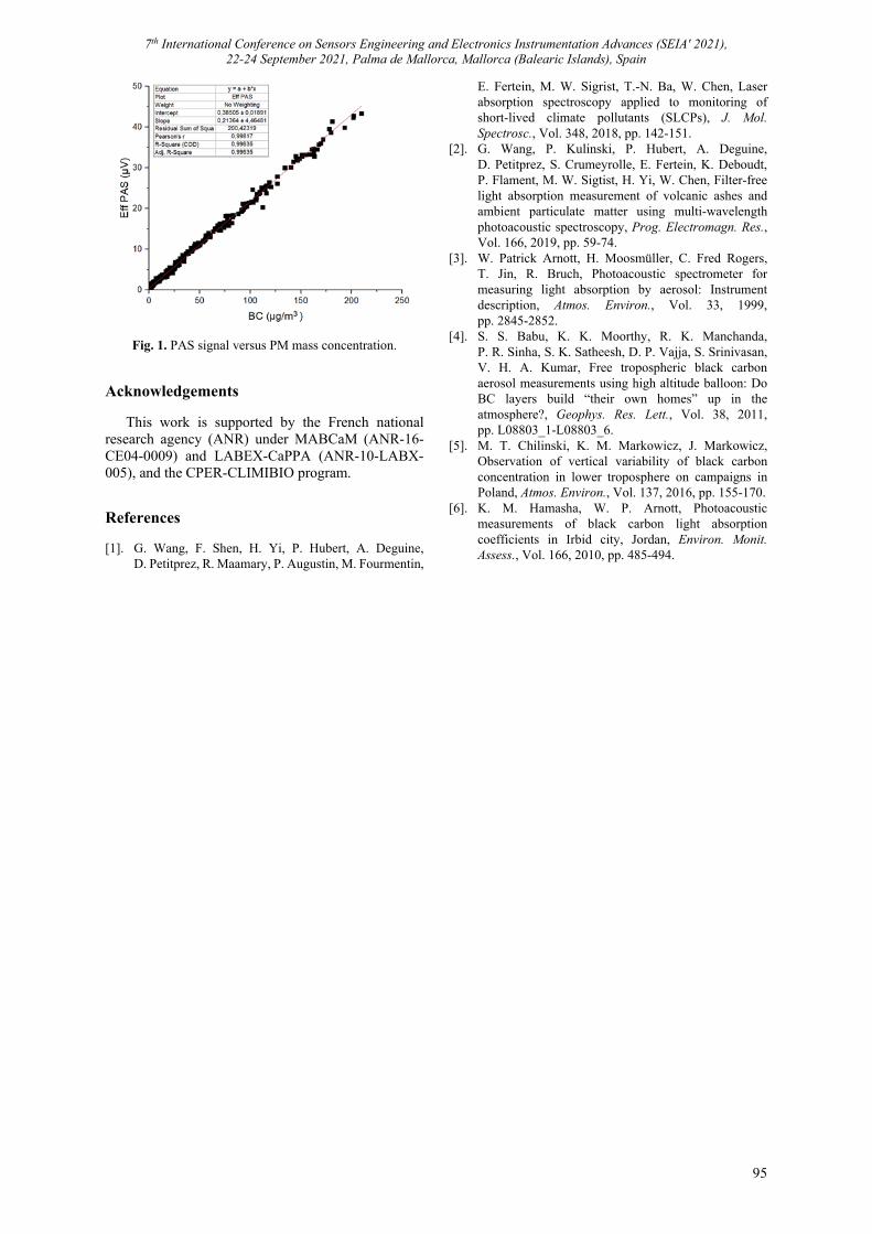
7th International Conference on Sensors Engineering and Electronics Instrumentation Advances (SEIA' 2021), 22-24 September 2021, Palma de Mallorca, Mallorca (Balearic Islands), Spain
95
Fig. 1. PAS signal versus PM mass concentration.
Acknowledgements
This work is supported by the French national research agency (ANR) under MABCaM (ANR-16-CE04-0009) and LABEX-CaPPA (ANR-10-LABX-005), and the CPER-CLIMIBIO program.
References [1]. G. Wang, F. Shen, H. Yi, P. Hubert, A. Deguine,
D. Petitprez, R. Maamary, P. Augustin, M. Fourmentin,
E. Fertein, M. W. Sigrist, T.-N. Ba, W. Chen, Laser absorption spectroscopy applied to monitoring of short-lived climate pollutants (SLCPs), J. Mol. Spectrosc., Vol. 348, 2018, pp. 142-151.
[2]. G. Wang, P. Kulinski, P. Hubert, A. Deguine, D. Petitprez, S. Crumeyrolle, E. Fertein, K. Deboudt, P. Flament, M. W. Sigtist, H. Yi, W. Chen, Filter-free light absorption measurement of volcanic ashes and ambient particulate matter using multi-wavelength photoacoustic spectroscopy, Prog. Electromagn. Res., Vol. 166, 2019, pp. 59-74.
[3]. W. Patrick Arnott, H. Moosmüller, C. Fred Rogers, T. Jin, R. Bruch, Photoacoustic spectrometer for measuring light absorption by aerosol: Instrument description, Atmos. Environ., Vol. 33, 1999, pp. 2845‑2852.
[4]. S. S. Babu, K. K. Moorthy, R. K. Manchanda, P. R. Sinha, S. K. Satheesh, D. P. Vajja, S. Srinivasan, V. H. A. Kumar, Free tropospheric black carbon aerosol measurements using high altitude balloon: Do BC layers build “their own homes” up in the atmosphere?, Geophys. Res. Lett., Vol. 38, 2011, pp. L08803_1-L08803_6.
[5]. M. T. Chilinski, K. M. Markowicz, J. Markowicz, Observation of vertical variability of black carbon concentration in lower troposphere on campaigns in Poland, Atmos. Environ., Vol. 137, 2016, pp. 155‑170.
[6]. K. M. Hamasha, W. P. Arnott, Photoacoustic measurements of black carbon light absorption coefficients in Irbid city, Jordan, Environ. Monit. Assess., Vol. 166, 2010, pp. 485‑494.
7th International Conference on Sensors Engineering and Electronics Instrumentation Advances (SEIA' 2021), 22-24 September 2021, Palma de Mallorca, Mallorca (Balearic Islands), Spain
96
(030)
Detecting Drifts and Offsets in Environmental Monitoring Networks
G. Jesus 1, A. Oliveira 1 and A. Casimiro 2 1 DHA-GTI, Laboratório Nacional de Engenharia Civil, Avenida do Brasil 101, 1700-066 Lisboa, Portugal
2 LASIGE, Faculdade de Ciências, Universidade de Lisboa, Campo Grande, 1749-016 Lisboa, Portugal
E-mail: [email protected] Summary: Sensor networks used in environmental monitoring applications are subject to harsh environmental conditions and hence prone to produce uncertainties in its measurements. Comparing to the common task of outlier detection in sensor data, we review herein the problem of detecting systematic failures such as drifts and offsets. Performing this detection in environmental monitoring networks becomes a hard problem especially when we need to distinguish true data errors from deviations due to natural phenomenon. In this paper, we introduce a new instantiation of a proven methodology for dependable runtime detection of outliers in environmental monitoring systems. We also characterize some limitations and assumptions of a solution to detect and correct drifts and offset failure situations. Lastly, we discuss the use of machine learning techniques to estimate the network sensors measurements based on the knowledge of processed past measurements alongside with the current neighbor sensors observations. Keywords: Data quality, Failure detection, Sensor fusion, Machine learning, Sensor networks, Aquatic monitoring.
1. Introduction
When monitoring harsh environments, deployed sensors have to perform under unfavorable conditions, producing several types of uncertainties. Measurements may be imprecise, incorrect, incomplete, incoherent or inappropriate to the problem at hand. Sensors may exhibit errors due to sensor or other (e.g. communication) faults, either outliers, temporary disturbances or systematic deviations. These errors can ultimately contribute to false warnings being issued or to lead to the issuing of wrong decisions. We focus on real environments subject to harsh conditions, namely aquatic environments. Also, many of the techniques for fault detection do not consider the presence of natural phenomena interfering with sensor measurements [1, 2]. These phenomena can ultimately lead to deviations in measurements that might be wrongly perceived as errors. In this paper we consider physical phenomena as events, which are natural occurrences and their impact on measurements should not lead to wrongly detect faulty behaviours.
In the past decade there have been many studies supporting the use of machine learning techniques and sensor fusion to identify or classify events, including failure situations. The most common situations are related to faulty data observations due to spurious errors, such as outliers. Herein, we introduce a solution to detect and correct offsets and drifts, characterized by a systematic failure behavior observed during a determined time interval and normally observable when a sensor is functioning during a long period of time without intervention.
Although faults in sensor networks have been covered exhaustively, the majority of the studies is dedicated to communication faults or outliers derived from sensor faults. In fact, detection and mitigation
techniques for drifts and offsets in the context of sensor networks have not been addressed thoroughly.
In this presentation we propose an instantiation of the methodology presented in [3], comprising machine learning strategies for the prediction of the expected sensor measurements of each sensor node, but now accounting only for faults related to drifts and offsets.
In Section 2, we identify related work on mechanisms and techniques for detecting offsets and drifts, including the use of data fusion strategies. In Section 3 we briefly overview some aspects of the methodology and in Section 4 we describe the proposed instantiation and its limitations and assumptions required to the application for drifts and offsets detection. 2. Related Work
In what concerns detection and correction methods for drifting and offset failure behaviors in sensor devices, there is a separation from single device and multiple devices (network).
In the first category, it is related mostly with calibration and its variants as a process to prevent and correct such failures. In contrast, in a multi-sensor situation it is possible to use data fusion techniques in order to detect and correct drifts and offsets.
For the sensor networks scenario, there is a limited number of studies considering both detection and correction mechanisms of offset and drifts failures. Offsets analyses are more common than drifting ones, in particular in applications related to digital imagery. One exception is [4], where the authors present a machine learning approach to detect faults in WSNs, using Hidden Markov Models to capture both the dynamics of the environment and the dynamics of the faults.
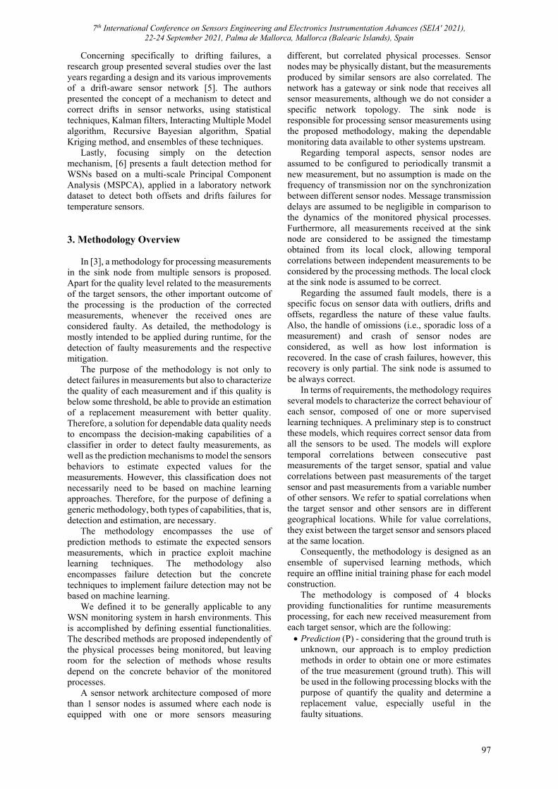
7th International Conference on Sensors Engineering and Electronics Instrumentation Advances (SEIA' 2021), 22-24 September 2021, Palma de Mallorca, Mallorca (Balearic Islands), Spain
97
Concerning specifically to drifting failures, a research group presented several studies over the last years regarding a design and its various improvements of a drift-aware sensor network [5]. The authors presented the concept of a mechanism to detect and correct drifts in sensor networks, using statistical techniques, Kalman filters, Interacting Multiple Model algorithm, Recursive Bayesian algorithm, Spatial Kriging method, and ensembles of these techniques.
Lastly, focusing simply on the detection mechanism, [6] presents a fault detection method for WSNs based on a multi-scale Principal Component Analysis (MSPCA), applied in a laboratory network dataset to detect both offsets and drifts failures for temperature sensors. 3. Methodology Overview
In [3], a methodology for processing measurements in the sink node from multiple sensors is proposed. Apart for the quality level related to the measurements of the target sensors, the other important outcome of the processing is the production of the corrected measurements, whenever the received ones are considered faulty. As detailed, the methodology is mostly intended to be applied during runtime, for the detection of faulty measurements and the respective mitigation.
The purpose of the methodology is not only to detect failures in measurements but also to characterize the quality of each measurement and if this quality is below some threshold, be able to provide an estimation of a replacement measurement with better quality. Therefore, a solution for dependable data quality needs to encompass the decision-making capabilities of a classifier in order to detect faulty measurements, as well as the prediction mechanisms to model the sensors behaviors to estimate expected values for the measurements. However, this classification does not necessarily need to be based on machine learning approaches. Therefore, for the purpose of defining a generic methodology, both types of capabilities, that is, detection and estimation, are necessary.
The methodology encompasses the use of prediction methods to estimate the expected sensors measurements, which in practice exploit machine learning techniques. The methodology also encompasses failure detection but the concrete techniques to implement failure detection may not be based on machine learning.
We defined it to be generally applicable to any WSN monitoring system in harsh environments. This is accomplished by defining essential functionalities. The described methods are proposed independently of the physical processes being monitored, but leaving room for the selection of methods whose results depend on the concrete behavior of the monitored processes.
A sensor network architecture composed of more than 1 sensor nodes is assumed where each node is equipped with one or more sensors measuring
different, but correlated physical processes. Sensor nodes may be physically distant, but the measurements produced by similar sensors are also correlated. The network has a gateway or sink node that receives all sensor measurements, although we do not consider a specific network topology. The sink node is responsible for processing sensor measurements using the proposed methodology, making the dependable monitoring data available to other systems upstream.
Regarding temporal aspects, sensor nodes are assumed to be configured to periodically transmit a new measurement, but no assumption is made on the frequency of transmission nor on the synchronization between different sensor nodes. Message transmission delays are assumed to be negligible in comparison to the dynamics of the monitored physical processes. Furthermore, all measurements received at the sink node are considered to be assigned the timestamp obtained from its local clock, allowing temporal correlations between independent measurements to be considered by the processing methods. The local clock at the sink node is assumed to be correct.
Regarding the assumed fault models, there is a specific focus on sensor data with outliers, drifts and offsets, regardless the nature of these value faults. Also, the handle of omissions (i.e., sporadic loss of a measurement) and crash of sensor nodes are considered, as well as how lost information is recovered. In the case of crash failures, however, this recovery is only partial. The sink node is assumed to be always correct.
In terms of requirements, the methodology requires several models to characterize the correct behaviour of each sensor, composed of one or more supervised learning techniques. A preliminary step is to construct these models, which requires correct sensor data from all the sensors to be used. The models will explore temporal correlations between consecutive past measurements of the target sensor, spatial and value correlations between past measurements of the target sensor and past measurements from a variable number of other sensors. We refer to spatial correlations when the target sensor and other sensors are in different geographical locations. While for value correlations, they exist between the target sensor and sensors placed at the same location.
Consequently, the methodology is designed as an ensemble of supervised learning methods, which require an offline initial training phase for each model construction.
The methodology is composed of 4 blocks providing functionalities for runtime measurements processing, for each new received measurement from each target sensor, which are the following: Prediction (P) - considering that the ground truth is
unknown, our approach is to employ prediction methods in order to obtain one or more estimates of the true measurement (ground truth). This will be used in the following processing blocks with the purpose of quantify the quality and determine a replacement value, especially useful in the faulty situations.
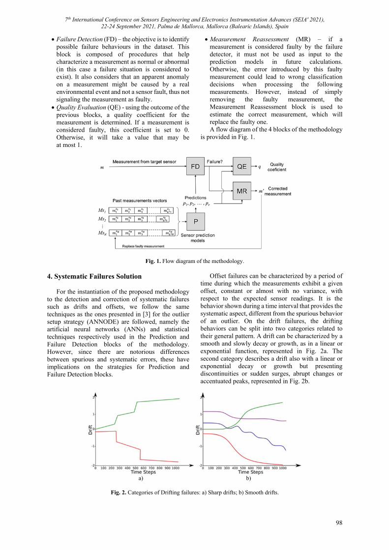
7th International Conference on Sensors Engineering and Electronics Instrumentation Advances (SEIA' 2021), 22-24 September 2021, Palma de Mallorca, Mallorca (Balearic Islands), Spain
98
Failure Detection (FD) – the objective is to identify possible failure behaviours in the dataset. This block is composed of procedures that help characterize a measurement as normal or abnormal (in this case a failure situation is considered to exist). It also considers that an apparent anomaly on a measurement might be caused by a real environmental event and not a sensor fault, thus not signaling the measurement as faulty.
Quality Evaluation (QE) - using the outcome of the previous blocks, a quality coefficient for the measurement is determined. If a measurement is considered faulty, this coefficient is set to 0. Otherwise, it will take a value that may be at most 1.
Measurement Reassessment (MR) – if a measurement is considered faulty by the failure detector, it must not be used as input to the prediction models in future calculations. Otherwise, the error introduced by this faulty measurement could lead to wrong classification decisions when processing the following measurements. However, instead of simply removing the faulty measurement, the Measurement Reassessment block is used to estimate the correct measurement, which will replace the faulty one. A flow diagram of the 4 blocks of the methodology
is provided in Fig. 1.
Fig. 1. Flow diagram of the methodology. 4. Systematic Failures Solution
For the instantiation of the proposed methodology to the detection and correction of systematic failures such as drifts and offsets, we follow the same techniques as the ones presented in [3] for the outlier setup strategy (ANNODE) are followed, namely the artificial neural networks (ANNs) and statistical techniques respectively used in the Prediction and Failure Detection blocks of the methodology. However, since there are notorious differences between spurious and systematic errors, these have implications on the strategies for Prediction and Failure Detection blocks.
Offset failures can be characterized by a period of time during which the measurements exhibit a given offset, constant or almost with no variance, with respect to the expected sensor readings. It is the behavior shown during a time interval that provides the systematic aspect, different from the spurious behavior of an outlier. On the drift failures, the drifting behaviors can be split into two categories related to their general pattern. A drift can be characterized by a smooth and slowly decay or growth, as in a linear or exponential function, represented in Fig. 2a. The second category describes a drift also with a linear or exponential decay or growth but presenting discontinuities or sudden surges, abrupt changes or accentuated peaks, represented in Fig. 2b.
a) b)
Fig. 2. Categories of Drifting failures: a) Sharp drifts; b) Smooth drifts.
7th International Conference on Sensors Engineering and Electronics Instrumentation Advances (SEIA' 2021), 22-24 September 2021, Palma de Mallorca, Mallorca (Balearic Islands), Spain
99
4.1. Prediction Block
A solution for the detection and correction of offsets and drifts should follow three steps. First, in a sensor network there must be a selection of the network sensor nodes that are highly likely to be correlated. This correlation can be verified by considering either the physical distance or through expert knowledge of the specific environment dynamics.
The second step is the selection of the data fusion techniques for the Prediction (P) block, considering that such techniques must be adequate to resolve the estimation problem (predicting the target sensor next measurement). Finally, the third step includes the selection of the specific datasets for the training process (if required) of the chosen techniques.
In [3], we defined the type and structure of ANNs to use for the datasets of a case study, in which for monitoring measurements of a given target sensor, the inputs are comprised of the vectors with a history of measurements of the neighbor sensors and possibly of the target sensor itself. Regarding the layer structure, besides the input and output layers, the ANNs are composed also with two hidden layers. The ANNs output is trained to be a prediction of the target sensor next measurement (single value).
In terms of the predictions provided by the ANNs (P block), there is a clear difference between outlier and systematic detection. For systematic failures detection, given that we have failure behaviors that may not vary abruptly as an outlier and affect systematically the target sensor measurements, in the prediction models we cannot consider predictions based on the target past measurements.
Consequently, we only consider for this solution, ANNs trained based on the measurements of the neighbor sensors. Therefore, we discard past measurements from the target sensor because these have a strong influence in the predictions and would lead to wrong predictions.
One important difference between systematic and spurious errors is that the former are observed over time while the latter are observed in a single measurement. Therefore, systematic errors cannot be detected as soon as they start, only after being observed for a certain time interval.
Another important aspect to consider for the specific situation of environment monitoring networks is that the sensors are widespread, which may diminish the prediction techniques accuracy. Without sensor redundancy (more than one sensor in the same place) and with less accurate estimations, we are required to obtain a more complete view of the monitoring system, based on the several neighbor sensors. 4.2. Failure Detection Block
In the Failure Detection (FD) block, similarly to the ANNODE solution [3], we consider a statistical technique as a comparison method, in order to
calculate the differences between each measurement and the corresponding predictions provided by the Prediction block (P). This statistical technique uses a training dataset to learn the probability distributions fittings between the errors of the prediction models defined in P and the expected measurements. Using the training dataset, the square errors between the measurement and each prediction are obtained and we are able to obtain the final cumulative density function (CDF). This CDF allows us to calculate the probability of the error between current target sensor reading and prediction. Therefore, by defining a threshold for error probability, we can assess the significance of the observed differences between the measurement and the predictions.
In this solution for the detection of systematic errors, we have different detection conditions from those formulated in ANNODE. Firstly, each measurement of the target sensor is compared with the predictions and the number of significant differences, which can be between zero and total number of predictions, is recorded. Then, these differences are evaluated over a significant temporal window to perform the intended detection of systematic failure.
For this systematic detection, a temporal window must be defined so we can distinguish single point situations from systematic failures or even from an environment-related event. These single point situations can be spurious errors or just regular fluctuations in the differences between the measurement and the corresponding predictions, in which the difference can be significant for that instant but not in a systematic manner. This temporal window will allow us to characterize correctly a systematic failure, either being an offset or a drift.
The temporal window will have a pre-defined time units, which is typically defined by the application and related with the required failure detection latency. The rule of thumb is that the window must include enough measurements to characterize the temporal scales of relevance with enough resolution for the phenomena at stake, depending also on the frequency of sensor measurements. The number of measurements in the window must be at least 3, such that it is possible to conclude that a certain behaviour is systematic, but it can be made larger as this will allow to achieve more precise conclusions. 5. Conclusions
We define drift and offset behaviors specifically in the context of an environmental sensor network that is different from the common cases of high-density sensor networks. Moreover, we introduce an instantiation according to a proposed methodology [3] comprising relevant prediction models for the next measurement of the target sensor, using machine learning techniques based only on the neighbors information.

7th International Conference on Sensors Engineering and Electronics Instrumentation Advances (SEIA' 2021), 22-24 September 2021, Palma de Mallorca, Mallorca (Balearic Islands), Spain
100
Acknowledgements
This paper is part of the work of project AQUAMON (PTDC/CCI-COM/30142/2017), funded by the Fundação para a Ciência e a Tecnologia (FCT). References [1]. E. W. Dereszynski, T. G. Dietterich, Spatiotemporal
models for data-anomaly detection in dynamic environmental monitoring campaigns, ACM Transactions on Sensor Networks (TOSN), Vol. 8, Issue 1, 2011, pp. 1-36.
[2]. V. Garcia-Font, C. Garrigues, H. Rifà-Pous, A comparative study of anomaly detection techniques for smart city wireless sensor networks, Sensors, Vol. 16, Issue 6, 2016, 868.
[3]. G. Jesus, A. Oliveira, A. Casimiro, Using machine learning for dependable outlier detection in environmental monitoring systems, ACM Transactions on Cyber-Physical Systems, Vol. 5, Issue 3, 2021, pp. 1-30.
[4]. E. U. Warriach, M. Aiello, K. Tei, A machine learning approach for identifying and classifying faults in wireless sensor network, in Proceedings of the IEEE 15th International Conference on Computational Science and Engineering (CSE’12), 2012, pp. 618-625.
[5]. M. Takruri, S. Challa, Drift aware wireless sensor networks, in Proceedings of the 10th International Conference on Information Fusion (Fusion’07), 2007, pp. 1-7.
[6]. Y. Xie, X. Chen, J. Zhao, Data fault detection for wireless sensor networks using multi-scale PCA method, in Proceedings of the 2nd International Conference on Artificial Intelligence, Management Science and Electronic Commerce (AIMSEC’11), 2011, pp. 7035-7038.
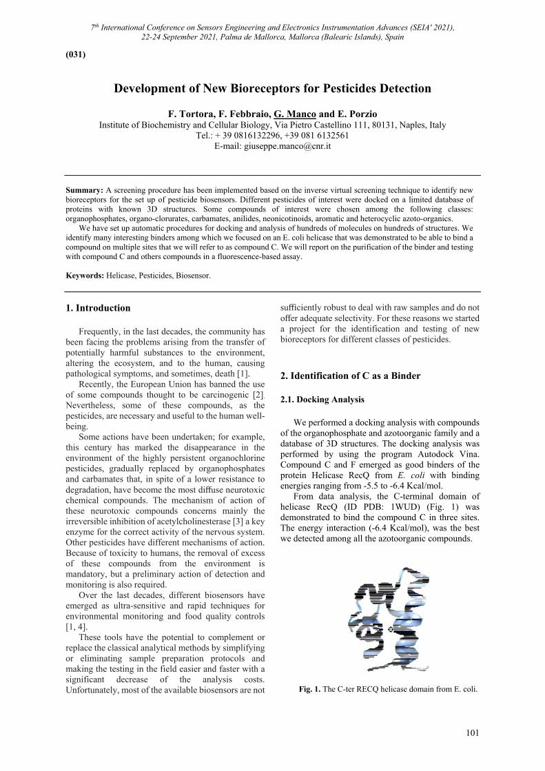
7th International Conference on Sensors Engineering and Electronics Instrumentation Advances (SEIA' 2021), 22-24 September 2021, Palma de Mallorca, Mallorca (Balearic Islands), Spain
101
(031)
Development of New Bioreceptors for Pesticides Detection
F. Tortora, F. Febbraio, G. Manco and E. Porzio Institute of Biochemistry and Cellular Biology, Via Pietro Castellino 111, 80131, Naples, Italy
Tel.: + 39 0816132296, +39 081 6132561 E-mail: [email protected]
Summary: A screening procedure has been implemented based on the inverse virtual screening technique to identify new bioreceptors for the set up of pesticide biosensors. Different pesticides of interest were docked on a limited database of proteins with known 3D structures. Some compounds of interest were chosen among the following classes: organophosphates, organo-clorurates, carbamates, anilides, neonicotinoids, aromatic and heterocyclic azoto-organics.
We have set up automatic procedures for docking and analysis of hundreds of molecules on hundreds of structures. We identify many interesting binders among which we focused on an E. coli helicase that was demonstrated to be able to bind a compound on multiple sites that we will refer to as compound C. We will report on the purification of the binder and testing with compound C and others compounds in a fluorescence-based assay. Keywords: Helicase, Pesticides, Biosensor. 1. Introduction
Frequently, in the last decades, the community has been facing the problems arising from the transfer of potentially harmful substances to the environment, altering the ecosystem, and to the human, causing pathological symptoms, and sometimes, death [1].
Recently, the European Union has banned the use of some compounds thought to be carcinogenic [2]. Nevertheless, some of these compounds, as the pesticides, are necessary and useful to the human well-being.
Some actions have been undertaken; for example, this century has marked the disappearance in the environment of the highly persistent organochlorine pesticides, gradually replaced by organophosphates and carbamates that, in spite of a lower resistance to degradation, have become the most diffuse neurotoxic chemical compounds. The mechanism of action of these neurotoxic compounds concerns mainly the irreversible inhibition of acetylcholinesterase [3] a key enzyme for the correct activity of the nervous system. Other pesticides have different mechanisms of action. Because of toxicity to humans, the removal of excess of these compounds from the environment is mandatory, but a preliminary action of detection and monitoring is also required.
Over the last decades, different biosensors have emerged as ultra-sensitive and rapid techniques for environmental monitoring and food quality controls [1, 4].
These tools have the potential to complement or replace the classical analytical methods by simplifying or eliminating sample preparation protocols and making the testing in the field easier and faster with a significant decrease of the analysis costs. Unfortunately, most of the available biosensors are not
sufficiently robust to deal with raw samples and do not offer adequate selectivity. For these reasons we started a project for the identification and testing of new bioreceptors for different classes of pesticides. 2. Identification of C as a Binder 2.1. Docking Analysis
We performed a docking analysis with compounds of the organophosphate and azotoorganic family and a database of 3D structures. The docking analysis was performed by using the program Autodock Vina. Compound C and F emerged as good binders of the protein Helicase RecQ from E. coli with binding energies ranging from -5.5 to -6.4 Kcal/mol.
From data analysis, the C-terminal domain of helicase RecQ (ID PDB: 1WUD) (Fig. 1) was demonstrated to bind the compound C in three sites. The energy interaction (-6.4 Kcal/mol), was the best we detected among all the azotoorganic compounds.
Fig. 1. The C-ter RECQ helicase domain from E. coli.
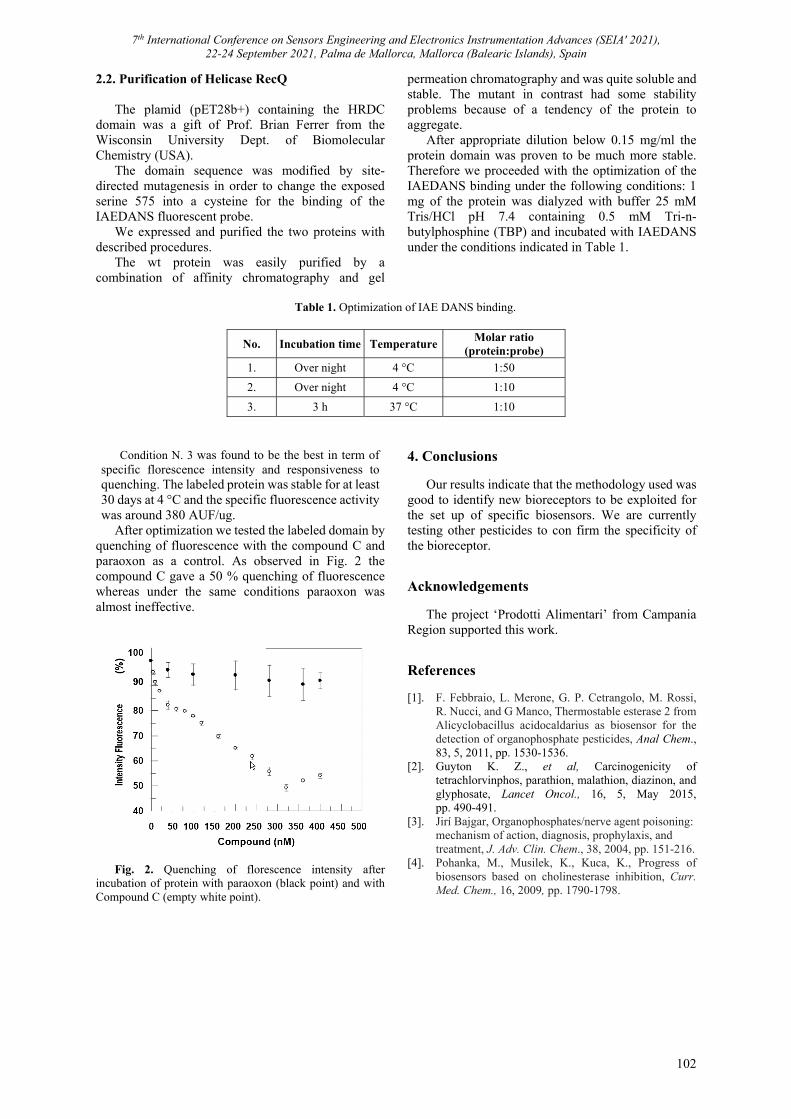
7th International Conference on Sensors Engineering and Electronics Instrumentation Advances (SEIA' 2021), 22-24 September 2021, Palma de Mallorca, Mallorca (Balearic Islands), Spain
102
2.2. Purification of Helicase RecQ
The plamid (pET28b+) containing the HRDC domain was a gift of Prof. Brian Ferrer from the Wisconsin University Dept. of Biomolecular Chemistry (USA).
The domain sequence was modified by site-directed mutagenesis in order to change the exposed serine 575 into a cysteine for the binding of the IAEDANS fluorescent probe.
We expressed and purified the two proteins with described procedures.
The wt protein was easily purified by a combination of affinity chromatography and gel
permeation chromatography and was quite soluble and stable. The mutant in contrast had some stability problems because of a tendency of the protein to aggregate.
After appropriate dilution below 0.15 mg/ml the protein domain was proven to be much more stable. Therefore we proceeded with the optimization of the IAEDANS binding under the following conditions: 1 mg of the protein was dialyzed with buffer 25 mM Tris/HCl pH 7.4 containing 0.5 mM Tri-n-butylphosphine (TBP) and incubated with IAEDANS under the conditions indicated in Table 1.
Table 1. Optimization of IAE DANS binding.
No. Incubation time TemperatureMolar ratio
(protein:probe)
1. Over night 4 °C 1:50
2. Over night 4 °C 1:10
3. 3 h 37 °C 1:10
Condition N. 3 was found to be the best in term of
specific florescence intensity and responsiveness to quenching. The labeled protein was stable for at least 30 days at 4 °C and the specific fluorescence activity was around 380 AUF/ug.
After optimization we tested the labeled domain by quenching of fluorescence with the compound C and paraoxon as a control. As observed in Fig. 2 the compound C gave a 50 % quenching of fluorescence whereas under the same conditions paraoxon was almost ineffective.
Fig. 2. Quenching of florescence intensity after
incubation of protein with paraoxon (black point) and with Compound C (empty white point).
4. Conclusions
Our results indicate that the methodology used was good to identify new bioreceptors to be exploited for the set up of specific biosensors. We are currently testing other pesticides to con firm the specificity of the bioreceptor.
Acknowledgements
The project ‘Prodotti Alimentari’ from Campania Region supported this work.
References [1]. F. Febbraio, L. Merone, G. P. Cetrangolo, M. Rossi,
R. Nucci, and G Manco, Thermostable esterase 2 from Alicyclobacillus acidocaldarius as biosensor for the detection of organophosphate pesticides, Anal Chem., 83, 5, 2011, pp. 1530-1536.
[2]. Guyton K. Z., et al, Carcinogenicity of tetrachlorvinphos, parathion, malathion, diazinon, and glyphosate, Lancet Oncol., 16, 5, May 2015, pp. 490-491.
[3]. Jirí Bajgar, Organophosphates/nerve agent poisoning: mechanism of action, diagnosis, prophylaxis, and treatment, J. Adv. Clin. Chem., 38, 2004, pp. 151-216.
[4]. Pohanka, M., Musilek, K., Kuca, K., Progress of biosensors based on cholinesterase inhibition, Curr. Med. Chem., 16, 2009, pp. 1790-1798.
7th International Conference on Sensors Engineering and Electronics Instrumentation Advances (SEIA' 2021), 22-24 September 2021, Palma de Mallorca, Mallorca (Balearic Islands), Spain
103
(033)
Intelligent Sensor Network for Home Monitoring of Vital Parameters
Ulrich H. P. Fischer, Jens-Uwe Just and Fabian Theuerkauf Harz University of Applied Sciences, Friedrichstr. 57, 38855 Wernigerode, Germany
Tel.: +49-(0)3943-659351, fax: +49-(0)3943-659399 Email: [email protected]
Summary: The measurement and compilation of vital human data is of particular importance, as it opens up the possibility of supporting a person in their area of life and being able to provide information as to whether diseases are developing or, for example, the gait changes too much so that an early fall could be avoided. Volatile organic components analysis is very interesting possibility for detecting deceases in the home area in a very early stage. Older multimorbid people can also continue to live medically safely in their own home with the help of this supporting analysis of vital parameters and gait parameters, which is the aim of this home monitoring project. Here, the Harz University has developed components for a distributed sensor network for the spectroscopic analysis of air and step analysis. The sensor system analyses the air in a room by measuring the optical spectral content of VOCs and the gait by special developed 3D G-sensors in a smart shoe insole. Keywords: Biosensors, Intelligent sensors, Volatile organic components sensors, Sensor fusion of real-time vital data, Gait analysis, Smart shoe sole.
1. Introduction
Health services, especially for older people, have been introduced very intensively into everyday life in recent years thanks to the rapid development of the transmission technology of the Internet of Things (IoT) [1-3]. In particular, the focus was on the prevention of diseases and the early detection of disease-related restrictions with a high risk, such as the early detection of a heart attack.
For this purpose, new types of sensor networks [4] came into play, together with intelligent systems for monitoring patients and checking the patient's health status. The ability of such intelligent systems to save and transmit the recorded vital data is of great importance in many areas of health care in telemedicine. These systems are usually portable (e.g. smart watch) [5, 6], or integrated in the apartment in order to guarantee non-invasive and remote surveillance [7]. Essentially, these systems are used to monitor the symptoms and status of patients for screening, follow-up care, or in the monitoring of care patients [8].
In particular, the area of monitoring in the household for so-called Ambient Assistant Living Systems (AAL) has been pushed very hard in the last ten years [9]. These systems essentially focus on the physical signals such as heart rate, blood pressure, skin temperature, breathing rate and body movements, as well as step sizes and step frequencies. The information that is available and collected by these signals can be further processed into clinically relevant information in order to prevent diseases. These wireless sensor networks include a number of biological sensors [7] that can be built and integrated electronically smaller and smaller and can therefore be easily integrated into a smart watch, for example. Each of these sensor systems has specific requirements for recognizing and recording symptoms.
Due to the increased integration capability, the components for applications have become significantly cheaper and are now in the low-cost range. They are relatively easy to install and, thanks to the long battery life, hardly any maintenance is necessary.
In this paper, two new types of sensor systems are presented, which measure the air quality optically in the home, as well as measure the step size, foot pressure and foot temperature at different points on the foot print in an intelligent insole. The collected data are transmitted via radio systems to a data server, from where it is called up and visualized.
The room air sensor uses special absorptions of VOC gas, which indicate the beginning of clinical pictures.
The presence of VOCs (volatile organic compounds) [10, 11] and other substances can provide indications (no conclusive diagnosis) of health problems:
H2 (hydrogen) -> lactose intolerance, fructose malabsorption, carbohydrate malabsorption, etc. gastrointestinal diseases;
C5H8 (isoprene) -> indicator for lung cancer (if deficient);
C2H6O (ethanol) -> lack of vitamin E and / or selenium;
C3H6O (acetone) -> insulin deficiency -> poss. Diabetes risk;
NH3 (ammonia) -> liver dysfunction (e.g. liver cirrhosis).
In addition to assessing the quality of indoor air for AAL applications, this system is also to be used for the detection of VOC in breathing gas. Since the presence of certain VOCs in exhaled air enables conclusions to be drawn about diseases such as lung cancer or metabolic disorders, the integration of a non-invasive permanent gas analysis in real-time medical care is
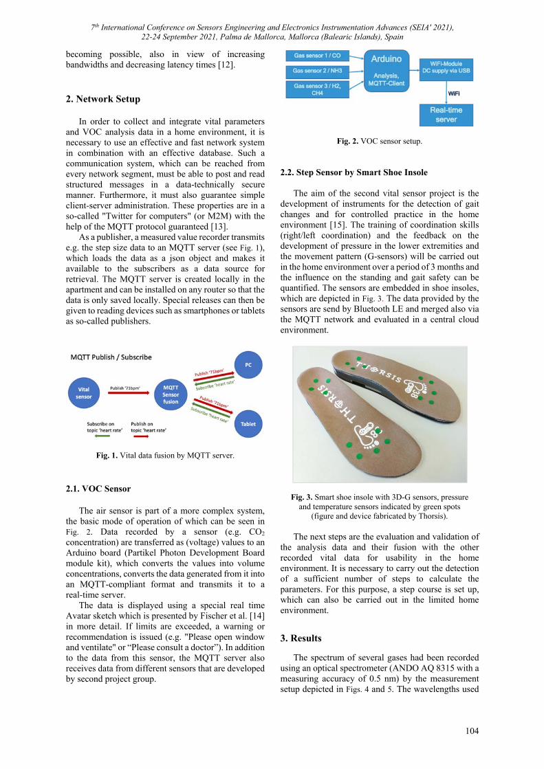
7th International Conference on Sensors Engineering and Electronics Instrumentation Advances (SEIA' 2021), 22-24 September 2021, Palma de Mallorca, Mallorca (Balearic Islands), Spain
104
becoming possible, also in view of increasing bandwidths and decreasing latency times [12].
2. Network Setup In order to collect and integrate vital parameters
and VOC analysis data in a home environment, it is necessary to use an effective and fast network system in combination with an effective database. Such a communication system, which can be reached from every network segment, must be able to post and read structured messages in a data-technically secure manner. Furthermore, it must also guarantee simple client-server administration. These properties are in a so-called "Twitter for computers" (or M2M) with the help of the MQTT protocol guaranteed [13].
As a publisher, a measured value recorder transmits e.g. the step size data to an MQTT server (see Fig. 1), which loads the data as a json object and makes it available to the subscribers as a data source for retrieval. The MQTT server is created locally in the apartment and can be installed on any router so that the data is only saved locally. Special releases can then be given to reading devices such as smartphones or tablets as so-called publishers.
Fig. 1. Vital data fusion by MQTT server.
2.1. VOC Sensor
The air sensor is part of a more complex system, the basic mode of operation of which can be seen in Fig. 2. Data recorded by a sensor (e.g. CO2 concentration) are transferred as (voltage) values to an Arduino board (Partikel Photon Development Board module kit), which converts the values into volume concentrations, converts the data generated from it into an MQTT-compliant format and transmits it to a real-time server.
The data is displayed using a special real time Avatar sketch which is presented by Fischer et al. [14] in more detail. If limits are exceeded, a warning or recommendation is issued (e.g. "Please open window and ventilate" or “Please consult a doctor”). In addition to the data from this sensor, the MQTT server also receives data from different sensors that are developed by second project group.
Fig. 2. VOC sensor setup. 2.2. Step Sensor by Smart Shoe Insole
The aim of the second vital sensor project is the development of instruments for the detection of gait changes and for controlled practice in the home environment [15]. The training of coordination skills (right/left coordination) and the feedback on the development of pressure in the lower extremities and the movement pattern (G-sensors) will be carried out in the home environment over a period of 3 months and the influence on the standing and gait safety can be quantified. The sensors are embedded in shoe insoles, which are depicted in Fig. 3. The data provided by the sensors are send by Bluetooth LE and merged also via the MQTT network and evaluated in a central cloud environment.
Fig. 3. Smart shoe insole with 3D-G sensors, pressure and temperature sensors indicated by green spots
(figure and device fabricated by Thorsis). The next steps are the evaluation and validation of
the analysis data and their fusion with the other recorded vital data for usability in the home environment. It is necessary to carry out the detection of a sufficient number of steps to calculate the parameters. For this purpose, a step course is set up, which can also be carried out in the limited home environment.
3. Results
The spectrum of several gases had been recorded using an optical spectrometer (ANDO AQ 8315 with a measuring accuracy of 0.5 nm) by the measurement setup depicted in Figs. 4 and 5. The wavelengths used
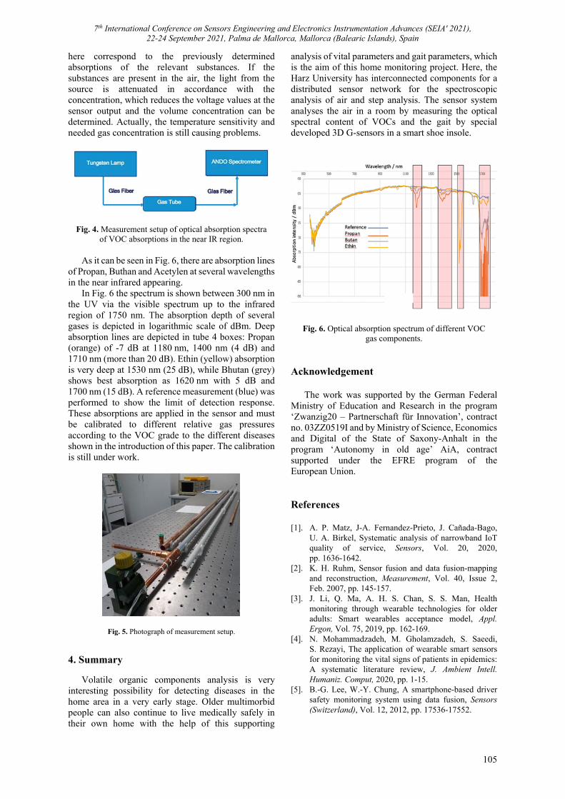
7th International Conference on Sensors Engineering and Electronics Instrumentation Advances (SEIA' 2021), 22-24 September 2021, Palma de Mallorca, Mallorca (Balearic Islands), Spain
105
here correspond to the previously determined absorptions of the relevant substances. If the substances are present in the air, the light from the source is attenuated in accordance with the concentration, which reduces the voltage values at the sensor output and the volume concentration can be determined. Actually, the temperature sensitivity and needed gas concentration is still causing problems.
Fig. 4. Measurement setup of optical absorption spectra of VOC absorptions in the near IR region.
As it can be seen in Fig. 6, there are absorption lines
of Propan, Buthan and Acetylen at several wavelengths in the near infrared appearing.
In Fig. 6 the spectrum is shown between 300 nm in the UV via the visible spectrum up to the infrared region of 1750 nm. The absorption depth of several gases is depicted in logarithmic scale of dBm. Deep absorption lines are depicted in tube 4 boxes: Propan (orange) of -7 dB at 1180 nm, 1400 nm (4 dB) and 1710 nm (more than 20 dB). Ethin (yellow) absorption is very deep at 1530 nm (25 dB), while Bhutan (grey) shows best absorption as 1620 nm with 5 dB and 1700 nm (15 dB). A reference measurement (blue) was performed to show the limit of detection response. These absorptions are applied in the sensor and must be calibrated to different relative gas pressures according to the VOC grade to the different diseases shown in the introduction of this paper. The calibration is still under work.
Fig. 5. Photograph of measurement setup.
4. Summary
Volatile organic components analysis is very interesting possibility for detecting diseases in the home area in a very early stage. Older multimorbid people can also continue to live medically safely in their own home with the help of this supporting
analysis of vital parameters and gait parameters, which is the aim of this home monitoring project. Here, the Harz University has interconnected components for a distributed sensor network for the spectroscopic analysis of air and step analysis. The sensor system analyses the air in a room by measuring the optical spectral content of VOCs and the gait by special developed 3D G-sensors in a smart shoe insole.
Fig. 6. Optical absorption spectrum of different VOC gas components.
Acknowledgement
The work was supported by the German Federal Ministry of Education and Research in the program ‘Zwanzig20 – Partnerschaft für Innovation’, contract no. 03ZZ0519I and by Ministry of Science, Economics and Digital of the State of Saxony-Anhalt in the program ‘Autonomy in old age’ AiA, contract supported under the EFRE program of the European Union. References [1]. A. P. Matz, J-A. Fernandez-Prieto, J. Cañada-Bago,
U. A. Birkel, Systematic analysis of narrowband IoT quality of service, Sensors, Vol. 20, 2020, pp. 1636-1642.
[2]. K. H. Ruhm, Sensor fusion and data fusion-mapping and reconstruction, Measurement, Vol. 40, Issue 2, Feb. 2007, pp. 145-157.
[3]. J. Li, Q. Ma, A. H. S. Chan, S. S. Man, Health monitoring through wearable technologies for older adults: Smart wearables acceptance model, Appl. Ergon, Vol. 75, 2019, pp. 162-169.
[4]. N. Mohammadzadeh, M. Gholamzadeh, S. Saeedi, S. Rezayi, The application of wearable smart sensors for monitoring the vital signs of patients in epidemics: A systematic literature review, J. Ambient Intell. Humaniz. Comput, 2020, pp. 1-15.
[5]. B.-G. Lee, W.-Y. Chung, A smartphone-based driver safety monitoring system using data fusion, Sensors (Switzerland), Vol. 12, 2012, pp. 17536-17552.

7th International Conference on Sensors Engineering and Electronics Instrumentation Advances (SEIA' 2021), 22-24 September 2021, Palma de Mallorca, Mallorca (Balearic Islands), Spain
106
[6]. S. Majumder, M. J. Deen, Smartphone sensors for health monitoring and diagnosis, Sensors, Vol. 19, Issue 9, 2019, 2164.
[7]. M. J. M. Breteler, E. Al, Wireless remote home monitoring of vital signs in patients discharged early after esophagectomy: Observational feasibility study, JMIR Perioper. Med, Vol. 3, Issue 2, 10.
[8]. R. Stodczyk, Ambient assisted living an overview of current applications, end-users and acceptance, Biomed. J. Sci. Tech. Res, Vol. 30, Issue 3, September 2020, pp. 23374-23384.
[9]. C. Bellos, A. Papadopoulos, R. Rosso, D. I. Fotiadis, Heterogeneous data fusion and intelligent techniques embedded in a mobile application for real-time chronic disease management, in Proceedings of the Annual International Conference of the IEEE Engineering in Medicine and Biology Society (EMBS’11), 2011, pp. 8303-8306.
[10]. P. Pasini, N. Powar, R. Gutierrez-Osuna, S. Daunert, A. Roda, Use of a gas-sensor array for detecting volatile
organic compounds (VOC) in chemically induced cells, Anal. Bioanal. Chem, Vol. 378, Issue 1, 2004, pp. 76-83.
[11]. M. R. R. Khan, B. H. Kang, S. H. Yeom, D. H. Kwon, S. W. Kang, Fiber-optic pulse width modulation sensor for low concentration VOC gas, Sensors Actuators B: Chem., Vol. 188, 2013, pp. 689-696.
[12]. U. H. P. Fischer-Hirchert, C. Reinboth, J.-U. Just, Entwicklung von Komponenten für ein verteiltes Sensorsystem zur Echtzeit-Analyse von Atemgas, in Proceedings of the BMC Kongress, 2019.
[13]. MQTT, https://mqtt.org [14]. J.-U. Just, C. Reinboth, A. Müller, U. Fischer-Hirchert,
Designing a distributed sensor system for the spectral analysis of ambient air, Biomed. Eng. – Biomed. Tech., Vol. 62, 2017, pp. 481-484.
[15]. P. Mertens, U. H. P. Fischer, Project Neuropathie-iA, https://forschung-sachsen-anhalt.de/project/ autonomie-alter-neuropath-2342
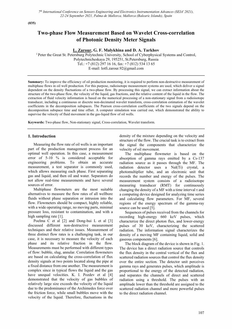
7th International Conference on Sensors Engineering and Electronics Instrumentation Advances (SEIA' 2021), 22-24 September 2021, Palma de Mallorca, Mallorca (Balearic Islands), Spain
107
(035)
Two-phase Flow Measurement Based on Wavelet Cross-correlation of Photonic Density Meter Signals
L. Zarour, G. F. Malykhina and D. A. Tarkhov
1 Peter the Great St. Petersburg Polytechnic University, School of Cyberphysical Systems and Control, Polytechnicheskaya 29, 195251, St.Petersburg, Russia
Tel.: +7 (812) 297 16 16, fax: +7 (812) 534 13 65 E-mail: [email protected]
Summary: To improve the efficiency of oil production monitoring, it is required to perform non-destructive measurement of multiphase flows in oil well production. For this purpose, radioisotope measurement systems are used, which deliver a signal dependent on the density fluctuations of a two-phase flow. By processing this signal, we can extract information about the structure of the two-phase flow, the velocity of the liquid, gas fractions, and the relative content of the liquid in the flow. The extraction of fluid velocity information is based on the numerical processing of a non-stationary signal from a radioisotope transducer, including a continuous or discrete non-decimated wavelet transform, cross-correlation estimation of the wavelet coefficients in the decomposition subspaces. The Pearson cross-correlation coefficients of the two signals depend on the decomposition subspace time and time offset. A computer simulation was carried out, which demonstrated the ability to supervise the velocity of fluid movement in the gas-liquid flow of oil wells. Keywords: Two-phase flow, Non-stationary signal, Cross-correlation, Wavelet transform.
1. Introduction
Measuring the flow rate of oil wells is an important part of the production management process for an optimal well operation. In this case, a measurement error of 5-10 % is considered acceptable for engineering problems. To obtain an accurate measurement, a test separator is commonly used, which allows measuring each phase. First separating gas and liquid, and then oil and water. Separators do not allow real-time measurements and have several sources of error.
Multiphase flowmeters are the most suitable alternatives to measure the flow rates of all wellbore fluids without phase separation or intrusion into the flow. Flowmeters should be compact, highly reliable, with a wide operating range, no moving parts, minimal pressure loss, resistant to contamination, and with a high sampling rate [1].
Poelma C et al [2] and Dong-hui L et al [3] discussed different non-destructive measurement techniques and their relative issues. Measurement of three distinct flow rates is a challenging task, in our case, it is necessary to measure the velocity of each phase and its relative fraction in the flow. Measurements must be performed with different types of flow: bubble, slug, annular. Correlation flowmeters are based on calculating the cross-correlation of flux density signals at two points located along the pipe at a fixed distance from one another. The measurement is complex since in typical flows the liquid and the gas have unequal velocities. K. I. Pozdev et al [4] demonstrated that the velocity of gas bubbles of relatively large size exceeds the velocity of the liquid due to the predominance of the Archimedes force over the friction force, while small bubbles move with the velocity of the liquid. Therefore, fluctuations in the
density of the mixture depending on the velocity and structure of the flow. The crucial task is to extract from the signal the components that characterize the velocity of oil movement.
The multiphase flowmeter is based on the absorption of gamma rays emitted by a Cs-137 radiation source as it passes through the MF. The radiation detector uses a Nal(Ti) crystal, a photomultiplier tube, and an electronic unit that records the number and energy of the pulses. The measurement system consists of a radioisotope measuring transducer (RMT) for continuously changing the density of a MF with a time interval τ and a computing device designed for analyzing time series and calculating flow parameters. For MF, several regions of the energy spectrum of the gamma-ray source can be used [5].
Sequences of pulses received from the channels for recording high-energy 660 keV pulses, which characterize the direct photon flux, and lower-energy pulses of 30 keV, characterizing the scattered radiation. The information signal characterizes the density of a moving MF containing liquid, solid and gaseous components [6].
The block diagram of the device is shown in Fig. 1. The device has a direct radiation source that controls the flux density in the central vertical of the flux and scattered radiation sources that control the flux density over the entire section. The detector unit perceives gamma rays and generates pulses, which amplitude is proportional to the energy of the detected radiation, and separates the channels of direct and scattered radiation using a threshold. The pulses with an amplitude lower than the threshold are assigned to the scattered radiation channel and more powerful pulses to the direct radiation channel.
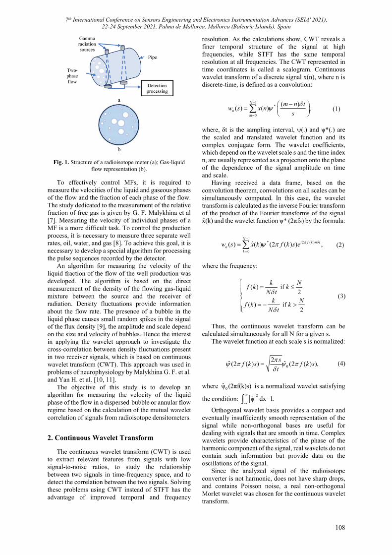
7th International Conference on Sensors Engineering and Electronics Instrumentation Advances (SEIA' 2021), 22-24 September 2021, Palma de Mallorca, Mallorca (Balearic Islands), Spain
108
a
b
Fig. 1. Structure of a radioisotope meter (a); Gas-liquid
flow representation (b).
To effectively control MFs, it is required to measure the velocities of the liquid and gaseous phases of the flow and the fraction of each phase of the flow. The study dedicated to the measurement of the relative fraction of free gas is given by G. F. Malykhina et al [7]. Measuring the velocity of individual phases of a MF is a more difficult task. To control the production process, it is necessary to measure three separate well rates, oil, water, and gas [8]. To achieve this goal, it is necessary to develop a special algorithm for processing the pulse sequences recorded by the detector.
An algorithm for measuring the velocity of the liquid fraction of the flow of the well production was developed. The algorithm is based on the direct measurement of the density of the flowing gas-liquid mixture between the source and the receiver of radiation. Density fluctuations provide information about the flow rate. The presence of a bubble in the liquid phase causes small random spikes in the signal of the flux density [9], the amplitude and scale depend on the size and velocity of bubbles. Hence the interest in applying the wavelet approach to investigate the cross-correlation between density fluctuations present in two receiver signals, which is based on continuous wavelet transform (CWT). This approach was used in problems of neurophysiology by Malykhina G. F. et al. and Yan H. et al. [10, 11].
The objective of this study is to develop an algorithm for measuring the velocity of the liquid phase of the flow in a dispersed-bubble or annular flow regime based on the calculation of the mutual wavelet correlation of signals from radioisotope densitometers.
2. Continuous Wavelet Transform
The continuous wavelet transform (CWT) is used to extract relevant features from signals with low signal-to-noise ratios, to study the relationship between two signals in time-frequency space, and to detect the correlation between the two signals. Solving these problems using CWT instead of STFT has the advantage of improved temporal and frequency
resolution. As the calculations show, CWT reveals a finer temporal structure of the signal at high frequencies, while STFT has the same temporal resolution at all frequencies. The CWT represented in time coordinates is called a scalogram. Continuous wavelet transform of a discrete signal x(n), where n is discrete-time, is defined as a convolution:
(1)
where, δt is the sampling interval, ψ(.) and ψ*(.) are the scaled and translated wavelet function and its complex conjugate form. The wavelet coefficients, which depend on the wavelet scale s and the time index n, are usually represented as a projection onto the plane of the dependence of the signal amplitude on time and scale.
Having received a data frame, based on the convolution theorem, convolutions on all scales can be simultaneously computed. In this case, the wavelet transform is calculated as the inverse Fourier transform of the product of the Fourier transforms of the signal x(k) and the wavelet function ψ* (2πfs) by the formula:
(2)
where the frequency:
( ) if 2
( ) if 2
k Nf k k
N tk N
f k kN t
(3)
Thus, the continuous wavelet transform can be
calculated simultaneously for all N for a given s. The wavelet function at each scale s is normalized:
0
2ˆ ˆ(2 ( ) ) (2 ( ) ),
sf k s f k s
t
(4)
where 0ψ (2πf(k)s) is a normalized wavelet satisfying
the condition: 2
-ψ dx=1.
Orthogonal wavelet basis provides a compact and eventually insufficiently smooth representation of the signal while non-orthogonal bases are useful for dealing with signals that are smooth in time. Complex wavelets provide characteristics of the phase of the harmonic component of the signal, real wavelets do not contain such information but provide data on the oscillations of the signal.
Since the analyzed signal of the radioisotope converter is not harmonic, does not have sharp drops, and contains Poisson noise, a real non-orthogonal Morlet wavelet was chosen for the continuous wavelet transform.
1*
0
( )( ) ( ) ,
N
nm
m n tw s x n
s
1* 2 ( )
0
ˆ( ) ( ) (2 ( ) ) ,N
i f k n tn
k
w s x k f k s e

7th International Conference on Sensors Engineering and Electronics Instrumentation Advances (SEIA' 2021), 22-24 September 2021, Palma de Mallorca, Mallorca (Balearic Islands), Spain
109
An arbitrary set of scales was used for the CWT scale to obtain a more complete representation. The scales are determined based on the number of samples N:
12
0
j= j log ,t
Ns
(5)
where, s0 is the smallest scale, j is the large scale j ≅ 2 δt. The value of δj depends on the width of the spectrum of the wavelet function. The value δt = 20 ms, s0, = 2 δt, N = 512, δj = 0.125. 3. Accuracy of Wavelet Coefficients Estimation
The normalized Fourier power spectrum is
given by:
2
2
ˆ( ),
2
N x k
(6)
Where N is the number of points, σ^2 is the
variance of the time series, x(n) is a normally distributed random variable, then both the real and imaginary parts of x(k) are usually normally
distributed. Since the square normally distributed variable has a chi-squared distribution with one degree of freedom when using real wavelets and with two degrees of freedom when using complex wavelets.
The local wavelet spectrum follows the average Fourier spectrum, if the original signals are normally distributed, then the wavelet coefficients are also usually normally distributed. The corresponding distribution for the power spectrum of the local wavelet is:
2
2
( )nw s
(7)
At time n on a scale of s has the distribution P(s)
x12 for real wavelets, P(s) is the average value of the spectrum at the scale s.
As with Fourier analysis, power spectrum wavelet smoothing can be used to increase the depth of field and increase confidence in regions of significant power. Unlike Fourier, anti-aliasing can be performed in either the time or scale domain. 4. Time and Scale Smoothing
Time smoothing is determined by the formula:
2
22
1
1( ) ( ) ,
n
n nn navg
w s w sn
(8)
where the length of the smoothing window is
2 1 1avgn n n (9)
By smoothing the wavelet spectrum, the degree of freedom of each point and the importance of the peaks in the power of the wavelet can be increased. By smoothing over all time samples, the global spectrum can be obtained as:
1
22
0
1( ) ( )
N
n nn
w s w sN
(10)
Smoothing at scales to study the power fluctuations
in the sub-bands of the scale, the average wavelet power at the scale can be defined as the weighted sum of the wavelet
Power spectrum on scales from s1 to s2:
22
2
1
( )( )
jn j
nj j j
w sj tw s
c s
(11)
Cross-correlation using the continuous wavelet
transform with a consideration of methods for estimating cross-correlation in a continuous wavelet region. This approach is used for the estimation of the double correlation function of the signals, which is calculated in terms of time and scale. Several variants of cross-correlation estimations can be used, including Pearson's linear correlation coefficient, Kendall's coefficient, and Spearman's coefficient.
For the continuous wavelet transform, the Morlet wavelet is used, which is a harmonic signal with a Gaussian window:
21
2 CBB
xx exp j F x exp
FF
(12)
The wavelet coefficients wx(a, b) of the signals x(n)
and y(n) are calculated using the continuous wavelet transform formula:
1
, ,N
x n
n btw a b x n t
s a
(13)
1
, ,N
y n
n btw a b y n t
s a
(14)
where Δt is the time step, b is the wavelet offset parameter, a is the wavelet scale parameter.
5. Correlation Estimation Methods
Pearson's linear correlation coefficient is the most commonly used linear correlation coefficient. For column xa in matrix X and column yb in matrix Y, the mean is:
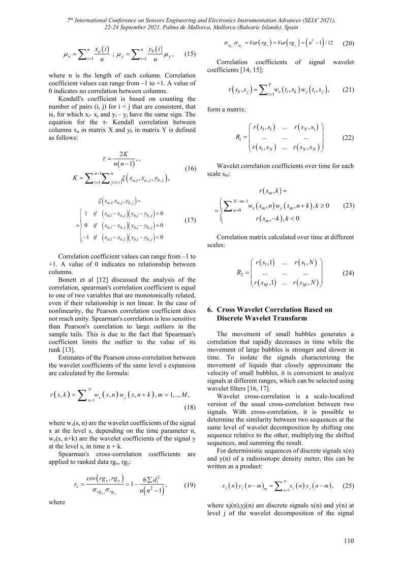
7th International Conference on Sensors Engineering and Electronics Instrumentation Advances (SEIA' 2021), 22-24 September 2021, Palma de Mallorca, Mallorca (Balearic Islands), Spain
110
1 1, ;
n na byix yi
x i y i
n n
(15)
where n is the length of each column. Correlation coefficient values can range from –1 to +1. A value of 0 indicates no correlation between columns.
Kendall's coefficient is based on counting the number of pairs (i, j) for i < j that are consistent, that is, for which xi- xj and yi – yj have the same sign. The equation for the τ- Kendall correlation between columns xa in matrix X and yb in matrix Y is defined as follows:
2
,1
K
n n
,
1
, , ,1 1, , ,
n n
a i a j b ji j iK x x y
(16)
, , ,
, , , ,
, , , ,
, , , ,
, ,
1 0
0 0
1 0
a i a j b j
a i a j b i b j
a i a j b i b j
a i a j b i b j
x x y
if x x y y
if x x y y
if x x y y
(17)
Correlation coefficient values can range from –1 to
+1. A value of 0 indicates no relationship between columns.
Bonett et al [12] discussed the analysis of the correlation, spearman's correlation coefficient is equal to one of two variables that are monotonically related, even if their relationship is not linear. In the case of nonlinearity, the Pearson correlation coefficient does not reach unity. Spearman's correlation is less sensitive than Pearson's correlation to large outliers in the sample tails. This is due to the fact that Spearman's coefficient limits the outlier to the value of its rank [13].
Estimates of the Pearson cross-correlation between the wavelet coefficients of the same level s expansion are calculated by the formula:
1
, , , , 1, .., ,N
x yn
r s k w s n w s n k m M
(18) where wx(s, n) are the wavelet coefficients of the signal x at the level s, depending on the time parameter n, wy(s, n+k) are the wavelet coefficients of the signal y at the level s, in time n + k.
Spearman's cross-correlation coefficients are applied to ranked data rgx, rgy:
2
2,
, 61 ,
1x y
x y is
rg rg
cov rg rg dr
n n
(19)
where
2
, 1 / 12x y
rg rg x yVar rg Var rg n (20)
Correlation coefficients of signal wavelet
coefficients [14, 15]:
1
, , , ,T
k j x i k y i jir s s w t s w t s
(21)
form a matrix:
1 1 1
1
1
, ... ,
... ... ...
, ... ,
N
N N N
r s s r s s
R
r s s r s s
(22)
Wavelet correlation coefficients over time for each
scale sm:
1
0
,
, , , 0
, , 0
m
N m
x m y mn
m
r s k
w s n w s n k k
r s k k
(23)
Correlation matrix calculated over time at different
scales:
1 1
2
,1 ... ,
... ... ...
,1 ... ,M M
r s r s N
R
r s r s N
(24)
6. Cross Wavelet Correlation Based on
Discrete Wavelet Transform
The movement of small bubbles generates a correlation that rapidly decreases in time while the movement of large bubbles is stronger and slower in time. To isolate the signals characterizing the movement of liquids that closely approximate the velocity of small bubbles, it is convenient to analyze signals at different ranges, which can be selected using wavelet filters [16, 17].
Wavelet cross-correlation is a scale-localized version of the usual cross-correlation between two signals. With cross-correlation, it is possible to determine the similarity between two sequences at the same level of wavelet decomposition by shifting one sequence relative to the other, multiplying the shifted sequences, and summing the result.
For deterministic sequences of discrete signals x(n) and y(n) of a radioisotope density meter, this can be written as a product:
1,
N
j j j jm nx n y n m x n y n m
(25)
where xj(n),yj(n) are discrete signals x(n) and y(n) at level j of the wavelet decomposition of the signal
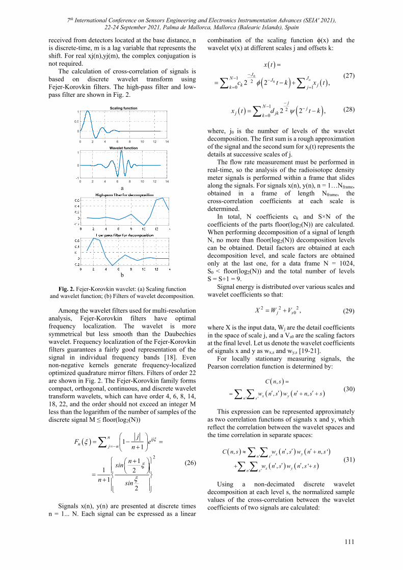
7th International Conference on Sensors Engineering and Electronics Instrumentation Advances (SEIA' 2021), 22-24 September 2021, Palma de Mallorca, Mallorca (Balearic Islands), Spain
111
received from detectors located at the base distance, n is discrete-time, m is a lag variable that represents the shift. For real xj(n),yj(m), the complex conjugation is not required.
The calculation of cross-correlation of signals is based on discrete wavelet transform using Fejer-Korovkin filters. The high-pass filter and low-pass filter are shown in Fig. 2.
a
b
Fig. 2. Fejer-Korovkin wavelet: (a) Scaling function
and wavelet function; (b) Filters of wavelet decomposition.
Among the wavelet filters used for multi-resolution analysis, Fejer-Korovkin filters have optimal frequency localization. The wavelet is more symmetrical but less smooth than the Daubechies wavelet. Frequency localization of the Fejer-Korovkin filters guarantees a fairly good representation of the signal in individual frequency bands [18]. Even non-negative kernels generate frequency-localized optimized quadrature mirror filters. Filters of order 22 are shown in Fig. 2. The Fejer-Korovkin family forms compact, orthogonal, continuous, and discrete wavelet transform wavelets, which can have order 4, 6, 8, 14, 18, 22, and the order should not exceed an integer M less than the logarithm of the number of samples of the discrete signal M ≤ floor(log2(N))
2
11
11 2
12
n ijn j n
jF e
n
nsin
n sin
(26)
Signals x(n), y(n) are presented at discrete times
n = 1... N. Each signal can be expressed as a linear
combination of the scaling function ϕ(x) and the wavelet ψ(x) at different scales j and offsets k:
0
01
20 1
2 2 ,o
JN JJ
k jk j
x t
c t k x t
(27)
12
02 2 ,
jN j
j jkkx t d t k
(28)
where, j0 is the number of levels of the wavelet decomposition. The first sum is a rough approximation of the signal and the second sum for xj(t) represents the details at successive scales of j.
The flow rate measurement must be performed in real-time, so the analysis of the radioisotope density meter signals is performed within a frame that slides along the signals. For signals x(n), y(n), n = 1…Nframe, obtained in a frame of length Nframe, the cross-correlation coefficients at each scale is determined.
In total, N coefficients ck and S×N of the coefficients of the parts floor(log2(N)) are calculated. When performing decomposition of a signal of length N, no more than floor(log2(N)) decomposition levels can be obtained. Detail factors are obtained at each decomposition level, and scale factors are obtained only at the last one, for a data frame N = 1024, S0 < floor(log2(N)) and the total number of levels S = S+1 = 9.
Signal energy is distributed over various scales and wavelet coefficients so that:
2 2 20 ,j sX W V (29)
where X is the input data, Wj are the detail coefficients in the space of scale j, and а Vs0 are the scaling factors at the final level. Let us denote the wavelet coefficients of signals x and y as wx,s and wy,s [19-21].
For locally stationary measuring signals, the Pearson correlation function is determined by:
' '
,
, ,x yn s
С n s
w n s w n n s s
(30)
This expression can be represented approximately as two correlation functions of signals x and y, which reflect the correlation between the wavelet spaces and the time correlation in separate spaces:
' '
' '
, , , '
, , '
x yn s
x yn s
С n s w n s w n n s
w n s w n s s
(31)
Using a non-decimated discrete wavelet decomposition at each level s, the normalized sample values of the cross-correlation between the wavelet coefficients of two signals are calculated:
0 2 4 6 8 10 12 14
0
0.5
1Scaling function
0 2 4 6 8 10 12 14-1
0
1
Wavelet function
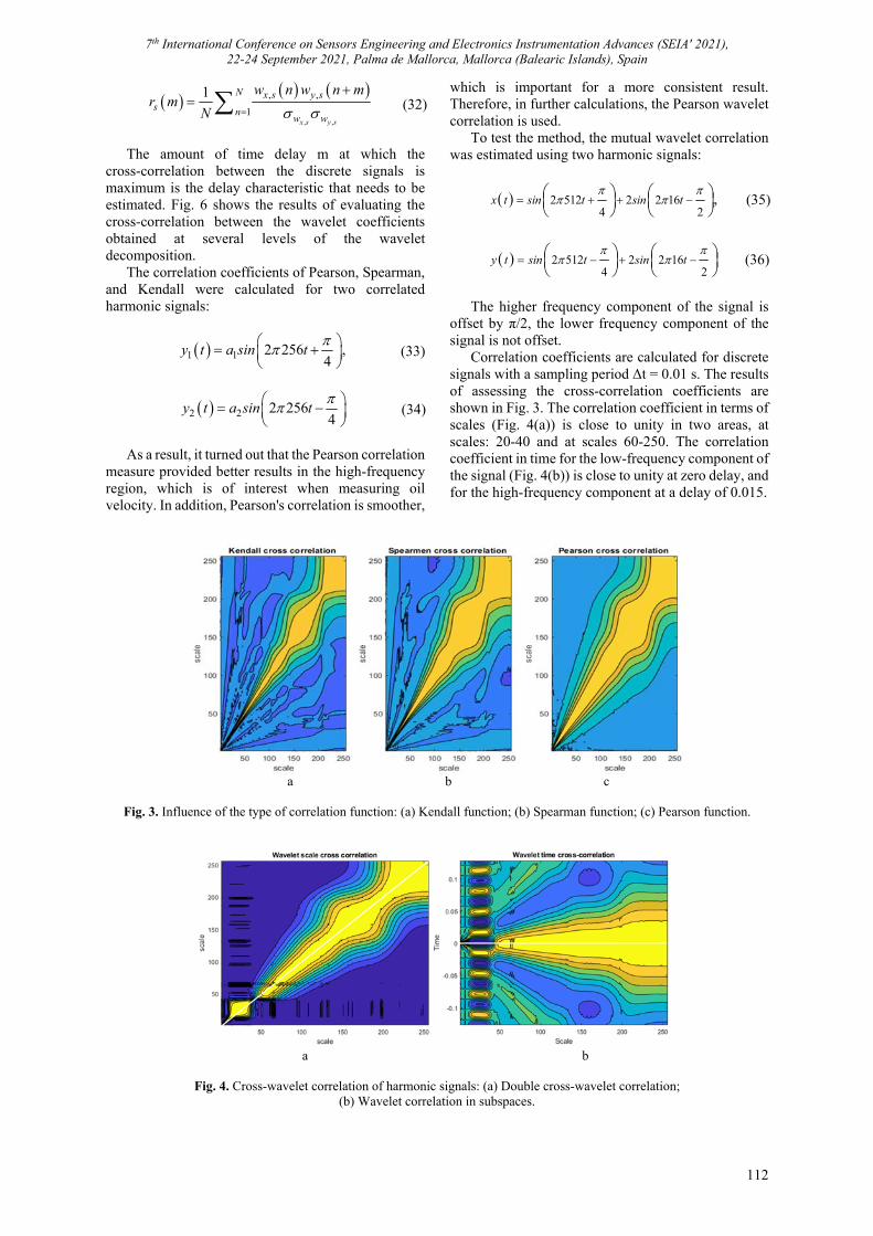
7th International Conference on Sensors Engineering and Electronics Instrumentation Advances (SEIA' 2021), 22-24 September 2021, Palma de Mallorca, Mallorca (Balearic Islands), Spain
112
, ,
, ,
1
1
x s y s
N x s y ss n
w w
w n w n mr m
N
(32)
The amount of time delay m at which the
cross-correlation between the discrete signals is maximum is the delay characteristic that needs to be estimated. Fig. 6 shows the results of evaluating the cross-correlation between the wavelet coefficients obtained at several levels of the wavelet decomposition.
The correlation coefficients of Pearson, Spearman, and Kendall were calculated for two correlated harmonic signals:
1 1 2 256 ,
4y t a sin t
(33)
2 2 2 2564
y t a sin t
(34)
As a result, it turned out that the Pearson correlation
measure provided better results in the high-frequency region, which is of interest when measuring oil velocity. In addition, Pearson's correlation is smoother,
which is important for a more consistent result. Therefore, in further calculations, the Pearson wavelet correlation is used.
To test the method, the mutual wavelet correlation was estimated using two harmonic signals:
2 512 2 2 164 2
,x t sin t sin t
(35)
2 512 2 2 164 2
y t sin t sin t
(36)
The higher frequency component of the signal is
offset by π/2, the lower frequency component of the signal is not offset.
Correlation coefficients are calculated for discrete signals with a sampling period Δt = 0.01 s. The results of assessing the cross-correlation coefficients are shown in Fig. 3. The correlation coefficient in terms of scales (Fig. 4(a)) is close to unity in two areas, at scales: 20-40 and at scales 60-250. The correlation coefficient in time for the low-frequency component of the signal (Fig. 4(b)) is close to unity at zero delay, and for the high-frequency component at a delay of 0.015.
a b c
Fig. 3. Influence of the type of correlation function: (a) Kendall function; (b) Spearman function; (c) Pearson function.
a b
Fig. 4. Cross-wavelet correlation of harmonic signals: (a) Double cross-wavelet correlation;
(b) Wavelet correlation in subspaces.
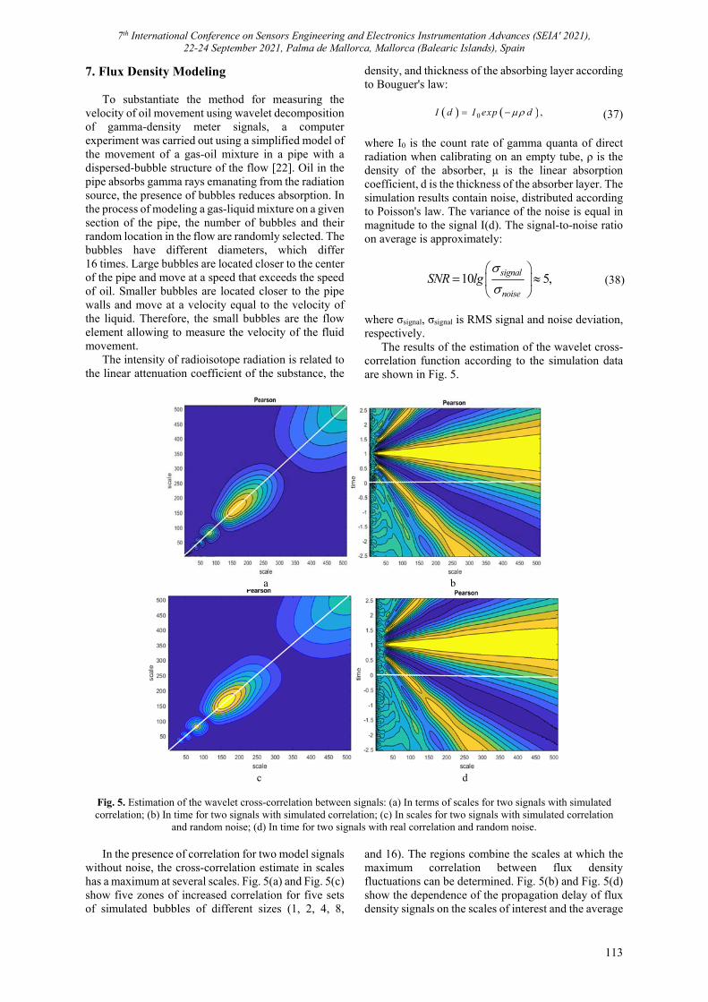
7th International Conference on Sensors Engineering and Electronics Instrumentation Advances (SEIA' 2021), 22-24 September 2021, Palma de Mallorca, Mallorca (Balearic Islands), Spain
113
7. Flux Density Modeling To substantiate the method for measuring the
velocity of oil movement using wavelet decomposition of gamma-density meter signals, a computer experiment was carried out using a simplified model of the movement of a gas-oil mixture in a pipe with a dispersed-bubble structure of the flow [22]. Oil in the pipe absorbs gamma rays emanating from the radiation source, the presence of bubbles reduces absorption. In the process of modeling a gas-liquid mixture on a given section of the pipe, the number of bubbles and their random location in the flow are randomly selected. The bubbles have different diameters, which differ 16 times. Large bubbles are located closer to the center of the pipe and move at a speed that exceeds the speed of oil. Smaller bubbles are located closer to the pipe walls and move at a velocity equal to the velocity of the liquid. Therefore, the small bubbles are the flow element allowing to measure the velocity of the fluid movement.
The intensity of radioisotope radiation is related to the linear attenuation coefficient of the substance, the
density, and thickness of the absorbing layer according to Bouguer's law:
0 ,I d I exp d (37)
where I0 is the count rate of gamma quanta of direct radiation when calibrating on an empty tube, ρ is the density of the absorber, μ is the linear absorption coefficient, d is the thickness of the absorber layer. The simulation results contain noise, distributed according to Poisson's law. The variance of the noise is equal in magnitude to the signal I(d). The signal-to-noise ratio on average is approximately:
10 5,
signal
noise
SNR lg
(38)
where σsignal, σsignal is RMS signal and noise deviation, respectively.
The results of the estimation of the wavelet cross-correlation function according to the simulation data are shown in Fig. 5.
a b
c d
Fig. 5. Estimation of the wavelet cross-correlation between signals: (a) In terms of scales for two signals with simulated correlation; (b) In time for two signals with simulated correlation; (c) In scales for two signals with simulated correlation
and random noise; (d) In time for two signals with real correlation and random noise.
In the presence of correlation for two model signals without noise, the cross-correlation estimate in scales has a maximum at several scales. Fig. 5(a) and Fig. 5(c) show five zones of increased correlation for five sets of simulated bubbles of different sizes (1, 2, 4, 8,
and 16). The regions combine the scales at which the maximum correlation between flux density fluctuations can be determined. Fig. 5(b) and Fig. 5(d) show the dependence of the propagation delay of flux density signals on the scales of interest and the average
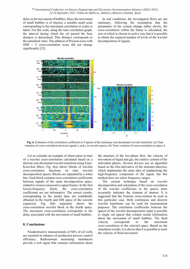
7th International Conference on Sensors Engineering and Electronics Instrumentation Advances (SEIA' 2021), 22-24 September 2021, Palma de Mallorca, Mallorca (Balearic Islands), Spain
114
delay in the movement of bubbles. Since the movement of small bubbles is of interest, a suitable small scale corresponding to the maximum correlation in scales is taken. For this scale, using the time correlation graph, the interval during which the oil passed the base distance is determined. This distance corresponds to the simulated value. The addition of Poisson noise with SNR = 5 cross-correlation score did not change significantly [23].
In real conditions, the investigated flows are not stationary, following the assumption that the parameters of the system change rather slowly, the cross-correlation within the frame is calculated, the size of which is chosen in such a way that it is possible to obtain the required number of levels of the wavelet decomposition of signals.
a b
Fig. 6. Estimates of the correlation coefficient in 9 spaces of the stationary non-decimated wavelet transform: (a) Time
variation of cross-correlation between signals x and y in wavelet spaces, (b) Time variation of cross-correlation in space 4.
Let us consider an example of observation in time of a wavelet cross-correlation calculated based on a discrete non-decimated wavelet transform using Fejer-Korovkin filters. Fig. 6(a) shows blocks of wavelet cross-correlation functions on nine wavelet decomposition spaces. Blocks are separated by a white line. Each block contains cross-correlation coefficients between signals of the same decomposition space, related to sixteen consecutive signal frames. In the first lowest-frequency block, the cross-correlation coefficients are not informative. The correct results, corresponding to the model data, are confidently obtained in the fourth and fifth space of the wavelet expansion. Fig. 6(b) separately shows the cross-correlation wavelet block in the fourth space. The maximum cross-correlation corresponds to the delay associated with the movement of small bubbles.
8. Conclusions
Nondestructive measurements of MFs of oil wells are essential to enhance oil production process control efficiency. Radioisotope measuring transducers provide a rich signal that contains information about
the structure of the two-phase flow, the velocity of movement of liquid and gas, the relative content of the individual phases. Several devices use an algorithm based on the first derivative of the structure-function, which implements the same idea of emphasizing the high-frequency component of the signal, but this method does not select frequency ranges.
The current technique based on wavelet decomposition and calculation of the cross-correlation of the wavelet coefficients in the spaces more accurately indicates the element of interest. It is suggested that the Pearson cross-relation be used in this particular case. Both continuous and discrete wavelet transforms can be used for measurement purposes. The correlation coefficients between the spaces of the wavelet decomposition make it possible to single out spaces that contain useful information about the movement of small bubbles. The fluid velocity corresponds to the maximum cross-correlation in the selected space. Based on the simulation results, it is shown that it is possible to track the velocity of fluid movement.

7th International Conference on Sensors Engineering and Electronics Instrumentation Advances (SEIA' 2021), 22-24 September 2021, Palma de Mallorca, Mallorca (Balearic Islands), Spain
115
Acknowledgements
The research is partially funded by the Ministry of Science and Higher Education of the Russian Federation as part of World-class Research Center program: Advanced Digital Technologies (contract No. 075-15-2020-934 dated 17.11.2020). References [1]. E. A. Mus, E. D. Toskey, S. J. F. Bascoul, E. C. Barber,
Development well testing enhancement using a multiphase flowmeter, in Proceedings of the SPE Annual Technical Conference and Exhibition, San Antonio, Texas, 2002, p. SPE-77769-MS.
[2]. C. Poelma, Measurement in opaque flows: a review of measurement techniques for dispersed multiphase flows, Acta Mechanica, Vol. 231, Issue 6, 2020, pp. 2089-2111.
[3]. L. Dong-hui, W. Ying-Xiang, L. Zhi-Biao, Z. Xing-Fu, Volumetric fraction measurement in oil-water-gas multiphase flow with dual energy gamma-ray system, Journal of Zhejiang University-SCIENCE A, Vol. 6, Issue 12, 2005, pp. 1405-1411.
[4]. K. I. Pozdev, S. A. Vershinin, O. S. Vernikovskaya, Oil and gas condensate fields. A systematic approach to multiphase flow control, Professionally about Oil, Vol. 4, Issue 6, 2017, pp. 59-63 (in Russian).
[5]. A. G. Grechko, A. I. Novikov, Review of underwater multi-phase flow meters, Gas Industry, Issue 1, pp. 71-74 (in Russian).
[6]. E. Toschi, E. Okugbaite, B. Teuveni, B. W. Hanssen, G. Smith, Evolution of multiphase flow measurements and their impact on operations management, Oil and Gas Review, 2003, pp. 69-77 (in Russian).
[7]. G. F. Malykhina, L. Zarour, D. A. Tarkhov, Measurement of the volume of gaseous and liquid fraction of the flow of oil wells, in Proceedings of the International Multi-Conference on Industrial Engineering and Modern Technologies (FarEastCon’20), 2020, pp. 1-5.
[8]. E. Khamehchi, M. Zolfagharroshan, M. R. Mahdiani, A robust method for estimating the two-phase flow rate of oil and gas using wellhead data, Journal of Petroleum Exploration and Production Technology, Vol. 10, Issue 6, 2020, pp. 2335-2347.
[9]. M. A. El-Moniem, A. H. El-Banbi, Effects of production, PVT and pipe roughness on multiphase flow correlations in gas wells, Journal of Petroleum Exploration and Production Technology, Vol. 10, Issue 7, 2020, pp. 2969-2988.
[10]. G. F. Malykhina, V. B. Semenyutin, D. A. Tarkhov, Digitalization of medical services for the detection of
cerebrovascular regulation based on signal coherence analysis, ACM, 2021 (in Russian).
[11]. H. Yan, Y. Zhang, Q. Yang, Time-delay estimation based on cross-correlation and wavelet denoising, in Proceedings of the Chinese Intelligent Automation Conference (CIAC’13), 2013, pp. 841-848.
[12]. D. G. Bonett, T. A. Wright, Sample size requirements for estimating Pearson, Kendall and Spearman correlations, Psychometrika, Vol. 65, Issue 1, 2000, pp. 23-28.
[13]. D. Rasch, Book review: Gibbons, J. D.: Nonparametric Statistical Inference 2nd Ed. Statistics: Textbooks and monographs Vol. 65. Marcel Dekker, Inc., New York and Basel, 1985, XV, 408 S, Biometrical Journal, Vol. 28, Issue 8, 1986, pp. 936-936.
[14]. C. V. Bozhokin, S. V. Zharko, N. V. Larionov, A. N. Litvinov, I. M. Sokolov, Wavelet correlation of non-stationary signals, Journal of Technical Physics, Vol. 87, Issue 6, 2017, pp. 822-830 (in Russian),
[15]. D. Maraun, J. Kurths, M. Holschneider, Nonstationary Gaussian processes in wavelet domain: Synthesis, estimation, and significance testing, Physical Review E, Vol. 75, Issue 1, 2007, 016707.
[16]. Y. Zhao, R. C. Laguna, Y. Zhao, et al., A wavelet-based correlation analysis framework to study cerebromuscular activity in essential tremor, Complexity, Vol. 2018, 2018, pp. 1-15.
[17]. T. D. Pering, G. Tamburello, A. J. S. McGonigle, E. Hanna, A. Aiuppa, Correlation of oscillatory behaviour in MATLAB using wavelets, Computers & Geosciences, Vol. 70, 2014, pp. 206-212.
[18]. M. Nielsen, On the construction and frequency localization of finite orthogonal quadrature filters, Journal of Approximation Theory, Vol. 108, Issue 1, 2001, pp. 36-52.
[19]. A. L. Goldberger, L. A. N. Amaral, L. Glass, et al., PhysioBank, PhysioToolkit, and PhysioNet: Components of a new research resource for complex physiologic signals, Circulation, Vol. 101, Issue 23, 2000, pp. E215-20.
[20]. G. B. Moody, Evaluating ECG Analyzers, http://www.physionet.org/physiotools/wfdb/doc/wag-src/eval0.tex
[21]. G. B. Moody, R. G. Mark, The impact of the MIT-BIH arrhythmia database, IEEE Engineering in Medicine and Biology Magazine, Vol. 20, Issue 3, 2001, pp. 45-50.
[22]. V. A. Vasiliev, T. A. Gunkina, A. O. Shesteren, Analysis of multi-phase flow forecasting methods, Oil-Field Business, Issue 2, 2016, pp. 11-15.
[23]. E. Souza, V. Félix, Wavelet cross-correlation in bivariate time-series analysis, TEMA (SÃO CARLOS), Vol. 19, 2018, pp. 391-403.
7th International Conference on Sensors Engineering and Electronics Instrumentation Advances (SEIA' 2021), 22-24 September 2021, Palma de Mallorca, Mallorca (Balearic Islands), Spain
116
(036)
A Small-scale Extensometer for Precise Strain Measurements of Thin Fibres with Millinewton Resolution
Ricardo Gridling, Alexander Spaett and Bernhard Zagar
1 Johannes Kepler University Linz, Institute for Measurement Technology, Altenberger Straße 69, 4040 Linz, Austria
Tel.: +43 732 2468 5920 E-mail: [email protected]
Summary: Thin fibres are very versatile components with outstanding mechanical characteristics. Therefore, there is great interest in the characterization of these properties. The strain measurement can only be realised contactless, as strain gauges or similar methods cannot be applied. We propose a precise, yet simple, small-scale and cost-effective strain-measurement approach. Forces in the Newton range with millinewton resolution can be applied, which is hardly achievable by conventional methods, such as load cells. A brushless permanent magnet motor drive is used for force application, due to its reliable and repeatable torque vs. current ratio. An approach is presented to perform the motor characterization, necessary for precise measurements, using a conventional precision balance. It is shown that a repeatability of less than 1.2 percent of the actual reading can be achieved with a rather simple and cost-effective measurement setup. Possible fields of application are cost-effective substitution of conventional micro tensile testing machines and direct integration in devices. Keywords: Micro extensometer, Force actuator, Fibre characterization, Brushless DC motor application, Motor characterization, Millinewton resolution.
1. Introduction
Thin fibres are omnipresent in nature and in daily life in a wide variety of areas. We encounter them in our hair, our clothing, in the fibre-reinforced parts of bicycles and other vehicles that take us to work, just to name a few examples.
Depending on type of fibre and its application, fibres are the versatile basis for soft and supple clothing, but also for reinforced mechanical components, which are among the materials with the highest stiffness-to-weight and strength-to-weight ratio [1, 2]. These interesting mechanical properties are essentially due to the shape of the fibre, as they are very long in relation to their thickness. Materials in fibre form often have significantly higher strength values than in their bulk form, which is, among other things, explained by the so-called size effect: The number of strength-reducing defects is statistically proportional to the volume; therefore, fibres can reach much higher strength properties than solid shapes of the same material [3].
Due to the versatility of fibres, it is of great interest to many industries to determine their mechanical properties, such as tensile strength, elastic modulus, etc., for structural, but also for cosmetic, textile and many other applications. Many fibrous materials have already intensively been studied, see e.g. [1] for an overview.
Testing of single fibres is often done with expensive, conventional tensile testing machines, e.g. [4], although this method is prone to measurement uncertainties. Most commercially available load cells, on the one hand, are oversized for testing fibres and therefore operated at only a fraction of their measurement range. On the other hand, suitable small
force load cells are very sensitive to ambient disturbance, e.g., blast and shock. Furthermore, they are very miniature and therefore difficult to handle.
Several other methods have been developed to obtain the mechanical properties of fibres, e.g. [5, 6]. There are also commercial solutions available for fibre testing, with superior force resolution, see [7] and [8]. All these techniques have in common to apply a strain to the probe and measure the force. This approach is called strain controlled tensile testing. However, it is often difficult to accurately determine the mechanical strain within a fibre, as strain gauges or similar methods cannot be applied to such thin objects. Usually, the strain is derived from the crosshead displacement, ignoring the slip of the probe in the grippers and other perturbances, which can severely limit the significance of the measurement.
To address these problems our current research covers optical strain measurement of thin fibres. In a parallel submitted paper we present an optical strain measurement system based on laser speckle correlation, which allows to measure strain within thin fibres in the diameter range of 2-50 µm without contact.
In order to support this approach, we present in this paper a possible robust direct force actuator principle with a high dynamic range that can be used in conjunction with the laser speckle strain measurement system. In this so-called load controlled tensile testing approach, the test force is imprinted directly and the resulting strain is the parameter to be measured. Additionally, the device should be a cost efficient, small-formatted, force actuator/observer for tensile testing of fibres. These features allow the actuator to be installed in existing systems.
7th International Conference on Sensors Engineering and Electronics Instrumentation Advances (SEIA' 2021), 22-24 September 2021, Palma de Mallorca, Mallorca (Balearic Islands), Spain
117
2. Operating Principle 2.1. Prerequisites Although fibres often have very high tensile strengths 𝜎 , their breaking force 𝐹
𝐹 𝜎 𝐴 𝜎 𝑑 𝜋/4, (1) still remains very low, since the cross Section 𝐴 with the diameter 𝑑 is minute. Even if a very high 𝜎 of 5000 MPa and 𝑑 = 50, 2 µm is assumed, the breaking force is less than 10, 0.016 N. Especially if a resolution of at least 1/100 of the measuring range is required, this large dynamic range of 1 to 105, which covers all typical diameters, can only be achieved with special production load cells.
Another problem with measuring forces via strain is the sensitivity to shocks of all kinds. Since the required forces are in the millinewton range, even a breath of wind or a passing truck on the street will lead to significant disturbances in the measurement results.
To counter these problems, the force is not measured but applied directly by means of an electromechanical energy conversion principle. 2.2. Possible Principles of Action
A very popular principle of action in micropositioning drives are piezoelectric actuators. However, these drives are prone to hysteresis errors up to 15 %, although several compensation algorithms exist [9]. In addition, these actuators often have only a small travel range, which can limit the measurements, as fibres stretch significantly.
Another method, often used in commercial products, is the use of high precision spindle drives, which is also a strain controlled approach. In this paper we take the opposite approach and imprint a force that leads to a strain, which we obtain by laser speckle displacement measurement. To do so, we make use of the electromechanical direct drive motor principle basing on the Lorentz force
𝐅 𝐼 𝐥 𝐁 , (2) which states, that a force 𝐅 proportional to the current 𝐼 acts on a current-carrying conductor of length 𝐥 subject to the magnetic field 𝐁, where bold letters indicate vectors. This principle is featured by its linear force vs. current dependency, resulting in a high force resolution if one can control the applied drive current over a large range. Fortunately, this is possible without any problems in the required range from microamperes to the low ampere range. 2.3. Application Structure
A promising option for this application are voice-coil actuators. Originally used in speakers, they
have become popular in drive applications where linearity, no hysteresis, fast acceleration and accurate control, etc., are a must [10]. However, commercially available voice coil actuators are often either positional actuators or just the actuator itself, without guiding or bearings, which means additional effort. Another unfavourable property is the fixed travel of linear voice coils, as the elongation of fibres differ considerably between different materials.
To overcome these drawbacks, a brushless permanent magnet motor drive, also brushless DC motor (BLDC) is used. From a theoretical point of view, this motor acts like a commutated version of a voice coil actuator, wound around a cylinder. The benefits are a wide variety of commercially available types with well-defined properties and unrestricted travel. The resulting mechanical quantity is now of course a torque. To apply the torque to the fibre, the fibre is wound around a reel attached to the motor shaft. Since the diameter of the reel is very large in relation to the fibre diameter, the influence of the curvature can be neglected in the most cases. 3. Motor Properties
BLDCs are basically multi-phase self-excited synchronous machines. In order to operate, these machines must be powered by a rotating electric field [11]. 3.1. Control Methods
To apply this rotating field, multiple control methods exist. The most established ones are Field Oriented Control (FOC) and Block Commutation [11].
With FOC, a sinusoidal current is applied to the motor phases in such a way, that it acts like a four-quadrant inverter driven DC motor in terms of dynamic performance [12]. However, this method requires considerable computational effort and continuous measurement of the motor characteristics, e.g., exact rotor position and phase currents.
Another, very simple approach to drive BLDCs with DC supply is block commutation [11], which lets the motor act like a conventional DC motor with the linear torque to current relationship
𝑀 𝑘 𝜗, 𝜑, 𝐼 𝐼, (3) where 𝑀, again, is the generated torque, 𝑘 is the torque constant, which – in real applications – depends on the temperature 𝜗, the rotor angle 𝜑 and, considering non-ideal properties, on the applied current 𝐼. To address these non-ideal properties with a feed-forward-correction, the motor must be extensively characterized. 3.2. Torque vs. Rotor Angle Relationship
A fact that cannot be neglected is the influence of the magnetisation of the permanent magnet and the winding design of the armature winding in connection
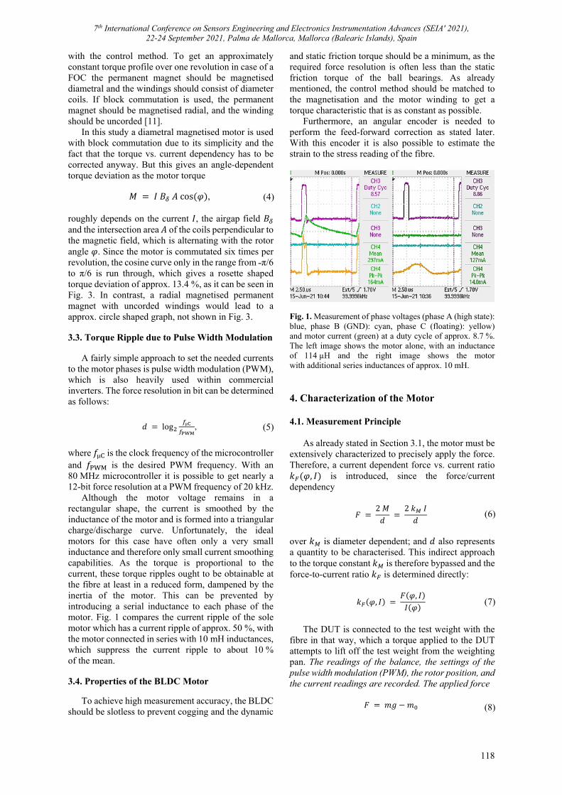
7th International Conference on Sensors Engineering and Electronics Instrumentation Advances (SEIA' 2021), 22-24 September 2021, Palma de Mallorca, Mallorca (Balearic Islands), Spain
118
with the control method. To get an approximately constant torque profile over one revolution in case of a FOC the permanent magnet should be magnetised diametral and the windings should consist of diameter coils. If block commutation is used, the permanent magnet should be magnetised radial, and the winding should be uncorded [11].
In this study a diametral magnetised motor is used with block commutation due to its simplicity and the fact that the torque vs. current dependency has to be corrected anyway. But this gives an angle-dependent torque deviation as the motor torque
𝑀 𝐼 𝐵 𝐴 cos 𝜑 , (4) roughly depends on the current 𝐼, the airgap field 𝐵 and the intersection area 𝐴 of the coils perpendicular to the magnetic field, which is alternating with the rotor angle 𝜑. Since the motor is commutated six times per revolution, the cosine curve only in the range from π/6 to π/6 is run through, which gives a rosette shaped torque deviation of approx. 13.4 %, as it can be seen in Fig. 3. In contrast, a radial magnetised permanent magnet with uncorded windings would lead to a approx. circle shaped graph, not shown in Fig. 3. 3.3. Torque Ripple due to Pulse Width Modulation
A fairly simple approach to set the needed currents to the motor phases is pulse width modulation (PWM), which is also heavily used within commercial inverters. The force resolution in bit can be determined as follows:
𝑑 log µ , (5)
where 𝑓µ is the clock frequency of the microcontroller and 𝑓 is the desired PWM frequency. With an 80 MHz microcontroller it is possible to get nearly a 12-bit force resolution at a PWM frequency of 20 kHz.
Although the motor voltage remains in a rectangular shape, the current is smoothed by the inductance of the motor and is formed into a triangular charge/discharge curve. Unfortunately, the ideal motors for this case have often only a very small inductance and therefore only small current smoothing capabilities. As the torque is proportional to the current, these torque ripples ought to be obtainable at the fibre at least in a reduced form, dampened by the inertia of the motor. This can be prevented by introducing a serial inductance to each phase of the motor. Fig. 1 compares the current ripple of the sole motor which has a current ripple of approx. 50 %, with the motor connected in series with 10 mH inductances, which suppress the current ripple to about 10 % of the mean. 3.4. Properties of the BLDC Motor
To achieve high measurement accuracy, the BLDC should be slotless to prevent cogging and the dynamic
and static friction torque should be a minimum, as the required force resolution is often less than the static friction torque of the ball bearings. As already mentioned, the control method should be matched to the magnetisation and the motor winding to get a torque characteristic that is as constant as possible.
Furthermore, an angular encoder is needed to perform the feed-forward correction as stated later. With this encoder it is also possible to estimate the strain to the stress reading of the fibre.
Fig. 1. Measurement of phase voltages (phase A (high state): blue, phase B (GND): cyan, phase C (floating): yellow) and motor current (green) at a duty cycle of approx. 8.7 %. The left image shows the motor alone, with an inductance of 114 µH and the right image shows the motor with additional series inductances of approx. 10 mH. 4. Characterization of the Motor 4.1. Measurement Principle
As already stated in Section 3.1, the motor must be extensively characterized to precisely apply the force. Therefore, a current dependent force vs. current ratio 𝑘 𝜑, 𝐼 is introduced, since the force/current dependency
𝐹2 𝑀
𝑑 2 𝑘 𝐼
𝑑 (6)
over 𝑘 is diameter dependent; and 𝑑 also represents a quantity to be characterised. This indirect approach to the torque constant 𝑘 is therefore bypassed and the force-to-current ratio 𝑘 is determined directly:
𝑘 𝜑, 𝐼𝐹 𝜑, 𝐼
𝐼 𝜑 (7)
The DUT is connected to the test weight with the
fibre in that way, which a torque applied to the DUT attempts to lift off the test weight from the weighting pan. The readings of the balance, the settings of the pulse width modulation (PWM), the rotor position, and the current readings are recorded. The applied force
𝐹 𝑚𝑔 𝑚 (8)
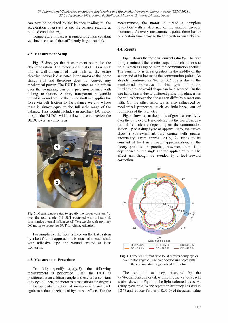
7th International Conference on Sensors Engineering and Electronics Instrumentation Advances (SEIA' 2021), 22-24 September 2021, Palma de Mallorca, Mallorca (Balearic Islands), Spain
119
can now be obtained by the balance reading 𝑚, the acceleration of gravity 𝑔 and the balance reading at no-load condition 𝑚 .
Temperature impact is assumed to remain constant vs. time because of the sufficiently large heat sink. 4.2. Measurement Setup
Fig. 2 displays the measurement setup for the characterization. The motor under test (DUT) is built into a well-dimensioned heat sink as the entire electrical power is dissipated in the motor as the motor stands still and therefore does not convey any mechanical power. The DUT is located on a platform over the weighting pan of a precision balance with 0.1 mg resolution. A thin, transparent polyamide thread is wound around the motor shaft and applies the force via belt friction to the balance weight, whose mass is almost equal to the full-scale range of the balance. This weight includes an auxiliary DC motor to spin the BLDC, which allows to characterize the BLDC over an entire turn.
Fig. 2. Measurement setup to specify the torque constant 𝑘 over the rotor angle. (1) DUT equipped with a heat sink to minimize thermal influence. (2) Test weight with auxiliary DC motor to rotate the DUT for characterization.
For simplicity, the fibre is fixed on the test system by a belt friction approach. It is attached to each shaft with adhesive tape and wound around at least two turns. 4.3. Measurement Procedure
To fully specify 𝑘 𝜑, 𝐼 , the following measurement is performed. First, the DUT is positioned at an arbitrary angle and excited a constant duty cycle. Then, the motor is turned about ten degrees in the opposite direction of measurement and back again to reduce mechanical hysteresis effects. For the
measurement, the motor is turned a complete revolution with a step size of the angular encoder increment. At every measurement point, there has to be a certain time delay so that the system can stabilize. 4.4. Results
Fig. 3 shows the force vs. current ratio 𝑘 . The first thing to notice is the rosette shape of the characteristic field, which is aligned with the commutation sectors. The sensitivity is at its greatest in the middle of the sector and at its lowest at the commutation points. As already mentioned in Section 3.2 this is due to the mechanical properties of this type of motor. Furthermore, an ovoid shape can be discerned. On the one hand, this is due to different phase impedances, as the values between the phases can differ by almost one fifth. On the other hand, 𝑘 is also influenced by mechanical properties, such as imbalance, out of roundness of the reel, etc.
Fig. 4 shows 𝑘 at the points of greatest sensitivity over the duty cycle. It is evident, that the force/current-ratio differs clearly depending on the commutation sector. Up to a duty cycle of approx. 20 %, the curves show a somewhat arbitrary course with greater uncertainty. From approx. 20 %, 𝑘 tends to be constant at least in a rough approximation, as the theory predicts. In practice, however, there is a dependence on the angle and the applied current. The effect can, though, be avoided by a feed-forward correction.
Fig. 3. Force vs. Current ratio 𝑘 at different duty cycles over motor angle 𝜑. The color-coded ring represents
the commutation segments of the motor.
The repetition accuracy, measured by the 95 %-confidence interval, with four observations each, is also shown in Fig. 4 as the light-coloured areas. At a duty cycle of 20 % the repetition accuracy lies within 1.2 % and reduces further to 0.55 % of the actual value
1
2
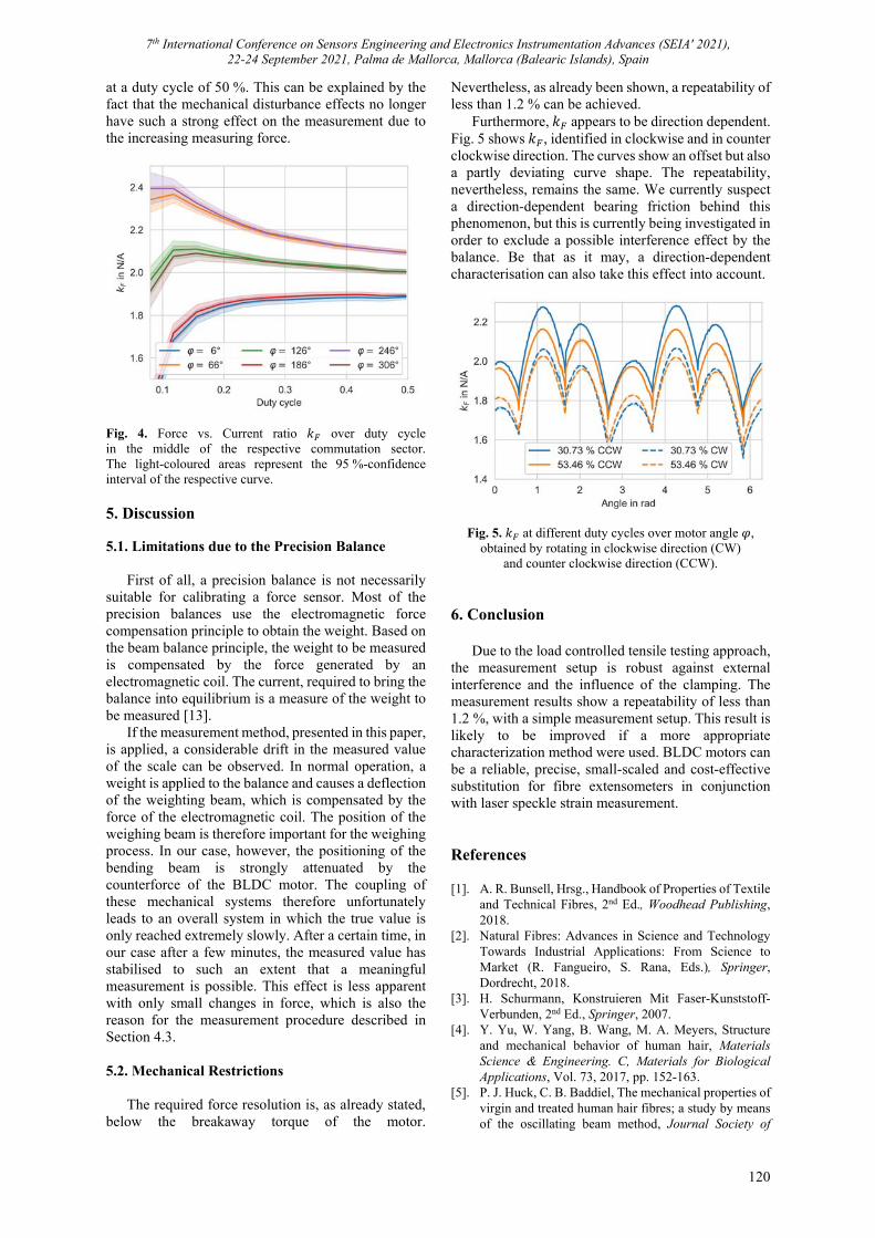
7th International Conference on Sensors Engineering and Electronics Instrumentation Advances (SEIA' 2021), 22-24 September 2021, Palma de Mallorca, Mallorca (Balearic Islands), Spain
120
at a duty cycle of 50 %. This can be explained by the fact that the mechanical disturbance effects no longer have such a strong effect on the measurement due to the increasing measuring force.
Fig. 4. Force vs. Current ratio 𝑘 over duty cycle in the middle of the respective commutation sector. The light-coloured areas represent the 95 %-confidence interval of the respective curve. 5. Discussion 5.1. Limitations due to the Precision Balance
First of all, a precision balance is not necessarily suitable for calibrating a force sensor. Most of the precision balances use the electromagnetic force compensation principle to obtain the weight. Based on the beam balance principle, the weight to be measured is compensated by the force generated by an electromagnetic coil. The current, required to bring the balance into equilibrium is a measure of the weight to be measured [13].
If the measurement method, presented in this paper, is applied, a considerable drift in the measured value of the scale can be observed. In normal operation, a weight is applied to the balance and causes a deflection of the weighting beam, which is compensated by the force of the electromagnetic coil. The position of the weighing beam is therefore important for the weighing process. In our case, however, the positioning of the bending beam is strongly attenuated by the counterforce of the BLDC motor. The coupling of these mechanical systems therefore unfortunately leads to an overall system in which the true value is only reached extremely slowly. After a certain time, in our case after a few minutes, the measured value has stabilised to such an extent that a meaningful measurement is possible. This effect is less apparent with only small changes in force, which is also the reason for the measurement procedure described in Section 4.3. 5.2. Mechanical Restrictions
The required force resolution is, as already stated, below the breakaway torque of the motor.
Nevertheless, as already been shown, a repeatability of less than 1.2 % can be achieved.
Furthermore, 𝑘 appears to be direction dependent. Fig. 5 shows 𝑘 , identified in clockwise and in counter clockwise direction. The curves show an offset but also a partly deviating curve shape. The repeatability, nevertheless, remains the same. We currently suspect a direction-dependent bearing friction behind this phenomenon, but this is currently being investigated in order to exclude a possible interference effect by the balance. Be that as it may, a direction-dependent characterisation can also take this effect into account.
Fig. 5. 𝑘 at different duty cycles over motor angle 𝜑, obtained by rotating in clockwise direction (CW)
and counter clockwise direction (CCW). 6. Conclusion
Due to the load controlled tensile testing approach, the measurement setup is robust against external interference and the influence of the clamping. The measurement results show a repeatability of less than 1.2 %, with a simple measurement setup. This result is likely to be improved if a more appropriate characterization method were used. BLDC motors can be a reliable, precise, small-scaled and cost-effective substitution for fibre extensometers in conjunction with laser speckle strain measurement. References [1]. A. R. Bunsell, Hrsg., Handbook of Properties of Textile
and Technical Fibres, 2nd Ed., Woodhead Publishing, 2018.
[2]. Natural Fibres: Advances in Science and Technology Towards Industrial Applications: From Science to Market (R. Fangueiro, S. Rana, Eds.), Springer, Dordrecht, 2018.
[3]. H. Schurmann, Konstruieren Mit Faser-Kunststoff-Verbunden, 2nd Ed., Springer, 2007.
[4]. Y. Yu, W. Yang, B. Wang, M. A. Meyers, Structure and mechanical behavior of human hair, Materials Science & Engineering. C, Materials for Biological Applications, Vol. 73, 2017, pp. 152-163.
[5]. P. J. Huck, C. B. Baddiel, The mechanical properties of virgin and treated human hair fibres; a study by means of the oscillating beam method, Journal Society of

7th International Conference on Sensors Engineering and Electronics Instrumentation Advances (SEIA' 2021), 22-24 September 2021, Palma de Mallorca, Mallorca (Balearic Islands), Spain
121
Cosmetic Chemists of Great Britain, Vol. 22, 1971, pp. 401-410.
[6]. A. R. Bunsell, J. W. S. Hearle, R. D. Hunter, An apparatus for fatigue-testing of fibres, Journal of Physics E: Scientific Instruments, Vol. 4, Issue 11, 1971, pp. 868-872.
[7]. Textechno – Textile testing technology, https://www.textechno.com/
[8]. Dia-Stron, https://www.diastron.com [9]. W. T. Ang, et al., Modeling rate-dependent hysteresis
in piezoelectric actuators, in Proceedings of the IEEE/RSJ International Conference on Intelligent Robots and Systems (IROS’03), Vol. 2, 2003, pp. 1975-1980.
[10]. X. M. Feng, et al., The technology and application of voice coil actuator, in Proceedings of the 2nd International Conference on Mechanic Automation and Control Engineering (MACE’11), 2011, pp. 892-895.
[11]. Handbuch Elektrische Kleinantriebe (H.-D. Stölting, E. Kallenbach, Eds.), Hanser, 2006.
[12]. R. Gabriel, et al., Field-oriented control of a standard AC motor using micro-processors, IEEE Transactions on Industry Applications, Vol. IA-16, Issue 2, 1980, pp. 186-192.
[13]. R. R. Marangoni, et al., Analysis of weighing cells based on the principle of electromagnetic force compensation, Measurement Science and Technology, Vol. 28, Issue 7, 2017, 075101.

7th International Conference on Sensors Engineering and Electronics Instrumentation Advances (SEIA' 2021), 22-24 September 2021, Palma de Mallorca, Mallorca (Balearic Islands), Spain
122
(037)
Facile and Electrically Reliable Electroplated Gold Contacts to p-type InAsSb Bulk-like Epilayers
S. Zlotnik 1, J. Wróbel 1, J. Boguski 1, M. Nyga 1, M. Kojdecki 2, and J. Wróbel 3
1 Military University of Technology, Institute of Applied Physics, 2 Kaliskiego Str., 00-908 Warsaw, Poland 2 Military University of Technology, Institute of Mathematics and Cryptology, 2 Kaliskiego Str., 00-908
Warsaw, Poland 3 Institute of Physics, Polish Academy of Sciences, Aleja Lotników 32/46, 02-668 Warsaw, Poland
Tel.: +48 261 839 991, fax: +48 261 839 470 E-mail: [email protected]
Summary: Narrow band gap semiconductors, namely ternary InAsSb alloys, find substantial technological importance for mid-infrared application as photodetectors in medical diagnostics or environmental monitoring. Thus, it is crucial to develop electrical contacts for these materials, fundamental blocks of any semiconductor devices. Here, it is presented that electroplated gold contacts can be considered as simple and reliable metallization technology for electrical response of test structure examination. Unalloyed electroplated Au to InAsSb exhibits specific contact resistivity lower than vacuum deposited standard Ti-Au. Moreover, temperature-dependent transport properties, carrier concentration and mobility, show similar trends with minor shift of transition temperature, probably associated with Au diffusion into Sb-containing compound. Keywords: InAsSb, Gold, Electrodeposition, TLM, Specific contact resistance, Hall effect measurements.
1. Introduction
Metallization acting as an electrical contact to narrow band gap (NBG) AIII-BV semiconductors is an integral part of devices based on these compounds, determining their performance and reliability. These contacts are a critical aspect for any optoelectronic components due to a fact that a carrier injection from an electrode to a semiconductor medium is provided. Among aforementioned NBG semiconductors are arsenides and antimonides, mainly InAs1-xSbx ternary alloys, being considered as strategic materials for mid-infrared (MIR) detection technology [1].
Technology of ohmic contacts at a metal/semiconductor interface is normally characterized by a parameter called specific contact resistivity (ρc), determined from current-voltage (I-V) measurements of well-defined metallic geometries. Regarding metallization studies to InAsSb, mostly subsequently deposited Ti, Pt and Au films obtained by vacuum technologies are used. The dry coating methods are considered beneficial to wet bath technologies due to environmental issues. However, the well-established electrochemical deposition by electrolytic processes is an attractive alternative because of lower system costs and process time [2]. It can be particularly important for device test structure characterization.
Normally, an InAsSb-based bulk photodiode grown epitaxially is composed of certain architecture, where a top p-type cladding is used as one of contact layers. Here, a comparative study of electroplated and vacuum deposited gold contacts to p-type InAsSb bulk-like device structure for complex electrical characterization is presented. Contact resistance measurement was implemented to estimate ρc, and
temperature-dependent transport properties, carrier concentration and mobility, namely by Hall effect measurements. 2. Experimental Details 2.1. p-InAsSb Epilayer Growth
The approx. 5.2 µm-thick Be-doped InAsSb layer with composition InAs0.19Sb0.81 was grown by RIBER Compact 21-DZ solid-source molecular beam epitaxy (MBE) system on a 2-inch semi-insulating GaAs substrate. The Be doped InAsSb layer was grown at 425 °C with 0.77 µm/h growth rate, and Be cell set at 810 °C. Other growth conditions are listed in our previous work [3]. 2.2. Characterization Methods
The I-V characteristics were measured using Source Measure Unit model Agilent B2902A. The Hall effect measurement were performed in the temperature range of 200-300 K at constant magnetic field of 0.54 T, as well as at variable magnetic field up to 10 T. The electrical characterization was conducted using the superconducting 16 T Cryogen-Free Magnet System (Cryogenic Ltd.) equipped with cryostat.
3. Results and Discussion
The Au contact deposition was conducted by two methods: i) wet technology (approx. 600 nm thick metallization), and ii) dry technology (approx. 150 nm
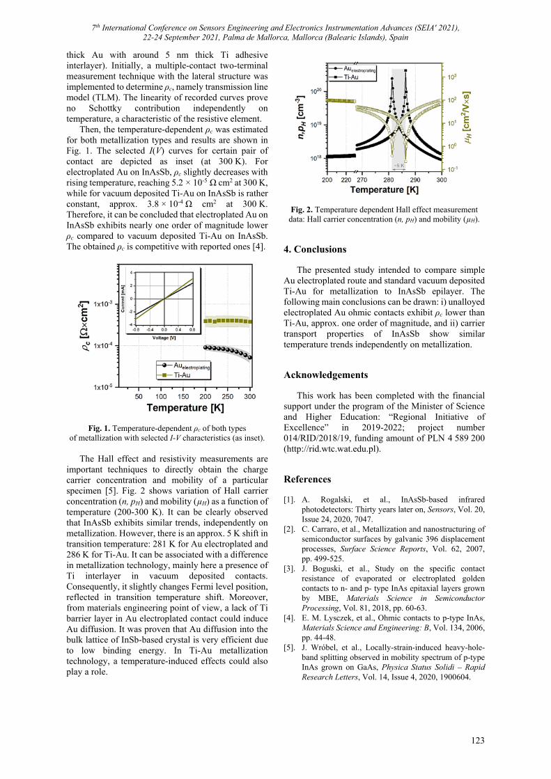
7th International Conference on Sensors Engineering and Electronics Instrumentation Advances (SEIA' 2021), 22-24 September 2021, Palma de Mallorca, Mallorca (Balearic Islands), Spain
123
thick Au with around 5 nm thick Ti adhesive interlayer). Initially, a multiple-contact two-terminal measurement technique with the lateral structure was implemented to determine ρc, namely transmission line model (TLM). The linearity of recorded curves prove no Schottky contribution independently on temperature, a characteristic of the resistive element.
Then, the temperature-dependent ρc was estimated for both metallization types and results are shown in Fig. 1. The selected I(V) curves for certain pair of contact are depicted as inset (at 300 K). For electroplated Au on InAsSb, ρc slightly decreases with rising temperature, reaching 5.2 × 10⁻⁵ Ω cm2 at 300 K, while for vacuum deposited Ti-Au on InAsSb is rather constant, approx. 3.8 × 10⁻⁴ Ω cm2 at 300 K. Therefore, it can be concluded that electroplated Au on InAsSb exhibits nearly one order of magnitude lower ρc compared to vacuum deposited Ti-Au on InAsSb. The obtained ρc is competitive with reported ones [4].
Fig. 1. Temperature-dependent ρc of both types of metallization with selected I-V characteristics (as inset).
The Hall effect and resistivity measurements are
important techniques to directly obtain the charge carrier concentration and mobility of a particular specimen [5]. Fig. 2 shows variation of Hall carrier concentration (n, pH) and mobility (µH) as a function of temperature (200-300 K). It can be clearly observed that InAsSb exhibits similar trends, independently on metallization. However, there is an approx. 5 K shift in transition temperature: 281 K for Au electroplated and 286 K for Ti-Au. It can be associated with a difference in metallization technology, mainly here a presence of Ti interlayer in vacuum deposited contacts. Consequently, it slightly changes Fermi level position, reflected in transition temperature shift. Moreover, from materials engineering point of view, a lack of Ti barrier layer in Au electroplated contact could induce Au diffusion. It was proven that Au diffusion into the bulk lattice of InSb-based crystal is very efficient due to low binding energy. In Ti-Au metallization technology, a temperature-induced effects could also play a role.
Fig. 2. Temperature dependent Hall effect measurement data: Hall carrier concentration (n, pH) and mobility (µH).
4. Conclusions
The presented study intended to compare simple Au electroplated route and standard vacuum deposited Ti-Au for metallization to InAsSb epilayer. The following main conclusions can be drawn: i) unalloyed electroplated Au ohmic contacts exhibit ρc lower than Ti-Au, approx. one order of magnitude, and ii) carrier transport properties of InAsSb show similar temperature trends independently on metallization. Acknowledgements
This work has been completed with the financial support under the program of the Minister of Science and Higher Education: “Regional Initiative of Excellence” in 2019-2022; project number 014/RID/2018/19, funding amount of PLN 4 589 200 (http://rid.wtc.wat.edu.pl). References [1]. A. Rogalski, et al., InAsSb-based infrared
photodetectors: Thirty years later on, Sensors, Vol. 20, Issue 24, 2020, 7047.
[2]. C. Carraro, et al., Metallization and nanostructuring of semiconductor surfaces by galvanic 396 displacement processes, Surface Science Reports, Vol. 62, 2007, pp. 499-525.
[3]. J. Boguski, et al., Study on the specific contact resistance of evaporated or electroplated golden contacts to n- and p- type InAs epitaxial layers grown by MBE, Materials Science in Semiconductor Processing, Vol. 81, 2018, pp. 60-63.
[4]. E. M. Lysczek, et al., Ohmic contacts to p-type InAs, Materials Science and Engineering: B, Vol. 134, 2006, pp. 44-48.
[5]. J. Wróbel, et al., Locally-strain-induced heavy-hole-band splitting observed in mobility spectrum of p-type InAs grown on GaAs, Physica Status Solidi – Rapid Research Letters, Vol. 14, Issue 4, 2020, 1900604.
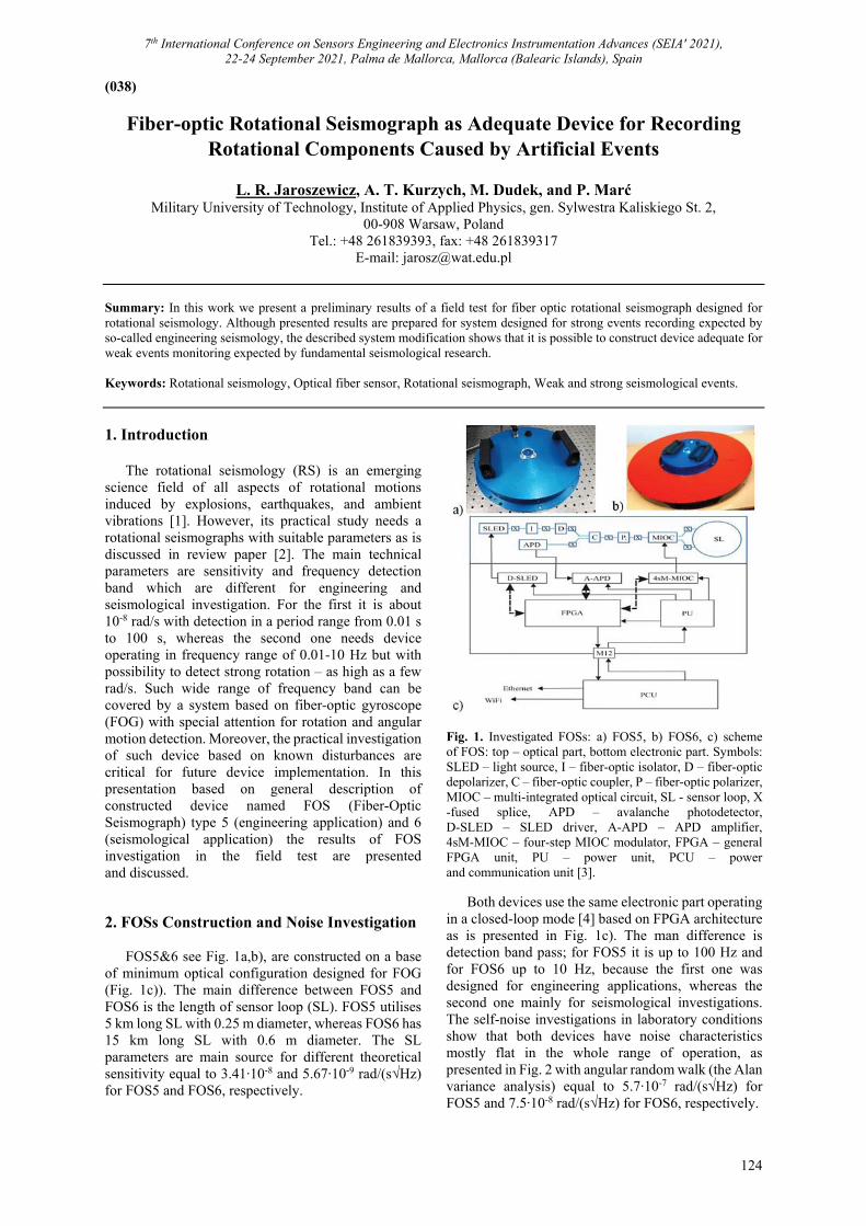
7th International Conference on Sensors Engineering and Electronics Instrumentation Advances (SEIA' 2021), 22-24 September 2021, Palma de Mallorca, Mallorca (Balearic Islands), Spain
124
(038)
Fiber-optic Rotational Seismograph as Adequate Device for Recording Rotational Components Caused by Artificial Events
L. R. Jaroszewicz, A. T. Kurzych, M. Dudek, and P. Marć
Military University of Technology, Institute of Applied Physics, gen. Sylwestra Kaliskiego St. 2, 00-908 Warsaw, Poland
Tel.: +48 261839393, fax: +48 261839317 E-mail: [email protected]
Summary: In this work we present a preliminary results of a field test for fiber optic rotational seismograph designed for rotational seismology. Although presented results are prepared for system designed for strong events recording expected by so-called engineering seismology, the described system modification shows that it is possible to construct device adequate for weak events monitoring expected by fundamental seismological research. Keywords: Rotational seismology, Optical fiber sensor, Rotational seismograph, Weak and strong seismological events.
1. Introduction
The rotational seismology (RS) is an emerging science field of all aspects of rotational motions induced by explosions, earthquakes, and ambient vibrations [1]. However, its practical study needs a rotational seismographs with suitable parameters as is discussed in review paper [2]. The main technical parameters are sensitivity and frequency detection band which are different for engineering and seismological investigation. For the first it is about 10-8 rad/s with detection in a period range from 0.01 s to 100 s, whereas the second one needs device operating in frequency range of 0.01-10 Hz but with possibility to detect strong rotation – as high as a few rad/s. Such wide range of frequency band can be covered by a system based on fiber-optic gyroscope (FOG) with special attention for rotation and angular motion detection. Moreover, the practical investigation of such device based on known disturbances are critical for future device implementation. In this presentation based on general description of constructed device named FOS (Fiber-Optic Seismograph) type 5 (engineering application) and 6 (seismological application) the results of FOS investigation in the field test are presented and discussed.
2. FOSs Construction and Noise Investigation
FOS5&6 see Fig. 1a,b), are constructed on a base of minimum optical configuration designed for FOG (Fig. 1c)). The main difference between FOS5 and FOS6 is the length of sensor loop (SL). FOS5 utilises 5 km long SL with 0.25 m diameter, whereas FOS6 has 15 km long SL with 0.6 m diameter. The SL parameters are main source for different theoretical sensitivity equal to 3.41∙10-8 and 5.67∙10-9 rad/(s√Hz) for FOS5 and FOS6, respectively.
Fig. 1. Investigated FOSs: a) FOS5, b) FOS6, c) scheme of FOS: top – optical part, bottom electronic part. Symbols: SLED – light source, I – fiber-optic isolator, D – fiber-optic depolarizer, C – fiber-optic coupler, P – fiber-optic polarizer, MIOC – multi-integrated optical circuit, SL - sensor loop, X -fused splice, APD – avalanche photodetector, D-SLED – SLED driver, A-APD – APD amplifier, 4sM-MIOC – four-step MIOC modulator, FPGA – general FPGA unit, PU – power unit, PCU – power and communication unit [3].
Both devices use the same electronic part operating in a closed-loop mode [4] based on FPGA architecture as is presented in Fig. 1c). The man difference is detection band pass; for FOS5 it is up to 100 Hz and for FOS6 up to 10 Hz, because the first one was designed for engineering applications, whereas the second one mainly for seismological investigations. The self-noise investigations in laboratory conditions show that both devices have noise characteristics mostly flat in the whole range of operation, as presented in Fig. 2 with angular random walk (the Alan variance analysis) equal to 5.7∙10-7 rad/(s√Hz) for FOS5 and 7.5∙10-8 rad/(s√Hz) for FOS6, respectively.
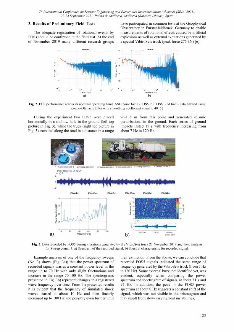
7th International Conference on Sensors Engineering and Electronics Instrumentation Advances (SEIA' 2021), 22-24 September 2021, Palma de Mallorca, Mallorca (Balearic Islands), Spain
125
3. Results of Preliminary Field Tests
The adequate registration of rotational events by FOSs should be confirmed in the field test. At the end of November 2019 many different research groups
have participated in common tests at the Geophysical Observatory in Fürstenfeldbruck, Germany to enable measurements of rotational effects caused by artificial explosions as well as external excitations generated by a special VibtroSeis truck (peak force 275 kN) [6].
a) b)
Fig. 2. FOS performance across its nominal operating band. ASD noise for: a) FOS5, b) FOS6. Red line – data filtered using
Konno-Ohmachi filter with smoothing coefficient equal to 40 [5]. During the experiment two FOS5 were placed
horizontally in a shallow hole in the ground (left top picture in Fig. 3), while the truck (right top picture in Fig. 3) travelled along the road in a distance in a range
96-138 m from this point and generated seismic perturbations in the ground. Each series of ground impacts lasted 15 s with frequency increasing from about 7 Hz to 120 Hz.
Fig. 3. Data recorded by FOS5 during vibrations generated by the VibroSeis truck 21 November 2019 and their analysis for Sweep count: 3: a) Spectrum of the recorded signal; b) Spectral characteristic for recorded signal.
Example analysis of one of the frequency sweeps
(No. 3) shows (Fig. 3a)) that the power spectrum of recorded signals was at a constant power level in the range up to 70 Hz with only slight fluctuations and increase in the range 70-100 Hz. The spectrograms presented in Fig. 3b) represent changes in a registered wave frequency over time. From the presented results it is evident that the frequency of simulated shock waves started at about 10 Hz and then linearly increased up to 100 Hz and possibly even further until
their extinction. From the above, we can conclude that recorded FOS5 signals indicated the same range of frequency generated by the VibroSeis truck (from 7 Hz to 120 Hz). Some external buzz, not identified yet, was evident, especially when comparing the power spectrum and spectrogram of signals, at about 7 Hz and 97 Hz. In addition, the peak in the FOS5 power spectrum at about 0 Hz suggests a constant shift of the signal, which was not visible in the seismogram and may result from slow-varying heat instabilities.

7th International Conference on Sensors Engineering and Electronics Instrumentation Advances (SEIA' 2021), 22-24 September 2021, Palma de Mallorca, Mallorca (Balearic Islands), Spain
126
4. Conclusions
The preliminary results obtained during field tests in Fürstenfeldbruck proved that the FOS5 device is fully capable of registering ground rotations in a whole frequency range designed for engineering seismology (strong signals with frequencies up to 100 Hz). However, because FOS6 utilises the same electronic part and differs mainly in SL, we believe that this device is capable of detection of rotation motions with amplitude at the magnitude of 10-8 rad/s and may be utilized as a universal sensor with high sensitivity in different RS applications. Acknowledgements
This research was financially supported by the Ministry of the National Defense of the Republic of Poland, project GBMON/13-995/2018/WAT.
References [1]. W. H. K. Lee, Seismology, rotation, in Encyclopedia of
Solid Earth Geophysics (H. K. Gupta, Ed.), Springer, Dordrecht, The Netherlands, 2019, pp. 1-12.
[2]. L. R. Jaroszewicz, A. Kurzych, et al,. Review of the usefulness of various rotational seismometers with laboratory results of fibre-optic ones tested for engineering applications, Sensors, Vol. 16, 2016, 2161.
[3]. A. T. Kurzych, L. R. Jaroszewicz, et al., Investigation of rotational motion in a reinforced concrete frame construction by a fiber optic gyroscope, Opto-Electron. Rev., Vol. 28, Issue 2, 2020, pp. 69-73.
[4]. H. C. Lefevre, P. Martin, et al., High-dynamic-range fiber gyro with all-digital signal processing, Proceedings of SPIE, Vol. 1367, 1991, pp. 72-80.
[5]. K. Konno, T. Ohmachi, Ground motion characteristics estimated from spectral ratio between horizontal and vertical components of microtremor, Bull. Seismol. Soc. Am., Vol. 88, Issue 1, 1998, pp. 228-241.
[6]. F. Bernauer, K. Behnen, et al., Rotation, strain and translation sensors performance tests with active seismic sources, Sensors, Vol. 21, 2021, 264.
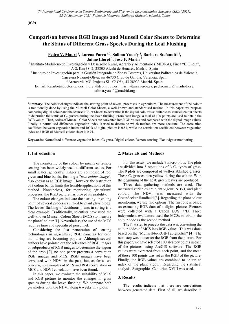
7th International Conference on Sensors Engineering and Electronics Instrumentation Advances (SEIA' 2021), 22-24 September 2021, Palma de Mallorca, Mallorca (Balearic Islands), Spain
127
(039)
Comparison between RGB Images and Munsell Color Sheets to Determine the Status of Different Grass Species During the Leaf Flushing
Pedro V. Mauri 1, Lorena Parra 1,2, Salima Yousfy 1, Barbara Stefanutti 2,
Jaime Lloret 2, Jose F. Marin 3
1 Instituto Madrileño de Investigación y Desarrollo Rural, Agrario y Alimentario (IMIDRA), Finca “El Encin”, A-2, Km 38, 2, 28805 Alcalá de Henares, Madrid, Spain
2 Instituto de Investigación para la Gestión Integrada de Zonas Costeras, Universitat Politècnica de València, Carretera Nazaret-Oliva, s/n 46730 Grao de Gandia, Valencia, Spain
3 Areaverde MG Projects SL. C/ Oña, 43 28933 Madrid. Spain E-mail: [email protected], [email protected], [email protected], [email protected],
[email protected] Summary: The colour changes indicate the starting point of several processes in agriculture. The measurement of the colour is traditionally done by using the Munsell Color Sheets, a well-known and standardised method. In this paper, we propose comparing digital colour and the Munsell Color Sheets to determine if the digital colour is as suitable as Munsell colour sheets to determine the status of C4 grasses during the leave flushing. From each image, a total of 100 points are used to obtain the RGB values. Then, codes of Munsell Color Sheets are converted into RGB values and compared with the digital image values. Finally, a normalised difference vegetation index is used to determine which method are more accurate. The correlation coefficient between vegetation index and RGB of digital picture is 0.54, while the correlation coefficient between vegetation index and RGB of Munsell colour sheet is 0.74. Keywords: Normalised difference vegetation index, C4 grass, Digital colour, Remote sensing, Plant vigour monitoring.
1. Introduction
The monitoring of the colour by means of remote sensing has been widely used at different scales. For small scales, generally, images are composed of red, green and blue bands, forming a "true colour image", also known as an RGB image. However, the restriction of 3 colour bands limits the feasible applications of this method. Nonetheless, for monitoring agricultural processes, the RGB picture has proved its usability.
The colour changes indicate the starting or ending point of several processes linked to plant physiology. The leaves flushing of deciduous plants in spring is a clear example. Traditionally, scientists have used the well-known Munsell Colour Sheets (MCS) to measure the plants' colour [1]. Nevertheless, the use of the MCS requires time and specialised personnel.
Considering the fast penetration of sensing technologies in agriculture, RGB cameras for crop monitoring are becoming popular. Although several authors have pointed out the relevance of RGB images or subproducts of RGB images to determine the vigour of the crop [2], no one paper presents a correlation RGB images and MCS. RGB images have been correlated with NDVI in the past, but, as far as we concern, no examples of MCS and RGB correlation or MCS and NDVI correlation have been found.
In this paper, we evaluate the suitability of MCS and RGB picture to monitor the changes in grass species during the leave flushing. We compare both parameters with the NDVI along 6 weeks in 9 plots.
2. Materials and Methods
For this assay, we include 9 micro-plots. The plots are divided into 3 repetitions of 3 C4 types of grass. The 9 plots are composed of well-established grasses. These C4 grasses turn yellow during the winter. With the beginning of the heat, green leaves are produced.
Three data gathering methods are used. The measured variables are plant vigour, NDVI, and plant colour. The NDVI was measured with the GreenSeeker Handheld [3]. Regarding the plant colour monitoring, we use two options. The first one is based on extracting RGB data of a digital picture. Pictures were collected with a Canon EOS 77D. Three independent evaluators used the MCSs to obtain the colour code as the second method.
The first step to process the data was converting the colour codes of MCS into RGB values. This was done based on the "Munsell-to-RGB-Tables.xlsm" [4]. The next step was to extract the RGB from the picture. For this paper, we have selected 100 aleatory points in each of the pictures using ArcGIS software. The RGB values were extracted from each point, and the mean of those 100 points was set as the RGB of the picture. Finally, the RGB values are combined to obtain an index of the plant vigour. Regarding the statistical analysis, Statgraphics Centurion XVIII was used. 3. Results
The results indicate that there are correlations between generated data. First of all, we describe in
7th International Conference on Sensors Engineering and Electronics Instrumentation Advances (SEIA' 2021), 22-24 September 2021, Palma de Mallorca, Mallorca (Balearic Islands), Spain
128
general terms the existing correlations. Fig. 1 outlines the correlations between included variables. We have selected the green band for this analysis as the individual RGB band among the individual RGB bands. We can identify MUNG as the G data obtained with the MCS and the DIGG as the G data obtained with the RGB values of the digital picture. Regarding the combination, the most relevant one is the red and green band combinations as G/R. Again, the prefix MUN or DIG indicates the origin of data. In Fig. 1, we can see the correlation coefficients; the p-value indicated in "*" and the data dispersion of each variable. The strongest correlation is for MUNG/R and NDVI. This correlation was not reported so far. The correlation of NDVI with DIGG/R is slightly lower but has the same statistical significance.
Fig. 1. Summary of correlations.
Following, we focus on the correlations between
MUNG/R and DIGG/R with the NDVI. In this step, simple regression models are explored. Fig. 2 displays the regression models between NDVI and DIGG/R. In this case, the correlation reaches -0.55 with a p-value of 0.0000. Meanwhile, Fig. 3 represents the regression model for NDVI and MUNG/R. The correlation coefficient for these two variables is 0.75 and the p-value 0.0000.
Fig. 2. Regression model for RGB of digital picture.
Fig. 3. Regression model for RGB of MCS. 4. Conclusion
In this paper, we have compared two methods of colour detection to evaluate plant vigour. Our results indicated that although both methods have similar p-values, MCS converted into RGB values have a higher correlation coefficient than the digital picture. Nonetheless, this effect can be caused by the way in which RGB values from the picture are extracted.
In future work, we will evaluate other ways of extracting RGB values considering the whole picture. Moreover, we will use these methods to compare the performance of the three grass species. Acknowledgements
This research and the contract of S.Y. were funded by project PDR18-XEROCESPED, under the PDR-CM 2014-2020, by the EU (European Agricultural Fund for Rural Development, EAFRD), Spanish Ministry of Agriculture, Fisheries and Food (MAPA) and Comunidad de Madrid regional government through IMIDRA and the contract of L.P. was funded by Conselleria de Educación, Cultura y Deporte with the Subvenciones para la contratación de personal investigador en fase postdoctoral, APOSTD/2019/04.
References
[1]. T. Mizunuma, et al., Sensitivity of colour indices for discriminating leaf colours from digital photographs, Methods in Ecology and Evolution, Vol. 5, Issue 10, 2014, pp. 1078-1085.
[2]. J. Marín, RGB vegetation indices, NDVI, and biomass as indicators to evaluate C3 and C4 turfgrass under different water conditions, Sustainability, Vol. 12, Issue 6, 2020, 2160.
[3]. GreenSeeker Datasheet, http://trl.trimble.com/docusha re/dsweb/Get/Document-475150/022503-1123A_Gree nSeeker_DS_MarketSmart_USL_0415_LR_web.pdf
[4]. Munsell-to-RGB-Tables.xlsm, https://www.munsellcolourscienceforpainters.com
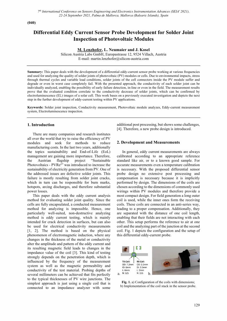
7th International Conference on Sensors Engineering and Electronics Instrumentation Advances (SEIA' 2021), 22-24 September 2021, Palma de Mallorca, Mallorca (Balearic Islands), Spain
129
(040)
Differential Eddy Current Sensor Probe Development for Solder Joint Inspection of Photovoltaic Modules
M. Lenzhofer, L. Neumaier and J. Kosel
Silicon Austria Labs GmbH, Europastrasse 12, 9524 Villach, Austria E-mail: [email protected]
Summary: This paper deals with the development of a differential eddy-current sensor probe working at various frequencies and used for analyzing the quality of solder joints of photovoltaic (PV) modules or cells. Due to environmental impacts, stress through thermal cycles and variable load conditions, solder joints of the cell connectors inside the PV module suffer and degrade or even in worst case completely fail. With the presented approach, the conductivity of each solder joint can be individually analyzed, enabling the possibility of early failure detection, in-line or even in the field. The measurement results prove that the evaluated condition correlate to the conductivity decrease of solder joints, which can be confirmed by electroluminescence (EL) images of a solar cell. This work bases on a previously executed investigation and depicts the next step in the further development of eddy-current testing within PV applications. Keywords: Solder joint inspection, Conductivity measurement, Photovoltaic module analyzes, Eddy-current measurement system, Electroluminescence inspection.
1. Introduction
There are many companies and research institutes all over the world that try to raise the efficiency of PV modules and seek for methods to reduce manufacturing costs. In the last two years, additionally the topics sustainability and End-of-Life (EoL) management are gaining more importance. Therefore, the Austrian flagship project “Sustainable Photovoltaics - PVRe²” was introduced to increase the sustainability of electricity generation from PV. One of the addressed issues are defective solder joints. This failure is mostly resulting from solder joint cracks, which in turn can be responsible for burn marks, hotspots, arcing discharges, and therefore substantial power losses.
This paper deals with the eddy current analysis method for evaluating solder joint quality. Since the cells are fully encapsulated, a conducted measurement method for analyzing is impossible. Hence, one particularly well-suited, non-destructive analyzing method is eddy current testing, which is mainly intended for crack detection in surfaces, but can also be used for electrical conductivity measurements [1, 2]. The method is based on the physical phenomenon of electromagnetic induction, where any changes in the thickness of the metal or conductivity alter the amplitude and pattern of the eddy current and its resulting magnetic field leads to changes in the impedance value of the coil [3]. This kind of testing strongly depends on the penetration depth, which is influenced by the frequency of the measurement system as well as the magnetic permeability and conductivity of the test material. Probing depths of several millimeters can be achieved that fits perfectly to the typical thicknesses of PV wire junctions. The simplest approach is just using a single coil that is connected to an impedance analyzer with some
additional post processing, but shows some challenges, [4]. Therefore, a new probe design is introduced.
2. Development and Measurements
In general, eddy current measurements are always calibrated according to an appropriate reference standard like air, or to a known good sample. For accurate measurements even a temperature calibration is necessary. With the proposed differential sensor probe design no extensive post processing and compensation is necessary because it is implicitly performed by design. The dimensions of the coils are chosen according to the dimensions of commonly used wirings within PV modules and therefore provide a most compact design. For field generation a long outer coil is used, while the inner ones form the receiving coils. These coils are connected in an anti-series way, leading to a proper compensation. Additionally, they are separated with the distance of one coil length, enabling that their fields are not interacting with each other. This setup performs the reference to air at one coil and the analyzing part of the junction at the second coil. Fig. 1 depicts the configuration and the setup of this differential eddy-current probe.
Fig. 1. a) Configuration of the coils with dimensions; b) Implementation of the coil stack in the sensor probe.
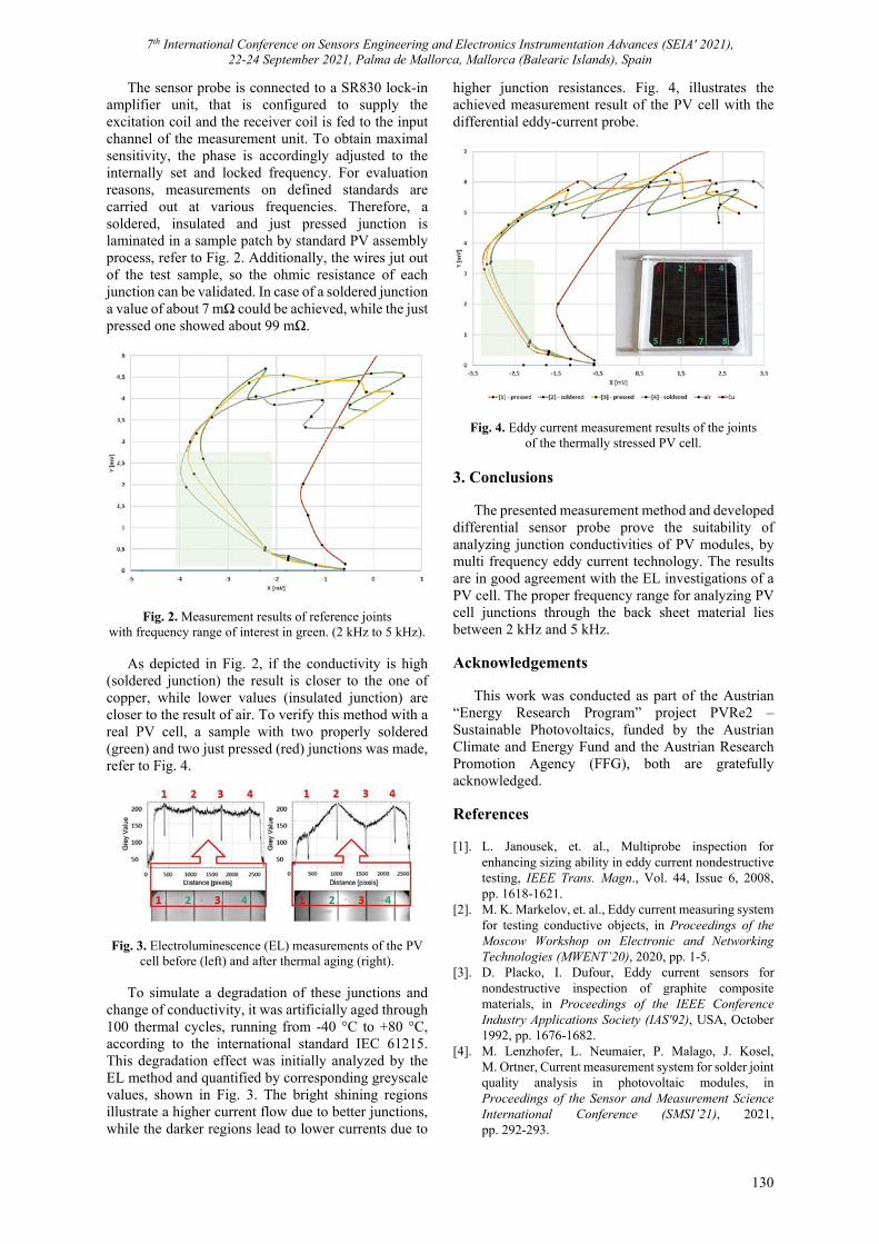
7th International Conference on Sensors Engineering and Electronics Instrumentation Advances (SEIA' 2021), 22-24 September 2021, Palma de Mallorca, Mallorca (Balearic Islands), Spain
130
The sensor probe is connected to a SR830 lock-in amplifier unit, that is configured to supply the excitation coil and the receiver coil is fed to the input channel of the measurement unit. To obtain maximal sensitivity, the phase is accordingly adjusted to the internally set and locked frequency. For evaluation reasons, measurements on defined standards are carried out at various frequencies. Therefore, a soldered, insulated and just pressed junction is laminated in a sample patch by standard PV assembly process, refer to Fig. 2. Additionally, the wires jut out of the test sample, so the ohmic resistance of each junction can be validated. In case of a soldered junction a value of about 7 mΩ could be achieved, while the just pressed one showed about 99 mΩ.
Fig. 2. Measurement results of reference joints with frequency range of interest in green. (2 kHz to 5 kHz).
As depicted in Fig. 2, if the conductivity is high
(soldered junction) the result is closer to the one of copper, while lower values (insulated junction) are closer to the result of air. To verify this method with a real PV cell, a sample with two properly soldered (green) and two just pressed (red) junctions was made, refer to Fig. 4.
Fig. 3. Electroluminescence (EL) measurements of the PV cell before (left) and after thermal aging (right).
To simulate a degradation of these junctions and
change of conductivity, it was artificially aged through 100 thermal cycles, running from -40 °C to +80 °C, according to the international standard IEC 61215. This degradation effect was initially analyzed by the EL method and quantified by corresponding greyscale values, shown in Fig. 3. The bright shining regions illustrate a higher current flow due to better junctions, while the darker regions lead to lower currents due to
higher junction resistances. Fig. 4, illustrates the achieved measurement result of the PV cell with the differential eddy-current probe.
Fig. 4. Eddy current measurement results of the joints of the thermally stressed PV cell.
3. Conclusions
The presented measurement method and developed differential sensor probe prove the suitability of analyzing junction conductivities of PV modules, by multi frequency eddy current technology. The results are in good agreement with the EL investigations of a PV cell. The proper frequency range for analyzing PV cell junctions through the back sheet material lies between 2 kHz and 5 kHz. Acknowledgements
This work was conducted as part of the Austrian “Energy Research Program” project PVRe2 – Sustainable Photovoltaics, funded by the Austrian Climate and Energy Fund and the Austrian Research Promotion Agency (FFG), both are gratefully acknowledged. References [1]. L. Janousek, et. al., Multiprobe inspection for
enhancing sizing ability in eddy current nondestructive testing, IEEE Trans. Magn., Vol. 44, Issue 6, 2008, pp. 1618-1621.
[2]. M. K. Markelov, et. al., Eddy current measuring system for testing conductive objects, in Proceedings of the Moscow Workshop on Electronic and Networking Technologies (MWENT’20), 2020, pp. 1-5.
[3]. D. Placko, I. Dufour, Eddy current sensors for nondestructive inspection of graphite composite materials, in Proceedings of the IEEE Conference Industry Applications Society (IAS'92), USA, October 1992, pp. 1676-1682.
[4]. M. Lenzhofer, L. Neumaier, P. Malago, J. Kosel, M. Ortner, Current measurement system for solder joint quality analysis in photovoltaic modules, in Proceedings of the Sensor and Measurement Science International Conference (SMSI’21), 2021, pp. 292-293.
7th International Conference on Sensors Engineering and Electronics Instrumentation Advances (SEIA' 2021), 22-24 September 2021, Palma de Mallorca, Mallorca (Balearic Islands), Spain
131
(041)
Delay Impact in the Stability of the Digital GMI Sensor Operating in Closed-loop
P. S. Traore, M. I. Correa, C. A. B. Mbodji
Ecole Supérieure Polytechnique (ESP), Université Cheikh Anta Diop (UCAD), Dakar, Sénégal Tel.: + (221)773999941
E-mail: [email protected] Summary: This paper presents a complete study of the delay in the stability of the digital GMI sensor operating in closed loop. The proposed sensor is made of Direct Digital Synthetiser (DDS) for the excitation of the GMI wire and a digital receiver composed of an Analog-to-digital converter (ADC) and a Digital Down Converter (DDC) for quadrature digital demodulation of the voltage across the GMI wire. The proposed approach allows to give the key implementation rules of each digital function involved in the digital GMI sensor in order to minimize delay and to ensure a proper functioning of the digital GMI magnetometer. In addition, the impact of the delay in the performance of the system is also discussed. Results show that, by respecting the proposed rules, the digital GMI sensor operates properly in closed loop. Keywords: GMI magnetometer, Digital electronic conditioning, Delay.
1. Introduction
Magnetic sensors are used in a wide variety of applications ranging from high density magnetic recording, non-contact current measurement, to spatial, military and biomedical applications [1]. A non-exhaustive list of these measurement devices may include Fluxgates, inductive sensors, Anisotropic MagnetoResistance (AMR), Giant MagnetoResistance (GMR) sensors, etc. [1]. Over the past two decades, the Giant Magneto-Impedance (GMI) effect has been intensively studied due to its attractive potential for realizing a highly sensitive magnetic sensor [2, 3]. It is defined by a high impedance variation of a ferromagnetic material when it is supplied by a high frequency (HF) excitation current and submitted to an external magnetic field. It has been shown that GMI sensors offer several advantages compared to conventional sensors. Some of the decisive advantage is the high sensitivity, the potential for miniaturization and the low energy consumption.
A typical configuration of GMI sensor is shown in Fig. 1. It requires a high frequency excitation current provided by an oscillator associated to a voltage-to-current converter. When the sensing element (the ferromagnetic material) is submitted to an external magnetic field, Hz, to be measured, the voltage across the sensing element is amplitude modulated by the measured field. A demodulator is generally used to have the information of the measured field. The relation between the sensor output and the magnetic field is characterized by the sensitivity. The GMI characteristic is strongly non-linear, to realize a sensor, it is generally magnetically biased in the region having the maximum of sensitivity. Biasing creates an offset at the sensor output corresponding to the impedance value at the bias point, a difference amplifier is generally used to suppress the offset that could be affected by temperature and strength [4, 5].
Oscillator
V‐I
Hz
iacDemodulator
Offset cancelling devices
Sensingelement
Fig. 1. Hardware architecture of a typical off-diagonal GMI sensor.
In the context of high sensitivity, the equivalent
magnetic noise level need to be improved. It characterizes the smallest magnetic field that the sensor can measure. It is defined by the ratio between the voltage noise spectral density (including the electronic conditioning noise and the noise of the sensing element) and the sensitivity of the sensor. Actually, all GMI sensors are associated with an analog electronic conditioning and several studies show that the equivalent magnetic noise is limited in the 1/f region by the intrinsic noise of the sensing element attributed to the fluctuation of the magnetization movement. In the white noise region, the smallest magnetic field that the sensor can measure is limited by the electronic conditioning noise [6]. The ultimate noise of the sensing element is not yet achieved in this region. In our recent work [7, 8] we have introduced the digital concept in order to reduce the electronic conditioning noise so as to achieve the ultimate noise performance. The proposed concept is based on a Digital Down Converter (DDC) for a quadrature digital demodulation. The voltage across the sensing element (generally in off-diagonal configuration for high sensitivity application) is digitized as close as possible to the sensing element.
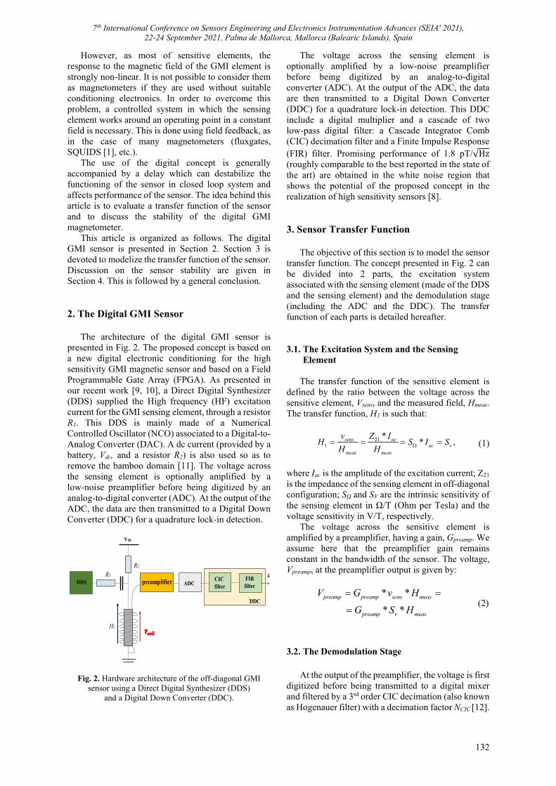
7th International Conference on Sensors Engineering and Electronics Instrumentation Advances (SEIA' 2021), 22-24 September 2021, Palma de Mallorca, Mallorca (Balearic Islands), Spain
132
However, as most of sensitive elements, the response to the magnetic field of the GMI element is strongly non-linear. It is not possible to consider them as magnetometers if they are used without suitable conditioning electronics. In order to overcome this problem, a controlled system in which the sensing element works around an operating point in a constant field is necessary. This is done using field feedback, as in the case of many magnetometers (fluxgates, SQUIDS [1], etc.).
The use of the digital concept is generally accompanied by a delay which can destabilize the functioning of the sensor in closed loop system and affects performance of the sensor. The idea behind this article is to evaluate a transfer function of the sensor and to discuss the stability of the digital GMI magnetometer.
This article is organized as follows. The digital GMI sensor is presented in Section 2. Section 3 is devoted to modelize the transfer function of the sensor. Discussion on the sensor stability are given in Section 4. This is followed by a general conclusion. 2. The Digital GMI Sensor
The architecture of the digital GMI sensor is presented in Fig. 2. The proposed concept is based on a new digital electronic conditioning for the high sensitivity GMI magnetic sensor and based on a Field Programmable Gate Array (FPGA). As presented in our recent work [9, 10], a Direct Digital Synthesizer (DDS) supplied the High frequency (HF) excitation current for the GMI sensing element, through a resistor R1. This DDS is mainly made of a Numerical Controlled Oscillator (NCO) associated to a Digital-to-Analog Converter (DAC). A dc current (provided by a battery, Vdc, and a resistor R2) is also used so as to remove the bamboo domain [11]. The voltage across the sensing element is optionally amplified by a low-noise preamplifier before being digitized by an analog-to-digital converter (ADC). At the output of the ADC, the data are then transmitted to a Digital Down Converter (DDC) for a quadrature lock-in detection.
preamplifier ADC
Vdc
CICfilter
FIR filter
DDC
DDSR1
Hz
R2
Fig. 2. Hardware architecture of the off-diagonal GMI sensor using a Direct Digital Synthesizer (DDS)
and a Digital Down Converter (DDC).
The voltage across the sensing element is optionally amplified by a low-noise preamplifier before being digitized by an analog-to-digital converter (ADC). At the output of the ADC, the data are then transmitted to a Digital Down Converter (DDC) for a quadrature lock-in detection. This DDC include a digital multiplier and a cascade of two low-pass digital filter: a Cascade Integrator Comb (CIC) decimation filter and a Finite Impulse Response (FIR) filter. Promising performance of 1.8 pT/√Hz (roughly comparable to the best reported in the state of the art) are obtained in the white noise region that shows the potential of the proposed concept in the realization of high sensitivity sensors [8]. 3. Sensor Transfer Function
The objective of this section is to model the sensor transfer function. The concept presented in Fig. 2 can be divided into 2 parts, the excitation system associated with the sensing element (made of the DDS and the sensing element) and the demodulation stage (including the ADC and the DDC). The transfer function of each parts is detailed hereafter. 3.1. The Excitation System and the Sensing Element
The transfer function of the sensitive element is defined by the ratio between the voltage across the sensitive element, Vsens, and the measured field, Hmeas. The transfer function, H1 is such that:
21
1
** ,sens ac
ac vmeas meas
v Z IH S I S
H H (1)
where Iac is the amplitude of the excitation current; Z21 is the impedance of the sensing element in off-diagonal configuration; SΩ and SV are the intrinsic sensitivity of the sensing element in Ω/T (Ohm per Tesla) and the voltage sensitivity in V/T, respectively.
The voltage across the sensitive element is amplified by a preamplifier, having a gain, Gpreamp. We assume here that the preamplifier gain remains constant in the bandwidth of the sensor. The voltage, Vpreamp, at the preamplifier output is given by:
* *
* *
preamp preamp sens meas
preamp v meas
V G v H
G S H
(2)
3.2. The Demodulation Stage
At the output of the preamplifier, the voltage is first digitized before being transmitted to a digital mixer and filtered by a 3rd order CIC decimation (also known as Hogenauer filter) with a decimation factor NCIC [12].
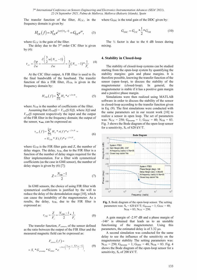
7th International Conference on Sensors Engineering and Electronics Instrumentation Advances (SEIA' 2021), 22-24 September 2021, Palma de Mallorca, Mallorca (Balearic Islands), Spain
133
The transfer function of the filter, HCIC, in the frequency domain is given by:
3 13 ,cicj f N jCIC CIC CICH f N e G e (3)
where GCIC is the gain of the filter.
The delay due to the 3rd order CIC filter is given by (4):
31
3 121 *
2
cic
cic cics
w NN
w w F
(4)
At the CIC filter output, A FIR filter is used to fix
the final bandwidth of the baseband. The transfer function of this a FIR filter, HFIR, is given in the frequency domain by:
2
0
* ,FIRN
j fkFIR k
k
H f H e
(5)
where NFIR is the number of coefficients of the filter.
Assuming that HFIR(f) = Vout(f)/X(f), where X(f) and Vout(f) represent respectively the input and the output of the FIR filter in the frequency domain; the output of the sensor, vout, can be expressed as:
2
0
2
* ( ) *
* ( ) * ,
FIRNj fk
out kk
j fZFIR
v f H x f e
G X f e
(6)
where GFIR is the FIR filter gain and Z, the number of delay stages. The delay, τFIR, due to the FIR filter is a function of the number of delay stages required for the filter implementation. For a filter with symmetrical coefficients (as the case in GMI sensor), the number of delay stages is given by (6) [7]:
1
2FIRN
Z
(7)
In GMI sensors, the choice of using FIR filter with
symmetrical coefficients is justified by the will to reduce the delay of the demodulation stage [10], which can cause the instability of the magnetometer. As a results, the delay, τFIR, due to the FIR filter is expressed as:
1 1
*2
FIRFIR
s s
NZ
F F
(8)
The transfer function, Fsensor, of the sensor defined
as the ratio between the output of the FIR filter and the measured magnetic field can be expressed as:
3 11
22 2* * * ,
CICFIR
sensor
NNj f
v preamp DDC
F f
S G G e
(9)
where GDDC is the total gain of the DDC given by:
1
* *2DDC CIC FIRG G G (10)
The ½ factor is due to the 6 dB losses during
mixing. 4. Stability in Closed-loop
The stability of closed-loop systems can be studied starting from the open-loop system by quantifying the stability margins: gain and phase margins. It is therefore possible, knowing the transfer function of the sensor (open–loop), to discuss the stability of the magnetometer (closed-loop). In general, the magnetometer is stable if it has a positive gain margin and a positive phase margin.
Simulations were then realized using MATLAB software in order to discuss the stability of the sensor in closed-loop according to the transfer function given in Eq. (9). The first simulations were conducted with the same parameters set in our recent work [10] to realize a sensor in open loop. The set of parameters was: NCIC = 250; Gpreamp = 1; GDDC = 40; NFIR = 83. Fig. 3 shows the Bode diagram of the open-loop sensor for a sensitivity, Sv of 620 kV/T.
Fig. 3. Bode diagram of the open-loop sensor. The setting parameters was: Sv = 620 kV/T; Gpreamp = 1; GDDC = 40;
NFIR = 83; NCIC = 250. A gain margin of -2.97 dB and a phase margin of
-146° is obtained that leads us to an unstable functioning of the magnetometer. Using this parameters, the estimated delay is of 3.32 µs.
A second simulation was conducted for the same delay to see the influence of the sensitivity on the magnetometer stability The setting parameters was: NCIC = 250; Gpreamp = 1; GDDC = 40; NFIR = 83. Fig. 4 shows the Bode diagram of the open-loop sensor for a sensitivity, Sv of 200 kV/T.
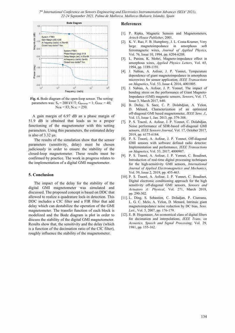
7th International Conference on Sensors Engineering and Electronics Instrumentation Advances (SEIA' 2021), 22-24 September 2021, Palma de Mallorca, Mallorca (Balearic Islands), Spain
134
Fig. 4. Bode diagram of the open-loop sensor. The setting parameters was: Sv = 200 kV/T; Gpreamp = 1; GDDC = 40;
NFIR = 83; NCIC = 250.
A gain margin of 6.97 dB an a phase margin of 51.9 dB is obtained that leads us to a proper functioning of the magnetometer with this setting parameters. Using this parameters, the estimated delay is also of 3.32 µs.
The results of the simulation show that the sensor parameters (sensitivity, delay) must be chosen judiciously in order to ensure the stability of the closed-loop magnetometer. These results must be confirmed by practice. The work in progress relates to the implementation of a digital GMI magnetometer.
5. Conclusion
The impact of the delay for the stability of the digital GMI magnetometer was simulated and discussed. The proposed concept is based on DDC that allowed to realize a quadrature lock-in detection. This DDC includes a CIC filter and a FIR filter that add delay which can destabilize the operation of the GMI magnetometer. The transfer function of each block is modelized and the Bode diagram is plot in order to discuss the stability of the digital GMI magnetometer. Results show that, the sensitivity and the delay (which is a function of the decimation ratio of the CIC filter), roughly influence the stability of the magnetometer.
References [1]. P. Ripka, Magnetic Sensors and Magnetometers,
Artech House Publisher, 2001. [2]. K. V. Rao, F. B. Humphrey, J. L. Costa-Kramer, Very
large magnetoimpedance in amorphous soft ferromagnetic wires, Journal of Applied Physics, Vol. 76, Issue 10, 1994, pp. 6204-6208.
[3]. L. Panina, K. Mohri, Magneto-impedance effect in amorphous wires, Applied Physics Letters, Vol. 65, 1994, pp. 1189-1191.
[4]. J. Nabias, A. Asfour, J. P. Yonnet, Temperature dependence of giant magnetoimpedance in amorphous microwires for sensor application, IEEE Transactions on Magnetics, Vol. 53, Issue 4, 2016, 4001005.
[5]. J. Nabias, A. Asfour, J. P. Yonnet, The impact of bending stress on the performance of Giant Magneto-Impedance (GMI) magnetic sensors, Sensors, Vol. 17, Issue 3, March 2017, 640.
[6]. B. Dufay, S. Saez, C. P. Dolabdjian, A. Yelon, D. Ménard, Characterization of an optimized off-diagonal GMI based magnetometer, IEEE Sens. J., Vol. 13, Issue 1, Jan. 2013, pp. 379-388.
[7]. P. S. Traoré, A. Asfour, J. P. Yonnet, C. Dolabdjan, Noise performance of SDR-based off-diagonal GMI sensors, IEEE Sensors Journal, Vol. 17, October 2017, 2019, pp. 6175-6184.
[8]. P. S. Traoré, A. Asfour, J. P. Yonnet, Off-diagonal GMI sensors with software defined radio detector: Implementation and performance, IEEE Transactions on Magnetics, Vol. 53, 2017, 4000907.
[9]. P. S. Traoré, A. Asfour, J. P. Yonnet, C. Boudinet, Introduction of real-time digital processing techniques for the high-sensitivity GMI sensors, International Journal of Applied Electromagnetics and Mechanics, Vol. 59, Issue 2, 2019, pp. 455-463.
[10]. P. S. Traoré, A. Asfour, J. P. Yonnet, C. Boudinet, Digital electronic conditioning approach for the high sensitivity off-diagonal GMI sensors, Sensors and Actuators A: Physical, Vol. 271, March 2018, pp. 290-302.
[11]. L. Ding, S. Sebastien, C. Doladjan, P. Ciureanu, L. G. C. Melo, A. Yelon, D. Menard, Intrinsic giant magnetoimpedance noise reduction by DC bias, Sens. Lett., Vol. 5, 2007, pp. 176-179.
[12]. E. B. Hogenauer, An economical class of digital filters for decimation and interpolations, IEEE Trans. on Acoustics, Speech and Signal Processing, Vol. 29, 1981, pp. 155-162.
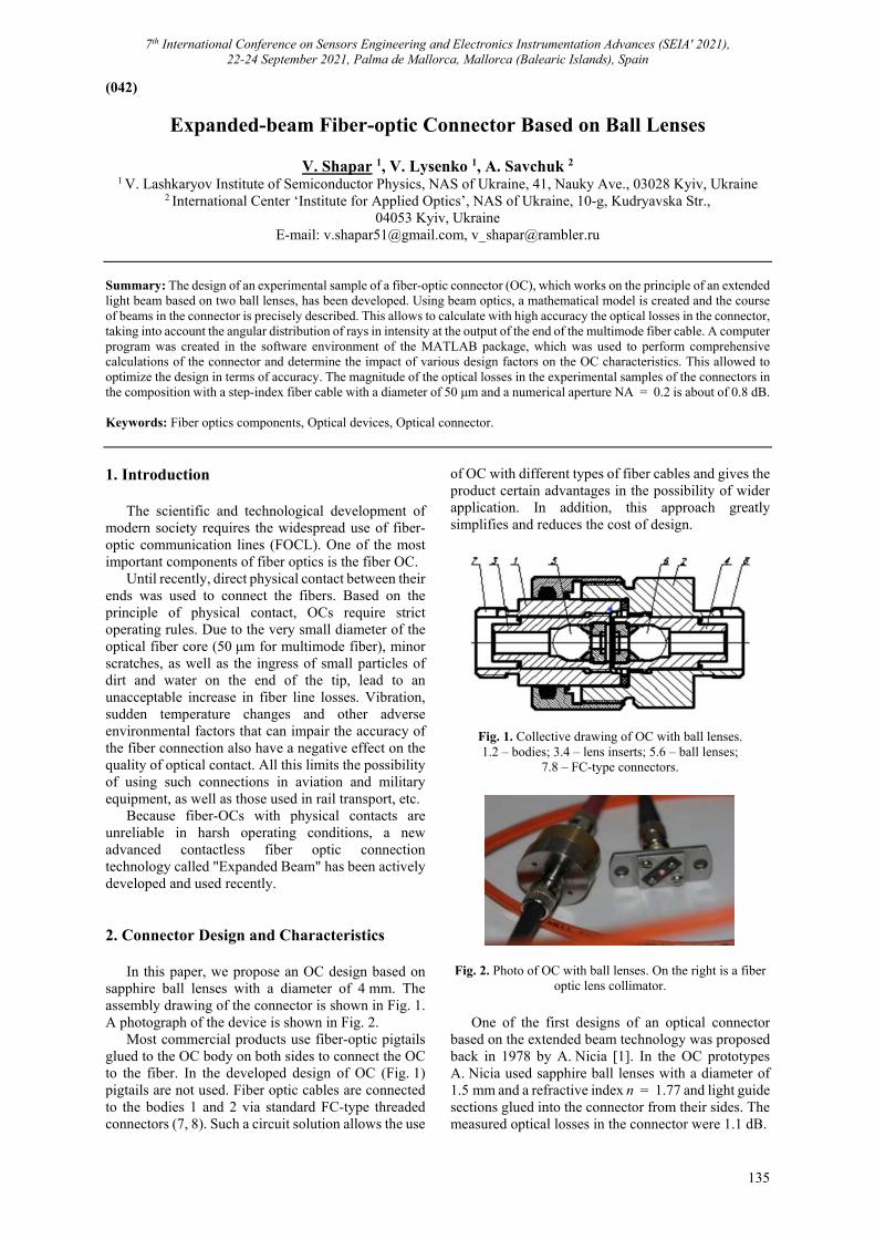
7th International Conference on Sensors Engineering and Electronics Instrumentation Advances (SEIA' 2021), 22-24 September 2021, Palma de Mallorca, Mallorca (Balearic Islands), Spain
135
(042)
Expanded-beam Fiber-optic Connector Based on Ball Lenses
V. Shapar 1, V. Lysenko 1, A. Savchuk 2
1 V. Lashkaryov Institute of Semiconductor Physics, NAS of Ukraine, 41, Nauky Ave., 03028 Kyiv, Ukraine 2 International Сenter ‘Institute for Applied Optics’, NAS of Ukraine, 10-g, Kudryavska Str.,
04053 Kyiv, Ukraine E-mail: [email protected], [email protected]
Summary: The design of an experimental sample of a fiber-optic connector (OC), which works on the principle of an extended light beam based on two ball lenses, has been developed. Using beam optics, a mathematical model is created and the course of beams in the connector is precisely described. This allows to calculate with high accuracy the optical losses in the connector, taking into account the angular distribution of rays in intensity at the output of the end of the multimode fiber cable. A computer program was created in the software environment of the MATLAB package, which was used to perform comprehensive calculations of the connector and determine the impact of various design factors on the OC characteristics. This allowed to optimize the design in terms of accuracy. The magnitude of the optical losses in the experimental samples of the connectors in the composition with a step-index fiber cable with a diameter of 50 μm and a numerical aperture NA = 0.2 is about of 0.8 dB.
Keywords: Fiber optics components, Optical devices, Optical connector.
1. Introduction
The scientific and technological development of modern society requires the widespread use of fiber-optic communication lines (FOCL). One of the most important components of fiber optics is the fiber OC.
Until recently, direct physical contact between their ends was used to connect the fibers. Based on the principle of physical contact, OCs require strict operating rules. Due to the very small diameter of the optical fiber core (50 μm for multimode fiber), minor scratches, as well as the ingress of small particles of dirt and water on the end of the tip, lead to an unacceptable increase in fiber line losses. Vibration, sudden temperature changes and other adverse environmental factors that can impair the accuracy of the fiber connection also have a negative effect on the quality of optical contact. All this limits the possibility of using such connections in aviation and military equipment, as well as those used in rail transport, etc.
Because fiber-OCs with physical contacts are unreliable in harsh operating conditions, a new advanced contactless fiber optic connection technology called "Expanded Beam" has been actively developed and used recently. 2. Connector Design and Characteristics
In this paper, we propose an OC design based on sapphire ball lenses with a diameter of 4 mm. The assembly drawing of the connector is shown in Fig. 1. A photograph of the device is shown in Fig. 2.
Most commercial products use fiber-optic pigtails glued to the OC body on both sides to connect the OC to the fiber. In the developed design of OC (Fig. 1) pigtails are not used. Fiber optic cables are connected to the bodies 1 and 2 via standard FC-type threaded connectors (7, 8). Such a circuit solution allows the use
of OC with different types of fiber cables and gives the product certain advantages in the possibility of wider application. In addition, this approach greatly simplifies and reduces the cost of design.
Fig. 1. Collective drawing of OC with ball lenses. 1.2 – bodies; 3.4 – lens inserts; 5.6 – ball lenses;
7.8 – FC-type connectors.
Fig. 2. Photo of OC with ball lenses. On the right is a fiber optic lens collimator.
One of the first designs of an optical connector
based on the extended beam technology was proposed back in 1978 by A. Nicia [1]. In the OC prototypes A. Nicia used sapphire ball lenses with a diameter of 1.5 mm and a refractive index n = 1.77 and light guide sections glued into the connector from their sides. The measured optical losses in the connector were 1.1 dB.
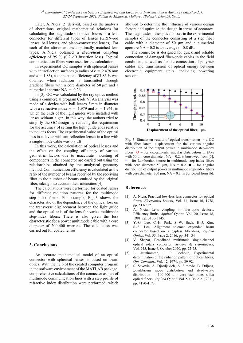
7th International Conference on Sensors Engineering and Electronics Instrumentation Advances (SEIA' 2021), 22-24 September 2021, Palma de Mallorca, Mallorca (Balearic Islands), Spain
136
Later, A. Nicia [2] derived, based on the analysis of aberrations, original mathematical relations for calculating the magnitude of optical losses in a lens connector for different types of lenses (GRIN-rod lenses, ball lenses, and plano-convex rod lenses). For each of the aforementioned optimally matched lens types, A. Nicia obtained a theoretical coupling efficiency of 95 % (0.2 dB insertion loss). Typical communication fibers were used for the calculation.
In experimental OC samples with spherical lenses with antireflection surfaces (a radius of r = 2.476 mm and n = 1.83), a connection efficiency of 83-85 % was obtained when radiation is transmitted through gradient fibers with a core diameter of 50 μm and a numerical aperture NA = 0.26
In [3], OC was calculated by the ray optics method using a commercial program Code V. An analysis was made of a device with ball lenses 3 mm in diameter with a refractive index n = 1.979 and n = 1.961, in which the ends of the light guides were installed with lenses without a gap. In this way, the authors tried to simplify the OC design by reducing the requirement for the accuracy of setting the light guide ends relative to the lens focus. The experimental value of the optical loss in a device with antireflection lenses in a line with a single-mode cable was 0.8 dB.
In this work, the calculation of optical losses and the effect on the coupling efficiency of various geometric factors due to inaccurate mounting of components in the connector are carried out using the relationships obtained by the analytical geometry method. Communication efficiency is calculated as the ratio of the number of beams received by the receiving fiber to the number of beams emitted by the original fiber, taking into account their intensities [4].
The calculations were performed for coated lenses for different radiation patterns for the multimode step-index fibers. For example, Fig. 3 shows the characteristic of the dependence of the optical loss on the transverse displacement between the light guide and the optical axis of the lens for varies multimode step-index fibers. There is also given the loss characteristic for a power multimode cable with a core diameter of 200-400 microns. The calculation was carried out for coated lenses. 3. Conclusions
An accurate mathematical model of an optical connector with spherical lenses is based on beam optics. With the help of the created computer program in the software environment of the MATLAB package, comprehensive calculations of the connector as part of multimode communication lines with a step profile of refractive index distribution were performed, which
allowed to determine the influence of various design factors and optimize the design in terms of accuracy. The magnitude of the optical losses in the experimental samples of the connector consisting of a step fiber cable with a diameter of 50 μm and a numerical aperture NA = 0.2 is an average of 0.8 dB.
The connector is designed for quick and reliable connection of damaged fiber-optic cables in the field conditions, as well as for the connection of polymer cables and transmission of optical energy between electronic equipment units, including powering sensors.
Fig. 3. Simulation results of optical transmission in a OC with fiber lateral displacement for the various angular distribution of the output power in multimode step-index fibers: Ο – for experimental angular distribution in fiber with 50 μm core diameter, NA = 0.2, is borrowed from [5]; * – for Lambertian source in multimode step-index fibers with core diameter 50 μm, NA = 0.2. – for angular distribution of output power in multimode step-index fibers with core diameter 200 μm, NA = 0.2, is borrowed from [6]. References [1]. A. Nicia, Practical low-loss lens connector for optical
fibres, Electronics Letters, Vol. 14, Issue 16, 1978, pp. 511-512.
[2]. A. Nicia, Lens coupling in fiber-optic devices: Efficiency limits, Applied Optics, Vol. 20, Issue 18, 1981, pp. 3136-3145.
[3]. Y.-G. Lee, C.-H. Park, S.-W. Back, H.-J. Kim, S.-S. Lee, Alignment tolerant expanded beam connector based on a gapless fiber-lens, Applied Optics, Vol. 55, Issue 2, 2016, pp. 341-344.
[4] V. Shapar, Broadband multimode single-channel optical rotary connector, Sensors & Transducers, Vol. 245, Issue 6, October 2020, pp. 72-75.
[5]. L. Jeunhomme, J. P. Pocholle, Experimental determination of the radiation pattern of optical fibres, Opt. Commun., Vol. 12, 1974, pp. 89-92.
[6]. S. Savovic, A. Djordjevich, A. Simovic, B. Drljaca, Equilibrium mode distribution and steady-state distribution in 100-400 μm core step-index silica optical fibers, Applied Optics, Vol. 50, Issue 21, 2011, pp. 4170-4173.
7th International Conference on Sensors Engineering and Electronics Instrumentation Advances (SEIA' 2021), 22-24 September 2021, Palma de Mallorca, Mallorca (Balearic Islands), Spain
137
(044)
Strain Measurement Within Thin Fibers Based on Subjective Laser Speckle Patterns
A. Spaett, R. Gridling 1 and B. G. Zagar
Johannes Kepler University Linz, Institute for Measurement Technology, Altenberger Straße 69, 4040 Linz, Austria
Tel.: +43 732 2468 5930 E-mail: [email protected]
Summary: The measurement of stress-strain curves of fibers poses a challenging task, since commonly used contacting techniques are not applicable. Therefore, we propose to employ a laser-speckle extensometer with a sufficiently high displacement resolution to be able to even derive strain values of the rather very stiff structural fibers. Due to the properties of laser speckle patterns stemming from fibers, they are especially well suited for the task. In order to measure the stress-strain curve one has to estimate local displacements between strained and initial loading for two surface elements separated by the base length the strain is to be determined over. This is a formidable task in itself, since shifts in the range of only 1/100 of the pixel pitch have to be resolved in order to enable the characterization of a wide range of different biological and technical fibers. Keywords: Strain measurement, Subjective laser speckle patterns, Fibers, Stress-strain curve.
1. Introduction
The measurement of stress-strain curves is commonly done by the use of contacting methods such as glued on strain gauges or fiber Bragg gratings. However, when considering the small size of technical or biological fibers, like human hair, it becomes evident that these contacting methods are not always applicable. Therefore, the use of non-contacting methods becomes a necessity. One method, which has been successfully applied to the analysis of human hair, is to take (magnified) images of the sample and try to estimate the strain by using digital image correlation (DIC) on the loaded fibers [1]. However, this technique oftentimes needs additional pairs of markers applied to the sample and the accuracy of DIC suffers when analyzing shifts lower than the camera’s pixel pitch. This in particular becomes an issue when stiffer materials are to be characterized.
A technique which circumvents the need for additional markers and can be applied for a wide range of materials is that of a laser speckle extensometer. Here, these markers are inherently formed by the technique itself while also offering high contrast for optically rough surfaces. In order to estimate the engineering strain within a specimen via this technique, estimates of two sufficiently distant observation spots and their load-dependent speckle pattern displacements is necessary [2]. Thus, in this contribution we elaborate on obtaining a high-resolution estimate of speckle displacement fields. Assuming a typical base length of 20 mm and a maximum strain of 10-3 the maximum elongation is a mere 20 µm that needs to be resolved into at least a few hundred increments so the estimation algorithm needs to resolve approximately 1/100 of a typical camera pixel's pitch.
In this contribution we concentrate on characterizing an estimation algorithm that is not subject to the inherent quantization the camera pixel size demands, but delivers – theoretically – arbitrarily fine resolved measurements. This is possible if one considers the shifting property of the Fourier transform analyzed in the spectral domain weighted by a measure of spectral correlation namely the spectral coherency [3].
The paper is organized as follows. Section 2 details the measurement principle, the optical setup, and the developed signal processing algorithms. Section 3 gives insight to considerations which have to be made when it comes to the size of the observed speckles. Section 4 presents the measurement results which have been achieved with the measurement setup presented in Section 2. Finally, Section 5 concludes the paper by giving a short summary and outlook. 2. Measurement Principle
The underlying idea of the strain measurement based on laser speckle patterns is that there is a relation between the behavior of the captured patterns and the change and movement of the specimen. Laser speckle patterns are deterministic, random looking patterns which form when sufficiently coherent light illuminates an optically rough surface [4].
In this paper a telecentric optical system is used for capturing laser speckle patterns. In [5] Yamaguchi has derived an equation governing the movement of the imaged speckles 𝐴 for the case of imaging the speckles with help of a telecentric optical system. This equation shows that in general not only the local movement of the specimen in the same direction 𝑎 influence the speckle movement. This is the movement
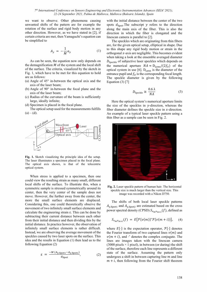
7th International Conference on Sensors Engineering and Electronics Instrumentation Advances (SEIA' 2021), 22-24 September 2021, Palma de Mallorca, Mallorca (Balearic Islands), Spain
138
we want to observe. Other phenomena causing unwanted shifts of the pattern are for example the rotation of the surface and rigid body motion in any other direction. However, as we have stated in [2], if certain criteria are met, then Yamaguchi’s equation can be simplified to
𝐴 1𝑀
𝑎 (1)
As can be seen, the equation now only depends on
the demagnification 𝑀 of the system and the local shift of the surface. The criteria, visualized by the sketch in Fig. 1, which have to be met for this equation to hold are as follows: (a) Angle of 45° in-between the optical axis and the
axis of the laser beam; (b) Angle of 90° in-between the focal plane and the
axis of the laser beam; (c) Radius of the curvature of the beam is sufficiently
large, ideally infinite; (d) Specimen is placed in the focal plane.
The optical setup used for the measurements fulfills (a) – (d).
Fig. 1. Sketch visualizing the principle idea of the setup. The laser illuminates a specimen placed in the focal plane. The optical axis shown, is that of the telecentric optical system.
When stress is applied to a specimen, then one
could view the resulting strain as many small, different local shifts of the surface. To illustrate this, when a symmetric sample is stressed symmetrically around its center, then the very center of the sample does not move. However, the further away from the center, the more the small surface elements are displaced. Considering this, one could theoretically observe the movement of two infinitely small surface elements and calculate the engineering strain ε. This can be done by subtracting their current distance between each other from their initial distance and then dividing this by the initial distance. In practice however, the observation of infinitely small surface elements is rather difficult. Instead, we are observing the average movement of the speckles caused by two laser spots on the surface. This idea and the results in Equation (1) then lead us to the following Equation (2)
ε , ,
, (2)
with the initial distance between the center of the two spots 𝑑 .The subscript 𝑦 refers to the direction along the main axis of the fiber. This is also the direction in which the fiber is elongated and the linescan camera is parallel to [2].
The speckles which are originating from thin fibers are, for the given optical setup, elliptical in shape. Due to this shape any rigid body motion or strain in the orthogonal 𝑥-axis are negligible. This becomes evident when taking a look at the ensemble averaged diameter 𝐷Speckle of subjective laser speckles which depends on the numerical aperture 𝑁𝐴 D / 2𝑓 of the optical system in use [6]. D is the diameter of the entrance pupil and 𝑓 is the corresponding focal length. The speckle diameter is given by the following Equation (3) [7]
𝐷Speckle ≅
0.6 λ𝑁𝐴
(3)
Here the optical system’s numerical aperture limits
the size of the speckles in 𝑦-direction, whereas the fiber diameter defines the speckle size in 𝑥-direction. An example of a typical laser speckle pattern using a thin fiber as a sample can be seen in Fig. 2.
Fig. 2. Laser speckle pattern of human hair. The horizontal speckle size is much larger than the vertical size. This
image was recorded with a Nikon D750. The shifts of both local laser speckle patterns
𝐴 , and 𝐴 , are estimated based on the cross power spectral density (CPSD) 𝑆 𝑓 , defined as
𝑆 𝑓 𝐸 ℱ 𝑣 𝑚 ∗ℱ 𝑣 𝑚 𝑖 , (4)
where 𝐸 ⋅ is the expectation operator, ℱ ⋅ denotes the Fourier transform of two captured lines 𝑣 𝑚 and 𝑣 𝑚 𝑖 , and ⋅∗ denotes the complex conjugate. The lines are images taken with the linescan camera (3000 pixels × 1 pixel), in between (or during) the shift of the surface, therefore each line represents a different state of the surface. Assuming the pattern only undergoes a shift in between capturing line 𝑚 and line 𝑚 𝑖, then following from the Fourier shift theorem
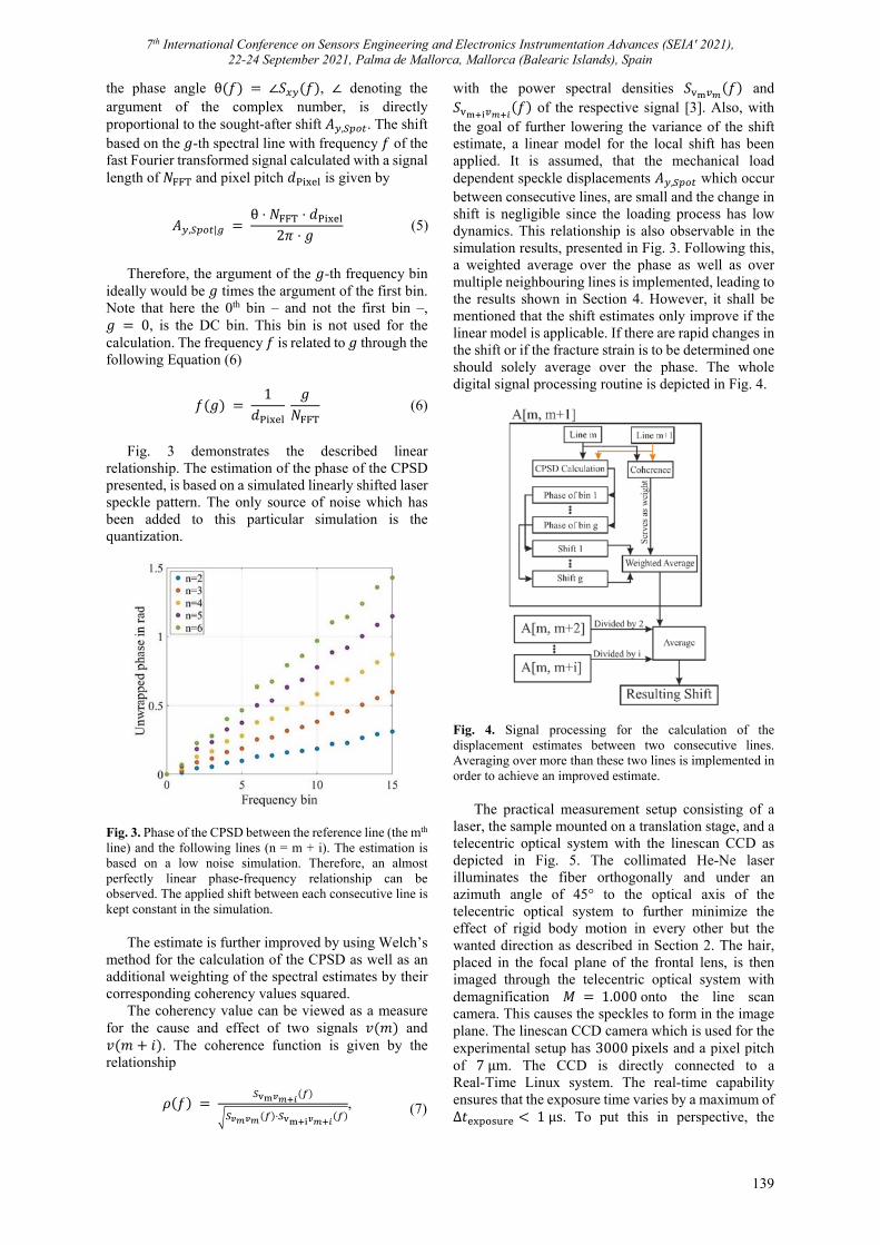
7th International Conference on Sensors Engineering and Electronics Instrumentation Advances (SEIA' 2021), 22-24 September 2021, Palma de Mallorca, Mallorca (Balearic Islands), Spain
139
the phase angle θ 𝑓 ∠𝑆 𝑓 , ∠ denoting the argument of the complex number, is directly proportional to the sought-after shift 𝐴 , . The shift based on the 𝑔-th spectral line with frequency 𝑓 of the fast Fourier transformed signal calculated with a signal length of 𝑁 and pixel pitch 𝑑 is given by
𝐴 , | θ ⋅ 𝑁 ⋅ 𝑑
2𝜋 ⋅ 𝑔 (5)
Therefore, the argument of the 𝑔-th frequency bin
ideally would be 𝑔 times the argument of the first bin. Note that here the 0th bin – and not the first bin –, 𝑔 0, is the DC bin. This bin is not used for the calculation. The frequency 𝑓 is related to 𝑔 through the following Equation (6)
𝑓 𝑔 1
𝑑
𝑔𝑁
(6)
Fig. 3 demonstrates the described linear
relationship. The estimation of the phase of the CPSD presented, is based on a simulated linearly shifted laser speckle pattern. The only source of noise which has been added to this particular simulation is the quantization.
Fig. 3. Phase of the CPSD between the reference line (the mth line) and the following lines (n = m + i). The estimation is based on a low noise simulation. Therefore, an almost perfectly linear phase-frequency relationship can be observed. The applied shift between each consecutive line is kept constant in the simulation.
The estimate is further improved by using Welch’s
method for the calculation of the CPSD as well as an additional weighting of the spectral estimates by their corresponding coherency values squared.
The coherency value can be viewed as a measure for the cause and effect of two signals 𝑣 𝑚 and 𝑣 𝑚 𝑖 . The coherence function is given by the relationship
𝜌 𝑓 ⋅
, (7)
with the power spectral densities 𝑆 𝑓 and 𝑆 𝑓 of the respective signal [3]. Also, with the goal of further lowering the variance of the shift estimate, a linear model for the local shift has been applied. It is assumed, that the mechanical load dependent speckle displacements 𝐴 , which occur between consecutive lines, are small and the change in shift is negligible since the loading process has low dynamics. This relationship is also observable in the simulation results, presented in Fig. 3. Following this, a weighted average over the phase as well as over multiple neighbouring lines is implemented, leading to the results shown in Section 4. However, it shall be mentioned that the shift estimates only improve if the linear model is applicable. If there are rapid changes in the shift or if the fracture strain is to be determined one should solely average over the phase. The whole digital signal processing routine is depicted in Fig. 4.
Fig. 4. Signal processing for the calculation of the displacement estimates between two consecutive lines. Averaging over more than these two lines is implemented in order to achieve an improved estimate.
The practical measurement setup consisting of a
laser, the sample mounted on a translation stage, and a telecentric optical system with the linescan CCD as depicted in Fig. 5. The collimated He-Ne laser illuminates the fiber orthogonally and under an azimuth angle of 45° to the optical axis of the telecentric optical system to further minimize the effect of rigid body motion in every other but the wanted direction as described in Section 2. The hair, placed in the focal plane of the frontal lens, is then imaged through the telecentric optical system with demagnification 𝑀 1.000 onto the line scan camera. This causes the speckles to form in the image plane. The linescan CCD camera which is used for the experimental setup has 3000 pixels and a pixel pitch of 7 µm. The CCD is directly connected to a Real-Time Linux system. The real-time capability ensures that the exposure time varies by a maximum of ∆𝑡 1 µs. To put this in perspective, the
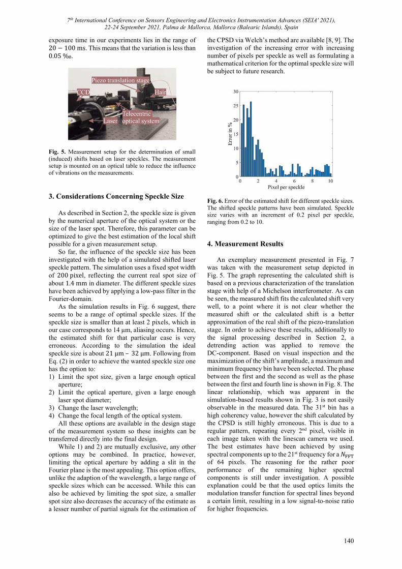
7th International Conference on Sensors Engineering and Electronics Instrumentation Advances (SEIA' 2021), 22-24 September 2021, Palma de Mallorca, Mallorca (Balearic Islands), Spain
140
exposure time in our experiments lies in the range of 20 100 ms. This means that the variation is less than 0.05 ‰.
Fig. 5. Measurement setup for the determination of small (induced) shifts based on laser speckles. The measurement setup is mounted on an optical table to reduce the influence of vibrations on the measurements.
3. Considerations Concerning Speckle Size
As described in Section 2, the speckle size is given by the numerical aperture of the optical system or the size of the laser spot. Therefore, this parameter can be optimized to give the best estimation of the local shift possible for a given measurement setup.
So far, the influence of the speckle size has been investigated with the help of a simulated shifted laser speckle pattern. The simulation uses a fixed spot width of 200 pixel, reflecting the current real spot size of about 1.4 mm in diameter. The different speckle sizes have been achieved by applying a low-pass filter in the Fourier-domain.
As the simulation results in Fig. 6 suggest, there seems to be a range of optimal speckle sizes. If the speckle size is smaller than at least 2 pixels, which in our case corresponds to 14 µm, aliasing occurs. Hence, the estimated shift for that particular case is very erroneous. According to the simulation the ideal speckle size is about 21 µm – 32 µm. Following from Eq. (2) in order to achieve the wanted speckle size one has the option to: 1) Limit the spot size, given a large enough optical
aperture; 2) Limit the optical aperture, given a large enough
laser spot diameter; 3) Change the laser wavelength; 4) Change the focal length of the optical system.
All these options are available in the design stage of the measurement system so these insights can be transferred directly into the final design.
While 1) and 2) are mutually exclusive, any other options may be combined. In practice, however, limiting the optical aperture by adding a slit in the Fourier plane is the most appealing. This option offers, unlike the adaption of the wavelength, a large range of speckle sizes which can be accessed. While this can also be achieved by limiting the spot size, a smaller spot size also decreases the accuracy of the estimate as a lesser number of partial signals for the estimation of
the CPSD via Welch’s method are available [8, 9]. The investigation of the increasing error with increasing number of pixels per speckle as well as formulating a mathematical criterion for the optimal speckle size will be subject to future research.
Fig. 6. Error of the estimated shift for different speckle sizes. The shifted speckle patterns have been simulated. Speckle size varies with an increment of 0.2 pixel per speckle, ranging from 0.2 to 10. 4. Measurement Results
An exemplary measurement presented in Fig. 7 was taken with the measurement setup depicted in Fig. 5. The graph representing the calculated shift is based on a previous characterization of the translation stage with help of a Michelson interferometer. As can be seen, the measured shift fits the calculated shift very well, to a point where it is not clear whether the measured shift or the calculated shift is a better approximation of the real shift of the piezo-translation stage. In order to achieve these results, additionally to the signal processing described in Section 2, a detrending action was applied to remove the DC-component. Based on visual inspection and the maximization of the shift’s amplitude, a maximum and minimum frequency bin have been selected. The phase between the first and the second as well as the phase between the first and fourth line is shown in Fig. 8. The linear relationship, which was apparent in the simulation-based results shown in Fig. 3 is not easily observable in the measured data. The 31st bin has a high coherency value, however the shift calculated by the CPSD is still highly erroneous. This is due to a regular pattern, repeating every 2nd pixel, visible in each image taken with the linescan camera we used. The best estimates have been achieved by using spectral components up to the 21st frequency for a 𝑁 of 64 pixels. The reasoning for the rather poor performance of the remaining higher spectral components is still under investigation. A possible explanation could be that the used optics limits the modulation transfer function for spectral lines beyond a certain limit, resulting in a low signal-to-noise ratio for higher frequencies.
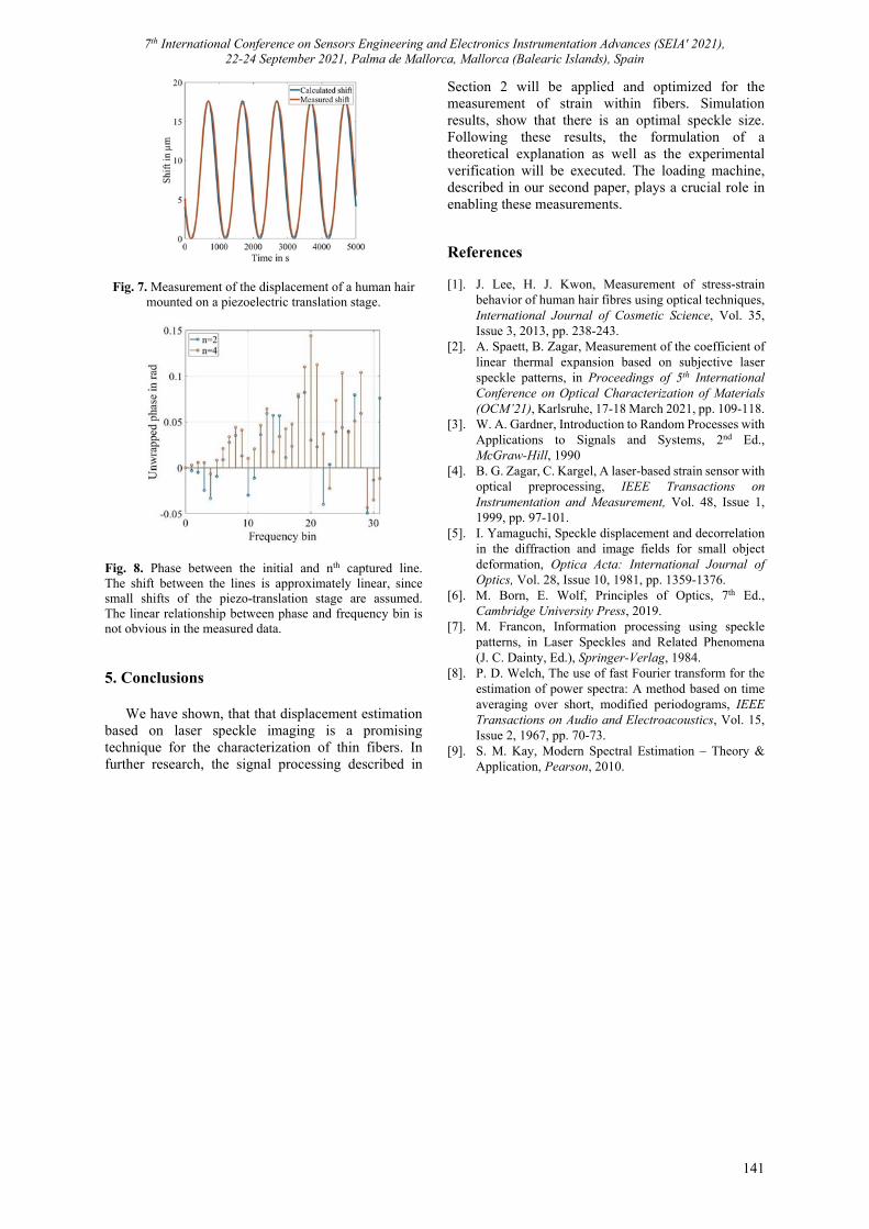
7th International Conference on Sensors Engineering and Electronics Instrumentation Advances (SEIA' 2021), 22-24 September 2021, Palma de Mallorca, Mallorca (Balearic Islands), Spain
141
Fig. 7. Measurement of the displacement of a human hair mounted on a piezoelectric translation stage.
Fig. 8. Phase between the initial and nth captured line. The shift between the lines is approximately linear, since small shifts of the piezo-translation stage are assumed. The linear relationship between phase and frequency bin is not obvious in the measured data. 5. Conclusions
We have shown, that that displacement estimation based on laser speckle imaging is a promising technique for the characterization of thin fibers. In further research, the signal processing described in
Section 2 will be applied and optimized for the measurement of strain within fibers. Simulation results, show that there is an optimal speckle size. Following these results, the formulation of a theoretical explanation as well as the experimental verification will be executed. The loading machine, described in our second paper, plays a crucial role in enabling these measurements. References [1]. J. Lee, H. J. Kwon, Measurement of stress-strain
behavior of human hair fibres using optical techniques, International Journal of Cosmetic Science, Vol. 35, Issue 3, 2013, pp. 238-243.
[2]. A. Spaett, B. Zagar, Measurement of the coefficient of linear thermal expansion based on subjective laser speckle patterns, in Proceedings of 5th International Conference on Optical Characterization of Materials (OCM’21), Karlsruhe, 17-18 March 2021, pp. 109-118.
[3]. W. A. Gardner, Introduction to Random Processes with Applications to Signals and Systems, 2nd Ed., McGraw-Hill, 1990
[4]. B. G. Zagar, C. Kargel, A laser-based strain sensor with optical preprocessing, IEEE Transactions on Instrumentation and Measurement, Vol. 48, Issue 1, 1999, pp. 97-101.
[5]. I. Yamaguchi, Speckle displacement and decorrelation in the diffraction and image fields for small object deformation, Optica Acta: International Journal of Optics, Vol. 28, Issue 10, 1981, pp. 1359-1376.
[6]. M. Born, E. Wolf, Principles of Optics, 7th Ed., Cambridge University Press, 2019.
[7]. M. Francon, Information processing using speckle patterns, in Laser Speckles and Related Phenomena (J. C. Dainty, Ed.), Springer-Verlag, 1984.
[8]. P. D. Welch, The use of fast Fourier transform for the estimation of power spectra: A method based on time averaging over short, modified periodograms, IEEE Transactions on Audio and Electroacoustics, Vol. 15, Issue 2, 1967, pp. 70-73.
[9]. S. M. Kay, Modern Spectral Estimation – Theory & Application, Pearson, 2010.
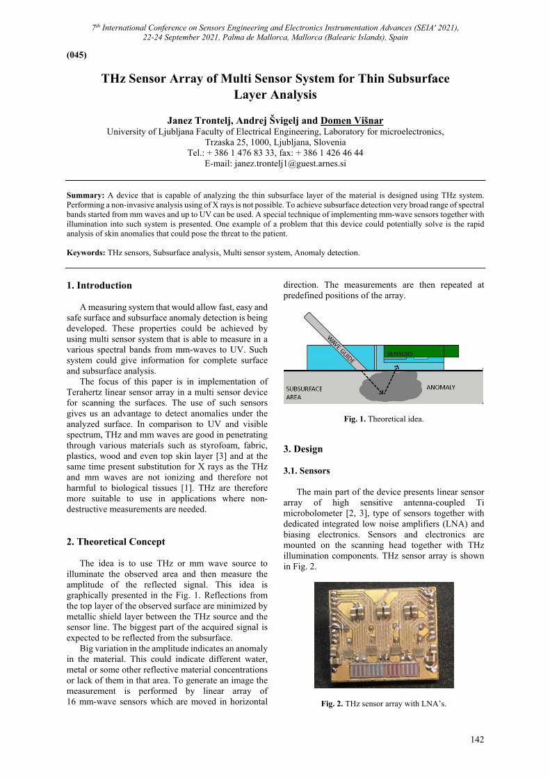
7th International Conference on Sensors Engineering and Electronics Instrumentation Advances (SEIA' 2021), 22-24 September 2021, Palma de Mallorca, Mallorca (Balearic Islands), Spain
142
(045)
THz Sensor Array of Multi Sensor System for Thin Subsurface Layer Analysis
Janez Trontelj, Andrej Švigelj and Domen Višnar
University of Ljubljana Faculty of Electrical Engineering, Laboratory for microelectronics, Trzaska 25, 1000, Ljubljana, Slovenia
Tel.: + 386 1 476 83 33, fax: + 386 1 426 46 44 E-mail: [email protected]
Summary: A device that is capable of analyzing the thin subsurface layer of the material is designed using THz system. Performing a non-invasive analysis using of X rays is not possible. To achieve subsurface detection very broad range of spectral bands started from mm waves and up to UV can be used. A special technique of implementing mm-wave sensors together with illumination into such system is presented. One example of a problem that this device could potentially solve is the rapid analysis of skin anomalies that could pose the threat to the patient. Keywords: THz sensors, Subsurface analysis, Multi sensor system, Anomaly detection.
1. Introduction
A measuring system that would allow fast, easy and safe surface and subsurface anomaly detection is being developed. These properties could be achieved by using multi sensor system that is able to measure in a various spectral bands from mm-waves to UV. Such system could give information for complete surface and subsurface analysis.
The focus of this paper is in implementation of Terahertz linear sensor array in a multi sensor device for scanning the surfaces. The use of such sensors gives us an advantage to detect anomalies under the analyzed surface. In comparison to UV and visible spectrum, THz and mm waves are good in penetrating through various materials such as styrofoam, fabric, plastics, wood and even top skin layer [3] and at the same time present substitution for X rays as the THz and mm waves are not ionizing and therefore not harmful to biological tissues [1]. THz are therefore more suitable to use in applications where non-destructive measurements are needed. 2. Theoretical Concept
The idea is to use THz or mm wave source to illuminate the observed area and then measure the amplitude of the reflected signal. This idea is graphically presented in the Fig. 1. Reflections from the top layer of the observed surface are minimized by metallic shield layer between the THz source and the sensor line. The biggest part of the acquired signal is expected to be reflected from the subsurface.
Big variation in the amplitude indicates an anomaly in the material. This could indicate different water, metal or some other reflective material concentrations or lack of them in that area. To generate an image the measurement is performed by linear array of 16 mm-wave sensors which are moved in horizontal
direction. The measurements are then repeated at predefined positions of the array.
Fig. 1. Theoretical idea.
3. Design 3.1. Sensors
The main part of the device presents linear sensor array of high sensitive antenna-coupled Ti microbolometer [2, 3], type of sensors together with dedicated integrated low noise amplifiers (LNA) and biasing electronics. Sensors and electronics are mounted on the scanning head together with THz illumination components. THz sensor array is shown in Fig. 2.
Fig. 2. THz sensor array with LNA’s.
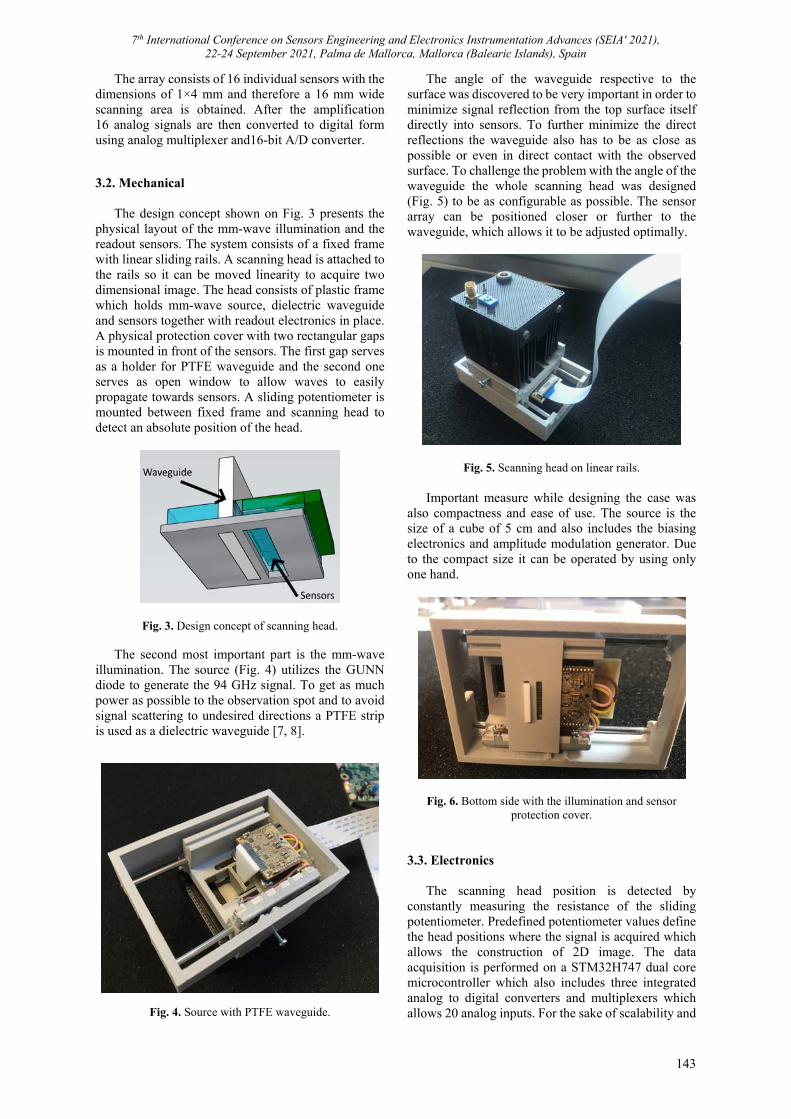
7th International Conference on Sensors Engineering and Electronics Instrumentation Advances (SEIA' 2021), 22-24 September 2021, Palma de Mallorca, Mallorca (Balearic Islands), Spain
143
The array consists of 16 individual sensors with the dimensions of 1×4 mm and therefore a 16 mm wide scanning area is obtained. After the amplification 16 analog signals are then converted to digital form using analog multiplexer and16-bit A/D converter. 3.2. Mechanical
The design concept shown on Fig. 3 presents the
physical layout of the mm-wave illumination and the readout sensors. The system consists of a fixed frame with linear sliding rails. A scanning head is attached to the rails so it can be moved linearity to acquire two dimensional image. The head consists of plastic frame which holds mm-wave source, dielectric waveguide and sensors together with readout electronics in place. A physical protection cover with two rectangular gaps is mounted in front of the sensors. The first gap serves as a holder for PTFE waveguide and the second one serves as open window to allow waves to easily propagate towards sensors. A sliding potentiometer is mounted between fixed frame and scanning head to detect an absolute position of the head.
Fig. 3. Design concept of scanning head.
The second most important part is the mm-wave illumination. The source (Fig. 4) utilizes the GUNN diode to generate the 94 GHz signal. To get as much power as possible to the observation spot and to avoid signal scattering to undesired directions a PTFE strip is used as a dielectric waveguide [7, 8].
Fig. 4. Source with PTFE waveguide.
The angle of the waveguide respective to the surface was discovered to be very important in order to minimize signal reflection from the top surface itself directly into sensors. To further minimize the direct reflections the waveguide also has to be as close as possible or even in direct contact with the observed surface. To challenge the problem with the angle of the waveguide the whole scanning head was designed (Fig. 5) to be as configurable as possible. The sensor array can be positioned closer or further to the waveguide, which allows it to be adjusted optimally.
Fig. 5. Scanning head on linear rails. Important measure while designing the case was
also compactness and ease of use. The source is the size of a cube of 5 cm and also includes the biasing electronics and amplitude modulation generator. Due to the compact size it can be operated by using only one hand.
Fig. 6. Bottom side with the illumination and sensor protection cover.
3.3. Electronics
The scanning head position is detected by constantly measuring the resistance of the sliding potentiometer. Predefined potentiometer values define the head positions where the signal is acquired which allows the construction of 2D image. The data acquisition is performed on a STM32H747 dual core microcontroller which also includes three integrated analog to digital converters and multiplexers which allows 20 analog inputs. For the sake of scalability and
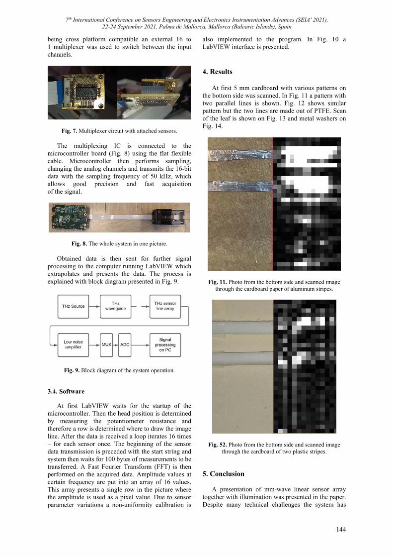
7th International Conference on Sensors Engineering and Electronics Instrumentation Advances (SEIA' 2021), 22-24 September 2021, Palma de Mallorca, Mallorca (Balearic Islands), Spain
144
being cross platform compatible an external 16 to 1 multiplexer was used to switch between the input channels.
Fig. 7. Multiplexer circuit with attached sensors.
The multiplexing IC is connected to the microcontroller board (Fig. 8) using the flat flexible cable. Microcontroller then performs sampling, changing the analog channels and transmits the 16-bit data with the sampling frequency of 50 kHz, which allows good precision and fast acquisition of the signal.
Fig. 8. The whole system in one picture.
Obtained data is then sent for further signal processing to the computer running LabVIEW which extrapolates and presents the data. The process is explained with block diagram presented in Fig. 9.
Fig. 9. Block diagram of the system operation. 3.4. Software
At first LabVIEW waits for the startup of the microcontroller. Then the head position is determined by measuring the potentiometer resistance and therefore a row is determined where to draw the image line. After the data is received a loop iterates 16 times – for each sensor once. The beginning of the sensor data transmission is preceded with the start string and system then waits for 100 bytes of measurements to be transferred. A Fast Fourier Transform (FFT) is then performed on the acquired data. Amplitude values at certain frequency are put into an array of 16 values. This array presents a single row in the picture where the amplitude is used as a pixel value. Due to sensor parameter variations a non-uniformity calibration is
also implemented to the program. In Fig. 10 a LabVIEW interface is presented.
4. Results
At first 5 mm cardboard with various patterns on the bottom side was scanned. In Fig. 11 a pattern with two parallel lines is shown. Fig. 12 shows similar pattern but the two lines are made out of PTFE. Scan of the leaf is shown on Fig. 13 and metal washers on Fig. 14.
Fig. 11. Photo from the bottom side and scanned image through the cardboard paper of aluminum stripes.
Fig. 52. Photo from the bottom side and scanned image through the cardboard of two plastic stripes.
5. Conclusion
A presentation of mm-wave linear sensor array together with illumination was presented in the paper. Despite many technical challenges the system has
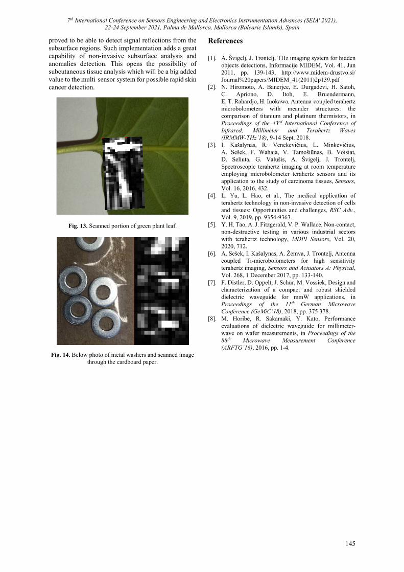
7th International Conference on Sensors Engineering and Electronics Instrumentation Advances (SEIA' 2021), 22-24 September 2021, Palma de Mallorca, Mallorca (Balearic Islands), Spain
145
proved to be able to detect signal reflections from the subsurface regions. Such implementation adds a great capability of non-invasive subsurface analysis and anomalies detection. This opens the possibility of subcutaneous tissue analysis which will be a big added value to the multi-sensor system for possible rapid skin cancer detection.
Fig. 13. Scanned portion of green plant leaf.
Fig. 14. Below photo of metal washers and scanned image through the cardboard paper.
References [1]. A. Švigelj, J. Trontelj, THz imaging system for hidden
objects detections, Informacije MIDEM, Vol. 41, Jun 2011, pp. 139-143, http://www.midem-drustvo.si/ Journal%20papers/MIDEM_41(2011)2p139.pdf
[2]. N. Hiromoto, A. Banerjee, E. Durgadevi, H. Satoh, C. Apriono, D. Itoh, E. Bruendermann, E. T. Rahardjo, H. Inokawa, Antenna-coupled terahertz microbolometers with meander structures: the comparison of titanium and platinum thermistors, in Proceedings of the 43rd International Conference of Infrared, Millimeter and Terahertz Waves (IRMMW-THz’18), 9-14 Sept. 2018.
[3]. I. Kašalynas, R. Venckevičius, L. Minkevičius, A. Sešek, F. Wahaia, V. Tamošiūnas, B. Voisiat, D. Seliuta, G. Valušis, A. Švigelj, J. Trontelj, Spectroscopic terahertz imaging at room temperature employing microbolometer terahertz sensors and its application to the study of carcinoma tissues, Sensors, Vol. 16, 2016, 432.
[4]. L. Yu, L. Hao, et al., The medical application of terahertz technology in non-invasive detection of cells and tissues: Opportunities and challenges, RSC Adv., Vol. 9, 2019, pp. 9354-9363.
[5]. Y. H. Tao, A. J. Fitzgerald, V. P. Wallace, Non-contact, non-destructive testing in various industrial sectors with terahertz technology, MDPI Sensors, Vol. 20, 2020, 712.
[6]. A. Sešek, I. Kašalynas, A. Žemva, J. Trontelj, Antenna coupled Ti-microbolometers for high sensitivity terahertz imaging, Sensors and Actuators A: Physical, Vol. 268, 1 December 2017, pp. 133-140.
[7]. F. Distler, D. Oppelt, J. Schür, M. Vossiek, Design and characterization of a compact and robust shielded dielectric waveguide for mmW applications, in Proceedings of the 11th German Microwave Conference (GeMiC’18), 2018, pp. 375 378.
[8]. M. Horibe, R. Sakamaki, Y. Kato, Performance evaluations of dielectric waveguide for millimeter-wave on wafer measurements, in Proceedings of the 88th Microwave Measurement Conference (ARFTG’16), 2016, pp. 1-4.
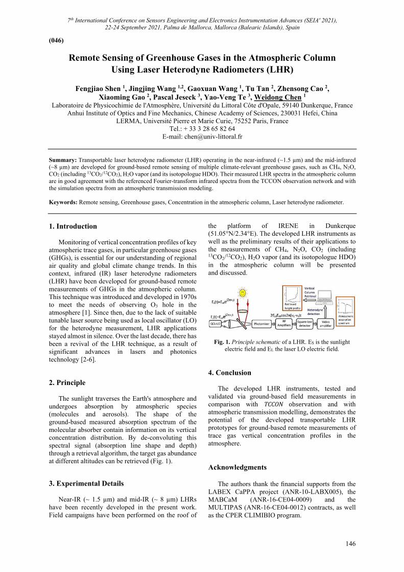
7th International Conference on Sensors Engineering and Electronics Instrumentation Advances (SEIA' 2021), 22-24 September 2021, Palma de Mallorca, Mallorca (Balearic Islands), Spain
146
(046)
Remote Sensing of Greenhouse Gases in the Atmospheric Column Using Laser Heterodyne Radiometers (LHR)
Fengjiao Shen 1, Jingjing Wang 1,2, Gaoxuan Wang 1, Tu Tan 2, Zhensong Cao 2,
Xiaoming Gao 2, Pascal Jeseck 3, Yao-Veng Te 3, Weidong Chen 1
Laboratoire de Physicochimie de l'Atmosphère, Université du Littoral Côte d'Opale, 59140 Dunkerque, France Anhui Institute of Optics and Fine Mechanics, Chinese Academy of Sciences, 230031 Hefei, China
LERMA, Université Pierre et Marie Curie, 75252 Paris, France Tel.: + 33 3 28 65 82 64
E-mail: [email protected] Summary:Transportable laser heterodyne radiometer (LHR) operating in the near-infrared (~1.5 µm) and the mid-infrared (~8 µm) are developed for ground-based remote sensing of multiple climate-relevant greenhouse gases, such as CH4, N2O, CO2 (including 13CO2/12CO2), H2O vapor (and its isotopologue HDO). Their measured LHR spectra in the atmospheric column are in good agreement with the referenced Fourier-transform infrared spectra from the TCCON observation network and with the simulation spectra from an atmospheric transmission modeling. Keywords: Remote sensing, Greenhouse gases, Concentration in the atmospheric column, Laser heterodyne radiometer.
1. Introduction
Monitoring of vertical concentration profiles of key atmospheric trace gases, in particular greenhouse gases (GHGs), is essential for our understanding of regional air quality and global climate change trends. In this context, infrared (IR) laser heterodyne radiometers (LHR) have been developed for ground-based remote measurements of GHGs in the atmospheric column. This technique was introduced and developed in 1970s to meet the needs of observing O3 hole in the atmosphere [1]. Since then, due to the lack of suitable tunable laser source being used as local oscillator (LO) for the heterodyne measurement, LHR applications stayed almost in silence. Over the last decade, there has been a revival of the LHR technique, as a result of significant advances in lasers and photonics technology [2-6]. 2. Principle
The sunlight traverses the Earth's atmosphere and undergoes absorption by atmospheric species (molecules and aerosols). The shape of the ground-based measured absorption spectrum of the molecular absorber contain information on its vertical concentration distribution. By de-convoluting this spectral signal (absorption line shape and depth) through a retrieval algorithm, the target gas abundance at different altitudes can be retrieved (Fig. 1). 3. Experimental Details
Near-IR (~ 1.5 µm) and mid-IR (~ 8 µm) LHRs have been recently developed in the present work. Field campaigns have been performed on the roof of
the platform of IRENE in Dunkerque (51.05°N/2.34°E). The developed LHR instruments as well as the preliminary results of their applications to the measurements of CH4, N2O, CO2 (including 13CO2/12CO2), H2O vapor (and its isotopologue HDO) in the atmospheric column will be presented and discussed.
Fig. 1. Principle schematic of a LHR. ES is the sunlight electric field and EL the laser LO electric field.
4. Conclusion
The developed LHR instruments, tested and validated via ground-based field measurements in comparison with TCCON observation and with atmospheric transmission modelling, demonstrates the potential of the developed transportable LHR prototypes for ground-based remote measurements of trace gas vertical concentration profiles in the atmosphere. Acknowledgments
The authors thank the financial supports from the LABEX CaPPA project (ANR-10-LABX005), the MABCaM (ANR-16-CE04-0009) and the MULTIPAS (ANR-16-CE04-0012) contracts, as well as the CPER CLIMIBIO program.

7th International Conference on Sensors Engineering and Electronics Instrumentation Advances (SEIA' 2021), 22-24 September 2021, Palma de Mallorca, Mallorca (Balearic Islands), Spain
147
References [1]. R. T. Menzies, R. K. Seals, Ozone monitoring with an
infrared heterodyne radiometer, Science, Vol. 197, 1977, pp. 1275-1277.
[2]. D. Weidmann, T. Tsai, N. A. Macleod, G. Wysocki, Atmospheric observations of multiple molecular species using ultra-high-resolution external cavity quantum cascade laser heterodyne radiometry, Opt. Lett., Vol. 36, 2011, pp. 1951-1953.
[3]. E. L. Wilson, M. L. McLinden, J. H. Miller, Miniaturized laser heterodyne radiometer for measurements of CO2 in the atmospheric column, Appl. Phys. B, Vol. 114, 2014, pp. 385-393.
[4]. A. Rodin, A. Klimchuk, A. Nadezhdinskiy, D. Churbanov, M. Spiridonov, High resolution heterodyne spectroscopy of the atmospheric methane
NIR absorption, Opt. Express, Vol. 22, 2014, pp. 13825-13834.
[5]. J. Wang, G. Wang, T. Tan, G. Zhu, C. Sun, Z. Cao, W. Chen, X. Gao, Mid-infrared laser heterodyne radiometer (LHR) based on a 3.53 μm room-temperature interband cascade laser, Opt. Express, Vol. 27, 2019, pp. 9610-9619.
[6]. F. Shen, G. Wang, J. Wang, T. Tan, G. Wang, P. Jeseck, Y.-V. Te, X. Gao, W. Chen, A transportable mid-infrared laser heterodyne radiometer operating in the shot-noise dominated regime, Opt. Lett., Vol. 46, 2021, pp. 3171-3174.
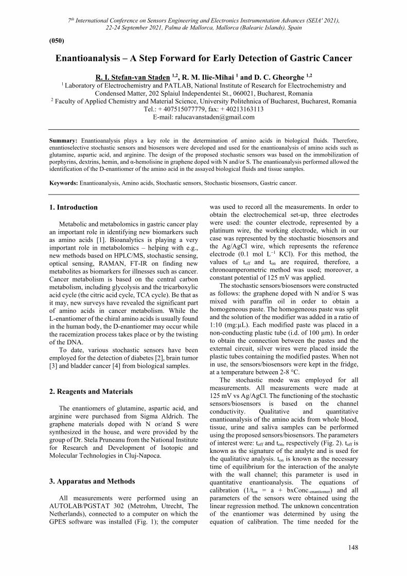
7th International Conference on Sensors Engineering and Electronics Instrumentation Advances (SEIA' 2021), 22-24 September 2021, Palma de Mallorca, Mallorca (Balearic Islands), Spain
148
(050)
Enantioanalysis – A Step Forward for Early Detection of Gastric Cancer
R. I. Stefan-van Staden 1,2, R. M. Ilie-Mihai 1 and D. C. Gheorghe 1,2
1 Laboratory of Electrochemistry and PATLAB, National Institute of Research for Electrochemistry and Condensed Matter, 202 Splaiul Independentei St., 060021, Bucharest, Romania
2 Faculty of Applied Chemistry and Material Science, University Politehnica of Bucharest, Bucharest, Romania Tel.: + 407515077779, fax: + 40213163113
E-mail: [email protected] Summary: Enantioanalysis plays a key role in the determination of amino acids in biological fluids. Therefore, enantioselective stochastic sensors and biosensors were developed and used for the enantioanalysis of amino acids such as glutamine, aspartic acid, and arginine. The design of the proposed stochastic sensors was based on the immobilization of porphyrins, dextrins, hemin, and α-hemolisine in graphene doped with N and/or S. The enantioanalysis performed allowed the identification of the D-enantiomer of the amino acid in the assayed biological fluids and tissue samples. Keywords: Enantioanalysis, Amino acids, Stochastic sensors, Stochastic biosensors, Gastric cancer.
1. Introduction
Metabolic and metabolomics in gastric cancer play an important role in identifying new biomarkers such as amino acids [1]. Bioanalytics is playing a very important role in metabolomics – helping with e.g., new methods based on HPLC/MS, stochastic sensing, optical sensing, RAMAN, FT-IR on finding new metabolites as biomarkers for illnesses such as cancer. Cancer metabolism is based on the central carbon metabolism, including glycolysis and the tricarboxylic acid cycle (the citric acid cycle, TCA cycle). Be that as it may, new surveys have revealed the significant part of amino acids in cancer metabolism. While the L-enantiomer of the chiral amino acids is usually found in the human body, the D-enantiomer may occur while the racemization process takes place or by the twisting of the DNA.
To date, various stochastic sensors have been employed for the detection of diabetes [2], brain tumor [3] and bladder cancer [4] from biological samples.
2. Reagents and Materials The enantiomers of glutamine, aspartic acid, and
arginine were purchased from Sigma Aldrich. The graphene materials doped with N or/and S were synthesized in the house, and were provided by the group of Dr. Stela Pruneanu from the National Institute for Research and Development of Isotopic and Molecular Technologies in Cluj-Napoca.
3. Apparatus and Methods
All measurements were performed using an AUTOLAB/PGSTAT 302 (Metrohm, Utrecht, The Netherlands), connected to a computer on which the GPES software was installed (Fig. 1); the computer
was used to record all the measurements. In order to obtain the electrochemical set-up, three electrodes were used: the counter electrode, represented by a platinum wire, the working electrode, which in our case was represented by the stochastic biosensors and the Ag/AgCl wire, which represents the reference electrode (0.1 mol L−1 KCl). For this method, the values of toff and ton are required, therefore, a chronoamperometric method was used; moreover, a constant potential of 125 mV was applied.
The stochastic sensors/biosensors were constructed as follows: the graphene doped with N and/or S was mixed with paraffin oil in order to obtain a homogeneous paste. The homogeneous paste was split and the solution of the modifier was added in a ratio of 1:10 (mg:µL). Each modified paste was placed in a non-conducting plastic tube (i.d. of 100 µm). In order to obtain the connection between the pastes and the external circuit, silver wires were placed inside the plastic tubes containing the modified pastes. When not in use, the sensors/biosensors were kept in the fridge, at a temperature between 2-8 °C.
The stochastic mode was employed for all measurements. All measurements were made at 125 mV vs Ag/AgCl. The functioning of the stochastic sensors/biosensors is based on the channel conductivity. Qualitative and quantitative enantioanalysis of the amino acids from whole blood, tissue, urine and saliva samples can be performed using the proposed sensors/biosensors. The parameters of interest were: toff and ton, respectively (Fig. 2). toff is known as the signature of the analyte and is used for the qualitative analysis. ton is known as the necessary time of equilibrium for the interaction of the analyte with the wall channel; this parameter is used in quantitative enantioanalysis. The equations of calibration (1/ton = a + bxConc.enantiomer) and all parameters of the sensors were obtained using the linear regression method. The unknown concentration of the enantiomer was determined by using the equation of calibration. The time needed for the
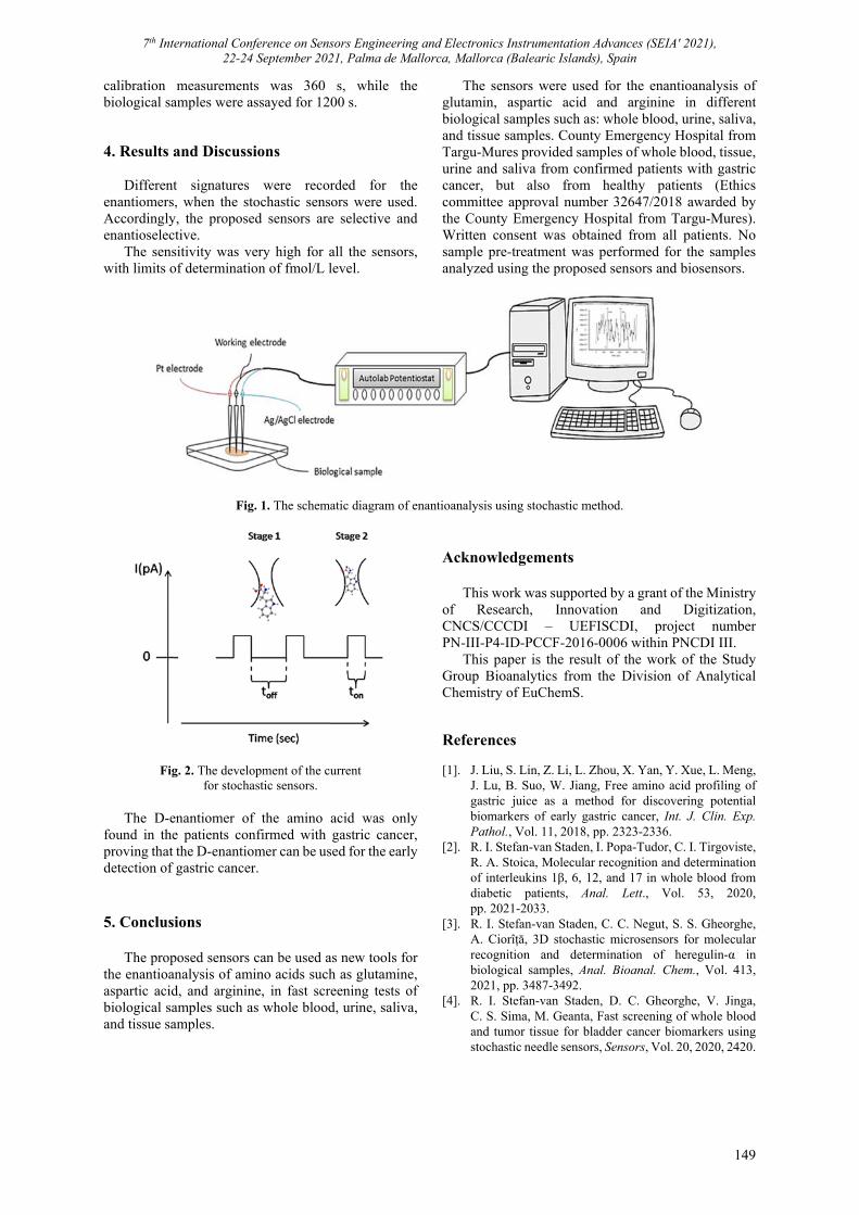
7th International Conference on Sensors Engineering and Electronics Instrumentation Advances (SEIA' 2021), 22-24 September 2021, Palma de Mallorca, Mallorca (Balearic Islands), Spain
149
calibration measurements was 360 s, while the biological samples were assayed for 1200 s. 4. Results and Discussions
Different signatures were recorded for the
enantiomers, when the stochastic sensors were used. Accordingly, the proposed sensors are selective and enantioselective.
The sensitivity was very high for all the sensors, with limits of determination of fmol/L level.
The sensors were used for the enantioanalysis of glutamin, aspartic acid and arginine in different biological samples such as: whole blood, urine, saliva, and tissue samples. County Emergency Hospital from Targu-Mures provided samples of whole blood, tissue, urine and saliva from confirmed patients with gastric cancer, but also from healthy patients (Ethics committee approval number 32647/2018 awarded by the County Emergency Hospital from Targu-Mures). Written consent was obtained from all patients. No sample pre-treatment was performed for the samples analyzed using the proposed sensors and biosensors.
Fig. 1. The schematic diagram of enantioanalysis using stochastic method.
Fig. 2. The development of the current for stochastic sensors.
The D-enantiomer of the amino acid was only
found in the patients confirmed with gastric cancer, proving that the D-enantiomer can be used for the early detection of gastric cancer. 5. Conclusions
The proposed sensors can be used as new tools for the enantioanalysis of amino acids such as glutamine, aspartic acid, and arginine, in fast screening tests of biological samples such as whole blood, urine, saliva, and tissue samples.
Acknowledgements
This work was supported by a grant of the Ministry of Research, Innovation and Digitization, CNCS/CCCDI – UEFISCDI, project number PN-III-P4-ID-PCCF-2016-0006 within PNCDI III.
This paper is the result of the work of the Study Group Bioanalytics from the Division of Analytical Chemistry of EuChemS. References [1]. J. Liu, S. Lin, Z. Li, L. Zhou, X. Yan, Y. Xue, L. Meng,
J. Lu, B. Suo, W. Jiang, Free amino acid profiling of gastric juice as a method for discovering potential biomarkers of early gastric cancer, Int. J. Clin. Exp. Pathol., Vol. 11, 2018, pp. 2323-2336.
[2]. R. I. Stefan-van Staden, I. Popa-Tudor, C. I. Tirgoviste, R. A. Stoica, Molecular recognition and determination of interleukins 1β, 6, 12, and 17 in whole blood from diabetic patients, Anal. Lett., Vol. 53, 2020, pp. 2021-2033.
[3]. R. I. Stefan-van Staden, C. C. Negut, S. S. Gheorghe, A. Ciorîță, 3D stochastic microsensors for molecular recognition and determination of heregulin-α in biological samples, Anal. Bioanal. Chem., Vol. 413, 2021, pp. 3487-3492.
[4]. R. I. Stefan-van Staden, D. C. Gheorghe, V. Jinga, C. S. Sima, M. Geanta, Fast screening of whole blood and tumor tissue for bladder cancer biomarkers using stochastic needle sensors, Sensors, Vol. 20, 2020, 2420.

7th International Conference on Sensors Engineering and Electronics Instrumentation Advances (SEIA' 2021), 22-24 September 2021, Palma de Mallorca, Mallorca (Balearic Islands), Spain
150
(051)
Stochastic Sensors for the Molecular Recognition and Determination of Heregulin-α in Biological Samples
C. Cioates Negut 1, R. I. Stefan-van Staden 1,2, S. S. Gheorghe 2 and M. Badulescu 3
1 Laboratory of Electrochemistry and PATLAB, National Institute of Research for Electrochemistry and Condensed Matter, 202 Splaiul Independentei St., 060021, Bucharest, Romania
2 Faculty of Applied Chemistry and Material Science, Politehnica University of Bucharest, Bucharest, Romania 3 Low Temperature Plasma Laboratory, National Institute for Lasers, Plasma and Radiation Physics (NILPRP),
409 Atomistilor St., 077125, Magurele, Romania E-mail: [email protected]
Summary: New materials were used for the design of the stochastic sensors for the assay of heregulin-α (HRG-α) in biological samples. HRG-α was selected as the biomarker of interest in order to diagnose brain cancer. The proposed stochastic sensors had limits of determinations of the order of fg mL−1 and high sensitivities. The linear concentration ranges of the stochastic sensors have covered the healthy people as well as the patients confirmed with brain cancer. Keywords: Stochastic sensors, Heregulin-α, Biological samples.
1. Introduction
Heregulin-α (HRG-α) has a very important role in regularly growth, invasion, and angiogenesis of brain tumours [1]. It also acts as a ligand between HER biomarkers [2]. The molecular recognition is very important in oncology for the early detection of cancer, or metastasis state. The quantity of HRG-α can indicate the stage of the cancer, and also can indicate if the tumour is going for metastasis. The molecular recognition step of HRG-α in biological samples, such as, whole blood and tumour tissue, is very important for the diagnosis of brain cancers. Therefore, the 2D and 3D stochastic sensors were designed and used for the molecular recognition and quantification of HRG-α in biological samples. In our researcher group, the molecular recognition was developed for the early detection of diverse types of cancer, such as: bladder cancer [3], brain cancer [4], lung cancer [5], and gastric cancer [6]. 2. Experimental 2.1. Materials and Methods
For all the measurements, an AUTOLAB/PGSTAT 12 (Metrohm, Utrecht, The Netherlands), linked to a computer with a GPES software was used. For all measurements, a conventional three electrodes system was used: the reference electrode (Ag/AgCl); the counter electrode, a platinum wire, and the working electrode (2 and 3 D sensors). All measurements were performed at room temperature inside the Faraday cage. A chronoamperometric method was used for the measurements of toff and ton, at a fixed potential (125 mV vs. Ag/AgCl). A coated nanocomposite thin film was synthesized using a cold plasma system, thermionic vacuum arc method, onto an organic based
substrate such as silk materials, which were used as 2D disposable stochastic sensors. Optical microscope images, Scanning Electron Microscopy images and the elemental analysis of the nanocomposite films were performed to characterize the surface morphologies of uncoated and coated silk materials. The morphological assessment of the pastes implicated in the 3D stochastic sensors construction were examined through a Scanning Electron Microscopy, using the SEM Hitachi SU8230, operated at 30 kV and coupled with an EDX detector. 2.2. Stochastic Mode
The chronoamperometric method was used for the qualitative and quantitative analysis of HRG-α, based on its signature (toff), as well as the corresponding ton values found in the diagrams recorded for the biological samples. These were used for the quantitative determination of the analyte in accordance with the equation of calibration (1):
1/𝑡 𝑎 𝑏 𝐶 , (1) where b is the sensitivity and 𝐶 is the concentration of the analyte. 2.3. Samples
The biological samples, such as the whole blood and tissue samples, were used to validate the proposed stochastic sensors and the molecular recognition of HRG-α. The University Emergency Hospital of Bucharest provided the samples from confirmed patients with brain cancer (informed consent was obtained from all patients, the University Ethics Committee from Medicine and Pharmacy "Carol
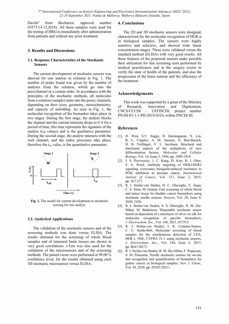
7th International Conference on Sensors Engineering and Electronics Instrumentation Advances (SEIA' 2021), 22-24 September 2021, Palma de Mallorca, Mallorca (Balearic Islands), Spain
151
Davila" from Bucharest, approval number 65573/14.12.2018). All these samples were used for the testing of HRG-α immediately after administration from patients and without any prior treatment. 3. Results and Discussions 3.1. Response Characteristics of the Stochastic Sensors
The current development of stochastic sensors was showed for one analyte in solution in Fig. 1. The number of peaks found was given by the number of analytes from the solution, which go into the pore/channel in a certain order. In accordance with the principles of the stochastic methods, all molecules from a solution (sample) enter into the pores/ channels, depending on their sizes, geometry, stereochemistry, and capacity of unfolding. As seen in Fig. 1, the molecular recognition of the biomarker takes place in two stages. During the first stage, the analyte blocks the channel and the current intensity drops to 0 A for a period of time; this time represents the signature of the analyte (toff values) and is the qualitative parameter. During the second stage, the analyte interacts with the wall channel, and the redox processes take place, therefore the ton value, is the quantitative parameter.
Fig. 1. The model for current development in stochastic sensing for one analyte.
3.2. Analytical Applications
The validation of the stochastic sensors and of the screening methods was done versus ELISA. The results obtained for the screening of whole blood samples and of tumoural brain tissues are shown in very good correlations. t-Test was also used for the validation of the microsensors and of the screening methods. The paired t-tests were performed at 99.00 % confidence level, for the results obtained using each 3D stochastic microsensor versus ELISA.
4. Conclusions
The 2D and 3D stochastic sensors were designed, characterized for the molecular recognition of HGR-α in biological samples. The sensors were highly sensitive and selective, and showed wide linear concentration ranges. These were validated versus the standard method (ELISA) with very good results. All these features of the proposed sensors make possible their utilization for fast screening tests performed by medical practitioners and in the surgery rooms to verify the state of health of the patients, and also the progression of the brain tumour and the efficiency of the treatment. Acknowledgements
This work was supported by a grant of the Ministry of Research, Innovation and Digitization, CNCS/CCCDI – UEFISCDI, project number PN-III-P1-1.1-PD-2019-0324, within PNCDI III. References [1]. D. Wen, S.V. Suggs, D. Karunagaran, N. Liu,
R. L. Cupples, A. M. Janssen, N. Ben-Baruch, D. B. Trollinger, V. L. Jacobsen, Structural and functional aspects of the multiplicity of new differentiation factors, Molecular and Cellular Biology, Vol. 14, Issue 3, 1994, pp. 1909-1919.
[2]. J. S. Poovassery, J. C. Kang, D. Kim, R. J. Ober, E. S. Ward, Antibody targeting of HER2/HER3 signaling overcomes heregulin-induced resistance to PI3K inhibition in prostate cancer, International Journal of Cancer, Vol. 137, Issue 2, 2015, pp. 267-277.
[3]. R. I. Stefan-van Staden, D. C. Gheorghe, V. Jinga, C. S. Sima, M. Geanta, Fast screening of whole blood and tumor tissue for bladder cancer biomarkers using stochastic needle sensors, Sensors, Vol. 20, Issue 8, 2020, 2420.
[4]. R. I. Stefan-van Staden, S. S. Gheorghe, R. M. Ilie-Mihai, M. Badulescu, Disposable stochastic sensor based on deposition of a nanolayer of silver on silk for molecular recognition of specific biomarkers, J. Electrochem. Soc., Vol. 168, 2021, 037515.
[5]. R. I. Stefan-van Staden, I. R. Comnea-Stancu, C. C. Surdu-Bob, Molecular screening of blood samples for the simultaneous detection of CEA, HER-1, NSE, CYFRA 21-1 using stochastic sensors, J. Electrochem. Soc., Vol. 164, Issue 6, 2017, pp. B267-B273.
[6]. R. I. Stefan-van Staden, R. M. Ilie-Mihai, F. Pogacean, S. M. Pruneanu, Needle stochastic sensors for on-site fast recognition and quantification of biomarkers for gastric cancer in biological samples, New J. Chem., Vol. 44, 2020, pp. 20203-20211.

7th International Conference on Sensors Engineering and Electronics Instrumentation Advances (SEIA' 2021), 22-24 September 2021, Palma de Mallorca, Mallorca (Balearic Islands), Spain
152
(052)
Flexible Fiber-optic Temperature Sensor for a Laser Surgery
A. S. Novikov 1,2, I. Usenov 1,2, D. Schweda1, P. Caffier 3, B. Limmer 4, V. Artyushenko 2 and H. J. Eichler 1
1 Technische Universität Berlin, Straße des 17. Juni 135, 10623 Berlin, Germany 2 Art photonics GmbH, Rudower Chaussee 46, 12489 Berlin, Germany 3 Charité-Universitätsmedizin, Charitéplatz 1, 10117 Berlin, Germany
4 Limmer Laser GmbH, Schwarzschildstraße 1, 12489 Berlin, Germany E-mail: [email protected]
Summary: Pyrometry is widely used in science, medicine and industry to measure the surface temperature of objects in a non-contact way. IR fibers are an ideal solution for flexible delivery of thermal radiation emitted from objects inside a complex structure like internal organs inside the human body. Silver halide polycrystalline infrared fibers (PIR) are transparent in a spectral range of 3-18 µm, which matches perfectly with the spectra of black body radiation for temperatures ranging from 20 °C to 200 °C. These fibers are non-toxic and allow small bending radii. They could become critical components in pyrometric systems for temperature-controlled laser surgeries. Here we discuss the ability of the PIR fibers for simultaneous laser power delivery and real-time temperature monitoring in laser surgery applications. Keywords: Pyrometry, Endoscopy, Infrared fiber, Laser surgery.
1. Introduction
Infrared (IR) thermometry or pyrometry relies on black-body radiation in the 5-14 µm wavelength range corresponding to peak temperatures from 300 °C to -65 °C. This technology is fast, noninvasive and can map the body temperature.
The temperature control via pyrometry can be utilized during laser surgery operations. One of the most critical parameters is the heated spot temperature, as a slight overheating may lead to severe thermal damage to the tissues, and too low temperature may lead to an insufficient result [1].
Polycrystalline infrared fibers (PIR) fibers made from solid solutions of silver halides (AgClxBr1-x) have high transparency over a vast spectral range of 3-18 µm, low losses for 10.6 µm (the operating wavelength of a widely used CO2 laser), insoluble in water, biocompatible, non-toxic, and very flexible [2]. The transmission region of such fibers is matched almost perfectly with the spectra of black body radiation in the 20-200 °C temperature range (Fig. 1),
making them perfect for implementing a noninvasive flexible temperature control, especially during surgical operations [3].
For 20-200 °C temperature range the dependence of the total power 𝑗 emitted from a black body and
delivered through a PIR fiber, on the temperature 𝑇 can be approximated as
𝑗 ~ 𝑇 , 𝑥 4.3, (1)
that is closed to the Stefan-Boltzmann law.
Two setups are proposed as laser surgical systems with real-time temperature control. The first setup is a compact novel fiberoptic pyrometer with an applicator that includes two fibers: application fiber to deliver laser radiation and a sensor fiber for temperature monitoring (Fig. 2).
The second setup is an optical system, where delivery of laser radiation and temperature monitoring are carried out using the same fiber (Fig. 3).
Fig. 1. Planck law and transmission of PIR fiber with 900/1000 µm core/clad diameters, 1 m length.
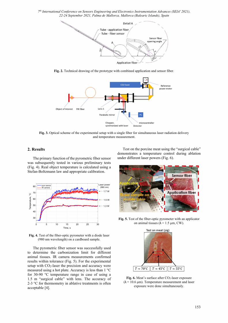
7th International Conference on Sensors Engineering and Electronics Instrumentation Advances (SEIA' 2021), 22-24 September 2021, Palma de Mallorca, Mallorca (Balearic Islands), Spain
153
Fig. 2. Technical drawing of the prototype with combined application and sensor fiber.
Fig. 3. Optical scheme of the experimental setup with a single fiber for simultaneous laser radiation delivery and temperature measurement.
2. Results
The primary function of the pyrometric fiber sensor was subsequently tested in various preliminary tests (Fig. 4). Real object temperature is calculated using a Stefan-Boltzmann law and appropriate calibration.
0 5 10 15 20 25 30
30
40
50
60
70
80Laser power (980 nm)
Tem
per
ature
, °C
Time, s
pyro sensor IR camera
1.7 W
1.5 W
1.3 W
Fig. 4. Test of the fiber-optic pyrometer with a diode laser (980 nm wavelength) on a cardboard sample.
The pyrometric fiber sensor was successfully used
to determine the carbonization limit for different animal tissues. IR camera measurements confirmed results within tolerance (Fig. 5). For the experimental setup with CO2-laser the precision and accuracy were measured using a hot plate. Accuracy is less than 1 °C for 30-90 °C temperature range in case of using a 1.5 m “surgical cable” with lens. The accuracy of 2-3 °C for thermometry in ablative treatments is often acceptable [4].
Test on the porcine meat using the “surgical cable” demonstrates a temperature control during ablation under different laser powers (Fig. 6).
Fig. 5. Test of the fiber-optic pyrometer with an applicator on animal tissues (λ = 1.5 µm, CW).
Fig. 6. Meat’s surface after CO2-laser exposure (λ = 10.6 μm). Temperature measurement and laser
exposure were done simultaneously.

7th International Conference on Sensors Engineering and Electronics Instrumentation Advances (SEIA' 2021), 22-24 September 2021, Palma de Mallorca, Mallorca (Balearic Islands), Spain
154
3. Conclusions
A novel surgical probe consisting of an application fiber for delivery of laser radiation and a sensor fiber for in-situ temperature control was developed and tested. An IR camera confirmed the prototype measurement results. The ability to use polycrystalline fibers in real-time temperature measuring devices was discussed, and a recalibration and measurement process was established. PIR fiber properties such as non-toxicity, biocompatibility and flexibility make them a perfect choice for laser surgery applications with real-time temperature monitoring which adds more control and possibility for automatic adjustments during the operation.
References [1]. D. Simhon, I. Gabay, G. Shpolyansky, T. Vasilyev,
I. Nur, R. Meidler, O. A. Hatoum, A. Katzir, M. Hashmonai, D. Kopelman. Temperature-controlled laser-soldering system and its clinical application for bonding skin incisions, Journal of Biomedical Optics, Vol. 20, Issue 12, 2015, pp. 1-8.
[2]. S. Shalem, A. Katzir, Silver halide infrared transmitting core/clad fibers with small cores, Proceedings of SPIE, Vol. 5317, 2004, pp. 13-21.
[3]. V. Artjushenko, V. Voitsekhovsky, V. Masychev, J. Zubov, V. Sysoev, Fibre optic device for simultaneous laser power transmission and temperature measuring of irradiated object, Electronics Letters, Vol. 20, 1984, pp. 983-984.
[4]. M. A. Lewis, R. M. Staruch, R. Chopra. Thermometry and ablation monitoring with ultrasound, International Journal of Hyperthermia, Vol. 31, 2015, pp. 163-181.
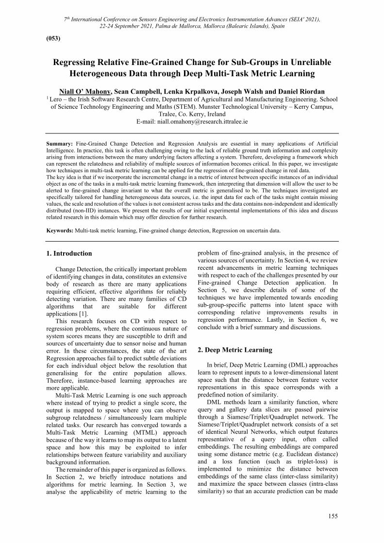
7th International Conference on Sensors Engineering and Electronics Instrumentation Advances (SEIA' 2021), 22-24 September 2021, Palma de Mallorca, Mallorca (Balearic Islands), Spain
155
(053)
Regressing Relative Fine-Grained Change for Sub-Groups in Unreliable Heterogeneous Data through Deep Multi-Task Metric Learning
Niall O’ Mahony, Sean Campbell, Lenka Krpalkova, Joseph Walsh and Daniel Riordan
1 Lero – the Irish Software Research Centre, Department of Agricultural and Manufacturing Engineering. School of Science Technology Engineering and Maths (STEM). Munster Technological University – Kerry Campus,
Tralee, Co. Kerry, Ireland E-mail: [email protected]
Summary: Fine-Grained Change Detection and Regression Analysis are essential in many applications of Artificial Intelligence. In practice, this task is often challenging owing to the lack of reliable ground truth information and complexity arising from interactions between the many underlying factors affecting a system. Therefore, developing a framework which can represent the relatedness and reliability of multiple sources of information becomes critical. In this paper, we investigate how techniques in multi-task metric learning can be applied for the regression of fine-grained change in real data. The key idea is that if we incorporate the incremental change in a metric of interest between specific instances of an individual object as one of the tasks in a multi-task metric learning framework, then interpreting that dimension will allow the user to be alerted to fine-grained change invariant to what the overall metric is generalised to be. The techniques investigated are specifically tailored for handling heterogeneous data sources, i.e. the input data for each of the tasks might contain missing values, the scale and resolution of the values is not consistent across tasks and the data contains non-independent and identically distributed (non-IID) instances. We present the results of our initial experimental implementations of this idea and discuss related research in this domain which may offer direction for further research. Keywords: Multi-task metric learning, Fine-grained change detection, Regression on uncertain data.
1. Introduction
Change Detection, the critically important problem of identifying changes in data, constitutes an extensive body of research as there are many applications requiring efficient, effective algorithms for reliably detecting variation. There are many families of CD algorithms that are suitable for different applications [1].
This research focuses on CD with respect to regression problems, where the continuous nature of system scores means they are susceptible to drift and sources of uncertainty due to sensor noise and human error. In these circumstances, the state of the art Regression approaches fail to predict subtle deviations for each individual object below the resolution that generalising for the entire population allows. Therefore, instance-based learning approaches are more applicable.
Multi-Task Metric Learning is one such approach where instead of trying to predict a single score, the output is mapped to space where you can observe subgroup relatedness / simultaneously learn multiple related tasks. Our research has converged towards a Multi-Task Metric Learning (MTML) approach because of the way it learns to map its output to a latent space and how this may be exploited to infer relationships between feature variability and auxiliary background information.
The remainder of this paper is organized as follows. In Section 2, we briefly introduce notations and algorithms for metric learning. In Section 3, we analyse the applicability of metric learning to the
problem of fine-grained analysis, in the presence of various sources of uncertainty. In Section 4, we review recent advancements in metric learning techniques with respect to each of the challenges presented by our Fine-grained Change Detection application. In Section 5, we describe details of some of the techniques we have implemented towards encoding sub-group-specific patterns into latent space with corresponding relative improvements results in regression performance. Lastly, in Section 6, we conclude with a brief summary and discussions.
2. Deep Metric Learning In brief, Deep Metric Learning (DML) approaches
learn to represent inputs to a lower-dimensional latent space such that the distance between feature vector representations in this space corresponds with a predefined notion of similarity.
DML methods learn a similarity function, where query and gallery data slices are passed pairwise through a Siamese/Triplet/Quadruplet network. The Siamese/Triplet/Quadruplet network consists of a set of identical Neural Networks, which output features representative of a query input, often called embeddings. The resulting embeddings are compared using some distance metric (e.g. Euclidean distance) and a loss function (such as triplet-loss) is implemented to minimize the distance between embeddings of the same class (inter-class similarity) and maximize the space between classes (intra-class similarity) so that an accurate prediction can be made
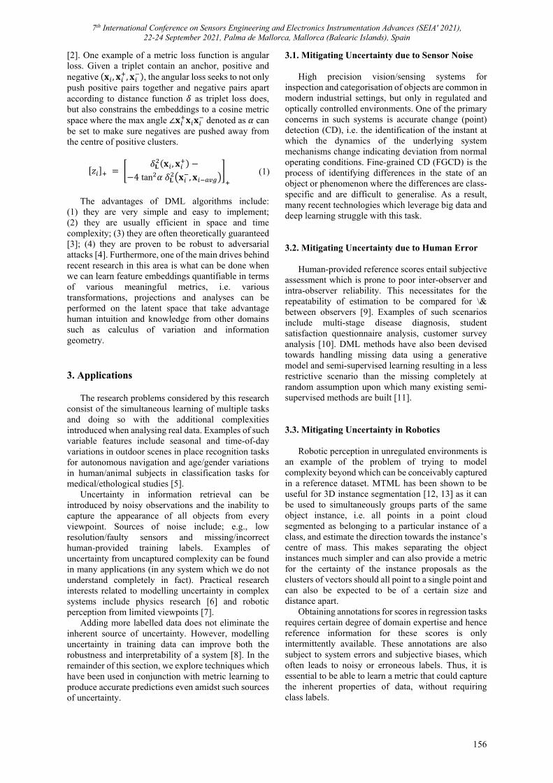
7th International Conference on Sensors Engineering and Electronics Instrumentation Advances (SEIA' 2021), 22-24 September 2021, Palma de Mallorca, Mallorca (Balearic Islands), Spain
156
[2]. One example of a metric loss function is angular loss. Given a triplet contain an anchor, positive and negative 𝐱 , 𝐱 , 𝐱 , the angular loss seeks to not only push positive pairs together and negative pairs apart according to distance function 𝛿 as triplet loss does, but also constrains the embeddings to a cosine metric space where the max angle ∠𝐱 𝐱 𝐱 denoted as 𝛼 can be set to make sure negatives are pushed away from the centre of positive clusters.
𝑧 𝛿𝐋 𝐱 , 𝐱
4 tan 𝛼 𝛿𝐋 𝐱 , 𝐱 (1)
The advantages of DML algorithms include:
(1) they are very simple and easy to implement; (2) they are usually efficient in space and time complexity; (3) they are often theoretically guaranteed [3]; (4) they are proven to be robust to adversarial attacks [4]. Furthermore, one of the main drives behind recent research in this area is what can be done when we can learn feature embeddings quantifiable in terms of various meaningful metrics, i.e. various transformations, projections and analyses can be performed on the latent space that take advantage human intuition and knowledge from other domains such as calculus of variation and information geometry. 3. Applications
The research problems considered by this research consist of the simultaneous learning of multiple tasks and doing so with the additional complexities introduced when analysing real data. Examples of such variable features include seasonal and time-of-day variations in outdoor scenes in place recognition tasks for autonomous navigation and age/gender variations in human/animal subjects in classification tasks for medical/ethological studies [5].
Uncertainty in information retrieval can be introduced by noisy observations and the inability to capture the appearance of all objects from every viewpoint. Sources of noise include; e.g., low resolution/faulty sensors and missing/incorrect human-provided training labels. Examples of uncertainty from uncaptured complexity can be found in many applications (in any system which we do not understand completely in fact). Practical research interests related to modelling uncertainty in complex systems include physics research [6] and robotic perception from limited viewpoints [7].
Adding more labelled data does not eliminate the inherent source of uncertainty. However, modelling uncertainty in training data can improve both the robustness and interpretability of a system [8]. In the remainder of this section, we explore techniques which have been used in conjunction with metric learning to produce accurate predictions even amidst such sources of uncertainty.
3.1. Mitigating Uncertainty due to Sensor Noise
High precision vision/sensing systems for inspection and categorisation of objects are common in modern industrial settings, but only in regulated and optically controlled environments. One of the primary concerns in such systems is accurate change (point) detection (CD), i.e. the identification of the instant at which the dynamics of the underlying system mechanisms change indicating deviation from normal operating conditions. Fine-grained CD (FGCD) is the process of identifying differences in the state of an object or phenomenon where the differences are class-specific and are difficult to generalise. As a result, many recent technologies which leverage big data and deep learning struggle with this task.
3.2. Mitigating Uncertainty due to Human Error Human-provided reference scores entail subjective
assessment which is prone to poor inter-observer and intra-observer reliability. This necessitates for the repeatability of estimation to be compared for \& between observers [9]. Examples of such scenarios include multi-stage disease diagnosis, student satisfaction questionnaire analysis, customer survey analysis [10]. DML methods have also been devised towards handling missing data using a generative model and semi-supervised learning resulting in a less restrictive scenario than the missing completely at random assumption upon which many existing semi-supervised methods are built [11].
3.3. Mitigating Uncertainty in Robotics
Robotic perception in unregulated environments is an example of the problem of trying to model complexity beyond which can be conceivably captured in a reference dataset. MTML has been shown to be useful for 3D instance segmentation [12, 13] as it can be used to simultaneously groups parts of the same object instance, i.e. all points in a point cloud segmented as belonging to a particular instance of a class, and estimate the direction towards the instance’s centre of mass. This makes separating the object instances much simpler and can also provide a metric for the certainty of the instance proposals as the clusters of vectors should all point to a single point and can also be expected to be of a certain size and distance apart.
Obtaining annotations for scores in regression tasks requires certain degree of domain expertise and hence reference information for these scores is only intermittently available. These annotations are also subject to system errors and subjective biases, which often leads to noisy or erroneous labels. Thus, it is essential to be able to learn a metric that could capture the inherent properties of data, without requiring class labels.

7th International Conference on Sensors Engineering and Electronics Instrumentation Advances (SEIA' 2021), 22-24 September 2021, Palma de Mallorca, Mallorca (Balearic Islands), Spain
157
4. Related Research
As most CD applications use nominal object classes, many papers applying the latest state-of-the-art to specific application-domains adopt the same methodology, by categorising the output arbitrary classes that ensure even representation across the available dataset. This may come at the cost of not being able to represent the desired output on ordinal, interval or ratio scales which may come naturally in some applications. Thus, they can only measure whether the individual items belong to certain distinct categories and it is not possible to quantify or rank order amongst the categories or perform arithmetic operations. A number of papers have proposed techniques for performing regression with DML [14, 15, 8].
In this section, we review the methods applicable to heterogeneous data from the viewpoint of a number of functionalities, specifically multi-task metric learning, geometry preservation and regression.
4.1. Multi-task Metric Learning
Multi-task Metric Learning (MTML) approaches jointly train a DML network to separate w.r.t. multiple tasks, thereby sharing useful information among the tasks, which can significantly improve upon the performance achievable in a single-task setting. MTML has been recently reviewed by [16].
Regarding subgroup and fine-grained analyses, propose a regularized multi-task learning framework with shared representation layers to encode the task relatedness [10]. Similarly, [5] present a framework for detecting the subgroups that have similar characters in feature space by using K-means clustering incorporated into the regression stage so that both tasks can be performed simultaneously.
It has been proposed in recent work that multiple features should be used for retrieval tasks to overcome the limitation of a single feature and further improve the performance. As most conventional distance metric learning methods fail to integrate the complementary information from multiple features to construct the distance metric, a novel multi-feature distance metric learning method for non-rigid 3D shape retrieval which can make full use of the complementary geometric information from multiple shape features has been presented [17]. An alternative formulation for multi-task learning has been proposed by [18] who use a version of the K Nearest Neighbour (KNN) algorithms (large margin nearest neighbour) but instead of relying on separating hyperplanes, its decision function is based on the nearest neighbour rule which inherently extends to many classes and becomes a natural fit for multi-task learning. This approach is advantageous as the feature space generated from Metric Learning crucially determines the performance of the KNN algorithm, i.e. the learned latent space is preserved, KNN just solves the multi-label problem within.
A challenge that has not been well explored in literature is tuple sampling strategies for metric learning in a multi-label setting. A critical element of metric learning is the selection of triplets during training (sometimes referred to as triplet mining). Triplets need to be chosen such that consecutive training batches vary gradually so that the weights learned by the network between batches are actually transferable but also so that all the important variations within the dataset get encountered with enough frequency during training so that the model can capture that variability. Different mechanisms for triplet mining exist. For example, hard triplet mining selects the most difficult triplets for each anchor by calculating the inter-embedding distance between each anchor and all positive and negative embeddings for that anchor. Hard triplet mining selects the most distant embedding in 𝑆 and the least distant embedding in 𝐷 for each anchor. Since it is computationally infeasible to aggregate loss over all 𝑂 𝑛 triplets and hard triplets can cause models to collapse, heuristics are used to speed up convergence. A well known miner is semi-hard negative mining which samples anchors and positives in batches from 𝒳 and 𝑆, and finds the closest negatives within the batch further away than 𝐷 𝑎, 𝑝 [19] Many of these sampling strategies can be quite computationally expensive as they require a forward pass of the network being trained to be run on every image in the dataset. This is why many approaches use mini-batches to fit the computational load within the limits of their machine. Many method randomly sample a set of images, assuming that a few random parameter vectors will represent certain elementary transformation operations like translation, scaling, rotation, contrast, and colourization.
4.2. Geometry Preserving Metric Learning
The saliency of the embedding space with respect to preserving the local structure of associated tasks/metrics can be increased by taking measures to preserve the intrinsic geometry of the input space. Many of these approaches utilise information geometry divergence measures such as von Neumann divergence [20] and Wassertein distance [3].
An alternative type of divergence measure is geometric divergence on graphs and manifolds. This can be achieved by fitting manifolds in latent space and including Riemannian metrics in the loss function [15], [21]. Graph-based methods involve representing feature vectors as graphs to capture interactions (i.e. edges) between individual features (i.e. nodes) and are becoming increasingly popular as there has been a massive surge of interest in geometric deep learning in recent years [22].
In their approach called Orthogonality based Probabilistic Unsupervised Metric Learning (OPML), Dutta et al. perform Riemannian Conjugate Gradient Descent (RCGD) to jointly learn the parameters [21]. Their implementation of Riemannian optimisation is stochastic, i.e. it samples the latent space at many
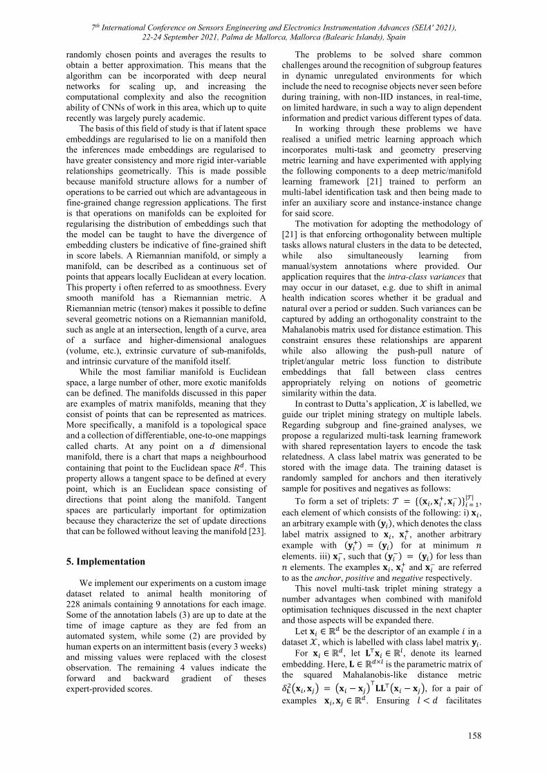
7th International Conference on Sensors Engineering and Electronics Instrumentation Advances (SEIA' 2021), 22-24 September 2021, Palma de Mallorca, Mallorca (Balearic Islands), Spain
158
randomly chosen points and averages the results to obtain a better approximation. This means that the algorithm can be incorporated with deep neural networks for scaling up, and increasing the computational complexity and also the recognition ability of CNNs of work in this area, which up to quite recently was largely purely academic.
The basis of this field of study is that if latent space embeddings are regularised to lie on a manifold then the inferences made embeddings are regularised to have greater consistency and more rigid inter-variable relationships geometrically. This is made possible because manifold structure allows for a number of operations to be carried out which are advantageous in fine-grained change regression applications. The first is that operations on manifolds can be exploited for regularising the distribution of embeddings such that the model can be taught to have the divergence of embedding clusters be indicative of fine-grained shift in score labels. A Riemannian manifold, or simply a manifold, can be described as a continuous set of points that appears locally Euclidean at every location. This property i often referred to as smoothness. Every smooth manifold has a Riemannian metric. A Riemannian metric (tensor) makes it possible to define several geometric notions on a Riemannian manifold, such as angle at an intersection, length of a curve, area of a surface and higher-dimensional analogues (volume, etc.), extrinsic curvature of sub-manifolds, and intrinsic curvature of the manifold itself.
While the most familiar manifold is Euclidean space, a large number of other, more exotic manifolds can be defined. The manifolds discussed in this paper are examples of matrix manifolds, meaning that they consist of points that can be represented as matrices. More specifically, a manifold is a topological space and a collection of differentiable, one-to-one mappings called charts. At any point on a 𝑑 dimensional manifold, there is a chart that maps a neighbourhood containing that point to the Euclidean space 𝑅 . This property allows a tangent space to be defined at every point, which is an Euclidean space consisting of directions that point along the manifold. Tangent spaces are particularly important for optimization because they characterize the set of update directions that can be followed without leaving the manifold [23].
5. Implementation
We implement our experiments on a custom image dataset related to animal health monitoring of 228 animals containing 9 annotations for each image. Some of the annotation labels (3) are up to date at the time of image capture as they are fed from an automated system, while some (2) are provided by human experts on an intermittent basis (every 3 weeks) and missing values were replaced with the closest observation. The remaining 4 values indicate the forward and backward gradient of theses expert-provided scores.
The problems to be solved share common challenges around the recognition of subgroup features in dynamic unregulated environments for which include the need to recognise objects never seen before during training, with non-IID instances, in real-time, on limited hardware, in such a way to align dependent information and predict various different types of data.
In working through these problems we have realised a unified metric learning approach which incorporates multi-task and geometry preserving metric learning and have experimented with applying the following components to a deep metric/manifold learning framework [21] trained to perform an multi-label identification task and then being made to infer an auxiliary score and instance-instance change for said score.
The motivation for adopting the methodology of [21] is that enforcing orthogonality between multiple tasks allows natural clusters in the data to be detected, while also simultaneously learning from manual/system annotations where provided. Our application requires that the intra-class variances that may occur in our dataset, e.g. due to shift in animal health indication scores whether it be gradual and natural over a period or sudden. Such variances can be captured by adding an orthogonality constraint to the Mahalanobis matrix used for distance estimation. This constraint ensures these relationships are apparent while also allowing the push-pull nature of triplet/angular metric loss function to distribute embeddings that fall between class centres appropriately relying on notions of geometric similarity within the data.
In contrast to Dutta’s application, 𝒳 is labelled, we guide our triplet mining strategy on multiple labels. Regarding subgroup and fine-grained analyses, we propose a regularized multi-task learning framework with shared representation layers to encode the task relatedness. A class label matrix was generated to be stored with the image data. The training dataset is randomly sampled for anchors and then iteratively sample for positives and negatives as follows:
To form a set of triplets: 𝒯 𝐱 , 𝐱 , 𝐱 |𝒯| ,
each element of which consists of the following: i) 𝐱 , an arbitrary example with 𝐲 , which denotes the class label matrix assigned to 𝐱 , 𝐱 , another arbitrary example with 𝐲 𝐲 for at minimum 𝑛 elements. iii) 𝐱 , such that 𝐲 𝐲 for less than 𝑛 elements. The examples 𝐱 , 𝐱 and 𝐱 are referred to as the anchor, positive and negative respectively.
This novel multi-task triplet mining strategy a number advantages when combined with manifold optimisation techniques discussed in the next chapter and those aspects will be expanded there.
Let 𝐱 ∈ ℝ be the descriptor of an example 𝑖 in a dataset 𝒳, which is labelled with class label matrix 𝐲 .
For 𝐱 ∈ ℝ , let 𝐋 𝐱 ∈ ℝ , denote its learned embedding. Here, 𝐋 ∈ ℝ is the parametric matrix of the squared Mahalanobis-like distance metric
𝛿𝐋 𝐱 , 𝐱 𝐱 𝐱 𝐋𝐋 𝐱 𝐱 , for a pair of examples 𝐱 , 𝐱 ∈ ℝ . Ensuring 𝑙 𝑑 facilitates

7th International Conference on Sensors Engineering and Electronics Instrumentation Advances (SEIA' 2021), 22-24 September 2021, Palma de Mallorca, Mallorca (Balearic Islands), Spain
159
dimensionality reduction. The goal is to learn the parametric matrix 𝐋.
min𝐑,𝐋
ℒ 𝐑, 𝐋 log𝑝
|𝒯|
Here, |𝒯| is the number of triplets formed. Using
𝒯, our goal is to learn 𝐋 in 𝛿𝐋 𝐱 , 𝐱 . In particular, we make use of our multi-task triplet sampling strategy of mining triplets using the multiple-labels. Let, the learned embeddings of the anchor and the positive be denoted as 𝐋 𝐱 and 𝐋 𝐱 respectively. The bilinear similarity between them can be expressed as 𝐋 𝐱 𝐋 𝐱 𝐱 𝐋𝐋 𝐱 .
Similarly to [10], we also implement shared representation layers to encode the task relatedness but differ in that we simply calculate the mean squared error (MSE) of a selected dimension of the feature embedding with the label of interest (generalised regression and relative change scores respectively).
5.1. Results
We perform experiments to study the following: 1. Effect of different sampling settings on the multi-task metric learning results. 2. Effect of the different hyperparameters on our method.
In Table 1, we report the results of the multi-task triplet sampler. For our method, we set α = 45∘, and embedding size of 128. We also indicate the nature of an approach, i.e., we use the OPML network by.
Table 1. Sensitivity of the multi-task triplet sampler and OPML network towards $n$, the number of elements in the class label matrix which must match to qualify as a positive sample.
n 2 3 4 5 6 7
OPML 71.2 62.3 50.2 42.5 47.0 61.6
The test of sensitivity to n, the number of elements in the class label matrix which must match to qualify as a positive sample yielded interesting results. When n is small, the labels which match can vary significantly within and between batches and hence the transition between training iterations is difficult to learn from. This gradually improves as n increases as is reflected in Table 1. Once greater than 6 of the 9 labels in the data needed to match, performance dropped again, suspect due to the limited number of anchor-positive pairs accepted.
In Table 2, we report the results of α, an important hyperparameter in OPML and the addition of a MSE component to the overall loss function. For our method, we arbitrarily set n = 5, and embedding size of 128. We also indicate the nature of an approach, i.e., whether it makes use of an additional final layer for
classification and regression or not. Note: lower loss is better.
Table 2. Sensitivity towards loss function and α with respect to loss values reached on the test data.
α 35∘ 40∘ 45∘ 50∘ 55∘ 60∘
Multi-task/OPML 73.4 70.5 69.5 68.7 71.7 72.4Multi-task/OPML+MSE
241.2 162.3 142.2 152.5 92.0 321.6
These results corresponds with ablation studies by [21] showing the effect of different components of OPML in that a value of α in the mid range of that tested gave the best results, where α is the upper-bound angle formed by the angle positive-anchor-negative in the angular loss function, however the loss values remained quite high suggesting that the model is not converging well. This may be due to the complexity of the base network compared to that used by [21]. 4. Conclusions
The multiple implementation scenarios where MTML solutions have been shown to be useful demonstrate that the proposed method is useful in many AI applications where the algorithm’s outputs are to be adapted to each use case.
This paper has also included the results of implementing some of these methods in addition to a novel multi-task triplet sampling strategy to quantify the effect of the hyperparameters of each element. It was found that enforcing too many labels to overlap impeded the convergence of the loss function as there was a limited number of anchor-positive pairs in the dataset. Allowing very little overlap of labels was also detrimental to performance as it allows too much variance between training iterations.
Adding a final layer to regress the embeddings to align to a set of auxiliary outputs hindered the training procedure which may have been due to over-constraining the loss function, to have to learn to space the vectors apart appropriately while simultaneously enforcing a feature which may have no or non-linear correlation to the auxiliary task. To this end, some of the kernel regression techniques [24] may improve performance.
Better results may be achieved if a metric loss function be used in the final layer and the intra-class distances are trained to correspond to the auxiliary tasks using the weighted MSE loss function. The benefit of the interaction of multiple features is to be included in efforts to minimise the regression error as it is why methods which use a Mahalanobis matrix for each metric are so common in MTML solutions.
We intend to further the research in this area by investigating how the mapping element of MTML may be exploited in situations where the salient features vary over time or due to changing underlying variables. One possible avenue would be to develop a

7th International Conference on Sensors Engineering and Electronics Instrumentation Advances (SEIA' 2021), 22-24 September 2021, Palma de Mallorca, Mallorca (Balearic Islands), Spain
160
technique to calculate the geometric divergence along each of the dimensions of the latent space/surface w.r.t isolated task-relevant subgroups in order to identify the local covariate geometry with respect to each task and easily recognise subtle changes in the same. Acknowledgements
This work was supported, in part, by Science Foundation Ireland grant 13/RC/2094 and co-funded under the European Regional Development Fund through the Southern \& Eastern Regional Operational Programme to Lero - the Irish Software Research Centre (www.lero.ie). The authors wish to acknowledge the DJEI/DES/SFI/HEA Irish Centre for High-End Computing (ICHEC) for the provision of computational facilities and support. References [1]. W. Shi, M. Zhang, R. Zhang, S. Chen, and Z. Zhan,
Change detection based on artificial intelligence: State-of-the-art and challenges, Remote Sensing, Vol. 12, Issue 10, May 2020, 1688.
[2]. N. O. Mahony, et al., One-shot learning for custom identification tasks: A review, Procedia Manufacturing, Vol. 38, 2019, pp. 186-193.
[3]. C. Shui, M. Abbasi, L. É. Robitaille, B. Wang, C. Gagné, A principled approach for learning task similarity in multitask learning, in Proceedings of the International Joint Conference on Artificial Intelligence (IJCAI’19), 2019, pp. 3446-3452.
[4]. L. Wang, X. Liu, J. Yi, Y. Jiang, C. J. Hsieh, Provably robust metric learning, in Proceedings of the Annual Conference on Advances in Neural Information Processing Systems (NeurIPS’20), 2020, pp. 1-12.
[5]. B. Liang, P. Wu, X. Tong, Y. Qiu, Regression and subgroup detection for heterogeneous samples, Computational Statistics, Vol. 35, Issue 4, 2020, pp. 1853-1878.
[6]. M. B. Chang, T. Ullman, A. Torralba, J. B. Tenenbaum, A compositional object-based approach to learning physical dynamics, in Proceedings of the 5th International Conference on Learning Representations (ICLR’17), Dec. 2017, pp. 1-15.
[7]. A. Kelly, Mobile Robotics: Mathematics, Models, and Methods, Vol. 9781107031, Cambridge University Press, New York, 2013.
[8]. A. Taha, Y.-T. Chen, T. Misu, A. Shrivastava, L. Davis, Unsupervised data uncertainty learning in visual retrieval systems, arXiv:1902.02586, arXiv, 2019.
[9]. Z. Wang, D. M. Anand, J. Moyne, D. M. Tilbury, Improved sensor fault detection, isolation, and mitigation using multiple observers approach, Systems
Science and Control Engineering, Vol. 5, Issue 1, 2017, pp. 70-96.
[10]. L. Wang, D. Zhu, Tackling ordinal regression problem for heterogeneous data: sparse and deep multi-task learning approaches, Data Mining and Knowledge Discovery, Vol. 35, Issue 3, 2021, pp. 1134-1161.
[11]. X. Liu, D. Zachariah, J. Wågberg, T. B. Schön, Reliable semi-supervised learning when labels are missing at random, arXiv:1811.10947, arXiv, 2018.
[12]. W. Wang, R. Yu, Q. Huang, U. Neumann, SGPN: similarity group proposal network for 3D point cloud instance segmentation, in Proceedings of the IEEE Computer Society Conference on Computer Vision and Pattern Recognition (CVPR’18), 2018, pp. 2569-2578.
[13]. J. Lahoud, B. Ghanem, M. R. Oswald, M. Pollefeys, 3D instance segmentation via multi-task metric learning, in Proceedings of the IEEE International Conference on Computer Vision (ICCV’19), 2019, pp. 9255-9265.
[14]. K. Q. Weinberger, G. Tesauro, Metric learning for kernel regression, Journal of Machine Learning Research, Vol. 2, 2007, pp. 612-619.
[15]. R. Huang, S. Sun, Kernel regression with sparse metric learning, Journal of Intelligent and Fuzzy Systems, Vol. 24, Issue 4, 2013, pp. 775-787.
[16]. P. Yang, K. Huang, A. Hussain, A review on multi-task metric learning, Big Data Analytics, Vol. 3, Issue 1, Dec. 2018, pp. 1-23.
[17]. H. Wang, H. Li, J. Peng, X. Fu, Multi-feature distance metric learning for non-rigid 3D shape retrieval, Multimedia Tools and Applications, Vol. 78, Issue 21, Nov. 2019, pp. 30943-30958.
[18]. K. Q. Weinberger, L. K. Saul, Distance metric learning for large margin nearest neighbor classification, Journal of Machine Learning Research, Vol. 10, Jan. 2009, pp. 207-244.
[19]. R. Manmatha, C. Y. Wu, A. J. Smola, P. Krahenbuhl, Sampling matters in deep embedding learning, in Proceedings of the IEEE International Conference on Computer Vision (ICCV’17), 2017, pp. 2859-2867.
[20]. P. Yang, K. Huang, C. L. Liu, Geometry preserving multi-task metric learning, Machine Learning, Vol. 92, Issue 1, Jul. 2013, pp. 133-175.
[21]. U. K. Dutta, M. Harandi, C. C. Sekhar, Unsupervised deep metric learning via orthogonality based probabilistic loss, IEEE Transactions on Artificial Intelligence, Vol. 1, Issue 1, 2021, pp. 74-84.
[22]. M. M. Bronstein, J. Bruna, Y. Lecun, A. Szlam, P. Vandergheynst, Geometric Deep Learning: Going beyond Euclidean data, IEEE Signal Processing Magazine, Vol. 34, Issue 4, 2017, pp. 18-42.
[23]. S. Giguere, F. Garcia, S. Mahadevan, A manifold approach to learning mutually orthogonal subspaces, arXiv:1703.02992, arXiv, 2017.
[24]. K. Q. Weinberger, G. Tesauro, Metric learning for kernel regression, in Proceedings of the Eleventh International Conference on Artificial Intelligence and Statistics (AISTATS’07), San Juan, Puerto Rico, March 21-24, 2007, pp. 612-619.
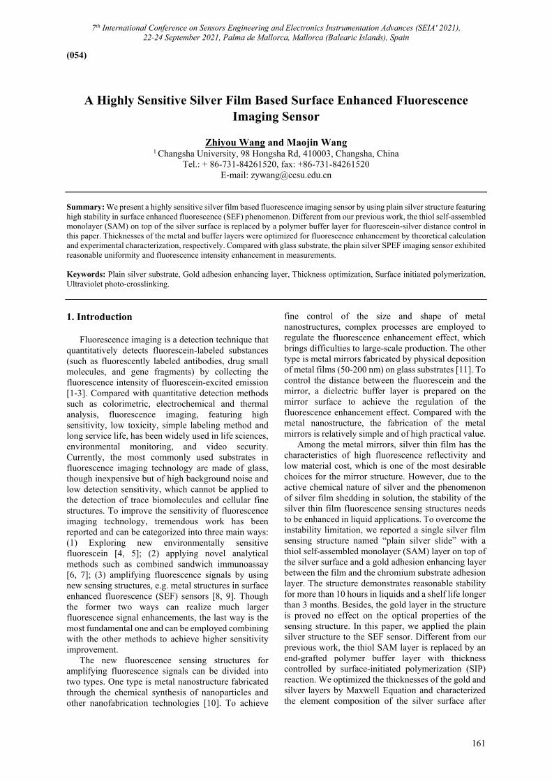
7th International Conference on Sensors Engineering and Electronics Instrumentation Advances (SEIA' 2021), 22-24 September 2021, Palma de Mallorca, Mallorca (Balearic Islands), Spain
161
(054)
A Highly Sensitive Silver Film Based Surface Enhanced Fluorescence Imaging Sensor
Zhiyou Wang and Maojin Wang
1 Changsha University, 98 Hongsha Rd, 410003, Changsha, China Tel.: + 86-731-84261520, fax: +86-731-84261520
E-mail: [email protected] Summary: We present a highly sensitive silver film based fluorescence imaging sensor by using plain silver structure featuring high stability in surface enhanced fluorescence (SEF) phenomenon. Different from our previous work, the thiol self-assembled monolayer (SAM) on top of the silver surface is replaced by a polymer buffer layer for fluorescein-silver distance control in this paper. Thicknesses of the metal and buffer layers were optimized for fluorescence enhancement by theoretical calculation and experimental characterization, respectively. Compared with glass substrate, the plain silver SPEF imaging sensor exhibited reasonable uniformity and fluorescence intensity enhancement in measurements. Keywords: Plain silver substrate, Gold adhesion enhancing layer, Thickness optimization, Surface initiated polymerization, Ultraviolet photo-crosslinking.
1. Introduction
Fluorescence imaging is a detection technique that quantitatively detects fluorescein-labeled substances (such as fluorescently labeled antibodies, drug small molecules, and gene fragments) by collecting the fluorescence intensity of fluorescein-excited emission [1-3]. Compared with quantitative detection methods such as colorimetric, electrochemical and thermal analysis, fluorescence imaging, featuring high sensitivity, low toxicity, simple labeling method and long service life, has been widely used in life sciences, environmental monitoring, and video security. Currently, the most commonly used substrates in fluorescence imaging technology are made of glass, though inexpensive but of high background noise and low detection sensitivity, which cannot be applied to the detection of trace biomolecules and cellular fine structures. To improve the sensitivity of fluorescence imaging technology, tremendous work has been reported and can be categorized into three main ways: (1) Exploring new environmentally sensitive fluorescein [4, 5]; (2) applying novel analytical methods such as combined sandwich immunoassay [6, 7]; (3) amplifying fluorescence signals by using new sensing structures, e.g. metal structures in surface enhanced fluorescence (SEF) sensors [8, 9]. Though the former two ways can realize much larger fluorescence signal enhancements, the last way is the most fundamental one and can be employed combining with the other methods to achieve higher sensitivity improvement.
The new fluorescence sensing structures for amplifying fluorescence signals can be divided into two types. One type is metal nanostructure fabricated through the chemical synthesis of nanoparticles and other nanofabrication technologies [10]. To achieve
fine control of the size and shape of metal nanostructures, complex processes are employed to regulate the fluorescence enhancement effect, which brings difficulties to large-scale production. The other type is metal mirrors fabricated by physical deposition of metal films (50-200 nm) on glass substrates [11]. To control the distance between the fluorescein and the mirror, a dielectric buffer layer is prepared on the mirror surface to achieve the regulation of the fluorescence enhancement effect. Compared with the metal nanostructure, the fabrication of the metal mirrors is relatively simple and of high practical value.
Among the metal mirrors, silver thin film has the characteristics of high fluorescence reflectivity and low material cost, which is one of the most desirable choices for the mirror structure. However, due to the active chemical nature of silver and the phenomenon of silver film shedding in solution, the stability of the silver thin film fluorescence sensing structures needs to be enhanced in liquid applications. To overcome the instability limitation, we reported a single silver film sensing structure named “plain silver slide” with a thiol self-assembled monolayer (SAM) layer on top of the silver surface and a gold adhesion enhancing layer between the film and the chromium substrate adhesion layer. The structure demonstrates reasonable stability for more than 10 hours in liquids and a shelf life longer than 3 months. Besides, the gold layer in the structure is proved no effect on the optical properties of the sensing structure. In this paper, we applied the plain silver structure to the SEF sensor. Different from our previous work, the thiol SAM layer is replaced by an end-grafted polymer buffer layer with thickness controlled by surface-initiated polymerization (SIP) reaction. We optimized the thicknesses of the gold and silver layers by Maxwell Equation and characterized the element composition of the silver surface after
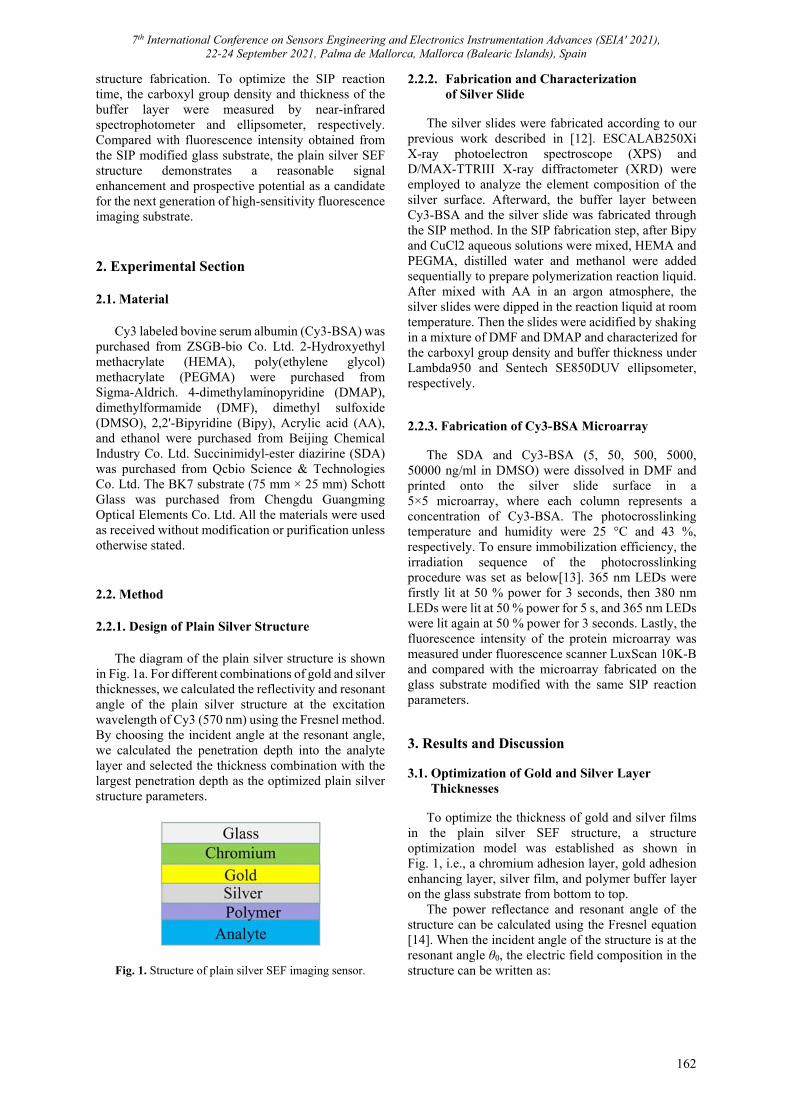
7th International Conference on Sensors Engineering and Electronics Instrumentation Advances (SEIA' 2021), 22-24 September 2021, Palma de Mallorca, Mallorca (Balearic Islands), Spain
162
structure fabrication. To optimize the SIP reaction time, the carboxyl group density and thickness of the buffer layer were measured by near-infrared spectrophotometer and ellipsometer, respectively. Compared with fluorescence intensity obtained from the SIP modified glass substrate, the plain silver SEF structure demonstrates a reasonable signal enhancement and prospective potential as a candidate for the next generation of high-sensitivity fluorescence imaging substrate.
2. Experimental Section 2.1. Material
Cy3 labeled bovine serum albumin (Cy3-BSA) was purchased from ZSGB-bio Co. Ltd. 2-Hydroxyethyl methacrylate (HEMA), poly(ethylene glycol) methacrylate (PEGMA) were purchased from Sigma-Aldrich. 4-dimethylaminopyridine (DMAP), dimethylformamide (DMF), dimethyl sulfoxide (DMSO), 2,2'-Bipyridine (Bipy), Acrylic acid (AA), and ethanol were purchased from Beijing Chemical Industry Co. Ltd. Succinimidyl-ester diazirine (SDA) was purchased from Qcbio Science & Technologies Co. Ltd. The BK7 substrate (75 mm × 25 mm) Schott Glass was purchased from Chengdu Guangming Optical Elements Co. Ltd. All the materials were used as received without modification or purification unless otherwise stated. 2.2. Method 2.2.1. Design of Plain Silver Structure
The diagram of the plain silver structure is shown in Fig. 1a. For different combinations of gold and silver thicknesses, we calculated the reflectivity and resonant angle of the plain silver structure at the excitation wavelength of Cy3 (570 nm) using the Fresnel method. By choosing the incident angle at the resonant angle, we calculated the penetration depth into the analyte layer and selected the thickness combination with the largest penetration depth as the optimized plain silver structure parameters.
Fig. 1. Structure of plain silver SEF imaging sensor.
2.2.2. Fabrication and Characterization of Silver Slide
The silver slides were fabricated according to our
previous work described in [12]. ESCALAB250Xi X-ray photoelectron spectroscope (XPS) and D/MAX-TTRIII X-ray diffractometer (XRD) were employed to analyze the element composition of the silver surface. Afterward, the buffer layer between Cy3-BSA and the silver slide was fabricated through the SIP method. In the SIP fabrication step, after Bipy and CuCl2 aqueous solutions were mixed, HEMA and PEGMA, distilled water and methanol were added sequentially to prepare polymerization reaction liquid. After mixed with AA in an argon atmosphere, the silver slides were dipped in the reaction liquid at room temperature. Then the slides were acidified by shaking in a mixture of DMF and DMAP and characterized for the carboxyl group density and buffer thickness under Lambda950 and Sentech SE850DUV ellipsometer, respectively. 2.2.3. Fabrication of Cy3-BSA Microarray
The SDA and Cy3-BSA (5, 50, 500, 5000, 50000 ng/ml in DMSO) were dissolved in DMF and printed onto the silver slide surface in a 5×5 microarray, where each column represents a concentration of Cy3-BSA. The photocrosslinking temperature and humidity were 25 °C and 43 %, respectively. To ensure immobilization efficiency, the irradiation sequence of the photocrosslinking procedure was set as below[13]. 365 nm LEDs were firstly lit at 50 % power for 3 seconds, then 380 nm LEDs were lit at 50 % power for 5 s, and 365 nm LEDs were lit again at 50 % power for 3 seconds. Lastly, the fluorescence intensity of the protein microarray was measured under fluorescence scanner LuxScan 10K-B and compared with the microarray fabricated on the glass substrate modified with the same SIP reaction parameters. 3. Results and Discussion 3.1. Optimization of Gold and Silver Layer Thicknesses
To optimize the thickness of gold and silver films in the plain silver SEF structure, a structure optimization model was established as shown in Fig. 1, i.e., a chromium adhesion layer, gold adhesion enhancing layer, silver film, and polymer buffer layer on the glass substrate from bottom to top.
The power reflectance and resonant angle of the structure can be calculated using the Fresnel equation [14]. When the incident angle of the structure is at the resonant angle θ0, the electric field composition in the structure can be written as:
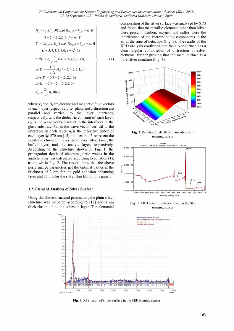
7th International Conference on Sensors Engineering and Electronics Instrumentation Advances (SEIA' 2021), 22-24 September 2021, Palma de Mallorca, Mallorca (Balearic Islands), Spain
163
, 0 ,
, , 0 ,
(0, , 0) exp[ ( )]
( 5, 4,3, 2,1, 0; 1)
( , 0, ) exp[ ( )]
( 5, 4, 3, 2,1, 0; 1)
1( 5, 4, 3, 2,1, 0)
1( 5, 4,3, 2,1, 0)
0( 5, 4,3, 2,1, 0)
i y i x z i
i x i z i x z i
i i i
i i
i i
i
H H j k x k z t
i j
E E E j k x k z t
i j
rotH E ic t
rotE H ic t
div E i
divH
0 0 0
0( 5, 4,3, 2,1, 0)
2sin
,
x
i
k n
(1)
where Ei and Hi are electric and magnetic field vectors in each layer respectively, xy plane and z-direction are parallel and vertical to the layer interfaces, respectively, εi is the dielectric constant of each layer, k0x is the wave vector parallel to the interfaces in the glass substrate, k0z,i is the wave vector vertical to the interfaces in each layer, ni is the refractive index of each layer @ 570 nm [15], indices 0 to 5 represent the substrate, chromium layer, gold layer, silver layer, the buffer layer, and the analyte layer, respectively. According to the structure shown in Fig. 1, the propagation depth of electromagnetic waves in the analyte layer was calculated according to equation (1), as shown in Fig. 2. The results show that the above performance parameters get the optimal values at the thickness of 2 nm for the gold adhesion enhancing layer and 55 nm for the silver thin film in this paper. 3.2. Element Analysis of Silver Surface Using the above structural parameters, the plain silver structure was prepared according to [12] and 3 nm thick chromium as the adhesion layer. The elemental
composition of the silver surface was analyzed by XPS and found that no metallic elements other than silver were present. Carbon, oxygen and sulfur were the interference of the corresponding components in the air at the time of detection (Fig. 3). The results of the XRD analysis confirmed that the silver surface has a clear angular composition of diffraction of silver elements, further proving that the metal surface is a pure silver structure (Fig. 4).
Fig. 2. Penetration depth of plain silver SEF imaging sensor.
Fig. 3. XRD result of silver surface in the SEF imaging sensor.
Fig. 4. XPS result of silver surface in the SEF imaging sensor.
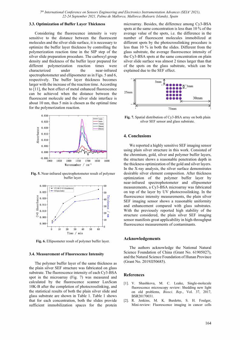
7th International Conference on Sensors Engineering and Electronics Instrumentation Advances (SEIA' 2021), 22-24 September 2021, Palma de Mallorca, Mallorca (Balearic Islands), Spain
164
3.3. Optimization of Buffer Layer Thickness
Considering the fluorescence intensity is very sensitive to the distance between the fluorescent molecules and the silver slide surface, it is necessary to optimize the buffer layer thickness by controlling the polymerization reaction time in the SIP step of the silver slide preparation procedure. The carboxyl group density and thickness of the buffer layer prepared for different polymerization reaction times were characterized under the near-infrared spectrophotometer and ellipsometer as in Figs. 5 and 6, respectively. The buffer layer thickness becomes larger with the increase of the reaction time. According to [11], the best effect of metal enhanced fluorescence can be achieved when the distance between the fluorescent molecule and the silver slide interface is about 10 nm, thus 5 min is chosen as the optimal time for the polymerization reaction.
Fig. 5. Near-infrared spectrophotometer result of polymer buffer layer.
Fig. 6. Ellipsometer result of polymer buffer layer.
3.4. Measurement of Fluorescence Intensity
The polymer buffer layer of the same thickness as the plain silver SEF structure was fabricated on glass substrate. The fluorescence intensity of each Cy3-BSA spot in the microarray (Fig. 7) was measured and calculated by the fluorescence scanner LuxScan 10K-B after the completion of photocrosslinking, and the statistical results of both the plain silver slide and glass substrate are shown in Table 1. Table 1 shows that for each concentration, both the slides provide sufficient immobilization spaces for the protein
microarray. Besides, the difference among Cy3-BSA spots at the same concentration is less than 10 % of the average value of the spots, i.e. the difference in the number of fluorescent molecules immobilized at different spots by the photocrosslinking procedure is less than 10 % in both the slides. Different from the glass substrate, the average fluorescence intensity of the Cy3-BSA spots at the same concentration on plain silver slide surface was almost 2 times larger than that of the spots on the glass substrate, which can be explained due to the SEF effect.
Fig. 7. Spatial distribution of Cy3-BSA array on both plain silver SEF sensor and glass substrate.
4. Conclusions
We reported a highly sensitive SEF imaging sensor using plain silver structure in this work. Consisted of the chromium, gold, silver and polymer buffer layers, the structure shows a reasonable penetration depth in the thickness optimization of the gold and silver layers. In the X-ray analysis, the silver surface demonstrates desirable silver element composition. After thickness optimization of the polymer buffer layer by near-infrared spectrophotometer and ellipsometer measurements, a Cy3-BSA microarray was fabricated on top of the layer by UV photocrosslinking. In the fluorescence intensity measurements, the plain silver SEF imaging sensor shows a reasonable uniformity and enhancement compared with glass substrates. With the previously reported high stability of the structure considered, the plain silver SEF imaging sensor manifests great applicability in high-throughput fluorescence measurements of contaminants. Acknowledgements
The authors acknowledge the National Natural Science Foundation of China (Grant No. 61905027), and the Natural Science Foundation of Hunan Province (Grant No. 2019JJ50685). References [1]. V. Shashkova, M. C. Leake, Single-molecule
fluorescence microscopy review: Shedding new light on old problems, Biosci. Rep., Vol. 37, 2017, BSR20170031.
[2]. R. Jenkins, M. K. Burdette, S. H. Foulger, Mini-review: Fluorescence imaging in cancer cells
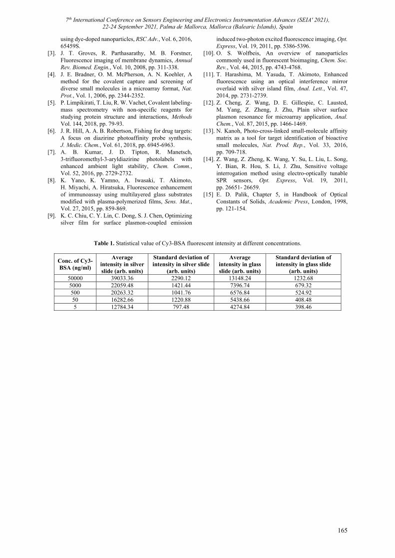
7th International Conference on Sensors Engineering and Electronics Instrumentation Advances (SEIA' 2021), 22-24 September 2021, Palma de Mallorca, Mallorca (Balearic Islands), Spain
165
using dye-doped nanoparticles, RSC Adv., Vol. 6, 2016, 65459S.
[3]. J. T. Groves, R. Parthasarathy, M. B. Forstner, Fluorescence imaging of membrane dynamics, Annual Rev. Biomed. Engin., Vol. 10, 2008, pp. 311-338.
[4]. J. E. Bradner, O. M. McPherson, A. N. Koehler, A method for the covalent capture and screening of diverse small molecules in a microarray format, Nat. Prot., Vol. 1, 2006, pp. 2344-2352.
[5]. P. Limpikirati, T. Liu, R. W. Vachet, Covalent labeling-mass spectrometry with non-specific reagents for studying protein structure and interactions, Methods Vol. 144, 2018, pp. 79-93.
[6]. J. R. Hill, A. A. B. Robertson, Fishing for drug targets: A focus on diazirine photoaffinity probe synthesis, J. Medic. Chem., Vol. 61, 2018, pp. 6945-6963.
[7]. A. B. Kumar, J. D. Tipton, R. Manetsch, 3-trifluoromethyl-3-aryldiazirine photolabels with enhanced ambient light stability, Chem. Comm., Vol. 52, 2016, pp. 2729-2732.
[8]. K. Yano, K. Yamno, A. Iwasaki, T. Akimoto, H. Miyachi, A. Hiratsuka, Fluorescence enhancement of immunoassay using multilayered glass substrates modified with plasma-polymerized films, Sens. Mat., Vol. 27, 2015, pp. 859-869.
[9]. K. C. Chiu, C. Y. Lin, C. Dong, S. J. Chen, Optimizing silver film for surface plasmon-coupled emission
induced two-photon excited fluorescence imaging, Opt. Express, Vol. 19, 2011, pp. 5386-5396.
[10]. O. S. Wolfbeis, An overview of nanoparticles commonly used in fluorescent bioimaging, Chem. Soc. Rev., Vol. 44, 2015, pp. 4743-4768.
[11]. T. Harashima, M. Yasuda, T. Akimoto, Enhanced fluorescence using an optical interference mirror overlaid with silver island film, Anal. Lett., Vol. 47, 2014, pp. 2731-2739.
[12]. Z. Cheng, Z. Wang, D. E. Gillespie, C. Lausted, M. Yang, Z. Zheng, J. Zhu, Plain silver surface plasmon resonance for microarray application, Anal. Chem., Vol. 87, 2015, pp. 1466-1469.
[13]. N. Kanoh, Photo-cross-linked small-molecule affinity matrix as a tool for target identification of bioactive small molecules, Nat. Prod. Rep., Vol. 33, 2016, pp. 709-718.
[14]. Z. Wang, Z. Zheng, K. Wang, Y. Su, L. Liu, L. Song, Y. Bian, R. Hou, S. Li, J. Zhu, Sensitive voltage interrogation method using electro-optically tunable SPR sensors, Opt. Express, Vol. 19, 2011, pp. 26651- 26659.
[15] E. D. Palik, Chapter 5, in Handbook of Optical Constants of Solids, Academic Press, London, 1998, pp. 121-154.
Table 1. Statistical value of Cy3-BSA fluorescent intensity at different concentrations.
Conc. of Cy3-BSA (ng/ml)
Average intensity in silver slide (arb. units)
Standard deviation of intensity in silver slide
(arb. units)
Average intensity in glass slide (arb. units)
Standard deviation of intensity in glass slide
(arb. units) 50000 39033.36 2290.12 13148.24 1232.68 5000 22059.48 1421.44 7396.74 679.32 500 20263.32 1041.76 6576.84 524.92 50 16282.66 1220.88 5438.66 408.48 5 12784.34 797.48 4274.84 398.46
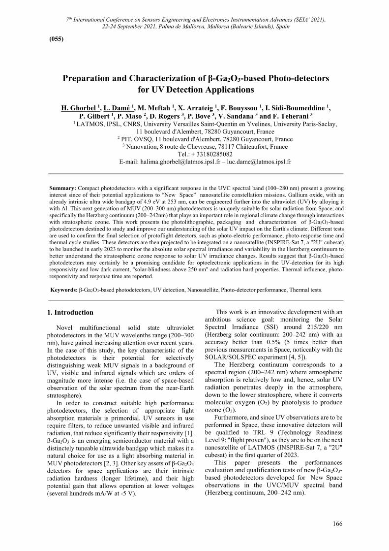
7th International Conference on Sensors Engineering and Electronics Instrumentation Advances (SEIA' 2021), 22-24 September 2021, Palma de Mallorca, Mallorca (Balearic Islands), Spain
166
(055)
Preparation and Characterization of β-Ga2O3-based Photo- detectors for UV Detection Applications
H. Ghorbel 1, L. Damé 1, M. Meftah 1, X. Arrateig 1, F. Bouyssou 1, I. Sidi-Boumeddine 1,
P. Gilbert 1, P. Maso 2, D. Rogers 3, P. Bove 3, V. Sandana 3 and F. Teherani 3 1 LATMOS, IPSL, CNRS, University Versailles Saint-Quentin en Yvelines, University Paris- Saclay,
11 boulevard d'Alembert, 78280 Guyancourt, France 2 PIT, OVSQ, 11 boulevard d'Alembert, 78280 Guyancourt, France
3 Nanovation, 8 route de Chevreuse, 78117 Châteaufort, France Tel.: + 33180285082
E-mail: [email protected] – [email protected]
Summary: Compact photodetectors with a significant response in the UVC spectral band (100–280 nm) present a growing interest since of their potential applications to “New Space” nanosatellite constellation missions. Gallium oxide, with an already intrinsic ultra wide bandgap of 4.9 eV at 253 nm, can be engineered further into the ultraviolet (UV) by alloying it with Al. This next generation of MUV (200–300 nm) photodetectors is uniquely suitable for solar radiation from Space, and specifically the Herzberg continuum (200–242nm) that plays an important role in regional climate change through interactions with stratospheric ozone. This work presents the photolithographic, packaging and characterization of β-Ga2O3-based photodetectors destined to study and improve our understanding of the solar UV impact on the Earth's climate. Different tests are used to confirm the final selection of protoflight detectors, such as photo-electric performance, photo-response time and thermal cycle studies. These detectors are then projected to be integrated on a nanosatellite (INSPIRE-Sat 7, a "2U" cubesat) to be launched in early 2023 to monitor the absolute solar spectral irradiance and variability in the Herzberg continuum to better understand the stratospheric ozone response to solar UV irradiance changes. Results suggest that β-Ga2O3-based photodetectors may certainly be a promising candidate for optoelectronic applications in the UV-detection for its high responsivity and low dark current, "solar-blindness above 250 nm" and radiation hard properties. Thermal influence, photo-responsivity and response time are reported. Keywords: β-Ga2O3-based photodetectors, UV detection, Nanosatellite, Photo-detector performance, Thermal tests.
1. Introduction Novel multifunctional solid state ultraviolet
photodetectors in the MUV wavelenths range (200–300 nm), have gained increasing attention over recent years. In the case of this study, the key characteristic of the photodetectors is their potential for selectively distinguishing weak MUV signals in a background of UV, visible and infrared signals which are orders of magnitude more intense (i.e. the case of space-based observation of the solar spectrum from the near-Earth stratosphere).
In order to construct suitable high performance photodetectors, the selection of appropriate light absorption materials is primordial. UV sensors in use require filters, to reduce unwanted visible and infrared radiation, that reduce significantly their responsivity [1]. ß-Ga2O3 is an emerging semiconductor material with a distinctely tuneable ultrawide bandgap which makes it a natural choice for use as a light absorbing material in MUV photodetectors [2, 3]. Other key assets of β-Ga2O3 detectors for space applications are their intrinsic radiation hardness (longer lifetime), and their high potential gain that allows operation at lower voltages (several hundreds mA/W at -5 V).
This work is an innovative development with an ambitious science goal: monitoring the Solar Spectral Irradiance (SSI) around 215/220 nm (Herzberg solar continuum: 200–242 nm) with an accuracy better than 0.5% (5 times better than previous measurements in Space, noticeably with the SOLAR/SOLSPEC experiment [4, 5]).
The Herzberg continuum corresponds to a spectral region (200–242 nm) where atmospheric absorption is relatively low and, hence, solar UV radiation penetrates deeply in the atmosphere, down to the lower stratosphere, where it converts molecular oxygen (O2) by photolysis to produce ozone (O3).
Furthermore, and since UV observations are to be performed in Space, these innovative detectors will be qualified to TRL 9 (Technology Readiness Level 9: "flight proven"), as they are to be on the next nanosatellite of LATMOS (INSPIRE-Sat 7, a "2U" cubesat) in the first quarter of 2023.
This paper presents the performances evaluation and qualification tests of new β-Ga2O3-based photodetectors developed for New Space observations in the UVC/MUV spectral band (Herzberg continuum, 200–242 nm).

7th International Conference on Sensors Engineering and Electronics Instrumentation Advances (SEIA' 2021), 22-24 September 2021, Palma de Mallorca, Mallorca (Balearic Islands), Spain
167
2. Method Metal-Semiconductor-Metal (MSM) devices were
formed by making two “back-to-back” Schottky diodes in the form of interdigited fingers (having widths and spacings of 2 μm, as shown in Fig. 1).
Fig. 2 shows the process flow for the development of an MSM photodetector (PD). This figure presents the principal main steps to achieve a final packaged PD.
In the first step, lightly doped n-type β-Ga2O3 films were deposited on Al2O3 substrates by Pulsed Laser Deposition (PLD) [6]. MSM devices were then formed by negative photolithography and Au/Ni contact deposition. Die singulation was then performed with a diamond saw. The singulated device die was soldered onto a TO can (TO-39) base and wires were wedge bonded to the MSM gold contact pads. The finished device was then encapsulated in dry nitrogen with a sapphire window cap. Back illumination adds performance.
Fig. 1. Schematic of MSN Inter-Digited-Transducer (IDT) structures with the corresponding circuit diagram
and a band structure representation.
Fig. 2. Process flow for the creation of an MSM photodetector.
Time response measurements were measured with
broad band square wave light pulses generated using an optical chopper. Termal cycling tests were made in a climatic chamber (Material Physico-Chimique ”MPC AN80”). The objective of the test was to measure the impact of temperature changes on the photo-current generated by polychromatic UV light. Tests were made between -30 and +50 degrees Celsius, which corresponds to their temperature environment for use in Space. The sensors were installed on a "breadboard" and
biased at -5V (the maximum voltage available on the power limited nanosatellite).
3. Results and Discussion 3.1 Selection Rationale
For low radiation flux detection between 200 and 242 nm, a very large signal-to-noise ratio is essential. Furthermore, the spectral response of the detector should be selective for the 200–242 nm range, centered at 215–220 nm, with a low full width at half maximum of the order of 35 nm and an excellent rejection so that the visible spectrum, which is much more intense, does not affect the measurement. In previous work [6] the authors showed that β-Ga2O3-based sensors can be engineered to combine both a spectral response peak in the 200–242 nm range and a very large rejection ratio of the visible solar spectrum. Thus, with the β-Ga2O3, we can simultaneously obtain the desired maximum response at 215–220 nm, a very high rejection ratio (> 1000 compared to the peak of sensitivity) at wavelengths ≥ 245–250 nm, and thereby achieve an excellent signal-to-noise ratio (dark current is very low: ≤ 1 pA). In practice these detectors are "solar blind above 250 nm" (since insensitive to visible and infrared light, "visible blindness"). Other key properties of detectors are their intrinsic radiation hardness (durable long term performances) and their wide operating temperature range (no need for cooling below 0, neither -20° or -40°).
Such detectors were realized right through from the wafer to the final packaged sensors (including device architecture development, photolithography, singulation, contacting, packaging and testing).
3.2. Photo-response Time
We investigated the electrical conductivity and the time response performance of the β-Ga2O3 based PD. With a bias of -5.0 V, the 200–250 nm UV illumination was turned-on to measure the time- dependent photo-response of the device. The light absorption layer of the oxide thin film is an important factor of the high response in our β-Ga2O3-based PD.
Fig. 3 shows that the photoresponse of the device to 10 minutes of illumination for various wavelengths of monochromatic illumination in the UV Band (220-250nm). The Figure shows that the switching and photoreponse of the device are rapid and stable, respectively.
Fig. 4 shows the response time and dynamics. Current is stable in time (< 1 %, mainly from measurements uncertainty) during a 10 hours test (Fig. 4 (a)).
We are investigating ways to improve rise time (ideally < 1s) but it should be noted that the measurements reported were made using a prober, and should be improved with the much better contacts provided by wire soldering.
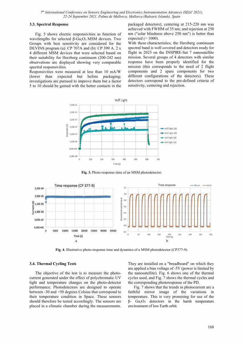
7th International Conference on Sensors Engineering and Electronics Instrumentation Advances (SEIA' 2021), 22-24 September 2021, Palma de Mallorca, Mallorca (Balearic Islands), Spain
168
3.3. Spectral Response
Fig. 5 shows electric responsivities as function of wavelengths for selected β-Ga2O3 MSM devices. Two Groups with best sensitivity are considered for the DEVINS program (a): CP 707A and (b): CP 399 A. 2 x 4 different MSM devices that were selected based on their suitability for Herzberg continuum (200-242 nm) observations are displayed showing very comparable spectral responsivities. Responsivities were measured at less than 10 mA/W (lower than expected but before packaging; investigations are pursued to improve them but a factor 5 to 10 should be gained with the better contacts in the
packaged detectors); centering at 215-220 nm was achieved with FWHM of 35 nm; and rejection at 250 nm ("solar blindness above 250 nm") is better than expected (> 1000). With these characteristics, the Herzberg continuum spectral band is well covered and detectors ready for flight in 2023 on the INSPIRE-Sat 7 nanosatellite mission. Several groups of 4 detectors with similar response have been properly identified for the mission (this corresponds to the need of 2 flight components and 2 spare components for two different configurations of the detectors). These detectors correspond to the pre-defined criteria of sensitivity, centering and rejection.
Fig. 3. Photo-response time of an MSM photodetector.
a b
Fig. 4. Illustrative photo-response time and dynamics of a MSM photodetector (CP377-9).
3.4. Thermal Cycling Tests
The objective of the test is to measure the photo-
current generated under the effect of polychromatic UV light and temperature changes on the photo-detector performance. Photodetectors are designed to operate between -30 and +50 degrees Celsius that correspond to their temperature condition in Space. These sensors should therefore be tested accordingly. The sensors are placed in a climatic chamber during the measurements.
They are installed on a "breadboard" on which they are applied a bias voltage of -5V (power is limited by the nanosatellite). Fig. 6 shows one of the thermal cycles used, and Fig. 7 shows the thermal cycles and the corresponding photoresponse of the PD.
Fig. 7 shows that the trends in photocurrent are a faithful mirror image of the variations in temperature. This is very promising for use of the β- Ga2O3 detectors in the harsh temperature environment of low Earth orbit.
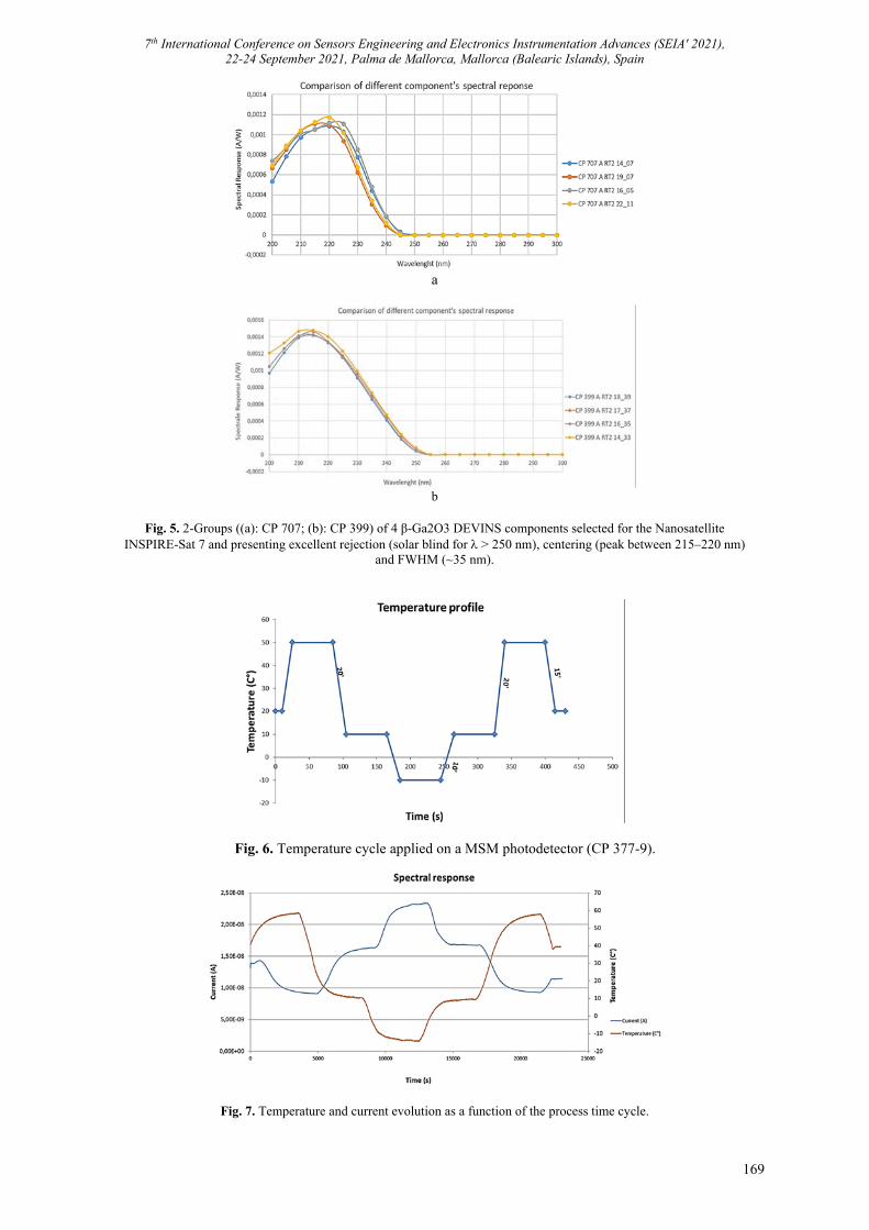
7th International Conference on Sensors Engineering and Electronics Instrumentation Advances (SEIA' 2021), 22-24 September 2021, Palma de Mallorca, Mallorca (Balearic Islands), Spain
169
a
b
Fig. 5. 2-Groups ((a): CP 707; (b): CP 399) of 4 β-Ga2O3 DEVINS components selected for the Nanosatellite
INSPIRE-Sat 7 and presenting excellent rejection (solar blind for > 250 nm), centering (peak between 215–220 nm) and FWHM (~35 nm).
Fig. 6. Temperature cycle applied on a MSM photodetector (CP 377-9).
Fig. 7. Temperature and current evolution as a function of the process time cycle.

7th International Conference on Sensors Engineering and Electronics Instrumentation Advances (SEIA' 2021), 22-24 September 2021, Palma de Mallorca, Mallorca (Balearic Islands), Spain
170
4. Conclusions
This study evidenced that 𝛽-Ga2O3 photodetectors can be extremelly robust and show excellent detection performance with high responsivity and short photo-response, along with a remarkably high rejection of visible and near UV wavelengths ("solar-blind property above 250 nm"). Hense, these detectors are very promising and are now ready for intensive calibrations (in the BIRA-IASB facilities in Brussels) before deployment on the upcoming nanosatellite of LATMOS, INSPIRE-Sat 7 (launch planned in 2023). In the near future, these detectors are projected for large solar and climate satellite constellation ventures.
Acknowledgements
We acknowledge support from the ANR (Agence Nationale de la Recherche) for the development of the photodetectors in the framework of the DEVINS program (DEep uV INnovative detector technologies for Space observations), from the CNRS (Centre National de la Recherche Scientifique), from the University Versailles Saint-Quentin-en-Yvelines (UVSQ) and from the Centre National d'Études Spatiales (CNES).
References [1]. Z. Xu, H. Deng, J. Xie, Y. Li, Y. Li,
Photoconductive UV detectors based on ZnO films prepared by sol-gel method, J. Sol. GelSci. Technol., Vol. 36, 2005, pp. 223-226.
[2]. D. Guo, Q. Guo, Z. Chen, Z. Wu, P. Li, W. Tang, Review of Ga2O3-based optoelectronic devices, Mater. Today Phys., Vol. 11, 2019, 100157.
[3]. Y. Chen, Y. Lu, M. Liao, Y. Tian, Q. Liu, C. Gao, X. Yang, C. Shan, 3D solar blind Ga2O3 photo detector array realized via origami method, Adv. Funct. Mater., Vol. 29, 2019, 1906040.
[4]. M. Meftah, L. Damé, et al., SOLAR-ISS, a New Solar Spectrum Based on Recent Observations, A&A, 611, 2018, A1.
[5]. M. Meftah, L. Damé, et al., UVSQ-SAT, A pathfinder CubeSat mission for observing essential climate variables, Remote Sensing, Vol. 12, Issue 1, 2020, 92.
[6]. D. J. Rogers, et al., Sharp/Tuneable UVC selectivity and extreme solar blindness in nominally grown undoped Ga2O3 MSM photodetectors by pulsed laser deposition, Proceedings of SPIE, Vol. 11687, 2021, 116872D.
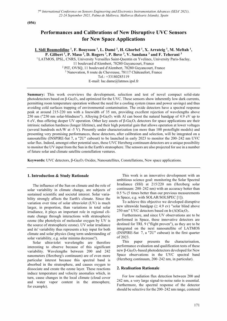
7th International Conference on Sensors Engineering and Electronics Instrumentation Advances (SEIA' 2021), 22-24 September 2021, Palma de Mallorca, Mallorca (Balearic Islands), Spain
171
(056)
Performances and Calibrations of New Disruptive UVC Sensors for New Space Applications
I. Sidi Boumeddine 1, F. Bouyssou 1, L. Damé 1, H. Ghorbel 1, X. Arrateig 1, M. Meftah 1,
P. Gilbert 1, P. Maso 2, D. Rogers 3, P. Bove 3, V. Sandana 3 and F. Teherani 3
1 LATMOS, IPSL, CNRS, University Versailles Saint-Quentin en Yvelines, University Paris-Saclay, 11 boulevard d'Alembert, 78280 Guyancourt, France
2 PIT, OVSQ, 11 boulevard d'Alembert, 78280 Guyancourt, France 3 Nanovation, 8 route de Chevreuse, 78117 Châteaufort, France
Tel.: +33180285119 E-mail: [email protected]
Summary: This work overviews the development, selection and test of novel compact solid-state photodetectors based on β-Ga2O3, and optimized for the UVC. These sensors show inherently low dark currents, permitting room temperature operation without the need for a cooling system (mass and power savings) and thus avoiding cold surfaces trapping of environmental contamination. The oxide detectors have a spectral response peak at around 215-220 nm with a linewidth of 35 nm, providing excellent rejection of wavelengths above 250 nm ("250 nm solar-blindness"). Alloying β-Ga2O3 with Al can boost the natural bandgap of 4.9 eV up to 6 eV, thus offering deeper UV operation. Other key assets of β-Ga2O3 detectors for space applications are their intrinsic radiation hardness (longer lifetime), and their high potential gain that allows operation at lower voltages (several hundreds mA/W at -5 V). Presently under characterization (on more than 100 protoflight models) and presenting very promising performances, these detectors, after calibration and selection, will be integrated on a nanosatellite (INSPIRE-Sat 7, a "2U" cubesat) to be launched in early 2023 to monitor the 200–242 nm UVC solar flux. Indeed, amongst other potential uses, these UVC Herzberg continuum detectors are a unique possibility to monitor the UV input from the Sun in the Earth's stratosphere. The sensors are also projected for use in a number of future solar and climate satellite constellation ventures. Keywords: UVC detectors, β-Ga2O3 Oxides, Nanosatellites, Constellations, New space applications. 1. Introduction & Study Rationale
The influence of the Sun on climate and the role of solar variability in climate change, are subjects of sustained scientific and societal interest. Solar varia-bility strongly affects the Earth's climate. Since the variation over time of solar ultraviolet (UV) is much larger, in proportion, than variations in total solar irradiance, it plays an important role in regional cli-mate change through interactions with stratospheric ozone (the photolysis of molecular oxygen by UV is the source of stratospheric ozone). UV solar irradiance and its' variability thus represents a key input for both climate and solar physics (long term understanding of solar variability, e.g. solar minima decrease?).
Solar ultraviolet wavelengths are therefore interesting to observe because of this significant variability. Wavelengths between 200 and 242 nanometers (Herzberg's continuum) are of even more particular interest because this spectral band is absorbed in the stratosphere, and causes oxygen to dissociate and create the ozone layer. These reactions induce temperature and velocity anomalies which, in turn, cause changes in the local climate (cloud cover and water vapor content in the atmosphere, for example).
This work is an innovative development with an ambitious science goal: monitoring the Solar Spectral Irradiance (SSI) at 215/220 nm (Herzberg solar continuum: 200–242 nm) with an accuracy better than 0.5 % (5 times better than our previous measurements in Space, e.g. with SOLAR/SOLSPEC [1]).
To achieve this objective we developed disruptive new ultrawide bandgap (≥ 4.9 ev) "solar blind above 250 nm" UVC detectors based on b-(Al)Ga2O3.
Furthermore, and since UV observations are to be performed in Space, these innovative detectors are destined for TRL 9 ("flight proven"), as they are to be integrated on the next nanosatellite of LATMOS (INSPIRE-Sat 7, a "2U" cubesat) in the first quarter of 2023.
This paper presents the characterisation, performance evaluation and qualification tests of these new β-Ga2O3-based photodetectors developed for New Space observations in the UVC spectral band (Herzberg continuum, 200–242 nm, in particular).
2. Realisation Rationale
For low radiation flux detection between 200 and 242 nm, a very large signal-to-noise ratio is essential. Furthermore, the spectral response of the detector should be selective for the 200–242 nm range, centered
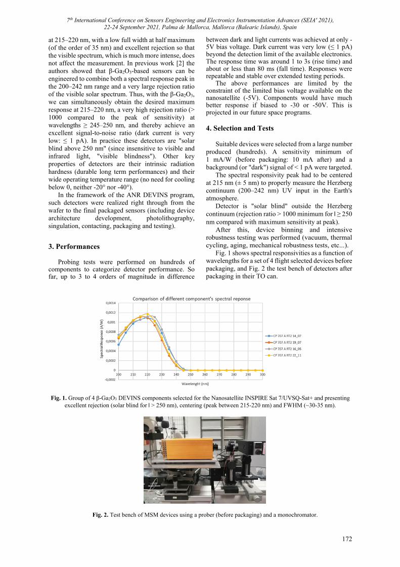
7th International Conference on Sensors Engineering and Electronics Instrumentation Advances (SEIA' 2021), 22-24 September 2021, Palma de Mallorca, Mallorca (Balearic Islands), Spain
172
at 215–220 nm, with a low full width at half maximum (of the order of 35 nm) and excellent rejection so that the visible spectrum, which is much more intense, does not affect the measurement. In previous work [2] the authors showed that β-Ga2O3-based sensors can be engineered to combine both a spectral response peak in the 200–242 nm range and a very large rejection ratio of the visible solar spectrum. Thus, with the β-Ga2O3, we can simultaneously obtain the desired maximum response at 215–220 nm, a very high rejection ratio (> 1000 compared to the peak of sensitivity) at wavelengths ≥ 245–250 nm, and thereby achieve an excellent signal-to-noise ratio (dark current is very low: ≤ 1 pA). In practice these detectors are "solar blind above 250 nm" (since insensitive to visible and infrared light, "visible blindness"). Other key properties of detectors are their intrinsic radiation hardness (durable long term performances) and their wide operating temperature range (no need for cooling below 0, neither -20° nor -40°).
In the framework of the ANR DEVINS program, such detectors were realized right through from the wafer to the final packaged sensors (including device architecture development, photolithography, singulation, contacting, packaging and testing).
3. Performances
Probing tests were performed on hundreds of components to categorize detector performance. So far, up to 3 to 4 orders of magnitude in difference
between dark and light currents was achieved at only -5V bias voltage. Dark current was very low (≤ 1 pA) beyond the detection limit of the available electronics. The response time was around 1 to 3s (rise time) and about or less than 80 ms (fall time). Responses were repeatable and stable over extended testing periods.
The above performances are limited by the constraint of the limited bias voltage available on the nanosatellite (-5V). Components would have much better response if biased to -30 or -50V. This is projected in our future space programs. 4. Selection and Tests
Suitable devices were selected from a large number produced (hundreds). A sensitivity minimum of 1 mA/W (before packaging: 10 mA after) and a background (or "dark") signal of < 1 pA were targeted.
The spectral responsivity peak had to be centered at 215 nm (± 5 nm) to properly measure the Herzberg continuum (200–242 nm) UV input in the Earth's atmosphere.
Detector is "solar blind" outside the Herzberg continuum (rejection ratio > 1000 minimum for l ≥ 250 nm compared with maximum sensitivity at peak).
After this, device binning and intensive robustness testing was performed (vacuum, thermal cycling, aging, mechanical robustness tests, etc...).
Fig. 1 shows spectral responsivities as a function of wavelengths for a set of 4 flight selected devices before packaging, and Fig. 2 the test bench of detectors after packaging in their TO can.
Fig. 1. Group of 4 β-Ga2O3 DEVINS components selected for the Nanosatellite INSPIRE Sat 7/UVSQ-Sat+ and presenting
excellent rejection (solar blind for l > 250 nm), centering (peak between 215-220 nm) and FWHM (~30-35 nm).
Fig. 2. Test bench of MSM devices using a prober (before packaging) and a monochromator.

7th International Conference on Sensors Engineering and Electronics Instrumentation Advances (SEIA' 2021), 22-24 September 2021, Palma de Mallorca, Mallorca (Balearic Islands), Spain
173
5. Conclusions
UVC detectors optimized for the 200–242 nm range were realized, tested and selected, and are now ready for intensive calibration (in the BIRA-IASB facilities in Brussels) before integration in the next LATMOS nanosatellite, INSPIRE-Sat 7 (launch planned for early 2023), and in projected future constellations. Acknowledgements
We acknowledge support from the ANR (Agence Nationale de la Recherche) for the development of
these detectors (DEVINS program: DEep uV INnovative detector technologies for Space observations). References [1]. M. Meftah, L. Damé, et al., UVSQ-SAT, a pathfinder
CubeSat mission for observing essential climate variables, Remote Sensing, Vol. 12, Issue 1, 2020, 92.
[2]. D. J. Rogers, et al., Sharp/tuneable UVC selectivity and extreme solar blindness in nominally grown undoped Ga2O3 MSM photodetectors by pulsed laser deposition, Proceedings of SPIE, Vol. 11687, 2021, 2D-1.
7th International Conference on Sensors Engineering and Electronics Instrumentation Advances (SEIA' 2021), 22-24 September 2021, Palma de Mallorca, Mallorca (Balearic Islands), Spain
174
(057)
Basic Study on Blood Coagulation Measurement in an Extracorporeal Circulation Circuit by LED Photoacoustic Method Using
an Extracorporeal Circulation Device
Takahiro Wabe 1, Ryo Suzuki 2,3, Akimitsu Fujii 4, Yohsuke Uchida 5, Kazuo Maruyama 2,3, Yasutaka Uchida 1
1 Teikyo University of Science, Department of Life & Health Sciences, Faculty of Life & Environmental Sciences, 2-2-1 Senjyusakuragi, Adachi-ku., Tokyo, Japan
2 Faculty of Pharma-Sciences, Teikyo University, Tokyo, Japan 3 Advanced Comprehensive Research Organization (ACRO), Tokyo, Japan
4 Tokyo college of Medico-Pharmaco Technology, Tokyo, Japan 5 Shuto iko, Tokyo, Japan
Tel.: + 8169101010, fax: + 8169103800 E-mail: [email protected]
Summary: In extracorporeal circulation devices such as ECMO, blood coagulation occurs due to various factors. Blood coagulation in the extracorporeal circulation circuit is detected ex post facto by existing pressure sensors. Subsequent detection of blood clots leads to the destruction of blood in the circuit, which is detrimental to the patient. Therefore, for the purpose of predictive maintenance in the extracorporeal circulation circuit, we will conduct basic research on measurement using photoacoustic imaging using LEDs as a light source and report it. As a result of the A-mode measurement, the number and intensity of photoacoustic waves changed remarkably with the passage of time, and it may be possible to measure the temporal change of blood coagulation in the extracorporeal circulation circuit that circulated blood. Keywords: Blood clotting, Photoacoustic imaging, LED, Circuit in an extracorporeal device, Temporal observation, MATLAB, Predictive maintenance.
1. Introduction
ECMO (Extracorporeal membrane oxygenation) is said to be the last bastion for the treatment of severely infected COVID-19 infections. An ECMO machine pumps blood from the body, supplies oxygen, removes carbon dioxide, and returns it to the body. It is a treatment that replaces respiratory and circulatory functions until the patient heals and recovers. In other words, it replaces the function of the lungs, so it is not a radical cure. The configuration of ECMO is shown in Fig.1. Respiratory failure is the most common cause of death for COVID-19, but the following can also be the cause of death. Causes of death are coagulation activation with excessive immune / inflammatory reactions, so-called cytokine storms, thrombosis, disseminated intravascular coagulation (DIC), and progression to multiple organ failure [1, 2].
In particular, thrombosis and DIC can lead to a rapid deterioration of the condition. Of course, even within the extracorporeal circulation circuit of ECMO, if blood coagulation progresses, it will become clogged and ECMO will not function. Extracorporeal circulation therapy such as ECMO is used in various fields such as heart-lung machines and acute blood purification devices. In the circuit that circulates blood outside the body, blood coagulation occurs due to various factors as described above [3, 4]. Various attempts have been made to prevent blood coagulation, and preventive measures using anticoagulants (such as heparin) are currently the mainstream [5, 6]. Heparin
coatings are used in extracorporeal circulation circuits to suppress coagulation caused by the reaction of blood with foreign bodies [7, 8]. However, since heparin also acts as a foreign substance, it is difficult to completely prevent blood coagulation on the circuit surface and in the dialyzer. When the circuit is clogged, it is detected by a pressure sensor inside the extracorporeal circuit. However, the detection will be ex post facto because it will be detected after the blood flow in the circuit becomes extremely slow or the circuit is clogged. Subsequent detection of blood coagulation leads to forcing medical staff to take immediate action such as discarding blood in the circuit or replacing the circuit, which is disadvantageous for patients and hospital staff. However, in order to observe changes in blood coagulation status in the extracorporeal circulation circuit in advance, a method with higher sensitivity than the conventional method is required. Therefore, a photoacoustic method was tried as a new measurement method. [9-11]. Basic research reports using photoacoustic imaging using LEDs as a light source were conducted at SEIA2019 and SEIA2020 [12, 13]. In photoacoustic imaging, the measurement target undergoes volume expansion due to the heat generated by the light source, and elastic waves are generated. Elastic waves are received and imaged by ultrasonic probes. Our study aims to observe the time course of blood coagulation that occurs in the extracorporeal circulation circuit during blood purification therapy. In this study, we used photoacoustic imaging with LEDs as the light source. The extracorporeal circulation
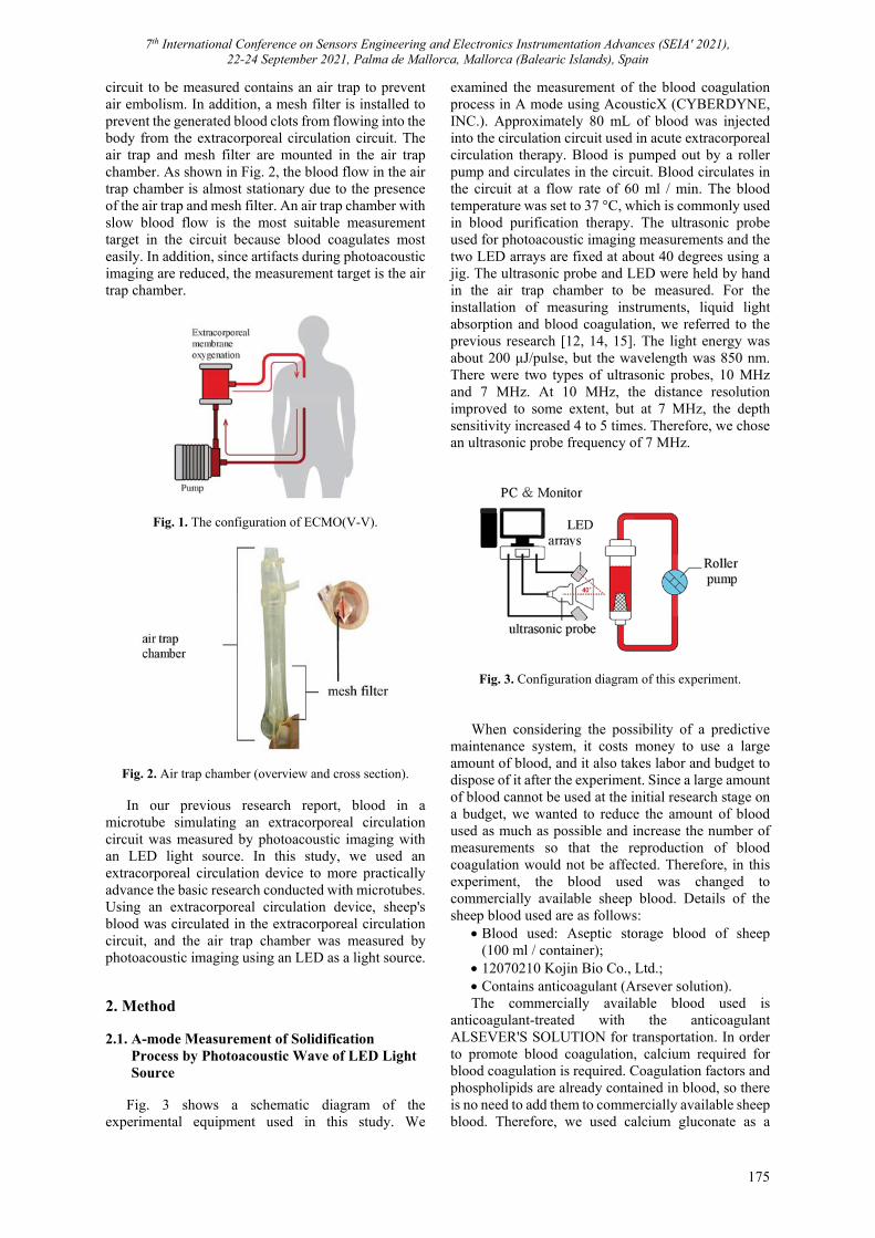
7th International Conference on Sensors Engineering and Electronics Instrumentation Advances (SEIA' 2021), 22-24 September 2021, Palma de Mallorca, Mallorca (Balearic Islands), Spain
175
circuit to be measured contains an air trap to prevent air embolism. In addition, a mesh filter is installed to prevent the generated blood clots from flowing into the body from the extracorporeal circulation circuit. The air trap and mesh filter are mounted in the air trap chamber. As shown in Fig. 2, the blood flow in the air trap chamber is almost stationary due to the presence of the air trap and mesh filter. An air trap chamber with slow blood flow is the most suitable measurement target in the circuit because blood coagulates most easily. In addition, since artifacts during photoacoustic imaging are reduced, the measurement target is the air trap chamber.
Fig. 1. The configuration of ECMO(V-V).
Fig. 2. Air trap chamber (overview and cross section). In our previous research report, blood in a
microtube simulating an extracorporeal circulation circuit was measured by photoacoustic imaging with an LED light source. In this study, we used an extracorporeal circulation device to more practically advance the basic research conducted with microtubes. Using an extracorporeal circulation device, sheep's blood was circulated in the extracorporeal circulation circuit, and the air trap chamber was measured by photoacoustic imaging using an LED as a light source. 2. Method 2.1. A-mode Measurement of Solidification Process by Photoacoustic Wave of LED Light Source
Fig. 3 shows a schematic diagram of the experimental equipment used in this study. We
examined the measurement of the blood coagulation process in A mode using AcousticX (CYBERDYNE, INC.). Approximately 80 mL of blood was injected into the circulation circuit used in acute extracorporeal circulation therapy. Blood is pumped out by a roller pump and circulates in the circuit. Blood circulates in the circuit at a flow rate of 60 ml / min. The blood temperature was set to 37 °C, which is commonly used in blood purification therapy. The ultrasonic probe used for photoacoustic imaging measurements and the two LED arrays are fixed at about 40 degrees using a jig. The ultrasonic probe and LED were held by hand in the air trap chamber to be measured. For the installation of measuring instruments, liquid light absorption and blood coagulation, we referred to the previous research [12, 14, 15]. The light energy was about 200 μJ/pulse, but the wavelength was 850 nm. There were two types of ultrasonic probes, 10 MHz and 7 MHz. At 10 MHz, the distance resolution improved to some extent, but at 7 MHz, the depth sensitivity increased 4 to 5 times. Therefore, we chose an ultrasonic probe frequency of 7 MHz.
Fig. 3. Configuration diagram of this experiment. When considering the possibility of a predictive
maintenance system, it costs money to use a large amount of blood, and it also takes labor and budget to dispose of it after the experiment. Since a large amount of blood cannot be used at the initial research stage on a budget, we wanted to reduce the amount of blood used as much as possible and increase the number of measurements so that the reproduction of blood coagulation would not be affected. Therefore, in this experiment, the blood used was changed to commercially available sheep blood. Details of the sheep blood used are as follows:
Blood used: Aseptic storage blood of sheep (100 ml / container);
12070210 Kojin Bio Co., Ltd.; Contains anticoagulant (Arsever solution). The commercially available blood used is
anticoagulant-treated with the anticoagulant ALSEVER'S SOLUTION for transportation. In order to promote blood coagulation, calcium required for blood coagulation is required. Coagulation factors and phospholipids are already contained in blood, so there is no need to add them to commercially available sheep blood. Therefore, we used calcium gluconate as a
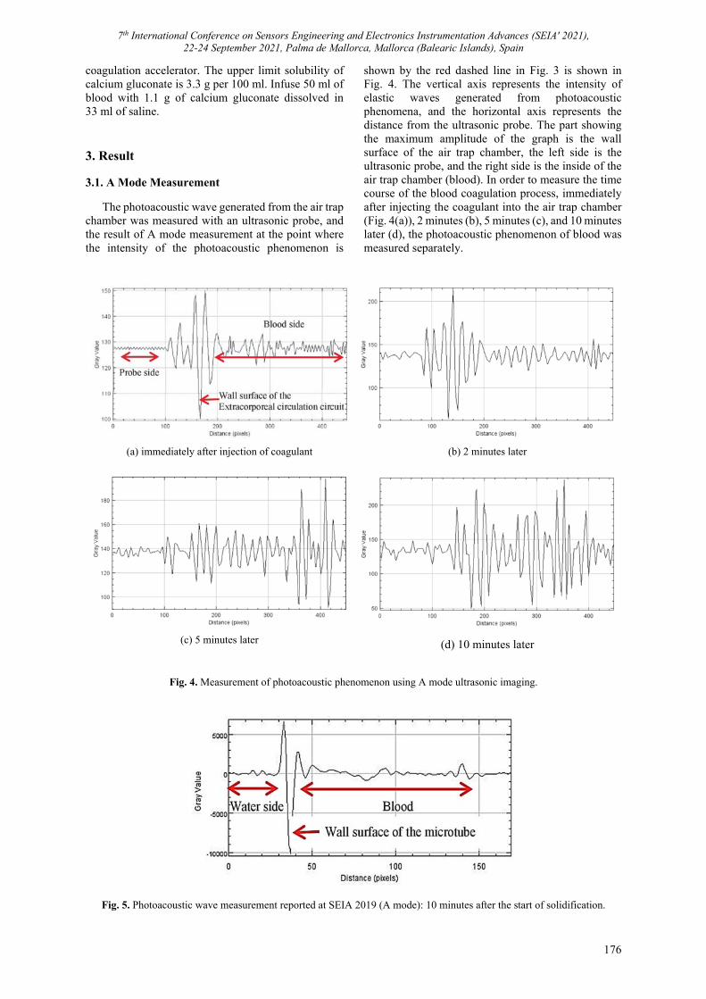
7th International Conference on Sensors Engineering and Electronics Instrumentation Advances (SEIA' 2021), 22-24 September 2021, Palma de Mallorca, Mallorca (Balearic Islands), Spain
176
coagulation accelerator. The upper limit solubility of calcium gluconate is 3.3 g per 100 ml. Infuse 50 ml of blood with 1.1 g of calcium gluconate dissolved in 33 ml of saline. 3. Result 3.1. A Mode Measurement
The photoacoustic wave generated from the air trap chamber was measured with an ultrasonic probe, and the result of A mode measurement at the point where the intensity of the photoacoustic phenomenon is
shown by the red dashed line in Fig. 3 is shown in Fig. 4. The vertical axis represents the intensity of elastic waves generated from photoacoustic phenomena, and the horizontal axis represents the distance from the ultrasonic probe. The part showing the maximum amplitude of the graph is the wall surface of the air trap chamber, the left side is the ultrasonic probe, and the right side is the inside of the air trap chamber (blood). In order to measure the time course of the blood coagulation process, immediately after injecting the coagulant into the air trap chamber (Fig. 4(a)), 2 minutes (b), 5 minutes (c), and 10 minutes later (d), the photoacoustic phenomenon of blood was measured separately.
(a) immediately after injection of coagulant
(b) 2 minutes later
(c) 5 minutes later
(d) 10 minutes later
Fig. 4. Measurement of photoacoustic phenomenon using A mode ultrasonic imaging.
Fig. 5. Photoacoustic wave measurement reported at SEIA 2019 (A mode): 10 minutes after the start of solidification.

7th International Conference on Sensors Engineering and Electronics Instrumentation Advances (SEIA' 2021), 22-24 September 2021, Palma de Mallorca, Mallorca (Balearic Islands), Spain
177
4. Conclusion
Over time, the position and amplitude of the photoacoustic waves measured by the ultrasonic probe changed. After injecting the coagulant into the blood in the circuit, as time went on, the amplitude increased so that it spread from the wall surface inside the air trap chamber. It was found that a similar change in amplitude position occurred when compared with the time course of blood coagulation of the microtube announced at SEIA 2019. Fig. 5 shows the SEIA 2019 report (A mode). In addition, the result of this experiment seems to be larger in terms of amplitude. This is because the air trap chamber with blood flow is the measurement target, unlike the microtube in the stationary state, so it is considered that the influence of blood flow appears in a waveform like noise. As with the measurement results of changes in blood coagulation in microtubes in SEIA 2019 over time, changes in blood coagulation in the extracorporeal circulation circuit can be measured using the extracorporeal circulation circuit, demonstrating the possibility of predictive maintenance in extracorporeal circulation therapy.
Acknowledgments
T. Wabe and Y. Uchida of Teikyo Univ. Of Sci. would like to thank Mr. N. Sato of CYBERDYNE, INC Research and Development Dept, for his cooperation in this experiment.
References [1]. N. Tang, D. Li, X. Wang, Z. Sun, Abnormal
coagulation parameters are associated with poor prognosis in patients with novel Corona virus pneumonia, J. Thromb. Haemost., Vol. 18, 2020, pp. 844-847.
[2]. P. Mehta, D. F. McAuley, M. Brown, E. Sanchez, R. S. Tattersall, J. J. Manson, HLH Across Speciality Collaboration, UK, COVID-19: Consider cytokine storm syndromes and immunosuppression, Lancet, Vol. 395, 2020, pp. 1033-1034.
[3]. J. Utley, Pathophysiology of cardiopulmonary bypass. Current issues, Car. Surg., Vol. 5, 1990, pp. 177-189.
[4]. Y. Mori, Blood compatible material, Kobunshi Ronbunshu, Vol. 42, Oct. 1985, pp. 601-615 (in Japanese).
[5]. L. Gott, J. D. Whiffen, R. C. Dutton, Heparin bonding on colloidal graphite surfaces, Science, Vol. 142, 1963, 1297.
[6]. I. O. Salyer, Medical Application of Plastic, Biomedical Material Symposium No. 1, Interscience, New York, 1971.
[7]. L. K. Segesser, B. M. Weiss, E. Garcia, A. Felten, M. L. Turina, Reduction and elimination of systemic heparinization during cardiopulmonary bypass, J. Thorac. Cardiovasc. Surg., Vol. 103, 1992, pp. 790-799.
[8]. V. Videm, T. E. Molines, P. Garred, J. L. Svennevig, Biocompatibility of extracorporeal circulation. In vitro comparison of heparin-coated and unmated oxygenator circuits, J. Thorac. Cardiovasc. Surg., Vol. 101, 1991, pp. 654-660.
[9]. H. Zhong, T. Duan, H. Lan, M. Zhou, F. Gao, Review of low-cost photoacoustic sensing and imaging based on laser diode and light-emitting diode, Sensors, Vol. 18, Issue 7, 2018, 2264.
[10]. T. J. Allen, P. C. Beard, High power visible light emitting diodes as pulsed excitation sources for biomedical photoacoustics, Biomedical Optics Express, Vol. 7, Issue 4, 2016, pp. 1260-1270.
[11]. A. B. Karpiouk, S. R. Aglyamov, S. Mallidi, J. Shah, W. G. Scott, J. M. Rubin, S. Y. Emelianov, Combined ultrasound and photoacoustic imaging to detect and stage deep vein thrombosis. phantom and ex vivo studies, J. Biomed. Opt., Vol. 13, Issue 5, Sep.-Oct. 2008, 054061.
[12]. T. Wabe, R. Suzuki, K. Maruyama, Y. Uchida, Possibility for temporal observation of thrombus generated in extracorporeal circulator circuit by photoacoustic imaging using LED, in Proceedings of the 5th International Conference on Sensors Engineering and Electronics Instrumentation Advances (SEIA'19), Canary Islands (Tenerife), Spain, 25-27 Sept. 2019, pp. 157-160.
[13]. T. Wabe, R. Suzuki, K. Maruyama,Y. Uchida, The measurement of blood coagulation process in extracorporeal circuit using LED photoacoustic imaging, Sensors & Transducers Journal, Vol. 237, Issues 9-10, September-October 2019, pp. 88-94.
[14]. R. J. Talbert, S. H. Holan, J. A. Viator, Photoacoustic discrimination of viable and thermally coagulated blood using a two-wavelength method for burn injury monitoring, IOP Publishing Physics in Medicine and Biology, Vol. 52, 2007, pp. 1815-1829.
[15]. T. Wabe, R. Suzuki, K. Maruyama, Y. Uchida, Possibility of extracting feature value from the changes in brightness over time of blood coagulation in the extracorporeal circuit, Sensors & Transducers Journal, Vol. 246, Issue 7, November 2020, pp. 64-70.
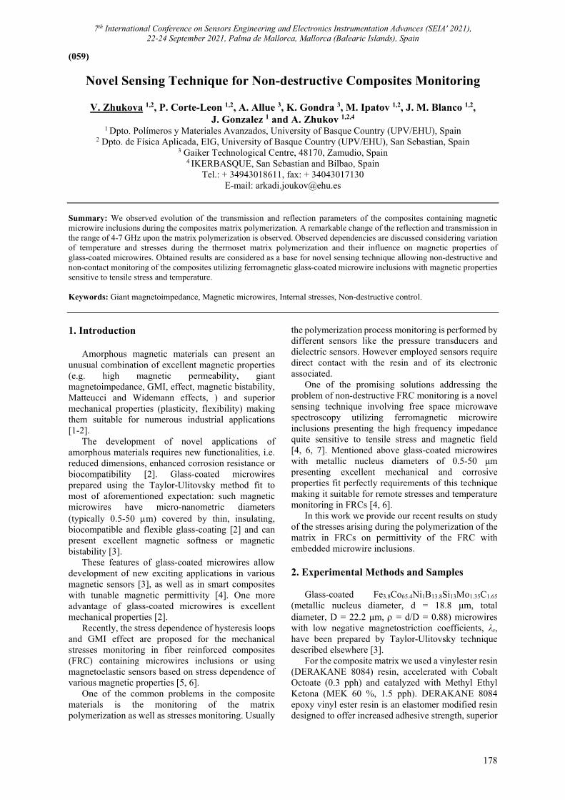
7th International Conference on Sensors Engineering and Electronics Instrumentation Advances (SEIA' 2021), 22-24 September 2021, Palma de Mallorca, Mallorca (Balearic Islands), Spain
178
(059)
Novel Sensing Technique for Non-destructive Composites Monitoring
V. Zhukova 1,2, P. Corte-Leon 1,2, A. Allue 3, K. Gondra 3, M. Ipatov 1,2, J. M. Blanco 1,2, J. Gonzalez 1 and A. Zhukov 1,2,4
1 Dpto. Polímeros y Materiales Avanzados, University of Basque Country (UPV/EHU), Spain 2 Dpto. de Física Aplicada, EIG, University of Basque Country (UPV/EHU), San Sebastian, Spain
3 Gaiker Technological Centre, 48170, Zamudio, Spain
4 IKERBASQUE, San Sebastian and Bilbao, Spain Tel.: + 34943018611, fax: + 34043017130
E-mail: [email protected] Summary: We observed evolution of the transmission and reflection parameters of the composites containing magnetic microwire inclusions during the composites matrix polymerization. A remarkable change of the reflection and transmission in the range of 4-7 GHz upon the matrix polymerization is observed. Observed dependencies are discussed considering variation of temperature and stresses during the thermoset matrix polymerization and their influence on magnetic properties of glass-coated microwires. Obtained results are considered as a base for novel sensing technique allowing non-destructive and non-contact monitoring of the composites utilizing ferromagnetic glass-coated microwire inclusions with magnetic properties sensitive to tensile stress and temperature. Keywords: Giant magnetoimpedance, Magnetic microwires, Internal stresses, Non-destructive control.
1. Introduction
Amorphous magnetic materials can present an unusual combination of excellent magnetic properties (e.g. high magnetic permeability, giant magnetoimpedance, GMI, effect, magnetic bistability, Matteucci and Widemann effects, ) and superior mechanical properties (plasticity, flexibility) making them suitable for numerous industrial applications [1-2].
The development of novel applications of amorphous materials requires new functionalities, i.e. reduced dimensions, enhanced corrosion resistance or biocompatibility [2]. Glass-coated microwires prepared using the Taylor-Ulitovsky method fit to most of aforementioned expectation: such magnetic microwires have micro-nanometric diameters (typically 0.5-50 m) covered by thin, insulating, biocompatible and flexible glass-coating [2] and can present excellent magnetic softness or magnetic bistability [3].
These features of glass-coated microwires allow development of new exciting applications in various magnetic sensors [3], as well as in smart composites with tunable magnetic permittivity [4]. One more advantage of glass-coated microwires is excellent mechanical properties [2].
Recently, the stress dependence of hysteresis loops and GMI effect are proposed for the mechanical stresses monitoring in fiber reinforced composites (FRC) containing microwires inclusions or using magnetoelastic sensors based on stress dependence of various magnetic properties [5, 6].
One of the common problems in the composite materials is the monitoring of the matrix polymerization as well as stresses monitoring. Usually
the polymerization process monitoring is performed by different sensors like the pressure transducers and dielectric sensors. However employed sensors require direct contact with the resin and of its electronic associated.
One of the promising solutions addressing the problem of non-destructive FRC monitoring is a novel sensing technique involving free space microwave spectroscopy utilizing ferromagnetic microwire inclusions presenting the high frequency impedance quite sensitive to tensile stress and magnetic field [4, 6, 7]. Mentioned above glass-coated microwires with metallic nucleus diameters of 0.5-50 μm presenting excellent mechanical and corrosive properties fit perfectly requirements of this technique making it suitable for remote stresses and temperature monitoring in FRCs [4, 6].
In this work we provide our recent results on study of the stresses arising during the polymerization of the matrix in FRCs on permittivity of the FRC with embedded microwire inclusions.
2. Experimental Methods and Samples
Glass-coated Fe3.8Co65.4Ni1B13.8Si13Mo1.35C1.65 (metallic nucleus diameter, d = 18.8 μm, total diameter, D = 22.2 μm, = d/D = 0.88) microwires with low negative magnetostriction coefficients, λs, have been prepared by Taylor-Ulitovsky technique described elsewhere [3].
For the composite matrix we used a vinylester resin (DERAKANE 8084) resin, accelerated with Cobalt Octoate (0.3 pph) and catalyzed with Methyl Ethyl Ketona (MEK 60 %, 1.5 pph). DERAKANE 8084 epoxy vinyl ester resin is an elastomer modified resin designed to offer increased adhesive strength, superior
7th International Conference on Sensors Engineering and Electronics Instrumentation Advances (SEIA' 2021), 22-24 September 2021, Palma de Mallorca, Mallorca (Balearic Islands), Spain
179
resistance to abrasion and severe mechanical stress, while providing greater toughness and elongation.
We used the free space measurement system previously described in details elsewhere [6, 7]. The reflection (R) and transmission (T) coefficients were measure in free-space. The experimental set-up consists of a pair of broadband horn antennas (1-17 GHz) and a vector network analyzer. The composite was placed in 20×20 cm2 window to avoid the edge effects. This window limits the applicable frequency range in 4-17 GHz. More detailed description of the free space systems is given in our previous publications [7]. In the present case we performed in-situ measurements: R and T coefficients have been measured during the matrix polymerization.
The composites with ordered glass coated amorphous wires embedded in the thermoset matrix polymerization were prepared.
3. Experimental Results and Discussion
As described above, we performed in-situ experiments of composites placed inside the un-echoic chamber with the glass-coated microwires embedded in a polymerized composite. We measured the transmission, T, and reflection, R, parameters of the composite containing Co-rich microwires (Fe3.8Co65.4Ni1B13.8Si13Mo1.35C1.65) using the free space system.
As can be appreciated from Fig. 1, considerable variation of the T-parameter is observed in the range frequency, f, of 4-7 GHz upon thermoset matrix polymerization (Fig. 1). A non-monotonic variation of T-parameter upon polymerization is observed (Fig. 1a). Additionally, a variation in R-values during the polymerization is observed (Fig. 1b).
Fig. 1. The Transmission, T (a) and reflection, R (a) parameters measured using free-space system during
the composite polymerization.
As we mentioned above, apart of the matrix heating, the polymerization is accompanied by change of density and shrinkage. Therefore we can assume that the matrix shrinkage produces compressive stresses in magnetic nucleus of glass-coated microwires.
Observed changes of electromagnetic properties can be related to two main phenomena arising during the composite matrix polymerization: heating and mechanical stresses. 4. Conclusions
We propose a novel sensing technique for non-destructive and non-contact monitoring of the composites utilizing ferromagnetic glass-coated Co-rich microwire inclusions with magnetic properties sensitive to tensile stress and temperature. Using the free space technique we observed considerable variation of the reflection and transmission in the range of 4-7 GHz upon the matrix polymerization. Observed dependencies are discussed considering variation of temperature and stresses during the thermoset matrix polymerization. References [1]. G. Herzer, Amorphous and nanocrystalline materials,
in: Encyclopedia of Materials: Science and Technology, Elsevier Science Ltd, 2001, pp. 149-157.
[2]. T. Goto, M. Nagano, N. Wehara, Mechanical properties of amorphous Fe80P16C3B1 filament produced by glass-coated melt spinning, Trans. JIM, Vol. 18, 1977, pp. 759-764.
[3]. A. Zhukov, M. Ipatov, V. Zhukova, Advances in giant magnetoimpedance of materials, Chapter 2, in Handbook of Magnetic Materials (K. H. J. Buschow, Ed.), Vol. 24, Elsevier B.V., 2015, pp. 139-236.
[4]. F. Qin, H. X. Peng, Ferromagnetic microwires enabled multifunctional composite materials, Prog. Mater. Sci., Vol. 58, 2013, pp. 183-259.
[5]. M. Churyukanova, S. Kaloshkin, E. Shuvaeva, A. Stepashkin, M. Zhdanova, A. Aronin, O. Aksenov, P. Arakelov, V. Zhukova, А. Zhukov, Non-contact method for stress monitoring based on stress dependence of magnetic properties of Fe-based microwires, J. Alloys Compd., Vol. 748, Issue 5, 2018, pp. 199-205.
[6]. A. Allue, P. Corte-León, K. Gondra, V. Zhukova, M. Ipatov, J. M. Blanco, J. Gonzalez, M. Churyukanova, S. Taskaev, A. Zhukov, Smart composites with embedded magnetic microwire inclusions allowing non-contact stresses and temperature monitoring, Composites Part A: Applied Science and Manufacturing, Vol. 120, 2019, pp. 12-20.
[7]. D. Makhnovskiy, A. Zhukov, V. Zhukova, J. Gonzalez, Tunable and self-sensing microwave composite materials incorporating ferromagnetic microwires, Advances in Science and Technology, Vol. 54, 2008, pp. 201-210.
t=0 t=10 min t=15 min t=20 min t=30 min t=60 min
4 5 6 7 8 9
50
55
60
65
70
Tra
nsm
issi
on
(%
)
frequency (GHz)
(a)
t < 15 min
t >15 min
4 6 8 10 12 14 16
0
20
40
60
80
100
t= 0 t= 10 min t= 15 min t= 30 min t= 60 min
Re
flect
ion
(%)
frequency (GHz)
(b)
t
t
t
7th International Conference on Sensors Engineering and Electronics Instrumentation Advances (SEIA' 2021), 22-24 September 2021, Palma de Mallorca, Mallorca (Balearic Islands), Spain
180
(061)
Optimization of Environmental Sensors Placement in Geophysical Research
A. Sokolov 1, K. Karroum 1, 2, H. Delbarre 1, Y. Ben Maissa 3 and M. Elhaziti 2
1 Laboratory for Physico-Chemistry of Atmosphere, University of Littoral Cote d’Opale, Dunkirk, France 2 LRIT-CNRST, URAC 29, Faculty of Sciences Mohammed V University in Rabat, Rabat, Morocco
3 Telecommunication Systems, Networks and Services Lab, National Institute of Posts and Telecommunications, Rabat, Morocco
E-mail: [email protected]
Summary: We propose an algorithm of optimization of environmental sensors deployment, based on a global minimization of the interpolation error. The approach was applied to find the best positions of sensors measuring PM10 atmospheric pollution in the Dunkirk region in France. A result of atmospheric pollution modeling was used as the true background value. It was shown that optimization of measuring stations could significantly reduce the error of pollution estimation. A necessary number of sensors could be estimated using the dependence of the error to the number. Keywords: Sensors’ deployment, optimization algorithms, PM10 atmospheric pollution, modelling.
1. Introduction
The positioning of measuring instruments is a key
question for an adequate description of the environment. If the ‘true’ background state of measuring environmental parameters, adequate interpolation technique (statistical or dynamic) and sensors deployment restrictions are known, the problem could often be reduced to a mathematical multivariant global optimization. This approach was applied for defining optimal positions of atmospheric aerosol pollution (PM10) sensors.
2. Datasets and Methods To define a background true atmospheric state two
datasets were employed. The first synthetic dataset is a 2D pollution distribution simulated by a simple Gaussian function. This dataset was used to calibrate algorithms and estimate stability/sensitivity of optimizations. The second dataset obtained from the air quality agency ATMO-Nord [1] corresponds to a one-year PM10 pollution at the ground level in the north of France in Dunkirk, simulated by ADMS atmospheric pollution model [2]. The quality of a measuring network can be
characterized by the difference 𝛿 𝛿𝑖 between interpolated and background true values:
𝛿 𝑝 𝑝 𝑥 , 𝑦 ,
where 𝑝 is a pollution value and 𝑥 , 𝑦 are coordinates of the ith sensor.
The minimizing error 𝜀 𝛿 , could be measured using different norms. A few p-norms were tested in the optimization problem:
, arg min 𝛿 , .
Additional constraints like a privileged (or prohibited) deployment area, maximal (or minimal) distance between sensors could be used in optimization. Additional constraints as a privileged (or prohibited) deployment area, maximal (or minimal) distance between sensors could be used in optimization. A few statistical interpolation techniques in 2D were tried, the list is below:
a) The inverse distance weighting; b) Linear interpolation with nearest neighbour
extrapolation; c) Natural neighbour with nearest neighbour
extrapolation; d) Cubic interpolation with nearest neighbour
extrapolation; e) Gaussian Process interpolation.
To find a global minimum of the error, the following algorithms were applied:
a) GlobalSearch Algorithm [3]; b) Genetic Algorithm [4, 5]; c) Particle Swarm Optimization [6, 7].
3. Area of Study
The Dunkirk region is characterized by high
population density (see Fig. 1) and multiple pollution sources mainly due to local industry (Arcelor Mittal Factory, Petrochemistry enterprises) and transport (the seaport in Dunkerque, English Channel traffic, European E40 and national A25 highway). The mean PM10 pollution value for one-month ADMS simulation in µg/m3 is presented in Fig. 2. The industrial and traffic sources could be seen. The existing pollution measurement network is shown in Fig. 2 by green stars.
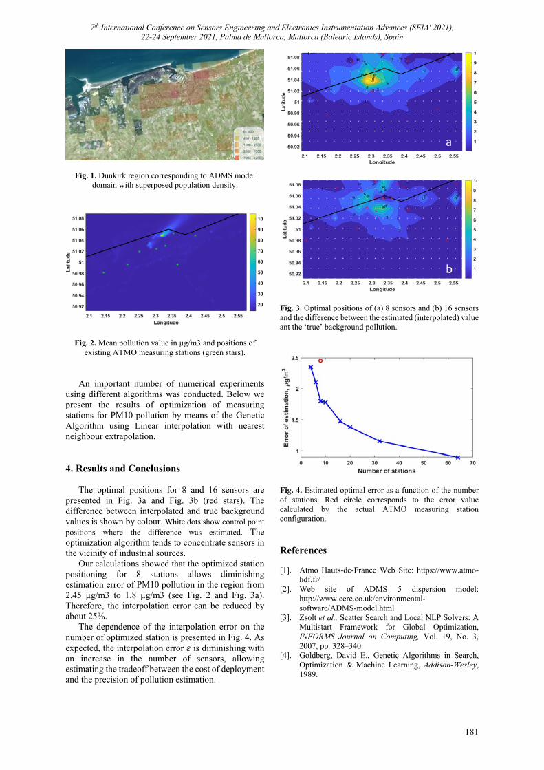
7th International Conference on Sensors Engineering and Electronics Instrumentation Advances (SEIA' 2021), 22-24 September 2021, Palma de Mallorca, Mallorca (Balearic Islands), Spain
181
Fig. 1. Dunkirk region corresponding to ADMS model domain with superposed population density.
Fig. 2. Mean pollution value in µg/m3 and positions of existing ATMO measuring stations (green stars).
An important number of numerical experiments using different algorithms was conducted. Below we present the results of optimization of measuring stations for PM10 pollution by means of the Genetic Algorithm using Linear interpolation with nearest neighbour extrapolation.
4. Results and Conclusions The optimal positions for 8 and 16 sensors are
presented in Fig. 3a and Fig. 3b (red stars). The difference between interpolated and true background values is shown by colour. White dots show control point positions where the difference was estimated. The optimization algorithm tends to concentrate sensors in the vicinity of industrial sources.
Our calculations showed that the optimized station positioning for 8 stations allows diminishing estimation error of PM10 pollution in the region from 2.45 µg/m3 to 1.8 µg/m3 (see Fig. 2 and Fig. 3a). Therefore, the interpolation error can be reduced by about 25%.
The dependence of the interpolation error on the number of optimized station is presented in Fig. 4. As expected, the interpolation error 𝜀 is diminishing with an increase in the number of sensors, allowing estimating the tradeoff between the cost of deployment and the precision of pollution estimation.
Fig. 3. Optimal positions of (a) 8 sensors and (b) 16 sensors and the difference between the estimated (interpolated) value ant the ‘true’ background pollution.
Fig. 4. Estimated optimal error as a function of the number of stations. Red circle corresponds to the error value calculated by the actual ATMO measuring station configuration.
References [1]. Atmo Hauts-de-France Web Site: https://www.atmo-
hdf.fr/ [2]. Web site of ADMS 5 dispersion model:
http://www.cerc.co.uk/environmental-software/ADMS-model.html
[3]. Zsolt et al., Scatter Search and Local NLP Solvers: A Multistart Framework for Global Optimization, INFORMS Journal on Computing, Vol. 19, No. 3, 2007, pp. 328–340.
[4]. Goldberg, David E., Genetic Algorithms in Search, Optimization & Machine Learning, Addison-Wesley, 1989.

7th International Conference on Sensors Engineering and Electronics Instrumentation Advances (SEIA' 2021), 22-24 September 2021, Palma de Mallorca, Mallorca (Balearic Islands), Spain
182
[5]. Sastry K., Goldberg D. E., Kendall G., Genetic Algorithms, in Search Methodologies, Burke E., Kendall G. (Eds.), Springer, Boston, USA, 2014.
[6]. Kennedy, J., and R. Eberhart, Particle Swarm Optimization, in Proceedings of the IEEE
International Conference on Neural Networks, Perth, Australia, 1995, pp. 1942–1945.
[7]. Merkle D., Middendorf M., Swarm Intelligence, in Search Methodologies, Burke E., Kendall G. (Eds.), Springer, Boston, USA, 2014.

7th International Conference on Sensors Engineering and Electronics Instrumentation Advances (SEIA' 2021), 22-24 September 2021, Palma de Mallorca, Mallorca (Balearic Islands), Spain
183
(063)
Cognitive Measurements and Fuzzy Reasoning in Monitoring and Decision Support System for Bridge Maintenance
Sergei Koltunov 1,2 and Maria Koroleva 1,2
1 Sirius University of Science and Technology, Olympiisky Ave 1, 354340, Sochi, Russia 2 Bauman Moscow State Technical University, 2-nd Baumanskaya 5b1, 105005, Moscow, Russia
E-mails: [email protected], [email protected] Summary: The article discusses the development of a monitoring and decision support system for the operation of the bridge. Central to this system is the fuzzy reasoning module developed by Matlab and based on the Sugeno algorithm, with a hybrid neuro-fuzzy network as a core. This model provides recommendations on the restriction of traffic on the bridge depending on the meteorological parameters of the environment and the state of the bridge construction, as well as recommendations for the bridge maintenance under circumstancies of ice drift. The article describes meteorological and structural parameters, their measurement and data processing methods by cognitive measurements, as well as methods for constructing a fuzzy inference scheme. Keywords: Monitoring system, Fuzzy logic, Fuzzy production rules, Cognitive measurement, Hybrid fuzzy-neural network.
1. Introduction
The development of modern rail transport places new demands on the state of the infrastructure, especially on such essential civil works as bridges. A pressing problem is the need for a significant increase in the overall construction volume with a rapidly increasing number of emergency installations. Thus, bridges with metal superstructures built at the turn of the 19th and 20th centuries, which exceeded the standard service life (80 years) by a factor of 1.5, do not allow the passage of trains with existing axle loads without limiting the speed of traffic.
In turn, the introduction into service of trains with higher axle loads will cause an increase in tension in bridge superstructures by a factor of 1.5-1.8 compared to existing ones. This could lead to an increase in fatigue damage in the superstructures calculated according to the standards of 1907, 1925 and 1931, and a significant reduction in their useful life [1, 2].
Thus, the need for advanced systems for monitoring bridge structures that ensure the safety of passenger and freight transport becomes evident.
The problem of monitoring is complex and includes the following tasks: measuring the key characteristics of complex technical objects and their physical and technical environment, and interpreting the results of measurements; analysis of the processes in the monitored objects and diagnosis of their current conditions, decision related to the operation of the bridge or its maintenance, based on acquired knowledge [3].
Therefore, the main element of scientific novelty of the work is the development of a model of a system of monitoring of a complex technical object as an intellectual environment.
The practical value of the work is to improve the effectiveness of monitoring processes by developing an extended definition of a complex monitoring
problem, Developing the architecture of an automated monitoring system as an intellectual environment and constructing a distributed perception system based on cognitive information and measurement devices.
An example of a practically implemented automated monitoring system is the Russian Island Bridge Monitoring System [10]. One of its components is the Integrated Security System (ISS). It protects the entire infrastructure of the bridge from external influences that could lead to the breakdown of its elements or to emergency situations.
However, according to this article, the system has a significant disadvantage: it is poorly represented by network technologies for obtaining information on the status of the bridge and does not use intellectual technologies.
2. Ice Drift Factor in the Monitoring of the Technical Condition of the Bridge
The vast majority of rivers, lakes and seas on the
territory of the Russian Federation freeze over. From time to time, there is ice drift on them.
At the temperature of the air below zero in the autumn, ice crystals first appear on the surface of the water, which ripen to form «tallow». Simultaneously, in places of weak currents, in creeks and near the coast, ice begins to freeze, forming tooks, or fast ice. Floating "tallow" and fragments of fast ice, surfaced bottom ice, freezing into ice floes, create a continuous ice drift. With a further decrease in temperature, these ice floes freeze up, and freeze-up sets in. The moments of the appearance of "tallow ", tooks, autumn ice drift and freeze-up are usually recorded at each bridge longer than 50 m.
In the spring, due to snow melting and a rise of the water level in a river still covered with solid ice, ice movements often take place. These movements, due to
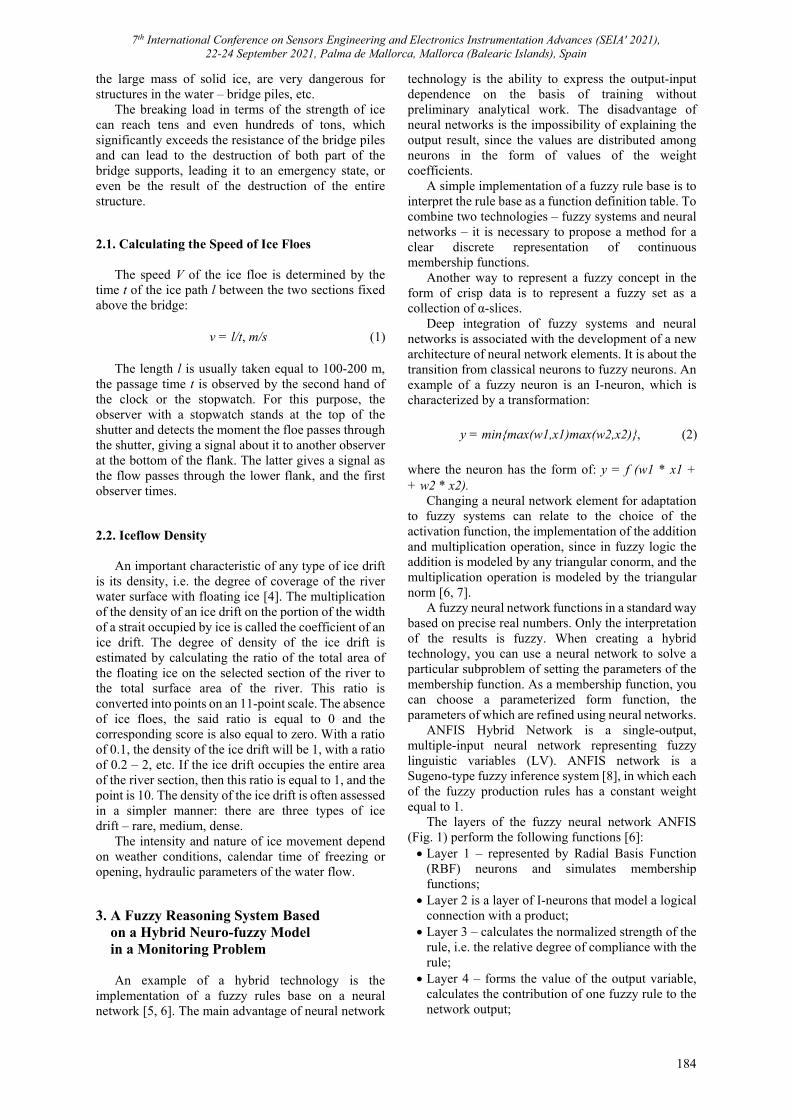
7th International Conference on Sensors Engineering and Electronics Instrumentation Advances (SEIA' 2021), 22-24 September 2021, Palma de Mallorca, Mallorca (Balearic Islands), Spain
184
the large mass of solid ice, are very dangerous for structures in the water – bridge piles, etc.
The breaking load in terms of the strength of ice can reach tens and even hundreds of tons, which significantly exceeds the resistance of the bridge piles and can lead to the destruction of both part of the bridge supports, leading it to an emergency state, or even be the result of the destruction of the entire structure. 2.1. Calculating the Speed of Ice Floes
The speed V of the ice floe is determined by the time t of the ice path l between the two sections fixed above the bridge:
v = l/t, m/s (1) The length l is usually taken equal to 100-200 m,
the passage time t is observed by the second hand of the clock or the stopwatch. For this purpose, the observer with a stopwatch stands at the top of the shutter and detects the moment the floe passes through the shutter, giving a signal about it to another observer at the bottom of the flank. The latter gives a signal as the flow passes through the lower flank, and the first observer times. 2.2. Iceflow Density
An important characteristic of any type of ice drift is its density, i.e. the degree of coverage of the river water surface with floating ice [4]. The multiplication of the density of an ice drift on the portion of the width of a strait occupied by ice is called the coefficient of an ice drift. The degree of density of the ice drift is estimated by calculating the ratio of the total area of the floating ice on the selected section of the river to the total surface area of the river. This ratio is converted into points on an 11-point scale. The absence of ice floes, the said ratio is equal to 0 and the corresponding score is also equal to zero. With a ratio of 0.1, the density of the ice drift will be 1, with a ratio of 0.2 – 2, etc. If the ice drift occupies the entire area of the river section, then this ratio is equal to 1, and the point is 10. The density of the ice drift is often assessed in a simpler manner: there are three types of ice drift – rare, medium, dense.
The intensity and nature of ice movement depend on weather conditions, calendar time of freezing or opening, hydraulic parameters of the water flow. 3. A Fuzzy Reasoning System Based on a Hybrid Neuro-fuzzy Model in a Monitoring Problem
An example of a hybrid technology is the implementation of a fuzzy rules base on a neural network [5, 6]. The main advantage of neural network
technology is the ability to express the output-input dependence on the basis of training without preliminary analytical work. The disadvantage of neural networks is the impossibility of explaining the output result, since the values are distributed among neurons in the form of values of the weight coefficients.
A simple implementation of a fuzzy rule base is to interpret the rule base as a function definition table. To combine two technologies – fuzzy systems and neural networks – it is necessary to propose a method for a clear discrete representation of continuous membership functions.
Another way to represent a fuzzy concept in the form of crisp data is to represent a fuzzy set as a collection of α-slices.
Deep integration of fuzzy systems and neural networks is associated with the development of a new architecture of neural network elements. It is about the transition from classical neurons to fuzzy neurons. An example of a fuzzy neuron is an I-neuron, which is characterized by a transformation:
y = minmax(w1,x1)max(w2,x2), (2)
where the neuron has the form of: y = f (w1 * x1 + + w2 * x2).
Changing a neural network element for adaptation to fuzzy systems can relate to the choice of the activation function, the implementation of the addition and multiplication operation, since in fuzzy logic the addition is modeled by any triangular conorm, and the multiplication operation is modeled by the triangular norm [6, 7].
A fuzzy neural network functions in a standard way based on precise real numbers. Only the interpretation of the results is fuzzy. When creating a hybrid technology, you can use a neural network to solve a particular subproblem of setting the parameters of the membership function. As a membership function, you can choose a parameterized form function, the parameters of which are refined using neural networks.
ANFIS Hybrid Network is a single-output, multiple-input neural network representing fuzzy linguistic variables (LV). ANFIS network is a Sugeno-type fuzzy inference system [8], in which each of the fuzzy production rules has a constant weight equal to 1.
The layers of the fuzzy neural network ANFIS (Fig. 1) perform the following functions [6]: Layer 1 – represented by Radial Basis Function
(RBF) neurons and simulates membership functions;
Layer 2 is a layer of I-neurons that model a logical connection with a product;
Layer 3 – calculates the normalized strength of the rule, i.e. the relative degree of compliance with the rule;
Layer 4 – forms the value of the output variable, calculates the contribution of one fuzzy rule to the network output;
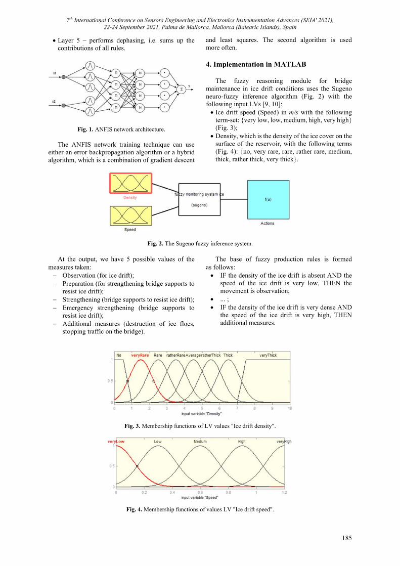
7th International Conference on Sensors Engineering and Electronics Instrumentation Advances (SEIA' 2021), 22-24 September 2021, Palma de Mallorca, Mallorca (Balearic Islands), Spain
185
Layer 5 – performs dephasing, i.e. sums up the contributions of all rules.
Fig. 1. ANFIS network architecture.
The ANFIS network training technique can use either an error backpropagation algorithm or a hybrid algorithm, which is a combination of gradient descent
and least squares. The second algorithm is used more often. 4. Implementation in MATLAB
The fuzzy reasoning module for bridge maintenance in ice drift conditions uses the Sugeno neuro-fuzzy inference algorithm (Fig. 2) with the following input LVs [9, 10]: Ice drift speed (Speed) in m/s with the following
term-set: very low, low, medium, high, very high (Fig. 3);
Density, which is the density of the ice cover on the surface of the reservoir, with the following terms (Fig. 4): no, very rare, rare, rather rare, medium, thick, rather thick, very thick.
Fig. 2. The Sugeno fuzzy inference system.
At the output, we have 5 possible values of the measures taken: Observation (for ice drift); Preparation (for strengthening bridge supports to
resist ice drift); Strengthening (bridge supports to resist ice drift); Emergency strengthening (bridge supports to
resist ice drift); Additional measures (destruction of ice floes,
stopping traffic on the bridge).
The base of fuzzy production rules is formed as follows: IF the density of the ice drift is absent AND the
speed of the ice drift is very low, THEN the movement is observation;
... ; IF the density of the ice drift is very dense AND
the speed of the ice drift is very high, THEN additional measures.
Fig. 3. Membership functions of LV values "Ice drift density".
Fig. 4. Membership functions of values LV "Ice drift speed".
7th International Conference on Sensors Engineering and Electronics Instrumentation Advances (SEIA' 2021), 22-24 September 2021, Palma de Mallorca, Mallorca (Balearic Islands), Spain
186
In total, 40 fuzzy rules were compiled in the Matlab system using Fuzzy Logic Toolbox, while the number of output variables of the model corresponds to the number of developed production rules.
After the automatic creation of the network, the ANFIS editor obtained the architecture shown on Fig. 5.
Fig. 5. The architecture of the created neuro-fuzzy.
To train the neural fuzzy network, two methods were applied: the backpropagation method and the hybrid optimization method. During the implementation of the model, the Hybrid Optimization Method was used, which showed a much better result.
When using the backpropagation method, it took about 500 epochs to establish an acceptable learning error, while training was not entirely adequate. Here we are faced with a case of retraining a neural network, when, instead of generalizing knowledge from a training sample, the network simply remembers it. At the same time, in the hybrid optimization method, we obtained an adequate result after only 20 learning epochs (Fig. 6).
The training sample looks like this:
4.5 0.6 0.3 5.5 0.6 0.5 6.5 0.6 0.5 7.5 0.6 0.7 0.5 0.9 0.1
The complete training sample contains 40 lines,
each of which contains the first two numbers – the values of the input parameters, the third number – the values of the output parameter. Column #1 – ice drift density, column #2 – ice drift speed, column #3 – measures taken.
The model was tested on a test sample and a comparative analysis of the error on the trained and untrained models (Fig. 7).
A test sample of 23 rows looks like this:
3.7 1.2 0.7 4.0 0.15 0.3 4.3 0.3 0.5 4.6 0.45 0.45 4.9 0.6 0.5
Fig. 6. Learning error when using the hybrid method.
Fig. 7. Testing the trained neuro-fuzzy model.
The output surface of the neuro-fuzzy model is shown in Fig. 8.
Fig. 8. Surface of the output of the neuro-fuzzy model.
The surface of the untrained fuzzy model has a rather pronounced linear character, which does not allow us to accurately determine the required measures for the maintenance of the bridge in the boundary states. The surface of the neuro-fuzzy model turned out to be more flexible. More accurately reflects the degree of measures taken, since there was a great horizontal line near the points of states of measures.
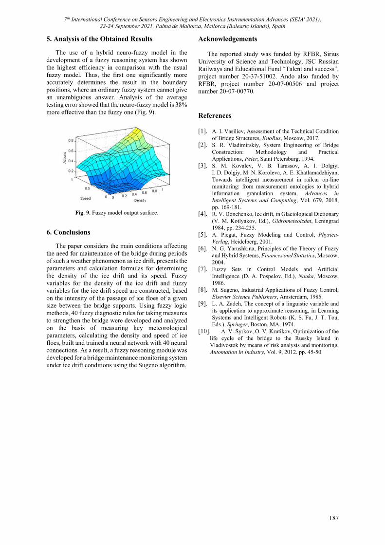
7th International Conference on Sensors Engineering and Electronics Instrumentation Advances (SEIA' 2021), 22-24 September 2021, Palma de Mallorca, Mallorca (Balearic Islands), Spain
187
5. Analysis of the Obtained Results
The use of a hybrid neuro-fuzzy model in the development of a fuzzy reasoning system has shown the highest efficiency in comparison with the usual fuzzy model. Thus, the first one significantly more accurately determines the result in the boundary positions, where an ordinary fuzzy system cannot give an unambiguous answer. Analysis of the average testing error showed that the neuro-fuzzy model is 38% more effective than the fuzzy one (Fig. 9).
Fig. 9. Fuzzy model output surface.
6. Conclusions
The paper considers the main conditions affecting the need for maintenance of the bridge during periods of such a weather phenomenon as ice drift, presents the parameters and calculation formulas for determining the density of the ice drift and its speed. Fuzzy variables for the density of the ice drift and fuzzy variables for the ice drift speed are constructed, based on the intensity of the passage of ice floes of a given size between the bridge supports. Using fuzzy logic methods, 40 fuzzy diagnostic rules for taking measures to strengthen the bridge were developed and analyzed on the basis of measuring key meteorological parameters, calculating the density and speed of ice floes, built and trained a neural network with 40 neural connections. As a result, a fuzzy reasoning module was developed for a bridge maintenance monitoring system under ice drift conditions using the Sugeno algorithm.
Acknowledgements
The reported study was funded by RFBR, Sirius University of Science and Technology, JSC Russian Railways and Educational Fund “Talent and success”, project number 20-37-51002. Ando also funded by RFBR, project number 20-07-00506 and project number 20-07-00770. References [1]. A. I. Vasiliev, Assessment of the Technical Condition
of Bridge Structures, KnoRus, Moscow, 2017. [2]. S. R. Vladimirskiy, System Engineering of Bridge
Construction: Methodology and Practical Applications, Peter, Saint Petersburg, 1994.
[3]. S. M. Kovalev, V. B. Tarassov, A. I. Dolgiy, I. D. Dolgiy, M. N. Koroleva, A. E. Khatlamadzhiyan, Towards intelligent measurement in railcar on-line monitoring: from measurement ontologies to hybrid information granulation system, Advances in Intelligent Systems and Computing, Vol. 679, 2018, pp. 169-181.
[4]. R. V. Donchenko, Ice drift, in Glaciological Dictionary (V. M. Kotlyakov, Ed.), Gidrometeoizdat, Leningrad 1984, pp. 234-235.
[5]. A. Piegat, Fuzzy Modeling and Control, Physica-Verlag, Heidelberg, 2001.
[6]. N. G. Yarushkina, Principles of the Theory of Fuzzy and Hybrid Systems, Finances and Statistics, Moscow, 2004.
[7]. Fuzzy Sets in Control Models and Artificial Intelligence (D. A. Pospelov, Ed.), Nauka, Moscow, 1986.
[8]. M. Sugeno, Industrial Applications of Fuzzy Control, Elsevier Science Publishers, Amsterdam, 1985.
[9]. L. A. Zadeh, The concept of a linguistic variable and its application to approximate reasoning, in Learning Systems and Intelligent Robots (K. S. Fu, J. T. Tou, Eds.), Springer, Boston, MA, 1974.
[10]. A. V. Syrkov, O. V. Krutikov, Optimization of the life cycle of the bridge to the Russky Island in Vladivostok by means of risk analysis and monitoring, Automation in Industry, Vol. 9, 2012. pp. 45-50.
7th International Conference on Sensors Engineering and Electronics Instrumentation Advances (SEIA' 2021), 22-24 September 2021, Palma de Mallorca, Mallorca (Balearic Islands), Spain
188
(064)
Soft Sensors on the Basis of Bayesian Intelligent Technologies
S. V. Prokopchina Financial University under the Government of the Russian Federation,
49 Leningradsky Prospekt, 125993, Moscow, Russia E-mail: [email protected]
Summary: The relevance of creating soft sensors for a wide range of practical tasks is confirmed by examples of their use in various fields of activity.
The most important issue in this case is the development of an effective methodology for their creation, focused on the functioning of sensors in real practical conditions, most often accompanied by significant information uncertainty.
The article notes that not enough attention is paid to the development of the theory of the construction of electronic sensors, as well as their metrological support by developers.
As a methodology for creating soft sensors for conditions of information uncertainty, the article proposes a methodology of the regularizing Bayesian approach and technologies based on it. The effectiveness of the proposed approach is confirmed by the practice of its application for the creation of soft sensors, examples of which are given in the article. Keywords: Soft sensors, Regularizing Bayesian approach, Metrology.
1. Introduction
The intellectualization of measuring methods and measuring instruments, which is being intensively implemented at the present time, has led to the active use of so-called "soft" approaches, methods and tools in measuring practice.
One such direction is the direction. Related to the development of concepts and methods for soft sensors.
According to the definition given in [2], «A soft sensor or virtual sensor is a common name for software in which several measurements are processed together. Usually, soft sensors are based on control theory and are also called a state observer."
As noted in [2], soft sensors are especially useful for data integration, where measurements of various characteristics are combined, for example, for monitoring equipment, for decision-making and management,
In modern developments, artificial intelligence methods and tools are used to create soft sensors, such as neural network technologies, systems based on the theory of fuzzy sets, Kalman filters.
However, at present, there is quite a little work on the creation of methodological foundations for the construction of soft sensors, as well as on their metrological support. These gaps are partially eliminated by implementing the following methodology.
In this article, a methodology and technologies based on the regularizing Bayesian approach (RBA). A distinctive feature of this methodology is its focus on the conditions of information uncertainty. This methodological basis served as the basis for the development of a number of applied systems for monitoring and managing complex complexes in energy, industrial, socio-economic applications.
2. Methodological Aspects of Creating Soft Sensors Based on RBA
One of the most important issues when creating soft sensors is the choice of a methodology for combining the readings of several devices into one integrated assessment of the state of the characteristics of the measuring object.
At the same time, the basic principles of measurement should be implemented: transparency, traceability, interpretability, metrological validity of integrated estimates.
It is important to note that the measurements of the characteristics of complex systems take place under conditions of considerable uncertainty.
In this article, the methodology of the regularizing Bayesian approach (RBA) and technologies based on it (BIT) is proposed as a methodology for convolution of measurement results of various sensors.
These technologies are considered in detail in the works [1, 3].
The convolution methodology is based on a modified Bayesian formula that allows implementing a Bayesian convolution under conditions of uncertainty or lack of information about the components of the Bayesian formula, in particular, about the form of the distribution law of the initial value, the penalty function, the likelihood function, the a priori probability of the measured parameters.
The form of the modified Bayesian formula for uncertainty conditions is represented by the following analytical dependence:
𝑃 ℎ , 𝑌
ℎ , 𝑌 ,∗ |
∑ ℎ , 𝑌 ℎ ,∗ 𝑌
, (1)
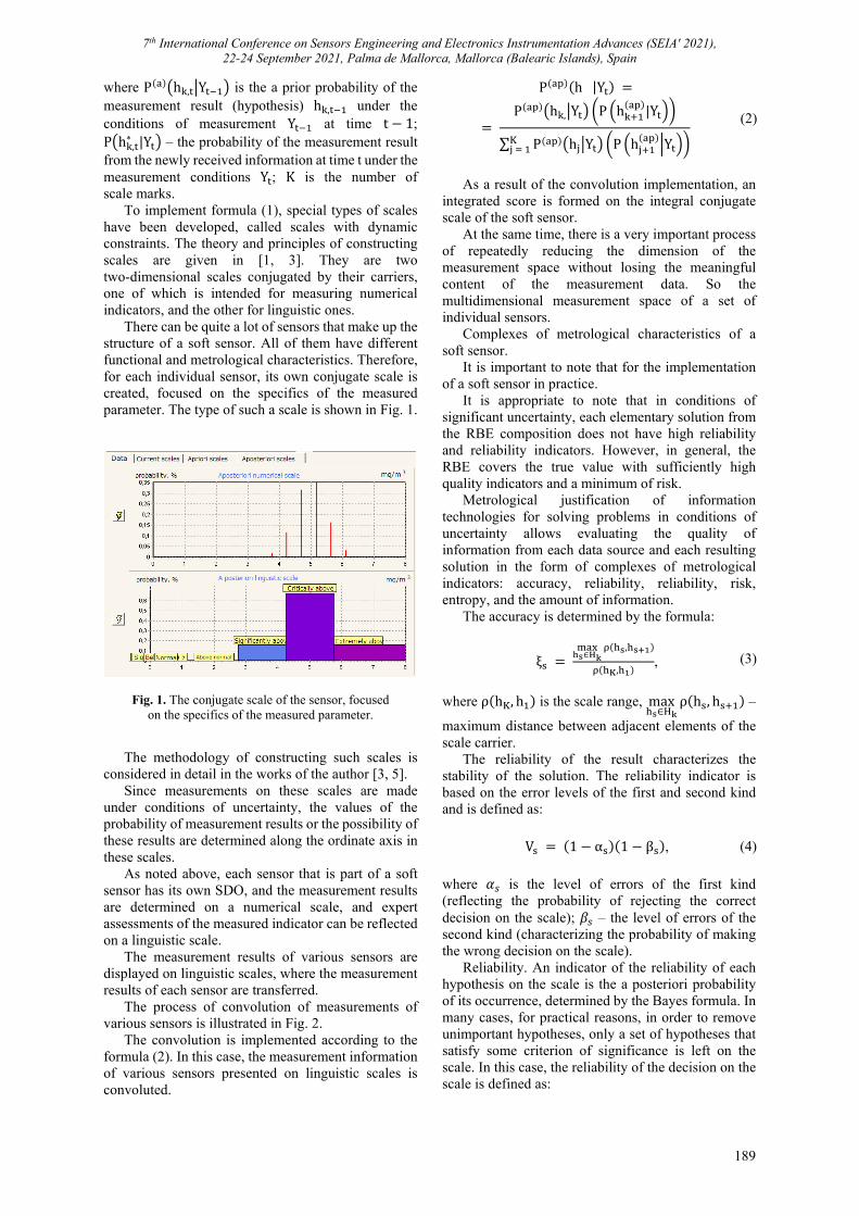
7th International Conference on Sensors Engineering and Electronics Instrumentation Advances (SEIA' 2021), 22-24 September 2021, Palma de Mallorca, Mallorca (Balearic Islands), Spain
189
where P h , Y is the a prior probability of the measurement result (hypothesis) h , under the conditions of measurement Y at time t 1; P h ,
∗ |Y – the probability of the measurement result from the newly received information at time t under the measurement conditions Y ; K is the number of scale marks.
To implement formula (1), special types of scales have been developed, called scales with dynamic constraints. The theory and principles of constructing scales are given in [1, 3]. They are two two-dimensional scales conjugated by their carriers, one of which is intended for measuring numerical indicators, and the other for linguistic ones.
There can be quite a lot of sensors that make up the structure of a soft sensor. All of them have different functional and metrological characteristics. Therefore, for each individual sensor, its own conjugate scale is created, focused on the specifics of the measured parameter. The type of such a scale is shown in Fig. 1.
Fig. 1. The conjugate scale of the sensor, focused on the specifics of the measured parameter.
The methodology of constructing such scales is
considered in detail in the works of the author [3, 5]. Since measurements on these scales are made
under conditions of uncertainty, the values of the probability of measurement results or the possibility of these results are determined along the ordinate axis in these scales.
As noted above, each sensor that is part of a soft sensor has its own SDO, and the measurement results are determined on a numerical scale, and expert assessments of the measured indicator can be reflected on a linguistic scale.
The measurement results of various sensors are displayed on linguistic scales, where the measurement results of each sensor are transferred.
The process of convolution of measurements of various sensors is illustrated in Fig. 2.
The convolution is implemented according to the formula (2). In this case, the measurement information of various sensors presented on linguistic scales is convoluted.
P h |Y
P h , Y P h |Y
∑ P h Y P h Y
(2)
As a result of the convolution implementation, an
integrated score is formed on the integral conjugate scale of the soft sensor.
At the same time, there is a very important process of repeatedly reducing the dimension of the measurement space without losing the meaningful content of the measurement data. So the multidimensional measurement space of a set of individual sensors.
Complexes of metrological characteristics of a soft sensor.
It is important to note that for the implementation of a soft sensor in practice.
It is appropriate to note that in conditions of significant uncertainty, each elementary solution from the RBE composition does not have high reliability and reliability indicators. However, in general, the RBE covers the true value with sufficiently high quality indicators and a minimum of risk.
Metrological justification of information technologies for solving problems in conditions of uncertainty allows evaluating the quality of information from each data source and each resulting solution in the form of complexes of metrological indicators: accuracy, reliability, reliability, risk, entropy, and the amount of information.
The accuracy is determined by the formula:
ξ∈
,
,, (3)
where ρ h , h is the scale range, max
∈ρ h , h –
maximum distance between adjacent elements of the scale carrier.
The reliability of the result characterizes the stability of the solution. The reliability indicator is based on the error levels of the first and second kind and is defined as:
V 1 α 1 β , (4)
where 𝛼 is the level of errors of the first kind (reflecting the probability of rejecting the correct decision on the scale); 𝛽 – the level of errors of the second kind (characterizing the probability of making the wrong decision on the scale).
Reliability. An indicator of the reliability of each hypothesis on the scale is the a posteriori probability of its occurrence, determined by the Bayes formula. In many cases, for practical reasons, in order to remove unimportant hypotheses, only a set of hypotheses that satisfy some criterion of significance is left on the scale. In this case, the reliability of the decision on the scale is defined as:
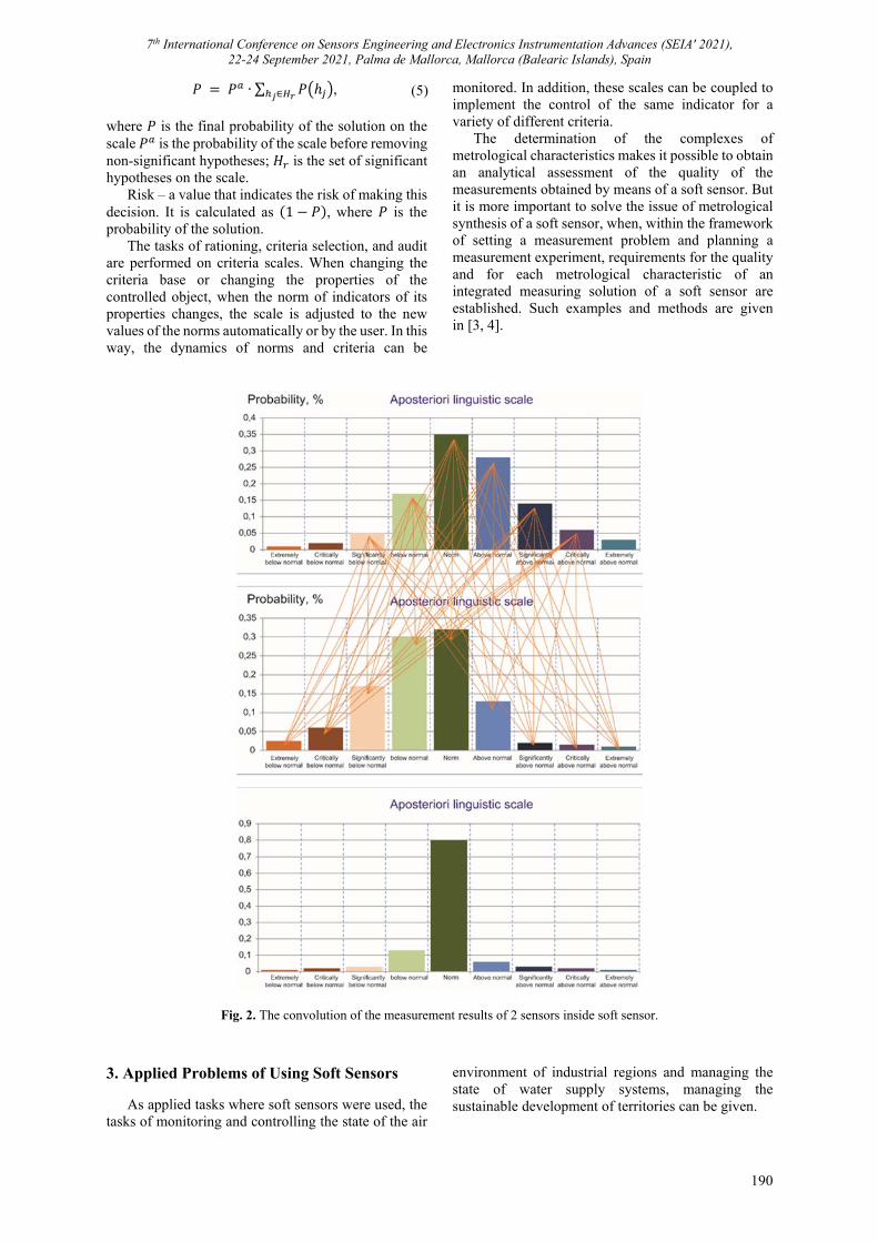
7th International Conference on Sensors Engineering and Electronics Instrumentation Advances (SEIA' 2021), 22-24 September 2021, Palma de Mallorca, Mallorca (Balearic Islands), Spain
190
𝑃 𝑃 ∙ ∑ 𝑃 ℎ∈ , (5)
where 𝑃 is the final probability of the solution on the scale 𝑃 is the probability of the scale before removing non-significant hypotheses; 𝐻 is the set of significant hypotheses on the scale.
Risk – a value that indicates the risk of making this decision. It is calculated as 1 𝑃 , where 𝑃 is the probability of the solution.
The tasks of rationing, criteria selection, and audit are performed on criteria scales. When changing the criteria base or changing the properties of the controlled object, when the norm of indicators of its properties changes, the scale is adjusted to the new values of the norms automatically or by the user. In this way, the dynamics of norms and criteria can be
monitored. In addition, these scales can be coupled to implement the control of the same indicator for a variety of different criteria.
The determination of the complexes of metrological characteristics makes it possible to obtain an analytical assessment of the quality of the measurements obtained by means of a soft sensor. But it is more important to solve the issue of metrological synthesis of a soft sensor, when, within the framework of setting a measurement problem and planning a measurement experiment, requirements for the quality and for each metrological characteristic of an integrated measuring solution of a soft sensor are established. Such examples and methods are given in [3, 4].
Fig. 2. The convolution of the measurement results of 2 sensors inside soft sensor.
3. Applied Problems of Using Soft Sensors
As applied tasks where soft sensors were used, the tasks of monitoring and controlling the state of the air
environment of industrial regions and managing the state of water supply systems, managing the sustainable development of territories can be given.
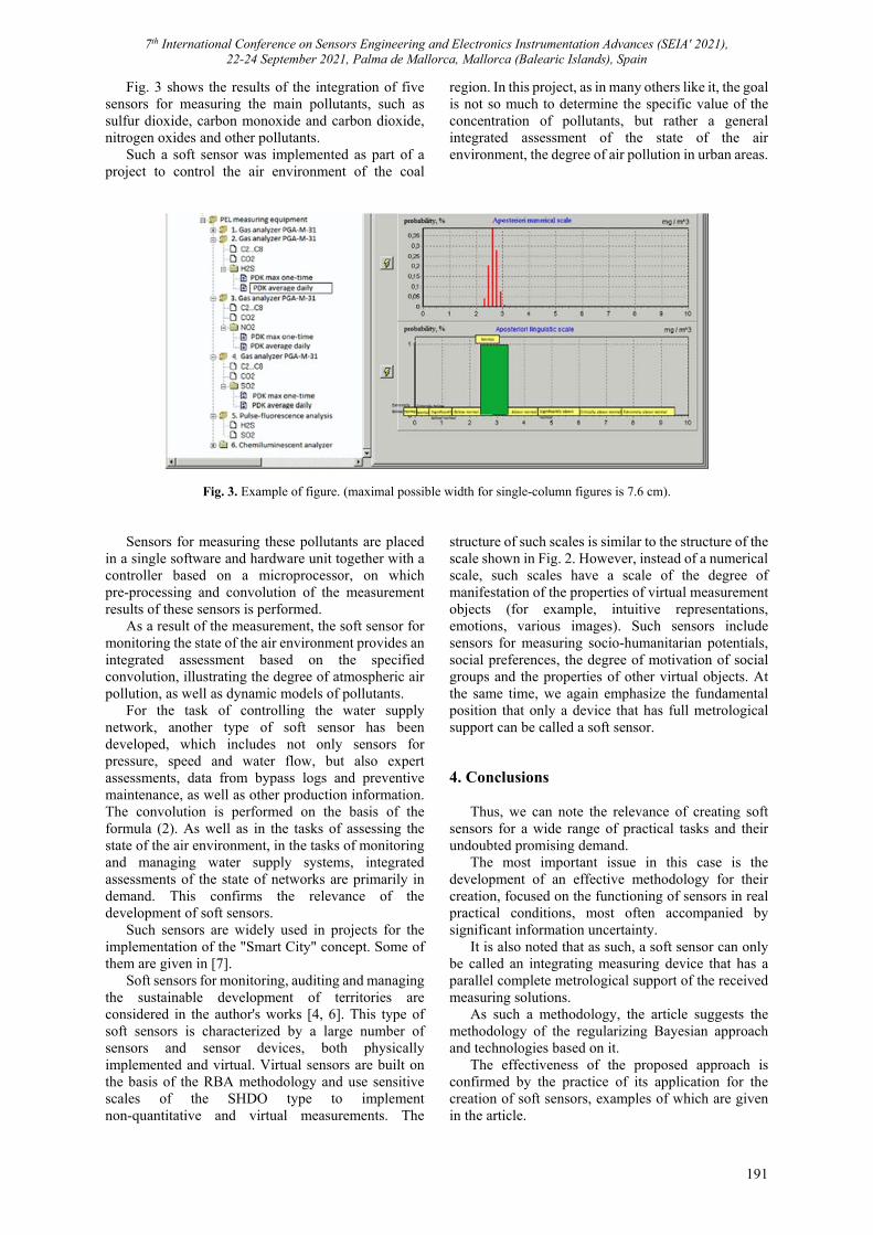
7th International Conference on Sensors Engineering and Electronics Instrumentation Advances (SEIA' 2021), 22-24 September 2021, Palma de Mallorca, Mallorca (Balearic Islands), Spain
191
Fig. 3 shows the results of the integration of five sensors for measuring the main pollutants, such as sulfur dioxide, carbon monoxide and carbon dioxide, nitrogen oxides and other pollutants.
Such a soft sensor was implemented as part of a project to control the air environment of the coal
region. In this project, as in many others like it, the goal is not so much to determine the specific value of the concentration of pollutants, but rather a general integrated assessment of the state of the air environment, the degree of air pollution in urban areas.
Fig. 3. Example of figure. (maximal possible width for single-column figures is 7.6 cm). Sensors for measuring these pollutants are placed
in a single software and hardware unit together with a controller based on a microprocessor, on which pre-processing and convolution of the measurement results of these sensors is performed.
As a result of the measurement, the soft sensor for monitoring the state of the air environment provides an integrated assessment based on the specified convolution, illustrating the degree of atmospheric air pollution, as well as dynamic models of pollutants.
For the task of controlling the water supply network, another type of soft sensor has been developed, which includes not only sensors for pressure, speed and water flow, but also expert assessments, data from bypass logs and preventive maintenance, as well as other production information. The convolution is performed on the basis of the formula (2). As well as in the tasks of assessing the state of the air environment, in the tasks of monitoring and managing water supply systems, integrated assessments of the state of networks are primarily in demand. This confirms the relevance of the development of soft sensors.
Such sensors are widely used in projects for the implementation of the "Smart City" concept. Some of them are given in [7].
Soft sensors for monitoring, auditing and managing the sustainable development of territories are considered in the author's works [4, 6]. This type of soft sensors is characterized by a large number of sensors and sensor devices, both physically implemented and virtual. Virtual sensors are built on the basis of the RBA methodology and use sensitive scales of the SHDO type to implement non-quantitative and virtual measurements. The
structure of such scales is similar to the structure of the scale shown in Fig. 2. However, instead of a numerical scale, such scales have a scale of the degree of manifestation of the properties of virtual measurement objects (for example, intuitive representations, emotions, various images). Such sensors include sensors for measuring socio-humanitarian potentials, social preferences, the degree of motivation of social groups and the properties of other virtual objects. At the same time, we again emphasize the fundamental position that only a device that has full metrological support can be called a soft sensor. 4. Conclusions
Thus, we can note the relevance of creating soft sensors for a wide range of practical tasks and their undoubted promising demand.
The most important issue in this case is the development of an effective methodology for their creation, focused on the functioning of sensors in real practical conditions, most often accompanied by significant information uncertainty.
It is also noted that as such, a soft sensor can only be called an integrating measuring device that has a parallel complete metrological support of the received measuring solutions.
As such a methodology, the article suggests the methodology of the regularizing Bayesian approach and technologies based on it.
The effectiveness of the proposed approach is confirmed by the practice of its application for the creation of soft sensors, examples of which are given in the article.

7th International Conference on Sensors Engineering and Electronics Instrumentation Advances (SEIA' 2021), 22-24 September 2021, Palma de Mallorca, Mallorca (Balearic Islands), Spain
192
References [1]. S. V. Prokopchina, Soft measurements: methodology
and application in scientific, technical and socio-economic problems of the digital economy, in Soft Measurements and Calculations, Publishing House: Limited Liability Company, Publishing House Scientific Library, Vol. 9, 2018, pp. 4-33.
[2]. https://hrwiki.ru/ [3]. S. Prokopchina, New trends in measurement theory:
Bayesian intelligent measurement and its application in the digital economy, CEUR Workshop Proceedings, Vol. 2782, 2020, pp. 80-88.
[4]. S. V. Prokopchina, Metrological aspects of intelligent measurements, Dep. v VINITI, Vol. 172, 1992, Issue 2032-92, pp. 90-101.
[5]. S. V. Prokopchina, Methodological foundations of scaling in modern measurement theory. Classification of measurement scales and their application under uncertainty based on Bayesian intelligent technologies, Journal of Physics: Conference Series, Vol. 1703, 2020, Issue 1, 012003.
[6]. S. V. Prokopchina, G. A. Shcherbakov, Yu. V. Efimov, Modeling of Economic Systems in Conditions of Uncertainty: A Textbook-Workshop (G. A. Shcherbakov, Ed.), Publishing House Scientific Library, 2018.
[7]. S. V. Prokopchina, Methods for implementing the concept of “Smart City” based on Bayesian intelligent technologies, Journal of Physics: Conference Series, Vol. 1703, Issue 1, 2020, 012018.
7th International Conference on Sensors Engineering and Electronics Instrumentation Advances (SEIA' 2021), 22-24 September 2021, Palma de Mallorca, Mallorca (Balearic Islands), Spain
193
(065)
Methods and Measurement Tools Based on Smart Sensors
S. S. Sergeev 1, M. D. Krysanov 1 and S. V. Prokopchina 2
1 Ltd. “TECHNOAS-SK” 2 Financial University under the Government of the Russian Federation,
49 Leningradsky Prospekt, 125993, Moscow, Russia E-mails: [email protected], [email protected]
Summary: In the article various types of smart sensors are considered. The architecture and methodological aspects are considered. The practical examples of application of such type of sensors are given. Keywords: Smart sensors, Measurements.
1. Introduction
The active development of artificial intelligence systems and Big Data processing places new requirements on primary sensors. This is primarily operational communication with processing systems, data reliability, their traceability over time and comparability with each other. In this regard, autonomous sensors, so-called smart sensors or smart probes, are being created in many countries. They usually do not have a screen, often do not process the signal, but transmit the primary data to the receiving device, where the main processing takes place.
A cell phone can act as a receiving device. Such probes are created by the leading manufacturers of sensors in the world, in particular by the company “Dough” from Germany. In Russia, such sensors were created by the company “TECHNO-AS”. One of the main activities of which is the development and production of portable devices for monitoring temperature, humidity, pressure and other physical parameters.
2. Methodology of Measurements by Means of Smart Sensors
The principle of operation of smart probes is based on the conversion of electrical signals entering the electronic unit from primary converters (sensors), and the transmission of calculated values via the BLE (Bluetooth Low Energy) radio protocol with a carrier frequency of 2.4 GHz to a device with the ThermoMonitor program installed on the Android operating system. The ThermoMonitor program processes the received data and displays it on the display of the Android device.
The principle of temperature measurement is based on the dependence of the electrical resistance of the thermal resistance sensor on the measured temperature, or on the dependence of the electrical voltage of the thermocouple sensor on the measured temperature.
The measurement of relative humidity is based on the change in the electrical capacitance of the sensors depending on the permittivity of the dielectric used as a moisture-sensitive layer.
The principle of atmospheric pressure measurement is based on piezoresistive pressure conversion.
Smart probes are portable multifunctional microprocessor devices and consist of an electronic unit with autonomous power supply, located in a plastic case, and measuring sensors for various purposes and designs. Resistance thermal converters (TS) with NSH according to GOST 6651-2009 thermoelectric converters (TP) with NSH according to GOST R 8.585-2001 are used as primary temperature converters in measuring probes, capacitive humidity sensors are used as primary humidity converters. The electronic unit consists of a microprocessor, an analog-to-digital converter, a lithium-polymer battery, a micro-USB connector for charging, a clock control button, an LED indicator, as well as a flash memory, in some modifications, for using a smart probe as a measuring recorder.
The developed and manufactured smart probes are made of two types: portable and stationary.
Smart probes are available in the following modifications.
Probe type: Smart submersible probe (NWPG); Smart submersible reinforced probe (NWPG); Smart air probe (SRV); Smart probe air high-precision (CVV); Smart probe surface (SZPV); Smart probe surface high-precision (SZPVT); Smart surface high-temperature probe (SZPVV); Smart surface magnetic probe (SZPM); Smart probe for connecting an external
thermoelectric converter (CVT); Smart probe of relative humidity and temperature
(CVL); Smart probe of atmospheric pressure (SZDA); Smart air wall-mounted probe (SSVN); Smart relative humidity and temperature
wall-mounted probe (SSVLN);
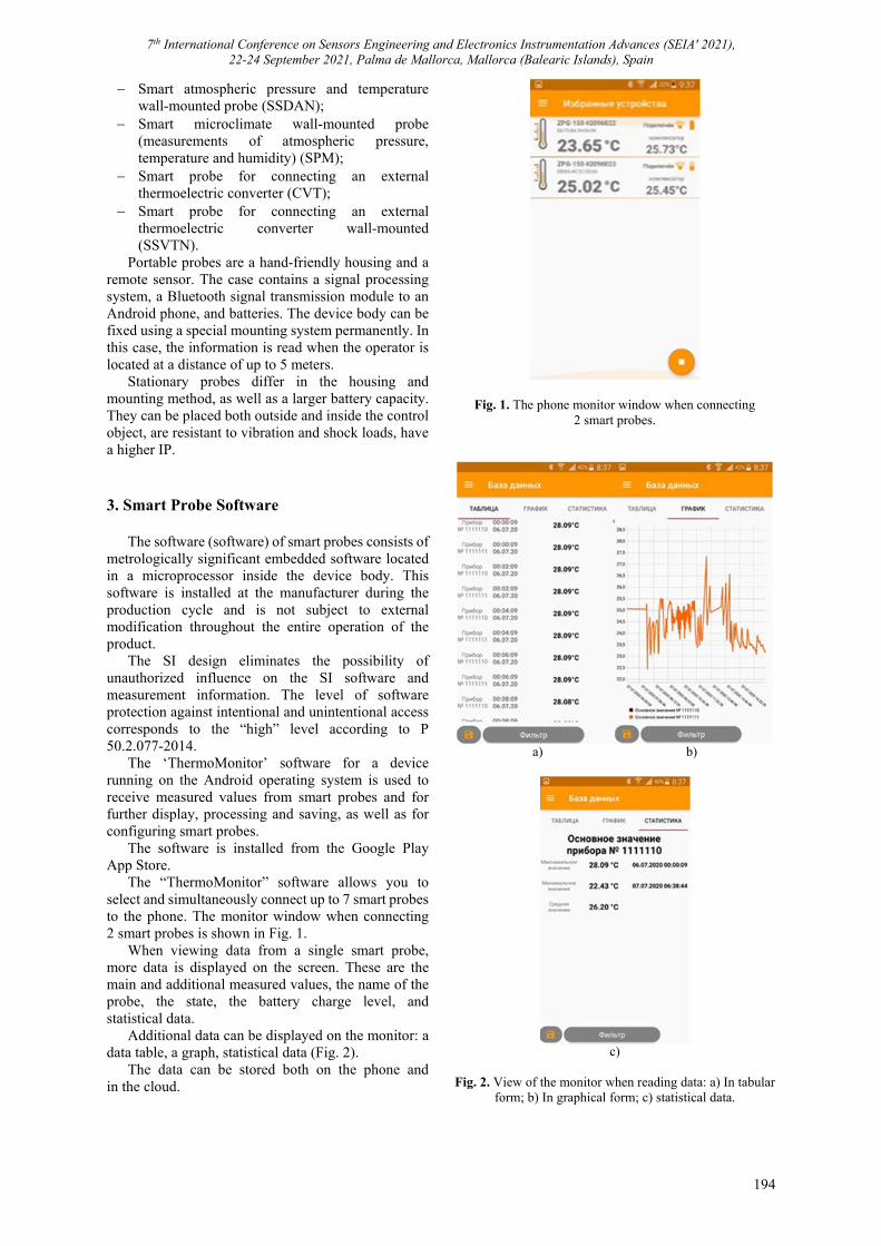
7th International Conference on Sensors Engineering and Electronics Instrumentation Advances (SEIA' 2021), 22-24 September 2021, Palma de Mallorca, Mallorca (Balearic Islands), Spain
194
Smart atmospheric pressure and temperature wall-mounted probe (SSDAN);
Smart microclimate wall-mounted probe (measurements of atmospheric pressure, temperature and humidity) (SPM);
Smart probe for connecting an external thermoelectric converter (CVT);
Smart probe for connecting an external thermoelectric converter wall-mounted (SSVTN).
Portable probes are a hand-friendly housing and a remote sensor. The case contains a signal processing system, a Bluetooth signal transmission module to an Android phone, and batteries. The device body can be fixed using a special mounting system permanently. In this case, the information is read when the operator is located at a distance of up to 5 meters.
Stationary probes differ in the housing and mounting method, as well as a larger battery capacity. They can be placed both outside and inside the control object, are resistant to vibration and shock loads, have a higher IP. 3. Smart Probe Software
The software (software) of smart probes consists of metrologically significant embedded software located in a microprocessor inside the device body. This software is installed at the manufacturer during the production cycle and is not subject to external modification throughout the entire operation of the product.
The SI design eliminates the possibility of unauthorized influence on the SI software and measurement information. The level of software protection against intentional and unintentional access corresponds to the “high” level according to P 50.2.077-2014.
The ‘ThermoMonitor’ software for a device running on the Android operating system is used to receive measured values from smart probes and for further display, processing and saving, as well as for configuring smart probes.
The software is installed from the Google Play App Store.
The “ThermoMonitor” software allows you to select and simultaneously connect up to 7 smart probes to the phone. The monitor window when connecting 2 smart probes is shown in Fig. 1.
When viewing data from a single smart probe, more data is displayed on the screen. These are the main and additional measured values, the name of the probe, the state, the battery charge level, and statistical data.
Additional data can be displayed on the monitor: a data table, a graph, statistical data (Fig. 2).
The data can be stored both on the phone and in the cloud.
Fig. 1. The phone monitor window when connecting 2 smart probes.
a) b)
c)
Fig. 2. View of the monitor when reading data: a) In tabular
form; b) In graphical form; c) statistical data.

7th International Conference on Sensors Engineering and Electronics Instrumentation Advances (SEIA' 2021), 22-24 September 2021, Palma de Mallorca, Mallorca (Balearic Islands), Spain
195
4. Conclusions
The smart probes produced have found wide application in many industries.
In the food industry for temperature control of liquids, dough, products during storage and heat treatment.
In construction, when controlling the temperature of solutions and thermal insulation properties of materials.
Such sensors are also used in greenhouses. In addition, smart probes can be part of
soft sensors.
References [1]. S. Prokopchina, New trends in measurement theory:
Bayesian intelligent measurement and its application in the digital economy, CEUR Workshop Proceedings, Vol. 2782, 2020, pp. 80-88.
7th International Conference on Sensors Engineering and Electronics Instrumentation Advances (SEIA' 2021), 22-24 September 2021, Palma de Mallorca, Mallorca (Balearic Islands), Spain
196
(066)
Digital Models of Smart Distributed Measuring Systems
Vladimir V. Alekseev, Natalia V. Orlova and Anastasia A. Minina Saint-Petersburg Electrotechnical University ETU ‘LETI’
Saint-Petersburg, Russia E-mails: [email protected], [email protected], [email protected]
Summary: The issues of the information organization of the measurement control system of a distributed object based on digital models of its main blocks, databases reflecting the functional organization of each block, its input and output values aimed at increasing the accuracy of static and dynamic measurements are considered. Keywords: Digital model, Distributed object, Intelligent measurement system, Control system, Analysis system, Management system.
1. Introduction
The basis of the distributed information and measurement system (IMS) is mobile IMS (MIMS). MIMS are placed on side of such vehicles as car, boat, helicopter, locomotive, etc. Mobile measuring systems have a number of advantages. First of all, this is the possibility of using expensive and high-precision measuring instruments (MI) to control important parameters of an object distributed at many points in space. They have found application in the environmental measurements for monitoring natural and man-made ecosystems, technological ones for monitoring the state of communications in various types of transport systems, security systems, etc.
MIMS carry out measurements of important parameters of an object at the distributed object's specified points. The measurement results are transmitted in real time to the analysis, processing and decision-making (management) system. The structure of the IMS, databases, software is formed based on the object structure [1-3]. Let's consider the issues of the IMS's information organization on the example of a distributed object, which is a railway transport system [2-5].
A multidimensional data space is formed during the IMS operation. Let's consider the features of organizing a large database of control measurements of a mobile measuring system, big data describing a digital model of a controlled object, control system, analysis system and management system.
The digital model reflects all the elements of the object and is an information system that includes a system of digital (software) models: an object (reference object model) containing a variety of states, operating modes, functions of interaction with the environment, etc.; control systems containing protocols, tables, databases of measurement results, etc.; analysis and output systems containing a variety of estimates, states, dynamics, working and current models, metrological support, etc.; management systems containing algorithms for the formation of control actions.
The structure of the digital model fully corresponds to the object structure. The figure shows the structure of a digital twin, which includes digital models of all levels.
2. Digital Model
Digital object model (DOM) is a software implementation of a mathematical model that describes the state and operating modes of an object using systems of equations, logical or statistical functions.
DOM is DM = F DMss1, s2, …, sos, DMdd1, d2, …, dod,where DMs is a set of digital models of the object state sо, sо = fx1, x2,…,xN, ν1, ν 2,…, ν M, xn is informative parameters, ν m is additional parameters, DMd is many digital models of the object's operating modes dо, dо = fv1, v2,…,vN, z1, z2,…,zM, vn is informative parameters, zm is additional parameters.
Digital model of the control system (DMCS) describes the structure of the information and measurement system (IMS), the operation modes of the measuring channels (MC), measured values, required accuracy, sampling intervals, MC schedule, structure of the database of measurement results (protocols, tables, databases), adaptation algorithms to changed situations (intelligent IMS), etc.
DMCS is: DН = F DНss1*, s2*, …, sos*, DНu*u1*, u2, * …, uod*, where DПs is a set of measurement results for the values of the object's state parameters sо, sо* = fx1*, x2*,…,xN*, ν 1*, ν 2*,…, ν M*, xn* is informative, ν m* is additional, DНu* is a set of digital models of the operating modes of measuring instruments (measuring channels) uо*, uо* = fu1*, u2*,…,uN*, z1*, z2*,…,zM*, un* is operation modes of measuring channels (means), zm* are the values of additional influencing variables.
Digital model of the analysis system (DMAS) is a software implementation of algorithmic support reflecting the object's features, all levels of its mathematical description, in order to analyse its
7th International Conference on Sensors Engineering and Electronics Instrumentation Advances (SEIA' 2021), 22-24 September 2021, Palma de Mallorca, Mallorca (Balearic Islands), Spain
197
current state, reliability of the analysed data and make the necessary decisions that ensure achievement of the required results of its functionality (the task to be solved by the object).
DMAS is: DА = F DАs s1*, s2*, …, sos*, DАd u1*, u2, * …, uod*, DM, DH, where DАs is a set of algorithms for analysing the object's state sо* = Аx1*, x2*,…,xN*, ν 1*, ν2*,…, ν M*, DАd is a set of algorithms for analysing the object's operation modes uо*, uо* = Аu1*, u2*,…,uN*, z1*, z2*,…,zM*.
Digital model of the management system (DMMS) is a software implementation of data generation algorithms for all control tools that ensure effective management of an object in all situations that may arise during its life cycles.
DMMS is: DС = F DСss1, s2, …, sos, DСdd1, d2, …, dod DM, DH, DA, where DСs is a set of digital models of functions aimed at forming the control actions sо, sо = f c1, c2,…,cM, x1, x2,…, xN , cm is control signals, xn is informative parameters, DСd is a variety of digital control functions for measuring instruments, operating modes of measuring channels dо, dо = fv1, v2,…,vN, z1, z2,…,zM, vn is operation modes of measuring instruments, zm is additional parameters. 3. Geo-information Technology
Geo-information technology provides a convenient description of the problem under consideration, conducting spatial digital modelling, spatial analysis, presentation of informative parameters in the form of uncorrelated sets (layers) that characterize the state of the controlled object and the means of a distributed measuring system [6].
The developed theoretical foundations for the analysis of the spatially distributed data by the methods of statistical analysis, machine learning and artificial intelligence are aimed at ensuring increased reliability of separating deviations in the controlled object's features and changing the properties of the controlling MIMS, detecting defects and preventing emergency situations.
As a result of the operation of the distributed IMS, a multidimensional database of control measurements is formed (DBCM) Н = h(m,l,d,t), which stores the results of all measurements of all MIMS included in the system for each period of its operation TDi; where: h is a set of control measurement results, m is a MIMS number, l is a number of the distributed object's area (territory, plot, etc.), d is a specified measurement point, t is measurement time.
To solve this problem, let’s select some subsets reflecting the specific nature of the conditions and measurement results. For example, subsets of the measurement results of the m-MIMS; subsets of the measurement results of the defect value at a given distance point by all MIMS; subset of the measurement results of the defect value at a given d point of the m-MIMS during the analysis from TD1 to TDТ, etc.
By conducting a statistical analysis of the measurement results of selected subsets (processing large data sets) and establishing statistical features and correlation relationships, algorithms are formed for separating and identifying the causes of changes in the control results: changes in the controlled object's features, changes in the metrological features of MIMS measuring instruments.
The use of digital models ensures timely detection of metrological failure of the measuring instrument and its output for the next calibration. Since modern complex natural and human-made objects require a variety of values (multi-physical measurements), the prevention of metrological failures is an urgent task.
4. Conclusions
Thus, the creation of applied algorithmic support for the IMS, control of complex, distributed in the space natural and human-made objects, based on digital models, provides, based on the analysis of large databases, improvement of the metrological features of the control carried out, expansion of the capabilities of distributed IMS in detecting defects and preventing emergencies for the complex distributed natural and human-made objects. References [1]. V. V. Alekseev, P. G. Korolev, N. I. Kurakina,
N. V. Orlova, Information-measuring and control systems for monitoring the state of distributed technical and natural objects, Instrumentation, Vol. 10, 2009, pp. 28-42.
[2]. V. V. Alekseev, A. M. Boronakhin, P. G. Korolev, N. V. Orlova, On-side information and measurement system for assessing the condition of the railway track. Metrological support, in Proceedings of the XXII International Conference on Soft Computing and Measurements (SCM’19), St. Petersburg. May 23-25, 2019, pp. 21-24.
[3]. V. V. Alekseev, P. G. Korolev, D. Yu. Larionov, M. N. Shilov, The concept of building a system of dynamic monitoring of a railway track, Bulletin of Saint-Petersburg State Electrotechnical University ‘LETI’, Vol. 10, 2014, pp. 45-49.
[4]. V. V. Alekseev, P. G. Korolev, N. V. Orlova, et al., Analysis of metrological features of measuring instruments of a distributed mobile measuring system based on a reference object model, in Proceedings of the XXIII International Conference on Soft Computing and Measurements (SCM’20), St. Petersburg, May 27-29, 2020, pp. 79-82.
[5]. V. V. Alekseev, N. V. Orlova, E. N. Sedunova, Reference model of a linear section of a railway, in Proceedings of the XX International Conference on Soft Calculations and Measurements (SCM’17), Vol. 2, St. Petersburg, May 24-26, 2017, pp. 256-260.
[6]. V. V. Alekseev, P. G. Korolev, N. V. Orlova, A. A. Minina, et al., Assessment of the State of the Railway Track Using Geoinformation Technology, Publishing House of Saint-Petersburg State Electrotechnical University ‘LETI’, 2018.

Related Documents