Segmenting Supply Chain Risk Using E/CTRM Systems Unifying Theory of Commodity Hedging and Arbitrage Segmenting Supply Chain Risk Using E/CTRM Systems Unifying Theory of Commodity

Segmenting Supply Chain Risk Using E/CTRM SystemsUnifying Theory of Commodity Hedging and Arbitrage

WORKING PAPERCirculating Draft: August 5, 2012

Michael “Mack” FrankfurterPartner, IQ3 Solutions Group

[email protected]

The findings, interpretations and conclusions expressed in this working paper are those of the author. Working papers describeresearch in progress and are published to elicit comments and to further debate. Any errors are the responsibility of the author. Thispaper can be downloaded without charge from the Social Science Research Network eLibrary at: http://ssrn.com/abstract=2124559

Copyright © 2012 IQ3 Solutions Group. Michael “Mack” Frankfurter, Author.

Page 2 of 51


Abstract:

The complexity of managing physical and financial risk throughout the commodity production,

processing and merchandising chain presents numerous challenges. To solve this problem commercials are

increasingly turning to Energy and Commodity Transaction Risk Management (E/CTRM) systems. Still, risk

management functionality within these systems is reported as falling short of requirements.1 Our discussion,

in response, provides an economic framework for developing commodity risk policy and evaluation tools. In

doing so, we unify the theory of normal backwardation with theory of storage, macroeconomic general

equilibrium with multiple equilibria and microeconomic agents,2 basis trading with arbitrage strategies, and

the hedging response function with elastic/inelastic supply-demand economics. After establishing axioms and

rules of inference, we investigate the agribusiness supply chain to help illustrate application.

Keywords: Agribusiness, Arbitrage, Backwardation, Basis Risk, Contango, Cost-of-Carry, Equilibrium, ExpectationsTheory, Hedging Pressure, Multiple Equilibria, No-Arbitrage Bounds, Supply Chain, Term Structure, Theory of Storage

JEL Classification: D82, D84, E12, G13, L92, O13, Q11, Q12, Q13, Q14, Q15, Q16

1 Chris Strickland, “Where’s the ‘RM’ in ETRM? (Part One),” Energy Risk Magazine, July 9, 2012.

2 “Multiple equilibria are likely to be present in dynamic models that have a large number of microeconomic agents.”From: Masanao Aoki, New Approaches to Macroeconomic Modeling: Evolutionary Stochastic Dynamics, MultipleEquilibria, and Externalities as Field Effects, Cambridge University Press, February 1998, p. 3.

Page 3 of 51


1. Introduction

The premise that properly functioning futures markets serve a valuable economic purpose is

validated by government policy.3 The primary benefit is that it allows commercial producers, processors

and consumers of an underlying cash commodity to hedge.4 The secondary benefit is that it functions as a

mechanism for transparent price discovery and liquidity which in turn helps to facilitate hedging

activities. Speculation plays a role in such activities, but is not the reason why these markets exist.

It follows that the reallocation of risk affords a reduction in commodity prices because businesses

need not offset adverse price changes with increased margins on products or services. In theory, the

reallocation of risk associated with commodity inputs and outputs results in increased capacity utilization.5

In practice, the complexity of managing risk throughout the commodity production, processing and

merchandising chain presents numerous challenges. To solve this problem commercials are increasingly

turning to Energy and Commodity Transaction Risk Management (E/CTRM) systems.

We initially focus on Spurgin’s (2000) “hedging response function” which provides a behavioral,

yet intuitive, framework for modeling hedging pressure. Next, we review classical commodity theory rooted

in the writings of early 20th century commodity price theorists, and relate these ideas to the concepts of

equilibrium and disequilibrium. This imparts a foundation for exploring “multiple equilibria arbitrage”

which derives from the Sonnenschein-Mantel-Debreu theorem. We then examine basis trading and how

basis risk is segmented into risk factors, and in what way inputs and outputs impact the hedging response

function depending on elastic versus inelastic supply-demand economics. To help illustrate these concepts

we investigate the agribusiness supply chain. Last, we encapsulate these ideas into multi-factor models.

Exordium on E/CTRM Systems

E/CTRM systems refer to a category of applications, technologies and tools that assist companies in

managing business processes associated with commodity asset and resource management. Such processes

involve: commodity production, processing, warehousing and merchandising; transportation planning,

scheduling and logistics; deal capture, trading and risk management; accounting and back office

administration such as clearing and settlement on the financial side, and settlement and invoicing on the

physical side; as well as managing physical and financial regulatory and compliance requirements.

3 “Futures markets play a critically important role in the U.S. economy.” From testimony of Reuben Jeffery III,Chairman U.S. Commodity Futures Trading Commission (CFTC) on November 2, 2005 before the Committee onEnergy and Commerce, United States House of Representatives.

4 By using futures or forward contracts to hedge, a producer, processor or consumer of an underlying asset canestablish a temporary substitute for a cash market transaction that will be realized at a future date.

5 Capacity utilization is a metric used to measure the rate at which potential output levels are being met or used.Capacity utilization rates can also be used to determine the level at which unit costs will increase.

Page 4 of 51

E/CTRM software originally evolved from FERC Order 636,6 which resulted in the wholesale

markets for natural gas in 1992, and FERC Order 888,7 which deregulated the wholesale electric power

markets in North America in 1996. Since that time, E/CTRM systems have expanded its base of usage to

encompass agribusiness and mining, as well as energy industries. The types of companies which use E/CTRM

systems include agribusiness concerns, oil majors and minors, power generators and utilities, petrochemical

and refiners, large industrial end users, and investment banks and hedge funds which trade commodities.

While an in-depth review of E/CTRM technologies is outside the scope of this paper, it is worth

noting that “there is no real standard for what comprises an [E/CTRM] system.”8 This is not surprising

given the variety of physical assets, geographic regions, regulatory regimes, and types of business models

involved in the commodity supply chain. Moreover, while there are standard functionalities integrated into

the major vendor software offerings, dissimilarities within horizontal and vertical market niches makes for

heterogeneous requirements with respect to both functionality and risk management. Indeed, this observation

lends credence to the notion of “multiple equilibria arbitrage” which is presented in this paper.

Exordium on Spot Prices

Commodity pricing theory has a tendency to discuss spot prices as a single representative price.

Reality is far different, and producers, processors and merchandisers who are involved in the cash

commodity markets mostly operate “without any formal guidelines on location, time or size of trading

unit and only informal requirements for reporting transactions (Anderson, Shafer and Haberer, 1996).”9

For example, the reported spot prices for cotton “represent an average price for various qualities

at multiple levels of production, i.e., they may include producer sales, inter-merchant trading, sales to

mills and cooperative pooling.”10 Likewise, the cash markets in the “fed cattle and beef, hog and pork,

and lamb and lamb meat industries” are often dispersed geographically with “on the spot” transactions

occurring vis-à-vis “auction barn sales; video or electronic auction sales; sales through order buyers,

dealers and brokers; and direct trades”.11 The Livestock Marketing Association (LMA), which is the voice

for the livestock marketing industry on legislative and regulatory issues, provides a comprehensive list of

livestock marketing/auctioneers throughout the U.S., reflecting the geographical spread of livestock spot

6 See: http://www.ferc.gov/legal/maj-ord-reg/land-docs/restruct.asp

7 See: http://www.ferc.gov/legal/maj-ord-reg/land-docs/order888.asp

8 CommodityPoint, CTRM Software Sourcebook, UtiliPoint International, May 2011, Ver. 3.

9 Joan Evans and James M. Mahoney, “The Effects of Daily Price Limits on Cotton Futures and Options Trading,”Federal Reserve Bank of New York, Research Paper No. 9627, August 1996, pp 4-5. [Reference: Anderson, Carl G.;Shafer, C. and Haberer, M., “Producer price for cotton qualities vague,” 1996 Beltwide Cotton Conference.]

10 Ibid., Evans and Mahoney (1996), p 5.

11 Grain Inspection, Pacers and Stockyard Administration, U.S. Department of Agriculture, GIPSA Livestock andMeat Marketing Study; Volume 1: Executive Summary and Overview, Final Report. Prepared by RTI International,Health, Social, and Economics Research, RTI Project Number 0209230, January 2007, p ES-1.

Page 5 of 51

price discovery.12/13 According to LMA’s website, local auctions are a vital part of the livestock industry,

serving producers and assuring a fair, competitive cash price through the auction method.

Alternatively, the forward markets for coffee and cocoa have increasingly used so-called “price to

be fixed” (PTBF) contracts where a relevant delivery month of the futures market is chosen as a reference to

determine or fix the price of the physicals contract. This mechanism allows use of the futures market to

hedge price risk, while ensuring delivery of a specific grade at a specific time and location vis-à-vis the

PTBF agreement. The futures position, on the other hand, is never held to delivery, but offset in the market

prior to contract delivery period. Given that grade, quality and location are material factors influencing cash

prices, PTBF is a means for commercial producers and merchandisers of coffee and cocoa to mitigate basis

risk.14 Note: similar instruments exist in other agricultural markets and are called “fixed basis contracts” in

the grain markets, “executable orders” in the sugar trade, and “on-call contracts” for cotton.

Hence, it can be argued that participants in the spot markets, which are generally unobserved and

opaque, establishes pricing in the capacity of “price-takers,” not “price-makers,” notwithstanding assertions

by certain economists to the contrary.15 For example, commercial hedgers such as agribusiness (e.g.,

farmers, elevators, ranchers, stockyards) reference prices in terms of a basis differential, i.e., how much

the cash price is “over” or “under” the referenced futures price.16 A 2010 study by the International Food

Policy Research Institute (IFPRI) supports this hypothesis and concluded that “the futures markets

analyzed generally dominate the spot markets.”17 As with the above discussion on E/CTRM systems, this

observation also lends credence to the notion of “multiple equilibria arbitrage”.18

2. Hedging Response Function19

The version of the hedging response function we present in this paper assumes there are three types

of participants in the futures market for a given commodity: (i) short hedgers; (ii) long hedgers; and (iii)

speculators. Short hedgers are sellers (i.e., producers, processors or merchandisers) who are net long the

underlying cash commodity and use the futures market to fix the sale price. Long hedgers are buyers (i.e.,

consumers, processors or merchandisers) who are net short the underlying cash commodity and use the

market to fix the purchase price. Speculators are traders who enter positions for financial gain.

12 Source: http://www.lmaweb.com See LMA Membership Directory.

13 The South Dakota Department of Agriculture lists forty livestock auction markets in South Dakota in 2007.Source: http://www.livestock.doa.sd.gov/livestock_markets.aspx

14 International Trade Centre, The Coffee Guide, 2002.15 Paul Krguman, “Commodities and speculation: metallic (and other) evidence,” The New York Times, April 20,2009. Also see: Robert Samuelson, “The Fallacy of Blaming Oil ‘Speculators’,” RealClear Politics, May 2, 2012.

16 John McKissick and George Shumaker, “Understanding and Using the Basis,” University of Georgia College ofAgricultural and Environmental Sciences, Bulletin 981/Revised February 1991. [Also see: Baldwin (1986)]

17 M. Hernandez and T. Maximo, “Examining the Dynamic Relationship between Spot and Future Prices of AgriculturalCommodities,” International Food Policy Research Institute, IFPRI Discussion Paper 00988, June 2010.

18 This discussion also suggests difficulty in performing empirical studies that require historical spot price data.

19 Richard Spurgin, “Some Thoughts on the Source of Return to Managed Futures,” Clark University/CISDM, 2000.

Page 6 of 51

The model further assumes that the futures market is symmetric (i.e., a zero sum game excluding

transaction costs), and that long and short hedgers respond differently to changes in the price of a good. If

supply/demand is in equilibrium then the hedging response is symmetric, and speculative capital will not

have an expected return.20 Otherwise, whenever short hedgers respond differently to changes in price versus

long hedgers, equilibrium is out of balance resulting in either a net short hedging response or net long

hedging response. This creates a demand for speculative capital to bridge the gap between hedgers, thereby

encouraging the flow of capital into net speculative positions. Moreover, if there is no commercial hedging

activity in a market, and all risk is held by speculators, the net returns to speculative capital will be zero

before transactions costs, and negative when costs are taken into consideration. Spurgin (2000) also lists the

insurance role of commodity futures and forwards as a necessary condition for the model, whereby

commercials need to have an economic rational to hedge.21 Such economic rational is predicated on inelastic

market conditions whereby changes in a good’s price is difficult to pass along the supply chain.

Notation and Definitions

To explain the hedging response model, we use the following notation and definitions:

Let (HS) represent short hedgers (e.g., producers); let (HL) represent long hedgers (e.g., consumers);

let (ΑΔ) represent speculators; and let (AΓ) represent arbitrageurs.22

Let S0 be the current spot price of the asset; Ft be the current price for future delivery of the underlying

asset, and E(St) be the expected future spot price of the underlying asset. It is noted that S0 is a known variable

equal to a price currently obtainable in the spot market for the underlying asset; Ft is a known variable equal

to the current futures or forward contract price quoted on a futures exchange or over-the-counter market; but

that E(St) is an unknown factor which converts into S0 at some future point in time.

Symmetric relationships shall be designated by the symbol ↔ whereas asymmetric relationships

shall be designated by the symbol → or ← with the arrow designating which direction risk premia is

transferred [e.g., (HS) → (ΑΔ), means that net risk premia was transferred from short hedger to speculators,

resulting in a net excess return to speculators].

Additionally, increasing commodity price is designated by the symbol (↑), including parentheses,

whereas decreasing commodity price are designated by the symbol (↓), including parentheses.

Last, counter-trend strategies are designated by C, and trend-following strategies are designated by

T; for example, (HS)·C refers to a short hedger following a counter-trend strategy.

20 The counterpoint to a balanced hedging response is a balanced speculative response, in that a speculator enteringinto a trade versus another speculator is symmetric, while noting there may be an asymmetric gain/loss outcome.

21 When describing the insurance role as a condition, Spurgin (2000) states: “In this kind of market, the forwardprice must be consistently below the expected future spot value.” This is a reference to “normal backwardation”.

22 Spurgin (2000) cites “arbitrageurs” as a fourth type of participant whose objective is to survey financial instrumentsand take relative value positions between such vehicles. Spurgin’s definition, however, doesn’t include relativevalue positions between physical assets and financial assets; whereas we note this activity is a form of arbitrage.

Page 7 of 51

Asymmetric Scenarios

Based on the hedging response model there are four possible asymmetric scenarios stemming from

behavioral predispositions, i.e., an inclination to either lock in profits or protect against losses; or an inclination

to let profits run or let losses run.23 This framework offers insight into whether trend-following strategies T or

counter-trend strategies C initiated by speculators (ΑΔ) will be successful over time.24

Scenario [A1]

A rise (↑) in commodity price (which is beneficial to producers) generates more initiative from

producers (HS) to lock in higher prices, resulting in a net short hedging position. In theory, consumers (HL)

who are harmed from this scenario have deferred hedging, and either believe that the price increase can be

passed along to its customers, or are hoping that prices will decrease prior to transacting.

Scenario [A2]

A drop (↓) in commodity price (which is beneficial to consumers) generates more initiative from

consumers (HL) to lock in lower costs, resulting in a net long hedging position. In theory, producers (HS)

who are harmed from this scenario have deferred hedging, and are either willing to absorb reduced margins

for their customers’ benefit, or hoping that prices will increase prior to transacting.

For both scenarios [A1] or [A2], the net hedging response will follow a counter-trend strategy.

Since the net speculative position (ΑΔ) is simply the inverse of the net hedging response, we will observe a

trend-following strategy in the net speculative response. Hence, in reaction to these kinds of hedging

scenarios, higher prices (↑) will theoretically result in a net-long trend-following speculative position for

scenario [A1], and lower prices (↓) will theoretically result in a net-short trend-following speculative position

for scenario [A2]. These scenarios can be described by the following propositions: scenario [A1] is expressed

as (↑) = (HS) → (ΑΔ) corresponding to (HS)·C → (ΑΔ)·T; and scenario [A2] is expressed as (↓) = (HL) → (ΑΔ)

corresponding to (HL)·C → (ΑΔ)·T. In each scenario, risk premia or excess return is transferred to (ΑΔ).

Scenario [B1]

A rise (↑) in commodity price causes consumers (HL) to be more concerned about guarding against

margin pressure than producers (HS) are about locking in profits; hence, a net long hedging position is

established. As producers (HS) benefit from this scenario, they are less inclined to hedge because there is no

need to protect against a loss, and/or because they want exposure to the potential of increased profitability.

Scenario [B2]

A drop (↓) in commodity price causes producers (HS) to be more concerned about guarding against

margin pressure than consumers (HL) are about locking in lower costs; hence, a net short hedging position is

established. As consumers (HL) benefit from this scenario, they are less inclined to hedge because there is no

need to protect against a loss, and/or because they want exposure to the potential for better margins.

23 Analysis of behavior is beyond scope of paper. See: M. Frankfurter, “Market risk: Known and unknowns,” FuturesMagazine, December 2010. Note: Spurgin (2000) frames hedging response in economic rather than behavioral terms.

24 Spurgin (2000) refers to counter-trend strategies as “responsive strategies”.

Page 8 of 51

For both scenarios [B1] or [B2], the net hedging response will follow a trend-following strategy.

Since the net speculative position (ΑΔ) is simply the inverse of the net hedge response, we will observe a

counter-trend strategy in the net speculative position. Hence, in reaction to these kinds of hedging

responses, higher prices (↑) will theoretically result in a net-short counter-trend speculative position for

scenario [B1], and lower prices (↓) will theoretically result in a net-long counter-trend speculative position

for scenario [B2]. These scenarios are described by the following propositions: scenario [B1] is expressed as

(↑) = (HL) → (ΑΔ) corresponding to (HL)·T → (ΑΔ)·C;25 and scenario [B2] is expressed as (↓) = (HS) → (ΑΔ)

corresponding to (HS)·T → (ΑΔ)·C. In each scenario, risk premia or excess return is transferred to (ΑΔ).

Insurance Role

The insurance-like context for explaining futures prices in the commodity markets was first

proposed by Keynes (1923, 1930) in his theory of normal backwardation. Essentially, Keynes believed that

hedgers have to pay speculators a risk premium to convince them to accept their risk. The following discusses

how Keynes’ theory of normal backwardation relates to the various hedging response function scenarios.

For scenarios [A1] or [B2], a futures market dominated by producers (HS) as opposed to consumers

(HL) will result in speculators (ΑΔ) having a net long futures position. As a consequence, normal backwardation

will be the prevailing market condition, whereby the futures contract will be priced below the expected

future spot price. This assumption can be restated as the proposition: if (HS) > (HL), then Ft < E(St).

For scenarios [A2] or [B1], a futures market dominated by consumers (HL) as opposed to producers

(HS) will result in speculators (ΑΔ) having a net short futures position. As a consequence, contango26 will be

the prevailing market condition, whereby the futures contract will be priced above the expected future spot

price. This assumption can be restated as the proposition: if (HL) > (HS), then Ft > E(St).

Perfect competition describes markets in which no participant is large enough to have “market

power,” for example, (HS) ↔ (HL) and (ΑΔ) ↔ (ΑΔ). According to Spurgin (2000), liquid futures markets

must exhibit asymmetric tendencies, only then “will a futures market provide a suitable vehicle for hedgers

to manage risk, and for speculative capital to earn positive expected return.” In other words, for liquid

futures markets to attract hedgers, one side at any point in time must exert greater net influence on market

price. Thus, depending on whether long hedgers or short hedgers are price-makers or price-takers (i.e., net

hedging response), the market will be predisposed toward backwardated or contango conditions.

Backwardated or contango predisposition for scenarios [A1], [A2], [B1] and [B2] is as follows:

25 (↑)(HL)·T → (ΑΔ)·C is consistent with a class of participants that has been termed “investulators”. In accordancewith the hedging response function, investors in commodity assets, nominally called speculators, are in fact hedgersresponding to market conditions in the capacity of a long hedger (HL)·T, i.e., hedging against the risk of commodityinflation. See testimony of Sean Cota on behalf of the Petroleum Marketers Association of America and the NewEngland Fuel Institute before the Commodity Futures Trading Commission, Washington, D.C., July 28, 2009.

26 Although the term “contango” was never used by Keynes when describing his theory, he acknowledged that undercertain conditions E(St) can be < S0. See: Rubenstein, A History of the Theory of Investments, 2006, p 52.

Page 9 of 51

Scenarios [A1] and [B1]

[A1] If (↑) and (HS) > (HL), then (HS)·C → (ΑΔ)·T and Ft < E(St)

[B1] If (↑) and (HL) > (HS), then (HL)·T → (ΑΔ)·C and Ft > E(St)

Scenarios [A2] and [B2]

[A2] If (↓) and (HL) > (HS), then (HL)·C → (ΑΔ)·T and Ft > E(St)

[B2] If (↓) and (HS) > (HL), then (HS)·T → (ΑΔ)·C and Ft < E(St)

Symmetric Scenario

[S1/S2] If (HS) = (HL), then Ft = E(St), where [S1] (HS) ↔ (HL) and [S2] (ΑΔ) ↔ (ΑΔ)

In line with Spurgin’s assertion above, we note that less liquid contracts, such as those based on

distant delivery dates, require hedgers to offer additional risk premia in order to attract speculators.

Multiple Price Vectors

Microfoundations literature depicts microeconomics as concerned only with individual behavior and

regards macroeconomic propositions as a consequence of the interaction between individual rational agents. In

contrast to microfoundations theory, the Sonnenschein-Mantel-Debreu theorem27 states that microeconomic

rationality assumptions have no equivalent macroeconomic implications; hence, there may be multiple price

vectors (i.e., multiple equilibria) involving Pareto efficiency. Colander et al. (2008) notes, “What makes

macroeconomics a separate field of study is the complex properties of aggregate behavior that emerges from

the interaction among subjects. Since in a complex system aggregate behavior cannot be deduced from an

analysis of individuals alone, representative-agent models fail to address the most basic questions of

macroeconomics.”28 As argued by Guesnerie (1992), “It is rational for individual players to have rational

expectations if other players have these very same rational expectations, but not necessarily otherwise.”29

Janssen (1993) concludes, “The term ‘rational expectations’ is thus rather misleading… [it] is an aggregate

hypothesis that cannot unconditionally be regarded as being based on [methodological individualism].”30

As can be inferred by the four asymmetric scenarios, it is possible, if not generally the case, that

individual behavior, in response to either rising or falling prices, may react differently at any point in time

to market conditions. Hence, in accordance with the Sonnenschein-Mantel-Debreu theorem, the behavior

27 Hugo F. Sonnenschein, “Do Walras Identity and Continuity Characterize the Class of Community Excess DemandFunctions?” Journal of Economic Theory, 6, 1973, p 345-54; Rudolf Mantel, “On the Characterization of ExcessDemand,” Journal of Economic Theory, 7, 1974, pp 348-353; Gerard Debreu, “Excess Demand Functions,” Journal ofMathematical Economics, 1, 1974, pp 15-21.

28 David Colander; Peter Howitt; Alan Kirman; Axel Leijonhufvud and Perry Mehrling, “Beyond DSGE Models: Towardan Empirically Based Macroeconomics,” American Economic Review, vol. 98(2), May 2008, p 236.

29 Maarten Janssen, “Microfoundations,” Tinbergen Institute Discussion Paper, TI 2006-041/1, p 6. [Reference: RogerGuesnerie, “An Exploration of the Eductive Justifications of the Rational Expectations Hypothesis,” AmericanEconomic Review, Vol. 82, No. 85, 1992, pp 1254-1278.]

30 Maarten Janssen, Microfoundations: A Critical Inquiry, London: Routledge, 1993, p 142.

Page 10 of 51

of hedgers and speculators [e.g., (HS)·C → (ΑΔ)·T; (HL)·T → (ΑΔ)·C; (HL)·C → (ΑΔ)·T; (HS)·T → (ΑΔ)·C;

(HS) ↔ (HL) and (ΑΔ) ↔ (ΑΔ)] may only be ascertained within the operating context of an individual agent.

Spurgin’s (2000) hedging response function, on the other hand, arises from microfoundations theory and

assumes a prevailing “net hedging response” is derived from the aggregate behavior of participants.

3. Multiple Equilibria Arbitrage

Keynes’ (1923, 1930) notion of an insurance-like risk premium posits that the quoted forward price is

driven below “anticipated future spot price” [i.e., E(St)] because the commodity is held back from market and

kept in storage.31 Hicks (1939, 1946) reckoned that consumers are generally better positioned to choose

amongst delivery alternatives as well as time their purchases; whereas producers have operational constraints,

are more exposed to commodity price fluctuations, and for that reason are under more pressure to hedge.32 The

Keynes-Hicks hypothesis depicts this attribute on the demand side for commodities as “congenital weakness”.

A major contribution to the theory of storage was Working’s (1948) research on “carry” versus “inverse-carry”

markets, with “inverse-carry” involving a producer’s commitment to deliver a commodity at a point in the

future superseding the increased reward that could result from selling that commodity in the present. As

described by Kaldor (1939), holding back a commodity in storage is referred to as “convenience yield,” and

together with congenital weakness forms the phenomenon known as “normal backwardation”.

Before proceeding, we note there are different semantics involving the terms “backwardation” and

“contango”. The definition of backwardation and contango as conventionally defined is aligned with Till’s

(2007) “term structure of the futures price curve”. This definition looks at the term structure, and compares

the nearby futures contract with such futures’ subsequent contract months. If the nearby futures contract

price F1 is trading at a premium (higher) than the second nearby or following successive delivery contracts

F2…n, the market is said to be in backwardation or an “inverse-carry” or negative carry market. If the nearby

futures contract price F1 is trading at a discount (lower) than the second nearby or following successive

delivery contracts F2…n, the market is said to be in contango or a “carry” or positive carry market. Note: the

definition of the term structure of futures price curve can be expanded to also encompass the relationship

between the current spot price S0 versus the nearby and successive futures contract prices Ft.

Conversely, Keynes (1930) statement, “The quoted forward price, though above the present spot

price, must fall below the anticipated future spot price by at least the amount of the normal backwardation,”33

expresses an uncommon interpretation. Keynes (1923, 1930) formulated his theory arguing that it is possible

to have the “expected future spot price” E(St), which in the real world is unobservable, valued above the

futures price Ft, even if the term structure exhibits positive carry, i.e., contango as conventionally defined.

31 Mark Rubenstein, A History of the Theory of Investments, Wiley Finance, 2006, pp 52-54.

32 Jodie Gunzberg and Hilary Till, “Absolute Returns in Commodity (Natural Resource) Futures Investments,”EDHEC Risk and Asset Management Research Centre, 2005, p 7.

33 John M. Keynes, A Treatise on Money, Volume II: The Applied Theory of Money, Macmillan, 1930, p 144.

Page 11 of 51


We use the following notation and definitions in this section on multiple equilibria arbitrage:

Again, let S0 be the current spot price of the asset; Ft be the current price for future delivery of the

underlying asset, and E(St) be the expected future spot price of the underlying asset. Once more, S0 is a known

variable equal to a price currently obtainable in the spot market for the underlying asset; Ft is a known

variable equal to the current futures or forward contract price quoted on a futures exchange or over-the-

counter market; but that E(St) is an unknown factor which converts into S0 at some future point in time.

Let ot' represent marginal outlay on storage including facilities, insurance and interest; ±yt' represent

marginal convenience yield –yt' (which increases as inventories decrease), or marginal inconvenience yield

+yt' (which originates from Kaldor’s observation of long hedgers);34 ±εt' represent a marginal error term

(which is required for arbitrage opportunities to exist); and t is the time to delivery of the underlying asset.

Note: when discussing Kaldor (1939), we reference marginal financing costs it' as a separate factor; and when

discussing Brennan (1958), we reference marginal risk-aversion rt' as a separate factor.

In addition to Ft, and E(St), the following notations and conditions illustrate positive carry and

negative (inverse) carry term structures, and establish backwardation and contango as separate concepts.

Let F0 be the current futures contract price for an illiquid futures contract trading after first notice

within the delivery period but prior to final physical delivery date and contract expiry date; let F1 be the

current futures contract price for the liquid nearby future delivery, and F2, F3, and Fn be the series of futures

contract prices for the second nearby, third nearby and subsequent future deliveries. Additionally, let E(S1)

be the expected future spot price for F1 future delivery, E(S2) be the expected future spot price for F2 future

delivery, E(S3) be the expected future spot price for F3 future delivery, and E(Sn) be the expected future spot

price for Fn future delivery. Note that E(S0) is consider equivalent to S0.

Using the above notation, S0 > F1 > F2 > F3 > Fn indicates a term structure reflecting negative carry;

and S0 < F1 < F2 < F3 < Fn indicates a term structure reflecting positive carry.35

Hence, if the term structure reflects positive carry, i.e., S0 < F1 < F2 < F3 < Fn, it is also possible for

the market to simultaneously be in backwardation, i.e., F1 < E(S1), F2 < E(S2), F3 < E(S3), and Fn < E(Sn).

Likewise, if the term structure reflects negative carry, i.e., S0 > F1 > F2 > F3 > Fn, it is also possible for the

market to simultaneously be in contango, i.e., F1 > E(S1), F2 > E(S2), F3 > E(S3), and Fn > E(Sn).36

34 The concept of an “inconvenience yield” is suggested by Kaldor’s (1939) observation of conditions when hedgersare forward buyers. Relates to (↑)(HL)·T → (ΑΔ)·C and class of participants termed “investulators”. See testimony ofSean Cota before the CFTC, Washington, D.C., July 28, 2009. Also see: Frankfurter and Accomazzo (2010), “TermStructure and Roll Yield: Not Your Father’s Backwardation” http://ssrn.com/abstract=1609776

35 While backwardation and contango are conventionally used as substitute terms to describe the term structures ofthe futures price curve, Keynes’ (1930) theory of normal backwardation references the expected future spot pricerelation. In order to preserve these conceptual subtleties, we use the terms positive and negative carry as reference tothe term structure, and the terms backwardation and contango as reference to the expected future spot price relation.

36 For an exposé on possible combinations of positive carry, negative carry, backwardation and contango relationships,see Frankfurter and Accomazzo (2010) discussion on “roll yield permutations”.

Page 12 of 51

We also carry forward concepts and notation from the prior section on the hedging response

model. Let (HS) represent short hedgers (e.g., producers); let (HL) represent long hedgers (e.g., consumers);

let (ΑΔ) represent speculators; and let (AΓ) represent arbitrageurs. In addition, let the symbol designate the

purchase of an asset or holding a long position by a participant; and let the symbol designate the sale of

an asset or holding a short position by a participant. [e.g., (ΑΔ)· signifies that speculators on a net

aggregate basis “went long” by purchasing the underlying asset or related futures.]

Carrying Charge Parity

Carrying charge or “cost-of-carry” is based on the theory of storage which evolved out of the

writings of Kaldor (1939) and Working (1949). The theory assumes that holders of commodities incur a

storage cost for financing and storing inventories (including insurance), as well as a convenience benefit

(i.e., convenience yield) of being able to use inventories the moment they are commercially needed. In

combination, storage cost and convenience yield is expressed as the cost-of-carry which is derived from

Kaldor’s equation Ft – S0 = ot' + it' – yt'. Using algebra, we can then extrapolate that S0 = Ft – ot' – it' + yt';

Ft = S0 + ot' + it' – yt'; and yt' = S0 – Ft + ot' + it'.37 Alternatively, Brennan (1958) defines the net marginal

cost of storage as: mt'(St) = ot'(St) + rt'(St) – ct'(St), where ot'(St) is the marginal outlay on physical storage,

rt'(St) is the marginal risk-aversion factor, and ct'(St) is the marginal convenience yield.

Since ot' and it' are exogenous (i.e., observable), whereas rt' and yt' are indigenous (i.e., interpolated),38

we propose two alternate equations to solve for cost-of-carry based on the difference between Ft and S0. First,

Kaldor’s (1939) and Brennan’s (1958) equations can be simplified as Ft = S0 + (ot' ± yt' ± εt'), where it' is

assumed to be an integrated variable of ot', and rt' is assumed to be an integrated factor of yt', plus a marginal

error term ±εt' which is required for arbitrage opportunities. Our second variant is for theoretical purposes

only, and rewrites εt' as a second derivative, i.e., Ft = S0 + (ot' – yt' · εt'), where εt' is a marginal error term from

which ±yt' can be derived, but only as a function of whether εt' is either ≥ 1 or ≤ 1 including scenarios where

εt' = 0, in which case the cost-of-carry consists of storage outlay only.39 This second equation preserves the

traditional notion of convenience yield as – yt'. In addition, both our versions of Kaldor’s original formula

retains the idea that yt' is discernible from exogenous variables such as storage outlay and/or financing costs.

Before proceeding, in order to logically develop concepts which underlie multiple eqilibria arbitrage,

we begin our discussion by initially removing ±εt' from our alternate Ft = S0 + (ot' ± yt' ± εt') equation.

37 Working (1948, 1949), who examined futures spreads versus prevailing inventories, found that “carrying chargesbehave like prices of storage as regards their relation to the quantity of stocks held in storage.” Accordingly, hedefined the cost-of-carry as the “difference at a given time between prices of a commodity for two different dates ofdelivery,” which relates to the ‘term structure of the futures price curve’ characteristic discussed in this paper.

38 Brennan (1958) propositions that “ot and rt are increasing functions of St so that the marginal outlay and marginalrisk aversion are either constant or are increasing functions of St, i.e., ot' > 0 and ot" ≥ 0; rt' > 0 and rt" ≥ 0. ct is alsoan increasing function of St, but the marginal convenience yield declines and reaches zero at some large level of stocks,

i.e., ct' ≥ 0 and ct" ≤ 0. The net marginal cost of storage in period t may be written as: mt'(St) = ot'(St) + rt'(St) – ct'(St).”

39 The reason we insert a marginal error term into the classical equations of Kaldor (1939) and Brennan (1958),when rt' and yt' have conventionally sufficed in accounting for risk aversion behavior and convenience yield based on therelationship between Ft and S0, is because it permits modeling backwardation and contango relative to E(St).

Page 13 of 51

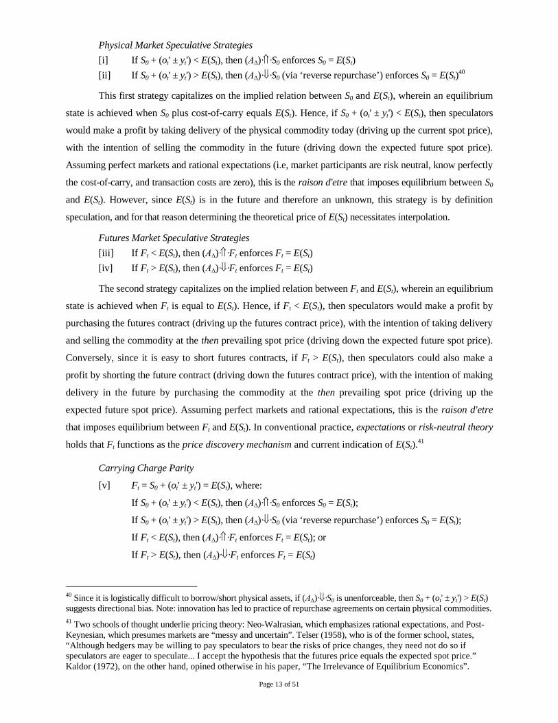
Physical Market Speculative Strategies

[i] If S0 + (ot' ± yt') < E(St), then (ΑΔ)··S0 enforces S0 = E(St)

[ii] If S0 + (ot' ± yt') > E(St), then (ΑΔ)··S0 (via ‘reverse repurchase’) enforces S0 = E(St)40

This first strategy capitalizes on the implied relation between S0 and E(St), wherein an equilibrium

state is achieved when S0 plus cost-of-carry equals E(St). Hence, if S0 + (ot' ± yt') < E(St), then speculators

would make a profit by taking delivery of the physical commodity today (driving up the current spot price),

with the intention of selling the commodity in the future (driving down the expected future spot price).

Assuming perfect markets and rational expectations (i.e, market participants are risk neutral, know perfectly

the cost-of-carry, and transaction costs are zero), this is the raison d'etre that imposes equilibrium between S0

and E(St). However, since E(St) is in the future and therefore an unknown, this strategy is by definition

speculation, and for that reason determining the theoretical price of E(St) necessitates interpolation.

Futures Market Speculative Strategies

[iii] If Ft < E(St), then (ΑΔ)··Ft enforces Ft = E(St)

[iv] If Ft > E(St), then (ΑΔ)··Ft enforces Ft = E(St)

The second strategy capitalizes on the implied relation between Ft and E(St), wherein an equilibrium

state is achieved when Ft is equal to E(St). Hence, if Ft < E(St), then speculators would make a profit by

purchasing the futures contract (driving up the futures contract price), with the intention of taking delivery

and selling the commodity at the then prevailing spot price (driving down the expected future spot price).

Conversely, since it is easy to short futures contracts, if Ft > E(St), then speculators could also make a

profit by shorting the future contract (driving down the futures contract price), with the intention of making

delivery in the future by purchasing the commodity at the then prevailing spot price (driving up the

expected future spot price). Assuming perfect markets and rational expectations, this is the raison d'etre

that imposes equilibrium between Ft and E(St). In conventional practice, expectations or risk-neutral theory

holds that Ft functions as the price discovery mechanism and current indication of E(St).41

Carrying Charge Parity

[v] Ft = S0 + (ot' ± yt') = E(St), where:

If S0 + (ot' ± yt') < E(St), then (ΑΔ)··S0 enforces S0 = E(St);

If S0 + (ot' ± yt') > E(St), then (ΑΔ)··S0 (via ‘reverse repurchase’) enforces S0 = E(St);

If Ft < E(St), then (ΑΔ)··Ft enforces Ft = E(St); or

If Ft > E(St), then (ΑΔ)··Ft enforces Ft = E(St)

40 Since it is logistically difficult to borrow/short physical assets, if (ΑΔ)··S0 is unenforceable, then S0 + (ot' ± yt') > E(St)suggests directional bias. Note: innovation has led to practice of repurchase agreements on certain physical commodities.

41 Two schools of thought underlie pricing theory: Neo-Walrasian, which emphasizes rational expectations, and Post-Keynesian, which presumes markets are “messy and uncertain”. Telser (1958), who is of the former school, states,“Although hedgers may be willing to pay speculators to bear the risks of price changes, they need not do so ifspeculators are eager to speculate... I accept the hypothesis that the futures price equals the expected spot price.”Kaldor (1972), on the other hand, opined otherwise in his paper, “The Irrelevance of Equilibrium Economics”.

Page 14 of 51

Assuming perfect markets and rational expectations, an equilibrium state is achieved when S0 plus

cost-of-carry equals Ft, and S0 plus cost-of-carry equals E(St), therefore Ft is equal to E(St). The only issue is

that within the paradigm of general equilibrium, carrying charge parity creates a logical fallacy…

Issue of Causal Relativity

Let’s assume Telser’s (1958) expectations theory that “the futures price equals the expected spot

price,” and in accordance with rational expectations and its allied assumption, the efficient market hypothesis

(EMH), the current futures price reflects equilibrium from which participants act as price-takers.

If Ft = S0 + (ot' ± yt') = E(St) expresses equilibrium, and the cost-of-carry (ot' ± yt') is determined from

the delta Ft – S0 as Kaldor (1939) propositioned, which then is used to infer the value of E(St) such that the

delta between S0 and E(St) also equates to (ot' ± yt'), how do we know when the fundamentals underlying

either ot' or yt' have shifted, noting that yt' is inferred by netting ot' from Ft – S0, as opposed to when an

arbitrage opportunity exists because Ft ≠ S0 + (ot' ± yt'), noting that arbitrage is what enforces equilibrium?

Hence, we posit that the viability of using Ft or S0 as a control condition to determine (ot' ± yt') much

less E(St) is suspect, if for the mere reason that one could inversely argue that rational expectations

minimizes the usefulness of carrying charge parity as a mechanism from which economic agents can make

arbitrage decisions. As Muth (1961) posited, “The way expectations are formed depends specifically on the

structure of the relevant system describing the economy.” In other words, models based on rational

expectations assume a predetermined equilibrium around which expectations are formed [e.g., Telser’s

Ft = E(St) or Kaldor’s Ft – S0 = (ot' ± yt')], which in effect reverses the model’s line of causation. Apropos of

carrying charge parity, Telser’s (1958) assumption eliminates arbitrageurs’ incentive to enforce Ft = E(St).

However, if there are situations, as Keynes (1930) suggests (and which the hedging response function

assumes), where Ft = S0 + (ot' ± yt') < E(St), or Ft = S0 + (ot' ± yt') > E(St), or alternatively Ft – S0 ≠ (ot' ± yt'),

then either: (i) incentive exists for arbitrageurs’ to enforce Ft = E(St); (ii) there is an unaccounted factor(s)

which should be incorporated into the model; and/or (iii) equilibrium cannot be determined from inherited

properties of individual behavior—ergo, there may be more than one price vector (i.e., multiple equilibria).

That’s why for practitioners applicability of carrying charge parity is largely dependent on whether

rational expectations is presumed to accurately reflect how the real world works, in which case the model is

ineffective because of circular reasoning;42 or whether markets are imperfect and rational expectations is a

deficient assumption, in which case there are real world opportunities to arbitrage for carrying charge parity.

The remainder of this paper is predicated on the latter conviction. We now reintroduce ±εt' into

proposition Ft = S0 + (ot' ± yt' ± εt') ≠ E(St) to indicate the existence of arbitrage opportunities.

42 “Fortunately, there is a simpler explanation – the model was wrong. Of course, all models are wrong. The onlymodel that is not wrong is reality and reality is not, by definition, a model.” From: Andrew G. Haldane, “Why BanksFailed the Stress Test,” Executive Director of Financial Stability, Bank of England; the basis for a speech given atthe Marcus-Evans Conference on Stress-Testing, February 9-10, 2009.

Page 15 of 51

Equilibrium Arbitrage Pressures

The problem facing arbitrageurs43 seeking to effect carrying charge parity is determining whether

t' = 0 and the fundamentals involving ot' and/or yt' have shifted; or t' < 0 or t' > 0 and there exists an

arbitrage opportunity. Since relationships between S0, Ft, E(St), ot', and yt' are recursive, in order to discover

if the market is mispriced, an arbitrageur must rely on real world observation in estimating exogenous

variables such as ot'. Conversely, the issue facing speculators with respect to speculative strategies is estimating

whether the market’s current implied cost-of-carry is accurate, which facilitates interpolation of E(St); or

estimating whether the market’s implied cost-of-carry is inaccurate and there exists a speculative opportunity.

In keeping with definitions established above, positive carry and negative carry shall reference the

term structure of the future price curve, whereas backwardation and contango shall reference the relation

between futures or forward prices and the expected future spot price. In this way, the seeming contradiction

between normal backwardation and theory of storage is reconciled, and semantics are clarified.

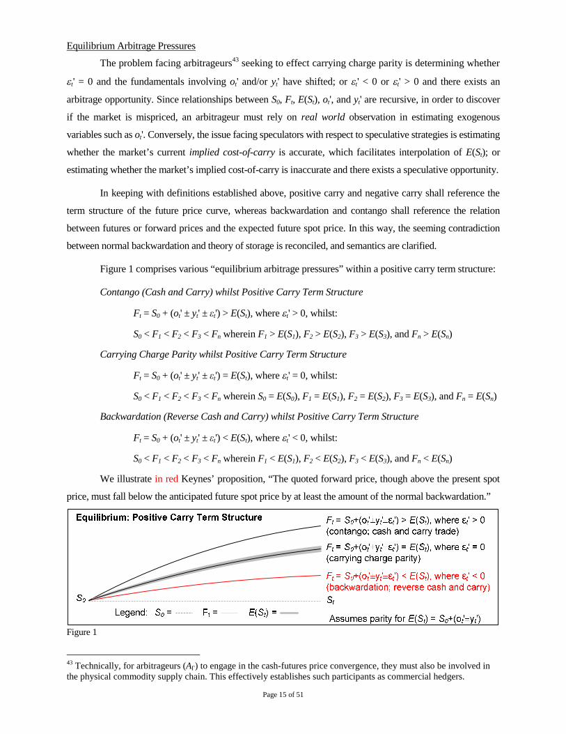
Figure 1 comprises various “equilibrium arbitrage pressures” within a positive carry term structure:

Contango (Cash and Carry) whilst Positive Carry Term Structure

Ft = S0 + (ot' ± yt' ± εt') > E(St), where t' > 0, whilst:

S0 < F1 < F2 < F3 < Fn wherein F1 > E(S1), F2 > E(S2), F3 > E(S3), and Fn > E(Sn)

Carrying Charge Parity whilst Positive Carry Term Structure

Ft = S0 + (ot' ± yt' ± εt') = E(St), where t' = 0, whilst:

S0 < F1 < F2 < F3 < Fn wherein S0 = E(S0), F1 = E(S1), F2 = E(S2), F3 = E(S3), and Fn = E(Sn)

Backwardation (Reverse Cash and Carry) whilst Positive Carry Term Structure

Ft = S0 + (ot' ± yt' ± εt') < E(St), where t' < 0, whilst:

S0 < F1 < F2 < F3 < Fn wherein F1 < E(S1), F2 < E(S2), F3 < E(S3), and Fn < E(Sn)

We illustrate in red Keynes’ proposition, “The quoted forward price, though above the present spot

price, must fall below the anticipated future spot price by at least the amount of the normal backwardation.”

Figure 1

43 Technically, for arbitrageurs (AΓ) to engage in the cash-futures price convergence, they must also be involved inthe physical commodity supply chain. This effectively establishes such participants as commercial hedgers.

Page 16 of 51

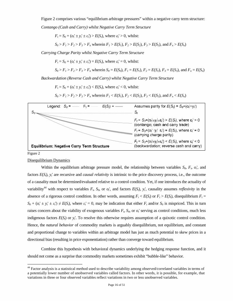
Figure 2 comprises various “equilibrium arbitrage pressures” within a negative carry term structure:

Contango (Cash and Carry) whilst Negative Carry Term Structure

Ft = S0 + (ot' ± yt' ± εt') > E(St), where t' > 0, whilst:

S0 > F1 > F2 > F3 > Fn wherein F1 > E(S1), F2 > E(S2), F3 > E(S3), and Fn > E(Sn)

Carrying Charge Parity whilst Negative Carry Term Structure

Ft = S0 + (ot' ± yt' ± εt') = E(St), where t' = 0, whilst:

S0 > F1 > F2 > F3 > Fn wherein S0 = E(S0), F1 = E(S1), F2 = E(S2), F3 = E(S3), and Fn = E(Sn)

Backwardation (Reverse Cash and Carry) whilst Negative Carry Term Structure

Ft = S0 + (ot' ± yt' ± εt') < E(St), where t' < 0, whilst:

S0 > F1 > F2 > F3 > Fn wherein F1 < E(S1), F2 < E(S2), F3 < E(S3), and Fn < E(Sn)

Figure 2

Disequilibrium Dynamics

Within the equilibrium arbitrage pressure model, the relationship between variables S0, Ft, ot', and

factors E(St), yt' are recursive and causal relativity is intrinsic to the price discovery process, i.e., the outcome

of a causality must be determined/evaluated relative to a control condition. Yet, if one introduces the actuality of

variability44 with respect to variables Ft, S0, or ot', and factors E(St), yt', causality assumes reflexivity in the

absence of a rigorous control condition. In other words, assuming Ft < E(St) or Ft > E(St), disequilibrium Ft =

S0 + (ot' ± yt' ± εt') ≠ E(St), where εt' = 0, may be indication that either Ft and/or S0 is mispriced. This in turn

raises concern about the viability of exogenous variables Ft, S0, or ot' serving as control conditions, much less

indigenous factors E(St) or yt'. To resolve this otherwise requires assumption of a quixotic control condition.

Hence, the natural behavior of commodity markets is arguably disequilibrium, not equilibrium, and constant

and proportional change to variables within an arbitrage model has just as much potential to skew prices in a

directional bias (resulting in price exponentiation) rather than converge toward equilibrium.

Combine this hypothesis with behavioral dynamics underlying the hedging response function, and it

should not come as a surprise that commodity markets sometimes exhibit “bubble-like” behavior.

44 Factor analysis is a statistical method used to describe variability among observed/correlated variables in terms ofa potentially lower number of unobserved variables called factors. In other words, it is possible, for example, thatvariations in three or four observed variables reflect variations in two or less unobserved variables.

Page 17 of 51

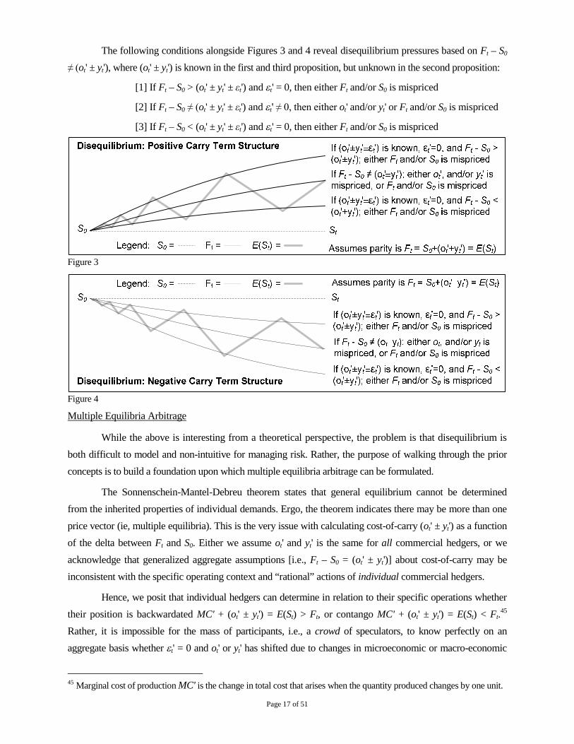
The following conditions alongside Figures 3 and 4 reveal disequilibrium pressures based on Ft – S0

≠ (ot' ± yt'), where (ot' ± yt') is known in the first and third proposition, but unknown in the second proposition:

[1] If Ft – S0 > (ot' ± yt' ± εt') and t' = 0, then either Ft and/or S0 is mispriced

[2] If Ft – S0 ≠ (ot' ± yt' ± εt') and t' ≠ 0, then either ot' and/or yt' or Ft and/or S0 is mispriced

[3] If Ft – S0 < (ot' ± yt' ± εt') and t' = 0, then either Ft and/or S0 is mispriced

Figure 3

Figure 4

Multiple Equilibria Arbitrage

While the above is interesting from a theoretical perspective, the problem is that disequilibrium is

both difficult to model and non-intuitive for managing risk. Rather, the purpose of walking through the prior

concepts is to build a foundation upon which multiple equilibria arbitrage can be formulated.

The Sonnenschein-Mantel-Debreu theorem states that general equilibrium cannot be determined

from the inherited properties of individual demands. Ergo, the theorem indicates there may be more than one

price vector (ie, multiple equilibria). This is the very issue with calculating cost-of-carry (ot' ± yt') as a function

of the delta between Ft and S0. Either we assume ot' and yt' is the same for all commercial hedgers, or we

acknowledge that generalized aggregate assumptions [i.e., Ft – S0 = (ot' ± yt')] about cost-of-carry may be

inconsistent with the specific operating context and “rational” actions of individual commercial hedgers.

Hence, we posit that individual hedgers can determine in relation to their specific operations whether

their position is backwardated MC' + (ot' ± yt') = E(St) > Ft, or contango MC' + (ot' ± yt') = E(St) < Ft.45

Rather, it is impossible for the mass of participants, i.e., a crowd of speculators, to know perfectly on an

aggregate basis whether t' = 0 and ot' or yt' has shifted due to changes in microeconomic or macro-economic

45 Marginal cost of production MC' is the change in total cost that arises when the quantity produced changes by one unit.

Page 18 of 51

influences, or whether t' < 0 or t' > 0 and an arbitrage opportunity exists. Thus, the Sonnenschein-Mantel-

Debreu theorem, involving multiple equilibria and Pareto efficiency, corroborates that at any point in time

market conditions may reflect pricing that provide arbitrage opportunities Ft = S0 + (ot' ± yt' ± εt') ≠ E(St).

Further, contrary hedging responses by individual bona fide hedgers to aggregate market pricing may reflect

perfectly “rational” responses given an individual hedger’s specific position and operating context.

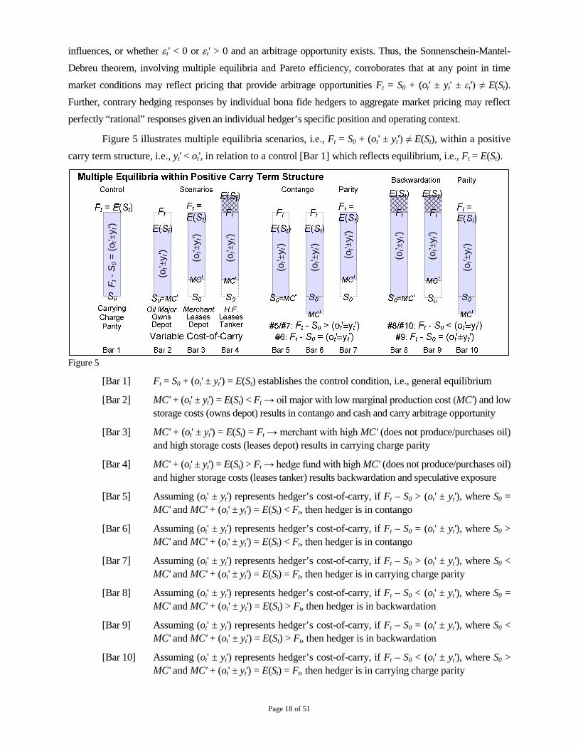
Figure 5 illustrates multiple equilibria scenarios, i.e., Ft = S0 + (ot' ± yt') ≠ E(St), within a positive

carry term structure, i.e., yt' < ot', in relation to a control [Bar 1] which reflects equilibrium, i.e., Ft = E(St).

Ft-

S0

=(o

t'±y

t')

(ot'±

yt')

(ot'±

y t')

(ot'±

y t')

(ot'±

yt')

(ot'±

yt')

(ot'±

y t')

(ot'±

y t')

(ot'±

y t')

(ot'±

y t')

Figure 5

[Bar 1] Ft = S0 + (ot' ± yt') = E(St) establishes the control condition, i.e., general equilibrium

[Bar 2] MC' + (ot' ± yt') = E(St) < Ft → oil major with low marginal production cost (MC') and low

storage costs (owns depot) results in contango and cash and carry arbitrage opportunity

[Bar 3] MC' + (ot' ± yt') = E(St) = Ft → merchant with high MC' (does not produce/purchases oil)

and high storage costs (leases depot) results in carrying charge parity

[Bar 4] MC' + (ot' ± yt') = E(St) > Ft → hedge fund with high MC' (does not produce/purchases oil)

and higher storage costs (leases tanker) results backwardation and speculative exposure

[Bar 5] Assuming (ot' ± yt') represents hedger’s cost-of-carry, if Ft – S0 > (ot' ± yt'), where S0 =

MC' and MC' + (ot' ± yt') = E(St) < Ft, then hedger is in contango

[Bar 6] Assuming (ot' ± yt') represents hedger’s cost-of-carry, if Ft – S0 = (ot' ± yt'), where S0 >

MC' and MC' + (ot' ± yt') = E(St) < Ft, then hedger is in contango

[Bar 7] Assuming (ot' ± yt') represents hedger’s cost-of-carry, if Ft – S0 > (ot' ± yt'), where S0 <

MC' and MC' + (ot' ± yt') = E(St) = Ft, then hedger is in carrying charge parity

[Bar 8] Assuming (ot' ± yt') represents hedger’s cost-of-carry, if Ft – S0 < (ot' ± yt'), where S0 =

MC' and MC' + (ot' ± yt') = E(St) > Ft, then hedger is in backwardation

[Bar 9] Assuming (ot' ± yt') represents hedger’s cost-of-carry, if Ft – S0 = (ot' ± yt'), where S0 <

MC' and MC' + (ot' ± yt') = E(St) > Ft, then hedger is in backwardation

[Bar 10] Assuming (ot' ± yt') represents hedger’s cost-of-carry, if Ft – S0 < (ot' ± yt'), where S0 >

MC' and MC' + (ot' ± yt') = E(St) = Ft, then hedger is in carrying charge parity

Page 19 of 51

4. Framework for Basis Trading

The body of theory presented above provides the underpinnings for developing multiple equilibria

multi-factor propositions.46 Propositions do not operate in a vacuum, however; rather they function within

boundary conditions. In combination, conditions, propositions and constraints47 provide context for managing

individual microeconomic basis risk exposure, and helps optimize basis trading strategies (e.g., position,

pricing, position entry/exit, marketing alternatives). This section adds basis concepts to our unifying theory.


Let (HS) represent short hedgers (e.g., producers); let (HL) represent long hedgers (e.g., consumers);

let (ΑΔ) represent speculators; and let (AΓ) represent arbitrageurs. Additionally, let the symbol designate

the purchase of an asset or holding a long position by a participant; and let the symbol designate the

sale of an asset or holding a short position by a participant. [e.g., (ΑΔ)· signifies that speculators on a net

aggregate basis “went long” by purchasing the underlying asset or related futures.]

We also add the following set of notations in order to model basis trading. Let Bt represent basis

wherein the futures price is subtracted from the spot price, i.e., Bt = S0 – Ft. In addition, let (–) represent

basis under, i.e., Bt·(–); let (+) represent basis over, i.e., Bt·(+); let represent strengthening basis, i.e., Bt·;

and let represent weakening basis, i.e., Bt·. These concepts are explained below.

Increasing instrument prices [e.g., S0, S1, Ft, etc.] are represented by the symbol (↑), including

parentheses; decreasing instrument prices are represented by the symbol (↓), including parentheses; and

sideway instrument prices are represented by the symbol (→), including parentheses [e.g., S0·(→)]. In

addition, let (↑↑), including parentheses, designate instrument prices that are rising faster; and let (↓↓),

including parentheses, designate instrument prices that are falling faster [e.g., S0·(↓↓)].

Principles of Basis Trading

“Basis” is defined as the difference between a specified local cash price and a futures or forward

price for a specified delivery period and location, i.e., S0 – Ft. Factors that influence basis include, but are

not limited to supply/demand, substitution, unequal borrowing/lending rates, warehousing (storage), insurance,

and transportation. Such aspects are investigated in the following section on Segmenting the Supply Chain.

In practice, basis Bt is conveyed in terms of a futures or forward contract spread “under” or “over”

the cash price S0, with basis under related to positive carry, and basis over related to negative carry. Figure 6

illustrates the inverse relationship between positive carry and negative basis, and negative carry and positive

basis. Basis occurs because supply/demand factors in local cash markets are different from the futures market.

46 Single-factor models attempts to account for contingencies like changes in interest rate or inflation, and are basedon equations in which one economic factor explains market phenomena and/or equilibrium asset prices. Multi-factormodels employ multiple factors in its computations to explain market phenomena and/or equilibrium asset prices.

47 “Condition” is defined as a set of boundaries that is used to simulate a large system; whereas “constraint” is adiscrete condition that a solution requires in order to satisfy an optimization problem.

Page 20 of 51

Price

Price

Contr

ary

Mark

etM

otio

n

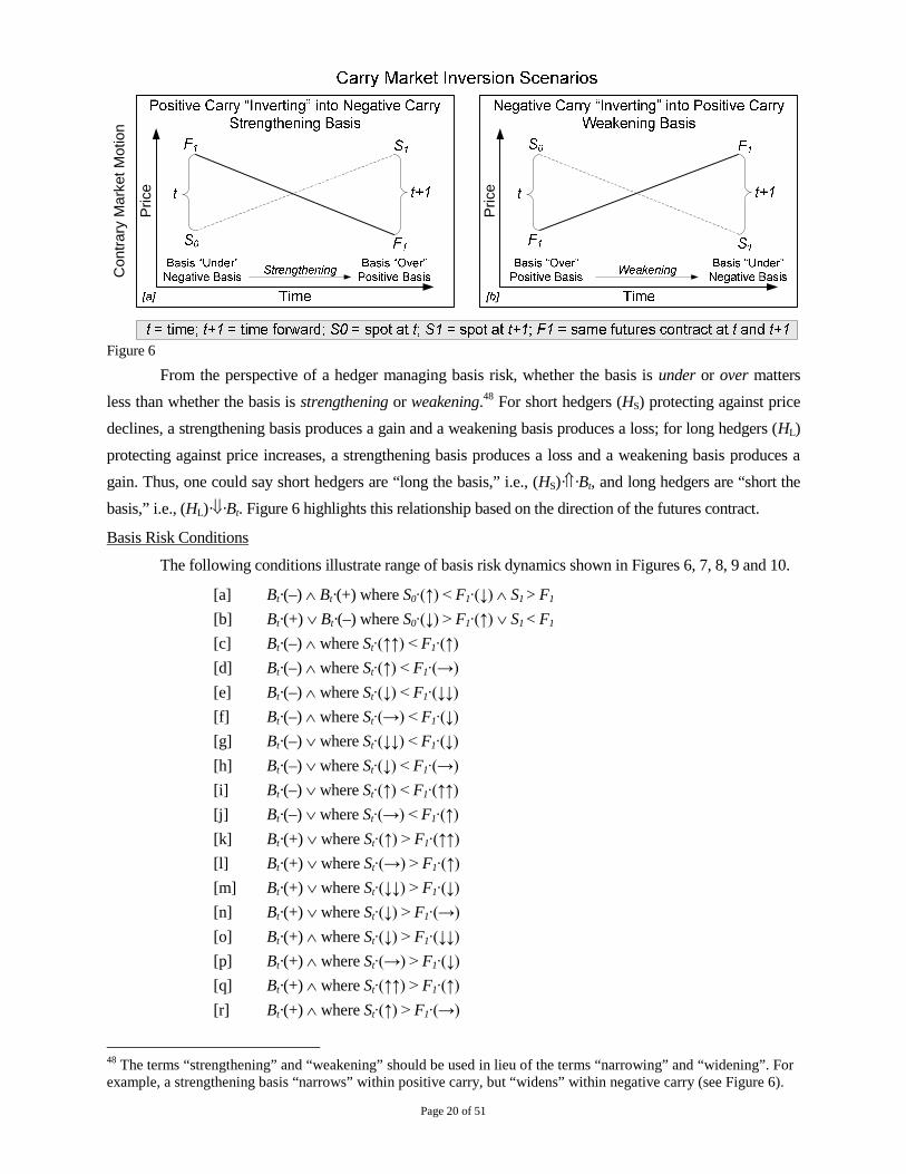
Figure 6

From the perspective of a hedger managing basis risk, whether the basis is under or over matters

less than whether the basis is strengthening or weakening.48 For short hedgers (HS) protecting against price

declines, a strengthening basis produces a gain and a weakening basis produces a loss; for long hedgers (HL)

protecting against price increases, a strengthening basis produces a loss and a weakening basis produces a

gain. Thus, one could say short hedgers are “long the basis,” i.e., (HS)··Bt, and long hedgers are “short the

basis,” i.e., (HL)··Bt. Figure 6 highlights this relationship based on the direction of the futures contract.

Basis Risk Conditions

The following conditions illustrate range of basis risk dynamics shown in Figures 6, 7, 8, 9 and 10.

[a] Bt·(–) Bt·(+) where S0·(↑) < F1·(↓) S1 > F1

[b] Bt·(+) Bt·(–) where S0·(↓) > F1·(↑) S1 < F1

[c] Bt·(–) where St·(↑↑) < F1·(↑)

[d] Bt·(–) where St·(↑) < F1·(→)

[e] Bt·(–) where St·(↓) < F1·(↓↓)

[f] Bt·(–) where St·(→) < F1·(↓)

[g] Bt·(–) where St·(↓↓) < F1·(↓)

[h] Bt·(–) where St·(↓) < F1·(→)

[i] Bt·(–) where St·(↑) < F1·(↑↑)

[j] Bt·(–) where St·(→) < F1·(↑)

[k] Bt·(+) where St·(↑) > F1·(↑↑)

[l] Bt·(+) where St·(→) > F1·(↑)

[m] Bt·(+) where St·(↓↓) > F1·(↓)

[n] Bt·(+) where St·(↓) > F1·(→)

[o] Bt·(+) where St·(↓) > F1·(↓↓)

[p] Bt·(+) where St·(→) > F1·(↓)

[q] Bt·(+) where St·(↑↑) > F1·(↑)

[r] Bt·(+) where St·(↑) > F1·(→)

48 The terms “strengthening” and “weakening” should be used in lieu of the terms “narrowing” and “widening”. Forexample, a strengthening basis “narrows” within positive carry, but “widens” within negative carry (see Figure 6).

Page 21 of 51

Positive Carry/Basis Under

Figure 7 illustrates strengthening basis scenarios within positive carry/basis under conditions.

Figure 7

Figure 8 illustrates weakening basis scenarios within positive carry/basis under conditions.

Figure 8

Page 22 of 51

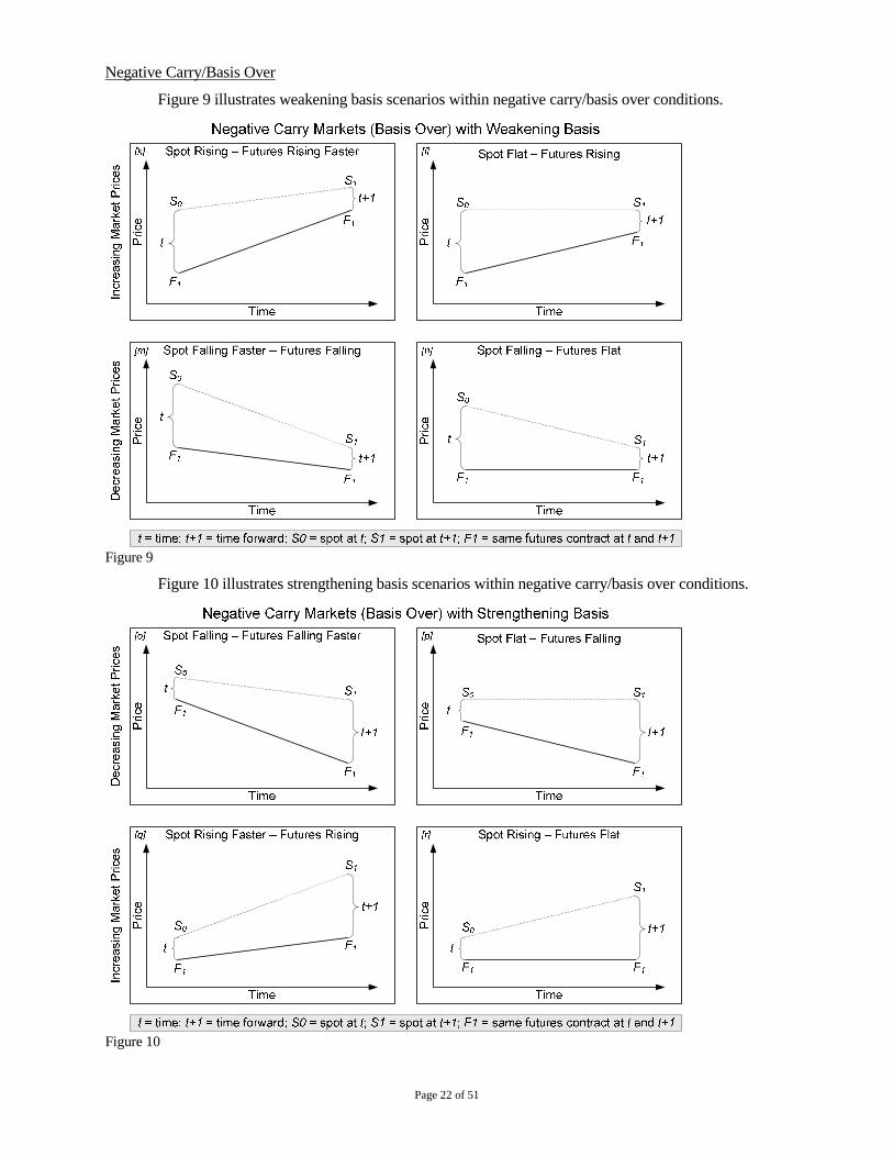
Negative Carry/Basis Over

Figure 9 illustrates weakening basis scenarios within negative carry/basis over conditions.

Figure 9

Figure 10 illustrates strengthening basis scenarios within negative carry/basis over conditions.

Figure 10

Page 23 of 51

Basis Trading Strategies

Hedgers can make better choices about when to market, where to market, and how to lock in prices

by following basis closely. Basis for storable products is influenced by two things: (i) the cost of getting the

commodity from point of production to point of delivery for domestic use or export/international use; and (ii)

local/regional supply-demand for a commodity as compared to global macroeconomic dynamics.

The first step in to compare the basis currently offered for the expected time of delivery with the

basis historically offered around such delivery time. As an example, factors that account for basis variation in

the grain markets include charges for elevation, cleaning, storage, and inspection (together known as elevator

tariffs). Interest rates also influence a farmer's net farm gate price, with storage length being a related factor—

the longer grain is stored, the higher the interest and storage charges will be.49

Consumers such as processors also use basis to attract commodities when they require it. Buyers

who, on any particular day, offer a higher local cash price than their competitors are in effect offering a

stronger basis than their competitors. As an example, a merchandiser with an export sale to deliver canola in

two months will encourage producer deliveries to its elevator system by strengthening the basis. The higher

cash price relative to the futures price will attract deliveries to that particular dealer. Conversely, an elevator

with excess grain in-store will discourage farm deliveries by weakening the basis. The lower cash price

signals producers to hold back deliveries to that particular warehouse, or make delivery to other elevators.

As basis is a signal of market forces, it serves as an important gauge as to whether a producer

should: (i) store and maintain title to the commodity (e.g., “on-farm storage” or “lease storage);” (ii) “spot

sale” at the nearby market price; (iii) contract to sell the commodity at the nearby bid, i.e., “cash sale

contract;” (iv) “forward contract” whereby terms are agreed upon in advance by the buyer and seller; (v)

enter into a “futures contract” in which the terms are standardized by the exchange’s contract specifications;

(vi) use a “fixed basis contract” that fixes the quantity, delivery period and basis, but leaves futures price

risk unhedged to be established at a later date; (vii) use a “hedge-to-arrive” (HTA) contract which fixes the

quantity, delivery period and futures price, but leaves the basis unhedged to be established at a later date;50

(viii) enter into a “minimum price contract” which in effect is a fixed basis contract with an embedded

option to allow upside participation; or (ix) enter into a contract which facilitates movement of a commodity

without establishing either a basis or futures price, variously known as “delayed price contract,” “no price

established,” “price later,” or “deferred price contract”.

For added flexibility, commercial hedgers can use various option strategies (e.g., calls and/or puts) to

hedge price risk, and then either maintain title to the commodity, or enter into a contract (e.g., basis contract).

49 Charlie Pearson, “Basis – How Cash Grain Prices are Established,” Alberta Agriculture and Rural Development,Provincial Crops Market Analyst. Published July 21, 2006; reviewed and revised on August 4, 2011.

50 Hedge-to-arrive contracts range from relatively simple, low-risk non-rolling versions in which basis risk is themain area of risk exposure, to much more complex types that allow producers to roll (change delivery dates) andpermit the next year’s crop to be priced initially with old-crop futures contracts.

Page 24 of 51

5. Segmenting the Supply Chain

Risks related to production costs, commodity substitution, financing considerations, merchandising

channels and marketing alternatives exist throughout the commodity supply chain. Because of the complexity

involved, industry participants are increasingly using E/CTRM systems to automate management of key

exposures (e.g., market, operations, credit, and compliance). When implementing such systems, supply chain

logistics and risk management factors specific to a particular business’ value chain needs to be analyzed.

Indeed, while there are many homogeneous activities (e.g., planning, scheduling, inventory control,

deal capture, trading, accounting, invoicing, clearing, settlement, compliance, reporting, etc.), dissimilarities

within vertical sectors (e.g., agribusiness, energy and mining) and between horizontal operations (e.g.,

producers, freight carriers, processors, merchandisers) makes for heterogeneous requirements.

Since it is not practical to provide an in-depth analysis of all the logistical and risk factors related to

each of the vertical and horizontal niches, the balance of our paper focuses on farming operations as a general

case study, while noting applicability to the various commodity value chains, generally.

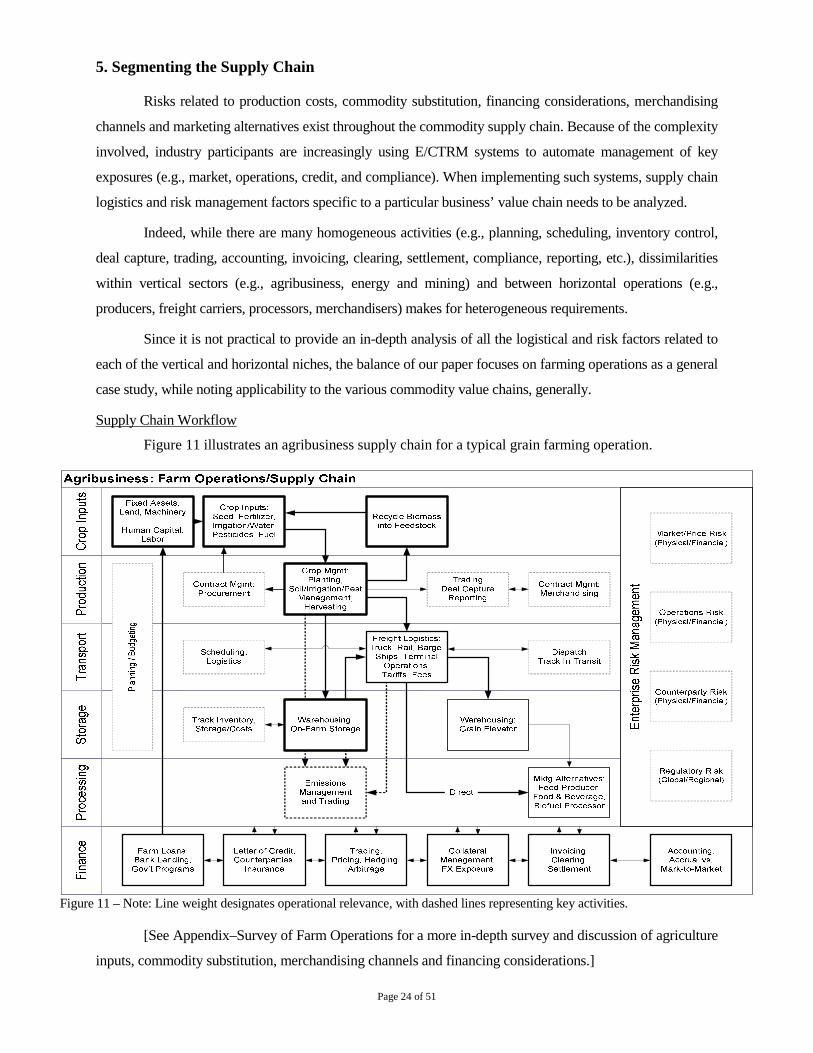
Supply Chain Workflow

Figure 11 illustrates an agribusiness supply chain for a typical grain farming operation.

Figure 11 – Note: Line weight designates operational relevance, with dashed lines representing key activities.

[See Appendix–Survey of Farm Operations for a more in-depth survey and discussion of agriculture

inputs, commodity substitution, merchandising channels and financing considerations.]

Page 25 of 51

Profit Maximization

Profit maximization is the process by which a firm determines the price and output level that returns

the greatest profit. There are two methods for determining maximization: (i) total revenue less total cost

which focuses on minimizing this difference; and (ii) marginal revenue less marginal cost, specifically

when marginal cost equals marginal revenue indicating that total profit has reached maximum point.

Production Costs

Marginal cost at each level of production includes any additional costs required to produce the next

unit. In practice, marginal costs include all “short run” costs that vary with the level of production whereas

“long run” costs are considered fixed costs. If the cost function is differentiated d,51 the marginal cost MC′ is

the cost of the next unit produced, where Q represents the production quantity, VC represents variable costs,

FC represents fixed costs, and TC represents total costs, i.e., MC′ = dTC / dQ = d(FC + VC) / dQ. Since

fixed costs do not vary with production quantity, it drops out of the equation when it is differentiated, i.e.,

d(FC + VC) / dQ = dVC / dQ.52 On the other hand, average total cost ATC, which is the total cost divided by

the number of units produced, includes fixed costs, i.e., ATC = (FC + VC) / Q.

Establishing marginal cost of production for agricultural goods is a function of investment into fixed

assets (e.g., land and equipment), crop inputs (e.g., seed, fertilizer, irrigation, pesticides, fuel), and labor.

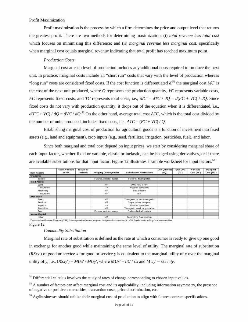
Since both marginal and total cost depend on input prices, we start by considering marginal share of

each input factor, whether fixed or variable, elastic or inelastic, can be hedged using derivatives, or if there

are available substitutions for that input factor. Figure 12 illustrates a sample worksheet for input factors.53

Input Factors

Fixed, Variable

or N/A

Elastic or

Inelastic Hedging Contingencies Substitution Alternatives

Unit Quantity

(dQ )

Total Cost

(TC )

Variable

Cost (VC )

Marginal

Cost (MC )

Financing

Interest Futures, options, swaps Fixed vs. floatng rates

Fixed Assets

Land N/A Own, rent, CRP*

- Insurance --> Weather derivatives

Machinery N/A Buy or lease

- Insurance N/A N/A

Crop Inputs

Seed N/A Transgenic vs. non-transgenic

Fertilizer N/A Crop rotation, compost

Irrigation --> Weather derivatives

Pesticides N/A Transgenic seed, crop rotation

Fuel Futures, options, swaps On-farm biofuel system

Human Capital

Labor N/A Technology / automation

*Conservation Reserve Program (CRP) is a cropland retirement program that provides incentives to shift fragile lands to long-term conservation.

Figure 12

Commodity Substitution

Marginal rate of substitution is defined as the rate at which a consumer is ready to give up one good

in exchange for another good while maintaining the same level of utility. The marginal rate of substitution

(RSxy′) of good or service x for good or service y is equivalent to the marginal utility of x over the marginal

utility of y, i.e., (RSxy′) = MUx′ / MUy′, where MUx′ = ∂U / ∂x and MUy′ = ∂U / ∂y.

51 Differential calculus involves the study of rates of change corresponding to chosen input values.

52 A number of factors can affect marginal cost and its applicability, including information asymmetry, the presenceof negative or positive externalities, transaction costs, price discrimination, etc.

53 Agribusinesses should unitize their marginal cost of production to align with futures contract specifications.

Page 26 of 51

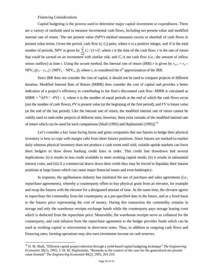
Financing Considerations

Capital budgeting is the process used to determine major capital investment or expenditures. There

are a variety of methods used to measure incremental cash flows, including net present value and modified

internal rate of return. The net present value (NPV) method measures excess or shortfall of cash flows in

present value terms. Given the period, cash flow (t, Ct) pairs, where n is a positive integer, and N is the total

number of periods, NPV is given by ∑ Ct / (1+r)t, where t is the time of the cash flow; r is the rate of return

that could be earned on an investment with similar risk; and Ct is net cash flow (i.e., the amount of inflow

minus outflow) at time t. Using the secant method, the internal rate of return (IRR) r is given by rn+1 = rn –

NPVn ((rn – rn–1) / (NPVn – NPVn–1)), where rn is considered the nth approximation of the IRR.

Since IRR does not consider the cost of capital, it should not be used to compare projects of different

duration. Modified Internal Rate of Return (MIRR) does consider the cost of capital and provides a better

indication of a project’s efficiency in contributing to the firm’s discounted cash flow. MIRR is calculated as

MIRR = n√(FV / –PV) – 1, where n is the number of equal periods at the end of which the cash flows occur

(not the number of cash flows), PV is present value (at the beginning of the first period), and FV is future value

(at the end of the last period). Like the internal rate of return, the modified internal rate of return cannot be

validly used to rank-order projects of different sizes, however, there exist variants of the modified internal rate

of return which can be used for such comparisons [Shull (1992) and Hajdasinski (1995)].54

Let’s consider a key issue facing farms and grain companies that use futures to hedge their physical

inventory is how to cope with margin calls from short futures positions. Since futures are marked-to-market

daily whereas physical inventory does not produce a cash event until sold, volatile upside markets can force

short hedgers to draw down banking credit lines in order. This credit line drawdown had several

implications: (i) it results in less credit available to meet working capital needs; (ii) it results in substantial

interest costs; and (iii) if a commercial draws down their credit they may be forced to liquidate their futures

positions at large losses which can cause major financial issues and even bankruptcy.

In response, the agribusiness industry has instituted the use of purchase and sales agreements (i.e.,

repurchase agreements), whereby a counterparty offers to buy physical grain from an elevator, for example

and swap the futures with the elevator for a designated amount of time. At the same time, the elevator agrees

to repurchase the commodity from the counterparty at a pre-specified date in the future, and at a fixed basis

to the futures price representing the cost of money. During this transaction the commodity remains in

storage and only the warehouse receipts exchange hands while the counterparty pays storage leasing costs

which is deducted from the repurchase price. Meanwhile, the warehouse receipts serve as collateral for the

counterparty, and cash infusion from the repurchase agreement to the hedger provides funds which can be

used as working capital or reinvestment in short-term notes. Thus, in addition to outgoing cash flows and

financing rates, farming operations may also earn investment income on cash reserves.

54 D. M. Shull, “Efficient capital project selection through a yield-based capital budgeting technique” The EngineeringEconomist 38(1), 1992, 1-18. M. Hajdasinski, “Remarks in the context of the case for the generalized net presentvalue formula” The Engineering Economist 40(2), 1995, 201-210.

Page 27 of 51

Merchandising Channels

We define merchandising as potential channels of distribution for commodity products including

modes of transportation, as opposed to marketing which is based on the goal of selling commodity products

as profitably as possible. Hence, merchandising relates to cost-of-carry within the commodity supply chain.

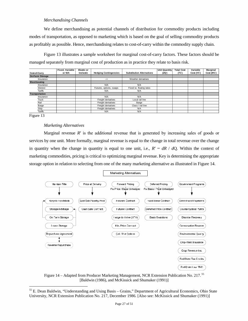
Figure 13 illustrates a sample worksheet for marginal cost-of-carry factors. These factors should be

managed separately from marginal cost of production as in practice they relate to basis risk.

Cost-of-Carry

Fixed, Variable

or N/A

Elastic or

Inelastic Hedging Contingencies Substitution Alternatives

Unit Quantity

(dQ )

Total Cost

(TC )

Variable

Cost (VC )

Marginal

Cost (MC )

On-Farm Storage

Insurance --> Weather derivatives

Warehousing

Insurance N/A N/A

Interest Futures, options, swaps Fixed vs. floatng rates

Tariffs N/A N/A

Transportation

Insurance N/A N/A

Truck Freight derivatives Local rail line

Rail Freight derivatives Barge

Barge Freight derivatives Class I rail line

Ship Freight derivatives N/A

Tariffs N/A N/A

Figure 13

Marketing Alternatives

Marginal revenue R′ is the additional revenue that is generated by increasing sales of goods or

services by one unit. More formally, marginal revenue is equal to the change in total revenue over the change

in quantity when the change in quantity is equal to one unit, i.e., R′ = dR / dQ. Within the context of

marketing commodities, pricing is critical to optimizing marginal revenue. Key is determining the appropriate

storage option in relation to selecting from one of the many marketing alternative as illustrated in Figure 14.

Figure 14 – Adapted from Producer Marketing Management, NCR Extension Publication No. 217. 55

[Baldwin (1986), and McKissick and Shumaker (1991)]

55 E. Dean Baldwin, “Understanding and Using Basis – Grains,” Department of Agricultural Economics, Ohio StateUniversity, NCR Extension Publication No. 217, December 1986. [Also see: McKissick and Shumaker (1991)]

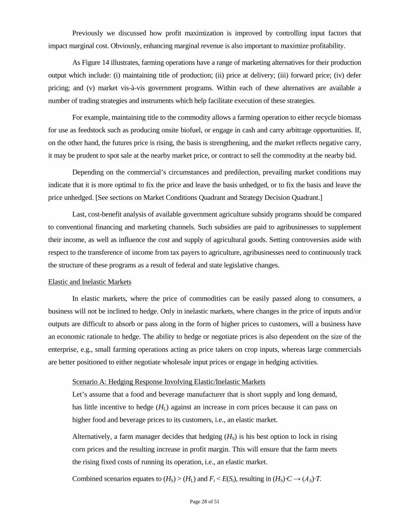
Page 28 of 51

Previously we discussed how profit maximization is improved by controlling input factors that

impact marginal cost. Obviously, enhancing marginal revenue is also important to maximize profitability.

As Figure 14 illustrates, farming operations have a range of marketing alternatives for their production

output which include: (i) maintaining title of production; (ii) price at delivery; (iii) forward price; (iv) defer

pricing; and (v) market vis-à-vis government programs. Within each of these alternatives are available a

number of trading strategies and instruments which help facilitate execution of these strategies.

For example, maintaining title to the commodity allows a farming operation to either recycle biomass

for use as feedstock such as producing onsite biofuel, or engage in cash and carry arbitrage opportunities. If,

on the other hand, the futures price is rising, the basis is strengthening, and the market reflects negative carry,

it may be prudent to spot sale at the nearby market price, or contract to sell the commodity at the nearby bid.

Depending on the commercial’s circumstances and predilection, prevailing market conditions may

indicate that it is more optimal to fix the price and leave the basis unhedged, or to fix the basis and leave the

price unhedged. [See sections on Market Conditions Quadrant and Strategy Decision Quadrant.]

Last, cost-benefit analysis of available government agriculture subsidy programs should be compared

to conventional financing and marketing channels. Such subsidies are paid to agribusinesses to supplement

their income, as well as influence the cost and supply of agricultural goods. Setting controversies aside with

respect to the transference of income from tax payers to agriculture, agribusinesses need to continuously track

the structure of these programs as a result of federal and state legislative changes.

Elastic and Inelastic Markets

In elastic markets, where the price of commodities can be easily passed along to consumers, a

business will not be inclined to hedge. Only in inelastic markets, where changes in the price of inputs and/or

outputs are difficult to absorb or pass along in the form of higher prices to customers, will a business have

an economic rationale to hedge. The ability to hedge or negotiate prices is also dependent on the size of the

enterprise, e.g., small farming operations acting as price takers on crop inputs, whereas large commercials

are better positioned to either negotiate wholesale input prices or engage in hedging activities.

Scenario A: Hedging Response Involving Elastic/Inelastic Markets

Let’s assume that a food and beverage manufacturer that is short supply and long demand,

has little incentive to hedge (HL) against an increase in corn prices because it can pass on

higher food and beverage prices to its customers, i.e., an elastic market.

Alternatively, a farm manager decides that hedging (HS) is his best option to lock in rising

corn prices and the resulting increase in profit margin. This will ensure that the farm meets

the rising fixed costs of running its operation, i.e., an elastic market.

Combined scenarios equates to (HS) > (HL) and Ft < E(St), resulting in (HS)·C → (ΑΔ)·T.

Page 29 of 51

Continuing, the food and beverage manufacturer borrows money at floating rates which later

increase. For the manufacturer, the economics are inelastic because it would have difficulty

passing along higher interest expense in the form of higher food and beverage prices. This

is because competitors that borrowed at fixed rates will not have a similar motivation to

raise prices on their products. As a result, the manufacturer may be inclined to hedge (HL).

Assuming rates (↑) and (HL) > (HS) causing Ft > E(St), then (HL)·T → (ΑΔ)·C; alternatively,

assuming rates (↓) and (HL) > (HS) causing Ft > E(St), then (HL)·C → (ΑΔ)·T.56

Scenario B: Hedging Response Involving Elastic/Inelastic Markets

Assume water rights are strictly regulated so that water authorities can not pass along costs

to farming operations. This describes an inelastic market in which farmers have no need to

enter into weather derivatives because the government ensures water availability and caps

price. From the farmer’s perspective, there is no need to hedge (HL) water costs.

In addition, because such regulations cap how much water authorities charge customers,

regulations combined with tax payer subsidies also deters hedging (HS) water production.

Combined scenarios equates to (HS) = (HL) and Ft = E(St), resulting in (HS) ↔ (HL).

Assuming water rights are deregulated, a regulated inelastic market evolves into an elastic

market. In this situation, private water wholesalers pass along their costs in water-related

infrastructure investments (e.g., desalination plants) and/or needed upgrades in aging water

and sewer systems.57 From the wholesalers’ perspective such costs for upgrades represent

an elastic output; however, water is an inelastic input from the perspective of farm operators.

Hence, if water wholesalers (HS) are less inclined to lock in profits than farmers are inclined

to hedge a rise in water prices, a rising market will result in (HL) > (HS), causing Ft > E(St)

and (HL)·T → (ΑΔ)·C. Equally, if water wholesalers (HS) are less inclined to hedge against

lower prices than farmers are inclined to lock in increased margins from lower prices, a

declining market will result in (HL) > (HS), causing Ft > E(St), yet this time (HL)·C → (ΑΔ)·T.

Conversely, if water wholesalers (HS) are more inclined to lock in profits than farmers are in

hedging a rise in water prices, a rising market will result in (HS) > (HL), causing Ft < E(St)

and (HS)·C → (ΑΔ)·T. Likewise, if water wholesalers (HS) are more inclined to hedge against

lower prices than farmers are inclined to lock in increased margins from lower prices, a

declining market will result in (HS) > (HL), causing Ft < E(St), yet this time (HS)·T → (ΑΔ)·C.

56 Example doesn’t take into consideration the inverse relationship between rates and principle. If the manufacturewere to use Treasury futures, then rising rates are hedged by shorting the Treasury futures, and vice-versa.

57 Jeremy Schwartz and Eric Dexheimer, “Growth of large private water companies brings higher water rates, littlerecourse for consumers,” American-Statesman, December 17, 2011.

Page 30 of 51

6. Multi-Factor Modeling

Given the preceding, we can now develop a framework for making informed trading decisions on

hedging and/or arbitrage transactions. The method is guided by a two-fold approach: first, assess the

macroeconomic environment and “general equilibrium” price dynamics based on reported market prices;

second, determine the company’s microeconomics based on input factors, marginal production cost, marginal

cost-of-carry and expected output value. The economic rationale for whether to enter into a hedging

transaction or not, however, is ultimately rooted in price-taking or price-making behavior.

Julien and Tricou (2006) state that “under a normative point of view [including for fundamental

reasons]… the universal price-taking behavior is more efficient than the universal price-making behavior.”58

This may be the case, but determining such efficiency is dependent on having accurate intelligence of the

fundamentals. As demonstrated by Calvo and Mendoza (2000), “in the presence of short-selling constraints,

the gains of gathering information at a fixed cost diminish as markets grow… [thereby] weakening incentives

for gathering costly information and by strengthening incentives for imitating arbitrary market portfolios.”59

However, if we assume a market participant possesses private information, such as that known by a

commercial hedger who has implemented a robust E/CTRM system, then multiple equilibria arbitrage suggests

such hedgers should be able to fundamentally determine in relation to their specific operations whether their

position is backwardated, i.e., MC' + (ot ± yt) = E(St) > Ft, or contango, i.e., MC' + (ot ± yt) = E(St) < Ft.

Further, since there is more than one price vector, as the Sonnenschein-Mantel-Debreu theorem attests,

informed participants are more likely to behave as price-makers, e.g., enter into arbitrage strategies.60

All the same, there are limitations with respect to market power and the ability to facilitate arbitrage.

First, as Julien and Tricou (2006) posit, price-taking behavior can be more efficient; second, the ability to

enter into arbitrage transactions requires storage. “Store-of-value” is extant in non-perishable commodities

(e.g., gold, oil); commodities that are moderately easy to store inherit risk (e.g., coffee, wheat); perishable

commodities (e.g., eggs), on the other hand, inhibit arbitrage except under very short time constraints.

The operative assumption for engaging in arbitrage, however, is having a robust E/CTRM system

that can effectively measure enterprise-wide risk. Due to the complexity of monitoring uncertain cash flows

generated by physical assets, “effective market and credit risk management… can only be achieved by using

a unified and consistent framework, and by applying a rigorous and disciplined process of identifying,

measuring and reporting risks across all business units and portfolios of an organization.”61

58 Ludovic A. Julien and Fabrice Tricou, “A note on price-taking and price-making behaviours in general equilibriumoligopoly models,” EconomiX Conference, Université Paris X-Nanterre, France, July 24, 2006.59 Guillermo Calvo and Enrique Mendoza, “A Rational Contagion and the Globalization of Securities Markets,”Journal of International Economics, Vol. 51, 2000, p 79.60 “Once one allows agents to place arbitrarily large orders–an implicit assumption in arbitrage–these orders then haveprice impact and limits to arbitrage arise endogenously.” From: Marzena Rostek and Marek Weretka, “Dynamic ThinMarkets,” University of Wisconsin-Madison, Department of Economics, August 11, 2009.61 Ibid., Chris Strickland (2012)

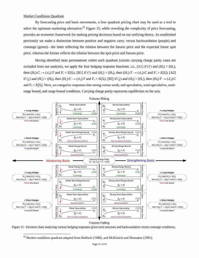
Page 31 of 51

Market Conditions Quadrant

By forecasting price and basis movements, a four quadrant pricing chart may be used as a tool to

select the optimum marketing alternative.62 Figure 15, while revealing the complexity of price forecasting,

provides an economic framework for making pricing decisions based on our unifying theory. As established

previously we make a distinction between positive and negative carry, versus backwardation (purple) and

contango (green)—the latter reflecting the relation between the futures price and the expected future spot

price, whereas the former reflects the relation between the spot price and futures price.

Having identified most permutations within each quadrant (certain carrying charge parity cases are

excluded from our analysis), we apply the four hedging response functions, i.e., [A1] if (↑) and (HS) > (HL),

then (HS)·C → (ΑΔ)·T and Ft < E(St); [B1] if (↑) and (HL) > (HS), then (HL)·T → (ΑΔ)·C and Ft > E(St); [A2]

if (↓) and (HL) > (HS), then (HL)·C → (ΑΔ)·T and Ft > E(St); [B2] if (↓) and (HS) > (HL), then (HS)·T → (ΑΔ)·C

and Ft < E(St). Next, we categorize responses into strong versus weak; and speculative, semi-speculative, semi-

range bound, and range bound conditions. Carrying charge parity represents equilibrium on the axis.

Futures Falling

Strengthening BasisWeakening Basis

S0

Ft

S0 > Ft

Strong Speculative

S0

Ft

S0 < Ft

Strong Semi-Range Bound

If (↓) and (HS) > (HL),

then (HS)·T → (ΑΔ)·C and Ft < E(St)

If (↓) and (HL) > (HS),

then (HL)·C → (ΑΔ)·T and Ft > E(St)

If (↓) and (HS) > (HL),

then (HS)·T → (ΑΔ)·C and Ft < E(St)

E(St)

E(St)

If (↓) and (HL) > (HS),

then (HL)·C → (ΑΔ)·T and Ft > E(St)

Normal Backwardation

Ne

ga

tive

Ca

rry

Ne

ga

tive

Ca

rryContango

Po

sitiv

eC

arry

+

> Short Hedger

> Long Hedger

S0

Ft

S0 > Ft

Strong Range Bound

E(St)

Backwardation+

Ne

ga

tive

Ca

rry

S0

Ft

S0 < Ft

Strong Semi-Speculative

E(St)

Contango

If (↑) and (HL) > (HS),

then (HL)·T → (ΑΔ)·C and Ft > E(St)

If (↑) and (HS) > (HL),

then (HS)·C → (ΑΔ)·T and Ft < E(St)

-

-

S0

Ft

S0 > Ft

Weak Speculative

S0

Ft

S0 < Ft

Weak Semi-Range Bound

E(St)

E(St)


Contango

-

S0

Ft

S0 > Ft

Weak Range Bound

E(St)

Backwardation

-

S0

Ft

S0 < Ft

Weak Semi-Speculative

E(St)

Contango

+

+

Ne

ga

tive

Ca

rry

Po

sitiv

eC

arr

y

> Long Hedger

If (↑) and (HL) > (HS),

then (HL)·T → (ΑΔ)·C and Ft > E(St)

> Short Hedger

If (↑) and (HS) > (HL),

then (HS)·C → (ΑΔ)·T and Ft < E(St)

“Long the Basis”“Long the Basis”

“Short the Basis”“Short the Basis”

S0

Ft

S0 < Ft

Strong Speculative E(St)


+

S0

Ft

S0 < Ft

Weak Speculative E(St)


-

S0

Ft

S0 > Ft

Strong Semi-Speculative

E(St)

Backwardation+

S0

Ft

S0 > Ft

Weak Semi-Speculative

E(St)

Backwardation

-

S0

Ft

S0 > Ft

Strong Semi-Range Bound

E(St)Contango-

S0

Ft

S0 > Ft

Weak Semi-Range Bound

E(St)Contango

+

Carrying Charge ParityS0 + (ot ± yt) = Ft = E(St)

Futures Rising

Po

sitiv

eC

arr

yP

ositiv

eC

arry

Ne

ga

tive

Ca

rryP

ositiv

eC

arry

Po

sitiv

eC

arr

yN

eg

ative

Ca

rry

S0

Ft

S0 < Ft

Strong Range Bound

E(St)

Contango

-

S0

Ft

S0 < Ft

Weak Range Bound

E(St)

Contango

+

> Short Hedger

> Long Hedger> Long Hedger

> Short Hedger

“Long the Basis”“Long the Basis”

“Short the Basis”“Short the Basis”

Figure 15 –Decision chart analyzing various hedging responses given term structure and backwardation versus contango conditions.

62 Market conditions quadrant adapted from Baldwin (1986), and McKissick and Shumaker (1991).

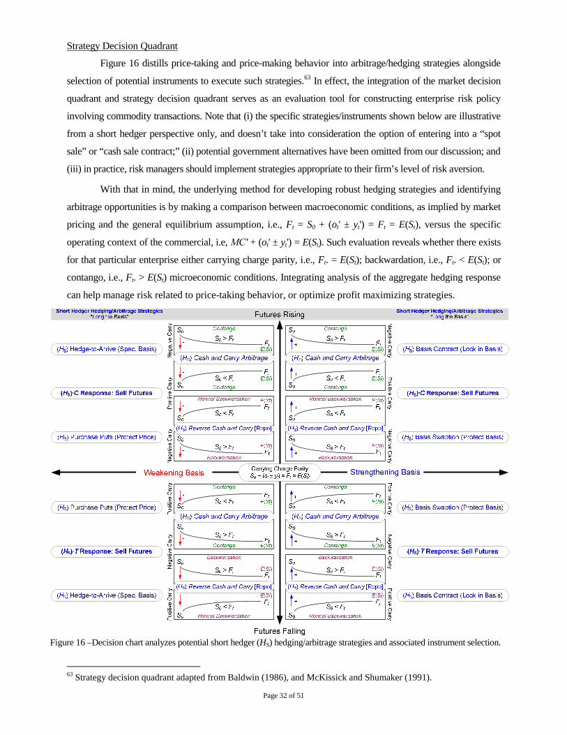
Page 32 of 51

Strategy Decision Quadrant

Figure 16 distills price-taking and price-making behavior into arbitrage/hedging strategies alongside

selection of potential instruments to execute such strategies.63 In effect, the integration of the market decision

quadrant and strategy decision quadrant serves as an evaluation tool for constructing enterprise risk policy

involving commodity transactions. Note that (i) the specific strategies/instruments shown below are illustrative

from a short hedger perspective only, and doesn’t take into consideration the option of entering into a “spot

sale” or “cash sale contract;” (ii) potential government alternatives have been omitted from our discussion; and

(iii) in practice, risk managers should implement strategies appropriate to their firm’s level of risk aversion.

With that in mind, the underlying method for developing robust hedging strategies and identifying

arbitrage opportunities is by making a comparison between macroeconomic conditions, as implied by market

pricing and the general equilibrium assumption, i.e., Ft = S0 + (ot' ± yt') = Ft = E(St), versus the specific

operating context of the commercial, i.e, MC′ + (ot' ± yt') = E(St). Such evaluation reveals whether there exists

for that particular enterprise either carrying charge parity, i.e., Ft. = E(St); backwardation, i.e., Ft. < E(St); or

contango, i.e., Ft. > E(St) microeconomic conditions. Integrating analysis of the aggregate hedging response

can help manage risk related to price-taking behavior, or optimize profit maximizing strategies.

Figure 16 –Decision chart analyzes potential short hedger (HS) hedging/arbitrage strategies and associated instrument selection.

63 Strategy decision quadrant adapted from Baldwin (1986), and McKissick and Shumaker (1991).

Page 33 of 51

Arbitrage Constraints

So far we have discussed conditions and propositions at length, but have spent little effort analyzing

constraints that are required to satisfy optimization problems. Evolving from the assumption that markets

eliminate any opportunity for risk-free profits is the principle of no-arbitrage. Our focus here is not to

provide a counterargument to the no-arbitrage principle64 and its sponsor, the efficient market hypothesis (see

prior section on Disequilibrium Dynamics); rather, our intention is to incorporate a method of calculating no-

arbitrage bounds which is in line with our unifying theory and has practical application.

No Arbitrage Bounds

Conventionally, no-arbitrage bounds is written as S0 + (ot' ± yt') ≤ Ft ≤ S0 + (ot' ± yt'), where if the

futures price trades within this range, no cash-and-carry or reverse cash-and-carry arbitrage transactions

will be profitable. However, we note that this equation is incongruous with the Kaldor’s (1939) equilibrium

proposition Ft – S0 = (ot' ± yt'), and Telser’s (1958) expectations axiom that Ft = E(St).65 Rather, an individual

hedger or arbitrageur should calculate no-arbitrage bounds based on their specific microeconomic situation

using the firm’s marginal production cost MC' and marginal cost-of-carry (ot' ± yt') as the variables.

Consequently, the general equilibrium function for marginal cost-of-carry can be given as GE(ot' ± yt'),

since Ft – S0 = (ot' ± yt') and equilibrium assumes Ft = S0 + (ot' ± yt') = E(St). In addition, an individual hedger’s

marginal cost-of-carry can be given as HA(ot' ± yt'), where ot' represents exogenous variables, and yt' represents

indigenous factors. Thus for HA(ot' ± yt'), carrying charge parity assumes MC' + (ot' ± yt') = E(St) = Ft,

backwardation assumes MC' + (ot' ± yt') = E(St) > Ft, and contango assumes MC' + (ot' ± yt') = E(St) < Ft.

To solve for inconsistencies inherent with the conventional equation, we can rewrite no-arbitrage

bounds as MC' + HA(ot' ± yt') = E(St) = Ft , whereby opportunities exist when MC' + HA(ot' ± yt') = E(St) > Ft,

or MC' + HA(ot' ± yt') = E(St) < Ft. Alternatively, we can calculate for probable no-arbitrage bounds by

comparing HA(ot' ± yt') and GE(ot' ± yt'), whereby HA(ot' ± yt') = GE(ot' ± yt') equates to carrying charge parity,

HA(ot' ± yt') > GE(ot' ± yt') equates to backwardated carrying charge, and HA(ot' ± yt') < GE(ot' ± yt') equates to

contango carrying charge. With this latter approach, we note that by comparing carrying charges only, the

result is a probable boundary because we should not assume MC' = S0 as MC' can be < or > S0.

We now extend the no-arbitrage bounds analysis by segmenting the cost-of-carry into its

component risks. Thus far we have assumed cost-of-carry is divided between observable exogenously

determined variables, i.e., marginal outlay on storage ot' (including facilities, insurance and interest), and

interpolated indigenously determined factors, i.e., marginal convenience/inconvenience yield ±yt'. These

two components (notwithstanding Brennan’s (1958) hypothesis on marginal risk-aversion) are sufficient for

64 Botond Köszegi, Kristóf Madarász and Máté Matolcsi, “A Failure of the No-Arbitrage Principle,” Department ofEconomics, University of California Berkeley, Rényi Institute of Mathematics, Budapest, July 2007.

65 See discussion in sections on Equilibrium Arbitrage Pressures and Disequilibrium Dynamics.

Page 34 of 51

calculating GE(ot' ± yt'), i.e., Ft – S0 = (ot' ± yt'); however, for a more accurate accounting of HA(ot' ± yt'), it is

beneficial to make a distinction between the various supply chain segments that constitute cost-of-carry.

Substituting for marginal outlay ot' in function HA(ot' ± yt'), let ot' instead represent the marginal cost

of leasing or owning warehouse facilities; let et' represent the marginal cost of insurance; let pt' represent the

marginal cost of transportation; let Bit' represent the marginal cost of borrowing (i.e., financing rate); let Lit'

represent the marginal return on lending (e.g., investment return on cash reserves); and let xt' represent the

marginal cost of transacting (e.g., bid-ask spread, commission, tariffs, fees). Since in the case of commercial

hedgers exogenous variables can be derived from observation (i.e., fundamental analysis), they should be

treated as independent variables, i.e., HA(ot' + et' + pt' + Bit' + Lit' + xt' ± yt'). In fact, interest rates and freight

are “commoditized” markets, and thus are organized as distinct markets, for example.

With respect to indigenous factors ±yt', Brennan (1958) introduced into the literature on commodity

theory the concept of marginal risk-aversion rt' and “the conditions on the second derivatives of ot, rt and ct

[that] insure that the solution is a maximum,” which we note are interpolations. Brennan’s seminal paper

addresses the question of when convenience motive is to be distinguished from the speculative motive, noting

that there is a “[thin] line of distinction between convenience and speculative stocks.” His theory “provides a

general hypothesis to explain the degree of hedging as well as intra- and inter-year storage behavior.”66 To

the extent that a firm can incorporate analysis of its marginal risk aversion it should.

Analysis of HA(ot' ± yt') ≤ ≥ GE(ot' ± yt') can be distilled into a comparison of synthetic lending rates

whereby the implied rate for GE(ot' ± yt') [i.e., GE(SLR)] is given by (Ft / S0 – 1)(d/365), and a “simplified”

implied rate for HA(ot' ± yt') [i.e., HA(SLR)] is given by (Ft / MC' – 1)(d/365), where d is number of days the

position is held, and the number of days for both GE(SLR) and HA(SLR) are the same. However, since

calculation for HA(SLR) [i.e., (Ft / MC' – 1)(d/365)] does not account for marginal cost factors, a “modified”

version HA(SLR') is given by ((Ft – (ot' + et' + pt' + Bit' + Lit' + xt' ± yt')) / MC' – 1)(d/365), whereby HA(SLR')

< GE(SLR) indicates a cash and carry arbitrage opportunity, and HA(SLR') > GE(SLR) indicates a reverse

cash and carry arbitrage opportunity [note notational difference between HA(SLR) and HA(SLR')].

7. Excursus

Over the past two decades there has been a paradigm shift in the structure of the global commodity

markets. The underlying cause for such change has been a combination of regulatory dynamics and

technological advances. Presently, new rules being promulgated under the Dodd-Frank Act is cause for an

unprecedented merging of the futures exchange and over-the-counter (OTC) derivatives industry models.67

At the same time, traditional open out-cry market-making on futures exchanges is morphing into automated

66 Michael J. Brennan, “The Supply of Storage,” American Economic Review, 47(1), 1958, pp 50-72.

67 Dodd-Frank Final Rules, Guidance and Orders http://www.cftc.gov/LawRegulation/DoddFrankAct/Dodd-FrankFinalRules/index.htm As of 6/15/2012, the CFTC has finalized 33 final rules and guidance and 7 final orders.

Page 35 of 51

order execution via algorithmic trading and high frequency trading.68 This evolution from a floor-based

model to an electronic model, alongside the allowance of pre-execution communications69 is having a

profound impact on how price discovery works in the global commodity markets.

Parallel with these developments, financial innovation involving the securitization of commodity

interests,70 and other factors such as the emergence of commodity index investors and commodities as an

asset class, as well as movement toward cash settled rather than physically settled contracts, is arguably also

having an influence on the traditional behavior of futures prices and cash-futures convergence.71 The

proposition “if (↑) and (HL) > (HS), then (HL)·T → (ΑΔ)·C and Ft > E(St)” supports this notion.

A 2010 study by the International Food Policy Research Institute (IFPRI) concluded that “the

futures markets analyzed generally dominate the spot markets.”72 Despite assertions by certain economists

to the contrary,73 price-taking behavior should not come as a surprise. When marketing commodities, futures

prices are in practice referenced by agribusiness participants in terms of a basis differential, i.e., how much

the cash price is “over” or “under” the referenced futures price [See McKissick and Shumaker (1991)].

In another publication, Excessive Speculation in Agriculture Commodities: Selected Writings from

2008–2011, the Institute for Agriculture and Trade Policy (IATP) observed that “Food prices and food

insecurity are front page news… While the deregulation of financial and commodity markets by themselves

did not cause the current recession, the insolvency of deregulated major financial institutions, and the

resulting credit freeze, certainly have lead to increased unemployment, poverty and food insecurity.”74

We note that both the IFPRI and IATP studies recommend alternative mechanisms and possible

improvements to address “disproportionate volatility” and “improper speculation” in agricultural markets.

Given that commodities play such a vital role in the global economy, the conclusion by these Institutes

highlights the importance of a credible price discovery process to promote sustainable economic growth.

Such sentiment is underscored by a series of public statements from various industry associations

representing the agricultural and energy sectors, reflecting a growing frustration with the derivatives markets.

68 Bryan Durkin, “The Impact of Algorithmic and High Frequency Trading on CME Group Inc. Markets” CFTCTechnology Advisory Committee, July 14, 2010.

69 CME, CBOT, NYMEX and COMEX Market Regulation Advisory Notice, CME Group RA1004-5, “Pre-Execution Communications” Advisory Date: April 6, 2010; Effective Date: April 18, 2010.

70 Elizabeth L. Ritter, “The Securitization of Commodities: Crossing a Gold (or Silver) Line in the Sand,” BusinessLaw Brief, Fall 2005.

71 Commodity Futures Trading Commission, “Hearing on Energy Position Limits and Hedge Exemptions,”Washington D.C., July 28-30, 2009; see testimony of John Lothian, July 29, 2009.

72 Ibid., Hernandez and Maximo (2010)

73 Paul Krguman “Commodities and speculation: metallic (and other) evidence,” New York Times, April 20, 2009.Also see: Robert Samuelson “The Fallacy of Blaming Oil ‘Speculators’,” RealClear Politics, May 2, 2012.

74 Ben Lilliston and Andrew Ranallo, “Excessive Speculation in Agriculture Commodities: Selected Writings from2008–2011,” Institute for Agriculture and Trade Policy, April 2011.

Page 36 of 51

Problem/Challenge

In a January 23, 2008 press release, the National Grain and Feed Association (NGFA) “warned the

CFTC of major underlying concerns over the predictability of convergence between cash and futures prices

during the futures delivery period, as well as problems with hedging and pricing efficiencies, that have

dramatically increased the need for grain elevators, feed mills and grain processors to access increased

capital to finance margin calls.”75 In the year prior, the Energy Market Oversight Coalition (EMOC),

representing more than eighty agricultural, motor vehicle, home heating fuel, public power and consumer

groups urged the passing of the “Close the Enron Loophole Act” (S.2058). Considering that this coalition

represented commercials, their public statement issued October 25, 2007 was a scathing indictment:

There is growing recognition by the American public that the dramatic rise in energy prices

may not be caused exclusively by supply and demand, but rather by speculative trading

conducted on unregulated energy commodity markets, or ‘dark markets,’ where a majority of

energy trades now occur. As financial speculators engage in wanton abuse of these opaque

markets for personal profit, there is a growing lack of consumer confidence in the market’s

ability to set a price for energy based on economic fundamentals… In light of unprecedented

speculation and volatility in the energy commodity markets, it is time to close gaps in federal

law that allow energy profiteers to distort the price of energy for personal gain.76

More recently, in a letter to the chairman of the CFTC, the National Corn Growers Association

(NCGA) requested a 30-day public comment period before grain traders are allowed 22-hour-per-day

electronic trading of grain and oilseed futures contracts.77 Echoing National Farmers Union (NFU) President

Roger Johnson who also sent a letter,78 NCGA President Niemeyer cited two key reasons for concern:

1. Allowing the futures markets to trade during the release of key U.S. Department of

Agriculture reports can lead to rampant market distortions. Growers use numerous USDA

reports to adjust their risk management strategies and futures positions. Trading through

release of these reports could lead to extreme volatility immediately following their release.

2. Growers routinely track futures and cash markets throughout the day, and make marketing

decisions based on market movements. It is impossible for growers, and many of the small

elevators they rely upon, to actively track markets through later afternoons and evening

trading sessions, let alone 22 hours per day.

Despite such urgings, the CFTC approved CME Group's request for expedited approval of its new

22-hour trading day proposal.79 On the other hand, it could be argued that the CME Group is competing to

75 “NGFA Urges CFTC to Delay, Study Impacts of Proposed Increase in Speculative Position Limits in Ag Futures”National Grain and Feed Association, News Release, January 23, 2008.

76 Energy Market Oversight Coalition, “Time to Rein in Excessive Energy Market Speculation and Close the Doorto Manipulation,” Letter to United States Senate, October 25, 2007.

77 “Letter to the Honorable Gary Gensler, Chairman, Commodity Futures Trading Commission” National CornGrowers Association, May 16, 2012. See: http://www.ncga.com/uploads/useruploads/cftc-ncga-ltr.pdf

78 “Letter to Gensler, Chairman, Commodity Futures Trading Commission” National Farmers Union, May 17, 2012.http://www.nfu.org/news/206-market-reform/1105-nfu-cftc-should-hold-comment-period-regarding-extended-trading-days

79 Katie Micik “CFTC OKs CME Group's 21-Hour Trading Day” DTN The Progressive Farmer, May 18, 2012.

Page 37 of 51

stay on equal footing with investment banks who took advantage of deregulation under the Commodity

Futures Modernization Act (CFMA) as a means to forge the OTC derivatives juggernaut. The passage of the

Dodd-Frank Act and CFTC rules promulgated thereunder now serve to formalize this off-exchange market

through the creation of Swap Exchange Facilities (SEFs) and Central Counterparty (CCPs) clearing.

As a result, we forecast that in the coming years market participants are going to witness increasing

fragmentation of liquidity across numerous Electronic Communication Networks (ECNs) akin to what

happened in the equity markets.80 In order for ECNs to provide the necessary liquidity to survive in a

competitive marketplace they are likely going to be reliant upon algorithmic trading and co-locating high

frequency traders. Further, we suspect such trading will have difficulty proceeding on physically settled

contracts, and as a result there will be a proliferation of cash settled contracts. We believe this situation will

only serve to further destabilize cash-futures convergence as noted by the NGFA.81

Opportunity/Solution

Conversations with a variety of participants in the futures industry and agribusiness sector, ranging

from floor traders to farmers, ranchers, elevator operators and agricultural analysts, reflect a wide-spread

sense of apprehension about changes currently sweeping the industry.82 Nevertheless, commercials have to

rely on commodity futures and derivatives markets for risk management purposes; hence, there needs to be

confidence that these markets reflect supply-demand fundamentals. The question is how?

Rather than fret about the inevitability of an industry paradigm shift, we believe there is a

significant opportunity for technology, in the form of commodity transaction risk management systems, to

help commercials optimize profit maximizing strategies, or at minimum, manage risk related to price-taking

behavior. No doubt the complexity of the commodity value chain at the intersection of physical logistics and

financial operations presents numerous challenges. A unifying theory of commodity hedging and arbitrage

concepts, however, provides an economic framework for implementing evaluation tools within E/CTRM

systems, as well as help construct robust enterprise risk policies involving commodity transactions.

80 “The number of SEFs that will launch to capture some of the market share remains unknown however, some havespeculated expect as many as 40 SEFs may launch with those less successful faltering as the new market landscapeevolves.” From: Neal Brady and Cliff Lewis “SEF Selection: Factors to Consider When Differentiating SEFs”DerivSource, June 18, 2012. Source: http://www.derivsource.com/content/sef-selection-factors-consider-when-differentiating-sefs

81 Altering commodity contract specifications from physically settled to cash settled is a form of dematerialization.For a discussion regarding impact of dematerialization on the securities markets see Donald, David C. (2007) “TheRise and Effects of the Indirect Holding System: How Corporate America Ceded Its Shareholders to Intermediaries”Working Paper Series No. 68, Institute for Law and Finance, University of Frankfurt, September 2007.

82 While we recognize this statement will be considered controversial amongst certain readers, one can reasonably argue,based on prima facie evidence, that there has been an ongoing crisis of confidence in market integrity post-2008.

Page 38 of 51

Appendix – Survey of Farm Operations

As enterprise risk management is a broad topic, in order to narrow the scope of our analysis we

focused on the supply chain related to agribusiness producers, processors and merchandisers. Specifically, we

referenced the grain markets while noting that the supply chain for other commodities such as electricity, gas,

oil, coal and emissions are materially different. This survey discusses our findings regarding farm operations.

One of the observations we made was the reflexive feedback loop that naturally exists within the

commodity supply chain. For example, farm operations require management of input costs such as fuel;

biomass is feedstock for biofuel outputs, which in turn feedbacks into commodity substitution dynamics. To

capture such dynamics in the real world, enterprises need risk engines which consider such complexities.

Agricultural Inputs

Farmers may either own their land or have land rental agreements. A 2010 study showed that the

cost of production is closely correlated with the gross revenue for crops. Part of the reason for the strong

relationship between gross revenue and costs of production is the relation between gross revenue and land

values. Between 1972 and 2010 land values in Iowa averaged 34% of the cost to produce corn and 45% to

produce soybeans. During that time, the percentage of total costs attributed to land has varied ~10%.83

A major impact on reduced costs has been new technologies. In the 1970s, the cost for machinery

increased fairly steady, but remained relatively stable during the 1980s and 1990s. Since 2000, however,

these costs have risen dramatically with a 2010 study showing equipment representing 24% of the total cost

for producing corn and 18% for producing soybeans.84 At the same time, labor is becoming less of a factor

in terms of costs of production, representing 6% of the cost to produce corn and 7% for soybeans.85

Seed procurement is based on local growing conditions and planned end use of the crop, including

marketability considerations. One of the major changes seen over the past decade has been in the use of

genetically modified seeds which contain prophylactic traits and have altered production practices. By being

pest resistant, farmers pay more for seed but reduce the need to manage pests. This in turn has caused a

reduction in the cost of herbicides, insecticides and fungicides (collectively ‘pesticides’) to protect crops

against competition from weeds, insects and disease, allowing increased yields per unit of land.

Crop nutrition also plays a key role, supplying plants with essential nutrients and minerals (e.g.,

nitrogen, phosphorus, potassium) for healthy plant growth. Crop rotation alone does not fully maintain crop

yield, but requires the use of fertilizers. Farmers who control the land and have fertilizer prices “locked in”

have already established two of the largest and most important crop production costs.86

83 AgDM Newsletter, December 2010. http://www.extension.iastate.edu/agdm/articles/duffy/DuffyDec10.html84 Ibid., AgDM Newsletter, December 2010.85 Ibid., AgDM Newsletter, December 2010.86 AgDM Newsletter, September 2011. http://www.extension.iastate.edu/agdm/articles/others/JohSept11.html

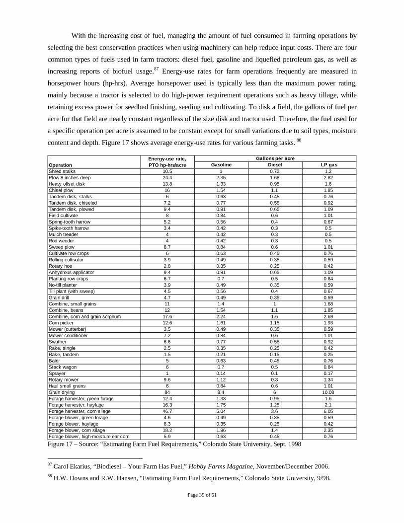
Page 39 of 51

With the increasing cost of fuel, managing the amount of fuel consumed in farming operations by

selecting the best conservation practices when using machinery can help reduce input costs. There are four

common types of fuels used in farm tractors: diesel fuel, gasoline and liquefied petroleum gas, as well as

increasing reports of biofuel usage.87 Energy-use rates for farm operations frequently are measured in

horsepower hours (hp-hrs). Average horsepower used is typically less than the maximum power rating,

mainly because a tractor is selected to do high-power requirement operations such as heavy tillage, while

retaining excess power for seedbed finishing, seeding and cultivating. To disk a field, the gallons of fuel per

acre for that field are nearly constant regardless of the size disk and tractor used. Therefore, the fuel used for

a specific operation per acre is assumed to be constant except for small variations due to soil types, moisture

content and depth. Figure 17 shows average energy-use rates for various farming tasks. 88

Gasoline Diesel LP gas

Shred stalks 10.5 1 0.72 1.2

Plow 8 inches deep 24.4 2.35 1.68 2.82

Heavy offset disk 13.8 1.33 0.95 1.6

Chisel plow 16 1.54 1.1 1.85

Tandem disk, stalks 6 0.63 0.45 0.76

Tandem disk, chiseled 7.2 0.77 0.55 0.92

Tandem disk, plowed 9.4 0.91 0.65 1.09

Field cultivate 8 0.84 0.6 1.01

Spring-tooth harrow 5.2 0.56 0.4 0.67

Spike-tooth harrow 3.4 0.42 0.3 0.5

Mulch treader 4 0.42 0.3 0.5

Rod weeder 4 0.42 0.3 0.5

Sweep plow 8.7 0.84 0.6 1.01

Cultivate row crops 6 0.63 0.45 0.76

Rolling cultivator 3.9 0.49 0.35 0.59

Rotary hoe 2.8 0.35 0.25 0.42

Anhydrous applicator 9.4 0.91 0.65 1.09

Planting row crops 6.7 0.7 0.5 0.84

No-till planter 3.9 0.49 0.35 0.59

Till plant (with sweep) 4.5 0.56 0.4 0.67

Grain drill 4.7 0.49 0.35 0.59

Combine, small grains 11 1.4 1 1.68

Combine, beans 12 1.54 1.1 1.85

Combine, corn and grain sorghum 17.6 2.24 1.6 2.69

Corn picker 12.6 1.61 1.15 1.93

Mower (cutterbar) 3.5 0.49 0.35 0.59

Mower conditioner 7.2 0.84 0.6 1.01

Swather 6.6 0.77 0.55 0.92

Rake, single 2.5 0.35 0.25 0.42

Rake, tandem 1.5 0.21 0.15 0.25

Baler 5 0.63 0.45 0.76

Stack wagon 6 0.7 0.5 0.84

Sprayer 1 0.14 0.1 0.17

Rotary mower 9.6 1.12 0.8 1.34

Haul small grains 6 0.84 0.6 1.01

Grain drying 84 8.4 6 10.08

Forage harvester, green forage 12.4 1.33 0.95 1.6

Forage harvester, haylage 16.3 1.75 1.25 2.1

Forage harvester, corn silage 46.7 5.04 3.6 6.05

Forage blower, green forage 4.6 0.49 0.35 0.59

Forage blower, haylage 8.3 0.35 0.25 0.42

Forage blower, corn silage 18.2 1.96 1.4 2.35

Forage blower, high-moisture ear corn 5.9 0.63 0.45 0.76

Energy-use rate,

PTO hp-hrs/acre

Gallons per acre

Operation

Figure 17 – Source: “Estimating Farm Fuel Requirements,” Colorado State University, Sept. 1998

87 Carol Ekarius, “Biodiesel – Your Farm Has Fuel,” Hobby Farms Magazine, November/December 2006.

88 H.W. Downs and R.W. Hansen, “Estimating Farm Fuel Requirements,” Colorado State University, 9/98.

Page 40 of 51

Another increasing concern for farm operations is water rights and reliable water supply. Since

1866, Congress has repeatedly recognized and protected the primary role of Western States in the allocation

and administration of the use of water. The Bureau of Reclamation, established in 1902, is the largest

wholesaler of water in the U.S., providing one out of five western farmers with irrigation water for ten

million acres of farmland that produce 60% of the nation's vegetables and 25% of its fruits and nuts.89 In

2004, the Council of State Governments reported that water availability and rights is an issue that “will not

be going away any time soon.”90 One “battle” included state officials in Texas demanding halt to a deal that

allowed Midland oil companies to sell water from the state’s public reserves to municipalities and ranchers

in drought-parched western Texas.91 In accordance with the McCarran Amendment,92 solutions must be based

on and recognize interstate compacts and U.S. Supreme Court decrees that allocate water between states,

water rights established under state and federal law, tribal water rights, and contracts for the use of water. 93

Commodity Substitution

A 2011 study facilitated by the Agricultural Research Service, the in-house research arm of the U.S.

Department of Agriculture, reported that it could take anywhere from 50 to 70 acres for a farmer with 1,000

acres, and an onsite crusher and biodiesel system, to grow enough canola to produce the fuel needed to run

on-farm operations. The team also found that in field trials, camelina plants produced an average of 2,000

pounds of seeds per acre in 80 days, which translates into 93 gallons of oil per acre. Safflower plants,

meanwhile, produced around 3,000 to 3,500 pounds of seeds per acre, and white mustard seed meal could

also be used as an organic fertilizer after the seeds were crushed to extract the oil for fuel.94

A different form of substitution in farming operations is crop rotation, which is the practice of

growing a series of dissimilar types of crops in the same area in sequential seasons. A key benefit is the

replenishment of nitrogen through the use of green manure in sequence with cereals and other crops. Crop

rotation also mitigates the build-up of pathogens and pests that often occurs when one crop species is

continuously planted, and can also improve soil structure and fertility by alternating deep-rooted and

89 U.S. Department of the Interior, Bureau of Reclamation. Retrieved July 28, 2012 http://www.usbr.gov/main/about/

90 Carolyn Orr, “Policy priorities for 2004,” Council of State Governments, CSG National Policy Task Forces andEmerging Trends Subcommittees, Chief Agriculture and Rural Policy Analyst, February 2004.

91 Ibid., Orr (2004)

92 McCarran Amendment, 43 USC. §666, guarantees that water rights created under applicable law will be recognizedunder both state and federal law. Congress created this guarantee by waiving the sovereign immunity of the UnitedStates so that it could be joined in comprehensive general adjudications of the rights to use water in state courts.

93 Statement of Mark Limbaugh, Deputy Commissioner, Bureau of Reclamation, U.S. Department of the Interior,before the Resources Committee, Subcommittee on Water and Power, U.S. House of Representatives on HR 2603Department of Interior and Water Rights, September 22, 2004.

94 Hal Collins and Rick Boydston, “Prospecting for Pacific Northwest Biofuel Crops,” Crop Protection and Quarantine(#304), Agricultural System Competitiveness and Sustainability (#216), and Bioenergy (#213), ARS Vegetable andForage Crops Research Laboratory in Prosser, February 2011.

Page 41 of 51

shallow-rooted plants. Using crop rotation farmers can keep their fields under continuous production,

instead of letting land lie fallow, as well as help reduce the need for fertilizers.95

Merchandising Alternatives

Development of the grain merchandising system has, since its beginnings, been influenced by the

availability of technology. Prior to trucking, excluding some minor river transportation, freight was by

horse-drawn wagons, which resulted in a large number of country elevators spaced only a few miles apart

on grain gathering rail lines.96 The grain handling and transportation system has since undergone

substantial change since that time, especially in the last couple of decades. Deregulation, competitive

pressures and branch line abandonment have forced many country elevators to close, while scores of new

high throughput elevators have been constructed across the prairies. The increasing competition has led to

an increase in efficiency incentives to improve service and realize operating savings.97

Farmers generally truck their grain to stations so as to maximize their net return. Trucks have cost

advantages for shorter distances (less than 250 to 500 miles) and function primarily as the short haul mode.

Railroads have a cost advantage in moving grain longer distances, but barges have an even greater

advantage where a waterway is available. A barge tow can carry the equivalent of roughly 15 rail cars or 60

trucks at a fraction of the cost of these other modes.98 The availability of barge transportation also helps check

rates charged by rail.99 Transportation premiums offer elevators a way to encourage deliveries from greater

distances, increasing total volume. When grain companies offer incentives to farmers to deliver grains to

specific locations (e.g., strengthened basis), modes of transportation become an important competitive tool.100

Mode of transportation utilized for grain merchandising is also highly dependent on the particular

supply chain. In general, three grain supply chains can be identified: (i) bulk grain for export, (ii) bulk grain

for the domestic market, and (iii) containerized specialty grain products. Each of these supply chains are tied

to their own infrastructure network. The bulk export system relies most heavily on river navigation and

Class I railroad trunk lines to reach seaport terminals. The domestic bulk market relies more heavily on rural

interstates or short line railroads to reach domestic processors and livestock farms. The container export

95 Michael D. Peel, “Crop Rotations for Increased Productivity,” North Dakota State University, EB-48 (Revised),January 1998. Available at: http://www.ag.ndsu.edu/pubs/plantsci/crops/eb48-1.htm

96 Dennis R. Ming and William W. Wilson, “The Evolving Country Grain Marketing System in North Dakota,”Upper Great Plains Transportation Institute Report No. 49, Agricultural Economics Report No. 169, July 1983.

97 Joon J. Park, William W. Wilson and D. Demcey Johnson, “Canadian Transportation and Grain Handling: IssuesAffecting the North American Barley Sector,” Agricultural Economics Report No. 427, September 1999.

98 Mary Jane Bolle, “Trade in the U.S. Gulf Region: Hurricanes Katrina, Rita and Beyond,” CRS Report forCongress, November 12, 2005, p. 3.

99 Christensen Associates, “A Study of Competition in the U.S. Freight Railroad Industry and Analysis of Proposalsthat Might Enhance Competition,” report to the Surface Transportation Board, November 2008.

100 Ibid., Park, Wilson and Johnson (1999)

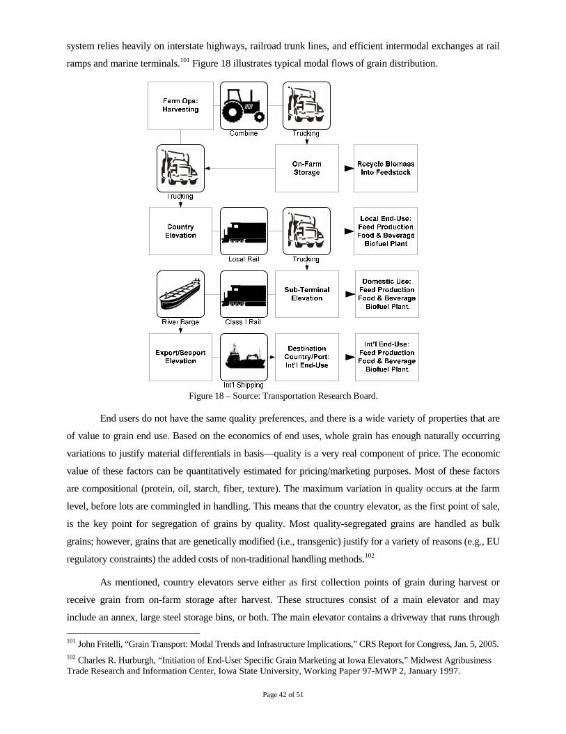
Page 42 of 51

system relies heavily on interstate highways, railroad trunk lines, and efficient intermodal exchanges at rail

ramps and marine terminals.101 Figure 18 illustrates typical modal flows of grain distribution.

Figure 18 – Source: Transportation Research Board.

End users do not have the same quality preferences, and there is a wide variety of properties that are

of value to grain end use. Based on the economics of end uses, whole grain has enough naturally occurring

variations to justify material differentials in basis—quality is a very real component of price. The economic

value of these factors can be quantitatively estimated for pricing/marketing purposes. Most of these factors

are compositional (protein, oil, starch, fiber, texture). The maximum variation in quality occurs at the farm

level, before lots are commingled in handling. This means that the country elevator, as the first point of sale,

is the key point for segregation of grains by quality. Most quality-segregated grains are handled as bulk

grains; however, grains that are genetically modified (i.e., transgenic) justify for a variety of reasons (e.g., EU

regulatory constraints) the added costs of non-traditional handling methods.102

As mentioned, country elevators serve either as first collection points of grain during harvest or

receive grain from on-farm storage after harvest. These structures consist of a main elevator and may

include an annex, large steel storage bins, or both. The main elevator contains a driveway that runs through

101 John Fritelli, “Grain Transport: Modal Trends and Infrastructure Implications,” CRS Report for Congress, Jan. 5, 2005.

102 Charles R. Hurburgh, “Initiation of End-User Specific Grain Marketing at Iowa Elevators,” Midwest AgribusinessTrade Research and Information Center, Iowa State University, Working Paper 97-MWP 2, January 1997.

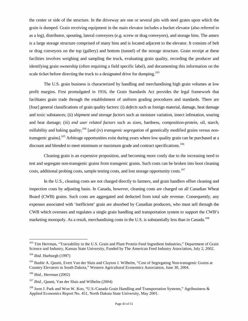
Page 43 of 51

the center or side of the structure. In the driveway are one or several pits with steel grates upon which the

grain is dumped. Grain receiving equipment in the main elevator includes a bucket elevator (also referred to

as a leg), distributor, spouting, lateral conveyors (e.g. screw or drag conveyors), and storage bins. The annex

is a large storage structure comprised of many bins and is located adjacent to the elevator. It consists of belt

or drag conveyors on the top (gallery) and bottom (tunnel) of the storage structure. Grain receipt at these

facilities involves weighing and sampling the truck, evaluating grain quality, recording the producer and

identifying grain ownership (often requiring a field specific label), and documenting this information on the

scale ticket before directing the truck to a designated drive for dumping.103

The U.S. grain business is characterized by handling and merchandising high grain volumes at low

profit margins. First promulgated in 1916, the Grain Standards Act provides the legal framework that

facilitates grain trade through the establishment of uniform grading procedures and standards. There are

[four] general classifications of grain quality factors: (i) defects such as foreign material, damage, heat damage

and toxic substances; (ii) shipment and storage factors such as moisture variation, insect infestation, souring

and heat damage; (iii) end user related factors such as sizes, hardness, composition-protein, oil, starch,

millability and baking quality;104 [and (iv) transgenic segregation of genetically modified grains versus non-

transgenic grains].105 Arbitrage opportunities exist during years where low quality grain can be purchased at a

discount and blended to meet minimum or maximum grade and contract specifications.106

Cleaning grain is an expensive proposition, and becoming more costly due to the increasing need to

test and segregate non-transgenic grains from transgenic grains. Such costs can be broken into boot cleaning

costs, additional probing costs, sample testing costs, and lost storage opportunity costs.107

In the U.S., cleaning costs are not charged directly to farmers, and grain handlers offset cleaning and

inspection costs by adjusting basis. In Canada, however, cleaning costs are charged on all Canadian Wheat

Board (CWB) grains. Such costs are aggregated and deducted from total sale revenue. Consequently, any

expenses associated with ‘inefficient’ grain are absorbed by Canadian producers, who must sell through the

CWB which oversees and regulates a single grain handling and transportation system to support the CWB’s

marketing monopoly. As a result, merchandising costs in the U.S. is substantially less than in Canada.108

103 Tim Herrman, “Traceability in the U.S. Grain and Plant Protein Feed Ingredient Industries,” Department of GrainScience and Industry, Kansas State University, Funded by The American Feed Industry Association, July 2, 2002.

104 Ibid. Hurburgh (1997)

105 Bashir A. Qasmi, Evert Van der Sluis and Clayton J. Wilhelm, “Cost of Segregating Non-transgenic Grains atCountry Elevators in South Dakota,” Western Agricultural Economics Association, June 30, 2004.

106 Ibid., Herrman (2002)

107 Ibid., Qasmi, Van der Sluis and Wilhelm (2004)

108 Joon J. Park and Won W. Koo, “U.S./Canada Grain Handling and Transportation Systems,” Agribusiness &Applied Economics Report No. 451, North Dakota State University, May 2001.

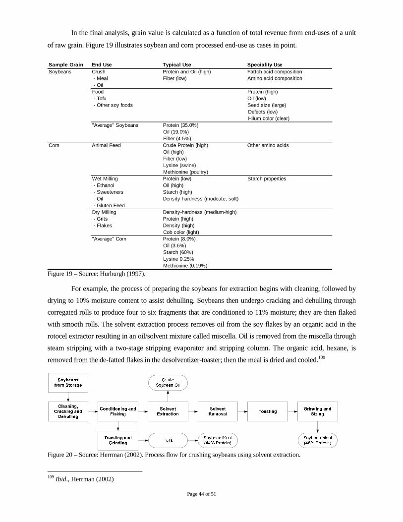
Page 44 of 51

In the final analysis, grain value is calculated as a function of total revenue from end-uses of a unit

of raw grain. Figure 19 illustrates soybean and corn processed end-use as cases in point.

Sample Grain End Use Typical Use Speciality Use

Soybeans Crush Protein and Oil (high) Fattch acid composition

- Meal Fiber (low) Amino acid composition

- Oil

Food Protein (high)

- Tofu Oil (low)

- Other soy foods Seed size (large)

Defects (low)

Hilum color (clear)

"Average" Soybeans Protein (35.0%)

Oil (19.0%)

Fiber (4.5%)

Corn Animal Feed Crude Protein (high) Other amino acids

Oil (high)

Fiber (low)

Lysine (swine)

Methionine (poultry)

Wet Milling Protein (low) Starch properties

- Ethanol Oil (high)

- Sweeteners Starch (high)

- Oil Density-hardness (modeate, soft)

- Gluten Feed

Dry Milling Density-hardness (medium-high)

- Grits Protein (high)

- Flakes Density (high)

Cob color (light)

"Average" Corn Protein (8.0%)

Oil (3.6%)

Starch (60%)

Lysine 0.25%

Methionine (0.19%)

Figure 19 – Source: Hurburgh (1997).

For example, the process of preparing the soybeans for extraction begins with cleaning, followed by

drying to 10% moisture content to assist dehulling. Soybeans then undergo cracking and dehulling through

corregated rolls to produce four to six fragments that are conditioned to 11% moisture; they are then flaked

with smooth rolls. The solvent extraction process removes oil from the soy flakes by an organic acid in the

rotocel extractor resulting in an oil/solvent mixture called miscella. Oil is removed from the miscella through

steam stripping with a two-stage stripping evaporator and stripping column. The organic acid, hexane, is

removed from the de-fatted flakes in the desolventizer-toaster; then the meal is dried and cooled.109

Figure 20 – Source: Herrman (2002). Process flow for crushing soybeans using solvent extraction.


Page 45 of 51

Corn used for food, feed and industrial purposes is subject to wet milling, while the remainder is

dry-milled for alcohol/ethanol production and masa production. Corn processed in wet milling is typically

separated into five components that include starch, germ, gluten, fiber, and steep liquor. In the past decade,

expanding ethanol production has boosted corn consumption and production of co-products.110

An alternative use of agricultural feedstock is the production of polymeric materials, e.g., plastics

and chemicals such as coatings and composites. Polymers from renewable resources have attracted an

increasing amount of attention over the last two decades, predominantly due to environmental concerns and

realization that petroleum resources are finite. Generally, polymers from renewable resources (PFRR) can

be classified into three groups: (i) natural polymers, such as starch, protein and cellulose; (ii) synthetic

polymers from natural monomers, such as polylactic acid (PLA); and (iii) polymers from microbial

fermentation, such as polyhydroxybutyrate (PHB). Like numerous other petroleum-based polymers, many

properties of PFRR can also be improved through blending and composite formation.111

A byproduct of agribusiness activities are emissions. Agricultural emissions are defined as those

resulting from the growing of crops, the rearing of livestock and the various ways in which soil is managed

to maximize crop and livestock production. The United Nations Framework Convention on Climate Change

(UNFCCC) holds that inventories account only for anthropogenic (human-induced) emissions. For some

emissions sources, notably some of those categorized as agricultural emissions, the distinction between

anthropogenic and non-anthropogenic is a relatively fine one. Similarly, under UNFCCC, agricultural

emissions do not include emissions from fuel used in agriculture as this falls under energy emissions.112

Agricultural subsidies can also be considered a form of merchandising. In the U.S., the Farm Act

categorizes government programs into four broad types. (1) Direct or fixed payments based on historical

cropping patterns on a fixed number of enrolled acres, and not linked to the operator's current decisions on

what to produce and when to market farm output. (2) Countercyclical payments, loan deficiency payments,

marketing loan gains, and certificate gains that depend on current market prices for enrolled commodities.

(3) Payments made on behalf of the Conservation Reserve Program, Environmental Quality Incentives

Program, and the Conservation Security Program. (4) Payments made by emergency and disaster relief

programs, and small miscellaneous programs such as the peanut and tobacco buyout programs.113


111 Long Yu, Katherine Dean, Lin Li, “Polymer blends and composites from renewable resources,” CommonwealthScientific and Industrial Research Organization, Australia; Centre for Polymer from Renewable Resources, SouthChina University of Technology, China; Prog. Polym. Sci. 31 (2006) 576–602.

112 Hugh Saddler and Helen King, “Agriculture and Emissions Trading; The Impossible Dream?” The AustraliaInstitute, Discussion Paper Number 102, October 2008.

113 Source: United States Department of Agriculture, Economic Research Service, “Farms Receiving GovernmentPayments,” http://www.ers.usda.gov/topics/farm-economy/farm-sector-income-finances/farms-receiving-government-payments.aspx Last updated: Saturday, May 26, 2012; Accessed July 30, 2012.

Page 46 of 51

Figure 21 illustrates how farm subsidies have remained high even in years of near record profits.

Figure 21 – Source: The Washington Post, July 2, 2006. Graphic: Cohen, Morgan and Stanton.

Financing Considerations

The Farm Credit System (FCS)114 and the commercial banking system have historically provided the

bulk of agricultural loans extended to farm borrowers. Other institutional sources of farm credit include the

Farm Service Agency (FSA)115 and life insurance companies. The farm loan guarantee scheme introduces a

third party in the lender-borrower relationship. A government sponsored farm loan guarantee scheme enables

farmers to avail of loans that without a guarantee would have been highly improbable to obtain.

The following provides a high level review of lending programs available to agribusinesses:

The FSA’s farm lending program involves both direct and guaranteed loans to family farmers and

ranchers to purchase farmland and finance agricultural production. Its mission includes stabilizing farm

income, helping farmers conserve land and water resources, providing credit to new or disadvantaged

farmers and ranchers, and helping farm operations recover from the effects of disaster.

The Rural Development Program of the USDA has legislative authority to implement its Business

and Industry Direct and Guaranteed Loan Programs. This program is designed to expand the availability of

credit for businesses that do not qualify for conventional bank financing in certain rural areas suffering from

fundamental and economic stress. Its primary purpose is to finance industry and employment, and improve

economic and environmental concerns in rural communities, including pollution abatement and control.

While the Small Business Administration (SBA) does not provide direct loans or grants to small

businesses, the SBA supports other organizations that provide loans, management training and services for

small businesses. The majority of SBA’s financial assistance is in the form of loan guarantees.

All but eleven states offer at least one agricultural loan program with some offering several. They

range from loans for “beginning” farmers, to disaster recovery loans, to short-term loans for getting through a

difficult season, to lines of credit for leasing equipment. One program of note is the Aggie Bond Beginning

114 The Farm Credit System (FCS) is a federally chartered network of cooperatives and related service organizationsthat lends to agricultural producers, rural homeowners, farm-related businesses, and public utility cooperatives in theUnited States. Congress established FCS as a government sponsored enterprise when it enacted the Federal Farm LoanAct in 1916. Current authority is in the Farm Credit Act of 1971 (P.L. 92-181, as amended; 12 U.S.C. 1200 et seq.).

115 Farm Service Agency (FSA) is a USDA agency which merged several predecessor agencies, including the AgriculturalStabilization and Conservation Service, the Federal Crop Insurance Corporation, and Farmers Home Administration.The Administrator reports to the Under Secretary of Agriculture for Farm and Foreign Agricultural Services.

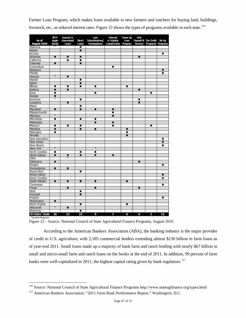
Page 47 of 51

Farmer Loan Program, which makes loans available to new farmers and ranchers for buying land, buildings,

livestock, etc., at reduced interest rates. Figure 22 shows the types of programs available in each state.116

Figure 22 – Source: National Council of State Agricultural Finance Programs, August 2010.

According to the American Bankers Association (ABA), the banking industry is the major provider

of credit to U.S. agriculture, with 2,185 commercial lenders extending almost $130 billion in farm loans as

of year-end 2011. Small loans made up a majority of bank farm and ranch lending with nearly $67 billion in

small and micro-small farm and ranch loans on the books at the end of 2011. In addition, 99 percent of farm

banks were well-capitalized in 2011, the highest capital rating given by bank regulators.117

116 Source: National Council of State Agricultural Finance Programs http://www.stateagfinance.org/types.html117 American Bankers Association, “2011 Farm Bank Performance Report,” Washington, D.C.

Page 48 of 51

Another form of farm financing is a standby letter of credit, which guarantees that farm operators will

pay a seller of products or services in full and on time, as sellers typically get paid after delivering the agreed

upon goods or completing work. Letters of credit are also issued to fulfill state government’s requirement that

a performance bond be posted for agricultural commodity dealer/commodity warehouse license applications.

Letters are written for specific periods of time, usually less than one year, and can be structured as part of a

commercial loan or line of credit. Unlike loans, letters of credit carry a fee paid on a quarterly or annual basis,

whether they are drawn on or not. In addition, commodity futures exchanges may accepts letters of credit

from approved banks. CME Clearing, for example, allows letters of credit issued in the Exchange’s name by

approved banks to be used for “100% of concentration requirement” subject to CME Rule 930.C.118/119

The issuance of standby letters of credit directly relates to concerns about managing counterparty

risk. Recognizing and controlling counterparty risk is essential in today’s marketplace. For example, a farm

operation prepays for fertilizer for the year and the supplier goes out of business without delivering; a

rancher ships young heifers to be raised and the landowner evicts the raiser and sells the calves to pay for

rent; or a biofuel plant contracts for silage from a local farm and the farmer fails to harvest in time. In

addition to volatile market price swings, drought, disease, fraud, and other unforeseen disasters all compound

the risk to an enterprise’s ongoing viability, while also magnifying the risk of counterparty default.

Of significant import with respect to credit risk and defaults are changes to the Bankruptcy Code in

2005 involving Chapter 11 bankruptcies. Harvard Law School Professor Roe noted that “Chapter 11 bars

bankrupt debtors from immediately repaying their creditors, so that the bankrupt firm can reorganize

without creditors’ cash demands shredding the bankrupt’s business. Not so for the bankrupt’s derivatives

counterparties, who, unlike most other secured creditors, can seize and immediately liquidate collateral,

readily net out gains and losses in their dealings with the bankrupt, terminate their contracts with the

bankrupt, and keep both preferential eve-of-bankruptcy payments and fraudulent conveyances they obtained

from the debtor, all in ways that favor them over the bankrupt’s other creditors.”120 MF Global, which filed

bankruptcy on October 31, 2011,121 has become a case study in regards to Professor Roe’s concerns.122

118 Source: http://www.cmegroup.com/clearing/financial-and-collateral-management/#lettersCredit Retrieved 7/30/12.119 Source: http://www.cmegroup.com/clearing/financial-and-collateral-management/list-of-approved-banks.html120 Mark J. Roe, “The Derivatives Market’s Payment Priorities as Financial Crisis Accelerator,” Harvard LawSchool, Roe-62 Stan. L. Rev. 539, March 6, 2011.121 Michael J. De La Merced and Ben Protess, “MF Global Files for Bankruptcy,” The New York Times Company,DealBook, October 31, 2011.122 “The CEA explicitly requires that FCMs treat and deal with all customer funds as belonging to such customers andthat customer funds “shall be separately accounted for and shall not be commingled with [FCM] funds.” Title 7 U.S.C.§ 6d(a)(2). Any entity that has received, or through which such funds have passed, ought to have the same duties. See,e.g., Title 17 C.F.R. § 190.08(a)(ii)(F) (customer property includes property that has been converted); see also Smith v.M&M Commodities, Inc. (1987) (finding that obligation to segregate customer funds and not to commingle them underTitle 7 U.S.C. § 6d creates a statutory, technical trust under the Bankruptcy Code).” Source: In re: MF Global Holdings,Ltd, et al., Chapter 11, Case No. 11-15059 (MG); In re: MF Global, Inc., Jointly Administered, Case No. 11-02790(MG) (SIPA); Response of the Commodity Customer Coalition to Trustee’s Memorandum Regarding the LegalPrinciples and Framework for the Allocation and Distribution of Customer Property; Doc 819, Filed 01/09/12.

Page 49 of 51

When entering into derivatives transactions to manage risk, commercial hedgers are required to put

up margin (i.e., good faith deposit) or pledge collateral, albeit at lower hedger requirements than speculators.

The term collateral management refers to a diverse range of activities involving the optimal use of eligible

assets to cover collateral calls. A related idea is collateral transformation which refers to the process whereby

an institution will transform non-eligible assets into eligible assets to enable a firm to meet its margin

requirements.123 One of the issues facing farms and grain companies that use futures to hedge their physical

inventory is how to cope with margin calls. Futures are marked-to-market daily whereas physical inventory

does not produce a cash event until sold. In response the industry developed repurchase agreements whereby

grain remains in storage during the transaction and only the warehouse receipts exchange hands. The

warehouse receipts serve as collateral and helps eliminate the risk of margin calls while providing funds

which can be used for working capital or other needs. Note: there is a net cost for this transaction.

An alternative method for agribusinesses to hedge risk is through crop insurance. Farmers and

ranchers use insurance to protect against either the loss of crops due to natural disasters, such as hail, drought,

and floods, or the loss of revenue due to declines in the prices of agricultural commodities. The two general

categories of crop insurance are crop-yield and crop-revenue. These include several kinds of federally

facilitated, but privately delivered, yield and revenue policies. There are also policies, such as hail insurance,

provided by the private sector without subsidy. Crop insurance warrants consideration as a financial

management tool in cases where (i) high debt to asset ratios limit the farmer’s ability to self insure and acts

like a substitute for equity; or (ii) a farm has a moderate to low debt to asset ratio but the owner prefers a

more predictable revenue stream versus relying on self-insurance.124 As insurance and derivatives are

competing tools for managing risk, farm operators should be well versed in the features of the insurance

being considered, as well as financial calculations so as to make appropriate cost-benefit decisions.

Last, but not least, farm operations must manage GAAP accounting including accounts receivables,

accounts payable, bank reconciliation, multi-currency accruals (if applicable), financial reporting, as well as

ensure compliance (e.g., Sarbanes-Oxley). The physical transaction side involves deal capture, invoicing,

settlement and tracking secondary costs such as transportation, tariffs and fees; while the financial side

involves clearing and settlement, and compliance with hedge accounting standards [e.g., AASB 139, ASC

815 (FAS 133), ASC 815-10 (FAS 161), CICA 3865, IAS 39 vs. IFRS 9, and SAS 133]. One consideration is

marked-to-market valuation versus accrual accounting, and “understanding how a marked-to-market profit

actually gets booked on an accrual basis.”125 Another aspect is position keeping in which physical and financial

positions are matched/offset, as well as risk analytics such as forecasting earnings and “what-if” scenarios.

Activities include classifying hedges as cash flow or fair value versus economic as discussed in this paper.

123 Nick Newport and Ted Allen, “Collateral Optimization – Your Questions Answered,” DerivSource, May 28, 2012.

124 Ben Chaffin, J. Roy Black and Xiaobin Cao, “Crop Yield Insurance: Choosing between Policies That Trigger onFarm Yields vs. County Yields,” Department of Agricultural Economics, Michigan State University, Staff Paper2004-30, December 2004.

125 CommodityPoint, CTRM Software Sourcebook, UtiliPoint International, May 2011, Ver. 3, p. 14.

Page 50 of 51

References:

Aoki, Masanao (1998). New Approaches to Macroeconomic Modeling: Evolutionary Stochastic Dynamics,Multiple Equilibria, and Externalities as Field Effects, Cambridge University Press, Feb. 1998, p. 3.

Baldwin, E. Dean (1986). “Understanding and Using Basis – Grains,” Department of Agricultural Economics,Ohio State University, NCR Extension Publication No. 217, December 1986.

Brennan, M. (1958). “The Supply of Storage,” American Economic Review, 47(1), pp 50-72.

Calvo, Guillermo and Mendoza, Enrique (2000). “A Rational Contagion and the Globalization of SecuritiesMarkets,” Journal of International Economics, Vol. 51, p 79.

Colander, David; Howitt, Peter; Kirman, Alan; Leijonhufvud, Axel and Mehrling, Perry (2008). “Beyond DSGEModels: Toward an Empirically Based Macroeconomics,” American Economic Review, American EconomicAssociation, 98(2), May 2008, pp 236-240.

Debreu, Gerard (1974). “Excess Demand Functions,” Journal of Mathematical Economics, 1, pp 15-21.

Durkin, Bryan (2010). “The Impact of Algorithmic and High Frequency Trading on CME Group Inc. Markets,”CFTC Technology Advisory Committee, July 14, 2010.

Evans, Joan and Mahoney, James M. (1996). “The Effects of Daily Price Limits on Cotton Futures and OptionsTrading,” Federal Reserve Bank of New York, Research Paper No. 9627, August 1996, pp 4-5.

Guesnerie, Roger (1992). “An Exploration of the Eductive Justifications of the Rational Expectations Hypothesis,”American Economic Review, 82(85), pp 1254-1278.

Gunzberg, Jodie and Till, Hilary (2005). “Absolute Returns in Commodity (Natural Resource) FuturesInvestments,” EDHEC Risk and Asset Management Research Centre.

Hajdasinski, M. (1995). “Remarks in the context of the case for the generalized net present value formula,” TheEngineering Economist 40(2), 1995, 201-210.

Hernandez, M. and Maximo, T. (2010). “Examining the Dynamic Relationship between Spot and Future Pricesof Agricultural Commodities,” IFPRI Discussion Paper 00988, June 2010.

Hicks, John R. (1939, 1946). Value and Capital: An Inquiry into Some Fundamental Principles of EconomicTheory, Oxford: Clarendon Press, 1939; revised second edition, 1946.

Janssen, Maarten C. W. (1993). Microfoundations: A Critical Inquiry, London: Routledge, p 142.

Janssen, Maarten C. W. (2006). “Microfoundations” Tinbergen Institute Discussion Paper, TI 2006-041/1.

Julien, Ludovic A. and Tricou, Fabrice (2006). “A note on price-taking and price-making behaviours in generalequilibrium oligopoly models,” EconomiX Conference, Université Paris X-Nanterre, France, July 24, 2006.

Kaldor, Nicholas (1939). “Speculation and Economic Stability” Review of Economic Studies, 7(1), pp 1-27.

Kaldor, Nicholas (1972). “The Irrelevance of Equilibrium Economics” The Economic Journal, Vol. 82 No. 328,pp 1237-1255.

Keynes, John Maynard (1923). “Some Aspects of Commodity Markets,” Manchester Guardian.

Keynes, John Maynard (1930). A Treatise on Money, Volume II: The Applied Theory of Money, London:Macmillan, 1930, pp 142-147.

Keynes, John Maynard (1937). “General Theory of Employment,” Quarterly Journal of Economics, CollectedWorks of John Maynard Keynes (CWK, 1973), vol. XIV, pp 109-223.

Köszegi, Botond, Madarász, Kristóf and Matolcsi, Máté (2007). “A Failure of the No-Arbitrage Principle,”University of California Berkeley, Rényi Institute of Mathematics, Budapest, July 2007.

Lilliston, Ben and Ranallo, Andrew (2011). “Excessive Speculation in Agriculture Commodities: SelectedWritings from 2008–2011,” Institute for Agriculture and Trade Policy, April 2011.

Mantel, Rudolf (1974). “On the Characterization of Excess Demand,” Journal of Economic Theory, 7,pp 348-353.

Page 51 of 51

McKissick, John and Shumaker, George (1991). “Understanding and Using the Basis,” University of GeorgiaCollege of Agricultural and Environmental Sciences, Bulletin 981/Revised February 1991.

Muth, John F. (1961). “Rational Expectations and the Theory of Price Movements,” Econometrica, 29(3), July1961, pp 315-335.

Pearson, Charlie (2006). “Basis – How Cash Grain Prices are Established,” Alberta Agriculture and RuralDevelopment, Provincial Crops Market Analyst. Published July 21, 2006; revised on August 4, 2011.

Ritter, Elizabeth L. (2005). “The Securitization of Commodities: Crossing a Gold (or Silver) Line in the Sand,”Business Law Brief, Fall 2005.

Rostek, Marzena and Weretka, Marek (2009). “Dynamic Thin Markets,” University of Wisconsin-Madison,Department of Economics, August 11, 2009

Rubenstein, Mark (2006). A History of the Theory of Investments, Publisher: Wiley Finance.

Shull, D. M. (1992). “Efficient capital project selection through a yield-based capital budgeting technique,” TheEngineering Economist 38(1), 1992, 1-18.

Sonnenschein, Hugo F. (1973). “Do Walras Identity and Continuity Characterize the Class of Community ExcessDemand Functions?” Journal of Economic Theory, 6, pp 345-354.

Spurgin, Richard (2000). “Some Thoughts on the Source of Return to Managed Futures,” Draft Article, ClarkUniversity and CISDM.

Telser, L.G. (1958). “Futures Trading and the Storage of Cotton and Wheat,” Journal of Political Economy, 66,pp 223-255.

Till, Hilary (2007). “Part I of A Long-Term Perspective on Commodity Futures Returns: Review of HistoricalLiterature,” Intelligent Commodity Investing,” (Till, and Eagleeye, Ed.), London: Risk Books, pp 39-82.

Working, Holbrook (1948). “Theory of the Inverse Carrying Charge in Futures Markets,” Journal of FarmEconomics, 30(1), pp 1-28.

Working, Holbrook (1949). “The Theory of Price of Storage,” American Economic Review, 39(6), December1949, pp 1254-1262.

Segmenting Supply Chain Risk Using E/CTRM Systems Unifying Theory of Commodity Hedging and Arbitrage Segmenting Supply Chain Risk Using E/CTRM Systems Unifying Theory of Commodity

Documents