Sediment Fingerprinting to Delineate Sources of Sediment in ...

Sediment Fingerprinting to Delineate Sources of Sediment in the Agricultural and

Forested Smith Creek Watershed, Virginia, USA

A.C. Gellis and L. Gorman Sanisaca

Research Impact Statement: Sediment fingerprinting helps identify and apportion sediment sources, includ-ing sediment derived from top soil and eroding streambanks, which are often overlooked sources of sediment tostreams.

ABSTRACT: The sediment fingerprinting approach was used to apportion fine-grained sediment to cropland,pasture, forests, and streambanks in the agricultural and forested Smith Creek, watershed, Virginia. SmithCreek is a showcase study area in the Chesapeake Bay watershed, where management actions to reduce nutri-ents and sediment are being monitored. Analyses of suspended sediment at the downstream and upstream sam-pling sites indicated streambanks were the major source of sediment (76% downstream and 70% upstream).Current management strategies proposed to reduce sediment loadings for Smith Creek do not target stream-banks as a source of sediment, whereas the results of this study indicate that management strategies to reducesediment loads in Smith Creek may be effective if directed toward managing streambank erosion. The results ofthis study also highlight the utility of sediment fingerprinting as a management tool to identify sedimentsources.

(KEYWORDS: sediment fingerprinting; bank erosion; Chesapeake Bay; sediment TMDL.)

INTRODUCTION

Worldwide, sediment is an important pollutantdegrading aquatic habitat and impacting infrastruc-ture, such as reservoirs (Strayer and Dudgeon 2010;Liu et al. 2017). In the United States (U.S.), sedimentis one of the leading causes of stream impairment(USEPA 2017). Fine sediment can reduce light pene-tration and suppress primary production in algae andmacrophytes (Yamada and Nakamura 2002; Izagirreet al. 2009; Jones et al. 2012). Deposited sedimentcan bury channel substrate and degrade habitat formacroinvertebrates (Jones et al. 2012) and fish (Searet al. 2016). In addition, fine sediment provides atransport vector for bound nutrients, heavy metals,

and other contaminants (Owens et al. 2001; Gerbers-dorf et al. 2011).

Sediment is a major contributor to ecologicaldegradation in Chesapeake Bay (Gellis and Brakebill2013). Smith Creek, along with two other streams inthe Chesapeake Bay watershed, was selected by theU.S. Department of Agriculture as a “showcase”study area, meaning that if successfully restored, itwould become a model for restoration efforts in theChesapeake Bay watershed (Epes 2010; Jenner 2010;USDA-NRCS 2017). Biological monitoring conductedby the Virginia Department of Environmental Qual-ity indicated Smith Creek was violating the state’sgeneral standard for aquatic life use where thestream should support the propagation and growth ofa balanced indigenous population of aquatic life

Paper No. JAWRA-17-0153-P of the Journal of the American Water Resources Association (JAWRA). Received November 28, 2017;accepted July 19, 2018. © 2018 American Water Resources Association. This article is a U.S. Government work and is in the public domainin the USA. Discussions are open until six months from issue publication.

Maryland-Delaware-DC Water Science Center (Gellis, Gorman Sanisaca), U.S. Geological Survey, Baltimore, Maryland, USA (Correspon-dence to Gellis: [email protected]).

Citation: Gellis, A.C., and L. Gorman Sanisaca. 2018. “Sediment Fingerprinting to Delineate Sources of Sediment in the Agricultural andForested Smith Creek Watershed, Virginia, USA.” Journal of the American Water Resources Association 1–25. https://doi.org/10.1111/1752-1688.12680.

JOURNAL OF THE AMERICAN WATER RESOURCES ASSOCIATION JAWRA1

JOURNAL OF THE AMERICAN WATER RESOURCES ASSOCIATION

AMERICAN WATER RESOURCES ASSOCIATION

https://doi.org/10.1111/1752-1688.12680

https://doi.org/10.1111/1752-1688.12680

(VADEQ 2009). The primary stressor on the aquaticcommunity was identified as sediment. In 2004, aTotal Maximum Daily Load (TMDL) was developedfor Smith Creek to reduce sediment loadings (VADEQ2009). The successful mitigation of sediment-relatedimpairments requires knowledge of the contributionof sediment from its various sources.

Attempting to relate sediment to its sources is adifficult task. Approaches for estimating sedimentsources include sediment budget studies (Gellis andWalling 2011; Gellis et al. 2016), geographic informa-tion system (GIS) and photogrammetric analysis (Fer-nandez et al. 2003; Curtis et al. 2005; Roering et al.2013; Hackney and Clayton 2015; Gellis et al. 2016),models (Aksoy and Cavvas 2005; USEPA 2008), andthe use of geochemical tracers or fingerprints (Wall-ing 2005; Gellis and Walling 2011; Mukundan et al.2012; Collins et al. 2017). Each of these approacheshas its advantages and disadvantages. Sediment bud-get approaches often rely on field measurements,which can provide useful data on erosion and deposi-tion rates, but are labor intensive, and can be spa-tially limited. Photogrammetry/GIS analysis andmodel analysis, although less intensive in terms oflabor and time, may produce a wide range of resultsthat need to be validated with data collected from thewatershed of interest. Ground-based and airbornelidar, as well as structure-from-motion photogramme-try with handheld cameras and unmanned aerial sys-tems (drones), are being increasingly used to describechannel morphology and topographic change (Fauxet al. 2009; Caroti et al. 2013; Roering et al. 2013;Caroti et al. 2015). The resultant scans, point clouds,and digital elevation maps can be overlain chronologi-cally to quantify the erosion and deposition of variouschannel sources. However, these techniques oftenrequire field validation and the representation ofmorphological elements requires a high point densitywith large data processing demands. In addition, res-olution and scale may restrict the applicability ofthese techniques to quantify topsoil erosion and ulti-mately do not quantify the delivery of these sedimentsources out of the watershed.

Sediment fingerprinting is an approach that hasbeen increasingly utilized to assist managers in identi-fying sources of sediment in a watershed (Collins,Walling, et al. 2010; Mukundan et al. 2012; Milleret al. 2015; Collins et al. 2017). The sediment finger-printing approach entails the identification of specificsediment sources through the establishment of a mini-mal set of physical and (or) chemical properties thatuniquely define each source in the watershed. In gen-eral, sediment fingerprinting results can provide infor-mation on the relative contribution of upland (soilerosion from various land use and land cover types)vs. channel contributions (streambanks and channel

beds) (Gellis and Walling 2011; Gellis et al. 2016). Dif-ferentiating between these two broad categories (up-land and channel sources) is important becausesediment-reduction management strategies differ bysource and require very different approaches — reduc-ing agricultural sources may involve soil conservationand tilling practices, whereas reducing channel sourcesof sediment may involve stream restoration, bank stabi-lization, and (or) grade control to arrest downcutting.The objective of this study was to identify the relativecontributions of sediment from cropland, pasture, for-est, and streambanks in the Smith Creek watershedusing the sediment fingerprinting approach.

MATERIALS AND METHODS

Study Area

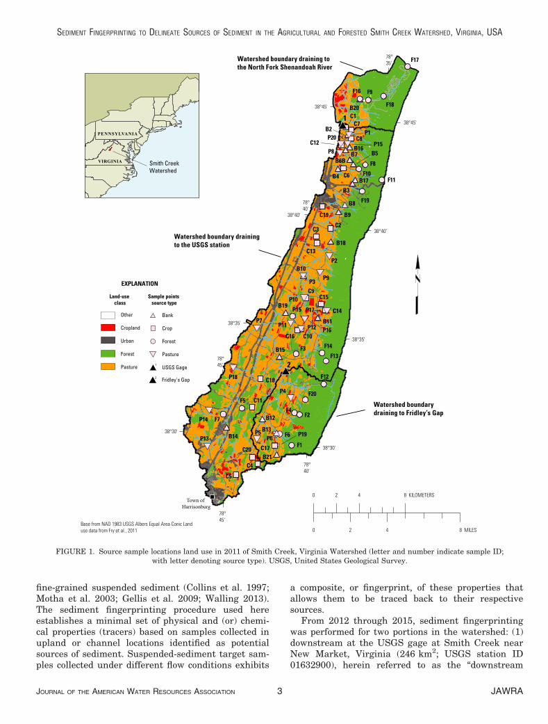
Smith Creek drains the Valley and Ridge Provincein the Chesapeake Bay watershed, with land use inthe area draining to the downstream station (in2011) consisting of forest, 48%; pasture, 41%; devel-oped, 8%; and cropland, 3% (Figure 1) (Homer et al.2015). The area draining to the downstream stationis underlain by dolostone and limestone (66%) andsandstone and shale (34%) (Dicken et al. 2005). Ele-vations range from 270 m at the lower reaches to890 m in the Massanutten Mountains on the easternside of the watershed. In the area draining to theupstream station, land use in 2011 was crop 2%; pas-ture 30%; forest 66%; and other 2% (Homer et al.2015), and bedrock is 58% dolostone/limestone and42% sandstone/shale (Dicken et al. 2005). Averageannual daily discharge recorded at the U.S. Geologi-cal Survey (USGS) gage, 1961–2016, was 2.14 m3/s(USGS 2016). Precipitation in the watershed mea-sured at the Dale Enterprise rain station near Har-risonburg, Virginia, averaged 915 mm/yr withtemperatures ranging from a July mean of 23°C to aJanuary mean of 0.44°C (University of North Caro-lina 2012). Most portions of Smith Creek are mean-dering, pool-riffle systems on gravel to sand bedswith occasional bedrock outcrops. Varying thick-nesses of sediment in channel storage (on the channelbed) were observed at select reaches, most noticeablyin pools. Fine sediment was also present within theinterstitial coarse substrate.

The Sediment Fingerprinting Approach

The sediment fingerprinting approach provides adirect method for quantifying watershed sources of

JAWRA JOURNAL OF THE AMERICAN WATER RESOURCES ASSOCIATION2

GELLIS AND GORMAN SANISACA

fine-grained suspended sediment (Collins et al. 1997;Motha et al. 2003; Gellis et al. 2009; Walling 2013).The sediment fingerprinting procedure used hereestablishes a minimal set of physical and (or) chemi-cal properties (tracers) based on samples collected inupland or channel locations identified as potentialsources of sediment. Suspended-sediment target sam-ples collected under different flow conditions exhibits

a composite, or fingerprint, of these properties thatallows them to be traced back to their respectivesources.

From 2012 through 2015, sediment fingerprintingwas performed for two portions in the watershed: (1)downstream at the USGS gage at Smith Creek nearNew Market, Virginia (246 km2; USGS station ID01632900), herein referred to as the “downstream

Watershed boundary draining tothe North Fork Shenandoah River

Watershed boundary drainingto the USGS station

Watershed boundarydraining to Fridley’s Gap

Bank

Crop

Forest

Pasture

Other

Cropland

Urban

Forest

Pasture

Sample points source type

Land-use class

EXPLANATION

F9

C1C7

P1B2

C8P20P15

B16P8 B7B6B

F11

F8

B5

B4 C6B17

F10

F19

B3

C19 B9

C2C3

B18

P2

C13

P9P3

B10

C9P10 C15

P17

B13

B19C14

P16

P15

P12P11

C16 C10

P7

F14

F13

F12

F3B15

C18P18

F20P4

F4F2

F7P14

F5 C11

B12

B14P13

C20

P5P6

F1

C5

C4B21

C17

F6 P19

B8

F17

F18B20

F16

C12

B11

38°45'

38°40'

38°35'

38°30'

78°45'

38°45'

38°40'

38°35'

38°30'

78°45'

78°40'

78°40'

78°35'

0 4 8 MILES2

0 4 8 KILOMETERS2

Base from NAD 1983 USGS Albers Equal Area Conic Land use data from Fry , 2011

Smith CreekWatershed

FIGURE 1. Source sample locations land use in 2011 of Smith Creek, Virginia Watershed (letter and number indicate sample ID;with letter denoting source type). USGS, United States Geological Survey.


SEDIMENT FINGERPRINTING TO DELINEATE SOURCES OF SEDIMENT IN THE AGRICULTURAL AND FORESTED SMITH CREEK WATERSHED, VIRGINIA, USA

station” and (2) upstream at Fridley’s Gap located ata point midway in the watershed (44.4 km2), hereinreferred to as the “upstream station” (Figure 1). Thesediment fingerprinting approach has been used in sev-eral watersheds of varying scales and land uses drain-ing the Chesapeake Bay watershed (Table 1). Previoussediment fingerprinting results for these watershedsindicate that sediment sources vary spatially and tem-porally, partly as a result of land use changes overtime, geology, storm factors, and sediment storage (Gel-lis et al. 2009; Gellis et al. 2015). Using this knowl-edge, we designed our sampling to account forvariability in land use and geology in order to deter-mine the sediment contribution from each source.

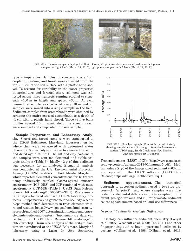
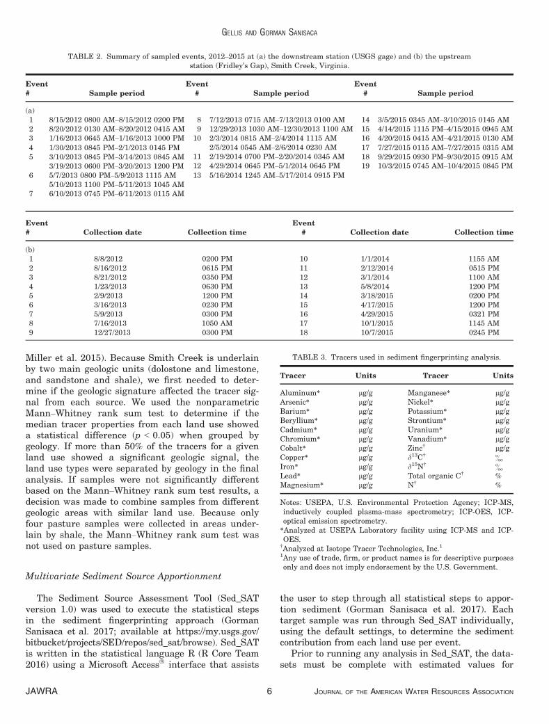
Target Samples. At both the downstream andupstream sampling stations, target samples of sus-pended sediment were collected during storm eventsin Smith Creek using a passive sampler (Phillipset al. 2000) (Figures 2 and 3). At both sampling sta-tions, two 120 cm length, 10 cm diameter PVC tubeswere each mounted on channel struts that were ham-mered into the channel bed. At the time of installa-tion at the downstream station (January 20, 2012),water entered each PVC tube at a river stage of1.0 m (discharge ~7.4 m3/s). The channel struts wereoften damaged at the downstream station duringlarge runoff events and on March 27, 2013, each PVCtube was mounted on a tree on each side of thestream, approximately 50 m from each other, whereflow entered the samplers at a river stage of 1.2 m(discharge ~11.0 m3/s). Sediment was retrieved afteran event and composited from each tube into onesample. At the upstream station, two passive sam-plers were installed on May 8, 2012. The upstreamstation is not gaged and the discharge that starts tofill each tube was not determined. During the studyperiod, 19 storm events were sampled at the down-stream station (Table 2a) and 18 samples were col-lected at the upstream station (Table 2b). Otherstudies that have used the Phillips et al. (2000) pas-sive sampler design include: Gellis et al. (2017) forstreams in the Midwest U.S.; Pulley and Rowntree(2016) in South Africa; and Collins, Zhang, et al.(2010) in the United Kingdom.

Source Samples. Sediment source samples toapportion sediment at the downstream station werecollected from cropland (n = 20), pasture (n = 20),forest (n = 20), and streambanks (n = 22) (Figure 1).A subset of source samples from the Fridley Gapwatershed was used to apportion sediment at theupstream station: pasture (n = 16), cropland (n = 11),forest (n = 8), and streambanks (n = 8) (Figure 1).Samples were not collected from the 8% of the water-shed identified as developed, as most of this land use

TABLE

1.Summary

ofsedim

entfingerprintingstudiesconducted

intheChesapea

keBaywatershed

.

Stream

name

Drain

age

area,km

2

Land

use

,%

Sedim

entso

urceapportionment(%

)

Reference

Agriculture1

Forest

Urban

upland2

Urban

Agriculture1

Forest

Urban

upland2

Street

residue

Construction

sites

Drain

age

ditches

Streambanks

Pocom

okeRiver,

Maryland–D

elaware

156.7

52

46

NA

146

13

——

—34

71

Mattawom

an

Creek

,Maryland

134.5

18

60

NA

19

17

29

——

23

—31

1

LittleCon

estoga

Creek

,Pen

nsylvania

109.5

45

4NA

49

77

——

—0

—23

1

Anacostia

River,

Maryland–

Districtof

Columbia

189.0

00

NA

100

——

30

13

——

58

2

MillStrea

mBranch

,Maryland

31.6

74

22

NA

2—

——

——

—100

3,4

Linganore

Creek

,Maryland

147.0

62

27

NA

845

3—

——

—52

5

Difficu

ltRun,

Virginia

14.2

NA

NA

46

54

——

110

——

89

6

Note:

Referen

ces:

1:Gelliset

al.(2009);2:Dev

ereu

xet

al.(2010);3:Bankset

al.(2010);4:Massou

diehet

al.(2012);5:Gelliset

al.(2015);6:Cash

manet

al.(2018).

1Agricu

lture

includes

pasture,hay,andcrop

land.

2Urbanuplandincludes

areasdefi

ned

aspark

s,lawns,

andforest.



type is impervious. Samples for source analysis fromcropland, pasture, and forest were collected from thetop ~1.0 cm of the soil surface with a plastic hand sho-vel. To account for variability in the tracer propertiesat agriculture and forested sites, sediment was col-lected across three transects running parallel to slope,each ~100 m in length and spaced ~30 m. At eachtransect, a sample was collected every 10 m and allsamples were mixed into a single sample in the field.Sediment samples from streambanks were obtained byscraping the entire exposed streambank to a depth of~1 cm with a plastic hand shovel. Three to five bankprofiles spaced 10 m apart along the stream reachwere sampled and composited into one sample.

Sample Preparation and Laboratory Analy-sis. Source and target samples were transported tothe USGS Baltimore, Maryland laboratory on icewhere they were wet-sieved with de-ionized waterthrough a 63-lm polyester sieve to remove the sand,and dried again at 60°C. The silt and clay portions ofthe samples were sent for elemental and stable iso-topic analysis (Table 3). Ideally ~2 g of fine sedimentwas necessary for all analyses. Elemental analysiswas conducted at the U.S. Environmental ProtectionAgency (USEPA) facilities in Fort Meade, Maryland,which reported elemental concentrations for 18 tracersusing inductively coupled plasma-optical emissionspectrometry (ICP-OES) and ICP combined with massspectrometry (ICP-MS) (Table 3; USGS Data ReleaseSource, https://doi.org/10.5066/f7rn36q1). The elemen-tal analysis followed standard USEPA laboratory pro-tocols (https://www.epa.gov/homeland-security-research/epa-method-2008-determination-trace-elements-waters-and-wastes; https://www.epa.gov/homeland-security-research/method-2007-determination-metals-and-trace-elements-water-and-wastes). Supplementary data canbe found at USGS Data Release https://doi.org/10.5066/f7rn36q1. Grain size analysis of the <63-lm frac-tion was conducted at the USGS Baltimore, Marylandlaboratory using a Laser In Situ Scattering

Transmissometer (LISST-100X); (http://www.sequoiasci.com/wp-content/uploads/2013/07/manual-5.pdf). Med-ian values (D50) of the fine-grained sediment (<63-lm)are reported in the LISST software (USGS DataRelease; https://doi.org/10.5066/f7rn36q1).

Sediment Apportionment. The statisticalapproach to apportion sediment used a two-step pro-cess—(1) “a priori” test, where samples were firsttested for elemental differences due to sampling in dif-ferent geologic terrains and (2) multivariate sedimentsource apportionment based on land use differences.

“A priori” Testing for Geologic Differences

Geology can influence sediment chemistry (Pouyatet al. 2007; Woodruff et al. 2009; Tan 2011) and otherfingerprinting studies have apportioned sediment bygeology (Collins et al. 1998; D’Haen et al. 2013;

FIGURE 2. Passive samplers deployed at Smith Creek, Virginia to collect suspended sediment (left photo,sampler on right bank [March 24, 2015]; right photo, sampler on left bank [March 28, 2012]).

FIGURE 3. Flow hydrograph (15 min) for period of studyshowing sampled events (1 through 19) at the downstream

station (USGS gage, Smith Creek near New Market,Virginia; station ID 01632900).



https://doi.org/10.5066/f7rn36q1

https://www.epa.gov/homeland-security-research/epa-method-2008-determination-trace-elements-waters-and-wastes



https://www.epa.gov/homeland-security-research/method-2007-determination-metals-and-trace-elements-water-and-wastes





http://www.sequoiasci.com/wp-content/uploads/2013/07/manual-5.pdf

http://www.sequoiasci.com/wp-content/uploads/2013/07/manual-5.pdf


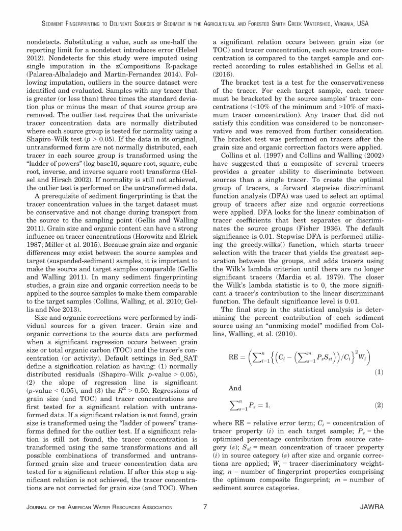
Miller et al. 2015). Because Smith Creek is underlainby two main geologic units (dolostone and limestone,and sandstone and shale), we first needed to deter-mine if the geologic signature affected the tracer sig-nal from each source. We used the nonparametricMann–Whitney rank sum test to determine if themedian tracer properties from each land use showeda statistical difference (p < 0.05) when grouped bygeology. If more than 50% of the tracers for a givenland use showed a significant geologic signal, theland use types were separated by geology in the finalanalysis. If samples were not significantly differentbased on the Mann–Whitney rank sum test results, adecision was made to combine samples from differentgeologic areas with similar land use. Because onlyfour pasture samples were collected in areas under-lain by shale, the Mann–Whitney rank sum test wasnot used on pasture samples.

Multivariate Sediment Source Apportionment

The Sediment Source Assessment Tool (Sed_SATversion 1.0) was used to execute the statistical stepsin the sediment fingerprinting approach (GormanSanisaca et al. 2017; available at https://my.usgs.gov/bitbucket/projects/SED/repos/sed_sat/browse). Sed_SATis written in the statistical language R (R Core Team2016) using a Microsoft Access� interface that assists

the user to step through all statistical steps to appor-tion sediment (Gorman Sanisaca et al. 2017). Eachtarget sample was run through Sed_SAT individually,using the default settings, to determine the sedimentcontribution from each land use per event.

Prior to running any analysis in Sed_SAT, the data-sets must be complete with estimated values for

TABLE 3. Tracers used in sediment fingerprinting analysis.

Tracer Units Tracer Units

Aluminum* lg/g Manganese* lg/gArsenic* lg/g Nickel* lg/gBarium* lg/g Potassium* lg/gBeryllium* lg/g Strontium* lg/gCadmium* lg/g Uranium* lg/gChromium* lg/g Vanadium* lg/gCobalt* lg/g Zinc† lg/gCopper* lg/g d13C† &Iron* lg/g d15N† &Lead* lg/g Total organic C† %Magnesium* lg/g N† %

Notes: USEPA, U.S. Environmental Protection Agency; ICP-MS,inductively coupled plasma-mass spectrometry; ICP-OES, ICP-optical emission spectrometry.*Analyzed at USEPA Laboratory facility using ICP-MS and ICP-OES.

†Analyzed at Isotope Tracer Technologies, Inc.11Any use of trade, firm, or product names is for descriptive purposesonly and does not imply endorsement by the U.S. Government.

TABLE 2. Summary of sampled events, 2012–2015 at (a) the downstream station (USGS gage) and (b) the upstreamstation (Fridley’s Gap), Smith Creek, Virginia.

Event# Sample period



(a)1 8/15/2012 0800 AM–8/15/2012 0200 PM 8 7/12/2013 0715 AM–7/13/2013 0100 AM 14 3/5/2015 0345 AM–3/10/2015 0145 AM2 8/20/2012 0130 AM–8/20/2012 0415 AM 9 12/29/2013 1030 AM–12/30/2013 1100 AM 15 4/14/2015 1115 PM–4/15/2015 0945 AM3 1/16/2013 0645 AM–1/16/2013 1000 PM 10 2/3/2014 0815 AM–2/4/2014 1115 AM

2/5/2014 0545 AM–2/6/2014 0230 AM16 4/20/2015 0415 AM–4/21/2015 0130 AM

4 1/30/2013 0845 PM–2/1/2013 0145 PM11 2/19/2014 0700 PM–2/20/2014 0345 AM

17 7/27/2015 0115 AM–7/27/2015 0315 AM5 3/10/2013 0845 PM–3/14/2013 0845 AM

3/19/2013 0600 PM–3/20/2013 1200 PM 12 4/29/2014 0645 PM–5/1/2014 0645 PM18 9/29/2015 0930 PM–9/30/2015 0915 AM

6 5/7/2013 0800 PM–5/9/2013 1115 AM5/10/2013 1100 PM–5/11/2013 1045 AM

13 5/16/2014 1245 AM–5/17/2014 0915 PM

19 10/3/2015 0745 AM–10/4/2015 0845 PM

7 6/10/2013 0745 PM–6/11/2013 0115 AM

Event# Collection date Collection time

Event# Collection date Collection time

(b)1 8/8/2012 0200 PM 10 1/1/2014 1155 AM2 8/16/2012 0615 PM 11 2/12/2014 0515 PM3 8/21/2012 0350 PM 12 3/1/2014 1100 AM4 1/23/2013 0630 PM 13 5/8/2014 1200 PM5 2/9/2013 1200 PM 14 3/18/2015 0200 PM6 3/16/2013 0230 PM 15 4/17/2015 1200 PM7 5/9/2013 0300 PM 16 4/29/2015 0321 PM8 7/16/2013 1050 AM 17 10/1/2015 1145 AM9 12/27/2013 0300 PM 18 10/7/2015 0245 PM



https://my.usgs.gov/bitbucket/projects/SED/repos/sed_sat/browse

https://my.usgs.gov/bitbucket/projects/SED/repos/sed_sat/browse

nondetects. Substituting a value, such as one-half thereporting limit for a nondetect introduces error (Helsel2012). Nondetects for this study were imputed usingsingle imputation in the zCompositions R-package(Palarea-Albaladejo and Martin-Fernandez 2014). Fol-lowing imputation, outliers in the source dataset wereidentified and evaluated. Samples with any tracer thatis greater (or less than) three times the standard devia-tion plus or minus the mean of that source group areremoved. The outlier test requires that the univariatetracer concentration data are normally distributedwhere each source group is tested for normality using aShapiro–Wilk test (p > 0.05). If the data in its original,untransformed form are not normally distributed, eachtracer in each source group is transformed using the“ladder of powers” (log base10, square root, square, cuberoot, inverse, and inverse square root) transforms (Hel-sel and Hirsch 2002). If normality is still not achieved,the outlier test is performed on the untransformed data.

A prerequisite of sediment fingerprinting is that thetracer concentration values in the target dataset mustbe conservative and not change during transport fromthe source to the sampling point (Gellis and Walling2011). Grain size and organic content can have a stronginfluence on tracer concentrations (Horowitz and Elrick1987; Miller et al. 2015). Because grain size and organicdifferences may exist between the source samples andtarget (suspended-sediment) samples, it is important tomake the source and target samples comparable (Gellisand Walling 2011). In many sediment fingerprintingstudies, a grain size and organic correction needs to beapplied to the source samples to make them comparableto the target samples (Collins, Walling, et al. 2010; Gel-lis and Noe 2013).

Size and organic corrections were performed by indi-vidual sources for a given tracer. Grain size andorganic corrections to the source data are performedwhen a significant regression occurs between grainsize or total organic carbon (TOC) and the tracer’s con-centration (or activity). Default settings in Sed_SATdefine a signification relation as having: (1) normallydistributed residuals (Shapiro–Wilk p-value > 0.05),(2) the slope of regression line is significant(p-value < 0.05), and (3) the R2 > 0.50. Regressions ofgrain size (and TOC) and tracer concentrations arefirst tested for a significant relation with untrans-formed data. If a significant relation is not found, grainsize is transformed using the “ladder of powers” trans-forms defined for the outlier test. If a significant rela-tion is still not found, the tracer concentration istransformed using the same transformations and allpossible combinations of transformed and untrans-formed grain size and tracer concentration data aretested for a significant relation. If after this step a sig-nificant relation is not achieved, the tracer concentra-tions are not corrected for grain size (and TOC). When

a significant relation occurs between grain size (orTOC) and tracer concentration, each source tracer con-centration is compared to the target sample and cor-rected according to rules established in Gellis et al.(2016).

The bracket test is a test for the conservativenessof the tracer. For each target sample, each tracermust be bracketed by the source samples’ tracer con-centrations (<10% of the minimum and >10% of maxi-mum tracer concentration). Any tracer that did notsatisfy this condition was considered to be nonconser-vative and was removed from further consideration.The bracket test was performed on tracers after thegrain size and organic correction factors were applied.

Collins et al. (1997) and Collins and Walling (2002)have suggested that a composite of several tracersprovides a greater ability to discriminate betweensources than a single tracer. To create the optimalgroup of tracers, a forward stepwise discriminantfunction analysis (DFA) was used to select an optimalgroup of tracers after size and organic correctionswere applied. DFA looks for the linear combination oftracer coefficients that best separates or discrimi-nates the source groups (Fisher 1936). The defaultsignificance is 0.01. Stepwise DFA is performed utiliz-ing the greedy.wilks() function, which starts tracerselection with the tracer that yields the greatest sep-aration between the groups, and adds tracers usingthe Wilk’s lambda criterion until there are no longersignificant tracers (Mardia et al. 1979). The closerthe Wilk’s lambda statistic is to 0, the more signifi-cant a tracer’s contribution to the linear discriminantfunction. The default significance level is 0.01.

The final step in the statistical analysis is deter-mining the percent contribution of each sedimentsource using an “unmixing model” modified from Col-lins, Walling, et al. (2010).

RE ¼Xn

i¼1Ci �

Xm

s¼1PsSsi

� �� =Ci

n o2Wi

� �

ð1Þ

And

Xn

s¼1Ps ¼ 1; ð2Þ

where RE = relative error term; Ci = concentration oftracer property (i) in each target sample; Ps = theoptimized percentage contribution from source cate-gory (s); Ssi = mean concentration of tracer property(i) in source category (s) after size and organic correc-tions are applied; Wi = tracer discriminatory weight-ing; n = number of fingerprint properties comprisingthe optimum composite fingerprint; m = number ofsediment source categories.



The unmixing model optimizes for the lowest rela-tive error value using all possible source percentagecombinations. The tracer discriminatory weightingvalue, Wi, is a weighting used to reflect tracer dis-criminatory power (Equation 1) (Collins, Walling,et al. 2010).

Wi ¼ Pi

Popt; ð3Þ

where Wi = tracer discriminatory weighting for traceri; Pi = percent of source type samples classified cor-rectly using tracer i. The percent of source type sam-ples classified correctly is output from the DFAstatistical results; Popt is the tracer that has the low-est percent of samples classified correctly. Thus, avalue of 1.0 has low power in discriminating samples.

Target samples from both the upstream and down-stream stations were input individually throughSed_SAT to apportion the sediment to cropland, pasture,forest, or streambanks. Source percentages are presentedfor: (1) each sample, (2) averaged for the entire study per-iod, and (3) weighted by the sediment load for each stormevent (only applicable to the downstream station).

Analysis of Uncertainty in the SedimentFingerprinting Approach

In Sed_SAT, the ability of the final set of tracersselected to apportion sediment is evaluated by: (1)the confusion matrix, (2) the source verification test(SVT), and (3) a Monte Carlo analysis (Gorman Sani-saca et al. 2017). The confusion matrix is produced instepwise DFA and describes the percent of sourcesamples correctly predicted for each group vs. theactual number of source samples in each group(Kohavi and Provost 1998).

The SVT is designed to determine how well the finalset of tracers discriminates the sources if the sourcesamples are treated as target samples. The correctedsource samples are entered as target samples intoSed_SAT. This test is designed to inform the user qual-itatively how well the final set of tracers can correctlyapportion sources. If source samples are not accuratelyidentified (i.e., <50% of the correct source) but arecharacterized as others sources, it may indicate thatthe sources have similar chemical signatures and adecision can be made to combine source types into ageneral category (e.g., cropland and pasture into agri-culture) (Gellis et al. 2015). In addition, if a sample isconsistently misclassified (e.g., <50%) for all targetsamples, the user may decide to remove this sampleand start the process again.

A Monte Carlo simulation was used to quantify theuncertainty in the sediment fingerprinting results

produced by the unmixing model (Collins and Walling2007; Gellis et al. 2016). In Sed_SAT, the MonteCarlo simulation randomly removes one sample fromeach of the source groups and the unmixing model isrun without these samples (Gorman Sanisaca et al.2017). The Monte Carlo simulation is run 1,000 timesper target sample. For each target sample, summarystatistics of the Monte Carlo simulation are output bySed_SAT. The difference between the final unmixingmodel results and the average of the 1,000 MonteCarlo results, and the minimum and maximumsource percentage results, as well as boxplots, areused to assess the sensitivity of the final apportion-ment to removal of individual source samples.

Weighting Results by Sediment Load

Water year suspended-sediment loads have beencomputed and published by the USGS for the down-stream station for 2011–2013 (Hyer et al. 2016). Sedi-ment data were not available for the upstream station.Hourly suspended-sediment loads obtained for thedownstream station were summed for the time periodof each sampled event. The sediment fingerprintingsource results for each sample were weighted by thesuspended-sediment load for each sample relative tothe total load for all samples and summed to get aweighted average for the period of study, as follows:

StormwtðnÞ ¼ SSstorm massnPni¼1 SSstorm massi

; ð4Þ

where Stormwt(n) is the weight given to the sedimentload transported for each sampled event (n); SSstormmass(n) is the suspended-sediment load (Mg) com-puted for each target sample period n; SSstorm massiis the summed sediment load transported for all sam-ples i (from 1 to n).

Sv ¼Xn

i¼1½SAvi � StormwtðnÞ�; ð5Þ

where Sv = storm-weighted source apportionment atthe downstream station, in percent for each source

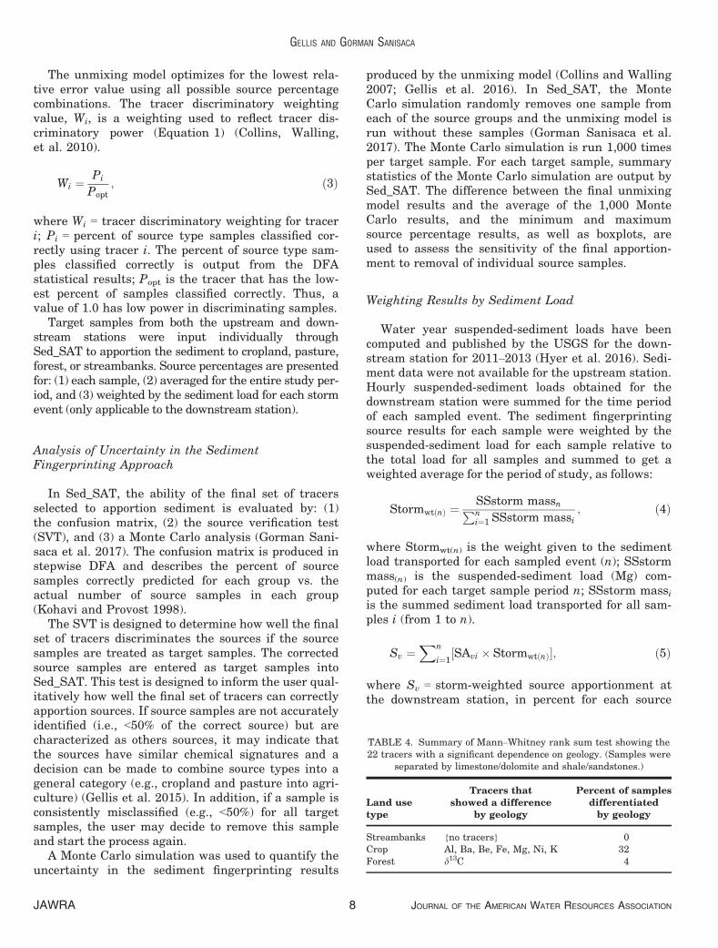
TABLE 4. Summary of Mann–Whitney rank sum test showing the22 tracers with a significant dependence on geology. (Samples were

separated by limestone/dolomite and shale/sandstones.)

Land usetype

Tracers thatshowed a difference

by geology

Percent of samplesdifferentiatedby geology

Streambanks {no tracers} 0Crop Al, Ba, Be, Fe, Mg, Ni, K 32Forest d13C 4



(v); (v = cropland, pasture, forest, and streambanks);SAvi = sediment source apportionment from the sedi-ment fingerprinting results (in percent) (Equation 1)for source (v) and sample i; n = number of sampledevents (i) = 19 at the downstream station.

Weighting the sediment fingerprinting results bythe sediment load for each sample incorporates theimportance of high loading events (Gellis and Walling2011). It should be pointed out that the suspended-

sediment load computations include particle sizes inthe sand range (>63 lm), whereas sediment finger-printing results are only for the <63-lm fraction.Analysis of 145 suspended-sediment samples fromSmith Creek collected between April 2010 andAugust 2017 (USGS 2016) indicate that on average73 � 24% is finer than 63 lm. Frequent suspended-sediment grain size analysis for each storm would berequired to compute a fine sediment load, which wasnot possible with the current data. Therefore, there issome error in determining fine sediment apportion-ment by weighting with suspended-sediment loadsthat contain sand.

RESULTS AND DISCUSSION

Geologic Differences in Tracer Concentrations

The Mann–Whitney rank sum test results for ele-mental and stable isotope tracer biases in areasunderlain by limestone/dolostone vs. sandstone/shaleshowed no significance for streambanks, seven trac-ers showed significant differences in croplands, andone tracer for forest (Table 4). Based on the low per-centage (<50%) of tracers showing a significant

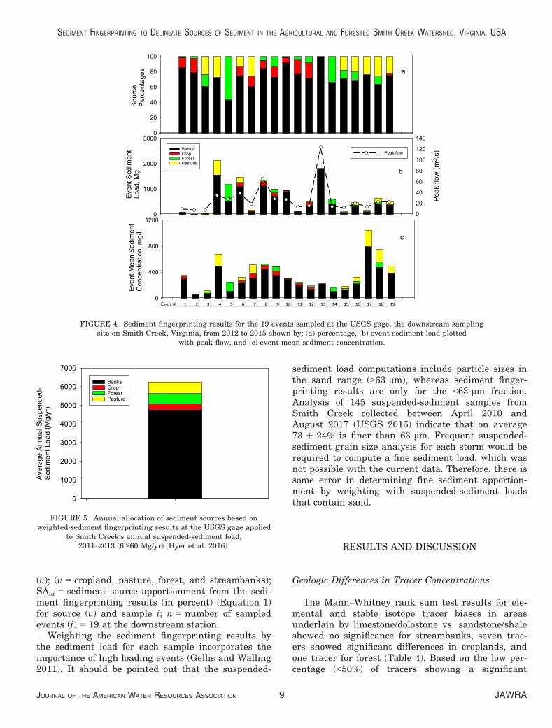
FIGURE 4. Sediment fingerprinting results for the 19 events sampled at the USGS gage, the downstream samplingsite on Smith Creek, Virginia, from 2012 to 2015 shown by: (a) percentage, (b) event sediment load plotted

with peak flow, and (c) event mean sediment concentration.

FIGURE 5. Annual allocation of sediment sources based onweighted-sediment fingerprinting results at the USGS gage applied

to Smith Creek’s annual suspended-sediment load,2011–2013 (6,260 Mg/yr) (Hyer et al. 2016).



difference in medians, we decided not to apportionthe source samples by geology.

Sediment Fingerprinting Source Apportionment andUncertainty

Sediment fingerprinting results are presented forthe downstream station (Figures 4 and 5; Table 5a)and the upstream station (Figure 6; Table 5b).

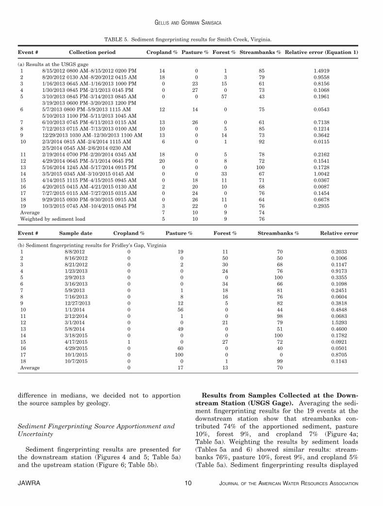
Results from Samples Collected at the Down-stream Station (USGS Gage). Averaging the sedi-ment fingerprinting results for the 19 events at thedownstream station show that streambanks con-tributed 74% of the apportioned sediment, pasture10%, forest 9%, and cropland 7% (Figure 4a;Table 5a). Weighting the results by sediment loads(Tables 5a and 6) showed similar results: stream-banks 76%, pasture 10%, forest 9%, and cropland 5%(Table 5a). Sediment fingerprinting results displayed

TABLE 5. Sediment fingerprinting results for Smith Creek, Virginia.

Event # Collection period Cropland % Pasture % Forest % Streambanks % Relative error (Equation 1)

(a) Results at the USGS gage1 8/15/2012 0800 AM–8/15/2012 0200 PM 14 0 1 85 1.49192 8/20/2012 0130 AM–8/20/2012 0415 AM 18 0 3 79 0.95583 1/16/2013 0645 AM–1/16/2013 1000 PM 0 23 15 61 0.81564 1/30/2013 0845 PM–2/1/2013 0145 PM 0 27 0 73 0.10685 3/10/2013 0845 PM–3/14/2013 0845 AM

3/19/2013 0600 PM–3/20/2013 1200 PM0 0 57 43 0.1961

6 5/7/2013 0800 PM–5/9/2013 1115 AM5/10/2013 1100 PM–5/11/2013 1045 AM

12 14 0 75 0.0543

7 6/10/2013 0745 PM–6/11/2013 0115 AM 13 26 0 61 0.71388 7/12/2013 0715 AM–7/13/2013 0100 AM 10 0 5 85 0.12149 12/29/2013 1030 AM–12/30/2013 1100 AM 13 0 14 73 0.364210 2/3/2014 0815 AM–2/4/2014 1115 AM

2/5/2014 0545 AM–2/6/2014 0230 AM6 0 1 92 0.0115

11 2/19/2014 0700 PM–2/20/2014 0345 AM 18 0 5 78 0.216212 4/29/2014 0645 PM–5/1/2014 0645 PM 20 0 8 72 0.154113 5/16/2014 1245 AM–5/17/2014 0915 PM 0 0 0 100 0.172814 3/5/2015 0345 AM–3/10/2015 0145 AM 0 0 33 67 1.004215 4/14/2015 1115 PM–4/15/2015 0945 AM 0 18 11 71 0.036716 4/20/2015 0415 AM–4/21/2015 0130 AM 2 20 10 68 0.008717 7/27/2015 0115 AM–7/27/2015 0315 AM 0 24 0 76 0.145418 9/29/2015 0930 PM–9/30/2015 0915 AM 0 26 11 64 0.667819 10/3/2015 0745 AM–10/4/2015 0845 PM 3 22 0 76 0.2935Average 7 10 9 74Weighted by sediment load 5 10 9 76

Event # Sample date Cropland % Pasture % Forest % Streambanks % Relative error

(b) Sediment fingerprinting results for Fridley’s Gap, Virginia1 8/8/2012 0 19 11 70 0.20332 8/16/2012 0 0 50 50 0.10063 8/21/2012 0 2 30 68 0.11474 1/23/2013 0 0 24 76 0.91735 2/9/2013 0 0 0 100 0.33556 3/16/2013 0 0 34 66 0.10987 5/9/2013 0 1 18 81 0.24518 7/16/2013 0 8 16 76 0.06049 12/27/2013 0 12 5 82 0.381810 1/1/2014 0 56 0 44 0.484811 2/12/2014 0 1 0 98 0.068312 3/1/2014 0 0 21 79 1.529313 5/8/2014 0 49 0 51 0.460014 3/18/2015 0 0 0 100 0.178215 4/17/2015 1 0 27 72 0.092116 4/29/2015 0 60 0 40 0.050117 10/1/2015 0 100 0 0 0.870518 10/7/2015 0 0 1 99 0.1143Average 0 17 13 70



by sediment concentration and sediment loadsshowed that streambanks were the largest source ofsediment during the highest sediment concentrationsand loading events (Figure 4b, 4c). Five of the sixhighest mean sediment concentrations (Table 6;events 17, 18, 4, 7, and 19) had >20% contributionfrom pasture (Figure 4c; Table 5a). Using theweighted-sediment apportionment results (Table 5a)and applying it to the average water year suspended-sediment load for Smith Creek (2011–2013; 6,260 Mg/yr) (Hyer et al. 2016) shows the following mass con-tributions by source: streambanks = 4,758 Mg/yr;pasture = 626 Mg/yr; forest = 563 Mg/yr; and crop-land = 313 Mg/yr (Figure 5).

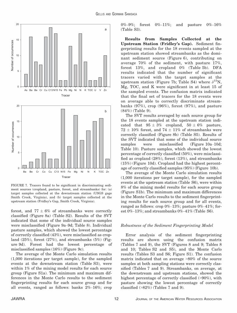
DFA results indicated that the number of significanttracers varied with the target samples (Figure 7a) atthe downstream station (Figure 7a; Table S1) whered13C, d15N, N, Ba, Mg, and Cu were significant in at

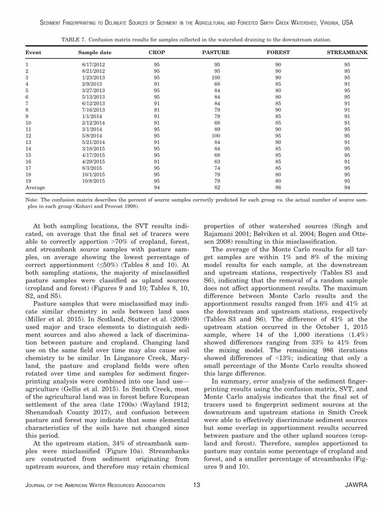
least 15 of the 19 target samples. It is important topoint out that a different set of tracers can be signifi-cant in discriminating the sources for any given tar-get sample (Figure 7). Since the size and organiccontent of each target sample effects the final cor-rected concentration of source samples, depending onthe grain size and organic content of the target sam-ple, and the bracket test removing tracers, differenttracers may be significant. The confusion matrix indi-cated that the final set of tracers for the 19 targetsamples were on average able to correctly discrimi-nate banks (94%), crop (94%), forest (86%), and pas-ture (82%) (Table 7). Pasture samples showed thegreatest range in source discrimination, from 63% to100% (Table 7).

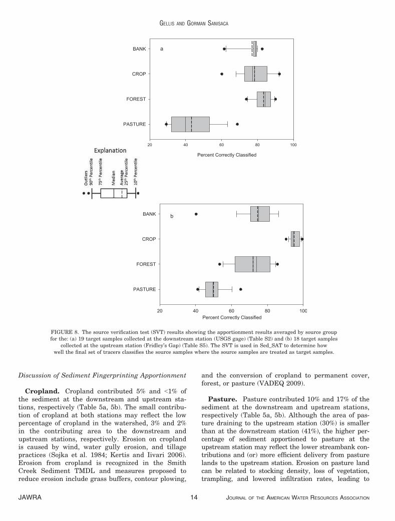
The SVT results averaged by source group for the 19sampled events at the downstream station indicatedthat 78 � 9% cropland, 43 � 12% pasture, 84 � 5%

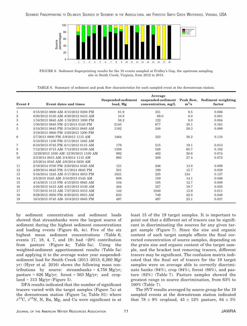
FIGURE 6. Sediment fingerprinting results for the 18 events sampled at Fridley’s Gap, the upstream samplingsite in Smith Creek, Virginia, from 2012 to 2015.

TABLE 6. Summary of sediment and peak flow characteristics for each sampled event at the downstream station.

Event # Event dates and timesSuspended-sediment

load, Mg

Averagesuspended-sedimentconcentration, mg/L

Peak flow,m3/s

Sediment weightingfactor

1 8/15/2012 0800 AM–8/15/2012 0200 PM 81.9 351 9.5 0.0062 8/20/2012 0130 AM–8/20/2012 0415 AM 10.8 69.0 8.0 0.0013 1/16/2013 0645 AM–1/16/2013 1000 PM 58.2 122 8.0 0.0044 1/30/2013 0845 PM–2/1/2013 0145 PM 2145 677 35.1 0.1615 3/10/2013 0845 PM–3/14/2013 0845 AM

3/19/2013 0600 PM–3/20/2013 1200 PM1182 248 28.3 0.089

6 5/7/2013 0800 PM–5/9/2013 1115 AM5/10/2013 1100 PM–5/11/2013 1045 AM

1464 323 38.2 0.110

7 6/10/2013 0745 PM–6/11/2013 0115 AM 179 515 19.1 0.0138 7/12/2013 0715 AM–7/13/2013 0100 AM 1356 528 65.7 0.1029 12/29/2013 1030 AM–12/30/2013 1100 AM 992 482 28.6 0.07410 2/3/2014 0815 AM–2/4/2014 1115 AM

2/5/2014 0545 AM–2/6/2014 0230 AM965 309 27.4 0.072

11 2/19/2014 0700 PM–2/20/2014 0345 AM 121 246 13.8 0.00912 4/29/2014 0645 PM–5/1/2014 0645 PM 501 189 15.7 0.03813 5/16/2014 1245 AM–5/17/2014 0915 PM 1821 225 124 0.13714 3/5/2015 0345 AM–3/10/2015 0145 AM 608 159 14.1 0.04615 4/14/2015 1115 PM–4/15/2015 0945 AM 104 185 12.7 0.00816 4/20/2015 0415 AM–4/21/2015 0130 AM 464 327 19.7 0.03517 7/27/2015 0115 AM–7/27/2015 0315 AM 142 1040 13.9 0.01118 9/29/2015 0930 PM–9/30/2015 0915 AM 633 749 22.8 0.04819 10/3/2015 0745 AM–10/4/2015 0845 PM 497 497 23.1 0.037



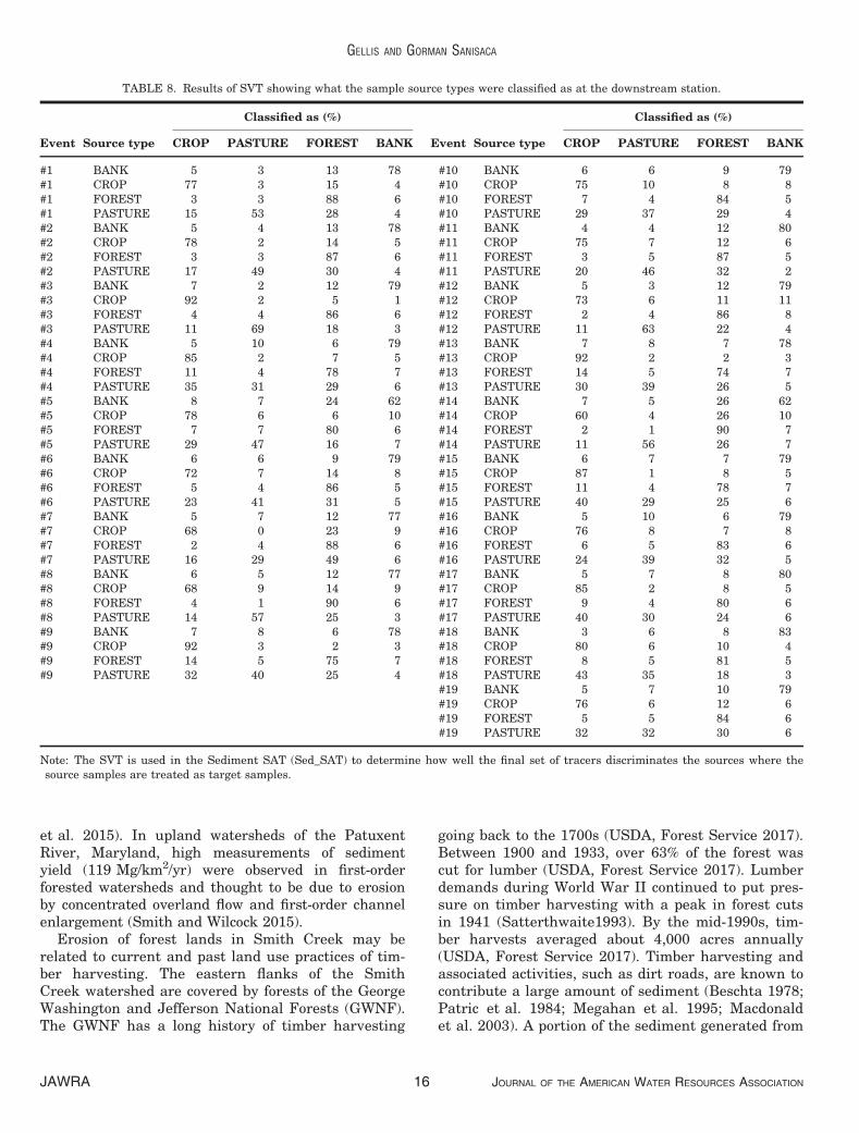
forest, and 77 � 6% of streambanks were correctlyclassified (Figure 8a) (Table S2). Results of the SVTindicated that some of the individual source sampleswere misclassified (Figure 9a–9d; Table 8). Individualpasture samples, which showed the lowest percentageof correctly classified (43%), were misclassified as crop-land (25%), forest (27%), and streambanks (5%) (Fig-ure 9d). Forest had the lowest percentage ofmisclassified samples (16%) (Figure 9c).

The average of the Monte Carlo simulation results(1,000 iterations per target sample), for the sampledevents at the downstream station (Table S3), werewithin 1% of the mixing model results for each sourcegroup (Figure S1a). The minimum and maximum dif-ferences in the Monte Carlo results to the sedimentfingerprinting results for each source group and forall events, ranged as follows: banks 2%–16%; crop

0%–9%; forest 0%–11%; and pasture 0%–16%(Table S3).

Results from Samples Collected at theUpstream Station (Fridley’s Gap). Sediment fin-gerprinting results for the 18 events sampled at theupstream station showed streambanks as the domi-nant sediment source (Figure 6), contributing onaverage 70% of the sediment, with pasture 17%,forest 13%, and cropland 0% (Table 5b). DFAresults indicated that the number of significanttracers varied with the target samples at theupstream station (Figure 7b; Table S4) where d15N,Mg, TOC, and K were significant in at least 15 ofthe sampled events. The confusion matrix indicatedthat the final set of tracers for the 18 events wereon average able to correctly discriminate stream-banks (97%), crop (96%), forest (97%), and pasture(84%) (Table 9).

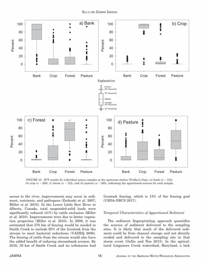
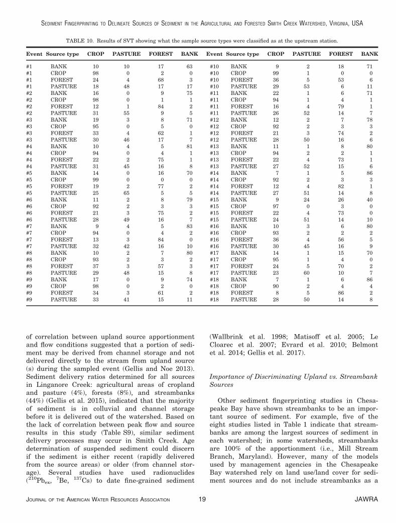
The SVT results averaged by each source group forthe 18 events sampled at the upstream station indi-cated that 95 � 3% cropland, 50 � 6% pasture,72 � 10% forest, and 74 � 11% of streambanks werecorrectly classified (Figure 8b) (Table S5). Results ofthe SVT indicated that some of the individual sourcesamples were misclassified (Figure 10a–10d;Table 10). Pasture samples, which showed the lowestpercentage of correctly classified (50%), were misclassi-fied as cropland (28%), forest (13%), and streambanks(15%) (Figure 10d). Cropland had the highest percent-age of correctly classified samples (95%) (Figure 10b).

The average of the Monte Carlo simulation results(1,000 iterations per target sample), for the sampledevents at the upstream station (Table S6), were within8% of the mixing model results for each source group(Figure S1b). The minimum and maximum differencesin the Monte Carlo results to the sediment fingerprint-ing results for each source group and for all events,ranged as follows: crop 0%–13%; pasture 0%–41%; for-est 0%–13%; and streambanks 0%–41% (Table S6).

Robustness of the Sediment Fingerprinting Model

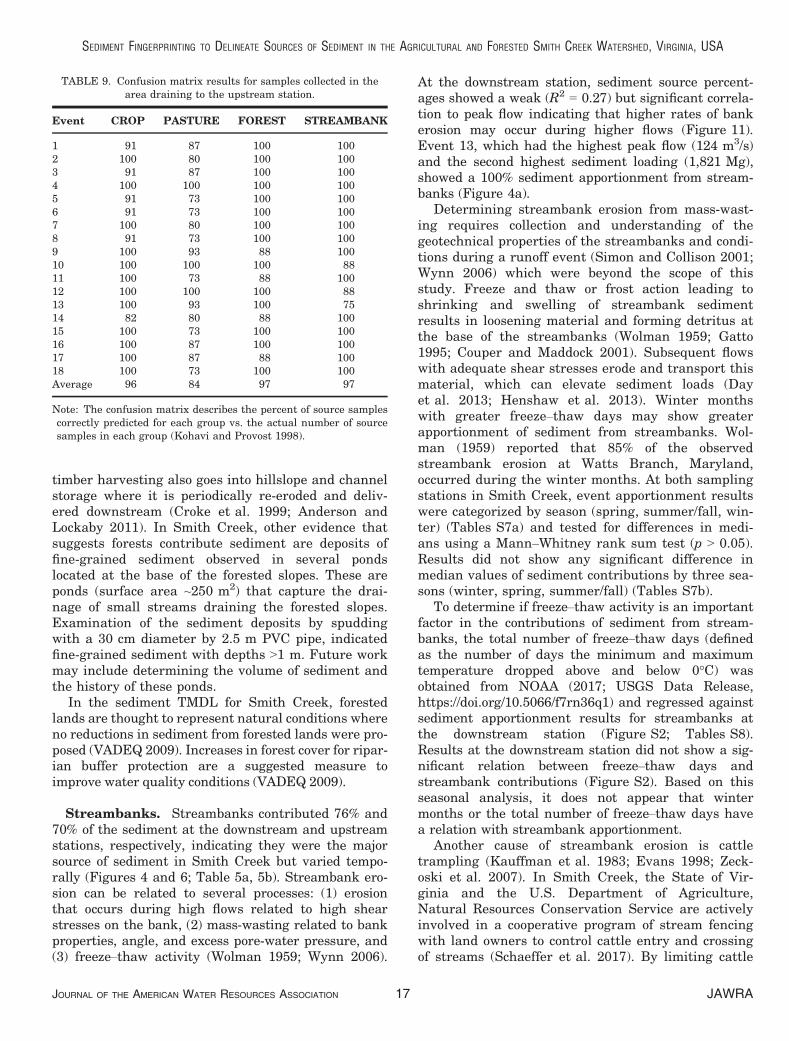
Error analysis of the sediment fingerprintingresults are shown using the confusion matrix(Tables 7 and 9), the SVT (Figures 8 and 9; Tables 8and 10; Tables S2 and S5), and the Monte Carloresults (Tables S3 and S6; Figure S1). The confusionmatrix indicated that on average >80% of the sourcesamples at both sampling stations were correctly clas-sified (Tables 7 and 9). Streambanks, on average, atthe downstream and upstream stations, showed thehighest percentage of correctly classified (>90%), withpasture showing the lowest percentage of correctlyclassified (>82%) (Tables 7 and 9).

FIGURE 7. Tracers found to be significant in discriminating sedi-ment sources (cropland, pasture, forest, and streambanks) for: (a)target samples collected at the downstream station (USGS gageSmith Creek, Virginia), and (b) target samples collected at theupstream station (Fridley’s Gap, Smith Creek, Virginia).



At both sampling locations, the SVT results indi-cated, on average that the final set of tracers wereable to correctly apportion >70% of cropland, forest,and streambank source samples with pasture sam-ples, on average showing the lowest percentage ofcorrect apportionment (≤50%) (Tables 8 and 10). Atboth sampling stations, the majority of misclassifiedpasture samples were classified as upland sources(cropland and forest) (Figures 9 and 10; Tables 8, 10,S2, and S5).

Pasture samples that were misclassified may indi-cate similar chemistry in soils between land uses(Miller et al. 2015). In Scotland, Stutter et al. (2009)used major and trace elements to distinguish sedi-ment sources and also showed a lack of discrimina-tion between pasture and cropland. Changing landuse on the same field over time may also cause soilchemistry to be similar. In Linganore Creek, Mary-land, the pasture and cropland fields were oftenrotated over time and samples for sediment finger-printing analysis were combined into one land use—agriculture (Gellis et al. 2015). In Smith Creek, mostof the agricultural land was in forest before Europeansettlement of the area (late 1700s) (Wayland 1912;Shenandoah County 2017), and confusion betweenpasture and forest may indicate that some elementalcharacteristics of the soils have not changed sincethis period.

At the upstream station, 34% of streambank sam-ples were misclassified (Figure 10a). Streambanksare constructed from sediment originating fromupstream sources, and therefore may retain chemical

properties of other watershed sources (Singh andRajamani 2001; Bølviken et al. 2004; Bogen and Otte-sen 2008) resulting in this misclassification.

The average of the Monte Carlo results for all tar-get samples are within 1% and 8% of the mixingmodel results for each sample, at the downstreamand upstream stations, respectively (Tables S3 andS6), indicating that the removal of a random sampledoes not affect apportionment results. The maximumdifference between Monte Carlo results and theapportionment results ranged from 16% and 41% atthe downstream and upstream stations, respectively(Tables S3 and S6). The difference of 41% at theupstream station occurred in the October 1, 2015sample, where 14 of the 1,000 iterations (1.4%)showed differences ranging from 33% to 41% fromthe mixing model. The remaining 986 iterationsshowed differences of <13%; indicating that only asmall percentage of the Monte Carlo results showedthis large difference.

In summary, error analysis of the sediment finger-printing results using the confusion matrix, SVT, andMonte Carlo analysis indicates that the final set oftracers used to fingerprint sediment sources at thedownstream and upstream stations in Smith Creekwere able to effectively discriminate sediment sourcesbut some overlap in apportionment results occurredbetween pasture and the other upland sources (crop-land and forest). Therefore, samples apportioned topasture may contain some percentage of cropland andforest, and a smaller percentage of streambanks (Fig-ures 9 and 10).

TABLE 7. Confusion matrix results for samples collected in the watershed draining to the downstream station.

Event Sample date CROP PASTURE FOREST STREAMBANK

1 8/17/2012 95 95 90 952 8/21/2012 95 95 90 953 1/23/2013 95 100 90 954 2/9/2013 91 68 85 915 3/27/2013 95 84 80 956 5/13/2013 95 84 80 957 6/12/2013 91 84 85 918 7/16/2013 91 79 90 919 1/1/2014 91 79 85 9110 2/12/2014 91 68 85 9111 3/1/2014 95 89 90 9512 5/8/2014 95 100 95 9513 5/21/2014 91 84 90 9114 3/18/2015 95 84 85 9515 4/17/2015 95 68 85 9516 4/29/2015 91 63 85 9117 8/3/2015 95 74 85 9518 10/1/2015 95 79 80 9519 10/8/2015 95 79 80 95Average 94 82 86 94

Note: The confusion matrix describes the percent of source samples correctly predicted for each group vs. the actual number of source sam-ples in each group (Kohavi and Provost 1998).



Discussion of Sediment Fingerprinting Apportionment

Cropland. Cropland contributed 5% and <1% ofthe sediment at the downstream and upstream sta-tions, respectively (Table 5a, 5b). The small contribu-tion of cropland at both stations may reflect the lowpercentage of cropland in the watershed, 3% and 2%in the contributing area to the downstream andupstream stations, respectively. Erosion on croplandis caused by wind, water gully erosion, and tillagepractices (Sojka et al. 1984; Kertis and Iivari 2006).Erosion from cropland is recognized in the SmithCreek Sediment TMDL and measures proposed toreduce erosion include grass buffers, contour plowing,

and the conversion of cropland to permanent cover,forest, or pasture (VADEQ 2009).

Pasture. Pasture contributed 10% and 17% of thesediment at the downstream and upstream stations,respectively (Table 5a, 5b). Although the area of pas-ture draining to the upstream station (30%) is smallerthan at the downstream station (41%), the higher per-centage of sediment apportioned to pasture at theupstream station may reflect the lower streambank con-tributions and (or) more efficient delivery from pasturelands to the upstream station. Erosion on pasture landcan be related to stocking density, loss of vegetation,trampling, and lowered infiltration rates, leading to

FIGURE 8. The source verification test (SVT) results showing the apportionment results averaged by source groupfor the: (a) 19 target samples collected at the downstream station (USGS gage) (Table S2) and (b) 18 target samples

collected at the upstream station (Fridley’s Gap) (Table S5). The SVT is used in Sed_SAT to determine howwell the final set of tracers classifies the source samples where the source samples are treated as target samples.



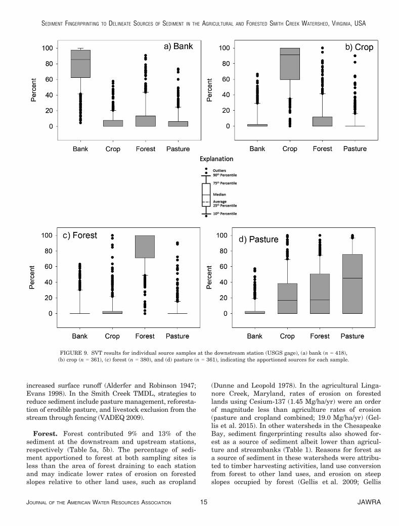
increased surface runoff (Alderfer and Robinson 1947;Evans 1998). In the Smith Creek TMDL, strategies toreduce sediment include pasture management, reforesta-tion of erodible pasture, and livestock exclusion from thestream through fencing (VADEQ 2009).

Forest. Forest contributed 9% and 13% of thesediment at the downstream and upstream stations,respectively (Table 5a, 5b). The percentage of sedi-ment apportioned to forest at both sampling sites isless than the area of forest draining to each stationand may indicate lower rates of erosion on forestedslopes relative to other land uses, such as cropland

(Dunne and Leopold 1978). In the agricultural Linga-nore Creek, Maryland, rates of erosion on forestedlands using Cesium-137 (1.45 Mg/ha/yr) were an orderof magnitude less than agriculture rates of erosion(pasture and cropland combined; 19.0 Mg/ha/yr) (Gel-lis et al. 2015). In other watersheds in the ChesapeakeBay, sediment fingerprinting results also showed for-est as a source of sediment albeit lower than agricul-ture and streambanks (Table 1). Reasons for forest asa source of sediment in these watersheds were attribu-ted to timber harvesting activities, land use conversionfrom forest to other land uses, and erosion on steepslopes occupied by forest (Gellis et al. 2009; Gellis

FIGURE 9. SVT results for individual source samples at the downstream station (USGS gage), (a) bank (n = 418),(b) crop (n = 361), (c) forest (n = 380), and (d) pasture (n = 361), indicating the apportioned sources for each sample.



et al. 2015). In upland watersheds of the PatuxentRiver, Maryland, high measurements of sedimentyield (119 Mg/km2/yr) were observed in first-orderforested watersheds and thought to be due to erosionby concentrated overland flow and first-order channelenlargement (Smith and Wilcock 2015).

Erosion of forest lands in Smith Creek may berelated to current and past land use practices of tim-ber harvesting. The eastern flanks of the SmithCreek watershed are covered by forests of the GeorgeWashington and Jefferson National Forests (GWNF).The GWNF has a long history of timber harvesting

going back to the 1700s (USDA, Forest Service 2017).Between 1900 and 1933, over 63% of the forest wascut for lumber (USDA, Forest Service 2017). Lumberdemands during World War II continued to put pres-sure on timber harvesting with a peak in forest cutsin 1941 (Satterthwaite1993). By the mid-1990s, tim-ber harvests averaged about 4,000 acres annually(USDA, Forest Service 2017). Timber harvesting andassociated activities, such as dirt roads, are known tocontribute a large amount of sediment (Beschta 1978;Patric et al. 1984; Megahan et al. 1995; Macdonaldet al. 2003). A portion of the sediment generated from

TABLE 8. Results of SVT showing what the sample source types were classified as at the downstream station.

Event Source type

Classified as (%)

Event Source type

Classified as (%)

CROP PASTURE FOREST BANK CROP PASTURE FOREST BANK

#1 BANK 5 3 13 78 #10 BANK 6 6 9 79#1 CROP 77 3 15 4 #10 CROP 75 10 8 8#1 FOREST 3 3 88 6 #10 FOREST 7 4 84 5#1 PASTURE 15 53 28 4 #10 PASTURE 29 37 29 4#2 BANK 5 4 13 78 #11 BANK 4 4 12 80#2 CROP 78 2 14 5 #11 CROP 75 7 12 6#2 FOREST 3 3 87 6 #11 FOREST 3 5 87 5#2 PASTURE 17 49 30 4 #11 PASTURE 20 46 32 2#3 BANK 7 2 12 79 #12 BANK 5 3 12 79#3 CROP 92 2 5 1 #12 CROP 73 6 11 11#3 FOREST 4 4 86 6 #12 FOREST 2 4 86 8#3 PASTURE 11 69 18 3 #12 PASTURE 11 63 22 4#4 BANK 5 10 6 79 #13 BANK 7 8 7 78#4 CROP 85 2 7 5 #13 CROP 92 2 2 3#4 FOREST 11 4 78 7 #13 FOREST 14 5 74 7#4 PASTURE 35 31 29 6 #13 PASTURE 30 39 26 5#5 BANK 8 7 24 62 #14 BANK 7 5 26 62#5 CROP 78 6 6 10 #14 CROP 60 4 26 10#5 FOREST 7 7 80 6 #14 FOREST 2 1 90 7#5 PASTURE 29 47 16 7 #14 PASTURE 11 56 26 7#6 BANK 6 6 9 79 #15 BANK 6 7 7 79#6 CROP 72 7 14 8 #15 CROP 87 1 8 5#6 FOREST 5 4 86 5 #15 FOREST 11 4 78 7#6 PASTURE 23 41 31 5 #15 PASTURE 40 29 25 6#7 BANK 5 7 12 77 #16 BANK 5 10 6 79#7 CROP 68 0 23 9 #16 CROP 76 8 7 8#7 FOREST 2 4 88 6 #16 FOREST 6 5 83 6#7 PASTURE 16 29 49 6 #16 PASTURE 24 39 32 5#8 BANK 6 5 12 77 #17 BANK 5 7 8 80#8 CROP 68 9 14 9 #17 CROP 85 2 8 5#8 FOREST 4 1 90 6 #17 FOREST 9 4 80 6#8 PASTURE 14 57 25 3 #17 PASTURE 40 30 24 6#9 BANK 7 8 6 78 #18 BANK 3 6 8 83#9 CROP 92 3 2 3 #18 CROP 80 6 10 4#9 FOREST 14 5 75 7 #18 FOREST 8 5 81 5#9 PASTURE 32 40 25 4 #18 PASTURE 43 35 18 3

#19 BANK 5 7 10 79#19 CROP 76 6 12 6#19 FOREST 5 5 84 6#19 PASTURE 32 32 30 6

Note: The SVT is used in the Sediment SAT (Sed_SAT) to determine how well the final set of tracers discriminates the sources where thesource samples are treated as target samples.



timber harvesting also goes into hillslope and channelstorage where it is periodically re-eroded and deliv-ered downstream (Croke et al. 1999; Anderson andLockaby 2011). In Smith Creek, other evidence thatsuggests forests contribute sediment are deposits offine-grained sediment observed in several pondslocated at the base of the forested slopes. These areponds (surface area ~250 m2) that capture the drai-nage of small streams draining the forested slopes.Examination of the sediment deposits by spuddingwith a 30 cm diameter by 2.5 m PVC pipe, indicatedfine-grained sediment with depths >1 m. Future workmay include determining the volume of sediment andthe history of these ponds.

In the sediment TMDL for Smith Creek, forestedlands are thought to represent natural conditions whereno reductions in sediment from forested lands were pro-posed (VADEQ 2009). Increases in forest cover for ripar-ian buffer protection are a suggested measure toimprove water quality conditions (VADEQ 2009).

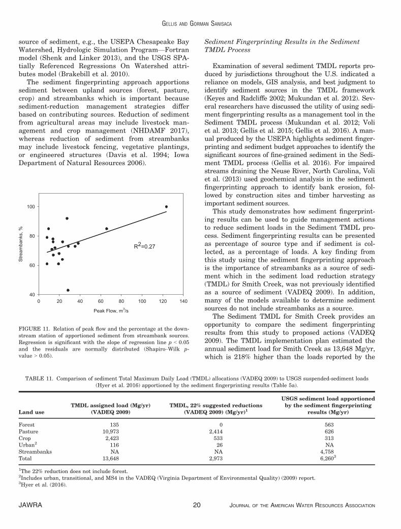
Streambanks. Streambanks contributed 76% and70% of the sediment at the downstream and upstreamstations, respectively, indicating they were the majorsource of sediment in Smith Creek but varied tempo-rally (Figures 4 and 6; Table 5a, 5b). Streambank ero-sion can be related to several processes: (1) erosionthat occurs during high flows related to high shearstresses on the bank, (2) mass-wasting related to bankproperties, angle, and excess pore-water pressure, and(3) freeze–thaw activity (Wolman 1959; Wynn 2006).

At the downstream station, sediment source percent-ages showed a weak (R2 = 0.27) but significant correla-tion to peak flow indicating that higher rates of bankerosion may occur during higher flows (Figure 11).Event 13, which had the highest peak flow (124 m3/s)and the second highest sediment loading (1,821 Mg),showed a 100% sediment apportionment from stream-banks (Figure 4a).

Determining streambank erosion from mass-wast-ing requires collection and understanding of thegeotechnical properties of the streambanks and condi-tions during a runoff event (Simon and Collison 2001;Wynn 2006) which were beyond the scope of thisstudy. Freeze and thaw or frost action leading toshrinking and swelling of streambank sedimentresults in loosening material and forming detritus atthe base of the streambanks (Wolman 1959; Gatto1995; Couper and Maddock 2001). Subsequent flowswith adequate shear stresses erode and transport thismaterial, which can elevate sediment loads (Dayet al. 2013; Henshaw et al. 2013). Winter monthswith greater freeze–thaw days may show greaterapportionment of sediment from streambanks. Wol-man (1959) reported that 85% of the observedstreambank erosion at Watts Branch, Maryland,occurred during the winter months. At both samplingstations in Smith Creek, event apportionment resultswere categorized by season (spring, summer/fall, win-ter) (Tables S7a) and tested for differences in medi-ans using a Mann–Whitney rank sum test (p > 0.05).Results did not show any significant difference inmedian values of sediment contributions by three sea-sons (winter, spring, summer/fall) (Tables S7b).

To determine if freeze–thaw activity is an importantfactor in the contributions of sediment from stream-banks, the total number of freeze–thaw days (definedas the number of days the minimum and maximumtemperature dropped above and below 0°C) wasobtained from NOAA (2017; USGS Data Release,https://doi.org/10.5066/f7rn36q1) and regressed againstsediment apportionment results for streambanks atthe downstream station (Figure S2; Tables S8).Results at the downstream station did not show a sig-nificant relation between freeze–thaw days andstreambank contributions (Figure S2). Based on thisseasonal analysis, it does not appear that wintermonths or the total number of freeze–thaw days havea relation with streambank apportionment.

Another cause of streambank erosion is cattletrampling (Kauffman et al. 1983; Evans 1998; Zeck-oski et al. 2007). In Smith Creek, the State of Vir-ginia and the U.S. Department of Agriculture,Natural Resources Conservation Service are activelyinvolved in a cooperative program of stream fencingwith land owners to control cattle entry and crossingof streams (Schaeffer et al. 2017). By limiting cattle

TABLE 9. Confusion matrix results for samples collected in thearea draining to the upstream station.

Event CROP PASTURE FOREST STREAMBANK

1 91 87 100 1002 100 80 100 1003 91 87 100 1004 100 100 100 1005 91 73 100 1006 91 73 100 1007 100 80 100 1008 91 73 100 1009 100 93 88 10010 100 100 100 8811 100 73 88 10012 100 100 100 8813 100 93 100 7514 82 80 88 10015 100 73 100 10016 100 87 100 10017 100 87 88 10018 100 73 100 100Average 96 84 97 97

Note: The confusion matrix describes the percent of source samplescorrectly predicted for each group vs. the actual number of sourcesamples in each group (Kohavi and Provost 1998).




access to the river, improvements may occur in sedi-ment, nutrients, and pathogens (Zeckoski et al. 2007;Miller et al. 2010). In the Lower Little Bow River inAlberta, Canada, total suspended-solid loads weresignificantly reduced (41%) by cattle exclusion (Milleret al. 2010). Improvements were due to better vegeta-tion properties (Miller et al. 2010). In 2009, it wasestimated that 278 km of fencing would be needed inSmith Creek to exclude 95% of the livestock from thestream to meet bacterial reductions (VADEQ 2009).The fencing of cattle from the stream would also havethe added benefit of reducing streambank erosion. By2016, 35 km of Smith Creek and its tributaries had

livestock fencing, which is 13% of the fencing goal(USDA-NRCS 2017).

Temporal Characteristics of Apportioned Sediment

The sediment fingerprinting approach quantifiesthe sources of sediment delivered to the samplingsites. It is likely that much of the delivered sedi-ment could be from channel storage and not directlyeroded and delivered to the sampling site in thatstorm event (Gellis and Noe 2013). In the agricul-tural Linganore Creek watershed, Maryland, a lack

FIGURE 10. SVT results for individual source samples at the upstream station (Fridley’s Gap), (a) bank (n = 152),(b) crop (n = 209), (c) forest (n = 152), and (d) pasture (n = 285), indicating the apportioned sources for each sample.



of correlation between upland source apportionmentand flow conditions suggested that a portion of sedi-ment may be derived from channel storage and notdelivered directly to the stream from upland source(s) during the sampled event (Gellis and Noe 2013).Sediment delivery ratios determined for all sourcesin Linganore Creek: agricultural areas of croplandand pasture (4%), forests (8%), and streambanks(44%) (Gellis et al. 2015), indicated that the majorityof sediment is in colluvial and channel storagebefore it is delivered out of the watershed. Based onthe lack of correlation between peak flow and sourceresults in this study (Table S9), similar sedimentdelivery processes may occur in Smith Creek. Agedetermination of suspended sediment could discernif the sediment is either recent (rapidly deliveredfrom the source areas) or older (from channel stor-age). Several studies have used radionuclides(210Pbex,

7Be, 137Cs) to date fine-grained sediment

(Wallbrink et al. 1998; Matisoff et al. 2005; LeCloarec et al. 2007; Evrard et al. 2010; Belmontet al. 2014; Gellis et al. 2017).

Importance of Discriminating Upland vs. StreambankSources

Other sediment fingerprinting studies in Chesa-peake Bay have shown streambanks to be an impor-tant source of sediment. For example, five of theeight studies listed in Table 1 indicate that stream-banks are among the largest sources of sediment ineach watershed; in some watersheds, streambanksare 100% of the apportionment (i.e., Mill StreamBranch, Maryland). However, many of the modelsused by management agencies in the ChesapeakeBay watershed rely on land use/land cover for sedi-ment sources and do not include streambanks as a

TABLE 10. Results of SVT showing what the sample source types were classified as at the upstream station.

Event Source type CROP PASTURE FOREST BANK Event Source type CROP PASTURE FOREST BANK

#1 BANK 10 10 17 63 #10 BANK 9 2 18 71#1 CROP 98 0 2 0 #10 CROP 99 1 0 0#1 FOREST 24 4 68 3 #10 FOREST 36 5 53 6#1 PASTURE 18 48 17 17 #10 PASTURE 29 53 6 11#2 BANK 16 0 9 75 #11 BANK 22 1 6 71#2 CROP 98 0 1 1 #11 CROP 94 1 4 1#2 FOREST 12 1 84 2 #11 FOREST 16 4 79 1#2 PASTURE 31 55 9 5 #11 PASTURE 26 52 14 7#3 BANK 19 3 8 71 #12 BANK 12 2 7 78#3 CROP 95 0 5 0 #12 CROP 92 2 3 3#3 FOREST 33 4 62 1 #12 FOREST 21 3 74 2#3 PASTURE 30 46 17 7 #12 PASTURE 28 50 16 6#4 BANK 10 4 5 81 #13 BANK 11 1 8 80#4 CROP 94 0 4 1 #13 CROP 94 2 2 1#4 FOREST 22 2 75 1 #13 FOREST 22 4 73 1#4 PASTURE 31 45 16 8 #13 PASTURE 27 52 15 6#5 BANK 14 0 16 70 #14 BANK 7 1 5 86#5 CROP 99 0 0 0 #14 CROP 92 2 3 3#5 FOREST 19 2 77 2 #14 FOREST 12 4 82 1#5 PASTURE 25 65 5 5 #14 PASTURE 27 51 14 8#6 BANK 11 2 8 79 #15 BANK 9 24 26 40#6 CROP 92 2 3 3 #15 CROP 97 0 3 0#6 FOREST 21 3 75 2 #15 FOREST 22 4 73 0#6 PASTURE 28 49 16 7 #15 PASTURE 24 51 14 10#7 BANK 9 4 5 83 #16 BANK 10 3 6 80#7 CROP 94 0 4 2 #16 CROP 93 2 2 2#7 FOREST 13 3 84 0 #16 FOREST 36 4 56 5#7 PASTURE 32 42 16 10 #16 PASTURE 30 45 16 9#8 BANK 10 2 7 80 #17 BANK 14 1 15 70#8 CROP 93 2 3 2 #17 CROP 95 1 4 0#8 FOREST 37 3 57 3 #17 FOREST 24 5 70 2#8 PASTURE 29 48 15 8 #17 PASTURE 23 60 10 7#9 BANK 17 0 9 74 #18 BANK 7 1 6 86#9 CROP 98 0 2 0 #18 CROP 90 2 4 4#9 FOREST 34 3 61 2 #18 FOREST 8 5 86 2#9 PASTURE 33 41 15 11 #18 PASTURE 28 50 14 8



source of sediment, e.g., the USEPA Chesapeake BayWatershed, Hydrologic Simulation Program—Fortranmodel (Shenk and Linker 2013), and the USGS SPA-tially Referenced Regressions On Watershed attri-butes model (Brakebill et al. 2010).

The sediment fingerprinting approach apportionssediment between upland sources (forest, pasture,crop) and streambanks which is important becausesediment-reduction management strategies differbased on contributing sources. Reduction of sedimentfrom agricultural areas may include livestock man-agement and crop management (NHDAMF 2017),whereas reduction of sediment from streambanksmay include livestock fencing, vegetative plantings,or engineered structures (Davis et al. 1994; IowaDepartment of Natural Resources 2006).

Sediment Fingerprinting Results in the SedimentTMDL Process

Examination of several sediment TMDL reports pro-duced by jurisdictions throughout the U.S. indicated areliance on models, GIS analysis, and best judgment toidentify sediment sources in the TMDL framework(Keyes and Radcliffe 2002; Mukundan et al. 2012). Sev-eral researchers have discussed the utility of using sedi-ment fingerprinting results as a management tool in theSediment TMDL process (Mukundan et al. 2012; Voliet al. 2013; Gellis et al. 2015; Gellis et al. 2016). A man-ual produced by the USEPA highlights sediment finger-printing and sediment budget approaches to identify thesignificant sources of fine-grained sediment in the Sedi-ment TMDL process (Gellis et al. 2016). For impairedstreams draining the Neuse River, North Carolina, Voliet al. (2013) used geochemical analysis in the sedimentfingerprinting approach to identify bank erosion, fol-lowed by construction sites and timber harvesting asimportant sediment sources.

This study demonstrates how sediment fingerprint-ing results can be used to guide management actionsto reduce sediment loads in the Sediment TMDL pro-cess. Sediment fingerprinting results can be presentedas percentage of source type and if sediment is col-lected, as a percentage of loads. A key finding fromthis study using the sediment fingerprinting approachis the importance of streambanks as a source of sedi-ment which in the sediment load reduction strategy(TMDL) for Smith Creek, was not previously identifiedas a source of sediment (VADEQ 2009). In addition,many of the models available to determine sedimentsources do not include streambanks as a source.

The Sediment TMDL for Smith Creek provides anopportunity to compare the sediment fingerprintingresults from this study to proposed actions (VADEQ2009). The TMDL implementation plan estimated theannual sediment load for Smith Creek as 13,648 Mg/yr,which is 218% higher than the loads reported by the

TABLE 11. Comparison of sediment Total Maximum Daily Load (TMDL) allocations (VADEQ 2009) to USGS suspended-sediment loads(Hyer et al. 2016) apportioned by the sediment fingerprinting results (Table 5a).

Land useTMDL assigned load (Mg/yr)

(VADEQ 2009)TMDL, 22% suggested reductions

(VADEQ 2009) (Mg/yr)1

USGS sediment load apportionedby the sediment fingerprinting

results (Mg/yr)

Forest 135 0 563Pasture 10,973 2,414 626Crop 2,423 533 313Urban2 116 26 NAStreambanks NA NA 4,758Total 13,648 2,973 6,2603

1The 22% reduction does not include forest.2Includes urban, transitional, and MS4 in the VADEQ (Virginia Department of Environmental Quality) (2009) report.3Hyer et al. (2016).

FIGURE 11. Relation of peak flow and the percentage at the down-stream station of apportioned sediment from streambank sources.Regression is significant with the slope of regression line p < 0.05and the residuals are normally distributed (Shapiro–Wilk p-value > 0.05).



USGS (6,260 Mg/yr; water years 2011–2013) (Hyeret al. 2016) (Table 11). Differences in the reported loadsare due to the different time periods examined — 2009for the implementation plan and 2011–2013 for theUSGS data — as well as the different methods used tocalculate loads. The USGS computed suspended-sedi-ment loads using the relation between discharge, turbid-ity, and suspended-sediment concentrations (Hyer et al.2016). The Sediment TMDL allocations are based on theGeneralized Watershed Loading Functions model,which incorporates the Universal Soil Loss Equation togenerate sediment (Haith et al. 1992). The TMDL imple-mentation plan proposes a 22% reduction in sedimentloads for all land uses except forest (0%) (Table 11). Thetotal of the proposed reductions is 2,973 Mg/yr, which isalmost half (47%) of the USGS annual sediment load. Itis also important to highlight that reductions in sedi-ment from streambanks, which is 4,758 Mg/yr appor-tioned by sediment fingerprinting (Figure 5; Table 11),are not identified as a sediment source in the TMDLimplementation plan (VADEQ 2009). Results of thisstudy suggest that reductions in sediment loads may beeffective if directed toward managing streambank ero-sion. Urban sediment, which is estimated as 116 Mg/yrin the TMDL implementation plan (VADEQ 2009), isnot included in the sediment fingerprinting results(Table 11). Future sediment fingerprinting studies mayinclude urban areas in their source assessment.

SUPPORTING INFORMATION

Additional supporting information may be foundonline under the Supporting Information tab for thisarticle: Additional figures of output from the Sedi-ment Source Assessment Tool (Sed_SAT) and regres-sion analysis.

DATA AVAILABILITY

The USGS Data Release may be accessed athttps://doi.org/10.5066/f7rn36q1. The data release isthe laboratory analysis results of the source and tar-get samples, and temperature data.

ACKNOWLEDGMENTS

We thank the U.S. Geological Survey (USGS) Chesapeake Bayprogram and U.S. Environmental Protection Agency (USEPA)Regions 3 and 5 for support of this project. We acknowledge RonLandy, Office of Research and Development (ORD), Regional

Science Liaison to USEPA Region 3, and Joseph P. Schubauer-Berigan, Office of Research and Development for administrativesupport for laboratory analysis; Cynthia Caporale, Robin Costas,and Karen Costa for elemental analysis at the USEPA Region 3Environmental Science Center in Fort Meade; Corina Cerovski-Darriau for USGS technical review; James Webber, USGS VirginiaScience Center on assistance with sediment loadings; ProfessorScott Eaton, James Madison University and students, JessicaAntos, Jeremy Butcher, Brandon Cohick, Charles Escobar, Johna-thon Garber, Jonathan Steinbauer, Zack Swartz, and Varqa Tavan-gar for assistance with sample collection; USGS scientists AnnaBaker, Jeff Klein, Lucas Nibert, and Chris Zink for help with sam-ple collection and preparation; Shannon Jackson for GIS support;and anonymous reviewers in the journal review process. Any use oftrade, firm, or product names is for descriptive purposes only anddoes not imply endorsement by the U.S. Government.

LITERATURE CITED

Aksoy, H., and M.L. Cavvas. 2005. “A Review of Hillslope andWatershed Scale Erosion and Sediment Transport Models.”Catena 64 (2–3): 247–71.

Alderfer, R.B., and R.R. Robinson. 1947. “Runoff from Pastures inRelation to Grazing Intensity and Soil Compaction.” Journal ofAmerican Society of Agronomy 39: 948–58.

Anderson, C., and B. Lockaby. 2011. “Research Gaps Related toForest Management and Stream Sediment in the UnitedStates.” Environmental Management 47: 303–13.

Banks, W.S.L., A.C. Gellis, and G. Noe. 2010. “Sources of Fine-Grained Suspended Sediment in Mill Stream Branch Water-shed, Corsica River Basin—A Tributary to the Chesapeake Bay,Maryland, 2009.” Proceedings of the 2nd Joint Federal Intera-gency, Las Vegas, Nevada, June 27–July 1, 2010, CD-ROMISBN 978-0-0779007-3-2, 6B, 12 p. https://acwi.gov/sos/pubs/2ndJFIC/Contents/6B_Banks_03_05_10_paper.pdf.

Belmont, P., J.K. Willenbring, S.P. Schottler, J. Marquard, K.Kumarasamy, and J. Hemmis. 2014. “Toward GeneralizableSediment Fingerprinting with Tracers That Are Conservativeand Non-Conservative over Sediment Routing Timescales.”Journal of Soils and Sediments 14 (8): 1479–92.

Beschta, R.L. 1978. “Long-Term Patterns of Sediment ProductionFollowing Road Construction and Logging in the Oregon CoastRange.” Water Resources Research 14 (6): 1011–16.

Bogen, J., and R.T. Ottesen. 2008. “Global Geochemical Mappingand Sediment-Associated Flux of Major World Rivers.” In Geol-ogy for Society, edited by T. Slagstad, 83–92, Special Publication11. Trondheim, Norway: Geological Survey of Norway.

Bølviken, B., J. Bogen, M. Jartun, M. Langedal, R.T. Ottesen, andT. Volden. 2004. “Overbank Sediments: A Natural Bed BlendingSampling Medium for Large-Scale Geochemical Mapping.” Che-mometrics and Intelligent Laboratory Systems 74: 183–99.

Brakebill, J.W., S.W. Ator, and G.E. Schwarz. 2010. “Sources ofSuspended-Sediment Flux in Streams of the Chesapeake BayWatershed: A Regional Application of the SPARROW Model.”Journal of the American Water Resources Association 46:757–76.

Caroti, G., F. Camiciottoli, A. Piemonte, and M. Redini. 2013. “TheAccuracy Analysis of Lidar-Derived Elevation Data for the Geo-metric Description of Cross-Sections of a Riverbed.” The Interna-tional Archives of the Photogrammetry, Remote Sensing andSpatial Information Sciences 40: 51–57. https://www.int-arch-photogramm-remote-sens-spatial-inf-sci.net/XL-5-W3/51/2013/isprsarchives-XL-5-W3-51-2013.pdf.

Caroti, G., I.M.E. Zaragoza, and A. Piemonte. 2015. “AccuracyAssessment in Structure from Motion 3D Reconstruction from




https://acwi.gov/sos/pubs/2ndJFIC/Contents/6B_Banks_03_05_10_paper.pdf

https://acwi.gov/sos/pubs/2ndJFIC/Contents/6B_Banks_03_05_10_paper.pdf

https://www.int-arch-photogramm-remote-sens-spatial-inf-sci.net/XL-5-W3/51/2013/isprsarchives-XL-5-W3-51-2013.pdf



UAV-Born Images: The Influence of the Data Processing Meth-ods.” The International Archives of the Photogrammetry, RemoteSensing and Spatial Information Sciences 40: 103–09.

Cashman, M.J., A.C. Gellis, L. Gorman Sanisaca, G. Noe, V. Coglian-dro, and A. Baker. 2018. “Bank-Derived Sediment Dominates in aSuburban Chesapeake Bay Watershed, Upper Difficult Run, Vir-ginia, USA.” River Research and Applications 1–13, https://doi.org/10.1002/rra.3325.

Collins, A.L., S. Pulley, I.D.L. Foster, A. Gellis, P. Porto, and A.J.Horowitz. 2017. “Sediment Source Fingerprinting as an Aid toCatchment Management: A Review of the Current State ofKnowledge and a Methodological Decision-Tree for End-Users.”Journal of Environmental Management 194: 86–108.

Collins, A.L., and D.E. Walling. 2002. “Selecting Fingerprint Prop-erties for Discriminating Potential Suspended Sediment Sourcesin River Basins.” Journal of Hydrology 261: 218–44.

Collins, A.L., and D.E. Walling. 2007. “The Storage and Provenanceof Fine Sediment on the Channel Bed of Two Contrasting Low-land Permeable Catchments, U.K..” River Research and Restora-tion 23 (4): 429–50.

Collins, A.L., D.E. Walling, and G.J.L. Leeks. 1997. “SedimentSources in the Upper Severn Catchment: A FingerprintingApproach.” Hydrology and Earth System Sciences 1 (3): 509–21.

Collins, A.L., D.E. Walling, and G.J.L. Leeks. 1998. “Use of Com-posite Fingerprints to Determine the Provenance of the Contem-porary Suspended Sediment Load Transported by Rivers.”Earth Surface Processes and Landforms 23: 31–52.

Collins, A.L., D.E. Walling, L. Webb, and P. King. 2010. “Appor-tioning Catchment Scale Sediment Sources Using a ModifiedComposite Fingerprinting Technique Incorporating PropertyWeightings and Prior Information.” Geoderma 155: 249–61.

Collins, A.L., Y. Zhang, D.E. Walling, S.E. Grenfell, and P. Smith.2010. “Tracing Sediment Loss from Eroding Farm Tracks Usinga Geochemical Fingerprinting Procedure Combining Local andGenetic Algorithm Optimization.” Science of the Total Environ-ment 408: 5461–71.

Couper, P.R., and I.P. Maddock. 2001. “Subaerial River Bank Ero-sion Processes and Their Interaction with Other Bank ErosionMechanisms on the River Arrow, Warwickshire, UK.” EarthSurface Processes and Landforms 26: 631–46.

Croke, J., P. Hairsine, and P. Fogary. 1999. “Sediment Transport,Redistribution and Storage on Logged Forest Hillslopes inSouth-Eastern Australia.” Hydrological Processes 13: 2705–20.

Curtis, J.A., L.E. Flint, C.N. Alpers, and S.M. Yarnell. 2005. “Con-ceptual Model of Sediment Processes in the Upper Yuba RiverWatershed, Sierra Nevada, CA.” Geomorphology 68: 149–66.

Davis, L., M. Brittingham, L. Garber, and D. Rourke. 1994.“Stream Bank Fencing: Green Banks, Clean Streams.” Univer-sity Park, PA: Penn State University. Extension Circular 397,12p. http://extension.psu.edu/plants/nutrient-management/educational/best-management-practices/stream-bank-fencing-green-banks-clean-streams/extension_publication_file.

Day, S.S., K.B. Gran, P. Belmont, and T. Wawrzyniec. 2013. “Mea-suring Bluff Erosion Part 2: Pairing Aerial Photographs andTerrestrial Laser Scanning to Create a Watershed Scale Sedi-ment Budget.” Earth Surface Processes and Landforms 38 (10):1068–82.

Devereux, O.H., K.L. Prestegaard, B.A. Needelman, and A.C. Gel-lis. 2010. “Suspended-Sediment Sources in an Urban Watershed,Northeast Branch Anacostia River, Maryland.” HydrologicalProcesses 24 (11): 1391–403.

D’Haen, K., G. Verstraeten, B. Dusar, P. Degryse, J. Haex, and M.Waelkens. 2013. “Unravelling Changing Sediment Sources in aMediterranean Mountain Catchment: A Bayesian Fingerprint-ing Approach.” Hydrological Processes 27: 896–910.

Dicken, C.L., S.W. Nicholson, J.D. Horton, S.A. Kinney, G. Gun-ther, M.P. Foose, and J.A.L. Mueller. 2005. “Integrated Geologic

Map Databases for the United States—Delaware, Maryland,New York, Pennsylvania, and Virginia.” U.S. Geological SurveyOpen-File Report 2005–1325. http://pubs.usgs.gov/of/2005/1325/.

Dunne, T., and L.B. Leopold. 1978. Water in Environmental Plan-ning. New York, NY: W.H. Freeman and Company.

Epes, C. 2010. “Bay Streams “Showcased” for Cleanup.” Bay Daily.http://cbf.typepad.com/bay_daily/2010/06/bay-streams-showcased-for-cleanup.html.

Evans, R. 1998. “The Erosional Impacts of Grazing Animals.” Pro-gress in Physical Geography 22 (2): 251–68.

Evrard, O., J. N�emery, N. Gratiot, C. Duvert, S. Ayrault, I.Lef�evre, J. Poulenard, C. Prat, P. Bont�e, and M. Esteves. 2010.“Sediment Dynamics During the Rainy Season in Tropical High-land Catchments of Central Mexico Using Fallout Radionu-clides.” Geomorphology 124: 42–54.

Faux, R.N., J.M. Buffington, M.G. Whitley, S.H. Lanigan, and B.B.Roper. 2009. “Use of Airborne Near-Infrared LiDAR for Deter-mining Channel Cross-Section Characteristics and MonitoringAquatic Habitat in Pacific Northwest Rivers: A PreliminaryAnalysis [Chapter 6].” In PNAMP Special Publication: RemoteSensing Applications for Aquatic Resource Monitoring, edited byJ.M. Bayer and J.L. Schei, 43–60. Cook, WA: Pacific NorthwestAquatic Monitoring partnership. https://www.fs.usda.gov/treesearch/pubs/33564.

Fernandez, C.J., W.D. McCool, and C. Stockle. 2003. “EstimationWater Erosion and Sediment Yield with GIS, RUSLE, andSEDD.” Journal of Soil and Water Conservation 58: 128–36.

Fisher, R.A. 1936. “The Use of Multiple Measurements in Taxo-nomic Problems.” Annals of Eugenics 7 (2): 179–88. https://doi.org/10.1111/j.1469-1809.1936.tb02137.x.

Fry, J., G. Xian, S. Jin, J. Dewitz, C. Homer, L. Yang, C. Barnes,N. Herold, and J. Wickham. 2011. “Completion of the 2006National Land Cover Database for the Conterminous UnitedStates.” Photogrammetric Engineering and Remote Sensing 77(9): 858–64.

Gatto, L.W. 1995. “Soil Freeze–Thaw Effects on Bank Erodibilityand Stability.” Special Report 95-24, 24 pp. Hanover, NH: U.S.Army Corps of Engineers Cold Regions Research & EngineeringLaboratory (CRREL). www.dtic.mil/get-tr-doc/pdf?AD=ADA301818.

Gellis, A., F. Fitzpatrick, and J. Schubauer-Berigan. 2016. “A Man-ual to Identify Sources of Fluvial Sediment.” EPA report, EPA/600/R-16/210, 106 p. https://nepis.epa.gov/Exe/ZyPDF.cgi/P100QVM1.PDF?Dockey=P100QVM1.PDF.

Gellis, A.C., and J.W. Brakebill. 2013. “Sediment Sources andTransport in the Chesapeake Bay Watershed.” U.S. GeologicalSurvey Chesapeake Bay Activities. 8 p. http://chesapeake.usgs.gov/sciencesummary-sedimentsourcesandtransport.html.

Gellis, A.C., C.C. Fuller, and P.C. Van Metre. 2017. “Sources andAges of Fine-Grained Sediment to Streams Using FalloutRadionuclides in the Midwestern United States.” Journal ofEnvironmental Management 194: 73–85. https://authors.elsevier.com/a/1Uqbs14Z6tPRB1.

Gellis, A.C., C.R. Hupp, M.J. Pavich, J.M. Landwehr, W.S.L.Banks, B.E. Hubbard, M.J. Langland, J.C. Ritchie, and J.M.Reuter. 2009. “Sources, Transport, and Storage of Sediment atSelected Sites in the Chesapeake Bay Watershed.” U.S. Geologi-cal Survey Scientific Investigations Report 2008-5186, 95 p.

Gellis, A.C., and G.B. Noe. 2013. “Sediment Source Analysis in theLinganore Creek Watershed, Maryland, USA, Using the Sedi-ment Fingerprinting Approach: 2008 to 2010.” In WatershedSediment Source Identification: Tools, Approaches, and CaseStudies, edited by R. Mukundan and A.C. Gellis, Special Issueof the Journal of Soils and Sediments 13 (10): 1735–53.

Gellis, A.C., G.B. Noe, J.W. Clune, M.K. Myers, C.R. Hupp, E.R.Schenk, and G.E. Schwarz. 2015. “Sources of Fine Grained Sedi-ment in the Linganore Creek Watershed, Frederick and Carroll



https://doi.org/10.1002/rra.3325

https://doi.org/10.1002/rra.3325

http://extension.psu.edu/plants/nutrient-management/educational/best-management-practices/stream-bank-fencing-green-banks-clean-streams/extension_publication_file



http://pubs.usgs.gov/of/2005/1325/

http://cbf.typepad.com/bay_daily/2010/06/bay-streams-showcased-for-cleanup.html

http://cbf.typepad.com/bay_daily/2010/06/bay-streams-showcased-for-cleanup.html

https://www.fs.usda.gov/treesearch/pubs/33564

https://www.fs.usda.gov/treesearch/pubs/33564

https://doi.org/10.1111/j.1469-1809.1936.tb02137.x

https://doi.org/10.1111/j.1469-1809.1936.tb02137.x

http://www.dtic.mil/get-tr-doc/pdf?AD=ADA301818

http://www.dtic.mil/get-tr-doc/pdf?AD=ADA301818

https://nepis.epa.gov/Exe/ZyPDF.cgi/P100QVM1.PDF?Dockey=P100QVM1.PDF

https://nepis.epa.gov/Exe/ZyPDF.cgi/P100QVM1.PDF?Dockey=P100QVM1.PDF

http://chesapeake.usgs.gov/sciencesummary-sedimentsourcesandtransport.html

http://chesapeake.usgs.gov/sciencesummary-sedimentsourcesandtransport.html

https://authors.elsevier.com/a/1Uqbs14Z6tPRB1

https://authors.elsevier.com/a/1Uqbs14Z6tPRB1

Counties, Maryland, 2008–10.” U.S. Geological Survey ScientificInvestigations Report 2014–5147, 56 p.

Gellis, A.C., and D.E. Walling. 2011. “Sediment-Source Fingerprint-ing (Tracing) and Sediment Budgets as Tools in Targeting Riverand Watershed Restoration Programs.” In Stream Restorationin Dynamic Fluvial Systems: Scientific Approaches, Analyses,and Tools, edited by A. Simon, S.J. Bennett, and J.M. Castro,American Geophysical Union Monograph Series 194: 263–91.

Gerbersdorf, S., H. Hollert, M. Brinkmann, S. Wieprecht, H.Sch€uttrumpf, and W. Manz. 2011. “Anthropogenic PollutantsAffect Ecosystem Services of Freshwater Sediments: The Needfor a “Triad Plus x” Approach.” Journal of Soils and Sediments11 (6): 1099–114.

Gorman Sanisaca, L.E., A.C. Gellis, and D.L. Lorenz. 2017. “Deter-mining the Sources of Fine-Grained Sediment Using the Sedi-ment Source Assessment Tool (Sed_SAT).” U.S. GeologicalSurvey Open File Report 2017–1062, 104 p. https://doi.org/10.3133/ofr20171062.

Hackney, C., and A.I. Clayton. 2015. “Unmanned Aerial Vehicles(UAVs) and Their Application in Geomorphic Mapping.” Geo-morphological Techniques, Chapter 2. Sec. 1.7:1–12. London,United Kingdom: British Society for Geomorphology.

Haith, D.A., R. Mandel, and R.S. Wu. 1992. “GWLF: GeneralizedWatershed Loading Functions.” Version 2.0, User’s Manual.Ithaca, NY: Department of Agricultural and Biological Engi-neering, Cornell University, 119 p. http://www.mapshed.psu.edu/Downloads/GWLFManual.pdf.

Helsel, D.R. 2012. Statistics for Censored Environmental DataUsing Minitab and R (Second Edition). New York, NY: JohnWiley & Sons.

Helsel, D.R., and R.M. Hirsch. 2002. “Statistical Methods in WaterResources Techniques.” U.S. Geological Survey Techniques ofWater Resources Investigations of the United States, Book 4,Chapter A3, 522 p.

Henshaw, A.J., C.R. Thorne, and N.J. Clifford. 2013. “IdentifyingCauses and Controls of River Bank Erosion in a British UplandCatchment.” Catena 100: 107–19.

Homer, C.G., J.A. Dewitz, L. Yang, S. Jin, P. Danielson, G. Xian, J.Coulston, N.D. Herold, J.D. Wickham, and K. Megown. 2015.“Completion of the 2011 National Land Cover Database for theConterminous United States-Representing a Decade of LandCover Change Information.” Photogrammetric Engineering andRemote Sensing 81 (5): 345–54.

Horowitz, A., and K. Elrick. 1987. “The Relation of Stream Sedi-ment Surface Area, Grain Size, and Composition to Trace Ele-ment Chemistry.” Applied Geochemistry 2: 437–51.

Hyer, K.E., J.M. Denver, M.J. Langland, J.S. Webber, J.K. B€ohlke,W.D. Hively, and J.W. Clune. 2016. “Spatial and Temporal Vari-ation of Stream Chemistry Associated with Contrasting Geologyand Land-Use Patterns in the Chesapeake Bay Watershed—Summary of Results from Smith Creek, Virginia; Upper ChesterRiver, Maryland; Conewago Creek, Pennsylvania; and DifficultRun, Virginia, 2010–2013.” U.S. Geological Survey ScientificInvestigations Report 2016–5093, 211 p. https://doi.org/10.3133/sir20165093.

Iowa Department of Natural Resources. 2006. “How to ControlStreambank Erosion.” USDA, Natural Resources ConservationService. Prepared by the Iowa Department of NaturalResources, in Cooperation with the U.S. Department of Agri-culture, 48 p. http://www.ctre.iastate.edu/erosion/manuals/streambank_erosion.pdf.

Izagirre, O., A. Serra, H. Guasch, and A. Elosegi. 2009. “Effects ofSediment Deposition on Periphytic Biomass, PhotosyntheticActivity and Algal Community Structure.” Science of the TotalEnvironment 407 (21): 5694–700.

Jenner, A. 2010. “Efforts Redoubled to Clean Showcase ChesapeakeBay Watersheds.” Lancaster Farming, The Farmers Choice. http://

www.lancasterfarming.com/efforts-redoubled-to-clean-showcase-chesapeake-bay-watersheds/article_c979191a-903a-57ef-9595-d18964921cfd.html.

Jones, J.I., J.F. Murphy, A.L. Collins, D.A. Sear, P.S. Naden, andP.D. Armitage. 2012. “The Impact of Fine Sediment on Macro-Invertebrates.” River Research and Applications 28 (8): 1055–71.

Kauffman, J.B., W.C. Krueger, and M. Vavra. 1983. “Impacts ofCattle on Streambanks in Northeastern Oregon.” Journal ofRange Management 36 (6): 683–85.

Kertis, C.A., and T.A. Iivari. 2006. “Soil Erosion on Cropland in theUnited States: Status and Trends for 1982–2003.” Proceedingsof the 8th Federal Interagency Sedimentation Conference, Reno,Nevada, April 2–6, 2006, 961–69.

Keyes, A.M., and D. Radcliffe. 2002. “A Protocol for EstablishingSediment TMDLs.” Sediment TMDL Technical Advisory Group,Developed for the Georgia Conservancy and The UGA Instituteof Ecology, 31 p. http://soilphysics.uga.edu/media/ProtocolForEstablishingSedimentTMDLs.pdf.

Kohavi, R., and F. Provost. 1998. “On Applied Research in MachineLearning.” Machine Learning 30 (2): 127–32.

Le Cloarec, M.F., P. Bont�e, I. Lef�evre, J.M. Mouchel, and S. Col-bert. 2007. “Distribution of 7Be, 210Pb and 137Cs in Watershedsof Different Scales in the Seine River Basin: Inventories andResidence Times.” The Science of the Total Environment 375(1–3): 125–39.

Liu, C., D.E. Walling, M. Spreafico, J. Ramasamy, H.D. Thulstrup,and A. Mishra. 2017. “Sediment Problems and Strategies forTheir Management, Experience from Several Large RiverBasins.” UNESCO Publication C-2017/WS/13, 16 p. Paris,France: United Nations Educational, Scientific and CulturalOrganization, International Hydrological Programme, Divisionof Water Sciences. http://unesdoc.unesco.org/images/0025/002587/258795e.pdf.

Macdonald, J.S., P.G. Beaudry, E.A. Macissac, and H.E. Herunter.2003. “The Effects of Forest Harvesting and Best ManagementPractices on Streamflow and Suspended Sediment Concentra-tions during Snowmelt in Headwater Streams in Subboreal For-ests of British Columbia, Canada.” Canadian Journal of ForestResearch 33: 1397–407.

Mardia, K.V., J.T. Kent, and J.M. Bibby. 1979. Multivariate Analy-sis (Probability and Mathematical Statistics) (First Edition).London, United Kingdom: Academic Press, ISBN 0-12-471250-9.

Massoudieh, A., A.C. Gellis, W.S. Banks, and M.E. Wieczorek.2012. “Suspended Sediment Source Apportionment in Chesa-peake Bay Watershed Using Bayesian Chemical Mass BalanceReceptor Modeling.” Hydrological Processes 27 (34): 2263–3374.https://doi.org/10.1002/hyp.9429.

Matisoff, G., C.G. Wilson, and P.J. Whiting. 2005. “The 7Be/210Pbxs Ratio as an Indicator of Suspended Sediment Age orFraction New Sediment in Suspension.” Earth Surface Processesand Landforms 30: 1191–201.

Megahan, W.F., J.G. King, and K.A. Seyesbagheri. 1995. “Hydro-logic and Erosional Responses of a Granitic Watershed to Heli-copter Logging and Broadcast Burning.” Forest Science 41 (4):777–95.

Miller, J.J., D.S. Chanasyk, T. Curtis, and W.D. Williams. 2010.“Influence of Streambank Fencing on the Environmental Qual-ity of Cattle-Excluded Pastures.” Journal of EnvironmentalQuality 39: 991–1000.

Miller, J.R., G. Mackin, and S.M. Orbock Miller. 2015. Applicationof Geochemical Tracers to Fluvial Sediment. Dordrecht, TheNetherlands: Springer International Publishing.

Motha, J.A., P.J. Wallbrink, P.B. Hairsine, and R.B. Grayson.2003. “Determining the Sources of Suspended Sediment in aForested Catchment in Southeastern Australia.” WaterResources Research 39 (3): 1056–69. https://doi.org/10.1029/2001WR000794.



https://doi.org/10.3133/ofr20171062

https://doi.org/10.3133/ofr20171062

http://www.mapshed.psu.edu/Downloads/GWLFManual.pdf

http://www.mapshed.psu.edu/Downloads/GWLFManual.pdf

https://doi.org/10.3133/sir20165093

https://doi.org/10.3133/sir20165093

http://www.ctre.iastate.edu/erosion/manuals/streambank_erosion.pdf

http://www.ctre.iastate.edu/erosion/manuals/streambank_erosion.pdf

http://www.lancasterfarming.com/efforts-redoubled-to-clean-showcase-chesapeake-bay-watersheds/article_c979191a-903a-57ef-9595-d18964921cfd.html




http://soilphysics.uga.edu/media/ProtocolForEstablishingSedimentTMDLs.pdf

http://soilphysics.uga.edu/media/ProtocolForEstablishingSedimentTMDLs.pdf

http://unesdoc.unesco.org/images/0025/002587/258795e.pdf

http://unesdoc.unesco.org/images/0025/002587/258795e.pdf

https://doi.org/10.1002/hyp.9429

https://doi.org/10.1029/2001WR000794

https://doi.org/10.1029/2001WR000794

Mukundan, R., D.E. Walling, A.C. Gellis, M.C. Slattery, and D.R.Radcliffe. 2012. “Sediment Source Fingerprinting: TransformingFrom a Research Tool to a Management Tool.” Journal of theAmerican Water Resources Association 48 (6): 1241–57.

NHDAMF (New Hampshire Department of Agriculture, Markets,and Food). 2017. “Manual of Best Management Practices(BMPs) for Agriculture in New Hampshire: Best ManagementPractices for the Handling of Agricultural Compost, Fertilizer,and Manure.” Prepared by the Agricultural Best ManagementPractices Task Force and the USDA Natural Resources Conser-vation Service (NRCS), Durham, NH for the New HampshireDepartment of Agriculture, Markets, and Food, Concord, NH,62 p. https://www.agriculture.nh.gov/publications-forms/documents/bmp-manual.pdf.

NOAA (National Oceanic and Atmospheric Agency). 2017.“National Centers for Environmental Information, Climate DataOnline.” https://www.ncdc.noaa.gov/cdo-web.

Owens, P., D.E. Walling, J. Carton, A.A. Meharg, J. Wright, andG.J.L. Leeks. 2001. “Downstream Changes in the Transport andStorage of Sediment-Associated Contaminants (P, Cr and PCBs)in Agricultural and Industrialized Drainage Basins.” Science ofthe Total Environment 266 (1): 177–86.

Palarea-Albaladejo, J., and J.A. Martin-Fernandez. 2014. zCompo-sitions: Imputation of Zeros and Nondetects in CompositionalData Sets. R package version 1.0.3.

Patric, J.H., J.O. Evans, and D. Helvey. 1984. “Summary of Sedi-ment Yield Data from Forested Land in the United States.”Journal of Forestry 82: 101–04.

Phillips, J.M., M.A. Russell, and D.E. Walling. 2000. “Time-Inte-grated Sampling of Fluvial Suspended Sediment: A SimpleMethodology for Small Catchments.” Hydrological Processes 14:2589–602.

Pouyat, V., I.D. Yesilonis, J. Russell-Anelli, and N.K. Neerchal.2007. “Soil Chemical and Physical Properties That DifferentiateUrban Land-Use and Cover Types.” Soil Science Society ofAmerica Journal 71 (3): 1010–19. https://doi.org/10.2136/sssaj2006.0164.

Pulley, S., and K. Rowntree. 2016. “The Use of an Ordinary ColourScanner to Fingerprint Sediment 21 Sources in the South Afri-can Karoo.” Journal of Environmental Management 165: 253–62. https://doi.org/10.1016/j.jenvman.2015.09.037.

R Core Team. 2016. R: A Language and Environment for StatisticalComputing. Vienna, Austria: R Foundation for Statistical Com-puting. https://www.R-project.org/.

Roering, J.J., B.H. Mackey, J.A. Marshall, K.E. Sweeney, N.I.Deligne, A.M. Booth, A.L. Handwerger, and C. Cerovski-Dar-riau. 2013. “Connecting the Dots with Airborne Lidar for Geo-morphic Fieldwork.” Geomorphology 200: 172–83.

Satterthwaite, J.L. 1993. “George Washington National Forest: AHistory.” Atlanta, GA: U.S. Department of Agriculture, ForestService, Southern Region, 54 p. https://www.fs.usda.gov/Internet/FSE_DOCUMENTS/stelprd3832787.pdf.

Schaeffer, E., A. Russ, C. Bernhardt, K. Burkhart, K. Kelderman,M. Greene, and T. Pelton. 2017. “Water Pollution from Live-stock in the Shenandoah Valley.” Report from the Environmen-tal Integrity Project. https://www.environmentalintegrity.org/wp-content/uploads/2017/02/Shenandoah-Report.pdf.

Sear, D.A., J.J. Jones, A.L. Collins, A. Hulin, N. Burke, S. Bateman,I. Pattison, and P.S. Naden. 2016. “Does Fine Sediment Source asWell as Quantity Affect Salmonid Embryo Mortality and Develop-ment?” Science of the Total Environment 541: 957–68.

Shenandoah County. 2017. “Shenandoah County, Regional Setting &History.” Shenandoah County Planning Department. http://shenandoahcountyva.us/planning/wp-content/uploads/sites/35/2014/01/1.pdf.

Shenk, G.W., and L.C. Linker. 2013. “Development and Applicationof the 2010 Chesapeake Bay Watershed Total Maximum Daily

Load Model.” Journal of the American Water Resources Associa-tion 49 (5): 1042–56.

Simon, A., and A. Collison. 2001. “Pore-Water Pressure Effects onthe Detachment of Cohesive Streambeds: Seepage Forces andMatric Suction.” Earth Surface Processes and Landforms 26:1421–42.

Singh, P., and V. Rajamani. 2001. “REE Geochemistry of RecentClastic Sediments from the Kaveri Floodplains, Southern India:Implication to Source Area Weathering and Sedimentary Pro-cesses.” Geochimica et Cosmochimica Acta 65: 3093–108.https://doi.org/10.1016/S0016-7037(01)00636-6.

Smith, S.M.C., and P.R. Wilcock. 2015. “Upland Sediment Supplyand Its Relation to Watershed Sediment Delivery.” Geomorphol-ogy 232: 33–46.

Sojka, R.E., G.W. Langdale, and D.L. Karlen. 1984. “VegetativeTechniques for Reducing Water Erosion of Cropland in theSoutheastern United States.” Advances in Agronomy 37: 155–81.

Strayer, D.L., and D. Dudgeon. 2010. “Freshwater BiodiversityConservation: Recent Progress and Future Challenges.” Fresh-water Science 29: 344–58.

Stutter, M.I., S.J. Langan, D.G. Lumsdon, and L.M. Clark. 2009. “Multi-Element Signatures of Stream Sediments and Sources Under Moder-ate to Low Flow Conditions.” Applied Geochemistry 24: 800–09.

Tan, K.H. 2011. Principles of Soil Chemistry (Fourth Edition). BocaRaton, FL: Taylor & Francis-CRC Press.

University of North Carolina. 2012. “The Southeast Regional Cli-mate Center, Historical Summaries for Virginia.” Dale Enter-prise, VA 1893–2012. http://www.sercc.com/climateinfo/historical/historical_va.html.

USDA (U.S. Department of Agriculture), Forest Service. 2017.“George Washington and Jefferson National Forests, LearningCenter.” https://www.fs.usda.gov/main/gwj/learning/history-culture.

USDA-NRCS (U.S. Department of Agriculture-Natural ResourceConservation Service). 2017. “Smith Creek, Virginia’s Chesa-peake Bay Showcase Watershed.” U.S. Department of Agricul-ture, Virginia Natural Resource Conservation Service, 2 p.https://www.nrcs.usda.gov/wps/PA_NRCSConsumption/download?cid=nrcseprd1318164&ext=pdf.

USEPA (U.S. Environmental Protection Agency). 2008. “Handbookfor Developing Watershed Plans to Restore and Protect OurWaters.” EPA 841-B-08-002, 400 p. Washington, D.C.: UnitedStates, Environmental Protection Agency, Office of Water, Non-point Source Control Branch. https://www.epa.gov/sites/production/files/2015-09/documents/2008_04_18_nps_watershed_handbook_handbook-2.pdf.

USEPA (U.S. Environmental Protection Agency). 2017. “NationalWater Quality Inventory—Report to Congress.” EPA 841-R-16-011, 22 p. https://www.epa.gov/waterdata/2017-national-water-quality-inventory-report-congress.

USGS (U.S. Geological Survey). 2016. “National Water InformationSystem (NWIS) Data Available on the World Wide Web (USGSWater Data for the Nation).” https://waterdata.usgs.gov/va/nwis/uv/?site_no=01632900&PARAmeter_cd=00065,00060,62620,00062.

VADEQ (Virginia Department of Environmental Quality). 2009.“TMDL Implementation Plan for Smith Creek.” VADEQ-VT-BSE, Document No. 2009-0001, Revised February 19, 2009,119 p. Prepared by, Virginia Tech Department of BiologicalSystems Engineering, and University of Virginia Institute forEnvironmental Negotiation. http://www.deq.virginia.gov/Portals/0/DEQ/Water/TMDL/ImplementationPlans/smithip.pdf.

Voli, M., K. Wegmann, D. Bohnenstiehl, E. Leithold, C. Osburn,and V. Polyakov. 2013. “Fingerprinting the Sources of Sus-pended Sediment Delivery to a Large Municipal Drinking WaterReservoir: Falls Lake, Neuse River, North Carolina, USA.”Journal of Soils and Sediments 13 (10): 1692–707.



https://www.agriculture.nh.gov/publications-forms/documents/bmp-manual.pdf

https://www.agriculture.nh.gov/publications-forms/documents/bmp-manual.pdf

https://www.ncdc.noaa.gov/cdo-web

https://doi.org/10.2136/sssaj2006.0164

https://doi.org/10.2136/sssaj2006.0164

https://doi.org/10.1016/j.jenvman.2015.09.037

https://www.R-project.org/

https://www.fs.usda.gov/Internet/FSE_DOCUMENTS/stelprd3832787.pdf

https://www.fs.usda.gov/Internet/FSE_DOCUMENTS/stelprd3832787.pdf

https://www.environmentalintegrity.org/wp-content/uploads/2017/02/Shenandoah-Report.pdf

https://www.environmentalintegrity.org/wp-content/uploads/2017/02/Shenandoah-Report.pdf

http://shenandoahcountyva.us/planning/wp-content/uploads/sites/35/2014/01/1.pdf



https://doi.org/10.1016/S0016-7037(01)00636-6

http://www.sercc.com/climateinfo/historical/historical_va.html

http://www.sercc.com/climateinfo/historical/historical_va.html

https://www.fs.usda.gov/main/gwj/learning/history-culture

https://www.fs.usda.gov/main/gwj/learning/history-culture

https://www.nrcs.usda.gov/wps/PA_NRCSConsumption/download?cid=nrcseprd1318164&ext=pdf

https://www.nrcs.usda.gov/wps/PA_NRCSConsumption/download?cid=nrcseprd1318164&ext=pdf

https://www.epa.gov/sites/production/files/2015-09/documents/2008_04_18_nps_watershed_handbook_handbook-2.pdf



https://www.epa.gov/waterdata/2017-national-water-quality-inventory-report-congress

https://www.epa.gov/waterdata/2017-national-water-quality-inventory-report-congress

https://waterdata.usgs.gov/va/nwis/uv/?site_no=01632900&PARAmeter_cd=00065,00060,62620,00062



http://www.deq.virginia.gov/Portals/0/DEQ/Water/TMDL/ImplementationPlans/smithip.pdf

http://www.deq.virginia.gov/Portals/0/DEQ/Water/TMDL/ImplementationPlans/smithip.pdf

Wallbrink, P.J., A.S. Murray, J.M. Olley, and E. Olive. 1998. “Deter-mining Sediment Sources and Transit Times of Suspended Sedi-ments in the Murrumbidgee River, NSW, Australia Using FalloutCs-137 and Pb-210.”Water Resources Research 34 (4): 879–87.

Walling, D.E. 2005. “Tracing Suspended Sediment Sources inCatchments and River Systems.” Science of the Total Environ-ment 344: 159–84.

Walling, D.E. 2013. “The Evolution of Sediment Source Finger-printing Investigations in Fluvial Systems.” Journal of Soil andSediment 13 (10): 1658–75.

Wayland, J. 1912. A History of Rockingham County, Virginia. Day-ton, VA: Ruebush-Elkins Co.

Wolman, M.G. 1959. “Factors Influencing Erosion of a CohesiveRiver Bank.” American Journal of Science 257: 204–16.

Woodruff, L.G., W.F. Cannon, D.D. Eberl, D.B. Smith, J.E. Kilburn,J.D. Horton, R.G. Garrett, and R.A. Klassen. 2009.

“Continental-Scale Patterns in Soil Geochemistry and Mineral-ogy: Results From Two Transects Across the United States andCanada.” Applied Geochemistry 24 (8): 1369–81. https://doi.org/10.1016/j.apgeochem.2009.04.009.

Wynn, T. 2006. “Streambank Retreat—A Primer.” WatershedUpdate 4: 1–14. http://www.awra.org/committees/techcom/watershed/pdfs/0401WU.pdf.

Yamada, H., and F. Nakamura. 2002. “Effect of Fine SedimentDeposition and Channel Works on Periphyton Biomass in theMakomanai River, Northern Japan.” River Research and Appli-cations 18 (5): 481–93.

Zeckoski, R., B. Benham, and C. Lunsford. 2007. “Streamside Live-stock Exclusion: A Tool for Increasing Farm Income andImproving Water Quality.” Virginia Cooperative ExtensionPublication No. 442-766. www.ext.vt.edu/pubs/bse/442-766/442-766.html.



https://doi.org/10.1016/j.apgeochem.2009.04.009

https://doi.org/10.1016/j.apgeochem.2009.04.009

http://www.awra.org/committees/techcom/watershed/pdfs/0401WU.pdf

http://www.awra.org/committees/techcom/watershed/pdfs/0401WU.pdf

http://www.ext.vt.edu/pubs/bse/442-766/442-766.html

http://www.ext.vt.edu/pubs/bse/442-766/442-766.html

Sediment Fingerprinting to Delineate Sources of Sediment in ...

Documents