1 Sediment Fingerprinting in Fluvial Systems: Review of Tracers, Sediment Sources and Mixing Models Arman Haddadchi 1 *, Darren S. Ryder 2 , Olivier Evrard 3 , Jon Olley 4 Abstract Suspended sediments in fluvial systems originate from a myriad of diffuse and point sources, with the relative contribution from each source varying over time and space. The process of sediment fingerprinting focuses on developing methods that enable discrete sediment sources to be identified from a composite sample of suspended material. This review identifies existing methodological steps for sediment fingerprinting including fluvial and source sampling, and critically compares biogeochemical and physical tracers used in fingerprinting studies. Implications of applying different mixing models to the same source data are explored using data from 41 catchments across Europe, Africa, Australia, Asia, and North and South America. The application of seven commonly used mixing models to two case studies from the US (North Fork Broad River watershed) and France (Bléone watershed) with local and global (genetic algorithm) optimization methods identified all outputs remained in the acceptable range of error defined by the original authors. We propose future sediment fingerprinting studies use models that combine the best explanatory parameters provided by the modified Collins (using correction factors) and Hughes (relying on iterations involving all data, and not only their mean values) models with optimization using genetic algorithms to best predict the relative contribution of sediment sources to fluvial systems. Key words: watershed; fluvial sampling; source tracing; modeling; local optimization; genetic algorithm. 1 Introduction The transport of sediment, and especially the fine sediment particles, can lead to a number of detrimental impacts for stream environments. Suspended sediment loads can lead to a decrease in water quality (Lartiges et al. 2001; Papanicolaou et al. 2003); a reduction of operational capacities in water supply facilities (Morris et al. 1997); an alteration of channel morphology (Wright et al. 1987); an increase in turbidity, restricting light penetration and thereby reducing primary production (Wood et al. 1997); and the smothering of biotic habitats (Richards et al. 1994). Furthermore, fine sediment export may facilitate substantial transfers of carbon and nutrients (Prosser et al. 2001). Suspended sediments originate from different sources, with the relative contribution from each source varying over time and space as a consequence of different erosional processes. Although several approaches to identify sediment sources exist, many approaches rely on visual estimates (Reid et al. 1996), modeling (Foster 1988), long-term field records (Gellis et al. 2005), or traditional monitoring techniques. The latter employs an indirect approach and involves measurements of erosion activity, including those based on erosion pins to measure the rates of surface lowering (Slattery et al. 1995; Lawler et al. 1999); and erosion plots to document the rates of soil loss from surface sources (Motha et al. 2002). Indirect approaches also face many issues including: a) primary assumptions about the origin of sediment sources, b) difficulty in recording erosion rates due to the spatial variability, and c) inability of these approaches to estimate sediment delivery to the streams (Walling 2005). A 1 Ph.D., Australian Rivers Institute, Griffith University, Nathan, Qld 4111, Australia. *Corresponding author, Email: [email protected] 2 Assoc. Prof., School of Environmental and Rural Sciences, University of New England, NSW, Australia. Email: [email protected] 3 Laboratoire des Sciences du Climat et de l’Environnement (LSCE/IPSL) - Unité Mixte de Recherche 8212 (CEA, CNRS, UVSQ), 91198‐Gif‐sur‐Yvette Cedex, France. Email: [email protected] 4 Professor, Australian Rivers Institute, Griffith University, Nathan, Qld 4111, Australia. Emali: [email protected]

Welcome message from author
This document is posted to help you gain knowledge. Please leave a comment to let me know what you think about it! Share it to your friends and learn new things together.
Transcript

1
Sediment Fingerprinting in Fluvial Systems: Review of Tracers, Sediment Sources and
Mixing Models
Arman Haddadchi1*, Darren S. Ryder2, Olivier Evrard3, Jon Olley4
Abstract
Suspended sediments in fluvial systems originate from a myriad of diffuse and point sources, with the relative
contribution from each source varying over time and space. The process of sediment fingerprinting focuses on
developing methods that enable discrete sediment sources to be identified from a composite sample of suspended
material. This review identifies existing methodological steps for sediment fingerprinting including fluvial and
source sampling, and critically compares biogeochemical and physical tracers used in fingerprinting studies.
Implications of applying different mixing models to the same source data are explored using data from 41 catchments
across Europe, Africa, Australia, Asia, and North and South America. The application of seven commonly used
mixing models to two case studies from the US (North Fork Broad River watershed) and France (Bléone watershed)
with local and global (genetic algorithm) optimization methods identified all outputs remained in the acceptable
range of error defined by the original authors. We propose future sediment fingerprinting studies use models that
combine the best explanatory parameters provided by the modified Collins (using correction factors) and Hughes
(relying on iterations involving all data, and not only their mean values) models with optimization using genetic
algorithms to best predict the relative contribution of sediment sources to fluvial systems.
Key words: watershed; fluvial sampling; source tracing; modeling; local optimization; genetic algorithm.
1 Introduction
The transport of sediment, and especially the fine sediment particles, can lead to a number of detrimental
impacts for stream environments. Suspended sediment loads can lead to a decrease in water quality (Lartiges et
al. 2001; Papanicolaou et al. 2003); a reduction of operational capacities in water supply facilities (Morris et al.
1997); an alteration of channel morphology (Wright et al. 1987); an increase in turbidity, restricting light
penetration and thereby reducing primary production (Wood et al. 1997); and the smothering of biotic habitats
(Richards et al. 1994). Furthermore, fine sediment export may facilitate substantial transfers of carbon and
nutrients (Prosser et al. 2001).
Suspended sediments originate from different sources, with the relative contribution from each source varying
over time and space as a consequence of different erosional processes. Although several approaches to identify
sediment sources exist, many approaches rely on visual estimates (Reid et al. 1996), modeling (Foster 1988),
long-term field records (Gellis et al. 2005), or traditional monitoring techniques. The latter employs an indirect
approach and involves measurements of erosion activity, including those based on erosion pins to measure the
rates of surface lowering (Slattery et al. 1995; Lawler et al. 1999); and erosion plots to document the rates of soil
loss from surface sources (Motha et al. 2002). Indirect approaches also face many issues including: a) primary
assumptions about the origin of sediment sources, b) difficulty in recording erosion rates due to the spatial
variability, and c) inability of these approaches to estimate sediment delivery to the streams (Walling 2005). A
1 Ph.D., Australian Rivers Institute, Griffith University, Nathan, Qld 4111, Australia. *Corresponding author, Email:
[email protected] 2 Assoc. Prof., School of Environmental and Rural Sciences, University of New England, NSW, Australia. Email:
[email protected] 3 Laboratoire des Sciences du Climat et de l’Environnement (LSCE/IPSL) - Unité Mixte de Recherche 8212 (CEA, CNRS,
UVSQ), 91198‐Gif‐sur‐Yvette Cedex, France. Email: [email protected] 4 Professor, Australian Rivers Institute, Griffith University, Nathan, Qld 4111, Australia. Emali: [email protected]

2
thorough review of the direct and indirect approaches to measure sediment mobilization can be found in Collins
and Walling (2004). Sediment fingerprinting methods provide a direct approach for quantifying sources of
sediment from individual river sections to watershed scale. The procedure involves characterizing the potential
sediment sources by their diagnostic chemical and physical properties, and comparing these to the properties of
transported fluvial material.
Figure 1 identifies the process common to the majority of sediment fingerprinting studies, even though the
methods used for collecting samples (fluvial and source samples), preliminary analyses, number and type of
tracers, statistical parameters to verify different tracers, and models to determine specific contribution from
discrete sources may vary among techniques.
Fig. 1 The process required for sediment fingerprinting in fluvial systems, including sample collection, tracer selection and
analyses, mixing model selection to determine sediment source contribution.
This paper builds on reviews of sediment fingerprinting studies from (Collins et al. 2004), Walling (2005) and
Davis et al. (2009) by focusing on: 1) comparison of different fluvial sampling methods used in sediment tracing
studies and their applicability for different hydrologic and morphologic river conditions; 2) describing the range
of sediment properties used to assign a fingerprint and the potential to quantitatively identify discrete sources of
sediment; 3) comparing the sources of suspended sediment from 41 watersheds around the globe; and 4)
comparing the variability in output from applying a common dataset from two case studies to seven commonly
used mixing models. This is the first study that compares the most prevalent mixing models (including the
application of genetic algorithms) to an actual dataset to quantify variability in the output depending on the
choice of mixing models.
2 Fluvial and source soil sampling
Sediment fingerprinting studies rely on the collection of different types of fluvial sediments and may include
river bed sediment (Olley et al. 2000; Dirszowsky 2004; Hughes et al. 2009; Evrard et al. 2011), dam reservoir
samples (Foster et al. 2007; Nosrati et al. 2011), floodplain surface (Collins et al. 2010a) and, most commonly,
samples of suspended load (Mizugaki et al. 2008; Devereux et al. 2010; Mukundan et al. 2010). In some studies,
soil samples were collected from spatially explicit watershed sources: from the top 0.5 cm (Gellis et al. 2009), 2
cm (Walling et al. 1995; Hughes et al. 2009; Collins et al. 2010a) or 5 cm (Gruszowski et al. 2003; Minella et al.
2004; Devereux et al. 2010) of the soil surface. Instead of collecting samples from different source types, Motha
et al. (2002) and Mizugaki et al. (2008) used a plot for each source type to simulate erosion process inside the

3
plots, and Olley and Caitcheon (2000) used deposited fine-grained sediments as source samples to average out
local source area heterogeneity. In a recent study Wilkinson et al. (In press) found that the estimated
contributions of spatial source areas within the large study catchments had narrower confidence intervals when
source areas were defined using sediment from geologically distinct river tributaries, rather than using soil
sampled from geological units in the catchment, since tributary sediment had less-variable geochemistry than
catchment soils.
Three primary methods used to collect suspended in-stream sediment samples across watersheds include point
samples, time-integrated samples and automated collection of water samples. Based on the type of instruments
used, point sampling consists of two approaches; collecting hundreds of liters of stream water and extracting
suspended sediment with a continuous flow centrifuge (e.g. Motha et al. 2003; Devereux et al. 2010); and in-
situ dewatering techniques using portable centrifuge or filtration systems (e.g. Horowitz et al. 1989). The
advantage of the former technique is that it prevents contamination by the successive samples collected.
Time-integrated samplers based on a flow velocity reduction leading to the settling of particles within a trap
(Phillips et al. 2000) have been widely adopted in sediment tracing research (Walling et al. 2008; Hatfield et al.
2009; Collins et al. 2010b), These collect samples of suspended sediment during flow events, and effectively
trap a representative sample of sediment with an effective particle size of <63µm (Phillips et al. 2000; Russell et
al. 2001); they sample through the hydrograph including the rising and falling limbs. Automated water samplers
are the more costly method but allow the collection of instantaneous samples, and therefore a better temporal
resolution for characterizing suspended sediment flux.
Comparisons among sampling strategies are outlined in Table 1, identifying the only two methods that provide
data necessary to calculate hysteresis effects are time-integrated and automatic water samplers. Hysteresis
impacts on the variation of suspended sediment loading in the falling and rising limb of an event (Williams
1989). Samples from time-integrated and automated water samplers can be representative of the whole
watershed area because of their temporal integration of transported sediment during events, but require a longer
period of time (>10 days) to collect samples. Point samplers have the benefit of quantifying the effect of
discharge on sediment contribution from different sources.
Table 1. Comparing different type of fluvial sampling methods
Determine
Hysteresis
effect
Representative
sample of whole
watershed
Enough quantity
of sample
Long sampling
time
Instantaneous effect
of flood events
Point samples
× × ×* ×
Time-Integrated
samples ** ×
Automated water
samples ** × ×
Bed load and
Flood plain
samples × × ×
Reservoir samples
× × × ×
*in in-situ dewatering techniques enough quantity of samples can be collected
**These samplers partially alleviate the hysteresis problem but trapping efficiency of the samplers might also change during
the hydrograph, the effect of which has not been quantified.
3 Fingerprint properties (Tracers)
A variety of chemical and physical tracer techniques have been used to investigate the sources of sediment and
nutrients to river systems. These tracing techniques all involve measuring of one or more parameters that
provide a 'fingerprint' to distinguish one source of sediment from another. For a parameter to be useful in tracing
the source of sediment it needs to be both measurable and conservative such that:
A tracer signal should be able to distinguish between sediments derived from different source areas;
For a given source of sediment, which does not change with respect to time, a sediment tracer signal must
also be constant in time or vary in a predictable way;
For a given source of sediment, which does not change with respect to distance along a transport path, a
sediment tracer signal must also be constant along this path or vary in a predictable way.

4
Tracers used in sediment fingerprinting studies include sediment color (Grimshaw et al. 1980), color properties
(Martínez-Carreras et al. 2010), plant pollen content (Brown 1985), major and trace elemental composition
(Jenns et al. 2002; Miller et al. 2005), rare earth elements (Zhang et al. 2008), mineral magnetic characteristics
(Hatfield et al. 2009), clay mineralogy (Motha et al. 2003), radionuclide characteristics (Vanden Bygaart et al.
2001; Estrany et al. 2010), organic matter content (Peart 1993; Walling et al. 1999), carbon and nitrogen stable
isotope ratios (Papanicolaou et al. 2003; Rhoton et al. 2008), Compound Specific Stable Isotope (CSSI) analysis
(Blake et al. 2012) and Diffuse Reflectance Infrared Fourier Transform Spectroscopy (DRIFTS) (Poulenard et
al. 2009; Evrard et al. 2012).
An advantage of physical tracers including color, density and fine sediment dimensions is they are readily
identifiable and easily measurable characteristics (Davis et al. 2009). However, these tracers can be non-
conservative and may change during transport. Grimshaw and Lewin (1980) and Peart (1993) successfully
determined sediment origin using only color as a tracer, whereas Vanden et al. (2001) unsuccessfully used
density as the sole tracer of sediment source due to large spatial variation in density values. More recently, Krein
et al. (2003) demonstrated that fractal dimension and particle color can provide a fast and easy approach to
determine the origin of sediments and the amount, location and process of sediment storage. Inorganic tracers
have been less successful for attributing specific soil-environmental processes than organic tracers because of
the large number of potential inorganic tracers and processes that may influence the elemental composition of
sediments during transport (Davis et al. 2009).
Sediment geochemistry has been widely used to identify the spatial sources of sediments delivered to
waterways (Olley et al. 2000; Hardy et al. 2010; Weltje et al. 2011). Rock types, through soil formation and
weathering, have a profound influence on the geochemical properties of their soils and accordingly the
geochemical characteristics of their eroded sediments (Klages et al. 1975; Olley et al. 2001). Different
underlying parent rock materials frequently results in spatial sources with distinct geochemical compositions
(Olley et al. 2001; Motha et al. 2002; Douglas et al. 2009). Sediments eroded from soils derived from a
particular rock type often maintain these distinct geochemical properties during sediment generation and
transport processes (Hughes et al. 2009). If sediments generated from parental rock types have distinguishable
major or trace elemental compositions then sources of transported sediment can be determined (Collins et al.
1996; Collins et al. 1998; Caitcheon et al. 2001) by characterizing and comparing the signature of suspended
sediment samples and samples from the source areas (Hughes et al. 2009).
A number of inorganic tracers including rare earth elements (Ce, Eu, La, Lu, Sm, Tb, Yb), trace elements (As,
Ba, Co, Cr, Cs, Hf, Sc, Ta, Th, Zn Ag, Ba, Cd, Cu, Mn, Ni, Pb, Sb, Se, Tl, V), major elements (Fe, K, Na, Al,
Ca, Mg, Ti, CaO, Na2O, K2O, Al2O3, Fe2O3, P2O5, MgO, SiO2, TiO2, Mn2O4), total inorganic carbon,
nitrogen, phosphorus, and a number of organic tracers including total organic carbon, nitrogen, phosphorus and
Loss on Ignition have been applied in sediment fingerprinting studies . Major elements, particularly the
relationship between Fe2O3 and Al2O3, provide useful tracers for discriminating soils with different rock forming
minerals (Dyer et al. 1996). The Chemical Index of Alteration (CIA) as proposed by (McLennan 1993) is a
useful tracer to identify chemical variations resulting from weathering.
Fallout radionuclide activities are commonly high in surface materials and low or non-existent in subsurface
materials (Walling 2005; Caitcheon et al. 2012; Olley et al. 2012), making them useful in distinguish surface and
subsurface materials. Furthermore, they frequently distinguish cultivated from uncultivated soils as
radionuclides are generally mixed throughout the ploughed layer. In addition, radionuclide tracers are well-
suited for use in heterogeneous watersheds since their concentrations are effectively independent of soil type and
underlying geology (Walling 2005; Caitcheon et al. 2012; Olley et al. 2012). The most commonly used fallout
radionuclides are 137
Cs, 210
Pb and 7Be.
137Cs, which has a half-life of 30.2 yr, is a product of nuclear weapons testing during the 1950s and the 1960s
(Loughran et al. 1995) and nuclear accidents (e.g., Chernobyl with significant fallout in Europe; Fukushima with
significant fallout in Japan). Global fallout of 137
Cs peaked in the early 1960s and reached zero in the mid-1980s.
The highest concentrations of 137
Cs are found in undisturbed areas such as forests or where soils were
translocated from undisturbed areas and not diluted (Matissoff et al. 2002; Nagle et al. 2004).
Lead-210 (210
Pb) is a product of atmospheric decay of 222
Rn gas (fallout 210
Pb) and in situ decay of 226
Ra, and
has a half-life of 22.26 years (Wallbrink et al. 1996). Fallout 210
Pb in a soil or sediment sample is the excess of 210
Pb activity over the 226
Ra supported component. This is known as ‘unsupported’ or ‘excess’ 210
Pb (210
Pbex).
Like 137
Cs, 210
Pbex generally accumulates in the top 10 cm of soil, but can differ with depth depending on local
environmental factors. In addition to fallout radionuclides, Radium-226 (226
Ra) is produced by in situ decay of
the uranium series. 226
Ra concentrations are more directly related to rock type (Walling et al. 1995), and can be
used as a geogenic radionuclide tracer.
5
Beryllium-7 is cosmogenic in origin through the spallation of nitrogen and oxygen atoms in the upper
atmosphere by cosmic rays. Beryllium-7 (7Be) is useful to discriminate surface soils from deeper layers as it is
commonly concentrated in the upper 5 mm of the soil profile (Zapata 2003). Unlike 210
Pb and 137
Cs, 7Be can
confirm the relative importance of recently mobilized surface materials due to its very short half-life of 53 days.
Nitrogen and carbon stable isotopes have shown greater potential sensitivity for detecting sediment sources
than total elemental composition, and therefore a powerful tool for identifying soil origin (Fox et al. 2008). The
stable isotopic signature of nitrogen (δ15
N) is a soil property proportional to the 15
N/14
N isotopic ratio; similarly
the carbon stable isotopic signature (δ13
C) is proportional to the 13
C/12
C isotopic ratio. The carbon to nitrogen
atomic ratio C/N is the ratio of total atomic carbon to nitrogen The dependence of δ15
N, δ13
C, and C/N on
vegetative cover and management, support the argument that the biogeochemical signature of eroded-soil will
reflect specific erosion processes (Fox et al. 2007).
The mineral magnetic properties of soils that are related to the underlying geology and soil type include low-
and high- frequency magnetic susceptibility (χlf, χhf), frequency depended susceptibility (χfd) anhysteretic
remanent magnetization (ARM), isothermal remanent magnetization (IRM), high-field remanent magnetization
(HIRM), and saturated isothermal remanent magnetization (SIRM). The advantages of using magnetic tracers to
determine discrete sediment sources are: a) the measurement methods are not time- and cost-intensive, b) their
potential to discriminate a sample using non-destructive techniques, and c) their high sensitivity to subtle
changes in a range of environmental settings (Maher 1998). The disadvantages of magnetic properties is that
they are highly particle size-dependent (Hatfield et al. 2009) and are not linearly additive (Lees 1997).
4 Sources of sediment
The development of fingerprinting techniques has enabled discrimination of diverse point and diffuse sources
of sediment, including forest roads (Madej 2001; Gruszowski et al. 2003; Minella et al. 2008), graveled roads
(Motha et al. 2004), arable lands (Walling et al. 1999; Walling et al. 2001), pasture lands (He et al. 1995; Collins
et al. 1997a; Owens et al. 2000), forest floor (Mizugaki et al. 2008), sub-surface areas (Russell et al. 2001;
Walling et al. 2008), channel banks (Slattery et al. 2000), landslides (Nelson et al. 2002), gully walls (Krause et
al. 2003) and urban sources (Carter et al. 2003).
Pastured lands (grassland topsoils) have been documented as one of the highest contributors to suspended
sediment transport in UK (He et al. 1995; Collins et al. 1997a; Owens et al. 2000; Gruszowski et al. 2003;
Collins et al. 2010a) due to soil deformation and compaction as a result of high livestock densities (Pietola et al.
2005). However, studies in France (Evrard et al. 2011), Australia (Motha et al. 2002) and Iran (Nosrati et al.
2011) show low soil erosion potential from pasturelands as a result of higher vegetative cover that retards both
sediment detachment and transport. Site-specific issues such as unvegetated surfaces during high precipitation,
increased slope, and reduced soil organic matter content can accelerate erosion processes from cultivated fields.
The importance of roads as sites of sediment origin, deposition and transport has been widely acknowledged
(Wemple et al. 2001; Ramos-Scharrón et al. 2007; Sheridan et al. 2008), and their contribution to sediment loads
exacerbated by their connectivity within drainage systems (Croke et al. 2001; Motha et al. 2004). A range of
sediment tracers have been used to successfully discriminate different types of roads as sediment sources
including forest roads (Motha et al. 2002; Mizugaki et al. 2008), street residue (Devereux et al. 2010), farm
tracks (Edwards et al. 2008; Collins et al. 2010b), unpaved roads or unmetalled roads (Mukundan et al. 2010;
Collins et al. 2010b) and paved roads or metalled roads (Gruszowski et al. 2003).
The relative importance of channel banks as sediment sources to drainage systems will vary among watersheds
due to geology and sediment type, hydrology, channel morphology and dimensions, and riparian land-use
pressures (Collins et al. 2010a). In south-eastern Australian, channel sources have been documented to
contribute up to 90% of the total sediment yield (Olley et al. 1993; Wallbrink et al. 1998; Wasson et al. 1998;
Caitcheon et al. 2012; Olley et al. 2012). In the UK, Walling (2005) suggested channel banks typically
contributed 50% of transported sediment load. In contrast, channel bank sources to suspended load have also
been found to be minimal (e.g. Chapman et al. 2001; Russell et al. 2001; Walling et al. 2001), highlighting the
importance of local conditions in regulating channel bank contributions.
A number of fingerprinting studies have developed methods to successfully discriminate geological sources of
sediment rather than sources originating from different land-uses. For example, Walling and Woodward (1995)
categorized the River Calm watershed (UK) into three dominant rock types including; Cretaceous/Eocene with
20% contribution, Triassic with 42% and Permian with 26.5%. In Australia, Olley and Caitcheon (2000) found
sediments in the Darling- Barwon watershed were mostly derived from sedimentary and granitic bed rock areas
and less (<5%) from basalt-derived component of cultivated areas, and Wilkinson et al. (2012) measured
sediment source contribution from surface and sub-surface soils of Granitoid, Mafic and sedimentary rock in 5

6
river locations and concluded that most of the fine sediment loss in the study area was derived from subsurface
soil sources. Similarly, Evrard et al. (2011), Poulenard et al. (2012) and Navratil et al. (2012) successfully
compared the contribution of four geological sources to river bed sediment and suspended sediment respectively,
within the Bléone watershed (France). To summarize the range of tracing techniques, their applicability and
success in discriminating among sources, Table 2 presents data from twenty five published sediment
fingerprinting studies covering 47 watersheds from Europe, Africa, Australia, Asia, and North and South
America.

7
Table 2. The range of tracing techniques, their applicability and success in discriminating among sources from twenty published sediment fingerprinting studies.
Study Physical
tracers Organic Inorganic
Radionucl
ide
Magnetic
tracers Best tracers
Description of location and sediment
sources
Most contributed area (percent
of contribution)
(Walling et al.
1993)
C, N 137Cs, 210Pb
χ ARM,
SIRM,
IRM
Jackmoor Brook Basin (UK) six
sources: two groups of pastures, three
groups of cultivated areas, channel
banks
Cultivated areas (57.5%), Pasture
surfaces (23.6%), Channel banks
(18.9%).
River Dart Basin four sources:
pasture, two groups of cultivated
fields, channel banks
Pasture surfaces (48.2%), Cultivated
areas (30.8%), Channel bank (21%),
(Walling et al.
1995)
C, N 137Cs, 210Pbex, 226Ra
χ, ARM,
SIRM,
IRM
River Culm Basin (UK) seven source
types: Cretacepus/Eocene pasture,
Cretacepus/Eocene cultivated,
Triassic pasture, Triassic cultivated,
Permian pasture, Permian cultivated,
and channel banks
Triassic cultivated (29.5 %), Permian
cultivated (19.7), Channel banks (12%)
(Slattery et al.
1995)
χlf, χhf
SIRM,
IRM
North Oxfordshire watershed (UK)
three sources: Cultivated areas,
channel banks, combined surficial
soil/channel bank areas
Cultivated areas (38%), Channel banks
(34%), combined surficial soil/channel
bank areas (28%)
Collins 1997 C, N, Ptot Fepyr, Fedit, Alpyr, Aldit,
Mnpyr, Fetot, Altot, Mntot,
Feoxa, Mnoxa, Aloxa, Cu, Zn,
Pb, Cr, Co, Ni, Na, Mg, Ca,
K,
137Cs Ca, Co, Na, Fedit,
Mnoxa, Ni
The Exe Basin (UK) four sources:
woodland, pasture areas, cultivated
areas, channel banks
The Exe basin: Pasture areas (71.7%),
Cultivated areas (20.4%), Channel
banks (5.3%), Woodland (2.6%).
Feoxa, Ca, C The Severn Basin (UK) four sources:
woodland, pasture areas, cultivated
areas, channel banks
The Severn basin: Pasture areas
(65.3%), Cultivated areas (25.4%),
Channel banks (7.5%), Woodland
(1.8%).
Collins 1997 Absolute
particle
size
C, N, Ptot Fepyr, Fedit, Mnpyr, Mndit,
Alpyr, Aldit, Fetot, Mntot,
Altot, Feoxa, Mnoxa, Aloxa,
Cu, Zn, Pb, Cr, Co, Ni, Na,
Mg, Ca, K
137Cs, 210pb
Ni, Co, K, Ptot, N The Dart Basin (UK) four sources:
woodland, pasture areas, cultivated
areas, channel banks
Pasture areas (78%), Cultivated areas
(14%), woodland (4.5%), channel
banks (3.5%)
N, Cu, 137Cs The Plynlimon Basin (Uk) three
sources: forest areas, pasture areas,
channel banks
Pasture areas (66%), Forest areas
(25%), Channel banks (9%)

8
Study Physical
tracers Organic Inorganic
Radionucl
ide
Magnetic
tracers Best tracers
Description of location and sediment
sources
Most contributed area (percent
of contribution)
Wallbrink,
Murray et al.
1998
137Cs, 210Pbex
137Cs, 210Pbex Murrumbidgee River (Australia)
uncultivated areas, cultivated areas,
channel banks
Uncultivated areas (78%), Cultivated
areas (22%)
(Walling et al.
1999)
C, N, P,
Ptot
Al, Ca, Cr, Cu, Fe, K,
Mg, Mn, Na, Ni, Pb, Sr, Zn,
total P
137Cs, 210Pbex, 226Ra
χ, SIRM N, Total P, Sr, Ni,
Zn
226Ra, 137Cs, 210Pbex, Fe, Al
Swale River (UK) four sources:
woodland, uncultivated areas,
cultivated areas, channel banks
Uncultivated areas (42%), Cultivated
areas (30%), Channel banks (28%)
Ure River four sources: woodland,
uncultivated areas, cultivated areas,
channel banks
Uncultivated areas (45%), Channel
banks (37%), Cultivated areas (17%)
Nidd River four sources: woodland,
uncultivated areas, cultivated areas,
channel banks
Uncultivated areas (75%), Channel
banks (15%)
Ouse River four sources: woodland,
uncultivated areas, cultivated areas,
channel banks
Cultivated areas (38%), Channel banks
(37%), Uncultivated areas (24.6%)
Wharfe River four sources:
woodland, uncultivated areas,
cultivated areas, channel banks
Uncultivated areas (69.5%), Channel
banks (22.5%)
(Nicholls
2001)
C, N Al, Ca, Cr, Co, Cu, Fe, Pb,
Mg, Mn, Ni, K, Sr, Na, Zn
137Cs, 210Pbex, 226Ra
226Ra, Fe, Cr, C, 137Cs, K, N
Upper Torridge watershed (UK) four
sources: channel banks, cultivated
area, pasture land, woodland
Pasture land (47%), Cultivated area
(28%), Channel Banks (23%)
(Russell et al.
2001)
C, N Al, Ca, Cr, Co, Cu, Fe, Pb,
Mg, Mn, Ni, K, Sr, Na, Zn,
As
137Cs, 210Pbex, 226Ra
χlf, χfd,
ARM,
SIRM,
IRM
Land use: Alp, Fe,
Mg, Mn, 137Cs, K,
χlf, ARM, SIRM
Belmont watershed (UK) five
sources: pasture areas, arable areas,
hopyards, channel banks, field drains
Field drains (55.3%), Arable areas
(17.5%), Hopyard (12%), Channel
banks (11%)
Soil type: Alp,
SIRM, ARM, 137Cs, Χlf, Pb, Mg,
K, Fe, Mn
Belmont watershed (UK) five
sources: Bromyard, Middleton,
Compton, channel banks, field drains
Field drains (54.5%), Bromyard
(12.9%), Channel banks (11.9%),
Middleton (11.8%)
Land use: 137Cs,
As, N, ARM,
SIRM, Pb, χlf, C
Jubilee watershed (UK) five sources:
pasture areas, arable areas, hopyards,
channel banks, field drains
Field drains (47.8%), Arable areas
(30.1%), Channel banks (12%),
Hopyards (7%)
Soil type: K, Mg,
As, Mn, 137Cs, χlf,
ARM, SIRM
Jubilee watershed (UK) four sources:
Bromyard, Middleton, channel banks,
field drains
Field drains (54.7%), Middleton
(30.5%), Channel banks (11.1%)
(Walling et al.
2001)
C, N Al, As, Cd, Co, Cr, Cu, Fe,
Mn, Ni, Pb, Sb, Sn, Sr, Zn,
137Cs, 210Pbex,
Ni, K, Cu, Cr, Ca,
Total of
Kaleya River Basin (Zambia) four
sources: communal cultivation areas,
Cultivated areas (66%), Bush grazing
areas (17%), Channel banks and

9
Study Physical
tracers Organic Inorganic
Radionucl
ide
Magnetic
tracers Best tracers
Description of location and sediment
sources
Most contributed area (percent
of contribution)
Ca, K Mg, Na, Aldit, Fedit,
Mndit, Alpyr, Fepyr, Mnpyr,
Ptot
226Ra Alpyrophosphate and
Aldit, Mndit, Aldit,
Sr, 137Cs, Co, Ptot
commercial cultivation areas, channel
banks and gullies, bush grazing areas
gullies (17%)
(Gruszowski et
al. 2003)
P, Fe, Al, Na, K, Mg, Ca,
Cd, Cu, Ni, Mn, Zn
137Cs χlf, χhf, χfd,
χfd%, χARM,
Sratio,
ARM,
IRM-100,
IRM880,
HIRM
χhf, χARM, IRM880,
Fe, Al, Na, Cu, 137Cs
River Leadon watershed (UK) five
sources: arable areas, grassland areas,
sub-soils, channel banks, road sources
Sub-soils (35%), Road sources (30%),
Grassland topsoils (13.8%), Arable
topsoils (13.6%), Channel banks (8%)
(Motha et al.
2004)
Al2O3/Fe2O3, Al2O3/(100-
SiO2), CIA
137Cs, 210Pbex
IRM850/χ Al2O3/Fe2O3,
Al2O3/(100-SiO2),
CIA, 137CS, 210Pbex
East Tarago watershed (Australia)
four sources: gravel-surfaced roads,
grouped lands (un-graveled roads,
pasture and cultivated lands on
basalt-derived soils), cultivated lands
on granite-derived soils, and forest
Gravel-surfaced roads (41%), Grouped
lands (18%), Cultivated lands on
granite-derived soils (13%) and
Forest(14%)
(Minella et al.
2004)
Ctot Ntot, Ptot, Ktot, Catot, Natot,
Mgtot, Cutot, Pbtot, Crtot,
Cotot, Zntot, Nitot, Fetot,
Mntot, Altot, Fedit,Feoxa,
Mndit, Aldit, Aloxa,
Fetot, Feoxa, Aloxa,
Mntot, Ca, P
Lajeado Ferreira River (Brazil) three
sources: field areas, pasture areas,
unpaved roads
Pasture areas (77.9%), Unpaved roads
(21.3%)
(Mizugaki et
al. 2008)
137Cs, 210Pbex
Two watersheds of Tsuzura River
(Japan): Hinoki 156 watershed four
sources: forest floor, landslide scar,
truck trail, channel bank; b) Hinoki
155 watershed two sources: forest
floor, landslide.
Hinoki 156 watershed: Forest Floor
(46%)
Hinoki 155 watershed: Forest Floor
(70%)
(Gellis et al.
2009)
P, N, C/N,
Ctot, δ13C,
δ15N
210Pbex N, Total C, δ13C,
δ15N, 210Pbex
Pokomoke River (US) four sources:
channel banks, ditch Bed, crop area,
forest area
Ditch bed (62%), Crop area (20%),
Stream and Ditch banks (14%)
P, N, C/N,
Ctot, δ13C,
δ15N
210Pbex Total C, C/N,
δ15N, δ13C
Mattawoman Creek (US) four source:
banks, construction sites, crop lands,
forest area
Forest (34%), Banks (28%), Crop land
(19%), Construction sites (19%)
C, P, N,
C/N, δ13C,
δ15N
210Pbex 137Cs
Organic C, δ13C, P Little Connestoga Creek (US) three
sources: channel banks, construction
sites, crop land
Cultivated areas (61%), Channel banks
(39%)
(Mukundan et
al. 2010)
Ctot, Ntot,
Ptot, Stot
Be, Mg, Al, K, Ca, Cr, Mn,
Fe, Co, Ni, Cu, Zn, As, Pb,
U
137Cs 137Cs, δ15N, Cr and
U
North Fork Broad River (US) three
sources: channel banks, construction
sites and unpaved roads, pastures
Channel banks (60%), Construction
sites and unpaved roads (23 to 30%),
Pastures (10 to 15%)

10
Study Physical
tracers Organic Inorganic
Radionucl
ide
Magnetic
tracers Best tracers
Description of location and sediment
sources
Most contributed area (percent
of contribution)
(Collins et al.
2010b)
Al, As, Ba, Bi, Cd, Ce, Co,
Cr, Cs, Cu, Dy, Er, Fe, Ga,
Gd, Ge, Hf, Ho, K, La, Li,
Mg, Mn, Mo, Na, Nd, Ni,
Pb, Pd, Pr, Rb, Sb, Sc, Sm,
Sn, Sr, Tb, Ti, Tl, V, Y, Yb,
Zn, Zr, P
South House Sub-
catchment: Tb, P,
Ge, Tl, Ga, Eu, Ba
Little Puddle Sub-
catchment: Tb, Ga,
Ba, Ge, Mn, Sm,
Bi.
Briantspuddle: Tb,
Pd, Y, Ge, FeGa,
Ti, Hf, Mn, Cr, Li.
South House, Little Puddle, Briants
Puddle sub-catchments (UK) four
source: pasture areas, cultivated
areas, farm tracks, channel banks
Pastu
re
areas
Cu
ltivate
d areas
Farm
tracks
Ch
ann
el
ban
ks
So
uth
Ho
use
46 7 1 46
Little
Pu
dd
l
e 45 16 12 27
Brian
ts
pu
dd
le
44 6 10 40
(Collins et al.
2010a)
Al, As, Ba, Bi, Cd, Ce, Co,
Cr, Cs, Cu, Dy, Er, Eu, Fe,
Ga, Gd, Ge, Hf, Ho, In, K,
La, Li, Mg, Mn, Mo, Na,
Nd, Ni, Pb, Pd, Pr, Rb, Sb,
Sc, Sm, Sn, Sr, Tb, Ti, Tl,
U, V, Y, Yb, Zn, Zr
Brue : Sb, Ti, Fe,
As, Mn, V, Ce, Ge
Cary : Sb, Ti, Fe,
Na, Bi, Zn, In, V,
Y, Pd, Cr, Sr
Halse Water: Sb,
Ti, Cd, Pd, Yb, Co,
As, K, Ba
Isle : Sb, In, Ti, Fe,
Na, Sn, Cu, Cr
Tone: Sr, Tl, Sb,
Hf, Ti, Ni, Pd, La,
Sc, Al, Zr, Yb,
Mg, Rb, Na, Sn
Upper Parrett: Sb,
Ti, Zn, Al, K, Sr,
Mg
Yeo: Sb, Ti, Na,
Fe, Sn, Cu, Al, V,
Bi, Co
River Brue, River Cary, River Halse,
River Isle, River Tone, Upper Parrett
River, Yeo River (UK) five sources:
pasture areas, cultivated areas,
channel banks/subsurface sources,
road verge, sewage treatment works
(STW)
Pastu
re
areas
Cu
ltivated
Ch
ann
el
ban
ks
Ro
ad
verg
es
ST
W
Bru
e
67 21 10 1 1
Car
y 38 6 43 11 2
Hals
e 29 57 12 11 1
Isle
44 12 30 11 3
To
n
e 51 13 22 13 1
Parret
t 60 17 18 3 2
Yeo
10 30 29 29 2

11
Study Physical
tracers Organic Inorganic
Radionucl
ide
Magnetic
tracers Best tracers
Description of location and sediment
sources
Most contributed area (percent
of contribution)
(Devereux et
al. 2010)
Ctot, Stot SiO2, Al2O3, Fe2O3, MgO,
CaO, Na2O, K2O, Tio2,
P2O5, MnO, Cr2O3, Ni, Sc,
Ba, Be, Co, Cs, Ga, Hf, Nb,
Rb, Sn, Sr, Ta, Th, U, V,
W, Zr, Y, La, Ce, Pr, Nd,
Sm, Eu, Gd, Tb, Dy, Ho,
Er, Tm, Yb, Lu, Mo, Cu,
Pb, Zn, Ni, As, Cd, Sb, Bi,
Ag, Au, Hg, Tl, Sc
137Cs, 40K Ho, Sr, W Northeast Branch Anacostia River
watershed (US) three sources:
channel banks, streets, upland areas
Channel banks (58%), Streets (13%),
Upland areas (30%)
(Kouhpeima et
al. 2010)
Clay
mineral;
Smaktite,
Colorite,
Illite,
Kaolinite
C,N,P Na, Mg, Ca, K, Cr, Co χlf, χfd Amrovan
watershed: C, P,
Kaolinite, K.
Royan watershed:
Cholorite, χfd, N, C
Amrovan watershed (Iran) three
geological formations: Quaternary,
Hezardareh, Upper Red, and gully
erosion
Upper red formation (36%), Hezar
dareh formation (28%), Gully erosion
(21%)
Royan watershed five geological
formations: Upper Red, Karaj, Lar,
Shemshak, Quaternary, and gully
erosion
Quaternary units (32%), Karaj
formation (33%), Gully erosion (27%)
(Nosrati et al.
2011)
Ctot, Ntot Al, B, Ba, Bi, Ca, Cd, Co,
Cr, Cu, Fe, Ga, K, Li, Mg,
Mn, Mo, Na, Ni, P, Pb, Se,
Sr, Te, Tl, Zn.
Biochemical tracers: ureas,
alkaline phosphatase, β-
glucosidase, dehydrogenase
Dehydrogenase, B,
Total C, Sr, Co, Tl
Hive watershed (Iran) three sources:
rangeland areas, orchard areas,
channel banks
Streambanks (70%), Pasture areas
(19%), Orchard areas (11%)
(Wilkinson,
Hancock et al.,
2012)
Ctot Al, As, Ba, Ca, Cl, Co , Cr,
Cu, Dy, Er, Eu, Fe, Ga , Gd
, Ge , Hf , Ho ,K ,La ,Mn
,Mo , Na , Nd, Ni, P, Pb,
Rb, Sc , Se, Si XRF 0.025 P
P P Sm , S ,Sr , Tb , Th , Ti
, Tl , Tm , U,V,Y , Yb,Zn ,
Zr.
137Cs, 210Pb
7Be 228Ra
137Cs, 210Pb, Ctot
Burdekin River Australia
Primarily Surface erosion, channel
bank erosion
Surface erosion (17%),
channel bank erosion (83%)
(Collins et al.
2012)
Al, As, Ba, Bi, Cd, Ce, Co,
Cr, Cs, Cu, Dy, Er, Eu, Fe,
Ga, Gd, Ge, Hf, Ho, K, La,
Li, Mg, Mn, Mo, Na, Nd,
Ni, Pb, Pd, Pr, Rb, Sb, Sc,
Sm, Sn, Sr, Tb, Ti, Tl, U,
Mg, U, Pd, Y, As,
Pr, Cu, Sr
River Axe watershed (UK) four
sources: pasture areas, cultivated
areas, channel banks/subsurface
sources, road verges.
Pasture areas (38%), road verges
(37%), channel banks/subsurface
sources (22%), cultivated areas (3%)

12
Study Physical
tracers Organic Inorganic
Radionucl
ide
Magnetic
tracers Best tracers
Description of location and sediment
sources
Most contributed area (percent
of contribution)
V, Y, Yb, Zn, Zr.
(Caitcheon,
Olley et al.,
2012)
137Cs, 210Pb
137Cs Daly River (Australia) two sources:
Surface erosion, Channel banks
erosion
Surface erosion (1%),
Channel bank erosion (99%)
Mitchell River (Australia)
Surface erosion, channel bank erosion
Surface erosion (3%),
Channel bank erosion (97%)
(Olley, Burton
et al 2012)
137Cs, 210Pb
137Cs Brisbane River Tributaries (Australia)
Surface erosion, channel bank erosion
Surface erosion (10%), channel bank
erosion (90%)
IRM850 = Isothermal remanent magnetization at 850 mT, χlf =Low frequency magnetic susceptibility, χfd = Frequency dependent magnetic susceptibility, tot= total, dit= dithionite,
oxa= oxalate, pyr=pyrophosphate

13
Common themes that emerge from the review presented in Table 2 are:
- Sub-soils, either from rill and gully systems or artificial drainage ditches make a substantial contribution in
UK and US watersheds (e.g., 48% and 55% for Jubilee and Belmont Catchment in Russell et al. 2001; 35%
for River Leadon in Gruszowski et al. 2003; 62% for Pokomoke River in Gellis et al. 2009).
- Channel banks are a consistent source of suspended sediment (e.g., Northeast Branch Anacostia River
watershed in Devereux et al. 2010; Southern Piedmont stream watershed in Mukundan et al. 2010; Hive
Watershed in Nosrati et al. 2011). Channel and gully erosion dominates in Australia catchments (Wallbrink
et al. 1998; Caitcheon et al. 2012; Olley et al. 2012; Wilkinson et al. In press).
- Upland sub-surface sources (construction sites and roads) can supply a disproportionately high amount of
sediment to drainage systems. (e.g., Devereux et al. 2010; Mukundan et al. 2010).
- Magnetic tracers are used in 8 out of 20 studies, and in 6 of these studies they were identified as among the
best tracers to differentiate source material. These tracers are used only in studies with a high sub-soil
contribution (e.g. Russel et al., 2001; Gruzowski et al., 2001) and not in catchments where the main
sediment supply is surface soils (e.g. Walling et al., 1999; Motha et al., 2004).
- Caesium-137 (137
Cs), Radium-226 (226
Ra) and excess Lead-210 (210
Pbex) are used as sediment tracers in 16,
6 and 13 studies, respectively. These radionuclide tracers were found to be the best tracers to discriminate
sediment sources in 12 studies for 137
Cs, 2 studies for 226
Ra and 5 studies for 210
Pbex. Fallout radionuclide
tracers were able to discriminate sediment sources among different land uses and geologic units. For
instance, 137
Cs was selected to discriminate sub-soil versus surface soil sources in (Walling et al. 1999;
Nicholls 2001; Mukundan et al. 2010; Caitcheon et al. 2012)
- In catchments with a high sub-soil
contribution (e.g. Nosrati et
al., 2011; Devereux et al., 2010) organic
tracers were not selected as best tracers, with the exception of Wilkinson Hancock et al., 2012.
- The use of N, C, P, δ15
N and δ13
C to discriminate between sources among land uses was successf
ul despite
their potentially unconservative behavior (e.g. δ15
N and δ13
C) during transport.
- Achieving discrimination among land use sources b
ased on chemical elements such as REE or metals is
poorly studied, and should be urgently addressed in future fingerprinting studies.
Figure 2 summarizes the data from Table 2 and indicates that sub-surface erosion accounts for between 2 to 76%,
and typically 15 to 30% of suspended loads. A composite of sources originating from surface erosion processes are
the dominant contributor of sediment to drainage systems in all watersheds with values of 70 to 85% commonly
estimated (Figure 2). Although the contribution from sub surface erosion (particularly channel banks), changes
among systems (as discussed in section 4), their importance as eroded material (sources) and its vicinity to storage
(sinks) in catchment budget system makes this the most difficult source to quantify in catchment-scale sediment
fingerprinting (see Parsons (2012)).
Fig. 2 Frequency distributions for the contribution of channel bank/Sub-surface and surface sources of sediment from the 47
watersheds reviewed in Table 2.

14
5 Mixing models
In geochemical tracing studies the relative contribution of source material to suspended sediment is usually
estimated using a multivariate mixing model. The literature describes many different mathematical forms of mixing
models (e.g., Collins et al. 1997a; Rowan et al. 2000; Motha et al. 2003; Evrard et al. 2011). In all mixing models,
the objective is to determine the source component proportions (x) in the suspended sediment samples by
minimizing the errors (Table 3).
The relative contribution of each source category must satisfy the following constraints:
a- The fraction of source contributions must lie between 0 and 1:
b- the percentage source contributions must sum to unity: ∑
Table 3. Commonly used mixing models and their modifications. To make the parameters of each model more comparable, all
parameters have been given consistent symbols.
Study Model Ref.
Slattery ∑ [∑ ]
(Slattery et al. 2000; Gruszowski et
al. 2003)
Collins ∑ {[ ∑ ] }
(Collins et al. 1997a; Mukundan et al.
2010; Nosrati et al. 2011)
Motha
√∑ ( ∑ )
(Motha et al. 2003; Motha et al. 2004)
Hughes ∑ (
∑ ∑
⁄
)
(Hughes et al. 2009)
Modified Collins ∑ {[ ∑ ] }
(Collins et al. 2010a; Collins et al.
2010b)
Landwehr (
)∑ | ∑
|
√∑
⁄
(Devereux et al. 2010)
Modified Landwehr
(
)∑| ∑
|
√∑ ⁄
⁄
(Gellis et al. 2009)
Where:
= concentration of fingerprint property (i) in sediment samples; = concentration of fingerprint property (i) in source
category (j); = percentage contribution from source category (j); = particle size correction factor for source category (j);
= organic matter content correction factor for source category (j); = tracer discriminatory weighting or tracer specific
weighting; = weighting representing the within-source variability of fingerprint property (i) in source category (j); =
variance of the measured values of tracer i in source area j; = the total number of samples for an individual source; n =
number of fingerprint properties; m = number of sediment source categories.
The modified Collins model algorithm (Collins et al. 2010a) uses the same approach as the original version
(Collins et al. 1997) to optimize the estimates of the relative contributions from the potential sediment sources, but it
includes additional property weightings and a different definition for the parameter. In the modified model, a
weighting ( ) was incorporated to reflect the within-source variability of individual tracer properties and ensure
that the fingerprint property values for a particular source characterized by the smallest standard deviation exerted
the greatest influence upon the optimized solutions (Collins et al. 2010a). The parameter in Collins (1997) is a
tracer-specific weighting that can be calculated from the inverse of the root of the variance for each tracer in all
sources. The parameter in the modified Collins is a tracer discriminatory weighting based on the percentage of
the source classified correctly using discriminant function analysis.
The Hughes mixing model (Hughes et al. 2009) is modified from Olley and Caitcheon (2000). This model applies
a Monte Carlo approach based on replicate samples (not their mean) and runs random iterations to obtain the lowest
error. Fundamental differences are evident between the Collins and Hughes models. Firstly, the Collins method uses
mean value for each tracer parameter pertaining to each specific source type, whereas the Hughes method uses all
individual source samples in the Monte Carlo procedure. Second, correction factors (e.g., particle size) are applied
only in the Collins method. The Landwehr model, used by Devereux et al. (2010), provides a more statistically
15
powerful model as it uses a normalized standard deviation from multiple sources rather than directly relating the
values of individual variables. A modified version of the Landwehr model, used by Gellis et al. (2009), model
provides additional statistical power by adding a term that divides the variance term in the denominator by mj (the
number of samples in a source area). This is particularly useful when using commonly found elemental tracers that
occur in very low concentrations.
5.1 Genetic algorithms and mixing models
It has been suggested that local optimization tools (e.g. Excel solver) are not appropriate to represent global
solutions (Collins et al. 2010b; Collins et al. 2012). In sediment fingerprinting studies, these methods are not able to
find the best optimum sediment contribution minimizing mixing model errors. To overcome this problem, (Collins
et al. 2012) proposed a revised modeling approach comparing the results of both local and global (genetic algorithm)
optimization tools to determine the uncertainties with the following goodness of fit (GOF) equation:
∑
( ∑ )
(1)
Genetic algorithms (GA) were developed as a stochastic search technique based on biological processes of natural
selection and the survival of the fittest. The advantages of GA as one of the most powerful optimization methods are
its applicability to non-convex, highly non-linear and complex problems (Goldberg 1989), its ability to generate
more than one optimum solution, and its independency from restrictive assumptions.
Advantages and differences of global optimization (Genetic Algorithms) compared to local optimization methods
can be listed as follows: a) unlike local methods, the GA uses the objective itself, not the derivative information; b)
the inherent random property of GA helps avoid local optima; c) when there are multiple solution points, it is
impossible for local optimization methods to find the solution because they cannot jump over to a global solution;
and d) through numerous variables global optimization is possible. Collins et al. (2010) compared the performance
of both local and global (genetic algorithm) optimization techniques, demonstrating that GA based on random initial
values minimized the objective functions compared to local searching techniques.
To explore the output differences from the application of GA to the datasets in this study, we used the GAtool in
MATLAB to compute sediment contribution of mixing models as objective functions. GA parameters were set up as
follows: population size = 50, cross over ratio = 0.5, mutation rate = 0.1, number of iterations = 10,000 and the use
of a single point cross over function along with a uniform selection procedure. Chromosome set-ups were computed
based on the number of sources (i.e. three and four sources for North Fork Broad River catchment and Bléone
catchments, respectively). As described in Collins et al. (2012) different values can be extracted from iterations of
GAs including mean and median of all iterations using (i) conventional random repeat sampling as applied in this
study or (ii) Latin hypercube sampling (LHS) method.
5.2 Comparison of mixing models
In this section, we use data from two sediment fingerprinting case studies in the North Fork Broad River (NFBR,
USA) watershed (Mukundan et al. 2010) and Bléone River watershed in France (Evrard et al. 2011) to compare
differences in relative contribution of sediment sources generated by applying the seven mixing models listed in
Table 3. There are some fundamental differences between these two studies; fluvial sampling sites in the NFBR
watershed were located at the end of the system, whereas sampling sites in the Bléone watershed were distributed as
a continuum along the Bléone River and Bès River, resulting in sampling location as an important parameter.
Sampling design was also influenced by differing objectives; discriminating sediment sources based on land-use in
the NFBR watershed, whereas in the Bléone watershed the objective was to discriminate geologic soil types.
5.2.1 North Fork Broad River watershed
North Fork Broad River (NFBR) is located in the Piedmont region of Georgia (USA) and drains an area of 182
km2. A total of 99 soil samples from three different land-uses were collected, consisting of 37 samples from
potentially erodible bank faces; 32 samples from construction sites and unpaved roads; and 30 samples from pasture
areas. Sediment samples were also collected from six different storm events (see Figure 3). Mukundan et al. (2010)
analyzed 21 tracers including 15 trace elements (Be, Mg, Al, K, Ca, Cr, Mn, Fe, Co, Ni, Cu, Zn, As, Pb, and U),
four total organic and inorganic elements (C, N, O, and S), stable isotope of N (δ15
N), and a radionuclide isotope
(137
Cs). Using discriminant function analysis (DFA) and removing non-conservative tracers based on their
concentrations in stream sediment, four sediment fingerprint properties (137
Cs, δ 15
N, Cr, U) were selected as inputs
into the mixing models (Table 4).

16
Table 4. Mean and standard deviation of the optimum fingerprint properties and their trace discriminatory weighting from DFA
in NFBR watershed.
Fingerprint
property selected
Mean Standard
Deviation
Wilks’ Lambda % source type
samples classified
correctly
Tracer
Discriminatory
weighting
δ 15N 4.67 (‰) 4.7 0.444 65.7 1.5
Cr 54.21 (mg kg-1) 51.5 0.336 57.6 1.3 137Cs 9.75 (Bq kg-1) 17.3 0.291 49.5 1.1
U 4.1 (mg kg-1) 2.8 0.289 43.3 1.0
Fig. 3 Percent relative contribution of three sediment sources (channel banks, construction sites, pastures) based on seven mixing
models and seven flood event in the NFBR watershed. Q is flow discharge in m3/s and T is turbidity in NTU (nephelometric
turbidity unit).

17
One of the aims of this review is to compare the variability in outputs from applying a common dataset to seven
widely used mixing models. Figure 3 provides clear evidence that the application of different mixing models to the
same dataset will produce dramatically different results. However, the contribution of sources in sediment transport,
using local optimization methods (simple bars) are more similar to each other than using global optimization
methods that has reduced variability within, but not among individual models. For example, on March 16 with 2.1
m3/s water discharge and turbidity of 38NTU, local optimization methods identified the contribution of channel
banks ranged between 55% with the Slattery model and 88% with the Hughes model. Differences in the contribution
of channel banks among models using GA are much more variable between the modified Collins model showing
that 96% of sediment originated from this source, and only 1% of material provided by this source according to
Landwehr and modified Landwehr mixing models.
The influence of discharge on the selection of model and optimization method is evidenced during the highest
discharge event (Q=32.5m3/s) on January 7
th. Using local optimization produces consistency in results among the 7
models compared with global optimization. For example, channel banks contributed between 82% with Landwehr
model and 93% with Slattery and Motha models using local optimization. Applying GA techniques to the dataset
produces a range of source contribution from channel banks from 91% with modified Collins to 0% with Landwehr
model.
In total, channel banks are the main sediment supply in all sampling events and GA-based mixing models, except
for Landwehr and modified Landwehr mixing models in which pasture areas were shown as dominant. Using local
optimization methods, channel banks remained the dominant source of sediment in all mixing models. Furthermore,
the results of the Motha model based on the root mean square of relative errors, and Slattery model based on the sum
of squares of errors are identical in both global and local optimization methods. Although the modified Landwehr
model divides the number of samples in a source area by the variance, the percentage source sediment contribution
is identical in both Landwehr and modified Landwehr models. This phenomenon is also observed for Collins and
modified Collins models when local optimization methods alone are considered.
5.2.2 Bléone watershed
The Bléone watershed is a 907 km² mountainous subalpine watershed located in the Durance River district in
south-eastern France. A total of 18 soil samples from four different geologic units were collected, consisting of 8
samples from Black marl; 6 from Marl-limestone sites; 2 from Quaternary deposits and 2 from Conglomerate.
Riverbed sediment was collected from three sites along the Bléone River, and at two sites along the Bès River and
their origin was calculated using the seven mixing models listed in Table 3.
Table 5. Mean and standard deviation of the best fingerprint properties and their tracer discriminatory weighting from DFA in
Bleon watershed.
Fingerprint
property selected
Mean Standard
Deviation
Wilks’ Lambda % source type
samples classified
correctly
Tracer
Discriminatory
weighting
Ra-226 23.5 7.9 0.0405 38.9 1.2
Al 4.7 1.6 0.0076 77.8 2.3
Ni 40.2 12 0.0024 33.3 1
V 75.3 24 0.0001 66.7 2
Cu 15.5 5.2 0.000515 44.4 1.3
Ag 0.2 0.08 0.000253 38.9 1.2
Forty fingerprint properties including radionuclide elements (137
Cs, 210
Pbex, 40
K, 226
Ra, 228
Ra, 228
Th, 234
Th), rare
earth elements (Ce, Eu, La, Lu, Sm, Tb, Yb), major elements (Fe, K, Na, Al, Ca, Mg, Ti) and trace elements (As,
Ba, Co, Cr, Cs, Hf, Sc, Ta, Th, Zn, Ag, Co, Cr, Cs, Hf, Sc, Ta, Th, Zn) were analyzed in both surface soil and
sediment samples. The ability of these tracers to discriminate between potential sediment sources was investigated
by conducting the Kruskal-Wallis H-test and discriminant function analysis (DFA). Finally, one geogenic
radionuclide (Ra-226) and five metal (Al, Ni, V, Cu, Ag) tracers were selected as the best tracers using DFA (Table
5).

18
Fig. 4 Percentage of relative contribution of four geologic sources to sediment (Black marl, Marl-limestone, Quaternary deposit,
Conglomerate) for seven mixing models and three sediment samples along the Bléone River, and two sediment samples along the
Bes River.
Contrary to the NFBR watershed, we cannot assess the stability of each mixing model in Bléone watershed as the
sampling locations change along both Bès and Bléone Rivers. All mixing models generate different percentages of
contributions using both local optimization and genetic algorithm optimization methods in the Bléone watershed (as
also reported in NFBR). The use of GA optimization produces a wider range of sediment source contributions than
using local methods. For example, at site BE7 of the Bès River (light grey), Black marl and Quaternary deposits are
identified as the main sediment supply using local optimization methods. In contrast, almost all suspended sediments
are identified as originating from Marl-limestone sources when using the modified Collins and Landwehr models
with GA optimization, with the Collins, Hughes, Motha and Slattery mixing models recording both the quaternary
deposit and black marl as the dominant sediment sources.
In both the NFBR and Blèon watersheds, the Motha and Slattery mixing models provide similar results for the
relative contribution of source sediments using both local and global optimization. In the Bléone watershed, the use
of GA and local optimization methods with the Landwehr and modified Landwehr models were not able to predict
similar source contributions for sediments, whereas these models gave identical results using both GA and local
optimization in the NFBR watershed.
5.2.3 Goodness of fit results
The accuracy of source contribution values resulting from the application of 7 mixing models and two optimization
methods can be tested with goodness-of-fit (GOF) values (Table 6).
19
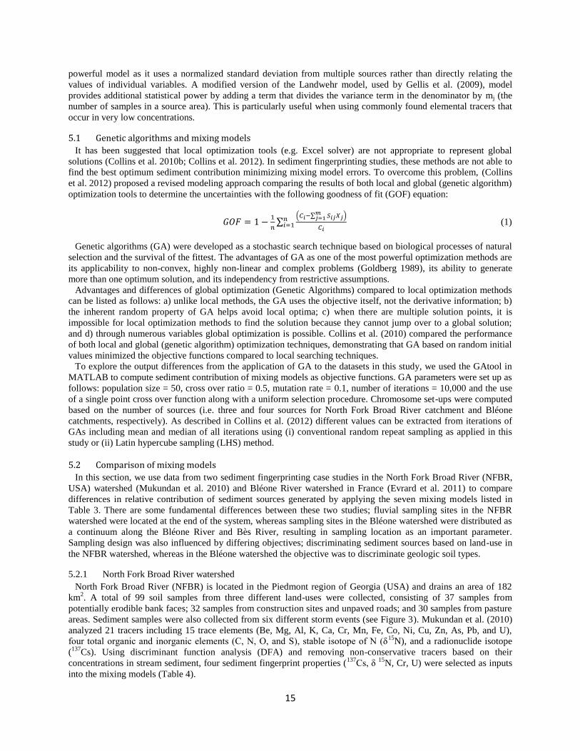
Table 6. GOF values of seven mixing model and two optimisations
Mixing models Optimization
method
GOF (%)
Bléone catchment NFBR catchment
Min Mean Max Min Mean Max
Collins GA 53 75.5 90 13.3 15.4 16.8
Local 62.2 76.8 89.2 30.3 54 79
Modified Collins GA 43.4 60.5 70 22.3 61 73.7
Local 60.8 72.5 87.8 18 55.7 75.3
Hughes GA 61.6 76.7 88.5 1 21.7 78
Local 63 77 88.6 35.7 60.3 75.4
Landwehr GA 48 63.7 74.7 <0 <0 <0
Local 59.7 75.6 88 25.5 48 67.3
Modified Landwehr GA 56 70.4 85 <0 <0 <0
Local 59.7 75.5 87.3 22.6 50.6 73.2
Motha GA 64.4 76.4 88 68.4 31 73.8
Local 64.4 76.3 88.8 48.7 23.3 77
Slattery GA 64.7 76.1 89 69.3 30.6 75
Local 62.8 76.3 88.8 67.5 28.2 77
Improved accuracy in both catchments was obtained when applying the original Collins model using a local
optimisation method than using a modified Collins mixing model. The use of GA in the modified Collins mixing
model, improved accuracy to 61% within the catchment with more source samples (NFBR with 99 source samples
in 3 sources), compared with local optimisation with a 55.7% goodness-of-fit. In the catchment with fewer sources
(Bleon with 18 source samples in 4 sources), local optimization was the more powerful method for calculating
source contributions (GOF=72.5%). In the Hughes model that uses the actual values rather than statistic parameters,
local optimization produced a higher goodness-of-fit of 77% and 60.3% in Bleon and NFBR catchments
respectively..
Comparing the application of all mixing models in each catchment, the Hughes mixing model appears a more
robust method in Bléone catchment using local optimization method (GOF=77%), and the modified Collins in
NFBR catchment using GA optimization (GOF= 61%).
6 Conclusion
Suspended sediments in fluvial systems can lead to a number of detrimental environmental and operational
impacts. Sediment fingerprinting techniques have been applied to fluvial systems to identify sources of sediment;
however the selection of model and optimization method can have profound effect on the output of sediment
fingerprinting analyses. This is the first review that has compared the most prevalent mixing models (including the
application of genetic algorithms) to an actual dataset to quantify variability in the output depending on the
application of mixing model.
All sediment fingerprinting studies must decide on the choice of field sampling methods, and selection of tracers
as well as mixing models. Allowing for time and budget constraints, the study objective should drive the field
sampling method. For example, fluvial sampling is the preferred method to determine the origin of sediment
deposited in a dam, whereas point sampling is the most appropriate method to monitor sediment contribution in a
flood event. Budget will also drive the selection of tracers used as sediment fingerprint properties. Physical tracers
are less expensive and can be measured easily, but they are not conservative and may lead to ambiguity in
interpretation of results. Geochemical tracers are favored due to large number of elements available for sediment
fingerprint measurements. Radionuclide tracers are the most powerful tracers to distinguish soils from different land
uses, but need expensive instruments.
Our review of 25 sediment fingerprinting studies identified land-use and geology as the most prevalent
discriminators of sediment sources. The relative importance of sediment sources to drainage systems should vary
among different catchments due to the contrasts in geology, watershed morphology, hydrology, connectivity of river
systems, human interference and many more factors. This inherent variability translates to a reliance on the final
step of all sediment fingerprinting studies; computing the contribution of different sediment sources via mixing
models. Using a common dataset, we have shown that different mixing models can identify different relative
contributions of sediment sources, but that the range of values among models are within an acceptable range of

20
errors (i.e. relative error, mean squared error etc.) in objective functions reported by the original authors. Based on
GOF, the modified Collins and Hughes mixing models are the most powerful models to estimate the source
contribution to transported sediments. Also, global optimization methods must be carefully applied when using the
Hughes mixing model. We suggest the use of a model that combines the best explanatory parameters from modified
Collins (it uses correction factors) and Hughes (it uses iterations of all data not mean values) with optimization
based on genetic algorithms would best predict the relative contribution of sediment sources to fluvial systems.
Acknowledgement
We would like to acknowledge Olivia H. Devereux and Andrew O. Hughes who provided advice on running
mixing models and Rajith Mukundan for providing NFBR catchment data. Reviews by Desmond E. Walling and
three anonymous referees improved the manuscript.
References
Blake, W. H., Ficken, K. J., Taylor, P., Russell, M. A. and Walling, D. E. 2012, Tracing crop-specific sediment
sources in agricultural catchments. Geomorphology Vol. 139–140, No., pp. 322-329.
Brown, A. G. 1985, The potential use of pollen in the identification of suspended sediment sources. Earth Surface
Processes and Landforms Vol. 10, No. 1, pp. 27-32.
Caitcheon, G., Prosser, I., Wallbrink, P., Douglas, G., Olley, J., Hughes, A., Hancock, G. and Scott, A. 2001,
Sediment delivery from Moreton Bay's main tributaries: a multifaceted approach to identifying sediment
sources. Third Australian Stream Management Conference, Brisbane, pp. 103-107.
Caitcheon, G. G., Olley, J. M., Pantus, F., Hancock, G. and Leslie, C. 2012, The dominant erosion processes
supplying fine sediment to three major rivers in tropical Australia, the Daly (NT), Mitchell (Qld) and
Flinders (Qld) Rivers. Geomorphology Vol. 151-152, No., pp. 188-195.
Carter, J., Owens, P. N., Walling, D. E. and Leeks, G. J. L. 2003, Fingerprinting suspended sediment sources in a
large urban river system. The Science of The Total Environment Vol. 314-316, No. 0, pp. 513-534.
Chapman, A. S., Foster, I. D. L., Lees, J. A., Hodgkinson, R. A. and Jackson, R. H. 2001, Particulate phosphorus
transport by sub-surface drainage from agricultural land in the UK. Environmental significance at the
catchment and national scale. Science of The Total Environment Vol. 266, No. 1-3, pp. 95-102.
Collins, A. L. and Walling, D. E. 2004, Documenting catchment suspended sediment sources: problems, approaches
and prospects. Progress in Physical Geography Vol. 28, No. 2, pp. 159-196.
Collins, A. L., Walling, D. E. and Leeks, G. J. L. 1996, Composite fingerprinting of the spatial source of fluvial
suspended sediment: a case study of the Exe and Severn river basins, United Kingdom. Géomorphologie:
relief, processus, environnement Vol. No., pp. 41-53.
Collins, A. L., Walling, D. E. and Leeks, G. J. L. 1997, Source type ascription for fluvial suspended sediment based
on a quantitative composite fingerorinting technique. Catena Vol. 29, No. 1, pp. 1-27.
Collins, A. L., Walling, D. E. and Leeks, G. J. L. 1997a, Fingerprinting the Origin of Fluvial Suspended Sediment in
Larger River Basins: Combining Assessment of Spatial Provenance and Source Type. Geografiska
Annaler. Series A, Physical Geography Vol. 79, No. 4, pp. 239-254.
Collins, A. L., Walling, D. E. and Leeks, G. J. L. 1998, Use of composite fingerprints to determine the provenance
of the contemporary suspended sediment load transported by rivers. Earth Surface Processes and
Landforms Vol. 23, No. 1, pp. 31-52.
Collins, A. L., Walling, D. E., Webb, L. and King, P. 2010a, Apportioning catchment scale sediment sources using a
modified composite fingerprinting technique incorporating property weightings and prior information.
Geoderma Vol. 155, No. 3-4, pp. 249-261.
Collins, A. L., Zhang, Y., Walling, D. E., Grenfell, S. E. and Smith, P. 2010b, Tracing sediment loss from eroding
farm tracks using a geochemical fingerprinting procedure combining local and genetic algorithm
optimisation. Science of The Total Environment Vol. 408, No. 22, pp. 5461-5471.
Collins, A. L., Zhang, Y., Walling, D. E., Grenfell, S. E., Smith, P., Grischeff, J., Locke, A., Sweetapple, A. and
Brogden, D. 2012, Quantifying fine-grained sediment sources in the River Axe catchment, southwest
England: application of a Monte Carlo numerical modelling framework incorporating local and genetic
algorithm optimisation. Hydrological Processes Vol. 26, No. 13, pp. 1962-1983.
Croke, J. and Mockler, S. 2001, Gully initiation and road-to-stream linkage in a forested catchment, southeastern
Australia. Earth Surface Processes and Landforms Vol. 26, No. 2, pp. 205-217.
Davis, M. and Fox, J. F. 2009, Sediment fingerprinting: Review of the method and future imrovements for allocating
nonpoint source pollution. Journal of Environmental Engineering Vol. 135, No. 7, pp. 490-504.

21
Devereux, O. H., Prestegaard, K. L., Needelman, B. A. and Gellis, A. C. 2010, Suspended-sediment sources in an
urban watershed, Northeast Branch Anacostia River, Maryland. Hydrological Processes Vol. 24, No. 11,
pp. 1391-1403.
Dirszowsky, R. W. 2004, Bed sediment sources and mixing in the glacierized upper Fraser River watershed, east-
central British Columbia. Earth Surface Processes and Landforms Vol. 29, No. 5, pp. 533-552.
Douglas, G., Caitcheon, G. G. and Palmer, M. 2009, Sediment source identification and residence times in the
Maroochy River estuary, southeast Queensland, Australia. Environmental Geology Vol. 57, No. 3, pp. 629-
639.
Dyer, F. J. and Olley, J. M. 1996, Preliminary results from determining sediment sources to the Tarago Reservoir,
Victoria, Australia: implications for sediment yield. In Erosion and Sediment Yield: Global and Regional
Perspectives (Proceedings of the Exeter Symposium), Wallingford, pp. 143-151.
Edwards, A. C. and Withers, P. J. A. 2008, Transport and delivery of suspended solids, nitrogen and phosphorus
from various sources to freshwaters in the UK. Journal of Hydrology Vol. 350, No. 3-4, pp. 144-153.
Estrany, J., Garcia, C. and Walling, D. E. 2010, An investigation of soil erosion and redistribution in a
Mediterranean lowland agricultural catchment using caesium-137. International Journal of Sediment
Research Vol. 25, No. 1, pp. 1-16.
Evrard, O., Navratil, O., Ayrault, S., Ahmadi, M., Némery, J., Legout, C., Lefèvre, I., Poirel, A., Bonté, P. and
Esteves, M. 2011, Combining suspended sediment monitoring and fingerprinting to determine the spatial
origin of fine sediment in a mountainous river catchment. Earth Surface Processes and Landforms Vol. 36,
No. 8, pp. 1072-1089.
Evrard, O., Poulenard, J., Némery, J., Ayrault, S., Gratiot, N., Duvert, C., Prat, C., Lefèvre, I., Bonté, P. and Esteves,
M. 2012, Tracing sediment sources in a tropical highland catchment of central Mexico by using
conventional and alternative fingerprinting methods. Hydrological Processes Vol. No., pp. n/a-n/a.
Foster, G. R. 1988, Modeling soil erosion and sediment. Soil erosion research methods, Ankeny, Iowa,, pp. 97-117.
Foster, I. D. L., Boardman, J. and Keay-Bright, J. 2007, Sediment tracing and environmental history for two
catchments, Karoo Uplands, South Africa. Geomorphology Vol. 90, No. 1-2, pp. 126-143.
Fox, J. F. and Papanicolaou, A. N. 2007, The Use of Carbon and Nitrogen Isotopes to Study Watershed Erosion
Processes. JAWRA Journal of the American Water Resources Association Vol. 43, No. 4, pp. 1047-1064.
Fox, J. F. and Papanicolaou, A. N. 2008, An un-mixing model to study watershed erosion processes. Advances in
Water Resources Vol. 31, No. 1, pp. 96-108.
Gellis, A. C., Emmett, W. W. and Leopold, L. B. 2005, Channel and hillslope processes revisited in the Arroyo de
los Frijoles watershed near Santa Fe, New Mexico. U.S. Geological Survey Professional Paper. 1704: 53.
Gellis, A. C., Hupp, C. R., Pavich, M. J., Landwehr, J. M., Banks, W. S. L., Hubbard, B. E., Langland, M. J.,
Ritchie, J. C. and Reuter, J. M. 2009, Sources, transport, and storage of sediment in the Chesapeake Bay
Watershed. U.S. Geological Survey Scientific Investigations Report 2008-5186: 95.
Goldberg, D. E. 1989, Genetic algorithms in search, optimization, and machine learning. Addison-Wesley, Reading,
MA, USA.
Grimshaw, D. L. and Lewin, J. 1980, Source identification for suspended sediments. Journal of Hydrology Vol. 47,
No. 1-2, pp. 151-162.
Gruszowski, K. E., Foster, I. D. L., Lees, J. A. and Charlesworth, S. M. 2003, Sediment sources and transport
pathways in a rural catchment, Herefordshire, UK. Hydrological Processes Vol. 17, No. 13, pp. 2665-2681.
Hardy, F., Bariteau, L., Lorrain, S., Theriault, I., Gagnon, G., Messier, D. and Rougerie, J. F. 2010, Geochemical
tracing and spatial evolution of the sediment bed load of the Romaine River, Quebec, Canada. CATENA
Vol. 81, No. 1, pp. 66-76.
Hatfield, R. G. and Maher, B. A. 2009, Fingerprinting upland sediment sources : particle size-specific magnetic
linkages between soils, lake and suspended sediments. Earth Surface Processes and Landforms Vol. 34, No.
10, pp. 1359-1373.
He, Q. and Owens, P. 1995, Determination of suspended sediment provenance using caesium-137, unsupported
lead-210 and radium-226: a numerical mixing model approach. In Sediment and Water Quality in River
Catchments. G. A. Foster IDL, Webb BW. Chichester, Wiley: 207-227.
Horowitz, A. J., Elrick, K. A. and Hooper, R. C. 1989, A comparison of instrumental dewatering methods for the
separation and concentration of suspended sediment for subsequent trace element analysis. Hydrological
Processes Vol. 3, No. 2, pp. 163-184.
Hughes, A. O., Olley, J. M., Croke, J. C. and McKergow, L. A. 2009, Sediment source changes over the last 250
years in a dry-tropical catchment, central Queensland, Australia. Geomorphology Vol. 104, No. 3-4, pp.
262-275.
22
Hughes, A. O., Olley, J. M., Croke, J. C. and McKergow, L. A. 2009, Sediment source changes over the last
250 years in a dry-tropical catchment, central Queensland, Australia. Geomorphology Vol. 104, No. 3-4,
pp. 262-275.
Jenns, N., Heppell, C. M., Burt, T. P., Walden, J. and Foster, I. D. L. 2002, Investigating contemporary and
historical sediment inputs to Slapton Higher Ley: an analysis of the robustness of source ascription methods
when applied to lake sediment data. Hydrological Processes Vol. 16, No. 17, pp. 3467-3486.
Klages, M. G. and Hsieh, Y. P. 1975, Suspended solids carried by the Gallatin River of southwestern Montana: II.
Using minerology for inferring sources. Journal of Environmental Quality Vol. 4, No. 1, pp. 68-73.
Kouhpeima, A., Feiznia, S., Ahmadi, H., Hashemi, S. A. and Zareiee, A. R. 2010, Application of quantitative
composite fingerprinting technique to identify the main sediment sources in two small catchments of Iran.
Hydrology and Earth System Sciences Vol. 7, No., pp. 6677-6698.
Krause, A. K., Franks, S. W., Kalma, J. D., Loughran, R. J. and Rowan, J. S. 2003, Multi-parameter fingerprinting
of sediment deposition in a small gullied catchment in SE Australia. CATENA Vol. 53, No. 4, pp. 327-348.
Krein, A., Petticrew, E. and Udelhoven, T. 2003, The use of fine sediment fractal dimensions and colour to
determine sediment sources in a small watershed. Catena Vol. 53, No. 2, pp. 165-179.
Lartiges, B. S., Deneux-Mustin, S., Villemin, G., Mustin, C., Barrès, O., Chamerois, M., Gerard, B. and Babut, M.
2001, Composition, structure and size distribution of suspended particulates from the Rhine River. Water
Research Vol. 35, No. 3, pp. 808-816.
Lawler, D. M., Grove, J. R., Couperthwaite, J. S. and Leeks, G. J. L. 1999, Downstream change in river bank
erosion rates in the Swale–Ouse system, northern England. Hydrological Processes Vol. 13, No. 7, pp. 977-
992.
Lees, J. A. 1997, Mineral magnetic properties of mixtures of environmental and synthetic materials: linear additivity
and interaction effects. Geophysical Journal International Vol. 131, No. 2, pp. 335-346.
Loughran, R. J. and Campbell, B. L. 1995, The identification of catchment sediment sources. In Sediment and Water
Quality in River Catchments. I. D. L. Foster, A. M. Gurnell and B. W. Webb. Chichester, Wiley: 189-205.
Madej, M. A. 2001, Erosion and sediment delivery following removal of forest roads. Earth Surface Processes and
Landforms Vol. 26, No. 2, pp. 175-190.
Maher, B. A. 1998, Magnetic properties of modern soils and Quaternary loessic paleosols: paleoclimatic
implications. Palaeogeography, Palaeoclimatology, Palaeoecology Vol. 137, No. 1-2, pp. 25-54.
Martínez-Carreras, N., Krein, A., Gallart, F., Iffly, J. F., Pfister, L., Hoffmann, L. and Owens, P. N. 2010,
Assessment of different colour parameters for discriminating potential suspended sediment sources and
provenance: A multi-scale study in Luxembourg. Geomorphology Vol. 118, No. 1-2, pp. 118-129.
Matissoff, G., C., B. E. and J., W. P. 2002, Soil Erosion and Sediment Sources in an Ohio Watershed using
Beryllium-7, Cesium-137, and Lead-210. Journal of Environmental Quality Vol. 31, No. 1, pp. 54-61.
McLennan, S. M. 1993, Weathering and global denudation. The Journal of Geology Vol. 101, No. 2, pp. 295-303.
Miller, J. R., Lord, M., Yurkovich, S., Mackin, G. and Kolenbrander, L. 2005, HISTORICAL TRENDS IN
SEDIMENTATION RATES AND SEDIMENT PROVENANCE, FAIRFIELD LAKE, WESTERN
NORTH CAROLINA1. JAWRA Journal of the American Water Resources Association Vol. 41, No. 5, pp.
1053-1075.
Minella, J. P. G., Merten, G. H. and Clarke, R. T. 2004, identification of sediment sources in a small rural drainage
basin. IAHS Publication, Wallingford, U. K.
Minella, J. P. G., Walling, D. E. and Merten, G. H. 2008, Combining sediment source tracing techniques with
traditional monitoring to assess the impact of improved land management on catchment sediment yields.
Journal of Hydrology Vol. 348, No. 3-4, pp. 546-563.
Mizugaki, S., Onda, Y., Fukuyama, T., Koga, S., Asai, H. and Hiramatsu, S. 2008, Estimation of suspended
sediment sources using 137Cs and 210Pbex in unmanaged Japanese cypress plantation watersheds in
southern Japan. Hydrological Processes Vol. 22, No. 23, pp. 4519-4531.
Morris, G. L. and Fan, J. 1997, Reservoir sedimentation handbook. McGraw-Hill, New York.
Motha, J. A., Wallbrink, P. J., Hairsine, P. B. and Grayson, R. B. 2002, Tracer properties of eroded sediment and
source material. Hydrological Processes Vol. 16, No., pp. 1983-2000.
Motha, J. A., Wallbrink, P. J., Hairsine, P. B. and Grayson, R. B. 2002, Tracer properties of eroded sediment and
source material. Hydrological Processes Vol. 16, No. 10, pp. 1983-2000.
Motha, J. A., Wallbrink, P. J., Hairsine, P. B. and Grayson, R. B. 2003, Determining the sources of suspended
sediment in a forested catchment in southeastern Australia. Water Resources Research Vol. 39, No. 3, pp.
1056-1070.

23
Motha, J. A., Wallbrink, P. J., Hairsine, P. B. and Grayson, R. B. 2004, Unsealed roads as suspended sediment
sources in an agricultural catchment in south-eastern Australia. Journal of Hydrology Vol. 286, No. 1-4, pp.
1-18.
Mukundan, R., Radcliffe, D. E., Ritchie, J. C., Risse, L. M. and McKinley, R. A. 2010, Sediment fingerprinting to
determine the source of suspended sediment in a southern Piedmont stream. Journal of environmental
Quality Vol. 39, No. 1, pp. 1328-1337.
Nagle, G. N. and Ritchie, J. C. 2004, Wheat field erosion rates and channel bottom sediment sources in an
intensively cropped northeastern Oregon drainage basin. Land Degradation & Development Vol. 15, No. 1,
pp. 15-26.
Navratil, O., Evrard, O., Esteves, M., Legout, C., Ayrault, S., Némery, J., Mate-Marin, A., Ahmadi, M., Lefèvre, I.,
Poirel, A. and Bonté, P. 2012, Temporal variability of suspended sediment sources in an alpine catchment
combining river/rainfall monitoring and sediment fingerprinting. Earth Surface Processes and Landforms
Vol. 37, No. 8, pp. 828-846.
Nelson, E. J. and Booth, D. B. 2002, Sediment sources in an urbanizing, mixed land-use watershed. Journal of
Hydrology Vol. 264, No. 1-4, pp. 51-68.
Nicholls, D. J. 2001, The source and behaviour of fine sediment deposits in the River Torridge Devon and their
implications for salmon spawning. PhD, University of Exeter.
Nosrati, K., Govers, G., Ahmadi, H., Sharifi, F., Amoozegar, M. A., Merckx, R. and Vanmaercke, M. 2011, An
exploratory study on the use of enzyme activities as sediment tracers: biochemical fingerprints?
International Journal of Sediment Research Vol. 26, No. 2, pp. 136-151.
Olley, J., Burton, J., Smolders, K., Pantus, F. and Pietsch, T. 2012, The application of fallout radionuclides to
determine the dominant erosion process in water supply catchments of subtropical South-east Queensland,
Australia. Hydrological Processes Vol. No., pp. n/a-n/a.
Olley, J. and Caitcheon, G. 2000, Major element chemistry of sediments from the Darling-Barwon river and its
tributaries: implications for sediment and phosphorus sources. Hydrological Processes Vol. 14, No. 7, pp.
1159-1175.
Olley, J. M. and Caitcheon, G. 2000, Major element chemistry of sediments from the Darling–Barwon river and its
tributaries: implications for sediment and phosphorus sources. Hydrological Processes Vol. 14, No. 7, pp.
1159-1175.
Olley, J. M., Caitcheon, G. G., Hancock, G. and Wallbrink, P. 2001, Tracing and dating techniques for sediment and
associated substances, CSIRO Land and Water, Canberra.
Olley, J. M., Caitcheon, G. G., Hancock, G. and Wallbrink, P. J. 2001, Tracing and dating techniques for sediment
and associated substances. CSIRO Land and Water, Canberra.
Olley, J. M., Murray, A. S., Mackenzie, D. H. and Edwards, K. 1993, Identifying sediment sources in a gullied
catchment using natural and anthropogenic radioactivity. Water Resour. Res. Vol. 29, No. 4, pp. 1037-
1043.
Owens, P. N., Walling, D. E. and Leeks, G. J. L. 2000, Tracing fluvial suspended sediment sources in the catchment
of the River Tweed, Scotland, using composite fingerprints and a numerical mixing model. Tracers in
Geomorphology. Chichester, Wiley: 291-307.
Papanicolaou, A. N., Fox, J. F. and Marshall, J. 2003, Soil fingerprinting in the Palouse basin, USA using stable
carbon and nitrogen isotopes. International Journal of Sediment Research Vol. 18, No. 2, pp. 291-297.
Parsons, A. J. 2012, How useful are catchment sediment budgets? Progress in Physical Geography Vol. 36, No. 1,
pp. 60-71.
Peart, M. R. 1993, Using sediment properties as natural tracers for sediment source: two case studies from Hong
Kong. Tracers in Hydrology. Proceedings of the Yokohama Symposium, IAHS Publication. 215: 313-318.
Phillips, J. M., Russell, M. A. and Walling, D. E. 2000, Time-integrated sampling of fluvial suspended sediment: a
simple methodology for small catchments. Hydrological Processes Vol. 14, No. 14, pp. 2589-2602.
Pietola, L., Horn, R. and Yli-Halla, M. 2005, Effects of trampling by cattle on the hydraulic and mechanical
properties of soil. Soil and Tillage Research Vol. 82, No. 1, pp. 99-108.
Poulenard, J., Legout, C., Némery, J., Bramorski, J., Navratil, O., Douchin, A., Fanget, B., Perrette, Y., Evrard, O.
and Esteves, M. 2012, Tracing sediment sources during floods using Diffuse Reflectance Infrared Fourier
Transform Spectrometry (DRIFTS): A case study in a highly erosive mountainous catchment (Southern
French Alps). Journal of Hydrology Vol. 414–415, No. 0, pp. 452-462.
Poulenard, J., Perrette, Y., Fanget, B., Quetin, P., Trevisan, D. and Dorioz, J. M. 2009, Infrared spectroscopy tracing
of sediment sources in a small rural watershed (French Alps). Science of The Total Environment Vol. 407,
No. 8, pp. 2808-2819.

24
Prosser, I. P., Rutherfurd, I. D., Olley, J. M., Young, W. J., Wallbrink, P. J. and Moran, C. J. 2001, Large-scale
patterns of erosion and sediment transport in river networks, with examples from Australia. Marine And
Freshwater Research Vol. 52, No. 1, pp. 81-99.
Ramos-Scharrón, C. E. and MacDonald, L. H. 2007, Measurement and prediction of natural and anthropogenic
sediment sources, St. John, U.S. Virgin Islands. Catena Vol. 71, No. 2, pp. 250-266.
Reid, L. M. and Dunne, T. 1996, Rapid evaluation of sediment budgets. Catena Verlag GMBH, Reiskirchen,
Germany.
Rhoton, F. E., Emmerich, W. E., DiCarlo, D. A., Nearing, M. A. and Ritchie, J. C. 2008, Identification of suspended
sediment sources using soil characteristics in a semiarid watershed. Soil Science Society of American
Journal Vol. 72, No. 4, pp. 1102-1112.
Richards, C. and Bacon, K. L. 1994, Influence of fine sediment on macroinvertebrate colonization of surface and
hyporheic stream substrates. Great Basin Naturalist Vol. 54, No., pp. 106-113.
Rowan, J. S., Goodwill, P. and Franks, S. W. 2000, Uncertainty estimation in fingerprinting suspended sediment
sources. Tracers in Geomorphology. I. D. L. Foster. Chichester, UK, Wiley: 279-290.
Russell, M. A., Walling, D. E. and Hodgkinson, R. A. 2001, Suspended sediment sources in two small lowland
agricultural catchments in the UK. Journal of Hydrology Vol. 252, No. 1-4, pp. 1-24.
Sheridan, G. J., Noske, P. J., Lane, P. N. J. and Sherwin, C. B. 2008, Using rainfall simulation and site
measurements to predict annual interrill erodibility and phosphorus generation rates from unsealed forest
roads: Validation against in-situ erosion measurements. Catena Vol. 73, No. 1, pp. 49-62.
Slattery, M., Walden, J. and Burt, T. P. 2000, Fingerprinting suspended sediment sources using mineral magnetic
measurements- A quantitative approach. Tracers in geomorphology, John Wiley and Sons: 309-322.
Slattery, M. C., Burt, T. P. and Walden, J. 1995, The application of mineral magnetic measurements to quantify
within-storm variations in suspended sediment sources. Tracer Technologies for Hydrological Systems.
Proceedings of a Boulder Symposium, IAHS Publication. 229: 143-151.
Vanden Bygaart, A. J. and Protz, R. 2001, Bomb-Fallout Cs-137 as a Marker of Geomorphic Stability in Dune
Sands and Soils, Pinery Provincial Park, Ontario, Canada. Earth Surface Processes and Landforms Vol. 26,
No., pp. 689-700.
Wallbrink, P. J. and Murray, A. S. 1996, Determining soil loss using the inventory ratio of excess Lead-210 to
Cesium-137. Soil Science Society of America, Madison, WI, ETATS-UNIS.
Wallbrink, P. J., Murray, A. S., Olley, J. M. and Olive, L. J. 1998, Determining sources and transit times of
suspended sediment in the Murrumbidgee River, New South Wales, Australia, using fallout 137Cs and
210Pb. Water Resour. Res. Vol. 34, No. 4, pp. 879-887.
Walling, D. E. 2005, Tracing suspended sediment sources in catchments and river systems. Science of The Total
Environment Vol. 344, No. 1-3, pp. 159-184.
Walling, D. E. and Amos, C. M. 1999, Source, storage and mobilisation of fine sediment in a chalk stream system.
Hydrological Processes Vol. 13, No. 3, pp. 323-340.
Walling, D. E., Collins, A. L., Sichingabula, H. M. and Leeks, G. J. L. 2001, Integrated assessment of catchment
suspended sediment budgets: a Zambian example. Land Degradation & Development Vol. 12, No. 5, pp.
387-415.
Walling, D. E., Collins, A. L. and Stroud, R. W. 2008, Tracing suspended sediment and particulate phosphorus
sources in catchments. Journal of Hydrology Vol. 350, No. 3-4, pp. 274-289.
Walling, D. E., Owens, P. N. and Leeks, G. J. L. 1999, Fingerprinting suspended sediment sources in the catchment
of the River Ouse, Yorkshire, UK. Hydrological Processes Vol. 13, No. 7, pp. 955-975.
Walling, D. E. and Woodward, J. C. 1995, Tracing sources of suspended sediment in river basins: a case study of
the River Culm, Devon, UK. Marine and Freshwater Research Vol. 46, No. 1, pp. 327-336.
Walling, D. E., Woodward, J. C. and Nicholas, A. P. 1993, A multi-parameter approach to fingerprinting suspended-
sediment sources IAHS publication.
Wasson, R. J., Mazari, R. K., Starr, B. and Clifton, G. 1998, The recent history of erosion and sedimentation on the
Southern Tablelands of southeastern Australia: sediment flux dominated by channel incision.
Geomorphology Vol. 24, No. 4, pp. 291-308.
Weltje, G. J. and Brommer, M. B. 2011, Sediment-budget modelling of multi-sourced basin fills: application to
recent deposits of the western Adriatic mud wedge (Italy). Basin Research Vol. 23, No. 3, pp. 291-308.
Wemple, B. C., Swanson, F. J. and Jones, J. A. 2001, Forest roads and geomorphic process interactions, Cascade
Range, Oregon. Earth Surface Processes and Landforms Vol. 26, No. 2, pp. 191-204.

25
Wilkinson, S. N., Hancock, G. J., Bartley, R., Hawdon, A. A. and Keen, R. J. In press, Using sediment tracing to
assess processes and spatial patterns of erosion in grazed rangelands, Burdekin River basin, Australia.
Agriculture, Ecosystems & Environment Vol. No. 0.
Williams, G. P. 1989, Sediment concentration versus water discharge during single hydrologic events in rivers.
Journal of Hydrology Vol. 111, No. 1–4, pp. 89-106.
Wood, P. J. and Armitage, P. D. 1997, Biological Effects of Fine Sediment in the Lotic Environment. Environmental
Management Vol. 21, No. 2, pp. 203-217.
Wright, J. F. and Berrie, A. D. 1987, Ecological effects of groundwater pumping and a natural drought on the upper
reaches of a chalk stream. Regulated Rivers: Research & Management Vol. 1, No. 2, pp. 145-160.
Zapata, F. 2003, The use of environmental radionuclides as tracers in soil erosion and sedimentation investigations:
recent advances and future developments. Soil and Tillage Research Vol. 69, No. 1-2, pp. 3-13.
Zhang, Q., Lei, T. and Zhao, J. 2008, Estimation of the detachment rate in eroding rills in flume experiments using
an REE tracing method. Geoderma Vol. 147, No. 1-2, pp. 8-15.
Related Documents