Securitization and Real Investment in Incomplete Markets

Securitization and Real Investment in Incomplete Markets∗

Vishal Gaur†, Sridhar Seshadri‡, Marti G. Subrahmanyam‡

August 15, 2007

Abstract

We study the impact of financial innovations on real investment decisions within the frame-work of an incomplete market economy comprised of firms, investors, and an intermediary. Thefirms face unique investment opportunities that arise in their business operations and can beundertaken at given reservation prices. The cash flows thus generated are not spanned by thesecurities traded in the financial market, and cannot be valued uniquely. The intermediarypurchases claims against these cash flows, pools them together, and sells tranches of primary orsecondary securities to the investors.

We derive necessary and sufficient conditions under which projects are undertaken due tothe intermediary’s actions and firms are amenable to the pool proposed by the intermediarycompared to the no-investment option or the option of forming alternative pools. We alsodetermine the structure of the new securities created by the intermediary and identify how itexploits the arbitrage opportunities available in the market. Our results have implications forvaluation of real investments, synergies among them, and their financing mechanisms.

Keywords: Incomplete markets, Securitization, Financial innovation, Real options.

∗The authors thank Kose John, Roy Radner and Rangarajan Sundaram for useful discussions. They also thank

participants in seminars at Columbia University, Ente Einaudi, Rome, University of Melbourne, New York University,

Rutgers University, the University of Venice, the Caesarea Center, Herzliya, Israel, and Stanford University, as well

as in the 2004 European Finance Association meetings in Maastricht, the 2004 Informs meetings in Denver, and the

2005 European FMA Conference in Siena, for comments and suggestions made during this research.†Johnson Graduate School of Management, Cornell University, Sage Hall, Ithaca, NY 14853-6201. E-mail:

[email protected].‡Leonard N. Stern School of Business, New York University, 44 West 4th St., New York, NY 10012. E-mail:

[email protected], [email protected].

1 Introduction

Do innovations in capital markets have an impact on real investment decisions, aside from providing

arbitrage opportunities to the innovators? In other words, do such innovations permit investments

in real assets that would otherwise not occur because they are too costly to finance? The casual

evidence suggests that the answers to these questions are in the affirmative, based on examples

such as venture capital, private equity, project finance, and securitization. In all these cases,

the innovations allow financing to be provided for projects that might not be undertaken in their

absence. Entrepreneurs and firm managers are able to undertake fresh investments in projects since

their “cost of capital” has been reduced by the innovations, thus making the net present value of

the projects positive.

Three alternative mechanisms may be responsible for the improved attractiveness of projects

as a result of a financial innovation. The first is a reduction in the impact of market frictions, such

as transaction costs, as a result of the innovation. The second is the effect of the innovation on the

amelioration of asymmetric information effects, particularly in the context of the principal-agent

relationship between investors on the one hand and the entrepreneur/manager on the other. The

third is through the effect of better matching of the cash flows to the needs of investors, in the

context of an incomplete financial market. The first two mechanisms have been used in a variety of

models proposed in the literature to study the impact of financial innovations on real investment

decisions. We examine the third mechanism, which has not been adequately studied thus far. We

study the impact of market incompleteness on real investment using only the no-arbitrage principle,

i.e., without making explicit assumptions about market frictions or information asymmetry.

The problem we pose is a fairly common one. Firms often have opportunities that are unique

to them and generate future cash flows that cannot be replicated by transactions in the existing

securities in the market. Such opportunities include capacity investment decisions, new product

launches, investment in distribution systems, lead time reduction, etc. In the standard paradigm

of financial economics, the value of a project is derived from capital market prices based on the

twin assumptions that the cash flows from the project can be replicated in the financial market and

1

that all agents are price-takers with respect to the market for financial claims. When markets are

incomplete, the value of a real asset cannot always be uniquely computed from capital market prices

using arbitrage pricing arguments, but only bounds can be placed on its present value. Therefore,

projects whose values are unambiguously greater than their reservation prices are financed, and

those whose values unambiguously fall below their respective reservation prices are rejected.

However, nothing specific can be said when the reservation price lies between these price bounds.

For example, a project to expand a distribution network, may fall into this category. The project

may be financed by securities that are, in turn, packaged and sold to investors through a securitiza-

tion structure, thus making the project viable, and perhaps even more attractive from a valuation

perspective than projects that are financed by conventional securities, such as straight debt or

equity. We study the impact of financial innovation on such real investments that cannot be valued

unambiguously in an incomplete capital market.

The specific financial innovation we consider is securitization, although our framework lends

itself to the analysis of other financial innovations. Since its beginning in the 1970s, the phenomenon

of securitization is now widespread in financial markets: mortgages, credit card receivables and

various types of corporate debt instruments have been securitized using a variety of alternative

structures. The common feature of these structures is that an intermediary purchases claims on

cash flows issued by various entities, pools these claims into a portfolio, and then tranches them

into marketable securities that cater to the investment needs of particular clienteles of investors.

To take the example of collateralized debt obligations (CDOs), the basic structure is that

a financial intermediary sets up a special purpose vehicle (SPV) that buys a portfolio of debt

instruments - bonds and/or loans - and adds credit derivatives on individual “names.” This is

referred to as pooling. The SPV then issues various claims against the pooled portfolio, which enjoy

different levels of seniority ranging from a super-senior claim, i.e., a high-grade AAA claim, which

has a negligible probability of not meeting its promised payment, to a medium-grade mezzanine

claim, say rated BBB+, which has a low but not negligible probability of such default, and finally,

to an equity security, which is viewed as risky. The structuring of the claims to match investor

tastes and risk preferences is referred to as tranching and the claims are referred to as tranches.

2

In our model, securitization transactions take place among three types of agents, namely, firms,

investors, and financial intermediaries. Firms have opportunities to create unique assets at given

reservation prices. Their objective is to maximize the time-zero value of these assets. Investors are

utility maximizers. Intermediaries purchase claims from firms that are fully backed by project cash

flows, and issue two types of securities to be sold to investors. They can issue securities that are

within the span of the financial market (marketable securities), or create new securities that are

not spanned by the market (secondary securities). Throughout our analysis, we assume that these

transactions are not large enough to influence the prices of existing securities traded in the market,

i.e., all agents are price-takers. In an arbitrage-free setting, we study whether the transactions

undertaken by the intermediary create value for firms and investors. The value for firms is created

by permitting investments in real assets that would not be undertaken otherwise. The value to

investors is created by satisfying demand for consumption better than the primary securities traded

in the financial market. Our model addresses several questions: Can the firms’ projects be financed

through securitization of claims issued against their cash flows? In view of the synergistic effect

of pooling assets, what are the incentives for firms to willingly transact with the intermediary?

Finally, what investor needs are served by the secondary securities issued by the intermediary, and,

in turn, how does that affect the financing of projects?

We first consider the impact of pooling. We analyze the setting in which the financial interme-

diary pools cash flows from the assets of several firms or divisions of a firm, and issues only such

securities as are within the span of the market. We allow firms to form coalitions with some or all

of the other firms to seek financing. Therefore, the outcome of the firms’ decision problem can be

modeled as a cooperative game. We show that there is a simple condition that is necessary and

sufficient for all firms to participate in the game. When this condition is not met, we prove that

there is a maximal pool of assets that can be created in the cooperative game. This pool is the

one that maximizes the value enhancement provided by pooling, and may or may not consist of all

assets of all firms. Thus, pure pooling (sans tranching) can provide not only value enhancement,

but also sustain the synergy through a price mechanism.

We then consider the joint pooling and tranching problem, in which a financial intermediary first

3

pools cash flows from several firms, and then issues securities against the pool. Through tranching,

the intermediary can customize securities to the needs of investors. Therefore, we expect pooling

and tranching to provide greater value than pure pooling alone. We show that the additional

value can be characterized using the structure of securities created. The securities created by the

intermediary can have up to three components; a component that is marketable, a second type that

exploits arbitrage opportunities available in the market due to the intermediary’s special ability

to design and sell securities to a subset of investors, and a third component that is the remainder

of the asset pool. The first is sold at exactly the market price, whereas the second is sold at a

price higher than the market’s upper bound; the third is sold at a price within the bounds given

by considerations of arbitrage. The presence or absence of these three components in the tranching

solution has a direct bearing upon the composition of the asset pool, and therefore, upon value

creation due to financing additional projects. We find that tranching plays a somewhat different

role than pooling. While tranching increases the value of the projects financed similar to pooling, it

could also result in more selective financing. Due to this effect, the set of projects that are financed

could shrink or expand, when compared to pooling alone.

It should be emphasized that the value creation studied in our paper is due to securities created

from the cash flows of new projects. This is fundamentally different from profits that can arise in

an incomplete market from arbitrage involving existing securities. We exclude such arbitrage in our

analysis, since we presume that it has already occurred prior to the innovation, and is reflected in

the initial equilibrium in the market.1 The value creation studied in our paper is also fundamentally

different from the mechanisms of risk pooling and operational flexibility studied in the operations

management literature. Our approach envisages the creation of new securities that augment those

available in the existing market, rather than merely repackaging existing securities. These new

securities make the valuation of some new projects more clear, and hence, viable.

Our results imply that the optimal real investment decision of a firm depends on the form1DeMarzo (2005) argues, quite correctly, that “market incompleteness cannot explain the construction of ... pools,

which do not augment the span of tradeable claims.” Our analysis refers to the creation of new securities that are

potentially outside the span of the existing market.

4

of financing chosen by it. Through securitization, the firm can value its real investment more

accurately as well as identify valuation synergies with other real investments. Thus, the decisions

of whether to undertake a real investment and in what quantity are affected. Our results can

be applied to other examples of financial intermediation in the context of market incompleteness,

such as the choice of investments by a venture capitalist, the optimal asset-liability mix of a bank,

mergers and acquisitions, and optimal financing.

This paper is organized as follows: §2 reviews the related literature on incomplete markets

and securitization; §3 presents the model setup and assumptions; §4 analyzes the conditions under

which there is value in pooling, and firms willingly participate in the creation of the asset pool; §5

analyzes the conditions under which there is value in pooling and tranching, and determines the

optimal tranching strategy; §6 presents a numerical example illustrating the results of our paper;

and §7 concludes with a discussion of the implications of our analysis.

2 Literature Review

Our research is related to the literature on securitization, valuation in incomplete markets, and

operations-finance interface. We summarize related results from these topics below.

Securitization is broadly defined as the issuance of securities in the capital market that are

backed or collateralized by a portfolio of assets. Specific examples of securitization include the

academic literature on “supershares” (i.e., tranches of the portfolio of all securities in the market),

primes and scores (i.e., income and capital gains portions of a stock), and “bull” and “bear” bonds.2

More recently, other examples of securitization have been analyzed by researchers, e.g., the assets of

insurance companies (Cummins (2004)), and those of firms in financial distress (Ayotte and Gaon

(2004)). The literature on securitization is fairly sparse. The rationale for the widespread use

of pooling and tranching in the asset-backed securities market is largely based on two alternative

economic explanations, market imperfections such as transaction costs, and information asymmetry.

In a study of the first explanation, Allen and Gale (1991) examine the incentive of a firm to issue2See Hakansson (1978), and Jarrow and O’Hara (1989) for details.

5

a new security when there are transaction costs. They study an exchange equilibrium that results

after the introduction of the new security in an incomplete market. They find that not every firm

needs to innovate. Even if a single firm amongst many similar ones, or a financial intermediary does

so, investors can benefit if short sales are permitted. The new security results in a readjustment

of consumption by investors, which, in turn, leads to a change in asset prices that may benefit

the firm. There are two implications of this shift: (a) the ex-post value of similar firms may be

equal, thus reducing the incentive of any one firm to innovate, and (b) the firm has an incentive to

innovate only if prices change, i.e., if competition is imperfect.

We draw upon the model of Allen and Gale (1991), but our approach differs from theirs in

significant ways. First, our model does not use a general equilibrium approach. The reason is

that we are interested in obtaining more specific results, without considering the complex feedback

effects that a general equilibrium analysis would entail. Second, we use a game-theoretic setting to

ensure participation by firms. Third, we do not explicitly model the cost of issuing claims, since we

wish to focus on value creation in a frictionless market. Fourth, our aim is to explicitly introduce

a third type of agent - firms - into the exchange equilibrium and study how they can benefit from

intermediation. Moreover, in our framework, the problem for firms is not just whether to issue new

claims against returns from existing assets; rather, the problem is to decide what new projects to

undertake. Lastly, in order to study the effect of intermediation and whether it helps more firms

to undertake investments (or firms to invest in more projects), we have to necessarily limit short

sales of secondary securities by investors - otherwise, investors can also intermediate. Therefore,

we confine the financial innovation activity to designated financial intermediaries.

Several researchers have studied the effect of information asymmetry between issuers and in-

vestors in the context of securitization (see, for example, Leland and Pyle (1977), DeMarzo and

Duffie (1999), and DeMarzo (2005)).3 Pooling and tranching of assets are considered beneficial to3There is an extensive literature on security design in the context of asymmetric information between “insiders”

and investors, which can be traced back to the signalling model proposed by Leland and Pyle (1977). We mention

here only those papers that are directly related to the securitization of claims by pooling and tranching. DeMarzo

and Duffie (1999) and DeMarzo (2005) provide a more detailed discussion of the broader literature.

6

both an informed issuer and an uninformed investor. The benefits to the issuer result from reducing

the incentive to gather information (Glaeser and Kallal 1997), reducing liquidity costs (DeMarzo

and Duffie 1999), and designing low-risk debt securities that minimize information asymmetry with

investors (DeMarzo 2005). The benefits to the investor result from the ability to split cash flows

into a risk-less debt and an equity claim (Gorton and Pennachi 1990), and reducing the adverse

selection problem (DeMarzo 2005).

Even though these explanations based on transaction costs and informational asymmetry might

explain the structure of securities to an extent, they do not provide the motivation to innovate or

securitize, especially in the context of originating firms, who then use the proceeds to undertake

more projects. In particular, DeMarzo (2005) assumes that the asset pool is given; the main issue

is whether tranching overcomes the information destruction effects of pure pooling. Our focus in

this paper is on the effect of market incompleteness on the value created by securitization through

the optimal design of both the pool and the tranches.

In the literature on valuation in incomplete markets, three approaches have been adopted for

pricing contingent claims, through bounds based on no-arbitrage, preference-based approaches that

impose restrictions on the utility functions of consumers, and approximate arbitrage-based argu-

ments. Under the arbitrage-based approach of Harrison and Kreps (1979), when the market is

incomplete, the securities whose cash flows are not spanned by the existing market do not have a

unique price, but have price bounds based on the no-arbitrage principle. In the second approach,

it is possible to restrict investor preferences or return distributions to get exact prices such as in

the capital asset pricing model (CAPM). An example of this approach is the literature on option

pricing using such preference restrictions, e.g., Perrakis and Ryan (1984), Levy (1985), Ritchken

(1985), Ritchken and Kuo (1989), and Mathur and Ritchken (1999). Recent research has focused on

the third approach in several ways, such as imposing economic restrictions in the arbitrage pricing

theory based on the reward-to-risk ratio or Sharpe ratio, combining the arbitrage-based and the

preference-based approaches, and imposing restrictions on the moments of the pricing kernel; see

for example, Shanken (1992), Hansen and Jagannathan (1991), Cochrane and Saa-Requejo (2000),

Bernardo and Ledoit (2000), and Bertsimas et al. (2001).

7

In contrast to the above approaches, we show that price bounds can be substantially sharpened

using no-arbitrage arguments alone when there are several contingent claims to be priced simul-

taneously. We use the arbitrage-based approach of Harrison and Kreps (1979) in our analysis. It

should not be construed that we are advocating only this approach. Instead, we believe that our

methodology shows how the set of projects that can be undertaken in an incomplete market ex-

pands due to intermediation. Indeed, one can derive an alternative formulation of our framework,

yielding more specific conclusions, if we impose the additional restrictions on investor preferences or

the reward-to-risk ratio in the market. By using an arbitrage-free framework, the question we are

able to answer is whether an intermediary can enhance the value by pooling assets from different

firms and tranching them for sale to investors.

In the operations management literature, several real investment decisions have been studied

under varying assumptions on asset pricing. Kogut and Kulatilaka (1994), Huchzermeier and

Cohen (1996) and Kouvelis (1999) investigate the effect of exchange rate uncertainty in a global

production/distribution network; Smith and McCardle (1999) analyze real options in a multi-

period oil drilling project; and Birge (2001) determines value maximization for a multi-period

capacity planning model. All these papers assume market completeness and risk neutral decision-

makers, but their characterization of operational flexibility and real options continues to hold in

incomplete markets as well. Buzacott and Zhang (2004), Li et al. (2005) and Birge and Xu

(2005) characterize the interaction between operational and financial decisions in the context of

market frictions such as bankruptcy and costly debt. Several other papers apply preference based

valuation to study operational and financial hedging for risk-averse decision-makers; these include

Van Mieghem (2003), Gaur and Seshadri (2005), Dong and Liu (2007), and Ding et al. (2007). Our

paper contributes to this research by showing how securitization in incomplete markets provides

value enhancement and affects real investment decisions under uncertainty. Thus, we investigate

the interaction between operational and financial decisions for risk-neutral decision-makers without

referring to any market frictions. Market incompleteness affects operational decisions because the

choice of an appropriate probability measure is a key input for stochastic optimization models. Our

paper addresses this issue.

8

3 Model Setup

We consider an Arrow-Debreu economy in which time is indexed as 0 and 1.4 The set of possible

states of nature at time 1 is Ω = ω1, ω2, . . . , ωK. For convenience, the state at time zero is denoted

as ω0. All agents have the same informational structure: The true state of nature is unknown at

t = 0 and is revealed at t = 1. Moreover, the K states are a complete enumeration of all possible

events of interest, i.e., the subjective probability of any decision-maker is positive for each of these

states and adds up to one when summed over all the states.

3.1 Securities Market

We start with a market in which N primary securities are traded via a financial exchange. Security

n has price pn and payoff Sn(ωk) in state k. These securities are issued by firms and purchased by

investors through the exchange. The securities market is arbitrage-free and frictionless, i.e., there

are no transaction costs associated with the sale or purchase of securities. To keep the analysis

uncluttered, cash flows are not discounted, i.e., the risk-free rate of interest is zero.

From standard theory, the absence of arbitrage is equivalent to postulating that there exists a

set, Θ, of risk neutral pricing measures over Ω under which all traded securities are uniquely priced,

i.e., Eq[Sn] = pn, for all n and for all q ∈ Θ. It is well known that the set Θ is spanned by a finite

set of independent linear pricing measures.5 These are labelled ql, l = 1, . . . , L. In particular,

when the set Θ is a singleton, the market is complete, else it is incomplete.

We use the following additional notation. Not every claim can be priced uniquely in an incom-

plete market. When a claim cannot be priced uniquely, the standard theory provides bounds for the

price of a claim Z that pays Z(ωk) in state k. Let V −(Z) = maxE[S] : S ≤ Z, S is attainable,

and let V +(Z) = minE[S] : S ≥ Z, S is attainable. V −(Z) and V +(Z) are well-defined and4The model described below can be extended to a multi-period setting with some added complexity in the notation.

However, the basic principles and results derived would still obtain.5A linear pricing measure is a probability measure that can take a value equal to zero in some states, whereas

a risk neutral probability measure is strictly positive in all states. Thus, the set Θ is the interior of the convex set

spanned by the set of independent linear pricing measures. The maximum dimension of this set equals the dimension

of the solution set to a feasible finite-dimensional linear program, and thus, is finite. See Pliska (1997).

9

finite, and correspond to the lower and upper bounds on the price of the claim Z. Given that the

set Θ is spanned by a finite set of independent linear pricing measures labeled ql, l = 1, . . . , L,

this can be formalized in the following Lemma. (All proofs are in the Appendix.)

Lemma 1. (i) V +(Z) = maxl∈L Eql[Z].

(ii) V −(Z) = minl∈L Eql[Z].

(iii) If the payoffs from the claim Z(ωk) are non-negative in all states, then these bounds are

unaffected by the inability of agents to short sell securities.

This lemma is needed for several proofs in the Appendix as well as for models in §4 and §5.

3.2 Agents

We consider three types of agents in our model: investors, firms, and intermediaries. Investors

are utility maximizers. Their decision problem is to construct a portfolio of primary securities

(subject to budget constraints), so as to maximize expected utility. Investors can buy or sell primary

securities, but cannot short secondary securities or issue securities. Firms own (real) assets and

issue primary securities that are fully backed by the cash flows from these assets. Firms can also

create new assets and sell claims against the cash-flows from these assets to intermediaries.6 They

negotiate with intermediaries to get the highest possible value for their assets that is consistent with

the prices prevailing in the financial market. Intermediaries facilitate transactions between firms

and investors by repackaging the claims purchased from the firms and issuing secondary securities

traded on the over-the-counter securities market. We stipulate that the claims sold by firms to the

intermediaries are fully backed by their asset cash flows, and the claims issued by the intermediaries

are fully backed by the assets purchased from firms. We also do not allow for short sales of secondary

securities or tranching of primary securities by intermediaries.7 These assumptions enable us to6The new assets created by firms may also include assets that are already in place, but not yet securitized. For

example, the loans made a bank that are presently held on the asset side of its balance sheet may be candidates for

securitization in a collateralized loan obligations structure. The bank would be a “firm” in the context of our model.

In these cases, of course, the decision to acquire the assets in question has already been made and, to that extent,

part of the analysis in this paper would not apply directly.7Our stylized description matches the construction of standard asset-backed CDOs, as opposed to synthetic CDOs.

10

isolate the roles of the three types of agents, and explicitly study the phenomenon of securitization

through the intermediaries. A secondary reason for these assumptions is to avoid transactions that

permit default in some states, because that would lead to complex questions relating to bankruptcy

and renegotiation, which are outside the purview of this paper.

Having broadly described the various agents, we set out the details of their decision making

problems as below:

Investors: We model investors by classifying them into investor types. The set of investor types

is finite and denoted as I. Each investor of type i has endowment ei(ωk) in state k. The utility

derived by type i investors is given by a von Neumann-Morgenstern function Ui : <×< → <+. Ui is

assumed to be concave, strictly increasing and bounded above. Investors maximize their expected

utility, subject to the constraint that consumption is non-negative in every state.

We denote the consumption of type i investors in state k as xik and let the subjective probability

of state k be Pi(ωk). Then, the investor derives expected utility equal to∑K

k=0 Pi(ωk)Ui(xi0, xik).

The portfolio of primary securities held by a type i investor is denoted as the N -tuple of real

numbers (αi1, αi2, . . . , αiN ), where αin is the amount of security n in the portfolio. The type i

investor’s decision problem can be written as

maxK∑

k=0

Pi(ωk)Ui(xi0, xik)

subject to

xik = ei(ωk) +N∑

n=1

αinSn(ωk), ∀ k = 1, 2, . . . ,K

xi0 = ei(ω0)−N∑

n=1

αinp(n)

xik ≥ 0, ∀ k = 0, 1, 2, . . . ,K.

The first constraint equates the consumption in each state at time 1 with the cash flow provided

by the portfolio and the endowment. The second specifies the budget constraint for investment in

primary securities at time 0. The third constraint specifies that the cash flow in each state at time

1 should be non-negative.

11

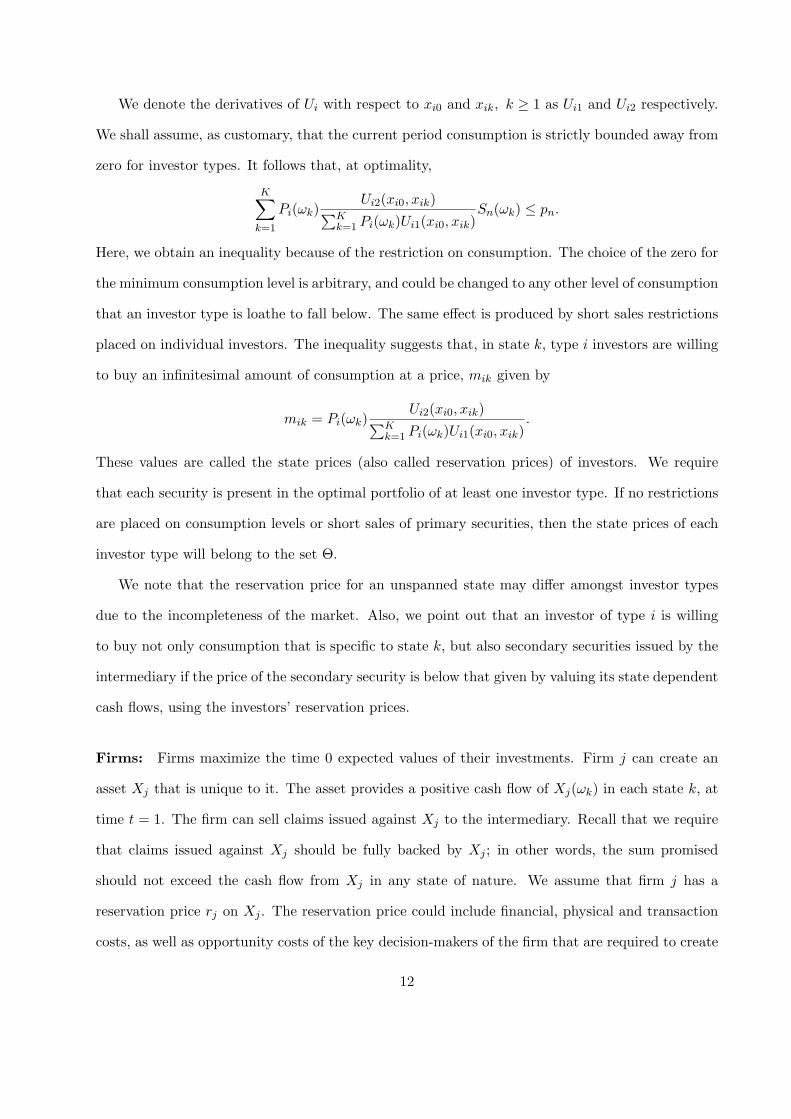
We denote the derivatives of Ui with respect to xi0 and xik, k ≥ 1 as Ui1 and Ui2 respectively.

We shall assume, as customary, that the current period consumption is strictly bounded away from

zero for investor types. It follows that, at optimality,

K∑k=1

Pi(ωk)Ui2(xi0, xik)∑K

k=1 Pi(ωk)Ui1(xi0, xik)Sn(ωk) ≤ pn.

Here, we obtain an inequality because of the restriction on consumption. The choice of the zero for

the minimum consumption level is arbitrary, and could be changed to any other level of consumption

that an investor type is loathe to fall below. The same effect is produced by short sales restrictions

placed on individual investors. The inequality suggests that, in state k, type i investors are willing

to buy an infinitesimal amount of consumption at a price, mik given by

mik = Pi(ωk)Ui2(xi0, xik)∑K

k=1 Pi(ωk)Ui1(xi0, xik).

These values are called the state prices (also called reservation prices) of investors. We require

that each security is present in the optimal portfolio of at least one investor type. If no restrictions

are placed on consumption levels or short sales of primary securities, then the state prices of each

investor type will belong to the set Θ.

We note that the reservation price for an unspanned state may differ amongst investor types

due to the incompleteness of the market. Also, we point out that an investor of type i is willing

to buy not only consumption that is specific to state k, but also secondary securities issued by the

intermediary if the price of the secondary security is below that given by valuing its state dependent

cash flows, using the investors’ reservation prices.

Firms: Firms maximize the time 0 expected values of their investments. Firm j can create an

asset Xj that is unique to it. The asset provides a positive cash flow of Xj(ωk) in each state k, at

time t = 1. The firm can sell claims issued against Xj to the intermediary. Recall that we require

that claims issued against Xj should be fully backed by Xj ; in other words, the sum promised

should not exceed the cash flow from Xj in any state of nature. We assume that firm j has a

reservation price rj on Xj . The reservation price could include financial, physical and transaction

costs, as well as opportunity costs of the key decision-makers of the firm that are required to create

12

the asset. The firm invests in the asset, if the net present value, given by the difference between

the selling price offered by the intermediary and the reservation price, is positive. Additionally,

firms cannot trade with other firms directly and also cannot issue claims that are not fully backed

by their assets. Let J denote the number of firms that wish to undertake investment projects at

time 0.

We assume that the total cash flow available from this set of firms in any state k,∑J

j=1 Xj(ωk),

is small relative to the size of the economy. Each firm, therefore, behaves as a price-taker in

the securities market. However, when the asset cannot be priced precisely, it negotiates with the

intermediary for obtaining the highest possible price for securitization of the asset. In the rest of

this paper, we use Xj to refer to both the j-th asset and the cash flows from the j-th asset.

Intermediaries: Intermediaries are agents who have knowledge about the firms’ and investors’

asset requirements. Notice that such knowledge is different from receiving a private signal regarding

the future outcome. Hence, intermediaries have no superior information about future cash flows,

relative to other agents in the economy. The intermediaries purchase assets from firms and repackage

them to sell to investors. They seek to exploit price enhancement through securitization operations

that increase the spanning of available securities. They use this superior ability to negotiate with

the firms for the prices of their assets. They use the knowledge about the investors’ preferences to

create new claims and price them correctly. An important aspect of the model is that intermediaries

act fairly by paying the same price for the same asset, independent of which firm is selling it to the

pool, and charging the same price for the same product even though it is sold to different customers.

The rationale for these fairness requirements is the possibility of entry and competition from other

intermediaries. However, we do not explicitly model competition amongst intermediaries beyond

imposing the fairness requirements and the participation constraints by firms that are discussed in

the next section. Hence, in what follows, we consider the securitization problem from the viewpoint

of a single intermediary.

The intermediary purchases claims from firms, pools them and packages them into different

tranches, and sells them as collateralized secondary securities. Pooling is defined as combining the

13

cash flows from claims issued by different firms in a proportion determined by the intermediary.

The intermediary is not restricted to purchasing only all or none of a firm’s cash flows. Instead, it

can purchase fractions (between 0 and 1) of the available assets. Tranching is defined as splitting

the pooled asset into sub-portfolios to be sold to different groups of investors, with the constraint

that the sub-portfolios be fully collateralized, i.e., fully backed by the claims purchased from the

firms. We assume that the intermediary can sell secondary securities to investors in a subset of the

investor classes, which is denoted as I1 ⊂ I.

4 Value of Pooling

We attribute the beneficial role played by the intermediary to two factors: the value enhancement

provided by pooling alone, and the value provided by tranching. In this section, we consider the

former. We analyze the problem of pooling the cash flows of some or all firms and valuing the

pooled asset by replicating its cash flows in the securities market. We use the lower bound V −(·)

as a measure of value, and thus, compute the lowest price at which the pooled asset can be sold

without presenting opportunities for arbitrage. The reason why V −(·) is taken as a measure of

value is that it is the price at which the claim can be sold for sure in the market without assuming

any knowledge about investors’ preferences and state prices. Of course, a price higher than V −(·)

is possible when preferences and state prices are known at least for a subset of investors. In §6, we

address how such higher value is realized through the tranching problem.

From one perspective, there is value to pooling if the lower bound on the pooled asset exceeds

the sum of the lower bounds on the individual assets. This is likely to happen in an incomplete

market, because firms can realize value from the residual cash flows (obtained after the marketable

part of the cash flows are stripped away) by giving them up to the intermediary for pooling. From

an entirely different, and somewhat more subtle, perspective, which is the focus of this paper, value

gets created when more projects are undertaken by firms, as a consequence of the innovation. We

describe how this real effect could come about due to intermediation.

Consider any given firm j. If rj ≤ V −(Xj), then clearly, firm j can profitably invest in asset Xj ,

14

even without pooling. If rj ≥ V +(Xj), then it does not make sense for the firm to invest in the asset

Xj . The interesting case is the one where V +(Xj) ≥ rj ≥ V −(Xj), because, in this case, the basis

for the decision to invest in Xj is ambiguous. For example, suppose that the cash flows of the pooled

asset are given by X(ωk) =∑

j Xj(ωk) for all k. Clearly, we have V −(X) ≥∑

j V −(Xj).8 This

example shows that pooling improves the spanning of cash flows across states, and thus, provides

value enhancement. However, we still need to consider the reservation prices of firms to determine if

pooling reduces the ambiguity regarding investment in assets. We say that there is value to pooling

in this latter sense if there is a linear combination of assets with weight 0 ≤ αj ≤ 1 for asset j

such that even though for one or more j’s V −(Xj) < rj , we obtain V −(∑

j(αjXj)) ≥∑

j(αjrj)

and αj > 0 for at least one of the firms whose value is below its reservation price. Another

way of defining this type of value creation is that set of projects fully or partially financed from

payments derived from the asset pool is larger than the set of such projects prior to pooling. In

our formulation, firms need not behave altruistically in creating the asset pool; therefore, as an

additional condition for value creation, we require that firms should have an incentive to pool their

assets only when they cannot benefit, individually or severally, from breaking away from the pool.

Theorem 1 shows the necessary condition for creating value through pooling. The rest of the

section determines sufficient conditions for value creation.

Theorem 1. (i) If there is a q ∈ Θ such that rj ≥ Eq[Xj ] ∀ j, then value cannot be created by

pooling the Xj’s.

(ii) Conversely, if there is no q ∈ Θ such that rj ≥ Eq[Xj ] ∀ j, then value can be created by

pooling the Xj’s.

The first part of the theorem states that if the reservation price for each asset is higher than its

value under a common pricing measure, then additional value cannot be created through pooling.

Conversely, if the condition in part (i) of the theorem fails to hold, then part(ii) states the positive

part of the result, that is, there exists a vector of weights (αj) such that pooling leads to value

8The left hand side is given by minimizing the sum of the cash flows from all assets over the set of probability

measures; whereas the right hand side the sum of the minimum of each individual cash flow. The minimum of the

sum is always larger than or equal to the sum of minimums.

15

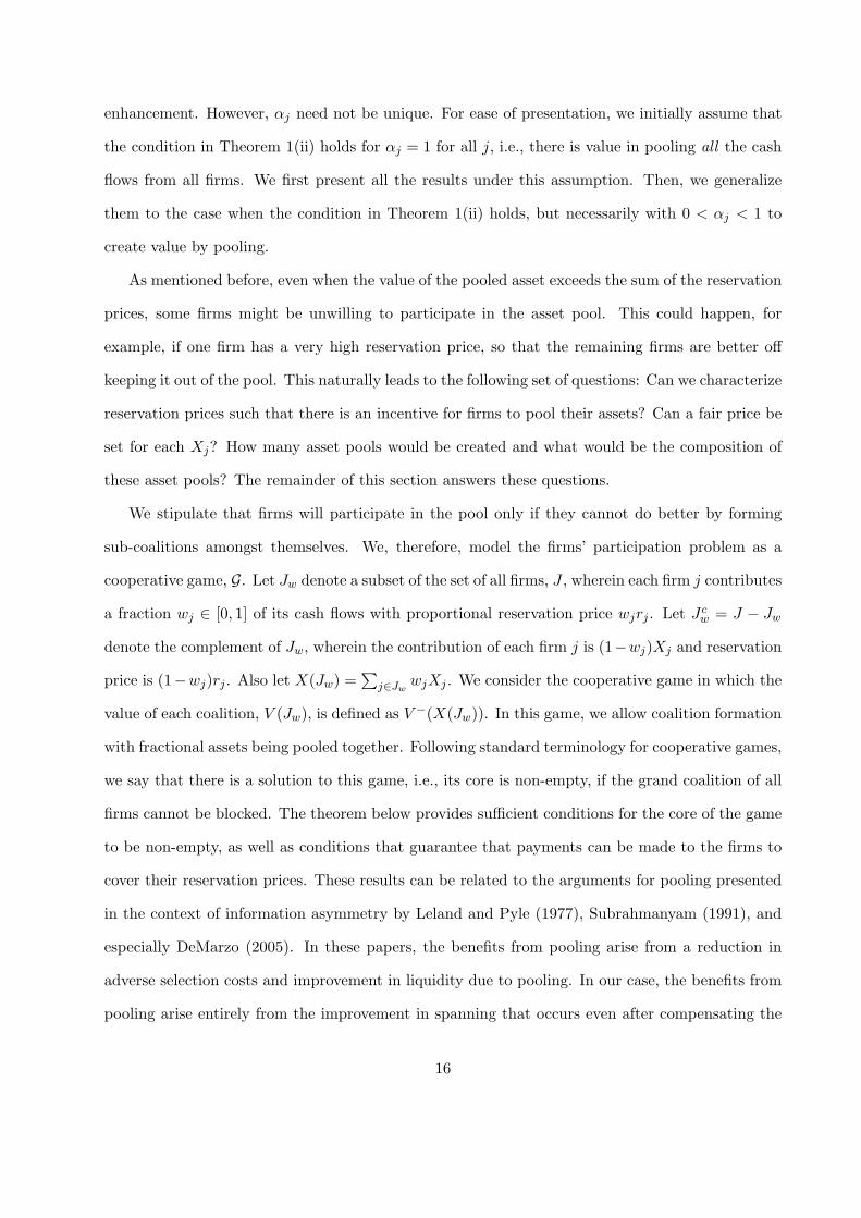
enhancement. However, αj need not be unique. For ease of presentation, we initially assume that

the condition in Theorem 1(ii) holds for αj = 1 for all j, i.e., there is value in pooling all the cash

flows from all firms. We first present all the results under this assumption. Then, we generalize

them to the case when the condition in Theorem 1(ii) holds, but necessarily with 0 < αj < 1 to

create value by pooling.

As mentioned before, even when the value of the pooled asset exceeds the sum of the reservation

prices, some firms might be unwilling to participate in the asset pool. This could happen, for

example, if one firm has a very high reservation price, so that the remaining firms are better off

keeping it out of the pool. This naturally leads to the following set of questions: Can we characterize

reservation prices such that there is an incentive for firms to pool their assets? Can a fair price be

set for each Xj? How many asset pools would be created and what would be the composition of

these asset pools? The remainder of this section answers these questions.

We stipulate that firms will participate in the pool only if they cannot do better by forming

sub-coalitions amongst themselves. We, therefore, model the firms’ participation problem as a

cooperative game, G. Let Jw denote a subset of the set of all firms, J , wherein each firm j contributes

a fraction wj ∈ [0, 1] of its cash flows with proportional reservation price wjrj . Let Jcw = J − Jw

denote the complement of Jw, wherein the contribution of each firm j is (1−wj)Xj and reservation

price is (1−wj)rj . Also let X(Jw) =∑

j∈JwwjXj . We consider the cooperative game in which the

value of each coalition, V (Jw), is defined as V −(X(Jw)). In this game, we allow coalition formation

with fractional assets being pooled together. Following standard terminology for cooperative games,

we say that there is a solution to this game, i.e., its core is non-empty, if the grand coalition of all

firms cannot be blocked. The theorem below provides sufficient conditions for the core of the game

to be non-empty, as well as conditions that guarantee that payments can be made to the firms to

cover their reservation prices. These results can be related to the arguments for pooling presented

in the context of information asymmetry by Leland and Pyle (1977), Subrahmanyam (1991), and

especially DeMarzo (2005). In these papers, the benefits from pooling arise from a reduction in

adverse selection costs and improvement in liquidity due to pooling. In our case, the benefits from

pooling arise entirely from the improvement in spanning that occurs even after compensating the

16

particular firms for their reservation prices. Clearly, both arguments complement each other in

explaining real world applications of pooling.

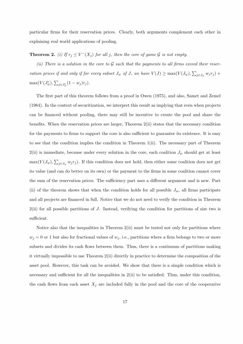
Theorem 2. (i) If rj ≤ V −(Xj) for all j, then the core of game G is not empty.

(ii) There is a solution in the core to G such that the payments to all firms exceed their reser-

vation prices if and only if for every subset Jw of J , we have V (J) ≥ max(V (Jw),∑

j∈Jwwjrj) +

max(V (Jcw),∑

j∈Jcw(1− wj)rj).

The first part of this theorem follows from a proof in Owen (1975), and also, Samet and Zemel

(1984). In the context of securitization, we interpret this result as implying that even when projects

can be financed without pooling, there may still be incentive to create the pool and share the

benefits. When the reservation prices are larger, Theorem 2(ii) states that the necessary condition

for the payments to firms to support the core is also sufficient to guarantee its existence. It is easy

to see that the condition implies the condition in Theorem 1(ii). The necessary part of Theorem

2(ii) is immediate, because under every solution in the core, each coalition Jw should get at least

max(V (Jw),∑

j∈Jwwjrj). If this condition does not hold, then either some coalition does not get

its value (and can do better on its own) or the payment to the firms in some coalition cannot cover

the sum of the reservation prices. The sufficiency part uses a different argument and is new. Part

(ii) of the theorem shows that when the condition holds for all possible Jw, all firms participate

and all projects are financed in full. Notice that we do not need to verify the condition in Theorem

2(ii) for all possible partitions of J . Instead, verifying the condition for partitions of size two is

sufficient.

Notice also that the inequalities in Theorem 2(ii) must be tested not only for partitions where

wj = 0 or 1 but also for fractional values of wj , i.e., partitions where a firm belongs to two or more

subsets and divides its cash flows between them. Thus, there is a continuum of partitions making

it virtually impossible to use Theorem 2(ii) directly in practice to determine the composition of the

asset pool. However, this task can be avoided. We show that there is a simple condition which is

necessary and sufficient for all the inequalities in 2(ii) to be satisfied. Thus, under this condition,

the cash flows from each asset Xj are included fully in the pool and the core of the cooperative

17

game is not empty.

Theorem 3. Let q ∈ Θ be a pricing measure under which∑

j Eq[Xj ] = V −(∑

j Xj). If Eq[Xj ] ≥ rj

for all j and some such q, then the sufficiency conditions in Theorem 2(ii) are satisfied. The

converse is also true.

We remark on the symmetry between this result and Theorem 1(i). The earlier result, viz.,

Theorem 1(i), is that if under a common pricing measure each asset’s value is less than its reservation

price then there is no value in pooling. The new result is that if under a pricing measure that

minimizes the value of the asset pool, the value of each asset equals or exceeds its reservation price

then value can be created by pooling all assets. Also, value is created (in the sense additional

projects are undertaken) if some project whose value was below the reservation price gets financed

through the pooling effect.

While Theorems 2 and 3 show that there exist payment schemes such that firms are willing to

participate in the game G, we need to address the question of actually determining the payment

scheme to the firms, which we now turn to. It is possible to show that there could be many such

schemes but we also require the scheme to be “fair.” It is difficult to work with the concept of

“fairness” in complete generality. However, a case can be made that if all firms are paid the same

price for a unit cash flow in state k, then the scheme is fair. We therefore restrict ourselves to

payments determined using a linear pricing measure. The following corollary complements the

results so far, because it uses the sufficient condition of the Theorem 3 to construct a linear pricing

scheme.

Corollary 1. If a pricing measure qp exists that is either an extreme point of the set of risk

neutral probability measures, or a convex combination of such extreme points, such that∑

j EqpXj =

V −(∑

j Xj), and the reservation prices satisfy rj ≤ EqpXj, then the grand coalition of all firms can

be sustained when firm j is paid EqpXj.

Corollary 1 shows that value enhancement from the first perspective, due to pooling, can be

construed to be given by the change in the pricing measure that is necessary to value the assets

correctly. This is readily seen by assuming that rj ≥ V −[Xj ] = Eqj [Xj ], that is, firm j cannot

18

decide whether to invest in the project based on the minimum valuation. Notice that the pricing

measure to determine the minimum value of each firm’s asset, qj , depends on the cash flow of the

asset which is being valued and it provides the lower bound V −[Xj ]. The measure to determine the

value when the project is considered to be part of the asset pool depends on the cash flow of the

entire asset pool. The use of this measure yields a higher value. The firm surely gains when the

reservation price lies within these two bounds. Moreover, when we are restricted to compensate

firms using the same pricing measure, we are assured that the gain from pooling can be used to

induce all firms to participate when rj ≤ EqpXj . This is the second source of value creation.

There are other interesting aspects to the corollary. The scheme is fair because it uses the same

pricing formula for each firm. The measure also prices the traded securities correctly. Thus, firms

can use a market benchmark to assure themselves that the intermediary is fair. In the next section,

we shall examine how far these results carry over when the intermediary can tranche the pool to

create secondary securities.

The above results characterize the situations in which all firms participate and contribute all

their assets. A critical condition for “full” participation by firms is Eqp(Xj) ≥ rj for all j and qp

as defined in Theorem 3. However, note that according to Theorem 1, there are situations where

there is value in pooling only fractions of cash flows of the firms. Further, the value of αj for

each firm j that provides value in pooling may not be unique. The following corollary highlights

one such solution. We show that there exists an optimal value of αj for each j, denoted α∗j,

that maximize the value of the pool. Further, if we treat α∗jXj ’s as the constituent assets instead

of Xj ’s, then Theorems 2 and 3 still apply to this asset pool.

Corollary 2. If the condition in Theorem 1 holds, then the value of pooling is maximized by solving

the linear program: max V −(∑

j αj(Xj))−∑

j αjrj, subject to 0 ≤ αj ≤ 1, ∀j. An optimal solution

to this linear program, α∗j for all j, is in the core of G. The assets of firms whose value exceeds

their respective reservation price will be included fully in this asset pool. Moreover, the cash flows

left over, (1− α∗j )Xj, do not provide any value in pooling.

Corollary 2 is consistent with Theorem 3 because if Eqp [Xj ] ≥ rj , for all j then it can be

19

shown that setting α∗j = 1 for all j gives an optimal solution to the linear program in Corollary 2.

It is difficult to construct a fair payment scheme, because it simultaneously requires limiting the

fraction of assets purchased at that price. Also, value creation from both perspectives is possible,

but, it is difficult to separate out the benefits given by the formation of the pool from that due to

securitization.

In summary, this section fully characterizes the value in pooling. Theorem 1(i) and (ii) show the

conditions under which there is no value in pooling, and those under which there is such value. In

the latter case, Theorems 2 and 3 and Corollary 2 together show that there is a maximal coalition

that can be sustained. This coalition achieves the maximum value of pooling. It includes all

the assets when the condition in Theorem 3 holds, and fractional assets otherwise. Corollary 1

guarantees the existence of a linear payment scheme for this coalition. The assets not included in

this coalition cannot be reconstituted as a separate value enhancing pool. The value creation comes

about due to synergies in cash flows amongst assets as viewed from the market prices of primary

securities. The value-maximizing behavior of a firm or a subset of firms does not impede the correct

(value maximizing) pool from forming. Thus, intermediation and pooling are predictable outcomes

in our setting, without reference to the preferences of individual agents.

5 Value of Pooling and Tranching

In this section, we assume that, in addition to tranches that are replicas of primary securities

already traded in the securities market, the intermediary can also create and sell new securities,

fully backed by the pool of assets, directly to investors. We call the former marketable tranches, and

the latter non-marketable tranches or secondary securities. If the sum of the prices of marketable

tranches (which are unique) and the prices of non-marketable tranche (which are obtained by selling

each tranche at investor-specific state prices mik) exceeds the value V −(·) obtained by pure pooling,

then we shall conclude that tranching provides value enhancement beyond pure pooling.

In general, the cash flows from a given asset pool, say,∑

j wjXj can be split into several

tranches, and each tranche offered to every investor type. Recall that mik denotes the state price

20

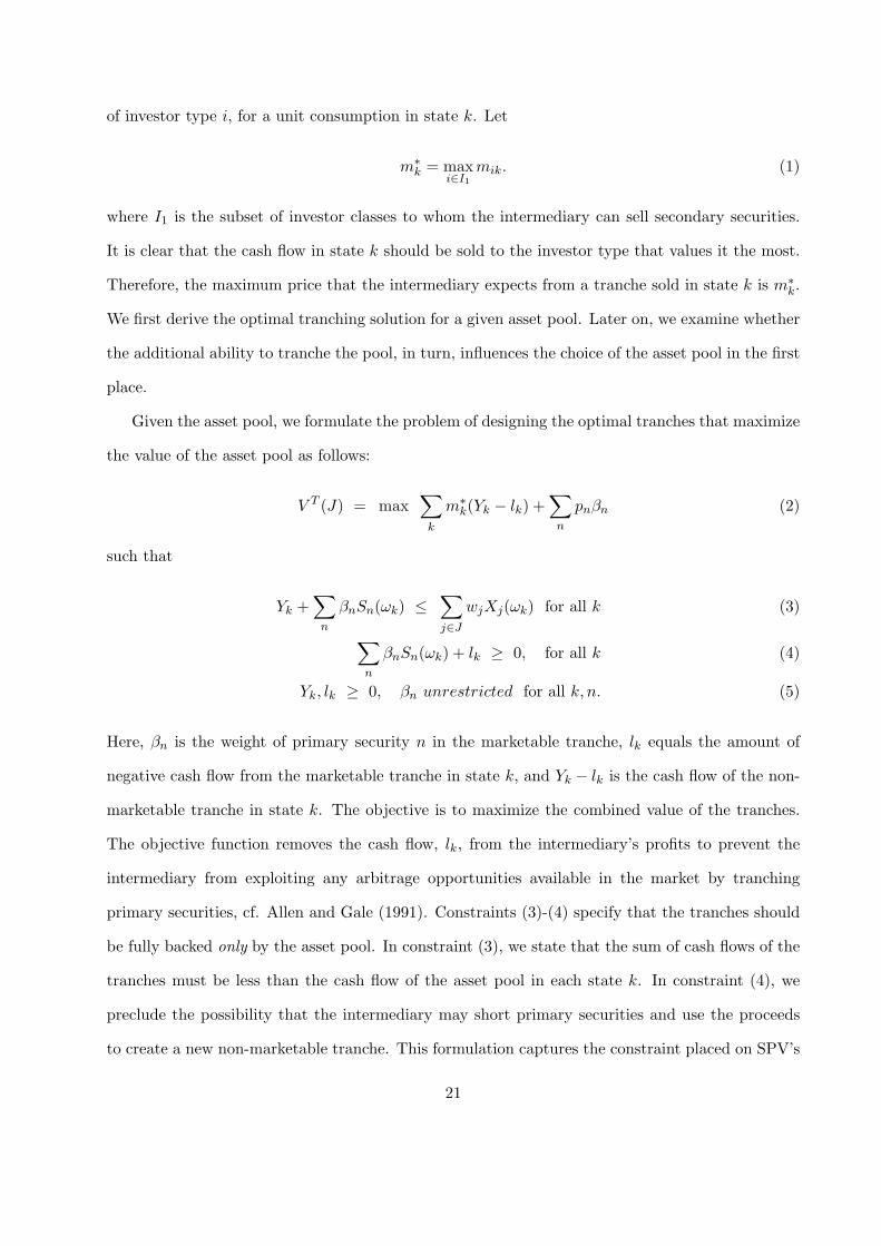
of investor type i, for a unit consumption in state k. Let

m∗k = max

i∈I1mik. (1)

where I1 is the subset of investor classes to whom the intermediary can sell secondary securities.

It is clear that the cash flow in state k should be sold to the investor type that values it the most.

Therefore, the maximum price that the intermediary expects from a tranche sold in state k is m∗k.

We first derive the optimal tranching solution for a given asset pool. Later on, we examine whether

the additional ability to tranche the pool, in turn, influences the choice of the asset pool in the first

place.

Given the asset pool, we formulate the problem of designing the optimal tranches that maximize

the value of the asset pool as follows:

V T (J) = max∑

k

m∗k(Yk − lk) +

∑n

pnβn (2)

such that

Yk +∑

n

βnSn(ωk) ≤∑j∈J

wjXj(ωk) for all k (3)

∑n

βnSn(ωk) + lk ≥ 0, for all k (4)

Yk, lk ≥ 0, βn unrestricted for all k, n. (5)

Here, βn is the weight of primary security n in the marketable tranche, lk equals the amount of

negative cash flow from the marketable tranche in state k, and Yk − lk is the cash flow of the non-

marketable tranche in state k. The objective is to maximize the combined value of the tranches.

The objective function removes the cash flow, lk, from the intermediary’s profits to prevent the

intermediary from exploiting any arbitrage opportunities available in the market by tranching

primary securities, cf. Allen and Gale (1991). Constraints (3)-(4) specify that the tranches should

be fully backed only by the asset pool. In constraint (3), we state that the sum of cash flows of the

tranches must be less than the cash flow of the asset pool in each state k. In constraint (4), we

preclude the possibility that the intermediary may short primary securities and use the proceeds

to create a new non-marketable tranche. This formulation captures the constraint placed on SPV’s

21

that any security issued by an SPV should be backed by the asset pool and not from any market

operation.9 Finally, the non-negativity constraints on Yk in (5) specify that short sales of secondary

securities are not allowed, i.e., the non-marketable tranche should only have positive components.

This is justified by recalling that consumption should be non-negative in all states.

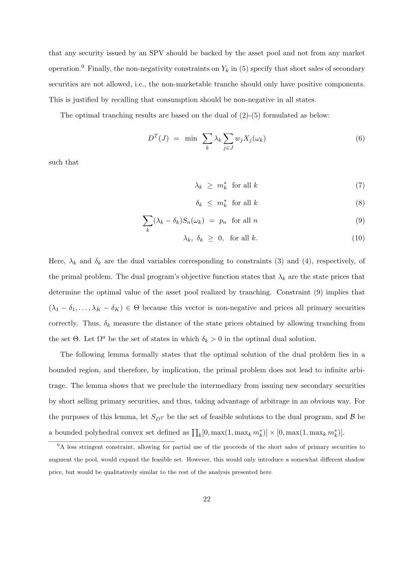
The optimal tranching results are based on the dual of (2)-(5) formulated as below:

DT (J) = min∑

k

λk

∑j∈J

wjXj(ωk) (6)

such that

λk ≥ m∗k for all k (7)

δk ≤ m∗k for all k (8)∑

k

(λk − δk)Sn(ωk) = pn for all n (9)

λk, δk ≥ 0, for all k. (10)

Here, λk and δk are the dual variables corresponding to constraints (3) and (4), respectively, of

the primal problem. The dual program’s objective function states that λk are the state prices that

determine the optimal value of the asset pool realized by tranching. Constraint (9) implies that

(λ1 − δ1, . . . , λK − δK) ∈ Θ because this vector is non-negative and prices all primary securities

correctly. Thus, δk measure the distance of the state prices obtained by allowing tranching from

the set Θ. Let Ωa be the set of states in which δk > 0 in the optimal dual solution.

The following lemma formally states that the optimal solution of the dual problem lies in a

bounded region, and therefore, by implication, the primal problem does not lead to infinite arbi-

trage. The lemma shows that we preclude the intermediary from issuing new secondary securities

by short selling primary securities, and thus, taking advantage of arbitrage in an obvious way. For

the purposes of this lemma, let SDT be the set of feasible solutions to the dual program, and B be

a bounded polyhedral convex set defined as∏

k[0,max(1,maxk m∗k)]× [0,max(1,maxk m∗

k)].

9A less stringent constraint, allowing for partial use of the proceeds of the short sales of primary securities to

augment the pool, would expand the feasible set. However, this would only introduce a somewhat different shadow

price, but would be qualitatively similar to the rest of the analysis presented here.

22

Lemma 2. The optimal solution to the dual problem is obtained by computing the value of the

asset pool at each extreme point of B⋂

SDT and taking the minimum value as the solution.

From this lemma, the primal problem V T (J) has a finite optimal solution. Therefore, the

tranching solution exploits only those arbitrage opportunities in the securities market that are

available to the intermediary due to the access to the asset pool and the subset of investors I1. It

does not include possible arbitrage opportunities that may exist in the market due to discrepancies

between the prices of primary securities in the market and the secondary securities demanded by

investors.10 The following theorem defines such opportunities and shows that they are completely

characterized by the set Ωa.

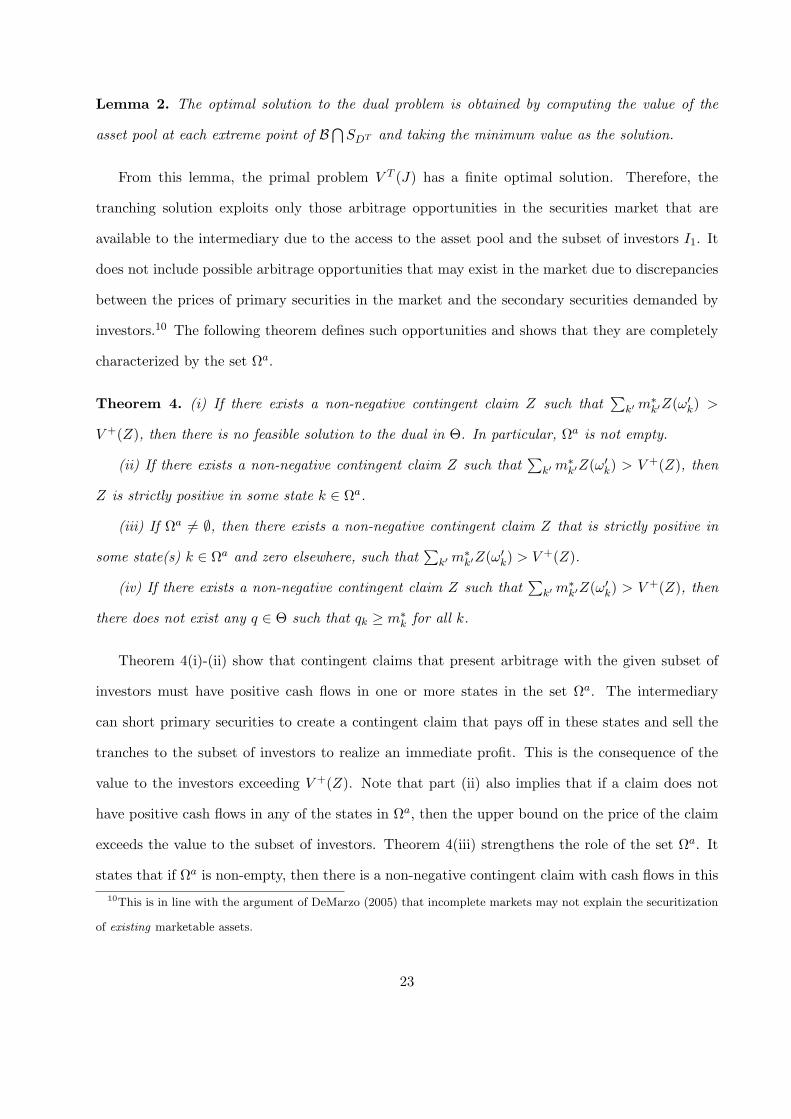
Theorem 4. (i) If there exists a non-negative contingent claim Z such that∑

k′ m∗k′Z(ω′

k) >

V +(Z), then there is no feasible solution to the dual in Θ. In particular, Ωa is not empty.

(ii) If there exists a non-negative contingent claim Z such that∑

k′ m∗k′Z(ω′

k) > V +(Z), then

Z is strictly positive in some state k ∈ Ωa.

(iii) If Ωa 6= ∅, then there exists a non-negative contingent claim Z that is strictly positive in

some state(s) k ∈ Ωa and zero elsewhere, such that∑

k′ m∗k′Z(ω′

k) > V +(Z).

(iv) If there exists a non-negative contingent claim Z such that∑

k′ m∗k′Z(ω′

k) > V +(Z), then

there does not exist any q ∈ Θ such that qk ≥ m∗k for all k.

Theorem 4(i)-(ii) show that contingent claims that present arbitrage with the given subset of

investors must have positive cash flows in one or more states in the set Ωa. The intermediary

can short primary securities to create a contingent claim that pays off in these states and sell the

tranches to the subset of investors to realize an immediate profit. This is the consequence of the

value to the investors exceeding V +(Z). Note that part (ii) also implies that if a claim does not

have positive cash flows in any of the states in Ωa, then the upper bound on the price of the claim

exceeds the value to the subset of investors. Theorem 4(iii) strengthens the role of the set Ωa. It

states that if Ωa is non-empty, then there is a non-negative contingent claim with cash flows in this10This is in line with the argument of DeMarzo (2005) that incomplete markets may not explain the securitization

of existing marketable assets.

23

set of states only, whose value to investors exceeds V +(Z). The last part of Theorem 4 is the dual

characterization which is mathematically the most useful of the three. Using this result, we can

now state the general structure of the secondary securities.

Let Y ∗k , l∗k, and β∗

n denote the optimal solution to the primal problem, and λ∗k and δ∗k denote

the optimal solution to the dual problem. We partition the optimal tranching solution into three

parts that we denote as T a, T I and Tm. Let T ak = Y ∗

k − l∗k if δ∗k > 0 and zero otherwise, let

T Ik = Y ∗

k − l∗k − T ak , and let Tm

k =∑

n βnSn(ωk). Here, Tm is the marketable tranche, T a consists

of the cash flows of the non-marketable tranche in states belonging to the set Ωa, and T I consists

of the cash flows of the non-marketable tranche in the remaining states. We partition the non-

marketable tranche in this manner because by the complementary slackness condition applied to

δ∗k, δ∗k > 0 implies that l∗k +∑

n β∗nSn(ωk) = 0, which further implies that Y ∗

k − l∗k =∑

j wjXj(ωk),

i.e., all the cash flows in state k are sold as secondary securities. Thus, according to Theorem 4, T a

fully exploits the arbitrage opportunities in the securities market due to the ability to design and

sell secondary securities to a subset of investors, while Tm and T I are not based on the existence

of arbitrage. T a is zero if there are no arbitrage opportunities available to the intermediary.

Note that the complementary slackness conditions also imply that the intermediary tranches all

of the cash flows in the asset pool in the states belonging to the set Ωa in the form of T a. Indeed,

we have Ta · Tm = 0 and Ta · TI = 0. Thus, the optimal solution to the primal problem V T (J) is

separable into one that corresponds to the tranches Ta and another that corresponds to the rest.

The value of T a is independent of changes in the cash flows of the asset pool in states Ω \Ωa, and

likewise, the values of Tm and T I are independent of the cash flows in states Ωa. To see this, define

X(ωk) =∑

j wjXj(ωk)− T ak as the asset pool after tranching T a. Set m∗

k = 0 for the states where

δ∗k > 0, and m∗k = m∗

k otherwise. Let DT denote the new dual problem. Clearly, DT has a feasible

solution in Θ. Due to the fact that T a is orthogonal to Tm and T I , the optimal solution to DT is

given by Tm and T I . Thus, the value of Tm and T I is independent of the value of T a. Therefore,

the asset pool decomposes into an ‘arbitrage part’, a marketable part and a residual part. In the

terminology of the securitization industry, roughly speaking, the first component can be referred

to as a “bespoke” tranche, the second one as a super-senior tranche, and the last one as the equity

24

tranche.

We can now specify the complete structure of the optimal tranching solution for a given asset

pool as stated in the theorem below. This theorem uses the results of Theorem 4 to show the

conditions under which the different tranches come about.

Theorem 5. The optimal solution to the tranching problem is represented by (T a, Tm, T I) as

defined above. Further,

(i) If there exists q ∈ Θ such that qk ≥ m∗k for all k, then T a ≡ 0.

(ii) If there exists q ∈ Θ such that qk ≤ m∗k for all k and qk < m∗

k for some k, then there exists

an optimal tranching solution in which Tm = T I ≡ 0.

(iii) Otherwise all three types of tranches may occur in the optimal solution.

We note from Theorem 5 that the differences among the three types of solutions to the tranching

problem do not depend on the cash flows in the asset pool, but only on the set Θ and the state

prices m∗k. Thus, an intermediary can verify the results in Theorems 4-5 without knowing the

cash flows in the asset pool or the willingness of individual firms to participate in the asset pool.

Further, the tranches in Tm might be bought by a different set of investors than I1, which is the

set of investors that buys tranches T a and T I .

Theorem 5 also clearly delineates the incremental value realized by tranching the given asset

pool∑

j wjXj . In case (i), λ∗ ∈ Θ, and thus, the optimal solution to the dual problem lies inside

the price bounds V −(∑

j wjXj) and V +(∑

j wjXj). By the constraints of the dual problem, this

solution is obtained in the set Θ⋂(λ1, . . . , λK) : λk ≥ m∗

k for all k. Since this is a subset of Θ,

pooling and tranching provides incremental value beyond V −(∑

j wjXj). In case (ii), the optimal

solution is given by Em∗ [T a], which is greater than V +(T a). In case (iii), the value of tranches Tm

and T I is as in case (i) and the value of tranche T a is as in case (ii). Due to the orthogonality of

T a with Tm and T I , the total value is equal to the sum of these two components. Thus, the value

from pooling and tranching is higher than V −(∑

j wjXj).

Thus far in this section, we have presented results for a given asset pool. We now examine the

implications of tranching on the formation of the asset pool. First, note that the optimal value

25

created through pooling and tranching will always be at least as large as that from pure pooling.

However, the asset pool that maximizes the value from pooling and tranching may not be the same

as that which maximizes the value from pure pooling. This naturally gives rise to questions whether

the optimal asset pool under pooling and tranching will be larger than that under pure pooling,

and whether it will include all the assets in the latter pool. We examine these questions for each

case in Theorem 5.

In case (i), all results of §4 apply if attention is restricted to the smaller set of pricing measures

ΘT = q : qk ≥ m∗k, q ∈ Θ. Thus, using the inferences in §4, the asset pool may consist of cash

flows from the individual firms in fractions or in full. Further, the mix of projects that get financed

may change compared to the solution in §4, however, the total value of the projects financed will

always increase. In case (ii), the optimal solution is linear in the cash flows X(ωk). Thus, the

solution degenerates into a pure tranching solution and there is value from tranching, but there

may not be value from pooling. The decision for each firm to go through the intermediary is made

separately based on whether Em∗ [Xj ] ≥ rj or not. Thus, each firm either participates in the pool

in full or not at all. The mix of projects financed may again change compared to §4, however,

there will be no fractional pooling in this case. In case (iii), the pooling and tranching solution lies

outside the set Θ. The remaining implications in this case are the same as in case (i). Thus, we

obtain the counter-intuitive conclusion that the optimal asset pool in pooling and tranching may

not include all the assets included in pure pooling, and may in fact be smaller than the latter.

6 Numerical Example

Consider a market with four states at time 1 denoted Ω = ω1, . . . , ω4 and two primary securities

with payoffs S1 = (1, 1, 1, 1) and S2 = (1, 0, 0.5, 1.5) at time 1 and prices p1 = p2 = 1 at time 0.

The set of risk neutral pricing measures over Ω is Θ = (x + 3y, x− y, 0.5− 2x, 0.5− 2y)⋂

[0, 1]4

with two degrees of freedom denoted x and y. The set Θ is spanned by three linear pricing

measures, Q1 = (0, 1/3, 0, 2/3), Q2 = (1, 0, 0, 0) and Q3 = (0, 0, 1/2, 1/2). Q1 corresponds to

x = 1/4, y = −1/12, Q2 corresponds to x = 1/4, y = 1/4 and Q3 corresponds to x = 0, y = 0.

26

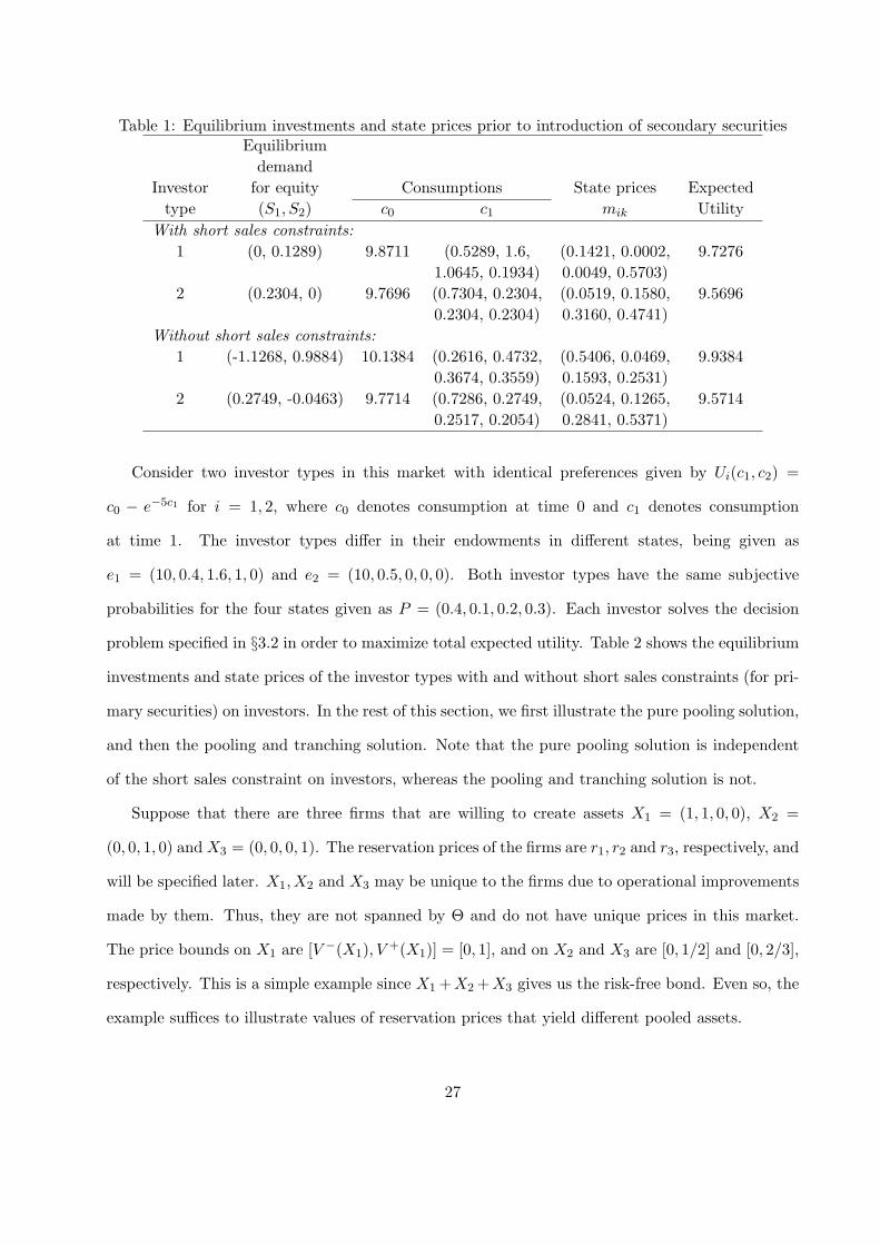
Table 1: Equilibrium investments and state prices prior to introduction of secondary securitiesEquilibrium

demandInvestor for equity Consumptions State prices Expected

type (S1, S2) c0 c1 mik UtilityWith short sales constraints:

1 (0, 0.1289) 9.8711 (0.5289, 1.6, (0.1421, 0.0002, 9.72761.0645, 0.1934) 0.0049, 0.5703)

2 (0.2304, 0) 9.7696 (0.7304, 0.2304, (0.0519, 0.1580, 9.56960.2304, 0.2304) 0.3160, 0.4741)

Without short sales constraints:1 (-1.1268, 0.9884) 10.1384 (0.2616, 0.4732, (0.5406, 0.0469, 9.9384

0.3674, 0.3559) 0.1593, 0.2531)2 (0.2749, -0.0463) 9.7714 (0.7286, 0.2749, (0.0524, 0.1265, 9.5714

0.2517, 0.2054) 0.2841, 0.5371)

Consider two investor types in this market with identical preferences given by Ui(c1, c2) =

c0 − e−5c1 for i = 1, 2, where c0 denotes consumption at time 0 and c1 denotes consumption

at time 1. The investor types differ in their endowments in different states, being given as

e1 = (10, 0.4, 1.6, 1, 0) and e2 = (10, 0.5, 0, 0, 0). Both investor types have the same subjective

probabilities for the four states given as P = (0.4, 0.1, 0.2, 0.3). Each investor solves the decision

problem specified in §3.2 in order to maximize total expected utility. Table 2 shows the equilibrium

investments and state prices of the investor types with and without short sales constraints (for pri-

mary securities) on investors. In the rest of this section, we first illustrate the pure pooling solution,

and then the pooling and tranching solution. Note that the pure pooling solution is independent

of the short sales constraint on investors, whereas the pooling and tranching solution is not.

Suppose that there are three firms that are willing to create assets X1 = (1, 1, 0, 0), X2 =

(0, 0, 1, 0) and X3 = (0, 0, 0, 1). The reservation prices of the firms are r1, r2 and r3, respectively, and

will be specified later. X1, X2 and X3 may be unique to the firms due to operational improvements

made by them. Thus, they are not spanned by Θ and do not have unique prices in this market.

The price bounds on X1 are [V −(X1), V +(X1)] = [0, 1], and on X2 and X3 are [0, 1/2] and [0, 2/3],

respectively. This is a simple example since X1 +X2 +X3 gives us the risk-free bond. Even so, the

example suffices to illustrate values of reservation prices that yield different pooled assets.

27

Conditions to determine the value of pooling. Clearly, not all values of r1, r2 and r3 will

lead to value creation. Theorem 1(i) tells us that there is no value in pooling X1, X2, and X3 in

any proportion if there exists a pricing measure q ∈ Θ (i.e., q is a convex combination, say (a, b, c),

of Q1, Q2, and Q3) such that the following inequalities are satisfied:

13a + b− r1 ≤ 0,

12c− r2 ≤ 0,

23a +

12c− r3 ≤ 0,

a + b + c = 1. (11)

Otherwise there can be value from pooling. For example, if

r1 = 0.26, r2 = 0.35, r3 = 0.4 (12)

then there is a feasible solution (a= 0.09, b = 0.23, c = 0.68) to the above inequalities, implying

that there is no value from pooling. As another example, if

r1 = 0.25, r2 = 0.5, r3 = 0.25 (13)

then there is no feasible solution to the above inequalities, implying that there can be value from

pooling.

Conditions for full pooling and fractional pooling. In the case when there is value from

pooling, the pool may be a grand coalition of all three assets or may be fractional. We apply

Theorem 3 to determine the values of reservation prices under which the grand coalition of all three

assets is sustainable. Since the grand coalition is the riskless bond, all q ∈ Θ achieve V −(X1 +X2 +

X3). Thus, by Theorem 3, we need to find a q ∈ Θ such that Eq[Xj ] ≥ rj for all j = 1, 2, 3. Solving

these simultaneous inequalities, as above in the application of Theorem 1, we obtain conditions

on r1, r2, and r3 under which the grand coalition is sustainable. These conditions could also be

obtained by reversing all the inequalities derived above.

For example, consider the values of r2 and r3 as given in (12) and set r1 = 0.25 − δ for some

δ ≥ 0. Then, it can be easily shown that there is value from pooling and the grand coalition is

28

sustainable. On the other hand, when reservation prices are as in (13), then the grand coalition

is not sustainable. To see this, all three constraints have to hold as equalities (as the pool is one

unit of the riskless bond). The last two constraints yield: a = -3/8, which is infeasible. Recall that

Theorem 1 tells us that there is value from pooling in this case. To find the maximal asset pool

given these reservation prices, we solve the LP given in Corollary 2:

max z − 0.25α1 − 0.5α2 − 0.25α3

such that

1/3α1 + 2/3α3 ≥ z,

α1 ≥ z,

1/2α2 + 1/2α3 ≥ z,

αj ∈ [0, 1] for all j.

Here, αj is the fraction of asset j included in the pool. The optimal solution is α1 = 12 and α3 = 1.

The LP has an optimal value of 18 . The asset pool is given by (1

2 , 12 , 0, 0) + (0, 0, 0, 1) = (1

2 , 12 , 0, 1).

The expected value under the extreme measures are 56 , 1

2 and 12 . The convex combination, 1

4 of

Q2 and 34 of Q3, yields the measure q = (1

4 , 0, 38 , 3

8), under which Eq[12X1] = 14 and Eq[X3] = 3

8 ,

both of which are greater than or equal to the corresponding reservation prices (Theorem 3). It

can be easily seen that this fractional pool is sustainable, and that there is no value in pooling

the remaining cash flows given by 0.5X1 + X2 = (0.5, 0.5, 1, 0) (the inequalities to be satisfied are

b/2 + a/6 ≤ 1/8 (corresponding to Eq[X1/2] ≤ r1/2) and c/2 ≤ 1 (corresponding to Eq[X2] ≤ r2)

which is trivially satisfied by (0, 0, 1) .

Linear payment scheme for the pooling solution. When either full pooling or fractional

pooling adds value, a pricing measure that satisfies the conditions in Corollary 1 gives a linear

payment scheme for subdividing the value of the pool between the participating firms. This payment

scheme ensures that the coalition of firms cannot be broken because none of the firms in the set J

can do better by forming an alternative coalition.

For example, in the case of full pooling with r1 = 0.2, r2 = 0.35, r3 = 0.4, there are infinitely

many admissible linear payment schemes. These payment schemes are given by convex combinations

29

of the following three state-price vectors: (0.15, 0.05, 0.35, 0.45), (0.225, 0.025, 0.35, 0.4), (0.2, 0, 0.4, 0.4).

All payment schemes provide payments to firms that are at least as large as their reservation prices.

Further, they distribute the surplus V −(X1 + X2 + X3)−∑

j rj among the firms.

In the case of fractional pooling with r1 = 0.25, r2 = 0.5, r3 = 0.25, there is a unique pricing

measure that yields the payment scheme, q = (14 , 0, 3

8 , 38).

Optimal pooling and tranching. We now illustrate the results of §5. Table 2 shows the optimal

tranching solution obtained for different asset pools both with and without short sales constraints

on investors. The first three rows of the table show the solutions for an asset pool comprised of

only X1 and X2 when there are short sales constraints on investors. Case A corresponds to when

the intermediary has access to investors of type 1 only, case B to investors of type 2 only, and case

C to investors of both types. The next three rows of the table, D-F, show the solutions when all

three assets, X1, X2 and X3 are pooled together, also with short sales constraints on investors. The

rest of the table repeats these cases when there are no short sales constraints on investors. Recall

the definition of m∗ from (1). The value of m∗ is obtained from the state prices in Table 1, and

varies depending on the set of investor types whom the intermediary can access.

The table highlights the structure of the tranching solution in various cases. First consider

the scenarios with short sales constraints. In cases A and D, the tranche T a is zero because the

intermediary is unable to exploit any arbitrage in the securities market when it has access to

investors of type 1 only. In cases B and E, T a is non-zero because the intermediary can exploit

arbitrage in states ω2 and ω3 when it has access to investors of type 2 only. Applying Theorem 4

to these cases, the contingent claim Z that achieves a value higher than V +(Z) under m∗ is given

by (0, 1, 2/3, 0). In cases C and F, T a includes all the cash flows in the asset pool because the

claim (1, 1, 1, 1) now achieves a value higher than 1 under m∗. Thus, state-wise partitioning of the

asset pool is optimal when the intermediary has access to both investor types. Notice that the

tranching solution corresponds to Theorem 5(i) in cases A and D, Theorem 5(ii) in cases C and F,

and Theorem 5(iii) in cases B and E.

Now consider the scenarios without short sales constraints. In cases A, B, D and E, the inter-

mediary has access to only one investor type, and since m1,m2 ∈ Θ, Theorem 5(i) applies. Thus,

30

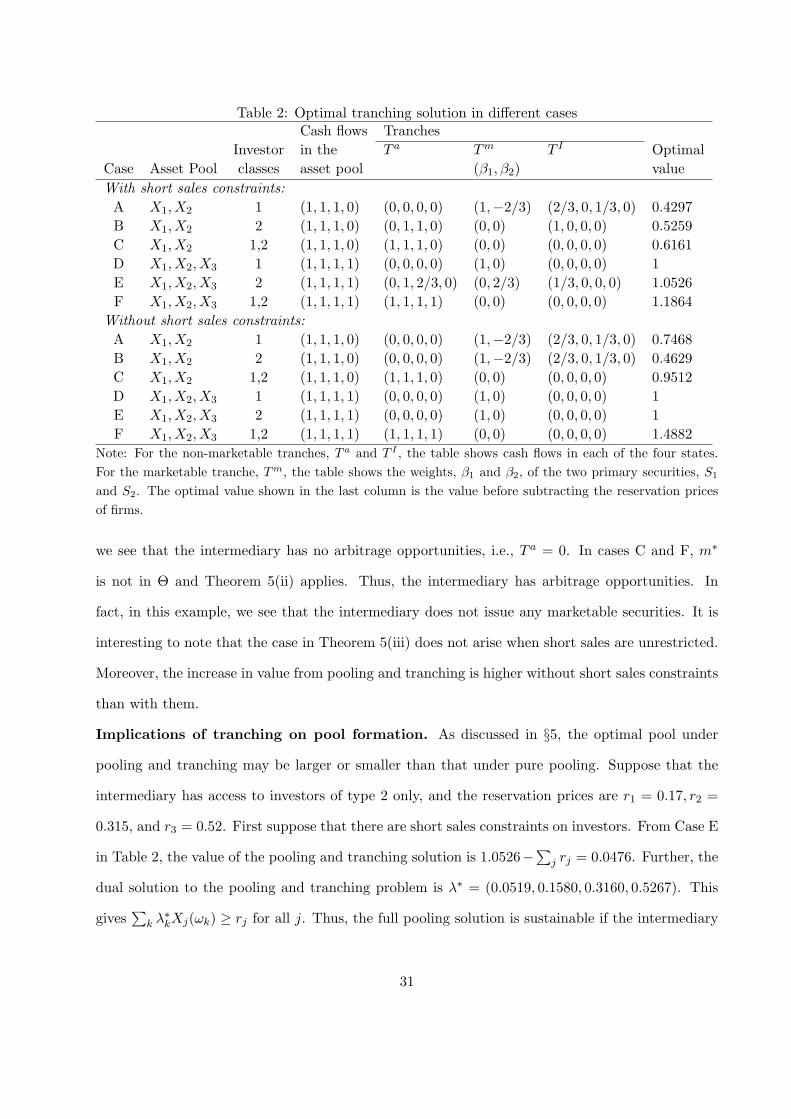
Table 2: Optimal tranching solution in different casesCash flows Tranches

Investor in the T a Tm T I OptimalCase Asset Pool classes asset pool (β1, β2) valueWith short sales constraints:A X1, X2 1 (1, 1, 1, 0) (0, 0, 0, 0) (1,−2/3) (2/3, 0, 1/3, 0) 0.4297B X1, X2 2 (1, 1, 1, 0) (0, 1, 1, 0) (0, 0) (1, 0, 0, 0) 0.5259C X1, X2 1,2 (1, 1, 1, 0) (1, 1, 1, 0) (0, 0) (0, 0, 0, 0) 0.6161D X1, X2, X3 1 (1, 1, 1, 1) (0, 0, 0, 0) (1, 0) (0, 0, 0, 0) 1E X1, X2, X3 2 (1, 1, 1, 1) (0, 1, 2/3, 0) (0, 2/3) (1/3, 0, 0, 0) 1.0526F X1, X2, X3 1,2 (1, 1, 1, 1) (1, 1, 1, 1) (0, 0) (0, 0, 0, 0) 1.1864

Without short sales constraints:A X1, X2 1 (1, 1, 1, 0) (0, 0, 0, 0) (1,−2/3) (2/3, 0, 1/3, 0) 0.7468B X1, X2 2 (1, 1, 1, 0) (0, 0, 0, 0) (1,−2/3) (2/3, 0, 1/3, 0) 0.4629C X1, X2 1,2 (1, 1, 1, 0) (1, 1, 1, 0) (0, 0) (0, 0, 0, 0) 0.9512D X1, X2, X3 1 (1, 1, 1, 1) (0, 0, 0, 0) (1, 0) (0, 0, 0, 0) 1E X1, X2, X3 2 (1, 1, 1, 1) (0, 0, 0, 0) (1, 0) (0, 0, 0, 0) 1F X1, X2, X3 1,2 (1, 1, 1, 1) (1, 1, 1, 1) (0, 0) (0, 0, 0, 0) 1.4882

Note: For the non-marketable tranches, T a and T I , the table shows cash flows in each of the four states.For the marketable tranche, Tm, the table shows the weights, β1 and β2, of the two primary securities, S1

and S2. The optimal value shown in the last column is the value before subtracting the reservation pricesof firms.

we see that the intermediary has no arbitrage opportunities, i.e., T a = 0. In cases C and F, m∗

is not in Θ and Theorem 5(ii) applies. Thus, the intermediary has arbitrage opportunities. In

fact, in this example, we see that the intermediary does not issue any marketable securities. It is

interesting to note that the case in Theorem 5(iii) does not arise when short sales are unrestricted.

Moreover, the increase in value from pooling and tranching is higher without short sales constraints

than with them.

Implications of tranching on pool formation. As discussed in §5, the optimal pool under

pooling and tranching may be larger or smaller than that under pure pooling. Suppose that the

intermediary has access to investors of type 2 only, and the reservation prices are r1 = 0.17, r2 =

0.315, and r3 = 0.52. First suppose that there are short sales constraints on investors. From Case E

in Table 2, the value of the pooling and tranching solution is 1.0526−∑

j rj = 0.0476. Further, the

dual solution to the pooling and tranching problem is λ∗ = (0.0519, 0.1580, 0.3160, 0.5267). This

gives∑

k λ∗kXj(ωk) ≥ rj for all j. Thus, the full pooling solution is sustainable if the intermediary

31

issues both marketable and non-marketable tranches. On the other hand, when there are no

short sales constraints on investors, the dual solution to the pooling and tranching problem is

λ∗ = (0.0524, 0.1265, 0.2841, 0.5371). In this case,∑

k λ∗kX2(ωk) < r2, implying that the full pooling

solution is not sustainable. The optimal value from pooling X1 and X3 is 0.716−0.17−0.52 = 0.026.

In the third case, if we restrict the intermediary to issue only marketable tranches, then inequalities

(11) can be used to determine whether there is value from pooling. We find that these inequalities

are feasible for the given reservation prices, proving that there is no value from pooling without

tranching. Thus, for these reservation prices, tranching results in a larger asset pool than pure

pooling.

Now suppose that the reservation prices are r1 = 0.17, r2 = 0.33, and r3 = 0.45. The inter-

mediary again has access to investors of type 2 only. We find that∑

k λ∗kXJ(ωk) < rj for j = 2

both with and without short sales constraints on investors. Thus, the full pooling solution is not

sustainable under pooling and tranching. With short sales constraints, we obtain a fractional pool,

X1 + X2/3 + X3, with a value of 0.11, and without short sales constraints, we obtain a different

fractional pool, X1 + X3, with a value of 0.096. Under pure pooling, however, the full pooling so-

lution is sustainable because the conditions in Theorem 3 are satisfied by these reservation prices.

The value of this solution is 0.05. Thus, tranching results in a smaller asset pool but with a higher

value than pure pooling. Thus, these examples show how tranching and the short sales constraint

affect the formation of the asset pool.

7 Discussion

In this paper, we have shown how securitization in incomplete markets creates value by enabling

real investment. This value creation takes place in two ways. First, due to pooling, the non-

marketable portions of the assets of firms increase in value. Second, the value creation by pooling

can be augmented by tranching the pooled assets and issuing new securities to investors. Value

creation does not automatically ensure that all real investment becomes more viable. Instead, the

set of pricing measures and the consumption demand from investors determine the composition of

32

the pool of real investments that can be sustained.

The real investment decisions in our model do not have to be yes-no decisions. More complex

optimization decisions can be easily incorporated in our framework. Consider the newsvendor model

of inventory management as a prototypical example. Suppose that the firm is unable to value the

newsvendor profit function because the demand for the product is not spanned by securities traded

in the financial market. One alternative available to the firm is to conservatively use the lower

bound from no-arbitrage pricing to make the optimal inventory decision. However, our analysis

shows that the firm can gain by jointly valuing its entire portfolio of inventory and other real

investment decisions through pooling. It can further gain by securitizing the cash flows from these

investments through tranching. These gains accrue because the firm is able to value its cash flows

more accurately and identify financial synergies among cash flows from different investments. In

addition, the optimal inventory decision of the firm can change as a result of these actions.

Other examples of investment decisions include setting up a new distribution center (DC) which

enables the firm to reduce lead time, and thus, better match supply with demand. If the products

sold by the firm are unique or if it is a frontrunner in supply chain responsiveness, then the cash

flows resulting from the investment in the DC may not be spanned by the securities traded in the

market. In such a case, the firm may find it difficult to secure financing or even determine the

viability of its investment. However, if the new DC fits within a group with active securitization,

then the firm would be able to enhance its valuation as well as secure financing.

Our paper can be extended in subsequent research in several ways. First, while the results in

this paper are obtained under the strict definition of arbitrage, our analysis could be combined with

price bounds derived under approximate arbitrage as in the recent literature. Under approximate

arbitrage, market incompleteness should still continue to provide a rationale for seeking value

enhancement through pooling and tranching. However, the imposition of a constraint that precludes

“approximate arbitrage”, instead of arbitrage, would restrict the set of feasible solutions to the

optimization problems considered in this paper. Additional analysis is required to determine the

optimal pooling and tranching strategies when subjected to the tighter constraints.

Second, in the analysis in this paper, we have not dealt with the problems of information

33

asymmetry. For instance, in our model, the tranches constructed by the intermediary need to be

verifiable for our results to hold. If investors can verify whether the claim has positive payoffs in

a state and if investors value consumption equally in every state, then the resulting partition of

claims will resemble the tranches offered in the CLO market. Of course, given the issues relating

to verifiability of the states, intermediaries need to handle the associated agency problems and be

more innovative in creating tranches – for example, those that pay when the economy is doing well

and those when it is doing poorly. We defer these issues to subsequent research.

Finally, an interesting aspect of securitization is when the pool has to be created and managed

dynamically. This problem is commonly faced by venture fund managers. The major differences

are that firms within the pool might not have the option to leave the pool, while firms that enter

later might enjoy greater bargaining power. Further, firms and the intermediary might have only

an imperfect forecast about which assets will become available in the future.

References

Allen, F., D. Gale. 1991. Arbitrage, Short Sales and Financial Innovation Econometrica. 59,

1041-1068.

Ayotte, K.M., S. Gaon. 2004. Asset-Backed Securities: Costs and Benefits of “Bankruptcy

Remoteness. Working Paper, Columbia Business School.

Bernardo, A. E., O. Ledoit. 2000. Gain, Loss and Asset Pricing. Journal of Political Economy.

108 144-172.

Bertsimas, D., L. Kogan, A. Lo. 2001. Hedging Derivative Securities and Incomplete Markets:

An ε-Arbitrage Approach. Operations Research. 49(3) 372-397.

Birge, J. 2000. Option Methods for Incorporating Risk into Linear Capacity Planning Models.

M&SOM. 2(1) 19-31.

Birge, J., X. Xu. 2005. Operational Decisions, Capital Structure, and Managerial Compensation:

A Newsvendor Perspective. Working Paper, Northwestern Univ.

34

Buzacott, J., R. Zhang. 2004. Inventory management with asset-based financing. Management

Science. 50(9) 1274-1292.

Cochrane, J. H., J. Saa-Requejo. 2000. Beyond Arbitrage: Good-Deal Asset Pricing Bounds in

Incomplete Markets. Journal of Political Economy. 108 79-119.

Cummins, J. D. 2004. Securitization of Life Insurance Assets and Liabilities, Working Paper,

Wharton School, University of Pennsylvania.

DeMarzo, P. M. 2005. The Pooling and Tranching of Securities: A Model of Informed Intermedi-

ation. Review of Financial Studies. 18, 1-36.

DeMarzo, P. M., D. Duffie. 1999. A liquidity based model of security design. Econometrica. 67,

65-99.

Ding, Q., L. Dong, P. Kouvelis. 2007. On the integration of production and financial hedging

decisions in global markets. Operations Research. 55 470-489.

Dong, L., H. Liu. 2005. Equilibrium Forward Contracts on Nonstorable Commodities in the

Presence of Market Power. Operations Research. 55 128-145.

Glaeser, E., H. Kallal. 1997. Thin markets, asymmetric information, and mortgage-backed secu-

rities. Journal of Financial Intermediation. 6, 64-86.

Gorton, G., G. Pennachi. 1990. Financial intermediaries and liquidity creation. Journal of

Finance. 45, 49-71.

Gaur, V., S. Seshadri. 2005. Hedging Inventory Risk through Market Instruments. M&SOM.

7(2) 103-120.

Hakansson, N. H. 1978. Welfare Aspects of Options and Supershares. Journal of Finance. 23,

759-776.

Hansen, L. P., R. Jagannathan. 1991. Implications of Security Market Data for Models of Dynamic

Economies. Journal of Political Economy. 99, 225-262.

35

Harrison, M., D. Kreps. 1979. Martingales and Arbitrage in Multiperiod Securities Markets.

Journal of Economic Theory. 20, 281-408.

Huchzermeier, A., M. Cohen. 1996. Valuing Operational Flexibility Under Exchange Rate Risk.

Operations Research 44(1) 100-113.

Jarrow, R., M. O’Hara. 1989. Primes and Scores: An Essay on Market Imperfections. Journal of

Finance. 44, 1263-1287.

Kogut, B., N. Kulatilaka. 1994. Operating Flexibility, Global Manufacturing, and the Option

Value of Multinational Network. Management Sci. 40(1) 123-139.

Kouvelis, P. 1999. Global Sourcing Strategies Under Exchange Rate Uncertainty, Chapter 20

in Quantitative Models For Supply Chain Management. Eds. S. Tayur, R. Ganeshan, M.

Magazine. Kluwer Academic Publishers, Boston.

Leland, H., D. Pyle. 1977. Information asymmetries, financial structure and financial intermedi-

aries. Journal of Finance. 32, 371-387.

Levy, H. 1985. Upper and Lower Bounds of Put and Call Option Value: Stochastic Dominance

Approach. Journal of Finance. 40, 1197-1217.

Li, L., M. Shubik, M. Sobel. 2005. Control of dividends, capital subscriptions, and physical

inventories. Working Paper, Yale School of Management.

Mathur, K., P. Ritchken. 1999. Minimum Option Prices under Decreasing Absolute Risk Aversion.

Review of Derivative Research. 3, 135-156.

Owen, G. 1975. On the Core of Linear Production Games. Mathematical Programming 358-370.

Perrakis, S., P. Ryan. 1984. Option Pricing in Discrete Time. Journal of Finance. 39, 519-525.

Pliska, S. R. 1997. Introduction to Mathematical Finance: Discrete Time Models. Blackwell

Publishers, Malden, MA.

Ritchken, P. 1985. On Option Pricing Bounds. Journal of Finance. 40, 1219-1233.

36

Ritchken, P., S. Kuo. 1988. Option Pricing with Finite Revision Opportunities. Journal of

Finance. 43, 301-308.

Samet, D. and Zemel, E. 1984. On the Core and Dual Set of Linear Programming Games.

Mathematics of Operations Research 9, 309-316.

Shanken, J. 1992. The Current State of the Arbitrage Pricing Theory. Journal of Finance. 47,

1569-1574.

Smith, J., K. McCardle. 1999. Options in the real world: Lessons learned in evaluating oil and

gas investments. Operations Research. 47(1) 1-15.

Subrahmanyam, A. 1991. A theory of trading in stock index futures. Review of Financial Studies.

4, 17-51.

Van Mieghem, J. 2003. Capacity Management, Investment and Hedging: Review and Recent

Developments. M&SOM. 5(4) 269-302.

37

Appendix

Proof of Lemma 1. We prove part (i). The proof for part (ii) is similar. Consider the linear

program:

min z

subject to

z ≥K∑

k=1

ql(ωk)Z(ωk) l = 1, . . . , L

z unsigned.

If z ≥∑

k ql(ωk)Z(ωk) for all l, then∑

l δlz ≥∑

l

∑k δlql(ωk)Z(ωk) for all δl ≥ 0,

∑l δl = 1.

Thus, z ≥ supq∈Θ Eq[Z(ωk)]. Therefore, the optimal solution to the linear program must be greater

than or equal to V +(Z). On the other hand, z = maxl∈L Eql[Z] is a feasible solution to the linear

program. But maxl∈L Eql[Z] ≤ supq∈Θ Eq[Z(ωk)]. Thus, V +(Z) = maxl∈L Eql

[Z].

For the proof of part (iii), consider the problem of maximizing the minimum marketable value

of a claim Z that pays Z(ωk) is state k.

max∑

n

αnpn

subject to

∑n

αnSn(ωk) ≤ Z(ωk) k = 1, . . . ,K

αn unsigned n = 1, . . . , N.

The objective is to maximize the market value of a portfolio of primary securities that pays less

cash flows than claim Z in every state k. The dual of this problem is given by:

min∑

k

λkZ(ωk)

subject to

∑k

λkSn(ωk) = pn n = 1, . . . , N

λk ≥ 0 k = 1, . . . ,K.

38

We require that∑

k λ∗kSn(ωk) = pn for every security n in the optimal dual solution. But this

condition, by definition, implies that the optimal dual solution is a pricing measure that belongs to

the set Θ. The proof follows by applying part (i) of the lemma. The validity of the upper bound

can be proven similarly. 2

Proof of Theorem 1. To prove (i) of the theorem, we show the equivalent statement that if

value can be created by pooling, then there does not exist any q ∈ Θ such that Eq[Xj ] ≤ rj for all

j. Consider the linear program:

max v −∑

j

αjrj

subject to

−∑

k

ql(ωk)∑

j

αjXj(ωk) + v ≤ 0, l = 1, . . . , L

αj ≥ 0, j = 1, . . . , J.

Here, the vector (αj) denotes the proportion in which the assets (Xj) are pooled together, and v

denotes the value of the asset pool in the securities market. The value of the asset pool is defined

as V −(∑

j αjXj) because this is the minimum price that the asset pool commands in the securities

market. To compute the value of the asset pool, we have used Lemma 1, i.e., the expected value

under each extreme pricing measure, ql, should be greater than or equal to the value v. The first L

constraints correspond to these requirements. The linear program seeks to obtain the combination

of assets that will maximize the difference between its value v and the combination of reservation

prices required to create the asset pool,∑

j αjrj .

If value can be created by pooling, then there exist weights αj such that the linear program is

feasible and

v −∑

j

αjrj > 0. (14)

Let θl ≥ 0 be any set of weights such that∑

l θl = 1. Multiply each of the L constraints with the

corresponding weight θl and add. Because the linear program is feasible, we get

−∑

k

∑l

θlql(ωk)

∑j

αjXj(ωk)

+ v ≤ 0. (15)

39

Here,∑

l θlql is a pricing measure in Θ, which we denote by q. Hence, (15) can be rewritten as

−Eq

∑j

αjXj

+ v ≤ 0. (16)

Combining (14) and (16), we get Eq

[∑j αjXj

]>∑

j αjrj . Equivalently, there exists j such that

Eq [Xj ] > rj .

Since θl are arbitrary and the set (θl) : θl ≥ 0,∑

l θl = 1 is a superset of Θ, we conclude

that, if value can be created by pooling, then there does not exist any q ∈ Θ such that Eq[Xj ] ≤ rj

for all j.

To prove (ii) of the theorem, consider the dual of the above linear program. The dual variables

µl will be associated with each of the constraints related to the expected value under extreme

pricing measure ql. The dual problem is:

min 0

subject to

∑l

µl = 1∑k

∑l

µlql(ωk)Xj(ωk) ≤ rj , j = 1, . . . , J

µl ≥ 0.

We wish to show that if no value can be created by pooling, then there exists q ∈ Θ such that

Eq[Xj ] ≤ rj for all j. Notice that by choosing all αj = 0, the primal problem is always feasible

and has a lower bound of zero. The only question is whether the primal has a bounded solution –

which by strong duality theorem can only be zero from the dual program’s objective function – or

an unbounded solution. The former situation is the one where pooling does not create value (and

the dual is feasible), and the latter situation is the one where pooling leads to value creation (and

the dual is infeasible). Thus, if no value can be created by pooling, then the primal has a bounded

solution and the dual is feasible. From the dual constraints, we observe that dual feasibility implies

that there exist weights µl such that under the pricing measure∑

l µlql, we have E[Xj ] ≤ rj for all

j. This proves the converse. 2

40

Proof of Theorem 2. We first show the proof of this theorem for partitions where wj = 0 or 1

and then extend it to the case of fractional wj . Since we restrict wj to be 0 or 1, we denote the

cash flows for any subset Jw of J simply as∑

j∈JwXj and the corresponding reservation prices as∑

j∈Jwrj .

The proof of part (i) of the theorem follows from the work of Owen (1975) and Samet and Zemel

(1984). We sketch the proof for completeness. Consider the problem of maximizing the value of

the portfolio formed from the assets of coalition Jw by selling tranches of primary securities against

it. The maximum value is given by solving the linear program:

max∑

n

βnpn

subject to

∑n

βnSn(ωk) ≤∑j∈Jw

Xj(ωk), k = 1, . . . ,K

βn ≥ 0, i = 1, . . . , N.

The dual to this problem is

min∑

k

λk

∑j∈Jw

Xj(ωk)

subject to

∑k

λkSn(ωk) ≥ pn, n = 1, . . . , N

λk ≥ 0, k = 1, . . . ,K.

Notice that the constraints to the dual program do not depend on the coalition formed because

the Xj ’s enter only the objective function. Moreover, the dual is feasible because the market is

arbitrage-free, that is, any q ∈ Θ will satisfy the dual constraints, i.e.,∑

k qkSn(ωk) = pn,∀n, q ∈ Θ.

Finally, as Xj(ωk) ≥ 0 for all j, the solution to the dual program is finite, as it cannot drop below

zero. Solve the problem for the grand coalition of all firms and obtain the optimal dual solution λ∗k.

As Xj(ωk) ≥ 0 for all j, by applying the same reasoning as in Lemma 1(iii), we can also assume

that these dual values constitute a pricing measure in Θ.

41

Consider the following solution to the cooperative game: Let firm j receive the payment∑k λ∗kXj(ωk). This is surely greater than or equal to V −(Xj), and therefore, by assumption,

larger than rj . By definition, the coalition Jw receives the sum of the payments to the firms in the

coalition. This sum equals or exceeds the maximum value obtained by solving the linear program

for just the coalition because: (a) the λ∗k’s constitute a dual feasible solution to the problem for

all Jw ⊆ J because, as noted earlier, the constraints of the dual problem do not depend on the

coalition formed; and (b) all dual feasible solutions are greater than or equal to the primal optimal

solution (by weak duality). This proves part (i).

For the proof of part (ii), the problem is to demonstrate the existence of a payment scheme that

works for all coalitions simultaneously. Redefine the value of a coalition without loss of generality to

be V (Jw) = max(V −(Jw),∑

j∈Jwrj). We first show that if the condition stated in part (ii) applies

to partitions comprised of two subsets, then it also applies to any arbitrary partition. That is, if

for every subset Jw of J , we have V (J) ≥ max(V (Jw),∑

j∈Jαrj)+max(V (Jc

w),∑

j∈Jcw

rj), then for

every partition J1, J2, . . . , Jk of J , the same inequalities hold. (Note that the reverse statement can

also be proven, implying that the two conditions are equivalent.) The proof is by contradiction.

Assume that the condition does not hold for some partition, J1, J2, . . . , Jk. Thus, by assumption,

V (J) <∑

i

max

V −(Ji),∑j∈Ji

rj

.

Without loss of generality, assume that for i = 1, 2, . . . . , h, max(V −(Ji),∑

j∈Jirj) = V −(Ji), and

for i = h + 1, h + 2, . . . . , k, max(V −(Ji),∑

j∈Jirj) =

∑j∈Ji

rj . Then, by super-additivity of the

value function (which follows from the definition of V −),

V −

(h⋃

i=1

Ji

)≥

h∑i=1

V −(Ji).

Let Jw =⋃h

i=1 Ji. By the condition given in part (ii) of Theorem 2, the definition of V (·), and the

42

discussion above, we have

V (J) ≥ V (Jw) + V (Jcw)

≥i=h∑i=1

V −(Ji) +k∑

j=h+1

∑j∈Ji

rj

=∑

i

max(V −(Ji),∑j∈Ji

rj).

This provides the necessary contradiction. The proof of part (ii) now appears to be immediate

because, under every solution in the core, each coalition Jw gets at least max(V (Jw),∑

j∈Jwrj).

Thus, the payment is sufficient to cover the reservation price. However, it must further be shown

that this can be done simultaneously for every coalition and not just coalition by coalition.

Consider the primal problem:

min 0

subject to

∑j∈Jw

πj ≥ V (Jw), for all Jw ⊆ J,

∑j

πj = V (J),

πj ≥ 0, for all j.

This program if feasible determines the payment schedule for the firms, i.e., firm j receives a

payment πj . The dual problem is:

max∑

Jw⊆J

λJwV (Jw) + λV (J)

subject to

∑Jw:j∈Jw

λJw + λ ≤ 0, j = 1, . . . , J,

λJw ≥ 0, λ unsigned.

The dual variables λJw correspond to the first set of constraints in the primal problem, and the

dual variable λ corresponds to the second constraint. Obviously, the dual problem is always feasible

(set all variables equal to zero). The dual solution will equal zero. Moreover, λ has to be less than

43

or equal to zero. All we need to show is that zero is the maximum possible solution to the dual. If

not, then the dual will be unbounded (by scaling all variables as large as desired), and therefore,

the primal will be infeasible. We proceed to show that the solution to the dual problem is bounded.

Consider the constraint to the dual corresponding to j = 1. This constraint along with λ ≤ 0

implies that: ∑Jw:1∈Jw

λJwV (Jw) + λ max(V (Jw) : 1 ∈ Jw, Jw ⊆ J) ≤ 0.

Similarly, the constraint corresponding to j = 2 yields

∑Jw:2∈Jw and 1∈Jc

w

λJwV (Jw) + λ max (V (Jw) : 2 ∈ Jw and 1 ∈ Jcw, Jw ⊆ J) ≤ 0.

We can write analogous inequalities for larger values of j. In general, we have

∑Jw:j∈Jw and 1,...,j−1⊆Jc

w

λJwV (Jw)+λ max (V (Jw) : j ∈ Jw and 1, . . . , j − 1 ⊆ Jcw, Jw ⊆ J) ≤ 0.

The sets where the maximum is attained over (Jw : j ∈ Jw and 1, . . . , j − 1 ⊆ Jcw, Jw ⊆ J) are

disjoint and their union is less than or equal to J . Adding up these inequalities gives

∑Jw⊆J

λJwV (Jw)+λ(max(V (Jw) : 1 ∈ Jw, Jw ⊆ J)+max (V (Jw) : 2 ∈ Jw and 1 ∈ Jcw, Jw ⊆ J)+. . .) ≤ 0.

Recalling that V (J) is greater than equal to the sum of the V (Ji)’s over any partition of J we

obtain ∑Jw⊆J

λJwV (Jw) + λV (J) ≤ 0.

Therefore, the optimal value of the dual problem is bounded above by zero. This implies that the

dual problem is feasible and bounded, and therefore, has an optimal solution. Therefore, by strong

duality theorem, the primal has a feasible solution.

This proves the theorem for wj = 0 or 1 for all j. The same proof applies for the case of

fractional wj when the number of subdivisions of each asset is finite. Thus, if each asset is broken

into a finite number of parts, treating each subdivided asset as a ‘undivided’ asset we get the result.

2

44

Proof of Theorem 3. Consider a partition of the assets, such that one coalition pools∑

j wjXj

with a reservation price of∑

j wjrj and the other coalition pools∑

j(1−wj)Xj with a reservation

price of∑

j(1 − wj)rj . By assumption,∑

j EqlwjXj ≥

∑j wjrj , and by definition

∑j Eql

wjXj ≥

V −(∑

j wjXj). Thus,∑

j EqlwjXj ≥ max(

∑j wjrj , V

−(∑

j wjXj)). Similarly,∑

j Eql(1−wj)Xj ≥

max(∑

j(1− wj)rj , V−(∑

j(1− wj)Xj)). Adding these, we get

V −

∑j

Xj

≥ max

V −(∑

j

wjXj),∑

j

wjrj

+ max

V −(∑

j

(1− wj)Xj),∑

j

(1− wj)rj

.

This proves the sufficiency part of the theorem.

For the necessity part, suppose that the solution with wj = 1 for all j is in the core, but the

condition in Theorem 3 does not hold, i.e., for each q ∈ Θ that achieves V −(∑

j Xj), there exists a

firm j such that Eq[Xj ] < rj . Consider the following linear program:

max v −∑

j

wjrj

subject to

v −∑

j

wjEql(Xj) ≤ 0 for all l,

wj ≤ 1 for all j,

v unsigned, wj ≥ 0 for all j.

This LP seeks the optimal fractions (wj ∈ [0, 1]) of all assets Xj to construct the asset pool if we

can buy the claim wjXj for the reservation price wjrj and the objective is to maximize the value

of the pool. The ql are the extreme risk-neutral pricing measures. The dual program is

min∑

j

γj

subject to

∑l

λl = 1,

−∑

l

λlEql(Xj) + γj ≥ − rj for all j,

γj , λl ≥ 0 for all j, l.

45

In this formulation, the λl’s are the dual variables corresponding to the first set of primal constraints,

and the γj ’s are the dual variables corresponding to the second set of primal constraints. Suppose

that the optimal solution to the dual problem is achieved at some values λ∗l , γ∗j . Let q∗ ∈ Θ be

such that∑

l λ∗l ql = q∗. By assumption, the optimal solution to the primal problem is w∗

j = 1 for

all j, and v∗ = V −(∑

j Xj) −∑

j rj . By complementary slackness applied to w∗j variables, we get

that the second constraint in the dual problem must be binding for all j in the optimal solution.

Thus, we have γ∗j = Eq∗ [Xj ] − rj for all j, and since γ∗j ≥ 0, we further have Eq∗ [Xj ] ≥ rj for

all j. Thus, the optimal solution to the dual problem is Eq∗ [∑

j Xj ] −∑

j rj . Equating this to

the optimal primal solution, we get that q∗ achieves the lower bound on the price of the pool, i.e.,

Eq∗ [∑

j Xj ] = V −(∑

j Xj). By assumption, this implies that there must be some firm j∗ for which

the second constraint in the dual problem has a slack, i.e., Eq∗(Xj∗) < rj∗ . However, this gives a

contradiction, and thus, proves the necessity part of the theorem. 2

Proof of Corollary 1. The choice of qp in part (i) follows from Lemma 1. Notice that when

the lower bound, V −(∑

j Xj), is achieved at several extreme points then a linear mixture of these

measures also gives the same lower bound. The second part follows from part (ii) of Theorem 2.

To see this, the optimal solution to the full coalition’s problem is the highest value that can be

obtained by pooling all assets, which must equal Eqp(∑

j Xj). Moreover, any linear pricing measure

that supports the core must be an optimal dual solution to the problem of determining V −(∑

j Xj).

Also, all optimal solutions to the dual problem are obtained as convex combinations of the optimal

extreme points solutions. Thus, if one such pricing measure can be found that not only supports

the core but also gives a value of each Xj larger than rj , then all firms will willingly participate in

creation of the pool. 2

Proof of Corollary 2. The value is maximized because this is the highest surplus that can be

generated after meeting all the reservation prices. The set of projects financed is maximal because

if another project could be added to the set with an increase to the objective function then the

current solution is not optimal.

Finally, let q be the measure under which the pooled assets attain their minimal value. Then, if

46

asset j is at a positive level in the pool then, EqXj > rj otherwise the dual constraint of the form

−EqXj + γ > −rj will have slack, which will mean that the asset j is at zero level in the primal

solution. Also, the set of assets wjXj satisfy the conditions of Theorem 3.

Finally, to show that the remaining assets cannot be pooled to create value, observe that under

the extreme pricing measure that minimizes the value of the pooled fractions of assets, the expected

value of the unpooled fractions of each asset is below its reservation price. Thus, applying Theorem

1(i) we get the result. 2

Proof of Lemma 2. We first note that the dual problem DT (J) has a feasible optimal solution

located in the bounded convex set given by the intersection of the set of feasible region of problem

DT (J) and B =∏

k[0,max(1,maxk m∗k)]× [0,max(1,maxk m∗

k)]. The proof of this assertion follows

from the fact that qk ≤ 1, so that we may bound the region in which we search for a feasible

solution by a hypercube that contains the largest values of λk and δk.

The proof of Lemma 2 now follows from the facts that the optimal dual solution is bounded

above by a feasible solution in B, and that the minimum is attained at an extreme point of B⋂

SDT

(cf: Lemma 1). 2

Proof of Theorem 4. (i) Assume to the contrary that there exists a solution to the dual problem,

DT (J), in Θ. This solution must be obtained by setting δ = 0 and λ = q for some q ∈ Θ. Since

the solution must satisfy all the dual constraints, multiplying constraints (7) by Z(ωk) and adding,

we get∑

k λkZ(ωk) ≥∑

k m∗kZ(ωk). However, this gives a contradiction because

∑k λkZ(ωk) =∑

k qkZ(ωk) < V +(Z). Therefore, there is no feasible solution to the dual problem in Θ. Further,

since λ /∈ Θ, we must have δk > 0 in some state k, so that Ωa 6= ∅.

(ii) Assume to the contrary that there exists a non-negative contingent claim Z such that∑k m∗

kZ(ωk) > V +(Z) but which is zero in all states in Ωa. Let (λ∗k, δ∗k) denote the optimal

solution of the dual problem. Because Z(ωk) = 0 for all k ∈ Ωa, we can set m∗k = 0 for these states.

Since δ∗k = 0 for all k solves the dual problem with Z as the asset pool, we have a feasible λ ∈ Θ.

Thus, applying the same step as in the proof of (i) above, we find that∑

k λkZ(ωk) ≥∑

k m∗kZ(ωk),

which contradicts the assertion that∑

k m∗kZ(ωk) > V +(Z). This proves the result.

47

(iii) Consider a modified primal problem where we drop the lk variables and the corresponding

constraints for k ∈ Ωa. Correspondingly, in the dual problem, we drop the variables δk and the

constraints δk ≤ m∗k for k ∈ Ωa. Note that the modified primal problem is always feasible, but the

modified dual problem is infeasible. Thus, the primal problem must be unbounded. This implies

that there is a marketable portfolio with cash flows that are used only in the states Ωa that can be

shorted to create non-marketable tranches to be sold to investors, and yields infinite profit.

(iv) As before, let Z ′ be the marketable security that gives the upper bound on Z. Arguing as

before, we get Eq[Z ′] < Em∗ [Z ′] for all q ∈ Θ. However, because Z ′ ≥ 0, if there is a q ≥ m∗, this

leads to a contradiction. 2

Proof of Theorem 5. (i) The proof of this part follows from Theorem 4(iv). If there exists

q ∈ Θ such that qk ≥ m∗k for all k, then the set Ωa is empty. Thus, by definition of T a, we obtain

that T a is zero in all states in the optimal solution.

(ii) If there exists q ∈ Θ such that qk ≤ m∗k for all k and qk < m∗

k for some k, then consider

the solution to the dual problem, DT (J), obtained by setting λk = m∗k and δk ≥ 0 for all k. This

solution is feasible and yields an objective function value of∑

k m∗k

(∑j wjXj(ωk)

). Also consider

the solution to the primal problem, V T (J), given by Yk =∑

j wjXj(ωk) for all k, lk = 0 for all k,

and βn = 0 for all n. This also gives an objective function value of∑

k m∗k

(∑j wjXj(ωk)

). Since

the primal objective function value is equal to the dual objective function value, these solutions are

optimal. Therefore, there exists an optimal tranching solution in which Tm = T I = 0.

(iii) This case is the complement of the possibilities covered in (i) and (ii). Hence, the proof

follows. 2

48