Incomplete Markets, Heterogeneity and Macroeconomic Dynamics Bruce Preston and Mauro Roca Presented by Yuki Ikeda February 2009 Preston and Roca (presenter: Yuki Ikeda) 02/03 1 / 20

Welcome message from author
This document is posted to help you gain knowledge. Please leave a comment to let me know what you think about it! Share it to your friends and learn new things together.
Transcript

Incomplete Markets, Heterogeneity and MacroeconomicDynamics
Bruce Preston and Mauro Roca
Presented by Yuki Ikeda
February 2009
Preston and Roca (presenter: Yuki Ikeda) 02/03 1 / 20

Introduction
Stochastic general equilibrium models with incomplete markets and acontinuum of heterogeneous agents
The problem: the state vector includes the whole cross-sectionaldistribution of wealth (in�nite-dimensional object) in the presence ofaggregate uncertainty
The pioneered method to solve this type of models: Krusell andSmith (1998)
Summarize the in�nite-dimensional cross-sectional distribution of assetby a �nite set of momentsThe behaviour of future aggregate capital can be almost perfectlydescribed using only the mean of the wealth distribution(Higher moments matter very little)
Preston and Roca (presenter: Yuki Ikeda) 02/03 2 / 20

Introduction
Stochastic general equilibrium models with incomplete markets and acontinuum of heterogeneous agents
The problem: the state vector includes the whole cross-sectionaldistribution of wealth (in�nite-dimensional object) in the presence ofaggregate uncertainty
The pioneered method to solve this type of models: Krusell andSmith (1998)
Summarize the in�nite-dimensional cross-sectional distribution of assetby a �nite set of moments
The behaviour of future aggregate capital can be almost perfectlydescribed using only the mean of the wealth distribution(Higher moments matter very little)
Preston and Roca (presenter: Yuki Ikeda) 02/03 2 / 20

Introduction
Stochastic general equilibrium models with incomplete markets and acontinuum of heterogeneous agents
The problem: the state vector includes the whole cross-sectionaldistribution of wealth (in�nite-dimensional object) in the presence ofaggregate uncertainty
The pioneered method to solve this type of models: Krusell andSmith (1998)
Summarize the in�nite-dimensional cross-sectional distribution of assetby a �nite set of momentsThe behaviour of future aggregate capital can be almost perfectlydescribed using only the mean of the wealth distribution(Higher moments matter very little)
Preston and Roca (presenter: Yuki Ikeda) 02/03 2 / 20

Introduction
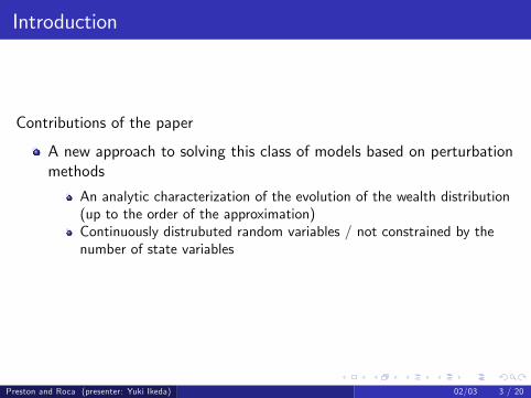
Contributions of the paper
A new approach to solving this class of models based on perturbationmethods
An analytic characterization of the evolution of the wealth distribution(up to the order of the approximation)Continuously distrubuted random variables / not constrained by thenumber of state variablesUnderstanding of the role of heterogeneity in aggregate dynamics
Preston and Roca (presenter: Yuki Ikeda) 02/03 3 / 20

Introduction
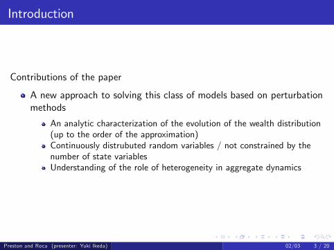
Contributions of the paper
A new approach to solving this class of models based on perturbationmethods
An analytic characterization of the evolution of the wealth distribution(up to the order of the approximation)
Continuously distrubuted random variables / not constrained by thenumber of state variablesUnderstanding of the role of heterogeneity in aggregate dynamics
Preston and Roca (presenter: Yuki Ikeda) 02/03 3 / 20
Introduction
Contributions of the paper
A new approach to solving this class of models based on perturbationmethods
An analytic characterization of the evolution of the wealth distribution(up to the order of the approximation)Continuously distrubuted random variables / not constrained by thenumber of state variables
Understanding of the role of heterogeneity in aggregate dynamics
Preston and Roca (presenter: Yuki Ikeda) 02/03 3 / 20
Introduction
Contributions of the paper
A new approach to solving this class of models based on perturbationmethods
An analytic characterization of the evolution of the wealth distribution(up to the order of the approximation)Continuously distrubuted random variables / not constrained by thenumber of state variablesUnderstanding of the role of heterogeneity in aggregate dynamics
Preston and Roca (presenter: Yuki Ikeda) 02/03 3 / 20

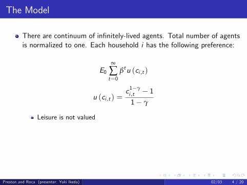
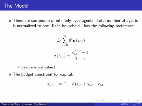
The Model
There are continuum of in�nitely-lived agents. Total number of agentsis normalized to one. Each household i has the following preference:
E0∞
∑t=0
βtu (ci ,t )
u (ci ,t ) =c1�γi ,t � 11� γ
Leisure is not valued
The budget constraint for capital:
ai ,t+1 = (1� δ)ai ,t + yi ,t � ci ,t
Preston and Roca (presenter: Yuki Ikeda) 02/03 4 / 20
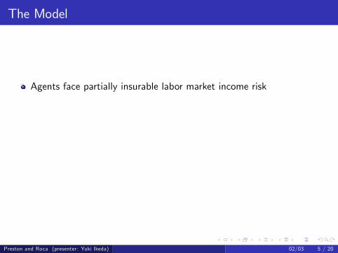
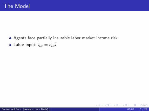
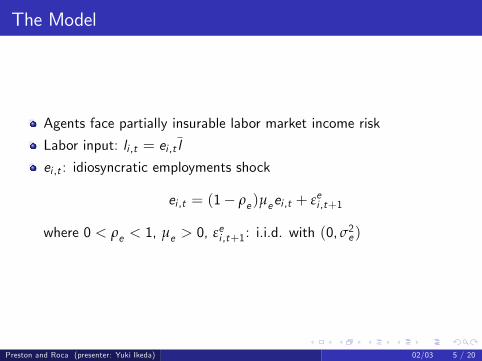
The Model
Agents face partially insurable labor market income risk
Labor input: li ,t = ei ,t l
ei ,t : idiosyncratic employments shock
ei ,t = (1� ρe )µeei ,t + εei ,t+1
where 0 < ρe < 1, µe > 0, εei ,t+1: i.i.d. with (0, σ2e )
Preston and Roca (presenter: Yuki Ikeda) 02/03 5 / 20
The Model
Agents face partially insurable labor market income risk
Labor input: li ,t = ei ,t l
ei ,t : idiosyncratic employments shock
ei ,t = (1� ρe )µeei ,t + εei ,t+1
where 0 < ρe < 1, µe > 0, εei ,t+1: i.i.d. with (0, σ2e )
Preston and Roca (presenter: Yuki Ikeda) 02/03 5 / 20
The Model
Agents face partially insurable labor market income risk
Labor input: li ,t = ei ,t l
ei ,t : idiosyncratic employments shock
ei ,t = (1� ρe )µeei ,t + εei ,t+1
where 0 < ρe < 1, µe > 0, εei ,t+1: i.i.d. with (0, σ2e )
Preston and Roca (presenter: Yuki Ikeda) 02/03 5 / 20

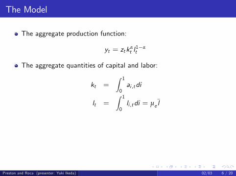
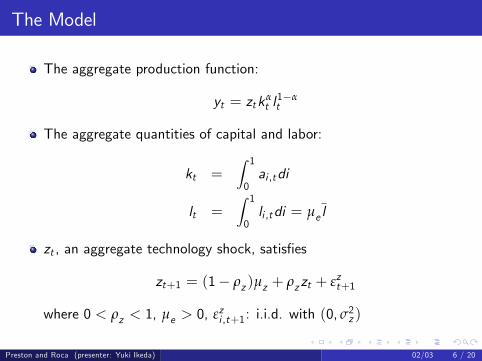
The Model
The aggregate production function:
yt = ztkαt l1�αt
The aggregate quantities of capital and labor:
kt =Z 1
0ai ,tdi
lt =Z 1
0li ,tdi = µe l
zt , an aggregate technology shock, satis�es
zt+1 = (1� ρz )µz + ρzzt + εzt+1
where 0 < ρz < 1, µe > 0, εzi ,t+1: i.i.d. with (0, σ2z )
Preston and Roca (presenter: Yuki Ikeda) 02/03 6 / 20
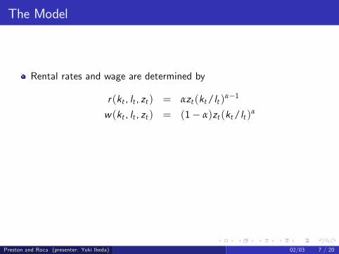
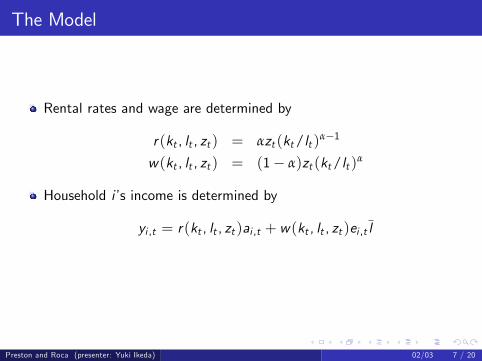
The Model
Rental rates and wage are determined by
r(kt , lt , zt ) = αzt (kt/lt )α�1
w(kt , lt , zt ) = (1� α)zt (kt/lt )α
Household i�s income is determined by
yi ,t = r(kt , lt , zt )ai ,t + w(kt , lt , zt )ei ,t l
Preston and Roca (presenter: Yuki Ikeda) 02/03 7 / 20
The Model
Rental rates and wage are determined by
r(kt , lt , zt ) = αzt (kt/lt )α�1
w(kt , lt , zt ) = (1� α)zt (kt/lt )α
Household i�s income is determined by
yi ,t = r(kt , lt , zt )ai ,t + w(kt , lt , zt )ei ,t l
Preston and Roca (presenter: Yuki Ikeda) 02/03 7 / 20
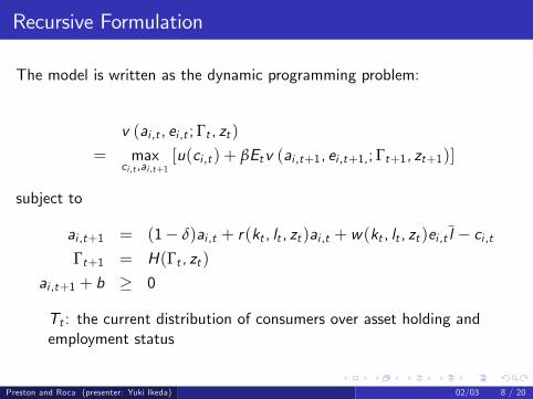
Recursive Formulation
The model is written as the dynamic programming problem:
v (ai ,t , ei ,t ; Γt , zt )= max
ci ,t ,ai ,t+1[u(ci ,t ) + βEtv (ai ,t+1, ei ,t+1,; Γt+1, zt+1)]
subject to
ai ,t+1 = (1� δ)ai ,t + r(kt , lt , zt )ai ,t + w(kt , lt , zt )ei ,t l � ci ,tΓt+1 = H(Γt , zt )
ai ,t+1 + b � 0
Tt : the current distribution of consumers over asset holding andemployment status
Preston and Roca (presenter: Yuki Ikeda) 02/03 8 / 20
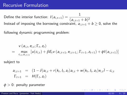
Recursive Formulation
De�ne the interior function: I (ai ,t+1) =1
(ai ,t+1 + b)2Instead of imposing the borrowing constraint, ai ,t+1 + b � 0, solve the
following dynamic programming problem:
v (ai ,t , ei ,t ; Γt , zt )= max
ci ,t ,ai ,t+1[u(ci ,t ) + βEtv (ai ,t+1, ei ,t+1,; Γt+1, zt+1) + φI (ai ,t+1)]
subject to
ai ,t+1 = (1� δ)ai ,t + r(kt , lt , zt )ai ,t + w(kt , lt , zt )ei ,t l � ci ,tΓt+1 = H(Γt , zt )
φ > 0: penalty parameter
Preston and Roca (presenter: Yuki Ikeda) 02/03 9 / 20
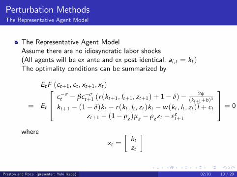
Perturbation MethodsThe Representative Agent Model
The Representative Agent ModelAssume there are no idiosyncratic labor shocks(All agents will be ex ante and ex post identical: ai ,t = kt )The optimality conditions can be summarized by
EtF (ct+1, ct , xt+1, xt )
= Et
264 c�σt � βc�σ
t+1 (r(kt+1, lt+1, zt+1) + 1� δ)� 2φ(kt+1+b)3
kt+1 � (1� δ)kt � r(kt , lt , zt )kt � w(kt , lt , zt )l + ctzt+1 � (1� ρz )µz � ρzzt � εzt+1
375 = 0where
xt =�ktzt
�
Preston and Roca (presenter: Yuki Ikeda) 02/03 10 / 20
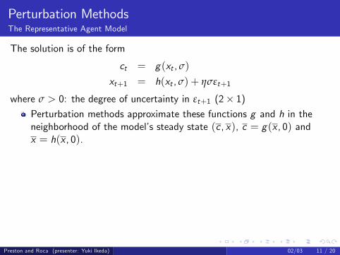
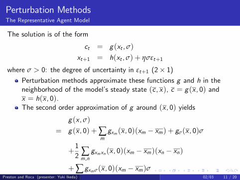
Perturbation MethodsThe Representative Agent Model
The solution is of the form
ct = g(xt , σ)
xt+1 = h(xt , σ) + ησεt+1
where σ > 0: the degree of uncertainty in εt+1 (2� 1)Perturbation methods approximate these functions g and h in theneighborhood of the model�s steady state (c , x), c = g(x , 0) andx = h(x , 0).
The second order approximation of g around (x , 0) yields
g(x , σ)
= g(x , 0) +∑mgxm (x , 0)(xm � xm) + gσ(x , 0)σ
+12 ∑m,ngxmxn (x , 0)(xm � xm)(xn � xn)
+∑mgxmσ(x , 0)(xm � xm)σ
+12 ∑m,ngσxm (x , 0)(xm � xm)σ+
12gσσ(x , 0)σ2
where m, n = 1, 2.
Preston and Roca (presenter: Yuki Ikeda) 02/03 11 / 20
Perturbation MethodsThe Representative Agent Model
The solution is of the form
ct = g(xt , σ)
xt+1 = h(xt , σ) + ησεt+1
where σ > 0: the degree of uncertainty in εt+1 (2� 1)Perturbation methods approximate these functions g and h in theneighborhood of the model�s steady state (c , x), c = g(x , 0) andx = h(x , 0).The second order approximation of g around (x , 0) yields
g(x , σ)
= g(x , 0) +∑mgxm (x , 0)(xm � xm) + gσ(x , 0)σ
+12 ∑m,ngxmxn (x , 0)(xm � xm)(xn � xn)
+∑mgxmσ(x , 0)(xm � xm)σ
+12 ∑m,ngσxm (x , 0)(xm � xm)σ+
12gσσ(x , 0)σ2
where m, n = 1, 2.
Preston and Roca (presenter: Yuki Ikeda) 02/03 11 / 20
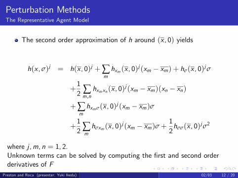
Perturbation MethodsThe Representative Agent Model
The second order approximation of h around (x , 0) yields
h(x , σ)j = h(x , 0)j +∑mhxm (x , 0)
j (xm � xm) + hσ(x , 0)jσ
+12 ∑m,nhxmxn (x , 0)
j (xm � xm)(xn � xn)
+∑mhxmσ(x , 0)j (xm � xm)σ
+12 ∑mhσxm (x , 0)
j (xm � xm)σ+12hσσ(x , 0)jσ2
where j ,m, n = 1, 2.Unknown terms can be solved by computing the �rst and second orderderivatives of F
Preston and Roca (presenter: Yuki Ikeda) 02/03 12 / 20
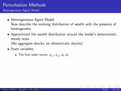
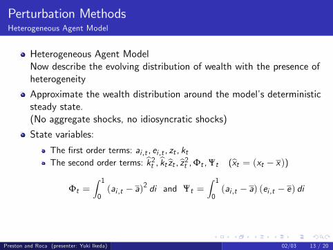
Perturbation MethodsHeterogeneous Agent Model
Heterogeneous Agent ModelNow describe the evolving distribution of wealth with the presence ofheterogeneity
Approximate the wealth distribution around the model�s deterministicsteady state.(No aggregate shocks, no idiosyncratic shocks)
State variables:
The �rst order terms: ai ,t , ei ,t , zt , ktThe second order terms: bk2t , bktbzt ,bz2t ,Φt ,Ψt (bxt = (xt � x))
Φt =Z 10(ai ,t � a)2 di and Ψt =
Z 10(ai ,t � a) (ei ,t � e) di
In sum, xt = [ai ,t , ei ,t , zt , kt ,Φt ,Ψt ]0
Preston and Roca (presenter: Yuki Ikeda) 02/03 13 / 20
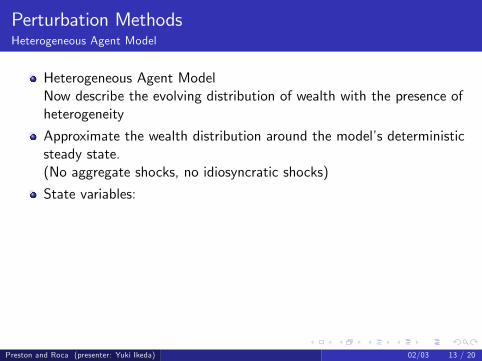
Perturbation MethodsHeterogeneous Agent Model
Heterogeneous Agent ModelNow describe the evolving distribution of wealth with the presence ofheterogeneity
Approximate the wealth distribution around the model�s deterministicsteady state.(No aggregate shocks, no idiosyncratic shocks)
State variables:
The �rst order terms: ai ,t , ei ,t , zt , kt
The second order terms: bk2t , bktbzt ,bz2t ,Φt ,Ψt (bxt = (xt � x))Φt =
Z 10(ai ,t � a)2 di and Ψt =
Z 10(ai ,t � a) (ei ,t � e) di
In sum, xt = [ai ,t , ei ,t , zt , kt ,Φt ,Ψt ]0
Preston and Roca (presenter: Yuki Ikeda) 02/03 13 / 20
Perturbation MethodsHeterogeneous Agent Model
Heterogeneous Agent ModelNow describe the evolving distribution of wealth with the presence ofheterogeneity
Approximate the wealth distribution around the model�s deterministicsteady state.(No aggregate shocks, no idiosyncratic shocks)
State variables:
The �rst order terms: ai ,t , ei ,t , zt , ktThe second order terms: bk2t , bktbzt ,bz2t ,Φt ,Ψt (bxt = (xt � x))
Φt =Z 10(ai ,t � a)2 di and Ψt =
Z 10(ai ,t � a) (ei ,t � e) di
In sum, xt = [ai ,t , ei ,t , zt , kt ,Φt ,Ψt ]0
Preston and Roca (presenter: Yuki Ikeda) 02/03 13 / 20
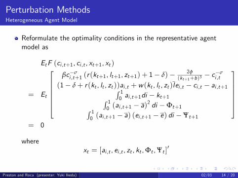
Perturbation MethodsHeterogeneous Agent Model
Reformulate the optimality conditions in the representative agentmodel as
EtF (ci ,t+1, ci ,t , xt+1, xt )
= Et
2666664βc�σi ,t+1 (r(kt+1, lt+1, zt+1) + 1� δ)� 2φ
(kt+1+b)3� c�σ
i ,t
(1� δ+ r(kt , lt , zt ))ai ,t + w(kt , lt , zt )lei ,t � ci ,t � ai ,t+1R 10 ai ,t+1di � kt+1R 1
0 (ai ,t+1 � a)2 di �Φt+1R 1
0 (ai ,t+1 � a) (ei ,t+1 � e) di �Ψt+1
3777775= 0
wherext = [ai ,t , ei ,t , zt , kt ,Φt ,Ψt ]
0
Preston and Roca (presenter: Yuki Ikeda) 02/03 14 / 20
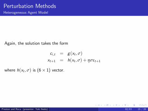
Perturbation MethodsHeterogeneous Agent Model
Again, the solution takes the form
ci ,t = g(xt , σ)
xt+1 = h(xt , σ) + ησεt+1
where h(xt , σ) is (6� 1) vector.
Preston and Roca (presenter: Yuki Ikeda) 02/03 15 / 20
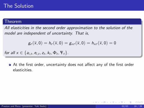
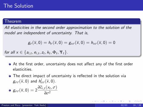
The Solution
TheoremAll elasticities in the second order approximation to the solution of themodel are independent of uncertainty. That is,
gσ(x , 0) = hσ(x , 0) = gxσ(x , 0) = hxσ(x , 0) = 0
for all x 2 fai ,t , ei ,t , zt , kt ,Φt ,Ψtg.
At the �rst order, uncertainty does not a¤ect any of the �rst orderelasticities.
The direct impact of uncertainty is re�ected in the solution viagσσ(x , 0) and h
jσσ(x , 0).
gσσ(x , 0) = 2∂bci ,t (xt , σ)
∂σ2
Preston and Roca (presenter: Yuki Ikeda) 02/03 16 / 20
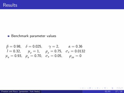
Results
Benchmark parameter values
β = 0.98, δ = 0.025, γ = 2, α = 0.36l = 0.32, µz = 1, ρz = 0.75, σz = 0.0132
µe = 0.93, ρe = 0.70, σe = 0.05, ρze = 0
Preston and Roca (presenter: Yuki Ikeda) 02/03 17 / 20

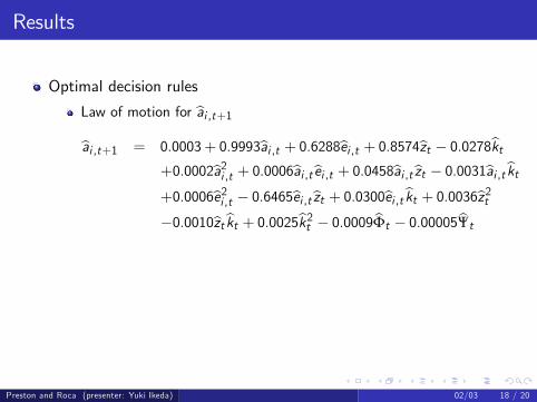
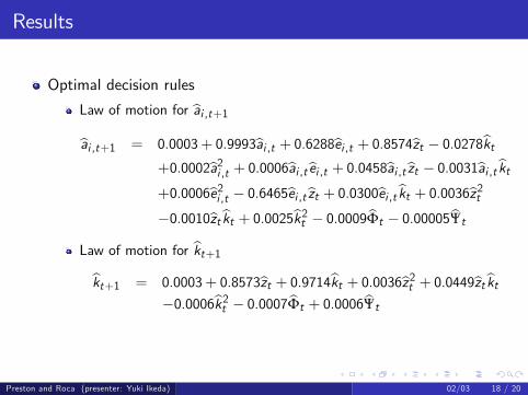
Results
Optimal decision rules
Law of motion for bai ,t+1bai ,t+1 = 0.0003+ 0.9993bai ,t + 0.6288bei ,t + 0.8574bzt � 0.0278bkt
+0.0002ba2i ,t + 0.0006bai ,tbei ,t + 0.0458bai ,tbzt � 0.0031bai ,tbkt+0.0006be2i ,t � 0.6465bei ,tbzt + 0.0300bei ,tbkt + 0.0036bz2t�0.0010bztbkt + 0.0025bk2t � 0.0009bΦt � 0.00005bΨt
Law of motion for bkt+1bkt+1 = 0.0003+ 0.8573bzt + 0.9714bkt + 0.0036bz2t + 0.0449bztbkt�0.0006bk2t � 0.0007bΦt + 0.0006bΨt
Preston and Roca (presenter: Yuki Ikeda) 02/03 18 / 20

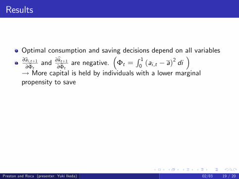
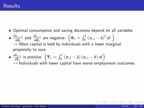
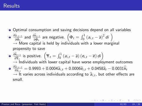
Results
Optimal consumption and saving decisions depend on all variables
∂bai ,t+1∂bΦt
and ∂bkt+1∂bΦt
are negative.�
Φt =R 10 (ai ,t � a)
2 di�
! More capital is held by individuals with a lower marginalpropensity to save∂bkt+1∂bΨt is positive.
�Ψt =
R 10 (ai ,t � a) (ei ,t � e) di
�! Individuals with lower capital have worse employment outcomes∂bai ,t+1
∂bai ,t = 0.9993+ 0.0004bai ,t + 0.0006bei ,t + 0.0458bzt � 0.0031bkt! It varies across individuals according to bai ,t , but other e¤ects aresmall.
Preston and Roca (presenter: Yuki Ikeda) 02/03 19 / 20
Results
Optimal consumption and saving decisions depend on all variables∂bai ,t+1
∂bΦtand ∂bkt+1
∂bΦtare negative.
�Φt =
R 10 (ai ,t � a)
2 di�
! More capital is held by individuals with a lower marginalpropensity to save
∂bkt+1∂bΨt is positive.
�Ψt =
R 10 (ai ,t � a) (ei ,t � e) di
�! Individuals with lower capital have worse employment outcomes∂bai ,t+1
∂bai ,t = 0.9993+ 0.0004bai ,t + 0.0006bei ,t + 0.0458bzt � 0.0031bkt! It varies across individuals according to bai ,t , but other e¤ects aresmall.
Preston and Roca (presenter: Yuki Ikeda) 02/03 19 / 20
Results
Optimal consumption and saving decisions depend on all variables∂bai ,t+1
∂bΦtand ∂bkt+1
∂bΦtare negative.
�Φt =
R 10 (ai ,t � a)
2 di�
! More capital is held by individuals with a lower marginalpropensity to save∂bkt+1∂bΨt is positive.
�Ψt =
R 10 (ai ,t � a) (ei ,t � e) di
�! Individuals with lower capital have worse employment outcomes
∂bai ,t+1∂bai ,t = 0.9993+ 0.0004bai ,t + 0.0006bei ,t + 0.0458bzt � 0.0031bkt! It varies across individuals according to bai ,t , but other e¤ects aresmall.
Preston and Roca (presenter: Yuki Ikeda) 02/03 19 / 20
Results
Optimal consumption and saving decisions depend on all variables∂bai ,t+1
∂bΦtand ∂bkt+1
∂bΦtare negative.
�Φt =
R 10 (ai ,t � a)
2 di�
! More capital is held by individuals with a lower marginalpropensity to save∂bkt+1∂bΨt is positive.
�Ψt =
R 10 (ai ,t � a) (ei ,t � e) di
�! Individuals with lower capital have worse employment outcomes∂bai ,t+1
∂bai ,t = 0.9993+ 0.0004bai ,t + 0.0006bei ,t + 0.0458bzt � 0.0031bkt! It varies across individuals according to bai ,t , but other e¤ects aresmall.
Preston and Roca (presenter: Yuki Ikeda) 02/03 19 / 20
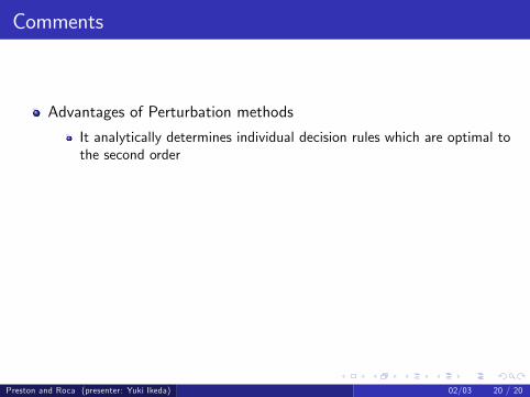
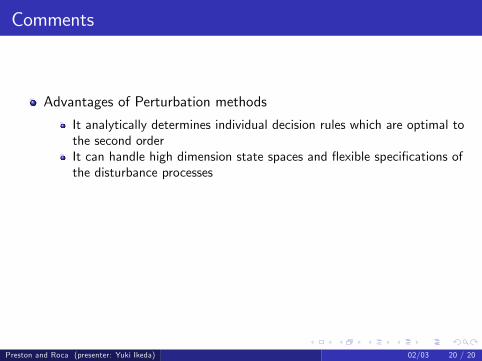
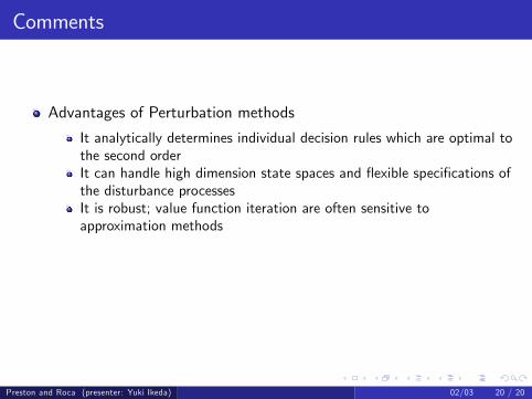
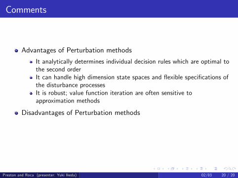
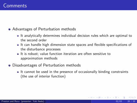
Comments
Advantages of Perturbation methods
It analytically determines individual decision rules which are optimal tothe second orderIt can handle high dimension state spaces and �exible speci�cations ofthe disturbance processesIt is robust; value function iteration are often sensitive toapproximation methods
Disadvantages of Perturbation methods
It cannot be used in the presence of occasionally binding constraints(the use of interior function)
Preston and Roca (presenter: Yuki Ikeda) 02/03 20 / 20
Comments
Advantages of Perturbation methods
It analytically determines individual decision rules which are optimal tothe second order
It can handle high dimension state spaces and �exible speci�cations ofthe disturbance processesIt is robust; value function iteration are often sensitive toapproximation methods
Disadvantages of Perturbation methods
It cannot be used in the presence of occasionally binding constraints(the use of interior function)
Preston and Roca (presenter: Yuki Ikeda) 02/03 20 / 20
Comments
Advantages of Perturbation methods
It analytically determines individual decision rules which are optimal tothe second orderIt can handle high dimension state spaces and �exible speci�cations ofthe disturbance processes
It is robust; value function iteration are often sensitive toapproximation methods
Disadvantages of Perturbation methods
It cannot be used in the presence of occasionally binding constraints(the use of interior function)
Preston and Roca (presenter: Yuki Ikeda) 02/03 20 / 20
Comments
Advantages of Perturbation methods
It analytically determines individual decision rules which are optimal tothe second orderIt can handle high dimension state spaces and �exible speci�cations ofthe disturbance processesIt is robust; value function iteration are often sensitive toapproximation methods
Disadvantages of Perturbation methods
It cannot be used in the presence of occasionally binding constraints(the use of interior function)
Preston and Roca (presenter: Yuki Ikeda) 02/03 20 / 20
Comments
Advantages of Perturbation methods
It analytically determines individual decision rules which are optimal tothe second orderIt can handle high dimension state spaces and �exible speci�cations ofthe disturbance processesIt is robust; value function iteration are often sensitive toapproximation methods
Disadvantages of Perturbation methods
It cannot be used in the presence of occasionally binding constraints(the use of interior function)
Preston and Roca (presenter: Yuki Ikeda) 02/03 20 / 20
Related Documents


