Seasonal Variation of Moisture Transport in Polar Regions ...

Oshima and Yamazaki

1

Polar Meteorol. Glaciol., 18, 00-00, 2004

© 2004 National Institute of Polar Research

Seasonal Variation of Moisture Transport in Polar Regions and

the Relation with Annular Modes

Kazuhiro Oshima1 and Koji Yamazaki1, 2

1 Graduate School of Environmental Earth Science, Hokkaido University, Sapporo, 060-0810

2 International Arctic Research Center, Frontier Research System for Global Change, Tokyo 105-6791

even page: K. Oshima and K. Yamazaki odd page: Moisture Transport in the Polar Regions

Oshima and Yamazaki

2

Abstract: Climatological seasonal variations of moisture transport and the interannual

variations associated with the annular modes in the Arctic and Antarctic regions are

investigated using 15-year ECMWF reanalysis data.

Over the Arctic, there are strong moisture inflows from the Atlantic and Pacific in all

seasons. Over the Antarctic, a strong moisture inflow exists around the Antarctic Peninsula in

all seasons and another strong inflow exists over the Bellingshausen Sea and the Amundsen

Sea in austral autumn and winter. Transient moisture flux is dominant over stationary flux and

transient flux variation mainly controls the seasonal variation of precipitation minus

evaporation (P-E) in both regions. The seasonal variations of P-E show a summer maximum

in the Arctic and a winter maximum in the Antarctic. It is mainly governed by the seasonal

variation of precipitable water variation in the Arctic and transient eddy activity in the

Antarctic.

The zonal mean poleward and eastward moisture fluxes in high latitudes are

positively correlated with annular modes in both regions. Positive polarity of the Arctic

Oscillation is associated with enhanced moisture inflow from the Atlantic, while positive

polarity of the Antarctic Oscillation is associated with enhanced moisture inflow west of the

Antarctic Peninsula.

key words: Atmospheric Moisture Budget, Polar Regions, Annular Mode, Reanalysis data

Oshima and Yamazaki

3

1. Introduction

The Arctic and Antarctic regions are moisture flux convergence areas, atmospheric

moisture transport is a primary input of water into the regions. The net input of water from the

atmosphere to the surface is the difference between precipitation and evaporation (P-E). P-E

is approximately equals the moisture flux convergence over a long period. Furthermore, the

moisture transport directly or indirectly affects the snow, sea ice and ice sheet over the regions.

Therefore, atmospheric moisture transport is a critical factor for water balance, especially

over the polar regions.

There have been some estimates of these quantities over the Arctic and Antarctic. There

are two estimation methods for P-E; one is an estimate from the atmospheric moisture budget

using rawinsonde, objective analysis or satellite data (e.g. Peixoto and Oort, 1983, 1992,

Bromwich et al., 1995, Groves and Francis, 2002a), the other is direct calculation of P and E.

The latter is estimated from rain gauge observations, snow depth measurements (e.g. Sellers,

1965, Baumgarner and Reichel, 1975, Giovinetto and Bull, 1987), objective analysis or model

output data (e.g. Cullather et al., 1998, Bromwich et al., 2000). In general, direct observations

suffer from local variations of precipitation. Moreover, surface observations are not reliable

over the Arctic Ocean and Antarctica, because the observation network is very sparse and

accurate measurement is difficult over Antarctica due to the severe climate and snow drift.

Giovinetto and Bull (1987) estimated the P-E (accumulation) over Antarctica from

glaciological data synthesis, but such data can only estimate the annual mean value. Since P

Oshima and Yamazaki

4

from objective analysis data is obtained from short-time integration of the forecast model, it

suffers from a spin-up problem. Although P from a climate model does not have the spin-up

problem, it totally depends on the model performance and the performance of many models is

not so good in polar regions. Therefore, the moisture budget method is superior to the direct

method in the Arctic and Antarctic regions.

On the moisture transport, the distribution of poleward moisture flux across 70°N that

contributes to the P-E over the region was investigated with rawinsonde data for 1974-1991

by Serreze et al. (1995) and a similar study was done for 1973-1995 by Serreze and Barry

(2000). These studies discussed the seasonal variation and the distribution of poleward

moisture flux across 70°N. Cullather et al. (2000) and Bromwich et al. (2000) compared

estimates from rawinsonde (Historical Arctic Rawinsonde Archive; HARA) with those from

reanalysis data (European Centre for Medium-range Weather Forecasts; ECMWF, National

Centers for Environmental Prediction and National Center for Atmospheric Research;

NCEP-NCAR) and they found that the meridional moisture flux from rawinsonde is smaller

than that from reanalysis in boreal summer. However, these studies did not present the

horizontal fields of moisture flux and its seasonal variations in detail.

Over the Antarctic, Yamazaki (1992, 1994, 1997), Bromwich et al. (1995) and Cullather

et al. (1998) estimated P-E with operational numerical analysis data. Yamazaki (1992, 1994)

found that P-E is large in austral winter and suggested that it is controlled by cyclone activity.

This peculiar seasonal variation was also presented by Bromwich et al. (1995). However, the

Oshima and Yamazaki

5

mechanism of this peculiar seasonal variation has not been quantitatively explained yet.

Bromwich et al. (1995) compared the three operational numerical analyses (ECMWF,

National Meteorological Center; NMC, Australian Bureau of Meteorology; ABM) and

rawinsonde data, and it was found that the ECMWF analysis provides good estimates for the

water budget.

The Arctic Oscillation (AO) is a dominant mode of atmospheric variability in the

wintertime Northern Hemisphere (Thompson and Wallace, 1998, 2000). The AO is a seesaw

of sea level pressure between the Arctic region and mid-latitudes, which shows an annular

pattern. Thus it is also named the Northern Hemisphere Annular Mode (NAM). The Southern

Hemisphere counterpart of the AO/NAM is called the Antarctic Oscillation (AAO) or the

Southern Hemisphere Annular Mode (SAM) (Gong and Wang, 1999, Thompson and Wallace,

2000). When the phase of the annular mode (AO or AAO) is positive, westerly winds around

60°N/S are enhanced and those around 35°N/S are reduced. Although the annular modes exist

throughout the year, they are most active during cold seasons.

Moisture transport is also related to the annular modes (AO and AAO). The zonal

mean poleward moisture flux at high-latitudes has a positive correlation with the AO and

AAO (Rogers et al. 2001, Boer et al. 2001). Although these studies show the zonal mean

moisture flux associated with the annular modes, the spatial patterns are not shown. Groves

and Francis (2002b) showed composite maps of moisture flux associated with high and low

polarities of the AO index. They calculated the moisture flux with moisture data from TOVS

Oshima and Yamazaki

6

and wind data from NCEP-NCAR. Their climatological moisture flux fields are different from

those in the present study. There are no studies on the spatial pattern associated with the AAO.

In this study, we examine the seasonal variation of moisture flux fields mainly using the

15-year (1979-1993) ECMWF reanalysis data; the focus is on net moisture inflow into the

polar regions. To isolate the effect of cyclone activity on moisture transport, we divide the

total moisture transport into transient and stationary components. For the atmospheric

moisture budget, most previous studies only presented the P-E estimates over the region

poleward from 70° (hereafter called the polar cap region), especially in the Arctic. However,

to assess the fresh water balance of the Arctic Ocean or the accumulation of moisture in

Antarctica, it is useful to examine the moisture budget over the Arctic Ocean or Antarctica.

Hence the moisture budget for the Arctic Ocean and Antarctica are also estimated.

Interannual variability of moisture transport associated with annular modes is also

investigated in this study. In particular, the spatial patterns in both regions are presented.

In section 2, we describe the data and method used in our analysis. The climatological

descriptions of moisture flux and moisture budget in both regions are presented in Section 3.

Interannual variability associated with annular modes is presented in section 4. We summarize

with some discussion in section 5.

2. Data and method

Two reanalysis data sets are used to estimate the moisture flux. The primary data set is

Oshima and Yamazaki

7

the 15-year ECMWF reanalysis (ERA, 1979-1993); the supplementary data set is the 24-year

National Centers for Environmental Prediction - Department of Energy (NCEP-DOE)

reanalysis-2 (NCEP R2, 1979-2002). Their horizontal resolutions are 2.5 degrees in latitude

and longitude in both data sets. Temporal resolution is twice-daily (12hours) in ERA and

fourth-daily (6hours) in NCEP R2.

Moisture flux <qv> in this paper is a vertical integral of moisture flux qv at each level

and is expressed as follows:

∫=Psurface

hPadpq

gq

300

1 vv , (1)

where q is the specific humidity, v is the horizontal wind vector and the brackets represent

vertical integration. The upper limit of the integral is set to 300 hPa, because moisture above

300 hPa is negligible.

Monthly mean moisture flux is computed from twice-daily or fourth-daily moisture flux.

The monthly mean total moisture flux can be divided into stationary flux and transient flux as

follows:

vvv ′′+= qqq , (2)

where the overbar represents the time average, represented by the monthly average in this

study, and the prime represents the deviation from the time average. Thus total flux (left hand

side) is expressed as a sum of stationary (first term of the right hand side) flux and transient

(second term of the right hand side) flux. The total flux is obtained from the monthly mean of

twice-daily (fourth-daily) flux and the stationary flux is calculated from the monthly mean

Oshima and Yamazaki

8

fields of wind, moisture and surface pressure. The transient flux is calculated by subtracting

the stationary flux from the total flux.

To estimate seasonal variations of precipitation minus evaporation (P-E) over both the

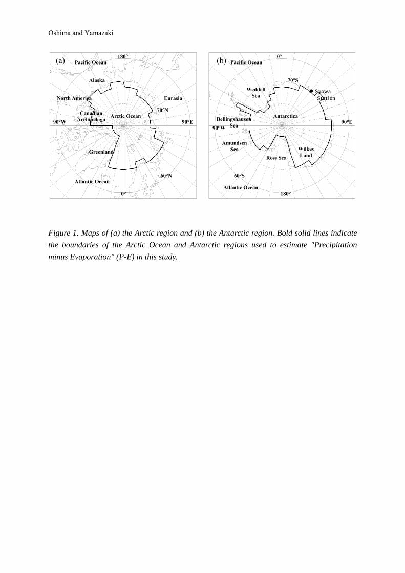
Arctic Ocean and Antarctica, we define the regions of the Arctic Ocean and Antarctica with

ERA land-sea mask data (Figure 1). P-E is estimated by the atmospheric moisture budget

equation as follows:

PEqdt

dPW−+><−∇= v , (3)

where PW is precipitable water. When we calculate an average over a long time period (i.e.,

seasonal mean), the time rate of change of PW, the left hand side of Equation (3), can be

neglected and Equation (3) is rewritten as:

,1∫ ⋅><−≈

><−∇≈−

dlqA

qEP

nv

v (4)

where A is the area of the region, l is the length along the boundary of the region and n is the

unit vector normal to the boundary of the region.

To clarify the relation between annular modes and moisture flux, the correlation

coefficients between Arctic and Antarctic Oscillation indices and zonal mean moisture flux

are calculated based on 15-year monthly mean data. Prior to the analysis, climatological

seasonal variation of moisture flux is removed from the moisture flux data. We show the

regression patterns for moisture flux upon the AO/AAO indices. The monthly mean AO and

AAO indices available at NOAA Climate Prediction Center are used.

Fig. 1

Oshima and Yamazaki

9

3. Climatology of atmospheric moisture transport and budget

3.1. The Arctic

3.1.1. Annual mean field

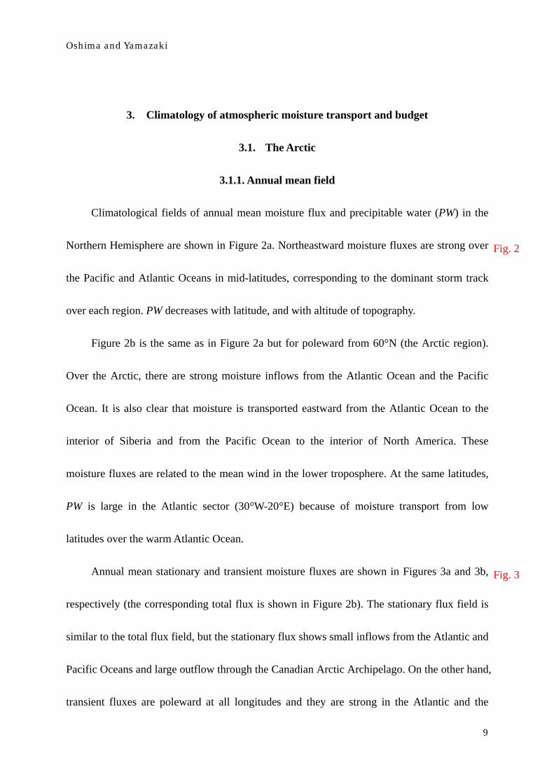
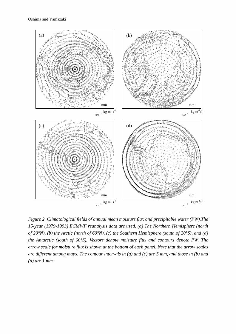
Climatological fields of annual mean moisture flux and precipitable water (PW) in the

Northern Hemisphere are shown in Figure 2a. Northeastward moisture fluxes are strong over

the Pacific and Atlantic Oceans in mid-latitudes, corresponding to the dominant storm track

over each region. PW decreases with latitude, and with altitude of topography.

Figure 2b is the same as in Figure 2a but for poleward from 60°N (the Arctic region).

Over the Arctic, there are strong moisture inflows from the Atlantic Ocean and the Pacific

Ocean. It is also clear that moisture is transported eastward from the Atlantic Ocean to the

interior of Siberia and from the Pacific Ocean to the interior of North America. These

moisture fluxes are related to the mean wind in the lower troposphere. At the same latitudes,

PW is large in the Atlantic sector (30°W-20°E) because of moisture transport from low

latitudes over the warm Atlantic Ocean.

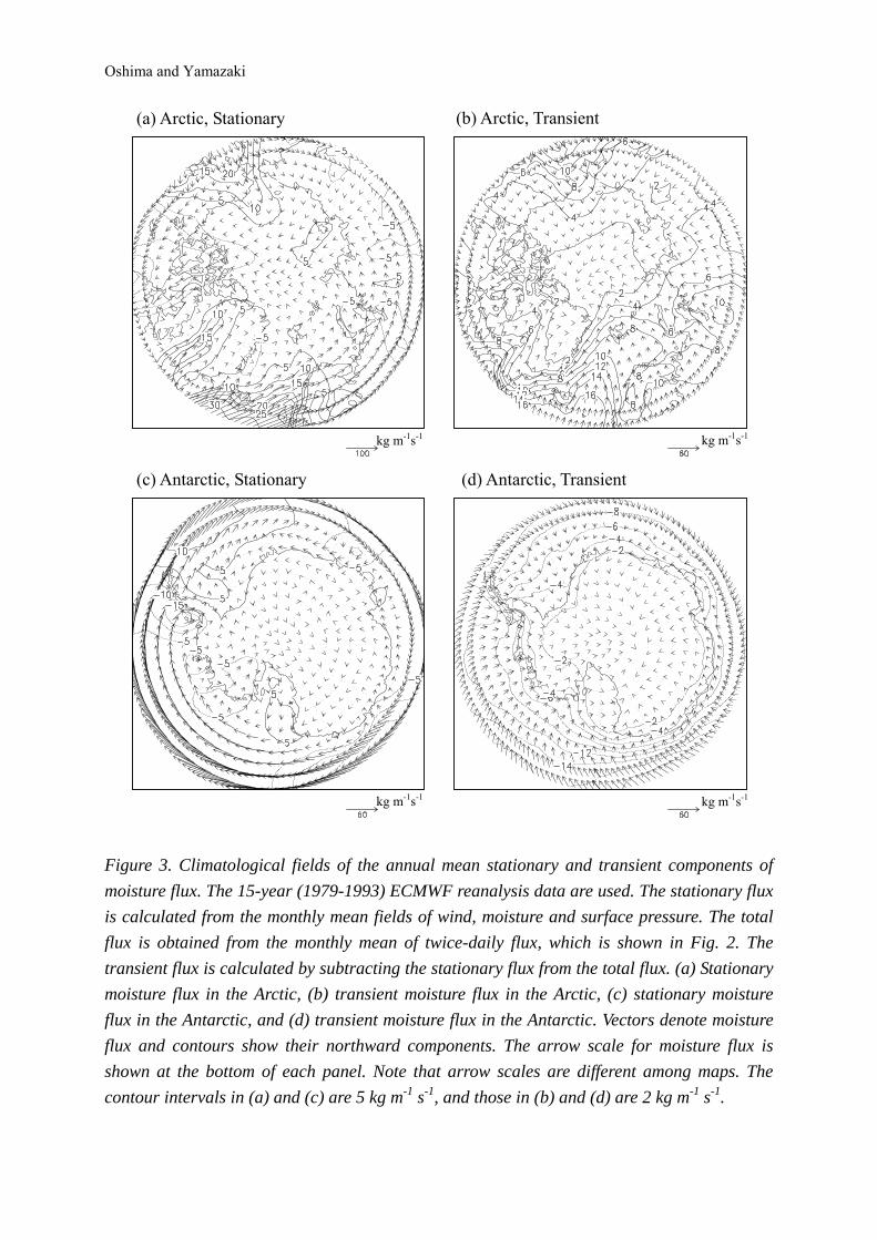
Annual mean stationary and transient moisture fluxes are shown in Figures 3a and 3b,

respectively (the corresponding total flux is shown in Figure 2b). The stationary flux field is

similar to the total flux field, but the stationary flux shows small inflows from the Atlantic and

Pacific Oceans and large outflow through the Canadian Arctic Archipelago. On the other hand,

transient fluxes are poleward at all longitudes and they are strong in the Atlantic and the

Fig. 2

Fig. 3

Oshima and Yamazaki

10

Pacific sectors (180°-15°W). Inflow can be seen on the western side of Greenland and in

Eastern Europe (45°E-90°E). Even over the Canadian Arctic Archipelago, where the

stationary flux shows large outflow from the Arctic, the transient flux indicates inflow to the

Arctic Ocean. In general, poleward flow (v'>0) is accompanied with more humid air (q'>0)

while equator-ward flow (v'<0) is accompanied with drier air (q'<0). Therefore, the

correlation between q' and v' is positive in the Northern Hemisphere. Thus, transient eddies,

typically associated with extratropical cyclones, transport moisture poleward.

3.1.2. Seasonal variation of moisture flux

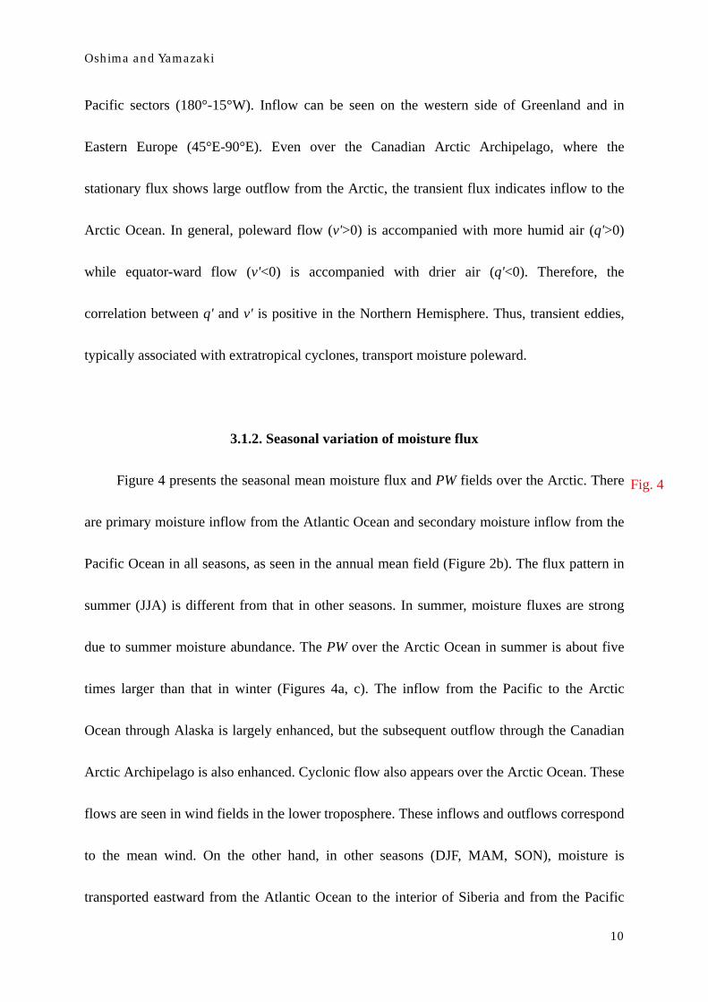
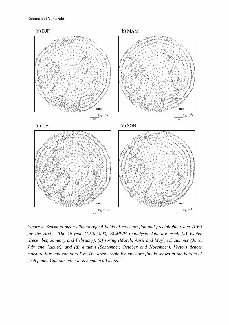
Figure 4 presents the seasonal mean moisture flux and PW fields over the Arctic. There

are primary moisture inflow from the Atlantic Ocean and secondary moisture inflow from the

Pacific Ocean in all seasons, as seen in the annual mean field (Figure 2b). The flux pattern in

summer (JJA) is different from that in other seasons. In summer, moisture fluxes are strong

due to summer moisture abundance. The PW over the Arctic Ocean in summer is about five

times larger than that in winter (Figures 4a, c). The inflow from the Pacific to the Arctic

Ocean through Alaska is largely enhanced, but the subsequent outflow through the Canadian

Arctic Archipelago is also enhanced. Cyclonic flow also appears over the Arctic Ocean. These

flows are seen in wind fields in the lower troposphere. These inflows and outflows correspond

to the mean wind. On the other hand, in other seasons (DJF, MAM, SON), moisture is

transported eastward from the Atlantic Ocean to the interior of Siberia and from the Pacific

Fig. 4

Oshima and Yamazaki

11

Ocean and Alaska to the interior of North America. In winter (DJF), the wind field shows a

cross-Arctic flow in the Arctic Ocean, but such a flow is not seen in the moisture flux (Figure

4a) due to small PW in this season.

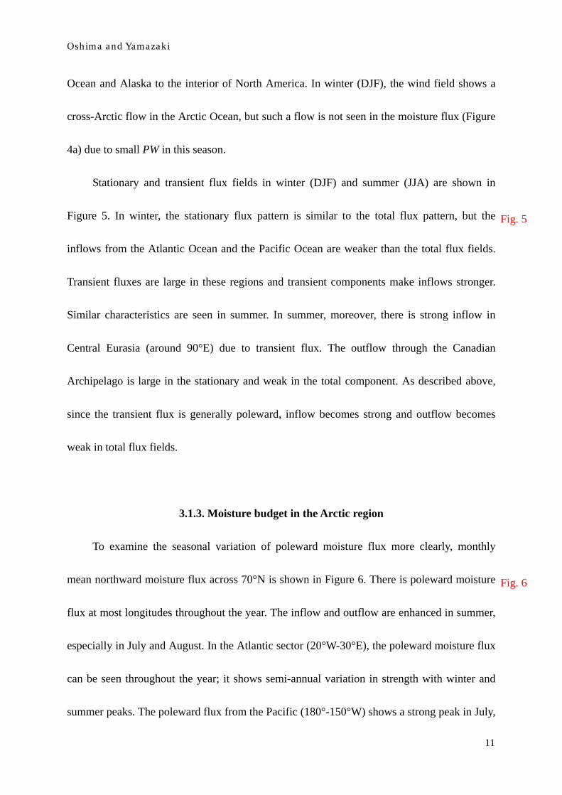
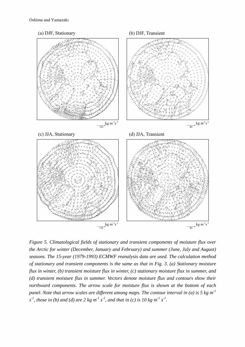
Stationary and transient flux fields in winter (DJF) and summer (JJA) are shown in

Figure 5. In winter, the stationary flux pattern is similar to the total flux pattern, but the

inflows from the Atlantic Ocean and the Pacific Ocean are weaker than the total flux fields.

Transient fluxes are large in these regions and transient components make inflows stronger.

Similar characteristics are seen in summer. In summer, moreover, there is strong inflow in

Central Eurasia (around 90°E) due to transient flux. The outflow through the Canadian

Archipelago is large in the stationary and weak in the total component. As described above,

since the transient flux is generally poleward, inflow becomes strong and outflow becomes

weak in total flux fields.

3.1.3. Moisture budget in the Arctic region

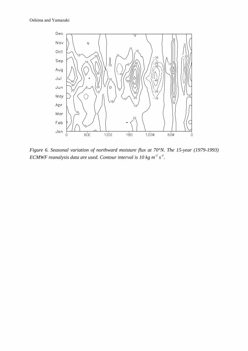
To examine the seasonal variation of poleward moisture flux more clearly, monthly

mean northward moisture flux across 70°N is shown in Figure 6. There is poleward moisture

flux at most longitudes throughout the year. The inflow and outflow are enhanced in summer,

especially in July and August. In the Atlantic sector (20°W-30°E), the poleward moisture flux

can be seen throughout the year; it shows semi-annual variation in strength with winter and

summer peaks. The poleward flux from the Pacific (180°-150°W) shows a strong peak in July,

Fig. 5

Fig. 6

Oshima and Yamazaki

12

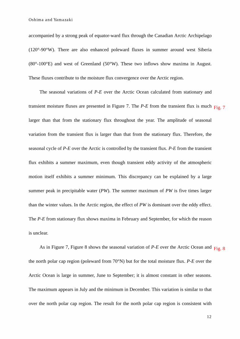
accompanied by a strong peak of equator-ward flux through the Canadian Arctic Archipelago

(120°-90°W). There are also enhanced poleward fluxes in summer around west Siberia

(80°-100°E) and west of Greenland (50°W). These two inflows show maxima in August.

These fluxes contribute to the moisture flux convergence over the Arctic region.

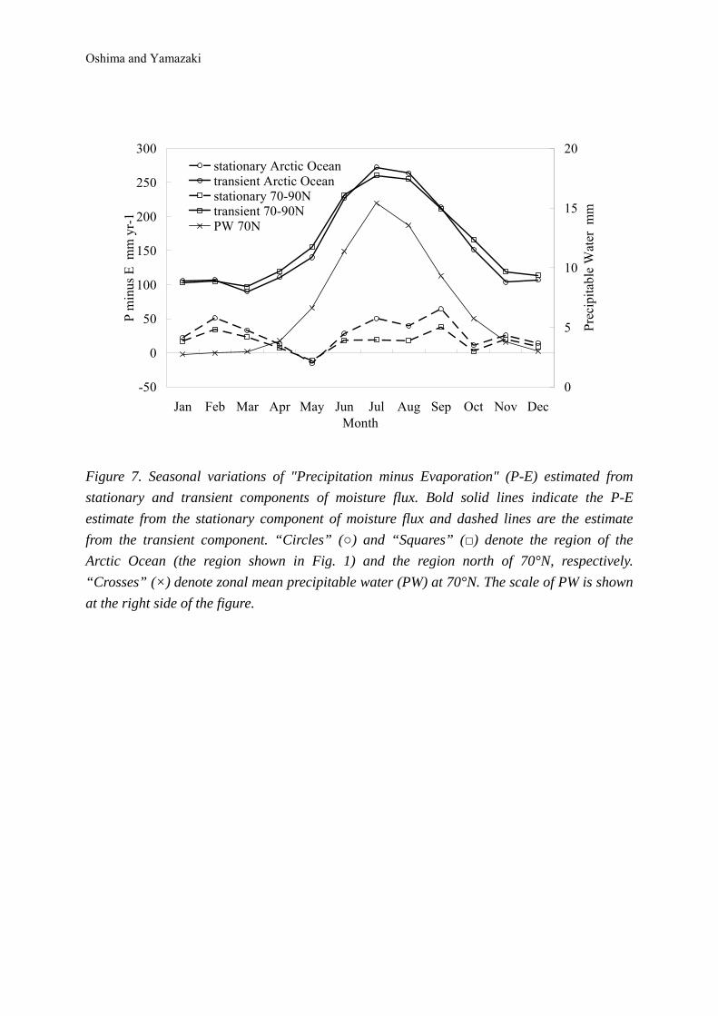
The seasonal variations of P-E over the Arctic Ocean calculated from stationary and

transient moisture fluxes are presented in Figure 7. The P-E from the transient flux is much

larger than that from the stationary flux throughout the year. The amplitude of seasonal

variation from the transient flux is larger than that from the stationary flux. Therefore, the

seasonal cycle of P-E over the Arctic is controlled by the transient flux. P-E from the transient

flux exhibits a summer maximum, even though transient eddy activity of the atmospheric

motion itself exhibits a summer minimum. This discrepancy can be explained by a large

summer peak in precipitable water (PW). The summer maximum of PW is five times larger

than the winter values. In the Arctic region, the effect of PW is dominant over the eddy effect.

The P-E from stationary flux shows maxima in February and September, for which the reason

is unclear.

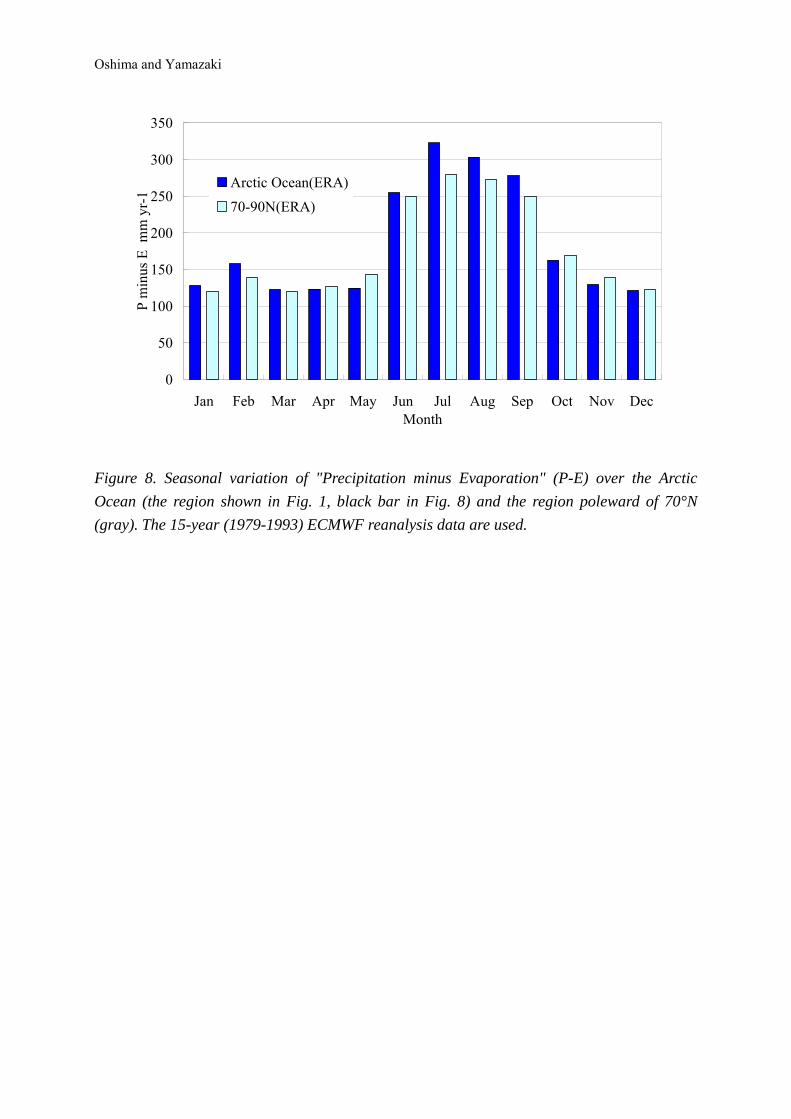
As in Figure 7, Figure 8 shows the seasonal variation of P-E over the Arctic Ocean and

the north polar cap region (poleward from 70°N) but for the total moisture flux. P-E over the

Arctic Ocean is large in summer, June to September; it is almost constant in other seasons.

The maximum appears in July and the minimum in December. This variation is similar to that

over the north polar cap region. The result for the north polar cap region is consistent with

Fig. 7

Fig. 8

Oshima and Yamazaki

13

previous studies (Cullather et al., 2000, Bromwich et al., 2000), based on reanalysis data.

Seasonal mean P-E over the Arctic and the north polar cap region derived from ERA are

shown in Table 1. Over the Arctic Ocean, the annual mean P-E is 186 mm/year, the summer

(JJA) mean is 294 mm/year and the winter (DJF) mean is 136 mm/year. These values over the

Arctic Ocean are larger than that over the north polar cap region. This is also seen in Figure 8.

This may be caused by the fact that the north polar cap region includes Greenland and

underestimates P-E over this region.

Table 2 presents the annual mean P-E over the Arctic Ocean, together with results from

previous studies. The values of P-E over both the Arctic Ocean and the north polar cap in this

study are reasonable. The P-E from NCEP R2 is a little larger than that from ERA. This is

consistent with Cullather et al. (2000). Bromwich et al. (2000) used the same ERA data set as

this study and therefore estimates over the polar cap region are almost the same. However, the

estimates over the Arctic Ocean are different, because Bromwich et al. (2000) defined a

simpler boundary of the Arctic Ocean than that of this study (Figure 1a). The estimates from

surface data vary widely. Those from atmospheric data, especially results from objective

analysis data, do not vary widely, but depend on the data set.

3.2. The Antarctic

3.2.1. Annual mean field

In the same way as the Arctic, results for the Antarctic region are shown in this section.

Table 1

Table 2

Oshima and Yamazaki

14

In the Southern Hemisphere, annual mean moisture flux and PW are zonal in comparison with

the Northern Hemisphere and eastward fluxes are strong in mid-latitudes (Figure 2c). Over

the Antarctic, the eastward flux is strong over the Antarctic Ocean surrounding Antarctica. A

westward moisture flux exists along the coastline of East Antarctica (Figure 2d). These

transports are related to the mean wind in the lower troposphere. The poleward flux is strong

around the Antarctic Peninsula and over the Bellingshausen and the Amundsen Seas.

Poleward fluxes also appear off Wilkes Land, and around Syowa Station. This corresponds to

the mean wind. These features are consistent with results in Yamazaki (1992, 1994, and

1997).

Annual mean stationary and transient flux fields are shown in Figure 3c and 3d.

Stationary fluxes are weaker than total fluxes, but the inflow regions are almost the same. In

addition, there are outflows over the Weddell Sea and Ross Sea. Such fluxes are not seen in

the total flux field. Transient fluxes are poleward at all latitudes. Thus, inflow of the total

component is strong around the Antarctic Peninsula, over the Bellingshausen and Amundsen

Seas, off Wilkes Land and around Syowa station. Over the Ross Sea and Weddell Sea,

stationary and transient fluxes almost cancel each other and the significant meridional

transports over the regions do not appear in the total field.

3.2.2. Seasonal variation of moisture flux

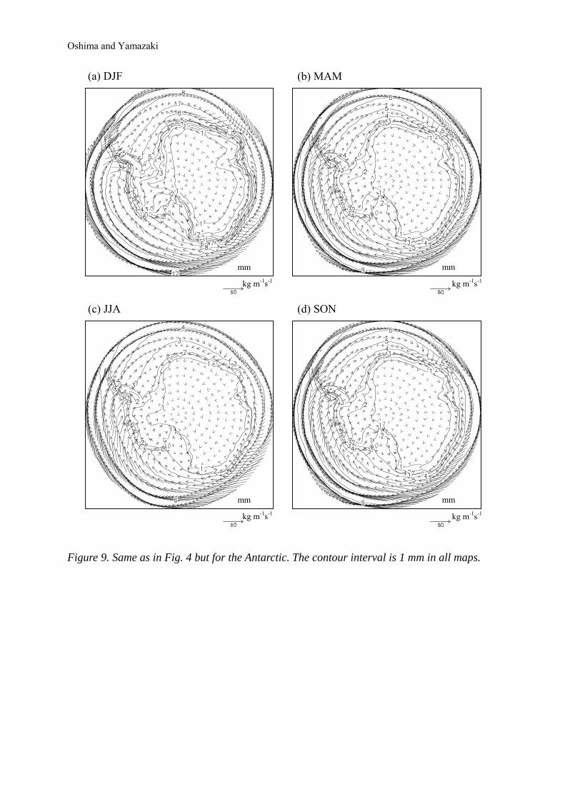
Figure 9 presents the seasonal mean moisture flux and PW fields over the Antarctic. Fig. 9

Oshima and Yamazaki

15

There is large eastward flux over the Antarctic Ocean surrounding Antarctica in all seasons.

This basically corresponds to the mean wind field in the lower troposphere. The poleward flux

is strong around the Antarctic Peninsula. In summer (DJF), the westward moisture flux

parallel to the coastline is significantly enhanced in East Antarctica, because the mean

low-level wind corresponding to the flux is strong in summer and the PW in summer is two

times larger than in winter. In autumn (MAM) and winter (JJA), poleward flux is enhanced

over the Bellingshausen Sea and the Amundsen Sea.

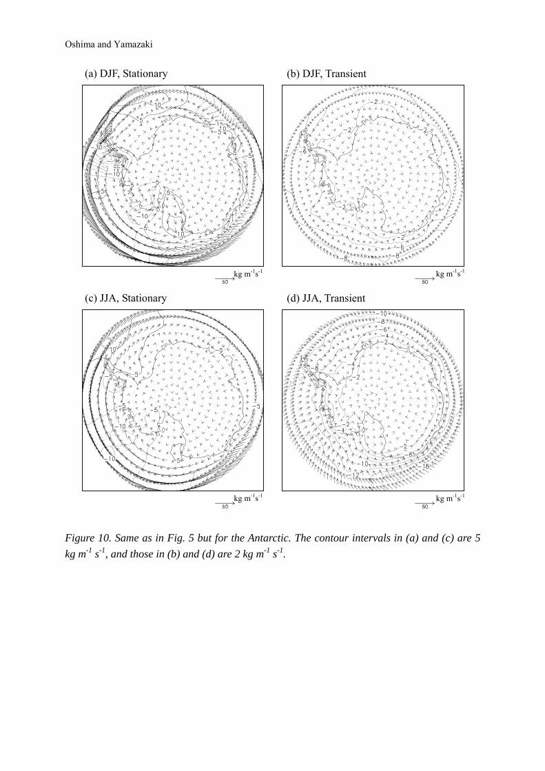
Stationary and transient fluxes in summer (DJF) and winter (JJA) are shown in Figure

10. There are similar inflow and outflow patterns in the stationary components in both

summer and winter. Due to PW increase in summer, the inflow and outflow are strong in

summer, especially around the Antarctic Peninsula, off Wilkes Land and around Syowa

station. In the Amundsen Sea, poleward stationary flux is enhanced in summer, which

corresponds to the eastern part of the stationary cyclone over the Ross Sea.

Transient poleward flux in winter is generally larger than that in summer even though

PW is two times larger in summer. This large transient flux indicates that the effect of cyclone

activity dominates over the PW effect around Antarctica.

3.2.3. Moisture budget in the Antarctic region

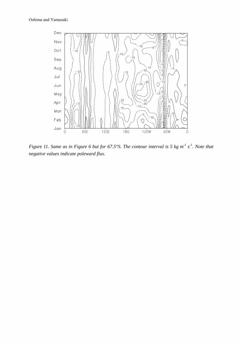
Seasonal variation of moisture inflow into the Antarctic at 67.5°S is shown in Figure 11.

We chose 67.5°S instead of 70°S, because the 70°S latitude circle passes through East

Fig. 10

Fig. 11

Oshima and Yamazaki

16

Antarctica. As in the Arctic, there is poleward moisture flux at most longitudes throughout the

year. Note that negative value means poleward flux. There is large poleward flux in summer

and small flux in winter around the Antarctic Peninsula (80°-60°W). However, there is large

poleward flux in early winter and small flux in summer over the Bellingshausen Sea and the

Amundsen Sea (150°-100°W). Large inflow exists around Syowa Station (20°-50°E) in late

summer, January to March. A small outflow appears around 60°E throughout the year and in

the sector between 45°W and 10°E in late summer.

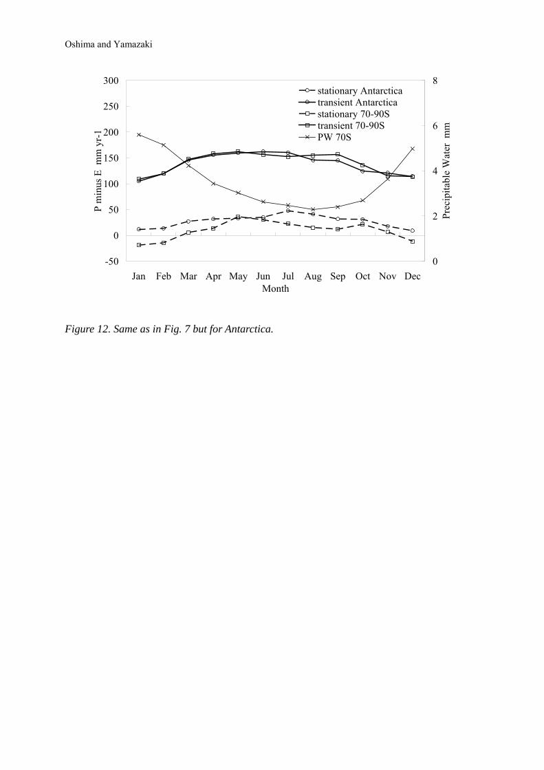
Figure 12 shows the seasonal variation of P-E over Antarctica. This is estimated from

stationary and transient moisture fluxes. As in the Arctic region, the P-E estimated from

transient flux is larger than that from stationary flux. However, the seasonal variation of P-E

from transient flux is comparable to that from stationary flux. The summer maximum of PW

over Antarctica is only two times larger than the winter minimum. This explains the peculiar

seasonal cycle of P-E over Antarctica. In Antarctica, the effect of eddy activity dominates

over the PW effect. The contribution from stationary flux also shows a winter maximum. This

is caused by the winter intensification and southern shift of the stationary cyclone in the Ross

Sea, which brings humid air poleward to the east of the cyclone (120°W-160°W, see Fig. 10c).

Both transient and stationary components contribute to cause this peculiar winter maximum of

P-E over the Antarctic region.

The seasonal variation of P-E over Antarctica and the south polar cap region estimated

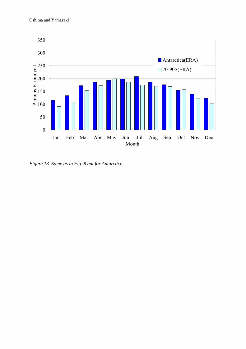
from total flux is presented in Figure 13. P-E varies gently. In spite of large PW in summer

Fig. 12

Fig. 13

Oshima and Yamazaki

17

and small PW in winter, P-E is large in winter and small in summer. The maximum appears in

July and the minimum in January. This is mainly because transient poleward moisture

transport associated with cyclone activity is enhanced in winter (JJA) as seen in Figures 9, 10

and 12. The stationary flux also contributes to this peculiar seasonal variation. P-E over the

south polar cap region has a maximum in May and a minimum in January. The present result

for Antarctica and the south polar cap region agrees with that of Bromwich et al. (1995).

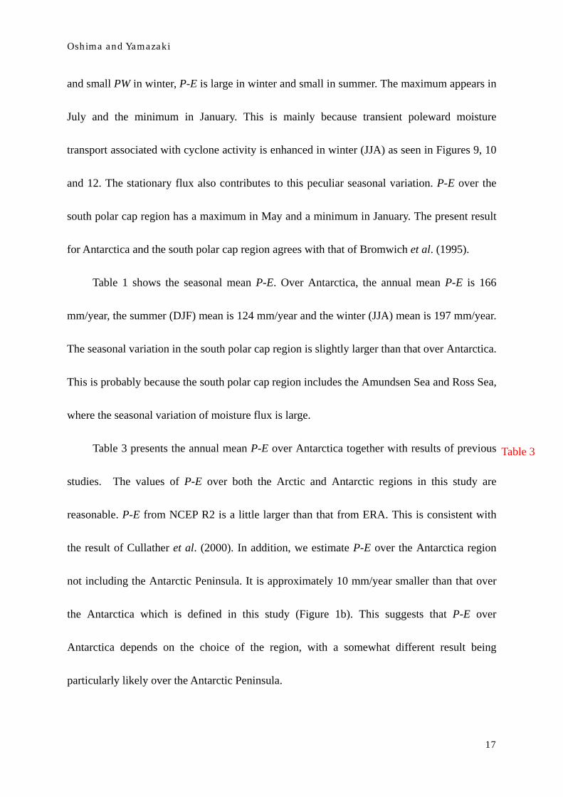
Table 1 shows the seasonal mean P-E. Over Antarctica, the annual mean P-E is 166

mm/year, the summer (DJF) mean is 124 mm/year and the winter (JJA) mean is 197 mm/year.

The seasonal variation in the south polar cap region is slightly larger than that over Antarctica.

This is probably because the south polar cap region includes the Amundsen Sea and Ross Sea,

where the seasonal variation of moisture flux is large.

Table 3 presents the annual mean P-E over Antarctica together with results of previous

studies. The values of P-E over both the Arctic and Antarctic regions in this study are

reasonable. P-E from NCEP R2 is a little larger than that from ERA. This is consistent with

the result of Cullather et al. (2000). In addition, we estimate P-E over the Antarctica region

not including the Antarctic Peninsula. It is approximately 10 mm/year smaller than that over

the Antarctica which is defined in this study (Figure 1b). This suggests that P-E over

Antarctica depends on the choice of the region, with a somewhat different result being

particularly likely over the Antarctic Peninsula.

Table 3

Oshima and Yamazaki

18

4. Interannual variation of moisture flux associated with annular modes

4.1. Arctic Oscillation

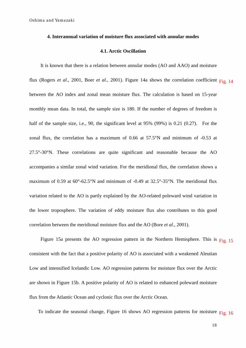
It is known that there is a relation between annular modes (AO and AAO) and moisture

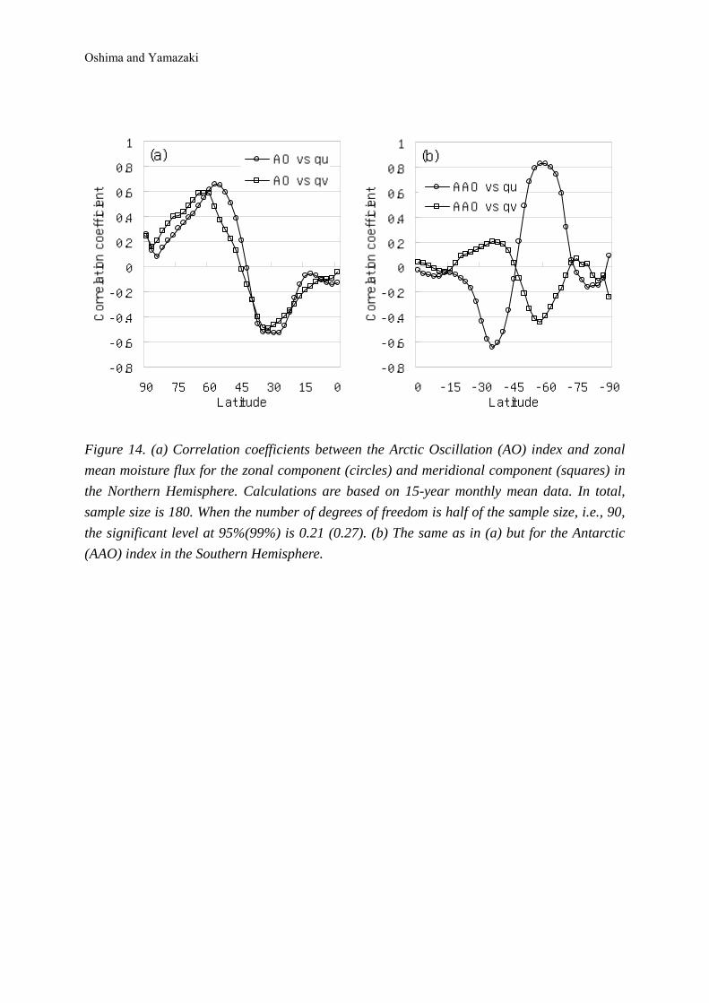
flux (Rogers et al., 2001, Boer et al., 2001). Figure 14a shows the correlation coefficient

between the AO index and zonal mean moisture flux. The calculation is based on 15-year

monthly mean data. In total, the sample size is 180. If the number of degrees of freedom is

half of the sample size, i.e., 90, the significant level at 95% (99%) is 0.21 (0.27). For the

zonal flux, the correlation has a maximum of 0.66 at 57.5°N and minimum of -0.53 at

27.5°-30°N. These correlations are quite significant and reasonable because the AO

accompanies a similar zonal wind variation. For the meridional flux, the correlation shows a

maximum of 0.59 at 60°-62.5°N and minimum of -0.49 at 32.5°-35°N. The meridional flux

variation related to the AO is partly explained by the AO-related poleward wind variation in

the lower troposphere. The variation of eddy moisture flux also contributes to this good

correlation between the meridional moisture flux and the AO (Bore et al., 2001).

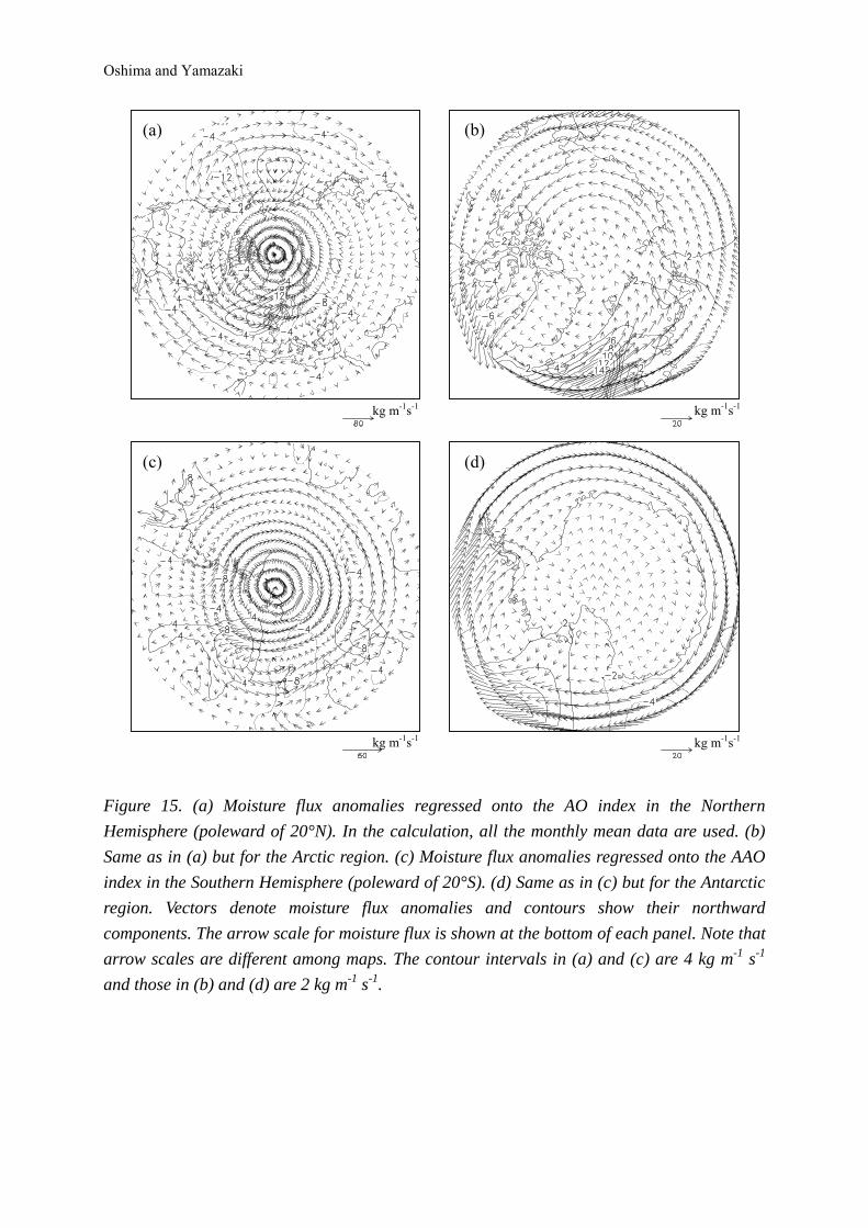
Figure 15a presents the AO regression pattern in the Northern Hemisphere. This is

consistent with the fact that a positive polarity of AO is associated with a weakened Aleutian

Low and intensified Icelandic Low. AO regression patterns for moisture flux over the Arctic

are shown in Figure 15b. A positive polarity of AO is related to enhanced poleward moisture

flux from the Atlantic Ocean and cyclonic flux over the Arctic Ocean.

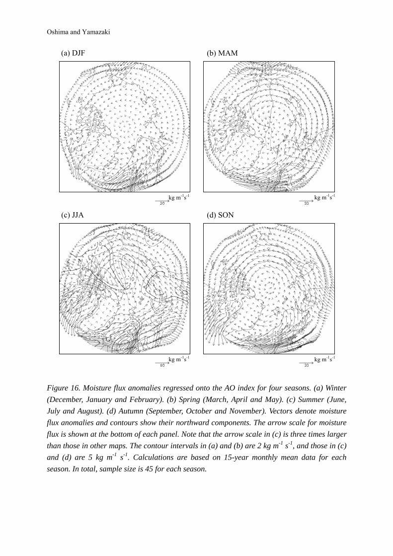
To indicate the seasonal change, Figure 16 shows AO regression patterns for moisture

Fig. 14

Fig. 15

Fig. 16

Oshima and Yamazaki

19

flux for four seasons. Positive polarity of the AO is associated with an enhanced poleward

moisture flux from the Atlantic Ocean in all seasons. It is also associated with an enhanced

poleward flux in central Eurasia and an enhanced equator-ward flux though the Canadian

Arctic Archipelago in boreal summer (JJA) and autumn (SON). The cyclonic flux over the

Arctic Ocean is enhanced in boreal spring (MAM), summer and autumn. Especially in

summer, these fluxes are enhanced. Note that the arrow scale in summer is three times larger

than that in other maps in Figure 16.

4.2. Antarctic Oscillation

Figure 14b shows the correlation coefficient between the AAO index and zonal mean

moisture flux. They also have significant correlations. For the zonal flux, the correlation

shows a maximum of 0.83 at 57.5°-60°S and minimum of -0.64 at 35°S. For the meridional

flux, the correlation shows a maximum of 0.20 at 35°-37.5°S and minimum of -0.44 at 57.5°S.

A similar discussion to that given for the AO can be applied to the AAO for the meridional

flux. The correlation coefficient between meridional moisture flux and AAO becomes zero at

75°S and remains small poleward of 75°S. This indicates that the AAO is not associated with

meridional flux in the interior of Antarctica. In contrast, the correlation coefficient at 75°N for

the AO is 0.4 and the effect of the AO extends farther poleward compared with that of AAO.

The spatial pattern of moisture flux regressed on the AAO index is shown in Figures 15c

and 15d. Eastward transports are enhanced in high-latitudes (about 60°S) and reduced in

Oshima and Yamazaki

20

mid-latitudes (about 40°S). This is consistent with the lower-tropospheric wind anomalies

related to the AAO. Furthermore, positive polarity of the AAO is related to cyclonic flux over

the Bellingshausen Sea and the Amundsen Sea. The magnitude of moisture flux vector in the

interior of Antarctica is very small. This corresponds to the low correlation coefficient

poleward of 70°S (Fig. 14b).

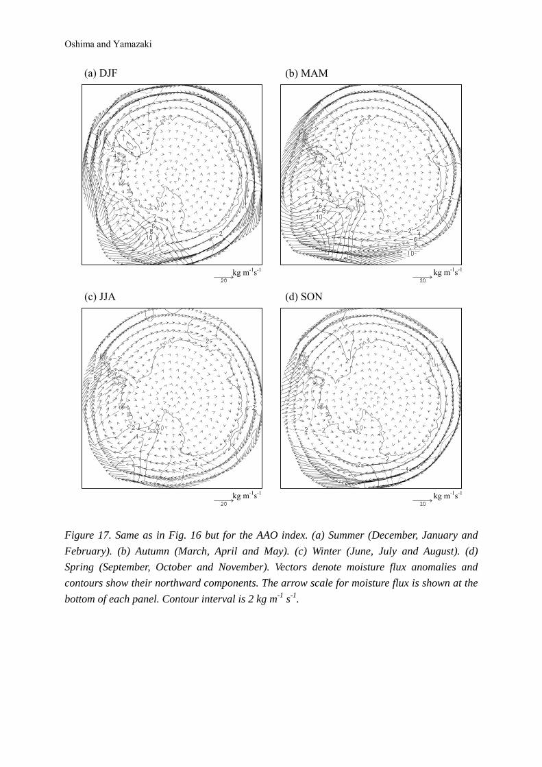
Figure 17 shows moisture flux anomalies regressed onto the AAO index for four seasons.

When the AAO is in a positive phase, eastward flux over the Antarctic Ocean surrounding

Antarctica, and cyclonic flux over the Bellingshausen Sea and the Amundsen Sea, are

enhanced. This cyclonic flux is enhanced especially in austral summer (DJF) and autumn

(MAM). This is also consistent with the lower-tropospheric wind anomalies related to the

AAO. Namely, a positive polarity of the AAO is related to deepened surface pressure over the

Amundsen Sea.

5. Discussion and Conclusions

We investigated the climatological seasonal variation of moisture transport over the

Arctic and Antarctic regions and the interannual variations of moisture flux associated with

annular modes, primarily using the 15-year ERA data set, and the NCEP R2 data set as a

supplement.

Over the Arctic, there are strong moisture inflows from the Atlantic Ocean and Pacific

Ocean in all seasons and strong outflow through the Canadian Arctic Archipelago in boreal

Fig. 17

Oshima and Yamazaki

21

summer. This inflow and outflow are especially enhanced in boreal summer due to the

summer moisture increase. We divided the total moisture flux into stationary and transient

components. The transient moisture flux is poleward at all longitudes and enhanced in boreal

summer. In particular, summer poleward flow from central Eurasia is caused by transient

moisture transport. The seasonal variation of moisture inflow into the Arctic is controlled

mainly by transient flux, which shows a boreal summer maximum due to large precipitable

water in boreal summer. Therefore, P-E over the Arctic exhibits a summer maximum.

Over the Antarctic, a strong moisture inflow exists west of the Antarctic Peninsula in all

seasons and over the Bellingshausen Sea and the Amundsen Sea in austral autumn and winter.

Most moisture inflows to Antarctica have maxima in austral summer and minima in winter,

but the inflows over the Bellingshausen Sea and the Amundsen Sea have maxima in winter

and minima in austral summer. As a result, the seasonal variation of P-E over the Antarctic

shows an austral winter maximum, which is opposite to that over the Arctic. Geographically,

the moisture inflow over the Bellingshausen Sea and the Amundsen Sea contributes to this

peculiar seasonal variation. When moisture flux is divided into stationary and transient

components, both components show a winter maximum, even though PW shows a summer

maximum.

Transient flux greatly contributes to P-E in both the Arctic and Antarctic regions.

Therefore, the seasonal variations of P-E over these regions are mainly explained by the effect

of poleward transient moisture flux, although stationary flux is comparable in the Antarctic

Oshima and Yamazaki

22

region. Over the Arctic, the seasonal variation of poleward transient moisture flux primarily

depends on the seasonal variation of PW and that over the Antarctic primarily depends on

cyclone activity.

The annual mean (P-E)s over the Arctic Ocean and Antarctica are 186 mm/year and 166

mm/year, respectively. This annual mean P-E over the Arctic Ocean is equivalent to 55×10-3

Sv (1 Sv = 106 m3 s-1, this unit is commonly used in oceanography). The river runoff into the

Arctic Ocean is 112-136×10-3 Sv. The sum of river runoff and P-E, 0.167-0.191 Sv, is the total

input of fresh water into the Arctic Ocean. Thus two thirds of fresh water input to the Arctic

Ocean comes from river runoff and one third from the atmosphere.

The Arctic Oscillation (AO) and zonal mean meridional moisture flux have a significant

positive correlation. The maximum correlation of 0.59 is found at 60°-62.5°N. The Antarctic

Oscillation (AAO) has the same relation to the poleward moisture flux. The maximum

correlation of -0.44 is found at 57.5°S. These results agree with previous studies (Boer et al.,

2001; Roger et al., 2001). It is also found that the AAO is not associated with meridional flux

in the interior of Antarctica.

Positive polarity of the AO is associated with a poleward moisture flux anomaly from

the Atlantic Ocean throughout the year, cyclonic flux in boreal spring, summer and autumn,

and equator-ward flux through the Canadian Arctic Archipelago in boreal summer and autumn.

Positive polarity of the AAO is associated with eastward moisture flux over the Antarctic

Ocean surrounding Antarctica and cyclonic flux over the Bellingshausen Sea and the

Oshima and Yamazaki

23

Amundsen Sea, especially in austral summer and autumn. Although, in austral summer,

westward moisture flux along the coastline of East Antarctica exists in the annual mean flux

field, positive polarity of the AAO is associated with eastward flux anomalies along the

coastline. Therefore, moisture flux anomalies over both the Arctic and the Antarctic related to

the annular modes correspond to lower-tropospheric wind anomalies. This is because moisture

is abundant in the lower troposphere.

The results from NCEP R2 are almost the same as those from ERA. Our results are

consistent with those of Bromwich et al. (2000) and Bromwich et al. (1995), who used ERA,

ECMWF, NCEP-NCAR or NMC, though the version is different. It is considered that these

differences are caused by differences in performance and horizontal resolutions of the models.

These estimations of the atmospheric moisture budget and clarification of the relations

between annular modes and moisture transports are helpful to assess the water cycle over the

entire polar regions and its interannual variations.

Acknowledgments

The authors benefited from useful comments given at The 26th NIPR Symposium on

Polar Meteorology and Glaciology at NIPR, Tokyo in 2003. We also thank two anonymous

reviewers for comments on the original manuscript. NCEP-DOE Reanalysis-2 data were

provided by the NOAA-CIRES Climate Diagnostics Center, Boulder, Colorado, USA, via

Oshima and Yamazaki

24

their Web site at http://www.cdc.noaa.gov/. The GFD DENNOU Library and GrADS were

used for analysis and drawing figures.

Oshima and Yamazaki

25

References

Baumgarner, A. and Reichel, E. (1975): The World Water Balance. Elsevier, 179p.

Boer, G. J., Fourest, S. and Yu, B. (2001): The Signature of the Annular Modes in the

Moisture Budget. J. Climate, 14, 3655-3665.

Bromwich, D. H., Cullather, R. I. and Serreze, M. C. (2000): Reanalyses Depictions of the

Arctic Atmospheric Moisture Budget. The Fresh Water Budget of the Arctic Ocean, ed.

By E.L. Lewis, Kluwer Academic Publishers, 163-196.

Bromwich, D. H., Robasky, F. M., Cullather, R. I. and Van Woert, M. L. (1995): The

Atmospheric Hydrologic Cycle over the Southern Ocean and Antarctica from Operational

Numerical Analyses. Mon. Wea. Rev., 123, 3518–3538.

Cullather, R. I., Bromwich, D. H. and Serreze, M. C. (2000): The Atmospheric Hydrologic

Cycle over the Arctic Basin from Reanalyses. Part I: Comparison with Observations and

Previous Studies. J. Climate, 13, 923-937.

Cullather, R. I., Bromwich, D. H. and Van Woert, M. L. (1998): Spatial and Temporal

Variability of Antarctic Precipitation from Atmospheric Methods. J. Climate, 11,

334-367.

Giovinetto, M. B. and Bull, C. (1987): Summary and analyses of surface mass balance

compilations for Antarctica, 1960-1985. Byrd Polar Res. Center Rep., 1, 90p.

Gong, D. and Wang, S. (1999): Definition of Antarctic Oscillation Index. Geophys. Res.

Lett., 26, 459-462.

Oshima and Yamazaki

26

Groves, D. G., and Francis, J. A. (2002a): Moisture budget of the Arctic atmosphere from

TOVS satellite data. J. Geophys. Res., 107(D19), 4391, doi: 10.1029/2001JD001191.

Groves, D. G., and Francis, J. A. (2002b): Variability of the Arctic atmospheric moisture

budget from TOVS satellite data. J. Geophys. Res., 107(D24), 4785, doi:

10.1029/2002JD002285.

Peixoto, J. P. and Oort, A. H. (1983): The atmospheric branch of the hydrological cycle and

climate. Variations in the Global Water Budget, ed. By A. Street-Perrott, M. Beran and R.

Ratcliffe, D. Reidel, 5-65.

Peixoto, J. P. and Oort, A. H. (1992): Physics of Climate. American Institute of Physics, 520

p.

Rogers, A. N., Bromwich, D. H., Sinclair, E. N. and Cullather, R. I. (2001): The Atmospheric

Hydrologic Cycle over the Arctic Basin from Reanalyses. Part II: Interannual Variability.

J. Climate, 14, 2414-2429.

Sellers, W. D. (1965): Physical Climatology. University of Chicago Press, 272 p.

Serreze, M. C. and Barry, R. G. (2000): Atmospheric components of the Arctic Ocean

hydrologic budget assessed from rawinsonde data. The Fresh Water Budget of the Arctic

Ocean, ed. By E. L. Lewis, Kluwer Academic Publishers, 141-161.

Serreze, M C., Barry, R. G. and Walsh, J. E. (1995): Atmospheric Water Vapor Characteristics

at 70°N. J. Climate, 8, 719-731.

Thompson, D. W. J., and Wallace, J. M. (1998): The Arctic Oscillation signature in the

Oshima and Yamazaki

27

wintertime geopotential height and temperature fields. Geophys. Res. Lett., 25,

1297-1300.

Thompson, D. W. J., and Wallace, J. M. (2000): Annular Modes in the Extratropical

Circulation. Part I: Month-to-Month Variability. J. Climate, 13, 1000-1016.

Yamazaki, K. (1992): Moisture Budget in the Antarctic Atmosphere. Proc. NIPR Symp.

Polar Meteorol. Glaciol., 6, 36-45.

Yamazaki, K. (1994): Moisture budget in the Antarctic atmosphere. Snow and Ice Covers:

Interactions with the Atmosphere and Ecosystems, ed. By H. G. Jones, T. D. Davies, A.

Ohmura and E. M. Morris, IAHS Publ., 223, 61-67.

Yamazaki, K. (1997): Seasonal Variation of Atmospheric Water Circulation in the Antarctic

Region Derived from Objective Analysis Data. Nankyoku Shiryo (Antarctic Rec.), 41,

149-160.

Oshima and Yamazaki

Table1. Seasonal mean and annual mean Precipitation minus Evaporation (P-E) over the Arctic Ocean and Antarctica based on 15-year (1979-1993) ECMWF reanalysis data. Unit is mm yr-1. DJF MAM JJA SON Annual

Arctic Ocean(ERA) 136 123 294 190 186 70°-90°N(ERA) 127 130 267 186 178 Antarctica(ERA) 124 184 197 157 166 70°-90°S(ERA) 99 175 177 149 150

Oshima and Yamazaki

Table 2. Annual mean Precipitation minus Evaporation (P-E) over the Arctic Ocean, comparison with previous studies. Unit is mm yr-1.

Arctic Ocean 70-90°N

Based on atmospheric data Peixoto and Oort, 1983 (rawinsonde): 1963-1973 --- 116 Serreze and Barry, 2000 (HARA, rawinsonde): 1974-1991 153 161 Groves and Francis, 2002 (TOVS satellite): 1979-1998 145 151 Bromwich et al., 2000 (ERA): 1979-1993 179 182 Bromwich et al., 2000 (NCEP-NCAR): 1979-1993 194 195 This study (ERA): 1979-1993 186 178 This study (NCEP R2): 1979-2002 198 198 Based on surface data Sellers (1965) multiyear 120 50 Baumgartner and Reichel (1975) 44 58

Oshima and Yamazaki

Table 3. Same and in Table 2. but for Antarctica.

Antarctica 70-90°S Based on atmospheric data

Peixoto and Oort, 1983 (rawinsonde): 1963-1973 --- 81 Yamazaki, 1992 (NMC):1986-1990 135 162 Bromwich et al., 1995 (ECMWF):1985-1992 157 140 Bromwich et al., 1995 (NMC):1985-1992 108 134 Cullather et al., 1998 (ECMWF): 1985-1995 151 --- This study (ERA): 1979-1993 166 150 This study (NCEP R2): 1979-2002 112 160 Based on surface data Sellers (1965) multiyear 30 35 Baumgartner and Reichel (1975) 141 147 Giovinetto and Bull (1987) 143 ---

Oshima and Yamazaki

Figure 1. Maps of (a) the Arctic region and (b) the Antarctic region. Bold solid lines indicate the boundaries of the Arctic Ocean and Antarctic regions used to estimate "Precipitation minus Evaporation" (P-E) in this study.

Arctic Ocean

Eurasia North America

Atlantic Ocean

Canadian Archipelago

Greenland

70°N

60°N

0°

180°

90°E 90°W

Pacific Ocean

Alaska

(a) (b)

Antarctica

70°S

60°S

180°

0°

90°E 90°W

Ross Sea

Amundsen Sea

Weddell Sea

BellingshausenSea

Wilkes Land

Atlantic Ocean

Pacific Ocean

● Syowa Station

Oshima and Yamazaki

Figure 2. Climatological fields of annual mean moisture flux and precipitable water (PW).The 15-year (1979-1993) ECMWF reanalysis data are used. (a) The Northern Hemisphere (north of 20°N), (b) the Arctic (north of 60°N), (c) the Southern Hemisphere (south of 20°S), and (d) the Antarctic (south of 60°S). Vectors denote moisture flux and contours denote PW. The arrow scale for moisture flux is shown at the bottom of each panel. Note that the arrow scales are different among maps. The contour intervals in (a) and (c) are 5 mm, and those in (b) and (d) are 1 mm.

(a) (b)

kg m-1s-1

(c) (d)

kg m-1s-1 kg m-1s-1

kg m-1s-1

mm

mm mm

mm

Oshima and Yamazaki

Figure 3. Climatological fields of the annual mean stationary and transient components of moisture flux. The 15-year (1979-1993) ECMWF reanalysis data are used. The stationary flux is calculated from the monthly mean fields of wind, moisture and surface pressure. The total flux is obtained from the monthly mean of twice-daily flux, which is shown in Fig. 2. The transient flux is calculated by subtracting the stationary flux from the total flux. (a) Stationary moisture flux in the Arctic, (b) transient moisture flux in the Arctic, (c) stationary moisture flux in the Antarctic, and (d) transient moisture flux in the Antarctic. Vectors denote moisture flux and contours show their northward components. The arrow scale for moisture flux is shown at the bottom of each panel. Note that arrow scales are different among maps. The contour intervals in (a) and (c) are 5 kg m-1 s-1, and those in (b) and (d) are 2 kg m-1 s-1.

(a) Arctic, Stationary (b) Arctic, Transient

kg m-1s-1

(c) Antarctic, Stationary (d) Antarctic, Transient

kg m-1s-1 kg m-1s-1

kg m-1s-1

Oshima and Yamazaki

Figure 4. Seasonal mean climatological fields of moisture flux and precipitable water (PW) for the Arctic. The 15-year (1979-1993) ECMWF reanalysis data are used. (a) Winter (December, January and February), (b) spring (March, April and May), (c) summer (June, July and August), and (d) autumn (September, October and November). Vectors denote moisture flux and contours PW. The arrow scale for moisture flux is shown at the bottom of each panel. Contour interval is 2 mm in all maps.

(a) DJF (b) MAM

(c) JJA (d) SON

kg m-1s-1

kg m-1s-1 kg m-1s-1

kg m-1s-1

mm mm

mm mm

Oshima and Yamazaki

Figure 5. Climatological fields of stationary and transient components of moisture flux over the Arctic for winter (December, January and February) and summer (June, July and August) seasons. The 15-year (1979-1993) ECMWF reanalysis data are used. The calculation method of stationary and transient components is the same as that in Fig. 3. (a) Stationary moisture flux in winter, (b) transient moisture flux in winter, (c) stationary moisture flux in summer, and (d) transient moisture flux in summer. Vectors denote moisture flux and contours show their northward components. The arrow scale for moisture flux is shown at the bottom of each panel. Note that arrow scales are different among maps. The contour interval in (a) is 5 kg m-1 s-1, those in (b) and (d) are 2 kg m-1 s-1, and that in (c) is 10 kg m-1 s-1.

(a) DJF, Stationary (b) DJF, Transient

(c) JJA, Stationary (d) JJA, Transient

kg m-1s-1

kg m-1s-1 kg m-1s-1

kg m-1s-1

Oshima and Yamazaki

Figure 6. Seasonal variation of northward moisture flux at 70°N. The 15-year (1979-1993) ECMWF reanalysis data are used. Contour interval is 10 kg m-1 s-1.

Oshima and Yamazaki

-50

0

50

100

150

200

250

300

Jan Feb Mar Apr May Jun Jul Aug Sep Oct Nov DecMonth

P m

inus

E m

m y

r-1

0

5

10

15

20

Prec

ipita

ble

Wat

er m

m

stationary Arctic Oceantransient Arctic Oceanstationary 70-90Ntransient 70-90NPW 70N

Figure 7. Seasonal variations of "Precipitation minus Evaporation" (P-E) estimated from stationary and transient components of moisture flux. Bold solid lines indicate the P-E estimate from the stationary component of moisture flux and dashed lines are the estimate from the transient component. “Circles” (○) and “Squares” (□) denote the region of the Arctic Ocean (the region shown in Fig. 1) and the region north of 70°N, respectively. “Crosses” (×) denote zonal mean precipitable water (PW) at 70°N. The scale of PW is shown at the right side of the figure.

Oshima and Yamazaki

0

50

100

150

200

250

300

350

Jan Feb Mar Apr May Jun Jul Aug Sep Oct Nov DecMonth

P m

inus

E m

m y

r-1

Arctic Ocean(ERA)

70-90N(ERA)

Figure 8. Seasonal variation of "Precipitation minus Evaporation" (P-E) over the Arctic Ocean (the region shown in Fig. 1, black bar in Fig. 8) and the region poleward of 70°N (gray). The 15-year (1979-1993) ECMWF reanalysis data are used.

Oshima and Yamazaki

Figure 9. Same as in Fig. 4 but for the Antarctic. The contour interval is 1 mm in all maps.

(a) DJF (b) MAM

(c) JJA (d) SON

kg m-1s-1

kg m-1s-1 kg m-1s-1

kg m-1s-1

mm mm

mm mm

Oshima and Yamazaki

Figure 10. Same as in Fig. 5 but for the Antarctic. The contour intervals in (a) and (c) are 5 kg m-1 s-1, and those in (b) and (d) are 2 kg m-1 s-1.

(a) DJF, Stationary (b) DJF, Transient

(c) JJA, Stationary (d) JJA, Transient

kg m-1s-1

kg m-1s-1 kg m-1s-1

kg m-1s-1

Oshima and Yamazaki

Figure 11. Same as in Figure 6 but for 67.5°S. The contour interval is 5 kg m-1 s-1. Note that negative values indicate poleward flux.

Oshima and Yamazaki

-50

0

50

100

150

200

250

300

Jan Feb Mar Apr May Jun Jul Aug Sep Oct Nov DecMonth

P m

inus

E m

m y

r-1

0

2

4

6

8

Prec

ipita

ble

Wat

er m

m

stationary Antarcticatransient Antarcticastationary 70-90Stransient 70-90SPW 70S

Figure 12. Same as in Fig. 7 but for Antarctica.

Oshima and Yamazaki

0

50

100

150

200

250

300

350

Jan Feb Mar Apr May Jun Jul Aug Sep Oct Nov DecMonth

P m

inus

E m

m y

r-1

Antarctica(ERA)

70-90S(ERA)

Figure 13. Same as in Fig. 8 but for Antarctica.

Oshima and Yamazaki

-0.8

-0.6

-0.4

-0.2

0

0.2

0.4

0.6

0.8

1

90 75 60 45 30 15 0Latitude

Correlation coefficient

AO vs qu

AO vs qv

(a)

-0.8

-0.6

-0.4

-0.2

0

0.2

0.4

0.6

0.8

1

0 -15 -30 -45 -60 -75 -90Latitude

Correlation coefficient AAO vs qu

AAO vs qv

(b)

Figure 14. (a) Correlation coefficients between the Arctic Oscillation (AO) index and zonal mean moisture flux for the zonal component (circles) and meridional component (squares) in the Northern Hemisphere. Calculations are based on 15-year monthly mean data. In total, sample size is 180. When the number of degrees of freedom is half of the sample size, i.e., 90, the significant level at 95%(99%) is 0.21 (0.27). (b) The same as in (a) but for the Antarctic (AAO) index in the Southern Hemisphere.

Oshima and Yamazaki

Figure 15. (a) Moisture flux anomalies regressed onto the AO index in the Northern Hemisphere (poleward of 20°N). In the calculation, all the monthly mean data are used. (b) Same as in (a) but for the Arctic region. (c) Moisture flux anomalies regressed onto the AAO index in the Southern Hemisphere (poleward of 20°S). (d) Same as in (c) but for the Antarctic region. Vectors denote moisture flux anomalies and contours show their northward components. The arrow scale for moisture flux is shown at the bottom of each panel. Note that arrow scales are different among maps. The contour intervals in (a) and (c) are 4 kg m-1 s-1 and those in (b) and (d) are 2 kg m-1 s-1.

(a) (b)

kg m-1s-1

(c) (d)

kg m-1s-1 kg m-1s-1

kg m-1s-1

Oshima and Yamazaki

Figure 16. Moisture flux anomalies regressed onto the AO index for four seasons. (a) Winter (December, January and February). (b) Spring (March, April and May). (c) Summer (June, July and August). (d) Autumn (September, October and November). Vectors denote moisture flux anomalies and contours show their northward components. The arrow scale for moisture flux is shown at the bottom of each panel. Note that the arrow scale in (c) is three times larger than those in other maps. The contour intervals in (a) and (b) are 2 kg m-1 s-1, and those in (c) and (d) are 5 kg m-1 s-1. Calculations are based on 15-year monthly mean data for each season. In total, sample size is 45 for each season.

(a) DJF (b) MAM

(c) JJA (d) SON

kg m-1s-1

kg m-1s-1 kg m-1s-1

kg m-1s-1

Oshima and Yamazaki

Figure 17. Same as in Fig. 16 but for the AAO index. (a) Summer (December, January and February). (b) Autumn (March, April and May). (c) Winter (June, July and August). (d) Spring (September, October and November). Vectors denote moisture flux anomalies and contours show their northward components. The arrow scale for moisture flux is shown at the bottom of each panel. Contour interval is 2 kg m-1 s-1.

(a) DJF (b) MAM

(c) JJA (d) SON

kg m-1s-1

kg m-1s-1 kg m-1s-1

kg m-1s-1