Scoring Model Predictions using Cross-Validation

Scoring Model Predictions using1

Cross-Validation∗2

Anna L. Smith Tian Zheng Andrew Gelman3

Department of Statistics4

Columbia University5

Draft of October 26, 20186

Abstract7

We formalize a framework for quantitatively assessing agreement between two8

datasets that are assumed to come from two distinct data generating mechanisms.9

We propose a methodology for prediction scoring which provides a measure of the10

distance between two unobserved data generating mechanisms (DGMs), along the11

dimension of a particular model. The cross-validated scores can be used to evalu-12

ate preregistered hypotheses and to perform model validation in the face of complex13

statistical models. Using human behavior data from the Next Generation Social Sci-14

ence (NGS2) program, we demonstrate that prediction scores can be used as model15

assessment tools and that they can reveal insights based on data collected from dif-16

ferent populations and across different settings. Our proposed cross-validated pre-17

diction scores are capable of quantifying true differences between data generating18

mechanisms, allow for the validation and assessment of complex models, and serve as19

valuable tools for reproducible research.20

Keywords: complex models; cross-validation; model assessment ; preregistration;21

reproducibility.22

1 Introduction23

To begin, we provide a description of the motivation for our proposed methodology, stem-24

ming first from recent recommendations for more reproducible research and second from25

the question of how to appropriately validate complex models. We provide a working26

definition for data generating mechanisms, which we rely on throughout the paper, and27

∗This material is based on research sponsored by the Defense Advanced Research Projects Agency(DARPA) agreement number D17AC00001. The content of the information does not necessarily reflect theposition or the policy of the Government, and no official endorsement should be inferred.

1

differentiate between predictive and inferential DGMs. Finally, we provide a summary of28

existing methods for tackling these two issues.29

1.1 Reproducible research30

Open Science Collaboration (2015)’s attempt to replicate one hundred high-impact psy-31

chological studies marked the real beginning of the scientific community’s latest struggle,32

the “replication crisis”, although many had commented on similar phenomena previously.33

In essence, this article highlighted the unfortunate fact that many scientific studies fail to34

replicate in practice.35

As a very simple example, suppose researchers at University A identify a positive effect36

for some new drug or treatment (e.g., they find evidence to reject a null hypothesis of no37

effect). Later, researchers at University B replicate University A’s study – closely following38

University A’s descriptions of subject recruitment (perhaps even increasing the sample39

size), experimental procedure, and analysis – but fail to identify a positive effect or even40

find the opposite, a negative effect. In cases like this one, we are faced with two separate41

studies that are concerned with the same scientific hypothesis, using the same experiments,42

but somehow reach different conclusions. This phenomenon has serious implications for the43

scientific community at large and for the general public; it impacts our ability to trust any44

single particular finding and results in the watering down of the credibility of science at45

large. Not surprisingly, this problem is not confined to one particular research domain46

(although much initial discussion focused on studies in psychology), but is a concern to47

scientific researchers in all fields.48

Closely related to replicability is the issue of reproducibility. A study or experiment49

(including its specific analytic procedure) is said to be replicable if when the study is50

repeated, with fresh data or subjects, similar results are achieved. An analysis is said to51

be reproducible if when the same data is analyzed again, identical results are achieved.52

Ideally, published scientific results should be the product of studies or experiments53

whose results can be independently replicated. This typically requires that the identified54

effect sizes are relatively large and can be accurately measured, samples sizes are relatively55

large, and the entire data collection and experimental procedures are well documented, as56

well as the results of the reproducible analyses (e.g., analytic procedures are well docu-57

mented and explained and all code and data are made publicly available, if possible). In58

practice, ensuring replicability and reproducibility is often not straightforward. In fact,59

since the identification of this replication crisis, it has become clear that no simple solution60

exists. Instead, advances in this area will necessitate concerted efforts for methodological61

improvement and more research on reproducibility across many fields. Recently, a variety62

of new initiatives in this vein have been proposed. For example, some qualitative recom-63

mendations can be found in Spies (2018) and Stodden et al. (2016) provide suggestions for64

computational methods.65

One recent recommendation involves the registration of hypothesis tests and scientific66

analyses prior to data collection (Humphreys et al., 2013; Gelman, 2013), so that one can67

2

avoid the “garden of forking paths,” a description offered by Gelman and Loken (2014)68

for the analytic pipeline in which decisions on data coding, exclusion, and analysis are69

made contingent on the data, thus inducing problems of multiple comparisons even if only70

one analysis is done on the particular data at hand. Ideally, prior to collecting any data71

whatsoever, researchers first prepare a preregistered plan of all data collection methods,72

modeling and analytic procedures, hypotheses, as well as plans for handling any unexpected73

deviations from this regime. This preregistration is made publicly available in some way,74

so that the researchers are held accountable to their preregistered plan. Just as simple75

random sampling is a prerequisite for classical interpretations of sampling probabilities,76

standard errors and point estimates, preregistration ensures that the classical interpretation77

of hypothesis tests and the resulting p-values is appropriate. It is worth pointing out that78

this sort of preregistration does not preclude further exploratory analyses; The point of79

preregistration is not to restrict analyses but rather to provide more structure to analyses80

that are already planned. For example, after data collection, a researcher may notice a81

pattern or posit a new explanation that motivates additional analyses. Such additional82

exploratory data analysis (beyond preregistered plans) are generally desirable as they can83

lead to new discoveries or hypotheses and even inspire additional confirmatory research. In84

some fields, researchers have the option of submitting such a preregistration to a scientific85

journal whom, if the submission is accepted, will agree to publish the research prior to86

any data collection or results. Such a manuscript is called a registered report and usually87

undergoes a round of peer review prior to the journal’s agreement to publish. Not only do88

registered reports encourage reproducible research, but they also help journals avoid the89

negative impacts of publication bias.90

1.2 Assessing preregistered hypotheses91

One requirement of these reports (both in the case of registered reports or preregistrations)92

is that the researchers make predictions about the scientific hypotheses to be assessed93

and models to be fit once data collection is complete. Once the analysis is complete, the94

researchers are faced with a natural question: how well do the preregistered predictions align95

with the observed data? This question requires a methodology to score the predictions, in96

the face of the materialized observations, usually through some form of “prediction scoring.”97

Further, prediction scoring represents one of the few quantitative recommendations for98

improving the reproducibility of scientific research.99

The form of such predictions will largely impact the types of scientific insights one100

can gain, as well as impact the procedure for prediction scoring. We will discuss such101

impacts further in Section 3. For now, consider the case where the researcher is able to102

make predictions about the resulting data at the observation-level (i.e., rather than at103

some higher summary or model estimate level). In practice, such predictions could come in104

the form of data from a previously conducted closely related study, as pilot data, or from105

simulated data that represents a priori knowledge on the true data generating mechanism.106

We may then think of prediction scoring as a measure of the agreement or distance between107

the assumed data generating mechanism (DGM) behind the preregistered predictions and108

3

DGM

Study A1? Study A2

DGM

raw data

D1

raw data

D2

model fitting

software?

Θ1, . . .Θp

predictions

predictionscore

Figure 1: Prediction scores measure the agreement between predictions and realized data.In the case of preregistered predictions, Study A1 represents a set of pilot data, or datafrom an existing study, or simulated data.

the true data generating mechanism (DGM) behind the realized observations, as in Figure109

1.110

In this sense, the replication crisis and the related push for more reproducible research111

motivate methodologies that can appropriately analyze and interpret scientific hypotheses112

or models across different settings. When performing a preregistered study, how can we113

quantitatively evaluate differences between the preregistered hypotheses or predictions and114

the observed data? More generally, when we have access to data that comes from dif-115

ferent settings of the same experimental framework (i.e., can be viewed as replications of116

each other), can we quantify and evaluate differences across these settings? The first step117

we propose is to view each of these (the set of predictions and the observed data) as re-118

alizations from two distinct data generating mechanisms that describe the experimental119

framework—the preregistered hypotheses or predictions follow from a DGM based on our120

prior knowledge or pilot data and the observed experimental data follows from the true121

observed DGM. In this sense, the evaluation of the preregistered hypotheses comes down122

to identifying differences between the two DGMs.123

1.3 Complex data generating mechanisms124

In our approach, we will use the term “data generating mechanism” to refer to a particular125

member of a family of probability distributions or equations that represent a set of (model)126

assumptions. In this sense, we can use subsets of this family to represent beliefs about the127

data generating mechanism that gave rise to the observed data, e.g., null and alternative128

hypotheses. For example, suppose we believe two sets of experimental data are exponen-129

tially distributed and we want to test hypotheses about the expected value of these two130

4

distributions, represented by the parameter λ. The DGM family is a set of distributions for131

λ and, for example, two members of this family that we might be interested in evaluating132

are p1(λ ≤ 5), representing a null hypothesis, and p2(λ > 5), representing an alternative133

hypothesis. Alternatively, we can think of the DGM family as a unifying experimental134

framework, such that experiments within this framework can be viewed as replications of135

each other. Continuing our previous example, perhaps two groups of researchers each ran136

an experiment where they recorded the waiting time between participants’ incoming calls137

on their personal phones and we want to compare the average waiting time across these138

experiments.139

In practice, we can categorize data generating mechanisms as falling within one of140

two distinct forms:141

1. predictive, where the data generating mechanism can be represented by a conditional142

probability distribution, p(y|x), or143

2. inferential, where the data generating mechanism can be represented by a distribution144

for a parameter or set of parameters, p(θ).145

For example, in regression-style analyses, we are most interested in the conditional146

distribution of some response, given fixed covariate or predictor values. Both parametric147

and non-parametric regression-style models and other forms of predictive analysis which148

focus on sampling values (from a probability distribution) for a response or outcome vari-149

able, y, given fixed covariate or predictor values, x, fall in the first case. On the other hand,150

many analyses focus on a particular marginal distribution, p(θ). For example, we may use151

linear regression to model some phenomenon but are only interested in one particular slope152

parameter (i.e., the effect size of one particular predictor). In the example with phone call153

waiting times mentioned above, we have conceptualized the data generating mechanism as154

a set of distributions for a model parameter, λ. However, for many complex models or155

datasets with highly nuanced features, choosing a single parameter or summary statistic156

upon which to base evaluation of differences between DGMs is not straightforward. In157

these cases, relying on a single summary measure to capture all relevant (unknown) differ-158

ences between DGMs has the potential to oversimplify true differences or, in worst cases,159

fail to detect true differences altogether. For this reason, the prediction scoring methodol-160

ogy which we propose below is focused primarily on scoring differences between predictive161

DGMs.162

1.4 Problem formulation163

Under these settings, the natural prediction scoring question is translated to the following:164

are these experiments or realizations products of the same DGM or are they distinct in165

some way? While this is certainly a natural question, it is ill-posed for most experimental166

social science research settings. In almost all cases, the data generating mechanisms do167

in fact vary across experiments or settings, even if only slightly. Instead, we will focus168

on answering the following: How much do the data generating mechanisms differ across169

5

settings (e.g., from preregistration to observed data) in a quantifiable way? Ultimately, we’d170

also like to be able to compare different ways that these differences across experimental171

frameworks (i.e., across experimental operationalizations of related scientific theories, ideas,172

or hypotheses) can be quantified.173

In practice, just like any other statistical method based on sampled data, the observed174

differences between any two data generating mechanisms have two sources. The first is by175

chance, i.e., random variation in the data such as different samples of participants with176

different covariates and behaviors, or random variation in model estimates due to stochastic177

modeling algorithms. The second source is the true differences between the two DGMs.178

The latter is what we care to infer to derive scientific insight. Any methodology to compare179

these data generating mechanisms based on observed differences needs to be able to set180

apart differences due to these two sources. We will return to this point in Section 3.181

Our proposed approach is to treat prediction scores as an instrument for quantify-182

ing the difference between our beliefs about the scientific process under study and reality,183

along a clearly specified “dimension”. With this language, we hope to evoke the type of184

instruments used by social scientists, where a variable is constructed to measure something185

abstract or unobserved in some sense and carries the same meaning under a general set-186

ting. For example, to measure a subject’s level of extraversion (which cannot be measured187

directly), a social scientist might design a survey that includes items that capture behavior188

indicative of extraversion. In a similar sense, we treat the true scientific process or data189

generating mechanism (DGM) as unobservable. This is a natural assumption, which sug-190

gests the construction of a numerical measure for the distance we are interested in (between191

our beliefs about that DGM and the true DGM) is not trivial and requires clear definitions192

and rigorous evaluation.193

As shown in Figure 1, prediction scores shall directly measure the distance or dif-194

ference, via a predictive model, between preregistered predictions and observations from195

experimental data. The preregistered predictions are conditioned on our beliefs about the196

DGM through the identification of pilot or sample data, and, often less discussed, through197

the choice of a particular model. The model and the form of the prediction jointly define an198

aspect of the DGM for which the prior belief will be evaluated against the reality using our199

proposed prediction scores. In this sense, prediction scores can be thought of as capturing200

two levels of scientific insight: (1) how well the predictions match the materialized obser-201

vations and (2) how well our belief agrees with the reality in terms of the data generating202

mechanism.203

2 Background204

As best we can tell, current practice for prediction scoring in registered reports generally205

consists of making predictions in the form of directional hypotheses (in some cases, pre-206

dictions for the relative effect size are also included) for model parameters or summary207

statistics and assessing these predictions by performing a corresponding hypothesis test208

and checking for a significant effect (for some examples of published registered reports, see209

6

the Zotero library maintained by the Center for Open Science: Mellor, 2018). Our proposed210

methodology will advance these methods in two main directions. First, it is general enough211

to accommodate parameter-level hypotheses (or other, higher-level summary statistics) as212

well as predictions at the individual-level or lowest level of analysis. Individual-level pre-213

dictions will allow for a more fine-grained assessment of the agreement between our prior214

beliefs and the true underlying DGM. We will also strongly encourage that these predic-215

tions incorporate appropriate measures of uncertainty, such as in the form of probabilistic216

forecasts. Second, our methodology will provide prediction scores on a continuous scale,217

which can be viewed as estimates of the distance between our prior beliefs and reality.218

Thus, we provide a quantitative measure of prediction performance rather than the simple219

binary detection of a significant effect.220

In order to provide these advances, we pull ideas and insights from related research221

in the statistical literature; Below, we briefly describe statistical methodology for the eval-222

uation of probabilistic forecasts, Bayesian software-checking procedures, and approximate223

cross-validation (a more thorough discussion is available in the Supplementary Materials).224

2.1 Diagnostic plots for probabilistic forecasts and scoring rules225

In the statistical literature, perhaps the most applicable line of research to inform pre-226

diction scoring for preregistered hypotheses is the evaluation of probabilistic forecasts and227

the theoretical development of scoring rules. Gneiting and Katzfuss (2014) provide a nice228

summary of recent research in this area. First, let us point out that a scoring function229

measures the agreement between a point prediction and an observation while a scoring rule230

measures the agreement between a probabilistic forecast (a predictive probability distri-231

bution over future quantities or events of interest, such as a posterior predictive density232

from a Bayesian analysis) and an observation. Naturally, a probabilistic forecast contains233

much more information than a simple point prediction and, most importantly, provides234

a suitable measure of the uncertainty associated with the predictions. For this reason,235

we will focus on probabilistic forecasts (for a review of issues with point forecasts and236

scoring rules, see Gneiting, 2011). The importance of probabilistic forecasts as a tool for237

statistical inference is well-motivated by Dawid (1984)’s framework for prequential anal-238

ysis, which frames the creation of sequential probability forecasts (over time) as the true239

focus and underlying motivation for classical statistical concepts and theory. Of course,240

with the advent of rapidly increasing computational power, MCMC and other estimation241

techniques have greatly increased analysts’ ability to create probabilistic forecasts. In fact,242

in the past, much of the literature surrounding the evaluation of probabilistic forecasts243

came out of weather forecasting research. Currently, probabilistic forecasts have been used244

in applications ranging from climate models, flood risk, seismic hazards, renewable energy245

availability, economic and financial risk management, election outcomes, demographic and246

epidemiological projections, health care management, and preventive medicine.247

Gneiting et al. (2004) and Gneiting et al. (2007) define two important characteristics248

of probabilistic forecasts: sharpness and calibration. In this context, sharpness is (solely) a249

property of the predictive distribution and refers to the concentration of the distribution.250

7

For a real-valued variable, we could measure the sharpness of the probabilistic forecast by251

considering the average width of prediction intervals. On the other hand, calibration is a252

property of both the predictive distribution and the materialized observations or events.253

A probabilistic forecast is calibrated if the distributional forecast is statistically consistent254

with the observations; In other words, the observations should be indistinguishable from255

random draws from the predictive distribution. Gneiting et al. (2007) outline various lev-256

els of calibration—probabilistic, exceedance, and marginal (listed here from most to least257

strict)—as well as provide diagnostic tools for identifying these properties in practice. It258

should be noted that calibration is defined in terms of asymptotic consistency between259

random variable representations for the probabilistic forecast and the true underlying dis-260

tribution for the observations (i.e., F is a CDF-valued random variable representing the261

probabilistic forecast and G is a CDF-valued random variable representing the true data262

generating mechanism). Thus, in practice, these random variables are themselves unobserv-263

able and diagnostic approaches using sample versions (using empirical CDFs) are necessary264

to assess the calibration of a particular forecast.265

To check for probabilistic calibration, histograms (or empirical CDFs, if the sample266

size is small) of the PIT (probability integral transform) values can be verified for unifor-267

mity (this idea can be traced as far back as Rosenblatt, 1952; Pearson, 1933, and perhaps268

earlier). In meteorological research, Talagrand et al. (1997) proposed a verification rank269

histogram or Talagrand diagram (Anderson, 1996; Hamill and Colucci, 1997) to assess the270

calibration of ensemble forecasts and Shephard (1994, page 129) has used a similar dia-271

gram to sess samples from an MCMC algorithm. However, in the introduction of their272

paper, Gneiting et al. (2007) demonstrate that merely checking for the uniformity of PIT273

values is insufficient for distinguishing the ideal forecaster from three (poorer) competitor274

forecasts. Instead of relying solely on the PIT diagnostic, the authors highlight additional275

diagnostics (described below) and advocate maximizing the sharpness of the predictive dis-276

tribution, subject to calibration, as mentioned above. To check for marginal calibration,277

Gneiting et al. (2007) suggest plotting differences between the average predictive CDF and278

the empirical CDF for the observations versus x. If the probabilistic forecast is marginally279

calibrated, we would expect to see only minor fluctuations about zero. Exceedance cali-280

bration does not allow for an obvious sample analogue.281

Additionally, scoring rules allow us to assess calibration and sharpness simultaneously.282

Taking a decision theoretic perspective, we can think of a scoring rule as a loss function. In283

this sense, we can interpret the scores as penalties that the forecaster wishes to minimize.284

In terms of the choice of a particular form for a scoring rule, one natural restriction is285

that the truth or true forecast should receive an optimal score. This is precisely what is286

meant by proper scoring rules (some examples include the logarithmic score, the quadratic287

score, the spherical score, the continuous ranked probability score, and the Brier score).288

In fact, Gneiting and Raftery (2007) point out that the log Bayes factor is equivalent289

to a logarithmic scoring rule in the no-parameter case (i.e. forecasts do not depend on290

parameters to be estimated from the data). This implies that the log Bayes factor can be291

used to compare competing forecasting rules, and not only to compare models. When the292

forecasting rules are specified only up to unknown parameters which will be estimated from293

8

the data, the authors outline a variation of cross-validation that could be used to replace294

the logarithmic score with other proper scoring rules, to estimate a predictive Bayes factor295

of some kind. While there are some connections to Bayesian methods, the literature on296

scoring rules and the evaluation of probabilistic forecasts generally assumes a frequentist or297

classical perspective. While the discussion is typically focused on predictions for continuous298

variables, Czado et al. (2009) provide extensions of many of these ideas for count variables.299

This literature provides a sound framework for comparing probabilistic forecasts or300

predictions (such as from preregistration materials) to observed data, where each compet-301

ing forecast could correspond to different modelling choices or assumptions. The diagnostic302

tools and recommendations for scoring rules outlined above allow this comparison to be303

nonparametric and thus, enable the comparison of non-nested, highly diverse models. How-304

ever, each of these diagnostic measures is necessarily model-based in that any diagnostic305

plot or set of scoring rules depends on the model assumptions used to create the probabilis-306

tic forecast. This complicates the interpretation of the scores or diagnostics themselves,307

as they measure not only differences between our prior beliefs and the realized data (i.e.308

between the preregistered predictions and observations) but also any differences between309

the modelling choices and the true underlying data generating mechanisms. We will pro-310

pose a prediction scoring framework that uses cross-validation to remove the dependence311

on model-based differences which enables us to quantitatively measure true differences312

between our prior beliefs and the realized data.313

2.2 Bayesian software-checking314

Although perhaps not obvious at first glance, recent proposals for algorithm-checking of315

Bayesian model fitting software (Cook et al., 2006; Talts et al., 2018) can also provide316

interesting insights in the prediction scoring setting. These proposals recommend simulat-317

ing fake data conditional on random draws from the prior distribution, running the model318

fitting software to obtain draws from the posterior distribution, and using a summary319

measure to diagnose the alignment between the draws from the posterior distribution and320

the random draws from the prior distribution. Based on the self-consistency property of321

the marginal posterior and the prior distribution, these draws should be indistinguishable322

from one another. To diagnose this alignment, Cook et al. (2006) suggest computing em-323

pirical quantiles, comparing the random draw form the prior distribution to the posterior324

distribution based on that particular draw. The authors suggest looking at histograms325

of these quantiles, demonstrating that if the software is working correctly, the quantiles326

should be approximately uniformly distributed. Talts et al. (2018) point out that the em-327

pirical quantiles are necessarily discrete and that artifacts of this discretization can lead to328

misleading diagnostic quantile histograms. Instead, the authors suggest computing rank329

statistics which will follow a discrete uniform distribution, if the software is correct. Ad-330

ditionally, Talts et al. (2018) provide a nice summary of the types of expected deviations331

from uniformity that one might observe in the diagnostic histograms with corresponding332

explanations of modelling choices or software errors that could lead to such deviations.333

In terms of the prediction scoring setting, we can think of this software-checking334

9

methodology as a special case where the chosen modelling strategy matches the underlying335

DGM exactly. We will borrow ideas from this methodology, such as the use of empirical336

quantiles and rank statistics and the self-consistency properties, to motivate our proposed337

prediction scoring framework.338

2.3 Bayesian model selection and approximate cross-validation339

As briefly mentioned previously, our proposed prediction scoring framework will utilize340

cross-validation to separate true DGM differences from purely model-based differences.341

Cross-validation, particularly for Bayesian analyses, has been a very active research area342

in recent years. First, we should point that many Bayesian model comparison summary343

statistics (such as AIC, DIC, WAIC) can be motivated by the estimation of out-of-sample344

predictive accuracy (see Vehtari et al., 2012, for a thorough review, from a formal deci-345

sion theoretic perspective), which of course is one of the goals of cross-validation as well.346

Gelman et al. (2014) provide a nice review of these model comparison summary mea-347

sures. As opposed to exact leave-one-out cross-validation (LOOCV), each of the Bayesian348

model summary statistics utilize the full predictive density and perform an adjustment349

(e.g., importance sampling, or division by an appropriate variance) to remove the effect350

of over-fitting, since no data was actually held out. The authors conclude the paper by351

citing cross-validation as their preferred method for model comparison, despite its high352

computational cost and requirement that data can be easily partitioned (i.e., partitioning353

is often not straight forward for dependent data). In this line of thought, Vehtari et al.354

(2017) develop an approximate version of leave-one-out cross-validation which implements355

Pareto-smoothing of the importance sampling weights to improve robustness to weak pri-356

ors or influential observations. Li et al. (2016) develop a version of cross-validation that357

can be applied to models with latent variables, which relies on an integrated predictive358

density. In application with competing probabilistic forecasts, Held et al. (2010) compare359

software fitting algorithms using approximate cross-validation and many of the diagnostic360

plots mentioned by Gneiting et al. (2007). Finally, Wang and Gelman (2014) and Millar361

(2018) address the problem of appropriate data partitioning and out-of-sample prediction362

error estimation for multilevel or hierarchical model selection using cross-validation and363

predictive accuracy. Wang and Gelman (2014) highlight the fact that model selection can364

be largely based on the size and structure of the hierarchical data.365

This line of research, and its proposed improvements and extensions of cross-validation366

in various Bayesian settings, can certainly be incorporated in the prediction scoring method-367

ology that we propose. Our contribution will be to expand this literature, from the perspec-368

tive of the registered reports setting as well as from the unique perspective offered by the set369

of NGS2 experiments (described in greater below). We formalize the use of cross-validation370

to appropriately adjust agreement measures between preregistered predictions and realized371

observations. In other words, we will recommend a unique combination of cross-validation372

and external validation to provide meaningful prediction scores and to enable nonparamet-373

ric model assessment. Further, in the application to NGS2, we will demonstrate how these374

cross-validated prediction scores can be used to assess scientific hypotheses across distinct375

10

experiments and data in a nonparametric way.376

3 Cross-validated prediction scoring377

In this section, we provide a general framework for our proposed prediction scoring method-378

ology. Our goal is to formalize the problem and provide concrete procedures that are general379

enough to be applicable to a variety of statistical models and analytic procedures.380

3.1 General framework381

For any family of data generating mechanisms, we will be interested in estimating the382

distance between different members of the same family. The assumption of a meaningful383

distance between DGMs is an essential element of this methodology; in order to make384

quantitative comparisons between DGMs, or between experimental settings, or between385

preregistered and confirmatory hypotheses, we need to define a distance between DGMs.386

Definition 3.1. For a particular family of data generating mechanisms, let the distance387

between any two members of the family be given by388

∆DGM = f (pi, pj)

where pi and pj are the ith and jth members of the particular DGM family and the choice389

of the function f is motivated by the form of the DGM family.390

Specifying the form of this distance is not straightforward. For example, consider the391

case where we are interested in measuring the distance between two straight lines in a two-392

dimensional Euclidean space. Candidate measures might include calculating the difference393

in the slope or calculating the Euclidean distance within some window. Each of these394

measures is a sensible candidate but could result in wildly different conclusions. The issue395

of choosing an appropriate distance metric is not unique to the example of lines in Euclidean396

space; a variety of candidate measures exist for assessing the distance or disagreement397

between sets, or network objects, or points in space, or shapes, etc. Instead, we argue that398

the form of this distance in the prediction scoring framework should be motivated by the399

form of the data generating mechanism family. For example, for predictive data generating400

mechanisms, we might consider conditional KL-divergence (also called relative conditional401

entropy), whereas for the inferential case, Lp distance is a more natural metric. Recall402

from Section 1, we want to move away from the simple binary question of disagreement403

across DGMs (i.e., are the two DGMs different?) and instead promote the quantification404

of a distance between them (i.e., how far apart are the two DGMs?).405

As mentioned previously, we will treat the prediction scores as an instrument for406

estimating this unobservable distance between data generating mechanisms. In essence, the407

prediction scores compare the difference between model-based predictions and real-world408

observations, and in many ways, can be viewed as a validation procedure. Traditionally,409

model validation is used to assess the predictive ability of the model. In this setting,410

11

Algorithm 1 Prediction Scoring for Predictive Inference

1: procedure Cross-Validation2: for k = 1, . . . K do3: x1,−k ← dataset x1 with kth observation(s) removed

4: θ|x1,−k, y1,−k ← estimate using model fitting software, p∗5: y1k ← prediction, given x1,−k, θ|x1,−k, y1,−k6: q1k ← g (y1k, y1k)

7: procedure Validation8: for k = 1, . . . K do9: θ|x1, y1 ← estimate using model fitting software, p∗

10: y2k ← prediction, given x2, θ|x1, y1

11: q2k ← g (y2k, y2k)

12: procedure Prediction Scoring13: ∆pred ← h (q1, q2)

we are less interested in the fit of any particular model and more interested in learning411

about potential differences in the data generating mechanism(s) across experiments or412

settings. Most importantly, note that validation captures differences due to both random413

noise and true differences. Instead of relying solely on validation measures, we propose using414

cross-validation to properly calibrate the measurements from validation (see Algorithm415

1 and Figure 2 for a description of our proposed methodology). In this way, we can416

separate the differences due to random variation (as measured by cross-validation) from417

any true differences between the the data generating mechanisms. Further, note that any418

decisions or conclusions based on validation or cross-validation results alone include the419

assumption that the researcher’s chosen model is correct. In this sense, any observed420

(apparent) differences between the data generating mechanisms could be due solely to an421

inadequate model. Instead, comparing results across validation and cross-validation avoids422

this issue. Because both routines rely on the same model fitting software, comparisons423

across these routines should be less sensitive to poor modelling choices. In this sense, we424

are using cross-validation to calibrate the results of the validation procedure.425

For DGMs belonging to the same family, let x1, x2 represent datasets corresponding426

to DGMs one and two, respectively. Let z represent the quantity of inference and p∗ be the427

model fitting software, described by model parameters, θ. As described in Algorithm 1 and428

Figure 2, the prediction scores are calculated as a difference between the distribution of429

prediction (dis)agreement measures across cross-validation and validation. For both cross-430

validation and validation procedures, we can define prediction (dis)agreement statistics as431

follows:432

qjk = g (zjk, zjk)

where zjk is the kth observation (or set of observations) for the jth dataset, zjk is a set433

of predictions for this observation(s), and g is the (dis)agreement measure. For cross-434

validation, zjk is estimated from a model that uses the jth dataset with kth observation435

(or set of observations removed). For validation, zjk is estimated from a model that uses436

12

DGM 1

p(1)

Experiment 1

p(1)1

∆DGM Experiment 2

p(1)2

Data 1 Data 2

model fittingsoftware

?

subsets

of Data 1

predictions

cross-validationagreement statistics

predictions

validationagreement statistics

∆pred

Figure 2: General outline of the proposed prediction scoring methodology for generic datagenerating mechanisms.

13

Model f g hlinear regression1 conditional KL-divergence empirical quantiles KL-divergencelogistic regression2 Lp distancelogistic regression3 - ROC curves visual inspectionGP model3 - MSE difference

Table 1: Examples of choices of f, g and h used in this and related work. 1Section 3.2;2Section 3.3; 3Smith et al. (2018)

the (j−1)th dataset, and plugs in any covariates or predictor variables observed in the jth437

dataset. The choice of g should be motivated by the model fitting software, p(i)? , chosen by438

the researcher. For example, when using a linear regression model in focusing on inference439

for the conditional distribution p(y|x), the predictions will be continuous and so quantiles440

are a natural choice. However, for logistic regression in the same predictive setting, the441

predictions will be probabilities (between 0 and 1) while the observations are binary. Some442

variant of the area under the curve (AUC) statistic would be a better choice for g.443

Finally, with these sets of (dis)agreement measures, we can compute the prediction444

score:445

∆pred = h (qj1 , qj2)

where q(i)j1

is the vector of cross-validation (dis)agreement statistics and q(i)j2

is the vector of446

validation (dis)agreement statistics for the ith experimental framework.447

Note that for each particular application, appropriate choices for f (measure of the448

true difference between the data generating mechanisms), g ((dis)agreement statistic for the449

cross-validation and validation predictions), and h (measure of the difference between the450

distributions of (dis)agreement statistics) must be made. As we have suggested above, these451

choices should be well motivated by the particular application. More specifically, f should452

be motivated by the form of the family of data generating mechanisms being considered,453

and g should be motivated by the researcher’s model fitting software. Additionally, the454

choice of h should be motivated by both of these considerations and the subsequent choices455

for f and g. Although this methodology would be simpler if f, g and h were universally456

specified, it is important that they appropriately capture the important features of the457

data generating mechanisms and are suitable to whatever model fitting software is chosen458

by the researcher (see Table 1 for some specific examples). Further, note that this sort459

of conditional specification is not unlike the choice of an appropriate link function for460

generalized linear models. Appropriate forms of f , g, and h may be derived for more461

complex settings (e.g, dependent data, such as networks or time series) in the future.462

3.2 Example: Linear regression463

To better understand this methodology, we turn now to an example in the predictive case, a464

Bayesian linear regression model, documented in Figure 4. In this setting, p(i)j = p

(i)j (y|x) is465

the conditional distribution of the outcome or response variable,y, given fixed values of the466

14

model space

DGM 1(unobserved)

DGM 2(unobserved)

dataset 1

dataset 2

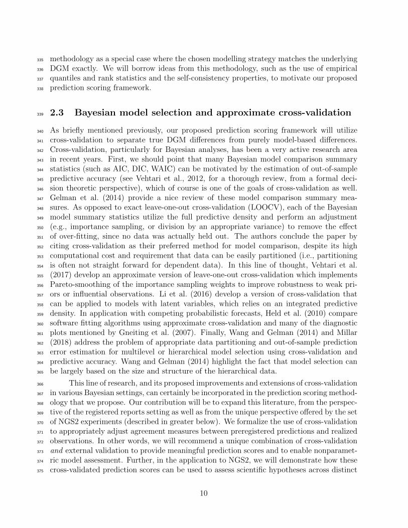
model-based predictions

(a) Differences between unobserved DGMs can be measured indirectly through model-based predictions.

model space

DGM 1(unobserved)

DGM 2(unobserved)

dataset 1

dataset 2

model-based predictions

distances between predictions and truthcross-validation

distances between predictions and truthvalidation

resampling distribution

(b) Cross-validation and validation account for sampling variability and separate modelfit issues from true DGM differences.

DGM 1(unobserved)

DGM 2(unobserved)

dataset 1

dataset 2

model space B

model space A

(c) Prediction scores measure the distance between DGMs along the dimension of themodel used to make predictions.

Figure 3: Geometric interpretation of the prediction scores.

15

predictors or covariates, x. The true difference between the data generating mechanisms467

is the conditional KL-divergence. In this Bayesian setting, predictions are draws from the468

posterior predictive distribution. For cross validation, this distribution, p(1)∗|−k is conditioned469

on the set of data (covariates and responses) from experiment 1 with the kth subset re-470

moved and provides a prediction for the kth subset of responses, corresponding to the kth471

set of covariates in experiment 1. For validation, the posterior predictive distribution, p(1)∗|1472

is conditioned on the entire set of data (covariates and responses) from experiment 1 and473

provides a prediction for the kth response, corresponding to the kth covariate in experi-474

ment 2. Finally, we estimate the true difference between the data generating mechanisms475

by calculating the KL-divergence between the distributions of (dis)agreement statistics476

across cross-validation, q(1)1 , and validation, q

(1)2 . Motivated by the Bayesian software-477

checking approaches of Cook et al. (2006) and Talts et al. (2018), a natural choice for the478

(dis)agreement statistics might be empirical quantiles or rank statistics.479

3.3 Example: Logistic regression480

To understand how this methodology can be used for inferential DGMs, consider the case481

where we assume the underlying process follows a simple logistice regression.482

4 Probabilistic behavior of prediction scores483

To understand how these prediction scores behave in practice and to get a sense of their484

asymptotic behavior, we have designed a simulation study that utilizes a simplified experi-485

mental design and models the outcome of interest with logistic regression. Many aspects of486

this simulation study were designed to complement related research that examines predic-487

tion scores for human behavior data in experimental social science research (Smith et al.,488

2018). We summarize the set up of this simulation study below and will detail how this489

study has been extended here to better examine the general probabilistic behavior of our490

prediction scoring methodology.491

In Smith et al. (2018), we consider K = 5 settings of a public goods game in which492

each participant has the opportunity to contribute (“cooperate”) or not (“defect”) to a set493

of pooled resources that will be multiplied and shared among all participants. Additionally,494

we imagine that some percentage of the total number of players, π = {0, 0.25, 0.50, 0.75, 1},495

are in fact bot participants whose behavior is strictly specified according to some set of496

algorithmic rules. The goal of these hypothetical experiments is to understand the ways in497

which participants’ decisions to cooperate are influenced by the presence of bots.498

True DGM. Let yijkt be the decision to cooperate (yijkt = 1) or defect (yijkt = 0) for theith individual in the jth cohort of the kth experimental setting for round t. Additionally,let zijk be an indicator of whether the ith participant in the jth cohort of the kth roundis a human participant (zijk = 1) or a bot (zijk). We will assume the true underlying data

16

DGM 1

p(1)(y|x)

Experiment 1

p(1)1 (y|x)

∆DGM (y|x) Experiment 2

p(1)2 (y|x)

raw data

x(1)11 , . . . , x

(1)1n1

y(1)11 , . . . , y

(1)1n1

raw data

x(1)21 . . . , x

(1)2n2

y(1)21 . . . , y

(1)2n2

model fittingsoftware

p(1)∗ (y|x)

?

predictions

y ∼ p(1)∗|1 (y|x)

remove ith observation

x(1)1,−i

y(1)1,−i

predictions

y(1)1i ∼ p

(1)∗|−i

(y|x(1)

1i

)

cross-validation

q1i = g(y(1)1i , y

(1)1i

)

predictions

y(1)2i ∼ p

(1)∗|1

(y|x(1)

2i

)

validation

q2i = g(y(1)2i , y

(1)2i

)∆pred(y|x)

Figure 4: Outline of the procedure for a predictive data generating mechanism, such aslinear regression.

17

generating mechanism is given by the following:

zijkiid∼ Bernoulli(πk)

Model 0: logit−1 [P (yijkt = 1|zijk = 1)] = β0 + β1t+ β2yijk,t−1 + β3y·jk,t−1

logit−1 [P (yijkt = 1|zijk = 0)] = β′0 + β′2yijk,t−1

where πk is the percentage of bots in the kth round, β0 and β′0 are baseline tendencies499

to cooperate, β1 captures any trend across the rounds, β2 and β′2 capture the tendency500

to switch between behaviors, and β3 represents the influence of team members’ decisions.501

Values for these parameters for the simulated data are provided and motivated in Smith502

et al. (2018).503

Prediction scoring details. In this setting, the DGMs being compared are predictive504

conditional distributions which we can refer to by p(yk|xk, πk). We perform this analysis in505

a Bayesian setting, so that predictions are draws from the posterior predictive distribution.506

To compare these predictions to the set of true observations, we compute receiver507

operating characteristic (ROC) curves and the corresponding area under the curve (AUC)508

statistics (Davis and Goadrich, 2006). These measures are very popular model fit as-509

sessment tools for logistic regression. In order to comptue these measures, we use L-fold510

cross-validation where L is chosen such that each partition contains roughly 500 observa-511

tions.512

Researcher models. To uncover true differences across the experimental settings, we513

consider the following three researcher models:514

Model 1: logit−1 [P (yijkt = 1)] = γ0 + γ1t,

Model 2: logit−1 [P (yijkt = 1)] = γ′0 + γ2yijk,t−1,

Model 3: logit−1 [P (yijkt = 1)] = γ′′0 + γ3y·jk,t−1,

where γ0 is a baseline tendency to cooperate, γ1 can capture some trends across the rounds,515

γ2 represents the influence of of the most recent decision, and γ3 represents the influence516

of team members’ decisions.517

Smith et al. (2018) provide interpretations of visual differences in the ROC curves518

across the different models and experimental settings. To summarize these results, the519

prediction scores behave as expected; they appear similar when comparing data generated520

from the same DGM and appear more different as the distance between DGMs (here,521

measured simply in terms of |πi − πj|) increases. This demonstrates that prediction scores522

can be used to uncover features of the DGM that vary across experimental settings, in a way523

that properly accounts for sampling variability. Additionally, the results of the simulation524

study indicate that Model 1 is the most sensitive to differences across the experimental525

settings. This is well-aligned with boxplots of the cooperation rate by round across each526

setting. In other words, when the model is aligned with true differences between the data527

18

Figure 5: Distance correlations for prediction scores.

generating mechanisms, the distance between the cross-validation and validation statistics528

reflects the true distance between the DGMs. In practice, relevant data patterns may529

be much more nuanced (i.e., not obvious from simple summary plots) and the true data530

generating mechanisms may be much more complex (i.e., it may be much more difficult to531

specify a model that predicts well).532

Extension to study probabilistic behavior . In order to get a sense of how these533

prediction scores behave asymptotically, we repeat the above simulation study many times534

and examine the relationship between the true distance between DGMs and our prediction535

scoring estimates of that distance. This requires defining a true distance between the data536

generating mechanisms. In this extended simulation, we consider two measures: (1) the537

difference between the percentage of bots, |πi−πj|, and (2) the conditional KL-divergence,538

calculated as follows:539

KL(p1, p2) =

To evaluate whether or not the prediction scoring estimates are well-aligned with these540

measures of the true underlying distance, we calculate distance covariances (Szekely et al.,541

2007). A distance covariance is a measure of dependence between two paired vectors that is542

capable of detecting both linear and nonlinear associations. If the vectors are independent,543

then the distance covariance is zero. We can treat each repetition of the above simulation544

study (where we compute prediction scores across all possible pairs of π) as a sample545

which gives rise to a vector of prediction scoring distance estimates. Then we examine the546

distribution of distance covariances, as a function of the (researcher) model used to make547

predictions. After repeating this simulation 1000 times, we plot the distance covariances548

in Figure 5.549

19

5 Network experiments in cooperative games550

The experiments proposed by the research teams in the (currently ongoing) Next Genera-551

tion Social Science (NGS2) program present a great opportunity to evaluate the proposed552

prediction scoring framework. This program funds multiple research teams over two cycles553

of experiments and is designed as a methodologically-focused effort to develop a fundamen-554

tal reimagining of the social science research cycle (Nosek et al., 2018). During each cycle,555

each research team will conduct distinct experimental social science studies regarding a556

shared research question. Prior to any data collection, each team will complete preregistra-557

tion materials, which includes predictions for study outcomes. In the following, we briefly558

describe the Gallup teams’ experiments for the first cycle of the program (for more de-559

tailed descriptions of each team’s planned and completed research, see the preregistration560

materials which have been made publicly available on the Open Science Framework Nosek561

et al., 2018).562

In the first cycle of the NGS2 program, the Gallup team provided an excellent appli-563

cation for our proposed prediction scoring methodology since their preregistered materials564

included pilot data from a previous study which informed their study hypotheses. This al-565

lows for an intuitive application of our proposed prediction scoring framework where we can566

compare the agreement between predictions for experimental data (based on the Gallup567

team’s proposed modeling strategy and their identified pilot data) and the materialized568

observations from the experiment itself.569

Experimental setting The first cycle of the NGS2 program focused on identifying path-570

ways towards the formation of collective identity and cooperative decisions. To address this571

research question, the Gallup team considered the role of social networks in the develop-572

ment of large-scale cooperation among individuals in an economic game. They used a573

logistic regression model to examine individuals decisions (cooperation or defection) and574

showed that social networks which can be frequently updated by participants (rather than575

fixed throughout the course of the game or randomly updated) foster cooperative decisions576

in this setting. The Gallup teams experiments were designed to mimic the experiments577

performed by Rand et al. (2011), and whose data can serve as a set of preregistration data.578

Experimenters randomly assigned participants to one of four conditions (see below) in579

a series of realizations of network experiments. In all conditions, subjects play a repeated580

cooperative dilemma (each game/session consists of multiple rounds) in an artificial social581

network created in the virtual laboratory. During each round of the game, each player can582

choose one of the following two actions: (1) cooperation: donate 50 units per neighbor,583

resulting in each neighbor actually gaining 100 units and (2) defection: donate nothing,584

resulting in neighbors getting nothing. After each round, players learn about the decisions585

of their neighbors and their own payoff. Additionally, the experimenters considered the586

following possible link-updating regimes for the social network in the game: (1) static or587

fixed links, (2) random link updating, where the entire network is regenerated at each588

round, (3) strategic link updating, where a randomly selected actor of a randomly selected589

pair may change the link status of that pair. The strategic link updating condition was590

20

Figure 6: Prediction scores for Gallup’s Cycle 1 Hypothesis 1.4: rapidly updating networkssupport cooperation, relative to all other conditions.

further split into two categories: (a) viscous, where 10% of the subject pairs were selected591

and (b) fluid, where 30% of the subject pairs are selected.592

Prediction scoring Recall, that we have suggested using quantiles or rank statistics593

as a disagreement statistic in our proposed prediction scoring methodology. However, for594

logistic regression, observations and predictions will be collections of 0s and 1s. Thus,595

using quantiles doesnt make sense in this setting. Instead, we can use the ROC (receiver596

operating characteristic) curve or precision-recall curve and the AUC (area under the curve)597

statistic to measure the agreement between observations and predictions. These measures598

are very popular model fit assessment tools for logistice regression. Thus, rather than599

comparing quantile distributions across cross-validation and validation, we will compare600

the distribution of AUC statistics across these settings. For this particular dataset, we will601

calculate the AUC statistic for the precision-recall curve. Generally, the precision-recall602

curve is preferred over the ROC curve whenever the data is imbalanced (see Davis and603

Goadrich, 2006, for more discussion). Finally, we need to point out that the AUC statistic604

is not defined for a single data point. Thus, we can not use leave-one-out cross-validation605

in our prediction scoring routine. Instead we partition the dataset into k subsets and use k-606

fold cross-validation, resulting in k AUC statistics. Similarly, when performing validation,607

we must again partition the data into subsets.608

As an example, consider Hypothesis 1.4 from the Gallup team’s preregistration mate-609

rials. They hypothesized that rapidly updating networks would support cooperation more610

21

Figure 7: Boxplots of average cooperation levels across rounds of Gallup’s Cycle 1 games.

than any other condition. To evaluate the prediction scores, we have compared the distri-611

bution of AUC statistics from cross-validation to those from validation as well as plotted612

the corresponding precision-recall curves from each of the k subroutines of cross-validation613

and validation (see Figure 6). The validation statistics measure differences due to both ran-614

dom noise and true differences between the DGMs (i.e., between our prior beliefs about the615

preregistered data and reality), while the cross-validation statistics only capture differences616

due to random noise or disagreement between the underlying DGM and the chosen model.617

In this case, we observe larger AUC statistics and better ROC curves in the validation618

routine. This indicates that there is less variability in individuals’ behavior in the experi-619

mental data, than in the preregistration data. In a sense, subjects in the Gallup experiment620

are acting in more predictable ways than the subjects from the previous experiment. And621

in fact, if we simply examine summary statistics of the in-game decisions themselves, we622

can see the same type of pattern. In Figure 7, we provide boxplots of individuals’ average623

cooperation levels across rounds of the game, where each color corresponds to a different624

link-updating experimental condition. Comparing the preregistration data (top row) to625

the experimental data (bottom row), we see that the boxplots are drastically narrower,626

indicating that there is less variability in participant behavior.627

This application serves as an illustration of how our prediction scoring can enable628

interesting scientific insights. Further, we demonstrated how this methodology can be629

adapted to appropriately address modelling choices (i.e., using distributions of AUC statis-630

tics, rather than quantiles) and demonstrates the type of diagnostic plots that can be used631

to interpret the resulting prediction scores.632

22

References633

Anderson, J. L. “A method for producing and evaluating probabilistic forecasts from634

ensemble model integrations.” Journal of Climate, 9(7):1518–1530 (1996).635

Cook, S. R., Gelman, A., and Rubin, D. B. “Validation of software for Bayesian models636

using posterior quantiles.” Journal of Computational and Graphical Statistics , 15(3):675–637

692 (2006).638

Czado, C., Gneiting, T., and Held, L. “Predictive model assessment for count data.”639

Biometrics , 65(4):1254–1261 (2009).640

Davis, J. and Goadrich, M. “The relationship between Precision-Recall and ROC curves.”641

In Proceedings of the 23rd international conference on Machine learning , 233–240. ACM642

(2006).643

Dawid, A. P. “Present position and potential developments: Some personal views: Statis-644

tical theory: The prequential approach.” Journal of the Royal Statistical Society. Series645

A (General), 278–292 (1984).646

Gelman, A. “Preregistration of studies and mock reports.” Political Analysis , 21(1):40–41647

(2013).648

Gelman, A., Hwang, J., and Vehtari, A. “Understanding predictive information criteria for649

Bayesian models.” Statistics and computing , 24(6):997–1016 (2014).650

Gelman, A. and Loken, E. “The statistical crisis in science.” American Scientist , 102:460651

– 465 (2014).652

Gneiting, T. “Making and evaluating point forecasts.” Journal of the American Statistical653

Association, 106(494):746–762 (2011).654

Gneiting, T., Balabdaoui, F., and Raftery, A. E. “Probabilistic forecasts, calibration and655

sharpness.” Journal of the Royal Statistical Society: Series B (Statistical Methodology),656

69(2):243–268 (2007).657

Gneiting, T. and Katzfuss, M. “Probabilistic forecasting.” Annual Review of Statistics and658

Its Application, 1:125–151 (2014).659

Gneiting, T., Raftery, A., Balabdaoui, F., and Westveld, A. “Verifying probabilistic fore-660

casts: Calibration and sharpness.” In Preprints, 17th Conf. on Probability and Statistics661

in the Atmospheric Sciences, Seattle, WA, Amer. Meteor. Soc, volume 2 (2004).662

Gneiting, T. and Raftery, A. E. “Strictly proper scoring rules, prediction, and estimation.”663

Journal of the American Statistical Association, 102(477):359–378 (2007).664

Hamill, T. M. and Colucci, S. J. “Verification of Eta–RSM short-range ensemble forecasts.”665

Monthly Weather Review , 125(6):1312–1327 (1997).666

Held, L., Schrodle, B., and Rue, H. “Posterior and cross-validatory predictive checks: a667

comparison of MCMC and INLA.” In Statistical modelling and regression structures ,668

91–110. Springer (2010).669

23

Humphreys, M., Sanchez de la Sierra, R., and Van der Windt, P. “Fishing, commitment,670

and communication: A proposal for comprehensive nonbinding research registration.”671

Political Analysis , 21(1):1–20 (2013).672

Li, L., Qiu, S., Zhang, B., and Feng, C. X. “Approximating cross-validatory predictive673

evaluation in Bayesian latent variable models with integrated IS and WAIC.” Statistics674

and Computing , 26(4):881–897 (2016).675

Mellor, D. “Registered reports library.” www.zotero.org/groups/479248/osf/items/collectio676

nKey/KEJP68G9. Center for Open Science (2018).677

Millar, R. B. “Conditional vs marginal estimation of the predictive loss of hierarchical678

models using WAIC and cross-validation.” Statistics and Computing , 28(2):375–385679

(2018).680

Nosek, B. A., Spitzer, M., Russell, A., Tully, E., Rajtmajer, S., Ahn, S.-H., Zheng, T., Foy,681

D., Kluch, S. P., Stewart, C., and et al. “NGS2 DARPA Program.” (2018).682

Open Science Collaboration. “Estimating the reproducibility of psychological science.”683

Science, 349(6251):aac4716 (2015).684

Pearson, K. “On a method of determining whether a sample of size n supposed to have685

been drawn from a parent population having a known probability integral has probably686

been drawn at random.” Biometrika, 379–410 (1933).687

Rand, D. G., Arbesman, S., and Christakis, N. A. “Dynamic social networks promote coop-688

eration in experiments with humans.” Proceedings of the National Academy of Sciences ,689

108(48):19193–19198 (2011).690

Rosenblatt, M. “Remarks on a multivariate transformation.” The annals of mathematical691

statistics , 23(3):470–472 (1952).692

Shephard, N. “Partial non-Gaussian state space.” Biometrika, 81(1):115–131 (1994).693

Smith, A., Zheng, T., and Gelman, A. “Evaluating drivers of human behaviors in experi-694

mental social science using prediction scoring.” (2018).695

Spies, J. R. “Reproducibility Rubric.” (2018).696

Stodden, V., McNutt, M., Bailey, D. H., Deelman, E., Gil, Y., Hanson, B., Heroux, M. A.,697

Ioannidis, J. P., and Taufer, M. “Enhancing reproducibility for computational methods.”698

Science, 354(6317):1240–1241 (2016).699

Szekely, G. J., Rizzo, M. L., Bakirov, N. K., et al. “Measuring and testing dependence by700

correlation of distances.” The annals of statistics , 35(6):2769–2794 (2007).701

Talagrand, O., Vautard, R., and Strauss, B. “Evaluation of probabilistic prediction systems,702

paper presented at ECMWF Workshop on Predictability, Eur. Cent. for Med. Range703

Weather Forecasts.” Reading, UK (1997).704

24

Talts, S., Betancourt, M., Simpson, D., Vehtari, A., and Gelman, A. “Validating705

Bayesian Inference Algorithms with Simulation-Based Calibration.” arXiv preprint706

arXiv:1804.06788 (2018).707

Vehtari, A., Gelman, A., and Gabry, J. “Practical Bayesian model evaluation using leave-708

one-out cross-validation and WAIC.” Statistics and Computing , 27(5):1413–1432 (2017).709

Vehtari, A., Ojanen, J., et al. “A survey of Bayesian predictive methods for model assess-710

ment, selection and comparison.” Statistics Surveys , 6:142–228 (2012).711

Wang, W. and Gelman, A. “Difficulty of selecting among multilevel models using predictive712

accuracy.” Statistics at its Interface, 7(1):1–88 (2014).713

25