MNRAS 000, 1–13 (2018) Preprint 24 December 2018 Compiled using MNRAS L A T E X style file v3.0 saprEMo: a simplified algorithm for predicting detections of electromagnetic transients in surveys S. Vinciguerra 1,2 , M. Branchesi 3,4 , R. Ciolfi 5,6 , I. Mandel 1,7 , C. J. Neijssel 1 , G. Stratta 8,9 1 Institute of Gravitational Wave Astronomy and School of Physics and Astronomy, University of Birmingham, B15 2TT, Birmingham, UK 2 Max Planck Institute for Gravitational Physics (Albert Einstein Institute), D-30167 Hannover, Germany 3 Gran Sasso Science Institute, Viale Francesco Crispi, 7, 67100 L’Aquila AQ, Italy 4 INFN, Laboratori Nazionali del Gran Sasso, I-67100 Assergi, Italy 5 INAF, Osservatorio Astronomico di Padova, Vicolo dell’Osservatorio 5, I-35122 Padova, Italy 6 INFN-TIFPA, Trento Institute for Fundamental Physics and Applications, Via Sommarive 14, I-38123 Trento, Italy 7 Monash Centre for Astrophysics, School of Physics and Astronomy, Monash University, Clayton, Victoria 3800, Australia 8 University of Urbino "Carlo Bo", Dipartimento di Scienze di Base e Fondamenti/Physics section, Via Santa Chiara, 27, 61029 Urbino, Italy 9 INFN, Sezione di Firenze, I-50019 Sesto Fiorentino, Firenze, Italy Accepted 14 Dec 2018. Received 23 Sep 2018; in original form 23 Sep 2018 ABSTRACT The multi-wavelength detection of GW170817 has inaugurated multi-messenger astronomy. The next step consists in interpreting observations coming from population of gravitational wave sources. We introduce saprEMo, a tool aimed at predicting the number of electromag- netic signals characterised by a specific light curve and spectrum, expected in a particular sky survey. By looking at past surveys, saprEMo allows us to constrain models of electromagnetic emission or event rates. Applying saprEMo to proposed astronomical missions/observing campaigns provides a perspective on their scientific impact and tests the effect of adopting different observational strategies. For our first case study, we adopt a model of spindown- powered X-ray emission predicted for a binary neutron star merger producing a long-lived neutron star. We apply saprEMo on data collected by XMM-Newton and Chandra and during 10 4 s of observations with the mission concept THESEUS. We demonstrate that our emission model and binary neutron star merger rate imply the presence of some signals in the XMM- Newton catalogs. We also show that the new class of X-ray transients found by Bauer et al. in the Chandra Deep Field-South is marginally consistent with the expected rate. Finally, by studying the mission concept THESEUS, we demonstrate the substantial impact of a much larger field of view in searches of X-ray transients. Key words: EM follow-up models – BNS mergers – rates – short gamma-ray bursts 1 INTRODUCTION GW170817 (Abbott et al. 2017a) has just opened the era of multi- messenger astronomy (Abbott et al. 2017b). The first coincident set of gravitational-waves and electromagnetic observations has al- ready provided an extraordinary insight into the physics of the bi- nary neutron star mergers. Among the key results of this revolu- tionary discovery is the confirmation of the association between the merger of two neutron stars (NSs) and (at least some) short gamma ray bursts (SGRBs) (Abbott et al. 2017b and refs. therein). The last radio VLBI observations demonstrate that a narrow jet was formed and prove the association with a classical SGRB (see Troja et al. 2017; Mooley et al. 2018a; Margutti et al. 2018; D’Avanzo et al. 2018; Lyman et al. 2018; Dobie et al. 2018; Mooley et al. 2018b; Ghirlanda et al. 2018). The intense multi-wavelength follow-ups of gamma ray bursts in the last decade have revealed new and unexpected features, such as early and late X-ray flares, extended emission, and X-ray plateaus (e.g., Berger 2014 and refs. therein). The challenges posed by this rich astronomical scenario motivated a growing interest of the community in investigating compact binary mergers from both the theoretical and observational points of view. Intensified theoret- ical efforts have been dedicated to explain these observations and coherently explore these and other possible electromagnetic signals generated by these sources. In order to validate the variety of proposed theoretical sce- narios in the context of multi-messenger astronomy with compact binary mergers, we present saprEMo. We developed saprEMo,a Simplified Algorithm for PRedict- ing ElectroMagnetic Observations, to evaluate how many electro- magnetic (EM) signals, characterised by a specific light curve and spectrum, should be present in a data set given some overall char- © 2018 The Authors arXiv:1809.08641v2 [astro-ph.IM] 20 Dec 2018

Welcome message from author
This document is posted to help you gain knowledge. Please leave a comment to let me know what you think about it! Share it to your friends and learn new things together.
Transcript
MNRAS 000, 1–13 (2018) Preprint 24 December 2018 Compiled using MNRAS LATEX style file v3.0
saprEMo: a simplified algorithm for predicting detections ofelectromagnetic transients in surveys
S. Vinciguerra1,2, M. Branchesi3,4, R. Ciolfi5,6, I. Mandel1,7, C. J. Neijssel1,G. Stratta 8,91 Institute of Gravitational Wave Astronomy and School of Physics and Astronomy, University of Birmingham, B15 2TT, Birmingham, UK2 Max Planck Institute for Gravitational Physics (Albert Einstein Institute), D-30167 Hannover, Germany3 Gran Sasso Science Institute, Viale Francesco Crispi, 7, 67100 L’Aquila AQ, Italy4 INFN, Laboratori Nazionali del Gran Sasso, I-67100 Assergi, Italy5 INAF, Osservatorio Astronomico di Padova, Vicolo dell’Osservatorio 5, I-35122 Padova, Italy6 INFN-TIFPA, Trento Institute for Fundamental Physics and Applications, Via Sommarive 14, I-38123 Trento, Italy7 Monash Centre for Astrophysics, School of Physics and Astronomy, Monash University, Clayton, Victoria 3800, Australia8 University of Urbino "Carlo Bo", Dipartimento di Scienze di Base e Fondamenti/Physics section, Via Santa Chiara, 27, 61029 Urbino, Italy9 INFN, Sezione di Firenze, I-50019 Sesto Fiorentino, Firenze, Italy
Accepted 14 Dec 2018. Received 23 Sep 2018; in original form 23 Sep 2018
ABSTRACTThe multi-wavelength detection of GW170817 has inaugurated multi-messenger astronomy.The next step consists in interpreting observations coming from population of gravitationalwave sources. We introduce saprEMo, a tool aimed at predicting the number of electromag-netic signals characterised by a specific light curve and spectrum, expected in a particular skysurvey. By looking at past surveys, saprEMo allows us to constrain models of electromagneticemission or event rates. Applying saprEMo to proposed astronomical missions/observingcampaigns provides a perspective on their scientific impact and tests the effect of adoptingdifferent observational strategies. For our first case study, we adopt a model of spindown-powered X-ray emission predicted for a binary neutron star merger producing a long-livedneutron star. We apply saprEMo on data collected by XMM-Newton and Chandra and during104s of observations with the mission concept THESEUS. We demonstrate that our emissionmodel and binary neutron star merger rate imply the presence of some signals in the XMM-Newton catalogs. We also show that the new class of X-ray transients found by Bauer et al.in the Chandra Deep Field-South is marginally consistent with the expected rate. Finally, bystudying the mission concept THESEUS, we demonstrate the substantial impact of a muchlarger field of view in searches of X-ray transients.
Key words: EM follow-up models – BNS mergers – rates – short gamma-ray bursts
1 INTRODUCTION
GW170817 (Abbott et al. 2017a) has just opened the era of multi-messenger astronomy (Abbott et al. 2017b). The first coincidentset of gravitational-waves and electromagnetic observations has al-ready provided an extraordinary insight into the physics of the bi-nary neutron star mergers. Among the key results of this revolu-tionary discovery is the confirmation of the association between themerger of two neutron stars (NSs) and (at least some) short gammaray bursts (SGRBs) (Abbott et al. 2017b and refs. therein). The lastradio VLBI observations demonstrate that a narrow jet was formedand prove the association with a classical SGRB (see Troja et al.2017; Mooley et al. 2018a; Margutti et al. 2018; D’Avanzo et al.2018; Lyman et al. 2018; Dobie et al. 2018; Mooley et al. 2018b;Ghirlanda et al. 2018).
The intense multi-wavelength follow-ups of gamma ray bursts
in the last decade have revealed new and unexpected features,such as early and late X-ray flares, extended emission, and X-rayplateaus (e.g., Berger 2014 and refs. therein). The challenges posedby this rich astronomical scenario motivated a growing interest ofthe community in investigating compact binary mergers from boththe theoretical and observational points of view. Intensified theoret-ical efforts have been dedicated to explain these observations andcoherently explore these and other possible electromagnetic signalsgenerated by these sources.
In order to validate the variety of proposed theoretical sce-narios in the context of multi-messenger astronomy with compactbinary mergers, we present saprEMo.
We developed saprEMo, a Simplified Algorithm for PRedict-ing ElectroMagnetic Observations, to evaluate how many electro-magnetic (EM) signals, characterised by a specific light curve andspectrum, should be present in a data set given some overall char-
© 2018 The Authors
arX
iv:1
809.
0864
1v2
[as
tro-
ph.I
M]
20
Dec
201
8
2 S. Vinciguerra et al.
acteristics of the astronomical survey and a cosmological rate ofcompact binary mergers. Predictions can be used both to validatethe theoretical scenarios against already collected data and to crit-ically examine the scientific means of future missions and theirobservational strategies. While we use compact binary mergers asthe prime multi-messenger targets, saprEMo can also be applied toother type of transients (e.g. core-collapse supernovae).
We describe the main features of saprEMo in Section 2. Asfirst case study, we use saprEMo to investigate the X-ray emis-sion from Binary NS (BNS) mergers leading to the formation ofa long-lived and strongly magnetized NS, following the model ofSiegel & Ciolfi 2016a,b (see Section 3.1). We apply saprEMo topresent X-ray surveys, collected by XMM-Newton (Jansen et al.2001; Strüder et al. 2001; Turner et al. 2001) and Chandra (Weis-skopf & Van Speybroeck 1996; Weisskopf et al. 2000), and studythe prospectives of the mission concept THESEUS (Amati et al.2018). Results are reported in Section 3.3 and discussed in Section4. Finally, in Section 5 we draw our conclusions summarising ourfirst results and outlining the main features and primary scopes ofsaprEMo. Throughout the paper we assume a flat cosmology with:H0 = 70 km s−1 Mpc−1, ΩM = 0.3 and ΩΛ = 0.7.
2 SAPREMO OUTLINE
saprEMo is a Python algorithm designed to predict howmany detectable electromagnetic signals, associated with a spe-cific EM emission (EMe) model, are present in a survey S.The full code and a short manual are publicly available athttps://github.com/saprEMo/source_code.According to instrument limitations (such field of view and spec-tral sensitivity), saprEMo estimates the number of signals whoseemission flux F at the observer is above the flux limit Flim of the Ssurvey. Accounting for the energy dependency of the survey sensi-tivity, we define detections on a instantaneous flux-based criterion:∃ g, t′ | Fg (t′) > Flim,g, where g labels the spectral band of thesurvey. We therefore simplify our analysis by treating detectabilityin each band independently, i.e., a source is considered to be de-tected if and only if it can be independently detected in at least oneinstrument band. More realistic treatments include flux integrationover the observation time and noise simulation (see Carbone et al.2017 and references therein for a discussion of these data analysisaspects).saprEMo does not directly consider the actual sky locations
observed by the survey S (even when applied to archival data) andinstead focuses on accounting for cosmological distances, relyingon the isotropy of the Universe.
2.1 Core analysis
saprEMo can be applied to any type of EM emission, from tran-sients to continuous sources emitting in any EM spectral range. Inthis work, we focus on X-ray transients associated with mergers ofneutron star binaries. The expected number of BNS mergers NBNS
in the volume enclosed within redshift zmax, in a time T at the ob-server, is:
NBNS = T∫ zmax
0
RV (z)1 + z
dVC
dzdz (1)
where RV (z) is the rate of BNS mergers per unit comoving volume,per unit source time. In our case zmax is the maximum distanceat which the emission following the model of interest EMe, can
be detected. zmax is calculated considering both the spectral shiftdue to the source redshift compared to the instrument energy bandEI ∼
[EI
min, EImax
]and the maximum luminosity distance, set by the
peak luminosity Lp(E) of the EMe model and the sensitivity Flim
of the survey. We only expect a fraction of NBNS to be observedby a specific instrument, depending on the emission properties andthe characteristics of the survey. The number of BNS mergers, de-tectable by the survey S such that the peak of the considered emis-sion EMe falls within the observing time, is given by:
Np = εFoV4π
T∫ zmax
0
RV (z)1 + z
dVcdz
dz (2)
The total observing time T can be expressed in terms of the surveyS as T = 〈Tobs〉 nobs, where nobs is the number of the observa-tions and 〈Tobs〉 is the average exposure time for observation. Ineq. (2), the field of view FoV of the instrument reduces the num-ber NBNS of signals present in the volume enclosed within zmax byFoV/4π. In the specific case of BNS mergers, the efficiency fac-tor ε typically includes the occurrence rate of a specific mergerremnant (εsr), which are expected to generate the emission EMe,and source geometry/observational restrictions such as collimation(εc = 1 − cos(θ), where θ is the beaming angle), so that ε ∼ εsr · εc.We designate as peaks the signals included in Np (see figure 1).This contribution only depends on the emission model by the in-tensity of the light curve peaks in the energy bands of the survey.This dependency is enclosed in zmax.
There is also a contribution, which we call tails (figure 1),from the mergers whose emission is detected only before (firstblock of eq. (3)) or after (second block of eq. (3)) the luminos-ity peaks (i.e., Lp is outside the observation period). The longer thelight curve is above Flim, the higher the probability of it being ob-served (see Carbone et al. 2017 for a detailed discussion of signalduration in the context of transient detectability and classification).To estimate this contribution, we need to account for the evolutionin time of the emission luminosity L(t′), which affects the horizonof the survey:
Nt = ε nobsFoV4π
∫ t′p
−∞
∫ zt(L(t′))
0
RV (z)1 + z
dVcdz
dz dt+∫ +∞
t′p
∫ zt(L(t′))
0
RV (z)1 + z
dVcdz
dz dt
= ε nobs
FoV4π
∫ +∞
−∞
∫ zt(L(t′))
0
RV (z)1 + z
dVcdz
dz dt
(3)
where t and t′ = t/(1 + z) are the time respectively in observer andsource frames and t′p is the time corresponding to the peak luminos-ity. zt (L(t′)) represents the horizon of the survey, given the specificintrinsic luminosity of the source L(t′). The integration time of eq.(3) is practically limited by the duration of the emission above theflux limit. At the moment, saprEMo does not correctly account forthe possibility of detecting multiple times the same event. Multipledetections of the same source might occur if the survey containsrepeated observations of the same sky locations and the time inter-val between the different exposures is shorter than the consideredemission EMe. While Np would be unaffected, in these cases Nt
would overestimate the expected number of events by these addi-tional detections. Under these specific conditions, Nt should thenbe considered as an upper limit. We refer the readers to Carboneet al. 2017 for discussions of transient detectability in the contextof multiple images of the same field.
MNRAS 000, 1–13 (2018)
saprEMo 3
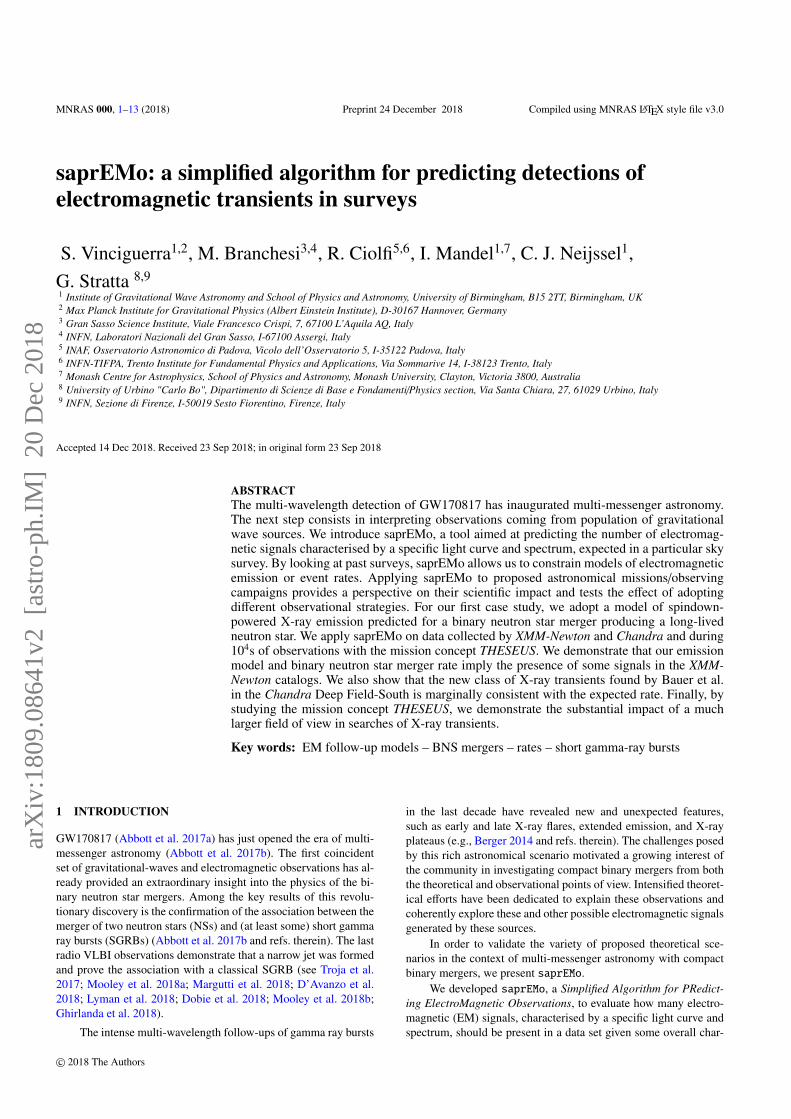
The ratio between the duration of the observable emission andthe typical exposure time determines the relative importance ofpeaks and tails. The trade off between these two contributions, aswell as their different origin, can be understood with figures 1 and2. For illustrative purposes, we consider only local events with un-physical rates and a generic triangular light curve. Figure 1 showshow tails events b and c can be observed during one exposure ofduration 〈Tobs〉. Figure 2 shows the impact of the transient observ-able duration on tails. Upper and lower panels represent exactly thesame scenarios (10 seconds of exposure of transients at z = 0 char-acterised by a 1 Hz rate) except for the transient duration, which isdoubled in the lower panel. The number of stars, which representthe peak contribution, is the same in both upper and lower panels,demonstrating that peaks are unaffected by the change of the tran-sient observable duration. However the tail contribution, given bythe number of pink triangles, doubles in the lower panel comparedto the upper one. On the contrary, extending the exposure to 20 sec-onds would double the number of peaks, while leaving unchangedthe number of tails. Given a fixed event rate, Np depends on theobserving time, while Nt depends on the duration of the events. Wereturn to this topic in section 4, when we discuss the results of thisstudy.
While eq. (2) and (3) explain the general concept behind thetool, they do not explicitly account for the energy (or wavelengthE = ~c/λ) dependence of light curves, instrument sensitivitiesand absorption. These effects are particularly important whenexploring the Universe at high redshift. We explain how theseeffects are implemented in saprEMo analysis in appendix A.
2.2 Inputs and Outputs
We now present inputs and outputs of saprEMo.
Inputs:
(i) light curves (LC), in terms of luminosity rest frame, of the EMemission EMe in different energy bins (if predicted by the model,also including energies outside the instrument sensitivity band, asthey might be redshifted into it, after accounting for cosmologycorrections);
(ii) astrophysical rate in the source frame RV (z);(iii) efficiency ε of the EM model EMe (ε should account for source
geometry/selection effects, such as collimation, as well as the fre-quency with which this type of astrophysical source generates theelectromagnetic emission EMe);
(iv) main instrument and survey properties:
• for each spectral band g of the survey S, minimum and max-imum energy included [Ei, Es]g;• corresponding flux limits [Flim]g;• average exposure time 〈Tobs〉;• field of view FoV 1;• number of observations nobs
1.
Outputs:
• Np and Nt: numbers of peaks and tails which are expected inthe survey S. The numbers of signals returned by saprEMo should
1 Or equivalently covered sky-area fsky ∼ nobsFOV
4π .
1 +1t0p
z = 0t = t0
Flim time
Flu
x
ab c
a 2 NphTobsi
b, c 2 Nt
Lp/(4D2)
Figure 1. Schematic representation of a peak (tp ∈ 〈Tobs〉) signal (a) and tails(b, c). The solid curves represent the part of signals EMe visible during theexposure time at the observer, the dashed components are the missed (becauseof time or flux restrictions) part of the emissions. The upper dotted line showsthe peak flux Fp = Lp/(4πD2), the lower line the flux limit of the survey.
Figure 2. Simplified examples of peaks and tails. In both upper and lower pan-els we report the detected flux (in arbitrary units on the y-axis) as a faction oftime at the observer. We assume a transient class emitting from z ∼ 0, charac-terised by the unrealistic rate 1 Hz and a fixed triangular light curve. The fluxlimit Flim is represented by the horizontal line. The transient light curves abovethe flux limit are shown in black solid lines. The light gray region highlights the10 s exposure window. The panels show the peak contribution, i.e. the eventswhose luminosity peak falls in the observational window (green stars) and thetail contribution, i.e. the events detected only before or after the luminosity peak(fuchsia lines and area). The only difference between upper and lower panels isthe duration of the transient light curve above the flux limit, respectively 1 s and2 s. Doubling the light curve duration results in doubling the number of tails,while leaving unchanged the number of peaks.
be interpreted as the expectation value of a Poisson process. There-fore Poisson statistical errors should be considered in addition tothe systematics due to rate and emission model uncertainties;• dNp/dz and dNt/dz: distributions of tail and peak numbers as
a function of redshift;• dNp/dlog(D) and dNt/dlog(D): expected distribution of signal
observed durations, obtained by convolving the approximate distri-bution of the survey exposure times Pobs with the light curve spanLCS observable at each step in redshift. For each redshift, the LCSrepresents the total time of the light curve which is above the fluxlimits at the observer frame (for more details see appendix A3). Toestimate the distribution of the signal durations, we analytically ap-proximate the exposure time distribution Pobs from the average ex-posure time 〈Tobs〉 (and standard deviation, when available) with aMaxwell-Boltzmann or Log-normal function, according to the userinput. For each data point saved from the cosmic integrations, we
MNRAS 000, 1–13 (2018)
4 S. Vinciguerra et al.
simulate Ntrials (for both peaks and tails) observation durations Tobs
and define for each of them the starting time ts. The starting timeis uniformly drawn from a time interval including both the expo-sure time of the specific trial Tobs and the observable emission atobserver (t′f − t′i )(1 + z) (where t′f and t′i are respectively the last andfirst LC time at source satisfying our detection criteria at redshift z).If ts is drawn in the interval Ip =
[tp − Tobs, tp
], where tp is the time
at observer correspondent to the luminosity peak, it contributes tothe peak distribution, otherwise it adds up to the tail distribution.For each simulated observation the total duration is then calculatedsumming only the contribution of light curve intervals whose fluxis above the limit;• dNp/dlog(F) and dNt/dlog(F): distributions of peak and tail
detection numbers as a function of maximum flux. At each step inredshift, necessary to compute the integral (2), saprEMo also cal-culates the associated flux. The fluxes are obtained by summing thecontribution of each energy and rescaling with the associated lumi-nosity distance. From the same observations simulated for estimat-ing the duration distributions, we obtain the expected distributionof maximum fluxes.
Distributions in redshift are useful to estimate the horizon of thesurvey to the emission EMe and for astrophysical interpretation.They provide a prior on the redshift distribution when a counterpartallowing z measurement is missing, or constrain cosmic rate evo-lution of BNS mergers when multi-wavelength observations yieldthe source distance. Distributions of fluxes and durations are robustobservables, which enable comparisons with real data 2.
3 APPLICATION TO SOFT X-RAY EMISSION FROMLONG-LIVED BINARY NEUTRON STAR MERGERREMNANTS
In the following, we consider a specific application of saprEMo tothe case of spindown-powered X-ray transients from long-lived NSremnants of BNS mergers.
Depending on the involved masses and the NS equation ofstate (EOS), a BNS merger can either produce a short-lived rem-nant, collapsing to a black hole (BH) within a fraction of a sec-ond, or a long-lived massive NS. The latter can survive for muchlonger spindown timescales (up to minutes, hours or more) priorto collapse or even be stable forever (Lasky et al. 2014; Lü et al.2015). After the discovery of NSs with a mass of ∼ 2 M (Demor-est et al. 2010; Antoniadis et al. 2013), different authors convergedto the idea that the fraction of BNS mergers leading to a long-livedNS remnants should range from a few percent up to more thanhalf (e.g., Piro et al. 2017). Information extracted from the mul-timessenger observations of the BNS merger event GW170817 didnot change this view, although more stringent constraints on theNS EOS were obtained from the GW signal (Abbott et al. 2018a),from various indications excluding the prompt collapse to a BH,and from the kilonova brightness and the relatively high mass ofthe merger ejecta (e.g., Margalit & Metzger 2017; Bauswein et al.
2 The reported flux distribution is calculated from the maximum the-oretical fluxes of detected events in our simulation (see paragraph ondNp/t/d log(D)-output). Quantitative comparisons with actual data wouldrequire a more detailed analysis, including the use of the instrument re-sponse, a realistic model for noise, the model used to convert photon countsinto a light curve, etc. (see for example Carbone et al. 2017, who modeledsome of these aspects).
2017; Radice et al. 2018; Rezzolla et al. 2018). An additional sup-porting element in favour of long-lived remnants is given by theobservation of long-lasting (∼ minutes to hours) X-ray transientsfollowing a significant fraction of SGRBs (e.g., Rowlinson et al.2013; Gompertz et al. 2014; Lü et al. 2015). Given the short ac-cretion timescale of a remnant disk onto the central BH (. 1 s),such long-lasting emission represents a challenge for the canoni-cal BH-disk scenario of SGRBs while it can be easily explainedby alternative scenarios involving a long-lived NS central engine,e.g., the magnetar (Zhang & Mészáros 2001; Metzger et al. 2008)and the time-reversal (Ciolfi & Siegel 2015; Ciolfi 2018) scenar-ios. According to this view, the fraction of SGRBs accompaniedby long-lasting X-ray transients might reflect the fraction of BNSmergers producing a long-lived NS.
If the merger remnant is a long-lived NS, its spindown-powered electromagnetic emission represents an additional energyreservoir that can potentially result in a detectable transient. Re-cent studies taking into account the reprocessing of this radiationacross the baryon-polluted environment surrounding the mergersite have shown that the resulting signal should peak at wave-lengths between optical and soft X-rays, with luminosities in therange 1043 − 1048 erg/s and time scales of minutes to days (e.g., Yuet al. 2013; Metzger & Piro 2014; Siegel & Ciolfi 2016a,b). Be-sides representing an explanation for the long-lasting X-ray tran-sients accompanying SGRBs, this spindown-powered emission is apromising counterpart to BNS mergers (e.g., Stratta et al. 2017 andrefs. therein), having the advantage of being both very luminousand nearly isotropic.
For our first direct application of saprEMo, we consider thespindown-powered transient model by Siegel & Ciolfi 2016a,b(hereafter SC16), described in the next Section 3.1, in which theemission is expected to peak in the soft X-ray band. This modelcannot be excluded or constrained by GW170817. The first X-rayobservations in the 2 − 10 keV band were performed by MAXY(Sugita et al. 2018) 4.6 hours after the merger with a sensitivity of8.6× 10−9 erg s−1 cm−2, well above the flux that the model predictsat that time after the merger.
In Section 3.2, we briefly describe the model of the BNSmerger rate adopted for this first study. Then, in Section 3.3 wepresent our results referring to three different X-ray satellites:XMM-Newton, Chandra, and the proposed THESEUS. We discussthese results in section 4.
3.1 Reference emission model
The model proposed by Siegel & Ciolfi (SC16) describes the evo-lution of the environment surrounding a long-lived NS formedas the result of a BNS merger. The spindown radiation from theNS injects energy into the system and interacts with the opticallythick baryon-loaded wind ejected isotropically in the early post-merger phase, rapidly forming a baryon-free high-pressure cavityor “nebula” (with properties analogous to a pulsar wind nebula) sur-rounded by a spherical shell of “ejecta” heated and accelerated bythe incoming radiation. As long as the ejecta remain optically thick,the non-thermal radiation from the nebula is reprocessed and ther-malised before eventually escaping. As soon as the ejecta becomeoptically thin, a signal rebrightening is expected, accompanied bya transition from dominantly thermal to non-thermal spectrum. The
MNRAS 000, 1–13 (2018)
saprEMo 5
102 100 102 104 106
Source time from merger [s]
1037
1039
1041
1043
1045
1047
1049
Lu
min
osit
y[e
rg/s]
0.2 1 keV
1 2 keV
2 3 keV
3 4 keV
4 5 keV
6 7 keV
0.2 7 keV
Source time since merger [s]<latexit sha1_base64="NEMJPWQ0TQBmWmQzI6x9Yt1Hi7E=">AAACDnicbZBLSwMxFIUz9VXra9Slm8FScFVmRNBlQRCXFe0DpkPJpHfa0CQzJBmhDC3u3fhX3LhQxK1rd/4bM20X2noh8HHOTXLvCRNGlXbdb6uwsrq2vlHcLG1t7+zu2fsHTRWnkkCDxCyW7RArYFRAQ1PNoJ1IwDxk0AqHl7nfugepaCzu9CiBgOO+oBElWBupa1c6HOtBGGW30xcnmnKYKCoMcpB9kBNfBeOuXXar7rScZfDmUEbzqnftr04vJikHoQnDSvmem+ggw1JTwmBc6qQKEkyGuA++QYE5qCCbrjN2KkbpOVEszRHamaq/b2SYKzXioenMh1eLXi7+5/mpji6CjIok1SDI7KMoZY6OnTwbp0clEM1GBjCR1MzqkAGWmGiTYMmE4C2uvAzN06rnVr2bs3Lt6mEWRxEdoWN0gjx0jmroGtVRAxH0iJ7RK3qznqwX6936mLUWrHmEh+hPWZ8/yOuePg==</latexit><latexit sha1_base64="NEMJPWQ0TQBmWmQzI6x9Yt1Hi7E=">AAACDnicbZBLSwMxFIUz9VXra9Slm8FScFVmRNBlQRCXFe0DpkPJpHfa0CQzJBmhDC3u3fhX3LhQxK1rd/4bM20X2noh8HHOTXLvCRNGlXbdb6uwsrq2vlHcLG1t7+zu2fsHTRWnkkCDxCyW7RArYFRAQ1PNoJ1IwDxk0AqHl7nfugepaCzu9CiBgOO+oBElWBupa1c6HOtBGGW30xcnmnKYKCoMcpB9kBNfBeOuXXar7rScZfDmUEbzqnftr04vJikHoQnDSvmem+ggw1JTwmBc6qQKEkyGuA++QYE5qCCbrjN2KkbpOVEszRHamaq/b2SYKzXioenMh1eLXi7+5/mpji6CjIok1SDI7KMoZY6OnTwbp0clEM1GBjCR1MzqkAGWmGiTYMmE4C2uvAzN06rnVr2bs3Lt6mEWRxEdoWN0gjx0jmroGtVRAxH0iJ7RK3qznqwX6936mLUWrHmEh+hPWZ8/yOuePg==</latexit><latexit sha1_base64="NEMJPWQ0TQBmWmQzI6x9Yt1Hi7E=">AAACDnicbZBLSwMxFIUz9VXra9Slm8FScFVmRNBlQRCXFe0DpkPJpHfa0CQzJBmhDC3u3fhX3LhQxK1rd/4bM20X2noh8HHOTXLvCRNGlXbdb6uwsrq2vlHcLG1t7+zu2fsHTRWnkkCDxCyW7RArYFRAQ1PNoJ1IwDxk0AqHl7nfugepaCzu9CiBgOO+oBElWBupa1c6HOtBGGW30xcnmnKYKCoMcpB9kBNfBeOuXXar7rScZfDmUEbzqnftr04vJikHoQnDSvmem+ggw1JTwmBc6qQKEkyGuA++QYE5qCCbrjN2KkbpOVEszRHamaq/b2SYKzXioenMh1eLXi7+5/mpji6CjIok1SDI7KMoZY6OnTwbp0clEM1GBjCR1MzqkAGWmGiTYMmE4C2uvAzN06rnVr2bs3Lt6mEWRxEdoWN0gjx0jmroGtVRAxH0iJ7RK3qznqwX6936mLUWrHmEh+hPWZ8/yOuePg==</latexit><latexit sha1_base64="NEMJPWQ0TQBmWmQzI6x9Yt1Hi7E=">AAACDnicbZBLSwMxFIUz9VXra9Slm8FScFVmRNBlQRCXFe0DpkPJpHfa0CQzJBmhDC3u3fhX3LhQxK1rd/4bM20X2noh8HHOTXLvCRNGlXbdb6uwsrq2vlHcLG1t7+zu2fsHTRWnkkCDxCyW7RArYFRAQ1PNoJ1IwDxk0AqHl7nfugepaCzu9CiBgOO+oBElWBupa1c6HOtBGGW30xcnmnKYKCoMcpB9kBNfBeOuXXar7rScZfDmUEbzqnftr04vJikHoQnDSvmem+ggw1JTwmBc6qQKEkyGuA++QYE5qCCbrjN2KkbpOVEszRHamaq/b2SYKzXioenMh1eLXi7+5/mpji6CjIok1SDI7KMoZY6OnTwbp0clEM1GBjCR1MzqkAGWmGiTYMmE4C2uvAzN06rnVr2bs3Lt6mEWRxEdoWN0gjx0jmroGtVRAxH0iJ7RK3qznqwX6936mLUWrHmEh+hPWZ8/yOuePg==</latexit>
Lum
inosi
ty[e
rg/s
]<latexit sha1_base64="PcwvsmUYfNhlFPTw+sbWxzcc77A=">AAACBHicbVDLSsNAFJ3UV62vqMtuBovgqiYi6LIgiAsXFewD0lAm00k7dB5hZiKEUNGNv+LGhSJu/Qh3/o3Tx0JbD1w4nHMv994TJYxq43nfTmFpeWV1rbhe2tjc2t5xd/eaWqYKkwaWTKp2hDRhVJCGoYaRdqII4hEjrWh4MfZbd0RpKsWtyRISctQXNKYYGSt13XKHIzOI4vw65VRITU12HxDVP9bhqOtWvKo3AVwk/oxUwAz1rvvV6UmcciIMZkjrwPcSE+ZIGYoZGZU6qSYJwkPUJ4GlAnGiw3zyxAgeWqUHY6lsCQMn6u+JHHGtMx7ZzvHJet4bi/95QWri8zCnIkkNEXi6KE4ZNBKOE4E9qgg2LLMEYUXtrRAPkELY2NxKNgR//uVF0jyp+l7Vvzmt1C4fpnEUQRkcgCPggzNQA1egDhoAg0fwDF7Bm/PkvDjvzse0teDMItwHf+B8/gD195lW</latexit><latexit sha1_base64="PcwvsmUYfNhlFPTw+sbWxzcc77A=">AAACBHicbVDLSsNAFJ3UV62vqMtuBovgqiYi6LIgiAsXFewD0lAm00k7dB5hZiKEUNGNv+LGhSJu/Qh3/o3Tx0JbD1w4nHMv994TJYxq43nfTmFpeWV1rbhe2tjc2t5xd/eaWqYKkwaWTKp2hDRhVJCGoYaRdqII4hEjrWh4MfZbd0RpKsWtyRISctQXNKYYGSt13XKHIzOI4vw65VRITU12HxDVP9bhqOtWvKo3AVwk/oxUwAz1rvvV6UmcciIMZkjrwPcSE+ZIGYoZGZU6qSYJwkPUJ4GlAnGiw3zyxAgeWqUHY6lsCQMn6u+JHHGtMx7ZzvHJet4bi/95QWri8zCnIkkNEXi6KE4ZNBKOE4E9qgg2LLMEYUXtrRAPkELY2NxKNgR//uVF0jyp+l7Vvzmt1C4fpnEUQRkcgCPggzNQA1egDhoAg0fwDF7Bm/PkvDjvzse0teDMItwHf+B8/gD195lW</latexit><latexit sha1_base64="PcwvsmUYfNhlFPTw+sbWxzcc77A=">AAACBHicbVDLSsNAFJ3UV62vqMtuBovgqiYi6LIgiAsXFewD0lAm00k7dB5hZiKEUNGNv+LGhSJu/Qh3/o3Tx0JbD1w4nHMv994TJYxq43nfTmFpeWV1rbhe2tjc2t5xd/eaWqYKkwaWTKp2hDRhVJCGoYaRdqII4hEjrWh4MfZbd0RpKsWtyRISctQXNKYYGSt13XKHIzOI4vw65VRITU12HxDVP9bhqOtWvKo3AVwk/oxUwAz1rvvV6UmcciIMZkjrwPcSE+ZIGYoZGZU6qSYJwkPUJ4GlAnGiw3zyxAgeWqUHY6lsCQMn6u+JHHGtMx7ZzvHJet4bi/95QWri8zCnIkkNEXi6KE4ZNBKOE4E9qgg2LLMEYUXtrRAPkELY2NxKNgR//uVF0jyp+l7Vvzmt1C4fpnEUQRkcgCPggzNQA1egDhoAg0fwDF7Bm/PkvDjvzse0teDMItwHf+B8/gD195lW</latexit><latexit sha1_base64="PcwvsmUYfNhlFPTw+sbWxzcc77A=">AAACBHicbVDLSsNAFJ3UV62vqMtuBovgqiYi6LIgiAsXFewD0lAm00k7dB5hZiKEUNGNv+LGhSJu/Qh3/o3Tx0JbD1w4nHMv994TJYxq43nfTmFpeWV1rbhe2tjc2t5xd/eaWqYKkwaWTKp2hDRhVJCGoYaRdqII4hEjrWh4MfZbd0RpKsWtyRISctQXNKYYGSt13XKHIzOI4vw65VRITU12HxDVP9bhqOtWvKo3AVwk/oxUwAz1rvvV6UmcciIMZkjrwPcSE+ZIGYoZGZU6qSYJwkPUJ4GlAnGiw3zyxAgeWqUHY6lsCQMn6u+JHHGtMx7ZzvHJet4bi/95QWri8zCnIkkNEXi6KE4ZNBKOE4E9qgg2LLMEYUXtrRAPkELY2NxKNgR//uVF0jyp+l7Vvzmt1C4fpnEUQRkcgCPggzNQA1egDhoAg0fwDF7Bm/PkvDjvzse0teDMItwHf+B8/gD195lW</latexit>
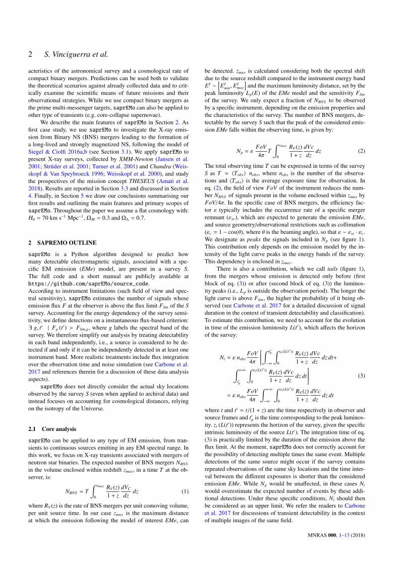
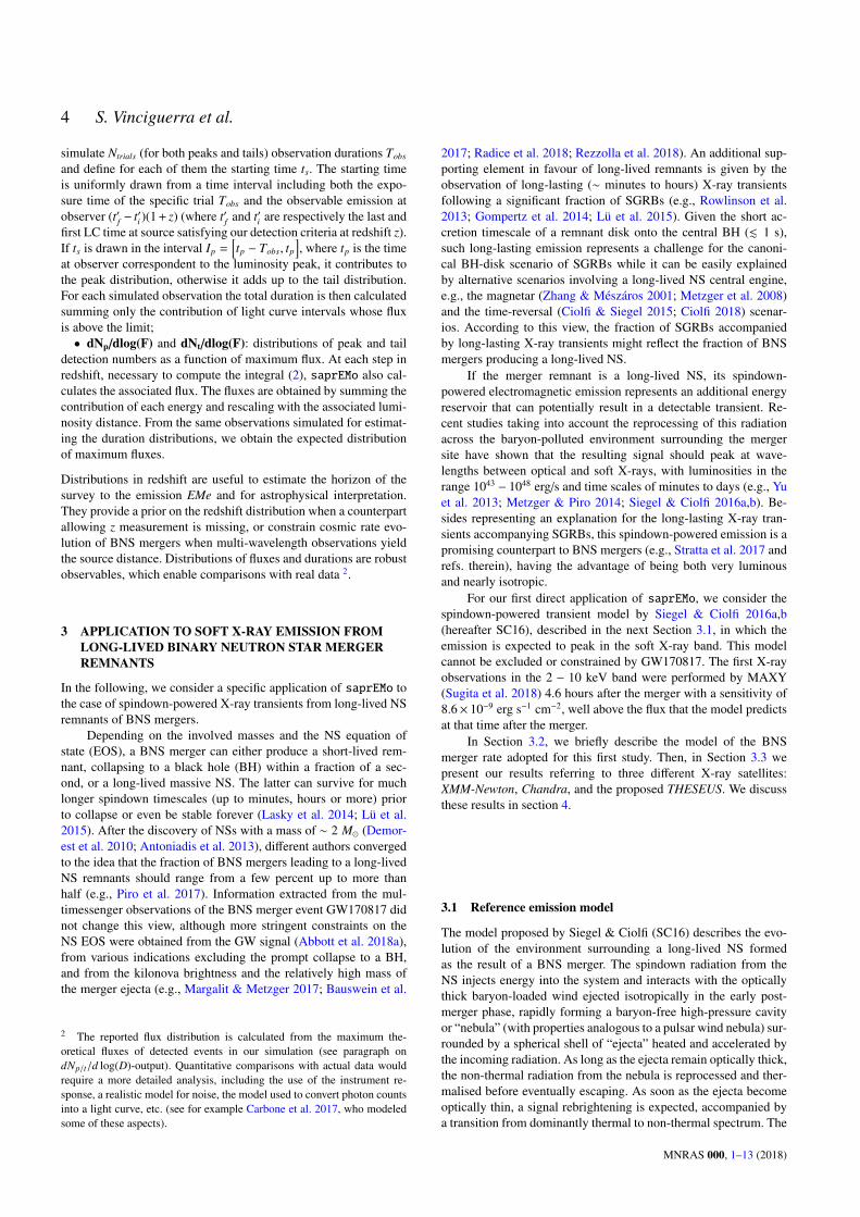
Figure 3. Light curve of the spindown-powered emission from a long-livedBNS merger remnant according to the model proposed by Siegel & Ciolfi2016a,b (corresponding to their “fiducial” case; see text). The solid curvesrepresent the contributions of different energy bands to the total light curve(dashed line).
model can also take into account the collapse of the NS to a BH atany time during the spindown phase.3
Exploring a wide range of physical parameters, Siegel & Ciolfifound that the escaping spindown-powered signal has a delayed on-set of ∼ 10 − 100 s and in most cases peaks ∼ 100 − 104 s aftermerger. Furthermore, the emission typically falls inside the soft X-ray band (peaking at ∼ 0.1 − 1 keV) and the peak luminosity is inthe range 1046 − 1048 erg s−1. In this work, we consider only onerepresentative case, corresponding to the “fiducial case” of SC16(SC16f) (this model is rescaled for the analysis in Section 3.3.2).The light curve and spectral distribution of this particular model areshown in figure 3. The main parameters of the model are as follows.The early baryon-loaded wind ejects mass isotropically at an initialrate of 5×10⁻³ M s−1, decreasing in time with a timescale of 0.5 s.The dipolar magnetic field strength at the poles of the NS is 1015 Gand the initial rotational energy of the NS is 5× 1052 erg (∼ ms ini-tial spin period). Moreover, in this case the remnant evolves withoutcollapsing to a BH. In figure 3 we can distinguish two importanttransitions. The first, around ∼ 10 s, marks the end of the earlybaryon wind phase and the beginning of the spindown phase. Thesecond, at several times 104 s, corresponds to the time when theejecta become optically thin. While the emission described by theabove model is essentially isotropic, allowing us to set εc ∼ 1,only a fraction of BNS mergers εLLNS is expected to generate along-lived neutron star. The value of this fraction mainly dependson the unknown NS EOS and distribution of component masses.Here, we assume for simplicity a one-to-one correspondence be-tween the fraction εLLNS and the fraction of SGRBs accompaniedby a long-lasting X-ray transient (i.e. extended emission and/or X-ray plateau). Following the analysis presented in Rowlinson et al.2013, we set εLLNS to 50%.
Once we assign εsr = εLLNS , the resulting total efficiency ofthe emission is ε ∼ εsr · εc = 50%.
3 We refer to Siegel & Ciolfi 2016a,b and Ciolfi 2016 for a detailed dis-cussion of the model and its current limitations.
3.2 BNS merger rate model
The dependence of the BNS merger rate on redshift is poorly ob-servationally constrained. Several models based on different as-sumptions have been proposed. For the present work we consider4 different rate models, a simplified (default) case and three furtherastrophysically-motivated scenarios:
DEFAULT : a constant BNS merger rate per unit comovingvolume per unit source time in the range RV (z) = [100 −10000] Gpc−3yr−1, extending up to a maximum redshift of z = 6;D2013 : the Monte Carlo population synthesis model of Dominik
et al. 2013 (their cosmological standard model, high-end metallic-ity scenario Belczynski et al. 2013.);G2016 : the analytic approximation based on SGRB observations
described in eq. (12) of Ghirlanda et al. 2016 (adopting the averagevalue of the parameter reported for case a with an opening angle of4.5 deg);MD2014 : the analytic prescription for the star formation history
proposed by Madau & Dickinson 2014 convolved with a probabil-ity distribution of delay times between formation and merger givenby the power low P(tdel) ∝ t−1
del, with a minimum delay time of 20 ×106 yr, normalised to the local BNS merger rate of 1540 Gpc−3yr−1,as estimated with GW170817 (1540+3200
−1220 Gpc−3yr−1 median and un-certainties at 90% probability, Abbott et al. 2017a).
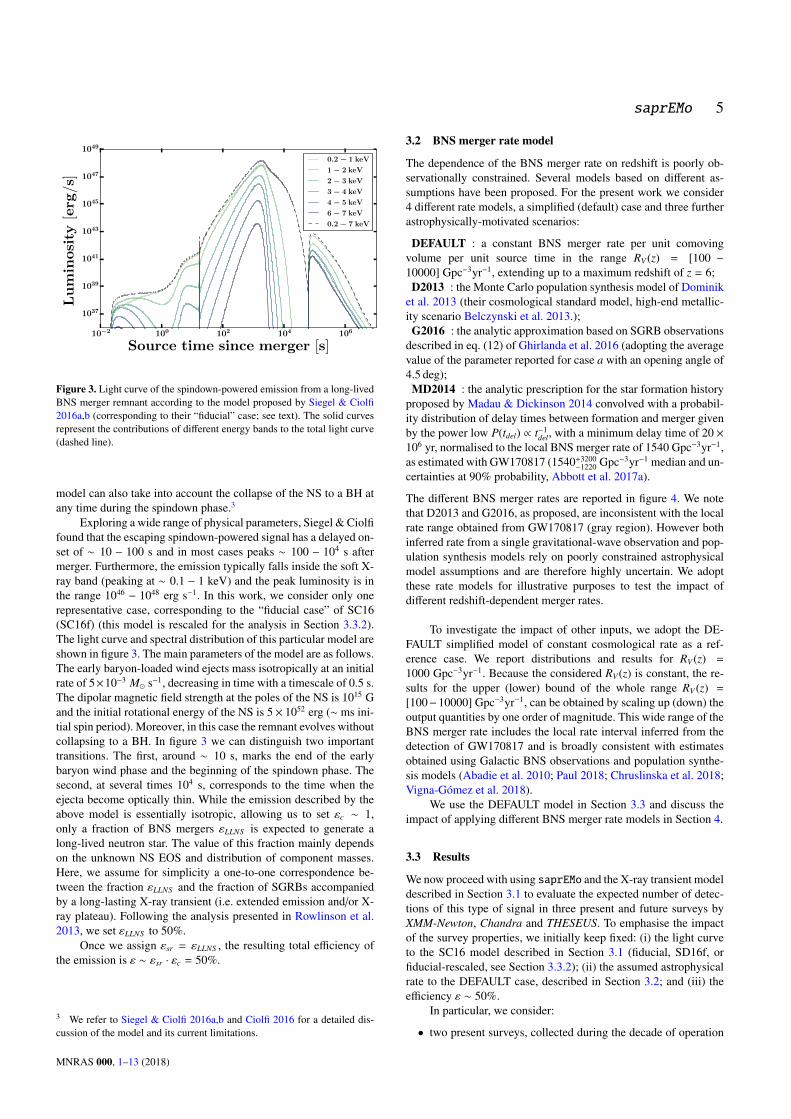
The different BNS merger rates are reported in figure 4. We notethat D2013 and G2016, as proposed, are inconsistent with the localrate range obtained from GW170817 (gray region). However bothinferred rate from a single gravitational-wave observation and pop-ulation synthesis models rely on poorly constrained astrophysicalmodel assumptions and are therefore highly uncertain. We adoptthese rate models for illustrative purposes to test the impact ofdifferent redshift-dependent merger rates.
To investigate the impact of other inputs, we adopt the DE-FAULT simplified model of constant cosmological rate as a ref-erence case. We report distributions and results for RV (z) =
1000 Gpc−3yr−1. Because the considered RV (z) is constant, the re-sults for the upper (lower) bound of the whole range RV (z) =
[100−10000] Gpc−3yr−1, can be obtained by scaling up (down) theoutput quantities by one order of magnitude. This wide range of theBNS merger rate includes the local rate interval inferred from thedetection of GW170817 and is broadly consistent with estimatesobtained using Galactic BNS observations and population synthe-sis models (Abadie et al. 2010; Paul 2018; Chruslinska et al. 2018;Vigna-Gómez et al. 2018).
We use the DEFAULT model in Section 3.3 and discuss theimpact of applying different BNS merger rate models in Section 4.
3.3 Results
We now proceed with using saprEMo and the X-ray transient modeldescribed in Section 3.1 to evaluate the expected number of detec-tions of this type of signal in three present and future surveys byXMM-Newton, Chandra and THESEUS. To emphasise the impactof the survey properties, we initially keep fixed: (i) the light curveto the SC16 model described in Section 3.1 (fiducial, SD16f, orfiducial-rescaled, see Section 3.3.2); (ii) the assumed astrophysicalrate to the DEFAULT case, described in Section 3.2; and (iii) theefficiency ε ∼ 50%.
In particular, we consider:
• two present surveys, collected during the decade of operation
MNRAS 000, 1–13 (2018)
6 S. Vinciguerra et al.
Figure 4. BNS merger rate as a function of redshift for different models:D2013 Dominik et al. 2013 in green, G2016 Ghirlanda et al. 2016 in blue,MD2014 Madau & Dickinson 2014 convolved with P(tdel) ∝ t−1
del in or-ange and our default constant model in violet: the solid line represents thereference rate of RV (z) = 1000 Gpc−3yr−1, while the light shadowed areaincludes the whole interval RV (z) = [100−10000] Gpc−3yr−1. The range inredshift is divided into z ≤ 1 and z > 1 to enhance the visibility of the con-straints set by the observation of GW170817 (gray area, 90% probability asreported in Abbott et al. 2017a), which only apply to the local Universe.
of XMM-Newton, to predict the expected number of detectable sig-nals in these archived data;• the Chandra Deep Field - South (CDF-S) data set to verify
whether the transient class discovered by Bauer et al. 2017 is sta-tistically consistent with the SC16 model;• 10 ks of THESEUS observations, to explore the sensitivity of
this mission concept to transients associated with BNS mergers,such as SC16f.
The main properties of the surveys are summarised in appendix B.
3.3.1 XMM-Newton
We apply saprEMo to two different collections of data obtainedby XMM-Newton; we call them SLEW and PO (Pointed Obser-vations), their characteristics are presented in the following. Thenumber of signals predicted by saprEMo are reported in table 1 4.In the case of XMM-Newton surveys, the sky locations of observa-tions have been used to estimate the impact of the absorption dueto the Milky Way (see appendix A2 for more details on our adoptedabsorption model).
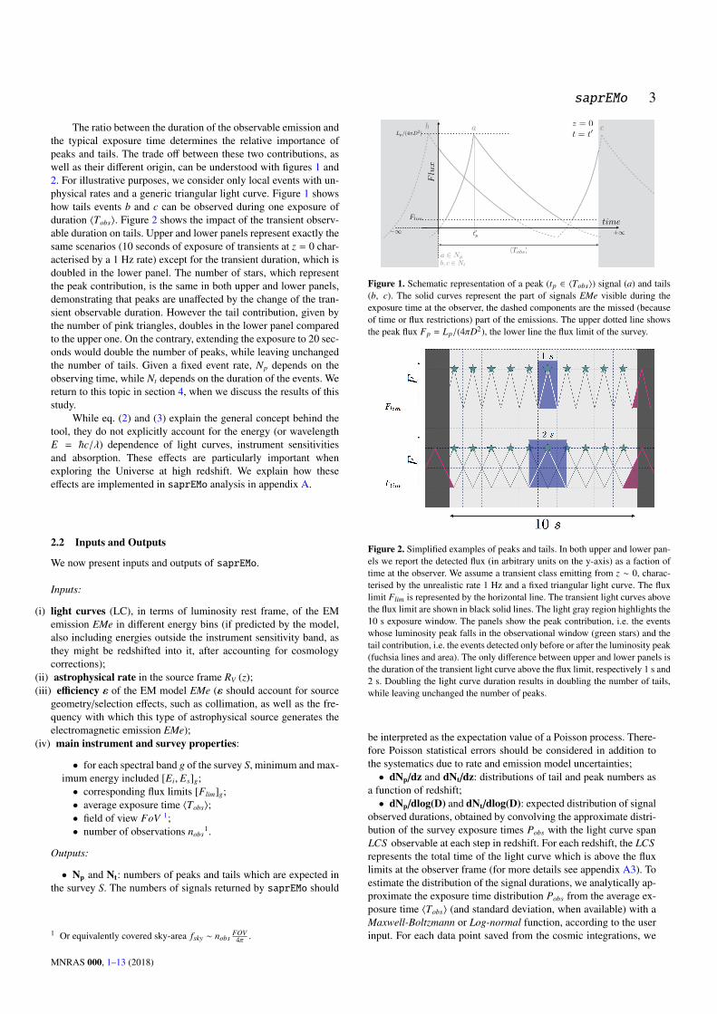
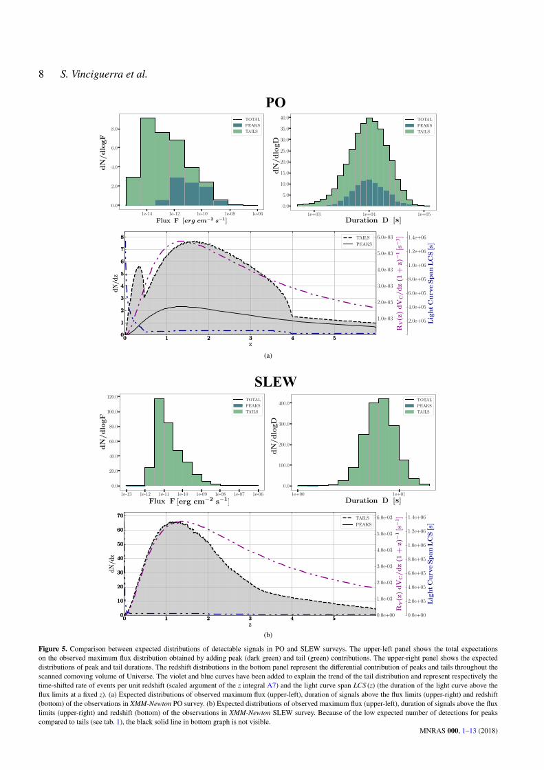
The PO survey is a collection of pointed observations made be-tween 3/2/2000 and 15/12/2016. The data belong to the XMM-Newton Serendipitous Source Catalog (3XMM DR7) (XMM-Newton SSC Consortium 2017a; Rosen et al. 2016).PO exposures are longer (typically 103 − 104 s) compared to theSLEW catalog (see following paragraph). This implies an exten-sion to lower fluxes (down to 10−15 − 10−16 erg s−1 cm−2), as fig-ure 5 (a) shows. The same figure shows that such low fluxes arehowever reached only by tails. This is because the luminosity of
4 For both the surveys, the statistical uncertainties due to the assumed Pois-son distribution are almost negligible compared to the systematics due touncertainty in the signal production efficiency ε and the BNS merger rate.
XMM-Newton Chandra THESEUS
PO SLEW CDF-S Case a Case b
Np 8 0 0.14 5 (4) 3 (2)
Nt 25 165 8 5 (3) 20 (11)
FoV [deg2] ∼ 0.2 0.08 3300
T [106s] ∼ 160 ∼ 1.06 ∼ 6.73 0.01
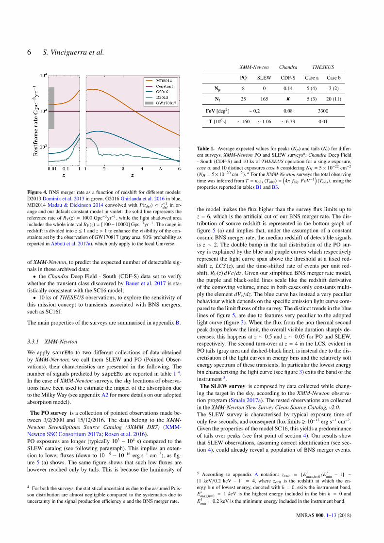
Table 1. Average expected values for peaks (Np) and tails (Nt) for differ-ent surveys. XMM-Newton PO and SLEW surveysa, Chandra Deep Field- South (CDF-S) and 10 ks of THESEUS operation for a single exposure,case a, and 10 distinct exposures case b considering NH = 5 × 10⁻²² cm−2
(NH = 5×10⁻²⁰ cm−2). a For the XMM-Newton surveys the total observingtime was inferred from T = nobs 〈Tobs〉 =
(4π fsky FoV−1
)〈Tobs〉, using the
properties reported in tables B1 and B3.
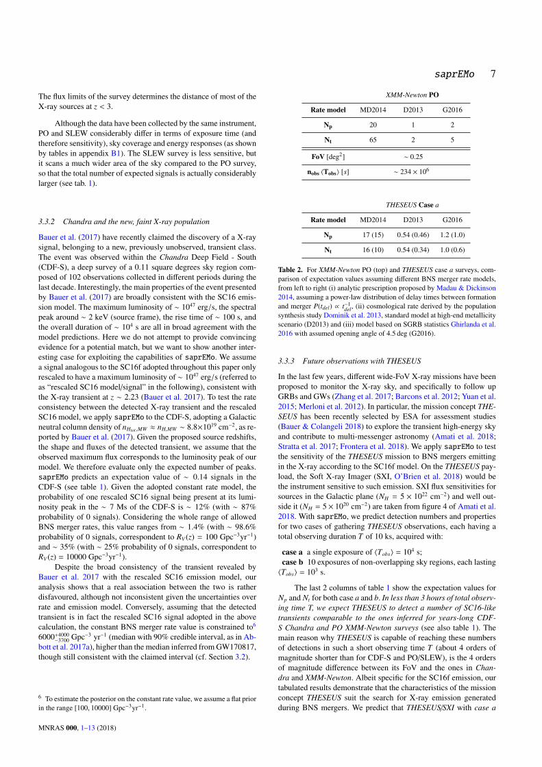
the model makes the flux higher than the survey flux limits up toz = 6, which is the artificial cut of our BNS merger rate. The dis-tribution of source redshift is represented in the bottom graph offigure 5 (a) and implies that, under the assumption of a constantcosmic BNS merger rate, the median redshift of detectable signalsis z ∼ 2. The double bump in the tail distribution of the PO sur-vey is explained by the blue and purple curves which respectivelyrepresent the light curve span above the threshold at a fixed red-shift z, LCS (z), and the time-shifted rate of events per unit red-shift, RV (z) dVc/dz. Given our simplified BNS merger rate model,the purple and black-solid lines scale like the redshift derivativeof the comoving volume, since in both cases only constants multi-ply the element dVc/dz. The blue curve has instead a very peculiarbehaviour which depends on the specific emission light curve com-pared to the limit fluxes of the survey. The distinct trends in the bluelines of figure 5, are due to features very peculiar to the adoptedlight curve (figure 3). When the flux from the non-thermal secondpeak drops below the limit, the overall visible duration sharply de-creases; this happens at z ∼ 0.5 and z ∼ 0.05 for PO and SLEW,respectively. The second turn-over at z = 4 in the LCS, evident inPO tails (gray area and dashed-black line), is instead due to the dis-cretisation of the light curves in energy bins and the relatively softenergy spectrum of these transients. In particular the lowest energybin characterising the light curve (see figure 3) exits the band of theinstrument 5.The SLEW survey is composed by data collected while chang-
ing the target in the sky, according to the XMM-Newton observa-tion program (Smale 2017a). The tested observations are collectedin the XMM-Newton Slew Survey Clean Source Catalog, v2.0.The SLEW survey is characterised by typical exposure time ofonly few seconds, and consequent flux limits & 10−13 erg s−1 cm−2.Given the properties of the model SC16, this yields a predominanceof tails over peaks (see first point of section 4). Our results showthat SLEW observations, assuming correct identification (see sec-tion 4), could already reveal a population of BNS merger events.
5 According to appendix A notation: zexit = [E′max,h=0/EImin − 1] ∼
[1 keV/0.2 keV − 1] = 4, where zexit is the redshift at which the en-ergy bin of lowest energy, denoted with h = 0, exits the instrument band,E′max,h=0 = 1 keV is the highest energy included in the bin h = 0 andEI
min = 0.2 keV is the minimum energy included in the instrument band.
MNRAS 000, 1–13 (2018)
saprEMo 7
The flux limits of the survey determines the distance of most of theX-ray sources at z < 3.
Although the data have been collected by the same instrument,PO and SLEW considerably differ in terms of exposure time (andtherefore sensitivity), sky coverage and energy responses (as shownby tables in appendix B1). The SLEW survey is less sensitive, butit scans a much wider area of the sky compared to the PO survey,so that the total number of expected signals is actually considerablylarger (see tab. 1).
3.3.2 Chandra and the new, faint X-ray population
Bauer et al. (2017) have recently claimed the discovery of a X-raysignal, belonging to a new, previously unobserved, transient class.The event was observed within the Chandra Deep Field - South(CDF-S), a deep survey of a 0.11 square degrees sky region com-posed of 102 observations collected in different periods during thelast decade. Interestingly, the main properties of the event presentedby Bauer et al. (2017) are broadly consistent with the SC16 emis-sion model. The maximum luminosity of ∼ 1047 erg/s, the spectralpeak around ∼ 2 keV (source frame), the rise time of ∼ 100 s, andthe overall duration of ∼ 104 s are all in broad agreement with themodel predictions. Here we do not attempt to provide convincingevidence for a potential match, but we want to show another inter-esting case for exploiting the capabilities of saprEMo. We assumea signal analogous to the SC16f adopted throughout this paper onlyrescaled to have a maximum luminosity of ∼ 1047 erg/s (referred toas “rescaled SC16 model/signal” in the following), consistent withthe X-ray transient at z ∼ 2.23 (Bauer et al. 2017). To test the rateconsistency between the detected X-ray transient and the rescaledSC16 model, we apply saprEMo to the CDF-S, adopting a Galacticneutral column density of nHtot ,MW ≈ nH,MW ∼ 8.8×1019 cm−2, as re-ported by Bauer et al. (2017). Given the proposed source redshifts,the shape and fluxes of the detected transient, we assume that theobserved maximum flux corresponds to the luminosity peak of ourmodel. We therefore evaluate only the expected number of peaks.saprEMo predicts an expectation value of ∼ 0.14 signals in theCDF-S (see table 1). Given the adopted constant rate model, theprobability of one rescaled SC16 signal being present at its lumi-nosity peak in the ∼ 7 Ms of the CDF-S is ∼ 12% (with ∼ 87%probability of 0 signals). Considering the whole range of allowedBNS merger rates, this value ranges from ∼ 1.4% (with ∼ 98.6%probability of 0 signals, correspondent to RV (z) = 100 Gpc−3yr−1)and ∼ 35% (with ∼ 25% probability of 0 signals, correspondent toRV (z) = 10000 Gpc−3yr−1).
Despite the broad consistency of the transient revealed byBauer et al. 2017 with the rescaled SC16 emission model, ouranalysis shows that a real association between the two is ratherdisfavoured, although not inconsistent given the uncertainties overrate and emission model. Conversely, assuming that the detectedtransient is in fact the rescaled SC16 signal adopted in the abovecalculation, the constant BNS merger rate value is constrained to6
6000+4000−3700 Gpc−3 yr−1 (median with 90% credible interval, as in Ab-
bott et al. 2017a), higher than the median inferred from GW170817,though still consistent with the claimed interval (cf. Section 3.2).
6 To estimate the posterior on the constant rate value, we assume a flat priorin the range [100, 10000] Gpc−3yr−1.
XMM-Newton PO
Rate model MD2014 D2013 G2016
Np 20 1 2
Nt 65 2 5
FoV [deg2] ∼ 0.25
nobs 〈Tobs〉 [s] ∼ 234 × 106
THESEUS Case a
Rate model MD2014 D2013 G2016
Np 17 (15) 0.54 (0.46) 1.2 (1.0)
Nt 16 (10) 0.54 (0.34) 1.0 (0.6)
Table 2. For XMM-Newton PO (top) and THESEUS case a surveys, com-parison of expectation values assuming different BNS merger rate models,from left to right (i) analytic prescription proposed by Madau & Dickinson2014, assuming a power-law distribution of delay times between formationand merger P(tdel) ∝ t−1
del, (ii) cosmological rate derived by the populationsynthesis study Dominik et al. 2013, standard model at high-end metallicityscenario (D2013) and (iii) model based on SGRB statistics Ghirlanda et al.2016 with assumed opening angle of 4.5 deg (G2016).
3.3.3 Future observations with THESEUS
In the last few years, different wide-FoV X-ray missions have beenproposed to monitor the X-ray sky, and specifically to follow upGRBs and GWs (Zhang et al. 2017; Barcons et al. 2012; Yuan et al.2015; Merloni et al. 2012). In particular, the mission concept THE-SEUS has been recently selected by ESA for assessment studies(Bauer & Colangeli 2018) to explore the transient high-energy skyand contribute to multi-messenger astronomy (Amati et al. 2018;Stratta et al. 2017; Frontera et al. 2018). We apply saprEMo to testthe sensitivity of the THESEUS mission to BNS mergers emittingin the X-ray according to the SC16f model. On the THESEUS pay-load, the Soft X-ray Imager (SXI, O’Brien et al. 2018) would bethe instrument sensitive to such emission. SXI flux sensitivities forsources in the Galactic plane (NH = 5 × 1022 cm−2) and well out-side it (NH = 5 × 1020 cm−2) are taken from figure 4 of Amati et al.2018. With saprEMo, we predict detection numbers and propertiesfor two cases of gathering THESEUS observations, each having atotal observing duration T of 10 ks, acquired with:
case a a single exposure of 〈Tobs〉 = 104 s;case b 10 exposures of non-overlapping sky regions, each lasting〈Tobs〉 = 103 s.
The last 2 columns of table 1 show the expectation values forNp and Nt for both case a and b. In less than 3 hours of total observ-ing time T, we expect THESEUS to detect a number of SC16-liketransients comparable to the ones inferred for years-long CDF-S Chandra and PO XMM-Newton surveys (see also table 1). Themain reason why THESEUS is capable of reaching these numbersof detections in such a short observing time T (about 4 orders ofmagnitude shorter than for CDF-S and PO/SLEW), is the 4 ordersof magnitude difference between its FoV and the ones in Chan-dra and XMM-Newton. Albeit specific for the SC16f emission, ourtabulated results demonstrate that the characteristics of the missionconcept THESEUS suit the search for X-ray emission generatedduring BNS mergers. We predict that THESEUS/SXI with case a
MNRAS 000, 1–13 (2018)
8 S. Vinciguerra et al.
0
1
2
3
4
5
6
7
8
dN
/dz
0 1 2 3 4 5z
0.0e+00
1.0e-03
2.0e-03
3.0e-03
4.0e-03
5.0e-03
6.0e-03
RV(z
)dV
C/dz
(1+
z)
1[s
1]
0.0e+00
2.0e+05
4.0e+05
6.0e+05
8.0e+05
1.0e+06
1.2e+06
1.4e+06
Lig
htC
urv
eSpan
LC
S[s
]
0
1
2
3
4
5
6
7
8
dN
/dz
0 1 2 3 4 5z
TAILS
PEAKS
1e-14 1e-12 1e-10 1e-08 1e-06
Flux F [erg cm2 s1]
0.0
2.0
4.0
6.0
8.0
dN
/dlo
gF
TOTAL
PEAKS
TAILS
1e-14 1e-12 1e-10 1e-08 1e-06
Flux F [erg cm2 s1]
0.0
2.0
4.0
6.0
8.0
dN
/dlo
gF
TOTAL
PEAKS
TAILS
1e+03 1e+04 1e+05 1e+06
Duration D [s]
0.0
0.5
1.0
1.5
2.0
2.5
3.0
3.5
4.0
dN
/dlo
gD
TOTAL
PEAKS
TAILS
1e+03 1e+04 1e+05 1e+06
Duration D [s]
0.0
0.5
1.0
1.5
2.0
2.5
3.0
3.5
4.0
dN
/dlo
gD
TOTAL
PEAKS
TAILS
1e+03 1e+04 1e+05 1e+06
Duration D [s]
0.0
0.5
1.0
1.5
2.0
2.5
3.0
3.5
4.0
dN
/dlo
gD
TOTAL
PEAKS
TAILS
[erg cm2 s1]<latexit sha1_base64="W184ZQ9ggQbeztYAYt3zMNpVeDE=">AAACBnicbVDLSgMxFM34rPU16lKEYBHcWGaKoMuiG5cV7AOmY8mkmTY0yQxJRijDdOPGX3HjQhG3foM7/8ZMOwttPRByOOde7r0niBlV2nG+raXlldW19dJGeXNre2fX3ttvqSiRmDRxxCLZCZAijArS1FQz0oklQTxgpB2MrnO//UCkopG40+OY+BwNBA0pRtpIPfuoy5EeBmHqETmYYH6fntWyiTKfm/lZz644VWcKuEjcglRAgUbP/ur2I5xwIjRmSCnPdWLtp0hqihnJyt1EkRjhERoQz1CBOFF+Oj0jgydG6cMwkuYJDafq744UcaXGPDCV+dJq3svF/zwv0eGln1IRJ5oIPBsUJgzqCOaZwD6VBGs2NgRhSc2uEA+RRFib5MomBHf+5EXSqlVdp+renlfqV0UcJXAIjsEpcMEFqIMb0ABNgMEjeAav4M16sl6sd+tjVrpkFT0H4A+szx+c3Zkx</latexit><latexit sha1_base64="W184ZQ9ggQbeztYAYt3zMNpVeDE=">AAACBnicbVDLSgMxFM34rPU16lKEYBHcWGaKoMuiG5cV7AOmY8mkmTY0yQxJRijDdOPGX3HjQhG3foM7/8ZMOwttPRByOOde7r0niBlV2nG+raXlldW19dJGeXNre2fX3ttvqSiRmDRxxCLZCZAijArS1FQz0oklQTxgpB2MrnO//UCkopG40+OY+BwNBA0pRtpIPfuoy5EeBmHqETmYYH6fntWyiTKfm/lZz644VWcKuEjcglRAgUbP/ur2I5xwIjRmSCnPdWLtp0hqihnJyt1EkRjhERoQz1CBOFF+Oj0jgydG6cMwkuYJDafq744UcaXGPDCV+dJq3svF/zwv0eGln1IRJ5oIPBsUJgzqCOaZwD6VBGs2NgRhSc2uEA+RRFib5MomBHf+5EXSqlVdp+renlfqV0UcJXAIjsEpcMEFqIMb0ABNgMEjeAav4M16sl6sd+tjVrpkFT0H4A+szx+c3Zkx</latexit><latexit sha1_base64="W184ZQ9ggQbeztYAYt3zMNpVeDE=">AAACBnicbVDLSgMxFM34rPU16lKEYBHcWGaKoMuiG5cV7AOmY8mkmTY0yQxJRijDdOPGX3HjQhG3foM7/8ZMOwttPRByOOde7r0niBlV2nG+raXlldW19dJGeXNre2fX3ttvqSiRmDRxxCLZCZAijArS1FQz0oklQTxgpB2MrnO//UCkopG40+OY+BwNBA0pRtpIPfuoy5EeBmHqETmYYH6fntWyiTKfm/lZz644VWcKuEjcglRAgUbP/ur2I5xwIjRmSCnPdWLtp0hqihnJyt1EkRjhERoQz1CBOFF+Oj0jgydG6cMwkuYJDafq744UcaXGPDCV+dJq3svF/zwv0eGln1IRJ5oIPBsUJgzqCOaZwD6VBGs2NgRhSc2uEA+RRFib5MomBHf+5EXSqlVdp+renlfqV0UcJXAIjsEpcMEFqIMb0ABNgMEjeAav4M16sl6sd+tjVrpkFT0H4A+szx+c3Zkx</latexit><latexit sha1_base64="W184ZQ9ggQbeztYAYt3zMNpVeDE=">AAACBnicbVDLSgMxFM34rPU16lKEYBHcWGaKoMuiG5cV7AOmY8mkmTY0yQxJRijDdOPGX3HjQhG3foM7/8ZMOwttPRByOOde7r0niBlV2nG+raXlldW19dJGeXNre2fX3ttvqSiRmDRxxCLZCZAijArS1FQz0oklQTxgpB2MrnO//UCkopG40+OY+BwNBA0pRtpIPfuoy5EeBmHqETmYYH6fntWyiTKfm/lZz644VWcKuEjcglRAgUbP/ur2I5xwIjRmSCnPdWLtp0hqihnJyt1EkRjhERoQz1CBOFF+Oj0jgydG6cMwkuYJDafq744UcaXGPDCV+dJq3svF/zwv0eGln1IRJ5oIPBsUJgzqCOaZwD6VBGs2NgRhSc2uEA+RRFib5MomBHf+5EXSqlVdp+renlfqV0UcJXAIjsEpcMEFqIMb0ABNgMEjeAav4M16sl6sd+tjVrpkFT0H4A+szx+c3Zkx</latexit>
[erg cm2 s1]<latexit sha1_base64="W184ZQ9ggQbeztYAYt3zMNpVeDE=">AAACBnicbVDLSgMxFM34rPU16lKEYBHcWGaKoMuiG5cV7AOmY8mkmTY0yQxJRijDdOPGX3HjQhG3foM7/8ZMOwttPRByOOde7r0niBlV2nG+raXlldW19dJGeXNre2fX3ttvqSiRmDRxxCLZCZAijArS1FQz0oklQTxgpB2MrnO//UCkopG40+OY+BwNBA0pRtpIPfuoy5EeBmHqETmYYH6fntWyiTKfm/lZz644VWcKuEjcglRAgUbP/ur2I5xwIjRmSCnPdWLtp0hqihnJyt1EkRjhERoQz1CBOFF+Oj0jgydG6cMwkuYJDafq744UcaXGPDCV+dJq3svF/zwv0eGln1IRJ5oIPBsUJgzqCOaZwD6VBGs2NgRhSc2uEA+RRFib5MomBHf+5EXSqlVdp+renlfqV0UcJXAIjsEpcMEFqIMb0ABNgMEjeAav4M16sl6sd+tjVrpkFT0H4A+szx+c3Zkx</latexit><latexit sha1_base64="W184ZQ9ggQbeztYAYt3zMNpVeDE=">AAACBnicbVDLSgMxFM34rPU16lKEYBHcWGaKoMuiG5cV7AOmY8mkmTY0yQxJRijDdOPGX3HjQhG3foM7/8ZMOwttPRByOOde7r0niBlV2nG+raXlldW19dJGeXNre2fX3ttvqSiRmDRxxCLZCZAijArS1FQz0oklQTxgpB2MrnO//UCkopG40+OY+BwNBA0pRtpIPfuoy5EeBmHqETmYYH6fntWyiTKfm/lZz644VWcKuEjcglRAgUbP/ur2I5xwIjRmSCnPdWLtp0hqihnJyt1EkRjhERoQz1CBOFF+Oj0jgydG6cMwkuYJDafq744UcaXGPDCV+dJq3svF/zwv0eGln1IRJ5oIPBsUJgzqCOaZwD6VBGs2NgRhSc2uEA+RRFib5MomBHf+5EXSqlVdp+renlfqV0UcJXAIjsEpcMEFqIMb0ABNgMEjeAav4M16sl6sd+tjVrpkFT0H4A+szx+c3Zkx</latexit><latexit sha1_base64="W184ZQ9ggQbeztYAYt3zMNpVeDE=">AAACBnicbVDLSgMxFM34rPU16lKEYBHcWGaKoMuiG5cV7AOmY8mkmTY0yQxJRijDdOPGX3HjQhG3foM7/8ZMOwttPRByOOde7r0niBlV2nG+raXlldW19dJGeXNre2fX3ttvqSiRmDRxxCLZCZAijArS1FQz0oklQTxgpB2MrnO//UCkopG40+OY+BwNBA0pRtpIPfuoy5EeBmHqETmYYH6fntWyiTKfm/lZz644VWcKuEjcglRAgUbP/ur2I5xwIjRmSCnPdWLtp0hqihnJyt1EkRjhERoQz1CBOFF+Oj0jgydG6cMwkuYJDafq744UcaXGPDCV+dJq3svF/zwv0eGln1IRJ5oIPBsUJgzqCOaZwD6VBGs2NgRhSc2uEA+RRFib5MomBHf+5EXSqlVdp+renlfqV0UcJXAIjsEpcMEFqIMb0ABNgMEjeAav4M16sl6sd+tjVrpkFT0H4A+szx+c3Zkx</latexit><latexit sha1_base64="W184ZQ9ggQbeztYAYt3zMNpVeDE=">AAACBnicbVDLSgMxFM34rPU16lKEYBHcWGaKoMuiG5cV7AOmY8mkmTY0yQxJRijDdOPGX3HjQhG3foM7/8ZMOwttPRByOOde7r0niBlV2nG+raXlldW19dJGeXNre2fX3ttvqSiRmDRxxCLZCZAijArS1FQz0oklQTxgpB2MrnO//UCkopG40+OY+BwNBA0pRtpIPfuoy5EeBmHqETmYYH6fntWyiTKfm/lZz644VWcKuEjcglRAgUbP/ur2I5xwIjRmSCnPdWLtp0hqihnJyt1EkRjhERoQz1CBOFF+Oj0jgydG6cMwkuYJDafq744UcaXGPDCV+dJq3svF/zwv0eGln1IRJ5oIPBsUJgzqCOaZwD6VBGs2NgRhSc2uEA+RRFib5MomBHf+5EXSqlVdp+renlfqV0UcJXAIjsEpcMEFqIMb0ABNgMEjeAav4M16sl6sd+tjVrpkFT0H4A+szx+c3Zkx</latexit>
1e-14 1e-12 1e-10 1e-08 1e-06
Flux F [erg cm2 s1]
0.0
2.0
4.0
6.0
8.0dN
/dlo
gF
TOTAL
PEAKS
TAILS
PO
1e+03 1e+04 1e+05
Duration D s[s]
0.0
5.0
10.0
15.0
20.0
25.0
30.0
35.0
40.0
dN
/dlo
gD
TOTAL
PEAKS
TAILS
0
10
20
30
40
50
60
70
dN
/dz
0 1 2 3 4 5z
0.0e+00
1.0e-03
2.0e-03
3.0e-03
4.0e-03
5.0e-03
6.0e-03
RV(z
)dV
C/dz
(1+
z)
1[s
1]
0.0e+00
2.0e+05
4.0e+05
6.0e+05
8.0e+05
1.0e+06
1.2e+06
1.4e+06
Lig
htC
urv
eSpan
LC
S[s
]
0
10
20
30
40
50
60
70
dN
/dz
0 1 2 3 4 5z
TAILS
PEAKS
1e-14 1e-12 1e-10 1e-08 1e-06
Flux F [erg cm2 s1]
1e+00
1e+02
1e+04
1e+06
1e+08
1e+10
1e+12
dN
/dF
TOTAL
PEAKS
TAILS
1e+01 1e+02
Duration D [s]
0.0
5.0
10.0
15.0
20.0
25.0
30.0
35.0
40.0
dN
/dlo
gD
TOTAL
PEAKS
TAILS
1e-14 1e-12 1e-10 1e-08 1e-06
Flux F [erg cm2 s1]
0.0
2.0
4.0
6.0
8.0
dN
/dlo
gF
TOTAL
PEAKS
TAILS
[erg cm2 s1]<latexit sha1_base64="W184ZQ9ggQbeztYAYt3zMNpVeDE=">AAACBnicbVDLSgMxFM34rPU16lKEYBHcWGaKoMuiG5cV7AOmY8mkmTY0yQxJRijDdOPGX3HjQhG3foM7/8ZMOwttPRByOOde7r0niBlV2nG+raXlldW19dJGeXNre2fX3ttvqSiRmDRxxCLZCZAijArS1FQz0oklQTxgpB2MrnO//UCkopG40+OY+BwNBA0pRtpIPfuoy5EeBmHqETmYYH6fntWyiTKfm/lZz644VWcKuEjcglRAgUbP/ur2I5xwIjRmSCnPdWLtp0hqihnJyt1EkRjhERoQz1CBOFF+Oj0jgydG6cMwkuYJDafq744UcaXGPDCV+dJq3svF/zwv0eGln1IRJ5oIPBsUJgzqCOaZwD6VBGs2NgRhSc2uEA+RRFib5MomBHf+5EXSqlVdp+renlfqV0UcJXAIjsEpcMEFqIMb0ABNgMEjeAav4M16sl6sd+tjVrpkFT0H4A+szx+c3Zkx</latexit><latexit sha1_base64="W184ZQ9ggQbeztYAYt3zMNpVeDE=">AAACBnicbVDLSgMxFM34rPU16lKEYBHcWGaKoMuiG5cV7AOmY8mkmTY0yQxJRijDdOPGX3HjQhG3foM7/8ZMOwttPRByOOde7r0niBlV2nG+raXlldW19dJGeXNre2fX3ttvqSiRmDRxxCLZCZAijArS1FQz0oklQTxgpB2MrnO//UCkopG40+OY+BwNBA0pRtpIPfuoy5EeBmHqETmYYH6fntWyiTKfm/lZz644VWcKuEjcglRAgUbP/ur2I5xwIjRmSCnPdWLtp0hqihnJyt1EkRjhERoQz1CBOFF+Oj0jgydG6cMwkuYJDafq744UcaXGPDCV+dJq3svF/zwv0eGln1IRJ5oIPBsUJgzqCOaZwD6VBGs2NgRhSc2uEA+RRFib5MomBHf+5EXSqlVdp+renlfqV0UcJXAIjsEpcMEFqIMb0ABNgMEjeAav4M16sl6sd+tjVrpkFT0H4A+szx+c3Zkx</latexit><latexit sha1_base64="W184ZQ9ggQbeztYAYt3zMNpVeDE=">AAACBnicbVDLSgMxFM34rPU16lKEYBHcWGaKoMuiG5cV7AOmY8mkmTY0yQxJRijDdOPGX3HjQhG3foM7/8ZMOwttPRByOOde7r0niBlV2nG+raXlldW19dJGeXNre2fX3ttvqSiRmDRxxCLZCZAijArS1FQz0oklQTxgpB2MrnO//UCkopG40+OY+BwNBA0pRtpIPfuoy5EeBmHqETmYYH6fntWyiTKfm/lZz644VWcKuEjcglRAgUbP/ur2I5xwIjRmSCnPdWLtp0hqihnJyt1EkRjhERoQz1CBOFF+Oj0jgydG6cMwkuYJDafq744UcaXGPDCV+dJq3svF/zwv0eGln1IRJ5oIPBsUJgzqCOaZwD6VBGs2NgRhSc2uEA+RRFib5MomBHf+5EXSqlVdp+renlfqV0UcJXAIjsEpcMEFqIMb0ABNgMEjeAav4M16sl6sd+tjVrpkFT0H4A+szx+c3Zkx</latexit><latexit sha1_base64="W184ZQ9ggQbeztYAYt3zMNpVeDE=">AAACBnicbVDLSgMxFM34rPU16lKEYBHcWGaKoMuiG5cV7AOmY8mkmTY0yQxJRijDdOPGX3HjQhG3foM7/8ZMOwttPRByOOde7r0niBlV2nG+raXlldW19dJGeXNre2fX3ttvqSiRmDRxxCLZCZAijArS1FQz0oklQTxgpB2MrnO//UCkopG40+OY+BwNBA0pRtpIPfuoy5EeBmHqETmYYH6fntWyiTKfm/lZz644VWcKuEjcglRAgUbP/ur2I5xwIjRmSCnPdWLtp0hqihnJyt1EkRjhERoQz1CBOFF+Oj0jgydG6cMwkuYJDafq744UcaXGPDCV+dJq3svF/zwv0eGln1IRJ5oIPBsUJgzqCOaZwD6VBGs2NgRhSc2uEA+RRFib5MomBHf+5EXSqlVdp+renlfqV0UcJXAIjsEpcMEFqIMb0ABNgMEjeAav4M16sl6sd+tjVrpkFT0H4A+szx+c3Zkx</latexit>
1e-12 1e-11 1e-10 1e-09 1e-08 1e-07 1e-06
Flux F [erg cm2 s1]
0.0
10.0
20.0
30.0
40.0
50.0
dN
/dlo
gF
TOTAL
PEAKS
TAILS
1e-14 1e-12 1e-10 1e-08 1e-06
Flux F [erg cm2 s1]
0.0
2.0
4.0
6.0
8.0dN
/dlo
gF
TOTAL
PEAKS
TAILS
1e+03 1e+04 1e+05 1e+06
Duration D [s]
0.0
0.5
1.0
1.5
2.0
2.5
3.0
3.5
4.0
dN
/dlo
gD
TOTAL
PEAKS
TAILS
[erg cm2 s1]<latexit sha1_base64="W184ZQ9ggQbeztYAYt3zMNpVeDE=">AAACBnicbVDLSgMxFM34rPU16lKEYBHcWGaKoMuiG5cV7AOmY8mkmTY0yQxJRijDdOPGX3HjQhG3foM7/8ZMOwttPRByOOde7r0niBlV2nG+raXlldW19dJGeXNre2fX3ttvqSiRmDRxxCLZCZAijArS1FQz0oklQTxgpB2MrnO//UCkopG40+OY+BwNBA0pRtpIPfuoy5EeBmHqETmYYH6fntWyiTKfm/lZz644VWcKuEjcglRAgUbP/ur2I5xwIjRmSCnPdWLtp0hqihnJyt1EkRjhERoQz1CBOFF+Oj0jgydG6cMwkuYJDafq744UcaXGPDCV+dJq3svF/zwv0eGln1IRJ5oIPBsUJgzqCOaZwD6VBGs2NgRhSc2uEA+RRFib5MomBHf+5EXSqlVdp+renlfqV0UcJXAIjsEpcMEFqIMb0ABNgMEjeAav4M16sl6sd+tjVrpkFT0H4A+szx+c3Zkx</latexit><latexit sha1_base64="W184ZQ9ggQbeztYAYt3zMNpVeDE=">AAACBnicbVDLSgMxFM34rPU16lKEYBHcWGaKoMuiG5cV7AOmY8mkmTY0yQxJRijDdOPGX3HjQhG3foM7/8ZMOwttPRByOOde7r0niBlV2nG+raXlldW19dJGeXNre2fX3ttvqSiRmDRxxCLZCZAijArS1FQz0oklQTxgpB2MrnO//UCkopG40+OY+BwNBA0pRtpIPfuoy5EeBmHqETmYYH6fntWyiTKfm/lZz644VWcKuEjcglRAgUbP/ur2I5xwIjRmSCnPdWLtp0hqihnJyt1EkRjhERoQz1CBOFF+Oj0jgydG6cMwkuYJDafq744UcaXGPDCV+dJq3svF/zwv0eGln1IRJ5oIPBsUJgzqCOaZwD6VBGs2NgRhSc2uEA+RRFib5MomBHf+5EXSqlVdp+renlfqV0UcJXAIjsEpcMEFqIMb0ABNgMEjeAav4M16sl6sd+tjVrpkFT0H4A+szx+c3Zkx</latexit><latexit sha1_base64="W184ZQ9ggQbeztYAYt3zMNpVeDE=">AAACBnicbVDLSgMxFM34rPU16lKEYBHcWGaKoMuiG5cV7AOmY8mkmTY0yQxJRijDdOPGX3HjQhG3foM7/8ZMOwttPRByOOde7r0niBlV2nG+raXlldW19dJGeXNre2fX3ttvqSiRmDRxxCLZCZAijArS1FQz0oklQTxgpB2MrnO//UCkopG40+OY+BwNBA0pRtpIPfuoy5EeBmHqETmYYH6fntWyiTKfm/lZz644VWcKuEjcglRAgUbP/ur2I5xwIjRmSCnPdWLtp0hqihnJyt1EkRjhERoQz1CBOFF+Oj0jgydG6cMwkuYJDafq744UcaXGPDCV+dJq3svF/zwv0eGln1IRJ5oIPBsUJgzqCOaZwD6VBGs2NgRhSc2uEA+RRFib5MomBHf+5EXSqlVdp+renlfqV0UcJXAIjsEpcMEFqIMb0ABNgMEjeAav4M16sl6sd+tjVrpkFT0H4A+szx+c3Zkx</latexit><latexit sha1_base64="W184ZQ9ggQbeztYAYt3zMNpVeDE=">AAACBnicbVDLSgMxFM34rPU16lKEYBHcWGaKoMuiG5cV7AOmY8mkmTY0yQxJRijDdOPGX3HjQhG3foM7/8ZMOwttPRByOOde7r0niBlV2nG+raXlldW19dJGeXNre2fX3ttvqSiRmDRxxCLZCZAijArS1FQz0oklQTxgpB2MrnO//UCkopG40+OY+BwNBA0pRtpIPfuoy5EeBmHqETmYYH6fntWyiTKfm/lZz644VWcKuEjcglRAgUbP/ur2I5xwIjRmSCnPdWLtp0hqihnJyt1EkRjhERoQz1CBOFF+Oj0jgydG6cMwkuYJDafq744UcaXGPDCV+dJq3svF/zwv0eGln1IRJ5oIPBsUJgzqCOaZwD6VBGs2NgRhSc2uEA+RRFib5MomBHf+5EXSqlVdp+renlfqV0UcJXAIjsEpcMEFqIMb0ABNgMEjeAav4M16sl6sd+tjVrpkFT0H4A+szx+c3Zkx</latexit>
SLEW
1e-14 1e-12 1e-10 1e-08 1e-06
Flux F [erg cm2 s1]
0.0
2.0
4.0
6.0
8.0
dN
/dlo
gF
TOTAL
PEAKS
TAILS
(a)
0
10
20
30
40
50
60
70
dN
/dz
0 1 2 3 4 5z
0.0e+00
1.0e-03
2.0e-03
3.0e-03
4.0e-03
5.0e-03
6.0e-03
RV(z
)dV
C/dz
(1+
z)
1[s
1]
0.0e+00
2.0e+05
4.0e+05
6.0e+05
8.0e+05
1.0e+06
1.2e+06
1.4e+06
Lig
htC
urv
eSpan
LC
S[s
]
0
10
20
30
40
50
60
70
dN
/dz
0 1 2 3 4 5z
TAILS
PEAKS
1e-14 1e-12 1e-10 1e-08 1e-06
Flux F [erg cm2 s1]
1e+00
1e+02
1e+04
1e+06
1e+08
1e+10
1e+12
dN
/dF
TOTAL
PEAKS
TAILS
1e+01 1e+02
Duration D [s]
0.0
5.0
10.0
15.0
20.0
25.0
30.0
35.0
40.0
dN
/dlo
gD
TOTAL
PEAKS
TAILS
1e-14 1e-12 1e-10 1e-08 1e-06
Flux F [erg cm2 s1]
0.0
2.0
4.0
6.0
8.0
dN
/dlo
gF
TOTAL
PEAKS
TAILS
[erg cm2 s1]<latexit sha1_base64="W184ZQ9ggQbeztYAYt3zMNpVeDE=">AAACBnicbVDLSgMxFM34rPU16lKEYBHcWGaKoMuiG5cV7AOmY8mkmTY0yQxJRijDdOPGX3HjQhG3foM7/8ZMOwttPRByOOde7r0niBlV2nG+raXlldW19dJGeXNre2fX3ttvqSiRmDRxxCLZCZAijArS1FQz0oklQTxgpB2MrnO//UCkopG40+OY+BwNBA0pRtpIPfuoy5EeBmHqETmYYH6fntWyiTKfm/lZz644VWcKuEjcglRAgUbP/ur2I5xwIjRmSCnPdWLtp0hqihnJyt1EkRjhERoQz1CBOFF+Oj0jgydG6cMwkuYJDafq744UcaXGPDCV+dJq3svF/zwv0eGln1IRJ5oIPBsUJgzqCOaZwD6VBGs2NgRhSc2uEA+RRFib5MomBHf+5EXSqlVdp+renlfqV0UcJXAIjsEpcMEFqIMb0ABNgMEjeAav4M16sl6sd+tjVrpkFT0H4A+szx+c3Zkx</latexit><latexit sha1_base64="W184ZQ9ggQbeztYAYt3zMNpVeDE=">AAACBnicbVDLSgMxFM34rPU16lKEYBHcWGaKoMuiG5cV7AOmY8mkmTY0yQxJRijDdOPGX3HjQhG3foM7/8ZMOwttPRByOOde7r0niBlV2nG+raXlldW19dJGeXNre2fX3ttvqSiRmDRxxCLZCZAijArS1FQz0oklQTxgpB2MrnO//UCkopG40+OY+BwNBA0pRtpIPfuoy5EeBmHqETmYYH6fntWyiTKfm/lZz644VWcKuEjcglRAgUbP/ur2I5xwIjRmSCnPdWLtp0hqihnJyt1EkRjhERoQz1CBOFF+Oj0jgydG6cMwkuYJDafq744UcaXGPDCV+dJq3svF/zwv0eGln1IRJ5oIPBsUJgzqCOaZwD6VBGs2NgRhSc2uEA+RRFib5MomBHf+5EXSqlVdp+renlfqV0UcJXAIjsEpcMEFqIMb0ABNgMEjeAav4M16sl6sd+tjVrpkFT0H4A+szx+c3Zkx</latexit><latexit sha1_base64="W184ZQ9ggQbeztYAYt3zMNpVeDE=">AAACBnicbVDLSgMxFM34rPU16lKEYBHcWGaKoMuiG5cV7AOmY8mkmTY0yQxJRijDdOPGX3HjQhG3foM7/8ZMOwttPRByOOde7r0niBlV2nG+raXlldW19dJGeXNre2fX3ttvqSiRmDRxxCLZCZAijArS1FQz0oklQTxgpB2MrnO//UCkopG40+OY+BwNBA0pRtpIPfuoy5EeBmHqETmYYH6fntWyiTKfm/lZz644VWcKuEjcglRAgUbP/ur2I5xwIjRmSCnPdWLtp0hqihnJyt1EkRjhERoQz1CBOFF+Oj0jgydG6cMwkuYJDafq744UcaXGPDCV+dJq3svF/zwv0eGln1IRJ5oIPBsUJgzqCOaZwD6VBGs2NgRhSc2uEA+RRFib5MomBHf+5EXSqlVdp+renlfqV0UcJXAIjsEpcMEFqIMb0ABNgMEjeAav4M16sl6sd+tjVrpkFT0H4A+szx+c3Zkx</latexit><latexit sha1_base64="W184ZQ9ggQbeztYAYt3zMNpVeDE=">AAACBnicbVDLSgMxFM34rPU16lKEYBHcWGaKoMuiG5cV7AOmY8mkmTY0yQxJRijDdOPGX3HjQhG3foM7/8ZMOwttPRByOOde7r0niBlV2nG+raXlldW19dJGeXNre2fX3ttvqSiRmDRxxCLZCZAijArS1FQz0oklQTxgpB2MrnO//UCkopG40+OY+BwNBA0pRtpIPfuoy5EeBmHqETmYYH6fntWyiTKfm/lZz644VWcKuEjcglRAgUbP/ur2I5xwIjRmSCnPdWLtp0hqihnJyt1EkRjhERoQz1CBOFF+Oj0jgydG6cMwkuYJDafq744UcaXGPDCV+dJq3svF/zwv0eGln1IRJ5oIPBsUJgzqCOaZwD6VBGs2NgRhSc2uEA+RRFib5MomBHf+5EXSqlVdp+renlfqV0UcJXAIjsEpcMEFqIMb0ABNgMEjeAav4M16sl6sd+tjVrpkFT0H4A+szx+c3Zkx</latexit>
1e-12 1e-11 1e-10 1e-09 1e-08 1e-07 1e-06
Flux F [erg cm2 s1]
0.0
10.0
20.0
30.0
40.0
50.0
dN
/dlo
gF
TOTAL
PEAKS
TAILS
1e-14 1e-12 1e-10 1e-08 1e-06
Flux F [erg cm2 s1]
0.0
2.0
4.0
6.0
8.0
dN
/dlo
gF
TOTAL
PEAKS
TAILS
1e+03 1e+04 1e+05 1e+06
Duration D [s]
0.0
0.5
1.0
1.5
2.0
2.5
3.0
3.5
4.0
dN
/dlo
gD
TOTAL
PEAKS
TAILS
[erg cm2 s1]<latexit sha1_base64="W184ZQ9ggQbeztYAYt3zMNpVeDE=">AAACBnicbVDLSgMxFM34rPU16lKEYBHcWGaKoMuiG5cV7AOmY8mkmTY0yQxJRijDdOPGX3HjQhG3foM7/8ZMOwttPRByOOde7r0niBlV2nG+raXlldW19dJGeXNre2fX3ttvqSiRmDRxxCLZCZAijArS1FQz0oklQTxgpB2MrnO//UCkopG40+OY+BwNBA0pRtpIPfuoy5EeBmHqETmYYH6fntWyiTKfm/lZz644VWcKuEjcglRAgUbP/ur2I5xwIjRmSCnPdWLtp0hqihnJyt1EkRjhERoQz1CBOFF+Oj0jgydG6cMwkuYJDafq744UcaXGPDCV+dJq3svF/zwv0eGln1IRJ5oIPBsUJgzqCOaZwD6VBGs2NgRhSc2uEA+RRFib5MomBHf+5EXSqlVdp+renlfqV0UcJXAIjsEpcMEFqIMb0ABNgMEjeAav4M16sl6sd+tjVrpkFT0H4A+szx+c3Zkx</latexit><latexit sha1_base64="W184ZQ9ggQbeztYAYt3zMNpVeDE=">AAACBnicbVDLSgMxFM34rPU16lKEYBHcWGaKoMuiG5cV7AOmY8mkmTY0yQxJRijDdOPGX3HjQhG3foM7/8ZMOwttPRByOOde7r0niBlV2nG+raXlldW19dJGeXNre2fX3ttvqSiRmDRxxCLZCZAijArS1FQz0oklQTxgpB2MrnO//UCkopG40+OY+BwNBA0pRtpIPfuoy5EeBmHqETmYYH6fntWyiTKfm/lZz644VWcKuEjcglRAgUbP/ur2I5xwIjRmSCnPdWLtp0hqihnJyt1EkRjhERoQz1CBOFF+Oj0jgydG6cMwkuYJDafq744UcaXGPDCV+dJq3svF/zwv0eGln1IRJ5oIPBsUJgzqCOaZwD6VBGs2NgRhSc2uEA+RRFib5MomBHf+5EXSqlVdp+renlfqV0UcJXAIjsEpcMEFqIMb0ABNgMEjeAav4M16sl6sd+tjVrpkFT0H4A+szx+c3Zkx</latexit><latexit sha1_base64="W184ZQ9ggQbeztYAYt3zMNpVeDE=">AAACBnicbVDLSgMxFM34rPU16lKEYBHcWGaKoMuiG5cV7AOmY8mkmTY0yQxJRijDdOPGX3HjQhG3foM7/8ZMOwttPRByOOde7r0niBlV2nG+raXlldW19dJGeXNre2fX3ttvqSiRmDRxxCLZCZAijArS1FQz0oklQTxgpB2MrnO//UCkopG40+OY+BwNBA0pRtpIPfuoy5EeBmHqETmYYH6fntWyiTKfm/lZz644VWcKuEjcglRAgUbP/ur2I5xwIjRmSCnPdWLtp0hqihnJyt1EkRjhERoQz1CBOFF+Oj0jgydG6cMwkuYJDafq744UcaXGPDCV+dJq3svF/zwv0eGln1IRJ5oIPBsUJgzqCOaZwD6VBGs2NgRhSc2uEA+RRFib5MomBHf+5EXSqlVdp+renlfqV0UcJXAIjsEpcMEFqIMb0ABNgMEjeAav4M16sl6sd+tjVrpkFT0H4A+szx+c3Zkx</latexit><latexit sha1_base64="W184ZQ9ggQbeztYAYt3zMNpVeDE=">AAACBnicbVDLSgMxFM34rPU16lKEYBHcWGaKoMuiG5cV7AOmY8mkmTY0yQxJRijDdOPGX3HjQhG3foM7/8ZMOwttPRByOOde7r0niBlV2nG+raXlldW19dJGeXNre2fX3ttvqSiRmDRxxCLZCZAijArS1FQz0oklQTxgpB2MrnO//UCkopG40+OY+BwNBA0pRtpIPfuoy5EeBmHqETmYYH6fntWyiTKfm/lZz644VWcKuEjcglRAgUbP/ur2I5xwIjRmSCnPdWLtp0hqihnJyt1EkRjhERoQz1CBOFF+Oj0jgydG6cMwkuYJDafq744UcaXGPDCV+dJq3svF/zwv0eGln1IRJ5oIPBsUJgzqCOaZwD6VBGs2NgRhSc2uEA+RRFib5MomBHf+5EXSqlVdp+renlfqV0UcJXAIjsEpcMEFqIMb0ABNgMEjeAav4M16sl6sd+tjVrpkFT0H4A+szx+c3Zkx</latexit>
SLEW
1e+00 1e+01
Duration D s[s]
0.0
100.0
200.0
300.0
400.0
dN
/dlo
gD
TOTAL
PEAKS
TAILS
1e-13 1e-12 1e-11 1e-10 1e-09 1e-08 1e-07 1e-06
Flux F [erg cm2 s1]
0.0
20.0
40.0
60.0
80.0
100.0
120.0
dN
/dlo
gF
TOTAL
PEAKS
TAILS
0
10
20
30
40
50
60
70
dN
/dz
0 1 2 3 4 5z
0.0e+00
1.0e-03
2.0e-03
3.0e-03
4.0e-03
5.0e-03
6.0e-03
RV(z
)dV
C/dz
(1+
z)
1[s
1]
0.0e+00
2.0e+05
4.0e+05
6.0e+05
8.0e+05
1.0e+06
1.2e+06
1.4e+06
Lig
htC
urv
eSpan
LC
S[s
]
0
10
20
30
40
50
60
70
dN
/dz
0 1 2 3 4 5z
TAILS
PEAKS
1e-14 1e-12 1e-10 1e-08 1e-06
Flux F [erg cm2 s1]
1e+00
1e+02
1e+04
1e+06
1e+08
1e+10
1e+12
dN
/dF
TOTAL
PEAKS
TAILS
1e+01 1e+02
Duration D [s]
0.0
5.0
10.0
15.0
20.0
25.0
30.0
35.0
40.0
dN
/dlo
gD
TOTAL
PEAKS
TAILS
1e-14 1e-12 1e-10 1e-08 1e-06
Flux F [erg cm2 s1]
0.0
2.0
4.0
6.0
8.0
dN
/dlo
gF
TOTAL
PEAKS
TAILS
[erg cm2 s1]<latexit sha1_base64="W184ZQ9ggQbeztYAYt3zMNpVeDE=">AAACBnicbVDLSgMxFM34rPU16lKEYBHcWGaKoMuiG5cV7AOmY8mkmTY0yQxJRijDdOPGX3HjQhG3foM7/8ZMOwttPRByOOde7r0niBlV2nG+raXlldW19dJGeXNre2fX3ttvqSiRmDRxxCLZCZAijArS1FQz0oklQTxgpB2MrnO//UCkopG40+OY+BwNBA0pRtpIPfuoy5EeBmHqETmYYH6fntWyiTKfm/lZz644VWcKuEjcglRAgUbP/ur2I5xwIjRmSCnPdWLtp0hqihnJyt1EkRjhERoQz1CBOFF+Oj0jgydG6cMwkuYJDafq744UcaXGPDCV+dJq3svF/zwv0eGln1IRJ5oIPBsUJgzqCOaZwD6VBGs2NgRhSc2uEA+RRFib5MomBHf+5EXSqlVdp+renlfqV0UcJXAIjsEpcMEFqIMb0ABNgMEjeAav4M16sl6sd+tjVrpkFT0H4A+szx+c3Zkx</latexit><latexit sha1_base64="W184ZQ9ggQbeztYAYt3zMNpVeDE=">AAACBnicbVDLSgMxFM34rPU16lKEYBHcWGaKoMuiG5cV7AOmY8mkmTY0yQxJRijDdOPGX3HjQhG3foM7/8ZMOwttPRByOOde7r0niBlV2nG+raXlldW19dJGeXNre2fX3ttvqSiRmDRxxCLZCZAijArS1FQz0oklQTxgpB2MrnO//UCkopG40+OY+BwNBA0pRtpIPfuoy5EeBmHqETmYYH6fntWyiTKfm/lZz644VWcKuEjcglRAgUbP/ur2I5xwIjRmSCnPdWLtp0hqihnJyt1EkRjhERoQz1CBOFF+Oj0jgydG6cMwkuYJDafq744UcaXGPDCV+dJq3svF/zwv0eGln1IRJ5oIPBsUJgzqCOaZwD6VBGs2NgRhSc2uEA+RRFib5MomBHf+5EXSqlVdp+renlfqV0UcJXAIjsEpcMEFqIMb0ABNgMEjeAav4M16sl6sd+tjVrpkFT0H4A+szx+c3Zkx</latexit><latexit sha1_base64="W184ZQ9ggQbeztYAYt3zMNpVeDE=">AAACBnicbVDLSgMxFM34rPU16lKEYBHcWGaKoMuiG5cV7AOmY8mkmTY0yQxJRijDdOPGX3HjQhG3foM7/8ZMOwttPRByOOde7r0niBlV2nG+raXlldW19dJGeXNre2fX3ttvqSiRmDRxxCLZCZAijArS1FQz0oklQTxgpB2MrnO//UCkopG40+OY+BwNBA0pRtpIPfuoy5EeBmHqETmYYH6fntWyiTKfm/lZz644VWcKuEjcglRAgUbP/ur2I5xwIjRmSCnPdWLtp0hqihnJyt1EkRjhERoQz1CBOFF+Oj0jgydG6cMwkuYJDafq744UcaXGPDCV+dJq3svF/zwv0eGln1IRJ5oIPBsUJgzqCOaZwD6VBGs2NgRhSc2uEA+RRFib5MomBHf+5EXSqlVdp+renlfqV0UcJXAIjsEpcMEFqIMb0ABNgMEjeAav4M16sl6sd+tjVrpkFT0H4A+szx+c3Zkx</latexit><latexit sha1_base64="W184ZQ9ggQbeztYAYt3zMNpVeDE=">AAACBnicbVDLSgMxFM34rPU16lKEYBHcWGaKoMuiG5cV7AOmY8mkmTY0yQxJRijDdOPGX3HjQhG3foM7/8ZMOwttPRByOOde7r0niBlV2nG+raXlldW19dJGeXNre2fX3ttvqSiRmDRxxCLZCZAijArS1FQz0oklQTxgpB2MrnO//UCkopG40+OY+BwNBA0pRtpIPfuoy5EeBmHqETmYYH6fntWyiTKfm/lZz644VWcKuEjcglRAgUbP/ur2I5xwIjRmSCnPdWLtp0hqihnJyt1EkRjhERoQz1CBOFF+Oj0jgydG6cMwkuYJDafq744UcaXGPDCV+dJq3svF/zwv0eGln1IRJ5oIPBsUJgzqCOaZwD6VBGs2NgRhSc2uEA+RRFib5MomBHf+5EXSqlVdp+renlfqV0UcJXAIjsEpcMEFqIMb0ABNgMEjeAav4M16sl6sd+tjVrpkFT0H4A+szx+c3Zkx</latexit>
1e-12 1e-11 1e-10 1e-09 1e-08 1e-07 1e-06
Flux F [erg cm2 s1]
0.0
10.0
20.0
30.0
40.0
50.0
dN
/dlo
gF
TOTAL
PEAKS
TAILS
1e-14 1e-12 1e-10 1e-08 1e-06
Flux F [erg cm2 s1]
0.0
2.0
4.0
6.0
8.0
dN
/dlo
gF
TOTAL
PEAKS
TAILS
1e+03 1e+04 1e+05 1e+06
Duration D [s]
0.0
0.5
1.0
1.5
2.0
2.5
3.0
3.5
4.0
dN
/dlo
gD
TOTAL
PEAKS
TAILS
[erg cm2 s1]<latexit sha1_base64="W184ZQ9ggQbeztYAYt3zMNpVeDE=">AAACBnicbVDLSgMxFM34rPU16lKEYBHcWGaKoMuiG5cV7AOmY8mkmTY0yQxJRijDdOPGX3HjQhG3foM7/8ZMOwttPRByOOde7r0niBlV2nG+raXlldW19dJGeXNre2fX3ttvqSiRmDRxxCLZCZAijArS1FQz0oklQTxgpB2MrnO//UCkopG40+OY+BwNBA0pRtpIPfuoy5EeBmHqETmYYH6fntWyiTKfm/lZz644VWcKuEjcglRAgUbP/ur2I5xwIjRmSCnPdWLtp0hqihnJyt1EkRjhERoQz1CBOFF+Oj0jgydG6cMwkuYJDafq744UcaXGPDCV+dJq3svF/zwv0eGln1IRJ5oIPBsUJgzqCOaZwD6VBGs2NgRhSc2uEA+RRFib5MomBHf+5EXSqlVdp+renlfqV0UcJXAIjsEpcMEFqIMb0ABNgMEjeAav4M16sl6sd+tjVrpkFT0H4A+szx+c3Zkx</latexit><latexit sha1_base64="W184ZQ9ggQbeztYAYt3zMNpVeDE=">AAACBnicbVDLSgMxFM34rPU16lKEYBHcWGaKoMuiG5cV7AOmY8mkmTY0yQxJRijDdOPGX3HjQhG3foM7/8ZMOwttPRByOOde7r0niBlV2nG+raXlldW19dJGeXNre2fX3ttvqSiRmDRxxCLZCZAijArS1FQz0oklQTxgpB2MrnO//UCkopG40+OY+BwNBA0pRtpIPfuoy5EeBmHqETmYYH6fntWyiTKfm/lZz644VWcKuEjcglRAgUbP/ur2I5xwIjRmSCnPdWLtp0hqihnJyt1EkRjhERoQz1CBOFF+Oj0jgydG6cMwkuYJDafq744UcaXGPDCV+dJq3svF/zwv0eGln1IRJ5oIPBsUJgzqCOaZwD6VBGs2NgRhSc2uEA+RRFib5MomBHf+5EXSqlVdp+renlfqV0UcJXAIjsEpcMEFqIMb0ABNgMEjeAav4M16sl6sd+tjVrpkFT0H4A+szx+c3Zkx</latexit><latexit sha1_base64="W184ZQ9ggQbeztYAYt3zMNpVeDE=">AAACBnicbVDLSgMxFM34rPU16lKEYBHcWGaKoMuiG5cV7AOmY8mkmTY0yQxJRijDdOPGX3HjQhG3foM7/8ZMOwttPRByOOde7r0niBlV2nG+raXlldW19dJGeXNre2fX3ttvqSiRmDRxxCLZCZAijArS1FQz0oklQTxgpB2MrnO//UCkopG40+OY+BwNBA0pRtpIPfuoy5EeBmHqETmYYH6fntWyiTKfm/lZz644VWcKuEjcglRAgUbP/ur2I5xwIjRmSCnPdWLtp0hqihnJyt1EkRjhERoQz1CBOFF+Oj0jgydG6cMwkuYJDafq744UcaXGPDCV+dJq3svF/zwv0eGln1IRJ5oIPBsUJgzqCOaZwD6VBGs2NgRhSc2uEA+RRFib5MomBHf+5EXSqlVdp+renlfqV0UcJXAIjsEpcMEFqIMb0ABNgMEjeAav4M16sl6sd+tjVrpkFT0H4A+szx+c3Zkx</latexit><latexit sha1_base64="W184ZQ9ggQbeztYAYt3zMNpVeDE=">AAACBnicbVDLSgMxFM34rPU16lKEYBHcWGaKoMuiG5cV7AOmY8mkmTY0yQxJRijDdOPGX3HjQhG3foM7/8ZMOwttPRByOOde7r0niBlV2nG+raXlldW19dJGeXNre2fX3ttvqSiRmDRxxCLZCZAijArS1FQz0oklQTxgpB2MrnO//UCkopG40+OY+BwNBA0pRtpIPfuoy5EeBmHqETmYYH6fntWyiTKfm/lZz644VWcKuEjcglRAgUbP/ur2I5xwIjRmSCnPdWLtp0hqihnJyt1EkRjhERoQz1CBOFF+Oj0jgydG6cMwkuYJDafq744UcaXGPDCV+dJq3svF/zwv0eGln1IRJ5oIPBsUJgzqCOaZwD6VBGs2NgRhSc2uEA+RRFib5MomBHf+5EXSqlVdp+renlfqV0UcJXAIjsEpcMEFqIMb0ABNgMEjeAav4M16sl6sd+tjVrpkFT0H4A+szx+c3Zkx</latexit>
1e+03 1e+04 1e+05 1e+06
Duration D [s]
0.0
0.5
1.0
1.5
2.0
2.5
3.0
3.5
4.0
dN
/dlo
gD
TOTAL
PEAKS
TAILS
[erg cm2 s1]<latexit sha1_base64="W184ZQ9ggQbeztYAYt3zMNpVeDE=">AAACBnicbVDLSgMxFM34rPU16lKEYBHcWGaKoMuiG5cV7AOmY8mkmTY0yQxJRijDdOPGX3HjQhG3foM7/8ZMOwttPRByOOde7r0niBlV2nG+raXlldW19dJGeXNre2fX3ttvqSiRmDRxxCLZCZAijArS1FQz0oklQTxgpB2MrnO//UCkopG40+OY+BwNBA0pRtpIPfuoy5EeBmHqETmYYH6fntWyiTKfm/lZz644VWcKuEjcglRAgUbP/ur2I5xwIjRmSCnPdWLtp0hqihnJyt1EkRjhERoQz1CBOFF+Oj0jgydG6cMwkuYJDafq744UcaXGPDCV+dJq3svF/zwv0eGln1IRJ5oIPBsUJgzqCOaZwD6VBGs2NgRhSc2uEA+RRFib5MomBHf+5EXSqlVdp+renlfqV0UcJXAIjsEpcMEFqIMb0ABNgMEjeAav4M16sl6sd+tjVrpkFT0H4A+szx+c3Zkx</latexit><latexit sha1_base64="W184ZQ9ggQbeztYAYt3zMNpVeDE=">AAACBnicbVDLSgMxFM34rPU16lKEYBHcWGaKoMuiG5cV7AOmY8mkmTY0yQxJRijDdOPGX3HjQhG3foM7/8ZMOwttPRByOOde7r0niBlV2nG+raXlldW19dJGeXNre2fX3ttvqSiRmDRxxCLZCZAijArS1FQz0oklQTxgpB2MrnO//UCkopG40+OY+BwNBA0pRtpIPfuoy5EeBmHqETmYYH6fntWyiTKfm/lZz644VWcKuEjcglRAgUbP/ur2I5xwIjRmSCnPdWLtp0hqihnJyt1EkRjhERoQz1CBOFF+Oj0jgydG6cMwkuYJDafq744UcaXGPDCV+dJq3svF/zwv0eGln1IRJ5oIPBsUJgzqCOaZwD6VBGs2NgRhSc2uEA+RRFib5MomBHf+5EXSqlVdp+renlfqV0UcJXAIjsEpcMEFqIMb0ABNgMEjeAav4M16sl6sd+tjVrpkFT0H4A+szx+c3Zkx</latexit><latexit sha1_base64="W184ZQ9ggQbeztYAYt3zMNpVeDE=">AAACBnicbVDLSgMxFM34rPU16lKEYBHcWGaKoMuiG5cV7AOmY8mkmTY0yQxJRijDdOPGX3HjQhG3foM7/8ZMOwttPRByOOde7r0niBlV2nG+raXlldW19dJGeXNre2fX3ttvqSiRmDRxxCLZCZAijArS1FQz0oklQTxgpB2MrnO//UCkopG40+OY+BwNBA0pRtpIPfuoy5EeBmHqETmYYH6fntWyiTKfm/lZz644VWcKuEjcglRAgUbP/ur2I5xwIjRmSCnPdWLtp0hqihnJyt1EkRjhERoQz1CBOFF+Oj0jgydG6cMwkuYJDafq744UcaXGPDCV+dJq3svF/zwv0eGln1IRJ5oIPBsUJgzqCOaZwD6VBGs2NgRhSc2uEA+RRFib5MomBHf+5EXSqlVdp+renlfqV0UcJXAIjsEpcMEFqIMb0ABNgMEjeAav4M16sl6sd+tjVrpkFT0H4A+szx+c3Zkx</latexit><latexit sha1_base64="W184ZQ9ggQbeztYAYt3zMNpVeDE=">AAACBnicbVDLSgMxFM34rPU16lKEYBHcWGaKoMuiG5cV7AOmY8mkmTY0yQxJRijDdOPGX3HjQhG3foM7/8ZMOwttPRByOOde7r0niBlV2nG+raXlldW19dJGeXNre2fX3ttvqSiRmDRxxCLZCZAijArS1FQz0oklQTxgpB2MrnO//UCkopG40+OY+BwNBA0pRtpIPfuoy5EeBmHqETmYYH6fntWyiTKfm/lZz644VWcKuEjcglRAgUbP/ur2I5xwIjRmSCnPdWLtp0hqihnJyt1EkRjhERoQz1CBOFF+Oj0jgydG6cMwkuYJDafq744UcaXGPDCV+dJq3svF/zwv0eGln1IRJ5oIPBsUJgzqCOaZwD6VBGs2NgRhSc2uEA+RRFib5MomBHf+5EXSqlVdp+renlfqV0UcJXAIjsEpcMEFqIMb0ABNgMEjeAav4M16sl6sd+tjVrpkFT0H4A+szx+c3Zkx</latexit>
SLEW
0
10
20
30
40
50
60
70
dN
/dz
0 1 2 3 4 5z
0.0e+00
1.0e-03
2.0e-03
3.0e-03
4.0e-03
5.0e-03
6.0e-03
RV(z
)dV
C/dz
(1+
z)
1[s
1]
0.0e+00
2.0e+05
4.0e+05
6.0e+05
8.0e+05
1.0e+06
1.2e+06
1.4e+06
Lig
htC
urv
eSpan
LC
S[s
]
0
10
20
30
40
50
60
70
dN
/dz
0 1 2 3 4 5z
TAILS
PEAKS
1e-14 1e-12 1e-10 1e-08 1e-06
Flux F [erg cm2 s1]
1e+00
1e+02
1e+04
1e+06
1e+08
1e+10
1e+12
dN
/dF
TOTAL
PEAKS
TAILS
1e+01 1e+02
Duration D [s]
0.0
5.0
10.0
15.0
20.0
25.0
30.0
35.0
40.0
dN
/dlo
gD
TOTAL
PEAKS
TAILS
1e-14 1e-12 1e-10 1e-08 1e-06
Flux F [erg cm2 s1]
0.0
2.0
4.0
6.0
8.0
dN
/dlo
gF
TOTAL
PEAKS
TAILS
[erg cm2 s1]<latexit sha1_base64="W184ZQ9ggQbeztYAYt3zMNpVeDE=">AAACBnicbVDLSgMxFM34rPU16lKEYBHcWGaKoMuiG5cV7AOmY8mkmTY0yQxJRijDdOPGX3HjQhG3foM7/8ZMOwttPRByOOde7r0niBlV2nG+raXlldW19dJGeXNre2fX3ttvqSiRmDRxxCLZCZAijArS1FQz0oklQTxgpB2MrnO//UCkopG40+OY+BwNBA0pRtpIPfuoy5EeBmHqETmYYH6fntWyiTKfm/lZz644VWcKuEjcglRAgUbP/ur2I5xwIjRmSCnPdWLtp0hqihnJyt1EkRjhERoQz1CBOFF+Oj0jgydG6cMwkuYJDafq744UcaXGPDCV+dJq3svF/zwv0eGln1IRJ5oIPBsUJgzqCOaZwD6VBGs2NgRhSc2uEA+RRFib5MomBHf+5EXSqlVdp+renlfqV0UcJXAIjsEpcMEFqIMb0ABNgMEjeAav4M16sl6sd+tjVrpkFT0H4A+szx+c3Zkx</latexit><latexit sha1_base64="W184ZQ9ggQbeztYAYt3zMNpVeDE=">AAACBnicbVDLSgMxFM34rPU16lKEYBHcWGaKoMuiG5cV7AOmY8mkmTY0yQxJRijDdOPGX3HjQhG3foM7/8ZMOwttPRByOOde7r0niBlV2nG+raXlldW19dJGeXNre2fX3ttvqSiRmDRxxCLZCZAijArS1FQz0oklQTxgpB2MrnO//UCkopG40+OY+BwNBA0pRtpIPfuoy5EeBmHqETmYYH6fntWyiTKfm/lZz644VWcKuEjcglRAgUbP/ur2I5xwIjRmSCnPdWLtp0hqihnJyt1EkRjhERoQz1CBOFF+Oj0jgydG6cMwkuYJDafq744UcaXGPDCV+dJq3svF/zwv0eGln1IRJ5oIPBsUJgzqCOaZwD6VBGs2NgRhSc2uEA+RRFib5MomBHf+5EXSqlVdp+renlfqV0UcJXAIjsEpcMEFqIMb0ABNgMEjeAav4M16sl6sd+tjVrpkFT0H4A+szx+c3Zkx</latexit><latexit sha1_base64="W184ZQ9ggQbeztYAYt3zMNpVeDE=">AAACBnicbVDLSgMxFM34rPU16lKEYBHcWGaKoMuiG5cV7AOmY8mkmTY0yQxJRijDdOPGX3HjQhG3foM7/8ZMOwttPRByOOde7r0niBlV2nG+raXlldW19dJGeXNre2fX3ttvqSiRmDRxxCLZCZAijArS1FQz0oklQTxgpB2MrnO//UCkopG40+OY+BwNBA0pRtpIPfuoy5EeBmHqETmYYH6fntWyiTKfm/lZz644VWcKuEjcglRAgUbP/ur2I5xwIjRmSCnPdWLtp0hqihnJyt1EkRjhERoQz1CBOFF+Oj0jgydG6cMwkuYJDafq744UcaXGPDCV+dJq3svF/zwv0eGln1IRJ5oIPBsUJgzqCOaZwD6VBGs2NgRhSc2uEA+RRFib5MomBHf+5EXSqlVdp+renlfqV0UcJXAIjsEpcMEFqIMb0ABNgMEjeAav4M16sl6sd+tjVrpkFT0H4A+szx+c3Zkx</latexit><latexit sha1_base64="W184ZQ9ggQbeztYAYt3zMNpVeDE=">AAACBnicbVDLSgMxFM34rPU16lKEYBHcWGaKoMuiG5cV7AOmY8mkmTY0yQxJRijDdOPGX3HjQhG3foM7/8ZMOwttPRByOOde7r0niBlV2nG+raXlldW19dJGeXNre2fX3ttvqSiRmDRxxCLZCZAijArS1FQz0oklQTxgpB2MrnO//UCkopG40+OY+BwNBA0pRtpIPfuoy5EeBmHqETmYYH6fntWyiTKfm/lZz644VWcKuEjcglRAgUbP/ur2I5xwIjRmSCnPdWLtp0hqihnJyt1EkRjhERoQz1CBOFF+Oj0jgydG6cMwkuYJDafq744UcaXGPDCV+dJq3svF/zwv0eGln1IRJ5oIPBsUJgzqCOaZwD6VBGs2NgRhSc2uEA+RRFib5MomBHf+5EXSqlVdp+renlfqV0UcJXAIjsEpcMEFqIMb0ABNgMEjeAav4M16sl6sd+tjVrpkFT0H4A+szx+c3Zkx</latexit>
1e-12 1e-11 1e-10 1e-09 1e-08 1e-07 1e-06
Flux F [erg cm2 s1]
0.0
10.0
20.0
30.0
40.0
50.0
dN
/dlo
gF
TOTAL
PEAKS
TAILS
1e-14 1e-12 1e-10 1e-08 1e-06
Flux F [erg cm2 s1]
0.0
2.0
4.0
6.0
8.0
dN
/dlo
gF
TOTAL
PEAKS
TAILS
1e+03 1e+04 1e+05 1e+06
Duration D [s]
0.0
0.5
1.0
1.5
2.0
2.5
3.0
3.5
4.0
dN
/dlo
gD
TOTAL
PEAKS
TAILS
[erg cm2 s1]<latexit sha1_base64="W184ZQ9ggQbeztYAYt3zMNpVeDE=">AAACBnicbVDLSgMxFM34rPU16lKEYBHcWGaKoMuiG5cV7AOmY8mkmTY0yQxJRijDdOPGX3HjQhG3foM7/8ZMOwttPRByOOde7r0niBlV2nG+raXlldW19dJGeXNre2fX3ttvqSiRmDRxxCLZCZAijArS1FQz0oklQTxgpB2MrnO//UCkopG40+OY+BwNBA0pRtpIPfuoy5EeBmHqETmYYH6fntWyiTKfm/lZz644VWcKuEjcglRAgUbP/ur2I5xwIjRmSCnPdWLtp0hqihnJyt1EkRjhERoQz1CBOFF+Oj0jgydG6cMwkuYJDafq744UcaXGPDCV+dJq3svF/zwv0eGln1IRJ5oIPBsUJgzqCOaZwD6VBGs2NgRhSc2uEA+RRFib5MomBHf+5EXSqlVdp+renlfqV0UcJXAIjsEpcMEFqIMb0ABNgMEjeAav4M16sl6sd+tjVrpkFT0H4A+szx+c3Zkx</latexit><latexit sha1_base64="W184ZQ9ggQbeztYAYt3zMNpVeDE=">AAACBnicbVDLSgMxFM34rPU16lKEYBHcWGaKoMuiG5cV7AOmY8mkmTY0yQxJRijDdOPGX3HjQhG3foM7/8ZMOwttPRByOOde7r0niBlV2nG+raXlldW19dJGeXNre2fX3ttvqSiRmDRxxCLZCZAijArS1FQz0oklQTxgpB2MrnO//UCkopG40+OY+BwNBA0pRtpIPfuoy5EeBmHqETmYYH6fntWyiTKfm/lZz644VWcKuEjcglRAgUbP/ur2I5xwIjRmSCnPdWLtp0hqihnJyt1EkRjhERoQz1CBOFF+Oj0jgydG6cMwkuYJDafq744UcaXGPDCV+dJq3svF/zwv0eGln1IRJ5oIPBsUJgzqCOaZwD6VBGs2NgRhSc2uEA+RRFib5MomBHf+5EXSqlVdp+renlfqV0UcJXAIjsEpcMEFqIMb0ABNgMEjeAav4M16sl6sd+tjVrpkFT0H4A+szx+c3Zkx</latexit><latexit sha1_base64="W184ZQ9ggQbeztYAYt3zMNpVeDE=">AAACBnicbVDLSgMxFM34rPU16lKEYBHcWGaKoMuiG5cV7AOmY8mkmTY0yQxJRijDdOPGX3HjQhG3foM7/8ZMOwttPRByOOde7r0niBlV2nG+raXlldW19dJGeXNre2fX3ttvqSiRmDRxxCLZCZAijArS1FQz0oklQTxgpB2MrnO//UCkopG40+OY+BwNBA0pRtpIPfuoy5EeBmHqETmYYH6fntWyiTKfm/lZz644VWcKuEjcglRAgUbP/ur2I5xwIjRmSCnPdWLtp0hqihnJyt1EkRjhERoQz1CBOFF+Oj0jgydG6cMwkuYJDafq744UcaXGPDCV+dJq3svF/zwv0eGln1IRJ5oIPBsUJgzqCOaZwD6VBGs2NgRhSc2uEA+RRFib5MomBHf+5EXSqlVdp+renlfqV0UcJXAIjsEpcMEFqIMb0ABNgMEjeAav4M16sl6sd+tjVrpkFT0H4A+szx+c3Zkx</latexit><latexit sha1_base64="W184ZQ9ggQbeztYAYt3zMNpVeDE=">AAACBnicbVDLSgMxFM34rPU16lKEYBHcWGaKoMuiG5cV7AOmY8mkmTY0yQxJRijDdOPGX3HjQhG3foM7/8ZMOwttPRByOOde7r0niBlV2nG+raXlldW19dJGeXNre2fX3ttvqSiRmDRxxCLZCZAijArS1FQz0oklQTxgpB2MrnO//UCkopG40+OY+BwNBA0pRtpIPfuoy5EeBmHqETmYYH6fntWyiTKfm/lZz644VWcKuEjcglRAgUbP/ur2I5xwIjRmSCnPdWLtp0hqihnJyt1EkRjhERoQz1CBOFF+Oj0jgydG6cMwkuYJDafq744UcaXGPDCV+dJq3svF/zwv0eGln1IRJ5oIPBsUJgzqCOaZwD6VBGs2NgRhSc2uEA+RRFib5MomBHf+5EXSqlVdp+renlfqV0UcJXAIjsEpcMEFqIMb0ABNgMEjeAav4M16sl6sd+tjVrpkFT0H4A+szx+c3Zkx</latexit>
1e+03 1e+04 1e+05 1e+06
Duration D [s]
0.0
0.5
1.0
1.5
2.0
2.5
3.0
3.5
4.0
dN
/dlo
gD
TOTAL
PEAKS
TAILS
[erg cm2 s1]<latexit sha1_base64="W184ZQ9ggQbeztYAYt3zMNpVeDE=">AAACBnicbVDLSgMxFM34rPU16lKEYBHcWGaKoMuiG5cV7AOmY8mkmTY0yQxJRijDdOPGX3HjQhG3foM7/8ZMOwttPRByOOde7r0niBlV2nG+raXlldW19dJGeXNre2fX3ttvqSiRmDRxxCLZCZAijArS1FQz0oklQTxgpB2MrnO//UCkopG40+OY+BwNBA0pRtpIPfuoy5EeBmHqETmYYH6fntWyiTKfm/lZz644VWcKuEjcglRAgUbP/ur2I5xwIjRmSCnPdWLtp0hqihnJyt1EkRjhERoQz1CBOFF+Oj0jgydG6cMwkuYJDafq744UcaXGPDCV+dJq3svF/zwv0eGln1IRJ5oIPBsUJgzqCOaZwD6VBGs2NgRhSc2uEA+RRFib5MomBHf+5EXSqlVdp+renlfqV0UcJXAIjsEpcMEFqIMb0ABNgMEjeAav4M16sl6sd+tjVrpkFT0H4A+szx+c3Zkx</latexit><latexit sha1_base64="W184ZQ9ggQbeztYAYt3zMNpVeDE=">AAACBnicbVDLSgMxFM34rPU16lKEYBHcWGaKoMuiG5cV7AOmY8mkmTY0yQxJRijDdOPGX3HjQhG3foM7/8ZMOwttPRByOOde7r0niBlV2nG+raXlldW19dJGeXNre2fX3ttvqSiRmDRxxCLZCZAijArS1FQz0oklQTxgpB2MrnO//UCkopG40+OY+BwNBA0pRtpIPfuoy5EeBmHqETmYYH6fntWyiTKfm/lZz644VWcKuEjcglRAgUbP/ur2I5xwIjRmSCnPdWLtp0hqihnJyt1EkRjhERoQz1CBOFF+Oj0jgydG6cMwkuYJDafq744UcaXGPDCV+dJq3svF/zwv0eGln1IRJ5oIPBsUJgzqCOaZwD6VBGs2NgRhSc2uEA+RRFib5MomBHf+5EXSqlVdp+renlfqV0UcJXAIjsEpcMEFqIMb0ABNgMEjeAav4M16sl6sd+tjVrpkFT0H4A+szx+c3Zkx</latexit><latexit sha1_base64="W184ZQ9ggQbeztYAYt3zMNpVeDE=">AAACBnicbVDLSgMxFM34rPU16lKEYBHcWGaKoMuiG5cV7AOmY8mkmTY0yQxJRijDdOPGX3HjQhG3foM7/8ZMOwttPRByOOde7r0niBlV2nG+raXlldW19dJGeXNre2fX3ttvqSiRmDRxxCLZCZAijArS1FQz0oklQTxgpB2MrnO//UCkopG40+OY+BwNBA0pRtpIPfuoy5EeBmHqETmYYH6fntWyiTKfm/lZz644VWcKuEjcglRAgUbP/ur2I5xwIjRmSCnPdWLtp0hqihnJyt1EkRjhERoQz1CBOFF+Oj0jgydG6cMwkuYJDafq744UcaXGPDCV+dJq3svF/zwv0eGln1IRJ5oIPBsUJgzqCOaZwD6VBGs2NgRhSc2uEA+RRFib5MomBHf+5EXSqlVdp+renlfqV0UcJXAIjsEpcMEFqIMb0ABNgMEjeAav4M16sl6sd+tjVrpkFT0H4A+szx+c3Zkx</latexit><latexit sha1_base64="W184ZQ9ggQbeztYAYt3zMNpVeDE=">AAACBnicbVDLSgMxFM34rPU16lKEYBHcWGaKoMuiG5cV7AOmY8mkmTY0yQxJRijDdOPGX3HjQhG3foM7/8ZMOwttPRByOOde7r0niBlV2nG+raXlldW19dJGeXNre2fX3ttvqSiRmDRxxCLZCZAijArS1FQz0oklQTxgpB2MrnO//UCkopG40+OY+BwNBA0pRtpIPfuoy5EeBmHqETmYYH6fntWyiTKfm/lZz644VWcKuEjcglRAgUbP/ur2I5xwIjRmSCnPdWLtp0hqihnJyt1EkRjhERoQz1CBOFF+Oj0jgydG6cMwkuYJDafq744UcaXGPDCV+dJq3svF/zwv0eGln1IRJ5oIPBsUJgzqCOaZwD6VBGs2NgRhSc2uEA+RRFib5MomBHf+5EXSqlVdp+renlfqV0UcJXAIjsEpcMEFqIMb0ABNgMEjeAav4M16sl6sd+tjVrpkFT0H4A+szx+c3Zkx</latexit>
SLEW
(b)
Figure 5. Comparison between expected distributions of detectable signals in PO and SLEW surveys. The upper-left panel shows the total expectationson the observed maximum flux distribution obtained by adding peak (dark green) and tail (green) contributions. The upper-right panel shows the expecteddistributions of peak and tail durations. The redshift distributions in the bottom panel represent the differential contribution of peaks and tails throughout thescanned comoving volume of Universe. The violet and blue curves have been added to explain the trend of the tail distribution and represent respectively thetime-shifted rate of events per unit redshift (scaled argument of the z integral A7) and the light curve span LCS (z) (the duration of the light curve above theflux limits at a fixed z). (a) Expected distributions of observed maximum flux (upper-left), duration of signals above the flux limits (upper-right) and redshift(bottom) of the observations in XMM-Newton PO survey. (b) Expected distributions of observed maximum flux (upper-left), duration of signals above the fluxlimits (upper-right) and redshift (bottom) of the observations in XMM-Newton SLEW survey. Because of the low expected number of detections for peakscompared to tails (see tab. 1), the black solid line in bottom graph is not visible.
MNRAS 000, 1–13 (2018)
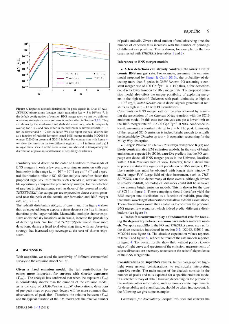
saprEMo 9
Figure 6. Expected redshift distribution for peak signals in 10 ks of THE-SEUS/SXI observations (opaque lines), assuming NH = 5 × 1020cm−2. Inthe default configuration of constant BNS merger rates we test two differentobserving strategies: case a and case b, as described in Section 3.3.3. Theyare shown by the solid-violet and dashed-fuchsia lines, which completelyoverlap for z . 2 and only differ in the maximum achieved redshift, z ∼ 3for the former and z ∼ 2 for the latter. We also report the peak distributionas a function of redshift for other tested BNS merger models: MD2014 inorange, D2013 in green and G2016 in blue. For comparison with figure 4,we show the results in the two different regimes: z > 1 in linear and z ≤ 1in logarithmic scale. For the same reason, we also add in transparency thedistribution of peaks missed because of sensitivity constraints.
sensitivity would detect on the order of hundreds to thousands ofBNS mergers in only a few years, assuming an emission with peakluminosity in the range Lp ∼ [1045 − 1048] erg cm−2 s−1 and a spec-tral distribution similar to SC16f. Our analysis therefore shows thatproposed large FoV instruments, such THESEUS, offer an incredi-ble opportunity compared to present deep surveys, for the detectionof rare but bright transients, such as those of the presented model.THESEUS/SXI-like campaigns are expected to detect events gener-ated near the peak of the cosmic star formation and BNS mergerrate, at z ∼ 1 − 3.The redshift distribution dNp/dz of case a and b in figure 6 showthat, as expected, longer exposure times decrease the flux limits andtherefore probe larger redshift. Meanwhile, multiple shorter expo-sures at distinct sky locations, as in case b, increase the probabilityof detecting tails. We find that THESEUS/SXI would make moredetections, during a fixed total observing time, with an observingstrategy that increased sky coverage at the cost of shorter expo-sures.
4 DISCUSSION
With saprEMo, we tested the sensitivity of different astronomicalsurveys to the emission model SC16f.
Given a fixed emission model, the tail contribution be-comes more important for surveys with shorter exposures〈Tobs〉. The analysis has confirmed that when the exposure 〈Tobs〉
is considerably shorter than the duration of the emission model,as is the case of XMM-Newton SLEW observations, detectionsof pre-peak rises or post-peak decays will be more common thanobservations of peak flux. Therefore the relation between 〈Tobs〉
and the typical duration of the EM model sets the relative number
of peaks and tails. Given a fixed amount of total observing time, thenumber of expected tails increases with the number of pointingsof different sky positions. This is shown, for example, by the twocases tested with THESEUS (see tables 1 and 2).
Inferences on BNS merger models
• A few detections can already constrain the lower limit ofcosmic BNS merger rate. For example, assuming the emissionmodel proposed by Siegel & Ciolfi 2016b, the probability of de-tecting more than 3 peaks in XMM-Newton PO assuming a con-stant merger rate of 100 Gp−3yr−1 is < 1%; thus, a few detectionscould set a lower limit on the BNS merger rate. The proposed emis-sion model also offers the unique possibility of exploring merg-ers in the high-redshift Universe: with peak luminosity as high as∼ 1048 erg/s, XMM-Newton could detect signals generated at red-shifts as high as z ∼ 15 with PO sensitivities.Constraints on BNS merger rate can be also obtained by assum-ing the association of the Chandra X-ray transient with the SC16emission model. In this case our analysis can put a lower limit onthe BNS merger rate of ∼ 2300 Gpc−3yr−1 at 90% confidence in-terval, assuming a constant rate up to z ∼ 6. The peak luminosityof the rescaled SC16 emission is indeed bright enough to actuallybe detectable by Chandra up to z ∼ 6, even after accounting for theMilky Way absorption.• Larger PO-like or THESEUS surveys will probe RV(z) and
likely constrain also EM emission models. In the case of brightemission, as expected by SC16, saprEMo predicts that the PO cam-paign can detect all BNS merger peaks in the Universe, localisedwithin XMM-Newton’s field of view. However, table 1 shows thatto probe a statistically significant population of BNS mergers, PO-like sensitivities must be obtained with longer time window Tand/or larger FoV. Large field of view instrument, such as THE-SEUS/SXI, can also detect many of these events. Although limitedto smaller redshift, cosmological distances could still be achievedif we assume bright emission models. This is shown for the caseof SC16 in figure 6. These campaigns should therefore yield theBNS merger rate distribution as a function of redshift, providingthat multi-wavelength observations will allow redshift associations.These observations would then enable us to constrain the proposedBNS merger rate scenarios, which indeed predict different z distri-butions (see figure 6).• Redshift measurement play a fundamental role for break-
ing the degeneracy between emission parameters and rate mod-els. We apply saprEMo to the PO and THESEUS cases, case a, forthe three scenarios introduced in section 3.2: D2013, G2016 andMD2014 (see figure 4). The absolute expectation values reportedin table 2 and figure 6 , reflect the trend of the rate models reportedin figure 4. The overall results show that, without perfect knowl-edge of light curve and spectrum of the emission, measurements ofsource distances are necessary to constrain the redshift dependenceof the BNS merger rate.
Considerations on saprEMo’s results. In this paragraph we high-light some general considerations, to realistically interpretingsaprEMo results. The main output of the analysis consists in thenumber of peaks and tails expected for a specific emission modelin a selected survey of data. However, depending on the purpose ofthe analysis, other information, such as more accurate requirementsfor detectability and classification, should be taken into account. Inthe following we give some examples.
Challenges for detectability: despite this does not concern the
MNRAS 000, 1–13 (2018)
10 S. Vinciguerra et al.
results presented in the previous session, short transients in longexposure observations can be lost in the integrated background flux.To overcome this issue, targeted analyses might be required (seefor e.g. the work of EXTraS group De Luca, A 2014 De Luca et al.2016 for detection of ∼ 102 s-lasting transients in PO).
Challenges for classifications: because of their definition, wegenerally expect durations and fluxes of tails to extend to lowervalues compared to the peak ones (as shown in figure 5 (a)). Thisgenerally worsen the performances of signal classifications andidentification among more common phenomena. In particular forour analyses, given the shape of SC16f’s light curve, tails shouldmostly appear as simple decaying signals, which can be challeng-ing to distinguish from other X-ray transients (e.g., tails of tidaldisruption events Lodato & Rossi 2011 or supernovae Dwarkadas& Gruszko 2012).The correct classification of X-ray events can also be challengedby short exposure times. This is for example the case of the SLEWsurvey, where observations typically last only few seconds. Indeedsome emission models, as SC16, predict a long-scale time evolu-tion of the emission properties which would likely result in detec-tions of dissimilar signals, challenging their association to a com-mon origin. Campaigns characterised by typically longer observa-tions, such as the XMM-Newton PO and Chandra CDF-S, are lessaffected by classification problems. The extension of the typical ex-posure time to thousands of seconds and improved spectral resolu-tion, allow for the acquisition of more informative data, simplifyingtransient identification.
5 SUMMARY AND OUTLOOK
In this study we showed some applications of our tool saprEMo; weapplied it on few present and possible future surveys, assuming aspecific emission model and cosmological BNS merger rate RV (z).In terms of multi-messenger astronomy, our results show that theluminosities predicted by the SC16 emission model can be detectedup to cosmological distances which extend much further than thehorizon of present (Aasi et al. 2016; Abbott et al. 2018b) and futuregravitational wave detectors (Sathyaprakash et al. 2012) to binaryneutron star mergers, both in the cases of current surveys, such asCDF-S and XMM-Newton PO and SLEW, and proposed missions,such as THESEUS.
saprEMo provides theoretical predictions allowing us:
• to compare predictions with actual data. E.g. we proved thatsome signals consistent with the model could already be detectedin present surveys of data such as XMM-Newton PO and SLEW;• to test potential associations. E.g. we proved that the new tran-
sient found by Bauer et al. 2017 is marginally consistent with themodel;• to assess the effectiveness of proposed mission concepts for
a specific type of signal. We illustrate the utility of saprEMo forevaluating proposed missions with a case study of THESEUS. Wedemonstrate that, with few years of operation, the large FoV ofTHESEUS/SXI could allow for the detection of up to thousandsof SC16-like signals, enabling considerable constrains on both theBNS merger rate and the emission models;• and to compare different observational strategies. saprEMo
can be used to determine advantages and disadvantages comparedto a particular emission, of adopting different observational strate-gies. With the case of THESEUS, we indeed demonstrate thatsaprEMo can compare observations characterised by different val-ues of typical exposure time 〈Tobs〉 and point out the main prop-
erties of the relative detections. In general, given a total observingtime T , different observational strategies can be applied; increas-ing the exposure time to increase the sensitivity or decreasing theexposure time to enlarge the sky coverage. The effect of adoptingdifferent exposures depends on several parameters, including bothsource and instrumental properties (such as rate, luminosity, fluxlimit dependence on exposure time, etc). In this paper, we specif-ically prove that, given THESEUS/SXI sensitivity as a function ofexposure time, 10 observations of disjoint sky areas lasting 1 kswould en-captured more SC16f-like transients than an extendedsingle pointing of 10 ks.
In general saprEMo allows us to test both survey and astrophysicalproperties. This study has mainly focused on the former, exploringthe impact of different trade offs among such properties (includingexposure time, sky localisation, and spectral sensitivity), assuminga single light curve model from SC16. However saprEMo can alsotest (and be used for inference on) astrophysical quantities such asemission duration, peak luminosity and spectra.Once the design sensitivity of Advanced gravitational-wave in-terferometers is achieved, GW detections of EM bright sources,such as GW170817, will occur more and more often and verylikely at lower SNRs. In this context of multi-messenger astron-omy, saprEMo can be used to optimize the analysis by identifyingspecific emission model. We conclude remarking that the flexibilityof the implemented methodology allows considerations of emissionmodel spanning the whole electromagnetic spectrum (e.g. kilono-vae models can also be tested). Moreover our analysis include nopriors on nature of EM sources, so that it can be applied to a widerange of astrophysical phenomena. With its analysis dedicated totreat high redshift effects, saprEMo particularly suits studies onemission of cosmological origin.
ACKNOWLEDGEMENTS
The authors thank L. Amati for his assistance with the case ofTHESEUS and for the useful comments. We thank A. Belfiore,A. De Luca, M.Marelli, D. Salvietti and A. Tiengo for the helpin understanding and interpreting XMM-Newton data. We thankR. Salvaterra for the useful suggestions and discussions. The re-search leading to these results has received funding from the Peo-ple Programme (Marie Curie Actions) of the European Union’sSeventh Framework Programme FP7/2007-2013/ (PEOPLE-2013-ITN) under REA grant agreement no. [606176]. This paper re-flects only the authors’ view and the European Union is not li-able for any use that may be made of the information containedtherein. G.S. acknowledges EGO support through a VESF fellow-ship (EGO-DIR-133-2015). This research has made use of dataobtained from XMMSL2, the Second XMM-Newton Slew SurveyCatalogue, produced by members of the XMM SOC, the EPICconsortium, and using work carried out in the context of the EX-TraS project ("Exploring the X-ray Transient and variable Sky",funded from the EU’s Seventh Framework Programme under grantagreement no. [607452]). This research has made use of data ob-tained from the 3XMM XMM-Newton serendipitous source cata-logue compiled by the 10 institutes of the XMM-Newton SurveyScience Centre selected by ESA.
REFERENCES
Aasi J., et al., 2016, Living Reviews in Relativity, 19, 1
MNRAS 000, 1–13 (2018)
saprEMo 11
Abadie J., et al., 2010, Classical and Quantum Gravity, 27, 173001Abbott B. P., et al., 2017a, Physical Review Letters, 119, 161101Abbott B. P., et al., 2017b, ApJ, 848, L12Abbott B. P., et al., 2018a, preprint, (arXiv:1805.11581)Abbott B. P., et al., 2018b, Living Reviews in Relativity, 21, 3Amati L., et al., 2018, Advances in Space Research, 62, 191Antoniadis J., et al., 2013, Science, 340, 448Barcons X., et al., 2012, preprint, (arXiv:1207.2745)Bauer M., Colangeli L., 2018, Space for Europe, https://www.esa.int/Our_Activities/Space_Science/ESA_selects_three_new_mission_concepts_for_study
Bauer F., et al., 2017, MNRAS, 467, 4841Bauswein A., Just O., Janka H.-T., Stergioulas N., 2017, ApJ, 850, L34Belczynski K., et al., 2013, Synthetic Universe, https://www.syntheticuniverse.org
Berger E., 2014, ARA&A, 52, 43Carbone D., van der Horst A. J., Wijers R. A., Rowlinson A., 2017, MN-
RAS, 465, 4106Chengalur J., Kanekar N., Roy N., 2013, MNRAS, 432, 3074Chruslinska M., et al., 2018, MNRAS, 474, 2937Ciolfi R., 2016, ApJ, 829, 72Ciolfi R., 2018, preprint, (arXiv:1804.03684)Ciolfi R., Siegel D., 2015, ApJ, 798, L36D’Avanzo P., et al., 2018, A&A, 613, L1De Luca, A 2014, Exploring the X-ray Transients and the vari-
able Sky, http://http://www.extras-fp7.eu/index.php/scientific-community/the-project
De Luca A., et al., 2016, The Universe of Digital Sky Surveys, 42, 291Demorest P., et al., 2010, Nature, 467, 1081Dobie D., et al., 2018, ApJ, 858, L15Dominik M., et al., 2013, ApJ, 779, 72Dwarkadas V., Gruszko J., 2012, MNRAS, 419, 1515ESA 2017, THE XMM-NEWTON SLEW SURVEY SOURCE CAT-
ALOGUE:XMMSL2, https://www.cosmos.esa.int/web/xmm-newton/xmmsl2-ug
Frontera F., et al., 2018, preprint, (arXiv:1802.01691)Ghirlanda G., et al., 2016, A&A, 594, A84Ghirlanda G., et al., 2018, preprint, (arXiv:1808.00469)Gompertz B., O’Brien P., Wynn G., 2014, MNRAS, 438, 240Jansen F., et al., 2001, A&A, 365, L1Kalberla P. M. W., et al., 2005, A&A, 440, 775Lasky P., et al., 2014, Phys. Rev. D, 89, 047302Lehmer B., et al., 2005, ApJS, 161, 21Lodato G., Rossi E., 2011, MNRAS, 410, 359Lü H., et al., 2015, ApJ, 805, 89Luo B., et al., 2017, ApJS, 228, 2Lyman J., et al., 2018, preprint, (arXiv:1801.02669)Madau P., Dickinson M., 2014, ARA&A, 52, 415Margalit B., Metzger B. D., 2017, ApJ, 850, L19Margutti R., et al., 2018, ApJ, 856, L18Merloni A., et al., 2012, preprint, (arXiv:1209.3114)Metzger B., Piro A., 2014, MNRAS, 439, 3916Metzger B., Quataert E., Thompson T., 2008, MNRAS, 385, 1455Mooley K., et al., 2018a, Nature, 554, 207Mooley K., et al., 2018b, Nature, 561, 355Morrison R., McCammon D., 1983, ApJ, 270, 119O’Brien P., et al., 2018, preprint, (arXiv:1802.01675)Paul D., 2018, MNRAS, 477, 4275Piro A., Giacomazzo B., Perna R., 2017, ApJ, 844, L19Radice D., Perego A., Zappa F., Bernuzzi S., 2018, ApJ, 852, L29Read A. M., Saxton R. D., 2016, EPIC-pn SLEW-specific PSF pa-
rameterisation, https://www.cosmos.esa.int/web/xmm-newton/ccf-release-notes
Rezzolla L., Most E. R., Weih L. R., 2018, ApJ, 852, L25Rosen S. R., et al., 2016, A&A, 590, A1Rowlinson A., et al., 2013, MNRAS, 430, 1061Sathyaprakash B., et al., 2012, Classical and Quantum Gravity, 29, 124013Saxton R., et al., 2008, A&A, 480, 611
Saxton R. D., et al., 2017, Optical loading in the XMM-Newton slewsource catalogue, http://xmm2.esac.esa.int/docs/documents/CAL-TN-0210-0-1.ps.gz
Siegel D., Ciolfi R., 2016a, ApJ, 819, 14Siegel D., Ciolfi R., 2016b, ApJ, 819, 15Smale A. P. the Astrophysics Science Division at NASA/GSFC t. H. E. A.
D. o. t. S. A. O., 2017b, CHANDFS7MS - Chandra Deep Field-South 7-Megasecond X-Ray Source Catalog, https://heasarc.gsfc.nasa.gov/W3Browse/chandra/chandfs7ms.html
Smale A. P. the Astrophysics Science Division at NASA/GSFC t. H. E.A. D. o. t. S. A. O., 2017a, XMMSLEWCLN - XMM-Newton SlewSurvey Clean Source Catalog, v2.0), https://heasarc.gsfc.nasa.gov/w3browse/all/xmmslewcln.html
Smale A. P. the Astrophysics Science Division at NASA/GSFC t. H. E.A. D. o. t. S. A. O., 2017c, XMMSSC - XMM-Newton SerendipitousSource Catalog (3XMM DR7 Version), https://heasarc.gsfc.nasa.gov/W3Browse/xmm-newton/xmmssc.html
Stratta G., et al., 2017, preprint, (arXiv:1712.08153)Strüder L., et al., 2001, A&A, 365, L18Sugita S., et al., 2018, Publications of the Astronomical Society of Japan,
70, 81Troja E., et al., 2017, Nature, 551, 71Turner M. J., et al., 2001, A&A, 365, L27Vigna-Gómez A., et al., 2018, MNRAS, 481, 4009Weisskopf M. C., Van Speybroeck L., 1996, Proc. SPIE, 2805, 2Weisskopf M. C., Tananbaum H. D., Van Speybroeck L. P., O’Dell S. L.,
2000, Proc. SPIE, 4012, 2Willingale R., et al., 2013, MNRAS, 431, 394XMM-Newton SSC Consortium 2017c, 3XMM-DR7, http://xmmssc.irap.omp.eu/Catalogue/3XMM-DR7/3XMM_DR7.html
XMM-Newton SSC Consortium 2017b, Table 2.1: A list of all9710 observations and exposures used for the 3XMM-DR7 sourcedetection, http://xmmssc.irap.omp.eu/Catalogue/3XMM-DR7/3xmmdr7_obslist.html
XMM-Newton SSC Consortium 2017a, XMMSSC - XMM-NewtonSerendipitous Source Catalog (3XMM DR7 Version), https://heasarc.gsfc.nasa.gov/w3browse/all/xmmssc.html
Yu Y., Zhang B., Gao H., 2013, ApJ, 776, L40Yuan W., et al., 2015, preprint (arXiv:1506.07735)Zhang B., Mészáros P., 2001, ApJ, 552, L35Zhang S. N., et al., 2017, Proc. SPIE, 9905, 9905
APPENDIX A: SAPREMO FEATURES
A1 Redshift / K-correction
To evaluate if the emission is visible in the g band of the instru-ment, we need to calculate the fraction of source light curve whichcontributes to the flux in the g band at the observer. Here we denoteeach energy band [EI
min, EImax]g with the label g; we use [EI
min, EImax]
without subscripts for the whole range of operation.We assume a set of light curves [Lh(t′)]hmax
h=0 , where each elementLh(t′) represents the emission in the source frame within a fixed henergy bin [E′min, E
′max]h. The redshifted energy bin h, associated to
the light-curve element Lh(t′), might only partially overlap with aninstrumental energy bin g. To consider only the part of the light-curve which contributes to the emission visible in the g energy bin,we calculate the fraction of the h energy bin that falls into the gband and assume the energy is uniform across its intrinsic spec-trum. Therefore for each numerical step in z, we calculate the emis-sion contribution to each g band:
Lg(t′, z) =
hmax∑h=0
Lh(t′)whg(z) (A1)
MNRAS 000, 1–13 (2018)
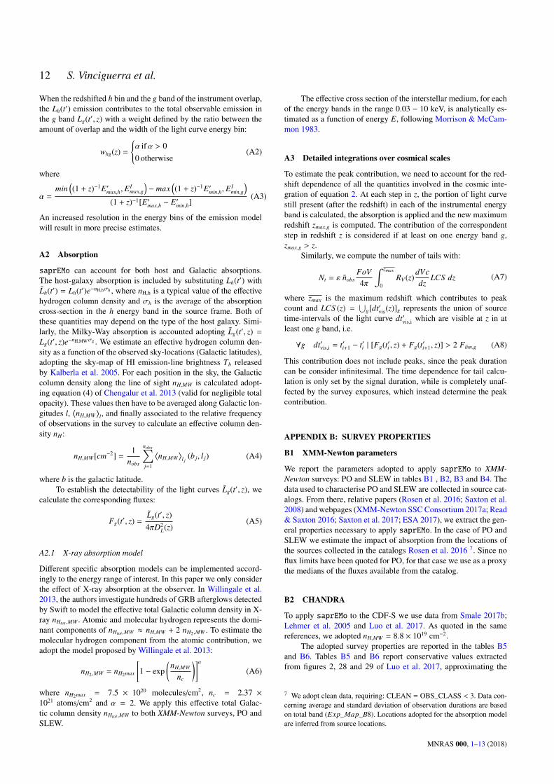
12 S. Vinciguerra et al.
When the redshifted h bin and the g band of the instrument overlap,the Lh(t′) emission contributes to the total observable emission inthe g band Lg(t′, z) with a weight defined by the ratio between theamount of overlap and the width of the light curve energy bin:
whg(z) =
α ifα > 00 otherwise
(A2)
where
α =min
((1 + z)−1E′max,h, E
Imax,g
)− max
((1 + z)−1E′min,h, E
Imin,g
)(1 + z)−1[E′max,h − E′min,h]
(A3)
An increased resolution in the energy bins of the emission modelwill result in more precise estimates.
A2 Absorption
saprEMo can account for both host and Galactic absorptions.The host-galaxy absorption is included by substituting Lh(t′) withLh(t′) = Lh(t′)e−nH,hσh , where nH,h is a typical value of the effectivehydrogen column density and σh is the average of the absorptioncross-section in the h energy band in the source frame. Both ofthese quantities may depend on the type of the host galaxy. Simi-larly, the Milky-Way absorption is accounted adopting Lg(t′, z) =
Lg(t′, z)e−nH,MWσg . We estimate an effective hydrogen column den-sity as a function of the observed sky-locations (Galactic latitudes),adopting the sky-map of HI emission-line brightness Tb releasedby Kalberla et al. 2005. For each position in the sky, the Galacticcolumn density along the line of sight nH,MW is calculated adopt-ing equation (4) of Chengalur et al. 2013 (valid for negligible totalopacity). These values then have to be averaged along Galactic lon-gitudes l,
⟨nH,MW
⟩l, and finally associated to the relative frequency
of observations in the survey to calculate an effective column den-sity nH :
nH,MW [cm−2] =1
nobs
nobs∑j=1
⟨nH,MW
⟩l j
(b j, l j) (A4)
where b is the galactic latitude.To establish the detectability of the light curves Lg(t′, z), we
calculate the corresponding fluxes:
Fg(t′, z) =Lg(t′, z)4πD2
L(z)(A5)
A2.1 X-ray absorption model
Different specific absorption models can be implemented accord-ingly to the energy range of interest. In this paper we only considerthe effect of X-ray absorption at the observer. In Willingale et al.2013, the authors investigate hundreds of GRB afterglows detectedby Swift to model the effective total Galactic column density in X-ray nHtot ,MW . Atomic and molecular hydrogen represents the domi-nant components of nHtot ,MW ≈ nH,MW + 2 nH2 ,MW . To estimate themolecular hydrogen component from the atomic contribution, weadopt the model proposed by Willingale et al. 2013:
nH2 ,MW = nH2max
[1 − exp
(nH,MW
nc
)]α(A6)
where nH2max = 7.5 × 10²⁰ molecules/cm2, nc = 2.37 ×10²¹ atoms/cm2 and α = 2. We apply this effective total Galac-tic column density nHtot ,MW to both XMM-Newton surveys, PO andSLEW.
The effective cross section of the interstellar medium, for eachof the energy bands in the range 0.03 − 10 keV, is analytically es-timated as a function of energy E, following Morrison & McCam-mon 1983.
A3 Detailed integrations over cosmical scales
To estimate the peak contribution, we need to account for the red-shift dependence of all the quantities involved in the cosmic inte-gration of equation 2. At each step in z, the portion of light curvestill present (after the redshift) in each of the instrumental energyband is calculated, the absorption is applied and the new maximumredshift zmax,g is computed. The contribution of the correspondentstep in redshift z is considered if at least on one energy band g,zmax,g > z.
Similarly, we compute the number of tails with:
Nt = ε nobsFoV4π
∫ zmax
0RV (z)
dVcdz
LCS dz (A7)
where zmax is the maximum redshift which contributes to peakcount and LCS (z) =
⋃g[dt′vis(z)]g represents the union of source
time-intervals of the light curve dt′vis,i which are visible at z in atleast one g band, i.e.
∀g dt′vis,i = t′i+1 − t′i | [Fg(t′i , z) + Fg(t′i+1, z)] > 2 Flim,g (A8)
This contribution does not include peaks, since the peak durationcan be consider infinitesimal. The time dependence for tail calcu-lation is only set by the signal duration, while is completely unaf-fected by the survey exposures, which instead determine the peakcontribution.
APPENDIX B: SURVEY PROPERTIES
B1 XMM-Newton parameters
We report the parameters adopted to apply saprEMo to XMM-Newton surveys: PO and SLEW in tables B1 , B2, B3 and B4. Thedata used to characterise PO and SLEW are collected in source cat-alogs. From there, relative papers (Rosen et al. 2016; Saxton et al.2008) and webpages (XMM-Newton SSC Consortium 2017a; Read& Saxton 2016; Saxton et al. 2017; ESA 2017), we extract the gen-eral properties necessary to apply saprEMo. In the case of PO andSLEW we estimate the impact of absorption from the locations ofthe sources collected in the catalogs Rosen et al. 2016 7. Since noflux limits have been quoted for PO, for that case we use as a proxythe medians of the fluxes available from the catalog.
B2 CHANDRA
To apply saprEMo to the CDF-S we use data from Smale 2017b;Lehmer et al. 2005 and Luo et al. 2017. As quoted in the samereferences, we adopted nH,MW = 8.8 × 1019 cm−2.
The adopted survey properties are reported in the tables B5and B6. Tables B5 and B6 report conservative values extractedfrom figures 2, 28 and 29 of Luo et al. 2017, approximating the
7 We adopt clean data, requiring: CLEAN = OBS_CLASS < 3. Data con-cerning average and standard deviation of observation durations are basedon total band (Exp_Map_B8). Locations adopted for the absorption modelare inferred from source locations.
MNRAS 000, 1–13 (2018)
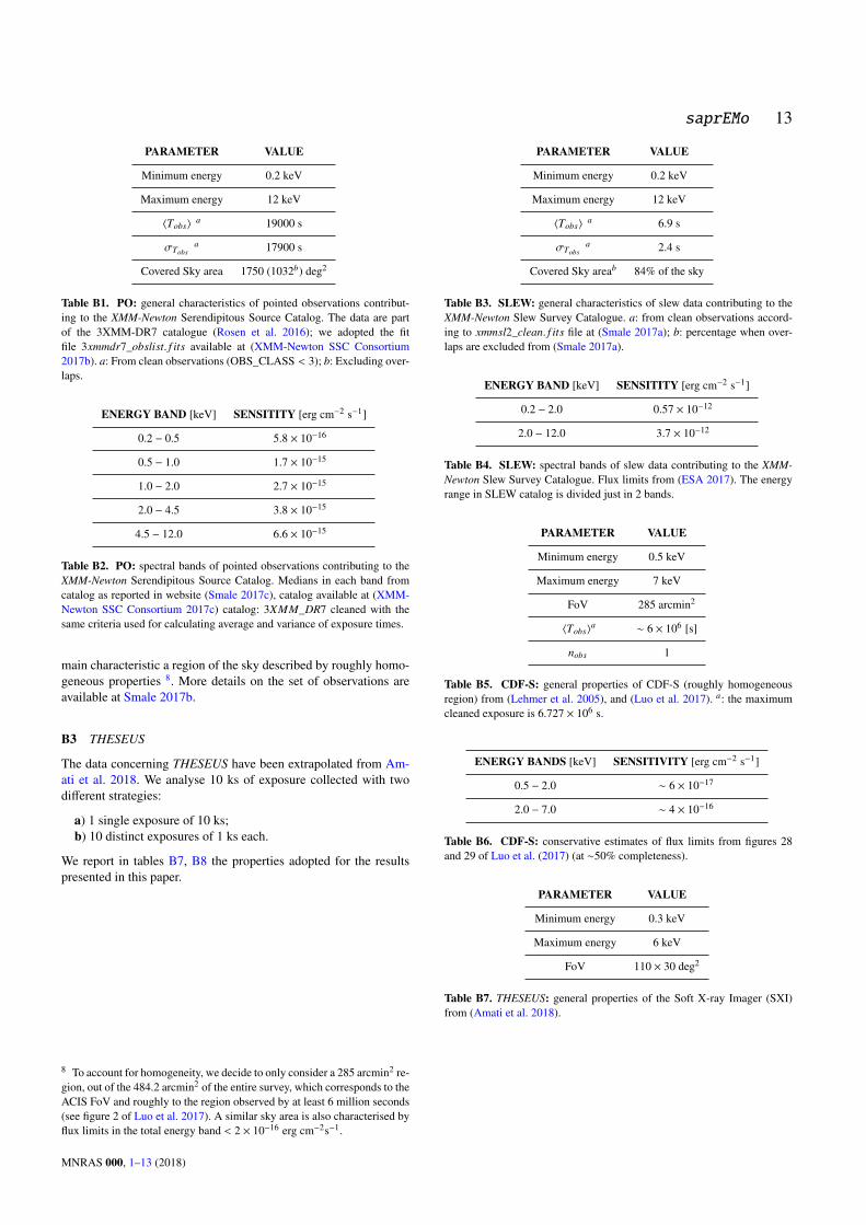
saprEMo 13
PARAMETER VALUE
Minimum energy 0.2 keV
Maximum energy 12 keV
〈Tobs〉a 19000 s
σTobsa 17900 s
Covered Sky area 1750 (1032b) deg2
Table B1. PO: general characteristics of pointed observations contribut-ing to the XMM-Newton Serendipitous Source Catalog. The data are partof the 3XMM-DR7 catalogue (Rosen et al. 2016); we adopted the fitfile 3xmmdr7_obslist. f its available at (XMM-Newton SSC Consortium2017b). a: From clean observations (OBS_CLASS < 3); b: Excluding over-laps.
ENERGY BAND [keV] SENSITITY [erg cm−2 s−1]
0.2 − 0.5 5.8 × 10⁻¹⁶
0.5 − 1.0 1.7 × 10⁻¹⁵
1.0 − 2.0 2.7 × 10⁻¹⁵
2.0 − 4.5 3.8 × 10⁻¹⁵
4.5 − 12.0 6.6 × 10⁻¹⁵
Table B2. PO: spectral bands of pointed observations contributing to theXMM-Newton Serendipitous Source Catalog. Medians in each band fromcatalog as reported in website (Smale 2017c), catalog available at (XMM-Newton SSC Consortium 2017c) catalog: 3XMM_DR7 cleaned with thesame criteria used for calculating average and variance of exposure times.
main characteristic a region of the sky described by roughly homo-geneous properties 8. More details on the set of observations areavailable at Smale 2017b.
B3 THESEUS
The data concerning THESEUS have been extrapolated from Am-ati et al. 2018. We analyse 10 ks of exposure collected with twodifferent strategies:
a) 1 single exposure of 10 ks;b) 10 distinct exposures of 1 ks each.
We report in tables B7, B8 the properties adopted for the resultspresented in this paper.
8 To account for homogeneity, we decide to only consider a 285 arcmin2 re-gion, out of the 484.2 arcmin2 of the entire survey, which corresponds to theACIS FoV and roughly to the region observed by at least 6 million seconds(see figure 2 of Luo et al. 2017). A similar sky area is also characterised byflux limits in the total energy band < 2 × 10⁻¹⁶ erg cm−2s−1.
PARAMETER VALUE
Minimum energy 0.2 keV
Maximum energy 12 keV
〈Tobs〉a 6.9 s
σTobsa 2.4 s
Covered Sky areab 84% of the sky
Table B3. SLEW: general characteristics of slew data contributing to theXMM-Newton Slew Survey Catalogue. a: from clean observations accord-ing to xmmsl2_clean. f its file at (Smale 2017a); b: percentage when over-laps are excluded from (Smale 2017a).
ENERGY BAND [keV] SENSITITY [erg cm−2 s−1]
0.2 − 2.0 0.57 × 10⁻¹²
2.0 − 12.0 3.7 × 10⁻¹²
Table B4. SLEW: spectral bands of slew data contributing to the XMM-Newton Slew Survey Catalogue. Flux limits from (ESA 2017). The energyrange in SLEW catalog is divided just in 2 bands.
PARAMETER VALUE
Minimum energy 0.5 keV
Maximum energy 7 keV
FoV 285 arcmin2
〈Tobs〉a ∼ 6 × 10⁶ [s]
nobs 1
Table B5. CDF-S: general properties of CDF-S (roughly homogeneousregion) from (Lehmer et al. 2005), and (Luo et al. 2017). a: the maximumcleaned exposure is 6.727 × 10⁶ s.
ENERGY BANDS [keV] SENSITIVITY [erg cm−2 s−1]
0.5 − 2.0 ∼ 6 × 10⁻¹⁷
2.0 − 7.0 ∼ 4 × 10⁻¹⁶
Table B6. CDF-S: conservative estimates of flux limits from figures 28and 29 of Luo et al. (2017) (at ∼50% completeness).
PARAMETER VALUE
Minimum energy 0.3 keV
Maximum energy 6 keV
FoV 110 × 30 deg2
Table B7. THESEUS: general properties of the Soft X-ray Imager (SXI)from (Amati et al. 2018).
MNRAS 000, 1–13 (2018)
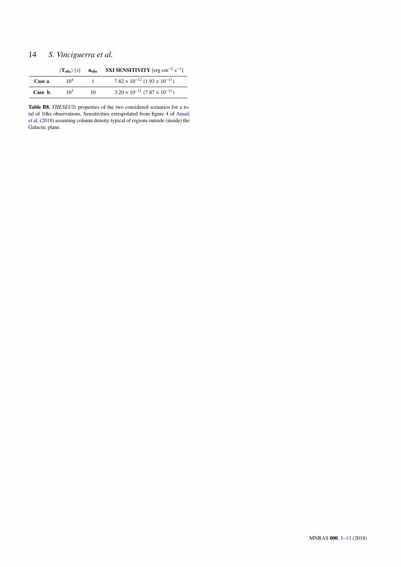
14 S. Vinciguerra et al.
〈Tobs〉 [s] nobs SXI SENSITIVITY [erg cm−2 s−1]
Case a. 104 1 7.82 × 10⁻¹² (1.93 × 10⁻¹¹)
Case b. 103 10 3.20 × 10⁻¹¹ (7.87 × 10⁻¹¹)
Table B8. THESEUS: properties of the two considered scenarios for a to-tal of 10ks observations. Sensitivities extrapolated from figure 4 of Amatiet al. (2018) assuming column density typical of regions outside (inside) theGalactic plane.
MNRAS 000, 1–13 (2018)
Related Documents