Construction of Simplified Boundary Surfaces from …graphics.cs.ucdavis.edu/~sdillard/vis07final.pdf · Construction of Simplified Boundary Surfaces from Serial-sectioned Metal

Construction of Simplified Boundary Surfacesfrom Serial-sectioned Metal Micrographs

Scott E. Dillard, John F. Bingert, Dan Thoma and Bernd Hamann, Member, IEEE

Abstract—We present a method for extracting boundary surfaces from segmented cross-section image data. We use a constrainedPotts model to interpolate an arbitrary number of region boundaries between segmented images. This produces a segmentedvolume from which we extract a triangulated boundary surface using well-known marching tetrahedra methods. This surface containsstaircase-like artifacts and an abundance of unnecessary triangles. We describe an approach that addresses these problems witha voxel-accurate simplification algorithm that reduces surface complexity by an order of magnitude. Our boundary interpolation andsimplification methods are novel contributions to the study of surface extraction from segmented cross-sections. We have applied ourmethod to construct polycrystal grain boundary surfaces from micrographs of a sample of the metal tantalum.

Index Terms—Surface extraction, Polygonal meshes, Visualization in Physical Sciences, Life Sciences and Engineering.

F

1 INTRODUCTION

Triangle meshes are a common representation of surface structures.They are convenient for visualizing surfaces using computer graphicshardware, and they provide a succinct and precise representation of asurface which can be used for further applications, such as simulations.In many imaging applications, a triangle mesh must be constructedfrom some other representation of the structure, such as a volume im-age (voxels) or a stack of planar curves. The problem of extracting asurface from either form of data has been studied extensively in thecomputer graphics and visualization fields. In this paper we makenovel contributions to the study of constructing surfaces from planarboundary curves and extracting separating surfaces from segmentedvolumes. We describe a method for interpolating segmented regionboundaries between planar sections which can track an arbitrary num-ber of regions, and we introduce an algorithm to extract a simplified,voxel-accurate triangle mesh from the resulting segmented volume.

Our method extracts crystal grain boundaries of polycrystalline ma-terials, given serially sectioned micrographs as input. The configura-tion of most materials of technological importance consists of poly-crystalline aggregates. The properties possessed by these polycrystalsare a function of the size, morphology, phase, and spatial correlationof the constituent crystals, along with any additional constituents suchas precipitates and inclusions, and defects such as voids and cracks.The spatial relationship of these features is therefore important towardunderstanding the relationship between structure and property that iscentral to the materials science discipline. The development of predic-tive material models also relies on accurate representations of struc-ture. Although two-dimensional sections reveal many microstructuralfeatures that may be statistically captured through stereological ap-proaches, for many cases a three-dimensional reconstruction is neces-sary to fully interpret the structure.

A sample of the metal tantalum was ground and imaged at intervalsof 5 microns, and each image has sub-micron resolution. Two types

• Scott E. Dillard is with the Institute for Data Analysis and Visualization(IDAV), University of California, Davis, E-mail: [email protected].

• John F. Bingert is with the Materials Science and Technology Division,Los Alamos National Laboratory, E-mail: [email protected].

• Dan Thoma is with the Materials Design Institute, Los Alamos NationalLaboratory, E-mail: [email protected].

• Bernd Hamann is with the Institute for Data Analysis and Visualization(IDAV), and the Department of Computer Science, University ofCalifornia, Davis, E-mail: [email protected].

Manuscript received 31 March 2007; accepted 1 August 2007; posted online27 October 2007.For information on obtaining reprints of this article, please send e-mail to:[email protected].

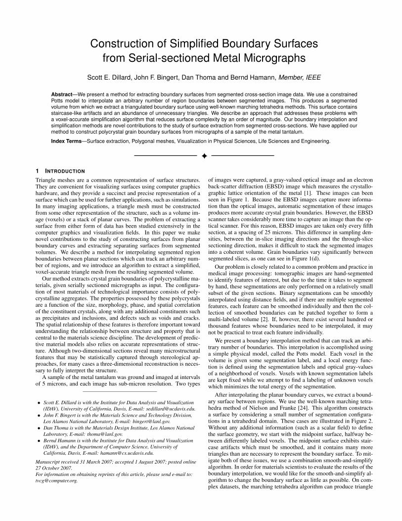
of images were captured, a gray-valued optical image and an electronback-scatter diffraction (EBSD) image which measures the crystallo-graphic lattice orientation of the metal [1]. These images can beenseen in Figure 1. Because the EBSD images capture more informa-tion than the optical images, automatic segmentation of these imagesproduces more accurate crystal grain boundaries. However, the EBSDscanner takes considerably more time to capture an image than the op-tical scanner. For this reason, EBSD images are taken only every fifthsection, at a spacing of 25 microns. This difference in sampling den-sities, between the in-slice imaging directions and the through-slicesectioning direction, makes it difficult to stack the segmented imagesinto a coherent volume. Grain boundaries vary significantly betweensegmented slices, as one can see in Figure 1(d).

Our problem is closely related to a common problem and practice inmedical image processing: tomographic images are hand-segmentedto identify features of interest, but due to the time it takes to segmentby hand, these segmentations are only performed on a relatively smallsubset of the given sections. Binary segmentations can be smoothlyinterpolated using distance fields, and if there are multiple segmentedfeatures, each feature can be smoothed individually and then the col-lection of smoothed boundaries can be patched together to form amulti-labeled volume [2]. If, however, there exist several hundred orthousand features whose boundaries need to be interpolated, it maynot be practical to treat each feature individually.

We present a boundary interpolation method that can track an arbi-trary number of boundaries. This interpolation is accomplished usinga simple physical model, called the Potts model. Each voxel in thevolume is given some segmentation label, and a local energy func-tion is defined using the segmentation labels and optical gray-valuesof a neighborhood of voxels. Voxels with known segmentation labelsare kept fixed while we attempt to find a labeling of unknown voxelswhich minimizes the total energy of the segmentation.

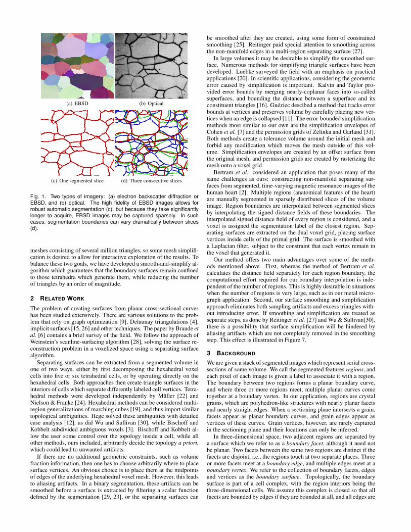
After interpolating the planar boundary curves, we extract a bound-ary surface between regions. We use the well-known marching tetra-hedra method of Nielson and Franke [24]. This algorithm constructsa surface by considering a small number of segmentation configura-tions in a tetrahedral domain. These cases are illustrated in Figure 2.Without any additional information (such as a scalar field) to definethe surface geometry, we start with the midpoint surface, halfway be-tween differently labeled voxels. The midpoint surface exhibits stair-case artifacts which must be smoothed, and it contains many moretriangles than are necessary to represent the boundary surface. To mit-igate both of these issues, we use a combination smooth-and-simplifyalgorithm. In order for materials scientists to evaluate the results of theboundary interpolation, we would like for the smooth-and-simplify al-gorithm to change the boundary surface as little as possible. On com-plex datasets, the marching tetrahedra algorithm can produce triangle

(a) EBSD (b) Optical

(c) One segmented slice (d) Three consecutive slices

Fig. 1. Two types of imagery: (a) electron backscatter diffraction orEBSD, and (b) optical. The high fidelity of EBSD images allows forrobust automatic segmentation (c), but because they take significantlylonger to acquire, EBSD images may be captured sparsely. In suchcases, segmentation boundaries can vary dramatically between slices(d).

meshes consisting of several million triangles, so some mesh simplifi-cation is desired to allow for interactive exploration of the results. Tobalance these two goals, we have developed a smooth-and-simplify al-gorithm which guarantees that the boundary surfaces remain confinedto those tetrahedra which generate them, while reducing the numberof triangles by an order of magnitude.

2 RELATED WORK

The problem of creating surfaces from planar cross-sectional curveshas been studied extensively. There are various solutions to the prob-lem that rely on graph optimization [9], Delaunay triangulations [4],implicit surfaces [15, 26] and other techniques. The paper by Braude etal. [6] contains a brief survey of the field. We follow the approach ofWeinstein’s scanline-surfacing algorithm [28], solving the surface re-construction problem in a voxelized space using a separating surfacealgorithm.

Separating surfaces can be extracted from a segmented volume inone of two ways, either by first decomposing the hexahedral voxelcells into five or six tetrahedral cells, or by operating directly on thehexahedral cells. Both approaches then create triangle surfaces in theinteriors of cells which separate differently labeled cell vertices. Tetra-hedral methods were developed independently by Muller [22] andNielson & Franke [24]. Hexahedral methods can be considered multi-region generalizations of marching cubes [19], and thus import similartopological ambiguities. Hege solved these ambiguities with detailedcase analysis [12], as did Wu and Sullivan [30], while Bischoff andKobbelt subdivided ambiguous voxels [3]. Bischoff and Kobbelt al-low the user some control over the topology inside a cell, while allother methods, ours included, arbitrarily decide the topology a priori,which could lead to unwanted artifacts.

If there are no additional geometric constraints, such as volumefraction information, then one has to choose arbitrarily where to placesurface vertices. An obvious choice is to place them at the midpointsof edges of the underlying hexahedral voxel mesh. However, this leadsto aliasing artifacts. In a binary segmentation, these artifacts can besmoothed before a surface is extracted by filtering a scalar functiondefined by the segmentation [29, 23], or the separating surfaces can

be smoothed after they are created, using some form of constrainedsmoothing [25]. Reitinger paid special attention to smoothing acrossthe non-manifold edges in a multi-region separating surface [27].

In large volumes it may be desirable to simplify the smoothed sur-face. Numerous methods for simplifying triangle surfaces have beendeveloped. Luebke surveyed the field with an emphasis on practicalapplications [20]. In scientific applications, considering the geometricerror caused by simplification is important. Kalvin and Taylor pro-vided error bounds by merging nearly-coplanar faces into so-calledsuperfaces, and bounding the distance between a superface and itsconstituent triangles [16]. Gueziec descibed a method that tracks errorbounds at vertices and preserves volume by carefully placing new ver-tices when an edge is collapsed [11]. The error-bounded simplificationmethods most similar to our own are the simplification envelopes ofCohen et al. [7] and the permission grids of Zelinka and Garland [31].Both methods create a tolerance volume around the initial mesh andforbid any modification which moves the mesh outside of this vol-ume. Simplification envelopes are created by an offset surface fromthe original mesh, and permission grids are created by rasterizing themesh onto a voxel grid.

Bertram et al. considered an application that poses many of thesame challenges as ours: constructing non-manifold separating sur-faces from segmented, time-varying magnetic resonance images of thehuman heart [2]. Multiple regions (anatomical features of the heart)are manually segmented in sparsely distributed slices of the volumeimage. Region boundaries are interpolated between segmented slicesby interpolating the signed distance fields of these boundaries. Theinterpolated signed distance field of every region is considered, and avoxel is assigned the segmentation label of the closest region. Sep-arating surfaces are extracted on the dual voxel grid, placing surfacevertices inside cells of the primal grid. The surface is smoothed witha Laplacian filter, subject to the constraint that each vertex remain inthe voxel that generated it.

Our method offers two main advantages over some of the meth-ods mentioned above. First, whereas the method of Bertram et al.calculates the distance field separately for each region boundary, thecomputational effort required for our boundary interpolation is inde-pendent of the number of regions. This is highly desirable in situationswhen the number of regions is very large, such as in our metal micro-graph application. Second, our surface smoothing and simplificationapproach eliminates both sampling artifacts and excess triangles with-out introducing error. If smoothing and simplification are treated asseparate steps, as done by Reitinger et al. [27] and Wu & Sullivan[30],there is a possibility that surface simplification will be hindered byaliasing artifacts which are not completely removed in the smoothingstep. This effect is illustrated in Figure 7.

3 BACKGROUND

We are given a stack of segmented images which represent serial cross-sections of some volume. We call the segmented features regions, andeach pixel of each image is given a label to associate it with a region.The boundary between two regions forms a planar boundary curve,and where three or more regions meet, multiple planar curves cometogether at a boundary vertex. In our application, regions are crystalgrains, which are polyhedron-like structures with nearly planar facetsand nearly straight edges. When a sectioning plane intersects a grain,facets appear as planar boundary curves, and grain edges appear asvertices of these curves. Grain vertices, however, are rarely capturedin the sectioning plane and their locations can only be inferred.

In three-dimensional space, two adjacent regions are separated bya surface which we refer to as a boundary facet, although it need notbe planar. Two facets between the same two regions are distinct if thefacets are disjoint, i.e., the regions touch at two separate places. Threeor more facets meet at a boundary edge, and multiple edges meet at aboundary vertex. We refer to the collection of boundary facets, edgesand vertices as the boundary surface. Topologically, the boundarysurface is part of a cell complex, with the region interiors being thethree-dimensional cells. We assume this complex is closed so that allfacets are bounded by edges if they are bounded at all, and all edges are

(a) Facet-type (b) Facet-type (c) Edge-type (d) Vertex-type

Fig. 2. Tetrahedral cases of the separating surface extraction algorithm.

bounded by vertices unless they form closed loops. We can ensure thisproperty by extending the segmented volume with a layer of “void”labels.

Avoiding topological ambiguities is a concern for any boundaryextraction method. We take the approach of imposing a tetrahe-dral domain over the rectilinear voxel grid, following Nielson andFranke [24]. Each hexahedral cell of the voxel grid is subdivided intofive tetrahedra. Vertices of the tetrahedra are labeled with their regionidentifier. To avoid confusion between a tetrahedral vertex of the voxelgrid and a triangular vertex of the separating surface, we refer to theformer as a domain vertex and the latter as a surface vertex, and weuse the same convention for edges and triangles.

We classify tetrahedra and triangles of the domain by counting thenumber of distinct labels at their vertices. Figure 2 illustrates thesecases. If a domain tetrahedron has two labels among its four vertices,then it is a facet-type tetrahedron and some patch of a facet passesthrough its interior. This patch intersects three or four faces of thetetrahedron, and these faces are also referred to as facet-type faces.If a tetrahedron has three labels, then it is an edge-type tetrahedronand some boundary edge passes through the interior. This boundaryedge enters the tetrahedron at one face, and leaves it at another face.These two faces are also edge-type, and the remaining two faces arefacet-type. A tetrahedron with four distinct labels is a vertex-type tetra-hedron. It joins four boundary edges and six boundary facets, and allfour of the tetrahedral faces are edge-type. Any tetrahedron, triangleor edge of the domain with vertices that are all similarly labeled iscalled interior-type.

A triangle mesh is a collection of vertices, pairs of the vertices(edges) and triplets of vertices (triangles). It is called a manifold trian-gle mesh without boundary if for every point on the surface we can finda small enough ball, centered on this point, which contains a piece ofthe surface that is homeomorphic to a plane. If the local area aroundsome point is homeomorphic to a half-plane, then the surface has aboundary. In the subsequent discussion, a manifold triangle mesh isone in which every edge is shared by exactly two triangles. If an edgeis incident on only one triangle, it is a boundary edge. If every edge isincident on one or two triangles, and every vertex is incident on zero ortwo boundary edges, then the mesh is manifold-with-boundary. A ver-tex which is incident on a non-manifold edge is a non-manifold vertex.We ignore other degenerate cases, such as a singular vertex shared bythe tips of two cones, because the separating surface algorithm doesnot produce surfaces in these configurations.

We represent the boundary surface as a non-manifold triangle mesh.It can be decomposed into manifold pieces which are the facets. Thesefacets are represented by manifold-with-boundary triangle meshes.The boundaries of the facets meet at non-manifold boundary edges.A property of the marching tetrahedra surface extraction algorithmis that three boundary facets meet at every boundary edge, and fourboundary edges will meet at every boundary vertex. (It is a coinci-dence that these are the same numbers of faces and edges meetingin a three-dimensional Voronoi diagram, which looks very much likeour polycrystal microstructure, and indeed many cellular structures innature.) Figure 3 illustrates a simple boundary surface example withthree regions, plus a void region for the surroundings.

Fig. 3. Boundary surface for a three-region segmentation with onesphere and two boxes. The non-manifold boundary edges are shownby red tubes and the boundary vertices are shown by black spheres.There are two vertices, four edges and six facets – one between eachpair of regions, and one between each region and the surroundings.

4 BOUNDARY INTERPOLATION

We start with a rasterized representation of the planar boundary curvesfor each slice, i.e., a segmented image. These images have been regis-tered, and correspondences have been made between regions in adja-cent slices, so that the same feature has the same label throughout theentire stack. At this point, a separating surface can already be extractedfrom the segmented volume using Weinstein’s scanline-surface algo-rithm [28], which we call “nearest-neighbor” boundary interpolation.If the spacing between segmented slices is adequately small, this willsuffice and we can move on to extracting and simplifying the surface.However, if the spacing is large, then the segmentation may changedramatically from one slice to the next, and we want to smoothly inter-polate the boundary curves between slices. We accomplish this usingthe Potts model.

The Potts model has received attention from the computer visioncommunity as a model for early vision, as a special case of Markovrandom fields [5]. It has also been studied by materials scientistsas a model of the formation and motion of crystal grain boundariesfrom thermally activated grain growth processes [13]. Indeed it is thisoverlap between computer vision and materials science that makes thePotts model particularly attractive for our application. In the computervision setting, the Potts energy of a pixel i in a labeled image L is

EP(i) = ∑j∈Ni

U(i, j) ·T (Li 6= L j). (1)

N is the neighborhood of pixels – in 3D we use a 26-voxel neigh-borhood. U is some image-dependent function and T (true) =1,T (false) = 0. Without an image-dependent weight, the Potts energysimply penalizes any neighboring pair of pixels which are labeled dif-ferently. In computer vision applications, a labeling which minimizesthe Potts energy for the whole image is sought as a discontinuity-preserving restoration or segmentation of the image, so that all re-gions with similar gray values are compactly clustered. Boykov et al.showed that minimizing the Potts energy is NP-hard and provided anefficient graph-cut algorithm which approximates the minimum withina factor of two [5]. However, the complexity of their algorithm de-pends on the number of segmentation labels, which we consider to beunbounded. To trade guaranteed optimization results for scalabilitywe use a Monte Carlo method, such as simulated annealing [17], thecomplexity of which is independent of the number of labels.

We use the Potts model to find likely region boundaries betweenslices in which the boundaries are known. The stack of segmentedimages is resampled onto a segmented volume L, where each imageoccupies a slice of the voxel grid according to its physical locationwithin the material volume. Slices of the volume which do not haveany boundary information are initialized with random segmentationlabels. We then iterate the following Monte Carlo procedure:

(a) Without optical (b) With optical

Fig. 4. Incorporating optical data into the Potts energy function improvesfidelity of the boundary reconstruction in the regions with unknown la-bels. In this image, the segmentation labels are represented by colorand the optical data is mapped to brightness.

1. Pick a voxel i at random from a slice which does not havesegmentation information. Save its label l0 = L(i). Calculatep0 = EP(i), the Potts energy for that voxel.

2. Calculate the set LN = {L( j)| j ∈ N(i)}, the set of all labels ofvoxels adjacent to voxel i.

3. Pick at random a label l1 from LN . Assign voxel i the label l1and recalculate the new Potts energy p1 = EP(i).

4. Pick a random number x ∈ [0,1]. If x < exp(−(p1− p0)/t), or ifp1 < p0, accept the new label l1, otherwise reject it and restorethe old label l0.

Here, t is the temperature parameter in simulated annealing. We re-strict the procedure to those voxels whose segmentation labels are notalready known, but the voxels with known grain labels participate inthe energy function EP. The entire system is therefore in a state that isvery close to the local minimum we are searching for, and since thosefixed voxels do not change their labels, the system consistently con-verges to the desired minimum. Because of the strong influence thatfixed voxels have on the system, it is not necessary to use a compli-cated cooling schedule for simulated annealing. Instead we use a con-stant non-zero temperature which is smaller than the expected Pottsenergy of a random labeling. We find that, for the energy scale givenby Equation 1 and a 26 voxel neighborhood, t = 0.9 is a good choice.Segmentation labels aggregate into smoothly varying regions whichagree with the known segmentation, but borders between regions mayfluctuate due to the non-zero temperature. To fix borders we “quench”the simulation by setting t = 0, causing the system to monotonicallytransition into a local minimum. We monitor the process visually inorder to determine when to quench the system, but fully automaticcooling schedules can be used if automation is required. Convergencecan be detected by monitoring the rate at which voxel labels change,and stopping when it falls below a threshold.

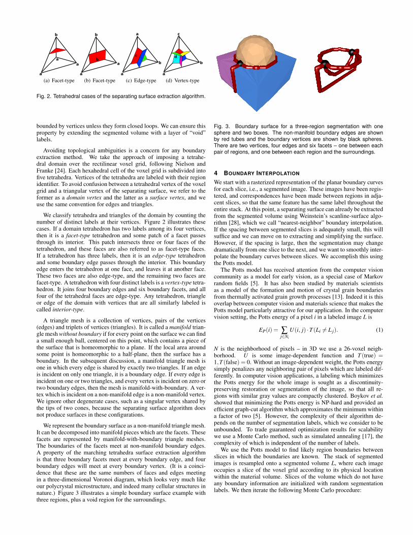
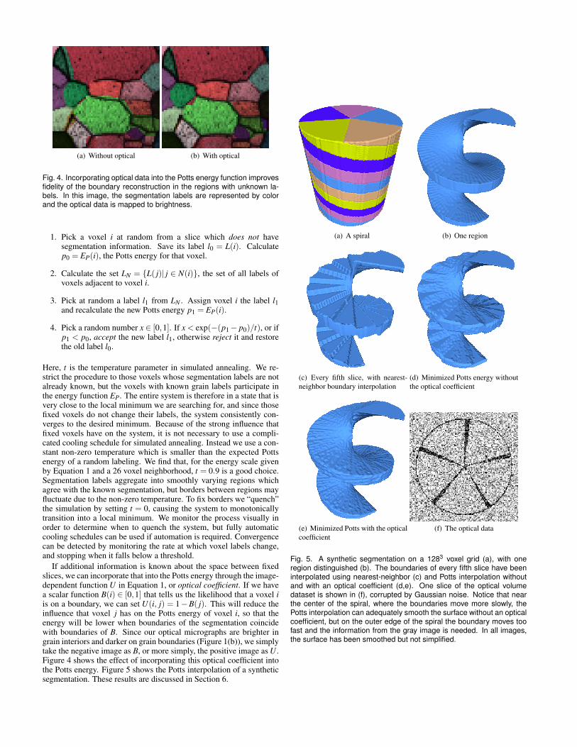
If additional information is known about the space between fixedslices, we can incorporate that into the Potts energy through the image-dependent function U in Equation 1, or optical coefficient. If we havea scalar function B(i) ∈ [0,1] that tells us the likelihood that a voxel iis on a boundary, we can set U(i, j) = 1−B( j). This will reduce theinfluence that voxel j has on the Potts energy of voxel i, so that theenergy will be lower when boundaries of the segmentation coincidewith boundaries of B. Since our optical micrographs are brighter ingrain interiors and darker on grain boundaries (Figure 1(b)), we simplytake the negative image as B, or more simply, the positive image as U .Figure 4 shows the effect of incorporating this optical coefficient intothe Potts energy. Figure 5 shows the Potts interpolation of a syntheticsegmentation. These results are discussed in Section 6.

(a) A spiral (b) One region

(c) Every fifth slice, with nearest-neighbor boundary interpolation

(d) Minimized Potts energy withoutthe optical coefficient

(e) Minimized Potts with the opticalcoefficient

(f) The optical data

Fig. 5. A synthetic segmentation on a 1283 voxel grid (a), with oneregion distinguished (b). The boundaries of every fifth slice have beeninterpolated using nearest-neighbor (c) and Potts interpolation withoutand with an optical coefficient (d,e). One slice of the optical volumedataset is shown in (f), corrupted by Gaussian noise. Notice that nearthe center of the spiral, where the boundaries move more slowly, thePotts interpolation can adequately smooth the surface without an opticalcoefficient, but on the outer edge of the spiral the boundary moves toofast and the information from the gray image is needed. In all images,the surface has been smoothed but not simplified.

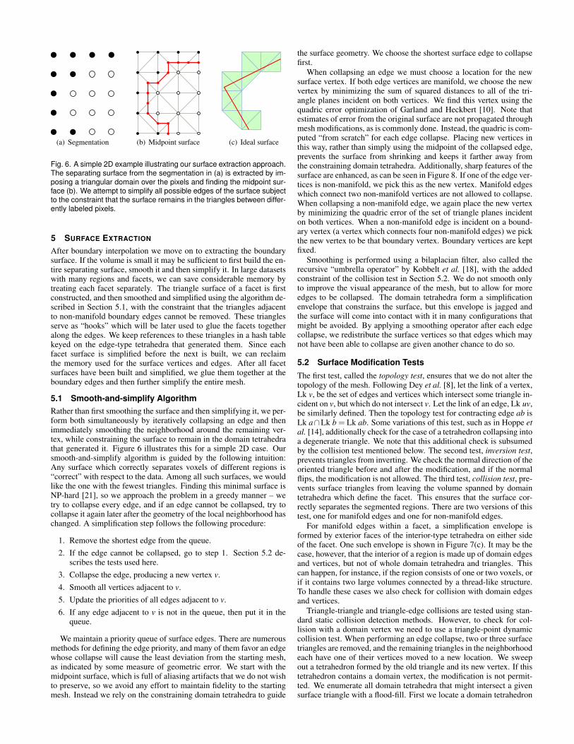
(a) Segmentation (b) Midpoint surface (c) Ideal surface

Fig. 6. A simple 2D example illustrating our surface extraction approach.The separating surface from the segmentation in (a) is extracted by im-posing a triangular domain over the pixels and finding the midpoint sur-face (b). We attempt to simplify all possible edges of the surface subjectto the constraint that the surface remains in the triangles between differ-ently labeled pixels.

5 SURFACE EXTRACTION

After boundary interpolation we move on to extracting the boundarysurface. If the volume is small it may be sufficient to first build the en-tire separating surface, smooth it and then simplify it. In large datasetswith many regions and facets, we can save considerable memory bytreating each facet separately. The triangle surface of a facet is firstconstructed, and then smoothed and simplified using the algorithm de-scribed in Section 5.1, with the constraint that the triangles adjacentto non-manifold boundary edges cannot be removed. These trianglesserve as “hooks” which will be later used to glue the facets togetheralong the edges. We keep references to these triangles in a hash tablekeyed on the edge-type tetrahedra that generated them. Since eachfacet surface is simplified before the next is built, we can reclaimthe memory used for the surface vertices and edges. After all facetsurfaces have been built and simplified, we glue them together at theboundary edges and then further simplify the entire mesh.

5.1 Smooth-and-simplify AlgorithmRather than first smoothing the surface and then simplifying it, we per-form both simultaneously by iteratively collapsing an edge and thenimmediately smoothing the neighborhood around the remaining ver-tex, while constraining the surface to remain in the domain tetrahedrathat generated it. Figure 6 illustrates this for a simple 2D case. Oursmooth-and-simplify algorithm is guided by the following intuition:Any surface which correctly separates voxels of different regions is“correct” with respect to the data. Among all such surfaces, we wouldlike the one with the fewest triangles. Finding this minimal surface isNP-hard [21], so we approach the problem in a greedy manner – wetry to collapse every edge, and if an edge cannot be collapsed, try tocollapse it again later after the geometry of the local neighborhood haschanged. A simplification step follows the following procedure:

1. Remove the shortest edge from the queue.2. If the edge cannot be collapsed, go to step 1. Section 5.2 de-

scribes the tests used here.3. Collapse the edge, producing a new vertex v.4. Smooth all vertices adjacent to v.5. Update the priorities of all edges adjacent to v.6. If any edge adjacent to v is not in the queue, then put it in the

queue.

We maintain a priority queue of surface edges. There are numerousmethods for defining the edge priority, and many of them favor an edgewhose collapse will cause the least deviation from the starting mesh,as indicated by some measure of geometric error. We start with themidpoint surface, which is full of aliasing artifacts that we do not wishto preserve, so we avoid any effort to maintain fidelity to the startingmesh. Instead we rely on the constraining domain tetrahedra to guide

the surface geometry. We choose the shortest surface edge to collapsefirst.

When collapsing an edge we must choose a location for the newsurface vertex. If both edge vertices are manifold, we choose the newvertex by minimizing the sum of squared distances to all of the tri-angle planes incident on both vertices. We find this vertex using thequadric error optimization of Garland and Heckbert [10]. Note thatestimates of error from the original surface are not propagated throughmesh modifications, as is commonly done. Instead, the quadric is com-puted “from scratch” for each edge collapse. Placing new vertices inthis way, rather than simply using the midpoint of the collapsed edge,prevents the surface from shrinking and keeps it farther away fromthe constraining domain tetrahedra. Additionally, sharp features of thesurface are enhanced, as can be seen in Figure 8. If one of the edge ver-tices is non-manifold, we pick this as the new vertex. Manifold edgeswhich connect two non-manifold vertices are not allowed to collapse.When collapsing a non-manifold edge, we again place the new vertexby minimizing the quadric error of the set of triangle planes incidenton both vertices. When a non-manifold edge is incident on a bound-ary vertex (a vertex which connects four non-manifold edges) we pickthe new vertex to be that boundary vertex. Boundary vertices are keptfixed.

Smoothing is performed using a bilaplacian filter, also called therecursive “umbrella operator” by Kobbelt et al. [18], with the addedconstraint of the collision test in Section 5.2. We do not smooth onlyto improve the visual appearance of the mesh, but to allow for moreedges to be collapsed. The domain tetrahedra form a simplificationenvelope that constrains the surface, but this envelope is jagged andthe surface will come into contact with it in many configurations thatmight be avoided. By applying a smoothing operator after each edgecollapse, we redistribute the surface vertices so that edges which maynot have been able to collapse are given another chance to do so.

5.2 Surface Modification TestsThe first test, called the topology test, ensures that we do not alter thetopology of the mesh. Following Dey et al. [8], let the link of a vertex,Lk v, be the set of edges and vertices which intersect some triangle in-cident on v, but which do not intersect v. Let the link of an edge, Lk uv,be similarly defined. Then the topology test for contracting edge ab isLk a∩Lk b = Lk ab. Some variations of this test, such as in Hoppe etal. [14], additionally check for the case of a tetrahedron collapsing intoa degenerate triangle. We note that this additional check is subsumedby the collision test mentioned below. The second test, inversion test,prevents triangles from inverting. We check the normal direction of theoriented triangle before and after the modification, and if the normalflips, the modification is not allowed. The third test, collision test, pre-vents surface triangles from leaving the volume spanned by domaintetrahedra which define the facet. This ensures that the surface cor-rectly separates the segmented regions. There are two versions of thistest, one for manifold edges and one for non-manifold edges.

For manifold edges within a facet, a simplification envelope isformed by exterior faces of the interior-type tetrahedra on either sideof the facet. One such envelope is shown in Figure 7(c). It may be thecase, however, that the interior of a region is made up of domain edgesand vertices, but not of whole domain tetrahedra and triangles. Thiscan happen, for instance, if the region consists of one or two voxels, orif it contains two large volumes connected by a thread-like structure.To handle these cases we also check for collision with domain edgesand vertices.

Triangle-triangle and triangle-edge collisions are tested using stan-dard static collision detection methods. However, to check for col-lision with a domain vertex we need to use a triangle-point dynamiccollision test. When performing an edge collapse, two or three surfacetriangles are removed, and the remaining triangles in the neighborhoodeach have one of their vertices moved to a new location. We sweepout a tetrahedron formed by the old triangle and its new vertex. If thistetrahedron contains a domain vertex, the modification is not permit-ted. We enumerate all domain tetrahedra that might intersect a givensurface triangle with a flood-fill. First we locate a domain tetrahedron

that intersects the surface triangle, then flood all neighbors of this tetra-hedron as long as their faces intersect the surface triangle. This mightalso be accomplished with more sophisticated triangle-voxel rasteri-zation, however we find the flood-fill is simple and robust, if not opti-mally efficient.

For non-manifold edges, we restrict the polyline of non-manifoldvertices to only intersect edge-type tetrahedra. Before a non-manifoldedge is modified, we follow the line segment of the edge through thetetrahedral mesh. If this segment intersects any tetrahedron that is notedge-type or vertex-type, the modification is not permitted.

6 RESULTS AND DISCUSSION

Figure 5 shows the results of Potts boundary interpolation on a syn-thetic dataset. A five-region spiral was rendered on to a 1283 voxelgrid. Figure 5(b) shows one of these regions. To simulate a sparsesampling of the segmentation in one dimension, we removed all seg-mentation information except for every fifth slice. Figure 5(c) showsthe reconstruction of the full volume using only every fifth slice. In thisimage the surface has been extracted from the 1282×25 voxel volume,then stretched out in the slicing direction. Figure 5(d) shows the resultsof Potts interpolation without an optical coefficient. Clearly the Pottsenergy defined in Equation 1 penalizes boundary surface area, andtherefor segmentations with minimal surface area are favored. Fur-ther, it is known that an unconstrained Potts model simulation movesboundaries by mean curvature motion [13]. However, since the Pottsenergy is defined over a small neighborhood of a regular lattice, weare only minimizing discrete approximations of surface area and cur-vature. When boundaries vary only slightly between slices, this dis-crete approximation suffices, but if boundaries change drastically thensmooth boundaries will have an insignificant energetic advantage overstaircase-like boundaries, due to discretization effects. Notice in Fig-ure 5(d) how the boundary becomes progressively less smooth as wemove from the center of the spiral outward, since the segmentationboundary is moving faster along the outer edge of the spiral. By in-cluding an optical coefficient in the Potts energy, we can coerce theboundary into regions which are believed to be more appropriate, byoffering it an energetic advantage in these regions. This boundary be-lief is quantified by the optical image, which may be noisy. (Surely, ifit was a high-quality image we could segment it automatically.) Fig-ure 5(f) shows one slice of the spiral boundary image, which has beencorrupted by Gaussian noise, and Figure 5(e) shows the segmentationproduced by incorporating this boundary image into the Potts energy.

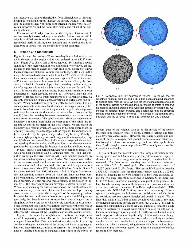
Figure 7 shows a comparison between two separating surfaces: onewhich has been smoothed with a Laplacian filter (7(a)) and then sim-plified using quadric error metrics (7(b)), and another produced byour smooth-and-simplify algorithm (7(d)). We compare our methodto quadric error-based simplification because it is a common simplifi-cation method and it has been used before to simplify separating sur-faces of segmented data [27]. Both simplified surfaces in Figure 7have been reduced from 8912 triangles to 242. In Figure 7(a) we cansee that sampling artifacts from the voxel grid have not been com-pletely smoothed. Any simplification method that attempts to preservemesh geometry will also preserve these artifacts, as can be seen in Fig-ure 7(b). The inner simplification envelope is shown in Figure 7(c).When simplified using the quadric error metric, the result surface doesnot stay entirely to one side of the simplification envelope, causingerrors where voxels lie on the wrong side of the separating surface.It is true that we could prevent these errors by not simplifying so ag-gressively, but there is no way to know how many triangles can besimplified before errors occur, without using some kind of error bound.Since our smooth-and-simplify algorithm incorporates the envelope asa hard constraint, we do not need to specify a target surface mesh size,rather we let it remove all the triangles it can without causing errors.

Figure 8 illustrates the simplification results on a simple non-manifold separating surface. The surface is simplified from 133,534triangles down to 986. This large reduction is the result of the manyco-planar triangles on the sides of the boxes, which can be aggregatedinto very large triangles, similar to superfaces [16]. Placing new ver-tices by quadric optimization enhances sharp edges of the boxes. In

(a) (b)

(c) (d)

Fig. 7. A sphere in a 323 segmented volume. In (a) we see thesmoothed midpoint surface, and in (b) it has been simplified accordingto quadric error metrics. In (c) we see the inner simplification envelopeof the sphere. Notice how the quadric error metric attempts to preservehighlighted sampling artifacts that were not completely smoothed. Ourmethod (d) ignores these artifacts, and guarantees that the simplifiedsurface does not cross the envelope. The surface in (a) contains 8912triangles, and the surfaces in (b) and (e) both contain 242 triangles.

smooth areas of the volume, such as on the surface of the sphere,the smoothing operator tends to evenly distribute vertices and trian-gles have nice aspect ratios. However, near sharp features and non-manifold edges, topological and geometric constraints can cause long,thin triangles to form. We acknowledge that, in certain applications,these “bad” triangles can cause problems. We currently make no effortto avoid such triangles.

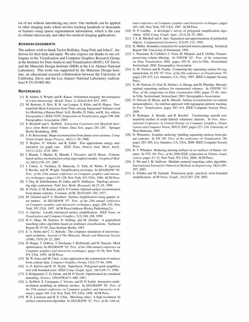
Figure 9 shows the microstructure of a sample of tantalum mea-suring approximately 1.6mm along the longest dimension. Figure 10shows a closer view where grains on the sample boundary have beenremoved. The Potts model boundary interpolation was performedon an 800 × 213 × 71 voxel grid. The segmentation consists of19,037 grains and 93,554 facets. The unsimplified surface contains23,754,424 triangles, and the simplified surface contains 2,303,982triangles. Because facets were simplified as they were extracted, us-ing the two-stage algorithm described in Section 5, no more than8,149,974 triangles were in memory at any point in the process. Ta-ble 1 lists the running times for the boundary interpolation and surfaceextraction, performed on an Intel Core Duo (single-threaded) 2.16GHzcomputer with 2GB RAM. Profiling reveals that the majority of time isspent in the triangle-triangle intersection collision test, which checksfor collisions between surface triangles and domain triangles. We be-lieve that using a hexhedral domain combined with one of the morecomplicated separating surface algorithms [12, 30, 27, 2] is likely toreduce the computational cost of these collision tests, since this couldallow for fast triangle-to-voxel rasterization to be used for collision de-tection, similar to permission grids [31]. Further research into this areacould improve performance significantly. Additionally, even thoughfew of the other surface reconstruction methods are designed to han-dle the datasets we consider here, a critical comparison between ourmethod and others is needed, using datasets with fewer regions, in or-der to determine where our method fits in the rich taxonomy of surfacereconstruction methods.

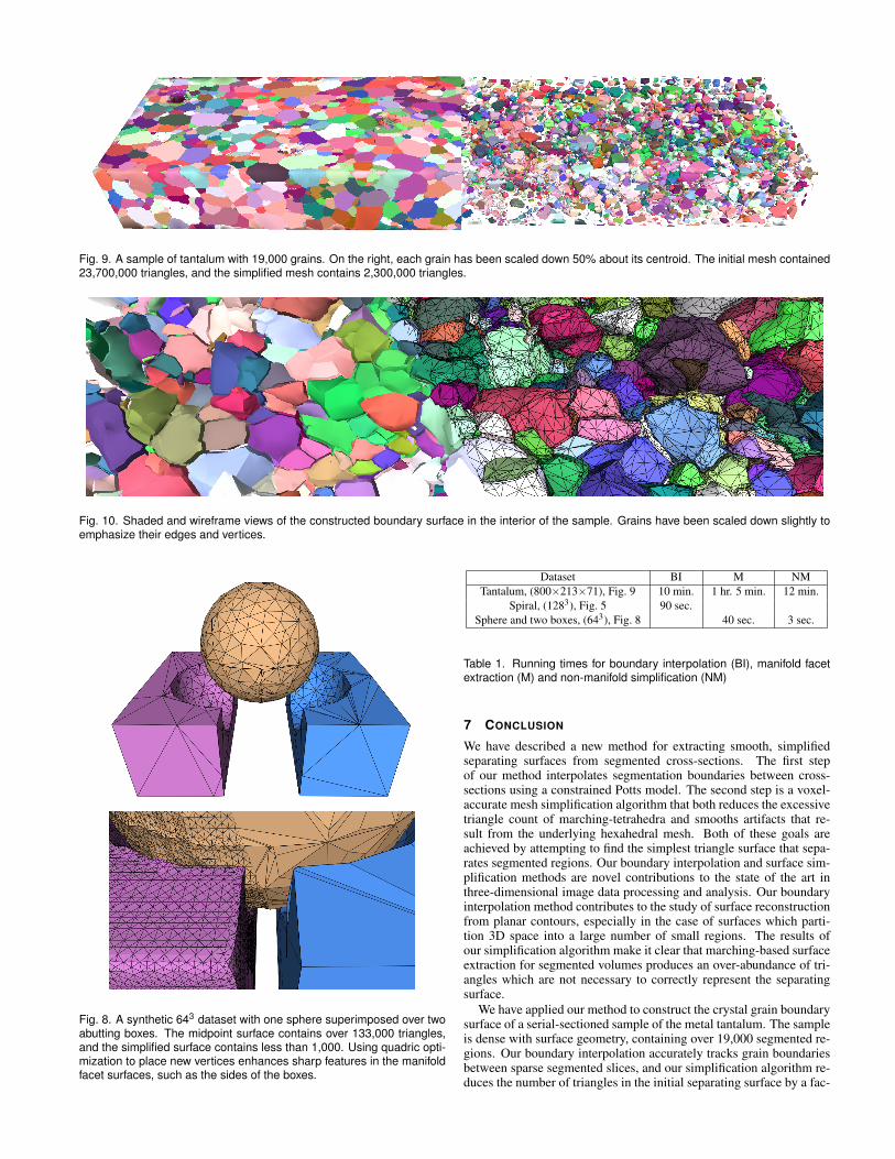
Fig. 9. A sample of tantalum with 19,000 grains. On the right, each grain has been scaled down 50% about its centroid. The initial mesh contained23,700,000 triangles, and the simplified mesh contains 2,300,000 triangles.

Fig. 10. Shaded and wireframe views of the constructed boundary surface in the interior of the sample. Grains have been scaled down slightly toemphasize their edges and vertices.

Fig. 8. A synthetic 643 dataset with one sphere superimposed over twoabutting boxes. The midpoint surface contains over 133,000 triangles,and the simplified surface contains less than 1,000. Using quadric opti-mization to place new vertices enhances sharp features in the manifoldfacet surfaces, such as the sides of the boxes.

Dataset BI M NMTantalum, (800×213×71), Fig. 9 10 min. 1 hr. 5 min. 12 min.

Spiral, (1283), Fig. 5 90 sec.Sphere and two boxes, (643), Fig. 8 40 sec. 3 sec.

Table 1. Running times for boundary interpolation (BI), manifold facetextraction (M) and non-manifold simplification (NM)

7 CONCLUSION

We have described a new method for extracting smooth, simplifiedseparating surfaces from segmented cross-sections. The first stepof our method interpolates segmentation boundaries between cross-sections using a constrained Potts model. The second step is a voxel-accurate mesh simplification algorithm that both reduces the excessivetriangle count of marching-tetrahedra and smooths artifacts that re-sult from the underlying hexahedral mesh. Both of these goals areachieved by attempting to find the simplest triangle surface that sepa-rates segmented regions. Our boundary interpolation and surface sim-plification methods are novel contributions to the state of the art inthree-dimensional image data processing and analysis. Our boundaryinterpolation method contributes to the study of surface reconstructionfrom planar contours, especially in the case of surfaces which parti-tion 3D space into a large number of small regions. The results ofour simplification algorithm make it clear that marching-based surfaceextraction for segmented volumes produces an over-abundance of tri-angles which are not necessary to correctly represent the separatingsurface.

We have applied our method to construct the crystal grain boundarysurface of a serial-sectioned sample of the metal tantalum. The sampleis dense with surface geometry, containing over 19,000 segmented re-gions. Our boundary interpolation accurately tracks grain boundariesbetween sparse segmented slices, and our simplification algorithm re-duces the number of triangles in the initial separating surface by a fac-

tor of ten without introducing any error. Our methods can be appliedto other imaging tasks which involve tracking hundreds or thousandsof features using sparse segmentation information, which is the casein cellular microscopy and other bio-medical imaging applications.

ACKNOWLEDGEMENTS

The authors wish to thank Taylor Holliday, Sung Park and John C. An-derson for their help and input. We also express our thanks to our col-leagues in the Visualization and Computer Graphics Research Group,at the Institute for Data Analysis and Visualization (IDAV), UC Davis,and the Materials Design Institute (MDI) at the Los Alamos NationalLaboratory. This work was supported by the Materials Design Insti-tute, an educational research collaboration between the University ofCalifornia, Davis and the Los Alamos National Laboratory (subcon-tract # 25110-002-06).

REFERENCES

[1] B. Adams, S. Wright, and K. Kunze. Orientation imaging: the emergenceof a new microscopy. Metall. Trans. A, 24A(4):819–831, 1993.

[2] M. Bertram, G. Reis, R. H. van Lengen, S. Kohn, and H. Hagen. Non-manifold Mesh Extraction from Time-varying Segmented Volumes usedfor Modeling a Human Heart. In K. Brodlie, D. Duke, and K. Joy, editors,Eurographics / IEEE VGTC Symposium on Visualization, pages 199–206.Eurographics Association, 2005.

[3] S. Bischoff and L. Kobbelt. Extracting Consistent and Manifold Inter-faces from Multi-valued Volume Data Sets, pages 281–285. SpringerBerlin Heidelberg, 2006.

[4] J.-D. Boissonnat. Shape reconstruction from planar cross sections. Comp.Vision Graph. Image Process., 44(1):1–29, 1988.

[5] Y. Boykov, O. Veksler, and R. Zabih. Fast approximate energy min-imization via graph cuts. IEEE Trans. Pattern Anal. Mach. Intell.,23(11):1222–1239, 2001.

[6] I. Braude, J. Marker, K. Museth, J. Nissanov, and D. Breen. Contour-based surface reconstruction using mpu implicit models. Graphical Mod-els, 69(2):139–157, 2007.

[7] J. Cohen, A. Varshney, D. Manocha, G. Turk, H. Weber, P. Agarwal,F. Brooks, and W. Wright. Simplification envelopes. In SIGGRAPH ’96:Proc. of the 23rd annual conference on Computer graphics and interac-tive techniques, pages 119–128, New York, NY, USA, 1996. ACM Press.

[8] T. Dey, H. Edelsbrunner, H. Guha, and D. Nekhayev. Topology preserv-ing edge contraction. Publ. Inst. Math. (Beograd), 66:23–45, 1999.

[9] H. Fuchs, Z. M. Kedem, and S. P. Uselton. Optimal surface reconstructionfrom planar contours. Commun. ACM, 20(10):693–702, 1977.

[10] M. Garland and P. S. Heckbert. Surface simplification using quadric er-ror metrics. In SIGGRAPH ’97: Proc. of the 24th annual conferenceon Computer graphics and interactive techniques, pages 209–216, NewYork, NY, USA, 1997. ACM Press/Addison-Wesley Publishing Co.

[11] A. Gueziec. Locally toleranced surface simplification. IEEE Trans. onVisualization and Computer Graphics, 5(2):168–189, 1999.

[12] H.-C. Hege, M. Seebass, D. Stalling, and M. Zockler. A generalizedmarching cubes algorithm based on nonbinary classifications. TechnicalReport SC 97-05, Zuse Institute Berlin, 1997.

[13] E. A. Holm and C. C. Battaile. The computer simulation of microstruc-tural evolution. Journal of The Minerals, Metals and Materials Society(JOM), 53(9):20–23, 2001.

[14] H. Hoppe, T. DeRose, T. Duchamp, J. McDonald, and W. Stuetzle. Meshoptimization. In SIGGRAPH ’93: Proc. of the 20th annual conference onComputer graphics and interactive techniques, pages 19–26, New York,NY, USA, 1993. ACM Press.

[15] M. W. Jones and M. Chen. A new approach to the construction of surfacesfrom contour data. Computer Graphics Forum, 13(3):75–84, 1994.

[16] A. D. Kalvin and R. H. Taylor. Superfaces: Polygonal mesh simplifica-tion with bounded error. IEEE Comp. Graph. Appl., 16(3):64–77, 1996.

[17] S. Kirkpatrick, C. D. Gelatt, and M. P. Vecchi. Optimization by simulatedannealing. Science, 220(4598):671–680, 1983.

[18] L. Kobbelt, S. Campagna, J. Vorsatz, and H.-P. Seidel. Interactive multi-resolution modeling on arbitrary meshes. In SIGGRAPH ’98: Proc. ofthe 25th annual conference on Computer graphics and interactive tech-niques, pages 105–114, New York, NY, USA, 1998. ACM Press.

[19] W. E. Lorensen and H. E. Cline. Marching cubes: A high resolution 3dsurface construction algorithm. In SIGGRAPH ’87: Proc. of the 14th an-

nual conference on Computer graphics and interactive techniques, pages163–169, New York, NY, USA, 1987. ACM Press.

[20] D. P. Luebke. A developer’s survey of polygonal simplification algo-rithms. IEEE Comp. Graph. Appl., 21(3):24–35, 2001.

[21] J. S. B. Mitchell and S. Suri. Separation and approximation of polyhedralobjects. Computational Geometry, 5(2):95–114, 1995.

[22] H. Muller. Boundary extraction for rasterized motion planning. TechnicalReport 566, University of Dortmund, 1995.

[23] L. Neumann, B. Csebfalvi, I. Viola, M. Mlejnek, and E. Groller. Feature-preserving volume filtering. In VISSYM ’02: Proc. of the symposiumon Data Visualisation 2002, pages 105–ff, Aire-la-Ville, Switzerland,Switzerland, 2002. Eurographics Association.

[24] G. M. Nielson and R. Franke. Computing the separating surface for seg-mented data. In VIS ’97: Proc. of the 8th conference on Visualization ’97,pages 229–233, Los Alamitos, CA, USA, 1997. IEEE Computer SocietyPress.

[25] G. M. Nielson, G. Graf, R. Holmes, A. Huang, and M. Phielipp. Shrouds:optimal separating surfaces for enumerated volumes. In VISSYM ’03:Proc. of the symposium on Data visualisation 2003, pages 75–84, Aire-la-Ville, Switzerland, Switzerland, 2003. Eurographics Association.

[26] O. Nilsson, D. Breen, and K. Museth. Surface reconstruction via contourmetamorphosis: An eulerian approach with lagrangian particle tracking.In Proc. Visualization, pages 407–414. IEEE Computer Society Press,2005.

[27] B. Reitinger, A. Bornik, and R. Beichel. Constructing smooth non-manifold meshes of multi-labeled volumetric datasets. In Proc. Inter-national Conference in Central Europe on Computer Graphics, Visual-ization and Computer Vision, WSCG 2005, pages 227–234. University ofWest Bohemia, 2005.

[28] D. Weinstein. Scanline surfacing: building separating surfaces from pla-nar contours. In VIS ’00: Proc. of the conference on Visualization ’00,pages 283–289, Los Alamitos, CA, USA, 2000. IEEE Computer SocietyPress.

[29] R. T. Whitaker. Reducing aliasing artifacts in iso-surfaces of binary vol-umes. In VVS ’00: Proc. of the 2000 IEEE symposium on Volume visual-ization, pages 23–32, New York, NY, USA, 2000. ACM Press.

[30] Z. Wu and J. M. Sullivan. Multiple material marching cubes algorithm.International Journal for Numerical Methods in Engineering, 58(2):189–207, 2003.

[31] S. Zelinka and M. Garland. Permission grids: practical, error-boundedsimplification. ACM Trans. Graph., 21(2):207–229, 2002.