Running-in of metallic surfaces in the boundary lubrication regime

Page 1

R

Ra

b

a

ARRAA

KRSB

1

otcioiotwootwrfiaarsattiT

0d

Wear 271 (2011) 1134– 1146

Contents lists available at ScienceDirect

Wear

j o ur nal ho me p age: www.elsev ier .com/ locate /wear

unning-in of metallic surfaces in the boundary lubrication regime

. Bosmana,∗, J. Holb, D.J. Schippera

University of Twente, Drienerlolaan 5, 7500 AE Enschede, The NetherlandsMaterials Innovation Institute (M2i), P.O. Box 5008, 2600 GA Delft, The Netherlands

r t i c l e i n f o

rticle history:eceived 31 December 2010eceived in revised form 4 April 2011ccepted 10 May 2011

a b s t r a c t

During the running-in of surfaces a change in roughness takes place. The presented model predicts thischange for concentrated contacts using an elasto-plastic contact model based on a semi-analytical-method recently developed. Combining this method with a local coefficient of friction, which is

vailable online 17 May 2011

eywords:unning-inliding wearoundary lubrication

determined using a mechanical threshold on the protective nature of the lubricant, and a strain relatedfailure to model the smoothening of surfaces protected by a lubricant, the surface topography can becalculated. Multiple examples using concentrated contacts are simulated using real engineering surfacesand realistic values for the properties of the chemical reaction layer as well as the nano crystalline layerpresent at and underneath the surface. The results obtained are realistic, indicating the usefulness of thedeveloped method.

. Introduction

During the lifetime of components different stages of wear mayccur such as: running-in, and steady state wear. The first stage ishe most dominant one determining the steady state wear rate ofomponents in contact while lubricated with an additive contain-ng lubricant. Some authors even suggest that the largest amountf material loss is present during running-in [1]. In the running-n stage the surface roughness changes due to plastic deformationf the surface asperities and local removal of material [2]. Throughhis process a system or process roughness is usually formed whichill be maintained during the lifetime of the component if the

perational conditions stay constant. However, if the system isverloaded in the running-in stage severe wear will take place andhe system will not reach a steady state situation, e.g. the systemill remain in a situation where only severe wear occurs without

eaching a steady state mild wear situation. Already during thisrst stage of wear the protection provided by the lubricant plays

crucial role. In this paper the model first discussed by Bosmannd Schipper [3] will be used to model the removal of base mate-ial. Here the assumption is made for a brittle material like hightrength carbonized metals, which is often used in tribologicalpplications, a criterion based on critical strain can be used. The cri-erion contains a twofold of conditions: first a critical strain needs

o be transcended and secondly the volume in which this criterions transcended needs to reach the surface as is depicted in Fig. 1.o determine the location and magnitude of the plastic volume

∗ Corresponding author. Tel.: +31 53 489 4784.E-mail address: [email protected] (R. Bosman).

043-1648/$ – see front matter © 2011 Elsevier B.V. All rights reserved.oi:10.1016/j.wear.2011.05.008

© 2011 Elsevier B.V. All rights reserved.

two models are needed: an elasto-plastic contact solver and sec-ondly a friction model capable of determining the local coefficientof friction; starting with a brief discussion on the contact solverused.

2. Contact model

The contact model used is based on the work first presented byJacq et al. [4] and later on adapted by Nelias [5] to include slidingcontacts. The complete model will not be discussed here and only abrief summary is given and the interested reader is referred to thededicated literature for more details. In the current study the maintheories which remain unchanged compared to the original codeare summarized and briefly explained, while some parts which arealtered are discussed in more detail. Starting with the reciprocaltheory applied to a semi-infinite volume with boundary G and vol-ume ˝. For this body different states are defined: an initial statewith internal strains (u, ε, �, fi) and a state for the time undefined:(u∗i, ε∗, �∗, f ∗

i). Using the reciprocal theory and the assumption that

the second state is the one in which the surface is loaded by a unitpressure p∗

iat the location A gives:

u3(A) =∑�c

piu∗3i(M, A)d�

︸ ︷︷ ︸ue(A)

+∑˝

ε0ij(M)Cijklε

∗ij(M, A)d˝

︸ ︷︷ ︸upl(A)

(1)

Here ue(A) is the elastic surface displacement and by statingε0ij

= εplij

, Upl(A) becomes the surface displacement due to the plasticstrains inside volume ˝. The surface displacement of the body cannow be expressed as a function of the contact pressure and the

Page 2

R. Bosman et al. / Wear 271

Nomenclature

a apparent contact width [m]B hardening coefficient [Pa]Cijkl compliance matrix [Pa]D influence coefficient. Surface deflection [m/Pa]E Young’s modulus [Pa]h(x,y) surface height [m]h thickness [m]k specific wear rate [mm3/N m]K eff. diffusion coefficient [nm s−1/2]N hardening exponent [–]strack wear track length [m]Sijkl influence coefficient stress [Pa]t time [s]T temperature [◦C]u displacement [m]V sliding velocity [m/s]x,y,z location observation point [m]x′,y′,z′ location excitation point [m]w wear volume [m3]

Greek lettersεij,ε strain/error [–]� yield function [Pa]v Poisson ratio [–]� stress [Pa]

Sub/superscriptelas elastic component [–]pl plastic component [–]eq equivalent [–]ij dimension index [–]max maximum [–]res residual [–]y yield [–]

Fig. 1. Graphical representation of the suggested wear criterion (dark gray is thevp

pa(i

u

w

olume removed, light gray is the volume transcending the maximum equivalentlastic strain) [3].

lastic strain. To calculate the plastic strains the subsurface stressesre needed. Using the reciprocal theory again and define a stateu∗∗, ε∗∗, �∗∗, f ∗∗

k) which can be seen as the state when a unit force

s applied inside volume at point B. This then results in:

k(B) =∫�

u∗∗ki (M, B)pi(M)d�︸ ︷︷ ︸

uek(B)

+∫˝

ε0ij(M)Cijklε

∗∗ij (M, B)d˝︸ ︷︷ ︸

uplk

(B)

(2)

Here stating ε0ij

= εplij

and only integrating over the volumehere the plastic strains are not zero = ˝pl the displacement field

(2011) 1134– 1146 1135

is written as a function of the elastic and the plastic strains. UsingHook’s law:

�totij (B)=Cijkl

[(12

(uek,l(B)+ue

l,k(B)))

+(

12

(uplk,l

+ uplk,l

)− εpl

kl

)](3)

Rewriting (3):

�totij (B) = �e

ij(B) + �resij (B) (4)

If now the unit pressure and unit force are replaced by completepressure and force fields, a solution can be found for a completerough contact situation, since the complete non-linear response ofthe system can be calculated. This is done by discretization of thesurface � into surface elements Ns of size �x × �y and the volumeinto elements Nv of size �x × �y × �z. On the surface elementsuniform pressures are acting and in the volume elements the strainsinside each volume element are assumed to be uniform. Startingwith the elastic surface displacement which then becomes the sumof the individual pressure patches:

uelas3 (x, y) =

N=Ns∑N=1

Dn3i(x − x′n, y − y′

n)pni (x′n, y′

n) (5)

Here xn, yn are the coordinates of observation and x′n, y′

n are thecoordinates of the center of the excitation patch n, the expressionsof Dn3i are given in the appendices, where i can have the value of 3 forthe displacement due to normal force and 1 for the displacementdue to traction. Next is the displacement due to the plastic strainsεpl

ij. Using the assumption of uniform strains within the volumeelements:

upl3 (x, y) =n=NV∑n=1

Dpl3i(x − x′n, y − y′

n, z′n)εpij(x′n, y′

n, z′n) (6)

Here (x, y) is the location of the point of observation on the sur-face and (x′

n, y′n, z′

n) are the coordinates of the excitation volumen. The expressions for Dpl3i are given in the appendices. The stressesfor the total system, given in Eq. (4), can also be expressed in asummation form:

�totij (x, y, z) =

n=Ns∑n=1

Selasijk (x − x′

n, y − y′n, z − z′n)pk

+n=Nv∑n=1

Splij

((x − x′n, y − y′

n, z − z′n, z + z′n)εplij

(x′n, y′

n, z′n)) (7)

Here the expressions for Selasij

and Splij

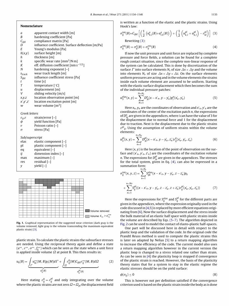
for the different parts aregiven in the appendices, where the expression originally used in thecode discussed in [4,5] is replaced by more efficient equations origi-nating from [6]. Now the surface displacement and the stress insidethe bulk material of an elastic half space with plastic strains insidethe volume are described by Eqs. (5–7). The algorithm depicted inFig. 2 can be used to model the contact of elasto-plastic half-spaces.

One part will be discussed here in detail with respect to theplastic loop and the validation of the code. In the original code thePrandtl Reuss method is used to compute the plastic strains thisis later on adapted by Nelias [5] to a return mapping algorithmto increase the efficiency of the code. The current model also usesa return mapping algorithm however in the current version theplastic loop is changed to a stress related one rather than strain.As can be seen in [4] the plasticity loop is stopped if convergenceof the plastic strain is reached. However, the basis of the plasticitytheory states that for a system to stay in the elastic regime theelastic stresses should be on the yield surface:

�(�ij) ≤ 0 (8)

This is however not per definition satisfied if the convergencecriterion used is based on the plastic strain inside the body as is done

Page 3

1136 R. Bosman et al. / Wear 27

ipeat

compensated in such a way that the plastic corrector is adjusted so

Fig. 2. The iterative process of solving the elasto-plastic contact.

n the previous version of the algorithm. In the current model thelasticity loop used is depicted in Fig. 3. This model is based on an

lastic predictor and plastic corrector scheme combined with thessociated Drucker flow rule. This method is chosen over a plas-ic predictor elastic corrector scheme, since the strains in hard and

Fig. 3. New “plasticity loop” based on the stress relaxatio

1 (2011) 1134– 1146

brittle metals, which are typically used in tribological systems, arelimited to a few percent. Normally the return mapping uses strainas an input, which is then rewritten to a stress through Hook’s law.However, since the elastic stress field for the elastic contact con-ditions can be calculated through the expression of Selas

ij3 and Selasij1 ,

which are given in the appendices, and the following expression:

�elascontij = pSelascont

ij3 + �pSelascontij1 (9)

The elastic stress coming out of the elastic contact is used as theinput stress state for the return mapping which is defined as:

�inijn=0= �elasreturn

ij = �elascontij − �cor

ij (10)

The stress coming out of the return algorithm will be on the yieldsurface. However, as the plastic strain will cause residual stressesthe real stress state will be, see also Eq. (7):

�totalij = �elascont

ij − �corij + �res

ij (εpij) (11)

This stress state will not be on the yield surface since thereturn mapping algorithm already corrected the elastic stress statethrough the plastic corrector to be on the yield surface. For thisreason the elastic guess going into the return mapping needs to be

the complete stress state is on the yield surface again:

�inijn+1= �elascon

ij + �rescompij (12)

n rather than on the relaxation of the plastic strain.

Page 4

R. Bosman et al. / Wear 271 (2011) 1134– 1146 1137

.,

,,,,:

21

etc

FhhconditionsInitial

p

klnklkl

ε

μElastic con tact:

klp

Elastic str esses:

contactσ

Plasticity Loop :

yresp σδσδε ,,

Residualdisplacement:

)(resklu

erroruuu

Nkl

NresklNreskl <− −

)(

)1)(()(

δ

δδ

)( )()1(

)1(

NresNres

Nresres

uuuu

δδλ

δδ

−+

=

−

−

yy

resresres

resresres

ppp

uuuσσ

δ

δσσσ

δεεε

=

+=

+=

+=

End loading

Wear remova l:

klklkl whh −=Update str ess /strain

End load cycle

Yes

Yes

END

No

No

No

rp

klh σε ,,

art of

rtegatsltich

�

ss

Fig. 4. Flowch

Here an iterative process, shown in Fig. 3, is used to find the cor-ect stress compensation such that the complete stress state is onhe yield surface. To speed up the calculation of the plastic strainven more the compensation for the residual stress used in the firstuess can be exchanged for the compensation of the previous iter-tion of the complete loop (n − 1) in Fig. 4. This method resembleshe method used in [7] however the plasticity loop suggested in thattudy is not unconditionally stable and secondly in their study onlyinear hardening laws are used to validate the model. To validatehe new plasticity loop numerical analyses of a 2D asperity, donen the in-house FEM package DIEKA [8], are compared to a full 3Dontact analysis using the code presented here. For the non-linearardening a Swift hardening law is used for the material behavior:

yield(εpl ) = B(C + εpl ˛)n (13)

eq eq

The parameters used are B = 1280 MPa, C = 4, n = 0.095 and iset to 106, representing AISI 52100 steel. For the geometry in theimulation a 0.5 mm asperity is pressed against a rigid flat surface

wear model.

under a load ranging from 0.1 to 600 times the critical load definedas [9]:

Fcritical =(��yield

)3(

3Req

Eeq

)2

(14)

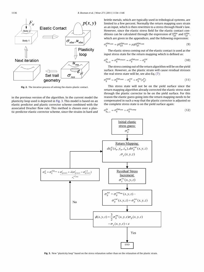
Here �yield is defined by Eq. (13). The results of this simulationare shown in Fig. 5. From this figure it can be concluded that theSAM results concur very well with the FEM results. However, theSAM model is based on small plastic deformations, e.g. the displace-ment field is not guaranteed to be continuous. Therefore, there is alimitation to the use of the model regarding the maximum equiv-

alent plastic strain allowed, as is shown in Fig. 6. In this figure itbecomes clear that up to an equivalent plastic strain of approxi-mately 10% the SAM gives reliable values, after which the modelstarts diverging significantly from the FEM results.

Page 5

1138 R. Bosman et al. / Wear 271 (2011) 1134– 1146

F d SAM( face u

3

mtctmffttw

ig. 5. (a) Normal pressure resulting from the calculation with the FEM package anc) Equivalent strain calculated using SAM. (d) Von Mises stress underneath the sur

. Wear model

As discussed in the introduction the contact regions within theodel can be split up into two parts: regions where oil protects

he surface and unprotected areas. Both regimes have a differentoefficient of friction with values in the range of 0.1 and 0.4, respec-ively. These values originate from measurements done in both the

ild wear regime and the severe wear regime [3,10]. The transitionrom the one to the other is seen as a stepwise phenomenon, if the

ailure criterion of the layer is transcended the coefficient “jumps”o the higher value. For the mild wear situation it is first assumedhat negligible wear will occur at these locations since the shearingill be located in the boundary layers formed on the steel surface

package at 100 times the critical load. (b) Equivalent strain calculated using FEM.sing FEM and (e) SAM.

and thus no bulk material will directly be removed. This corre-sponds well with real systems running under mild wear conditionssince particles generated by this type of systems are mainly builtup from chemical products which originated from the oil [11,12].The severe, local wear is based on the brittle wear behavior of highstrength carbon steels and is associated with a high coefficient offriction. The philosophy underlying the model presented here isintroduced by Nelias [13], using an overall coefficient of frictionof 0.4. The wear model is found upon a recent study of Oila [14],

who suggested that material removal was related to micro-cracksunderneath the surface and was implemented in the current formu-lation by Bosman and Schipper [3], incorporating a local coefficientof friction. To predict the formation of these micro-cracks a crack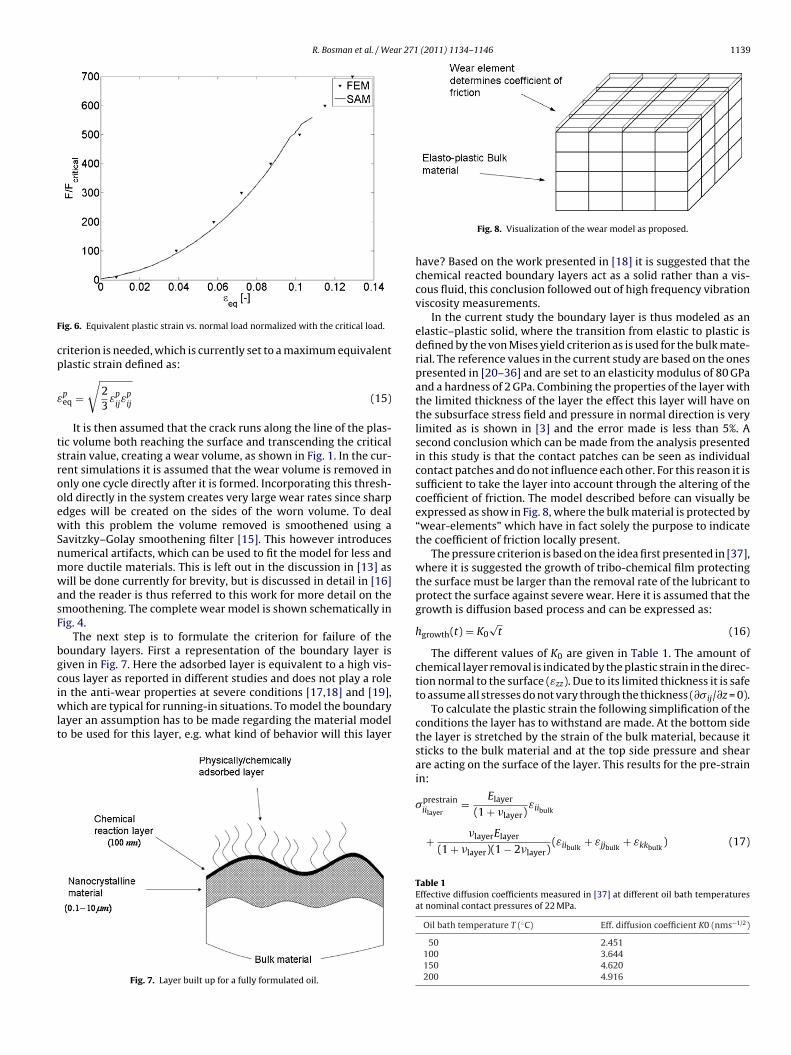

Page 6

R. Bosman et al. / Wear 271 (2011) 1134– 1146 1139

F

cp

ε

tsrooewSnmwasF

bgciwlt

ig. 6. Equivalent plastic strain vs. normal load normalized with the critical load.

riterion is needed, which is currently set to a maximum equivalentlastic strain defined as:

peq =

√23εpijεpij

(15)

It is then assumed that the crack runs along the line of the plas-ic volume both reaching the surface and transcending the criticaltrain value, creating a wear volume, as shown in Fig. 1. In the cur-ent simulations it is assumed that the wear volume is removed innly one cycle directly after it is formed. Incorporating this thresh-ld directly in the system creates very large wear rates since sharpdges will be created on the sides of the worn volume. To dealith this problem the volume removed is smoothened using a

avitzky–Golay smoothening filter [15]. This however introducesumerical artifacts, which can be used to fit the model for less andore ductile materials. This is left out in the discussion in [13] asill be done currently for brevity, but is discussed in detail in [16]

nd the reader is thus referred to this work for more detail on themoothening. The complete wear model is shown schematically inig. 4.

The next step is to formulate the criterion for failure of theoundary layers. First a representation of the boundary layer isiven in Fig. 7. Here the adsorbed layer is equivalent to a high vis-ous layer as reported in different studies and does not play a rolen the anti-wear properties at severe conditions [17,18] and [19],

hich are typical for running-in situations. To model the boundaryayer an assumption has to be made regarding the material modelo be used for this layer, e.g. what kind of behavior will this layer

Fig. 7. Layer built up for a fully formulated oil.

Fig. 8. Visualization of the wear model as proposed.

have? Based on the work presented in [18] it is suggested that thechemical reacted boundary layers act as a solid rather than a vis-cous fluid, this conclusion followed out of high frequency vibrationviscosity measurements.

In the current study the boundary layer is thus modeled as anelastic–plastic solid, where the transition from elastic to plastic isdefined by the von Mises yield criterion as is used for the bulk mate-rial. The reference values in the current study are based on the onespresented in [20–36] and are set to an elasticity modulus of 80 GPaand a hardness of 2 GPa. Combining the properties of the layer withthe limited thickness of the layer the effect this layer will have onthe subsurface stress field and pressure in normal direction is verylimited as is shown in [3] and the error made is less than 5%. Asecond conclusion which can be made from the analysis presentedin this study is that the contact patches can be seen as individualcontact patches and do not influence each other. For this reason it issufficient to take the layer into account through the altering of thecoefficient of friction. The model described before can visually beexpressed as show in Fig. 8, where the bulk material is protected by“wear-elements” which have in fact solely the purpose to indicatethe coefficient of friction locally present.

The pressure criterion is based on the idea first presented in [37],where it is suggested the growth of tribo-chemical film protectingthe surface must be larger than the removal rate of the lubricant toprotect the surface against severe wear. Here it is assumed that thegrowth is diffusion based process and can be expressed as:

hgrowth(t) = K0√t (16)

The different values of K0 are given in Table 1. The amount ofchemical layer removal is indicated by the plastic strain in the direc-tion normal to the surface (εzz). Due to its limited thickness it is safeto assume all stresses do not vary through the thickness (∂�ij/∂z = 0).

To calculate the plastic strain the following simplification of theconditions the layer has to withstand are made. At the bottom sidethe layer is stretched by the strain of the bulk material, because itsticks to the bulk material and at the top side pressure and shearare acting on the surface of the layer. This results for the pre-strainin:

�prestrain = Elayerε

iilayer (1 + layer)iibulk

+ layerElayer

(1 + layer)(1 − 2layer)(εiibulk

+ εjjbulk+ εkkbulk

) (17)

Table 1Effective diffusion coefficients measured in [37] at different oil bath temperaturesat nominal contact pressures of 22 MPa.

Oil bath temperature T (◦C) Eff. diffusion coefficient K0 (nms−1/2)

50 2.451100 3.644150 4.620200 4.916

Page 7

1140 R. Bosman et al. / Wear 271 (2011) 1134– 1146

Fr

wa

�

�

lsgoF

t

taa

ε

ttm

4

ditamtsasrivi3rtoT

different studies only mild chemical wear is observed.To simulate this situation the following macroscopic settings

are used: a load of 225 N is put on a pin with a diameter 6.2 mm

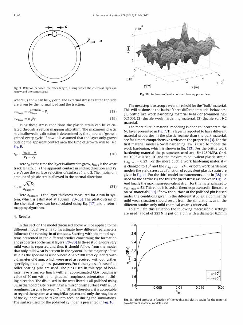
ig. 9. Relation between the track length, during which the chemical layer canenew and the contact area.

here i, j and k can be x, y or z. The external stresses at the top sidere given by the normal load and the traction:

zzlayer = �prestrainzzlayer

+ Pij (18)

xzlayer = �ijPij (19)

Using these stress conditions the plastic strain can be calcu-ated through a return mapping algorithm. The maximum plastictrain allowed in z direction is determined by the amount of growthained every cycle. If now it is assumed that the layer only growsutside the apparent contact area the time of growth will be, seeig. 9:

gr = strack − a∣∣V1 − V2

∣∣ (20)

Here tgr is the time the layer is allowed to grow, strack is the wearrack length, a is the apparent contact in sliding direction and V1re V2 are the surface velocities of surfaces 1 and 2. The maximummount of plastic strain allowed in the normal direction:

zz =√tgrK0

hbalance(21)

Here hbalance is the layer thickness measured for a run in sys-em, which is estimated at 100 nm [20–36]. The plastic strain ofhe chemical layer can be calculated using Eq. (17) and a return

apping algorithm.

. Results

In this section the model discussed above will be applied to theifferent model systems to investigate how different parameters

nfluence the running-in of contacts. Starting with the model sys-ems presented in the different studies concerning the formationnd properties of chemical layers [20–36]. In these studies only veryild wear is reported and thus it should follow from the model

hat only mild wear is present in the system. In the majority of thetudies the specimens used where AISI 52100 steel cylinders with

diameter of 6 mm, which were used as received, without furtherpecifying the roughness parameters. For these types of tests oftenoller bearing pins are used. The pins used in this type of bear-ngs have a surface finish with an approximated CLA roughnessalue of 70 nm with a longitudinal roughness orientation in slid-ng direction. The disk used in the tests listed is all polished using

�m diamond paste resulting in a mirror finish surface with a CLA

oughness varying between 7 and 10 nm. Therefore, it is acceptableo regard the system as a rough/flat system and only the roughnessf the cylinder will be taken into account during the simulations.he surface used for the polished cylinder is presented in Fig. 10.

Fig. 10. Surface profile of a polished bearing pin surface.

The next step is to setup a wear threshold for the “bulk” material.This will be done on the basis of three different material behaviors:(1) brittle like work hardening material behavior (common AISI52100), (2) ductile work hardening material, (3) ductile soft NCmaterial.

The more ductile material modeling is done to incorporate theNC layer presented in Fig. 7. This layer is reported to have differentmaterial properties in the plastic regime than the bulk material,see for a more comprehensive review on the properties [3]. For thefirst material model a Swift hardening law is used to model thework hardening, which is shown in Eq. (13). For the brittle workhardening material the parameters used are: B = 1280 MPa, C = 4,n = 0.095 is set 106 and the maximum equivalent plastic strain:εpleq max = 0.2%. For the more ductile work hardening material ˛

is changed to 105 and the εpleq max = 2%. For both work hardeningmodels the yield stress as a function of equivalent plastic strain aregiven in Fig. 11. For the third model measurements done in [38] areused for the hardness (and thus the yield stress) as shown in Fig. 12.And finally the maximum equivalent strain for this material is set toεpleq max = 5%. This value is based on theories presented in literatureon NC materials [39]. If now the surface of the polished pin is usedunder the conditions given in the different studies, a dominantlymild wear situation should result from the simulations, as in the

Fig. 11. Yield stress as a function of the equivalent plastic strain for the materialtwo different material models used.

Page 8

R. Bosman et al. / Wear 271 (2011) 1134– 1146 1141

Fr

awaat

Fm

ig. 12. Hardness profile as a function of the depth from the surface for a systemunning under boundary lubrication and mild wear conditions conditions [38].

nd a length of 11 mm, resulting in a pressure of 500 MPa [24]

ith an average speed of 0.3 m/s and a track length of 14 mm at

temperature of 100 ◦C results in a growth rate of 1 nm per cyclepproximately using the values of K0 given in Table 1. Using a layerhickness of 100 nm this results in a maximum plastic indentation

Fig. 13. Loading sequence used for the calculations.

ig. 14. Worn surface using the smooth surface combined with the NC materialodel. Transparent surface is the worn part (compared with Fig. 10).

Fig. 15. (a) Wear volume vs. load cycle. (b) Coefficient of friction vs. load cycle.

of the chemical layer of 1% using Eq. (21). The normal pressure of500 MPa is realized by putting a load of 1.6 N on the surface geom-etry presented in Fig. 10. This load is applied in a linear increasingand decreasing signal as shown in Figs. 13 and 14.

A load cycle refers to a complete increase and decrease of thenormal load while a load step refers to one incremental load step. Asmentioned before the simulation using the smooth surface shouldresult in a predominately mild wear situation, which is the case forboth the brittle and ductile material behavior, as no material is lostthrough direct material removal, however this does not exclude

mild microscopic wear through chemical removal of bulk materialas is discussed in [40]. However, for the NC material during thefirst few cycles a limited amount of wear is presented, as can be

Fig. 16. Surface profile of a hard turned disk surface.

Page 9

1142 R. Bosman et al. / Wear 271 (2011) 1134– 1146

Ffi

stc6coa

Fso

ig. 17. Representative result using the wear model combined with the rough sur-ace and the brittle material behavior for a total of 25 load cylces. Transparent surfaces the worn part compared to Fig. 16.

een in Fig. 15. It is furthermore assumed that the wear is limitedo the rougher pin, since it is in constant contact. If now one loadycle corresponds to the displacement of the grid size, in this case4 �m, a resulting specific wear rate as function of the load cycles

an be calculated and is 2 × 10−6 mm3/N m. Here also the coefficientf friction is presented and as can be seen both values are in goodgreement with general values reported in general literature [41]

ig. 18. (a) Wear volume for the different values of ˛. ( = 0 also indicates no pres-ure effect on the Young’s modulus) 9b) coefficient of friction for the different valuesf ˛.

Fig. 19. (a) Wear volume (W) normalized with the wear volume of = 0 and no

hydrostatic effect on the Young’s modulus (W0) for the different values of (b)coefficient of friction for the different values of ˛.

validating the model as proposed, as well as the assumption thatthere is indeed a NC layer present in the first few microns presentunderneath the surface as is proposed in [3].

To investigate the influences of different parameters in themodel under more severe wear conditions the smooth surface isreplaced by a rough on in the simulation as is shown in Fig. 16. As arethe macroscopic contact conditions: a contact width of 300 �m andtotal wear track of 314.5 mm (e.g. disk diameter of 100 mm) com-bined with a oil bath temperature of 100 ◦C and a sliding speed of1 m/s are used. This gives a growth of the chemical layer of approx-imately 2 nm each contact cycle. Using an average chemical layerthickness of 100 nm results in εzzmax = 2%, which will be used as thethreshold for the frictional jump in the simulations following. Thenominal contact pressure for the contact simulations is reduced toapproximately 150 MPa for the rough surface.

In contradiction to the relatively smooth surface the roughsurface undergoes severe wear and the surface roughness is sig-nificantly smoothened to a roughness close to the roughness ofthe polished pins at the load carrying locations as can be seen inFigs. 17–19, even though the nominal contact pressure is a fac-tor 3 lower. Comparing the results of the three different materialsshown in Fig. 20, it can be concluded that most material is lost inthe first 5 cycles for the brittle material. As the surface roughnessdoes not change after the first few cycles the coefficient of frictionstays high. For the more ductile material and the NC material thewear volume is still increasing after 25 load cycles as is the coeffi-cient of friction stabilizing. However, as can be concluded from theresults a surface with a NC layer underneath is the most efficientin reducing the friction by lowering the surface roughness. Since

the coefficient of friction for this material is already at a lower levelas for the other materials while the volume loss is the least. Thiswould be a situation that is most preferable in real engineering sys-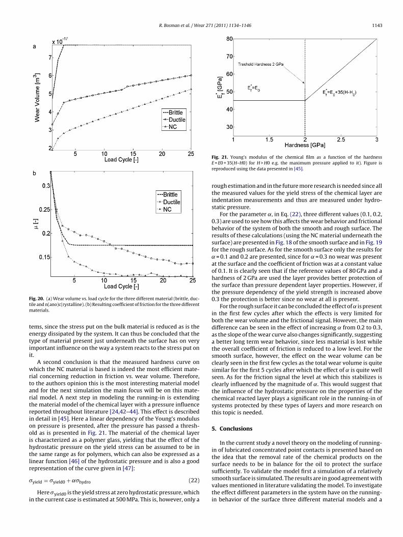

Page 10

R. Bosman et al. / Wear 271 (2011) 1134– 1146 1143

Ftm

tetii

wrtartriooihtlr

�

i

ig. 20. (a) Wear volume vs. load cycle for the three different material (brittle, duc-ile and n(ano)c(rystalline). (b) Resulting coefficient of friction for the three different

aterials.

ems, since the stress put on the bulk material is reduced as is thenergy dissipated by the system. It can thus be concluded that theype of material present just underneath the surface has on verymportant influence on the way a system reacts to the stress put ont.

A second conclusion is that the measured hardness curve onhich the NC material is based is indeed the most efficient mate-

ial concerning reduction in friction vs. wear volume. Therefore,o the authors opinion this is the most interesting material modelnd for the next simulation the main focus will be on this mate-ial model. A next step in modeling the running-in is extendinghe material model of the chemical layer with a pressure influenceeported throughout literature [24,42–44]. This effect is describedn detail in [45]. Here a linear dependency of the Young’s modulusn pressure is presented, after the pressure has passed a thresh-ld as is presented in Fig. 21. The material of the chemical layers characterized as a polymer glass, yielding that the effect of theydrostatic pressure on the yield stress can be assumed to be inhe same range as for polymers, which can also be expressed as ainear function [46] of the hydrostatic pressure and is also a goodepresentation of the curve given in [47]:

yield = �yield0 + ˛�hydro (22)

Here �yield0 is the yield stress at zero hydrostatic pressure, whichn the current case is estimated at 500 MPa. This is, however, only a

Fig. 21. Young’s modulus of the chemical film as a function of the hardnessE = E0 + 35(H–H0) for H > H0 e.g. the maximum pressure applied to it). Figure isreproduced using the data presented in [45].

rough estimation and in the future more research is needed since allthe measured values for the yield stress of the chemical layer areindentation measurements and thus are measured under hydro-static pressure.

For the parameter ˛, in Eq. (22), three different values (0.1, 0.2,0.3) are used to see how this affects the wear behavior and frictionalbehavior of the system of both the smooth and rough surface. Theresults of these calculations (using the NC material underneath thesurface) are presented in Fig. 18 of the smooth surface and in Fig. 19for the rough surface. As for the smooth surface only the results for

= 0.1 and 0.2 are presented, since for = 0.3 no wear was presentat the surface and the coefficient of friction was at a constant valueof 0.1. It is clearly seen that if the reference values of 80 GPa and ahardness of 2 GPa are used the layer provides better protection ofthe surface than pressure dependent layer properties. However, ifthe pressure dependency of the yield strength is increased above0.3 the protection is better since no wear at all is present.

For the rough surface it can be concluded the effect of is presentin the first few cycles after which the effects is very limited forboth the wear volume and the frictional signal. However, the maindifference can be seen in the effect of increasing from 0.2 to 0.3,as the slope of the wear curve also changes significantly, suggestinga better long term wear behavior, since less material is lost whilethe overall coefficient of friction is reduced to a low level. For thesmooth surface, however, the effect on the wear volume can beclearly seen in the first few cycles as the total wear volume is quitesimilar for the first 5 cycles after which the effect of is quite wellseen. As for the friction signal the level at which this stabilizes isclearly influenced by the magnitude of ˛. This would suggest thatthe influence of the hydrostatic pressure on the properties of thechemical reacted layer plays a significant role in the running-in ofsystems protected by these types of layers and more research onthis topic is needed.

5. Conclusions

In the current study a novel theory on the modeling of running-in of lubricated concentrated point contacts is presented based onthe idea that the removal rate of the chemical products on thesurface needs to be in balance for the oil to protect the surfacesufficiently. To validate the model first a simulation of a relatively

smooth surface is simulated. The results are in good agreement withvalues mentioned in literature validating the model. To investigatethe effect different parameters in the system have on the running-in behavior of the surface three different material models and a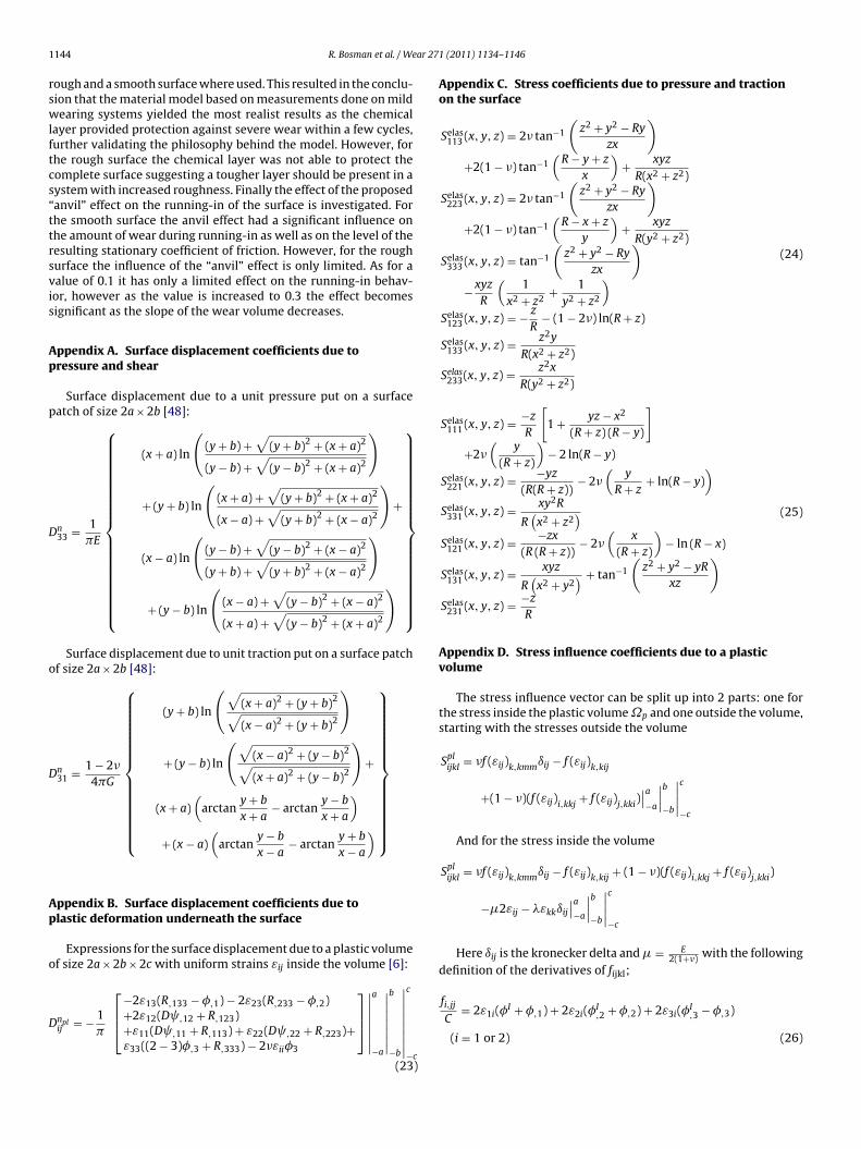

Page 11

1 ar 27

rswlftcs“ttrsvis

Ap

p

D

o

D

Ap

o

D

Here ıij is the kronecker delta and � = 2(1+) with the followingdefinition of the derivatives of fijkl;

fi,jj = 2ε1i(�I + �,1) + 2ε2i(�

I + �,2) + 2ε3i(�I − �,3)

144 R. Bosman et al. / We

ough and a smooth surface where used. This resulted in the conclu-ion that the material model based on measurements done on mildearing systems yielded the most realist results as the chemical

ayer provided protection against severe wear within a few cycles,urther validating the philosophy behind the model. However, forhe rough surface the chemical layer was not able to protect theomplete surface suggesting a tougher layer should be present in aystem with increased roughness. Finally the effect of the proposedanvil” effect on the running-in of the surface is investigated. Forhe smooth surface the anvil effect had a significant influence onhe amount of wear during running-in as well as on the level of theesulting stationary coefficient of friction. However, for the roughurface the influence of the “anvil” effect is only limited. As for aalue of 0.1 it has only a limited effect on the running-in behav-or, however as the value is increased to 0.3 the effect becomesignificant as the slope of the wear volume decreases.

ppendix A. Surface displacement coefficients due toressure and shear

Surface displacement due to a unit pressure put on a surfaceatch of size 2a × 2b [48]:

n33 = 1

�E

⎧⎪⎪⎪⎪⎪⎪⎪⎪⎪⎪⎪⎪⎪⎪⎪⎪⎪⎨⎪⎪⎪⎪⎪⎪⎪⎪⎪⎪⎪⎪⎪⎪⎪⎪⎪⎩

(x + a) ln

((y + b) +

√(y + b)2 + (x + a)2

(y − b) +√

(y − b)2 + (x + a)2

)

+ (y + b) ln

((x + a) +

√(y + b)2 + (x + a)2

(x − a) +√

(y + b)2 + (x − a)2

)+

(x − a) ln

((y − b) +

√(y − b)2 + (x − a)2

(y + b) +√

(y + b)2 + (x − a)2

)

+ (y − b) ln

((x − a) +

√(y − b)2 + (x − a)2

(x + a) +√

(y − b)2 + (x + a)2

)

⎫⎪⎪⎪⎪⎪⎪⎪⎪⎪⎪⎪⎪⎪⎪⎪⎪⎪⎬⎪⎪⎪⎪⎪⎪⎪⎪⎪⎪⎪⎪⎪⎪⎪⎪⎪⎭

Surface displacement due to unit traction put on a surface patchf size 2a × 2b [48]:

n31 = 1 − 2

4�G

⎧⎪⎪⎪⎪⎪⎪⎪⎪⎪⎪⎪⎪⎪⎨⎪⎪⎪⎪⎪⎪⎪⎪⎪⎪⎪⎪⎪⎩

(y + b) ln

(√(x + a)2 + (y + b)2√(x − a)2 + (y + b)2

)

+ (y − b) ln

(√(x − a)2 + (y − b)2√(x + a)2 + (y − b)2

)+

(x + a)(

arctany + b

x + a− arctan

y − b

x + a

)+ (x − a)

(arctan

y − b

x − a− arctan

y + b

x − a

)

⎫⎪⎪⎪⎪⎪⎪⎪⎪⎪⎪⎪⎪⎪⎬⎪⎪⎪⎪⎪⎪⎪⎪⎪⎪⎪⎪⎪⎭

ppendix B. Surface displacement coefficients due tolastic deformation underneath the surface

Expressions for the surface displacement due to a plastic volumef size 2a × 2b × 2c with uniform strains εij inside the volume [6]:

⎡−2ε13(R,133 − �,1) − 2ε23(R,233 − �,2)⎤∣∣∣a ∣∣∣b ∣∣∣∣c

nplij = − 1

�⎢⎣+2ε12(D ,12 + R,123)

+ε11(D ,11 + R,113) + ε22(D ,22 + R,223)+ε33((2 − 3)�,3 + R,333) − 2εii�3

⎥⎦∣∣∣∣−a

∣∣∣∣−b

∣∣∣∣−c

(23)

1 (2011) 1134– 1146

Appendix C. Stress coefficients due to pressure and tractionon the surface

Selas113 (x, y, z) = 2 tan−1

(z2 + y2 − Ry

zx

)+2(1 − ) tan−1

(R − y + z

x

)+ xyz

R(x2 + z2)

Selas223 (x, y, z) = 2 tan−1

(z2 + y2 − Ry

zx

)+2(1 − ) tan−1

(R − x + z

y

)+ xyz

R(y2 + z2)

Selas333 (x, y, z) = tan−1

(z2 + y2 − Ry

zx

)−xyzR

(1

x2 + z2+ 1y2 + z2

)Selas

123 (x, y, z) = − zR

− (1 − 2) ln(R + z)

Selas133 (x, y, z) = z2y

R(x2 + z2)

Selas233(x, y, z) = z2x

R(y2 + z2)

(24)

Selas111 (x, y, z) = −z

R

[1 + yz − x2

(R + z) (R − y)

]+2

(y

(R + z)

)− 2 ln(R − y)

Selas221 (x, y, z) = −yz

(R(R + z))− 2

(y

R + z+ ln(R − y)

)Selas

331 (x, y, z) = xy2R

R(x2 + z2

)Selas

121 (x, y, z) = −zx(R (R + z))

− 2(

x

(R + z)

)− ln (R − x)

Selas131 (x, y, z) = xyz

R(x2 + y2

) + tan−1

(z2 + y2 − yR

xz

)Selas

231 (x, y, z) = −zR

(25)

Appendix D. Stress influence coefficients due to a plasticvolume

The stress influence vector can be split up into 2 parts: one forthe stress inside the plastic volume ˝p and one outside the volume,starting with the stresses outside the volume

Splijkl

= f (εij)k,kmmıij − f (εij)k,kij

+(1 − )(f (εij)i,kkj + f (εij)j,kki)∣∣a−a

∣∣∣b−b

∣∣∣∣c−c

And for the stress inside the volume

Splijkl

= f (εij)k,kmmıij − f (εij)k,kij + (1 − )(f (εij)i,kkj + f (εij)j,kki)

−�2εij − �εkkıij∣∣a−a

∣∣∣b−b

∣∣∣∣c−c

E

C ,2 ,3

(i = 1 or 2) (26)

Page 12

ar 271

)

)

√d��s

�

�

�

�

R

R

R

(

[

[

[

[

[

[

[

[

R. Bosman et al. / We

f3,jjC

= 2ε13(�I,1 + 4x3 − 4R,133 + 3�,1)

+ 2ε23(�I,2 + 4x3�,23 − 4R,233 + 3�,2)

+ 8ε12(−x3�,12 + R,123 + D ,12)

+ 4ε11(−x3�,22 + R,113 + D ,11) + 4ε22(−x3�,22 + R,223 + D ,22)

+ 2ε33(�I,3 − 2x3�,33 + 2R,333 − (5 − 4)�,3) − 8�,3 (27)

fm,jjmC

= 4ε13(�I,13 − 2R,1333 + 2x3�,133 + 3�,13)

+ 4ε23(�I,23 − 2R,2333 + 2x3�233 + �,23)

+ 4ε12(�I,12 + 2R,1233 − 2x3�,123 + (1 − 4)�,12)

+ 2ε11(�I,11 + 2R,1133 − 2x3�,113 + (1 − 4)�,11)

+ 2ε22(�I,22 + 2R,2233 − 2x3�,223 + (1 − 4)�,22)

+ 2ε33(�I,33 + 2R,3333 − 2x3�,333 − (7 − 4)�,33) − 8εii�,33 (28)

fj,jC

= 2ε13(RI,13 − (3 − 4)R,13 + 4(1 − )x3�,1 − 2x3R,133 + 2x23�,13

+2ε23(RI,23 − (3 − 4)R,23 + 4(1 − )x3�,2 − 2x3R,233 + 2x23�,23)

+2ε12(RI,12 − (1 − 2D2)R,12 + 4(1 − )D(x3 + x′3) ,12 + 2x3R,123

−2x23�,12)

+ε11(RI,11 + (1 − 2D2)R,11 + 4(1 − )D(x3 + x′3) ,11 + 2x3R,113

−2x23�,11)

+ε22(RI,22 + (1 − 2D2)R,22 + 4(1 − )D(x3 + x′3) ,22 + 2x3R,2213

−2x23�,22)

+ε33(RI,33 + (3 − 4)R,33 + 8(1 − )x3�,3 − 4(1 − )D� + 2x3R,333

−2x23�,33)

−2εii(�I + (3 − 4)� + 2x3�,3) (29

Here the functions R, , � are defined as r = R =(x − x′) + (y − y′) + (z − z′), = ln(R + �3) and � = 1/R. The

erivatives of this functions are given using k /= j /= i and1 = x − x′, �2 = y − y′, �3 = z − z′ (convolution/infinite space) or3 = z + z′ (correlation/halfspace) which is indicated by either auperscript I or absence of one:

,k = �j ln [r + �l] + �l ln[r + �j

]− �kUk

,kl = ln[r + �j

]�,kk = −Uk�,kkk = −�iVl − �lVi

,kkl = �kVk�,123k = −�kr3�,kkll = −�k�lWj

,kkkk = �l�kWj + �k�jWl �,kkkl = Vj − �2kWj

,kkl = �k ln[r + �j

]R,kkk = �i ln [r + �l] + �l ln

[r + �j

]− 2�kUk

,123k = �kr

R,kkkl = ln[r + �j

]+ �2

kVj R,kkll = �k�lVj

,kkkk = −�j�kVl − �l�kVj − 2Uk R,123kl =−�k�lr3

For and �3 the derivative with respect to �3 become � and + R,3) respectively so in the following only indices k and l are

[

(2011) 1134– 1146 1145

used which are both different and have the value of 1 or 2:

,kk = −�k ln [r + �l] − 2�3Xk ,12 = �3 ln [r + �3] − r

,kkk = −2 ln [r + �l] − (�2k

+ �23)Vl − (�3 − r)�lV3 ,kkl = − �k

r + �34(�3 ),kkk = 2�l ln [r + �3] − �3(�2

k+ �2

3)Vl − �3�l(�3 − r)V3 − 4�kUk

2(�3 ),kkl = �k ln [r + �3] − �k�3

r + �32(�3 ),kkll = �k�lV3

+ �k�l�3

(r + �3)2r

4(�3 )4,kkll = V3�l�k

(�3

r− 2)

+�3�k[�l(�3 − r)W3 − 6Vl + (�2

k+ �2

3)Wl

]− 4Uk

4(�3 ),kkkl = 2 ln [r + �3] + (3�2k

− 2�23)V3 + �3�2

l(�3 − r)W3

+�2lr + (�2

k+ �2

3)�3

r3(30)

The different functions used in (30) are:

Uk = tan−1

[�i�j�kr

](31)

Vk = 1r(r + �k)

(32)

Wk = 2r + �k

r3(r + �k)2

(33)

Xk = tan−1 �k(r + �l + �j)

(34)

References

[1] H. So, R.C. Lin, The combined effects of ZDDP, surface texture and hardness onthe running-in of ferrous metals, Tribology International 32 (1999) 143–153.

[2] I.M Hutchings, Friction and Wear of Engineering Materials, Edward Arnold,Cambridge, 1992.

[3] R. Bosman, D.J. Schipper, Running-in of systems protected by additive-rich oils,Tribology Letters (2010) 1–20.

[4] C. Jacq, D. Nelias, G. Lormand, D. Girodin, Development of a three-dimensionalsemi-analytical elastic-plastic contact code, Journal of Tribology 124 (2002)653–667.

[5] D. Nelias, E. Antaluca, V. Boucly, S. Cretu, A three-dimensional semianalyti-cal model for elastic-plastic sliding contacts, Journal of Tribology 129 (2007)761–771.

[6] S.B. Liu, Q. Wang, Elastic fields due to eigenstrains in a half-space, Journal ofApplied Mechanics-Transactions of the ASME 72 (2005) 871–878.

[7] Z.-J. Wang, W.-Z. Wang, Y.-Z. Hu, H. Wang, A numerical elastic–plastic contactmodel for rough surfaces, Tribology Transactions 53 (2010) 224–238.

[8] University of Twente, 2008, available from: www.dieka.org.[9] K.L. Johnson, Contact Mechanics, Cambridge University Press, Cambridge, 1985.10] M.v. Drogen, The transition to adhesive wear of lubricated concentrated con-

tacts, PhD Thesis, University of Twente, 2005, p. 105, www.tr.ctw.utwente.nl.11] M.Z. Huq, P.B. Aswath, R.L. Elsenbaumer, TEM studies of anti-wear films/wear

particles generated under boundary conditions lubrication, Tribology Interna-tional 40 (2007) 111–116.

12] C. Minfray, T. Le Mogne, J.-M. Martin, T. Onodera, S. Nara, S. Takahashi, H. Tsuboi,M. Koyama, A. Endou, H. Takaba, M. Kubo, C.A. Del Carpio, A. Miyamoto, Exper-imental and molecular dynamics simulations of tribochemical reactions withZDDP: zinc phosphate iron oxide reaction, Tribology Transactions 51 (2008)589–601.

13] D. Nelias, V. Boucly, M. Brunet, Elastic–plastic contact between rough sur-faces: proposal for a wear or running-in model, Journal of Tribology 128 (2006)236–244.

14] A. Oila, S.J. Bull, Assessment of the factors influencing micropitting inrolling/sliding contacts, Wear 258 (2005) 1510–1524.

15] W. Press, S. Teukolsky, W. Vetterling, B. Flannery, Numerical Recipes in C++:The Art Of Scientific Computing, Cambridge University Press, 2002.

16] V. Boucly, Semi-analytical modeling of the transient-elastic-plastic contact andits application to asperity collision, Wear and Running-in of Surfaces, PhD The-sis, Lyon, 2008, p 203.

17] S. Bec, A. Tonck, J.M. Georges, G.W. Roper, Synergistic effects of MoDTC and

ZDTP on frictional behaviour of tribofilms at the nanometer scale, TribologyLetters 17 (2004) 797–809.

18] C. Minfray, J.-M. Martin, M. Belin, T.L. Mogne, M.P.G.D.D. Dowson, A.A. Lubrecht,A Novel Experimental Analysis of the Rheology of ZDDP Tribofilms, Tribologyand Interface Engineering Series, Elsevier, 2003, pp. 807–817.

Page 13

1 ar 27

[

[

[

[

[

[

[

[

[

[

[

[

[

[

[

[

[

[

[

[

[

[

[

[

[

[

[

[

146 R. Bosman et al. / We

19] A. Tonck, S. Bec, J.M. Georges, R.C. Coy, J.C. Bell, G.W. Roper, Structure andMechanical Properties of ZDTP films in Oil, Tribology Series, Elsevier, 1999,pp. 39–47.

20] M.A. Nicholls, P.R. Norton, G.M. Bancroft, M. Kasrai, T. Do, B.H. Frazer, G.D.Stasio, Nanometer scale chemomechanical characterizaton of antiwear films,Tribology Letters 17 (2003) 205–336.

21] Z. Zhang, Tribofilms generated from ZDDP and DDP on steel surfaces: part I,Tribology Letters 17 (2005) 211–220.

22] J.P. Ye, S. Araki, M. Kano, Y. Yasuda, Nanometer-scale mechanical/structuralproperties of molybdenum dithiocarbamate and zinc dialkylsithiophosphatetribofilms and friction reduction mechanism, Japanese Journal of AppliedPhysics Part 1: Regular Papers Brief Communications & Review Papers 44(2005) 5358–5361.

23] J.M. Martin, C. Grossiord, T. Le Mogne, S. Bec, A. Tonck, The two-layer structureof zndtp tribofilms Part 1: AES, XPS and XANES analyses, Tribology International34 (2001) 523–530.

24] M. Kasrai, S. Marina, B.G.Y.E.S. Micheal, R.P. Ray, X-ray adsorption study of theeffect of calcium sulfonate on antiwear film formation generated from neutraland basic ZDDPs: part 1—phosporus species, Tribology Transactions 46 (2003)434–442.

25] M.A. Nicholls, T. Do, P.R. Norton, M. Kasrai, G.M. Bancroft, Review of thelubrication of metallic surfaces by zinc dialkyl-dithiophosphates, TribologyInternational 38 (2005) 15–39.

26] M. Aktary, M.T. McDermott, G.A. McAlpine, Morphology and nanomechanicalproperties of ZDDP antiwear films as a function of tribological contact time,Tribology Letters 12 (2002) 155–162.

27] M.A. Nicholls, G.M. Bancroft, P.R. Norton, M. Kasrai, G. De Stasio, B.H. Frazer,L.M. Wiese, Chemomechanical properties of antiwear films using X-ray absorp-tion microscopy and nanoindentation techniques, Tribology Letters 17 (2004)245–259.

28] J.P. Ye, M. Kano, Y. Yasuda, Evaluation of nanoscale friction depth distributionin ZDDP and MoDTC tribochemical reacted films using a nanoscratch method,Tribology Letters 16 (2004) 107–112.

29] H.B. Ji, M.A. Nicholls, P.R. Norton, M. Kasrai, T.W. Capehart, T.A. Perry, Y.T. Cheng,Zinc-dialkyl-dithiophosphate antiwear films: dependence on contact pressureand sliding speed, Wear 258 (2005) 789–799.

30] S. Bec, A. Tonck, J.M. Georges, R.C. Coy, J.C. Bell, G.W. Roper, Relationship

between mechanical properties and structures of zinc dithiophosphate anti-wear films, Proceedings of the Royal Society of London Series A: MathematicalPhysical and Engineering Sciences 455 (1999) 4181–4203.

31] K. Komvopoulos, V. Do, E.S. Yamaguchi, P.R. Ryason, Nanomechanicaland nanotribological properties of an antiwear tribofilm produced from

[

[

1 (2011) 1134– 1146

phosphorus-containing additives on boundary-lubricated steel surfaces, Jour-nal of Tribology-Transactions of the ASME 126 (2004) 775–780.

32] O.L. Warren, Nanomechanical properties of films derived from zincdialkyldithiophosphate, Tribology Letters 4 (1998) 189–198.

33] C. Minfray, J.M. Martin, C. Esnouf, T. Le Mogne, R. Kersting, B. Hagenhoff, Amulti-technique approach of tribofilm characterisation, Thin Solid Films 447(2004) 272–277.

34] G. Pereira, A varialbe temperature mechanical analysis of ZDDP-derived anti-wear films formed on 52100 steel, Wear (2006) 461–470.

35] G.M. Bancroft, M. Kasrai, M. Fuller, Z. Yin, K. Fyfe, K.H. Tan, Mechanisms oftribochemical film formation: stabilityof tribo- and thermally-generated ZDDPfilms, Tribology Letters 3 (1997) 47–51.

36] K. Topolovec-Miklozic, T. Forbus, H. Spikes, Film thickness and roughness ofZDDP antiwear films, Tribology Letters 26 (2007) 161–171.

37] H. So, Y.C. Lin, The theory of antiwear for ZDDP at elevated temperature inboundary lubrication condition, Wear 177 (1994) 105–115.

38] D. Shakhvorostov, B. Gleising, R. Büscher, W. Dudzinski, A. Fischer, M. Scherge,Microstructure of tribologically induced nanolayers produced at ultra-lowwear rates, Wear 263 (2007) 1259–1265.

39] M.A. Meyers, A. Mishra, D.J. Benson, Mechanical properties of nanocrys-talline materials, Progress in Materials Science 51 (2006) 427–556.

40] R. Bosman, D.J. Schipper, Mild wear prediction of boundary-lubricated contacts,Tribology Letters, in press.

41] A. William Ruff, Friction and Wear Data Bank, in: Modern Tribology Handbook,Two Volume Set, CRC Press, 2000.

42] N.J. Mosey, M.H. Muser, T.K. Woo, Molecular mechanisms for the functionalityof lubricant additives, Science 307 (2005) 1612–1615.

43] N.J. Mosey, T.K. Woo, M. Kasrai, P.R. Norton, G.M. Bancroft, M.H. Müser, Inter-pretation of experiments on ZDDP anti-wear films through pressure-inducedcross-linking, Tribology Letters 24 (2006) 105–114.

44] J. Tse, Y. Song, Z. Liu, Effects of temperature and pressure on ZDDP, TribologyLetters 28 (2007) 45–49.

45] K. Demmou, S. Bec, J.L. Loubet, Effect of Hydrostatic Pressure on the ElasticProperties of ZDTP Tribofilms, Cornell University Library, 2007.

46] J. Rottler, M.O. Robbins, Yield conditions for deformation of amorphous polymerglasses, Physical Review E 64 (2001) 051801.

47] K. Demmou, S. Bec, J.-L. Loubet, J.-M. Martin, Temperature effects on mechanicalproperties of zinc dithiophosphate tribofilms, Tribology International 39 (2006)1558–1563.

48] K. Willner, Fully coupled frictional contact using elastic halfspace theory, Jour-nal of Tribology 130 (2008) 031405–31408.