Salt Uptake in Natural Channels Traversing Mancos Shales in ...

Page 1

Utah State University Utah State University

DigitalCommons@USU DigitalCommons@USU

Reports Utah Water Research Laboratory

January 1982

Salt Uptake in Natural Channels Traversing Mancos Shales in the Salt Uptake in Natural Channels Traversing Mancos Shales in the

Price River Basin, Utah Price River Basin, Utah

J. Paul Riley

D. George Chadwick

Lester S. Dixon

L. Douglas James

William J. Grenney

Eugene K. Israelsen

Follow this and additional works at: https://digitalcommons.usu.edu/water_rep

Part of the Civil and Environmental Engineering Commons, and the Water Resource Management

Commons

Recommended Citation Recommended Citation Riley, J. Paul; Chadwick, D. George; Dixon, Lester S.; James, L. Douglas; Grenney, William J.; and Israelsen, Eugene K., "Salt Uptake in Natural Channels Traversing Mancos Shales in the Price River Basin, Utah" (1982). Reports. Paper 123. https://digitalcommons.usu.edu/water_rep/123

This Report is brought to you for free and open access by the Utah Water Research Laboratory at DigitalCommons@USU. It has been accepted for inclusion in Reports by an authorized administrator of DigitalCommons@USU. For more information, please contact [email protected].

Page 2

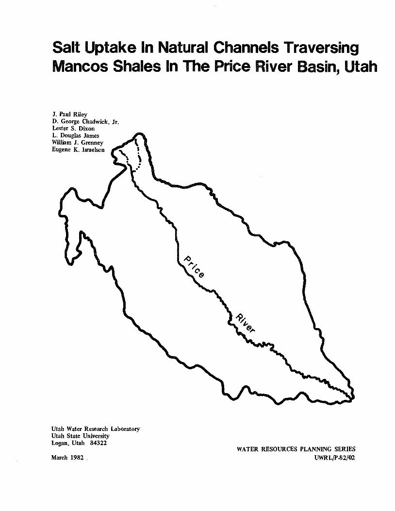
Salt Uptake In Natural Channels Traversing Mancos Shales In The Price River Basin, Utah

J. Paul Riley D. George Chadwick, Jr. Lester S. Dixon L. Douglas James William J. Grenney Eugene K. lsraeJsen

Utah Water Research Laboratory Utah State University Logan, Utah 84322

March 1982 . WATER RESOURCES PLANNING SERIES

UWRL/P-82/02

Page 3

SALT UPTAKE IN NATURAL CHANNELS TRAVERSING MANCOS

SHALES IN THE PRICE RIVER BASIN, UTAH

by

J. Paul Riley D. George Chadwick. Jr.

Lester S. Dixon L. Douglas James

William J. Grenney and

Eugene K. Israelsen

WATER RESOURCES PLANNING SERIES UWRL/P-82/02

Utah Water Research Laboratory Utah State University

Logan, Utah 84322

March 1982

Page 4

ABSTRACT

Field and laboratory measurements of process rates for runoff and salt movement were used to develop and calibrate a hydrosalinity model of outflows from the Price River Basin at Woodside, Utah. The field measurements were specifically used to formulate a model for esti­mating surface flow (both overland and from small ephemeral channels) in the Coal Creek Basin on the valley floor of the Price River Basin. The basin simulation assessment model (BSAM) was used to combine local flows and model total outflow from the Price River.

The results must be regarded as a first generation model that, while giving ostensibly reasonable results, needs much additional refinement and validation by collecting additional field data. As to field data, observed salt loading rates reached 518 pounds per square mile daily, groundwater inflow declined steadily throughout the summer but maintained constant salt concentrations, channel efflorescence varied more than 100 fold with the largest concentrations occurring in saturated bed material, and turbulent mixing and cyclic drying added to salt disMolution rates.

Extrapolation of tl;te results with the Coal Creek model showed only a very small percentage of the salt loading from the valley floor to originate from natural lands. BSAM showed average annual salt leaving the Basin at Woodside to be 190,000 tons, 114,000 coming from the mountain area and 76,000 from the valley floor. Of the valley floor contribution, only 3,500 tons are produced by surface runoff from nonirrigated areas.

Topics to be emphasized in further model development include salt contribution from percolation snowmelt on natural lands, ground­water movement, the formation and dissolution of efflorescence, and salt-sediment transport by the sharp hydrographs on small ephemeral streams.

iii

Page 5

ACKNOT.1LEDGMENTS

Funding for this study was provided in part by the U.S. Bureau of Reclamation .• Contract Number l4-06-D-769l (UHRL project WG178).

iv

Page 6

Chapter

I

II

III

IV

V

TABLE OF CONTENTS

INTRODUCTION

The Problem Study Objectives Significance of the Study Literature Review .

Streamflow and salinity functions Salinity models

Hydrosalinity of the Price River Basin

THE PRICE RIVER BASIN

Topography Geology

Streamflows Water quality Groundwater Vegetation Economy

STUDY METHODS AND PROCEDURES

Scope of the Study. Stream Surveys and Reconnaissance. Coal Creek Instrumentation . Stream Sampling and Field Tests Laboratory Tests

FIELD INVESTIGATION RESULTS FROM THE STUDY

Page

1

1 2 3 3

3 6

8

11

11 11

12 13 15 15 16

17

17 17 18 19 21

23

Salinity and the Price River Basin 23 Coal Creek Study Area. 27

Meteorology . 27 Coal Creek storm runoff 27 Coal Creek flow and quality measurements. . 29 Salinity from the Coal Creek channel sediments. 29 Mineral dissolution from the Coal Creek

channel material . 33 Time rates of dissolution. 36 Macrochannel induced streamflow studies 37

Discussion and Analysis of Results 42

THE HYDROSALINITY MODEL.

Introduction.

Modeling strategy System identification

Hydrology Component

Precipitation (RAIN) Precipitation excess (HYDRGY) Surface runoff (SRO)

v

45

45

45 45

45

45 53 53

Page 7

Chapter

TABLE OF CONTENTS (CONTINUED)

Salinity Component (SALIN)

Overland flow salt loading Channel salt loading

VI MODEL APPLICATION TO THE COAL CREEK DRAINAGE

Application Procedure . Simulation Results .

Estimated salt output from Coal Creek Model sensitivity .... Estimated salt output at Woodside

VII BASIN-WIDE HYDROSALINITY STUDY

Introduction Data Results

VIII SUMMARY, CONCLUSIONS, ih~D RECOMMENDATIONS

Summary Conclusions Recommendations

SELECTED BIBLIOGRAPHY

APPENDIX A: CHEMICAL METHODS AND PROCEDURES

APPENDIX B: FIELD SURVEY DATA

APPENDIX C: COAL CREEK FIELD DATA

APPENDIX D: LABORATORY DATA .

APPENDIX E: LISTINGS OF THE HYDROLOGIC/SALINITY MODELS

vi

Page

54

54 54

57

57 59

59 60 60

65

65 65 65

77

77 78 78

79

83

85

91

125

139

Page 8

LIST OF FIGURES

Figure Page

1.1 Price River Basin 2

1.2 Daily conductance and the mean daily discharge measure­ments for the Gila River at Bylas, Arizona, during August 1943 3

1.3 Relation of chloride concentration to water discharge rate for the Saline River, Kansas . 4

1.4 Salt load versus annual surface runoff 5

1.5 Flow (cfs) and salinity (ppm) for typical storms on the West Bitter Creek watershed, Oklahoma 6

1.6 Hypothetical antecedent flow index 7

1.7 Irrigated and potentially arable land in the Price River Basin 9

2.1 Predominant geologic formations of the Price River Basin 11

2.2 Mancos Shale cross-section 12

2.3 Mean annual water yield in inches 13

2.4 Price River Valley estimated annual water budget in acre-feet/year 15

3.1 Coal Creek instrumentation 18

3.2 The Coal Creek study section showing ephermeral trib-utaries and soil samples sites . 20

3.3 Channel configuration and instrumentation sites for the macrochannel study 20

4.1 Discharge and conductivity versus date, from the Price River at Woodside 24

4.2 Conductivity versus discharge, for the Price River at Woodside 24

4.3 Price River flow profile for October 19 to 21, 1976 . 25

4.4 Price River salinity profile for October 19 to 21, 1976. 25

4.5 Price River Basin sampling sites listed by Mundorff (1972) 26

4.6 Desert Seep Wash vicinity map 27

4.7 Lower Coal Creek flow hydrograph, beginning August 8, 1976 28

4.8 Conductivity at Coal Creek upper site 31

4.9 Flow at Coal Creek upper site 31

4.10 Coal Creek conductivity of the spring inflow 31

vii

Page 9

·

Figure

4.11

4.12

4.13

4.14

4.15

4.16

4.17

4.18

4.19

4.20

4.21

4.22

4.23

4.24

4.25

5.1

5.2

5.3

5.4

5.5

5.6

5.7

5.8

5.9

6.1

6.2

6.3

6.4

LIST OF FIGURES (CONTINUED)

Page

Coal Creek lateral inflow from the spring 31

Coal Creek conductivity at the middle site 32

Coal Creek flow at the middle site 32

Coal Creek conductivity at the lower site 32

Coal Creek flow at the lower site . 32

Accumulated conductivity from laboratory salt dissolu-tion 36

Illustrative effect of wetting and drying cycles on conductivity 37

Illustrative macrochannel salt concentration response 38

Accumulated salt load versus accumulated flow at flumes 2, 3, and 4 of the macrochannel, August 26, 1976 39

Macrochannel salt (8/26/76)

Macrochannel salt (9/9/76)

Salt dissolution

load versus the square-root of time

load versus the square-root of time

from macrochannel bedload material

40

40

41

Typical salinity sensor response curves 43

Channel 2-1 salt load coefficient . 44

Channel 1-2 salt loading coefficient 44

Steps in the development and application of a simula-tion model 46

Idealized natural hydrosalinity system 47

Simplified conceptual natural hydrosalinity system 48

Gumbel distribution of days with precipitation in June 49

Log-normal distribution of daily precipitation for May 50

Normal distribution of storm runoff for June, July, and August 51

Characteristic storm hyetograph 52

Drainage characteristics of the Coal Creek subbasin 55

Primary channel wetted perimeter subdivision 56

The subbasins and macrochannels of the Coal Creek drainage 57

Model representation of Coal Creek 58

Model response to 0.2 mID of surface runoff (lower Coal Creek site) 59

Conductivities as a function of time for different channel distances traveled 62

viii

Page 10

~ .

Figure

6.5

7.1

7.2

7.3

7.4

7.5

7.6

7.7

7.8

7.9

7.10

C.l

C.2

C.3

C.4

C.5

LIST OF FIGURES (CONTINUED)

Page

Salt load as a function of channel distance to the 0.4 power 62

Hydrologic system as conceptualized for BSAM 66

Price River BSAMl simulated water flows at Woodside (1973-1975) 68

Price River BSAMl simulated salt flows at Woodside (1973-1975) 69

Price River BSAMI simulated salt concentrations at Woodside (1973-1975) 69

Change in Price River hydrograph at Woodside caused by reducing ungaged inflow by 20 percent 70

Change in Price River salt output at Woodside caused by reducing ungaged inflow by 20 percent . . . 71

Change in Price River hydrograph at Woodside caused by increasing irrigation efficiencies by 10 percent . 72

Change in Price River salt output at Woodside caused by increasing irrigation efficiencies by 10 percent 73

Change in Price River hydro graph at Woodside caused by changing to crops with smaller consumptive uses 74

Change in Price River salt output at Woodside caused by changing to crops with a smaller consumptive use 75

Channel cross sections, Coal

Channel cross sections, Coal

Channel cross sections of the

Macro channe 1 flow hydro graphs

Macrochannel flow hydrographs

ix

Creek downstream

Creek upstream

Macrochannel

for August 26, 1976

for September 9, 1976

92

92

119

120

121

Page 11

Table

1.1

1.2

2.1

2.2

2.3

4.1

4.2

4.3

4.4

4.5

4.6

LIST OF TABLES

Salinity sources

Water budget for the valley floor area of the Price River Basin

Mean monthly and annual temperatures and precipitations for stations in the Price River drainage area .

Mean monthly and annual runoff for stations in acre feet in the Price River drainage area

Farming types and percent of total in the drainage

Linear regression analysis of chemical constituents versus electrical conductivity from four observation sites on Coal Creek

Observed chemical concentrations in Coal Creek

Soil conductivities for beds and banks for Coal Creek locations .

Results of t-tests for significant differences among soil extract electrical conductivities of samples taken from Coal Creek and Coal Creek tributaries

Effect of rinsing and drying on accumulated conductivity .

Analysis of variance for significance of the effect of rinsing and drying .

4.7 Total accumulated conductivity including additional

4.8

4.9

4 10

4.11

4.12

4.13

5.1

5.2

6.1

treatment .

Analysis of variance for significance of the effect of additional rinsing and drying

Comparison of mineral dissolution rates with time and grain size

Linear regression of accumulated salt load versus the square-root of time

Macrochannel salt loading per unit channel length

Mean salt dissolution rates for macrochannel sediments

Analysis of salt dissolution rates for channel receiving no overland flow

Comparison of output from subroutine RAIN with monthly recorded rainfalls .

Coefficients of overland flow load function for the various members of the Mancos Shale

Primary channel characteristics

xi

Page

6

8

· 14

14

16

30

33

· 33

· 34

· 35

· 35

· 35

· 35

· 37

39

39

· 41

· 42

52

54

58

Page 12

Table

6.2

6.3

6.4

6.5

6.6

6.7

6.8

6.9

7.1

7.2

8.1

A.l

A.2

A.3

B.l

B.2

B.3

C.l

C.2

C.3

C.4

C.5

C.6

C.7

C.8

C.9

0.1

0.2

LIST OF TABLES (CONTINUED)

Subbasin characteristics

Channel and salt loading characteristics

Simulated annual salt load from natural channels in the Coal Creek study area .

Coefficient values for application of the hydro salinity model of the Coal Creek drainage

Extrapolated annual salt load at Woodside

Accumulated salt mass vs. accumulated flow for various shale types .

Coefficients in the microchannel salt loading function y = axb

Estimated salt production from surface flows for various shale types in the Price River Basin

Correlations used to estimate 1973-1975 flows at Heiner

Price River flows at Woodside with various management options as estimated by BSAMI

Estimated salt loading from natural channels

Methods and procedures, College of Eastern Utah Chemistry Department

Methods and procedures, Utah Water Research Laboratory

Methods and procedures, USU Soils Laboratory

Price River Basin field study

Price River Basin intensive survey 8/26/75

Price River profile survey

Coal Creek conductivity profile

Coal Creek water quality

Soil 1:1 saturation results

Coal Creek weather data

Coal Creek storm data

Surface crust salt potential

Macrochannel study of August 26, 1976

Macrochannel study of September 9, 1976

Soil sensor results .

Saturation dissolution results

Saturation dissolution data, samples rinsed and dried

xii

59

59

60

60

61

61

63

63

67

76

77

83

83

84

86

88

89

92

93

97

103

III

118

122

123

124

126

DO

Page 13

LIST OF TABLES (CONTINUED) ~

Tables Page

D.3 Rotoevaporator dissolution results . 134

D.4 Power function coefficients for dissolution from different grain sizes in quiescent water 134

D.5 Macrochannel sediment results (8/26/76) 135

D.6 Least squares regression analysis of Equation 4.3 137

E.l. a The stochastic rainfall subroutine (RAIN) 140

E.l. b A sample of rainfall data generated by RAIN 141

E.l. c Hydrologic extractions subroutine (HYDRGY), including the plant consumptive use subroutine (CONSUM) 150

E.2.a Fortran listing of the hydrologic-salinity model for surface runoff 154

E.2.b Model parameters and des.criptions 162

E.2.c Input data list and format 163

E.3.a Fortran listing of the simplified model for predicting salt pickup by.overland and microchannel flows 164

E.3.b Typical output 168

E.4.a The correlation procedures used to estimate flows at Heiner 174

E.4.b Output from the calibration run 176

xiii

Page 14

CHAPTER I

INTRODUCTION

The Problem

Salinity is a major issue in the Lower' Colorado River Basin. A criterion for flow­weighted average annual salinity concen­tration of 879 mgtl was established in 1976 as a maximum for flows at Imperial Dam. Three years before, the seven basin states had formed a Colorado River Basin Salinity Control Forum to coordinate salinity control efforts. A provision, known as Minute 242, in an agreement with Mexico, assured that waters delivered to the Mexican diversion point would have an annual average salinity of no more than 115 ppm over tha t of wa ter arriving at Imperial Dam. While average annual salinities have decreased from 890 mgtl in 1970 to a little below 800 mgtl in 1981, a decline probably associated with the filling of Lake Powell, the expectation for the long run is for increasing salinity levels unless an effective control program is established. Any major future increases in salinity would only add to already major losses to agriculture and damages to munici­pal and industrial water users (U. S. Depart­ment of the Interior 1974 and Andersen and Kleinman 1978).

Multiple methods are being explored to hold down salinity concentrations. Two principal alternatives exist. One is to remove salt from the water through construc­tion of a desalting complex as has been authorized by PL 93-320 for the United States to fulfill its obligation with Mexico. A potentially less expensiv~ alternative is to reduce the concentration of salt reaching the mouth of the Colorado. The concentration may be reduced either by adding to the water or by reducing the salt. The high economic value of water in the Lower Basin makes using more to transport salt unattractive and focuses attention on ways to reduce the salt content.

One approach to reducing salt content is to reduce the amount of salt leaving the Upper Basin either by augmenting natural salt precipitation processes or by finding an economically attractive use for salt brine. Explored options include salt precipitation in'reservoirs (Messer et a1. 1981), export of salt brines as the conveying fluid in coal slu rry pipelines (Israelsen, et a1. 1980), and use of the salt for electric power production in salt-gradient solar ponds (Riley and Batty 1982). All three have cost or technical feasibility problems.

1

Alternatives for reducing the original salt loading entering the river system are even more difficult to evaluate because the salt sources are so many and so diffuse. Salts enter the Colorado River after being leached from irrigated soils, concentrated by evapotranspiration, and returned as agri­cultural drainage. Municipal and industrial uses add salts from extracted groundwater, expose salt bearing materials to weathering, and increase leaching as a result of outside water uses in residential areas. Fossil fuel extraction and processing in the Upper Basin are being particularly watched as future threats.

All of these man-caused sources of salt loading add to the larger natural salt loading. Mineral springs and natural groundwater seeping from marine formations abound. Natural diffuse sources are scat­tered over vast areas of open land.

Blackman et a1. (1973) estimate that 37 percent of the total salt loading to the Colorado River occurs from diffuse sources in the Upper Basin. Mountainous areas yield most of the river flow from a relatively small fraction of the catchment and supply relatively high quality water. As the streams traverse the immense, semiarid lowlands, little flow is added and water quality deteriorates as water is used con­sumptively and the streams interact with natural salt bearing geological formations.

The Price River subbasin of Central Utah (Figure 1.1) is a miniature of this salt loading pattern. Relatively high quality flow (less than 1000 mg/l TDS or total dissolved solids) originates in mountainous headwater areas. After emerging from the mountains, the river traverses an irrigated area amounting to about 2 percent of the total catchment. Further downstream, it crosses large areas of natural and range lands. It contacts a marine formation high in soluble salt content called the Mancos Shale. Finally, it reaches Woodside with an average dissolved solids concentration of about 2500 mgtI.

This most downstream river section, where the Price River flows through arid range lands having an average annual precipi­tation of only about 8 inches, provides a setting to study and quantify natural salt loading. Hopefully, the relationships derived and the understanding gained from

Page 15

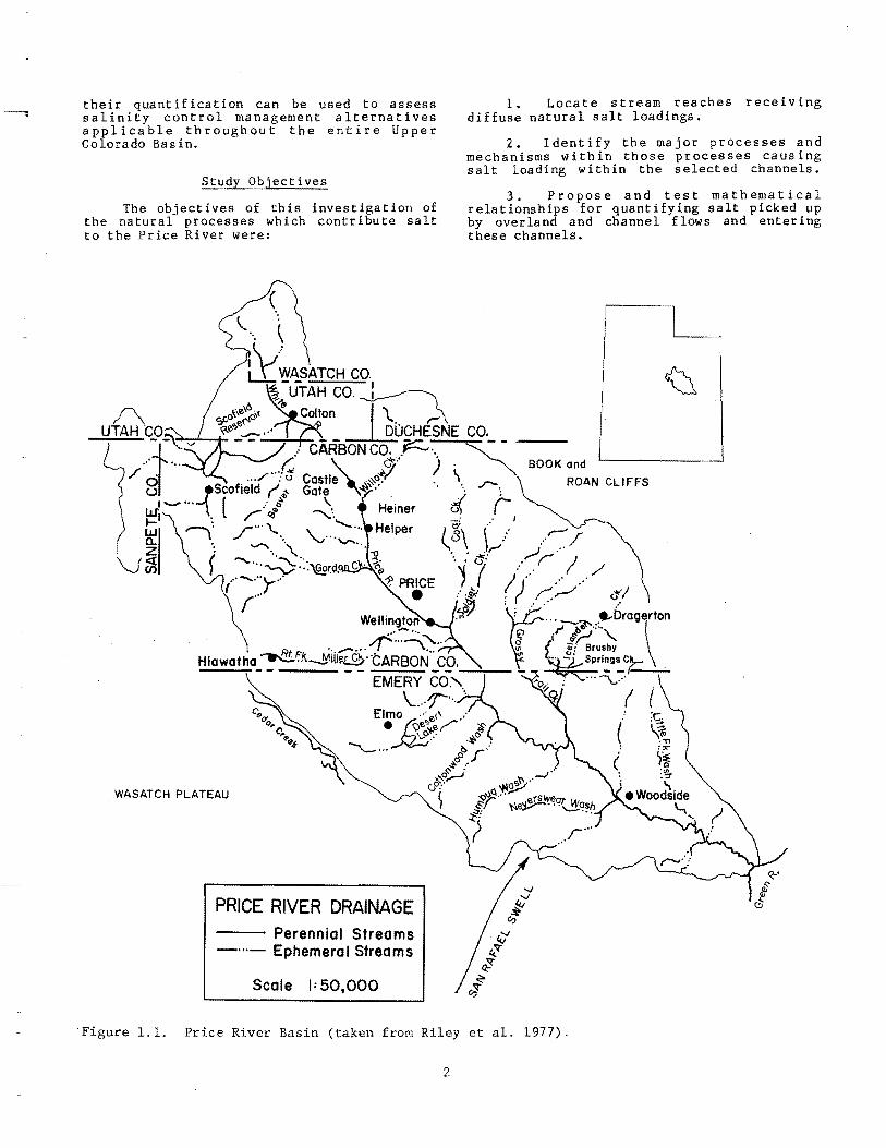
their quantification can be used to assess salinity control management alternatives applicable throughout the entire Upper Colorado Basin.

Study Objectives

The objectives of this investigation of the natural processes which contribute salt to the Price River were:

(.

WASATCH PLATEAU

PRICE RIVER DRAINAGE Perennial Streams Ephemeral Streams

Scale ,: 50,000

1. Locate stream reaches receiving diffuse natural salt loadings.

2. Identify the major processes and mechanisms within those processes causing salt loading within the selected channels.

3. Propose and test mathematical relationships for quantifying salt picked up by overland and channel flows and entering these channels.

I

BOOK and

ROAN CLIFFS

Figure 1.1. Price River Basin (taken from Riley et al. 1977).

2

Page 16

4. Integcate the selected relationships into a mathematical model of the natural processes loading the stream with salts.

5. Employ the hydrosalinity model in analysis of the contribution of salt loadings from natural areas in the Price River Basin.

Significance of the Study

A well founded understanding of salt loading processes is required to develop effective salinity management programs for the arid Colorado River Basin. The under­standing needs to identify and describe the physical processes picking salt up from diffuse sources and carrying it downstream, establish quantitative relationships for estimating salt loading and transport, and thereby provide a basis for selecting promising land and water management programs and predicting how well they will perform. The effort to build that understanding has been severely handicapped by the paucity of data on salt movement. Hence, this study seeks both to collect data and to model, to do both simultaneously in an interactive way with the hope of advancing 01"!"/'! quickly to the needed understanding.

According to Hyatt et al. (1970), "Research is needed to improve relationships for predicting water quality as a function of parameters such as various watershed characteristics and hydrology. Because of the complex processes which occur in a watershed, it is likely these relationships will need to be empirical in nature. As improved relationships are developed, theX can be incorporated into system models. I

This project developed a first generation mathematical model capable of simulating the major salinity uptake mechanisms from an ephemeral catchment in the Mancos Shale wildlands. Such simulation begins quantita­tive definition of relationships between catchment characteristics and salt loading in a rigorous way that can later be used in examining ways a salinity control program can reduce salt loading. Without the discipline of a verified model for their assessment, management proposals are only guesses.

Literature Review

Streamflow and salinity functions

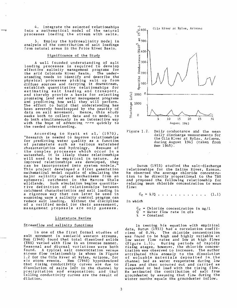
In one of the first formal studies of salt movement in semiarid western streams, Hem (1948) found that total dissolved solids (TDS) varied with flow in an inverse manner. Seasonal and diurnal variations were both found. A typical salt concentration versus stream flow relationship is shown in Figure 1.2 for the Gila River at Bylas, Arizona, for six storm events. Hem (1948) hypothesized that rising conductivity curves are due to dissolution of salts left in the channel by precipitation and evaporation; and that falling conductivity curves are the result of dilution.

3

u600 Gila River at Bylas, Arizona 0

If)

N

'-' co 500

If)

0 ......

~ 400 '-"

Cli U 0::

1:1300 <J ::l \ 'g 8200 <J ."

""' 'j 100 <J) Lv P,

tf.l

~

2000 0 Cfl

""' U '-"

<J) 1000 <>0 ... l'\l ,.c <J Cfl 0 ." Cl

5 10 15 20 25 31 August 1943

Figure 1.2. Daily conductance and the mean daily discharge measurements for the Gila River at Bylas, Arizona, during August 1943 (taken from Hem 1948).

Durum (1953) studied the salt-discharge relationships for the Saline River, Kansas. He observed the average chloride concentra­t ion to be directly proportional to the TDS and proposed the following relationship for relating mean chloride concentration to mean flow:

Cc k/Q............ (1.1)

in which

Cc Chloride concentration in mg/l Q Water flow rate in cfs k Constant

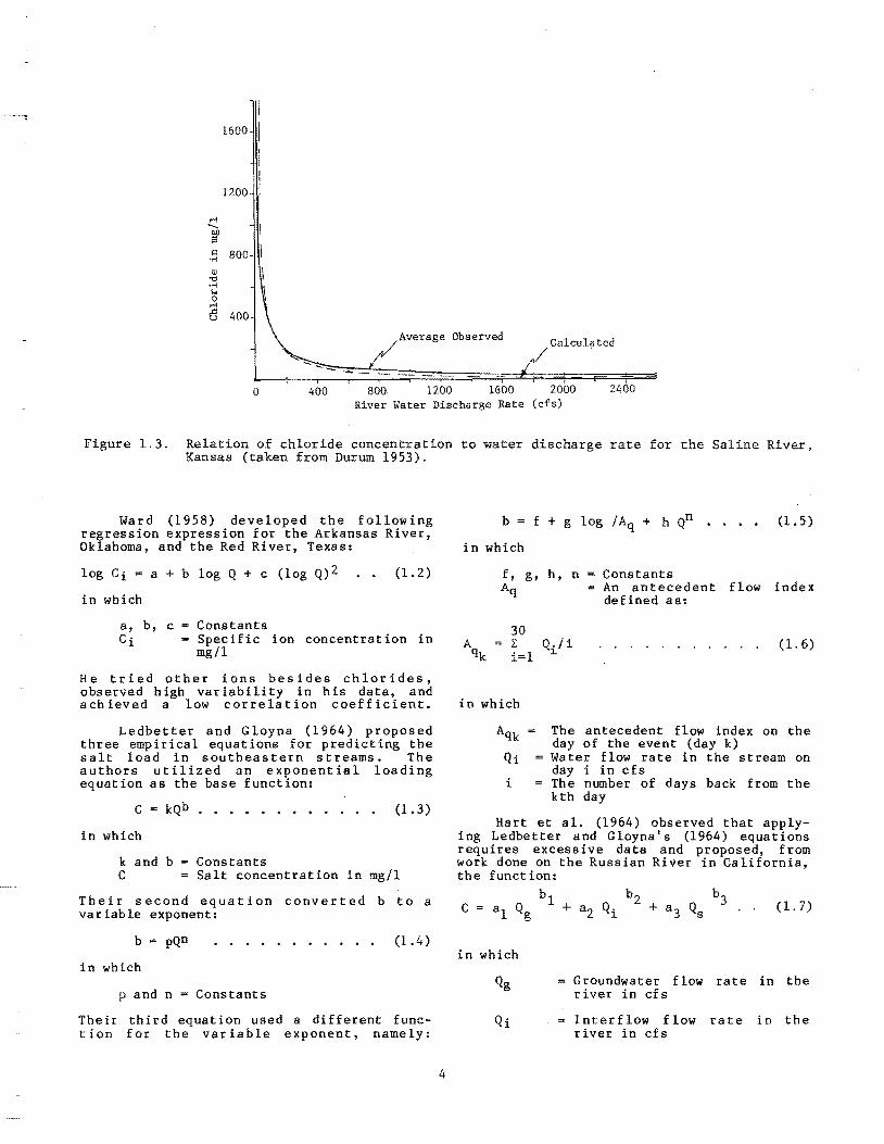
In testing his equation with empirical data, Durum (1953) had a correlation coeffi­cient of 0.94. The chloride concentration was found to be high and highly variable at low water flow rates and low at high flows (Figure 1.3). During periods of rapidly rising stages, however, the chloride concen­tration was'observed to increase. The author attributed this anomaly to the dissolution of soluable materials deposited in. the channel bed as water evaporates during low flows and then scoured out and carried as suspended or bed load with the rising flow. He estimated the contribution of salt from groundwater by assuming that flow during the winter months equals the groundwater inflow.

Page 17

.-i "-

rf

1600

1200

o~ 800 <lJ

"CJ OM j.4 o

.-i

a 400

Average Observed -=,.-L~lculated

o 400 800, 1200 1600 2000 2400 River Water Discharge Rate (cfs)

Figure 1.3. Relation of chloride concentration to water discharge rate for the Saline River, Kansas (taken from Durum 1953).

Ward (1958) developed the following regression expression for the Arkansas River, Oklahoma, and the Red River, Texas:

log Ci = a + b log Q + c (log Q)2 (1. 2)

in which

a, b, c = Constants Ci Specific ion concentration in

mg/l

He tried other ions besides chlorides, observed high variability in his data, and achieved a low correlation coefficient.

Ledbetter and Gloyna (1964) proposed three empirical equations for predicting the salt load in southeastern streams. The authors utilized an exponential loading equation as the base function:

C = kQ b • • • • • • • • • • • (1.3)

in which

k and b = Constants C Salt concentration in mg/l

Their second equation converted b to a variable exponent:

b pQn (1.4)

in which

p and n = Constants

Their third equation used a different func­tion for the variable exponent, namely:

4

b = f + g log / Aq + h Qn • . .• (1 .5)

in which

f, g, h, n = Constants Aq An antecedent flow index

defined as:

(1. 6)

in which

i

The antecedent flow index on the day of the event (day k) Water flow rate in the stream on day i in cfs The number of days back from the kth day

Hart et al. (1964) observed that apply­ing Ledbetter and Gloyna's (1964) equations requires excessive data and proposed, from work done on the Russian River in California, the function:

C (1. 7)

in which

Qg Groundwater flow rate in the river in cfs

Qi Interflow flow rate in the river in cfs

Page 18

a and b

Surface flow rate in the river in cfs

Constants determined by a regression based on field observations

In this relationship, salt loading is divided among three flow paths and var ies expo­nentially with respect to flow.

Langbein and Dawdy (1964) suggested that watershed chemical weathering can be de­scribed according to Nernst's law and pro­posed the functions:

dL/dt (1. 8)

in which

L Dissolved mass t Time D Maximum rate of dissolution Cs Saturation concentration A Drainage area under consideration

By simple mass balance differencing, Equation 1.8 may be represented as:

in which

(1. 9)

Concentration of influent water (water in the river channel enter­ing the area drained by the sub­basin of area, A)

Concentration of effluent water (water leaving the subbasin of area, A)

AlgebraiC manipUlation of Equation 1.9 yields:

Cs (1 + Ci Q/DA) C = ....... (1.10)

o 1 + QCs/DA

Equations 1.8 to 1.10 are nearly the same as those proposed by Jurinak et a1. (1977) 13 years later.

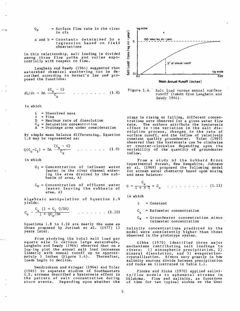
From studying the total salt load per square mile in various large watersheds, Langbein and Dawdy (1964) observed that on a log-log plot the annua 1 sa It load increases linearly with annual runoff up to approxi­mately 3 inches (Figure 1.4). Thereafter, loads begin to decline.

Hendrickson and Krieger (1964) and Toler (1965) in separate studies of Southeastern U.S. streams described a hysteresis effect in the pattern of salt concentration during storm events. Depending upon whether the

5

log scale

-I I 3" of annual runoff

I

~ 0.1 0.1

I I log scale

3,69

Mean Annual Runoff (inches)

Figure 1.4.' Salt load versus annual surface runoff (taken from Langbein and Dawdy 1964).

stage is rlslng or falling, different concen­trations were observed for a given water flow rate. The authors attribute the hysteresis effect to time variation in the salt dis­solution process, changes in the rate of surface runoff, and the inflow of relatively constant quality groundwater. Toler (1965) observed that the hysteresis can be clockwise or counter-clockwi se depending upon the variability of the quantity of groundwater inflow.

From a stu d y 0 f the Hub bar d B roo k Experimental Forest, New Hampshire, Johnson et a1. (1969) proposed the following model for stream water chemistry based upon mixing and mass balance:

C .......... (1.11)

in which

S Constant

C = Rainwater concentration a

Cs Groundwa ter concentra t ion mi nus rainwater concentration

Salinity concentrations predicted by the model were consistently higher than those observed in the prototype system.

Gibbs (1970) identified three major mechanisms contributing salt loadings to rivers: 1) atmospheric precipitation, 2) mineral dissolution, and 3) evaporation­crystallization. Rivers vary greatly in how salinity sources divide between precipitation and rocks as illustrated in Table 1.1.

Pionke and Nicks (1970) applied salini­ty/flow models to ephemeral streams in Oklahoma. Flow and salinity, as functions of time for two typical storms on the West

Page 19

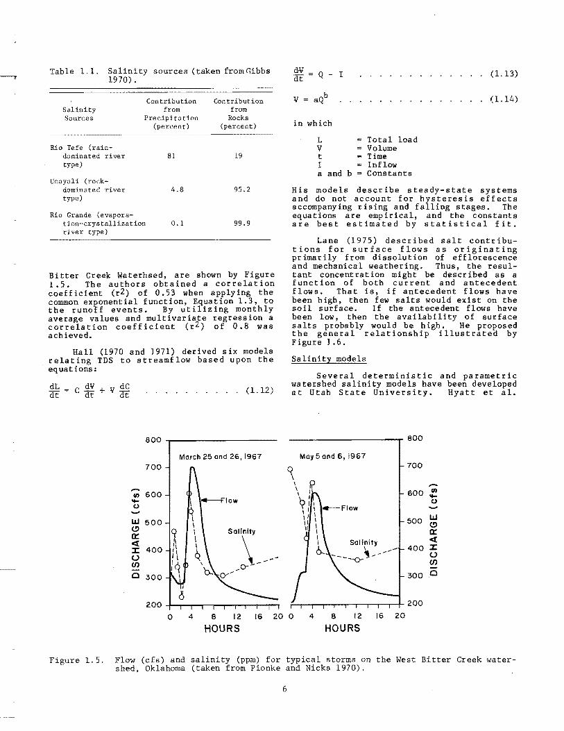
Table 1.1. Salinity sources (taken from Gibbs 1970).

Contribution from Salinity

Sources Precipitation (percent)

Rio Tefe (rain­dominated river type)

Ucayali (rock­dominated river type)

Rio Grande (evapora­tion-crystallization river type)

81

4.8

0.1

Contribution from

Rocks (percent)

19

95.2

99.9

Bi tter Creek Waterhsed, are shown by Figure 1.5. The authors obtained a correlation coefficient (r2) of 0.53 when applying the common exponential function, Equation 1.3, to the runoff events. By utilizing monthly average values and multivariate regression a correlation coefficient (r2) of 0.8 was achieved.

Hall (1970 and 1971) derived six models relating TDS to streamflow based upon the equations:

dL dt

-(I) .... (J -I.&J

(.!) a::: « J: (.) (/)

C

. . . . . . . . . . (1.12)

800

March 25 and 26, 1967 700

600

500 Salinity

\ -~-400

.... 0---

300 0'"

d-V dt Q I (1.13)

. . . . . . . . . . . .. (1.14)

in which

L V t I a and b

Total load Volume Time Inflow Constants

His models describe steady-state systems and do not account for hysteresis effects accompanying rising and falling stages. The equations are empirical, and the constants are best estimated by statistical fit.

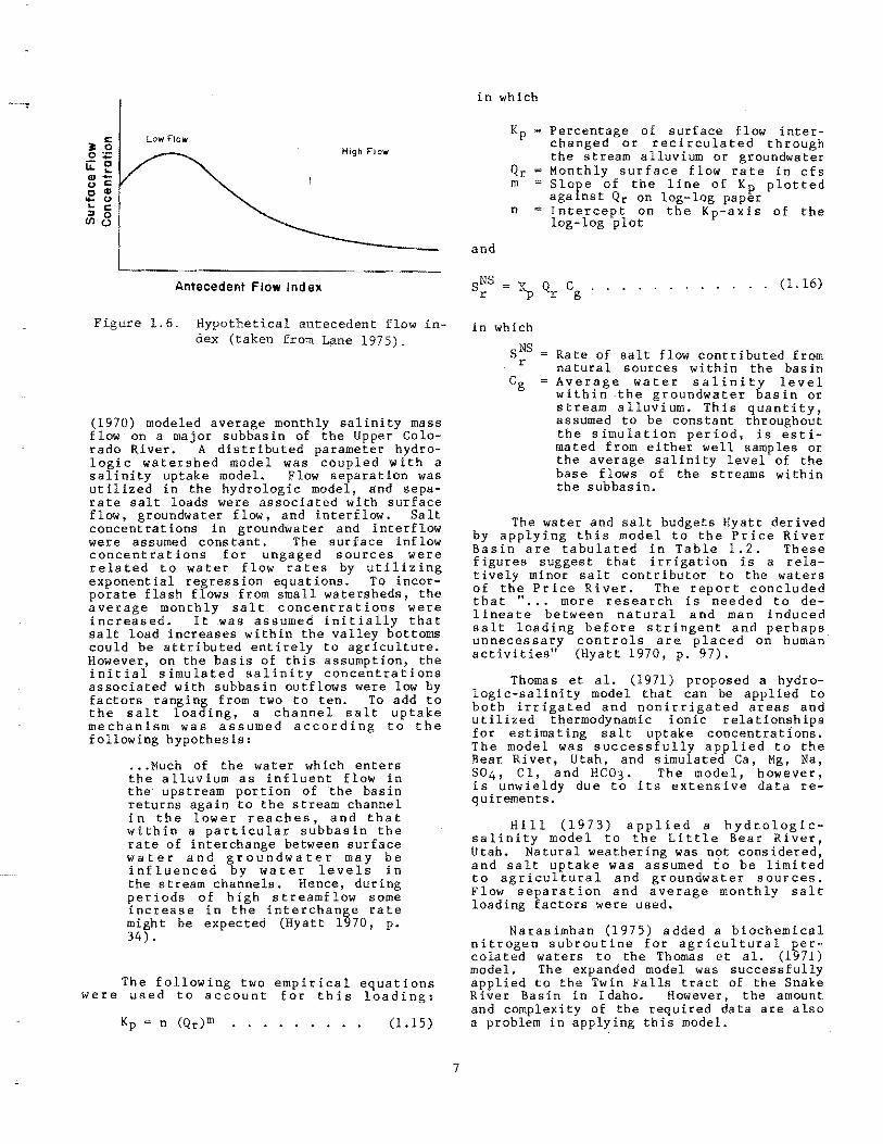
Lane (1975) described salt contribu­tions for surface flows as originating primarily from dissolution of efflorescence and mechanical weathering. Thus, the resul­tant concentration might be described as a function of both current and antecedent flows. That is, if antecedent flows have been high, then few salts would exist on the soil surface. If the antecedent flows have been low, then the availability of surface salts probably would be high. He proposed the general relationship illustrated by Figure 1.6.

Salinity models

Several deterministic and parametric watershed salinity models have been developed at Utah State University. Hyatt et a1.

800

May 5 and 6, 1967 700

-600 (I) .... (J -

500 I.&J (.!) a::: «

400 J: (.) (/)

300 C

o 4 8 12 16 20 0 4 8 12 16 20

HOURS HOURS

Figure 1.5. Flow (cfs) and salinity (ppm) for typical storms on the West Bitter Creek water­shed, Oklahoma (taken from Pionke and Nicks 1970).

6

Page 20

): 5 0:;::

- 0 u.. "-<D-o C o <D

.... 0 .. C ::J 0 WC)

Lo," Flo,"

Antecedent Flow Index

Figure 1.6. Hypothetical antecedent flow in­dex (taken fro~ L~ne 1975).

(1970) modeled average monthly salinity mass flow on a major subbasin of the Upper Colo­rado River. A distributed parameter hydro­logic watershed model was coupled with a salinity uptake modeL Flow separation was utilized in the hydrologic model, and sepa­rate salt loads were associated with surface flow, groundwater flow, and interflow. Salt concentrations in groundwater and interflow were assumed cons tant. The surface inflow concentrations for ungaged sources were related to water flow rates by utilizing exponential regression equations. To incor­porate flash flows from small watersheds, the average monthly salt concentrations were increased. It ~as assumed initially that salt load increases within the valley bottoms could be attributed entirely to agriculture. ~o~e~er, o~ the basis o~ ~his assumption, the InItIal SImulated salInIty concentrations associated with subbasin outflows were low by factors ranging from two to ten. To add to the salt loading, a channel salt uptake mechanism was assumed according to the following hypothesis:

.•. Much of the water which enters the alluvium as influent flow in the upstream portion of the basin returns again to the stream channel in the lower reaches, and that within a particular subbasin the rate of interchange between surface water and groundwater may be influenced by water levels in the stream channels. Hence, during periods of high streamflow some increase in the interchange rate might be expected (Hyatt 1970, p. 34).

The following two empirical equations were used to account for this loading:

n (Qr)m (1.15)

7

in

and

which

Kp

Qr m

n

Percentage of surface flow inter­changed or recirculated through the stream alluvium or groundwater Monthly surface flow rate in cfs Slope of the line of Kp plotted agaInst Qr on log-log paper Intercept on the Kp-axis of the log-log plot

Kp Qr

Cg

. . • . . . . . . . . . (1. 16)

in which

SNS r Rate of salt flow contributed from

natural sources within the bas in A,:er~ge water salinity level wIthIn the groundwater basin or stream alluvium. This quantity, assumed to be constant throughout the simulation period, is esti­mated from either well samples or the average salinity level of the base flows of the streams within the subbasin.

The water and salt budgets Hyatt derived by applying this model to the Price River Basin are tabulated in Table 1.2. These figures suggest that irrigation is a rela­tively minor salt contributor to the waters of the Price River. The report concluded that " ... more research is needed to de­lineate between natural and man induced salt loading before stringent and perhaps unnecessary controls are placed on human activities" (Hyatt 1970, p. 97).

. Thom~s. et a1. (1971) proposed a hydro­logIc-salInIty model that can be applied to both irrigated and nonirrigated areas and utilized thermodynamic ionic relationships for estimating salt uptake concentrations. The model was successfully applied to the Bear River, Utah, and simulated Ca, Mg, Na, S04, Cl, and HC03. The model, however is unwieldy due to its extensive data re: quirements.

. H,ill (1973) applie.d a hydr.ologic­salInIty model to the LIttle Bear River Utah. Natural weathering was not considered' and salt uptake was assumed to be limited to agricultural and groundwater sources. Flow separation and average monthly salt loading factors were used.

Narasimhan (1975) added a biochemical nitrogen subroutine for agricultural per­colated waters to the Thomas et al. (1971) model. The expanded model was successfully applied to the Twin Falls tract of the Snake River Basin in Idaho. However, the amount and complexity of the required data are also a problem in applying this model.

Page 21

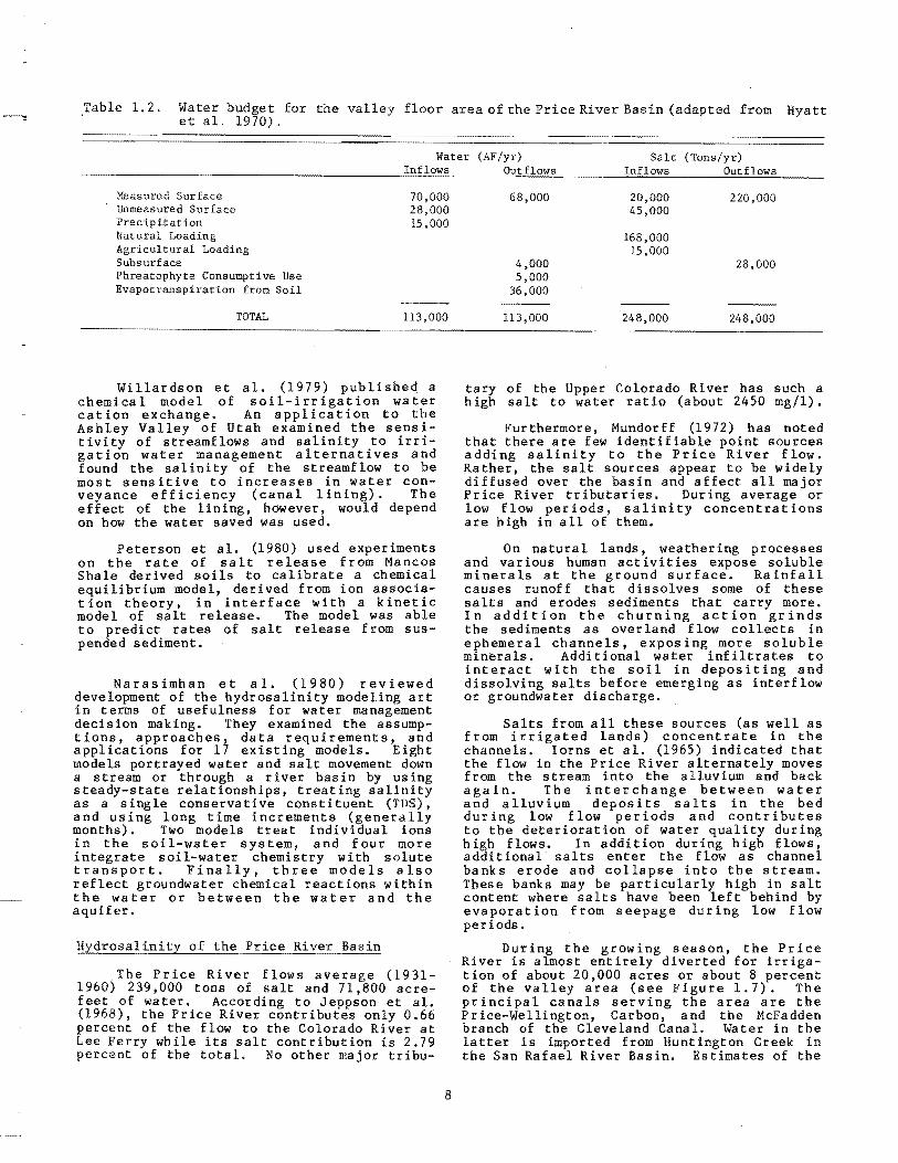
Table 1.2. Water budget for the valley floor area of the Price River Basin (adapted from Hyatt et al. 1970).

Water (AF/yr) Salt (Tons/yr)

Measured Surface 70,000 Unmeasured Surface 28,000 Precipitation 15,000 Natural Loading Agricultural Loading Subsurface Phreatophyte Consumptive Use Evapotranspiration from Soil

TOTAL 113,000

Willardson et a1. (1979) published a chemical model of soil-irrigation water cation exchange. An application to the Ashley Valley of Utah examined the sensi­tivity of streamflows and salinity to irri­gation water management alternatives and found the salinity of the streamflow to be most sensitive to increases in water con­veyance efficiency (canal lining). The effect of the lining, however, would depend on how the water saved was used.

Peterson et a1. (1980) used experiments on the rate of salt release from Mancos Shale derived soils to calibrate a chemical equilibrium model, derived from ion associa­tion theory, in interface with a kinetic model of salt release. The model was able to predict rates of salt release from sus­pended sediment.

Narasimhan et a1. (1980) reviewed development of the hydrosalinity modeling art in terms of usefulness for water management deci s ion making. They exami ned the ass ump­tions, approaches, data requirements, and applications for 17 existing models. Eight models portrayed water and salt movement down a stream or through a river basin by using steady-state relationships, treating salinity as a single conservative constituent (TDS), and using long time increments (generally months). Two models treat individual ions in the soil-water system, and four more integrate soil-water chemistry with solute transport. Finally, three models also reflect groundwater chemical reactions within the water or between the water and the aquifer.

Hydrosalinity of the Price River Basin

The Price River flows average (1931-1960) 239,000 tons of salt and 71,800 acre­feet of water. According to Jeppson et a1. (1968), the Price River contributes only 0.66 percent of the flow to the Colorado River at Lee Ferry while its salt contribution is 2.79 percent of the total. No other major tribu-

8

68,000 20,000 220,000 45,000

168,000 15,000

4,000 28,000 5,000

36,000

113,000 248,000 248,000

tary of the Upper Colorado River has such a high salt to water ratio (about 2450 mg/l).

Furthermore, Mundorff (1972) has noted that there are few identifiable point sources adding salinity to the Price River flow. Rather, the salt sources appear to be widely diffused over the basin and affect all major Price River tributaries. During average or low flow periods, salinity concentrations are high in all of them.

On natural lands, weathering processes and various human activities expose soluble minerals at the ground surface. Rainfall causes runoff that dissolves some of these salts and erodes sediments that carry more. In addition the churning action grinds the sediments as overland flow collects in ephemeral channels, exposing more soluble minerals. Additional water infiltrates to interact with the soil in depositing and dissolving salts before emerging as interflow or groundwater discharge.

Salts from all these sources (as well as from irrigated lands) concentrate in the channels. Iorns et al. (1965) indicated that the flow in the Price River alternately moves from the stream into the alluvium and back again. The interchange between water and alluvium deposits salts in the bed during low flow periods and contributes to the deterioration of water quality during high flows. In addition during high flows, additional salts enter the flow as channel banks erode and collapse into the stream. These banks may be particularly high in salt content where salts have been left behind by evaporat ion from seepage during low flow periods.

During the growing season, the Price RiVer is almost entirely diverted for irriga­tion of about 20,000 acres or about 8 percent of the valley area (see Figure 1.7). The principal canals serving the area are the Price-Wellington, Carbon, and the McFadden branch of the Cleveland Canal. Water in the latter is imported from Huntington Creek in the San Rafael River Basin. Estimates of the

Page 22

SCALE

"50,000

LEGEND -

E:m = Irrigated Land (1965)

• = Potentially Arable Land

N

Fi~ure 1. 7. Irrigated and potentially arable land in the Price River Basin (Utah Division of ~-1ater Resources 1975).

salt contribution from irrigation range from about 6 percent, or 15,000 tons per year, by Hyatt et a1. (1970) to about 33 percent, or 80,000 tons per year by Gifford et al. (1975).

Ponce (1975) conducted an intensive field investigation of salt pickup by over­land flows crossing Mancos Shale wildlands. Overland runoff was generated at several geologic locations in attempts to quantify salt movement, erosion, /ilnd loading rates. Spatial heterogeneity, however, was so extreme that the results are inconclusive. His best hypothesis was that salt pickup can be described as a function of dilution (added water increasing transport capacity), erosion (separation of sediment particles from natural formations), dissolution (separation of the salt ions from the sediment parti­cles), and an interaction of the three. He fit six empirical salt uptake equations to the observed data and achieved the best correlation (r2 = 0.64) with the function:

TOS t = Bo + B1P - BrQs

in which

Predicted salinity surface runoff Precipitation rate Surface runoff rate

B1. and Br = Constants

(1.17 )

of the

9

Ponce (1975) concluded that the salt load that occurs with surface runoff is largely related to erosion. His quantitative analysis indicated that surface salt loading is not a unique function of rainfall in­tensity but also depends on many other unspecified factors. He also estimated that only 0.5 percent of the total salt loading at woodside can be attributed to overland flow from natural areas.

Whitmore (1976) sampled Mancos Shale at nine different sites within the Price River valley. Based on laboratory analyses of these samples, he proposed that salt dissolu­tion is diffusion controlled and that two distinct dissolution rates occur. One is a fast reaction in which 80 to 90 percent of the available salt is released from the shale surface within the first 2 minutes after runoff across it begins. A second slower reaction occurs as the remaining salt slowly goes into solution. The fast rates are attributed to indigenous salt on particles at the surface of the soil, and the slow rates are thought to reflect mineral weathering.

White (1977a) examined salt production from microchannels in the Price River valley. He documented the extreme surface mineral heterogeneity of the channels and described the salinity uptake in the channels as a rapid dissolution of surface salts followed

Page 23

by slow mineral weathering (very similar to the pattern Whitmore had previously found for overland flow). Based on measurements of dissolved salts and sediment, a linear predictive equation for salt load was de­veloped. Good results were obtained;

10

however, the equation is of limited practical. application because sediment load 1s a difficult independent variable to measure or predict. He concluded that "microchannels contribute 3.4 percent of the total salt load of the Price River at Woodside."

Page 24

CHAPTER II

THE PRICE RIVER BASIN

Topography

The Price River Basin, located primarily in Carbon and Emery Counties of east-central Utah, has a total drainage area of about 1850 square miles (Figure 1.1). The Price RiVer flows 133 miles in a generally southeasterly direction from Scofield Reservoir and enters the Green River above the town of Green River, Utah. The basin elevation ranges from about 4,200 feet above mean sea level at its confluence with the Green River to 10,443 feet at Monument Peak in the western portion of the basin.

The dominant physiogra.p!· it: features of the basin are thg Wasatch Plateau, Book and Roan Cliffs, and the San Rafael Swell. On the west, the Wasatch Plateau rises abruptly from the Price River lowlands to a mean altitude of 9000 feet. Its sedimentary beds dip gently away from the San Rafael Swell located at the southern end of the basin. The swell is an asymmetrical anti­cline roughly 80 miles long and 30 miles wide. The region is known for its topography of concentric plateaus and massive cliffs. The Book and Roan Cliffs bound the north and east portions of the basin as they extend for 150 mi les from Wes t Centra 1 Colorado to Castle Gate and then south. Stokes and Cohenour (1956) have described the. cliffs as consisting predominantly of shales and sandstone marked by deep canyons and finger­like gravel-capped benches. The weathering gravel caps varl in thickness from 50 feet at the base 0 the mountains to a thin covering in the valley. Much of the cap area is cultivated, but production levels on many of the farms have deteriorated because of salt accumulation in the soil.

Geology

The geology of the Upper Colorado River Basin is the dominant factor determining the occurrence, behavior, and chemical qualities of its water resources (Hyatt et a1. 1970). Surface rocks and soils of marine shale origin are the predominant source of stream salinity (Mundorff 1972).

An extensive marine formation, known as Mancos Shale, has been identified as a major natural contributor of salts to the Colorado River. The formation, which underlies approximately 25 percent (470 mi 2 ) of the Price River drainage, is approximately 5000 feet thick and dips generally concentrically

11

away from the San Rafael Swell. The result is a U-shaped formation (with the top of the U pointing north), 10 miles widg, passing through the lowlands of the Pr ice River Basin.

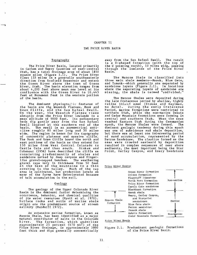
The Mancos Shale is classified into three main shale members--Masuk, Blue Gate, and T.ununk--which generally are separated by sandstone layers (Figure 2.1). In locations where the separating layers of sandstone are missing, the shale is termed "undivided."

The Mancos Shales were deposited during the late Cretaceous period by shallow, highly l'aline inland seas (Stokes and Heylman, no date). During the early Cretaceous Period, marine formations were restricted to northern Utah, while the non-marine Dakota and Cedar Mountain formations were forming in central and southern Utah. When the seas reached Eastern Utah during the Cenomanian epoch, the Mancos Shales were formed. The dominant geologic tendency during this epoch was one of subsidence and shale deposition, but there was at least one intervening period of sand accumulat ion, represented by the Ferron Sandstone. The clastics formed as the seas were crowded eastward by deposition resulted in complex sequences of near shore sediments, the most important being the Star Point, Garley Canyon, and Emery Sandstone

Price River. Source

f Mancos Shale

formation

1

Figure 2.1.

Green River formation Colton formation Flagstaff limestone North Horn formation Price River formation Castle Gate sandstone Blackhawk formation Masuk shale Emery, Garley Canyon,

and Starpoint sandstones

Blue Gate shale Ferron sandstone Tununk shale Dakota formation Cedar Mountain formation

I Non-marine

-t-Marine

+ Non-mar~ne t

Predominant geologic formations of the Price River Basin.

Page 25

Formations. These clastics grade eastward into the shales. As the Cretaceous Period drew to a close, central Utah emerged from the sea, and the later formations are all nonmarine.

The Price River headwaters in the Green River Formation. Most of the river flow, approximately 85 percent, originates in the Wasatch Plateau and from the Book and Roan Cliffs (Utah Division of Water Resources 1975). The river traverses the newer non­marine formations until reaching the Mancos Shales at Castle Gate. From there the river traverses the Mancos formations to Woodside.

The three major formations of the Mancos Shales (Masuk, Blue Gate, and Tununk) are separated in places by the sandstone tongues (Figure 2.2). The mar ine shales are de­scribed as drab and slightly bluish-gray and contain some thick lenses of calcareous sandstone, limestone, and concretionary beds. The shales characteristically vary greatly in salt content and are relatively impermeable and erodable. Burge (1974) attributes the impermeability of the shales to the fineness of the contained clays and the rapid weather­ing to cyclic dehydration-hydration of the entrained salts, particularly mirabilite (Na2S04 • 10H20) and thenardite (Na2S04).

At elevations above 1,000 feet, average annual precipitation varies between 30 inches and 12 inches and mostly occurs during the winter (Mundorff 1972). Precipitation on the river valley averages less than 10 inches annually, and most rainfall is during the late summer. These summer and fall storms produce almost all of the surface runoff and erosion on the valley floor. Average pre­cipitation and temperature data for selected stations are given in Table 2.1.

Summer storms are typically short duration thunderstorms while most winter precipitation comes from relatively low intensity frontal storms. During the winter, frontal storms from the Gulf of Alaska produce snowpacks in the surrounding uplands. Thunderstorms during the late summer months

2000'

o·

r-------=i Miles

develop as warm moist air from the Gulf of Mexico moves into the valley. Monthly distributions of precipitation at selected stations are given in Table 2.1.

On the highest 30 percent of the area, about 65 percent of the precipitation falls from October through April, and most of it is snow. The spring melt provides irrigation water for agriculture.

Streamflows

Most of the outflow from the Price River Basin originates as snowmelt. The summer thunderstorms are usually of short duration, localized, and intense. Surge flows can develop in the valley channels, eroding and transporting large masses of sediment. Most tributary streams become completely dry during low flow periods.

Average annual yield for the Price River Basin ranges from less than 1 inch in the valley to over 12 inches in the mountains (Figure 2.3). Although about 50 percent of the total basin is below 6,400 feet, only 10 percent of the total water yield originates from these lower elevations. Annual runoff from the Price River' valley is estimated to be 1.08 inches or about 9 percent of the average annual precipitation of 11.7 inches.

Streamflow in the principal streams is highly regulated. Most summer flows are diverted for use within the basin. Scofield Reservoir (capacity 45,000 acre-feet), located near the headwaters of the Price River, stores runoff for release during the irrigation season.

Jeppson et a1. (1968), using the Thorn­thwaite formula, estimated the evapotrans­piration for the valley to generally exceed 24 inches annually. This is about 2.5 times the precipitation, and thus irrigation is used to make up for the moisture deficient in agricultural areas. Water enters the valley floor from the river and tributaries and as imports. Approximately 28,000 acre-feet per year are imported from Huntington Creek

PRICE CITY & PRICE RIVER

FARNHAM fu~TICLINE (North and San Rafael Sw~ll)

Figure 2.2. Mancos Shale cross-section (taken from Williams 1975).

12

Page 26

""'" ('", \ PRICE RIVER DRAINAGE e;-:-8~ 7~Wasatch Co.

~ .... \Utd"hco:'---, -" '"\ 1::\ Colton 0 '-4 ~ \ (Uto, CO'-oJ· I I ~2i D",,, .. Co.

) ~ 12 / /,-'" a HelPer. \.. C~ ~!:J \'\i Price 2 \\

"J\84 2 1 I!J 1 ~\.:

\\\ \ \ WC1ti ng ton ';;1\ \ , Dragerton I ~:hja ___ ~o~_~ ________ ~ __ )

"\I Emery Co. y~ ""'-J Elmo I

, 0 J

'\ I \ Scale I: 50,000 "" (

"'-"" Woodside \

" /9 '\ 1"\,../,-,- ('\.. \

"\.....,....., --.I

Figure 2.3. Mean annual water yield in inches (Utah Division of Water Resources 1975).

in the San Rafael Basin. Consumptive use occurs in municipalities, irrigated areas, and natural wetlands. About half of the inflow leaves the basin, as, river outflow at woodside. Figure 2.4 depicts the estimated mean annual water budget.

Table 2.2 shows the mean monthly flows at selected gaging stations. In the central basin, only Desert Seep Wash is gaged. In total, the tributaries contribute approxi­mately 39,000 acre-feet of water per year to the valley.

Water quality

The streams within the upland canyons generally contain relatively high quality wa ter of les s than 500 mgt!. Except for periods of high snowmelt runoff, all of the Price River lowland tributaries contribute low quality water (Mundorff 1972). Other­wise, the streams show no significant sea­sonal variation in total dissolved solids concentration.

13

Within the valley stream channels, efflorescence (salt crusted around the channel periphery) accumulates durin~ periods of low flow. During per iods of runoff, the ef florescence is disSolved and flushed into the stream.

Mundorff (1972) regards diffuse agricul­tural return flows as a probable major source of salt input to the Price River. Williams (1975) hypothesized that a major salt loading source was the surface runoff from rains and snow over the Mancos Shale badlands. He also discusses the possibility of saline flow from the sandstone clastics and identifies coal processing as another possible major con­tributor.

In the upper Price River drainage, suspended solids are not a problem; but in the valley, concentrations as high as 64,800 mg/l have been recorded. On one day when samples were taken along the Price River, total suspended solids ranged from 180 mg/l above Scofield to 226 mg/l at Heiner and 2,119 mg/l at woodside (Mundorff 1972).

Page 27

t-' ..,..

.J

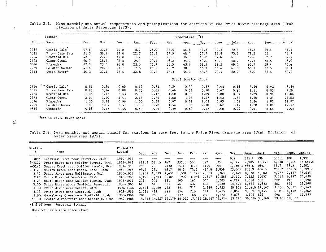
Table 2.1. Mean monthly and annual temperatures and precipitations for stations in the Price River drainage area (Utah Division of Water Resources 1975).

No ..

1214 7015 7724 1472 3896 7959 3413

1214 7015 7724 1472 3896 7959 9629

Station

Name

Castle Dalea

Price Game Farm Scofield Dam Clear Creek Hiawatha Soldier SUlmnit Green Rivera

"Castle Dalea

Price Game Farm Scofield Dam Clear Creek Hiawatha Soldier Summit I%odside

Oct.

47.6 51.3 42.1 40.7 47.8 41.6 54.3

0.86 0.96 1.08 2.02 1.33 1.06 0.88

aNot in Price River Basin.

Nov.

33.2 36.9 27.5 28.4 33.8 28.3 37.5

0.54 0.54 1.17 1. 70 0.78 1.07 0.73

Dec.

24.0 27.0 17.8 22.8 26.0 21.1 28.4

0.60 0.88 1. 43 2.41 0.96 1. 51 0.48

Jan.

18.2 22.7 13.2 19.4 23.0 17.6 22.8

0.69 0.73 2.66 2.65 LOO 1. 50 0.50

Feb.

25.0 29.9 16.2 20.7 26.7 20.9 32.5

0.61 0.65 2. 13 2.69 0.89 1. 70 0.39

Temperature (OF)

Mar. Apr. Hay June July Aug. Sept.

37.5 39.0 25.1 26.2 33.5 28 •. 2 43.3

46.8 48.4 36.1 35.2 43.6 38.1 54.2

54.8 57.7 46.0 44.0 52.5 46.2 63.8

Precipitation (In.)

0 .. 54 0.66 1.48 2.68 0.97 1. 54 0.39

0.54 0.61 0.98 1. 95 0.91 1.01 0.64

0.57 0.70 1.09 1. 57 1. 08 1.10 0.52

64.3 66.8 54.6 52. 62.2 53.4 72.5

0.48 0.67 0.88 1.43 0.95 0.62 0.48

70.4 73.3 61.1 58.7 69.1 61.3 80.7

0.88 0.90 0.94 1. 53 1.18 1. 17 0.49

68.2 71.2 59.6 57.7 66.7 60.1 78.0

1.16 loll 1.29 1.56 1.84 1. 38 0.91

59.4 63 52.7 50.5 59.4 52.5 68.4

0.92 0.83 0.96 1. 34 1.00 1.06 0.66

Annual

45.8 48.9 37.7 38.0 45.4 39.1 53.0

8.39 9.24

16.04 23.53 12.87 14.72 7.05

Table 2.2. Hean monthly and annual runoff for stations in acre feet in the Price River area (Utah Division of Water Resources 1975).

Station Period of

3095 Fairview Ditch near Fairview, Utah 1 1950-1966 9.2 325.4 536 363.1 100 9-3117 Price River near Soldier Summit, Utah 1962-1963 629.3 680.5 767 351.5 336 392 875 4,395 7,905 11,275 6,530 3,515 9-3127 Beaver Creek near Soldier Summit, Utah 1961-1966 29 29 21:8 25.1 31.2 84.9 395 1,056.3 569.6 164.4 56.7 38.8 9-3128 Willow Creek near Castle Gate, Utah 1963-1966 99.4 71.1 35.7 40.9 73.5 434.8 1,059 23,665 863.3 466.3 237.2 161.5

3140 Price River near Wellington, Utah 1950-1958 1,957 1,673 1,451 1,381 1,675 2,623 8,743 17 ,149 8,378 3,180 4,268 2,157 3145 Price River at \%odside, Utah 1946-1966 4,491 3,593 2,505 1,909 3,036 7 ,617 10,568 15,301 7,355 5,007 7,753 6,297 3125 l-/hite River near Soldier Summit, Utah 1938-1966 228 208 181 165 167 344 3,283 6,217 1,688 560 292 215 3105 Price River Above Scofield Reservoir 1939-1966 640 616 525 461 432 636 3,630 15,472 6,622 1,683 882 591 3130 Price River near Heiner, Utah 1934-1966 2,635 1,069 742 591 714 2,289 9,725 20,863 13,410 11 167 7,436 5,042 3115 Price River near Scofield, Utah 1918-1966 1,696 411 292 154 210 211 1,435 8,852 9,580 6,060 4,156 3100 Gooseberry Creek near Scofield, Utah 1940-1966 281 256 208 177 168 230 1,172 6,078 3,109 498 304

*3110 Scofield Reservoir near Scofield, Utah 1942-1966 14,418 14,527 15,179 16,310 17,413 18,862 21,924 33,225 36,986 ~O,860 23,655 18,827

*End 2>f Honth Reservoir Storage

IDoes not drain into Price River

] ,334 37,651.5 2,502 5 909.2

,635 75,439 13,598 32,190 75,743 42,202 13,33.1

Page 28

Figure 2.4. Price River Valley estimated annual water budget in acre-feet/year. (Taken from Utah Division of Water Resources 1975).

Groundwater

The use of groundwater within the central basin is limited by the quality of the water available. Total dissolved solids have ranged from 3,600 to 73,000 mg/l in exploratory wells. Only the best of this water is useful even for stock watering.

Above the central basin primarily in the Colton area, groundwater is of high quality. Cordova (1964) estimated that approximately 3,000 a cre- feet per yea r of g roundwa ter presently were being withdrawn by pumping and by outflow from springs and seeps. He also estimated that an additional 4,000 acre-feet per year of groundwater resources. could be

15

developed. Clyde et a1. (1981) described groundwater quantity and quality in Pleasant Valley just upstream from Scofield Reservoir.

Vegetation

The principal vegetative types on natural or uncultivated lands in the basin are Yellow Pine and Douglas Fir in the headwater areas, Pinyon-Juniper on the gravel caps of the lower slopes, and Shadscale­Sagebrush in the valley bottoms (Mundorff 1972). It is from these Shadscale-Sagebrush lands that the vast majority of the salt pickup by overland and microchannel flow occurs.

Page 29

Economy

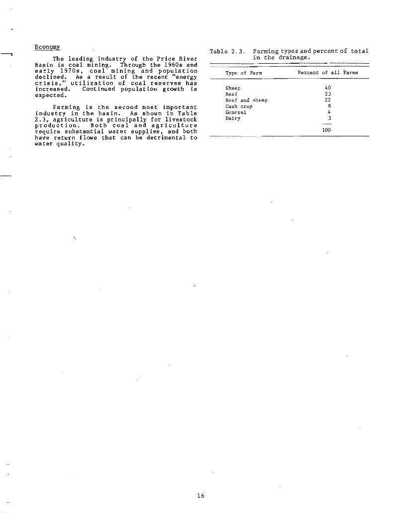
The leading industry of the Price River Basin is coal mining. Through the 1960s and early 1970s, coal mining and population declined. As a result of the recent "energy crisis," utilization of coal reserves has increased. Continued population growth is expected.

Farming is the second most important industry in the basin. As shown in Table 2.3, agriculture is principally for livestock production. Both coal and agriculture require substantial water supplies, and both have return flows that can be detrimental to water quality.

\

16

Table 2.3. Farming types and percent of total in the drainage.

Type of Farm

Sheep Beef Beef and sheep Cash crop General Dairy

Percent of all Farms

40 23 22

8 4 3

100

Page 30

CHAPTER III

STUDY METHODS AND PROCEDURES

Scope of the Study

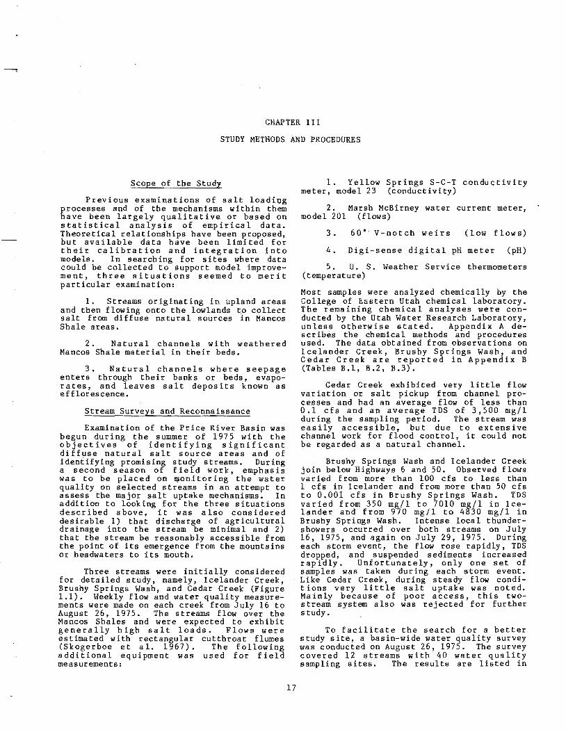
Previous examinations of salt loadi~g processes and of the mechanisms within them have been largely qualitative or based on statistical analysis of empirical data. Theoretical relationships have been proposed, but available data have been limited for their calibration and integration into models. In searching for sites where data could be collected to support model improve­ment, three situations seemed to merit particular examination:

1. Streams originating in upland areas and then flowing onto the lowlands to collect salt from diffuse natural sources in Mancos Shale areas.

2. Natural channels with weathered Mancos Shale material in their beds.

3. Natural channels where seepage enters through their banks or beds, evapo­rates, and leaves salt deposits known as efflorescence.

Stream Surveys and Reconnaissance

Examination of the Price River Basin was begun during the summer of 1975 with the objectives of identifying significant diffuse natural salt source areas and of identifying promising study streams. During a second season of field work, emphas is was to be placed on .onitoring the water quality on selected streams in an attempt to assess the major salt uptake mechanisms. In addi t ion to looking for the three situations described above. it was also considered desirable 1) that discharge of agricultural drainage into the stream be minimal and 2) that the stream be reasonably accessible from the point of its emergence from the mountains or headwaters to its mouth.

Three streams were initially considered for detailed study, namely, Icelander Creek, Brushy Springs Wash, and Cedar Creek (Figure 1.1). Weekly flow and water quality measure­ments were made on each creek from July 16 to August 26, 1975. The streams flow over the Mancos Shales and were expected to exhibit generally high salt loads. Flows were es tima ted with rectangular cutthroa t flumes (Skogerboe et a 1. 1967). The following additional equipment was used for field measurements:

17

1. Yellow Springs S-C-T conductivity meter, model 23 (conductivity)

2. Marsh McBirney water current meter, model 201 (flows)

3. 60· V-notch weirs (low flows)

4. Digi-sense digital pH meter (pH)

5. U. S. Weather Service thermometers (temperature)

Most samples were analyzed chemically by the College of Eastern Utah chemical laboratory. The remaining chemical analyses were con­ducted by the Utah Water Research Laboratory, unless otherwise stated. Appendix A de­scribes the chemical methods and procedures used. The data obtained from observations on Icelander Creek, Brushy Springs Wash, and Cedar Creek are reported in Appendix B (Tables B.l, B.2, B.3).

Cedar Creek exhibited very little flow variation or salt pickup from channel pro­cesses and had an average flow of less than 0.1 cfs and an average TDS of 3,500 mg/l during the sampling period. The stream was eas ily access ible, bu t due to extens i ve channel work for flood control, it could not be regarded as a natural channel.

Brushy Springs Wash and Icelander Creek join below Highways 6 and 50. Observed flows varied from more than 100 cfs to less than 1 cfs in Icelander and from more than 50 cfs to 0.001 cfs in Brushy Springs Wash. TDS varied from 350 mg/l to 7010 mg/l in Ice­lander and from 970 mg/l to 4830 mg/l in Brushy Springs Wash. Intense local thunder­showers occurred over both streams on July 16, 1975, and again on July 29, 1975. During each storm event, the flow rose rapidly, TDS dropped, and suspended sediments increased rapidly. Unfortunately, only one set of samples was taken during each storm event. Like Cedar Creek, during steady flow condi­t ions very little salt uptake was noted. Ma inly because of poor access, this two­s tream system a Iso was rej ected for fur ther study.

To facilitate the search for a better study site, a basin-wide water quality survey was conducted on August 26, 1975. The survey covered 12 streams with 40 water quality sampling sites. The results are listed in

Page 31

Appendix B (Table B.2). The flowing streams characteristically pick up salts as they move across the valley floor to the Price River. Many of the streams which drain wildlands contribute very little flow during the summer months.

The survey indicated that the salt load in the observed streams was large, with a mean TDS observation of 3650 mg/l and an observed high of 9800 mg/I. Under such high salt loadings, the springs may have reached saturation with regards to several significant minerals.

Coal Creek Instrumentation

Coal Creek (Figure 3.1) was chosen for instrumentation for detailed study. The Coal Creek catchment originates in the Book Cliffs, and the stream flows in a southerly

direction to its confluence with the Price River near the town of Wellington. An upper control site (Figure 3.1) was located at the point at which the stream emerges from the Book Cliffs. The flow at this location is essentially perennial, with a baseflow of about 1 cfs during the snowmelt period declining to 0.1 cfs in the late summer. The average stream salinity at this point is about 500 mg/l. Dissolved salts are rapidly picked up with a TDS of 3420 mg/l measured at Highways 6 and 50 (Appendix B).

An 8.2 mile study section was chosen extending downstream from the base of the Book Cliffs. Access to the Coal Creek channel was gained from a paved road which is located adjacent to the channel on the west side, and which traverses the entire length of the study section. The catchment, except for a small irrigated farm, consists of natural lands.

Upper Control Site (RC,RT,RQ,P)

Spring

Middle Site (RT,RRH,W,NR, RP)

East Raingage (P)

Lower Control Site (RC,RT,RQ,P)

Figure 3.1. Coal Creek instrumentation.

18

~ N I

I I I

0 I 2 Scale (miles)

RQ- Recording Flow NR- Net Radiation RT - Recording Temperature RC- Recording Conductivity P - Cumulative Precipitation W -Cumulative Wind Speed RRH- Recording Relative Humidity RP-Recording Precipitation

I 3

Page 32

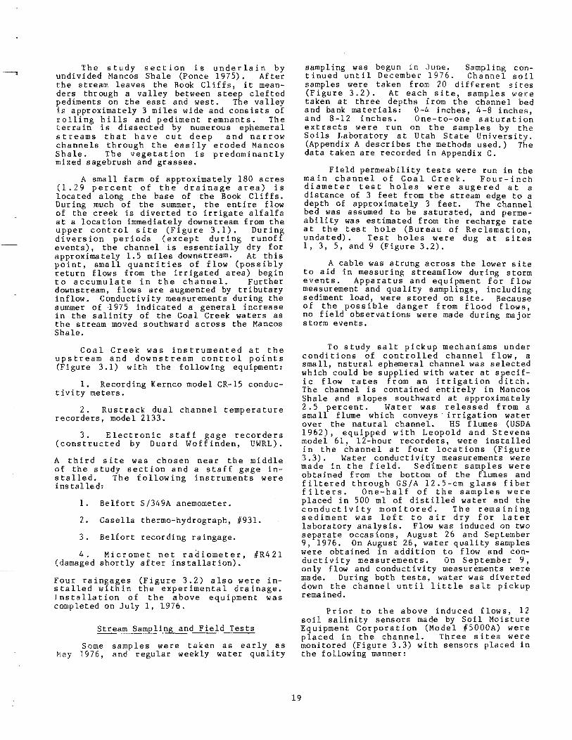
The study section is underlain by undivided Mancos Shale (Ponce 1975). After the stream leaves the Book Cliffs, it mean­de rs thr ough a va lley between steep clef ted pediments on the east and west. The valley is approximately 3 miles wide and consists of rolling hills and pediment remnants. The terrain is dissected by numerous ephemeral streams that have cut deep and narrow channels through the easily eroded Mancos Shale. The vegetat ion is predominantly mixed sagebrush and grasses.

A small farm of approximately 180 acres (1.29 percent of the drainage area) is located along the base of the Book Cliffs. During much of the summer, the entire flow of the creek is diverted to irrigate alfalfa at a location immediately downstream from the upper control site (Figure 3.1). During diversion periods (except during runoff events), the channel is essentially dry for approximately 1.5 miles downstream. At this point, small quantities of flow (possibly return flows from the irrigated area) begin to accumulate in the channel. Further downstream, flows are augmented by tributary inflow. Conductivity measurements during the summer of ·1975 indicated a general increase in the salinity of the Coal Creek waters as the stream moved southward across the Mancos Shale.

Coal Creek was instrumented at the upstream and downstream control points (Figure 3.1) with the following equipment I

1. Recording Kernco model CR-15 conduc­tivity meters.

2. Rustrack dual channel temperature recorders, model 2133.

3. Electronic staff gage recorders (constructed by Duard Woffinden, UWRL).

A third site was chosen near the middle of the study section and a staff gage in­stalled. The following instruments were ins taIled:

1. Belfort S/349A anemometer.

2. Casella thermo-hydrograph, '931.

3. Belfort recording raingage.

4. Micromet net radiometer, ,R421 (damaged shortly after installation).

Four raingages (Figure 3.2) also were in­stalled within the experimental drainage. Installation of the above equipment was completed on July 1, 1976.

Stream Sampling and Field Tests

Some Jvlay 1976,

samples were taken as early as and regular weekly water quality

sampling was begun in June. Sampling con­tinued until December 1976. Channel soil samples were taken from 20 different sites (Figure 3.2). At each site, samples wer:e taken at three depths from the channel bed and bank materials: 0-4 inches, 4-8 inches and 8-12 inches. One-to-one saturatio~ ex~racts were run on the samples by the SOlIs Laboratory at Utah State University. (Appendix A describes the methods used.) The data taken are recorded in Appendix C.

Field permeability tests were run in the main channel of Coal Creek. Four-inch diameter test holes were augered at a distance of 3 feet from the stream edge to a depth of approximately 3 feet. The channel bed was assumed to be saturated, and perme­ability was estimated from the recharge rate at the test hole (Bureau of Reclamation undated). Test holes were dug at site~ 1, 3, 5, and 9 (Figure 3.2).

A cable was strung across the lower site to aid in measuring streamflow during storm events. Apparatus and equipment for flow measurement and quality samplings, including sediment load, were stored on site. Because of the possible danger from flood flows no field observations were made during majo~ storm events.

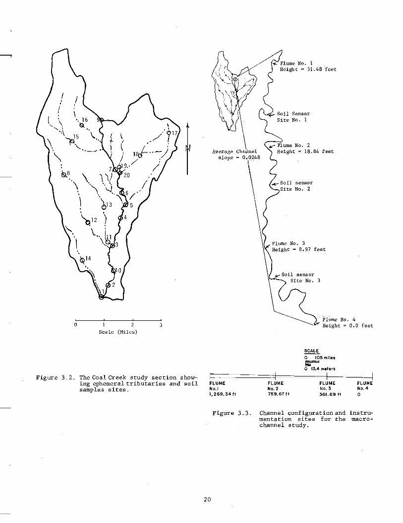
To study salt pickup mechanisms under con d i t ion s 0 f con t roll e d c han n elf low, a small, natural ephemeral channel was selected which could be supplied with water at specif­ic flow rates from an irrigation ditch. The channel is contained entirely in Mancos Shale and slopes southward at approximately 2.5 percent. Water was released from a small flume which conveys· irrigation water over the natural channel. HS flumes (USDA 1962), equipped with Leopold and Stevens model 61, 12-hour recorders, were installed in the channel at four locations (Figure 3.3). Water conductivity measurements were made in the field. Sediment samples were obtained from the bottom of the flumes and filtered through GS/A 12.5-cm glass fiber filters. One-half of the samples were placed in 500 ml of distilled water and the conductivity monitored. The remaining sediment was left to air dry for later laboratory analysis. Flow was induced on two separa te occas ions, August 26 and September 9, 1976. On August 26, water quality samples were obtained in addition to flow and con­ductivity measurements. On September 9, only flow and conductivity measurements were made. During both tests, water was diverted down the channel until little salt pickup remained.

Prior to the above induced flows, 12 soil salinity sensors made by Soil Moisture Equipment Corporation (Model ,SOOOA) were placed in the channel. Three sites were monitored (Figure 3.3) with sensors placed in the following manner:

19

Page 33

\ ",:

'. 16 Q

" -.\ 15

\ 'fl , '\...

\

o 2

Scale (Miles) 3

Figure 3.2. The Coal Creek study section show­ing ephemeral tributaries and soil samples sites.

Average slop,e

FLUME No.1 1,269.34 ft

FLUME No.2 759. 67ft

'feet

feet

, Flume No.4 Height = 0.0 feet

SCALE

o 105 miles

~ o 13.4 meters

FLUME No.3 361. 69 ft

FLUME No.4 o

Figure 3.3. Channel configuration and instru­mentation sites for the macro­channel study.

20

Page 34

Site 1 Buried verti­.cally in the channel bottom

6 cm depth 18 cm depth 29 cm depth 41 cm depth

Site 2 Buried horizon­tally in the channel bank

3 cm depth 13 cm depth 24 cm depth 36 cm depth

Site 3 Buried verti­cally in the

channel bottom

4 cm depth 13 cm depth 23 cm depth 33 cm depth

The sensors were adapted to be monitored weekly with a Yellow Springs Model 33 con­ductivity meter.

At the beginning of each flow test, accumulated salt (efflorescence) was esti­mated by removing a l-cm deep sample from the channel bottom at the three soil sensor sites. The samples were dried at 103"C for 24 hours, weighed, placed in 1 liter of distilled water, mixed for 1 minute, and settled for 30 seconds. The conductivity was then measured.

Laboratory Tests

To assist in defining in-channel salt pickup mechanisms, laboratory studies were proposed. The increased control over experimental variables in the laboratory was expected to define specific mechanisms more clearly than was possible under field condi­tions. The initial tests utilized a re­circulating tilting flume charged with sediment obtained from channel bottoms in the Price River valley. The objective of the tests was to develop relationships of rates of salt dissolution versus flow.

Several problems were encountered: 1) mass movement of the sediment, 2) nonuniform flow, and 3) plugging of the recirculation system. The flume tests, therefore, were abandoned in favor of simpler sediment-jar tests. All data recorded during these laboratory tests are in Appendix D.

Potential salt contributions from both suspended sediment and bed-load were ex­amined. Nine sediment samples were obtained from the macrochannel study (Figure 3.3). Each sample was halved in the field and removed from solution by vacuum filtering through a Whatman CF/A 12.5 cm glass fiber filter. One-half of the sample was placed in 500 ml of distilled water, and one-half was air dried. Prior to each measurement, the saturated sample was vigorously mixed, allowed to settle, and the conductivity was measured. The dried samples were weighed, sieved, and the grain size fraction calcu­lated. The samples were then saturated with distilled water at a 1:1 weight ratio and the conductivity monitored as previously de­scribed.

To test if wetting and drying cycles increased salt release as suggested by Burge

21

(1974), a simple test was designed. Shale samples were obtained from exposed formations at four sites within the Coal Creek drainage (Figure 3.1):

1. Macrochannel 2. Middle site 3. Spring 4. Lower site

Fragments passing a 1 3/8" sieve and reta ined upon a I" sieve were rinsed wi th distilled water and dried at 103·C for 24 hours. The remaining portion of the four samples were divided into six subsamples; three for a control group and three for an experimental group. The subsamples were saturated with distilled water at a 1:1 weight ratio. Periodically, the temperature was measured, then the sample was gently stirred; and following settling, conductivity was measured. On days 2 and 43 from the beginning of the laboratory test, the experi­mental group was rinsed with distilled water and dried at 103"C for 24 hours. After drying, the samples were again saturated. On day 45, the control group was rinsed with distilled water and saturated.

To estimate the rate of salt release from the shale samples with respect to grain size and cyclic weather ing, two tests were conducted. For both tests, the shale samples were separated into four size fractions by sieving (Appendix 0, Table 0-4). For the first test, six 10-gm subsamples' from each size fraction (for a total of 96 subsamples) were obtained. The subsamples were saturated with 20 ml of distilled water and mixed in a Precision Scientific water bath and shaker (Model #66802) at 25'C for 30 seconds, 5 minutes, 30 minutes, 8 hours, 24 hours, and 72 hours, respectively. At the end of each time period a sample was removed, vacuum­filtered through a Whatman GF/A glass fiber filter, and the conductivity was measured with a Brinkman conductivity bridge.

For the second test, 50 gms of shale from each size fraction (for a total of 16 subsamples) were obtained. Each subsample was saturated with 100 ml of distilled water and placed within a Brinkmann rotoevaporator and an auxiliary (50'C) water bath, respec­t ively. The rotoevaporator was rotated slowly for 15 minutes, after which 5 ml of supernatant was removed and filtered through a Whatman GF/A glass fiber filter. The conductivity of the filtrate was measured with a Beckman model RC-19 conductivity bridge. A vacuum was applied to the remain­ing sample, and the sample was rotated rapidly for approximately 1 hour or until completely dry. Distilled water (100 ml) was then added, and the process was repeated an average of four times for each subsample. The results of these analyses are also included in Appendix D.

Page 35

CHAPTER IV

FIELD INVESTIGATION RESULTS FROM THE STUDY

Salinity and the Price River Basin

The time pattern in which the salt load is carried by the Price River results from a complex combination of interactions among time variable hydrologic processes. Natural groundwaters seep slowly into the stream to evaporate in the dry bed leaving encrusted salt behind. Waters diverted for irrigation 1 e a c h sal t s from so iI, and the ret urn flows also add salt as the seep into the stream. Storm runoff hydrographs rise rapidly, picking up salts dissolved on the bed, churning bed sediments, and carrying the salts mixed with those sediments. After the storm, the flows recede rapidly,· and the salts and sediments return to the bed a distance downstream from where they were before, determined by the size of the storm. Return flows work to keep the stream flowing through the dry season, carrying a more concentrated salt load, initially because of the salts leached from the soil and over the long run because of the consumptive use of water.

For genera 1 representat ion of the time patterns, daily flows and conductivities (a surrogate for total dissolved solids) are plotted for 1970 in Figure 4.1. As flow is an important factor determining salt trans­port, daily conductivities are plotted versus average daily flows for the Price River at woodside for the 5-year period 1970-74 on a log-log basis (Figure 4.2). The line follow­ing the form of Equation 1.3 and having the best fit is shown on the figure and has a correlation coefficient of 0.648. The student t-test (Lapin 1975) showed the null hypothesis that the slope of the regression line was equal to zero to be rejected at the 99 percent confidence level. The conclusion at this point was that flow is definitely significant in determining salinity but that other factors also need to be considered.

According to Hendrickson and Krieger (1964), one needs to explore the different mineral dissolution characteristics of water flowing into the stream along various paths. Gunnerson (1967) explained the hysteresis in the annual pattern of monthly flows and conductivities for Columbia River subbasins in terms of the annual variation in dominant flow paths.

23

Discharge and salinity profiles along the Price River are shown by Figures 4.3 and 4.4, respectively, for data taken during a sampling survey on October 19 to 21, 1976 (Appendix B, Table B.3). Most of the flow was being diverted from the river above the Ci ty of Price (r iver mi Ie 10). Downstream from the city, both the flow and the salinity increased rapidly. The predominant cations were sodium, calcium, and magnesium, and sulfate was the main anion. Figures 4.3 and 4.4 together suggest that the Price River salinity loading largely enters the stream by return flows and tributary inflows below Pr ice.

To aid in identifying diffuse salt. source areas in the Price River Basin, Mundorff's (1972) water quality samples of varying repetition at 71 sites over a 30-year period (Figure 4.5) were evaluated statisti­cally. The sample sites were considered independent treatments, and mean salt load­i ngs per sample site were ca lculated as pounds per day per square mi Ie of drainage. The null hypothesis that the treatment means were equivalent was tested by comparing an individual treatment with the average of the rema ining treatments·. Student t-values were calculated (Neter and Wasserman 1974), but the results were not conclusive.

Three sampling sites, numbers 31, 50, and 52 (Figure 4.5), were identified as collecting runoff from areas of high salt loading. The three (Drunkards Wash, Desert Lake Wash, and Desert Seep Wash) drain irri­ga ted farm land and exh ibi t a high average salt load, 518, 416, and 423 pounds per square mile of drainage per day, respective­ly. Drunkards Wash exhibited a large salt load in part because one of the sampling observations was made during a storm surge transporting a large flux of salt.

Figure 4.6 shows the major tributaries and canals in the proximity of Desert Seep Wash and Desert Lake Wash with average observed conductivity levels at measured points. As indicated by this figure, the average salinity level of the Price River increased by approximately 30 percent at its confluence with Desert Seep Wash. However, because of the strong influence of ·agricul­ture, Desert Seep Wash was not examined further in this study of salinity contri­butions from natural areas.

Page 36

---. 10000

1000

,...... <!l

4-1 U

QJ oo 100 I-l C\l

..c:: <J <!l

- • .-1 P

10

o

Figure 4.1.

10000 ... i

8000 ~ ~

6000 ...

2000 i-,

1000 IO

7000 Conductivity

6000

__ Discharge

5000

"""' <!l 0

1 4000 ~

t-.,.; > • .-1 ..,

3000 <J ::l 'tl I:l 0 u

2000

1000

50 100 150 200 250 300 350 400 Days (Oct. 1,1969-Sept.30,1970)

Discharge and conductivity versus date, from the Price River at Woodside. (Taken from USGS 1970).

.' . - ...... .. , Log condo

r

, "' .....

.'

4,.033-. :::>'58*Log discharge 0.648

. .. ..

.'

. . ,. __ J .. .1 .• 1. l_ . ...I._l..--_._ ...... 1 .. " __ ~J".~,~ .. L J .. _"...l_ .. L;.~ • ..J...-...:-_._,_ .J ___ "_~,_J_ ... J.,,~,.tA_ .. .L.-t.. .. .L,~LJ

100 lonn 10000 Discharge, (cfs)

Figure 4.2. Conductivity versus discharge, for the Price River at Woodside. (Taken from USGS 1970-74) .

24

Page 37

50 Cottonwood.

40 ,-. til

4-!

~ Castle Gate

<1) OJ)

~ ,C:: t.! til 'N ~

20

Creek

10

o 10 20 30 40 50 60 70 80 River Miles

Figure 4.3. Price River flow profile for October 19 to 21, 1976.

5000

4000

,-. 3000 r-l

---~ Salt concentration at mile 60 constituent ~

2000 5°4 2000 Cl 53 Na 500 Hg 121 Ca 339

1000 TDS 3526

, I

0 20 30 40 5'0 60 70 80 River Miles

Figure 4.4. Price River salinity profile for October 19 to 21, 1976.

25

Page 38

PRICE RIVER BASIN

Figure 4.5. Price River Basin sampling sites listed by Mundorff (1972).

26

Page 39

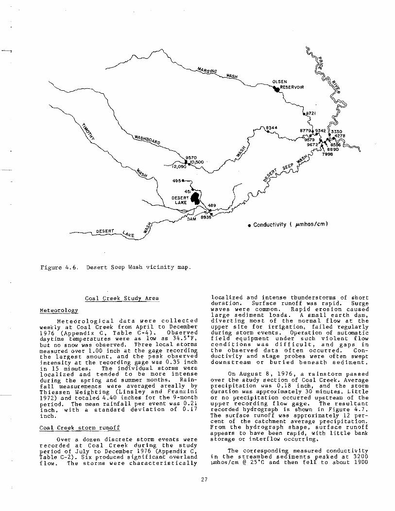
Figure 4.6. Desert Seep Wash vicinity map.

Coal Creek Study Area

Meteorology

Meteorological data were collected weekly at Coal Creek from April to December 1976 (Appendix C, Table C-4). Observed daytime temperatures were as low as 34.S·F, but no snow was observed. Three local storms measured over 1.00 inch at the gage recording the largest amount, and the peak observed intensity at the recording gage was 0.35 inch in 15 minutes. The individual storms were localized and tended to be more intense during the spring and summer months. Rain­fall measurements were averaged areally by Thiessen Weighting (Linsley and Franzini 1972) and totaled 4.40 inches for the 9-month period. The mean rainfall per event was 0.21 inch, with a standard deviation of 0.17 inch.

Coal Creek storm runoff

Over a dozen discrete storm events were recorded at Coal Creek during the study period of July to December 1976 (Appendix C, Table C-2). Six produced significant overland flow. The storms were characteristically

27

• Conductivity ( ",mhos/cm)

localized and intense thunderstorms of short duration. Surface runoff was rapid. Surge waves were common. Rapid erosion caused large sediment loads. A small earth dam, diverting most of the normal flow at the upper site for irrigation, failed regularly during storm events. Operation of automatic field equipment under such violent flow conditions was difficult, and gaps in the observed data often occurred. Con­ductivity and stage probes were often swept downstream or buried beneath sediment.

On August 8, 1976, a rainstorm passed over the study section of Coal Creek. Average precipitation was 0.18 inch, and the storm duration was approximately 30 minutes. Little or no precipitation occurred upstream of the upper recording flow gage. The resultant recorded hydrograph is shown in Figure 4.7. The surface runoff was approximately 12 per­cent of the catchment average precipitation. From the hydrograph shape, surface runoff appears to have been rapid, with little bank storage or interflow occurring.

The corresponding measured conductivity in the streambed sediments peaked at 3200 j.JIllhos/cm @ 25°C and then fell to about 1900

Page 40

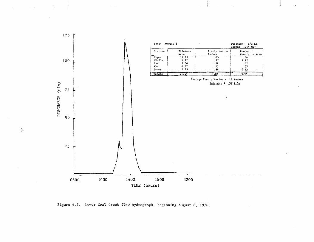
N 00

"'" Ul

125

100

't 75 '-'

J;:t:I

~ ~ u Cf.)

1-4 c:.

50

25

0600 1000 1400

Date: August 8

Station

Upper Middle East West Lower

Totals

1800 TIME (hours)

Thiessen Area

11.23 3.17 1.36 4.42 1.28

21.46

Precipitation Inches

.05

.37

.38

.13

.88

1.81

Duration: 1/2 hr. Began: 1245 MST

Product Precip. x Area

.56 1.17

.52

.57 1.13

3.95

Average Precipitation = .18 inches

Intensity ~ .36 in/hr

2200

Figure 4.7. Lower Coal Creek flow hydrograph, beginning August 8, 1976.

j

Page 41

flmhos/cm @ 25"C. The conductivity probe was buried under sediment, and a delayed response masked the shape and timing of the halograph. Wb ile some sediment induced error is probable, the above maximum and minimum conductivity values are close.

Coal Creek flow and guality measurements

Conductivity and flow measurements made on Coal Creek during 1976 are plotted on Figures 4.8 to 4.15 inclusive for sites shown on Figures 3.1 and 3.2. The average observed streamflow in Coal Creek, below the Book C li f f s , dec li ned from 1. 5 c f sin Apr il to 0.25 cfs in August (Figure 4.9). The mix of anions and cations ,at the upper site was fa irly constant (Appendix C, Table C-2). Conductivity increased from an average of 750 flmh 0 sic mat 25· C inA p r i 1 to 1000 flmhos/cm at 25°C in October with measurements made every 30 days (Figure 4.8). Sharply lower values of conductivity were observed after a storm event. This is attributed to the dilution effects of overland flow and to the low quantities of residual salts held in the sediments of the Coal ~reek channel.

Linear regression analyses were applied to estimate six chemical constituents using conductivity as the independent variable. The t-test was used to test the null hypothesis that the slope of the regression line equals zero.

Y == a + b [Conductivity] •.••• (4.1)

in which

Y

a and b

TDS or individual ion concen­tration Constants

The results are shown in Table 4.1. The low correlation coefficients were due primarily to grouping of the observed values within a very small range; this is particularly evident at the spring where the quantities of flow and chemical constituents varied in too small a range for meaningful regression to be possible.

At no time were overland return flows from the irrigated land associated with an increase in conductivity of more than 10 percent of that measured at the upper site. Because of seepage, the flow diminished and often disappeared in the 3-mile section below the upper site (Figure 3.1). Approximately 3 miles below the Book Cliffs, water enters Coal Creek from numerous small seeps and one large spring. The source and the extent of the aquifer supplying the seeps and spring are unknown (Gwynn 1976).

Discharge and water quality at the spring were monitored. Flow (Figure 4.11) was observed to peak at 0.1 cfs during April and to steadily decline to 0.04 cfs during December. Conductivity (Figure 4.10) remained

29

stable with an observed mean of 2759 flmhos/cm at 25"C and a standard deviation of 235 flrnhos/cm at 25°C. Data presented in Appendix C (Table C-2) also show that the concentra­tions of the chemical ions in the spring discharge were nearly constant.

The middle sampling site was located approximately 3.25 miles below Coal Creek's emergence from the Book Cliffs (Figure 3.1). The observed flows were generally low, except following storm events, and came from the spring and seeps immediately upstream (Figure 4.13). The conductivity ranged from approxi­mately 1000 flmhos/cm at 25·C to 3200 flmhos/cm at 25°C (Figure 4.12). The large variation in conductivity was due to dilution by storm runoff. At low flows, the majority of the flow originated as groundwater of approxi­mately 2760 jJmhos/cm at 25·C. At high flows the majority of the flow originated as sur­face runoff from either the upper part of the subbasin or above the upper site and ex­hibited little channel salt uptake. Parti­cularly high correlations with conductivity (Table 4.1) were obtained at this site for TDS and sulfate.

The flow at the lower site, 8.2 miles downstream from the Book Cliffs (Figure 3.1), was highly ephemeral (Figure 4.15) •. Much of the flow passing the middle site was lost through channel seepage and evaporation between the two sites. During periods of continuous flow, very little salt uptake occurred in the Coal Creek channel, and the conductivity of the lower site approached that of the upper site (Figure 4.14). During periods of low flow, when groundwater repre­sented the major source of flow, the con­ductivity equaled or exceeded the mean groundwater conductivity. From Table 4.1 high correlation coefficients (Equation 4.3) were obtained for TDS, sulfate, magnesium, and chloride. The null hypothesis was rejected at the 0.99 confidence level for all seven regressions.

Mean measured values of anions and cations at each site are listed in Table 4.2. On a given date, TDS measurements at the middle and lower sites usually were very close (Appendix C, Table C.2). The smaller mean va lue of the TDS at the lower site (Table 4.2) is explained on the basis that a larger number of samples were taken at this location than at the middle site during spring runoff.

Salinity from the Coal Creek channel sediments

The natural channel bottoms in the Coal Creek basin are composed of unconsolidated bed material and exposed Mancos Shale. The channels display surface efflorescence varying from a dense white blanket to inter­mittent small discrete deposits. Mass transport of the channel bed material by major storm events' was observed during the study reported here and by Mundorff (1972). During relatively steady and uniform low flow

Page 42

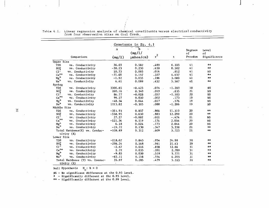
J

Table 4.1. Linear regression analysis of chemical constituents. versus electrical conductivity from four observation sites on Coal Creek.

Constants in Eg. 4.1 a - --b

Degrees Level (mg/I/

2 of of

Comparison (mg/I) llmhos/cm) r t Freedom Significance

Upper TDS vs. Conductivity 36.03 0.582 .489 6.105 41 ** 504 vs. Conductivity -38.23 0.230 .650 8.502 41 ** Cl- vs. Conductivity 10.23 0.003 .016 .812 41 NS Ca++ vs. Conductivity .,.71.00 0.157 .337 4.457 41 ** Mg+ vs. Conductivity -1.92 0.035 .196 3.080 41 ** Na+ vs. Conductivity 4.41 0.089 .432 5.587 41 **

Spring TDS vs. Conductivity 3300.65 -0.425 .074 -1.203 18 NS 504 vs. Conductivity 260.16 0.340 .019 .635 21 NS CI- vs. Conductivity 86.77 -0.028 .057 -1.103 20 NS Ca++ vs. Conductivity 99.27 0.030 .002 .173 19 NS Mg+ vs. Conductivity -48.34 0.044 .017 .576 19 NS Na+ vs. Conductivity 1213.82 -0.305 .080 -1.286 19 NS

w Middle Site 0 TDS vs. Conductivity -311. 93 0.857 .864 11. 310 20 **

SO?; vs. Conductivity -558.95 0.630 .883 12.299 20 ** CI- vs. Conductivity 27.27 -0.002 .011 -.474 21 NS Ca++ vs. Conductivity -121.56 0.119 .174 2.054 .20 NS Mg+ vs. Conductivity 6.18 0.024 .173 2.044 20 NS Na+ vs. Conductivity -19.72 0.130 .347 3.338 21 ** Total Hardness(Y) vs. Conduc- -108.89 0.312 .609 5.725 21 **

tivity (X) Lower Site

TDS vs. Conductivity -218.07 0.843 .954 24.98 30 ** 504 vs. Conductivity -298.24 0.548 .941 21.43 29 ** CI- vs. Conductivity -2.67 0.016 .838 12.66 31 ** Ca++ vs. Conductivity 2.72 0.035 .201 2.789 31 ** Mg+ vs. Conductivity -9.85 0.030 .518 5.771 31 ** Na+ vs. Conductivity -65.11 0.156 .554 6.205 31 ** Total Hardness (Y) vs. Conduc- 35.97 0.285 .479 5.333 31 **

tivit:t (X)

Null Hypothesis H : B 0 0

NS - No significant difference at the 0.95 level. * - Significantly different at the 0.95 level. ** - Significantly different at the 0.99 level.

Page 43

---" u 0

4000 UPPER SITE 10 .N

~ '" 3000 0 .s::; E ::I..

>- 2000 I-:> i= U ::>

1000

0 Z 0 U

16 15 15 14 14 13 12 12 " II MAR. APR. MAY JUlIE JULY AUG. SEPT. OCT. NOV. DEC.

Figure 4.8. Conductivity at Coal Creek upper site.

8.0 UPPER SITE

'";;; -.=! 6.0

IJJ (!) 0:: « 4.0 :t: U (/)

0 2.0

16 15 15 14 14 13 12 12 II II MAR APR. MAY JU lIE JULY AUG. SEPT. OCT. NO.1. DEC.

Figure 4.9. Flow at Coal Creek upper site.

u 0

~ 4000 SPRING

@

'" 0 3000 .t:.

E ::I..

>- 2000 !:: 2! I-U 1000 ::> 0 Z 0 u

16 15 15 14 14 13 12 12 II II MAR. APR. MAY J"-'IE JULY AUG. SEPT. OCT. NOV. DEC.

Figure 4.10. Coal Creek conductivity of the spring inflow.

0.20 SPRING

'" -(.) 0.15

IJJ (!) 0:: « 0.10 :t: U (/)

a 0.05

16 15 15 14 14 13 12 12 II II MAR. APR. MAY JUNE JULY AUG. SEPT. OCT. NOV. DEC.

Figure 4.11. Coal Creek lateral inflow from the spring.

31

Page 44

u 4000 0 MIDDLE SITE

It) N

~ 3000 S e frozen-&. E 5 2000 >-l-s: i= U

1000 ::I 0 z 8

16 15 15 14 14 13 12 12 II II MAR. A PRo MAY Jr.N: JULY AUG. SEPT. OCT. NOlI. DEC.

Figure 4.12. Coal Creek conductivity at the middle site.

1.00 MIDDLE SITE

-III ... 0.75 0 -W (!) 0: 0.50 <I. J: U (1'J

0 0.25

16 15 15 14 14 13 12 12 II II MAR. APR. MAY JU~ JULY AUG. SEPT. OCT. NOV. DEC.

Figure 4.13. Coal Creek flow at the middle site.

32

u Ih 4000 LOWER SITE N

~

.2 3000

E :t.

2000 >-l-s: i= 1000 u ::I 0 Z 0 U

16 15 15 14 14 13 12 12 II " MAR. APR. MAY Ji.N: JllY AUG. SEPT. OCT. NfN. OEC.

Figure 4.14. Coal Creek conductivity at the lower site.

4.0 LOWER SITE

3.0

2.0

1.0

1615151414131212 "" MAR. APR. MAY Jr.N: JllY AUG. SEPT. OCT. NW DEC.

Figure 4.15. Coal Creek flow at the lower site.

Page 45

Table 4.2. Observed chemical concentrations in Coal Creek.

Site

Upper

Spring

Middle

Lower

X ::: mean

X 8

X \

18 v £.

s X s

TDS mg!l

513 153

2109 164

1901 534

1388 598

153 50

1176 161

1137 363 771 397

observed value s ::: standard deviation

Cl­mg!l

13 5 9

12 22 12 29 12

cart mg!l

51 41

184 79

184 166 69 54

Mgt+ mg!l

26 14 76 32 69 34 48 29

Na+ mg!l

79 23

360 111 315 128 242 153

conditions, little or no salt uptake was observed in the natural channels.

Sixty sediment samples were taken from channels throughout the Coal Creek study area, and conductivities were determined for their 1:1 saturation extracts. The objective was to determine if significant differences as salinity sources existed in materials taken from different depths, between banks and beds, and between main stem and tributary channels. The resulting chemical extract data are listed in Appendix C (Table C-3).

The predominant anion extracted was sulfate, with an observed mean concentration of 2245 mg/l and a standard deviation of 1955 mg/l. Much smaller concentrations of chloride and carbonates were found. The predominant cations were calcium, magnesium, and sodium with means of 299, 179, and 426 mg/l and standard deviations of 168, 217, and 587 mg/l, respectively. Relatively small concentrations of potassium were also found.

The means and standard deviations of the conductivities of the channel sediments segregated by the three-way classification are listed in Table 4.3. A student t-test was conducted to examine for significant di fferences among means assuming unequal variances (Lapin 1975). The results are listed in Table 4.4.

The only significant differences de­tected were in the bank materials and at depths greater than 10 cm between Coal Creek and its tributaries, and these were only valid at the 95 percent level. Significant salinity differences related to channel processes or geomorphology, even if they exist, are very difficult to detect because of extreme heterogeneity of Mancos Shale and Mancos Shale derived soils in the area (Ponce 1975).

To estimate the approximate magnitude of efflorescence in the natural channels, 1 cm deep soil samples were taken at the sites of

33

Table 4.3. Soil conductivities for beds and banks for Coal Creek locations.

Depth (em)

Number of Observations

Coal Creek Channel

0-10 9 10-20 9 20-30 9

Coal Creek Banks

0-10 21 10-20 21 20-30 21

Coal Creek Tributary Channels

0-10 lO-20 20-30

lO lO 10

Coal Creek Tributary Banks

0-10 lO-20 20-30

20 20 20

Deviation

2.34 2.24 1.99 3.00 2.22 3.18

3.30 2.60 2.66 2.13 2.92 2.53

lO.82 12.69 8.50 13.50 5.21 4.13

6.13 5.87 5.01 3.S5 5.37 4.15

the sediment samples of February 9 and July 8, 1977. From the efflorescence samples, the conductivity was measured, the TDS was esti­mated (Equation 4.2), and the efflorescent density in gm/m2-cm was calculated.

TDS = 1.04 (EC) - 551 •••••• (4.2)

in which

TDS Total dissolvea solids in mg/l EC Conductivity in mmhos/cm @ 25°C

The results are listed in Appendix C. The estimated effluorescent density ranged from a low of 18 gm/m2-cm to a high of 9387 gm/m2-cm measured in a Coal Creek tributary called Bitter Creek. This channel receives a small amount of interflow from the irrigated farmland (Figure 3.1). The mean effluorescent density was 1187 gm/m2-cm with a standard deviation of 2230 gm/m2-cm. The predominant efflorescent source is believed to be soil­water evaporation as described by Nakayama et a1. (1973) and resulting in particularly heavy deposits on concave surfaces below saturated soil profiles and other locations where soil water comes to the surface.

Mineral dissolution from the Coal Creek channel material

Salt dissolution rates were measured in the laboratory by placing samples of un­weathered Mancos Shale in quiescent distilled water and measuring conductivities of the solution periodically. For this purpose, six shale samples each were taken from four Coal Creek sites.

Page 46

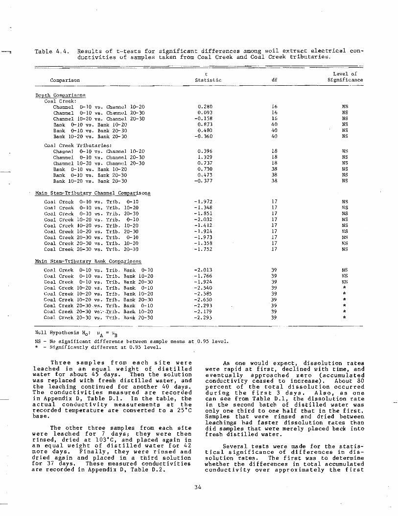
Table 4.4. Results·of t-tests for significant differences among soil extract electrical con­ductivities of samples taken from Coal Creek and Coal Creek tributaries.

Comparison

Depth Comparisons Coal Creek:

Channel 0-10 VS. Channel 10-20 Channel 0-10 vs. Channel 20-30 Channel 10-20 vs. Channel 20-30 Bank 0-10 vs. Bank 10-20 Bank 0-10 VS. Bank 20-30 Bank 10-20 VS. Bank 20-30

Coal Creek Tributaries: Channel 0-10 vs. Channel 10-20 Channel 0-10 vs. Channel 20-30 Channel 10-20 vs. Channel 20-30 Bank 0-10 VS. Bank 10-20 Bank 0-10 VS. Bank 20-30 Bank 10-20 vs. Bank 20-30

Main Ste~Tributary Channel Comparisons

Coal Creek 0-10 vs. Trib. Coal Creek 0-10 vs. Trib. Coal Creek 0-10 VB. Trib. Coal Creek 10-20 vs. Trib. Coal Creek 10-20 vs. Trib. Coal Creek 10-20 vs. Trib. Coal Creek 20-30 VS. Trib. Coal Creek 20-30 vs. Trib. Coal Creek 20-30 VS. Trib.

0-10 10-20 20-30 0-10

10-20 20-30 0-10

10-20 20-30

Main Stem-Tributary Bank Comparisons

Coal Creek 0-10 vs. Trib. Bank 0-10 Coal Creek 0-10 VS. Trib. Bank 10-20 Coal Creek 0-10 VS. Trib. Bank 20-30 Coal Creek 10-20 vs. Trib. Bank 0-10 Coal Creek 10-20 vs. Trib. Bank 10-20 Coal Creek 10-20 vs. Trib. Bank 20-30 Coal Creek 20-30.vs. Trib. Bank 0-10 Coal Creek 20-30 vs>.lFib. Bank 10-20 Coal Creek 20-30 vs. Trib. Bank 20-30

Null Hypothesis He: ~A ~B

t Statistic

0.280 0.093

-0.158 0.873 0.480

-0.360

0.396 1. 329 0.737 0.730 0.473

-0.377

-1.972 -1. 348 -1. 851 -2.032 -1.412 -1. 924 -1.973 -1. 358 -1.752

-2.013 -1. 766 -1.924 -2.540 -2.585 -2.650 -2.293 -2.179 -2.295

df

16 16 16 40 40 40

18 18 18 38 38 38

17 17 17 17 17 17 17 17 17

39 39 39 39 39 39 39 39 39

Level of Significance

NS NS NS NS NS NS

NS NS NS NS NS NS

NS NS NS NS NS NS NS NS NS

NS NS NS

* * * * * *

NS - No significant difference between sample means at 0.95 level. * - Significantly different at 0.95 level.

Three samples from each site were leached in an equal weight of distilled water for about 45 days. Then the solution was replaced with fresh distilled water, and the leach ing cont inued for another 40 days. The conductivities measured are recorded in Appendix D, Table D.l. In the table, the actual conductivity measurements at the recorded temperature are converted to a 25·C base.

The other three samples from each site were leached for 7 days; they were then rinsed, dried at 103·C, and placed again in an equal weight of distilled water for 42 more days. Finally, they were rinsed and dried again and placed in a third solution for 37 days. These measured conductivities are recorded in Appendix D, Table D.2.

34

As one would expect, dissolution rates were rapid at first, declined with time, and eventually approached zero (accumulated conduct i vity ceased to increase). About 80 percent of the total dissolution occurred during the first 3 days. Also, as one can see from Table D.l, the dissolution rate in the second batch of distilled water was only one third to one half that in the first. Samples that were rinsed and dried between leachings had faster dissolution rates than did samples that were merely placed back into fresh distilled water.

Several tests were made for the statis­tical significance of differences in dis­solution rates. The first was to determine whether the differences in total accumulated conductivity over approximately the first

Page 47

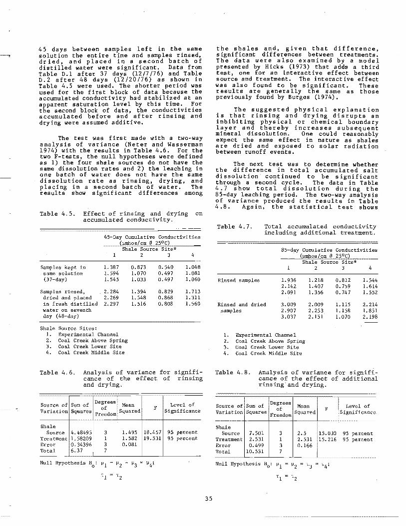
45 days between samples left in the same solution the entire time and samples rinsed, dried, and placed in a second batch of distilled water were significant. Data from Table 0.1 after 37 days (12/7/76) and Table 0.2 after 48 days (12/20/76) as shown in Table 4.5 were used. The shorter period was used for the first block of data because the accumulated conductivity had stabilized at an apparent saturation level by this time. For the second block of data, the conductivities accumulated before and after rinsing and drying were assumed additive.

The test was first made with a two-way analysis of variance (Neter and Wasserman 1974) with the results in Table 4.6. For the two F-tests, the null hypotheses were defined as 1) the four shale sources do not have the same .dissolution rates and 2) the leaching in one. batch of water does not have the same dissolution rate as rinsing, drying, and placing in a sel:!ond batch of water. The results show significant differences among

Table 4.5. Effect of rinsing and drying on accumulated conductivity.

45-Day Cumulative Conductivities (~mhos/cm @ 25°C) Shale Source Site*

1 234

Samples kept in 1.387 0.873 0.540 1.048 same solution 1.594 1.070 0.497 1.081 (37-day) 1. 545 1.033 0.497 1.060

Samples rinsed, 2.284 1.394 0.829 1.713 dried and placed 2.269 1.548 0.868 1.311 in fresh distilled 2.297 1. 516 0.808 1.560 water on seventh day (48-day)

Shale Source Sites: 1. EXperimental Channel 2. Coal Creek Above Spring 3. Coal Creek Lower Site 4. Coal Creek Middle Site

Table 4.6. Analysis of variance for signifi­cance of the effect of rinsing and drying.

Source of Sum of Degrees Mean Level of Variation Squares of Squared F Significance Freedom

Shale Source 4.48495 3 1.495 18.457 95 percent

Treatment 1.58209 1 1.582 19.531 95 percent Error 0.34396 3 0.081 Total 6.37 7

• Null Hypothesis Ho: VI \1 2

35

the shales and, given that difference, significant differences between treatments. The data were also examined by a model presented by Hicks (1973) that adds a third test, one for an interactive effect between source and treatment. The interactive effect was also found to be significant. These results are generally the same as those previously found by Burges (1974).

The suggested physical explanation is that rinsing and drying disrupts an inhibiting physical or chemical boundary layer and thereby increases subsequent mineral dissolution. One could reasonably expect the same effect in nature as shales are dried and exposed to solar radiation between runoff events.

The next test was to determi ne whether the difference in total accumulated salt dissolution continued to be significant through a second cycle. The data in Table 4.7 show total dissolution during the 85-day leaching period. The two-way analysis of variance p~oduced the results in Table 4.8. Again, the statistical test shows

Table 4.7. Total accumulated conductivity including additional treatment.

Rinsed samples

Rinsed and dried samples

85-day Cumulative Conductivities (vmnos/cm @ 25°C) Shale Source Site*

123 4

1. 936 1.218 0.812 1.544 2.142 1. 407 0.759 1. 614 2.091 1. 356 0.747 1.552

3.009 2.009 1.115 2.214 2.907 2.253 1.158 1.851 3.037 2.151 1.070 2.198

1. Experimental Channel 2. Coal Creek Above Spring 3. Coal Creek Lower Site 4. Coal Creek Middle Site

Table 4.8. Analysis of variance for signifi­cance of the effect of additional rinsing· and drying.

Source of Sum of Degrees Mean Level of

Variation Squares of Squared F Significance Freedom

Shale Source 7.501 3 2.5 15.030 95 percent

Treatment 2.531 1 2.531 115.216 95 percent Error 0.499 3 0.166 Total 10.531 7

Null Hypothesis Ho: \1 1 ~2

~----- ------_ ............................... _--

Page 48

significant differences among shales and a continuing significant difference between treatments on the seventh day.

The differences were probed once more by testing dissolution amounts during the second 40-day treatment period. The results in Table 4.8 cover the entire 85-day period and thus, according to the results reported in Table 4.6, would be significant if a constant dissolution were added during the second 40-day period. Therefore, Hicks' (1973) model was used to test for significant differences amon~ shales, between treatments, and in interactlon between the two. Again, all three differences were found significant.

The results of these tests 'have impor­tant implications. Dissolution rates vary significantly among shales and with the history of wetting and drying as the material moves downstream. The many shale sources and histories will make it very difficult to estimate dissolution rates in a given stream. Also, the tendency of wetting and drying cycles to increase dissolution would cause more of the salts in the bed material of ephemeral channels to be leached out before the bed material reaches a larger stream. Material directly entering a perennial stream may move through the system with much more of its salt content in tact. These materials may continue as an important salt source downstream on the Colorado River for years.

Time rates of dissolution

Whitmore (1976) found that when salt dissolution rates are plotted against the

0 2000 0 LO N @ 1500 I/)

0 s:. E :l. 1000 -

>-I-> 500 I-0 :::> 0 z a

square root of time a broken curve of the sort illustrated by Figure 4.16 results. Accordingly, an attempt was made to fit the dissolution data with a square root model of the form:

C = Kl TO.5. •• • ••••.•• (4.3)

in which

C The specific conductance in ~mhos, at time T

T Time in minutes Kl A dissolution

In order to determine the effect of grain size on dissolution rates, accumulated conductivities were also measured in the laboratory for shale samples separated by grain size with the results shown in Table D.4. Equation 4.3 fit the data with a single constant 11 rather than with the breakpoint shown in Figure 4.16. Eighty percent of the 72-hour conductivity was obtained after a mean of 9.4 hours, with a standard deviation of 7.1 hours, as compared to the few minutes found by Whitmore (1976) for Mancos soil. The advanced weathering state of the channel material used by Whitmore probably accounts for the rapid dissolution that he observed.

The results of the student t-test analysis for differences by grain size of the 3D-second and 72-hour conductivity values are presented in Table 4.9. The significant increase in 3D-second dissolution for smaller grain sizes is evidence that the initial rate of salt dissolution increases with partial surface area.

0 a 100 200 300 0

SQUARE ROOT OF TIME (minO.5 )

Figure 4.16. Accumulated conductivity from laboratory salt dissolution.

36

Page 49

Table 4.9. Comparison of mineral dissolution rates with time and grain size.

t Level of Comparison Statistic df

Significance

30-second comparisons 114 vs. (flO -0.195 6 NS 114 vs. 1120 -2.856 6 '" 114 vs. 1160 -6.173 6 "'* 1110 vs. 1120 -3.040 6 * 1110 vs. 1160 -6.350 6 ** 1120 vs. 1160 -4.132 6 **

72-hour comparisons 114 vs. no 0.275 6 NS 114 vs. 1120 -1. 437 6 NS #4 VS. 1/60 -1. 804 6 NS 1110 VS. 1120 -1. 770 6 NS 1110 vs. /160 -1. 925 6 NS 1/20 vs. 1160 -1. 172 6 NS

Null Hypothesis Ho: ]l = A ]lB

NS No significant difference between sample means at the 0.95 level.

* - Significantly different at the 0.95 level. ** - Significantly different at the 0.99 level.

A test was designed to estimate the effect of the number of wet/dry cycles on salt release rates for various shale size fractions. Shale samples from the four sites were crushed and separated into four size fractions, for a total of 16 individual samples. From each sample, 50 grams of soil were saturated· with 100 ml of distilled water and placed within a Brinkmann Roto­evaporator (rotovap) and water bath. By this method, numerous wet/dry cycles are possible within a I-day period. Because salts are removed in a 5 ml aliquot, a 5 percent adjustment was assumed to be necessary after each successive wet/dry cycle. The con­ductivi ty values were linearly adjusted and corrected to 25°C. The results are presented in Appendix C (Table C.2). The test was terminated after 10 samples were evaluated.

Figure 4.17 illustrates the results. An increase in dissolution causing greater solution conductivity after the first drying cycle was observed for all of the samples •. The increase ranged from 5 percent to 43 percent with ~ mean of 21 percent and standard deviation of 12 percent. Following the second drying cycle, only three of the 10 samples had an increase in conductivity. The variation ranged from a minus 8 percent to a positive 10 percent, with a mean of a minus 2 percent and a s tanda rd devia t ion of 6 per­cent. Further wet/dry cycles generally brought additional conductivity declines.

The unexpected decline in conductivity after just one cycle may be due to experi­mental error or to characteristics of the rotovap. During the drying, vigorous

800

foj.- - ...J:.' ...-C·t- -_l.." ,- ....... I -E)- - ,,' "" / (J

°ll'l600 / '" / <!!J ( ~

---(/)

0

!400

it! H :> H

"" 0 0 Site 2. Fraction (J

:::> ~ 200 ... , _L'\ Site 1, Fraction 0 ,;;- ... " (J

0 2 3 4 5 CYCLE NUMBER

Figure 4.17. Illustrative effect of wetting and drying cycles on conductivity.

boiling of the slurry occurred, and the larger aggregates were rapidly eroded. Thus, it is possible that the mineral dissolution was accelerated to the point that most of the salts were released from the shale samples after only one cycle. Variation in the conductivity of the following cycles might have been caused by irregular mass loss during drying. Solids splashed into the condensor unit during evaporation, and no adjustment was made for their mass.

The rate of salt release from a shale surface would be expected to be rapid at first and then to decline as the supply of surface salt diminished, leaving the much slower release of salts entrained beneath the surface of the relatively impermeable shale •

. Under steady-state flow conditions, the salts would be released by diffusion-controlled dissolution from the submerged shale. Oven­drying of the sample (sun drying in the field) increases the surface area of the shale as water of hydration is lost, frac­turing develops, and diffusion inhibiting boundary layers are disrup~ed.

37

Macrochannel induced streamflow studies

One problem in measuring salt pickup from various salinity sources is that of

1

1

Page 50

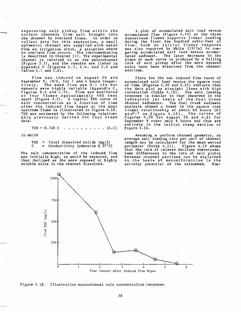
separating salt pickup from within the surface channels from salt brought into the channel by overland flows. In order to collect data for this separation, a small ephemeral channel was supplied with water from an irrigation ditch, a situation where no overland flow occurs. The instrumentation is described in Chapter III. The experimental channel is referred to as the macrochannel (Figure 3.3), and the results are listed in Appendix C (Figures C.3, C.4, and C.S and Tables C.7 and C.8).

Flow was induced on August 26 and September 9, 1976, for 7 and 4 hours respec­tively. The mean flow was 0.1 cfs but amounts were highly variable (Appendix C, Figures C.4 and C.S). Flow was monitored at four flumes approximately 400 feet apart (Figure 3.3). A typical TDS curve of salt concentration as a function of time after the induced flow began at the most upstream flume is illustrated in Figure 4.18. TDS was estimated by the following relation­ship previously derived for Coal Creek data.

TDS = 0.746 C •••••••••• (4.4)

in which

TDS Total dissolved solids (mg/l) C Conductivity (~mhos/cm @ 2S·C)

The salt concentration of the induced flow was initially high, as would be expected, and then declined as the more exposed or highly soluble salts in the channel dissolved.

750

r-. rl' ...... en 8 <Il 500 p E-<

~ 0 rl r,.

250

A plot of accumulated salt load versus accumulated flow (Figure 4.19) at the three downstream flumes supports linear loading during the first few hundred cubic-feet of flow. Such an initial linear response was also reported by White (1977a) in com­paring accumulated salt load versus accumu­lated sediment. The later decrease in the slope of each curve is produced by a falling rate of salt pickup after the more exposed salts have been dissolved from the channel sections.

Plots for the two induced flow tests of accumulated salt load versus the square root of time (Figures 4.20 and 4.21) indicate that the data plot as straight lines with high correlation (Table 4.10). The salt loading response is similar to that observed in the laboratory jar tests of the Coal Creek channel sediments. The Coal Creek sediment analysis showed a break in the square root linear relationship at about 60 hours (6S minO• S on Figure 4.16). The curves of Figures 4.20 for August 26 and 4.21 for September 9 cover only 6 hours and thus are entirely in the initial steep section of Figure 4.16.

Assuming a uniform channel geometry, an average salt loading rate per unit of channel length may be calculated for the mean wetted perimeter (Table 4.11). Figure 4.19 shows that the rate of release declines downstream. Some differences in the rate of salt pickup between channel sections can be explained on the basis of nonuniformities in the salinity potential of the streambed. How-

4 5 6 Time (hours) After Induced Flow Began

Figure 4.18. Illustrative macrochannel salt concentration response.

38

Page 51

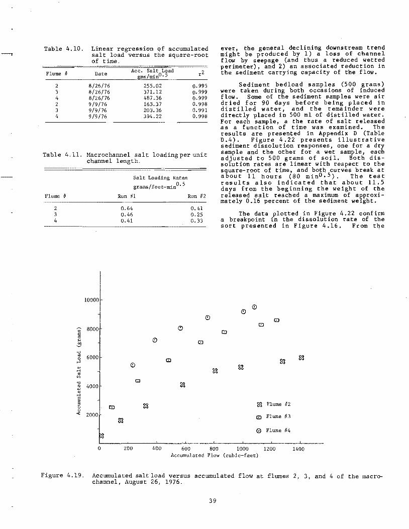
Table 4.10. Linear regression of accumulated salt load versus the square-root of time.

Flume # Date r2

2 8/26/76 255.02 0.995 3 8/26/76 371.12 0.999 4 8/26/76 487.36 0.999 2 9/9/76 163.37 0.998 3 9/9/76 203.36 0.991 4 9/9/76 394.22 0.998

Table 4.11. Macrochannel salt loading per unit channel length.

Flume II

2 3 4

,..... OJ s <Il I-l bO '-'

rQ <Il 0

,...l

... .-I <Il

'" rQ (!) ... <Il

.-I ;:!

3 cJ cJ

<:

10000 -

8000

6000

4000

r:::u 2000

°

Salt Loading Rates

grams/feet-minO. 5

Run #1 Run #2

0.64 0.46 0.41

0

m

200

(!)

Cil

m

400

(!)

IZl

m

600

0.41 0.25 0.33

CD

0

m

800 Accumulated Flow

ever, the general declining downstream trend might be produced by 1) a loss of channel flow by seepage (and thus a reduced wetted perimeter), and 2) an associated reduction in the sediment carrying capacity of the flow.

Sediment bedload samples (500 grams) were taken during both occasions of induced flow. Some of the sediment samples were air dried for 90 days before being placed in distilled water, and the remainder were directly placed in 500 ml of distilled water. For each sample, a the rate of salt released as a function of time was examined. The results are presented in Appendix 0 (Table D.4). Figure 4.22 presents illustrative sediment dissolution responses, one for a dry sample and the other for a wet sample, each adjusted to 500 grams of soil. Both dis­solution rates are linear with respect to the square-root of time, and botQ curves break at about 11 hours (80 minO• 5 ). The test results also indicated that about 11.5 days from the beginning the weight of the released salt reached a maximum of approxi':' mately 0.16 percent of the sediment weight.

The data plotted in Figure 4.22 confirm a breakpoint in the dissolution rate of the sort presented in Figure 4.16. From the

(!) 0

IZl IZl

IZl

m m m

m Flume 112

I.!I Fltune 113

0 Flume #4

~ .. -1000 1200 1400

(cubic-feet)

Figure 4.19. Accumulated salt load versus accumulated flow at flumes 2, 3, and 4 of the macro­channel, August 26, 1976.

39

Page 52

t1 10 . ...:l

....

8000

~ 4000

I ::.il2000

o 5

&3 Flume It2

I!I Flume It3

o Flume It4

10 15 20 25 30 SQUARE ROOT OF TIME (minO. 5)

Figure 4.20. Macrochannel salt load versus the square-root of time (8/26/76).

8000

-;;) ~ 6000

'" bO ~

~ .... ~ 4000 '" ~ j ~ § 2000 ...:

o

~ Flume lIZ

I!I Flume it 3

o Flume 1t4

5 10 15 20 SQUARE ROOT OF TIME (minO. 5)

25

Figure 4.21. Macrochannel salt load versus the square-root of time (9/9/76).

40

30

Page 53

0.8

o 50

Slope=.0053 r2 = .99

r-.. <11

o

'" .,..; en S ~ ;;0 000 .a '-'"

Slope=.0007 r2 .83

~Flume #1 Dried Sediment Sample 8/26/76

~Flume #1 Wet Sediment Sample 9/9/76

Slopes in gro/minD.5

300 100 150 200 SQUARE ROOT OF TIME (minO. 5)

250

Figure 4.22. Salt dissolution from macrochannel bedload material.

replications in the four samples in each set, the two slopes and the breakpoint time were calculated. The results are listed in Table 4.12. Comparisons were made among sediment samples of the total salt release at 1) the end of the steep portion of the curve (Figure 4.22), and 2) at 11.5 days. A t-statistic was used to test the null hypothesis that tbe accumulated conductivity means were equivalent with the results listed in Table 4.13. Drying tbe sediment signi­f icantly increased tbe salt released during tbe steep portion of the curve. However, after 11.5 days there was no significant difference in the cumulative salt release for tbe two sample treatments.

Table 4.12. Mean salt dissolution rates for macrochannel sediments.

Soil salinity sensors were installed in tbe macrochannel on August 15, 1976, and monitored weekly (Figure 3.3). The sensors bad been saturated witb a 4000-l.!mbos/cm (at 2S·C) solution of calcium and sodium chloride. The manufacturer of the sensors, Soil Mois­ture Equipment, Inc. (1976), recommend the following operating ranges for the _ensors:

1. A soil moisture tension range of from 1 to 15 bars.

2. A conductivity range of from 500 to 30,000 l.!mbos/cm at 25°C.

41

Estimated Salt @ Time Breakpoint

Wet Sediment Samples 8/26/76

X 0.094 S 0.081

Dried Sediment Samples 8/26/76

X 0.341 S 0.071

Wet Sediment Samples 9/9/76

X 0.070 S 0.023

Estimated Salt @ Time

It = 125

0.672 0.236

0.705 0.133

0.740 0.176

0.00462 0.00226

0.00384 0.00120

0.00670 0.00156

*

83.38 1.00

92.41 10.36

4 replications for each group of samples K1, L1• K2 defined on Figure 4.16 *No break observed in curve

K2 gros/

minO. 5

*

0.00107 0.00062

0.00156 0.00110

Page 54

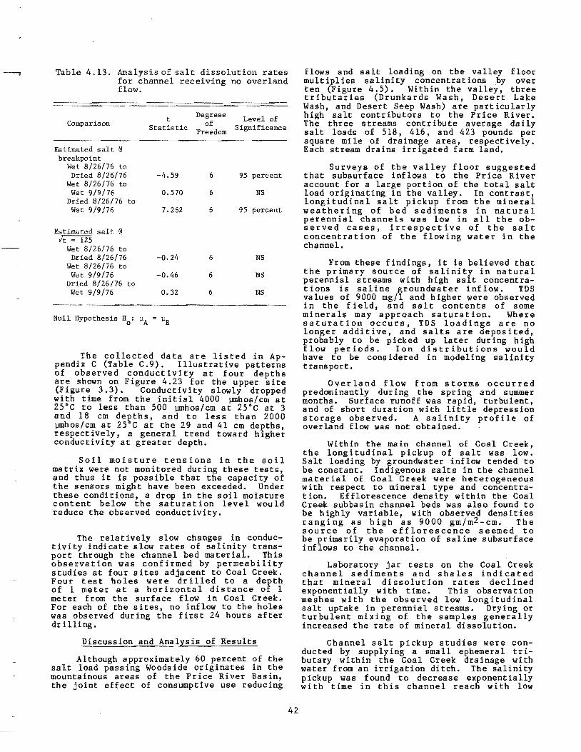
Table 4.13. Analysis of sal t dissolution rates for channel receiving no overland flow.

Comparison

Estimated salt @ breakpoint

Wet 8/26/76 to Dried 8/26/76

Wet 8/26/76 to Wet 9/9/76

Dried 8/26/76 to Wet 9/9/76

Estimated salt @ It = 125

Wet 8/26/76 to Dried 8/26/76

Wet 8/26/76 to Wet 9/9/76

Dried 8/26/76 to Wet 9/9/76

t Statistic

-4.59

0.570

7.262

-0.24

-0.46

0.32

Null Hypothesis Ho: ~A = ~B

Degrees of

Freedom

6

6

6

6

6

6

Level of Significance

95 percent

NS

95 percent

NS

NS

NS

The collected data are listed in Ap­pendix C (Table C.9). Illustrative patterns of observed conductivity at four depths are shown on Figure 4.23 for the upper site (Figure 3.3). Conductivity slowly dropped with time from the initial 4000 ].llllhos/cm at 25°C to less than 500 J.lIllhos/cm at 25°C at 3 and 18 cm depths, and to less than 2000 umbos/cm at 25°C at the 29 and 41 cm depths, respect ively, a general trend toward higher conductivity at greater depth.

Soil moisture tensions in the soil matrix were not monitored during these tests, and thus it is possible that the capacity of the sensors might have been exceeded. Under these conditions, a drop in the soil moisture content below the saturation level would reduce the observed conductivi~y.

The relatively slow changes in conduc­tivity indicate slow rates of salinity trans­port through the channel bed material. This observation was confirmed by permeability studies at four sites adjacent to Coal Creek. Four test holes were drilled to a depth of 1 meter at a horizontal distance of 1 meter from the surface flow in Coal Creek. For each of the sites, no inflow to the holes was observed during the first 24 hours after dr illing.

Discussion and Analysis of Results

Although approximately 60 percent of the salt load passing Woodside originates in the mountainous areas of the Price River Basin, the joint effect of consumptive use reducing

42

flows and salt loading on the valley floor mUltiplies salinity concentrations .by over ten (Figure 4.5). Within the valley, three tributaries (Drunkards Wash, Desert Lake Wash, and Desert Seep Wash) are particularly high salt contributors to the Price River. The three streams contribute average daily salt loads of 518, 416, and 423 pounds per square mi Ie of drainage area, respectively. Each stream drains irrigated farm land.

Surveys of the valley floor suggested that subsurface inflows to the Price River account for a large portion of the total salt load originating in the valley. In contrast, longitudinal salt pickup from the mineral weathering of bed sediments in natural perennial channels was low in all the ob­served cases, irrespective of the salt concentration of the flowing water in the channel.

From these findings, it is believed that the primary source of salinity in natural perennial streams with high salt concentra­tions is saline groundwater inflow. TDS values of 9000 mg/l and higher were observed in the field, and salt contents of some minerals may approach saturation. Where saturation occurs, TDS loadings are no longer additive, and salts are deposited, probably to be picked up later during high flow periods. Ion distributions would have to be considered in modeling salinity transport.

Overland flow from storms occurred predominantly during the spring and summer months. Surface runoff was rapid, turbulent, and of short duration with little depression storage observed. A sali ni ty profi Ie of overland flow was not obtained.

Within the main channel of Coal Creek, the longitudinal pickup of salt was low. Salt loading by groundwater inflow tended to be constant. Indigenous salts in the channel material of Coal Creek were heterogeneous with respect to mineral type and concentra­tion. Efflorescence density within the Coal Creek subbasin channel beds was also found to be highly variable, with observed densities ranging as high as 9000 gm/m2-cm. The sou r ceo f the e f flo res c e n c e seem edt 0 be primarily evaporation of saline subsurface inflows to the channel.

Laboratory jar tests on the Coal Creek channel sediments and shales indicated that mineral dissolution rates declined exponentially with time. This observation meshes with the observed low longitudinal salt uptake in perennial streams. Drying or turbulent mixing of the samples generally increased the rate of mineral dissolution.

Channel salt pickup studies were con­ducted by supplying a small ephemeral tri­butary within the Coal Creek drainage with water from an irrigation ditch. The salinity pickup was found to decrease exponentially with time in this channel reach with low

Page 55

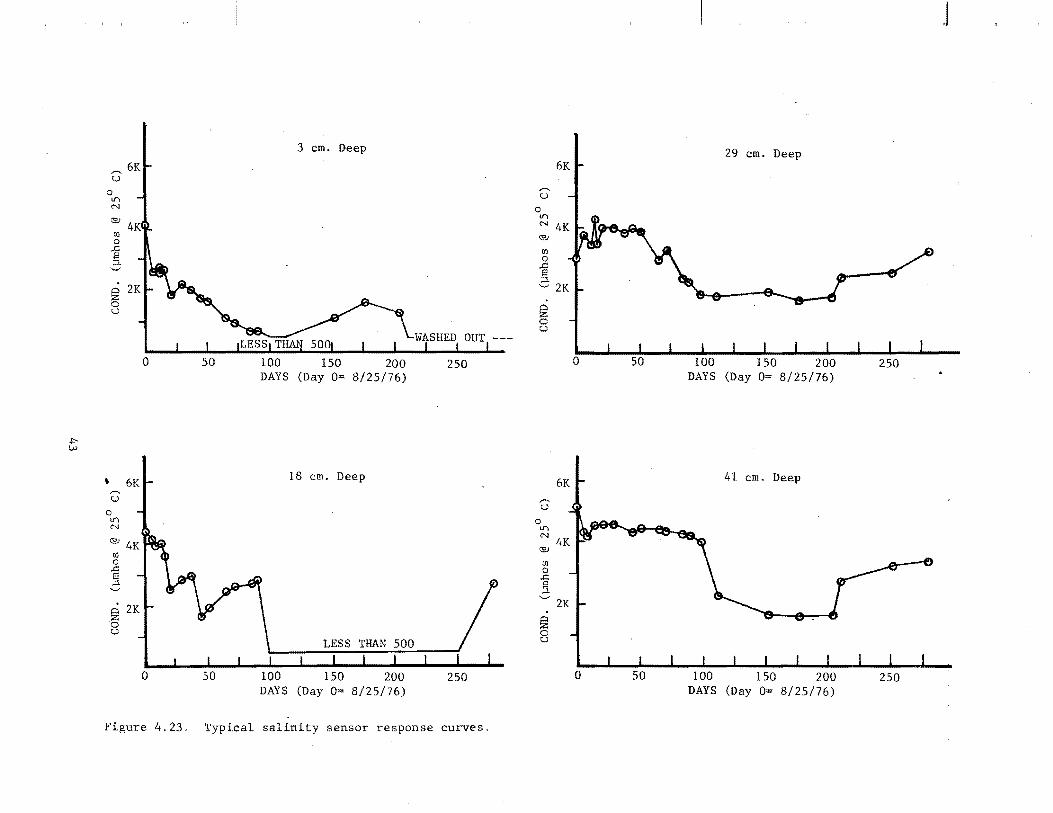
..,. l,.V

o~ 61

~ 2Kt

, 6K """' u

a I/') N

~ o u

0

~-50

3 cm. Deep

-~

100 150 200 250 DAYS (Day 0= 8/25/76)

18 em. Deep

150 200 250 DAYS (Day 0= 8/25/76)

Figure 4.23. Typical salinity sensor response curves.

6K

"""' u a

I/')

N 4K ®

til a -§ ;::l. '-' 2K

~ 0 u

"""' u

~ o u

6K

I

l 0

o

J

29 cm. Deep

50 100 150 200 250 DAYS (Day 0= 8/25/76)

41 cm. Deep

50 100 150 200 250 DAYS (Day 0= 8/25/76)

Page 56

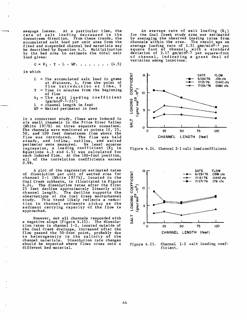
seepage losses. At a particular time, the rate of salt loading decreased in the downstream direction. From these trends, the accumulated salt load per unit area from the fixed and suspended channel bed materials may be described by Equation 4.3. Multiplication by the bed area to estimate the total salt load gives:

C = KI • T • L • WP •••••••• (4.5)

in which

C = The accumulated salt load in grams at distance, L, from the point of flow introduction at time, T Time in minutes from the beginning of flow The salt loading coefficient (gm/mi nO.5-ft2) channel length in feet Wetted perimeter in feet

In a concurrent study, flows were induced in six small channels in the Price River Valley (White 1977b) on three separate occasions. The channels were monitored at points 10, 25, 50, and 100 feet downstream from where the flow was introduced. The flow was held steady, and inflow, outflow, and wetted perimeter were measured. By least sQuares regression, a loading coefficient (KI in Equations 4.3 and 4.5) was calculated for each induced flow. At the 100-foot position, all of the correlation coefficients exceed 0.98.

A plot of the regression estimated rates of dissolution per unit of wetted area for channel 2-1 (White 1977b), located in the Coal Creek subbasin, is illustrated in Figure 4.24. The dissolution rates after the first 25 feet decline approximately linearly with channel length. The decline supports the observations of the Coal Creek macrochanne1 study. This trend likely reflects a reduc­t ion in channel sediments pickup as the sediment carrying capacity of the flow is approached.

However, not all channels responded with a negative slope (Figure 4.25). The dissolu­tion rates in channel 1-2, located outside of the Coal Creek drainage, increased after the flow passed the 50-foot point, probably due to heterogeneity in the salinity of the channel materials. Dissolution rate changes should be expected where flows cross onto a different bed material.

44

An average rate of salt loading (Kl) for the Coal Creek study area was estimated by averaging the observed loading rates from channels within the area. The result was an average loading rate of 2.51 gms/minO•5 per square foot of channel with a standard deviation of 3.17 gm/minO•5 per square-foot of channel, indicating a great deal of variation among locations.

I- 15 DATE FLOW z IJJ -- 5129176 .109 cts U --- 7113176 .0442 cfs Li: u.. --6- 7/29176 .0981 cts L1J 0'" (,) :: 10

I

(.!).q

Z ~e 0 E <l "-0

<I) 5 E ...I 0>

~ • ...... ~ <l en 0

0

Figure 4.24.

I­Z !:Y (,)

tt

15

~ "':: 10 (,) I

(.!)~c Z .-o E <l ';i; 3 ~ I­..J

5

25 50. 75 100

CHANNEL LENGTH (feet)

Channel 2-1 sal t load coefficient.

DATE ___ 6/29176 --6- 7113176 ___ 7/27176

FLOW .0981 cfs .0442 cfs .176 cfs

<l en 0 ~-----...I------~-------~------~---

o

Figure 4.25.

25 50 75 100

CHANNEL LENGTH (feet)

Channel 1-2 salt loading coef­ficient.

Page 57

--.

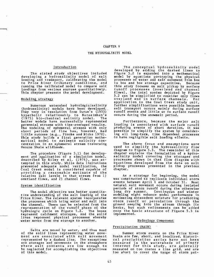
CHAPTER V

THE HYDROSALINITY MODEL

The stated study objectives included developing a hydrosalinity model of salt loading and transport, calibrating the model to Price River tributary conditions, and running the calibrated model to compare salt loadings from various sources quantitatively. This chapter presents the model development.

Modeling strategy

Numerous watershed hydrologic/salinity (hydrosalinity) models have been developed. They vary in resolution from Durum's (1953) hyperbolic relationship to Narasimhan's (1975) bio-chemical salinity model. The better models have successfully represented perennial streams with time-averaged results. The modeling of ephemeral streams with only short periods of flow has, however, had little success (e.g., Pionke and Nicks 1970). This study builds a first generation mathe­matical model to estimate salinity con­centration in an ephemeral stream traversing Mancos Shale wildlands.

The procedure (Figure 5.1) for develop­ment and application of a simulation model, described by Riley et al. (1974), was at­tempted in this study. While data limitations prevented adequate model verification, the Coal Creek model is considered capable of providing a reasonable estimate of the relative salt levels in that stream from 1) overland flows, and 2) channel flows.

The model objective was better quantita­tive understanding of the salt loading of the Price River. The relevant system incorporates the processes. which b~ing water and salt into the channel. These can be selected from the representation of the runoff phase of the hydrologic cycle on Figure 5.2. The boxes represent catchment storages, and the solid lines represent physical processes whereby water moves from one storage to another.

Salts are moved by water, and thus most of the solid lines representing water move­ment are associated with salt movement represented by a dashed line. The exceptions are storages and movements in the atmosphere where salt contents are low enough to be neglected for accomplishing the objectives of this model.

45

The conceptual hydrosalinity model developed by adding the dashed lines to Figure 5.2 is expanded into a mathematical model by equations portraying the physical processes of water and salt movement from box to box and box storage capacities. Because this study focuses on salt pickup by surface runoff processes (overland and channel flows), the total system depicted by Figure 5.2 can be simplified to consider only flows overland and in surface channels. For application to the Coal Creek study unit, further simplifications were possible because salt transport occurs mainly during surface runoff events and little or no surface runoff occurs during the snowmelt period.

Furthermore, because the major salt loading is associated with surface runoff producing events of 'short duration, it was possible to simplify the system by consider­ing all long-term, time dependent processes to have negligible salt loading effects.

The above focus and assumftions were used to simplify the hydrosa inity flow diagram to Figure 5.3. The remainder of this chapter explains the formulation of a hydro­salinity model covering the storages and processes shown in that flow diagram with equations developed from the data on salt pickup processes presented in the previous chapter.

As a strategy for beginning, the model was constructed to replicate individual storm events between April 1 and October 31. Most natural salt movement occurs during isolated periods of storm runoff during the otherwise long dry summer. Continuous and winter modeling might enhance model performance in estimating antecedent moisture for predicting storm runoff or percolat ion through the ground seeping into the stream through its banks, but such refinements can be added once the basic structure of Figure 5.3 is implemented.

Hydrology Component

PreCipitation (RAIN)

Summer storm events on the Price River Basin are few, short, and localized. Histori­cal precipitation series have not been measured in the watersheds of primary interest for this study, are generally measured on too coarse a time grid, and are too short to cover the range of storm pat-

Page 58

--

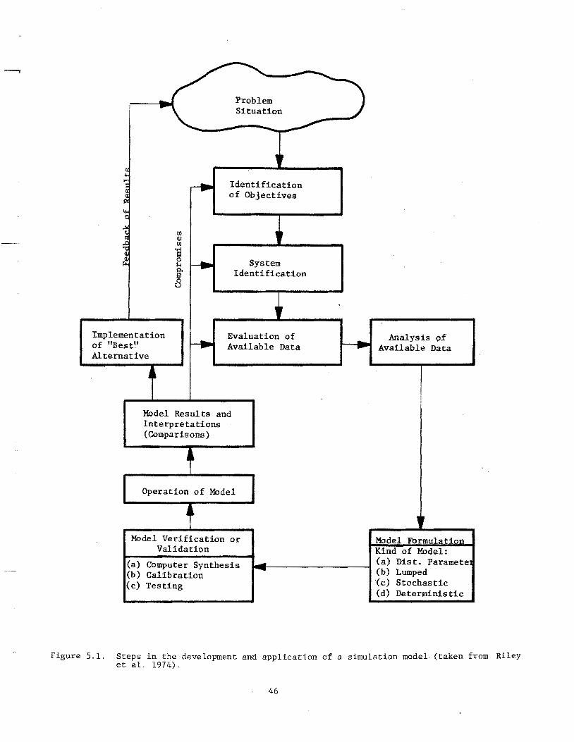
{f) w {f)

SI 0 1-1

-Problem Situation

-I"""'""

,r Identification of Objectives

,r System

~ ~ Identification

0 0

~r

Implementation of "Best~1 Alternative

f---II-Evaluation of Available Data

MOdel Results and Interpretations (Comparisons)

Operation of MOdel

Model Verification or Validation

(a) Computer Synthesis (b) Calibration (c) Testing

---

.. - Analysis of Available Data

" MOdel Formulati~ Kind of Model: (a) Dist. Paramete (b) Lumped (c) Stochastic (d) Deterministic

Figure 5.1. Steps in the development and application of a simulation model (taken from Riley et al. 1974).

46

Page 59

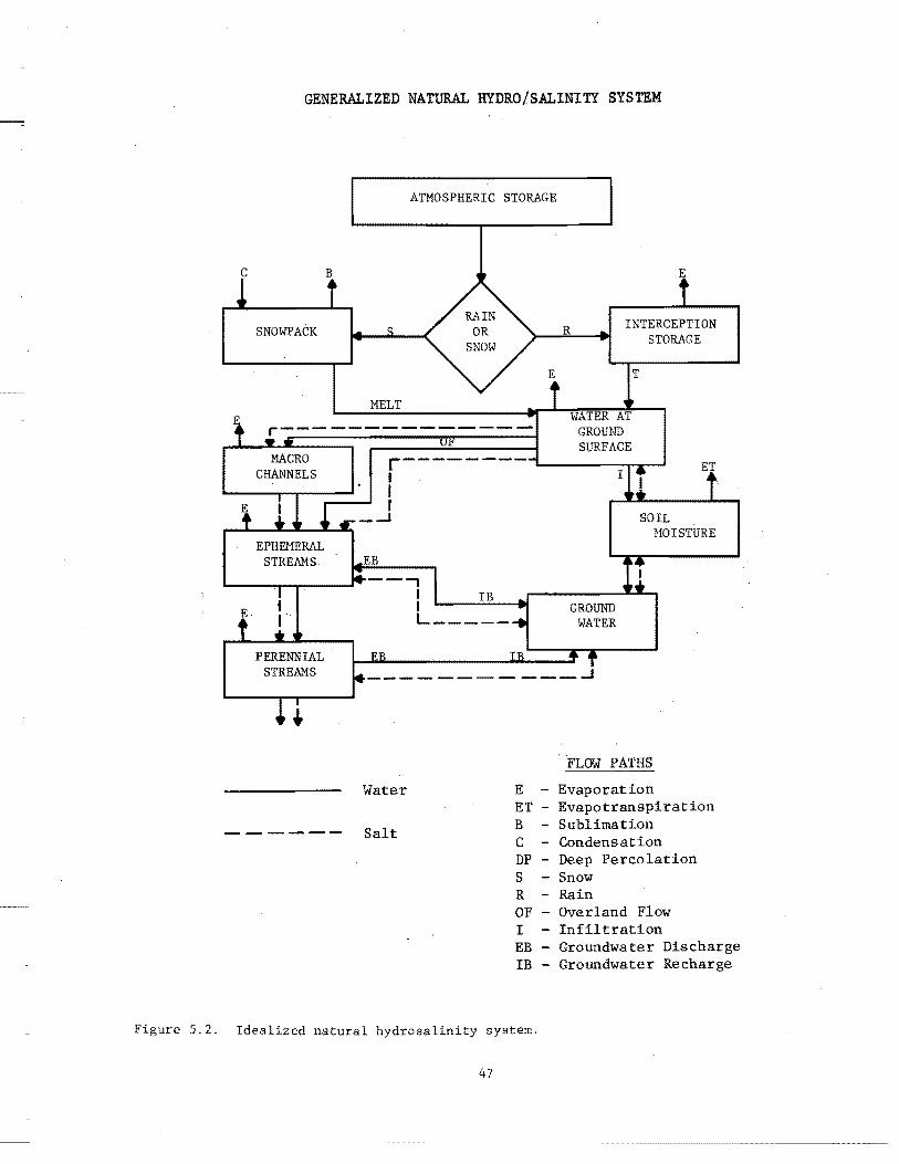
GENERALIZED NATURAL HYDRO/SALINITY SYSTEM

ATMOSPHERIC STORAGE

C B E

E

SNOWP ACK >-~R~---ill'l INTERCEPTION

STORAGE

E T

MELT

r-------------- GROUND SURFACE

MACRO CHANNELS

r - - - - - --- L..-....----r""lr---o-i I . I

I r

_..J

Water

IB GROUND

WATER

SOIL HOISTURE

FLOW PATHS

E - Evaporation

------ Salt

ET - Evapotranspiration B - Sublimation C - Condensation DP - Deep Percolation S - Snow R - Rain OF - Overland Flow I - Infiltration EB - Groundwater Discharge IB - Groundwater Recharge

5.2. Idealized natural hydrosalinity system.

47

----------- -----------_ .................. -

Page 60

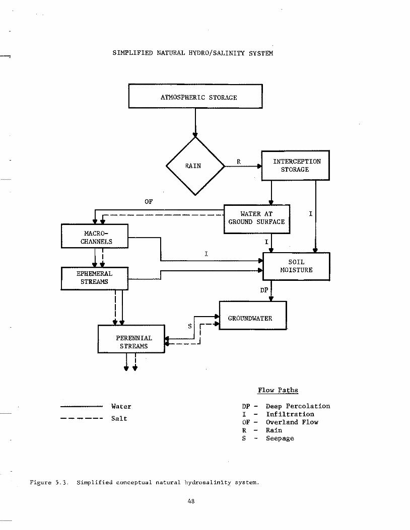
SIMPLIFIED NATURAL HYDRO/SALINITY SYSTEM

ATMOSPHERIC STORAGE

RAIN R

OF

... -

•

INTERCEPTION STORAGE

~.------------- WATER AT GROUND SURFACE

I

MACRO­CHANNELS

EPHEMERAL STREAMS

I I I •• PERENNIAL

STREAMS

Water

------ Salt

I

..

.. I

•

DP •

GROUNDWATER

SOIL HOISTURE

"

S r-~ __________ __ !.II I ~ ___ J

DP -I -OF -

Flow Paths

Deep Percolation Infiltration Overland Flow

R - Rain S Seepage

Figure 5.3. Simplified conceptual natural hydrosalinity system.

48

Page 61

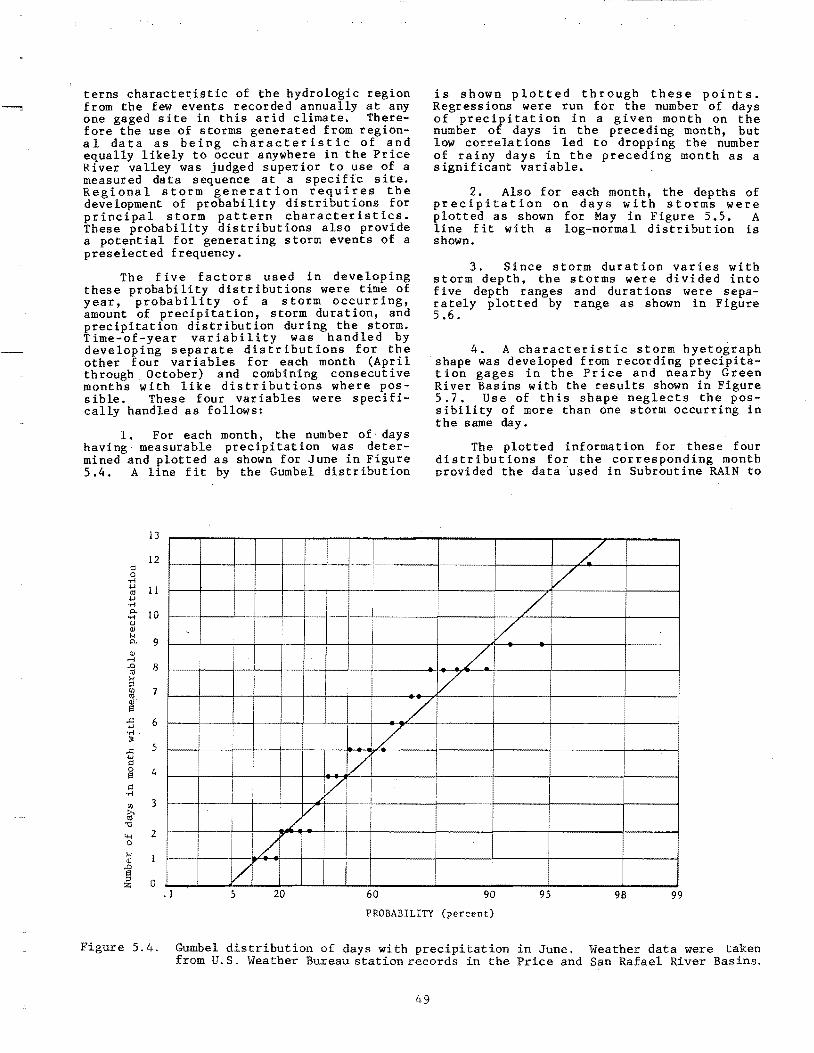
terns characte~istic of the hydrologic region from the few events recorded annually at any one gaged site in this arid climate. There­fore the use of storms generated from region­al data as being characteristic of and equally likely to occur anywhere in the Price River valley was judged superior to use of a measured data sequence at a specific site. Regional storm generation requires the development of probability distributions for principal storm pattern characteristics. These probability distributions also provide a potential for generating storm events of a preselected frequency.

The five factors used in developing these probability distributions were time of year, probability of a storm occurring, amount of precipitation, storm duration, and precipitation distribution during the storm. Time-of-year variability was handled by developing separate distributions for the other four variables for each month (April through October) and combining consecutive months with like distributions where pos­sible. These four variables were specifi­cally handled as follows:

1. For each month, the number of days having measurable precipitation was deter­mined and plotted as shown for June in Figure 5.4. A line fit by the Gumbel distribution

13

12

" 0 -

I -M .... 11 '" .... ..... i 0- 10 ..... oJ (l) k 0- 9

I !

I -(l)

,...;

~ 8 k ::l

"' 7 01 <If a .c 6 .... ..... :J: .c 5 .... " 0 {, s

" -M

"' 3 ~

"d

4-1 2 0

k (l)

11 ::l 0 Z

! / I / i

I VI I VI !

/ i iL iL

j VI • 1 5 20 60

is shown plotted through these points. Regressions were run for the number of days of precipitation in a given month on the number of days in the preceding month, but low correlations led to dropping the number of rainy days in the preceding month as a significant variable.

2. Also for each month, the depths of precipitation on days with storms were plotted as shown for May in Figure 5.5. A line fit with a log-normal distribution is shown.

3. Since storm duration varies with storm depth, the storms were divided into five depth ranges and durations were sepa­rately plotted by range as shown in Figure 5.6.

4. A characteristic storm hyetograph shape was developed from recording precipita­tion gages in the Price and nearby Green River Basins with the results shown in Figure 5.7. Use of this shape neglects the pos­sibility of more than one storm occurring in the same day.

The plotted information for these four distributions for the corresponding month provided the data used in Subroutine RAIN to

/ /

/ /

/. y

!

i

I I 90 95 98 99

PROBABILITY (percent)

Figure 5.4. Gumbel distribution of days with precipitation in June. Weather data were taken from U. S. Weather Bureau station records in the Price and San Rafael River Basins.

49

Page 62

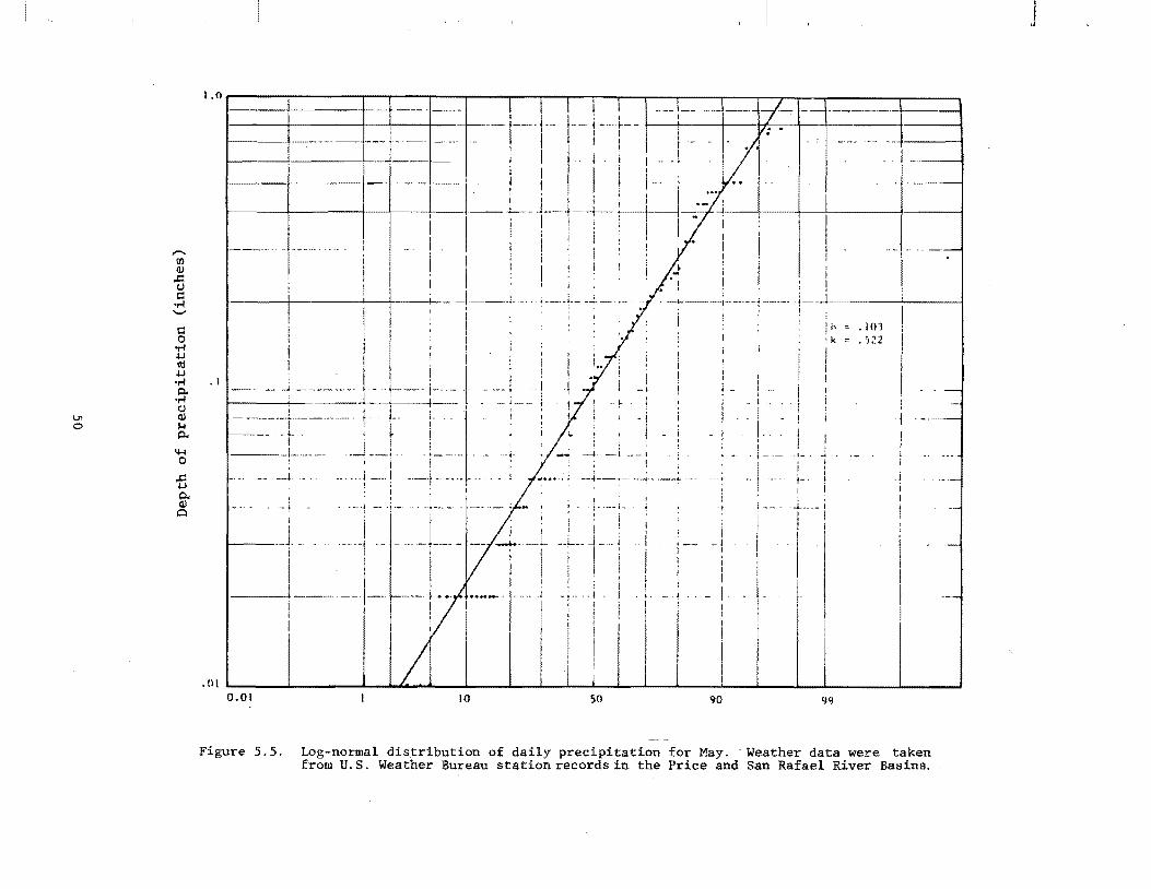
..." o

,....,. (/)

<!l ..t:: () (::

..-! '-'

(:: 0

..-! +J ClI +J ..-! ~

..-! () <!l I-i ~

4-l 0

..t:: +J ~ <!l t:l

1.0ri----~--------r--r--~--~----r-~--~~--r__r--r_--_r--_r~'l:_1I----:_=c====:J ---f-----t--+! --"---

.1

-I.

-- i

! I

I------J

. () I I t.

0.01

.. ,-.. _-

I I -.1 I

.- .-!.

- !

!

I i .... 1

10

! l-

- i !

--1 _i

-- .. --..... -- -4- , __ ... -- __ . .4

,. -__ I_ I

-. ! I

I

;0

! I

I I I ,

90

! -_. I i

I I I. I

I I i I

i : -t---" !

I I i !

i-

I I

" = .101 k . ',22

99

I

,j i I

Figure 5.5. Log-normal distribution of daily precipitation for May .. Weather data were taken from U. S. Weather Bureau station records in the Price and San Rafael River Basins.

J

Page 63

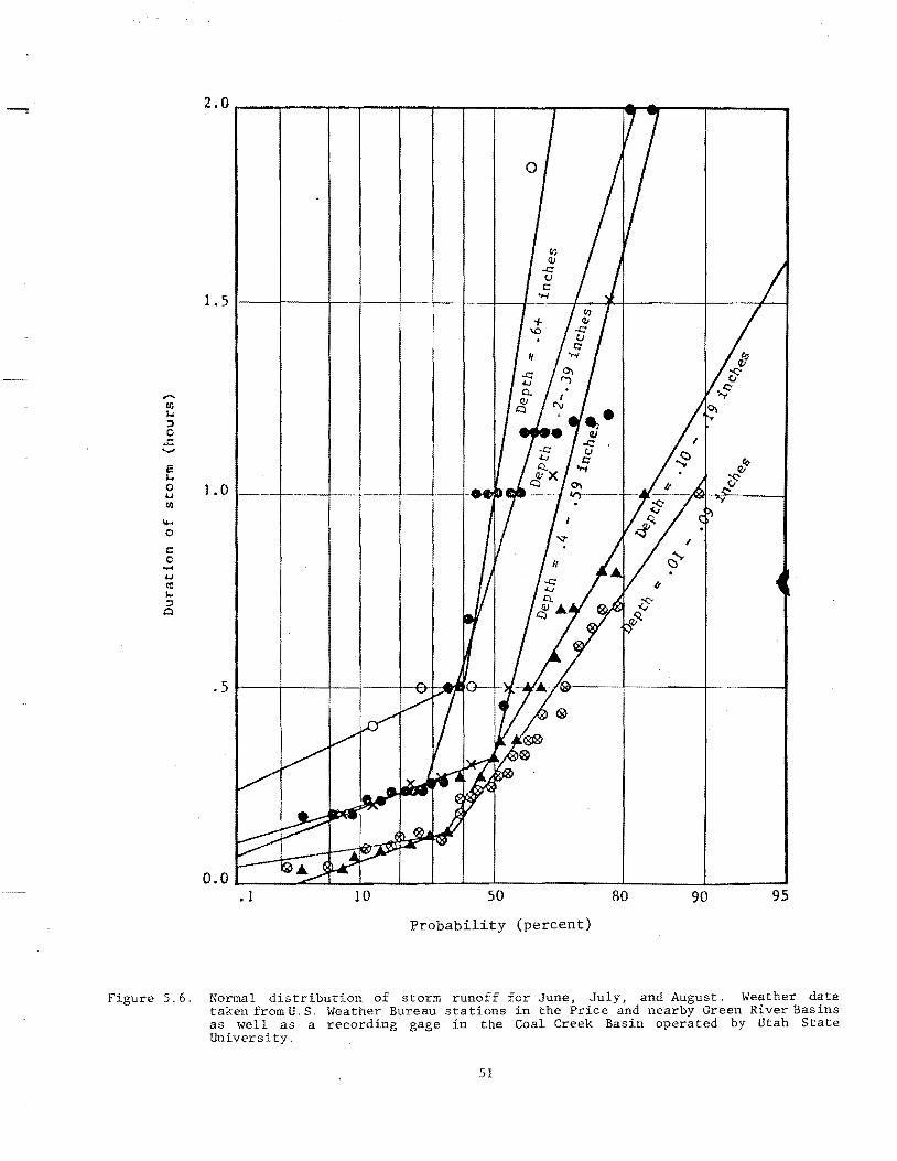
2.0r--,----r_~--r_1I_.--r_--_r----_.~r_--r_--~_

1. 5 ~-+----!---l

E E 1. 0 --.-1-__ .... til

~

o c: o ...

Io.J

lC I.. :::l

Cl

O.O~ __ ~~~~ __ ~~ __ ~~ __________ L-____ -L ____ ~

. 1 10 50 80 90 95

Probability (percent)

Figure 5.6. Normal distribution of storm runoff for June, July, and August. Weather data takenfromU.S. Weather Bureau stations in the Price and nearby Green River Basins as well as a recording gage in the Coal Creek Basin operated by Utah State University.

51

Page 64

generate storm hydrographs in the following procedure:

1. Select a number of rainy days at random (or as associated with the desired probability) from Figure 5.4.

2. Select the dates of these rainy days at random from the number of dates in that month of the year.

3. For each selected date for a rainy day, select a depth at random from Figure 5.5 and an associated duration from Figure 5.6 .

. 3

.2

.1

4. Divide the storm duration into five equal increments and distribute the depth among those increments to form a hyetograph of the shape of Figure 5.7.

For an overview of how well subroutine RAIN matches actual precipitation patterns, simulated and recorded monthly rainfall averages and standard deviations for a 24-year period are tabulated in Table 5.1. Storm intensity comparisons would be better for assessing how well the model will match runoff peaks and associated sediment and salt loads, but there were no data for

0'L-------4-------~------~--------~----~ 20 40 60 80 100

PERCENTAGE OF STORM LENGTH (%)

Figure 5.7. Characteristic storm hyetograph.

Table 5.1. Comparison of output from subroutine RAIN with monthly recorded rainfalls.

Actual Precipitationa RAIN Results

Month Average Standard Average Standard Precipitation Deviation Precipitation Deviation

(inches) (inches) (inches) (inches)

April 0.59 0.52 0.51 0.44 May 0.72 0.74 0.65 0.79 June 0.94 0.93 1.13 0.96 July 0.98 0.74 1. 21 1.05 August 1.11 0.97 1.06 0.91 September 1.15 1.18 1.30 1.37 October 1.26 1.29 1.55 1.48

aObtained from precipitation gages in the Price River Basin.

52

Page 65

this purpose besides those used to develop the model. As Table 5.1 shows, RAIN produced standard deviations which are very close to actual values and average monthly totals a little but not significantly higher than recorded values. A listing of the model is contained in Appendix E (Table E.2).

Precipitation excess (HYDRGY)

Surface runoff (overland flow) picks up salt and transports it to the channel. The second subroutine was developed to calculate surface runoff from the storm hyetographs produced by RAIN. This subroutine (HYDRGY) was modified from previous work (Riley et al. 1974) to fit the needs of this study.

The subroutine subtracts interception and depression storages from the first part of the rainfall hyetograph. Then infiltration begins. The infiltration rate is assumed to decline exponentially from a field measured maximum rate when the soil is at the wilting point to afield measured minimum rate when the soil is at field capacity. Soil moisture conditions at the beginning of a storm dictate the initial point on the infiltration curve. The precipitation excess is estimated as the volume of the rainfall hyetograph minus interception and depression storage and minus an infiltration volume estimated from the infiltration curve. Negative values are taken to indicate no runoff.

The HYDRGY subroutine is initialized with a beginning soil moisture. HYDRGY deter­mines the soil moisture recharge during storms. A subroutine (CONSUM) employs the Jensen-Haise consumptive use equation (Jensen 1973) to determine soil moisture depletion between storms. These two subroutines there­fore maintain a running estimate of the ante­cedent moisture level for use by HYDRGY in computing the precipitation excess during each storm. A listing of the two subroutines HYDRGY and CONSUM is in Appendix E.

Surface runoff (SRO)

This component of the model routes the precipitation excess generated by HYDRGY through the successive surface runoff stages of. overland flow, microchannel flow, and prImary channel flow. Three flow routing techniques were considered. Two were the Saint-Venant equati,?ns de.scribed by Jeppson (1974) and the kInematIc wave equations described by Henderson (1971). However neither of these techniques was adopted because of extensive data requirements on flow and channel characteristics. The re~ativelysimple Ml!s~inghum routing equation (LInsley and FranZIn1 1972) was considered satisfactory for the small watersheds of this study. Henderson (1971) noted that the Muskinghum technique provides a fair approxi­mation for natural floods in rivers whose slopes exceed 0.002.

53

Given an estimated inflow volume to the study area from upstream, a hydrograph was formed by:

Lt = Ibase + AD • [1 - cos(a·t)]

in which

Channel inflow at time t Base channel inflow

• (5.1)

Lt Ibase= AD = a

One-half hydrograph peak inflow Constant, 2'IT/T

T Tributary basin time to peak

The inflow is then routed down successive storage reaches by the Muskinghum method. Lateral inflow, groundwater inflow, seepage, and diversions are added at the top of a reach.

The Muskinghum coefficients K and X were adjusted to provide the best reproduction of observed hydrographs following a method described in Chow (1964). Once calibrated, the coefficient X was assumed constant and the coefficient K was varied with the floW­rate. Stability of the Muskinghum method is generally insured when:

2 K X < lit < K • • (5.2)

in which

K Time routing constant X Inflow effect routing constant lit The time step

Failure to select a time step for routing that meets these conditions may result in oscillating flow values or other errors (Linsley and Franzini 1972).

. Overland flow and lateral channel storm event flows are routed to the main channel by assuming that the flows can be represented as two linear reservoirs in series (Chow 1964). Storage is assumed to be directly propor­tional to outflow.

• (5.3)

in which

S Storage 6 Outflow K2 Storage coefficient

The first order finite differencing of Equation 5.3 with respect to time followed by algebraic manipulation gives:

6Z = 61 + C (11 - 61) + l/Z C (IZ - II)

(5.4 )

lit C K

Z + 1/2 lit ••••••.•• (5.5)

Page 66

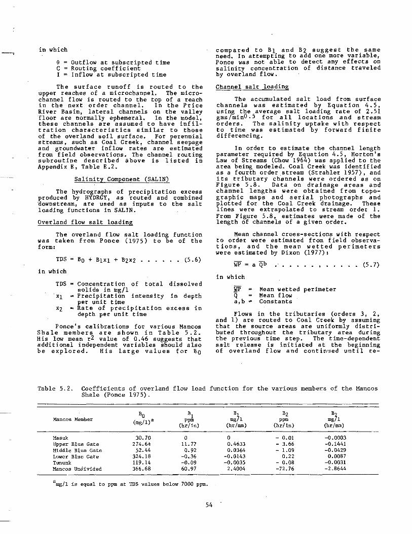
in which

e Outflow at subscripted time C Routing coefficient I Inflow'at subscripted time

The surface runoff is routed to the upper reaches of a microchannel. The micro­channel flow is routed to the top of a reach in the next order channel. In the Price River Basin, lateral channels on the valley floor are normally ephemeral. In the model, these channels are assumed to have infil­tration characteristics similar to those of the overland soil surface. For perennial streams, such as Coal Creek, channel seepage and groundwater inflow rates are estimated from field observations. The channel routing subroutine described above is listed in Appendix E, Table E.2.

Salinity Component (SALIN)

The hydrographs of precipitation excess produced by HYDRGY, as routed and combined 'downstream, are used as inputs to the salt loading functions in SALIN.

Overland flow salt loading

The overland flow salt loading function was taken from Ponce (1975) to be of the form:

TDS BO + Blxl + B2x2 •••••• (5.6)

in which

TDS Concentration of total dissolved solids in mg/l

Xl Precipitation intensity in depth per unit time

x2 = Rate of precipitation excess in depth per unit time

Ponce's calibrations for various Mancos Shale members are shown in Table 5.2. His low mean r2 value of 0.46 suggests that additional independent variables should also be explored. His large values for BO

compared to Bl and B2 suggest the same need. In attempting to add one more variable, Ponce was not able to detect any effects on salinity concentration of distance traveled by overland flow.

Channel salt loading

The accumulated salt load from surface channels was estimated by Equation 4.5, using the average salt loading rate of 2.51 gms/minO• 5 for all locations and stream orders. The salinity uptake with respect to time was estimated by forward finite differencing.

In order to estimate the channel length parameter required by Equation 4.5, Horton's Law of Streams (Chow 1964) was applied to the area being modeled. Coal Creek was identified as a fourth order.stream (Strahler 1957), and its tributary channels were ordered as on Figure 5.8. Data on drainage areas and channel lengths were obtained from topo­graphic maps and aerial photographs and plotted for the Coal Creek drainage. These lines were extrapolated to stream order 1. From Figure 5.8, estimates were made of the length of channels of a given order.

Mean channel cross-sections with respect to order were estimated from field observa­tions, and the mean wetted perimeters were estimated by Dixon (1977):

WP a 'Qb .'. • • • • , • • • • • (5.7)

in which

HP Mean wetted perimeter Q Mean flow a,b Constants

Flows in the tributaries (orders 3, 2, and 1) are routed to Coal Creek by assuming that the source areas are uniformly distri­buted throughout the tributary area during the previous time step. The time-dependent salt release is initiated at the beginning of overland flow and continued until re-

Table 5.2. Coefficients of overland flow load function for the various members of the Mancos Shale (Ponce 1975).

BO Bl B B2 m!h Mancos Member (mg/l)a ppm mgh ppm

(hr/in) (hr/mm) (hr/in) (hr/mm)

Mas uk 30.70 0 0 - 0.01 -0.0003 Upper Blue Gate 274.64 11. 77 0.4633 - 3.66 -0.1441 Middle Blue Gate 52.44 0.92 0.0364 - 1.09 -0.0429 Lower Blue Gate 324.18 -0.36 -0.0143 0.22 0.0087 Tununk 119.14 -0.09 -0.0035 - 0.08 -0.0031 Mancos Undivided 366.68 60.97 2.4004 -72.76 -2.8644

amg/l is equal to ppm at TOS values below 7000 ppm.

54

Page 67

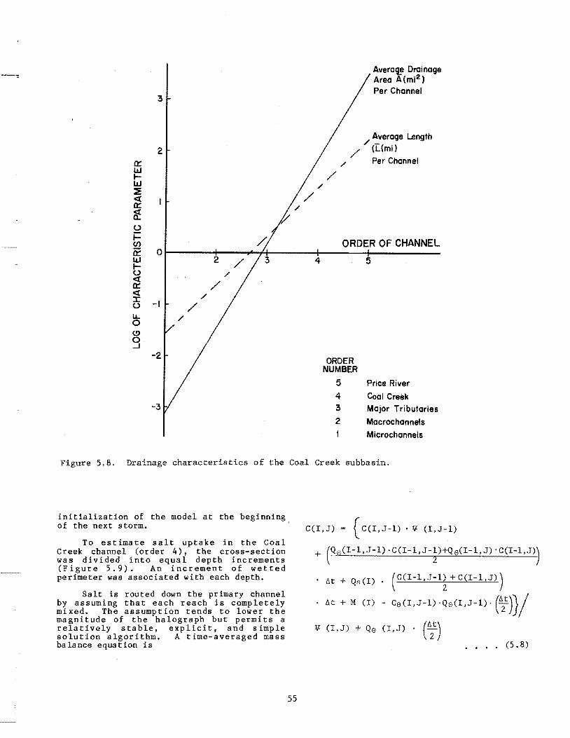
3

2 a::: IJJ I-IJJ ~ « a::: ~ u I-CJ)

a::: 0 IJJ 2 I-U «

/ a::: « / ::J: U -I / u.. / 0 (!) 0 ...J

-2

-3

4

/

Avera~ Drainage Area A(mi2) Per Channel

Average Length /-

/ (L(mi) Per Channel /

/

ORDER OF CHANNEL

ORDER NUMBER

5 4 3

5

Price River

Coal Creek Major Tributaries

2 Macrochannels

Microchannels

Figure 5.8. Drainage characteristics of the Coal Creek subbasin.

initialization of the model at the beginning, of the next storm.

To estimate salt uptake in the Coal Creek channel (order 4), the cross-section was divided into equal depth increments (Figure 5.9). An increment of wetted perimeter was associated with each depth.

Salt is routed down the primary channel by assuming that each reach is completely mixed. The assumption tends to lower the magnitude of the halograph but permits a relatively stable, explicit, and simple solution algorithm. A time-averaged mass ba la nce equa t ion is

55

C(I,J) { C(I,J-l) • ¥ (I,J-l)

+ (Q8(I-l,J-l).C(I-l,J-~)+Qe(I-l,J)'C(I-l,J)j

tlt + Qs(I) (C(I-l,J-l~ +C(I-l,J»)

tlt + M (I) - Ce(I,J-l) ·Qe(I,J-l)· (tl2t)}j ¥ (I,J) + Qe (I,J) . (tl;)

.••• (5.8)

Page 68

in which

C(I,J)

1-1 J-l Qs

Average salinity in reach I at time J

Qe C,

-V-/i.t M

Upstream reach Previous time step Seepage Reach outflow Concentration Storm volume in the reach I

== Time step == Salt mass pickup

The stability of Equation 5.8 requires:

1. Continuity of flow with respect to the primary channel.

(I -1, 2. QsSI) < Qe [(I-I, J) + Qe J-l ]/2

3. /i.t < 2 • -V- [ (I, J -1 ) /Q e (1, J-l)]

A listing of the program is in Appendix E (Table E .2). Also included is a listing and description of the model parameters,

56

input data, and format required by the model. The one-dimensional model simulates storm hydrographs and halographs, assuming the intrinsic salinity sources to be homogeneous and ·uniformly distributed across the water­shed and salinity uptake to be additive and conservative. For modeling areas without irrigated agriculture, groundwater flow was not considered significant and was not included in the model.

Time, T3

T2 lj

Figure 5.9. Primary channel wetted perimeter subdivision.

Page 69

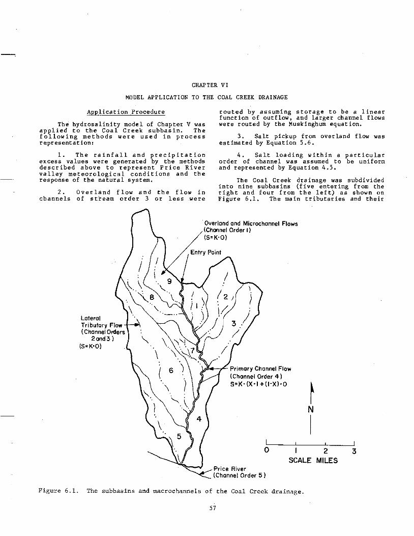
CHAPTER VI

MODEL APPLICATION TO THE COAL CREEK DRAINAGE

Application Procedure

The hydrosalinity model of Chapter V was applied to the Coal Creek subbasin. The following methods were used in process representation:

1. The rainfall and precipitation excess values were generated by the methods described above to represent Price River valley meteorological conditions and the response of the natural system.

2. Overland flow and the flow in channels of stream order 3 or less .were

routed by assuming storage to be a linear function of outflow, and larger channel flows were routed by the Muskinghum equation.

3. Salt pickup from overland flow was estimated by Equation 5.6.

4. Salt loading within a particular order of channel was assumed to be uniform and represented by Equation 4.5.

The Coal Creek drainage was subdivided into nine subbasins (five entering from the right and four from the left) as shown on Figure 6.1. The main tributaries and their

Overland and Microchannel Flows (Channel Order I)

Lateral Tributary Flow (Channel Orders

2and3 ) (S=K'O)

(S=K'O)

\Jj:II''--r- Primary Channel Flow (Channel Order 4) S=K' (X'I +(I-X)'O

o

~ N

I 2

SCALE MILES

Figure 6.1. The subbasins and macrochannels of the Coal Creek drainage.

57

3

Page 70

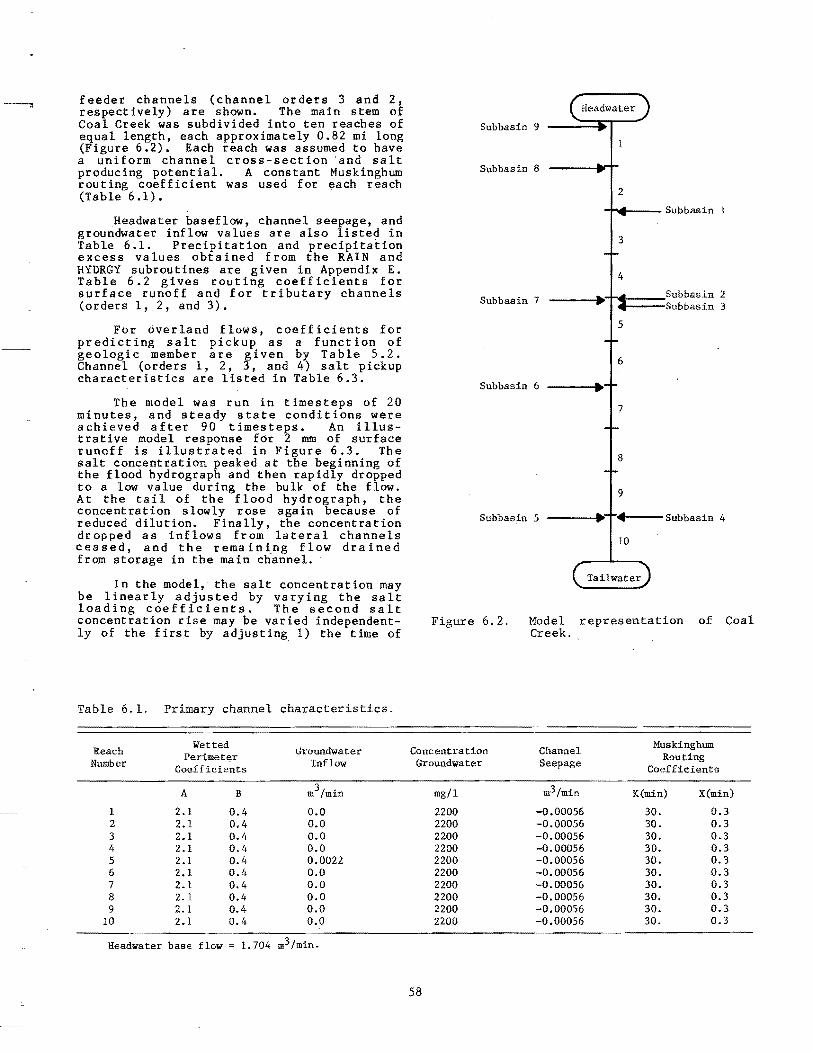
feeder channels (channel orders 3 and 2, respectively) are shown. The main stem of Coal Creek was subdivided into ten reaches of equal length, each approximately 0.82 mi long (Figure 6.2). Each reach was assumed to have a uniform channel cross-section 'and salt producing potential. A constant Muskinghum routing coefficient was used for each reach (Table 6.1).

Headwater baseflow, channel seepage, and groundwater inflow values are also listed in Table 6.1. Precipitation and precipitation excess values obtained from the RAIN and HYDRGY subroutines are given in Appendix E. Table 6.2 gives routing coefficients for surface runoff and for tributary channels (orders 1, 2, and 3).

For overland flows, coefficients for predicting salt pickup as a function of geologic member are given by Table 5.2. Channel (orders 1, 2, 3, and 4) salt pickup characteristics are listed in Table 6.3.

The model was run in timesteps of 20 minutes, and steady state conditions were achieved after 90 timesteps. An illus­trative model response for 2 mm of surface runoff is illustrated in Figure 6.3. The salt concentration peaked at the beginning of the flood hydrograph and then rapidly dropped to a low value during the bulk of the flow. At the tail of the flood hydrograph, the concentration slowly rose again because of reduced dilution. Finally, the concentration dropped as inflows from lateral channels ceased, and the remaini_ng flow drained from storage in the main channel.

In the model, the salt concentration may be linearly adjusted by varying the salt loading coefficients. The second salt concentration rise may be varied independent­ly of the first by adjusting. 1) the time of

Table 6.l. Primary channel characteristics.

Reach Wetted

lil'oundwater Number

Perimeter Inflow Coefficients

A B m3/min

1 2.1 0.4 0.0 2 2.1 0.4 0.0 3 2.1 0.4 0.0 4 2.1 0.4 0.0 5 2.1 0.4 0.0022 6 2.1 0.4 0.0 7 2.1 0.4 0.0 8 2.1 0.4 0.0 9 2.1 0.4 0.0

10 2.1 0.4 0.0

Headwater base flow 1.704 m3/min.

Subbasin 9

Subbasin 8

Subbasin 7

Subbasin 6

Subbasin 5

2

...... .. -- Subbasin 1

3

4 ___ ~"''''1"1===Subbasin 2

Subbasin 3

5

6

• 7

8

9

---~.";-~"f---Subbasin 4

10

Figure 6.2. Model representation of Coal Creek.

Concentration Channel Muskinghum Routing Groundwater Seepage Coefficients

mg/l m3/min K(min) X (min)

2200 -0.00056 30. 0.3 2200 -0.00056 30. 0.3 2200 -0.00056 30. 0.3 2200 -0.00056 30. 0.3 2200 -0.00056 30. 0.3 2200 -0.00056 30. 0.3 2200 -0.00056 30. 0.3 2200 -0.00056 30. 0.3 2200 -0.00056 30. 0.3 2200 -0.00056 30. 0.3

58

Page 71

Table 6.2.

Subbasin Number

1 2 3 4 5 6 7 8 9

Table 6.3.

Stream Order

1 2 3 4

Subbasin characteristics.

Area

(km2)

2.823 6.035 7.122 3.937 4.869

14.711 3.263 8.366 4.455

Overland Flow

Routing Coefficient

(min. )

11. 11. 11. II. 11. 11. 11. 11. 11.

Tributary Flow

Routing Coefficient

(min. )

47. 57. 57. 15. 62. 72. 21. 62. 31.

application of the second salt loading coefficient, and 2) the value of the second coefficient. However, data were not available for model validation.

Simulation Results

Estimated salt output from Coal Creek

The model was run utilizing generated precipitation data for a 3-year period. The simulated annual and average salt loads by source are given in Table 6.4. The average estimated salt load from the natural channels and overland flow is 121 x 107 gms p~r year.

Channel and salt loading characteristics.

Mean Mean Wetted Perimeter Density Coefficients km/km2

45. 57.10 2.33 0.245 0.233 404. 12.80 2.24 0.29 0.233

3211. 2.86 2.14 0.34 0.233 32110. 0.57 2.10 0.40 0.233

400

/-'\ ___ FLOW I \.........-I \ I \

300 I \ I \ I I I \ I \ I \

f \ , , ., I \ I 1/ \

I CONCENTRATION 200

100

I \I \ I \ I \ r \ I \

\ \ , \

J \ \-__ .J I

I I

o o 5 10 15

TIM E (hours)

20 25

2500

2000

1500

1000

500 30

0.120 0.120 0.120 0.120

z o ..... « a::: ..... z w (.) z o (.)

Figure 6.3. Model response to 0.2 rum of surface runoff (lower Coal Creek site).

59

Page 72

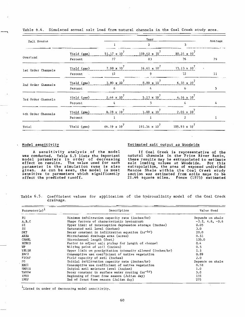
Table 6.4. Simulated annual salt load from natural channels in the Coal Creek study area.

Salt Source Year Average 2 3

Overland 79

1st Order Channels Percent 12 9 12 11

2nd Order Channels !!~!~_i~L ________ 2.:.!?2_~U2~ __________ ~.:.2Q_~_l2~ _________ ~.:..~~_~_!2~ Percent 6 4 6 5

3rd Order Channels !!~!~_.~~~2 ________ ~.:.~~_~_!Q~ __________ ~.:.~2_~_!Q~ ______ .. __ ~.:.!L~_!Q~ Percent 4 3 4 4

4th Order Channels 777

!!~!~_i~~2 _________ Q.:.Z~_~_!Q ___________ !.:.~~_~_!Q __________ ~.:.Q~_~_!Q_ Percent 1 2

Total Yield (gms) 66.19 x 10 7 191. 34 x 107 105.93 x 10 7

Model sensitivity Estimated salt output as Woodside

A sensitivi ty analysis. of the model was conducted. Table 6.5 lists the important model parameters in order of decreasing effect on results. The value used for each parameter in the simulation runs is also given. As can be seen, the model is most sensitive to parameters which significantly affect the predicted runoff.

If Coal Creek is representative of the natural channels in the' Price River Basin, these results may be extrapolated to estimate salt loading values at Woodside. For this extrapolation, the area of exposed undivided Mancos Shale within the Coal Creek study sect ion was estimated from solIs maps to be 21.46 square miles. Ponce (1975) estimated

Table 6.5. Coefficient values for application of the hydrosalinity model of the Coal Creek drainage.

Parameter (s) 1 Description Value Used

FC A,B,C SI SS DKT AREA CHANL XCRCO WP TELIM XKC2 FICAP FO XKC1 SMOIS TAVSW IFRS IFRF

Minimum infiltration capacity rate (inches!hr) Shape factors of characteristic hyetograph Upper limit of interception depression storage (inches) Saturated soil level (inches) Decay constant in infiltration equation (hr-hr) Microchannel drainage area (acres) Microchannel length (feet) Factor to adjust salt pickup for length of channel Wilting point of soil (inches) Upper limit on precipitation intensity allowed (inches/hr) Consumptive use coefficient of native vegetation Field capacity of soil (inches) Initial infiltration capacity rate (inches/hr) Consumptive use coefficient of native vegetation Initial soil moisture level (inches) Decay constant in surface water routing (hr-hr) Beginning of frost free season (Julian day) End of frost free season (Julian day)

1Listed in order of decreasing model sensitivity.

60

Depends on shale -3.2, 4.8, -0.6 0.05 3.0 20.0 0.51 120.0 0.4 0.5 1.5 0.89 2.0

Depends on shale 0.58 1.0 5.0 135 275

Page 73

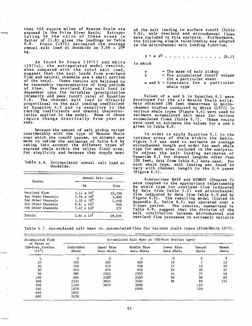
that 468 square miles of Mancos Shale are exposed in the Price River Basin. Extrapo­lating by the ratio of these areas (a factor of 21.8) gives the loadings on Table 6.6. Ponce (1975.) estimated the average annual salt load at Woodside as 3.68 x 108 kg.

As found by Ponce (1975) and White (1977a), the extrapolated model results, when compared with the total salt load, suggest that the salt loads from overland flow and natural channels are a small portion of the total. These results are believed to be reasonably representative of long periods of time. The overland flow salt load is dependent upon the variables (precipitation intensity and peak runoff rate) of Equation 5.6. The channel salt load is directly proportional to the salt loading coefficient of Equation 4.5 and is sensitive to the routing coefficients and channel character­istics applied in the model. None of these inputs change drastically from year to year.

Because the amount of salt pickup varies cons iderably with the type of Mancos Shale over which the runoff passes., an attempt was made to refine the estimates of Table 6.6 by taking into account the different types of exposed shale within the valley floor area. For simplicity and because they supply most

Table 6.6. Extrapolated annual salt load at Woodside.

Source

Overland Flow 1st Order Channels 2nd Order Channels 3rd Order Channels 4th Order'Channels

Annual Salt Load,

kg

2.11 x 107 2.74 x 106 1.32 x 106 8.61 x 105 3.42 x 105

Tons

23.250 3,000 1,450

950 375

-----------------------------------------------------Totals 29.025

of the salt loading to surface runoff (Table 6.6), only overland and microchannel flows were included in this analysis. Furthermore, the following simple relationship was adopted as the microchannel salt loading function.

y - a xb •• '" ••••••••• (6.1)

in which

y x

a and b

The mass of salt pickup The accumulated runoff volume for a particular event COnstants for a particular shale type

Values of a and b in Equation 6.1 were developed for the six Mancos Shale soils. Data obtained 100 feet downstream in micro­channel studies conducted by'White (1977) in various shale types (Figure 6.4) were used to estimate accumulated salt mass for various accumulated flows (Table 6.7). These reults were used to estimate the values for a and b given in Table 6.8.

In order to apply Equation 6.1 to the various areas of shale within the basin, Figure 5.8 was used to estimate an average microchannel length and order for each shale type for each area included in the analysis. To adjust the salt loading estimates of Equation 6.1 for channel lengths other than 100 feet, data from Table 6.7 were used. For each shale type, salt loading was found to vary with channel length to the 0.4 power (Figure 6.5).

Subroutines RAIN and HYDRGY (Chapter V) were coupled to the appropriate relationship by shale type for overland flow (adjusted by data from Table 5.2) and microchannel flow (adjusted by data from Table 6.9 and by Figure 6.5). The resulting model (listed in Appendix E, Table E.3) was operated over a 3-year period. The results, summarized by Table 6.9, suggest that the division of the salt contribution between microchannel and overland flow processes is extremely variable

Table 6.7. Accumulated salt mass vs. accumulated flow for various shale types (from White 1977).

Accumulated Flow Accumulated Salt Mass at 10o-Foot Station (gms) of Water at

100-Foot Station Undivided Upper Blue Middle Blue Lower Blue Tununk Masuk (ft3) Shale Gate Shale Gate Shale Gate Shale Shale Shale

0 0 0 0 0 0 0 10 105 320 400 10 7 12 20 195 575 700 17 12 20 30 265 870 950 32 20 27 50 385 1355 1350 44 27 40

100 685 2200 2400 58 50 80 200 1335 3045 3500 96 88 132 300 1540 3950 3900 110 400 1670 4900 120 600 1955 800 2120

Page 74

~

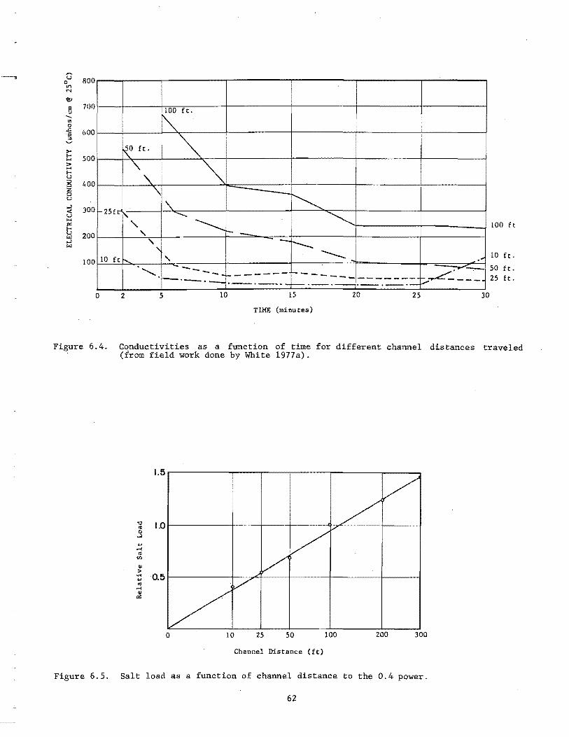
u 800 0 11"1 N

'!!I

B 700 ""-

'" 0 .c 600 Ii

:::I.

>-.... 500 ..... > ..... .... u ::;, 400 <=l Z 0 U

,..l 300 « u i- 25 f t" .... "" .... u 200 1&.1 ...l 1&.1

100 10 ft

o

~ ft.

KO ft. ~ " ~ " '\ - -~ "-

!\. ........ ~ ~ "'- , 1-_ , i -I--,I

----r-.. , . "" . ........... -- . -;0>_ --. 1------- ...._----- ------- ~.,....c:----'-'- '-'---c---._-.- ._-. __ .-

2 5 10 15 20 25 30

TIME (minutes)

100 ft

10 ft .

50 ft . 25 ft.

Figure 6.4. Conductivities as a function of time for different channel distances traveled (trom field work done by White 1977a).

1.5 I

/ _/

----4

V /'

V

1/ V

"IJ 1.0 r; 0

...l

... .... '" <Il

OJ ;.. .... 0.5 ... '" .... OJ

""

o 10 25 50 100 200 300

Channel Distance (ft)

Figure 6.5. Salt load as a function of channel distance to the 0.4 power.

62

Page 75

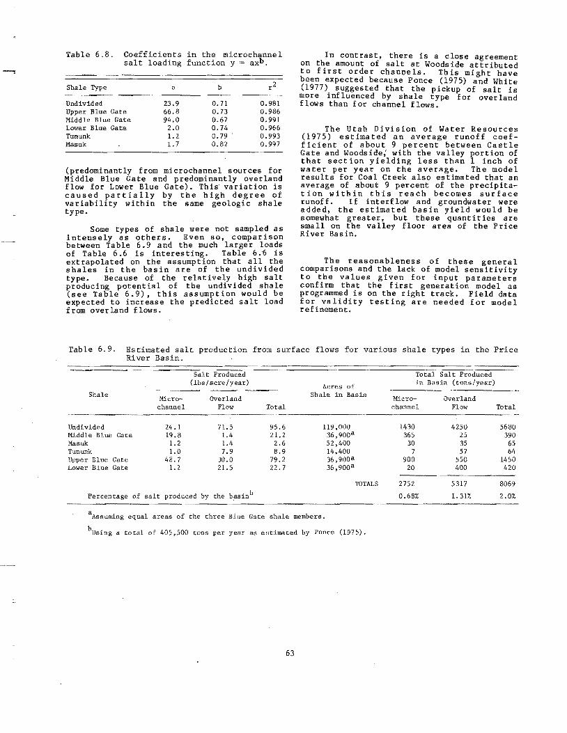
Table 6.8. Coefficients in the microchanne 1 salt loading function y = axb .

Shale Type a b r2

Undivided 23.9 0.71 0.981 Upper j3lue Gate 66.8 0.73 0.986 Middle Blue Gate 94.0 0.67 0.991 Lower Blue Gate 2.0 0.74 0.966 Tununk 1.2 0.79 0.993 Mas uk 1.7 0.82 0.997

(predominantly from microchannel sources for Middle Blue Gate and predominantly overland flow for Lower Blue Gate). This variation is caused partially by the high degree of variability within the same geologic shale type.

Some types of shale were not sampled as intensely as others. Even so, comparison between Table 6.9 and the much larger loads of Table 6.6 is interesting. Table 6.·6 is extrapolated on the assumption that all the shales in the basin are of the undivided type. Because of the relatively high salt producing potential of the undivided shale (see Table 6.9), this assumption would be expected to increase the predicted salt load from overland flows.

In contrast, there is a close agreement on the amount of salt at Woodside attributed to first order channels. This might have been expected because Ponce (1975) and White (1977) suggested that the pickup of salt is mOre influenced by shale type for overland flows than for channel flows.

The Utah Division of Water Resources (1975) estimated an average runoff coef­ficient of about 9 percent between Castle Gate and Woodside; with the valley portion of that section yielding less than 1 inch of water per year on the average. The model results for Coal Creek also estimated that an average of about 9 percent of the precipita­tion within this reach becomes surface runoff. If interflow and groundwater were added, the estimated basin yield would be somewhat greater, but these quantities are small on the valley floor area of the Price Ri ver Bas in.

The reasonableness of these general comparisons and the lack of model sensitivity to the values given for input parameters confirm that the first generation model as programmed is on the right track. Field data for validity testing are needed for model refinement.

Table 6.9. Estimated salt production from surface flows for various shale types in the Price River Basin.

(lbs/ acre/year) Acres of in Basin (tons/year)

Shale lncro- Overland

Shale in Basin Micro- Overland channel Flow Total channel Flow Total

Undivided 24.1 71.5 95.6 119,000 1430 4250 5680 Middle Blue Gate 19.8 1.4 21.2 36,900a 365 25 390 }!asuk 1.2 1.4 2.6 52,400 30 35 65 Tununk 1.0 7.9 8.9 14,400 7 57 64 Upper Blue Gate 48.7 30.0 79.2 36,900a 900 550 1450 Lower Blue Gate 1.2 21.5 22.7 36,900a 20 400 420

TOTALS 2752 5317 8069

Percentage of salt produced by the basinb 0.68% 1. 31% 2.0% ---------_ .. _--_ .. _------------------

aAssuming equal areas of the three Blue Gate shale members.

bUSing a total of 405,500 tons per year as estimated by Ponce (1975).

63

Page 76

CHAPTER VII

BASIN-WIDE HYDROSALINITY STUDY

Introduction

Narasimhan et a1. (1980) compared a number of hydrosalinity models and concluded that the models generally suffer the weak­nesses of oversimplifications of 1) chemical processes, 2) surface-soil-groundwater interactions, and 3) salt pickup phenomena. N everthel,ess, us ing one of the best of the available models, additional insight into water and salt flows within the Price River Basin was sought by applying BSAMl, developed by Huber et a1. (1976). The model employs water and salt mass balance accounting on a monthly time interval through the representa­tion of the hydrologic system shown in Figure 7. L In the application, only the runoff and salt fluxes from the valley bottom lands were considered.

·Data

The BSAM modeling was based on the USGS gaging station near Heiner, where Price River emerges from the mountains onto the valley floor for water years 1973 through 1975.· Since that station was discontinued in 1969, regression analyses were performed correlating flows.for each month of the year at Heiner during the 1960s with recorded flows at USGS gages at Willow Creek, Beaver Creek, White River, and Scofield Reservoir (all of which are upstream of Heiner--see Figure 1.1). During the winter months, only flows at Willow Creek and Scofield Reservoir were used because of inaccurate or incom­plete records at the other two stations. Many combinations of recorded flow records were examined. The highest correlations are tabulated in Table 7.1.

Precipitation and temperature data from the weather stations at Hiawatha, Sunnyside, and Price Warehouse were also used as input data for BSAM. These stations are scattered within the basin and provide fairly repre­sentative temperature data. More precipita­t ion gages would have been helpful. I t is apparent from an examination of precipita­t ion and streamflow records that localized thunderstorms causing significant runoff may miss all three precipitation gages. This causes error in the calibration of the model.

Gordon Creek and Desert Seep Wash, two major tributaries of the Price River, were modeled to estimate ungaged surface inflows of water and salt. These runs proved un-

. satisfactory in that there was more salt

65

inflow than salt ou<t:flow, implying a net deposit of salt in the valley. Desert Seep Wash drains agricultural lands and, at the gaging station, is more indicative of agricultural loading than of natural inflows. Hence, Desert Seep Wash was not modeled further.

Records in the State Engineer's office were examined for canal diversion data. Canal water imported from the San Rafael Basin is not measured, and this quantity, therefore, was estimated from the irrigated acreage served. . Estimates of groundwater inflow were taken from Cordova (1964).

Results

The match with recorded data achieved in calibrating BSAMI to Price River flows at Woodside is portrayed.for water flow (Figure 7.2), total salt flow (Figure 7.3), and salt concentration (Figure 7.4). BSAMI models total salt outflow from the basin by summing loadings from various sources. The amount of salt loading indicated by the model as coming from agricultural lands suggest them to be a major salt source in the Price River Basin. Of the approximately 190,000 tons of salt leaving the basin at woodside annually during the calibration period, about 76,000 tons or 40 percent originated within the central basin. Model results also indicate that about 3,500 tons originated with ungaged overland flow and pickup by channel process­es. These figures agree closely with the estimates given in Chapter VI.

The remaining 72,500 tons of salt originating annually within the central basin are from surface agricultural return flows and groundwater inflows to the Price River. Agriculture is thus an important salt source.

Approximately 114,000 tons of salt were modeled during 1973-1975 as entering the central portion of the basin in approximately 120,000 acre-feet of water (average TDS approximately 700 mg/l). but only about 75,000 acre-feet of water were modeled leaving the basin. Even without any salt pickup in the baSin, the outgoing TDS would be about 1100 mg/l--a significant increase from the 700 mg/l--just from concen­tration effects caused by evapotranspiration. A large portion of this loss is from agri­cultural crops.

Model results indicate that irrigation efficiencies in the valley are fairly high--

Page 77

£

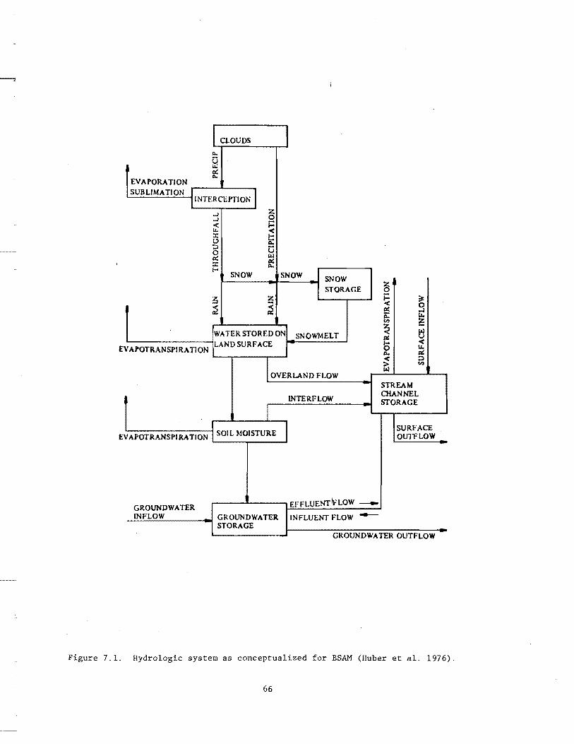
E

CLOUDS

EVAPORATION SUB LIMA TI ON 1.-----1...---,1

I INTERCEPTION

...l

...l

i;'; :r: t.:> ::> o c:x:: :r: f-<

SNOW SNOW SNOW

STORAGE

WA TER STORED ON SNOWMELT

VAPOTRANSPI RA TI ON LAND SURFACE

l OVERLAND FLOW

lNTERFLOW

I V APOTRANSPI RA TJON SOIL MOISTURE

GROUNDWATER ....-__ ..L-__ --. EFFLUENT iF LOW ---

---:;:IN.;.:;F...;;L:..;;O'-'W-'--__ --111001 GROUNDWATER INFLUENT FLOW --STORAGE

STREAM CHANNEL STORAGE

SURFACE OUTFLOW

GROUNDWATER OUTFLOW

Figure 7.1. Hydrologic system as conceptualized for BSAM (Huber et a1. 1976).

66

Page 78

-Table 7.1. Correlations used to estimate 1973-1975 flows at Heiner.

Month Equation

Jan. H ~ 543 + 0.19 (SR) + 3.83 (we)

Feb. H ; 421 + 0.67 (SR) + 3.1 (We)

Mar. H ; 907 + 1.06 (SR) + 2.3 (we)

Apr. H 1749 + 1.05 (SR) + 3.2 (WC)

May H 137 + 3.95 (Be) + 1.84 (we) + 0.62 (WR) + 0.98 (SR)

Jun. H ; 137 + 3.95 (Be) + 1. 84 (we) + 0.62 (WR) + 0.98 (SR)

Jul. H ; -1309 - 10.0 (Be) + 7.57 (we) + 2.16 (WR) + 1.03 (SR)

Aug. H 1309 - 10.0 (Be) + 7.57 (we) + 2.16 (WR) + 1. 03 (SR)

Sep. H ; -1309 - 10.0 (Be) + 7.57 (we) + 2.16 (WR) + 1. 03 (SR)

Oct. H ; -166 + 0.96 (SR) + 5.76 (we)

Nov. H ; 155 + 1.0 (SR) + 4.1 (we)

Dec. H 866 + 0.08 (SR) + 7.4 (WC)

H Flow at Heiner (AF/mo)

SR ; Flow at Scofield Reservoir (AF/mo)

WC ; Flow at Willow Creek (AF/mo)

WR ; Flow at White River (AF/mo)

Be Flow at Beaver Creek (AF!mo)

79 percent for conveyance efficiency and 85 percent for application efficiency. The application efficiency seems high, but model calibration was sensitive to this parameter and 85 gave the best match.

The model calibration indicated a lag of about 7 months in deep percolation flows. Agricultural return flows were esti­mated to have a dissolved solids concentra­tion of about 5350 mg/l. These concentrations appear reasonable in that Desert Seep Wash drains a major portion of the agricultural lands of the basin and typically has dis­solved solids concentrations from 2500 to 4000 mgtl. Reduced dilution may account for the difference between Desert Seep Wash concentrations and the 5350 mgtl predicted, for agricultural return flows by BSAMl. Another possibility would be that the cali­brated 85 percent application efficiency is too high.

Simulation runs were also made to project the effects on flows at Woodside of different management alternatives. The

67

Degrees of Freedom

5 0.59

5 0.67

5 0.993

5 0.997

15 0.98

15 0.98

15 0.95

15 0.95

15 0.95

5 0.95

5 0.96

5 0.85

results are summarized in Table 7.2 and highlighted as follows:

1. Ungaged inflow was reduced by 20 percent to determine the effect of upstream detention. The results showed an increase in basin outflow dissolved solids concentrations of about 1.6 percent but a decrease in total salt outflow of about 2.3 percent (Figures 7.5 and 7.6).

2. I rrigation efficiencies were raised by 10 percent to determine the effect of improved i rrigat ion techniques. Results showed an increase in the dissolved solids concentration (TDS) of the basin outflow of 7.1 percent, but a decrease in total salt output of about 7.3 percent (Figures 7.7 and

, 7.8) •

3. Alfalfa (a high water user) on 9200 acres was changed to corn (a low water user), and 1000 acres of phreatophytes were elimi­nated. Dissolved solids concentrations stayed constant while total salt output rose 5.5 percent (Figures 7.9 and 7.10).

Page 79

".....

OJ

" QI I.>. I QI .. 0:. < ... 0

III .,., c: It III ;:I

] t: II:

~ :.... .. ~ OJ

to: :. >.

.:::: ... c:: e :I:

45

40

35

30

25

20

15

]0

5 ., I

I I

I I i

n • J I

I, I ~

-' :

I

L., I L.

Observed Computed

... .., I I I I I I

: I I I I

o~ __________________ _ ONDJFMAMJJASONDJFMAMJJASONDJFMAMJJAS

1973 1974 1975

Water Year

Figure 7.2. Price River BSAM1 simulated water flows at Woodside (1973-1975).

68

Page 80

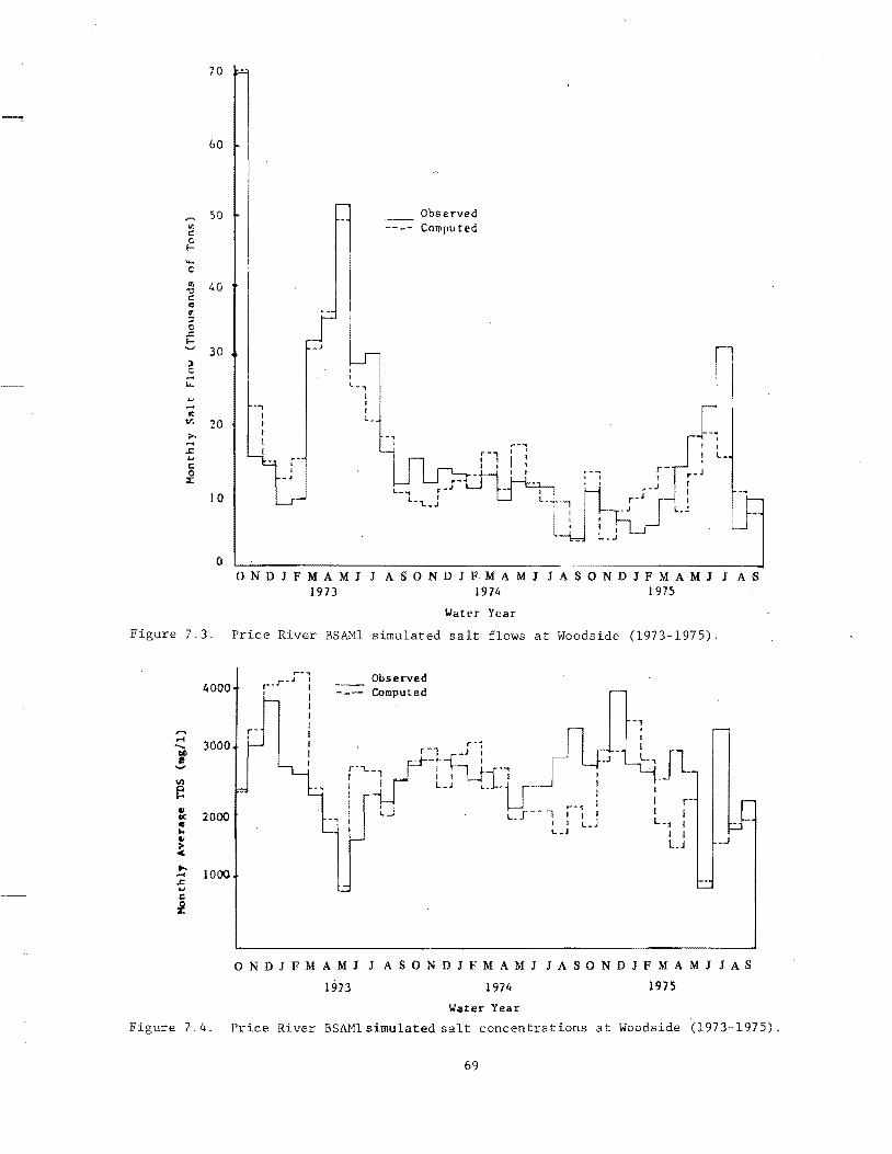
V­c: C

!:-

) c -L.o.

It II:

>, .... .r:: .... c 0

!I:

70

60

50

20

10

o

Observed ---- Computed

I

_J h n I , . I l_, I

--, I I

I l_ I ,

", I , I

o N D J F M A M J J A SON D J F. M A M J J A SON D J F M A M J J AS 1973 1974 1975

Water Year

Figure 7.3, Price River BSAMl simulated salt flows at Woodside (1973-1975).

4000

,.... ~ 3000 f .....

e ~ 2000 • l-e,

~

!:: 1000 .J:; ... ~

~

~-,

r .. r-.J : , I ,

I I r- I I I I

Observed Computed

I I r-I I L., I

I I L.J .J

ONDJFMAMJ J ASONDJFMAMJ JASONDJFMAMJJAS

1973 1974 1975

Water Year

Figure 7.4, Price River BSAMlsimulated salt concentrations at Woodside (1973-1975).

69

Page 81

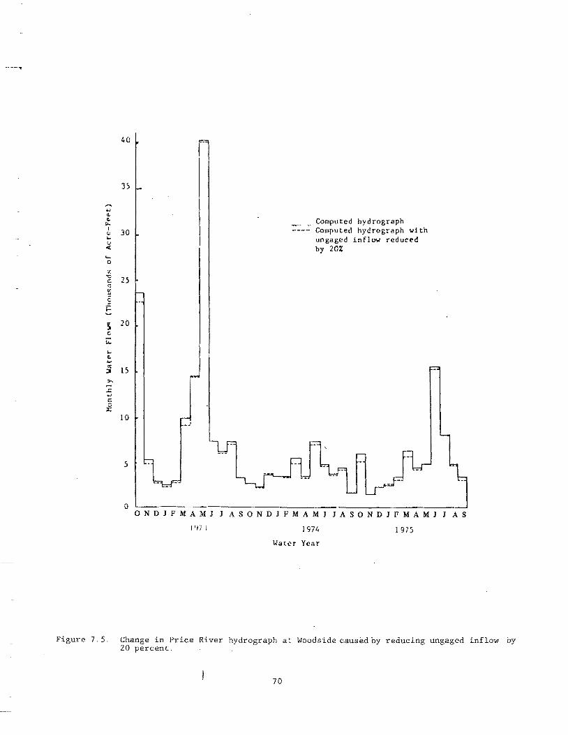
40 n 35

..... ... II> CI Computed hydrograph ~ I

30 Computed hydrograph with <;J ... ungaged inflow reduced u « by 20% .... 0

'J: -c 25 c: 0: u:

§ j:::

~ 20 c;;

i:: ... " .... It is :I

>. .-.::: .... c:: c ~

10 .J

o ONDJFMAMJ J ASONDJFMAMJ JASONDJFMAMJ J AS

I 'I i I J 974 J 975

Water Year

Figure 7.5. Change in Price River hydrograph at Woodside caused by reducing ungaged inflow by 20 percent.

70

Page 82

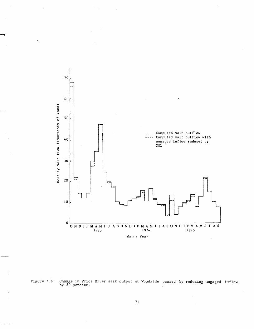
60

til C 0 I-.... 50 0

til -0 C II:

~ Computed salt ou t flow c. Computed salt outflow with ~ 40 ungaged inflow reduced by .....

~ 20%

i:

c:: 30 , v. -' >,

.t::. ... c £ 20

10

OL------------------------------------------------------~ ONDJFMAMJ J ASONDJFMAMJ JASONDJFMAMJ J A,S

1973 1974 1975

Wat,'r Year

Figure 7.6. Change in Price River salt output at Woodside caused by reducing ungaged inflow by 20 percent.

71

Page 83

.... c cr.

"'0 t:

40

35

30

: 20 ::: o

..c: i-

5

o

.1

Computed water outflow Computed water outflow with irrigation efficiencies raised by 10%

.... , I • , I • I • I

I , • L.

• • • I '-. .,

".

----------.~--.

ONDJFMAMJ J ASONDJFMAMJ JASONDJFMAMJ J AS

1973 1974 1975

\..'ater Yeilr

Figure 7.7. Change in Price River hydrograph at Woodside caused by increasing irrigation ef­ficiencies by 10 percent.

72

Page 84

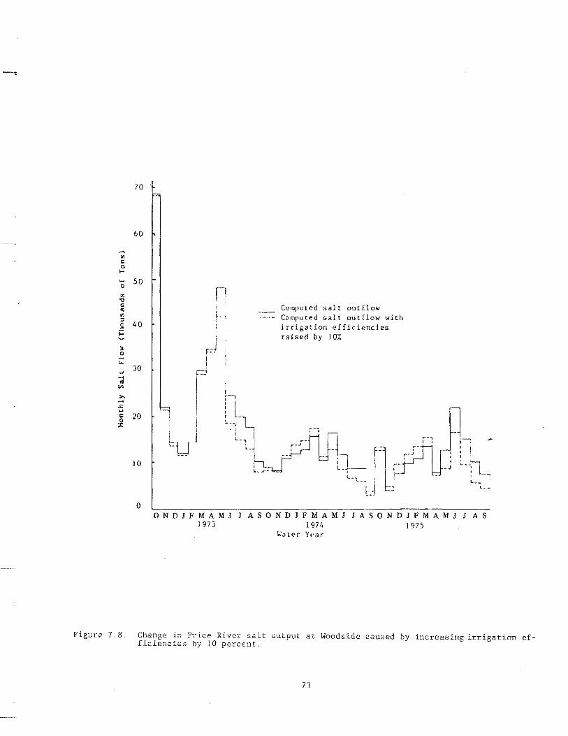
70 .

60

<11 c: 0 ....

..... 50 0

tr.

" ::: <'C g; :J

40 S E ) 0

u.. .... )0

~ en

>. ...... .r: ... c 20 0 ;I:

10

o

j' F- -I I r

I , I

V

j

fl ~-.~ • I

I L_,

Con~uted salt outflow Computed sal t out flow with irrigation efficiencies raised by ]07.

r-, I , .--:

I I I

I

L

ONDJFMAMJ J ASONDJFMAMJ JASONDJFMAMJ J AS ]973 1974 1975

'Water Y('ar

Figure 7.8. Change in Price River salt output at Woodside caused by increasing irrigation ef­ficiencies by 10 percent.

73

Page 85

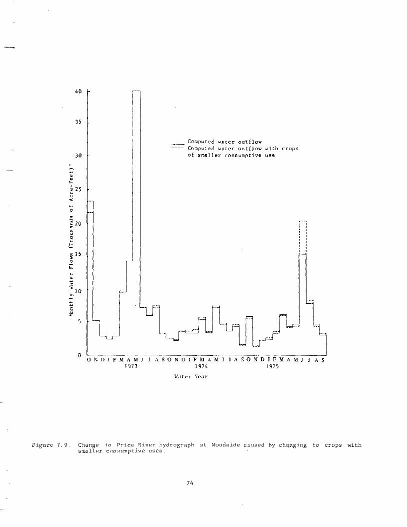
40

35

30

---... !II !II ~

125 ... u < .... 0

0)

~ 20 '" 0: ;, 0

.J: f-..... ~ 15 0 -"'-... !II

~ 3

10 >-....,

.r: u c ~

5 l

Computed wAter outflow Computed water outflow with crops of smaller consumptive use

-.., . I

o --- -.-------' ONDJFMAMJ JASONDJFMAMJJASONDJFMAMJJAS

1973 1974 1975

Figure 7.9. Change in Price River hydrograph at Woodside caused by changing to crops with smaller consumptive uses.

74

Page 86

--"

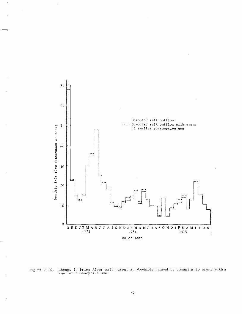
7U

60

III .')0 c: c I-

.... c CI: -g 4() 0; If:

c: .c: I-

:Jo c t.-

o; Vl

>,

.c: .., c: c :r:

)0

20

10

r-

Computed salt outflow Computed salt outflow with crops of smaller consumptive use

o L-______________________________________________________ ~

ONDJFMAMJ J ASONDJFMAMJ JASONDJFMAMJ J AS 1'173 1974 1975

Figure 7.10. Change in Price River salt output at Woodside caused by changing to crops witha smaller consumptive use.

75

Page 87

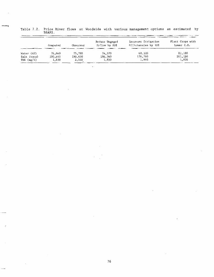
Table 7.2. Price River flows at Woodside with various management options as estimated by BSAMl.

Reduce Ungaged Increase Irrigation Plant Crops with Computed Observed Inflow by 20% Efficiencies by 10% Lower C. U.

Water (AF) 76,640 75,780 74,370 68,310 81,180 Salt (tons) 190,640 190,650 186,340 176,760 201,150 TDS (mg/l) 1,830 2, 1,850 1,960 1,830

76

Page 88

CHAPTER VIII

SUMMARY, CONCLUSIONS, AND RECOMMENDATIONS

Summary

Within the Price River valley, salt enters the river as it is carried by over­land flow from natural areas, agricultural drainage, and groundwater inflow entering the stream from natural and man-caused sources. Within the river, it is carried by the flow, deposited in the bed sediments, and picked up again by later flows as hydrographs rise and fall.

About 40 percent of the salts leaving the basin annually originate from valley areas, and up to 95 percent of these are associated with agriculturally induced and other groundwater inflows to the stream. The highest observed loading rate was 518 pounds per square mile of catchment daily.

A selected natural channel, Coal Creek, traversing the Mancos Shale wildlands was instrumented and observed during the summer of 1976. Occasional rapid cloud-burst surface runoff was of short duration. Automatic field recording equipment was repeatedly damaged by rocks and debris. Longitudinal salt uptake in the channel was low. Groundwater inflow declined steadily throughout the summer but was of constant quality. The indigenous salts of the bed material were heterogeneous. The largest concentration of entrained soluble salt was approximately 0.7 percent by weight of the channel bed material. Channel efflorescence varied from 18 to 9387 gm/m2-cm. The largest concentrations occurred in channel depres­sions and saturated bed material. The lowest concentrations occurred in dry channels with shallow sediment deposits over bedrock. Transport of salt from the soil matrix of the channel bed material to the exposed surfaces of the channel was inhibited by the low hydraulic conduct ivi ty of the Mancos Shale derived soils.

Mineral dissolution from the Coal Creek channel material was studied in the labora­tory. The time rate of dissolution was low and decreased with time. Turbulent mixing or cyclic drying of the bed material increased the dissolution rates.

Artificial flows were added on two separate occasions into an ephemeral channel within the Coal Creek subbasin. Again, salt uptake tended to decrease exponentially with time. Equation 4.6 describes the accumulated salt loading with an avera~e loading coef­ficient, Kl, of 2.51 gm/ft2-minO•5 •

A hydrosalinity surface runoff model was developed and applied for estimating the salt contributions from overland flow from natural channels. The proportions of the total salt load at Woodside, listed in Table 8.1, were obtained.

A simplified version of the model was applied to the various shale types throughout the Price River Basin. Because most of the salt pickup from surface runoff occurs from the overland and first order channel flows,

. only these two regimes were included. In addition, the relationship used to represent the salt pickup process in the microchannels (Equation 6.1), while perhaps not repre­senting the process as well as that used in the Coal Creek model (Equation 4.6), could more easily be calibrated to various shale types. The results agree reasonably well with those previously reported by Ponce (1975) and White (1977a).

77

According to the results obtained by applying BSAMI approximately 114,000 tons of salt leaving the basin annually at Woods ide originate in the mountainous areas. Thus, the loading rate in the mountains (350 square miles) averages 0.51 tons/acre per year. About 76,000 tons per year are derived from the 1,500 square mi les of the central basin for a loading rate of 0.08 tons/acre per year. The model further predicts that of this total about 3,500 tons are produced by surface runoff from the nonagricultural

Table 8.1. Estimated salt loading from natural channels.

Natural Salt Source

Overland Flow 1st Order Channels 2nd Order Channels 3rd Order Channels 4th Order Channels

TOTALS

Percent Total Annual Salt Load at Woodside

Extrapolation from the Coal Creek Study

Area Assuming all Basin Shales are Undivided

5.70 0.74 0.36 0.23 0.09 7.19

Application of the Coal Creek Hodel to the Various Basin

Shale Types

2.10 1.10 0.36 0.23 0.09 3.88

Page 89

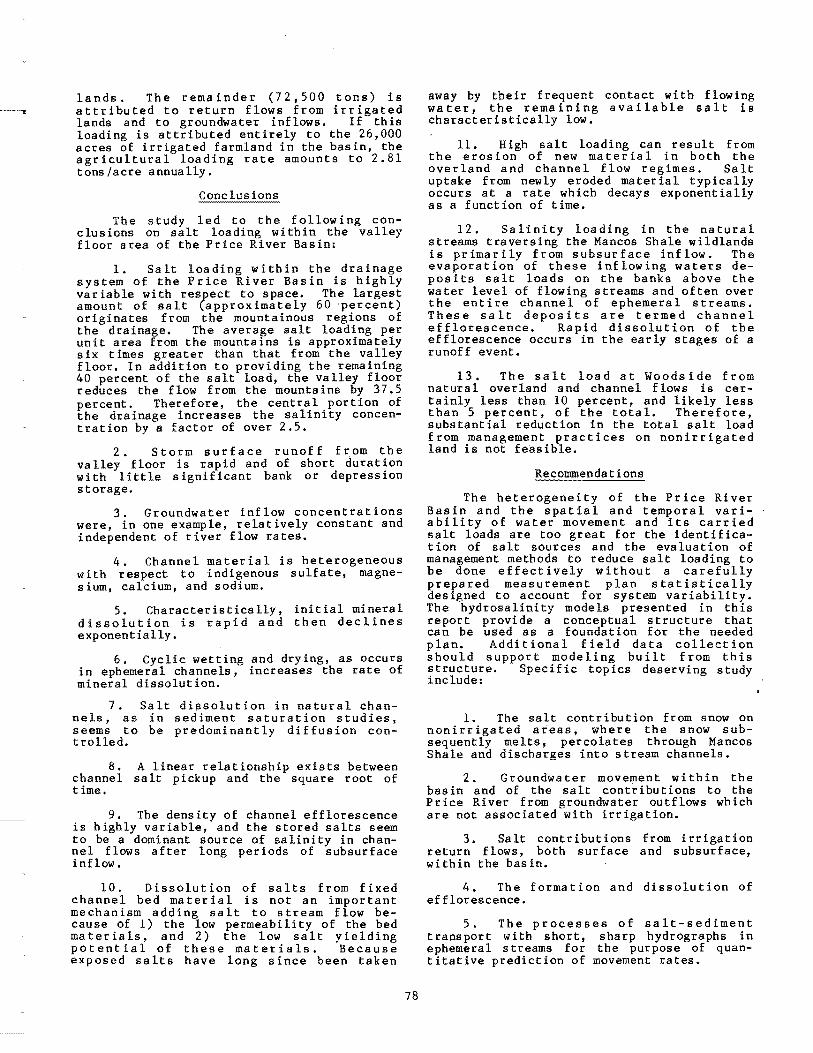
lands. The remainder (72,500 tons) is attributed to return flows from irrigated lands and to groundwater inflows. If this loading is attributed entirely to the 26,000 acres of irrigated farmland in the basin, the agricultural loading rate amounts to 2.81 tons/acre annually.

The study led to the following con­clusions on salt loading wi thin the valley floor area of the Price River Basin:

1. Salt loading within the drainage system of the Price River Basin is highly variable with respect to space. The largest amount of salt (approximately 60 percent) originates from the mountainous regions of the drainage. The average salt loading per unit area from the mountains is approximately six times greater than that from the valley floor. In addition to providing the remaining 40 percent of the salt load, the valley floor reduces the flow from the mountains by 37.5 percent. Therefore, the central portion of the drainage increases the salinity concen­tration by a factor of over 2.5.

2. Storm surface runoff from the valley floor is rapid and of short duration with little significant bank or depression storage.

3. Groundwater inflow concentrations were, in one example, relatively constant and independent of river flow rates.

4. Channel material is heterogeneous with respect to indigenous sulfate, magne­sium, calcium, and sodium.

5. Characteristically, initial mineral dissolution is rapid and then declines exponentially.

6. Cyclic wetting and drying, as occurs in ephemeral channels, increases the rate of mineral dissolution.

7. Salt dissolution in natural chan­nels, as in sediment saturation studies, seems to be predominantly diffusion con­trolled.

8. A linear relationship exists between channel salt pickup and the square root of time.

9. The density of channel efflorescence is highly variable, and the stored salts seem to be a dominant source of salinity in chan­nel flows after long periods of subsurface inflow.

10. Dissolution of salts from fixed channel bed material is not an important mechanism adding salt to stream flow be­cause of 1) the low permeability of the bed materials, and 2) the low salt yielding potential of these materials. Because exposed salts have long since been taken

78

away by their frequent contact with flowing wa t e r , the r e ma i n i n g a va i 1 a b 1 e sal tis characteristically low.

11. High salt loading can result from the erosion of new material in both the overland and channel flow regimes. Salt uptake from newly eroded material typically occurs at a rate which decays exponentially as a function of time.

12. Salinity loading in the natural streams traversing the Mancos Shale wildlands is primarily from subsurface inflow. The evaporation of these inflowing waters de­pos i ts salt loads on the banks above the water level of flowing streams and often over the entire channel of ephemeral streams. These salt deposits are termed channel efflorescence. Rapid dissolution of the efflorescence occurs in the early stages of a runof f event.

13. The salt load at Woodside from natural overland and channel flows is cer­tainly less than 10 percent, and likely less than 5 percent, of the total. Therefore, substantial reduction in the total salt load from management practices on nonirrigated land is not feasible.

Recommendations

The heterogeneity of the Price River Basin and the spatial and temporal vari­ability of water movement and its carried salt loads are too great for the identifica­t ion of salt sources and the evaluation of management methods to reduce salt loading to be done effectively without a carefully prepared measurement plan statistically designed to account for system variability. The hydrosalinity models presented in this report provide a conceptual structure that can be used as a foundation for the needed plan. Additional field data collection should support modeling built from this structure. Specific topics deserving study include:

1. The salt contribution from snow on nonirrigated areas, where the snow sub­sequently melts, percolates through Mancos Shale and discharges into stream channels.

2. Groundwater movement wi thin the basin and of the salt contributions to the Price River from groundwater outflows which are not associated with irrigation.

3. Salt contributions from irrigation return flows, both surface and subsurface, within the basin.

4. The formation and dissolution of efflorescence.

5. The processes of salt-sediment transport with short, sharp hydrographs in ephemeral streams for the purpose of quan­titative prediction of movement rates.

Page 90

SELECTED BIBLIOGRAPHY

Andersen, J. C., and A. P. Kleinman. 1978. Salinity management options for the Colorado River. Utah Water Research Laboratory UWRL/P-78/03. June.

Blackman, W. C., Jr., J. V. Rouse, G. R. Schillinger, and W. H. Shafer, Jr. 1973. Mineral pollution in the Colorado River Basin. Journal of Water Pollution Control Federation, 45(7) :1517-1557. July.

Bureau of Reclamation. Series 520 Land Drainage Techniques and Standards, United States Bureau of Reclamation, pp. 56-67. (unpublished, tentative field and laboratory procedures. Part 524.1.1) •

Burge, D. L. 1974. Professor of Geology, College of Eastern Utah at Price. (Unpublished notes)

Chadwick, D. George. 1977. Hydro-salinity modeling in the Price River Basin. M.S. Thesis. College of Engineering, Utah State University, Logan, UT.

Chow, V. T. 1964. Handbook of applied hy-drology, a compedium of water-resources tech nology. McGr aw-H ill Book Company, New York, N.Y. pp. 1418.

Clyde, C. G., D. B. George, K. M. Lee, P. Pucel, and W. Hay. ,1981. Water quality in Pleasant Valley, Utah. UWRL/H-81/02, Utah Water Research Laboratory, Utah State University, Logan, Utah.

Cordova, Robert M. 1964. Hydrogeologic reconnaissance of part of the headwaters area of the Price River, Utah. Water Resources Bullet in 14, Utah Geologi cal and Mineralogical Survey. March.

Dixon, Lester S. 1975. Adaption and appli­cation of the dynamic QUAL-I I model to the lower Jordan River. M.S. Thesis, Utah State University, Logan, Utah. pp. 105.

Dixon, Lester S. 1978. A mathematical model of salinity uptake in natural channels traversing Mancos Shale badlands. PhD Dissertation, Utah State University, Logan, Utah 84322.

79

Durum, Walton H. 1953. Relationship of the mineral constituents in solution to stream flow, Saline River near Russell, Kansas. Transactions of American Geophysical Union, 34(3) :435-442. June.

Feltis, R. D. '1966. Water from bedrock in the Colorado River Plateau of Utah. U.S. Geological Survey in cooperation with the Utah Oil and Gas Conservation Commission. Technical Publication 15, Utah State Engineer.

Feth, J. H. 1971. Mechanisms controlling world water chemistry. Evaporation­Crystallization Process: Science, 172(3985):870-872. May.

Fisher, P. W., et al. 1968. Atmospheric contributions to water quality of streams in the Hubbard Brook Experi­mental Forest, New Hampshire. Water Resources Research, 4(5):1115-1126. October.

Gibbs, R. J. 1970. Mechanisms controlling world water chemistry. Science, 170(3962):1088-1090. December.

Gifford, G. F., R. H. Hawkins, J. J. Jurinak, S. L. Ponce, and J. P. Riley. 1975. Effects of land processes on diffuse sources of salinity in the Upper Colo­rado River Basin. Report to the Bureau of Land Management and Bureau of Reclamation. U.S. Department of Interior. Utah Agr icultural Experiment Station, Utah State University, Logan, Utah.

Gunnerson, C. G. 1967. Streamflow and quality in the Columbia River Basin. American Society of Civil Engineers, Journal of the Sanitation Engineering Division, 93:1-16.

Gwynn, Ed. 1976. USGS Division of Oil and Gas, Salt Lake City. Personal inter­view, concerning oil well in Coal Creek (lra1~age.

Hall, Francis R. 1970. Dissolved solids-discharge relationships 1. Mixing models. Water Resources Research, 6(3):845-850. June.

Page 91

--" Hall, Francis R. 1971. Dissolved solids­discharge relationships 2. Applications to field data. Water Resources Research, 7(3):591-601. June.

Hart, F. C., P.H. King, and G. Tchobanoglous. 1964. Discussion of "predictive tech­niques for water quality inorganics" by J. E. Ledbetter and E. F. Gloyna. American Society of Civil Engineers, Sanitary Engineering Division Journal, 90(SA5):63-64. October.

Hem, J. D. 1948. Fluctuations in concentra­tion of dissolved solids of some south­western streams. Transactions, American Geophysical Union, 29(1):80:83.

Henderson, F. M. 1971. Open channel flow. MacMi llan Company, 886 3rd Avenue, New York, N.Y. 6th Edition. p.522.

Hendrickson, G. E., and R. A. Krieger. 1964. Geochemistry of natural waters of the Blue Grass Region, Kentucky. U.S. Geological Survey Water Supply Paper 1700.

Hicks, C. R. 1?73. Fundamental concepts In the desIgn of experiments. Holt Rinehart and Winston. pp. 85-103.

Hill, R. W. 1973. A computer model of the hydrologic and salinity flow systems within a river basin. PhD Dissertation, Utah State University, Logan, Utah. p. 202.

Huber, A. Leon, Eugene K. Israelsen, Robert W. Hill, and J. Paul Riley. 1976. BSAM. Basin simulation assessment model documentation and user manual. Utah Water Research Laboratory, Utah State University, Logan, Utah.

Hyatt, M. Leon, J. Paul Riley, M. Lynn McKee, and Eugene K. lsraelsen. 1970. Computer simulation of the hydrologic-salinity flow system within the Upper Colorado River Basin. Utah Water Research Laboratory, PRWG54-1, Utah State Univer­sity, Logan, Utah.

lorns, W. V. 1971. Quality of water. Colorado River Basin Progress Report #5.

lorns, W. V., C. H. Hembree, and G. L. Oakland. 1965. Water resources of the upper Colorado River Basin. Technical Report Professional Paper 441. U.S. Geological Survey.

Israelsen, C. E., et al. 1980. Use of saline water in energy development. Utah Water Research Laboratory UWRL!P-80!04.

80

Jensen, M. E., Ed. 1973. Consumptive use of water and irrigation water require­ments. A report prepared by the Techni­cal Committee on Irrigation Water Requirements of the Irrigation and Planning Division of ASCE.

Jeppson, R. W., G. L. Ashcroft, A. L. Huber, G. V. Skogerboe, and J. M. Bagley. 1968. Hydrologic atlas of Utah. Utah Water Research Laboratory, PRWG35-1, Utah State University, Logan, Utah.

Jeppson, R. W. 1974. Simulation of steady and unsteady flows in channels and rivers. Utah Water Research Laboratory, PRYNE-074-0-1, Utah State University, Logan, Utah.

Johnson, Noye M., Gene K. Likens, F. H. Bormann, O. W. Fisher, and R. S. Pierce. 1969. A working model for the vari­ation in stream water chemistry at Hubbard Brook Experimental Forest, New Hampshire. Water Resources Research, 5(6):1353-1363.

Jurinak, J. J., J. G. Whitmore, and R. J. Wagenet. 1977. Kinetics of salt release from a saline solI. Soil Science Society of America Journal, 41(4):721-724. July-August.

Kennedy, Vance C. 1971. Silica variation in stream water with time and discharge. Vances in Chemistry Series, 106:94-130.

Korven, H. C., and J. C. Wilcox. 1964. . Effects of flow variations on the salt

content and reaction of a mountain creek. Canadian Journal of Soil Science, 44:352-359.

Lane, William L. 1975. Extraction of information on inorganic water quality. Hydrology Papers, Colorado State Univer­sity, Fort Collins, Colorado. 73:74.

Langbein, W. B., and O. R. Dawdy. 1964. Occurrence of dissolved solids in surface waters in the United States. U.S. Geological Survey Professional Paper 5010. pp. 0115-0117.

Lapin, Lawrence. 1975. Statistics, meaning and method. Harcourt Brace Dovanovich Inc.,NewYork,N.Y. p.591.

Ledbetter, J. 0., and E. F. Gloyna. 1964. Predictive techniques for water quality inorganics. J ourna 1 of the Sani tary Engineering Division, pp. 127-151. February.

Lenz, A. T., and C. N. Sawyer. 1944. Esti­mation of stream-flow from alkalinity­determinations. Transactions, American Geophysical Union, 26(6):1005-1010.

Page 92

Linsley, R. K., and J. B. Franzini. 1972. Water resources engineering. McGraw­Hill Book Company, 2nd Edition, p. 690.

Linsley, R.K., M.A. Kohler, J. L. H. Paulhus. 1958. Hydrology for engineers. McGraw­Hill Book Company, Inc., New York, N.Y. 340 p. (referred to by Hyatt et a1. 1970).

Messer, J. J., E. K. Israelsen, and V. Dean Adams. 1981. Natural salinity removal processes in reservoirs. Utah Water Research Laboratory UWRL/Q-8l/03.

Mundorff, J. C. 1972. Reconnaissance of chemical quality of surface water and fluvial sediment in the Price River Basin, Utah. Utah Department of Natural Resources, Technical Publication No. 39.

Narasimhan, V. A. 1975. A hydro-quality model to predict the effects of biologi­cal transformation on the chemical quality of return flow. PhD Disserta­tion, Utah State University, Logan, Utah.

Narasimhan, V. A., A. L. Huber, J. P. Riley, and J. J. Jurinak. 1980. Development of procedures to evaluate salinity management strategies in irrigation return flow. UWRL/P-80/03, Utah Water Research Laboratory, Utah State Univer­sity, Logan, Utah.

Nakayama, F. S., R. D. Jackson, B.A. Kimball, and R. J. Reginato. 1973. Diurnal soil-water evaporation chloride movement and accumulation near the soil surface. Soil Science Society of American Proceedings, 37:509-513.

Neter, J., and W. Wasserman. 1974. Applied linear statistical models. Published by Richard D. Irwin Inc., Homewood, Illinois. p. 842.

Peterson, S. R., J. J. Jurinak, and R. J. Wagenet. 1980. Salt release from suspended sediments, a simulation model. Utah Agricultural Experiment Station, Utah State University. Research Report 62, December.

Pinder, G. F., and J. F. Jones. 1969. Determination of the groundwater com­ponent of peak discharge from the chemistry of total runoff. Water Resources Research, 5(2):438-445.

Pionke, H. B., and A. D. Nicks. 1970. The effect of selected hydrologic variables on stream salinity. International Association of Scientific Hydrology Bulletin, 15(4) :13-21.

81

Pionke, H. B., A. D. Nicks, and R. R. Schoof. 1972. Estimating salinity of streams in the southwestern United States. Water Resources Research, 8(6):1597-1604.

Ponce, S. L. 1975. Examination of a non­point source loading function for the Mancos Shale wildlands of the Price River Basin, Utah. PhD Dissertation, Utah State University, Logan, Utah.

Riley, J. P., and J. C. Batty. 1982. The potential for solar pond development in Utah. Utah Water Research Laboratory. Manuscript in review.

Riley, J. Paul, and David S. Bowles. 1976. Low flow modeling in small steep water­sheds. Journal of the Hydraulics Division, ASCE, September.

Riley, J. Paul, David S. Bowles, and D. George Chadwick. 1977. Preliminary identification of the salt pickup and transport processes in the Price River Basin, Utah. Presented at the Third International Hydrology Symposium, Fort Collins, Colorado. June.

Riley, J. Paul, Vernon J. Rogers, and George B. Shih. 1974. Hydrologic model studies of the Mt. Olympus Cove area of Salt Lake County. Utah Water Research Laboratory, Utah State University, Logan, Utah.

Skogerboe, G. V., M. L. Hyatt, and K. O. Eggleston. 1967. Design and calibration of submerged open channel flow measure­ment structures; Part 3 - Cutthroat flumes. Utah Water Research Laboratory, WG3l-4. Utah State University, Logan, Utah.

Soil Moisture Equipment Corporation. 1976. Operating instructions for the Cat. No. 5000-A and 5100-A soil salinity sensors. (supplied upon request) P.O. Box 30025, Santa Barbara, California 93105.

Stokes, W. L., and R. E. Cohenour. 1956. Geologic atlas of Utah, Emery County; Utah Geological and Mineralogical Survey University of Utah, p. 65.

Stokes, W. L., and E. B. Heylman. (no date) Outline of the geologic history and stratigraphy of Utah, Utah Geologic and Mineral Survey, University of Utah, p. 34.

Strahler, A. N. 1957. Quantitative analysis of watershed geomorphology. Trans­actions, American Geophysical Union, 38(6):913-920. December.

Thomas, J.L., J.P. Riley, and E.K. Israelsen. 1971. A computer model of the quantity and chemical quality of return flow. Utah Water Research Laboratory, PRWG77-1, Utah State University, Logan, Utah.

Page 93

Toler, L. G.1965. Relation between chemi­cal quality and water discharge in Spring Creek, Southwestern. Georgia. U.S. Geological Survey Professional Paper 525-C, pp. C209-C213.

USDA. 1962. Agricultural handbook No. 224. Field manual for research in agricul­tural hydrology. U.S. Government Printing Office, Washington, D.C.

U.S. Department of Commerce. 1960. Climate.s of the states. Office of the National Oceanic and Atmospheric Administration. II:921-934.

Utah Division of Water Resources. 1975. Hydrologic inventory of the Price River Basin. Utah State Department of Natural Resources, Division of Water Resources, June. pp. 63.

Utah State University. 1975. River regional assessment Volumes, Utah Water Research Logan, Utah. October.

Colorado study.. 4

Laboratory,

Van Denburgh, A. S., and J. H. Feth. 196~. Solute erosion and chloride balance in selected river basins of the western conterminous United States. Water Resources Research, 1(4}:537-541.

82

Visocky, A. P. 1970. Estimating the ground­water contribution to storm runoff by the electrical conductance method. Groundwater, 8(2):5-10.

Ward, J. C., II. 1958. Correlation of stream flow quantity with quality. Thesis presented to the University of Oklahoma, Norman, Oklahoma.

White, R. B. 1977a. Salt production from micro-channels in the Price River Basin, Utah. M.S. Thesis, Utah State Univer­sity, Logan, Utah. pp. 121.

White, R. B. 1977b. Unpublished basic data micro-channel study from the Price River Basin, Utah. Department of Water Resources, Utah State University, Logan, Utah, Supplied upon request.

Whitmore, J. C. 1976. Some aspects of the salinity of Mancos Shale and Mancos derived soils. M.S. Thesis, Utah State University, Logan, Utah. p. 69.

Willardson, L. S., R. J. Hanks, and J. J. Jurinak. 1979. Impact of water and soils having high source-sink potentials on water and salinity management under irrigation in the Upper Colorado River Basin. Utah Water Research Laboratory UWRL/P-79/06.

Williams, J. S. 1975. The natural salinity of the Colorado River. Utah Water Research Laboratory, Utah State Univer­sity, Logan, Utah. Occasional Paper 7.

Page 94

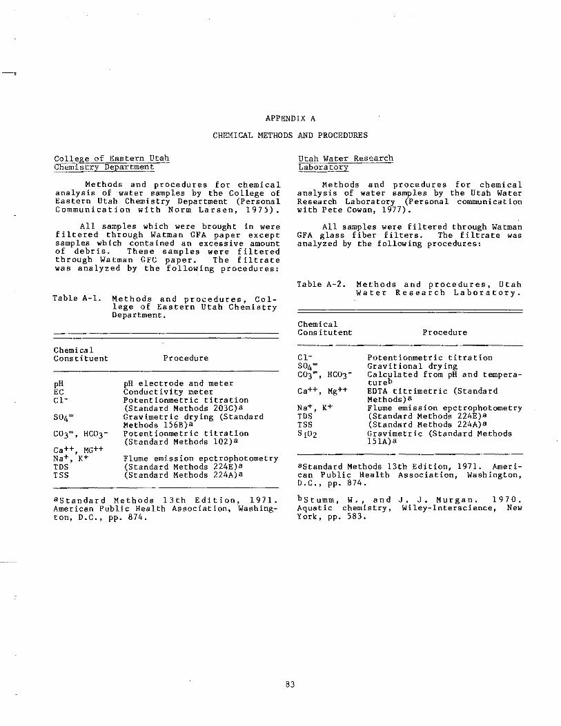
APPENDIX A

CHEMICAL METHODS AND PROCEDURES

College of Eastern Utah Chemistry Department

Methods and procedures for chemical. analysis of water samples by the College of Eastern Utah Chemistry Department (Personal Communication with Norm Larsen, 1975).

All samples which were brought in were filtered through Watman GFA paper except samples which contained an excessive amount of debris. These samples were filtered through Watman GFC paper. The filtrate was analyzed by the following procedures:

Table A-I. Methods and procedures, Col­lege of Eastern Utah Chemistry Department.

Chemical Constituent

pH EC Cl-

S04=

C03=, HCOr

Ca++, MG++ Na+, K+ TDS TSS

Procedure

pH electrode and meter Conductivity meter Potentionmetric titration (Standard Methods 203c)a Gravimetric drying (Standard Methods 156B)a Potentionmetric titration (Standard Methods 102)a

Flume emission epctrophotometry (Standard Methods 224E)a (Standard Methods 224A)a

astandard Methods 13th Edition, 1971. American Public Health Association, Washing­ton, D.C., pp. 874.

83

Utah Water Research Laboratory

Methods and procedures for chemical analysis of water samples by the Utah Water Research Laboratory (Personal communication with Pete Cowan, 1977).

All samples were filtered through Watman GFA glass fiber filters. The filtrate was analyzed by the following procedures:

Table A-2. Methods and procedures, Utah Water Research Laboratory.

Chemical Consitutent

Cl­S04= C03=, HC03-

Ca++, Mg++

Na+, K+ TDS TSS Si02

Procedure

Potentionmetric titration Gravitional drying Calculated from pH and tempera­tureb EDTA titrimetric (Standard Methods)a Flume emission epctrophotometry (Standard Methods 224E)a (Standard Methods 224A)a Gravimetric (Standard Methods 151A)a

astandard Methods 13th Edition, 1971. Ameri­can Public Health Association, Washington, D.C., pp. 874.

bStumm, W., and J. J. Murgan. 1970. Aquatic chemistry, Wiley-Interscience, New York, pp. 583.

Page 95

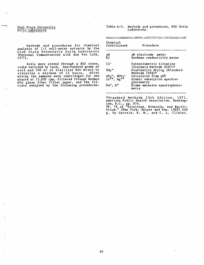
Utah State University Soils Laboratory

Methods and procedures for chemical analysis of 1: 1 soil-water extracts by the Utah State University Soils Laboratory (Personal Communication with Abe Van Luik, 1977).

Soils were sieved through a 1120 sieve, rocks excluded by hand. One-hundred grams of soil and 100 ml of distilled H20 mixed by vibration a minimum of 12 hours. After mixing the samples were centrifuged for one minute at 15,000 rpm, filtered through Watman GFA glass fiber filter paper, and the fil­trate analyzed by the following procedures:

84

Table A-3. Methods and procedures, USU Soils Laboratory.

Chemical Constitutent

pH EC

Cl­

S04=

CO"l=, HCO"l­Ca'f+, Mg+'f

Na+, K+

Procedure

pH electrode meter Bechman conductivity meter

Potentiometric titration (Standard Methods 203c)a Gravimetric drying (Standard Methods 156B)a Calculated from pHb Atomic adsorption spectro­photometry Elome emission spectrophoto­metry

astandard Methods 13th Edition, 1971. American Public Health Association, Washing­ton, D.C., PoP. 874. bP. 76 of 'Solutions, Minerals, and Equili­brium," (New York: Harper and Row, 1965) 450 p. by Garrels, R. M., and C. L. Clinist.

Page 96

APPENDIX B

FIELD SURVEY DATA

85

Page 97

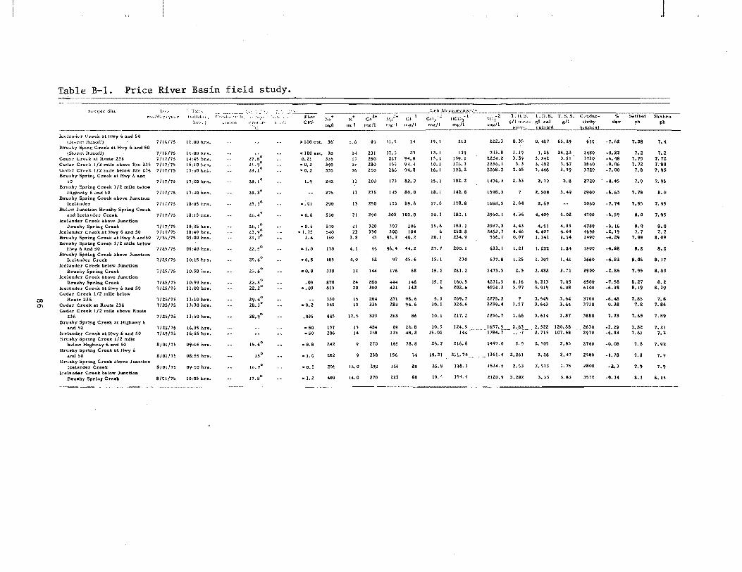
00 <"

J

Table B-1. Price River Basin field study.

;,),"H!,lc Sill: -~~~~~~==~~~~~ 1).,.· rnc',I,l;, .... J il';I:: (rl'llJt .• r,

hl"" I

Ti:: , .', ..... .. _--Flow

1.,.,/1 CFS 1,+

n~ 1

C"Z+ :\!o:":+ (;1

mdl ~~It>!!l

:-; .. + n>fl

141 !,,,,.~

It':1.:1'lJllh·y Creek at Hwy 6 and SO (.)h,rm .ii,.unoff)

l1ru .... l:.y Splng Creek al Hwy 6 and SO iSlvrm Runoff)

Ceu!lr (.;rl;'t·X iM Rnl1U: 2.36 Cedar ere.-k 1/2 mile above Rtc Z3f,. Ct.'ll:.%' Cr~''''k liZ mile below Rtc Z:!;6 Brushy Sprin:. Creek at Hwy 6 and

50 BrllEhy Cre~k 1/2 mU~ b~low

711 1,/7,

7/l(./7, 7/J 7/75 7/17/75 7/1717>

7/17/75

Highway and SO 11l7/7$ Brushy Sprins Creek above ]uneti,un

lcelande-r 7/17/75 Bel.:lw Junction Spring Creek

and Jcelancer 7/17175 kelander Creek above Junction.

Creek .at Hwy 6 and 50

Creek at Hwy 6 andSO 7/7.';/75 C reck 1/ Z mile below

Icelander Creek below Junction Creek

above Junctlon Creek

6 and 50

Cedar Creek: at R.oute 236 Cedar Creek 1/2 mile above Route

z36 Creek at Highway 6

Icelnnder Creek at Hwy 6 and SO Spring Creek 1/2 mile v Hiilhway 6 and SO

Brushy Spring Creek at Hwy b artd SO

Brushy Spring Creek above Junctiort

7/ZS/7>

7/Z5/7>

7/25/15

7/ZS/7> 7/2,/75

7/ZS/75

7/Z9/75 7/29/15

S/01/75

S/01175

Icelander Creek 8/01/15 . 1~f:1artd.r <;reek bela"" Juncti<m.

Bruaby Sprins Crf:e1t 8/01175

1(1;00 hr:..

l():OO hu. 14:45 un. 15!10 h;(5. 15:;0 h;rs.

17:I!Ohu.

17:·IOhn.

18:05 hra.

18:JS'hu.

18:25 hra. 18:49 hu. 09:00 hn.

09:40 hrs.

10:15 hrs.

10:30 hra.

10,39 11:00

13:10 hra. U!30 hra.

13:50 hra.

16:35 hu. 16:55 ara.

09~lS hu.

08:S5 hu.

09'SO hra.

10:05 bra.

7.7 ~8° 7.(.,,,0

l8.1o

28.1°

28.3"

1.3. )0

Zi,.4?

lb.

22.5°

2S. nO

~5.6°

29.4° 28.3

0

28.90

15.60

15°

It..7°

17.8°

» 100 ellt. 36'

< 100 eat. SO 0.21 335

.. O. 2 390 • 0.2 335

1.9 242

·.01

·0.6

• O. 6 ~ 1.75

1.4

-1.0

'" 0.8

-0.9

.09 - .09

-0.2

.0'35

• 50 ::; 50

• 0.8

.. 1.0

.. o. 5

'" 1.2

Z75

290

5;0'

:'70 540 150

170

185

330

870 813

330 345

4<5

137 206

242

202

Z06

400

b.O

H 17 I. 16

II

13

13

21

II lZ

3.S

4.1

'.0

12

Z4 20

15 B

12.5

n 14

12.0

14.0

.4

231 250 Z80 260

zoo

31.5

37. ;; Z67 Ilj9 lbt.

173

14

Z3 94.8 9-1.4 94.8

82.0

235 145 SO.O

250 153 S9.6

2'10 303 102.0

320 307 106 330 300 104

43 93.7 40.2

46 96.4 44.2

52 97 45.6

144

>so 300

264 335

323

48. 3f-8

270

238

19,0

270

176 ... 421

68

148 14Z

271 98.6 281 94.6

263

69 Il5

165

156

166

Zz3

86

26.8 48.2

18.8

74

80

80

19.1

12. I 1;.1 1~.1

16.1

J5.1

IS.1

17.6

10.1

1>.6 6

ZO.1

27.7

15.

15.1

15.1 6

5.5 10.1

10.1

10.5 15.01

26.7

19.21

lS.l:S

19. '

213

119 Jl9.1 176.3 192. Z

192. Z

142.8

178.8

18~. 1

183. I 250.8 Z34.9

200.1

230

261. 2

160.5 ZOZ.6

269.7 324.6

217.2

IZ4.5 144

216.6

211.74

198.3

154. '*

IZ2.3

7H.S UZ-I.Z UJEJ.1 2268.2

1474.3

1598.3

0.3f,

1.19 3.39 3.3

3 •• ,

2.33

168~.5 2.64

2950. I 4.36

29S7.3 4.43 ltiS3.7 4.46

556.1 0.97

633.1 1.21

617.8 1. Z5

1475.5 2.5

4271.5 6.16 40U.2 5.97

2275.2 ? 2Z39.4 3.57

Z256.7 3.66

.. 1497.0 Z.5

1351.4 2.261

1534.5 Z.53

2120.9 3.28Z

O. -187

1.26 3.HZ 3.402 3,448

2.3,

2.508

2.69

4.409

4.51 4.407 1.142

1.222

I. 307

2.482

6.213 5.919

3.549 3.643

3.614

65.29

24.23 3.51 3. ,7 3.59

2.8

3.49

5.02

4.85 4.6' I.H

1.2'

1.41

2.71

7.05 6.08

3.6. 3.64

3.87

Z.5ZZ 120.88 2.715 107.58

2.505 2.83

2.28 2.47

Z.513 1.75

3.33 3.83

610

1480 3730 3840 3720

2no

2900

3060

4700

4780 4690 1490

1600

1680

2900

6500 6100

noo 3710

3880

2630 2970

2160

2580

2800

3550

·7.62

.0.2Z

.4.48 ·9.06 .7.00

•• 4.45

.6.63

·7.74

·,.59

.3.16 -2.19 .·1.29

.4.88

-4.83

.2.86

.7.58 -6.18

.6 • .a 0.38

7.73

.2.29 -6.31

·0.08

.1.78

.2.3

·0.14

7.38

7.2 7.75 7.n

7.8

7.9

7.78

7.95

8.0

8.0 7.7

7.98

8.2

8.05

7.95

8.27 8.19

7.85 7.8

7.65

7.82 7.61

7.8

7.8

7.9

8.1

7.'

7.2 7.n 7."88 7.95

7.95

8.0

7.95

7.95

8.0 7.7

8.09

8.2

8.17

8.03

8.Z 8.19

7.8 7.86

7.89

7.21 7.2

7.92.

7.9

7.9

8.15

Page 98

(Xl -....J

Table B-l. Continued.

:,.;,lnple Sit;:

-Icelander Creek above Junl;tion Brushy Spt"in,g Creek

lcel::tndcr Creek :it HW)' 6 and so

LJ,ltc

mo/d:.r/,/t.:.lr

Ceda.r Creek 112 mile below Rte 236 8/01/75 CCtl.1.r Creek 1/2. mile t\bove Rte 2:36 Ced .. r Creek at Ronte 136 Brushy Spring Creek at Hwy 6: a.lI'l:d 50 IcelandeT Creek Lelow Junction

Srushy Spring Creek a/08/7$ Icelander Creek above Jun~tion

Brushy Spring Creek RlOS/75 Icelander Creek at Hwy 6: and SO 8fOS/7S Cedar Creek!; Z mile beloW Route

ZJ6 8/08/75 e.da,);' Creek liZ mile otbove Route

23. Ceda r Cret:tk at Route ZJb Bruaily Spring Creek at Hwy 6 and

50 8/14/75 lcei~nder Creek beloW Junt::tion

.Brushy Spring Creek 8/14/75 Icelander Creek abovt' Junction

Brllliihy Spring Creck lcela:lfler Creek ilt Hwy 6 and SO Cedllr Creek lIZ mile beloW Route

Z3i:1 C(."dar Creek at Route 236 Ccdiilr Creek 1/2 m}lc al:mve Route

Z36 Spring Croek (upstream) :r Creek below JUlt tiol'l

h.:.'I.'J'Hh~'" (down::trei1n) o!>ovc Jun<:ti')n'~J,~i!75 lleL.Illclf,..r Creek iupstrc,nnl Cp,j,ll' Cr~~ck ,dtJwnoitI'cam) C<;:<iar Grc(.'k lup~tr",.<Ull Ccd.,lr Cl'(:;t'k (Bridge}

hr •• hrs.

iZ:30 hrs. [3:00 hra. 13:25 h ... 8.

09:30 hrs.

10:15 hra.

10~35o hu. 10:50 hrs.

12:55 hrs~

13:25 hrs. 13~.j5 hu.

09;00 Ius.

Q9:55 hra,

10:150 hr4. 10:35 hrli.

hra. hr!'.

14<301ll:'ti. 08:00 hn. 08::0 lIrs. 09dO hn. Oq;.i::i hr.';. 12.,05 nr:l.

hr5. hI'S.

----.-----~-

18.('/'

20: 26,1 23.3

0

2t).7° 15.t/'

18,3°

20° to. 6°

t7. ZO

2b.7° .n.So

4263. Z S.OQ

4473.5 lB. 7°

4l2l.8 19. 4192.5

2<)01.6 3UO.4 41'H.2 ,1.!·l".6 i :,,(,.0

:",'04. b ~.!:-C\. 2 lv7L4

28.00

27.0Q

zs. S° 17..3° Il.So" 13.1° 14.8°

~3.0: 2·1. S 2,4.0°

III 0.8 0.8 .09 .03

- .06 .005

.04

.04

.05

.07

.035 .0£

.001

.015

.OZ

.02

.08 • O~J

".08 ... 35

.3S

.4',

.1 .07

... ~ OB

~ ... + n>;ll

500 485 345 <03 335 540

tooo

1000 870

345

4lS 335

550

935

915 813

335 335

'" 600 '1'5 ?15 813 H! 43(' ,n~·

1";+

n~ll

Jo.7 18.0 13.0 J z. 0

13.0 9

18

16 19

15

14 IS

II

22

19 19

" 30

13 11 21 23 1',

H

"

l+ C.

mgtl

>85 .31 298 Z93 303 398

450

437 412

Z80

290 290

3S{}

41 (;

3(,0 lBO

300 ;1(1

,81}

390 4M 37fJ ~,',i'

Z,',t' !,',t, (:'1 /:

267 90 .2S3 87 27'J 94 248 62. a 270 9Z 30E; 143

475 152.Z

498 152.0 44& 145.6

305 97.0

219 84.4 2';8 94.0

367 In.-I

513 150.0

509 150.0 474 HZ. d

301 94.0 l')!) ,)0. i')

l77i 84. l 3<:4 162. t) 50(, 1":2. () :,f)H 148.0 ., () 1.,12. q

30'\ ',1·1. [~

2,'. ~ l. ()

'j:',!)

27.6

20. II 20.11 30.3

25. Z

20.1 35,2

26 • .2

30.2 29.2

2(, • .2

30 • .2

40. Z 3';'.l

'·L.2 31.:. ~

.2~. : 4-1.3 37 ... 3B • .1: HI,.:

HI. 2: ~=", 2 j. , .~

188.5 .2Z6.4 137.9 255. i 184.3 314.9

197.0

.2'44.7 209.3

167.3

Z36. S 169.0

207. S

230.0

ZI)'1. "

}[.:.. ! 20'1. j

Zt;q. 3 3O'J.'; 240. ·i

2':'J. '. 2)",. I lO'I. g

~2 ', . .j

;U't.1

-2 Lli.!-i. tIt u ... .,1~

• _______ l>.;~~ ,I

Z"'41.0 236Z.0 22IZ.6 223 ... 0 2192,5 280(,.0

4507.6

4461.5 4071.8

Z>71-0

4.064 3.73f;1 3. i06 3.55

3.411 4.549

7.010

6.970 6.600

3.560

.2273.1 3.650 2239.0 3.~00

2~90. 0 4.570

4349.1 6.580

4403.9 6,500

4047.1 6.110

2Z0's, Z 3. HO ::'17').3 3.400

a39. i') 3,580 Ju~Z.3 ·Lf;":,I} B()i:I.-I (,.(,.,i'i

-ll40. '5 1>. '120 ~'J,H,. f) t,.. "J7I, .' i.fl". i1 \. ",·1(,

:~~ '" i. J '. (,11,

;!Lllli., L 5JI)

·l. [)~b. l'.S.S. .:/l (;.,11· gil (;\1:~

~ ... 3.72 3.49 3.61

3.5 4.55

6.825

b.831 b. ll1

3.524

3.bll

3.4M

4.534

6.639

&. boa 6. J 14

3 • .f53

3,479

3.591 4. &. t.. HZ S.97:; 3. "iOI)

~. 67'1 J. 1'1'"

... ~7 4.27 3.84 4.95 3.74 4.71

6.97 6. '51

3.65

3.50 3.74:

7.01

6.59 (h 06

1.6" 3.30

3.74

6. Sl I,~ Os 3. SO 3.1,') ,L:.,

COllI(U<:· Hvity

UUlll1\\sj

40'50 3990 3600' 3150

? 4720

70'00

6900 6500

3730

3880 3740

4670

b"OO

6100

('200

3640 3590

3~OO 5eo') tHno (,7u')

Id}()(l

J7,>1) 3t;i'1 }7l f J

"

dev

1.76 1.21 1.56

_1.51 0_ 75 0.44

Stltilf'd

ph

8.05 8.18

8_1 7.9.2 8.03 7.74

8: 10

8_10 7.89

7.9

7.75 8.00

8.13

8.l0

8.11

8.10 7.91

7. b2 7.tH> B.2') g.20 a. Z9 H. ~O 8,0S ~. I~

J

SiI·dH.'1\

l'h

8.1 8.12 8.0>

7_9 8.0 7.9

8.32

8_ 1< 7.95

7.95

7.90 8.05

s.zo

8. Zl

K. 1~

8.11 7~~8

7.84 7.90 B.29 ~. '\iJ

ti. J1 h. \,

8. In H. ;~ ..

Page 99

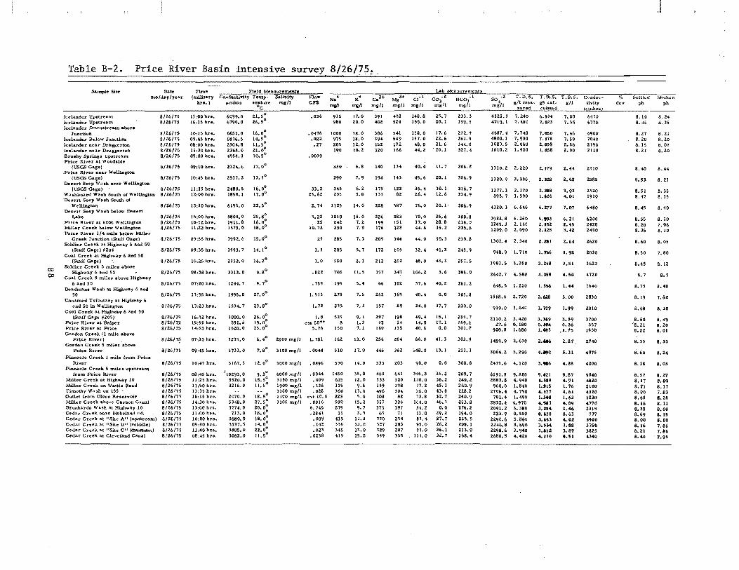
00 <:Xl

Table B-2. Price River Basin intensive survey 8/26/?5!

Sample Site Date rno/day/year

Tim_ (military

h .... )

lcelander Upetream Icelander Upetream Icelander Downstream above

Junction Icelander Below Junction Icelander near DraggeTtoo Icelander near Dragserton Brupby Springe Upstream Price rUver at Wood.ide

(USGS Gage) .Price River near Wellington

(USGS Cage) Desert Seep Waeb ftc.r Wellington

(USGS Gage) Washboard Wa,h South of WeUington "Desert Seep W;;Lsb South of

Wellington De&ert Seep Wash below Den"

Loke Price RiveT at HZ06 Wellington M.iller Creek below Wellington Price River 1/4 mile below Miller

Cruk Junction (Staff Gage) Soldier Creek at Highwa.y 6 and 50

(Staff Gage) ~204 Coal Creek at Highway 6 and 50

(Staff Gage) Soldier Creek $ mile. above

Highway 6 and 50 Coal Creek S miles above Highway

6 and $0 Dea.dman. Wash at Highway 6 a1)d

50

6 and $0

Prit:::e River

Pinnacle Creek 1 mUe tram Price River

Pinnat:::le Creek Smiles up.tream from Prke River

Miller Creek at Highwa.y 10 Miller Creek on Wattis Road Timuth)<' Wash on 155 . Outlet from Ohlen Reservoir Miller Creek abovE" CarbQ-n C.-nal Drunka.rds Wa"h at Highway 10 Cedar Creek near Mohrlalld rd. Cedar Creek at "Site AU (upntream) Ceda.r Creek at "Site un (middle) Cedar Creek at "Site Cit ~) Ceda,f Creek at Cleveland Canal

8/26175 8/26175

8/26/75 8/26/75, 8/26/75 8/26/75 8/26/75

8/26/75

8/26/75

8126175 8/26/75

8/26/75

8/26175 8/26/75 8/Z6/75

8/26175

8/26175

6/26/75

8/26/75

8/26/75

8/26/75

6/26/75

6/26175

11:00 hu. 16:15 hu ..

10.15 hr ... 09:45 hr •• 08:00 hr •• 15:30 hra. 09:00 hu.

09:10 bra.

10:45 hu.

11:15 hu. 12:00 hu.

13:30 bu ..

U:OO bu. 10:5Z hr ... 11 :2Z hu.

09:55 hra.

09:35 bra.

10:25 hu.

08:38 hr».

07:20 hr ••

13:55 hu.

13.23 hr ••

16:3iehra. 15.55 hra. 14:50 hr.~

8/2617~ 07,30 hra.

6/26/75 09,,5 hra.

6/26175 10,'7 hro.

6/26175 8/26175 6/26/75 8/26175 6/26/75 6/26/75 8/26/75 6/26175 8/26/75 8/26/'/5 8/26175 8/26/75

08:45 hu. 11 :25 hl'$~ 11:50 hu.

hra. hra.

14:30 hu. 13:00 hra. 11 :00 hra. 10:00 hra. 0'i:30 hra. 11:40 hra. OS:~5 hu.

Field MnauremeftU Gonductivity Temp- Salinity

.... mhos eratuu mg/l ·c

6099.0 21.5° 6790.0 26.5"

6655.0 6836.5 230'.8 ZZ68.0 '954.9

2324.6

2517.2

2480.5 1858.1

6195.0

5800.0 1911.8 1679.0

1992.6

1593.1

2532.0

3312.0

1244.7

1995.0

1534.7

3000.0 291.5

1520.0

16.0" 14.;° 1l~ 5° 21.0° 10.5°

17.0°

17.5°

16.0° 17.0°

2Z.5°

25.8° 16.0" 18.0°

15.0°

14.1°

16.2°

9.8°

9.7°

Z7.00

Z3.8o,

26.0° 19.0° 2:5.0°

Flo .. en

.036

.0476 .0~2 .27

.0039

33.2 23.62

2.74

3.22 25

10.72

25

1.3

3.0

.OZZ

.759

1.513

1.72

est 5.76

):2:33~O 6.40, 2:000 mgll 1.781

5733 .. 0 7.8° 3100 mgll .0044

5167~S 12:.00' lOOOmg/l .0896

3216.0

2070.0 5348.0 3774.0 113.0

3680.0 3137.5 3885.0 3082.0

18 .. sO' 2:7~So 20.00, 28.0° lS.0O'

J4.0O'

2Z.So 11 .. SO

.0044 .009 .136 .oZ8

cst 10.0 .0016 6. H5 • Z841

.009 • HZ .023

.0238

Na+

zrct!.

915 980

1000 975 205 19'0

330

290

345 231

1125

1010 242 290

285

205

100

705

191

275

235

521 8

110

162

510

570

1450 615 115 360 225 590 275

11 415 335 345 .15

K+

"l!11

17.0 20.0

18.0 18.0 12.0 10.2

6.8

7.9

6.2 5.8

14.0

15.0 7.2 1.0

7.3

5.7

8.1

u.s

5.' 7.5

7.3

9.1 1.3 1.1

13.0

17.0

14.0

35.0 lZ.O 9.6

13.0 5.0

IS.Q 9.7 3.3

11.3 13 .. 0 JS.O 15.2

caZ+ mg/l

391 402

386 394 152 120

140

194

175 131

228

226 199 176

209

172

21Z

157

66

Z62

157

207 52

160

MgZ.+

mg/l

478 524

541 549 172 166

134

143

122 82

387

383 151 128

1"

105

202

347

102

169

89

198 14

135

Cl· l

mg/l

148.8 159.0

158.0 157.0 48.0 44.2

40 .. 4

45.6

35.4 26.4

76.0

70.0 37.0 44.6

44.0

n.4

48.0

106.2

37.6

40.4

24.0

49.4 14.0 40.6

Lab M~3!i\lr .. menttl:

Col-Z: lJ(':;03~1 mg/l tng!I

25.7 20.1

17.6 22.6 21. G

, 20.1

11. 7

20.1

10.1 12.6

20.1·

25.6 28.8 35.2

50.3

41.2

43. ):

l.6

40. !

0.0

37.7

15.1 17.1 0.0

233.3 199.5

272.7 261. 9 344. B 32:7.4

206.2

306.9

316.7 234.9

306.9

300.8 238.0 235.5

239.B

245.9

257.5

385.0

261.2

305.8

230.0

255.7 .69.6 lOI.7

256 26. 66.0 41. 3 303.9

446 362: L4S~ 0 13.1

333 Z03 90.0 0.0

463 333 149 496 108 35~ 371

65 330 327 329 349

641 320 198 304

82 326 197 71

21. 283 287 355

3'15.2 HO.O

17.2 ;'6.0 03.8

1(4.0 34. Z 13.0 83.4 95.0 9~.0

IH.O

35.2 36.2 45.3 43.8 32.7 '6.3 0.0

29.2 27.7 26.2 26.1 32:.7

211.3

300.8

209.7 249.2 260.9 228.2 240.9 253.8 276.2

208.1 213.0 168.4

'325.3 4719.1

4687.4 4800.1 1083.5 1010.2

IlI0.2

1320.9

1277.3 898.7

4120.3

3922.8 1249.3 1209.0

1302.4

948.9

1981.5

2642.7

648.5

1568.6

939.0

2110.2 27.6

900.8

7.240 7. 'SO

7.740 1.930 2~ OGO 1.920

2.220

2.390,

2.170 1.590

6.6'0

6.250 2.160 2.090

2.340

1.710

3.250

4.580

1.210

2.720

1.640

3.420 0.180 1.6BO

1499.9 2.630

l084.2 5.290

2'75.6 4.120

6191.8 2883.8 960.0

2706.4 181.4

2il2.4

2680.5

9.aoo 4.940 1.840 4.750 1.'90

6.5)4 7.023

7.C'l0 7.I1B 2.038 1.8.18

2.179

2.128

2.2lI8 1.626

6.271

5. "-l 2.1'2 2.125

2.2lI1

1. 'lS6

3.258

4.358

1.3S6

2.628

1.719

l.)69 0.»< 1.,,5

2.1.16

4 • .,.2

3.,.6

9.421 ... 5419 1.llS ... 177 1._ ... sa3 l.n" 0."0 3.'51 3.U4 3.'12 4.130

7.03 7.35

7.46 7.69 2.26 2.00

2.4'

2.65

3.03 4.01

7.07

6.21 2.45 3.U

2.64

1.98

3 .. 51

4.50

1.44

3.00

1.99

3.59 0.26 1.75

2.87

5.31

4.2a

9.87 4.91 1.76 4.01 1.63 4.B9 3.46 0.63 4.02 3.88 3.87 •• 51

Conduo.::­tivity

{j,l.9U1\lSJ

6430 6770

6900 1040 2190 2110

2.S}O

2585

2:520 1910

6480

6200 2no Z4S0

2620

2030

3620

.no

1640

2830

2010

3700 351

1930

2740

4975

4Z00

9040 4820 2100 4320 1830 4770 3315

777 3900 3750 3825 4340

% dev

$ctUl."d

ph

8.10 8,4&

8.2:7 8.20 8. IS 8.21

8.40

S.53

8.51 8.47

B.45

8. S5 8. Zo 8.35

8.60

8.50

8.48

8.1

8.75

8.19

8.6B

a.50 .'8.21 8.22

8.33

8.60

8.3B

8.57 8.17 8.71 8.00 B.65 8.16 S.35 8.69 8.00 8.16 8.21 8.40

J

Shakt:n ph

B.2. 8.35

8,2.l 8.2.0 B.07 8.2.0

8.44

8.21

B.35 8.15

8.40

8. SO 7.96 8.10

8.05

1.80

8.12

8.5

8.40

7.82

8.30

8.49 8.20 8.01

8.ll

8.24

8.03

~n

~~ ~H

~. L2i 8.11 ~OO L~ ~OO ~H ~H

~"

Page 100

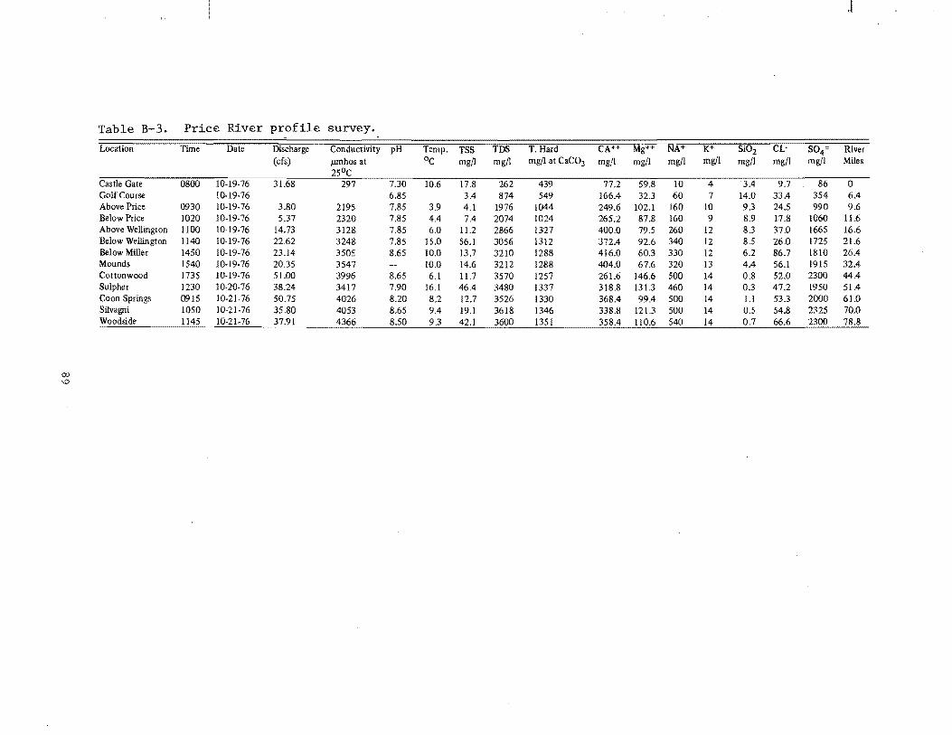
(Xl

'-'>

Table B-3.

Location

Castle Gate Go!fCourse Above Price Below Price Above Wellington Be!ow Wellington Below Miller Mounds Cottonwood Sulpher Coon Springs Silvagni Woodside

Price River profile survey.

Time Date Discharge Conductivity (cfs) Mffihos at

250C 0800 10-19-76 31.68 297

10·19-76 0930 1O-!9-76 3.80 2195 1020 10-19-76 5.37 2320 1100 10·19-76 14.73 3128 1140 10·19·76 22.62 3248 1450 10·19-76 23.14 3505 1540 10·19-76 20.35 3547 1735 10·19-76 51.00 3996 1230 10·20-76 38.24 3417 0915 10-21-76 50.75 4026 1050 10·21-76 35.80 4053 1145 10-21-76 37.91 4366

pH Temp. TSS TOO °c mgt! mgt!

7.30 10.6 17.8 262 6.85 3.4 874 7.85 3.9 4.1 1976 7.85 4.4 7.4 2074 7.85 6.0 11.2 2866 7.85 15.0 56.1 3056 8.65 10.0 13.7 3210

10.0 14.6 3212 8.65 6.1 11.7 3570 7.90 16.1 46.4 3480 8.20 8.2 12.7 3526 8.65 9.4 19.1 3618 8.50 9.3 42.1 3600

.I

T. Hard CA++ MgH NA+ K+ Si02 CL- S04= River mg/I at CaC03 mgt! mg/! mg!1 mg/! mgt! mg/I mg/I Miles

439 77.2 59.8 10 4 3.4 9.7 86 0 549 166.4 32.3 60 7 14.0 33.4 354 6.4

!044 249.6 102.1 160 10 9.3 24.5 990 9.6 1024 265.2 87.8 160 9 8.9 !7.8 1060 11.6 1327 400.0 79.5 260 12 8.3 37.0 1665 16.6 1312 372.4 92.6 340 12 8.5 26.0 1725 21.6 1288 416.0 60.3 330 12 6.2 86.7 1810 26.4 1288 404.0 67.6 320 13 4.4 56.1 1915 32.4 1257 261.6 146.6 500 14 0.8 52.0 2300 44.4 1337 318.8 131.3 460 14 0.3 47.2 !950 51.4 1330 368.4 99.4 500 14 1.1 53.3 2000 61.0 1346 338.8 121.3 500 14 0.5 54.8 2325 70.0 1351 358.4 110.6 540 14 0.7 66.6 2300 78.8

Page 101

APPENDIX C

COAL CREEK FIELD DATA

91

Page 102

CHANNEL CROSS-SECTIONS COAL CREEK DOWNSTREAM CONTROL SECTION

T .­-..... 11-------:

7ft --j

Scale

slope = .006 ft 1ft

-- -- -- -- -- -- -- -- -- -- -- ---- -- -- ------- -- --- --- --- --- --- -- ------ -- --- -- -- ---------- - -- -- -- -----

Figure C-l. Channel cross sections, Coal Creek downstream.

CHANNEL CROSS-SECTIONS COAL CREEK UPSTREAM CONTROL SECTION

r

Scale

slope = .016

Figure C-2. Channel cross section, Coal Creek upstream.

Table C-l. Coal Creek conductivity profile.

Site Location Conductivity Temperature Measured Total Alka-in>miles from Ilmhos/cm linity mgt! as Upper Site @ 250 C °c pH CaC03

8.2 4630 21.5 8.56 273 7.5 3678 23.0 8.40 287 7.1 3382 21.0 8.40 284 6.3 3172 24.0 8.40 279 5.6 3044 21.7 8.52 298 4.3 3363 22.0 7.50 339 3.8 2642 18.0 7.81 343 2.2 798 24.5 8.41 291

Tributary receiv- 21732 25.0 8.00 590 ing in terflow

1.4 804 23.0 8.40 266 Irrigation Ditch 749 22.0 8.58 267

0.3 759 22.5 8.60 269

92

Page 103

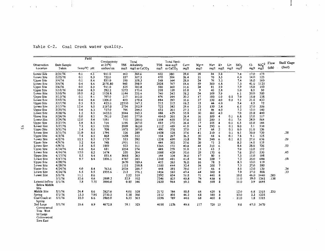
J

Table C-2. Coal Creek water quality.

Field Conductivity Total Total Hard-

SO-2 Flow Staff Gage Observation Date Sample at 250 C TSS Alkalinity TDS ness mg/l Ca++ Mg++ Na+ K+ Li+ Si0t1

CI-Location Taken TempOC pfl umhos/em mg/l mg/l as CaC03 mgfl asCaC03 mg/l mg/I mg/I mg/l mg/l mg mg/l mgfI (cfs) (feet)

Lower Site 2/21/76 0.1 8.1 911.0 162 360.6 602 380 29.4 28 84 3.8 7.4 17.0 175 Lower Site 2/25/76 0.1 8.3 722.0 227 307.5 470 304 26.4 21 70 3.5 6.3 14.0 125 Upper Site 3/4/76 0.1 8.4 837.0 100 358.3 548 344 28.8 24 76 3.2 7.4 16.0 160 Lower Site 3/4/76 0.4 8.4 2576.80 960 298.9 2028 767 54.4 59 360 4.8 7.3 41.0 1125 Upper Site 3/6/76 0.0 8.3 911.0 525 383.8 580 360 31.6 24 81 2.9 7.9 15.0 150 Upper Site 3/10/76 10.0 8.3 282.2 5272 173.4 238 150 15.8 9 40 2.8 5.0 8.5 50 Lower Site 3/10/76 10.0 8.2 . 1128.8 1144 225.4 740 342 28.2 24 109 3.9 6.1 20.0 380 Upper Site 3/13/76 0.1 8.1 707.0 217 312.0 476 244 20.2 17 100 5.0 0.1 7.0 15.0 138 Lower Site 3/13/76 0.4 8.4 1306.0 403 279.8 884 393 33.6 27 130 4.0 0.1 7.1 21.0 432 Upper Site 3/17/76 0.5 8.3 423.0 22510 247.2 212 212 18.2 15 44 4.0 5.4 8.5 72 Lower Site 3/17/76 12.4 8.5 1197.0 2734 202.9 722 342 29.4 23 130 3.8 6.5 17.0 356 Upper Site 3/20/76 0.4 8.3 727.0 796 299.5 432 261 27.2 15 86 4.0 7.2 13.0 140 Lower Site 3/20/76 1.2 8.3 1422.0 2044 242.3 888 429 35.8 30 160 4.0 7.0 23.0 480 Upper Site 3/24/76 0.6 8.5 791.0 2160 277.0 464.0 261 26.4 16 100 4 0.1 6.8 12.0 117 Lower Site 3/24/76 12.0 8.4 1581 715 280.0 1104 458 37.6 32 280 5 0.1 7.6 24.0 564 Upper Site 3/27/76 5.8 8.3 714 1196 267.0 492 272 26.4 17 105 4 0.1 6.5 15.0 144

\0 Lower Site 3/27/76 7.2 8.5 1520 2009 262.0 1112 489 41.0 34 290 6 0.1 8.0 2.1 538 \.,oj Upper Site 3/31/76 5.4 8.5 708 1875 307.0 490 278 27.0 17 66 2 0.1 8.0 11.0 126

Lower Site 3/31/76 11.0 8.5 1794 326 289 1408 528 37.6 41 210 5 0.1 8.5 30.0 720 .28 Upper Site 4/2/76 7.4 8.5 81i8 1658 312 514 297 26.2 20 68 4 0.1 7.8 9.1 125 Lower Site 4/2/76 12.3 8.5 1729 553 292 1238 490 33.8 39 240 6 0.1 8.2 27.0 636 .29 Upper Site 4/9/76 3.2 8.4 748 1931 311 444 302 27.6 20 73 2 8.2 14.0 125 Lower Site 4/9/76 3.5 8.5 1859 923 311 1266 571 40.8 44 210 6 8.8 28.0 726 .53 Upper Site 4/14/76 6.0 8.4 691 3254 274 448 279 31.0 15 63 5 7.0 12.0 132 Lower Site 4/14/76 12.0 8.5 1474 550 264 1008 420 35.6 29 170 6 7.6 23.0 530 .45 Upper Site 4/17/76 8.5 8.4 851.4 3668 263 544 324 36.0 17 80 5 7.3 15.0 198 Lower Site 4/17/76 9.7 8.4 1806.1 4787 245 1248 491 41.8 34 220 7 7.2 25.0 684 .58 Upper Site 4/20/76 2670 289.4 452 265 26.0 16 78 5 8.3 13.0 119 Lower Site 4/20/76 1111 258.8 1100 444 32.4 34 200 7 7.3 27.0 580 Upper Site 4/24/76 4.0 8.4 763.6 2024 286.7 448 291 29.6 17 66 4 8.5 12.0 120 .24 Lower Site 4/24/76 6.5 8.5 1935.6 212 276.1 1454 582 43.4 44 260 8 7.9 27.0 808 .33 Lower Site 5/1/76 11.1 8.6 2.52 310 2392 854 51.8 71 440 8 10.0 46.0 1440 .283

5/1/76 15.6 8.6 2889.2 52.9 332 2246 823 40.8 74 430 8 11.0 39.0 1265 .138 Lateriallnflow 5/1/76 7.8 7.75 3900.0 0.85 346 2820 964 50.2 86 560 8 11.0 3.9 1695

Below Middle Site

Middle Site 5/1/76 24.4 8.6 2827.0 4.01 328 2172 784 50.8 64 420 8 12.0 6.8 1315 .233 Spring 5/1/76 13.3 7.95 2730.0 5.38 366 2112 801 46.2 68 380 8 12.0 2.2 1225 Coal Creek at 5/1/76 23.9 8.6 2805.0 8.35 363 2238 789 44.6 68 400 8 11.0 1.8 1215

Spring 2nd Large 5/1/76 25.6 8.9 4672.8 78.1 323 4038 1226 49.8 117 720 13 9.6 67.0 2470

Cottonwood Tree West 1st Large Cottonwood Tree East

Page 104

J

Table C-2. Continued.

'FIeliJ Conductivity Total Total Hard·

CI. SO 2 Flow' Staff Gage Observa tion Date Sample at 2SOC TSS Alkalinity TDS ness mg/l Ca++ Mg++ Na+ K+ Jj+ SiOl Location Taken TempoC pH umhos/em mg/l mgtl as CaC03 mg/1 as CaC03 mg/l mg/I mg/I mg/I mg/I mg mg/1 mgtt ,(cfs) (feet)

At Power 5/1/76 23.3 8.9 2891.2 22.8 268 2468 957 44.8 88 370 11 9.3 61.0 1515 Line Below 1st Ranch House

5/1/76 8.7 4.06 283 2476 872 45.8 77 440 10 H.q 49.0 1475 Upper Site 5/1/76 8.6 819 276 474 276 22.2 20 65 4 8.2 14.0 130 Upper Site 4/27/76 10.4 8.3 838.0 1560 286.7 504 276 24.8 18 64 2 7.5 14.0 131 .39 Lower Site 4/27/76 17.0 8.4 2487.0 52.9 260.7 1926 683 41.4 57, 260 6 8.2 40.0 1120 .34 Upper Site 5/5/76 12.0 8.4 737.5 565 255.4 440 264 21.4 19 54 2 6.8 14.0 112 Lower Site 5/5/76 16.3 8.5 3265.1 15.1 252.5 2594 869 47.8 76 450 8 8.6 53.0 1500 .29 Upper Site 5/8/76 10.0 8.4 698.4 1114.0 274.8 456 280 23.4 20 53 2 7.6 12.0 100 .39 Lower Site 5/8/76 13.0 8.4 2094.4 431 271.9 1562 589 49.8 41 230 6 8.2 32.0 446 .39 Upper Site 5/12/76 15.0 748.2 437 544 516 32.2 43 60 2 8.1 13.0 124 Lower Site 5/12/76 20.5 2940.2 4.32 2376 1634 160.0 100 500 6 8,8 48.0 1324 .30 Upper Site 5/19/76 16.2 8.4 727.3 252 258,5 526 522 65.4 23 63 2 7.9 13.0 105 Lower Site 5/19/76 21.2 8.1 2164 8.20 270.9 1684 1212 76.4 100 100 6 8.2 35.0 1088 Upper Site 5/22/76 18.5 689.7 790.0 538 266 22.6 18 18 2 ' 7.9 11.0 103 Lower Site 5/22/76 21.2 1082 2093 672 274 30.8 14 75 3 8.2 12.0 250 Upper Site 5/26/76 18.7 8.32 687.0 255.5 Lower Site 5/26/76 26.0 8.26 1331.4 241.0

'" Upper Site 5/29176 10.1 8.4 661.5 253 282.2 398 256 22.0 18 53 3 6.9 12.0 98

.f:- Lower Site 5/29/76 12.0 8.4 1904.2 139 256.5 1348 567 33.6 48 215 4 8.3 30.0 696 Upper Site 6/3/76 19.0 8.6 681.6 259.7 Lower Site 6/3/76 25.2 8.5 2191.9 Spring 7/9/76 14.8 6.4 2734 3.0 204 820 183.2 88 310 8 11.7 1.0 1100 .086 Upper Site 7/9/76 12.8 8.1 826 13.4 274 295 48.4 42.3 70 5 7.0 13.0 152 .36 .155· Middle Site 7/9/76 0.7 1996 812 153.2 104.2 230 8 10.7 33.0 1865 ' 3.78 Spring 7/15/76 13.0 7.9 2862 2.3 8182 768 91.6 131.0 10 10.7 41.0 2100 .086 Upper 7/15/76 27.\1 8.65 818 3.4 6526 283 36.8 46.4 60 5 7.0 15.0 199 .45 .17 Middle 7/15/76 25.5 3050 20.4 1797 840 143.2 '86.8 230 8 11.2 0.5 1260 3.745 Spring 7/22/76 15.3 7.20 2612 3.7 1882 808 176.8 88.9 260 8 11.6 1.0 980 .086 Upper 7/22/76 13.3 8.95 776 41.3 312 291 73.2 26.2 70 5 7.7 13.0 108 .73 .21 Lower 7/22/76 29.2 8.20 1465 169.0 842 461 100.0 • 51.3 135 6 23.0 480 .23 .34 Middle 7/22/76 26.5 8.15 1629 431.0 1010 509 113.2 54.9 135 7 9.4 23.0 480 3.81 Upper 7/17/76 20.3 8.8 820 39.9 258 291 43.2 44.5 65 6 7.6 20.0 125 .39 .16 Middle 7/27/76 20.3 8.6 2547 :16.6 1592 735 153.2 85.5 210 9 9.3 24.0 900 3.77 Loftr 7/27/76 24.0 8.3 2367 24.5 1784 655 .150.0 68.0 210 9 9.3 36.0 890 .119 .32 Upper 7/28/76 18.0 8.7 893 92.2 476 299 46.8 44.2 95 6 8.0 15.0 159 .316 .15 Middle 7/28/76 20.0 8.5 2895. 54.3 1932 792 150.0 101.3 260 8 10.2 31.0 1200 .148 3.76 Lo_ 7/28/76 23.0 8.65 3018 613.0 1924 760 130.0 105.7 295 10 11.1 46.0 1310 .058 .315 Spring 7/29/76 12.0 7.15 2802 1.5 1848 865 180.0 100.8 280 8, 9.3 1.0 1050 .09 Upper 8/5/76 26.0 939 30.4 302 307 83.2 24.1 80 6 9.9 14.0 161 .175 Spring 8/5/76 13.0 7.30 3026 4.4 1722 857 196.8 88.7 185 8 8.8 0.5 925 .079 Middle 8/5116 27.0 8.60 1340 137.0 616 412 106.8 35.2 120 8 11.9 20.0 326 1.073 3.92 Lo_ 8/5/76 27.0 8.60 1413 879.0 694 420 153.2 9.0 90 9 11.2 21.0 436 .721 .465

Page 105

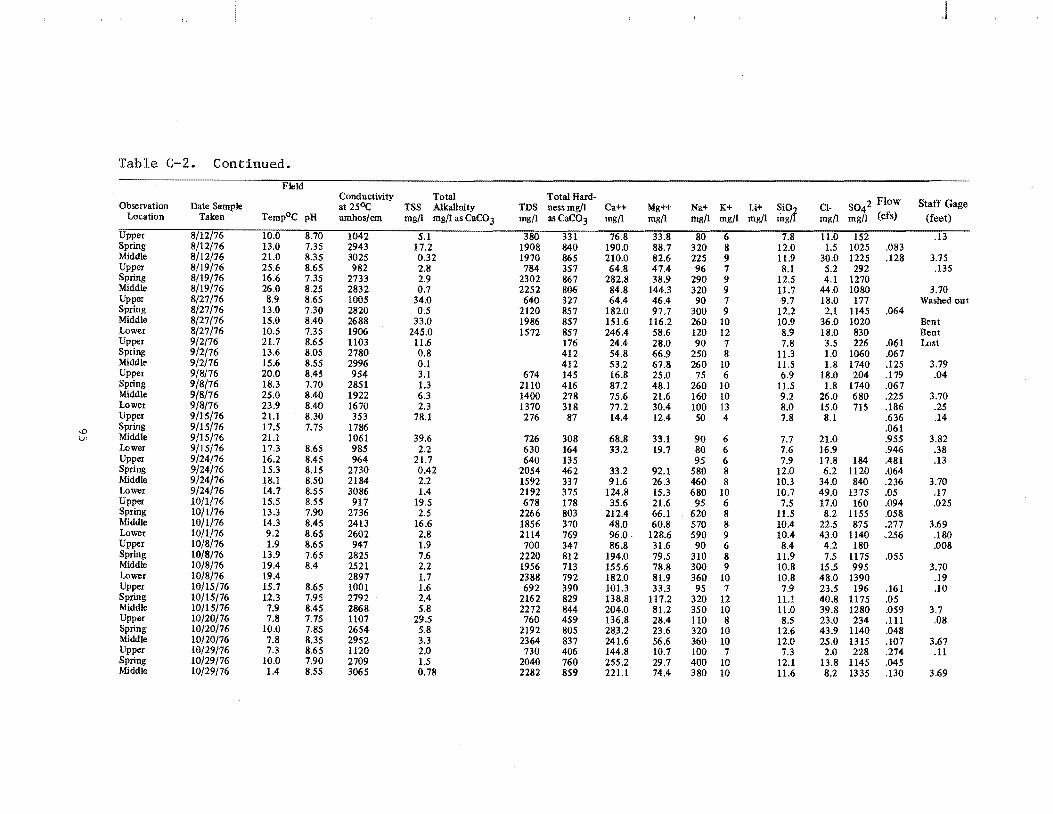
J

Table C-2. Continued.

Field Conductivity Total Total Hard-

CI- S042 Flow Staff Gage Observation Date Sample at 250C TSS Alkalinity TDS ness mg/l Ca++ Mg++ Na+ K+ Li+ SiOJ Location Taken TempoC pH umhos/cm mgjI mg/I as CaC03 mg/l as CaC03 mg/l mg/l mg/l mg/l mgjl mg mg/l mgjl (cfs) (feet)

Upper 8/12/76 10.0 8.70 1042 5.1 380 331 76.8 33.8 80 6 7.8 11.0 152 .13 Spring 8/12/76 13.0 7.35 2943 17.2 1908 840 190.0 88.7 320 8 12.0 1.5 1025 .083 Middle 8/12/16 21.0 8.35 3025 0.32 1970 865 210.0 82.6 225 9 11.9 30.0 1225 .128 3.75 Upper 8/19/76 25.6 8.65 982 2.8 784 357 64.8 47.4 96 7 8.1 5.2 292 .135 Spring 8/19/76 16.6 7.35 2733 2.9 2302 867 282.8 38.9 290 9 12.5 4.1 1270 Middle 8/19/76 26.0 8.25 2832 0.7 2252 806 84.8 144.3 320 9 11.7 44.0 1080 3.70 Upper 8/27/76 8.9 8.65 1005 34.0 640 327 64.4 46.4 90 7 9.7 18.0 177 Washed out Spring 8/27/76 13.0 7.30 2820 0.5 2120 857 182.0 97.7 300 9 12.2 2.1 1145 .064 Middle 8/27/76 15.0 8.40 2688 33.0 1986 857 151.6 116.2 260 10 10.9 36.0 1020 Bent Lower 8/27/76 10.5 7.35 1906 245.0 1572 857 246.4 58.6 120 12 8.9 18.0 830 Bent Upper 9/2/76 21.7 8.65 1103 11.6 176 24.4 28.0 90 7 7.8 3.5 226 .061 Lost Spring 9/2/76 13.6 8.05 2780 0.8 412 54.8 66.9 250 8 11.3 1.0 1060 .067 Middle 9/2/76 15.6 8.55 2996 0.1 412 53.2 67.8 260 10 11.5 1.8 1740 .125 3.79 Upper 9/8/76 20.0 8.45 954 3.1 674 145 16.8 25.0 75 6 6.9 18.0 204 .179 .04 Spring 9/8/76 18.3 7.70 2851 1.3 2110 416 87.2 48.1 260 10 11.5 1.8 1740 .067 Middle 9/8/76 25.0 8.40 1922 6.3 1400 278 75.6 21.6 160 10 9.2 26.0 680 .225 3.70 Lower 9/8/76 23.9 8.40 1670 2.3 1370 318 77.2 30.4 100 13 8.0 15.0 715 .186 .25 Upper 9/15/76 21.1 8.30 353 78.1 276 87 14.4 12.4 50 4 7.8 8.1 .636 .14

'" Spring 9/15/76 17.5 7.75 1786 .061

V1 Middle 9/15/76 21.1 1061 39.6 726 308 68.8 33.1 90 6 7.7 21.0 .955 3.82 Lower 9/15/76 17.3 8.65 985 2.2 630 164 33.2 19.7 80 6 7.6 16.9 .946 .38 Upper 9/24/76 16.2 8.45 964 21.7 640 135 95 6 7.9 17.8 184 .481 .13 Spring 9/24/76 15.3 8.15 2730 0.42 2054 462 33.2 92.1 580 8 12.0 6.2 1120 .064 Middle 9/24/76 18.1 8.50 2184 2.2 1592 337 91.6 26.3 460 8 10.3 34.0 840 .236 3.70 Lower 9/24/76 14.7 8.55 3086 1.4 2192 375 124.8 15.3 680 10 10.7 49.0 1375 .05 .17 Upper 1011/76 15.5 8.55 917 19.5 678 178 35.6 21.6 95 6 7.5 17.0 160 .094 .025 Spring 10/1/76 13.3 7.90 2736 2.5 2266 803 212.4 66.1 620 8 11.5 8.2 1155 .058 Middle 10/1/76 14.3 8.45 2413 16.6 1856 370 48.0 60.8 570 8 10.4 22.5 875 .277 3.69 Lower 10/1/76 9.2 8.65 2602 2.8 2114 769 96.0· 128.6 590 9 10.4 43.0 1140 .256 .180 Upper 10/8/76 1.9 8.65 947 1.9 700 347 86.8 31.6 90 6 8.4 4.2 180 .008 Spring 10/8/76 13.9 7.65 2825 7.6 2220 812 194.0 79.5 310 8 11.9 7.5 1175 .055 Middle 10/8/76 19.4 8.4 2521 2.2 1956 713 155.6 78.8 300 9 10.8 15.5 995 3.70 Lower 10/8/76 19.4 2897 1.7 2388 792 182.0 81.9 360 10 10.8 48.0 1390 .19 Upper 10/15/76 15.7 8.65 1001 1.6 692 390 101.3 33.3 95 7 7.9 23.5 196 .161 .10 Spring 10/15/76 12.3 7.95 2792 2.4 2162 829 138.8 117.2 320 12 11.1 40.8 1175 .05 Middle 10/15/76 7.9 8.45 2868 5.8 2272 844 204.0 81.2 350 10 11.0 39.8 1280 .059 3.7 Upper 10/20/76 7.8 7.75 1107 29.5 760 459 136.8 28.4 110 8 8.5 23.0 234 .111 .08 Spring 10/20/76 10.0 7.85 2654 5.8 2192 805 28.3.2 23.6 320 10 12.6 43.9 1140 .048 Middle 10/20/76 7.8 8.35 2952 3.3 2364 837 241.6 56.6 360 10 12.0 25.0 1315 .107 3.67 Upper 10/29/76 7.3 8.65 1120 2.0 730 406 144.8 10.7 100 7 7.3 2.0 228 .274 .11 Spring 10/29/76 10.0 7.90 2709 1.5 2040 760 255.2 29.7 400 10 12.1 13.8 1145 .045 Middle 10/29/76 1.4 8.55 3065 0.78 2282 859 221.1 74.4 380 10 11.6 8.2 1335 .130 3.69

Page 106

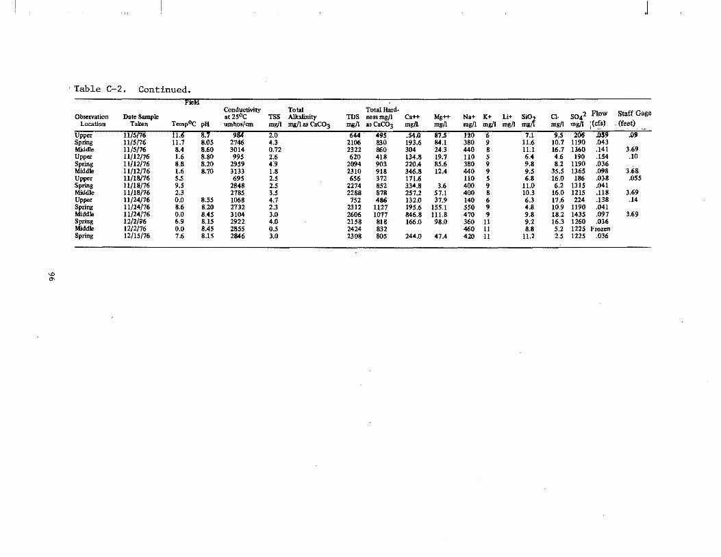
\0 0'

I Table C-2. Continued. "T!ela"

Observation Date Sample Location Taken TempoC pH

Upper 11/5/76 h.6 8.1 Spring 11/5/76 11.7 8.05 Middle 11/5/76 8.4 8.60 Upper 11/12/76 1.6 8.80 Spring 11/12/76 8.8 8.20 Middle 11/12/76 1.6 8.70 Upper 11/18/76 5.5 Spring 11/18/76 9.5 Middle 11/18/76 2.3 Upper 11/24/76 0.0 8.55 Spring 11/24/76 8.6 8.20 Middle 11/24/76 0.0 8.45 Spring 12/2/'i/6 6.9 8.15 Middle 12/2/76 0.0 8.45 Spring 12/15/76 7.6 8.15

Conductivity Total Total Hard-at 25°C TSS Alkalinity TDS ness mgt! umhos/em mgt! mg/I as CaC03 mg/! as CaC03

984 2.0 644 495 2746 4.3 2106 830 3014 0.72 2322 860 995 2.6 620 418

2959 4:9 2094 903 3133 1.8 2310 918 695 2.5 656 372

2848 2.5 2274 852 2785 3.5 2288 878 1068 4.7 752 486 2732 2.3 2312 1127 3104 3.0 2606 1077 2922 4.0 2158 818 2855 0.5 2424 832 2846 3.0 2308 805

J

C!. SO 2 Flow Staff Gage Ca++ Mg++ Na+ K+ Li+ SiOl mg/1 mg/! mgt! mg/l mg/l mg mg/t mgh :(cfs) I (feet)

I '".

.54.0 87.5 120 6 7.1 9.5 206 .039 .09 193.6 84.1 380 9 11.6 U).7 1190 .043 304 24.3 440 8 11.1 16.7 1360 .141 3.69 134.8 19.7 110 5 6.4 4.6 190 .154 .10 22Q.4 85.6 380 9 9.8 8.2 1190 .036 346.8 12.4 440 9 9.5 35.5 1365 .098 3.68 171.6 110 5 6.8 16.0 186 .038 .055 334.8 3.6 400 9 11.0 6.2 1315 .041 257.2 57.1 400 8 10.3 16.0 1215 .118 3.69 132.0 37.9 140 6 6.3 17.6 224 .138 .14 195.6 155.1 550 9 4.8 10.9 1190 .041 846.8 111.8 470 9 9.8 18.2 1435 .097 3.69 166.0 98.0 360 11 9.2 16.3 1260 .036

460 II 8.8 5.2 1225 Frozen 244.0 47.4 420 11 11.2 2.5 1225 .036

Page 107

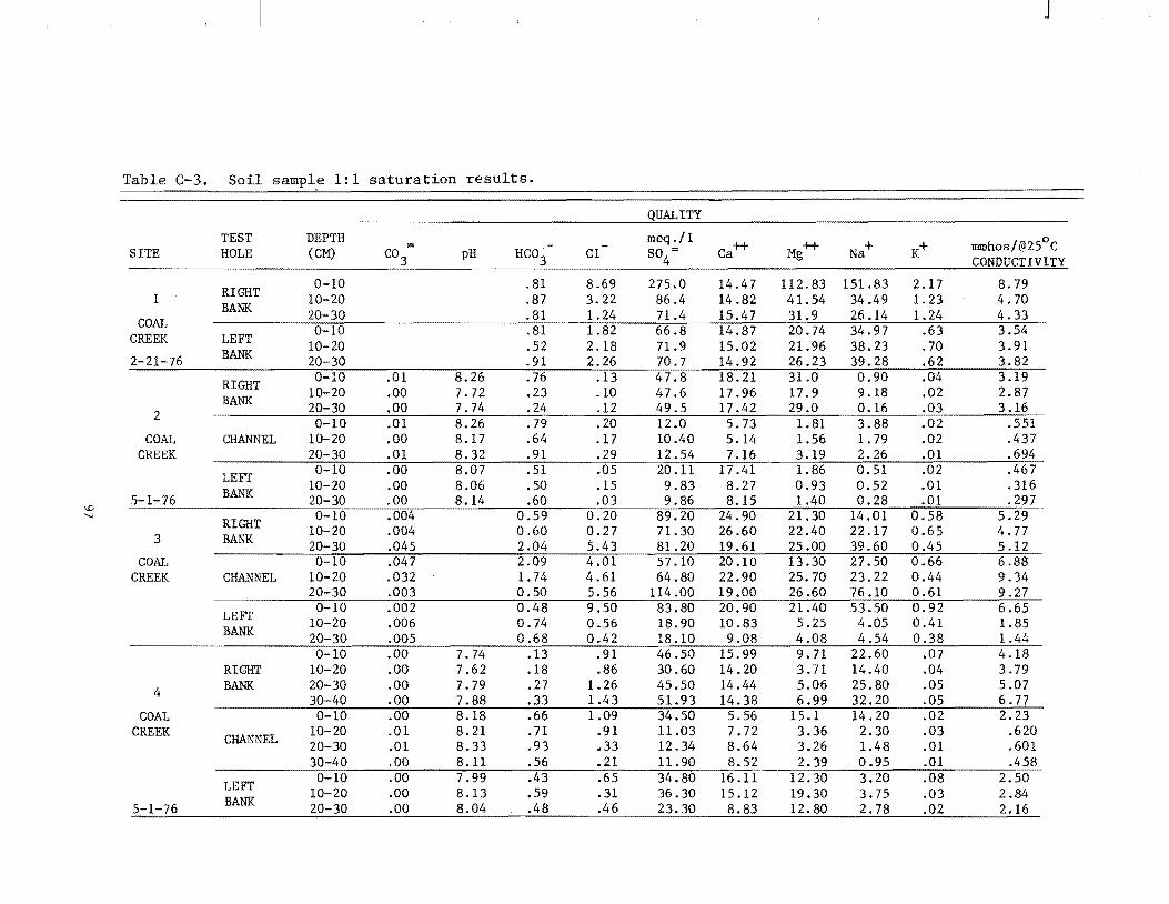
J

Table C-3. Soil sampl~ 1:1 saturation results. -------

QUALITY

TEST DEPTH meq ./1 Ca++ Mg++ Na+ K+ mmhos/@250C SITE HOLE (CM) pH Cl

RIGHT 0-10 .81 8.69 275.0 14.47 112.83 151.83 2.17 8.79 1 10-20 .87 3.22 86.4 14.82 41.54 34.49 1.23 4.70 BANK 20-30 .81 1.24 71.4 15.47 31.9 26.14 1.24 4.33 COAL 0-10 .81 1.82 66.8 14.87 20.74 34.97 .63 3.54 CREEK LEFT 10-20 .52 2.18 71.9 15.02 21.96 38.23 .70 3.91

2-21-76 BANK 20-30 .91 2.26 70.7 14.92 26.23 39.28 .62 3.82

RIGHT 0-10 .01 8.26 .76 .13 47.8 18.21 31.0 0.90 .04 3.19 10-20 .00 7.72 .23 .10 47.6 17.96 17.9 9.18 .02 2.87 BANK 20-30 .00 7.74 .24 .12 49.5 17.42 29.0 0.16 .03 3.16 2 0-10 .01 8.26 .79 .20 12.0 5.73 1.81 3.88 .02 .551

COAL CHANNEL 10-20 .00 8.17 .64 .17 10.40 5.14 1.56 1. 79 .02 .437 CREEK 20-30 .01 8.32 .91 .29 12.54 7.16 3.19 2.26 .01 .694

LEFT 0-10 .00 8.07 .51 .05 20.11 17.41 1.86 0.51 .02 .467 10-20 .00 8.06 .50 .15 9.83 8.27 0.93 0.52 .01 .316

5-1-76 BANK 20-30 .00 8.14 .60 .03 9.86 8.15 1.40 0.28 .01 .297 \0

0-10 .004 0.59 0.20 89.20 24.90 21.30 14.01 0.58 5.29 "-J

RIGHT 10-20 .004 0.60 0.27 71.30 26.60 22.40 22.17 0.65 4.77 3 BANK 20-30 .045 2.04 5.43 81.20 19.61 25.00 39.60 0.45 5.12 COAL 0-10 .047 2.09 4.01 57.10 20.10 13.30 27.50 0.66 6.88

CREEK CHANNEL 10-20 .032 1. 74 4.61 64.80 22.90 25.70 23.22 0.44 9.34 20-30 .003 0.50 5.56 114.00 19.00 26.60 76.10 0.61 9.27

LEFT 0-10 .002 0.48 9.50 83.80 20.90 21.40 53.50 0.92 6.65 10-20 .006 0.74 0.56 18.90 10.83 5.25 4.05 0.41 1.85 BANK 20-30 .005 0.68 0.42 18.10 9.08 4.08 4.54 0.38 1.44 0-10 .00 7.74 .13 .91 46.50 15.99 9.71 22.60 .07 4.18

RIGHT 10-20 .00 7.62 .18 .86 30.60 14.20 3.71 14.40 .04 3.79

4 BANK 20-30 .00 7.79 .27 1.26 45.50 14.44 5.06 25.80 .05 5.07 30-40 .00 7.88 .33 1.43 51.93 14.38 6.99 32.20 .05 6.77

COAL 0-10 .00 8.18 .66 1.09 34.50 5.56 15.1 14.20 .02 2.23 CREEK CHANNEL 10-20 .01 8.21 .71 .91 11.03 7.72 3.36 2.30 .03 .620

20-30 .01 8.33 .93 .33 12.34 8.64 3.26 1.48 .01 .601 30-40 .00 8.11 .56 .21 11.90 8.52 2.39 0.95 .01 .458

LEFT 0-10 .00 7.99 .43 .65 34.80 16.11 12.30 3.20 .08 2.50 10-20 .00 8.13 .59 .31 36.30 15.12 19.30 3.75 .03 2.84

5-1-76 BANK 20-30 .00 8.04 .48 .46 23.30 8.83 12.80 2.78 .02 2.16

Page 108

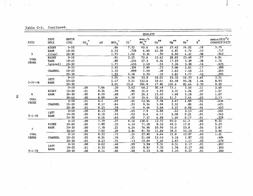
J

Table C-3. Continued.

QUALITY

TEST DEPTH =

meq ./1 Ca++ Mg++ Na+ K+

mmhos/@250C - -SITE HOLE (CM) C03 pH HC03 Cl SO = CONDUCTIVITY 4 RIGHT 0-10 .84 7.32 40.6 6.64 27.45 24.01 .18 3.79 BANK 10-20 1.53 .738 6.90 11.39 4.87 4.74 .10 .717

5 (clay) 20-30 1. 75 1.02 8.34 .70 6.90 4.31 .08 .942

COAL RIGHT 0-10 .81 2.25 70.6 15.42 28.85 23.49 .77 4.81 BANK 10-20 .88 .254 27.3 6.34 17.19 5.39 .38 1.76 CREEK (gravel) 20-30 1. 75 .455 2.40 .53 7.26 3.38 .16 .625

0-10 1.92 .301 2.90 .73 2.06 2.61 .17 .388 CHANNEL 10-20 1.53 .099 ·1.09 .28 1.62 1.49 .11 .265

20-30 1.92 4.18 0.20 .33 3.82 1.77 .10 .295

LEFT 0-10 1.04 4.46 53.8 18.01 25.33 16.70 1.61 3.51

2-21-76 BANK 10-20 1.47 3.11 152.6 18.01 61.59 95.26 1.56 8.95 20-30 2.01 12.6 204.9 17.81 124.6 81.64 2.33 9.50 0-10 .00 7.66 .20 3.42 48.2 30.49 17 .1 5.05 .11 2.60

RIGHT 10-20 .01 8.24 .76 .86 11.0 5.93 3.31 4.26 .07 1.07 \0

6 BANK 20-30 .00 8.19 .68 .97 26.3 15.40 7.69 5.18 .07 1.67 co 30-40 .00 8.09 .54 1.10 35.6 22.53 11.7 2.44 .03 2.13 COAL 0-10 .01 8.2 .69 .24 12.94 7.78 3.67 1.89 .01 .634 CREEK CHANNEL 10-20 .00 8.17 .64 .20 9.54 5.99 2.52 .80 .01 .421

20-30 .01 8.25 .78 .16 9.46 5.68 2.37 0.98 .01 .405

LEFT 0-10 .00 8.13 .59 .05 7.9 4.88 .42 3.15 .01 .181

5-1-76 BANK 10-20 .00 8.10 .55 .03 6.4 6.17 1.08 0.21 .01 .245 20-30 .00 8.16 .63 .00 7.57 6.98 1.40 0.17 .01 .229 0-10 .00 7.79 .27 6.16 138.0 12.72 93~0 41.3 .06 9.22

RIGHT 10-20 .01 7.90 .35 4.10 71. 2() 8.33 49.3 17 .8 .03 5.25

7 BANK 20-30 .00 7.78 .21 4.24 70.90 10.99 55.0 15.8 .04 5.87 30-40 .00 7.82 .29 3.84 81.70 11.60 59.0 13.10 .02 5.86

COAL 0-10 .01 8.22 .72 .31 27.90 4.44 11.9 12.97 .02 1.21 CREEK CHANNEL 10-20 .01 8.24 .76 .21 21.68 15.43 5.16 1.87 .02 .484

20-30 .01 8.23 .74 .13 10.60 7.16 2.67 1.11 .02 .476

LEFT 0-10 .00 8.02 .46 .09 5.98 5.31 0.51 0.17 .01 .207

BANK 10-20 .01 8.35 .98 .03 8.87 7.35 1.76 0.17 .02 .302 5-1-76 20-30 .00 8.14 .60 .08 6.23 5.56 1.25 0.27 .01 .260

Page 109

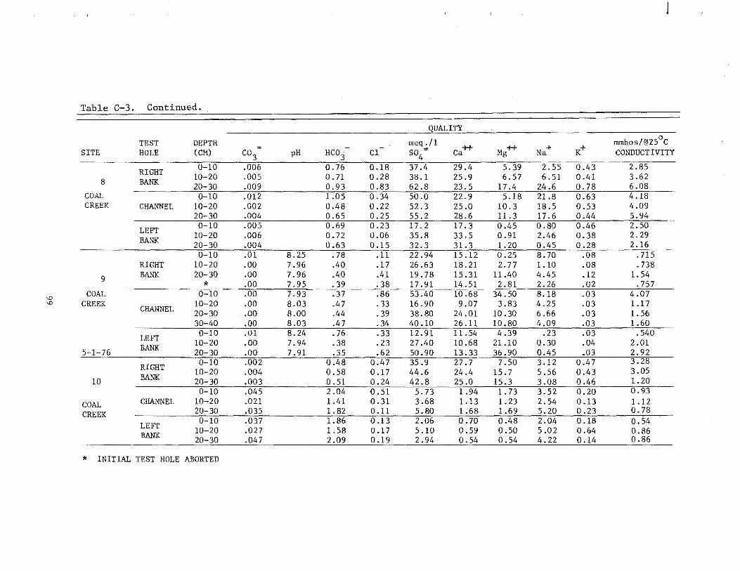
J

Table C-3. Continued

gUALITY:

TEST DEPTH meq ./1 Ca++ Mg++ Na+ K+

mmhos/@250C (CM)

=: SO =: CONDUCTIVITY SITE HOLE C03 pH HC03 C1 4

RIGHT 0-10 .006 0.76 0.18 37.4 29.4 5.39 2.55 0.43 2.85 10-20 .005 0.71 0.28 38.1 25.9 6.57 6.51 0.41 3.62

8 BANK 20-30 .009 0.93 0.83 62.8 23.5 17.4 24.6 0.78 6.08 COAL 0-10 .012 1.05 0.34 50.0 22.9 5.18 21.8 0.63 4.18 CREEK CHANNEL 10-20 .002 0.48 0.22 52.3 25.0 10.3 18.5 0.53 4.09

20-30 .004 0.65 0.25 55.2 28.6 11.3 17.6 0.44 5.94

LEFT 0-10 .005 0.69 0.23 17.2 17.3 0.45 0.80 0.46 2.50 10-20 .006 0.72 0.06 35.8 33.5 0.91 2.46 0.38 2.29

BANK 20-30 .004 0.63 0.15 32.3 31.3 1.20 0.45 0.28 2.16 0-10 .01 8.25 .78 .11 22.94 15.12 0.25 8.70 .08 .715

RIGHT 10-20 .00 7.96 .40 .17 26.63 18.21 2.77 1.10 .08 .738

9 BANK 20-30 .00 7.96 .40 .41 19.78 15.31 11.40 4.45 .12 1. 54

* .00 7.95 .39 .38 17.91 14.51 2.81 2.26 .02 .757

\0 COAL 0-10 .00 7.93 .37 .86 53.40 10 .68 34.50 8.18 .03 4.07

\0 CREEK 10-20 .00 8.03 .47 .33 16.90 9.07 3.83 4.25 .03 1.17 CHANNEL 20-30 .00 8.00 .44 .39 38.80 24.01 10.30 6.66 .03 1. 56 30-40 .00 8.03 .47 .34 40.10 26.11 10.80 4.09 .03 1.60

LEFT 0-10 .01 8.24 .76 .33 12.91 11.54 4.39 .23 .03 .540 10-20 .00 7.94 .38 .23 27.40 10.68 21.10 0.30 .04 2.01

5-1-76 BANK 20-30 .00 7.91 .35 .62 50.90 13.33 36.90 0.45 .03 2.92

RIGHT 0-10 .002 0.48 0.47 35.9 27.7 7.50 3.12 0.47 3.28 10-20 .004 0.58 0.17 44.6 24.4 15.7 5.56 0.43 3.05

10 BANK 20-30 .003 0.51 0.24 42.8 25.0 15.3 3.08 0.46 1.20 0-10 .045 2.04 0.51 5.73 1.94 1. 73 3.52 0.20 0.93

COAL CHANNEL 10-20 .021 1.41 0.31 3.68 1.13 1.23 2.54 0.13 1.12 CREEK 20-30 .035 1.82 0.11 5.80 1.68 1.69 5.20 0.23 0.78

LEFT 0-10 .037 1.86 0.13 2.06 0.70 0.48 2.04 0.18 0.54 10-20 .027 1.58 0.17 5.10 0.59 0.50 5.02 0.64 0.86 BANK 4.22 0.14 0.86

* INITIAL TEST HOLE ABORTED

Page 110

.I

Table C-3. Continued.

QUALITY

TEST DEPTH = - meq. 11 Ca++ Mg++ Na+ K+

mmhos/@250C (CM) - SO = CONDUCTIVITY SITE HOLE C03

pH HC03 Cl 4

RIGHT 0-10 1.07 .475 32.7 19.21 9.77, .82 .68 1.98 11 BANK 10-20 1.03 .408 34.6 20.69 12.92 .66 .84 2.02

20-30 .455 31.9 19.11 9.11 1.07 .74 2.28 WEST 0-10 1.01 .341 21.9 8.63 10.29 4.74 .32 1.31 TRIBUTARY CHANNEL 10-20 1.23 .498 35.5 15.57 10.5 7.57 .35 1.65

20-30 .91 .337 38.9 18.41 12.07 5.26 .30 1.88

LEFT 0-10 .40 1.14 .376 7.93 2.54 5.08 1.11 .922

2-21-76 BANK 10-20 1.07 .337 33.4 18.46 13.06 .94 .43 1.66 20-30 .91 .652 37.9 18.41 15.13 2.45 .35 2.19 0-10 .107 3.16 8.39 119.0 20.81 7.28 100.3 0.65 17.4

RIGHT 10-20 .039 1.90 4.35 106.0 22.8 18.5 74.9 0.50 8.9

12 BANK 20-30 .019 1.32 5.30 130.0 19.86 8.24 107.0 0.48 11.66 30-40 .018 1.29 2.93 79.0 15.82 6.32 50.2 0.40 9.01

.... WEST 0-10 .013 1.12 0.11 28.2 25.95 3.93 1.48 0.47 1.81 0

TRIBUTARY CHANNEL 10-20 .009 .93 0.08 21.8 19.51 2.74 0.94 0.45 1.38 0

20-30 .007 .81 0.15 21.7 17.57 2.31 2.06 0.37 2.46

LEFT 0-10 .007 0.79 0.20 22.1 22.90 0.71 0.22 0.45 2.35

BANK 10-20 .005 0.68 0.16 23.4 24.1 0.52 0.29 0.46 2.23 20-30 .005 0.69 0.16 33.8 31.4 1.90 1.2 0.49 2.32

RIGHT 0-10 .054 2.24 3.90 151.00 21.36 42.20 87.80 0.67 18.9 10-20 .014 1.15 0.91 81.20 22.01 13.20 44.50 0.47 6.41

13 BANK 20-30 .004 0.59 1.13 92.70 18.06 14.60 57.20 0.47 11.48

WEST 0-10 .022 1.44 3.95 134.00 25.65 35.20 77.30 0.81 23.5 TRIBUTARY CHANNEL 10-20 .007 0.81 2.11 92.00 13.37 13.50 67.68 0.57 14.66

20-30 .001 0.32 1.62 96.40 19.31 17.30 64.58 0.60 13.70

LEFT 0-10 .014 1.15 0.92 46.10 26.05 9.13 10.11 0.75 4.82

BANK 10-20 .007 0.83 0.85 46.90 26.95 10.00 15.30 0.89 4.67 20-30 .001 0.36 0.92 64.40 26.35 11.60 27.35 6.10 5.39

RIGHT 0-10 .005 0.69 0.50 46.8 24.90 6.19 16.4 0.55 6.98

BANK 10-20 .006 0.74 0.64 61.6 19.3 12.6 34.5 0.40 6.75 14 20-30 .011 1.00 0.92 84.2 22.8 21.7 44.2 0.52 6.48

WEST 0-10 .007 0.83 0.60 49.9 13.8 6.27 32.7 0.55 6.03

TRIBUTARY CHANNEL 10-20 .006 0.72 0.68 63.0 24.0 6.71 32.3 0.46 6.55 20-30 .011 0.76 0.41 70.5 25.7 13.8 32.0 0.48 6.48

LEFT 0-10 .045 2.04 2.25 110. 17.7 20.7 72.4 0.89 4.52

BANK 10-20 .029 1.66 1.95 98.9 19.0 23.5 61.0 0.68 7.67 20-30 .003 0.55 1.28 83.6 20.1 11.8 52.1 0.63 8.24

Page 111

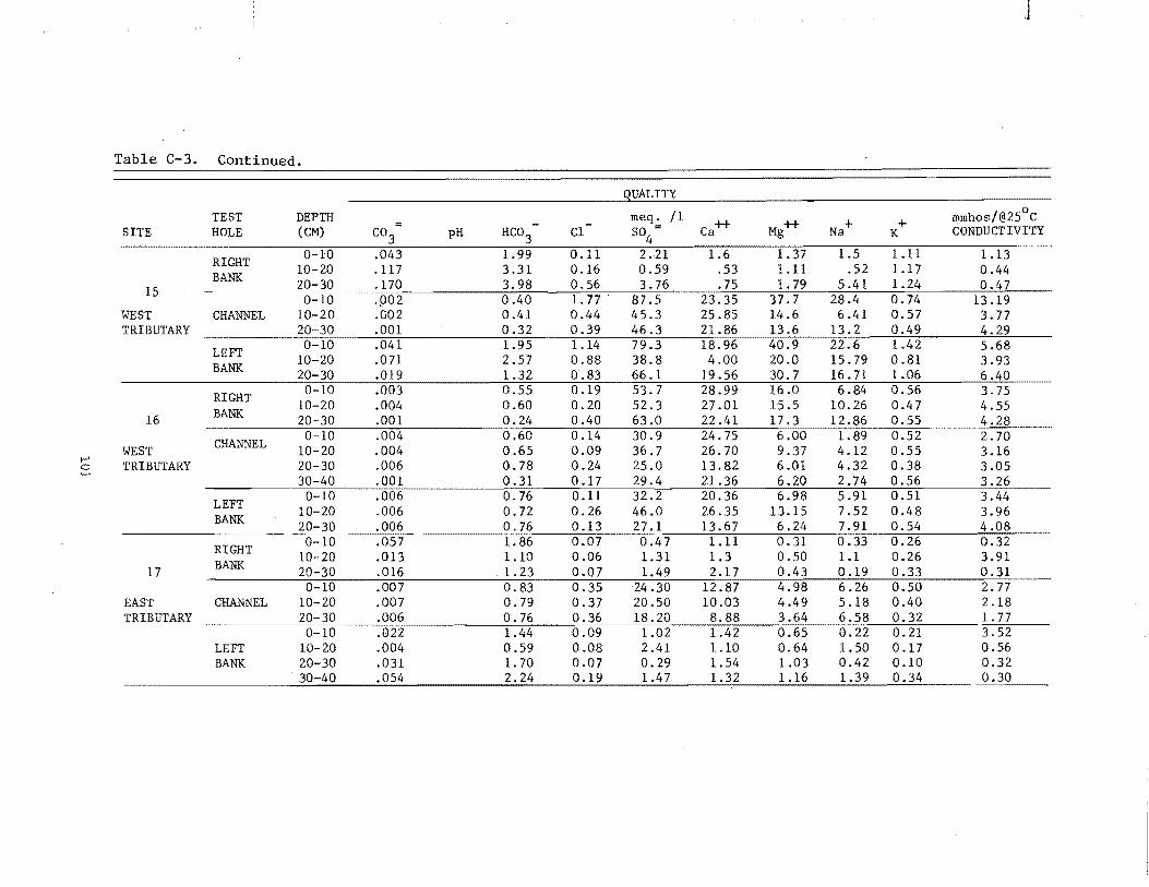
J

Table C-3. Continued.

gUALITY

TEST DEPTH meq. 11 Ca++ Mg++ Na+ + mmhos/@250C

(CM) Cl - SO = CONDUCTIVITY SITE HOLE C03 pH HC03 4 K

RIGHT 0-10 .043 1.99 0.11 2.21 1.6 1.37 1.5 1.11 1.13 10-20 .117 3.31 0.16 0.59 .53 1.11 .52 1.17 0.44 BANK 20-30 .170 3.98 0.56 3.76 .75 1. 79 5.41 1.24 0.47 15 -------------

0-10 :902 1.77" 23.35 37.7 28.4 0.74 0.40 87.5 13.19 WEST CHANNEL 10-20 .G02 0.41 0.44 45.3 25.85 14.6 6.41 0.57 3.77 TRIBUTARY 20-30 .001 0.32 0.39 46.3 21.86 13.6 13.2 0.49 4.29

LEFT 0-10 .041 1.95 1.14 79.3 18.96 40.9 22.6 1.42 5.68 10-20 .071 2.57 0.88 38.8 4.00 20.0 15.79 0.81 3.93 BANK 20-30 .019 1.32 0.83 66.1 19.56 30.7 16.71 1.06 6.40

RIGHT 0-10 .003 0.55 0.19 53.7- 28.99 16.0 6.84 0.56 3.75 10-20 .004 0.60 0.20 52.3 27.01 15.5 10.26 0.47 4.55

16 BANK 20-30 .001 0.24 0.40 63.0 22.41 17.3 12.86 0.55 4.28

CHANNEL 0-10 .004 0.60 0.14 30.9 24.75 6.00 1. 89 0.52 2.70 WEST 10-20 .004 0.65 0.09 36.7 26.70 9.37 4.12 0.55 3.16

t-' TRIBUTARY 20-30 .006 0.78 0.24 25.0 13.82 6.01 4.32 0.38 3.05 0 t-' 30-40 .001 0.31 0.17 29.4 21.36 6.20 2.74 0.56 3.26

LEFT 0-10 .006 0.76 0.11 32.2 20.36 6.98 5.91 0.51 3.44 10-20 .006 0.72 0.26 46.0 26.35 13.15 7.52 0.48 3.96 BANK 20-30 .006 0.76 0.13 27.1 13.67 6.24 7.91 0.54 4.08

RIGHT 0-10 .057 1. 86 0.07 0.47 1.11 0.31 0.33 0.26 0.32 10-20 .013 1.10 0.06 1.31 1.3 0.50 1.1 0.26 3.91

17 BANK 20-30 .016 _ 1.23 0.07 1.49 2.17 0.43 0.19 0.33 0.31 0-10 .007 0.83 0.35 24.30 12.87 4.98 6.26 0.50 2.77

EAST CHANNEL 10-20 .007 0.79 0.37 20.50 10.03 4.49 5.18 0.40 2.18 TRIBUTARY 20-30 .006 0.76 0.36 18.20 8.88 3.64 6.58 0.32 1.77

0-10 .022 1.44 0.09 1.02 1.42 6.65 0.22 0.21 3.52 LEFT 10-20 .004 0.59 0.08 2.41 1.10 0.64 1.50 0.17 0.56 BANK 20-30 .031 1. 70 0.07 0.29 1.54 1.03 0.42 0.10 0.32

30-40 .054 2.24 0.19 1.47 1.32 1.16 1.39 0.34 0.30

Page 112

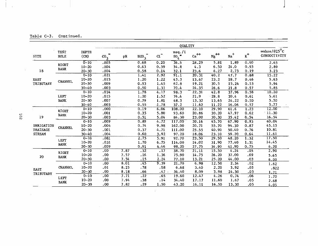
J

Table C-3. Continued.

QUALITY . 0

TEST DEPTH meq./l mmhos/@25 C (CM)

.. - - Ca+t Mg+t Na+ K+ CONDUCTIVITY SITE HOLE C03 pH Hoo3 Cl SO ..

4

RIGHT 0-10 .005 0.68 0.20 36.5 28.29 5.81 1.89 0.40 2.65 10-20 .004 0.63 0.39 34.8 4.3 6.50 24.0 0.93 2.89

18 BANK 20-30 .004 0.58 0.14 32.1 23.6 6.27 2.73 0.19 3.23 0-10 .021 1.41 2.92 91.1 20.31 40.2 47.7 0.88 15.22

EAST CHANNEL 1O~20 .015 1.20 1.22 43.3 13.67 23.2 18.7 0.46 5.63 TRIBUTARY 20-30 .009 0.93 1.45 62.8 19.21 30.5 15.24 0.53 5.94

30-40 .003 0.50 1.31 70.4 24.35 26.6 21.8 0.57 5.85 0-10 .034 1. 78 4.17 98.3 22.31 42.8 37.96 0.58 10.20

LEFl' 10-20 .015 1.20 1.52 76.4 21.9 28.8 30.4 0.61 5.61 BANK 20-30 .007 0.79 1.81 48.3 13.32 13.65 24.22 0.50 5.50

30-40 .003 0.55 ·1.78 37.2 11.62 11.22 16.06 0.57 5.77

RIGHT 0-10 .000 0.19 6.06 108.00 22.10 29.90 61.6 1.23 12.00 I-' BANK 10-20 .001 0.35 5.80 93.60 20.86 30.20 47.97 0.62 . 11.30 0 19 20-30 .003 0.51 5.04 84.30 23.00 30.30 35.42 0.54 16.54 tv

0-10 .009 0.89 4.72 117.00 20.16 45.70 67.90 0.93 40.04 IRRIGATION

CHANNEL 10-20 .006 0.74 9.98 162.00 20.71 55.70 94.30 0.87 45.15 DRAINAGE 20-30 .001 0.37 4.71 111.00 25.55 40.90 50.40 0.76 10.81 STREAM 30-40 .004 0.60 3.92 97.20 18.06 23.10 59.20 0.64 11.61

LEFl' 0-10 .081 2.75 5.91 92.70 23.50 29.50 48.20 1.32 17.50 10-20 .031 1. 70 6.75 114.00 14.02 31.90 77.40 1.31 14.45

BANK 20-30 .009 0.91 4.46 98.20 27.75 34.90 41.90 0.75 6.20

RIGHT 0-10 .00 7.87 .32 .17 38.70 21.11 15.50 4.24 .05 2.90

20 BANK 10-20 .00 7.57 .16 1.36 75.90 14.75 26.20 37.00 .09 5.65 20-30 .00 7.54 .15 2.24 77.10 13.21 25.20 44.00 .03 6.00 0-10 .00 8.01 .45 9.39 21.70 6.98 12.50 2.34 .02 1.62

EAST CHANNEL 10-20 .01 8.25 .78 .08 6.68 3.40 2.20 3.92 .03 .822 TRIBUTARY 20-30 .00 8.18 .66 .47 . 34.40 8.09 3.98 24.30 .03 1.Zl

LEFl' 0-10 .00 7.71 .22 .65 19.60 12.47 4.26 0.74 .06 1. 70 BANK

10-20 .00 7.94 .38 .14 34.40 17.17 11.60 1.67 .05 2.68 20-30 .00 7.82 .29 1.50 43.20 16.11 16.50 13.30 .05 4.05

Page 113

J

Table C-4. Coal Creek weather data.

Duration

Lower 56°F Lower 62°F ,Spring Middle 62°F 47.50 F 35% 0 Upper 56°F 40°F 22% Rain Gage

Installed Middle 4/29/76 1055 62°F 45.5OF 27% Not installed

yet Upper 4/29/76 1215 63°F 45°F 23% .05 Lower 4/29/76 0930 64°F 46°F 24% .03 Lower 4/30/76 1435 69°F 48°F 20% Upper 4/30/76 1705 64.5OF 44.5OF 17.5% Middle 4/30/76 1545 66°F 46°F 21% installed 4/30/76 Middle 5/1/.76 1445 Spring 5/1/76 1520 Lower 5/1/76 0900

'""' Upper 5/1/76 1700

0 Upper 5/6/76 1930 .11 Light w .07 Light

Middle 5/7/76 1145 .18 Upper 5/7/76 1330 .28 Lower 5/7/76 1430 .11

Rain Gage West 5/7/76 1235 .17 5/8 to .05 Light 5/14

Lower 5/13/76 1000 78.SoF 55°F 22% .07 Lower 5/14/76 1328 86°F 60°F 22% Upper 5/14/76 1452 85°F 58°F 20.5% .07 Middle 5/14/76 1658 81°F 56°F 20.5% Upper 5/20/76 0845 o Cloudy 5/20 .35 2 hours Lower 5/20/76 1000 67.30F 0

Rain Gage West 5/20/76 1500 n.8oF .02 Middle 5/20/76 1555 69°F 0 5/21 .35 2 1/2 hours Middle 5/21/76 0947 55.9O F .02

Page 114

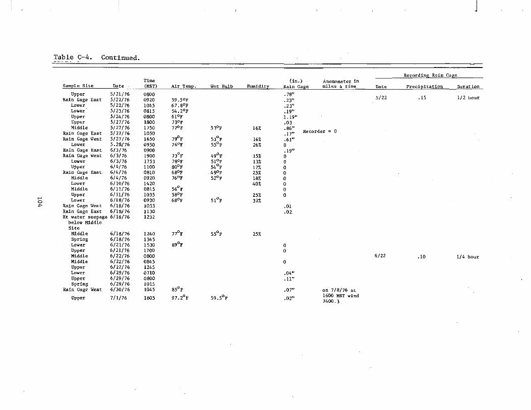
t-' o

""

J

Table C-4. Continued.

Recording Rain C~ge Time (in.) Anemometer in

Sample Site Date (MST) Air Temp. Wet Bulb Humidity Rain Gage miles & time Date Precipitation Duration

Upper 5/21/76 0800 .78" Rain Gage East 5/22/76 0920 59.50F .23"

Lower 5/22/76 1045 67.8oF .23" Lower 5/23/76 0815 54.2oF .19" Upper 5/24/76 0800 61°F 1.19" Upper 5/27/76 1800 nOF .03 Middle 5/27/76 1750 77°F 53°F 16% .86"

Rain Gage East 5/27/76 1050 .17" Recorder = 0 Rain Gage West 5/27/76 1650 79°F 53°F 16% .61"

Lower 5.28/76 0950 76°F 55°F 26% 0 Rain Gage East 6/3/76 0900 .19" Rain Gage West 6/3/76 1900 73°F 49°F 15% 0

Lower 6/3/76 1753 780F 51°F 13% 0 Upper 6/4/76 1100 80°F 54°F 17% 0

Rain Gage East- 6/4/76 0810 680F . 49°F 25% 0 Middle 6/4/76 0920 76°F 52°F 18% 0 Lower 6/10/76 1420 40% 0 Middle 6/11/76 0815 56°F 0 Upper 6/11/76 1035 58°F 25% 0 Lower 6/18/76 0930 68°F 51°F 32%

Rain Gage West 6/18/76 1053 Rain Gage East 6/18/76 1130 Ht water seepage 6/18/76 1232

below Middle Site Middle Spring Lower Upper Middle Middle Upper Lower Upper Spring

Rain Gage West

Upper

6/18/76 6/18/76 6/21/76 6/21/76 6/22/76 6/22/76 6/22/76 6/29/76 6/29/76 6/29/76 6/30/76

7/1/76

1240 1345 1530 1700 0800 0845 1245 0710 0800 1015 1045

1605

77°F

89°F

85°F

97.2°F

55°F 25%

59.50 F

.01

.02

o o

o

.04"

.11"

.07"

.02"

on 7/8/76 at 1600 MST wind 7400.3

5/22 .15 1/2 hour

6/22 .10 1/4 hour

Page 115

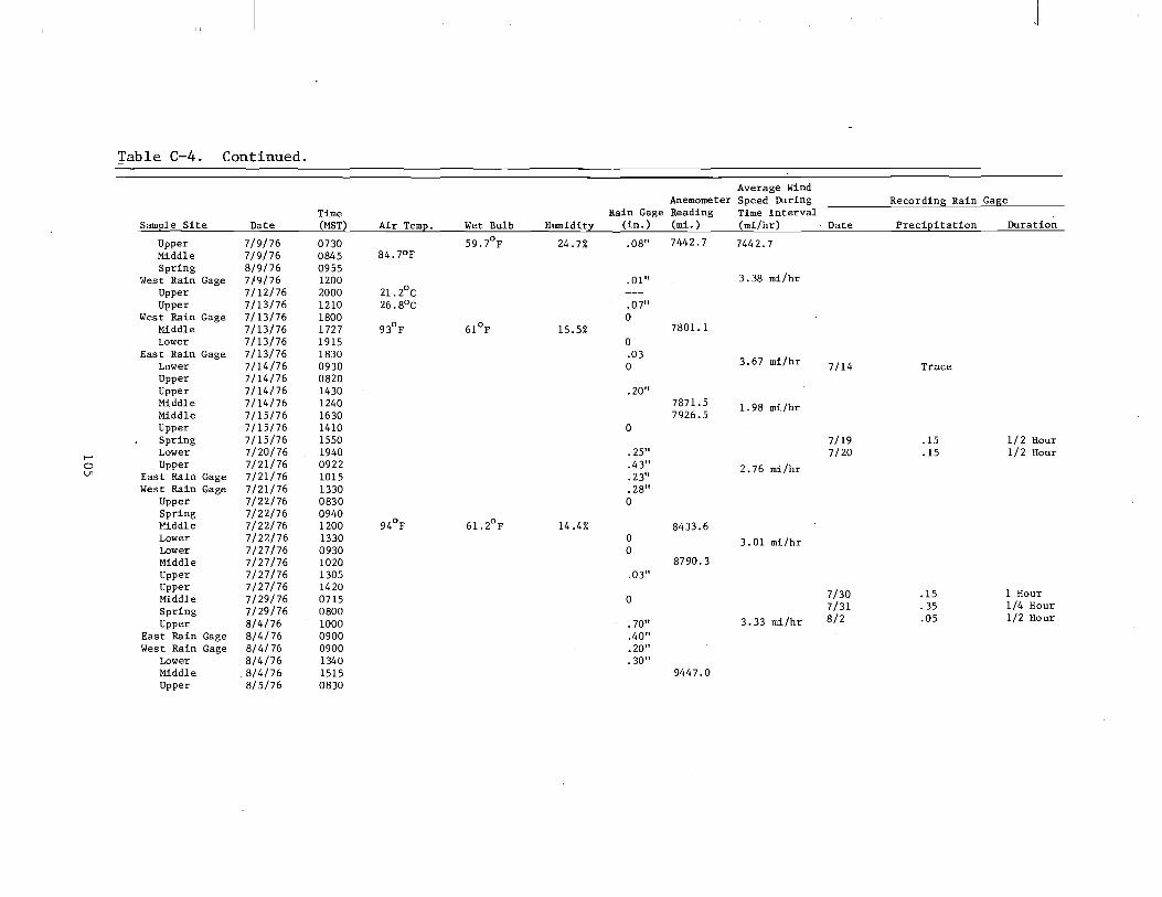
J

Table C-4. Continued.

Average Wind Anemometer Speed During Recording Rain Gage

Time Rain Gage Reading Time Interval Samj2le Site Date (MST) Air Temj2. Wet Bulb Humidit}:': (in. ) (mi. ) (mi/hr) Date PreciEitation Duration

Upper 7/9/76 0730 59.7oF 24.7% .08" 7442.7 7442.7 Middle 7/9/76 0845 84.7oF Spring 8/9/76 0955

West Rain Gage 7/9/76 1200 .01" 3.38 mi/hr Upper 7/12/76 2000 21. 2°C Upper 7/13/76 1210 26.8°C .07"

Wes·t Rain Gage 7/13/76 1800 0 Middle 7/13/76 1727 93°F 61°F 15.5% 7801.1 Lower 7/13/76 1915 0

East Rain Gage 7/13/76 1830 .03 3.67 mi/hr Lower 7/14/76 0930 0 7/14 Trace

Upper 7/14/76 0820 Upper 7/14/76 1430 .20" Middle 7/14/76 1240 7871. 5 1.98 mi/hr Middle 7/15/76 1630 7926.5 Upper 7/15/76 1410 0 Spring 7/15/76 1550 7/19 .15 1/2 Hour

,... Lower 7/20/76 1940 .25" 7/20 .15 1/2 Hour 0 Upper 7/21/76 0922 .43" 2.76 mi/hr lJl East Rain Gage 7/21/76 1015 .23"

West Rain Gage 7/21/76 1330 .28" Upper 7/22/76 0830 0 Spring 7/22/76 0940 Middle 7/22/76 1200 94°F 61. 2°F 14.4% 8433.6 Lower 7/22/76 1330 0 3.01 mi/hr Lower 7/27/76 0930 0 Middle 7/27/76 1020 8790.3 Upper 7/27/76 1305 .03" Upper 7/27/76 1420

7/30 .15 1 Hour Middle 7/29/76 0715 0 Spring 7/29/76 0800 7/31 .35 1/4 Hour

Upper 8/4/76 1000 .70" 3.33 mi/hr 8/2 .05 1/2 Hour

East Rain Gage 8/4/76 0900 .40" West Rain Gage 8/4/76 0900 .20"

Lower 8/4/76 1340 .30" Middle 8/4/76 1515 9447.0 Upper 8/5/76 0830

Page 116

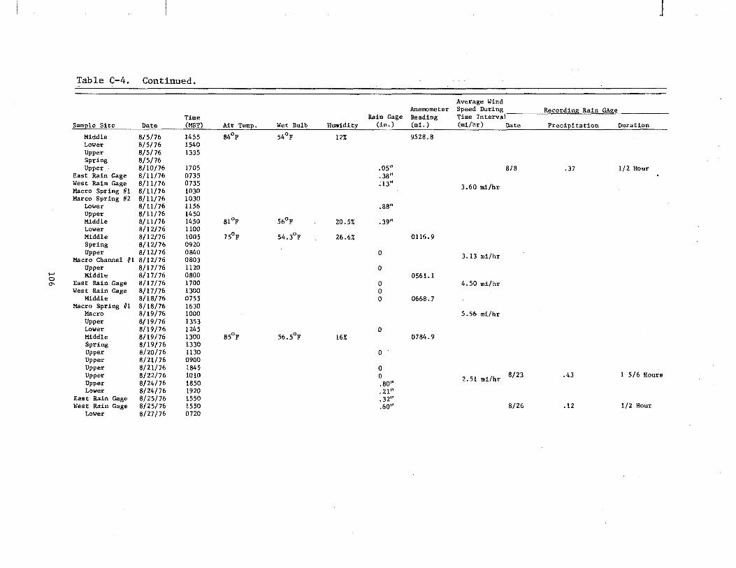
.J

Table C-4. Continued.

Average Wind Anemometer Speed During Recordi~ Rain GAge

Time Rain Gage Reading Time Interval SamEle Site Date (MST) Air Temp. Wet Bulb Humidity (in. ) (mi. ) (mi/hr) Date Precipitation Duration

Middle 8/5/16 1455 84°F 54°F 12% 9528.8 Lower 8/5/76 1540 Upper 8/5/76 1335 Spring 8/5/76 Upper - 8/10/76 1705 .05" 8/8 .37 1/2 Hour

East Rain Gage 8/11/76 0735 .38" West Rain Gage 8/11/76 0735 .13" 3.60 mi/hr Macro Spring III 8/11/76 1030 Marco Spring 1i2 8/U/76 1030

Lower 8/11/76 1156 .88" Upper 8/11/76 1450 Middle 8/11/76 1450 81°F 56°F 20.5% .39" Lower 8/12/76 1100 Middle 8/12/76 1005 75°F 54.3OF 26.6% 0116.9 Spring 8/12/76 0920 Upper 8/12/76 0840 0 3.13 mi/hr Macro Channel iiI 8/12/76 0803 Upper 8/17/76 1120 0

t--' Middle 8/17/76 0800 0561.1 0 0"- East Rain Gage 8/17/76 1700 0 4.50 mi/hr

West Rain Gage 8/17/76 1300 0 Middle 8/18/76 0755 0 0668.7

Macro Spring iiI 8/18/76 1630 Macro 8/19/76 1000 5.56 mi/hr Upper 8/19/76 1353 Lower 8/19/76 1245 0 Middle 8/19/76 1300 _ 85°F 56.50 F 16% 0784.9 Spring 8/19/76 1330 Upper 8/20/76 1130 0 Upper 8/21/76 0900 Upper 8/21/76 1845 0 Upper 8/22/76 1010 0 2.51 mi/hr 8/23 .43 1 5/6 Hours Upper 8/24/76 1850 .80" Lower 8/24/76 1920 .21"

East Rain Gage 8/25/76 1550 .32" West Rain Gage 8/25/76 1550 .60" 8/26 .12 1/2 Hour

Lower 8/27/76 0720

Page 117

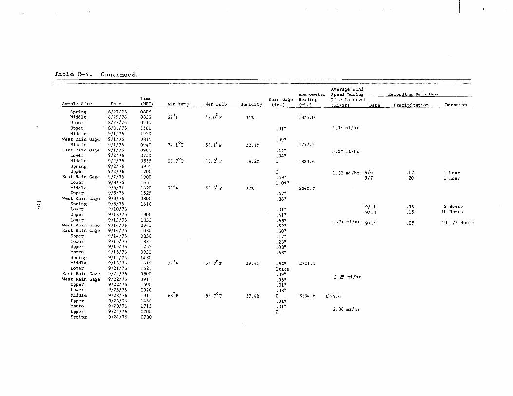
Table C-4. Continued.

Anemometer Recording Rain Ga~ _____

tation Duration

Upper 8/27/76 Upper 8/31/76 1500 .01" 5.08 mi/hr Middle 9/1/76 1920

West Rain Gage 9/1/76 0815 .09" Middle 9/1/76 0940 74.1oF 52.1oF 22.1% 1747.5

East Rain Gage 9/1/76 0900 .14" 3.27 rni/hr Lower 9/2/76 0750 .04" Middle 9/2/76 0855 69.7oF 48. 19.2% 0 1823.6 Spring 9/2/76 0955 Upper 9/2/76 1200 0 1.32 rni/hr 9/6 .12 1 Hour

East Rain Gage 9/7/76 1900 .49" 9/7 .20 1 Hour Lower 9/8/76 1655 1.09" Middle 9/8/76 1620 74°F 55. 32% 2260.7 Upper 9/8/76 1525 .42"

Hest Rain Gage 9/8/76 0800 .36" ,..... Spring 9/8/76 1610 0 9/11 .35 3 Hours '-.J Lower 9/10/76 .01" 9/13 .15 10 Hours Upper 9/13/76 1900 .41" Lower 9/13/76 1835 .63" 2.74 mi/hr 9/14 .05 10 1/2 Hours West Rain Gage 9/14/76 0945 .52"

East Rain Gage 9/14/76 1030 .60" Upper 9/14/76 0830 .17" Lower 9/15/76 1825 .28" Upper 9/15/76 1255 .08" Macro 9/15/76 0930 .63" Spring 9/15/76 1430 Middle 9/15/76 1615 7SoF 57.30 F 29.4% .52" 2721. 1 Lower 9/21/76 1525 Trace

East Rain Gage 9/22/76 0800 .09" 3.25 rni/hr West Rain Gage 9/22/76 0915 .05" Upper 9/22/76 1500 .01" Lower 9/23/76 0920 .03" Middle 9/23/76 1315 680 p 52.7op 37.4% 0 3334.6 3334.6 Upper 9/23/76 1450 .01" Macro 9/23/76 1715 .01" 2.30 mi/hr 9/24/76 0700 0

9/24/76 0730

Page 118

J

Table C-4. Continued.

Average Wind Anemometer Speed During Recordi~ Rain Gase

Time Rain Gage Reading Time Interval Samj!l1n& Site Date (MST) Air Tem!!. Wet Bulb Humiditl (in.) (mi. ) (mi/hr) Date Preci2itation Duration

Middle 9/24/76 0820 63.7oF 54.5O F 58.2% 0 3378.4 9/1.4 .05 2 1/4 Hours Lower 9/24/76 0920 0 9/25 .02 1 1/2 Hours Lower 9/30/76 1800 .06" 2.86 mi/hr West Rain Gage 9/30/76 1030 .02"

East Rain Gage 9/30/76 1010 .05" Upper lO/I/76 1200 .49" Middle 10/1/76 0925 65.54°F 49.4oF 32.4% .06" 3862.2 Lower 10/1/76 0815 0

Coal Spring 10/1/76 1040 Macro Rain Gage 10/1/76 1400 .44" 3.13 mi/hr East Rain Gage 10/6/76 1430 .44"

Lower 10/6/76 1015 .41" West Rain Gage 10/6/76 1345 .43"

Lower 10/7/76 0825 0 Macro Rain Gage 10/8/76 0945 .56" 10.2 .47 14 Hours

Spring 10/8/76 1335 .Lower 10/8/76 1510 0 I-' Middle 10/8/76 1435 65.7oF 46.2oF 20.7% .54" 4403.7 0

00 Upper 10/8/76 0907 .73" East Rain Gage 10/13/76 1450 0 West Rain Gage 10/13/76 1530 0

Lower 10/14/76 0900 0 2.65 mi/hr Upper 10/15/76 1600 0

Macro Rain Gage 10/15/76 1235 0 10/2 .47 14 Hours Middle 10/15/76 0845 57.3OF 41.30 F 23.6% 0 4833.8 Spring 10/15/76 1050 Lower 10/15/76 0745 Upper 10/20/76 1615 Spring 10/20/76 1645 Middle 10/20/76 1716 0

East Rain Gage 10/20/76 0 3.03 mi/hr 10/3 .04 12 Hours Macro Rain Gage 10/20/76 0 West Rain Gage 10/20/76 0 West Rain Gage 10/27/76 1630 0

Upper 10/27/76 1700 Lower 10/28/76 1535 0

Page 119

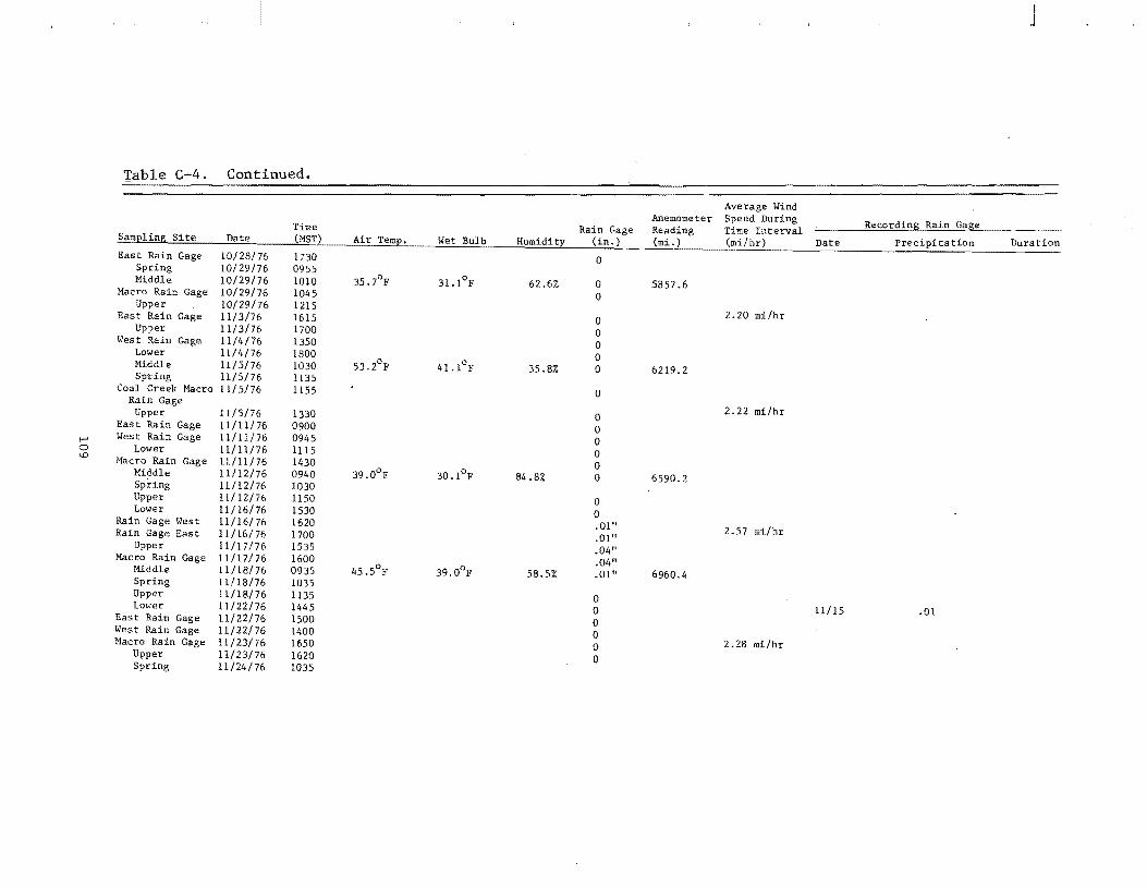
J

Table C-4. Continued.

Average Wind Anemometer Speed During Recording Rain Gage Time Rain Gage Reading Time Interval

SamEl ing Site Date (MST) Air Tero~. Wet Bulb Humidit;l! (in. ) Date Precipitation Duration East Rain Gage 10/28/76 1730 0

Spring 10/29/76 0955 Middle 10/29/76 1010 35 31. 1°F 62.6% 0 5857.6

Macro Rain Gage 10/29/76 1045 0 Upper 10/29/76 1215

2.20 mi/hr East Rain Gage 1113/76 1615 0 Upper 11/3/76 1700 0 West Rain Gage 11/4/76 1350 0 Lower 11/4/76 1800 0

Middle 11/5/76 1030 53.2op 41.1op 35.8% 0 6219.2 Spring 11/5/76 1135 Coal Creek Macro 11/5/76 1155 0 Rain Gage

2.22 mi/hr Upper 11/5/76 1330 0 Eas t Rain Gage 11/11/76 0900 0

..... West Rain Gage 11/11/76 0945 0 0 Lower 11/11/76 1115 0 1.0 Macro Rain Gage 11/11/76 1430 0

Middle 11/12/76 0940 39.0oF 30.1oF 84.8% 0 6590.2 Spring 11/12/76 1030 Upper 11/12/76 1150 0 Lower 11/16/76 1530 0 Rain Gage West 11/16/76 1620 .01" 2.57 m1/hr Rain Gage East 11/16/76 1700 .01" Upper 11/17/76 1535 .04"

Macro Rain Gage 11/17/76 1600 .04" Middle 11/18/76 0935 45.50 F 39.0op 58.5% .01" 6960.4 Spring 11/18/76 1035 Upper 11/18/76 1135 0 Lower 11/22/76 1445 0 11/15 .01 East Rain Gage 11/22/76 1500 0 West Rain 11/22/76 1400 0 Macro Rain 11/23/76 1650 0 2.28 m1/hr Upper 11/23/76 1620 0 Spring 11/24/76 1035

Page 120

Table C-4. Continued.

Humidity Middle 11/24/76 0945 34.50 F 28.1oF 46.3% Upper 11/24/76 1140 Lower

Macro Rain Gage 0900 West Rain Gage 090S East Rain Gage 12/2/76 0955

Upper 12/2/76 1145 Spring 12/2/76 1510 Middle 12/2/76 ISS0 41.0oF 31.SoF 35%

Macro Rain Gage 12/1S/76 0945 Upper 12/1S/76 0925 Spring 12/15/76 1155 Middle 12/1S/76 1510 50.7oF 36.2oF 21.4%

West Rain Gage 12/15/76 1415 East Rain Gage 12/15/76 1615

Lower 12/15/76 1715

!-' !-' 0

Rain Gage (in. )

o o

.01" Trace Trace .02"

0 0

0 0 0

Anemometer Reading (mi.)

7289.7

7827.7

8506.5

J

Wind

Recording Bain Gage

Date Precipitation Duration

3.16 mi/hr

2.18 mi/hr

Page 121

-.

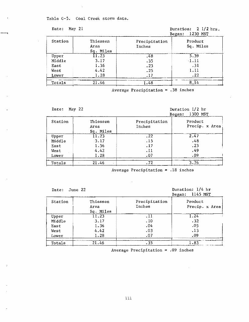
Table C-5. Coal Creek storm data.

Date: May 21

--.

Station

Upper Middle East West Lower

Totals

Date: May 22

Station

Upper Middle East West Lower

Totals

Date: June 22

Station I

Upper Middle East West Lower

Totals

Thiessen Area Sq. Miles

11.23 3.17 1.36 4.42 1. 28

21.46

Thiessen Area Sq. Miles

11.23 3.17 1.36 4.42 1. 28

21.46

Thiessen Area Sq. Miles

11.23 3.17 1.36 4.42 1.28

21.46

Duration: 2 1/2 hrs. Began: 1230 M ST

Precipitation Product Inches Sq. Miles

.48 I

5.39 .35 ·1.11 .23 .31 .25 1.11 .17 .22

1.48 8.14

Average Precipitation = .38 inches

Duration 1/ 2 hr B 1300 MST egan:

Precipitation Product I Inches Precip. x Area·

.22 2.47

.15 .48

.17 .23

.11 .49

.07 .09

.72 3.76

Average Precipitation = .18 inches

I Precipitation Inches

.11

.10

.04

I .03

i .07

.35

Duration: 1/4 hr Began: 1145 MST

Product Precip. x Area

1.24 .32 .05 .13 .09

1.83

Average Precipitation .09 inches

111

Page 122

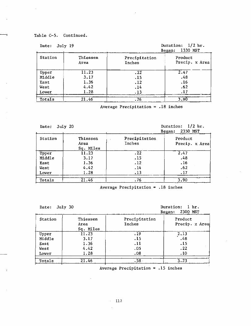
Table C-5. Continued.

Date: July 19

Station Thiessen Area

Upper 11.23 Middle 3.17 East 1.36 West 4.42 Lower 1.28

Totals 21.46

Date: July 20

Station Thiessen Area Sq. Miles

Upper 11.23 Middle 3.17 East 1.36 West 4.42 Lower 1.28

Totals 21.46

Date: July 30

Station Thiessen Area Sq. Miles

Upper 11.23 Middle 3.17 East 1.36 West 4.42 Lower 1.28

Totals 21.46

Duration: 1/2 hr. B 1330 MST egan:

Precipitation Product Inches Precip. x Area

.22 2.47

.15 .48

.12 .16

.14 .62

.13 .17

.76 3.90

Average Precipitation = .18 inches

Duration: 1/2 hr. B 2350 MST ~gan:

Precipitation Product Inches Precip. x Area

.22 2.47

.15 .48

.12 .16

.14 .62

.13 .17

.76 3.90

Average Precipitation = .18 inches

Precipitation Inches

.19

.15

.11

.05

.08

.58

Duration: 1 hr. B 2300 MST ~gan:

Product Precip. x Area

2.13 <

.48

.15

.22

.10

3.23

Average Precipitation = .15 inches

112

Page 123

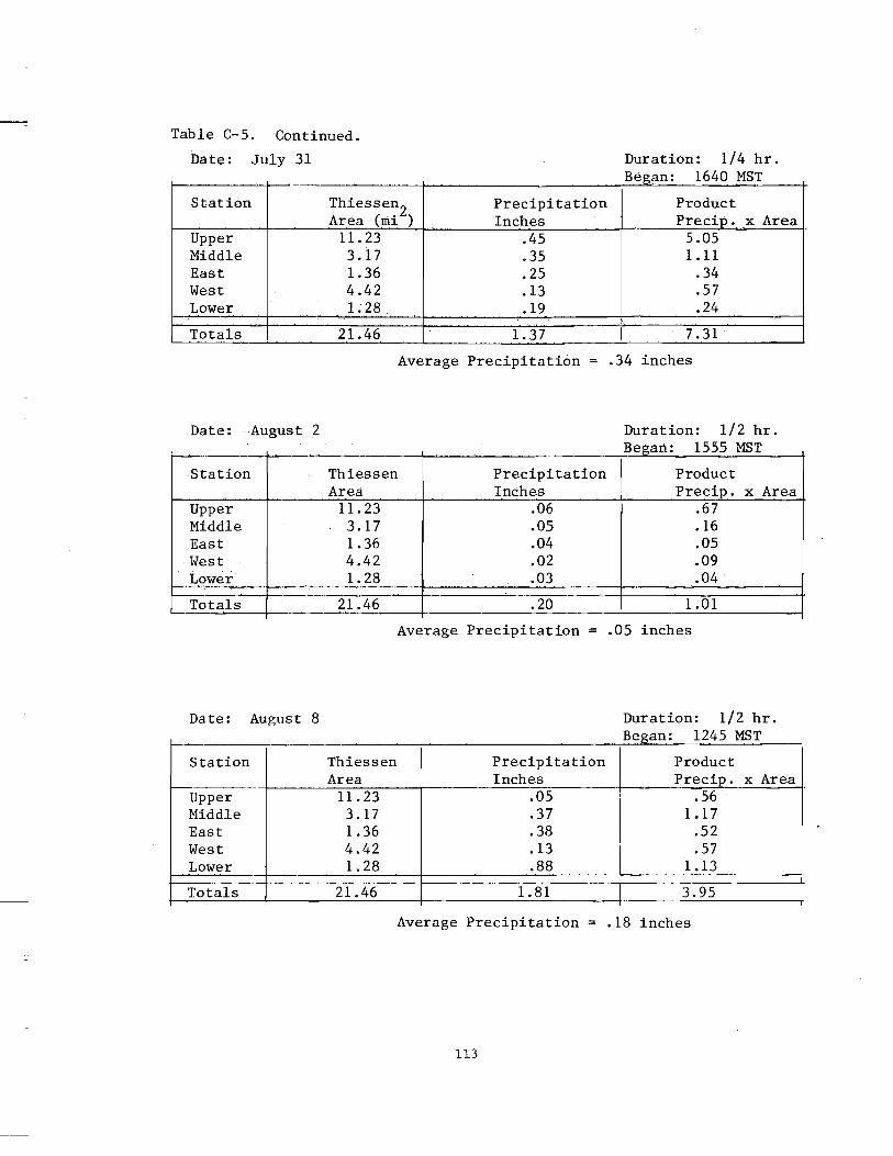
Table C-5. Continued.

Date: July 31

Station Thiessen2 Precipitation Area (mi ) Inches

Upper 11.23 .45 Middle 3.17 .35 East 1.36 .25 West 4.42 .13 Lower 1.28 .19

Totals 21.46 1. 37

Average Precipitation

Date: August 2

Station Thiessen Precipitation Area Inches

Upper 11.23 .06 Middle 3.17 .05 East 1.36 .04 West 4.42 .02 Lower 1.28 .03

Totals 21.46 .20

Average Precipitation

Date: August 8

Station Thiessen Precipitation Area Inches

Upper 11.23 .05 Middle 3.17 .37 East 1.36 .38 West 4.42 .13 Lower 1.28 .88

Totals 21.46 1.81

Average Precipitation

113

Duration: 1/4 hr. B 1640 MST egan:

Product PreCip. x Area

5.05 1.11

.34

.57

.24

7.31

.34 inches

Duration: 1/2 hr. Began: 1555 MS T

Product PreCip. x Area

.67

.16

.05

.09

.04

1.01

.05 inches

Duration: 1/2 hr. Began' 1245 MST .

Product Precip. x Area

.56 1.17

.52

.57 1.13

3.95

.18 inches

Page 124

Table C-5.Continued.

Date: August 22 Duration: 1 5/6 hrs. B 1835 MST egan:

Station Thiessen2 Precipitation Product

Area (mi ) Inches Precip. x Area Upper 11.23 .80 8.98 Middle 3.17 .43 1.36 East 1.36 .32 .44 West 4.42 .60 2.65 Lower 1.28 .21 .27

Totals 21.46 2.36 13.70

Average Precipitation = .64 inches

Date: August 26 Duration: 1/6 hr. B 1440 MST egan:

Station Thiessen2 Precipitation Product Area (mi ) Inches Precip. x Area

Upper 11.23 .01 .11 Middle 3.17 .12 .38 East 1.36 .14 .19 West 4.42 .09 .40 Lower 1.28 .04 .05

Totals 21.46 .40 1.13

Average Precipitation = .05 inches

Date: September 6

Station Thiessen2 Area (mi ) Upper 11.23 Middle 3.17 East 1.36 West 4.42 Lower 1.28

Totals 21.46

Duration: 1 hr. .. Began: 1355 MST

Precipitation Product Inches Precip. x Area

.16 1.80

.12 .38

.18 .24

.14 .62

.41 .52

1.01 3.56

Average Precipitation = .17 inches

114

Page 125

-" Table C-5. Continued.

Date: September 7

Station Thiessen2 Precipitation Area (mi ) Inches

Upper 11.23 .26 Middle 3.17 .20 East 1.36 .31 West 4.42 .23 Lower 1.28 .68

Totals 21.46 1.68

Average Precipitation

Date: September 11

Station Thiessen2 I Precipitation

Area (mi ) Inches Upper 11.23 .41 Middle 3.17 .35 East 1.36 .42 West 4.42 .36 Lower 1.28 .63

Totals 21.46 2.17 Average Precipitation

Date: September 13

Station Thiessen2 Precipitation Area (mi ) Inches

Upper 11.23 .17 Middle 3.17 .15 East 1.36 .18 West 4.42 .16 Lower 1.28 .21

Totals 21.46 .87

Duration: 1 hr. Began' 0500 MST .

Product Precip x Area

2.92 .63 .42

1.02 .87

5.86

.27 inches

Duration: 3 hr. B 1730 MST egan:

Product Precip. x Area

4.60 1.11

.57 1.59

.81

8.68 .41 inches

Duration: 10 hr. B 1915 MST egan:

ProduCt Precip x Area

1.91 .48 .24 .71 .27

3.61

Average Precipitation = .17 inches

115

Page 126

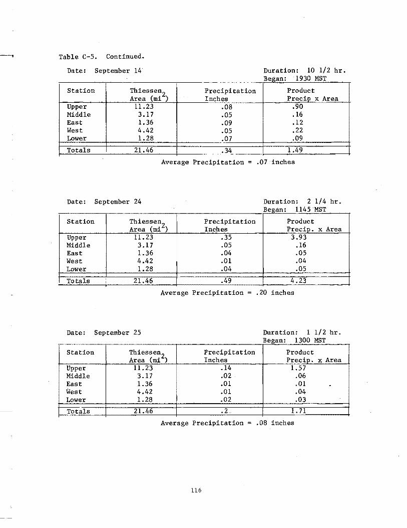
--, Table C-5. Continued.

Date: September 14 Duration: 10 1/2 hr. Began: 1930 MS T

Station Thiessen2 Precipitation Product Area (mi ) Inches Preci~ x Area

Upper 11.23 .08 .90 Middle 3.17 .05 .16 East 1.36 .09 .12 West 4.42 .05 .22 Lower 1.28 .07 .09

Totals 21.46 .34 1.49

Average Precipitation = .07 inches

Date: September 24 Duration: 2 1/4 hr. B 1145 MS egan: T

Station Thiessen2

Precipitation Product Area (ud ) Inches Precip. x Area

Upper 11.23 .35 3.93 Middle 3.17 .05 .16 East 1.36 .04 .05 West 4.42 .01 .04 Lower 1.28 .04 .05

Totals 21.46 .49 4.23

Average Precipitation = .20 inches

Date: September 25 Duration: 1 1/2 hr. B 1300 MST egan:

Station Thiessen2 Precipitation Product

Area (mi ) Inches Precipe x Area Upper 11.23 .14 1.57 Middle 3.17 .02 .06 East 1.36 .01 .01 . West 4.42 .01 .04 Lower 1.28 .02 .03

Totals 21.46 .2_ 1.71

Average Precipitation = .08 inches

116

Page 127

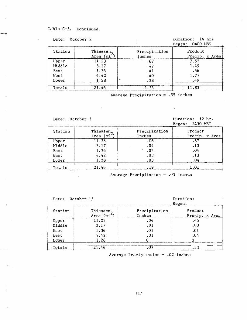
Table C-5. Continued.

Date: October 2

Station Thiessen2 Area (mi )

Upper 11.23 Middle 3.17 East 1.36 West 4.42 Lower 1.28

Totals 21.46

Precipitation Inches

.67

.47

.41

.40

.38

2.33

Duration: 14 hrs Began- 0400 MET .

Product Precip. x Area

7.52 1.49

.56 1.77

.49

11.83

Average Precipitation = .55 inches

Date: October 3

Station Thiessen2 Area (mi ) Upper 11.23 Middle 3.17 East 1.36 West 4.42 Lower 1.28

Totals 21.46

Precipitation Inches

.06

.04

.03

.03

.03

.19

Duration: 12 hr. Began' 2430 MST .

Product Precip. x Area

.67

.13

.04

.13

.04

1.01

Average Precipitation = .05 inches

Date: October 1~ Duration: B egan: ...

Station Thiessen2 Precipitation Product

Area (mi ) Inches Precip. x Area Upper 11.23 .04 .45 Middle 3.17 .01 .03 East 1.36 .01 .01 West 4.42 .01 .04 Lower 1.28 0 0

Totals 21.46 .07 .53

Average Precipitation = .02 inches

ll7

Page 128

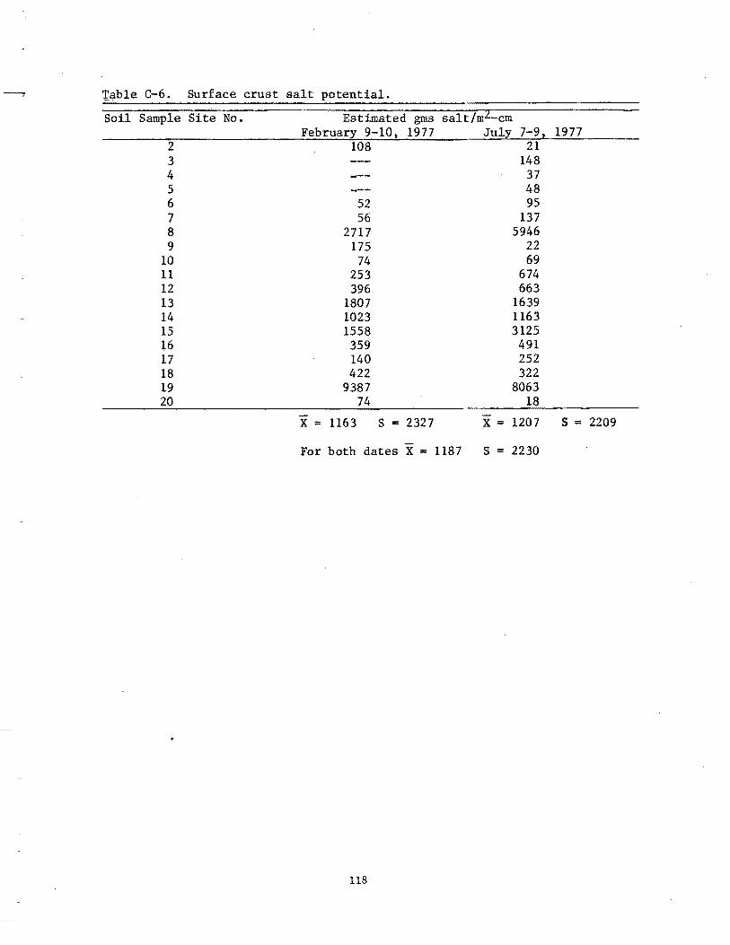
· 'table C-6. Surface crust salt potential.

Soil Sample Site No. Estimated gros salt/mZ-cm February 9-10, 1977 July 7-9, 1977

2 108 21 3 148 4 --- 37 5 48 6 52 95 7 56 l37 8 2717 5946 9 175 22

10 74 69 11 253 674 12 396 663 13 1807 1639 14 1023 1163 15 1558 3125 16 359 491 17 140 252 18 422 322 19 9387 8063 20 74 18

X = 1163 S = 2327 X = 1207 S = 2209

For both dates X = 1187 S = 2230

118

Page 129

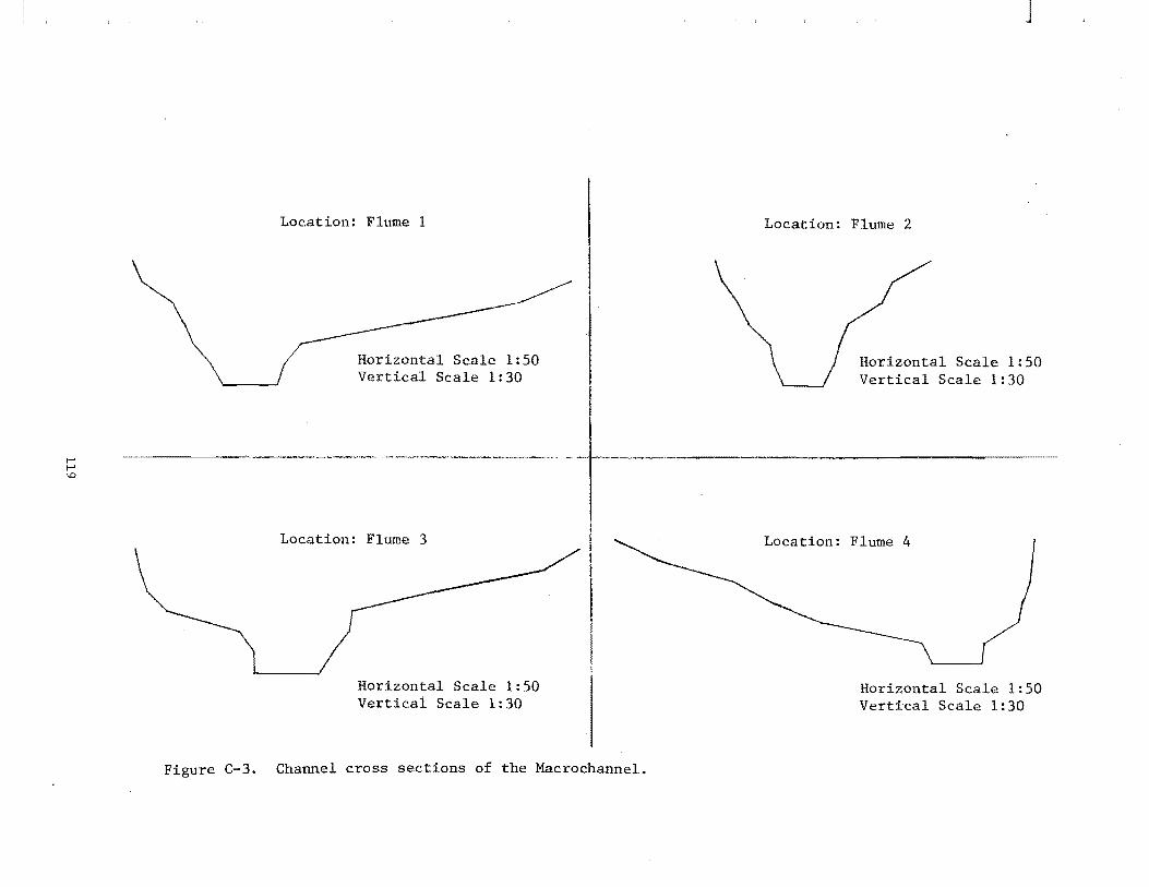
I-' I-' -.0

Location: Flume 1

Horizontal Scale 1:50 Vertical Scale 1:30

--_.- ---._,,_.-----------+---<-Location: Flume 3

Horizontal Scale 1:50 Vertical Scale 1:30

I I !

Figure C-3. Channel cross sections of the Macrochannel.

J

Location: Flume 2

Horizontal Scale 1:50 Vertical Scale 1:30

Location: Flume 4

Horizontal Scale 1:50 Vertical Scale 1:30

Page 130

J

.IS~ h . IS

Flume 1 I 1\ Flume 2

"'""' "'""' (fl (fl 4-l 4-l

::.. 10 ::'.10 Pa

~~ Pa

~ ~ ;3

~~r ;3

~.OS ~.OSI f\1~ I I r. tV¥ ~ I \ I ) J

H ~

I • 0 1 2 3 4 S 6 7 0 1 2 3' 4 S 6 7

TIME (hours) TIME (hours)

I-' N

• ISr .IS 0

0 I Flume 3 t,. Flume 4 "'""' "'""' (fl (fl

tl.l0 tl.lO '-' '-'

Pa

h Pa

~ nn ~ ;3 ~.O5 1\ ~.OS H H ~ ~

3 4 5 6 7 o 1 3 4 S 6 TIME (hours) TIME (hours)

Figure C-4. Macrochannel flow hydrographs for August 26~ 1976.

Page 131

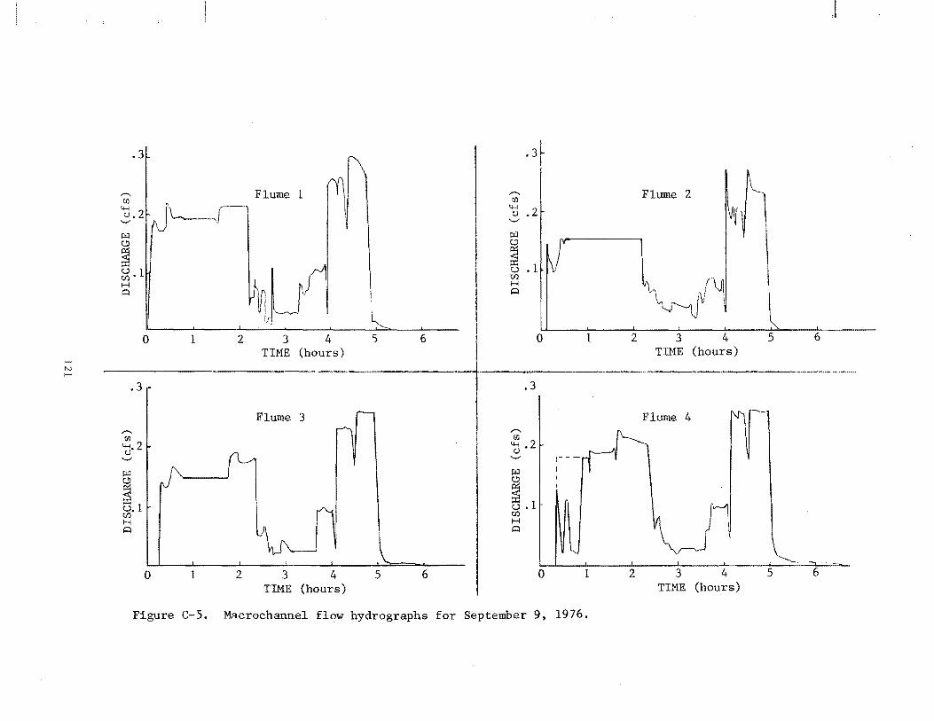
I-' N !-'

,....... [/)

.3

'ij . 2 '-"

t:J;:l

~ ~ .1 H ~

o

.3

,....... [/)

4-<.2 u '-'

t:J;:l

~ u.1 r:.t:J H ~

o

1

1

Flume 1

-11

2 3 4 TIME (hours)

Flume 3

2 3 4 TIME (hours)

5 6

5 6

.3~ ,....... [/)

'ij .2 '-'

t:J;:l

~ u .1 r:.t:J H ~

o

.3

""" [/)

4-< .2 u '-'

~

~ u .1 r:.t:J H ~

o

1

1

Figure C-S. Macrochannel flow hydrographs for September 9, 1976.

J

Flume 2 vh ~f~

2 3 4 5 6 TIME (hours)

Flume 4

Jl 2 3 4 5 6

TIME (hours)

Page 132

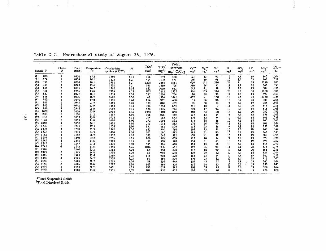
J

Table C-7. Macrochannel study of August 26, 1976.

TSSa b i Total

so = Flow Flume Time Temperature Conductivity Ph IDS \ Hardness Ca++ Mg++ Na+ K+ SiOJ cr Sample # # (MST) °c (umhos@25OC) mg/! mgtl mgtl CaCo3 mg/l mg/I mg/l mg/l mg mg!l mgtI rfs

#1 810 1 0810 17.2 1308 8.15 166 872 480 121 43 90 9 7.8 19 340 .064 #1 824 1 0824 16.1 1523 8.2 424 1032 571 146 50 96 12 8.9 23 466 .057 #2 734 2 0734 16.1 3361 8.2 1278 2868 1551 620 141 230 28 9 38 1520 .003 #2 748 2 0748 19.4 1730 8.3 141 1250 776 310 66 97 14 6.9 20 665 .033 #2 835 2 0835 16.7 1510 8.35 182 1030 612 245 41 88 12 7.1 19 508 .036 #3 756 3 0756 15.6 2906 8.25 857 2542 1337 364 103 220 20 8.2 30 1600 .006 #3 827 3 0827 16.1 1714 8.35 787 1216 704 186 58 90 12 7.8 19 599 .050 #4 816 4 0816 16.7 2540 8.30 42 1924 1041 432 160 18 8.5 23 1110 .035 #1 840 1 0840 17.8 1318 8.40 284 912 480 133 36 88 10 8.2 18 380 .051 #1 945 1 0945 21.7 1269 8.25 132 840 459 85 60 84 9 7.9 19 364 .019 #2 945 2 0945 23.9 1483 8.15 394 1074 653 261 48 9 11 7.7 19 444 .038 #3 944 3 0944 25.0 1619 8.15 538 1196 714 208 47 92 13 8.0 19 615 .003 #4 1000 4 1000 23.9 1934 8.15 1258 1480 888 250 63 100 16 8.3 20 750 .023

I-' #1 1100 I llOO 21.2 1257 8.00 106 826 469 117 43 84 9 7.9 18 336 .063 !'oJ #2 1057 2 1057 23.8 1428 8.15 214 1052 643 170 53 84 10 6.9 18 445 .039 N #3 1055 3 1055 25.0 1416 8.00 292 1002 592 174 38 86 10 7.5 18 500 .065

#4 1050 4 1050 26.1 1495 8.05 211 1014 582 174 36 90 II 8.1 18 506 .064 #1 1205 1 1205 22.5 1276 8.00 137 852 500 113 53 86 9 7.8 18 352 .068 #2 1200 2 1200 23.3 1390 8.20 132 944 510 166 23 86 10 7.7 19 446 .042 #3 1203 3 1203 24.3 1496 8.20 507 1090 582 182 31 90 10 7.3 19 546 .043 #4 1152 4 1152 26.7 1532 8.10 763 1042 592 170 41 88 10 7.7 19 600 .095 #1 1240 1 1240 22.2 1256 8.15 100 848 459 117 40 84 9 7.3 19 370 .098 #2 1245 2 1245 21.6 1314 8.15. 50 868 510 154 31 83 10 7.7 19 398 .052 #3 1247 3 1247 21.2 1400 8.10 355 924 480 168 15 . 88 10 7.2 18 444 .079 #4 1245 4 1245 21.6 1448 8.25 1016 936 551 162 36 90 11 8.1 20 436 .078 #1 1346 1 1346 22.2 1352 8.20 65 868 490 117 48 90 10 8.1 20 366 .015 #2 1343 2 1343 24.8 1334 8.20 58 948 510 139 39 82 10 7.7 18 424 .044 #3 1345 3 1345 23.6 1386 8.25 115 918 520 154 33 84 10 7.4 19 440 .079 #4 1345 4 1345 24.2 1369 8.25 97 884 520 170 23 82 10 . 7.7 19 416 .067 #1 1445 1 1445 20.7 1263 8.20 88 816 449 182 43 77 9 7.8 19 340 .064 #2 1445 2 1445 20.6 1287 8.30 149 884 520 152 34 83 10 7.5 19 382 .045 #3 1444 3 1444 20.7 1471 8.25 193 1024 582 186 28 88 11 6.9 19 500 .064 #4 1448 4 1448 21,2 1551 8,39 109 1158 622 292 28 90 11 8.6 19 436 .060

iTotal Suspended Solids brotal Dissolved Solids

Page 133

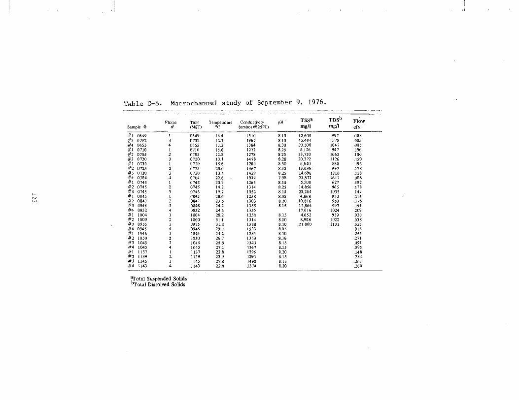
.I

Table C-S. Macrochannel study of September 9, 1976.

Flume Time Temperatwe Conductivity pH TSSa TDSb Flow Sample # # (MST) DC (umhos @25°C) mg/l mg/l cfs

0649 1 0649 16.4 1310 8.10 12,600 997 .088 0702 3 0702 12.7 1967 8.10 45,404 1578 .005 0655 4 0655 13.2 1384 8.30 23,508 1047 .005 0710 1 0710 15.6 1272 8.25 8,136 947 .196 0705 2 0705 12.8 1278 8.25 13,720 1062 .100 0720 3 0720 13.1 1478 8.20 30,372 1126 .150 0730 1 0730 15.6 1260 8.30 6,640 888 .195 0725 2 0725 20,0 1367 8.15 13,036. 997 .178 0730 3 0730 13.4 1429 8.25 14,696 1210 .158 0704 4 0704 22.6 1934 7.90 23,872 1617 .008 0745 1 0745 20.9 1265 8.15 5,500 627 .192 0745 2 0745 14.8 1314 8.25 14,856 965 .178

.-' 0745 3 0745 19.7 1052 8.15 23,204 1035 .147 N 0845 1 0845 28.4 1258 8.05 4,868 933 .214 VJ 0847 2 0847 23.5 1303 8.20 10,816 950 .178

0846 3 0846 24.2 1355 8.15 12,864 997 .191 0852 4 0852 24.6 1355 17,016 1024 .209 1004 1 1004 28,2 1258 8.15 4,652 939 .030 1000 2 1000 31.1 1314 8.10 8,988 1022 .038 0955 3 0955 31.8 1388 8.10 21.800 1132 .025 0945 4 0945 29.7 1533 8.05 .016 1046 I 1046 24,2 1284 8,10 .256 1050 2 1050 26.7 1353 8.10 .271 1045 3 1045 25.8 1343 8.15 .091 1045 4 1045 27.1 1367 8.15 .095 1137 I 1137 22,8 1296 8,20 .148 1139 2 1139 23,9 1293 8.15 .234 1145 3 1145 23.8 1490 8.15 .261 1143 4 1143 22.8 1374 8.20 .260

ilfotal Suspended Solids brotal Dissolved Solids

Page 134

...... IV ~

Table C-9. Soil sensur results.

Date UPPER 5783 5779 5768

8/25/76 15.20 /4100 17.30 /4400 19.60 /3010 8/31/76 24.5°/2600 19.5°/4100 19.6°/3715 9/2/76 16.8°/2600 17.8°/3950 19.8°/3600 9/7/76 17.7°/2700 19.0°/4050 20.1 °/3450 9/8/76 12.8°/2520 14.2°/3950 17.5°/4320 9{9/16 10.4°/2600 14.2°/3975 17.4°/3500 9/9/76 11.3°/2700 13.8°/4025 17.2°/3430 9/9/76 16.6°/2590 15.0°/3925 16.6°/3550 9/10/76 15.9°/3625 17.5°/3475 9/15/76 12.7°/1825 14.2°/2575 16.6°/4000 9/23/76 16.6°/2200 16.3°/2900 17.3°/4000 10/1/16 14.8°{2000 13.3°/2990 15.0°/3825 10/8/76 5.0°/1800 7.8°/1625 11.2°/4000 10/15/76 8.7°/1650 9.6°/1950 12.0°/3850 10/29/76 2.8°/1100 5.4°/2425 8.4°/2975 11/5/76 . 4.5°/950 6.20 {2650 8.9°/3300 11{17/76 4.7°/700 5.3°/2700 7.5°/2425 11/23/76 3.6°/700 4.5°/2825 6.7°/2275 12{1/76 0.00<500 0.00<500 2.3°/1860 12{15/76 0.0°<500 0.0°<500 2.00{1820 1{25/77 0.0°/1100 .70<500 2.3°/1950 2/18/77 0.40 {1675 1.3°<500 3.2°/1700 3/17/77 3.6°/1300 3.30<500 4.8°/1850 3{24{77 5.3°<500 3.00<500 4.5°/2450 5{5/77 "CI 15.00<500 13.80{2600 6/2/77 " 12.80{2700 13.3O{3080 .c

~g

MIDDLE 5762 5784 5777

18.30 /5150 19.8% 775 19.4°/7950 18.40 /4325 23.7°/6200 23.0°/15200 19.0°/4200 26.1°/5500 22.2°/13120 18.6°/4520 16.7°/4900 18.3°/12500 17.5°/4600 21.1°/5420 19.4°/12100 17.3°/4600 12.0°/5510 14.4°/12675 16.8°/4600 13.8°/5120 14.4°/12500 16.6°/4675 20.60 {6130 20.3 0 {12500 16.80 {4600 20.7°/6575 18.6°/14100 16.10 {4590 21.8°/6300 18.40 {13600 16.3°/4620 19.6°/4000 19.3°/12920 14.7°/4600 20.3°/3950 18.8°/13020 11.7°/4325 16.6°/9220 12.0°/4475 16.0°/4250 8.8°/4425 12.8°/3120 9.0°/4410 12.3°/2810 7.3°/4320 8.3°/2400 6.70 {4250 ~ 6.5°/2300

" 2.8°/4050 0 2.9°/2300 2.3°/2350 1 2.20{1975 1.8°/1700 ~ 0.0°/9825 2.70{1675 7.7°/4350 3.9°/1700 6.0°/2250 4.1°/2800 8.9°/700

11.80 {3300 "CI

12.6°/3450 .!! ;g 1..----

J

LOWER 5767 5756 5796 5751 5776 5757

18.2°/6020 19'.00 /7350 " 14.20 /11700 14.8°/7450 16.60 /5900 17.8°/17175 21.1°/7625 20.6°/9175 32.3°/1250 23.5°/5920 19.8°/4900 18.2°/14720 19.4°/7550 19.5°/10575 26.8°/1425 18.4°/5650 17.5°/4220 17.8°/14550 19.0°/6750 19.5°/8150 16.0°/2700 19.0°/5350 19.0°/3900 18.2°/12175 17.8°/6290 17.80 {80oo 19.5°/3375 15.s°{5625 14.8°/4600 16.6°/12050 16.6°/6500 17.5°{7950 8.3°/2300 12.4°{5125 14.8°/4600 16.7°/112125 16.4°{6450 17.5°/7725 12.00 {2800 12.4°/5125 14.5°/4700 16.3°/12120 13.8°/7500 18.4°/7750 25.2°/3220 16.6°/6200 16.20 {4820 15.8°/12450 13.8°/8250 17.8°/8150 20.7°/3620 17.40 {5600 15.8°/4820 16.3°/12600 16.30 {7350 16.4°/8750 22.8°/2720 15.7°/4700 14.3°/4950 . 15.2°/12600 18.2°/6875 18.1°/8300 19.8°/<500 19.8°/3800 18.3°/3420 16.7°/10825 16.6°/6220 16.3°/1100 25.2°/<500 18.3°/4090 15.4°/3475 14.3°/9200 11.5°/6175 11.7°/7850

I

9.4°/2450 8.0°/3620 10.2°/9300 14.2{)/4920 13.80 {6325 14.6°/2150 11.1 °/2700 11.1°/8450 9.7°/3820 9.6°/5200 3.4°/3250 4.3°/1625 6.6°/5625

10.80 {2720 10.6°/5750 .4.20 {825 5.2°/1400 7.2°/5100 8.7°{3520 9.1 0 {5150 3.80<500 5.6°/1120 6.1°/5100 7.70{3475 8.30 {5200 ~ 2.50<500 3.7°/1150 5.2°/5090

'" 3.2°/3340 3.8°{4230 0 0.0°<500 0.00<500 1.2°/5230 1.7°/3220 2.60 {4500

"CI 0.00<500 0.0°<500 0.8°/5070 ~ 0.00{3830 1.00{5500 ~ 0.00<500 0.4°/620 1.7°/4500

5.2°/4275 4.6°/6450 3.50{875 1.5°/700 2.4°{3750 4.2°/3750 4.50{6325 4.50{600 3.8°/800 4.2°/3750 5.0°/4990 4.6°{7430 5.20<500 4.00{1425 4.2°/1200 "CI 14.0°/5500 17.4°<500 14.~°<500 12.3°{1850

-I~ 16.30{8760 17.80{4075 13.8°/5730 12.8°/5320 ~ g

Page 135

APPENDIX D

LABORATORY DATA

125

Page 136

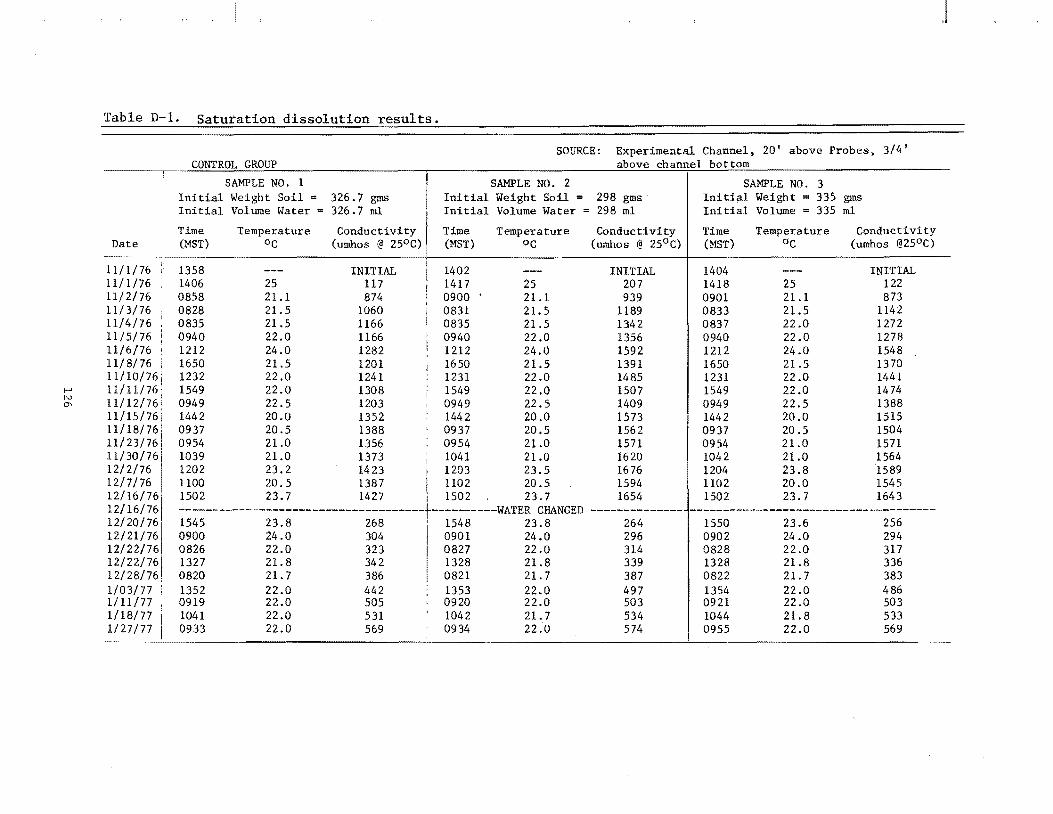
Table D-l. Saturation dissolution results.

SOURCE: Experimental Channel, 20' above Probes, 3/4' CONTROL GROUP above channel bottom

SAMPLE NO. 1 ! SAMPLE NO. 2 SAMPLE NO. 3 Initial Weight Soil = 326.7 gms I Initial Weight Soil = 298 gros· Initial Weight = 335 gms Initial Volume Water = 326.7 m1 I Initial Volume Water = 298 ml Initial Volume 335 ml

Time Temperature Conductivity Time Temperature Conductivity Time Temperature Conductivity Date (MST) 0c (umbos @ 250C) (MST) oc (umbos @ 250 C) (MST) °c (umhos @250C)

11/1/76 1358 INITIAL 1402 INITIAL 1404 INITIAL 11/1/76 1406 25 117 1417 25 207 1418 25 122 11/2/76 0858 21.1 874 0900 21.1 939 0901 21.1 873 11/3/76 0828 21.5 1060 0831 21.5 1189 0833 21.5 1142 11/4/76 0835 21.5 1166 0835 21.5 1342 0837 22.0 1272 11/5/76 0940 22.0 1166 0940 22.0 1356 0940 . 22.0 1278 11/6/76 1212 24.0 1282 1212 24.0 1592 1212 24.0 1548 11/8/76: 1650 21.5 1201 1650 21.5 1391 1650 21.5 1370 11/10/76; 1232 22.0 1241 1231 22.0 1485 1231 22.0 1441

to-' 11/11/76' 1549 22.0 1308 1549 22.0 1507 1549 22.0 1474 ~ 11/12/76: 0949 22.5 1203 0949 22.5 1409 0949 22.5 1388

11/15/76 1442 20.0 1352 1442 20.0 1573 1442 20.0 1515 11/18/76 0937 20.5 1388 0937 20.5 1562 0937 20.5 1504 11/23/76 0954 21.0 1356 0954 21.0 1571 0954 21.0 1571 11/30/76 1039 21.0 1373 1041 21.0 1620 1042 21.0 1564 12/2/76 1202 23.2 1423 1203 23.5 1676 1204 23.8 1589 12/7/76 llOO 20.5 1387 I 1102 20.5 1594 1102 20.0 1545 12/16/76 1502 23.7 1427: 1502, 23.7 1654 1502 23.7 1643 12/16/761 -------------------------------------t----------WATER CHANGED -------~------ -------------------------------------12/20/761 1545 23.8 268 i 1548 23.8 264 1550 23.6 256 12/21/76 0900 24.0 304 10901 24.0 296 0902 24.0 294 12/22/76 0826 22.0 323 I 0827 22.0 314 0828 22.0 317 12/22/7611' 1327 21. 8 342 i 1328 21.8 339 1328 21.8 336 12/28/76, 0820 21. 7 386 I 0821 21. 7 387 0822 21. 7 383 1/03/77' 1352 22.0 442 1353 22.0 497 1354 22.0 486 1/11/77 0919 22.0 505 0920 22.0 503 0921 22.0 503 1/18/77 1041 22.0 531 1042 21. 7 534 1044 21.8 533 1/27/77 0933 22.0 569 0934 22.0 574 0955 22.0 569

Page 137

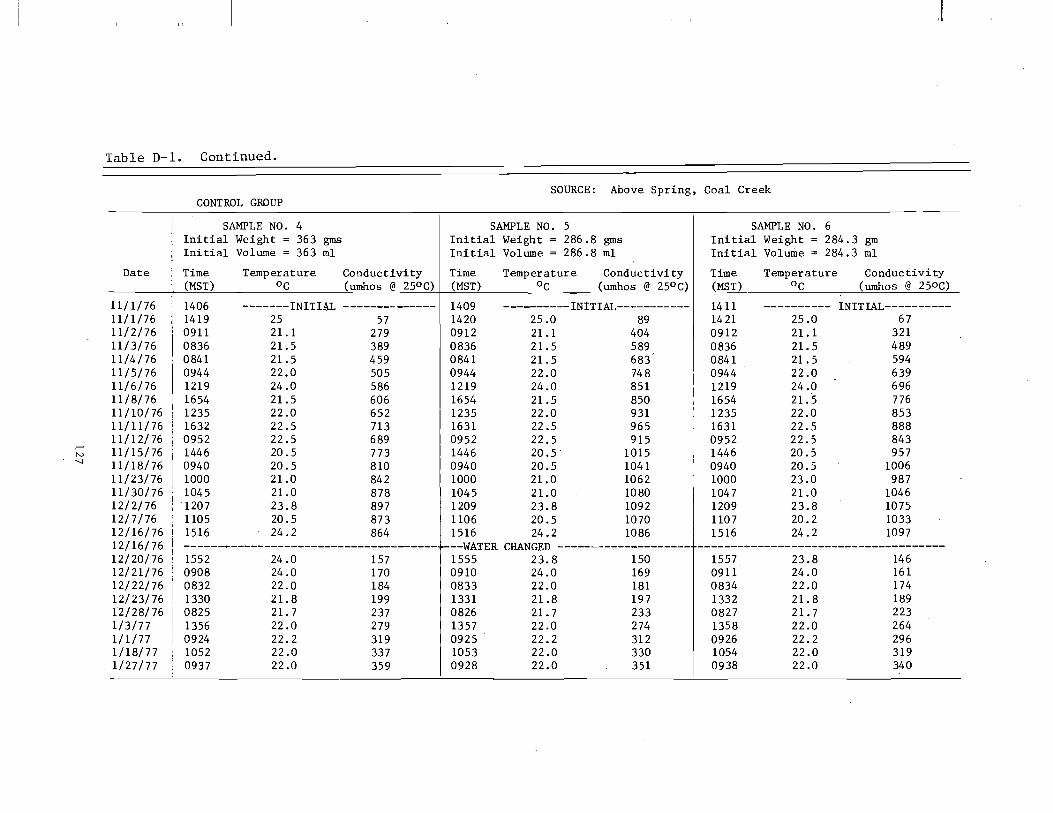
I-' N -...j

Table D-l. Continued.

CONTROL GROUP

SAMPLE NO. 4 Initial Weight = 363 gms Initial Volume = 363 ml

Date Time Temperature Conductivity (MST) °c (umhos @ 250C)

11/1/76 1406 -------INITIAL --------------11/1/76 1419 25 57 11/2/76 0911 21.1 279 11/3/76 0836 21.5 389 11/4/76 0841 21.5 459 11/5/76 0944 22.0 505 11/6/76 1219 24.0 586 11/8/76 1654 21.5 606 11/10/76 I 1235 22.0 652 11/11/76 I 1632 22.5 713 11/12/76 I 0952 22.5 689 11/15/76 I 1446 20.5 773 11/18/76 0940 20.5 810 11/23/76 I 1000 21.0 842 11/30/76 I 1045 21.0 878 12/2/76 : 1207 23.8 897 12/7/76 1105 20.5 873 12/16/76 1516 24.2 864 12/16/76 --------------------------------------12/20/76 1552 24.0 157 12/21/76 0908 24.0 170 12/22/76 0832 22.0 184 12/23/76 1330 21.8 199 12/28/76 0825 21.7 237 1/3/77 1356 22.0 279 1/1/77 0924 22.2 319 1/18/77 1052 22.0 337 1/27/77 0937 22.0 359

J

SOURCE: Above Spring, Coal Creek

SAMPLE NO. 5 SAMPLE NO. 6 Initial Weight = 286.8 gros Initial Weight = 284.3 gm Initial Volume = 286.8 ml Initial Volume = 284.3 ml

Time Temperature Conductivity Time Temperature Conductivity (MST) °c (umhos @ 250C) (MST) °c (umhos @ 250C)

1409 ----------INITIAL----------- 1411 ---------- iNITIAL----------1420 25.0 89 1421 25.0 67 0912 21.1 404 0912 21.1 321 0836 21.5 589 0836 21. 5 489 0841 21.5 683 0841 21.5 594 0944 22.0 748 0944 22.0 639 1219 24.0 851 1219 24.0 696 1654 21.5 850 1654 21.5 776 1235 22.0 931 1235 22.0 853 1631 22.5 965 1631 22.5 888 0952 22.5 915 0952 22.5 843 1446 20.5 1015 1446 20.5 957 0940 20.5 1041 0940 20.5 1006 1000 21.0 1062 1000 23.0 987 1045 21.0 1080 1047 21.0 1046 1209 23.8 1092 1209 23.8 1075 1106 20.5 1070 1107 20.2 1033 1516 24.2 1086 1516 24.2 1097

r---WATER CHANGED -------------------- -------~-----------------------------

1555 23.8 150 1557 23.8 146 0910 24.0 169 0911 24.0 161 0833 22.0 181 0834 22.0 174 1331 21.8 197 1332 21. 8 189 0826 21.7 233 0827 21.7 223 1357 22.0 274 1358 22.0 264 0925 22.2 312 0926 22.2 296 1053 22.0 330 1054 22.0 319 0928 22.0 351 0938 22.0 340

Page 138

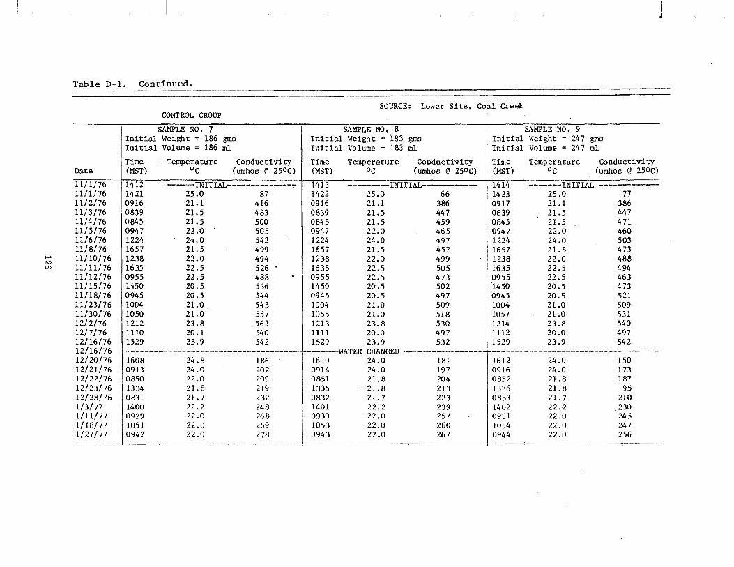
I-' N 00

Table D-l. Continued.

CONTROL GROUP

SAMPLE NO. 7 Initial Weight = 186 gms Initial Volume = 186 ml

Time Temperature Conductivity Date (MST) °c (umhos @ 250 C)

11/1/76 1412 - --INITIAL- --- -- --11/1/76 1421 25.0 87 11/2/76 0916 21.1 416 11/3/76 0839 21.5 483 11/4/76 0845 21.5 500 11/5/76 0947 22.0 505 11/6/76 1224 24.0 542 11/8/76 1657 21.5 499 11/10/76 1438 22.0 494 11/11/76 1635 22.5 526 • 11/12/76 0955 22.5 488 . 11/15/76 1450 20.5 536 11/18/76 0945 20.5 544 11/23/76 1004 21.0 543 11/30/76 1050 21.0 557 12/2/76 1212 23.8 562 12/7/76 1110 20.1 540 12/16/76 1529 23.9 542 12/16/76 --------------------------------------12/20/76 1608 24.8 186 12/21/76 0913 24.0 202 12/22/76 0850 22.0 209 12/23/76 1334 21.8 219 12/28/76 0831 21. 7 232 1/3/77 1400 22.2 248 1/11/77 .0929 22.0 268 1/18/77 l1051 22.0 269 1/27/77 0942 22.0 278

j

SOURCE: Lower Site. Coal Creek

SAMPLE NO.8 SAMPLE NO.9 Initial Weight = 183 gms Initial Weight = 247 gms Initial Volume = 183 ml Initial Volume = 247 ml

Time Temperature Conductivity Time . Temperature Conductivity (MST) °C (umbos @ 250 C) (MST) °c (umbos @ 250 C)

1413 - - -- INITIAL---- ------ 1414 . INITIAL --- ------ -1422 25.0 66 1423 25.0 77 0916 21.1 386 0917 21.1 386 0839 21.5 447 0839 21.5 447 0845 21.5 459 0845 21.5 471 0947 22.0 465 0947 22.0 460 1224 24.0 497 1224 24.0 503 1657 21.5 457 1657 21.5 473 1238 22.0 499 1238 22.0 488 1635 22.5 505 1635 22.5 494 0955 22.5 473 0955 22.5 463 1450 20.5 502 1450 20.5 473 0945 20.5 497 0945 20.5 521 1004 21.0 509 1004 21.0 509 1055 21.0 518 1057 21.0 531 1213 23.8 530 1214 23.8 540 1111 20.0 497 1112 20.0 497 1529 23.9 532 1529 23.9 542

~-------wATER CHANGED ----------------- ------------------------------------1610 24.0 181 1612 24.0 150 0914 24.0 197 0916 24.0 173 0851 21.8 204 0852 21.8 187 1335 21.8 213 1336 21.8 195 0832 21. 7 223 0833 21.7 210 1401 22.2 239 1402 22.2 230 0930 22.0 257 0931 22.0 245 1053 22.0 260 1054 22.0 247 0943 22.0 267 0944 22~0 256

Page 139

I-' f',.)

'"

Table D-I. Continued.

CONTROL GROUP

Initial Weight = 208 gros Initial Volume = 208 ml

I Time Temperature Conductivity Date (MST) °C (umhos @ 250 C)

11/1/76 1415 ------INITIAL--------------11/1/76 1424 25.0 88 11/2/76 0914 21.1 725 11/3/76 0841 21.5 895 11/4/76 0849 21.5 907 11/5/76 0951 22.0 931 11/6/76 1230 24.0 1006 11/8/76 1700 21.5 924 11/10/76 1241 22.0 936 11/11/76 1637 22.5 987 11/12/76 0958 22.5 925 11/15/76 1452 20.5 1015 11/18/76 0948 20.5 1018 11/23/76 1007 21.0 1029 11/30/76 1059 21.0 1058 12/2/76 1217 23.8 1086 12/7/76 1116 20.0 1048 12/16/76 1537 23.1 1062 12/16/76 -----~--------------~-------------~--12/20/76 1614 24.0 317 12/21/76 0919 24.0 345 12/22/76 0855 22.0 367 12/23/76 1337 22.0 378 12/28/76 0835 21.7 406 1/3/77 1405 22.0 444 1/1/77 0933 22.2 481 1/18/77 1056 22.0 492 1/27/77 0946 22.0 504

.J

SOURCE: Middle Site, Coal Creek

Initial Weight = 222 gros Initial Weight = Initial Volume = 222 ml Initial Volume = Time Temperature Conductivity Time Temperature Conductivity (MST) °C (umhos @ 250 C) (MST) °c (umhos @ 250 C)

1416 --------INITIAL------------ 1416 ---------INITIAL-----------1424 25.0 74 1425 25.0 85 0915 21.1 784 0915 21.1 743 0841 21.5 942 0841 21.5 883 0849 21.5 954 0849 21.5 907 0951 22.0 976 0951 22.0 931 1230 24.0 1061 1230 24.0 1006 1700 21.5 988 1700 21.5 935 1241 22.0 1053 1241 22.0 997 1637 22.5 1064 1637 22.5 1009 0958 22.5 1003 0958 22.5 967 1452 20.5 1095 1452 20.5 1038 09.48 20.5 1122 0948 20.5 1052 1007 21.0 1130 1007 21.0 1063 1100 21.0 1170 1102 21.0 1080 1219 23.8 1189 1220 23.5 1110 1117 20.0 1081 1118 20.0 1060 1537 23.1 1166 1537 23.1 1145

------WATER CHANGED-------------------- --------------------------------------1616 24.0 316 1617 24.0 276 0920 24.0 354 0922 24.0 321 0856 22.0 377 0857 22.0 348 1338 22.0 391 1339 22.0 363 0836 21.7 425 0837 21.7 390 1406 22.0 464 1407 22.0 437 0934 22.2 509 0935 22.2 470 1057 22.0 528 1058 22.0 487 0947 22.0 541 0948 22.0 502

_._ .. _ ...... _-

Page 140

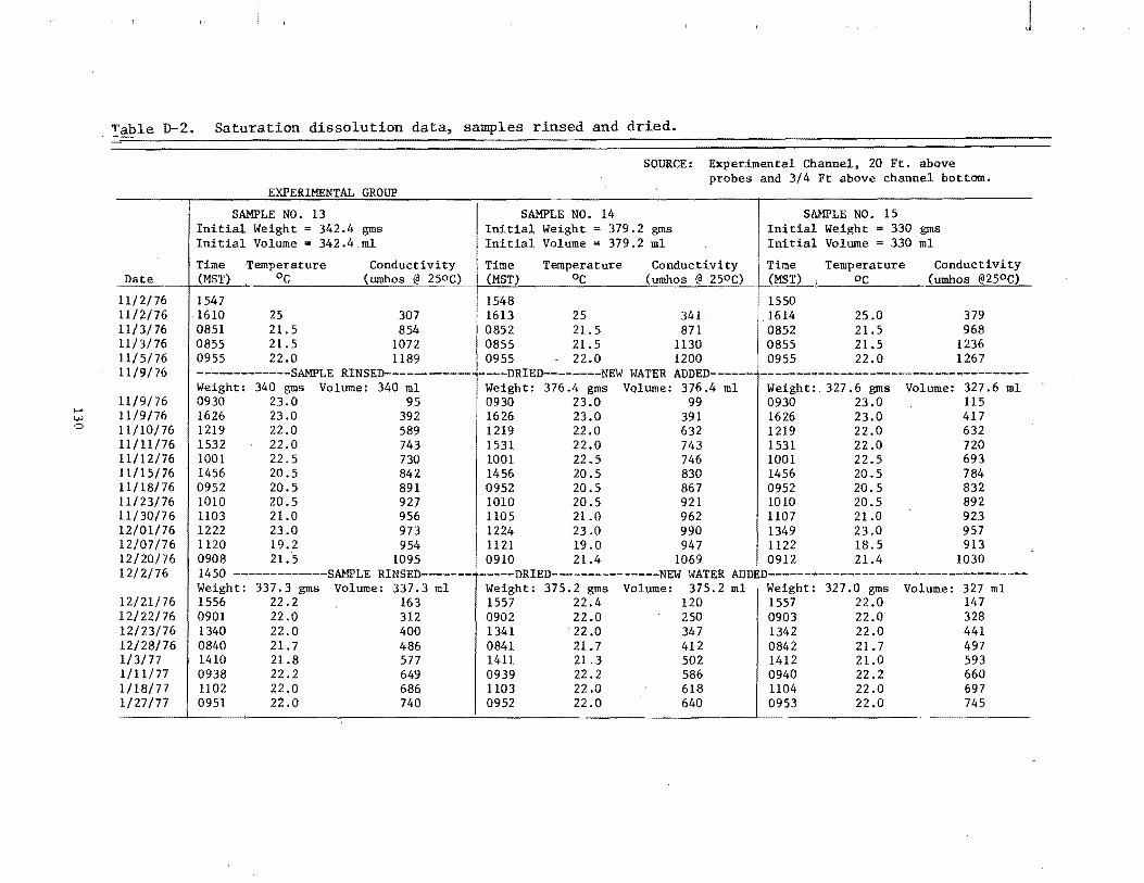
t-' (.oJ

o

J

!~ble D-2. Saturation dissolution data, samples rinsed and dried.

EXPERIMENTAL GROUP

SAMPLE NO. 13 Initial Weight = 342.4 gros Initial Volume = 342.4 ml

Time ·Temperature Conductivity Date (MST) °c (umhos @ 250~L

11/2/76 1547 11/2/76 1610 25 307 11/3/76 0851 21.5 854 11/3/76 0855 21.5 1072 11/5/76 0955 22.0 1189 11/9/76 -------------SAMPLE RINSED------------

Weight: 340 gros Volume: 340 ml 11/9/76 0930 23.0 95 11/9/76 1626 23.0 392 11/10/76 1219 22.0 589 11 /11/76 1532 22.0 743 11/12/76 1001 22.5 730 11/15/76 1456 20.5 842 11/18/76 0952 20.5 891 11/23/76 1010 20.5 927 11/30/76 1103 21.0 956 12/01/76 1222 23.0 973 12/07/76 1120 19.2 954 12/20/76 0908 21.5 1095 12/2/76 1450 -------------SAMPLE RINSED--~----

Weight: 337.3 gros Volume: 337.3 ml 12/21/76 1556 22.2 163 12/22/76 0901 22.0 312 12/23/76 1340 22.0 400 12/28/76 0840 21.7 486 1/3/77 1410 21.8 577 1/11/77 0938 22.2 649 1/18/77 1102 22.0 686 1/27/77 0951 22.0 740

SOURCE: Experimental Channel, 20 Ft. above probes and 3/4 Ft above channel bottom.

SAMPLE NO. 14 SAMPLE NO. 15 Initial Weight = 379.2 gros Initial Weight = 330 gros Initial Volume = 379.2 ml Initial Volume = 330 ml

Time Temperature Conductivity Time Temperature Conductivity (MST) °c (umhos @ 250 C) (MST); oC (umhos @250 C)

1548 1550 1613 25 341 1614 25.0 379 0852 21.5 871 0852 21.5 968 0855 21.5 1130 0855 21.5 1236 0955 22.0 1200 0955 22.0 1267

----DRIED--------NEW WATER ADDED------ ---------------------------~---------Weight: 376.4 gms Volume: 376.4 ml Weight:. 327.6 gros Volume: 327.6 ml 0930 23.0 99 0930 23.0 115 1626 23.0 391 1626 23.0 417 1219 22.0 632 1219 22.0 632 1531 22.0 743 1531 22.0 720 1001 22.5 746 1001 22.5 693 1456 20.5 830 1456 20.5 784 0952 20.5 867 0952 20.5 832 1010 20.5 921 1010 20.5 892 1105 21.0 962 1107 21.0 923 1224 23.0 990 1349 23.0 957 1121 19.0 947 1122 18.5 913 0910 21.4 1069 0912 21.4 1030

-----DRIED---------------NEW WATER ADDED------------------------------------Weight: 375.2 gros Volume: 375.2 ml Weight: 327.0 gros Volume: 327 ml 1557 22.4 120 1557 22.0 147 0902 22.0 250 0903 22.0 328 1341 ·22.0 347 1342 22.0 441 0841 21.7 412 0842 21.7 497 1411 21.3 502 1412 21.0 593 0939 22.2 586 0940 22.2 660 1103 22.0 618 1104 22.0 697 0952 22.0 640 0953 22.0 745

-.

Page 141

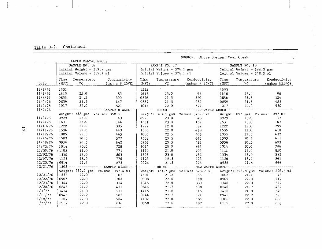
t--' W t--'

Table D-2. Continued.

EXPERIMENTAL GROUP SAMPLE NO. 16

Initial Weight 359.7 gills Initial Volume = 359.7 ml

I Time Temperature Conductivity Date I (MST) °c (umhos @ 250 C)

11/2/76 1551 11/2/76 1615 25.0 83 11/3/76 0856 21.5 300 1l/4/76 0859 21.5 447 11/5/76 1017 22.0 521 11/9/76 " ----------------------SAMPLE RINSED---

Weight: 358 gms Volume: 358 rnl 11/9/76 0929 23.0 43 11/9/76 " 1631 23.0 144 11/10/76 1222 22.0 305 11/11/76 1536 22.0 443 11/12/76 1005 22.5 463 11/15/76 1503 20.5 577 11/18/76 0956 20.5 642 11/23/76 1014 20.0 728 11 /30/76 1108 21.0 771 12/02/76 1350 23.0 803 12/07/76 1123 18.5 776 12/20/76 0914 21.4 873 12/21/76 1505 -----------------SAMPLE RINSED---

Weight: 357.4 gms Volume: 357.4 ml 12/21/76 1558 22.0 63 12/22/76 0907 22.0 202 12/23/76 1344 22.0 314 12/28/76 0845 21. 7 451 1/3/77 1414 21.0 531 1/11/77 0943 22.2 582 1/18/77 1107 22.0 584

22.0 618

J

SOURCE: Above Spring, Coal Creek

SAMPLE NO. 1 ~ SAMPLE NO. 18 Initial Weight = 374.1 gms Initial Weight = 398.3 gills Initial Volume = 374.1 ml 'Initial Volume = 348.3 ml

Time Temperature Conductivity Time Temperature Conductivity (MST) °c (umhos @ 25°C) (MST) °c (umbos @250C)

1552 1553 1617 25.0 96 1618 25.0 96 0856 21.5 330 0856 21.5 324 0859 21.5 489 0859 21.5 483 10 17 22.0 572 1017 22.0 550

-------" DRIED -------------NEW WATER ADDED-------------------'--------------Weight: 373.9 grns Volume 378.9 ml Weigh t: 897 grns Volume: 397 ml 0929 23.0 48 0929 23.0 53 1631 23.0 152 1631 23.0 167 1222 22.0 332 1222 22.0 299 1536 22.0 438 1536 22.0 410 1005 22.5 463 1005 22.5 432 1503 20.5 646 1503 20.5 611 0956 20.5 ;28 " 0956 20.5 693 1014 20.0 844 1014 20.0 786 1110 21.0 906 1111 21.0 850 1353 23.0 962 1354 23.0 885 1125 18.5 925 1126 18.2 861 0926 21.5 976 0928 21.5 966

r-------,"--DRIED-------------NEW WATER ADDED--~-----------------------------Weight: 373.7 gms Volume: 373.7 rnl Weight: 396.8 grns Volume: 396.8 ml 1601 21.2 56 1602 21.4 73 0908 22.0 198 0909 22.0 217 1345 22.0 330 1346 22.0 327 0846 21.7 508 0846 21. 7 452 1415 21.0 616 1416 21.0 540 0944 22.2 671 0945 22.2 593 1107 22.0 686 1108 22.0 606 0958 22.0 707 0959 22.0 638

- -"

Page 142

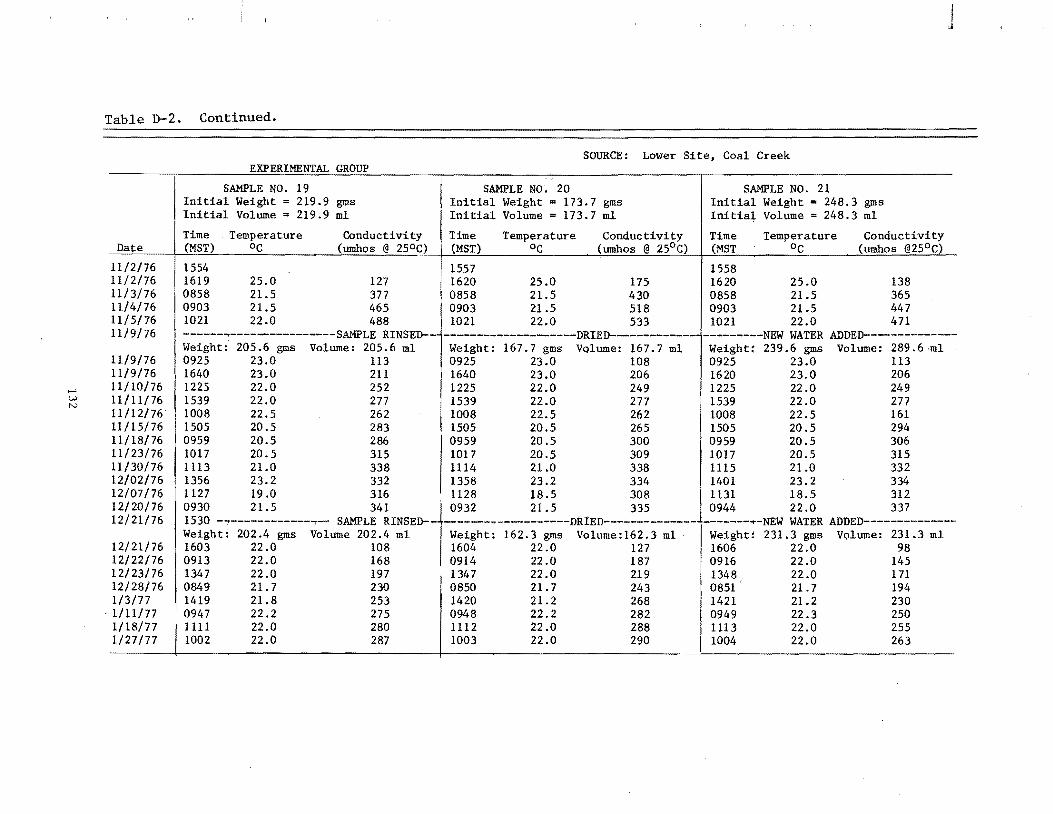
~ W N

J

Table D-2. Continued.

SOURCE: Lower Site, Coal Creek EXPERIMENTAL GROUP

SAMPLE NO. 19 SAMPLE NO.. 20 SAMPLE NO. 21 Initial Weight = 219.9 gms Initial Weight = 173.7 gms Initial Weight = 248.3 gms Initial Volume = 219.9 ml Initial Volume = 173.7 ml Initia+ Volume = 248.3 ml

Time Temperature Conductivity Time Temperature Conductivity Time Temperature Conductivity Date (MST) °C (umbos @ 250C) (MST) °C (umbos @ 250 C) (MST °c (umhos @250C)

11/2/76 1554 1557 1558 11/2/76 1619 25.0 127 1620 25.0 175 1620 25.0 138 11/3/76 0858 21.5 377 0858 21.5 430 0858 21.5 365 11/4/76 0903 21.5 465 0903 21.5 518 0903 21.5 447 11/5/76 1021 22.0 488 1021 22.0 533 1021 22.0 471 11/9/76 ------:----------------SAMPLE RINSED-- --------------------DRIED------------- --~------NEW WATER ADDED--------------

Weight: 205.6 gms Volume: 205.6 ml Weight: 167.7 gms Vqlume: 167.7 ml Weight: 239.6 gms Volume: 289.6 ·ml 11/9/76 0925 23.0 113 0925 23.0 108 0925 23.0 113 11/9/76 1640 23.0 211 1640 23.0 206 1620 23.0 206 11/10/76 1225 22.0 252 1225 22.0 249 1225 22.0 249 11/11/76 1539 22.0 277 1539 22.0 277 1539 22.0 277 11/12/76 1008 22.5 262 1008 22.5 262 1008 22.5 161 11/15/76 1505 20.5 283 1505 20.5 265 1505 20.5 294 11/18/76 0959 20.5 286 0959 20.5 300 0959 20.5 306 11/23/76 1017 20.5 315 1017 20.5 309 1017 20.5 315 11/30/76 1113 21.0 338 1114 21.0 338 1115 21.0 332 12/02/76 1356 23.2 332 1358 23.2 334 1401 23.2 334 12/07/76 1127 19.0 316 1128 18.5 308 1131 18.5 312 12/20/76

~;;g -----:~~:-------- SAMPL~4!INSED--t-~~:--------::~:--DR1ED----=~:------- 0944 22.0 337 12/21/76 -------~-NEW WATER ADDED--------------

Weight: 202.4 gms Volume 202.4 ml Weight: 162.3 gms Volume:162.3 ml . Weight: 231.3 gms Volume: 231.3 ml 12/21/76 1603 22.0 108 1604 22.0 127 1606 22.0 98 12/22/76 0913 22.0 168 0914 22.0 187 0916 22.0 145 12/23/76 1347 22.0 197 1347 22.0 219 1348. 22.0 171 12/28/76 0849 21.7 230 0850 21.7 243 0851 21.7 194 1/3/77 1419 21.8 253 1420 21.2 268 1421 21.2 230 1/11/77 0947 22.2 275 0948 22.2 282 0949 22.3 250 1/18/77 1111 22.0 280 1112 22.0 288 1113 22.0 255 1/27/77 1002 22.0 287 1003 22.0 290 1004 22.0 263

Page 143

J

Table D-2. Continued.

EXPERIMENTAL GROUP SOURCE: Middle Site, Coal Creek

SAMPLE NO. 22 SAMPLE NO. 23 SAMPLE NO. 24 Initial Weight 185.4 ns Initial Weight = 218.1 gms Initial Weight = 240.3 gms Initial Volume 185.4 m Initial Volume = 418.1 ml Initial Volume 240.3 ml

Date ~onductivity Time Temperature Conductivity Time Temperature Conductivity llmhos @ 25°C) (MST) °c (umhos @ 25°C) (MST) °C (umhos @ 25°C)

Time Temperature (MST) 0C

11/2/76 1600 1601 1602 11/2/76 1621 25 175 1622 25 151 1623 25 163 11/3/76 0900 21.5 824 0900 21.5 754 0900 21.5 754 11/4/76 0906 21.5 1013 0906 21.5 954 0906 21.5 977 11/5/76 1025 22 1020 1025 22 976 1025 22 1021 11/9/76 3AMPLE RINSED-- ----------------------DRIED-------------- --------NEW WATER ADDED-----------------

Weight: 180.5 gms Volume 180.5 ml Weight: 211.2 gms Volume: 211 ml Weight: 235.1 gms Volume:235 ml 11/9/76 0923 23 239 0923 23 206 0923 23 247 11/9/76 1643 23 424 1643 23 381 1643 23 463 11/10/76 1229 22 554 1229 22 565 1229 22 654 11/11/76 1542 22 621 1541 22 598 1541 22 709 11/12/76 1011 22.5 596 1011 22.5 576 1012 22.5 679 11/15/76 1507 20.5 623 1507 20.5 646 1507 20.5 726

t-' 11/18/76 \..V \..V 11/23/76

648 1002 20.5 670 1002 20.5 763 671 1021 20 705 1021 20 809

1002 20.5 1021 20

11/30/76 1116 21 709 1118 21 720 1120 21 838 12/2/76 1402 23 693 1403 23 753 1405 23 869 12/7/76 1132 18.2 649 1133 18 704 1134 18 831 12/20/76 0946 21.8 693 0948 21.8 776 0950 21.8 920 12/21/76 1535 ------------------- SAMPLE RINSED-- ----------------------DRIED-------------- --------NEW WATER ADDED-----------------

Weight: 163.9 gms Volume 163.9 ml Weight: 206.8 gms Volume: 206.8 ml Weight: 231.3 gms Volume:231.3 ml 12/21/76 1607 20 201 1608 20 156 1609 20.5 206 12/22/76 0919 22 334 0920 22 278 0921 22 358 12/23/76 1349 22 382 1349 22 354 1350 22 441 12/28/76 0854 21.7 422 0855 21.7 418 0856 21. 7 497 1/3/77 1424 21 457 1425 21 469 1425 21 550 1/11/77 0953 22.2 489 0954 22.2 515 0955 22.2 602 1/18/77 1115 22 494 1116 22 529 1117 22 619 1/27/77 1006 22 502 1007 22 541 1007 22 640

Page 144

I-' W .,..

Table D-3. Rotoevaporator dissolution results.

GRAIN SIZE I II III IV

PASSED 3/8 #4 #10 #20 RETAINED #4 #10 #20 #60 Cycle

Specific conductance Cvmhos/cm @ 250 C) No. 515 408 561 718 0 735 544 647 800 1 722 564 712 801 2 667 699 655 700 3

Site 1 719 676 640 4 703 704 742 5

873 688 6 _______________________ Z~~ __________________________________ l __ _ 748 655 902 1397 0 867 808 951 1651 1 804 779 905 1598 2

Site 2 747 698 910 1528 3 744 926 920 1410 4 735 989 5

717 6 ----------------------------------------------------------------. 349 639 0 439 684 1

Site 3 411 630 2 723 3 635 4 638 5

J

Table D-4. Power function coefficients for dissolution from different grain sizes in quiescent water.

PASSED RETAINED

Site 1

GRAIN SIZE 3/8 #4 #10 #20 #4 #10 #20 #60 Specific conductance Cvmhos/cm @ 250 C) 192 218 266 538 270 315 509 743 399 585 705 804 756 826 759 872 930 906 782 894 956 881 1045 1046

a=466:31 a=522.87 a=603.98 a=787.36 b=.192 b=.165 b=.127 b=.061

r 2=.987 r 2=.936 r 2=.87 r 2=.90

8 24 72

Time (Hours)

.008333

.08333

.5

-------------275-------249-------419-------765--------------700833-----'

367 390 624 844 .0833 459 552 726 1013 .5

Site 2 610 634 821 1213 8 784 736 797 1536 24 817 825 883 1332 72

a=496.22 a=507.01 a=678.91 a=1063.40 b=.123 b=.124 b=.072 b=.074

r 2=.992 r 2=.951 r 2=.866 r 2=.92 -------------168-------174-------291-------490--------------700833------

225 257 442 607 .0833 308 410 537 666 .5

Site 3 482 749 524 620 8 578 621 632 725 24 740 653 705 795 72

a=350.64 a=403.96 a=491.82 a=636.07 b=.163 b=.158 b=.083 b=.042

r 2=.996 r 2=.910 r 2=.878 r 2=.805 -------------166-------184-------309-------649--------------755833-------

252 245 431 724 .0833 338 364 601 1022 .5

Site 366 369 1062 1463 8 439 447 847 1949 24 507 524 1215 2270 72

a=314.42 a=325.95 a=641.05 a-;;U63.08 b=.1l2 b=.107b=.148 b=.145

r 2=.947 r 2=.936 r 2=.945 r 2=.923 Concentration fit to the power function C at b

'X=755.00 X=720.75 X=962 X=1360.75 S=187.95 S=163.14 S=218.47 8=644.65

Page 145

Table D-5. Macrochannel sediment results (8/26/76) (sediment dried then D. W. as added on a 1 to 1 basis.)

Flume No. 1 Flume No. 2 Flume No. 3 Flume No. 4 Sediment Wt: 414.68 gms Sediment Wt: 485.16 gms Sediment Wt: Sediment Wt: 470.4 gms ~~~~!~_~~~~~~_~~~~_~~! ______ ~~~~!~_~~~~~~_£~~~_~~! ______ ~~~E!~_~~~~~~ ______________ ~~E!~_!~~~~~_Q~~Q_~~! Time Condo Time Condo Time Condo Time Condo (hrs) ~mhos@250C (hrs) ~mhos@250C (lus) j.lmhos@250C (hrs) J.lmhos@250C

~

0 0 0 0 a z 0 0 .77 1993 .85 1116 ro 0 .85 854 o rt

26.83 2591 26.83 1625 rt 26.83 1437 t'l

119.47 2808 119.47 2059 >-30 III 0 119.77 1809

287.92 2767 287.83 2209 i"">:: 287.55 1981 roO<! 336.42 2861 336.37 2397 o ::r 336.77 2100 rt

455.88 2804 455.88 2329 tfl 456.20 2106 815.40 2955 815.35 2583 ro 815.65 2439 Q.

988.65 2875 988.68 2555 ,..,.

989.02 2423 I

--------------~-----

Table D-5. Continued.

Flume No.1 Flume No.2 Flume No.3 Flume No.4 Sediment Wt: 414.68 gms Sediment Wt: 485.16 gms Sediment Wt: Sediment Wt: 470.4 gms ~~~E!~_~~~~~~ __ Q~~Q_~~! _____ ~~~E!=_~~~=~~_~~~~_~~! ______ ~~~E!~_~~~~~~ ______________ ~~~E!~_~~~~~~_Q~~Q_~! Time Cond. Time Cond. Time (hr~ jimhos@250C_ (hrs) __ ~o.c:-s:::.@2=:5::..o.:_C'___.__>(:.:h~rs=) o --=~O~-"--=-~ 0 0 0

.85 866 .77 558 .85 26.83 1460 26.83 1189 26.83

119.47 1850 119.97 1642 119.63 287.87 2115 287.75 1834 288.02 336.68 2318 336.95 1990 336.55 455.90 2173 456.43 2032 456.05 815.37 2359 815.85 2356 815.50 988.62 2323 989.30 2355 988.85

Table D-5. Continued.

Condo )lmhos@250C

o 638 848 950

1035 1111 1082 1142 1090

Flume No. 1 Sediment Wt: 337.8 gms

Flume No.2 Sediment Wt: 420.4 gms

Flume No. 3 Sediment Wt: 352.1 gms

Time (hrs)

o .85

26.80 119.48 287.85 336.48 455.90 815.37 988.70

Condo ll!lIhos@250C

o 723

1201 1526 1958 1979 2053 2405 2379

Flume No. 4 Sediment Wt: 320.5 gms

--------------------------~------------------------------------------------------------------------------Time Condo Time Condo Time Condo Time Condo ~hrs) llmhos@250c (hrs) j.lmhos@250C (hrs) jJmhos@250C (hrs) j.lmhos@250C

0 0 0 0 0 0 0 0 .85 752 .85 689 .85 1071 .85 1002

26.87 1189 26.83 1366 26.83 1460 26.83 1637 119.72 1596 120.55 1730 119.45 1650 119.85 1977 287.52 1662 287.32 2003 287.83 1722 287.67 2149 336.70 1705 336.55 2133 336.46 1770 336.83 2254 456.18 1731 455.98 2140 455.90 1733 456.33 2210 815.58 1938 815.43 2527 815.36 1864 815.73 2510 986.98 1906 988.80 2471 988.71 1817 989.18 2467

-------

135

Page 146

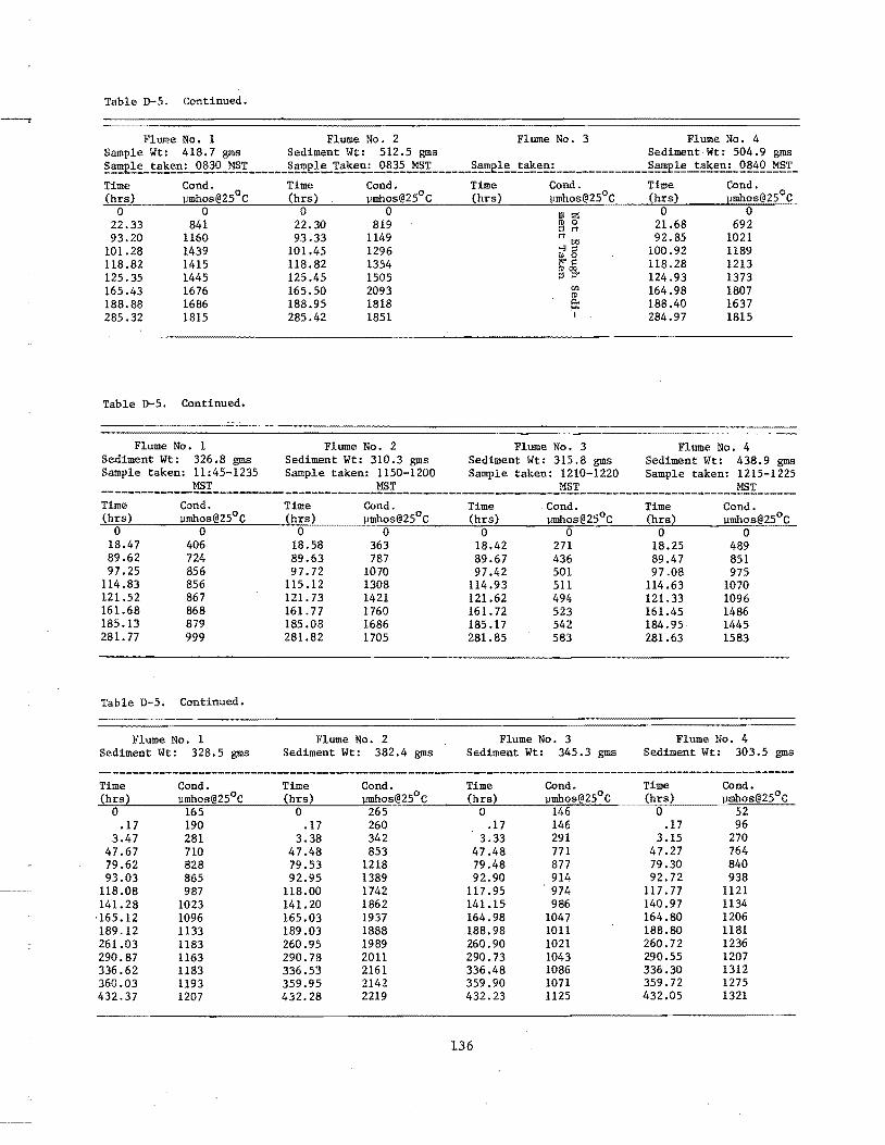
Table D-5. Continued.

Flume No.1 Flume No.2 Flume No.3 Flume No.4 Sample Wt: 418.7 gros Sediment Wt: 512.5 gros Sediment Wt: 504.9 gms ~!~£!~_!~~~~~_Q83Q_~! ______ ~~£!~!~~~~~_Q~~~_~~! ______ ~~~2!~_!~~~~~ ______________ ~~~2!~_!~~~~~_Q~~Q_~~!_ Time Cond. Time Cond. Time Cond. Time Cond. 0 (hrs) ~mhos@250C (hrs) ~mhos@250C (hrs) ~mhos@250C (hrs) ~mhos@25 C

o 0 0 0 0 0 22.33 841 22.30 819 m g 21.68 692 93.20 1160 93.33 1149 rt [rJ 92.85 1021

101.28 1439 101.45 1296 ~ 5 100.92 1189 118.82 1415 118.82 1354 it ~ 118.28 1213 125.35 1445 125.45 1505 ::I ;:r 124.93 1373 165.43 1676 165.50 2093 rc 164.98 1807 188.88 1686 188.95 1818 !: 188.40 1637 285.32 1815 285.42 1851 I 284.97 1815

Table D-5. Continued.

Flume No. 1 Flume No. 2 Flume No. 3 Flume No.4 Sediment Wt: 326.8 gros Sediment Wt: 310.3 gros Sediment Wt: 315.8 gros Sediment Wt: 438.9 gms Sample taken: 11:45-1235 Sample taken: 1150-1200 Sample taken: 1210-1220 Sample taken: 1215-1225

MST MST MST MST -------------------------------------------------------------------------------------------~--------------Time Condo (hrs) ~mhos@250C

0 0 18.47 406 89.62 724 97.25 856

114.83 856 121.52 867 161.68 868 185.13 879 281.77 999

Table D-5. Continued.

Flume No. 1 Sediment Wt: 328.5 gros

Time Condo (hrs) ~mhos@250C

0 0 18.58 363 89.63 787 97.72 1070

115.12 1308 121.73 1421 161.77 1760 185.08 1686 281.82 1705

Flume No. 2 Sediment Wt: 382.4 gros

Time -Condo (hrs) ~mhos@250C

0 0 18.42 271 89.67 436 97.42 501

114.93 511 121.62 494 161. 72 523 185.17 542 281.85 583

Flume No.3 Sediment Wt: 345.3 gms

Time Condo (hrs) ~mhos@250C

0 0 18.25 489 89.47 851 97.08 975

114.63 1070 121.33 1096 161.45 1486 184.95 1445 281.63 1583

Flume No. 4 Sediment Wt: 303.5 gms

-----------------------------------------------------------------------------------~----------------------Time Condo Time Condo Time Condo Time Condo (hrs! Ilmhos@250C (hrs) Ilmhos@250C (hrs) ~mhos@250C (hrs) ~mhos@250C

0 165 0 265 0 146 0 52 .17 190 .17 260 .17 146 .17 96

3.47 281 3.38 342 3.33 291 3.15 270 47.67 710 47.48 853 47.48 771 47.27 764 79.62 828 79.53 1218 79.48 877 79.30 840 93.03 865 92.95 1389 92.90 914 92.72 938

118.08 987 118.00 1742 117.95 974 117.77 1121 141.28 1023 141.20 1862 141.15 986 140.97 1134 -165.12 1096 165.03 1937 164.98 1047 164.80 1206 189.12 1133 189.03 1888 188.98 1011 188.80 1181 261.03 1183 260.95 1989 260.90 1021 260.72 1236 290.87 1163 290.78 2011 290.73 1043 290.55 1207 336.62 1183 336.53 2161 336.48 1086 336.30 1312 360.03 1193 359.95 2142 359.90 1071 359.72 1275 432.37 1207 432.28 2219 432.23 1125 432.05 1321

136

Page 147

J

Table D-6. Least squares regression analysis of Equation 4.3. ~ -- ---.-.. ---- .. --~~

___ ._ w·____ .,.._ _ ~ -.~----

Location Grain Size Limit K2

2 Passed Retained K1 r 1 hours r 2 ._--- ._-,._--_.- -.---.. ,--~ .. -. -----. '-

Site 1 3/8 II 4 .000321 .996 9.00 .000065 .760 Site 1 II 4 1110 .000580 .996 6.81 .000033 .605 Site 1 tHO 1120 .000651 .930 4.06 .000051 .913 Site 1 1120 1160 .000374 .766 4.82 .000029 .960 Site 2 3/8 II 4 .000275 .957 6.72 .000045 .857 Site 2 /I 4 /110 .000458 .974 5.49 .000034 .97R Site 2 1110 1120 .000442 .851 5.41 .000017 .822 Site 2 1120 1160 .000388 .999 7.80 .000042 .430 Site 3 3/8 II 4 .000216 .990 8.76 .000044 .999 Site 3 II 4 1110 .000366 .999 11.94 -.000014 .367 Site 3 1110 1/20 .000360 .892 4.64 .000023 .884 Site 3 1120 #30 .000253 .854 4.00 .000019 .754 Site 4 3/8 II 4 .000257 .959 5.11 .000022 .979 Site 4 /I 4 1110 .000282 .999 4.99 .000021 .941

f-' Site 4 /110 1120 .000445 .988 7.36 .000062 .646 VJ Site 4 1120 1160 .000599 .984 .08 .000155 .952 " --,_ .. ,-_.- ~-,-. -----

Page 148

APPENDIX E

LISTINGS OF THE HYDROLOGIC/SALINITY MODELS

139

Page 149

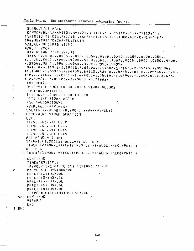
Table E-l.a. The stochastic rainfall subroutine (RAIN).

SIJ~jRllUl INE RAIN . en r4 M D NIB L t< t now ( 1 2) , i3 V I l2 ) t 'J rl ( .1 ~ , ~ , , In 2 ( l? , tl • , X '\ T1 ( 1 ? • e:: ) ,

1 11 K 1 l ( 1 " , ~i ) • 0 E r: 1 s ( l~' , 5 ) , ,( K ~I S ( 1 (I ) , t' li!s ( 1 (' I , if) U iii • 1\ , 8 • C • 1-11 • Ii ~ , Ii 3 , Ift4,H5,lUIPRE,CIIANCL,TI:.LIM 51 B-L K ~ I P H r C I P I 5 ) , 1 J /''; E. ./I"\LKJU/MUf\I

OP1lllSJ ulJ P (27 J ,U 1(7) ) 1\ T 1\ PI. fl U 0 1. , • U (I (15 , • U f) J (I , • u u ~ II , • n 1 u U , • (1200 •• l. 2. 50 , • 0,", U 0 , • (IS (J U ,

,., • 1 (I U II , • i:! (Ion, • .3 U (Ill , • 4 000 , • 50 f) n , • (ill 0 U , • 7000 , • Boo Ii , • 9 (I 0 0 , • 9 S 0 G , • '1600 , •• 9750, .9AflQ, .9900, .:)950, .3:1')0, .9995, ,99991

n"TA R/j.719U~,3.29U53,~.a9u~6'2.~75"3,~,3;~~~,2.05~75,1.~599b, ·1 • 7 r) () ,; y, I • ~.'I 'I f\ '3 , 1 • C'~! 1 h 1'\ , • £l oJ 1(,2 , • C,2 ... 1.0 , • c.: ~ ~ ::5 ':I , • (HI all 0 , - • 2 Ie; :3;3 ~i , - • 5 c: 1+ .

• 'If' , •• 84 .1 f, 2." - 1 • , e J. '5:: , - 1 • b 4 4 !j ~ , - 1 .. 7 ~) U 6 'J , - 1 • '1 : 9 '.;16 , - c: • 0 I) 3 7 5 , - c. • 3? b 3 5 , *-?575~~,-3.0~023,-3.~~O~3,-~.7190~1

T01PRl=O. r. ()rlE.H M l fJE. r'itElliEI1 U~ IwT 1\ STor-<~ OLtu~~

rHS=~A~DnM(IDUMJ J r ( [J It S • "T • C ~ , I\fJ t r) GuT U 5 (Ill

r ilF'Tt:IU"1NE ~lOHM OE.·PIH pn" =R MJOO~H I DUM) )( \I = H L I\N G I! ( P R V , F , It ) VnL=lU •• *(ALGGI0(8V(~O~I)+XV*X~VIM~NI)

C Df re:RfoI\l~( STOHM DURATrcrJ LV:l IF(VOL.br •• l1 LV=2 IF(VnL.bE,.~) LV=3 trlvoL.uE •• 41 LV=4 rF(VrIL.(;F •• f'~1 LV=5 I' R r = p 1\ IJ 0 t) M ( Il JlII"1 I IFIPln.LT.O[CISII·'Uh,LVIJ :;J 1lJ ~ r 11"1 Eo: H I 2 f M (l '" , L \I ) -t )I t\ 1 ~ I !'Ii I) r I , L V I * ( -1\ LOG I - 1.\ LOG f PH r I I ) G/J TO b

'i TJ (.Ill = BI 1 04'0 f-It LV H X 1\ TJ I rvlnr~ , L V I * I - 1\ LOb ( - 1\ LOG I P k T I J I

,. tON fJ NUt: T Jf\E:1\8S IT 1 r~E) J F ( VOL /1 ule • G T • T U. 1 \1) 1 t P\.~ = \I 0 L / f! L tr~

r CI\LClILI\]"[ HYE.10GHI\Pll rn~t lPlll=Hlt\/(JL F' fl t c. 1 ,,' ( ~ ) = ~ 12 i V t l. PP(C J P (~l :'134 \11K p II. ~ l: J P ( II ) :: 114 .. " 0 L PIU ['1 tl (~I =!l5~ \lUI. 1 0 I PPf ~ lHlt-H2·PI3.f HII HI'5,iIlVOL

~ 00 CON' r Il\ttlC REluRri EN\)

3 END

140

Page 150

Table E-l. b. A of rainfall data generated by RAIN. -~~-----...... ~~--' --- -..-.::-- --,.-",-- ~,-

• _._., _____ •• _ .......... _.:-........ __ •• ~ • ..i_._ ___ _'_ • • _,....,..~,~_"" ..... .--....,_..__... ............... _.--'--__ "". ~ '"- "._

-~ Date Duration Precipitation Runoff (Hours) (inches) (inches)

4/9 1.13 0.16 0.00

4/10 1. 910 0.410 0.00 0.041 0.000 0.103 0.000 0.124 0.005 0.104 0.000 0.041 0.000

4/11 0.51 0.06 0.00

4/13 2.00 0.54 0.01 0.054 0.000 0.136 0.010 0.163 0.000 0.136 0.000 0.054 0.000

4/29 4.00 0.12 0.00

7/03 0.06 0.09 0.03 0.009 0.000 0.021 0.000 0.026 0.004 0.021 0.019 0.009 0.007

7/14 0.80 0.10 0.00

7/18 0.08 0.09 0.03 0.009 0.000 0.022 0.000 0.026 0.004 0.022 0.019 0.009 0.006

7/19 0.57 0.46 0.26 0.046 0.000 0.116 0.090 0.139 0.100 0.116 0.066 0.046 0.000

7/21 0.56 0.04 0.00

7/23 0.15 0.03 0.00

7/16 0.52 0.10 0.01 0.010 0.000 0.025 0.000 0.031 0.000 0.025 0.006

141

Page 151

Page 152

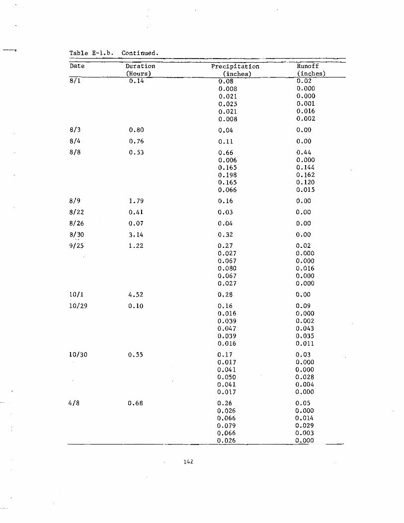
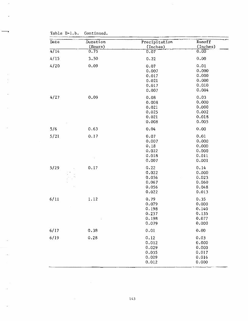
-... Table E-l. b. Continued.

Date Duration Precipitation Runoff (Hours) (Inches) (Inches)

4/14 0.75 0.07 0.00

4/15 3.50 0.22 0.00

4/20 0.09 0.07 0.01 0.007 0.000 0.017 0.000 0.021 0.000 0.017 0.010 0.007 0.004

4/27 0.09 0.08 0.03 0.008 0.000 0.021 0.000 0.025 0.002 0.021 0.018 0.008 0.005

5/6 0.63 0.04 0.00

5/21 0.17 0.07 0.01 0.007 0.000 0.18 0.000 0.022 0.000 0.018 0.011 0.007 0.001

5/29 0.17 0.22 0.14 0.022 0.000 0.056 0.023 0.067 0.060 0.056 0.048 0.022 0.013

6/11 1.12 0.79 0.35 0.079 0.000 0.198 0.140 0.237 0.135 0.198 0.077 0.079 0.000

6/17 0.38 0.01 0.00

6/19 0.28 0.12 0.03 0.012 0.000 0.029 0.000 0.035 0.017 0.029 0.016 0.012 0.000

143

Page 153

Table E-1.b. Continued. --

Date Duration Precipitation Runoff (Hours) (inches) (inches)

6/28 0.68 0.18 0.03 0.018 0.000 0.045 0.000 0.054 0.026 0.045 0.000 0.018 0.000

6/30 0.08 0.07 0.02 0.007 0.000 0.018 0.000 0.021 0.000 0.018 0.012 0.007 0.005

7/5 1.03 0.37 0.05 0.037 0.000 0.092 0.030 0.111 0.020 0.092 0.000 0.037 0.000

7/11 0.07 0.08 0.02 0.008 0.000 0.019 0.000 0.023 0.000 0.019 0.016 0.008 0.006

7/13 0.47 0.67 0.45 0.067 0.001 0.168 0.138 0.202 0.164 0.168 0.125 0.067 0.021

7/16 0.06 0.08 0.02 0.008 0.000 0.020 0.000 0.024 0.000 0.020 0.018 0.008 0.006

7/22 0.23 0.03 0.00

7/23 0.73 0.13 0.00 0.013 0.000 0.032 0.000 0.039 0.003 0.032 0.000

144

Page 154

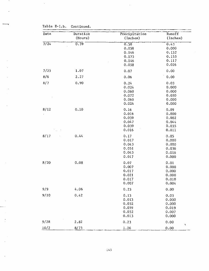
----" Table E-l. b. Continued.

Date Duration Precipitation Runoff (Hours) (Inches) (Inches)

7/24 0.39 0.58 0.43 0.058 0.000 0.146 0.132 0.175 0.153 0.146 0.117 0.058 0.026

7/25 1.07 0.07 0.00

8/6 2.27 0.06 0.00

8/7 0.90 0.24 0.03 0.024 0.000 0.060 0.000 0.072 0.030 0.060 0.000 0.024 0.000

8/12 0.10 0.16 0.09 0.016 0.000 0.039 0.002 0.047 0.044 0.039 0.035 0.016 0.011

8/17 0.44 0.17 0.05 0.017 0.000 0.043 0.000 0.051 0.036 0.043 0.016 0.017 0.000

8/20 0.08 0.07 0.01 0.007 0.000 0.017 0.000 0.021 0.000 0.017 0.010 0.007 0.004

9/9 4.06 0.23 0.00

9/10 0.42 0.13 0.03 0.013 0.000 0.032 0.000 0.039 0.019 0.032 0.007 0.013 0.000

9/28 2.82 0.23 0.00

10/2 8/73 1.26 0.00

145

Page 155

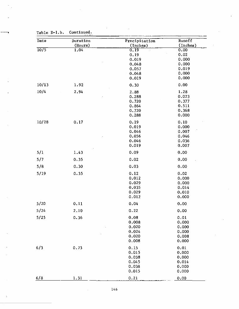
-, Table E-1.b. Continued.

Date Duration Precipitation Runoff (Hours) (Inches) (Inches)

10/5 1.04 0.19 0.00 0.19 0.02 0.019 0.000 0.048 0.000 0.057 0.019 0.048 0.000 0.019 0.000

10/13 1.92 0.30 0.00

10/4 2.94 2.88 1.28 0.288 0.023 0.720 0.377 0.864 0.511 0.720 0.368 0.288 0.000

10/28 0.17 0.19 0.10 0.019 0.000 0.046 0.007 0.056 0.046 0.046 0.036 0.019 0.007

5/1 1.43 0.09 0.00

5/7 0.35 0.02 0.00

5/8 0.30 0.03 0.00

5/19 0.35 0.12 0.02 0.012 0.000 0.029 0.000 0.035 0.014 0.029 0.010 0.012 0.000

5/20 0.11 0.04 0.00

5/24 2.10 0.22 0.00

5/25 0.36 0.08 0.01 0.008 0.000 0.020 0.000 0.024 0.000 0.020 0.008 0.008 0.000

6/3 0.73 0.15 0.01 0.015 0.000 0.038 0.000 0.045 0.014 0.038 0.000 0.015 0.000

6/8 1. 31 0.21 0.00

146

Page 156

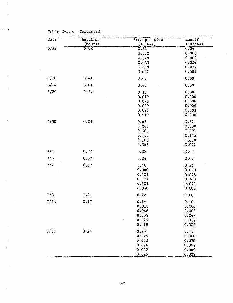
-" Table E-l. b. Continued.

Date Duration Precipitation Runoff (Hours) (Inches) (Inches)

6/12 0.08 0.12 0.06 0.012 0.000 0.029 0.000 0.035 0.024 0.029 0.027 0.012 0.009

6/20 0.41 0.02 0.00

6/24 3.01 0.45 0.00

6/29 0.57 0.10 0.00 0.010 0.000 0.025 0.000 0.030 0.000 0.025 0.003 0.010 0.000

6/30 0.29 0.43 0.32 0.043 0.000 0.107 0.091 0.129 0.ll5 0.107 0.090 0.043 0.022

7/4 0.77 0.02 0.00

7/6 0.32 0.04 0.00

7/7 0.37 0.40 0.26 0.040 0.000 0.101 0.078 0.121 0.100 0.101 0.074 0.040 0.009

7/8 1.46 0.22 0:00

7/12 0.17 0.18 0.10 0.018 0.000 0.046 0.009 0.055 0.048 0.046 0.037 0.018 0.008

7/13 0.24 0.25 0.15 0.025 0.000 0.062 0.030 0.074 0.064 0.062 0.049

147

Page 157

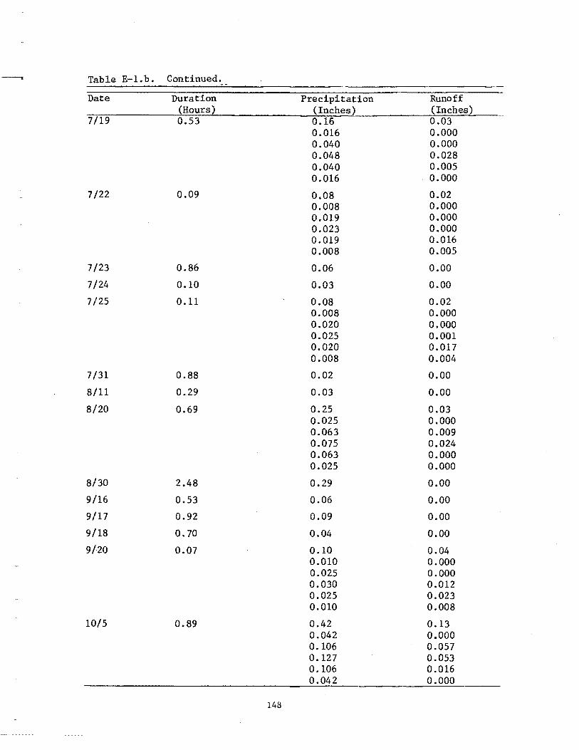
--- Table E-l. b. Continued.

Date Duration Precipitation Runoff (Hours) (Inches) (Inches)

7/19 0.53 0.16 0.03 0.016 0.000 0.040 0.000 0.048 0.028 0.040 0.005 0.016 . 0.000

7/22 0.09 0.08 0.02 0.008 0.000 0.019 0.000 0.023 0.000 0.019 0.016 0.008 0.005

7/23 0.86 0.06 0.00

7/24 0.10 0.03 0.00

7/25 0.11 0.08 0.02 0.008 0.000 0.020 0.000 0.025 0.001 0.020 0.017 0.008 0.004

7/31 0.88 0.02 0.00

8/11 0.29 0.03 0.00

8/20 0.69 0.25 0.03 0.025 0.000 0.063 0.009 0.075 0.024 0.063 0.000 0.025 0.000

8/30 2.48 0.29 0.00

9/16 0.53 0.06 0.00

9/17 0.92 0.09 0.00

9/18 0.70 0.04 0.00

9/20 0.07 0.10 0.04 0.010 0.000 0.025 0.000 0.030 0.012 0.025 0.023 0.010 0.008

10/5 0.89 0.42 0.13 0.042 0.000 0.106 0.057 0.127 0.053 0.106 0.016 0.042 0.000

148

Page 158

,.

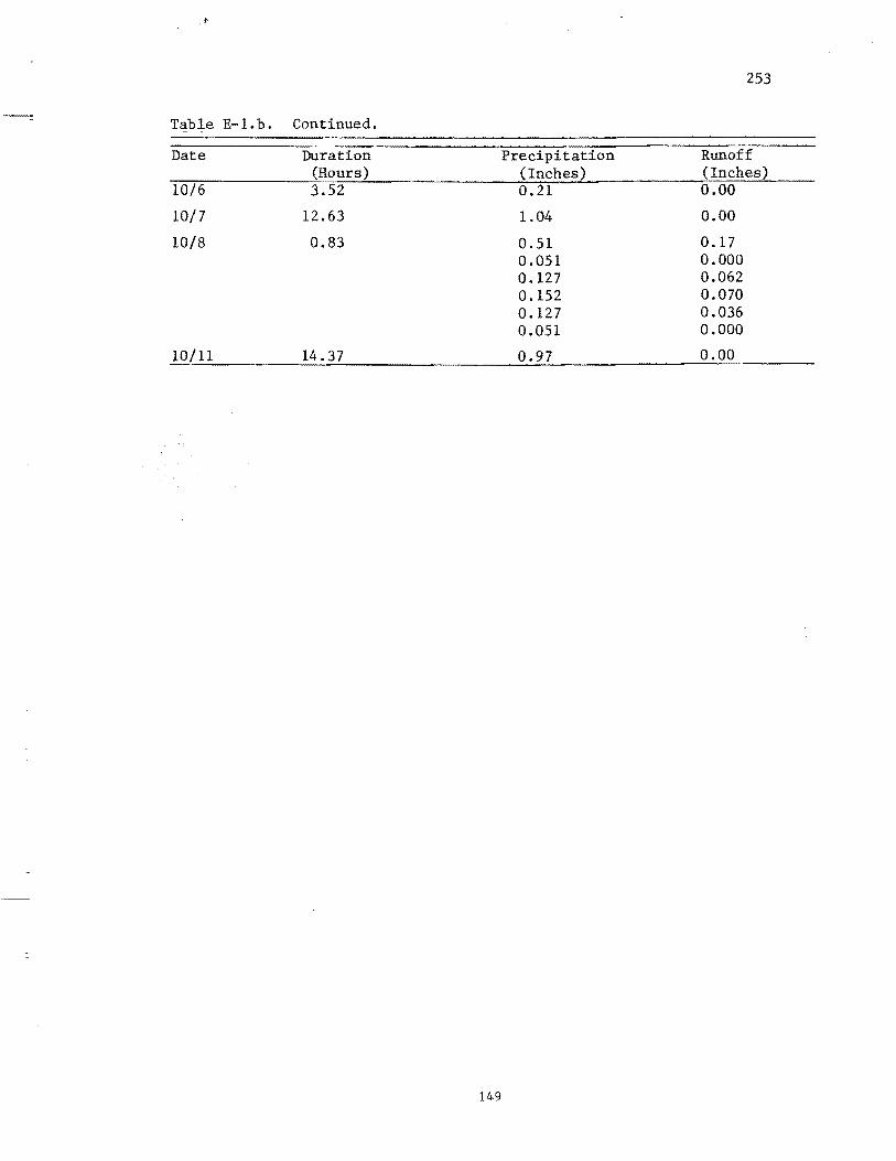
253

-. Table E-Lb. Continued.

Date Duration Precipitation Runoff (Hours) (Inches) (Inches)

10/6 3.52 0.21 0.00

10/7 12.63 1.04 0.00

10/8 0.83 0.51 0.17 0.051 0.000 0.127 0.062 0.152 0.070 0.127 0.036 0.051 0.000

10/11 14.37 0.97 0.00

149

Page 159

I-' VI o

.J

Table E-l.c. Hydrologic extractions subroutine (HYDRGY), including the plant consumptive use_§gQ~o~tine (CONSUM). = .. "·w ..... •

C

SUBROUTrN~ ~VORGV C 0101 Mt'}"J l/9LK~/RUNOFF(~),~~,SMOTS,WP (j 1 BlI< t.l1 F' C , F n , S I ,01( T , ~ U MR 0, TAU S W • !:IlJ NS 5/BLI(5/PRECIP(5),TI Mf

C TNJTI'LIZATTON

C

QUN5'O: ~S\WsO.

T"JDsO rT:J() fii'wt:l1. SLJMPT.".

'510'111). SI)M~I·O. 51.1 '" 4t q t'} ': 1'\ • SU/ooICC:!"I. 00 1;>0 II.t,C; PPT.PRECIP(tJ) SRO=O. IHI~I:O.

516=0. 5UMPT:eSIJMPT+PPT

C TNTFRCEPTTON ANn "EPRFSSION 5TORAG~

OSI=Sr-Sro rF(pPT·~ST)5~,~3.5Q

IS? stO'l:~tO+PI:'T SUMst:~UM~r+pcT

RAIN-O. S!A:PPT GO TO 55

53 510:51 SUMSI=SUM~I+~1 ,UTNS". SIA.51 GO TO '55

51.1 ~JO=SI SI}~~I=SIIM5T+n51 R6T"=PPT-"ST STAa[)SI

55 CONTINUE C

C TNFTlTRATTn" RAIN=fHTN+R;1It tF'(rNn.~~." Gn Tn 00 TII(ALn~((~S-5~OI5'/~5')~(·D~T) FTII:FC+(F~-FC)·~XPC·D~T.T) r,O TO<H3

qq FTI=FTF qs T:lT+TIME/~:

C

FTF.FC+(F~_FC)·fVP(-DKT*T) F'TII(FT1+F'TF)/2. 5FW.RAIN_FT.TIMf/~: IF(SFW)6a,elJ.~e

C SOIL MOISTURF STORAGE 6Q SMorS=5~OI5+RArN

IF(SMOr5~GE.SS' SKOTS=SS-,Ol RSW.O. 5FIIII=0. INO.O GO TO e3

bb SMorS.5MoTS+~T*TtME/S, ,"'rhlt

C C SU~FACf wATER A~UTI"'G

IF(SMOIS.Lf~S5) G~ TO t11 5FW.SFIt/+S"10TS-SS SMors=ss

111 RSW=SFW*f~P(.TAUSW)

SIilO.SFW-R5W SU~S~O.SU~~AO+SRO

Page 160

...... V1 ......

Table E-l.c. Continued.

c e RUNOF"

r:

~3 Cl"t.lTlt.lUE RUNnFFCII'.S~O SU~RO.SIJ~R"+FHINOF' C J I' RUNS.RIJNS+RUNOFF (t I 1

120 eONTTNUF. R!TlIRN ,NO

'5I.I· .. n"llltTTI.,;~ r"~:~IIM

C" ~~"'Ol'll ?/BL~?/~V~D~~(5),~~,~~"r~.~p

t> I I) t t< bIt L 6 T , f r t: A r;. , .1 nAY, C T , JET, IF Q r: • J r: ~ S , lC f( C 1 , X"': C ? • T ~ ') 10 I, ( oJ I T ~ ') ''I ( 1 ~ , * I ·i L I( , 1'\ I ~ (I 'I C~Ll SU~~~(JD~~,rL6T,~S)

C A I, L T ~ " 1= ( J i) 6 " , T t '" ) T~(JO.v.~T.t~~'.A~n.)"~Y.lT.l~~F) v~C:,Kr?

I~(J'LY.L~.T~O~.CC.J'IV.GE.IF~r:) XKC=t~Cl El~=CT*(Te~·'r)·~~/(5~5.0 •• 3~~t(T~ON(~nN'~32.» F.T:n:ICC*E'H'/t?CiU ~fl:(ALOGr(tO~.*(~~OI~-WP')/(~ICAP-~P)+l.'IU.~l~)·ET ~ '11H S = S ~ (1 r ~ - A ~ T TF(S~OIS.tT.~~' 5~C15=~g ~e:TI}l:"

r;:·'n

J

Page 161

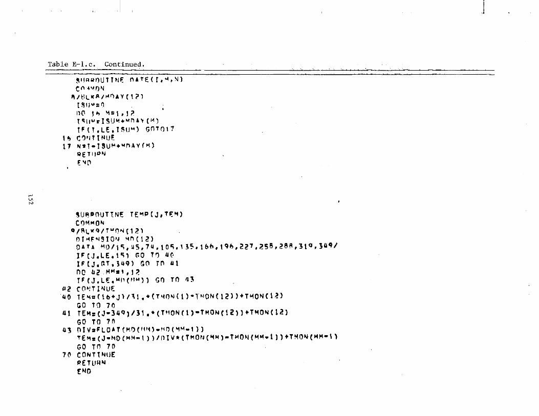
;-' VI N

Table E-l.c. Continued.

~"RQI)UTT~JF. nATE(J,M,'II) (;1"I04'HJ"I

1\ I tl L I( ~ I M n " V ( \ ? 1 PHJ\f: I) 1')(1 ,-, "':,,!;> t'Hlu~ISIj~ ... ~.mAY (104)

tFCT.LE.nW"" GnTr)l1 ,~ C'l·ITtNUF. 11 N'l·tSU~ ... ~nAV(M)

RETII P "J

~'1t'

'UR.POUTtNE TE~P(J,T~M) C O'~MON

°/"'LWq/T"'~"I(12) n r "'1 F "I S I 0 ,~ 4 n ( 1 2 ) DATA MO/t~,~S,7U,tO~"~~'lbh,tq~,2~1,2S8,2e~,l1Q,3"~1 JF(J.LE.t~' ~O T~ ~O IF(J.GT.JOq) GO Tn u1 no 02 MHa',!'-TF(J.LE.MflCPfM)l GO TO '13

a 2 COli! T 1 ~ U E ijO TEMa(tb"'Jl/'1 •• (T~n~(1)·T~ONC12».T~O~C1~)

GO TO 70 u t T EM = (J. 3 4 q ) 13 1 •• ( T ~t 0 N (1 ) • T M 0 N (12 1 , + T M 0 N C 12 )

GO TO 7n IJ] n I V :I FLO A T ( M f) ( " '1 , •• ~ r') ( MM. , ) )

TEM=(J.MOCHM_I))/nIV*(TMON(MM).TMO~(MM.l)'+TMO~(MM·'1

GO TO 70 7(\ CONTtNIJE

P.ETU~~ [NO

J

"-

Page 162

Table E-l.c. Continued.

-; I III ~ n II T 1 'I E E' S (T , r ) ~:1.~'~Q*FV~('\.07-~3'6./(T+?71.1)) QF r ".,', F.'H)

~ U .~ ~ (11 1 T r 'IJ € t:; I J Po r.;> c:; ( ~, , 'W' L AT, Q 5 ) I") T ... t" OJ , 1 "'1 v 1_ ,,, ( 1 ~ , , 'I L 'J n ( 1 P , , '( L 5 , ( 1 A , , L 1'1 A Y ( 1 p. )

Ii 6 r ~ • I. \ n I IJ , 7 • , 11 ~ IJ • , Ci ~ i-I • , " 7 ,1 • , 7 7 Ci • , ,,:, Ci : ' (.'I ':? ~ • , Q h 7 • , '11 r; • , q 6 !) • , q? 1 •• tA~~.,Y~~ •• ~~3.,~~u.,U~~.,U6~.,~71.1 ~6TA t~Jn/~§1.,3~n.,u\a.,5~3.,6R~.,A07:,QtO"q72~,qql"Q61. ,qOt" ~1~~.,~17.,~~u.,U~Q.,3~~.,'\7.,33t.1 ~~'A ~~~~/t~Q.,2~~.,?A~.,1J1Q.,S15 •• 712:,~b7"q5A~,qeq.,q5~.,RSa,.

~ '72S.,~~~ •• Otu •• ~~~ •• 2,u.,,7~.,'~~.1 t; '1 ~ r 6 L" \ Y I f\ , 1 '3 , :~ IJ , 5 ~ , ~ () , 1 r) 3, t ~ b , .1 u t) , 1 7 " , t I') b , ? 2 n , 24'3 , 2 h b , 2" q , 3 1 2 ,

,. ~ -; i..I , -~ '.,,, , ,.., C; I

'V) -'1 .~ : 1 , 1 j" r r: ( . T • t, t' • L l'l A 'f ( '1 ') ~ " T ~ b'

f'I (I r "I' 1 T r "J 'J ~ "1 \':I=I."~T(.Jl

;) ,. 1 '.! ~ :. I) " r (, '" h V ( '1 , ,

!') '111 = F IJl ~ T {L:"l A Y ('1"1 1 ) ;;l X ": ( 'k • I') ~ '1 ) I ( l' -~ \ - "'I J,! J1 )

r'('~ST.~F.a~.' ~" T0 ~~ PY=(~LAT·'n.)/tn. J..l ~ ~: < I. 3'! (' I. 1 ) ... "" y • ( -. t ~ fl ( ... ) .. l( L 3 0 ( ... Of 1 ) ) '( S T ': (I. '" ,I ( '1 .. 1 ) + u '( • r )' L U (I r'" ) ... ~ L. a 0 ( M. 1 , ) R~=~~~+pv+(q3T_~~Q)

r.n Tf') &3 ~2 PY:(~L~r_un.)/ln.

R c:j "'\ 'e '( VJ I') ( .,. 1 ) ... Cll( * ( '{ L (J n pI ) .. ~ L " 0 ( '4. \ ) ) uST~.L5~("-1)·PY·(~L5n(M)"'XL50[~·') ~S=~~~+Clv*rqST-~~Q'

... ~ "FT I~'"

!=: "H)

J

Page 163

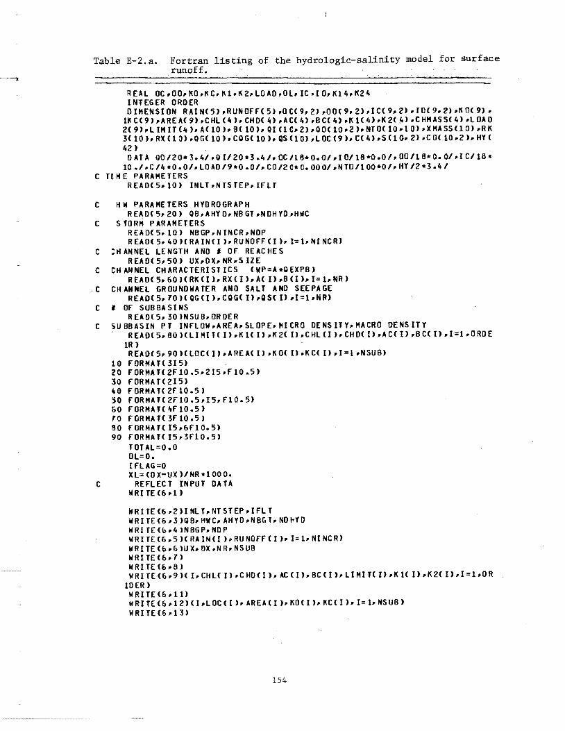
Table E-2.a. Fortran listing of the hydrologic-salinity model for surface runoff.

REAL OC.OO,KO.KC.K1.K2.LOAO,Ol.IC,10,K14.KZ4 I NTEGER ORDER o IHENSI ON RAI Ne 5) .RUNOFF( 5),0 t< 9. 2) ,OOC 9, Z).I ce 9. 2). 10( 9. 2),K DC 9) •

1K C(9) ,ARE A( 9) ,CHL (4). CHOe 4) .At< 4) .B CC 4) .1( 1C 4).K 2( {.).C HHASS( 4) .L OA D 2( 9) .. L IH IT (4 ). A( 10" B( 10)" QI C1 C, Z) "Q OC 10"Z h NT O( 10,10) "X HA SS (1 0) ,R K 3( 10) .. RX (1 () , Q G( 10). CO G( 10 ). QS (1 0) .L OC (9). C( 4) .S C1 0, 2) .C OC 10,Z ), H'f( 42 )

D AT A 00120* 3. 4/,01120*3.4 haC 118*0.01" I 0/18*0.0" 00/18*0. 01,,1 C/18 * 10 ."C 14 *0 .Ot.. LOAD 19 *0.01" CO 12 0* 0.0001 ,NTO 11 00*01. HY 12 *3 .41

C Tl H E PARAHETERS READ(5,,10) INLT.NTSTEP"IFlT

C HW PARAHETERS HYOROGRAPH REAO(5.20) OB.AHYO.NBGT.NOHYO .• HWC

C STORM PARAHETERS REAOC5,10) NBGP.NtNCR.NDP REA DC 5. 40)( RA IN (I ),. RU NOFF CI h 1= 1. NI NC R)

C :H ANNEL LENGTH AND' OF REACHES READ( 5. 50) ux.OX. NR,S IZE

C CHANNEL CHARACTERISTICS (WP=A*OUPB) R EAD( 5, E)O)( RK CI ). RXC I), A( I) .B (I ), 1= 1, NR )

C CHANNEL GROUNDWATER AND SALT AND SEEPAGE READe S, 70)( OGCI ). COG( I) ,OS( n ,1=bNR)

C , OF SUB BA S t NS R UD( 5.30 )NSU B. OR OER

C SUBBASIN PT INFLOW.AREA,SLOPE.MICRO DENSlTy.HACRO DENSITY READ(S.80)(LIHIT(I).K1(I),K2(I).CHL(I),CHD(I).AC(t).BC(t).1=1.0RDE

1R) READ( 5.90)( LOC( I) .AREA( I) .KO( n,K C( I). I=1.NSUB)

10 FORHAT(315) 20 FORHATe2f10.5.2I5.flO.5) 30 FORHA TC ZIS) ~o fORHAT(2F10.S) 50 FORHAT(2f10.S.I5,F10.5) &0 FORHAT(4f10.5) 70 FORHAT(3F 10.5) 50 FORHATCI5.E)F10.5) 90 fORHAT(15,3F10.5)

TOTAL=O.O OL=O. I fLAG=O X L= (0 X-UX )1 NR *1 00 O.

C REFLEC T INPUT DA TA WRITE (E),l)

W RI TE (E).2 JI NL T. NT ST EP. IFL T WRITE (E).3 )OB. HWC. AHYD ,NBG T. ND ",YO WRITE(6.4)NBGP.NDP WRITE (6.5)( RA IN CI ), RU NOfF (I ), l= I. NI NC R) WRITE(6.6)UX,DX,NR,NSUB WRI T[(6. 7)

W RITEC6. 8) WRIT E (6 ,9 )( I. CH LC J) , C HD ( I ). AC <I ),. BC CI ),. LI HI J( n • K U 1) • K 2( I) , I :: 1 .0 R

10ER) WRITE(6.1U WRITE(6.12)(I.LOC(I).AREA(I).KO(I).KC(I).I=1.NSUB) WRITEC6,13)

154

Page 164

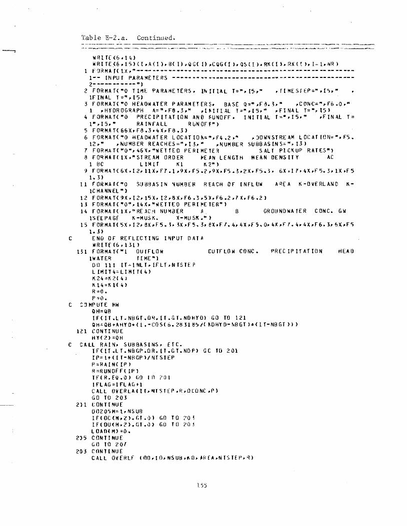
Table E-2.a. Continued.

W R I Tf (6 • 1 4 ) W R I f E .< & , 1 '» ( I , A ( I ) • B ( I) • Q G ( I) , C Q G (I ). Q S ( I ) • RK ( I ). R X ( r ). i =- 1, N R )

1 fORMA T( 1 X," -- -- -- -- -- ---- -- -- -- -- -- -- -- -- -- -- -- -- -- -- -- -- -- -- -- ---1-- INPUT PARAMETERS --------------------------.. -------------------2- ---- ---- -- .. )

2 FORHAH"O TIME PARAMETERS, INITIAL T=",I5,," , TlMESTEP::::".I');." 1FINAL T=",15>

3 FORHAH"O HEAOWATER PARAMETERS, BASE Q:::",F8.3," ,CONC=",F6.0." 1 "HYOROGRAPH A=".FS.3," ,I(lITI~L T",",15." ,FINAL T=",15)

4 FORHAH"O PRECIPITHION AND liUNOfF. INITIAL T",",15," .FINAl T= 1",15." RAINFALL RUNOFF")

5 FORHAT(&6X.F8.3.4X.F8.3> 6 FORHAH"O HEADWATER LOCATIOt\=",F4.2." ,DOWNSTREAM LOCATION=".F5.

12," ,NUMBER REACHES::::",13," .NUMBER SUBBASINS",". 13) 7 FORMAH"O".46X,"WETfEO PERIMETER SALT PICKUP RATES") 8 FORHAT<lX."STREAM ORDER "[AN LENGTH MEAN OENSITY AC

1 BC LIMIT Kl 1'\2") 9 FORMAT(6X.I2.11X,F7.1,9X.F5.2,9X.F5.3,2X.F5.~. 6X.I7.4X.fS.3.1X.F5

1. ~) 11 FORHAH"O SUBBASIN I'jUHBER REACH OF INFLOW AREA K-OVERLAND K-

lCHANNEL tt)

12 FORHAH9X.I2,I'5X.12.8X.F&.3.SlC,F&.2.7X.F&.2) 13 FORHAT("0".14X."wETTEO PERI~E1ER") 14 FORMAHIX."RE.\Crt NUHaER (I B GROllNDWATER CONC. GW

ISEEPAGE K-MUSK. X-MUSK.") 15 r OR MA T< 5 X • 12, 8X, F '5. J. 3X, F '5. 3, ex, Fl. 4. 4 X ,f '5. 0:0 ItX :of 7. 4 .. 4X .. F &. 3 .. 6 X .Pi

1.3) C END OF REfLECTING I~PUT OAT A

WRITE(6.131 ) 131 FORMAH"1 OUTFLOW CUTFLO .. CONC. PRECIPlTATION HEAO

1WAH~ TIME") o 0 11 I IT =; I NLT • [r LT • N T 5 T EP L IHIT4;;:: LlHI f( 1+) K24=K2(41 1'\}I+=1'\1(4) R=O. p=o.

C :0 HPUlE HW QH=QB IF(IT.LT.NBGT.OR.IT.GT.NDHYO) GO TO 121 Q H::: QB +A HY 0* ( 1 • - CO S( 6. 28 H 8') I( M) HY 0- NB G T ) .. ( I Too NB G T ) ) )

121 CONTINUE HH l) =QH

C CAll RAIN. SUBBASINS. ETC. IF(lT.LT.NBGP.OR.lT.GT.NDP) GC TO 201 IP=l+(lf-NBGPl/NTSrEP P=RAIN(IP) R=RUNOFf( IP) If(R.EQ.Q) GO In 201 IFLAG=IFLAG+l CALL OVERlA(II.NISffP.R.OCONC.P) GO 10 203

211 C ON TI NU E 00205H=1.NSUB IF(OCCH,l).GI.O) GO TO ?O' IF(OU(H.2).GI.O) GO TO 20j LOA£HH)=O.

2)5 CONTINUE GO TO 207

20] CONTINUE CALL OVERLF (nO,IO.NSU!:I.I\O. _RfA.NTSTEf>.'n

155

Page 165

Table E-2.a. Continued.

CAll CHANF'l(OC, IC,NSUB"I(C"OO, hTSTEP) C All SALT UP (00, OC ,CHl ,CHD ,ORO ER,NSU B, AC ,BC, Kl,1<2, AR EA,l 1M IT,C HHAS S

I" OMASS" OCONC, NTSTEP, IT"lOAO "C ,Ol, NBGP) 2'J7 CON TI NUE

C CALL HW AND ROUTE FLOW CAll ROUT[(QH,OI, OO,NR,RK,RX" ttTSTEP"QG"OS,OC,NSUB,lOC) CAll CH ANSA (IT, NR, NTS TEP, INLT "A,B ,Xl" OJ ,QO, K14, 1<24, LI HI "uS IZ E, C, X

IMASS, ORDER, NTO) NTlME=I T O=QO(NR,2) QHW=OH

C ROUTE SAL T 00531 =1 ,NR 00 51 I< = .. N SU B If(I.NE.lOC(K» GO TO 51 XMASS (I )=XMASS( I) +lOADCK)

H CONTINUE X TS TE P= NT STEP X MASS CI )= XM AS S( I) +C QG (I )* QG (I )*XTST EP 00 53 l =1.2 AX=RKU) BX=RK<I )*RX( I) QOUT=OO(l,l) OIN=QICI.U S U,l )=AX*QOUT+BX*( OI N-QOUT)

B CONTINUE IF(00(NR.2).lE.O) GO TO 61

C SALT ROUTED DOWNSTREAM CAll· RT ESl HS,C o. XMAS 5, 00" 0 I. ~R,N TS TEP" liwc, HY. OS) GO TO 62

31 CO(NR,2)=O. 62 CONTINUE

CS=CO(NR,2) 0052I=l,NR 0ICI,1)=OICI,2)

;2 00(1,1)=00(1,2) H Y( 1)=H Y( 2)

C END SALT ROUTI NG WRITE(6,141) O"CS,P,QHW,NTI"E

lU FORMAT<3X,F'8.3,,13X.F6.0,13X,F3.2,10X,F'6.3,7X,IIt) TOT Al=T OT Al +QO( NR, 2) * CO (N R, 2) *NTS TE P

111 CON TI NUE If R ITE (6.311 )

311 FORMAH-l't,"TOTAl SALT lOAD FIiOM EVENT, GRAMS-"'O","STREAH OR 10ER CONTRIBUT ION") WRITE(6,31Z) (I,C(I),I=l,ORDE~)

312 F'ORHAT(5X,I2,IOX,EIO.3J WRITE (6,313) Ol

313 FORMA f( IX," OVERLA ND", 6X,E 10.3 ) 00314 N= I, ORDER

314 Ol=Ol +C C N)

WRITE(6,315) Ol,TOTAl 315 FORMAHllX," SUH=",EI2.J," TOTAl=",EI2.3)

5 TOP END

156

Page 166

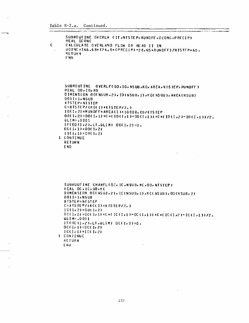
Table E-2.a. Continued.

SUBROUTINE OVERLA (IT~NTSTEP~RUNOfF~OCONC~PRECIP) REAL OCONC

C CALCULATE OVERLAND FLOW OR RE_D IT IN OCJ~C=366.68+(24.0*(PRECIP)-2e.65*RUNOfF)/NTSTEP*60. RET UR N ENO

SUBROUTINE OVERLFCOO~IO~NSUB~KD~AREA~~HSTEP~RUNOFF) REAL OO~IO~KO

DIMENSION OO(NSUB~2)~IO(NSUB~l>~KO(NSUB)~AREA(NSUB) D011=1~NSUB OSTEP=NTSTEP C=XTSTEP/(KO( 1)+)(JSTEP/2.) IO(I~2)=RUNOFf*AREA(I)*10COO.CO/XTSTEP o 0 ( I ~ 2) = 0 0 ( I ~ 1) + C * ( I 0 ( I ~ 1 ) - 00 ( I ~ 1 » t C * ( I 0 ( I ~ 2 ) - 10 ( I ~ 1 » /2 • QLlM=.OOOl IF(OOCI~2).LT.QLlM) OO(I~2)=O. OO( I~ 1>=DO( 1~2) IO( I~ 1>=IO( 1~2)

1 CONTINUE RET UR N END

SUBROUT INE CHANfLCOC~ IC~NSUB~ tcC~OO~ NTSTEP) REA L DC ~ I C ~ 00 ~ K C DIMENSION OC(NSUd~2)~IC(NSUB~l)~KCCNSUB)~OO(NSUB~2) 001 1= 1~ NSUB XTSTE.P=NTSTEP C=XT5TEP/(KCC I) tX TSTEP/2.) IC(I~2)=OO(b2)

o C ( I ~ 2) = a C ( I ~ 1) t C * ( I C ( I ~ 1 ) - OC ( I ~ 1 » t C * ( I C ( I ~ 2 ) - I C ( I ~ 1 ) ) /2 • Q LI 11= .0001 I f ( nc ( I .2 ) • LT. Q LIM) 0 C ( I. 2) =0 • OC( I. 1) =OC( 1.2) ICCI.U=IC( 1.2) CONrll~UE

R ET U~ N ENU

157

Page 167

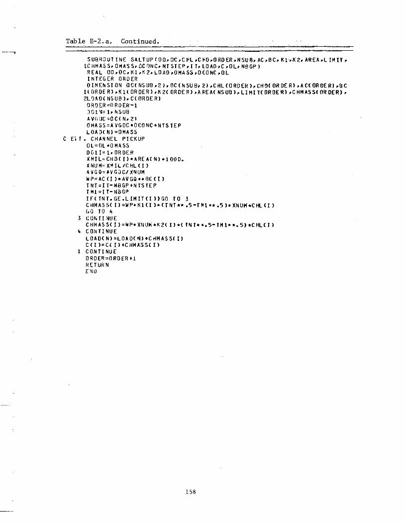
Table E-2.a. Continued.

SUBR:) ur I NE SALT UP (0 O. OC.C t-IL.C r:O .. ORD ER .. N SU B. AC .. BC .. KbK 2. AREA .. L 1M IT .. 1C HMAS S. OMAS S. ac ON C. NT S rEP. IT .to Ao .. e.o L. NB GP )

REAL OO.OC.Kl .. ~2.LOAO.OHASs .. OCONe .. OL INTEGER ORDER DIM E~ S ION 00 ( NS US .. 2). OC O. SU B .. 2) .. C HLC 0 RD EH ) .. CH D( OR DE R) • A C( OR DE R) .. B C

1< OR DE R) .. K 1< OR DE R) .. I( 2( ORDE R) .. A fiE Ae NS UB h LI HI H OROE R) .. C HH AS se OR OER) .. 2LQADCNSUB).C(ORDER)

OROER=ORDER-l )01 \1= 1. fIISUB AVGOC=OC(N .. 2) OHASS=AVGQC *OCONC*NTS TEP LOA:>( N)=OHASS

C EiT. CHANNEL PICKUP OL=Ol+OHASS DOII=l.OROER )(MIL;;;CHD( I>*AREA(N)*1000. X NU H= Xi'! I llC HL ( I ) AVGO::; AVGJCI XNUH 1i;>=AC (J )*AVGQ**BCCI) TNT=IT-NBGP+NTSTEP TH1=IT-NBGP IFcrNT.GE.LIHIT(I»GO TO 3 CHHASS( l)=WP*Kl<I )*<TNTu .5-TM1**.5)*XNU.hCHLU) ('0 TO 4

3 CONTINUE C HIHS S( I) =WP* XIWI'i *K 2( I) *( TN T. *. 5- TH 1 * •• 5) .C HL< I )

,. CONTINUE lOAD(N)=lOAO(N)+CHHASS(I) C ( I ) = C C I ) +C HH AS SCI)

1 CONTINUE OROER=O RDER +1 RETURN ENU

158

Page 168

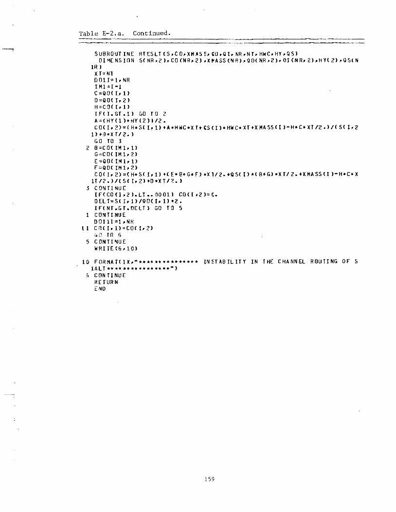
Table E-2.a. Continued.

SUBROUTINE RTESLT(S.CO~XHAS~.~O,QI,NR,NT.H~C,HY.QS) DIMENSION S(NR.2).CO(NR~2).X~ASS(NR),QO(NR.2).OI(NR.2).HY{2).QS(N

lR) XT=NT OOlI=l.NR IM1::I-l C =QO( 1,1) 0=00(1,2) H=CO( I, 1)

I f'( I. G T • 1) GO T 0 2 A={HYCI )+HY<2H/2. C O( 1,2):: ( H* S( I, 1) + A *H WC*X T H:S <I ) * HW C* XT +X MA SS ( I ) - H* C* XT 12 .) I( S{ 1.2

1)+!l*Xf/2. ) GO TO 3

2 B=.CO{IM1.1) G=CO(IM1.2) E=QO{IMl.l) f=OOCIM1,2) CO ( I. 2) = ( H* S ( I, 1) +( E'" B+ G* f) *X T 12. +Q S( I) * ( B+ G) * X T 12. + X lolA 5S C I ) - H * C Ir X

1T It! • ) I ( S ( I. 2) +0 * X T 12. ) 3 CON T I NU E

IF<CO(l.2).LT •• OOOl) CO<I.2)=C. OEL T=S{ I.D/OO( 1.1> *2. If(NT.GT.OELT) GO TO 5

1 CONTINUE DOllI=l.NR

II Cr)(I,1>=COCI.2) (][l TO I)

5 CONTINUE WRITE (6~ 10)

10 FORMAHIX~"*************** INSTABILITY IN THE CHANNEL ROUTING Of S lAl T ** ** **** **** ** **")

o CONTINUE RETURN c: NO

159

Page 169

--, Table E-2.a. Continued.

SUBROUT INE CHAHSA( IT, NR,NT5 TEP, INLT ,A,B,XL, QI,QO, KO,K hLI MI T, SIZE, lC,XHASS,ORDER.NTO)

REAL KO,K h LO AD I NTEGER ORDER DIMENSION A(NR).B(NR).QI(~R.2),QO(NR,2).NTO(NR,10).XMASS(NR).C(ORO

lER) C CAlCULATE MEAN FLOWS

XTSTEP=NTSTEP DDlI=l.NR Q M= ( Q HI,. 2 ) + Q HI, 1 ) + Q 0 ( I. 1) +0 0 ( r. 2) ) / 4 • IF(QM.LE.O) GO TO 73 AXP2=A(I)*QM**B(I)*XL GO TO 74

r 3 A XP2=O. 74 CONTINUE

4 CONTI NUE C CALCULATE AREAS

AR=O. NAR=O

3 NAR;NAR+l A R= AR +5 I Z E Z=(AXP2-AR)/SIZE NDIfF=(AXP2-AR)/SIZE 1 f( NO IFf)9, 8.7

7 CONTI NUE GO TO 3

8 CONTI NUE GO TO 25

9 C DNTI NUE GO TO 1000

C CALCULATE AREAS ~5 CONTINUE

0010M=I,NAR H(NTO(J,M).NE.O) GO TO 10 NTO(I,H)=IT-NTSTEP

10 CONTI NUE If(Z.GE.O) GO TO 26 Z:::Z+1

26 CONTI NUE XMASS(I )=0. LOAO=O. 0027M=I,N AR TNT=IT-NTO(I,M) XMASS(I);XMASS(I)+lOAO TloIl=TNT-NTSTEP rf<TNT.GT.LIMIT) GO TO 28 lOA D= SI ZE *K 0* <T NT **.5 -TMI ** .5 ) GO TO 27

26 LOAO=SIZE*Kl*<TNT**.5-TM1**.5) 27 CON TI NUE

XMASS (I )=)cMASS( f) +Z*LOAO C (ORDER );C( ORDER) +XMASS(I)

1 CONTINUE GO Tll 1QOl

10)v WI<IfEC6.100)

IJO FORMAH1J(.'ERROR IN CHANSALP) 1001 CON T1 NU E

R£T URt.l £ NO

160

Page 170

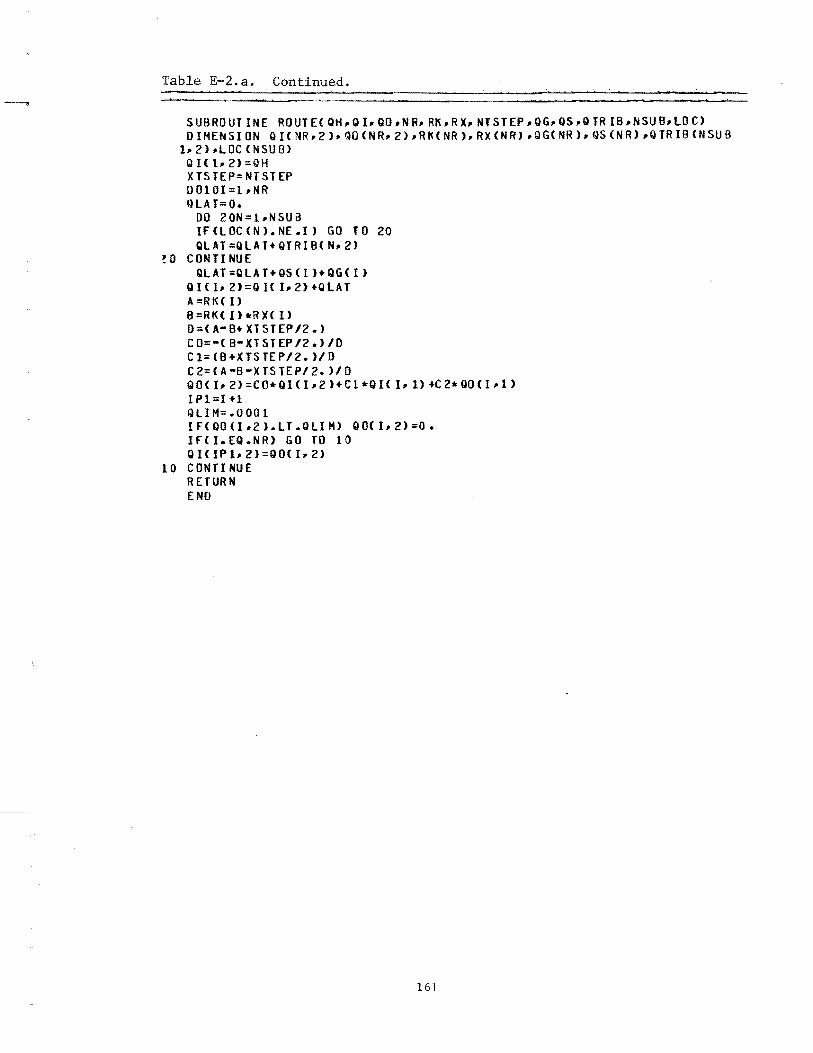
Table E-2.a. Continued.

SUBROUTINE ROUTE(QH,QI,QO,NR,RK,RX,NfSTEP,OG,QS,OTRIB,NSUB,lOC) DIMENSION QICNR,2),QOCNR,2),RKCNR).RXCNR),QGCNR),QSCNR),OTRIBCNSUB

1,2).LOCCNSUB) QI<1.2):OH XTS TEP= NT ST EP DOI01=1,NR QLA T= O.

00 20N=1.NSU a IFCLOCCN).NE.I) GO fO 20 QLAT=QLAT+QTRIBC N, 2)

~O CONTINUE QL AT =Q L A 1+ OS ( I )+ QG ( I )

Q l( I, 2) =0 H I. 2)+QlAT A =RKC 1)

B=RK(l)*RX( 1> 0=( A- Bt XTSTEP 12.) C 0= - ( B- Xl STEP 12 • ) 10 Cl=CB+l(TSTEP/2. )/0 C2=(A-B-XTSTEP/2. )lD Q 0 CI, 2) :: CO * Q l( I • 2 )+ C 1 * 0 l( I, 1) +C 2* 00 ( J, 1)

I Pl=1 +1 QUM=.0001 IF ( 00 (I ,2 ).Ll • Q LI H) 00( I, 2) =0 • IFCI.EQ.NR) GO TO 10 01( IPt .. 2)=QO( I, 2)

to CONTINUE RETURN ENO

161

Page 171

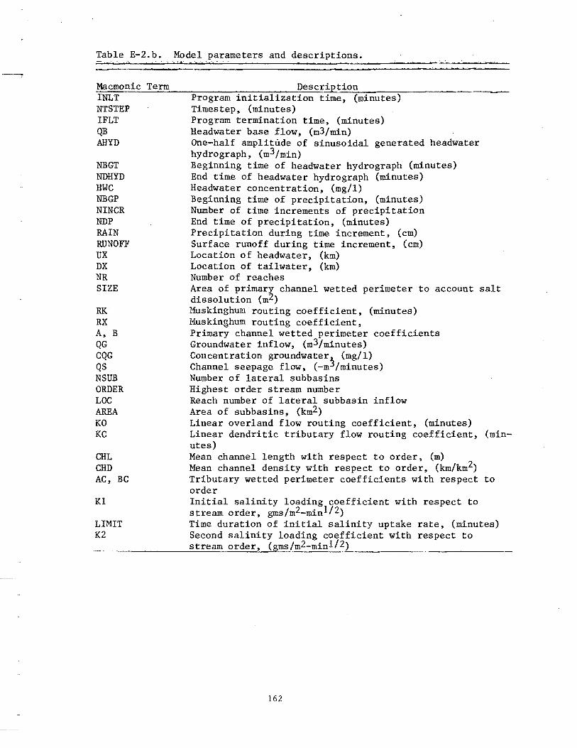
Table E-2. b.

--" Macmonic Term INLT NTSTEP IFLT QB AHYD

NBGT NDHYD HWC NBGP NINCR NDP RAIN RUNOFF UX DX NR SIZE

RK RX A, B QG CQG QS NSUB ORDER LOC AREA KO KC

CHL CHD AC, BC

KI

LIMIT K2

Model parameters and descriptions. ",I." •

Description Program initialization time, (minutes) Timestep, (minutes) Program termination time, (minutes) Headwater base .flow, (m3/min) One-half amplitude of sinusoidal generated headwater hydrograph, (m3/min) Beginning time of headwater hydro graph (minutes) End time of headwater hydrograph (minutes) Headwater concentration, (mg/l) Beginning time of precipitation, (minutes) Number of time increments of precipitation End time of precipitation, (minutes) Precipitation during time increment. (cm) Surface runoff during time increment. (em) Location of headwater, (km) Location of tailwater, (km) Number of reaches Area of primary channel wetted perimeter to account salt dissolution (m2) Muskinghumrouting coefficient, (minutes) Muskinghum routing coefficient, Primary channel wetted perimeter coefficients Groundwater inflow, (m3/minutes) Concentration groundwater3 (mg/l) Channel seepage flow. (-m /minutes) Number of lateral subbasins Highest order stream number Reach number of lateral subbasin inflow Area of subbasins, (km2) Linear overland flow routing coefficient, (minutes) Linear dendritic tributary flow routing coefficient, (min­utes) Mean channel length with respect to order, (m) Mean channel density with respect to order, (km/km2) Tributary wetted perimeter coefficients with respect to order Initial salinity loading coefficient with respect to stream order. gms/m2-minl/2) Time duration of initial salinity uptake rate, (minutes) Second salinity loading coefficient with respect to stream order, (gms/m2-minl/2)

162

Page 172

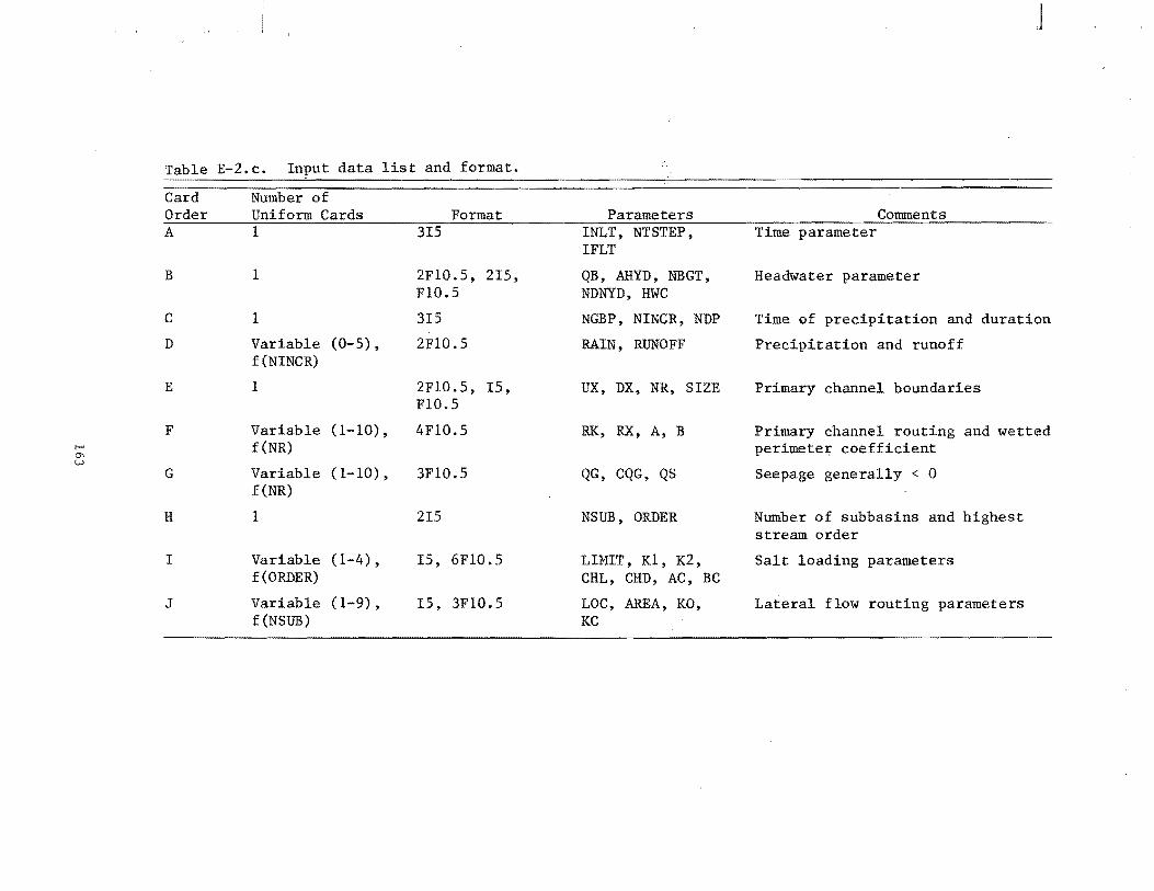
I-' Cl' W

Table E-2.c. Input data list and format.

Card Order A

B

C

D

E

F

G

H

I

J

Number of Uniform Cards 1

1

1

Variable (0-5), f(NINCR)

1

Variable (1-10), f(NR)

Variable (1-10), f(NR)

1

Variable (1-4), f(ORDER)

Variable (1-9), f(NSUB)

Format 315

2FlO.5, 215, F10.5

315

2F10.5

2FlO.5, IS, FlO.5

4F10.S

3FlO.5

215

15, 6FlO.5

IS, 3F10.S

Parameters INLT, NT STEP , IFLT

QB, AHYD, NBGT, NDNYD, HWC

NGBP, NINCR, NDP

RAIN, RUNOFF

UX, DX, NR, SIZE

RK, RX, A, B

QG, CQG, QS

NSUB, ORDER

LIMIT, K1, K2, CHL, CHD, AC, BC

LOC, AREA, KO, KC

J

Comments Time parameter

Headwater parameter

Time of precipitation and duration

Precipitation and runoff

Primary channel boundaries

Primary channel routing and wetted perimeter coefficient

Seepage generally < 0

Number of subbasins and highest stream order

Salt loading parameters

Lateral flow routing parameters

Page 173

Table E-3.a. Fortran listing of the simplified model for predicting salt pickup by overland and microchannel flows.

C ~JCROC~ANNEL HYDAOSALtN1TV MO~[L C

C

COM~ON/RLK"X~V(12),8V(12',BT'(t2,~)~eT2(12,5);~~Tl(12 '~l; 1XKT2(12,5).D!Ctl(t2,5),XKNS(12),8N8(lZ),IDUM,A,~,C,Hl ,H2,H], I~U,~5,TOTPRE,CHANCE,T!LtM 1/~L~l/RUNO'F(5',SS,SMOIS,W' _ .. . 3/~l~3/SALT(5),ILOP!,~INT,IALTT,8o,8t,e~,IO'S,8eWS,ICH (5),10'(5),

"~'A Q/Rl~a/'C"~,8I,D~T,SUMRO,TAU8W~~UN8 "RL~~/PRfCIP(5),TtM! J' _ ~ ~/RL~"XLAT"ICAP,JDAV,CT,A!T,1'.',I'R.,XKC1,.kCZ,TX 7/ RlIt7/MONTClZ) "'''lIt8/HDAVClZ) Q/PlkQ/T MON(12) */BlI<l O/~ON

OA'& HD'Y/'1,Z&,Jt,lO,11'lO'~1,31,JO;3i,]O,31/, . ~ . DATA HONT/.JAN~,.'!8~,wMAR·,~APR~,·M'V~,·JUNW,WJUL·,WAUG·,· IE'-, .·OCT·,·NOV·,~O!C"I

C READ D'TA A!An(5,JOZ)(~kV(J),Jat,tZ)

c

REAO(5,JOZ)(8Y(J),Jat,12) 1)0 to Iat.~ RE,~(~,J02)(8Tt(J,I),Jat,'2) R'AO(5.302)eBTZ(J,!),Jal,IZ) REAOC~,30~)(XkTl(J,t),J·t,12) RE,nC5.302)CXKTlfJ,I),J."lZ)

10 RfAD(5,]02)(D!CI8(J,I),J.t,lZ) READ(5,]02)(XkN8(J),J.l,lZ) READC5.302)(ANS(J),J.l,tl) RE'I)CS.1oZ)(THONeJ),J.l,11) '. R!AD(5,300) A,B,CtIO,81,BZ,SLOP[.X1NT.,HANL ~ . A.!AO(5,l'OO' .S"!.'MOI','C,'O,DkT.,A"e:A,TAU'W·,~CHCO . A(lOC~,300) fLrV.TMAX,TMIN,XLAT,W';'JeAP,~wel,XWCz,T[LIM AfA~(~.)Ol) IDUM,NUMy •• ,N.DAy,N!OAY,!' •• ,I'.' WQfTECfJ,152)

WRIT!CfJ,11J1) wqfT~(a,*II)A,B,C;BO,el,82,ILOP!,XINT,CHANL WAITE(a,*II) sa,St,SMOI8,'C,'O,OkT;AR!A,TAU8W,XC Weo ~qITE(,,*'I)~L[V,TM'X,TMIN,XLAT,WP,~tCAP,X~Cl,XKCl,TfL 1M

WPTTE(b,*II) IDUM,NUMVRS,N8DAV,N£DAV,I'RS,I'R' W~r'E(b,3b3)

,no ~~RM&'t1'IO.O,2F5;O) '''I 'nRIo4A'C&ttO) Jn2 'O~Io4AT('l'~.J'

164

Page 174

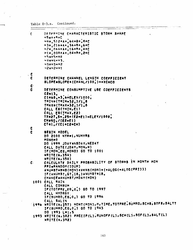
Table E-3.a. Continued. --'-~.- -... ---~=-================.--~~-: .. :--------------.

C DF.Tr~~I~E CHAqACTERISTIC STORM SHAPE 1-15.,+I\+C

, C C

CI C

C C

C·

1001

" , ..

i " • l-Ia •• ~'2.A+.h~.B+.~·C I-Il·t21~.' •• lh.B+".e 1-I?!nha.A+.1b.~+,a·c Hl·.OOB.A •• ~a*A •• 2·C 1-I'\.I-IS· ... u lo4u.IoIU· ... l. H3.1-13- H (1

!~2.""2· ... t

DET£RMINE CHANNEL LENCTH COrFFICJI~T ILO,r.SLOpr*(CHANL/JOO.)**XCHCO

DET.,RHIN! CONIUMPTIVE UIE COE'FICrrNTI Ca.1J; .' . cS •• a.-l.'·!LIV/l000. THIN8CTMIN-Sa;)/,;8 TMAX.CTMAX.J2.)/S.8 CALL [8(TMtN,!I) CALL ~ICTMAX,!2) TX.,1.S-.I!*fEI-Il).ELIV/1000: CH.1J9· / ([2.ES) CT.l./fCStC2*CH)

BlltN HODrL DO 2000 NVR.l,NUMV-S MONO.O DOt999 JDAV.NIDAV,NfDAV CALL DAT£tJDAV,MON,M) 1'(MON:!Q,MONO) GO TO 1001 W"IT!C',154) W"ITIC,,150) CALCULAT! OAILV PR08ABILITV 0' STORMS iN MONTH MON '~I.RANDOMflOUM) lNUMST.8NICMON)tWKNSCMON)*C-ALOGC.ALnGt PRI'» t'(ANUMST.GT:18;)ANU~8T81'~ CHANCE8AHUMIT/MOAVfMOH) C'LL IUIN CALL CONSUM I'(TOT'R!.f.Q~O:) CO TO 1997 CALL HVDRGV 1'(~UMRO~!Q~O.) GO TD 199b CALL SALIN ... . .-WRtTEC6,l!T) ~ONTCMON),M'TIME,TOTPR!,SUMRO'SCH8,snFS,SALTT I'CIUMRO.[Q.O.) CO TO 1943 DO t 99} L 81,5 .. .,' WAITfC.,J8l) 'RECr'CL),AUNO"CL),SCH(L),SO'CL),8ALTCL) WAIT!Ch,19"

165

Page 175

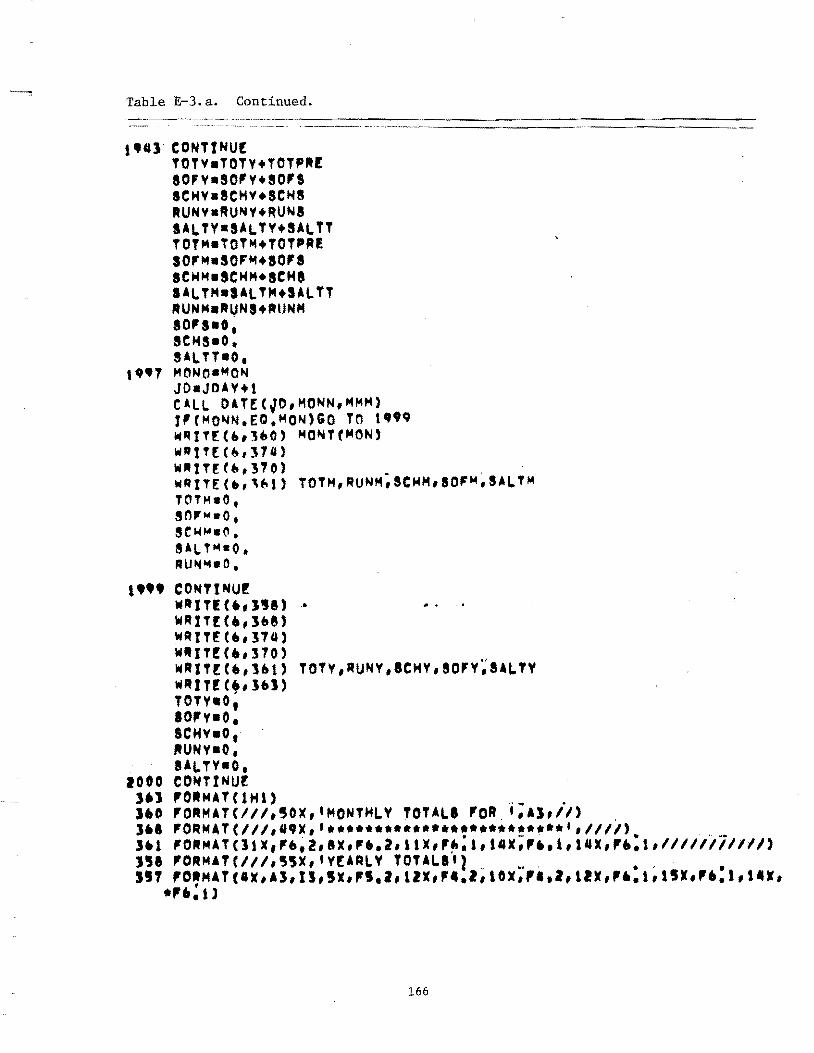
Table E-3.a. Continued.

1'''] CONTtNU[ TOTV_TOTV+TOTPRE aOFV-SO"V+SO"S aCHV-aCHV.SCHS AUNV-RUNV+RUNI IALTV a8ALTV+SALTT TOTM_TOT~+TOT'R!

SO,,"'a80F"'+10'S ICH"'-SCHM·SCHI IALTH_SALTM+SALTT .tuNMaRVNS+,.UNM 80"S-0. SCHS-O. SALTT-O.

, •• ., MONoaMON JOaJDAV+l CALL DAT[(~D,MONN,MHM) J'(MO~N.EC.MON)GO Tn t"q WqrT[(b,]bO) "'ONT(MON) w"tT[(~,:HII)

w"tH:(~,3"O) WRITECb,"l) TOTH,RUNM;SCHH,SOF~~S.LTH TOTMaO. sn'MWo. SCH"'aO. S·LT ... ·O. 'WN .... O.

I'"~ CONTINU! WAITfC"I!I) >. WAIT!C',3b8) WRIT[(.,]1Cl, W"IT[C',]10) WAIT[C.,l'l) TOTV,RUNV,ICHV,aO'V~S'LTY W't! T! C., JbJ) TOTV.O; 10"'1-0. aCHV-O. "UNV-O. IALTV-O.

1000 CONTINU! 3'] ,OR.UTClHl) '" . 1'0 'ORMATCIII,50X,'MONTHLY TOTALI 'OR ',4],11) ],. 'ORMATCIII, .. 'X,'*.*.*.***************.**.',III') . . -' ... ,. "" .. ]" "ORMATC]lX,"b.2,8X,'b,2,lIX,'~.l,14X"',t,1"X".,1,111 11111111) ]58 'OR,..ATCII/,'5X, 'VEARLY TOTALII}, .. '. • . • SST ,ORHATf.X,A3,IS"x"1.2,l'.".,',lOX,,.,2,l'X,".1,'!X"',I,t.x, ,

*".1)

166

Page 176

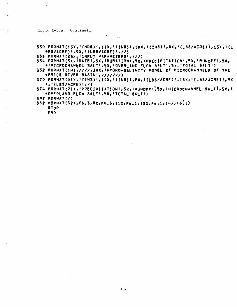
Table E-3.a. Continued.

1'0 'ORMAT(15X"(HRS)j,11X;'(INS)~,tOX;'(tN.)"AX"(Le8/AC~!)~,IJX;'CL *SS/ACRE)','X,'CLBS/ACR!)',II)

J'] 'ORMAT(2!X~tINPUr PARAMETERS',III), ' J'Q 'ORMAT(5X, 'OATEt,5X,IDURATION',5X,'PR[CIPITATlPNt,5X,IRUNnF,t,5x,

.'MICROCHAN~!L SALTI,SX,'OVERLAND 'LOW SALT',5X,ITOTAL SALT') J52 'OAMATC1Hl,IIII,JUX,'HYDRO-SALINITV MODEL OF MICROCHANNfLS OF TH!

.'RIe[ RIVtR BAIIN),IIIIIII) ITO 'OA~AT(S'X,j(INS)',tOX,'(IN8)'.~X'~(L88/ACRf)l,lJX.I(LBS/ACRE)~"X

*,'CLBS/ACR[)',/) ITU 'OR~AT(l1X,IPR!CIPITATION,,5X"RlJNO,,':5X"MICROCM'NNEL SALTI,5X,t

.OV~QLAND FLOW SALTI,~X,tTOTAL SALT') Jqz 'OR~ATC/) ,__ SAl 'OANAT(IZX,Fb.3,8x,Fb.l,11X,".1,15X,Fb.l,lUX,Fb.l)

STOP ,ND

167

Page 177

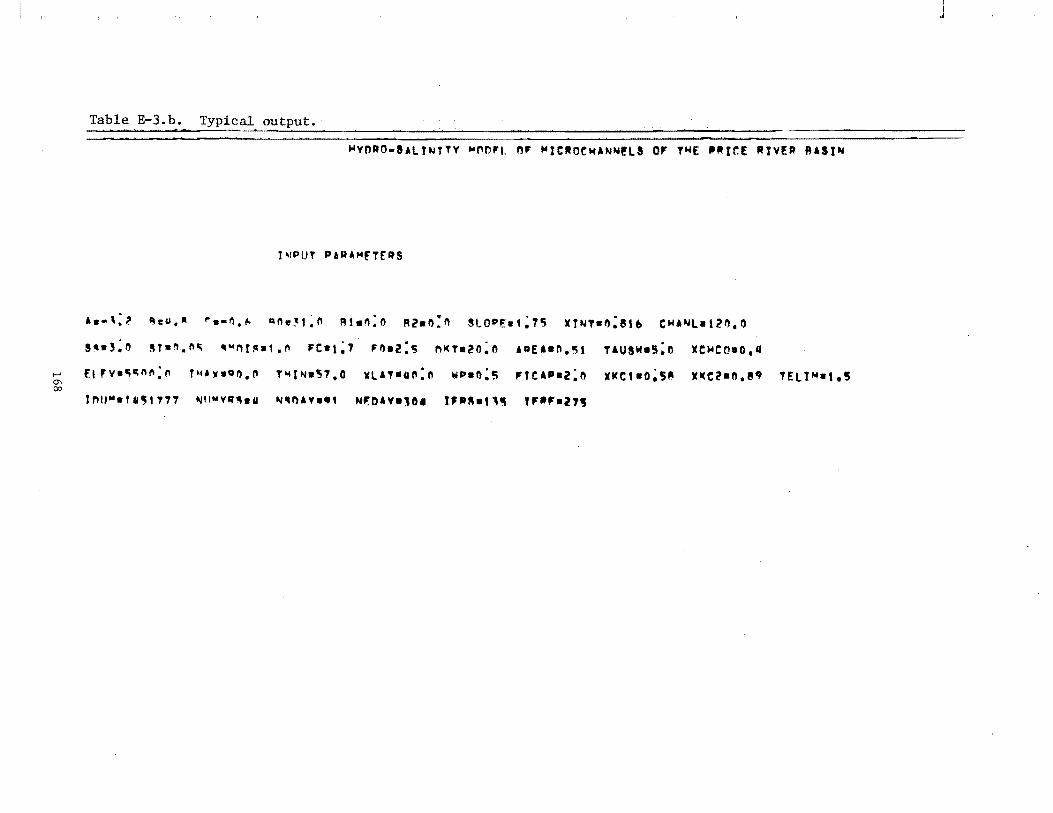
..... 0' 00

Table E-3.b. Typical output.

~VORO.SAltNTTV ~~n'l. n~ ~JCROr.NANN!lS 0' TNE ,RIr.E RtV~R BASIN

I~PUT PAR'~FTERS

A •• \:~ ~cu •• ~.-n.~ Qn.~t~n Rt.n:o A2.~:n SLOPE.'~1~ XJNT.~:8t. CNANla12n.O

S~.!:O ~T.~.n~ ~W"t~a,.n 'C.l~7 '~.2:~ ~KT.20:n 'DEl.n.~1 TAUSW.5;O XeNCOao.a

£1 Fv.~~nn;n Tll.w.Qn." T~IN.51.0 XLAT.an:n wp.n:~ 'TCl'.2:n WKC'.O;5~ X~Cl.n~!q TELIMat.~

r"'tJ III., 115'17' NlI"'VR~.1I N"I')&UI., Nfl:Dl"-U. I,R"., '" t'.'.l"~

J

Page 178

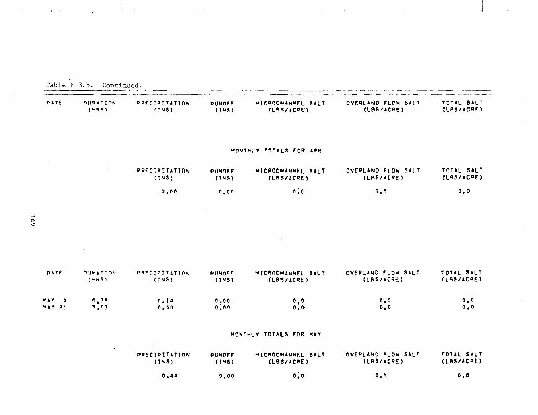
t-' 0' I,!)

Table E-3.b. Continued.

!"Of

[HTF

MAY lJ

"'AV 21

n ,,~ aT It'H,J

("'Q~'

"IJ'" A T T I"\~: C"I<S)

n,!" ".113

ClI'H ]I'TT ATIn~ (TN!! )

PPf(TPyTATTOlo.J (l ~J5)

o,l'In

ppr:CIPtTATTt"It,J fTNS,

('I.111 n.10

PPEc]ptTATln"l (TNS)

O.lIa

DUNnr:,. nt,j~)

~JCP~CWA"JNFL SALT (L"~/.cqn

~nNT~LV TnTAL~ FOR APQ

QUNnFF O"lS}

1l.(l1'I

CHI~JOr:F

(J"'S'

0.00 0:('\('1

~JCPOC~ANN~L SALT CLASI ACRf)

1l.0

MICQOC~ANNEL SALT (L8SIACQE)

0,0 0.0

MONTHLV TOTALS 'OR MAY

IIIUNO" (litiS)

0.00

MICROCHANNfL SALT (LBS/ACRE)

o~o

OVERLA~D FLOW SALT CL~SIACRO

OvfIllLA"'D FLOW SALT (LI~S/ACRE )

O.n

OVERLA~D FLOW SALT (LAS/ACRE)

0,1l O~O

OVERLAND FLOW SALT CLRSIACIIIE)

0.0

TOTAL SAL T CL8SIACRE)

TOTAL SAL T ClQS/ACIIIE)

0.0

TOTAL SAL T CL8S/HIIIE)

0.0 I'l,O

TOT AL SALT (LAS/ACRE)

0.0

Page 179

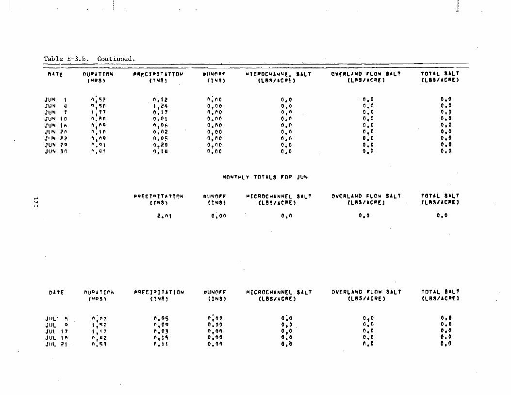
t-' ...... o

Table E-3.b. Continued.

D6T[

JUN Ju.... £I JUN T Jlt'" In JU'" If, Jllt./ ?n JIIN 11 JUN 1q JUIII In

DHE

JilL' C;

JlJl (j

JUt 17 JUL ,. Jill ~ I

"u·ntoN (IoIR5'

n;l)~ °,151'1 , ,17 I'I.~I'I 0;1'10 1'1 • 11'1 '1,nQ 1\.<11

".01

nuC'TIn~ r"'D!lPtl

n;n7 t,o;(, 1 , • 7 (lt U2 n.'H

IIUt,Cr-rTlTlON (TNS)

n.12 1,24 0.11 I).Ot 0,06 0."2 n.os O.iO o~U

prH.:ct"tHTtl'lN (TNS,

2.1)1

pl:?HIoITnrON (tNS,

".tIS n,Oct n,03 (I, t'l n .11

_UNtI'" MtC-OCWINN[L ,ILT (1"'8, (I.. 8 III I&C Itf ,

1'1:(10 0,0 0./)0 0.0 "~1'I0 o,n 0.1'10 O.n n.no 0.(\ 0,00 0.0 0,1'10 0,0 0.1)0 0.0 1':00 O~O

Mnt./T~LY TOTILS 'OR JUN

"UNl'ln' (t-"~H

o~on

DUNn.H (INS'

1'1;00 0,00 n,nn o.no (j.nn

MICAOCWINNEL SILT (leslie'!)

o.n

MICROCWINNEL SILT (LU/le.f)

0:0 0,0 0,0 G.O 0,'

OVf~LINO 'LOW ,ILT (L'-SIICrtn

0.0 t)~0 0,0 0,0 0.0 1',0 O~o 0.0 0,0

OVERLIND FLnw SILT (Les/lC"! )

0,0

OVEILAND FLOW SALT (L8S/ICAE)

0,0 0.0 0,0 0.0 n,"

J

TOTAL ilL T (LISIIC.€ )

OeD 0,0 /).0 OlD 0,0 0,0 0,& 0,0 0,0

TOTAL SILT (LIUIAC"E>

0.0

TOTAL SILT (LUIIC"! )

0,1 0,0 O.D I,D 0.0

Page 180

f-' '-l f-'

Table E-3.b. Continued.

OAT" I'HIO,T tn'-l ("D~)

'lit; ".OE; AUG iI

" I -- I 'Ue: e;. 0.12 'I)G " /l • I 1'1

F'''FCTDITATIOt.J (T~S,

n.",

PPECIPTTaTTC'N ( T ~I S )

n.7r. 11.21 n. :n II • 1 /'I

PRECIPITATION (INS'

I.l~

.rHITWl V TOTALS 't'R JIlL

PUNO" (T~~)

f).on

"lJ~OFF ( I ~J S ,

n~on CI~(I(\ 0.(\0 O~('I(\

MICPO~WA~Nfl SALT Cl~~IlCq~ )

0.0

MICROC"ANNEL SALT (LBS/ACPE)

o.n 0.0 n.o 0.0

MCNTwLV TOTALS FOR AUG

RUNO" (INS)

o~on

MICROC~A~NEL SALT (LIS/ACA£)

o~o

OVERLANO FLOW SALT CL8S/ACAI::'

0.0

OVERLAND FLOW SALT (L8S/ACPF)

0.0 O~O 0.0 0.0

OVERLAND FLOW SALT (LB8/ACR£)

0.0

TOTAL SAL T (LBSIACRE)

0.0

TOTAL SAL T (LU/ACRE)

0.0 n.o 0.0 0.0

TOTAL SALT CLBSIACJlE)

0.0

J

Page 181

......

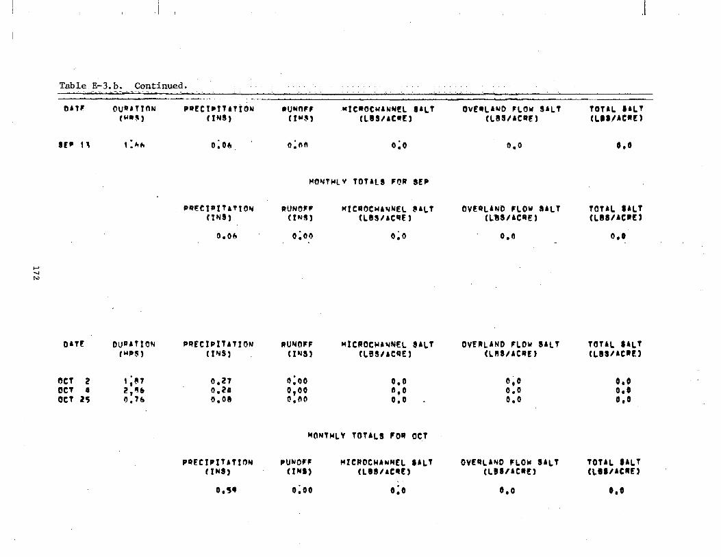
...... N

Table E-3. b. Continued.

1)1"

If' "

DATE

OCT 2 OCT I OCT Z~

DU.' nnN ( .... ,)

,:-.,.,

DUIUT!ON ''''''5)

';87 2,~. O.7@t

'.lCU'ITaTiON (INS)

0;06

pr:r!(:J" ITa T t ON tiNS,

0.06

PAEC 11111 TA T! ON (INS)

0,Z7 1'1.21 0.08

PREC!PITaTlDN (IN')

0.5'

.. UNn" etNs,

1'1;1'111

NIC-OC ... INN!l ,ILT (LIS/AC-!)

0;0

MO~T~LY TOTIlS '~R SE'

RUNO" etNS)

0; I)()

.UNO" Ut.lS)

0;00 0,00 (!,n(l

MIC"OC"'A~NEL ~ALT (lBSlAC'fE)

O~O

NICROC~I~NEL ,ALT (LBSIICRE)

0,0 tI.O O~O

NONTWLY TOTALS '0" OCT

pUNO" UNt,

0;00

MICADCHANN£1. "LT (LIS/IC.!)

0:0

OV£_l'WD 'LOW SALT (L8SIIC"!)

n.o

OVERLAND 'lOW liLT (LtlS/ICAE)

0.0

OVERLAND FLOW SALT (LUIIC"U

0,0 0.0 0.0

OY£RL'ND 'LOW SALT (lillie"!)

0.0

J

TOTAL lilT (LU/Ae"!)

0.0

TOTAL liLT (LIllie"!)

0.0

TOTAL UlT (LI!lSIIC"lD

0,0 0.0 0.0

TOTAL SALT (LII/Ae,,!,

0.0

Page 182

~,..,

-' 101 "III" _u

CO .. -' ...... CO .. ., .... e 0-, ~ .....

.... ...J c It.!

':.ILJ Ocr Ju b.. .. C>

...... OeD 0 2., .. -' -' ..... Ilr ILl > 0

• • .... ., ...J .. ... • ., • ., • -' iU Q

-' .. .... a .. .. :Zu 0 l- I. 2 .. C' • ........ .... .. :.t:r.

• Uti", ... • C-' -' • Q. ......

• • U .. • ... .... • ~ ... • • • • • .. ... ..... c .. ... ., Q C2 ;Z .... 0 ::> ...... Q

"t:I 2 Ol C> :::I ~ .-·ri ... 0 +-l .... en § ..... 2 :::r

A-U ... '-

U &0..

'J Q

...0, Q. , I

C"f")' I 1

[Ill

Oll

~j 173

Page 183

Table E-4 .• _~!, . The co;-relation procedures used to estimate flows at Heiner.

IET-~.55.' PT-l-1 10-1.1 £'STATPAC'KREFDEL USTATPAC1KR£GT IRUNNUJG la575 ENTER"'YES) TO RESTRICT OUTPUT TO THE AOV

,., 110 ENTER. IX' S, IY' 5 I, • ENTER 'YES) FOR AN INTERCEPT YES ENTER DEVI CE CODE FOR DATA INPUT,S, 11 OR 11 5' .

ENTER NUMBER OF DATA TRANSFORMATIONS YOU VANT TO MAKE, " TO 21 I .

DlTtR (YES) TO TAKE LOG OF Y' S NO .. • -

DlTER EACH RECO HO, X' S F01.1.0VED BY Y' S­ENTER ?END TO END DATA INPUT ~6~, 11, 1151 '76, ~I' 1~61 715,38, I II DEl. 715,38, 1171 165,128,1851 565, 1,922 ,?11·IDEl. 72"-',756 '66113" DEl. '661 14, 1111 tDiD

I

NEAliS AND 5- D-I .75111429E+13 - 19571383E+13 2 .331~2857E+12 .~~82718IE+12 3 ·.117~IIIIIIE+I~ .36862185E+13

ENTER (YES) FOR UNCORRECTED SS SP

,., liD

CORRECTED SS AND SP 1 - 229823~3E+86 2 -12856857E+15 3 .8152881IE+16

CORRELATION El.EHENTS

• 2'3~5286E+15 "9121~IIIE+15

I 1.11111 8.~1551 1.~19~5 2 1-11111 1.9,99. 3 ".11111

INVERS£ MATRIX • I -52174111£-15 --92191235£-15

2 .99261757E~I~

REGRESSION MAL.YSIS or VARIAJI&.& 3

174

• 1 772381IE+'6

Page 184

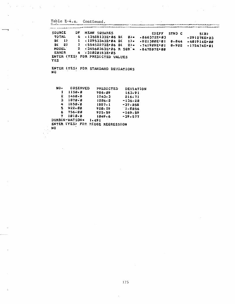
Table E-4.a. Continued.

SOURCE DY MEAN SQUARES TOTAL 6. 13588133&+06 B( I> I ~12953343E+04 B( 2> I ~55452273E+06 MODEJ.." 2 ~ 34560363&+06 ERROR 4- 31021183E+05

B( 0>­B( 1). B( 2). R SQR".

ENTER (YES> YOR PREDICTED VALUES YES -

ENTER (YES> FOR STANDARD DEVIATIONS NO

COEYY STND C .866372E+83 .82130I:'1E-01 8.844 .74191:'19E+'" 0.91:'12 • 84761:'17E+00

NO. OBSERVED 1 1150.0 2 1460~0

PR£DICTED 986.09 1243.3 121:'16':2 1667.1 920.19 925.59 1049.6

DEVIATION 163.91 216';71

3 1070':" 4 1850"0 5 922.0" 6 756':"0 7 1010.0

DURBIN-WATSON. ENTER ·(YES> FOR NO -

1.491

-136.21:'1 -37.058 ·1.8056

-169.59 -39.577

RIDGE REGRESSION

175

S(B) • 291278£+03 .4819 14£+ II • 175474E+II

Page 185

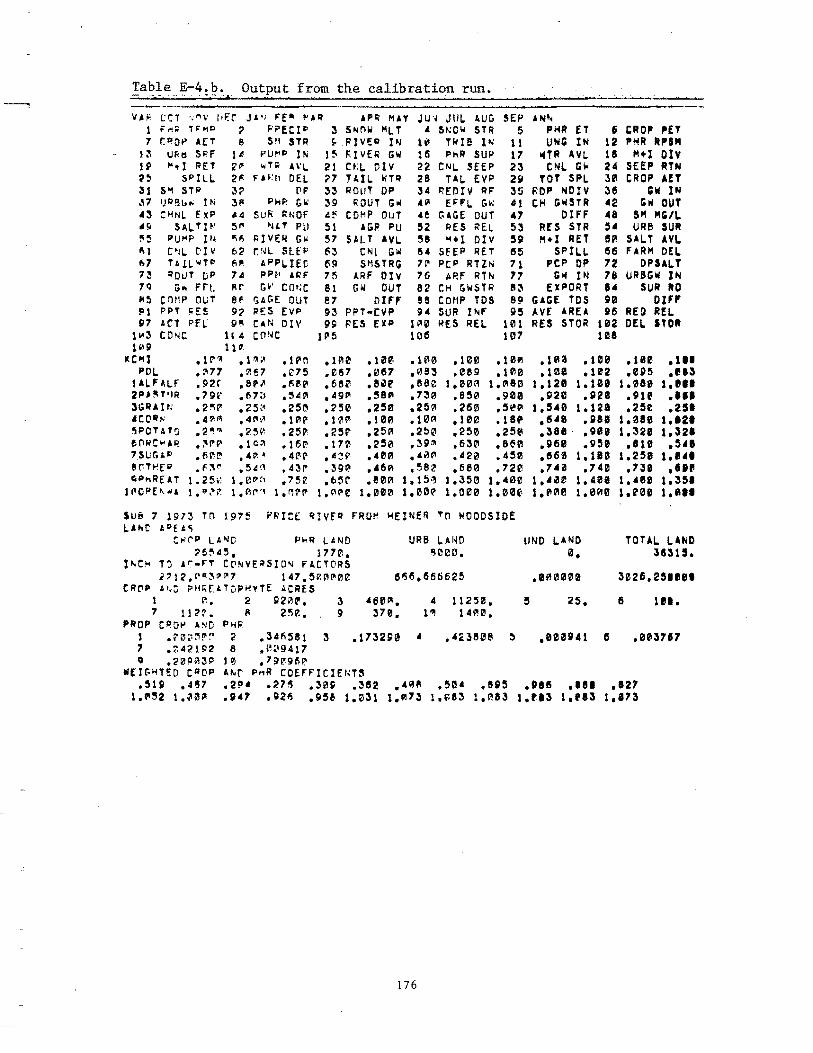
Table E-4.b. Output from the calibration run. - ......... , ,-.. ,. · ... -~6·

VA'" eeT ,;I'\V '.F.{: J"I FEll "' .. ~ 1 F~~ T~~P r P?ECIP 7 [~DP .lET 8 S" STq

13 U~d S~f 1~ PU~P IN lP ~.1 RET 2P wT~ AV~

?~ SPILL 2~ F"~h DEL 31 S~ STP ~~ PF J7 yD9~~ IN 3~ PHR G~

'3 CHNL ExP ,. SU" ~NOF '9 SALTI~ ~~ ~,T PU ~~ PU"P 1~ ~ft RIVE~ Gw ~I C~~ ~Iv 62 [NL StEP 67 T&LL~T~ fi~ App~IEr 73 ~OUT UP 74 pP~ "~F 7Q G~ frL 8r G~ CO~C

H~ COMP OUT 8f ~AGE OUT PI PPT ~ES 92 RES EVP g7 ACT PEL 9~ CAN DIV 1~3 CONt 1(. CONC 1~9 11~

KC~l .lr~ .1~~ POL .~77 .~~7

lALFALF .92r .8'~ 2Pj~T'IR .7!H' .ti7;} 3GRAI~ .2~P .25~ 'CO~N .4~~ .4~~ 5POTATO .2·~ .2~p

60RC~Aq .~p~ .1C~ 7SUGAP .60~ •• p,' er.T~EP .f.~~ .54~

~p"REAT 1.Z5~ 1.BP~

.1P!'!

.e75

.~II~

.5.41'1

.25!:1

.IPlP

.251'!

.161'

.4('11"

APII MAY 3 SNOW MLT ~ FlvED I'"

I!' "IVEI< GW 21 n;L OIV ';7 TAIL WT~

33 IiOUT OP 39 ~OUT G­

CDMP OUT "GP. PU

SALT AV~ CNl GIt! SMSTRG

ARF DIV GW OUT

OIFF PPT-EVP I"E5 EXP

.11'10

.e1l7

.680 • .491'1 .250 .1I1I !" .2!H' .17~ .A~V. ,39P. .(>5('

.10"

.057

.8~r

.5811'1

.250

.100

.25~

.250 •• 00 .'61' .801'1

J u·~ JilL AUG • &11:0101 STR

11/1 THle It< 115 PiotR SUP 22 CN~ SEEP 28 TAL EVP 34 P.EOIV RF 4IQI EFF~ Gw .~ CaGE OUT 52 tiES ~EL 58 ".1 Dlv 114 SEEP RET 71' pcP FlTZIli 76 ARf RTII4 82 CH (iWSTR 88 COUP TDS u SUR 1II4F

1~0 IlES REL 1015

.UHl ,089

SEP "1\1'. PHR ET UNG IN

WTR AVL CNL G\tI

5 11 17 23 251 TOT SPL 3!i ~OP NDIV 41 tfo! GIIISTR Al7 OIFF 53 R£'S STR 551 11+1 RET 1!15 SPILL 71 PCP DP 77 GI( IN 8;.\ 89 515

101 107

.10f!

.100

EXPORT GAGE TDS AVf AREA RES STQR

.1~0

.083

.88~

.730

.250

.11i'l0i

.2!)~

.351 111

.'0~

.58l

1.00A .850 .261'1 .100 .250 .630 ,420 .681'1

1.1'180 ,5100

• lliH1 .lIae

1.12111 .g20

.101/1

.102 1.108

.1iI2111 .5"'''' .18' .25e .8~0 .450 ,720

1.5A10 .5'0 .388· • II 5IIl .5tHI .7'"

1.41110

1.128 .IISI • g 1118 .Sl50

I~OPE~~' l.~~~ 1.AP1 1."l"e 1.000 1.15·" 1.1i'l0~

1.356 1.000

1.41'10 1.000 1.IH""

1.11111 .740

1.401 1.0110

$US 7 1973 TO 1P75 PRICE QIVfQ FRO~ HEINER ~o WOODSIDE L ..... e A0f: H

CROP PET PHR ItpS'"

M+1 DIV SEEP RTN tROP AfT

Gill IN GW OUT

Sill "'GIL UR8 SUR

SALT AVL F ARM DEL

DPSALT URBGW IN

SUR ItO olFI"

REQ REL DEL STOlt

• 100 .0P5

1.1'180 .lIU .25t

1.881 1.3211

.8U1 1.258

.730 1.'08 1.r00

.UI

."U l.ell .1" .UI

1.'21 1.UI

.5411 I.e •• ,It II

1.351 1 ....

c~rp LA~D P~R LAND URB LAND UNO LAND TOTAL LAND '5!"5. 1770. SlleD. 0. 311315.

l~C~ T~ ,r.FT C~NVE~SIO~ FACTORS ~'12.~Q~PP7 lA7.5v.~P0e e~6.a56625 .0~0000 3026.251'el

CRrp A~D PH~rAToP~'TE ACRES 1 ? 2 92~~. 3 .60~. 4 112~0. 5 25. 6 1.1. 7 112~. ~ 25~. 9 370. l~ 14~0.

PROP C~D~ AND PH~

1 .r0~~'? 2 ,34RS81 3 .173290 4 .41380~ ~ .000941 e .0037.7 7 .;'21P2 8 .~~Q417 Q .2~9A3P 10 .7Q?o9fiP.

WfI;HTED CROP A.r PnR COEfFICIENT~ .519 .4~7 .2~4 .27~ .30S .352 .4~~ .504 .ag5 .9al .Ial .127

1,~52 1.~0~ .9.7 .926 .95e 1.031 I.A73 1.f.83 1.~a3 l.rl3 l.r83 1.173

176

Page 186

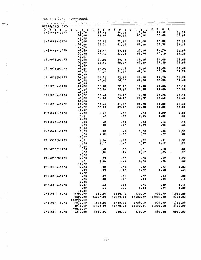
Table E-4.b. Continued. . ·1 ..... -

HYDROLOGIC on. 3 '3 1 1 1 1 1 1 ~ e • II • e I 1 1 1 e 1 e e UUhATtiA1t73 ~1.70 U.41J 20.C'lf 18.50 2 ••• 0 ~1.70

3D.IIR .... , lSI!!. 0' 15:1.0' 155 •• HII 55.'" '1.50

lHIAWATHA197. '3.80 ~5.00 27.00 20.U 25.111 31.20 3D.911 55.70 61.01 67.00 67.50 511.11 4,.7.

lHI''''TH_1975 .... 50 33.'111 23.10 21.0111 2'.715 31." ;)5.'1' 47.40 57.21 68.7" tilS. U 58.20 ·2.D7

lSUNNVSID1973 ".ge 29.00 20.1l!0 151.08 24.0111 32.'0 3D.I1IP 52.1S0 1S0.0P! 65.1f! 67.20 55.,e 42.3P

UUNNYSID1P74 49.1210 3'.0IIJ 'l7.e0 1I5.0P! 21.f.IB :58.1' '0.5P1 55.2111 61.01'1 67.111" 61S.50 58.7. 4'.49

UUNNYSID1975 :>0.30 :U.70 22.90 21.1H'1 24.20 U.2I 35.80 '6.'0 51S.50 69.20 155. !HI 5t.4' 43.1'19

lPRICE WA1973 52.30 3~.00 22.015 16.90 215.80 37.1' '5.10 57.9'" 1S5. U 71.90 72.30 63.tI!I 47. HI

1PRICE WA1974 55.70 38.'0 251.20 18.lSe 23.2111 '2.11 '5.Pl0 61.1Sl'l 74.20 78.IIlt' 73.60 611 •• 40 50.66

,

lPPICE Id191~ !lS.71l 38.'0 31.30 25.,,1'1 31.110 41.31 "3.7111 53.tilll 59.90 12.30 71.00 63.81 <18.97

~MIAIo."TI'IA1913 4.51'1 1.73 1.30 .2' 1.22 1." 1.11 • "11 .55 2.95 1.15 .37

17.29 2M I AI ... THAlI>7' • HI .45 .61 .S4 .13 .l'

.5P .00 .0{1\ 1.59 .28 .33 ~.11S

2 .. I AI. ATriA 1915 3.35 .89 •• 9 1.00 .8B l,S!! .511 1.01 1.86 .62 .77 .67

13.57 tSU~"VSI01P13 oIl.31 1.34 1.17 .52 .41 1.51

.A4 1.15 1 • .010 1.97 1.17 .21 lti.l1'1

UIJN"YSI~19'" .56 .42 .36 .81 .Ut .117 .56 .O0 .0' 2.1;! .35 .21

5.60 UUNI./VSID15l75 '.08 .22 .53 .71S • !5S1 2.22

.ISI 1.114 1.4' 3.05 .06 .32 15.72

2PRICE WA1973 4.3. .83 .68 .511 .97 1.13 •• g .28 1.26 1.72 1.20 .3'

13.72 2PIIICf WA197' .26 .25 • 5 !II . "" .03 .ee

.06 .II1II .111~ .3.01 .06 .16 2.36

2PRICE IoIU975 3.8' .36 .2~ .76 .59 1.11 .I'lr/l • 7' .92 1.5 • .06 1.26

11.51S 3HEINER 1973 2'00.0'" 789.99 DU.1'l1/! 679.99 839.99 U55e.1II

9!00.1'l0 .01330'.00 12800.00 U!10".01" 13!500.00 !57U.U Hl2959.ge

3HEINER 1974 ~879.99 1!5re.0t 1700.11111) 1029.09 939.99 17!59. U .979.99 17.U.III' SJAIHl .00 101~0.0ii 1 U00. 0111 3739.519

70029.91' 3HfJ NER 1~"!5 125E'. r.e 1139.99 9:50.0110 1579.99 85111.U 2I!lU. U

177

Page 187

Table E-4. b. Continued. .,.:.. ,

----" 1I"I!)Q.1"9 lP3t'e.fllI' 2n~"'.N· 173vil'.;r 1311'10.11/) 7Ue.1II '"' 3~P. 98

16 TOSH[ ,~n .7S;.9!" f1rr.0" 35IJ.\lSi ~U.tP '18.;' 'U.U 3~9.9r 4ce.p.:!, '39,99 :>~ft4.l'Ie ~09. 519 5'P.U ASP.I/'i

If; TOSHE 197. ':;1'.99 559.P' o4t'!lI.~~ 609, tv 50P.9P lIIle,lIB ~!')P.99 539.951 "i29.9P 5IP.DO 52!J. DO elP.PI !!-'2,.9

16 TDSHf 1975 -7"r ,14'" 57!J.P9 '0t'.00 550.lIIf '511,01 '5I.n 7~I'l,PP 55e,"" 35'11,Plt'! .5r • ., .5e.1I0 UP.tv 521.56

41l"?Dl:iT Hi73 6'0.k'lP 3\"0,0r. 36!3.1'Ii' 2.II!,,,~ 220.80 2'0.'" 7:>:',"'~ ~Pln0.e., 7(l0~.PPl 6el'lZ,flI'I :>006. B0 3'011.111"

2q27f\.~rl 4II',;:>I)I<T 197. 1:>\'!P.pt~ 7r.~.01'1 31ll0,00 2:10."0 2(110.00 5e0."

.. ~HH". 1'.0 70ll0. RlDl 57~e.00 4750.0P 401i'A.00 2'118," 2o~r('l.0('1

.IMPORT 1Q7!> !l5( .• (11'" .5e.PEl 300.~1' 200.00 25111.U 500." : (\A~\.:IIe: !>4C9!.1":!l 630;.('10 67521.00 630111. ee .000.U

:\,-~c"I"."'(II

17 liHI'lS 19n 7PP..l'!r. 7010.01 7:'10.00 7P10.00 700.00 7111t1.U 7~0.ilP 721111.00 700.00 70.a.0~ ·71!11ll.0e 711111.01 611!i.;9

17 IMTOS 1974 700.0" 700.10 700.l':e 700.00 718i:l.'''' 701.110 71'[email protected] 7V11'.0GJ 7el1l,00 700.00 700.00 70!.'1.ee #\119.9!l

17 1 fo'T !'IS IP'5 7"~.0{l 7('0.06' 700.11Ji'I 1U.Bf' 700.1i 7n.'" ")~ .1lI(!i 7U.0@! 700.00 7U.lle 700.00 700.ee !!9~.99

~GORC~ 1973 ~2.0I1" .0P .00 .0e .elll .80· 2~.~1I 2~e.1Ile 1S21.519 333.DP 203.99 2:10.00

1711.!!I~ ~GO'l;:1< U74 n~. 09 13.00 ."''' .01" ,Be 32.0~

1111.9 11 2110.f11'1 21P1,I'!A 118.5151 115.D~ 115.110 127 1.!I!l

!5r.ORCII 1975 43.~"! ,1111'1 .1>10 .,,'" .B0 • era 7 ... PII" 371.(1)9 44~.911 1 illS. 951 167.IID 112.111

1~12.!il9 111 TCs~n 15173 2799. 0 9 31119.519 3790.9£1 37!HI.IID 50519.5111 27n.u

2299.91) 229P.519 22519.99 2399.119 2011;.," 1508.10 :>136~.f16

111 T~5C~ II;11l 21!~P.99 1899.951 35"0.00 37~9.911 51P5I.IIP 25U.PSI 251:19.99 ~r!il9, P9 2UIl.99 211'99.951 21PII.n 351111.151 '9'!5.6f

l~ TOSCu 1Q7~ ?799.99 3U".0~ l50~.e\:'l "IH~0.f)f 5:9P.n 2i1U.U 2~1I9.99 30N'I.0D1 22"9.1151 2000.~0 1!-i;l9.U 311011.110 2924.99

f\ CANAL 11/n 15~g.9Q 750.0P 920.99 1'H9.9D 579.tP 721.119 2""'r.00 13129.519 182Ii:l o .!:l9 1:i52P.1l1l 1211311.5111 peu.1B

76C 79.!ilti 6 cuaL 197<1 "'~Q.Pj:l 191Q.Sl9 81S/.tlll 619,519 ,!'ISI.U 1'50.10

!!i.H~9 .99 '8559.~SI 1.175".0~ 12279,951 U4U.9D 61711.10 783519.9~

6 CANAL 197:) 2239.99 1229,99 7611.1/5/ (1151.99 731l.PO 2~'Il.gp 2739.gll 13[159.99 261 79.llg 17335/.519 1:>71Y.U 106151.111

8:'1499.9!'1 7 ,\oj IN lQ73 33~.~0 :530.VlI'! 331J.1"0 330,111' 330.81 331.11

"3~.M 330.00 J30.~0 33.6.00 338.81 331.111 J~er. 'H"

7 lOW It. 1974 33..:.1'1'1 33t'l,013 n~.0\.'! 3321.0. 33111.80 nl.n '53r.~" 33~.~~ 33l'!.~0 UIII,er. 33 •• Ie U ••••

"11/61- .1>1'

7 Ii'" II>. t915 33;-.?" 330."'" 3~l'!.0" 330.00 338." 331.11

178

Page 188

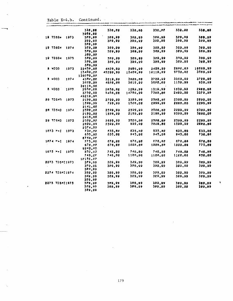
Table E-4. b. Continued. Ij

-----, 3U.81 330.00 3U.10 33m.Flt 331.00 nl.'"

;!ISlet. 00 111 TOSG\Ii 1S1'3 31'19.11!) 3U.SlP 30D.P; 308.011 3U.ts! 3'" • lIP

30D.99 3P!SI.iP 309.U 30S1.PII 3n. PII 3;!ISI.PS1 3111P.9P

111 TOSGW lP74 301. III 31'!9.it 3U.U 30P.IIP 3U.P' 3ell.11I 31'1P.SH) 3011.IIP 3U.IIP 3011.SlP 30P.9llI 311D.1P 38D.9P

111 TDSGW 11l'5 3QlP.1I9 31l19.P9 :l09.PP 3ep. SIll 3~P.PP :l0II.11P 30".9' 309.U 30g.P9 30S1.9P 30P.SISI :In ,PP 30P.IlP

8 101000 1973 22 451'1.00 41'129.SlP 2P89.PP 2451.PP 281110.U UIHISI,III 1!\.50,CQl 45209,99 13469.9P U1U,PSl 5'50.U 358P. SIP

1:1!,HH"p.911! 8 101000 19'4 43 P1 WO.00 321P.PP 38U.Pl0 372P.PP 336P.PP 3'21.'"

302S1.PP 461"0.00 3619 .PSI 3fi1/!2.1.'!IIl 115P.fn p:sP.PP 3911!~.g6

8 WOOD 19,.5 2951'1.1';0 2(1150.00 128S1.99 131P.9P 1t53P.9P uee, "" 375P.9$/ 5451'1.08 14751:1.99 '300.e' 240P.9P 337P.SHI

A!l21S1.911

'" Toswn 1P'3 215111.99 2711P.P9 3311g.99 2508.0r 23S1P.PII 2UP,PP 159P.99 799,IIP 1500.00 20U.SlP 2080.00 nu.", 21·1.56

2'S19.g9 IPI TOSWO 19704 2501/) .00 2599.Slg 2500.00 22PSI.9II 23"P.IISI 21 Slg.SHI 18P9.PP 2 Unll.PII 21U,PP 2:SP9.PII 3ee0.111 2415.65

u T[lSWD U75 ~5:!10.A0 2699.5151 35151'.00 2501.0' 23gP.PSI 22tP.PP 26gp.9~ 2 31i!~. 99 8S1g.9P ~"L!0.n 1:SPP.g9 21'8.80 2374.gp

11'73 "'·l 19'3 ,3(11.t'lA t!3:S.U 635.1'10 535.01!! 635.18 G35.0fIl 635.a0 635.00 !'.l4'.00 94!!i.0l' P45.80 731.80

87.9."1" 11117. .... l U74 77!1.CH'l /570.00 6'tII.00 tl70.tlll' 670.l1li 0711.88

670.I'!III 670.00 100(:1.0'" 1000.0P. 10U.08 775 0 U 92 413."'''

it'!:! "·l I1H'5 850.~Hl 740.00 74 0.00 7.0.00 740.00 748.e9 74 0."1'1 740.00 110111.1110 1100.0fJ S1EB.n 11'&.18

lr1 8e.",t" 2273 TDS"'I1!~n 3'9. !Hl 3'1!~.g51 3.59.99 309.P9 3051.519 3eS1.U

3Pil.51' 309.pg 3"'9.51P 3051.519 30P.9; 3"".P9 309.99

2274 TOSI1U5l74 3011.99 30P.;9 3051.119 32'9.5151 30P.9g 3eSl.SlP 3011.99 3011.9P 31HI.9; 3U.pg 309.IIP 3U.,,; 30P.99

2275 TOll'll 19'5 31'19.1151 3f1!1.U 30S1.n 3011.t9 3,g.U 31 •• " ,. 3I!1P.!HI 31P.PI! 311".gp 3.P.U :l0P.P; ~I!P.U 30g.Pg

179

Page 189

Table E-4.b. Continued.

--~ VA~ ( " 1 !In 4!5.63 31.13 2"'.66 18.13 25.015 33. II

A1.~3 ~2.915 ~!1. 50 57.3' 151.11 57." .:'I.fi9

VA~e 1) 197.:1 ~9.23 ~"I!p' 27,73 18.21.'1 23.115 U.U 41.8111 ~7.50 65 .... olI 70,1511 61.U 152.115 <1'5.64

V He( 1) 197~ !!il.5!'! 35.'" 25.76 ?2,3:S 215. a:s 34. :,., :\&.31'! 49.13 57.815 70.08 117.53 slI.n 45."1

VAk ( ?) 1<~n 4.38 1.30 1.'"5 .48 .515 1.415 • I! 1 .61 1. "7 2.21 1.14 ,3 •

1~.'\'1 VUle 7) 1974 .3:\ .37 .4£1 .7P- .0(1 .07

• c:'l .1.'1111 ."-1 1.3S .23 .23 '.J7

VAR ( 2) IQ1~ 3.76 .'9 .42 .'" .72 1.62 .39 1.10 1 •• r 1.13 .29 .75

13.65 VAR( 3) 1973 2.1/I~.F'''' 78P,9!) 130111.:111'1 879.99 e3P,pp 155e,eII

9611:'.0(11 433{',1'I.1')1'J 128PJ0.0i' 10100.00 135710.00 57011.l1l/I itl:> !iI~9. 98

VAK ( 3) 1~74 2819.99 1 !5P0,IUl 170Z.00 102P.IO 113P.9" 1 ".,. P" "9711.911 174ec,.e0 13'''''0,0'' S UPlr..0" 11000.111 3731 • .,0

7N1J2!.1.P6 VAR( 3) 19'5 t2"1~.r.1i! 1139,P9 9!50.0e' 1579.99 850.00 202P.9"

!\~!l9.9!.1 1030f11.n 279"'1II.0e 1730fl.00 13100.01 7ue.1iII 81'~!59.ge

YUI ( t) 19'3 65.'. r~ 3~1,'!.00 360.00 240.210 220.111 251il.ee 75\~.r'" 5""IlJ.ee 7r.00."'" 6~30.0I1l 5mu.n 3:SU • III

2927".iHl ~jR( <I, 19H 15!/,~."'[/J 7"1'I.r.0 300. ~'H' 202'.0f! 2CH'J.00 5ee.0Il

~~"~.;Je 'rr.0.Ql3 !S,5e.ell' 4750.08 4000.0fII 240e.1IlfJ 20/lP:".['~

VAr:; ( A' IP7!5 ..-·~.rtl 450.0'" 303.!'!' 200.0P 2'0.00 5U.eI lva0.rn !'iAn.1lI0 6300.~0 67!11'1.00 60U.1il0 .eee.80

32 1<1 (H" • e ~ vue "l) 19'3 52.~r ,01'1 .0" ,f!P .llIe .00

lA .1'1" 2~0.00 ~21,g9 1133. n 2i1l3.U 231.et!I 1711.g9

If j~ ( !') 1~7~ 2l5.P9 13.00 . '''' .1110 .80 32.0111 191.90 280.I'JA 2U',0n 116.Sl9 lH5.PIl P5,eA

,n 1.99 VARe 5) 1!H~ 43.~PI • o I!! .0C .00 .0111 ,"0

7~1 .1'1 ('I 371.9g <l41'!,99 1I:i~. gg 107 • .,9 82.U 1312.99

vue 6) 1w73 1659.99 7513.0" 929.9!) 151P.Slg 579,99 7211.119 ~'"~3.~e 13129.9Q 18209.9; 25529.91) 12935).99 ~0011l,0fl

't"~7!I.gl5 vue 6) 1!:'l7<1 <1429.99 l!H9.99 819.99 151.,.99 5'9.gp 145£1.00

fI\"(II9.99 18559.99 14'5[/J.~r. 122'9.P9 1I/l41.,.P9 617.,.119 7t<399.P5

VAR ( 6) 297!" 2239.119 1221'.99 76li/,99 IU9.99 739.'''} 135".1Ul 2739.90 13B69,519 Hil'II.QSl 1733P.9g 1,7lS1.gg un g • 00

8~4!)9.95 VAR( 7) 1£l73 330."::'1 331l1.P\'II 3321.1'\'" 330,0'" 330. QH'I 331.n

33;l.r~ 331".£191 330.0~ 330.8' 330.l!l'I J31.11! 39~;Il.Ct'l

V'~ ( 7) 1974 ;'3 "l. :"\, ~3"'.1'!0 331.:l~ 331'1.0A 330.1'18 3n.ee 33"'. "':l ~H.i'''' 33~."0 330.U 330.ee nl,u

3P~ .. 1!.~~ VARe 7) 1;7!'i 3~:>.P~ 33t'.I"r. 33;,.,",V 33 •• IJp. 33111.11 n ....

3::5:".1';'- 33,.1'11' 33~."V 330.II1II 330,11 n ....

180

Page 190

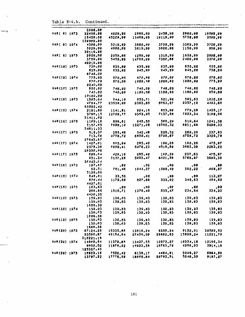
Table E-4. b. Continued.

3UI.Bf! - VAR ( e) U73. 2245e,1I 4eu.gp 2DU.DP 245'.5111 2ea0,1' lUU.D9 lS45lh0e 452U .lUJ l:UU.U ull1.DP 57,..18 3!U.n

13510P9.pe VAR ( 8) 1l~7 4 '300. VIe :U1P.5I.s~ 3800. "0 372111.5151 331511.1111 372P.5I11

3USl.U A6BfJ.1'0 315151.11111 3111110.00 11 511.5151 85P.U 311110.915

VAR ( a) U75 21150.00 20511.110 12U.U 1311.SID UU.D9 2808 • II!! 375!h99 5'5111.11' 147tHI.951 730f.1Ie 24119.8' 3378.119

'92U.915 VlR (10) 1973 731'1.10 53'.'0 535.1'J0 1535.0I!I 635.08 U5.0IJ

535.210 1535.0e 9'5."~ 9,5.08 51'5.01 738.80 11740.0"

VU (10) U7. 775.00 1570.0'" 671'!.Q10 67111.01" 570.IUI 678.80 e7~.e0 670.00 1000. 'If! U8e.fIlI!I 10110 .1lII 775.ee

51241'1.00 VU (111') Hl7!.'! 850.00 7'z.a0 740.00 74e.u 740.80 748.11

74".00 7'e.u 1100.00 1100.'" 1180.00 '50.81 10180.00

VlR C un 11173 U65.64 15".111 553.71 521.110 l5n.53 1832.2111 .7t!U.77 23530.00 5131113.85 eP-53.27 51357.15 40411~.8!!

63552,42 VU (16) lP7. 21511.89 1141.11 5124.16 a53.U 779.28 1'35.17

3700.15 12715111.77 51353.95 7137.8fl 79U.3' 31eB.5e 51411.112

VAR (16) 1975 '1IeD.18 na.1St 5'5.5l5 51'18.29 tHg.U 1241.58 :n57.!55 755151.10 13271.21 105II1II.32 8811.18 5118.:53

5.811,33 VU(17) 15173 618.37 U5.40 3.2.48 228.32 2e5l.2SI 237.113

713.50 .7515.72 56551.'1 5708.117 4755.72 un-.TI 278.5.117

VARO" 1517. 1'27.ill 15 55.51. 285.40 1510.26 190.211 .75.117 2378.35 fl6551.U 5470.23 ,518.811 381!l5.31 2213.22

U35Q1.1'18 VAR(17) 1975 en.tiA '28.10 285.40 191!.28 237.S;) '75,1S7

D!S1.:5A 5137.25 51193.47 8421.5a 5788.11 3115.38 3V4.3.fil

VU(Ul 15173 lP7.!7 .00 .111~ .00 ,88 .Ie 62.51 781.46 194114.27 10851.'2 582.22 1'61.17

~126.66 VU(U) 11)7.4 6'1,81 33.56 .00 .0e .ea 113,17

1578.44 "27.~1

11711.61'5 627.8e 333.g2 3'5.83 4(1'.10

VAR(1e) 197~ 1!53.63 .00 .00 ,IU~ .lIe .00 256.!IJ 1518,71 1378.4$1 535.,7 234.14 334,:n

"2111.35 VolR (lSI) 11173 139.03 139,03 139.1113 1351.03 1351.03 139,83

139.03 1351.03 13$1,03 UP.03 1351.03 13!t,03 1668.38

VAR(19) 1974 13111.03 131).03 139.03 1351.03 13;.03 139.13 13D.Pl3 139.03 UP.03 13P.03 139.13 139.03

Usa.38 vu (1S1) 1975 U9.~3 139.03 1311.03 13P.83 13t.1I3 139.83

139.t:l3 1351.03 139.11;3 l:u.n 13g,e3 lU.1I3 21588.38

VARCU) 15173 67124.2I!l 15335.68 U815.24 8358.2' gU2.g1 3050P.83 33598.07 "11154,64 27.5~.90 288I2.n 158211.24 11221.71)

318221.1& V"R (2rn 197. 14SPg.SI" 11378,8" 13'27.55 12573.27 10~3'.1II 12166.3'

11"5111.52 11171.22 ll11a23.58 111763.71) 4Ua.113 3IH4.1B 125327.43

UII (211) U7' lun.te 7522.42 SU8.17 ..... 111 5U9.27 1114,16 117.,.22 17771.5' lUU.e. 211783.51 524111.55 '"7.27

181

Page 191

Table E-4. b. Continued. --.

U6·11.'tI UI (21) 1~73 31117.!'!! 2e1.'3 261.53 267.53 287.n 217.13

287.!'I3 U1.'3 3I8.U ;n8.U 3DI.U 317.55 3612.2'

VlR (22) 1111. 3215.51 2U.?7 282.27 282.27 212.27 212.27 282.27 at2.27 '21.:51 .21.31 421." 321.51

3!.1I2.91!1 VU(2) 11175 3!511.11 311.16 :Ul.7I 311.71 311.71 311.71

311.715 311.715 '153." '63 •• ' '153.4. 358.11 "288.93

PRICE RIYER FRO~ HEINER TO WOODSIDE II' -I ~ e e 75 .llfE.'1 .1'~E-'5 .1.,E-.5 .leeE-,5

IDT~ I I 1 I I I 1 1 1 1 1 I IDILMOI ••• e .eell .en .eell" .ell .n ••• ea .IIU .ee •• u •• eu .... 08J COE1.0001 •• eel.ee.l.ee.I.II •• 1.88.1.I.III •••• I •• e.I.18.1 •• a01 ••••• 8.el.,el

PAR I 2 ;) .. 5 • 7 8 iii 11 .000 .31, 27.011' 33.0" 3.110021Ie.00818'2 •• DD 1 •• 81119..... 3.15.'

5.50e 2 •• '1 IC.0" 7.00e 1.1.. 1.018 .2" .111 .7D, .85' 1~'''.00' .31r .21' .~e. .••• .eeI1010.ee. .Ie. ..'e 1.'5'

.95e 1.310 1.1" I.... 1.... 1.281 •••• .2ee .5e8 .5"

.51e .e.e .Iel .e.. •••• •••• •••• •••• ..Iee I •••• 1.'08 1.311 2.e1l8 2.'" 5.0" .1" .,.. .e.. .8el •• el .8e. .e'l .e.. .e.. •••• •••• ."11 .'" ••• e .ee • • ,.. .ee. •••• 2.5~t •• 1' ••• 53 •• e............ • •••••••••••

35...... •••• I.'" .~2' •••.•• , .••• 1.72. •••• .I.e •••• 5e' •• II. 7.... .'3' I.... .5" I.;)~' •••• ."1 •••••• 123' ••••• 11.1 •••• 21.'.' •• 3 •••••••• 8.e •••• S...... •••• •••• .'" •••• • •••

182

Page 192

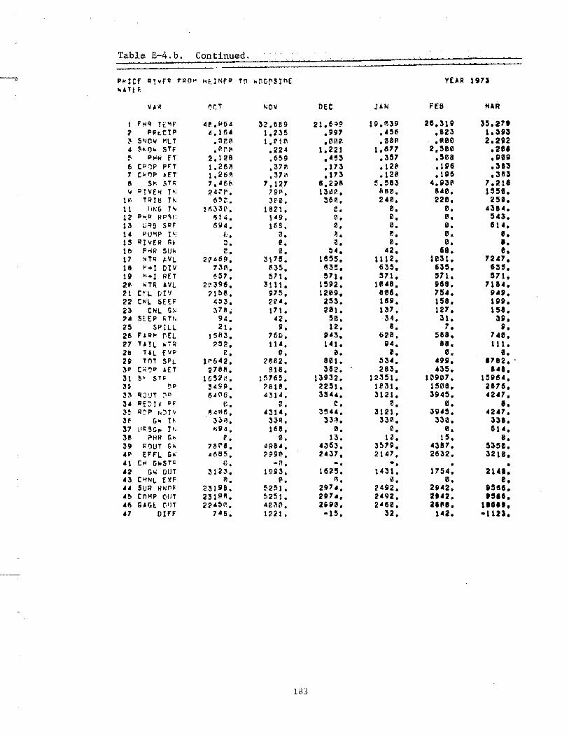
Table E-4.b. Continued.

~ PklCf 'i!vfl:; 1'"010'" HUNf P T['1 "ClC['ISInE 'tEAR U7~ 10011 tI,

V.R ~r.T t.;OV DEC JU' FEB "AR

I Ft<q TE"IP 4~.!i64 32,659 2l.6~9 19.A39 U.31g 3:1.27' , Pht:I P 4.1t1. 1.:C3!5 .n7 •• 56 .U3 l.an

" S!'!Ow MLT .~r,0 1.1'11'1 .0A~ .001'1 .fIlU) 2.2112

" ~~·O" STF • "r. r~ .224 1.221 1.15'17 2.510 .211 !I PI-'ri n 2.12B .6!19 .'!53 .357 .508 .glg 6 C"'1P PF'T 1.26" • 37~ ,173 0121' • UI6 .383 7 Cl<fJP AfT 1 .2 !)ill .37i11 .173 .128 .U5 .3U l'I 5"'. S n: 7,4511 7.127 6,2.11 !!.!583 iI.g3(/! 7.21S 1,/ PTVE>j 1 ~: 242!,· • 79"'. 13~~. 860. 840, 1551.

111, TRlt:! 1'" 6~~. 3f'0. 3601. 2'0, 22f1l, 25 •• 11 11,,(; 1'" ll'i~30, 18:C 1. 0, 0. 0. .38'. 12 ;:>".11 I'IPC;/: "i'':. t·it. 0. ". 0. 5.3. 13 li~B SlO'F 15114. !tiB. 0, 0. ICI. 614. l' PU"IP 1'-, Vl. 121, ;!I. e. 0. I. 15 ~IvER r.~ :l. fl. O!I. 0. Ill. I. lb PHI? SUI< ~. 0. 5'. 42. U. e. 17 wTQ ~VL 2(14611. 3175. 1!5S5. 11 12. 1031. 72.7. 18 "+1 DIY 7;\1'1. t'i3!5. e35. 635. U5. 635. U "'·1 RET ~!57. 571. 5'11. 571. 571. 571. 2f. I>TI\ ,VL 2:>395. 3111. un. le.8. U8. 718'. 21 crL DIV '1!)8. 975. un. 805. 754. 0"'. 22 CNL SHF (~3. 2~'. 253. 169. 158. ,u. 23 CNL G:, ~78. 171. 2G11. 137. 127. 151. ,. StEP I'TI. 9(. "2. ~0. 34. 31. 3~. 2~ SPILL 2t. 9. 12. 8. 7. ~. 26 F'~fo! N:L 1583. 76[J. 0'3. ti28. :ifI8. 7.11. 27 HIL ",-:-;( ~~2. 11011. 1'1. ;4. 88. 111. 211 UL. £V~ ~. 11\. 0. iI'. 0. I. 211 TIn SPI. 11'642. 2882. Ul. 53". .gg. 1182. 3" C~':lll AET 2788. B 18. 3112. 263. il35. . ... 31 !S' STI:< lG52". l!i76~. 13932. 123:51. USl07. 15.,tU. :.H !:':~ ~4S9. :>eu. 22!S1. 1 e 31. 1508. 2876. 3~ ~OUT :"1' 15406. 4314. 3!U'. 3121. 3Sl4S, '2'7, 3" REO!v 1:>. [1. 0. C!l. 0, 0, e. 3~ 1lt:F' r..:)l\t . ~4~15. .31'. 35". 3121 • 3;.5. '247 • 3f' (;" H 33"1. 33A. 33~. 33P1. 330. 338. 37 l11\313,. p. fii94. 168. 0. 0. 0. 61'. 3! Pt<1l Go. V. 0. 13. u. 1!~, e. 39 ROUT (;t. 78 r e. .sg8". 4'H53. 3~7;. '387. 5350. ,111 EFFL Go; 4685. '~Sl0. 2.37. 2147. 2632. :nn. '1 £:1'1 (;Io5TII ~ . -!'l. -. -. • • ., G", OUT 3123. 195)3. 162'. 1431. 1754, 21 ... 43 CIoINL E XP A. "'. 1"1, 0. 0. e. .. SUR Hl\inF 23 P~B. ~2~1. 297 •• 2492. 211'2. 1556. '!'l CnMP {HIT 231~HI. ~2!51. 217 •• 2.92. 2142. n ... 'I!I GU,Ot. (lIlT 2'4~(l. 4e~~. 2VPIIl. 2"60. 2 ..... "''', ., DIFF 7 4 6. 12:Ct • -15, 32. 1'2. ·"n.

183

Page 193

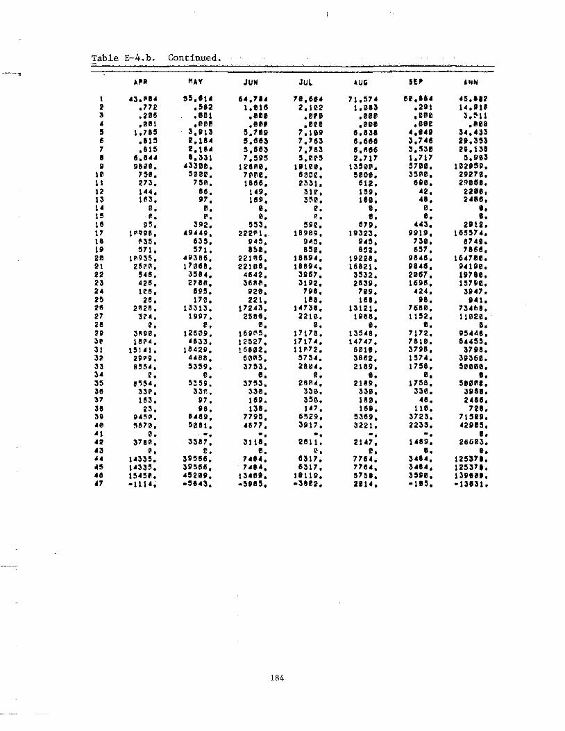
Table E-4. b. Continued.

" APR "AY JUN JUI. AUG Sf' ANN

1 '3.fll' 55.11' u.n. 7',6U 71.57' &II,IU '5."~ 2 .772 • 582 1.tH8 2.122 1.0U .211 14.DU :s .20G .eu .elll • lIU .0U ,100 3.f'U • .01111 ,001 ,elf! .eu ,00' .102 .eee 5 1.715 3,iU 5,710 7 ,lIU~ 1.131 ',e4O 3,.433 IS .111 5 2.U4 5,813 7.7G3 !I,65G ;J.T·tIS U.3n 7 .815 2,U" 5,1583 7.7153 15.1116 3.5311 u.nl I 8.8" '.Ul 7.5D5 5,ml'5 2.717 1.717 5.913 i g&~0. 43300. I:lUe. l,ue. 135011, 5708. I "USg.

10 75111. 5001!!. 700e. 8~D0. '000. 351'1". 211278. 11 273. 75f1. 1855. 2331. GU. ue. 2gUI. 12 1'4, IG. 1.g. Ur. 15D. '2. 22111, 13 163, i7. 159, 35111. In. 4a. 2015. l' 0. fl. e. 0. •• e. e. I!!! -'. "'. B. PI. •• I, e. 18 95. 392. 553. 590. 1751. .n. uu. 17 lPUB. • 9.4D. 222!l11. 18989. IU23. Ding. 1655i' •• 18 ~3!5. 635. D'5. 945. 9 .. 5. 73e. 1Ii'41. u 571. 571. a~ra. 850. 8!'l0. 657. 78615. 2I1l l(/1g3~. ,i38G. 221U. UU'. 19221. DI48. 16.7Ie. 21 25t'I'!. 170118. 22108. 18894. 115821. D848. D.UB. n "15. 358 •• 415"2, 3D67. 3532. 2 lUI 7 • 1D78I. 23 4215. 2710. 31580, 31"2. 2113i. lfHll5. 157i1. 2. lf15. 895. D20. 7i8. 700. ,24. :sa41. 2' 2e. 170. 221, 188. 1151, D8. D.l. 215 21'1!2!!. 13313. 172.3. l'7::U. IU21. 768B. 7;,.61. 27 3U. 1!HI 7. 2588. 2210. 15/68. 11152. 11020. i8 t. e. 0. 0. e. I. II. 2P 3"00. 126~9. 16111"5, 17178. 13548, 7172. D!5UI. ;u 18P4. ·&~3, 12527, 17174. 14747. 781B. 6U55. 31 15141. 18429. 16802. 11~72. sue. 37D8. 3718. 32 29PII. "811. 60V!!5. 1573 •• ~8112, 1157 •• 3U61. 33 85!U. 5359. 3153. 2804. 218D. 17!'l8. 5UBI. ~\4 l'. 0. II. Iil. I. 111, I. 35 e'H~'. 5:!!5I1l. 37!53. 291'14. uu. 1758. !5l1i1Jfll. 311 33'. 33~. 3~C!l. 3:10. ~3B. 3~C!l. 3ilSl • 31 1153. 01. lU. ;:UI!I. 1BrII. .a. UBI, n 23. 118. ua. 1". 1611. 11B. 728. 39 II'~"'. '.eg. 77D5. 6!'1Z9. 538D. 3723. 71"". .lie !'I157t1 • 5081. ,11". ~917. 3221. 2233. 'UII!5. ·1 0. -. -. -. -. -. e. • 2 ~'S0 • 3:187. 3111. 281 1. 2147. un. zun. '3 QI. e. e. I!!. e. I. e. .II. l.n!5 • 3g5158. 7 ..... 8317. 77154. ~.u. U!5nl. .,

1·~3' • U511ts. . 7 •••• 1317. 778 •• ~.I' . 121537 I • • 11 1!5.!51'1. • 521111, 13.111. IIlli. 5751 • ~511e. lUte •• 0 ·111'~ • 51'3. .5111!5, .31102 • 2114. -1", -UUI.

184

Page 194

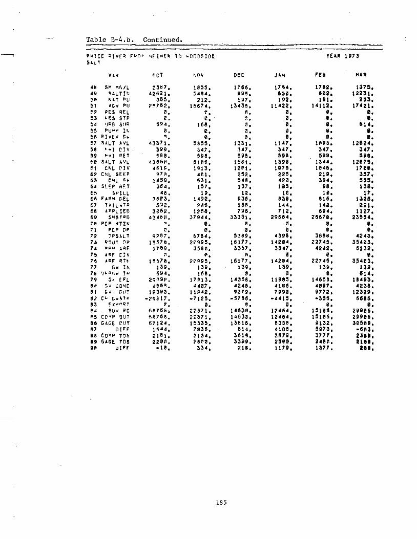
Table E-4.b. Continued. .

~ pwycr ~!>Jf:~ FIJI)'" '1FII'IEiol Tn IoiOOI)~IDE YE4R 1'173 Ui.,l

VAH (lCT t;{'\v DEC JA"l FE8 MAR

48 SI". 1'It;/L 231.17. U55. 17156. 17"4. 1712. lnlS. 4~ 'AL TPl 4~621. :54"4. P91S. a50. lU. 1223S. ~'" NAT FlU 38~. 212. 197. 192. 1111. 253. ~1 AGw PI.! ?!'I7i52. 15674. 13'35, 11 422. 14112. 17.21. !'o' ~ES qEL c. r. III. III. 8. I. ~3 ~'J:S STP ~. t •. Z. Z. I. I. ~4 IJRg StiR 594. 16e. <'l. 0. I. 61., 5!! I' U "'I-' It. 0. 0. 11l. ill. I. I. 511 RIVE .. r. .. "I. 0. 0. e. I. I. ~7 SALT AVL 43371. !SeMI. 1331. 1,.7. 111U, 1282 •• 58 ~ + I cry 399. 347. J47. 347. 3.7. ;U7. '9 "·1 RET '588. 55111. 5\111. !lpa. 5PB. su. t>'" SALT /oVL 431561". 61Q1f1. 1581. 1398. 13". 1287!l. 111 r:~L ["IV 4fi1~. 1<:113. 12"'1. 1075. 10415. 1718. 6~ C"<L SEEP Q7!i\. 4P, 1. 252. 225. 21D. 357. 5~ C:I.iL ~" l·:sg. 1531. 54S. 423. 394. 555. 6 .. StEP RF.T 3fi4. 157. 137. 105. U. 138. 65 ~I-'lLL 415. 19. 12. 10. u. 17. 61\ FA~M r-EL ~6r3. 1492. 51315. a:sa • 815. 1325. H TiILOiTIl !5;/C. ,.15. 11511. 144. 140. 221. 615 APPLIED 3<:l152. 1~158. 7!16. 712. 604. 1127. 159 5MSTOr, '34t>0, 37\)'4. 33351. 29664. 25570. 2355 •• 7101 pcp RTZN ,. 0. '-. 0. III. B. . , 71 pcP C;P 0. e. 0. 0. 0. e. 72 "PSALT Q;?1(\7. 6784. 5389. 4398. 3581$. 4243. 73 'inul f'\P 1'5~78. 2W"!Hl5. 16177. 14204. 22145. 35403. 74 lOP'" AIo?F 1789. 3 5l!1/J. 3;)57. 3341. 4242. 15132. 75 &I;F C'lv 1'1. lII. 01. fl. 0. e. 7~ A ElF' C!Tt 15!l78. 2Vg95. 1IH17 • 14204. 22745. 3,403. 17 CIOI It.. 139. 13101. 139. 13111. 13S1. 1311. 76 I..', !=lr.w Ir..: 61i1 •• 1158. 0. fiI. II. '14. 79 :; .. [FL 29:'1gf'. 17U3. 14CHl!. 11985. 14658. lun. 8 ... ~. co~c ,,~t5I1\. "411l7. '2415. 4111l6. 4"';7. 4231. 81 r, .. (lUi 193!i13. 11!)42. 93751. 751911. 51772. 12328. el C" r; .. !HP -2gel'. .. 7125. • 57815. • ... 15 • -355. 615U • 83 !XI-'nI(T ~. 111. ~. III. 0. e. 1:\4 SUK RC 61171')(;. 22371. 141530. 124154. 1511115 • 2UeI5. 1'5 CC'''!? OUT ~1S76e. 22371. 146JIIl. 12'54. 15106. 251111015 • 86 GAGE CUT 67124. 15335. 138115. 8358. w132. 3050S1. Pl7 DIFF !!II44. 711l315. 814. 41015. 55173. -603. 88 co",p TOS 21 8 1. ~134. 3t51!!. ~1!I751. 3177 • un. 10 CAGE TOS 22001. ~8"e. 331019. 2!51!111l. a4er.. UIlI. u UIH • 1~. 334 • 218. 117;. 1:577. ZIlI.

185

Page 195

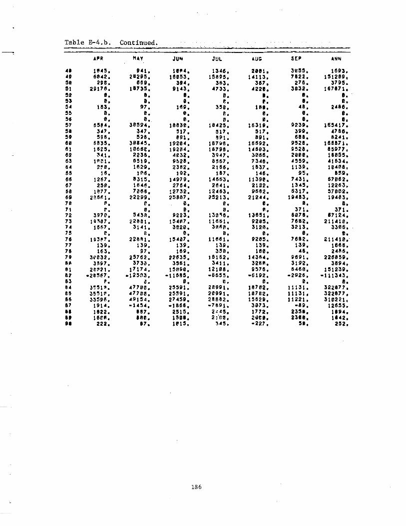
Table E-4. h. Continued.

-A'R Hu JUIoI JUL. .lU, IE' ANN

... 1 .. 5 • 141. U ..... 1346. 21111. 30SS. 115U. 0 6U2. 2821S. 115053. lS8P5. 141 U. 1822. 1S1211l1, se 2n. eu. 3U, 3113. 367. 276. 3715. 51 21H78. l"SS. 1143. 4733. U2I. 31132. 167171. 52 e. I. I. e. I. II. e. 53 II. I. I. e. •• I. e • 54 U13. 97. IfUI. 3511l. lU. "8. 2486. 55 0. II. e. I'l. 0. 8. e. 515 0. 0. I. 0. I. e. I. 57 155e4. 305114. 18SU. 18425. 16311. 9231. 16S417. 5. 34'. 347. 517. 517. 517. 391. .7ee. 5t !lg8. 5~8. !!Pl. SPI. ISH. 681. 8241. 50 61135. 30845. lP2U. 187"8. 16592. 9528. 16U71. tit lU5. 106U. lP2114. 18798. 141503. 9528. 85177 • U ~4.1. 2238. 4n2. 39.7. 30815. 20e0. 181155. 153 1(1\01. 65151. Pe,28. 85157. 7348. 4559. 41634. 64 2~0. 1629. 2382. 2156. lU7. 1139. 104"8. n us. lAI5. 102. 187. 1415. 95. 8:151. tlS 1267. 8315. 14979. 14563. 1139(1. 7431. 57 III tl 2. tl7 25P.. 16415. 27154. 2841. 21i1l2. U45. 122153. 68 1077. 7i1le8. 127!2. 12463. 96152. 6317. 57002. n 2~6f11. 22299. 25807. 25213 • 21244. 19483. 19483. 71 (II. f. B. 0. Ill. I. II, 71 "'. 0. ID. 0. II. 371. 371. 72 397O. 543A. P2U. 130"!8. UI5!U. 8078. 87124. 73 10 :0.87. 0: 2881. 1541'!7. 118111. 9285. 71582. 211"10. 74 1867. 31·U. 3320. 301511. 3120. 3213. 3306. 75 I'!. 0. 0. 0. II. I. II. 7Ii 11'31''' • 228"1. 154m7. lUlU. US5. 71582. 211410.

" l:U. 139. 139. 139. 139. 1351. 115151l. 71 163. 97. 115~. 3S0. lBe. 48. 24"6.

" 3rr32. 25762. 221535. 111162. 143154. Sltl91. 2215851'1. S. 3SP7. 3730. 3561. 3'11. 328". 31112. 389., 81 2ep21. 17174. 150"1. 12 U8. 1'/5715. 64150. 151231'1. U -2e~67. -125~3. -11685. -8655. • 6192. -2926. "111:543 • n P. !ZI. 0. El. 0. Ill. e. IU 3~51~. 4771110. 25591. 221991. 18702. 11131. 322877. 85 35511" , 47700. 25591. 2091'11. 18702. 11131. 322877. 8& 335S1e. 49154. 27.51'1. 28882. 15621'1. 11221. 310221. 87 1914, -1454. -Utll. .7891. 3073. -81'/. 12155:1. II 1122. U7. 2S15. 2.e45. 1772. 2351. 11S14. It 1tU!~II. IU. 15111. 21'00. 2\JU. nil. 1142. III 222. '7. 11'15. 34S. -227. 51. 252.

186

Page 196

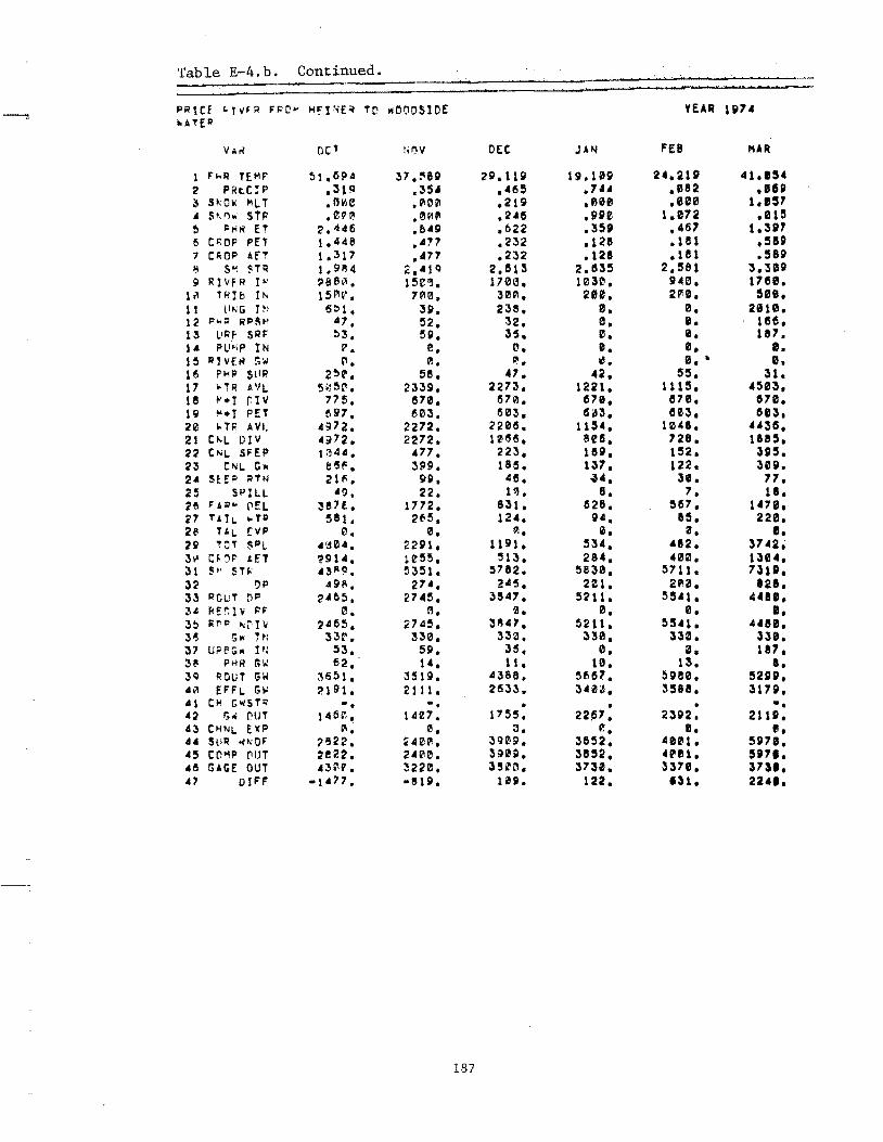
Table E-4.b. Continued. f '.

......., P0l1CE L!VH/ FI1CI' ~fF·EO/ T(' 1'10(10510£ VEAR UH "ATE~

V .. ~ acT tHlY DEC JAN FEB MAR

1 F..,r; TEMF' !II .151:14 ~1.!'Ieg 29.11 g 11'1.10; 24.2U 41.I!U '2 PRt.CIP .31~ .;,,,. •• 65 .74' .1'82 .au 3 5"0;: IoILT • 0i'd~ • "'HI .219 .0011 .011'10 1. e:S7 .. 5 ',"hi STF .l'l!"P.I .!!l~pI .2.6 .ne 1.172 .01!! !I ~H~ ET 2."45 .&.9 .622 .35SJ .467 1.31117 6 CROP PET 1. 448 .4'7 .2~2 .128 .181 • !Seo 7 CI<OP An 1.317 .417 .232 .128 .1151 • !SIP ~ 5~ ~TQ 1. 9R 4 2. '1':) 2.(113 2.535 2.581 3.381 !tl I( I VF R I ~, '861~. 151."13. 1700. 1030. 940. 171511.

Ii'! T~Ib I'" 15 P1 V. 7A0. 30A. 200. 21'11. 5eB. lt ('''G Pi 5::>1. 39. 238. 0. Ill. 2110. 12 p,,:. RP!i\~! ·7. 52. ~2. 0. B. 1155. 13 L'!!Ifo SRF !J3. 5P. 35. !!I. III. U7. 14 i'll"P IN 1". e. 0. I. e. I. 15 Rlvf~ !;w ". 1'1. ~. III. Ill. t e. 1/\ PHI' SilO! 2!1r. 515. 47. 42. 55. 31. 17 I"TR H'L 5;l5r. 2339. 2273. 1221. 1115 • 4503. 115 ,.,.y r.Iv 775. (170. 671'1. 1571/1. (170. "". 19 !".y P!:T ('97. 603. 603. 1503. (103. G13. 20 lOT;; • Vl. 4!P2. 2272 • 2208. 11:U. 1041. "35. 21 C"'L DIY 'ii/12. 2272. 10IHI. ef5. 728. 1185. U C"'L SFE!' 1~44. • 77. 223 • up. 152. 3S!5. 23 C"'L C", est'. 399. 185. 137. 122. 30S1. 24 SHP ~TN 21". 9P. 415. ~4. 38. 77. 2~ SPILl. '9. 22. u. 8. 7. 11. 26 F",I:1" rn 3157£. 1712. 831. 1528. '157. 1·78. '21 TAlL. .. T~ 581. 265. 12 •• 94. 85. 228. 28 TAL (liP tl. 0. CII. e. 0. I. 29 TOT ~Pl • ~,u. 2291. 1191. 534 • ,U2. 3742i 3~ C~~I' LET ?914. 1t5!5. 513. 284. 4011!. 1304. 31 s,· sn; '3~t::I. 5351. ,,82. 5830. 5711. 73U. 32 !)P 491'1. 274. 245. 201. 2P3. 128. 3! I:1CUT tiP ~'65. 2745. 3847. 5211. 55'1. .uU, 3'" FIE!'; 1 v I:'F 0. A. !a. 0. 0. e. 3~ lil'!) .. ['n 2455. 274~. 3"47. 5211. 5!S·H. 4481. 3~ r;IO H~ 33(' • 330. 330. 33111. 33;!. nl. 37 UPt'::; .. I I, 53. 59. 315. 21. 3. U7. 3~ PHR Giol 62. ". 11. 10. 13. e. 3Q ROUT GW ;,551. 351!i1. 4388. 5~!57. 59811l. !SUS! • • ill EFFL G.,: '-1 91. 2111. 2i53~. 3'~:6. 3588. U79 • .1 Cloi GWST~ -. -. • • • -. 42 !;,j OUT 145r,. 1421. 1755. 22~7. 231>2. 21U. 43 CI1NL EleP "'. e. 3. 0. e. II, 4. !W~ ott\:OF ''122. ~40~. 3909. 3852. 4001. '978. '5 cr.~p ('IlT 2!22. 2.00. 3;»0;. 3852. 4Ul. 517'. • 15 GAGE OUT • 3"V. 32221. 3!I!O • 3731. 3378, 3731 • .7 OIFF -1 47 7. -819. U9. 122. 'U. n ...

187

Page 197

Table E-4.b. Continued.

--, AIt" t1AY JUN JUL- AU' SEP ANN

! '3.8n u.n. 88.661 7'.199 72.65~ 6~.IU '8.11179 2 .3U .1Il"'0 .012 1.282 .218 .221 4.154 3 .U5 .000 .flB[I .001' .~00 .O00 1.292 • .0111'.1 ,eel'! .fl0f! ,UII ,01'1"- ,eu .000 5 1,877 '.788 e.555 7,DIS' 7. fl83 ',773 U,llUl 6 .858 2.673 '6,511.12 8.70111 S.U5 '.'15 33,113 7 .858 2.673 6.!UI2 8.111 ',328 2.15' 27.'515 8 •• 558 7.238 4.376 ,532 .elU .Ite 2.687 SI 498111. 17403. 130"11, UIU. 110011.1 • 37'0. 71U9. l' 2!SI'! II , 700Pl, 57'f. '751oh UlI!fJ • 2.08. 29UIII, 11 575, lue. 5:n, 351, 348. 285. ,9U. U 58. 1. 189. 32, 32. 612. 13 6e. • 2. 213 • 36. 315. 15$12. l' p. p. II. 1'1. 1'.1, I. III.

l' 0. 0. II. 0. I. I, 0. 115 174. 5155, 772. 7t18. 81111. 537. '13'. 17 8:1183, 25t164. l1U21. 152'59. 151'5. un. 106d2, 18 1570. 157111. 1000. l:'1e!'!. 101'111.1. 775. 92'1. 19 er,3. 1533. 90111. 9t'",. gn. 697. 8316. 21 8216, 2:>597. 19321. 15109. 15045. 15115. 105558. 21 8211S. 24127, IP17 •• 151159. 13~'5. 611:5. ueae. 22 l72!1. !l1lt1515. 40215. 3185. 28", 1284. 20'1116. 23 I:U2. 3956. 32.7. 2573. 22ft5. 1172. 165ee. 2' 335. 989. 811. 15'3. 571. 268. .125. 25 82. 2·U. 191. 151. US. 51. 988. 215 6"08. 18519, 14951. 11832. 10'155, '771. 16503, 27 961. 2822. 22'3. 1774. 1584, 715. 11.7:5. 21 e, fl. II, '. I. e. I. n 6329. I'P97. 12711. 1269 •• g.u. '~'5, 7.218. 3. lU'. '9Ul. 1438 •• 179.2. 95715 • 011515. 60734. 31 lUI!3. lti012, ~151UJ. 1178. I. 0. I. :u 11.1~1I. '15'. 461st! • 3.53. 1111156. II. 17282 • ~3 215"3. 1281, 5.7. 31U. 272. 227. 29115., ~4 t. !!I. I. 0. 0, II. e. 35 ,.1' .. :'1. 1287. 647, 3P •• 272. 227. 297U, :u ;\3~. 3:U~ • 330. 330. 330. 330. 38511. 37 !!i8. 2. 213. 315, 3e. I5U. 3' "3. 141 • 193. !P1. 2"2. 134. U33. n '338. :>433. 41!l::U. 331 •• 2722. 1532. 'P883. 'II! 28~3. 3259. 2.21. 19118. 1633. 919. 29nl, '1 -. • -, -. -. -. -. 42 1735, 2173. 11513. 1325. !Za9. 1512. 151853. 43 0. 2. I. 0. fl. fl. 1/1, 4. 38.15. 7793. 51'102. 3~14. '953. lt1915. '9l1e •• • & 31'./1. 7793. !IlUI2 • 311'. 'U3, 1596. OIU. •• 3113111. 46U. 3152111. :se 0i!I • 1160. 9151. 39118.' • 7 815. 31n. 1382. 3141 • 36113. 7315. te7'"

188

Page 198

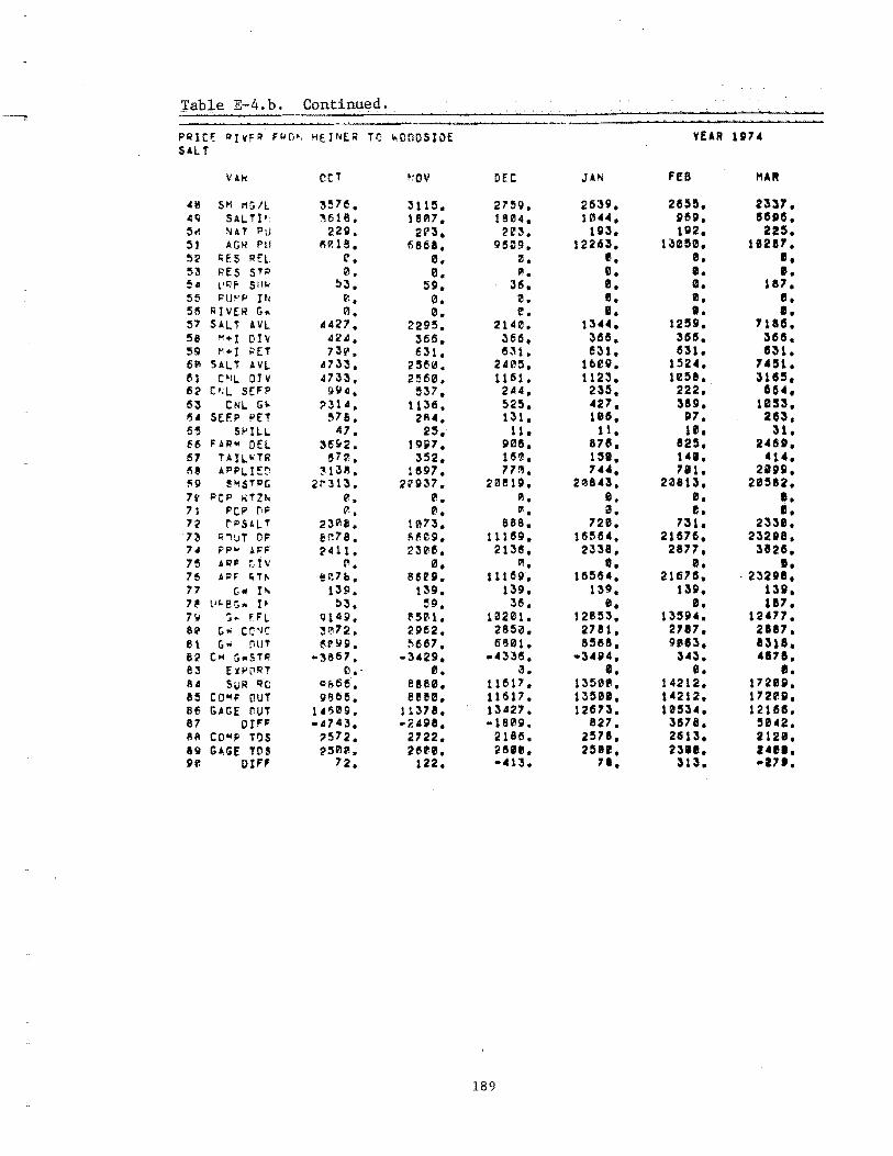
Table E-4. b. Continued .. . . ---. P'IICr: ~1YFI? Fli 0-, HUN£R TO to.OOOSIDE YEAR U14 SAL T

VAl< ecT "~OY DEC JAN 'I!:e MAl'!

411 SM I1G/L 3576. 3115. 2159. 263~. 2&55. 2337. 4Q SAL TIl Mi16. 181117. 1804. 1044. P/5S1. 80DO. :hl 'IIAT FlU 229. 2r3. 2e3, H13. 192. 225. :il "Gil PU 1'I!'l1!. 6858. 91509. 12263, 13050. U2I7. 52 CiES FlEL. r. 0. :!l. I. 0. II. 53 PES S'P 0. 0. PI. I. e. I. ~. l'll f Sill< :13. 59. 36. e. I. 187. 55 PU~'p J t, r.. 0. 0. fl. e. I. 515 RIVER G .. 0. 0. \!l. ID. e. e. 57 SALT AVL 4421. 2295. 2140. I:U4. 12551. 71115 • 58 '1+1 on 42". 356. 3615. 3es. 31U5. 31515. 59 ~"l lIET 73J1!. 631. 1531. 831. 831. 831. 61'1 SALT HL <1733. 25~~. 2405. lbeg. 1524. 7451. til C"L DJ\! 4733. 2560. 1161. 1123. US8. 3lCS5. 62 C';L srFP 9~4. 537. 244. 235. 222. 15154 • 63 CNL. G"- ~31". 11315. 525. 427. USI. 11153. 15. SEF.P PET !'i7S. 21\4. 131. U8. 117. 283. 6'5 SI'ILL- 41. 25. 11. 11. U. U, /56 FARM DEL 3tili2. 19~7. 5IIilS. 67(1. 825, 24&0. 57 TA IL-I'TII el7r. 352. 115'1.. lSI. 1411. 414. lie APPL.H~ ~131\. 11597. 17A. 744. 1U. 2Ut. t'i9 ~"STI'.lG 2r:H3. U937. 20eu. 20843. 20813. 2iHI82. 7i' pcp I<TZI. r.. !!!. Ill. iii. I. ,. 7S PCP ill' 1'1. 0. "'. 15. e. II. 12 !"PS£L T 231118. 1073. U8. 720. 131. 23311. n ::;"uT OF en78. ~~09. 11169. 115~84. 21876. 232118. 74 FP" AFF ~411. 230/5. 21315. 2338. 2877. 3820. 7~ AI1F r,tv 1'1. 0. 1'1. e. 0, I. 76 A !:IF liT", @r.7b. 8HSI. U115!!. 115564. 21578. ·232118. 77 (.011 It. 13P. 13g. 13g. 13~. 13g. I:U. H tH·e!; .. I~ ~3. :i9. 36. iii. 0. U7. 7,* ,.. fFL QI 4 P. P501. 10201. 12853. 135g4. 12477. ~ .. 811' C; .. C:C'l\: ~i'l72. 29f2. 285". 2181. 2181. 2187. 81 G" rill' 151" \I 51 • e'l681. 5!101. 81588. 91J153. nUl 82 CM G .. STP. -36 5 1. -3429, .. 43315. -341J4. 343. 41S7I. e3 ElIPrRT " .. 0. ~. fl. a. II. 8.G SUR I:/C; 0&515, 8e80. 111517. 135011. 14212. 172a;. 85 COMP OUT 9IHi15. Be ee. 11617. 13501. 14212. PUt. 66 GAGE OUT 1.~11l9. 11318. 13427. 12573. un4. 121U. 87 DJ"F -<11 4 3. -2498. -1809. 821. 3&78. 15042. 811 Cowp T05 ~572. 2722. 2188. 2518. 21513. 2120. IQ GAtoE TOS P5P10. 28U. aen. 25U. nil. 14111. 1;0 DI" 72. 122. -413. 71. :SU. -27'.

189

Page 199

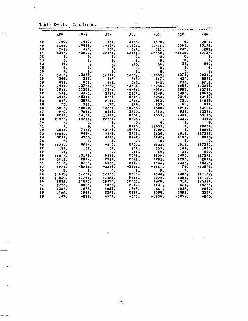
Table E-4.b. Continued.

--~ APR • 11 AV JU~ JUl lUG SfP ANN

48 17S19. U20. 1611. 2473. 5110'. I. 25115. 4(1 U5B. 1S142S1. 14834. 1 U5G. 11128. 5383. '5142. ~e 251. 428. 3151. 321. 321. 240. 3202. '1 5403. -21'1512. -2U11. -2Hl. -255111. -1136. 521'7. '2 e. 0. III. 0. Z. I. II. 53 tI. II. e. 0. I. I. I. 54 156. • 2. 213, 315. 315. 15512. 55 !!I. 0. ". 0. •• I. I. 56 fl. iii, I. 0. e. 0. I. 51 1311'!. 224315. 1

'3", 13USI. 1356S1, 15311, SlSlni.

51 366. 315(1, 547. 541. 547. 424. 5U0. 551 1531. 531. 5142. SI"2. 5142. 13m. 8712. 150 7!1U. 22101. 11731. 1"084. 1351155. 6685. UU41. 151 1~S1. 223518. 1181U. 1'~84. 12512. 6685. Sl3731. 152 15P2. '4!U, 31597. 2951. 21540. 1403. 19683. 153 3546. 103U. 85157. 6&15. 605 •• 3U6. 441152. 15 .. sell. . 2518. 2141. 1103. 1513. 754. 1111411. 15!5 7'. 213. 115. 14(1). 12'. (16. 037. 1515 5913. 16159Pl. 13131. 10gB'. gUO, 5214. 13118. 151 U19. 3tH>8. 2'U. 21'102, l1U. 925. 132151. 611 502e. 14187, 11f112. Sl337. 833'. "'32. 1521"3. In 21913. 28711. 212111'. Slzge. • .'432. 4432. 11 0. III. II. 0. I. I. e, n e. B. B. 8413. 1113'. I. 2UBI. 12 315M! • '.48. 1311S. 18171. 519t. I. 'UU. 13 182551. U3". 42415. 2153. 2125. 15111. 1273315. ,. 5fe'. 4S133. 4827. '140. 574Z. 6193. 301'. 15 11'. 0. ". III. I. '. I. 115 18269. 8834. 42415. 2153. 212~. U1l 1 127336. 11 139. 1351. 1351. 13Sl. 1351. 1351. 115158 • 18 fill. • 2. 213. 315. 36. U2. n 11'877. 13119. 9581. 161P. 15208. 34516. 1175112. iii! 3011!. 25174. 25112. 2841. 2792. 21518. 28ln. u 71 U. 81815. 6387. 51U. 4133. 2330. 783g,. U !lUI. • 21'181. -221". -2381. -1181. 73. -12572 • 83 e. 0. 0. 0. 0. I. 0. U 1 te'32. 1716 •• 12400. 9823. 9505. 4488. 1·111112. 85 11~32. 1

'764. 12400. P823. g50'. 4488. 141Ua.

86 P~5g. 11678. 10823. HUI53. 4098. 3914. 125327. 87 2113. '8815 • 15115. -9410. 5407. ~14. 1577'. II 2387. le77. 1823. 18./1. 1 .... 1. U41. 2012. n 2\ SIP. lUe. 22l11li. 221111'. 2801. 31310. 2357 • PI 187. -222. -311. -353. -1151. -1052. -275.

190

Page 200

Table E-4.b. Continued.

Pf,'J Cf II I vf q Fr.O~ HfINE~ TO WOODSIDE YEAR 11I7~ --- "'TEll

VA~ nCT ~·tW DEC JAN "E8 MAl'

\ FhQ H"1P 54.074 37.274 27 .~~" 23."11 28.17' 311.22' 2 PRECIP ~.~7~ •• 155 .'0? .75111 .118, 1.545 3 S~C1W "LT .91",1.\ • rill" .0~6 .010 .557 1.2315

• SI>:('IOI ST~ .0"" .i1CQI .395 1.1 t3 1.;'111 • .,12 ~ PHR ET ~.74t1 .e28 .5711 .4'0 .5" .87;' 6 C~ OF PET 1. b 22 .'65 .215 .158 .210 .'111 7 C:~'IjP A~T \.ti22 .4155 .215 .158 .210 .411 II 5'1 ST~ 2.'17 2.70' 2.1573 2.154!» 3.0155 5.171 Q RJV!:,R_ 1~ 12:>:':. 11'0. g!5~. !5111ll. 850. 211;".

10 HIS Y ~, e~". 45111. 302. 2211ll. 251'1. 508. 11 'J~li yt.; ",51'1. 0. .. 0. 5115. 2541. ... 12 F'HR ~P5~ 527. ~8. 1 • I. U. '11/1. 1~ l'~B SIIF 596. 77. 1 • 0. Sl2. '153. 1~ PU~'P I~ 0. II. ~. 0. 0. •• 1~ RlVEw c:w ". 0. 0. fJ. Ill. '. 16 PHR SlJQ !Il. '2. 157. 52. III. I. 17 IooTIi 'VL 71518. 11594. 12215. 861. 2158. 5112. lB "'+1 nv 85&>. 740. 7''''. 7'81. 7'". 7'111. lSI "+1 RET 7155. 15615. 15615. 1568. 15156. 815S. 20 .,;Tr. AVL 7113. Hi20. 1152. 787. 21'178. 51f11. 21 C:t.L DIV ::1912. 1599. 1001. 787. 11152. 17151. 22 C~L SEE'" ~11. 33~. 213. 1155. 212. 371. 23 CNL. r. .. ~1"'. 277. 172. 133. 181ll. 282. 2. HPl:h 127. 651. '3. 33. '0. 73. 2~ SPJLL 29. 15. 10. 7. SI. 17 .• 2~ Fjll" eEL 22 71. 12 47 • 7BtII. 61'. 751!J. 1378. 27 TA 1L ~~F 3 4 r. 167. 117. Sl2. 112. 2.,15. 26 TAL EVP 0. 1'1. 0. 0. 0. e. ~q T:lT 5P L 98'6. 2089. 678. 522. 1871. 73215. 3" C:=(lF .:.ET ~~gl'l. lC'!2!i1. 477. 3451. 4156. UI. 3\ 5" STCI 53 48. ~~B3. 55113. 58150. 15711. 11';'8. 3? OF' Q07. 425. 27!3. 225. 484. 17511. 33 I:CIJ'l' [lP 6"7. 1277. 30S115. 411'13. 315112. 2132. 34 RE':l!v ~~ c. 0. 0. 0. 0. II. 3~ Rep ",rrll "i07. 1277 • 3e5le. 411'11. 36112. 21;'2. 36 Go< IN 331.". 332. 33". 330. 3311. 3311. 37 UF3G .. I" " 5516. 77. 1 • 0. 82. '8;'. 38 ~H~ f';t..: PI. J II. 115. 13. 0. e. 351 "OUT G'" ?;'I 4 3. 1952. 358'. • 4~53. 427:5. ;, 111. 4'" EFFL. r;w 1226. 1171. 21'0. 2732. 25155. 1'71. '1 CH GJiSTIi . -. . • -. -. '2 GIo' OUT 1117. 7e0. 1.32. 1821. 1711. 1247. 43 CHNL EXP I'!. 0. '11. e. •• I. 4. SUR R"lOF 57P7. 1395. 2':1'8. 21132. 31102. 151315. . ~ c:otolP (HIT !'I7117. 13115. 2428. 2~;'2. lIU. 613 •• .11 GAGE O'JT 29:>~. 2P'~1!J. 129~. 132eJ. 115'". 2111. • 7 DIFF 2"l·7. -~5'. llH. lS12. 2112. uu •

191

Page 201

192

Page 202

193

Page 203

194