SOCIETY OF P ETROLEUM EVALUATION ENGINEERS CALGARY CHAPTER MEMBERS R.K. AGRAWAL H.J. HELWERDA R. PACHOLK MAILING ADDRESS: Bankers Hall P.O. Box 22298 Calgary, Alberta T2P 4J1 O B.R. ASHTON R.A. HENNIG D. PADDOCK S.E. BALOG H. JUNG J. PHILLIPS R.G. BERTRAM P.S. KANDEL G. ROBINSON L. BOWNS F. KIRKHAM B. RUSSELL G.S. BRANT C. LABELLE S. N. SEDGWICK K.D. BROWN J.R LACEY P. SIDEY M.J. BRUSSET R.G. LAVOIE F. SIEGLE C.W. CHAPMAN D. LONGFIELD N. STEWART N.A. CLELAND K. MACLEOD A.A. SZABO K. CRERAR K. MASTERS D.TUTT K.H. CROWTHER P. MATSALLA P. WELCH J.P. DIELWART G. METCALFE D.M. WRIGHT D. C. ELLIOTT F. MOLYNEAUX W. G. WRIGHT B. EMSLIE R.R. MOTTAHEDEH J. ESSEX T. NAZARKO D. H. GILBERT R. ODD APRIL 28, 2004 REQUEST FOR PUBLIC COMMENT CANADIAN OIL AND GAS EVALUATION HANDBOOK (COGEH) VOLUME 2 The Society of Petroleum Evaluation Engineers Calgary Chapter (SPEE Calgary Chapter) hereby notifies all interested parties that Volume 2 of the Canadian Oil and Gas Evaluation Handbook is now available in draft form for public review and comment. A copy of this draft COGEH Volume 2 (“Draft”) entitled Detailed Guidelines for Estimation and Classification of Oil and Gas Resources and Reserves can be accessed electronically via the following websites: www.petsoc.org (Petroleum Society of CIM) www.albertasecurities.com (Alberta Securities Commission) www.speca.ca (Society of Petroleum Engineers, Canadian Section – link only) Interested parties wishing to comment or propose changes to the Draft should clearly identify themselves with appropriate contact details and forward their specific comments, including the particular section, page and line number(s) to which their comments pertain, to the SPEE Calgary Chapter either by: E-mail to: [email protected] Or Mail to: SPEE Calgary Chapter Bankers Hall P.O. Box 22298 Calgary, AB T2P 4J1 The deadline for submission of comments and/or proposed changes is May 31, 2004. The SPEE Calgary Chapter, through its COGEH Standing Committee, will review and consider all submissions and shall also retain full discretion to determine which proposed changes (in whole or in part), if any, are accepted and incorporated into the COGEH Volume 2, First Edition. All parties accessing the Draft are reminded that, with the exception of making paper copies for purposes of review as contemplated via this public comment process, the Draft is copyrighted and is subject to standard copyright restrictions relating to unauthorized reproduction, use or transmission. All copies are to be destroyed after expiration of the comment period. In addition, the guidance contained within the COGEH volumes will remain subject to revision, addition or clarification in the future.

Welcome message from author
This document is posted to help you gain knowledge. Please leave a comment to let me know what you think about it! Share it to your friends and learn new things together.
Transcript

SOCIETY OF PETROLEUM EVALUATION ENGINEERS CALGARY CHAPTER
MEMBERS R.K. AGRAWAL H.J. HELWERDA R. PACHOLK
MAILING ADDRESS: Bankers Hall P.O. Box 22298 Calgary, Alberta T2P 4J1
OB.R. ASHTON R.A. HENNIG D. PADDOCK S.E. BALOG H. JUNG J. PHILLIPS R.G. BERTRAM P.S. KANDEL G. ROBINSON L. BOWNS F. KIRKHAM B. RUSSELL G.S. BRANT C. LABELLE S. N. SEDGWICK K.D. BROWN J.R LACEY P. SIDEY M.J. BRUSSET R.G. LAVOIE F. SIEGLE C.W. CHAPMAN D. LONGFIELD N. STEWART N.A. CLELAND K. MACLEOD A.A. SZABO K. CRERAR K. MASTERS D.TUTT K.H. CROWTHER P. MATSALLA P. WELCH J.P. DIELWART G. METCALFE D.M. WRIGHT D. C. ELLIOTT F. MOLYNEAUX W. G. WRIGHT B. EMSLIE R.R. MOTTAHEDEH J. ESSEX T. NAZARKO D. H. GILBERT R. ODD
APRIL 28, 2004
REQUEST FOR PUBLIC COMMENT
CANADIAN OIL AND GAS EVALUATION HANDBOOK (COGEH) VOLUME 2
The Society of Petroleum Evaluation Engineers Calgary Chapter (SPEE Calgary Chapter) hereby notifies all interested parties that Volume 2 of the Canadian Oil and Gas Evaluation Handbook is now available in draft form for public review and comment. A copy of this draft COGEH Volume 2 (“Draft”) entitled Detailed Guidelines for Estimation and Classification of Oil and Gas Resources and Reserves can be accessed electronically via the following websites:
www.petsoc.org (Petroleum Society of CIM) www.albertasecurities.com (Alberta Securities Commission) www.speca.ca (Society of Petroleum Engineers, Canadian Section – link only)
Interested parties wishing to comment or propose changes to the Draft should clearly identify themselves with appropriate contact details and forward their specific comments, including the particular section, page and line number(s) to which their comments pertain, to the SPEE Calgary Chapter either by:
E-mail to: [email protected] Or Mail to: SPEE Calgary Chapter Bankers Hall P.O. Box 22298 Calgary, AB T2P 4J1
The deadline for submission of comments and/or proposed changes is May 31, 2004. The SPEE Calgary Chapter, through its COGEH Standing Committee, will review and consider all submissions and shall also retain full discretion to determine which proposed changes (in whole or in part), if any, are accepted and incorporated into the COGEH Volume 2, First Edition. All parties accessing the Draft are reminded that, with the exception of making paper copies for purposes of review as contemplated via this public comment process, the Draft is copyrighted and is subject to standard copyright restrictions relating to unauthorized reproduction, use or transmission. All copies are to be destroyed after expiration of the comment period. In addition, the guidance contained within the COGEH volumes will remain subject to revision, addition or clarification in the future.
1
2
3
CANADIAN 4
OIL AND GAS 5
EVALUATION HANDBOOK 6
First Edition 7
April 28, 2004 8
9
Volume 2 10
Detailed Guidelines for 11
Estimation and Classification 12
of Oil and Gas Resources and Reserves 13
14
Prepared by 15
Society of Petroleum Evaluation Engineers 16 (Calgary Chapter) 17
and 18
Canadian Institute of Mining, Metallurgy & Petroleum 19 (Petroleum Society) 20
21
Copy No.: _______________________________________ 21 22 Recipient: _______________________________________ 23 24 25 26 27 28 29 30 2004 by the Society of Petroleum Evaluation Engineers (SPEE) (Calgary Chapter). 31 32 33 All rights reserved. No part of this Handbook may be reproduced or transmitted in any form 34 or by any means, electronic or mechanical, including photocopying, recording, or by any 35 information storage and retrieval system, without permission in writing from SPEE (Calgary 36 Chapter). 37 38 39 40 41 42 43 National Library of Canada Cataloguing in Publication 44 45
The Canadian oil and gas evaluation handbook / prepared by Society of 46 Petroleum Evaluation Engineers (Calgary Chapter), and Canadian Institute of 47 Mining, Metallurgy and Petroleum (Petroleum Society). 48 49 50 51 Includes index. 52 Contents: v. 1. Reserves definitions & evaluation practices and procedures -- 53 v. 2. Detailed guidelines for estimation and classification of oil and gas 54 resources and reserves. 55 ISBN 0-9730695-0-3 (v.1).--ISBN 0-9730695-1-1 (v.2) 56 57
1. Oil fields--Valuation--Canada. I. Society of Petroleum 58 Evaluation Engineers. Calgary Chapter II. Canadian Institute of 59 Mining, Metallurgy and Petroleum. Petroleum Society 60 61 62 HD9574.C2C32 2002 338.2'328'0971 C2002-910572-2 63 64 65 66 67 Editing and layout by Copper Communications, Calgary AB 68 69 70 Contact: Society of Petroleum Evaluation Engineers (Calgary Chapter), Banker’s Hall, P.O. Box 22298, 71 Calgary AB T2P 4J172
1
2
DISCLAIMER 3
The Canadian Oil and Gas Evaluation Handbook, Volume 2 was prepared by the Calgary Chapter 4 of the Society of Petroleum Evaluation Engineers (SPEE Calgary Chapter), the Petroleum Society 5 of the Canadian Institute of Mining, Metallurgy & Petroleum (Petroleum Society) and 6 contributing authors (Co-authors). In addition, the SPEE Calgary Chapter, the Petroleum Society, 7 and Co-authors prepared and published the Canadian Oil and Gas Evaluation Handbook, Volume 8 1 (ISBN0-9730695-0-3) (Volumes 1 and 2 together are here referred to as “the Handbook”). The 9 SPEE Calgary Chapter, Petroleum Society, and Co-authors specifically disclaim any liability, 10 loss, or risk, personal or otherwise, incurred as a consequence, directly or indirectly, of the use 11 and application of any of the contents of the Handbook. The Handbook is intended primarily for 12 use in Canada, and reflects recommended practice for evaluations and reporting of reserves 13 information in Canada. It may also have application to other jurisdictions as a general guideline 14 for reserves estimation. The SPEE Calgary Chapter, Petroleum Society, and Co-authors have 15 made every effort to ensure the accuracy and reliability of the information contained in the 16 Handbook and to qualify best practices for the conduct of reserves evaluations and reporting of 17 reserves information. However, the SPEE Calgary Chapter, Petroleum Society, and Co-authors 18 make no representation, warranty, or guarantee as to the validity, reliability, or acceptability of 19 the contents of the Handbook, and disclaim any responsibility or liability for any loss or damage 20 arising from the use of the Handbook for any purpose, including and without limitation any 21 reports or filings, reserves evaluation results, conclusions, recommendations, or any decisions 22 made as a consequence of the use of the Handbook. 23
The SPEE Calgary Chapter, Petroleum Society, and Co-authors recognize that no set of 24 definitions, practices, and guidelines of general application can be constructed and presented to 25 suit all circumstances or a combination of circumstances that may arise, nor is there any substitute 26 for the exercise of professional judgement in the determination of what constitutes fair 27 presentation or good practice in a particular case. 28

Table of Contents 1
©SPEE (Calgary Chapter) First Edition — April 28, 2004
TABLE OF CONTENTS VOLUME 1 RESERVES DEFINITIONS AND EVALUATION PRACTICES AND
PROCEDURES
VOLUME 2 DETAILED GUIDELINES FOR ESTIMATION AND CLASSIFICATION OF OIL AND GAS RESOURCES AND RESERVES
PREFACE Section 1 INTRODUCTION.................................................................................................... 1-1
1.1 Introduction ..................................................................................................................... 1-3 Section 2 RESOURCES CLASSIFICATIONS AND DEFINITIONS.................................... 2-1
2.1 Introduction ..................................................................................................................... 2-3 Section 3 DEFINITIONS OF RESERVES .............................................................................. 3-1
3.1 Introduction ..................................................................................................................... 3-3 3.1.1 Background — Development of Reserves Definitions............................................. 3-3 3.1.2 Introduction to Reserves Definitions ........................................................................ 3-4
3.2 Reserves Categories ........................................................................................................ 3-4 3.2.1 Proved Reserves........................................................................................................ 3-5 3.2.2 Probable Reserves..................................................................................................... 3-5 3.2.3 Possible Reserves...................................................................................................... 3-5
3.3 Development and Production Status ............................................................................... 3-6 3.3.1 Developed Reserves.................................................................................................. 3-6
a. Developed Producing Reserves ................................................................................ 3-6 b. Developed Non-Producing Reserves........................................................................ 3-6
3.3.2 Undeveloped Reserves.............................................................................................. 3-7 3.4 Levels of Certainty for Entity and Reported Reserves .................................................... 3-7
Section 4 UNCERTAINTY AND STATISTICAL CONCEPTS ............................................ 4-1
4.1 Introduction ..................................................................................................................... 4-3 4.2 Uncertainty in Reserves Estimation ................................................................................ 4-4
4.2.1 Definitions of Terms Relating to Certainty .............................................................. 4-5 4.2.2 Certainty Concepts in the Classification of Reserves ............................................... 4-7
4.3 Deterministic and Probabilistic Methods ........................................................................ 4-8 4.3.1 Deterministic Method ............................................................................................... 4-8
a. Risk-Based Reserves Estimates................................................................................ 4-9 b. Uncertainty-Based Reserves Estimates .................................................................... 4-9
4.3.2 Probabilistic Method................................................................................................. 4-9 4.4 Aggregation of Reserves Estimates............................................................................... 4-10
4.4.1 Aggregating Probabilistic Estimates....................................................................... 4-10 4.4.2 Aggregating Deterministic Estimates ..................................................................... 4-11 4.4.3 Comparison of Deterministic and Probabilistic Estimates ..................................... 4-12
2 Volume 2 — Resources and Reserves Estimation and Classification Guidelines
Canadian Oil and Gas Evaluation Handbook ©SPEE (Calgary Chapter)
4.5 Meeting Certainty Requirements Using Deterministic Methods .................................. 4-13 4.5.1 Deterministic Estimates Considering Minimum, Best Estimate and Maximum
Values ..................................................................................................................... 4-13 a. Confidence Levels Resulting from Application of Minimum, Best Estimate, and Maximum Guidelines ..................................................................................................... 4-15
4.5.2 Simple Example Problem Involving Uncertainty ................................................... 4-16 a. Dice Problem.......................................................................................................... 4-17 b. A Simple Gas Material Balance Example .............................................................. 4-20
i. Deterministic Approach...................................................................................... 4-20 ii. Probabilistic Approach ....................................................................................... 4-21
4.6 Probabilistic Check of Deterministic Estimates ............................................................ 4-22 4.7 Application of Guidelines to the Probabilistic Method................................................. 4-22
Section 5 GENERAL REQUIREMENTS FOR CLASSIFICATION OF RESERVES........... 5-1
5.1 Introduction ..................................................................................................................... 5-3 5.2 Ownership Considerations .............................................................................................. 5-3 5.3 Drilling Requirements ..................................................................................................... 5-4 5.4 Testing Requirements...................................................................................................... 5-5 5.5 Regulatory Considerations .............................................................................................. 5-6 5.6 Timing of Production and Development ......................................................................... 5-7 5.7 Economic Requirements.................................................................................................. 5-8
5.7.1 Forecast Prices and Costs ......................................................................................... 5-9 5.7.2 Constant Prices and Costs....................................................................................... 5-10 5.7.3 Booking Guideline.................................................................................................. 5-10
Section 6 PROCEDURES FOR ESTIMATION AND CLASSIFICATION OF RESERVES 6-1
6.1 Introduction ..................................................................................................................... 6-6 6.1.1 Reserves Confidence Levels ..................................................................................... 6-6
a. Proved Reserves ....................................................................................................... 6-6 i. Entity Level .......................................................................................................... 6-6 ii. Property Level ...................................................................................................... 6-7 iii. Reported Level ................................................................................................. 6-7
b. Proved Plus Probable Reserves ................................................................................ 6-7 c. Proved Plus Probable Plus Possible Reserves .......................................................... 6-7
6.1.2 Reserves Validation—Reported Level ..................................................................... 6-7 6.2 Analogy Methods ............................................................................................................ 6-8
6.2.1 Use of Analogies as a Primary Method .................................................................... 6-9 a. When Other Methods are Not Reliable .................................................................... 6-9 b. Heavy Oil Cold Production ...................................................................................... 6-9 c. Undeveloped Reserves Assigned for Infill Drilling ............................................... 6-10
6.2.2 Use of Analogies for Specific Reserves Parameters ............................................... 6-11 a. Areal Assignments.................................................................................................. 6-11 b. Recovery Factors .................................................................................................... 6-11 c. Performance Characteristics ................................................................................... 6-11
6.3 Volumetric Methods...................................................................................................... 6-12 6.3.1 Data Used for Volumetric Methods........................................................................ 6-12
Table of Contents 3
©SPEE (Calgary Chapter) First Edition — April 28, 2004
a. Geophysical Data.................................................................................................... 6-12 b. Geological Data ...................................................................................................... 6-13
i. Presence of Hydrocarbons .................................................................................. 6-14 ii. Net Pay ............................................................................................................... 6-15 iii. Porosity........................................................................................................... 6-17 iv. Hydrocarbon Saturation.................................................................................. 6-18 v. Pool Area/Drainage Area/Well Spacing Unit..................................................... 6-18
c. Reservoir Engineering Data.................................................................................... 6-20 i. Fluid Analysis..................................................................................................... 6-20 ii. Formation Volume Factor .................................................................................. 6-21 iii. Gas Compressibility Factor ............................................................................ 6-21 iv. Reservoir Pressure .......................................................................................... 6-21 v. Reservoir Temperature ....................................................................................... 6-22 vi. Gas Shrinkage................................................................................................. 6-22 vii. Well Test Analysis ......................................................................................... 6-22 viii. Extended Flow Tests ...................................................................................... 6-23 ix. Reservoir Drive Mechanisms ......................................................................... 6-23 x. Reservoir Simulation Modelling ........................................................................ 6-24 xi. Recovery Factor.............................................................................................. 6-24
6.3.2 Guidelines for Reserves Assignments in Single-Well Pools .................................. 6-26 6.3.3 Guidelines for Reserves Assignments in Multi-Well Pools.................................... 6-33
6.4 Material Balance Methods............................................................................................. 6-42 6.4.1 General Considerations in the Use of Material Balance Methods for Gas
Reservoirs ............................................................................................................... 6-42 6.4.2 Consideration of Reservoir Properties .................................................................... 6-43
a. Aquifers .................................................................................................................. 6-43 b. Reservoir Permeability ........................................................................................... 6-43 c. Multi-Well Reservoirs ............................................................................................ 6-44 d. Multi-Layer Reservoirs .......................................................................................... 6-44 e. Naturally Fractured Reservoirs............................................................................... 6-44
6.4.3 Consideration of Fluid Properties ........................................................................... 6-45 a. Dry Gas Reservoirs................................................................................................. 6-45 b. Wet Gas Reservoirs ................................................................................................ 6-45 c. Retrograde Condensate Reservoirs......................................................................... 6-45
6.4.4 Consideration of Quality of Pressure Data ............................................................. 6-45 a. Types of Pressure Measurements ........................................................................... 6-45 b. Number of Pressure Measurements........................................................................ 6-46 c. Correlation of the Pressure Data Points.................................................................. 6-46 d. High-Permeability Reservoirs ................................................................................ 6-46 e. Low-Permeability Reservoirs ................................................................................. 6-46
6.4.5 Consideration of Degree of Pressure Depletion...................................................... 6-47 6.4.6 Guidelines for Determining Proved, Probable and Possible Reserves ................... 6-47
a. Assess well groupings in multi-well pools. ............................................................ 6-47 b. Review reservoir and fluid properties. ................................................................... 6-48 c. Review inconsistent data points. ............................................................................ 6-48 d. Determine OGIP for each reserves category. ......................................................... 6-48
4 Volume 2 — Resources and Reserves Estimation and Classification Guidelines
Canadian Oil and Gas Evaluation Handbook ©SPEE (Calgary Chapter)
e. Compare the OGIP to that found using other methods........................................... 6-48 f. Determine recovery factors and reserves................................................................ 6-49
6.4.7 Special Situations.................................................................................................... 6-49 a. OGIP Calculations based on Initial Production Tests ............................................ 6-49 b. Allocation of Reserves in Multi-Well Pools........................................................... 6-49 c. Drainage Outside Company Owned Lands ............................................................ 6-50
6.4.8 Examples................................................................................................................. 6-51 6.4.9 General Considerations in the Use of Material Balance Methods for Oil
Reservoirs ............................................................................................................... 6-55 6.5 Production Decline Methods ......................................................................................... 6-55
6.5.1 Types of Decline Analysis ...................................................................................... 6-56 a. Type Curve Matching............................................................................................. 6-56 b. Curve Fitting........................................................................................................... 6-56
6.5.2 Limitations of Methods........................................................................................... 6-57 6.5.3 Factors Affecting Decline Behaviour ..................................................................... 6-58
a. Rock and Fluid properties ...................................................................................... 6-58 i. Stratification ....................................................................................................... 6-58 ii. Wettability .......................................................................................................... 6-59 iii. Relative Permeability ..................................................................................... 6-59 iv. Permeability.................................................................................................... 6-59 v. Fracturing ........................................................................................................... 6-59 vi. Back Pressure Slope ....................................................................................... 6-59
b. Reservoir Geometry and Drive Mechanism ........................................................... 6-60 i. Vertical Displacement ........................................................................................ 6-60 ii. Coning ................................................................................................................ 6-60 iii. Horizontal Displacement ................................................................................ 6-60 iv. Unconsolidated Heavy Oil Reservoirs ........................................................... 6-60
c. Completion and Operating Practices ...................................................................... 6-60 i. Skin Factors ........................................................................................................ 6-60 ii. Fluid Rate Changes............................................................................................. 6-61 iii. Workovers ...................................................................................................... 6-61 iv. Infill Drilling .................................................................................................. 6-61 v. Regulatory Constraints ....................................................................................... 6-61 vi. Facility Constraints......................................................................................... 6-61
d. Type of Wellbore.................................................................................................... 6-61 i. Horizontal versus Vertical Wellbore .................................................................. 6-61 ii. Coning Situations ............................................................................................... 6-62 iii. Wellbore Contact............................................................................................ 6-62
6.5.4 Guidelines for Individual Well Decline Analysis ................................................... 6-62 a. Reservoir Properties Review .................................................................................. 6-62 b. Analogy Review ..................................................................................................... 6-62 c. Transient Period Estimation ................................................................................... 6-62
i. Buildup Analysis ................................................................................................ 6-63 ii. Type Curve Analysis .......................................................................................... 6-63
d. Final Rate Determination ....................................................................................... 6-63 e. Operating Constraint Review ................................................................................. 6-63
Table of Contents 5
©SPEE (Calgary Chapter) First Edition — April 28, 2004
f. Data Review ........................................................................................................... 6-63 g. Re-Initialization...................................................................................................... 6-64 h. Oil-Cut Analysis..................................................................................................... 6-64 i. Line-Pressure Adjustments..................................................................................... 6-64 j. Interference Effects ................................................................................................ 6-64 k. Production Forecasts .............................................................................................. 6-64
6.5.5 Guidelines for Group Decline Analysis .................................................................. 6-65 a. Grouping................................................................................................................. 6-65 b. Voidage Replacement............................................................................................. 6-65 c. Breakthrough Behaviour ........................................................................................ 6-65
6.5.6 Guidelines for Reserves Classification from Decline Analysis .............................. 6-66 6.5.7 Decline Examples ................................................................................................... 6-67
6.6 Reservoir Simulation Methods...................................................................................... 6-83 6.7 Reserves Related to Future Drilling and Planned Enhanced Recovery Projects........... 6-83
6.7.1 Additional Reserves Related to Future Drilling...................................................... 6-83 a. Drilling Spacing Unit ............................................................................................. 6-83 b. Infill Wells.............................................................................................................. 6-83 c. Infill Analysis ......................................................................................................... 6-84 d. Delineation or Step-Out Wells ............................................................................... 6-84
i. Classification ...................................................................................................... 6-85 ii. Qualifiers to Classification ................................................................................. 6-85 iii. Adjustments for Reservoir Quality................................................................. 6-85
e. Drilling Statistics .................................................................................................... 6-86 f. Likelihood of Drilling............................................................................................. 6-86 g. Time Constraints .................................................................................................... 6-88
6.7.2 Examples of Future Drilling ................................................................................... 6-89 6.7.3 Reserves Related to Planned Enhanced Recovery Projects .................................... 6-94
a. Proved Criteria (1P)................................................................................................ 6-94 b. Proved + Probable Criteria (2P) ............................................................................. 6-97 c. Proved + Probable + Possible Criteria (3P)............................................................ 6-98
6.7.4 Planned EOR Examples.......................................................................................... 6-99 6.8 Integration of Reserves Estimation Methods .............................................................. 6-101
a. Volumetric Methods............................................................................................. 6-102 b. Analogy Methods ................................................................................................. 6-102 c. Decline Curve Methods........................................................................................ 6-103 d. Material Balance Methods for Gas Reservoirs..................................................... 6-103 e. Reservoir Simulation ............................................................................................ 6-103
Section 7 VALIDATION AND RECONCILIATION OF RESERVES AND VALUE ESTIMATES .............................................................................................................................. 7-1
7.1 Introduction ..................................................................................................................... 7-3 7.2 Reserves Validation......................................................................................................... 7-3 7.3 Reserves Reconciliations................................................................................................. 7-5
7.3.1 Introduction............................................................................................................... 7-5 7.3.2 Product Types ........................................................................................................... 7-5 7.3.3 Reserves Change Categories..................................................................................... 7-6

6 Volume 2 — Resources and Reserves Estimation and Classification Guidelines
Canadian Oil and Gas Evaluation Handbook ©SPEE (Calgary Chapter)
7.3.4 Discussion of Special Reserves Change Situations .................................................. 7-8 7.3.5 Example Reserves Reconciliation............................................................................. 7-9
7.4 Net Present Values Reconciliations............................................................................... 7-11 7.4.1 Introduction............................................................................................................. 7-11 7.4.2 Net Present Value Change Categories .................................................................... 7-11
APPENDICES A — GLOSSARY B — REFERENCES
INDEX

Table of Contents 7
©SPEE (Calgary Chapter) First Edition — April 28, 2004
LIST OF TABLES
Table 4-1 Approximate Confidence Level of the Value at Mid-Point Between the Minimum or Maximum and Best Estimate ................................. 4-16
Table 6-1 Decline Examples — Summary of Analysis .................................................... 6-82
Table 7-1 Reserves Revisions by Category ........................................................................ 7-4
Table 7-2 Sample Reserves Reconciliation Company Net Reserves (Mbbl) Light and Medium Crude Oil ........................................................................... 7-10
Table 7-3 Reconciliation of Changes in Net Present Values of Future Net Revenue Discounted at 10% Per Year ............................................................................ 7-14
8 Volume 2 — Resources and Reserves Estimation and Classification Guidelines
Canadian Oil and Gas Evaluation Handbook ©SPEE (Calgary Chapter)
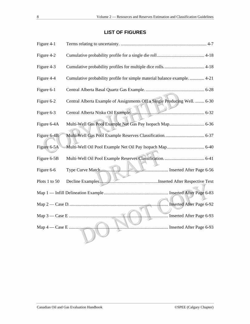
LIST OF FIGURES
Figure 4-1 Terms relating to uncertainty. ............................................................................ 4-7
Figure 4-2 Cumulative probability profile for a single die roll.......................................... 4-18
Figure 4-3 Cumulative probability profiles for multiple dice rolls. ................................... 4-18
Figure 4-4 Cumulative probability profile for simple material balance example. ............. 4-21
Figure 6-1 Central Alberta Basal Quartz Gas Example. .................................................... 6-28
Figure 6-2 Central Alberta Example of Assignments Off a Single Producing Well. ........ 6-30
Figure 6-3 Central Alberta Nisku Oil Example. ................................................................ 6-32
Figure 6-4A Multi-Well Gas Pool Example Net Gas Pay Isopach Map............................... 6-36
Figure 6-4B Multi-Well Gas Pool Example Reserves Classification................................... 6-37
Figure 6-5A Multi-Well Oil Pool Example Net Oil Pay Isopach Map................................. 6-40
Figure 6-5B Multi-Well Oil Pool Example Reserves Classification. ................................... 6-41
Figure 6-6 Type Curve Match............................................................ Inserted After Page 6-56
Plots 1 to 50 Decline Examples....................................................Inserted After Respective Text
Map 1 — Infill Delineation Example......................................................... Inserted After Page 6-83
Map 2 — Case D. ....................................................................................... Inserted After Page 6-92
Map 3 — Case E ........................................................................................ Inserted After Page 6-93
Map 4 — Case E ........................................................................................ Inserted After Page 6-93
Preface 1
©SPEE (Calgary Chapter) First Edition — April 28, 2004
PREFACE (Volumes 1 & 2) 1
The First Edition of the Canadian Oil and Gas Evaluation Handbook (COGEH) currently consists 2 of two complementary volumes, titled Reserves Definitions and Evaluation Practices and 3 Procedures (Volume 1, published June 2002) and Detailed Guidelines for Estimation and 4 Classification of Oil and Gas Resources and Reserves (Volume 2, published June 2004), that 5 provide a set of standards for the preparation of oil and gas reserves evaluations in Canada. These 6 volumes are expected to be updated, amended, and/or expanded over time. The evaluation 7 standards and guidelines set out in the COGEH Volumes 1 & 2 (the Handbook) are considered by 8 the Calgary Chapter of the Society of Petroleum Evaluation Engineers (SPEE Calgary Chapter) to 9 be the benchmark for Canadian oil and gas evaluation practice. Accordingly, in October 2003 the 10 SPEE Calgary Chapter adopted the following official position regarding the use of the Handbook 11 for purposes of preparing oil and gas reserves evaluations in Canada: 12
1. The Handbook is, by any reasonable current measure, the single most comprehensive set 13 of technical standards available dealing with oil and gas reserves evaluation practice; and 14
2. The SPEE Calgary Chapter expects that all Canadian companies, whether public or 15 private, will use the standards and guidelines set out in the Handbook when preparing, 16 reporting, and disclosing their oil and gas reserves evaluation results. 17
Rules, regulations, or other legislative or regulatory provisions may permit deviation from the 18 evaluation standards set out in the Handbook. Regardless of this, the SPEE Calgary Chapter 19 expects that all evaluators involved in the preparation of oil and gas reserves evaluations for 20 public disclosure in Canada will adhere to formally documented and comprehensive standards, 21 practices, procedures, and guidelines that clearly meet or exceed those set out within the 22 Handbook. Further, it is emphasized that the Handbook should be used and considered by 23 evaluators in its entirety and that it is neither appropriate nor acceptable for an evaluator to use or 24 exclude portions of the guidance on a selective basis unless it has valid, technically compelling 25 reasons for doing so. 26
In the event that an evaluator is permitted to deviate from the Handbook in the preparation of a 27 reserves evaluation intended for public disclosure in Canada, it is further expected that the 28 evaluator shall disclose this fact in writing within its evaluation report, together with an 29 explanation of the deviation. 30


1
2
3
4
5
6
SECTION 1 7
INTRODUCTION 8
9

1-2 Volume 2 — Resources and Reserves Estimation and Classification Guidelines
Canadian Oil and Gas Evaluation Handbook ©SPEE (Calgary Chapter)
TABLE OF CONTENTS 9 Section 1 INTRODUCTION.................................................................................................... 1-1 10
1.1 Introduction ..................................................................................................................... 1-3 11 12
13
Section 1 — Introduction 1-3
©SPEE (Calgary Chapter) First Edition — April 28, 2004
1.1 Introduction 13
Petroleum is found in many forms and in widely varying and complex geological 14 environments. Petroleum resources and reserves are always estimated under 15 conditions of uncertainty, which include incomplete and imprecise data. The 16 objective of resources and reserves definitions is to provide a framework of 17 nomenclature that permits reliable and consistent estimation and classification of 18 petroleum quantities. 19
The objective of this Volume 2 of the Canadian Oil and Gas Evaluation Handbook 20 (COGEH) is to provide additional guidelines for applying the reserves and resources 21 definitions provided in COGEH Volume 1, in order to assist in achieving consistency 22 in approach and in resulting estimates. Volume 2 includes guidelines and examples of 23 recommended procedures for estimating oil and gas resources and reserves for a 24 variety of situations. Even these expanded guidelines cannot provide a precise or 25 unique approach to be taken for all complex situations and reserves estimation 26 problems that will be encountered. The intent of Volume 2 is to provide guidance to 27 evaluators on a wide array of reserves estimation scenarios requiring specific 28 considerations or methodologies to be applied. This guidance will also form a basis 29 for estimating and classifying resources and reserves in more complex situations. 30
Users of resources and reserves estimates must be aware that no amount of refining 31 of definitions and guidelines will remove the conditions of uncertainty under which 32 estimates are prepared. The degree of diligence applied to acquisition and scrutiny of 33 data is influenced by the end use of the estimates, and this in itself could cause 34 estimates to vary. The application of definitions and guidelines requires significant 35 experience and objective judgement in determining the most appropriate estimation 36 methods, performing a sound technical analysis, and classifying the final estimates. 37 With the application of sound judgement and the guidance contained in this Volume 38 2, different qualified evaluators using the same information at the same time should 39 produce reserves estimates that are not materially different. 40
This Volume 2 is intended for use by experienced evaluators. A good understanding 41 of fundamental geoscientific and reservoir engineering principles and methods is 42 essential to proper application of the guidelines provided. While basic reservoir 43 analysis considerations will be identified to provide clarity, users of Volume 2 will be 44 directed to additional reference material that sets out fundamental reserves estimation 45 methods. 46

1-4 Volume 2 — Resources and Reserves Estimation and Classification Guidelines
Canadian Oil and Gas Evaluation Handbook ©SPEE (Calgary Chapter)
The definitions of reserves and resources allow for use of both deterministic and 47 probabilistic methods. These guidelines will, therefore, address issues relating to both 48 of these analytical approaches. However, reserves estimation and reporting continues 49 to be dominated by deterministic methods. The primary focus of Volume 2 is the 50 philosophy of classifying reserves estimates within a range of possible outcomes as 51 proved, probable, and possible. 52

1
2
3
4
5
6
SECTION 2 7
RESOURCES CLASSIFICATIONS AND DEFINITIONS 8
9

2-2 Volume 2 — Resources and Reserves Estimation and Classification Guidelines
Canadian Oil and Gas Evaluation Handbook ©SPEE (Calgary Chapter)
TABLE OF CONTENTS 9 Section 2 RESOURCES CLASSIFICATIONS AND DEFINITIONS.................................... 2-1 10
2.1 Introduction ..................................................................................................................... 2-3 11 12
13

Section 2 — Resources Classifications and Definitions 2-3
©SPEE (Calgary Chapter) First Edition — April 28, 2004
2.1 Introduction 13
Preparation by the COGEH committee of additional guidance for the estimation and 14 classification of resources is ongoing and will be provided in this Section in updates 15 of COGEH Volume 2. In the interim, evaluators preparing estimates of resources are 16 directed to the material provided in COGEH Volume 1. 17


1
2
3
4
5
6
SECTION 3 7
DEFINITIONS OF RESERVES 8
9
3-2 Volume 2 — Resources and Reserves Estimation and Classification Guidelines
Canadian Oil and Gas Evaluation Handbook ©SPEE (Calgary Chapter)
TABLE OF CONTENTS 9 Section 3 DEFINITIONS OF RESERVES .............................................................................. 3-1 10
3.1 Introduction ..................................................................................................................... 3-3 11 3.1.1 Background — Development of Reserves Definitions............................................. 3-3 12 3.1.2 Introduction to Reserves Definitions ........................................................................ 3-4 13
3.2 Reserves Categories ........................................................................................................ 3-4 14 3.2.1 Proved Reserves........................................................................................................ 3-5 15 3.2.2 Probable Reserves..................................................................................................... 3-5 16 3.2.3 Possible Reserves...................................................................................................... 3-5 17
3.3 Development and Production Status ............................................................................... 3-6 18 3.3.1 Developed Reserves.................................................................................................. 3-6 19
a. Developed Producing Reserves ................................................................................ 3-6 20 b. Developed Non-Producing Reserves........................................................................ 3-6 21
3.3.2 Undeveloped Reserves.............................................................................................. 3-7 22 3.4 Levels of Certainty for Entity and Reported Reserves .................................................... 3-7 23 24
25
Section 3 — Definitions of Reserves 3-3
©SPEE (Calgary Chapter) First Edition — April 28, 2004
3.1 Introduction 25
3.1.1 Background — Development of Reserves Definitions 26
The Petroleum Society of the Canadian Institute of Mining, Metallurgy and 27 Petroleum (CIM) Standing Committee on Reserves Definitions (the Committee) was 28 formed in 1989 in recognition of the shortcomings of oil and gas reserves definitions 29 existing at that time. In 1993, the Committee published reserves definitions, which 30 also were included in the Petroleum Society’s Monograph 1, Determination of Oil 31 and Gas Reserves. The definitions addressed the use of both deterministic and 32 probabilistic methods and included ranges of cumulative probability of exceedance 33 for proved, probable, and possible reserves of 80+ percent, 40 to 80 percent, and 10 34 to 40 percent, respectively. After publication, the Committee continued to debate, 35 review, and refine the definitions. This work included surveying industry practices 36 and opinions. These definitions were not widely adopted, and the Canadian Securities 37 Commissions’ National Policy 2-B remained the basis for most reserves reporting in 38 Canada. 39
The Society of Petroleum Engineers (SPE) and the World Petroleum Congresses 40 (WPC) jointly published revised reserves definitions in 1997. Similar to the CIM 41 definitions, the SPE/WPC definitions allowed for use of both deterministic and 42 probabilistic methods. However, for probabilistic methods, the SPE/WPC definitions 43 stipulated minimum cumulative probabilities of exceedance of 90, 50 and 10 percent 44 (P90, P50, and P10) for proved, proved + probable, and proved + probable + possible 45 reserves, respectively. These probabilities were generally in keeping with the existing 46 world standard. 47
In 1998, the Alberta Securities Commission (ASC), on behalf of the Canadian 48 Securities Administrators (CSA), formed the Oil and Gas Securities Task Force (the 49 Task Force) to review disclosure regulations, with reserves definitions being one item 50 under review. The Task Force requested assistance from the Committee with 51 definitions and guidelines to replace National Policy 2-B definitions for use in 52 Canadian securities reporting. Discussions between the Task Force, reserves 53 evaluators, the Committee, and the Calgary Chapter of the Society of Petroleum 54 Evaluation Engineers (SPEE) lead to revised reserves definitions and guidelines. 55 These were first published in draft form for industry comment in June 1999. 56
In keeping with the prior CIM definitions, the revised definitions again allowed for 57 use of both deterministic and probabilistic methods. The Committee adopted the P90, 58 P50, and P10 criteria in the SPE/WPC definitions for proved, proved + probable, and 59
3-4 Volume 2 — Resources and Reserves Estimation and Classification Guidelines
Canadian Oil and Gas Evaluation Handbook ©SPEE (Calgary Chapter)
proved + probable + possible reserves, respectively. The general guidelines attempted 60 to address the relationship between probabilistic and deterministic estimates. The 61 summary guidelines attempted to clarify the level at which the probability targets 62 were to be met. 63
After review of industry comments, the definitions were included in the CSA’s 64 National Instrument 51-101 (NI 51-101), which was published for public comment in 65 January 2002. Following a review of feedback, the definitions were finalized in 66 August 2002. 67
3.1.2 Introduction to Reserves Definitions 68
Oil and gas reserves estimation is inherently uncertain. The reserves categories of 69 proved, probable, and possible have been established to reflect the degree of 70 uncertainty and to indicate the probability of recovery. 71
The estimation and classification of reserves requires the application of professional 72 judgement, combined with geological and engineering knowledge, to assess whether 73 or not specific reserves classification criteria have been satisfied. Knowledge of 74 statistics and of the concepts of uncertainty, risk, probability, and of deterministic and 75 probabilistic estimation methods, is required to correctly apply reserves definitions. 76 These topics are discussed in greater detail within the guidelines that follow this 77 section. 78
The reserves definitions and summary guidelines provided in COGEH Volume 1, 79 Section 5 are repeated here for convenience and are subject to further clarification. 80 Direct excerpts from the reserves definitions are italicized to distinguish the formal 81 definitions from the additional clarification of this Volume 2. 82
The following definitions apply to estimates of both individual reserves entities and 83 the aggregate of estimates for multiple reserves entities. 84
3.2 Reserves Categories 85
Reserves are estimated remaining quantities of oil and natural gas and related 86 substances anticipated to be recoverable from known accumulations, from a given 87 date forward, based on 88
• analysis of drilling, geological, geophysical, and engineering data; 89
• the use of established technology; 90
Section 3 — Definitions of Reserves 3-5
©SPEE (Calgary Chapter) First Edition — April 28, 2004
• specified economic conditions, which are generally accepted as being 91 reasonable and shall be disclosed. 92
Reserves are a subset of resources—that portion of the original resource base that is 93 discovered, remaining, and economically recoverable. Further clarification of the 94 general requirements for classification of estimated recoverable quantities as 95 reserves, rather than contingent or prospective resources, is provided in Section 5. 96
Reserves are classified according to the degree of certainty associated with the 97 estimates. Sections 3.4 and 4 discuss the concepts of certainty and probability and the 98 relationship between certainty and reserves estimates for the various categories. 99
In addition to the degree of certainty, there are other criteria that must be met for 100 classifying reserves. These are summarized in the general guidelines in Volume 1, 101 Section 5 and detailed in Section 6 of this Volume 2. 102
3.2.1 Proved Reserves 103
Proved reserves are those reserves that can be estimated with a high degree of 104 certainty to be recoverable. It is likely that the actual remaining quantities recovered 105 will exceed the estimated proved reserves. 106
This brief definition shows proved reserves to be a “conservative” estimate of the 107 remaining recoverable quantities. 108
3.2.2 Probable Reserves 109
Probable reserves are those additional reserves that are less certain to be recovered 110 than proved reserves. It is equally likely that the actual remaining quantities 111 recovered will be greater or less than the sum of the estimated proved + probable 112 reserves. 113
This definition shows the proved + probable estimate to be a “best estimate” of the 114 remaining recoverable quantities. The proved + probable reserves estimate is the 115 quantity that best represents the expected outcome with no optimism or conservatism, 116 and as such is of key importance in reserves evaluation and reporting. 117
3.2.3 Possible Reserves 118
Possible reserves are those additional reserves that are less certain to be recovered 119 than probable reserves. It is unlikely that the actual remaining quantities recovered 120 will exceed the sum of the estimated proved + probable + possible reserves. 121
3-6 Volume 2 — Resources and Reserves Estimation and Classification Guidelines
Canadian Oil and Gas Evaluation Handbook ©SPEE (Calgary Chapter)
This definition shows proved + probable + possible reserves to be an “optimistic” 122 estimate of the remaining recoverable quantities. 123
3.3 Development and Production Status 124
Each of the reserves categories (proved, probable and possible) may be divided into 125 developed and undeveloped categories. 126
3.3.1 Developed Reserves 127
Developed reserves are those reserves that are expected to be recovered from 128 existing wells and installed facilities or, if facilities have not been installed, that 129 would involve a low expenditure (e.g. when compared to the cost of drilling a well) to 130 put the reserves on production. The developed category may be subdivided into 131 producing and non-producing. 132
a. Developed Producing Reserves 133
Developed producing reserves are those reserves that are expected to be recovered 134 from completion intervals open at the time of the estimate. These reserves may be 135 currently producing or, if shut-in, they must have previously been on production, and 136 the date of resumption of production must be known with reasonable certainty. 137
Reserves may also be classified as developed producing in the following cases: 138
• reserves associated with simple re-perforation of an existing well within a 139 vertically contiguous producing zone where conventional operating practice 140 involves progressive well recompletion to optimize depletion, 141
• reserves associated with a currently non-producing entity that is forecast with 142 reasonable certainty to be producing as of the effective date of the reserves 143 estimate, 144
• commonly, those gas reserves associated with increasing compression 145 horsepower or restaging of compression. Reserves requiring an initial 146 installation of compression are generally classified as undeveloped. 147
b. Developed Non-Producing Reserves 148
Developed non-producing reserves are those reserves that either have not been on 149 production, or have previously been on production, but are shut-in, and the date of 150 resumption of production is unknown. 151
Section 3 — Definitions of Reserves 3-7
©SPEE (Calgary Chapter) First Edition — April 28, 2004
Reserves classified as developed non-producing include reserves requiring a short 152 well tie-in or production facilities, or behind-pipe reserves requiring recompletion, 153 where capital requirements are small relative to the cost of a well. As a rough guide, 154 costs should be less than 50% of the cost of drilling and casing a new well in order to 155 be classified as developed. 156
3.3.2 Undeveloped Reserves 157
Undeveloped reserves are those reserves expected to be recovered from known 158 accumulations where a significant expenditure (e.g., when compared to the cost of 159 drilling a well) is required to render them capable of production. They must fully 160 meet the requirements of the reserves classification (proved, probable, possible) to 161 which they are assigned. 162
Reserves classified as undeveloped include 163
• reserves associated with drilling, 164
• reserves requiring capital expenditures for tie-in or production facilities, or 165 behind-pipe reserves requiring completion/recompletion and/or stimulation, 166 where costs are significant relative to the cost of drilling a well. As a rough 167 guide, reserves should be classified as undeveloped if costs are more than 168 50% of the cost of drilling and casing a new well. 169
• gas reserves requiring an initial installation of compression facilities, unless 170 costs are small, in which case the associated reserves may be classified as 171 developed non-producing. 172
In multi-well pools it may be appropriate to allocate total pool reserves between the 173 developed and undeveloped categories or to subdivide the developed reserves for the 174 pool between developed producing and developed non-producing. This allocation 175 should be based on the estimator’s assessment as to the reserves that will be 176 recovered from specific wells, facilities, and completion intervals in the pool and 177 their respective development and production status. 178
3.4 Levels of Certainty for Entity and Reported Reserves 179
The qualitative certainty levels contained in the definitions in Section 3.2 are 180 applicable to individual Reserves Entities, which refers to the lowest level at which 181 reserves calculations are performed, and to Reported Reserves, which refers to the 182 highest level sum of individual entity estimates for which reserves estimates are 183
3-8 Volume 2 — Resources and Reserves Estimation and Classification Guidelines
Canadian Oil and Gas Evaluation Handbook ©SPEE (Calgary Chapter)
presented. Reported Reserves should target the following levels of certainty under a 184 specific set of economic conditions: 185
• at least a 90 percent probability that the quantities actually recovered will 186 equal or exceed the estimated proved reserves. 187
• at least a 50 percent probability that the quantities actually recovered will 188 equal or exceed the sum of the estimated proved + probable reserves. 189
• at least a 10 percent probability that the quantities actually recovered will 190 equal or exceed the sum of the estimated proved + probable + possible 191 reserves. 192
A quantitative measure of the certainty levels pertaining to estimates prepared for the 193 various reserves categories is desirable to provide a clearer understanding of the 194 associated risks and uncertainties. However, the majority of reserves estimates will 195 be prepared using deterministic methods that do not provide a mathematically 196 derived quantitative measure of probability. In principle, there should be no 197 difference between estimates prepared using probabilistic or deterministic methods. 198
The intent of including quantitative probability levels in the reserves definitions is to 199 provide greater clarity of the uncertainty and risk associated with reserves estimates, 200 for both evaluators and users of these estimates. The inclusion of probabilities is not 201 intended to necessitate the use of probabilistic methods, but to allow for their use. It 202 is also not intended that these definitions require radical new processes for reserves 203 estimation. The probability targets for proved reserves are considered to be consistent 204 with the spirit and intent of the predecessor definitions for securities reporting in 205 Canada that were contained in Canadian National Policy 2-B (NP 2-B). The concepts 206 that actual reserves will equal or exceed the reported proved reserves estimate at least 207 nine times out of ten, and that the proved + probable estimate represents a realistic or 208 best estimate are in keeping with the reasonable expectations of users of reserves 209 estimates and of the public. 210
It is emphasized that the stated probability targets (i.e., P90, P50, and P10) are 211 minimum confidence levels. That these minimum probability levels be targeted at the 212 aggregate reported level should not be interpreted as allowing lower certainty for 213 entity level reserves estimates than implied in the NP 2-B definitions (or other 214 definitions in use, including the SPC/WPC and U.S. Securities Exchange 215 Commission definitions). It is not intended that evaluators adjust individual estimates 216 of reserves within a portfolio in an attempt to meet a specific confidence level. 217 Rather, application of the guidelines and procedures for reserves estimation and 218
Section 3 — Definitions of Reserves 3-9
©SPEE (Calgary Chapter) First Edition — April 28, 2004
classification provided in COGEH Volumes 1 and 2 are intended to yield aggregate 219 results that will meet or exceed these minimum confidence level targets. 220
The COGEH guidelines and constraints for deterministic estimates of proved 221 reserves are consistent with SEC and SPE/WPC definitions and guidelines for proved 222 reserves. Guidelines for probabilistic estimates of proved reserves are in keeping with 223 procedures recommended in SPE/WPC guidelines and with best practices used 224 worldwide. 225
Sections 4 through 6 provide standard approaches for evaluators preparing estimates 226 of reserves using both deterministic and probabilistic methods. Clarification 227 regarding certainty levels associated with reserves estimates and the impact of 228 aggregation is provided in Section 4. 229
The concept that even deterministic estimates should target a minimum probability 230 level has been perhaps the most widely discussed and controversial feature of the 231 COGEH reserves definitions. It is expected that updates of COGEH Volume 2 will 232 continue to provide additional clarification regarding reserves estimates and certainty 233 levels.234


1
2
3
4
5
6
SECTION 4 7
UNCERTAINTY AND STATISTICAL CONCEPTS 8
9
4-2 Volume 2 — Resources and Reserves Estimation and Classification Guidelines
Canadian Oil and Gas Evaluation Handbook ©SPEE (Calgary Chapter)
TABLE OF CONTENTS 9 Section 4 UNCERTAINTY AND STATISTICAL CONCEPTS ................................................ 4-1 10
4.1 Introduction ..................................................................................................................... 4-3 11 4.2 Uncertainty in Reserves Estimation ................................................................................ 4-4 12
4.2.1 Definitions of Terms Relating to Certainty .............................................................. 4-5 13 4.2.2 Certainty Concepts in the Classification of Reserves ............................................... 4-7 14
4.3 Deterministic and Probabilistic Methods ........................................................................ 4-8 15 4.3.1 Deterministic Method ............................................................................................... 4-8 16
a. Risk-Based Reserves Estimates................................................................................ 4-9 17 b. Uncertainty-Based Reserves Estimates .................................................................... 4-9 18
4.3.2 Probabilistic Method................................................................................................. 4-9 19 4.4 Aggregation of Reserves Estimates............................................................................... 4-10 20
4.4.1 Aggregating Probabilistic Estimates....................................................................... 4-10 21 4.4.2 Aggregating Deterministic Estimates ..................................................................... 4-11 22 4.4.3 Comparison of Deterministic and Probabilistic Estimates ..................................... 4-12 23
4.5 Meeting Certainty Requirements Using Deterministic Methods .................................. 4-13 24 4.5.1 Deterministic Estimates Considering Minimum, Best Estimate and Maximum 25
Values ..................................................................................................................... 4-13 26 a. Confidence Levels Resulting from Application of Minimum, Best Estimate, and 27 Maximum Guidelines ..................................................................................................... 4-15 28
4.5.2 Simple Example Problem Involving Uncertainty ................................................... 4-16 29 a. Dice Problem.......................................................................................................... 4-17 30 b. A Simple Gas Material Balance Example .............................................................. 4-20 31
i. Deterministic Approach...................................................................................... 4-20 32 ii. Probabilistic Approach ....................................................................................... 4-21 33
4.6 Probabilistic Check of Deterministic Estimates ............................................................ 4-22 34 4.7 Application of Guidelines to the Probabilistic Method................................................. 4-22 35
36 37
38
Section 4 — Uncertainty and Statistical Concepts 4-3
©SPEE (Calgary Chapter) First Edition — April 28, 2004
4.1 Introduction 38
Reserves estimation has characteristics common to any measurement process that 39 uses uncertain data. An understanding of statistical concepts and the associated 40 terminology is essential to understanding the certainty associated with reserves 41 definitions and categories. The inclusion of quantitative confidence levels with the 42 COGEH reserves definitions has increased the understanding of statistical concepts 43 by users of reserves data. As has been previously stated, the inclusion of probabilistic 44 concepts in the reserves definitions was not intended to necessitate the use of 45 probabilistic methods in evaluations, but rather to provide a greater clarity of the 46 risks and uncertainty associated with reserves estimates. 47
Probabilistic methods have been used in the oil and gas industry for many years. The 48 most common applications of probabilistic analyses in North America have been for 49 internal use for portfolio management purposes, examination of acquisition and 50 divestment opportunities, and analyses of significant fields with large uncertainties 51 (typically in the delineation or early production stage). Since reserves definitions set 52 out by North American securities regulators have not (prior to adoption of NI 51-101 53 in Canada) addressed the use of probabilistic methods, the reserves booking and 54 disclosure process has almost exclusively relied on deterministic methods. 55
Many of the terms used to describe the level of certainty associated with reserves 56 estimates are based on quantitative probabilistic estimation methods. However, it is 57 an underlying principle in the COGEH guidelines that qualitative assessments of 58 certainty are made whenever deterministic estimation methods are employed. 59 Statistical principles also apply to deterministic estimates, because there is an 60 inferred probability associated with each deterministic estimate. Notwithstanding that 61 the reserves definitions include statistical concepts and make allowance for the use of 62 probabilistic methods, it is expected that reserves estimation will continue to be 63 dominated by deterministic estimates. 64
Inclusion of probabilities in the COGEH reserves definitions has caused great debate 65 amongst evaluators. The following outlines two primary areas of debate with 66 abbreviated clarification. Further commentary on these issues is provided later in this 67 Section of Volume 2. 68
• Reserves estimation will continue to be dominated by deterministic methods. 69 Given that the probability associated with such estimates is unknown, how can 70 one satisfy these quantitative probability targets? 71
4-4 Volume 2 — Resources and Reserves Estimation and Classification Guidelines
Canadian Oil and Gas Evaluation Handbook ©SPEE (Calgary Chapter)
General COGEH guidelines stipulate that a deterministic estimate of proved + 72 probable reserves is a realistic or “best estimate.” Proved and proved + probable 73 + possible are, respectively, conservative and optimistic estimates of remaining 74 reserves. Adherence to these basic principles and the additional guidelines 75 provided in COGEH will yield results that will satisfy the probability targets. 76
• Where are the probability targets to be achieved? The definitions indicate that 77 the probability targets are to be met at the aggregate level reported (Reported 78 Reserves). Is this intended to allow for different estimates for the same entity as a 79 result of different grouping of entities (i.e., different companies) due to the 80 impact of aggregation of estimates? 81
When probabilistic methods are used, the guidelines provided in COGEH 82 stipulate that the impact of aggregation must not be considered beyond the 83 property (or field) level. That is, property total reserves estimates with 84 appropriate confidence level for each reserves category (e.g., P90 for proved) are 85 summed arithmetically with estimates for other properties to derive the reported 86 total. Similarly, when deterministic estimates are made, each property must meet 87 appropriate certainty level criteria (e.g., high certainty for proved reserves, that 88 is, much greater likelihood of positive than negative revisions in the future) 89 independently from the other properties within the portfolio evaluated. Since 90 deterministic estimates of proved + probable reserves will approximate mean 91 values, the probability associated with these estimates will not be materially 92 affected by aggregation. The certainty requirements for proved reserves will be 93 satisfied with a deterministic approach provided there are sufficient independent 94 estimates in the summation. When Reported Reserves are dominated by 95 estimates with significant uncertainty for a very small number of entities, 96 particular attention may be required to achieve appropriate confidence levels for 97 the aggregate. 98
A primary objective of reserves definitions and guidelines is to ensure that different 99 qualified evaluators using the same information at the same time will produce 100 reserves estimates that are not materially different. In the absence of bias, the range 101 within which reserves estimates should fall depends on the quantity and quality of the 102 data available, and the extent of the analysis of the data. 103
4.2 Uncertainty in Reserves Estimation 104
The reader is referred to COGEH Volume 1, Section 9, which provides an expanded 105 discussion of uncertainty and probability and their impact on reserves evaluators and 106 users of reserves information. 107
Section 4 — Uncertainty and Statistical Concepts 4-5
©SPEE (Calgary Chapter) First Edition — April 28, 2004
Reserves estimation always involves uncertainty. The degree of uncertainty in a 108 reserves estimate is primarily a function of the quantity and quality of the data 109 available, which is largely dependent on the level of delineation and extent of 110 depletion of an accumulation. Generally, the range of estimates of reserves 111 diminishes as an accumulation is developed and produced and more technical data 112 are obtained. 113
The categories of proved, probable, and possible reserves have been established to 114 reflect the level of uncertainty and to provide an indication of the probability of 115 recovery. Because a single value estimate provides no indication of the degree of 116 uncertainty, reserves estimates should be provided as a range. However, when 117 uncertainty is very small, or when the estimated reserves are very small relative to the 118 group of entities being evaluated, it is acceptable to record only a single estimate of 119 reserves. In this case, the best estimate = 2P = 1P = 3P reserves. In all other cases, 120 reserves should be recorded as a range. 121
4.2.1 Definitions of Terms Relating to Certainty 122
The concepts of “best estimate,” “confidence” or “confidence level,” “most likely,” 123 “mean,” “expected value,” “probability,” etc. are important as they relate to reserves 124 estimates. Certain of these expressions have definite meanings in mathematics and 125 statistics while others do not. The following provides clarification of the meaning and 126 usage of these terms in this Volume 2. 127
Best estimate is widely used in this Volume 2 to describe the value, derived by an 128 evaluator using deterministic methods, that best represents the expected outcome 129 with no optimism or conservatism. When a deterministic single best estimate of 130 reserves is prepared, this estimate, subject to other appropriate constraints, represents 131 proved + probable reserves. 132
Confidence or confidence level is the degree of certainty associated with an 133 estimate. When used in relation to deterministic estimates, the term confidence level 134 is a qualitative measure of the degree of certainty. Confidence level is also used in 135 this Volume 2 in the context of a probabilistic analysis to indicate the probability of 136 exceeding a particular value. For example, a P90 confidence level means that there is 137 a 90 percent probability of equalling or exceeding the estimated value. 138
Expected value is synonymous with the arithmetic mean or average. It is the value 139 obtained by dividing the sum of the values in a distribution by the number of values. 140
Maximum is the largest of a set of numbers or the highest quantity possible. In the 141 deterministic reserves estimation process described in Volume 2, maximum refers to 142
4-6 Volume 2 — Resources and Reserves Estimation and Classification Guidelines
Canadian Oil and Gas Evaluation Handbook ©SPEE (Calgary Chapter)
a practical maximum value, which is an evaluator’s estimate of a reasonable 143 maximum expectation (based on experience and judgement and on deterministic 144 methods), rather than an absolute maximum. 145
Mean or arithmetic mean is synonymous with expected value. 146
Median is the value for which there is an equal probability that the outcome will be 147 higher or lower. As noted above, the definition of and target for proved + probable 148 reserves is the median (P50). 149
Minimum is the least of a set of numbers or the lowest quantity possible. In the 150 deterministic reserves estimation process described in Volume 2, minimum refers to 151 a practical minimum value, which is an evaluator’s estimate of a reasonable 152 minimum expectation (based on experience and judgement and on deterministic 153 methods), rather than an absolute minimum. 154
Mode is the most likely or most probable outcome. In statistics, the mode is the value 155 that occurs most frequently. 156
Most likely is synonymous with mode as defined above. 157
Probability is the extent to which an event is likely to occur, expressed as the ratio of 158 the number of favourable cases divided by the total number of cases. 159
Figure 4-1 illustrates many of the statistical terms. 160
161
162
163
164
Section 4 — Uncertainty and Statistical Concepts 4-7
©SPEE (Calgary Chapter) First Edition — April 28, 2004
165
Figure 4-1 Terms Relating to Uncertainty. 166
4.2.2 Certainty Concepts in the Classification of Reserves 167
In a broad sense, reserves categories reflect the following expectations with regard to 168 the associated estimates: 169
Reserves Category Confidence Characterization 170
Proved (1P) Conservative 171
Proved + Probable (2P) Best Estimate 172
Proved + Probable + Possible (3P) Optimistic 173
There are three important levels at which estimations are made and recorded for 174 reserves management and reporting: 175
Entity Level: the lowest level at which reserves estimation is performed. For 176 example, a reserves entity may be an individual well zone, a 177 group of well zones, or a pool. 178
4-8 Volume 2 — Resources and Reserves Estimation and Classification Guidelines
Canadian Oil and Gas Evaluation Handbook ©SPEE (Calgary Chapter)
Property Level: In COGEH, “property” is a term used to describe a grouping of 179 interests in oil and gas entities in a common geographic area 180 (e.g., a field). Property groupings are defined primarily for asset 181 management purposes to facilitate functions such as production 182 and financial accounting and land, contract, and records 183 management. A property will typically (but not always) consist 184 of several reserves entities. 185
Reported Level: the highest level for which reserves estimates are presented for a 186 specific reserves classification; the sum of all of the individual 187 entity and property level reserves estimates. 188
The evaluation process begins with estimating reserves at the entity level for proved, 189 proved + probable, and proved + probable + possible categories. After the entities are 190 individually evaluated, they are aggregated to provide the total reserves estimates for 191 properties and for the total of a company or other enterprise. Because the proved and 192 the proved + probable + possible reserves estimates are conservative and optimistic 193 estimates, respectively, the addition of these estimates results in further degrees of 194 conservatism and optimism in the aggregation due to statistical considerations. These 195 concepts will be explained in more detail in the following sections. 196
4.3 Deterministic and Probabilistic Methods 197
Reserves estimates may be prepared using either deterministic or probabilistic 198 methods. The following is a brief description of these approaches and the relationship 199 between the methods. 200
4.3.1 Deterministic Method 201
The deterministic method, the one most commonly employed in reserves estimation, 202 involves the experience and judgement of an experienced evaluator in selecting a 203 single value for each parameter in the reserves calculation. There are two 204 deterministic approaches currently in use, referred to as risk-based and uncertainty-205 based (SPE 2001 NEED FULL REFERENCE). Both approaches are described 206 below; however, the uncertainty-based approach is more consistent with the COGEH 207 reserves definitions and guidelines. The uncertainty-based approach is strongly 208 recommended over the risk-based approach. 209
Section 4 — Uncertainty and Statistical Concepts 4-9
©SPEE (Calgary Chapter) First Edition — April 28, 2004
a. Risk-Based Reserves Estimates 210
A single discrete value for each parameter is selected based on the evaluator’s best 211 estimate. No uncertainty is indicated in the resulting reserves estimates for each 212 reserves entity; the entire quantity is classified according to the risk of that quantity 213 not being produced. Low-risk reserves are classified as proved, moderate-risk 214 reserves (including reserves not meeting specific criteria for classification as proved) 215 as probable, and high-risk reserves as possible. In this approach, producing reserves 216 entities commonly have only proved reserves identified. Probable or possible 217 reserves are assigned only in instances of higher uncertainty, and when identified, 218 these categories reflect the incremental development “wedges” with greater risk of 219 recovery. This approach has been common for reserves estimation in North America 220 due to U.S. SEC and Canadian NP 2-B reserves definitions and large numbers of 221 mature reserves entities. 222
b. Uncertainty-Based Reserves Estimates 223
A discrete value for each parameter is selected based on the evaluator’s 224 determination of the value that is most appropriate for the corresponding reserves 225 category. The resulting range of estimates for each reserves entity prepared for the 226 various reserves categories reflects the associated degree of uncertainty. Proved 227 reserves are those reserves having a high degree of confidence of recovery, proved + 228 probable reserves are the best estimate recoverable quantities, and proved + probable 229 + possible reserves capture the “upside” case. A single reserves estimate (2P = 1P = 230 3P) for an individual reserves entity is only acceptable when the uncertainty 231 associated with an estimate is very small or when remaining reserves are not 232 significant. This approach to deterministic estimates, which is the one most 233 commonly used internationally, is effectively a scenario-based approach. 234
The uncertainty-based approach indicates the degree of uncertainty in estimates for 235 all reserves entities and allows for tracking and reconciliation of estimates of various 236 categories. This approach to reserves estimation, which recognizes a range of 237 possible outcomes for all reserves entities, is generally consistent with the 238 probabilistic method. 239
4.3.2 Probabilistic Method 240
Probabilistic analysis involves defining the full range of values for each unknown 241 parameter. This method usually consists of employing computer software to perform 242 repetitive calculations to generate the full range of possible outcomes and their 243 associated probability of occurrence (e.g., Monte Carlo Simulation). Reserves 244 estimates can be extracted directly from the probabilistic model as the value 245
4-10 Volume 2 — Resources and Reserves Estimation and Classification Guidelines
Canadian Oil and Gas Evaluation Handbook ©SPEE (Calgary Chapter)
corresponding to the various confidence levels in the reserves definitions (i.e., 1P, 2P, 246 and 3P at P90, P50, and P10, respectively). 247
As with the deterministic method, estimation of the range and character of the 248 unknown parameters in the probabilistic model requires objectivity and significant 249 experience and judgement. Results from probabilistic analyses are not unique and are 250 not necessarily more reliable than those from deterministic analyses. 251
The reserves definitions and guidelines require that when probabilistic models are 252 used, dependencies between variables and individual estimates, and criteria that 253 restrict the range of values allowed within the model, be properly accounted for. 254 These issues and other issues relating to the aggregation of estimates are addressed in 255 the following sections. 256
4.4 Aggregation of Reserves Estimates 257
Reserves estimates are prepared at the individual entity level, which may be a well 258 zone, a group of well zones, or a pool. These reserves estimates are summed to obtain 259 total estimates for properties (and often other groupings such as business unit, 260 district, and country) and companies. The total reserves disclosed (Reported 261 Reserves) are usually the aggregate of a number of properties, which in turn usually 262 consist of a number of reserves entities. 263
4.4.1 Aggregating Probabilistic Estimates 264
When probabilistic techniques are used in reserves estimation, aggregation is usually 265 performed within the probabilistic model. It is critical that such models appropriately 266 include all dependencies between variables and components within the aggregation. 267 Where dependencies and specific criteria contained in the guidelines have been 268 treated appropriately (Section 4.8), reserves for the various categories are defined by 269 the confidence levels set out in Section 3.4, subject to the considerations set out 270 below. 271
Reserves estimates are used for a variety of purposes, including planning, reserves 272 reconciliation, accounting, securities disclosure, and asset transactions. These uses 273 will generally necessitate tabulations of reserves estimates at lower aggregation 274 levels than the total Reported Reserves. Statistical aggregation of a tabulation of 275 values, which does not result in a straightforward arithmetic addition, is not accepted 276 for most reporting purposes. For these reasons, and due to the lack of general 277 acceptance of probabilistic aggregation up to the company level, reserves should not 278 be aggregated probabilistically beyond the property (or field) level. 279
Section 4 — Uncertainty and Statistical Concepts 4-11
©SPEE (Calgary Chapter) First Edition — April 28, 2004
Beyond the property (or field) level, discrete estimates for each reserves category 280 resulting from separate probabilistic analyses must be summed arithmetically. As a 281 result, Reported Reserves will meet or exceed the probability requirements in Section 282 3.4, regardless of dependencies between separate probabilistic analyses, and may be 283 summed with deterministic estimates within each reserves category (i.e., 1P, 2P, 3P). 284
It is recognized that the foregoing approach can impose an additional measure of 285 conservatism when proved reserves are derived from a number of independent 286 probabilistic analyses, because there is a greater than 90 percent probability of 287 achieving at least the arithmetic sum of independent P90 estimates. Nonetheless, this 288 is considered to be an acceptable consequence, given the need for a discrete 289 accounting of component proved estimates. 290
Conversely, this approach could cause the sum of proved + probable + possible 291 reserves derived from a number of probabilistic analyses to fail to meet the P10 292 confidence level. Given the limited application for proved + probable + possible 293 aggregate total Reported Reserves, this is also an acceptable consequence. 294
4.4.2 Aggregating Deterministic Estimates 295
When deterministic methods are used, Reported Reserves are simply the arithmetic 296 sum of all estimates within each reserves category. Entity-level deterministic 297 estimates have implicit associated probability levels. Consequently, fundamental 298 principles of the Central Limit Theorem are applicable to deterministic estimates. 299 Evaluators and users of reserves information must understand the effect of 300 summation on the confidence levels associated with estimates. Arithmetic summation 301 of independent estimates having confidence levels greater than P50 will result in a 302 total with a higher certainty; arithmetic summation of estimates having confidence 303 levels less than P50 will yield a total with a lower certainty. 304
The definitions and guidelines describe a conservative approach in the deterministic 305 estimation of proved reserves. When a deterministic proved reserves estimate is the 306 product of many individual uncertain parameters, it is not appropriate to select the 307 most conservative value for each and every parameter; this would result in an 308 unrealistically low value. Similarly, when the total reserves of a property consists of 309 the sum of many individual independent entity estimates, it is not appropriate to 310 apply a very conservative approach for each individual entity reserves estimate; this 311 would result in an unrealistically low total property reserves. Application of these 312 principles will provide results that are directionally consistent with a probabilistic 313 approach. As with the probabilistic approach, a high level of certainty (i.e., much 314 greater likelihood of positive than negative revision) must be met at the property 315
4-12 Volume 2 — Resources and Reserves Estimation and Classification Guidelines
Canadian Oil and Gas Evaluation Handbook ©SPEE (Calgary Chapter)
level, and this property confidence level requirement is not dependent on the other 316 properties within the total portfolio evaluated. The probability target of at least 90 317 percent for proved Reported Reserves will be satisfied with a deterministic approach 318 provided there are sufficient independent high certainty estimates in the summation 319 (see Sections 4.6 and 4.7). 320
Because proved + probable reserves prepared by deterministic methods, following 321 the guidelines in this Volume 2, will yield results that approximate mean values, then 322 the probability associated with proved + probable estimates will essentially be 323 unaffected by aggregation. 324
Possible reserves estimates capture some of the upside reserves potential—they are 325 an optimistic estimate of the reserves that could be recovered. Contrary to proved 326 estimates, the likelihood of recovering the sum of all of the independent entity proved 327 + probable + possible reserves decreases with the number of independent entity 328 estimates in the summation. It is not appropriate to apply a very optimistic approach 329 for each individual entity 3P reserves estimate—this would result in unrealistically 330 high total property reserves. 331
4.4.3 Comparison of Deterministic and Probabilistic Estimates 332
The uncertainty-based deterministic approach to preparing reserves estimates is 333 comparable to the probabilistic method. In the deterministic approach, however, only 334 three scenarios (1P, 2P, and 3P) are prepared honouring the uncertainty in input 335 parameters and/or prediction of future performance. The resulting range of reserves 336 estimates reflects the degree of uncertainty. In the probabilistic method, the full 337 ranges of input parameters are defined and results include the full range of possible 338 outcomes. The deterministic results, therefore, represent a subset of the values 339 determined using the probabilistic method. 340
As the COGEH reserves definitions allow for use of either a deterministic or 341 probabilistic approach, there should, ideally, be no significant difference between 342 reserves estimates prepared using either analytical method. In practice, differences 343 will occur between the estimates resulting from the two methods, depending on the 344 nature of the risks and uncertainties associated with the reserves evaluated. Due to 345 different treatments of aggregation of component estimates in probabilistic and 346 deterministic methods (statistical aggregation versus arithmetic summation, 347 respectively), direct comparisons of probabilistic and deterministic estimates of 348 proved reserves should only be made at the level of aggregation for which estimates 349 are intended to be equivalent. It is intended that there should not be a material 350 difference between aggregate results of estimates (Reported Reserves) prepared using 351
Section 4 — Uncertainty and Statistical Concepts 4-13
©SPEE (Calgary Chapter) First Edition — April 28, 2004
deterministic or probabilistic methods or a combination of these. The guidelines 352 provided, relating to the certainty associated with reserves estimates, requires that 353 evaluators consider the probability associated with recovery of the estimated reserves 354 even when the reserves estimates are derived deterministically (Section 4.7). 355 Evaluators must in some cases apply constraints for certain reserves categories (a 356 more deterministic approach; see Section 4.8) to the range of input parameters 357 included in a probabilistic model. 358
It is reiterated that it is not intended that evaluators should adjust individual entity 359 reserves estimates to attempt to meet the specific confidence levels in the definitions 360 (e.g., a P90 confidence level for the aggregate reported proved reserves). The numeric 361 confidence levels referred to in the definitions are minimum targets. The application 362 of the COGEH guidelines for reserves estimation is intended to yield aggregate 363 results that meet or exceed these probability levels. For example, guidelines relating 364 to probabilistic estimates that preclude probabilistic aggregation beyond the property 365 total level will cause aggregate proved reserves to have a greater than P90 confidence 366 level if each property in a company’s portfolio is evaluated probabilistically. 367
4.5 Meeting Certainty Requirements Using Deterministic 368 Methods 369
This section reviews the significance of the Central Limit Theorem to reserves 370 estimation and provides guidelines for estimating entity level reserves. A key factor 371 in deterministic reserves evaluations impacting consistency is the selection of the 372 discrete values within the range of possible outcomes as 1P, 2P, and 3P reserves. The 373 following sections have intentionally used very elementary examples to illustrate 374 concepts of uncertainty and aggregation. These fundamental concepts are extended to 375 more practical oil and gas reserves estimation examples in Section 6. 376
4.5.1 Deterministic Estimates Considering Minimum, Best Estimate and 377 Maximum Values 378
Selection and use of the most conservative parameters for calculating proved reserves 379 may result in an unrealistically low estimate. Summing with other very conservative 380 estimates to arrive at an aggregate further compounds this conservatism. Conversely, 381 use of the most optimistic parameters for the proved + probable + possible reserves 382 estimation may result in unreasonably high estimates. 383
In general, when reserves are estimated as the product of several parameters, the best 384 estimate (i.e., neither conservative nor optimistic) should first be determined for all 385 parameters. Appropriate constraints (e.g., limiting reserves to the lowest known 386
4-14 Volume 2 — Resources and Reserves Estimation and Classification Guidelines
Canadian Oil and Gas Evaluation Handbook ©SPEE (Calgary Chapter)
hydrocarbons; restricting reservoir extent beyond well control, etc.), must be imposed 387 on the portions of the subject reservoir that may be considered for the various 388 reserves categories. Subject to the impact of imposing these constraints, one or two of 389 the key parameters may then be varied from the best estimate to result in appropriate 390 certainty levels for final estimates in each reserves category. This approach is 391 discussed in greater detail, with illustrative examples, in Section 6. 392
In many cases, estimating minimum, best estimate, and maximum reserves can be 393 straightforward, but the attribution of the appropriate proved and proved + probable + 394 possible reserves estimates can be difficult. In such cases, the following is a 395 recommended deterministic approach that will generally satisfy the certainty 396 requirements of the COGEH reserves definitions: 397
• Determine best estimate reserves as those estimated reserves that are 398 identified when a single value must be presented with no optimism or 399 conservatism. This estimate is generally classified as a proved + probable 400 reserves estimate. As noted in Section 4.2, when uncertainty is very small 401 (and/or reserves very small), it is acceptable to record the best estimate value 402 of reserves, which usually is the 2P estimate, as equal to 1P and 3P (i.e., best 403 estimate = 2P = 1P = 3P). 404
• Determine the practical minimum and maximum reserves; that is, those 405 values that the evaluator is highly confident will bracket the quantities that 406 will actually be recovered. No firm minimum probability expectations are 407 required for this approach. However, as a guide, the evaluator should target 408 this interval to bracket the actual reserves at least 8 or 9 times out of 10 (i.e., 409 roughly the P90 to P10 or P20 interval). 410
• In some cases, evaluators may prefer to determine the minimum and the 411 maximum value before determining the best estimate reserves. The order of 412 the determination of these values is unimportant; however, the determination 413 of all three values is encouraged (whether or not all categories are reported) 414 to assist in achieving consistency in reserves estimation. 415
• As a general guide, the proved estimate should usually fall within the range 416 of 1/3 to 2/3 of the difference between the proved + probable estimate and 417 the minimum (e.g., if proved + probable is 1000 and the minimum is 700, 418 proved would usually lie between 800 and 900). The final estimate of proved 419 reserves is subject to the judgement of the evaluator, the quality of data, the 420 quality of fit of projections relative to actual historical performance, the 421 quantity and quality of analogies, and the significance of the estimate in the 422
Section 4 — Uncertainty and Statistical Concepts 4-15
©SPEE (Calgary Chapter) First Edition — April 28, 2004
property aggregate. Issues relating to the impact of aggregation and portfolio 423 effect should not extend beyond the evaluated property. In certain cases, such 424 as higher risk estimates that are critical to the overall reserves of an evaluated 425 property, it may be appropriate to assign proved reserves at or near the 426 minimum estimate. Depending on the nature of the uncertainties and 427 available data, a probabilistic check may be warranted. 428
• Similarly, the proved + probable + possible reserves estimate should 429 generally lie in the range of 1/3 to 2/3 of the difference between the proved + 430 probable estimate and the maximum. 431
In some cases, proved reserves estimates are constrained by specific criteria limiting 432 the assignment of proved reserves, for example, lowest known hydrocarbons. In such 433 cases, the upper limit of the proved reserves estimate is the lesser of the reserves 434 determined using the above approach without these constraints and the reserves 435 determined applying the appropriate constraints along with the best estimates for all 436 other parameters. 437
a. Confidence Levels Resulting from Application of Minimum, Best 438 Estimate, and Maximum Guidelines 439
When a deterministic approach is used as described in the foregoing, the quantitative 440 confidence levels associated with the best estimate, minimum, and maximum and the 441 resulting reserves estimates are not known. Nonetheless, each of these values has an 442 associated probability of occurrence and, therefore, basic principles of statistics 443 apply. It is useful to examine approximate quantitative confidence levels associated 444 with such estimates applying basic principles of statistics. 445
Table 4-1 provides an indication of the quantitative confidence levels associated with 446 deterministic estimates prepared following general guidelines in Section 4.6.1 for a 447 single estimate or the arithmetic sum of several (independent, equal size) estimates 448 (i.e., similar to summing estimates for one or many reserves entities composing a 449 property). 450
451 452
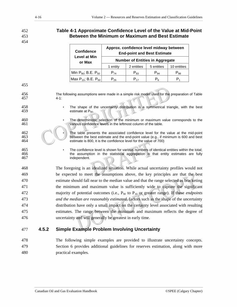
4-16 Volume 2 — Resources and Reserves Estimation and Classification Guidelines
Canadian Oil and Gas Evaluation Handbook ©SPEE (Calgary Chapter)
Table 4-1 Approximate Confidence Level of the Value at Mid-Point 452 Between the Minimum or Maximum and Best Estimate 453
454 Approx. confidence level midway between
End-point and Best Estimate
Number of Entities in Aggregate
Confidence Level at Min
or Max 1 entity 2 entities 5 entities 10 entities
Min P90; B.E. P50 P74 P83 P94 P98
Max P10; B.E. P50 P26 P17 P6 P1
455
The following assumptions were made in a simple risk model used for the preparation of Table 456 4-1: 457
• The shape of the uncertainty distribution is a symmetrical triangle, with the best 458 estimate at P50. 459
• The deterministic selection of the minimum or maximum value corresponds to the 460 various confidence levels in the leftmost column of the table. 461
• The table presents the associated confidence level for the value at the mid-point 462 between the best estimate and the end-point value (e.g., if minimum is 600 and best 463 estimate is 800, it is the confidence level for the value of 700) 464
• The confidence level is shown for various numbers of identical entities within the total; 465 the assumption in the statistical aggregation is that entity estimates are fully 466 independent. 467
The foregoing is an idealized situation. While actual uncertainty profiles would not 468 be expected to meet the assumptions above, the key principles are that the best 469 estimate should fall near to the median value and that the range selected as bracketing 470 the minimum and maximum value is sufficiently wide to capture the significant 471 majority of potential outcomes (i.e., P90 to P10 or greater range). If these endpoints 472 and the median are reasonably estimated, factors such as the shape of the uncertainty 473 distribution have only a small impact on the certainty level associated with resulting 474 estimates. The range between the minimum and maximum reflects the degree of 475 uncertainty and will generally be greatest in early time. 476
4.5.2 Simple Example Problem Involving Uncertainty 477
The following simple examples are provided to illustrate uncertainty concepts. 478 Section 6 provides additional guidelines for reserves estimation, along with more 479 practical examples. 480
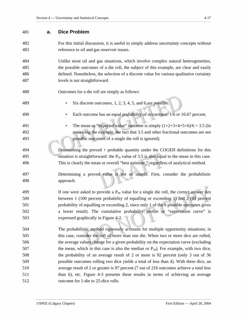
Section 4 — Uncertainty and Statistical Concepts 4-17
©SPEE (Calgary Chapter) First Edition — April 28, 2004
a. Dice Problem 481
For this initial discussion, it is useful to simply address uncertainty concepts without 482 reference to oil and gas reservoir issues. 483
Unlike most oil and gas situations, which involve complex natural heterogeneities, 484 the possible outcomes of a die roll, the subject of this example, are clear and easily 485 defined. Nonetheless, the selection of a discrete value for various qualitative certainty 486 levels is not straightforward. 487
Outcomes for a die roll are simply as follows: 488
• Six discrete outcomes, 1, 2, 3, 4, 5, and 6,are possible. 489
• Each outcome has an equal probability of occurrence: 1/6 or 16.67 percent. 490
• The mean or “expected value” outcome is simply (1+2+3+4+5+6)/6 = 3.5 (In 491 reviewing the example, the fact that 3.5 and other fractional outcomes are not 492 possible outcomes of a single die roll is ignored). 493
Determining the proved + probable quantity under the COGEH definitions for this 494 situation is straightforward: the P50 value of 3.5 is also equal to the mean in this case. 495 This is clearly the mean or overall “best estimate,” regardless of analytical method. 496
Determining a proved value is not so simple. First, consider the probabilistic 497 approach. 498
If one were asked to provide a P90 value for a single die roll, the correct answer lies 499 between 1 (100 percent probability of equalling or exceeding 1) and 2 (83 percent 500 probability of equalling or exceeding 2, since only 1 of the 6 possible outcomes gives 501 a lower result). The cumulative probability profile or “expectation curve” is 502 expressed graphically in Figure 4-2. 503
The probabilistic method rigorously accounts for multiple opportunity situations; in 504 this case, consider the roll of more than one die. When two or more dice are rolled, 505 the average values change for a given probability on the expectation curve (excluding 506 the mean, which in this case is also the median or P50). For example, with two dice, 507 the probability of an average result of 2 or more is 92 percent (only 3 out of 36 508 possible outcomes rolling two dice yields a total of less than 4). With three dice, an 509 average result of 2 or greater is 97 percent (7 out of 216 outcomes achieve a total less 510 than 6), etc. Figure 4-3 presents these results in terms of achieving an average 511 outcome for 1-die to 25-dice rolls. 512
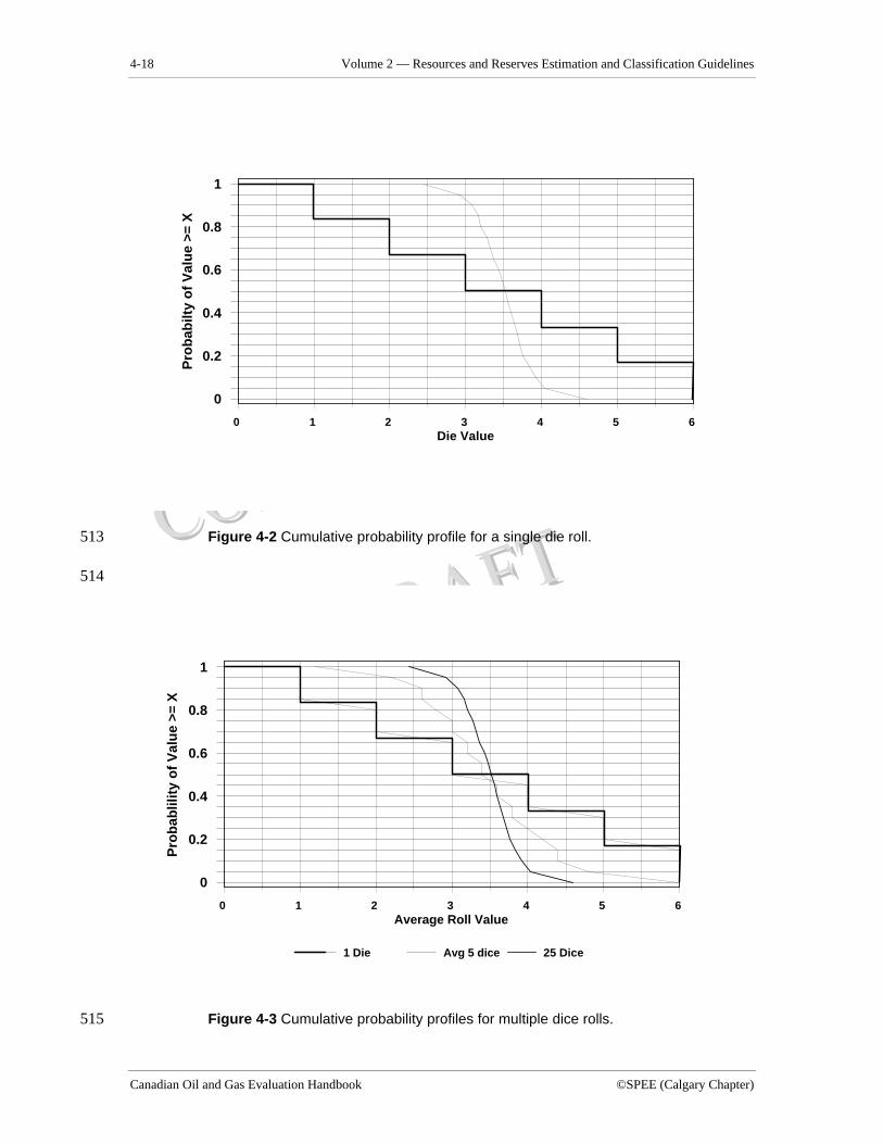
4-18 Volume 2 — Resources and Reserves Estimation and Classification Guidelines
Canadian Oil and Gas Evaluation Handbook ©SPEE (Calgary Chapter)
Figure 4-2 Cumulative probability profile for a single die roll. 513
514
Figure 4-3 Cumulative probability profiles for multiple dice rolls. 515
0 1 2 3 4 5 6 Die Value
0
0.2
0.4
0.6
0.8
1P
rob
abilt
y o
f V
alu
e >=
X
0 1 2 3 4 5 6 Average Roll Value
0
0.2
0.4
0.6
0.8
1
Pro
bab
lilit
y o
f V
alu
e >=
X
1 Die Avg 5 dice 25 Dice
Section 4 — Uncertainty and Statistical Concepts 4-19
©SPEE (Calgary Chapter) First Edition — April 28, 2004
In a probabilistic analysis, one would focus on the aggregate result of all of the die 516 rolls. That is, if discrete 1P, 2P, and 3P values were required, these values would be 517 selected from the aggregate P90, P50, and P10, respectively. In an oil and gas situation, 518 this is comparable to probabilistic aggregation of reserves estimates, which is 519 permitted up to the total property (or field) level for the determination of total 520 reserves. For example, for a group of five dice, the appropriate 1P, 2P, and 3P would 521 be roughly 12.5, 17.5 and 22.5, respectively (i.e., five times 2.5, 3.5, and 4.5, 522 respectively). 523
Now consider a deterministic approach to this problem. As stated previously, the 524 expected value or best estimate is straightforward at 3.5 and this would be recorded 525 as the proved + probable estimate. 526
Relating the approach in Section 4.5.2 to the foregoing dice example, the evaluator 527 might select a value of 1 as the practical minimum (in this case, also the absolute 528 minimum). With this value, a proved + probable “best estimate” value of 3.5, and the 529 1/3 to 2/3 difference guideline, the proved value is in the range of 1.83 to 2.67. 530 Similarly, on the upside, a practical maximum of 6 results in a proved + probable + 531 possible estimate of 4.33 to 5.17. 532
Consider now how the evaluator selects the final estimates within these ranges: 533
The quality of data and availability of analogies aren’t relevant considerations in this 534 case and the evaluator has good knowledge of the uncertainty. The primary 535 consideration as to where in this range to assign proved reserves is the number of 536 “opportunities” in the evaluated “property.” If there were only a few opportunities, 537 the evaluator should assign each a proved value near the low end of the proved range 538 and the high end of the proved + probable + possible range (2 and 5, respectively). 539 For a large number of opportunities, the opposite end of the range is appropriate. 540
For example, for a group of five dice, the appropriate 1P, 2P, and 3P would be 541 roughly 2.5, 3.5, and 4.5 per die or 12.5, 17.5, and 22.5 in total, respectively, which 542 corresponds to the probabilistic solution at the “property” level. 543
For the special case of only a single “opportunity” in the evaluated “property” where 544 this “property” was critical to the overall portfolio being evaluated, the evaluator 545 would need to consider that it would be more appropriate to place the deterministic 546 proved estimate at or near the practical minimum. 547
548
4-20 Volume 2 — Resources and Reserves Estimation and Classification Guidelines
Canadian Oil and Gas Evaluation Handbook ©SPEE (Calgary Chapter)
b. A Simple Gas Material Balance Example 549
Consider this approach in a simple oil and gas example. 550
After a thorough analysis of a gas reservoir, the following is concluded: 551 552
Original Gas In Place 553
• minimum (no practical chance of being less): 90 Bcf 554
• best estimate: 100 Bcf 555
• maximum (no practical chance of exceeding): 110 Bcf 556
Recovery Factor 557
• minimum (considering liquid loading potential, etc.): 82 percent 558
• best estimate: 85 percent 559
• maximum (given optimal performance): 88 percent 560
Cumulative Production to Date 561
• 50 Bcf 562
The following discusses the philosophy of reserves assignments for the various 563 reserves categories. 564
i. Deterministic Approach 565
Determination of the proved + probable case is straightforward in this example: 566 proved + probable reserves are calculated as 100 x 85% - 50 = 35.0 Bcf. 567
The proved and proved + probable + possible reserves could be calculated 568 deterministically by (1) using the minimum/maximum approach discussed above, or 569 (2) selecting appropriate OGIP and recovery factors for each of these categories. 570
(1) The minimum and maximum for this approach are intended to be practical limits, 571 so the product of two or more parameters using endpoints overstate the range of 572 values. The minimum OGIP of 90 Bcf and a somewhat lower than best estimate 573 recovery factor, say 84 percent, are appropriate for the minimum value calculation. 574 Similarly, the maximum is derived using the maximum OGIP and an 86 percent 575 recovery factor. This results in a range of minimum to best estimate reserves of 25.6 576 to 35.0 Bcf. Given no other information, proved reserves are estimated at about the 577 midpoint of this range: 30 Bcf. A similar approach results in a proved + probable + 578 possible reserves estimate of 40 Bcf. 579
580
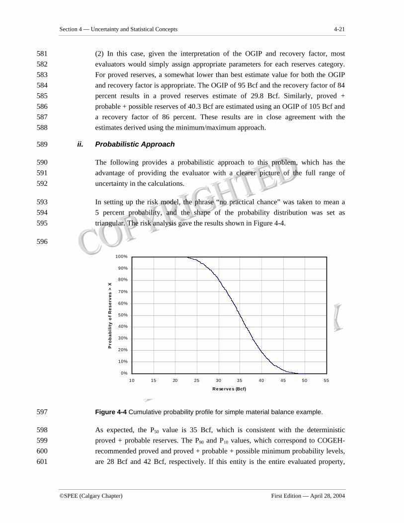
Section 4 — Uncertainty and Statistical Concepts 4-21
©SPEE (Calgary Chapter) First Edition — April 28, 2004
(2) In this case, given the interpretation of the OGIP and recovery factor, most 581 evaluators would simply assign appropriate parameters for each reserves category. 582 For proved reserves, a somewhat lower than best estimate value for both the OGIP 583 and recovery factor is appropriate. The OGIP of 95 Bcf and the recovery factor of 84 584 percent results in a proved reserves estimate of 29.8 Bcf. Similarly, proved + 585 probable + possible reserves of 40.3 Bcf are estimated using an OGIP of 105 Bcf and 586 a recovery factor of 86 percent. These results are in close agreement with the 587 estimates derived using the minimum/maximum approach. 588
ii. Probabilistic Approach 589
The following provides a probabilistic approach to this problem, which has the 590 advantage of providing the evaluator with a clearer picture of the full range of 591 uncertainty in the calculations. 592
In setting up the risk model, the phrase “no practical chance” was taken to mean a 593 5 percent probability, and the shape of the probability distribution was set as 594 triangular. The risk analysis gave the results shown in Figure 4-4. 595
596
Figure 4-4 Cumulative probability profile for simple material balance example. 597
As expected, the P50 value is 35 Bcf, which is consistent with the deterministic 598 proved + probable reserves. The P90 and P10 values, which correspond to COGEH-599 recommended proved and proved + probable + possible minimum probability levels, 600 are 28 Bcf and 42 Bcf, respectively. If this entity is the entire evaluated property, 601
0%
10%
20%
30%
40%
50%
60%
70%
80%
90%
100%
10 15 20 25 30 35 40 45 50 55
Rese rve s (Bcf)
Pro
ba
bil
ity
of
Re
se
rves
> X
4-22 Volume 2 — Resources and Reserves Estimation and Classification Guidelines
Canadian Oil and Gas Evaluation Handbook ©SPEE (Calgary Chapter)
these are the values that would be recorded for those reserves categories. If the 602 property contained other entities, it would be acceptable to include those entities in a 603 larger probabilistic model, aggregate the estimates up to the property total, and record 604 total property reserves at the P90, P50, and P10 levels for the corresponding reserves 605 categories. 606
The above probabilistic solution to this simple problem is not unique. The gas 607 reserves probability distribution depends on interpretation of the phrase “no practical 608 chance.” For example, had no practical chance had been interpreted as near zero 609 probability, the P90 reserves would have increased to 30 Bcf, and P10 reserves 610 decreased to about 40 Bcf. If no practical chance had been interpreted as 10 percent 611 probability, the range would be 26 to 44 Bcf. The selection of a triangular frequency 612 distribution for the variables also impacts the outcome to some extent. 613
4.6 Probabilistic Check of Deterministic Estimates 614
Where a very small number of entities dominate in the Reported Reserves, a 615 probabilistic check of aggregate proved reserves is encouraged. If confidence levels 616 of the reserves estimates for these key entities fall significantly below the probability 617 targets defined in Section 3.4, then the aggregate Reported Reserves will likely fail to 618 meet these certainty criteria. Given this outcome, an evaluator should review both the 619 probabilistic and deterministic assessments for potential inconsistencies in logic 620 and/or mathematical errors. If necessary, reserves estimates should be adjusted to 621 satisfy the Reported Reserves certainty criteria. 622
4.7 Application of Guidelines to the Probabilistic Method 623
The guidelines provided in COGEH include specific limits to parameters for reserves 624 estimation. For example, volumetric estimates are restricted by the lowest known 625 hydrocarbons. These constraints are derived from other commonly used reserves 626 definitions and guidelines (e.g., U.S. SEC) and existing standard industry practice, 627 and have been included in COGEH because they are reasonable restrictions. 628 Furthermore, imposition of these restrictions is necessary to promote compatibility 629 with securities reporting regulations in jurisdictions outside of Canada. However, 630 inclusion of these discrete limits in a risk simulation can conflict with standard 631 probabilistic procedures, which require that input parameters honour the full range of 632 technically valid potential values. 633
Regardless of analytical method, the restrictions contained in the guidelines must be 634 adhered to. Two general approaches are acceptable when probabilistic methods are 635
Section 4 — Uncertainty and Statistical Concepts 4-23
©SPEE (Calgary Chapter) First Edition — April 28, 2004
used in cases where imposition of these discrete restrictions significantly impacts 636 reserves estimates: 637
• Constrain the input parameters in the probabilistic model. In this 638 approach, the probabilistic model input is constrained to exclude values that 639 do not meet reserves classification criteria. These constraints are usually only 640 an issue for proved reserves and, therefore, this approach may be most 641 applicable for individual entity analyses specifically to determine proved 642 reserves. It is generally not appropriate to constrain the probabilistic model 643 and then select the P90 value as the proved estimate, because the constraint 644 can already impose a significant degree of conservatism on the outcome of 645 the model. The P90 value of a constrained model could be very conservative. 646 Depending on the degree of impact of the constraint on the calculated 647 reserves, the proved value should lie between the P90 and mean value of the 648 constrained probabilistic model. 649
• Perform a deterministic check. In this approach, a probabilistic model is 650 prepared for an entire property (or field) using conventional probabilistic 651 methods, i.e., allowing for the unconstrained full range of valid inputs to the 652 model. Property totals are checked against deterministic estimates, which 653 have included all appropriate constraints (e.g., testing requirements, LKH). 654 Aggregate estimates prepared using probabilistic methods must not exceed 655 those prepared using deterministic approach. 656


1
2
3
4
5
6
SECTION 5 7
GENERAL REQUIREMENTS 8
FOR CLASSIFICATION OF RESERVES 9
10
5-2 Volume 2 — Resources and Reserves Estimation and Classification Guidelines
Canadian Oil and Gas Evaluation Handbook ©SPEE (Calgary Chapter)
TABLE OF CONTENTS 10 Section 5 GENERAL REQUIREMENTS FOR CLASSIFICATION OF RESERVES .............. 5-1 11
5.1 Introduction ..................................................................................................................... 5-3 12 5.2 Ownership Considerations .............................................................................................. 5-3 13 5.3 Drilling Requirements ..................................................................................................... 5-4 14 5.4 Testing Requirements...................................................................................................... 5-5 15 5.5 Regulatory Considerations .............................................................................................. 5-6 16 5.6 Timing of Production and Development ......................................................................... 5-7 17 5.7 Economic Requirements.................................................................................................. 5-8 18
5.7.1 Forecast Prices and Costs ......................................................................................... 5-9 19 5.7.2 Constant Prices and Costs....................................................................................... 5-10 20 5.7.3 Booking Guideline.................................................................................................. 5-10 21 22
23
Section 5 — General Requirements for Classification of Reserves 5-3
©SPEE (Calgary Chapter) First Edition — April 28, 2004
5.1 Introduction 23
The general requirements for the classification of reserves are very important for 24 evaluators and need to be applied consistently. The assignment of proved, probable, 25 or possible reserves by an evaluator necessitates that all of the general requirements 26 for classification of reserves have been carefully considered and, at a minimum, been 27 satisfied. Quantities that do not meet the requirements for reserves should be 28 classified as resources. 29
This section expands upon the guidelines provided in COGEH Volume 1, Sections 30 5.5.4 and 7.5.3 and adds two new requirements: ownership and the timing of 31 production and development. The general requirements set out here must be carefully 32 considered by the evaluator prior to the assignment of reserves to a well, pool, or 33 field. 34
Reserves are defined as marketable quantities of oil, gas, and associated products and 35 they reflect the prices for the product in the condition (upgraded or not upgraded, 36 processed or unprocessed) in which they are sold. Reserves exclude any field or 37 processing losses incurred prior to the point of sale (fuel, flare, shrinkage, etc.). 38
5.2 Ownership Considerations 39
The first requirement for assignment of reserves relates to the company’s ownership 40 in the subsurface mineral rights or the contractual right to exploit and produce. The 41 company’s ownership in the oil and gas reserves is usually defined through a working 42 or royalty interest. This interest must permit the company to participate in 43 exploration, exploitation, production, and sale of production, today and in the future. 44
Securities regulations require that a company have an ownership interest to report 45 and disclose reserves. Therefore, evaluators should only assign reserves to lands in 46 which the company has an interest. 47
An exception would be offset drainage, where the estimated reserves associated with 48 interest wells exceeds the recoverable quantities underlying the interest lands. In 49 assigning reserves related to offset drainage, an evaluator must reasonably consider 50 the right and opportunity of the other owner(s) to exploit their lands and mitigate loss 51 of reserves. 52
Ownership and related information are generally available to the evaluator through 53 land records. The land records provide details of contractual obligations (burdens) 54
5-4 Volume 2 — Resources and Reserves Estimation and Classification Guidelines
Canadian Oil and Gas Evaluation Handbook ©SPEE (Calgary Chapter)
pertaining to the working interest, such as lessor (Crown and freehold) or gross 55 overriding royalties, net carried interests, net profits, or other encumbrances on 56 production or income. The evaluator may also review revenue and expense 57 statements, or other financial documents to verify the application of the contractual 58 obligations as applied by the operator. Additional guidelines on this subject are 59 provided in COGEH Volume 1, Section 4.5. 60
Internationally, ownership terms may be more complex and, therefore, the evaluator 61 might need additional assistance. Note that participation by a company in a technical 62 service contract might not meet the definition of ownership in reserves as defined by 63 certain regulators. 64
Company gross reserves are defined as the working interest or net carried interest 65 share of the reserves prior to the deduction of interests owned by others (burdens). 66 Royalty interest reserves cannot be included in the company gross reserves. 67 Internationally, for production sharing agreements or contracts, company interest 68 reserves are calculated using either the company working interest or paying interest 69 share of production. 70
The definition of company net reserves includes working, net carried, and royalty 71 interest reserves after deduction of all applicable burdens. Internationally, for 72 production sharing agreements or contracts, net company interest reserves are 73 calculated as either the company working interest or paying interest share of 74 production to cost recovery, plus the company profit interest share of production 75 minus all applicable payments to others, excluding income taxes. 76
Net profits interests are generally (agreement specific) considered an interest in 77 production income only, and not in production. Therefore, reserves (gross or net) are 78 usually not assigned. However, company net reserves should be reduced for payment 79 of a net profits interest to governments (right to take payment in kind), using the 80 revenue interest method. 81
5.3 Drilling Requirements 82
The second requirement for assignment of reserves relates to drilling. Reserves may 83 only be assigned to known accumulations that have been penetrated by a wellbore. 84 The identification of a known accumulation must be consistent with the evaluator’s 85 model for the trapping mechanism and be confirmed by drilling. Oil and gas 86 quantities estimated to be recoverable from potential accumulations that have not 87 been penetrated by a wellbore should be considered resources. 88
Section 5 — General Requirements for Classification of Reserves 5-5
©SPEE (Calgary Chapter) First Edition — April 28, 2004
Reserves must not be assigned if the well(s) that penetrated the known accumulation 89 is separated from the lands being evaluated by non-productive reservoir (i.e., absence 90 of reservoir, structurally low, or uneconomic test results). An example is a situation 91 where the geological and/or geophysical model indicated that the top of the reservoir 92 was below the water contact between the productive well(s) and the lands to be 93 evaluated. In this case, the potentially recoverable oil and gas quantities relate to an 94 unproved structural model on the lands (undrilled at present) and should be classified 95 as resources, not reserves. 96
Undrilled fault blocks cannot be assigned proved reserves in a formation, until 97 penetrated and tested. The evaluator could assign probable or possible reserves to 98 undrilled fault blocks in a structure, offsetting a commercially tested well, after 99 considering factors such as reservoir quality, hydrocarbon migration path, seismic 100 confirmation, fault seal, and results from drilling an adjacent fault block(s). Probable 101 reserves may be attributed to offsetting fault blocks provided the formation is 102 expected to be structurally higher and no reduction in reservoir quality is anticipated. 103 If the formation in the offsetting fault block is expected to be structurally lower, the 104 evaluator may at best assign possible reserves. 105
It is not necessary that a discovery or development well be capable of being used for 106 production to assign reserves. However, the risk to re-drill a well capable of 107 production should be considered by the evaluator in determining the reserves 108 category. 109
5.4 Testing Requirements 110
The third requirement for assignment of reserves relates to testing. The wellbore must 111 have penetrated the reservoir and a production test conducted. The evaluator must be 112 reasonably certain that the test produced fluids from the reservoir to which reserves 113 are being assigned. 114
The test must provide confirmation that the reservoir is capable of commercial 115 production in order for proved reserves to be assigned to a new accumulation. 116 Therefore, tests such as repeat formation tests (“RFT”) and modular dynamic tests 117 (“MDT”) in themselves are not deemed to be adequate confirmation of a successful 118 production test for the initial well in a new accumulation. Untested wells in a new 119 accumulation (drilled, logged and/or cored, but not tested) may be assigned probable 120 or possible reserves provided that offsetting known accumulations, with similar or 121 reduced reservoir properties, were successfully tested or produced at commercial 122 quantities. 123
5-6 Volume 2 — Resources and Reserves Estimation and Classification Guidelines
Canadian Oil and Gas Evaluation Handbook ©SPEE (Calgary Chapter)
There are two types of flow tests (drillstem and production) generally used in the 124 industry. These tests are conducted to measure flow rates and reservoir properties and 125 to collect a representative sample of the reservoir fluids. 126
Drillstem tests are designed to obtain a stabilized initial and final reservoir pressure, 127 flow rates, and samples of the reservoir fluids. A drillstem test is typically conducted 128 in open-hole conditions and, therefore, it is important that the packers seal the 129 reservoir from external pressure and fluid influx. Packer failure can render the 130 drillstem test invalid and require a re-test prior to reserves being assigned. The 131 drillstem test involves opening and closing the valve in the tool for short periods of 132 time to produce reservoir fluids and allow the pressure measurements. Drillstem test 133 data can be analyzed to determine reservoir pressure and permeability and to estimate 134 stabilized flow rates. 135
A closed chamber drillstem test measures downhole pressures and collects a small 136 sample of the reservoir fluid in the drill string. Although production rate can be 137 estimated based on the fluid recovery, the small quantity of reservoir fluids collected 138 during a closed chamber test might not satisfy the requirement for evidence of 139 economic productivity. 140
Production tests are performed on recently completed wells or on wells that have 141 produced for a period of time. The test uses pressure recorders to continuously 142 measure flowing and build-up pressures. The test also requires surface equipment to 143 measure the flow rates of the well. The test design parameters may vary, but for the 144 assignment of reserves, the evaluator should consider evidence of stabilized flow 145 rate, delivery pressure, reservoir damage, drainage area, and boundary conditions. 146
The evaluator should analyze the well test to determine if results are satisfactory for 147 the assignment of reserves. The confidence in drillstem and closed chamber test 148 results is not as high as that associated with an extended production test. The well test 149 result is important in classifying the reserves for a non-producing wellbore. 150
5.5 Regulatory Considerations 151
The fourth requirement for assignment of reserves relates to regulatory compliance. 152 The company’s development plan will require applications that relate to drilling, 153 completion, testing, processing facilities, and transportation infrastructure. Additional 154 applications may also need to be submitted for public consultation on environmental, 155 archaeological, and water management issues. 156
Section 5 — General Requirements for Classification of Reserves 5-7
©SPEE (Calgary Chapter) First Edition — April 28, 2004
If the operator has not filed or received approval for all necessary development 157 applications, the evaluator may still assign reserves, provided that development is not 158 prohibited by government regulation (e.g., environmentally sensitive area). The 159 reserves category used by the evaluator should reflect their level of confidence in the 160 future approval of the outstanding applications. 161
In a partial ownership situation, where a pooling or other agreement is required to 162 drill a well, the evaluator must have a reasonable expectation regarding the outcome 163 of the agreement to assign reserves. 164
Reserves assignments related to reduced spacing, secondary or tertiary projects 165 generally require regulatory approval for these types of applications. Additional 166 development applications are usually required from regulatory agencies for the 167 production, injection, or disposal of fluids related to these types of projects. The 168 evaluator may assign proved reserves to a downspacing development provided that 169 the company has received regulatory approval or the approval has a high probability 170 of being granted based on offsetting analogous projects. Otherwise, the evaluator 171 may consider the additional quantities associated with downspacing to be probable, 172 possible or contingent resources, depending on the probability of the approval being 173 granted. 174
The evaluator must also consider the existence of necessary infrastructure related to 175 processing and transportation and of a market for sale of the reserves. If the company 176 does not have an ownership interest in existing infrastructure, the evaluator may 177 assign reserves if an agreement is realistic (available capacity or expansion 178 capability). If the necessary infrastructure is not available, firm development plans 179 are not in place or regulatory applications have not been filed, then the evaluator 180 cannot assign reserves (e.g., northern Canada). These quantities would be classified 181 as contingent resources. 182
Automatic renewal of licenses, permits, concessions, and commercial agreements 183 cannot be assumed for proved reserves booking, unless there is a long and clear track 184 record that shows that the renewal application and subsequent approval are a matter 185 of course. 186
5.6 Timing of Production and Development 187
The fifth requirement for assignment of reserves relates to timing of production and 188 development. This pertains to reserves with very long production forecasts, non-189 producing reserves near infrastructure, or significant reserves developments. 190
5-8 Volume 2 — Resources and Reserves Estimation and Classification Guidelines
Canadian Oil and Gas Evaluation Handbook ©SPEE (Calgary Chapter)
Production forecasts generated by curve fitting or matching techniques, reservoir 191 simulation, or other engineering methods may project quantities beyond a 50-year 192 timeframe. Evaluators understand that such production forecasts have increasing 193 degrees of risk with time. The uncertainties in long-life production forecasts relate to 194 the long-term reliability of the forecasts, whether the quantities will be recovered 195 within the useful life of the field infrastructure, and economics. In addition, the net 196 present value (discount rate greater than zero) of the forecast quantities after 50 years 197 is negligible and immaterial to most stakeholders. Therefore, it is recommended that 198 quantities be classified as contingent resources beyond a period of 50 years from the 199 evaluation effective date. An evaluator may, however, consider a reasonable 200 development scheme to allow these quantities to be recovered within a 50-year 201 period (additional drilling, workovers, facility expansion, etc.). 202
Non-producing reserves that are near existing infrastructure and require minor capital 203 should be developed within a two-year period. If these reserves have not been 204 developed, the evaluator needs to review the technical and economic merit, and 205 appropriateness, of the current reserves category. Exceptions to the guideline are non-206 producing reserves awaiting depletion of another producing zone in the same 207 wellbore or reserves constrained by facility or market limitations. 208
If significant capital is required for field development or infrastructure construction 209 (offshore, oilsands, etc.), then to be classified as proved reserves, a commitment to 210 spending must occur within two years for smaller projects and three years for larger 211 projects. To be classified as proved + probable reserves, a commitment to spending 212 significant capital must occur within three years for smaller projects and five years 213 for larger projects. An exception could be related to fields that are clearly 214 commercial, but development is delayed for logistical reasons (facility constraints, 215 gas contract or allowable limitations, etc.). 216
5.7 Economic Requirements 217
The sixth requirement for assignment of reserves relates to economics. Only those 218 marketable quantities that are economically recoverable can be classified as reserves. 219 The economic requirement is based solely on future costs and does not consider past 220 (sunk) costs. Economic evaluation procedures and criteria, which address the 221 technical, financial, and regulatory issues, are described in COGEH Volume 1 222 Section 7. 223
Section 5 — General Requirements for Classification of Reserves 5-9
©SPEE (Calgary Chapter) First Edition — April 28, 2004
5.7.1 Forecast Prices and Costs 224
In practice, reserves should initially meet the economic requirement based on 225 economic conditions that are generally accepted as being reasonable. The economic 226 requirement must be applied successfully to all categories of reserves assigned. The 227 evaluator must consider estimates of production, prices, all capital and operating 228 (fixed and variable split) costs, regulatory approvals, and general and administrative 229 costs incurred at the field. These costs should be developed with consideration for the 230 confidence level of each reserves category (high, most likely, or low certainty). For 231 example, future operating or capital cost reductions should not be considered for the 232 proved category unless incorporated in a current field development plan and deemed 233 feasible by the evaluator. 234
Revenue from third-party processing should not be used to significantly reduce 235 operating expenses at the field. Processing revenue of less than 10 percent of field 236 expenses may be used to reduce these costs if the revenue is expected to continue in 237 the future. 238
Undeveloped reserves must have a sufficient rate of return to justify the level of 239 capital expenditure associated with the project. The required rate of return is a 240 function of the risk associated with the project. High-risk projects require a greater 241 rate of return than low-risk projects. The minimum rate of return for low risk to 242 moderate risk capital projects should be guided by the discount rates generally used 243 for valuing oil and gas asset transactions. However, the rate of return for low risk 244 capital projects cannot be less than the return on secure money market investments. 245
The evaluation of undeveloped reserves requires a plausible development plan, 246 appropriate capital and operating costs, and abandonment and reclamation costs in 247 order to properly assess economic viability. If a project is not economically viable for 248 a proved reserves development, this does not preclude the booking of probable and/or 249 possible reserves if a reasonable return on investment is achieved. However, the 250 evaluator should not book stand-alone possible reserves unless the company is more 251 likely than not to proceed with the required investment. An expected monetary value 252 methodology will assist the evaluator in reaching an opinion on the merit and 253 likelihood of the company proceeding with the required investment. 254
The economic requirement for a proved reserves assignment must not include 255 projections of future drilling or infrastructure development by other companies that 256 are not currently known. (e.g., stranded gas wells or oil wells). 257
5-10 Volume 2 — Resources and Reserves Estimation and Classification Guidelines
Canadian Oil and Gas Evaluation Handbook ©SPEE (Calgary Chapter)
5.7.2 Constant Prices and Costs 258
Securities commissions and other agencies commonly require that evaluations of 259 reserves be prepared under a scenario of constant prices and costs. This requirement 260 is usually based on the prices in effect on the last day of the fiscal year (e.g., 261 December 31st) and the actual company costs for the fiscal year. 262
5.7.3 Booking Guideline 263
If both forecast and constant economic requirements are satisfied, then reserves 264 should be reported. 265
If the reserves are economic for only the forecast prices and costs (e.g., uneconomic 266 constant economics), the evaluator will generally report these reserves. However, 267 should the economic requirement be successful for only the constant prices and costs 268 (e.g., uneconomic forecast economics), the evaluator will generally not report these 269 reserves. It is recommended that the evaluator consider the materiality of these 270 reserves to the issuer when only one of two economic tests is met. 271
©SPEE (Calgary Chapter) First Edition — April 28, 2004
1
2
3
4
5
6
SECTION 6 7
PROCEDURES FOR ESTIMATION 8
AND CLASSIFICATION OF RESERVES 9
10
6-2 Volume 2 — Resources and Reserves Estimation and Classification Guidelines
Canadian Oil and Gas Evaluation Handbook ©SPEE (Calgary Chapter)
TABLE OF CONTENTS 10 Section 6 PROCEDURES FOR ESTIMATION AND CLASSIFICATION OF RESERVES 6-1 11
6.1 Introduction ..................................................................................................................... 6-6 12 6.1.1 Reserves Confidence Levels ..................................................................................... 6-6 13
a. Proved Reserves........................................................................................................ 6-6 14 i. Entity Level............................................................................................................... 6-6 15 ii. Property Level........................................................................................................... 6-7 16 iii. Reported Level ................................................................................................... 6-7 17
b. Proved Plus Probable Reserves................................................................................. 6-7 18 c. Proved Plus Probable Plus Possible Reserves........................................................... 6-7 19
6.1.2 Reserves Validation—Reported Level ..................................................................... 6-7 20 6.2 Analogy Methods ............................................................................................................ 6-8 21
6.2.1 Use of Analogies as a Primary Method .................................................................... 6-9 22 a. When Other Methods are Not Reliable..................................................................... 6-9 23 b. Heavy Oil Cold Production....................................................................................... 6-9 24 c. Undeveloped Reserves Assigned for Infill Drilling................................................ 6-10 25
6.2.2 Use of Analogies for Specific Reserves Parameters ............................................... 6-11 26 a. Areal Assignments.................................................................................................. 6-11 27 b. Recovery Factors .................................................................................................... 6-11 28 c. Performance Characteristics ................................................................................... 6-11 29
6.3 Volumetric Methods...................................................................................................... 6-12 30 6.3.1 Data Used for Volumetric Methods........................................................................ 6-12 31
a. Geophysical Data.................................................................................................... 6-12 32 b. Geological Data ...................................................................................................... 6-13 33
i. Presence of Hydrocarbons ...................................................................................... 6-14 34 ii. Net Pay.................................................................................................................... 6-15 35 iii. Porosity............................................................................................................. 6-17 36 iv. Hydrocarbon Saturation ................................................................................... 6-18 37 v. Pool Area/Drainage Area/Well Spacing Unit ......................................................... 6-18 38
c. Reservoir Engineering Data.................................................................................... 6-20 39 i. Fluid Analysis ......................................................................................................... 6-20 40 ii. Formation Volume Factor....................................................................................... 6-21 41 iii. Gas Compressibility Factor .............................................................................. 6-21 42 iv. Reservoir Pressure............................................................................................ 6-21 43 v. Reservoir Temperature ........................................................................................... 6-22 44 vi. Gas Shrinkage .................................................................................................. 6-22 45 vii. Well Test Analysis ........................................................................................... 6-22 46 viii. Extended Flow Tests ........................................................................................ 6-23 47 ix. Reservoir Drive Mechanisms ........................................................................... 6-23 48 x. Reservoir Simulation Modelling............................................................................. 6-24 49 xi. Recovery Factor ............................................................................................... 6-24 50
6.3.2 Guidelines for Reserves Assignments in Single-Well Pools .................................. 6-26 51 Example 1: Gas in a fluvial channel sand reservoir ............................................... 6-26 52 Example 2: Heavy oil in a regional marine sand reservoir..................................... 6-28 53 Example 2: Heavy oil in a regional marine sand reservoir..................................... 6-29 54 Example 3: Light oil in a shelf carbonate reservoir................................................ 6-31 55
Section 6 — Procedures for Estimation and Classification of Reserves 6-3
©SPEE (Calgary Chapter) First Edition — April 28, 2004
6.3.3 Guidelines for Reserves Assignments in Multi-Well Pools.................................... 6-33 56 Example 1: Multi-Well Gas Pool ........................................................................... 6-34 57 Example 2: Multi-Well Oil Pool ............................................................................ 6-38 58
6.4 Material Balance Methods............................................................................................. 6-42 59 6.4.1 General Considerations in the Use of Material Balance Methods for Gas 60
Reservoirs ............................................................................................................... 6-42 61 6.4.2 Consideration of Reservoir Properties .................................................................... 6-43 62
a. Aquifers .................................................................................................................. 6-43 63 b. Reservoir Permeability ........................................................................................... 6-43 64 c. Multi-Well Reservoirs ............................................................................................ 6-44 65 d. Multi-Layer Reservoirs........................................................................................... 6-44 66 e. Naturally Fractured Reservoirs ............................................................................... 6-44 67
6.4.3 Consideration of Fluid Properties ........................................................................... 6-45 68 a. Dry Gas Reservoirs................................................................................................. 6-45 69 b. Wet Gas Reservoirs ................................................................................................ 6-45 70 c. Retrograde Condensate Reservoirs ......................................................................... 6-45 71
6.4.4 Consideration of Quality of Pressure Data ............................................................. 6-45 72 a. Types of Pressure Measurements............................................................................ 6-45 73 b. Number of Pressure Measurements ........................................................................ 6-46 74 c. Correlation of the Pressure Data Points .................................................................. 6-46 75 d. High-Permeability Reservoirs................................................................................. 6-46 76 e. Low-Permeability Reservoirs ................................................................................. 6-46 77
6.4.5 Consideration of Degree of Pressure Depletion...................................................... 6-47 78 6.4.6 Guidelines for Determining Proved, Probable and Possible Reserves ................... 6-47 79
a. Assess well groupings in multi-well pools. ............................................................ 6-47 80 b. Review reservoir and fluid properties..................................................................... 6-48 81 c. Review inconsistent data points.............................................................................. 6-48 82 d. Determine OGIP for each reserves category........................................................... 6-48 83 e. Compare the OGIP to that found using other methods........................................... 6-48 84 f. Determine recovery factors and reserves. ............................................................... 6-49 85
6.4.7 Special Situations.................................................................................................... 6-49 86 a. OGIP Calculations based on Initial Production Tests............................................. 6-49 87 b. Allocation of Reserves in Multi-Well Pools ........................................................... 6-49 88 c. Drainage Outside Company Owned Lands............................................................. 6-50 89
6.4.8 Examples................................................................................................................. 6-51 90 Material Balance Estimation of Reserves with Good Data Correlation – Single Well 91 Pool......................................................................................................................... 6-51 92 Material Balance Estimation of Reserves with Moderate Data Scatter – Single Well 93 Pool......................................................................................................................... 6-53 94
6.4.9 General Considerations in the Use of Material Balance Methods for Oil 95 Reservoirs ............................................................................................................... 6-55 96
6.5 Production Decline Methods ......................................................................................... 6-55 97 6.5.1 Types of Decline Analysis ...................................................................................... 6-56 98
a. Type Curve Matching ............................................................................................. 6-56 99 b. Curve Fitting........................................................................................................... 6-56 100
6.5.2 Limitations of Methods........................................................................................... 6-57 101
6-4 Volume 2 — Resources and Reserves Estimation and Classification Guidelines
Canadian Oil and Gas Evaluation Handbook ©SPEE (Calgary Chapter)
6.5.3 Factors Affecting Decline Behaviour ..................................................................... 6-58 102 a. Rock and Fluid properties....................................................................................... 6-58 103
i. Stratification............................................................................................................ 6-58 104 ii. Wettability .............................................................................................................. 6-59 105 iii. Relative Permeability ....................................................................................... 6-59 106 iv. Permeability ..................................................................................................... 6-59 107 v. Fracturing................................................................................................................ 6-59 108 vi. Back Pressure Slope ......................................................................................... 6-59 109
b. Reservoir Geometry and Drive Mechanism ........................................................... 6-60 110 i. Vertical Displacement............................................................................................. 6-60 111 ii. Coning..................................................................................................................... 6-60 112 iii. Horizontal Displacement.................................................................................. 6-60 113 iv. Unconsolidated Heavy Oil Reservoirs ............................................................. 6-60 114
c. Completion and Operating Practices ...................................................................... 6-60 115 i. Skin Factors ............................................................................................................ 6-60 116 ii. Fluid Rate Changes................................................................................................. 6-61 117 iii. Workovers ........................................................................................................ 6-61 118 iv. Infill Drilling .................................................................................................... 6-61 119 v. Regulatory Constraints ........................................................................................... 6-61 120 vi. Facility Constraints .......................................................................................... 6-61 121
d. Type of Wellbore .................................................................................................... 6-61 122 i. Horizontal versus Vertical Wellbore ...................................................................... 6-61 123 ii. Coning Situations.................................................................................................... 6-62 124 iii. Wellbore Contact.............................................................................................. 6-62 125
6.5.4 Guidelines for Individual Well Decline Analysis ................................................... 6-62 126 a. Reservoir Properties Review................................................................................... 6-62 127 b. Analogy Review ..................................................................................................... 6-62 128 c. Transient Period Estimation.................................................................................... 6-62 129
i. Buildup Analysis..................................................................................................... 6-63 130 ii. Type Curve Analysis .............................................................................................. 6-63 131
d. Final Rate Determination........................................................................................ 6-63 132 e. Operating Constraint Review.................................................................................. 6-63 133 f. Data Review............................................................................................................ 6-63 134 g. Re-Initialization ...................................................................................................... 6-64 135 h. Oil-Cut Analysis ..................................................................................................... 6-64 136 i. Line-Pressure Adjustments ..................................................................................... 6-64 137 j. Interference Effects................................................................................................. 6-64 138 k. Production Forecasts............................................................................................... 6-64 139
6.5.5 Guidelines for Group Decline Analysis .................................................................. 6-65 140 a. Grouping ................................................................................................................. 6-65 141 b. Voidage Replacement ............................................................................................. 6-65 142 c. Breakthrough Behaviour......................................................................................... 6-65 143
6.5.6 Guidelines for Reserves Classification from Decline Analysis .............................. 6-66 144 6.5.7 Decline Examples ................................................................................................... 6-67 145
Gas Example A....................................................................................................... 6-67 146 Gas Example B....................................................................................................... 6-69 147
Section 6 — Procedures for Estimation and Classification of Reserves 6-5
©SPEE (Calgary Chapter) First Edition — April 28, 2004
Gas Example C....................................................................................................... 6-70 148 Gas Example D....................................................................................................... 6-71 149 Gas Example E ....................................................................................................... 6-72 150 Gas Example F ....................................................................................................... 6-73 151 Oil Example A........................................................................................................ 6-74 152 Oil Example B ........................................................................................................ 6-75 153 Oil Example C ........................................................................................................ 6-76 154 Oil Example D........................................................................................................ 6-77 155 Oil Example E ........................................................................................................ 6-78 156 Oil Example F (Group Analysis)............................................................................ 6-79 157 Oil Example G (Group Analysis) ........................................................................... 6-80 158 Oil Example H........................................................................................................ 6-81 159
6.6 Reservoir Simulation Methods...................................................................................... 6-83 160 6.7 Reserves Related to Future Drilling and Planned Enhanced Recovery Projects........... 6-83 161
6.7.1 Additional Reserves Related to Future Drilling...................................................... 6-83 162 a. Drilling Spacing Unit.............................................................................................. 6-83 163 b. Infill Wells .............................................................................................................. 6-83 164 c. Infill Analysis ......................................................................................................... 6-84 165 d. Delineation or Step-Out Wells................................................................................ 6-84 166
i. Classification .......................................................................................................... 6-85 167 ii. Qualifiers to Classification ..................................................................................... 6-85 168 iii. Adjustments for Reservoir Quality................................................................... 6-85 169
e. Drilling Statistics .................................................................................................... 6-86 170 f. Likelihood of Drilling............................................................................................. 6-86 171 g. Time Constraints..................................................................................................... 6-88 172
6.7.2 Examples of Future Drilling ................................................................................... 6-89 173 Case A1 .................................................................................................................. 6-89 174 Case A2 .................................................................................................................. 6-89 175 Case B..................................................................................................................... 6-90 176 Case C..................................................................................................................... 6-91 177 Case D .................................................................................................................... 6-92 178 Case E..................................................................................................................... 6-93 179
6.7.3 Reserves Related to Planned Enhanced Recovery Projects .................................... 6-94 180 a. Proved Criteria (1P) ................................................................................................ 6-94 181 b. Proved + Probable Criteria (2P).............................................................................. 6-97 182 c. Proved + Probable + Possible Criteria (3P) ............................................................ 6-98 183
6.7.4 Planned EOR Examples.......................................................................................... 6-99 184 Case G .................................................................................................................... 6-99 185 Case H .................................................................................................................. 6-100 186
6.8 Integration of Reserves Estimation Methods .............................................................. 6-101 187 a. Volumetric Methods ............................................................................................. 6-102 188 b. Analogy Methods.................................................................................................. 6-102 189 c. Decline Curve Methods ........................................................................................ 6-103 190 d. Material Balance Methods for Gas Reservoirs ..................................................... 6-103 191 e. Reservoir Simulation ............................................................................................ 6-103 192
193 194
6-6 Volume 2 — Resources and Reserves Estimation and Classification Guidelines
Canadian Oil and Gas Evaluation Handbook ©SPEE (Calgary Chapter)
6.1 Introduction 194
The estimation and classification of reserves is predicated on data quantity and 195 quality, applicable regulatory guidelines, current and forecast economic conditions, 196 and the training and experience of the evaluator. For these reasons, the reserves 197 estimate or classification may vary between evaluators using the same technical and 198 financial data. The goal of this section is to promote consistency in reserves estimates 199 and reserves classification by all evaluators. This material is intended to expand on 200 the general guidelines contained in COGEH Volume 1, Sections 5.5.5 and 7.2 201
Evaluators are encouraged to consider all appropriate methods when estimating and 202 classifying reserves. This section reviews reserves estimation procedures commonly 203 used by evaluators—such as analogy, volumetrics, material balance, production 204 decline, and reservoir simulation—and the integration of these methods. Also 205 addressed are reserves estimation issues related to future drilling and planned 206 enhanced recovery projects. The material provides an overview of the principles, 207 estimation procedures, and classification recommendations, as well as examples to 208 illustrate the recommended guidelines. 209
The guidelines contained in this section are intended to be a “best practices” 210 reference for evaluators. The evaluator’s approach to reserves estimation or 211 classification should only vary from the guidelines provided in this section when 212 there is a compelling technical reason to do so. If this is the case, then a full 213 explanation should be given. 214
6.1.1 Reserves Confidence Levels 215
The “best practices” guidelines in this section should not be interpreted by the 216 evaluator in such a way as to contradict the requirements set out in Section 5 of 217 COGEH Volume 1 or Section 3 of COGEH Volume 2. 218
a. Proved Reserves 219
i. Entity Level 220
The requirement for proved reserves at the entity level is a “conservative” estimate of 221 the actual quantities that will be recovered. Although “conservative” is not 222 statistically defined in COGEH Volume 1 or 2, a proved reserves estimate should be 223 less than the proved + probable estimate. When the uncertainty is large, the degree of 224 conservatism should be larger than if the uncertainty is small. 225
Section 6 — Procedures for Estimation and Classification of Reserves 6-7
©SPEE (Calgary Chapter) First Edition — April 28, 2004
ii. Property Level 226
The requirement for proved reserves at the property level is a “high” degree of 227 certainty that the actual quantities will be recovered. A high degree of certainty 228 implies that there should be a much greater likelihood of positive compared to 229 negative future annual proved revisions. 230
iii. Reported Level 231
The requirement for proved reserves at the reported level is at least a 90 percent 232 probability that the actual quantities will be recovered. 233
b. Proved Plus Probable Reserves 234
The requirements also specify that the proved + probable reserves should be the best 235 estimate at the entity, property, and reported levels and have at least a 50 percent 236 probability that the actual quantities recovered will equal or exceed the estimated 237 proved + probable reserves. 238
c. Proved Plus Probable Plus Possible Reserves 239
The requirements also specify that the proved + probable + possible reserves should 240 be an optimistic estimate at the entity, property, and reported levels. It is expected 241 that, at the reported level, the proved + probable + possible reserves will have at least 242 a 10 percent probability that the actual quantities recovered will equal or exceed the 243 estimate. 244
6.1.2 Reserves Validation—Reported Level 245
Reserves validation is a method of determining if reported level reserves were 246 prepared in a manner consistent with the COGEH definitions. Each year the reported 247 level technical revision for the proved reserves is expected to result in a positive 248 adjustment, after accounting for reserves additions or reductions related to activities 249 throughout the year (exploration discoveries, drilling extensions, infill drilling, 250 improved recovery, acquisitions, dispositions, economic factors, and annual 251 production). Should a negative proved adjustment occur, it is expected that the 252 reserves will be revised to ensure compliance in future years. The proved + probable 253 reserves at the reported level should remain relatively constant with time. The proved 254 + probable + possible reserves should decrease with time. 255
6-8 Volume 2 — Resources and Reserves Estimation and Classification Guidelines
Canadian Oil and Gas Evaluation Handbook ©SPEE (Calgary Chapter)
6.2 Analogy Methods 256
Analogy methods are important to a reserves evaluator as a primary reserves 257 estimation method when other methods are not considered reliable and for checking 258 the results of other evaluation approaches. 259
The importance of using analogy methods with other reserves evaluation methods 260 cannot be overstated. Consider an example of a single well gas pool where the 261 volumetric estimate of the original gas in place is based on wellbore petrophysical 262 parameters, the regulatory drilling spacing unit, and a theoretical recovery factor 263 based on a low reservoir abandonment pressure. Even though the well could be 264 capable of draining a very large area, comparison of areal extent with analogous 265 pools in the area could show drainage areas significantly smaller than the regulatory 266 well spacing indicates. Likewise, comparison of recovery factors with analogous 267 pools could also show values significantly lower than indicated. A review of the areal 268 extent and recovery factors in analogous pools in this case may prevent a potential 269 overestimate of the gas reserves. 270
Because so many aspects of reserves estimation are based on limited or indirect 271 information, it is important that the evaluator compare all of the reserves parameters 272 to those in analogous reservoirs. In some cases, this could involve a quick check by 273 the evaluator and a judgement, based on the evaluator’s experience, that the 274 parameter in question falls within an expected range of values. In other cases, it could 275 involve a detailed statistical review. Where estimated values for the reserves under 276 study are significantly different from those in analogous reservoirs without technical 277 justification, adjustments should be made in the subject analysis. 278
It is important when relying on analogies to ensure that they are valid. Many aspects 279 of the intended analogy should be compared: reservoir properties, fluid properties, 280 presence of fluid contacts, productivity, etc. A valid analogy is one in which all of the 281 characteristics that contribute to the reserves estimate are similar to the subject 282 reservoir. As long as the key characteristics are not significantly inferior, appropriate 283 adjustments should be made to reflect the differences. In some cases, there will 284 simply not be any valid analogies; in those cases, a more conservative approach 285 should be applied in reserves estimation. 286
The use of analogy methods as a primary reserves estimation method and as a 287 supplement to other methods is described in more detail in Sections 6.2.1 and 6.2.2, 288 respectively. Guidelines for their application are also provided. 289
Section 6 — Procedures for Estimation and Classification of Reserves 6-9
©SPEE (Calgary Chapter) First Edition — April 28, 2004
6.2.1 Use of Analogies as a Primary Method 290
a. When Other Methods are Not Reliable 291
Reserves evaluators sometimes encounter situations where a well has no pressure 292 data, wellbore data is unavailable or insufficient to allow for reliable volumetrically 293 determined reserves estimates, and the well production exhibits no decline. In other 294 situations, the volumetric data might be inconsistent with well productivity, for 295 example, where a standard analysis of the volumetric data shows either unreasonably 296 long or unreasonably short production life. In these instances, the evaluator must use 297 analogies as a guide to estimating reserves. The evaluator typically reviews all the 298 available reservoir and fluid characteristics and then applies judgement, based on 299 experience, to estimate a range of reserves. The production rate is often used as the 300 basis for the reserves estimates, and a reserves life index (remaining reserves divided 301 by current production rates) is applied based on the observed reserves life indices of 302 analogous wells. 303
The best estimate of reserves using analogies generally represents proved + probable 304 reserves. Because there is usually significant uncertainty in the reserves estimates of 305 this type, an additional level of conservatism must be applied to the proved reserves 306 estimates. 307
b. Heavy Oil Cold Production 308
The high-permeability, unconsolidated sand, heavy oil reservoirs in eastern Alberta 309 and southwestern Saskatchewan often have high sand production rates along with 310 high and very stable oil production rates for a few years, followed by a steep decline 311 thereafter. The sand production is believed to be due to a “wormhole effect” in the 312 reservoir and it assists in reservoir recovery. 313
A common problem with these reservoirs is difficulty in applying either decline 314 curve analysis or volumetric methods to estimate reserves, at least early in the 315 production life. Although volumetric calculations of oil in place can be made, 316 individual well recoveries of ultimate reserves are usually independent of the well’s 317 net pay and correlate better to productivity, due to uncertainty in effective drainage 318 areas. 319
Reserves estimation early in the well life commonly uses some multiple of the initial 320 well productivity. This multiple is based on a statistical analysis of the reserves life 321 indices of analogous older wells in the same field. 322

6-10 Volume 2 — Resources and Reserves Estimation and Classification Guidelines
Canadian Oil and Gas Evaluation Handbook ©SPEE (Calgary Chapter)
Proved + probable reserves estimates should usually be based on the average or 323 median reserves life index determined for analogous wells. Proved reserves estimates 324 should be reduced from the proved + probable estimates, in some cases significantly 325 reduced, to reflect the greater uncertainty in using this method of analysis. 326
It is important to ensure that analogous wells used in this analysis are truly 327 analogous. Different well spacing or significantly different oil or water production 328 rates could require further adjustment to the values assigned. 329
c. Undeveloped Reserves Assigned for Infill Drilling 330
In mature reservoirs with successive programs of infill drilling on smaller and 331 smaller well spacing, undeveloped reserves for further infill drilling are usually 332 determined by statistically analyzing the recoverable reserves for each successive 333 vintage of infill wells. This method is often applied to the shallow gas formations 334 (Milk River and Medicine Hat) of southeastern Alberta and southwestern 335 Saskatchewan, as well as many oil reservoirs (both light and heavy oil) developed on 336 progressively smaller and smaller well spacing. 337
Usually the reserves for producing wells in these situations are estimated by decline 338 analyses, and the declining trend of recovery for each year of infill drilling is 339 extrapolated into the future to predict recoveries. Volumetric analysis checks should 340 be conducted on a total field basis. 341
For this method of grouping wells by drilling date to yield reliable results, there 342 should be several vintages of infill drilling with a consistent declining trend of initial 343 production rates and recoverable reserves for each vintage. 344
It is important when analyzing the trend of recovery over time to assess how much of 345 the recovery from future wells will be incremental and how much will be 346 acceleration. If initial production rates and estimated reserves recovery are decreasing 347 with each phase of drilling, then interference between wells is occurring and a 348 significant portion of the recovery from the future infill wells will be acceleration. 349
The proved + probable reserves estimates should be based on the best estimate 350 determined from the statistical review, considering only that portion of the recovery 351 incremental to the older wells. The uncertainty in reserves estimates in these 352 instances is primarily due to difficulties in estimating incremental recoveries versus 353 production acceleration. 354
Section 6 — Procedures for Estimation and Classification of Reserves 6-11
©SPEE (Calgary Chapter) First Edition — April 28, 2004
6.2.2 Use of Analogies for Specific Reserves Parameters 355
a. Areal Assignments 356
The most difficult reserves parameter to determine early in the life of an oil or gas 357 well is commonly the areal extent of the reservoir. When estimating reserves for 358 smaller single-well pools without the benefit of definitive seismic information, the 359 area should be based on a review of analogous mature pools in the area. It is 360 important when comparing analogous pools to consider that progressively smaller 361 pools are encountered in a mature area. An analysis of the historical trend toward 362 smaller and smaller single-well gas pools in Alberta and estimation of their areal 363 extent were presented in a 1989 paper prepared by Andy Warren of the Alberta 364 Energy Resources Conservation Board (Warren 1989). 365
b. Recovery Factors 366
Recovery factors early in the life of a reservoir are commonly based on analogies. 367 Other information such as abandonment pressures or fluid displacement efficiencies 368 must be considered, but the behaviour of analogous reservoirs is an important guide 369 to recovery factors. Ideally, the analogous reservoirs should be located near the 370 subject reservoir, but if unavailable, more distant analogies are acceptable. The key is 371 that they are valid analogies. 372
c. Performance Characteristics 373
The forecast of future production performance for oil and gas reservoirs is often 374 based on analogies. Reservoir and fluid characteristics help the evaluator predict 375 future decline behaviour and trends in gas/oil, water/oil, or water/gas ratios. It is also 376 important to consider the long-term production behaviour of nearby mature 377 analogies. 378
For example, for a gas well declining at a consistent rate for several years, many 379 evaluators extrapolate the decline trend to an economic limit. A review of nearby 380 analogous wells could show that they initially declined in the same manner but 381 experienced water loading in late life, causing truncation of production before 382 reaching the expected economic limit. This behaviour in analogous wells must be 383 considered in the reserves estimates and production forecasts for the subject 384 reservoir. 385
6-12 Volume 2 — Resources and Reserves Estimation and Classification Guidelines
Canadian Oil and Gas Evaluation Handbook ©SPEE (Calgary Chapter)
6.3 Volumetric Methods 386
Volumetric methods are used to estimate oil and gas reserves or to check on 387 estimates derived from material balance or decline analysis methods. Volumetric 388 methods estimate 389
• the quantity of original oil and gas in place, using reservoir parameters 390 determined from analysis of geophysical, geological, petrophysical, and 391 reservoir engineering data; 392
• the economically recoverable quantities of oil, gas, and by-products. 393
Volumetric estimates of original gas and oil in place are subject to a degree of 394 uncertainty commensurate with the type, amount, and quality of the data being used. 395 In addition, recovery factors used to estimate reserves volumetrically are typically 396 estimated from analogous pools, empirical formulae that consider viscosity, 397 permeability, reservoir thickness, and drive mechanism, or “rules of thumb.” The 398 inherent uncertainty in volumetric estimates can only be mitigated by acquiring 399 additional or better reservoir and production data. 400
6.3.1 Data Used for Volumetric Methods 401
Three general types of data are used in volumetric methods: geophysical, geological, 402 and reservoir engineering data. Following are guidelines for analyzing and applying 403 these data in volumetric calculations. 404
a. Geophysical Data 405
Geophysical data are used to define the shape and size of the oil and gas bearing 406 reservoir. The quality of the geophysical interpretation depends on the quantity and 407 quality of the seismic data, the quality and quantity of supporting geological data, the 408 interpretation method used, and the experience of the geophysicist. 409
Typically, the end result of geophysical mapping is a structure map of the top of the 410 reservoir, which can be used to estimate the gross rock volume of the hydrocarbon 411 bearing portion of the reservoir. Where sufficient reservoir data are available for 412 calibration, reservoir quality may also be inferred from seismic attribute analysis. In 413 some cases, direct oil and gas indicators are also interpreted and incorporated into the 414 geophysical mapping. 415
Seismic interpretation has numerous pitfalls. Even with modern 3-D seismic 416 interpretation, for example, time-to-depth conversion can result in significant 417
Section 6 — Procedures for Estimation and Classification of Reserves 6-13
©SPEE (Calgary Chapter) First Edition — April 28, 2004
uncertainty in the structural interpretation of field flanks, resulting in large 418 uncertainty in the area of closure and, therefore, in the volumetric estimate of 419 hydrocarbons in place. In addition, the reservoir might not be a seismic reflector, and 420 its structure might have to be inferred by mapping another reflector either above or 421 below it, resulting in uncertainty that must be recognized in the evaluation. It is 422 imperative that a professional geophysicist with relevant experience interprets any 423 geophysical data, or audits an interpretation of such data, used to support volumetric 424 reserves estimates. 425
The estimation of reserves within a seismically defined pool must take into 426 consideration all interpretational uncertainties. Whether in mature or frontier areas, 427 reserves must not be automatically assigned to an entire seismically defined closure, 428 even when productive wells have been drilled and fluid interfaces are reasonably 429 known. This issue is discussed in Section 6.3.1.b.v, below. 430
In addition to its use in estimating in-place volumes of oil or gas, geophysical 431 interpretation also provides critical information relating to estimation of recovery 432 factors. The presence of compartmentalization, proximity to an aquifer, or cross-fault 433 communication, for example, will impact ultimate recoveries and should be 434 incorporated into recovery factor estimates. 435
b. Geological Data 436
Geological data used in volumetric reserves estimates are derived from wells that 437 penetrate the reservoir, including wells that fall outside a pool boundary. Such data 438 include well logs, drill cuttings, mud gas logs, conventional or special core analysis, 439 and well test or completion results. Many sources describe the proper interpretation 440 of such data, and interpretation will not be addressed here. It is crucial, however, that 441 geological data be evaluated by an experienced geologist with an understanding of 442 the uncertainties inherent in both the data and its interpretation, and the assumptions 443 made during the interpretation. 444
In volumetric estimates, the geological data are used to establish the presence of both 445 hydrocarbons and reservoir; to estimate net pay thickness, reservoir porosity and 446 hydrocarbon saturation; to identify pool boundaries; and to either map the pool or 447 provide an estimate of the appropriate drainage area for a single well assignment. In 448 addition, the geological data provide critical input for the estimation of appropriate 449 recovery factors, including porosity type and distribution, reservoir continuity and 450 heterogeneity, and presence or absence of an associated aquifer. 451
6-14 Volume 2 — Resources and Reserves Estimation and Classification Guidelines
Canadian Oil and Gas Evaluation Handbook ©SPEE (Calgary Chapter)
i. Presence of Hydrocarbons 452
Evidence of hydrocarbons can come from many sources during the process of drilling 453 and completing a well, including drilling mud shows, kicks, cuttings, cores, well log 454 analysis, drillstem tests, swab reports, and production tests. While these sources are 455 all evidence of the presence of hydrocarbons within the rock, the reserves definition 456 clearly requires that the reservoir be capable of producing at commercial rates. In 457 addition, the presence of hydrocarbons in a wellbore does not automatically mean 458 that those hydrocarbons are present across a well spacing unit. 459
If well log analysis is the primary evidence of oil or gas in a well, commercial 460 production must be established in the same reservoir in the same area before 461 consideration can be given to the assignment of reserves to that well. Even then, if 462 there remains some question as to the commercial productivity of the well, the 463 reserves classification should be downgraded or no reserves attributed to the well 464 without a test. 465
Hydrocarbon shows in drilling mud or from kicks, cuttings or cores must be 466 supported by well log analysis at the very least, before consideration can be given to 467 the assignment of reserves to a well. In such cases, the presence of hydrocarbons 468 might have been demonstrated in the wellbore, but uncertainty regarding productivity 469 will generally be too high to warrant the assignment of reserves. 470
The assignment of reserves based on well log analysis in the absence of a productive 471 test is of particular importance in heavy oil sands in east-central Alberta. From log 472 analysis, numerous Mannville sands in that area are unquestionably saturated with 473 heavy oil; however, not all are capable of commercial production. Subtle variations 474 in reservoir quality and oil viscosity, undetectable on well logs, can prevent the zone 475 from producing at commercial rates. Therefore, other Mannville sands, even other 476 productive sands within the same wellbore, cannot be used as analogies in such cases. 477 This is but one example where reserves should not be assigned unless that particular 478 zone has been satisfactorily tested in the well itself or in an adjacent well, and the 479 quality of the reservoir in question is interpreted to be at least as good as the analogy. 480
In establishing the productive capability of a reservoir, there is a hierarchy of data 481 based on an increasing radius of investigation: production data should take 482 precedence over completion test results, which in turn should take precedence over 483 drillstem test results, because the radius of investigation is progressively increasing. 484 Such a hierarchy might seem obvious, but it is sometimes ignored. If a well was 485 successfully tested but did not produce commercially upon completion, for example, 486 proved reserves cannot be assigned, even though the operator might claim that a poor 487
Section 6 — Procedures for Estimation and Classification of Reserves 6-15
©SPEE (Calgary Chapter) First Edition — April 28, 2004
stimulation was to blame. Probable reserves could be assigned, at best, in such a case 488 if convincing evidence was available to show that a more modern stimulation 489 technique works in that reservoir in that area. However, the risk that the formation 490 will be damaged beyond rehabilitation in that well must also be considered. In cases 491 where a more definitive data source is overridden in the assignment of reserves, the 492 exception must be properly documented. 493
ii. Net Pay 494
Usually, reservoir information is obtained from well logs and, ideally, sufficient core 495 data are available to verify the well log interpretations, to develop porosity-496 permeability relationships, and to estimate cutoffs required to identify reservoir-497 quality rock and net pay within the zones of interest. 498
A reservoir rock is “any porous and permeable rock potentially capable of containing 499 hydrocarbons within its pore system” (Development Geology Reference Manual, 500 AAPG Methods in Exploration Series No.10, AAPG, 1992,p. 286). Pay, or net pay, is 501 “that part of a reservoir unit from which hydrocarbons can be produced at economic 502 rates given a specific production method” (ibid). Therefore, although the 503 permeability of a rock might be sufficient to permit hydrocarbons to migrate into its 504 pore system over geological time, the permeability might be too low to permit the 505 production of those hydrocarbons at commercial rates. 506
The distinction between gross and net pay is made by applying cutoffs in the 507 petrophysical analysis. The fundamental cutoff for determination of net pay is the in-508 situ relative permeability of the reservoir to the hydrocarbon of interest. Because 509 relative permeability data are not usually acquired, ambient permeability 510 measurements from conventional core analysis are used for this purpose. It must be 511 recognized that there are several important inaccuracies associated with this 512 substitution: 513
• Conventional permeability measurements are routinely conducted using air, 514 not reservoir fluids. 515
• The measurements are conducted at ambient, rather than in-situ, conditions, 516 without considering the compressibility of the rock or fluids. 517
When an ambient permeability cutoff is used, a water saturation or bulk water 518 volume (porosity x water saturation) cutoff is also applied in order to reflect the 519 limiting conditions at which the oil or gas can produce at an economic rate. 520
6-16 Volume 2 — Resources and Reserves Estimation and Classification Guidelines
Canadian Oil and Gas Evaluation Handbook ©SPEE (Calgary Chapter)
Often, however, even conventional permeability data are either unavailable or limited 521 for a given reservoir, and a corresponding porosity cutoff is used instead. In such 522 cases, the porosity cutoff must be based on a porosity-permeability correlation that 523 has been calibrated to production from the same or a valid analogous reservoir. 524
Cutoffs vary with fluid type, porosity distribution, and recovery mechanism. 525
In identifying net pay, the data sources may be ranked into a hierarchy based on their 526 relationship to the productive reservoir. Core data, for example, provide direct 527 measurements of the permeability of the rock itself, and take precedence over indirect 528 data sources such as well logs. Similarly, well logs that qualitatively indicate 529 permeability, such as micrologs, take precedence over porosity logs, especially in 530 cases where the porosity-permeability relationship is known, or suspected, to be 531 tenuous due to diagenesis or fracturing. Exceptions, of course, are numerous: for 532 example, the core might not be representative of the reservoir due to large vugs, or 533 the well log might not be valid due to borehole caving. In cases where a more 534 definitive data source is overridden in the assignment of reserves, however, the 535 exception must be appropriately documented. 536
In volumetrically estimating reserves for single-well pools, the observed wellbore net 537 pay thickness is often applied across a full or partial statutory spacing unit. This 538 assumption must not be made without considering reservoir facies, extent, structure, 539 post-depositional history, and the presence of fluid contacts. Such consideration often 540 requires the review or evaluation of several offsetting wells. Examples are as follows: 541
• Lateral variation should be expected in fluvial channel fill reservoirs due to 542 the cut-and-fill nature of their deposition. Therefore, offsetting wells within 543 the same channel system should be reviewed for production and/or 544 stratigraphic variability before wellbore net pay is assumed to be constant 545 across an assigned drainage area. 546
• Highly permeable reservoirs, such as conglomerates or oolite shoals, could 547 test at very high rates even if they are very thin and extend over small areas. 548 In most situations, productivity has no direct relationship to reserves; 549 sufficient geological evaluation must be conducted to estimate appropriate 550 drainage areas. 551
• Even in extensive marine sands, net pay in a given well could be completely 552 truncated by a fluid interface a short distance from the well, simply as a 553 result of regional dip. A brief review of offsetting wells is usually sufficient 554 to confirm regional structure and assess a drainage area appropriate for the 555 wellbore net pay. 556
Section 6 — Procedures for Estimation and Classification of Reserves 6-17
©SPEE (Calgary Chapter) First Edition — April 28, 2004
• The reservoir could have been exposed during its history and eroded. While 557 evaluating the well, the geologist should routinely correlate reservoirs 558 suspected of being eroded into adjacent wells to support the assumption of 559 continuity across an assigned drainage area. 560
In some reservoirs, net pays and, therefore, reserves, are very difficult to estimate 561 with confidence. Examples are fractured reservoirs, such as those that occur along the 562 Alberta foothills, and laminated reservoirs, such as those that occur in southeastern 563 Alberta. In fractured reservoirs, there could be no relationship between permeability 564 and porosity because matrix porosity could be ineffective and productivity entirely 565 fracture-dependent. In laminated sandstone reservoirs, the sand laminae could be too 566 thin to be detected on well logs. In such cases, volumetric estimates usually carry a 567 very high degree of uncertainty, and it is often preferable to forecast production and 568 estimate reserves based on type-well production forecasts. Such forecasts should be 569 developed from analogous wells and/or based on modelling of the well test results. 570 The reserves category and estimates in such cases must reflect the degree of 571 uncertainty associated with the available data. 572
iii. Porosity 573
In estimating reserves for single well pools, the assumption is usually made that the 574 porosity is constant across the entire pool. This assumption might not be valid in 575 many geological situations (e.g., in channel fill sands, where the porosity usually 576 degrades upwards), and should be confirmed in every case by reviewing other wells 577 in the same area. 578
In multi-well pools, it is common to estimate an average thickness-weighted porosity 579 using all wells in the pool. In most cases, this is adequate. However, in pools that 580 demonstrate reservoir heterogeneity, or in detailed geological models used as input 581 for reservoir simulation, it might be appropriate to generate an iso-porosity map. The 582 appropriateness of a simple average versus a detailed map to define porosity in multi-583 wells should be considered in every case before reserves are estimated. 584
Although the estimation of effective porosity will not be discussed here, two 585 particular types of reservoirs are worthy of note: shaly sandstone reservoirs and 586 fractured reservoirs. 587
Volumetric estimates of oil and gas contained within shaly sandstone reservoirs can 588 carry significant uncertainty relating to the estimation of effective porosity. In such 589 reservoirs, well log readings may be affected by thin beds and/or high clay content, 590 and even core analyses could be inaccurate due to dehydration of the clay minerals if 591 the core was not properly preserved and/or analyzed under humidity controlled 592
6-18 Volume 2 — Resources and Reserves Estimation and Classification Guidelines
Canadian Oil and Gas Evaluation Handbook ©SPEE (Calgary Chapter)
conditions. In such cases, consideration should be given to estimating reserves by 593 analogy if the effective reservoir volume cannot be confidently estimated. 594
Volumetric estimates of reserves in fractured reservoirs must also be made with 595 caution. The matrix rock in such a reservoir could be porous but impermeable, and 596 the reservoir could be entirely dependent on fractures for both storage and 597 deliverability. In such reservoirs, there is likely to be a large disparity between net 598 pays determined using standard permeability or porosity cutoffs, and volumetric 599 estimates might correlate poorly to reserves estimated from material balance, decline 600 analysis, or deliverability modelling. All available data must be used to estimate the 601 quantities and classification of reserves assigned in such cases, rather than assuming 602 the volumetric estimates are valid. It might be more appropriate to forecast 603 production and estimate reserves based on type-well production forecasts, as 604 discussed in the previous section addressing fractured reservoirs. 605
iv. Hydrocarbon Saturation 606
In assigning reserves to single well pools, the assumption is also made that the 607 hydrocarbon saturation is constant across the entire area of the pool. It is good 608 practice to consider the possibility that it might not be applicable. The most obvious 609 exception to this assumption occurs in transition zones, where progressively more 610 reservoir containing lower water saturation is present within the pay column updip of 611 the interface. 612
In multi-well pools, it is common to estimate average porosity-thickness-weighted 613 saturations using all wells in the pool. In most cases, this is adequate; however, in 614 pools that demonstrate reservoir heterogeneity or in detailed geological models used 615 as input for reservoir simulation, it might be appropriate to generate an iso-saturation 616 map. 617
v. Pool Area/Drainage Area/Well Spacing Unit 618
The drainage area often has the greatest variability in the volumetric method. In the 619 early stages of appraisal drilling of extensive reservoirs, volumetric reserves 620 estimates are often made on an individual well basis using drainage areas equal to 621 statutory spacing units: 640 acres for a gas well, 160 acres for a light oil well, and 40 622 acres for a heavy oil well. Caution should be exercised in assuming the well drainage 623 area to be equal to the spacing unit, as it is not uncommon for wells to drain 624 significantly smaller areas. Drainage area assignments should reflect analogous well 625 performance, the perceived geological risk, the productivity of the zone being 626 evaluated, and the potential for drainage by offsetting wells. Seismic data are often 627
Section 6 — Procedures for Estimation and Classification of Reserves 6-19
©SPEE (Calgary Chapter) First Edition — April 28, 2004
useful in estimating pool areas and in identifying any potential barriers to fluid flow, 628 such as faults. 629
Geological factors affecting drainage area may be depositional or post-depositional. 630 Identification of the depositional environment of the reservoir is very important in 631 estimating an appropriate drainage area. Fluvial sands, for example, are notoriously 632 variable and can cover from several acres to several sections, whereas marine sands 633 can be regionally extensive, covering several townships. Post-depositional factors are 634 also important and include structural movement, erosion, and diagenesis. These 635 factors and variations are well known for the Western Canadian Sedimentary Basin 636 and many examples could be cited. Suffice it to say that, in the assignment of 637 reserves to a well, the importance of geological assessment of the depositional facies 638 and post-depositional history of the reservoir being evaluated cannot be over-639 stressed. 640
In multi-well pools, geological mapping is required for volumetric reserves estimates. 641 Reserves can be assigned to areas between wells if the wells can be demonstrated to 642 be in the same pool. This is discussed in some detail in Section 6.7. 643
The estimation of oil and gas reserves in a seismically defined pool must take into 644 account all interpretational uncertainties. In situations where the seismically defined 645 closure significantly exceeds the expected drainage area of the existing wells, for 646 example, the evaluator should consider whether 647
• the reservoir might be absent or ineffective within the mapped closure as a 648 result of depositional facies variation, diagenetic heterogeneity, or erosion; 649
• the seismic interpretation might be subject to significant uncertainty as a 650 result of issues such as time-to-depth conversion; or 651
• the mapped closure might be compartmentalized by stratigraphic variation, 652 erosion, or sub-seismic faulting. 653
In such cases, the entire closure might be assigned proved, probable, and possible 654 reserves, depending on the confidence level associated with the interpretation. As 655 further drilling confirms both the structural interpretation and the reservoir continuity 656 across the structure, probable and possible reserves should be progressively upgraded 657 to the proved and probable categories, respectively. Caution in the classification of 658 the reserves is warranted, because performance or pressure data might show the pool 659 to be compartmentalized, requiring more wells and capital. Alternatively, further 660 analysis might show the time-to-depth conversion to be incorrect on the flanks, 661
6-20 Volume 2 — Resources and Reserves Estimation and Classification Guidelines
Canadian Oil and Gas Evaluation Handbook ©SPEE (Calgary Chapter)
resulting in a reduction in the area of the closure and the in-place oil and gas 662 quantities. 663
In reservoirs where fluid contacts are unknown, volumetric calculation of proved 664 reserves must be restricted to the lowest known structural elevation of the occurrence 665 of hydrocarbons (LKH). The identification of fluid contacts may be based on well log 666 interpretation, core analyses, test results or pressure-depth plots. Where a conclusive 667 contact has not been defined in a reservoir (e.g., where a regional hydrostatic gradient 668 established from other wells is used in a pressure-depth plot), sufficient verification 669 must be conducted to justify the use of such data in the interpretation. If offsetting 670 well control demonstrates reservoir continuity and provides a relevant highest known 671 water elevation (HKW), sufficient pressure and fluid density data might be available 672 to estimate the interface elevation. Failing this, probable reserves may be assigned to 673 that portion of the pool down to an elevation midway between the LKH and the 674 HKW. However, such an assignment will depend on both the vertical and lateral 675 distances between the well control and the expected drainage area of the productive 676 wells. 677
In assigning reserves updip of an oil well in a seismically defined closure, the 678 possibility of a gas cap must also be considered. If PVT data for the oil are 679 unavailable, correlations from analogous fields should be used to estimate whether an 680 associated gas cap might be present. Failing this, acceptable industry correlations of 681 oil gravity, reservoir pressure, and reservoir temperature should be employed to 682 estimate the bubble-point pressure of the oil. Extrapolation of the reservoir pressure 683 gradient to the structural crest should then show whether the reservoir pressure is 684 below the bubble point on the crest of the structure. If such is the case, consideration 685 should be given to the assignment of gas reserves in addition to oil reserves. 686
c. Reservoir Engineering Data 687
i. Fluid Analysis 688
Fluid analysis data are required to characterize the reservoir fluid. Fluid samples are 689 usually collected from the reservoir early in the life of the field for laboratory PVT 690 analysis. Reservoir fluids are usually divided into black oil, volatile oil, retrograde 691 gas, and non-retrograde gas. If an analysis is not available, published correlations or 692 an analysis of similar fluids from nearby properties may be used. Fluid properties 693 such as formation volume factor, viscosity, solution gas/oil ratio, and density are used 694 in volumetric calculations to relate reservoir hydrocarbon volumes to surface 695 volumes, or in analytical equations and correlations to estimate recovery factors 696 based on reservoir fluid type and drive mechanism. 697
Section 6 — Procedures for Estimation and Classification of Reserves 6-21
©SPEE (Calgary Chapter) First Edition — April 28, 2004
ii. Formation Volume Factor 698
Laboratory PVT analysis of a hydrocarbon sample provides data on the oil and gas 699 formation volume factors. If laboratory data are not available, the formation volume 700 factor may be estimated with a reasonable degree of accuracy using empirical 701 equations. 702
The volumetric calculation uses the initial oil or gas formation volume factor at the 703 initial reservoir pressure and temperature. If no laboratory analysis is available, data 704 from oil well tests at initial reservoir conditions may be used to estimate the bubble-705 point pressure and the initial formation volume factor using empirical correlations. 706 These correlations have been developed to estimate the initial formation volume 707 factor for two general cases: 708
• Saturated oil reservoir: initial reservoir pressure at bubble-point pressure; 709
• Undersaturated oil reservoir: initial reservoir pressure greater than bubble-710 point pressure. 711
The gas formation volume factor may be estimated from correlations, given the 712 composition or specific gravity of the reservoir gas. 713
iii. Gas Compressibility Factor 714
The gas compressibility factor or gas deviation factor can be estimated from 715 correlations, provided the critical temperature and critical pressure of the gas are 716 known. The accuracy of the estimate depends on the quality of the gas analysis being 717 used and how representative it is of the produced gas. Because a compressibility 718 factor is only correct at the pressure and temperature used in the estimation, it is 719 important to ensure that the reservoir pressure and temperature data are reliable. For 720 gas containing significant amounts of non-hydrocarbon components, such as carbon 721 dioxide, hydrogen sulphide, or nitrogen, appropriate corrections must be made in 722 estimating the gas compressibility factor. 723
iv. Reservoir Pressure 724
Accurate measurement of initial reservoir pressure is extremely important in the 725 estimation of oil or gas reserves. For an oil reservoir, comparison of initial pressure 726 with bubble-point pressure can provide valuable information as to whether the 727 reservoir is undersaturated or saturated. In addition, accurate initial formation 728 pressure is very important for analysis of the reservoir drive mechanism and for 729 subsequent material balance calculations. The duration of the shut-in period is critical 730 in obtaining reliable pressure information. The lower the permeability of the reservoir 731
6-22 Volume 2 — Resources and Reserves Estimation and Classification Guidelines
Canadian Oil and Gas Evaluation Handbook ©SPEE (Calgary Chapter)
and the higher the viscosities of the reservoir fluids, the longer will be the shut-in 732 period. 733
v. Reservoir Temperature 734
It is important to obtain accurate reservoir temperature, because laboratory PVT data 735 are obtained at reservoir temperature for an oil reservoir. In addition, accurate 736 reservoir temperature is required for the volumetric estimation of the original gas in 737 place (OGIP). It is desirable to determine the initial temperature versus depth profile 738 of a producing well using a continuously recording subsurface temperature gauge 739 under stabilized bottom-hole conditions, preferably with a static bottom-hole pressure 740 measurement. Temperature measured during open-hole logging will tend to be lower 741 than the normal formation temperature due to the cooling effect of the circulating 742 drilling fluids. In a cased well, the measured temperature will tend to understate the 743 true formation temperature if temperature equilibrium has not yet been reached in the 744 wellbore. 745
For volumetric calculations, the reservoir temperature is estimated at the reservoir 746 datum depth. 747
vi. Gas Shrinkage 748
In many fields, gas must be processed prior to sale to remove non-hydrocarbon 749 components, such as hydrogen sulphide and carbon dioxide. Small amounts of non-750 hydrocarbon components can remain in the gas as long as the pipeline specifications 751 are achieved. If the gas is rich in liquids (condensate), the liquids must also be 752 removed. The quantity of liquids removed will depend on the processing facility and 753 its efficiency. The removal of components from the wellhead (raw) gas stream will 754 result in a reduction of the downstream (sales) gas volumes. In addition, some of the 755 processed gas could be used as fuel gas to operate field equipment. These shrinkages 756 must be accounted for in reserves estimates, which must reflect saleable gas volumes. 757
vii. Well Test Analysis 758
Well testing during the early life of a well can provide critical productivity, rock and 759 fluid properties information, as follows: 760
• production rate; 761
• pressure and temperature measurements; 762
• fluid samples for PVT analysis; 763
Section 6 — Procedures for Estimation and Classification of Reserves 6-23
©SPEE (Calgary Chapter) First Edition — April 28, 2004
• skin factor; 764
• formation characteristics (permeability, fractures, layering); 765
• influence of boundary conditions (faults, depletion). 766
A well-planned test that integrates as much open-hole logging and geological 767 information as possible can capture critical formation fluid property data, 768 transmissibility of the reservoir, and the radius of investigation during the infinite 769 acting pseudo-steady-state and steady-state flow periods. The formation fluid 770 property data and transmissibility provide valuable information for volumetric 771 calculations. 772
viii. Extended Flow Tests 773
Extended well testing is used in evaluating marginal oil and gas reservoirs to 774 determine their economic viability. The test, which can last weeks or months, 775 provides engineering data for the estimation of oil and gas in place and the 776 assessment of the nature and strength of the drive mechanism, before committing to a 777 full-scale development. The data collected from the test are usually applied to a 778 material balance equation to estimate oil and gas in place. As with other well tests, 779 there are basic difficulties facing the engineer in interpreting the results. Unknowns, 780 including aquifer strength, changes in oil and water formation volume factors with 781 declining pressure, and the production contribution of lower permeability rock in a 782 heterogeneous reservoir, can lead to either underestimation or overestimation of the 783 oil and gas in place. 784
ix. Reservoir Drive Mechanisms 785
For oil reservoirs, there are five natural drive mechanisms: gravity segregation drive, 786 fluid and rock expansion drive, solution gas drive, water drive, and gas cap drive. In 787 general, the main drive mechanism for a field changes from one type to another 788 during its producing life. For example, fluid and rock expansion could dominate at 789 pressures above the bubble point and solution gas drive below bubble point. If 790 conditions for a water drive are present, it will gain dominance with time. 791
For gas reservoirs, the typical drive mechanism is either pressure depletion or water 792 drive. Once a volumetric estimate of oil or gas in place is made, the engineer must 793 determine the drive mechanism(s) applicable to the reservoir, based on the limited 794 geological, reservoir engineering, and production data. An understanding of the drive 795 mechanism permits the engineer to estimate a range of recovery factors from the 796
6-24 Volume 2 — Resources and Reserves Estimation and Classification Guidelines
Canadian Oil and Gas Evaluation Handbook ©SPEE (Calgary Chapter)
analysis of production data—by reservoir engineering computations, by analogy with 797 producing pools in an analogous reservoir, or by a combination of these methods. 798
x. Reservoir Simulation Modelling 799
Reservoir simulation modelling is a computer simulation using complex 800 mathematical formulations, numerical approximations, and reservoir descriptions to 801 predict well and/or reservoir performance. Reservoir simulation can be a powerful 802 tool to estimate reserves potential if significant production data are available for a 803 history match. A history-matched model can provide a more reliable prediction of 804 future performance than other engineering calculations or using observed recoveries 805 in analogous pools. 806
On the other hand, the quantity and quality of geological, production, and pressure 807 data available for a reservoir in the early stages of production could be very limited, 808 introducing many uncertainties into a reservoir simulation. In addition, a short 809 production history does not allow a history match to check if the input data are 810 adequate for identifying the reservoir mechanisms responsible for the observed field 811 behaviour. Therefore, the predicted recovery from the simulation must be cross-812 checked for consistency with other engineering calculations or observed recoveries in 813 analogous pools. If the reserves assignment for a pool with a short production history 814 is based on a predicted recovery from simulation, only a portion of the predicted 815 recovery should be considered proved reserves, and the remaining portion may be 816 considered probable or possible reserves. The transfer of portions of probable or 817 possible reserves to proved reserves would occur as more production data become 818 available and as the well performance substantiates the simulation prediction. 819
xi. Recovery Factor 820
Estimates of recovery factors are based on analysis of well production data, analogy 821 with producing pools in analogous reservoirs, or empirical equations. Recovery 822 factors are a function of the drive mechanism, the rock and fluid properties, and the 823 development plan to be applied. Because a recovery factor must be estimated early in 824 the producing life of a pool, usually with limited geological and engineering data, it 825 carries a high degree of uncertainty. Therefore, the best estimate of the expected 826 recovery factor should be used to estimate the proved + probable reserves. 827
The estimation of recovery factors in certain types of reservoir require extra caution: 828
• Thin Pay Overlying Water. Initially, high production rates with minimum 829 water production may be observed in such pools. However, water production 830 can increase rapidly after a brief period of production. A lower recovery 831
Section 6 — Procedures for Estimation and Classification of Reserves 6-25
©SPEE (Calgary Chapter) First Edition — April 28, 2004
factor should be assigned to such pools, compared to water-free reservoirs. In 832 addition, as a general guide, 50 percent to 75 percent of the lower recovery 833 factor should be used in estimation of proved reserves. Engineers must not be 834 influenced to use a high recovery factor because of a very short reservoir life 835 index based on the high initial rate. 836
• Fractured Reservoirs. Accurate estimation of volumetric reserves in 837 naturally fractured reservoirs is difficult due to the presence of a dual-838 porosity system. The difficulty is attributed to the heterogeneity of the 839 reservoir rock, with a wide variation in porosity, permeability, and water 840 saturation between the fracture system and the matrix system. Defining the 841 area of drainage presents yet another challenge. The drainage area in a 842 naturally fractured reservoir is usually oriented along the open fracture 843 systems, with significant areas included from nearby reservoir rock 844 containing matrix porosity and permeability. Because of uncertainty in 845 determining the drainage area and flow characteristics of dual-porosity 846 systems, volumetric reserves estimates in fractured reservoirs are subject to 847 substantial uncertainty. The estimates should be compared with observed 848 recoveries from analogous reservoirs and refined with performance analysis 849 as more production data become available. 850
• Over-Pressured Reservoirs. As pressure is depleted in an over-pressured 851 sandstone, the reservoir evolves from being fluid-supported to being grain-852 supported, and permeability reduction can occur as a result of physical 853 failure of the sand grains. In such cases, production rates and, likely, 854 recovery factors can be drastically reduced. In addition, sand production 855 could cause operational problems, further impacting production rates and, 856 possibly, recovery factors. It is recommended that caution be exercised in 857 assigning recovery factors to, and classifying reserves in, such reservoirs 858 until the reservoir pressure approaches hydrostatic pressure and the long-term 859 production characteristics of the pool are established. 860
Due to the high degree of uncertainty in reserves estimates in the early life of a well 861 or a pool, only a portion of the “best estimate” reserves should be classified as 862 proved. As cumulative production increases and more technical information becomes 863 available, the uncertainty will decrease, resulting in a progressive transfer of probable 864 reserves to proved reserves. 865
6-26 Volume 2 — Resources and Reserves Estimation and Classification Guidelines
Canadian Oil and Gas Evaluation Handbook ©SPEE (Calgary Chapter)
6.3.2 Guidelines for Reserves Assignments in Single-Well Pools 866
As noted in 6.2.2, drainage area estimates used in volumetric calculations in the early 867 stages of a single-well discovery must be guided by local geological knowledge, such 868 as the type of reservoir and its depositional environment, as well as any other data, 869 such as seismic, which might provide an indication of the pool area. For example, a 870 conventional gas spacing unit of 640 acres is not appropriate if geological 871 information shows the reservoir to be a pinnacle reef that in analogous pools might 872 cover less than 160 acres. Similarly, other depositional environments that result in 873 narrow reservoirs or reservoirs with limited extent should be identified and used to 874 control the areas assigned to single well pools. It is the responsibility of the evaluator 875 to incorporate all available knowledge in the estimation of the most appropriate area 876 assignment. Average wellbore parameters calculated for the well should be used in 877 the volumetric estimates. 878
Three examples of single well assignments follow. 879
Example 1: Gas in a fluvial channel sand reservoir 880
Background 881 The well to be evaluated is the 10-26 well shown in Figure 6-1. The well has been on 882 production for two years at a steady rate of 700 Mcf/d and the cumulative production 883 is 500 MMcf. No decline analysis is possible and no bottom-hole pressure data are 884 available. In the last month, the water/gas ratio increased to 15 bbl/MMcf from the 885 historical average of 5 bbl/MMcf. 886
The geologist has identified the reservoir as a Basal Quartz sand and interpreted it to 887 be a fluvial channel fill unit based on well log character. The reservoir is developed 888 almost to the top of the channel and is interpreted to contain 20 ft of net gas pay 889 overlying almost 50 ft of wet sand. 890
The pay zone has been correlated into the immediate offsets and is equivalent to 891
• a gas-bearing sand in the abandoned 4-26 well on the same section, also 892 interpreted to be a channel fill unit; 893
• a gas-bearing sand in the producing 3-35 gas well, which could be either a 894 channel edge facies or a regional marine sand, based on well log character. 895
Drainage Area 896 The nominal drainage area assignment for a gas-bearing channel fill sand reservoir in 897 this area is 320 acres, which yields a volumetric OGIP of 3.0 Bcf. Before assigning 898
Section 6 — Procedures for Estimation and Classification of Reserves 6-27
©SPEE (Calgary Chapter) First Edition — April 28, 2004
this area to the well, however, the continuity of the pay zone into the offsetting wells 899 must be investigated. 900
The results of the investigations were as follows: 901
• The gas zone in 4-26 had the same original gas-water contact as 10-26 but it 902 is interpreted to be depleted based on the presence of original and secondary 903 gas-water contacts on the well logs and on the completion results. The 904 depletion is interpreted to have been caused by production of 1.0 Bcf from 905 the same zone in the abandoned gas well at 10-23. Therefore, 4-26 is not 906 interpreted to be in the same pool as 10-26. 907
• The 3-35 well has produced only 80 MMcf over two years and the rate has 908 been steady at 50 Mcf/d for the last year. No pressure data are available to 909 verify that the wells are in the same pool; however, it appears that 3-35 is 910 starting to slug water, and a check of the structures shows the zone to be 10 ft 911 higher than the porosity top in 10-26. Based on this information, the two 912 wells are interpreted to be in separate pools. 913
The offsets have been satisfactorily reconciled and an assignment of 320 acres is 914 considered reasonable for the 10-26 well. 915
Reserves 916 Given the presence of underlying water, the well rate, and concerns regarding the 917 recent increase in the water/gas ratio, a range of recovery factors was used to assign 918 the original recoverable raw gas reserves to different categories, as follows: 919
• proved: 3.0 * 50% = 1.5 Bcf RRG 920
• proved + probable: 3.0 * 60% = 1.8 Bcf RRG 921
• proved + probable + possible: 3.0 * 70% = 2.1 Bcf RRG 922
Offsetting Locations 923
No assignment of reserves to offsetting locations is justified, because well 10-23 was 924 interpreted to be a single well pool based on the analysis of offset well information. 925
926
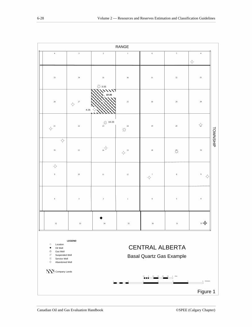
6-28 Volume 2 — Resources and Reserves Estimation and Classification Guidelines
Canadian Oil and Gas Evaluation Handbook ©SPEE (Calgary Chapter)
926
kilometers1. 0. 1. 2. 3. 4. 5.
miles0.2 0. 0.2 0.4 0.6 0.8 1.
LEGEND
Location
Oil Well
Gas Well
Suspended Well
Service Well
Abandoned Well
32313635343332
4
9
16
21
28
33
5
8
17
20
29
32
6
7
18
19
30
31
1
12
13
24
25
36
2
11
14
23
26
35
3
10
15
22
27
34
4
9
16
21
28
33
4-26
10-26
3-35
10-23
4561234
Basal Quartz Gas Example
Company Lands
CENTRAL ALBERTA
TOW
NS
HIP
RANGE
Figure 1
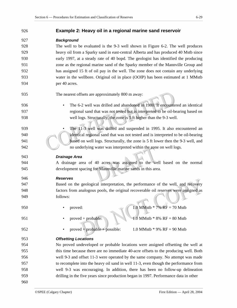
Section 6 — Procedures for Estimation and Classification of Reserves 6-29
©SPEE (Calgary Chapter) First Edition — April 28, 2004
Example 2: Heavy oil in a regional marine sand reservoir 926
Background 927 The well to be evaluated is the 9-3 well shown in Figure 6-2. The well produces 928 heavy oil from a Sparky sand in east-central Alberta and has produced 40 Mstb since 929 early 1997, at a steady rate of 40 bopd. The geologist has identified the producing 930 zone as the regional marine sand of the Sparky member of the Mannville Group and 931 has assigned 15 ft of oil pay in the well. The zone does not contain any underlying 932 water in the wellbore. Original oil in place (OOIP) has been estimated at 1 MMstb 933 per 40 acres. 934
The nearest offsets are approximately 800 m away: 935
• The 6-2 well was drilled and abandoned in 1980. It encountered an identical 936 regional sand that was not tested but is interpreted to be oil-bearing based on 937 well logs. Structurally, the zone is 5 ft higher than the 9-3 well. 938
• The 11-3 well was drilled and suspended in 1995. It also encountered an 939 identical regional sand that was not tested and is interpreted to be oil-bearing 940 based on well logs. Structurally, the zone is 5 ft lower then the 9-3 well, and 941 no underlying water was interpreted within the zone on well logs. 942
Drainage Area 943 A drainage area of 40 acres was assigned to the well based on the normal 944 development spacing for Mannville marine sands in this area. 945
Reserves 946 Based on the geological interpretation, the performance of the well, and recovery 947 factors from analogous pools, the original recoverable oil reserves were assigned as 948 follows: 949
• proved: 1.0 MMstb * 7% RF = 70 Mstb 950
• proved + probable: 1.0 MMstb * 8% RF = 80 Mstb 951
• proved + probable + possible: 1.0 MMstb * 9% RF = 90 Mstb 952
Offsetting Locations 953 No proved undeveloped or probable locations were assigned offsetting the well at 954 this time because there are no immediate 40-acre offsets to the producing well. Both 955 well 9-3 and offset 11-3 were operated by the same company. No attempt was made 956 to recomplete into the heavy oil sand in well 11-3, even though the performance from 957 well 9-3 was encouraging. In addition, there has been no follow-up delineation 958 drilling in the five years since production began in 1997. Performance data in other 959
960
6-30 Volume 2 — Resources and Reserves Estimation and Classification Guidelines
Canadian Oil and Gas Evaluation Handbook ©SPEE (Calgary Chapter)
960
kilometers1. 0. 1. 2. 3. 4. 5.
miles0.2 0. 0.2 0.4 0.6 0.8 1.
LEGEND
Location
Oil Well
Gas Well
Suspended Well
Service Well
Abandoned Well
32313635343332
4
9
16
21
28
33
5
8
17
20
29
32
6
7
18
19
30
31
1
12
13
24
25
36
2
11
14
23
26
35
3
10
15
22
27
34
4
9
16
21
28
33
4561234
Example of Assignments off aSingle Producing Well
Company Lands
CENTRAL ALBERTA
TOW
NS
HIP
RANGE
Figure 2
9-311-3
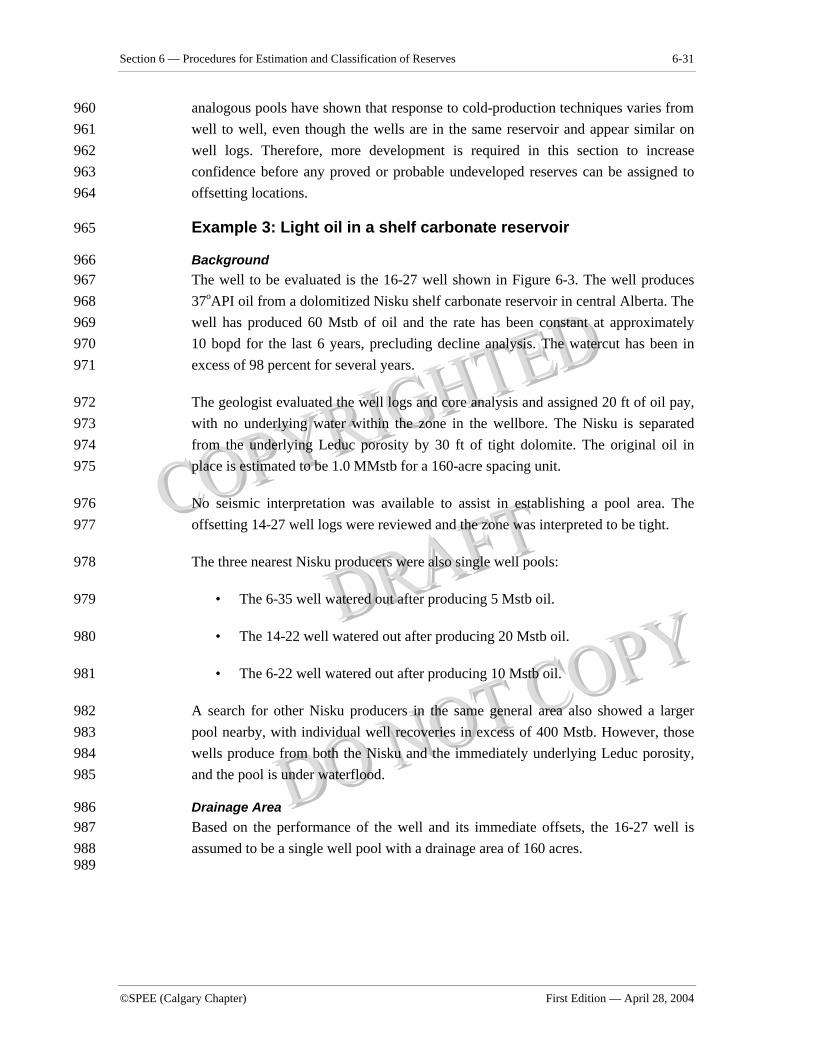
Section 6 — Procedures for Estimation and Classification of Reserves 6-31
©SPEE (Calgary Chapter) First Edition — April 28, 2004
analogous pools have shown that response to cold-production techniques varies from 960 well to well, even though the wells are in the same reservoir and appear similar on 961 well logs. Therefore, more development is required in this section to increase 962 confidence before any proved or probable undeveloped reserves can be assigned to 963 offsetting locations. 964
Example 3: Light oil in a shelf carbonate reservoir 965
Background 966 The well to be evaluated is the 16-27 well shown in Figure 6-3. The well produces 967 37oAPI oil from a dolomitized Nisku shelf carbonate reservoir in central Alberta. The 968 well has produced 60 Mstb of oil and the rate has been constant at approximately 969 10 bopd for the last 6 years, precluding decline analysis. The watercut has been in 970 excess of 98 percent for several years. 971
The geologist evaluated the well logs and core analysis and assigned 20 ft of oil pay, 972 with no underlying water within the zone in the wellbore. The Nisku is separated 973 from the underlying Leduc porosity by 30 ft of tight dolomite. The original oil in 974 place is estimated to be 1.0 MMstb for a 160-acre spacing unit. 975
No seismic interpretation was available to assist in establishing a pool area. The 976 offsetting 14-27 well logs were reviewed and the zone was interpreted to be tight. 977
The three nearest Nisku producers were also single well pools: 978
• The 6-35 well watered out after producing 5 Mstb oil. 979
• The 14-22 well watered out after producing 20 Mstb oil. 980
• The 6-22 well watered out after producing 10 Mstb oil. 981
A search for other Nisku producers in the same general area also showed a larger 982 pool nearby, with individual well recoveries in excess of 400 Mstb. However, those 983 wells produce from both the Nisku and the immediately underlying Leduc porosity, 984 and the pool is under waterflood. 985
Drainage Area 986 Based on the performance of the well and its immediate offsets, the 16-27 well is 987 assumed to be a single well pool with a drainage area of 160 acres. 988
989
6-32 Volume 2 — Resources and Reserves Estimation and Classification Guidelines
Canadian Oil and Gas Evaluation Handbook ©SPEE (Calgary Chapter)
989
kilometers1. 0. 1. 2. 3. 4. 5.
miles0.2 0. 0.2 0.4 0.6 0.8 1.
LEGEND
Location
Oil Well
Gas Well
Suspended Well
Service Well
Abandoned Well
32313635343332
4
9
16
21
28
33
5
8
17
20
29
32
6
7
18
19
30
31
1
12
13
24
25
36
2
11
14
23
26
35
3
10
15
22
27
34
4
9
16
21
28
33
4561234
Nisku Oil Example
Company Lands
CENTRAL ALBERTA
TOW
NS
HIP
RANGE
Figure 3
16-27
14-22
6-35
6-22
Section 6 — Procedures for Estimation and Classification of Reserves 6-33
©SPEE (Calgary Chapter) First Edition — April 28, 2004
Reserves 989 Original recoverable oil reserves were assigned to the 16-27 well as follows: 990
• proved: 1.0 MMstb * 7% RF = 70 Mstb 991
• proved + probable: 1.0 MMstb * 8% RF = 80 Mstb 992
• proved + probable + possible: 1.0 MMstb * 9% RF = 90 Mstb 993
Offsetting Locations 994 No assignment of reserves to offsetting locations within the same section is justified. 995 The zone is not porous in the offsetting spacing unit to the west, and the undrilled 996 spacing unit to the south is offset by the obviously uneconomic well 14-22. 997
6.3.3 Guidelines for Reserves Assignments in Multi-Well Pools 998
If an oil or gas accumulation can be shown to be continuous through geological 999 mapping, reserves may be assigned to undrilled locations within that pool. The 1000 reserves category assigned to each spacing unit within the pool will depend on the 1001 confidence with which the reserves can be estimated. 1002
The producing wells within a pool provide the most relevant information for 1003 estimating drainage areas and recovery factors, as well as assigning reserves to 1004 undrilled locations within the pool. If the production of wells within the pool is not 1005 mature enough for such purposes, the performance of analogous wells and pools 1006 should be used, taking care to establish that such wells and pools are truly analogous. 1007
In assigning reserves in any category within a pool, consideration must be given to all 1008 relevant factors, including, but not limited to geological control, reservoir quality, 1009 well performance, drainage area, underlying water, overlying gas, drive mechanism, 1010 addition of compression, artificial lift, potential for infill drilling and potential for 1011 enhanced recovery. Analogous pools can provide valuable information for analyzing 1012 the impact of such factors on reserves estimation and classification. 1013
It is important to recognize that a proved entity should also be assigned probable 1014 reserves, such that the proved + probable recovery factor represents the most likely 1015 recoverable volume from that entity. A proved recovery factor should then be 1016 established, bearing in mind the requirement of high confidence in the reported pool 1017 reserves. A proved + probable + possible recovery factor may also be established 1018 based on improved recovery or field optimization, bearing in mind the requirement of 1019 low confidence in the reported pool reserves. 1020
6-34 Volume 2 — Resources and Reserves Estimation and Classification Guidelines
Canadian Oil and Gas Evaluation Handbook ©SPEE (Calgary Chapter)
It is expected that the industry standard for volumetric reserves estimation will 1021 continue to be a single net pay isopach map representing the most likely estimate of 1022 the extent and configuration of a pool. In some cases, however, it may be appropriate 1023 to generate multiple maps, representing the maximum, most likely, and minimum 1024 pool configurations, in order to quantify the effects of particular uncertainties in the 1025 volumetric estimates. Alternatively, the most likely rock volume within a pool may 1026 be mathematically increased to reflect the possible rock volume for the purposes of 1027 assigning possible reserves. The preferred method of making such an adjustment is to 1028 use a probabilistic analysis . However, it may be acceptable to simply “gross up” the 1029 pool rock volume by a nominal amount based on observed variability of the 1030 volumetric parameters and uncertainty in the geological mapping. In using such a 1031 procedure, however, care must be taken to relate the calculated volume and pool area 1032 to the actual lands to ensure that any potential equity issues are addressed. 1033
Generic examples illustrating the assignment of reserves within a multi-well gas pool 1034 and a multi-well oil pool are presented in the following discussion to illustrate the 1035 application of the guidelines discussed in this volume. For presentation purposes, it is 1036 customary to identify the reserves category for each spacing unit within a pool 1037 superimposed on a net pay isopach map of the pool. With the assignment of multiple 1038 reserves categories to spacing units within a pool, however, such a map may become 1039 confusing. To avoid such confusion in the following examples, the individual 1040 reserves categories are shown on separate maps. 1041
Example 1: Multi-Well Gas Pool 1042
A generic multi-well gas pool is illustrated in Figure 6-4A. The pool contains three 1043 gas wells producing from a shallow marine sandstone that has been interpreted from 1044 well control to be continuous across the mapped area. The updip limit of the pool is 1045 controlled by a facies change from sand to shale and the downdip limit is controlled 1046 by a gas-water interface, as shown on the map. The pool boundaries are estimated, 1047 having been interpolated from the existing well control, and are considered by the 1048 geologist to represent the most likely extent of the pool. 1049
The individual reserves assignments within the pool are shown in Figure 6-4B. 1050
From a comparison of well performance and volumetric calculations, the producing 1051 wells were each expected to drain the proved + probable reserves from at least a 640-1052 acre spacing unit, and past work showed this to be true for analogous pools in this 1053 area. Thus, this spacing unit was honoured in assigning reserves within the pool. 1054
The key to assigning reserves to the pool is the estimation of the most likely (proved 1055 + probable) recovery factor. In this example, the gas overlies water, and a most likely 1056
Section 6 — Procedures for Estimation and Classification of Reserves 6-35
©SPEE (Calgary Chapter) First Edition — April 28, 2004
recovery factor of 65% was estimated using initial pressure, abandonment pressure 1057 and the expected impact of water influx. To reflect uncertainty concerning the impact 1058 of the underlying water on ultimate recovery, and bearing in mind the requirement 1059 for high confidence in the proved reserves, the proved recovery factor was estimated 1060 to be 50%. To acknowledge the possibility that the aquifer might be less active than 1061 is currently expected, a proved + probable + possible recovery factor of 75% was 1062 also estimated for the pool. 1063
The statutory spacing units containing the producing wells (sections 17, 13 ,and 24) 1064 were thus assigned proved developed producing (PDP) reserves and probable 1065 developed (PBD) reserves as shown in Figure 4B. Probable developed reserves were 1066 also assigned to the partial spacing units downdip of the PDP lands (sections 8, 9, 16, 1067 and 12), because they will not be independently developed and are expected to be 1068 drained by the PDP wells. 1069
Based on the estimated wellbore drainage area and the expectation of similar net pay 1070 and structural position from the geological mapping, the mapped lands within one 1071 spacing unit of the proved developed producing (PDP) lands were considered to 1072 contain proved undeveloped (PU) reserves. These lands (sections 18, 19, 14, and 23) 1073 were assigned the proved recovery factor established for the PDP wells. No PU 1074 reserves were assigned to the partial spacing units along the pool edges, based on 1075 uncertainties regarding either presence of reservoir (updip edge) or economic 1076 recovery (downdip edge close to underlying water). 1077
The lands assigned PU reserves (sections 18, 19, 14, and 23) were also assigned 1078 probable undeveloped (PBU) reserves and the partial spacing units offsetting the PU 1079 lands (sections 7, 20, 30, 11, 25, and 26) were also assigned PBU reserves on the 1080 expectation of their drainage by existing and future wells. In addition, probable 1081 undeveloped (PBU) reserves were assigned to the mapped area within one spacing 1082 unit of the proved lands (sections 10, 15, 22, and 27), based on the geological 1083 mapping and the performance of the producing wells. These lands were assigned the 1084 proved + probable recovery factor established for the PDP reserves. The partial 1085 spacing units along the pool edges were expected to be drained by existing and future 1086 wells. 1087
Each of the proved and probable reserves entities may also be assigned possible 1088 reserves. In this example, the entire pool was assigned possible reserves assuming the 1089 aquifer may be less active than currently expected. An ultimate recovery factor of 1090 75% was estimated for this case and the reserves were assigned as possible developed 1091 (PosD) and possible undeveloped (PosU), as shown in Figure 4B. It should be noted 1092 that the pool volume could also have been increased to reflect the possibility of 1093
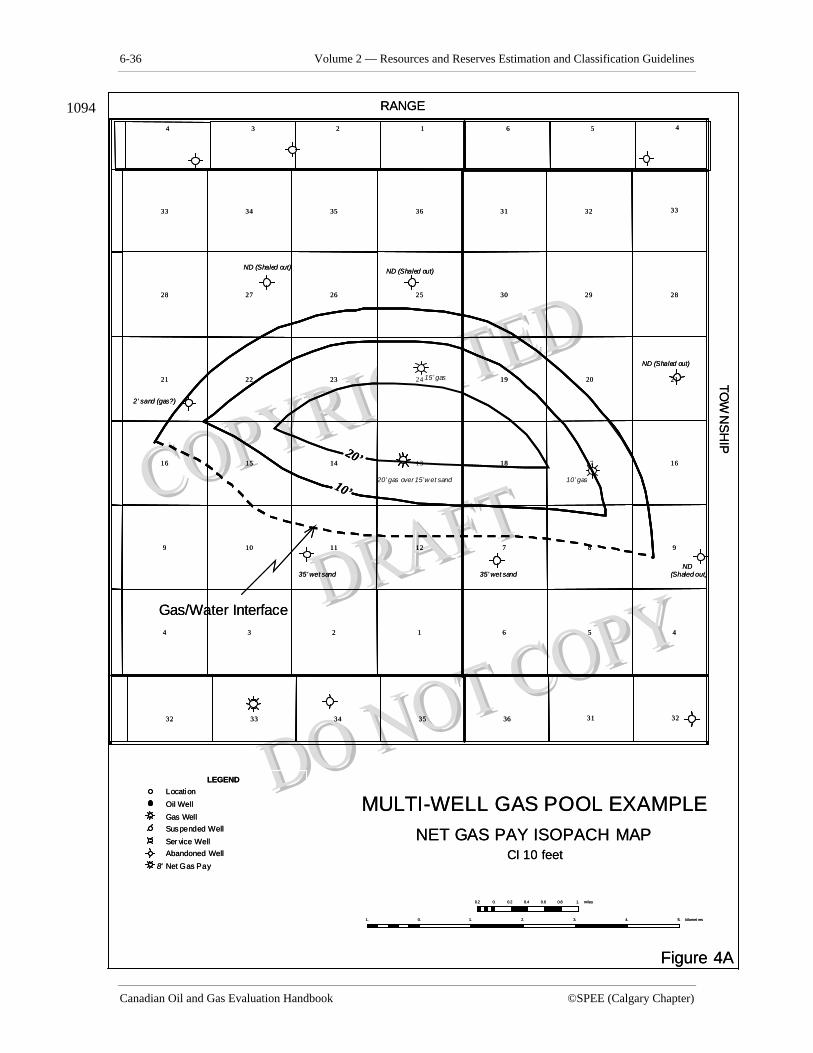
6-36 Volume 2 — Resources and Reserves Estimation and Classification Guidelines
Canadian Oil and Gas Evaluation Handbook ©SPEE (Calgary Chapter)
1094
kilomet ers1. 0. 1. 2. 3. 4. 5.
miles0.2 0. 0.2 0.4 0.6 0.8 1.
LEGENDLocati on
Oil Well
Gas WellSuspended Well
Ser vice WellAbandoned Well
Net Gas Pay
32313635343332
4
9
16
21
28
33
5
8
17
20
29
32
6
7
18
19
30
31
1
12
13
24
25
36
2
11
14
23
26
35
3
10
15
22
27
34
4
9
16
21
28
33
4561234
ND (Shaled out)
Gas/Water Interface
8'
NET GAS PAY ISOPACH MAP
MULTI-WELL GAS POOL EXAMPLE
TOW
NS
HIP
RANGE
CI 10 feet
Figure 4A
ND (Shaled out)
ND (Shaled out)
2’ sand (gas?)
ND(Shaled out)35’ wet sand35’ wet sand
15’ gas
20’ gas over 15’ wet sand 10’ gas
20’
10’
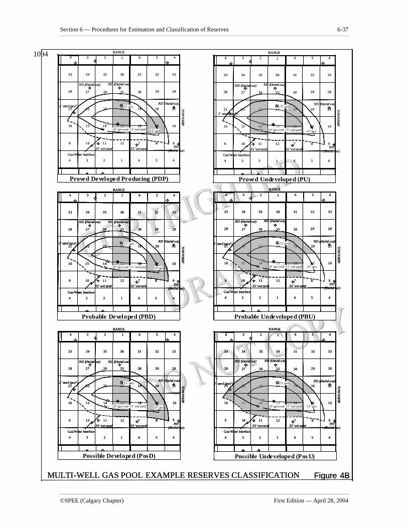
Section 6 — Procedures for Estimation and Classification of Reserves 6-37
©SPEE (Calgary Chapter) First Edition — April 28, 2004
1094
32313635343332
4
9
16
21
28
33
5
8
17
20
29
32
6
7
18
19
30
31
1
12
13
24
25
36
2
11
14
23
26
35
3
10
15
22
27
34
4
9
16
21
28
33
4561234
ND (Shaled out)
Gas/Water Interface
TOW
NSH
IP
RANGE
ND (Shaled out)
ND (Shaled out)
2’ sand (gas?)
ND(Shaled out)35’ wet sand35’ wet sand
15’ gas
20’ gas over 15’ wet sand10
20
Possible Undeveloped (Pos U)
10’ gas
32313635343332
4
9
16
21
28
33
5
8
17
20
29
32
6
7
18
19
30
31
1
12
13
24
25
36
2
11
14
23
26
35
3
10
15
22
27
34
4
9
16
21
28
33
4561234
ND (Shaled out)
Gas/Water Interface
TOW
NSH
IP
RANGE
ND (Shaled out)
ND (Shaled out)
2’ sand (gas?)
ND(Shaled out)35’ wet sand35’ wet sand
15’ gas
20’ gas over 15’ wet sand10
20
10’ gas
Possible Developed (PosD)
Figure 4BMULTI-WELL GAS POOL EXAMPLE RESERVES CLASSIFICATION
RANGE
32313635343332
4
9
16
21
28
33
5
8
17
20
29
32
6
7
18
19
30
31
1
12
13
24
25
36
2
11
14
23
26
35
3
10
15
22
27
34
4
9
16
21
28
33
4561234
ND (Shaled out)
Gas/Water Interface
TOW
NSH
IP
RANGE
ND (Shaled out)
ND (Shaled out)
2’ sand (gas?)
ND(Shaled out)
35’ wet sand35’ wet sand
15’ gas
20’ gas over 15’ wet sand10
20
10’ gas
Probable Developed (PBD)
32313635343332
4
9
16
21
28
33
5
8
17
20
29
32
6
7
18
19
30
31
1
12
13
24
25
36
2
11
14
23
26
35
3
10
15
22
27
34
4
9
16
21
28
33
4561234
ND (Shaled out)
Gas/Water Interface
TOW
NSH
IP
RANGE
ND (Shaled out)
ND (Shaled out)
2’ sand (gas?)
ND(Shaled out)35’ wet sand35’ wet sand
15’ gas
20’ gas over 15’ wet sand10
20
Proved Undeveloped (PU)
32313635343332
4
9
16
21
28
33
5
8
17
20
29
32
6
7
18
19
30
31
1
12
13
24
25
36
2
11
14
23
26
35
3
10
15
22
27
34
4
9
16
21
28
33
4561234
ND (Shaled out)
Gas/Water Interface
TOW
NSH
IP
RANGE
ND (Shaled out)
ND (Shaled out)
2’ sand (gas?)
ND(Shaled out)35’ wet sand35’ wet sand
15’ gas
20’ gas over 15’ wet sand10
20
Probable Undeveloped (PBU)
10’ gas
10’ gas
32313635343332
4
9
16
21
28
33
5
8
17
20
29
32
6
7
18
19
30
31
1
12
13
24
25
36
2
11
14
23
26
35
3
10
15
22
27
34
4
9
16
21
28
33
4561234
ND (Shaled out)
Gas/Water Interface
TOW
NSH
IP
ND (Shaled out)
ND (Shaled out)
2’ sand (gas?)
ND(Shaled out)35’ wet sand35’ wet sand
20’ gas over 15’ wet sand10
20
15’ gas
Proved Developed Producing (PDP)
10’ gas
32313635343332
4
9
16
21
28
33
5
8
17
20
29
32
6
7
18
19
30
31
1
12
13
24
25
36
2
11
14
23
26
35
3
10
15
22
27
34
4
9
16
21
28
33
4561234
ND (Shaled out)
Gas/Water Interface
TOW
NSH
IP
RANGE
ND (Shaled out)
ND (Shaled out)
2’ sand (gas?)
ND(Shaled out)35’ wet sand35’ wet sand
15’ gas
20’ gas over 15’ wet sand10
20
Possible Undeveloped (Pos U)
10’ gas
32313635343332
4
9
16
21
28
33
5
8
17
20
29
32
6
7
18
19
30
31
1
12
13
24
25
36
2
11
14
23
26
35
3
10
15
22
27
34
4
9
16
21
28
33
4561234
ND (Shaled out)
Gas/Water Interface
TOW
NSH
IP
RANGE
ND (Shaled out)
ND (Shaled out)
2’ sand (gas?)
ND(Shaled out)35’ wet sand35’ wet sand
15’ gas
20’ gas over 15’ wet sand10
20
10’ gas
Possible Developed (PosD) 32313635343332
4
9
16
21
28
33
5
8
17
20
29
32
6
7
18
19
30
31
1
12
13
24
25
36
2
11
14
23
26
35
3
10
15
22
27
34
4
9
16
21
28
33
4561234
ND (Shaled out)
Gas/Water Interface
TOW
NSH
IP
RANGE
ND (Shaled out)
ND (Shaled out)
2’ sand (gas?)
ND(Shaled out)35’ wet sand35’ wet sand
15’ gas
20’ gas over 15’ wet sand10
20
10’ gas
Possible Developed (PosD)
Figure 4BMULTI-WELL GAS POOL EXAMPLE RESERVES CLASSIFICATION
RANGE
32313635343332
4
9
16
21
28
33
5
8
17
20
29
32
6
7
18
19
30
31
1
12
13
24
25
36
2
11
14
23
26
35
3
10
15
22
27
34
4
9
16
21
28
33
4561234
ND (Shaled out)
Gas/Water Interface
TOW
NSH
IP
RANGE
ND (Shaled out)
ND (Shaled out)
2’ sand (gas?)
ND(Shaled out)
35’ wet sand35’ wet sand
15’ gas
20’ gas over 15’ wet sand10
20
10’ gas
Probable Developed (PBD) 32313635343332
4
9
16
21
28
33
5
8
17
20
29
32
6
7
18
19
30
31
1
12
13
24
25
36
2
11
14
23
26
35
3
10
15
22
27
34
4
9
16
21
28
33
4561234
ND (Shaled out)
Gas/Water Interface
TOW
NSH
IP
RANGE
ND (Shaled out)
ND (Shaled out)
2’ sand (gas?)
ND(Shaled out)
35’ wet sand35’ wet sand
15’ gas
20’ gas over 15’ wet sand10
20
10’ gas
Probable Developed (PBD)
32313635343332
4
9
16
21
28
33
5
8
17
20
29
32
6
7
18
19
30
31
1
12
13
24
25
36
2
11
14
23
26
35
3
10
15
22
27
34
4
9
16
21
28
33
4561234
ND (Shaled out)
Gas/Water Interface
TOW
NSH
IP
RANGE
ND (Shaled out)
ND (Shaled out)
2’ sand (gas?)
ND(Shaled out)35’ wet sand35’ wet sand
15’ gas
20’ gas over 15’ wet sand10
20
Proved Undeveloped (PU)
32313635343332
4
9
16
21
28
33
5
8
17
20
29
32
6
7
18
19
30
31
1
12
13
24
25
36
2
11
14
23
26
35
3
10
15
22
27
34
4
9
16
21
28
33
4561234
ND (Shaled out)
Gas/Water Interface
TOW
NSH
IP
RANGE
ND (Shaled out)
ND (Shaled out)
2’ sand (gas?)
ND(Shaled out)35’ wet sand35’ wet sand
15’ gas
20’ gas over 15’ wet sand10
20
Probable Undeveloped (PBU)
10’ gas
10’ gas
32313635343332
4
9
16
21
28
33
5
8
17
20
29
32
6
7
18
19
30
31
1
12
13
24
25
36
2
11
14
23
26
35
3
10
15
22
27
34
4
9
16
21
28
33
4561234
ND (Shaled out)
Gas/Water Interface
TOW
NSH
IP
ND (Shaled out)
ND (Shaled out)
2’ sand (gas?)
ND(Shaled out)35’ wet sand35’ wet sand
20’ gas over 15’ wet sand10
20
15’ gas
Proved Developed Producing (PDP)
10’ gas
6-38 Volume 2 — Resources and Reserves Estimation and Classification Guidelines
Canadian Oil and Gas Evaluation Handbook ©SPEE (Calgary Chapter)
encountering higher net pays, higher porosities or lower water saturations on the 1094 undrilled spacing units, or the likelihood that the pool area may be larger than 1095 currently expected. 1096
Example 2: Multi-Well Oil Pool 1097
A generic multi-well oil pool is illustrated in Figure 6-5A. The pool contains fourteen 1098 wells producing light gravity oil from a shallow marine sandstone that has been 1099 interpreted from well control to be continuous across the mapped area. The updip 1100 limit of the pool is controlled by a facies change from sand to shale and is reasonably 1101 well defined from well control. The downdip limit is controlled by an oil-water 1102 interface and its location is reasonably well defined from well control. The map is 1103 considered by the geologist to represent the most likely extent of the pool. 1104
The pool is under primary production and the operator has no plans to implement an 1105 enhanced recovery scheme in the foreseeable future. Several analogous pools are 1106 being waterflooded, with mixed results. 1107
The individual reserves assignments within the pool are shown in Figure 6-5B. 1108
From a comparison of well performance and volumetric calculations, the producing 1109 wells were each expected to drain the proved + probable reserves from a 160-acre 1110 spacing unit; thus, this spacing unit was used to assign reserves to undrilled locations 1111 within the pool. 1112
The key to assigning reserves to the pool is the estimation of the most likely (proved 1113 + probable) recovery factor. In this case, an appropriate recovery factor was 1114 estimated from a combination of production performance, analogous pool 1115 performance, and empirical correlations. A proved recovery factor was then 1116 estimated to reflect uncertainty concerning the impact of the underlying water on 1117 ultimate recovery, and bearing in mind the requirement of high confidence in the 1118 reported pool proved reserves. A proved + probable + possible recovery factor was 1119 also estimated based on the potential for enhanced recovery, bearing in mind the 1120 requirement of low confidence in the reported pool reserves. 1121
The spacing units containing the producing wells were thus assigned proved 1122 developed producing (PDP) reserves and probable developed (PBD) reserves as 1123 shown in Figure 5B. PDP and PBD reserves were also assigned to several partial 1124 spacing units along the updip pool edge based on confidence in the geological 1125 mapping and the expectation that they would be drained by the existing wells. 1126
Section 6 — Procedures for Estimation and Classification of Reserves 6-39
©SPEE (Calgary Chapter) First Edition — April 28, 2004
Using the geological mapping and expected wellbore drainage area, the mapped 1127 lands within one spacing unit of each proved developed producing (PDP) well were 1128 considered to contain proved undeveloped (PU) reserves, with several exceptions. 1129 The exceptions were at both ends and along the downdip portion of the pool and were 1130 based on uncertainties regarding either the location of the pool edge or structure, 1131 resulting from sparse well control. The PU lands consist of one partial and seven full 1132 spacing units. The partial spacing unit lies at the updip edge of the pool, is defined by 1133 well control, and is expected to be drained by existing or future wells. 1134
The lands assigned PU reserves were also assigned probable undeveloped (PBU) 1135 reserves. In addition, PBU reserves were assigned to one partial and five full spacing 1136 units at the eastern and western ends of the pool and along the downdip edge, based 1137 on consideration of expected net pay thickness, structural position relative to the oil-1138 water contact and the presence of a producing well at a similar elevation in the pool. 1139 These lands all offset proved spacing units. 1140
Each of the proved and probable reserves entities may also be assigned possible 1141 reserves. In this example, possible reserves were assigned to the entire pool based on 1142 the potential for enhanced recovery. Although the operator has no plans to water-1143 flood the pool in the foreseeable future, several analogous pools are under 1144 waterflood, but with mixed results. The economic viability of developing the possible 1145 reserves was verified using the average incremental recovery factor established for 1146 analogous pools. Because the waterflood would require a significant capital 1147 expenditure, the possible reserves were classified as undeveloped (PosU). It should 1148 be noted that the pool volume could also have been increased to reflect the possibility 1149 of encountering higher net pays, higher porosities, or lower water saturations on the 1150 undrilled spacing units, or the likelihood that the pool area may be larger than 1151 currently expected. 1152
1153 1154
6-40 Volume 2 — Resources and Reserves Estimation and Classification Guidelines
Canadian Oil and Gas Evaluation Handbook ©SPEE (Calgary Chapter)
1154
LEGEND
Locati onOil Well
Gas Well
Suspended WellSer vice Well
Abandoned WellNet Oil Pay
31363534333231
6
7
18
19
30
31
1
12
13
24
25
36
2
11
14
23
26
35
3
10
15
22
27
34
4
9
16
21
28
33
5
8
17
20
29
32
6
7
18
19
30
31
0'
Oil/Water Interface
13'
TOW
NS
HIP
RANGE
Figure 5A
10’
20’
kilomet ers1. 0. 1. 2. 3. 4. 5.
miles0.2 0. 0.2 0.4 0.6 0.8 1.
NET OIL PAY ISOPACH MAPMULTI-WELL OIL POOL EXAMPLE
CI 10 feet
LEGEND
Locati onOil Well
Gas Well
Suspended WellSer vice Well
Abandoned WellNet Oil Pay
31363534333231
6
7
18
19
30
31
1
12
13
24
25
36
2
11
14
23
26
35
3
10
15
22
27
34
4
9
16
21
28
33
5
8
17
20
29
32
6
7
18
19
30
31
LEGEND
Locati onOil Well
Gas Well
Suspended WellSer vice Well
Abandoned WellNet Oil Pay
31363534333231
6
7
18
19
30
31
1
12
13
24
25
36
2
11
14
23
26
35
3
10
15
22
27
34
4
9
16
21
28
33
5
8
17
20
29
32
6
7
18
19
30
31
0'
Oil/Water Interface
13'
TOW
NS
HIP
RANGE
Figure 5A
10’
20’
kilomet ers1. 0. 1. 2. 3. 4. 5.
miles0.2 0. 0.2 0.4 0.6 0.8 1.
NET OIL PAY ISOPACH MAPMULTI-WELL OIL POOL EXAMPLE
CI 10 feet
kilomet ers1. 0. 1. 2. 3. 4. 5. kilomet ers1. 0. 1. 2. 3. 4. 5.
miles0.2 0. 0.2 0.4 0.6 0.8 1. miles0.2 0. 0.2 0.4 0.6 0.8 1.
NET OIL PAY ISOPACH MAPMULTI-WELL OIL POOL EXAMPLE
CI 10 feet
Section 6 — Procedures for Estimation and Classification of Reserves 6-41
©SPEE (Calgary Chapter) First Edition — April 28, 2004
1154
31363534333231
6
7
18
19
30
31
1
12
13
24
25
36
2
11
14
23
26
35
3
10
15
22
27
34
4
9
16
21
28
33
5
8
17
20
29
32
6
7
18
19
30
31
Oil/Water Interface
TO
WN
SHIP
RANGE
10’
20’
Probable Undeveloped (PU)
31363534333231
6
7
18
19
30
31
1
12
13
24
25
36
2
11
14
23
26
35
3
10
15
22
27
34
4
9
16
21
28
33
5
8
17
20
29
32
6
7
18
19
30
31
Oil/Water Interface
TOW
NSH
IP
RANGE
10’
20’
Proved Developed Producing (PDP)
Figure 5BMULTI-WELL OIL POOL EXAMPLE RESERVES CLASSIFICATION
31363534333231
6
7
18
19
30
31
1
12
13
24
25
36
2
11
14
23
26
35
3
10
15
22
27
34
4
9
16
21
28
33
5
8
17
20
29
32
6
7
18
19
30
31
Oil/Water Interface
TO
WN
SHIP
RANGE
10’
20’
Proved Undeveloped (PU)
31363534333231
6
7
18
19
30
31
1
12
13
24
25
36
2
11
14
23
26
35
3
10
15
22
27
34
4
9
16
21
28
33
5
8
17
20
29
32
6
7
18
19
30
31
Oil/Water Interface
TO
WN
SHIP
RANGE
10’
20’
Possible Developed (PosD)
31363534333231
6
7
18
19
30
31
1
12
13
24
25
36
2
11
14
23
26
35
3
10
15
22
27
34
4
9
16
21
28
33
5
8
17
20
29
32
6
7
18
19
30
31
Oil/Water Interface
TO
WN
SHIP
RANGE
10’
20’
Probable Developed (PBD)
31363534333231
6
7
18
19
30
31
1
12
13
24
25
36
2
11
14
23
26
35
3
10
15
22
27
34
4
9
16
21
28
33
5
8
17
20
29
32
6
7
18
19
30
31
Oil/Water Interface
TO
WN
SHIP
RANGE
10’
20’
Possible Undeveloped (Pos U)
31363534333231
6
7
18
19
30
31
1
12
13
24
25
36
2
11
14
23
26
35
3
10
15
22
27
34
4
9
16
21
28
33
5
8
17
20
29
32
6
7
18
19
30
31
Oil/Water Interface
TO
WN
SHIP
RANGE
10’
20’
Probable Undeveloped (PU)
31363534333231
6
7
18
19
30
31
1
12
13
24
25
36
2
11
14
23
26
35
3
10
15
22
27
34
4
9
16
21
28
33
5
8
17
20
29
32
6
7
18
19
30
31
Oil/Water Interface
TOW
NSH
IP
RANGE
10’
20’
Proved Developed Producing (PDP)
Figure 5BMULTI-WELL OIL POOL EXAMPLE RESERVES CLASSIFICATION
31363534333231
6
7
18
19
30
31
1
12
13
24
25
36
2
11
14
23
26
35
3
10
15
22
27
34
4
9
16
21
28
33
5
8
17
20
29
32
6
7
18
19
30
31
Oil/Water Interface
TO
WN
SHIP
RANGE
10’
20’
Proved Undeveloped (PU)
31363534333231
6
7
18
19
30
31
1
12
13
24
25
36
2
11
14
23
26
35
3
10
15
22
27
34
4
9
16
21
28
33
5
8
17
20
29
32
6
7
18
19
30
31
Oil/Water Interface
TO
WN
SHIP
RANGE
10’
20’
Possible Developed (PosD)
31363534333231
6
7
18
19
30
31
1
12
13
24
25
36
2
11
14
23
26
35
3
10
15
22
27
34
4
9
16
21
28
33
5
8
17
20
29
32
6
7
18
19
30
31
Oil/Water Interface
TO
WN
SHIP
RANGE
10’
20’
Probable Developed (PBD)
31363534333231
6
7
18
19
30
31
1
12
13
24
25
36
2
11
14
23
26
35
3
10
15
22
27
34
4
9
16
21
28
33
5
8
17
20
29
32
6
7
18
19
30
31
Oil/Water Interface
TO
WN
SHIP
RANGE
10’
20’
Possible Undeveloped (Pos U) 31363534333231
6
7
18
19
30
31
1
12
13
24
25
36
2
11
14
23
26
35
3
10
15
22
27
34
4
9
16
21
28
33
5
8
17
20
29
32
6
7
18
19
30
31
Oil/Water Interface
TO
WN
SHIP
RANGE
10’
20’
31363534333231
6
7
18
19
30
31
1
12
13
24
25
36
2
11
14
23
26
35
3
10
15
22
27
34
4
9
16
21
28
33
5
8
17
20
29
32
6
7
18
19
30
31
Oil/Water Interface
TO
WN
SHIP
RANGE
10’
20’
Possible Undeveloped (Pos U)
6-42 Volume 2 — Resources and Reserves Estimation and Classification Guidelines
Canadian Oil and Gas Evaluation Handbook ©SPEE (Calgary Chapter)
1154
6.4 Material Balance Methods 1155
Material balance methods of reserves estimation involve the analysis of pressure 1156 behaviour as reservoir fluids are withdrawn, and usually result in more reliable 1157 reserves estimates than those obtained using volumetric methods. Confident reserves 1158 estimates require a significant amount of reservoir fluid depletion, accurate reservoir 1159 pressures, knowledge of aquifer characteristics, and information on rock and fluid 1160 properties. In complex situations such as those involving water influx, multi-phase 1161 behaviour, and layered or low-permeability reservoirs, material balance estimates 1162 alone could provide erroneous results. In these cases, therefore, results must always 1163 be compared with those obtained using other methods. 1164
The most common application of material balance methods is the use of P/Z versus 1165 cumulative gas production plots to determine original gas in place. This is only the 1166 first step in the determination of the gas reserves, and similar factors considered 1167 when using volumetric methods must be considered when using material balance 1168 methods to estimate recovery factors and recoverable reserves. 1169
Material balance methods for oil reservoirs can be applied analytically, but are more 1170 often applied with a numerical reservoir simulator, with the reservoir properties 1171 varied to match the average reservoir pressure and fluid production history. Both 1172 fluids in place and future recoverable oil reserves can be estimated using these 1173 methods. 1174
Use of material balance methods on gas reservoirs is discussed below. Their use on 1175 oil reservoirs is only briefly discussed, in Section 6.4.10. 1176
6.4.1 General Considerations in the Use of Material Balance Methods 1177 for Gas Reservoirs 1178
Rarely does an analysis of all of the geological and engineering data for a reservoir 1179 lead to a perfectly clear determination of the original fluids in place and recoverable 1180 reserves, and different analytical methods will often yield different results. Material 1181 balance methods are only one alternative and must not be relied upon without 1182 considering others. Only through an understanding of the reservoir and fluid 1183 properties and the limitations of material balance methods can the evaluator 1184 determine reliable estimates of original gas in place and recoverable reserves and 1185 understand the level of confidence that should be placed on the values determined. 1186
Section 6 — Procedures for Estimation and Classification of Reserves 6-43
©SPEE (Calgary Chapter) First Edition — April 28, 2004
Various factors must be considered in the application of material balance methods, 1187 some of which are discussed below. 1188
6.4.2 Consideration of Reservoir Properties 1189
a. Aquifers 1190
An incorrect determination of original gas in place using material balance methods 1191 can occur when water from an underlying aquifer invades the gas-saturated portion of 1192 the reservoir. The size of the water zone relative to the size of the gas-saturated zone, 1193 the permeability of the gas and water zones, and the rate of and amount of production 1194 from the gas reservoir affect the degree of aquifer influx. 1195
Upward curvature of the P/Z plot is often considered an indicator of an active aquifer. 1196 However, there are many reservoir situations, particularly in the case of a high-1197 permeability aquifer or low gas withdrawal rates, where the P/Z line appears to be 1198 straight, yet significant water encroachment into the gas zone could be occurring. In 1199 some cases, the P/Z data points could follow a straight line, yet the gas column could 1200 be completely flooded out, with only a partial reduction in the reservoir pressure. 1201
Recovery factors for gas reservoirs with a water drive may be significantly lower 1202 than those for reservoirs producing by gas expansion alone. The impact of water 1203 encroachment on recovery factor is related to the following factors: 1204
• the volume of gas trapped by the encroaching aquifer, 1205
• the higher pressure at which the reservoir is abandoned, 1206
• the gas volume displaced by water influx. 1207
Depending on aquifer “strength,” recovery factors for water drive reservoirs are 1208 commonly reduced by 30 to 50 percent of the recovery that would be expected 1209 without a water drive. 1210
If aquifer pressure support is observed or considered likely, analytical material 1211 balance methods that take this into account (see, for example, Slider 1976), or a 1212 numerical reservoir simulator, should be used. 1213
b. Reservoir Permeability 1214
Reservoir pressure measurements in low-permeability reservoirs require either long 1215 buildup times or the application of pressure transient analysis methods to determine 1216 average reservoir pressures. An understanding of the reservoir permeability and the 1217
6-44 Volume 2 — Resources and Reserves Estimation and Classification Guidelines
Canadian Oil and Gas Evaluation Handbook ©SPEE (Calgary Chapter)
conditions under which the pressure data points were taken are essential to determine 1218 the reliance to be placed on the data points, especially if there is a poor correlation in 1219 pressure measurements over time. 1220
c. Multi-Well Reservoirs 1221
Material balance methods for multi-well pools should only be applied on a total pool 1222 basis and include all of the wells interpreted to be producing from the subject 1223 reservoir. 1224
Pressure gradients often exist throughout large multi-well pools in medium to low 1225 permeability. In pools where multiple pressure readings are taken over a short period 1226 of time, these pressures should be appropriately averaged to determine the average 1227 pool pressure. Unless the pressure readings are reasonably well distributed 1228 throughout the pool, they should be weighted by the pore volume they appear to be 1229 draining. 1230
Often material balance calculations for extensive pools include pressure readings 1231 from new wells. It must be recognized that new wells are usually drilled in the least 1232 depleted areas of a pool. Accordingly, the estimate of average reservoir pressure must 1233 account for the lower pressure areas of the pool (usually requiring averaging with 1234 pressure readings for older wells). 1235
d. Multi-Layer Reservoirs 1236
Reservoirs that contain multiple layers of differing permeability require very careful 1237 determination of average reservoir pressures. Pressure distributions can vary in each 1238 layer, and the correct determination of an average pressure for all the layers requires 1239 careful analysis of the data. Unless very detailed pressure transient analysis work is 1240 conducted, very long buildups are required to determine reliable average reservoir 1241 pressures. Caution must also be taken when estimating recovery factors in multi-layer 1242 reservoirs, because low-permeability layers may have significantly lower recovery 1243 factors than the high-permeability layers. 1244
e. Naturally Fractured Reservoirs 1245
Naturally fractured reservoirs usually consist of a high-volume, low-permeability 1246 matrix system and a low-volume, high-permeability fracture system. Pressures could 1247 build up rapidly when a well is shut in, but because of the presence of the low-1248 permeability matrix, long pressure buildups or detailed pressure transient analyses are 1249 required in naturally fractured reservoirs to determine reliable average reservoir 1250 pressures. 1251
Section 6 — Procedures for Estimation and Classification of Reserves 6-45
©SPEE (Calgary Chapter) First Edition — April 28, 2004
6.4.3 Consideration of Fluid Properties 1252
a. Dry Gas Reservoirs 1253
Material balance P/Z plots for dry gas reservoirs do not require any special 1254 adjustments to the produced volumes prior to preparing the material balance plots. 1255
b. Wet Gas Reservoirs 1256
Use of material balance methods to determine the original gas in place for wet gas 1257 fluids could require a more sophisticated analysis than a simple P/Z plot. In these 1258 situations, significant volumes of natural gas liquids may be produced at the surface. 1259 Proper analysis of wet gas reservoirs requires the conversion of surface-produced 1260 volumes of gas and liquids to gas-equivalent volumes. This requires representative 1261 fluid samples, preferably early in the life of the reservoir, and accurate measurement 1262 of the PVT properties. 1263
Although most gas reservoirs produce some natural gas liquids, if the produced 1264 liquids content is low (in the 10 to 40 bbl per MMcf range) and relatively constant 1265 over time, use of only wellhead gas volumes may be acceptable. 1266
c. Retrograde Condensate Reservoirs 1267
Use of material balance methods to determine the original gas in place for retrograde 1268 condensate reservoirs below the dew point is not possible using the simple P/Z plot if 1269 large volumes of liquids are produced due to the changing fluid composition during 1270 the decline in reservoir pressures. In these situations, a compositional reservoir 1271 simulator should be used, provided sufficient pressure decline and PVT data are 1272 available. 1273
6.4.4 Consideration of Quality of Pressure Data 1274
a. Types of Pressure Measurements 1275
Pressure is the most important data in a material balance analysis and also the most 1276 susceptible to error. Reservoir pressures may be measured with downhole or surface 1277 gauges and may be single point or continuous transient measurements. 1278
All pressure measurements should be referenced to either the midpoint of 1279 perforations in the case of a single well, or to a common reservoir datum in the case 1280 of multi-well pools. Bottom-hole pressures are more reliable than surface pressure 1281 measurements, because conversion of pressure readings from surface to bottom-hole 1282
6-46 Volume 2 — Resources and Reserves Estimation and Classification Guidelines
Canadian Oil and Gas Evaluation Handbook ©SPEE (Calgary Chapter)
conditions might be inaccurate if the presence of wellbore fluids is not properly taken 1283 into account. 1284
Single point, or static gradient, pressure measurements are only reliable in material 1285 balance plots when the well has been shut in for a sufficiently long period of time. If 1286 reservoir pressures are still increasing at the time of pressure measurement, 1287 continuous pressure measurements over a period of several days must be taken and 1288 pressure transient analyses conducted to properly determine the estimated built-up 1289 pressure. 1290
b. Number of Pressure Measurements 1291
Although a determination of original gas in place can be made with as few as two 1292 pressure measurements, more confidence is obtained as more measurements are 1293 taken. In multi-well pools, more confidence is obtained by having multiple 1294 measurements of every well in the pool. 1295
c. Correlation of the Pressure Data Points 1296
The better the correlation of the data points in a straight line on the P/Z plot, the more 1297 confidence in the determination of the original gas in place. P/Z plots with a high 1298 degree of scatter should not be relied upon for an original gas in place determination, 1299 and other reserves determination methods should be used. 1300
d. High-Permeability Reservoirs 1301
Reservoir pressures build up quickly in high-permeability reservoirs; therefore, 1302 pressure measurements typically follow a consistent trend on a material balance plot. 1303 Pressure measurements that do not follow the trend should not be accepted without 1304 being reviewed. 1305
e. Low-Permeability Reservoirs 1306
Material balance plots for low-permeability, multi-layer, or naturally fractured 1307 reservoirs often have a significant scattering of the data points. In this situation, a 1308 more careful analysis of the pressure data should be conducted to ascertain which 1309 data points are the most representative of the average reservoir pressure. Usually, 1310 only pressure data based on pressure transient analyses or pressures taken from shut-1311 in wells are reliable. Commonly, data points unadjusted through pressure transient 1312 analyses are excluded due to insufficient pressure buildup time. However, it is also 1313 possible to over-correct pressures in a pressure transient analysis, resulting in 1314 adjusted pressures that are too high. 1315
Section 6 — Procedures for Estimation and Classification of Reserves 6-47
©SPEE (Calgary Chapter) First Edition — April 28, 2004
6.4.5 Consideration of Degree of Pressure Depletion 1316
Confidence in material balance calculations depends on the accuracy of the pressure 1317 measurements as well as the degree of pressure depletion. Earlier in the life of the 1318 property, pressure measurements must be very accurate, whereas later in the life of 1319 the property, errors in pressure measurements are more tolerable as the general trend 1320 will be well established. 1321
Usually a minimum of 5 to 15 percent depletion is required for accurate estimates of 1322 the original gas in place, provided that the evaluator is reasonably certain there is no 1323 aquifer pressure support, the reservoir has high permeability, and there are high-1324 quality, fully-built-up pressure data. 1325
Pressure depletion as low as 5 percent may be acceptable in high-permeability 1326 reservoirs where several accurate pressure measurements follow a consistent trend on 1327 the P/Z plot and where there is little likelihood of aquifer support. It must be 1328 appreciated that with only a 5 percent pressure depletion, an error of +/- 1 percent in 1329 the reservoir pressure estimate will result in an error of -16 percent/+24 percent in the 1330 original gas in place estimate. 1331
In situations with lower permeability reservoirs, where few pressure measurements 1332 exist and where there is uncertainty over aquifer support, as much as 25 percent or 1333 more depletion could be required for a reasonably confident estimate of the original 1334 gas in place. 1335
In any case, the potential inaccuracies in material balance estimates should be 1336 weighed against the uncertainties in other reserves estimation methods. Even if 1337 material balance estimates are not considered to be accurate, they can provide a good 1338 basis for a directional adjustment to early life reserves estimates prepared with other 1339 methods such as volumetric calculations. 1340
6.4.6 Guidelines for Determining Proved, Probable and Possible 1341 Reserves 1342
a. Assess well groupings in multi-well pools. 1343
For multi-well pools, review all available pressure and production data to determine 1344 which wells are producing from the same pool. This will usually start by grouping 1345 wells according to geologically defined pools, then confirming that each well is 1346 following the same pressure-time trend. The use of pressure versus time plots will 1347 help to determine similar pressure decline trends. It is important to ensure that the 1348
6-48 Volume 2 — Resources and Reserves Estimation and Classification Guidelines
Canadian Oil and Gas Evaluation Handbook ©SPEE (Calgary Chapter)
pressure data points are all corrected to a common datum depth and are properly 1349 built-up pressures. 1350
b. Review reservoir and fluid properties. 1351
Review the reservoir and fluid characteristics to determine if any of the following 1352 situations could be occurring: 1353
• Pressure support from an aquifer. 1354
• Low-permeability and/or multiple layers of varying permeability leading to 1355 incomplete pressure buildup. 1356
• Pressure gradients occurring across a large or elongated pool. 1357
c. Review inconsistent data points. 1358
Where there is poor correlation of data points, determine how each pressure data 1359 point was obtained, and determine which data points are most representative of the 1360 average reservoir P/Z and which might need to be excluded from the analysis. 1361 Depending on the amount and accuracy of the data and numbers of wells, 1362 mathematical weighting of the pressure points by pore volume could provide a better 1363 estimate of the average reservoir pressure at a given point in time. 1364
d. Determine OGIP for each reserves category. 1365
If there is reasonable correlation of the data points, extrapolate the P/Z data to the 1366 cumulative production X-axis, either manually or with a linear regression best-fit 1367 line, to determine the original gas in place. This represents a proved + probable 1368 original gas in place estimate. If there are numerous data points, very good 1369 correlation of the data, and reasonable pressure depletion, the level of uncertainty 1370 will be relatively low, and proved and proved + probable + possible OGIP could be 1371 the same value. If there is more uncertainty in the OGIP estimate, the proved OGIP 1372 would typically be between 1/3 and 2/3 of the difference between the proved + 1373 probable estimate and a practical minimum OGIP estimate. Similarly the proved + 1374 probable + possible OGIP estimate would typically be between 1/3 and 2/3 of the 1375 difference between the proved + probable estimate and a practical maximum OGIP 1376 estimate. 1377
e. Compare the OGIP to that found using other methods. 1378
Compare the material balance OGIP to the OGIP determined using volumetric 1379 methods. In cases where the material balance OGIP is much higher than the 1380
Section 6 — Procedures for Estimation and Classification of Reserves 6-49
©SPEE (Calgary Chapter) First Edition — April 28, 2004
volumetric OGIP, reconsider whether pressure support from an aquifer could be 1381 occurring, and reassess the OGIP. 1382
f. Determine recovery factors and reserves. 1383
Recovery factors should be based on methods similar to those described under 1384 volumetric methods in Section 6.3.1.c.xi. In a simple dry gas situation, recovery 1385 factor can be determined by estimating the minimum wellhead pressure that will 1386 yield an economic flow rate, and relating this pressure to static bottom-hole 1387 conditions and applying the following formula: 1388
Recovery Factor = 1-(P/Z)abandonment/(P/Z)initial 1389
Factors such as increasing water production or liquid loading in the later life of a 1390 pool, multi-layer, or low-permeability gas reservoirs complicate the estimation of 1391 recovery factor and commonly result in recoveries lower than the idealized situation. 1392
Different recovery factors are usually applied to each reserves category , especially 1393 when there is some uncertainty in the analysis. The proved + probable recovery 1394 factor should be the best estimate considering all of the relevant factors. The proved 1395 recovery factor would typically be between 1/3 and 2/3 of the difference between the 1396 proved + probable estimate and a practical minimum recovery factor estimate. 1397 Similarly the proved + probable + possible recovery factor estimate would typically 1398 be between 1/3 and 2/3 of the difference between the proved + probable estimate and 1399 a practical maximum recovery factor estimate. 1400
6.4.7 Special Situations 1401
a. OGIP Calculations based on Initial Production Tests 1402
Often gas in place estimates are based on pressure data taken before and after an 1403 initial production test, where the reservoir pressure depletion could be much less than 1404 one percent. An original gas in place estimate using these data is not considered 1405 reliable. It does, however, provide important information for future material balance 1406 estimates and can provide early indications of whether the reservoir size is limited. 1407
b. Allocation of Reserves in Multi-Well Pools 1408
In relatively mature multi-well pools with varying ownership, reserves must often be 1409 allocated to individual wells. When using material balance methods, the total pool 1410 gas in place is usually determined using the methods described above, and then the 1411 remaining reserves are allocated to individual wells based on their share of current 1412
6-50 Volume 2 — Resources and Reserves Estimation and Classification Guidelines
Canadian Oil and Gas Evaluation Handbook ©SPEE (Calgary Chapter)
and future production. The forecast production rates must be based on a reasonable 1413 expectation, considering likely operational changes and the possibility of future 1414 drilling, which will provide additional drainage points in the reservoir. 1415
For example, in a situation where a pool has two producing wells and no further 1416 drilling is likely, the remaining reserves are usually allocated to each of the two wells 1417 according to their current production rates. 1418
c. Drainage Outside Company Owned Lands 1419
In cases where the original gas in place determined by material balance methods 1420 appears to extend outside company owned lands, consideration must be given to 1421 likely production from non-owned lands in the future, either from existing wells or 1422 future wells. 1423
For example, a well is producing from a gas pool and has a reliable material balance 1424 plot. A comparison of the calculated original gas in place to geological data indicates 1425 that the pool likely covers an area larger than the well’s spacing unit. If no other 1426 wells are to be drilled, then this well should recover all of the remaining pool’s 1427 OGIP. However, barring any physical, economic, or regulatory restrictions to 1428 additional wells being drilled in the pool, the evaluator must consider the probability 1429 that additional wells will be drilled and remaining pool reserves will be shared with 1430 other wells. The actual reserves recovered by each well will depend upon the number 1431 of additional wells and how soon they will be drilled. The evaluator must apply 1432 reasonable judgement regarding how many wells will be drilled and their timelines. 1433 The evaluator should be guided by the assumption of prudent reservoir and business 1434 practices in the operation of the subject and competitor lands. 1435
1436
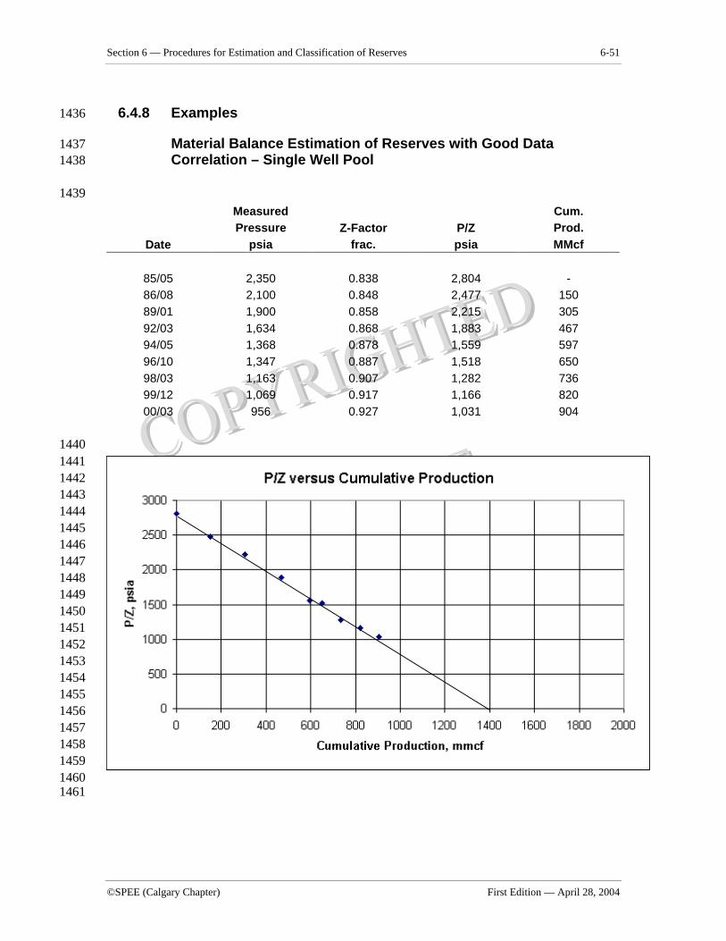
Section 6 — Procedures for Estimation and Classification of Reserves 6-51
©SPEE (Calgary Chapter) First Edition — April 28, 2004
6.4.8 Examples 1436
Material Balance Estimation of Reserves with Good Data 1437 Correlation – Single Well Pool 1438
1439
Date
Measured Pressure
psia Z-Factor
frac. P/Z psia
Cum. Prod. MMcf
85/05 2,350 0.838 2,804 - 86/08 2,100 0.848 2,477 150 89/01 1,900 0.858 2,215 305 92/03 1,634 0.868 1,883 467 94/05 1,368 0.878 1,559 597 96/10 1,347 0.887 1,518 650 98/03 1,163 0.907 1,282 736 99/12 1,069 0.917 1,166 820 00/03 956 0.927 1,031 904
1440 1441 1442 1443 1444 1445 1446 1447 1448 1449 1450 1451 1452 1453 1454 1455 1456 1457 1458 1459 1460
1461
6-52 Volume 2 — Resources and Reserves Estimation and Classification Guidelines
Canadian Oil and Gas Evaluation Handbook ©SPEE (Calgary Chapter)
Original Gas in Place Determination 1461 1. Data Review: 1462
a) There are many data points and they have a good correlation. 1463
b) Geological data, the exhibited pressure data, and a review of analogous 1464 pools does not indicate the likelihood of aquifer support. 1465
2. Proved + Probable OGIP Estimate: 1400 MMcf based on above P/Z versus 1466 Cumulative Production Line. 1467
3. Proved OGIP Estimate: Same value as the proved + probable, due to high 1468 depletion, many data points, and very good correlation of data points. 1469
4. Proved + Probable + Possible OGIP Estimate: Same value as the proved + 1470 probable, due to high depletion, many data points, and very good correlation of 1471 data points. 1472
Reserves Determination 1473 1. Data Review: 1474
a) The reservoir has good permeability and it is likely that economic rates 1475 can be supported down to reservoir pressures of 200 to 400 psia. 1476
b) A review of performance of analogous pools in the area indicates that 1477 water production is rarely a problem late in the life of each pool. 1478
c) Recovery factors of analogous pools are usually in the 86 to 94 percent 1479 range, with a median value of approximately 90 percent. 1480
d) Reserves based on decline curve methods are consistent with the pressure 1481 decline trend. 1482
2. Proved + Probable Reserves Estimate: Based on a recovery factor of 90 percent. 1483
3. Proved Reserves Estimate: Based on 1/2 of the difference between the practical 1484 minimum of 86 percent and the proved + probable estimate of 90 percent, for an 1485 88 percent recovery factor. 1486
4. Proved + Probable + Possible Reserves Estimate: Based on 1/2 of the difference 1487 between the practical maximum of 94 percent and the proved + probable estimate 1488 of 90 percent, for a 92 percent recovery factor. 1489
Section 6 — Procedures for Estimation and Classification of Reserves 6-53
©SPEE (Calgary Chapter) First Edition — April 28, 2004
Material Balance Estimation of Reserves with Moderate Data Scatter 1490 – Single Well Pool 1491
1492
Date
Measured Pressure
psia
Z-Factor
frac.
P/Z psia
Cum.Prod.
MMcf
85/05 2,350 0.838 2,804 -
86/08 2,056 0.848 2,425 150
87/02 2,025 0.852 2,377 250
88/01 1,988 0.847 2,347 289
92/03 1,654 0.868 1,906 467
94/05 1,343 0.878 1,530 597
1493 1494
1495 1496
Practical Maximum
Proved + Probable + Possible
6-54 Volume 2 — Resources and Reserves Estimation and Classification Guidelines
Canadian Oil and Gas Evaluation Handbook ©SPEE (Calgary Chapter)
Original Gas in Place Determination 1496 1. Data Review: 1497
a) There are a few data points, but they have a poor correlation. 1498
b) Geological data, the exhibited pressure data, and a review of analogous 1499 pools does not indicate the likelihood of aquifer support. 1500
c) Volumetric methods indicate a range in OGIP of 1,200 to 1,800 MMcf. 1501
2. Proved + Probable OGIP Estimate: 1,550 MMcf. 1502
3. Proved OGIP Estimate: 1,400 MMcf (approximately midway between the 1503 practical minimum and the proved + probable estimate). 1504
4. Proved + Probable + Possible OGIP Estimate: 1,700 MMcf (approximately 1505 midway between the practical maximum and the proved + probable estimate). 1506
Reserves Estimation 1507 1. Data Review: 1508
a) The reservoir has low permeability, which is likely contributing to 1509 inconsistent pressure buildups and a poor correlation of data points. 1510
b) A review of performance of analogous pools in the area indicates that 1511 water wellbore loading could be a problem late in the life of each pool. 1512
c) Recovery factors of analogous pools are usually 55 to 85 percent, with a 1513 median value of approximately 70 percent. 1514
d) Reserves based on decline curve methods are consistent with the pressure 1515 decline trend. 1516
2. Proved + Probable Reserves Estimate: Based on a recovery factor of 70 percent 1517 on an OGIP of 1,550 MMcf, resulting in an original recoverable reserves 1518 estimate of 1,085 MMcf. 1519
3. Proved Reserves Estimate: Based on a 65 percent recovery factor and an OGIP of 1520 1,400 MMcf, resulting in an original recoverable reserves estimate of 910 MMcf. 1521
4. Proved + Probable + Possible Reserves Estimate: Based on a 75 percent recovery 1522 factor (approximately 1/3 of the difference between the proved + probable and 1523 the practical maximum estimate higher than the proved + probable estimate) and 1524
Section 6 — Procedures for Estimation and Classification of Reserves 6-55
©SPEE (Calgary Chapter) First Edition — April 28, 2004
an OGIP of 1,700 MMcf, resulting in an original recoverable reserves estimate of 1525 1,275 MMcf. 1526
6.4.9 General Considerations in the Use of Material Balance Methods 1527 for Oil Reservoirs 1528
Use of material balance analysis methods for oil reservoirs, like non-associated gas 1529 reservoirs, is based on the premise that the reservoir pore volume changes in a 1530 predictable manner as the pressure declines when oil, gas and/or water are produced. 1531 It is, therefore, possible to equate the expansion of the reservoir fluids upon pressure 1532 drop to the reservoir voidage caused by the production of oil, gas, and water minus 1533 the water influx. The generalized equations can be applied to any type of gas or oil 1534 reservoir where the technique discussed above for gas reservoirs constitutes a special 1535 case. 1536
The successful application of this technique requires an accurate history of the 1537 average reservoir pressure and produced volumes of various phases, as well as the 1538 PVT data for all the phases involved over the pressure range considered. 1539
The most useful application of material balance concepts requires the concurrent use 1540 of fluid flow equations, therefore introducing the time dimension into the analysis. 1541 Although classical material balance techniques were used quite extensively in the 1542 past, they are now largely replaced by numerical reservoir simulators that are 1543 essentially multi-dimensional, multi-phase, and dynamic material balance programs. 1544
6.5 Production Decline Methods 1545
Production decline analysis refers to the analysis of declining production rates as 1546 reservoir fluids are withdrawn. Production declines occur mainly because of pressure 1547 depletion, displacement by another fluid (usually water), or a combination of these 1548 two. Reserves (economically recoverable by definition) are determined by 1549 extrapolation of production rate decline trends to an economic limit. The production 1550 trends derived are used to prepare production forecasts for economic evaluation 1551 purposes. Decline analysis is one of the most widely used reserves interpretation 1552 techniques. It is one of the most reliable methods of analyzing reserves of wells with 1553 sufficient production history, provided it is used properly. Misuse of the method can 1554 result in serious inaccuracies in reserves estimates. A recognizable decline trend must 1555 be apparent in order to perform decline analysis. 1556
6-56 Volume 2 — Resources and Reserves Estimation and Classification Guidelines
Canadian Oil and Gas Evaluation Handbook ©SPEE (Calgary Chapter)
6.5.1 Types of Decline Analysis 1557
There are two main types of decline interpretation techniques: curve fitting and type 1558 curve matching. Both methods can be used in depletion drive pools that are 1559 characterized by transient and pseudo-steady-state (PSS) flow regimes. Figure 6-6, 1560 following this page, illustrates the transient and PSS flow regimes on dimensionless 1561 scales. The transient period occurs prior to the drainage radius reaching boundary 1562 conditions, with PSS flow occurring thereafter. 1563
Only curve fitting is applicable in pressure-supported pools such as waterfloods, 1564 miscible floods, and water drives. Pressure-supported decline behaviour is more 1565 complex than depletion behaviour, because it is characterized by multiple flow 1566 regimes. For example, a waterflooded pool initially produces under transient and PSS 1567 flow, then steady-state flow after commencement of water injection, and, finally, post 1568 water breakthrough flow behaviour. 1569
a. Type Curve Matching 1570
The type curve matching method was developed by M.J. Fetkovich (1973?) and 1571 consists of converting and plotting production data with dimensionless variables, then 1572 overlaying curves to obtain a type curve match (Figure 6-6). The match of the 1573 transient portion of the curve is used to characterize permeability and skin factor. The 1574 inflection point in the type curve is used to quantify drainage area. Finally, the 1575 matching of the Arps depletion stem in the PSS flow regime is used to quantify 1576 recoverable reserves. Computer software packages are available to assist in type 1577 curve analysis. 1578
A key observation in this technique is that the transient decline behaviour does not 1579 relate to the PSS or depletion decline behaviour. This is an important consideration 1580 when dealing with low-permeability reservoirs that have long transient periods. 1581
b. Curve Fitting 1582
Curve fitting is usually the method implied when referring to decline analysis, and it 1583 is the most common method in use today. The curve fitting method refers to 1584 numerically fitting a curve through historical production data with the assumption 1585 that future production decline will be represented by this numerical relationship. The 1586 equation most commonly used was developed by Arps in 1944 (Arps 1945) to 1587 represent a constant flowing pressure solution to a well of fixed drainage radius. 1588
q(t) = qi 1589 (1+bDit)1/b 1590
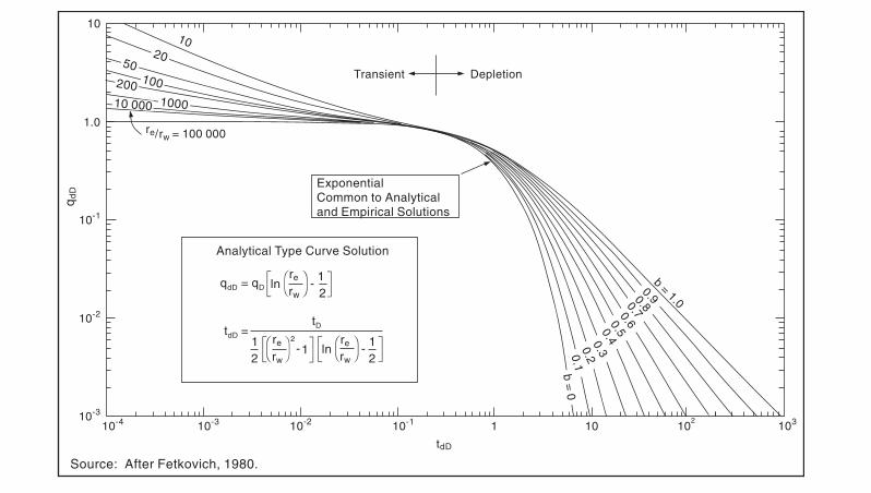
230
DETERMINATION OF OIL AND GAS RESERVES
18.5.4 Dimensionless Solutions andType-Curve Matching
Fetkovich (1980) used simplified material balance andinflow performance relationships for both gas and oilwells to show that the Arps’ empirical equations matchup with some of the classical solutions to the radial flowdiffusivity equation. Exponential decline was shown tobe the long-time solution to the constant terminalpressure case (constant bottom-hole pressure). Theshort-time (transient) solution is a function of thereservoir size expressed as re/rw ratios (re = externalboundary radius, rw = wellbore radius). Fetkovich dem-onstrated that for oil wells (slightly compressiblesingle-phase flow) the type of decline does not changewith the drawdown. On the other hand, for gas wells(compressible single-phase flow) it was demonstratedthat a change in back pressure changes the type of de-cline. This finding helps explain the reliability of declineanalysis for oil wells. In many practical cases, wells areproduced at capacity and the bottom-hole pressure doesnot change significantly over time (i.e., the well ispumped off). Fetkovich demonstrated that empiricaldecline curve analysis has a solid theoretical base.
Figure 18.5-6 shows his analytical transient type curvescombined with Arps’ empirical depletion type curves.The depletion type curves are essentially the same asthose proposed by Gentry; however, Fetkovich plottedq/qi instead of qi/q and used log-log coordinates tofacilitate type-curve matching. It is apparent from Fig-ure 18.5-6 that the transition from transient to depletionbehaviour occurs at a dimensionless time of approxi-mately 0.3. Figure 18.5-6 also shows that until thedimensionless time exceeds 0.3, it is impossible to knowthe type of decline that ultimately develops. Thus, thesafest approach to extrapolating trends early in the lifeof a well is to assume an exponential decline.
Type-curve matching was first used to interpretpressure buildup and drawdown data. The procedure in-volves comparing the pressure-time data from a wellwith a family of dimensionless solutions. The same gen-eral procedure is used for decline data. Fetkovichsummarizes the procedure as follows:
1. The actual rate-time production data are plotted ona log-log tracing paper of the same size as the typecurves to be used. Any convenient units can beused for rate or time because a change in units
103
10
1.0
qd
D
10-1
10-2
10-3
10-4 10-3 10-2 10-1
tdD
1 10 102
re/rw = 100 000
10
b = 1.00.20.1
0.50.40.3
0.60.7
0.80.9
DepletionTransient
qdD = qD lnre
rw-
12
ExponentialCommon to Analyticaland Empirical Solutions
lnre re
rw rw- -
1 12 2
tdD =2
1
tD
Analytical Type Curve Solution
2050
100200100010 000
Source: After Fetkovich, 1980.
b = 0
Figure 18.5-6 Composite of Analytical and Empirical Type Curves
Section 6 — Procedures for Estimation and Classification of Reserves 6-57
©SPEE (Calgary Chapter) First Edition — April 28, 2004
Where, 1591
qi = initial rate 1592
q(t) = rate at time t 1593
b = decline exponent 1594
Di = initial decline 1595
The best fit can be either exponential when b approaches 0, hyperbolic when b > 0, or 1596 harmonic when b = 1. 1597
The best fit can be computer calculated or visual. Visual best fit exponential decline 1598 is based on a straight line arithmetic rate vs. cumulative production plot, or a straight 1599 line log of rate vs. time. Visual best fit harmonic decline is based on a straight line 1600 log rate vs. cumulative production plot. Visual best fit hyperbolic decline is derived 1601 by overlaying calculated profiles on rate vs. cumulative production plots. 1602
Other decline methods in use today such as water/oil ratio, oil-cut trend analysis, and 1603 Blasingame type curve matching are variations of the above two methods. 1604
6.5.2 Limitations of Methods 1605
Decline methods have a number of theoretical limitations: 1606
• Decline equations are only arithmetic approximations for future behaviour based 1607 on historic behaviour. Reservoir geometry, properties, and operating conditions 1608 could be such that no single relationship is valid for the remaining life of a well. 1609
• Only the PSS phase of production history for depletion drive reservoirs can be 1610 analyzed with curve fitting methods. The transient period must be excluded from 1611 the curve fitting. For type curve matching, the entire history may be used. 1612
• Constant wellbore pressure conditions must exist to reliably curve fit and type 1613 curve match. If these conditions are not met, there are methods of normalizing 1614 the data for more accurate results. If normalization is not performed, then the fit 1615 represents the case where the rate of pressure change continues at the same pace 1616 throughout the life of the well, which is not valid. Often, wellbore flowing 1617 pressure history is not available; therefore, engineers must use their knowledge 1618 and experience to determine which and how historical data should be curve fit. 1619
The normalization equation for a gas well is as follows: 1620
6-58 Volume 2 — Resources and Reserves Estimation and Classification Guidelines
Canadian Oil and Gas Evaluation Handbook ©SPEE (Calgary Chapter)
Normalized Rate = Measured Rate x ((Pts2 –Pmlp
2)/(Pts2-Pnlp
2))n 1621
Where, 1622
Pts = static wellhead pressure 1623
Pmlp = measured line pressure 1624
Pnlp = normalized line pressure 1625
N = wellhead deliverability exponent 1626
• Pressure-supported reservoirs can be analyzed with curve fitting, but not type 1627 curve matching. The fit is only representative for the duration of the flow regime; 1628 therefore, curve fitting should not be performed to determine reserves until 1629 injected fluid breakthrough trends are exhibited (post breakthrough regime). 1630
• Harmonic decline behaviour should be used with caution, because it may not be 1631 clear how long the well will continue harmonic behaviour. Harmonic rate 1632 declines extrapolate to infinity at zero rate; therefore, at some point they must 1633 become exponential. The practical significance is whether this occurs prior to or 1634 after reaching economic limit. 1635
• Future drilling affects current decline trends. The derived fits are only valid for 1636 the existing field development. Further field development such as infill drilling 1637 will change the decline behaviour of offset wells if interference occurs. The 1638 uncertainty lies in predicting when interference occurs. 1639
6.5.3 Factors Affecting Decline Behaviour 1640
There are certain factors that determine whether declines are steep, shallow, 1641 exponential, hyperbolic, or harmonic. These factors include rock and fluid properties, 1642 reservoir geometry, drive mechanisms, completion techniques, operating practices, 1643 and type of wellbore. Reservoir engineers must have an understanding of these 1644 factors prior to analyzing decline trends, in order to make a reliable assessment. 1645
a. Rock and Fluid properties 1646
i. Stratification 1647
Reservoirs with a high degree of stratification or high permeability variation tend to 1648 decline along hyperbolic or harmonic trends, while homogeneous reservoirs tend to 1649
Section 6 — Procedures for Estimation and Classification of Reserves 6-59
©SPEE (Calgary Chapter) First Edition — April 28, 2004
decline along exponential trends. This is a result of differential expansion of drainage 1650 radii in the layers and differential depletion of the layers (Fetkovich et al. 1996). 1651
ii. Wettability 1652
Strongly oil-wet rocks combined with low-gravity (high-viscosity) crude oils will 1653 exhibit hyperbolic or harmonic trends following water breakthrough, because of the 1654 shape of the fractional flow curve. Also, in oil-wet rocks, interfacial tension tends to 1655 bind the oil to the rock surface, causing oil to become increasingly difficult to recover 1656 as water saturation increases, which results in hyperbolic or harmonic trends. 1657 Strongly water-wet rocks combined with high-gravity (low-viscosity) crude oils tend 1658 to decline more exponentially. 1659
iii. Relative Permeability 1660
Masoner (1998) examined the effect of the shape of relative permeability 1661 relationships in secondary and tertiary recovery schemes on the Arps decline 1662 exponent. In general, more curvature in relative permeability curves results in higher 1663 decline exponents. 1664
iv. Permeability 1665
Low-permeability reservoirs have a long transition period, which is frequently super 1666 harmonic in nature, followed by shallow PSS decline trends. High-permeability 1667 reservoirs, if produced at capacity, have steeper decline trends compared to lower 1668 permeability reservoirs of similar volume. These steeper declines tend to be more 1669 exponential. 1670
v. Fracturing 1671
Fractured reservoirs can exhibit exponential to harmonic behaviour, depending on the 1672 contribution of the matrix to the dual porosity behaviour. 1673
vi. Back Pressure Slope 1674
Fetkovich et al. (1996) demonstrated that the theoretical values of the Arps decline 1675 exponent below bubble point are a function of the slope of the back-pressure curve. 1676 The decline exponent approaches zero for high-permeability, tubing-limited flow 1677 behaviour, where the back-pressure slope is 0.5, whereas the decline exponent is 0.33 1678 (oil) and 0.5 (gas) for low-permeability reservoirs that are reservoir limited. Values 1679 greater than 0.5 can be demonstrated for layered no-cross-flow reservoirs. 1680
6-60 Volume 2 — Resources and Reserves Estimation and Classification Guidelines
Canadian Oil and Gas Evaluation Handbook ©SPEE (Calgary Chapter)
b. Reservoir Geometry and Drive Mechanism 1681
i. Vertical Displacement 1682
Reservoirs with vertical displacement drive mechanisms usually exhibit non-1683 declining behaviour prior to breakthrough of the displacing fluid, exponential decline 1684 after breakthrough of the displacement fluid as the oil and gas column thins, and 1685 hyperbolic decline behaviour when coning dominates the flow characteristics in late 1686 stage depletion of the reservoir. In the case of gas wells, the post breakthrough 1687 decline can be very steep. In these cases, prior to breakthrough, volumetric, analogy, 1688 and/or material balance methods that consider aquifer influx must be used to 1689 establish reserve estimates. 1690
ii. Coning 1691
For bottom-water drive oil reservoirs, coning behaviour usually results in hyperbolic 1692 decline trends. The decline tends to be more exponential for low viscosity and/or 1693 water-wet systems and more harmonic for high viscosity and/or oil wet systems. 1694
iii. Horizontal Displacement 1695
Decline behaviour in horizontal displacement drive mechanisms is a function of the 1696 rock and fluid properties of the reservoirs. 1697
iv. Unconsolidated Heavy Oil Reservoirs 1698
Unconsolidated sandstone solution-gas drive heavy oil reservoirs usually exhibit 1699 increasing productivity as the wellbore radius increases with sand production, a 1700 period of constant productivity as sand production reduces, then catastrophic decline 1701 behaviour due to wormhole collapse and/or foamy oil viscosity behaviour. Reserves 1702 analysis for these types of reservoirs must be based on volumetric or statistical 1703 reserves life index methods. 1704
c. Completion and Operating Practices 1705
i. Skin Factors 1706
Skin factors affect decline performance by changing the productivity as well as the 1707 decline slope of wells. Positive skin factors are caused by wellbore damage, which 1708 decreases productivity. Negative skin factors are usually a result of wellbore 1709 stimulation, which increases productivity. In addition to productivity changes, 1710 negative skin factors result in more hyperbolic bending of production declines during 1711 the transient phase. 1712
Section 6 — Procedures for Estimation and Classification of Reserves 6-61
©SPEE (Calgary Chapter) First Edition — April 28, 2004
ii. Fluid Rate Changes 1713
Total fluid (water plus oil) rate changes can be caused by changes in drawdown, 1714 over-injection, or under-injection. While total fluid rates are increasing, oil rate 1715 decline trends are dampened. Increasing or decreasing drawdown of a well violates 1716 the constant flowing pressure assumption of decline analysis and, therefore, will 1717 result in an unreliable decline fit. 1718
iii. Workovers 1719
Workovers on wells cause sudden increases in production rates. The future decline of 1720 a well after a workover is often difficult to predict. If the workover opens up 1721 previously unaccessed reservoir, the producing reserves of the well will now be the 1722 previously accessed reserves derived from decline analysis plus reserves associated 1723 with the new accessed reservoir, which can be estimated from volumetric analysis. If 1724 the workover simply removes wellbore damage, reserves can be estimated by 1725 examining decline trends prior to the wellbore damage. This procedure relies 1726 extensively on the judgement and experience of the evaluator in picking the correct 1727 trend. Workovers often result in a combination of both of the above results. Caution 1728 must be exercised in assessing results immediately after a workover, because 1729 production rates are likely in transient, not PSS, flow. In these cases, a review of the 1730 results of analogous workovers could be beneficial in assessing results. 1731
iv. Infill Drilling 1732
Infill drilling can affect decline behaviour of offset wells because of drainage 1733 interference; therefore, decline analysis is only valid for the current well 1734 configuration. 1735
v. Regulatory Constraints 1736
Regulatory constraints such as oil well allowables mask decline behaviour. 1737
vi. Facility Constraints 1738
Facility throughput limitations can also mask decline behaviour. 1739
d. Type of Wellbore 1740
i. Horizontal versus Vertical Wellbore 1741
Decline behaviour of horizontal wells is different from that of vertical wells, though 1742 the decline interpretation techniques are similar. 1743
6-62 Volume 2 — Resources and Reserves Estimation and Classification Guidelines
Canadian Oil and Gas Evaluation Handbook ©SPEE (Calgary Chapter)
ii. Coning Situations 1744
Horizontal wells are often drilled to reduce drawdown, which masks early decline 1745 behaviour. Also, due to the geometry of the cone, decline profiles in horizontal wells 1746 after the transient period are usually less hyperbolic than vertical wells. 1747
iii. Wellbore Contact 1748
Horizontal wells are also drilled to increase wellbore contact with the reservoir. This 1749 causes higher initial production rates and steeper initial transient flow decline rates 1750 than those obtained by drilling vertical wells. 1751
6.5.4 Guidelines for Individual Well Decline Analysis 1752
In light of the numerous factors described above that affect decline trends, the 1753 following generalized guidelines are recommended when performing decline 1754 analysis. 1755
a. Reservoir Properties Review 1756
Understand the depletion mechanism and rock and fluid properties. This does not 1757 necessarily entail a detailed geological study, but rather a review of the log character 1758 to get a sense of the presence or absence of bottom water and the degree of 1759 stratification or variability. A review of the fluid analysis also establishes the gravity 1760 and viscosity of the oil being produced, or the quantity of liquids, in the case of a gas 1761 well. 1762
b. Analogy Review 1763
Review regional decline trends of more mature wells in the same zone with similar 1764 reservoir properties, especially for wells with little production history. The more 1765 similar the reservoir properties and the closer the location of the analogy to the well 1766 being analyzed, the more valid the analogy. It is important to review the late-time 1767 behaviour of analogies to verify if change in flow behaviour, such as liquid loading, 1768 occurs. 1769
c. Transient Period Estimation 1770
Estimate the length of the transient period. This will establish whether the well has 1771 sufficient history for use of the curve fitting technique. Exclude the transient period 1772 data when curve fitting, but include the transient period when type curve matching. 1773 For transient flow, only decline analogies or volumetric methods can be used to 1774 establish reserves. The estimation of the length of the transient period is not always 1775
Section 6 — Procedures for Estimation and Classification of Reserves 6-63
©SPEE (Calgary Chapter) First Edition — April 28, 2004
straightforward. In high-permeability reservoirs, the period is usually short enough so 1776 as not to be a concern. In low-permeability reservoirs, this period can be lengthy and 1777 the transition to PSS can be unclear. There are two main ways to determine the 1778 transient period: 1779
i. Buildup Analysis 1780
If the buildup is still transient, the permeability calculated from the buildup can be 1781 used, along with an estimated drainage area, to calculate the time to PSS. If the well 1782 is in a defined pool, the drainage area can be reasonably well established; however, 1783 often the drainage area is not clearly defined. If the buildup shows boundary effects, 1784 the drainage areas are more clearly defined and the time to PSS more reliable. If 1785 boundaries are exhibited, then pressure buildup extrapolations and material balance 1786 analysis could also be performed. 1787
ii. Type Curve Analysis 1788
If Fetkovich type curve analysis is done, then the entire well history is used, with the 1789 inflection point of the dimensionless rate vs. time being the time to PSS. As a 1790 diagnostic indicator, log cumulative production vs. log producing time may be 1791 plotted, with the departure from straight line behaviour marking the start of PSS 1792 behaviour. 1793
d. Final Rate Determination 1794
Calculate the final rate to be used for decline analysis. This is usually either the 1795 economic limit or a value less than the economic limit when economic programs are 1796 used to determine the actual economic limit under different pricing scenarios. In the 1797 case of gas wells with water and/or oil and gas liquid production, it may be the 1798 physical lifting limit of the fluids in the wellbore. A review of water/gas ratio trends 1799 could be useful in establishing final rates at practical maximum water/gas ratio limits. 1800
e. Operating Constraint Review 1801
Use periods of constant operating constraints when fitting curves, or normalize data 1802 to reflect constant bottom-hole pressure conditions. For gas wells, review flowing 1803 wellhead pressure histories, if available, prior to establishing the decline matches. 1804
f. Data Review 1805
Select data that most closely represent stabilized conditions (i.e., calendar-day trends 1806 in low-permeability reservoirs and producing-day trends in high-permeability 1807
6-64 Volume 2 — Resources and Reserves Estimation and Classification Guidelines
Canadian Oil and Gas Evaluation Handbook ©SPEE (Calgary Chapter)
reservoirs.) Rate vs. cumulative production relationships must be used instead of log 1808 rate vs. time relationships to prevent inaccuracies caused by shut-in times. 1809
g. Re-Initialization 1810
Re-initialize declines after changes in drawdown, workovers, or stimulations. Initial 1811 production rates after these activities will be transient in nature and might not 1812 necessarily represent longer-term PSS trends. 1813
h. Oil-Cut Analysis 1814
Use oil-cut analysis when fluid rates are constant or increasing gradually. If fluid 1815 rates are increasing quickly, a transient flow period is introduced, which will not be 1816 representative of longer-term declines. In these cases, go back to periods of constant 1817 or gradually changing fluid rates to establish long-term trends. Use these 1818 extrapolations to estimate end-point reserves, and then adjust initial rates and 1819 exponents to match near-term behaviour. 1820
i. Line-Pressure Adjustments 1821
Account for increased reserves and rates from future line-pressure reductions for gas 1822 wells. This can be calculated from first principles based on the change in flowing 1823 pressure conditions relative to bottom-hole pressures. If line pressures have been 1824 reducing throughout the well’s history, further adjustments might not be necessary, 1825 because historical curvature of the decline trend might already be caused by line 1826 pressure reductions. In these cases, normalization of data is the only rigorous method 1827 of determining reliable decline characteristics. 1828
j. Interference Effects 1829
The potential for interference effects must be considered when selecting long-term 1830 decline characteristics. 1831
k. Production Forecasts 1832
Production forecast trends should normally be consistent with historical trends. 1833 However, as a result of consideration of the influences described above, production 1834 forecast trends used for evaluation purposes may not always be consistent with 1835 historical data. For major property reporting purposes, explanations of these instances 1836 should be provided (COGEH Volume 1, Section 11.2.2). 1837
Section 6 — Procedures for Estimation and Classification of Reserves 6-65
©SPEE (Calgary Chapter) First Edition — April 28, 2004
6.5.5 Guidelines for Group Decline Analysis 1838
Group decline analysis is usually performed to reduce evaluation time and smooth 1839 statistical variations and interference effects. The general guidelines for single-well 1840 analysis apply; however, some additional guidelines relating to group analysis are as 1841 follows. 1842
a. Grouping 1843
Wells should be grouped by common characteristics so as not to mix different 1844 profiles that do not, as a group, give the same numeric answer. Common grouping 1845 techniques in sequence of order include 1846
• pool (so as not to mix unrelated reservoirs), 1847
• pattern or drive mechanism (so as not to mix EOR versus primary profiles), 1848
• geographic region (to allow for regional volumetric comparisons), 1849
• producing versus shut-in (for existing wells), 1850
• startup date (to prevent increasing well counts), 1851
• productivity or water cut (to group wells of similar decline trend), 1852
• common working interests, 1853
• common group meters (in the case of shallow gas areas, where wells are 1854 infrequently tested and allocated production from the group meters). 1855
b. Voidage Replacement 1856
Decline trends in the case of EOR schemes should be matched during periods of 1857 stable voidage replacement. If the EOR scheme is not capable of maintaining 1858 voidage, then decline fits of recent rate trends are applicable. 1859
c. Breakthrough Behaviour 1860
Also for EOR schemes, decline forecasts are only reliable if they exhibit post 1861 breakthrough behaviour. If breakthrough has not been established, then volumetric or 1862 simulation methods must be used. If breakthrough is established in some of the 1863 geographic regions but not in others, then decline analysis should be used in the areas 1864 with breakthrough, and analogous recovery factors or decline profiles should be 1865 applied to determine reserves in the non-breakthrough areas. 1866
6-66 Volume 2 — Resources and Reserves Estimation and Classification Guidelines
Canadian Oil and Gas Evaluation Handbook ©SPEE (Calgary Chapter)
6.5.6 Guidelines for Reserves Classification from Decline Analysis 1867
If all the above factors are considered, a computer-generated best fit will give an 1868 initial guide as to the reserves assignment. The choice of best estimate case reserves, 1869 which represents the 2P reserves estimate, must be made after considering the quality 1870 of the fit, the uniqueness of the fit, the range of expected exponents, and the 1871 reasonableness of the reserves or life. Caution must be used, however, if relying on 1872 computer generated best fits, because there is always reservoir uncertainty and late-1873 time behaviour, which may change decline rates and exponents in the future. A 1874 review of the decline behaviour of more mature analogous wells in the area is 1875 required to prevent inappropriate derivation of decline exponents. The choice of fit 1876 should match current decline behaviour and reasonably fit long-term trends. If 1877 decline characteristics have changed during the life of a well because of outside 1878 influences (interference from other wells, water breakthrough, damage, workovers, 1879 stimulations, etc.) it is not appropriate to match long-term trends. 1880
If there is no material difference in the quality of a computer generated fit for a wide 1881 range of decline rates and exponents, then the evaluator must use judgement in 1882 picking the most reasonable decline rate and exponent based on his understanding of 1883 the reservoir characteristics and analogies. It is recommended that secondary 1884 methods, such as volumetrics and material balance, be considered for all significant 1885 entities with high exponents, poorly defined, or non-unique decline trends. For 2P 1886 determination, if very little information is available on analogies or reservoir 1887 characteristics, the decline analysis must be performed using the lowest exponent that 1888 reasonably fits the data. 1889
It is also acceptable to visually fit curves to pick the most reasonable decline rate and 1890 exponent, using the best estimate exponent derived from analogies or reservoir 1891 characteristics. 1892
After decline fits are derived for 2P reserves, proved reserves are estimated by either 1893 reducing the exponent, increasing the current decline rate, or selecting more 1894 conservative data points and refitting the data. Usually, depending on data scatter, a 1895 target reduction of between 1/3 and 2/3 of the difference between 2P and a 1896 reasonable minimum estimate meets acceptable proved confidence criteria. Wells 1897 with definitive decline trends may have little or no range between proved and 2P, 1898 whereas wells with more data scatter or less maturity may have a higher range. 1899
Similarly, the exponent is increased, the current decline rate decreased, or more 1900 optimistic data points selected and the data refitted for 3P determination. A target 1901
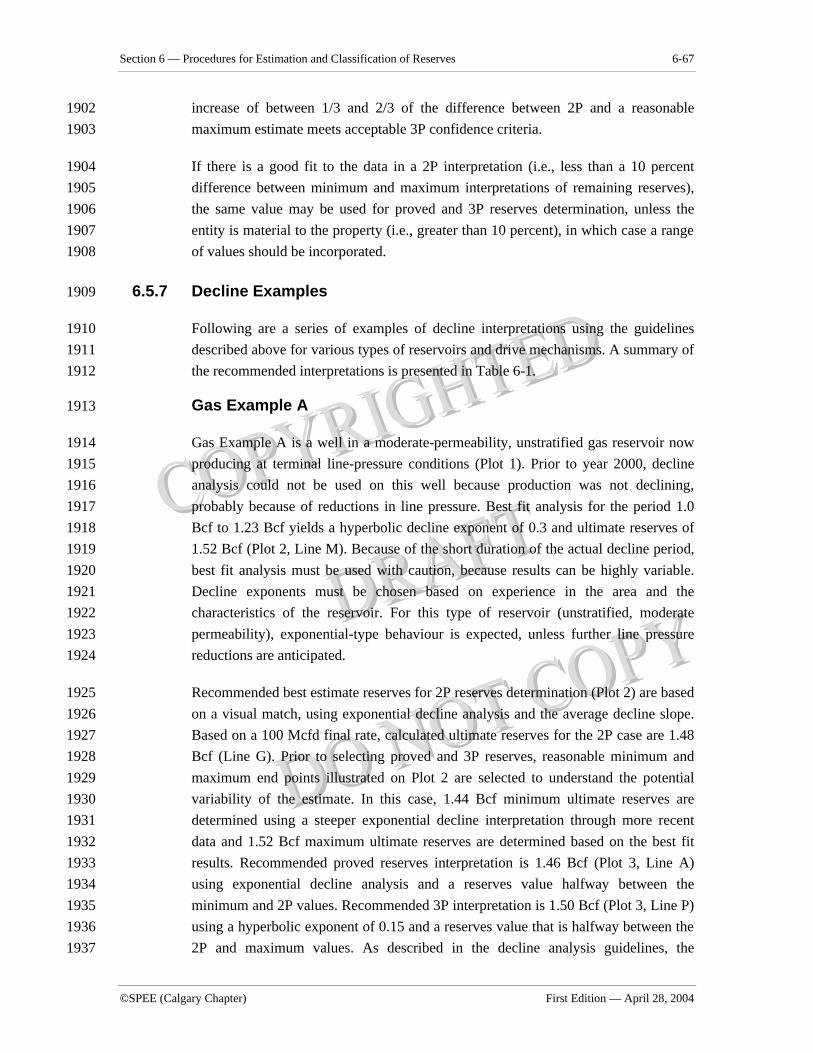
Section 6 — Procedures for Estimation and Classification of Reserves 6-67
©SPEE (Calgary Chapter) First Edition — April 28, 2004
increase of between 1/3 and 2/3 of the difference between 2P and a reasonable 1902 maximum estimate meets acceptable 3P confidence criteria. 1903
If there is a good fit to the data in a 2P interpretation (i.e., less than a 10 percent 1904 difference between minimum and maximum interpretations of remaining reserves), 1905 the same value may be used for proved and 3P reserves determination, unless the 1906 entity is material to the property (i.e., greater than 10 percent), in which case a range 1907 of values should be incorporated. 1908
6.5.7 Decline Examples 1909
Following are a series of examples of decline interpretations using the guidelines 1910 described above for various types of reservoirs and drive mechanisms. A summary of 1911 the recommended interpretations is presented in Table 6-1. 1912
Gas Example A 1913
Gas Example A is a well in a moderate-permeability, unstratified gas reservoir now 1914 producing at terminal line-pressure conditions (Plot 1). Prior to year 2000, decline 1915 analysis could not be used on this well because production was not declining, 1916 probably because of reductions in line pressure. Best fit analysis for the period 1.0 1917 Bcf to 1.23 Bcf yields a hyperbolic decline exponent of 0.3 and ultimate reserves of 1918 1.52 Bcf (Plot 2, Line M). Because of the short duration of the actual decline period, 1919 best fit analysis must be used with caution, because results can be highly variable. 1920 Decline exponents must be chosen based on experience in the area and the 1921 characteristics of the reservoir. For this type of reservoir (unstratified, moderate 1922 permeability), exponential-type behaviour is expected, unless further line pressure 1923 reductions are anticipated. 1924
Recommended best estimate reserves for 2P reserves determination (Plot 2) are based 1925 on a visual match, using exponential decline analysis and the average decline slope. 1926 Based on a 100 Mcfd final rate, calculated ultimate reserves for the 2P case are 1.48 1927 Bcf (Line G). Prior to selecting proved and 3P reserves, reasonable minimum and 1928 maximum end points illustrated on Plot 2 are selected to understand the potential 1929 variability of the estimate. In this case, 1.44 Bcf minimum ultimate reserves are 1930 determined using a steeper exponential decline interpretation through more recent 1931 data and 1.52 Bcf maximum ultimate reserves are determined based on the best fit 1932 results. Recommended proved reserves interpretation is 1.46 Bcf (Plot 3, Line A) 1933 using exponential decline analysis and a reserves value halfway between the 1934 minimum and 2P values. Recommended 3P interpretation is 1.50 Bcf (Plot 3, Line P) 1935 using a hyperbolic exponent of 0.15 and a reserves value that is halfway between the 1936 2P and maximum values. As described in the decline analysis guidelines, the 1937

6-68 Volume 2 — Resources and Reserves Estimation and Classification Guidelines
Canadian Oil and Gas Evaluation Handbook ©SPEE (Calgary Chapter)
selection of proved values between 1/3 and 2/3 of the distance between minimum and 1938 best estimate values is acceptable. Similarly, the selection of 3P values between 1/3 1939 and 2/3 of the distance between maximum and best estimate values is acceptable. 1940
In this example, a 100 Mcfd final rate is chosen, because of water lifting capacity 1941 rather than economic limit. A review of wells in the area indicates most wells cease 1942 production at a rate of 100 Mcfd. The reported water production on the plots is likely 1943 not meaningful because of lack of reliable measurement. 1944
1945
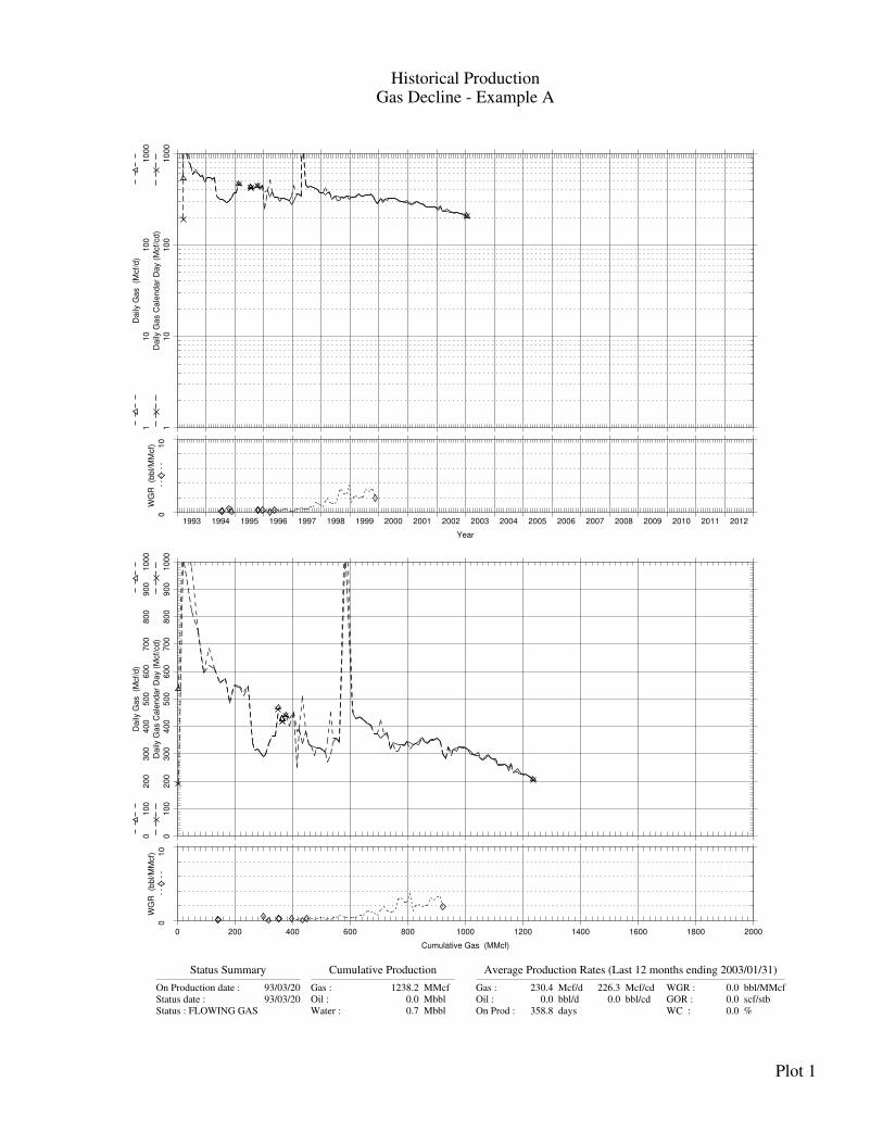
Historical ProductionGas Decline - Example A
Status Summary
On Production date : 93/03/20
Status date : 93/03/20
Status : FLOWING GAS
Cumulative Production
Gas : 1238.2 MMcf
Oil : 0.0 Mbbl
Water : 0.7 Mbbl
Average Production Rates (Last 12 months ending 2003/01/31)
Gas : 230.4 Mcf/d
Oil : 0.0 bbl/d
On Prod : 358.8 days
226.3 Mcf/cd
0.0 bbl/cd
WGR : 0.0 bbl/MMcf
GOR : 0.0 scf/stb
WC : 0.0 %
Plot 1
1993 1994 1995 1996 1997 1998 1999 2000 2001 2002 2003 2004 2005 2006 2007 2008 2009 2010 2011 2012
Year
11
01
00
10
00
Da
ily G
as C
ale
nd
ar
Da
y (
Mcf/
cd
)
11
01
00
10
00
Da
ily G
as
(Mcf/
d)
01
0
WG
R
(bb
l/M
Mcf)
0 200 400 600 800 1000 1200 1400 1600 1800 2000
Cumulative Gas (MMcf)
01
00
20
03
00
40
05
00
60
07
00
80
09
00
10
00
Da
ily G
as C
ale
nd
ar
Da
y (
Mcf/
cd
)
01
00
20
03
00
40
05
00
60
07
00
80
09
00
10
00
Da
ily G
as
(Mcf/
d)
01
0
WG
R
(bb
l/M
Mcf)
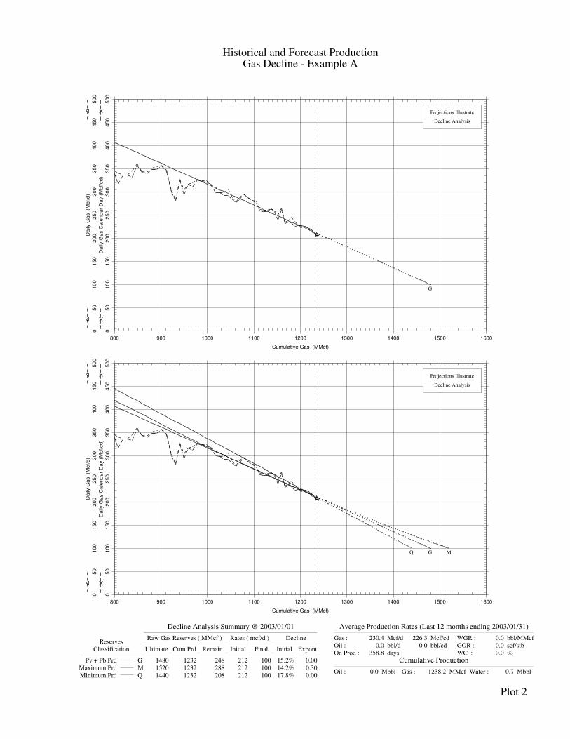
Historical and Forecast ProductionGas Decline - Example A
Decline Analysis Summary @ 2003/01/01
ReservesRaw Gas Reserves ( MMcf ) Rates ( mcf/d ) Decline
Classification Ultimate Cum Prd Remain Initial Final Initial Expont
Pv + Pb Prd G 1480 1232 248 212 100 15.2% 0.00
Maximum Prd M 1520 1232 288 212 100 14.2% 0.30
Minimum Prd Q 1440 1232 208 212 100 17.8% 0.00
Average Production Rates (Last 12 months ending 2003/01/31)
Gas : 230.4 Mcf/d
Oil : 0.0 bbl/d
On Prod : 358.8 days
226.3 Mcf/cd
0.0 bbl/cd
WGR : 0.0 bbl/MMcf
GOR : 0.0 scf/stb
WC : 0.0 %
Cumulative Production
Oil : 0.0 Mbbl Gas : 1238.2 MMcf Water : 0.7 Mbbl
Plot 2
800 900 1000 1100 1200 1300 1400 1500 1600
Cumulative Gas (MMcf)
05
01
00
15
02
00
25
03
00
35
04
00
45
05
00
Da
ily G
as C
ale
nd
ar
Da
y (
Mcf/
cd
)
05
01
00
15
02
00
25
03
00
35
04
00
45
05
00
Da
ily G
as
(Mcf/
d)
G
Projections Illustrate
Decline Analysis
800 900 1000 1100 1200 1300 1400 1500 1600
Cumulative Gas (MMcf)
05
01
00
15
02
00
25
03
00
35
04
00
45
05
00
Da
ily G
as C
ale
nd
ar
Da
y (
Mcf/
cd
)
05
01
00
15
02
00
25
03
00
35
04
00
45
05
00
Da
ily G
as
(Mcf/
d)
G
Projections Illustrate
Decline Analysis
MQ
Historical and Forecast ProductionGas Decline - Example A
Decline Analysis Summary @ 2003/01/01
ReservesRaw Gas Reserves ( MMcf ) Rates ( mcf/d ) Decline
Classification Ultimate Cum Prd Remain Initial Final Initial Expont
Pv Prd A 1460 1232 228 212 100 16.4% 0.00
Pv + Pb Prd G 1480 1232 248 212 100 15.2% 0.00
Pv + Pb + Poss Prd P 1500 1232 268 212 100 14.6% 0.15
Average Production Rates (Last 12 months ending 2003/01/31)
Gas : 230.4 Mcf/d
Oil : 0.0 bbl/d
On Prod : 358.8 days
226.3 Mcf/cd
0.0 bbl/cd
WGR : 0.0 bbl/MMcf
GOR : 0.0 scf/stb
WC : 0.0 %
Cumulative Production
Oil : 0.0 Mbbl Gas : 1238.2 MMcf Water : 0.7 Mbbl
Plot 3
800 900 1000 1100 1200 1300 1400 1500 1600
Cumulative Gas (MMcf)
05
01
00
15
02
00
25
03
00
35
04
00
45
05
00
Da
ily G
as C
ale
nd
ar
Da
y (
Mcf/
cd
)
05
01
00
15
02
00
25
03
00
35
04
00
45
05
00
Da
ily G
as
(Mcf/
d)
A
Projections Illustrate
Decline Analysis
G P
800 900 1000 1100 1200 1300 1400 1500 1600
Cumulative Gas (MMcf)
05
01
00
15
02
00
25
03
00
35
04
00
45
05
00
Da
ily G
as C
ale
nd
ar
Da
y (
Mcf/
cd
)
05
01
00
15
02
00
25
03
00
35
04
00
45
05
00
Da
ily G
as
(Mcf/
d)
A
Projections Illustrate
Decline Analysis
G MPQ
Section 6 — Procedures for Estimation and Classification of Reserves 6-69
©SPEE (Calgary Chapter) First Edition — April 28, 2004
Gas Example B 1945
Gas Example B is a well in a moderate-permeability, unstratified gas reservoir in the 1946 early stage of depletion (Plot 4). Line pressure is approximately 300 psi, with future 1947 terminal line-pressure conditions expected to be 100 psi. This future line-pressure 1948 reduction is calculated to increase recovery by approximately 21 percent over 1949 extrapolations at current conditions. As this is a known moderate-permeability 1950 unstratified reservoir, decline behaviour is expected to be exponential under current 1951 line-pressure conditions, and slightly hyperbolic with future line-pressure reductions. 1952
Recommended best estimate reserves for 2P reserves determination of 3.07 Bcf (Plot 1953 5, Line G) are estimated by increasing the current minimum exponential forecast 1954 reserves of 2.53 Bcf (Line Q) by a factor of 1.21 to reflect recovery with additional 1955 line-pressure reduction. A hyperbolic decline exponent of 0.2 is selected to match 1956 this forecast end point at a 50 Mcfd final rate (liquid loading limit) with the current 1957 decline slope. Prior to selecting proved and 3P reserves, reasonable minimum and 1958 maximum end points illustrated on Plot 5 are selected to understand the potential 1959 variability of the estimate. In this case, 2.53 Bcf minimum ultimate reserves is 1960 determined using an exponential decline interpretation through recent data, while 1961 4.10 Bcf maximum ultimate reserves is determined using an optimistic 0.5 decline 1962 exponent, to reflect the possibility of remote tighter gas contribution in addition to 1963 increases because of line-pressure reductions. Recommended proved reserves 1964 interpretation is 2.74 Bcf (Plot 6, Line A), using exponential decline analysis and a 1965 reserves value between the minimum and 2P values. Recommended 3P interpretation 1966 is 3.52 Bcf (Plot 6, Line P) using a hyperbolic exponent of 0.35 and a reserves value 1967 between the 2P and maximum values. As described in the decline analysis guidelines, 1968 the selection of proved values between 1/3 and 2/3 of the distance between minimum 1969 and best estimate values is acceptable. Similarly, the selection of values between 1/3 1970 and 2/3 of the distance between maximum and best estimate values is acceptable. 1971
Actual performance of the well resulted in cumulative production of 3.00 Bcf (Plot 1972 7). As expected, hyperbolic bending was very slight due to moderate line-pressure 1973 reductions. In this particular case, the 2P estimate was slightly high; however, the 1974 proved estimate was exceeded. 1975
1976 1977
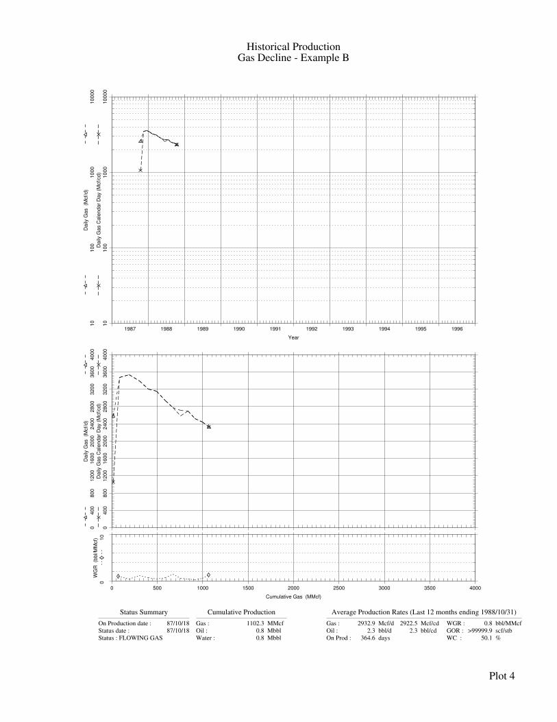
Historical ProductionGas Decline - Example B
Status Summary
On Production date : 87/10/18
Status date : 87/10/18
Status : FLOWING GAS
Cumulative Production
Gas : 1102.3 MMcf
Oil : 0.8 Mbbl
Water : 0.8 Mbbl
Average Production Rates (Last 12 months ending 1988/10/31)
Gas : 2932.9 Mcf/d
Oil : 2.3 bbl/d
On Prod : 364.6 days
2922.5 Mcf/cd
2.3 bbl/cd
WGR : 0.8 bbl/MMcf
GOR : >99999.9 scf/stb
WC : 50.1 %
Plot 4
1987 1988 1989 1990 1991 1992 1993 1994 1995 1996
Year
10
10
01
00
01
00
00
Da
ily G
as C
ale
nd
ar
Da
y (
Mcf/
cd
)
10
10
01
00
01
00
00
Da
ily G
as
(Mcf/
d)
0 500 1000 1500 2000 2500 3000 3500 4000
Cumulative Gas (MMcf)
04
00
80
01
20
01
60
02
00
02
40
02
80
03
20
03
60
04
00
0
Da
ily G
as C
ale
nd
ar
Da
y (
Mcf/
cd
)
04
00
80
01
20
01
60
02
00
02
40
02
80
03
20
03
60
04
00
0
Da
ily G
as
(Mcf/
d)
01
0
WG
R
(bb
l/M
Mcf)
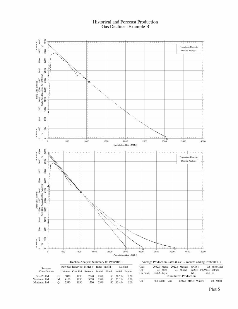
Historical and Forecast ProductionGas Decline - Example B
Decline Analysis Summary @ 1988/10/01
ReservesRaw Gas Reserves ( MMcf ) Rates ( mcf/d ) Decline
Classification Ultimate Cum Prd Remain Initial Final Initial Expont
Pv + Pb Prd G 3070 1030 2040 2390 50 38.5% 0.20
Maximum Prd M 4100 1030 3070 2390 50 35.3% 0.50
Minimum Prd Q 2530 1030 1500 2390 50 43.4% 0.00
Average Production Rates (Last 12 months ending 1988/10/31)
Gas : 2932.9 Mcf/d
Oil : 2.3 bbl/d
On Prod : 364.6 days
2922.5 Mcf/cd
2.3 bbl/cd
WGR : 0.8 bbl/MMcf
GOR : >99999.9 scf/stb
WC : 50.1 %
Cumulative Production
Oil : 0.8 Mbbl Gas : 1102.3 MMcf Water : 0.8 Mbbl
Plot 5
0 500 1000 1500 2000 2500 3000 3500 4000
Cumulative Gas (MMcf)
04
00
80
01
20
01
60
02
00
02
40
02
80
03
20
03
60
04
00
0
Da
ily G
as C
ale
nd
ar
Da
y (
Mcf/
cd
)
04
00
80
01
20
01
60
02
00
02
40
02
80
03
20
03
60
04
00
0
Da
ily G
as
(Mcf/
d)
G
Projections Illustrate
Decline Analysis
0 500 1000 1500 2000 2500 3000 3500 4000 4500 5000
Cumulative Gas (MMcf)
04
00
80
01
20
01
60
02
00
02
40
02
80
03
20
03
60
04
00
0
Da
ily G
as C
ale
nd
ar
Da
y (
Mcf/
cd
)
04
00
80
01
20
01
60
02
00
02
40
02
80
03
20
03
60
04
00
0
Da
ily G
as
(Mcf/
d)
G
Projections Illustrate
Decline Analysis
MQ
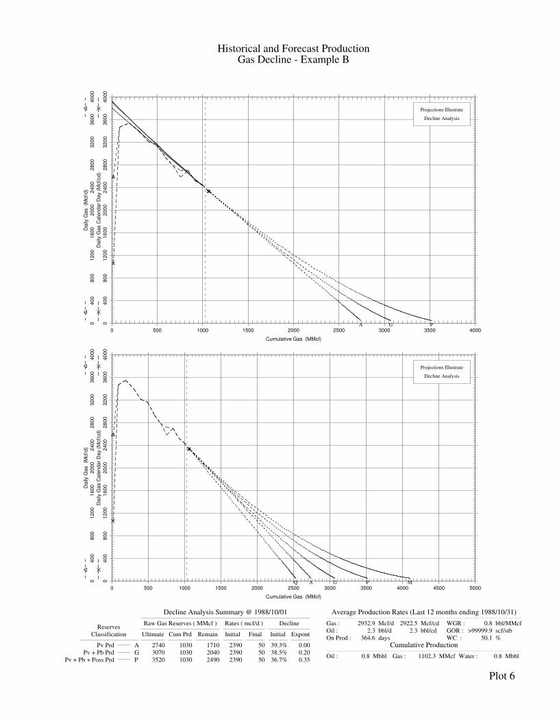
Historical and Forecast ProductionGas Decline - Example B
Decline Analysis Summary @ 1988/10/01
ReservesRaw Gas Reserves ( MMcf ) Rates ( mcf/d ) Decline
Classification Ultimate Cum Prd Remain Initial Final Initial Expont
Pv Prd A 2740 1030 1710 2390 50 39.3% 0.00
Pv + Pb Prd G 3070 1030 2040 2390 50 38.5% 0.20
Pv + Pb + Poss Prd P 3520 1030 2490 2390 50 36.7% 0.35
Average Production Rates (Last 12 months ending 1988/10/31)
Gas : 2932.9 Mcf/d
Oil : 2.3 bbl/d
On Prod : 364.6 days
2922.5 Mcf/cd
2.3 bbl/cd
WGR : 0.8 bbl/MMcf
GOR : >99999.9 scf/stb
WC : 50.1 %
Cumulative Production
Oil : 0.8 Mbbl Gas : 1102.3 MMcf Water : 0.8 Mbbl
Plot 6
0 500 1000 1500 2000 2500 3000 3500 4000
Cumulative Gas (MMcf)
04
00
80
01
20
01
60
02
00
02
40
02
80
03
20
03
60
04
00
0
Da
ily G
as C
ale
nd
ar
Da
y (
Mcf/
cd
)
04
00
80
01
20
01
60
02
00
02
40
02
80
03
20
03
60
04
00
0
Da
ily G
as
(Mcf/
d)
A
Projections Illustrate
Decline Analysis
G P
0 500 1000 1500 2000 2500 3000 3500 4000 4500 5000
Cumulative Gas (MMcf)
04
00
80
01
20
01
60
02
00
02
40
02
80
03
20
03
60
04
00
0
Da
ily G
as C
ale
nd
ar
Da
y (
Mcf/
cd
)
04
00
80
01
20
01
60
02
00
02
40
02
80
03
20
03
60
04
00
0
Da
ily G
as
(Mcf/
d)
A
Projections Illustrate
Decline Analysis
G MPQ
Historical and Forecast ProductionGas Decline - Example B
Decline Analysis Summary @ 1988/10/01
ReservesRaw Gas Reserves ( MMcf ) Rates ( mcf/d ) Decline
Classification Ultimate Cum Prd Remain Initial Final Initial Expont
Pv Prd A 2740 1030 1710 2390 50 39.3% 0.00
Pv + Pb Prd G 3070 1030 2040 2390 50 38.5% 0.20
Pv + Pb + Poss Prd P 3520 1030 2490 2390 50 36.7% 0.35
Average Production Rates (Last 12 months ending 2002/10/31)
Gas : 14.3 Mcf/d
Oil : 0.0 bbl/d
On Prod : 342.3 days
13.9 Mcf/cd
0.0 bbl/cd
WGR : 2.2 bbl/MMcf
GOR : 0.0 scf/stb
WC : 100.0 %
Cumulative Production
Oil : 1.9 Mbbl Gas : 3001.8 MMcf Water : 3.6 Mbbl
Plot 7
0 500 1000 1500 2000 2500 3000 3500 4000
Cumulative Gas (MMcf)
04
00
80
01
20
01
60
02
00
02
40
02
80
03
20
03
60
04
00
0
Da
ily G
as C
ale
nd
ar
Da
y (
Mcf/
cd
)
04
00
80
01
20
01
60
02
00
02
40
02
80
03
20
03
60
04
00
0
Da
ily G
as
(Mcf/
d)
A
Projections Illustrate
Decline Analysis
G P
0 500 1000 1500 2000 2500 3000 3500 4000
Cumulative Gas (MMcf)
10
10
01
00
01
00
00
Da
ily G
as C
ale
nd
ar
Da
y (
Mcf/
cd
)
10
10
01
00
01
00
00
Da
ily G
as
(Mcf/
d)
02
00
WG
R
(bb
l/M
Mcf)
A
Projections Illustrate
Decline Analysis
G P
6-70 Volume 2 — Resources and Reserves Estimation and Classification Guidelines
Canadian Oil and Gas Evaluation Handbook ©SPEE (Calgary Chapter)
Gas Example C 1977
Gas Example C is a well in a moderate-permeability, unstratified gas reservoir (Plot 1978 8). It is the same example as Example B, except with more production history. No 1979 future line-pressure reductions are anticipated. Best fit analysis calculated for the 1980 period from 0.8 Bcf to 2.2 Bcf yields a hyperbolic exponent of 0.7 and ultimate 1981 reserves of 4.42 Bcf (Plot 9, Line M). This value should not be used for reserves 1982 determination, because line-pressure reductions over the fit period have caused the 1983 slope changes. As this is a known moderate-permeability unstratified reservoir with 1984 no expected additional line-pressure reductions, expected decline exponents should 1985 be low. 1986
The recommended best estimate reserve for 2P reserves determination (Plot 10) is 1987 based on a visual match of current decline rate and exponential decline. Based on a 1988 50 Mcfd final rate (liquid loading limit), calculated ultimate reserves for the 2P case 1989 are 2.96 Bcf (Line G). Prior to selecting proved and 3P reserves, reasonable 1990 minimum and maximum end points illustrated on Plot 10 are selected to understand 1991 the potential variability of the estimate. In this case, 2.90 Bcf minimum ultimate 1992 reserves are determined using an exponential decline interpretation through recent 1993 data, while 3.18 Bcf maximum ultimate reserves are determined using an optimistic 1994 0.3 decline exponent. Recommended proved reserves determination is 2.93 Bcf (Plot 1995 11, Line A), using exponential decline analysis and a reserves value between the 1996 minimum and 2P values. Recommended 3P determination is 3.03 Bcf (Plot 11, Line 1997 P), using a hyperbolic exponent of 0.15 and a reserves value between the 2P and 1998 maximum values. As described in the decline analysis guidelines, the selection of 1999 proved values between 1/3 and 2/3 of the distance between minimum and best 2000 estimate values is acceptable. Similarly, the selection of 3P values between 1/3 and 2001 2/3 of the distance between maximum and best estimate values is acceptable. Due to 2002 the more extensive production history than the previous example, the differences 2003 between the reserves categories are reduced. Actual full-life well performance is 2004 illustrated on Plot 12. 2005
2006 2007
Historical ProductionGas Decline - Example C
Status Summary
On Production date : 87/10/18
Status date : 87/10/18
Status : FLOWING GAS
Cumulative Production
Gas : 2258.6 MMcf
Oil : 1.4 Mbbl
Water : 2.0 Mbbl
Average Production Rates (Last 12 months ending 1991/01/31)
Gas : 1082.0 Mcf/d
Oil : 0.5 bbl/d
On Prod : 363.2 days
1076.2 Mcf/cd
0.5 bbl/cd
WGR : 1.2 bbl/MMcf
GOR : >99999.9 scf/stb
WC : 73.6 %
Plot 8
1987 1988 1989 1990 1991 1992 1993 1994 1995 1996
Year
10
10
01
00
01
00
00
Da
ily G
as C
ale
nd
ar
Da
y (
Mcf/
cd
)
10
10
01
00
01
00
00
Da
ily G
as
(Mcf/
d)
02
0
WG
R
(bb
l/M
Mcf)
0 500 1000 1500 2000 2500 3000 3500 4000
Cumulative Gas (MMcf)
04
00
80
01
20
01
60
02
00
02
40
02
80
03
20
03
60
04
00
0
Da
ily G
as C
ale
nd
ar
Da
y (
Mcf/
cd
)
04
00
80
01
20
01
60
02
00
02
40
02
80
03
20
03
60
04
00
0
Da
ily G
as
(Mcf/
d)
01
0
WG
R
(bb
l/M
Mcf)
Historical and Forecast ProductionGas Decline - Example C
Decline Analysis Summary @ 1991/01/01
ReservesRaw Gas Reserves ( MMcf ) Rates ( mcf/d ) Decline
Classification Ultimate Cum Prd Remain Initial Final Initial Expont
Maximum Prd M 4424 2231 2193 946 50 24.3% 0.70
Average Production Rates (Last 12 months ending 1991/01/31)
Gas : 1082.0 Mcf/d
Oil : 0.5 bbl/d
On Prod : 363.2 days
1076.2 Mcf/cd
0.5 bbl/cd
WGR : 1.2 bbl/MMcf
GOR : >99999.9 scf/stb
WC : 73.6 %
Cumulative Production
Oil : 1.4 Mbbl Gas : 2258.6 MMcf Water : 2.0 Mbbl
Plot 9
0 500 1000 1500 2000 2500 3000 3500 4000 4500 5000
Cumulative Gas (MMcf)
04
00
80
01
20
01
60
02
00
02
40
02
80
03
20
03
60
04
00
0
Da
ily G
as C
ale
nd
ar
Da
y (
Mcf/
cd
)
04
00
80
01
20
01
60
02
00
02
40
02
80
03
20
03
60
04
00
0
Da
ily G
as
(Mcf/
d)
M
Projections Illustrate
Decline Analysis
0 500 1000 1500 2000 2500 3000 3500 4000 4500 5000
Cumulative Gas (MMcf)
10
10
01
00
01
00
00
Da
ily G
as C
ale
nd
ar
Da
y (
Mcf/
cd
)
10
10
01
00
01
00
00
Da
ily G
as
(Mcf/
d)
M
Projections Illustrate
Decline Analysis
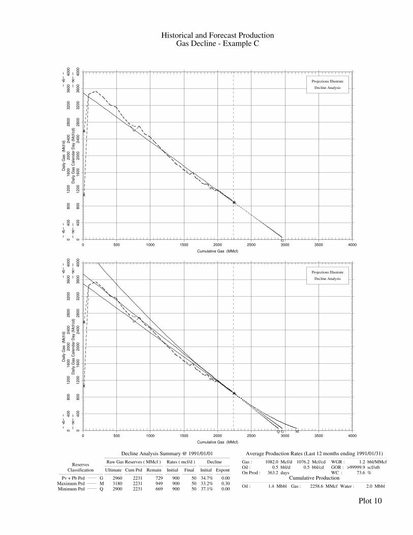
Historical and Forecast ProductionGas Decline - Example C
Decline Analysis Summary @ 1991/01/01
ReservesRaw Gas Reserves ( MMcf ) Rates ( mcf/d ) Decline
Classification Ultimate Cum Prd Remain Initial Final Initial Expont
Pv + Pb Prd G 2960 2231 729 900 50 34.7% 0.00
Maximum Prd M 3180 2231 949 900 50 33.2% 0.30
Minimum Prd Q 2900 2231 669 900 50 37.1% 0.00
Average Production Rates (Last 12 months ending 1991/01/31)
Gas : 1082.0 Mcf/d
Oil : 0.5 bbl/d
On Prod : 363.2 days
1076.2 Mcf/cd
0.5 bbl/cd
WGR : 1.2 bbl/MMcf
GOR : >99999.9 scf/stb
WC : 73.6 %
Cumulative Production
Oil : 1.4 Mbbl Gas : 2258.6 MMcf Water : 2.0 Mbbl
Plot 10
0 500 1000 1500 2000 2500 3000 3500 4000
Cumulative Gas (MMcf)
04
00
80
01
20
01
60
02
00
02
40
02
80
03
20
03
60
04
00
0
Da
ily G
as C
ale
nd
ar
Da
y (
Mcf/
cd
)
04
00
80
01
20
01
60
02
00
02
40
02
80
03
20
03
60
04
00
0
Da
ily G
as
(Mcf/
d)
G
Projections Illustrate
Decline Analysis
0 500 1000 1500 2000 2500 3000 3500 4000
Cumulative Gas (MMcf)
04
00
80
01
20
01
60
02
00
02
40
02
80
03
20
03
60
04
00
0
Da
ily G
as C
ale
nd
ar
Da
y (
Mcf/
cd
)
04
00
80
01
20
01
60
02
00
02
40
02
80
03
20
03
60
04
00
0
Da
ily G
as
(Mcf/
d)
G
Projections Illustrate
Decline Analysis
MQ
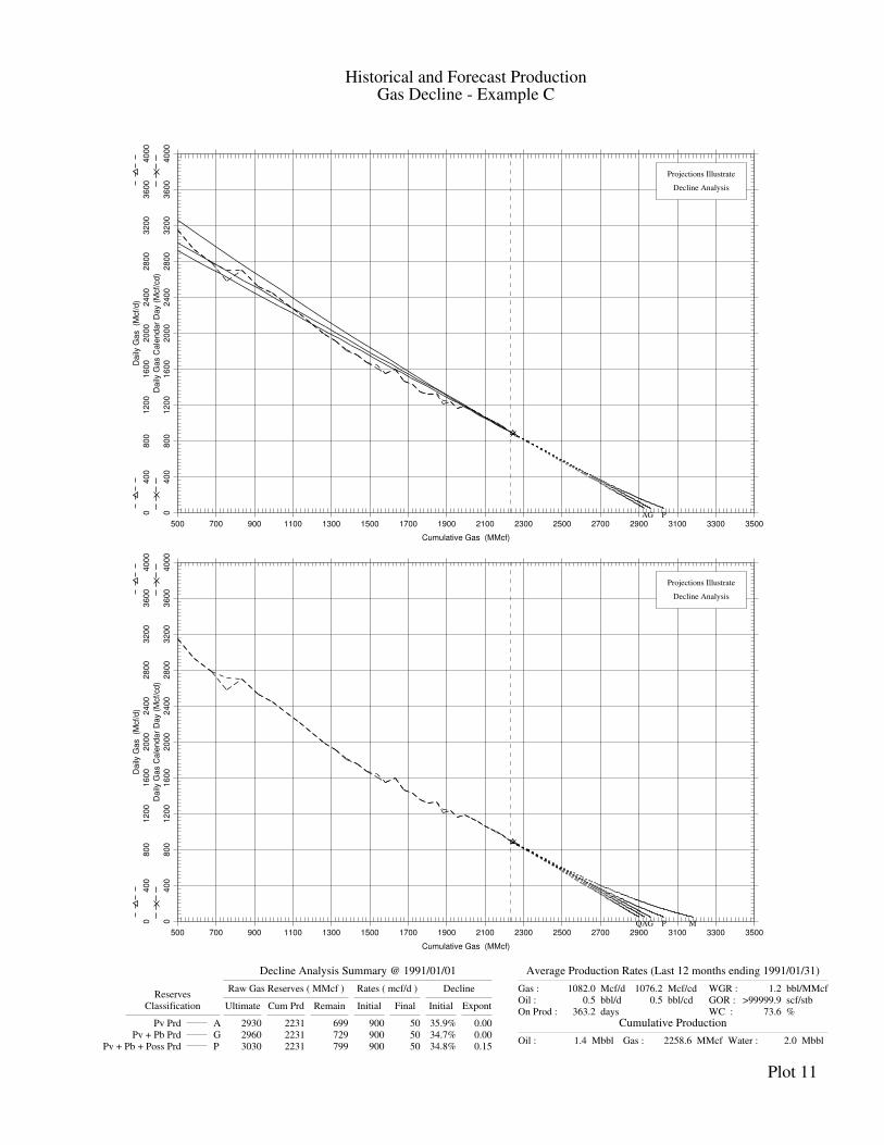
Historical and Forecast ProductionGas Decline - Example C
Decline Analysis Summary @ 1991/01/01
ReservesRaw Gas Reserves ( MMcf ) Rates ( mcf/d ) Decline
Classification Ultimate Cum Prd Remain Initial Final Initial Expont
Pv Prd A 2930 2231 699 900 50 35.9% 0.00
Pv + Pb Prd G 2960 2231 729 900 50 34.7% 0.00
Pv + Pb + Poss Prd P 3030 2231 799 900 50 34.8% 0.15
Average Production Rates (Last 12 months ending 1991/01/31)
Gas : 1082.0 Mcf/d
Oil : 0.5 bbl/d
On Prod : 363.2 days
1076.2 Mcf/cd
0.5 bbl/cd
WGR : 1.2 bbl/MMcf
GOR : >99999.9 scf/stb
WC : 73.6 %
Cumulative Production
Oil : 1.4 Mbbl Gas : 2258.6 MMcf Water : 2.0 Mbbl
Plot 11
500 700 900 1100 1300 1500 1700 1900 2100 2300 2500 2700 2900 3100 3300 3500
Cumulative Gas (MMcf)
04
00
80
01
20
01
60
02
00
02
40
02
80
03
20
03
60
04
00
0
Da
ily G
as C
ale
nd
ar
Da
y (
Mcf/
cd
)
04
00
80
01
20
01
60
02
00
02
40
02
80
03
20
03
60
04
00
0
Da
ily G
as
(Mcf/
d)
A
Projections Illustrate
Decline Analysis
G P
500 700 900 1100 1300 1500 1700 1900 2100 2300 2500 2700 2900 3100 3300 3500
Cumulative Gas (MMcf)
04
00
80
01
20
01
60
02
00
02
40
02
80
03
20
03
60
04
00
0
Da
ily G
as C
ale
nd
ar
Da
y (
Mcf/
cd
)
04
00
80
01
20
01
60
02
00
02
40
02
80
03
20
03
60
04
00
0
Da
ily G
as
(Mcf/
d)
A
Projections Illustrate
Decline Analysis
G MPQ
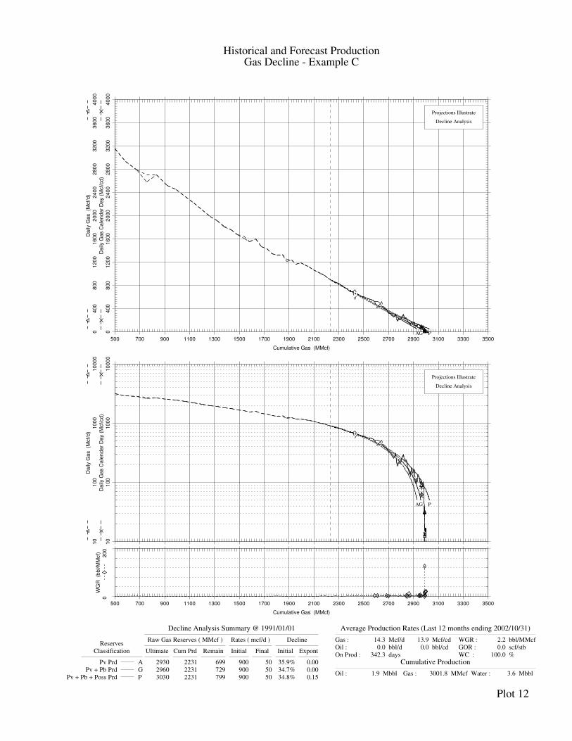
Historical and Forecast ProductionGas Decline - Example C
Decline Analysis Summary @ 1991/01/01
ReservesRaw Gas Reserves ( MMcf ) Rates ( mcf/d ) Decline
Classification Ultimate Cum Prd Remain Initial Final Initial Expont
Pv Prd A 2930 2231 699 900 50 35.9% 0.00
Pv + Pb Prd G 2960 2231 729 900 50 34.7% 0.00
Pv + Pb + Poss Prd P 3030 2231 799 900 50 34.8% 0.15
Average Production Rates (Last 12 months ending 2002/10/31)
Gas : 14.3 Mcf/d
Oil : 0.0 bbl/d
On Prod : 342.3 days
13.9 Mcf/cd
0.0 bbl/cd
WGR : 2.2 bbl/MMcf
GOR : 0.0 scf/stb
WC : 100.0 %
Cumulative Production
Oil : 1.9 Mbbl Gas : 3001.8 MMcf Water : 3.6 Mbbl
Plot 12
500 700 900 1100 1300 1500 1700 1900 2100 2300 2500 2700 2900 3100 3300 3500
Cumulative Gas (MMcf)
04
00
80
01
20
01
60
02
00
02
40
02
80
03
20
03
60
04
00
0
Da
ily G
as C
ale
nd
ar
Da
y (
Mcf/
cd
)
04
00
80
01
20
01
60
02
00
02
40
02
80
03
20
03
60
04
00
0
Da
ily G
as
(Mcf/
d)
A
Projections Illustrate
Decline Analysis
G P
500 700 900 1100 1300 1500 1700 1900 2100 2300 2500 2700 2900 3100 3300 3500
Cumulative Gas (MMcf)
10
10
01
00
01
00
00
Da
ily G
as C
ale
nd
ar
Da
y (
Mcf/
cd
)
10
10
01
00
01
00
00
Da
ily G
as
(Mcf/
d)
02
00
WG
R
(bb
l/M
Mcf)
A
Projections Illustrate
Decline Analysis
G P

Section 6 — Procedures for Estimation and Classification of Reserves 6-71
©SPEE (Calgary Chapter) First Edition — April 28, 2004
Gas Example D 2007
Gas Example D is a well in a low-permeability, highly stratified gas reservoir (Plot 2008 13). Curve fitting was only performed after January 1, 1996 (3 Bcf cumulative 2009 production), when the well was calculated from pressure transient analysis to be in 2010 pseudo-steady-state flow. Best fit decline analysis results in a decline exponent of 2011 1.35 and ultimate reserves of 15.2 Bcf, with a 216-year reserves life (Plot 14, Line 2012 M). Due to the stratified, low-permeability nature of the reservoir, decline behaviour 2013 is expected to be hyperbolic. The best fit exponent appears to be an unreasonably 2014 high exponent (over 1), possibly a result of line-pressure fluctuations occurring 2015 during the fit period, or a dual-permeability system not accurately represented by the 2016 Arps decline equation. In the absence of substantiation from volumetric data or more 2017 detailed reservoir modelling, use of this best fit exponent is not advised. 2018
The recommended best estimate exponent for 2P reserves determination is the use of 2019 a reasonably high hyperbolic decline exponent that is less than 1. In this case, an 2020 exponent of 0.8 is selected based on a review of analogous wells in the area, which 2021 yields ultimate reserves of 9.6 Bcf with an 88-year reserves life (Line G). Prior to 2022 selecting proved and 3P reserves, reasonable minimum and maximum end points, 2023 illustrated on Plot 15, are selected to understand the potential variability of the 2024 estimate. In this case, 7.3 Bcf minimum ultimate reserves were determined using a 2025 hyperbolic decline exponent of 0.3, while 12.9 Bcf maximum ultimate reserves were 2026 determined using an optimistic 1.2 decline exponent. Decline curves calculated using 2027 exponents outside this range do not yield reasonable fits to the historical trend. 2028
The recommended proved interpretation uses a 0.6 hyperbolic decline exponent, 2029 which yields ultimate reserves of 8.5 Bcf with a 62-year reserves life (Plot 16, Line 2030 A). The recommended 3P interpretation uses a harmonic decline exponent, which 2031 yields ultimate reserves of 11.0 Bcf with a 126-year reserves life (Plot 16, Line P). 2032
Imposing a 50-year limit on reserves classification, as recommended previously in 2033 these guidelines, will reduce ultimate proved reserves to 8.3 Bcf, 2P reserves to 8.7 2034 Bcf, and 3P reserves to 9.0 Bcf. In this case, the potential for downspacing should be 2035 reviewed in order to capture pool reserves in a meaningful time period. 2036
2037 2038
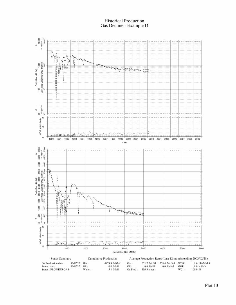
Historical ProductionGas Decline - Example D
Status Summary
On Production date : 90/07/12
Status date : 90/07/12
Status : FLOWING GAS
Cumulative Production
Gas : 4979.9 MMcf
Oil : 0.0 Mbbl
Water : 5.1 Mbbl
Average Production Rates (Last 12 months ending 2003/02/28)
Gas : 671.7 Mcf/d
Oil : 0.0 bbl/d
On Prod : 303.3 days
558.4 Mcf/cd
0.0 bbl/cd
WGR : 1.6 bbl/MMcf
GOR : 0.0 scf/stb
WC : 100.0 %
Plot 13
1990 1991 1992 1993 1994 1995 1996 1997 1998 1999 2000 2001 2002 2003 2004 2005 2006 2007 2008 2009
Year
10
10
01
00
01
00
00
Da
ily G
as C
ale
nd
ar
Da
y (
Mcf/
cd
)
10
10
01
00
01
00
00
Da
ily G
as
(Mcf/
d)
01
0
WG
R
(bb
l/M
Mcf)
0 1000 2000 3000 4000 5000 6000 7000 8000
Cumulative Gas (MMcf)
05
00
10
00
15
00
20
00
25
00
30
00
35
00
40
00
45
00
50
00
Da
ily G
as C
ale
nd
ar
Da
y (
Mcf/
cd
)
05
00
10
00
15
00
20
00
25
00
30
00
35
00
40
00
45
00
50
00
Da
ily G
as
(Mcf/
d)
01
0
WG
R
(bb
l/M
Mcf)
Historical and Forecast ProductionGas Decline - Example D
Decline Analysis Summary @ 2003/02/01
ReservesRaw Gas Reserves ( MMcf ) Rates ( mcf/d ) Decline
Classification Ultimate Cum Prd Remain Initial Final Initial Expont
Maximum Prd M 15200 4965 10235 545 50 6.7% 1.35
Average Production Rates (Last 12 months ending 2003/02/28)
Gas : 671.7 Mcf/d
Oil : 0.0 bbl/d
On Prod : 303.3 days
558.4 Mcf/cd
0.0 bbl/cd
WGR : 1.6 bbl/MMcf
GOR : 0.0 scf/stb
WC : 100.0 %
Cumulative Production
Oil : 0.0 Mbbl Gas : 4979.9 MMcf Water : 5.1 Mbbl
Plot 14
0 2000 4000 6000 8000 10000 12000 14000 16000 18000 20000
Cumulative Gas (MMcf)
04
00
80
01
20
01
60
02
00
02
40
02
80
03
20
03
60
04
00
0
Da
ily G
as C
ale
nd
ar
Da
y (
Mcf/
cd
)
04
00
80
01
20
01
60
02
00
02
40
02
80
03
20
03
60
04
00
0
Da
ily G
as
(Mcf/
d)
19
90
19
92
19
94
19
96
19
98
20
00
20
02
20
04
20
06
20
08
20
10
Ye
ar
M
Projections Illustrate
Decline Analysis
0 2000 4000 6000 8000 10000 12000 14000 16000 18000 20000
Cumulative Gas (MMcf)
10
10
01
00
01
00
00
Da
ily G
as C
ale
nd
ar
Da
y (
Mcf/
cd
)
10
10
01
00
01
00
00
Da
ily G
as
(Mcf/
d)
M
Projections Illustrate
Decline Analysis
Historical and Forecast ProductionGas Decline - Example D
Decline Analysis Summary @ 2003/02/01
ReservesRaw Gas Reserves ( MMcf ) Rates ( mcf/d ) Decline
Classification Ultimate Cum Prd Remain Initial Final Initial Expont
Pv + Pb Prd G 9600 4965 4635 545 50 7.6% 0.80
Maximum Prd M 12900 4965 7935 545 50 7.1% 1.20
Minimum Prd Q 7300 4965 2335 545 50 9.3% 0.30
Average Production Rates (Last 12 months ending 2003/02/28)
Gas : 671.7 Mcf/d
Oil : 0.0 bbl/d
On Prod : 303.3 days
558.4 Mcf/cd
0.0 bbl/cd
WGR : 1.6 bbl/MMcf
GOR : 0.0 scf/stb
WC : 100.0 %
Cumulative Production
Oil : 0.0 Mbbl Gas : 4979.9 MMcf Water : 5.1 Mbbl
Plot 15
0 1000 2000 3000 4000 5000 6000 7000 8000 9000 10000 11000 12000 13000 14000 15000
Cumulative Gas (MMcf)
04
00
80
01
20
01
60
02
00
02
40
02
80
03
20
03
60
04
00
0
Da
ily G
as C
ale
nd
ar
Da
y (
Mcf/
cd
)
04
00
80
01
20
01
60
02
00
02
40
02
80
03
20
03
60
04
00
0
Da
ily G
as
(Mcf/
d)
G
Projections Illustrate
Decline Analysis
MQ
Historical and Forecast ProductionGas Decline - Example D
Decline Analysis Summary @ 2003/02/01
ReservesRaw Gas Reserves ( MMcf ) Rates ( mcf/d ) Decline
Classification Ultimate Cum Prd Remain Initial Final Initial Expont
Pv Prd A 8500 4965 3535 545 50 8.1% 0.60
Pv + Pb Prd G 9600 4965 4635 545 50 7.6% 0.80
Pv + Pb + Poss Prd P 11000 4965 6035 545 50 7.3% 1.00
Average Production Rates (Last 12 months ending 2003/06/30)
Gas : 657.7 Mcf/d
Oil : 0.0 bbl/d
On Prod : 299.0 days
538.9 Mcf/cd
0.0 bbl/cd
WGR : 1.6 bbl/MMcf
GOR : 0.0 scf/stb
WC : 100.0 %
Cumulative Production
Oil : 0.0 Mbbl Gas : 5044.4 MMcf Water : 5.2 Mbbl
Plot 16
3000 4000 5000 6000 7000 8000 9000 10000 11000 12000 13000
Cumulative Gas (MMcf)
02
00
40
06
00
80
01
00
01
20
01
40
01
60
01
80
02
00
0
Da
ily G
as C
ale
nd
ar
Da
y (
Mcf/
cd
)
02
00
40
06
00
80
01
00
01
20
01
40
01
60
01
80
02
00
0
Da
ily G
as
(Mcf/
d)
A
Projections Illustrate
Decline Analysis
G P
3000 4000 5000 6000 7000 8000 9000 10000 11000 12000 13000
Cumulative Gas (MMcf)
02
00
40
06
00
80
01
00
01
20
01
40
01
60
01
80
02
00
0
Da
ily G
as C
ale
nd
ar
Da
y (
Mcf/
cd
)
02
00
40
06
00
80
01
00
01
20
01
40
01
60
01
80
02
00
0
Da
ily G
as
(Mcf/
d)
A
Projections Illustrate
Decline Analysis
G MPQ
6-72 Volume 2 — Resources and Reserves Estimation and Classification Guidelines
Canadian Oil and Gas Evaluation Handbook ©SPEE (Calgary Chapter)
Gas Example E 2038
Gas Example E is a well in a low-permeability, moderately stratified gas reservoir 2039 (Plot 17). Curve fitting is only performed after cumulative production of 0.9 Bcf, 2040 when the well is determined from type curve analysis to be in pseudo-steady-state 2041 flow. Reasonable fits can be achieved using a range of hyperbolic exponents. 2042
In this case, recommended best estimate interpretation for 2P reserves uses a 0.6 2043 hyperbolic decline based on visual fitting of the data and a review of analogous wells 2044 in the area, which yields ultimate reserves of 2.36 Bcf (Plot 18, Line G). Prior to 2045 selecting proved and 3P reserves, reasonable minimum and maximum end points, 2046 illustrated on Plot 18, are selected to understand the potential variability of the 2047 estimate. In this case, 2.09 Bcf minimum ultimate reserves are determined using a 2048 hyperbolic decline exponent of 0.2, while 2.74 Bcf maximum ultimate reserves are 2049 determined using an optimistic harmonic analysis. Decline curves calculated using 2050 exponents outside this range do not yield reasonable fits to the historical trend. 2051
The recommended proved interpretation uses a 0.4 hyperbolic decline exponent, 2052 which yields ultimate reserves of 2.19 Bcf (Plot 19, Line A). The recommended 3P 2053 interpretation uses a 0.8 hyperbolic decline exponent, which yields ultimate reserves 2054 of 2.54 Bcf (Plot 19, Line P). 2055
Decline interpretation was performed on the calendar-day decline trends, as is the 2056 recommended practice for low-permeability reservoirs. The well was produced 2057 intermittently to prevent liquid loading. 2058
2059 2060
Historical ProductionGas Decline - Example E
Status Summary
On Production date : 94/11/22
Status date : 94/11/16
Status : FLOWING GAS
Cumulative Production
Gas : 1512.0 MMcf
Oil : 0.0 Mbbl
Water : 2.5 Mbbl
Average Production Rates (Last 12 months ending 2003/01/31)
Gas : 376.9 Mcf/d
Oil : 0.0 bbl/d
On Prod : 242.6 days
248.4 Mcf/cd
0.0 bbl/cd
WGR : 1.4 bbl/MMcf
GOR : 0.0 scf/stb
WC : 100.0 %
Plot 17
1994 1995 1996 1997 1998 1999 2000 2001 2002 2003
Year
10
10
01
00
01
00
00
Da
ily G
as C
ale
nd
ar
Da
y (
Mcf/
cd
)
10
10
01
00
01
00
00
Da
ily G
as
(Mcf/
d)
02
0
WG
R
(bb
l/M
Mcf)
0 200 400 600 800 1000 1200 1400 1600 1800 2000
Cumulative Gas (MMcf)
02
50
50
07
50
10
00
12
50
15
00
17
50
20
00
22
50
25
00
Da
ily G
as C
ale
nd
ar
Da
y (
Mcf/
cd
)
02
50
50
07
50
10
00
12
50
15
00
17
50
20
00
22
50
25
00
Da
ily G
as
(Mcf/
d)
02
0
WG
R
(bb
l/M
Mcf)
Historical and Forecast ProductionGas Decline - Example E
Decline Analysis Summary @ 2003/01/01
ReservesRaw Gas Reserves ( MMcf ) Rates ( mcf/d ) Decline
Classification Ultimate Cum Prd Remain Initial Final Initial Expont
Pv + Pb Prd G 2360 1505 855 238 50 10.8% 0.60
Maximum Prd M 2740 1505 1235 238 50 9.9% 1.00
Minimum Prd Q 2090 1505 585 237 50 12.2% 0.20
Average Production Rates (Last 12 months ending 2003/06/30)
Gas : 364.0 Mcf/d
Oil : 0.0 bbl/d
On Prod : 236.4 days
234.2 Mcf/cd
0.0 bbl/cd
WGR : 1.8 bbl/MMcf
GOR : 0.0 scf/stb
WC : 100.0 %
Cumulative Production
Oil : 0.0 Mbbl Gas : 1545.7 MMcf Water : 2.5 Mbbl
Plot 18
0 200 400 600 800 1000 1200 1400 1600 1800 2000 2200 2400 2600 2800 3000
Cumulative Gas (MMcf)
01
00
20
03
00
40
05
00
60
07
00
80
09
00
10
00
Da
ily G
as C
ale
nd
ar
Da
y (
Mcf/
cd
)
01
00
20
03
00
40
05
00
60
07
00
80
09
00
10
00
Da
ily G
as
(Mcf/
d)
G
Projections Illustrate
Decline Analysis
0 200 400 600 800 1000 1200 1400 1600 1800 2000 2200 2400 2600 2800 3000
Cumulative Gas (MMcf)
01
00
20
03
00
40
05
00
60
07
00
80
09
00
10
00
Da
ily G
as C
ale
nd
ar
Da
y (
Mcf/
cd
)
01
00
20
03
00
40
05
00
60
07
00
80
09
00
10
00
Da
ily G
as
(Mcf/
d)
G
Projections Illustrate
Decline Analysis
MQ
Historical and Forecast ProductionGas Decline - Example E
Decline Analysis Summary @ 2003/01/01
ReservesRaw Gas Reserves ( MMcf ) Rates ( mcf/d ) Decline
Classification Ultimate Cum Prd Remain Initial Final Initial Expont
Pv Prd A 2190 1505 685 237 50 11.7% 0.40
Pv + Pb Prd G 2360 1505 855 238 50 10.8% 0.60
Pv + Pb + Poss Prd P 2540 1505 1035 238 50 10.2% 0.80
Average Production Rates (Last 12 months ending 2003/06/30)
Gas : 364.0 Mcf/d
Oil : 0.0 bbl/d
On Prod : 236.4 days
234.2 Mcf/cd
0.0 bbl/cd
WGR : 1.8 bbl/MMcf
GOR : 0.0 scf/stb
WC : 100.0 %
Cumulative Production
Oil : 0.0 Mbbl Gas : 1545.7 MMcf Water : 2.5 Mbbl
Plot 19
0 200 400 600 800 1000 1200 1400 1600 1800 2000 2200 2400 2600 2800 3000
Cumulative Gas (MMcf)
01
00
20
03
00
40
05
00
60
07
00
80
09
00
10
00
Da
ily G
as C
ale
nd
ar
Da
y (
Mcf/
cd
)
01
00
20
03
00
40
05
00
60
07
00
80
09
00
10
00
Da
ily G
as
(Mcf/
d)
A
Projections Illustrate
Decline Analysis
G P
0 200 400 600 800 1000 1200 1400 1600 1800 2000 2200 2400 2600 2800 3000
Cumulative Gas (MMcf)
01
00
20
03
00
40
05
00
60
07
00
80
09
00
10
00
Da
ily G
as C
ale
nd
ar
Da
y (
Mcf/
cd
)
01
00
20
03
00
40
05
00
60
07
00
80
09
00
10
00
Da
ily G
as
(Mcf/
d)
A
Projections Illustrate
Decline Analysis
G MPQ

Section 6 — Procedures for Estimation and Classification of Reserves 6-73
©SPEE (Calgary Chapter) First Edition — April 28, 2004
Gas Example F 2060
Gas Example F is a well in a pool with an active water drive (Plot 20). Decline 2061 analysis cannot be used for most of the producing life of the pool, because pressure 2062 support suppresses the production decline. Production decline does not commence 2063 until the onset of water production, at which time decline is very steep. Volumetric or 2064 analogy methods must be used to analyze wells of this nature until the onset of 2065 production decline. Once production decline commences, volumetric data is of 2066 secondary importance. 2067
2068 2069
Historical and Forecast ProductionGas Decline - Example F
Decline Analysis Summary @ 2003/01/01
ReservesRaw Gas Reserves ( MMcf ) Rates ( mcf/d ) Decline
Classification Ultimate Cum Prd Remain Initial Final Initial Expont
Maximum Prd M 5015 5006 9 150 100 86.3% 0.00
Average Production Rates (Last 12 months ending 2001/08/31)
Gas : 376.2 Mcf/d
Oil : 0.0 bbl/d
On Prod : 154.3 days
183.5 Mcf/cd
0.0 bbl/cd
WGR : 0.0 bbl/MMcf
GOR : 0.0 scf/stb
WC : 0.0 %
Cumulative Production
Oil : 0.0 Mbbl Gas : 5005.8 MMcf Water : 85.9 Mbbl
Plot 20
1994 1995 1996 1997 1998 1999 2000 2001 2002 2003 2004 2005 2006 2007 2008 2009 2010 2011
Year
10
10
01
00
01
00
00
Da
ily G
as C
ale
nd
ar
Da
y (
Mcf/
cd
)
10
10
01
00
01
00
00
Da
ily G
as
(Mcf/
d)
05
00
WG
R
(bb
l/M
Mcf)
M
Projections Illustrate
Production Forecast
0 500 1000 1500 2000 2500 3000 3500 4000 4500 5000 5500 6000
Cumulative Gas (MMcf)
01
00
02
00
03
00
04
00
05
00
06
00
07
00
08
00
09
00
01
00
00
Da
ily G
as C
ale
nd
ar
Da
y (
Mcf/
cd
)
01
00
02
00
03
00
04
00
05
00
06
00
07
00
08
00
09
00
01
00
00
Da
ily G
as
(Mcf/
d)
05
00
WG
R
(bb
l/M
Mcf)
19
94
19
95
19
96
19
97
19
98
19
99
20
00
20
01
20
02
20
03
20
04
Ye
ar
M
Projections Illustrate
Decline Analysis
6-74 Volume 2 — Resources and Reserves Estimation and Classification Guidelines
Canadian Oil and Gas Evaluation Handbook ©SPEE (Calgary Chapter)
Oil Example A 2069
Oil Example A is a well in a moderate-permeability, unstratified solution-gas drive 2070 oil pool with production history to April 1994, as illustrated on Plot 21. Production 2071 from the well was originally constrained by GOR penalty, which was removed in late 2072 1992. Reasonable visual fits can be achieved using a range of hyperbolic exponents 2073 between 0 and 0.4. This range is in line with the range of decline exponents of 0 to 2074 0.33 for single-layer oil reservoirs producing below bubble point, as derived by 2075 Fetkovich et al. (1996). The recommended best estimate interpretation for 2P 2076 reserves uses a 0.2 hyperbolic decline (midpoint of range) based on a review of other 2077 analogous wells in the area, which yields ultimate reserves of 137 Mstb (Plot 22, 2078 Line G). Minimum and maximum reserves of 130 Mstb and 145 Mstb are established 2079 using exponents of 0 and 0.4, respectively (Plot 22, Lines Q and M). The 2080 recommended proved interpretation uses a 0.1 hyperbolic decline exponent, which 2081 yields ultimate reserves of 133 Mstb (Plot 23, Line A), while the recommended 3P 2082 interpretation uses a 0.3 hyperbolic decline exponent, which yields ultimate reserves 2083 of 141 Mstb (Plot 23, Line P). 2084
Actual results to mid 1997 exceeded the proved forecast and followed the 2P 2085 forecast. Results thereafter exceeded both forecasts because of a stimulation 2086 treatment performed on the well. Prior to actual results, the effect of a well 2087 stimulation is difficult to determine from curve-fit decline analysis alone. Type curve 2088 decline analysis is sometimes used to quantify wellbore damage and potential 2089 improvement. 2090
2091 2092
Historical ProductionOil Decline Example A
Status Summary
On Production date : 86/11/09
Status date : 86/11/01
Status : PUMPING OIL
Cumulative Production
Gas : 166.2 MMcf
Oil : 111.0 Mbbl
Water : 0.1 Mbbl
Average Production Rates (Last 12 months ending 1994/04/30)
Gas : 131.6 Mcf/d
Oil : 36.1 bbl/d
On Prod : 352.0 days
127.7 Mcf/cd
34.8 bbl/cd
WGR : 0.0 bbl/MMcf
GOR : 3669.7 scf/stb
WC : 0.0 %
Plot 21
1986 1987 1988 1989 1990 1991 1992 1993 1994 1995
Year
11
01
00
10
00
Da
ily O
il C
ale
nd
ar
Da
y (
bb
l/cd
)
11
01
00
10
00
Da
ily O
il (
bb
l/d
)
05
00
0
GO
R
(scf/
stb
)
01
00
Wtr
Cu
t (
%)
0 20 40 60 80 100 120 140 160 180 200
Cumulative Oil (Mbbl)
02
04
06
08
01
00
12
01
40
16
01
80
20
0
Da
ily O
il C
ale
nd
ar
Da
y (
bb
l/cd
)
02
04
06
08
01
00
12
01
40
16
01
80
20
0
Da
ily O
il (
bb
l/d
)
05
00
0
GO
R
(scf/
stb
)
Historical and Forecast ProductionOil Decline Example A
Decline Analysis Summary @ 1994/04/01
ReservesReserves ( Mbbl ) Rates ( bbl/d ) Decline
Classification Ultimate Cum Prd Remain Initial Final Initial Expont
Pv + Pb Prd G 137 110 27 32 5 33.2% 0.20
Maximum Prd M 145 110 35 32 5 29.5% 0.40
Minimum Prd Q 130 110 20 32 5 39.0% 0.00
Average Production Rates (Last 12 months ending 1994/04/30)
Gas : 131.6 Mcf/d
Oil : 36.1 bbl/d
On Prod : 352.0 days
127.7 Mcf/cd
34.8 bbl/cd
WGR : 0.0 bbl/MMcf
GOR : 3669.7 scf/stb
WC : 0.0 %
Cumulative Production
Oil : 111.0 Mbbl Gas : 166.2 MMcf Water : 0.1 Mbbl
Plot 22
0 10 20 30 40 50 60 70 80 90 100 110 120 130 140 150
Cumulative Oil (Mbbl)
02
04
06
08
01
00
12
01
40
16
01
80
20
0
Da
ily O
il C
ale
nd
ar
Da
y (
bb
l/cd
)
02
04
06
08
01
00
12
01
40
16
01
80
20
0
Da
ily O
il (
bb
l/d
)
G
Projections Illustrate
Decline Analysis
0 10 20 30 40 50 60 70 80 90 100 110 120 130 140 150
Cumulative Oil (Mbbl)
02
04
06
08
01
00
12
01
40
16
01
80
20
0
Da
ily O
il C
ale
nd
ar
Da
y (
bb
l/cd
)
02
04
06
08
01
00
12
01
40
16
01
80
20
0
Da
ily O
il (
bb
l/d
)
G
Projections Illustrate
Decline Analysis
MQ
Historical and Forecast ProductionOil Decline Example A
Reserves Summary @ 1994/04/01
ReservesReserves ( Mbbl )
Classification Ultimate Cum Prd Remain Reserves Method(s)
Pv Prd A 133 110 23 Decline
Pv + Pb Prd G 137 110 27 Decline
Pv + Pb + Poss Prd P 141 110 31 Decline
Average Production Rates (Last 12 months ending 1994/04/30)
Gas : 131.6 Mcf/d
Oil : 36.1 bbl/d
On Prod : 352.0 days
127.7 Mcf/cd
34.8 bbl/cd
WGR : 0.0 bbl/MMcf
GOR : 3669.7 scf/stb
WC : 0.0 %
Cumulative Production
Oil : 111.0 Mbbl Gas : 166.2 MMcf Water : 0.1 Mbbl
Plot 23
60 70 80 90 100 110 120 130 140 150 160
Cumulative Oil (Mbbl)
01
02
03
04
05
06
07
08
09
01
00
Da
ily O
il C
ale
nd
ar
Da
y (
bb
l/cd
)
01
02
03
04
05
06
07
08
09
01
00
Da
ily O
il (
bb
l/d
)
A
Projections Illustrate
Production Forecast
G
P
60 70 80 90 100 110 120 130 140 150 160
Cumulative Oil (Mbbl)
01
02
03
04
05
06
07
08
09
01
00
Da
ily O
il C
ale
nd
ar
Da
y (
bb
l/cd
)
01
02
03
04
05
06
07
08
09
01
00
Da
ily O
il (
bb
l/d
)
A
Projections Illustrate
Decline Analysis
G MPQ
Section 6 — Procedures for Estimation and Classification of Reserves 6-75
©SPEE (Calgary Chapter) First Edition — April 28, 2004
Oil Example B 2092
Oil Example B is a well in a moderate-permeability, unstratified solution-gas drive 2093 oil pool with production history to January 1999, as illustrated on Plot 24 (Same as 2094 Example A, only later in life). A workover performed in mid 1998 on the well to 2095 remove wellbore damage successfully increased productivity. Because of the short 2096 duration of production decline after the workover, judgements must be made 2097 regarding expected future performance. The recommended best estimate 2098 interpretation for 2P reserves uses a 0.2 hyperbolic decline along with a match to 2099 previous producing day trends, as illustrated on Plot 25, Line G, and approximately 2100 parallels the latest pre-stimulation decline trend. This yields ultimate reserves of 153 2101 Mstb. The interpretation assumes that the original producing day trend was 2102 undamaged and that the current post-stimulation behaviour will be restored to this 2103 trend. Minimum reserves of 142 Mstb (Plot 25, Line Q) were determined using the 2104 reserves forecast from the decline trend prior to the workover. This assumes no 2105 incremental reserves from the workover. Maximum reserves of 165 Mstb (Plot 25, 2106 Line M) are estimated using a higher decline exponent of 0.4 and a flatter decline 2107 trend. The recommended proved reserves assignment of 147 Mstb (Plot 26, Line A) 2108 is derived using a value midway between the minimum and 2P case. The 2109 recommended 3P reserves of 158 Mstb are estimated using a value midway between 2110 the 2P and maximum case (Plot 26, Line P). 2111
Actual results to date depicted on Plot 26 exceed the 2P forecast and generally follow 2112 the maximum forecast. This illustrates the difficulty in predicting performance of 2113 new workovers. If production rate after a workover has not stabilized, performance 2114 predictions should be made using the expected stabilized rate. 2115
2116 2117
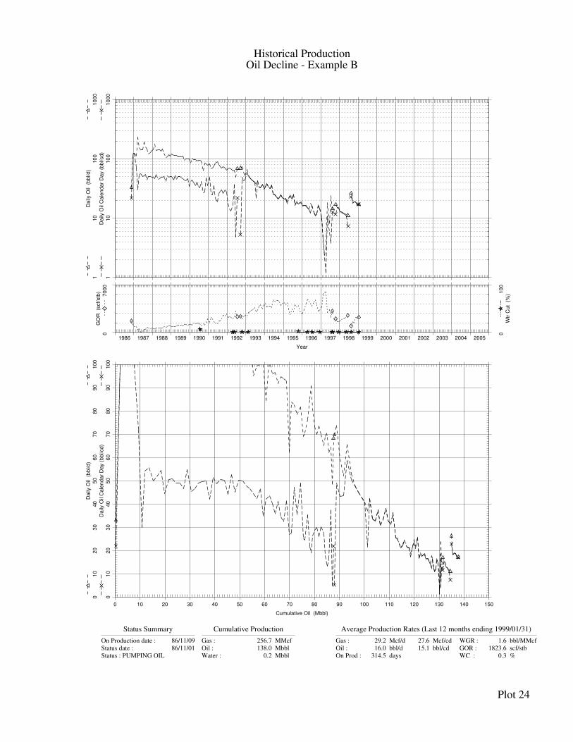
Historical ProductionOil Decline - Example B
Status Summary
On Production date : 86/11/09
Status date : 86/11/01
Status : PUMPING OIL
Cumulative Production
Gas : 256.7 MMcf
Oil : 138.0 Mbbl
Water : 0.2 Mbbl
Average Production Rates (Last 12 months ending 1999/01/31)
Gas : 29.2 Mcf/d
Oil : 16.0 bbl/d
On Prod : 314.5 days
27.6 Mcf/cd
15.1 bbl/cd
WGR : 1.6 bbl/MMcf
GOR : 1823.6 scf/stb
WC : 0.3 %
Plot 24
1986 1987 1988 1989 1990 1991 1992 1993 1994 1995 1996 1997 1998 1999 2000 2001 2002 2003 2004 2005
Year
11
01
00
10
00
Da
ily O
il C
ale
nd
ar
Da
y (
bb
l/cd
)
11
01
00
10
00
Da
ily O
il (
bb
l/d
)
07
00
0
GO
R
(scf/
stb
)
01
00
Wtr
Cu
t (
%)
0 10 20 30 40 50 60 70 80 90 100 110 120 130 140 150
Cumulative Oil (Mbbl)
01
02
03
04
05
06
07
08
09
01
00
Da
ily O
il C
ale
nd
ar
Da
y (
bb
l/cd
)
01
02
03
04
05
06
07
08
09
01
00
Da
ily O
il (
bb
l/d
)
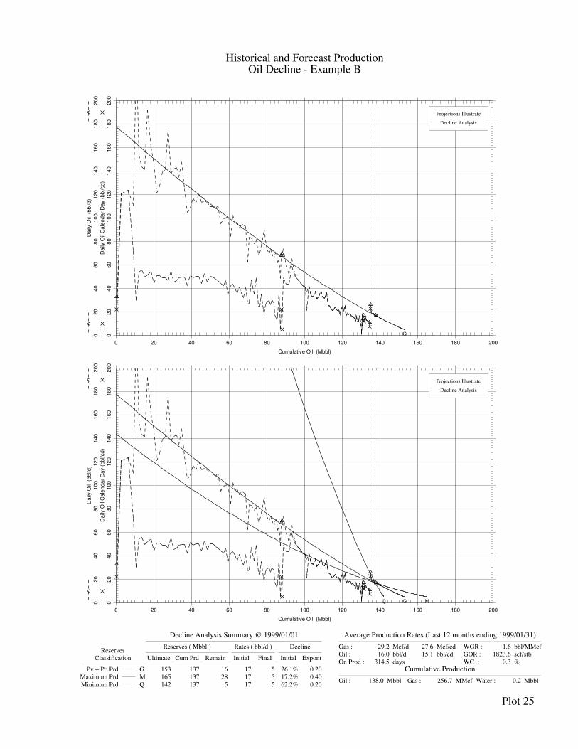
Historical and Forecast ProductionOil Decline - Example B
Decline Analysis Summary @ 1999/01/01
ReservesReserves ( Mbbl ) Rates ( bbl/d ) Decline
Classification Ultimate Cum Prd Remain Initial Final Initial Expont
Pv + Pb Prd G 153 137 16 17 5 26.1% 0.20
Maximum Prd M 165 137 28 17 5 17.2% 0.40
Minimum Prd Q 142 137 5 17 5 62.2% 0.20
Average Production Rates (Last 12 months ending 1999/01/31)
Gas : 29.2 Mcf/d
Oil : 16.0 bbl/d
On Prod : 314.5 days
27.6 Mcf/cd
15.1 bbl/cd
WGR : 1.6 bbl/MMcf
GOR : 1823.6 scf/stb
WC : 0.3 %
Cumulative Production
Oil : 138.0 Mbbl Gas : 256.7 MMcf Water : 0.2 Mbbl
Plot 25
0 20 40 60 80 100 120 140 160 180 200
Cumulative Oil (Mbbl)
02
04
06
08
01
00
12
01
40
16
01
80
20
0
Da
ily O
il C
ale
nd
ar
Da
y (
bb
l/cd
)
02
04
06
08
01
00
12
01
40
16
01
80
20
0
Da
ily O
il (
bb
l/d
)
G
Projections Illustrate
Decline Analysis
0 20 40 60 80 100 120 140 160 180 200
Cumulative Oil (Mbbl)
02
04
06
08
01
00
12
01
40
16
01
80
20
0
Da
ily O
il C
ale
nd
ar
Da
y (
bb
l/cd
)
02
04
06
08
01
00
12
01
40
16
01
80
20
0
Da
ily O
il (
bb
l/d
)
G
Projections Illustrate
Decline Analysis
MQ
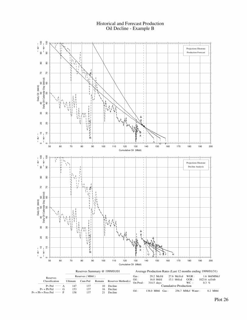
Historical and Forecast ProductionOil Decline - Example B
Reserves Summary @ 1999/01/01
ReservesReserves ( Mbbl )
Classification Ultimate Cum Prd Remain Reserves Method(s)
Pv Prd A 147 137 10 Decline
Pv + Pb Prd G 153 137 16 Decline
Pv + Pb + Poss Prd P 158 137 21 Decline
Average Production Rates (Last 12 months ending 1999/01/31)
Gas : 29.2 Mcf/d
Oil : 16.0 bbl/d
On Prod : 314.5 days
27.6 Mcf/cd
15.1 bbl/cd
WGR : 1.6 bbl/MMcf
GOR : 1823.6 scf/stb
WC : 0.3 %
Cumulative Production
Oil : 138.0 Mbbl Gas : 256.7 MMcf Water : 0.2 Mbbl
Plot 26
50 60 70 80 90 100 110 120 130 140 150 160 170 180 190 200
Cumulative Oil (Mbbl)
01
02
03
04
05
06
07
08
09
01
00
Da
ily O
il C
ale
nd
ar
Da
y (
bb
l/cd
)
01
02
03
04
05
06
07
08
09
01
00
Da
ily O
il (
bb
l/d
)
A
Projections Illustrate
Production Forecast
G P
50 60 70 80 90 100 110 120 130 140 150 160 170 180 190 200
Cumulative Oil (Mbbl)
01
02
03
04
05
06
07
08
09
01
00
Da
ily O
il C
ale
nd
ar
Da
y (
bb
l/cd
)
01
02
03
04
05
06
07
08
09
01
00
Da
ily O
il (
bb
l/d
)
A
Projections Illustrate
Decline Analysis
G MPQ
6-76 Volume 2 — Resources and Reserves Estimation and Classification Guidelines
Canadian Oil and Gas Evaluation Handbook ©SPEE (Calgary Chapter)
Oil Example C 2117
Oil Example C is a well in a moderate-permeability, unstratified, pattern 2118 waterflooded water-wet reservoir. Production history to July 1968 is depicted on Plot 2119 27. As there does not appear to be any hyperbolic bending of the oil-rate or oil-cut 2120 curves, consistent with this type of reservoir, the recommended interpretation for 2P 2121 reserves uses an exponential decline, which yields ultimate reserves of 377 Mstb. 2122 Both oil-rate and oil-cut trends were examined in determining the estimate, as 2123 depicted on Plots 28 and 29, respectively, Line G. However, the oil-cut trends appear 2124 more consistent. An oil rate economic limit of 8 bopd is used (based on a review of 2125 operating costs), which corresponds to a 5.44 percent oil-cut limit. Minimum and 2126 maximum reserves of 364 Mstb and 388 Mstb, respectively, are estimated. The 2127 minimum estimate reflects current exponential oil-rate decline trends (Plot 28, Line 2128 Q), while the maximum reflects some hyperbolic bending on the oil-cut trend (Plot 2129 29, Line M). The recommended proved reserves assignment of 371 Mstb (Plots 30 2130 and 31, Line A) is derived using a value between the minimum and 2P case. 2131 Recommended 3P reserves of 381 Mstb are estimated using a value between the 2P 2132 and maximum case (Plots 30 and 31, Line P). 2133
Actual performance of the well indicates ultimate recovery of 369 Mstb, though it 2134 appeared to have been produced to a higher final rate than that forecast (perhaps 2135 because of a higher economic limit at the time). Rates at the time of shut-in, however, 2136 were consistent with the forecast. 2137
2138 2139
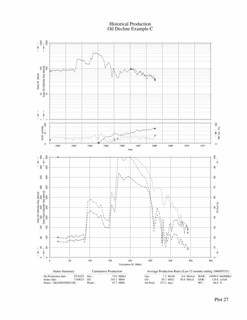
Historical ProductionOil Decline Example C
Status Summary
On Production date : 55/10/25
Status date : 73/08/23
Status : ABANDONED OIL
Cumulative Production
Gas : 72.8 MMcf
Oil : 343.7 Mbbl
Water : 97.7 Mbbl
Average Production Rates (Last 12 months ending 1968/07/31)
Gas : 7.3 Mcf/d
Oil : 56.7 bbl/d
On Prod : 327.2 days
6.6 Mcf/cd
50.8 bbl/cd
WGR : >9999.9 bbl/MMcf
GOR : 129.6 scf/stb
WC : 66.6 %
Plot 27
1962 1963 1964 1965 1966 1967 1968 1969 1970 1971
Year
11
01
00
10
00
Da
ily O
il C
ale
nd
ar
Da
y (
bb
l/cd
)
11
01
00
10
00
Da
ily O
il (
bb
l/d
)
05
00
GO
R
(scf/
stb
)
01
00
Wtr
Cu
t (
%)
0 50 100 150 200 250 300 350 400
Cumulative Oil (Mbbl)
05
01
00
15
02
00
25
03
00
35
04
00
45
05
00
Da
ily F
luid
Ca
len
da
r D
ay (
bb
l/cd
)
04
08
01
20
16
02
00
24
02
80
32
03
60
40
0
Da
ily O
il C
ale
nd
ar
Da
y (
bb
l/cd
)
01
02
03
04
05
06
07
08
09
01
00
Oil
Cu
t (%
)
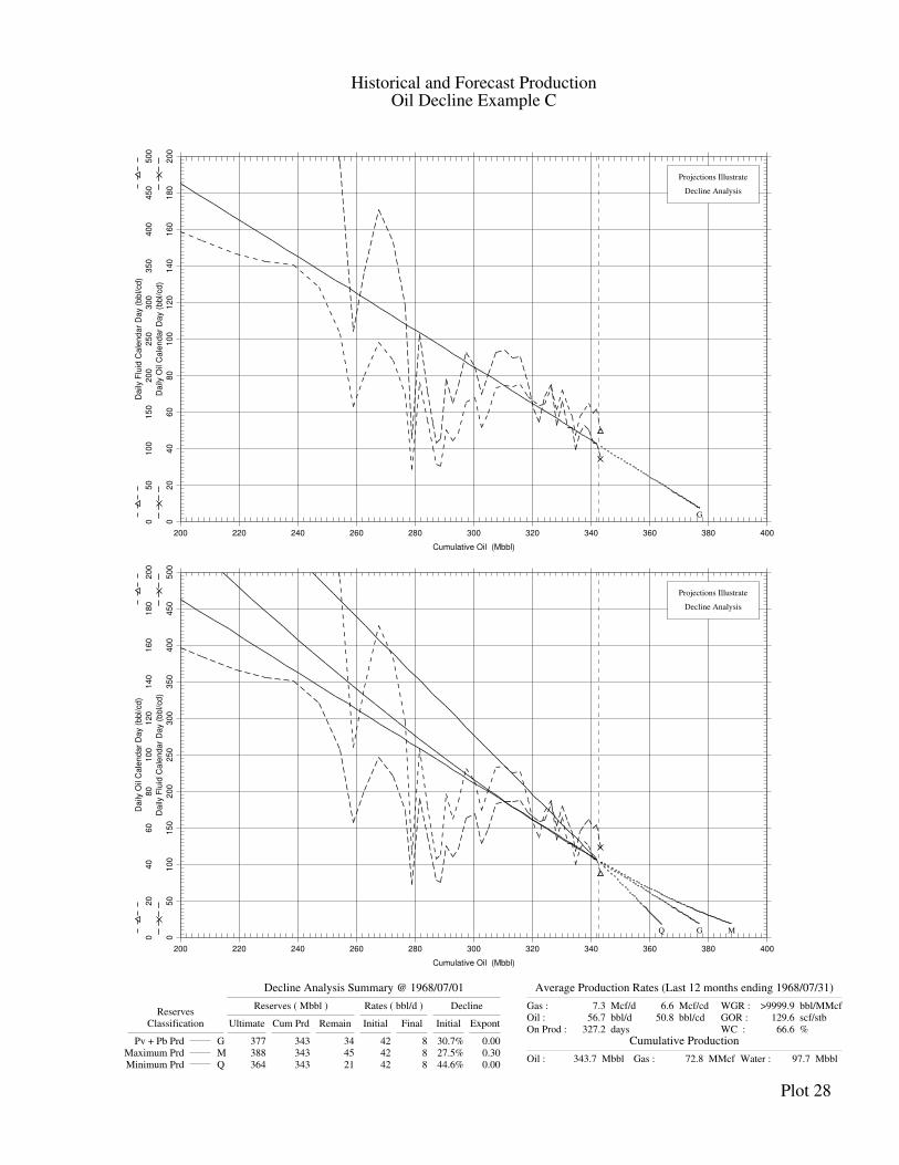
Historical and Forecast ProductionOil Decline Example C
Decline Analysis Summary @ 1968/07/01
ReservesReserves ( Mbbl ) Rates ( bbl/d ) Decline
Classification Ultimate Cum Prd Remain Initial Final Initial Expont
Pv + Pb Prd G 377 343 34 42 8 30.7% 0.00
Maximum Prd M 388 343 45 42 8 27.5% 0.30
Minimum Prd Q 364 343 21 42 8 44.6% 0.00
Average Production Rates (Last 12 months ending 1968/07/31)
Gas : 7.3 Mcf/d
Oil : 56.7 bbl/d
On Prod : 327.2 days
6.6 Mcf/cd
50.8 bbl/cd
WGR : >9999.9 bbl/MMcf
GOR : 129.6 scf/stb
WC : 66.6 %
Cumulative Production
Oil : 343.7 Mbbl Gas : 72.8 MMcf Water : 97.7 Mbbl
Plot 28
200 220 240 260 280 300 320 340 360 380 400
Cumulative Oil (Mbbl)
02
04
06
08
01
00
12
01
40
16
01
80
20
0
Da
ily O
il C
ale
nd
ar
Da
y (
bb
l/cd
)
05
01
00
15
02
00
25
03
00
35
04
00
45
05
00
Da
ily F
luid
Ca
len
da
r D
ay (
bb
l/cd
)
G
Projections Illustrate
Decline Analysis
200 220 240 260 280 300 320 340 360 380 400
Cumulative Oil (Mbbl)
05
01
00
15
02
00
25
03
00
35
04
00
45
05
00
Da
ily F
luid
Ca
len
da
r D
ay (
bb
l/cd
)
02
04
06
08
01
00
12
01
40
16
01
80
20
0
Da
ily O
il C
ale
nd
ar
Da
y (
bb
l/cd
)
G
Projections Illustrate
Decline Analysis
MQ
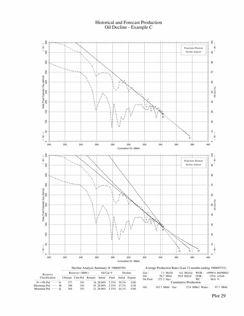
Historical and Forecast ProductionOil Decline - Example C
Decline Analysis Summary @ 1968/07/01
ReservesReserves ( Mbbl ) Oil Cut % Decline
Classification Ultimate Cum Prd Remain Initial Final Initial Expont
Pv + Pb Prd G 377 343 34 28.00% 5.33% 30.3% 0.00
Maximum Prd M 388 343 45 28.00% 5.33% 27.1% 0.30
Minimum Prd Q 364 343 21 28.00% 5.33% 44.1% 0.00
Average Production Rates (Last 12 months ending 1968/07/31)
Gas : 7.3 Mcf/d
Oil : 56.7 bbl/d
On Prod : 327.2 days
6.6 Mcf/cd
50.8 bbl/cd
WGR : >9999.9 bbl/MMcf
GOR : 129.6 scf/stb
WC : 66.6 %
Cumulative Production
Oil : 343.7 Mbbl Gas : 72.8 MMcf Water : 97.7 Mbbl
Plot 29
200 220 240 260 280 300 320 340 360 380 400
Cumulative Oil (Mbbl)
05
01
00
15
02
00
25
03
00
35
04
00
45
05
00
Da
ily F
luid
Ca
len
da
r D
ay (
bb
l/cd
)
01
02
03
04
05
06
07
08
09
01
00
Oil
Cu
t (%
)
G
Projections Illustrate
Decline Analysis
200 220 240 260 280 300 320 340 360 380 400
Cumulative Oil (Mbbl)
05
01
00
15
02
00
25
03
00
35
04
00
45
05
00
Da
ily F
luid
Ca
len
da
r D
ay (
bb
l/cd
)
01
02
03
04
05
06
07
08
09
01
00
Oil
Cu
t (%
)
G
Projections Illustrate
Decline Analysis
MQ
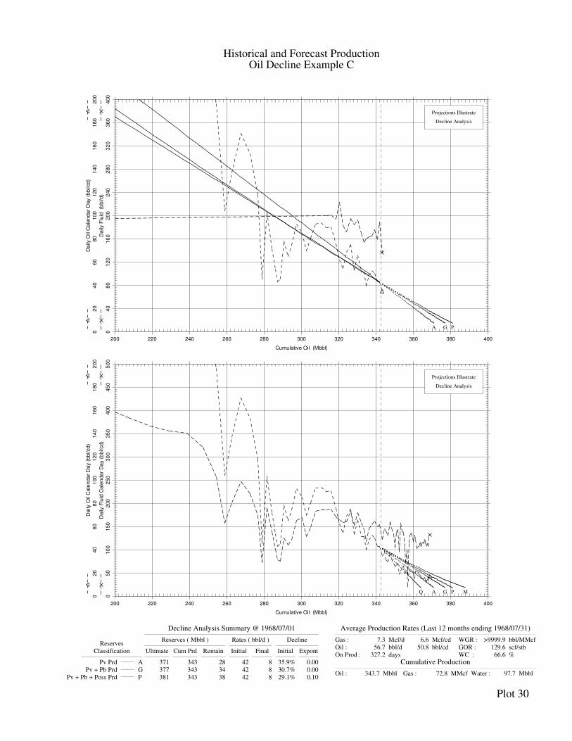
Historical and Forecast ProductionOil Decline Example C
Decline Analysis Summary @ 1968/07/01
ReservesReserves ( Mbbl ) Rates ( bbl/d ) Decline
Classification Ultimate Cum Prd Remain Initial Final Initial Expont
Pv Prd A 371 343 28 42 8 35.9% 0.00
Pv + Pb Prd G 377 343 34 42 8 30.7% 0.00
Pv + Pb + Poss Prd P 381 343 38 42 8 29.1% 0.10
Average Production Rates (Last 12 months ending 1968/07/31)
Gas : 7.3 Mcf/d
Oil : 56.7 bbl/d
On Prod : 327.2 days
6.6 Mcf/cd
50.8 bbl/cd
WGR : >9999.9 bbl/MMcf
GOR : 129.6 scf/stb
WC : 66.6 %
Cumulative Production
Oil : 343.7 Mbbl Gas : 72.8 MMcf Water : 97.7 Mbbl
Plot 30
200 220 240 260 280 300 320 340 360 380 400
Cumulative Oil (Mbbl)
04
08
01
20
16
02
00
24
02
80
32
03
60
40
0
Da
ily F
luid
(b
bl/d
)
02
04
06
08
01
00
12
01
40
16
01
80
20
0
Da
ily O
il C
ale
nd
ar
Da
y (
bb
l/cd
)
A
Projections Illustrate
Decline Analysis
G P
200 220 240 260 280 300 320 340 360 380 400
Cumulative Oil (Mbbl)
05
01
00
15
02
00
25
03
00
35
04
00
45
05
00
Da
ily F
luid
Ca
len
da
r D
ay (
bb
l/cd
)
02
04
06
08
01
00
12
01
40
16
01
80
20
0
Da
ily O
il C
ale
nd
ar
Da
y (
bb
l/cd
)
A
Projections Illustrate
Decline Analysis
G MPQ
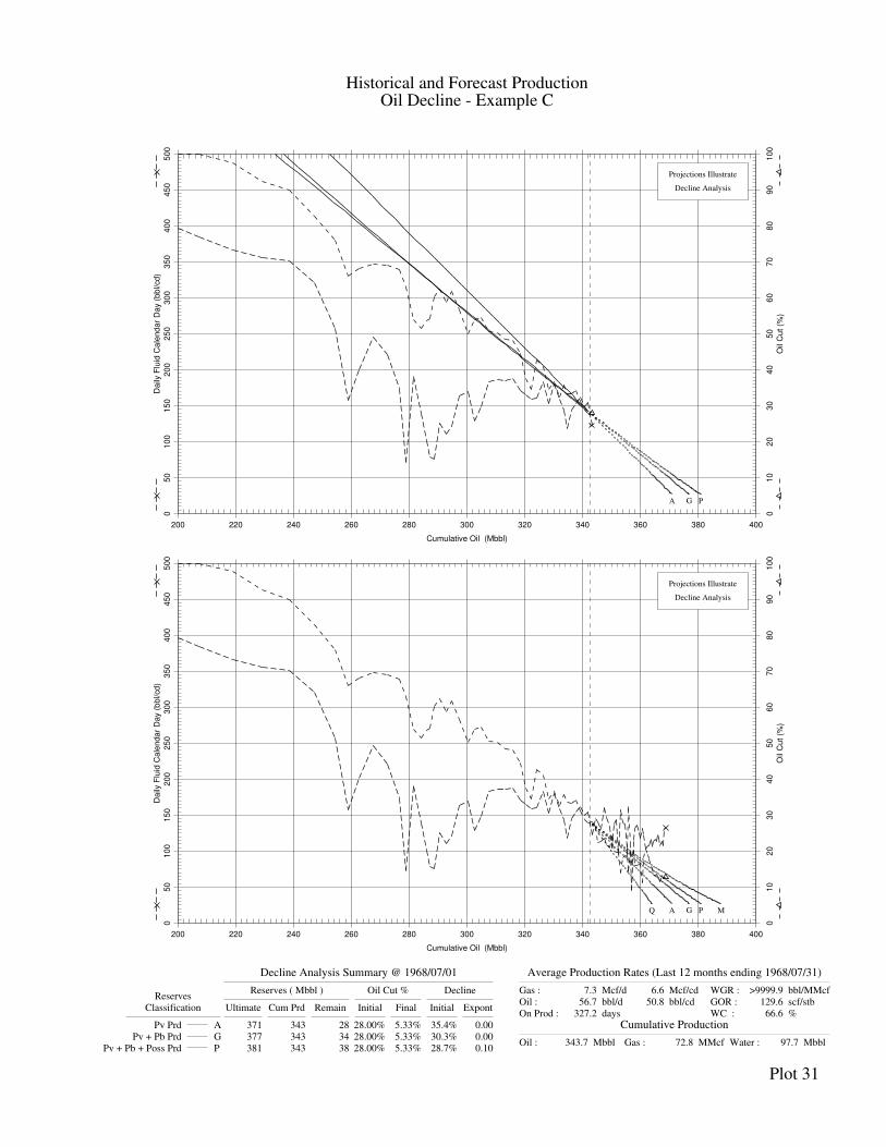
Historical and Forecast ProductionOil Decline - Example C
Decline Analysis Summary @ 1968/07/01
ReservesReserves ( Mbbl ) Oil Cut % Decline
Classification Ultimate Cum Prd Remain Initial Final Initial Expont
Pv Prd A 371 343 28 28.00% 5.33% 35.4% 0.00
Pv + Pb Prd G 377 343 34 28.00% 5.33% 30.3% 0.00
Pv + Pb + Poss Prd P 381 343 38 28.00% 5.33% 28.7% 0.10
Average Production Rates (Last 12 months ending 1968/07/31)
Gas : 7.3 Mcf/d
Oil : 56.7 bbl/d
On Prod : 327.2 days
6.6 Mcf/cd
50.8 bbl/cd
WGR : >9999.9 bbl/MMcf
GOR : 129.6 scf/stb
WC : 66.6 %
Cumulative Production
Oil : 343.7 Mbbl Gas : 72.8 MMcf Water : 97.7 Mbbl
Plot 31
200 220 240 260 280 300 320 340 360 380 400
Cumulative Oil (Mbbl)
05
01
00
15
02
00
25
03
00
35
04
00
45
05
00
Da
ily F
luid
Ca
len
da
r D
ay (
bb
l/cd
)
01
02
03
04
05
06
07
08
09
01
00
Oil
Cu
t (%
)
A
Projections Illustrate
Decline Analysis
G P
200 220 240 260 280 300 320 340 360 380 400
Cumulative Oil (Mbbl)
05
01
00
15
02
00
25
03
00
35
04
00
45
05
00
Da
ily F
luid
Ca
len
da
r D
ay (
bb
l/cd
)
01
02
03
04
05
06
07
08
09
01
00
Oil
Cu
t (%
)
A
Projections Illustrate
Decline Analysis
G MPQ
Section 6 — Procedures for Estimation and Classification of Reserves 6-77
©SPEE (Calgary Chapter) First Edition — April 28, 2004
Oil Example D 2139
Oil Example D is a well in a moderate-permeability, stratified, pattern waterflooded 2140 water-wet reservoir with production history to January 1, 1994, as illustrated on Plot 2141 32. Based on the stratified nature of the reservoir, the recommended interpretation for 2142 2P reserves uses a hyperbolic decline exponent of 0.4 (based on visual best fit and a 2143 review of analogous wells in the area), which yields ultimate reserves of 640 Mstb 2144 (Plot 33, Line G). A range of reasonable visual fits using exponential decline for 2145 minimum (Line Q) and a 0.6 exponent for maximum (Line M) are also illustrated on 2146 Plot 33. The recommended proved (Line A) and 3P (Line P) interpretations used 2147 exponents of 0.3 and 0.5, as depicted on Plot 34. Reserves estimated using these 2148 values are approximately 1/3 lower, and 1/3 higher, than the difference between the 2149 2P and minimum and maximum, respectively. 2150
Both oil-rate and oil-cut trends were considered in deriving the curve fits. Actual well 2151 performance after 1994 is illustrated on Plot 34. Performance is on trend to achieve 2152 the 2P reserves estimate. 2153
2154 2155
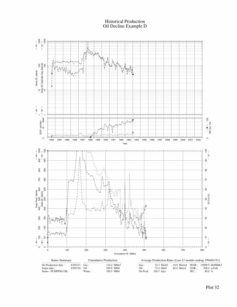
Historical ProductionOil Decline Example D
Status Summary
On Production date : 83/07/21
Status date : 83/07/16
Status : PUMPING OIL
Cumulative Production
Gas : 116.4 MMcf
Oil : 509.9 Mbbl
Water : 350.5 Mbbl
Average Production Rates (Last 12 months ending 1994/01/31)
Gas : 22.3 Mcf/d
Oil : 72.4 bbl/d
On Prod : 326.7 days
19.9 Mcf/cd
64.4 bbl/cd
WGR : >9999.9 bbl/MMcf
GOR : 308.4 scf/stb
WC : 80.8 %
Plot 32
1983 1984 1985 1986 1987 1988 1989 1990 1991 1992 1993 1994 1995 1996 1997 1998 1999 2000 2001 2002
Year
11
01
00
10
00
Da
ily O
il C
ale
nd
ar
Da
y (
bb
l/cd
)
11
01
00
10
00
Da
ily O
il (
bb
l/d
)
02
00
0
GO
R
(scf/
stb
)
01
00
Wtr
Cu
t (
%)
0 100 200 300 400 500 600 700 800
Cumulative Oil (Mbbl)
05
01
00
15
02
00
25
03
00
35
04
00
45
05
00
Da
ily O
il (
bb
l/d
)
01
00
20
03
00
40
05
00
60
07
00
80
09
00
10
00
Da
ily F
luid
(b
bl/d
)
01
02
03
04
05
06
07
08
09
01
00
Oil
Cu
t (%
)
Historical and Forecast ProductionOil Decline Example D
Decline Analysis Summary @ 1994/01/01
ReservesReserves ( Mbbl ) Rates ( bbl/d ) Decline
Classification Ultimate Cum Prd Remain Initial Final Initial Expont
Pv + Pb Prd G 640 509 131 66 5 20.5% 0.40
Maximum Prd M 689 509 180 66 5 18.3% 0.60
Minimum Prd Q 580 509 71 66 5 26.8% 0.00
Average Production Rates (Last 12 months ending 1994/01/31)
Gas : 22.3 Mcf/d
Oil : 72.4 bbl/d
On Prod : 326.7 days
19.9 Mcf/cd
64.4 bbl/cd
WGR : >9999.9 bbl/MMcf
GOR : 308.4 scf/stb
WC : 80.8 %
Cumulative Production
Oil : 509.9 Mbbl Gas : 116.4 MMcf Water : 350.5 Mbbl
Plot 33
0 100 200 300 400 500 600 700 800
Cumulative Oil (Mbbl)
08
01
60
24
03
20
40
04
80
56
06
40
72
08
00
Da
ily F
luid
(b
bl/d
)
04
08
01
20
16
02
00
24
02
80
32
03
60
40
0
Da
ily O
il C
ale
nd
ar
Da
y (
bb
l/cd
)
G
Projections Illustrate
Decline Analysis
200 250 300 350 400 450 500 550 600 650 700
Cumulative Oil (Mbbl)
08
01
60
24
03
20
40
04
80
56
06
40
72
08
00
Da
ily F
luid
(b
bl/d
)
04
08
01
20
16
02
00
24
02
80
32
03
60
40
0
Da
ily O
il C
ale
nd
ar
Da
y (
bb
l/cd
)
G
Projections Illustrate
Decline Analysis
MQ
Historical and Forecast ProductionOil Decline Example D
Decline Analysis Summary @ 1994/01/01
ReservesReserves ( Mbbl ) Rates ( bbl/d ) Decline
Classification Ultimate Cum Prd Remain Initial Final Initial Expont
Pv Prd A 619 509 110 66 5 22.2% 0.30
Pv + Pb Prd G 640 509 131 66 5 20.5% 0.40
Pv + Pb + Poss Prd P 661 509 152 66 5 19.5% 0.50
Average Production Rates (Last 12 months ending 1994/01/31)
Gas : 22.3 Mcf/d
Oil : 72.4 bbl/d
On Prod : 326.7 days
19.9 Mcf/cd
64.4 bbl/cd
WGR : >9999.9 bbl/MMcf
GOR : 308.4 scf/stb
WC : 80.8 %
Cumulative Production
Oil : 509.9 Mbbl Gas : 116.4 MMcf Water : 350.5 Mbbl
Plot 34
200 250 300 350 400 450 500 550 600 650 700
Cumulative Oil (Mbbl)
08
01
60
24
03
20
40
04
80
56
06
40
72
08
00
Da
ily F
luid
(b
bl/d
)
04
08
01
20
16
02
00
24
02
80
32
03
60
40
0
Da
ily O
il C
ale
nd
ar
Da
y (
bb
l/cd
)
01
02
03
04
05
06
07
08
09
01
00
Oil
Cu
t (%
)
A
Projections Illustrate
Decline Analysis
G P
200 250 300 350 400 450 500 550 600 650 700
Cumulative Oil (Mbbl)
02
04
06
08
01
00
12
01
40
16
01
80
20
0
Da
ily O
il (
bb
l/d
)
04
08
01
20
16
02
00
24
02
80
32
03
60
40
0
Da
ily F
luid
(b
bl/d
)
A
Projections Illustrate
Decline Analysis
G MPQ
6-78 Volume 2 — Resources and Reserves Estimation and Classification Guidelines
Canadian Oil and Gas Evaluation Handbook ©SPEE (Calgary Chapter)
Oil Example E 2155
Oil Example E is a well in a high-permeability, unstratified, bottom-water drive oil-2156 wet reservoir with production history as illustrated on Plot 35. As fluid rates are 2157 continually increasing during the life of the well, oil-cut analysis is used for decline 2158 interpretation. An economic oil-cut limit of 0.7 percent is calculated from a review of 2159 operating costs and expected future fluid production rates. From visual curve fitting 2160 and a review of analogous wells in the area, the recommended best estimate 2161 interpretation for 2P reserves uses a hyperbolic decline exponent of 0.9, which yields 2162 ultimate reserves of 856 Mstb (Plot 36, Line G). Reasonable fits can be achieved 2163 using a range of hyperbolic exponents between 0.7 (minimum, Line Q) and 1.0 2164 (maximum, Line M), as depicted on Plot 37. The recommended proved interpretation 2165 uses a hyperbolic exponent of 0.8, which yields ultimate reserves of 793 Mstb (Plot 2166 38, Line A).The recommended 3P interpretation uses a hyperbolic exponent of 0.95, 2167 which yields ultimate reserves of 895 Mstb (Plot 38, Line P). 2168
After the date of the decline analysis, a workover in 1999 improved oil-cut 2169 performance temporarily; however, actual performance is back to the original 2P oil-2170 cut trend. 2171
2172 2173
Historical ProductionOil Decline Example E
Status Summary
On Production date : 87/03/01
Status date : 87/03/01
Status : PUMPING OIL
Cumulative Production
Gas : 111.7 MMcf
Oil : 514.6 Mbbl
Water : 1400.9 Mbbl
Average Production Rates (Last 12 months ending 1998/01/31)
Gas : 43.0 Mcf/d
Oil : 217.5 bbl/d
On Prod : 360.8 days
42.5 Mcf/cd
215.2 bbl/cd
WGR : >9999.9 bbl/MMcf
GOR : 198.2 scf/stb
WC : 89.0 %
Plot 35
1987 1988 1989 1990 1991 1992 1993 1994 1995 1996 1997 1998 1999 2000 2001 2002 2003 2004 2005 2006
Year
11
01
00
10
00
Da
ily O
il C
ale
nd
ar
Da
y (
bb
l/cd
)
11
01
00
10
00
Da
ily O
il (
bb
l/d
)
03
00
0
GO
R
(scf/
stb
)
01
00
Wtr
Cu
t (
%)
0 100 200 300 400 500 600 700 800
Cumulative Oil (Mbbl)
04
08
01
20
16
02
00
24
02
80
32
03
60
40
0
Da
ily O
il (
bb
l/d
)
04
00
80
01
20
01
60
02
00
02
40
02
80
03
20
03
60
04
00
0
Da
ily F
luid
(b
bl/d
)
01
02
03
04
05
06
07
08
09
01
00
Oil
Cu
t (%
)
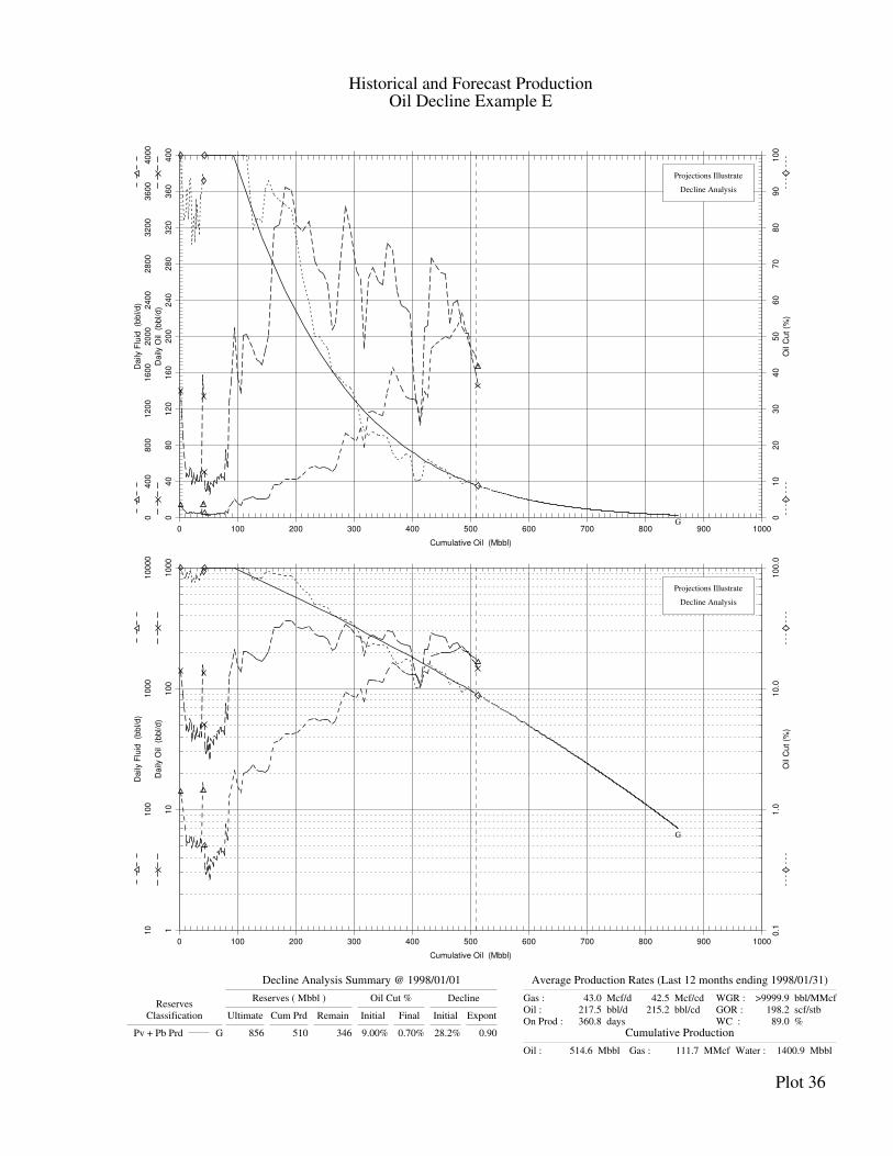
Historical and Forecast ProductionOil Decline Example E
Decline Analysis Summary @ 1998/01/01
ReservesReserves ( Mbbl ) Oil Cut % Decline
Classification Ultimate Cum Prd Remain Initial Final Initial Expont
Pv + Pb Prd G 856 510 346 9.00% 0.70% 28.2% 0.90
Average Production Rates (Last 12 months ending 1998/01/31)
Gas : 43.0 Mcf/d
Oil : 217.5 bbl/d
On Prod : 360.8 days
42.5 Mcf/cd
215.2 bbl/cd
WGR : >9999.9 bbl/MMcf
GOR : 198.2 scf/stb
WC : 89.0 %
Cumulative Production
Oil : 514.6 Mbbl Gas : 111.7 MMcf Water : 1400.9 Mbbl
Plot 36
0 100 200 300 400 500 600 700 800 900 1000
Cumulative Oil (Mbbl)
04
08
01
20
16
02
00
24
02
80
32
03
60
40
0
Da
ily O
il (
bb
l/d
)
04
00
80
01
20
01
60
02
00
02
40
02
80
03
20
03
60
04
00
0
Da
ily F
luid
(b
bl/d
)
01
02
03
04
05
06
07
08
09
01
00
Oil
Cu
t (%
)
G
Projections Illustrate
Decline Analysis
0 100 200 300 400 500 600 700 800 900 1000
Cumulative Oil (Mbbl)
11
01
00
10
00
Da
ily O
il (
bb
l/d
)
10
10
01
00
01
00
00
Da
ily F
luid
(b
bl/d
)
0.1
1.0
10
.01
00
.0
Oil
Cu
t (%
)
G
Projections Illustrate
Decline Analysis
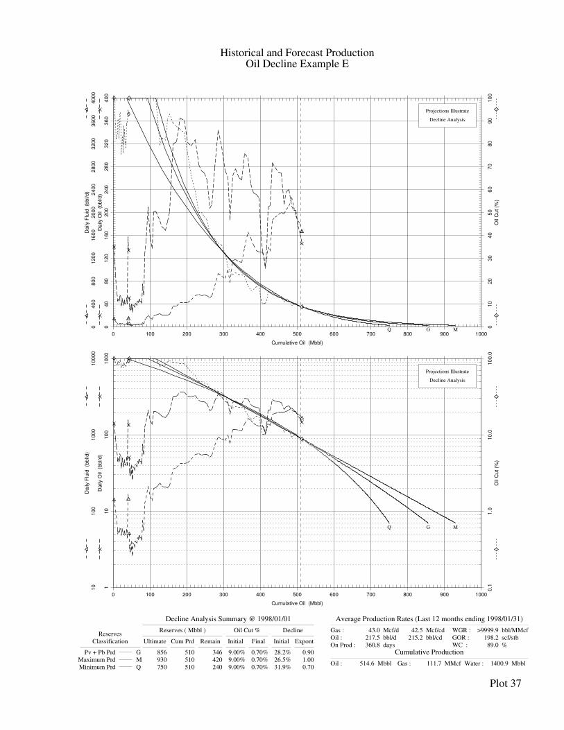
Historical and Forecast ProductionOil Decline Example E
Decline Analysis Summary @ 1998/01/01
ReservesReserves ( Mbbl ) Oil Cut % Decline
Classification Ultimate Cum Prd Remain Initial Final Initial Expont
Pv + Pb Prd G 856 510 346 9.00% 0.70% 28.2% 0.90
Maximum Prd M 930 510 420 9.00% 0.70% 26.5% 1.00
Minimum Prd Q 750 510 240 9.00% 0.70% 31.9% 0.70
Average Production Rates (Last 12 months ending 1998/01/31)
Gas : 43.0 Mcf/d
Oil : 217.5 bbl/d
On Prod : 360.8 days
42.5 Mcf/cd
215.2 bbl/cd
WGR : >9999.9 bbl/MMcf
GOR : 198.2 scf/stb
WC : 89.0 %
Cumulative Production
Oil : 514.6 Mbbl Gas : 111.7 MMcf Water : 1400.9 Mbbl
Plot 37
0 100 200 300 400 500 600 700 800 900 1000
Cumulative Oil (Mbbl)
04
08
01
20
16
02
00
24
02
80
32
03
60
40
0
Da
ily O
il (
bb
l/d
)
04
00
80
01
20
01
60
02
00
02
40
02
80
03
20
03
60
04
00
0
Da
ily F
luid
(b
bl/d
)
01
02
03
04
05
06
07
08
09
01
00
Oil
Cu
t (%
)
G
Projections Illustrate
Decline Analysis
MQ
0 100 200 300 400 500 600 700 800 900 1000
Cumulative Oil (Mbbl)
11
01
00
10
00
Da
ily O
il (
bb
l/d
)
10
10
01
00
01
00
00
Da
ily F
luid
(b
bl/d
)
0.1
1.0
10
.01
00
.0
Oil
Cu
t (%
)
G
Projections Illustrate
Decline Analysis
MQ
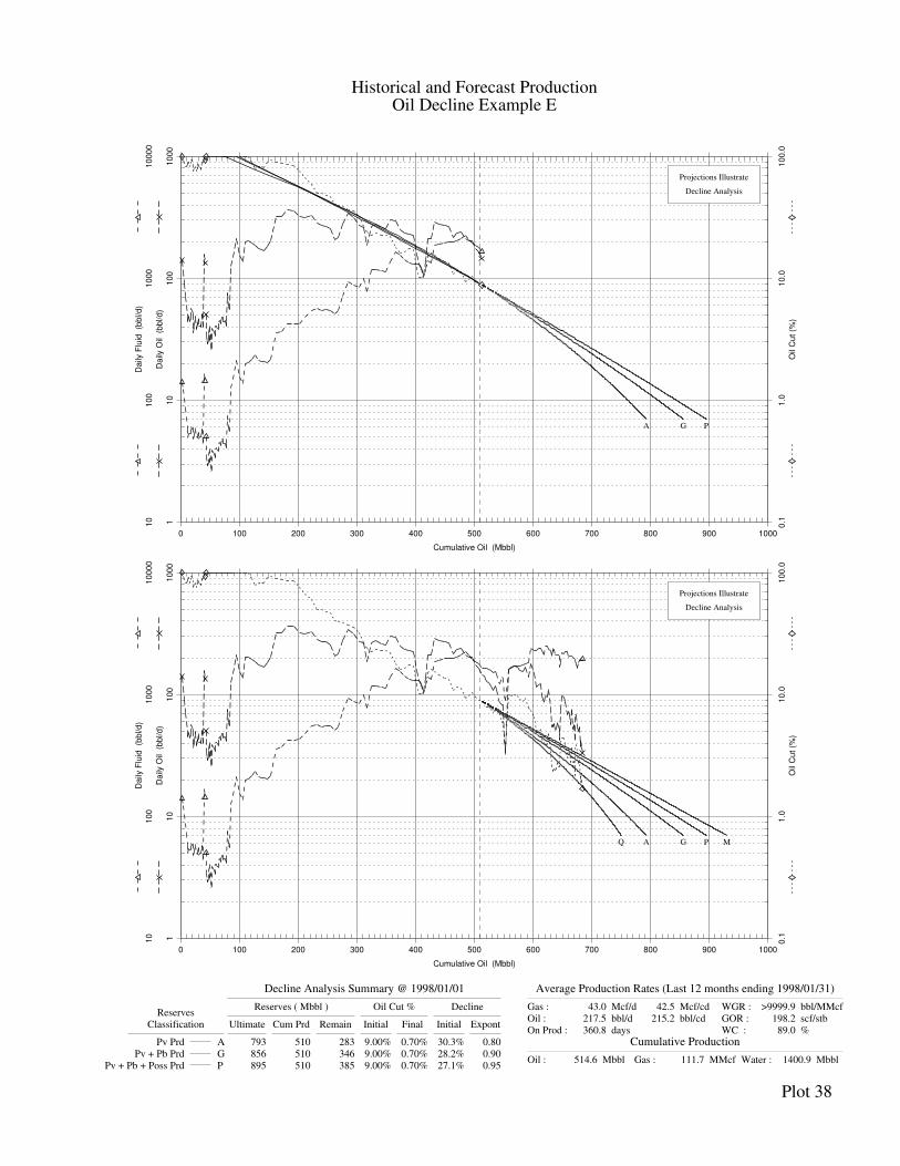
Historical and Forecast ProductionOil Decline Example E
Decline Analysis Summary @ 1998/01/01
ReservesReserves ( Mbbl ) Oil Cut % Decline
Classification Ultimate Cum Prd Remain Initial Final Initial Expont
Pv Prd A 793 510 283 9.00% 0.70% 30.3% 0.80
Pv + Pb Prd G 856 510 346 9.00% 0.70% 28.2% 0.90
Pv + Pb + Poss Prd P 895 510 385 9.00% 0.70% 27.1% 0.95
Average Production Rates (Last 12 months ending 1998/01/31)
Gas : 43.0 Mcf/d
Oil : 217.5 bbl/d
On Prod : 360.8 days
42.5 Mcf/cd
215.2 bbl/cd
WGR : >9999.9 bbl/MMcf
GOR : 198.2 scf/stb
WC : 89.0 %
Cumulative Production
Oil : 514.6 Mbbl Gas : 111.7 MMcf Water : 1400.9 Mbbl
Plot 38
0 100 200 300 400 500 600 700 800 900 1000
Cumulative Oil (Mbbl)
11
01
00
10
00
Da
ily O
il (
bb
l/d
)
10
10
01
00
01
00
00
Da
ily F
luid
(b
bl/d
)
0.1
1.0
10
.01
00
.0
Oil
Cu
t (%
)
A
Projections Illustrate
Decline Analysis
G P
0 100 200 300 400 500 600 700 800 900 1000
Cumulative Oil (Mbbl)
11
01
00
10
00
Da
ily O
il (
bb
l/d
)
10
10
01
00
01
00
00
Da
ily F
luid
(b
bl/d
)
0.1
1.0
10
.01
00
.0
Oil
Cu
t (%
)
A
Projections Illustrate
Decline Analysis
G MPQ
Section 6 — Procedures for Estimation and Classification of Reserves 6-79
©SPEE (Calgary Chapter) First Edition — April 28, 2004
Oil Example F (Group Analysis) 2173
Oil Example F is a group of wells in a high-permeability unstratified bottom-water 2174 drive oil-wet reservoir. The group production plot to July 1995 is illustrated on Plot 2175 39. Wells were added in 1992, 1993, and 1994. This continual addition of wells 2176 makes group decline interpretation more difficult, because the addition of new wells 2177 lowers the overall group oil cut and increases the overall group fluid rate. Decline 2178 analysis was, therefore, performed on each group of wells sorted by start-up date, 2179 using oil-cut trend analysis as illustrated on Plots 40 through 45. For each group, 2180 minimum (Line Q), best estimate (2P, Line G) and maximum (Line M) values are 2181 derived from visual curve fits using decline exponents of 0.6, 0.8, and 1.0, 2182 respectively, and a review of analogous pools in the area. Proved (Line A) and 3P 2183 (Line P) reserves are estimated using decline exponents of 0.7 and 0.9, respectively. 2184
Analysis of each group uses oil-cut trend analysis, because the oil-rate trends are 2185 more sensitive to fluid rate changes. If available, decline analysis should be 2186 performed during periods of constant fluid rates so as to prevent any transient effects 2187 of additional drawdown. For periods of constant fluid production, the results of the 2188 two methods will coincide. 2189
A review of performance for the pool since 1995 indicates the 2P forecast is a good 2190 match with actual production (Plot 46), with the proved forecast being slightly lower 2191 than actual performance. On a start-up group basis, actual performance is between 2192 the proved and 2P forecasts for the 1992 wells, coincident with the proved forecast 2193 for the 1993 wells, and above the 2P forecast for the 1994 wells. The underestimate 2194 of the 1994 wells and overestimate of the 1993 wells could be a result of interference 2195 between the well groups. 2196
2197 2198
Historical ProductionOil Decline Example F (All Wells)
Cumulative Production
Gas : 952.5 MMcf
Oil : 6210.4 Mbbl
Water : 52879.5 Mbbl
Average Production Rates (Last 12 months ending 1995/07/31)
Gas : 1328.2 Mcf/d
Oil : 6078.9 bbl/d
Avg Wells : 77.4
1213.1 Mcf/cd
5567.6 bbl/cd
WGR : >9999.9 bbl/MMcf
GOR : 217.4 scf/stb
WC : 93.8 %
Plot 39
1992 1993 1994 1995 1996 1997 1998 1999 2000 2001
Year
09
0
# O
il W
ells
(m
on
th)
10
10
01
00
01
00
00
Da
ily O
il C
ale
nd
ar
Da
y (
bb
l/cd
)
10
10
01
00
01
00
00
Da
ily O
il (
bb
l/d
)
08
00
GO
R
(scf/
stb
)
11
01
00
10
00
Wa
ter
Cu
t (%
)
0 1000 2000 3000 4000 5000 6000 7000 8000 9000 10000 11000 12000 13000 14000 15000
Cumulative Oil (Mbbl)
09
0
# O
il W
ells
(m
on
th)
08
00
16
00
24
00
32
00
40
00
48
00
56
00
64
00
72
00
80
00
Da
ily O
il (
bb
l/d
)
02
04
06
08
01
00
12
01
40
16
01
80
20
0
Da
ily F
luid
(M
bb
l/d
)
01
02
03
04
05
06
07
08
09
01
00
Oil
Cu
t (%
)

Historical and Forecast ProductionEXAMPLE F 1992 WELLS
Decline Analysis Summary @ 1995/07/01
ReservesReserves ( Mbbl ) Oil Cut % Decline
Classification Ultimate Cum Prd Remain Initial Final Initial Expont
Pv + Pb Prd G 5420 3530 1890 4.00% 0.70% 35.9% 0.80
Maximum Prd M 6110 3530 2580 4.00% 0.70% 31.7% 1.00
Minimum Prd Q 5030 3530 1500 4.00% 0.70% 38.9% 0.60
Average Production Rates (Last 12 months ending 1995/07/31)
Gas : 538.9 Mcf/d
Oil : 2534.3 bbl/d
Avg Wells : 32.4
500.2 Mcf/cd
2346.7 bbl/cd
WGR : >9999.9 bbl/MMcf
GOR : 212.7 scf/stb
WC : 94.9 %
Cumulative Production
Oil : 3586.8 Mbbl Gas : 481.5 MMcf Water : 31328.2 Mbbl
Plot 40
1992 1993 1994 1995 1996 1997 1998 1999 2000 2001
Year
04
0
# O
il W
ells
(m
on
th)
10
10
01
00
01
00
00
Da
ily O
il C
ale
nd
ar
Da
y (
bb
l/cd
)
10
10
01
00
01
00
00
Da
ily O
il (
bb
l/d
)
06
00
GO
R
(scf/
stb
)
11
01
00
10
00
Wa
ter
Cu
t (%
)
0 1000 2000 3000 4000 5000 6000 7000 8000
Cumulative Oil (Mbbl)
10
10
01
00
01
00
00
Da
ily O
il (
bb
l/d
)
10
01
00
01
00
00
10
00
00
Da
ily F
luid
(b
bl/d
)
0.1
1.0
10
.01
00
.0
Oil
Cu
t (%
)
G
Projections Illustrate
Decline Analysis
MQ
Historical and Forecast ProductionEXAMPLE F 1992 WELLS
Decline Analysis Summary @ 1995/07/01
ReservesReserves ( Mbbl ) Oil Cut % Decline
Classification Ultimate Cum Prd Remain Initial Final Initial Expont
Pv Prd A 5160 3530 1630 4.00% 0.70% 38.2% 0.70
Pv + Pb Prd G 5420 3530 1890 4.00% 0.70% 35.9% 0.80
Pv + Pb + Poss Prd P 5790 3530 2260 4.00% 0.70% 33.2% 0.90
Average Production Rates (Last 12 months ending 1995/07/31)
Gas : 538.9 Mcf/d
Oil : 2534.3 bbl/d
Avg Wells : 32.4
500.2 Mcf/cd
2346.7 bbl/cd
WGR : >9999.9 bbl/MMcf
GOR : 212.7 scf/stb
WC : 94.9 %
Cumulative Production
Oil : 3586.8 Mbbl Gas : 481.5 MMcf Water : 31328.2 Mbbl
Plot 41
0 500 1000 1500 2000 2500 3000 3500 4000 4500 5000 5500 6000
Cumulative Oil (Mbbl)
10
10
01
00
01
00
00
Da
ily O
il (
bb
l/d
)
10
01
00
01
00
00
10
00
00
Da
ily F
luid
(b
bl/d
)
0.1
1.0
10
.01
00
.0
Oil
Cu
t (%
)
A
Projections Illustrate
Decline Analysis
G P
0 1000 2000 3000 4000 5000 6000 7000 8000
Cumulative Oil (Mbbl)
10
10
01
00
01
00
00
Da
ily O
il (
bb
l/d
)
10
01
00
01
00
00
10
00
00
Da
ily F
luid
(b
bl/d
)
0.1
1.0
10
.01
00
.0
Oil
Cu
t (%
)
A
Projections Illustrate
Decline Analysis
G MPQ
Historical and Forecast ProductionEXAMPLE F 1993 WELLS
Decline Analysis Summary @ 1995/07/01
ReservesReserves ( Mbbl ) Oil Cut % Decline
Classification Ultimate Cum Prd Remain Initial Final Initial Expont
Pv + Pb Prd G 4100 2236 1864 5.00% 0.70% 37.6% 0.80
Maximum Prd M 4560 2236 2324 5.00% 0.70% 35.7% 1.00
Minimum Prd Q 3710 2236 1474 5.00% 0.70% 40.4% 0.60
Average Production Rates (Last 12 months ending 1995/07/31)
Gas : 529.0 Mcf/d
Oil : 2479.0 bbl/d
Avg Wells : 32.7
490.2 Mcf/cd
2308.8 bbl/cd
WGR : >9999.9 bbl/MMcf
GOR : 211.9 scf/stb
WC : 93.5 %
Cumulative Production
Oil : 2290.6 Mbbl Gas : 389.9 MMcf Water : 18754.7 Mbbl
Plot 42
1993 1994 1995 1996 1997 1998 1999 2000 2001 2002
Year
04
0
# O
il W
ells
(m
on
th)
10
10
01
00
01
00
00
Da
ily O
il C
ale
nd
ar
Da
y (
bb
l/cd
)
10
10
01
00
01
00
00
Da
ily O
il (
bb
l/d
)
08
00
GO
R
(scf/
stb
)
11
01
00
10
00
Wa
ter
Cu
t (%
)
0 500 1000 1500 2000 2500 3000 3500 4000 4500 5000
Cumulative Oil (Mbbl)
10
10
01
00
01
00
00
Da
ily O
il (
bb
l/d
)
10
01
00
01
00
00
10
00
00
Da
ily F
luid
(b
bl/d
)
0.1
1.0
10
.01
00
.0
Oil
Cu
t (%
)
G
Projections Illustrate
Decline Analysis
MQ
Historical and Forecast ProductionEXAMPLE F 1993 WELLS
Decline Analysis Summary @ 1995/07/01
ReservesReserves ( Mbbl ) Oil Cut % Decline
Classification Ultimate Cum Prd Remain Initial Final Initial Expont
Pv Prd A 3890 2236 1654 5.00% 0.70% 39.0% 0.70
Pv + Pb Prd G 4100 2236 1864 5.00% 0.70% 37.6% 0.80
Pv + Pb + Poss Prd P 4290 2236 2054 5.00% 0.70% 36.9% 0.90
Average Production Rates (Last 12 months ending 1995/07/31)
Gas : 529.0 Mcf/d
Oil : 2479.0 bbl/d
Avg Wells : 32.7
490.2 Mcf/cd
2308.8 bbl/cd
WGR : >9999.9 bbl/MMcf
GOR : 211.9 scf/stb
WC : 93.5 %
Cumulative Production
Oil : 2290.6 Mbbl Gas : 389.9 MMcf Water : 18754.7 Mbbl
Plot 43
0 500 1000 1500 2000 2500 3000 3500 4000 4500 5000
Cumulative Oil (Mbbl)
10
10
01
00
01
00
00
Da
ily O
il (
bb
l/d
)
10
01
00
01
00
00
10
00
00
Da
ily F
luid
(b
bl/d
)
0.1
1.0
10
.01
00
.0
Oil
Cu
t (%
)
A
Projections Illustrate
Decline Analysis
G P
0 500 1000 1500 2000 2500 3000 3500 4000 4500 5000
Cumulative Oil (Mbbl)
10
10
01
00
01
00
00
Da
ily O
il (
bb
l/d
)
10
01
00
01
00
00
10
00
00
Da
ily F
luid
(b
bl/d
)
0.1
1.0
10
.01
00
.0
Oil
Cu
t (%
)
A
Projections Illustrate
Decline Analysis
G MPQ
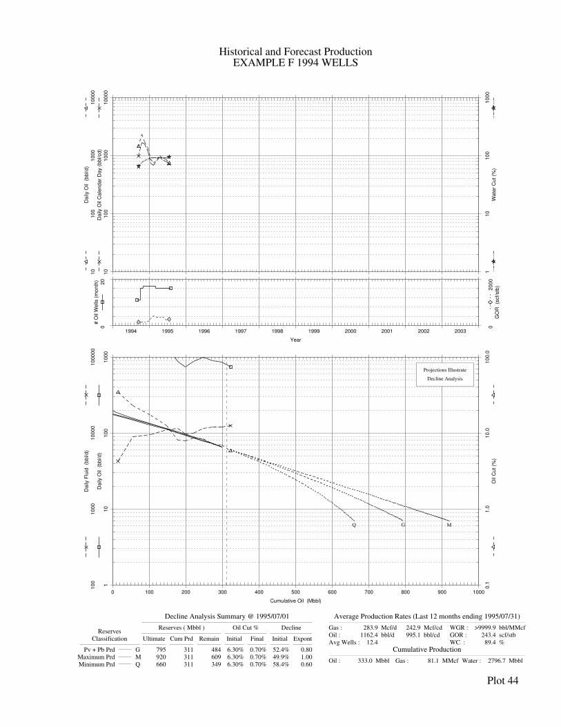
Historical and Forecast ProductionEXAMPLE F 1994 WELLS
Decline Analysis Summary @ 1995/07/01
ReservesReserves ( Mbbl ) Oil Cut % Decline
Classification Ultimate Cum Prd Remain Initial Final Initial Expont
Pv + Pb Prd G 795 311 484 6.30% 0.70% 52.4% 0.80
Maximum Prd M 920 311 609 6.30% 0.70% 49.9% 1.00
Minimum Prd Q 660 311 349 6.30% 0.70% 58.4% 0.60
Average Production Rates (Last 12 months ending 1995/07/31)
Gas : 283.9 Mcf/d
Oil : 1162.4 bbl/d
Avg Wells : 12.4
242.9 Mcf/cd
995.1 bbl/cd
WGR : >9999.9 bbl/MMcf
GOR : 243.4 scf/stb
WC : 89.4 %
Cumulative Production
Oil : 333.0 Mbbl Gas : 81.1 MMcf Water : 2796.7 Mbbl
Plot 44
1994 1995 1996 1997 1998 1999 2000 2001 2002 2003
Year
02
0
# O
il W
ells
(m
on
th)
10
10
01
00
01
00
00
Da
ily O
il C
ale
nd
ar
Da
y (
bb
l/cd
)
10
10
01
00
01
00
00
Da
ily O
il (
bb
l/d
)
02
00
0
GO
R
(scf/
stb
)
11
01
00
10
00
Wa
ter
Cu
t (%
)
0 100 200 300 400 500 600 700 800 900 1000
Cumulative Oil (Mbbl)
11
01
00
10
00
Da
ily O
il (
bb
l/d
)
10
01
00
01
00
00
10
00
00
Da
ily F
luid
(b
bl/d
)
0.1
1.0
10
.01
00
.0
Oil
Cu
t (%
)
G
Projections Illustrate
Decline Analysis
MQ
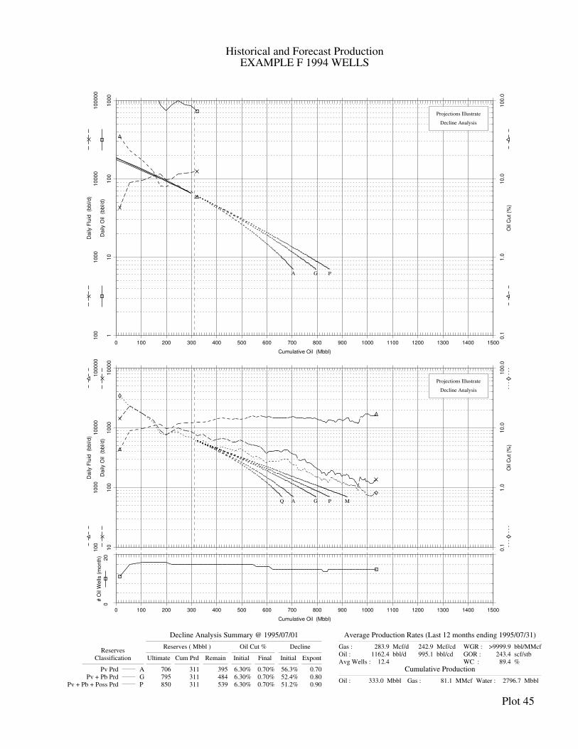
Historical and Forecast ProductionEXAMPLE F 1994 WELLS
Decline Analysis Summary @ 1995/07/01
ReservesReserves ( Mbbl ) Oil Cut % Decline
Classification Ultimate Cum Prd Remain Initial Final Initial Expont
Pv Prd A 706 311 395 6.30% 0.70% 56.3% 0.70
Pv + Pb Prd G 795 311 484 6.30% 0.70% 52.4% 0.80
Pv + Pb + Poss Prd P 850 311 539 6.30% 0.70% 51.2% 0.90
Average Production Rates (Last 12 months ending 1995/07/31)
Gas : 283.9 Mcf/d
Oil : 1162.4 bbl/d
Avg Wells : 12.4
242.9 Mcf/cd
995.1 bbl/cd
WGR : >9999.9 bbl/MMcf
GOR : 243.4 scf/stb
WC : 89.4 %
Cumulative Production
Oil : 333.0 Mbbl Gas : 81.1 MMcf Water : 2796.7 Mbbl
Plot 45
0 100 200 300 400 500 600 700 800 900 1000 1100 1200 1300 1400 1500
Cumulative Oil (Mbbl)
11
01
00
10
00
Da
ily O
il (
bb
l/d
)
10
01
00
01
00
00
10
00
00
Da
ily F
luid
(b
bl/d
)
0.1
1.0
10
.01
00
.0
Oil
Cu
t (%
)
A
Projections Illustrate
Decline Analysis
G P
0 100 200 300 400 500 600 700 800 900 1000 1100 1200 1300 1400 1500
Cumulative Oil (Mbbl)
02
0
# O
il W
ells
(m
on
th)
10
10
01
00
01
00
00
Da
ily O
il (
bb
l/d
)
10
01
00
01
00
00
10
00
00
Da
ily F
luid
(b
bl/d
)
0.1
1.0
10
.01
00
.0
Oil
Cu
t (%
)
A
Projections Illustrate
Decline Analysis
G MPQ
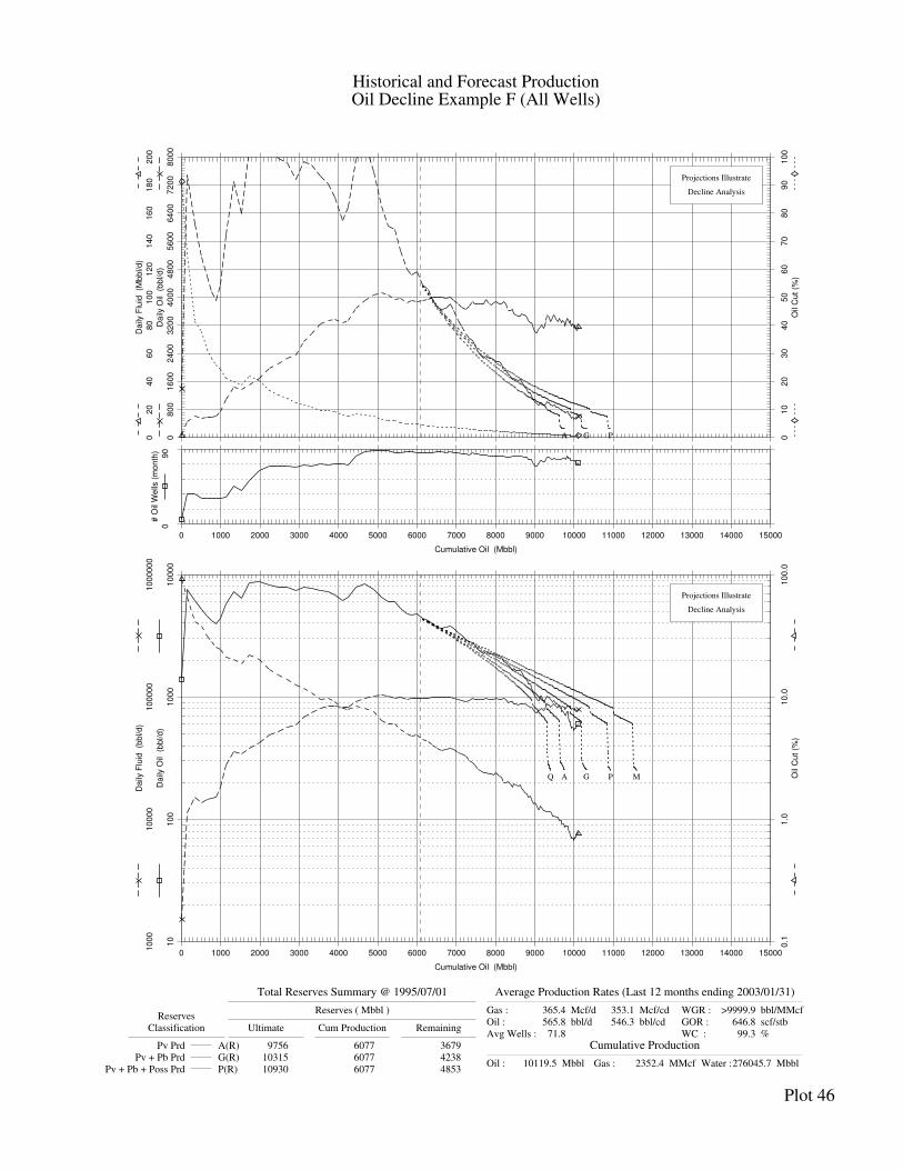
Historical and Forecast ProductionOil Decline Example F (All Wells)
Total Reserves Summary @ 1995/07/01
ReservesReserves ( Mbbl )
Classification Ultimate Cum Production Remaining
Pv Prd A(R) 9756 6077 3679
Pv + Pb Prd G(R) 10315 6077 4238
Pv + Pb + Poss Prd P(R) 10930 6077 4853
Average Production Rates (Last 12 months ending 2003/01/31)
Gas : 365.4 Mcf/d
Oil : 565.8 bbl/d
Avg Wells : 71.8
353.1 Mcf/cd
546.3 bbl/cd
WGR : >9999.9 bbl/MMcf
GOR : 646.8 scf/stb
WC : 99.3 %
Cumulative Production
Oil : 10119.5 Mbbl Gas : 2352.4 MMcf Water :276045.7 Mbbl
Plot 46
0 1000 2000 3000 4000 5000 6000 7000 8000 9000 10000 11000 12000 13000 14000 15000
Cumulative Oil (Mbbl)
09
0
# O
il W
ells
(m
on
th)
08
00
16
00
24
00
32
00
40
00
48
00
56
00
64
00
72
00
80
00
Da
ily O
il (
bb
l/d
)
02
04
06
08
01
00
12
01
40
16
01
80
20
0
Da
ily F
luid
(M
bb
l/d
)
01
02
03
04
05
06
07
08
09
01
00
Oil
Cu
t (%
)
A
Projections Illustrate
Decline Analysis
G P
0 1000 2000 3000 4000 5000 6000 7000 8000 9000 10000 11000 12000 13000 14000 15000
Cumulative Oil (Mbbl)
10
10
01
00
01
00
00
Da
ily O
il (
bb
l/d
)
10
00
10
00
01
00
00
01
00
00
00
Da
ily F
luid
(b
bl/d
)
0.1
1.0
10
.01
00
.0
Oil
Cu
t (%
)
A
Projections Illustrate
Decline Analysis
G MPQ
6-80 Volume 2 — Resources and Reserves Estimation and Classification Guidelines
Canadian Oil and Gas Evaluation Handbook ©SPEE (Calgary Chapter)
Oil Example G (Group Analysis) 2198
Oil Example G is a bottom-water drive, thick, highly permeable, unstratified light oil 2199 reservoir with an overlying gas cap. The production history to January 1990 is 2200 illustrated on Plot 47. The recommended interpretation from visual curve fitting for 2201 2P reserves uses a hyperbolic decline exponent of 0.2, which yields ultimate reserves 2202 of 519 MMstb (Plot 48, Line G). Reasonable visual fits can be achieved using 2203 hyperbolic exponents between 0 (minimum, Line Q) and 0.4 (maximum, Line M). 2204 Proved and 3P reserves are estimated using hyperbolic exponents of 0.1 (Line A) and 2205 0.3 (Line P), respectively, as depicted on Plot 49. 2206
Actual performance since the date of the decline analysis was initially along the 2207 proved forecast, then above the forecast due to a series of recompletion workovers to 2208 better target the remaining oil column. The stabilization of production rates that 2209 occurred as a result of the workovers is not predictable from decline analysis. 2210 Volumetric rationalization of oil-water and gas-water contact movements is required 2211 to identify and quantify the recompletion reserves opportunities. 2212
2213 2214
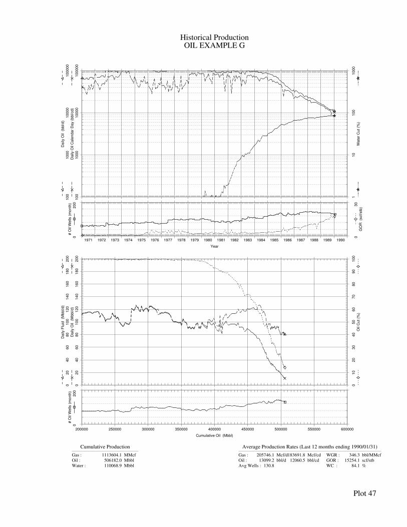
Historical ProductionOIL EXAMPLE G
Cumulative Production
Gas : 1113604.1 MMcf
Oil : 506182.0 Mbbl
Water : 110068.9 Mbbl
Average Production Rates (Last 12 months ending 1990/01/31)
Gas : 205746.1 Mcf/d
Oil : 13099.2 bbl/d
Avg Wells : 130.8
183691.8 Mcf/cd
12060.5 bbl/cd
WGR : 346.3 bbl/MMcf
GOR : 15254.1 scf/stb
WC : 84.1 %
Plot 47
1971 1972 1973 1974 1975 1976 1977 1978 1979 1980 1981 1982 1983 1984 1985 1986 1987 1988 1989 1990
Year
02
00
# O
il W
ells
(m
on
th)
10
01
00
01
00
00
10
00
00
Da
ily O
il C
ale
nd
ar
Da
y (
bb
l/cd
)
10
01
00
01
00
00
10
00
00
Da
ily O
il (
bb
l/d
)
03
0
GO
R
(scf/
stb
)
11
01
00
10
00
Wa
ter
Cu
t (%
)
200000 250000 300000 350000 400000 450000 500000 550000 600000
Cumulative Oil (Mbbl)
02
00
# O
il W
ells
(m
on
th)
02
04
06
08
01
00
12
01
40
16
01
80
20
0
Da
ily O
il (
Mb
bl/d
)
02
04
06
08
01
00
12
01
40
16
01
80
20
0
Da
ily F
luid
(M
bb
l/d
)
01
02
03
04
05
06
07
08
09
01
00
Oil
Cu
t (%
)
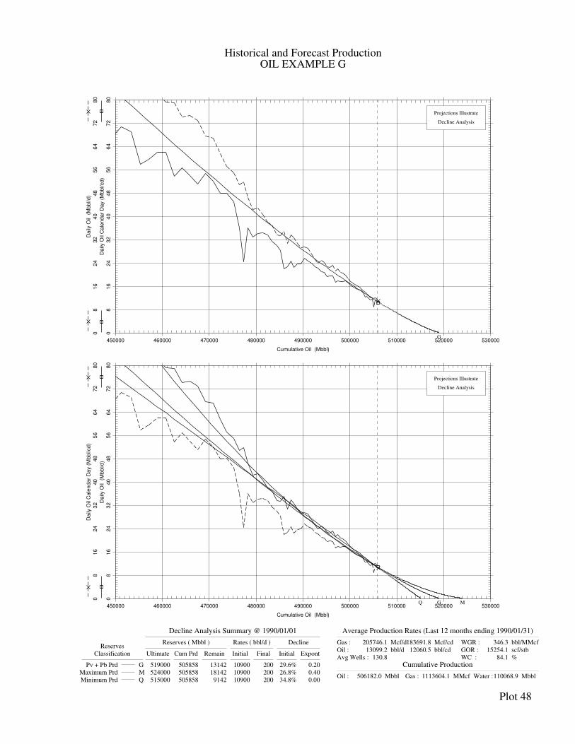
Historical and Forecast ProductionOIL EXAMPLE G
Decline Analysis Summary @ 1990/01/01
ReservesReserves ( Mbbl ) Rates ( bbl/d ) Decline
Classification Ultimate Cum Prd Remain Initial Final Initial Expont
Pv + Pb Prd G 519000 505858 13142 10900 200 29.6% 0.20
Maximum Prd M 524000 505858 18142 10900 200 26.8% 0.40
Minimum Prd Q 515000 505858 9142 10900 200 34.8% 0.00
Average Production Rates (Last 12 months ending 1990/01/31)
Gas : 205746.1 Mcf/d
Oil : 13099.2 bbl/d
Avg Wells : 130.8
183691.8 Mcf/cd
12060.5 bbl/cd
WGR : 346.3 bbl/MMcf
GOR : 15254.1 scf/stb
WC : 84.1 %
Cumulative Production
Oil : 506182.0 Mbbl Gas : 1113604.1 MMcf Water :110068.9 Mbbl
Plot 48
450000 460000 470000 480000 490000 500000 510000 520000 530000
Cumulative Oil (Mbbl)
08
16
24
32
40
48
56
64
72
80
Da
ily O
il C
ale
nd
ar
Da
y (
Mb
bl/cd
)
08
16
24
32
40
48
56
64
72
80
Da
ily O
il (
Mb
bl/d
)
G
Projections Illustrate
Decline Analysis
450000 460000 470000 480000 490000 500000 510000 520000 530000
Cumulative Oil (Mbbl)
08
16
24
32
40
48
56
64
72
80
Da
ily O
il (
Mb
bl/d
)
08
16
24
32
40
48
56
64
72
80
Da
ily O
il C
ale
nd
ar
Da
y (
Mb
bl/cd
)
G
Projections Illustrate
Decline Analysis
MQ
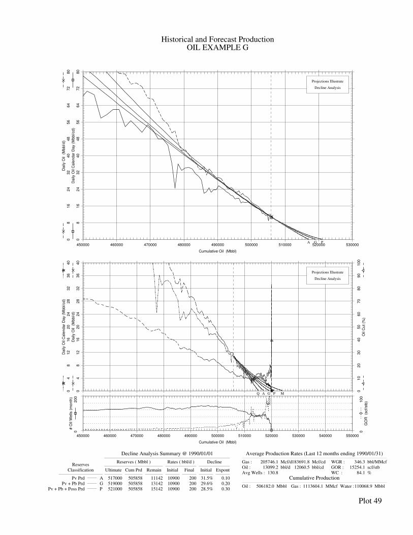
Historical and Forecast ProductionOIL EXAMPLE G
Decline Analysis Summary @ 1990/01/01
ReservesReserves ( Mbbl ) Rates ( bbl/d ) Decline
Classification Ultimate Cum Prd Remain Initial Final Initial Expont
Pv Prd A 517000 505858 11142 10900 200 31.5% 0.10
Pv + Pb Prd G 519000 505858 13142 10900 200 29.6% 0.20
Pv + Pb + Poss Prd P 521000 505858 15142 10900 200 28.5% 0.30
Average Production Rates (Last 12 months ending 1990/01/31)
Gas : 205746.1 Mcf/d
Oil : 13099.2 bbl/d
Avg Wells : 130.8
183691.8 Mcf/cd
12060.5 bbl/cd
WGR : 346.3 bbl/MMcf
GOR : 15254.1 scf/stb
WC : 84.1 %
Cumulative Production
Oil : 506182.0 Mbbl Gas : 1113604.1 MMcf Water :110068.9 Mbbl
Plot 49
450000 460000 470000 480000 490000 500000 510000 520000 530000
Cumulative Oil (Mbbl)
08
16
24
32
40
48
56
64
72
80
Da
ily O
il C
ale
nd
ar
Da
y (
Mb
bl/cd
)
08
16
24
32
40
48
56
64
72
80
Da
ily O
il (
Mb
bl/d
)
A
Projections Illustrate
Decline Analysis
G P
450000 460000 470000 480000 490000 500000 510000 520000 530000 540000 550000
Cumulative Oil (Mbbl)
02
00
# O
il W
ells
(m
on
th)
04
81
21
62
02
42
83
23
64
0
Da
ily O
il (
Mb
bl/d
)
01
02
03
04
05
06
07
08
09
01
00
Oil
Cu
t (%
)0
10
0
GO
R
(scf/
stb
)
04
81
21
62
02
42
83
23
64
0
Da
ily O
il C
ale
nd
ar
Da
y (
Mb
bl/cd
)
A
Projections Illustrate
Decline Analysis
G MPQ
Section 6 — Procedures for Estimation and Classification of Reserves 6-81
©SPEE (Calgary Chapter) First Edition — April 28, 2004
Oil Example H 2214
Oil Example H is a well in an unconsolidated, low GOR heavy oil well (Plot 50). 2215 Wells of this type cannot be analyzed from decline analysis and must be rationalized 2216 volumetrically using analogous recovery factors or performance analogies for 2217 reservoirs of this type. Production rates increase throughout the life of the well, 2218 because sand production continually increases the effective wellbore radius, and 2219 foamy oil behaviour with depressurization increases oil mobility. At some point, 2220 however, reservoir energy is lost, and/or the wellbore wormholes collapse, and the 2221 well ceases production. 2222
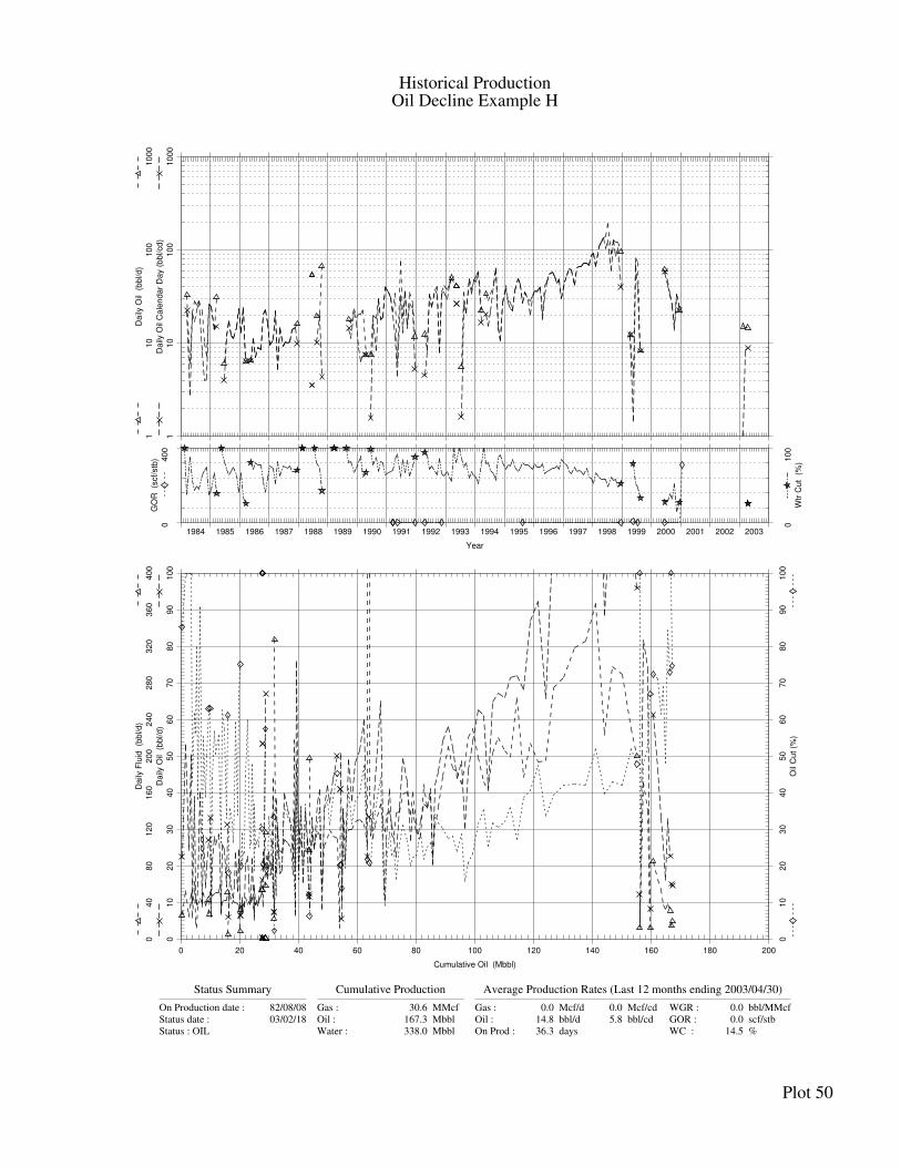
Historical ProductionOil Decline Example H
Status Summary
On Production date : 82/08/08
Status date : 03/02/18
Status : OIL
Cumulative Production
Gas : 30.6 MMcf
Oil : 167.3 Mbbl
Water : 338.0 Mbbl
Average Production Rates (Last 12 months ending 2003/04/30)
Gas : 0.0 Mcf/d
Oil : 14.8 bbl/d
On Prod : 36.3 days
0.0 Mcf/cd
5.8 bbl/cd
WGR : 0.0 bbl/MMcf
GOR : 0.0 scf/stb
WC : 14.5 %
Plot 50
1984 1985 1986 1987 1988 1989 1990 1991 1992 1993 1994 1995 1996 1997 1998 1999 2000 2001 2002 2003
Year
11
01
00
10
00
Da
ily O
il C
ale
nd
ar
Da
y (
bb
l/cd
)
11
01
00
10
00
Da
ily O
il (
bb
l/d
)
04
00
GO
R
(scf/
stb
)
01
00
Wtr
Cu
t (
%)
0 20 40 60 80 100 120 140 160 180 200
Cumulative Oil (Mbbl)
01
02
03
04
05
06
07
08
09
01
00
Da
ily O
il (
bb
l/d
)
04
08
01
20
16
02
00
24
02
80
32
03
60
40
0
Da
ily F
luid
(b
bl/d
)
01
02
03
04
05
06
07
08
09
01
00
Oil
Cu
t (%
)
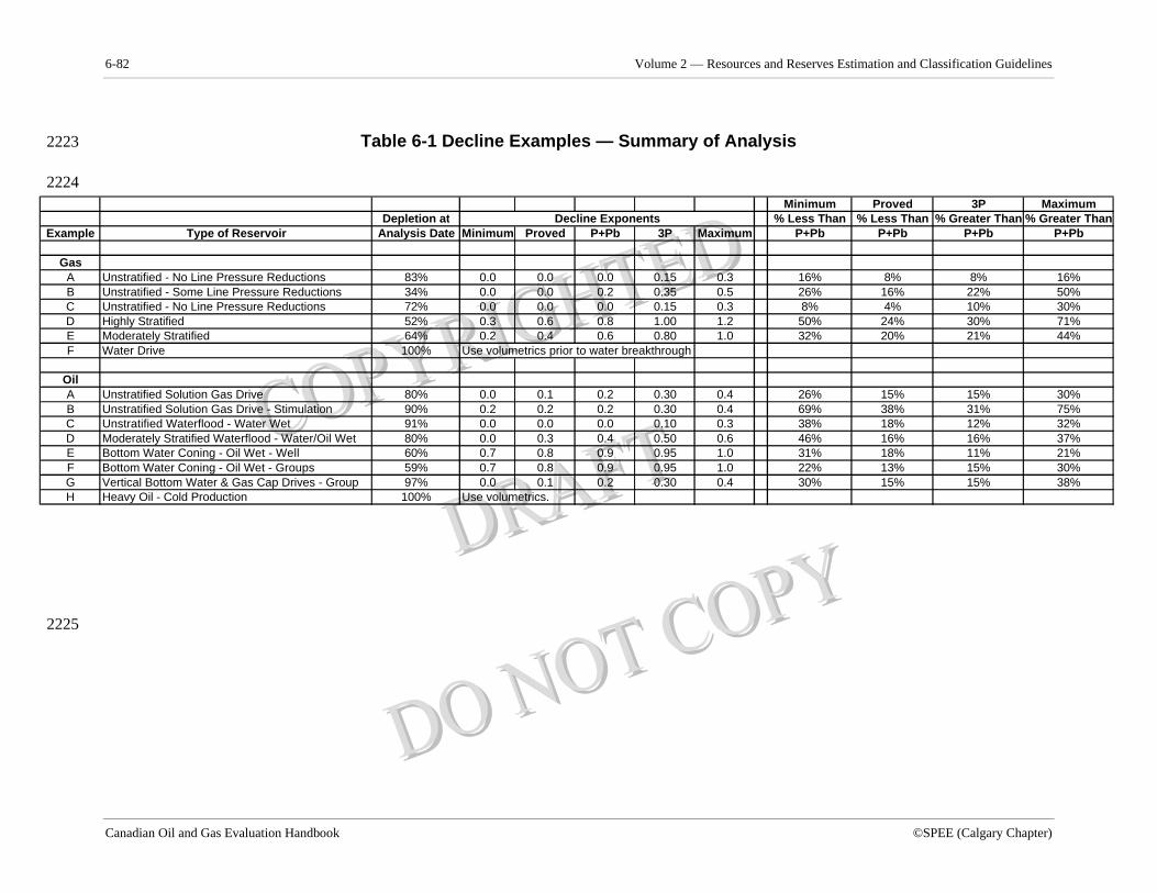
6-82 Volume 2 — Resources and Reserves Estimation and Classification Guidelines
Canadian Oil and Gas Evaluation Handbook ©SPEE (Calgary Chapter)
Table 6-1 Decline Examples — Summary of Analysis 2223
2224
2225
Minimum Proved 3P MaximumDepletion at % Less Than % Less Than % Greater Than % Greater Than
Example Type of Reservoir Analysis Date Minimum Proved P+Pb 3P Maximum P+Pb P+Pb P+Pb P+Pb
GasA Unstratified - No Line Pressure Reductions 83% 0.0 0.0 0.0 0.15 0.3 16% 8% 8% 16%B Unstratified - Some Line Pressure Reductions 34% 0.0 0.0 0.2 0.35 0.5 26% 16% 22% 50%C Unstratified - No Line Pressure Reductions 72% 0.0 0.0 0.0 0.15 0.3 8% 4% 10% 30%D Highly Stratified 52% 0.3 0.6 0.8 1.00 1.2 50% 24% 30% 71%E Moderately Stratified 64% 0.2 0.4 0.6 0.80 1.0 32% 20% 21% 44%F Water Drive 100% Use volumetrics prior to water breakthrough
OilA Unstratified Solution Gas Drive 80% 0.0 0.1 0.2 0.30 0.4 26% 15% 15% 30%B Unstratified Solution Gas Drive - Stimulation 90% 0.2 0.2 0.2 0.30 0.4 69% 38% 31% 75%C Unstratified Waterflood - Water Wet 91% 0.0 0.0 0.0 0.10 0.3 38% 18% 12% 32%D Moderately Stratified Waterflood - Water/Oil Wet 80% 0.0 0.3 0.4 0.50 0.6 46% 16% 16% 37%E Bottom Water Coning - Oil Wet - Well 60% 0.7 0.8 0.9 0.95 1.0 31% 18% 11% 21%F Bottom Water Coning - Oil Wet - Groups 59% 0.7 0.8 0.9 0.95 1.0 22% 13% 15% 30%G Vertical Bottom Water & Gas Cap Drives - Group 97% 0.0 0.1 0.2 0.30 0.4 30% 15% 15% 38%H Heavy Oil - Cold Production 100% Use volumetrics.
Decline Exponents
Section 6 — Procedures for Estimation and Classification of Reserves 6-83
©SPEE (Calgary Chapter) First Edition — April 28, 2004
6.6 Reservoir Simulation Methods 2226
(IN PROGRESS) 2227
6.7 Reserves Related to Future Drilling and Planned 2228 Enhanced Recovery Projects 2229
Reserves assignments relating to planned drilling and enhanced recovery projects are 2230 classified as undeveloped. The classification of the reserves assignment as proved, 2231 probable or possible depends on both technical and implementation risk, the 2232 guidelines for which are discussed in this section. 2233
6.7.1 Additional Reserves Related to Future Drilling 2234
Undeveloped reserves may be assigned to either infill or delineation/step-out wells as 2235 described below. Reserves may not be assigned to planned exploratory wells 2236 penetrating undiscovered accumulations. 2237
a. Drilling Spacing Unit 2238
Drilling spacing unit (DSU) is the regulated drilling spacing size for an oil and gas 2239 accumulation. The spacing size might or might not coincide with the practical 2240 drainage area of a well. Usually a DSU is one section for gas and 1/4 section for oil. 2241 Gas DSUs are usually larger than oil DSUs, because the lower viscosity of gas allows 2242 for larger drainage area capability, not because gas pools are larger than oil pools. 2243 Reservoirs with high viscosity fluid or lower permeability rock will usually have 2244 smaller DSUs. DSUs are commonly used in North America, but not elsewhere. In 2245 reservoirs where DSUs are not established, the evaluator must use informed 2246 judgement as to a reasonable spacing unit size for developing the reservoir. 2247
b. Infill Wells 2248
Infill wells are wells drilled between two existing wells or within triangulation of 2249 three offset wells in a known common accumulation, as illustrated on Map 1. Infill 2250 wells are drilled to accelerate and/or improve recovery. In primary reservoirs, infill 2251 wells may be drilled if the practical drainage area of the existing wells is too small to 2252 effectively develop the pool in a timely manner. They may also be drilled to access 2253 pore volume not currently connected to existing wellbores. In EOR schemes, infill 2254 wells are drilled to improve sweep efficiency and/or pore volume connectivity. 2255
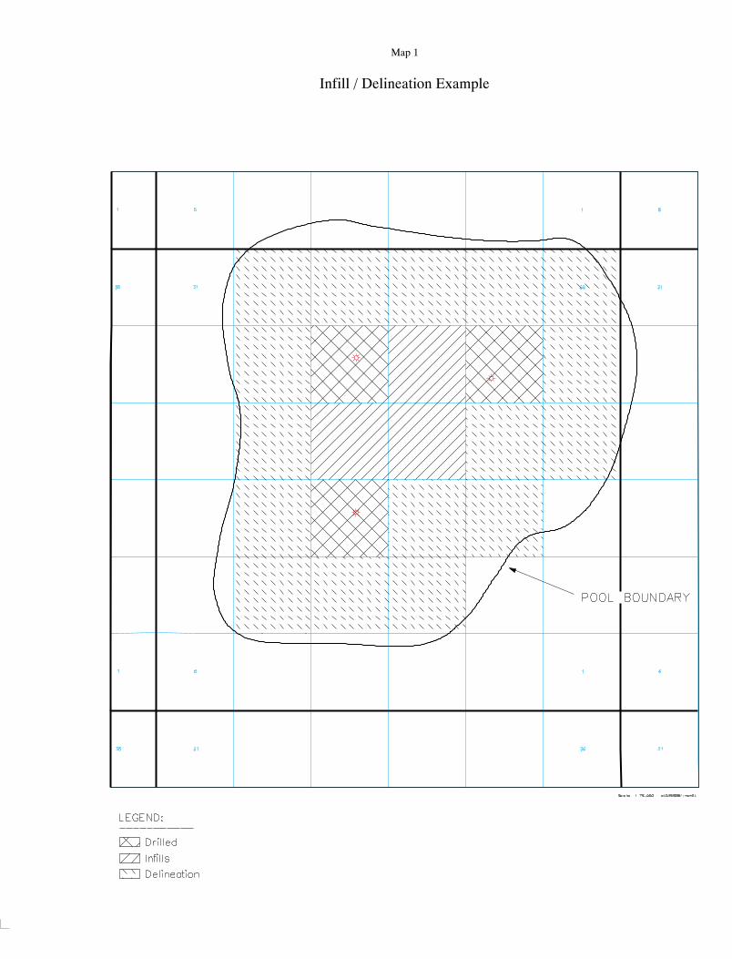
6-84 Volume 2 — Resources and Reserves Estimation and Classification Guidelines
Canadian Oil and Gas Evaluation Handbook ©SPEE (Calgary Chapter)
Reserves from infill wells may be proved, probable, or possible, depending on the 2256 amount and reliability of data and on the technical assessment. An assessment must 2257 be made of incremental versus accelerated recovery associated with the wells, and 2258 accounted for in the total pool reserves assignment. Where possible, the results of 2259 analogous infill drilling schemes should be reviewed to assist in the assessment. The 2260 best estimate of incremental recovery is classified as 2P. The initial proved increment 2261 is usually equal to the 2P value minus between 1/3 and 2/3 of the difference between 2262 the 2P and a reasonable minimum estimate. Similarly, the initial 3P increment is 2263 usually equal to the 2P value plus between 1/3 and 2/3 of the difference between the 2264 2P and a reasonable maximum estimate. It is common practice to classify a 2265 reasonable portion of infill well reserves as proved. The proved increment should 2266 increase once drilling confirms actual productivity, pressure, and water cut. 2267
c. Infill Analysis 2268
Low-permeability, high-viscosity oil, and/or discontinuous reservoirs require denser 2269 drilling spacing than do high-permeability, low viscosity oil, and/or homogeneous 2270 reservoirs to effectively drain the reservoir. When reliable volumetric data are 2271 available, recovery factors from decline analysis of existing producing wells can be 2272 determined. Using analytical calculations or reservoir modelling, recovery factors for 2273 planned infill drilling can be calculated. These calculated incremental reserves for 2274 planned drilling are either 3P or 2P values. The portion classified as proved and 2275 probable depends on the reliability of the volumetric data and cutoff criteria. 2276
Volumetric data are often unreliable in low-permeability reservoirs due to uncertainty 2277 in estimating effective pay. In these cases, the only reliable way of estimating 2278 incremental reserves for infill drilling is through analogies to other similar infill 2279 drilling projects that have quantifiable results. If volumetric data or analogies are not 2280 available or reliable, then incremental reserves from infill drilling should only be 2281 classified as possible. 2282
d. Delineation or Step-Out Wells 2283
Delineation or step-out wells are wells drilled in discovered pools that are not infill 2284 wells, as depicted on Map 1. Delineation wells are usually drilled to drain parts of the 2285 pool not currently being drained by existing wells and to substantiate pool mapping. 2286 Delineation drilling usually occurs in pools with primary recovery schemes, because 2287 enhanced recovery schemes are usually only implemented after the pool has been 2288 delineated. An exception to this is where new seismic data or reprocessing has 2289 redefined pool edges after implementation of an EOR scheme. 2290
Section 7 — Validation and Reconciliation of Reserves and Value Estimates 6-85
©SPEE (Calgary Chapter) First Edition — April 28, 2004
i. Classification 2291
Reserves from delineation wells may be proved, probable, or possible, depending on 2292 geological confidence. For pools that are not fully delineated, there are usually halos 2293 of proved, probable and possible locations surrounding existing well control. The size 2294 and shape of these halos and the number of locations therein depend on the amount, 2295 quality, and reliability of the data and on the geological interpretation. An evaluator 2296 must decide, based on the available data, if the mapping of the pool represents 2P or 2297 3P confidence levels. A suggested method of classifying drilling locations is to 2298 contour proved and probable limits on net pay mapping, with the limits defined as 2299 percentages of the distance between the pool edge and well control. The percentages 2300 selected depend on the evaluator’s confidence in the mapping. The pore volumes of 2301 the proposed locations are those calculated from these undeveloped halos. Unless 2302 probabilistic methods are used, the best estimate pay cutoffs should be used in the 2303 mapping preparation. 2304
ii. Qualifiers to Classification 2305
Notwithstanding the above guidelines, only reserves of locations in spacing units 2306 directly or diagonally adjacent to currently drilled productive spacing units may be 2307 classified as proved, provided the evaluator has high certainty in the reservoir 2308 continuity and productivity at the locations. Locations beyond one spacing unit step-2309 out are usually not classified as proved, unless compelling evidence of reservoir 2310 continuity, such as seismic data, pressure data, and well control, are available. Best 2311 estimate interpretations of reservoir mapping, properties, and recovery should be 2312 considered when classifying reserves as 2P. Usually, only wells that are an additional 2313 DSU step-out from proved locations are classified as probable, unless reasonable 2314 evidence of reservoir continuity is available. Delineation wells located in regions 2315 between best estimate and low certainty interpretations of reservoir mapping are 2316 classified as possible. It is up to the geological and engineering evaluators to classify 2317 the portions of the mapped reservoir as proved, probable, or possible. If best estimate 2318 mapping was prepared, there will be no possible locations within the mapped extent, 2319 because these will all be 2P locations. If 3P reserves are desired, either a halo of 2320 possible reservoir extent and reservoir parameters must be derived, or else 3P 2321 mapping must be prepared. 2322
iii. Adjustments for Reservoir Quality 2323
When estimating reserves of future drilling locations, evaluators must recognize the 2324 risks related to, and the recoverability of, oil and gas in place. In some types of 2325 reservoirs, permeability is lower closer to the edge of pools, which frequently lowers 2326 recovery factors. In other types of reservoirs, wells located closer to pool edges are 2327
6-86 Volume 2 — Resources and Reserves Estimation and Classification Guidelines
Canadian Oil and Gas Evaluation Handbook ©SPEE (Calgary Chapter)
closer to water contacts, which could also result in impeded recovery efficiency. In 2328 these types of reservoirs, reduced proved and 2P recovery factors should be assigned 2329 to delineation wells to reflect this behaviour. 2330
e. Drilling Statistics 2331
Historical drilling statistics are often reviewed as a guide to estimate reserves or 2332 resources for an area. Historical statistics include items such as success rates and 2333 median and average reserves per well. For undrilled accumulations, volumes derived 2334 on the basis of historical statistics must not be classified as reserves, because these 2335 are prospective resources, not reserves. 2336
In certain types of pools that are mapped extensively (continuous deposits), reservoir 2337 quality is random and unpredictable. Drilling in these types of reservoirs results in 2338 successes and failures within the boundaries of the defined pool. In these types of 2339 deposits, in addition to conventional technical analysis of recoverable reserves, 2340 proved + probable reserves assignments for future drilling locations should consider 2341 the average reserves per well of past drilling, including successes and failures. The 2342 difference between the median and mean values should be considered when 2343 estimating 2P reserves. For proved reserves assignments, more conservative reserves 2344 per well should be assigned after considering the range in historical results of past 2345 drilling. Also, as a guide for multi-well programs, the number of proved locations 2346 should be limited to between 1/3 and 2/3 of the number of 2P locations, provided 2347 technical proved criteria are also met. 2348
Similar to drilling statistics, historical statistics should also be reviewed when 2349 assessing reserves of workover programs. 2350
f. Likelihood of Drilling 2351
The likelihood that a well will be drilled is a consideration in classifying reserves. 2352 Future wells that an evaluator believes have a high probability of being drilled should 2353 be classified as proved, provided other proved certainty criteria are met. For probable 2354 reserves, a high probability of drilling is preferred, but a reasonable probability (more 2355 often than not) is acceptable provided further risking is applied as described below. 2356 For possible reserves, a lower probability is acceptable, but there should be at least a 2357 50% probability the well will be drilled. 2358
The timeline of drilling must reflect operator plans and potential access problems, 2359 and there must be no perceived impediments to approval. Locations that have 2360 uncertainty of being drilled because of potential regulatory constraints should not be 2361 classified as proved or probable. 2362
Section 7 — Validation and Reconciliation of Reserves and Value Estimates 6-87
©SPEE (Calgary Chapter) First Edition — April 28, 2004
Because, for most routine drilling programs, companies might only have firm plans 2363 for the upcoming fiscal year, the likelihood of drilling falls to the judgement of the 2364 evaluator. If the drilling locations being assessed by the evaluator are not in the 2365 company plans, the reasons for this should be examined prior to classifying reserves: 2366
• If the operator has not yet completed an assessment of the locations and the 2367 evaluator strongly believes they are viable economic locations, then proved 2368 or probable reserves, depending on confidence levels, may be assigned, with 2369 the drilling scheduled for subsequent years. 2370
• If the operator has examined the locations and believes they are not 2371 technically justified, then the evaluator should reassess the locations, because 2372 there could be some uncertainty in the success of the drilling program. If the 2373 evaluator, upon reconsideration, still believes in the merits of the drilling 2374 program and that it will eventually be undertaken, then proved or probable 2375 reserves, depending on the evaluator’s confidence level, may still be 2376 assigned, with implementation delayed sufficiently in the future. These 2377 situations, where an evaluator assigns proved or probable reserves to 2378 locations the operator indicates will not be drilled, should be rare. In these 2379 cases, if the project is a multi-well program, a staged approach to classifying 2380 the locations as proved or probable could be warranted to confirm 2381 performance prior to classifying the remaining wells. If the operator is not 2382 planning to drill certain locations that the evaluator has assessed as 2383 technically possible, it is unreasonable to expect that the wells will be drilled. 2384 Therefore, no reserves should be assigned. 2385
• If the drilling project economics are marginal, the evaluator should review 2386 evidence of commitment to the project prior to classifying reserves as 2387 proved, probable, or possible. As in the above situation, if the project is a 2388 multi-well program, a staged approach to classifying the locations as proved 2389 or probable could be warranted to confirm performance prior to classifying 2390 the remaining wells. Technically certain but marginally economic projects 2391 require evidence of company commitment before being classified as proved. 2392 Such evidence may be in the form of AFEs, budgets, or letters of intent from 2393 the company. 2394
• If reserves have been previously assigned to drilling locations, but the 2395 drilling plans have been deferred, the evaluator should examine the reason 2396 for the deferral. If drilling economics are marginal, the deferral could 2397 indicate lack of company commitment and the reserves should be reclassified 2398 in a higher risk category. If the technical and/or economic merit is still 2399
6-88 Volume 2 — Resources and Reserves Estimation and Classification Guidelines
Canadian Oil and Gas Evaluation Handbook ©SPEE (Calgary Chapter)
viable, but the deferral is due to budget constraints, the reserves classification 2400 should not be changed. If technical or economic issues have changed, then 2401 the reserves classification should be reassessed to reflect the change. The 2402 production and economic forecasts will also change to reflect the new 2403 timeline. 2404
For reserves classification, if technically probable well locations do not have a high 2405 probability, but have a reasonable probability, of being drilled, an allowance should 2406 be made in order to achieve a 50 percent probability that the estimate will be met or 2407 exceeded. This is illustrated in the situation where six well locations have probable 2408 reserves of 2 Bcf/well. The locations have been included in the operator’s budget, but 2409 they have marginal economics and have not received approval for drilling. The 2410 evaluator believes there is only a 50/50 chance the wells will actually be drilled. In 2411 this situation, the P50 reserves are 6 Bcf (six wells x 2 Bcf/well x 50 percent chance of 2412 drilling). If the evaluator includes all six wells as probable, without an allowance, the 2413 probable reserves in the evaluation are 12 Bcf, which will not meet the definitional 2414 requirement for probable certainty of at least 50 percent. The recommendation in this 2415 situation is for the evaluator to schedule only the risked number of probable wells, 2416 which in this case are three, with the remainder classified as possible. For the 2417 situation where only one probable location is forecast with a 50/50 chance of being 2418 drilled, half the reserves and capital should be used in the analysis. (This is not the 2419 same situation where a well is forecast to be drilled with a 50 percent chance of 2420 success, in which case 100 percent of the capital and the risked reserves are used). 2421 When probable locations have a high certainty of being drilled, this further allowance 2422 is not necessary. 2423
For wells that are technically possible locations but have less than a 50% likelihood 2424 of being drilled and placed onstream in a reasonable timeframe, no reserves should 2425 be assigned, because these are more suitably classified as contingent resources. 2426
g. Time Constraints 2427
Time constraints of drilling programs should not affect reserves classification 2428 decisions, as long as the certainty of their occurrence meets the appropriate reserves 2429 classification criteria, and provided there are technically and economically justified 2430 and logical reasons for delayed drilling (e.g., facility constraints, allowable 2431 constraints, capital budget constraints, orderly development). For drilling programs 2432 that are marginally economic, proved reserves should be limited to the extent to 2433 which the company has shown commitment. Marginally economic projects outside 2434 the time period committed by the company should be classified as probable or 2435 possible, depending on the levels of technical and implementation certainty. Because 2436
Section 7 — Validation and Reconciliation of Reserves and Value Estimates 6-89
©SPEE (Calgary Chapter) First Edition — April 28, 2004
the likelihood of implementation has diminished for these uncommitted locations, 2437 only the risked portion of the drilling should be assigned probable reserves, as 2438 described in section f. above. 2439
6.7.2 Examples of Future Drilling 2440
Case A1 2441
Background 2442 A low-permeability shallow gas area was initially developed on 640-acre spacing. 2443 After a decade of history, the area is being considered for downspacing to 320-acre 2444 spacing. Due to the shale content of the sand, volumetric data are unreliable. Based 2445 on decline analysis, the existing wells drilled on 640-acre spacing are forecast to 2446 recover 1 Bcf/well of 2P reserves) and 0.9 Bcf/well of proved reserves. A number of 2447 320-acre analagous infill drilling projects in the area have been reviewed. The 2448 analogous wells with similar productivity to the subject area demonstrated that 2449 downspacing increased incremental reserves per section by between 40 percent and 2450 80 percent of the initial well, with the average being 60 percent. Downspacing 2451 approval has not been obtained, but is highly likely based on similar approvals in the 2452 area. What initial incremental reserves assignments should be made for the proposed 2453 subject infill drilling program? 2454
Recommendation 2455
• 2P incremental reserves: = 0.6 Bcf/section based on the average expectation 2456 of the analogy wells. 2457
• 1P incremental reserves: 0.4 Bcf/section based on the low expectation of the 2458 analogy wells. 2459
• 3P incremental reserves: 0.8 Bcf/section based on the high expectation of the 2460 analogy wells. 2461
It is expected that the 0.4 Bcf value will likely increase to 0.5 Bcf upon verification 2462 of expected initial rates with actual tests, and eventually to 0.6 Bcf with additional 2463 performance support. 2464
Case A2 2465
Background 2466 In Case A1, after additional performance, the 2P reserves of the first well in the 2467 section are established at 0.9 Bcf/well and the second well is established at 0.7 2468 Bcf/well, for a total of 1.6 Bcf/section. Proved reserves are 0.1 Bcf less per well, for a 2469 total of 1.4 Bcf/section. The operator is now planning to drill two more wells per 2470
6-90 Volume 2 — Resources and Reserves Estimation and Classification Guidelines
Canadian Oil and Gas Evaluation Handbook ©SPEE (Calgary Chapter)
section so as to develop the area on 160-acre spacing. No other analogous areas have 2471 been developed on 160-acre spacing. To estimate the incremental reserves, the 2472 operator has conducted a modelling study using initial assumed reservoir parameters 2473 and adjusting them to match the results of both the first and second existing wells. 2474 The model indicates that incremental reserves of 0.6 Bcf per section will result from 2475 drilling the additional two wells per section. Modelling accuracy from sensitivity 2476 analysis is estimated at +/-0.2bcf. A minimum 0.5 Bcf per section is required for the 2477 project to be economic. Current drilling spacing approval is two wells per section. 2478 Application for downspacing has been made based on the results of the modelling 2479 work; however, approval has not been obtained. There may be issues with surface 2480 lease owners and offset mineral lease owners regarding the project, but these can 2481 likely be resolved. What initial incremental reserves assignments should be made for 2482 the proposed subject infill drilling program? 2483
Recommendation 2484
• 2P incremental reserves: 0.6 Bcf/section based on the modelling work and 2485 expectation of approval. 2486
• 1P incremental reserves: nil because the high certainty incremental reserves 2487 value is not economic, there are no analogies, and there may be problems 2488 obtaining downspacing approval. 2489
• 3P incremental reserves: 0.8 Bcf/section based on the modelling work. 2490
If the evaluator’s technical assessment was that the high-certainty reserves were 0.5 2491 Bcf/section (i.e., economic) and that project approval was highly certain, then proved 2492 reserves of 0.5 Bcf/section may be assigned, despite the absence of analogies. In all 2493 cases, the technical assessment must conclude that the model is reliably set up and 2494 calibrated to reflect performance of both the initial and second phases of drilling. 2495
Case B 2496
Background 2497 An unconsolidated sand heavy oil reservoir producing under cold production 2498 technology is developed on 40-acre spacing. Based on typical reserves life indices 2499 and performance of some wells that are near depletion, proved, 2P, and 3P recovery 2500 factors are estimated at 6 percent, 7 percent, and 8 percent, respectively. Other 2501 analogous pools in the area developed on 20-acre spacing usually recover 10 percent 2502 to 18 percent of OOIP, with an average of 15 percent. The operator is not planning 2503 any drilling, because of capital constraints; however, the evaluator believes that 20-2504
Section 7 — Validation and Reconciliation of Reserves and Value Estimates 6-91
©SPEE (Calgary Chapter) First Edition — April 28, 2004
acre infill drilling is warranted. What recovery factors and development program 2505 should be assigned to the property? 2506
Recommendation 2507
• 2P Case: Assume development on 20-acre spacing, commencing in the future 2508 (but not within the first year). Estimated recovery factor = 14 percent based 2509 on analogy to other areas limited by existing 2P per-well recoveries. 2510
• 1P Case: Assume development on 20-acre spacing, commencing in the future 2511 (but not within the first year). Estimated recovery factor = 10 percent (i.e., 4 2512 percent incremental) based on analogy to the low end of recovery of other 2513 areas. 2514
• 3P Case: Assume development on 20-acre spacing, commencing in the future 2515 (but not within the first year). Estimated recovery factor = 16 percent based 2516 on analogy to the high end of recovery of other areas limited by existing 3P 2517 per-well recoveries. 2518
If there is a technical reason for infill drilling to be unsuccessful (such as pressure 2519 depletion, which could prevent foamy oil behaviour in the infill wells), then proved 2520 reserves must not be assigned. In this situation, the analogous reservoirs described 2521 above are not truly analogous due to different depletion histories; 2P reserves will 2522 only be assigned if the evaluator is convinced that this is not likely to be the case. 2523
In this case, since the delay in development is a result of capital constraints and not 2524 due to marginal economics or technical concerns, timing does not affect the reserves 2525 classification. If the project were marginally economic, however, timing would affect 2526 the reserves classification. For small marginal projects, the operator must have plans 2527 to commence the project in two years. 2528
Case C 2529
Background 2530 A light-oil pattern waterflood in a stratified reservoir is developed on 160-acre 2531 spacing. From decline analysis the wells are forecast to recover 23 percent and 25 2532 percent of OOIP for the proved and 2P reserves cases, respectively. Water 2533 breakthrough is minimal. The operator is considering infill drilling a portion of the 2534 reservoir to 80-acre spacing. No infill wells have been drilled to date and there are no 2535 analogous pools upon which to base the success of such a scheme. A reservoir 2536 simulation study indicates a recovery factor of 27 percent on 160-acre spacing and 32 2537 percent with infill drilling. However, results highly depend on relative permeability 2538
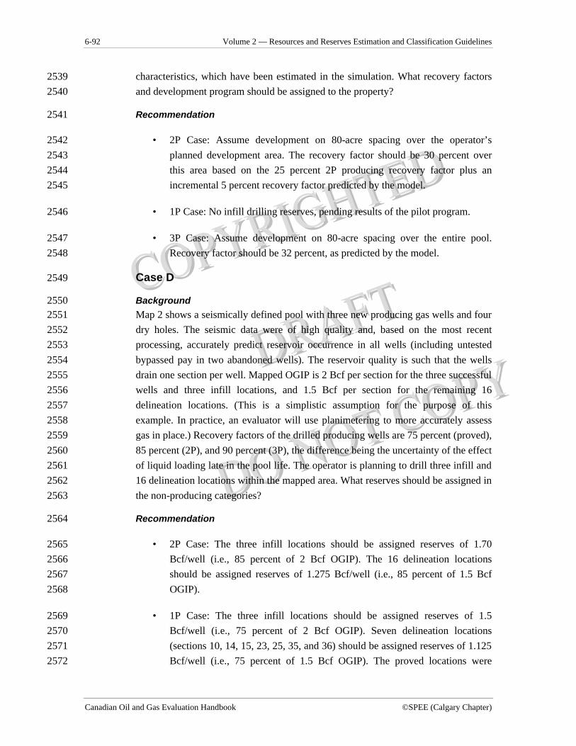
6-92 Volume 2 — Resources and Reserves Estimation and Classification Guidelines
Canadian Oil and Gas Evaluation Handbook ©SPEE (Calgary Chapter)
characteristics, which have been estimated in the simulation. What recovery factors 2539 and development program should be assigned to the property? 2540
Recommendation 2541
• 2P Case: Assume development on 80-acre spacing over the operator’s 2542 planned development area. The recovery factor should be 30 percent over 2543 this area based on the 25 percent 2P producing recovery factor plus an 2544 incremental 5 percent recovery factor predicted by the model. 2545
• 1P Case: No infill drilling reserves, pending results of the pilot program. 2546
• 3P Case: Assume development on 80-acre spacing over the entire pool. 2547 Recovery factor should be 32 percent, as predicted by the model. 2548
Case D 2549
Background 2550 Map 2 shows a seismically defined pool with three new producing gas wells and four 2551 dry holes. The seismic data were of high quality and, based on the most recent 2552 processing, accurately predict reservoir occurrence in all wells (including untested 2553 bypassed pay in two abandoned wells). The reservoir quality is such that the wells 2554 drain one section per well. Mapped OGIP is 2 Bcf per section for the three successful 2555 wells and three infill locations, and 1.5 Bcf per section for the remaining 16 2556 delineation locations. (This is a simplistic assumption for the purpose of this 2557 example. In practice, an evaluator will use planimetering to more accurately assess 2558 gas in place.) Recovery factors of the drilled producing wells are 75 percent (proved), 2559 85 percent (2P), and 90 percent (3P), the difference being the uncertainty of the effect 2560 of liquid loading late in the pool life. The operator is planning to drill three infill and 2561 16 delineation locations within the mapped area. What reserves should be assigned in 2562 the non-producing categories? 2563
Recommendation 2564
• 2P Case: The three infill locations should be assigned reserves of 1.70 2565 Bcf/well (i.e., 85 percent of 2 Bcf OGIP). The 16 delineation locations 2566 should be assigned reserves of 1.275 Bcf/well (i.e., 85 percent of 1.5 Bcf 2567 OGIP). 2568
• 1P Case: The three infill locations should be assigned reserves of 1.5 2569 Bcf/well (i.e., 75 percent of 2 Bcf OGIP). Seven delineation locations 2570 (sections 10, 14, 15, 23, 25, 35, and 36) should be assigned reserves of 1.125 2571 Bcf/well (i.e., 75 percent of 1.5 Bcf OGIP). The proved locations were 2572
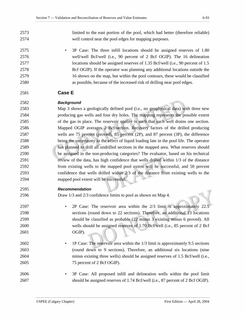
Section 7 — Validation and Reconciliation of Reserves and Value Estimates 6-93
©SPEE (Calgary Chapter) First Edition — April 28, 2004
limited to the east portion of the pool, which had better (therefore reliable) 2573 well control near the pool edges for mapping purposes. 2574
• 3P Case: The three infill locations should be assigned reserves of 1.80 2575 well/well Bcf/well (i.e., 90 percent of 2 Bcf OGIP). The 16 delineation 2576 locations should be assigned reserves of 1.35 Bcf/well (i.e., 90 percent of 1.5 2577 Bcf OGIP). If the operator was planning any additional locations outside the 2578 16 shown on the map, but within the pool contours, these would be classified 2579 as possible, because of the increased risk of drilling near pool edges. 2580
Case E 2581
Background 2582 Map 3 shows a geologically defined pool (i.e., no geophysical data) with three new 2583 producing gas wells and four dry holes. The mapping represents the possible extent 2584 of the gas in place. The reservoir quality is such that each well drains one section. 2585 Mapped OGIP averages 2 Bcf/section. Recovery factors of the drilled producing 2586 wells are 75 percent (proved), 85 percent (2P), and 87 percent (3P), the difference 2587 being the uncertainty in the effect of liquid loading late in the pool life. The operator 2588 has planned to drill all undrilled sections in the mapped area. What reserves should 2589 be assigned in the non-producing categories? The evaluator, based on his technical 2590 review of the data, has high confidence that wells drilled within 1/3 of the distance 2591 from existing wells to the mapped pool extent will be successful, and 50 percent 2592 confidence that wells drilled within 2/3 of the distance from existing wells to the 2593 mapped pool extent will be successful. 2594
Recommendation 2595 Draw 1/3 and 2/3 confidence limits to pool as shown on Map 4. 2596
• 2P Case: The reservoir area within the 2/3 limit is approximately 22.5 2597 sections (round down to 22 sections). Therefore, an additional 13 locations 2598 should be classified as probable (22 minus 3 existing minus 6 proved). All 2599 wells should be assigned reserves of 1.70 Bcf/well (i.e., 85 percent of 2 Bcf 2600 OGIP). 2601
• 1P Case: The reservoir area within the 1/3 limit is approximately 9.5 sections 2602 (round down to 9 sections). Therefore, an additional six locations (nine 2603 minus existing three wells) should be assigned reserves of 1.5 Bcf/well (i.e., 2604 75 percent of 2 Bcf OGIP). 2605
• 3P Case: All proposed infill and delineation wells within the pool limit 2606 should be assigned reserves of 1.74 Bcf/well (i.e., 87 percent of 2 Bcf OGIP). 2607
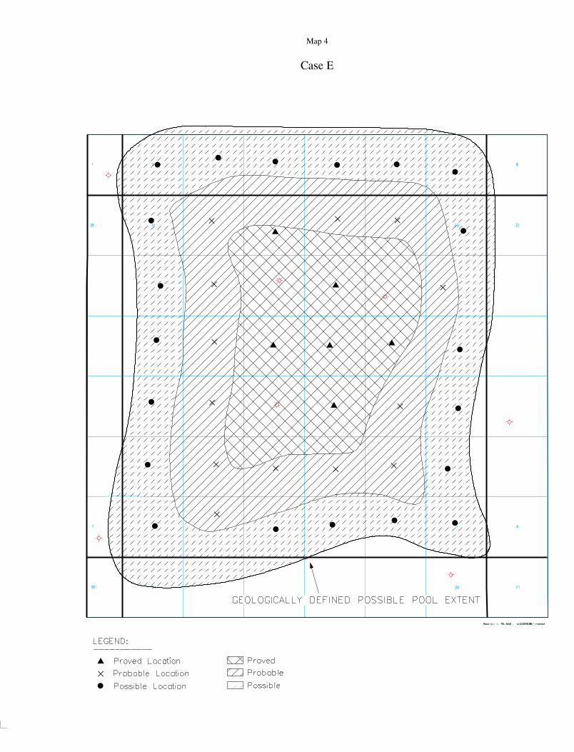
6-94 Volume 2 — Resources and Reserves Estimation and Classification Guidelines
Canadian Oil and Gas Evaluation Handbook ©SPEE (Calgary Chapter)
2608
6.7.3 Reserves Related to Planned Enhanced Recovery Projects 2609
Enhanced recovery includes all methods for supplementing natural reservoir forces 2610 and energy or increasing ultimate recovery from a reservoir. These methods include 2611 the following: 2612
• Water Injection, 2613
• Gas Injection, 2614
• Miscible Fluid Displacement, 2615
• Polymer Flooding, 2616
• Microemulsion Flooding, 2617
• Steam Injection, 2618
• In-Situ Combustion. 2619
a. Proved Criteria (1P) 2620
Proved reserves may be assigned to planned enhanced recovery projects when the 2621 following criteria are met: 2622
• Repeated commercial success of the enhanced recovery process has been 2623 demonstrated in reservoirs in the area with analogous rock and fluid 2624 properties or by an operational pilot scheme within the approval area. 2625
• The project is highly likely to be carried out in the near future. This may be 2626 demonstrated by factors such as the commitment of project funding. 2627
• Where required, either regulatory approvals have been obtained, or no 2628 regulatory impediments are expected, as clearly demonstrated by the 2629 approval of analogous projects. 2630
• Suitable feasibility studies have been conducted. 2631
Repeated commercial success has been demonstrated if there are at least three 2632 analogous operational projects known to be economically and technically successful, 2633 based on available data and public statements of the operators. The first commercial 2634 application of a process cannot rely on analogies and requires actual performance of a 2635

Section 7 — Validation and Reconciliation of Reserves and Value Estimates 6-95
©SPEE (Calgary Chapter) First Edition — April 28, 2004
pilot or operational scheme upon which to justify a proved classification. For 2636 established conventional EOR processes such as waterfloods, one operational scheme 2637 in an area is sufficient to demonstrate economic and technical viability. 2638
“Reservoirs in the area” refers to an oil and gas accumulation of similar geological 2639 age; depositional, diagenetic, and structural setting and history; and internal reservoir 2640 architecture in the same basin as the subject reservoir. There are no fixed distance 2641 criteria for the area as long as these criteria are met. 2642
Analogous rock and fluid properties include the following properties, which affect 2643 the performance of an enhanced recovery scheme: 2644
• porosity, 2645
• porosity type (i.e., single or dual (fractured) systems), 2646
• permeability, 2647
• permeability orientation, 2648
• permeability distribution, 2649
• water saturation, 2650
• oil gravity and viscosity, 2651
• solution GOR, 2652
• bubble point, 2653
• relative permeability, 2654
• well spacing, 2655
• pressure, 2656
• depth, 2657
• thickness, 2658
• continuity, 2659
• stage of depletion, 2660
• injected fluid properties (compatibility, mobility, relative permeability), 2661
6-96 Volume 2 — Resources and Reserves Estimation and Classification Guidelines
Canadian Oil and Gas Evaluation Handbook ©SPEE (Calgary Chapter)
• reservoir architecture. 2662
Measurement data on some of the analogous properties in the proposed scheme, such 2663 as relative permeability, might not be required if the analogous project is located 2664 close enough to infer the measurement. If data on critical properties have not been 2665 obtained on proposed projects in order to make proper analogy comparisons, or if the 2666 analogy is too distant from the proposed project, then proved reserves by analogy 2667 cannot be assigned. Properties need not be the same as or superior to the analogy, but 2668 engineering adjustments must be made to reflect the differences, provided the key 2669 properties are not materially inferior. 2670
Pilot schemes are scaled-down non-commercial projects that must be scaled up to 2671 commercial application. Care must be taken to reliably scale up performance and 2672 costs. Phases of a pilot are injection, initial response, and breakthrough behaviour. A 2673 pilot needs to be into breakthrough behaviour in order to judge success of the 2674 scheme. 2675
Likelihood of implementation influences reserves classification of a project. Part of 2676 this likelihood involves the processes of conducting studies, completing applications, 2677 and obtaining approvals. Items under the company’s control include cost estimates, 2678 feasibility studies, implementation timelines, regulatory applications, environmental 2679 studies, capital budgets and unitization negotiations, as well as final approvals of 2680 AFEs and budgets. Items not under the company’s control include unitization, 2681 environmental constraints, and regulatory approvals. 2682
For proved reserves classification, the company must show commitment to 2683 implement the project. This pertains to all processes under the company’s control. 2684 The degree of commitment required for reserves booking varies, depending on the 2685 nature and size of the EOR project. For small routine waterflood projects, processes 2686 such as budgeting, timeline preparation, and commencement of regulatory 2687 applications could be sufficient to show company commitment. For larger, non-2688 routine EOR processes, final AFE and regulatory approvals could be required. The 2689 situations where proved EOR reserves are assigned without company commitment 2690 must be very rare. 2691
To meet high certainty of implementation in the near future, a commitment to initial 2692 significant capital spending must be within the next three years for large projects and 2693 two years for small projects. 2694
A suitable feasibility study incorporates analysis of both the geological and 2695 engineering aspects of the proposed scheme. A detailed geological definition is 2696 required, with sufficient well spacing and/or seismic control to characterize reservoir 2697
Section 7 — Validation and Reconciliation of Reserves and Value Estimates 6-97
©SPEE (Calgary Chapter) First Edition — April 28, 2004
properties and geometry. The engineering analysis must address not only the 2698 reserves, but rate of production response, injection requirements (both source and 2699 rates), breakthrough behaviour, and cost of development. The study need not be a 2700 reservoir simulation; however, for complex reservoirs, a reservoir simulation may be 2701 the only practical method of predicting response. In routine EOR applications, the 2702 feasibility study could simply be a scaling of analogous projects. 2703
Initially, only a portion of reserves can be classified as proved. Prior to 2704 implementation of a project, the best estimate reserves value is recommended a 2P 2705 classification. The initial proved increment is usually equal to the 2P value minus 2706 between 1/3 and 2/3 of the difference between the 2P and a reasonable minimum 2707 estimate. Similarly, the initial 3P increment is usually equal to the 2P value plus 2708 between 1/3 and 2/3 of the difference between the 2P and a reasonable maximum 2709 estimate. The portion of proved classification increases toward the best estimate 2710 value as injectivity is established, as response is exhibited, and as breakthrough 2711 trends are established. 2712
EOR schemes are frequently implemented in a phased approach. If only minor capital 2713 compared to the initial project is required (i.e., less than 50 percent), then all 2714 proposed phases may be classified as proved, provided the expansion area is 2715 analogous to the initial phase. If significant capital (i.e., more than 50 percent of the 2716 initial project) is required for future phases, then the future phases are treated using 2717 the same criteria as the initial phase. 2718
b. Proved + Probable Criteria (2P) 2719
Proved + probable reserves may be assigned when a planned enhanced recovery 2720 project does not meet the requirements for classification as proved. However, the 2721 following criteria are met: 2722
• The project can be shown to be practically and technically reasonable. 2723
• Commercial success of the enhanced recovery process has been 2724 demonstrated in reservoirs with analogous rock and fluid properties but not 2725 necessarily in the area of the reservoir. 2726
• It is reasonably certain that the project will be implemented. 2727
Practical and reasonable tests are judged from the results of feasibility studies. These 2728 studies are similar to those described for the proved criteria, though the degree of 2729 geological control to define the reservoir may be less. 2730
6-98 Volume 2 — Resources and Reserves Estimation and Classification Guidelines
Canadian Oil and Gas Evaluation Handbook ©SPEE (Calgary Chapter)
Reservoir properties of a proposed project should be similar to those of the analogous 2731 project, with adjustments made for any differences. 2732
Reasonably certain implementation refers, in the case of small routine waterflood 2733 projects, to evidence such as planning, budgeting and timeline preparation. For 2734 larger, non-routine EOR processes, final regulatory and AFE approvals could be 2735 required. Also, to meet reasonable certainty of implementation, commitment to initial 2736 significant capital spending must be within 5 years for large projects and 3 years for 2737 small projects. 2738
Best estimate estimates of reserves must be used for 2P reserves bookings. 2739
When the first phase of an EOR project is classified as 2P, and if only minor capital 2740 compared to the initial phase is required (i.e., less than 50 percent), all future phased 2741 expansions within existing approval or expansion areas may be classified as 2P, 2742 provided there is no perceived technical, economic or regulatory impediment to these 2743 phased expansions proceeding. If significant capital (i.e., more than 50 percent of the 2744 initial project) is required for future phases, then the future phases are treated using 2745 the same criteria as the initial phase. 2746
As mentioned in the infill drilling discussion, if technically probable EOR projects do 2747 not have a high probability of being implemented, but have a reasonable probability 2748 (more often than not), further risking must be applied to achieve a 50 percent 2749 probability that the estimate will be met or exceeded (see Section 6.7.1.f for the 2750 procedure). 2751
c. Proved + Probable + Possible Criteria (3P) 2752
Proved + probable + possible reserves may be assigned when a planned enhanced 2753 recovery project does not meet the requirements for classification as proved or 2754 probable; however, the following criteria are met: 2755
• The project can be shown to be practically and technically reasonable. 2756
• Commercial success of the enhanced recovery process has been 2757 demonstrated in reservoirs with analogous rock and fluid properties, but there 2758 remains some doubt that the process will be successful in the subject 2759 reservoir. 2760
• It is reasonable that the project will be implemented. 2761
Practically and technically reasonable requirements are met if theoretical calculations 2762 show economically recoverable reserves are achievable. 2763
Section 7 — Validation and Reconciliation of Reserves and Value Estimates 6-99
©SPEE (Calgary Chapter) First Edition — April 28, 2004
Acceptable uncertainty relating to possible reserves may include a process not being 2764 tested in the same geological horizon or certain rock or fluid properties being 2765 dissimilar to a commercial analogy. 2766
Reasonable implementation criteria are met if technical analysis indicates the project 2767 is economically worth pursuing, even if the company does not have firm plans to 2768 proceed. As a guide, the evaluator should believe there is at least an equal chance of 2769 the project proceeding as not. Projects with a low chance of being implemented 2770 should not be classified as reserves, but as contingent resources. 2771
6.7.4 Planned EOR Examples 2772
Case G 2773
Background 2774 A new oil pool has been discovered and delineated. Relative permeability tests 2775 indicate the reservoir is amenable to waterflood. The operator is planning on 2776 installing a waterflood scheme and has conducted a reservoir simulation study. There 2777 have been no other waterflood schemes attempted in this horizon in the area, because 2778 reservoir continuity and formation plugging due to water susceptibility are potential 2779 issues. There have been waterfloods implemented in other horizons in the area. The 2780 simulation study, using reasonable economic limits, predicts primary recovery of 10 2781 percent of OOIP and waterflood recovery of 30 percent of OOIP. Decline analysis 2782 and analogies to other pools in the area in the same horizon indicate proved and 2P 2783 primary recovery factors of 8 percent and 9 percent, respectively. Initially the plan is 2784 to implement a pilot scheme over 20 percent of the reservoir, which will be expanded 2785 to the entire reservoir pending the results of the pilot scheme. What recovery factors 2786 should be assigned for the total proved and total 2P categories and over what portion 2787 of the reservoir at this time? 2788
Recommendation 2789
• 2P Case: Assign a 25 percent waterflood recovery factor over 20 percent of 2790 the reservoir (pilot area) and 9 percent primary recovery factor over 80 2791 percent of the reservoir (non-pilot area). The 25 percent factor is 80 percent 2792 of the simulation results, to account for probable simulation inaccuracy. (The 2793 simulation appears to overestimate primary reserves and there is no actual 2794 breakthrough behaviour to simulate actual relative permeability 2795 characteristics.) Waterflood reserves are not assigned to the non-pilot area, 2796 because the pool-wide waterflood implementation is contingent upon the 2797 success of the pilot. If the main perceived risk of the waterflood was that of 2798 injectivity, then probable waterflood reserves using a 25 percent recovery 2799
6-100 Volume 2 — Resources and Reserves Estimation and Classification Guidelines
Canadian Oil and Gas Evaluation Handbook ©SPEE (Calgary Chapter)
factor could be assigned to the entire pool once the pilot demonstrated 2800 injectivity. 2801
• 1P Case: Assign a primary recovery factor of 8 percent for the entire pool. 2802 Because there are no analogies available in the same horizon, proved 2803 waterflood reserves cannot be assigned. Initial proved waterflood reserves 2804 assignment will occur once production response is known, and could be 2805 applied to the entire pool at a value warranted by the degree and stage of 2806 response. A recommended initial proved recovery factor will likely be 2807 between 15 and 20 percent of OOIP, which represents primary plus 1/3 to 2/3 2808 of the difference between 2P waterflood and primary recovery factors. 2809
• 3P Case: Assign a 30 percent recovery factor over the entire reservoir, based 2810 on the simulation results. There is no evidence as yet to suggest that this 2811 value is a maximum recovery factor, thus the use of the value for 3P 2812 classification. 2813
Case H 2814
Background 2815 A horizontal CO2 miscible flood scheme is proposed for an oil unit currently under 2816 pattern waterflood. A pilot CO2 scheme has been implemented, and early 2817 performance exceeds that predicted by a reservoir simulation study of the pilot area. 2818 This study predicted incremental reserves of 15 percent. The operator is planning two 2819 stages of expansion. The first stage, to be implemented over the next three years, is in 2820 high-quality areas of the reservoir analogous to the pilot area. The second stage, to be 2821 implemented within the next five years, is in lower quality areas. Simulation studies 2822 have not been conducted over the first and second stages; however, analytical studies 2823 indicate recovery in the first stage should be identical to the pilot area, whereas 2824 recovery in the second stage should be 80 percent that of the pilot area. What 2825 reserves and categories should be assigned to the various phases at this point in time? 2826
Recommendation 2827
• 2P Case: 15 percent incremental reserves over the pilot area plus Stage 1, and 2828 12 percent incremental over Stage 2 based on the simulation results. 2829
• 1P Case: 9 percent incremental reserves over the pilot area plus Stage 1. No 2830 CO2 reserves over Stage 2. An initial incremental EOR reserves estimate 2831 midway between the 2P estimate and a perceived minimum incremental 2832 recovery factor of 3 percent was assigned. This compares to the 2833 recommended range of between 1/3 to 2/3 of the difference between 2P and 2834
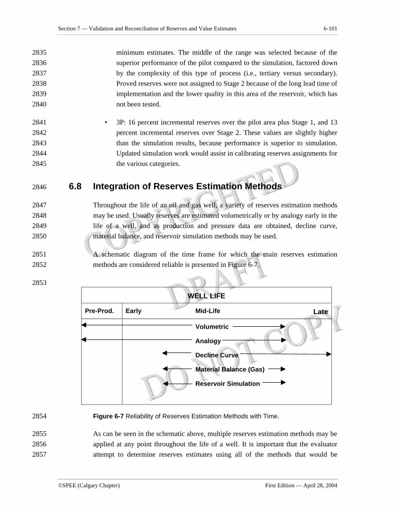
Section 7 — Validation and Reconciliation of Reserves and Value Estimates 6-101
©SPEE (Calgary Chapter) First Edition — April 28, 2004
minimum estimates. The middle of the range was selected because of the 2835 superior performance of the pilot compared to the simulation, factored down 2836 by the complexity of this type of process (i.e., tertiary versus secondary). 2837 Proved reserves were not assigned to Stage 2 because of the long lead time of 2838 implementation and the lower quality in this area of the reservoir, which has 2839 not been tested. 2840
• 3P: 16 percent incremental reserves over the pilot area plus Stage 1, and 13 2841 percent incremental reserves over Stage 2. These values are slightly higher 2842 than the simulation results, because performance is superior to simulation. 2843 Updated simulation work would assist in calibrating reserves assignments for 2844 the various categories. 2845
6.8 Integration of Reserves Estimation Methods 2846
Throughout the life of an oil and gas well, a variety of reserves estimation methods 2847 may be used. Usually reserves are estimated volumetrically or by analogy early in the 2848 life of a well, and as production and pressure data are obtained, decline curve, 2849 material balance, and reservoir simulation methods may be used. 2850
A schematic diagram of the time frame for which the main reserves estimation 2851 methods are considered reliable is presented in Figure 6-7. 2852
2853
WELL LIFE
Pre-Prod. Early Mid-Life Late
Volumetric
Analogy
Decline Curve
Material Balance (Gas)
Reservoir Simulation
Figure 6-7 Reliability of Reserves Estimation Methods with Time. 2854
As can be seen in the schematic above, multiple reserves estimation methods may be 2855 applied at any point throughout the life of a well. It is important that the evaluator 2856 attempt to determine reserves estimates using all of the methods that would be 2857
6-102 Volume 2 — Resources and Reserves Estimation and Classification Guidelines
Canadian Oil and Gas Evaluation Handbook ©SPEE (Calgary Chapter)
considered reliable at the time the estimate is made (except perhaps a reservoir 2858 simulation, because of the complexity and cost of such an analysis). In the case of 2859 material properties, more than one method should be used to determine reserves. 2860
Different methods often yield different reserves estimates, which the evaluator should 2861 attempt to reconcile. In some cases, the reconciliation is obvious; for example, when 2862 comparing a decline curve estimate based on a consistent decline trend to a 2863 volumetric estimate for a single well pool. In this case, more reliance would be 2864 placed on the decline curve estimate if the areal extent required to arrive at a similar 2865 estimate determined by decline methods was within an expected range of values. On 2866 the other hand, if the areal extent would have to be significantly larger than the 2867 acreage owned by the company to arrive at the decline curve estimated reserves, 2868 possibly indicating the well is draining non-owned lands, a reserves estimate 2869 somewhat less than the decline curve estimate should be applied to allow for 2870 additional drilling that may capture some of the reserves currently being drained by 2871 the subject well. 2872
Other sections of this Volume 2 have provided detailed guidelines regarding the 2873 conditions under which each reserves estimation method is reliable, and on the proper 2874 application of each method. A brief summary of the requirements for reliable 2875 estimates using each method is presented below. 2876
a. Volumetric Methods 2877
• Usually the only methods available prior to significant production. 2878
• Most reliable in multi-well pools that have good well control and well-2879 defined reservoir properties. 2880
• Tend to be less reliable in single-well pools. 2881
• Reserves should be consistent with demonstrated productivity and analogous 2882 pools. 2883
b. Analogy Methods 2884
• Usually the primary estimation method when all other methods are 2885 considered less reliable. 2886
• Reserves estimated using other methods should always be compared to 2887 reserves estimates for analogous reserves to ensure they are within an 2888 expected range. 2889
Section 7 — Validation and Reconciliation of Reserves and Value Estimates 6-103
©SPEE (Calgary Chapter) First Edition — April 28, 2004
c. Decline Curve Methods 2890
• Considered the most reliable reserves estimation method, provided a 2891 consistent decline trend has been established and operating conditions are 2892 constant. 2893
• Production decline trends are not reliable in cases where reservoir or fluid 2894 characteristics indicate that increasing gas/oil, water/oil, or water/gas ratios 2895 will occur in later life, until those trends are well established. 2896
• Production decline trends are not reliable in an oil reservoir under water 2897 drive or waterflood, until water-cut trends are well established. 2898
• Most reliable reserves estimation method late in the life of a reservoir. 2899
d. Material Balance Methods for Gas Reservoirs 2900
• Usually requires at least 5 to 15 percent pressure decline. 2901
• Most reliable in high-permeability reservoirs and when there are many high-2902 quality data points and consistent pressure decline. 2903
• If aquifer pressure support is present, it must be accounted for. 2904
• Less reliable early in the life of low-permeability reservoirs where it is 2905 difficult to determine average reservoir pressures, in cases with few data 2906 points, and in cases with poor correlation of pressure data points. 2907
e. Reservoir Simulation 2908
• Requires a sound geological model, a properly gridded reservoir model, and 2909 good quality petrophysical PVT and pressure data. 2910
• Requires a significant volume of production and pressure decline and a good 2911 history match of past performance. 2912
• Less reliable in water drive reservoirs or oil reservoirs being waterflooded, 2913 until significant water breakthrough has occurred. 2914
2915


©SPEE (Calgary Chapter) First Edition — April 28, 2004
1
2
3
4
5
6
SECTION 7 7
VALIDATION AND RECONCILIATION 8
OF RESERVES AND VALUE ESTIMATES 9
10
7-2 Volume 2 — Resources and Reserves Estimation and Classification Guidelines
Canadian Oil and Gas Evaluation Handbook ©SPEE (Calgary Chapter)
TABLE OF CONTENTS 10 Section 7 VALIDATION AND RECONCILIATION OF RESERVES AND VALUE 11 ESTIMATES .............................................................................................................................. 7-1 12
7.1 Introduction ..................................................................................................................... 7-3 13 7.2 Reserves Validation......................................................................................................... 7-3 14 7.3 Reserves Reconciliations................................................................................................. 7-5 15
7.3.1 Introduction............................................................................................................... 7-5 16 7.3.2 Product Types ........................................................................................................... 7-5 17 7.3.3 Reserves Change Categories..................................................................................... 7-6 18 7.3.4 Discussion of Special Reserves Change Situations .................................................. 7-8 19 7.3.5 Example Reserves Reconciliation............................................................................. 7-9 20
7.4 Net Present Values Reconciliations............................................................................... 7-11 21 7.4.1 Introduction............................................................................................................. 7-11 22 7.4.2 Net Present Value Change Categories .................................................................... 7-11 23 24
25
Section 7 — Validation and Reconciliation of Reserves and Value Estimates 7-3
©SPEE (Calgary Chapter) First Edition — April 28, 2004
7.1 Introduction 25
Because of the uncertainty in estimating oil and gas reserves, the actual reserves 26 recovered from a reservoir will not be known until production reaches the economic 27 limit and the reservoir is abandoned. Even then, future improvements in technology 28 and economics could allow the reservoir to be redeveloped and additional reserves 29 produced. 30
In an evaluation of reserves, the evaluator must prepare estimates of the remaining oil 31 and gas reserves for individual reservoirs, usually on an annual basis, according to 32 the definitions and guidelines specified in COGEH. Those estimates will vary in the 33 future because of production, capital investments, changing economic conditions, and 34 further technical data. On a corporate level, acquisitions, dispositions, and new 35 discoveries will also affect the overall reserves of a company from one evaluation to 36 the next. 37
The process of identifying and categorizing the reasons for changes in reserves 38 estimates from one evaluation to the next is called a reserves reconciliation. The 39 primary reasons for conducting a reserves reconciliation are to track reserves changes 40 and to understand the reasons for those changes. A secondary reason is to verify that 41 past reserves estimates met the definitions and guidelines specified in COGEH. 42
A discussion of reserves reconciliation and validation of previous reserves estimates 43 is presented in this section. Reconciliations of net present values of oil and gas 44 reserves are also presented. Submissions of these reconciliations to securities 45 regulators could require different reserves change categories and reconciliation 46 procedures than those presented below. However, the guidelines presented below can 47 be adapted to most Canadian and American requirements. 48
7.2 Reserves Validation 49
Validation that past crude oil and natural gas reserves estimates meet the reserves 50 definitions and guidelines in COGEH is discussed in COGEH Volume 1, Section 51 5.5.6. This procedure involves the tracking of technical reserves revisions over time 52 for each of the proved, proved + probable, and proved + probable + possible reserves 53 categories. This procedure only validates past reserves estimates and does not 54 necessarily ensure that current estimates are consistent with the definitions. 55
Because of the uncertainty in estimating oil and gas reserves, some entity reserves 56 estimates will have positive revisions with successive evaluations (increase in 57
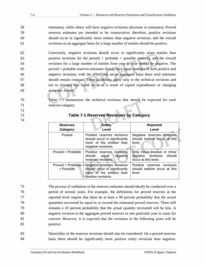
7-4 Volume 2 — Resources and Reserves Estimation and Classification Guidelines
Canadian Oil and Gas Evaluation Handbook ©SPEE (Calgary Chapter)
estimates), while others will have negative revisions (decrease in estimates). Proved 58 reserves estimates are intended to be conservative; therefore, positive revisions 59 should occur in significantly more entities than negative revisions, and the overall 60 revisions on an aggregate basis for a large number of entities should be positive. 61
Conversely, negative revisions should occur in significantly more entities than 62 positive revisions for the proved + probable + possible reserves, and the overall 63 revisions for a large number of entities from year to year should be negative. The 64 proved + probable reserves estimates should have equal numbers of both positive and 65 negative revisions, with the effect that on an aggregate basis these total estimates 66 should remain constant. These guidelines apply only to the technical revisions and 67 not to changes that could occur as a result of capital expenditures or changing 68 economic factors. 69
Table 7-1 summarizes the technical revisions that should be expected for each 70 reserves category. 71 72
Table 7-1 Reserves Revisions by Category 73 74
Reserves Category
Entity Level
Reported Level
Proved Positive reserves revisions should occur in significantly more of the entities than negative revisions.
Negative reserves revisions should seldom occur at this level.
Proved + Probable Positive reserves revisions should equal negative reserves revisions.
Only minor positive or minor negative revisions should occur at this level.
Proved + Probable + Possible
Negative reserves revisions should occur in significantly more of the entities than positive revisions.
Positive reserves revisions should seldom occur at this level.
The process of validation of the reserves estimates should ideally be conducted over a 75 period of several years. For example, the definitions for proved reserves at the 76 reported level require that there be at least a 90 percent probability that the actual 77 quantities recovered be equal to or exceed the estimated proved reserves. There still 78 remains a 10 percent probability that the actual quantity recovered will be less. A 79 negative revision in the aggregate proved reserves in one particular year is cause for 80 concern. However, it is expected that the revisions in the following years will be 81 positive. 82
Materiality of the reserves revisions should also be considered. On a proved reserves 83 basis there should be significantly more positive entity revisions than negative. 84
Section 7 — Validation and Reconciliation of Reserves and Value Estimates 7-5
©SPEE (Calgary Chapter) First Edition — April 28, 2004
However, a large number of very small negative entity revisions could be 85 significantly offset by a few very large positive entity revisions. On a reported level, 86 the expectation is that a multi-year average of the aggregate proved reserves revisions 87 will be positive. 88
As an example of the validation process, consider the reserves reconciliation in Table 89 7-2. A validation of the reserves adds up all the technical revisions over the four-year 90 period. The proved technical revisions over the four-year period total 40 Mbbl, while 91 the proved + probable technical revisions are zero. Both of these values are in the 92 range expected overall. 93
7.3 Reserves Reconciliations 94
7.3.1 Introduction 95
Reserves reconciliations should be undertaken to identify and categorize the changes 96 in reserves estimates between the previous and current reserves evaluations. 97
Canadian securities regulations require reserves reconciliations to be conducted on a 98 net reserves basis (after deducting royalties owned by others, but including royalties 99 owned) for public reporting purposes. It is recommended that the reconciliation be 100 prepared using the reserves estimates from the forecast prices and cost evaluation. 101 However, the constant prices and costs evaluation may also be used for regulatory 102 reporting purposes. 103
Reconciliations of reserves in Canada on a Company net reserves basis are more 104 complex than on a Company gross reserves basis due to price and rate sensitive 105 royalties. Various royalty incentive programs can also cause the net Company 106 reserves to change without a change in the gross Company reserves. A discussion of 107 the treatment of these effects is provided later in this section. 108
The reconciliation may be prepared by the evaluator on a property-by-property basis, 109 and then aggregated to arrive at a reported level reconciliation. The reconciliation 110 should be prepared for the total proved, probable, and total proved + probable 111 reserves categories, and should be separately prepared by country. 112
7.3.2 Product Types 113
Separate reserves reconciliations should be prepared for each of the following 114 product types: 115
• light and medium oil (combined), 116
7-6 Volume 2 — Resources and Reserves Estimation and Classification Guidelines
Canadian Oil and Gas Evaluation Handbook ©SPEE (Calgary Chapter)
• heavy oil, 117
• natural gas, 118
• natural gas liquids, 119
• bitumen, 120
• synthetic oil, 121
• non-conventional oil and gas (including coalbed methane, hydrates, etc.) 122
A reconciliation of bitumen reserves could be combined with heavy oil if the bitumen 123 quantities are relatively minor. Likewise, a reconciliation of synthetic oil reserves 124 could be combined with light and medium oil if the synthetic reserves are not 125 significant. 126
The Canadian regulations allow solution gas and natural gas liquids reserves to be 127 excluded from the reserves reconciliation, because they are usually not significant 128 compared to the oil and total natural gas quantities. Even so, evaluators may want to 129 capture all reserves changes. 130
7.3.3 Reserves Change Categories 131
In performing a reserves reconciliation, the following categories of reserves changes 132 should be considered: 133
a. Opening Balance: Company net reserves that were recorded as the closing 134 balance of the previous reconciliation. 135
b. Exploration Discoveries: Additions to reserves in reservoirs where no reserves 136 were previously booked. Any positive or negative reserves changes to an entity 137 after the initial assignment should be recorded as a technical revision. 138
c. Drilling Extensions: Additions to reserves resulting from capital expenditures 139 for step-out drilling in previously discovered reservoirs. Any positive or negative 140 reserves changes to an entity after the initial assignment should be recorded as a 141 technical revision, except as noted in Section 7.3.4a. 142
d. Infill Drilling: Additions to reserves resulting from capital expenditures for infill 143 drilling in previously discovered reservoirs that were not drilled as part of an 144 enhanced recovery schemes. Any positive or negative reserves changes to an 145
Section 7 — Validation and Reconciliation of Reserves and Value Estimates 7-7
©SPEE (Calgary Chapter) First Edition — April 28, 2004
entity after the initial assignment should be recorded as a technical revision, 146 except as noted in Section 7.3.4a. 147
e. Improved Recovery: Additions to reserves resulting from capital expenditures 148 associated with the installation of improved recovery schemes (secondary or 149 tertiary projects such as waterfloods, miscible injection, SAGD, etc.). This may 150 include both injection wells and infill production wells associated with the 151 improved recovery project. Any positive or negative reserves changes to an entity 152 after the initial assignment should be recorded as a technical revision, except as 153 noted in Section 7.3.4a. 154
Reserves added as a result of capital expenditures not specifically for drilling or 155 enhanced recovery projects, such as for compression and improved gathering 156 systems, are also included in this category. 157
f. Technical Revisions: Positive or negative reserves revisions to a reserves entity 158 resulting from new technical data or revised interpretations on previously 159 assigned reserves. Positive technical revisions are usually associated with better 160 reservoir performance and negative revisions with poorer reservoir performance. 161
g. Acquisitions: Positive additions to reserves estimates as a result of purchasing 162 oil and gas properties or increasing an interest in currently owned properties. The 163 reserves additions are recorded at the closing date of the acquisition (after 164 adjustment for any reserves changes between the end of the reporting period and 165 the closing date of the acquisition). 166
h. Dispositions: Reductions in reserve estimates as a result of selling all or a 167 portion of an interest in oil and gas properties. The reserves reductions are 168 recorded at the closing date of the disposition (after adjustment for any reserves 169 changes between the start of the reporting period and the closing date of the 170 disposition). 171
i. Economic Factors: Changes to reserves between the current and previous 172 reporting periods resulting from different price forecasts, inflation rates, and 173 regulatory changes. These changes could affect not only the life of the reservoirs 174 but also royalty rates and reversionary interests. These changes may be positive 175 or negative. The common method to estimate these changes is to re-run the old 176 evaluation, using the current evaluation’s price forecast or fiscal terms, and 177 compare the differences in net reserves. 178
7-8 Volume 2 — Resources and Reserves Estimation and Classification Guidelines
Canadian Oil and Gas Evaluation Handbook ©SPEE (Calgary Chapter)
j. Production: Reductions in the reserves estimates due to production during the 179 time period being reconciled. These quantities may include estimated production 180 for recent periods when actual sales quantities are not available. 181
k. Closing Balance: Company net reserves at the end of the time period being 182 reconciled. 183
7.3.4 Discussion of Special Reserves Change Situations 184
a. Changes in Reserves Category from Probable to Proved. If all of the 185 reserves assigned to an exploration discovery, a drilling extension, infill drilling, 186 or an improved recovery project are initially classified as probable, they may be 187 classified as a proved addition, in the same reserves change category, in the year 188 when the reserves are transferred to proved (with a corresponding negative 189 probable addition). For multi-phased improved recovery projects, the 190 reclassification of phases from probable to proved would result in a proved 191 addition for that phase in the same reserves change category in the year when the 192 reserves are transferred. Any subsequent changes to the proved or probable 193 reserves assignment should be recorded as a technical revision. 194
b. Changes in Development Status: Changes to the production status, between 195 proved producing, proved non-producing, proved undeveloped, etc. are not 196 usually included in the reserves reconciliation. Evaluators may choose to create 197 sub-categories for the transfer of reserves between different production statuses, 198 but only the total proved, probable, and total proved + probable categories are 199 normally reported. 200
c. Changes due to Different Operating and Capital Cost Assumptions: 201 Changes resulting from different operating and capital cost assumptions should 202 be included in the technical revision category. An exception may be capital 203 expenditures to reduce operating costs, such as the installation of a battery to 204 reduce trucking costs. Reserves additions in this case are classified as improved 205 recovery. 206
d. Errors in Interests and Encumbrances: Changes to reserves resulting from 207 the correction of an incorrect company interest or royalty payable are usually 208 categorized as technical revisions. Changes to government royalty formulas are 209 usually included in the economic factors category. 210
In practice, precisely identifying all of the individual changes that occur to a reserves 211 portfolio from one year to the next is difficult, if not impossible. The evaluator 212 should attempt to identify the most material changes, and then group the remaining 213
Section 7 — Validation and Reconciliation of Reserves and Value Estimates 7-9
©SPEE (Calgary Chapter) First Edition — April 28, 2004
minor changes into the technical revisions category so that the annual reconciliation 214 balances. 215
7.3.5 Example Reserves Reconciliation 216
The following example illustrates a typical reserves reconciliation. It is based on a 217 new company that participates for a 50 percent working interest in an exploration 218 well and considers typical reserves changes over the first four years. Table 7-2 shows 219 the reconciliation of those changes. 220
Summary of Changes in Year 1 221
1. Opening balance nil. 222
2. An exploration well was successfully drilled, logged, and tested. It was 223 volumetrically estimated to have 50 Mbbl of net recoverable proved reserves and 50 224 Mbbl of net recoverable probable reserves. This addition is recorded as an 225 exploration discovery. 226
Summary of Changes in Year 2 227
1. The well started production in early January and 20 Mbbl of net probable 228 reserves were transferred from the probable to the proved category. This change 229 is recorded as a technical revision, positive in the proved category and negative 230 in the probable category (no change in the proved + probable category). 231
2. An extension well is drilled and 60 Mbbl of net recoverable proved reserves and 232 40 Mbbl of net recoverable probable reserves are assigned. 233
3. Company net share of production during the year was 10 Mbbl. 234
Summary of Changes in Year 3 235
1. Company net share of production during the year was 20 Mbbl. 236
2. Other nearby reservoirs were successfully waterflooded, so a feasibility study 237 was conducted. The study was favourable, so 50 Mbbl of net probable reserves 238 were assigned. 239
3. At the end of the year, a technical revision was made, based on good production 240 performance, to transfer 20 Mbbl of net probable reserves to the proved category. 241
242 243
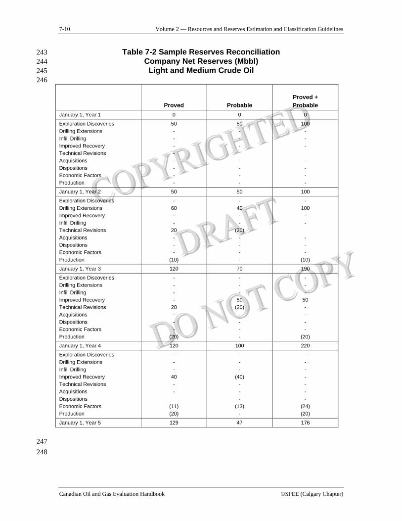
7-10 Volume 2 — Resources and Reserves Estimation and Classification Guidelines
Canadian Oil and Gas Evaluation Handbook ©SPEE (Calgary Chapter)
Table 7-2 Sample Reserves Reconciliation 243 Company Net Reserves (Mbbl) 244
Light and Medium Crude Oil 245 246
Proved
Probable
Proved + Probable
January 1, Year 1 0 0 0
Exploration Discoveries Drilling Extensions Infill Drilling Improved Recovery Technical Revisions Acquisitions Dispositions Economic Factors Production
50 - - - - - - - -
50 - - - - - - -
100 - - - - - - -
January 1, Year 2 50 50 100
Exploration Discoveries Drilling Extensions Improved Recovery Infill Drilling Technical Revisions Acquisitions Dispositions Economic Factors Production
- 60 - -
20 - - -
(10)
- 40 - -
(20) - - - -
- 100
- - - - -
(10)
January 1, Year 3 120 70 190
Exploration Discoveries Drilling Extensions Infill Drilling Improved Recovery Technical Revisions Acquisitions Dispositions Economic Factors Production
- - - -
20 - - -
(20)
- - -
50 (20)
- - - -
- - -
50 - - - -
(20)
January 1, Year 4 120 100 220
Exploration Discoveries Drilling Extensions Infill Drilling Improved Recovery Technical Revisions Acquisitions Dispositions Economic Factors Production
- - -
40 - -
(11) (20)
- - -
(40) - - -
(13) -
- - - - - - -
(24) (20)
January 1, Year 5 129 47 176
247 248
Section 7 — Validation and Reconciliation of Reserves and Value Estimates 7-11
©SPEE (Calgary Chapter) First Edition — April 28, 2004
Summary of Changes in Year 4 248
1. The waterflood was initiated and 40 Mbbl of net probable reserves were 249 transferred from probable to proved. Because this is the first booking for the 250 improved recovery reserves for this project in the proved category, the transfer 251 was recorded as a proved improved recovery addition and a negative probable 252 improved recovery addition. 253
2. Company net share of production during the year was 20 Mbbl. 254
3. Government royalty formulas were changed at the end of the year, resulting in an 255 effective drop of 10 percent of the Company’s share of net reserves. 256
7.4 Net Present Values Reconciliations 257
7.4.1 Introduction 258
The Canadian securities regulations also require a reconciliation of net present values 259 for reporting purposes. This reconciliation is only required for proved reserves net 260 present values at a 10 percent discount rate before income taxes, using constant 261 prices and costs. 262
A net present value reconciliation is more complex than a reserves reconciliation 263 because of numerous changes that can occur in economic and technical factors, many 264 of which are dependent on each other. 265
Reconciliation should be presented as shown in Table 7-3. 266
7.4.2 Net Present Value Change Categories 267
A summary of the categories of changes that should be considered in a net present 268 value reconciliation, and the recommended procedure to determine those values, is 269 presented below: 270
a. Oil and Gas Sales During the Period. This category is based on the actual gross 271 revenues minus royalties minus production costs for the reporting period. This value is 272 determined on a before-tax basis. 273
b. Changes Due to Prices. This category is based on the net present value before taxes of 274 the difference between 275
7-12 Volume 2 — Resources and Reserves Estimation and Classification Guidelines
Canadian Oil and Gas Evaluation Handbook ©SPEE (Calgary Chapter)
1. the net revenue forecast (gross revenues minus royalties and production 276 costs) at the beginning of the period, and 277
2. the net revenue forecast at the beginning of the period, recalculated using 278 the actual prices for the reporting period, and the December 31 prices 279 after the reporting period. Changes to royalty and production cost 280 assumptions should also be included in this recalculated revenue 281 forecast, though in practice only significant changes are included. 282
c. Actual Development Costs During the Period. This category is based on the 283 actual development costs for the reporting period. Exploration and acquisition 284 costs should be excluded. 285
d. Changes in Future Development Costs. This category is based on the net 286 present value of the difference between 287
1. the forecast of future development costs at the beginning of the period, 288 and, 289
2. the actual development costs for the period plus the forecast development 290 costs at the end of the period. 291
e. Changes Resulting from Extensions, Infill Drilling and Improved Recovery. 292 This category includes the net present value before taxes of all reserves changes 293 due to extensions, infill drilling, and improved recovery. This value should be 294 calculated at the end of the period and determined using the end of the period 295 constant prices and costs. 296
f. Changes Resulting from Discoveries. This category includes the net present 297 value before income taxes of all reserves changes due to discoveries. This value 298 should be calculated at the end of the period and determined using the end of the 299 period constant prices and costs. 300
g. Changes Resulting from Acquisitions of Reserves. This category includes the 301 net present value before income taxes of all reserves changes due to acquisitions 302 of reserves. This value should be calculated at the end of the period and 303 determined using the end of the period constant prices and costs. 304
h. Changes Resulting from Dispositions of Reserves. This category includes the 305 net present value before taxes of all reserves changes due to dispositions of 306 reserves. This value should be determined using the net revenue forecast for the 307
Section 7 — Validation and Reconciliation of Reserves and Value Estimates 7-13
©SPEE (Calgary Chapter) First Edition — April 28, 2004
disposed properties that was calculated at the start of the period but adjusted to an 308 effective date of the disposition. 309
i. Accretion of Discount. The additional net present value before tax of the 310 previous year’s revenue forecast, determined by discounting to the end of the 311 current period rather than the start of the period. It is usually calculated as 312 10 percent of the beginning of the period net present value. 313
j. Other Significant Factors. Any other significant factors resulting in a change to 314 the net present values before tax and not accounted for above should be listed 315 separately. 316
k. Net Changes in Income Tax. This category is calculated as the difference 317 between the net present value of the estimated income taxes at the start of the 318 period and the net present value of the actual taxes during the period plus the 319 forecast taxes at the end of the period. 320
l. Changes Resulting from Technical Reserves Revisions Plus Effects of 321 Timing. Because it is difficult to calculate the effect on the net present value on 322 all technical reserves revisions, and the effect of changes to the timing of 323 development, this category should be calculated after accounting for all other 324 changes, by subtracting the previous year net present value after tax and all of the 325 changes estimated above from the current year net present value after tax. 326
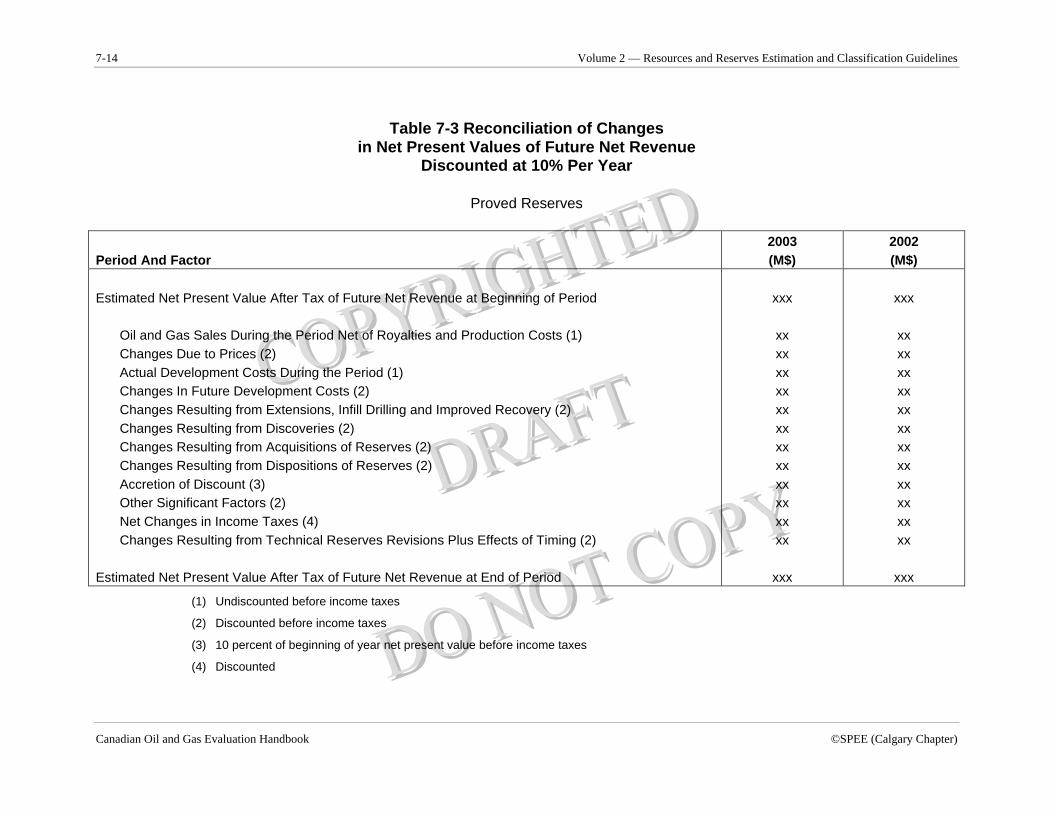
7-14 Volume 2 — Resources and Reserves Estimation and Classification Guidelines
Canadian Oil and Gas Evaluation Handbook ©SPEE (Calgary Chapter)
Table 7-3 Reconciliation of Changes in Net Present Values of Future Net Revenue
Discounted at 10% Per Year
Proved Reserves
Period And Factor
2003 (M$)
2002 (M$)
Estimated Net Present Value After Tax of Future Net Revenue at Beginning of Period Oil and Gas Sales During the Period Net of Royalties and Production Costs (1) Changes Due to Prices (2) Actual Development Costs During the Period (1) Changes In Future Development Costs (2) Changes Resulting from Extensions, Infill Drilling and Improved Recovery (2) Changes Resulting from Discoveries (2) Changes Resulting from Acquisitions of Reserves (2) Changes Resulting from Dispositions of Reserves (2) Accretion of Discount (3) Other Significant Factors (2) Net Changes in Income Taxes (4) Changes Resulting from Technical Reserves Revisions Plus Effects of Timing (2) Estimated Net Present Value After Tax of Future Net Revenue at End of Period
xxx
xx xx xx xx xx xx xx xx xx xx xx xx
xxx
xxx
xx xx xx xx xx xx xx xx xx xx xx xx
xxx
(1) Undiscounted before income taxes
(2) Discounted before income taxes
(3) 10 percent of beginning of year net present value before income taxes
(4) Discounted

Appendices 1
©SPEE (Calgary Chapter) First Edition — April 28, 2004
APPENDIX A — GlossaryAccelerated production. The recovery of the reserves of a pool at a faster rate than a base production scenario with no recovery of incremental reserves. Accumulation. An individual body of petroleum in a reservoir Acidizing. A method of well stimulation using acid (to increase productivity); conducted mostly in carbonates. Acoustic log. A measurement of the interval transit time of compressional seismic waves in rocks near the wellbore of a liquid-filled borehole; used chiefly for estimating porosity and lithology; also referred to as sonic log. Aggregate /Aggregation - The sum total of, or the process of totalling, individual estimates in a collection of separate estimates. Analogous fields. Fields having similar properties that are at a more advanced stage of development or production history than the field of specific interest, and that may provide concepts or patterns to assist in the interpretation of more limited data. Anhydrite. A granular, white or light-colored evaporite mineral (CaSO4), often found together with rock salt. Annulus. The space around the tubing in a wellbore, the outer wall of which may be the wall of either the borehole or the casing. Aquifer. A stratum below the surface of the earth capable of producing water. Arithmetic mean. The average obtained by dividing the sum of a distribution by the number of its addends. Asphaltene. Any of the dark solid constituents of crude oils and other bitumens that are soluble in carbon disulphide but insoluble in paraffin naphthas. Beta model. A numerical simulator used to model black oil systems; also referred to as black oil model.
Bias. A systematic deviation from the actual value or distribution; a combination of two effects: displacement bias and variability bias. Bitumen. Refer to Crude bitumen. Black oil model. Refer to Beta model. Black oil. Refers to a system in which the volume of fluid is primarily a function of reservoir pressure and constant temperature. A system that is not a black oil system includes compositional variables. Bottom water. Sand layers at the bottom of a formation which contain mobile water that appreciably affects reservoir performance; water in strata underlying an oil- or gas-bearing formation. Bottom-hole pressure. The pressure in a well at a point opposite the producing formation as recorded by a bottom-hole pressure recorder. Bottom-hole temperature. The temperature in a well at a point opposite the producing formation. Bubble point. In a solution of two or more components, the pressure at which the first bubbles of gas appear; same as saturation pressure. Bulk density. Density of the combined pore volume and rock volume; measured, for example, by a density log. Bulk volume. Total volume of a formation including the pore volume and the rock volume. Butanes. In addition to its normal scientific meaning of C4H10 (a mixture of two gaseous paraffins, normal butane and isobutane), a mixture mainly of butanes that ordinarily may contain some propane or pentanes. Capillarity. The effect of surface attraction forces among oil, gas, water, and rock in retaining fluid saturations within the pore structure of a porous medium. Refer to Capillary pressure.
2 Volume 2 — Resources and Reserves Estimation and Classification Guidelines
Canadian Oil and Gas Evaluation Handbook ©SPEE (Calgary Chapter)
Capillary pressure. A force per unit area resulting from surface forces at the interface between two immiscible fluids. Carbon dioxide flooding. A recovery process in which carbon dioxide is injected into an oil reservoir to improve recovery. Carbonates. Sedimentary rocks primarily composed of calcium carbonate (limestone) or calcium magnesium carbonate (dolomite), which form many petroleum reservoirs. Cementation. The process of precipitation or growth of a binding material around grains or fragments of rock. Chase gas. Gas used to displace another phase in an enhanced recovery process. Chemical flooding. A recovery process in which chemicals added to water are injected into an oil reservoir to improve recovery. Choke. An orifice installed in a line to restrict the flow and control the rate of production. Clastics. Sedimentary rocks composed of fragments of pre-existing rocks; sandstone is a clastic rock. Clay lattice. A three-dimensional pattern of clay parts in space. Compaction. A decrease in volume of sediments as a result of compressive stress, usually resulting from continued depositional loading by accumulation of overlying sediments. Completion interval. The portion of the wellbore that has been perforated or is open to the formation. Compressibility. The rate of change in volume of rock and fluids with decrease in pressure. Compressibility is a major contributor to recovery efficiency and a cornerstone of reservoir performance. Condensate. A mixture of pentanes and heavier hydrocarbons recovered as a liquid from field separators, scrubbers or other gathering facilities, or at the inlet of a processing plant before the gas is processed.
Conductivity. A property of an electrical conductor defined as the electrical current per unit area divided by the voltage drop per unit length. Confidence level. The qualitative degree of certainty associated with an estimated value. Conformance efficiency. The fraction of total reservoir volume that is contacted by injected fluid as a result of discontinuities in the reservoir; also referred to as continuity factor. Conglomerate. A sedimentary rock composed of coarse-grained rock fragments, pebbles or cobbles cemented together in a fine-grained matrix. Coning. A cone of gas or water that forms in the reservoir due to pressure drawdown at the perforations. Connate water. The original water of deposition trapped in the interstices of the reservoir rock. Conventional crude oil. Crude oil that, at a particular time, can be technically and economically produced through a well using normal production practices and without altering the natural viscous state of the oil. Conventional natural gas. Natural gas that occurs in a normal, porous, permeable reservoir rock and that, at a particular time, can be technically and economically produced using normal production practices. Cricondentherm. Maximum temperature at which two phases (for example, liquid and vapour) can exist. Critical gas saturation. Saturation at which free gas in a reservoir becomes mobile. Critical pressure. The pressure required to condense a gas at the critical temperature, above which, regardless of pressure, the gas cannot be liquefied. Critical temperature. That temperature above which a substance can exist only in the gaseous state, no matter what pressure is exerted.
Appendices 3
©SPEE (Calgary Chapter) First Edition — April 28, 2004
Crude bitumen or bitumen. A naturally occurring viscous mixture consisting mainly of pentanes and heavier hydrocarbons. Its viscosity is greater than 10 000 mPa-s (cp) measured at original temperature in the reservoir and atmospheric pressure, on a gas-free basis. Crude bitumen may contain sulphur and other non-hydrocarbon compounds. Crude oil or Oil. A mixture, consisting mainly of pentanes and heavier hydrocarbons, that exists in the liquid phase in reservoirs and remains liquid at atmospheric pressure and temperature. Crude oil may contain small amounts of sulphur and other non- hydrocarbons, but does not include liquids obtained from the processing of natural gas. Classes of crude oil are often reported on the basis of density, sometimes with different meanings. Acceptable ranges are as follows: • Light: less than 870 kg/m3 (greater than
31.10 API) • Medium: 870 to 920 kg/m3 (31.1 to
22.30 API) • Heavy: 920 to 1000 kg/m3 (22.3 to 100
API) • Extra-heavy: greater than 1000 kg/m3
(less than 100 API) D'Arcy's Law. The basic law of fluid flow through a porous medium that expresses how easily a fluid of a certain viscosity flows through a rock under a pressure gradient. Decision tree. A graphical summary of the possible outcomes and probabilities of the events that comprise a project. Density log. A radioactivity log for open-hole surveying that responds to variations in the specific gravity of formations; an excellent porosity -measuring device, especially for shaly sands. It is a contact log (i.e., a detector held against the wall of the hole). The tool emits neutrons and then
measures the secondary gamma radiation that is scattered back to the detector. Density. The ratio of the mass of an object to its volume. Depletion. The reduction, or exhaustion of a well or pool’s commercial volumes of crude oil or natural gas and related substances by production. Depositional environment. The conditions under which sediments were laid down. detecting device and examined under ultraviolet light to detect the presence of oil or gas. Often carried out in a portable laboratory set up at the well. Deterministic method. A method of estimating an uncertain outcome whereby discrete values are used for each parameter in a calculation. Differential liberation. The liberation of gas from oil as pressure is reduced wherein the evolved gas is separated from its associated oil; usually the physical model related to transport of oil and gas through the formation during the majority of the primary depletion life. Dip. The angle at which a stratum is inclined from the horizontal. Discounted cash flow. Future cash converted to present conditions using an appropriate discount rate. Displacement bias. A shift of the whole frequency distribution curve to higher or lower values. Displacement efficiency. The fraction of initial oil saturation that is displaceable by a given injection fluid. Displacement process. The process by which oil is displaced by water, gas, or another fluid. Disposal well. A well used for the disposal of salt water. The water is pumped into a subsurface formation sealed off from other formations by impervious strata of rock.
4 Volume 2 — Resources and Reserves Estimation and Classification Guidelines
Canadian Oil and Gas Evaluation Handbook ©SPEE (Calgary Chapter)
Dolomite (CaMg(CO3)2). A common rock-forming mineral. Dolomitization. The process whereby limestone is altered to dolomite by the substitution of magnesium carbonate for a portion of the original calcium carbonate. Drainage area. The area of a pool contributing oil or gas to a well. Drillstem test. The procedure used to gather data on a formation to determine its potential productivity before installing casing in a well. In the drillstem testing tool are a packer, valves or ports that may be opened and closed from the surface, a sample chamber and a pressure-recording device. The tool is lowered in the wellbore on a string of drill pipe and the packer set, isolating the formation to be tested from the formations above and below and supporting the fluid column above the packer. A port on the tool is opened to allow the trapped pressure below the packer to bleed off into the drill pipe, gradually exposing the formation to atmospheric pressure and allowing the well to produce to the surface, where the well fluids may be sampled and inspected. From a record of the pressure readings, a number of facts about the formation may be inferred. Effective Date. The effective date, also referred to as the "As of Date," serves two purposed in an oil and gas reserves evaluation: (1) It is the cut-off date for all geological, engineering, and financial data after which no new information can be included in the evaluation. (2) It is the date to which all future net revenue or other cash flow forecasts are discounted to determine present worth values. Efflux. Quantities of hydrocarbons, water or other fluids that leave a reservoir or zone of interest via permeable formation boundaries.
Electrical conductivity. Used for estimating reservoir properties; reciprocal of electrical resistivity. Refer to Conductivity. Electrical resistivity. The reciprocal of electrical conductivity; used for estimating properties such as water saturation and fracture porosity. It is one of the most useeful measurements in boreholegeophysics. Enhanced recovery. See recovery. Entity. In the context of a “reserves entity”, entity refers to the distinct item for which a reserves calculation is performed prior to aggregation; an entity may, for example, consist of a well-zone, a group of wells or a pool. Established reserves. Those reserves recoverable under current technology and present and anticipated economic conditions, specifically proved by drilling, testing or production, plus that judgement portion of contiguous recoverable reserves that is interpreted, from geological, geophysical or similar information, to exist with reasonable certainty. This is a term that has been used historically in Canada, particularly by regulatory agencies, and typically comprises proved reserves plus one-half probable reserves. Established technology. Methods that have been proven to be successful in commercial applications. Ethane. In addition to its normal scientific meaning of C2H6 (a colourless, odourless gas of the alkane series), a mixture mainly of ethane that may contain some methane or propane. Evaporite. Deposits of mineral salts from sea water or salt lakes due to evaporation of the water. Expectation. The mean of all possible outcomes of an event. Facies. Part of a bed of sedimentary rock of similar depositional environment, composition, appearance and properties.

Appendices 5
©SPEE (Calgary Chapter) First Edition — April 28, 2004
Fault plane. A surface along which faulting has occurred. Fault. A break in subsurface strata. Often strata on one side of the fault line have been displaced (upward, downward, or laterally) relative to their original position. Field. A defined geographical area consisting of one or more pools. Fines migration. The dislocation and movement of fine particles within a reservoir. Fines migration can cause damage or impair permeability by blocking pore throats. Flash liberation. The liberation of gas from oil as pressure is reduced wherein the evolved gas remains in contact with the liquid phase. Flow test. A test of the ability of a well to produce fluids usually at a constant rate. Fluid contact - The surface or interface in a reservoir separating two regions characterized by predominant differences in fluid saturation. Because of capillary and other phenomena, fluid-saturation change is not necessarily abrupt or complete, nor is the surface necessarily horizontal. Fluid saturation. The portion of porosity in a reservoir that is occupied by a fluid. Fluid viscosity. Internal friction of a fluid, caused by molecular interactions, that makes it resist a tendency to flow. Fold. A flexure of rock strata into arches and troughs, produced by earth movements. Formation heterogeneity. Variation both laterally and vertically of properties such as porosity, permeability, and formation thickness. Formation imaging. Logs that generate images (or "pictures") of the borehole from various sources including sonic and resistivity devices. Formation pressure. The pressure in a formation at a defined depth.
Formation temperature. The temperature at a given point within a formation. Temperature usually increases with depth. Formation volume. The volume of fluid, at formation pressure and temperature, that results in one barrel of stock tank oil. Fractional flow. Phase flow rate as a fraction of total flow rate. Fracturing. A stimulation to increase productivity that results in the formation of a fracture in the wellbore area; conducted mostly in clastics. Free-water level. The level or depth at which capillary pressure is equal to zero and which, in rocks of variable pore structure, is the only truly level reference line between hydrocarbons and water. Friable. Describes a substance that is easily rubbed, crumbled, or pulverized into powder. Gamma ray detector. A device that is capable of sensing and measuring the amount of gamma particles emitted by certain radioactive substances. Gas chromatography. The process of separating constituents of a mixture by permitting a solution of the mixture to flow through a column of adsorbent on which the different substances are selectively separated into distinct bands or spots. Gas compressibility factor. A factor used to correct the Ideal Gas Law (pv = nRT) to actual measurements. Gas. Refer to Natural gas. Gas-oil ratio. The ratio of gas in solution to the oil volume in which it is dissolved, usually expressed in cubic feet of gas per barrel of liquid at 101.325 kPa (14.65 psia) and 15.6ºC (60ºF). Genetic sand unit. Formation consisting of sands from the same origin. Geostatistics. A specific statistical technique (based on the statistics of regionalized variables) that uses the position
6 Volume 2 — Resources and Reserves Estimation and Classification Guidelines
Canadian Oil and Gas Evaluation Handbook ©SPEE (Calgary Chapter)
as well as the magnitude of a parameter; classical statistics does not generally use position. Other spatial statistics methods also exist. Gravity drainage. The movement of oil in a reservoir toward a wellbore resulting from the force of gravity. Gravity override. Preferential movement of one fluid over another due to density differences. Gross pay. The gross economically productive thickness of a formation containing hydrocarbons. Gross swept volume. The reservoir rock volume that is swept by injected fluid. Heavy or extra-heavy crude oils, as defined by the density ranges given, but with viscosities greater than 10 000 mPa⋅s measured at original temperature in the reservoir and atmospheric pressure, on a gas-free basis, would generally be classified as crude bitumen. Heavy or extra-heavy crude oils, as defined by the density ranges given, with viscosities greater than 10 000 mPa-s measured at original temperature in the reservoir and atmospheric pressure, on a gas-free basis, would generally be classified as crude bitumen. Heterogeneity. A lack of uniformity in formation properties such as permeability, porosity and thickness. Homogeneity. Uniformity of reservoir properties in all directions. Horizontal sweep efficiency. The areal fraction of a pattern contacted by the injected fluid; also referred to as areal sweep efficiency. Horizontal waterflood scheme. The injection of water in a pattern of wells with oil production from wells completed between injectors. Hybrid sand unit. A formation with sands from different origins.
Hydrate. A hydrocarbon and water compound that forms under reduced pressure and temperature in gathering, compression, and transmission facilities for gas; flakes of hydrate resemble snow or ice and impede fluid flow. Hydrocarbon pore volume. The pore volume in a reservoir containing hydrocarbons; the product of hydrocarbon-filled thickness, porosity, and hydrocarbon saturation usually expressed for a unit area. May be represented on a contour map as a type of volumetric map. Hydrocarbons. Solid, liquid or gas made up of compounds of carbon and hydrogen in varying proportions. Hydrocarbons in place. The total quantity of hydrocarbons estimated to be contained in an accumulation, at a given time. Hydrodynamic flow. The motion and action of water and other liquids in the subsurface. Hydrodynamic trap. An oil or gas reservoir trapped by surrounding water movement; usually leads to tilted water-oil contacts. Hydrodynamics. The study of the motion of a fluid and of the interactions of the fluid with its boundaries, especially in the incompressible ideal (frictionless) case. Hydrostatic head. The pressure exerted by a body of water at rest. Hysteresis. A change in process path in successive experimental tests. Ideal Gas Law. The volume occupied by an ideal gas depends only upon temperature, pressure, and the number of molecules (moles) present (pv = nRT). Imbibition. The increase in saturation of the wetting phase in a porous medium with time. Improved recovery. See recovery. In situ recovery. A term that is used, when referring to oil sands, for the process of
Appendices 7
©SPEE (Calgary Chapter) First Edition — April 28, 2004
recovering crude bitumen from oil sands other than by surface mining. Incremental reserves. The additional quantities of crude oil, natural gas and related substances that can be recovered by an enhancement to production conditions. Infill well(s). A well (or wells) that is drilled within a known accumulation. Influx. Quantities of hydrocarbons, water or other fluids that enter a reservoir or a designated portion of a reservoir through permeable formation boundaries. Initial reserves. A term often used to refer to reserves prior to deduction of any production. Alternatively, initial reserves can be described as the sum of remaining reserves and cumulative production at the time of the estimate. Initial volumes in place. The gross volume of crude oil, natural gas and related substances estimated, at a particular time, to be initially contained in a reservoir before any volume has been produced and without regard for the extent to which such volumes will be recovered. Injection. The pumping of fluids into the reservoir via wellbores, for wellbore conditioning or stimulation or for improved recovery operations. Intercalation. Insertion of a bed or stratum of one material between layers of another material. Interfacial tension. The force per unit length existing at the interface between two immiscible fluids. Interference effects. The change in a well’s production and recovery caused by the operation of other wells within a common reservoir. Irreducible water saturation. The minimum water saturation that can be obtained in a reservoir under normal operations.
Isochrone. A line on a chart connecting all points having the same time of occurrence of particular phenomena or of a particular value of a quantity. Isolating packers. Devices used for isolating an interval in a well. Isopach map. A geological map of subsurface strata showing contours of the thickness of a given formation underlying an area; one type of volumetric map. Isotherm. A line connecting points of equal temperature. Isothermal. Having constant temperature; at constant temperature. J function. A dimensionless grouping of the physical properties of a rock and its saturating fluids proposed by Leverett. Kerogen. A solid bituminous substance occurring in certain shales that decomposes to oil and natural gas when heated. Klinkenberg. Mathematical correction of laboratory air permeability measurements (made on formation material) into equivalent liquid permeability values, necessitated by gas slippage in pores. Known accumulation. An accumulation that has been penetrated by a well. In general, the well must have demonstrated the existence of hydrocarbons by flow testing in order for the accumulation to be classified as “known”. However, where log and/or core data exist and there is a good analogy to a nearby and geologically comparable known accumulation, this may suffice. Laterolog. A resistivity measuring device using electrodes in which a current is forced through the formation in a sheet of predetermined thickness, so that the measurement involves a limited vertical extent. Liquefied petroleum gases. A term commonly used to refer to hydrocarbon mixtures consisting predominantly of
8 Volume 2 — Resources and Reserves Estimation and Classification Guidelines
Canadian Oil and Gas Evaluation Handbook ©SPEE (Calgary Chapter)
propane and butanes. In Canada, ethane is also frequently included. Lithification. The conversion of unconsolidated deposits into solid rock by compaction and cementing together of the individual rock grains. Lithology. The description of the physical character of a rock as determined by eye or with a low-power magnifier; based on color, structures, mineralogic components, and grain size. LKH (lowest known hydrocarbon). The lowest structural elevation of hydrocarbons in a well or pool that has been confirmed by well logs, testing or pressure analysis. Marketable natural gas. Natural gas that meets specifications for its sale, whether it occurs naturally or results from the processing of raw natural gas. Field and plant fuel losses to the point of the sale must be excluded from the marketable quantity. The heating value of marketable natural gas may vary considerably, depending upon its composition, and therefore quantities are usually expressed not only in volumes, but also in terms of energy content. Reserves are always reported as marketable quantities. Material balance method. Engineering methods of analysing project performance based on mass-balance concepts, wherein expansion of in-situ rock and fluids is related to influx-efflux and production-injection streams. Material balance methods are commonly used to determine fluids in-place or predict production performance. Matrix. The continuous, fine-grained material in which large grains of a sediment or sedimentary rock are embedded. Mean. The most commonly used measure of central tendency; the average value of repeated trials. The mean represents the most probable value of an estimate of reserve volume or value. Median. A measure of central tendency; the middle value or the arithmetic mean of the
two middle values of a list of numbers, for a list containing an odd or even number of members, respectively. Geometrically, the value that divides a histogram or frequency distribution into two parts of equal area; also the 50 percent probability level on a cumulative distribution function or expectation curve. Methane. In addition to its normal scientific meaning of CH4 (a light, odourless, colourless gaseous hydrocarbon), a mixture mainly of methane that ordinarily may contain some ethane, nitrogen, helium or carbon dioxide. Micellar flooding. The addition of surfactants to injected water to reduce interfacial tension. Micro-fractures. Fractures not easily seen by the naked eye; might be seen in thin sections. They usually feed macro-fractures. Microlog. A wellbore resistivity log recorded with electrodes mounted at short distances from each other in the face of a rubber-padded microresistivity sonde and with different depths of investigation. Comparison of the two curves identifies mudcake which indirectly identifies the presence of permeable formation. Microporosity. Porosity that is visible only at high magnification and that is generally not effective. Miscibility. The tendency or capacity of two or more liquids to form a uniform blend, that is, to dissolve in each other; degrees are total miscibility, partial miscibility, and immiscibility. Miscible flooding. A recovery process in which a fluid (a "solvent") that is capable of dissolving into the crude oil it contacts is injected into an oil reservoir to improve recovery. Mobility ratio. The ratio of the mobility of the displacing phase behind the flood front to the displaced phase ahead of the flood front.
Appendices 9
©SPEE (Calgary Chapter) First Edition — April 28, 2004
Mobility. The ratio of the permeability of a given phase to the viscosity of that phase. Phase mobility is an indication of how easily that phase moves in the reservoir. Mode. A measure of central tendency; the most commonly occurring value of a set of numbers. Mole. An amount of substance of a system which contains as many elementary units as there are atoms of carbon in 0.012 kilogram of the pure nuclide carbon-12; the elementary unit must be specified and may be an atom, a molecule, an ion, an electron, a photon, or even a specified group of such units. Morphology. The observation of the form of lands. Mudcake. The residue that forms on the wall of the borehole as the drilling mud loses filtrate into porous and permeable formations; also called well cake or filter cake. Mud-gas log. The recording of information derived from examination and analysis of formation cuttings made by the bit and mud circulated out of the hole. A portion of the mud is diverted through a gas- Multi-phase behaviour. The equilibrium relationships between at least two fluids such as water, crude oil, or natural gas and related substances either in pools or above ground in gas-oil production facilities. Multi-well pools. Pools which contain more than one well. Natural fracture. A discontinuity in rock caused by diastrophism, deep erosion of the overburden, or volume shrinkage. Examples would include shales that lose water, the cooling of igneous rock, and the desiccation of sedimentary rock. Natural gas liquids. Those hydrocarbon components that can be recovered from natural gas as liquids including, but not limited to, ethane, propane, butanes,
pentanes plus, condensate, and small quantities of nonhydrocarbons. Natural gas or gas. A mixture of lighter hydrocarbons that exist either in the gaseous phase or in solution in crude oil in reservoirs but are gaseous at atmospheric conditions. Natural gas may contain sulphur or other non-hydrocarbon compounds. Net present value. The value obtained when all cash flow streams, including the investment, are discounted to the present and totalled. Neutron log. A radioactive device that emits high energy neutrons and records a curve which responds primarily to the amount of hydrogen in the formation. Thus, in clean formation where the pores are filled with water or oil, the neutron log measures the amount of liquid-filled porosity. Nonconventional crude oil. Crude oil that is not classified as conventional crude oil. An example would be kerogen contained in oil shale deposits. Bitumen is also generally included in the non-conventional crude oil category as a matter of practice, although some wells may produce at commercial rates without steam injection. Also referred to as unconventional crude oil. Nonconventional natural gas. Natural gas that is not classified as conventional natural gas. An example would be coal-bed methane. Also referred to as unconventional natural gas. Nuclear magnetism inject log. A tool that uses a pulsed nuclear magnetic resonance analyzed to determine fluid content, total and free fluid porosity, and permeability. Oil sands. Deposits of sand or sandstone or other sedimentary rocks that contain crude bitumen. Oolite. A spherical to ellipsoidal body, 0.25 to 2.00 mm in diameter, which may or may not have a nucleus, and has concentric or radial structure or both; usually calcareous,
10 Volume 2 — Resources and Reserves Estimation and Classification Guidelines
Canadian Oil and Gas Evaluation Handbook ©SPEE (Calgary Chapter)
but may be hematitic or of other composition. Operating conditions. The conditions (eg. temperature, pressure and rates) under which a well or pool is being depleted. Pentanes plus. A mixture mainly of pentanes and heavier hydrocarbons, which ordinarily may contain some butanes, and which is obtained from the processing of raw gas condensate or crude oil. Permeability. Property of a porous medium relating to the capacity of the medium to transmit fluids. Permeameter. A device for measuring permeability by measuring the flow of fluid through a sample across which there is a pressure drop. Petroleum. A naturally occurring mixture consisting predominantly of hydrocarbons in the gaseous, liquid or solid phase. Phase behaviour. The equilibrium relationships between water, liquid hydrocarbons, and dissolved or free gas, either in reservoirs or as separated aboveground in gas-oil production facilities. Pilot. A small-scale test or trial operation that is used to assess the suitability of a method for commercial application. Polymer flooding. The addition of polymers to injected water to improve mobility ratios and increase oil recovery. Pool. An individual and separate accumulation of petroleum in a reservoir. Pore volume. The pores in a rock considered collectively; the product of porous thickness times porosity. May be represented on a contour map, a type of volumetric map. Porosimetry. The measurement of the porosity of reservoir rock s. Porosity. The ratio of the aggregate volume of interstices in a rock to its total volume. It is usually stated as a percentage.
Pressure depletion. Pressure decline in a reservoir due to oil or gas production. Pressure transient analysis. The estimation of reservoir properties from measurements of flow, buildup and drawdown pressures. Primary recovery.- See recovery. Probabilistic method. A method of estimating an uncertain outcome whereby a range of values is used for each parameter in a calculation. Results are generally expressed as a range with an associated probability of occurrence. Probability. The extent to which an event is likely to occur, measured by the ratio of the favourable cases to the whole number of cases possible. Production decline analysis. Analytical methods that use historical production data to estimate the future production and/or reserves for an entity. Production tests. Tests conducted to determine the productivity of a given reservoir. Propane. In addition to its normal scientific meaning of C3H8 (a heavy, colourless hydrocarbon of the paraffin series), a mixture mainly of propane that ordinarily may contain some ethane or butanes. Pseudo-critical and pseudo-reduced properties (temperature and pressure). Properties of pure hydrocarbons are often the same when expressed in terms of their reduced properties. The same reduced-state relationships often apply to multicomponent systems if "pseudo" critical temperatures and pressures are used rather than the true critical properties of the systems. The ratios of the temperature and pressure of interest to the pseudo-critical temperature and pressure are called the pseudo-reduced temperature and pressure respectively. Pulsed neutron log. A special cased-hole logging tool that uses radioactivity reaction time to obtain measurements of water saturation, residual oil saturation, and fluid
Appendices 11
©SPEE (Calgary Chapter) First Edition — April 28, 2004
contents in the formation outside the casing of an oil well. PVT data. Information describing the physical inter-relationship of pressure, volume, and temperature of reservoir fluids and various production and injection streams. Pyrobitumen. Any of various dark-colored, relatively hard, nonvolatile hydrocarbon substances often associated with mineral matter, which decompose upon heating to yield bitumens. Pyrolysis. The breaking apart of complex molecules into simpler units by the use of heat, as in obtaining gasoline from heavy oil. Raw natural gas. Natural gas as it is produced from the reservoir prior to processing. It is gaseous at the conditions under which its volume is measured or estimated and may include varying amounts of heavier hydrocarbons (that may liquefy at atmospheric conditions) and water vapour. May also contain sulphur and other nonhydrocarbon compounds. Raw natural gas is generally not suitable for end use. Recovery factor - The fraction of petroleum-in-place that is estimated to be recoverable from a pool. Recovery:
Enhanced recovery. A term that, in Canada, is equivalent to improved recovery. Improved recovery. The extraction of additional crude oil, natural gas and related substances from reservoirs through a production process other than natural depletion. Includes both secondary and tertiary recovery processes such as pressure maintenance, cycling, waterflooding, thermal methods, chemical flooding, and the use of miscible and immiscible displacement fluids.
Primary recovery. The extraction of crude oil, natural gas and related substances from reservoirs utilizing only the natural energy available in the reservoirs. Secondary recovery. The extraction of additional crude oil, natural gas and related substances from reservoirs through pressure maintenance schemes such as waterflooding or gas injection. Tertiary recovery. The extraction of additional crude oil, natural gas and related substances from reservoirs using recovery methods other than primary or secondary recovery. A tertiary process can be implemented without a preceding primary or secondary recovery scheme.
Related substances. In the context of this document, those substances that are either separate products or are by-products of crude oil, natural gas and crude bitumen. Remaining reserves. Initial reserves less cumulative production at the time of the estimate. Reservoir. A porous and permeable subsurface rock formation that contains a separate accumulation of petroleum that is confined by impermeable rock or water barriers and is characterized by a single pressure system. Reservoir continuity. No interruption of a reservoir by faults, facies changes, or any other type of heterogeneity. Residual oil saturation. Following a recovery process, the oil saturation at which oil will no longer flow in a normal immiscible water-oil system. Resin. Any of a class of solid or semisolid organic products of natural or synthetic origin with no definite melting point, generally of high molecular weight; most resins are polymers. Resistivity log. The measurement of subsurface electrical resistivity accomplished either by sending current into

12 Volume 2 — Resources and Reserves Estimation and Classification Guidelines
Canadian Oil and Gas Evaluation Handbook ©SPEE (Calgary Chapter)
the formation and measuring the ease of electrical flow or by inducing an electrical current into the formation and measuring how large it is. Resistivity. The electrical resistance offered to the passage of current; the inverse of conductivity. Risk. The probability of loss or failure. Rock volume. The volume of rock contained within a specified area. Salt dome intrusive. A subsurface mound or dome of salt. Sandwich loss. The volume of oil remaining unswept at the top of a reservoir after water flooding or at the bottom of the reservoir after gas or miscible flooding. Saturated oil. Oil that contains all the gas that is capable of dissolving given the compositions of that oil and gas at the particular temperature and pressure. Saturation pressure. Also known as bubble-point pressure; the pressure at which the first bubble of gas comes out of solution. Saturation. Refer to Fluid Saturation. Secondary recovery. See recovery. Seismic. The measurement of the response to energy waves travelling through rock layers. The energy waves may be created by earthquakes, explosives or by dropping or vibrating a heavy weight. Some energy is reflected whenever the waves cross an interface of rock layers of distinctly different properties. Measurements can be made at the surface of travel time, which may be related to depth, and wave amplitude variations, which may relate to changes in rock properties (porosity, etc.). Separator. An oilfield vessel or series of vessels in which pressure is reduced so that the dissolved gas associated with reservoir oil is flashed off or removed as a separate phase. Also known as gas separator, oilfield separator, oil-gas separator, and oil separator.
Shrinkage factor. The reciprocal of the formation volume factor expressed as barrels of stock tank oil per barrel of reservoir oil. Shrinkage. The decrease in volume of a liquid phase caused by the release of solution gas or by the thermal contraction of the liquid; the reciprocal of formation volume factor. Shut in. When used in reference to a reserves entity, “shut in” implies that the entity is capable of production but is not currently producing. Solution gas. Natural gas that is dissolved in crude oil in the reservoir at original reservoir conditions and that is normally produced with the crude oil; also known as dissolved gas. Solvent flooding. Refer to Miscible flooding. Sonic log. A device that measures the time required for a sound wave to travel through a definite length of formation. Refer to Acoustic log. Sour gas. Natural gas that contains corrosive, sulphur-bearing compounds such as hydrogen sulphide, sulphur dioxide, and mercaptans. Specific gravity. The ratio of the density of a material to the density of some standard material, such as water at a specified temperature, 4ºC or 60ºF or (for gases) air at standard conditions of pressure and temperature. Spontaneous potential. A recording of the difference between the electrical potential of a movable electrode in the borehole and the electrical potential of a fixed surface electrode. Stabilized flow - The steady-state or pseudo steady-state flow conditions that exist when a well has been produced at a constant rate for a sufficient time such that pressure and rate distributions throughout a pool do not change with time or change at a uniform rate throughout the pool. The stabilized flow
Appendices 13
©SPEE (Calgary Chapter) First Edition — April 28, 2004
period is always preceded by a period of transient flow. Static gradient. Pressure measured in a wellbore at various depths while a well is shut in. Statistics. The science of collecting, analyzing, presenting, and interpreting data . Stock tank cubic metre. One cubic metre of oil at standard temperature and atmospheric pressure. Stratification. A structure produced by deposition of sediments in beds or layers (strata), laminae, lenses, wedges, and other essentially tabular units. Stratigraphic trap. A type of reservoir capable of holding oil or gas, in which the trap is formed by a change in the characteristics of the formation, which could be loss of porosity and permeability or a break in its continuity. Stratum - A sheet-like body or layer of sedimentary rock, visually separable from other layers above and below; a bed. It has been defined as a stratigraphic unit that may be composed of a number of beds. Stringer. A narrow vein or irregular filament of mineral traversing a rock mass of different materials. Structural trap. A type of reservoir containing oil and/or gas, formed by deformation of the earth's crust that seals off the oil and gas accumulation in the reservoir, forming a trap. Anticlines, salt domes, and faulting of different kinds form structural traps. Structure map. A map showing contour lines drawn through points of equal elevation on a stratum, key bed, or horizon, in order to depict the attitude of the rocks. Sulphur. As used in the petroleum industry, the elemental sulphur recovered by conversion of hydrogen sulphide and other sulphur compounds extracted from crude oil, natural gas or crude bitumen.
Surface loss. The quantity of natural gas removed at field processing plants as a result of the recovery of liquids and related products and the removal of nonhydrocarbon compounds, plus the gas used for fuel; also referred to as shrinkage. Surfactant. A soluble compound that reduces the surface tension of liquids, or reduces interfacial tension between two liquids or a liquid and a solid. Sweep efficiency. The volume swept by a displacing fluid divided by the total volume being flooded. Sweet gas. A petroleum natural gas containing no corrosive components, such as hydrogen sulphide, sulphur dioxide, and mercaptans. Synthetic crude oil. A mixture of hydrocarbons derived by upgrading crude bitumen from oil sands, and kerogen from oil shales or other substances such as coal. May contain sulphur or other nonhydrocarbon compounds and has many similarities to crude oil. Tertiary recovery - See recovery. Thermal conductivity. The heat flow across a surface per unit area per unit time, divided by the negative of the rate of change of temperature with distance in a direction perpendicular to the surface. Tilts. Blocks that have received a marked tilt in regions of block faulting. Regional tilts occur on the margins of basins of subsidence in the earth's crust. Tool resolution. The precision of a tool to investigate a given property. Transient flow. The unsteady state or non-stabilized flow period prior to steady state or pseudo steady state flow. The duration of the transient flow period will vary depending on rock and fluid properties. Transition zone. The interval directly above the free water level in a reservoir where capillary effects result in significant changes
14 Volume 2 — Resources and Reserves Estimation and Classification Guidelines
Canadian Oil and Gas Evaluation Handbook ©SPEE (Calgary Chapter)
in water and hydrocarbon saturation s in response to pore structure variations and elevation. Transmissibility. The ability of a reservoir to conduct fluids spatially in response to pressure differentials. Depends upon permeability and formation flow geometry. Production potential depends heavily upon reservoir transmissibility. Trap. A mass of porous, permeable rock that is sealed on top and down both flanks by nonporous, impermeable rock that prevents the free migration of hydrocarbons and concentrates them in a limited space. Uncertainty. The spectrum of possible outcomes of an evaluation. Ultimate potential recovery. A term sometimes used to refer to an estimate at a particular time of the initial reserves that will have become developed in an area by the time all exploratory and development activity has ceased, having regard for the geological prospects of the area, the known technology, and the anticipated economic conditions. It includes cumulative production; remaining proved, probable and possible reserves; and future additions to reserves through extensions and revisions to existing pools and the discovery of new pools. It may also be described as initial reserves plus those other resources that may be recoverable in the future. Uncertainty. The range of possible outcomes of an estimate. Unconformity. Lack of continuity in deposition between rock strata in contact with one another corresponding to a gap in the stratigraphic record; the surface of contact between rock beds in which there is a discontinuity in the ages of the rocks. Unconsolidated sand. A sand formation in which individual grains are not cemented together. If an unconsolidated sandstone produces oil or gas, it will produce sand if not controlled or corrected.
Undersaturated oil reservoir. A reservoir that is above the bubble-point pressure. Undersaturated oil. Oil that is capable of absorbing more gas than is present in the reservoir. Undersaturated oil typically displays relatively low compressibility and hence a rapid pressure decline with production. Unitization. A term denoting the joint operation of separately owned producing leases in a pool or reservoir. Upgrading. The process of converting crude bitumen or heavy crude oil into synthetic crude oil. Utilization rate. In an enhanced oil recovery process, the amount of gas or fluid injected per incremental oil recovered. Variability bias. An alteration in the shape of a frequency distribution curve. Verification. The process of establishing the validity of an event or result. Vertical sweep efficiency. The vertical fraction of reservoir swept by injected fluid. Vertical waterflood scheme. The injection of water at wells completed at the bottom of the formation; oil production is from wells completed at the top of the formation. Vesicle. A cavity in lava formed by entrapment of a gas bubble during solidification. Viscous fingering. Faster advance of a displacing phase as compared to the displaced phase due to an unfavorable mobility ratio. Voidage replacement ratio. The quotient of voidage replacement divided by reservoir voidage. Voidage replacement. The volume at reservoir conditions of fluids injected into a producing pool to offset fluid withdrawals during depletion. Voidage. The reservoir volume of hydrocarbons and water removed from the
Appendices 15
©SPEE (Calgary Chapter) First Edition — April 28, 2004
formation via wellbores during a term of producing operations. Volumetric estimation. An estimate of hydrocarbon or water volume based on a combination of geological maps and other data which in total must account for the reservoir area, thickness, porosity, hydrocarbon and water saturation. Volumetric mapping. A contour map of a parameter or combination of parameters that relate to reservoir volume. Vugs. Pore spaces that are larger than would be expected from the normal fitting together of the grains that compose the rock framework. Vugs are often formed during dolomitization. Water channelling. Preferential movement of water towards a wellbore due to unfavourable mobility ratio and pressure drawdown at the wellbore or due to the presence of higher permeability streaks.
Water influx. The movement of water into crude oil or natural gas pools as a result of production. Water injector. A well in which water has been injected into an underground stratum to increase reservoir pressure. Water saturation. Portion of the pore volume occupied by water. Waterflooding. An improved recovery process in which water is injected into a reservoir to increase oil recovery. Weighted-mean. The number obtained by multiplying each value of x by the probability (or probability density) of x and then summing (or integrating) over the range of x. Well density. The intensity of drilling in a given area. Wellbore. The hole drilled by the bit. Wetting phase. The liquid phase (oil, gas or water) that "wets" reservoir rock.
1
16 Volume 2 — Resources and Reserves Estimation and Classification Guidelines
Canadian Oil and Gas Evaluation Handbook ©SPEE (Calgary Chapter)
APPENDIX B — REFERENCES 1
2
3
………….(1992) Development Geology Reference Manual. AAPG Methods in Exploration 4 Series, No. 10. AAPG, 286 p. 5
Arps, J.J. (1945) Analysis of Decline Curves. Transactions of the AIME, Vol. 160, p. 228–247. 6
Fetkovich, M.J. (1973) Decline Curve Analysis Using Type Curves. SPE Paper No. 4629 7 presented at the 48th Annual Fall Meeting of the SPE of AIME, Las Vegas, NV. 8
Fetkovich, M.J. (1980) Decline Analysis Using Type Curves. JPT, Vol. 32, No. 6, p. 1065–1077. 9
Fetkovich, M.J., Fetkovich, E.J., and Fetkovich, M.D. (1996) Useful Concepts for Decline-Curve 10 Forecasting, Reserve Estimation, and Analysis. SPE Paper No. 28628, SPE Reservoir 11 Engineering,February, p. 13–21. 12
Masoner, L.O. (1998) Decline Analysis Relationship to Relative Permeability in Secondary and 13 Tertiary Recovery. SPE Paper No. 39928 presented at the SPE Rocky Mountain Regional/Low-14 Permeability reservoirs Symposium and Exhibition, Denver, CO. 15
Slider, H.C. (1976) Practical Petroleum Reservoir Engineering Methods. PennWell Books, 16 Tulsa, OK. 17
SPE 2001 ……….. 18
Warren, A. (1989) Alberta’s Small Gas Pool Reserves. Paper No. 89-40-10 presented at the 40th 19 Annual Technical Meeting of the Petroleum Society of CIM, Banff, AB. 20
Index 1
©SPEE (Calgary Chapter) First Edition — April 28, 2004
INDEX
A
acceleration recovery, 6-10, 6-11, 6-88 aggregation, 3-9, 4-4, 4-8, 4-10, 4-11, 4-12,
4-13, 4-14, 4-15, 4-23, 7-4, 7-5, 7-6 analogy method, 6-8–6-11, 6-66, 6-107 aquifers, 6-45 area assignments, 6-11
B
back pressure, 6-63 best estimate, 3-5, 4-4, 4-5, 4-14, 4-16, 6-9,
6-10, 6-25, 6-26, 6-51, 6-69, 6-70, 6-88, 6-89, 6-101, 6-102
best practice, 3-9 booking, 5-10 buildup analysis, 6-66 burdens, 5-4
C
Central Limit Theorem, 4-11, 4-14 certainty, 4-3, 4-12, 4-13, 4-14, 4-23, 6-90,
6-92 certainty levels, 3-8 Company gross reserves, 5-4, 7-5 Company net reserves, 5-4, 7-5, 7-6, 7-8 completion test, 6-14 compositional reservoir simulator, 6-47 confidence, 3-9, 4-5, 4-10, 4-13, 4-16, 6-20,
6-44, 6-70, 6-89, 6-91, 6-97 conglomerates, 6-16 coning, 6-63, 6-65 conservative estimate, 3-5, 4-4, 4-12, 7-4 constant prices and costs, 5-10, 7-5, 7-12, 7-
13 constraints, 4-14, 4-24 contingent resources, 5-7, 5-8, 6-92, 6-103 core data, 6-15, 6-16 curve fitting, 6-59, 6-60, 6-61, 6-66 cutoffs, 6-15–6-18
D
decline method, 6-58–6-86, 6-107 decline rate, 6-69, 6-70, 6-73 delineation wells, 6-88 deterministic estimates, 3-8, 4-3, 4-4, 4-5, 4-
6, 4-8, 4-11, 4-12, 4-14, 4-21, 4-23 developed non-producing reserves, 3-7 developed producing reserves, 3-6 developed reserves, 3-6 development well, 5-5, 5-7 dice problem, 4-18 drainage area, 6-19 drilling, 5-4 drilling statistics, 6-90 drillstem test, 5-6, 6-14 drive mechanisms, 6-24, 6-63 dry gas reservoir, 6-47
E
economics, 5-8 enhanced recovery, 6-98–6-103, 7-7 entity, 3-8, 3-9, 4-8, 4-14 estimation procedures, 6-1 expected value, 4-6 exponential decline, 6-60, 6-61, 6-62, 6-63 extended flow test, 6-23
F
facility constraints, 6-65 fault blocks, 5-5 feasibility study, 6-101 fluid analysis, 6-21 fluid flow equations, 6-58 fluid properties, 6-47 fluid rate, 6-64 fluvial channel, 6-16, 6-26 fluvial sands, 6-19 forecast prices, 5-9 formation volume factor, 6-21 fractured reservoir, 6-25, 6-47, 6-63 future drilling, 6-87–6-98
2 Volume 2 — Resources and Reserves Estimation and Classification Guidelines
Canadian Oil and Gas Evaluation Handbook ©SPEE (Calgary Chapter)
G
gas compressibility factor, 6-21 gas shrinkage, 6-22 geological data, 6-13 geophysical data, 6-12 gross pay, 6-15 group decline, 6-68
H
harmonic decline, 6-60, 6-61, 6-62, 6-63 heavy oil, 6-9, 6-14, 6-19, 6-64, 7-6 high-permeability reservoir, 6-48 horizontal displacement, 6-63 horizontal wells, 6-65 hydrocarbon saturation, 6-18 hydrocarbons, 6-14 hyperbolic decline, 6-60, 6-62, 6-63, 6-64
I
incremental recovery, 6-10, 6-88 infill analysis, 6-88 infill drilling, 6-10, 6-61, 6-65, 6-88, 7-7, 7-
8, 7-13 infill wells, 6-87 infrastructure, 5-7 interference effects, 6-68
L
line pressure, 6-68 linear regression, 6-51 low-permeability reservoir, 6-49
M
marine sands, 6-17, 6-19, 6-30 material balance method, 4-21, 6-44–6-58,
6-108 maximum, 4-6, 4-14, 4-15, 4-16, 4-21 mean, 4-6 median, 4-6 minimum, 4-6, 4-14, 4-15, 4-16, 4-21 mode, 4-6 multi-layer reservoir, 6-46 multi-well pool, 3-7, 6-17, 6-18, 6-19, 6-34,
6-46, 6-48, 6-50, 6-52, 6-90, 6-91, 6-107
N
net pay, 6-15, 6-16 net present value, 7-12 net present value revisions, 7-12 net profits interests, 5-4 no practical chance, 4-23 non-owned lands, 6-52, 6-107 non-producing reserves, 5-8 normalization equation, 6-61 numerical reservoir simulator, 6-44, 6-45, 6-
58
O
offset drainage, 5-3 OGIP, 4-21 oil cut, 6-67 oil reservoirs, 6-58 oolite shoals, 6-16 operating constraint, 6-67 optimistic estimate, 3-6, 4-4 over-pressured reservoir, 6-25 ownership, 5-3
P
P/Z plot, 6-44, 6-45, 6-47, 6-48, 6-49 performance, 6-11 permeability, 6-46, 6-62 pilot schemes, 6-99, 6-100 pinnacle reef, 6-26 pool area, 6-19 porosity, 6-17 possible reserves, 3-5 pressure data, 6-48 pressure depletion, 6-49 pressure measurements, 6-48 probabilistic estimates, 3-8, 4-3, 4-4, 4-5, 4-
10, 4-12, 4-22, 4-23 probability, 3-8, 4-6 probable reserves, 3-5 production data, 6-14 production forecasts, 6-68 production test, 5-5, 5-6, 6-52 property, 4-8, 4-11, 4-12 prospective resources, 6-90
Appendices 3
©SPEE (Calgary Chapter) First Edition — April 28, 2004
proved + probable + possible reserves, 3-4, 4-7, 4-15, 6-7, 6-103
proved + probable reserves, 3-4, 4-7, 4-15, 6-7, 6-102
proved reserves, 3-3, 3-5, 4-7, 4-15, 6-6, 6-34, 6-98
pseudo-steady-state flow, 6-59, 6-60, 6-62, 6-64, 6-66, 6-67
R
rate determination, 6-67 recovery factors, 6-11, 6-25 regulations, 6-65, 6-91, 6-99, 6-101, 6-102,
7-5, 7-6, 7-8, 7-12 regulatory compliance, 5-6 re-initialization, 6-67 relative permeability, 6-62 reported reserves, 3-8, 4-4, 4-8, 4-11, 4-12,
4-13, 4-23, 6-68, 7-4, 7-5 reserves, 3-4, 5-3, 5-4 reserves categories, 3-4, 6-51 reserves classification, 6-1, 6-69 reserves definitions, 3-1 reserves estimation, 6-106 reserves guidelines, 6-50 reserves reconciliation, 6-106, 7-1, 7-3, 7-5,
7-12 reserves revision, 7-3, 7-4, 7-5, 7-6, 7-8, 7-
12, 7-14 reserves validation, 6-7, 7-3 reservoir pressure, 6-22 reservoir properties, 6-45, 6-66 reservoir rock, 6-15 reservoir simulation method, 6-24, 6-87, 6-
108 reservoir temperature, 6-22 resources, 5-5 retrograde condensate reservoir, 6-47 risk-based estimates, 4-8, 4-9 royalty interest, 5-3
S
securities regulations, 5-3 single-well pool, 6-11, 6-16, 6-26, 6-107 skin factors, 6-64 spacing unit, 6-19, 6-26, 6-87 STATISTICS, 4-1 stratification, 6-62
T
testing, 5-5 thin pay, 6-25 time constraints, 6-93 time-to-depth conversion, 6-12, 6-20 timing, 5-8 transient flow, 6-59, 6-60, 6-64, 6-65, 6-66,
6-67 type curve matching, 6-59, 6-60, 6-61, 6-66,
6-67
U
uncertainty, 4-1, 4-5, 4-7, 4-14, 6-9, 6-10, 6-12, 6-13, 6-14, 6-17, 6-18, 6-20, 6-24, 6-25, 6-26, 6-51, 6-61, 6-88, 6-103, 7-3, 7-4
uncertainty-based estimates, 4-8, 4-9, 4-12 undeveloped reserves, 3-7, 5-9
V
vertical displacement, 6-63 vertical wells, 6-65 voidage replacement, 6-69 volumetric method, 4-23, 6-18, 6-35, 6-12–
6-44, 6-107
W
well test, 6-23 wellbore, 6-65 wet gas reservoir, 6-47 wettability, 6-62 working interest, 5-3 workovers, 6-64
Related Documents