Running head: Genetic Map for the Laboratory Mouse

1

A New Standard Genetic Map for the Laboratory Mouse

Running head: Genetic Map for the Laboratory Mouse

Allison Cox1, Cheryl Ackert-Bicknell1, Beth L. Dumont2, Yueming Ding1, Jordana Tzenova

Bell3, Gudrun A. Brockmann4, Jon E Wergedal5 , Carol Bult1, Beverly Paigen1, Jonathan Flint3,

Shirng-Wern Tsaih1, Gary A. Churchill*1, Karl W. Broman6

1 The Jackson Laboratory, Bar Harbor, Maine, United States of America, 2 Laboratory of

Genetics, University of Wisconsin, Madison, Wisconsin, United States of America, 3 Wellcome

Trust Centre for Human Genetics, University of Oxford, Oxford, United Kingdom, 4 Breeding

Biology and Molecular Genetics, Institute of Animal Sciences, Humboldt-Universität zu Berlin,

10115 Berlin, Germany, 5 J.L. Pettis Memorial VA Medical Center, Loma Linda, California,

92357, 6 Department of Biostatistics and Medical Informatics, University of Wisconsin,

Madison, Wisconsin, United States of America,

*Corresponding author: [email protected]

Genetics: Published Articles Ahead of Print, published on June 17, 2009 as 10.1534/genetics.109.105486

2

ABSTRACT

Genetic maps provide a means to estimate the probability of co-inheritance of linked loci

as they are transmitted across generations in both experimental and natural populations.

However, in the age of whole genome sequences, physical distances measured in base pairs of

DNA provide the standard coordinates for navigating the myriad features of genomes. Although

genetic and physical maps are colinear, there are well-characterized and sometimes dramatic

heterogeneities in the average frequency of meiotic recombination events that occur along the

physical extent of chromosomes. There also are documented differences in the recombination

landscape between the two sexes. We have revisited high-resolution genetic map data from a

large heterogeneous mouse population, reported by Shifman et al., and have constructed a

revised genetic map of the mouse genome, incorporating 10,195 single nucleotide

polymorphisms and based on a set of 47 families, comprising 3546 meioses. The revised map

provides a different picture of recombination in the mouse from that reported previously. We

have further integrated the genetic and physical maps of the genome, incorporated SSLP markers

from other genetic maps into this new framework. We demonstrate that utilization of the revised

genetic map improves QTL mapping, partially due to the resolution of hitherto undetected errors

in marker ordering along the chromosome.

3

INTRODUCTION

Genetic maps exist for hundreds of different species and genetic map construction

continues to play an important role in the characterization of genomes (CHOWDHARY and

RAUDSEPP 2006; KONG et al. 2002; STAPLEY et al. 2008; TANKSLEY et al. 1992). A genetic map

defines the linear order and relative distances among a set of marker loci in units that correspond

to the frequency of meiotic recombination between the loci. Until recently mouse genetic maps

based on simple sequence length polymorphism (SSLP) markers (LYON 1976) have been

sufficient for most experimental purposes, since, unlike the hundreds of thousands of markers

required in human genetic association studies, a relatively small number of markers is needed to

map in crosses between inbred mouse strains. However recent developments in whole genome

high resolution mapping in the mouse (CHURCHILL et al. 2004; VALDAR et al. 2006) and interest

in examining recombination rates at an ultra fine-scale (MYERS et al. 2005), have reawakened

the need to develop a high resolution genetic map in the mouse

The current standard genetic map of the mouse has been compiled from a substantial

body of historical data and maintained by the Mouse Genome Informatics (MGI) project at The

Jackson Laboratory (BULT et al. 2008). We will refer to it as the MGI map. The primary sources

of data used to construct the MGI map were two mapping panels, described here. However, the

current map is based on a consensus developed by the Chromosome Committees (2000) using all

available published data. The map has continued to be maintained by MGI with the addition of

4

new genetic markers and data but, because the map is based on consensus, published errors may

have been perpetuated.

The Jackson Laboratory developed a genetic map based on two sets of 94 progeny

obtained from reciprocal backcrosses (BSB and BSS) between inbred strains C57BL/6J and

SPRET/EiJ (ROWE et al. 1994). These strains represent two different species of mouse (Mus

musculus and Mus spretus). The map provides a wealth of genetic information but problems with

male fertility restrict breeding options and thus the map is female specific. This may also have

resulted in some multi-locus distortion in the mapping panel (MONTAGUTELLI et al. 1996).

Currently 1372 and 4913 markers have been typed on the BSB and BSS backcross panels,

respectively (BROMAN et al. 2002). Researchers at The Whitehead Institute and MIT developed

a map of 4006 SSLPs markers using an intercross population of 46 mice derived from strains OB

(C57BL/6J-Lepob/ob) and CAST (CAST/EiJ) (DIETRICH et al. 1994). The parental strains OB and

CAST are both derived from Mus musculus but CAST is from a distinct subspecies, M. m.

castaneus. The intercross mating strategy produces observable recombination from both male

and female parents but the two cannot be distinguished. Thus the map is sex averaged and based

on 92 meioses. The Whitehead/MIT map was expanded to include 7377 SSLP markers

(DIETRICH et al. 1996). These are denoted as, e.g., D7Mit54, where “7” indicates the

chromosome to which the marker is mapped and “54” is an arbitrary index. They are commonly

referred to as “Mit” markers.

Map resolution is limited by the number of observable recombination events in each of

these panels. With 94 meioses (in each backcross) and an average of 14 recombination events

per haploid genome transmitted, limiting resolution is on the order of 1 cM. A much larger

5

panel would be needed to achieve subcentimorgan resolution and to accurately position high

density sets of SNP markers.

Here we propose a new standard genetic map of the laboratory mouse based on data from

a large heterogeneous stock (HS) mouse population descended from eight inbred strains,

(DBA/2J, C3H/HeJ, AKR/J, A/J, BALB/cJ, CBA/J, C57BL/6J and LP/J) representing a diverse

sample of the classical inbred strains (PETKOV et al. 2004). Shifman et al (SHIFMAN et al. 2006)

calculated genetic maps based on 11,247 informative SNP markers in 2,293 HS individuals. The

marker set is dense with 99% of the SNP intervals under 500 kb, 81.2% below 250 kb and an

estimated allele inheritance-based accuracy of 99.98%. Map positions were calculated

separately for male and female meioses using CRIMAP software (GREEN P 1990) and the total

length of the sex-averaged map is 1630 cM, as defined by the most distal SNP markers in their

panel. The MGI map is 1783 cM based on the most distal available marker position for each

chromosome. However, based on the most distal shared markers, the original Shifman map at

1612 cM is substantially longer than the MGI map at 1445 cM. It was not immediately clear if

this discrepancy was due to the nature of recombination in the HS population or to their method

of map estimation.

There are at least two methodological problems with the HS map reported in (SHIFMAN et

al. 2006). First, the map was constructed using a sliding window of 5-15 SNPs, in order to

handle eight multi-generation families within the CRIMAP software. Ideally, one considers all

markers on a chromosome simultaneously in constructing a genetic map, and we found that this

could be accomplished by splitting the complex pedigrees into sibships. While splitting the

pedigrees results in slightly less efficient estimates of inter-marker distances, this approach

should incur no bias. Maps based on the full set of markers but with the complex pedigrees split

6

into sibships are thus arguably better than maps based on the full pedigrees but with a sliding

window of 5–15 markers. Second, analysis of families with incomplete parental genotypes may

have contributed to an inflated map size. 16 out of the 72 families lack parental genotypes or

have genotypes for just one parent (15 out of the 72), and many of them are small (26 have 6 or

fewer siblings). Sibships with no parental genotype data, on their own, can give no information

about sex-specific recombination rates. In conjunction with other sibships for which parental

genotypes are available, they can provide some information, but the CRIMAP software (last

modified in 1990) makes some approximations that result in large bias even in the sex-averaged

genetic maps for small sibships lacking parental genotype data.

For these reasons, we recomputed the mouse genetic map based on the original data

reported and discuss differences between the original Shifman map and the revised Shifman map

below. The revised Shifman map provides a markedly different picture of recombination in the

mouse: the estimated sex-averaged chromosome lengths correspond more closely to those in the

original MGI map, the sex difference in the overall recombination rate is greatly reduced, and

numerous narrow regions of high recombination rate, apparent in the original Shifman map, have

disappeared.

We propose the revised Shifman map as a new standard genetic map for the mouse. The

new genetic map represents a substantial improvement over the existing MGI map due to the

large number of meioses and to the genetic diversity of strains in the HS population. We have

generated male, female and sex averaged genetic maps with physical positions and updated locus

identifiers. We have established the correspondence between physical and genetic positions of

7080 Mit markers and corrected inconsistencies in the MGI map. We provide a web based tool

for the interpolation of new marker loci onto the genetic map and for converting genetic map

7

positions to NCBI mouse build 37 coordinates. Lastly, we examined the effect of changing to

this new revised genetic map on QTL mapping in five previously published data sets (BEAMER et

al. 1999; BEAMER et al. 2001; ISHIMORI et al. 2004; ISHIMORI et al. 2008; WERGEDAL et al.

2006).

METHODS

Data Cleaning

We reviewed the quality of the raw genotype data from Shifman et al., and identified a

set of 11 individuals whose genotypes were discrepant from their parents or offspring; these

individuals were omitted from our analysis. We also identified 26 individuals recorded to be

female but whose genotype data indicated that they were male. The sex for these individuals was

switched. We omitted genotypes with quality score < 0.4. We used Pedcheck (O'CONNELL and

WEEKS 1998) to identify genotypes inconsistent between parents and offspring, and omitted the

genotypes deemed to be in error. The large sibships and low apparent genotyping error rate

greatly simplified this task. We used the chrompic option of CRIMAP to identify unlikely tight

double-recombination events indicative of genotyping errors. We omitted the offending genotype

for apparent double-recombinants containing a single typed marker and separated by <10cM in

sex-specific distance. We omitted 176 genotypes due to Mendelian inconsistencies and another

538 genotypes that resulted in tight double-recombination events. In all, ~3.2 per 100,000

genotypes were omitted. The final data set included 22,500,431 genotypes.

The eight complex pedigrees were split into sibships (with parents and grandparents,

when available). The largest sibships could not be handled in CRIMAP, and so sibships with >

20 siblings were split in half. One sibship with 48 siblings was split into three sibships with 16

8

siblings each. Sibships with genotype data on just one parent and with eight or fewer siblings

were omitted. Sibships with no parental genotype data were also omitted. While the largest of

these might have been used to estimate the sex-averaged maps, we felt it best to use the same set

of data for both the sex-specific and the sex-averaged maps. In all, 25 of the 72 nuclear families

were omitted. The final data comprised 3546 meioses.

The revised maps were estimated with CRIMAP (GREEN P 1990), using the Kosambi

map function. Recombination rates (cM/Mb) were estimated using a sliding 5 Mb window.

Locating Markers on the Physical Genome

Physical positions of 10,202 SNPs used in the Shifman study were mapped to the mouse

Build 37 genome by BLAT (http://genome.ucsc.edu/cgi-bin/hgBlat) using the 100 bp flanking

sequence on both sides of each SNP. Out of 10,202 total SNPs, 10,196 were mapped uniquely to

Build 37 and 6 SNPs were mapped to more than one location – these multiply mapped SNPs

were omitted from the revised map (listed in Supplemental Table T1).

Nomenclature for Mit markers varies across the on-line databases, such as MGI, UCSC

and NCBI. We have identified Mit markers based on the unique MGI Primer Pair ID (PPID).

We obtained 7080 Mit Markers corresponding to 7052 PPIDs in the MGI database

(ftp://ftp.informatics.jax.org/pub/reports/PRB_PrimerSeq.rpt). A single PPID may be associated

with more than one Mit marker symbol and these synonymous symbols are grouped together in

our database. All marker symbols associated with the same PPID were consolidated and

tabulated. There were some marker names associated with more than one primer pair and these

are flagged in our database.

Of the 7052 PPIDs, 45 did not have a primer sequence listed. The remaining 7007

unique primer pairs were mapped to the NCBI Build 37 mouse genome using the “in silico PCR”

9

(isPcr) software (HINRICHS et al. 2006) with minimum primer length of 18 base pairs (bp) and a

minimum match size of 15 bp. The maximum product length allowed is 4000 bps, but primer

pairs with amplicon lengths greater than 1000 were not considered an alignment. In this way, we

mapped 6049 primer pairs to unique positions on the NCBI mouse build 37 genome and 144

primer pairs mapped to more than one genomic location (Listed in Supplemental Table T2). For

the remaining 814 primer pairs, we again used the online version of isPCR

(http://genome.ucsc.edu/cgi-bin/hgPcr?command=start), but reduced the minimum primer length

to 15 bp. Using this method, we mapped 31 primer pairs to one location and 3 pairs to more than

one location. The final remaining 780 primer pairs were deemed “unmappable” (listed in

Supplemental Table T3). They are flagged in our database and we have retained historical

genetic map positions. For each marker in the database, it is noted which of the above methods

was used in mapping the primer pair. In total we mapped 6080 primer pairs corresponding to

6388 Mit marker names.

Genetic map positions are relative. To anchor the genetic map, we assigned 0 bp in the

physical map to 0 cM in the genetic map. The genetic position of the most proximal SNP was

calculated based on its Mb position using the average recombination rate (cM/Mb) for that

chromosome. We note that physical coordinates up to 3Mb in the mouse reference sequence are

place holders for unknown or unsequenced DNA near the centromere of each chromosome.

Placing the Mit Markers on the new genetic map

We assigned male, female and sex-averaged cM positions to the Mit Markers using linear

interpolation based on their physical positions relative to the Shifman SNPs. Given the high

density of SNPs, more sophisticated methods of interpolation should not provide any

improvement. A total of sixteen Mit markers at the distal ends of chromosomes 5, 8, 15, 16, 18

10

and X did not have flanking SNPs and we assigned these markers to genetic map positions based

on their physical position by extrapolation using the chromosome-wide average recombination

rate.

If available, the previous genetic map position is listed in the Mit Marker database.

While it is not possible to interpolate the un-mapped Mit markers onto the new genetic map, it

may be necessary to assign updated genetic map positions for the purpose of reanalyzing

historical data. We manually assigned new genetic map positions to unmapped markers based

on their MGI cM position. This was done by determining average base-pair positions of mapped

markers with the same MGI cM position and then assigning the updated cM position of the

mapped marker(s) to the unmapped marker at hand. In updating the QTL archive with the

revised Shifman map, we assigned non-Mit markers to genetic map positions in this manner. In

some cases we found that the genotyping data from a cross are consistent with this assignment

and have retained the marker; in other cases there appear to be discrepancies and the suspect

marker has been removed. We ran quality control checks on the genotypes in the archival data,

but we did not revise the analysis of QTL positions.

Mit markers that aligned to multiple chromosomal positions in build 37 that were less

than 1 Mb apart were interpolated based on the average physical position of the alignments.

Markers with multiple alignments to chromosomal positions greater than 1 Mb apart or on more

than one chromosome were assigned cM positions in the same manner as the unmapped markers,

based on their MGI position. In the database, any map position not determined by the

interpolation of one definitive physical position to the Shifman SNPs is flagged as unreliable.

Data sets used QTL for re-analysis

11

Genotypes and phenotype data were obtained from five F2 mouse mapping crosses:

B6xCAST (BEAMER et al. 1999), B6xC3H (BEAMER et al. 2001; KOLLER et al. 2003), B6x129

(ISHIMORI et al. 2004), NZBxRF (WERGEDAL et al. 2006) and NZBxSM (ISHIMORI et al. 2008).

The ACUC approval and detailed genotyping and phenotyping methods can be found in the

original papers. The primary phenotype of interest here is bone mineral density (BMD). For

B6xC3H and NZBxRF, average cortical bone thickness at the mid-diaphysis (bone geometry)

and ultimate load at failure (strength) were also examined. These traits share some but not all

QTL with BMD in the original studies.

Primary QTL Analysis

All QTL analyses were done using the R/qtl software package (BROMAN et al. 2003)

(version 1.09-43, http://www/rqtl.org/). Phenotypic outliers were removed prior to QTL

analyses. Genotype data were also examined and obvious errors were corrected in a parallel

manner for both analysis. Particular attention was paid to marker order diagnostics using the

recombination fraction plot function in R/qtl (plot.rf). If a marker order issue was identified, the

issue was corrected. In all cases, the phenotype trait data was transformed to correct for any

skewing of the data using the van der Waerden normal score method (LEHMANN and D'ABRERA

1988). For each data set and for each map version, a single locus mainscan for QTL was

performed and LOD scores were calculated at 2 cM intervals across the genome using the “imp”

or imputation method in R/qtl (SEN and CHURCHILL 2001). Thresholds for significant and

suggestive QTL were determined based on 1000 permutations of the data (CHURCHILL and

DOERGE 1994). A QTL was considered to be suggestive if the LOD score exceeded the 37%

threshold and significant if it exceeded the 95% threshold. These thresholds were chosen as

widely accepted cutoffs for suggestive and significant QTL (LANDER and KRUGLYAK 1995).

12

The goal of this analysis was to examine the effect of the new genetic map on single QTL, so no

pairwise genome scans were run and no attempt to fit the multi-locus model was done.

The NZBxSM cross was the only cross to have data available from both male and female

animals. For this cross, sex was considered as both an additive and interactive covariate. Each

model was examined for the effect of the new map on the QTL.

Assessment of effects of map change on QTL mapping

First we determined whether a QTL exceeded the suggestive threshold for either analysis.

For QTL found in both analyses, LOD score profiles were compared for correspondence in peak

positioning, shape and significance level. We scored QTL as follows:

1. No change between new and old map.

2. A shift in peak location by more than 5 cM, but no change in shape or marker closest

to the peak.

3. A change in marker identified as being closest to the peak but no change in peak

shape or location.

4. A change in QTL peak shape, which may result in a changed peak height of greater

than one LOD point. Marker closest to the peak may have changed.

13

RESULTS

The Revised Shifman Map

We have constructed revised genetic maps for the mouse genome based on genotype data

from a large HS population (SHIFMAN et al. 2006) as described in Methods. The revised maps

incorporate 10,195 SNPs and are based on a total of 3546 meioses. An important feature of an

integrated genetic and physical map is that it provides a characterization of recombination rate

across the genome, and the revised Shifman map provides a striking different characterization of

recombination in the mouse than the original Shifman map.

Differences between the MGI, revised, and original Shifman maps were assessed by

comparing chromosome lengths between the most proximal and distal markers shared in

common among the maps (Table 1). Mit markers with extrapolated positions were excluded from

these comparisons. The revised Shifman map is notably shorter than the original Shifman map:

the sex-averaged autosomal map length is 11% shorter, the female map length is 16% shorter,

and the male map length is 4% shorter in the revised map compared to the original Shifman map.

In fact, the sex-averaged chromosome lengths in the revised map correspond more closely to the

MGI map. The average absolute difference between the chromosome lengths in the original

Shifman map and the MGI map is 9.4 cM, while the corresponding number comparing the

revised Shifman map and the MGI map is 4.6 cM. Particularly notable are chromosomes 4, 5, 6,

and 9, whose lengths are quite similar in the revised Shifman map and MGI map but are much

longer in the original Shifman map. It should be noted, however, that chromosome 16 is quite a

bit longer in the revised Shifman map.

14

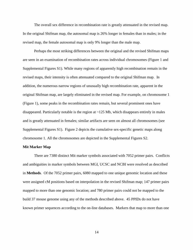
The overall sex difference in recombination rate is greatly attenuated in the revised map.

In the original Shifman map, the autosomal map is 26% longer in females than in males; in the

revised map, the female autosomal map is only 9% longer than the male map.

Perhaps the most striking differences between the original and the revised Shifman maps

are seen in an examination of recombination rates across individual chromosomes (Figure 1 and

Supplemental Figures S1). While many regions of apparently high recombination remain in the

revised maps, their intensity is often attenuated compared to the original Shifman map. In

addition, the numerous narrow regions of unusually high recombination rate, apparent in the

original Shifman map, are largely eliminated in the revised map. For example, on chromosome 1

(Figure 1), some peaks in the recombination rates remain, but several prominent ones have

disappeared. Particularly notable is the region at ~125 Mb, which disappears entirely in males

and is greatly attenuated in females; similar artifacts are seen on almost all chromosomes (see

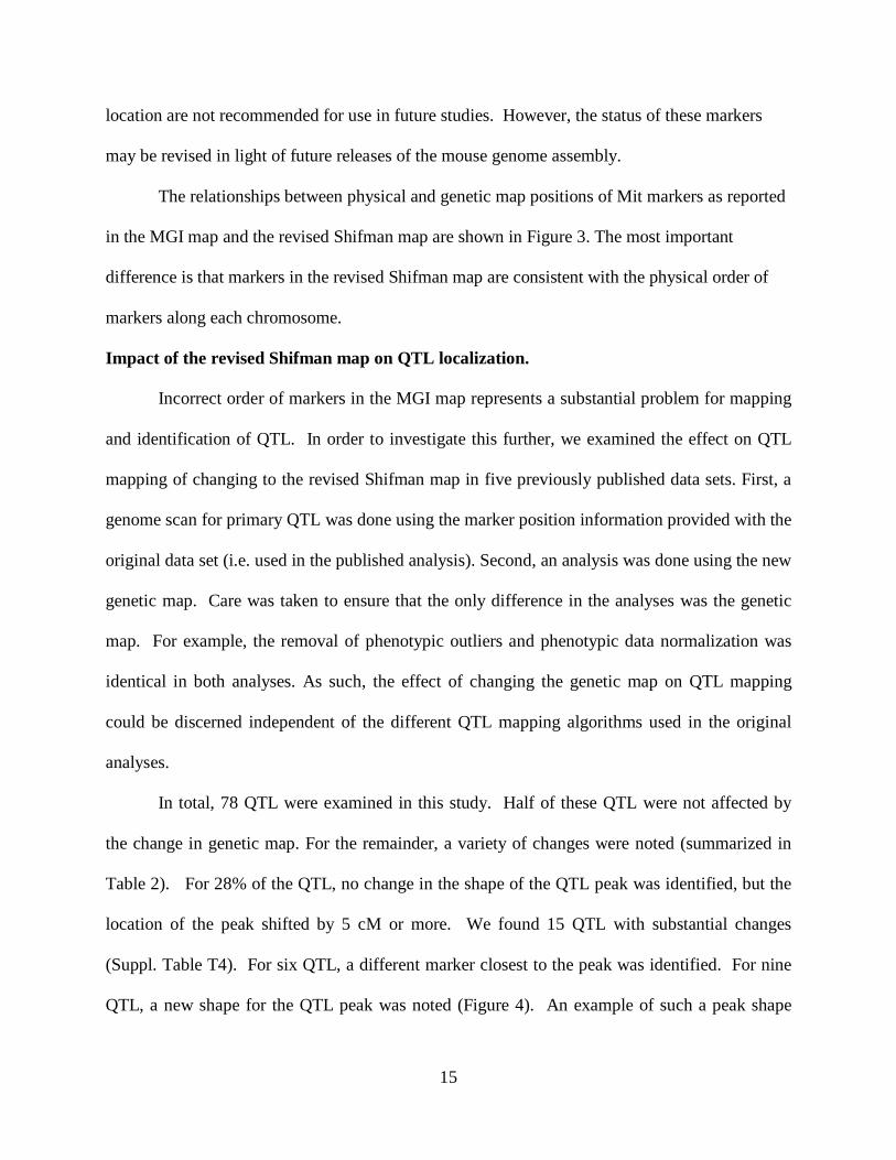
Supplemental Figures S1). Figure 2 depicts the cumulative sex-specific genetic maps along

chromosome 1. All the chromosomes are depicted in the Supplemental Figures S2.

Mit Marker Map

There are 7380 distinct Mit marker symbols associated with 7052 primer pairs. Conflicts

and ambiguities in marker symbols between MGI, UCSC and NCBI were resolved as described

in Methods. Of the 7052 primer pairs, 6080 mapped to one unique genomic location and these

were assigned cM positions based on interpolation in the revised Shifman map; 147 primer pairs

mapped to more than one genomic location; and 780 primer pairs could not be mapped to the

build 37 mouse genome using any of the methods described above. 45 PPIDs do not have

known primer sequences according to the on-line databases. Markers that map to more than one

15

location are not recommended for use in future studies. However, the status of these markers

may be revised in light of future releases of the mouse genome assembly.

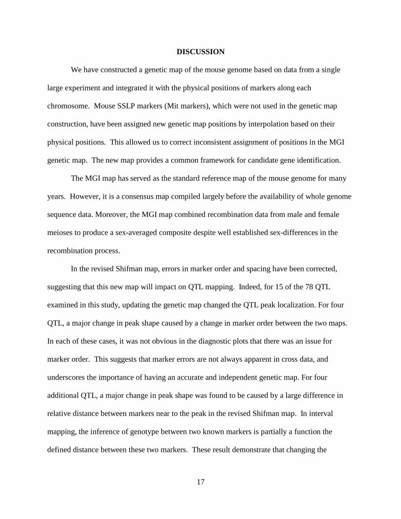
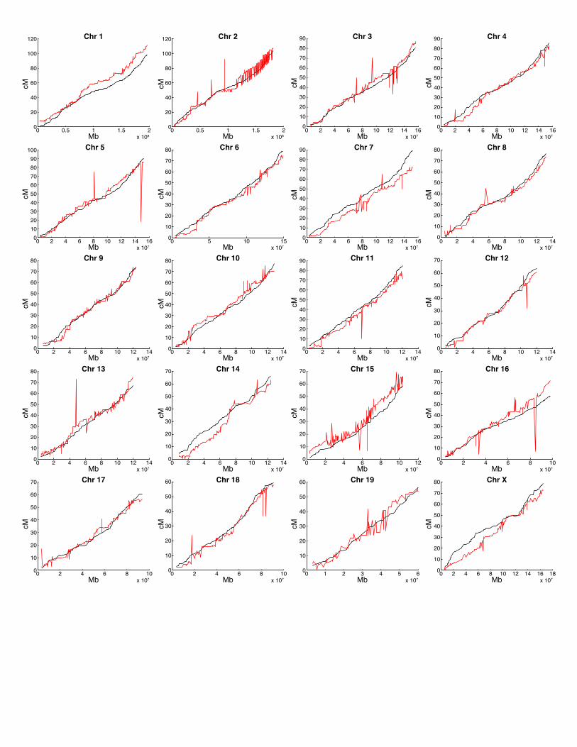
The relationships between physical and genetic map positions of Mit markers as reported

in the MGI map and the revised Shifman map are shown in Figure 3. The most important

difference is that markers in the revised Shifman map are consistent with the physical order of

markers along each chromosome.

Impact of the revised Shifman map on QTL localization.

Incorrect order of markers in the MGI map represents a substantial problem for mapping

and identification of QTL. In order to investigate this further, we examined the effect on QTL

mapping of changing to the revised Shifman map in five previously published data sets. First, a

genome scan for primary QTL was done using the marker position information provided with the

original data set (i.e. used in the published analysis). Second, an analysis was done using the new

genetic map. Care was taken to ensure that the only difference in the analyses was the genetic

map. For example, the removal of phenotypic outliers and phenotypic data normalization was

identical in both analyses. As such, the effect of changing the genetic map on QTL mapping

could be discerned independent of the different QTL mapping algorithms used in the original

analyses.

In total, 78 QTL were examined in this study. Half of these QTL were not affected by

the change in genetic map. For the remainder, a variety of changes were noted (summarized in

Table 2). For 28% of the QTL, no change in the shape of the QTL peak was identified, but the

location of the peak shifted by 5 cM or more. We found 15 QTL with substantial changes

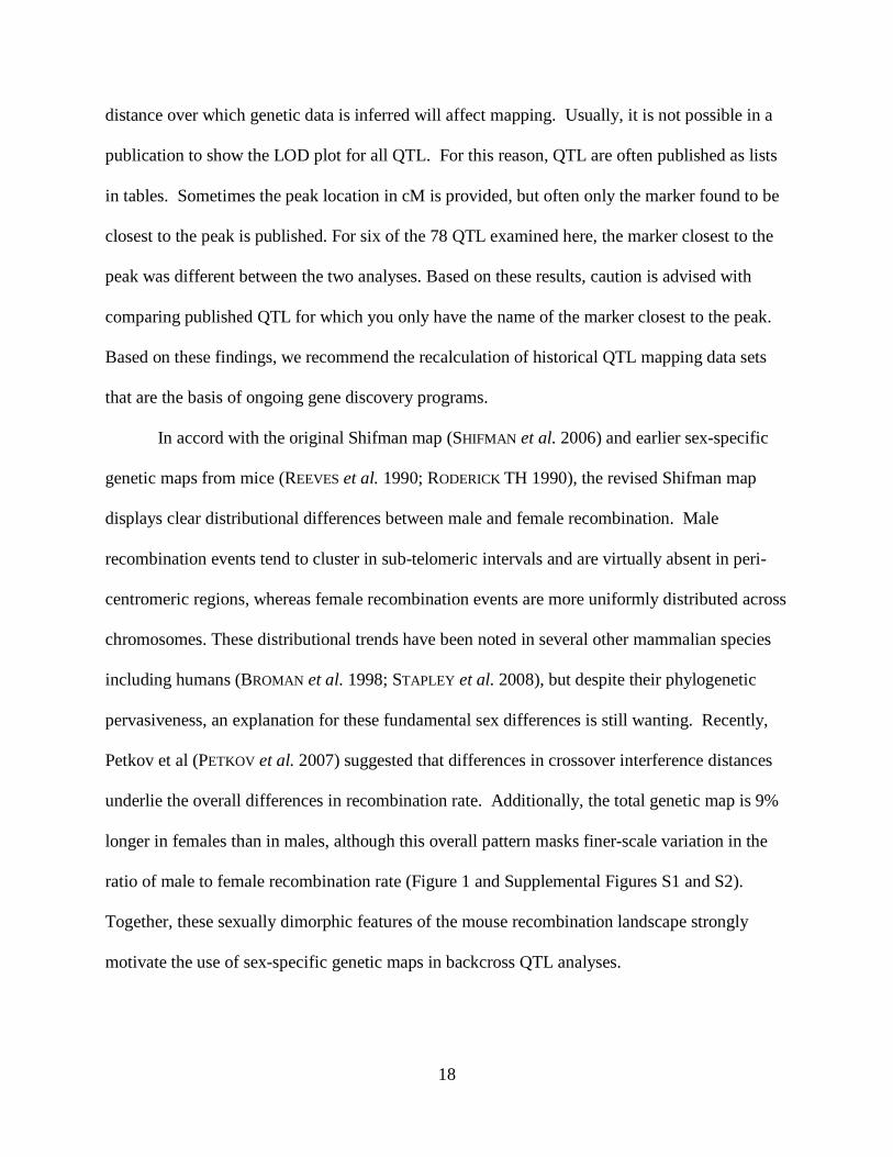
(Suppl. Table T4). For six QTL, a different marker closest to the peak was identified. For nine

QTL, a new shape for the QTL peak was noted (Figure 4). An example of such a peak shape

16

change is presented in Figure 4A,B. In this example, the third and fourth markers are reversed in

order when comparing the two maps. This switch in marker order was not detected using

standard marker quality control checks during either analysis. The LOD score associated with

the peak was different in two of the QTL for which a change in peak shape was noted.

Specifically, for one QTL the change in LOD resulted in a failure to identify the QTL in the

analysis utilizing the traditional map. In summary, for 15 of 78 QTL (19%), a mapping issue

was identified that could impact the identification of the underlying gene.

Resources

The revised genetic map and the updated Mit marker database are available in a tab-

delimited text format online at http://cgd.jax.org/mousemapconverter/. A web interface allows

the user to convert between genetic and physical map coordinates and to query the positions of

mouse markers. Male, female and sex-averaged positions are available. The original data from

Shifman et al., and the cleaned the data are also posted here. We will periodically update these

resources as new versions of the mouse genome assembly are released.

Historical QTL data have been generated with a changing standard genetic map or, quite

often, with a genetic map constructed de-novo based on the cross data. This inconsistency

presents a roadblock to integrated analysis of common QTL. We are actively curating available

historical QTL datasets by updating marker positions to the revised Shifman map. This resource

also provides the original phenotype and genotype data, and references to the original

publications. These data are available at http://qtlarchive.org or through the mouse phenome

database (http://www.jax.org/phenome/QTL) .

17

DISCUSSION

We have constructed a genetic map of the mouse genome based on data from a single

large experiment and integrated it with the physical positions of markers along each

chromosome. Mouse SSLP markers (Mit markers), which were not used in the genetic map

construction, have been assigned new genetic map positions by interpolation based on their

physical positions. This allowed us to correct inconsistent assignment of positions in the MGI

genetic map. The new map provides a common framework for candidate gene identification.

The MGI map has served as the standard reference map of the mouse genome for many

years. However, it is a consensus map compiled largely before the availability of whole genome

sequence data. Moreover, the MGI map combined recombination data from male and female

meioses to produce a sex-averaged composite despite well established sex-differences in the

recombination process.

In the revised Shifman map, errors in marker order and spacing have been corrected,

suggesting that this new map will impact on QTL mapping. Indeed, for 15 of the 78 QTL

examined in this study, updating the genetic map changed the QTL peak localization. For four

QTL, a major change in peak shape caused by a change in marker order between the two maps.

In each of these cases, it was not obvious in the diagnostic plots that there was an issue for

marker order. This suggests that marker errors are not always apparent in cross data, and

underscores the importance of having an accurate and independent genetic map. For four

additional QTL, a major change in peak shape was found to be caused by a large difference in

relative distance between markers near to the peak in the revised Shifman map. In interval

mapping, the inference of genotype between two known markers is partially a function the

defined distance between these two markers. These result demonstrate that changing the

18

distance over which genetic data is inferred will affect mapping. Usually, it is not possible in a

publication to show the LOD plot for all QTL. For this reason, QTL are often published as lists

in tables. Sometimes the peak location in cM is provided, but often only the marker found to be

closest to the peak is published. For six of the 78 QTL examined here, the marker closest to the

peak was different between the two analyses. Based on these results, caution is advised with

comparing published QTL for which you only have the name of the marker closest to the peak.

Based on these findings, we recommend the recalculation of historical QTL mapping data sets

that are the basis of ongoing gene discovery programs.

In accord with the original Shifman map (SHIFMAN et al. 2006) and earlier sex-specific

genetic maps from mice (REEVES et al. 1990; RODERICK TH 1990), the revised Shifman map

displays clear distributional differences between male and female recombination. Male

recombination events tend to cluster in sub-telomeric intervals and are virtually absent in peri-

centromeric regions, whereas female recombination events are more uniformly distributed across

chromosomes. These distributional trends have been noted in several other mammalian species

including humans (BROMAN et al. 1998; STAPLEY et al. 2008), but despite their phylogenetic

pervasiveness, an explanation for these fundamental sex differences is still wanting. Recently,

Petkov et al (PETKOV et al. 2007) suggested that differences in crossover interference distances

underlie the overall differences in recombination rate. Additionally, the total genetic map is 9%

longer in females than in males, although this overall pattern masks finer-scale variation in the

ratio of male to female recombination rate (Figure 1 and Supplemental Figures S1 and S2).

Together, these sexually dimorphic features of the mouse recombination landscape strongly

motivate the use of sex-specific genetic maps in backcross QTL analyses.

19

The HS pedigrees are composed of animals with admixed genomes bearing contributions

from 8 classical laboratory strains. It is well established that individuals and different inbred

mouse strains vary with respect to both the distribution and overall intensity of recombination

(COOP and PRZEWORSKI 2007; KOEHLER et al. 2002). This fact carries important implications for

the interpretation of the genetic maps presented here. Most notably, the recombination fractions

we report represent an average over the 8 founding strains and are likely to differ from

recombination frequencies calculated in independent mouse crosses. These inter-strain

differences in recombination are due to the cumulative effects of trans-acting recombination

modifying loci and their interaction with cis-acting DNA sequences (GREY C 2009; PARVANOV E

2009); the precise identification of these genetic variants poses an exciting and important

challenge to the field of genetics (PAIGEN et al. 2008).

Despite the presence of individual-level variation in recombination rate, at the scale of

resolution required for most genetic studies (~1Mb), recombination rates are conserved across

different strain combinations (2000; DURET and ARNDT 2008). Paigen et al. (PAIGEN et al. 2008)

found that at a ~2 Mb interval, their B6xCAST high-resolution (min. 225 kb) chromosome 1

map correlates highly with the original Shifman map; this interval is likely decreased to closer to

1 Mb in comparison to the revised map presented here. In addition, the regions of low and high

recombination occur in parallel comparing the two maps. Thus, the strain average genetic map

presented here will serve a useful and practical approximation to the distribution and intensity of

recombination events in any mouse strain. The large number of meiosis surveyed across the HS

pedigree and the extraordinary number of genetic loci placed on this map combine to present the

mouse community with a genetic resource unparalleled in other experimental model systems.

This map is equipped with sufficient precision for most types of genetic crosses, including

20

backcross, intercross, recombinant inbred and advanced intercross designs. It provides

consistent genetic map coordinates that are directly tied to the physical genome.

ACKNOWLEDGEMENTS

This work was supported by the National Institutes of Health with grants GM070683

(GAC), GM074244 (KWB) and HL077796 (BP), 5T32HD07065(CLAB), AR053992 (CLAB),

NIGMS Centers of Excellence in systems biology GM076468 (GAC), and the Federal Ministry

for Education and Research, Germany (NGFN project 01GS0486, GAB). The Shared Scientific

Services were supported in part by a Basic Cancer Center Core Grant from the National Cancer

Institute CA34196 to the Jackson Laboratory.

The authors thank Ben King, Randy von Smith, Stephen Grubb, Nazira Bektassova and

Keith Sheppard for advice and assistance with informatics and database tools. We thank Ken

Paigen, Janan Eppig, Petko Petkov, Thomas Gridley and Lucy Rowe for critical discussion and

review.

REFERENCES

2000 The 2000 Chromosome Committee reports for the Mouse Genome. Mamm Genome 11:

943-960.

BEAMER, W., K. L. SHULTZ, G. A. CHURCHILL, W. FRANKEL, D. J. BAYLINK et al., 1999

Quantitative trait loci for bone density in C57BL/6J and CAST/EiJ. Mammalian Genome

10: 1043-1049.

21

BEAMER, W. G., K. L. SHULTZ, L. R. DONAHUE, G. CHURCHILL, S. SEN et al., 2001 Quantitative

trait loci for femoral and lumbar vertebral bone mineral density in C57BL/6J and

C3H/HeJ inbred strains of mice. J Bone Miner Res 16: 1195-1206.

BROMAN, K. W., J. C. MURRAY, V. C. SHEFFIELD, R. L. WHITE and J. L. WEBER, 1998

Comprehensive human genetic maps: individual and sex-specific variation in

recombination. Am J Hum Genet 63: 861-869.

BROMAN, K. W., L. B. ROWE, G. A. CHURCHILL and K. PAIGEN, 2002 Crossover interference in

the mouse. Genetics 160: 1123-1131.

BROMAN, K. W., H. WU, S. SEN and G. A. CHURCHILL, 2003 R/qtl: QTL mapping in

experimental crosses. Bioinformatics 19: 889-890.

BULT, C. J., J. T. EPPIG, J. A. KADIN, J. E. RICHARDSON and J. A. BLAKE, 2008 The Mouse

Genome Database (MGD): mouse biology and model systems. Nucleic Acids Res 36:

D724-728.

CHOWDHARY, B. P., and T. RAUDSEPP, 2006 The horse genome. Genome Dyn 2: 97-110.

CHURCHILL, G. A., D. C. AIREY, H. ALLAYEE, J. M. ANGEL, A. D. ATTIE et al., 2004 The

Collaborative Cross, a community resource for the genetic analysis of complex traits. Nat

Genet 36: 1133-1137.

CHURCHILL, G. A., and R. W. DOERGE, 1994 Empirical Threshold Values for Quantitative Triat

Mapping. Genetics 138: 963-971.

COOP, G., and M. PRZEWORSKI, 2007 An evolutionary view of human recombination. Nat Rev

Genet 8: 23-34.

DIETRICH, W. F., J. MILLER, R. STEEN, M. A. MERCHANT, D. DAMRON-BOLES et al., 1996 A

comprehensive genetic map of the mouse genome. Nature 380: 149-152.

22

DIETRICH, W. F., J. C. MILLER, R. G. STEEN, M. MERCHANT, D. DAMRON et al., 1994 A genetic

map of the mouse with 4,006 simple sequence length polymorphisms. Nat Genet 7: 220-

245.

DURET, L., and P. F. ARNDT, 2008 The impact of recombination on nucleotide substitutions in

the human genome. PLoS Genet 4: e1000071.

GREEN P, K. F. A. S. C., 1990 Documentation for CRI-MAP, version 2.4, pp.

GREY C, F. B., AND B DE MASSY, 2009 Long distance regulation of initiation of meiotic

recombination. PLoS Biol in press.

HINRICHS, A. S., D. KAROLCHIK, R. BAERTSCH, G. P. BARBER, G. BEJERANO et al., 2006 The

UCSC Genome Browser Database: update 2006. Nucleic Acids Res 34: D590-598.

ISHIMORI, N., R. LI, P. KELMENSON, R. KORSTANJE, K. WALSH et al., 2004 Quantitative trait loci

that determine plasma lipids and obesity in C57BL/6J and 129S1/SvImJ inbred mice. J

Lipid Res 45: 1624-1632.

ISHIMORI, N., I. M. STYLIANOU, R. KORSTANJE, M. A. MARION, R. LI et al., 2008 Quantitative

Trait Loci for Bone Mineral Density in an SM/J by NZB/BlNJ Intercross Population and

Identification of Trps1 as a Probable Candidate Gene. Journal of Bone and Mineral

Research 0: 1-41.

KOEHLER, K. E., J. P. CHERRY, A. LYNN, P. A. HUNT and T. J. HASSOLD, 2002 Genetic control of

mammalian meiotic recombination. I. Variation in exchange frequencies among males

from inbred mouse strains. Genetics 162: 297-306.

KOLLER, D., J. SCHRIEFER, Q. SUN, K. SHULTZ, L. DONAHUE et al., 2003 Genetic effects for

femoral biomechanics, structure, and density in C57BL/6J and C3H/HeJ inbred mouse

strains. J Bone Miner Res 18: 1758-1765.

23

KONG, A., D. F. GUDBJARTSSON, J. SAINZ, G. M. JONSDOTTIR, S. A. GUDJONSSON et al., 2002 A

high-resolution recombination map of the human genome. Nat Genet 31: 241-247.

LANDER, E. S., and L. KRUGLYAK, 1995 Genetic Dissection of complex traits: guidelines for

interpreting and reporting linkage results. Nat Genet 11: 241-247.

LEHMANN, E., and H. D'ABRERA, 1988 Nonparametrics: Statistical Methods Based on Ranks.

McGraw-Hill.

LYON, M. F., 1976 Distribution of crossing-over in mouse chromosomes. Genet Res 28: 291-

299.

MONTAGUTELLI, X., R. TURNER and J. H. NADEAU, 1996 Epistatic control of non-Mendelian

inheritance in mouse interspecific crosses. Genetics 143: 1739-1752.

MYERS, S., L. BOTTOLO, C. FREEMAN, G. MCVEAN and P. DONNELLY, 2005 A fine-scale map of

recombination rates and hotspots across the human genome. Science 310: 321-324.

O'CONNELL, J. R., and D. E. WEEKS, 1998 PedCheck: a program for identification of genotype

incompatibilities in linkage analysis. Am J Hum Genet 63: 259-266.

PAIGEN, K., J. P. SZATKIEWICZ, K. SAWYER, N. LEAHY, E. D. PARVANOV et al., 2008 The

recombinational anatomy of a mouse chromosome. PLoS Genet 4: e1000119.

PARVANOV E, N. S., P PETKOV, AND K PAIGEN. , 2009 Trans-regulation of mouse meiotic

recombination. PLoS Biol in press.

PETKOV, P. M., K. W. BROMAN, J. P. SZATKIEWICZ and K. PAIGEN, 2007 Crossover interference

underlies sex differences in recombination rates. Trends Genet 23: 539-542.

PETKOV, P. M., Y. DING, M. A. CASSELL, W. ZHANG, G. WAGNER et al., 2004 An efficient SNP

system for mouse genome scanning and elucidating strain relationships. Genome Res 14:

1806-1811.

24

REEVES, R. H., M. R. CROWLEY, B. F. O'HARA and J. D. GEARHART, 1990 Sex, strain, and

species differences affect recombination across an evolutionarily conserved segment of

mouse chromosome 16. Genomics 8: 141-148.

RODERICK TH, A. H., 1990 Differences in recombination due to sex in mice. Mouse News

Letters 85: 87.

ROWE, L. B., J. H. NADEAU, R. TURNER, W. N. FRANKEL, V. A. LETTS et al., 1994 Maps from

two interspecific backcross DNA panels available as a community genetic mapping

resource. Mamm Genome 5: 253-274.

SEN, S., and G. A. CHURCHILL, 2001 A Statistical Framework for Quantitative Trait Mapping.

Genetics 159: 371-387.

SHIFMAN, S., J. T. BELL, R. R. COPLEY, M. S. TAYLOR, R. W. WILLIAMS et al., 2006 A high-

resolution single nucleotide polymorphism genetic map of the mouse genome. PLoS Biol

4: e395.

STAPLEY, J., T. R. BIRKHEAD, T. BURKE and J. SLATE, 2008 A linkage map of the zebra finch

Taeniopygia guttata provides new insights into avian genome evolution. Genetics 179:

651-667.

TANKSLEY, S. D., M. W. GANAL, J. P. PRINCE, M. C. DE VICENTE, M. W. BONIERBALE et al.,

1992 High density molecular linkage maps of the tomato and potato genomes. Genetics

132: 1141-1160.

VALDAR, W., J. FLINT and R. MOTT, 2006 Simulating the collaborative cross: power of

quantitative trait loci detection and mapping resolution in large sets of recombinant

inbred strains of mice. Genetics 172: 1783-1797.

25

WERGEDAL, J., C. ACKERT-BICKNELL, S. TSAIH, M. SHENG, S. MOHAN et al., 2006 Femur

mechanical properties in the F2 progeny of an NZB/B1NJ x RF/J cross are regulated

predominantly by genetic loci that regulate bone geometry. J Bone Miner Res 21: 1256-

1266.

FIGURE LEGENDS

FIGURE 1: COMPARISON OF THE ORIGINAL AND REVISED GENETIC MAPS

Sex-averaged recombination rates (2a) and Sex-specific recombination rates (2b) for the original

and revised genetic maps of Chromosome 1. Maps are based on data from Shifman et al., (2006)

as described in Methods. Figures showing all chromosomes can be found in Supplemental

Figure S1.

FIGURE 2: CUMULATIVE GENETIC MAPS OF CHROMOSOME 1

Dotted lines show the original Shifman map; solid lines are from the revised Shifman map.

Female, male and sex-averaged maps are shown in red, blue and black, respectively.

Supplemental Figure S2 shows the cumulative maps for each chromosome.

FIGURE 3: PHYSICAL AND GENETIC POSITIONS OF MARKERS

Genetic marker positions (cM) are plotted against their physical positions (Mb) for the MGI

genetic map (red) and the revised Shifman map (black). Marker ordering errors in the MGI map

26

are indicated by non-monotone fluctuations. In contrast, the curves for the revised map are

smooth and monotone.

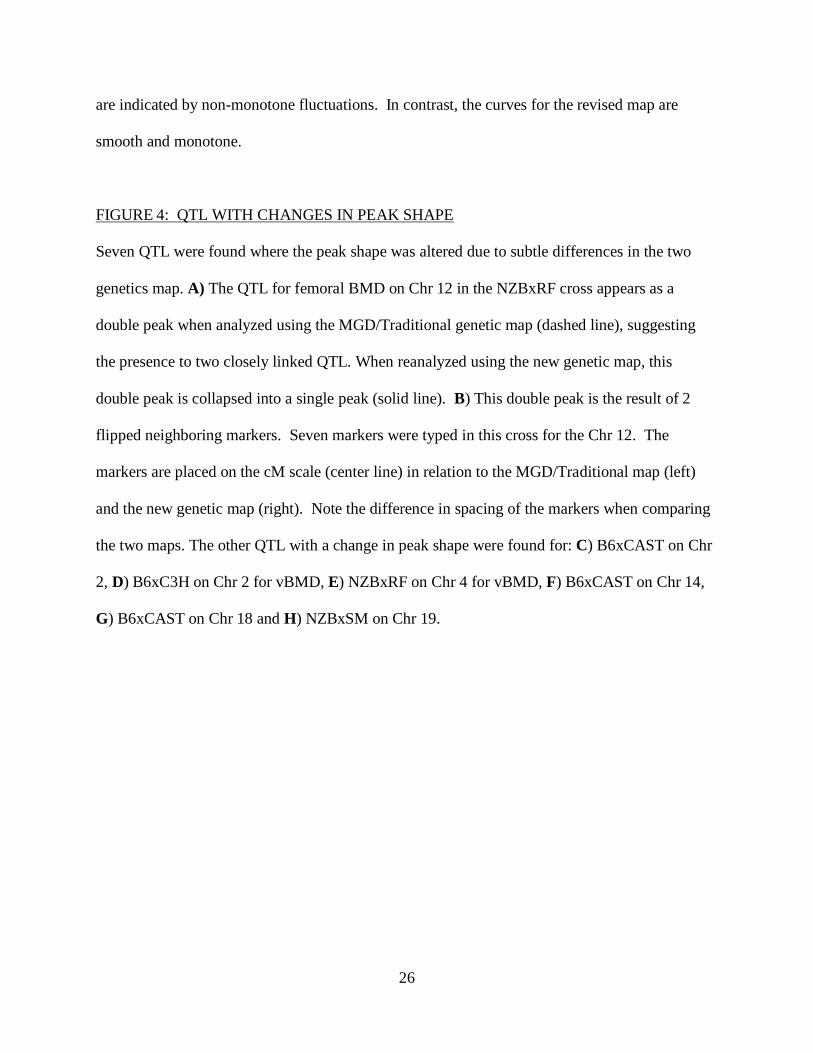
FIGURE 4: QTL WITH CHANGES IN PEAK SHAPE

Seven QTL were found where the peak shape was altered due to subtle differences in the two

genetics map. A) The QTL for femoral BMD on Chr 12 in the NZBxRF cross appears as a

double peak when analyzed using the MGD/Traditional genetic map (dashed line), suggesting

the presence to two closely linked QTL. When reanalyzed using the new genetic map, this

double peak is collapsed into a single peak (solid line). B) This double peak is the result of 2

flipped neighboring markers. Seven markers were typed in this cross for the Chr 12. The

markers are placed on the cM scale (center line) in relation to the MGD/Traditional map (left)

and the new genetic map (right). Note the difference in spacing of the markers when comparing

the two maps. The other QTL with a change in peak shape were found for: C) B6xCAST on Chr

2, D) B6xC3H on Chr 2 for vBMD, E) NZBxRF on Chr 4 for vBMD, F) B6xCAST on Chr 14,

G) B6xCAST on Chr 18 and H) NZBxSM on Chr 19.

Table 1. Chromosome Lengths and Recombination Rates Based on Positions of Most Proximal and Distal Mit Markers, Shared Among the Revised Shifman, Original Shifman and MGI Maps

aposition on sex-averaged map - except for Chromosome X; these cM positions are based on the female map.

Most proximal Mit

Marker Most distal Mit Marker total map length Chromosome-average Recombination Rate

Revised Original MGI Revised Original MGI Chr. MarkerID Mb MarkerID Mb Shifmana Shifmana (standard) Shifmana Shifmana (standard)

1 D1Mit475 3.64 D1Mit155 196.26 96.55 117.83 103.60 0.50 0.61 0.54

2 D2Mit312 3.15 D2Mit457 180.99 101.82 108.22 107.00 0.57 0.61 0.60

3 D3Mit150 5.35 D3Mit89 156.50 78.83 86.80 83.70 0.52 0.57 0.55

4 D4Mit149 3.58 D4Mit51 154.42 84.13 99.86 82.70 0.56 0.66 0.55

5 D5Mit69 3.53 D5Mit169 150.23 86.97 105.61 85.00 0.59 0.72 0.58

6 D6Mit231 3.48 D6Mit390 148.41 76.69 89.72 73.73 0.53 0.62 0.51

7 D7Mit21 3.27 D7Mit141 152.14 87.05 89.42 71.90 0.58 0.60 0.48

8 D8Mit155 4.98 D8Mit156 131.42 73.96 80.20 72.00 0.58 0.63 0.57

9 D9Mit186 6.26 D9Mit322 123.10 71.46 85.23 70.00 0.61 0.73 0.60

10 D10Mit49 4.14 D10Mit269 128.39 75.29 83.11 68.00 0.61 0.67 0.55

11 D11Mit1 3.47 D11Mit104 119.17 80.85 91.20 78.75 0.70 0.79 0.68

12 D12Mit264 5.31 D12Mit144 120.30 61.00 68.55 60.00 0.53 0.60 0.52

13 D13Mit235 4.22 D13Mit35 120.13 64.85 69.46 71.00 0.56 0.60 0.61

14 D14Mit110 8.99 D14Mit107 124.00 61.37 59.38 59.50 0.53 0.52 0.52

15 D15Mit12 3.16 D15Mit160 102.99 56.40 64.34 59.80 0.56 0.64 0.60

16 D16Mit32 3.96 D16Mit71 97.13 54.73 62.93 68.95 0.59 0.68 0.74

17 D17Mit164 3.92 D17Mit123 93.60 58.56 62.74 52.60 0.65 0.70 0.59

18 D18Mit65 3.73 D18Mit25 89.74 56.67 64.07 55.00 0.66 0.74 0.64

19 D19Mit32 3.28 D19Mit108 59.96 53.24 53.35 49.50 0.94 0.94 0.87

X DXMit101 5.68 DXMit100 165.35 76.16 69.83 72.50 0.48 0.44 0.45

total 1456.58 1611.84 1445.23

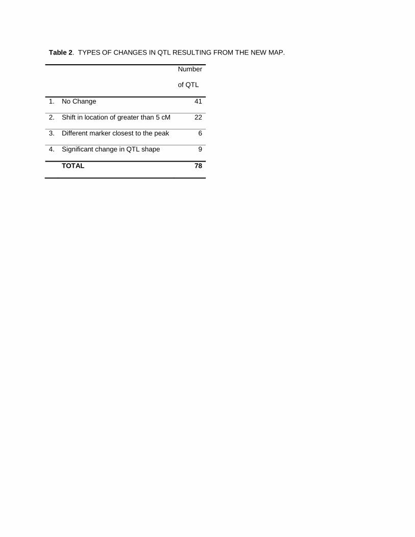
Table 2. TYPES OF CHANGES IN QTL RESULTING FROM THE NEW MAP.

Number

of QTL

1. No Change 41

2. Shift in location of greater than 5 cM 22

3. Different marker closest to the peak 6

4. Significant change in QTL shape 9

TOTAL 78

50 100 150

0.0

0.5

1.0

1.5

2.0

Sex−averaged recombination rates

Position (Mb)

cM/M

b

A

RevisedShifman et al.

50 100 150

Sex−specific recombination rates

Position (Mb)

cM/M

b

B

2

1

0

1

2 femalemale

RevisedShifman et al.

Mal

eF

emal

e

0 0.5 1 1.5 2x 108

0

20

40

60

80

100

120 Chr 1

Mb

cM

0 2 4 6 8 10 12 14 16x 107

0

10

20

30

40

50

60

70

80

90 Chr 3

Mb

cM

0 2 4 6 8 10 12 14 16x 107

0

10

20

30

40

50

60

70

80

90

100 Chr 5

Mb

cM

0 2 4 6 8 10 12 14 16x 107

0

10

20

30

40

50

60

70

80

90 Chr 7

Mb

cM

0 2 4 6 8 10 12 14x 107

0

10

20

30

40

50

60

70

80 Chr 9

Mb

cM

0 0.5 1 1.5 2x 108

0

20

40

60

80

100

120 Chr 2

Mb

cM

0 2 4 6 8 10 12 14 16x 107

0

10

20

30

40

50

60

70

80

90 Chr 4

Mb

cM

0 5 10 15x 107

0

10

20

30

40

50

60

70

80 Chr 6

Mb

cM

0 2 4 6 8 10 12 14x 107

0

10

20

30

40

50

60

70

80 Chr 8

Mb

cM

0 2 4 6 8 10 12 14x 107

0

10

20

30

40

50

60

70

80 Chr 10

Mb

cM

0 2 4 6 8 10 12 14x 107

0

10

20

30

40

50

60

70

80

90 Chr 11

Mb

cM

0 2 4 6 8 10 12 14x 107

0

10

20

30

40

50

60

70 Chr 12

Mb

cM

0 2 4 6 8 10 12 14x 107

0

10

20

30

40

50

60

70

80 Chr 13

Mb

cM

0 2 4 6 8 10 12 14x 107

0

10

20

30

40

50

60

70 Chr 14

Mb

cM

0 2 4 6 8 10 12x 107

0

10

20

30

40

50

60

70 Chr 15

Mb

cM

0 2 4 6 8 10x 107

0

10

20

30

40

50

60

70

80 Chr 16

Mb

cM

0 2 4 6 8 10x 107

0

10

20

30

40

50

60

70 Chr 17

Mb

cM

0 2 4 6 8 10x 107

0

10

20

30

40

50

60 Chr 18

Mb

cM

0 1 2 3 4 5 6x 107

0

10

20

30

40

50

60 Chr 19

Mb

cM

0 2 4 6 8 10 12 14 16 18x 107

0

10

20

30

40

50

60

70

80 Chr X

Mb

cM

A BChr12

D12Mit182

D12Mit285

D12Mit97

D12Mit262D12NDS2

Traditional

D12Mit201D12Mit91

D12Mit182

D12Mit285D12Mit201D12Mit91

D12Mit97

D12Mit262

D12NDS2

New

F

C

G H

D E

LO

DL

OD

LO

D

Traditional MapNew Shifman Map

0.0

0 10 20 30 40 50 60

0.5

1.0

1.5

2.0

2.5

3.0

3.5

Map position (cM)

Map position (cM) Map position (cM) Map position (cM)

0.00 20 40 60 80 100

0.5

1.0

1.5

0.00 20 40 60 80

1.0

2.0

3.0

4.0

0.00 10 20 30 40 50 60 70

0.5

1.0

1.5

2.0

2.5

0.00 10 20 30 40 50 60

1.0

2.0

3.0

0.00 10 20 30 40 50

0.5

1.0

1.5

2.0

0.00 10 20 30 40 50

0.5

1.0

1.5

2.0

2.5