ROBUST TECHNIQUES FOR COMPUTER VISION

ROBUST TECHNIQUES

FOR COMPUTER VISION

Peter MeerElectrical and Computer Engineering Department

Rutgers University

This is a chapter from the upcoming book Emerging Topics in ComputerVision, Gerard Medioni and Sing Bing Kang (Eds.), Prentice Hall, 2004.

��

3 ROBUST TECHNIQUES FOR COMPUTER VISION 13.1 Robustness in Visual Tasks 1

3.2 Models and Estimation Problems 4

3.2.1 Elements of a Model 4

3.2.2 Estimation of a Model 9

3.2.3 Robustness of an Estimator 11

3.2.4 Definition of Robustness 13

3.2.5 Taxonomy of Estimation Problems 15

3.2.6 Linear Errors-in-Variables Regression Model 18

3.2.7 Objective Function Optimization 21

3.3 Location Estimation 26

3.3.1 Why Nonparametric Methods 26

3.3.2 Kernel Density Estimation 28

3.3.3 Adaptive Mean Shift 32

3.3.4 Applications 36

3.4 Robust Regression 42

3.4.1 Least Squares Family 43

3.4.2 M-estimators 47

3.4.3 Median Absolute Deviation Scale Estimate 49

3.4.4 LMedS, RANSAC and Hough Transform 51

3.4.5 The pbM-estimator 55

3.4.6 Applications 59

3.4.7 Structured Outliers 61

3.5 Conclusion 63

BIBLIOGRAPHY 65

i

ii

Chapter 4

� � � � � � � � � � � ��

�� !�#"$�&%'"(�)��*,+.-�*/�102�Visual information makes up about seventy five percent of all the sensorial informationreceived by a person during a lifetime. This information is processed not only efficientlybut also transparently. Our awe of visual perception was perhaps the best captured by theseventeenth century british essayist Joseph Addison in an essay on imagination [1].

Our sight is the most perfect and most delightful of all our senses. It fills themind with the largest variety of ideas, converses with its objects at the greatestdistance, and continues the longest in action without being tired or satiatedwith its proper enjoyments.

The ultimate goal of computer vision is to mimic human visual perception. Therefore,in the broadest sense, robustness of a computer vision algorithm is judged against the per-formance of a human observer performing an equivalent task. In this context, robustness isthe ability to extract the visual information of relevance for a specific task, even when thisinformation is carried only by a small subset of the data, and/or is significantly differentfrom an already stored representation.

To understand why the performance of generic computer vision algorithms is still faraway from that of human visual perception, we should consider the hierarchy of computervision tasks. They can be roughly classified into three large categories:

– low level, dealing with extraction from a single image of salient simple features, suchas edges, corners, homogeneous regions, curve fragments;

– intermediate level, dealing with extraction of semantically relevant characteristicsfrom one or more images, such as grouped features, depth, motion information;

– high level, dealing with the interpretation of the extracted information.

A similar hierarchy is difficult to distinguish in human visual perception, which appears asa single integrated unit. In the visual tasks performed by a human observer an extensive top-down information flow carrying representations derived at higher levels seems to controlthe processing at lower levels. See [85] for a discussion on the nature of these interactions.

1

2 �� "! � � � ��#�%$'&�(*),+'-�.

A large amount of psychophysical evidence supports this “closed loop” model of hu-man visual perception. Preattentive vision phenomena, in which salient information pops-out from the image, e.g., [55], [110], or perceptual constancies, in which changes in theappearance of a familiar object are attributed to external causes [36, Chap.9], are onlysome of the examples. Similar behavior is yet to be achieved in generic computer visiontechniques. For example, preattentive vision type processing seems to imply that a regionof interest is delineated before extracting its salient features.

To approach the issue of robustness in computer vision, will start by mentioning one ofthe simplest perceptual constancies, the shape constancy. Consider a door opening in frontof an observer. As the door opens, its image changes from a rectangle to a trapezoid butthe observer will report only the movement. That is, additional information not availablein the input data was also taken into account. We know that a door is a rigid structure,and therefore it is very unlikely that its image changed due to a nonrigid transformation.Since the perceptual constancies are based on rules embedded in the visual system, theycan be also deceived. A well known example is the Ames room in which the rules used forperspective foreshortening compensation are violated [36, p.241].

The previous example does not seem to reveal much. Any computer vision algorithmof rigid motion recovery is based on a similar approach. However, the example emphasizesthat the employed rigid motion model is only associated with the data and is not intrinsicto it. We could use a completely different model, say of nonrigid doors, but the resultwould not be satisfactory. Robustness thus is closely related to the availability of a modeladequate for the goal of the task.

In today’s computer vision algorithms the information flow is almost exclusively bottom-up. Feature extraction is followed by grouping into semantical primitives, which in turn isfollowed by a task specific interpretation of the ensemble of primitives. The lack of top-down information flow is arguably the main reason why computer vision techniques cannotyet autonomously handle visual data under a wide range of operating conditions. This factis well understood in the vision community and different approaches were proposed tosimulate the top-down information stream.

The increasingly popular Bayesian paradigm is such an attempt. By using a probabilis-tic representation for the possible outcomes, multiple hypotheses are incorporated into theprocessing, which in turn guide the information recovery. The dependence of the procedureon the accuracy of the employed representation is relaxed in the semiparametric or nonpara-metric Bayesian methods, such as particle filtering for motion problems [51]. Incorporatinga learning component into computer vision techniques, e.g., [3], [29], is another, somewhatsimilar approach to use higher level information during the processing.

Comparison with human visual perception is not a practical way to arrive to a definitionof robustness for computer vision algorithms. For example, robustness in the context of thehuman visual system extends to abstract concepts. We can recognize a chair independentof its design, size or the period in which it was made. However, in a somewhat similarexperiment, when an object recognition system was programmed to decide if a simpledrawing represents a chair, the results were rather mixed [97].

We will not consider high level processes when examining the robustness of visionalgorithms, neither will discuss the role of top-down information flow. A computer vision

�+�� ) � �� .�� ) � + � �� ! � �� &�� & �� 3

algorithm will be called robust if it can tolerate outliers, i.e., data which does not obey theassumed model. This definition is similar to the one used in statistics for robustness [40,p.6]

In a broad informal sense, robust statistics is a body of knowledge, partly for-malized into “theories of statistics,” relating to deviations from idealized as-sumptions in statistics.

Robust techniques are used in computer vision for at least thirty years. In fact, thosemost popular today are related to old methods proposed to solve specific image understand-ing or pattern recognition problems. Some of them were rediscovered only in the last fewyears.

The best known example is the Hough transform, a technique to extract multiple in-stances of a low-dimensional manifold from a noisy background. The Hough transform isa US Patent granted in 1962 [47] for the detection of linear trajectories of subatomic parti-cles in a bubble chamber. In the rare cases when Hough transform is explicitly referencedthis patent is used, though an earlier publication also exists [46]. Similarly, the most pop-ular robust regression methods today in computer vision belong to the family of randomsample consensus (RANSAC), proposed in 1980 to solve the perspective n-point problem[25]. The usually employed reference is [26]. An old pattern recognition technique for den-sity gradient estimation proposed in 1975 [32], the mean shift, recently became a widelyused methods for feature space analysis. See also [31, p.535].

In theoretical statistics, investigation of robustness started in the early 1960s, and thefirst robust estimator, the M-estimator, was introduced by Huber in 1964. See [49] forthe relevant references. Another popular family of robust estimators, including the leastmedian of squares (LMedS), was introduced by Rousseeuw in 1984 [87]. By the end of1980s these robust techniques became known in the computer vision community.

Application of robust methods to vision problems was restricted at the beginning toreplacing a nonrobust parameter estimation module with its robust counterpart, e.g., [4],[41], [59], [103]. See also the review paper [75]. While this approach was successful inmost of the cases, soon also some failures were reported [78]. Today we know that thesefailures are due to the inability of most robust estimators to handle data in which morethan one structure is present [9], [98], a situation frequently met in computer vision butalmost never in statistics. For example, a window operator often covers an image patchwhich contains two homogeneous regions of almost equal sizes, or there can be severalindependently moving objects in a visual scene.

Large part of today’s robust computer vision toolbox is indigenous. There are goodreasons for this. The techniques imported from statistics were designed for data with char-acteristics significantly different from that of the data in computer vision. If the data doesnot obey the assumptions implied by the method of analysis, the desired performance maynot be achieved. The development of robust techniques in the vision community (such asRANSAC) were motivated by applications. In these techniques the user has more free-dom to adjust the procedure to the specific data than in a similar technique taken from thestatistical literature (such as LMedS). Thus, some of the theoretical limitations of a robustmethod can be alleviated by data specific tuning, which sometimes resulted in attributing

4 �� "! � � � ��#�%$'&�(*),+'-�.

better performance to a technique than is theoretically possible in the general case.A decade ago, when a vision task was solved with a robust technique, the focus of

the research was on the methodology and not on the application. Today the emphasis haschanged, and often the employed robust techniques are barely mentioned. It is no longer ofinterest to have an exhaustive survey of “robust computer vision”. For some representativeresults see the review paper [99] or the special issue [95].

The goal of this chapter is to focus on the theoretical foundations of the robust methodsin the context of computer vision applications. We will provide a unified treatment formost estimation problems, and put the emphasis on the underlying concepts and not on thedetails of implementation of a specific technique. Will describe the assumptions embeddedin the different classes of robust methods, and clarify some misconceptions often arising inthe vision literature. Based on this theoretical analysis new robust methods, better suitedfor the complexity of computer vision tasks, can be designed.

�� + �#* ��!"� * �!"(�� + �� In this section we examine the basic concepts involved in parameter estimation. We de-scribe the different components of a model and show how to find the adequate model fora given computer vision problem. Estimation is analyzed as a generic problem, and thedifferences between nonrobust and robust methods are emphasized. We also discuss therole of the optimization criterion in solving an estimation problem.

�� + �� ,�/�� *�� +The goal of data analysis is to provide for data spanning a very high-dimensional spacean equivalent low-dimensional representation. A set of measurements consisting of � datavectors �� can be regarded as a point in �� . If the data can be described by a modelwith only �� parameters, we have a much more compact representation. Should newdata points become available, their relation to the initial data then can be established usingonly the model. A model has two main components

– the constraint equation;

– the measurement equation.

The constraint describes our a priori knowledge about the nature of the process generatingthe data, while the measurement equation describes the way the data was obtained.

In the general case a constraint has two levels. The first level is that of the quantitiesproviding the input into the estimation. These variables !#"%$#&('('('(&)" �

*can be obtained either

by direct measurement or can be the output of another process. The variables are groupedtogether in the context of the process to be modeled. Each ensemble of values for the �variables provides a single input data point, a � -dimensional vector �+�� .

At the second level of a constraint the variables are combined into carriers, also calledas basis functions

,.-0/21 -43 "4$5&('('('(&)" �6 /71 -83 � 6 9 /;: &('('('<&)=>' (4.2.1)

�+�� ) � �� .�� + � & �� ) � � &*) � �� - �� + � 5

A carrier is usually a simple nonlinear function in a subset of the variables. In computervision most carriers are monomials.

The constraint is a set of algebraic expressions in the carriers and the parameters�� & � $5&('('('(& �� 3�, $ &('('('<& , �� & � $5&('('('(& �� 6 /�� /;: &('('('<&�� ' (4.2.2)

One of the goals of the estimation process is to find the values of these parameters, i.e., tomold the constraint to the available measurements.

The constraint captures our a priori knowledge about the physical and/or geometricalrelations underlying the process in which the data was generated, Thus, the constraint isvalid only for the true (uncorrupted) values of the variables. In general these values are notavailable. The estimation process replaces in the constraint the true values of the variableswith their corrected values, and the true values of the parameters with their estimates. Wewill return to this issue in Section 3.2.2.

The expression of the constraint (3.2.2) is too general for our discussion and we willonly use a scalar (univariate) constraint, i.e., � / : , which is linear in the carriers and theparameters �� /�� /�� 1 $ 3 � 6�� 1 � 3 � 6 � (4.2.3)

where the parameter�!�

associated with the constant carrier was renamed�

, all the othercarriers were gathered into the vector

�, and the parameters into the vector

�. The linear

structure of this model implies that = / � . Note that the constraint (3.2.3) in general isnonlinear in the variables.

The parameters�

and�

are defined in (3.2.3) only up to a multiplicative constant. Thisambiguity can be eliminated in many different ways. We will show in Section 3.2.6 thatoften it is advantageous to impose " � " / : . Any condition additional to (3.2.3) is calledan ancillary constraint.

In some applications one of the variables has to be singled out. This variable, denoted# , is called the dependent variable while all the other ones are independent variables whichenter into the constraint through the carriers. The constraint becomes

# / ��(4.2.4)

and the parameters are no longer ambiguous.To illustrate the role of the variables and carriers in a constraint, will consider the case

of the ellipse (Figure 3.1). The constraint can be written as

3 �%$ �'& 6 �)( 3 �%$ �'& 6 $ : /�� (4.2.5)

where the two variables are the coordinates of a point on the ellipse, �� /*� "4$ ",+ � . The

constraint has five parameters. The two coordinates of the ellipse center �)& , and the threedistinct elements of the -/.0- symmetric, positive definite matrix

(. The constraint is

rewritten under the form (3.2.3) as�� $ "4$ � � +<",+ � �!1 " +$� ��2 "4$ ",+ � �!3 " ++ /4� (4.2.6)

6 �� "! � � � ��#�%$'&�(*),+'-�.

0 50 100 150 200 250 300

0

20

40

60

80

100

120

140

160

180

200

y1

y2

Figure 4.1. A typical nonlinear regression problem. Estimate the parameters of the ellipsefrom the noisy data points.

where � / ��& (

� & $ : � � / � $ - � �& ( � $ $ - � $ + � +�+ � ' (4.2.7)

Three of the five carriers �� / � "4$ ",+>" +$ "4$ ",+ " ++ � (4.2.8)

are nonlinear functions in the variables.Ellipse estimation uses the constraint (3.2.6). This constraint, however, has not five but

six parameters which are again defined only up to a multiplicative constant. Furthermore,the same constraint can also represent two other conics: a parabola or a hyperbola. Theambiguity of the parameters therefore is eliminated by using the ancillary constraint whichenforces that the quadratic expression (3.2.6) represents an ellipse

� �!1 �!3 $ � +2 /;: ' (4.2.9)

The nonlinearity of the constraint in the variables makes ellipse estimation a difficult prob-lem. See [27], [57], [72], [118] for different approaches and discussions.

For most of the variables only the noise corrupted version of their true value is available.Depending on the nature of the data, the noise is due to the measurement errors, or to theinherent uncertainty at the output of another estimation process. While for conveniencewe will use the term measurements for any input into an estimation process, the abovedistinction about the origin of the data should be kept in mind.

The general assumption in computer vision problems is that the noise is additive. Thus,the measurement equation is

�� / ��

�� /;: &('('('<&)� (4.2.10)

where �� is the true value of �� , the � -th measurement. The subscript ‘o’ denotes thetrue value of a measurement. Since the constraints (3.2.3) or (3.2.4) capture our a prioriknowledge, they are valid for the true values of the measurements or parameters, and shouldhave been written as � ��

�� /�� or # � / ��

��

(4.2.11)

�+�� ) � �� .�� + � & �� ) � � &*) � �� - �� + � 7

where�� /

� 3 � � 6 . In the ellipse example ".$ � and ",+ � should have been used in (3.2.6).The noise corrupting the measurements is assumed to be independent and identically

distributed (i.i.d.) �� 3�� &�� +�� 6 (4.2.12)

where�� 3 � 6 stands for a general symmetric distribution of independent outcomes. Note

that this distribution does not necessarily has to be normal. A warning is in order, though.By characterizing the noise only with its first two central moments we implicitly agree tonormality, since only the normal distribution is defined uniquely by these two moments.

The independency assumption usually holds when the input data points are physicalmeasurements, but may be violated when the data is the output of another estimation pro-cess. It is possible to take into account the correlation between two data points � � and � - inthe estimation, e.g., [76], but it is rarely used in computer vision algorithm. Most often thisis not a crucial omission since the main source of performance degradation is the failure ofthe constraint to adequately model the structure of the data.

The covariance of the noise is the product of two components in (3.2.12). The shapeof the noise distribution is determined by the matrix � . This matrix is assumed to beknown and can also be singular. Indeed for those variables which are available withouterror there is no variation along their dimensions in � � . The shape matrix is normalized tohave �� / : , where in the singular case the determinant is computed as the productof nonzero eigenvalues (which are also the singular values for a covariance matrix). Forindependent variables the matrix �� is diagonal, and if all the independent variables arecorrupted by the same measurement noise, � /�� . This is often the case when variablesof the same nature (e.g., spatial coordinates) are measured in the physical world. Note thatthe independency of the � measurements �� , and the independency of the � variables " are not necessarily related properties.

The second component of the noise covariance is the scale � , which in general is notknown. The main messages of this chapter will be that

robustness in computer vision cannot be achieved without having access to areasonably correct value of the scale.

The importance of scale is illustrated through the simple example in Figure 3.2. All thedata points except the one marked with the star, belong to the same (linear) model in Figure3.2a. The points obeying the model are called inliers and the point far away is an outlier.The shape of the noise corrupting the inliers is circular symmetric, i.e., � + �� / � + � + . Thedata in Figure 3.2b differs from the data in Figure 3.2a only by the value of the scale � .Should the value of � from the first case be used when analyzing the data in the secondcase, many inliers will be discarded with severe consequences on the performance of theestimation process.

The true values of the variables are not available, and instead of � �� and at the beginningof the estimation process the measurement � � has to be used to compute the carriers. Thefirst two central moments of the noise associated with a carrier can be approximated byerror propagation.

Let , � -0/21 -43 � � 6 be the9-th element,

9 / : &('('('<&� , of the carrier vector�� /

� 3 � � 6 ��

�, computed for the � -th measurement ��0� � � , � />: &('('('<&)� . Since the measurement

8 �� "! � � � ��#�%$'&�(*),+'-�.

60 80 100 120 140 160 180 200 220 240

−50

0

50

100

150

200

250

300

350

y1

y 2

60 80 100 120 140 160 180 200 220 240

−50

0

50

100

150

200

250

300

350

y1

y 2

(a) (b)

Figure 4.2. The importance of scale. The difference between the data in (a) and (b) is onlyin the scale of the noise.

vectors � � are assumed to be independent, the carrier vectors�� are also independent ran-

dom variables.The second order Taylor expansion of the carrier , � - around the corresponding true

value , � - � /71 -83 � �� 6 is

, � -��2, � - �� 1 -83 �� 6� � �

�3 �� $ �� 6

� :- 3 �� $ �� 6

�� + 1 -43 �� 6� � � � � 3 �� $ �� 6 (4.2.13)

where �� is the gradient of the carrier with respect to the vector of the variables

� , and � -83 �� 6 / �� is its Hessian matrix, both computed in the true value ofthe variables �� . From the measurement equation (3.2.10) and (3.2.13) the second orderapproximation for the expected value of the noise corrupting the carrier , � - is

E � , � - $ , � - � � / � +- �� -83 � �� 6 � (4.2.14)

which shows that this noise is not necessarily zero-mean. The first order approximation ofthe noise covariance obtained by straightforward error propagation�� $ �

�� / � + ! � / � +�" $# � 3 � �� 6 � ��" $# �43 � �� 6 (4.2.15)

where " $# � 3 � �� 6 is the Jacobian of the carrier vector�

with respect to the vector of thevariables � , computed in the true values �� . In general the moments of the noise corruptingthe carriers are functions of � �� and thus are point dependent. A point dependent noiseprocess is called heteroscedastic. Note that the dependence is through the true values ofthe variables, which in general are not available. In practice, the true values are substitutedwith the measurements.

To illustrate the heteroscedasticity of the carrier noise we return to the example of theellipse. From (3.2.8) we obtain the Jacobian" $# � / � : � - "4$ ",+ �� : � "4$ - ",+ � (4.2.16)

�+�� ) � �� .�� + � & �� ) � � &*) � �� - �� + � 9

and the Hessians

�0$ / � + /4� � 1 / � - �� 2 / � � :: � � � 3 / � � �� - � ' (4.2.17)

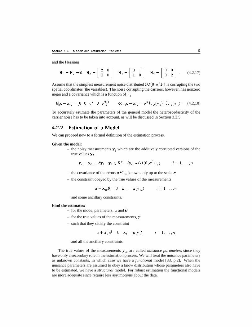
Assume that the simplest measurement noise distributed�� 3�� &�� + � + 6 is corrupting the two

spatial coordinates (the variables). The noise corrupting the carriers, however, has nonzeromean and a covariance which is a function of � �

E � � $ �� / � � � � + � � + � � �� $ �

� � / � + " $# � 3 � � 6 � " $# � 3 � � 6 ' (4.2.18)

To accurately estimate the parameters of the general model the heteroscedasticity of thecarrier noise has to be taken into account, as will be discussed in Section 3.2.5.

�� !"� * �!"(��&�� *�� +We can proceed now to a formal definition of the estimation process.

Given the model:– the noisy measurements � � which are the additively corrupted versions of the

true values � �� / ��

��

�� 3�� &�� + �� 6 � / : &('('('<&)�

– the covariance of the errors � + �� , known only up to the scale �– the constraint obeyed by the true values of the measurements� ��

�� /4� �

�� /� 3 �� 6 � /;: &('('('<&)�

and some ancillary constraints.

Find the estimates:– for the model parameters,

�

�and

�

�– for the true values of the measurements,

��– such that they satisfy the constraint

�

� ��

� ��

� /��

�� /

� 3 �� 6 � /;: &('('('<&)�and all the ancillary constraints.

The true values of the measurements �� are called nuisance parameters since theyhave only a secondary role in the estimation process. We will treat the nuisance parametersas unknown constants, in which case we have a functional model [33, p.2]. When thenuisance parameters are assumed to obey a know distribution whose parameters also haveto be estimated, we have a structural model. For robust estimation the functional modelsare more adequate since require less assumptions about the data.

10 �� "! � � � ��#�%$'&�(*),+'-�.

The estimation of a functional model has two distinct parts. First, the parameter esti-mates are obtained in the main parameter estimation procedure, followed by the compu-tation of the nuisance parameter estimates in the data correction procedure. The nuisanceparameter estimates

�� are called the corrected data points. The data correction procedureis usually not more than the projection of the measurements �� on the already estimatedconstraint surface.

The parameter estimates are obtained by (most often) seeking the global minima of anobjective function. The variables of the objective function are the normalized distancesbetween the measurements and their true values. They are defined from the squared Maha-lanobis distances� +� / :

� + 3 �� $ �� 6� �� 3 �� $ � �� 6 /

:� +�� /;: &('('('<&)� (4.2.19)

where ‘+’ stands for the pseudoinverse operator since the matrix � can be singular, inwhich case (3.2.19) is only a pseudodistance. Note that

� �� . Through the estimationprocedure the �� are replaced with

�� and the distance� � becomes the absolute value of

the normalized residual.The objective function � 3 � $ &('('('(& � � 6 is always a positive semidefinite function taking

value zero only when all the distances are zero. We should distinguish between homoge-neous and nonhomogeneous objective functions. A homogeneous objective function hasthe property

� 3 � $ &('('('<& � � 6 /:� � 3 "

�� $ " �� &('('('<&�" � � � " �� 6 (4.2.20)

where " � � � " � / � � � �� $��+ is the covariance weighted norm of the measurement

error. The homogeneity of an objective function is an important property in the estimation.Only for homogeneous objective functions we have

� �

�& �

� � / � �� 3 � $ &('('('(& � � 6 / � �� " � � $ " � &('('('(&�" � � � " �� (4.2.21)

meaning that the scale � does not play any role in the main estimation process. Since thevalue of the scale is not known a priori, by removing it an important source for performancedeterioration is eliminated. All the following objective functions are homogeneous

�� / :�

�� $

� +� �� / :�

�� $

� � �� "! � / � $#� (4.2.22)

where, �� yields the family of least squares estimators, �� the least absolute devia-tions estimator, and �%� "! � the family of least � -th order statistics estimators. In an LkOSestimator the distances are assumed sorted in ascending order, and the � -th element ofthe list is minimized. If � / �'& - , the least median of squares (LMedS) estimator, to bediscussed in detail in Section 3.4.4, is obtained.

The most important example of nonhomogeneous objective functions is that of the M-estimators

�%( / :�

�� $*) 3

� � 6 (4.2.23)

�+�� ) � �� .�� + � & �� ) � � &*) � �� - �� + � 11

where ) 3�� 6 is a nonnegative, even-symmetric loss function, nondecreasing with� � � . The

class of �%( includes as particular cases �%�� and �� , for ) 3�� 6 /�� + and ) 3�� 6 / � � � ,respectively, but in general this objective function is not homogeneous. The family of M-estimators to be discussed in Section 3.4.2 have the loss function

) 3�� 6 /�� : $ 3 : $ � + 6�� :: � � � : (4.2.24)

where� /*� & : & -.&�� . It will be shown later in the chapter that all the robust techniques

popular today in computer vision can be described as M-estimators.The definitions introduced so far implicitly assumed that all the � data points obey the

model, i.e., are inliers. In this case nonrobust estimation technique provide a satisfactoryresult. In the presence of outliers, only ��$ � � measurements are inliers and obey (3.2.3).The number ��$ is not know. The measurement equation (3.2.10) becomes

�� / ��

�� 3�� &�� + �� 6 � /;: &('('('<&)��$ (4.2.25)

�� / 3 ��$� : 6 &('('('<&)�

where nothing is assumed known about the ��$ ��$ outliers. Sometimes in robust methodsproposed in computer vision, such as [100], [107], [114], the outliers were modeled asobeying a uniform distribution.

A robust method has to determine ��$ simultaneously with the estimation of the inliermodel parameters. Since ��$ is unknown, at the beginning of the estimation process themodel is still defined for � / : &('('('<&)� . Only through the optimization of an adequateobjective function are the data points classified into inliers or outliers. The result of therobust estimation is the inlier/outlier dichotomy of the data.

The estimation process maps the input, the set of measurements � � , � / : &('('('<&)� intothe output, the estimates

�

�,

�

�and

�� . The measurements are noisy and the uncertaintyabout their true value is mapped into the uncertainty about the true value of the estimates.The computational procedure employed to obtain the estimates is called the estimator. Todescribe the properties of an estimator the estimates are treated as random variables. Theestimate

�

�will be used generically in the next two sections to discuss these properties.

�� !� �� * � ��!"� * ��Depending on � , the number of available measurements, we should distinguish betweensmall (finite) sample and large (asymptotic) sample properties of an estimator [76, Secs.6,7].In the latter case � becomes large enough that further increase in its value no longer hasa significant influence on the estimates. Many of the estimator properties proven in theo-retical statistics are asymptotic, and are not necessarily valid for small data sets. Rigorousanalysis of small sample properties is difficult. See [86] for examples in pattern recogni-tion.

What is a small or a large sample depends on the estimation problem at hand. Wheneverthe model is not accurate even for a large number of measurements the estimate remainshighly sensitive to the input. This situation is frequently present in computer vision, where

12 �� "! � � � ��#�%$'&�(*),+'-�.

only a few tasks would qualify as large scale behavior of the employed estimator. Wewill not discuss here asymptotic properties, such as the consistency, which describes therelation of the estimate to its true value when the number of data points grows unbounded.Our focus is on the bias of an estimator, the property which is also central in establishingwhether the estimator is robust or not.

Let�

be the true value of the estimate�

�. The estimator mapping the measurements ��

into�

�is unbiased if

E � �

� � / �(4.2.26)

where the expectation is taken over all possible sets of measurements of size � , i.e., overthe joint distribution of the � variables. Assume now that the input data contains � $ inliersand ��$+��$ outliers. In a “thought” experiment we keep all the inliers fixed and allow theoutliers to be placed anywhere in � � , the space of the measurements �� . Clearly, someof these arrangements will have a larger effect on

�

�than others. Will define the maximum

bias as � �� 3 ��$5&)� 6 / max� " �

� $ � " (4.2.27)

where � stands for the arrangements of the � $ ��$ outliers. Will say that an estimatorexhibits a globally robust behavior in a given task if and only if

for ��$�� 3 ��$5&)� 6 �� (4.2.28)

where � � � is a threshold depending on the task. That is, the presence of outliers cannotintroduce an estimation error beyond the tolerance deemed acceptable for that task. Toqualitatively assess the robustness of the estimator we can define

� 3 � 6 / : $ �� $� while (3.2.28) holds (4.2.29)

which measures its outlier rejection capability. Note that the definition is based on theworst case situation which may not appear in practice.

The robustness of an estimator is assured by the employed objective function. Amongthe three homogeneous objective functions in (3.2.22), minimization of two criteria, theleast squares �%�� and the least absolute deviations �%�� , does not yield robust estima-tors. A striking example for the (less known) nonrobustness of the latter is discussed in[90, p.20]. The LS and LAD estimators are not robust since their homogeneous objectivefunction (3.2.20) is also symmetric. The value of a symmetric function is invariant underthe permutations of its variables, the distances

� � in our case. Thus, in a symmetric functionall the variables have equal importance.

To understand why these two objective functions lead to a nonrobust estimator, considerthe data containing a single outlier located far away from all the other points, the inliers(Figure 3.2a). The scale of the inlier noise, � , has no bearing on the minimization of ahomogeneous objective function (3.2.21). The symmetry of the objective function, on theother hand, implies that during the optimization all the data points, including the outlier, aretreated in the same way. For a parameter estimate close to the true value the outlier yieldsa very large measurement error " � ��" � . The optimization procedure therefore tries to

�+�� ) � �� .�� + � & �� ) � � &*) � �� - �� + � 13

compensate for this error and biases the fit toward the outlier. For any threshold � on thetolerated estimation errors, the outlier can be placed far enough from the inliers such that(3.2.28) is not satisfied. This means � 3 � 6 /�� .

In a robust technique the objective function cannot be both symmetric and homoge-neous. For the M-estimators ��( (3.2.23) is only symmetric, while the least � -th orderstatistics objective function �%� "! � (3.2.20) is only homogeneous.

Consider �� "! � . When at least � measurements in the data are inliers and the param-eter estimate is close to the true value, the � -th error is computed based on an inlier and itis small. The influence of the outliers is avoided, and if (3.2.28) is satisfied, for the LkOSestimator � 3 � 6 / 3 �%$ � 6 &5� . As will be shown in the next section, the condition (3.2.28)depends on the level of noise corrupting the inliers. When the noise is large, the value of� 3 � 6 decreases. Therefore, it is important to realize that � 3 � 6 only measures the globalrobustness of the employed estimator in the context of the task. However, this is what wereally care about in an application!

Several strategies can be adopted to define the value of � . Prior to the estimation process� can be set to a given percentage of the number of points � . For example, if � / �'& - theleast median of squares (LMedS) estimator [87] is obtained. Similarly, the value of � canbe defined implicitly by setting the level of the allowed measurement noise and maximizingthe number of data points within this tolerance. This is the approach used in the randomsample consensus (RANSAC) estimator [26] which solves

�

� / arg� � � � � $#� subject to " � � $#

� " � �� 3 � 6 (4.2.30)

where � 3 � 6 is a user set threshold related to the scale of the inlier noise. In a third, lessgeneric strategy, an auxiliary optimization process is introduced to determine the best valueof � by analyzing a sequence of scale estimates [63], [77].

Beside the global robustness property discussed until now, the local robustness of anestimator also has to be considered when evaluating performance. Local robustness ismeasured through the gross error sensitivity which describes the worst influence a singlemeasurement can have on the value of the estimate [90, p.191]. Local robustness is a centralconcept in the theoretical analysis of robust estimators and has a complex relation to globalrobustness e.g., [40], [69]. It also has important practical implications.

Large gross error sensitivity (poor local robustness) means that for a critical arrange-ment of the � data points, a slight change in the value of a measurement � � yields anunexpectedly large change in the value of the estimate

�

�. Such behavior is certainly unde-

sirable. Several robust estimators in computer vision, such as LMedS and RANSAC havelarge gross error sensitivity, as will be shown in Section 3.4.4.

�� ," �!"(�� !�We have defined global robustness in a task specific manner. An estimator is consideredrobust only when the estimation error is guaranteed to be less than what can be toleratedin the application (3.2.28). This definition is different from the one used in statistic, whereglobal robustness is closely related to the breakdown point of an estimator. The (explosion)

14 �� "! � � � ��#�%$'&�(*),+'-�.

breakdown point is the minimum percentage of outliers in the data for which the valueof maximum bias becomes unbounded [90, p.117]. Also, the maximum bias is defined instatistics relative to a typically good estimate computed with all the points being inliers,and not relative to the true value as in (3.2.27).

For computer vision problems the statistical definition of robustness is too narrow. First,a finite maximum bias can still imply unacceptably large estimation errors. Second, instatistics the estimators of models linear in the variables are often required to be affineequivariant, i.e., an affine transformation of the input (measurements) should change theoutput (estimates) by the inverse of that transformation [90, p.116]. It can be shown thatthe breakdown point of an affine equivariant estimator cannot exceed 0.5, i.e., the inliersmust be the absolute majority in the data [90, p.253], [69]. According to the definition ofrobustness in statistics, once the number of outliers exceeds that of inliers, the former canbe arranged into a false structure thus compromising the estimation process.

Our definition of robust behavior is better suited for estimation in computer visionwhere often the information of interest is carried by less than half of the data points and/orthe data may also contain multiple structures. Data with multiple structures is characterizedby the presence of several instances of the same model, each corresponding in (3.2.11) to adifferent set of parameters

� & � , � / : &('('('(&�� . Independently moving objects in a scene

is just one example in which such data can appear. (The case of simultaneous presence ofdifferent models is too rare to be considered here.)

The data in Figure 3.3 is a simple example of the multistructured case. Outliers notbelonging to any of the model instances can also be present. During the estimation of anyof the individual structures, all the other data points act as outliers. Multistructured data isvery challenging and once the measurement noise becomes large (Figure 3.3b) none of thecurrent robust estimators can handle it. Theoretical analysis of robust processing for datacontaining two structures can be found in [9], [98], and we will discuss it in Section 3.4.7.

The definition of robustness employed here, beside being better suited for data in com-puter vision, also has the advantage of highlighting the complex relation between � , thescale of the inlier noise and � 3 � 6 , the amount of outlier tolerance. To avoid misconcep-tions we do not recommend the use of the term breakdown point in the context of computervision.

Assume for the moment that the data contains only inliers. Since the input is corruptedby measurement noise, the estimate

�

�will differ from the true value

�. The larger the scale

of the inlier noise, the higher the probability of a significant deviation between�

and�

�. The

inherent uncertainty of an estimate computed from noisy data thus sets a lower bound on � (3.2.28). Several such bounds can be defined, the best known being the Cramer-Rao bound[76, p.78]. Most bounds are computed under strict assumptions about the distribution of themeasurement noise. Given the complexity of the visual data, the significance of a bound ina real application is often questionable. For a discussion of the Cramer-Rao bound in thecontext of computer vision see [58, Chap. 14], and for an example [96].

Next, assume that the employed robust method can handle the percentage of outlierspresent in the data. After the outliers were removed, the estimate

�

�is computed from less

data points and therefore it is less reliable (a small sample property). The probability ofa larger deviation from the true value increases, which is equivalent to an increase of the

�+�� ) � �� .�� + � & �� ) � � &*) � �� - �� + � 15

0 10 20 30 40 50 60 70 80 90 100 11030

40

50

60

70

80

90

100

110

120

y1

y 2

0 20 40 60 80 100 1200

50

100

150

y1

y 2

(a) (b)

Figure 4.3. Multistructured data. The measurement noise is small in (a) and large in (b).The line is the fit obtained with the least median of squares (LMedS) estimator.

lower bound on � . Thus, for a given level of the measurement noise (the value of � ), asthe employed estimator has to remove more outliers from the data, the chance of largerestimation errors (the lower bound on � ) also increases. The same effect is obtained whenthe number of removed outliers is kept the same but the level of the measurement noiseincreases.

In practice, the tolerance threshold � is set by the application to be solved. Whenthe level of the measurement noise corrupting the inliers increases, eventually we are nolonger able to keep the estimation errors below � . Based on our definition of robustnessthe estimator no longer can be considered as being robust! Note that by defining robustnessthrough the breakdown point, as it is done in statistics, the failure of the estimator wouldnot have been recorded. Our definition of robustness also covers the numerical robustnessof a nonrobust estimator when all the data obeys the model. In this case the focus isexclusively on the size of the estimation errors, and the property is related to the efficiencyof the estimator.

The loss of robustness is best illustrated with multistructured data. For example, theLMedS estimator was designed to reject up to half the points being outliers. When used torobustly fit a line to the data in Figure 3.3a, correctly recovers the lower structure whichcontains sixty percent of the points. However, when applied to the similar but heavilycorrupted data in Figure 3.3b, LMedS completely fails and the obtained fit is not differentfrom that of the nonrobust least squares [9], [78], [98]. As will be shown in Section 3.4.7,the failure of LMedS is part of a more general deficiency of robust estimators.

�� -�*�� !"� * �!"(�� + �� The model described at the beginning of Section 3.2.2, the measurement equation

� � / � ��

� � � � �� 3�� &�� +�� 6 � /;: &('('('<&)� (4.2.31)

and the constraint � ��

� /4� �� /

� 3 �� 6 � /;: &('('('<&)� (4.2.32)

16 �� "! � � � ��#�%$'&�(*),+'-�.

05

1015

20

0

5

10

15

200

5

10

15

y1y2

z

Figure 4.4. A typical traditional regression problem. Estimate the parameters of the surfacedefined on a sampling grid.

is general enough to apply to almost all computer vision problems. The constraint is linearin the parameters

�and

�, but nonlinear in the variables �� . A model in which all the

variables are measured with errors is called in statistics an errors-in-variables (EIV) model[112], [116].

We have already discussed in Section 3.2.1 the problem of ellipse fitting using suchnonlinear EIV model (Figure 3.1). Nonlinear EIV models also appear in any computervision problem in which the constraint has to capture an incidence relation in projectivegeometry. For example, consider the epipolar constraint between the affine coordinates ofcorresponding points in two images � and �

� "��$ � "�� + � : � �� " � $ � " � + � : � /�� (4.2.33)

where�

is a rank two matrix [43, Chap.8]. When this bilinear constraint is rewritten as(3.2.32) four of the eight carriers�� /�� " � $ � " � + � "��$ � "�� + � " � $ � "��$ � " � + � "��$ � " � + � "��$ � " � + � "�� + � � (4.2.34)

are nonlinear functions in the variables. Several nonlinear EIV models used in recovering3D structure from uncalibrated image sequences are discussed in [34].

To obtain an unbiased estimate, the parameters of a nonlinear EIV model have tobe computed with nonlinear optimization techniques such as the Levenberg-Marquardtmethod. See [43, Appen.4] for a discussion. However, the estimation problem can bealso approached as a linear model in the carriers and taking into account the heteroscedas-ticity of the noise process associated with the carriers (Section 3.2.1). Several such tech-niques were proposed in the computer vision literature: the renormalization method [58],the heteroscedastic errors-in-variables (HEIV) estimator [64], [71], [70] and the funda-mental numerical scheme (FNS) [12]. All of them return estimates unbiased in a first orderapproximation.

Since the focus of this chapter is on robust estimation, we will only use the less general,linear errors-in-variables regression model. In this case the carriers are linear expressionsin the variables, and the constraint (3.2.32) becomes��

��

� /�� /;: &('('('<&)��' (4.2.35)

�+�� ) � �� .�� + � & �� ) � � &*) � �� - �� + � 17

0 2 4 6 8 10

0246810

0

1

2

3

4

5

6

7

8

9

10

y1y2

y3

Figure 4.5. A typical location problem. Determine the center of the cluster.

An important particular case of the general EIV model is obtained by considering theconstraint (3.2.4). This is the traditional regression model where only a single variable,denoted # , is measured with error and therefore the measurement equation becomes

# � /4# �� # � � # � � �� 3 � &�� + 6 � /;: &('('('<&)� (4.2.36)

�� / �� /;: &('('('<&)�while the constraint is expressed as

# �� / ��

� �� /

� 3 �� 6 � /;: &('('('<&)� ' (4.2.37)

Note that the nonlinearity of the carriers is no longer relevant in the traditional regressionmodel since now their value is known.

In traditional regression the covariance matrix of the variable vector� � / � # � � � +�� / � + � : � �� (4.2.38)

has rank one, and the normalized distances,� � (3.2.19) used in the objective functions

become

� +� / :� + 3�� $ � �� 6 � �� 3�� $ � �� 6 / 3 # � $ # �� 6 +

� + / � � # �� +

' (4.2.39)

The two regression models, the linear EIV (3.2.35) and the traditional (3.2.37), has to beestimated with different least squares techniques, as will be shown in Section 3.4.1. Usingthe method optimal for traditional regression when estimating an EIV regression model,yields biased estimates. In computer vision the traditional regression model appears almostexclusively only when an image defined on the sampling grid is to be processed. In thiscase the pixel coordinates are the independent variables and can be considered availableuncorrupted (Figure 3.4).

All the models discussed so far were related the class of regression problems. A second,equally important class of estimation problems also exist. They are the location problems in

18 �� "! � � � ��#�%$'&�(*),+'-�.

which the goal is to determine an estimate for the “center” of a set of noisy measurements.The location problems are closely related to clustering in pattern recognition.

In practice a location problem is of interest only in the context of robust estimation.The measurement equation is

� � / � ��

�� / : &('('('(&)��$ (4.2.40)

� � � /;3 ��$� : 6 &('('('(&)�

with the constraint�� /

�� /;: &('('('<&)��$ (4.2.41)

with ��$ , the number of inliers, unknown.The important difference from the regression case (3.2.25) is that now we do not assume

that the noise corrupting the inliers can be characterized by a single covariance matrix, i.e.,the cloud of inliers has an elliptical shape. This will allow to handle data such as in Figure3.5.

The goal of the estimation process in a location problem is twofold.

– Find a robust estimate�

�for the center of the � measurements.

– Select the ��$ data points associated with this center.

The discussion in Section 3.2.4 about the definition of robustness also applies to locationestimation.

While handling multistructured data in regression problems is an open research ques-tion, clustering multistructured data is the main application of the location estimators. Thefeature spaces derived from visual data are complex and usually contain several clusters.The goal of feature space analysis is to delineate each significant cluster through a robustlocation estimation process. We will return to location estimation in Section 3.3.

�� "$�� * � � �(� �� "$�� % * � "(* � + � � �� !� "(�� +To focus on the issue of robustness in regression problems, only the simplest linear errors-in-variables (EIV) regression model (3.2.35) will be used. The measurements are corruptedby i.i.d. noise

�� / ��

��

�� 3�� &�� + � � 6 � /;: &('('('<&)� (4.2.42)

where the number of variables � was aligned with � the dimension of the parameter vector�. The constraint is rewritten under the more convenient form

� 3 �� 6 / ��

� $ � /4� � /;: &('('('<&)� ' (4.2.43)

To eliminate the ambiguity up to a constant of the parameters the following two ancillaryconstraints are used

" � " /;: � � � ' (4.2.44)

�+�� ) � �� .�� + � & �� ) � � &*) � �� - �� + � 19

Figure 4.6. The concepts of the linear errors-in-variables regression model. The constraintis in the Hessian normal form.

The three constraints together define the Hessian normal form of a plane in ��. Figure 3.6

shows the interpretation of the two parameters. The unit vector�

is the direction of thenormal, while

�is the distance from the origin.

In general, given a surface � 3 � � 6 / � in ��, the first order approximation of the

shortest Euclidean distance from a point � to the surface is [111, p.101]

" ��$ �� "�� 3 � 6 �

"�� 3 �� 6 " (4.2.45)

where�� is the orthogonal projection of the point onto the surface, and �� 3 �� 6 is the gradient

computed in the location of that projection. The quantity � 3 � 6 is called the algebraicdistance, and it can be shown that it is zero only when � / � � , i.e., the point is on thesurface.

Taking into account the linearity of the constraint (3.2.43) and that�

has unit norm,(3.2.45) becomes " �%$ �� " / � � 3 � 6 � (4.2.46)

i.e., the Euclidean distance from a point to a hyperplane written under the Hessian normalform is the absolute value of the algebraic distance.

When all the data points obey the model the least squares objective function ��(3.2.22) is used to estimate the parameters of the linear EIV regression model. The i.i.d.measurement noise (3.2.42) simplifies the expression of the distances

� � (3.2.19) and theminimization problem (3.2.21) can be written as

� �

�& �

� � / � �� :�

�� $ " � � $ ��," + ' (4.2.47)

Combining (3.2.46) and (3.2.47) we obtain

� �

�& �

� � / � �� :�

�� $ � 3 � �

6 + ' (4.2.48)

20 �� "! � � � ��#�%$'&�(*),+'-�.

To solve (3.2.48) the true values �� are replaced with the orthogonal projection of the �� -sonto the hyperplane. The orthogonal projections

�� associated with the solution�

�& �

�are

the corrected values of the measurements � � , and satisfy (Figure 3.6)

�� 3 �� 6 / ��

� $ �

� /�� /;: &('('('<&)��' (4.2.49)

The estimation process (to be discussed in Section 3.4.1) returns the parameter es-timates, after which the ancillary constrains (3.2.44) can be imposed. The employedparametrization of the linear model

� $ / � � � � � � /�� $ � + �� $ (4.2.50)

however is redundant. The vector�

being a unit vector it is restricted to the � -dimensionalunit sphere in

� �. This can be taken into account by expressing

�in polar angles [116] as,� / � 3�� 6

�2/ � � $ � + �� $ �� .- �� 9 / : & �� &� $�- � � � �� $ � - � (4.2.51)

where the mapping is

� $ 3�� 6 / � � � � $ �� + � � � � �� $� + 3�� 6 / � � � � $ �� +�� $�!1 3�� 6 / � � � � $ �� 1 �� +

... (4.2.52)�� $ 3�� 6 / � � � � $ �� +�� 3�� 6 / �� $ 'The polar angles �%- and

�provide the second representation of a hyperplane

� + /�� / � � $ � + �� $ � � � ��' (4.2.53)

The � + representation being based in part on the mapping from the unit sphere to�

�� $ , is inherently discontinuos. See [24, Chap. 5] for a detailed discussion of suchrepresentations. The problem is well known in the context of Hough transform, where thisparametrization is widely used.

To illustrate the discontinuity of the mapping, consider the representation of a line,� / - . In this case only a single polar angle � is needed and the equation of a line in theHessian normal form is

"4$�� ",+ � � � � $ � /4� ' (4.2.54)

In Figures 3.7a and 3.7b two pairs of lines are shown, each pair having the same�

butdifferent polar angles. Take � $ /�� . The lines in Figure 3.7a have the relation � + /��

,while those in Figure 3.7b � + / - � $ � . When represented in the � + parameter space(Figure 3.7c) the four lines are mapped into four points.

�+�� ) � �� .�� + � & �� ) � � &*) � �� - �� + � 21

−1 −0.5 0 0.5 1−1

−0.5

0

0.5

1

y1

y 2 la2

la1

α

α

0 1 2 3−2

−1.5

−1

−0.5

0

0.5

1

1.5

2

y1

y 2

lb1

lb2

β− β

0 0.5 1 1.5 20

0.5

1

1.5

2

2.5

3

la1

la2

lb1

lb2

β /π

α

−2 0 2 4−3

−2

−1

0

1

2

3

la1

la2

lb1

lb2

y1

y 2

(a) (b) (c) (d)

Figure 4.7. Discontinuous mappings due to the polar representation of�

. (a) Two lineswith same

�and antipodal polar angles � . (b) Two lines with same

�and polar angles �

differing only in sign. (c) The � + parameter space. (d) The � 1parameter space.

Let now�� for the first pair, and �

� � for the second pair. In the input space eachpair of lines merges into a single line, but the four points in the � + parameter space remaindistinct, as shown by the arrows in Figure 3.7c.

A different parameterization of the hyperplane in ��

can avoid this problem, though norepresentation of the Hessian normal form can provide a continuous mapping into a featurespace. In the new parameterization all the hyperplanes not passing through the origin arerepresented by their point closest to the origin. This point has the coordinates

�'�and is the

intersection of the plane with the normal from the origin. The new parametrization is

� 1 / �'� / � � � $ � � + �� ' (4.2.55)

It is important to notice that the space of � 1is in fact the space of the input as can also be

seen from Figure 3.6. Thus, when the pairs of lines collapse, so do their representations inthe � 1

space (Figure 3.7d).Planes which contain the origin have to be treated separately. In practice this also ap-

plies to planes passing near the origin. A plane with small�

is translated along the directionof the normal

�with a known quantity � . The plane is then represented as �

�. When =

planes are close to the origin the direction of translation is

�� $

�� and the parameters of

each translated plane are adjusted accordingly. After processing in the � 1space it is easy

to convert back to the � $ representation.Estimation of the linear EIV regression model parameters by total least squares (Section

3.4.1) uses the � $ parametrization. The � + parametrization will be employed in the robustestimation of the model (Section 3.4.5). The parametrization � 1

is useful when the problemof robust multiple regression is approached as a feature space analysis problem [9].

�� #�� !" � � � �� !"(��/�!"� "�� * �!"(��The objective functions used in robust estimation are often nondifferentiable and analyti-cal optimization methods, like those based on the gradient, cannot be employed. The � -thorder statistics, �%� "! � (3.2.22) is such an objective function. Nondifferentiable objective

22 �� "! � � � ��#�%$'&�(*),+'-�.

functions also have many local extrema and to avoid being trapped in one of these minimathe optimization procedure should be run starting from several initial positions. A numeri-cal technique to implement robust estimators with nondifferentiable objective functions, isbased on elemental subsets.

An elemental subset is the smallest number of data points required to fully instantiatea model. In the linear EIV regression case this means � points in a general position, i.e.,the points define a basis for a 3 � $ : 6 -dimensional affine subspace in �

�[90, p. 257]. For

example, if � / � not all three points can lie on a line in 3D.The � points in an elemental subset thus define a full rank system of equations from

which the model parameters�

and�

can be computed analytically. Note that using �points suffices to solve this homogeneous system. The ancillary constraint " � " / : isimposed at the end. The obtained parameter vector � $ / � � � � � �

will be called, with aslight abuse of notation, a model candidate.

The number of possibly distinct elemental subsets in the data

� �� , can be very large.

In practice an exhaustive search over all the elemental subsets is not feasible, and a randomsampling of this ensemble has to be used. The sampling drastically reduces the amount ofcomputations at the price of a negligible decrease in the outlier rejection capability of theimplemented robust estimator.

Assume that the number of inliers in the data is ��$ , and that � elemental subsets, � -tuples, were drawn independently from that data. The probability that none of these subsetscontains only inliers is (after disregarding the artifacts due to the finite sample size)

�� /�� : $ � ��$� � �� ' (4.2.56)

We can choose a small probability�� to bound upward

�� . Then the equation

�� / �� (4.2.57)

provides the value of � as a function of the percentage of inliers ��$$&5� , the dimensionof the parameter space � and

�� . This probabilistic sampling strategy was appliedindependently in computer vision for the RANSAC estimator [26] and in statistics for theLMedS estimator [90, p.198].

Several important observations has to be made. The value of � obtained from (3.2.57)is an absolute lower bound since it implies that any elemental subset which contains onlyinliers can provide a satisfactory model candidate. However, the model candidates arecomputed from the smallest possible number of data points and the influence of the noiseis the largest possible. Thus, the assumption used to compute � is not guaranteed to besatisfied once the measurement noise becomes significant. In practice � $ is not know priorto the estimation, and the value of � has to be chosen large enough to compensate for theinlier noise under a worst case scenario.

Nevertheless, it is not recommended to increase the size of the subsets. The reason isimmediately revealed if we define in a drawing of subsets of size � � � , the probability of

�+�� ) � �� .�� + � & �� ) � � &*) � �� - �� + � 23

success as obtaining a subset which contains only inliers

�� & & �� /� ��$

� ��

/ �� $�

� � ��$)$ ��$ � ' (4.2.58)

This probability is maximized when � / � .Optimization of an objective function using random elemental subsets is only a compu-

tational tool and has no bearing on the robustness of the corresponding estimator. This factis not always recognized in the computer vision literature. However, any estimator can beimplemented using the following numerical optimization procedure.

Objective Function Optimization With Elemental Subsets

– Repeat � times:1. choose an elemental subset (� -tuple) by random sampling;

2. compute the corresponding model candidate;

3. compute the value of the objective function by assuming the model candidatevalid for all the data points.

– The parameter estimate is the model candidate yielding the smallest (largest) objec-tive function value.

This procedure can be applied the same way for the nonrobust least squares objective func-tion �� as for the the robust least � -th order statistics �%� "! � (3.2.22). However, whilean analytical solution is available for the former (Section 3.4.1), for the latter the aboveprocedure is the only practical way to obtain the estimates.

Performing an exhaustive search over all elemental subsets does not guarantee to findthe global extremum of the objective function since not every location in the parameterspace can be visited. Finding the global extremum, however, most often is also not re-quired. When a robust estimator is implemented with the elemental subsets based searchprocedure, the goal is only to obtain the inlier/outlier dichotomy, i.e., to select the “good”data. The robust estimate corresponding to an elemental subset is then refined by process-ing the selected inliers with a nonrobust (least squares) estimator. See [88] for an extensivediscussion of the related issues from a statistical perspective.

The number of required elemental subsets � can be significantly reduced when infor-mation about the reliability of the data points is available. This information can be eitherprovided by the user, or can be derived from the data through an auxiliary estimation pro-cess. The elemental subsets are then chosen with a guided sampling biased toward thepoints having a higher probability to be inliers. See [104] and [105] for computer visionexamples.

We have emphasized that the random sampling of elemental subsets is not more than acomputational procedure. However, guided sampling has a different nature since it relieson a fuzzy pre-classification of the data (derived automatically, or supplied by the user).Guided sampling can yield a significant improvement in the performance of the estimator

24 �� "! � � � ��#�%$'&�(*),+'-�.

relative to the unguided approach. The better quality of the elemental subsets can be con-verted into either less samples in the numerical optimization (while preserving the outlierrejection capacity � 3 � 6 of the estimator), or into an increase of � 3 � 6 (while preserving thesame number of elemental subsets � ).

We conclude that guided sampling should be regarded as a robust technique, while therandom sampling procedure should be not. Their subtle but important difference has to berecognized when designing robust methods for solving complex vision tasks.

In most applications information reliable enough to guide the sampling is not available.However, the amount of computations still can be reduced by performing in the space of theparameters local searches with optimization techniques which do not rely on derivatives.For example, in [91] line search was proposed to improve the implementation of the LMedSestimator. Let � $ / � � �

� ��

be the currently best model candidate, as measured bythe value of the objective function. From the next elemental subset the model candidate� $ /*� � � � � �

is computed. The objective function is then assessed at several locationsalong the line segment � $ $ � $ , and if an improvement relative to � $ is obtained the bestmodel candidate is updated.

In Section 3.4.5 we will use a more effective multidimensional unconstrained optimiza-tion technique, the simplex based direct search. The simplex search is a heuristic methodproposed in 1965 by Nelder and Mead [79]. See also [83, Sec.10.4]. Simplex search is aheuristic with no theoretical foundations. Recently direct search methods became again ofinterest and significant progress was reported in the literature [66] [115], but in our contextthere is no need to use these computationally more intensive techniques.

To take into account the fact that�

is a unit vector, the simplex search should be per-formed in the space of the polar angles � � � �� $ . A simplex in

� �� $ is the volumedelineated by � vertices in a nondegenerate position, i.e., the points define an affine basisin� �� $ . For example, in

� + the simplex is a triangle, in� 1

it is a tetrahedron. In ourcase, the vertices of the simplex are the polar angle vectors � � � �� $ , � / : &('('('(&� ,representing � unit vectors

� � � �. Each vertex is associated with the value of a scalar

function � / � 3�� 6. For example, � 3�� 6 can be the objective function of an estimator.

The goal of the search is to find the global (say) maximum of this function.We can always assume that at the beginning of an iteration the vertices are labeled such

that ��$ � �!+ � �� . In each iteration an attempt is made to improve the least favor-able value of the function, �8$ in our case, by trying to find a new location �� $ for the vertex� $ such that ��$�� 3�� $ 6 .

Simplex Based Direct Search Iteration

First�� the centroid of the nonminimum vertices, �

, ��/ -.&('('('<&� , is obtained. The newlocation is then computed with one of the following operations along the direction

�� $ � $ :reflection, expansion and contraction.

1. The reflection of � $ , denoted �� (Figure 3.8a) is defined as

�� / � $ � 3 : $ 6 �� (4.2.59)

�+�� ) � �� .�� + � & �� ) � � &*) � �� - �� + � 25

1 1.5 2 2.50

0.5

1

1.5

2

2.5

β1

β 2

β1

β2

β3

β−

β1’

1 1.5 2 2.50

0.5

1

1.5

2

2.5

β1

β 2

β1

β2

β3

β−

β1’

1 1.5 2 2.50

0.5

1

1.5

2

2.5

β1

β 2

β1

β2

β3

β−

β1’

1 1.5 2 2.50

0.5

1

1.5

2

2.5

β1

β 2

β1

β2

β3

β−

β’1

1 1.5 2 2.50

0.5

1

1.5

2

2.5

β1

β 2

β1

β2

β3

β−

β’1

1 1.5 2 2.50

0.5

1

1.5

2

2.5

β1

β 2

β1

β2

β3

β−

β’1

1 1.5 2 2.50

0.5

1

1.5

2

2.5

β1

β 2

β1

β2

β3

β−

β’1

1 1.5 2 2.50

0.5

1

1.5

2

2.5

β1

β 2

β1

β2

β3

β−

β’1

1 1.5 2 2.50

0.5

1

1.5

2

2.5

β1

β 2

β1

β2

β3

β−

β’1

1 1.5 2 2.50

0.5

1

1.5

2

2.5

β1

β 2

β1

β2

β3

β−

β’1

1 1.5 2 2.50

0.5

1

1.5

2

2.5

β1

β 2

β1

β2

β3

β−

β’1

1 1.5 2 2.50

0.5

1

1.5

2

2.5

β1

β 2

β1

β2

β3

β−

β1’

1 1.5 2 2.50

0.5

1

1.5

2

2.5

β1

β 2

β1

β2

β3

β−

β1’

1 1.5 2 2.50

0.5

1

1.5

2

2.5

β1

β 2

β1

β2

β3

β−

β1’

1 1.5 2 2.50

0.5

1

1.5

2

2.5

β1

β 2

β1

β2

β3

β−

β1’

1 1.5 2 2.50

0.5

1

1.5

2

2.5

β1

β 2

β1

β2

β3

β−

β’1

1 1.5 2 2.50

0.5

1

1.5

2

2.5

β1

β 2

β1

β2

β3

β−

β’1

1 1.5 2 2.50

0.5

1

1.5

2

2.5

β1

β 2

β1

β2

β3

β−

β’1

1 1.5 2 2.50

0.5

1

1.5

2

2.5

β1

β 2

β1

β2

β3

β−

β’1

1 1.5 2 2.50

0.5

1

1.5

2

2.5

β1

β 2

β1

β2

β3

β−

β’1

1 1.5 2 2.50

0.5

1

1.5

2

2.5

β1

β 2

β1

β2

β3

β−

β’1

1 1.5 2 2.50

0.5

1

1.5

2

2.5

β1

β 2

β1

β2

β3

β−

β’1

1 1.5 2 2.50

0.5

1

1.5

2

2.5

β1

β 2

β1

β2

β3

β−

β’1

1 1.5 2 2.50

0.5

1

1.5

2

2.5

β1

β 2

β1

β2

β3

β−

β1’

1 1.5 2 2.50

0.5

1

1.5

2

2.5

β1

β 2

β1

β2

β3

β−

β1’

1 1.5 2 2.50

0.5

1

1.5

2

2.5

β1

β 2

β1

β2

β3

β−

β1’

1 1.5 2 2.50

0.5

1

1.5

2

2.5

β1

β 2

β1

β2

β3

β−

β’1

1 1.5 2 2.50

0.5

1

1.5

2

2.5

β1

β 2

β1

β2

β3

β−

β’1

1 1.5 2 2.50

0.5

1

1.5

2

2.5

β1

β 2

β1

β2

β3

β−

β’1

1 1.5 2 2.50

0.5

1

1.5

2

2.5

β1

β 2

β1

β2

β3

β−

β’1

1 1.5 2 2.50

0.5

1

1.5

2

2.5

β1

β 2

β1

β2

β3

β−

β’1

1 1.5 2 2.50

0.5

1

1.5

2

2.5

β1

β 2

β1

β2

β3

β−

β’1

1 1.5 2 2.50

0.5

1

1.5

2

2.5

β1

β 2

β1

β2

β3

β−

β1’

1 1.5 2 2.50

0.5

1

1.5

2

2.5

β1

β 2

β1

β2

β3

β−

β1’

1 1.5 2 2.50

0.5

1

1.5

2

2.5

β1

β 2

β1

β2

β3

β−

β1’

1 1.5 2 2.50

0.5

1

1.5

2

2.5

β1

β 2

β1

β2

β3

β−

β’1

1 1.5 2 2.50

0.5

1

1.5

2

2.5

β1

β 2

β1

β2

β3

β−

β’1

1 1.5 2 2.50

0.5

1

1.5

2

2.5

β1

β 2

β1

β2

β3

β−

β’1

1 1.5 2 2.50

0.5

1

1.5

2

2.5

β1

β 2

β1

β2

β3

β−

β’1

1 1.5 2 2.50

0.5

1

1.5

2

2.5

β1

β 2

β1

β2

β3

β−

β’1

1 1.5 2 2.50

0.5

1

1.5

2

2.5

β1

β 2

β1

β2

β3

β−

β’1

1 1.5 2 2.50

0.5

1

1.5

2

2.5

β1

β 2

β1

β2

β3

β−

β’1

(a) (b) (c) (d)

Figure 4.8. Basic operations in simplex based direct search. (a) Reflection. (b) Expansion.(c) Outside contraction. (d) Inside contraction.

where � � is the reflection coefficient. If � + � � 3�� 6 � � � , then �� $ / �� and thenext iteration is started.

2. If � 3�� 6 � � , i.e., the reflection has produced a new maximum, the simplex isexpanded by moving �� to �� (Figure 3.8b)

�� / � �� 3 : $ � 6 �� (4.2.60)

where the expansion coefficient � : . If � 3�� 6 � 3�� 6 the expansion is success-ful and �� $ / �� . Else, �� $ / �� . The next iteration is started.

3. If � 3�� 6 � �!+ , the vector � $ � is defined as either � $ or �� , whichever has the largerassociated function value, and a contraction is performed

�� / & � $ �� 3 : $ & 6 �� ' (4.2.61)

First, a contraction coefficient � � & � : is chosen for outside contraction (Figure3.8c). If � 3�� 6 � 3�� $ �

6, then �� $ / �� and the next iteration is started. Otherwise,

an inside contraction is performed (Figure 3.8d) in which & is replaced with $ & ,and the condition � 3�� 6 � 3�� $ �

6is again verified.

4. Should both contractions fail all the vertices are updated

� �� $ :-� � � � �� / : &('('('<& 3 � $ : 6 (4.2.62)

and the next iteration is started.

Recommended values for the coefficients are / $ : & � / : ' �.& & /4� ' � .To assess the convergence of the search several stopping criteria can be employed. Forexample, the variance of the � function values � should fall below a threshold which isexponentially decreasing with the dimension of the space, or the ratio of the smallest andlargest function values �8$$& � � should be close to one. Similarly, the volume of the simplex

26 �� "! � � � ��#�%$'&�(*),+'-�.

020

4060

80

0

20

40

60

80

0

20

40

60

80

y1

y2

y 3

2040

6080

100

0

20

40

60

80

100

−50

0

50

L*

u*

v*

(a) (b)

Figure 4.9. Multistructured data in the location estimation problem. (a) The “traditional”case. (b) A typical computer vision example.

should shrink below a dimension dependent threshold. In practice, the most effective stop-ping criteria are application specific incorporating additional information which was notused during the optimization.

In the previous sections we have analyzed the problem of robust estimation from ageneric point of view. We can proceed now to examine the two classes of estimation prob-lems: location and regression. In each case will introduce a new robust technique whoseimproved behavior was achieved by systematically exploiting the principles discussed sofar.

�� /� * �!"(��!"� * �!"(��In this section will show that in the context of computer vision tasks often only nonpara-metric approaches can provide a robust solution for the location estimation problem. Weemploy a class of nonparametric techniques in which the data points are regarded as sam-ples from an unknown probability density. The location estimates are then defined as themodes of this density. Explicit computation of the density is avoided by using the meanshift procedure.

�� * � *�� 4� " ;� � �� The most general model of the location problem is that of multiple structures

� / : &('('('<&�� = $ /;: �� =�� $ / ��$� :

� �� / � �� / � � � / = &('('('(& 3 = � $ $ : 6

�� /;3 ��$� : 6 &('('('(&)� (4.3.1)

with no information being available about the nature of the inlier noise�� , the � $ ��$

outliers, or the number of structures present in the data � . The model (3.3.1) is also used

�+�� ) � �� .�� *&*) � �� ) � � &*) � �� 27

in cluster analysis, the equivalent pattern recognition problem. Clustering under its mostgeneral form is an unsupervised learning method of unknown categories from incompleteprior information [52, p. 242]. The books [52], [21, Chap. 10], [44, Sec.14.3] provide acomplete coverage of the related pattern recognition literature.

Many of the pattern recognition methods are not adequate for data analysis in computervision. To illustrate their limitations will compare the two data sets shown in Figure 3.9.The data in Figure 3.9a obeys what is assumed in traditional clustering methods whenthe proximity to a cluster center is measured as a function of Euclidean or Mahalanobisdistances. In this case the shape of the clusters is restricted to elliptical and the inliers areassumed to be normally distributed around the true cluster centers. A different metric willimpose a different shape on the clusters. The number of the structures (clusters) � , is aparameter to be supplied by the user and has a large influence on the quality of the results.While the value of � can be also derived from the data by optimizing a cluster validityindex, this approach is not robust since it is based on (possibly erroneous) data partitions.

Expectation maximization (EM) is a frequently used technique today in computer visionto model the data. See [44, Sec.8.5.2] for a short description. The EM algorithm also relieson strong prior assumptions. A likelihood function, defined from a mixture of predefined(most often normal) probability densities, is maximized. The obtained partition of the datathus employs “tiles” of given shape. The number of required mixture components is oftendifficult to determine, and the association of these components with true cluster centersmay not be obvious.

Examine now the data in Figure 3.9b in which the pixels of a color image were mappedinto the three-dimensional � �� color space. The significant clusters correspond to sim-ilarly colored pixels in the image. The clusters have a large variety of shapes and theirnumber is not obvious. Any technique which imposes a preset shape on the clusters willhave difficulties to accurately separate � significant structures from the background clutterwhile simultaneously also having to determine the value of � .

Following our goal oriented approach toward robustness (Section 3.2.3) a location es-timator should be declared robust only if it returns a satisfactory result. From the abovediscussion can be concluded that robustly solving location problems in computer visionoften requires techniques which use the least possible amount of prior assumptions aboutthe data. Such techniques belong to the family of nonparametric methods.

In nonparametric methods the � data points are regarded as outcomes from an (un-known) probability distribution � 3 � 6 . Each data point is assumed to have an equal proba-bility

Prob � � / � � � / :� � / : &('('('(&)��' (4.3.2)

When several points have the same value, the probability is �� $ times the multiplicity.

The ensemble of points defines the empirical distribution � 3 � � � $ �� 6

of the data. Theempirical distribution is the nonparametric maximum likelihood estimate of the distributionfrom which the data was drawn [22, p.310]. It is also the “least committed” description ofthe data.

Every clustering technique exploits the fact that the clusters are the denser regions inthe space. However, this observation can be pushed further in the class of nonparamet-

28 �� "! � � � ��#�%$'&�(*),+'-�.

ric methods considered here, for which a region of higher density implies more probableoutcomes of the random variable � . Therefore, in each dense region the location estimate(cluster center) should be associated with the most probable value of � , i.e., with the localmode of the empirical distribution

�

� � / � �� 3 � � � $ �� 6 � /;: &('('('<&�� ' (4.3.3)

Note that by detecting all the significant modes of the empirical distribution the numberof clusters � is automatically determined. The mode based clustering techniques makeextensive use of density estimation during data analysis.

�� + � �,�� " � � ��!"� * �!"(��The modes of a random variable � are the local maxima of its probability density func-tion � 3 � 6 . However, only the empirical distribution, the data points � � , � / : &('('('<&)� areavailable. To accurately determine the locations of the modes, first a continuous estimateof the underlying density

�

� 3 � 6 has to be defined. Later we will see that this step can beeliminated by directly estimating the gradient of the density (Section 3.3.3).

To estimate the probability density in � a small neighborhood is defined around � . Theneighborhood usually has a simple shape: cube, sphere or ellipsoid. Let its volume be � � ,and = � be the number of data points inside. Then the density estimate is [21, Sec.4.2]

�

� 3 � 6 / = �� (4.3.4)

which can be employed in two different ways.

– In the nearest neighbors approach, the neigborhoods (the volumes � � ) are scaled tokeep the number of points = � constant. A mode corresponds to a location in whichthe neighborhood has the smallest volume.

– In the kernel density approach, the neigborhoods have the same volume � � and thenumber of points = � inside are counted. A mode corresponds to a location in whichthe neighborhood contains the largest number of points.

The minimum volume ellipsoid (MVE) robust location estimator proposed in statistics[90, p.258], is a technique related to the nearest neighbors approach. The ellipsoids aredefined by elemental subsets obtained through random sampling, and the numerical opti-mization procedure discussed in Section 3.2.7 is employed. The location estimate is thecenter of the smallest ellipsoid which contains a given percentage of the data points. Ina robust clustering method proposed in computer vision the MVE estimator was used tosequentially remove the clusters from the data, starting from the largest [53]. However,by imposing an elliptical shape for the clusters severe artifacts were introduced and themethod was never successful in real vision applications.

For our goal of finding the local maxima of�

� 3 � 6 , the kernel density methods are moresuitable. Kernel density estimation is a widely used technique in statistics and pattern

�+�� ) � �� .�� *&*) � �� ) � � &*) � �� 29

0 20 40 60 80 100 1200

1

2

3

4

5

6

7

8

x0 20 40 60 80 100 120

−1

−0.5

0

0.5

1

1.5

2

x0 20 40 60 80 100

0

0.005

0.01

0.015

0.02

0.025

0.03

x

f(x)

(a) (b) (c)

Figure 4.10. Kernel density estimation. (a) Histogram of the data. (b) Some of the em-ployed kernels. (c) The estimated density.

recognition, where it is also called the Parzen window method. See [93], [113] for a de-scription in statistics, and [21, Sec.4.3] [44, Sec. 6.6] for a description in pattern recogni-tion.

Will start with the simplest case of one-dimensional data. Let " � , � / : &('('('<&)� , bescalar measurements drawn from an arbitrary probability distribution � 3 " 6 . The kerneldensity estimate

�

� 3 " 6 of this distribution is obtained based on a kernel function � 3�� 6 anda bandwidth � as the average

�

� 3 " 6 /:��

�� $ �

� "�$ " �� ' (4.3.5)

Only the class of symmetric kernel functions with bounded support will be considered.They satisfy the following properties

� 3�� 6 / � for� � � : � $

� $ � 3�� 6 /;: (4.3.6)

� 3�� 6 / � 3 $ � 6 � � � 3�� $ 6 � � 3�� + 6 for� � $ �� + � '

Other conditions on the kernel function or on the density to be estimated [113, p.18], are ofless significance in practice. The even symmetry of the kernel function allows us to defineits profile � 3�� 6

� 3�� 6 / � 3�� + 6 � 3�� 6 � � for � � � � : (4.3.7)

where is a normalization constant determined by (3.3.6). The shape of the kernel impliesthat the profile is a monotonically decreasing function.

The kernel density estimate is a continuous function derived from the discrete data,the empirical distribution. An example is shown in Figure 3.10. When instead of thehistogram of the � points (Figure 3.10a) the data is represented as an ordered list (Figure3.10b, bottom), we are in fact using the empirical distribution. By placing a kernel in eachpoint (Figure 3.10b) the data is convolved with the symmetric kernel function. The densityestimate in a given location is the average of the contributions from each kernel (Figure

30 �� "! � � � ��#�%$'&�(*),+'-�.

3.10c). Since the employed kernel has a finite support, not all the points contribute to adensity estimate. The bandwidth � scales the size of the kernels, i.e., the number of pointswhose contribution is averaged when computing the estimate. The bandwidth thus controlsthe amount of smoothing present in

�

� 3 " 6 .For multivariate measurements ��

, in the most general case, the bandwidth �is replaced by a symmetric, positive definite bandwidth matrix � . The estimate of theprobability distribution at location � is still computed as the average

�

� 3 � 6 /:�

�� $ � � 3 �%$ �� 6 (4.3.8)

where the bandwidth matrix � scales the kernel support to be radial symmetric, i.e., to havethe desired elliptical shape and size

� � 3�� 6 / � �� $��+ � 3 � � $��+ � 6 ' (4.3.9)

Since only circular symmetric prototype kernels � 3�� 6 will be considered, we have, usingthe profile � 3�� 6

� 3�� 6 / � � � 3�� 6 ' (4.3.10)

From (3.3.8), taking into account (3.3.10) and (3.3.9) results

�

� 3 � 6 / � �� $��+ ��

� � $ � � 3 �%$ �� 6� � � $ 3 �/$ � � 6 �

/ � �� $��+ ��

� � $ � �� &)�� &�� + � (4.3.11)

where the expression � � � &)��)&�� +denotes the squared Mahalanobis distance from � to �� .

The case � / � + � � is the most often used. The kernels then have a circular support whoseradius is controlled by the bandwidth � and (3.3.8) becomes

�

� � 3 � 6 /:

�� $ �

� �/$ � �� / � �

�� $ �

�� %$ ��

�� +�� (4.3.12)

where the dependence of the density estimate on the kernel was made explicit.The quality of a density estimate

�

� 3 � 6 is assessed in statistics using the asymptoticmean integrated error (AMISE), i.e., the integrated mean square error

MISE 3 � 6 /�

E � � 3 � 6 $ �

� 3 � 6� + � � ' (4.3.13)

between the true density and its estimate for ��

while �� at a slower rate.

The expectation is taken over all data sets of size n. Since the bandwidth � of a circularsymmetric kernel has a strong influence on the quality of

�

� 3 � 6 , the bandwidth minimizing

�+�� ) � �� .�� *&*) � �� ) � � &*) � �� 31

an approximation of the AMISE error is of interest. Unfortunately, this bandwidth dependson � 3 � 6 , the unknown density [113, Sec.4.3].

For the univariate case several practical rules are available [113, Sec.3.2]. For example,the information about � 3 " 6 is substituted with

�� , a robust scale estimate derived from thedata

�� /� - � � � 3 � 6�� + 3 � 6 + � � $�

3�� (4.3.14)

where

� + 3 � 6 / � $� $� + � 3�� 6 � � � 3 � 6 / � $

� $ � 3�� 6 + � � (4.3.15)

The scale estimate�� will be discussed in Section 3.4.3.

For a given bandwidth the AMISE measure is minimized by the Epanechnikov kernel[113, p.104] having the profile

�� 3�� 6 / � : $ � � � � � :� � : (4.3.16)

which yields the kernel

� � 3 � 6 / � $+ � $� 3 �

� - 6 3 : $4" � " + 6 " � " � :� otherwise(4.3.17)

where � is the volume of the � -dimensional unit sphere. Other kernels can also be defined.The truncated normal has the profile

� 3�� 6 / �� :� � : (4.3.18)

where � is chosen such that ��

is already negligible small. Neither of the two profilesdefined above have continuous derivatives at the boundary � /;: . This condition is satisfied(for the first two derivatives) by the biweight kernel having the profile

� � 3�� 6 / � 3 : $ � 6 1 � � � � :� � : (4.3.19)

Its name here is taken from robust statistics, in the kernel density estimation literature it iscalled the triweight kernel [113, p.31].

The bandwidth matrix � is the critical parameter of a kernel density estimator. Forexample, if the region of summation (bandwidth) is too large, significant features of thedistribution, like multimodality, can be missed by oversmoothing. Furthermore, locallythe data can have very different densities and using a single bandwidth matrix often is notenough to obtain a satisfactory estimate.

There are two ways to adapt the bandwidth to the local structure, in each case the adap-tive behavior being achieved by first performing a pilot density estimation. The bandwidth

32 �� "! � � � ��#�%$'&�(*),+'-�.

matrix can be either associated with the location � in which the distribution is to be esti-mated, or each measurement �� can be taken into account in (3.3.8) with its own bandwidthmatrix

�

� � 3 � 6 /:�

�� $ � � � 3 �%$ �� 6 ' (4.3.20)

It can be shown that (3.3.20), called the sample point density estimator, has superior statis-tical properties [39].

The local maxima of the density � 3 � 6 are by definition the roots of the equation

�� 3 � 6 /�� (4.3.21)

i.e., the zeros of the density gradient. Note that the converse is not true since any stationarypoint of � 3 � 6 satisfies (3.3.21). The true density, however, is not available and in practicethe estimate of the gradient

�

�� 3 � 6 has to be used.In the next section we describe the mean shift technique which avoids explicit compu-

tation of the density estimate when solving (3.3.21). The mean shift procedure also asso-ciates each data point to the nearest density maximum and thus performs a nonparametricclustering in which the shape of the clusters is not set a priori.

�� * �/�!" � � � � * �� ," �The mean shift method was described in several publications [16], [18], [17]. Here weare considering its most general form in which each measurement � � be associated witha known bandwidth matrix � � , � / : &('('('<&)� . Taking the gradient of the sample pointdensity estimator (3.3.20) we obtain, after recalling (3.3.11) and exploiting the linearity ofthe expression

�

�� 3 � 6��

� � 3 � 6 (4.3.22)

/ - � ��

�� $ � �� $��+ � � $� 3 �%$ �� 6 � � � � � � &)�� &�� + � '

The function � 3�, 6 / $ � � 3�, 6 satisfies the properties of a profile, and thus we can define thekernel

� 3�� 6 / �� 3�� 6 . For example, for the Epanechnikov kernel the correspondingnew profile is

�� 3�� 6 / � : � � � � :� � : (4.3.23)

and thus� � 3�� 6 is the uniform kernel. For convenience will introduce the notation

(� 3 � 6 / �� $��+ � � $� � � � � � &)�� &�� + � ' (4.3.24)

From the definition of � 3�� 6 and (3.3.7)(� 3 � 6 /�� &)��)&�� : ' (4.3.25)

�+�� ) � �� .�� *&*) � �� ) � � &*) � �� 33

Then (3.3.22) can be written as

�

�� 3 � 6 / - � ��

� �� $

(� 3 � 6

�� $

(� 3 � 6

� � $ �� $

(� 3 � 6 � � $ �� (4.3.26)

and the roots of the equation (3.3.21) are the solutions of

� /� �� $

(� 3 � 6

� � $ �� $

(� 3 � 6 �� (4.3.27)

which can be solved only iteratively

�� $� / � �� $

(�� $ ��

� � $(�� /4� & : &('('(' (4.3.28)

The meaning of an iteration becomes apparent if we consider the particular case � � / � +� �yielding

� /� �� $ �� + ��

� �� + �

� �� $ � � � � + ��

�� + � (4.3.29)

and which becomes when all � � / �

� /� �� $ ��

�� + �� $ � � ��

�� + � ' (4.3.30)

From (3.3.25) we see that at every step only a local weighted mean is computed. Therobustness of the mode detection method is the direct consequence of this property. In thenext iteration the computation is repeated centered on the previously computed mean. Thedifference between the current and previous locations, the vector� � � � $� / � � � � $� $ � � � � � /4� & : &('('(' (4.3.31)

is called the mean shift vector, where the fact that the weighted averages are computed withthe kernel

�was made explicit. Adapting (3.3.26) to the two particular cases above it can

be shown that � � � � $� / �

�� 3 � � � � 6�

� 3 � � � � 6 (4.3.32)

where is a positive constant. Thus, the mean shift vector is aligned with the gradientestimate of the density, and the window of computations is always moved toward regions

34 �� "! � � � ��#�%$'&�(*),+'-�.

200 300 400 500 600 700 800200

300

400

500

600

700

800

y

y1

y 2

200 300 400 500 600 700 800200

300

400

500

600

700

800

y

y1

y 2

(a) (b) (c)

Figure 4.11. The main steps in mean shift based clustering. (a) Computation of theweighted mean in the general case. (b) Mean shift trajectories of two points in a bimodaldata. (c) Basins of attraction.

of higher density. See [17] for the details. A relation similar to (3.3.32) still holds inthe general case, but now the mean shift and gradient vectors are connected by a lineartransformation.

In the mean shift procedure the user controls the resolution of the data analysis by pro-viding the bandwidth information. Since most often circular symmetric kernels are used,only the bandwith parameters � � are needed.

Mean Shift Procedure

1. Choose a data point � � as the initial � � � � .2. Compute � � � � $� & � / � & : &('('(' the weighted mean of the points at less than unit

Mahalanobis distance from � � � � . Each point is considered with its own metric.

3. Verify if

�� $� �� is less than the tolerance. If yes, stop.

4. Replace � � � � with � � � � $� , i.e., move the processing toward a region with higher pointdensity. Return to Step 2.

The most important properties of the mean shift procedure are illustrated graphically inFigure 3.11. In Figure 3.11a the setup of the weighted mean computation in the generalcase is shown. The kernel associated with a data point is nonzero only within the ellipticalregion centered on that point. Thus, only those points contribute to the weighted mean in� whose kernel support contains � .

The evolution of the iterative procedure is shown in Figure 3.11b for the simplest caseof identical circular kernels (3.3.30). When the locations of the points in a window areaveraged, the result is biased toward the region of higher point density in that window.By moving the window into the new position we move uphill on the density surface. The

�+�� ) � �� .�� *&*) � �� ) � � &*) � �� 35

300 350 400 450 500 550 600 650 700300

350

400

450

500

550

600

650

700

x1

x 2

300400

500600

700

300

400

500

600

7000

0.5

1

1.5

2

2.5

3

x 10−7

x2

x1

f(x)

300 350 400 450 500 550 600 650 700300

350

400

450

500

550

600

650

700

x1

x 2

(a) (b) (c)

Figure 4.12. An example of clustering using the mean shift procedure. (a) The two-dimensional input. (b) Kernel density estimate of the underlying distribution. (c) Thebasins of attraction of the three significant modes (marked ‘

�’).

mean shift procedure is a gradient ascent type technique. The processing climbs toward thehighest point on the side of the density surface on which the initial position � � � � was placed.At convergence (which can be proven) the local maximum of the density, the sought mode,is detected.

The two initializations in Figure 3.11b are on different components of this mixture oftwo Gaussians. Therefore, while the two mean shift procedures start from nearby locations,they converge to different modes, both of which are accurate location estimates.

A nonparametric classification of the data into clusters can be obtained by starting amean shift procedure from every data point. A set of points converging to nearby locationsdefines the basin of attraction of a mode. Since the points are processed independently theshape of the basin of attraction is not restricted in any way. The basins of attraction of thetwo modes of a Gaussian mixture (Figure 3.11c) were obtained without using the nature ofthe distributions.

The two-dimensional data in Figure 3.12a illustrates the power of the mean shift basedclustering. The three clusters have arbitrary shapes and the background is heavily clutteredwith outliers. Traditional clustering methods would have difficulty yielding satisfactoryresults. The three significant modes in the data are clearly revealed in a kernel density esti-mate (Figure 3.12b). The mean shift procedure detects all three modes, and the associatedbasins of attraction provide a good delineation of the individual clusters (Figure 3.12c). Inpractice, using only a subset of the data points suffices for an accurate delineation. See [16]for details of the mean shift based clustering.

The original mean shift procedure was proposed in 1975 by Fukunaga and Hostetler[32]. See also [31, p.535]. It came again into attention with the paper [10]. In spite ofits excellent qualities, mean shift is less known in the statistical literature. The book [93,Sec.6.2.2] discusses [32], and a similar technique is proposed in [11] for bias reduction indensity estimation.

The simplest, fixed bandwith mean shift procedure in which all � � / � + � � , is the onemost frequently used in computer vision applications. The adaptive mean shift procedurediscussed in this section, however, is not difficult to implement with circular symmetric

36 �� "! � � � ��#�%$'&�(*),+'-�.

kernels, i.e., � � / � +� � � . The bandwidth value � � associated with the data point �� can bedefined as the distance to the � -th neighbor, i.e., for the pilot density estimation the nearestneighbors approach is used. An implementation for high dimensional spaces is describedin [35]. Other, more sophisticated methods for local bandwidth selection are describedin [15], [18]. Given the complexity of the visual data, such methods, which are based onassumptions about the local structure, may not provide any significant gain in performance.

�� +(" * �!"(��We will sketch now two applications of the fixed bandwith mean shift procedure, i.e., cir-cular kernels with � � / � + � � .

– discontinuity preserving filtering and segmentation of color images;– tracking of nonrigid objects in a color image sequence.

These applications are the subject of [17] and [19] respectively, which should be consultedfor details.

An image can be regarded as a vector field defined on the two-dimensional lattice.The dimension of the field is one in the gray level case and three for color images. Theimage coordinates belong to the spatial domain, while the gray level or color informationis in the range domain. To be able to use in the mean shift procedure circular symmetrickernels the validity of an Euclidean metric must be verified for both domains. This is mostoften true in the spatial domain and for gray level images in the range domain. For colorimages, mapping the RGB input into the � �� (or � � � � � � ) color space provides theclosest possible Euclidean approximation for the perception of color differences by humanobservers.

The goal in image filtering and segmentation is to generate an accurate piecewise con-stant representation of the input. The constant parts should correspond in the input imageto contiguous regions with similarly colored pixels, while the discontinuities to significantchanges in color. This is achieved by considering the spatial and range domains jointly. Inthe joint domain the basin of attraction of a mode corresponds to a contiguous homoge-neous region in the input image and the valley between two modes most often represents asignificant color discontinuity in the input. The joint mean shift procedure uses a productkernel

� 3 � 6 / � � � ��

� �� + � �

� �� + � (4.3.33)

where ��

and �

are the spatial and the range parts of the feature vector, � 3�� 6 is the profileof the kernel used in both domains (though they can also differ), � � and � are the employedbandwidths parameters, and is the normalization constant. The dimension of the rangedomain � , is one for the gray level and three for the color images. The user sets the valueof the two bandwidth parameters according to the desired resolution of the image analysis.

In discontinuity preserving filtering every pixel is allocated to the nearest mode in thejoint domain. All the pixels in the basin of attraction of the mode get the range value of thatmode. From the spatial arrangement of the basins of attraction the region adjacency graph(RAG) of the input image is then derived. A transitive closure algorithm is performed on

�+�� ) � �� .�� *&*) � �� ) � � &*) � �� 37

the RAG and the basins of attraction of adjacent modes with similar range values are fused.The result is the segmented image.

The gray level image example in Figure 3.13 illustrates the role of the mean shift proce-dure. The small region of interest (ROI) in Figure 3.13a is shown in a wireframe represen-tation in Figure 3.13b. The three-dimensional

�kernel used in the mean shift procedure

(3.3.30) is in the top-left corner. The kernel is the product of two uniform kernels: a circu-lar symmetric two-dimensional kernel in the spatial domain and a one-dimensional kernelfor the gray values.

At every step of the mean shift procedure, the average of the 3D data points is com-puted and the kernel is moved to the next location. When the kernel is defined at a pixelon the high plateau on the right in Figure 3.13b, adjacent pixels (neighbors in the spatialdomain) have very different gray level values and will not contribute to the average. Thisis how the mean shift procedure achieves the discontinuity preserving filtering. Note thatthe probability density function whose local mode is sought cannot be visualized since itwould require a four-dimensional space, the fourth dimension being that of the density.

The result of the segmentation for the ROI is shown in Figure 3.13c, and for the entireimage in Figure 3.13d. A more accurate segmentation is obtained if edge information isincorporated into the mean shift procedure (Figures 3.13e and 3.13f). The technique isdescribed in [13].

A color image example is shown in Figure 3.14. The input has large homogeneous re-gions, and after filtering (Figures 3.14b and 3.14c) many of the delineated regions alreadycorrespond to semantically meaningful parts of the image. However, this is more the ex-ception than the rule in filtering. A more realistic filtering process can be observed aroundthe windows, where many small regions (basins of attraction containing only a few pixels)are present. These regions are either fused or attached to a larger neighbor during the tran-sitive closure process on the RAG, and the segmented image (Figures 3.14d and 3.14e) isless cluttered. The quality of any segmentation, however, can be assessed only through theperformance of subsequent processing modules for which it serves as input.

The discontinuity preserving filtering and the image segmentation algorithm were inte-grated together with a novel edge detection technique [74] in the Edge Detection and ImageSegmentatiON (EDISON) system [13]. The C++ source code of EDISON is available onthe web at

www.caip.rutgers.edu/riul/

The second application of the mean shift procedure is tracking of a dynamically chang-ing neighborhood in a sequence of color images. This is a critical module in many objectrecognition and surveillance tasks. The problem is solved by analyzing the image sequenceas pairs of two consecutive frames. See [19] for a complete discussion.

The neighborhood to be tracked, i.e., the target model in the first image contains � �pixels. We are interested only in the amount of relative translation of the target betweenthe two frames. Therefore, without loss of generality the target model can be consideredcentered on � � / � . In the next frame, the target candidate is centered on � and contains� pixels.

38 �� "! � � � ��#�%$'&�(*),+'-�.

(a) (b)

(c) (d)

(e) (f)

Figure 4.13. The image segmentation algorithm. (a) The gray level input image with aregion of interest (ROI) marked. (b) The wireframe representation of the ROI and the 3Dwindow used in the mean shift procedure. (c) The segmented ROI. (d) The segmentedimage. (e) The segmented ROI when local discontinuity information is integrated into themean shift procedure. (f) The segmented image.

�+�� ) � �� .�� *&*) � �� ) � � &*) � �� 39

(a)

(b) (c)

(d) (e)

Figure 4.14. A color image filtering/segmentation example. (a) The input image. (b) Thefiltered image. (c) The boundaries of the delineated regions. (d) The segmented image. (e)The boundaries of the delineated regions.

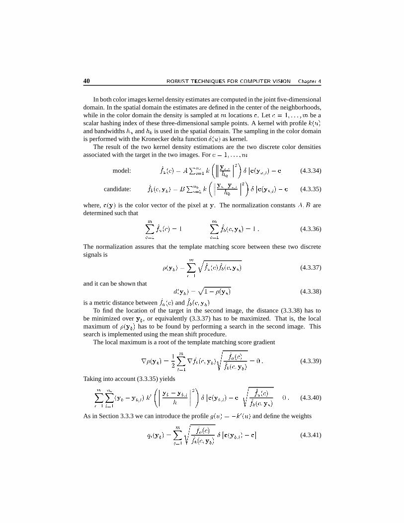
40 �� "! � � � ��#�%$'&�(*),+'-�.

In both color images kernel density estimates are computed in the joint five-dimensionaldomain. In the spatial domain the estimates are defined in the center of the neighborhoods,while in the color domain the density is sampled at = locations � . Let /�: &('('('<&)= be ascalar hashing index of these three-dimensional sample points. A kernel with profile � 3�� 6and bandwidths � � and � is used in the spatial domain. The sampling in the color domainis performed with the Kronecker delta function

� 3�� 6 as kernel.The result of the two kernel density estimations are the two discrete color densities

associated with the target in the two images. For /;: &('('('<&)=model:

�

� �43 6 / � � �� $ � � �� + � �� 3 � � � � 6 $�� (4.3.34)

candidate:�

� 3 &)� 6 / � � �� $ � � �� + � �� 3 � � � 6 $�� (4.3.35)

where, � 3 � 6 is the color vector of the pixel at � . The normalization constants � & � aredetermined such that ��

& � $�

� �43 6 /;:��& � $

�

� 3 &)� 6 / : ' (4.3.36)

The normalization assures that the template matching score between these two discretesignals is

) 3 � 6 /

��& � $

��

� �43 6 �

� 3 &)� 6 (4.3.37)

and it can be shown that � 3 � 6 /� : $ ) 3 � 6

(4.3.38)

is a metric distance between�

� �43 6 and�

� 3 &)� 6To find the location of the target in the second image, the distance (3.3.38) has to

be minimized over � , or equivalently (3.3.37) has to be maximized. That is, the localmaximum of ) 3 �

6has to be found by performing a search in the second image. This

search is implemented using the mean shift procedure.The local maximum is a root of the template matching score gradient

� ) 3 � 6 / :

-��& � $ �

�

� 3 &)� 6��

� �43 6�

� 3 &)� 6/�� ' (4.3.39)

Taking into account (3.3.35) yields��& � $

�� $ 3 � $ � � � 6 � �

� �� $ � � ��

�� +�� 3 � � � 6 $��

� �43 6�

� 3 &)� 6/4� ' (4.3.40)

As in Section 3.3.3 we can introduce the profile � 3�� 6 / $ � � 3�� 6 and define the weights

� � 3 � 6 /��& � $

� �

� �83 6�

� 3 &)� 6�� 3 � � � 6 $�� (4.3.41)

�+�� ) � �� .�� *&*) � �� ) � � &*) � �� 41

(a) (b)

(c) (d)

Figure 4.15. An example of the tracking algorithm. (a) The first frame of a color imagesequence with the target model manually defined as the marked elliptical region. (b) to (d)Localization of the target in different frames.

and obtain the iterative solution of (3.3.39) from

� � � � $� /� �� $ � � � � � � � � � � � � � � �

�� + �

� �� $ � � � � � � � � ��

�� + � (4.3.42)

which is a mean shift procedure, the only difference being that at each step the weights(3.3.41) are also computed.

In Figure 3.15 four frames of an image sequence are shown. The target model, definedin the first frame (Figure 3.15a), is successfully tracked throughout the sequence. As canbe seen, the localization is satisfactory in spite of the target candidates’ color distributionbeing significantly different from that of the model. While the model can be updated as wemove along the sequence, the main reason for the good performance is the small amount oftranslation of the target region between two consecutive frames. The search in the secondimage always starts from the location of the target model center in the first image. Themean shift procedure then finds the nearest mode of the template matching score, and withhigh probability this is the target candidate location we are looking for. See [19] for moreexamples and extensions of the tracking algorithm, and [14] for a version with automatic

42 �� "! � � � ��#�%$'&�(*),+'-�.

bandwidth selection.The robust solution of the location estimation problem presented in this section put the

emphasis on employing the least possible amount of a priori assumptions about the dataand belongs to the class of nonparametric techniques. Nonparametric techniques require alarger number of data points supporting the estimation process than their parametric coun-terparts. In parametric methods the data is more constrained, and as long as the model isobeyed the parametric methods are better in extrapolating over regions where data is notavailable. However, if the model is not correct a parametric method will still impose it atthe price of severe estimation errors. This important trade-off must be kept in mind whenfeature space analysis is used in a complex computer vision task.

�� !� "(��The linear errors-in-variables (EIV) regression model (Section 3.2.6) is employed for thediscussion of the different regression techniques. In this model the inliers are measured as

�� / � ��

��

�� 3�� &�� + � � 6 � /;: &('('('<&)��$ (4.4.1)

and their true values obey the constraints

� 3 �� 6 / ��

� $ � /4� � / : &('('('<&)��$ " � " / : � � � ' (4.4.2)

The number of inliers must be much larger than the number of free parameters of the model,��$�� . Nothing is assumed about the � $ ��$ outliers.

After a robust method selects the inliers they are often postprocessed with a nonrobusttechnique from the least squares (LS) family to obtain the final parameter. Therefore, westart by discussing the LS estimators. Next, the family of M-estimators is introduced andthe importance of the scale parameter related to the noise of the inliers is emphasized.

All the robust regression methods popular today in computer vision can be describedwithin the framework of M-estimation and thus their performance also depends on theaccuracy of the scale parameter. To avoid this deficiency, we approach M-estimation in adifferent way and introduce the pbM-estimator which does not require the user to providethe value of the scale.

In Section 3.2.5 it was shown that when a nonlinear EIV regression model is processedas a linear model in the carriers, the associated noise is heteroscedastic. Since the robustmethods discussed in this section assume the model (3.4.1) and (3.4.2), they return biasedestimates if employed for solving nonlinear EIV regression problems. However, this doesnot mean they should not be used! The role of any robust estimator is only to establish asatisfactory inlier/outlier dichotomy. As long as most of the inliers were recovered fromthe data, postprocessing with the proper nonlinear (and nonrobust) method will provide thecorrect estimates.

Regression in the presence of multiple structures in the data will not be consideredbeyond the particular case of two structures in the context of structured outliers. We willshow why all the robust regression methods fail to handle such data once the measurementnoise becomes large.

�+�� ) � �� .�� .�� )�� +��- + � � �� 43

Each of the regression techniques in this section is related to one of the objective func-tions described in Section 3.2.2. Using the same objective function location models canalso be estimated, but we will not discuss these location estimators. For example, manyof the traditional clustering methods belong to the least squares family [52, Sec.3.3.2], orthere is a close connection between the mean shift procedure and M-estimators of location[17].

�� /� */�� * � � � �/*�� " + �We have seen in Section 3.2.3 that the least squares family of estimators is not robustsince its objective function �%�� (3.2.22) is a symmetric function in all the measurements.Therefore, in this section will assume that the data contains only inliers, i.e., � / � $ .

The parameter estimates of the linear EIV regression model are obtained by solving theminimization

� �

�& �

� � / � �� :�

�� $ " � � $ � �� " + / � ��

:�

�� $ � 3 � �

6 + (4.4.3)

subject to (3.4.2). The minimization yields the total least squares (TLS) estimator. For anin-depth analysis of the TLS estimation see the book [112]. Related problems were alreadydiscussed in the nineteenth century [33, p.30], though the method most frequently usedtoday, based on the singular value decomposition (SVD) was proposed only in 1970 byGolub and Reinsch [37]. See the book [38] for the linear algebra background.

To solve the minimization problem (3.4.3) will define the � . � matrices of the mea-surements � and of the true values � �

� /�� $ � + �� / � � $ � � + � ��

� � ' (4.4.4)

Then (3.4.3) can be rewritten as

� �

�& �

� � / � �� "�� $�� " +� (4.4.5)

subject to� �

� $ �� / � � (4.4.6)

where�� 3��

6is a vector in � � of all ones (zeros), and "� " � is the Frobenius norm of the

matrix .The parameter

�is eliminated next. The data is centered by using the orthogonal pro-

jector matrix � / � � $ $�� which has the property �

�� / � � . It is easy to verify

that

� / �� /�� $ � + �� / � � $ :

�� $ �� / �� $ �� ' (4.4.7)

The matrix � � / �� is similarly defined. The parameter estimate

�

�is then obtained

from the minimization�

� / � �� " � $ � � " +� (4.4.8)

44 �� "! � � � ��#�%$'&�(*),+'-�.

subject to � �� /�� ' (4.4.9)

The constraint (3.4.9) implies that the rank of the true data matrix � � is only � $ : and that

the true�

spans its null space. Indeed, our linear model requires that the true data pointsbelong to a hyperplane in �

�which is a 3 � $ : 6 -dimensional affine subspace. The vector�

is the unit normal to this plane.The available measurements, however, are located nearby the hyperplane and thus the

measurement matrix � has full rank � . The solution of the TLS thus is the rank �/$ :

approximation of � . This approximation is obtained from the SVD of

� written as adyadic sum

� /��

� $ � � � � (4.4.10)

where the singular vectors � � , � / : &('('('(&)� and

� - , 9 / : &('('('<&� provide orthonormalbases for the four linear subspaces associated with the matrix

� [38, Sec.2.6.2], and � $ � � + � �� are the singular values of this full rank matrix.

The optimum approximation yielding the minimum Frobenius norm for the error is thetruncation of the dyadic sum (3.4.10) at � $ : terms [112, p.31]

� � /�� $� � $

� � � � (4.4.11)

where the matrix� � contains the centered corrected measurements

� � . These corrected mea-surements are the orthogonal projections of the available

� � on the hyperplane characterizedby the parameter estimates (Figure 3.6). The TLS estimator is also known as orthogonalleast squares.

The rank one null space of� � is spanned by

� � , the right singular vector associated withthe smallest singular value

� � of � [38, p.72]. Since

� � is a unit vector�

� / � � ' (4.4.12)

The estimate of�

is obtained by reversing the centering operation�

� / ��

�

�' (4.4.13)

The parameter estimates of the linear EIV model can be also obtained in a different,though completely equivalent way. We define the carrier vector

�by augmenting the vari-

ables with a constant� /�� $ : � � � + / � + � � � �� (4.4.14)

which implies that the covariance matrix of the carriers is singular. Using the � . 3 �� : 6

matrices� /�� $ � + ��

�� / � � $ � � + � ��

� ��

(4.4.15)

�+�� ) � �� .�� .�� )�� +��- + � � �� 45

the constraint (3.4.6) can be written as

� � � / � � � /�� " � " /;: � � � (4.4.16)

where the subscript ‘1’ of this parametrization in Section 3.2.6 was dropped.Using Lagrangian multipliers it can be shown that the parameter estimate

�� is theeigenvector of the generalized eigenproblem

��

� � /�� (4.4.17)

corresponding to the smallest eigenvalue � � � � . This eigenproblem is equivalent to thedefinition of the right singular values of the matrix

� [38, Sec.8.3]. The condition " �

� " / :is then imposed on the vector

�� .The first order approximation for the covariance of the parameter estimate is [70,

Sec.5.2.2] �� / �� + 3 ��

� $ � � � � 6 � (4.4.18)

where the pseudoinverse has to be used since the matrix has rank � following (3.4.17). Theestimate of the noise standard deviation is

�� + / � �� $ �� 3 �� 6 +��$�� : / � � � �� $�� : /

� +��$�� : (4.4.19)

where�� 3 �� 6 / �

��

� $ �

�are the residuals. The covariances for the other parametriza-

tions of the linear EIV model, � + (3.2.53) and � 1(3.2.55) can be obtained through error

propagation.Note that when computing the TLS estimate with either of the two methods, special

care has to be taken to execute all the required processing steps. The first approach startswith the data being centered, while in the second approach a generalized eigenproblem hasto be solved. These steps are sometimes neglected in computer vision algorithms.

In the traditional linear regression model only the variable # is corrupted by noise(3.2.36), and the constraint is

# �� / ��

� �� /

� 3 � �� 6 � /;: &('('('<&)� ' (4.4.20)

This model is actually valid for fewer computer vision problems (Figure 3.4) than it is usedin the literature. The corresponding estimator is the well known (ordinary) least squares(OLS)

�� / 3 �� 6

� $ �� / �� + 3 �

�� 6

� $ �� + / � �� $ # +�� $�� (4.4.21)

where

� � /� � $ � � + � ��

� �: : �� : ��

� / � # $ # + �� # �� ' (4.4.22)

46 �� "! � � � ��#�%$'&�(*),+'-�.

−10 0 10 20 30 40 50

0

20

40

60

80

100

120

140

160

180

y1

y 2

TrueOLSTLS

−40 −20 0 20 40−2

−1

0

1

2

3

4

5

6

7

8

α

θ 1

−40 −20 0 20 40−2

−1

0

1

2

3

4

5

6

7

8

α

θ 1

(a) (b) (c)

Figure 4.16. OLS vs. TLS estimation of a linear EIV model. (a) A typical trial. (b) Thescatterplot of the OLS estimates. A significant bias is present. (c) The scatterplot of theTLS estimates. The true parameter values correspond to the location marked ‘

�’.

If the matrix� � is poorly conditioned the pseudoinverse should be used instead of the full

inverse.In the presence of significant measurement noise, using the OLS estimator when the

data obeys the full EIV model (3.4.1) results in biased estimates [112, p.232]. This isillustrated in Figure 3.16. The � / � � data points are generated from the model

� "4$ � $ ",+ � � : /�� 3�� & � + � + 6 (4.4.23)

where � � 3 � 6 stands for independent normally distributed noise. Note that the constraint isnot in the Hessian normal form but�� $ "4$ � $ ",+ � /4� � $ / �

� /;: (4.4.24)

where, in order to compare the performance of the OLS and TLS estimators, the parameter� + was set to -1. When the traditional regression model is associated with this data it isassumed that

",+ � � # � / � $ "4$ � �0� � # � � � 3 � & � + 6 (4.4.25)

and the OLS estimator (3.4.21) is used to find�� $ and

�

�. The scatterplot of the result of 100

trials is shown in Figure 3.16b, and the estimates are far away from the true values.Either TLS estimation method discussed above can be employed to find the TLS esti-

mate. However, to eliminate the multiplicative ambiguity of the parameters the ancillaryconstraint

�� + / $ : has to be used. See [112, Sec. 2.3.2]. The TLS estimates are unbiasedand the scatterplot is centered on the true values (Figure 3.16c).

Throughout this section we have tacitly assumed that the data is not degenerate, i.e.,the measurement matrix � has full rank � . Both the TLS and OLS estimators can beadapted for the rank deficient case, though then the parameter estimates are no longerunique. Techniques similar to the ones described in this section yield minimum normsolutions. See [112, Chap.3] for the case of the TLS estimator.

�+�� ) � �� .�� .�� )�� +��- + � � �� 47

−2 −1 0 1 20

0.5

1

1.5

u

ρ bw(u

)

−2 −1.5 −1 −0.5 0 0.5 1 1.5 20

1

2

3

4

5

6

u

w(u

)

−2 −1 0 1 20

0.5

1

1.5

u

ρ zo(u

)

(a) (b) (c)

Figure 4.17. Redescending M-estimators. (a) Biweight loss function. (b) The weightfunction for biweight. (c) Zero-one loss function.

�� !"� * �� The robust equivalent of the least squares family are the M-estimators, first proposed in1964 by Huber as a generalization of the maximum likelihood technique in which contam-inations in the data distribution are tolerated. See [67] for an introduction to M-estimatorsand [49] for a more in-depth discussion. We will focus only on the class of M-estimatorsmost recommended for computer vision applications.

The robust formulation of (3.2.48) is

� �

�& �

� � / � �� :�

�� $*)

� :�

� 3 �� 6 � / � �� %( (4.4.26)

where � is a parameter which depends on � , the (unknown) scale of the inlier noise (3.4.1).With a slight abuse of notation � will also be called scale. The loss function ) 3�� 6 satisfiesthe following properties: nonnegative with ) 3 �

6 / � , even symmetric ) 3�� 6 / ) 3 $ � 6 , andnondecreasing with

� � � . For ) 3�� 6 / � + we obtain the LS objective function (3.4.3).The different M-estimators introduced in the statistical literature differ through the dis-

tribution assumed for the data. See [5] for a discussion in the context of computer vision.However, none of these distributions will provide an accurate model in a real application.Thus, the distinctive theoretical properties of different M-estimators are less relevant inpractice.

The redescending M-estimators are characterized by bounded loss functions

� � ) 3�� 6 � : � � �� : ) 3�� 6 / : � � � : ' (4.4.27)

As will be shown below, in a redescending M-estimator only those data points which areat distance less than � from the current fit are taken into account. This yields better outlierrejection properties than that of the M-estimators with nonredescending loss functions [69],[116].

The following class of redescending loss functions covers several important M-estimators

) 3�� 6 /�� : $ 3 : $ � + 6�� :: � � � : (4.4.28)

48 �� "! � � � ��#�%$'&�(*),+'-�.

where� / : & -.&�� . The loss functions have continuous derivatives up the 3 � $ : 6 -th order,

and a unique minimum in ) 3 �6 /�� .

Tukey’s biweight function ) �� 3�� 6 (Figure 3.17a) is obtained for� / � [67, p.295]. This

loss function is widely used in the statistical literature and was known at least a centurybefore robust estimation [40, p.151]. See also [42, vol.I, p.323]. The loss function obtainedfor

� / - will be denoted )� 3�� 6 . The case

� / : yields the skipped mean loss function, aname borrowed from robust location estimators [90, p.181]

)� � 3�� 6 / � � + � � �� :

: � � � : (4.4.29)

which has discontinuous first derivative. It is often used in vision applications, e.g., [109].In the objective function of any M-estimator the geometric distances (3.2.46) are nor-

malized by the scale � . Since ) 3�� 6 is an even function we do not need to use absolutevalues in (3.4.26). In redescending M-estimators the scale acts as a hard rejection thresh-old, and thus its value is of paramount importance. For the moment we will assume that asatisfactory value is already available for � , but will return to this topic in Section 3.4.3.

The M-estimator equivalent to the total least squares is obtained following either TLSmethod discussed in Section 3.4.1. For example, it can be shown that instead of (3.4.17),the M-estimate of � (3.4.16) is the eigenvector corresponding to the the smallest eigenvalueof the generalized eigenproblem

�� / � � (4.4.30)

where� �� .� is the diagonal matrix of the nonnegative weights

� � /��3�� 6 / :� ��) 3�� 6� � � � � � / �� 3 � � 6

�� /;: &('('('<&)��' (4.4.31)

Thus, in redescending M-estimators ��3�� 6 / � for� � � : , i.e., the data points whose

residual�� 3 �� 6 / �

��

� $ �

�relative to the current fit is larger than the scale threshold �

are discarded from the computations. The weights � �� 3�� 6 /�� 3 : $ � + 6 + derived from thebiweight loss function are shown in Figure 3.17b. The weigths derived from the )

� 3�� 6 lossfunction are proportional to the Epanechnikov kernel (3.3.17). For traditional regressioninstead of (3.4.21) the M-estimate is

�� /;3 �� 6

� $ �� ' (4.4.32)

The residuals�� 3 �� 6 in the weights � � require values for the parameter estimates. There-

fore, the M-estimates can be found only by an iterative procedure.

M-estimation with Iterative Weighted Least SquaresGiven the scale � .

1. Obtain the initial parameter estimate�� with total least squares.

2. Compute the weights � � � � $�� & � /4� & : &('('(' .

�+�� ) � �� .�� .�� )�� +��- + � � �� 49

3. Obtain the updated parameter estimates,�� $� .

4. Verify if " �� $� $ �� " is less than the tolerance. If yes, stop.

5. Replace�� with

�� $� . Return to Step 2.

For the traditional regression the procedure is identical. See [67, p.306]. A different wayof computing linear EIV regression M-estimates is described in [116].

The objective function minimized for redescending M-estimators is not convex, andtherefore the convergence to a global minimum is not guaranteed. Nevertheless, in practiceconvergence is always achieved [67, p.307], and if the initial fit and the chosen scale valueare adequate, the obtained solution is satisfactory. These two conditions are much more in-fluential than the precise nature of the employed loss function. Note that at every iterationall the data points regarded as inliers are processed, and thus there is no need for postpro-cessing, as is the case with the elemental subsets based numerical optimization techniquediscussed in Section 3.2.7.

In the statistical literature often the scale threshold � is defined as the product between�� the robust estimate for the standard deviation of the inlier noise (3.4.1) and a tuningconstant. The tuning constant is derived from the asymptotic properties of the simplestlocation estimator, the mean [67, p.296]. Therefore its value is rarely meaningful in realapplications. Our definition of redescending M-estimators avoids the problem of tuning byusing the inlier/outlier classification threshold as the scale parameter � .

The case� /�� in (3.4.28) yields the zero-one loss function

) � � 3�� 6 / � � � � �� :: � � � : (4.4.33)

shown in Figure 3.17c. The zero-one loss function is also a redescending M-estimator,however, is no longer continuous and does not have a unique minimum in � / � . Itis only mentioned since in Section 3.4.4 will be used to link the M-estimators to otherrobust regression techniques such as LMedS or RANSAC. The zero-one M-estimator isnot recommended in applications. The weight function (3.4.31) is nonzero only at theboundary and the corresponding M-estimator has poor local robustness properties. That is,in a critical data configuration a single data point can have a very large influence on theparameter estimates.

�� "(* � � ��!� + �/�� /"(* �!"(�� *,+ � ��!"� * ��Access to a reliable scale parameter � is a necessary condition for the minimization proce-dure (3.4.26) to succeed. The scale � is a strictly monotonically increasing function of �the standard deviation of the inlier noise. Since � is a nuisance parameter of the model, itcan be estimated together with

�and

�at every iteration of the M-estimation process [67,

p.307]. An example of a vision application employing this approach is [7]. However, thestrategy is less robust than providing the main estimation process with a fixed scale value[68]. In the latter case we talk about an M-estimator with auxiliary scale [69], [101].

50 �� "! � � � ��#�%$'&�(*),+'-�.

0 50 100 150 200 250

−100

−50

0

50

100

150

y1

y 2

0 50 100 150 200 250

−100

−50

0

50

100

150

y1

y 2

−4 −2 0 2 4 6 8 100

5

10

15

20

25

−4 −2 0 2 4 6 8 10−0.5

−0.4

−0.3

−0.2

−0.1

0

0.1

(a) (b) (c)

Figure 4.18. Sensitivity of the M-estimation to the�

� �� scale value. Dashed line–initialTLS fit. Solid line–biweight M-estimate. (a) /�: ' � . (b) / �%' � . (c) Overestimation ofthe scale in the presence of skewness. The median of the residuals is marked ‘+’ under thesorted data points. The bar below corresponds to

� �

� �� computed with / � .

Two different approaches can be used to obtain the scale prior to the parameter estima-tion. It can be either arbitrarily set by the user, or it can be derived from the data in a pilotestimation procedure. The first approach is widely used in the robust regression techniquesdeveloped within the vision community, such as RANSAC or Hough transform. The reasonis that it allows an easy way to tune a method to the available data. The second approach isoften adopted in the statistical literature for M-estimators and is implicitly employed in theLMedS estimator.

The most frequently used off-line scale estimator is the median absolute deviation(MAD), which is based on the residuals

�� 3 � � 6 relative to an initial (nonrobust TLS) fit

�

� �� / med�� 3 �� 6 $ med- �� 3 � - 6 � (4.4.34)

where is a constant to be set by the user. The MAD scale estimate measures the spread ofthe residuals around their median.

In the statistical literature the constant in (3.4.34) is often taken as /�: ' �� - � . How-ever, this value is used to obtain a consistent estimate for � when all the residuals obey anormal distribution [67, p.302]. In computer vision applications where often the percentageof outliers is high, the conditions is strongly violated. In the redescending M-estimators therole of the scale parameter � is to define the inlier/outlier classification threshold. The orderof magnitude of the scale can be established by computing the MAD expression, and therejection threshold is then set as a multiple of this value. There is no need for assumptionsabout the residual distribution. In [106] the standard deviation of the inlier noise

�� wascomputed as 1.4826 times a robust scale estimate similar to MAD, the minimum of theLMedS optimization criterion (3.4.36). The rejection threshold was set at : ' � � �� by assum-ing normally distributed residuals. The result is actually three times the computed MADvalue, and could be obtained by setting / � without any assumption about the distributionof the residuals.

The example in Figures 3.18a and 3.18b illustrates not only the importance of the scale

�+�� ) � �� .�� .�� )�� +��- + � � �� 51

value for M-estimation but also the danger of being locked into the nature of the residu-als. The data contains 100 inliers and 75 outliers, and as expected the initial TLS fit iscompletely wrong. When the scale parameter is set small by choosing for

�

� �� the con-stant /;: ' � , at convergence the final M-estimate is satisfactory (Figure 3.18a). When thescale

�

� �� is larger, / �%' � , the optimization process converges to a local minimum ofthe objective function. This minimum does not correspond to a robust fit (Figure 3.18b).Note that / �%' � is about the value of the constant which would have been used under theassumption of normally distributed inlier noise.

The location estimator employed for centering the residuals in (3.4.34) is the median,while the MAD estimate is computed with the second, outer median. However, the me-dian is a reliable estimator only when the distribution underlying the data is unimodal andsymmetric [49, p.29]. It is easy to see that for a heavily skewed distribution, i.e., with along tail on one side, the median will be biased toward the tail. For such distributions theMAD estimator severely overestimates the scale since the 50th percentile of the centeredresiduals is now shifted toward the boundary of the inlier distribution. The tail is most oftendue to outliers, and the amount of overestimation increases with both the decrease of theinlier/outlier ratio and the lengthening of the tail. In the example in Figure 3.18c the inliers(at the left) were obtained from a standard normal distribution. The median is 0.73 insteadof zero. The scale computed with / � is

�

� �� / � ' � � which in much larger than 2.5, areasonable value for the spread of the inliers. Again, should be chosen smaller.

Scale estimators which avoid centering the data were proposed in the statistical litera-ture [89], but they are computationally intensive and their advantage for vision applicationsis not immediate. We must conclude that the MAD scale estimate has to be used with carein robust algorithms dealing with real data. Whenever available, independent informationprovided by the problem at hand should be exploited to validate the obtained scale. The in-fluence of the scale parameter � on the performance of M-estimators can be entirely avoidedby a different approach toward this family of robust estimators. This will be discussed inSection 3.4.5.

�� * �� &- � * �� (�The origin of these three robust techniques was described in Section 3.1. Now will showthat they all can be expressed as M-estimators with auxiliary scale.

The least median of squares (LMedS) estimator is a least � -th order statistics estimator(3.2.22) for �+/ �'& - , and is the main topic of the book [90]. The LMedS estimates areobtained from � �

�& �

� � / � �� med� � 3 �� 6 + (4.4.35)

but in practice we can use

� �

�& �

� � / � �� med�� 3 � � 6 � ' (4.4.36)

The difference between the two definitions is largely theoretical, and becomes relevant onlywhen the number of data points � is small and even, while the median is computed as the

52 �� "! � � � ��#�%$'&�(*),+'-�.

0 50 100 150 200 250

−100

−50

0

50

100

150

y1

y 2

0 50 100 150 200

−40

−20

0

20

40

60

80

100

120

140

160

y1

y 2

(a) (b)

Figure 4.19. The difference between LMedS and RANSAC. (a) LMeds: finds the locationof the narrowest band containing half the data. (b) RANSAC: finds the location of thedensest band of width specified by the user.

average of the two central values [90, p.126]. Once the median is defined as the � �'& - � -th or-der statistics, the two definitions always yield the same solution. By minimizing the medianof the residuals, the LMedS estimator finds in the space of the data the narrowest cylinderwhich contains at least half the points (Figure 3.19a). The minimization is performed withthe elemental subsets based search technique discussed in Section 3.2.7.

The scale parameter � does not appear explicitly in the above definition of the LMedSestimator. Instead of setting an upper bound on the value of the scale, the inlier/outlierthreshold of the redescending M-estimator, in the LMedS a lower bound on the percent-age of inliers (fifty percent) is imposed. This eliminates the need for the user to guessthe amount of measurement noise, and as long as the inliers are in absolute majority, asomewhat better robust behavior is obtained. For example, the LMedS estimator will suc-cessfully process the data in Figure 3.18a.

The relation between the scale parameter and the bound on the percentage of inliers isrevealed if the equivalent condition of half the data points being outside of the cylinder, iswritten as

:�

�� $*) � �

� :�

� 3 �� 6 � / :- (4.4.37)

where ) � � is the zero-one loss function (3.4.33), and the scale parameter is now regarded asa function of the residuals � � � 3 � $ 6 &('('('(& � 3 � �

6 �. By defining � / med�

� � 3 � � 6 � the LMedS

estimator becomes

� �

�& �

� � / � �� 3 � $ 6 &('('('(& � 3 � �6 �

subject to (3.4.37). (4.4.38)

The new definition of LMedS is a particular case of the S-estimators, which while pop-ular in statistics, are not widely know in the vision community. For an introduction toS-estimators see [90, pp.135–143], and for a more detailed treatment in the context of EIV

�+�� ) � �� .�� .�� )�� +��- + � � �� 53

0 5 10 150

5

10

15

20

y

z

OLSLMedSFinal

0 5 10 150

5

10

15

20

y

z

OLSLMedSFinal

(a) (b)

Figure 4.20. The poor local robustness of the LMedS estimator. The difference betweenthe data sets in (a) and (b) is that the point 3 � & �%' � 6 was moved to 3 � & �%' - 6 .

models [116]. Let�

� be the minimum of � in (3.4.38). Then, it can be shown that

� �

�& �

� � / � �� :�

�� $ ) � �

� :�

�

� 3 � � 6 � (4.4.39)

and thus the S-estimators are in fact M-estimators with auxiliary scale.The value of

�

� can also be used as a scale estimator for the noise corrupting the inliers.All the observations made in Section 3.4.3 remain valid. For example, when the inliersare no longer the absolute majority in the data the LMedS fit is incorrect, and the residualsused to compute

�

� are not reliable.The Random Sample Consensus (RANSAC) estimator predates the LMedS [26]. Since

the same elemental subsets based procedure is used to optimize their objective function,sometimes the two techniques were mistakenly considered as being very similar, e.g., [75].However, their similarity should be judged examining the objective functions and not theway the optimization is implemented. In LMedS the scale is computed from a conditionset on the percentage of inliers (3.4.38). In RANSAC the following minimization problemis solved

� �

�& �

� � / � �� :�

�� $*) � �

� :�

�

� 3 � � 6 � given�

� (4.4.40)

that is, the scale is provided by the user. This is a critical difference. Note that (3.4.40)is the same as (3.2.30). Since it is relative easy to tune RANSAC to the data, it can alsohandle situations in which LMedS would already fail due to the large percentage of outliers(Figure 3.19b). Today RANSAC replaced LMedS in most vision applications, e.g., [65],[84], [108].

The use of the zero-one loss function in both LMedS and RANSAC yields very poorlocal robustness properties, as it is illustrated in Figure 3.20, an example inspired by [2].The � / : - data points appear to be a simple case of robust linear regression for whichthe traditional regression model (3.2.37) was used. The single outlier on the right corruptsthe least squares (OLS) estimator. The LMedS estimator, however, succeeds to recover

54 �� "! � � � ��#�%$'&�(*),+'-�.

the correct fit (Figure 3.20a), and the ordinary least squares postprocessing of the pointsdeclared inliers (Final), does not yield any further change. The data in Figure 3.20b seemsto be the same but now the LMedS, and therefore the postprocessing, completely failed.Actually the difference between the two data sets is that the point 3 � & �%' � 6 was moved to3 � & �%' - 6 .

The configuration of this data, however, is a critical one. The six points in the centercan be grouped either with the points which appear to be also inliers (Figure 3.20a), or withthe single outlier on the right (Figure 3.20b). In either case the grouping yields an absolutemajority of points which is preferred by LMedS. There is a hidden bimodality in the data,and as a consequence a delicate equilibrium exist between the correct and the incorrect fit.

In this example the LMedS minimization (3.4.36) seeks the narrowest band containingat least six data points. The width of the band is measured along the # axis, and its boundaryis always defined by two of the data points [90, p.126]. This is equivalent to using the zero-one loss function in the optimization criterion (3.4.39). A small shift of one of the pointsthus can change to which fit does the value of the minimum in (3.4.36) correspond to. Theinstability of the LMedS is discussed in a practical setting in [45], while more theoreticalissues are addressed in [23]. A similar behavior is also present in RANSAC due to (3.4.40).

For both LMedS and RANSAC several variants were introduced in which the zero-one loss function is replaced by a smooth function. Since then more point have nonzeroweights in the optimization, the local robustness properties of the estimators improve. Theleast trimmed squares (LTS) estimator [90, p.132]

� �

�& �

� � / � �� $ � 3 �

6 +� # � (4.4.41)

minimizes the sum of squares of the � smallest residuals, where � has to be provided bythe user. Similar to LMedS, the absolute values of the residuals can also be used.

In the first smooth variant of RANSAC the zero-one loss function was replaced with theskipped mean (3.4.29), and was called MSAC [109]. Recently the same loss function wasused in a maximum a posteriori formulation of RANSAC, the MAPSAC estimator [105].A maximum likelihood motivated variant, the MLESAC [107], uses a Gaussian kernel forthe inliers. Guided sampling is incorporated into the IMPSAC version of RANSAC [105].In every variant of RANSAC the user has to provide a reasonably accurate scale value fora satisfactory performance.

The use of zero-one loss function is not the only (or main) cause of the failure of LMedS(or RANSAC). In Section 3.4.7 we show that there is a more general problem in applyingrobust regression methods to multistructured data.

The only robust method designed to handle multistructured data is the Hough trans-form. The idea of Hough transform is to replace the regression problems in the inputdomain with location problems in the space of the parameters. Then, each significant modein the parameter space corresponds to an instance of the model in the input space. There isa huge literature dedicated to every conceivable aspect of this technique. The survey papers[50], [62], [82] contain hundreds of references.

Since we are focusing here on the connection between the redescending M-estimators

�+�� ) � �� .�� .�� )�� +��- + � � �� 55

and the Hough transform, only the randomized Hough transform (RHT) will be considered[56]. Their equivalence is the most straightforward, but the same equivalence also existsfor all the other variants of the Hough transform as well. The feature space in RHT is builtwith elemental subsets, and thus we have a mapping from � data points to a point in theparameter space.

Traditionally the parameter space is quantized into bins, i.e., it is an accumulator. Thebins containing the largest number of votes yield the parameters of the significant structuresin the input domain. This can be described formally as

� �

�& �� / � �� :

�� $ � � � � � � & �� &('('('<& �� 3 � � 6 � (4.4.42)

where �� 3�� 6 />: $ ) � � 3�� 6 and � � & �� &('('('(& �� define the size (scale) of a bin along

each parameter coordinate. The index � stands for the different local maxima. Note thatthe parametrization uses the polar angles as discussed in Section 3.2.6.

The definition (3.4.42) is that of a redescending M-estimator with auxiliary scale, wherethe criterion is a maximization instead of a minimization. The accuracy of the scale param-eters is a necessary condition for a satisfactory performance, an issue widely discussed inthe Hough transform literature. The advantage of distributing the votes around adjacentbins was recognized early [102]. Later the equivalence with M-estimators was also identi-fied, and the zero-one loss function is often replaced with a continuous function [61], [60],[80].

In this section we have shown that all the robust techniques popular in computer visioncan be reformulated as M-estimators. In Section 3.4.3 we have emphasized that the scalehas a crucial influence on the performance of M-estimators. In the next section we removethis dependence by approaching the M-estimators in a different way.

�� - �� !"� * ��The minimization criterion (3.4.26) of the M-estimators is rewritten as

� �

�& �

� � / � �� :�

�� $ �

� � �� $ �� 3�� 6 / �� : $ ) 3�� 6 � (4.4.43)

where � 3�� 6 is called the M-kernel function. Note that for a redescending M-estimator� 3�� 6 / � for

� � � : (3.4.27). The positive normalization constant �� assures that � 3�� 6 isa proper kernel (3.3.6).

Consider the unit vector�

defining a line through the origin in ��. The projections of

the � data points �� on this line have the one-dimensional (intrinsic) coordinates , � / ��

.Following (3.3.5) the density of the set of points , � , � / : &('('('<&)� , estimated with the kernel� 3�� 6 and the bandwidth

�� is

�

�� 3�, 6 / :

� �� $ �

�� $ ,��

�' (4.4.44)

56 �� "! � � � ��#�%$'&�(*),+'-�.

0 200 400 600 800 1000

−100

0

100

200

300

400

500

600

700

800

θ1

θ2

y1

y 2

200 300 400 500 600 700 800 900 10000

0.005

0.01

0.015

x

f θ 1(x)

200 300 400 500 600 700 800 900 10000

0.005

0.01

0.015

x

f θ 2(x)

(a) (b) (c)

Figure 4.21. M-estimation through projection pursuit. When the data in the rectangleis projected orthogonally on different directions (a), the mode of the estimated density issmaller for an arbitrary direction (b), than for the direction of the normal to the linearstructure (c).

Comparing (3.4.43) and (3.4.44) we can observe that if � 3�� 6 is taken as the kernel function,and

�� is substituted for the scale � , the M-estimation criterion becomes

�

� / � ��

�� 3�, 6

�(4.4.45)

�

� / � ��

� �

� 3�, 6 ' (4.4.46)

Given the M-kernel � 3�� 6 , the bandwidth parameter�� can be estimated from the data

according to (3.3.14). Since, as will be shown below, the value of the bandwidth has aweak influence on the the result of the M-estimation, for the entire family of redescendingloss functions (3.4.28) we can use

�� / �� $� 3 med�

� � �� $ med- �

�- � � ' (4.4.47)

The MAD estimator is employed in (3.4.47) but its limitations (Section 3.4.3) are of lessconcern in this context. Also, it is easy to recognize when the data is not corrupted since theMAD expression becomes too small. In this case, instead of the density estimation mostoften a simple search over the projected points suffices.

The geometric interpretation of the new definition of M-estimators is similar to that ofthe LMedS and RANSAC techniques shown in Figure 3.19. The closer is the projectiondirection to the normal of the linear structure, the tighter are grouped the projected inlierstogether which increases the mode of the estimated density (Figure 3.21). Again a cylin-der having the highest density in the data has to be located. The new approach is calledprojection based M-estimator, or pbM-estimator.

The relations (3.4.45) and (3.4.46) are the projection pursuit definition of an M-estimator.Projection pursuit was proposed by Friedman and Tukey in 1974 [30] to solve data analy-sis problems by seeking “interesting” low-dimensional projections of the multidimensionaldata. The informative value of a projection is measured with a projection index, such as thequantity inside the brackets in (3.4.45). The papers [48] [54] survey all the related topics.

�+�� ) � �� .�� .�� )�� +��- + � � �� 57

It should be emphasized that in the projection pursuit literature the name projection pursuitregression refers to a technique different from ours. There, a nonlinear additive model isestimated by adding a new term to the model after each iteration, e.g., [44, Sec.11.2].

When in the statistical literature a linear regression problem is solved through projectionpursuit, either nonrobustly [20], or robustly [90, p.143], the projection index is a scaleestimate. Similar to the S-estimators the solution is obtained by minimizing the scale, nowover the projection directions. The robust scale estimates, like the MAD (3.4.34) or themedian of the absolute value of the residuals (3.4.38), however, have severe deficienciesfor skewed distributions, as was discussed in Section 3.4.3. Thus, their use as projectionindex will not guarantee a better performance than that of the original implementation ofthe regression technique.

Projections were employed before in computer vision. In [81] a highly accurate im-plementation of the Hough transform was achieved by using local projections of the pixelsonto a set of directions. Straight edges in the image were then found by detecting the max-ima in the numerically differentiated projections. The � +�� estimator, proposed recently inthe statistical literature [92], solves a minimization problem similar to the kernel densityestimate formulation of M-estimators, however, the focus is on the parametric model of theinlier residual distribution.

The critical parameter of the redescending M-estimators is the scale � , the inlier/outlierselection threshold. The novelty of the pbM-estimator is the way the scale parameter is ma-nipulated. The pbM-estimator avoids the need of M-estimators for an accurate scale priorto estimation by using the bandwidth

�� as scale during the search for the optimal pro-jection direction. The bandwidth being an approximation of the AMISE optimal solution(3.3.13) tries to preserve the sensitivity of the density estimation process as the number ofdata points � becomes large. This is the reason for the �

� $� 3 factor in (3.4.47). Since��

is the outlier rejection threshold at this stage, a too small value increases the probability ofassigning incorrectly the optimal projection direction to a local alignment of points. Thus,it is recommended that once � becomes large, say � : � 1

, the computed bandwith valueis slightly increased by a factor which is monotonic in � .

After the optimal projection direction�

�was found, the actual inlier/outlier dichotomy

of the data is defined by analyzing the shape of the density around the mode. The nearestlocal minima on the left and on the right correspond in �

�, the space of the data, to the

transition between the inliers belonging to the sought structure (which has a higher density)and the background clutter of the outliers (which has a lower density). The locations of theminima define the values

�$ �

� + . Together with�

�they yield the two hyperplanes in �

�separating the inliers from the outliers. Note that the equivalent scale of the M-estimator is� /

� + $ �$ , and that the minima may not be symmetrically located relative to the mode.

The 2D data in the example in Figure 3.22a contains 100 inliers and 500 outliers. Thedensity of the points projected on the direction of the true normal (Figure 3.22b) has a sharpmode. Since the pbM-estimator deals only with one-dimensional densities, there is no needto use the mean shift procedure (Section 3.3.3) to find the modes, and a simple heuristicsuffices to define the local minima if they are not obvious.

The advantage of the pbM-estimator arises from using a more adequate scale in theoptimization. In our example, the

�

� �� scale estimate based on the TLS initial fit (to the

58 �� "! � � � ��#�%$'&�(*),+'-�.

−30 −20 −10 0 10 20 30

10

15

20

25

30

35

40

45

y1

y 2

−10 0 10 20 30 40 50 600

0.02

0.04

0.06

0.08

0.1

0.12

0.14

0.16

0.18

x

fθ(x)

| |

| |

(a) (b)

Figure 4.22. Determining the inlier/outlier dichotomy through the density of the projecteddata. (a) 2D data. Solid line: optimal projection direction. Dashed lines: boundaries ofthe detected inlier region. (b) The kernel density estimate of the projected points. Verticaldashed lines: the left and right local minima. The bar at the top is the scale

� �

� �� com-puted with / � . The bar below is

� ��

�, the size of the kernel support. Both are centered

on the mode.

whole data) and computed with / � , is about ten times larger than��

�, the bandwith

computed for the optimal projection direction (Figure 3.22b). When a redescending M-estimator uses

�

� �� , the optimization of the objective function is based on a too largeband, which almost certainly leads to a nonrobust behavior.

Sometimes the detection of the minima can be fragile. See the right minimum in Figure3.22b. A slight change in the projected location of a few data points could have changedthis boundary to the next, much more significant local minimum. However, this sensitivityis tolerated by pbM-estimator. First, by the nature of the projection pursuit many differentprojections are investigated and thus it is probable that at least one satisfactory band isfound. Second, from any reasonable inlier/outlier dichotomy of the data postprocessing ofthe points declared inliers (the region bounded by the two hyperplanes in �

�) can recover

the correct estimates. Since the true inliers are with high probability the absolute majorityamong the points declared inliers, the robust LTS estimator (3.4.41) can now be used.

The significant improvement in outlier tolerance of the pbM-estimator was obtained atthe price of replacing the iterative weighted least squares algorithm of the traditional M-estimation with a search in �

�for the optimal projection direction

�

�. This search can be

efficiently implemented using the simplex based technique discussed in Section 3.2.7.A randomly selected � -tuple of points (an elemental subset) defines the projection di-

rection�

, from which the corresponding polar angles � are computed (3.2.52). The vector� is the first vertex of the initial simplex in �� $ . The remaining � $ : vertices are then

defined as � /�� / : &('('('<& 3 � $ : 6 (4.4.48)

where� � � �� $ is a vector of 0-s except a 1 in the � -th element, and

�is a small angle.

While the value of�

can depend on the dimension of the space, using a constant value such

�+�� ) � �� .�� .�� )�� +��- + � � �� 59

as� / � & : - , seems to suffice in practice. Because

�is only a projection direction, during

the search the polar angles are allowed to wander outside the limits assuring a uniquemapping in (3.2.52). The simplex based maximization of the projection index (3.4.45)does not have to be extremely accurate, and the number of iterations in the search shouldbe relative small.

The projection based implementation of the M-estimators is summarized below.

The pbM-estimator

– Repeat � times:

1. choose an elemental subset (� -tuple) by random sampling;

2. compute the TLS estimate of�

;

3. build the initial simplex in the space of polar angles � ;

4. perform a simplex based direct search to find the local maximum of the projec-tion index.

– Find the left and right local minima around the mode of the density corresponding tothe largest projection index.

– Define the inlier/outlier dichotomy of the data. Postprocess the inliers to find thefinal estimates of

�and

�.

�� +(" * �!"(��The superior outlier tolerance of the pbM-estimator relative to other robust techniques isillustrated with two experiments. The percentage of inliers in the data is assumed unknownand can be significantly less than that of the outliers. Therefore the LMedS estimator cannotbe applied. It is shown in [107] that MLESAC and MSAC have very similar performanceand are superior to RANSAC. We have compared RANSAC and MSAC with the pbM-estimator.

In both experiments ground truth was available, and the true standard deviation of theinliers �� could be computed. The output of any robust regression is the inlier/outlierdichotomy of the data. Let the standard deviation of the points declared inliers measuredrelative to the true fit be

�� . The performance of the different estimators was comparedthrough the ratio

�� & �� . For a satisfactory result this ratio should be very close to one.The same number of computational units is used for all the techniques. A computational

unit is either processing of one elemental subset (RANSAC), or one iteration in the simplexbased direct search (pbM). The number of iterations in a search was restricted to 25, butoften it ended earlier. Thus, the amount of computations attributed to the pbM-estimator isan upper bound.

In the first experiment the synthetic data contained 100 inlier points obeying an eight-dimensional linear EIV regression model (3.4.2). The measurement noise was normallydistributed with covariance matrix � + �� . A variable percentage of outliers was uniformlydistributed within the bounding box of the region occupied in

� �by the inliers. The number

of computational units was 5000, i.e., RANSAC used 5000 elemental subsets while the

60 �� "! � � � ��#�%$'&�(*),+'-�.

10 20 30 40 50 60 70 80 900

2

4

6

8

10

12

percentage of outliers

σin

/σt

pbMMSACo

MSACm

RANSAC

Figure 4.23. RANSAC vs. pbM-estimator. The relative standard deviation of the residualsfunction of the percentage of outliers. Eight dimensional synthetic data. The employedscale threshold: RANSAC –

�

� �� ; MSACm –�

� �� ; MSACo – � � � � . The pbM-estimatorhas no tuning parameter. The vertical bars mark one standard deviation from the mean.

pbM-estimator initiated 200 local searches. For each experimental condition 100 trialswere run. The true sample standard deviation of the inliers � � , was computed in each trial.

The scale provided to RANSAC was the�

� �� , based on the TLS fit to the data andcomputed with / � . The same scale was used for MSAC. However, in an optimalsetting MSAC was also run with the scale � � � � / : ' � � �� . Note that this information is notavailable in practice! The graphs in Figure 3.23 show that for any percentage of outliers thepbM-estimator performs at least as well as MSAC tuned to the optimal scale. This superiorperformance is obtained in a completely unsupervised fashion. The only parameters usedby the pbM-estimator are the generic normalized amplitude values needed for the definitionof the local minima. They do not depend on the data or on the application.

In the second experiment, two far apart frames from the corridor sequence (Figures3.24a and 3.24b) were used to estimate the epipolar geometry from point correspondences.As was shown in Section 3.2.5 this is a nonlinear estimation problem, and therefore therole of a robust regression estimator based on the linear EIV model is restricted to selectingthe correct matches. Subsequent use of a nonlinear (and nonrobust) method can recover theunbiased estimates. Several such methods are discussed in [117].

The Harris corner detector [111, Sec.4.3] was used to establish the correspondences,from which 265 point pairs were retained. The histogram of the residuals computed asorthogonal distances from the ground truth plane in 8D, is shown in Figure 3.24c. The 105points in the central peak of the histogram were considered the inliers (Figure 3.24d). Theirstandard deviation was � � /�� ' � � .

The number of computational units was 15000, i.e., the pbM-estimator used 600 searches.Again, MSAC was tuned to either the optimal scale � � � � or to the scale derived from theMAD estimate,

�

� �� . The number true inliers among the points selected by an estimatorand the ratio between the standard deviation of the selected points and that of the true inlier

�+�� ) � �� .�� .�� )�� +��- + � � �� 61

−150 −100 −50 0 50 1000

10

20

30

40

50

60

70

80

90

100

residuals −3 −2 −1 0 1 2 3

0

2

4

6

8

10

12

14

16

18

inlier residuals

(a) (b) (c) (d)

Figure 4.24. Estimating the epipolar geometry for two frames of the corridor sequence. (a)and (b) The input images with the points used for correspondences marked. (c) Histogramof the residuals from the ground truth. (d) Histogram of the inliers.

noise are shown in the table below.

selected points/true inliers�� & ��

MSAC ( � �� ) 219/105 42.32MSAC ( � � � � ) 98/87 1.69

pbM 95/88 1.36

The pbM-estimator succeeds to recover the data of interest, and behaves like an opti-mally tuned technique from the RANSAC family. However, in practice the tuning infor-mation is not available.

�� 4� �� #�/� +("(�� The problem of multistructured data is not considered in this chapter, but a discussion of ro-bust regression cannot be complete without mentioning the issue of structured outliers. Thisis a particular case of multistructured data, when only two structures are present and theexample shown in Figure 3.3 is a typical case. For such data, once the measurement noisebecomes significant all the robust techniques, M-estimators (including the pbM-estimator),LMedS and RANSAC behave similarly to the nonrobust least squares estimator. This wasfirst observed for the LMedS [78], and was extensively analyzed in [98]. Here we describea more recent approach [9].

The true structures in Figure 3.3b are horizontal lines. The lower one contains 60points and the upper one 40 points. Thus, a robust regression method should return thelower structure as inliers. The measurement noise was normally distributed with covariance� + � + , � / : � . In Section 3.4.4 it was shown that all robust techniques can be regarded asM-estimators. Therefore we consider the expression

� 3 � � � & � 6 / :�

�� $*)

� "4$�� ",+ � � � � $ �� (4.4.49)

which defines a family of curves parameterized in�

and � of the line model (3.2.54) and

62 �� "! � � � ��#�%$'&�(*),+'-�.

0 20 40 60 800

0.2

0.4

0.6

0.8

1

s

ε(s;

α,β)

0 50 100 1500

0.2

0.4

0.6

0.8

1

sε(

s;α,

β)0 5 10 15 20 25

0.5

0.6

0.7

0.8

0.9

1

s

ε(s;

α,β)

0 5 10 15 20 250.5

0.6

0.7

0.8

0.9

1

s

ε(s;

α,β)

(a) (b) (c) (d)

Figure 4.25. Dependence of � 3 � � � & � 6 on the scale � for the data in Figure 3.3b. (a) Zero-one loss function. (b) Biweight loss function. (c) The top-left region of (a). (d) The top-leftregion of (b). Solid line – envelope � � � � 3 �

6. Dashed line – true parameters of the lower

structure. Dotdashed line – true parameters of the upper structure. Dotted line – leastsquares fit parameters.

in the scale � . The envelope of this family

� � � � 3 �6 / �� 3 � � � & � 6 (4.4.50)

represents the value of the M-estimation minimization criterion (3.4.26) as a function ofscale.

By definition, for a given value of � the curve � 3 � � � & � 6 can be only above (or touching)the envelope. The comparison of the envelope with a curve � 3 � � � & � 6 describes the relationbetween the employed

�& � and the parameter values minimizing (3.4.49). Three sets of

line parameters were investigated using the zero-one (Figure 3.25a) and the biweigth (Fig-ure 3.25b) loss functions: the true parameters of the two structures (

� / � � & : �,� � ��/ � & - ),and the least squares parameter estimates (

� �� & � �� ). The LS parameters yield a line sim-ilar to the one in Figure 3.3b, a nonrobust result.

Consider the case of zero-one loss function and the parameters of the lower structure(dashed line in Figure 3.25a). For this loss function � 3 � � � � & � & - 6 is the percentage ofdata points outside the horizontal band centered on " + / � � and with half-width � . Asexpected the curve has a plateau around � / � ' � corresponding to the band having one ofits boundaries in the transition region between the two structures. Once the band extendsinto the second structure � 3 � � � � & � & - 6 further decreases. The curve, however, is not onlyalways above the envelope, but most often also above the curve � 3 � � � �� & � �� 6 . See themagnified area of small scales in Figure 3.25c.

For a given value of the scale (as in RANSAC) a fit similar to least squares will beprefered since it yields a smaller value for (3.4.49). The measurement noise being large, aband containing half the data (as in LMedS) corresponds to a scale �

: - , the value aroundwhich the least squares fit begins to dominate the optimization (Figure 3.25a). As a resultthe LMedS will always fail (Figure 3.3b). Note also the very narrow range of scale values(around � / : � ) for which � 3 � � � � & � & - 6 is below � 3 � � � �� & � �� 6 . It shows how accuratelyhas the user to tune an estimator in the RANSAC family for a satisfactory performance.

The behavior for the biweight loss function is identical, only the curves are smoother

�+�� ) � �� .�� 63

due to the weigthed averages (Figures 3.25b and 3.25d). When the noise corrupting thestructures is small, in Figure 3.3a it is � / - , the envelope and the curve � 3 � � � � & � & - 6overlap for � � �

which suffices for the LMedS criterion. See [9] for details.We can conclude that multistructured data has to be processed first by breaking it into

parts in which one structure dominates. The technique in [8] combines several of the pro-cedures discussed in this chapter. The sampling was guided by local data density, i.e., itwas assumed that the structures and the background can be roughly separated by a globalthreshold on nearest neighbor distances. The pbM-estimator was employed as the estima-tion module, and the final parameters were obtained by applying adaptive mean shift to afeature space. The technique had a Hough transform flavor, though no scale parameterswere required. The density assumption, however, may fail when the structures are definedby linearizing a nonlinear problem, as it is often the case in 3D vision. Handling such mul-tistructured data embedded in a significant background clutter, remains an open question.

�� + �� "(��Our goal in this chapter was to approach robust estimation from the point of view of apractitioner. We have used a common statistical framework with solid theoretical founda-tions to discuss the different types and classes of robust estimators. Therefore, we did notdwell on techniques which have an excellent robust behavior but are of a somewhat ad-hocnature. These techniques, such as tensor voting [73], can provide valuable tools for solvingdifficult computer vision problems.

Another disregarded topic was the issue of diagnosis. Should an algorithm be able todetermine its own failure, one can already talk about robust behavior. When in the late1980’s robust methods became popular in the vision community, the paper [28] was oftenconsidered as the first robust work in the vision literature. The special issue [94] and thebook [6] contain representative collections of papers for the state-of-the-art today.

We have emphasized the importance of embedding into the employed model the leastpossible amount of assumptions necessary for the task at hand. In this way the developedalgorithms are more suitable for vision applications, where the data is often more complexthan in the statistical literature. However, there is a tradeoff to satisfy. As the modelbecomes less committed (more nonparametric), its power to extrapolate from the availabledata also decreases. How much is modeled rigorously and how much is purely data drivenis an important decision of the designer of an algorithm. The material presented in thischapter was intended to help in taking this decision.

� /0/�� + � � �� ,�/��I must thank to several of my current and former graduate students whose work is directlyor indirectly present on every page: Haifeng Chen, Dorin Comaniciu, Bogdan Georgescu,Yoram Leedan and Bogdan Matei. Long discussions with Dave Tyler from the StatisticsDepartment, Rutgers University helped to crystallize many of the ideas described in thispaper. Should they be mistaken, the blame is entirely mine. Preparation of the material wassupported by the National Science Foundation under the grant IRI 99-87695.

64 �� "! � � � ��#�%$'&�(*),+'-�.

� � � � � � � ��

[1] J. Addison. Pleasures of imagination. Spectator, 6, No. 411, June 21, 1712.

[2] G. Antille and H. El May. The use of slices in the LMS and the method of densityslices: Foundation and comparison. In Y. Dodge and J. Whittaker, editors, Proc. 10thSymp. Computat. Statist., Neuchatel, volume I, pages 441–445. Physica-Verlag, 1992.

[3] T. Arbel and F. P. Ferrie. On sequential accumulation of evidence. Intl. J. of ComputerVision, 43:205–230, 2001.

[4] P. J. Besl, J. B. Birch, and L. T. Watson. Robust window operators. In Proceedings of the2nd International Conference on Computer Vision, pages 591–600, Tampa, FL, December1988.

[5] M.J. Black and A. Rangarajan. On the unification of line processes, outlier rejection,and robust statistics with applications in early vision. Intl. J. of Computer Vision, 19:57–91,1996.

[6] K. J. Bowyer and P. J. Phillips, editors. Empirical evaluation techniques in computervision. IEEE Computer Society, 1998.

[7] K. L. Boyer, M. J. Mirza, and G. Ganguly. The robust sequential estimator: A generalapproach and its application to surface organization in range data. IEEE Trans. PatternAnal. Machine Intell., 16:987–1001, 1994.

[8] H. Chen and P. Meer. Robust computer vision through kernel density estimation. InProc. European Conf. on Computer Vision, Copenhagen, Denmark, volume I, pages 236–250, May 2002.

[9] H. Chen, P. Meer, and D. E. Tyler. Robust regression for data with multiple structures.In 2001 IEEE Conference on Computer Vision and Pattern Recognition, volume I, pages1069–1075, Kauai, HI, December 2001.

[10] Y. Cheng. Mean shift, mode seeking, and clustering. IEEE Trans. Pattern Anal. Ma-chine Intell., 17:790–799, 1995.

65

66 � � � � � �- &�(�$��

[11] E. Choi and P. Hall. Data sharpening as a prelude to density estimation. Biometrika,86:941–947, 1999.

[12] W. Chojnacki, M. J. Brooks, A. van den Hengel, and D. Gawley. On the fitting ofsurfaces to data with covariances. IEEE Trans. Pattern Anal. Machine Intell., 22:1294–1303, 2000.

[13] C.M. Christoudias, B. Georgescu, and P. Meer. Synergism in low-level vision. In Proc.16th International Conference on Pattern Recognition, Quebec City, Canada, volume IV,pages 150–155, August 2002.

[14] R. T. Collins. Mean-shift blob tracking through scale space. In Proc. IEEE Conf. onComputer Vision and Pattern Recognition, Madison, WI, volume II, pages 234–240, 2003.

[15] D. Comaniciu. An algorithm for data-driven bandwidth selection. IEEE Trans. PatternAnal. Machine Intell., 25:281–288, 2003.

[16] D. Comaniciu and P. Meer. Distribution free decomposition of multivariate data. Pat-tern Analysis and Applications, 2:22–30, 1999.

[17] D. Comaniciu and P. Meer. Mean shift: A robust approach toward feature space anal-ysis. IEEE Trans. Pattern Anal. Machine Intell., 24:603–619, 2002.

[18] D. Comaniciu, V. Ramesh, and P. Meer. The variable bandwidth mean shift and data-driven scale selection. In Proc. 8th Intl. Conf. on Computer Vision, Vancouver, Canada,volume I, pages 438–445, July 2001.

[19] D. Comaniciu, V. Ramesh, and P. Meer. Kernel-based object tracking. IEEE Trans.Pattern Anal. Machine Intell., 25:564–577, 2003.

[20] D. Donoho, I. Johnstone, P. Rousseeuw, and W. Stahel. Discussion: Projection pursuit.Annals of Statistics, 13:496–500, 1985.

[21] R.O. Duda, P.E. Hart, and D.G. Stork. Pattern Classification. Wiley, second edition,2001.

[22] B. Efron and R. Tibshirani. An Introduction to the Bootstrap. Chapman & Hall, NewYork, 1993.

[23] S. P. Ellis. Instability of least squares, least absolute deviation and least median ofsquares linear regression. Statistical Science, 13:337–350, 1998.

[24] O. Faugeras. Three-Dimensional Computer Vision. MIT Press, 1993.

[25] M.A. Fischler and R.C. Bolles. Random sample consensus: A paradigm for modelfitting with applications to image analysis and automated cartography. In DARPA ImageUnderstanding Workshop, pages 71–88, University of Maryland, College Park, April 1980.

� � � � � �- &�(�$�� 67

[26] M.A. Fischler and R.C. Bolles. Random sample consensus: A paradigm for model fit-ting with applications to image analysis and automated cartography. Comm. Assoc. Comp.Mach, 24(6):381–395, 1981.

[27] A.W. Fitzgibbon, M. Pilu, and R.B. Fisher. Direct least square fitting of ellipses. IEEETrans. Pattern Anal. Machine Intell., 21:476–480, 1999.

[28] W. Forstner. Reliability analysis of parameter estimation in linear models with applica-tions to mensuration problems in computer vision. Computer Vision, Graphics, and ImageProcessing, 40:273–310, 1987.

[29] W. T. Freeman, E. G. Pasztor, and O. W. Carmichael. Learning in low-level vision.Intl. J. of Computer Vision, 40:25–47, 2000.

[30] J. H. Friedman and J. W. Tukey. A projection pursuit algorithm for exploratory dataanalysis. IEEE Trans. Comput., 23:881–889, 1974.

[31] K. Fukunaga. Introduction to Statistical Pattern Recognition. Academic Press, secondedition, 1990.

[32] K. Fukunaga and L. D. Hostetler. The estimation of the gradient of a density function,with applications in pattern recognition. IEEE Trans. Information Theory, 21:32–40, 1975.

[33] W. Fuller. Measurement Error Models. Wiley, 1987.

[34] B. Georgescu and P. Meer. Balanced recovery of 3D structure and camera motion fromuncalibrated image sequences. In Proc. European Conf. on Computer Vision, Copenhagen,Denmark, volume II, pages 294–308, 2002.

[35] B. Georgescu, I. Shimshoni, and P. Meer. Mean shift based clustering in high dimen-sions: A tecture classification example. In Proc. 9th Intl. Conf. on Computer Vision, Nice,France, October 2003.

[36] E. B. Goldstein. Sensation and Perception. Wadsworth Publishing Co., 2nd edition,1987.

[37] G. H. Golub and C. Reinsch. Singular value decomposition and least squares solutions.Number. Math., 14:403–420, 1970.

[38] G. H. Golub and C. F. Van Loan. Matrix Computations. John Hopkins U. Press, secondedition, 1989.

[39] P. Hall, T.C. Hui, and J.S. Marron. Improved variable window kernel estimates ofprobability densities. Annals of Statistics, 23:1–10, 1995.

[40] R. Hampel, E.M. Ronchetti, P.J. Rousseeuw, and W.A. Stahel. Robust Statistics. TheApproach Based on Influence Function. Wiley, 1986.

68 � � � � � �- &�(�$��

[41] R. M. Haralick and H. Joo. 2D-3D pose estimation. In Proceedings of the 9th In-ternational Conference on Pattern Recognition, pages 385–391, Rome, Italy, November1988.

[42] R. M. Haralick and L. G. Shapiro. Computer and Robot Vision. Addison-Wesley, 1992.

[43] R. Hartley and A. Zisserman. Multiple View Geometry in Computer Vision. CambridgeUniversity Press, 2000.

[44] T. Hastie, R. Tibshirani, and J. Friedman. The Elements of Statistical Learning.Springer, 2001.

[45] T. P. Hettmansperger and S. J. Sheather. A cautionary note on the method of leastmedian of squares. The American Statistician, 46:79–83, 1992.

[46] P.V.C. Hough. Machine analysis of bubble chamber pictures. In International Con-ference on High Energy Accelerators and Instrumentation, Centre Europeenne pour laRecherch Nucleaire (CERN), 1959.

[47] P.V.C. Hough. Method and means for recognizing complex patterns. US Patent3,069,654, December 18, 1962.

[48] P. J. Huber. Projection pursuit (with discussion). Annals of Statistics, 13:435–525,1985.

[49] P. J. Huber. Robust Statistical Procedures. SIAM, second edition, 1996.

[50] J. Illingworth and J. V. Kittler. A survey of the Hough transform. Computer Vision,Graphics, and Image Processing, 44:87–116, 1988.

[51] M. Isard and A. Blake. Condensation - Conditional density propagation for visualtracking. Intl. J. of Computer Vision, 29:5–28, 1998.

[52] A. K. Jain and R. C. Dubes. Algorithms for Clustering Data. Prentice Hall, 1988.

[53] J.M. Jolion, P. Meer, and S. Bataouche. Robust clustering with applications in com-puter vision. IEEE Trans. Pattern Anal. Machine Intell., 13:791–802, 1991.

[54] M. C. Jones and R. Sibson. What is projection pursuit? (with discussion). J. RoyalStat. Soc. A, 150:1–37, 1987.

[55] B. Julesz. Early vision and focal attention. Rev. of Modern Physics, 63:735–772, 1991.

[56] H. Kalviainen, P. Hirvonen, L. Xu, and E. Oja. Probabilistic and nonprobabilisticHough transforms: Overview and comparisons. Image and Vision Computing, 13:239–252, 1995.

[57] K. Kanatani. Statistical bias of conic fitting and renormalization. IEEE Trans. PatternAnal. Machine Intell., 16:320–326, 1994.

� � � � � �- &�(�$�� 69

[58] K. Kanatani. Statistical Optimization for Geometric Computation: Theory and Prac-tice. Elsevier, 1996.

[59] D.Y. Kim, J.J. Kim, P. Meer, D. Mintz, and A. Rosenfeld. Robust computer vision:The least median of squares approach. In Proceedings 1989 DARPA Image UnderstandingWorkshop, pages 1117–1134, Palo Alto, CA, May 1989.

[60] N. Kiryati and A. M. Bruckstein. What’s in a set of points? IEEE Trans. Pattern Anal.Machine Intell., 14:496–500, 1992.

[61] N. Kiryati and A. M. Bruckstein. Heteroscedastic Hough transform (HtHT): An effi-cient method for robust line fitting in the ‘errors in the variables’ problem. Computer Visionand Image Understanding, 78:69–83, 2000.

[62] V. F. Leavers. Survey: Which Hough transform? Computer Vision, Graphics, andImage Processing, 58:250–264, 1993.

[63] K.M. Lee, P. Meer, and R.H. Park. Robust adaptive segmentation of range images.IEEE Trans. Pattern Anal. Machine Intell., 20:200–205, 1998.

[64] Y. Leedan and P. Meer. Heteroscedastic regression in computer vision: Problems withbilinear constraint. Intl. J. of Computer Vision, 37:127–150, 2000.

[65] A. Leonardis and H. Bischof. Robust recognition using eigenimages. Computer Visionand Image Understanding, 78:99–118, 2000.

[66] R. M. Lewis, V. Torczon, and M. W. Trosset. Direct search methods: Then and now. J.Computational and Applied Math., 124:191–207, 2000.

[67] G. Li. Robust regression. In D. C. Hoaglin, F. Mosteller, and J. W. Tukey, editors,Exploring Data Tables, Trends, and Shapes, pages 281–343. Wiley, 1985.

[68] R. A. Maronna and V. J. Yohai. The breakdown point of simulataneous general Mestimates of regression and scale. J. of Amer. Stat. Assoc., 86:699–703, 1991.

[69] R. D. Martin, V. J. Yohai, and R. H. Zamar. Min-max bias robust regression. Annals ofStatistics, 17:1608–1630, 1989.

[70] B. Matei. Heteroscedastic Errors-in-Variables Models in Computer Vision. PhD thesis,Department of Electrical and Computer Engineering, Rutgers University, 2001. Availableat http://www.caip.rutgers.edu/riul/research/theses.html.

[71] B. Matei and P. Meer. Bootstrapping errors-in-variables models. In B. Triggs, A. Zis-serman, and R. Szelisky, editors, Vision Algorithms: Theory and Practice, pages 236–252.Springer, 2000.

[72] B. Matei and P. Meer. Reduction of bias in maximum likelihood ellipse fitting. In15th International Conference on Computer Vision and Pattern Recog., volume III, pages802–806, Barcelona, Spain, September 2000.

70 � � � � � �- &�(�$��

[73] G. Medioni and P. Mordohai. The tensor voting framework. In G. Medioni and S. B.Kang, editors, Emerging Topics in Computer Vision. Prentice Hall, 2004.

[74] P. Meer and B. Georgescu. Edge detection with embedded confidence. IEEE Trans.Pattern Anal. Machine Intell., 23:1351–1365, 2001.

[75] P. Meer, D. Mintz, D. Y. Kim, and A. Rosenfeld. Robust regression methods in com-puter vision: A review. Intl. J. of Computer Vision, 6:59–70, 1991.

[76] J. M. Mendel. Lessons in Estimation Theory for Signal Processing, Communications,and Control. Prentice Hall, 1995.

[77] J. V. Miller and C. V. Stewart. MUSE: Robust surface fitting using unbiased scaleestimates. In CVPR96, pages 300–306, June 1996.

[78] D. Mintz, P. Meer, and A. Rosenfeld. Consensus by decomposition: A paradigm forfast high breakdown point robust estimation. In Proceedings 1991 DARPA Image Under-standing Workshop, pages 345–362, La Jolla, CA, January 1992.

[79] J. A. Nelder and R. Mead. A simplex method for function minimization. ComputerJournal, 7:308–313, 1965.

[80] P. L. Palmer, J. Kittler, and M. Petrou. An optimizing line finder using a Hough trans-form algorithm. Computer Vision and Image Understanding, 67:1–23, 1997.

[81] D. Petkovic, W. Niblack, and M. Flickner. Projection-based high accuracy measure-ment of straight line edges. Machine Vision and Appl., 1:183–199, 1988.

[82] P. D. Picton. Hough transform references. Internat. J. of Patt. Rec and Artific. Intell.,1:413–425, 1987.

[83] W. H. Press, S. A. Teukolsky, W. T. Vetterling, and B. P. Flannery. Numerical Recipesin C. Cambridge University Press, second edition, 1992.

[84] P. Pritchett and A. Zisserman. Wide baseline stereo matching. In 6th InternationalConference on Computer Vision, pages 754–760, Bombay, India, January 1998.

[85] Z. Pylyshyn. Is vision continuous with cognition? The case for cognitive impene-trability of visual perception. Behavioral and Brain Sciences, 22:341–423, 1999. (withcomments).

[86] S.J. Raudys and A.K. Jain. Small sample size effects in statistical pattern recognition:Recommendations for practitioners. IEEE Trans. Pattern Anal. Machine Intell., 13:252–264, 1991.

[87] P. J. Rousseeuw. Least median of squares regression. J. of Amer. Stat. Assoc., 79:871–880, 1984.

[88] P. J. Rousseeuw. Unconventional features of positive-breakdown estimators. Statistics& Prob. Letters, 19:417–431, 1994.

� � � � � �- &�(�$�� 71

[89] P. J. Rousseeuw and C. Croux. Alternatives to the median absolute deviation. J. ofAmer. Stat. Assoc., 88:1273–1283, 1993.

[90] P. J. Rousseeuw and A. M. Leroy. Robust Regression and Outlier Detection. Wiley,1987.

[91] D. Ruppert and D. G. Simpson. Comment on “Unmasking Multivariate Outliers andLeverage Points”, by P. J. Rousseeuw and B. C. van Zomeren. J. of Amer. Stat. Assoc.,85:644–646, 1990.

[92] D. W. Scott. Parametric statistical modeling by minimum integrated square error. Tech-nometrics, 43:247–285, 2001.

[93] B. W. Silverman. Density Estimation for Statistics and Data Analysis. Chapman &Hall, 1986.

[94] Special Issue. Performance evaluation. Machine Vision and Appl., 9(5/6), 1997.

[95] Special Issue. Robust statistical techniques in image understanding. Computer Visionand Image Understanding, 78, April 2000.

[96] G. Speyer and M. Werman. Parameter estimates for a pencil of lines: Bounds andestimators. In Proc. European Conf. on Computer Vision, Copenhagen, Denmark, volume I,pages 432–446, 2002.

[97] L. Stark and K.W. Bowyer. Achieving generalized object recognition through reason-ing about association of function to structure. IEEE Trans. Pattern Anal. Machine Intell.,13:1097–1104, 1991.

[98] C. V. Stewart. Bias in robust estimation caused by discontinuities and multiple struc-tures. IEEE Trans. Pattern Anal. Machine Intell., 19:818–833, 1997.

[99] C. V. Stewart. Robust parameter estimation in computer vision. SIAM Reviews,41:513–537, 1999.

[100] C.V. Stewart. Minpran: A new robust estimator for computer vision. IEEE Trans.Pattern Anal. Machine Intell., 17:925–938, 1995.

[101] K. S. Tatsuoka and D. E. Tyler. On the uniqueness of S and constrained M-functionalsunder non-elliptical distributions. Annals of Statistics, 28:1219–1243, 2000.

[102] P. R. Thrift and S. M. Dunn. Approximating point-set images by line segments usinga variation of the Hough transform. Computer Vision, Graphics, and Image Processing,21:383–394, 1983.

[103] A. Tirumalai and B. G. Schunk. Robust surface approximation using least median ofsquares. Technical Report CSE-TR-13-89, Artificial Intelligence Laboratory, 1988. Uni-versity of Michigan, Ann Arbor.

72 � � � � � �- &�(�$��

[104] B. Tordoff and D.W. Murray. Guided sampling and consensus for motion estimation.In 7th European Conference on Computer Vision, volume I, pages 82–96, Copenhagen,Denmark, May 2002.

[105] P. H. S. Torr and C. Davidson. IMPSAC: Synthesis of importance sampling andrandom sample consensus. IEEE Trans. Pattern Anal. Machine Intell., 25:354–364, 2003.

[106] P. H. S. Torr and D. W. Murray. The development and comparison of robust methodsfor estimating the fundamental matrix. Intl. J. of Computer Vision, 24:271–300, 1997.

[107] P. H. S. Torr and A. Zisserman. MLESAC: A new robust estimator with applicationto estimating image geometry. Computer Vision and Image Understanding, 78:138–156,2000.

[108] P. H. S. Torr, A. Zisserman, and S. J. Maybank. Robust detection of degenerateconfigurations while estimating the fundamental matrix. Computer Vision and Image Un-derstanding, 71:312–333, 1998.

[109] P.H.S. Torr and A. Zisserman. Robust computation and parametrization of multi-ple view relations. In 6th International Conference on Computer Vision, pages 727–732,Bombay, India, January 1998.

[110] A. Treisman. Features and objects in visual processing. Scientific American, 254:114–125, 1986.

[111] E. Trucco and A. Verri. Introductory Techniques for 3-D Computer Vision. PrenticeHall, 1998.

[112] S. Van Huffel and J. Vandewalle. The Total Least Squares Problem. ComputationalAspects and Analysis. Society for Industrial and Applied Mathematics, 1991.

[113] M. P. Wand and M.C. Jones. Kernel Smoothing. Chapman & Hall, 1995.

[114] I. Weiss. Line fitting in a noisy image. IEEE Trans. Pattern Anal. Machine Intell.,11:325–329, 1989.

[115] M. H. Wright. Direct search methods: Once scorned, now respectable. In D. H.Griffiths and G. A. Watson, editors, Numerical Analysis 1995, pages 191–208. Addison-Wesley Longman, 1996.

[116] R. H. Zamar. Robust estimation in the errors-in-variables model. Biometrika, 76:149–160, 1989.

[117] Z. Zhang. Determining the epipolar geometry and its uncertainty: A review. Intl. J.of Computer Vision, 27:161–195, 1998.

[118] Z.Y. Zhang. Parameter-estimation techniques: A tutorial with application to conicfitting. Image and Vision Computing, 15:59–76, 1997.

ROBUST TECHNIQUES FOR COMPUTER VISION

Documents