Normalization and Transformation Techniques for Robust ...

17

Normalization and Transformation Techniques for Robust Speaker Recognition

Dalei Wu, Baojie Li and Hui Jiang Department of Computer Science and Engineering, York University,

Toronto, Ont., Canada

1. Introduction

Recognizing a person’s identity by voice is one of intrinsic capabilities for human beings.

Automatic speaker recognition (SR) is a computational task for computers to perform a similar

task, i.e., to recognize human identity based on voice characteristics. By taking a voice signal as

input, automatic speaker recognition systems extract distinctive information from the input,

usually using signal processing techniques, and then recognize a speaker’s identity based on

the extracted information by comparing it with the knowledge previously learned at a training

stage. The extracted distinctive information is encoded in a sequence of feature vectors, which

is referred to as frame sequence. In terms of purposes of applications, SR tasks can be classified

into two categories: speaker identification and speaker verification.

Speaker identification (SI) is an application to recognize a speaker’s identity from a given

group of enrolled speakers. If a speaker is assumed to be always in the enrolled speaker group,

it is referred to as the closed set speaker identification; Otherwise, it is referred to as the open

set speaker identification. On the other hand, speaker verification (SV) is an application to

verify a speaker identity by simply making a binary decision, i.e., answering an identity

question by either yes or no. SV is one of biometric authentication techniques, along with

others, such as fingerprint (Jain et al., 2000) or iris authentication (Daugman, 2004).

In the past decades, a variety of techniques for modeling and decision-making have been proposed to speaker recognition and proved to work effectively to some extent. In this chapter, we shall not delve too much into the survey for these techniques, but rather focus on normalization and transformation techniques for robust speaker recognition. For a tutorial of the conventional modeling and recognizing techniques, the reader can refer to (Campbell, 1999; Reynolds, 2002; Bimbot et al., 2004). Here, we just make it explicit that among many techniques the most successful ones are Gaussian mixture model (GMM) and hidden Markov model (HMM). With GMM/HMM, high performance can be achieved in sound working conditions, such as in a quiet environment, and for broadband speech. However, these techniques run into problems in realistic applications, since many realistic applications can not always satisfy the requirements of clean and quiet environments. Instead, the working environments are more adverse, noisy and sometimes in narrow-band width, for instance, telephony speech. Most SR systems degrade their performance substantially in adverse conditions. To deal with the difficulties, robust speaker recognition is such a topic for study. O

pen

Acc

ess

Dat

abas

e w

ww

.inte

chw

eb.o

rg

Source: Speech Recognition, Technologies and Applications, Book edited by: France Mihelič and Janez Žibert, ISBN 978-953-7619-29-9, pp. 550, November 2008, I-Tech, Vienna, Austria

www.intechopen.com

Speech Recognition, Technologies and Applications

312

As robust speech recognition does, robust speaker recognition is concerned with improving performance of speaker recognition systems in adverse or noisy (additive and convolutional noise) conditions and making systems more robust to a variety of mismatch conditions. The essential problem for robust speaker recognition is the existence of mismatch between training and test stages. As the most prominent SR systems adopt statistical methods as their main modeling technique, such as GMM and HMM, these systems confront the common issues held by all the statistical modeling methods, i.e., vulnerable to any mismatch between the training and test stages. In noisy environments, the mismatch inevitably becomes larger than in clean conditions, due to a larger range of data variance caused by the interference of ambient noise. Hence, how to deal with a variety of types of mismatch becomes a crucial issue for robust speaker recognition. Much research has been devoted for solving the problem of mismatch in last decades. To summarize these techniques for robust speaker recognition is the main purpose of this chapter. To the authors’ best knowledge, so far there is no any article in the literature to survey this subject, although some more general tutorials for speaker recognition exist (Campbell, 1999; Reynolds, 2002; Bimbot et al., 2004). Different from these tutorials, we shall only focus on reviewing the techniques that aim to reduce or at least alleviate the mismatch for robust speaker recognition in terms of normalization and transformation at two levels, i.e., normalization/transformation at the score level and normalization/transformation at the feature level. In order to avoid confusion and also be easier to discuss directions for future work in later sections, we shall explicitly explain the terms of normalization and transformation we used above. Consistent to its general meaning, normalization, we mean here, is a sort of mapping functions, which map from one domain to another. The mapped images in the new domain often hold a property of zero mean and unit variance in a general sense. By transformation, we refer to more general mapping functions which do not possess the property of zero mean and unit variance. Although these two terms are distinctive in subtle meanings, they are sometimes used by different authors, depending on their preferences. In this chapter, we may use them exchangeably without confusion. Just by using these techniques, speaker recognition systems become more robust to realistic environments. Normalization at the score level is one of noise reduction methods, which normalizes log-

likelihood scores at the decision stage. A log-likelihood score, for short, score, is a

logarithmic probability for a given input frame sequence generated based on a statistical

model. Since the calculated log-likelihood scores depend on test environments, the purpose

of normalization aims at reducing this mismatch between a training and test set by adapting

the distribution of scores to test environments, for instance, by shifting the means and

changing the range of variance of the score distribution. The normalization techniques at the

score level are mostly often used in speaker verification, though they can be also applied to

speaker identification, because they are extremely powerful to reduce the mismatch between

the claimant speaker and its impostors. Thus, in our introduction to normalization

techniques at the score levels, we shall use some terminologies from speaker verification,

such as claimant speaker/model, or impostor (world) speaker/model, without explicitly

emphasizing these techniques being applied to speaker identification as well. The reader

who is not familiar with these terminologies can refer to (Wu, 2008) for more details.

The techniques for score normalization basically includes Z-norm (Li et al., 1988; Rosenberg et al., 1996), WMAP (Fredouille et al., 1999), T-norm (Auckenthaler et al., 2000), and D-norm

www.intechopen.com


313

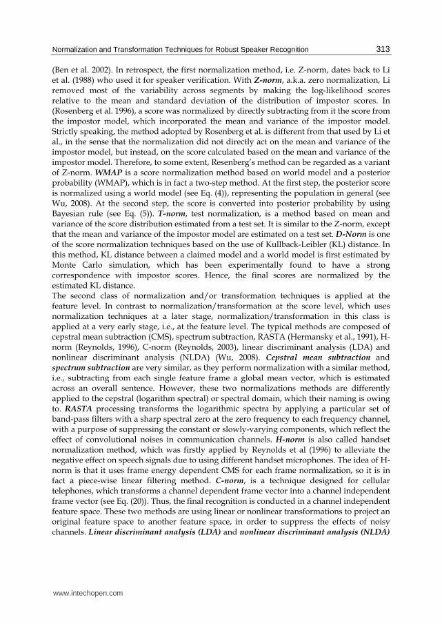
(Ben et al. 2002). In retrospect, the first normalization method, i.e. Z-norm, dates back to Li et al. (1988) who used it for speaker verification. With Z-norm, a.k.a. zero normalization, Li removed most of the variability across segments by making the log-likelihood scores relative to the mean and standard deviation of the distribution of impostor scores. In (Rosenberg et al. 1996), a score was normalized by directly subtracting from it the score from the impostor model, which incorporated the mean and variance of the impostor model. Strictly speaking, the method adopted by Rosenberg et al. is different from that used by Li et al., in the sense that the normalization did not directly act on the mean and variance of the impostor model, but instead, on the score calculated based on the mean and variance of the impostor model. Therefore, to some extent, Resenberg’s method can be regarded as a variant of Z-norm. WMAP is a score normalization method based on world model and a posterior probability (WMAP), which is in fact a two-step method. At the first step, the posterior score is normalized using a world model (see Eq. (4)), representing the population in general (see Wu, 2008). At the second step, the score is converted into posterior probability by using Bayesian rule (see Eq. (5)). T-norm, test normalization, is a method based on mean and variance of the score distribution estimated from a test set. It is similar to the Z-norm, except that the mean and variance of the impostor model are estimated on a test set. D-Norm is one of the score normalization techniques based on the use of Kullback-Leibler (KL) distance. In this method, KL distance between a claimed model and a world model is first estimated by Monte Carlo simulation, which has been experimentally found to have a strong correspondence with impostor scores. Hence, the final scores are normalized by the estimated KL distance. The second class of normalization and/or transformation techniques is applied at the feature level. In contrast to normalization/transformation at the score level, which uses normalization techniques at a later stage, normalization/transformation in this class is applied at a very early stage, i.e., at the feature level. The typical methods are composed of cepstral mean subtraction (CMS), spectrum subtraction, RASTA (Hermansky et al., 1991), H-norm (Reynolds, 1996), C-norm (Reynolds, 2003), linear discriminant analysis (LDA) and nonlinear discriminant analysis (NLDA) (Wu, 2008). Cepstral mean subtraction and spectrum subtraction are very similar, as they perform normalization with a similar method, i.e., subtracting from each single feature frame a global mean vector, which is estimated across an overall sentence. However, these two normalizations methods are differently applied to the cepstral (logarithm spectral) or spectral domain, which their naming is owing to. RASTA processing transforms the logarithmic spectra by applying a particular set of band-pass filters with a sharp spectral zero at the zero frequency to each frequency channel, with a purpose of suppressing the constant or slowly-varying components, which reflect the effect of convolutional noises in communication channels. H-norm is also called handset normalization method, which was firstly applied by Reynolds et al (1996) to alleviate the negative effect on speech signals due to using different handset microphones. The idea of H-norm is that it uses frame energy dependent CMS for each frame normalization, so it is in fact a piece-wise linear filtering method. C-norm, is a technique designed for cellular telephones, which transforms a channel dependent frame vector into a channel independent frame vector (see Eq. (20)). Thus, the final recognition is conducted in a channel independent feature space. These two methods are using linear or nonlinear transformations to project an original feature space to another feature space, in order to suppress the effects of noisy channels. Linear discriminant analysis (LDA) and nonlinear discriminant analysis (NLDA)

www.intechopen.com


314

are applied to this case. LDA seeks the directions to maximize the ratio of between-class covariance to within-class covariance by linear algebra, whereas NLDA seeks the directions in a nonlinear manner implemented by neural network. The details for these normalization and transformations methods will be presented in Section 2 and 3. The remainder of this chapter is organized as follows: in Section 2, the score normalization techniques are firstly summarized in details, following the order presented in the overview above. In Section 3, the description to the normalization and transformation at the feature level is given. In Section 4, some recent efforts are presented. The discussions and limitations are commented in Section 5. In Section 6, final remarks concerning possible extensions and future works are given. Finally, this chapter is concluded with our conclusions in Section 7.

2. Normalization techniques at the score level

2.1 Z-Norm Zero normalization, Z-norm in short, is one of score normalization methods applied for speaker verification at the score level, which was firstly proposed by Li et al. (1988). In Li’s proposal, variations in a given utterance can be removed by making the log-likelihood scores relative to the mean and variance of the distribution of the impostor scores. Concretely speaking, let L(xi│S) be a log-likelihood score for a given speaker model S and a

given feature frame xi, where an overall utterance is denoted by X={xi}, i∈[1,N]. Here L(xi│S) is also called raw score. We shall then refer to Lnorm(xi│S) as the normalized log-likelihood score. Based on the notations, we have the following equation,

(1)

and the normalized score,

(2)

where ┤I and σI are the mean and standard deviation of the distribution of the impostor scores, which are calculated based on the impostor model SI. The original Z-norm was later improved by a variant method, which was proposed by Rosenberg et al. (1996) to normalize a raw log-likelihood score relative to the score obtained from an impostor model, i.e.,

(3)

where S is the claimed speaker and SI represents the impostors of speaker S. In fact, this variant version has become more widely used than the first version of Z-norm. For instance, the next presented normalization method – WMAP adopts it as the first step of normalization.

2.2 WMAP WMAP is referred to as score normalization based on world model and a posterior probability. WMAP consists of two stages. It uses a posterior probability at the second stage

www.intechopen.com


315

to substitute for the score normalized by a world model at the first stage. This procedure can be described as follows: Step1: normalization using the world model. With the log-likelihood score L(X│S) for the

speaker S and the utterance X, and the log-likelihood score L(X│ S ) for the world model of

speaker S and utterance X, the normalized score is then given by

(4)

This step is called score normalization by world model. Step 2: normalization as a posterior probability. At the second step, the score Rs is further normalized as a posterior probability using the Bayes’ rule, i.e.,

(5)

where P(S) and P( S ) are prior probabilities for target speaker and impostor, P(Rs|S) and

P(Rs| S ) are the probability for the ratio Rs generated by the speaker model S and impostor

model S respectively, which can be estimated based on a development set.

From these formulae, we can see the most advantage of WMAP, compared with Z-norm, is its two stage scheme for score normalization. The first step for normalization focuses on the difference between target and impostor scores. This difference may vary in a certain range. Thus, in the second normalization, the score difference is converted into the range of [0, 1], a posterior probability, which renders a more stable score.

2.3 T-norm T-norm is also called as test-norm because this method is based on the estimation on the test set. Essentially, T-norm can be regarded as a further improved version of Z-norm, as the normalization formula is very similar to that of Z-norm, at least in formality. That is, a normalized score is obtained by

(6)

where ┤I_test and σI_test are the mean and standard deviation of the distribution of the impostor scores estimated on a test set. In contrast, for Z-norm, the corresponding ┤I and σI are estimated on the training set (see Eq. (2)). As there is always mismatch between a training and test set, the mean and standard

deviation estimated on a test set should be more accurate than those estimated on a training

set and therefore it naturally results in that performance of T-norm is superior to that of Z-

norm. This is one biggest advantage of T-norm. However, one of the major drawbacks for T-

norm is that it may require more test data in order to attain sufficiently good estimation,

which is sometime impossible and impractical.

2.3 D-norm D-norm is a score normalization based on Kullback-Leibler (KL) distance. In Ben et al. (2002), D-norm was proposed to use KL distance between a claimed speaker’s and the

www.intechopen.com


316

impostor’s models as a normalization factor, because it was experimentally found that the KL distance has a strong correspondence with the impostor scores. In more details, let us firstly define the KL distance. For a probability density function p(X|S) of speaker S and an utterance X, and a probability density function p(X|W) of the speaker S’s world model W and an utterance X, the KL distance of S to W, KLw is denoted by

(7)

where E p[�] is an expectation under the law p. Similarly, the KL distance of W to S, KLw is defined as an symmetric distance KL2.

(8)

Hence, the KL distance between S and W is defined by

(9)

Direct computation of KL distance according to Eqs.(7)-(9) is not possible for most complex statistical distributions of pS and pW, such as GMM or HMM. Instead, the Monte Carlo simulation method is normally employed. The essential idea of the Monte-Carlo simulation is to randomly generate some synthetic data for both claimed and impostor models. Let us denote a synthetic data from a speaker S

by and a synthetic data from an impostor model W by . And also suppose a Gaussian

mixture model (GMM) is used to model speaker S and the world model W, i.e.,

(10)

where is a normal distribution with mean μi and covariance Σi, and m is the total

number of mixtures. Then according to the Monte-Carlo method, a synthetic data is generated with

transforming a random vector, , which is generated from a standard normal distribution

with zero-mean and unit-variance. The transformation is done with the specific mean and variance, which are parameters related to one Gaussian, randomly selected among all the mixtures in a given GMM

(11)

As the most important assumption of D-norm, the KL distance is assumed to have a strong correspondence with the impostor score, which was experimentally supported in Ben et al. (2002), i.e.,

(12)

where α=2.5, used by Ben et al. (2002).

www.intechopen.com


317

Finally, at the last step, the normalized score is obtained by the equation,

(13)

This is the overall procedure for D-norm.

3. Transformation techniques at the feature level

3.1 Cepstral (spectral) mean subtraction Cepstral mean subtraction (CMS) is one of the most widely used normalization methods at the feature level and also a basis for other normalization methods (Reynolds, 2002). Given an utterance X={xi}, i∈[1,N]with a feature frame xi, the mean vector m of all the frames, for the given utterance, is calculated as follows:

(14)

The normalized feature with CMS is then expressed by

(15)

The idea of CMS is simply based on the assumption that noise level is consistently stable across a given sentence, so that by subtracting the mean vector from each feature frame, the background and channel noise could be possibly removed. However, it should be noted that speaking characteristics are most likely to be removed as well by this subtraction, as they are characterized by an individual speaker’s speaking manner and should therefore also be consistently stable across a sentence at least. Another normalization method at the feature level, which is very similar to CMS, is spectral mean subtraction (SMS). While CMS does mean subtraction in the cepstral domain, SMS instead conducts subtraction in the spectral domain. Due to their extremely similarity in methods, their normalization effects share the same pros and cons.

3.2 RASTA processing RASTA processing transforms the logarithmic spectra by applying a particular set of band-pass filters with a sharp spectral zero at the zero frequency to each frequency channel, with a purpose of suppressing the constant or slowly-varying components, which reflect the effect of convolutional factors in communication channels. As is known (Hermansky et al. 1991), linear distortions, as caused by telecommunication channels or different microphones, appear as an additive constant in the log spectrum. So with band-pass filters in the log domain, the effects of additive or channel noise could be substantially alleviated. This is the essential idea for RASTA processing. Concretely speaking, the RASTA processing is carried out on the logarithmic bark-scale spectral domain by Hermansky et al (1991). So it can be considered as an additional step, inserted between the first (logarithm spectrum conversion) and the second step (equal loudness transform) in the common steps of the conventional perceptual linear prediction features (PLP) (Hermansky, 1990). After this additional step is taken, the other conventional steps from PLP, e.g. equal loudness transform, inverse logarithmic spectra, etc. are accordingly conducted. For this additional step, in a certain

www.intechopen.com


318

frequency channel (a set of frequency channels is divided in order to extract features by a set of filters at the stage of feature extraction in speech processing, more details can refer to Wu, 2008; Young et al. 2002), a band-pass filtering is used as RASTA processing, through an IIR filter with the transfer function

(16)

The low cut-off frequency of the filter determines the fastest spectral changes which are

ignored by RASTA processing, whereas the high cut-off frequency then determines the

fastest spectral changes which are preserved in a channel.

3.3 H-norm H-norm is referred to as handset normalization, which is a technique especially designed for

speaker normalization over various handsets. Essentially, it can be considered as a variant of

CMS, because H-norm does energy dependent CMS for different energy “channels”.

Concretely speaking, for an input frame stream {xi} and its corresponding frame energies

{ei}, the energies are divided into L levels {El}, l∈[1,L] , on each of which a mean vector ml is

calculated according to the equation,

(17)

whereis the number of frames whose energy levels are in [El, El+1]. Then for H-norm, a frame xi is normalized by energy dependent CMS, i.e.

(18)

So the H-norm is to some extent more like a piecewise CMS, using different CMS at different energy levels. This renders H-norm to be probably more subtle and therefore more accurate than the uniform CMS scheme.

3.4 C-norm C-norm is referred to as cellular normalization which was proposed by Reynolds (2003) for

compensation of channel effects of cellular phones. However, C-norm is also called a

method of feature mapping, because C-norm is based on a mapping function from a channel

dependent feature space into a channel independent feature space. The final recognition

procedure is done on the mapped, channel independent feature space. Following the

symbols, which we used above, xt is denoted as a frame at time t in a channel dependent

(CD) feature space, anda frame at time t in a channel independent (CI) feature space. The

GMM modeling for the channel dependent feature space is denoted GCD as and the GMM

for the channel independent feature space is denoted as GCI. The Gaussian mixture to which

a frame xt belongs is chosen according to the maximum likelihood criterion, i.e.

(19)

www.intechopen.com


319

where a Gaussian mixture is defined by its weight, mean and standard deviation

. Thus, by a transformation f(�), a CI frame feature yt is mapped from xt

according to

(20)

where i is a Gaussian mixture to which xt belongs and is determined in terms of Eq. (19). After the transformation, the final recognition is conducted on the CI feature space, which is expected with the advantages of channel compensation.

3.5 Principal component analysis Principal component analysis (PCA) is a canonical method to find some of the largest variance directions of a given set of data samples. If the vectors pointed by these directions are used as a set of bases for a new feature space, then an original feature space can be transformed into the new feature space. That is, for any d-dimensional feature frame xi in the original feature space X, we have a transformation obtained by PCA, such that the original feature space X is transformed into a new one Y,

and xt is transformed into yt, i.e.

(21)

The transformation matrix W can be sought by diagonalization of the covariance matrix C of the given data set X. If we set X=[x1,x2,…,xn], where n is the size of the given data set, then the covariance matrix C is defined as

(22)

By diagonalizing the covariance matrix C, we have

(23)

where u’s are principal vectors and ┣’s are the variances (or principal values) on the basis of u’s. Thus, by sorting the principal vectors according their principal values, we have the transformation W in such a form,

So the transformed feature yt is

(24)

This is the traditional PCA, which is implemented with linear algebra. However, there is another variant of PCA, which is implemented with one type of neural networks – multi-layer perceptron (MLP). MLP is well known to be able to approximate any continuous linear and nonlinear function. Therefore, it has a wide range of applications in feature transformation. Let us first present how an MLP network is used to realize the functionality

www.intechopen.com


320

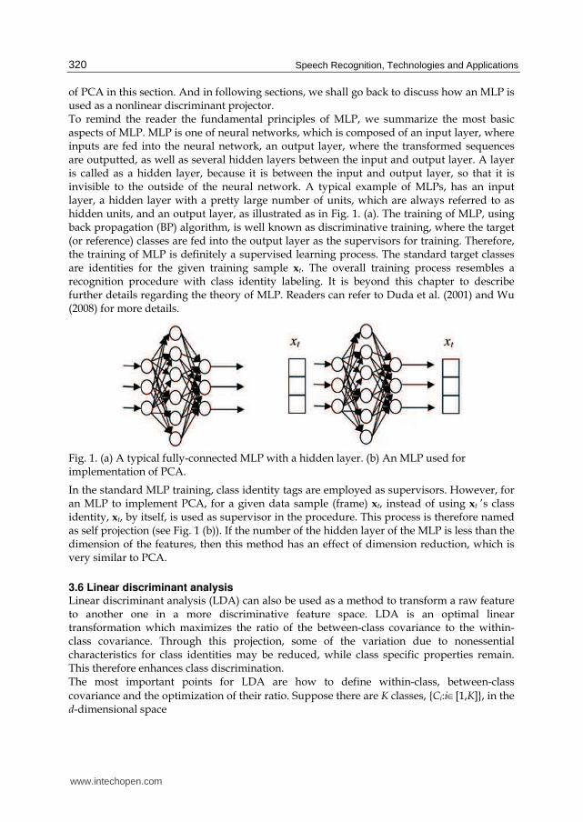
of PCA in this section. And in following sections, we shall go back to discuss how an MLP is used as a nonlinear discriminant projector. To remind the reader the fundamental principles of MLP, we summarize the most basic aspects of MLP. MLP is one of neural networks, which is composed of an input layer, where inputs are fed into the neural network, an output layer, where the transformed sequences are outputted, as well as several hidden layers between the input and output layer. A layer is called as a hidden layer, because it is between the input and output layer, so that it is invisible to the outside of the neural network. A typical example of MLPs, has an input layer, a hidden layer with a pretty large number of units, which are always referred to as hidden units, and an output layer, as illustrated as in Fig. 1. (a). The training of MLP, using back propagation (BP) algorithm, is well known as discriminative training, where the target (or reference) classes are fed into the output layer as the supervisors for training. Therefore, the training of MLP is definitely a supervised learning process. The standard target classes are identities for the given training sample xt. The overall training process resembles a recognition procedure with class identity labeling. It is beyond this chapter to describe further details regarding the theory of MLP. Readers can refer to Duda et al. (2001) and Wu (2008) for more details.

Fig. 1. (a) A typical fully-connected MLP with a hidden layer. (b) An MLP used for implementation of PCA.

In the standard MLP training, class identity tags are employed as supervisors. However, for an MLP to implement PCA, for a given data sample (frame) xt, instead of using xt ’s class identity, xt, by itself, is used as supervisor in the procedure. This process is therefore named as self projection (see Fig. 1 (b)). If the number of the hidden layer of the MLP is less than the dimension of the features, then this method has an effect of dimension reduction, which is very similar to PCA.

3.6 Linear discriminant analysis Linear discriminant analysis (LDA) can also be used as a method to transform a raw feature to another one in a more discriminative feature space. LDA is an optimal linear transformation which maximizes the ratio of the between-class covariance to the within-class covariance. Through this projection, some of the variation due to nonessential characteristics for class identities may be reduced, while class specific properties remain. This therefore enhances class discrimination. The most important points for LDA are how to define within-class, between-class

covariance and the optimization of their ratio. Suppose there are K classes, {Ci:i∈[1,K]}, in the d-dimensional space

www.intechopen.com


321

the m-dimensional projected space

and there is an optimal linear transformation W, such that Y=WTX. Denote by the mean vector in Space Y for class Ck and mk the mean vector in Space X for

class Ck. As such, the within-class covariance of Space Y can be rewritten as

(25)

where Sw is the within-class covariance of Space X.

The between-class covariance of Space Y can be expressed as

(26)

where Sb is the between-class covariance of Space X. So the optimization objective function is the ratio between the between-class and within-

class covariance, i.e.

(27)

Solving this optimization problem (see Wu, 2008 for more details), we can have

(28)

where wi and ┣i are the i-th eigenvector and eigenvalue, respectively. If the number of

eigenvectors selected for the transformation is less than m, then LDA in fact reduces the

dimensionality of a mapped space. This is the most often case for the application of LDA.

3.7 Nonlinear discriminant analysis Besides linear transforms such as PCA and LDA, nonlinear transforms can also be employed

as a method of transformations at the feature level. This type of methods is named as

nonlinear discriminant analysis (NLDA). There are two folds of meanings for the essence of

the NLDA. First, it is one of discriminant algorithms. The goal of the NLDA is quite similar

to that held by the LDA. They are both aiming at maximizing the between-class covariance

and simultaneously minimizing the within-class covariance. Second, the maximization

procedure for the NLDA is not carried out in a linear way, but in a nonlinear way. These

two properties reflect the most important aspects of the NLDA.

On the other hand, the NLDA is sort of an extension to the LDA. A nonlinear function degenerates to a linear function, when a certain condition is specified. A set of nonlinear functions can be regarded as a super set that contains a set of linear functions. Thus, the NLDA is an extension to the LDA. Normally, NLDA is implemented by neural networks

www.intechopen.com


322

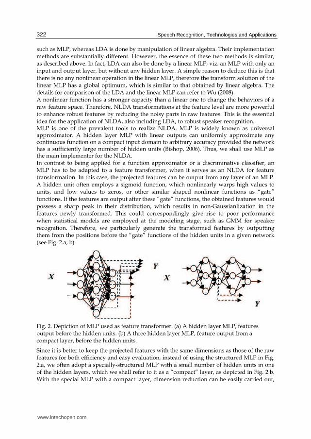
such as MLP, whereas LDA is done by manipulation of linear algebra. Their implementation methods are substantially different. However, the essence of these two methods is similar, as described above. In fact, LDA can also be done by a linear MLP, viz. an MLP with only an input and output layer, but without any hidden layer. A simple reason to deduce this is that there is no any nonlinear operation in the linear MLP, therefore the transform solution of the linear MLP has a global optimum, which is similar to that obtained by linear algebra. The details for comparison of the LDA and the linear MLP can refer to Wu (2008). A nonlinear function has a stronger capacity than a linear one to change the behaviors of a raw feature space. Therefore, NLDA transformations at the feature level are more powerful to enhance robust features by reducing the noisy parts in raw features. This is the essential idea for the application of NLDA, also including LDA, to robust speaker recognition. MLP is one of the prevalent tools to realize NLDA. MLP is widely known as universal approximator. A hidden layer MLP with linear outputs can uniformly approximate any continuous function on a compact input domain to arbitrary accuracy provided the network has a sufficiently large number of hidden units (Bishop, 2006). Thus, we shall use MLP as the main implementer for the NLDA. In contrast to being applied for a function approximator or a discriminative classifier, an MLP has to be adapted to a feature transformer, when it serves as an NLDA for feature transformation. In this case, the projected features can be output from any layer of an MLP. A hidden unit often employs a sigmoid function, which nonlinearly warps high values to units, and low values to zeros, or other similar shaped nonlinear functions as “gate” functions. If the features are output after these “gate” functions, the obtained features would possess a sharp peak in their distribution, which results in non-Gaussianlization in the features newly transformed. This could correspondingly give rise to poor performance when statistical models are employed at the modeling stage, such as GMM for speaker recognition. Therefore, we particularly generate the transformed features by outputting them from the positions before the “gate” functions of the hidden units in a given network (see Fig. 2.a, b).

Fig. 2. Depiction of MLP used as feature transformer. (a) A hidden layer MLP, features output before the hidden units. (b) A three hidden layer MLP, feature output from a compact layer, before the hidden units.

Since it is better to keep the projected features with the same dimensions as those of the raw features for both efficiency and easy evaluation, instead of using the structured MLP in Fig. 2.a, we often adopt a specially-structured MLP with a small number of hidden units in one of the hidden layers, which we shall refer to it as a “compact” layer, as depicted in Fig. 2.b. With the special MLP with a compact layer, dimension reduction can be easily carried out,

www.intechopen.com


323

as often do LDA and PCA. It thus provides the full capability to evaluate transformed and raw features with the same dimensionality. This is the basic scheme for an MLP to be employed as feature transformer at the feature level. We have known that new features are output from a certain hidden layer. However, we do not know how to train a MLP yet. The MLP is trained on a class set. How to construct such a set for training is very crucial for an MLP to work efficiently. The classes selected in the set are the sources of knowledge for an MLP to learn discriminatively. So they are directly related to the recognition purposes of applications. For instance, in speech recognition, the monophone class is often used for MLP training. For speaker recognition, the training class set is naturally composed of speaker identities. However, NLDA is not straightforward to be applied to robust speaker recognition, although we have known that speaker identities are used as target classes for MLP training. Because, compared with speech recognition, the number of speakers is substantially larger in speaker recognition, while such size for speech recognition is roughly about 30 in terms of phonemes. Therefore, it is impractical or even impossible to use thousands of speakers as the training classes for an MLP. Instead, we use a subset of speakers, which are most representative of the overall population, and therefore referred to as speaker basis, for MLP training. It is said to be “speaker basis selection” concerning how to select the optimal basis speakers (Wu et al., 2005a, 2005b; Morris et al., 2005). The basic idea for speaker basis selection is based on an approximated Kullback-Leibler (KL) distance between any two speakers, say, Si and Sk. By the definition of KL distance (Eq.(7)), the distance between Si and Si is written as the sum of two KL distance KL(Si║Sk) and its reverse KL(Sk║Si).

(29)

whererepresents an utterance. This cannot be evaluated in closed form when p(x│Si) is modeled by a GMM. However, provided P(Si)= P(Sk), Eq.(29) can be simplified as the expectation of K(Si, Sk, k).

(30)

where K(Si, Sk, k) equals to

(31)

Based on a development set Dev, the expectation of K(Si, Sk, k) can be approximated by the data samples on the set Dev, i.e.,

(32)

With the approximated KL distance between any two speakers, we can further define the average distance from one speaker to the overall speakers, the population.

www.intechopen.com


324

(33)

where S is the set of the speaker population and ║S║ is the total number of speakers in S.

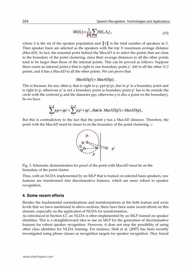
Then speaker basis are selected as the speakers with the top N maximum average distance

(MaxAD). In fact, the essential point behind the MaxAD is to select the points that are close

to the boundary of the point clustering, since their average distances to all the other points

tend to be larger than those of the internal points. This can be proved as follows. Suppose

there exists an internal point p that is right to one boundary point p’, left to all the other N-2

points, and it has a MaxAD to all the other points. We can prove that

This is because: for any other pi that is right to p, ppi<p’pi, due to p’ is a boundary point and is right to p, otherwise p’ is not a boundary point (a boundary point p’ has to be outside the circle with the centroid pi

and the diameter ppi; otherwise p is also a point on the boundary).

So we have

But this is contradictory to the fact that the point p has a MaxAD distance. Therefore, the

point with the MaxAD must be closer to on the boundary of the point clustering. □

Fig. 3. Schematic demonstration for proof of the point with MaxAD must be on the boundary of the point cluster.

Thus, with an NLDA implemented by an MLP that is trained on selected basis speakers, raw

features are transformed into discriminative features, which are more robust to speaker

recognition.

4. Some recent efforts

Besides the fundamental normalizations and transformations at the both feature and score levels that we have mentioned in above sections, there have been some recent efforts on this domain, especially on the application of NLDA for transformation. As introduced in Section 4.7, an NLDA is often implemented by an MLP trained on speaker identities. This is a straightforward idea to use an MLP for the generation of discriminative features for robust speaker recognition. However, it does not stop the possibility of using other class identities for NLDA training. For instance, Stoll et al. (2007) has been recently investigated using phone classes as recognition targets for speaker recognition. They found

www.intechopen.com


325

that the discriminative features generated with such a trained MLP also contain a lot of information for speaker discrimination. This method is named as Tandem/HATS-MLP, because such a structure for MLP training was firstly proposed for speech recognition (Chen et al., 2004; Zhu et al. 2004). The investigation of the complementary property of discriminative features to other types of features and modeling approaches, is an alternative direction for extending the method of NLDA for robust speaker recognition. Konig and Heck first found that discriminative features are complementary to the mel-scaled cepstral features (MFCCs) and suggested these two different types of features can be linearly combined as composite features (Konig et al. 1998; Heck et al. 2000). Stoll et al. (Stoll et al. 2007) used the discriminative features as inputs for support vector machines (SVM) for robust speaker recognition and found it outperforms the conventional GMM method. All these efforts confirm that the discriminative features are harmonic to other feature types as well as other modeling techniques. Using multiple MLPs (MMLPs) as feature transformer is also a possible extension to the NLDA framework. The MMLP scheme was proposed to exploit the local clustering information in the distribution of the raw feature space (Wu, 2008b). According to the idea of MMLP, the raw feature space is firstly partitioned into a group of clusters by using either phonetic labeling information or an unsupervised recognition method of GMM. Then a sub-MLP is employed as a feature transformer within each cluster. The obtained discriminative features are then “softly”(using affine combination) or “hardly” (using switch selection) combined into the final discriminative features for recognition. This method has been found to outperform the conventional GMM method and to be marginally better than SMLP. More work is needed in future study.

5. Discussions: capacities and limitations

In this section, we shall comment, mainly from two different perspectives, capacities and limitations of normalization and transformation methods at both score and feature levels. In one way, we discuss how these techniques help to reduce mismatch between training and test conditions is considered. In the second one, we discuss how these methods are combined with other parts of SR systems, as either early or late processing module.

5.1 Mismatch reduction How to deal with noises is a universal topic for robust speaker recognition. All the methods reviewed in this chapter are absolutely concerned with this topic. However, noises can normally be categorized into two groups, i.e., additive noise and convolutional noise. The additive noise further consists of environmental noise and cross-talking from other speakers, while convolutional noise is mainly caused by communication channels. For most noise, it occurs in a sudden and unpredictable way. Its interference results in a huge mismatch from the models trained before-hand, which in turn often severely degrades system performance. Thus, for robust speaker recognition, one of the key problems is how to reduce mismatch between different training and test scenarios. Of course, mismatch always exits, no matter how hard a system is carefully prepared. So a smart system knows how to compensate a variety of mismatches, whereas a poor system does not. We shall see, in such a context, how well each of the normalization methods works in terms of mismatch reduction.

www.intechopen.com


326

Let us first check score level normalizations. Z-norm validates its method on the basis of an

assumption that scores of an impostor model should hold the same tendency as the

hypothesized one when they are under the same circumstances, obviously including

mismatched conditions, such as noises. Z-norm should have general capabilities to reduce

mismatch caused by both additive and convolutiional noises. However, this method may

fail when scores of the impostor are not tightly linked in change tendency with scores of the

claimant, which is often highly possible in realistic applications. T-norm is an extension to

Z-norm, and still based on the same assumption. So T-norm has the similar capacities and

limitations for mismatch reduction. However, T-norm is better than Z-norm, since

distribution statistics of impostors are directly estimated from a separate test set. Hence, it

can further reduce the mismatch between training and test conditions. WMAP is a two-step

method. Its first step is quite similar to Z-norm, but WMAP enhances its normalization

power by converting its decision scores into posterior probabilities so as to be much easier to

be compared using a single global threshold. However, WMAP doesn’t use any test data

because WMAP uses scores calculated from the world model, not from the distribution of

test data. It may prevent from enhancing the capacities of WMAP to reduce mismatch.

Therefore, this may imply a possible extension to WMAP, in which a score is calculated

from a world model estimated on the test set, and then used for the normalization in the

first step, the posterior probability is computed in the second step. This scheme can be

referred to as T-WMAP, which can extend WMAP to possibly better capacities for mismatch

reduction. D-norm is a quite different approach, but it is also based on the same assumption

as Z-norm, that is, normalization based on impostor scores may eliminate mismatch

between training and test set. The only distinguished aspect is that D-norm uses Monte-

Carlo simulation to estimate KL-distance to replace the impostor scores, conditioned on a

strong correspondence experimentally found between them. In addition, D-norm does not

use the test data either. Hence, it suggests a possible extension for D-norm, which employs

test data, and therefore should be referred to as TD-norm.

We further check feature level transformations. CMS and spectrum subtraction are obviously based on an assumption that noise is stationary across a whole utterance, e.g. convolutional noises. Therefore, CMS is useful to reduce the mismatch caused by stationary noise in an utterance. However, it does not excel at dealing with some non-stationary noise, such as dynamic ambient noise and cross-talking. RASTA uses a set of band-pass filters to suppress constant or slowly-varying noises. At this point, RASTA is quite similar to CMS on the effect to eliminate convolutional noise, whereas it has limited capacities to handle the mismatch resulted in by other dynamic noises. H-norm is an extension of CMS to deal with handset mismatch in multiple energy channels. Based on the same assumption, H-norm is also mostly effective to handle constant channel noises, especially for reduction of handset mismatch. C-norm is a technique to design for alleviating the mismatch due to different cellular phones. It further extends CMS by transforming a channel dependent feature to a channel independent feature with the consideration of not only the mean vector, but also covariance matrix of a feature space. From this perspective, C-norm is an advanced version of CMS with more powerful capacities to normalize data to a universal scale with zero mean and unit variance. However, C-norm is also based on a similar assumption and therefore especially effective for the mismatch due to stationary noise. From here, we can see that all the above techniques can in fact be put into a framework based on the same assumption that

www.intechopen.com


327

noise is stationary across an utterance. This obviously renders these normalization methods particular efficient for convolution noises as in telephony speech. The other subgroup of normalization methods at the feature level doesn’t base on the assumption of stationary noise. But, instead, the transformation is learned from an overall training set and thus the methods in this group take advantage of more data. In this group, PCA is a non-discriminant method. It seeks several largest variance directions to project a raw feature space to a new feature space. During this process, PCA often makes the projected feature space more compact and therefore is employed as a popular method of dimension reduction. An implement assumption is that noise components may not have the same directions as principal variances. So it may reduce the noise components that are vertical to the principal variances by applying PCA to the raw features. However, the noise components that are horizontal to the principal variances still remain. According to this property, PCA has a moderate capacity to deal with the mismatch resulted from a wide range of noises. LDA extends PCA with the same feature of dimension reduction, to linear discriminative training. The discriminative learning is efficient to alleviate the mismatch caused by all the noise types, whatever is additive or convolutional noise. Only the essential characteristics related to class identities are supposed to remain, while all other negative noisy factors are supposed to be removed. NLDA further extends LDA to a case of nonlinear discriminative training. As nonlinear discriminative training can degenerate to the linear discriminative training by manipulating a special topology of MLP (see Section 3.7), NLDA has more powerful capacities to enhance “useful” features and compensates harmful ones. In terms of mismatch reduction, NLDA and LDA are applicable to a wide range of noise, so as to be considered as broad-spectrum “antibiotic” for robust speaker recognition, whereas the others as narrow-spectrum “antibiotic”. Based on the above analysis, we can summarize that some of normalization techniques are particularly calibrated for specific types of mismatch, where others are generally effective. Roughly speaking, score normalizations are often more “narrow”, but the feature level transformations are more or less “broad” in mismatch reduction. This distinction may imply the possibility of integrating these techniques into a single framework.

5.2 Processing at early and late stage Another distinction between feature and score transformation is the time at which

transformation is applied. Transformation is applied at the early stage for feature

transformation, while it is used at the late stage for score level normalization. Generally

speaking, the earlier processing is applied; the less chance noise components may negatively

affect system performance. Judging from this pointview, feature transformation should

attain more powerful capacities to deal with noise components, especially in a wider range,

because the noise and useful parts are not blended by the modeling procedure yet. This

definitely leaves more chances for robust normalization algorithms to work on noise

reduction.

However, there are also advantages to apply normalization and transformation at the score level. The normalization methods at the score level often have lower computational complexity for implementation and application because at the score level, the high dimensional features have already been converted into a score domain that is often a scalar. Therefore, any further processing on the 1-d scores is pretty simple and efficient. This advantage thus renders the score normalizations are more efficient for realistic applications,

www.intechopen.com


328

at least in terms of computation requirements. For instance, they can be efficiently applied to some real-time applications, such as applications running on PDAs, or mobile phones, whereas the feature normalizations have a bit higher complexity for these application scenarios. Due to the pros and cons of feature and score level normalizations, we may raise such a question if it is possible to combine them into a universal framework and fully utilize their advantages. The answer is “Yes”. One simple combination of feature and score level normalizations is definitely possible. However, these methods can also be integrated. For instance, it may be possible to apply NLDA at the score level, to project raw scores to better discriminative scores, as does NLDA for feature projection. This pre-processing at the score level can be referred to NLDA score transformation. By such an NLDA transformation, some confused scores may be corrected. This is just as an example, given for elucidating the idea of combining feature and score level transformation. Bearing in mind this idea, many other similar methods may be proposed to further improve robustness of speaker recognition systems in noisy conditions.

6. Final remarks: possible extensions

With summarization of work of normalization and transformation at the feature and score levels, we almost have gone through the most popular techniques for robust speaker recognition. However, another possible direction of work should not be ignored, that is transformation at the model level. This has seldom been investigated in the literature, therefore we did not summarize this direction as a separate section. Instead, we put it here in a section to discuss possible extensions. If transformation is applied at the model level, this type of techniques is often referred to as model adaptation or compensation in speech recognition (Gales, 1995). So if a similar method is applied to robust speaker recognition, we may refer to it as speaker model compensation (SMC). A direct application of SMC is to adapt a well trained model to a particular mismatched condition only using test data. If the test data is adequate, multiple transforms can be applied to different groups of Gaussian mixtures. Otherwise, a global transform can be applied to the overall Gaussian components. In future work, this idea is worth to be investigated. Another example of the application of model level transformation goes to recent work of using speaker model synthesis based on cohort speakers (Wei et al., 2007), although it embodies the idea of synthesis indeed, but not the idea of adaptation. In this method, any new speaker model is synthesized by a set of cohort speaker models. The mismatch can be reduced in this manner by cohort speaker models being trained before hand based on channel dependent data. With the model transformation being added, a general framework for robust speaker recognition is complete with all three directions. The future work will substantially rely on them for further development of robust speaker recognition. However, compared with feature and score level transformation, there are relatively fewer efforts dedicated at the model level. More work could be done under this direction with the possibility of successful extensions, in terms of the authors’ point of view. It should be promising for future work. In the chapter, we have mentioned some extensions as possible future work for robust speaker recognition. In order to make it clearer to readers, who may be of interest, we shall summarize them in the following as the final remarks:

• T-WMAP: extending WMAP to test set (Section 5.1).

www.intechopen.com


329

• TD-nom: extending D-norm to test set (Section 5.1).

• NLDA transformation at the score level (Section 5.2).

• SMC adaptation for speaker recognition (Section 6).

• SVM score transformation: this is another possibility to apply NLDA at the score level. Instead of using MLP, support vector machine (SVM) is also possible to be used for score normalization.

• Combination of the feature, model and score transformations (Section 5.2). The possible extensions can never be exhausted. We listed them here just as examples to demonstrate the possible direction for future work.

7. Conclusion

Robust speaker recognition faces a variety of challenges for identifying or verifying speaker identities in noisy environments, which cause a large range of variance in feature space and therefore are extremely difficult for statistical modeling. To compensate this effect, much research efforts have been dedicated in this area. In this chapter, we have mainly summarized these efforts into two categories, namely normalization techniques at the score level and transformation techniques at the feature level. The capacities and limitations of these methods are discussed. Moreover, we also introduce some recent advances in this area. Based on these discussions, we have concluded this paper with possible extensions for future work.

8. References

Auckenthaler, R.; Carey, M., et al. (2000). Score normalization for text-independent speaker verification systems. Digital Signal Processing Vol. 10, pp. 42-54.

Ben, M.; Blouet, R. & Bimbot, F. (2002). A Monte-Carlo method for score normalization in Automatic speaker verification using Kullback-Leibler distances. Proceedings of IEEE ICASSP ’02, vol. 1, pp. 689–692.

Bimbot, F., et al. (2004). A tutorial on text-independent speaker verification. EURASIP. Vol. 4, pp. 430-451.

Bishop, M. (2006). Pattern Recognition and Machine Learning, Springer Press. Campbell, J. P. (1997). Speaker recognition: a tutorial, Proceedings of IEEE Vol. 85, No. 9, pp.

1437-1462. Chen, B.; Zhu, Q. & Morgan, N. (2004). Learning long-term temporal features in LVCSR

using neural network. Proceedings of ICSLP’04. Daugman, J. G. (2004). How iris recognition works. IEEE Trans. Circuits and Syst. For Video

Tech. Vol. 14, No. 1, pp. 21-30. Duda, R. & Hart., P. (2001). Pattern classification, Willey Press. Fredouille, C.; Bonastre, J.-F. & Merlin, T. (1999) . Similarity normalization method based on

world model and a posteriori probability for speaker verification. Proceedings of Eurospeech’99, pp. 983–986.

Gales, M. (1995). Model based techniques for robust speech recognition. Ph.D. thesis, Cambridge University.

Heck, L.; Konig, Y. et al. (2000). Robustness to telephone handset distortion in speaker recognition by discriminative feature design. Speech Communication Vol. 31, pp. 181-192.

www.intechopen.com


330

Hermansky, H. (1990). Perceptual linear prediction (PLP) analysis for speech. J. Acoustic. Soc. Am., pp.1738-1752.

Hermansky, H.; Morgan, N., et al. (1991). Rasta-Plp speech analysis. ICSI Technical Report TR-91-069, Berkeley, California.

Jain, A. K. & Pankanti, S. (2000). Fingerprint classification and recognition. The image and video handbook.

Jin, Q. & Waibel, A. (2000). Application of LDA to speaker recognition. Proceedings of ICSLP’00.

Konig, Y. & Heck, L. (1998). Nonlinear discriminant feature extraction for robust text-independent speaker recognition. Proceedings of RLA2C, ESCA workshop on Speaker Recognition and its Commercail and Forensic Applications, pp. 72-75.

Li, K. P. & Porter, J. E. (1988). Normalizations and selection of speech segments for speaker recognition scoring. Proceedings of ICASSP ’88, Vol. 1, pp. 595–598.

Morris, A. C.; Wu, D. & Koreman, J. (2005). MLP trained to classify a small number of speakers generates discriminative features for improved speaker recognition. Proceedings of IEEE ICCST 2005.

Reynolds, D.A. (1996). The effect of handset variability on speaker recognition performance: experiments on the switchboard corpus. Proceedings of IEEE ICASSP ’96, Vol. 1, pp. 113–116.

Reynolds, D. A. (2002). An Overview of Automatic Speaker Recognition Technology. Proceedings of ICASSP'02.

Reynolds, D A. (2003). Channel robust speaker verification via feature mapping. Proceedings of ICASSP’03, Vol. 2, 53-56.

Rosenberg, A.E. & Parthasarathy, S. (1996). Speaker background models for connected digit password speaker verification. Proceedings of ICASSP ’96, Vol. 1, pp. 81–84.

Stoll, L.; Frankel, J. & Mirghafori, N. (2007). Speaker recognition via nonlinear discriminant features. Proceedings of NOLISP’07.

Sturim, D. E. & Reynolds, D.A. (2005). Speaker adaptive cohort selection for tnorm in text-independent speaker verification. Proceedings of ICASSP’05, Vol. 1, pp. 741–744.

Wei, W.; Zheng, T. F. & Xu, M. X. (2007). A cohort-based speaker model synthesis for mismatched channels in speaker verification. IEEE Trans. ON Audio, Speech, and Language Processing, Vol. 15, No. 6, August, 2007.

Wu, D.; Morris, A. & Koreman J. (2005a). MLP internal representation as discriminative features for improved speaker recognition. in Nonlinear Analyses and Algorithms for Speech Processing Part II (series: Lecture Notes in Computer Science), pp. 72-80.

Wu, D.; Morris, A. & Koreman, J. (2005b). Discriminative features by MLP preprocessing for robust speaker recognition in noise. Proceedings of ESSV 2005, 2005, pp 181-188.

Wu, D. (2008a). Discriminative Preprocessing of Speech, VDM Verlag Press, ISBN: 978-3-8364-3658-8.

Wu, D.; Li, J. & Wu, H. (2008b). Improving text-independent speaker recognition with locally nonlinear transformation. Technical report, Computer Science and Engineering Department, York University, Canada.

Young, S., et al. (2002). The HTK book V3.2. Cambridge University. Zhu, Q.; Chen, B & Morgan, N. (2004). On using MLP features in LVCSR. Proceedings of

ICSLP’04.

www.intechopen.com

Speech RecognitionEdited by France Mihelic and Janez Zibert

ISBN 978-953-7619-29-9Hard cover, 550 pagesPublisher InTechPublished online 01, November, 2008Published in print edition November, 2008

InTech EuropeUniversity Campus STeP Ri Slavka Krautzeka 83/A 51000 Rijeka, Croatia Phone: +385 (51) 770 447 Fax: +385 (51) 686 166www.intechopen.com

InTech ChinaUnit 405, Office Block, Hotel Equatorial Shanghai No.65, Yan An Road (West), Shanghai, 200040, China

Phone: +86-21-62489820 Fax: +86-21-62489821

Chapters in the first part of the book cover all the essential speech processing techniques for building robust,automatic speech recognition systems: the representation for speech signals and the methods for speech-features extraction, acoustic and language modeling, efficient algorithms for searching the hypothesis space,and multimodal approaches to speech recognition. The last part of the book is devoted to other speechprocessing applications that can use the information from automatic speech recognition for speakeridentification and tracking, for prosody modeling in emotion-detection systems and in other speech processingapplications that are able to operate in real-world environments, like mobile communication services and smarthomes.

How to referenceIn order to correctly reference this scholarly work, feel free to copy and paste the following:

Dalei Wu, Baojie Li and Hui Jiang (2008). Normalization and Transformation Techniques for Robust SpeakerRecognition, Speech Recognition, France Mihelic and Janez Zibert (Ed.), ISBN: 978-953-7619-29-9, InTech,Available from:http://www.intechopen.com/books/speech_recognition/normalization_and_transformation_techniques_for_robust_speaker_recognition

© 2008 The Author(s). Licensee IntechOpen. This chapter is distributedunder the terms of the Creative Commons Attribution-NonCommercial-ShareAlike-3.0 License, which permits use, distribution and reproduction fornon-commercial purposes, provided the original is properly cited andderivative works building on this content are distributed under the samelicense.

https://creativecommons.org/licenses/by-nc-sa/3.0/

Normalization and Transformation Techniques for Robust ...

Documents