Robust fractionation in cancer radiotherapy Ali Ajdari 1,2* , Archis Ghate 2 1 Department of Radiation Oncology, Massachusetts General Hospital & Harvard Medical School, Boston, MA 2 Department of Industrial & Systems Engineering, University of Washington, Seattle, WA January 2016 Abstract In cancer radiotherapy, the standard formulation of the optimal fractionation problem based on the linear-quadratic dose-response model is a non-convex quadratically constrained quadratic program (QCQP). An optimal solution for this QCQP can be derived by solving a two-variable linear program. Feasibility of this solution, however, crucially depends on the so-called alpha- over-beta ratios for the organs-at-risk, whose true values are unknown. Consequently, the dosing schedule presumed optimal, in fact, may not even be feasible in practice. We address this by proposing a robust counterpart of the nominal formulation. We show that a robust solution can be derived by solving a small number of two-variable linear programs, each with a small number of constraints. We quantify the price of robustness, and compare the incidence and extent of infeasibility of the nominal and robust solutions via numerical experiments. 1 Background and motivation The goal in external beam radiotherapy for cancer is to maximize damage to the tumor while limiting toxic effects of radiation on nearby organs-at-risk (OAR). Treatment is typically delivered over multiple treatment sessions called fractions. This leads to a well-known optimization problem, often referred to as the fractionation problem . The goal in this problem is to find the number of fractions N and a corresponding sequence ~ d =(d 1 ,d 2 ,...,d N ) of doses so as to maximize tumor- damage while ensuring that the OAR can safely tolerate these doses. The fundamental tradeoffs in this problem are as follows. Normal-cells often have a better damage-repair capability than tumor- cells. Temporal dispersion of dose across multiple fractions thus gives the OAR time to recover between sessions. For most tumors, a large number of fractions with a small dose per fraction allows the treatment planner to inflict more damage on the tumor as compared to administering a small number of fractions with a large dose per fraction. However, tumors can proliferate over the treatment course, and thus a shorter course might work better as it kills the tumor before any significant proliferation. Thus the question is whether or not and how the treatment planner can exploit, for patients’ benefit, the differences in the way in which tumors and OAR respond to radiation. * Email: [email protected] 1 arXiv:2108.03209v1 [math.OC] 6 Aug 2021

Welcome message from author
This document is posted to help you gain knowledge. Please leave a comment to let me know what you think about it! Share it to your friends and learn new things together.
Transcript
Robust fractionation in cancer radiotherapy
Ali Ajdari1,2∗, Archis Ghate2
1Department of Radiation Oncology, Massachusetts General Hospital & Harvard MedicalSchool, Boston, MA
2Department of Industrial & Systems Engineering, University of Washington, Seattle, WA
January 2016
Abstract
In cancer radiotherapy, the standard formulation of the optimal fractionation problem basedon the linear-quadratic dose-response model is a non-convex quadratically constrained quadraticprogram (QCQP). An optimal solution for this QCQP can be derived by solving a two-variablelinear program. Feasibility of this solution, however, crucially depends on the so-called alpha-over-beta ratios for the organs-at-risk, whose true values are unknown. Consequently, the dosingschedule presumed optimal, in fact, may not even be feasible in practice. We address this byproposing a robust counterpart of the nominal formulation. We show that a robust solution canbe derived by solving a small number of two-variable linear programs, each with a small numberof constraints. We quantify the price of robustness, and compare the incidence and extent ofinfeasibility of the nominal and robust solutions via numerical experiments.
1 Background and motivation
The goal in external beam radiotherapy for cancer is to maximize damage to the tumor whilelimiting toxic effects of radiation on nearby organs-at-risk (OAR). Treatment is typically deliveredover multiple treatment sessions called fractions. This leads to a well-known optimization problem,often referred to as the fractionation problem. The goal in this problem is to find the number offractions N and a corresponding sequence ~d = (d1, d2, . . . , dN ) of doses so as to maximize tumor-damage while ensuring that the OAR can safely tolerate these doses. The fundamental tradeoffs inthis problem are as follows. Normal-cells often have a better damage-repair capability than tumor-cells. Temporal dispersion of dose across multiple fractions thus gives the OAR time to recoverbetween sessions. For most tumors, a large number of fractions with a small dose per fractionallows the treatment planner to inflict more damage on the tumor as compared to administeringa small number of fractions with a large dose per fraction. However, tumors can proliferate overthe treatment course, and thus a shorter course might work better as it kills the tumor beforeany significant proliferation. Thus the question is whether or not and how the treatment plannercan exploit, for patients’ benefit, the differences in the way in which tumors and OAR respond toradiation.
∗Email: [email protected]
1
arX
iv:2
108.
0320
9v1
[m
ath.
OC
] 6
Aug
202
1
1.1 Mathematical formulations of the fractionation problem
The fractionation problem has been studied extensively, both clinically and mathematically, for overa century [22]. Mathematical formulations of this problem routinely rely on the linear-quadratic(LQ) cell-survival model [14]. Key parameters of the LQ model include the so-called α/β ratios forthe OAR. Research that uses this LQ model has evolved from single-OAR formulations, to two-OARformulations, and, more recently, to models with multiple OAR. All of these formulations belong tothe class of non-convex quadratically constrained quadratic programs (QCQPs) — problems knownto be computationally difficult in general. A closed-form optimal solution is available for the singleOAR case (see, for example, [7, 12, 13, 15, 20, 28] and references therein). One paper provided anoptimal dosing scheme using Karush-Kuhn-Tucker conditions for the two-OAR case for a fixed N[5]. A simulated annealing heuristic was applied to a two-OAR formulation in [29].
The most recent multiple-OAR formulation of this problem (see [24, 26]) is given by
(FRAC) max~d, N
α0
N∑t=1
dt + β0
N∑t=1
d2t − τ(N) (1)
N∑t=1
dt + ρm
N∑t=1
d2t ≤ BEDm, m ∈M, (2)
~d ≥ 0, (3)
1 ≤ N ≤ Nmax, integer. (4)
In this problem, α0, β0 are the tumor’s dose-response parameters as per the LQ model. The termτ(N) in the objective function accounts for tumor proliferation and is given by
τ(N) =[(N − 1)− Tlag]+ ln 2
Tdouble, (5)
where [(N − 1)− Tlag]+ is defined as max {0, (N − 1)− Tlag}. Here, Tlag is the time-lag (in days)after which tumor proliferation starts after treatment initiation; and Tdouble (in days) denotes thedoubling time for the tumor. This proliferation term assumes that a single fraction is administeredevery day; it can be generalized to accommodate other fractionation schemes as described in [24].The objective function equals the biological effect (BE) of ~d on the tumor, which is to be maximized.In constraints (2), M = {1, 2, . . . , n} is the set of n ≥ 1 OAR. The parameter ρm = βm/αm is theaforementioned (inverse) ratio of dose-response parameters for OAR m ∈ M. The left hand sideof each constraint equals the biologically effective dose (BED) administered to the correspondingOAR. The term on the right hand side is given by BEDm = Dm+ρmD
2m/Nm. It equals the BED of
a conventional treatment schedule that administers a total dose of Dm in Nm equal-dosage fractionsand that OAR m is known to tolerate. Thus, each of these constraints ensures that, for each OAR,the BED of ~d is no more than what is safe for that OAR. In constraint (4), Nmax is the maximumnumber of fractions that is logistically feasible in the treatment protocol. In the sequel, we willoften refer to (FRAC) as the nominal problem.
1.2 Optimal solution of the nominal fractionation problem
An optimal solution for this multiple-OAR case was provided in [24]; this solution works either whenα0/β0 ≤ min
m∈M(αm/βm) or when α0/β0 ≥ max
m∈M(αm/βm). The first provably optimal solution that
works irrespective of the ordering of these ratios for the multiple-OAR case was recently derived in
2

[26] based on the doctoral dissertation of Saberian [23]. This solution was obtained by equivalentlyreformulating (FRAC) for each fixed N as a two-variable linear program (LP) with n + 2 linearconstraints and non-negativity constraints on the two variables. The two variables in this LP are
x =N∑t=1
dt and y =N∑t=1
d2t and the LP is given by
(2VARLP) maxx,y
α0x+ β0y − τ(N) (6)
x+ ρmy ≤ BEDm, m ∈M, (7)
y ≤ γ∗x, (8)
c∗x ≤ y, (9)
x ≥ 0, (10)
y ≥ 0, (11)
where γ∗ = minm∈M
bm(1) and c∗ = minm∈M
bm(N) with bm(N) =−1+√
1+4ρmBEDm/N
2ρmfor m ∈ M and
for all N ≥ 1. Specifically, for each fixed N , if x∗, y∗ is an optimal solution of this LP, then thedosing schedule (q, p, p, . . . , p︸ ︷︷ ︸
N−1 times
), where
p =x∗
N
[1−
√√√√1−
(1− y∗
(x∗)2
)(N
N − 1
)], (12)
q = x∗ − (N − 1)p, (13)
is optimal. Moreover, it can be shown that there are only three possibilities for x∗ and y∗. Thefirst is where
√y∗ = x∗ and then p = 0 (this is called a single-dosage solution); the second is
where√Ny∗ = x∗ and then p = q (this is called an equal-dosage solution); and the third is where√
y∗ < x∗ <√Ny∗ and then 0 6= p 6= q 6= 0 (this is called an unequal-dosage solution) (see [23, 26]
for details). An optimal number of fractions can then be found by substituting a dosing scheduleso obtained into the objective function in (FRAC) for each N ∈ {1, 2, . . . , Nmax} and picking theone that yields the largest tumor BE. Consequently, (FRAC) is solved by solving exactly Nmax
two-variable LPs.
1.3 Limitations of existing formulations and our contributions
One drawback of all aforementioned formulations of the fractionation problem based on the LQmodel is that the values of ρm are not known. Thus, a dosing schedule derived using estimated or“nominal” values of these parameters may not even be feasible in practice.
In a recent unpublished manuscript [2], Badri et al., independently of an earlier (May 2015)unpublished version of our present work, attempted to remedy this by studying a robust formulationof the above fractionation problem. In their formulation, the treatment planner derives a robustsolution by assuming that the ρm values vary within a known non-negative interval. However,the crucial dependence of the right hand side BEDm on ρm in constraints (2) was ignored in thatmanuscript. This meant that an optimal solution to their robust formulation was obtained byreplacing ρm on the left hand side in (2) by its largest possible value. This implied that the robustsolution is derived simply by solving the two-variable LP in [23, 26]. Unfortunately, since the righthand side in constraints (2) in fact explicitly depends on ρm, such a simplified solution might not
3
be robust in practice. Badri et al. rectified this limitation in an updated unpublished variation [1]of their original manuscript, again independently of the earlier (May 2015) unpublished version ofour present work that they cited.
The main focus of the original and the updated versions by Badri et al. was on a chance con-strained formulation of the problem, which required the treatment planner to know the probabilitydistribution of alpha-over-beta ratios, and which called for a computationally more demanding solu-tion approach than what is needed for the robust formulation. On the plus side, a potential benefitof the resulting chance constrained solution is that it might be less conservative than the robustsolution (although this is perhaps impossible to verify rigorously). Given their alternative focus,Badri et al. gave a somewhat cursory treatment to the robust approach in both their manuscripts,did not present an infeasibility analysis of the resulting robust solutions, did not quantify the priceof robustness, and only included minimal sensitivity results.
Here we study essentially the same robust problem as in the updated version of Badri et al. Wedo, however, provide mathematical and clinical insights missing in their work. Firstly, we presentour solution approach in much more detail. We show that, for each fixed N , an optimal solution tothe non-convex robust problem can be recovered by solving n+ 1 two-variable LPs. Consequently,the robust fractionation problem is solved by solving (n+ 1)Nmax two-variable LPs; each of theseLPs includes n + 2 linear constraints and non-negativity constraints on the two variables. Weperform sensitivity analyses with respect to the values of Tlag and Tdouble currently available inthe clinical literature to numerically quantify the price of robustness. We also provide qualitativeand quantitative comparisons between the nominal and robust fractionation schedules. Finally, wepresent an extensive analysis of the infeasibility suffered by the nominal and robust solutions in abroad range of scenarios.
This paper is organized as follows. Our robust formulation is described in the next section.The solution approach is detailed in Section 3. Numerical results are presented in Section 4. Weconclude with a summary of our contributions, an outline of some variations and limitations of ourmodel, and opportunities for future work.
2 A robust formulation
We refer the reader to [3] for a textbook and to [4] for a survey on robust optimization. We employa standard interval uncertainty model from these existing works to construct a robust counterpartof the nominal problem (FRAC). Specifically, we use ρ̃m to denote the “true” unknown value ofρm, for m = 1, . . . , n. We assume that this unknown value belongs to a known interval of values[ρminm , ρmax
m ]; here 0 < ρminm ≤ ρmax
m < ∞. We wish to find an N, ~d pair that is feasible to BEDconstraints (2) for all m ∈ M no matter what true values ρ̃m are realized (as long as they belongto the aforementioned intervals). The resulting robust counterpart of (FRAC) is given by
max~d, N
α0
N∑t=1
dt + β0
N∑t=1
d2t − τ(N) (14)
N∑t=1
dt + ρ̃m
(N∑t=1
d2t −
D2m
Nm
)≤ Dm, m ∈M, ∀ρ̃m ∈ [ρmin
m , ρmaxm ], (15)
~d ≥ 0, (16)
1 ≤ N ≤ Nmax, integer. (17)
Note here that, for simplicity of exposition, our formulation does not consider uncertainty in thevalues of α0 and β0 for the tumor. It is standard in robust optimization to not include uncertainty
4
in the objective function coefficients. Uncertainty in these tumor parameters can, however, beeasily incorporated by maximizing the worst-case value of the objective function (we accomplishthis in our numerical results in Section 4.3).
By introducing ρmeanm = (ρmax
m + ρminm )/2 and ρrange
m = (ρmaxm − ρmin
m )/2, and after some simplealgebra, we can see that for each OAR m ∈ M, constraint 15 is equivalent to the followingconstraint:
N∑t=1
dt + ρmeanm
N∑t=1
d2t + ρrange
m
∣∣∣∣∣N∑t=1
d2t −
D2m
Nm
∣∣∣∣∣ ≤ Dm + ρmeanm
D2m
Nm. (18)
Thus, by defining the shorthand notation RCm = Dm + ρmeanm
D2m
Nm, and putting the above pieces
together, we can rewrite the robust counterpart (14)-(17) as
(RFRAC) f∗ = max~d, N
α0
N∑t=1
dt + β0
N∑t=1
d2t − τ(N) (19)
N∑t=1
dt + ρmeanm
N∑t=1
d2t + ρrange
m
∣∣∣∣∣N∑t=1
d2t −
D2m
Nm
∣∣∣∣∣ ≤ RCm, m ∈M, (20)
~d ≥ 0, (21)
1 ≤ N ≤ Nmax, integer. (22)
As in the nominal problem, in order to solve this robust problem, we first solve the problemsobtained by fixing N at 1, 2, . . . , Nmax. For each fixed N , let ~d∗(N) = (d∗1(N), . . . , d∗N (N)) denotethe corresponding optimal dosing sequence. We then compare the objective values of these N dosingsequences and pick the best. Thus, the problem we need to solve for each fixed N ∈ {1, 2, . . . , Nmax}is given by
(RFRAC(N)) f∗(N) = max~d
α0
N∑t=1
dt + β0
N∑t=1
d2t − τ(N) (23)
N∑t=1
dt + ρmeanm
N∑t=1
d2t + ρrange
m
∣∣∣∣∣N∑t=1
d2t −
D2m
Nm
∣∣∣∣∣ ≤ RCm, m ∈M, (24)
~d ≥ 0. (25)
Note that when ρminm = ρmax
m = ρm, for m = 1, 2, . . . , n, that is, when there is no uncertainty inthese dose-response parameters, (RFRAC(N)) reduces to the nominal QCQP (FRAC) with N fixedas presented in Section 1, and which was solved recently as a two-variable LP in [23, 26]. Note,however, that the objective function as well as the constraints in (RFRAC(N)) are non-convex,and the problem is at least as hard as the nominal QCQP. The objective function in the nominalQCQP is identical in form to what we have in (RFRAC(N)), but the convex, quadratic constraintsin the nominal QCQP do not include the absolute value term that appears in the correspondingconstraints in (RFRAC(N)). Specifically, it is this absolute value term that makes the robustcounterpart harder to solve as compared to the nominal problem. To overcome this challenge, wedecompose the feasible region of (RFRAC(N)) into n+1 subregions in a way such that the problemover each subregion can be solved via a two-variable LP. The details of this procedure are discussedin the next section.
5
3 Optimal solution of the robust formulation
To handle the absolute value term on the left hand side in constraints (24), we decompose thenon-negative orthant {~d ∈ <N |~d ≥ 0} as follows. For each OAR m ∈M, consider two possibilities:
the first is whereN∑t=1
d2t ≥ D2
m/Nm and the second isN∑t=1
d2t < D2
m/Nm. Suppose, in the rest of this
section, without loss of generality that D21/N1 ≤ D2
2/N2 ≤ . . . ≤ D2n/Nn. Then, if there is a ~d ≥ 0
and an OAR m ∈ M such thatN∑t=1
d2t ≥ D2
m/Nm, then for this ~d, we have thatN∑t=1
d2t ≥ D2
m′/Nm′
for all m′ < m. Similarly, if there is a ~d ≥ 0 and an OAR m ∈ M such thatN∑t=1
d2t < D2
m/Nm,
then for this ~d, we have thatN∑t=1
d2t < D2
m′/Nm′ for all m′ > m. This means that the non-negative
orthant {~d ∈ <N |~d ≥ 0} is partitioned into n + 1 subregions indexed by k = 0, 1, 2, . . . , n. In the
kth region,N∑t=1
d2t ≥ D2
m/Nm for the first k OAR andN∑t=1
d2t < D2
m/Nm for the last n − k OAR.
Let RC+ = Dm+ρmaxm
D2m
Nmand RC− = Dm+ρmin
mD2
mNm
. Then, simple algebra reveals that for all ~d in
the kth subregion, constraint (24) reduces toN∑t=1
dt + ρmaxm
N∑t=1
d2t ≤ RC+
m for OAR m = 1, 2, . . . , k
when k 6= 0; and it reduces toN∑t=1
dt + ρminm
N∑t=1
d2t ≤ RC−m for OAR k + 1, k + 2, . . . , n when k 6= n.
As a result of the above discussion, (RFRAC(N)) is solved by solving n + 1 subproblems andthen picking a dosing schedule with the largest tumor BE from the resulting n+ 1 solutions. Thekth subproblem is given by
(kSub(N)) max~d
α0
N∑t=1
dt + β0
N∑t=1
d2t − τ(N) (26)
N∑t=1
dt + ρmaxm
N∑t=1
d2t ≤ RC+
m, m = 1, 2, . . . , k, k 6= 0, (27)
N∑t=1
dt + ρminm
N∑t=1
d2t ≤ RC−m, m = k + 1, k + 2, . . . , n, k 6= n, (28)
N∑t=1
d2t ≥
D2m
Nm, m = 1, 2, . . . , k, k 6= 0, (29)
N∑t=1
d2t <
D2m
Nm, m = k + 1, k + 2, . . . , n, k 6= n, (30)
~d ≥ 0. (31)
In addition, owing to the fact that D21/N1 ≤ D2
2/N2 ≤ . . . ≤ D2n/Nn, the group of n constraints
in (29)-(30) reduces to at most two constraints:N∑t=1
d2t ≥
D2k
Nkwhen k 6= 0 and
N∑t=1
d2t <
D2k+1
Nk+1when
k 6= n. After replacing this second strict inequality with a non-strict inequality1, this simplifies the
1This can be rigorously justified by proving that if there is a feasible dosing schedule that satisfiesN∑t=1
d2t =D2
k+1
Nk+1
6
kth subproblem to
(kSub(N)) f∗(N ; k) = max~d
α0
N∑t=1
dt + β0
N∑t=1
d2t − τ(N) (32)
N∑t=1
dt + ρmaxm
N∑t=1
d2t ≤ RC+
m, m = 1, 2, . . . , k, k 6= 0, (33)
N∑t=1
dt + ρminm
N∑t=1
d2t ≤ RC−m, m = k + 1, k + 2, . . . , n, k 6= n, (34)
N∑t=1
d2t ≥
D2k
Nk, k 6= 0, (35)
N∑t=1
d2t ≤
D2k+1
Nk+1, k 6= n, (36)
~d ≥ 0. (37)
The objective function and the constraints (33)-(34) in this subproblem are identical in formto that in the nominal problem (FRAC) with N fixed. Thus, the only difference between thissubproblem and the nominal problem is the appearance of the additional constraints (35)-(36). Inorder to solve this problem, we first relax these two constraints and use the variable transformation
x =N∑t=1
dt and y =N∑t=1
d2t as in [23, 26], to convert the relaxed subproblem into an equivalent
two-variable LP. To write this LP compactly, we first introduce additional notation. Let
RCkm =
{RC+
m, for m = 1, 2, . . . , k, k 6= 0,
RC−m, for m = k + 1, k + 2, . . . , n, k 6= n;(38)
and similarly,
ρkm =
{ρmaxm , for m = 1, 2, . . . , k, k 6= 0,
ρminm , for m = k + 1, k + 2, . . . , n, k 6= n.
(39)
Moreover, let
ck = minm∈M
−1 +√
1 + 4ρkmRCkm/N
2ρkm, and (40)
γk = minm∈M
−1 +√
1 + 4ρkmRCkm
2ρkm. (41)
Then, the two-variable LP can be written as
(2VARLPkSub(N)) maxx,y
α0x+ β0y − τ(N) (42)
x+ ρkmy ≤ RCkm, m ∈M, (43)
in the kth subproblem with a non-strict inequality, then this dosing schedule is feasible to the k + 1st subproblemwith a strict inequality; consequently, using non-strict inequalities does not alter optimality in our overall group ofn + 1 subproblems with strict inequalities. We omit the details of this proof for brevity.
7
y ≤ γkx, (44)
ckx ≤ y, (45)
x ≥ 0, (46)
y ≥ 0. (47)
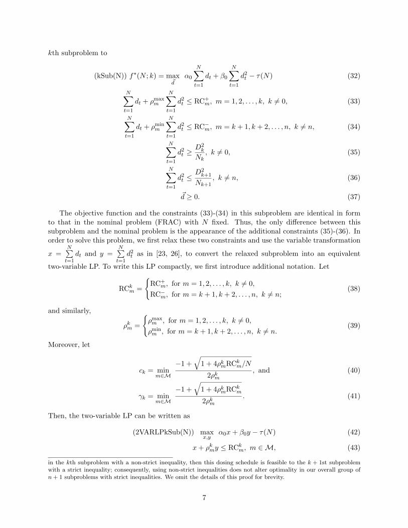
Let x∗, y∗ be an optimal solution to this two-variable LP. IfD2
kNk≤ y∗ ≤ D2
k+1
Nk+1as required by
constraints (35)-(36), we are done. If not, then an optimal solution can be recovered as explainedin Figure 1. Then, finally, a corresponding dosing schedule ~d∗(N) = (d∗1(N), d∗2(N), . . . , d∗N (N)) =(q, p, p, . . . , p︸ ︷︷ ︸
N−1 times
) that is optimal to problem (kSub(N)) is recovered by formulas (12)-(13).
y
x
(A)
(B)
(C)
(D)
(E)
Optimal solution
),( yxf
),( yxfy
x
NDy /2
11
NDy /2
22
Optimal sol. via
solving (SubLP)
Optimal sol. via
solving (SubLP)
Alt. optimal sol.
when (A) is optimal
Alt. optimal sol.
when (C) is optimal
(A)
(B)
(C)
(D)
2x
y
Nxy/2
2x
y
Nxy/2
(E)
(F)
(a) (b)
xcy*
xy
*
Figure 1: (a) A schematic illustration of the relationship between adjacent points in the feasible region of the subproblem k.When (C) is optimal, due to the linearity of the constraint and the objective function, it can be easily shown (via geometricor analytical proof) that the denoted points in the left-hand and right-hand side of the optimal point (C) are ranked as followsin terms of their objective value: (A)�(B)�(C) and similarly, (E)�(D)�(C). (b) A schematic illustration of the method forderiving the alternative optimal solution when optimal solution obtained by solving the relaxed subproblem (SubLP k) doesnot belong to the feasible region of subproblem k. By following the same logic as in (a), we can argue that when (A) or (D) arethe primary optimal solutions and are cut off by y1 or y2, (B) or (C) are the next-best optimal solutions, respectively. Also,because of the slope of the objective function, (B) and (C) are superior to (F) and (E), respectively.
4 Numerical experiments
4.1 Qualitative properties of robust solutions
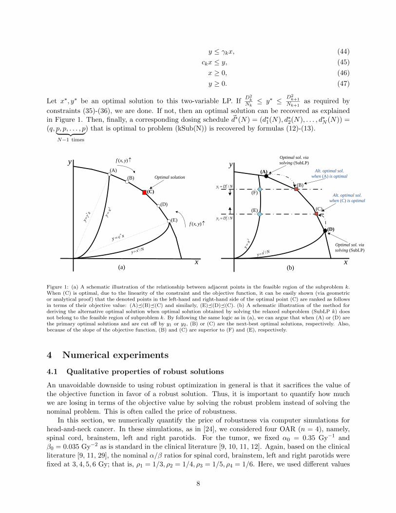
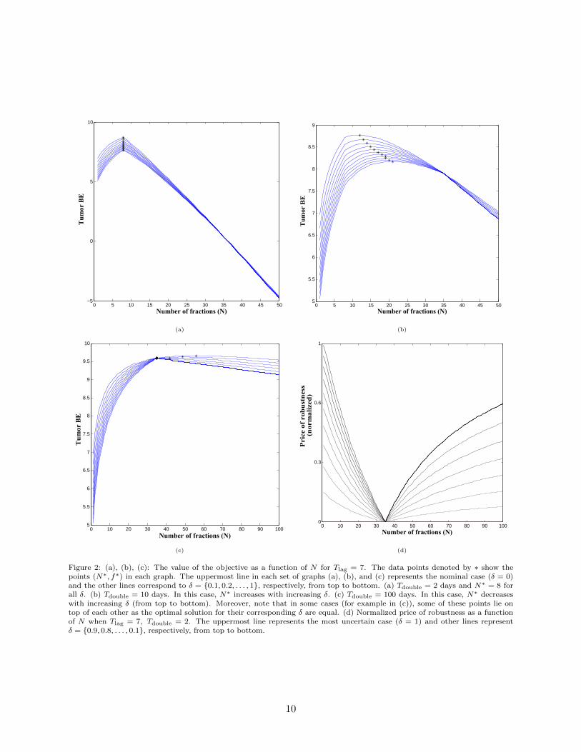
An unavoidable downside to using robust optimization in general is that it sacrifices the value ofthe objective function in favor of a robust solution. Thus, it is important to quantify how muchwe are losing in terms of the objective value by solving the robust problem instead of solving thenominal problem. This is often called the price of robustness.
In this section, we numerically quantify the price of robustness via computer simulations forhead-and-neck cancer. In these simulations, as in [24], we considered four OAR (n = 4), namely,spinal cord, brainstem, left and right parotids. For the tumor, we fixed α0 = 0.35 Gy−1 andβ0 = 0.035 Gy−2 as is standard in the clinical literature [9, 10, 11, 12]. Again, based on the clinicalliterature [9, 11, 29], the nominal α/β ratios for spinal cord, brainstem, left and right parotids werefixed at 3, 4, 5, 6 Gy; that is, ρ1 = 1/3, ρ2 = 1/4, ρ3 = 1/5, ρ4 = 1/6. Here, we used different values
8

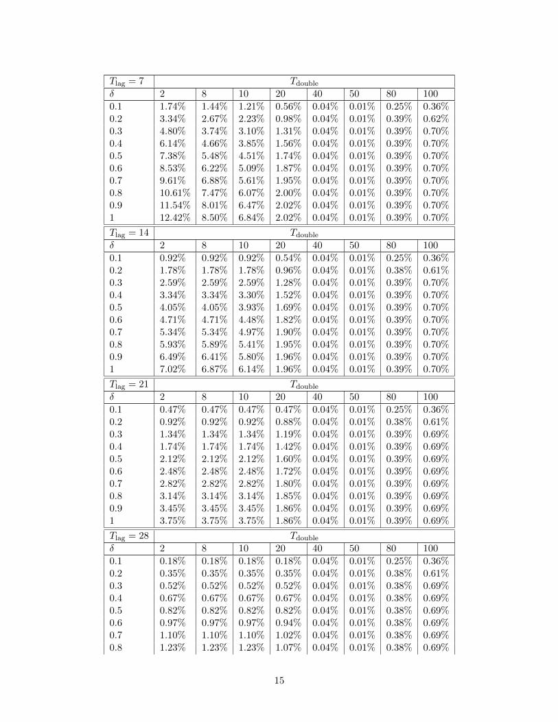
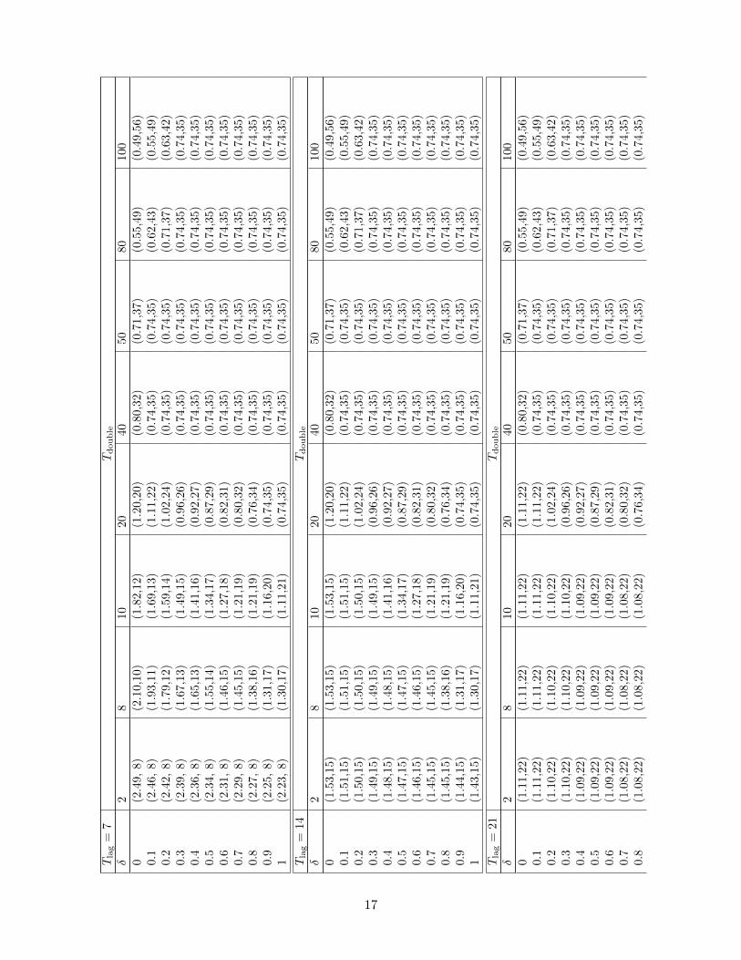
of nominal ratios for different OAR to fully explore the various possibilities that could arise in arobust formulation with multiple OAR. The tolerance doses for these OAR were fixed at 45, 50,26, and 28 Gy, respectively, and the conventional number of fractions Nm was fixed at 35 days forall OAR similar to the standard QUANTEC treatment protocol [19]. Nmax was set to 100 days.The uncertainty intervals were parameterized as ρ̃m ∈ [(1− δ)ρm, (1 + δ)ρm], where δ ∈ [0, 1]. Thisallowed us to easily quantify the price of robustness as a function of the uncertainty level δ. Wevaried δ from 0 (to represent the nominal case) to 1 (to denote the most uncertain case with 100%uncertainty) in increments of 0.1. All experiments were carried out in MATLAB on a laptop with2.20 GHz Intel Core2 Duo CPU and 2 GB of memory, running a Microsoft Windows 8.1 operatingsystem. Tables 1 and 2 summarize the results of our experiments for different values of Tlag, Tdouble,and δ. In these tables, Tlag values were set to 7, 14, 21, 28, 35 days based on [11] and Tdouble valueswere set to 2, 8, 10, 20, 40, 50, 80, 100 days based on [9, 11, 21, 29]. We are aware that the value of35 days for Tlag is perhaps too high; similarly, the values of 80 and 100 days for Tdouble are alsoperhaps too high for head-and-neck cancer. These somewhat extreme values were included in oursimulations to fully explore possible trends in various results of interest.
Table 1 shows, as expected, that the price of robustness increases with increasing δ for each Tlag,Tdouble combination. Overall, the price of robustness seems to be quite small in most experimentswith an average of 1.27% over all 400 experiments. The first, second, and third quartiles were0.12%, 0.47%, and 1.44%, respectively.
For each Tlag, δ combination in Table 1, the price of robustness first decreases with increasingTdouble, reaches the smallest value when Tdouble = 50 days and then increases. This trend isconsistent with the corresponding trend in the difference between Nm = 35 and N∗ that can beinferred from Table 2. Specifically, for each Tlag, δ combination, the magnitude of Nm−N∗ decreaseswith increasing Tdouble, reaches about a day or two when Tdouble = 50, and then increases. In fact,as we can see in Figure 2(d), when N = Nm = 35, the price of robustness is exactly zero; morestrongly, we found that this held true irrespective of the values of δ, Tlag, and Tdouble. A detailedalgebraic proof of this fact can be developed, but is omitted here for brevity. Roughly speaking, thekey idea in this proof is that when N = Nm, the BED constraints reduce to total dose constraints;this eliminates the dependence of the BED constraint on ρm and hence an equal-dosage solutionthat splits the tolerance dose across N fractions is optimal to the nominal and the robust problem.Consequently, the price of robustness is zero. Finally, for any combination of δ and Tdouble inTable 1, the price of robustness decreases as Tlag increases. Again, this is also consistent with thecorresponding trend in the magnitude of Nm −N∗.
A closer look at Table 2 reveals that the evolution of N∗ with δ for various fixed combinations ofTdouble and Tlag does not exhibit a universal trend. For instance, when Tlag = 7 days and Tdouble = 2days, N∗ = 8 for all δ (also see Figure 2 (a)). However, N∗ increases with increasing δ when Tlag = 7days and Tdouble = 10 days (Figure 2 (b)). On the other hand, N∗ decreases as δ increases whenTlag = 7 days and Tdouble = 100 days (Figure 2 (c)). Consistent with this observation, Table 2 alsoshows that for each fixed combination of Tdouble and Tlag, optimal doses do not exhibit a universalqualitative trend as a function of δ.
Finally, our robust solutions continue to exhibit qualitative trends that are well-establishedin the nominal case (see [24] and references therein). For instance, N∗ increases with increasingTdouble for any fixed δ, Tlag combination; similarly, N∗ also increases as Tlag increases for any fixedδ, Tdouble combination.
9
0 5 10 15 20 25 30 35 40 45 50−5
0
5
10
Tum
or B
E
Number of fractions (N)
(a)
0 5 10 15 20 25 30 35 40 45 505
5.5
6
6.5
7
7.5
8
8.5
9
Number of fractions (N)Tu
mor
BE
(b)
0 10 20 30 40 50 60 70 80 90 1005
5.5
6
6.5
7
7.5
8
8.5
9
9.5
10
Number of fractions (N)
Tum
or B
E
(c)
0 10 20 30 40 50 60 70 80 90 1000
0.3
0.6
1
Number of fractions (N)
Pric
e of
rob
ustn
ess
(nor
mal
ized
)
(d)
Figure 2: (a), (b), (c): The value of the objective as a function of N for Tlag = 7. The data points denoted by ∗ show thepoints (N∗, f∗) in each graph. The uppermost line in each set of graphs (a), (b), and (c) represents the nominal case (δ = 0)and the other lines correspond to δ = {0.1, 0.2, . . . , 1}, respectively, from top to bottom. (a) Tdouble = 2 days and N∗ = 8 forall δ. (b) Tdouble = 10 days. In this case, N∗ increases with increasing δ. (c) Tdouble = 100 days. In this case, N∗ decreaseswith increasing δ (from top to bottom). Moreover, note that in some cases (for example in (c)), some of these points lie ontop of each other as the optimal solution for their corresponding δ are equal. (d) Normalized price of robustness as a functionof N when Tlag = 7, Tdouble = 2. The uppermost line represents the most uncertain case (δ = 1) and other lines representδ = {0.9, 0.8, . . . , 0.1}, respectively, from top to bottom.
10
4.2 Infeasibility tests
As mentioned before, the primary motivation for the robust formulation is that the optimal solutionobtained by solving the nominal formulation is guaranteed to be feasible only for nominal valuesof ρ. This means that if the actual ρ values turn out to be different than the nominal, the nominalsolution might become infeasible. To quantify the frequency and extent of such infeasibility, wefirst performed a set of numerical experiments where the realized values of ρ were assumed to equalvarious grid-points in the uncertainty intervals around the nominal values. It turned out that whileρ varied in this manner over grid-points inside the uncertainty interval, the nominal solution wasinfeasible in about 75% of the cases; the robust solution of course remained feasible in all cases.The amount of infeasibility in some cases was rather large — close to 50%, with an average of10.5%. The first, second, and third quartiles were 3.99%, 8.44%, and 15.76%, respectively. Giventhe relatively small price of robustness reported in Section 4.1, this suggests that it might beworthwhile to implement the robust dosing schedules rather than the nominal ones.
In the robust counterpart, we assumed that the value of ρ for each OAR belongs to a knowninterval. Therefore, any solution to our robust formulation is guaranteed to be feasible only as longas this assumption holds. Due to the uncertainty in the actual values of ρ, however, this assumptioncould be violated. In that case, our robust solution might not be feasible after all. To test theimpact of this unfortunate occurrence, we performed numerical experiments where ρ values werevaried outside the predetermined uncertainty interval. In particular, for each uncertainty levelδ and constraint m, five grid-points were chosen at ρ̃m = (1 + δ + γ)ρm and five grid-points atρ̃m = (1− δ − γ)ρm, where γ ∈ {0.1, 0.2, . . . , 0.5} and ρm denotes the nominal value. The nominalsolution was infeasible in over 65% of the cases, while the robust solution was infeasible in 43%of the cases. The amount of infeasibility was found to be statistically lower (via a pairwise t-testat the p = 0.05 significance level) for the robust solution than the nominal solution over all cases.This is encouraging because it suggests that the robust solution might be “more robust” than thenominal solution even when ρ values are outside the uncertainty intervals (although it does notappear possible to rigorously state and prove this claim).
4.3 Uncertainty in tumor parameters
Throughout this paper, we assumed that the values of the tumor parameters α0 and β0 were known.In this section, we investigate the effect of uncertainty in these tumor parameters. We assume thatboth α̃0 and β̃0 belong to a known interval. That is, α̃0 ∈ [αmin
0 , αmax0 ] and β̃0 ∈ [βmin
0 , βmax0 ].
Since we are maximizing the objective function, the worst realization of the problem occurs whenα̃0 = αmin
0 , β̃0 = βmin0 . That is, the robust objective value is simply attained by replacing α̃0
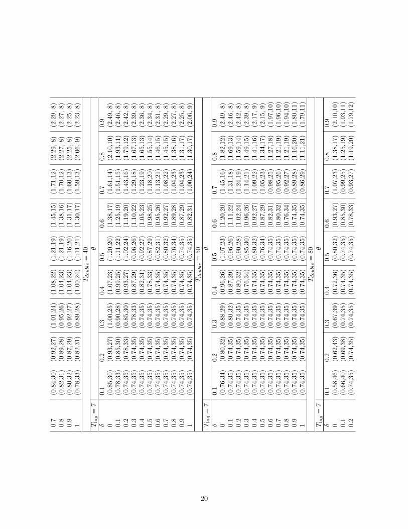
and β̃0 by their minimum values. Table 3 shows the effect of this uncertainty, assuming thatα̃0 ∈ [(1− θ)α̂0, (1 + θ)α̂0] and β̃0 ∈ [(1− θ)β̂0, (1 + θ)β̂0]. Here, the nominal values α̂0 and β̂0 wereset to 0.35 Gy and 0.035 Gy−2, respectively, and θ was varied in the set {0.1, 0.2, . . . , 0.9}. A quickinspection of the table reveals that as the tumor uncertainty level increases, the number of fractionsdecreases and the dose delivered in each session increases. In other words, higher uncertainty intumor parameters causes it to behave similar to faster-proliferating tumors.
5 Discussion
Most existing research on robust optimization in cancer radiotherapy focuses on incorporatinguncertainty in the actual dose delivered to various anatomical regions of interest via intensitymodulated radiation therapy (IMRT) and other treatment methods. Causes of this uncertainty
11
include patient movement, say due to breathing, or setup errors at the time of treatment delivery(see, for instance, [6, 8, 16, 17, 18, 27] and references therein).
In this paper, we provided a robust formulation of the fractionation problem. Perhaps more im-portantly, we also described in detail a simple method for exact solution of this robust formulation.Although our robust formulation is, at first glance, inevitably at least as hard as a non-convexQCQP, we were able to show that it can be solved to optimality by solving a few two-variableLPs with a few constraints each. Our numerical experiments provided insights into the behaviorof nominal and robust dosing schedules and also quantified the price of robustness. Overall, ourcomparison of the frequency and amount of infeasibility incurred by the nominal and the robustsolutions suggests that the robust solutions are indeed statistically more feasible and yet pay arelatively small price of robustness. This could provide motivation for future investigations intothe use of biological dose-response models such as the LQ model for planning radiation treatmentas the uncertainty in dose-response parameters has been the main obstacle in widespread relianceon these models (see [14]).
Note that the nominal fractionation model in [24, 26] used the concept of sparing factors tomodel the doses delivered to the various OAR. For instance, if dose dt is given to the tumor infraction t, then the dose to OAR m ∈ M equals smdt; here, sm is a non-negative sparing factor.In this paper, we did not use such sparing factors because they would have been distracting to themain message of our work. We do emphasize, however, that our solution procedure in Section 3would work even if such sparing factors were included. More strongly, our solution method wouldwork even if the true values of these sparing factors were unknown but were instead assumed tobelong to a non-negative interval. This can be done simply by using the largest values of thesesparing factors in our robust formulation as in [1].
In a recent unpublished manuscript based on the doctoral dissertation of Saberian [23], Saberianet al. [25] presented a spatiotemporally integrated formulation of the fractionation problem. Thedecision variables in that formulation were N and the intensity profiles of the IMRT radiation fieldsemployed in each fraction. The numbers of variables and constraints in that non-convex formulationare as large as tens of thousands. It would be interesting in the future to formulate the robustcounterpart of that model and to devise efficient approximate solution methods.
6 Acknowledgment
Funded in part by the National Science Foundation through grant #CMMI 1054026.
References
[1] H Badri, Y Watanabe, and K Leder. Robust and probabilistic optimization of dose schedulesin radiotherapy. available online at arxiv.org/pdf/1503.00399v2.pdf, June 2015.
[2] H Badri, Y Watanabe, and K Leder. Robust optimization of dose schedules in radiotherapy.available online at arxiv.org/pdf/1503.00399v1.pdf, March 2015.
[3] A Ben-Tal, L El Ghaoui, and A Nemirovski. Robust Optimization. Princeton University Press,Princeton, NJ, USA, 2009.
[4] D Bertsimas, D B Brown, and C Caramanis. Theory and applications of robust optimization.SIAM Review, 53(3):464–501, 2011.
12
[5] A Bertuzzi, C Bruni F Papa, and C Sinisgalli. Optimal solution for a cancer radiotherapyproblem. Journal of Mathematical Biology, 66(1-2):311–349, 2013.
[6] T Bortfeld, T C Y Chan, A Trofimov, and J N Tsitsiklis. Robust management of motionuncertainty in intensity modulated radiation therapy. Operations Research, 56(6):1461–1473,2008.
[7] T Bortfeld, J Ramakrishnan, J N Tsitsiklis, and J Unkelbach. Optimization of radio-therapy fractionation schedules in the presence of tumor repopluation. forthcoming in IN-FORMS Journal on Computing, prepring available at http://pages.discovery.wisc.edu/
~jramakrishnan/BRT2015_repop.pdf, May 2015.
[8] T C Y Chan, T Bortfeld, and J Tsitsiklis. A robust approach to IMRT optimization. Physicsin Medicine and Biology, 51:2567–2583, 2006.
[9] J F Fowler. How worthwhile are short schedules in radiotherapy?: A series of exploratorycalculations. Radiotherapy and Oncology, 18(2):165–181, 1990.
[10] J F Fowler. Biological factors influencing optimum fractionation in radiation therapy. ActaOncologica, 40(6):712–717, 2001.
[11] J F Fowler. Is there an optimal overall time for head and neck radiotherapy? a review withnew modeling. Clinical Oncology, 19(1):8–27, 2007.
[12] J F Fowler. Optimum overall times II: Extended modelling for head and neck radiotherapy.Clinical Oncology, 20(2):113–126, 2008.
[13] J F Fowler and M A Ritter. A rationale for fractionation for slowly proliferating tumors suchas prostatic adenocarcinoma. International Journal of Radiation Oncology Biology Physics,32(2):521–529, 1995.
[14] E J Hall and A J Giaccia. Radiobiology for the Radiologist. Lippincott Williams & Wilkins,Philadelphia, Pennsylvania, USA, 2005.
[15] B Jones, L T Tan, and R G Dale. Derivation of the optimum dose per fraction from the linearquadratic model. The British Journal of Radiology, 68(812):894–902, 1995.
[16] H Mahmoudzadeh, J Lee, T C Y Chan, and T G Purdie. Robust optimization methods forcardiac sparing in tangential breast IMRT. Medical Physics, 42(5):2212, 2015.
[17] H Mahmoudzadeh, T G Purdie, and T C Y Chan. Constraint generation methods for robustoptimization in radiation therapy. forthcoming in Operations Research for Health Care, June2015.
[18] P A Mar and T C Y Chan. Adaptive and robust radiation therapy in the presence of drift.Physics in Medicine and Biology, 60(9):3599–3615, 2015.
[19] L B Marks, E D Yorke, A Jackson, R K Ten Haken, L S Constine, A Eisbruch, S M Bentzen,J Nam, and J O Deasy. Use of normal tissue complication probability models in the clinic.International Journal of Radiation Oncology Biology Physics, 76(3):S10–S19, 2010.
13
[20] M Mizuta, S Takao, H Date, N Kishimoto, K L Sutherland, R Onimaru, and H Shirato. Amathematical study to select fractionation regimen based on physical dose distribution andthe linear-quadratic model. International Journal of Radiation Oncology Biology Physics,84(3):829 – 833, 2012.
[21] X S Qi, Q Yang, S P Lee, X A Li, and D Wang. An estimation of radiobiological parametersfor head-and-neck cancer cells and the clinical implications. Cancers, 4:566–580, 2012.
[22] S Rockwell. Experimental radiotherapy: a brief history. Radiation Research,150(Supplement):S157–S169, November 1998.
[23] F Saberian. Convex and Dynamic Optimization with Learning for Adaptive Biologically Con-formal Radiotherapy. unpublished doctoral dissertation, University of Washington, Industrialand Systems Engineering, May 2015.
[24] F Saberian, A Ghate, and M Kim. Optimal fractionation in radiotherapy with multiple normaltissues. forthcoming in Mathematical Medicine and Biology, online preprint available at doi:10.1093/imammb/dqv015, May 2015.
[25] F Saberian, A Ghate, and M Kim. Spatiotemporally integrated fractionation in radiotherapy.under review at INFORMS Journal on Computing, preprint available at http://faculty.
washington.edu/archis/upaper-apr-2015.pdf, April 2015.
[26] F Saberian, A Ghate, and M Kim. A two-variable linear program solves the standard linear–quadratic formulation of the fractionation problem in cancer radiotherapy. Operations ResearchLetters, 43(3):254 – 258, 2015.
[27] J Unkelbach, T C Y Chan, and T Bortfeld. Accounting for range uncertainties in the optimiza-tion of intensity modulated proton therapy. Physics in Medicine and Biology, 52:2755–2773,2007.
[28] J Unkelbach, D Craft, E Saleri, J Ramakrishnan, and T Bortfeld. The dependence of opti-mal fractionation schemes on the spatial dose distribution. Physics in Medicine and Biology,58(1):159–167, 2013.
[29] Y Yang and L Xing. Optimization of radiotherapy dose-time fractionation with considerationof tumor specific biology. Medical Physics, 32(12):3666–3677, 2005.
14
Tlag = 7 Tdouble
δ 2 8 10 20 40 50 80 100
0.1 1.74% 1.44% 1.21% 0.56% 0.04% 0.01% 0.25% 0.36%0.2 3.34% 2.67% 2.23% 0.98% 0.04% 0.01% 0.39% 0.62%0.3 4.80% 3.74% 3.10% 1.31% 0.04% 0.01% 0.39% 0.70%0.4 6.14% 4.66% 3.85% 1.56% 0.04% 0.01% 0.39% 0.70%0.5 7.38% 5.48% 4.51% 1.74% 0.04% 0.01% 0.39% 0.70%0.6 8.53% 6.22% 5.09% 1.87% 0.04% 0.01% 0.39% 0.70%0.7 9.61% 6.88% 5.61% 1.95% 0.04% 0.01% 0.39% 0.70%0.8 10.61% 7.47% 6.07% 2.00% 0.04% 0.01% 0.39% 0.70%0.9 11.54% 8.01% 6.47% 2.02% 0.04% 0.01% 0.39% 0.70%1 12.42% 8.50% 6.84% 2.02% 0.04% 0.01% 0.39% 0.70%
Tlag = 14 Tdouble
δ 2 8 10 20 40 50 80 100
0.1 0.92% 0.92% 0.92% 0.54% 0.04% 0.01% 0.25% 0.36%0.2 1.78% 1.78% 1.78% 0.96% 0.04% 0.01% 0.38% 0.61%0.3 2.59% 2.59% 2.59% 1.28% 0.04% 0.01% 0.39% 0.70%0.4 3.34% 3.34% 3.30% 1.52% 0.04% 0.01% 0.39% 0.70%0.5 4.05% 4.05% 3.93% 1.69% 0.04% 0.01% 0.39% 0.70%0.6 4.71% 4.71% 4.48% 1.82% 0.04% 0.01% 0.39% 0.70%0.7 5.34% 5.34% 4.97% 1.90% 0.04% 0.01% 0.39% 0.70%0.8 5.93% 5.89% 5.41% 1.95% 0.04% 0.01% 0.39% 0.70%0.9 6.49% 6.41% 5.80% 1.96% 0.04% 0.01% 0.39% 0.70%1 7.02% 6.87% 6.14% 1.96% 0.04% 0.01% 0.39% 0.70%
Tlag = 21 Tdouble
δ 2 8 10 20 40 50 80 100
0.1 0.47% 0.47% 0.47% 0.47% 0.04% 0.01% 0.25% 0.36%0.2 0.92% 0.92% 0.92% 0.88% 0.04% 0.01% 0.38% 0.61%0.3 1.34% 1.34% 1.34% 1.19% 0.04% 0.01% 0.39% 0.69%0.4 1.74% 1.74% 1.74% 1.42% 0.04% 0.01% 0.39% 0.69%0.5 2.12% 2.12% 2.12% 1.60% 0.04% 0.01% 0.39% 0.69%0.6 2.48% 2.48% 2.48% 1.72% 0.04% 0.01% 0.39% 0.69%0.7 2.82% 2.82% 2.82% 1.80% 0.04% 0.01% 0.39% 0.69%0.8 3.14% 3.14% 3.14% 1.85% 0.04% 0.01% 0.39% 0.69%0.9 3.45% 3.45% 3.45% 1.86% 0.04% 0.01% 0.39% 0.69%1 3.75% 3.75% 3.75% 1.86% 0.04% 0.01% 0.39% 0.69%
Tlag = 28 Tdouble
δ 2 8 10 20 40 50 80 100
0.1 0.18% 0.18% 0.18% 0.18% 0.04% 0.01% 0.25% 0.36%0.2 0.35% 0.35% 0.35% 0.35% 0.04% 0.01% 0.38% 0.61%0.3 0.52% 0.52% 0.52% 0.52% 0.04% 0.01% 0.38% 0.69%0.4 0.67% 0.67% 0.67% 0.67% 0.04% 0.01% 0.38% 0.69%0.5 0.82% 0.82% 0.82% 0.82% 0.04% 0.01% 0.38% 0.69%0.6 0.97% 0.97% 0.97% 0.94% 0.04% 0.01% 0.38% 0.69%0.7 1.10% 1.10% 1.10% 1.02% 0.04% 0.01% 0.38% 0.69%0.8 1.23% 1.23% 1.23% 1.07% 0.04% 0.01% 0.38% 0.69%
15

0.9 1.36% 1.36% 1.36% 1.08% 0.04% 0.01% 0.38% 0.69%1 1.48% 1.48% 1.48% 1.08% 0.04% 0.01% 0.38% 0.69%
Tlag = 35 Tdouble
δ 2 8 10 20 40 50 80 100
0.1 0.03% 0.03% 0.03% 0.03% 0.03% 0.03% 0.25% 0.36%0.2 0.06% 0.06% 0.06% 0.06% 0.06% 0.06% 0.38% 0.61%0.3 0.08% 0.08% 0.08% 0.08% 0.08% 0.09% 0.41% 0.69%0.4 0.12% 0.12% 0.12% 0.12% 0.12% 0.12% 0.44% 0.72%0.5 0.15% 0.15% 0.15% 0.15% 0.15% 0.15% 0.47% 0.76%0.6 0.15% 0.15% 0.15% 0.15% 0.15% 0.15% 0.47% 0.76%0.7 0.15% 0.15% 0.15% 0.15% 0.15% 0.15% 0.47% 0.76%0.8 0.15% 0.15% 0.15% 0.15% 0.15% 0.15% 0.47% 0.76%0.9 0.15% 0.15% 0.15% 0.15% 0.15% 0.15% 0.47% 0.76%1 0.15% 0.15% 0.15% 0.15% 0.15% 0.15% 0.47% 0.76%
Table 1: The price of robustness for different combinations of Tlag, Tdouble, and δ. The price of robustness equals ( g∗−f∗
g∗ )×100%,
where f∗ and g∗ are the optimal values of the robust and the nominal formulations, respectively.
16
Tlag
=7
Tdouble
δ2
810
20
40
50
80
100
0(2
.49,
8)(2
.10,
10)
(1.8
2,1
2)
(1.2
0,2
0)
(0.8
0,3
2)
(0.7
1,3
7)
(0.5
5,4
9)
(0.4
9,5
6)
0.1
(2.4
6,8)
(1.9
3,11
)(1
.69,1
3)
(1.1
1,2
2)
(0.7
4,3
5)
(0.7
4,3
5)
(0.6
2,4
3)
(0.5
5,4
9)
0.2
(2.4
2,8)
(1.7
9,12
)(1
.59,1
4)
(1.0
2,2
4)
(0.7
4,3
5)
(0.7
4,3
5)
(0.7
1,3
7)
(0.6
3,4
2)
0.3
(2.3
9,8)
(1.6
7,13
)(1
.49,1
5)
(0.9
6,2
6)
(0.7
4,3
5)
(0.7
4,3
5)
(0.7
4,3
5)
(0.7
4,3
5)
0.4
(2.3
6,8)
(1.6
5,13
)(1
.41,1
6)
(0.9
2,2
7)
(0.7
4,3
5)
(0.7
4,3
5)
(0.7
4,3
5)
(0.7
4,3
5)
0.5
(2.3
4,8)
(1.5
5,14
)(1
.34,1
7)
(0.8
7,2
9)
(0.7
4,3
5)
(0.7
4,3
5)
(0.7
4,3
5)
(0.7
4,3
5)
0.6
(2.3
1,8)
(1.4
6,15
)(1
.27,1
8)
(0.8
2,3
1)
(0.7
4,3
5)
(0.7
4,3
5)
(0.7
4,3
5)
(0.7
4,3
5)
0.7
(2.2
9,8)
(1.4
5,15
)(1
.21,1
9)
(0.8
0,3
2)
(0.7
4,3
5)
(0.7
4,3
5)
(0.7
4,3
5)
(0.7
4,3
5)
0.8
(2.2
7,8)
(1.3
8,16
)(1
.21,1
9)
(0.7
6,3
4)
(0.7
4,3
5)
(0.7
4,3
5)
(0.7
4,3
5)
(0.7
4,3
5)
0.9
(2.2
5,8)
(1.3
1,17
)(1
.16,2
0)
(0.7
4,3
5)
(0.7
4,3
5)
(0.7
4,3
5)
(0.7
4,3
5)
(0.7
4,3
5)
1(2
.23,
8)(1
.30,
17)
(1.1
1,2
1)
(0.7
4,3
5)
(0.7
4,3
5)
(0.7
4,3
5)
(0.7
4,3
5)
(0.7
4,3
5)
Tlag
=14
Tdouble
δ2
810
20
40
50
80
100
0(1
.53,
15)
(1.5
3,15
)(1
.53,1
5)
(1.2
0,2
0)
(0.8
0,3
2)
(0.7
1,3
7)
(0.5
5,4
9)
(0.4
9,5
6)
0.1
(1.5
1,15
)(1
.51,
15)
(1.5
1,1
5)
(1.1
1,2
2)
(0.7
4,3
5)
(0.7
4,3
5)
(0.6
2,4
3)
(0.5
5,4
9)
0.2
(1.5
0,15
)(1
.50,
15)
(1.5
0,1
5)
(1.0
2,2
4)
(0.7
4,3
5)
(0.7
4,3
5)
(0.7
1,3
7)
(0.6
3,4
2)
0.3
(1.4
9,15
)(1
.49,
15)
(1.4
9,1
5)
(0.9
6,2
6)
(0.7
4,3
5)
(0.7
4,3
5)
(0.7
4,3
5)
(0.7
4,3
5)
0.4
(1.4
8,15
)(1
.48,
15)
(1.4
1,1
6)
(0.9
2,2
7)
(0.7
4,3
5)
(0.7
4,3
5)
(0.7
4,3
5)
(0.7
4,3
5)
0.5
(1.4
7,15
)(1
.47,
15)
(1.3
4,1
7)
(0.8
7,2
9)
(0.7
4,3
5)
(0.7
4,3
5)
(0.7
4,3
5)
(0.7
4,3
5)
0.6
(1.4
6,15
)(1
.46,
15)
(1.2
7,1
8)
(0.8
2,3
1)
(0.7
4,3
5)
(0.7
4,3
5)
(0.7
4,3
5)
(0.7
4,3
5)
0.7
(1.4
5,15
)(1
.45,
15)
(1.2
1,1
9)
(0.8
0,3
2)
(0.7
4,3
5)
(0.7
4,3
5)
(0.7
4,3
5)
(0.7
4,3
5)
0.8
(1.4
5,15
)(1
.38,
16)
(1.2
1,1
9)
(0.7
6,3
4)
(0.7
4,3
5)
(0.7
4,3
5)
(0.7
4,3
5)
(0.7
4,3
5)
0.9
(1.4
4,15
)(1
.31,
17)
(1.1
6,2
0)
(0.7
4,3
5)
(0.7
4,3
5)
(0.7
4,3
5)
(0.7
4,3
5)
(0.7
4,3
5)
1(1
.43,
15)
(1.3
0,17
)(1
.11,2
1)
(0.7
4,3
5)
(0.7
4,3
5)
(0.7
4,3
5)
(0.7
4,3
5)
(0.7
4,3
5)
Tlag
=21
Tdouble
δ2
810
20
40
50
80
100
0(1
.11,
22)
(1.1
1,22
)(1
.11,2
2)
(1.1
1,2
2)
(0.8
0,3
2)
(0.7
1,3
7)
(0.5
5,4
9)
(0.4
9,5
6)
0.1
(1.1
1,22
)(1
.11,
22)
(1.1
1,2
2)
(1.1
1,2
2)
(0.7
4,3
5)
(0.7
4,3
5)
(0.6
2,4
3)
(0.5
5,4
9)
0.2
(1.1
0,22
)(1
.10,
22)
(1.1
0,2
2)
(1.0
2,2
4)
(0.7
4,3
5)
(0.7
4,3
5)
(0.7
1,3
7)
(0.6
3,4
2)
0.3
(1.1
0,22
)(1
.10,
22)
(1.1
0,2
2)
(0.9
6,2
6)
(0.7
4,3
5)
(0.7
4,3
5)
(0.7
4,3
5)
(0.7
4,3
5)
0.4
(1.0
9,22
)(1
.09,
22)
(1.0
9,2
2)
(0.9
2,2
7)
(0.7
4,3
5)
(0.7
4,3
5)
(0.7
4,3
5)
(0.7
4,3
5)
0.5
(1.0
9,22
)(1
.09,
22)
(1.0
9,2
2)
(0.8
7,2
9)
(0.7
4,3
5)
(0.7
4,3
5)
(0.7
4,3
5)
(0.7
4,3
5)
0.6
(1.0
9,22
)(1
.09,
22)
(1.0
9,2
2)
(0.8
2,3
1)
(0.7
4,3
5)
(0.7
4,3
5)
(0.7
4,3
5)
(0.7
4,3
5)
0.7
(1.0
8,22
)(1
.08,
22)
(1.0
8,2
2)
(0.8
0,3
2)
(0.7
4,3
5)
(0.7
4,3
5)
(0.7
4,3
5)
(0.7
4,3
5)
0.8
(1.0
8,22
)(1
.08,
22)
(1.0
8,2
2)
(0.7
6,3
4)
(0.7
4,3
5)
(0.7
4,3
5)
(0.7
4,3
5)
(0.7
4,3
5)
17

0.9
(1.0
8,22
)(1
.08,
22)
(1.0
8,2
2)
(0.7
4,3
5)
(0.7
4,3
5)
(0.7
4,3
5)
(0.7
4,3
5)
(0.7
4,3
5)
1(1
.07,
22)
(1.0
7,22
)(1
.07,2
2)
(0.7
4,3
5)
(0.7
4,3
5)
(0.7
4,3
5)
(0.7
4,3
5)
(0.7
4,3
5)
Tlag
=28
Tdouble
δ2
810
20
40
50
80
100
0(0
.88,
29)
(0.8
8,29
)(0
.88,2
9)
(0.8
8,2
9)
(0.8
0,3
2)
(0.7
1,3
7)
(0.5
5,4
9)
(0.4
9,5
6)
0.1
(0.8
7,29
)(0
.87,
29)
(0.8
7,2
9)
(0.8
7,2
9)
(0.7
4,3
5)
(0.7
4,3
5)
(0.6
2,4
3)
(0.5
5,4
9)
0.2
(0.8
7,29
)(0
.87,
29)
(0.8
7,2
9)
(0.8
7,2
9)
(0.7
4,3
5)
(0.7
4,3
5)
(0.7
1,3
7)
(0.6
3,4
2)
0.3
(0.8
7,29
)(0
.87,
29)
(0.8
7,2
9)
(0.8
7,2
9)
(0.7
4,3
5)
(0.7
4,3
5)
(0.7
4,3
5)
(0.7
4,3
5)
0.4
(0.8
7,29
)(0
.87,
29)
(0.8
7,2
9)
(0.8
7,2
9)
(0.7
4,3
5)
(0.7
4,3
5)
(0.7
4,3
5)
(0.7
4,3
5)
0.5
(0.8
7,29
)(0
.87,
29)
(0.8
7,2
9)
(0.8
7,2
9)
(0.7
4,3
5)
(0.7
4,3
5)
(0.7
4,3
5)
(0.7
4,3
5)
0.6
(0.8
7,29
)(0
.87,
29)
(0.8
7,2
9)
(0.8
2,3
1)
(0.7
4,3
5)
(0.7
4,3
5)
(0.7
4,3
5)
(0.7
4,3
5)
0.7
(0.8
7,29
)(0
.87,
29)
(0.8
7,2
9)
(0.8
0,3
2)
(0.7
4,3
5)
(0.7
4,3
5)
(0.7
4,3
5)
(0.7
4,3
5)
0.8
(0.8
7,29
)(0
.87,
29)
(0.8
7,2
9)
(0.7
6,3
4)
(0.7
4,3
5)
(0.7
4,3
5)
(0.7
4,3
5)
(0.7
4,3
5)
0.9
(0.8
7,29
)(0
.87,
29)
(0.8
7,2
9)
(0.7
4,3
5)
(0.7
4,3
5)
(0.7
4,3
5)
(0.7
4,3
5)
(0.7
4,3
5)
1(0
.86,
29)
(0.8
6,29
)(0
.86,2
9)
(0.7
4,3
5)
(0.7
4,3
5)
(0.7
4,3
5)
(0.7
4,3
5)
(0.7
4,3
5)
Tlag
=35
Tdouble
δ2
810
20
40
50
80
100
0(0
.72,
36)
(0.7
2,36
)(0
.72,3
6)
(0.7
2,3
6)
(0.7
2,3
6)
(0.7
1,3
7)
(0.5
5,4
9)
(0.4
9,5
6)
0.1
(0.7
2,36
)(0
.72,
36)
(0.7
2,3
6)
(0.7
2,3
6)
(0.7
2,3
6)
(0.7
2,3
6)
(0.6
2,4
3)
(0.5
5,4
9)
0.2
(0.7
2,36
)(0
.72,
36)
(0.7
2,3
6)
(0.7
2,3
6)
(0.7
2,3
6)
(0.7
2,3
6)
(0.7
1,3
7)
(0.6
3,4
2)
0.3
(0.7
2,36
)(0
.72,
36)
(0.7
2,3
6)
(0.7
2,3
6)
(0.7
2,3
6)
(0.7
2,3
6)
(0.7
2,3
6)
(0.7
2,3
6)
0.4
(0.7
2,36
)(0
.72,
36)
(0.7
2,3
6)
(0.7
2,3
6)
(0.7
2,3
6)
(0.7
2,3
6)
(0.7
2,3
6)
(0.7
2,3
6)
0.5
(0.7
4,35
)(0
.74,
35)
(0.7
4,3
5)
(0.7
4,3
5)
(0.7
4,3
5)
(0.7
4,3
5)
(0.7
4,3
5)
(0.7
4,3
5)
0.6
(1.4
4,0.
70,3
6)*
(1.4
4,0.
70,3
6)*
(1.4
4,0
.70,3
6)*
(1.4
4,0
.70,3
6)*
(1.4
4,0
.70,3
6)*
(1.4
4,0
.70,3
6)*
(1.4
4,0
.70,3
6)*
(1.4
4,0
.70,3
6)*
0.7
(1.4
4,0.
70,3
6)*
(1.4
4,0.
70,3
6)*
(1.4
4,0
.70,3
6)*
(1.4
4,0
.70,3
6)*
(1.4
4,0
.70,3
6)*
(1.4
4,0
.70,3
6)*
(1.4
4,0
.70,3
6)*
(1.4
4,0
.70,3
6)*
0.8
(0.7
4,35
)(0
.74,
35)
(0.7
4,3
5)
(0.7
4,3
5)
(0.7
4,3
5)
(0.7
4,3
5)
(0.7
4,3
5)
(0.7
4,3
5)
0.9
(1.4
4,0.
70,3
6)*
(1.4
4,0.
70,3
6)*
(1.4
4,0
.70,3
6)*
(1.4
4,0
.70,3
6)*
(1.4
4,0
.70,3
6)*
(1.4
4,0
.70,3
6)*
(1.4
4,0
.70,3
6)*
(1.4
4,0
.70,3
6)*
1(1
.44,
0.70
,36)
*(1
.44,
0.70
,36)
*(1
.44,0
.70,3
6)*
(1.4
4,0
.70,3
6)*
(1.4
4,0
.70,3
6)*
(1.4
4,0
.70,3
6)*
(1.4
4,0
.70,3
6)*
(1.4
4,0
.70,3
6)*
Tab
le2:
Th
eop
tim
al
solu
tion
(d∗,N∗)
of
the
rob
ust
an
dn
om
inal
mod
els
for
diff
eren
tco
mb
inati
on
sofTlag,T
double
,an
dδ.
Th
efi
rst
row
inea
chse
ctio
nof
the
tab
lesh
ow
sth
eso
luti
on
of
the
nom
inal
case
(δ=
0).
Th
eca
ses
mark
edw
ith
an
ast
eris
k(∗
)yie
ldu
neq
ual-
dosa
ge
solu
tion
sch
ara
cter
ized
by
two
dose
valu
es(q,p
)(r
ecall
form
ula
s(1
2)-
(13))
an
danN∗
valu
ein
that
ord
er.
18

Tdouble
=8
Tlag
=7
θδ
0.1
0.2
0.3
0.4
0.5
0.6
0.7
0.8
0.9
0(2
.28,
9)(2
.49,
8)
(2.4
9,
8)
(2.4
9,
8)
(2.4
9,
8)
(2.4
9,
8)
(2.4
9,
8)
(2.4
9,
8)
(2.4
9,
8)
0.1
(2.0
8,10
)(2
.25,
9)
(2.4
6,
8)
(2.4
6,
8)
(2.4
6,
8)
(2.4
6,
8)
(2.4
6,
8)
(2.4
6,
8)
(2.4
6,
8)
0.2
(1.9
1,11
)(2
.05,
10)
(2.2
2,
9)
(2.4
2,
8)
(2.4
2,
8)
(2.4
2,
8)
(2.4
2,
8)
(2.4
2,
8)
(2.4
2,
8)
0.3
(1.8
9,11
)(2
.03,
10)
(2.1
9,
9)
(2.3
9,
8)
(2.3
9,
8)
(2.3
9,
8)
(2.3
9,
8)
(2.3
9,
8)
(2.3
9,
8)
0.4
(1.7
5,12
)(1
.87,
11)
(2.0
1,1
0)
(2.3
6,
8)
(2.3
6,
8)
(2.3
6,
8)
(2.3
6,
8)
(2.3
6,
8)
(2.3
6,
8)
0.5
(1.6
4,13
)(1
.74,
12)
(1.9
9,1
0)
(2.1
5,
9)
(2.3
4,
8)
(2.3
4,
8)
(2.3
4,
8)
(2.3
4,
8)
(2.3
4,
8)
0.6
(1.6
3,13
)(1
.73,
12)
(1.8
4,1
1)
(2.1
3,
9)
(2.3
1,
8)
(2.3
1,
8)
(2.3
1,
8)
(2.3
1,
8)
(2.3
1,
8)
0.7
(1.5
3,14
)(1
.62,
13)
(1.8
3,1
1)
(1.9
6,1
0)
(2.2
9,
8)
(2.2
9,
8)
(2.2
9,
8)
(2.2
9,
8)
(2.2
9,
8)
0.8
(1.4
5,15
)(1
.61,
13)
(1.7
0,1
2)
(1.9
4,1
0)
(2.2
7,
8)
(2.2
7,
8)
(2.2
7,
8)
(2.2
7,
8)
(2.2
7,
8)
0.9
(1.4
4,15
)(1
.51,
14)
(1.6
9,1
2)
(1.9
3,1
0)
(2.2
5,
8)
(2.2
5,
8)
(2.2
5,
8)
(2.2
5,
8)
(2.2
5,
8)
1(1
.36,
16)
(1.5
0,14
)(1
.68,1
2)
(1.7
9,1
1)
(2.0
6,
9)
(2.2
3,
8)
(2.2
3,
8)
(2.2
3,
8)
(2.2
3,
8)
Tdouble
=10
Tlag
=7
θδ
0.1
0.2
0.3
0.4
0.5
0.6
0.7
0.8
0.9
0(1
.95,
11)
(2.1
0,10
)(2
.28,
9)
(2.4
9,
8)
(2.4
9,
8)
(2.4
9,
8)
(2.4
9,
8)
(2.4
9,
8)
(2.4
9,
8)
0.1
(1.8
0,12
)(1
.93,
11)
(2.0
8,1
0)
(2.4
6,
8)
(2.4
6,
8)
(2.4
6,
8)
(2.4
6,
8)
(2.4
6,
8)
(2.4
6,
8)
0.2
(1.6
8,13
)(1
.79,
12)
(2.0
5,1
0)
(2.2
2,
9)
(2.4
2,
8)
(2.4
2,
8)
(2.4
2,
8)
(2.4
2,
8)
(2.4
2,
8)
0.3
(1.5
7,14
)(1
.67,
13)
(1.8
9,1
1)
(2.0
3,1
0)
(2.3
9,
8)
(2.3
9,
8)
(2.3
9,
8)
(2.3
9,
8)
(2.3
9,
8)
0.4
(1.4
8,15
)(1
.65,
13)
(1.7
5,1
2)
(2.0
1,1
0)
(2.1
7,
9)
(2.3
6,
8)
(2.3
6,
8)
(2.3
6,
8)
(2.3
6,
8)
0.5
(1.4
0,16
)(1
.55,
14)
(1.6
4,1
3)
(1.8
6,1
1)
(2.1
5,
9)
(2.3
4,
8)
(2.3
4,
8)
(2.3
4,
8)
(2.3
4,
8)
0.6
(1.3
9,16
)(1
.46,
15)
(1.6
3,1
3)
(1.8
4,1
1)
(1.9
7,1
0)
(2.3
1,
8)
(2.3
1,
8)
(2.3
1,
8)
(2.3
1,
8)
0.7
(1.3
2,17
)(1
.45,
15)
(1.5
3,1
4)
(1.7
1,1
2)
(1.9
6,1
0)
(2.2
9,
8)
(2.2
9,
8)
(2.2
9,
8)
(2.2
9,
8)
0.8
(1.2
6,18
)(1
.38,
16)
(1.5
2,1
4)
(1.7
0,1
2)
(1.9
4,1
0)
(2.2
7,
8)
(2.2
7,
8)
(2.2
7,
8)
(2.2
7,
8)
0.9
(1.2
5,18
)(1
.31,
17)
(1.4
4,1
5)
(1.6
0,1
3)
(1.8
0,1
1)
(2.2
5,
8)
(2.2
5,
8)
(2.2
5,
8)
(2.2
5,
8)
1(1
.20,
19)
(1.3
0,17
)(1
.43,1
5)
(1.5
9,1
3)
(1.7
9,1
1)
(2.0
6,
9)
(2.2
3,
8)
(2.2
3,
8)
(2.2
3,
8)
Tdouble
=20
Tlag
=7
θδ
0.1
0.2
0.3
0.4
0.5
0.6
0.7
0.8
0.9
0(1
.31,
18)
(1.3
8,17
)(1
.53,1
5)
(1.6
1,1
4)
(1.8
2,1
2)
(2.1
0,1
0)
(2.4
9,
8)
(2.4
9,
8)
(2.4
9,
8)
0.1
(1.2
0,20
)(1
.25,
19)
(1.3
7,1
7)
(1.5
1,1
5)
(1.6
9,1
3)
(1.9
3,1
1)
(2.4
6,
8)
(2.4
6,
8)
(2.4
6,
8)
0.2
(1.1
0,22
)(1
.19,
20)
(1.3
0,1
8)
(1.4
3,1
6)
(1.5
9,1
4)
(1.7
9,1
2)
(2.2
2,
9)
(2.4
2,
8)
(2.4
2,
8)
0.3
(1.0
2,24
)(1
.10,
22)
(1.1
9,2
0)
(1.2
9,1
8)
(1.4
9,1
5)
(1.6
7,1
3)
(2.0
3,1
0)
(2.3
9,
8)
(2.3
9,
8)
0.4
(0.9
8,25
)(1
.05,
23)
(1.1
3,2
1)
(1.2
3,1
9)
(1.4
1,1
6)
(1.6
5,1
3)
(2.0
1,1
0)
(2.3
6,
8)
(2.3
6,
8)
0.5
(0.9
2,27
)(0
.98,
25)
(1.0
9,2
2)
(1.1
8,2
0)
(1.3
4,1
7)
(1.5
5,1
4)
(1.8
6,1
1)
(2.3
4,
8)
(2.3
4,
8)
0.6
(0.8
9,28
)(0
.95,
26)
(1.0
5,2
3)
(1.1
3,2
1)
(1.2
7,1
8)
(1.4
6,1
5)
(1.8
4,1
1)
(2.3
1,
8)
(2.3
1,
8)
19
0.7
(0.8
4,30
)(0
.92,
27)
(1.0
1,2
4)
(1.0
8,2
2)
(1.2
1,1
9)
(1.4
5,1
5)
(1.7
1,1
2)
(2.2
9,
8)
(2.2
9,
8)
0.8
(0.8
2,31
)(0
.89,
28)
(0.9
5,2
6)
(1.0
4,2
3)
(1.2
1,1
9)
(1.3
8,1
6)
(1.7
0,1
2)
(2.2
7,
8)
(2.2
7,
8)
0.9
(0.8
0,32
)(0
.87,
29)
(0.9
2,2
7)
(1.0
4,2
3)
(1.1
6,2
0)
(1.3
1,1
7)
(1.6
0,1
3)
(2.2
5,
8)
(2.2
5,
8)
1(0
.78,
33)
(0.8
2,31
)(0
.89,2
8)
(1.0
0,2
4)
(1.1
1,2
1)
(1.3
0,1
7)
(1.5
9,1
3)
(2.0
6,
9)
(2.2
3,
8)
Tdouble
=40
Tlag
=7
θδ
0.1
0.2
0.3
0.4
0.5
0.6
0.7
0.8
0.9
0(0
.85,
30)
(0.9
3,27
)(1
.00,2
5)
(1.0
7,2
3)
(1.2
0,2
0)
(1.3
8,1
7)
(1.6
1,1
4)
(2.1
0,1
0)
(2.4
9,
8)
0.1
(0.7
8,33
)(0
.85,
30)
(0.9
0,2
8)
(0.9
9,2
5)
(1.1
1,2
2)
(1.2
5,1
9)
(1.5
1,1
5)
(1.9
3,1
1)
(2.4
6,
8)
0.2
(0.7
4,35
)(0
.78,
33)
(0.8
5,3
0)
(0.9
3,2
7)
(1.0
2,2
4)
(1.1
9,2
0)
(1.4
3,1
6)
(1.7
9,1
2)
(2.4
2,
8)
0.3
(0.7
4,35
)(0
.74,
35)
(0.7
8,3
3)
(0.8
7,2
9)
(0.9
6,2
6)
(1.1
0,2
2)
(1.2
9,1
8)
(1.6
7,1
3)
(2.3
9,
8)
0.4
(0.7
4,35
)(0
.74,
35)
(0.7
4,3
5)
(0.8
2,3
1)
(0.9
2,2
7)
(1.0
5,2
3)
(1.2
3,1
9)
(1.6
5,1
3)
(2.3
6,
8)
0.5
(0.7
4,35
)(0
.74,
35)
(0.7
4,3
5)
(0.7
8,3
3)
(0.8
7,2
9)
(0.9
8,2
5)
(1.1
8,2
0)
(1.5
5,1
4)
(2.3
4,
8)
0.6
(0.7
4,35
)(0
.74,
35)
(0.7
4,3
5)
(0.7
4,3
5)
(0.8
2,3
1)
(0.9
5,2
6)
(1.1
3,2
1)
(1.4
6,1
5)
(2.3
1,
8)
0.7
(0.7
4,35
)(0
.74,
35)
(0.7
4,3
5)
(0.7
4,3
5)
(0.8
0,3
2)
(0.9
2,2
7)
(1.0
8,2
2)
(1.4
5,1
5)
(2.2
9,
8)
0.8
(0.7
4,35
)(0
.74,
35)
(0.7
4,3
5)
(0.7
4,3
5)
(0.7
6,3
4)
(0.8
9,2
8)
(1.0
4,2
3)
(1.3
8,1
6)
(2.2
7,
8)
0.9
(0.7
4,35
)(0
.74,
35)
(0.7
4,3
5)
(0.7
4,3
5)
(0.7
4,3
5)
(0.8
7,2
9)
(1.0
4,2
3)
(1.3
1,1
7)
(2.2
5,
8)
1(0
.74,
35)
(0.7
4,35
)(0
.74,3
5)
(0.7
4,3
5)
(0.7
4,3
5)
(0.8
2,3
1)
(1.0
0,2
4)
(1.3
0,1
7)
(2.0
6,
9)
Tdouble
=50
Tlag
=7
θδ
0.1
0.2
0.3
0.4
0.5
0.6
0.7
0.8
0.9
0(0
.76,
34)
(0.8
0,32
)(0
.88,2
9)
(0.9
6,2
6)
(1.0
7,2
3)
(1.2
0,2
0)
(1.4
5,1
6)
(1.8
2,1
2)
(2.4
9,
8)
0.1
(0.7
4,35
)(0
.74,
35)
(0.8
0,3
2)
(0.8
7,2
9)
(0.9
6,2
6)
(1.1
1,2
2)
(1.3
1,1
8)
(1.6
9,1
3)
(2.4
6,
8)
0.2
(0.7
4,35
)(0
.74,
35)
(0.7
4,3
5)
(0.8
0,3
2)
(0.9
0,2
8)
(1.0
2,2
4)
(1.2
4,1
9)
(1.5
9,1
4)
(2.4
2,
8)
0.3
(0.7
4,35
)(0
.74,
35)
(0.7
4,3
5)
(0.7
6,3
4)
(0.8
5,3
0)
(0.9
6,2
6)
(1.1
4,2
1)
(1.4
9,1
5)
(2.3
9,
8)
0.4
(0.7
4,35
)(0
.74,
35)
(0.7
4,3
5)
(0.7
4,3
5)
(0.8
0,3
2)
(0.9
2,2
7)
(1.0
9,2
2)
(1.4
1,1
6)
(2.1
7,
9)
0.5
(0.7
4,35
)(0
.74,
35)
(0.7
4,3
5)
(0.7
4,3
5)
(0.7
6,3
4)
(0.8
7,2
9)
(1.0
5,2
3)
(1.3
4,1
7)
(2.1
5,
9)
0.6
(0.7
4,35
)(0
.74,
35)
(0.7
4,3
5)
(0.7
4,3
5)
(0.7
4,3
5)
(0.8
2,3
1)
(0.9
8,2
5)
(1.2
7,1
8)
(1.9
7,1
0)
0.7
(0.7
4,35
)(0
.74,
35)
(0.7
4,3
5)
(0.7
4,3
5)
(0.7
4,3
5)
(0.8
0,3
2)
(0.9
5,2
6)
(1.2
1,1
9)
(1.9
6,1
0)
0.8
(0.7
4,35
)(0
.74,
35)
(0.7
4,3
5)
(0.7
4,3
5)
(0.7
4,3
5)
(0.7
6,3
4)
(0.9
2,2
7)
(1.2
1,1
9)
(1.9
4,1
0)
0.9
(0.7
4,35
)(0
.74,
35)
(0.7
4,3
5)
(0.7
4,3
5)
(0.7
4,3
5)
(0.7
4,3
5)
(0.8
9,2
8)
(1.1
6,2
0)
(1.8
0,1
1)
1(0
.74,
35)
(0.7
4,35
)(0
.74,3
5)
(0.7
4,3
5)
(0.7
4,3
5)
(0.7
4,3
5)
(0.8
6,2
9)
(1.1
1,2
1)
(1.7
9,1
1)
Tdouble
=80
Tlag
=7
θδ
0.1
0.2
0.3
0.4
0.5
0.6
0.7
0.8
0.9
0(0
.58,
46)
(0.6
2,43
)(0
.67,3
9)
(0.7
2,3
6)
(0.8
0,3
2)
(0.9
3,2
7)
(1.0
7,2
3)
(1.3
8,1
7)
(2.1
0,1
0)
0.1
(0.6
6,40
)(0
.69,
38)
(0.7
4,3
5)
(0.7
4,3
5)
(0.7
4,3
5)
(0.8
5,3
0)
(0.9
9,2
5)
(1.2
5,1
9)
(1.9
3,1
1)
0.2
(0.7
4,35
)(0
.74,
35)
(0.7
4,3
5)
(0.7
4,3
5)
(0.7
4,3
5)
(0.7
8,3
3)
(0.9
3,2
7)
(1.1
9,2
0)
(1.7
9,1
2)
20
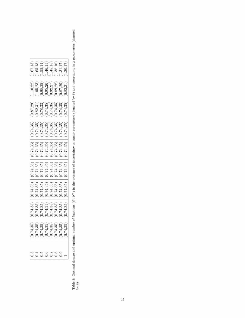
0.3
(0.7
4,35
)(0
.74,
35)
(0.7
4,3
5)
(0.7
4,3
5)
(0.7
4,3
5)
(0.7
4,3
5)
(0.8
7,2
9)
(1.1
0,2
2)
(1.6
7,1
3)
0.4
(0.7
4,35
)(0
.74,
35)
(0.7
4,3
5)
(0.7
4,3
5)
(0.7
4,3
5)
(0.7
4,3
5)
(0.8
2,3
1)
(1.0
5,2
3)
(1.6
5,1
3)
0.5
(0.7
4,35
)(0
.74,
35)
(0.7
4,3
5)
(0.7
4,3
5)
(0.7
4,3
5)
(0.7
4,3
5)
(0.7
8,3
3)
(0.9
8,2
5)
(1.5
5,1
4)
0.6
(0.7
4,35
)(0
.74,
35)
(0.7
4,3
5)
(0.7
4,3
5)
(0.7
4,3
5)
(0.7
4,3
5)
(0.7
4,3
5)
(0.9
5,2
6)
(1.4
6,1
5)
0.7
(0.7
4,35
)(0
.74,
35)
(0.7
4,3
5)
(0.7
4,3
5)
(0.7
4,3
5)
(0.7
4,3
5)
(0.7
4,3
5)
(0.9
2,2
7)
(1.4
5,1
5)
0.8
(0.7
4,35
)(0
.74,
35)
(0.7
4,3
5)
(0.7
4,3
5)
(0.7
4,3
5)
(0.7
4,3
5)
(0.7
4,3
5)
(0.8
9,2
8)
(1.3
8,1
6)
0.9
(0.7
4,35
)(0
.74,
35)
(0.7
4,3
5)
(0.7
4,3
5)
(0.7
4,3
5)
(0.7
4,3
5)
(0.7
4,3
5)
(0.8
7,2
9)
(1.3
1,1
7)
1(0
.74,
35)
(0.7
4,35
)(0
.74,3
5)
(0.7
4,3
5)
(0.7
4,3
5)
(0.7
4,3
5)
(0.7
4,3
5)
(0.8
2,3
1)
(1.3
0,1
7)
Tab
le3:
Op
tim
al
dosa
ge
an
dop
tim
al
nu
mb
erof
fract
ion
s(d∗,N∗)
inth
ep
rese
nce
of
un
cert
ain
tyin
tum
or
para
met
ers
(den
ote
dbyθ)
an
du
nce
rtain
tyinρ
para
met
ers
(den
ote
dbyδ).
21
Related Documents