Robot Manipulator Control and Computational Cost

University of Pennsylvania University of Pennsylvania

ScholarlyCommons ScholarlyCommons

Technical Reports (CIS) Department of Computer & Information Science

February 1988

Robot Manipulator Control and Computational Cost Robot Manipulator Control and Computational Cost

Yehong Zhang University of Pennsylvania

Richard P. Paul University of Pennsylvania

Follow this and additional works at: https://repository.upenn.edu/cis_reports

Recommended Citation Recommended Citation Yehong Zhang and Richard P. Paul, "Robot Manipulator Control and Computational Cost", . February 1988.

University of Pennsylvania Department of Computer and Information Science Technical Report No. MS-CIS-88-10.

This paper is posted at ScholarlyCommons. https://repository.upenn.edu/cis_reports/621 For more information, please contact [email protected].

Robot Manipulator Control and Computational Cost Robot Manipulator Control and Computational Cost

Abstract Abstract In this paper robot control algorithms are considered from the point of view of computational complexity. All the algorithms provide for hybrid position and force control which is appropriate to unstructured environments. Both joint coordinate and generalized coordinate motion schemes are considered. The findings are interesting in that the peripheral processing involved in all methods, sometimes, swamps the orders of magnitude differences in computation involved in the inner loops. It is also interesting to note the similarity in complexity between direct methods and differential. Between joint coordinate methods and generalized coordinate methods there is a general two to one ratio in complexity. In general a 0.75 M Flop, 1.25 Mip machine is required to provide for a control rate of 250 hz.

Comments Comments University of Pennsylvania Department of Computer and Information Science Technical Report No. MS-CIS-88-10.

This technical report is available at ScholarlyCommons: https://repository.upenn.edu/cis_reports/621

ROBOT MANIPULATOR CONTROL AND COMPUTATIONAL

COST YehongZhang Richard P. Paul

MS-CIS-88-10 GRASP LAB 134

Department of Computer and Information Science School of Engineering and Applied Science

University of Pennsylvania Philadelphia, PA 191 04

February 1988

Acknowledgements: This material is based upon work supported by the National Bureau of Standards under the Commerce Department Grant No. 60NANB7D0749

Robot Manipulator Control and Computational Cost

Yehong Zhang

Richard P. Paul

Computer and Information Science Department University of Pennsylvania

Philadelphia, PA 19104

ABSTRACT

In this paper robot control algorithms are considered from the point of view of computational complexity. All the algorithms provide for hybrid position and force control which is appropri- ate to unstructured environments. Both joint coordinate and generalized coordinate motion schemes are considered. The findings are interesting in that the peripheral processing in- volved in all methods, sometimes, swamps the orders of magni- tude differences in computation involved in the inner loops. It is also interesting to note the similarity in complexity between direct methods and differential. Between joint coordinate meth- ods and generalized coordinate methods there is a general two to one ratio in complexity. In general a 0.75 M Flop, 1.25 Mip machine is required to provide for a control rate of 250 hz.

lThis material is based upon work supported by the National Bureau of Standards under the Commerce Department Grant No. 60NANB7D0749. Any opinions, findings, conclusions or recommendations expressed in this publication are those of the authors and do not necessarily reflect the views of the National Bureau of Standards.

Contents

1 Introduction 1

2 The Need to Provide both Force and Motion Control 1

3 Generalized and Operational Coordinates 4

4 The Description of Motion and its Computational Cost 5 4.1 Joint Coordinate Motion . . . . . . . . . . . . . . . . . . . . 6 4.2 Orthogonal Coordinate Motion . . . . . . . . . . . . . . . . 7

5 Control 8 5.1 Free Joint Method . . . . . . . . . . . . . . . . . . . . . . . 10 5.2 Modified Free Joint Method . . . . . . . . . . . . . . . . . . 12 5.3 Hybrid Motion and Force Control . . . . . . . . . . . . . . . 14 5.4 Modified Hybrid Control Formulation . . . . . . . . . . . . 15 5.5 Operational Space Control . . . . . . . . . . . . . . . . . . . 17 5.6 Stiffness Control . . . . . . . . . . . . . . . . . . . . . . . . 19 5.7 Impedance Control . . . . . . . . . . . . . . . . . . . . . . . 21

6 Dynamics 22

7 Control Rates 23

8 VAX Instruction to Floating Point Ratio 25

9 Computational Cost Summary 26

10 Discussion 26

1 Introduction

Active force control capability is one of the most important characteris- tics of an intelligent robot. By actively controlling contact forces with the environment, a robot is able to perform highly sophisticated assembly op- erations which involve geometric constraints in the task space. Over the past years, much research has been done in this area and a few strate- gies for combined motion and force control emerged, such as the free joint method of Paul and Shimano, hybrid motion/force control strategy of Raib- ert and Craig, operational space formulation of Khatib, stiffness control of Salisbury and impedance control of Hogan. All these met hods represent different levels of computational complexity and as such impose different computational constraints on the controller. Our attempt is to compare the above motion/force control strategies from the perspective of computation. By doing so, we hope to shed more light on one of the most important aspects of robot control, namely computational complexity.

2 The Need to Provide both Force and Mo- tion Control

When working in a perfectly structured world we do not need sensing: a structured world in which the dimensions of all parts are within tolerance and in which careful planning has taken place to ensure that such parts can be assembled, a world in which everything is precisely located and everything functions as planned, a world in which all necessary jigs[l9] have been designed and provided.

When any lack of structure occurs, however, we must rely on sensors. If something is misplaced, or if something will not fit, relying on a sensor-less, geometry controlled approach would be a disaster. Sensors have two roles, to monitor task execution and to establish the state of the world. Both these tasks require the use of a world model. Both tasks also require rea- soning and planning. Establishing the state of the world requires a sensor strategy and the interpretation of sensor data in terms of the world model. Monitoring task execution also requires sensor strategies and interpretation of sensor readings in terms of the world model. Errors, when they occur, are detected by the interpretation of sensor data, once again in terms of

the world model. If this is to be done reliably a number of independent sensors are needed (sensors fail also). Once an error state is determined, appropriate recovery action must be planned. If a part is dropped on the floor, then it may be left, but if it is dropped inside a mechanism where it could prevent functioning, then it must either be retrieved or the mecha- nism replaced. Error recovery is not simple.

Of all the sensors that a robot might have, force sens ing is the most fundamental. Bl ind people f unc t ion qui te well in t h e world bu t people w h o have n o k ines the t ic feedback are total ly helpless. Consider the well structured world of manufacturing with a task fully under position control: the detection of any unexpected force is a clear indication that something has gone wrong. Force sens ing c a n provide th i s vi tal i n fo rma t ion . In any situation where complete structure is absent, force sensing becomes primary in the sequencing of a task. Consider teleoperation where tasks have some structure[l].

The general-purpose manipulator may be used for moving ob- jects, moving levers and knobs, assembling parts, and manipu- lating wrenches. In all these operations the manipulator must come into physical contact with the object before the desired force and movement can be made on it. A collision occurs when the manipulator makes this contact. General-purpose manipu- lation consists essentially of a series of collisions with unwanted forces, the application of wanted forces, and the application of desired motions. The collision forces should be low, and any other unwanted forces should also be small.

Three clear states may be identified:

1. Motion in free space.

2. Contact.

3. The exertion of a force.

This work of Goertz influenced the use of force sequencing in the ma- nipulator control system WAVE[12] and later that of Inoue[3]. Two types of commands were included in a language WAVE describing a sequence of manipulator motions.

STOP terminate the current motion when a force equal to the argument is detected, also known as a "guarded move"[20].

FORCE during the next motion, the force in a given direction, is to be controlled to the value given as an argument. If the force is specified to be zero then the manipulator is "free" to move in the direction specified.

A further command allowed for a force to be applied by the manipulator, of course, the manipulator would have to be free in the direction

Taking a different approach in the "Force Vector Assembler Concept 171" commanded manipulator Cartesian velocities could be modified by mea- sured end-effector forces and moments

Off-diagonal elements of the matrix M allowed for motion to be specified in directions orthogonal to an applied force. A curious side effect of this produced a switching phenomenon similar to that described above-a con- tinuous control system with two states. T h e end e$ector would trace along a n edge unt i l a corner was reached and then proceed to trace along the next edge. Unfortunately it was not possible to continue in this fashion along the following edge. A similar "switching" phenomenon occurs in a special device for making chamfer-less insertions. T h e pin is brought in to the hole at a n angle, o n contact a linkage rotates the pin t o align it with the hole axis whereupon insertion occurs. These phenomena are, however, limited to only two states and do not generalize further. Recently this type of control has formed the basis of more complex insertion strategies [6] in the form of a "generalized damper" in which the force expected is proportional to the velocity error along some direction. Both of these strategies are lim- ited to two-st ate systems. A task to insert a key into a lock, turn the lock 180 degrees, and then withdraw the key, cannot be characterized by such a continuous system. It is, however, simple to describe such a task in terms of force/displacement transitions and control mode switches such as used in WAVE 1141.

The computational complexity in solving the reasoning and multiple real-time sensor processing are significant. We will, however, limit this study to the position and force control of a single manipulator working in

a dynamic environment in which one or more objects may be in relative motion.

Generalized and Operational Coordinates Each component of a system has a unique coordinate system in which its state variables are most naturally expressed. An electric motor has its output shaft angle and shaft velocity as state variables; a camera reports observations in terms of scan line and position within the scan line; a robot manipulator is described in terms of its joint angles and their velocities; a milling machine is described in terms of its axes and their velocities. If various components are to work together there is a need for some form of common coordinate system which may be used directly to pass information between components. Information may be passed in terms of this common coordinate system or may be passed in terms of local coordinate systems defined in terms of this common coordinate system. The correct choice of coordinate systems is vital to the simplification of the description of spatial relationships.

Any orthogonal coordinate system may be used for the common coor- dinate system and although Cartesian coordinates are usually chosen other coordinate systems may be used cylindrical, spherical, etc. In in certain situations one orthogonal coordinate system might have advantages over an- other, however, the transformation between them are all fairly equivalent and it is customary to employ Cartesian coordinates described by homoge- neous transformations as this represent at ion minimizes the computational cost of performing the transformations.

There is a computational cost involved in transforming between coordi- nate systems and it is usual in robotics to define local coordinate systems to reduce the number of transformation to one or two transformations in order to relate between components. The computation is cost is of the order of 60 flops (floating point operations) but might double if re-normalization of the result is employed.

Transformations are provided between each device and some local Carte- sian coordinate frame described by a homogeneous transformation. The cost of this transformation varies with the device, however, one of the most complex devices is the manipulator itself. In the case of manipulators it is

always possible to define the transformation between the generalized joint coordinates and a Cartesian coordinate frame located at its terminal link, for the PUMA manipulator this involves some 141 flops. The inverse rela- tionship, between Cartesian terminal link coordinates and generalized joint coordinates, is not always possible. However, if certain kinematic restric- tions are met [16] this is also possible; for the Puma this involves some 227 flops.

In practice then, sensor observations would be transformed by a non- linear sensor transformation into Cartesian sensor coordinates, these would then be transformed into base coordinates by a homogeneous transforma- tion product. This might be followed by a second transformation into manipulator tool coordinates, representing a second homogeneous transfor- mation and then finally into manipulator joint coordinates using the inverse kinematic transformation. This method results in absolute coordinates be- ing available at all times.

An alternative approach, in the case of small changes to a reference position, is to use Jacobians representing the differential change between the initial coordinates and the final coordinates. Even if this is done in a number of steps: from the sensor to Cartesian coordinates, from the sen- sor Cartesian coordinates to the manipulator coordinates, and finally from manipulator coordinates to joint coordinates. Each of these transformation involves a minimum of 66 flops. This method also involves the updating of the Jacobians involving considerably more arithmetic operations.

It can be seen that both methods, absolute and differential transforma- tion, are fairly equivalent and in practice the absolute method is usually employed.

4 The Description of Motion and its Com- putational Cost

Manipulator motion is possible in either joint coordinates or in Cartesian coordinates. In the former case the manipulator joints move along straight lines in joint space whereas in the latter the terminal link of the manipulator moves along straight lines in Cartesian space. Joint motion, while well defined, does not result in straight line motion in Cartesian coordinates.

However, joint coordinates represent the state variables of manipulators and they define the extremum constraints on motion, maximum speed, acceleration, motion limit, etc. and if time optimal motions are desired then joint motion is natural. In the terminal phases of many motions a well defined motion is needed and in this case Cartesian motion is more desirable; time optimization is not so important as is the simplicity of the description of the motion in space.

One of the first methods of coordinated control of manipulators was by Paul in 1972 [12]. The method involved control of the manipulator in joint coordinates, that is, each joint of the manipulator was driven at the same relative speed. Thus at mid-trajectory each joint was exactly half way between its initial position and the desired final position. If the mo- tion end-point specification was given in Cartesian coordinates the inverse kinematics would be called to determine the end-point specification in joint coordinates [8]. This could be done before the manipulator was moved and thus the computational rate at which the inverse kinematics could be cal- culated was immaterial1. Once the final and initial joint coordinates have been obtained their difference may be reduced to zero in some simple man- ner maintaining continuity of one or more derivatives (continuity of velocity and acceleration) [lo]. A fifth order polynominal with time as independent variable will suffice for this purpose.

4.1 Joint Coordinate Motion

The motion from B to C may be defined in joint coordinates as a function of h by obtaining the joint coordinates corresponding to positions B and C, eB and Oc, as:

8 = reBc + s~lve(EXPR;+~(t ) )

'The multiple solutions obtainable with a six-degree-of-freedom manipulator were ini- tially thought to be a simple problem and simple algorithms such as picking the solution whose joint angles were closest to the current ones were often employed. It developed that the selection of the solution was of great importance. Its selection is complicated and is now normally just left to the programmer, suitable for robot level languages, but will become a problem when task level programming is attempted.

where = solve(B) - solve(C)

r = l - h

The variable r changes from 1 to 0 as the motion is made. When r = 1 at the beginning of the motion 6' = OB the initial position. When r = 0 at the end of the motion 6 = s~ lve (ExPR;+~) , the desired final position. h is defined as a function of time to provide for continuity of motion. A fifth order polynominal is required. In addition there is a discontinuity in position and velocity between the two motion segments and a further fifth order polynominal is also required [Ill.

4.2 Orthogonal Coordinate Motion

If an orthogonal motion is desired from B to C then the position equation must be modified to include a drive transform D(r) [13] in EXPR. The drive transform represents a translation d and rotation 1C, about an axis e in space proportional to r , 1 < r <= 0. When the argument r is zero, representing the end of the motion, D(r) reduces to an identity transform. The position of the drive transform in the equation determines the frame in which the rot ation is defined. We can rewrite the previous motion equation with the drive transform included in the form

Here L; represents the transform expression to the left of D and R; repre- sents the transform expression to the right. At the beginning of the motion from B to C position B is defined by equation the above equation. This position is also defined with respect to position C.

which we may solve for D(1)

iFrom D(1) we may obtain d, e, and 1C, and the orthogonal motion from position B to position C may then be described by

where r = l - h

as r varies from 1 to 0. A problem with both schemes is picking the time for the motion. Once

a time is picked a well controlled motion is obtainable however; like the configuration which was initially picked using some simple algorithm the picking of the time is extremely complicated. If the time is too small the the manipulator will not be able to track the specified motion. The time is dependent on the dynamics, drive systems, previous and subsequent mo- tions. Although much research has been devoted to this problem it remains a formidable computational problem only to be undertaken if repeated mo- tions are to be made. However, if repeated motions are to be made then far simpler techniques are available which use the actual manipulator and gradually decrease the time of motion segments until some criteria has been met. In practice a very conservative motion capability is assumed so that none of these problems surface, however, the manipulator runs at typically 30% to 50% of potential. This is a problem in factory automation but is not a problem in intelligent robotics when careful motions normally require that the manipulator move slowly in a very well controlled manner.

5 Control

The control of a robot is a complicated task. It requires task planning, tra- jectory generation, kinematic solution , implement ation of control, dynamic evaluation and servoing. All these subtasks are associated with a certain amount of computation. Furthermore the nature of the subtask also de- termines the rate at which the computation should be carried out. It thus becomes necessary to classify computation into categories and determine the rate of computation for each category accordingly.

In this paper, we divide the computational task into the following cat- egories. Kinematic computation and dynamic computation. The first cat - egory consists of the configuration dependent quantities, those parameters of the control which only depend on the position of the manipulator not on its velocity or acceleration. The dynamic category consists of the dynamic trajectory generation, control law computation and joint servoing. The computations in the dynamic category have to be carried out at the control

rate. However, the computations in the kinematic category need be carried out only at the rate of change in robot configuration. This rate is consid- erably slower than the sampling rate and so the distinction between these two categories allows the controller to have a two-layer structure. While all the dynamic computations are done in a real time process, the kinematic computations are executed in a slower background process.

The amount of computation for the control of a robot also depends on the robot type, our results are obtained for a PUMA260, which is fairly typical of modern robots. The forward and inverse kinematic solutions are obtained symbolically, and so is the Jacobian[S]. The calculation of the dynamics quantities is based on a method developed by Paul and Izaguirre [4]. The results are listed in Table 1.

In the following section, we shall compare seven force/motion control methods according to the computational loads in both the kinematic and dynamic categories. They are listed below.

1. Free Joint Method by Paul.

2. Modified Free Joint Method by Shimano.

3. Hybrid Control by Raibert and Craig.

4. Modified Hybrid Control by Zhang.

5. Operational Space Control by Khatib.

6. Stiffness Control by Salisbury.

7. Impedance Control by Hogan.

For each method of control, a control diagram is drawn. To reflect the layered nature of control, a vertical line is drawn that separates the kinematic process from the dynamic one. To ease the burden of counting operations, all boxes and summation junctions are numbered. In general, all boxed quantities are either constants or can be computed at the kinematic rate. But the ones in the dynamic region have contributions to the dynamic computational load due to the multiplications and additions involved in computing the real-time quantities. Similarly, summation junctions in the

dynamic region contain dynamic computations and those in the kinematic region contain kinematic computations.

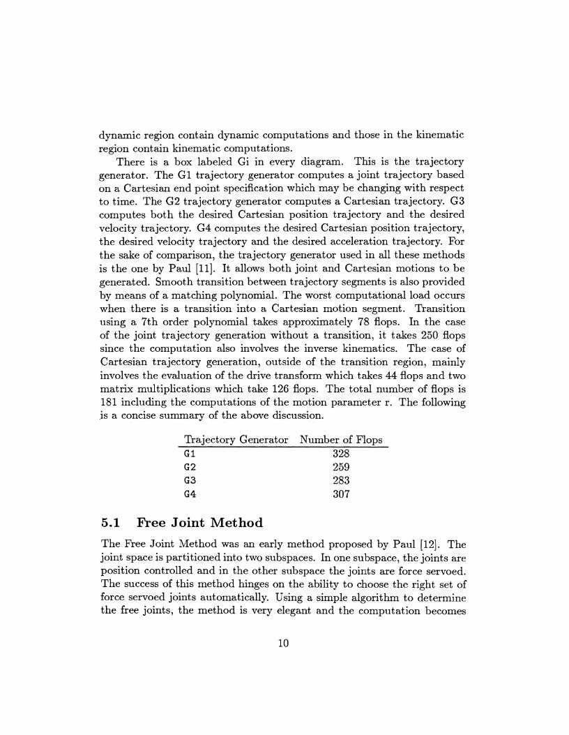
There is a box labeled Gi in every diagram. This is the trajectory generator. The G 1 trajectory generator computes a joint trajectory based on a Cartesian end point specification which may be changing with respect to time. The G2 trajectory generator computes a Cartesian trajectory. G3 computes both the desired Cartesian position trajectory and the desired velocity trajectory. G4 computes the desired Cartesian position trajectory, the desired velocity trajectory and the desired acceleration trajectory. For the sake of comparison, the trajectory generator used in all these methods is the one by Paul [Ill. It allows both joint and Cartesian motions to be generated. Smooth transition between trajectory segments is also provided by means of a matching polynomial. The worst computational load occurs when there is a transition into a Cartesian motion segment. Transition using a 7th order polynomial takes approximately 78 flops. In the case of the joint trajectory generation without a transition, it takes 250 flops since the computation also involves the inverse kinematics. The case of Cartesian trajectory generation, outside of the transition region, mainly involves the evaluation of the drive transform which takes 44 flops and two matrix multiplications which take 126 flops. The total number of flops is 181 including the computations of the motion parameter r. The following is a concise summary of the above discussion.

Trajectory Generator Number of Flops GI 328

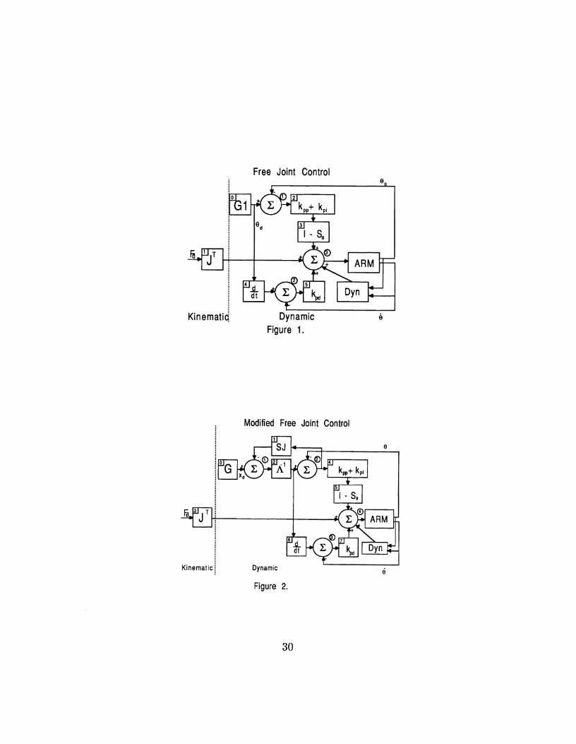
5.1 Free Joint Method The Free Joint Method was an early method proposed by Paul [12]. The joint space is partitioned into two subspaces. In one subspace, the joints are position controlled and in the other subspace the joints are force servoed. The success of this method hinges on the ability to choose the right set of force servoed joints automatically. Using a simple algorithm to determine the free joints, the method is very elegant and the computation becomes

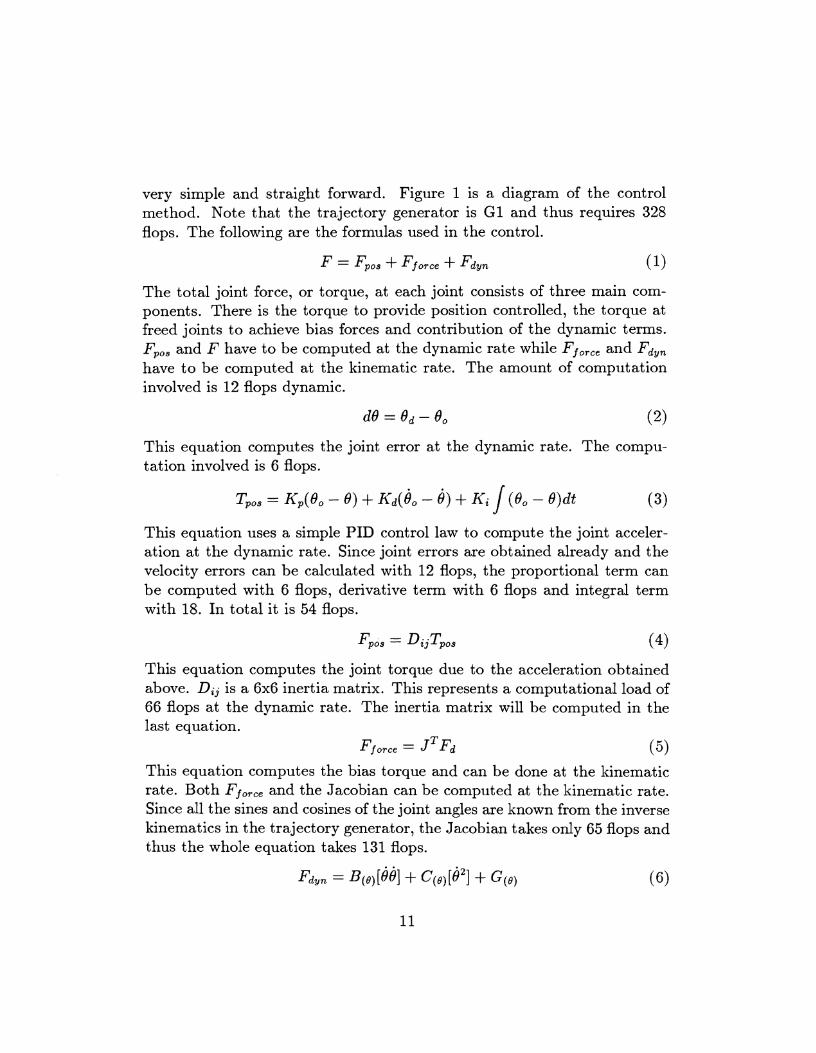
very simple and straight forward. Figure 1 is a diagram of the control method. Note that the trajectory generator is GI and thus requires 328 flops. The following are the formulas used in the control.

The total joint force, or torque, at each joint consists of three main com- ponents. There is the torque to provide position controlled, the torque at freed joints to achieve bias forces and contribution of the dynamic terms. F,,, and F have to be computed at the dynamic rate while FfOTce and Fdyn have to be computed at the kinematic rate. The amount of computation involved is 12 flops dynamic.

This equation computes the joint error at the dynamic rate. The compu- tation involved is 6 flops.

This equation uses a simple PID control law to compute the joint acceler- ation at the dynamic rate. Since joint errors are obtained already and the velocity errors can be calculated with 12 flops, the proportional term can be computed with 6 flops, derivative term with 6 flops and integral term with 18. In total it is 54 flops.

This equation computes the joint torque due to the acceleration obtained above. Dij is a 6x6 inertia matrix. This represents a computational load of 66 flops at the dynamic rate. The inertia matrix will be computed in the last equation.

Fforce = J ~ F ~ ( 5 ) This equation computes the bias torque and can be done at the kinematic rate. Both Ff0,,, and the Jacobian can be computed at the kinematic rate. Since all the sines and cosines of the joint angles are known from the inverse kinematics in the trajectory generator, the Jacobian takes only 65 flops and thus the whole equation takes 131 flops.

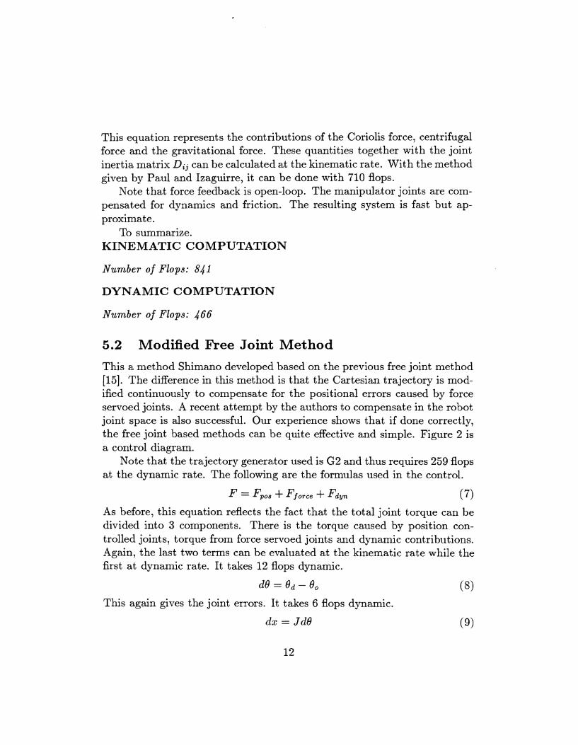
This equation represents the contributions of the Coriolis force, centrifugal force and the gravitational force. These quantities together with the joint inertia matrix Dij can be calculated at the kinematic rate. With the method given by Paul and Izaguirre, it can be done with 710 flops.

Note that force feedback is open-loop. The manipulator joints are com- pensated for dynamics and friction. The resulting system is fast but ap- proximat e.

To summarize. KINEMATIC COMPUTATION

Number of Flops: 841

DYNAMIC COMPUTATION

Number of Flops: 466

5.2 Modified Free Joint Method

This a method Shimano developed based on the previous free joint method [15]. The difference in this method is that the Cartesian trajectory is mod- ified continuously to compensate for the positional errors caused by force servoed joints. A recent attempt by the authors to compensate in the robot joint space is also successful. Our experience shows that if done correctly, the free joint based methods can be quite effective and simple. Figure 2 is a control diagram.

Note that the trajectory generator used is G2 and thus requires 259 flops at the dynamic rate. The following are the formulas used in the control.

F = F p o , + Fjorce + Fdyn (7 ) As before, this equation reflects the fact that the total joint torque can be divided into 3 components. There is the torque caused by position con- trolled joints, torque from force servoed joints and dynamic contributions. Again, the last two terms can be evaluated at the kinematic rate while the first at dynamic rate. It takes 12 flops dynamic.

This again gives the joint errors. It takes 6 flops dynamic.

This equation calculates the Cartesian error caused by the joint errors. The Jacobian can be computed at the kinematic rate. So this means a kinematic computational load of 65 flops and a dynamic computational load of 66.

This equation forms the differential change matrix to be used in modifying the Cartesian trajectory of the robot. It does not need any computation.

This is the modification of the Cartesian trajectory. The maximum com- putational load is 6 flops.

dd = A;:) ( 12)

This equation is the inverse kinematics. It is transforming the modified Cartesian trajectory into the desired joint trajectory. It takes a total of 227 flops of dynamic computation.

This equation utilizes a PID control law to compute the joint acceleration. All the computation has to be carried out at the dynamic rate. As seen before, it takes 54 flops.

Fpos = D i j T p o s ( 14 )

This equation gives the joint torque caused by the joint acceleration. It requires 66 flops.

F f o ~ c e = ( I - S O ) J ~ F ~ ( I 5 ) This calculates the bias torque to be applied. Since the Jacobian is al- ready computed. The worst case for this equation is 66 flops of kinematic computation.

Fdyn = ~ ( O ) [ d b ] + C ( O ) [ ~ ~ ] + G(0) ( I 6 ) This is the rest of the dynamics terms and can be similarly computed as we did in the previous method. It takes 710 flops at the kinematic rate.

To summarize. KINEMATIC COMPUTATION

Number of Flops: 841

DYNAMIC COMPUTATION

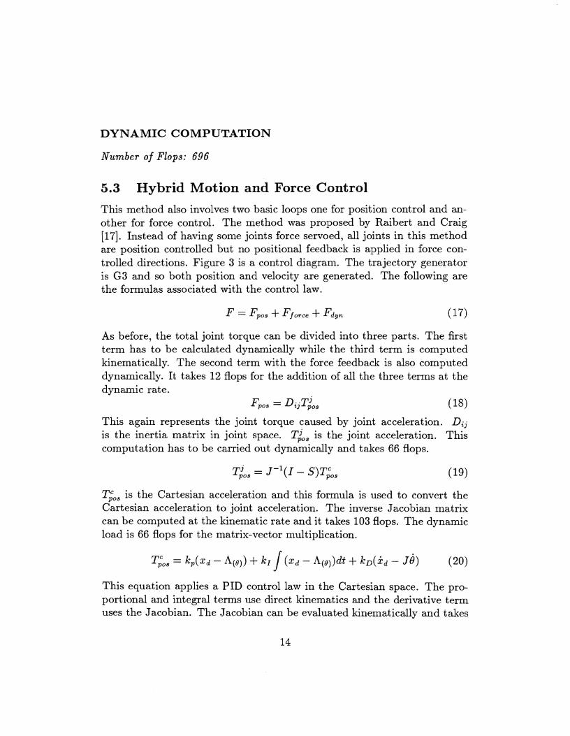
Number of Flops: 696

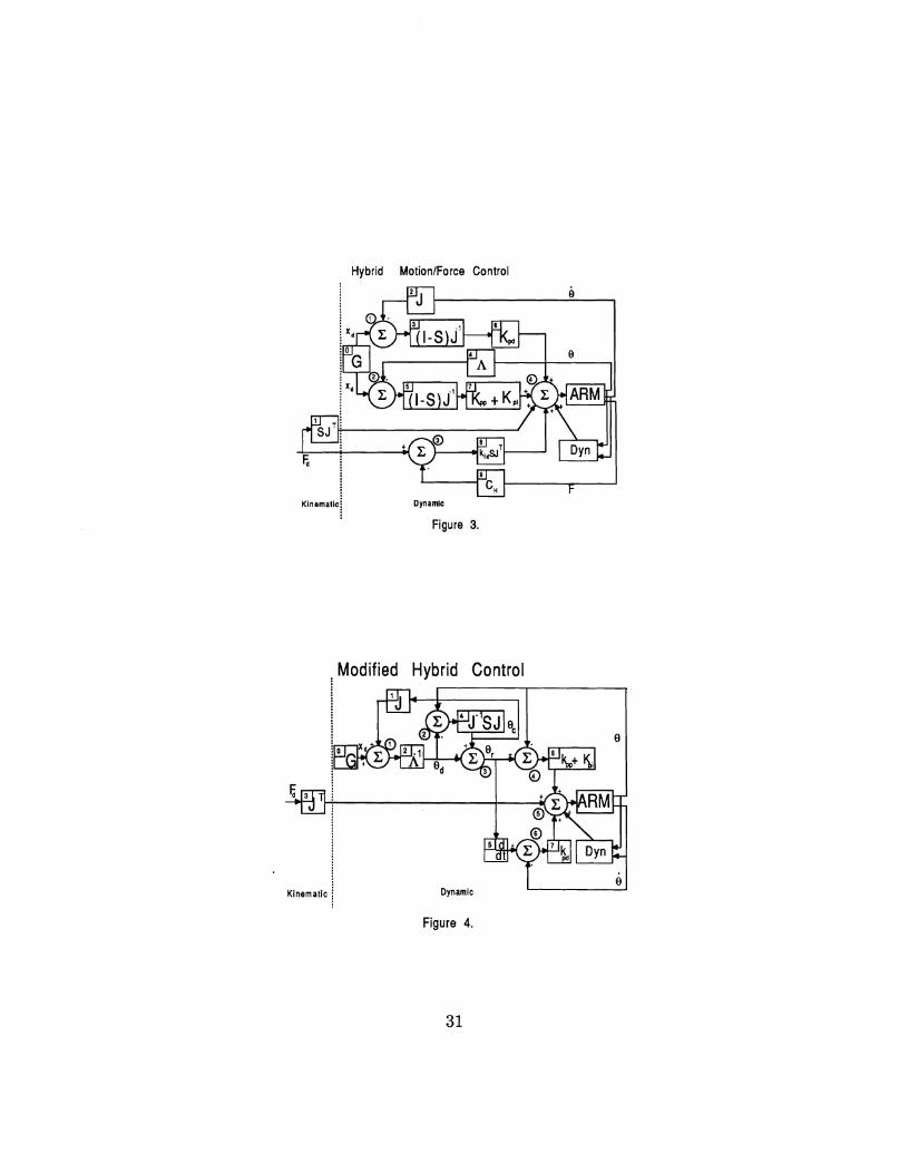
5.3 Hybrid Motion and Force Control This method also involves two basic loops one for position control and an- other for force control. The method was proposed by Raibert and Craig [17]. Instead of having some joints force servoed, all joints in this method are position controlled but no positional feedback is applied in force con- trolled directions. Figure 3 is a control diagram. The trajectory generator is G3 and so both position and velocity are generated. The following are the formulas associated with the control law.

As before, the total joint torque can be divided into three parts. The first term has to be calculated dynamically while the third term is computed kinematically. The second term with the force feedback is also computed dynamically. It takes 12 flops for the addition of all the three terms at the dynamic rate.

Fpos = DijTjOs (18)

This again represents the joint torque caused by joint acceleration. Dij is the inertia matrix in joint space. Tio, is the joint acceleration. This computation has to be carried out dynamically and takes 66 flops.

T,",, is the Cartesian acceleration and this formula is used to convert the Cartesian acceleration to joint acceleration. The inverse Jacobian matrix can be computed at the kinematic rate and it takes 103 flops. The dynamic load is 66 flops for the matrix-vector multiplication.

This equation applies a PID control law in the Cartesian space. The pro- portional and integral terms use direct kinematics and the derivative term uses the Jacobian. The Jacobian can be evaluated kinematically and takes

65 flops assuming that the sin and cos of joint angles will be obtained in the kinematics. But everything else has to be computed dynamically. Knowing that the forward kinematics takes 141 flops the proportional term requires 153 flops. The integral term requires 18 flops. The derivative term takes 78 flops. In total, it takes 261 flops of dynamic computation and 65 flops of kinematic computation.

Since Jacobian is already calculated in the last equation, the first term requires only 66 flops of kinematic computation. The second term takes 144 flops. In total, this equation takes 66 flops of kinematic computation and 150 flops of dynamic computation.

This term is basically the same as in the last two methods and it takes 710 flops of kinematic computation. Note that there is force feedback. The servo uses a PID control law in the joint space. Also note that the kinematics has to be evaluated every time in the servo.

In summary. KINEMATIC COMPUTATION

Number of Flops: 944

DYNAMIC COMPUTATION

Number of Flops: 858 It is obvious that this method is computationally more expensive. That

in part is due to the fact that errors are dealt with in the Cartesian space. In particular, joint angles have to be mapped into the Cartesian space using forward kinematics.

5.4 Modified Hybrid Control Formulation

The Modified Hybrid Control Formulation was aimed at reducing the com- putational load of the original hybrid method[21]. It shares many charac- teristics with the original hybrid control method, but the errors are dealt with in the joint space. Figure 4 is a control diagram of the method.

Note that the trajectory generator is G2. That implies a dynamic com- putational load of 259 flops. The following equations constitute the main body of formulation.

As before, this equation represents 12 flops of dynamic computation.

The joint error calculation takes 6 flops of dynamic computation.

This is the equation that modifies the Cartesian trajectory. It takes 65 flops of kinematic computation to calculate the Jacobian assuming that sin and cos values of the joint angles are available from solving the inverse kinematics. Dynamic computation is 72 flops.

This is the inverse kinematic function and it requires 227 flops of dynamic computation.

8, = J-'(I - S ) ~ d 8 (27 ) This equation calculates the joint compensation for compliance. Notice that J - l ( I - S ) J can be evaluated at the kinematic rate. Since I - S is a diagonal selection matrix, J M 1 ( I - S) J is really one matrix multiply. Therefore there are 499 flops of kinematic computation and 66 flops of dynamic computation. Among the 499 flops, the computation of J-' takes 103 and J - l ( I - s) J takes 396.

This represents the modification of the desired joint trajectory using the joint compensation 8,. It takes 6 flops of dynamic computation.

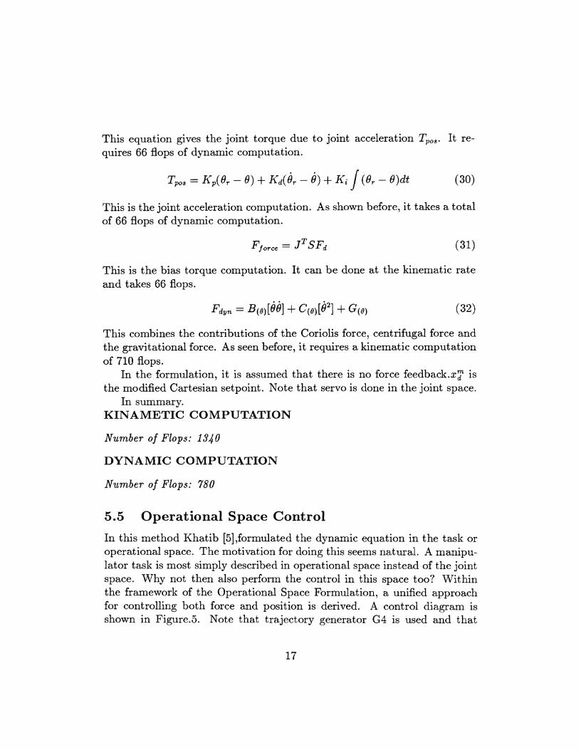
This equation gives the joint torque due to joint acceleration T,,,. It re- quires 66 flops of dynamic computation.

This is the joint acceleration computation. As shown before, it takes a total of 66 flops of dynamic computation.

This is the bias torque computation. It can be done at the kinematic rate and takes 66 flops.

This combines the contributions of the Coriolis force, centrifugal force and the gravitational force. As seen before, it requires a kinematic computation of 710 flops.

In the formulation, it is assumed that there is no force feedback.^? is the modified Cartesian setpoint. Note that servo is done in the joint space.

In summary. KINAMETIC COMPUTATION

Number of Flops: 194 0

DYNAMIC COMPUTATION

Number of Flops: 780

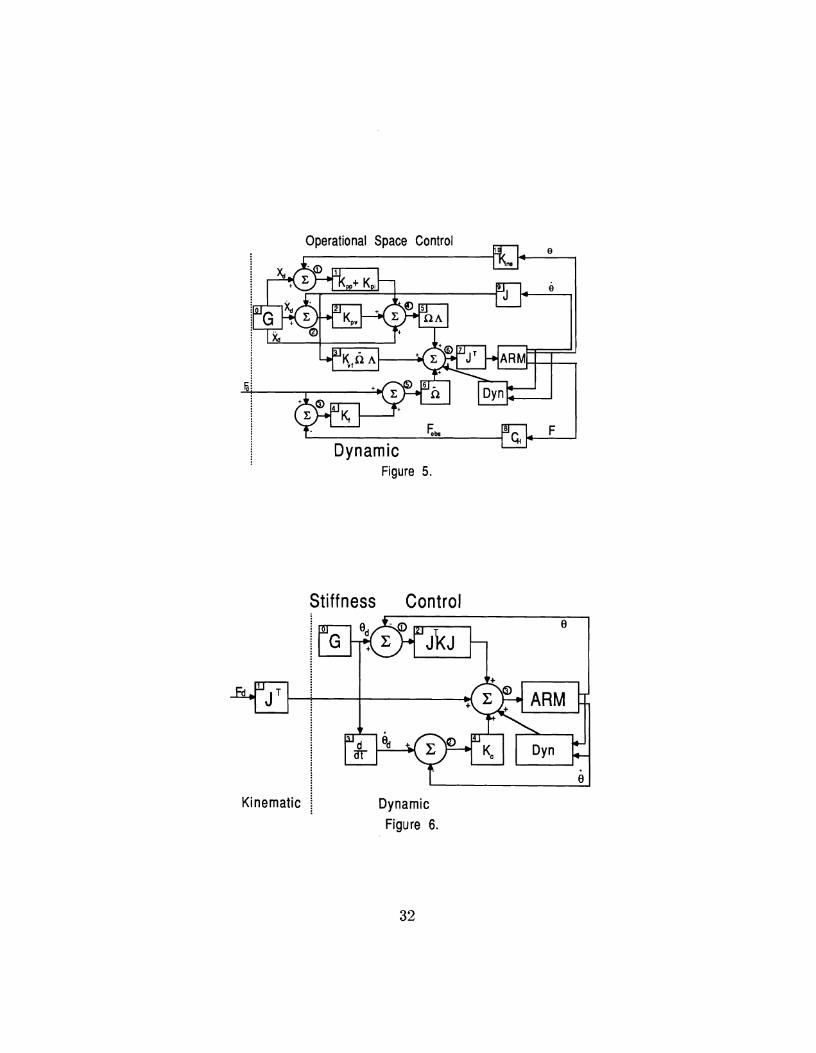
5.5 Operational Space Control

In this method Khatib [5],formulated the dynamic equation in the task or operational space. The motivation for doing this seems natural. A manipu- lator task is most simply described in operational space instead of the joint space. Why not then also perform the control in this space too? Within the framework of the Operational Space Formulation, a unified approach for controlling both force and position is derived. A control diagram is shown in Figure.5. Note that trajectory generator G4 is used and that

takes 307 flops of dynamic computation. The following are the formulas in the formulation.

F = A x , + P(x,.i.) + P(2) (33)

This equation is the dynamics equation of the robot formulated in the operational space. A, is the operational space inertia matrix and is crucial to the control of the robot.

This is the corresponding dynamics equation in the joint space. This is important because all the Cartesian coefficients of the dynamics equation are to be derived from the joint based coefficients.

Again, the total force is divided into 3 components. J can be computed at the kinematic rate and it takes 65 flops assuming that the sin and cos of the joints are known from the kinematics. Dynamic computation is 78

In this equation, the operational inertia matrix is obtained. Kinematic computation consists of computing J-l, (J-l)TA J-I. The first can be done with 103 flops and the latter with 792 flops.

This equation gives the Cartesian force for position servo. It has 180 flops of kinematic computation and 66 flops of dynamic computation.

This equation computes the acceleration in the operational space. It in- volves the forward kinematics and the Jacobian. The dynamic computation is 249 flops.

Ff O T C . = fiF&Tm f A ( * ) ~ F , ' (39) This is the force due to force servo. It contains a operational force term and a velocity damping term. The amount of dynamic computation is 102 flops and that of kinematic computation is 36 flops.

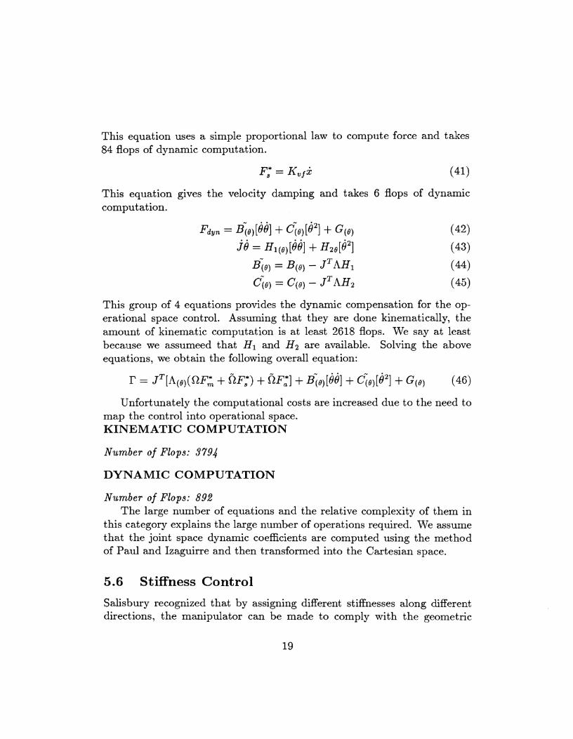
This equation uses a simple proportional law to compute force and takes 84 flops of dynamic computation.

This equation gives the velocity damping and takes 6 flops of dynamic computation.

This group of 4 equations provides the dynamic compensation for the op- erational space control. Assuming that they are done kinematically, the amount of kinematic computation is at least 2618 flops. We say at least because we assumeed that HI and H2 are available. Solving the above equations, we obtain the following overall equation:

Unfortunately the computational costs are increased due to the need to map the control into operational space. KINEMATIC COMPUTATION

Number of Flops: 3794

DYNAMIC COMPUTATION

Number of Flops: 892 The large number of equations and the relative complexity of them in

this category explains the large number of operations required. We assume that the joint space dynamic coefficients are computed using the method of Paul and Izaguirre and then transformed into the Cartesian space.

5.6 Stiffness Control

Salisbury recognized that by assigning different stiffnesses along different directions, the manipulator can be made to comply with the geometric

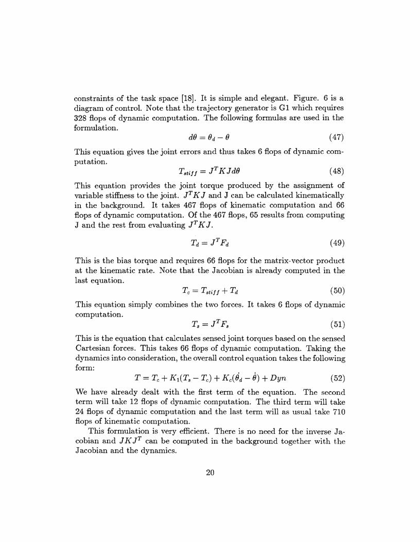
constraints of the task space [18]. It is simple and elegant. Figure. 6 is a diagram of control. Note that the trajectory generator is G1 which requires 328 flops of dynamic computation. The following formulas are used in the formulation.

d0 = Od - 0 (47)

This equation gives the joint errors and thus takes 6 flops of dynamic com- put ation.

T , , ; ~ ~ = J~ K ~ d 0 (48)

This equation provides the joint torque produced by the assignment of variable stiffness to the joint. JTKJ and J can be calculated kinematically in the background. It takes 467 flops of kinematic computation and 66 flops of dynamic computation. Of the 467 flops, 65 results from computing J and the rest from evaluating JT K J.

This is the bias torque and requires 66 flops for the matrix-vector product at the kinematic rate. Note that the Jacobian is already computed in the last equation.

Tc = Tstiff + Td (50)

This equation simply combines the two forces. It takes 6 flops of dynamic computation.

T, = J ~ F , (51)

This is the equation that calculates sensed joint torques based on the sensed Cartesian forces. This takes 66 flops of dynamic computation. Taking the dynamics into consideration, the overall control equation takes the following form:

T = T, + KI(Ts - Tc) + h',(Bd - 6) + Dyn (52)

We have already dealt with the first term of the equation. The second term will take 12 flops of dynamic computation. The third term will take 24 flops of dynamic computation and the last term will as usual take 710 flops of kinematic computation.

This formulation is very efficient. There is no need for the inverse Ja- cobian and J I I ' J ~ can be computed in the background together with the Jacobian and the dynamics.

In summary. KINEMATIC COMPUTATION

Number of Fbops: 1243

DYNAMIC COMPUTATION

Number of Flops: 520

5.7 Impedance Control

Many force control strategies become unstable when a rigid manipulator comes into contact with a rigid environment. To solve this problem, Hogan argues that the dynamic nature of interaction dictates that the impedance of the mechanical system be controlled instead of either force or position [2]. Figure 7 is a control diagram of the method.

The following are the formulas used in the control formulation.

Tactuator = JTFtip (53)

t i - e x e n a = A(~)G + c ( ~ , ~ ) B + ~ ( 8 ) (54)

(55)

The above equations give the dynamics equation of the robot when it is interacting with the environment.

These are the differential relationships between Cartesian and joint veloci- ties and accelerations.

This is the impedance model assumed.

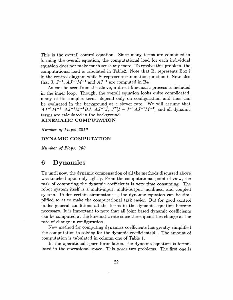
This is the overall control equation. Since many terms are combined in forming the overall equation, the computational load for each individual equation does not make much sense any more. To resolve this problem, the computational load is tabulated in Table2. Note that Bi represents Box i in the control diagram while Si represents summation junction i. Note also that J, J-l, AJ-'M-' and AJ-' are computed in B4

As can be seen from the above, a direct kinematic process is included in the inner loop. Though, the overall equation looks quite complicated, many of its complex terms depend only on configuration and thus can be evaluated in the background at a slower rate. We will assume that AJ-'M-', AJ-'M-'B J, AJ-' J, JTII - J-TAJ-lM-'] and all dynamic terms are calculated in the background. KINEMATIC COMPUTATION

Number of Flops: 2210

DYNAMIC COMPUTATION

Number of Flops: 700

Dynamics

Up until now, the dynamic compensation of all the methods discussed above was touched upon only lightly. From the computational point of view, the task of computing the dynamic coefficients is very time consuming. The robot system itself is a multi-input, multi-output, nonlinear and coupled system. Under certain circumstances, the dynamic equation can be sim- plified so as to make the computational task easier. But for good control under general conditions all the terms in the dynamic equation become necessary. It is important to note that all joint based dynamic coefficients can be computed at the kinematic rate since these quantities change at the rate of change in configuration.

New method for computing dynamics coefficients has greatly simplified the computation in solving for the dynamic coefficients [4] . The amount of computation is tabulated in column one of Table 1.

In the operational space formulation, the dynamic equation is formu- lated in the operational space. This poses two problems. The first one is

that all dynamic coefficients in the operational space can only be obtained by transforming the coefficients from joint space. This transformation is a heavy computational task. Secondly, these coefficients have to be updated at a rate faster than the kinematic one because they change rapidly as a function of the inverse Jacobian.

from the results obtained above, it is evident that dynamics computa- tion dominates the computational load. We believe that direct joint torque sensing is a promising alternative By sensing the joint output torque di- rectly it is possible to eliminate the need for the dynamics computations.

Control Rates

The rate at which the set point must be evaluated is related to the natural frequencies of the manipulator. While this is a complicated subject a fig- ure of ten times the lowest dominant frequency may be used and is readily understandable. For anthropomorphically sized manipulators natural fre- quencies are of the order of a few hertz and control frequencies are the of the order of some tens of hertz. The Puma is run at 35 hertz, other com- mercial manipulators run at 83 hertz and at 200 hertz. The actual control of the joint is however a different matter. Electric motors have much higher natural frequencies, tens of hertz being typical. These may be controlled to provide stiff ~osition controlled joints by controlling them at hundreds of hertz, the Puma joints are controlled at over 1000 hertz other manip- ulators use special purpose chips to perform the control at four kilohertz. This form of joint control may be viewed as a form of velocity servo and relegated to special purpose chips of analog devices. We are concerned with the position control of the manipulator, the regulator which specifies the velocities to this inner joint controller. We believe, we may set this rate at 250 hertz for an anthropomorphically sized manipulator in order to provide for smooth control. Increasing the rate beyond 250 hertz only provides for diminishing returns. Decreasing it tends to cause roughness in the control and eventually inst ability.

A second computation rate is also involved. This relates to the compu- tation of parameters, such as the manipulator instantaneous inertia, Jaco- bians, gravity loading, etc. These parameters depend only on the position of the manipulator, not on its velocity. As the position of a manipulator

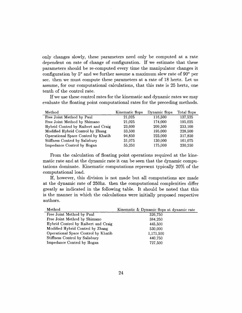
only changes slowly, these parameters need only be computed at a rate dependent on rate of change of configuration. If we estimate that these parameters should be re-computed every time the manipulator changes it configuration by 5' and we further assume a maximum slew rate of 90' per sec. then we must compute these parameters at a rate of 18 hertz. Let us assume, for our computational calculations, that this rate is 25 hertz, one tenth of the control rate.

If we use these control rates for the kinematic and dynamic rates we may evaluate the floating point computational rates for the preceding methods.

Method Free Joint Method by Paul Free Joint Method by Sh' imano Hybrid Control by Raibert and Craig Modified Hybrid Control by Zhang Operational Space Control by Khatib Stiffness Control by Salisbury Impedance Control by Hogan

Kinematic flops 21,025 21,025 23,600 33,500 94,850 31,075 55,250

Dynamic flops Total flops 116,500 137,525 174,000 195,025 209,500 233,100 195,000 228,500 223,000 317,850 130,000 161,075 175,000 230,250

From the calculation of floating point operations required at the kine- matic rate and at the dynamic rate it can be seen that the dynamic compu- tations dominate. Kinematic computations represent typically 20% of the computational load.

If, however, this division is not made but all computations are made at the dynamic rate of 250hz. then the computational complexities differ greatly as indicated in the following table. It should be noted that this is the manner in which the calculations were initially proposed respective authors.

Method Kinematic & Dynamic flops at dynamic rate Free Joint Method by Paul 326,750 Free Joint Method by Shimano Hybrid Control by Raibert and Craig Modified Hybrid Control by Zhang Operational Space Control by Khatib Stiffness Control by Salisbury Impedance Control by Hogan

VAX Instruction to Floating Point Ratio

We have examined two functions in detail in order to obtain the ratio between floating point instructions and machine instructions for optimized "C" code running on the VAX. The two routines were matrix multiply t imes and direct kinematics for the Puma 560 manipulator j n t -t o -tr. These routines make use of a number of trigonometric and mathematics functions listed below:

Function Flops Mips s q r t 10 3 0 s i n 8 18 cos 7 17 at an2 8 25

Other arc trigonometric functions involve a s q r t and call to atan2. Step-by-step execution of the t imes algorithm, with normalization, re- vealed 135 flops and 324 instructions executed giving a mips to flops ratio of 2.40. Step-by-step execution of the j n t - t o - t r direct kinematics routine revealed 164 flops and 393 instructions executed to give a mips to flops ratio of, once again, 2.40.

These observed flop counts agree well with the count of arithmetic op- erations in each of the algorithms. It is a strange coincidence that both basic robotics functions yielded identical mips to flops ratios of 2.40. As these are basic routines the execution of which occupies a large fraction of the cpu cycles we are, I believe, justified in using them to estimate the mip requirements of a processor based on a count of arithmetic operation counts in the algorithms.

We might note here that the vax generates very efficient code for ex- pressions of the form

If floating point variables are used they must all be converted by moving them first into registers resulting in poorer code

cvtfd b, rO cvtfd c, r1 muld2 rO, r1 cvtfd d, rO cvtfd e, r2 muld2 r1, r2 cvtdf r2, a

Similar code to this would be required for the 86020 as its addressing modes require that one operand is always in a register. This represents a two-to- one increase in instruction fetches. It is also interesting to note that over half of the arithmetic operations in the matrix multiply routine are related to re-normalizing the result.

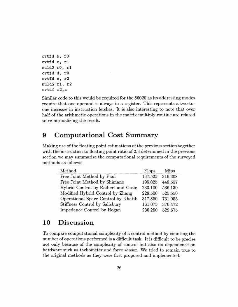
9 Computational Cost Summary

Making use of the floating point estimations of the previous section together with the instruction to floating point ratio of 2.3 determined in the previous section we may summarize the computational requirements of the surveyed methods as follows:

Met hod Flops Mips Free Joint Method by Paul 137,525 316,308 Free Joint Method by Shimano 195,025 448,557 Hybrid Control by Raibert and Craig 233,100 536,130 Modified Hybrid Control by Zhang 228,500 525,550 Operational Space Control by Khatib 317,850 731,055 Stiffness Control by Salisbury 161,075 370,472 Impedance Control by Hogan 230,250 529,575

10 Discussion

To compare computational complexity of a control method by counting the number of operations performed is a difficult task. It is difficult to be precise not only because of the complexity of control but also its dependence on hardware such as tachometer and force sensor. We tried to remain true to the original methods as they were first proposed and implemented.

It should be kept in mind that computational load varies depending on the number of directions of force control. To simplify the analysis, we assumed worst case situation for each category. Another important thing to remember is that there are other factors other than the computational load that impose real time constraints such as information transfer. Per- haps even more important is the way in which the total computation is distributed among different computers. By taking advantage of the ma- trix structure of the formulation, a parallel matrix processor can greatly facilitate the computation.

Assuming that the controller is organized in the layered manner separat- ing kinematic computations from dynamic computations one may observe an almost 50% reduction in computational complexity by employing joint space methods over operational space methods. A more overriding con- sideration in the selection of a method, however, relates to the inherent robustness of the joint space methods even though they require the map- ping of a task into joint space. In the case of redundant manipulators, not considered here, joint space methods become mandatory as it is joint space that the redundancy of the manipulators is represented.

It is also interesting to note that differential methods involving Jaco- bians and their inverses require a great number of arithmetic operations in performing the transformations; compare the Hybrid Control met hod proposed by Raibert and Craig based on absolute transformations to the modified hybrid control method which is based on differential methods.

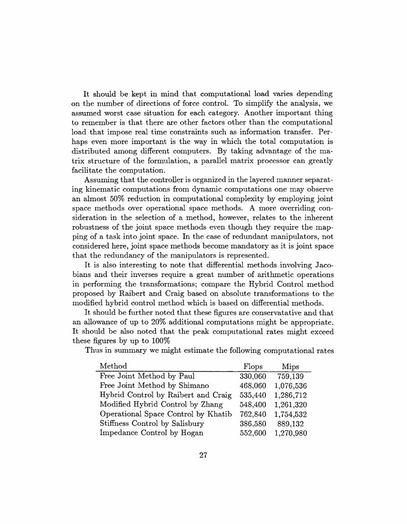
It should be further noted that these figures are conservatative and that an allowance of up to 20% additional computations might be appropriate. It should be also noted that the peak computational rates might exceed these figures by up to 100%

Thus in summary we might estimate the following computational rates

Method Flops Mips Free Joint Method by Paul 330,060 759,139 Free Joint Method by Shimano 468,060 1,076,536 Hybrid Control by Raibert and Craig 535,440 1,286,712 Modified Hybrid Control by Zhang 548,400 1,261,320 Operational Space Control by Khatib 762,840 1,754,532 Stiffness Control by Salisbury 386,580 889,132 Impedance Control by Hogan 552,600 1,270,980

Thus if joint space control methods are employed a 0.5 M flop, 1 Mips machine would be appropriate. If operational space methods are employed a 0.75 M flop, 1.5 Mips machine would be appropriate.

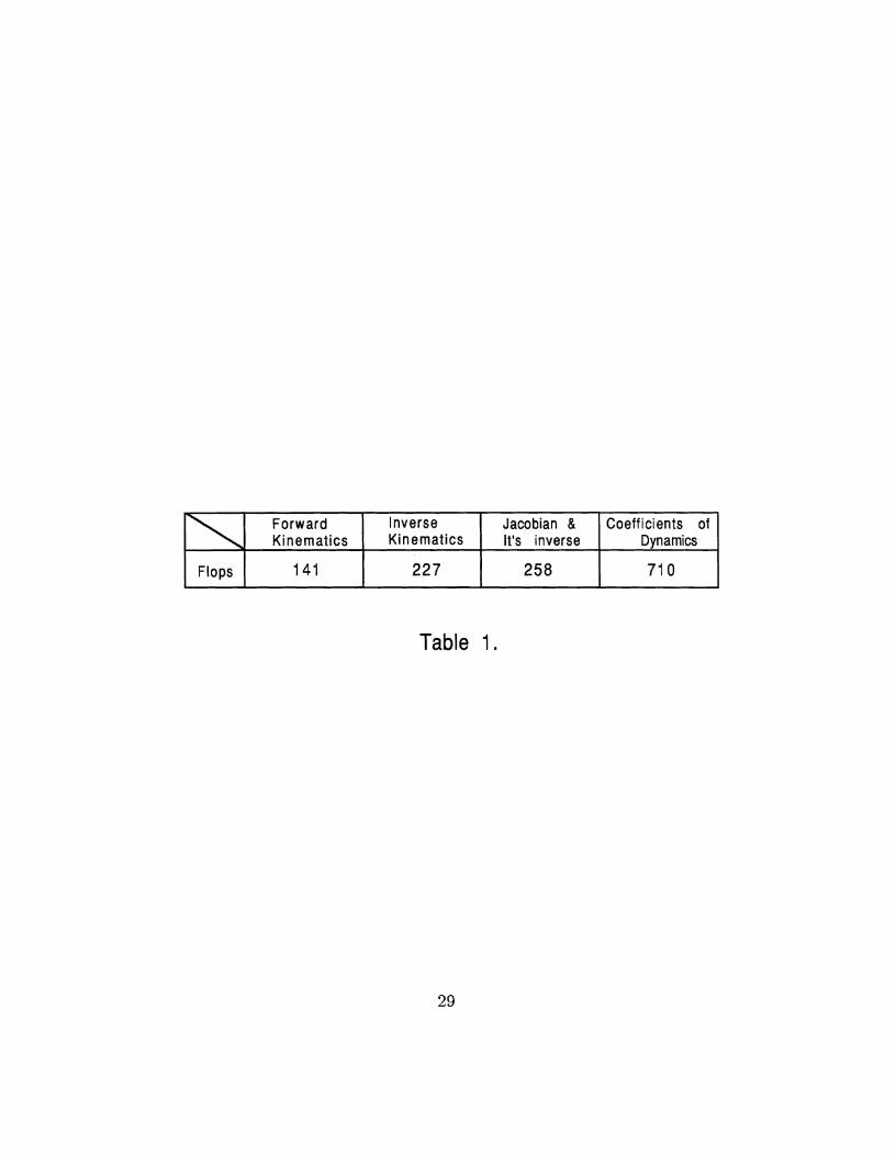
Table 1.

Flops

Jacobian & It's inverse

258

Coefficients of Dynamics

71 0

Forward Kinematics

141

Inverse Kinematics

227

Free Joint Control

Kinematid Dynamic i Figure 1.

Modified Free Joint Control

Kinematic f Dynamic I I

i

Figure 2.

Hybrid MotionIForce Control

~ inemal ic ; Dynamic

Figure 3.

. Modified Hybrid Control

Kinematic i

Figure 4.

Stiffness Control

Kinematic I Dynamic

Figure 6.

Impedance Control

Dynamic Figure 7.

Table 2

References

[I] Ray C. Goertz. Manipulators used for handling radioactive materials. In E. M. Bennett, editor, Human Factors in Technology, chapter 27, McGraw Hill, 1963.

[2] Neville Hogan. Stable execution of contact tasks using impedance con- trol. In Proceedings of the IEEE International Conference on Robotics and Automation, 1987.

131 Hirochika Inoue. Force Feedback in Precise Assembly Tasks. Techni- cal Report AIM-308, Artificial Intelligence Laboratory, Massachusetts Institute of Technology, Cambridge, MA, August 1974.

[4] Alberto Izaguirre and R. P. Paul. Computation of the inertia and gravitational coefficients of the dynamic equations of the robots. In Proceedings of the IEEE International Conference on Robotics and Au- tomation, pages 1024-1032, March 1985.

[5] Oussama Khatib. The operational space formulation in the analysis, design, and control of robot manipulators. In Olivier Faugeras and Georges Giralt, editors, Robotics Research: The Third International Symposium, pages 263-270, MIT Press, Cambridge, Massachusetts, 1986.

[6] Tom& Lozano-Pefez, Matthew T. Mason, and Russell H. Taylor. Au- tomatic synthesis of fine-motion strategies for robots. In Michael Brady and Richard Paul, editors, Robotics Research: The First In- ternational Symposium, pages 65-96, MIT Press, Cambridge, Mas- sachuset ts, 1984.

[7] James L. Nevins and Daniel E. Whitney. The force vector assembler concept. In Proceedings, First CISM-IFTOMM Symposium on The- o r y and Practice of Robots and Manipulators, Udine, Italy, September 1973.

[8] R. P. Paul and Charles N. Stevenson. Kinematics of robot wrists. The International Journal of Robotics Research, 2(1):31-38, 1983.

[9] R. P. Paul and Hong Zhang. Computationally efficient kinematics for manipulators with spherical wrists based on the homogeneous trans-

formation representation. T h e International Journal of Robotics R e - search, 5(2), 1986. Special Issue on Kinematics.

[lo] R. P. Paul and Hong Zhang. Robot motion trajectory specification and generation. In Proceedings of Second International S y m p o s i u m of Robotics Research, Kyoto, JAPAN, August 1984.

[ll] R. P. Paul and Hong Zhang. Robot motion trajectory specification and generation. In Hideo Hanafusa and Hirochika Inoue, editors, Robotics Research: T h e Second International Sympos ium, pages 373-380, MIT Press, Cambridge, Massachusetts, 1985.

[I21 Richard P. Paul. Modeling, Trajectory Calculation and Servoing of a Computer Controlled A r m . Technical Report AIM 177, Stanford Artificial Intelligence Laboratory, St anford University, 1972.

[13] Richard P. Paul. Robot Manipulators: Mathemat ics , Programming, and Control. M I T Press Series in Artificial Intelligence, MIT Press, Cambridge, Massachusetts, 1981.

[14] Richard P. Paul. WAVE: a model-based language for manipulator control. T h e Industrial Robot, 4(1):10-17, March 1977.

[15] Richard P. Paul and Bruce Shimano. Compliance and control. In Proceedings of the Joint Au tomat ic Controls Conference, pages 694- 699, 1976.

[16] Donald L. Pieper. T h e Kinemat ic s of Manipulators Under Computer Control. Technical Report AIM-72, St anford Artificial Intelligence Laboratory, Stanford University, Stanford, CA 94305, 1968.

[I71 Marc H. Raibert and John J. Craig. Hybrid position/force control of manipulators. Trans. A S M E Journal o f Dynamics , Sys tems, Measure- m e n t , and Control, 102:126-133, June 1981.

[18] J.K. Salisbury. Active stiffness control of a robot manipulator in carte- sian coordin ates. In Proceedings o f the I E E E International Conference o n Decision and Control, New Mexico, United States, 1980.

[I91 Daniel E. Whitney. Real robots don't need jigs. In Proceedings of the I E E E International Conference o n Robotics and Au tomat ion , pages 746-752, April 1986.

[20] Peter M. Will and David D. Grossman. An experimental system for computer controlled mechanical assembly. I E E E Teans. o n Comput - ers, C-24(9):879-888, 1975.

[21] Hong Zhang and R. P. Paul. Hybrid control of robot manipulators. In Proceedings of the I E E E International Conference o n Robotics and Automat ion, pages 602-607, March 1985.