Riemannian mathematical morphology

Riemannian Mathematical Morphology

Jesus Angulo, Santiago Velasco-Forero

To cite this version:

Jesus Angulo, Santiago Velasco-Forero. Riemannian Mathematical Morphology. 2014. <hal-00877144v2>

HAL Id: hal-00877144

https://hal-mines-paristech.archives-ouvertes.fr/hal-00877144v2

Submitted on 18 Feb 2014

HAL is a multi-disciplinary open accessarchive for the deposit and dissemination of sci-entific research documents, whether they are pub-lished or not. The documents may come fromteaching and research institutions in France orabroad, or from public or private research centers.

L’archive ouverte pluridisciplinaire HAL, estdestinee au depot et a la diffusion de documentsscientifiques de niveau recherche, publies ou non,emanant des etablissements d’enseignement et derecherche francais ou etrangers, des laboratoirespublics ou prives.

Riemannian Mathematical Morphology⋆

Jesus Anguloa, Santiago Velasco-Forerob

aMINES ParisTech, CMM - Centre de Morphologie Mathematique, 35 rue St Honore 77305 Fontainebleau Cedex, FrancebNational University of Singapore, Department of Mathematics

Abstract

This paper introduces mathematical morphology operators for real-valued images whose support space is a Riemannian manifold.

The starting point consists in replacing the Euclidean distance in the canonic quadratic structuring function by the Riemannian dis-

tance used for the adjoint dilation/erosion. We then extend the canonic case to a most general framework of Riemannian operators

based on the notion of admissible Riemannian structuring function. An alternative paradigm of morphological Riemannian oper-

ators involves an external structuring function which is parallel transported to each point on the manifold. Besides the definition

of the various Riemannian dilation/erosion and Riemannian opening/closing, their main properties are studied. We show also how

recent results on Lasry–Lions regularization can be used for non-smooth image filtering based on morphological Riemannian oper-

ators. Theoretical connections with previous works on adaptive morphology and manifold shape morphology are also considered.

From a practical viewpoint, various useful image embedding into Riemannian manifolds are formalized, with some illustrative

examples of morphological processing real-valued 3D surfaces.

Keywords: mathematical morphology, manifold nonlinear image processing, Riemannian images, Riemannian image embedding,

Riemannian structuring function, morphological processing of surfaces

1. Introduction1

Pioneered for Boolean random sets (Matheron, 1975), ex-2

tended latter to grey-level images (Serra, 1982) and more gen-3

erally formulated in the framework of complete lattices (Serra,4

1988; Heijmans, 1994), mathematical morphology is a nonlin-5

ear image processing methodology useful for solving efficiently6

many image analysis tasks (Soille, 1999). Our motivation in7

this paper is to formulate morphological operators for scalar8

functions on curved spaces.9

Let E be the Euclidean Rd or discrete space Z

d (support

space) and let T be a set of grey-levels (space of values). It

is assumed that T = R = R ∪ −∞,+∞. A grey-level im-

age is represented by a function f : E → T , f ∈ F (E,T ),

i.e., f maps each pixel x ∈ E into a grey-level value in T .

Given a grey-level image, the two basic morphological map-

pings F (E,T ) → F (E,T ) are the dilation and the erosion

given respectively by

δb( f )(x) = ( f ⊕ b)(x) = supy∈E f (y) + b(y − x) ,

εb( f )(x) = ( f ⊖ b)(x) = infy∈E f (y) − b(y + x) ,

where b ∈ F (E,T ) is the structuring function which deter-10

mines the effect of the operator. By allowing infinity values, the11

further convention for ambiguous expressions should be con-12

sidered: f (y)+b(x−y) = −∞when f (y) = −∞ or b(x−y) = −∞,13

⋆This is an extended version of a paper that appeared at the 13th Interna-

tional Symposium of Mathematical Morphology held in May 27-29 in Uppsala,

Sweden

Email addresses: [email protected] (Jesus

Angulo), [email protected] (Santiago Velasco-Forero)

and that f (y)−b(y+x) = +∞when f (y) = +∞ or b(y+x) = −∞.14

We easily note that both are invariant under translations in the15

spatial (“horizontal”) space E and in the grey-level (“vertical”)16

space T , i.e., f (x) 7→ fh,α(x) = f (x − h) + α, x ∈ E and α ∈ R,17

then δb( fh,α)(x) = δb( f )(x − h) + α. The other morphological18

operators, such as the opening and the closing, are obtained by19

composition of dilation/erosion (Serra, 1982; Heijmans, 1994).20

The structuring function is usually a parametric multi-scale

family (Jackway and Deriche, 1996) bλ(x), where λ > 0 is the

scale parameter such that bλ(x) = λb(x/λ) and which satisfies

the semi-group property (bλ⊕bµ)(x) = bλ+µ(x). It is well known

in the state-of-the-art of Euclidean morphology that the canonic

family of structuring functions is the quadratic (or parabolic)

one (Maragos, 1995; van den Boomgaard and Dorst, 1997); i.e.,

bλ(x) = qλ(x) = −‖x‖2

2λ.

The most commonly studied framework, which additionally

presents better properties of invariance, is based on flat structur-

ing functions, called structuring elements. More precisely, let B

be a Boolean set defined at the origin, i.e., B ⊆ E or B ∈ P(E),

which defines the “shape” of the structuring element, the asso-

ciated structuring function is given by

b(x) =

0 if x ∈ B

−∞ if x ∈ Bc

where Bc is the complement set of B in P(E). Hence, the flat21

dilation and flat erosion can be computed respectively by the22

moving local maxima and minima filters.23

Preprint submitted to Elsevier February 18, 2014

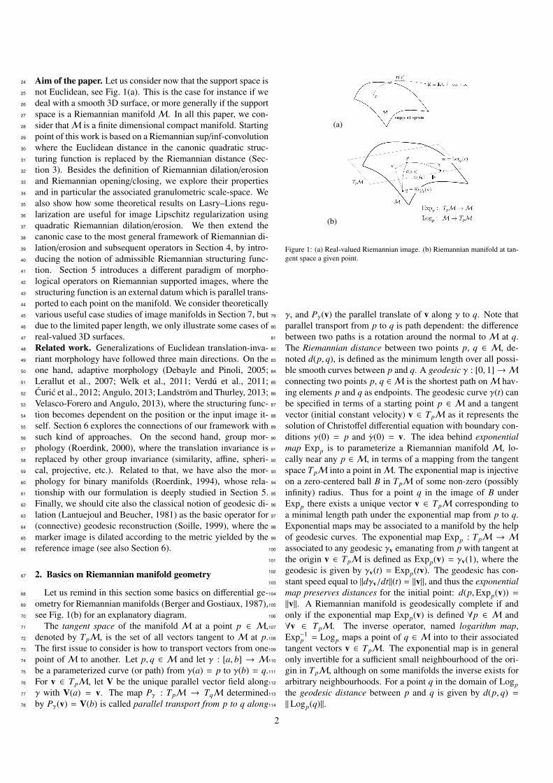
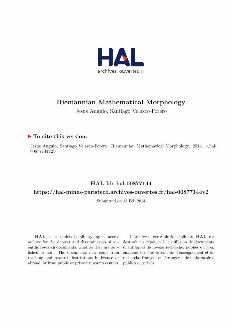
Aim of the paper. Let us consider now that the support space is24

not Euclidean, see Fig. 1(a). This is the case for instance if we25

deal with a smooth 3D surface, or more generally if the support26

space is a Riemannian manifoldM. In all this paper, we con-27

sider thatM is a finite dimensional compact manifold. Starting28

point of this work is based on a Riemannian sup/inf-convolution29

where the Euclidean distance in the canonic quadratic struc-30

turing function is replaced by the Riemannian distance (Sec-31

tion 3). Besides the definition of Riemannian dilation/erosion32

and Riemannian opening/closing, we explore their properties33

and in particular the associated granulometric scale-space. We34

also show how some theoretical results on Lasry–Lions regu-35

larization are useful for image Lipschitz regularization using36

quadratic Riemannian dilation/erosion. We then extend the37

canonic case to the most general framework of Riemannian di-38

lation/erosion and subsequent operators in Section 4, by intro-39

ducing the notion of admissible Riemannian structuring func-40

tion. Section 5 introduces a different paradigm of morpho-41

logical operators on Riemannian supported images, where the42

structuring function is an external datum which is parallel trans-43

ported to each point on the manifold. We consider theoretically44

various useful case studies of image manifolds in Section 7, but45

due to the limited paper length, we only illustrate some cases of46

real-valued 3D surfaces.47

Related work. Generalizations of Euclidean translation-inva-48

riant morphology have followed three main directions. On the49

one hand, adaptive morphology (Debayle and Pinoli, 2005;50

Lerallut et al., 2007; Welk et al., 2011; Verdu et al., 2011;51

Curic et al., 2012; Angulo, 2013; Landstrom and Thurley, 2013;52

Velasco-Forero and Angulo, 2013), where the structuring func-53

tion becomes dependent on the position or the input image it-54

self. Section 6 explores the connections of our framework with55

such kind of approaches. On the second hand, group mor-56

phology (Roerdink, 2000), where the translation invariance is57

replaced by other group invariance (similarity, affine, spheri-58

cal, projective, etc.). Related to that, we have also the mor-59

phology for binary manifolds (Roerdink, 1994), whose rela-60

tionship with our formulation is deeply studied in Section 5.61

Finally, we should cite also the classical notion of geodesic di-62

lation (Lantuejoul and Beucher, 1981) as the basic operator for63

(connective) geodesic reconstruction (Soille, 1999), where the64

marker image is dilated according to the metric yielded by the65

reference image (see also Section 6).66

2. Basics on Riemannian manifold geometry67

Let us remind in this section some basics on differential ge-68

ometry for Riemannian manifolds (Berger and Gostiaux, 1987),69

see Fig. 1(b) for an explanatory diagram.70

The tangent space of the manifold M at a point p ∈ M,71

denoted by TpM, is the set of all vectors tangent to M at p.72

The first issue to consider is how to transport vectors from one73

point of M to another. Let p, q ∈ M and let γ : [a, b] → M74

be a parameterized curve (or path) from γ(a) = p to γ(b) = q.75

For v ∈ TpM, let V be the unique parallel vector field along76

γ with V(a) = v. The map Pγ : TpM → TqM determined77

by Pγ(v) = V(b) is called parallel transport from p to q along78

(a)

(b)

Figure 1: (a) Real-valued Riemannian image. (b) Riemannian manifold at tan-

gent space a given point.

γ, and Pγ(v) the parallel translate of v along γ to q. Note that79

parallel transport from p to q is path dependent: the difference80

between two paths is a rotation around the normal to M at q.81

The Riemannian distance between two points p, q ∈ M, de-82

noted d(p, q), is defined as the minimum length over all possi-83

ble smooth curves between p and q. A geodesic γ : [0, 1]→M84

connecting two points p, q ∈ M is the shortest path onM hav-85

ing elements p and q as endpoints. The geodesic curve γ(t) can86

be specified in terms of a starting point p ∈ M and a tangent87

vector (initial constant velocity) v ∈ TpM as it represents the88

solution of Christoffel differential equation with boundary con-89

ditions γ(0) = p and γ(0) = v. The idea behind exponential90

map Expp is to parameterize a Riemannian manifold M, lo-91

cally near any p ∈ M, in terms of a mapping from the tangent92

space TpM into a point inM. The exponential map is injective93

on a zero-centered ball B in TpM of some non-zero (possibly94

infinity) radius. Thus for a point q in the image of B under95

Expp there exists a unique vector v ∈ TpM corresponding to96

a minimal length path under the exponential map from p to q.97

Exponential maps may be associated to a manifold by the help98

of geodesic curves. The exponential map Expp : TpM → M99

associated to any geodesic γv emanating from p with tangent at100

the origin v ∈ TpM is defined as Expp(v) = γv(1), where the101

geodesic is given by γv(t) = Expp(tv). The geodesic has con-102

stant speed equal to ‖dγv/dt‖(t) = ‖v‖, and thus the exponential103

map preserves distances for the initial point: d(p,Expp(v)) =104

‖v‖. A Riemannian manifold is geodesically complete if and105

only if the exponential map Expp(v) is defined ∀p ∈ M and106

∀v ∈ TpM. The inverse operator, named logarithm map,107

Exp−1p = Logp maps a point of q ∈ M into to their associated108

tangent vectors v ∈ TpM. The exponential map is in general109

only invertible for a sufficient small neighbourhood of the ori-110

gin in TpM, although on some manifolds the inverse exists for111

arbitrary neighbourhoods. For a point q in the domain of Logp112

the geodesic distance between p and q is given by d(p, q) =113

‖Logp(q)‖.114

2

3. Canonic Riemannian dilation and erosion115

Let us start by a formal definition of the two basic canonic116

morphological operators for images supported on a Riemannian117

manifold.118

Definition 1. Let M a complete Riemannian manifold and

dM : M × M → R+, (x, y) 7→ dM(x, y), is the geodesic dis-

tance onM, for any image f : M → R, R = R ∪ −∞,+∞,

so f ∈ F (M,R) and for λ > 0 we define for every x ∈ M the

canonic Riemannian dilation of f of scale parameter λ as

δλ( f )(x) = supy∈M

f (y) −1

2λdM(x, y)2

(1)

and the canonic Riemannian erosion of f of parameter λ as

ελ( f )(x) = infy∈M

f (y) +1

2λdM(x, y)2

(2)

An obvious property of the canonic Riemannian dilation and119

erosion is the duality by the involution f (x) 7→ ∁ f (x) = − f (x),120

i.e., δλ( f ) = ∁ελ(∁ f ). As in classical Euclidean morphology,121

the adjunction relationship is fundamental for the construction122

of the rest of morphological operators.123

Proposition 2. For any two real-valued images defined on the

same Riemannian manifold M, i.e., f , g : M → R, the pair

(ελ, δλ) is called the canonic Riemannian adjunction

δλ( f )(x) ≤ g(x)⇔ f (x) ≤ ελ(g)(x) (3)

Hence, we have an adjunction if both images f and g are

defined on the same Riemannian manifoldM, or in other terms,

when the same “quadratic geodesic structuring function”:

qλ(x; y) = −1

2λdM(x, y)2, (4)

is considered for pixel x 7→ qλ(x; y), y ∈ M in both f and

g. This result implies in particular that the canonic Rieman-

nian dilation commutes with the supremum and the dual ero-

sion with the infimum, i.e., for a given collection of images

fi ∈ F (M,R), i ∈ I, we have

δλ

∨

i∈I

fi

=∨

i∈I

δλ( fi); ελ

∧

i∈I

fi

=∧

i∈I

ελ( fi).

In addition, using the classical result on adjunctions in complete124

lattices (Heijmans, 1994), we state that the composition prod-125

ucts of the pair (ελ, δλ) lead to the adjoint opening and adjoint126

closing if and only the field of geodesic structuring functions is127

computed on a common manifoldM.128

Definition 3. Given an image f ∈ F (M,R), the canonic Rie-

mannian opening and canonic Riemannian closing of scale pa-

rameter λ are respectively given by

γλ( f )(x) = supz∈M

infy∈M

f (y) +1

2λdM(z, y)2 −

1

2λdM(z, x)2

, (5)

and

ϕλ( f )(x) = infz∈M

supy∈M

f (y) −1

2λdM(z, y)2 +

1

2λdM(z, x)2

. (6)

This technical point is very important since in some image129

manifold embedding the Riemannian manifold support M of130

image f depends itself on f . IfM does not depends on f , the131

canonic Riemannian opening and closing are respectively given132

by γλ( f ) = δλ (ελ( f )), and ϕλ( f ) = ελ (δλ( f )). We notice that133

this issue was already considered by Roerdink (2009) for the134

case of adaptive neighbourhood morphology.135

Having the canonic Riemannian opening and closing, all the136

other morphological filters defined by composition of them are137

easily obtained.138

3.1. Properties of δλ( f ) and ελ( f )139

Classical properties of Euclidean dilation and erosion have140

also the equivalent for Riemannian manifold M, and they do141

not dependent on the geometry ofM.142

Proposition 4. LetM be a Riemannian manifold, and let f , g ∈143

F (M,R) two real valued images M. We have the following144

properties for the canonic Riemannian operators.145

1. (Increaseness) If f (x) ≤ g(x), ∀x ∈ M then δλ( f )(x) ≤146

δλ(g)(x) and ελ( f )(x) ≤ ελ(g)(x), ∀x ∈ M and ∀λ > 0.147

2. (Extensivity and anti-extensivity) δλ( f )(x) ≥ f (x) and148

ελ( f )(x) ≤ f (x), ∀x ∈ M and ∀λ > 0.149

3. (Ordering property) If 0 < λ1 < λ2 then δλ2( f )(x) ≥150

δλ1( f )(x) and ελ2

( f )(x) ≤ ελ1( f )(x).151

4. (Invariance under isometry) If T :M→M is an isometry152

of M and if f is invariant under T , i.e., f (Tz) = f (z)153

for all z ∈ M, then the Riemannian dilation and erosion154

are also invariant under T , i.e., δλ( f )(Tz) = δλ( f )(z) and155

ελ( f )(Tz) = ελ( f )(z), ∀z ∈ M and ∀λ > 0.156

5. (Extrema preservation) We have sup δλ( f ) = sup f and157

inf ελ( f ) = inf f , moreover if f is lower (resp. upper)158

semicontinuous then every minimizer (resp. maximizer) of159

ελ( f ) (resp. δλ( f )) is a minimizer (resp. maximizer) of f ,160

and conversely.161

3.2. Flat isotropic Riemannian dilation and erosion162

In order to obtain the counterpart of flat isotropic Euclidean

dilation and erosion, we replace the quadratic structuring func-

tion qλ(x, y) by a flat structuring function given by the geodesic

ball of radius r centered at x, i.e.,

Br(x) = y : dM(x, y) ≤ r, r > 0. (7)

The corresponding flat isotropic Riemannian dilation and163

erosion of size r are given by:164

δBr( f )(x) = sup

f (y) : y ∈ Br(x)

, (8)

εBr( f )(x) = inf f (y) : y ∈ Br(x) . (9)

where Br(x) is the transposed shape of ball Br(x). Correspond-165

ing flat isotropic Riemannian opening and closing are obtained166

by composition of operators (8) and (9):167

γBr( f ) = δBr

(

εBr( f )

)

; ϕBr( f ) = εBr

(

δBr( f )

)

. (10)

All the properties formulated for canonic operators hold for flat168

isotropic ones too. For practical applications, it should be noted169

that flat operators typically lead to stronger filtering effects than170

the quadratic ones.171

3

3.3. Riemannian granulometries:172

scale-space properties of γλ( f ) and ϕλ( f )173

For the canonic Riemannian opening and closing, we have174

also the classical properties which are naturally proved as a con-175

sequence of the adjunction, see (Heijmans, 1994).176

Proposition 5. Let γλ( f ) and ϕλ( f ) be respectively the canonic177

Riemannian opening and closing of an image f ∈ F (M,R).178

1. γλ( f ) and ϕλ( f ) are both increasing operators.179

2. γλ( f ) is anti-extensive and ϕλ( f ) extensive with the fol-

lowing ordering relationships, i.e., for for 0 < λ1 ≤ λ2, we

have:

γλ2( f )(x) ≤ γλ1

( f )(x) ≤ f (x) ≤ ϕλ1( f )(x) ≤ ϕλ2

( f )(x);

(11)

3. idempotency of both operators, γλ (γλ( f )) = γλ( f ) and180

ϕλ (ϕλ( f )) = ϕλ( f )181

Property 3 on idempotency together with the increaseness de-182

fines a family of so-called algebraic openings/closings (Serra,183

1988; Heijmans, 1994) larger than the one associated to the184

composition of dilation/erosion. Idempotent and increasing185

operators are also known as ethmomorphisms by Kiselman186

(2007). Anti-extensivity and extensivity involves that γλ is a187

anoiktomorphism and ϕλ a cleistomorphism. One of the most188

classical results in morphological operators provided us an ex-189

ample of algebraic opening: given a collection of openings γi,190

increasing, idempotent and anti-extensive operators for all i, the191

supremum of them supi γi is also an opening (Matheron, 1975).192

A dual result is obtained for the closing by changing the sup by193

the inf.194

The class of openings (resp. closings) is neither closed un-195

der infimum (resp. opening) or a generic composition. There is196

however a semi-group property leading to a scale-space frame-197

work for opening/closing operators, known as granulometries.198

The notion of granulometry in Euclidean morphology is sum-199

marized in the following results (Matheron, 1975; Serra, 1988).200

Theorem 6 (Matheron (1975), Serra (1988)). A parameter-

ized family γλλ>0 of flat openings from F (E,T ) into F (E,T )

is a granulometry (or size ditritribution) when

γλ1γλ2= γλ2

γλ1= γsup(λ1,λ2); λ1, λ2 > 0. (12)

Condition (12) is equivalent to both

γλ1≤ γλ2

; λ1 ≥ λ2 > 0; (13)

Bλ1⊆ Bλ2

; λ1 ≥ λ2 > 0

where Bλ is the invariance domain of the opening at scale λ;201

i.e., the family of structuring elements Bs such that B = γλ(B)202

(Serra, 1988).203

By duality, we introduce antisize distributions as the families of204

closings ϕλλ>0.205

Axiom (12) shows how translation invariant flat openings are

composed and highlights their semi-group structure. Equivalent

condition (13) emphasizes the monotonicity of the granulome-

try with respect to λ: the opening becomes more and more ac-

tive as λ increases. When dealing with Euclidean spaces, Math-

eron (1975) introduced the notion of Euclidean granulometry

as the size distribution being translationally invariant and com-

patible with homothetics, i.e., γλ( f (x)) = λγ1( f (λ−1x)), where

f ∈ F (E,T ) is an Euclidean grey-level images. More pre-

cisely, a family of mappings γλ is an Euclidean granulometry if

and only if there exist a class B′ such that

γλ( f ) =∨

B∈B′

∨

µ≥λ

γµB( f ).

Then the domain of invariance Bλ are equal to λB, where B is

the class closed under union, translation and homothetics ≥ 1,

which is generated by B′. If we reduce the class B′ to a single

element B, the associated size distribution becomes

γλ( f ) =∨

µ≥λ

γµB( f ).

The following key result simplifies the situation. The size dis-206

tribution by a compact structuring element B is equivalent to207

γλ( f ) = γλB( f ) if and only if B is convex. The extension208

of granulometric theory to non-flat structuring functions was209

deeply studied in (Kraus et al., 1993). In particular, it was210

proven that one can build grey-level Euclidean granulometries211

with one structuring function if and only if this function has a212

convex compact domain and is constant there (flat function).213

We can naturally extend Matheron axiomatic to the general214

case of openings in Riemannian supported images. We start215

by giving a result which is valid for families of openings ψλ216

(idempotent and anti-extensive operators) more general than the217

canonic Riemannian openings.218

Proposition 7. Given the set of Riemannian openings ψλλ>0

indexed according to the positive parameter λ, but not nec-

essary ordered between them, the corresponding Riemannian

granulometry on image f ∈ F (M,R) is the family of multi-

scale openings Γλλ>0 generated as

Γλ( f ) =∨

µ≥λ

ψµ( f )

such that the granulometric semi-group law holds for any pair

of scales:

Γλ1

(

Γλ2( f )

)

= Γλ2

(

Γλ1( f )

)

= Γsup(λ1,λ2)( f ). (14)

In the particular case of canonic Riemannian openings, γλλ>0,219

we always have γλ1≤ γλ2

if λ1 ≥ λ2 > 0. Hence, Γλ( f ) = γλ220

and consequently γλλ>0 is a granulometry. This is also valid221

for flat isotropic Riemannian openings.222

The Riemannian case closest to Matheron’s Euclidean gran-223

ulometries corresponds to the flat isotropic Riemannian open-224

ings γBrassociated to a concave quadratic geodesic structuring225

function qλ(x, y). Or in other terms, the case of a Riemannian226

manifold M where the Riemannian distance is always a con-227

vex function, since this fact involves that Br(x) as defined in (7)228

4

is a convex set for any r at any x ∈ M. Obviously, the flat229

convex Riemannian granulometry

γBr

r>0 is not translation in-230

variant but we have that Br1(x) ⊆ Br2

(x), for r2 ≥ r1 and for any231

x ∈ M, which involves a natural sieving selection of features in232

the neighborhood of any point x.233

A Riemannian distance function which is convex is not only234

useful for scale-space properties. As discussed just below, one235

has powerful results of regularization too.236

3.4. Concavity of qλ(x; y) and Lipschitz image regularization237

using (ελ, δλ)238

Lasry–Lions regularization (Lasry and Lions, 1986) is a the-239

ory of nonsmooth approximation for functions in Hilbert spaces240

using combinations of Euclidean dilation and erosion with241

quadratic structuring functions, which leads to the approxima-242

tion of bounded lower or upper-semicontinuous functions with243

Lipschitz continuous derivatives which approximate f , with-244

out assuming convexity of f . The approach was generalized245

in (Attouch and Aze, 1993) to semicontinuous, non necessarily246

bounded, quadratically minorized/majorized functions defined247

on Rn. More precisely, we have.248

Theorem 8 (Lasry and Lions(1986), Attouch and Aze(1993)).249

For all 0 < µ < λ, let us define for a given image f the Lasry-250

Lions regularizers based on Euclidean dilation and erosion by251

a quadratic structuring function qλ as:252

( fλ)µ(x) =(

( f ⊖ qλ) ⊕ qµ)

(x),

( f λ)µ(x) =(

( f ⊕ qλ) ⊖ qµ)

(x).

• Let f be a bounded uniformly continuous scalar func-253

tions in Rn. Then the functions ( fλ)µ and ( f λ)µ con-254

verge uniformly to f when λ, µ → 0, and belong to the255

class C1,1

b(Rn) (i.e., bounded continuously differentiable256

with a Lipschitz continuous gradient), namely |∇( fλ)µ(x)−257

∇( fλ)µ(y)| ≤ Mλ,µ‖x − y‖ and |∇( f λ)µ(x) − ∇( f λ)µ(y)| ≤258

Mλ,µ‖x − y‖, where Mλ,µ = (µ−1, (λ − µ)−1).259

• Let f : E ⊆ Rn → R ∪ +∞ be a lower-semicontinuous260

function and g : E ⊆ Rn → R ∪ −∞ an upper-261

semicontinuous. We assume the growing conditions f (x) ≥262

− c2(1+ ‖x‖2), c ≥ 0 (quadratically minorized), then g(x) ≤263

c′

2(1 + ‖x‖2), c′ ≥ 0 (quadratically majorized). Then for264

0 < µ < λ < c−1 and 0 < µ < λ < c′−1 the regularizes265

( fλ)µ and (gλ)µ are C1,1

b(Rn) functions, whose gradient is266

Lipschitz continuous with constant max(µ−1, (1 − λc)−1c).267

In addition they converge point-wise respectively to f and268

g when λ, µ→ 0.269

Hence, we can replace the bounded and uniformly continuous270

assumptions by rather general growing conditions. The idea is271

that given a quadratically majorized function g of parameter c′,272

the quadratic dilation f ⊕ qλ with λ < c′−1 produces a λ-weakly273

convex function. Then for any µ < λ (strictly smaller than the274

dilation scale), the corresponding quadratic erosion ( f ⊕ qλ)⊖qµ275

produces a function belongings to the class of bounded C1, with276

has Lipschitz continuous gradient. Note that the key element277

of this approximation is the transfer of the regularity of the278

quadratic kernel associated to its concavity and smoothness of279

qλ to the function f .280

Lasry–Lions regularization has been recently generalized to281

finite dimensional compact manifolds Bernard (2010); Bernard282

and Zavidovique (2013), and consequently these results can be283

used to show how Riemannian morphological operators are ap-284

propriate for image regularization. More precisely, let us focus285

on the case where M is finite dimensional compact Cartan–286

Hadamard manifold, hence every two points can be connected287

by a minimizing geodesic. We remind that a Cartan–Hada-288

mard manifold is a simply connected Riemannian manifoldM289

with sectional curvature K ≤ 0 (Lang, 1999). Let A be a290

closed convex subset of M. Then the distance function to A,291

x 7→ dM(x, A), where dM(x, A) = inf dM(x, y) : y ∈ A is C1292

smooth on M \ A and, moreover, the square of the distance293

function x 7→ dM(x, A)2 is C1 smooth and convex on all of294

M (Azagra and Ferrera, 2006). Consequently, ifM is a Cartan–295

Hadamard manifold, the structuring function x 7→ q(x, y), ∀y ∈296

M, is always a concave function; or equivalently, −q(x, y) is a297

convex function.298

Theorem 9. Let M be a compact finite dimensional Cartan–299

Hadamard manifold. LetΩ ⊂ M be a bounded set ofM. Given300

a image f ∈ F (Ω,R), for all 0 < µ < λ let us define the301

Riemannian Lasry–Lions regularizers:302

( fλ)µ(x) = supz∈M

infy∈M

f (y) +1

2λdM(z, y)2 −

1

2µdM(z, x)2

( f λ)µ(x) = infz∈M

supy∈M

f (y) −1

2λdM(z, y)2 +

1

2µdM(z, x)2

We have ( fλ)µ ≤ f and ( f λ)µ ≥ f .303

• Let f be a bounded uniformly continuous image in Ω.304

Then the images ( fλ)µ and ( f λ)µ belong to the class305

C1,1

b(Ω) and converges uniformly to f on Ω.306

• Assume that there exists c, c′ > 0, such that we have

the following growing conditions for semicontinuous func-

tions F (Ω,R):

f (x) ≥ −c

2(1+d(x, x0)2), g(x) ≤

c′

2(1+d(x, x0)2), x0 ∈ M.

Then, for all 0 < µ < λ < c−1 the pseudo-opened image307

( fλ)µ and for all 0 < µ < λ < c′−1 the pseudo-closed im-308

age (gλ)µ are of class C1,1

b(Ω). In addition, they converge309

point-wise respectively to f and g.310

We remark that this result is theoretically valid only for311

bounded images supported on bounded subsets on manifolds312

of nonpositive sectional curvature. However, in practice we ob-313

serve that it works for bounded images on bounded surfaces314

of positive and negative curvature. By the way, one should315

note that our result conjectured in (Angulo and Velasco-Forero,316

2013) was too general since the support space of the image317

should be a bounded set Ω. As discussed in Bernard (2010)318

and Bernard and Zavidovique (2013), more general versions of319

5

Lasry-Lions regularization can be obtained in Riemannian man-320

ifolds. In particular the case of compact nonnegative curvature321

manifolds is relevant for optimal transport problems (Villani,322

2009).323

4. Generalized Riemannian morphological operators324

We have discussed the canonic case on Riemannian math-325

ematical morphology associated to the structuring function326

qλ(x, y). Let consider now the most general family of Rieman-327

nian operators. We start by introducing the minimal properties328

that a Riemannian structuring function should verify.329

Definition 10. Let M be a Riemannian manifold. A mapping330

b :M×M→ R defined for any pair of points inM is said an331

admissible Riemannian structuring function inM if and only if332

1. b(x, y) ≤ 0, ∀x, y ∈ M (non-positivity);333

2. b(x, x) = 0, ∀x ∈ M (maximality at the diagonal).334

Now, we can introduce the pair of dilation and erosion for any335

image f according to b.336

Definition 11. Given an admissible Riemannian structuring337

function b in a Riemannian manifold M, the Riemannian di-338

lation and Riemannian erosion of an image f ∈ F (M,R) by b339

are given respectively by340

δb( f )(x) = supy∈M

f (y) + b(x, y) , (15)

εb( f )(x) = infy∈M f (y) − b(y, x) . (16)

Note that this formulation has been considered recently in341

the framework of adaptive morphology (Curic and Luengo-342

Hendriks, 2013). Both are increasing operators which, by the343

maximality at the diagonal, preserves the extrema. By the non-344

positivity, Riemannian dilation is extensive and erosion is anti-345

extensive. In addition, we can easily check that the pair (εb, δb)346

forms an adjunction as in Proposition 3. Consequently, their347

composition leads to the Riemannian opening and closing ac-348

cording to the admissible Riemannian structuring function b349

given respectively by:350

γb( f )(x) = supz∈M

infy∈M f (y) − b(y, z) + b(z, x) , (17)

ϕb( f )(x) = infz∈M

supy∈M

f (y) + b(z, y) − b(x, z) . (18)

Remarkably, the symmetry of b is not a necessary condition for351

the adjunction. Examples of such asymmetric structuring func-352

tions have recently appeared in the context of stochastic mor-353

phology (Angulo and Velasco-Forero, 2013), non-local mor-354

phology (Velasco-Forero and Angulo, 2013) and saliency-based355

adaptive morphology (Curic and Luengo-Hendriks, 2013).356

In our framework, we propose a general form of any admissi-

ble Riemannian structuring function b(x, y), ∀x, y ∈ M, which

should be decomposable into the sum of two terms:

b(x, y) = αbsym(x, y) + βbasym(x, y), α, β ≥ 0. (19)

Symmetric structuring function. The symmetric term of

the structuring function will be a scaled p-norm shaped func-

tion depending exclusively on the Riemannian distance, i.e.,

bsym(x, y) = bsym(y, x) = kλ,p (dM(x, y)) such that

kλ,p (η) = −Cp

ηp

p−1

λ1

p−1

; λ > 0, p > 1,

where the normalization factor is given by Cp = (p − 1)p−

p

p−1 .357

We note that with the shape parameter p = 2 we recover the358

canonic quadratic structuring function. In fact, this general-359

ization of the quadratic structuring is inspired from the solu-360

tion of a generalized morphological PDE (Lions et al., 1987):361

ut(t, x) + ‖ux(t, x)‖p = 0, (t, x) ∈ (0,+∞) × E; u(0, x) = f (x),362

x ∈ E, since the quadratic one is the solution of the classi-363

cal (Hamilton-Jacobi) morphological PDE (Bardi et al., 1984;364

Crandall et al., 1992): ut(t, x)+ ‖ux(t, x)‖2 = 0. Asymptotically,365

one is dealing with almost flat shapes over M as p → 1; as366

p > 2 increases and p→ ∞ the shape of kλ,p (η) evolves from a367

parabolic shape p = 2, i.e., term on dM(x, y)2, to the limit case,368

which is a conic shape, i.e., term on dM(x, y).369

We note that ifM is a Cartan–Hadamard manifold, the sym-370

metric part bsym(x, y) is a concave function for any λ > 0 and371

any p > 1.372

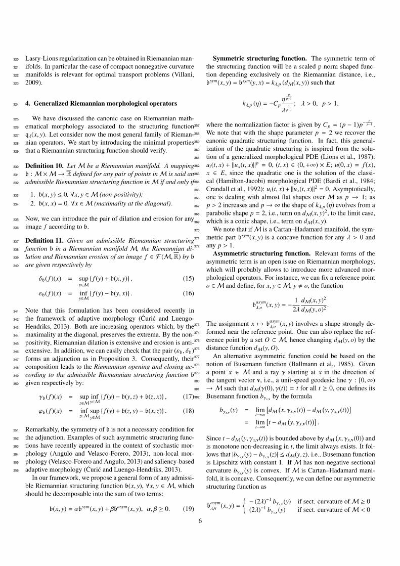
Asymmetric structuring function. Relevant forms of the

asymmetric term is an open issue on Riemannian morphology,

which will probably allows to introduce more advanced mor-

phological operators. For instance, we can fix a reference point

o ∈ M and define, for x, y ∈ M, y , o, the function

basym

λ,o(x, y) = −

1

2λ

dM(x, y)2

dM(y, o)2.

The assignment x 7→ basym

λ,o(x, y) involves a shape strongly de-373

formed near the reference point. One can also replace the ref-374

erence point by a set O ⊂ M, hence changing dM(y, o) by the375

distance function dM(y,O).376

An alternative asymmetric function could be based on the377

notion of Busemann function (Ballmann et al., 1985). Given378

a point x ∈ M and a ray γ starting at x in the direction of379

the tangent vector v, i.e., a unit-speed geodesic line γ : [0,∞)380

→ M such that dM(γ(0), γ(t)) = t for all t ≥ 0, one defines its381

Busemann function bγx,vby the formula382

bγx,v(y) = lim

t→∞

[

dM(

x, γx,v(t))

− dM(

y, γx,v(t))]

= limt→∞

[

t − dM(

y, γx,v(t))]

.

Since t − dM(

y, γx,v(t))

is bounded above by dM(

x, γx,v(0))

and

is monotone non-decreasing in t, the limit always exists. It fol-

lows that |bγx,v(y) − bγx,v

(z)| ≤ dM(y, z), i.e., Busemann function

is Lipschitz with constant 1. If M has non-negative sectional

curvature bγx,v(y) is convex. If M is Cartan–Hadamard mani-

fold, it is concave. Consequently, we can define our asymmetric

structuring function as

basym

λ,v(x, y) =

− (2λ)−1 bγx,v(y) if sect. curvature ofM ≥ 0

(2λ)−1 bγx,v(y) if sect. curvature ofM < 0

6

From a practical viewpoint, asymmetric structuring functions383

obtained by Busemann functions allow to introduce a shape384

which depends on the distance between the point x and a kind385

of orthogonal projection of point y on the geodesic along the386

direction v. Hence, it could be a way to introduce directional387

Riemannian operators.388

5. Parallel transport of a fixed external structuring func-389

tion390

Previous Riemannian morphological operators are based on391

geodesic structuring functions b(x; y) which are defined by the392

geodesic distance function onM. Let us consider now the case393

where a prior (semi-continuous) structuring function b external394

to M is given and it should be adapted to each point x ∈ M.395

Our approach is inspired from Roerdink (1994) formulation of396

dilation/erosion for binary images on smooth surfaces.397

5.1. Manifold morphology398

The idea behind the binary Riemannian morphology on smo-

oth surfaces introduced in (Roerdink, 1994) is to replace the

translation invariance by the parallel transport (the transforma-

tions are referred to as “covariant” operations). Let M be a

(geodesically complete) Riemannian manifold and P(M) de-

notes the set of all subsets of M. A binary image X on the

manifold is just X ∈ P(M). Let A ⊂ M be the basic structur-

ing, a subset which is defined on the tangent space at a given

point ω ofM by A = Logω(A) ⊂ TωM. Let γ = γ[p,q] be a path

from p to q, then the operator

τγ(A) = Expq Pγ Logp(A) = B,

transports the subset A of p to the set B of q. As the image of the

set X under parallel translation from p to q will depend in gen-

eral on which path is taken; the solution proposed in (Roerdink,

1994), denoted by δRoerdinkA

, is to consider all possible paths

from p to q. The mapping δRoerdinkA

: P(M) → P(M) given

by

δRoerdinkA (X) =

⋃

x∈M

⋃

γ

τγ(A) =⋃

x∈M

⋃

γ

Expx Pγ[ω,x]Logω(A),

(20)

is a dilation of image X according to the structuring element A.

Using the symmetry group morphology (Roerdink, 2000), this

operator can be rewritten as

δRoerdinkA (X) =

⋃

x∈M

Expx

Pγ[ω,x]Logω

(A),

where A =⋃

s∈Σ sA, with Σ being the holonomy group around399

the normal at ω. For instance, if A = Logω(A) is a line segment400

of length r starting at ω then A is a disk of radius r centered at401

ω.402

5.2. bω-transported Riemannian dilation and erosion403

Coming back to our framework of real-valued images on404

a geodesically complete Riemannian manifold M. From our405

viewpoint, it seems more appropriate to fix the reference struc-406

turing element as a Boolean set S on the tangent space at the407

reference point ω ∈ M, i.e., S ω ⊂ TωM. More precisely, let408

S ω be a compact set which contains the origin of TωM. We can409

now formulate the S ω-transported flat Riemannian dilation and410

erosion as411

δS ω( f )(x) = sup

f (y) : y ∈ Expx Pγgeo

[ω,x]S ω

, (21)

εS ω( f )(x) = inf

f (y) : y ∈ Expx Pγgeo

[ω,x]S ω

. (22)

Thus, in comparison to dilation (20), we prefer to consider in412

our case that the parallel transport from ω to x is done exclu-413

sively along the geodesic path γgeo

[ω,x]between ω and x, i.e., if S ω414

is a line in ω then it will be also at x a line, but rotated.415

This idea leads to a natural extension to the case where

the fixed datum is an upper-semicontinuous structuring func-

tion bω(v), defined in the Euclidean tangent space at ω, i.e.,

bω : TωM → [−∞, 0]. Let consider now the upper level sets

(or cross-section) of bω obtained by thresholding at a value l:

Xl(bω) = v ∈ TωM : bω(v) ≥ l , ∀l ∈ [−∞, 0]. (23)

The set of upper level sets constitutes a family of decreasing

closed sets: l ≥ m ⇒ Xl ⊆ Xm and Xl = ∩Xm,m < l. Any

function bω(v) can be now viewed as a unique stack of its cross-

sections, which leads to the following reconstruction property:

bω(v) = sup l ∈ [−∞, 0] : v ∈ Xl(bω) , ∀v ∈ TωM. (24)

Using this representation, the corresponding Riemannian struc-

turing function at ω is given by bω(ω, y) = supl ∈ [−∞, 0] : z ∈

Expω Xl(bω). In the case of a different point x ∈ M, the cross-

section should be transported to the tangent space of x before

mapping back toM, i.e.,

bω(x, y) = sup

l ∈ [−∞, 0] : z ∈ Expx Pγgeo

[ω,x]Xl(bω)

.

Finally, the bω-transported Riemannian dilation and erosion of416

image f are given respectively by417

δbω ( f )(x) = supy∈M

f (y) + bω(x, y) , (25)

εbω ( f )(x) = infy∈M f (y) − bω(y, x) . (26)

Obviously, the case of a concave structuring function bω is418

particularly well defined since in such a case, its cross-sections419

are convex sets. In addition, if M is a Cartan–Hadamard420

manifold, the corresponding Riemannian structuring function421

bω(x, y) is also a concave function.422

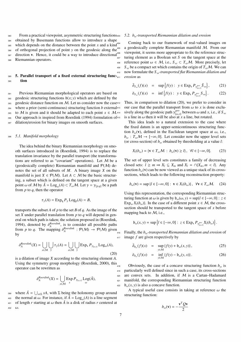
A typical useful case consists in taking at reference ω the

structuring function:

bω(v) = −vT Qv

2

7

where Q is a d × d symmetric positive definite matrix, d being423

the dimension of manifold M. It corresponds just to a gener-424

alized quadratic function such that the eigenvectors of Q de-425

fine the principal directions of the concentric ellipsoids and the426

eigenvalues their eccentricity. Therefore, we can introduce by427

means of Q an anisotropic/directional shape on bω(x, y). We428

can easily check that Q = 1λ

I, I being the identity matrix of di-429

mension d, corresponds just to the canonic Riemannian dilation430

and erosion (1) and (2).431

Without an explicit expression of the exponential map, we432

cannot compute straightforwardly the bω-transported Rieman-433

nian dilation and erosion on a Riemannian manifoldM. This is434

for instance the situation when is f is an image on a 3D smooth435

surface. Hence, in the case of applications to valued surfaces,436

manifold learning techniques as LOGMAP (Brun et al., 2005)437

can be used to numerically obtain the transported cross-sections438

onM.439

6. Connections with classical Euclidean morphology440

6.1. Spatially-invariant operators441

First of all, it is obvious that the Riemannian dilation/erosion442

naturally extends the quadratic Euclidean dilation/erosion for443

images F (Rd,R) by considering that the intrinsic distance is444

the Euclidean one (or the discrete one for Zd), i.e., dM(x, y) =445

‖x − y‖ = dspace(x, y).446

By the way, we note also that definition of the Riemannian447

flat dilation and erosion of size r given in (8) and (9) are com-448

patible with the formulation of the classical geodesic dilation449

and erosion (Lantuejoul and Beucher, 1981) of size r of im-450

age f (marker) constrained by the image g (reference or mask),451

δg,λ( f ) and εg,λ( f ), which underly the operators by reconstruc-452

tion (Soille, 1999), where the upper-level sets of the reference453

image g are considered as the manifoldM where the geodesic454

distance is defined.455

6.2. Adaptive (spatially-variant) operators456

From (Kimmel et al., 1997), the idea of embedding a 2D

grey-level image f ∈ F (R2,R), x = (x1, x2), into a surface

embedded in R3, i.e.,

f (x) 7→ ξx = (x1, x2, α f (x1, x2)), α > 0,

where α is a scaling parameter useful for controlling intensity457

distances, has become popular in differential geometry inspired458

image processing. This embedded Riemannian manifoldM =459

R2×R has a product metric of type ds2

M= ds2

space+αds2f, where460

ds2space = dx2

1+ dx2

2and ds2

f= d f 2. The geodesic distance461

between two points ξx, ξy ∈ M is the length of the shortest path462

between the points, i.e., dM(ξx, ξy) = minγ=γ[ξx ,ξy ]

∫

γdsM.463

As shown in (Welk et al., 2011), this is essentially the frame-464

work behind the morphological amoebas (Lerallut et al., 2007),465

which are flat spatially adaptive structuring functions centered466

in a point x, Aλ(x), computed by thresholding the geodesic dis-467

tance at radius λ > 0, i.e., Aλ(x) =

y ∈ E : dM(ξx, ξy) < λ

. In468

(a)

(b) (c)

(d) (e)

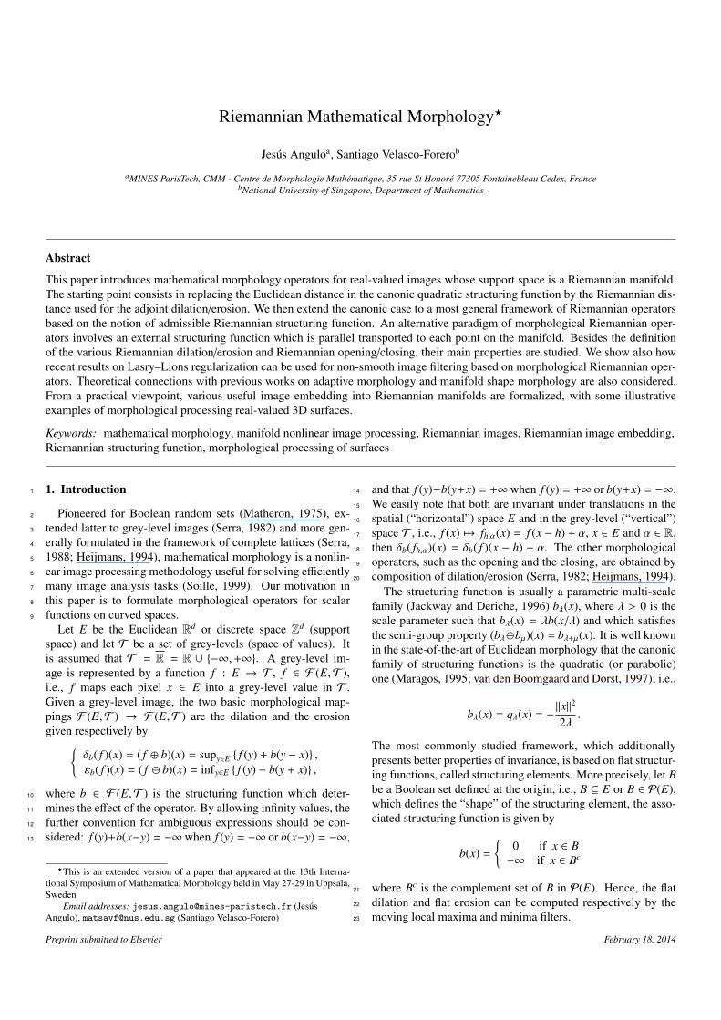
(f) (g)

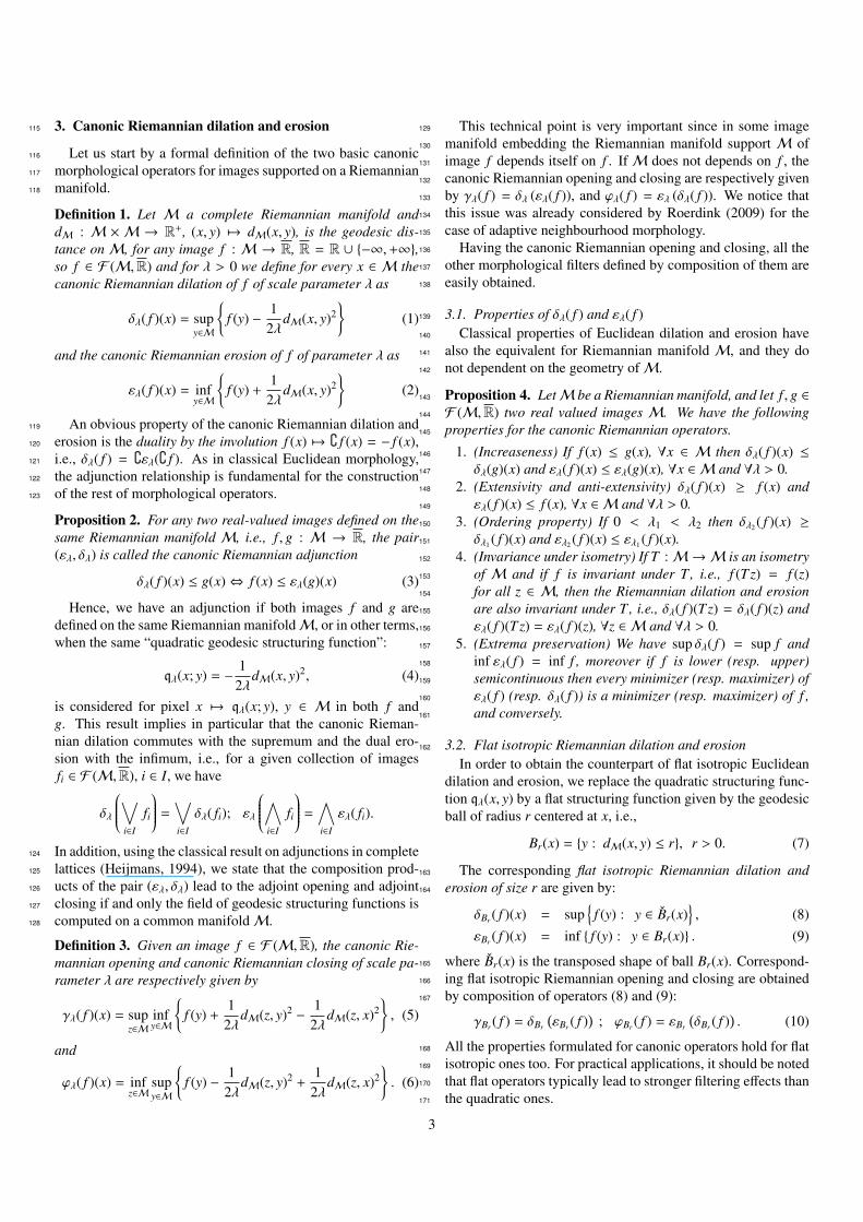
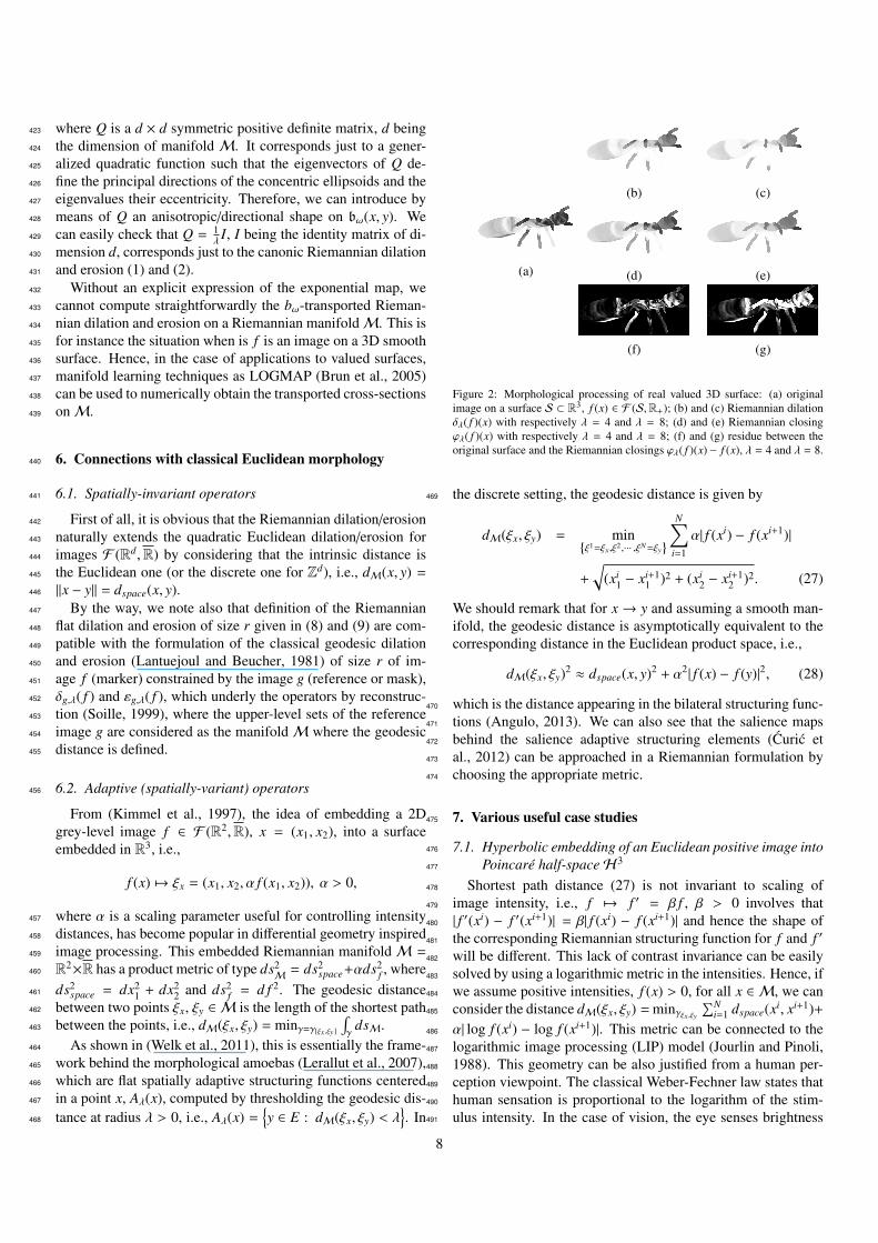
Figure 2: Morphological processing of real valued 3D surface: (a) original

image on a surface S ⊂ R3, f (x) ∈ F (S,R+); (b) and (c) Riemannian dilation

δλ( f )(x) with respectively λ = 4 and λ = 8; (d) and (e) Riemannian closing

ϕλ( f )(x) with respectively λ = 4 and λ = 8; (f) and (g) residue between the

original surface and the Riemannian closings ϕλ( f )(x)− f (x), λ = 4 and λ = 8.

the discrete setting, the geodesic distance is given by469

dM(ξx, ξy) = minξ1=ξx,ξ2,··· ,ξN=ξy

N∑

i=1

α| f (xi) − f (xi+1)|

+

√

(xi1− xi+1

1)2 + (xi

2− xi+1

2)2. (27)

We should remark that for x → y and assuming a smooth man-

ifold, the geodesic distance is asymptotically equivalent to the

corresponding distance in the Euclidean product space, i.e.,

dM(ξx, ξy)2 ≈ dspace(x, y)2 + α2| f (x) − f (y)|2, (28)

which is the distance appearing in the bilateral structuring func-470

tions (Angulo, 2013). We can also see that the salience maps471

behind the salience adaptive structuring elements (Curic et472

al., 2012) can be approached in a Riemannian formulation by473

choosing the appropriate metric.474

7. Various useful case studies475

7.1. Hyperbolic embedding of an Euclidean positive image into476

Poincare half-spaceH3477

Shortest path distance (27) is not invariant to scaling of478

image intensity, i.e., f 7→ f ′ = β f , β > 0 involves that479

| f ′(xi) − f ′(xi+1)| = β| f (xi) − f (xi+1)| and hence the shape of480

the corresponding Riemannian structuring function for f and f ′481

will be different. This lack of contrast invariance can be easily482

solved by using a logarithmic metric in the intensities. Hence, if483

we assume positive intensities, f (x) > 0, for all x ∈ M, we can484

consider the distance dM(ξx, ξy) =minγξx ,ξy

∑Ni=1 dspace(xi, xi+1)+485

α| log f (xi) − log f (xi+1)|. This metric can be connected to the486

logarithmic image processing (LIP) model (Jourlin and Pinoli,487

1988). This geometry can be also justified from a human per-488

ception viewpoint. The classical Weber-Fechner law states that489

human sensation is proportional to the logarithm of the stim-490

ulus intensity. In the case of vision, the eye senses brightness491

8

approximately according to the Weber-Fechner law over a mod-492

erate range.493

Following the same assumption of positive intensities, wecan also consider that a 2D image can be embedded into the

hyperbolic space H3 (Cannon et al., 1997). More particularly

the (Poincare) upper half-space model is the domain H3 =

(x1, x2, x3) ∈ R3 | x3 > 0 with the Riemannian metric

ds2H3 =

dx21+dx2

2+dx2

3

x23

. This space has constant negative sec-

tional curvature. If we consider the image embedding f (x) 7→

ξx = (x1, x2, f (x1, x2)) ∈ H3, the Riemannian distance neededfor morphological operators will be given by

dM(ξx, ξy) = minγξx ,ξy

N∑

i=1

cosh−1

1 +(xi

1− xi+1

1)2 + (xi

2− xi+1

2)2 + ( f (xi) − f (xi+1))2

2 f (xi) f (xi+1)

.

(29)

The geometry of this space is extremely rich in particular con-494

cerning the invariance and isometric symmetry. Hence, dis-495

tance (29) is for instance invariant to translations ξ = (x1, x2, x3)496

7→ ξ + α, α ∈ R, scaling ξ 7→ βξ, β > 0. A specific theory on497

granulometric scale-space properties in this embedding can be498

intended.499

7.2. Embedding an Euclidean image into the structure tensor500

manifold501

Besides the space×intensity embeddings discussed just502

above, we can consider other more alternative non-Euclidean503

geometric embedding of scalar images, using for instance the504

local structure.505

More precisely, given a 2D Euclidean image f (x) = f (x1, x2)

∈ F (R2,R), the structure tensor representing the local orien-tation and edge information (Forstner and Gulch, 1987) is ob-tained by Gaussian smoothing of the dyadic product ∇ f∇ f T :

S ( f )(x) = Gσ∗(

∇ f (x1, x2)∇ f (x1, x2)T)

=

(

sx1 x1(x1, x2) sx1 ,x2

(x1, x2)

sx1 x2(x1, x2) sx2 x2

(x1, x2)

)

where ∇ f (x1, x2) =(

∂ f (x1 ,x2)

∂x1,∂ f (x1 ,x2)

∂x2

)Tis the 2D spatial inten-506

sity gradient and Gσ stands for a Gaussian smoothing with507

a standard deviation of σ. From a mathematical viewpoint,508

S ( f )(x) : E → SPD(2) is an image where at each pixel509

we have a symmetric positive (semi-)definite matrix 2 × 2.510

The differential geometry in the manifold SPD(n) is very511

well-known (Bhatia, 2007). Namely, the metric is given512

by ds2S PD(n)

= tr(M−1dMM−1dM) and the Riemannian dis-513

tance is defined as dS PD(n)(M1,M2) = ‖ log(

M−1/2

1M2M

−1/2

1

)

‖F ,514

∀M1,M2 ∈ SPD(n). Let consider now the embedding f (x) 7→515

ξx = (x1, x2, αS ( f )(x1, x2)), α > 0, in the product manifold516

M = R2 × SPD(2), which has the product metric ds2

M=517

ds2space + αds2

S PD(2). It is a (complete, not compact, nega-518

tive sectional curved) Riemannian manifold of geodesic dis-519

tance given by dM(ξx, ξy) = minγξx ,ξy

∑Ni=1 dspace(xi, xi+1) +α520

dS PD(n)(S ( f )(xi), S ( f )(xi+1)), which is asymptotically equal to521

dM(ξx, ξy)2 ≈ dspace(x, y)2 + αdS PD(2)(S ( f )(x), S ( f )(y))2.522

By means of this embedding, we can compute anisotropic523

morphological operators following the flow coherence of im-524

age structures. This embedding is related to previous adaptive525

approaches such as (Verdu et al., 2011) and (Landstrom and526

Thurley, 2013).527

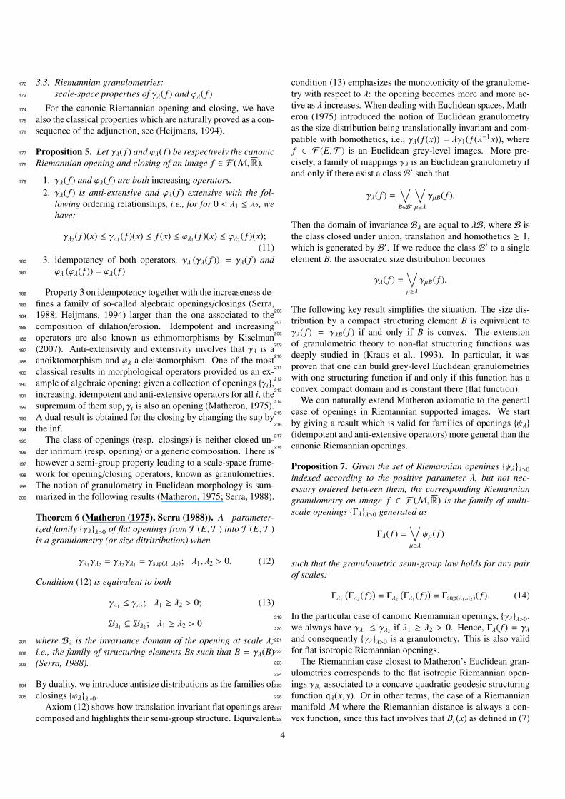
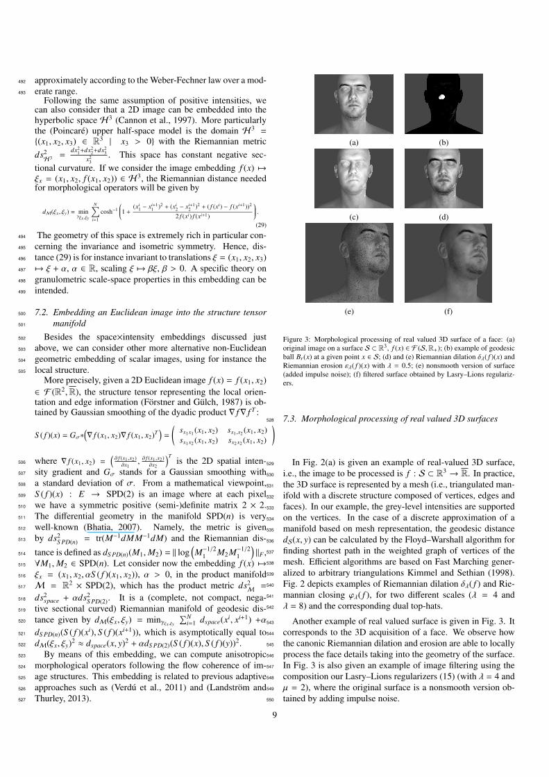
(a) (b)

(c) (d)

(e) (f)

Figure 3: Morphological processing of real valued 3D surface of a face: (a)

original image on a surface S ⊂ R3, f (x) ∈ F (S,R+); (b) example of geodesic

ball Br(x) at a given point x ∈ S; (d) and (e) Riemannian dilation δλ( f )(x) and

Riemannian erosion ελ( f )(x) with λ = 0.5; (e) nonsmooth version of surface

(added impulse noise); (f) filtered surface obtained by Lasry–Lions regulariz-

ers.

7.3. Morphological processing of real valued 3D surfaces528

In Fig. 2(a) is given an example of real-valued 3D surface,529

i.e., the image to be processed is f : S ⊂ R3 → R. In practice,530

the 3D surface is represented by a mesh (i.e., triangulated man-531

ifold with a discrete structure composed of vertices, edges and532

faces). In our example, the grey-level intensities are supported533

on the vertices. In the case of a discrete approximation of a534

manifold based on mesh representation, the geodesic distance535

dS(x, y) can be calculated by the Floyd–Warshall algorithm for536

finding shortest path in the weighted graph of vertices of the537

mesh. Efficient algorithms are based on Fast Marching gener-538

alized to arbitrary triangulations Kimmel and Sethian (1998).539

Fig. 2 depicts examples of Riemannian dilation δλ( f ) and Rie-540

mannian closing ϕλ( f ), for two different scales (λ = 4 and541

λ = 8) and the corresponding dual top-hats.542

Another example of real valued surface is given in Fig. 3. It543

corresponds to the 3D acquisition of a face. We observe how544

the canonic Riemannian dilation and erosion are able to locally545

process the face details taking into the geometry of the surface.546

In Fig. 3 is also given an example of image filtering using the547

composition our Lasry–Lions regularizers (15) (with λ = 4 and548

µ = 2), where the original surface is a nonsmooth version ob-549

tained by adding impulse noise.550

9

8. Conclusions551

We have introduced in this paper a general theory for the552

formulation of mathematical morphology operators for images553

valued on Riemannian manifolds. We have defined the main554

operators and studied their fundamental properties. We have555

considered two main families of operators. On the one hand,556

morphological operators based on an admissible Riemannian557

structuring function which is adaptively obtained for each point558

x according to the geometry of the manifold. On the other559

hand, morphological operators founded on an external Eu-560

clidean structuring function which is parallel transported to the561

tangent space at each point x and then mapped to the manifold.562

We have also discussed some original Riemannian embedding563

of Euclidean images onto Cartan–Hadamard manifolds. This564

is the case of the Poincare half-space H3 as well as the struc-565

ture tensor manifold. Riemannian structuring functions defined566

on Cartan–Hadamard manifolds are particular rich in terms of567

scale-space properties as well as in Lipschitz regularization.568

Acknowledgment. The authors would like to thank the anonymous569

reviewer who pointed out the problem of the result on Lasry-Lions570

regularization for the case of unbounded support space or unbounded571

functions.572

Remark on related work. In the last stages of writing this paper,573

we learned of the work (Azagra and Ferrera, 2014) where it is provided574

a complete analysis of the generalization of Lasry-Lions regularization575

for bounded functions in manifolds of bounded sectional curvature.576

References577

J. Angulo. Morphological Bilateral Filtering. SIAM Journal on Imaging Sci-578

ences, 6(3):1790–1822, 2013.579

J. Angulo and S. Velasco-Forero. Mathematical morphology for real-valued im-580

ages on Riemannian manifolds. In Proc. of ISMM’13 (11th International581

Symposium on Mathematical Morphology), Springer LNCS 7883, p. 279–582

291, 2013.583

J. Angulo and S. Velasco-Forero. Stochastic Morphological Filtering and584

Bellman-Maslov Chains. In Proc. of ISMM’13 (11th International Sym-585

posium on Mathematical Morphology), Springer LNCS 7883, p. 171–182,586

2013.587

D. Attouch, D. Aze. Approximation and regularization of arbitray functions in588

Hilbert spaces by the Lasry-Lions method. Annales de l’I.H.P., section C,589

10(3): 289–312, 1993.590

D. Azagra, J. Ferrera. Inf-Convolution and Regularization of Convex Func-591

tions on Riemannian Manifols of Nonpositive Curvature. Rev. Mat. Complut.592

19(2): 323–345, 2006.593

D. Azagra, J. Ferrera. Regularization by sup-inf convolutions on Riemannian594

manifolds: an extension of Lasry-Lions theorem to manifolds of bounded595

curvature. arXiv preprint arXiv:1401.5053, 2014.596

W. Ballmann, M. Gromov, V. Schroeder. Manifolds of nonpositive curvature.597

Progr. Math., 61, Birkhauser, 1985.598

M. Bardi, L.C. Evans. On Hopf’s formulas for solutions of Hamilton- Ja-599

cobi equations. Nonlinear Analysis, Theory, Methods and Applications,600

8(11):1373–1381, 1984.601

R. Bhatia. Positive Definite Matrices. Princeton University Press, 2007.602

P. Bernard. Lasry-Lions regularization and a lemma of Ilmanen. Rend. Semin.603

Mat. Univ. Padova, 124:221–229, 2010.604

P. Bernard, M. Zavidovique. Regularization of Subsolutions in Discrete Weak605

KAM Theory. Canadian Journal of Mathematics, 65:740–756, 2013.606

M. Berger, B. Gostiaux. Differential Geometry: Manifolds, Curves, and Sur-607

faces. Springer, 1987.608

R. van den Boomgaard, L. Dorst. The morphological equivalent of Gaussian609

scale-space. In Proc. of Gaussian Scale-Space Theory, 203–220, Kluwer,610

1997.611

A. Brun, C.-F. Westin, M. Herberthson, H. Knutsson. Fast Manifold Learning612

Based on Riemannian Normal Coordinates. In Proc. of 14th Scandinavian613

Conference (SCIA’05), Springer LNCS 3540, 920–929, 2005.614

J.W. Cannon, W.J. Floyd, R. Kenyon, W.R. Parry. Hyperbolic Geometry. Fla-615

vors of Geometry, MSRI Publications, Vol. 31, 1997.616

M.G. Crandall, H. Ishii, P.-L. Lions. User’s guide to viscosity solutions of sec-617

ond order partial differential equations. Bulletin of the American Mathemat-618

ical Society, 27(1):1–67, 1992.619

V. Curic, C.L. Luengo Hendriks, G. Borgefors. Salience adaptive structuring620

elements. IEEE Journal of Selected Topics in Signal Processing, 6(7): 809–621

819, 2012.622

V. Curic and C.L. Luengo-Hendriks. Salience-Based Parabolic Structuring623

Functions. In Proc. of ISMM’13 (11th International Symposium on Math-624

ematical Morphology), Springer LNCS 7883, p. 183–194, 2013.625

J. Debayle and J. C. Pinoli. Spatially Adaptive Morphological Image Filter-626

ing using Intrinsic Structuring Elements. Image Analysis and Stereology,627

24(3):145–158, 2005.628

W. Forstner, E. Gulch. A fast operator for detection and precise location of629

distinct points, corners and centres of circular features. In Proc. of ISPRS630

Intercommission Conference on Fast Processing of Photogrammetric Data,631

p. 281–304, 1987.632

H.J.A.M. Heijmans. Morphological image operators. Academic Press, Boston,633

1994.634

P.T. Jackway, M. Deriche. Scale-Space Properties of the Multiscale Morpholog-635

ical Dilation-Erosion. IEEE Trans. Pattern Anal. Mach. Intell., 18(1): 38–636

51, 1996.637

M. Jourlin, J.C. Pinoli. A model for logarithmic image processing. Journal of638

Microscopy, 149(1):21–35, 1988.639

R. Kimmel, N. Sochen, R. Malladi. Images as embedding maps and minimal640

surfaces: movies, color, and volumetric medical images. In Proc. of IEEE641

CVPR’97, pp. 350–355, 1997.642

R. Kimmel, J.A. Sethian. Computing geodesic paths on manifolds. Proc. of643

National Academy of Sci., 95(15): 8431–8435, 1998.644

C. Kiselman. Division of mappings between complete lattices. In Proc. of the645

8th International Symposium on Mathematical Morphology (ISMM’07), Rio646

de Janeiro, Brazil, MCT/INPE, vol. 1, p. 27–38.647

E.J. Kraus, H.J.A.M. Heijmans, E.R. Dougherty. Gray-scale granulometries648

compatible with spatial scalings. Signal Processing, 34(1): 1–17, 1993.649

A. Landstrom, M.J. Thurley. Adaptive morphology using tensor-based ellipti-650

cal structuring elements. Pattern Recognition Letters, 34(12): 1416–1422,651

2013.652

S. Lang. Fundamentals of differential geometry. Springer-Verlag, 1999.653

C. Lantuejoul, S. Beucher. On the use of the geodesic metric in image analysis.654

Journal of Microscopy, 121(1): 39–49, 1981.655

J.M. Lasry, P.-L. Lions. A remark on regularization in Hilbert spaces. Israel656

Journal of Mathematics, 55: 257–266, 1986657

R. Lerallut, E. Decenciere, F. Meyer. Image filtering using morphological658

amoebas. Image and Vision Computing, 25(4): 395–404, 2007.659

P.-L. Lions, P.E. Souganidis, J.L. Vasquez. The Relation Between the Porous660

Medium and the Eikonal Equations in Several Space Dimensions. Revista661

Matematica Iberoamericana, 3 : 275–340, 1987.662

P. Maragos. Slope Transforms: Theory and Application to Nonlinear Signal663

Processing. IEEE Trans. on Signal Processing, 43(4): 864–877, 1995.664

G. Matheron. Random sets and integral geometry. John Wiley & Sons, 1975.665

J.B.T.M. Roerdink. Manifold shape: from differential geometry to mathemat-666

ical morphology. In Shape in Picture, NATO ASI F 126, pp. 209–223,667

Springer, 1994.668

J.B.T.M. Roerdink. Group morphology. Pattern Recognition, 33: 877–895,669

2000.670

J.B.T.M. Roerdink. Adaptivity and group invariance in mathematical morphol-671

ogy. In Proc. of ICIP’09, 2009.672

J. Serra. Image Analysis and Mathematical Morphology, Academic Press, Lon-673

don, 1988.674

J. Serra. Image Analysis and Mathematical Morphology. Vol II: Theoretical675

Advances, Academic Press, London, 1988.676

P. Soille. Morphological Image Analysis, Springer-Verlag, Berlin, 1999.677

S. Velasco-Forero and J. Angulo. On Nonlocal Mathematical Morphology. In678

Proc. of ISMM’13 (11th International Symposium on Mathematical Mor-679

phology), Springer LNCS 7883, p. 219–230, 2013.680

R. Verdu, J. Angulo and J. Serra.Anisotropic morphological filters with681

spatially-variant structuring elements based on image-dependent gradient682

10

fields. IEEE Trans. on Image Processing, 20(1): 200–212, 2011.683

C. Villani. Optimal transport, old and new, Grundlehren der mathematischen684

Wissenschaften, Vol.338, Springer-Verlag, 2009.685

M. Welk, M. Breuß, O. Vogel. Morphological amoebas are self-snakes. Journal686

of Mathematical Imaging and Vision, 39(2):87–99, 2011.687

11