A Logical Perspective on Mathematical Morphology A MsC Thesis in Artificial Intelligence Brammert Ottens supervisors Marco Aiello Rein van den Boomgaard February 2, 2007

Welcome message from author
This document is posted to help you gain knowledge. Please leave a comment to let me know what you think about it! Share it to your friends and learn new things together.
Transcript

A Logical Perspective on Mathematical Morphology
A MsC Thesis in Artificial Intelligence
Brammert Ottens
supervisorsMarco Aiello
Rein van den Boomgaard
February 2, 2007

ii
abstract
In this thesis a link between Mathematical Morphology and modal Logic is investigated. Fromthe dilation a new modal language is distilled for which two separate axiomatisations are given. Bothin an extended modal logic. This is due to the fact that the notion of singletions is needed in theaxiomatizations. The applications of this new language in the field of qualitative spatial reasoningare explored. Furthermore, a reasoning method based on resolution is given and a experimentalimplementation is provided.

iii
Acknowledgements
First of all I would like to thank Marco Aiello. Without his help and supervision this thesis wouldnever have come into being. I would also like to thank Yde Venema, Agata Ciabattoni and RosalieIemhoff for the fruitful discussions and the critical but very helpful comments on my early writings.Also, I would like to thank Rein van de Boomgaard for helping me find a supervisor abroad.
My thanks also goes to Scharham Dustard for giving me an office space at the VitaLab in Viennawhere I have spend six months of my life. I would like to thank Carlos Areces for providing me withthe source code of HyLoRes and I would also Like to thank Gerben de Vries for taking the trouble ofreading my Thesis.
Finally my thanks and admiration go to my girlfriend, Mirjam de Vries for the support she gaveme during all the ups and downs that come with writing a thesis.

iv
Contents
1 Introduction 1
2 Morphological and logical Preliminaries 52.1 Morphological preliminaries . . . . . . . . . . . . . . . . . . . . . . . . . . . . . . . . . 5
2.1.1 Dilation and Erosion . . . . . . . . . . . . . . . . . . . . . . . . . . . . . . . . . 52.1.2 Applications . . . . . . . . . . . . . . . . . . . . . . . . . . . . . . . . . . . . . 72.1.3 Algebraic theory . . . . . . . . . . . . . . . . . . . . . . . . . . . . . . . . . . . 8
2.2 Logical preliminaries . . . . . . . . . . . . . . . . . . . . . . . . . . . . . . . . . . . . . 132.2.1 Propositional logic . . . . . . . . . . . . . . . . . . . . . . . . . . . . . . . . . . 132.2.2 Modal logic . . . . . . . . . . . . . . . . . . . . . . . . . . . . . . . . . . . . . . 15
2.3 Frame definability and Completeness . . . . . . . . . . . . . . . . . . . . . . . . . . . . 182.3.1 Frame definability . . . . . . . . . . . . . . . . . . . . . . . . . . . . . . . . . . 182.3.2 Completeness . . . . . . . . . . . . . . . . . . . . . . . . . . . . . . . . . . . . . 18
2.4 Summary . . . . . . . . . . . . . . . . . . . . . . . . . . . . . . . . . . . . . . . . . . . 20
3 The Morpho-Language 213.1 Mathematical Morphology and Logic . . . . . . . . . . . . . . . . . . . . . . . . . . . . 213.2 Morpho-Language . . . . . . . . . . . . . . . . . . . . . . . . . . . . . . . . . . . . . . 223.3 Hybrid Logic . . . . . . . . . . . . . . . . . . . . . . . . . . . . . . . . . . . . . . . . . 273.4 Summary . . . . . . . . . . . . . . . . . . . . . . . . . . . . . . . . . . . . . . . . . . . 30
4 Resolution in the morpho-language 314.1 Resolution . . . . . . . . . . . . . . . . . . . . . . . . . . . . . . . . . . . . . . . . . . . 31
4.1.1 Basic concepts . . . . . . . . . . . . . . . . . . . . . . . . . . . . . . . . . . . . 314.1.2 Propositional resolution . . . . . . . . . . . . . . . . . . . . . . . . . . . . . . . 32
4.2 Morpho-resolution . . . . . . . . . . . . . . . . . . . . . . . . . . . . . . . . . . . . . . 334.2.1 Hybrid resolution . . . . . . . . . . . . . . . . . . . . . . . . . . . . . . . . . . . 334.2.2 Resolution rules for the morpho-logic . . . . . . . . . . . . . . . . . . . . . . . . 35
4.3 HyLoRes . . . . . . . . . . . . . . . . . . . . . . . . . . . . . . . . . . . . . . . . . . . 394.3.1 Implementation . . . . . . . . . . . . . . . . . . . . . . . . . . . . . . . . . . . . 40
4.4 HyLoMorphRes . . . . . . . . . . . . . . . . . . . . . . . . . . . . . . . . . . . . . . . . 414.4.1 Adding support for the binary modalities . . . . . . . . . . . . . . . . . . . . . 414.4.2 Adding support for the additional resolution rules . . . . . . . . . . . . . . . . 414.4.3 Summary . . . . . . . . . . . . . . . . . . . . . . . . . . . . . . . . . . . . . . . 42
v

vi CONTENTS
5 Preliminary Evaluation 435.1 Experimental setup . . . . . . . . . . . . . . . . . . . . . . . . . . . . . . . . . . . . . . 435.2 Results . . . . . . . . . . . . . . . . . . . . . . . . . . . . . . . . . . . . . . . . . . . . . 44
5.2.1 Interaction . . . . . . . . . . . . . . . . . . . . . . . . . . . . . . . . . . . . . . 445.2.2 Overall performance . . . . . . . . . . . . . . . . . . . . . . . . . . . . . . . . . 45
5.3 Discussion . . . . . . . . . . . . . . . . . . . . . . . . . . . . . . . . . . . . . . . . . . . 465.4 Summary . . . . . . . . . . . . . . . . . . . . . . . . . . . . . . . . . . . . . . . . . . . 47
6 The Morpho-Language Landscape 496.1 Introduction . . . . . . . . . . . . . . . . . . . . . . . . . . . . . . . . . . . . . . . . . . 496.2 Binary filters . . . . . . . . . . . . . . . . . . . . . . . . . . . . . . . . . . . . . . . . . 50
6.2.1 Expressible filters . . . . . . . . . . . . . . . . . . . . . . . . . . . . . . . . . . . 506.2.2 Non expressible filters . . . . . . . . . . . . . . . . . . . . . . . . . . . . . . . . 52
6.3 Qualitative Spatial Reasoning . . . . . . . . . . . . . . . . . . . . . . . . . . . . . . . . 546.3.1 RCC-8 . . . . . . . . . . . . . . . . . . . . . . . . . . . . . . . . . . . . . . . . . 576.3.2 Further Spatial Concepts . . . . . . . . . . . . . . . . . . . . . . . . . . . . . . 57
6.4 Extending the morpho-language . . . . . . . . . . . . . . . . . . . . . . . . . . . . . . . 606.4.1 Counting . . . . . . . . . . . . . . . . . . . . . . . . . . . . . . . . . . . . . . . 616.4.2 Specifying geometric properties of a region . . . . . . . . . . . . . . . . . . . . 616.4.3 Quantification over the number of dilations . . . . . . . . . . . . . . . . . . . . 62
6.5 Summary . . . . . . . . . . . . . . . . . . . . . . . . . . . . . . . . . . . . . . . . . . . 62
7 Conclusion 63
A Algebra: main definitions 65
B Resolution for modal-morpho-logics 69B.1 introduction . . . . . . . . . . . . . . . . . . . . . . . . . . . . . . . . . . . . . . . . . . 69B.2 The logic . . . . . . . . . . . . . . . . . . . . . . . . . . . . . . . . . . . . . . . . . . . 69B.3 Hybrid logic and resolution . . . . . . . . . . . . . . . . . . . . . . . . . . . . . . . . . 70B.4 Refutational completeness . . . . . . . . . . . . . . . . . . . . . . . . . . . . . . . . . . 73
C Formulas used for evaluation 79C.1 Formulas of modal depth 0 . . . . . . . . . . . . . . . . . . . . . . . . . . . . . . . . . 79C.2 Formulas of modal depth 1 . . . . . . . . . . . . . . . . . . . . . . . . . . . . . . . . . 79C.3 Formulas of modal depth 2 . . . . . . . . . . . . . . . . . . . . . . . . . . . . . . . . . 79C.4 Formulas of modal depth 3 . . . . . . . . . . . . . . . . . . . . . . . . . . . . . . . . . 80
D Completeness of pure morpho formulas 81
Chapter 1
Introduction
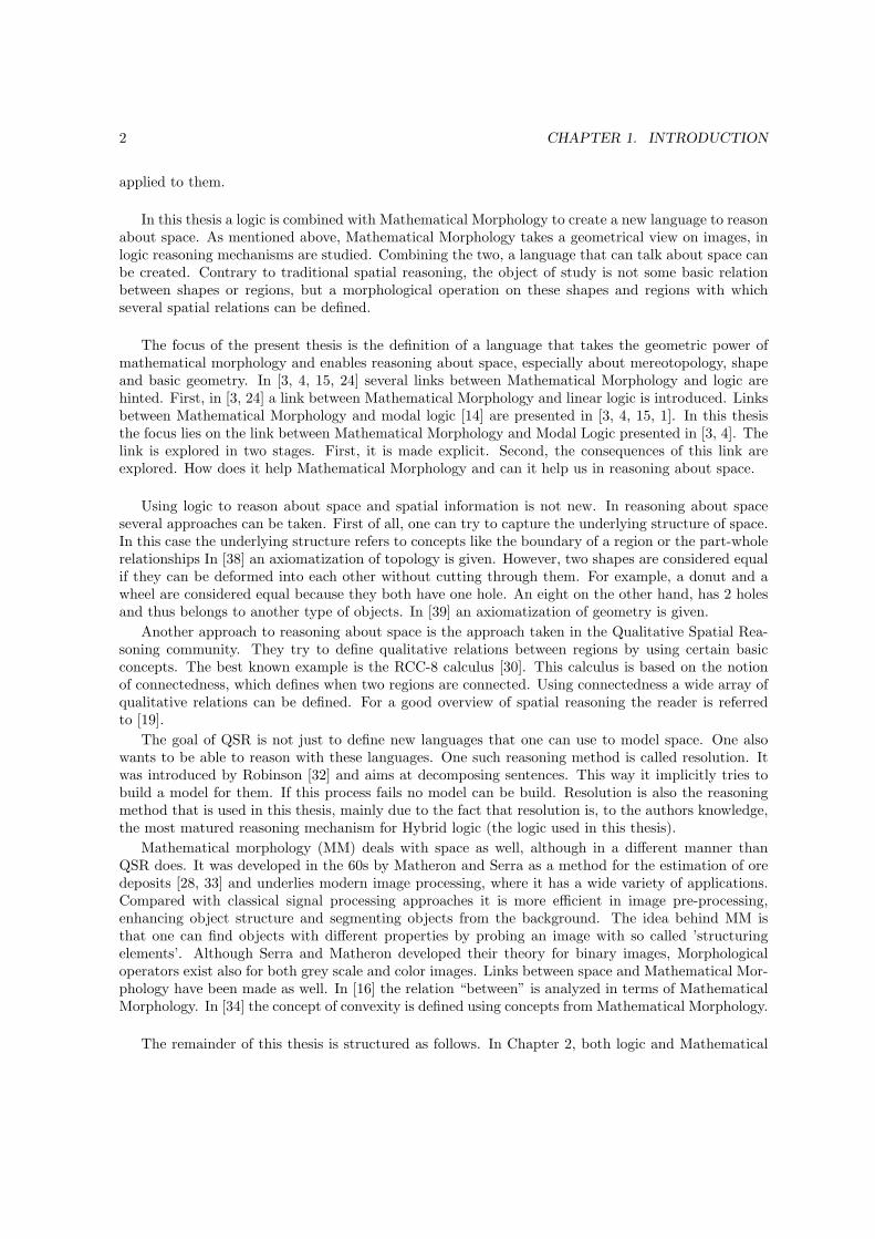
The field of computer vision has the objective of making computers “see”, where by seeing we meanthe interpretation of visual data. Visual data can consist of a camera feed coming from a camera, butalso a collection of figures, a scan of a text or photo or perhaps even a radar image. One of the thingsthat all these forms of data have in common is that they have a spatial component. The objects thatare “visible” in the data have spatial relations to other objects occurring in the data. This spatialdata is very important, also in our everyday life. We use it to navigate through a room, to recognizeobjects and so on.
Apart from having a scientific relevance, computer vision is also applicable in a wide range of non-scientific fields. For instance, in the medical world many new imaging techniques are being developedto help doctors analyze this MRI-data. Techniques like MRI-scanners provide a huge amount of visualdata that either needs to be pre-processed or analyzed in order for the doctors to be able to do theirjobs. In providing good surveillance of public places like airports a large array of cameras is used.Most of the time, the amount of data that is produced by these cameras is too large to be analyzedby a single person. Computers must help in automatically analyzing the images captured by thesesecurity cameras.
Mathematical Morphology is one of the techniques that is used, for instance in computer vision, tosolve the above mentioned problems. Above that, it is still an active field of research. MathematicalMorphology is a geometric language of shape. It views images as collections of regions and makes useof geometrical relations between shapes to analyze and modify images. However, the MathematicalMorphologyprocess works mindlessly. One is not able to use the techniques of Mathematical Mor-phology to reason about the information in the pictures. One can only use it’s techniques to distillinformation from images.
If one wants to reason about information, one normally looks at logic because, traditionally, logicis the field that studies reasoning. Aristotle started formalizing human reasoning using syllogisms like“All humans are mortal, Socrates is human thus Socrates is mortal”. From these early beginningslogic has come very far and these days extends from mathematics to linguistics and beyond. One ofthe subjects logic has found its way into is space. What does logic have to do with space, one mightask. One of the fields that tries to give an answer to this question is the field of Qualitative SpatialReasoning (QSR). QSR is a general way to look at space. Objects, or regions, have certain propertiesand satisfy relations between each other. For example, an object can be a circle, a square or some moreexotic shape. A region can touch another region or it can be separated from this region. Note thatthese relations are qualitative. The actual distance or size of an object does not matter. Often basicspatial relations between shapes or regions are the focus of QSR. It tries to formalize these relationsand characterizations of regions in space. Since an image is a two dimensional space QSR can also be
1
2 CHAPTER 1. INTRODUCTION
applied to them.
In this thesis a logic is combined with Mathematical Morphology to create a new language to reasonabout space. As mentioned above, Mathematical Morphology takes a geometrical view on images, inlogic reasoning mechanisms are studied. Combining the two, a language that can talk about space canbe created. Contrary to traditional spatial reasoning, the object of study is not some basic relationbetween shapes or regions, but a morphological operation on these shapes and regions with whichseveral spatial relations can be defined.
The focus of the present thesis is the definition of a language that takes the geometric power ofmathematical morphology and enables reasoning about space, especially about mereotopology, shapeand basic geometry. In [3, 4, 15, 24] several links between Mathematical Morphology and logic arehinted. First, in [3, 24] a link between Mathematical Morphology and linear logic is introduced. Linksbetween Mathematical Morphology and modal logic [14] are presented in [3, 4, 15, 1]. In this thesisthe focus lies on the link between Mathematical Morphology and Modal Logic presented in [3, 4]. Thelink is explored in two stages. First, it is made explicit. Second, the consequences of this link areexplored. How does it help Mathematical Morphology and can it help us in reasoning about space.
Using logic to reason about space and spatial information is not new. In reasoning about spaceseveral approaches can be taken. First of all, one can try to capture the underlying structure of space.In this case the underlying structure refers to concepts like the boundary of a region or the part-wholerelationships In [38] an axiomatization of topology is given. However, two shapes are considered equalif they can be deformed into each other without cutting through them. For example, a donut and awheel are considered equal because they both have one hole. An eight on the other hand, has 2 holesand thus belongs to another type of objects. In [39] an axiomatization of geometry is given.
Another approach to reasoning about space is the approach taken in the Qualitative Spatial Rea-soning community. They try to define qualitative relations between regions by using certain basicconcepts. The best known example is the RCC-8 calculus [30]. This calculus is based on the notionof connectedness, which defines when two regions are connected. Using connectedness a wide array ofqualitative relations can be defined. For a good overview of spatial reasoning the reader is referredto [19].
The goal of QSR is not just to define new languages that one can use to model space. One alsowants to be able to reason with these languages. One such reasoning method is called resolution. Itwas introduced by Robinson [32] and aims at decomposing sentences. This way it implicitly tries tobuild a model for them. If this process fails no model can be build. Resolution is also the reasoningmethod that is used in this thesis, mainly due to the fact that resolution is, to the authors knowledge,the most matured reasoning mechanism for Hybrid logic (the logic used in this thesis).
Mathematical morphology (MM) deals with space as well, although in a different manner thanQSR does. It was developed in the 60s by Matheron and Serra as a method for the estimation of oredeposits [28, 33] and underlies modern image processing, where it has a wide variety of applications.Compared with classical signal processing approaches it is more efficient in image pre-processing,enhancing object structure and segmenting objects from the background. The idea behind MM isthat one can find objects with different properties by probing an image with so called ’structuringelements’. Although Serra and Matheron developed their theory for binary images, Morphologicaloperators exist also for both grey scale and color images. Links between space and Mathematical Mor-phology have been made as well. In [16] the relation “between” is analyzed in terms of MathematicalMorphology. In [34] the concept of convexity is defined using concepts from Mathematical Morphology.
The remainder of this thesis is structured as follows. In Chapter 2, both logic and Mathematical
3
Morphology are briefly introduced. In Chapter 3, the link between Mathematical Morphology andmodal logic is formalized and proven in the form of a new language, the morpho language. In Chapter4, a resolution calculus is proposed. It facilitates reasoning with the morpho language. The calculusis implemented in an existing theorem prover. Chapter 5 discusses the results of experimenting withthe theorem prover introduced in Chapter 4 and finally in Chapter 6, the expressive power of thenew language is explored, both with respect to Mathematical Morphology and with respect to SpatialReasoning. Chapter 7 holds the conclusions.
Parts of this thesis have been published in [1].

4 CHAPTER 1. INTRODUCTION

Chapter 2
Morphological and logicalPreliminaries
Mathematical Morphology is an image processing tool that is used to extract geometric informationfrom pictures. It’s was conceived in 1965 and has since developed into a mature field of it’s own.
Logic is a field that studies both formal languages as well as human reasoning. It’s origins lie inancient Greece, and it has since developed into a field with a wide array of applications. From naturallanguage understanding to process verification. Several links between Mathematical Morphology andlogic exist, allowing us to create a formal language that can be used to both study MathematicalMorphology and model spatial reasoning.
In Section 1, we introduce Mathematical Morphology by giving a brief overview of it’s history andlooking at both the practical side and the underlying algebraic theory. In Section 2, we introduce thebasic logical concepts that are needed in the following treatment. First we give a brief introductionto logic. Second, we introduce Modal Logic. Finally, in Section 3, we introduce the concepts of framedefinability and completeness.
2.1 Morphological preliminaries
Mathematical Morphology [22, 33, 35] was born in 1965 from the work of J. Serra and G. Materhorn(for a comprehensive overview on the birth of MM see [29]). They were working on methods forthe estimation of ore deposits and found the operations that today from the basis of MathematicalMorphology. From then on, Mathematical Morphology has evolved into a field of it’s own, withapplications mainly in Image Processing. The idea behind MM is that one can find objects withdifferent properties by probing an image with so called ‘structuring elements’. The probing is done bytwo operations, the dilation and the erosion. Although Serra and Materhorn developed their theoryfor binary images, morphological operators exist for both gray scale and color images as well. Forreasons of simplicity, we focus on binary images.
First, we explain in more detail what Mathematical Morphology is and how it is used in computervision. Second, we explain the algebraic theory behind Mathematical Morphology.
2.1.1 Dilation and Erosion
Mathematical Morphology consists of a set of operations on images. All these operations are con-structed by combining two basic operations, the dilation and erosion. Both are used to ‘probe’ theimage using a structuring element. The dilation, defined in Definition 2.1.1, can be used to see whether
5

6 CHAPTER 2. MORPHOLOGICAL AND LOGICAL PRELIMINARIES
an object fits a specific region outside a shape. The erosion, defined in Definition 2.1.2, can be usedto see whether a shape (the structuring element) fits in another shape.
Definition 2.1.1 Dilation: Given an image A and a structuring element B, a dilation ⊕ is definedas follows
A⊕B = {x ∈ R2|Bx ∩A 6= ∅} = {a+ b|a ∈ A, b ∈ B}
where Yx = {x+ y|y ∈ Y } and B = {−b|b ∈ B}.
Definition 2.1.2 Erosion: Given an image A and a structuring element B, an erosion is definedas follows
AB = {x ∈ R2|Bx ∈ A}
One of the main ideas in Mathematical Morphology is to view images as sets. In the binary casefor example, an image is a subset of the R2. This enables us not only to use the dilation and erosion,but also the concepts of union (A ∪B), intersection (A ∩B) and complement (A).
(a) Original figure (b) Dilation (c) Erosion
Figure 2.1: dilation and erosion (with a circular structuring element)
Referring to Figure 2.1, the dilation of an image is equivalent to stamping the structuring elementin each pixel in the image. The erosion is equivalent to finding all the points such that the structuringelement is contained in the shape when placed on the point.
The dilation and erosion have some nice properties. First of all, erosion and dilation are each othersdual. This means that the following equation holds
A⊕B = A B (2.1)
Informally, dilating an image with a structuring element is equivalent to eroding the complement withthe mirrored structuring element (see Figure 2.2). The dilation and erosion are not just two operators,they are linked. Another piece of evidence of this link is the following
A⊕B ⊆ Y ⇔ A ⊆ Y B (2.2)
This equation tells us that if a region A is contained in a region Y after dilation with B, theoriginal region A is contained in the erosion of Y with B. However, there are some differences in theproperties that dilation and erosion posses. For example, it is the case that the dilation distributesover the union, while the erosion distributes over the intersection. This is illustrated by the followingformula’s
2.1. MORPHOLOGICAL PRELIMINARIES 7
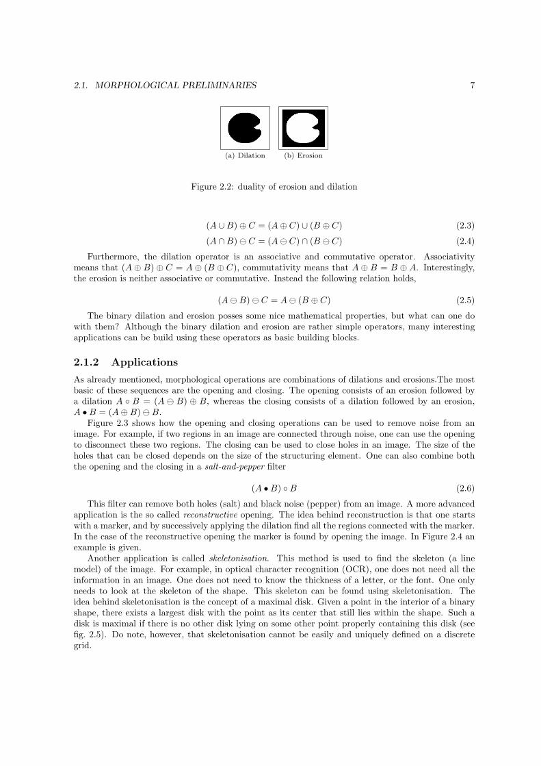
(a) Dilation (b) Erosion
Figure 2.2: duality of erosion and dilation
(A ∪B)⊕ C = (A⊕ C) ∪ (B ⊕ C) (2.3)
(A ∩B) C = (A C) ∩ (B C) (2.4)
Furthermore, the dilation operator is an associative and commutative operator. Associativitymeans that (A ⊕ B) ⊕ C = A ⊕ (B ⊕ C), commutativity means that A ⊕ B = B ⊕ A. Interestingly,the erosion is neither associative or commutative. Instead the following relation holds,
(AB) C = A (B ⊕ C) (2.5)
The binary dilation and erosion posses some nice mathematical properties, but what can one dowith them? Although the binary dilation and erosion are rather simple operators, many interestingapplications can be build using these operators as basic building blocks.
2.1.2 Applications
As already mentioned, morphological operations are combinations of dilations and erosions.The mostbasic of these sequences are the opening and closing. The opening consists of an erosion followed bya dilation A ◦ B = (A B) ⊕ B, whereas the closing consists of a dilation followed by an erosion,A •B = (A⊕B)B.
Figure 2.3 shows how the opening and closing operations can be used to remove noise from animage. For example, if two regions in an image are connected through noise, one can use the openingto disconnect these two regions. The closing can be used to close holes in an image. The size of theholes that can be closed depends on the size of the structuring element. One can also combine boththe opening and the closing in a salt-and-pepper filter
(A •B) ◦B (2.6)
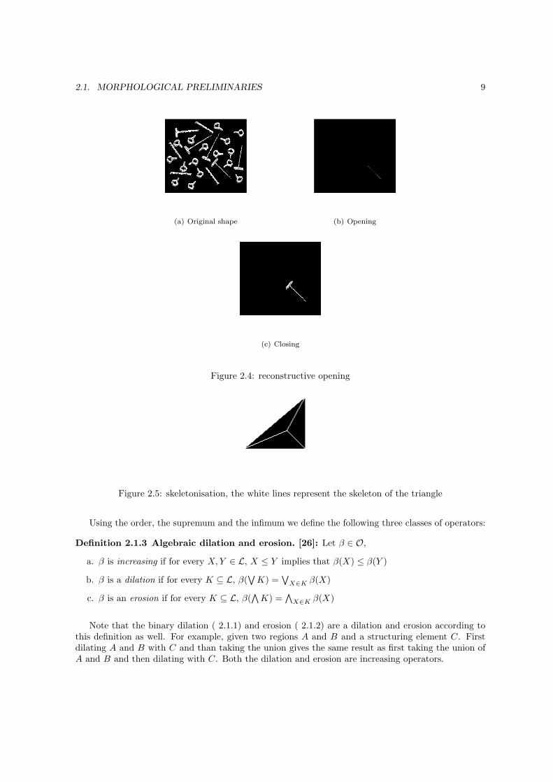
This filter can remove both holes (salt) and black noise (pepper) from an image. A more advancedapplication is the so called reconstructive opening. The idea behind reconstruction is that one startswith a marker, and by successively applying the dilation find all the regions connected with the marker.In the case of the reconstructive opening the marker is found by opening the image. In Figure 2.4 anexample is given.
Another application is called skeletonisation. This method is used to find the skeleton (a linemodel) of the image. For example, in optical character recognition (OCR), one does not need all theinformation in an image. One does not need to know the thickness of a letter, or the font. One onlyneeds to look at the skeleton of the shape. This skeleton can be found using skeletonisation. Theidea behind skeletonisation is the concept of a maximal disk. Given a point in the interior of a binaryshape, there exists a largest disk with the point as its center that still lies within the shape. Such adisk is maximal if there is no other disk lying on some other point properly containing this disk (seefig. 2.5). Do note, however, that skeletonisation cannot be easily and uniquely defined on a discretegrid.

8 CHAPTER 2. MORPHOLOGICAL AND LOGICAL PRELIMINARIES
(a) Original shape (b) Opening
(c) Closing
Figure 2.3: Dilation and erosion
Finally we briefly introduce the operator that started everything, the hit-or-miss transform. Thehit-or-miss transform is a filter that passes shapes with certain properties, but blocks shapes withother properties. For example, using this filter it is possible to get all the points in an image that lieon a left edge. A nice example is seen in Figure 2.6. For a more thorough introduction see chapter 6.
2.1.3 Algebraic theory
Mathematical Morphology is not only about binary images, this binary interpretation is part of amuch more generic theory which is called the algebraic basis of Mathematical Morphology [26]. Thealgebraic theory brings to the surface the link between Mathematical Morphology and modal logic.
In introducing the algebraic theory of Mathematical Morphology we follow [26]. In the following it isassumed that the concepts of a partial order, group and complete lattice are known. In appendix A.0.6more information can be found.
The first thing we can observe is that there is some kind of order in the structure containing thesubsets of R2. On can say that a set A is a subset of another set B, and this subset relation definesan order on the set of subsets of R2. It is what one calls a partial order. For example, look at theset A = {a, b, c}. This is a set containing three elements. Both {a} and {a, b} are subsets of A and{a} ⊆ {a, b}. We can thus say that {a} is smaller than {a, b}. Furthermore, taking the set-operatorsunion and intersection, where the former is the supremum and the latter is the infimum, (P(R2),⊆)is a complete lattice.
It turns out that the dilation and erosion operators are part of a larger theory on complete lattices.In the following, consider a complete lattice L with the order relation ≤, supremum and infimum, leastelement O and greatest element I. Elements of L will be denoted by X,Y, Z. The set O is the set oftransformations on L. A transformation β ∈ O is a function β : L → L. An element from O will becalled an operator.
2.1. MORPHOLOGICAL PRELIMINARIES 9
(a) Original shape (b) Opening
(c) Closing
Figure 2.4: reconstructive opening
Figure 2.5: skeletonisation, the white lines represent the skeleton of the triangle
Using the order, the supremum and the infimum we define the following three classes of operators:
Definition 2.1.3 Algebraic dilation and erosion. [26]: Let β ∈ O,
a. β is increasing if for every X,Y ∈ L, X ≤ Y implies that β(X) ≤ β(Y )
b. β is a dilation if for every K ⊆ L, β(∨K) =
∨X∈K β(X)
c. β is an erosion if for every K ⊆ L, β(∧K) =
∧X∈K β(X)
Note that the binary dilation ( 2.1.1) and erosion ( 2.1.2) are a dilation and erosion according tothis definition as well. For example, given two regions A and B and a structuring element C. Firstdilating A and B with C and than taking the union gives the same result as first taking the union ofA and B and then dilating with C. Both the dilation and erosion are increasing operators.

10 CHAPTER 2. MORPHOLOGICAL AND LOGICAL PRELIMINARIES
(a) Original shape (b) right side of the triangle
(c) mask
Figure 2.6: hit-or-miss
We have already seen that the dilation and erosion are related. Outside the fact that they are eachothers dual, they satisfy equation 2.2. The term adjunction, defined below, is a generalization of thisconcept.
Definition 2.1.4 Let δ, ε ∈ O. Then we say that (ε, δ) is an adjunction if for every X,Y ∈ L, wehave that
δ(X) ≤ Y ⇔ X ≤ ε(Y )
ε is called the upper adjoint and δ the lower adjoint.
Looking closely at Equation 2.2, one can see that the binary dilation and erosion together form anadjunction in which ⊕ is the lower adjoint and is the upper adjoint.
The following proposition tells us that there is a very strong link between the notions of algebraicdilation and algebraic erosion and the notion of an adjunct.
Proposition 2.1.5 Let δ, ε ∈ O. If (ε, δ) is an adjunction, then δ is a dilation and ε and erosion
The proof can be found in [26]. Another aspect of the binary dilation and erosion as defined in(2.1.1) and (2.1.2) is that they are translation invariant. By this we mean that first translating an imageand then applying the dilation/erosion yields the same result as first applying the dilation/erosion andthen translating the result. This property, the translation invariance, can also be generalized to thegeneral framework presented here.
In the case of binary MM, a translation maps subsets of R2 to subsets of R2. It does that in sucha way that it preserves the subset-relation. Hence, it is an automorphism. We write Aut(L) for theset of automorphism of L. Given an automorphism τ ∈ Aut(L) and an operator o ∈ O we say that ois τ -invariant if oτ = τo. Given a subset T of Aut(L), we say that o is T -invariant if o is τ -invariantfor every τ ∈ T .

2.1. MORPHOLOGICAL PRELIMINARIES 11
It turns out that Aut(L), together with composition is a group. By definition every isomorphismhas a reverse. And in the case of automorphism, this reverse is an automorphism itself. Furthermore,given any Q ⊆ O, the automorphisms of L that commute with every element of Q form a subgroup ofAut(L). Thus, every T-invariant set of operators for some T ⊆ Aut(L) is a group.
Given a group of automorphisms T , an adjunction (ε, δ) is called a T -adjunction if δ is a T -dilationand ε is a T -erosion. In the case of Euclidean space (E), translation invariant dilations and erosionscan be constructed from translations. First, we fix the origin o. Second, every point x defines a uniquetranslation τx defined by τx(o) = x. For X ⊂ E , τx(X) = Xx. For every A,B ∈ E definitions 2.1.1and 2.1.2 give us that
X ⊕ Y =⋃
y∈Y
τy(X) and X Y =⋂
y∈Y
τ−1y (X)
Using the notation from the complete lattice theory, the dilation δA : X → X ⊕A and the erosionεA : X → X A have the following decomposition in terms of translations:
δA =∨a∈A
τa and εA =∧a∈A
τ−1a
We can generalize this result to an arbitrary complete lattice L. However, it does not work forarbitrary operators. Hence, we must define the set of operators for which this result is possible. To dothis, first look at the properties of Euclidean spaces. The important concepts above are the translationsand the singletons that define these translations. Considering the singletons, in Euclidean spaces weknow that all the subsets can be build from singletons (the points in space) using the union operation.This property can be generalized to a general complete lattice in the following manner.
Definition 2.1.6 Sup-generating subset Given a complete lattice (L,≤), a sup-generating subsetl is a subset of L s.t. every element of L can be written as a supremum of elements of l.
In the case of Euclidean spaces, l is the set of singletons (i.e. l = R2) and the supremum is theunion. Looking at the translations on the Euclidean space, we see that the group of translations iscommutative and transitive on the set of singletons. Furthermore, a translation of a singleton setalways gives us another singleton set. These properties combined give us that we can define a uniquetranslation τx by τx(o) = x.
Generalizing to arbitrary complete lattices, this gives us the following basic assumption, consideringa complete lattice L and a commutative group T of automorphisms of L,
Basic Assumption 1 L has a sup generating subset l s.t.
• T leaves l invariant, in other words for every τ ∈ T and x ∈ l, τ(x) ∈ l
• T is transitive on l, in other words for every x, y ∈ l, there exists τ ∈ T such that τ(x) = y.
From the basic assumption we can conclude that for every x, y ∈ l, there is a unique τ ∈ T s.t.τ(x) = y. This follows from the following facts. Suppose that τ1(x) = τ2(x) = y. Then τ−1
1 τ2(x) = x.Because of the basic assumption we know that for any z ∈ l, there is some τ3 ∈ T s.t. τ3(x) = z. Soτ−11 τ2(z) = (τ−1
1 τ2)τ3(x) = τ3(τ−11 τ2)(x) = τ3(x) = z. We now know that for all z ∈ l, τ−1
1 τ2(z) = z.Thus ∀z ∈ l we have that τ2(z) = τ1(z), hence τ1 = τ2.
Using the fact that for every x, u ∈ l there is a unique τ ∈ T such that τ(x) = y we can defineseveral operators on l.

12 CHAPTER 2. MORPHOLOGICAL AND LOGICAL PRELIMINARIES
Definition 2.1.7 Fix some o ∈ l. Next, for every x ∈ l define τx as the unique element of T s.t.τx(o) = x. Using this bijection between l and T we can define the binary addition on l by
x+ y = τxτy(o) = τx(y) = τy(x)
Furthermore, we define −y by τ−1y . Thus
x− y = x+ (−y) = τxτ−1y (o) = τ−1
y (x)
For X ∈ L we define τy(X) = Xy = {τy(x)|x ∈ X}
The structure (l,+,−, o) constitutes a group. If we apply this to the Euclidean space, we can takethe set of singletons as l and T naturally becomes the set of all translations on the set E of points.
Using the group created by the operators from Definition 2.1.7 we can define the following binaryoperators
Definition 2.1.8 Given a complete lattice L, a sup-generating subset l and X,Y ⊆ L
• X⊕Y =∨
y∈l(Y )Xy
• XY =∧
u∈l(Y )X−y
with l : L → l s.t. l(X) = {x ∈ l|x ≤ X}
Proposition 3.5 in [26] tells us the following:
Proposition 2.1.9 For X,Y ∈ L and x, y ∈ l we have,
• X⊕Y = Y ⊕X =∨{x+ y|x ∈ l(X), y ∈ l(Y )}
• XY =∨{z ∈ l|Yz ≤ X}
We now define the operators δA and εA by
δA =∨
a∈l(A)
τa and εA =∧
a∈l(A)
τa (2.7)
moreover, we have that
δA(X) = X⊕A and εA(X) = XA (2.8)
To end this section, let us look at the following theorem (Theorem 3.6 in [26]).
Theorem 2.1.10 For any A ∈ L, (εA, δA) is a T -adjunction on L. Moreover, any T - adjunction hasthis form.
Using Theorem 2.1.10 and 2.1.5 we state that for each subset A of a complete lattice L, we canfind a dilation δ and an erosion ε such that δ(X) = X⊕A and ε(X) = XA. This tells us that everytranslation invariant operator can be written as a union of translations. The fact that operators canbe written in this form lies at the heart of the link between Mathematical Morphology and logic.

2.2. LOGICAL PRELIMINARIES 13
2.2 Logical preliminaries
In the following we give a brief introduction to logic. We introduce both propositional and modal logicand the notation that will be used in the rest of this treatment. The most well know logic is first orderlogic. This logic is not treated in the present section but for more information we refer to [42, 14].
Historically, logic has been the study of reasoning. It was designed to formalize the reasoningprocesses of the human mind. To formalize these processes, one needs a formal language. Such aformal language is exactly what the link between Mathematical Morphology and logic consists of. Butbefore we reach that language, we start with a more intuitive language to explain the basic conceptsneeded in the rest of this treatment.
2.2.1 Propositional logic
Propositional logic is a simple language that is meant to formalize the reasoning with propositions.Propositions can be statements about the world, for instance,
• today was a rainy day
• Bart is a boy
• I have an umbrella
These propositions can be either true or false. However, reasoning with propositions is morethan just stating the truth of a proposition. One can also combine several propositions into morecomplicated statements like
• today was a rainy day and I have an umbrella
• If I have an umbrella, then I do not get wet
• Bart is a boy or Bart is a girl
In formalizing propositions, a proposition is usually denoted with p, q or r to generalize fromspecific propositions. We say that prop is the set of all propositions. For creating more complicatedstatements involving several propositions, we have the following notation
• and: ∧
• or: ∨
• if,then: →
• not: ¬
• if and only if: ↔
Furthermore, we have the symbols ⊥ and > that denote false and true respectively. These symbolsare from here on called connectives and we can use them to combine propositions.
In fact, we can do the same with less symbols. For example, the ∧ can also be written using only∨ and ¬. Then p ∧ q is equal to ¬(¬p ∨ ¬q). We therefore arrive at the following
Definition 2.2.1 Sentence: We call a formula ϕ a sentence if it adheres to the following
ϕ := p|⊥|¬ϕ|ϕ ∨ ψ with p ∈ prop, with ψ a sentence.

14 CHAPTER 2. MORPHOLOGICAL AND LOGICAL PRELIMINARIES
As for the other connectives, they can be written as follows. ϕ ∧ ψ = ¬(¬ϕ ∧ ¬ψ), ϕ→ ψ = ¬ϕ ∨ ψ,ϕ↔ ψ = (ϕ→ ψ) ∧ (ψ → ϕ) and > = ¬⊥.
Some examples of sentences are
• p ∧ q
• (p ∨ q) → r
• (p→ q) ↔ (q → p)
We have defined the language of propositional logic, but still need to define its semantics. Weneed to define what the connectives mean. In the propositional language, one can discern two parts.First, we have the propositions and second the connectives that are used to combine propositions intomore complex propositions. In defining the semantics again a division is made between defining thesemantics of the propositions and the semantics of the connectives.
First consider the propositions. A proposition can be either true or false. Which propositions aretrue and which are false is captured in the notion of a model.
Definition 2.2.2 Model: In propositional logic a model M consists of a valuation VM. A valuationis a function V : prop 7→ {true, false} that assigns to every proposition p a truth value. To say thata formula (sentence) ϕ is true in a model M we use the following notation
M |= ϕ
If a formula is true in every model, it is called a tautology. Furthermore, V(⊥) = False and M 2 ϕmeans that ϕ is not true in M.
Using this notion of a model we define the propositional semantics.
Definition 2.2.3 Propositional semantics: Given a model M
• M |= p with p ∈ prop iff1 V(p) = true
• M 2 ⊥
• M |= ¬ϕ iff M 2 ϕ
• M |= ϕ ∨ ψ iff M |= ϕ or M |= ψ
To end this section, we provide some examples of propositional sentences. For example, the sentencep∨¬p is a simple example of a tautology. It tells us that either p is true or not true, which obviouslyalways is the case. A more elaborate tautology is for example (p → (q → p)). It says that p impliesthat q implies p. At first sight it is not very clear that this formula is true regardless of the valuationused. However, we can rewrite the → to a ∨, we get the formula ¬p ∨ (¬q ∨ p), which we again canrewrite to (p ∧ q) → p. This formula has hidden inside it the formula p → p, which again is anotherway of writing p ∨ ¬p and this is also a tautology.
Next, suppose that we have the following proposition
• When it rains the road is wet
This proposition contains the propositions ”it rains” and ”the road is wet”. Denote the formerwith p and the later with q. The propositional logic formula that captures the above proposition is
p→ q
Then, given the fact that p is true, i.e. it rains, one can deduce that the road must be wet. This isa very simple example of how propositional logic can be used to model the real world using simplepropositions.
1We use iff to stand for if and only if.

2.2. LOGICAL PRELIMINARIES 15
2.2.2 Modal logic
In propositional logic one can talk about propositions, but that is where it ends. A model consist of aset of propositional variables and their truth assignments. There is no further structure in the model.Modal logic is a family of logics that enables more structure in a model. This structure is present inthe form of relations between the elements of a modal model. Hence, one can say that modal logic isthe logic of relations.
We first look at the basic modal language. The language of the basic modal logic is an extensionof the propositional language defined in Section 2.2.1.
Definition 2.2.4 Basic language: A formula ϕ is a sentence if
ϕ := p|⊥|¬ϕ|ϕ ∨ ϕ|3ϕ| with p ∈ prop
The symbols ∧,→ and ↔ have the same definitions. Furthermore, we define the symbol 2 = ¬3¬.The difference between this definition and Definition 2.2.1 are the symbols 3 and 2. The 3 and 2
are called modalities and are used to probe the structure of a model, which is captured by a frame.The way in which truth for propositional letters is defined is very different from the way used inpropositional logic. Where in the latter a propositional letter is either true or false, in modal logic apropositional letter can be true in several worlds. Thus, it’s truth value is denoted by a set of worldsin which it is true, rather then just true or false. This results in the following definition of a model.
Definition 2.2.5 Frames and models: A frame for the basic modal language F is a pair (W,R).W is a non-empty set of worlds, R is a binary relation s.t. R ⊆ P(W ×W ). A model M is a pair(F ,V) in which F is a frame and V : prop 7→ P(W ) a function. If M = (F ,V) for some valuation Vwe say that M is based on F . A model is thus a frame enriched with a valuation.
The notation M, w ϕ denotes the fact that the formula ϕ is true in the model M on world w.M, w 1 ϕ says that ϕ is false on the world w in M. Where w is an element of W .
Note that the notation introduced above is different from the notation introduced in Defini-tion 2.2.2. This is because we want to distinguish between truth in propositional logic and modallogic.
Example 2.2.6 A simple frame is
•1
~~||||
||||
•2 // •3
``BBBBBBBB
W = {1, 2, 3}, R = {(1, 2), (2, 3), (3, 1)}
If we for example take the valuation V(p) = {1, 2} and V(q) = {2, 3} we get the following model
Example 2.2.7
•{p}1
}}zzzz
zzzz
•{p,q}2
// •{q}3
aaBBBBBBBB

16 CHAPTER 2. MORPHOLOGICAL AND LOGICAL PRELIMINARIES
Just as in Definition 2.2.3 we use the notion of a model to define the semantics of the connectivesand modalities.
Definition 2.2.8 Semantics: Given a model M = (W,R,V) and a w ∈W we say that
• M, w p with p ∈ prop iff w ∈ V(p)
• M, w ¬ϕ iff M, w 1 ϕ
• M, w ϕ ∨ ψ iff M, w ϕ or M, w ψ
• M, w 3ϕ iff there exists a v ∈W s.t. (w, v) ∈ R and M, v ϕ
The meaning of the normal connectives is straightforward. The meaning of the modalities howeverdeserves some more explanation. The definition states that a formula 3ϕ is true in a model M on aworld w if there is a world v s.t. (w, v) ∈ R and ϕ is true on v. So 3ϕ is true on a world w if there isa world v that has a relation with w, and v makes ϕ true. In the same way, 2 will get the followingmeaning.
M, w 2ϕ iff for all v ∈W s.t. (w, v) ∈ R implies M, v ϕ
In other words. 2ϕ is true in a world w if and only if ϕ is true in every world v reachable from w.
Example 2.2.9 The formula 3p is true in the following model on world 1
•{p}2
•1
==||||||||
""EEEE
EEEE
•3
with W = {1, 2, 3}, R = {(1, 2), (1, 3)} and V(p) = {2}.
However, the formula 2p is not true on world 1 in the model from Example 2.2.9 because there is aworld accessible from 1 where p is not true. Note that 2p is true on the worlds 2 and 3 because theydo not have any successors.
Definition 2.2.10 Satisfiability and validity: A formula ϕ is satisfiable in a model M if there isa world w ∈W s.t. M, w ϕ. A formula ϕ is valid on a model M if for every world w ∈W it is thecase that M, w ϕ. We say that ϕ is valid on a frame F , denoted by F ϕ if it is valid on everymodel M based on F . A formula is valid with respect to a family of frames if it is valid on everyframe in the family. The same goes for families of models.
Using the notion of validity on a frame, we can create restrictions on the types of frames we wantto consider. For example, the formula p→ 3p is only valid on a frame, if the frame is reflexive. Thismeans that, given a frame F , for all w ∈ W we have that (w,w) ∈ R. One can see that this is thecase through the following reasoning. Suppose that a frame F is not reflexive and p → 3p is valid.This means that there is a world w ∈ W such that (w,w) /∈ R. Now take the valuation V such thatV(p) = {w}. This means that w is the only world that satisfies p. Hence, for the model M = (F ,V)
2.2. LOGICAL PRELIMINARIES 17
we have that M, w 2 p → 3p because p is true in w, but since w is the only world that satisfies p,and w cannot reach itself, 3p is false.
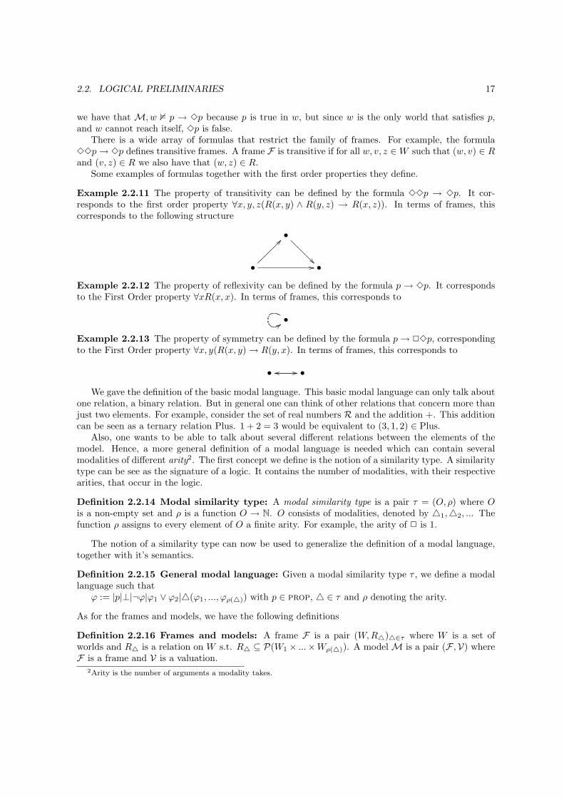
There is a wide array of formulas that restrict the family of frames. For example, the formula33p→ 3p defines transitive frames. A frame F is transitive if for all w, v, z ∈W such that (w, v) ∈ Rand (v, z) ∈ R we also have that (w, z) ∈ R.
Some examples of formulas together with the first order properties they define.
Example 2.2.11 The property of transitivity can be defined by the formula 33p → 3p. It cor-responds to the first order property ∀x, y, z(R(x, y) ∧ R(y, z) → R(x, z)). In terms of frames, thiscorresponds to the following structure
•
��@@@
@@@@
•
??������� // •
Example 2.2.12 The property of reflexivity can be defined by the formula p → 3p. It correspondsto the First Order property ∀xR(x, x). In terms of frames, this corresponds to
•::
Example 2.2.13 The property of symmetry can be defined by the formula p→ 23p, correspondingto the First Order property ∀x, y(R(x, y) → R(y, x). In terms of frames, this corresponds to
• // •oo
We gave the definition of the basic modal language. This basic modal language can only talk aboutone relation, a binary relation. But in general one can think of other relations that concern more thanjust two elements. For example, consider the set of real numbers R and the addition +. This additioncan be seen as a ternary relation Plus. 1 + 2 = 3 would be equivalent to (3, 1, 2) ∈ Plus.
Also, one wants to be able to talk about several different relations between the elements of themodel. Hence, a more general definition of a modal language is needed which can contain severalmodalities of different arity2. The first concept we define is the notion of a similarity type. A similaritytype can be see as the signature of a logic. It contains the number of modalities, with their respectivearities, that occur in the logic.
Definition 2.2.14 Modal similarity type: A modal similarity type is a pair τ = (O, ρ) where Ois a non-empty set and ρ is a function O → N. O consists of modalities, denoted by 41,42, ... Thefunction ρ assigns to every element of O a finite arity. For example, the arity of 2 is 1.
The notion of a similarity type can now be used to generalize the definition of a modal language,together with it’s semantics.
Definition 2.2.15 General modal language: Given a modal similarity type τ , we define a modallanguage such that
ϕ := |p|⊥|¬ϕ|ϕ1 ∨ ϕ2|4(ϕ1, ..., ϕρ(4)) with p ∈ prop, 4 ∈ τ and ρ denoting the arity.
As for the frames and models, we have the following definitions
Definition 2.2.16 Frames and models: A frame F is a pair (W,R4)4∈τ where W is a set ofworlds and R4 is a relation on W s.t. R4 ⊆ P(W1 × ...×Wρ(4)). A model M is a pair (F ,V) whereF is a frame and V is a valuation.
2Arity is the number of arguments a modality takes.

18 CHAPTER 2. MORPHOLOGICAL AND LOGICAL PRELIMINARIES
The semantics for the connectives and ⊥ does not change, and the dual of 4 is defined as Oϕ :=¬4¬ϕ. Only the semantics for the modalities remains to be given.
Definition 2.2.17 General modal semantics: Given a model M = (W,R,V) and a world w ∈W
M, w 4(ϕ1, ..., ϕn) iff ∃v1, ..., vn ∈W with (w, v1, ..., vn) ∈ R4 such that ∀i,M, vi ϕi
Using this definition we are able to define logics for more complex structures, like for examplegroups that contain several relations between the elements of the model.
2.3 Frame definability and Completeness
We can define families of frames by modal formulas. In this section we formalise this notion. Further-more, we look at the set of formulas that is true in a set of models and at the mechanisms that allowsone to automatically find all these formulas.
2.3.1 Frame definability
We have already seen that the formula 33p → 3p defines the class of transitive frames and thatp → 3p defines the class of reflexive frames. Both these properties are first order properties. Thatmeans that we can express them in First Order Logic.
Example 2.3.1 For example, the formulas defining reflexivity, transitivity and symmetry all haveFirst Order counterparts which are expressed in Table 2.1.
Modal Logic First Order Logic33p→ 3p ∀x, y, z(R(x, y) ∧R(y, z) → R(x, z))3p→ p ∀xR(x, x)p→ 23p ∀x, yR(x, y) → R(y, x)
Table 2.1: some modal formulas and their First Order counterparts.
To make the notion of frame definability more formal, we introduce the following definition.
Definition 2.3.2 Frame definability: Given a similarity type τ , ϕ a formula of this type and C aclass of τ -frames, we say that ϕ defines C if for all frames F , F is in C if and only if F ϕ. Given aset of τ -formulas Γ, we say that Γ defines C if a frame F is in C if and only if F Γ.
A class of frames is modaly definable if there exists a formula or set of formulas that define thisclass.
2.3.2 Completeness
We have already seen that we can define a class of frames S by using formulas. One can ask oneself thequestion what the set of formulas ΛS is that is valid on this class of frames. Perhaps more interestingly,is there a mechanism to find this Λ?
The answer to this question comes in the form of the notion of a normal modal logic. A normalmodal logic is a set of formulas that satisfies the following properties.
2.3. FRAME DEFINABILITY AND COMPLETENESS 19
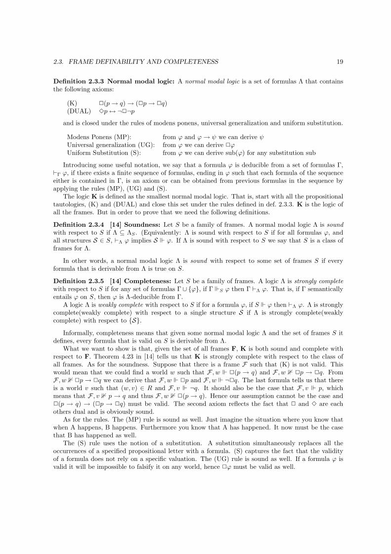
Definition 2.3.3 Normal modal logic: A normal modal logic is a set of formulas Λ that containsthe following axioms:
(K) 2(p→ q) → (2p→ 2q)(DUAL) 3p↔ ¬2¬p
and is closed under the rules of modens ponens, universal generalization and uniform substitution.
Modens Ponens (MP): from ϕ and ϕ→ ψ we can derive ψUniversal generalization (UG): from ϕ we can derive 2ϕUniform Substitution (S): from ϕ we can derive sub(ϕ) for any substitution sub
Introducing some useful notation, we say that a formula ϕ is deducible from a set of formulas Γ,`Γ ϕ, if there exists a finite sequence of formulas, ending in ϕ such that each formula of the sequenceeither is contained in Γ, is an axiom or can be obtained from previous formulas in the sequence byapplying the rules (MP), (UG) and (S).
The logic K is defined as the smallest normal modal logic. That is, start with all the propositionaltautologies, (K) and (DUAL) and close this set under the rules defined in def. 2.3.3. K is the logic ofall the frames. But in order to prove that we need the following definitions.
Definition 2.3.4 [14] Soundness: Let S be a family of frames. A normal modal logic Λ is soundwith respect to S if Λ ⊆ ΛS . (Equivalently: Λ is sound with respect to S if for all formulas ϕ, andall structures S ∈ S, `Λ ϕ implies S ϕ. If Λ is sound with respect to S we say that S is a class offrames for Λ.
In other words, a normal modal logic Λ is sound with respect to some set of frames S if everyformula that is derivable from Λ is true on S.
Definition 2.3.5 [14] Completeness: Let S be a family of frames. A logic Λ is strongly completewith respect to S if for any set of formulas Γ∪ {ϕ}, if Γ S ϕ then Γ `Λ ϕ. That is, if Γ semanticallyentails ϕ on S, then ϕ is Λ-deducible from Γ.
A logic Λ is weakly complete with respect to S if for a formula ϕ, if S ϕ then `Λ ϕ. Λ is stronglycomplete(weakly complete) with respect to a single structure S if Λ is strongly complete(weaklycomplete) with respect to {S}.
Informally, completeness means that given some normal modal logic Λ and the set of frames S itdefines, every formula that is valid on S is derivable from Λ.
What we want to show is that, given the set of all frames F, K is both sound and complete withrespect to F. Theorem 4.23 in [14] tells us that K is strongly complete with respect to the class ofall frames. As for the soundness. Suppose that there is a frame F such that (K) is not valid. Thiswould mean that we could find a world w such that F , w 2(p → q) and F , w 1 2p → 2q. FromF , w 1 2p→ 2q we can derive that F , w 2p and F , w ¬2q. The last formula tells us that thereis a world v such that (w, v) ∈ R and F , v ¬q. It should also be the case that F , v p, whichmeans that F , v 1 p → q and thus F , w 1 2(p → q). Hence our assumption cannot be the case and2(p → q) → (2p → 2q) must be valid. The second axiom reflects the fact that 2 and 3 are eachothers dual and is obviously sound.
As for the rules. The (MP) rule is sound as well. Just imagine the situation where you know thatwhen A happens, B happens. Furthermore you know that A has happened. It now must be the casethat B has happened as well.
The (S) rule uses the notion of a substitution. A substitution simultaneously replaces all theoccurrences of a specified propositional letter with a formula. (S) captures the fact that the validityof a formula does not rely on a specific valuation. The (UG) rule is sound as well. If a formula ϕ isvalid it will be impossible to falsify it on any world, hence 2ϕ must be valid as well.
20 CHAPTER 2. MORPHOLOGICAL AND LOGICAL PRELIMINARIES
2.4 Summary
Mathematical morphology is a formalism that is widely used in image processing. It consists of 2basic operators, the dilation and the erosion. Using these operations many image operators can bedefined. Furthermore, Mathematical Morphology has a solid algebraic base. The dilation and erosioncan be defined in terms of operators on a complete lattice. Hence, the framework of mathematicalmorphology can be lifted to an arbitrary complete lattice.
Modal logic can be seen as the logic of relations. Modal formulas can isolate families of framesthat contain the same property. After isolating the set of frames, one can ask oneself what the set offormulas is that is valid on this set of frames. Furthermore, one can ask oneself how one can createthis set of frames.
In the chapters to come we investigate the connection between Mathematical Morphology andmodal logic and show how these two fields can be combined into a theory of qualitative spatial rea-soning.
Chapter 3
The Morpho-Language
At first sight there are several connections between Mathematical Morphology and logic. First, thedilation and erosion are adjuncts of each other. In logic the concept of adjunction is know under thename residuation. Linear logic is a logic that captures such residuals. Second, is the link betweenMathematical Morphology and modal logic, arrow logic in particular (for a comprehensive overviewof arrow logic see [43]). Arrow logic is a modal logic where the definitions of the modalities resemblethe way in which translation invariant operators can be written. [3, 24] Finally, Isabelle Bloch finds alink between mathematical morphology and modal logic by taking the neighborhood relation as theframe relation [15, 2].
The focus of the this treatment lies on the link between Mathematical Morphology and arrowlogic. To this end we introduce a new modal language, the morpho-language based on a modal logiccontaining a binary modality.
The remainder of this chapter has the following form. In Section 1, the intuitive connectionbetween Mathematical Morphology and modal (arrow) logic is specified. In Section 2, the languageand semantics of the morpho-language are introduced, an axiomatization for the logic is given and it isshown that it is complete. Finally, in Section 3, hybrid logic is introduced and an hybrid axiomatizationof the morpho-language is given.
3.1 Mathematical Morphology and Logic
Arrow logic is a modal logic that consist of 3 modalities. A nullary, a unary and a binary modality.Together, they constitute the following language:
Definition 3.1.1 Arrow logic: The language of arrow logic consists of the following
ϕ := p|e|¬ϕ|ϕ ∨ ψ| ⊗ ϕ|ϕ⊕ψ
Where p ∈ prop.
The other connectives are defined using the usual shorthands. As for the duals, define ⊗ϕ = ¬⊗¬ϕand ϕ⊕ψ = ¬(¬ϕ⊕¬ψ). Although arrow logic was created to be the basic modal logic of arrows, wedo not go into the details of the arrow semantics. We only use the semantics that have been definedin [43] to point at the similarity with the definition of translation invariant dilation.
Definition 3.1.2 A frame for arrow logic consists of three relations (I,R,C), thus a model is a tupleof the form M = (W, I,R,C,V).
21
22 CHAPTER 3. THE MORPHO-LANGUAGE
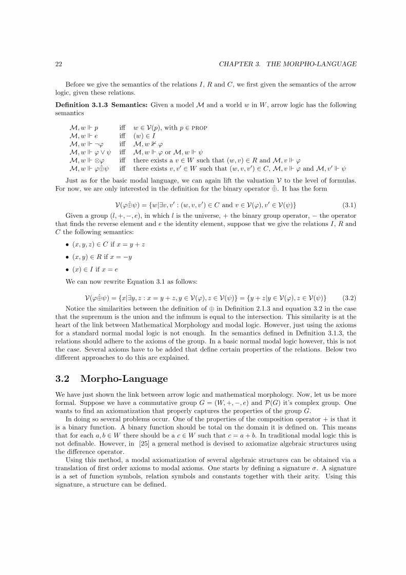
Before we give the semantics of the relations I, R and C, we first given the semantics of the arrowlogic, given these relations.
Definition 3.1.3 Semantics: Given a model M and a world w in W , arrow logic has the followingsemantics
M, w p iff w ∈ V(p), with p ∈ propM, w e iff (w) ∈ IM, w ¬ϕ iff M, w 1 ϕM, w ϕ ∨ ψ iff M, w ϕ or M, w ψM, w ⊗ϕ iff there exists a v ∈W such that (w, v) ∈ R and M, v ϕM, w ϕ⊕ψ iff there exists v, v′ ∈W such that (w, v, v′) ∈ C, M, v ϕ and M, v′ ψ
Just as for the basic modal language, we can again lift the valuation V to the level of formulas.For now, we are only interested in the definition for the binary operator ⊕. It has the form
V(ϕ⊕ψ) = {w|∃v, v′ : (w, v, v′) ∈ C and v ∈ V(ϕ), v′ ∈ V(ψ)} (3.1)
Given a group (l,+,−, e), in which l is the universe, + the binary group operator, − the operatorthat finds the reverse element and e the identity element, suppose that we give the relations I, R andC the following semantics:
• (x, y, z) ∈ C if x = y + z
• (x, y) ∈ R if x = −y
• (x) ∈ I if x = e
We can now rewrite Equation 3.1 as follows:
V(ϕ⊕ψ) = {x|∃y, z : x = y + z, y ∈ V(ϕ), z ∈ V(ψ)} = {y + z|y ∈ V(ϕ), z ∈ V(ψ)} (3.2)
Notice the similarities between the definition of ⊕ in Definition 2.1.3 and equation 3.2 in the casethat the supremum is the union and the infimum is equal to the intersection. This similarity is at theheart of the link between Mathematical Morphology and modal logic. However, just using the axiomsfor a standard normal modal logic is not enough. In the semantics defined in Definition 3.1.3, therelations should adhere to the axioms of the group. In a basic normal modal logic however, this is notthe case. Several axioms have to be added that define certain properties of the relations. Below twodifferent approaches to do this are explained.
3.2 Morpho-Language
We have just shown the link between arrow logic and mathematical morphology. Now, let us be moreformal. Suppose we have a commutative group G = (W,+,−, e) and P(G) it’s complex group. Onewants to find an axiomatization that properly captures the properties of the group G.
In doing so several problems occur. One of the properties of the composition operator + is that itis a binary function. A binary function should be total on the domain it is defined on. This meansthat for each a, b ∈W there should be a c ∈W such that c = a+ b. In traditional modal logic this isnot definable. However, in [25] a general method is devised to axiomatize algebraic structures usingthe difference operator.
Using this method, a modal axiomatization of several algebraic structures can be obtained via atranslation of first order axioms to modal axioms. One starts by defining a signature σ. A signatureis a set of function symbols, relation symbols and constants together with their arity. Using thissignature, a structure can be defined.
3.2. MORPHO-LANGUAGE 23
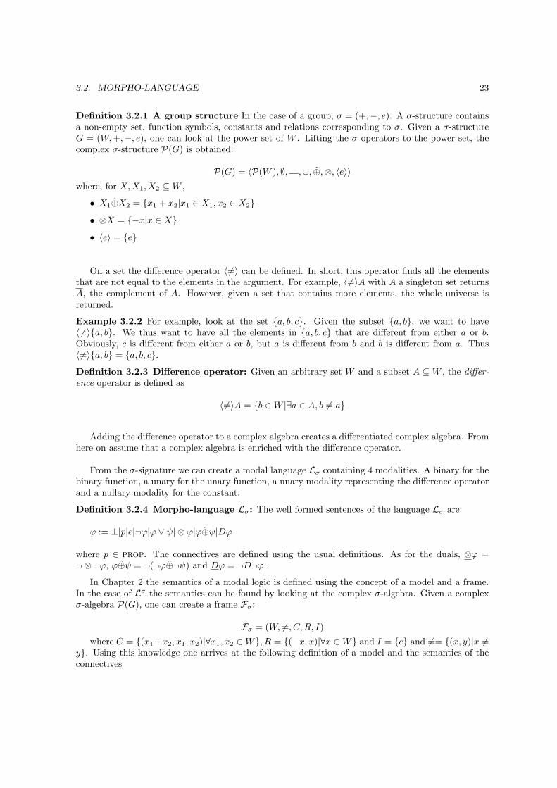
Definition 3.2.1 A group structure In the case of a group, σ = (+,−, e). A σ-structure containsa non-empty set, function symbols, constants and relations corresponding to σ. Given a σ-structureG = (W,+,−, e), one can look at the power set of W . Lifting the σ operators to the power set, thecomplex σ-structure P(G) is obtained.
P(G) = 〈P(W ), ∅, ,∪, ⊕,⊗, 〈e〉〉where, for X,X1, X2 ⊆W ,
• X1⊕X2 = {x1 + x2|x1 ∈ X1, x2 ∈ X2}
• ⊗X = {−x|x ∈ X}
• 〈e〉 = {e}
On a set the difference operator 〈6=〉 can be defined. In short, this operator finds all the elementsthat are not equal to the elements in the argument. For example, 〈6=〉A with A a singleton set returnsA, the complement of A. However, given a set that contains more elements, the whole universe isreturned.
Example 3.2.2 For example, look at the set {a, b, c}. Given the subset {a, b}, we want to have〈6=〉{a, b}. We thus want to have all the elements in {a, b, c} that are different from either a or b.Obviously, c is different from either a or b, but a is different from b and b is different from a. Thus〈6=〉{a, b} = {a, b, c}.
Definition 3.2.3 Difference operator: Given an arbitrary set W and a subset A ⊆W , the differ-ence operator is defined as
〈6=〉A = {b ∈W |∃a ∈ A, b 6= a}
Adding the difference operator to a complex algebra creates a differentiated complex algebra. Fromhere on assume that a complex algebra is enriched with the difference operator.
From the σ-signature we can create a modal language Lσ containing 4 modalities. A binary for thebinary function, a unary for the unary function, a unary modality representing the difference operatorand a nullary modality for the constant.
Definition 3.2.4 Morpho-language Lσ: The well formed sentences of the language Lσ are:
ϕ := ⊥|p|e|¬ϕ|ϕ ∨ ψ| ⊗ ϕ|ϕ⊕ψ|Dϕ
where p ∈ prop. The connectives are defined using the usual definitions. As for the duals, ⊗ϕ =¬ ⊗ ¬ϕ, ϕ⊕ψ = ¬(¬ϕ⊕¬ψ) and Dϕ = ¬D¬ϕ.
In Chapter 2 the semantics of a modal logic is defined using the concept of a model and a frame.In the case of Lσ the semantics can be found by looking at the complex σ-algebra. Given a complexσ-algebra P(G), one can create a frame Fσ:
Fσ = (W, 6=, C,R, I)where C = {(x1+x2, x1, x2)|∀x1, x2 ∈W}, R = {(−x, x)|∀x ∈W} and I = {e} and 6== {(x, y)|x 6=
y}. Using this knowledge one arrives at the following definition of a model and the semantics of theconnectives

24 CHAPTER 3. THE MORPHO-LANGUAGE
Definition 3.2.5 Mσ: Given a complex σ-algebra P(G), a model Mσ can be obtained through thefollowing definition Mσ = (Fσ,V) with V : prop 7→ P(W ).
Definition 3.2.6 Semantics of Lσ: Given a model Mσ and a world w in Mσ the semantics isdefined as:
M, w ⊥ is never trueM, w p iff w ∈ V(p), with p ∈ propM, w e iff (w) ∈ IM, w ¬ϕ iff M, w 1 ϕM, w ϕ ∨ ψ iff M, w ϕ or M, w ψM, w ⊗ϕ iff there exists a v ∈W such that (w, v) ∈ R and M, v ϕM, w ϕ⊕ψ iff there exists v, v′ ∈W such that (w, v, v′) ∈ C, M, v ϕ and M, v′ ψM, w Dϕ iff there exists a v ∈W such that v 6= w and M, v ϕ
Satisfiability and validity are defined as usual.
The final goal of the method is to give an axiomatization of a class of σ-structures C. From a classC, a class of complex σ-algebras can be created, denoted by C∗. The family of frames accompanyingC∗ is denoted by F ∗. Before going to the class of σ-structures axiomatized by the group axioms, firstan axiomatization is given for the class of all σ-structures.
The axiomatization consists of two parts. First, a set of inference rules is given. Some of thesehave already been introduced, namely the uniform substitution, modus ponens and necessitation. Theremaining set of rules is introduced to give the difference operator the proper meaning. Second, a setof axioms is given that define certain properties of the modalities and how they interact with eachother.
Before giving the axiomatization, two modalities need to be defined that are used in the axiomati-zation. Both modalities are defined using the difference modality D. The first modality that is definedis called the universal modality.
Definition 3.2.7 Universal modality: Given the difference operator D, the universal modality Uis defined as:
Uϕ := ϕ ∧ ¬D¬ϕ
The purpose of the universal modality is to define global truth. That is, a formula of the form Uϕis true in a model if and only if ϕ is true everywhere in the model. The dual of U , E is defined asEϕ = ¬U¬ϕ and means that ϕ is true somewhere in the model.
The other modality that must be defined is the only modality. This modality has the power tostate that a formula is true in only one point in the model.
Definition 3.2.8 Only modality Given the difference operator D, the only modality O is definedas:
Oϕ := ϕ ∧ ¬Dϕ
We are now ready to state the axiomatization of the class of all σ-structures.
Definition 3.2.9 Inference rules: The inference rules that are necessary for a complete axiomati-zation are the following:
Uniform substitution(SUB):ϕ
sub(ϕ)
Where sub(ϕ) is the result of an application of any uniform substitution of formulas for variables inϕ.

3.2. MORPHO-LANGUAGE 25
Modens Ponens(MP):ϕ,ϕ→ ψ
ψ
Necessitation for U(N(U)):ϕUϕ
Witness rule (W⊗):ϕ→ (⊗(Op→ ψ))
ϕ→ (⊗ψ)for some p not occurring in ϕ or ψ
Witness rule (W⊕1):
ϕ→ ((Op→ ψ1)⊕ψ2)ϕ→ ψ1⊕ψ2
for some p not occurring in ϕ,ψ1 or ψ2
Witness rule (W⊕2):
ϕ→ (ψ1⊕(Op→ ψ2))ϕ→ ψ1⊕ψ2
for some p not occurring in ϕ,ψ1 or ψ2
Definition 3.2.10 General Axioms: The following axioms are needed to arrive at a completeaxiomatization of a structure containing a binary and a unary operator and a constant.
(K⊕,r) p⊕(q → r) → ((p⊕q) → (p⊕r))(K⊕,l) (p→ q)⊕r → ((p⊕r) → (q⊕r))(K⊗) ⊗(p→ q) → (⊗p→ ⊗q)(Dual⊗ ⊗p→ ¬⊗ ¬p(Dual⊕) p⊕q → ¬(¬p⊕¬q)(D1) p ∨D¬Dp(D2) DDp→ (A ∨Dp)(U⊗) Up→ ⊗p(U⊕1
) Up→ p⊕q(U⊕2
) Up→ q⊕p(e1) EOe(e2) e→ Oe(⊗1) EOp→ E ⊗Op(⊗2) ⊗Op→ O⊗Op(⊕1) EOp ∧ EOq → E(Op⊕Oq)(⊕@) Op⊕Oq → O(Op⊕Oq)
Before giving the completeness proof, first an explanation of the axioms is in order. The axiomsK⊕,r, K⊕,r, K⊗ and the duals are given in order for Lσ to be a normal modal logic. The axiomsD1, D2, U⊗, U⊕1
and U⊕2are given for the axiomatization of the difference operator. Next, the e1
and e2 axioms say that e exists and that e is unique. The axioms ⊗1, ⊗2, ⊕1 and ⊕2 make sure that∀x∃yRxy and ∀xy∃zCzxy.
Theorem 2.20 in [25] tells us that this axiomatization is complete for the class of all σ-structures.The next step is to define an axiomatization for the class of σ-structures adhering to the group axioms:
associativity ∀abc((a+ b) + c = a+ (b+ c))neutral element ∀a(a+ e = e+ a = a)inverse element ∀a(a+ (−a) = e)commutativity ∀ab((a+ b = b+ a))
The method from [25] gives a translation to translate first order universal formulas to formulasfrom Lσ. However, the translation assumes that the universal first order formula does not containany nested operators. That is, the atomic formulas are of the form x = x1, x = e, x = x1 + x2
and x = −x1, where x, x1, x2 are variables. This assumption has no influence on the generality of thetranslation because every universal formula can be unnested to a new and equivalent universal formulacontaining no nestings.
26 CHAPTER 3. THE MORPHO-LANGUAGE
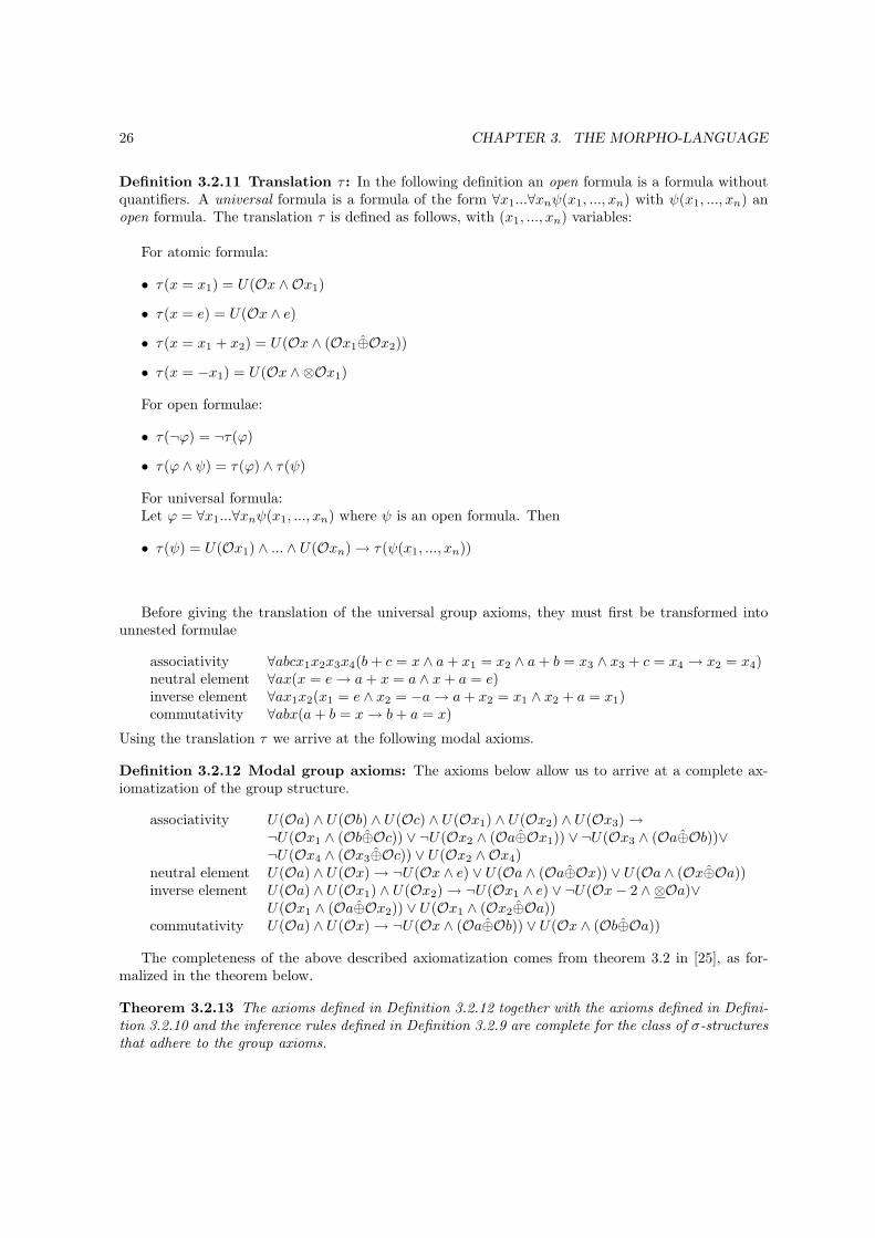
Definition 3.2.11 Translation τ : In the following definition an open formula is a formula withoutquantifiers. A universal formula is a formula of the form ∀x1...∀xnψ(x1, ..., xn) with ψ(x1, ..., xn) anopen formula. The translation τ is defined as follows, with (x1, ..., xn) variables:
For atomic formula:
• τ(x = x1) = U(Ox ∧ Ox1)
• τ(x = e) = U(Ox ∧ e)
• τ(x = x1 + x2) = U(Ox ∧ (Ox1⊕Ox2))
• τ(x = −x1) = U(Ox ∧ ⊗Ox1)
For open formulae:
• τ(¬ϕ) = ¬τ(ϕ)
• τ(ϕ ∧ ψ) = τ(ϕ) ∧ τ(ψ)
For universal formula:Let ϕ = ∀x1...∀xnψ(x1, ..., xn) where ψ is an open formula. Then
• τ(ψ) = U(Ox1) ∧ ... ∧ U(Oxn) → τ(ψ(x1, ..., xn))
Before giving the translation of the universal group axioms, they must first be transformed intounnested formulae
associativity ∀abcx1x2x3x4(b+ c = x ∧ a+ x1 = x2 ∧ a+ b = x3 ∧ x3 + c = x4 → x2 = x4)neutral element ∀ax(x = e→ a+ x = a ∧ x+ a = e)inverse element ∀ax1x2(x1 = e ∧ x2 = −a→ a+ x2 = x1 ∧ x2 + a = x1)commutativity ∀abx(a+ b = x→ b+ a = x)
Using the translation τ we arrive at the following modal axioms.
Definition 3.2.12 Modal group axioms: The axioms below allow us to arrive at a complete ax-iomatization of the group structure.
associativity U(Oa) ∧ U(Ob) ∧ U(Oc) ∧ U(Ox1) ∧ U(Ox2) ∧ U(Ox3) →¬U(Ox1 ∧ (Ob⊕Oc)) ∨ ¬U(Ox2 ∧ (Oa⊕Ox1)) ∨ ¬U(Ox3 ∧ (Oa⊕Ob))∨¬U(Ox4 ∧ (Ox3⊕Oc)) ∨ U(Ox2 ∧ Ox4)
neutral element U(Oa) ∧ U(Ox) → ¬U(Ox ∧ e) ∨ U(Oa ∧ (Oa⊕Ox)) ∨ U(Oa ∧ (Ox⊕Oa))inverse element U(Oa) ∧ U(Ox1) ∧ U(Ox2) → ¬U(Ox1 ∧ e) ∨ ¬U(Ox− 2 ∧ ⊗Oa)∨
U(Ox1 ∧ (Oa⊕Ox2)) ∨ U(Ox1 ∧ (Ox2⊕Oa))commutativity U(Oa) ∧ U(Ox) → ¬U(Ox ∧ (Oa⊕Ob)) ∨ U(Ox ∧ (Ob⊕Oa))
The completeness of the above described axiomatization comes from theorem 3.2 in [25], as for-malized in the theorem below.
Theorem 3.2.13 The axioms defined in Definition 3.2.12 together with the axioms defined in Defini-tion 3.2.10 and the inference rules defined in Definition 3.2.9 are complete for the class of σ-structuresthat adhere to the group axioms.
3.3. HYBRID LOGIC 27
The proof of this theorem follows directly from theorem 3.2 in [25].The next step that we want to take is to create a resolution calculus to perform automated reason-
ing. For a logic containing the difference operator nothing is known about creating and implementinga theorem prover. Above that, the axioms that are obtained through the above method are veryun-intuitive and unwieldy. Fortunately, there is another way of extending modal logic that does allowadaptation to a resolution calculus. Namely by moving to a modal logic called hybrid logic.
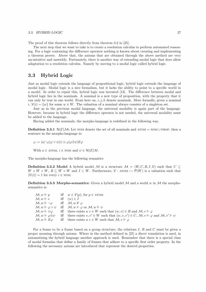
3.3 Hybrid Logic
Just as modal logic extends the language of propositional logic, hybrid logic extends the language ofmodal logic. Modal logic is a nice formalism, but it lacks the ability to point to a specific world ina model. In order to repair this, hybrid logic was invented [13]. The difference between modal andhybrid logic lies in the nominals. A nominal is a new type of proposition, with the property that itcan only be true in one world. From here on, i, j, k denote nominals. More formally, given a nominali, V(i) = {w} for some w ∈W . The valuation of a nominal always consists of a singleton set.
Just as in the previous modal language, the universal modality is again part of the language.However, because in hybrid logic the difference operator is not needed, the universal modality mustbe added to the language.
Having added the nominals, the morpho-language is redefined in the following way.
Definition 3.3.1 H(E)M: Let nom denote the set of all nominals and atom = nom∪ prop, then asentence in the morpho-language is:
ϕ := |a|¬ϕ|ϕ ∨ ψ|e| ⊗ ϕ|ϕ⊕ψ|Eϕ
With a ∈ atom, i ∈ nom and ψ ∈ H(E)M .
The morpho-language has the following semantics
Definition 3.3.2 Model A hybrid model M is a structure M = (W,C,R, I,V) such that C ⊆W ×W ×W , R ⊆ W ×W and I ⊂ W . Furthermore, V : atom 7→ P(W ) is a valuation such that|V(i)| = 1 for every i ∈ nom.
Definition 3.3.3 Morpho-semantics: Given a hybrid model M and a world w in M the morpho-semantics is:
M, w p iff w ∈ V(p), for p ∈ atomM, w e iff (w) ∈ IM, w ¬ϕ iff M, w 1 ϕM, w ϕ ∨ ψ iff M, w ϕ or M, w ψM, w ⊗ϕ iff there exists a v ∈W such that (w, v) ∈ R and M, v ϕM, w ϕ⊕ψ iff there exists v, v′ ∈W such that (w, v, v′) ∈ C, M, v ϕ and M, v′ ψM, w Eϕ iff there exists a v ∈W such that M, v ϕ
For a frame to be a frame based on a group structure, the relations I, R and C must be given aproper meaning through axioms. Where in the method defined in [25] a direct translation is used, inaxiomatizing the hybrid language another approach is used. Remember that there is a special classof modal formulas that define a family of frames that adhere to a specific first order property. In thefollowing the necessary axioms are introduced that represent the desired properties.

28 CHAPTER 3. THE MORPHO-LANGUAGE
total⊕) Ei ∧ Ej → Ei⊕j(unique⊕) E(i ∧ j1⊕j2) ∧ E(k ∧ j1⊕j2) → E(j ∧ k)(Ass1) (i⊕j)⊕k → i⊕(j⊕k)(Ass2) i⊕(j⊕k) → (i⊕j)⊕k(comm) i⊕j → j⊕i(rev1) ⊗i→ ⊗i(rev2) ⊗j → ⊗j(rev2) i⊕(⊗i) → e(rev3) e→ i⊕(⊗i)(id1) i⊕e→ i(id2) i→ i⊕e
Table 3.1: The morpho-logic axioms
We can distinguish 3 types of axioms: the axioms that define the properties for ⊕, the axioms thatdefine the properties for ⊗ and the axioms that define how e, ⊕ and ⊗ cooperate. All the axioms aregrouped in Table 3.1 First the axioms that define the properties of ⊕. ⊕ must axiomatize a binaryfunction which is total. A function is total if it is defined on every element of it’s domain. Furthermore,a binary function maps every input to a unique element in the domain. Thus we have the followingtwo axioms:
(total⊕) Ei ∧ Ej → Ei⊕j(unique⊕) E(i ∧ j1⊕j2) ∧ E(k ∧ j1⊕j2) → E(j ∧ k)
Furthermore, ⊕ is both associative and commutative:
(Ass1) (i⊕j)⊕k → i⊕(j⊕k)(Ass2) i⊕(j⊕k) → (i⊕j)⊕k(comm) i⊕j → j⊕i
To give the proper meaning to the modality ⊗, it should represent a total function as well. This iscaptured by the following 2 axioms:
(rev1) ⊗j → ⊗j(rev2) ⊗i→ ⊗i
The axiom (rev1) defines the fact that ∀x∃yRxy. That is, R is total. The second axiom definesthe following property: ∀xyzRxy ∧ Rxz → y = z. As for the interplay between ⊕, ⊗ and e we havethe following axioms, inspired by the first order group axioms:
(rev2) i⊕(⊗i) → e(rev3) e→ i⊕(⊗i)(id1) i⊕e→ i(id2) i→ i⊕e
From here on the set of axioms (total⊕) through (id2), defined in Table 3.1, is denoted by Σmorpho.Because the morpho-logic contains nominals, we need to redefine what is meant with completenesswith respect to a family of formulas. A set of formulas is a normal hybrid logic if it adheres to thefollowing Definition [40].
Definition 3.3.4 Normal hybrid logic: Given a similarity type τ , a normal hybrid logic over τ
3.3. HYBRID LOGIC 29
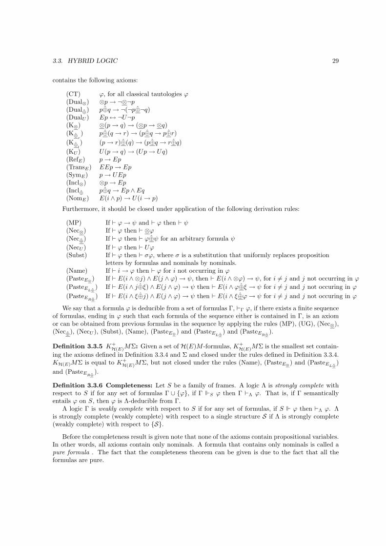
contains the following axioms:
(CT) ϕ, for all classical tautologies ϕ(Dual⊗) ⊗p→ ¬⊗¬p(Dual⊕) p⊕q → ¬(¬p⊕¬q)(DualU ) Ep↔ ¬U¬p(K⊗) ⊗(p→ q) → (⊗p→ ⊗q)(K⊕
r) p⊕(q → r) → (p⊕q → p⊕r)
(K⊕l) (p→ r)⊕(q) → (p⊕q → r⊕q)
(KU ) U(p→ q) → (Up→ Uq)(RefE) p→ Ep(TransE) EEp→ Ep(SymE) p→ UEp(Incl⊗) ⊗p→ Ep(Incl⊕ p⊕q → Ep ∧ Eq(NomE) E(i ∧ p) → U(i→ p)
Furthermore, it should be closed under application of the following derivation rules:
(MP) If ` ϕ→ ψ and ` ϕ then ` ψ(Nec⊗) If ` ϕ then ` ⊗ϕ(Nec⊕) If ` ϕ then ` ϕ⊕ψ for an arbitrary formula ψ(NecU ) If ` ϕ then ` Uϕ(Subst) If ` ϕ then ` σϕ, where σ is a substitution that uniformly replaces proposition
letters by formulas and nominals by nominals.(Name) If ` i→ ϕ then ` ϕ for i not occurring in ϕ(PasteE⊗) If ` E(i ∧ ⊗j) ∧ E(j ∧ ϕ) → ψ, then ` E(i ∧ ⊗ϕ) → ψ, for i 6= j and j not occurring in ϕ(PasteEL⊕
) If ` E(i ∧ j⊕ξ) ∧ E(j ∧ ϕ) → ψ then ` E(i ∧ ϕ⊕ξ → ψ for i 6= j and j not occuring in ϕ(PasteER⊕
) If ` E(i ∧ ξ⊕j) ∧ E(j ∧ ϕ) → ψ then ` E(i ∧ ξ⊕ϕ→ ψ for i 6= j and j not occuring in ϕ
We say that a formula ϕ is deducible from a set of formulas Γ, `Γ ϕ, if there exists a finite sequenceof formulas, ending in ϕ such that each formula of the sequence either is contained in Γ, is an axiomor can be obtained from previous formulas in the sequence by applying the rules (MP), (UG), (Nec⊗),(Nec⊕), (NecU ), (Subst), (Name), (PasteE⊗) and (PasteEL⊕
) and (PasteER⊕).
Definition 3.3.5 K+H(E)MΣ: Given a set of H(E)M -formulas, K+
H(E)MΣ is the smallest set contain-ing the axioms defined in Definition 3.3.4 and Σ and closed under the rules defined in Definition 3.3.4.KH(E)MΣ is equal to K+
H(E)MΣ, but not closed under the rules (Name), (PasteE⊗) and (PasteEL⊕)
and (PasteER⊕).
Definition 3.3.6 Completeness: Let S be a family of frames. A logic Λ is strongly complete withrespect to S if for any set of formulas Γ ∪ {ϕ}, if Γ S ϕ then Γ `Λ ϕ. That is, if Γ semanticallyentails ϕ on S, then ϕ is Λ-deducible from Γ.
A logic Γ is weakly complete with respect to S if for any set of formulas, if S ϕ then `Λ ϕ. Λis strongly complete (weakly complete) with respect to a single structure S if Λ is strongly complete(weakly complete) with respect to {S}.
Before the completeness result is given note that none of the axioms contain propositional variables.In other words, all axioms contain only nominals. A formula that contains only nominals is called apure formula . The fact that the completeness theorem can be given is due to the fact that all theformulas are pure.
30 CHAPTER 3. THE MORPHO-LANGUAGE
Theorem 3.3.7 K+H(E)MΣmorpho is strongly complete with respect to the set of frames defined by
Σmorpho.
Proofsketch. As we have already seen, all the axioms are pure formulas. One can show that everypure formula is di-persistent. Thus, given Theorem 5.3.16 in [40], which can be generalized to thehybrid arrow logic, we have that the axioms are complete for the family of frames that they define.For the proof, see Appendix D. qed
We have seen two types of axiomatization of the morphological dilation. One in modal logic and onein hybrid logic. The first axiomatization is given because the steps that are taken to go from the firstorder axioms to an axiomatization are very clear and understandable. However, the axiomatizationgives us very long and not easy to read set of axioms. In hybrid logic the axiomatization is muchmore readable and intuitive. Above all, much more is known about automated theorem proving usinghybrid logic.
3.4 Summary
The link between mathematical morphology and modal logic presented in [4] is a link between thetranslation invariant operators and arrow logic. But arrow logic itself is not strong enough to axiom-atize Mathematical Morphology. To be able to do this, the difference operator has to be added to thelanguage, together with the difference axioms and the (WIT) derivation rules.
However, automated theorem proving using the difference operator is not well known. Hence, it ismore convenient to axiomatize the language using hybrid logic. Hybrid logic is an extension of modallogic using nominals. Nominals behave like propositions, with the restriction that they can be true atonly one point in the model. Furthermore, the universal modality E is introduced. Due to the factthat ⊕ must be a total function, the logic must be able to represent the fact that a formula must betrue somewhere in the model. This can be done using the universal modality. Using hybrid logic wearrive at a complete axiomatization of mathematical morphology, creating the morpho-language.

Chapter 4
Resolution in the morpho-language
What does the link between Mathematical Morphology and modal logic add to the knowledge andunderstanding of Mathematical Morphology? The morpho-logic consists of a set of axioms togetherwith a set of derivation rules. Combining these, new formulas can be generated that are valid in allthe models. This means that properties of Mathematical Morphology can be generated automatically.A simple example is the fact that the dilation distributes over the ∨, which is a general property ofevery normal modal logic. The problem with using the derivation rules is that one can only generateformulas from the axioms. Hence, it is not obvious how to prove that a certain formula is in fact a validformula. For this purpose several general techniques have been developed that work quite well with alot of different logics. One of these techniques is called resolution [32] and is the focus of what follows.Other theorem proving techniques for hybrid logic exist, but to the best of the authors knowledgeresolution is the most matured form of reasoning for hybrid logics. Hence this form of reasoning ischosen to pursue further.
The remainder of this chapter is organized as follows. In Section 1 resolution is explained inmore detail. In Section 2 a resolution calculus is introduced for the morpho-logic. In Section 3 animplementation of the resolution calculus for the morpho-logic is discussed.
4.1 Resolution
Resolution is a method that tries to answer the question of satisfiability. More precisely, it tries toanswer the question of negative satisfiability. It aims at finding a proof that shows that a formula orset of formulas is not satisfiable. This means that there is no model such that this formula or set offormulas is true in some world in the model. Resolution has first been introduced by J.A. Robinsonin [32].
Using resolution, the question whether a formula ϕ is valid can be answered by searching for a proofthat ¬ϕ is not satisfiable. If the negation of a formula is always false, the formula itself must alwaysbe true and thus must be valid. Before we can introduce resolution, several basic concepts have to berecalled. Note that the definitions assume that propositional resolution is used. After propositionalresolution is explained, it is extended to cope with the modalities present in modal logic.
4.1.1 Basic concepts
A resolution theorem prover takes as input a formula. This formula however, is in a special kind ofform. This form is called the conjunctive normal form,
31
32 CHAPTER 4. RESOLUTION IN THE MORPHO-LANGUAGE
Definition 4.1.1 Conjunctive normal form: A formula ϕ is in conjunctive normal form if it is ofthe form
(ψ1,1 ∨ ... ∨ ψ1,m) ∧ ... ∧ (ψn,1 ∨ ... ∨ ψn,k)
With ψi,j either a propositional variable or a negated propositional variable. Thus, a formula is inconjunctive normal form if it is a conjunction of disjunctions. In the modal case, a formula that hasthe form 2ϕ or 3ϕ is also considered a literal because it cannot be decomposed in terms of ∨ and ∧any further.
Note that for every formula an equivalent formula in conjunctive normal form exists. Thus w.l.g wecan assume that every formula is in conjunctive normal form. However, a formula is not representedas one formula. A formula is split into sub-formulas.
Definition 4.1.2 Clauses and literals: A formula ϕ is called a literal if it is a propositional variable.A formula ϕ is called a negated variable if it is a negated propositional literal. These literals are usedto form a clause . A clause is a set of literals and a clause is satisfied if one of the literals is satisfied.The clauses are grouped together into a set of clauses. This set of clauses is satisfied if all the clausesin the set are satisfied.
4.1.2 Propositional resolution
The basic principal of propositional resolution, actually, of resolution in general is the following.Suppose one has two clauses. One clause of the form {p, q} and one clause of the form {¬p, q}. Sinceboth clauses must be true at the same time, and the truth values of the 2 literals p and ¬p are oppositeone can combine both clauses while removing the opposing literals. This is due to the fact that oneof p and ¬p must be false, thus at least one of the other entries in one of the clauses must be true.Therefore we can ignore the formulas p and ¬p and focus on the rest of the clauses. This operationgives us a clause of the form {q}. The rule that belongs to this operation is called the resolution ruleand has the following form:
Definition 4.1.3 Resolution rule: Given 2 clauses {q1, ..., qi, p, qi+1, ..., qn} and {r1, ..., rj ,¬p, rj+1, ..., rm}with {q1, ..., qi, qi+1, ..., qn, r1, ..., rj , rj+1, ..., rm} literals and p ∈ prop we have the following rule
{q1, ..., qi, p, qi+1, ..., qn} {r1, ..., rj ,¬p, rj+1, ..., rm}{q1, ..., qi, qi+1, ..., qn, r1, ..., rj , rj+1, ..., rm}
The result of the resolution step is called the resolvent. Resolving two clauses means applying theresolution rule to the two clauses. Note that in each resolution step only one literal may be resolved.It is not allowed to resolve 2 literals in one step.
But how does one go from such a simple rule to proving whether a formula is satisfiable? Thebasic idea is the following. The first step of resolution is to bring all the formulas into conjunctivenormal form and then creating a set of clauses. All these clauses must simultaneously be satisfied ina model for the original formula. By using the resolution rule, one tries to deduce the empty clause.Arriving at the empty clause means that there is a clause that must be satisfied but that does notcontain anything that can be satisfied. Hence the set of clauses cannot be satisfied.
Example 4.1.4 For example, look at the formula (p→ q)∧(q → r)∧p∧¬r. Rewritten in conjunctivenormal form this formula has the form (¬p ∨ q) ∧ (¬q ∨ r) ∧ p ∧ ¬r, giving the following clauses:{¬p, q}, {¬q, r}, {p}, {¬r}. Applying the resolution rule, one creates the resolution tree shown inFigure 4.1

4.2. MORPHO-RESOLUTION 33
{¬p, q}
��
{p}
vvmmmmmmmmmmmmmmmm
{q}
��
{¬q, r}
vvmmmmmmmmmmmmmm
{r}
��
{¬r}
vvmmmmmmmmmmmmmmmm
{}
Figure 4.1: An example of a resolution proof
Definition 4.1.5 Refutation: A refutation of a set of clauses is a sequence of applications of therefutation rule such that the end result is the empty clause.
Resolution is used to proof the validity of a sentence in the following manner.
Definition 4.1.6 Proof: Suppose one wants to proof that a formula ϕ is valid. This is done byapplying resolution on ¬ϕ. If ¬ϕ has a refutation it is valid. This is denoted by `propres ϕ. If aformula ϕ follows logically from a set of formula Γ, one can proof this by finding a refutation for theclausal form of Γ ∪ {¬ϕ}. This is denoted by Γ `propres ϕ
To show that resolution really does the trick, recall the following proposition. For the proof werefer to [32].
Proposition 4.1.7 Given a set of clauses Σ, Σ is propositionally unsatisfiable iff there exists a refu-tation of Σ.
Resolution is not limited to propositional logic but can be applied to a wide array of logics includingmodal logic and hybrid logic. In these cases the simple resolution rule is not enough and additionalrules have to be defined.
4.2 Morpho-resolution
As mentioned above, resolution is not limited to propositional logic. In [6, 23] a resolution calculusfor modal logic is introduced that allows for modal resolution. Furthermore, [6] also introduces aresolution calculus for hybrid logic.
4.2.1 Hybrid resolution
With propositional resolution the resolution rule is sufficient. But in modal and hybrid logic thisresolution rule is not sufficient any more. Suppose that we have two modal clauses {3p} and {2¬p}.The former clause says that there is an accessible world that makes p true while the latter clause tellsus that each accessible world makes ¬p true. Obviously this cannot be the case, but the resolutionrule cannot be applied on these two clauses. A way of bringing the resolution ”inside” is needed. Oneway to do this is by using labels (see [6]). Fortunately hybrid logic contains a property that enables

34 CHAPTER 4. RESOLUTION IN THE MORPHO-LANGUAGE
us to bring the resolution inside in a very natural way. The nominals in the language can be used aslabels of worlds.
First of all, all the formulas in a set of clauses need to be in the form @iϕ. This has no consequencesfor the result of the prover because if a formula @iϕ is satisfiable, ϕ is satisfiable as well and vice-versa.Second, we need to transform the formulas to negation normal form.
Definition 4.2.1 Negation normal form: A formula is in negation normal form when only propo-sitional letters and nominals occur in the scope of a negation.
One can transform a formula to negated normal form by using the function nf . nf is an operationthat takes as input a formula and outputs an equivalent formula in negated normal form.
nf(p) = pnf(¬p) = pnf(¬¬ϕ) = ϕnf(¬ ⊗ (ϕ)) = ⊗nf(¬ϕ)nf(¬⊗(ϕ)) = ⊗nf(¬ϕ)nf(¬ϕ⊕ψ) = (nf(¬ϕ))⊕(nf(¬ψ))nf(¬(ϕ ∨ ψ)) = (nf(¬ϕ) ∧ nf(¬ψ))nf(¬(ϕ ∧ ψ)) = (nf(¬ϕ) ∨ nf(¬ψ))nf(¬@iϕ) = @inf(¬ϕ)
Given a set of clauses, Σ, we create a new set of clauses Σ′ = {@inf(ϕ)|ϕ ∈ Σ}. Let us haveanother look at the previous clauses. They now get the form {@i3p} and {@i2¬p}. Formula @i3ptells us that there should be a world accessible from the world labelled by i that makes p true. We canlabel this new world by adding a new nominal j and the following clauses: {@i3j} and {@jp}. Theformula 2¬p tells us that each world accessible from the world with label i makes ¬p true. Combinethis with the clause {@i3j} and one can see that {@j¬p} must be the case as well. This brings usto the rules (3) and (2) in Table 4.2. One now has both @ip and @i¬p. On these two formulas thenormal resolution rule can be applied, resulting in the empty clause. The normal resolution rule isrepresented by rule (R).
Observe that a formula of the form @i@jϕ is equivalent to @jϕ. This brings us to the @-rule.In using the above introduced rules (3) and (2) one creates a new formula {@jϕ}. It is possible
that ϕ is not in conjunctive normal form and not of the form 3ϕ or 2ϕ. When this happens thereare two possibilities. Either it is a conjunction or a disjunction. To be able to handle these situationsthe (∧) and (∨) rules in Table 4.2 are introduced.
The rules introduced so far are sufficient to take care of the modalities and the connectives (see [6]).But what about the satisfaction operator? Consider the following situation. Suppose we have the setof clauses {{@i3j}, {@jp}, {@jk}, {@k¬p}}. Since a nominal can point to only one world k and jmust point to the same world, thus this set of clauses is not satisfiable. But with the present rulesthe empty clause is not derivable. What happens is that the satisfaction operator introduces a formof equational reasoning. To see why, let us translate the formula @ij to first order logic. We then getthe formula ∃x(x = i ∧ x = j) which can be simplified to the formula i = j.
In first order logic the way to deal with equational reasoning in resolution is by using paramodula-tion [9, 17]. In first order logic a set of clauses is said to be equationally satisfiable if resolution withthe axioms shown in Table 4.1 does not produce the empty clause.
Performing resolution with these additional clauses produces a lot of unnecessary resolution steps.To solve this problem, in [17] paramodulation is introduced to replace reasoning with the symmetry andtransitivity axioms. In the case of hybrid logic the paramodulation rule amounts to the (PARAM)-rulein Table 4.2. This rule basically replaces every occurrence of a nominal i with the equivalent nominal
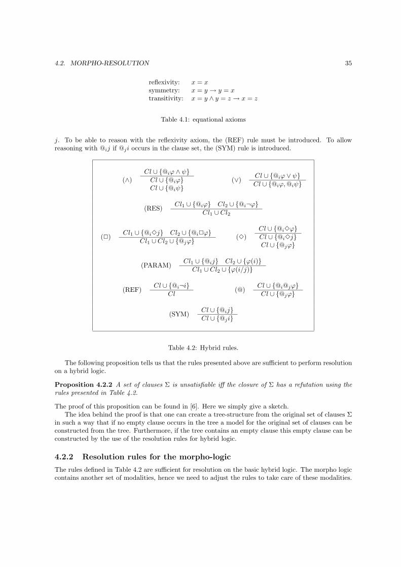
4.2. MORPHO-RESOLUTION 35
reflexivity: x = xsymmetry: x = y → y = xtransitivity: x = y ∧ y = z → x = z
Table 4.1: equational axioms
j. To be able to reason with the reflexivity axiom, the (REF) rule must be introduced. To allowreasoning with @ij if @ji occurs in the clause set, the (SYM) rule is introduced.
(∧)Cl ∪ {@iϕ ∧ ψ}Cl ∪ {@iϕ}Cl ∪ {@iψ}
(∨)Cl ∪ {@iϕ ∨ ψ}Cl ∪ {@iϕ,@iψ}
(RES)Cl1 ∪ {@iϕ} Cl2 ∪ {@i¬ϕ}
Cl1 ∪ Cl2
(2)Cl1 ∪ {@i3j} Cl2 ∪ {@i2ϕ}
Cl1 ∪ Cl2 ∪ {@jϕ}(3)
Cl ∪ {@i3ϕ}Cl ∪ {@i3j}Cl ∪ {@jϕ}
(PARAM)Cl1 ∪ {@ij} Cl2 ∪ {ϕ(i)}
Cl1 ∪ Cl2 ∪ {ϕ(i/j)}
(REF)Cl ∪ {@i¬i}
Cl(@)
Cl ∪ {@i@jϕ}Cl ∪ {@jϕ}
(SYM)Cl ∪ {@ij}Cl ∪ {@ji}
Table 4.2: Hybrid rules.
The following proposition tells us that the rules presented above are sufficient to perform resolutionon a hybrid logic.
Proposition 4.2.2 A set of clauses Σ is unsatisfiable iff the closure of Σ has a refutation using therules presented in Table 4.2.
The proof of this proposition can be found in [6]. Here we simply give a sketch.The idea behind the proof is that one can create a tree-structure from the original set of clauses Σ
in such a way that if no empty clause occurs in the tree a model for the original set of clauses can beconstructed from the tree. Furthermore, if the tree contains an empty clause this empty clause can beconstructed by the use of the resolution rules for hybrid logic.
4.2.2 Resolution rules for the morpho-logic
The rules defined in Table 4.2 are sufficient for resolution on the basic hybrid logic. The morpho logiccontains another set of modalities, hence we need to adjust the rules to take care of these modalities.

36 CHAPTER 4. RESOLUTION IN THE MORPHO-LANGUAGE
Furthermore, these modalities satisfy a set of axioms. These axioms must be taken into considerationas well.
Before looking at the axioms, we consider the modalities of the morpho language. The morpholanguage contains three modalities, the ⊗, the ⊕ and the E. The first is a unary modality and can betaken care of by using the rules defined in Table 4.2. The ⊕ on the other hand, is a binary modalityand requires some new rules. The rule for the ⊕ modality introduces a new relation in the samemanner that the ⊗ rule does. The ⊕ rule on the other hand works a little differently. ϕ⊕ψ meansthat for each relation j1⊕j2 it is either the case that @j1ϕ or @j2ψ. This is captured by putting bothformulas in one clause and making sure that at least one of them is true. Creating two clauses wouldbe to strong, because then both formulas should be satisfiable.
The third modality, the universal modality, has the following meaning. Eϕ is true if ϕ is truesomewhere in the model. Thus, a point must be introduced that makes ϕ true, meaning that if aclause of the form {Eϕ} ∪ C is found, a clause of the form {@iϕ} ∪ C must be created for i a newnominal. Aϕ is true if ϕ is true everywhere in the model. Thus, if clause of the form {Aϕ} ∪ C1 isfound combined with a clause of the form {ψ}∪C2 then a clause {@iϕ}∪C1 ∪C2 must be formed forevery nominal i that occurs in ψ.
Finally, note that @iEϕ and Eϕ are equivalent (the same holds for A). For this reason the (@E)and (@A) rules are introduced.
The rules for the ⊗, ⊕, E and there respective dualities are shown in Table 4.3.
(A)Cl1 ∪ {Aϕ} Cl2 ∪ {ψ}Cl1 ∪ Cl2 ∪ {@iϕ}
, where i occurs in ψ (E)Cl ∪ {Eϕ}Cl ∪ {@iϕ}
, where i is new
(⊗ )Cl1 ∪ {@i⊗ϕ} Cl2 ∪ {@i ⊗ (j)}
Cl1 ∪ Cl2 ∪ {@jϕ}(⊗ )
Cl ∪ {@i ⊗ ϕ}Cl ∪ {@i ⊗ (j)}Cl ∪ {@jϕ}
, where j is new
(@E)Cl ∪ {@Eϕ}Cl ∪ {Eϕ} (@A)
Cl ∪ {@Aϕ}Cl ∪ {Aϕ}
(⊕)Cl1 ∪ {@iϕ⊕ψ} Cl2 ∪ {@i(j1⊕j2)}
Cl1 ∪ Cl2 ∪ {@j1ϕ ,@j2ψ}
(⊕)
Cl ∪ {@i(ϕ⊕ψ)}Cl ∪ {@i(j1⊕j2)}Cl ∪ {@j1ϕ}Cl ∪ {@j2ψ}
, where j1 and j2 are new
Table 4.3: Resolution rules for the morpho modalities.
To incorporate the axioms a new set rules must be introduced. The reason for this is the following.The rules defined above make sure that the model that can be found by the construction used in theproof is a normal hybrid model. However, this model does not necessarily satisfy the morpho-axiomsas defined in Table 3.1.
The rules that are needed are defined in Table 4.4. Next, we go over every rule and show what it’spurpose is. Before we go further, note that the rules assume that there is a clause of the form {@ie}in the original set of clauses. This is done to make more efficient rules possible.
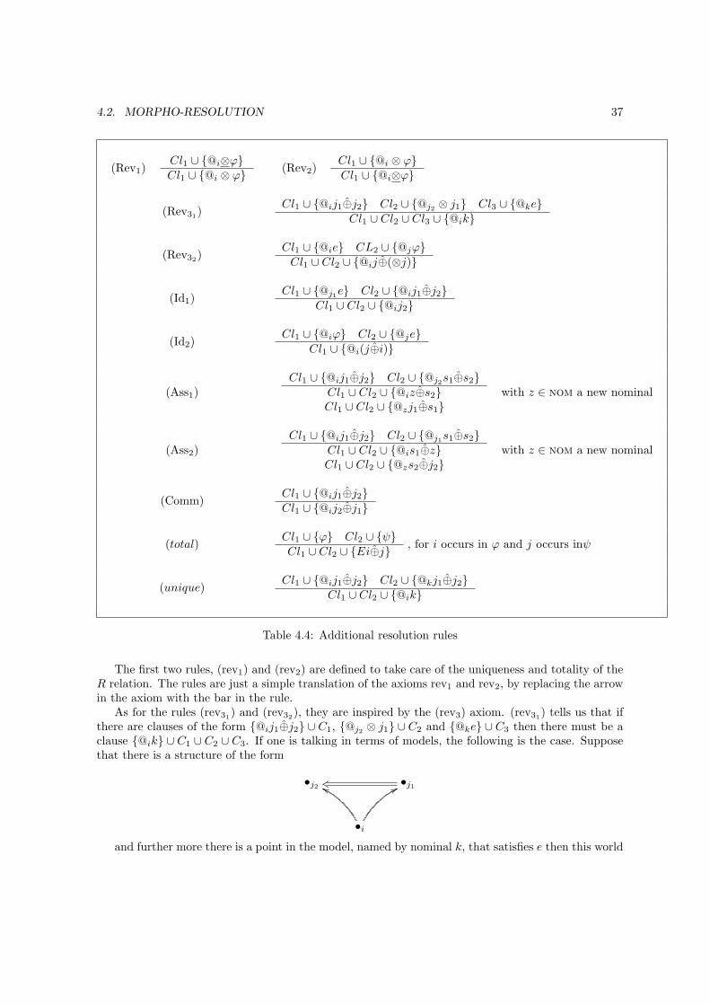
4.2. MORPHO-RESOLUTION 37
(Rev1)Cl1 ∪ {@i⊗ϕ}Cl1 ∪ {@i ⊗ ϕ} (Rev2)
Cl1 ∪ {@i ⊗ ϕ}Cl1 ∪ {@i⊗ϕ}
(Rev31)Cl1 ∪ {@ij1⊕j2} Cl2 ∪ {@j2 ⊗ j1} Cl3 ∪ {@ke}
Cl1 ∪ Cl2 ∪ Cl3 ∪ {@ik}
(Rev32)Cl1 ∪ {@ie} CL2 ∪ {@jϕ}Cl1 ∪ Cl2 ∪ {@ij⊕(⊗j)}
(Id1)Cl1 ∪ {@j1e} Cl2 ∪ {@ij1⊕j2}
Cl1 ∪ Cl2 ∪ {@ij2}
(Id2)Cl1 ∪ {@iϕ} Cl2 ∪ {@je}
Cl1 ∪ {@i(j⊕i)}
(Ass1)Cl1 ∪ {@ij1⊕j2} Cl2 ∪ {@j2s1⊕s2}
Cl1 ∪ Cl2 ∪ {@iz⊕s2}Cl1 ∪ Cl2 ∪ {@zj1⊕s1}
with z ∈ nom a new nominal
(Ass2)Cl1 ∪ {@ij1⊕j2} Cl2 ∪ {@j1s1⊕s2}
Cl1 ∪ Cl2 ∪ {@is1⊕z}Cl1 ∪ Cl2 ∪ {@zs2⊕j2}
with z ∈ nom a new nominal
(Comm)Cl1 ∪ {@ij1⊕j2}Cl1 ∪ {@ij2⊕j1}
(total)Cl1 ∪ {ϕ} Cl2 ∪ {ψ}Cl1 ∪ Cl2 ∪ {Ei⊕j}
, for i occurs in ϕ and j occurs inψ
(unique)Cl1 ∪ {@ij1⊕j2} Cl2 ∪ {@kj1⊕j2}
Cl1 ∪ Cl2 ∪ {@ik}
Table 4.4: Additional resolution rules
The first two rules, (rev1) and (rev2) are defined to take care of the uniqueness and totality of theR relation. The rules are just a simple translation of the axioms rev1 and rev2, by replacing the arrowin the axiom with the bar in the rule.
As for the rules (rev31) and (rev32), they are inspired by the (rev3) axiom. (rev31) tells us that ifthere are clauses of the form {@ij1⊕j2} ∪ C1, {@j2 ⊗ j1} ∪ C2 and {@ke} ∪ C3 then there must be aclause {@ik} ∪ C1 ∪ C2 ∪ C3. If one is talking in terms of models, the following is the case. Supposethat there is a structure of the form
•j2 •j1ks
•i
gg 77
and further more there is a point in the model, named by nominal k, that satisfies e then this world
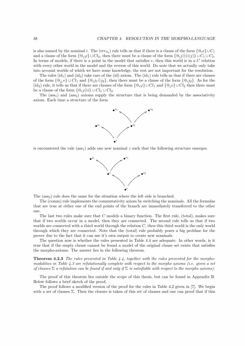
38 CHAPTER 4. RESOLUTION IN THE MORPHO-LANGUAGE
is also named by the nominal i. The (rev32) rule tells us that if there is a clause of the form {@ie}∪C1
and a clause of the form {@jϕ}∪Cl2, then there must be a clause of the form {@ij⊕(⊗j)}∪C1 ∪C2.In terms of models, if there is a point in the model that satisfies e, then this world is in a C relationwith every other world in the model and the reverse of this world. Do note that we actually only takeinto account worlds of which we have some knowledge, the rest are not important for the resolution.
The rules (id1) and (id2) take care of the (id) axiom. The (id1) rule tells us that if there are clausesof the form {@j1e} ∪ Cl1 and {@ij1⊕j2}, then there must be a clause of the form {@ij2}. As for the(id2) rule, it tells us that if there are clauses of the form {@iϕ}∪Cl1 and {@je}∪Cl2 then there mustbe a clause of the form {@ij⊕i} ∪ Cl1 ∪ Cl2.
The (ass1) and (ass2) axioms supply the structure that is being demanded by the associativityaxiom. Each time a structure of the form
•s1 •s2
•j1 •j2
77gg
•i
77gg
is encountered the rule (ass1) adds one new nominal z such that the following structure emerges.
•j1 •s1
•z
gg 77
•s2
•i
77gg
The (ass2) rule does the same for the situation where the left side is branched.The (comm) rule implements the commutativity axiom by switching the nominals. All the formulas
that are true at either one of the end points of the branch are immediately transferred to the otherone.
The last two rules make sure that C models a binary function. The first rule, (total), makes surethat if two worlds occur in a model, then they are connected. The second rule tells us that if twoworlds are connected with a third world through the relation C, then this third world is the only worldthrough which they are connected. Note that the (total) rule probably poses a big problme for theprover due to the fact that it can use it’s own output to create new nominals.
The question now is whether the rules presented in Table 4.4 are adequate. In other words, is ittrue that if the empty clause cannot be found a model of the original clause set exists that satisfiesthe morpho-axioms. The answer lies in the following theorem.
Theorem 4.2.3 The rules presented in Table 4.4, together with the rules presented for the morpho-modalities in Table 4.3 are refutationally complete with respect to the morpho axioms (i.e. given a setof clauses Σ a refutation can be found if and only if Σ is satisfiable with respect to the morpho axioms).
The proof of this theorem lies outside the scope of this thesis, but can be found in Appendix B.Below follows a brief sketch of the proof.
The proof follows a modified version of the proof for the rules in Table 4.2 given in [7]. We beginwith a set of clauses Σ. Then the closure is taken of this set of clauses and one can proof that if this
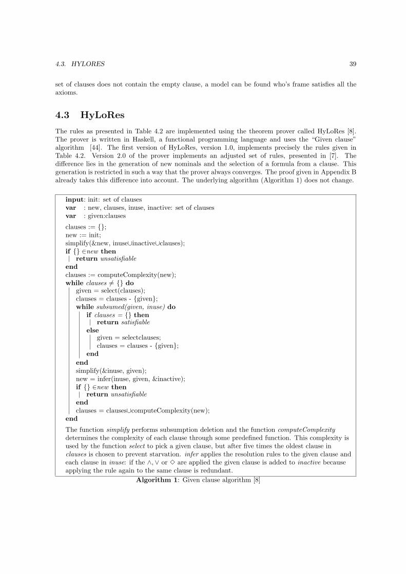
4.3. HYLORES 39
set of clauses does not contain the empty clause, a model can be found who’s frame satisfies all theaxioms.
4.3 HyLoRes
The rules as presented in Table 4.2 are implemented using the theorem prover called HyLoRes [8].The prover is written in Haskell, a functional programming language and uses the “Given clause”algorithm [44]. The first version of HyLoRes, version 1.0, implements precisely the rules given inTable 4.2. Version 2.0 of the prover implements an adjusted set of rules, presented in [7]. Thedifference lies in the generation of new nominals and the selection of a formula from a clause. Thisgeneration is restricted in such a way that the prover always converges. The proof given in Appendix Balready takes this difference into account. The underlying algorithm (Algorithm 1) does not change.
input: init: set of clausesvar : new, clauses, inuse, inactive: set of clausesvar : given:clauses
clauses := {};new := init;simplify(&new, inuse∪inactive∪clauses);if {} ∈new then
return unsatisfiableendclauses := computeComplexity(new);while clauses 6= {} do
given = select(clauses);clauses = clauses - {given};while subsumed(given, inuse) do
if clauses = {} thenreturn satisfiable
elsegiven = selectclauses;clauses = clauses - {given};
endendsimplify(&inuse, given);new = infer(inuse, given, &inactive);if {} ∈new then
return unsatisfiableendclauses = clauses∪computeComplexity(new);
end
The function simplify performs subsumption deletion and the function computeComplexitydetermines the complexity of each clause through some predefined function. This complexity isused by the function select to pick a given clause, but after five times the oldest clause inclauses is chosen to prevent starvation. infer applies the resolution rules to the given clause andeach clause in inuse: if the ∧,∨ or 3 are applied the given clause is added to inactive becauseapplying the rule again to the same clause is redundant.
Algorithm 1: Given clause algorithm [8]
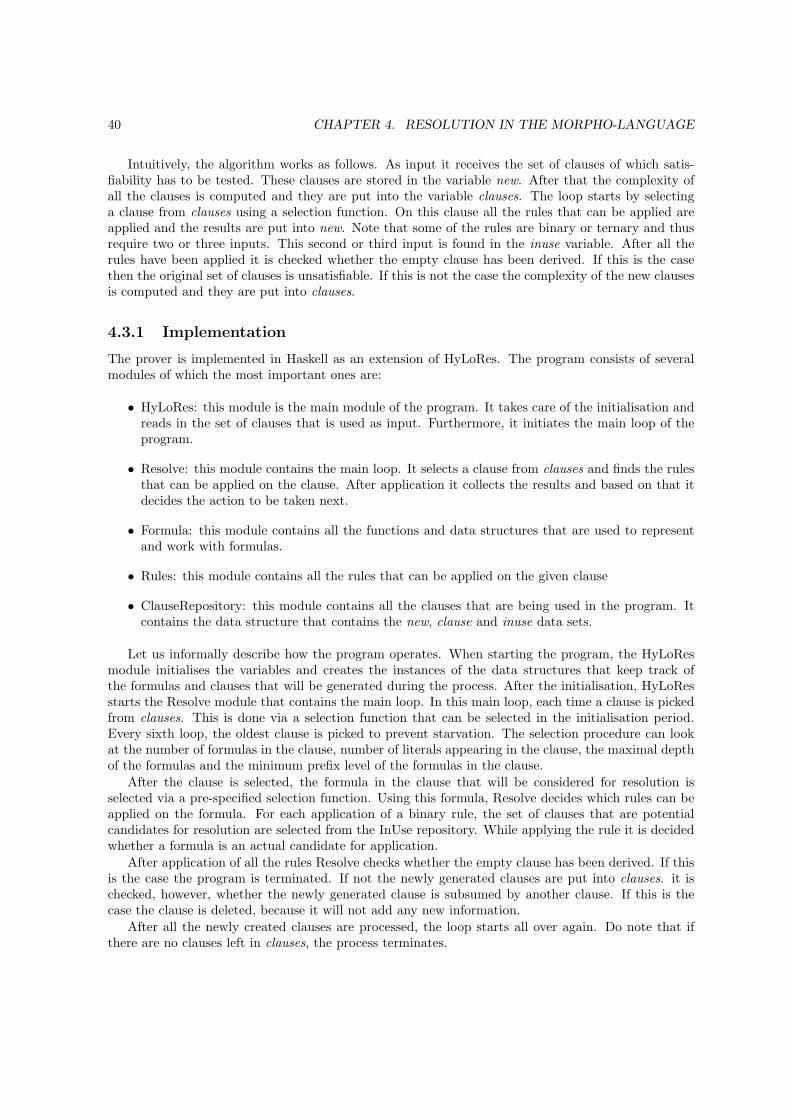
40 CHAPTER 4. RESOLUTION IN THE MORPHO-LANGUAGE
Intuitively, the algorithm works as follows. As input it receives the set of clauses of which satis-fiability has to be tested. These clauses are stored in the variable new. After that the complexity ofall the clauses is computed and they are put into the variable clauses. The loop starts by selectinga clause from clauses using a selection function. On this clause all the rules that can be applied areapplied and the results are put into new. Note that some of the rules are binary or ternary and thusrequire two or three inputs. This second or third input is found in the inuse variable. After all therules have been applied it is checked whether the empty clause has been derived. If this is the casethen the original set of clauses is unsatisfiable. If this is not the case the complexity of the new clausesis computed and they are put into clauses.
4.3.1 Implementation
The prover is implemented in Haskell as an extension of HyLoRes. The program consists of severalmodules of which the most important ones are:
• HyLoRes: this module is the main module of the program. It takes care of the initialisation andreads in the set of clauses that is used as input. Furthermore, it initiates the main loop of theprogram.
• Resolve: this module contains the main loop. It selects a clause from clauses and finds the rulesthat can be applied on the clause. After application it collects the results and based on that itdecides the action to be taken next.
• Formula: this module contains all the functions and data structures that are used to representand work with formulas.
• Rules: this module contains all the rules that can be applied on the given clause
• ClauseRepository: this module contains all the clauses that are being used in the program. Itcontains the data structure that contains the new, clause and inuse data sets.
Let us informally describe how the program operates. When starting the program, the HyLoResmodule initialises the variables and creates the instances of the data structures that keep track ofthe formulas and clauses that will be generated during the process. After the initialisation, HyLoResstarts the Resolve module that contains the main loop. In this main loop, each time a clause is pickedfrom clauses. This is done via a selection function that can be selected in the initialisation period.Every sixth loop, the oldest clause is picked to prevent starvation. The selection procedure can lookat the number of formulas in the clause, number of literals appearing in the clause, the maximal depthof the formulas and the minimum prefix level of the formulas in the clause.
After the clause is selected, the formula in the clause that will be considered for resolution isselected via a pre-specified selection function. Using this formula, Resolve decides which rules can beapplied on the formula. For each application of a binary rule, the set of clauses that are potentialcandidates for resolution are selected from the InUse repository. While applying the rule it is decidedwhether a formula is an actual candidate for application.
After application of all the rules Resolve checks whether the empty clause has been derived. If thisis the case the program is terminated. If not the newly generated clauses are put into clauses. it ischecked, however, whether the newly generated clause is subsumed by another clause. If this is thecase the clause is deleted, because it will not add any new information.
After all the newly created clauses are processed, the loop starts all over again. Do note that ifthere are no clauses left in clauses, the process terminates.

4.4. HYLOMORPHRES 41
4.4 HyLoMorphRes
Hylores is designed to handle unary modalities. However, the morpho-language contains both a binarymodality, a universal modality and a constant. Furthermore, the morpho-logic contains several axiomsthat need to be taken into account in proving theorems. This means that in adjusting the prover tocope with the morpho-logic, the following adjustments need to be made:
• the support for a binary modality has to be implemented,
• the support for the unary modality has to be implemented,
• the rules for the new binary modality have to be implemented,
• the rules for the axioms presented in Table 4.4 have to be implemented.
4.4.1 Adding support for the binary modalities
The original software was designed for the unary modalities 3 and 2. In adjusting the implementationof HyLoRes to fit the requirements for the morpho-language, this unary modality is chosen to representthe⊗ and⊗modalities. This leaves us with the binary modalities ⊕ and ⊕ and the universal modalitiesA and E.
The first step in implementing the support is to adjust the HyloParse.hs and HyloLex.hs modulesthat process the input of the program. The HyloParse module is created using the parser genera-tor Happy (http://www.haskell.org/happy). Adding new tokens for the ⊕, ⊕, A and E operators issufficient.
The module HyloLex uses the parsed tokens to create the data structures in which the formulasare captured. This is done in a case statement and adding a new case for the new tokens is sufficient.The functions that are used to create the data structures, and the definition of the data structureFormula are found in the module Formula.hs. This module also contains the code for calculating theorder of formulas and the code for creating new formulas and nominals from old formulas. Hence, thismodule needs to be adjusted as well.
Every formula belongs to a certain family. For example, the formula @i⊗j belongs to the familyof relations Relnm. Adding two new modalities means that five new families must be added. Thesenew families are PRelnm, AtPBox, AtPDia, Ef and Uf. Finally, the module PrettyPrint.hs needs tobe adjusted so that the correct information can be given to the user.
As for adding the rules, this must be done by adjusting Rules.hs and RuleMetadata.hs. Rules.hscontains the implementation for the different rules and RuleMetadata.hs contains some additional datathat is needed for the implementation in Rules.hs.
In implementing the rules, one rule was needed for the PBox family and one for the PDia family.Furthermore, two rules needed to be implemented in order for the paramodulation to be effective. Forthe universal modality four more rules needed implementation.
All the rules are applied in Resolve.hs, the module that contains the main loop. This is done by afunction that checks what family the selected formula is in and according to that information appliesa number of rules on this formula. Thus the appropriate families must be added to this function andfurthermore, it must be defined which families of formulas can be used as second argument to thebinary rules. This last part must be done in the module ClauseRepository.hs.
4.4.2 Adding support for the additional resolution rules
Adding support for the binary relations is only one part of what must be done. The additionalrules that take care of the extra requirements of the morpho-language must be implemented as well.
42 CHAPTER 4. RESOLUTION IN THE MORPHO-LANGUAGE
This means that Rule.hs, RuleMetadata.hs, Resolve.hs, ClauseRepository.hs and Formula.hs must bechanged.
The first thing that one can notice is that some of the rules require more that two arguments. InResolve different handlers are used when unary or binary rules are needed, hence a new handler mustbe implemented that can handle the application of a ternary rule.
Second, in Rules.hs the ternary rule must be introduced as a new type of rule. After these prereq-uisites are met, the rules can be implemented. This also means adjusting Formula.hs because that isthe only place in which formulas can be manipulated and new formulas can be created. The actualcontents of the type Formula is not known outside of this module.
It is not necessary to keep track of the application of rules, because every time a new clause iscreated this is recorded by the program and hence a clause will only occur once in the set clauses.
4.4.3 Summary
Several methods exists to automatically prove whether a certain formula or set of formulas is valid in acertain logic. We have chosen the method of resolution to create a theorem prover that is able to provetheorems for the morpho-logic. For this purpose a new resolution calculus is created. This calculus isimplemented in an existing theorem prover, called HyLoRes. The prover has been extend in such away that it can now cope with binary modalities, the universal modality and the extra requirementsfor the morpho-logic.
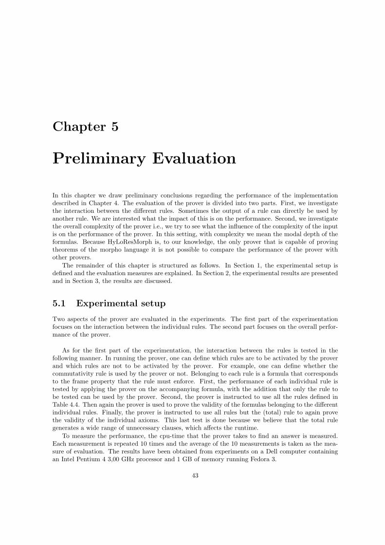
Chapter 5
Preliminary Evaluation
In this chapter we draw preliminary conclusions regarding the performance of the implementationdescribed in Chapter 4. The evaluation of the prover is divided into two parts. First, we investigatethe interaction between the different rules. Sometimes the output of a rule can directly be used byanother rule. We are interested what the impact of this is on the performance. Second, we investigatethe overall complexity of the prover i.e., we try to see what the influence of the complexity of the inputis on the performance of the prover. In this setting, with complexity we mean the modal depth of theformulas. Because HyLoResMorph is, to our knowledge, the only prover that is capable of provingtheorems of the morpho language it is not possible to compare the performance of the prover withother provers.
The remainder of this chapter is structured as follows. In Section 1, the experimental setup isdefined and the evaluation measures are explained. In Section 2, the experimental results are presentedand in Section 3, the results are discussed.
5.1 Experimental setup
Two aspects of the prover are evaluated in the experiments. The first part of the experimentationfocuses on the interaction between the individual rules. The second part focuses on the overall perfor-mance of the prover.
As for the first part of the experimentation, the interaction between the rules is tested in thefollowing manner. In running the prover, one can define which rules are to be activated by the proverand which rules are not to be activated by the prover. For example, one can define whether thecommutativity rule is used by the prover or not. Belonging to each rule is a formula that correspondsto the frame property that the rule must enforce. First, the performance of each individual rule istested by applying the prover on the accompanying formula, with the addition that only the rule tobe tested can be used by the prover. Second, the prover is instructed to use all the rules defined inTable 4.4. Then again the prover is used to prove the validity of the formulas belonging to the differentindividual rules. Finally, the prover is instructed to use all rules but the (total) rule to again provethe validity of the individual axioms. This last test is done because we believe that the total rulegenerates a wide range of unnecessary clauses, which affects the runtime.
To measure the performance, the cpu-time that the prover takes to find an answer is measured.Each measurement is repeated 10 times and the average of the 10 measurements is taken as the mea-sure of evaluation. The results have been obtained from experiments on a Dell computer containingan Intel Pentium 4 3,00 GHz processor and 1 GB of memory running Fedora 3.
43

44 CHAPTER 5. PRELIMINARY EVALUATION
The second part of the experimentation consists of testing the overall performance of the prover.This is done by giving the prover formulas of different complexity. With complexity the depth of theformulas is meant, i.e., the number of modalities that occur in the formula. For the test, 16 formulasof increasing modal depth have been generated. Four formulas of depth 0, four of depth 1, four ofdepth 2 and four of depth 3. As a measure of evaluation the cpu-time that the prover needs to findan answer is measured. Due to the possible non-termination a time-out of 15 minutes in cpu-time hasbeen put in place.
5.2 Results
First, we provide the results of the experiments to evaluate the interaction between the axioms. Nextthe results for the overall performance of the prover are presented.
5.2.1 Interaction
Figure 5.1: The individual rules.
The results of the three different tests are presented in the Figures 5.1, 5.2 and 5.3. On the verticalaxes the cpu-time is shown. Each bar represents one of the axioms belonging to the rules. One can seein Figure 5.1 that the prover needs more time to prove the validity of the (total) axiom than to provethe other axioms. Another thing one can observe is that if all the rules are turned on (see Figure 5.2),the overall time needed to find an answer increases as well, but not uniformly. For example, the timeneeded to compute an answer for the rev32, id1 and comm axioms increases significantly more thanthe time needed to compute an answer for the other axioms. The time needed to find an answer forthe ass1, ass2 and total axioms increases so much that they are of the charts. To illustrate this, thetime needed to compute an answer for the (total) axiom is approximately 200 seconds. As for the ass1and ass2 axioms, an out of memory message is given before an answer is reached. Figure 5.3 showsthat turning off the (total) rule reduces the needed time significantly, except for the id1 and commaxioms. Figure 5.3 also shows that the id1 and comm rules need significantly more time compared to
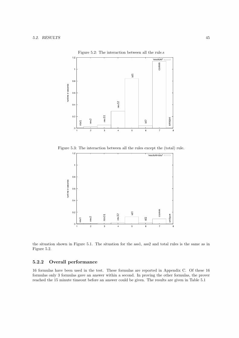
5.2. RESULTS 45
Figure 5.2: The interaction between all the rule.s
Figure 5.3: The interaction between all the rules except the (total) rule.
the situation shown in Figure 5.1. The situation for the ass1, ass2 and total rules is the same as inFigure 5.2.
5.2.2 Overall performance
16 formulas have been used in the test. These formulas are reported in Appendix C. Of these 16formulas only 3 formulas gave an answer within a second. In proving the other formulas, the proverreached the 15 minute timeout before an answer could be given. The results are given in Table 5.1

46 CHAPTER 5. PRELIMINARY EVALUATION
Modal Depth Formula elapsed timeModal Depth 0 Formula 1 Time out
Formula 2 3.0e−3 sFormula 3 Time outFormula 4 Time out
Modal Depth 1 Formula 1 Time outFormula 2 Time outFormula 3 5.5992e−2 sFormula 4 Time out
Modal Depth 2 Formula 1 4.252354 sFormula 2 Time outFormula 3 Time outFormula 4 Time out
Modal Depth 3 Formula 1 Time outFormula 2 Time outFormula 3 Time outFormula 4 Time out
Table 5.1: Overall performance results
5.3 Discussion
Clearly, performance is an issue for a prover such as HyLoRes. One can discern two different problems.The first problem lies in the fact that if a set of clauses is unsatisfiable the prover does not terminate.The second problem is the explosion of time-consumption if all the rules are used simultaneously.
The first problem is due to the total rule. The total rule takes as input formulas of the form ϕ andψ. Each nominal i that occurs in ϕ is combined with a nominal j that occurs in ψ to create the formulaEi ⊕ j. This new formula then creates a new nominal, on which the total rule can again be applied.A loop unrolls that does not stop unless the empty clause is found. Figure 5.1 is a good illustrationof this. As one can see, the prover needs far more time to prove the total axiom than it needs toprove another axiom. The results of the overall performance test also illustrate the non-termination.The three formulas that did give an answer where satisfiable, the other thirteen formulas where not.Therefore, they would never stop if the timeout would not have been placed.
The second problem is due to the interaction between several rules. In this interaction many clausesare generated that are not needed for the actual proof. This over-generation of clauses makes it harderfor the prover to find the proper clauses that are needed for the proof and has several causes. Wepinpoint the causes by looking at the Figures 5.2 and 5.3. The first observation that one can makeis that the performance shown in Figure 5.2 is about ten times as low as the performance shown inFigure 5.3. The only difference is that in Figure 5.3 the total rule is not used. Thus the total rule isa big cause of over-generation.
The second observation that one can make is that the rev32, id1 and comm axioms see a greaterincrease in needed time than the other axioms (not looking at ass1, ass2 and total). To see whichrules are actually used in the proof we turn our attention to Tables 5.2, 5.3 and 5.4. In these tablesthe rules that are used in the corresponding proofs are shown, together with the number of times eachrule is invoked. One can see that the rev32, id2, comm, ass1 and ass2 rules are the rules that have themost invocations. Looking at the specific rules one can see why this is the case.
First, we note that the rev32 and id2 rules take a formula of the form @jϕ and a formula of theform @ie. They respectively create formulas of the form @ij ⊕ (⊗j) and @ji⊕ j. The former formula

5.4. SUMMARY 47
can be decomposed in @ij ⊕ s and @s ⊗ j, enabling the application of the comm rule, and again theid2 rule and the rev32 rule. After this, we have the formulas @ij⊕s and @si⊕j, which can be used bythe ass1 rule, which introduces a new nominal z and a new formula of the form @zϕ. On this formulaagain id2 and rev32 can be applied, starting the loop all over again.
Looking at the Tables 5.2, 5.3, 5.4 one must also note that the usage of the total rule has littleeffect on the usage of the other rules. However, because the total rule can “feed” itself, i.e., it canindirectly be applied on its own result, thus yielding a high number of applications.
We end by making the observation that the runtimes that are given in Table 5.1 are increasing.Although no graph is made, one can see that the needed time increases very fast. Where a formulaof depth 0 needs a millisecond, a formula of depth 1 needs ten milliseconds and a formula of depth 2needs 4 seconds. Without generalizing, one might say that it is possible that the time-consumptioncould grow exponentially with the complexity of the formula.
Summarizing, the main problem in the interaction between the rules is the creation of new nominals.Thus, if one wants to improve the performance of the prover, the creation of new nominals must becontrolled further. For example, note that in the application of the ass1 rule on formulas of the form@ij1 ⊕ j2 and @j2s1 ⊕ s2, new formulas of the form @iz ⊕ s2 and @zj1 ⊕ s1 are created. On thesetwo formulas the ass2 rule can be applied, creating @ij1 ⊕ z1 and @z1s1 ⊕ s2. By application of theunique rule z1 and j2 must point to the same world, thus if one can make the calculus recognize thissituation one can stop the generation of a wide range of unnecessary rules.
Rules applications (all without total) applications (all)R Box rule: 5 5R PBox rule: 1 1R PDia rule: 8 9R Par rule: 33 48R ParRel rule: 1 1R Conj rule: 1 1R Rev1 rule: 3 3R Rev2 rule: 3 4R Rev31 rule: 4 5R Rev32 rule: 58 74R Id1 rule: 8 12R Id2 rule: 34 40R Comm rule: 16 26R Ass1 rule: 2 4R Ass2 rule: 3 6R Udia: - 18R Uniq: - 1R total rule: - 646
Table 5.2: Rule application for the rev32 axiom
5.4 Summary
The theorem prover discussed in chapter 4 is tested. The results from these tests show that the mainperformance problem of the prover is due to the (total) rule. Although this prover is far from perfect,it is a first step in finding a way of automated reasoning with the morpho-logic.

48 CHAPTER 5. PRELIMINARY EVALUATION
Rules applications (all without total) applications (all)R ResP rule: 1 1R Box rule: 7 6R PDia rule: 13 10R Par rule: 35 20R ParPRel rule: 2 -R Conj rule: 1 1R Rev1 rule: 6 6R Rev2 rule: 6 6R Rev31 rule: 7 5R Rev32 rule: 85 65R Id1 rule: 12 9R Id2 rule: 63 54R Comm rule: 33 21R Ass1 rule: 39 23R Ass2 rule: 56 55R Udia: - 16R Uniq: 6 -R total rule: - 1068
Table 5.3: Rule application for the Id1 axiom
Rules applications (all without total) applications (all)R ResP rule: 2 2R Box rule: 6 7R PBox rule: 7 6R PDia rule: 7 7R Par rule: 15 8R Conj rule: 1 1R Rev1 rule: 6 6R Rev2 rule: 6 6R Rev31 rule: 6 5R Rev32 rule: 58 52R Id1 rule: 11 9R Id2 rule: 55 55R Comm rule: 23 17R Ass1 rule: 32 32R Ass2 rule: 53 73R Udia: - 22R Uniq: 4 1R total rule: - 1509
Table 5.4: Rule application for the Comm axiom
Chapter 6
The Morpho-Language Landscape
6.1 Introduction
The Morpho-language defined in Chapter 3 is able to talk about Mathematical Morphology’s basicconstituents: dilation and erosion. Just as Mathematical Morphology is more than simply applying thedilation and erosion, the morpho-language can express more than just the dilation and erosion. Mostapplications of MM are build up out of several dilations and erosions with several specific structuringelements. One group of these applications are the filters. Filters are operations on an image that,the name already gives it away, filter out some information captured in the image. There are severalclasses of images, namely binary, grey scale and color images. The morpho-language can be appliedto all of them but for reasons of simplicity we will only look at the filters for binary images. We areinterested in filters that we can express in the morpho-language. That is, if we can express the filtersin the language, we can reason with them and we can automatically see what the properties of thefilters are. It turns out that not all the filters can be expressed in the morpho-language. Therefore wewill also try to see what extensions of the language will be needed to be able to express these filters
Filters are only one interesting application of MM. In images a lot of spatial information is stored.Therefore we could also consider the intuitive spatial relations between regions and the role that MMand the morpho-language can play in finding and representing these relations. Qualitative SpatialReasoning (QSR) deals with the formalization of space. It tries to find a formal language that issuited to represent spatial concepts and can be used to reason with these concepts. MM is a formalismthat searches for geometric properties of shapes. These geometric properties can be used in QSR. Itwould be interesting to see to what extend the morpho-language is suited for QSR and which spatialconcepts can be expressed in the language.
The remainder of this chapter is structured as follows. In Section 2, we first explain what filtersare and what different properties they have. We identify which filters can be represented in themorpho-language and which cannot. According to this we identify the extensions that we need inorder to be able to express the remaining filters. In Section 3, we recall the basic concepts behindQSR, what has already been done in the field and what role MM has already played in it, whichspatial relations can be expressed in the morpho-language and what extensions need to be introducedto express further concepts such as nearness. Finally, in Section 4 we suggest a formalization for theextensions overviewed in the present morpho-language landscape.
49

50 CHAPTER 6. THE MORPHO-LANGUAGE LANDSCAPE
6.2 Binary filters
Morphological filters are operations on images that filter out certain information contained in theimage. For example, openings and closings are very basic filters that can filter out irregularities inan image by removing regions that cannot contain a certain structuring element, respectively fillingholes that are smaller than a certain structuring element. Openings and closings are useful becausewhen an image is recorded, noise could cause certain unconnected regions to be connected or certainconnected regions to be unconnected. In this context, a region is connected if for each set of points(x, y) in the region, there is a path from x to y that does not leave the region.
More formally, a filter f is an operator f : V 7→ V that takes as input an element of V and returnsan element of V . In the case of binary images, V = P(R2). Filters can be classified by using thefollowing properties:
• translation invariant: A filter f is translation invariant if, given a translation t, for all Af(t(A)) = t(f(A)). That is, first translating an image and than applying the filter yields thesame result as first applying the filter and than translating the result.
• increasing: A filter f is increasing if for all A and B, given the fact that A ⊆ B, f(A) ⊆ f(B).For example, dilation and erosion are both increasing operators.
• extensive: A filter f is extensive if for all A, A ⊆ f(A). In other words, the resulting region isalways bigger than the original region.
• anti-extensive: A filter f is anti-extensive if for all A, f(A) ⊆ A. In other words, the resultingregion always lies inside the original region.
• idempotence: A filter f is idempotent if applying the filter twice yields the same result asapplying the filter once. More formally, for all A, f(f(A)) = f(A).
In [22] a set of binary filters is presented. This set of binary filters is a set that is widely used inpractice in the fields of medical imaging, mineralogy and OCR. We only look at filters presented in [22].
6.2.1 Expressible filters
Some filters are expressible in the morpho-language. The constituents of the morpho-language are,besides the dilation and erosion, the reverse operator, the Boolean complement, the intersection andthe union. The question is which filters in [22] are expressible in the morpho-language. All theexpressible binary filters are collected in Table 6.1. We divide the filters in translation invariant filtersand filters that are not translation invariant.
Translation invariant filters
Let us first consider the opening and closing. The opening and closing are used to filter out noisefrom the image. What kind of noise is filtered depends on the structuring element that is used. Theopening has the form
A ◦B = (AB)⊕B
The closing has the formA •B = (A⊕B)B
Where AB = ¬(¬A⊕ ⊗ B). The opening is extensive, idempotent and increasing. The closing alsois idempotent and increasing but anti-extensive.

6.2. BINARY FILTERS 51
From the opening and closing the opening top-hat and closing top-hat can be constructed. Thesetwo filters give what is removed in the opening or added in the closing respectively. The openingtop-hat has the form A◦B = A−A ◦B. If we translate this to the morpho-language we get
A◦B = A ∧ ¬(A ◦B)
The closing top-hat has the form A•B = (A ◦B)−A. If we translate this to the morpho-language weget
A•B = (A •B) ∧ ¬AThe opening top-hat is anti-extensive, but the closing top-hat has non of the above mentioned prop-erties.
There are three types of filters that give a boundary of a shape. These are the internal boundaryA− (AB), the external boundary (A⊕B)−A and the morphological gradient (A⊕B)− (AB).In the morpho-language we can express these filters in the following manner. The internal boundaryis equivalent to the expression
A ∧ ¬(AB)
the external boundary to the expression
(A⊕B) ∧ ¬A
and the morphological gradient to the expression
(A⊕B) ∧ ¬(AB)
As for the properties of these filters, the internal boundary is anti-extensive. The other boundaryoperators do not have any of the properties listed in Section 6.2.
The next operator we express in the morpho-language is the hit-or-miss transform. This operatoris mainly used to filter out objects that do have certain properties but lack others. The form of thehit-and-miss transform is A~ T = ((AE)− (A F )) where T = (E,F ) and E ⊂ F . The fact thatE is a subset of F means that E and F are disjoint. The expression
A~ T = ((AE) ∧ ¬(AF )) ∧ U(E → ¬F )
where T = (E,F ) is the morpho-language equivalent of this filter. T is called the hit-or-miss template.The function of U(E → ¬F ) is to capture the fact that E must be a subset of F .
Using the hit-or-miss transform we can create the thinning filter. The thinning filter takes a shapeand removes the outer layer of the shape. The exact form of this outer layer is dependent on thestructuring element that is being used. In MM, thinning is defined as A � T = A − (A ~ T ). In themorpho-language this definition is equivalent to
A� T = A ∧ ¬(A~ T )
Sequential thinning is the successive application of a sequence of thinnings. Given a set of hit-or-misstemplates, T1, T2, ..., Tn, sequential thinning is (((A� T1)� T2)...� Tn).
Non translation invariant filters
Interestingly, only two expressible filters are not translation invariant. These two filters are the con-ditional dilation and conditional erosion. Both are increasing operators and have the form A⊕C B =(A⊕B) ∩ C and (AC B) = (AB) ∩ C respectively. The goal of these two operators is to restrictthe range of the operator. Where the result of the normal dilation/erosion can range over the entireR2, the range of the conditional dilation/erosion will be in C. This is illustrated in Figure 6.1. In themorpho-language these operators get the following form:
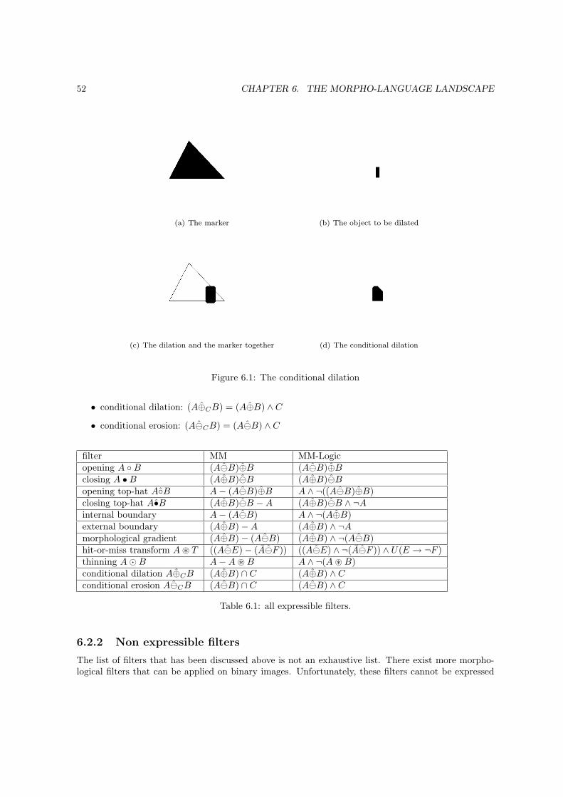
52 CHAPTER 6. THE MORPHO-LANGUAGE LANDSCAPE
(a) The marker (b) The object to be dilated
(c) The dilation and the marker together (d) The conditional dilation
Figure 6.1: The conditional dilation
• conditional dilation: (A⊕CB) = (A⊕B) ∧ C
• conditional erosion: (ACB) = (AB) ∧ C
filter MM MM-Logicopening A ◦B (AB)⊕B (AB)⊕Bclosing A •B (A⊕B)B (A⊕B)Bopening top-hat A◦B A− (AB)⊕B A ∧ ¬((AB)⊕B)closing top-hat A•B (A⊕B)B −A (A⊕B)B ∧ ¬Ainternal boundary A− (AB) A ∧ ¬(A⊕B)external boundary (A⊕B)−A (A⊕B) ∧ ¬Amorphological gradient (A⊕B)− (AB) (A⊕B) ∧ ¬(AB)hit-or-miss transform A~ T ((AE)− (AF )) ((AE) ∧ ¬(AF )) ∧ U(E → ¬F )thinning A�B A−A~B A ∧ ¬(A~B)conditional dilation A⊕CB (A⊕B) ∩ C (A⊕B) ∧ Cconditional erosion ACB (AB) ∩ C (AB) ∧ C
Table 6.1: all expressible filters.
6.2.2 Non expressible filters
The list of filters that has been discussed above is not an exhaustive list. There exist more morpho-logical filters that can be applied on binary images. Unfortunately, these filters cannot be expressed

6.2. BINARY FILTERS 53
(a) Picture with noise (b) After the salt and pepper filterhas been used
Figure 6.2: The salt and pepper filter.
in the morpho language.
Translation invariant filters
It turns out that there is only one translation invariant filter described in [22] that is not expressiblein the morpho-language. This is the Alternating Sequence Filter (ASF). Informally, the ASF is afilter that alternates the openings and closings. Each time a combination of opening and closing isperformed the structuring element is enlarged by dilating it with the original structuring element.The ASF has the form ASFn
B(S) = ((((S • B) ◦ B) • 2B) ◦ 2B)... • nB) ◦ nB). nB is a shortcut for(((B ⊕1 B)⊕2 B)...⊕n−1 B) in which ⊕m tells us that it is the mth application of the dilation. Justas the opening and closing are used to filter out noise, the ASF is used to filter out noise. One niceexample is the salt-n-pepper filter, see Figure 6.2. It filters out both white and black noise. In orderto represent this filter in the morpho-language, we need to be able to count the number of applicationsof the dilation.
Non translation invariant filters
The size-n geodesic dilation and erosion are two filters that serve as building blocks for further filterapplications. Their forms are S⊕n
T B and SnT B respectively. ⊕n
T means that the conditional dilationis performed n times.
Using these two operations we can reconstruct parts of an image with the so called inf-geodesicand sup-geodesic reconstruction:
• inf-geodesic reconstruction: T 4B S = (S ⊕∞T B)
• sup-geodesic reconstruction: T 5B S = (S ∞T B)
The S works as a marker and T is the picture from which we want to reconstruct. What one doesis select several points in an image (the marker), and find the connected components of these pointsby successively dilating them. Since we restrict the outcome to the original picture, at some point thedilations will have no more effect. In theory the dilation is performed infinitely, but in practice onecan stop when there are no further changes. These reconstructions assume that the marker is given.
It is also possible to find the markers in the image automatically. The following 3 filters do exactlythat.

54 CHAPTER 6. THE MORPHO-LANGUAGE LANDSCAPE
• reconstructive opening: A ◦E B = A4E (A ◦B)
• reconstructive opening top-hat: A◦EB = A− (A ◦E B)
• reconstructive closing: A •E B = (A •B)5E A
In the case of the reconstructive opening, the marker is found by opening the original image Awith a structuring element B. This filter can be used to detect shapes with certain properties in animage. The reconstructive opening top-hat can be used to delete shapes with certain properties froman image. The reconstructive closing is a connected operator. In short this means that it makes theimage coarser. It deletes all the regions in the complement of the image that are not fully filled by theclosing.
All the reconstructions are based on the size-n geodesic dilation and erosion. What needs tobe added to the morpho-language is therefore the ability to count the number of occurrences of aconditional dilation/erosion.
On can also combine several reconstructive openings/closing. This way one creates a reconstructiveτ -opening. What one does is, given a set of structuring elements {B1, ...Bn}, find the reconstructiveopening of all these Bi with the same image. {B1, ..., Bn} is called the base. This results in thefollowing operation:
n⋃i=1
A ◦E Bi
The reconstructive radial opening is a special instance of such a reconstructive τ -opening. Thebase is a set of linear structuring elements of varying angle. This brings us to the following propertythat would be nice to have. The ability to say something about the shape of the structuring elements.Or, more generally, to be able to specify properties of regions. For example, one might want to definea sphere or a directional element.
Two other filters that need the ability to specify the shape of a region are the bounded dilationand erosion. Both are a special instance of the conditional dilation and erosion respectively in whichthe condition is the region of the image S, denoted by V [S].
In summary, there are filters that cannot be expressed by the morpho-language. If we want toincorporate them we need to add to the language the ability to count the number of applications ofa conditional dilation or erosion and we should have the ability to specify properties of a region. Forexample, we want to be able to say that a region denotes a circle, or that it is convex.
6.3 Qualitative Spatial Reasoning
In our every day life we make use of spatial reasoning. We use it to navigate through a room, weuse it to recognize objects and so on. The field of Qualitative Spatial Reasoning (QSR) deals withthe formalization of spatial reasoning. In order to reason about space one needs to have a languagein which one can represent spatial concepts and an inference mechanism. Finding an appropriatelanguage has been the mayor focus of QSR in the last decades. For an overview of spatial reasoningsee [19] and [36].
One of the most influential QSR languages has been the RCC (Region Connected Calculus)from [31] and the RCC-8 calculus defined in [30]. In Figure 6.3 the eight different relations areshown. One can see them as the spatial equivalent of the Allen relations ([5], [41]) for time. TheRCC-8 language is based on the notion of connection. In [20] three definitions of connection are given.Just to illustrate the concept of connection (see also Figure 6.4) we give one of these definitions:
• C(x, y) ⇔ x ∩ c(y) 6= ∅ or c(x) ∩ y 6= ∅
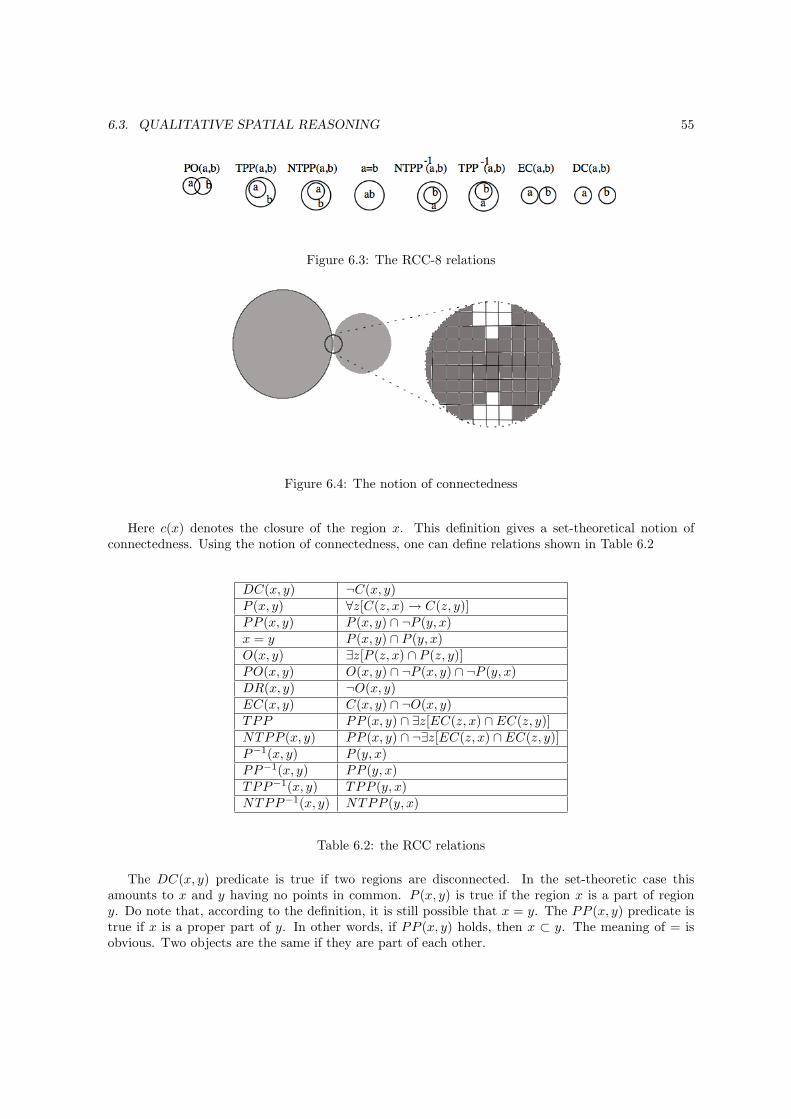
6.3. QUALITATIVE SPATIAL REASONING 55
Figure 6.3: The RCC-8 relations
Figure 6.4: The notion of connectedness
Here c(x) denotes the closure of the region x. This definition gives a set-theoretical notion ofconnectedness. Using the notion of connectedness, one can define relations shown in Table 6.2
DC(x, y) ¬C(x, y)P (x, y) ∀z[C(z, x) → C(z, y)]PP (x, y) P (x, y) ∩ ¬P (y, x)x = y P (x, y) ∩ P (y, x)O(x, y) ∃z[P (z, x) ∩ P (z, y)]PO(x, y) O(x, y) ∩ ¬P (x, y) ∩ ¬P (y, x)DR(x, y) ¬O(x, y)EC(x, y) C(x, y) ∩ ¬O(x, y)TPP PP (x, y) ∩ ∃z[EC(z, x) ∩ EC(z, y)]NTPP (x, y) PP (x, y) ∩ ¬∃z[EC(z, x) ∩ EC(z, y)]P−1(x, y) P (y, x)PP−1(x, y) PP (y, x)TPP−1(x, y) TPP (y, x)NTPP−1(x, y) NTPP (y, x)
Table 6.2: the RCC relations
The DC(x, y) predicate is true if two regions are disconnected. In the set-theoretic case thisamounts to x and y having no points in common. P (x, y) is true if the region x is a part of regiony. Do note that, according to the definition, it is still possible that x = y. The PP (x, y) predicate istrue if x is a proper part of y. In other words, if PP (x, y) holds, then x ⊂ y. The meaning of = isobvious. Two objects are the same if they are part of each other.
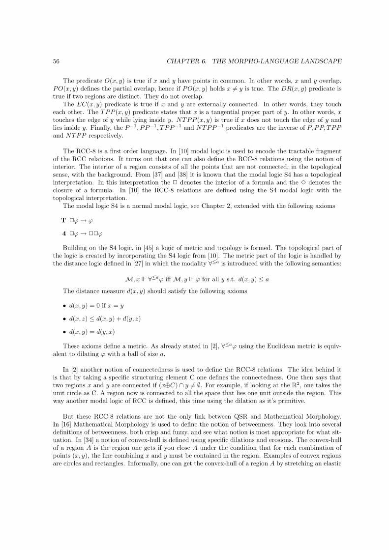
56 CHAPTER 6. THE MORPHO-LANGUAGE LANDSCAPE
The predicate O(x, y) is true if x and y have points in common. In other words, x and y overlap.PO(x, y) defines the partial overlap, hence if PO(x, y) holds x 6= y is true. The DR(x, y) predicate istrue if two regions are distinct. They do not overlap.
The EC(x, y) predicate is true if x and y are externally connected. In other words, they toucheach other. The TPP (x, y) predicate states that x is a tangential proper part of y. In other words, xtouches the edge of y while lying inside y. NTPP (x, y) is true if x does not touch the edge of y andlies inside y. Finally, the P−1, PP−1, TPP−1 and NTPP−1 predicates are the inverse of P, PP, TPPand NTPP respectively.
The RCC-8 is a first order language. In [10] modal logic is used to encode the tractable fragmentof the RCC relations. It turns out that one can also define the RCC-8 relations using the notion ofinterior. The interior of a region consists of all the points that are not connected, in the topologicalsense, with the background. From [37] and [38] it is known that the modal logic S4 has a topologicalinterpretation. In this interpretation the 2 denotes the interior of a formula and the 3 denotes theclosure of a formula. In [10] the RCC-8 relations are defined using the S4 modal logic with thetopological interpretation.
The modal logic S4 is a normal modal logic, see Chapter 2, extended with the following axioms
T 2ϕ→ ϕ
4 2ϕ→ 22ϕ
Building on the S4 logic, in [45] a logic of metric and topology is formed. The topological part ofthe logic is created by incorporating the S4 logic from [10]. The metric part of the logic is handled bythe distance logic defined in [27] in which the modality ∀≤a is introduced with the following semantics:
M, x ∀≤aϕ iff M, y ϕ for all y s.t. d(x, y) ≤ a
The distance measure d(x, y) should satisfy the following axioms
• d(x, y) = 0 if x = y
• d(x, z) ≤ d(x, y) + d(y, z)
• d(x, y) = d(y, x)
These axioms define a metric. As already stated in [2], ∀≤aϕ using the Euclidean metric is equiv-alent to dilating ϕ with a ball of size a.
In [2] another notion of connectedness is used to define the RCC-8 relations. The idea behind itis that by taking a specific structuring element C one defines the connectedness. One then says thattwo regions x and y are connected if (x⊕C) ∩ y 6= ∅. For example, if looking at the R2, one takes theunit circle as C. A region now is connected to all the space that lies one unit outside the region. Thisway another modal logic of RCC is defined, this time using the dilation as it’s primitive.
But these RCC-8 relations are not the only link between QSR and Mathematical Morphology.In [16] Mathematical Morphology is used to define the notion of betweenness. They look into severaldefinitions of betweenness, both crisp and fuzzy, and see what notion is most appropriate for what sit-uation. In [34] a notion of convex-hull is defined using specific dilations and erosions. The convex-hullof a region A is the region one gets if you close A under the condition that for each combination ofpoints (x, y), the line combining x and y must be contained in the region. Examples of convex regionsare circles and rectangles. Informally, one can get the convex-hull of a region A by stretching an elastic
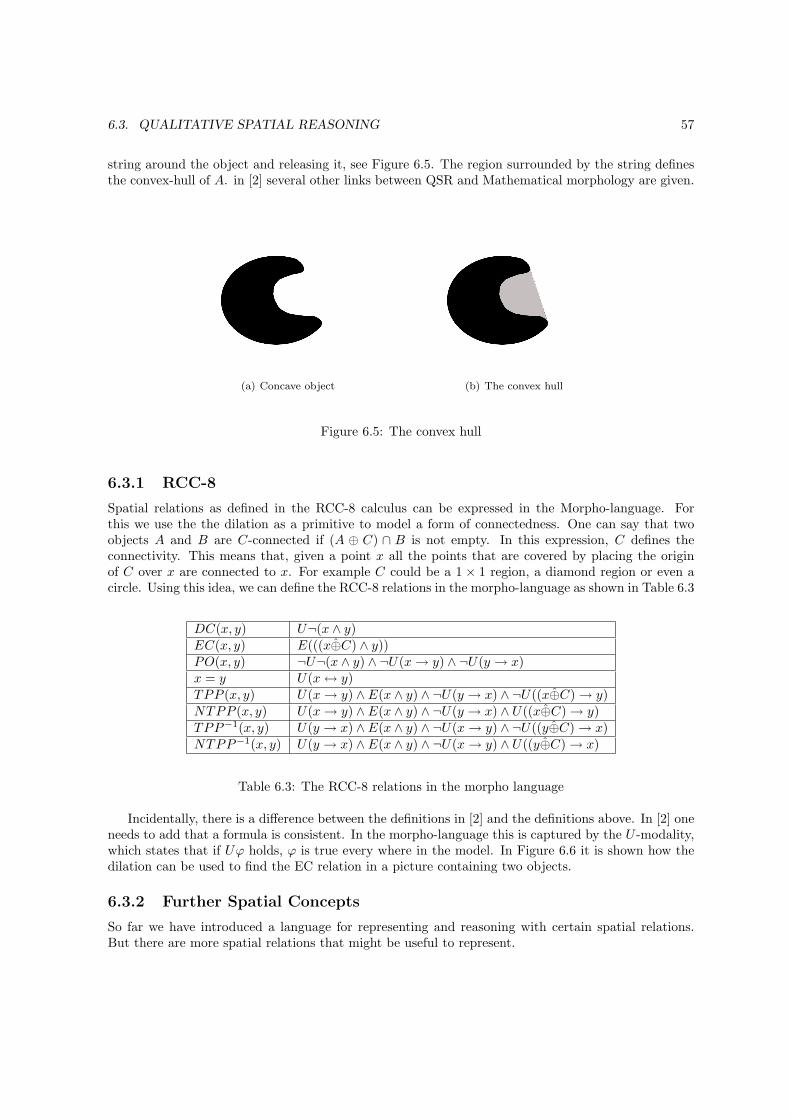
6.3. QUALITATIVE SPATIAL REASONING 57
string around the object and releasing it, see Figure 6.5. The region surrounded by the string definesthe convex-hull of A. in [2] several other links between QSR and Mathematical morphology are given.
(a) Concave object (b) The convex hull
Figure 6.5: The convex hull
6.3.1 RCC-8
Spatial relations as defined in the RCC-8 calculus can be expressed in the Morpho-language. Forthis we use the the dilation as a primitive to model a form of connectedness. One can say that twoobjects A and B are C-connected if (A ⊕ C) ∩ B is not empty. In this expression, C defines theconnectivity. This means that, given a point x all the points that are covered by placing the originof C over x are connected to x. For example C could be a 1 × 1 region, a diamond region or even acircle. Using this idea, we can define the RCC-8 relations in the morpho-language as shown in Table 6.3
DC(x, y) U¬(x ∧ y)EC(x, y) E(((x⊕C) ∧ y))PO(x, y) ¬U¬(x ∧ y) ∧ ¬U(x→ y) ∧ ¬U(y → x)x = y U(x↔ y)TPP (x, y) U(x→ y) ∧ E(x ∧ y) ∧ ¬U(y → x) ∧ ¬U((x⊕C) → y)NTPP (x, y) U(x→ y) ∧ E(x ∧ y) ∧ ¬U(y → x) ∧ U((x⊕C) → y)TPP−1(x, y) U(y → x) ∧ E(x ∧ y) ∧ ¬U(x→ y) ∧ ¬U((y⊕C) → x)NTPP−1(x, y) U(y → x) ∧ E(x ∧ y) ∧ ¬U(x→ y) ∧ U((y⊕C) → x)
Table 6.3: The RCC-8 relations in the morpho language
Incidentally, there is a difference between the definitions in [2] and the definitions above. In [2] oneneeds to add that a formula is consistent. In the morpho-language this is captured by the U -modality,which states that if Uϕ holds, ϕ is true every where in the model. In Figure 6.6 it is shown how thedilation can be used to find the EC relation in a picture containing two objects.
6.3.2 Further Spatial Concepts
So far we have introduced a language for representing and reasoning with certain spatial relations.But there are more spatial relations that might be useful to represent.
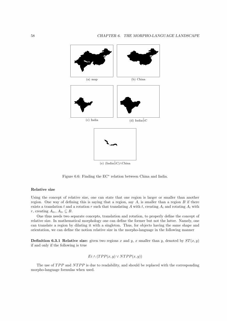
58 CHAPTER 6. THE MORPHO-LANGUAGE LANDSCAPE
(a) map (b) China
(c) India (d) India ˆ⊕C
(e) (India ˆ⊕C)∧China
Figure 6.6: Finding the EC∗ relation between China and India.
Relative size
Using the concept of relative size, one can state that one region is larger or smaller than anotherregion. One way of defining this is saying that a region, say A, is smaller than a region B if thereexists a translation t and a rotation r such that translating A with t, creating At and rotating At withr, creating Atr, Atr ⊆ B.
One thus needs two separate concepts, translation and rotation, to properly define the concept ofrelative size. In mathematical morphology one can define the former but not the latter. Namely, onecan translate a region by dilating it with a singleton. Thus, for objects having the same shape andorientation, we can define the notion relative size in the morpho-language in the following manner
Definition 6.3.1 Relative size: given two regions x and y, x smaller than y, denoted by ST (x, y)if and only if the following is true
Ei ∧ (TPP (x, y) ∨NTPP (x, y))
The use of TPP and NTPP is due to readability, and should be replaced with the correspondingmorpho-language formulas when used.
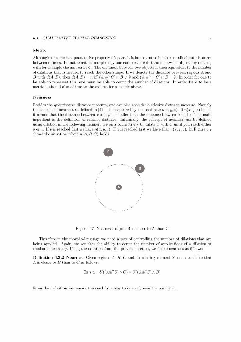
6.3. QUALITATIVE SPATIAL REASONING 59
Metric
Although a metric is a quantitative property of space, it is important to be able to talk about distancesbetween objects. In mathematical morphology one can measure distances between objects by dilatingwith for example the unit circle C. The distances between two objects is then equivalent to the numberof dilations that is needed to reach the other shape. If we denote the distance between regions A andB with d(A,B), then d(A,B) = n iff (A⊕n C) ∩B 6= ∅ and (A⊕n−1 C) ∩B = ∅. In order for one tobe able to represent this, one must be able to count the number of dilations. In order for d to be ametric it should also adhere to the axioms for a metric above.
Nearness
Besides the quantitative distance measure, one can also consider a relative distance measure. Namelythe concept of nearness as defined in [41]. It is captured by the predicate n(x, y, z). If n(x, y, z) holds,it means that the distance between x and y is smaller than the distance between x and z. The mainingredient is the definition of relative distance. Informally, the concept of nearness can be definedusing dilation in the following manner. Given a connectivity C, dilate x with C until you reach eithery or z. If y is reached first we have n(x, y, z). If z is reached first we have that n(x, z, y). In Figure 6.7shows the situation where n(A,B,C) holds.
Figure 6.7: Nearness: object B is closer to A than C
Therefore in the morpho-language we need a way of controlling the number of dilations that arebeing applied. Again, we see that the ability to count the number of applications of a dilation orerosion is necessary. Using the notation from the previous section, we define nearness as follows:
Definition 6.3.2 Nearness Given regions A, B, C and structuring element S, one can define thatA is closer to B than to C as follows:
∃n s.t. ¬U((A⊕nS) ∧ C) ∧ U((A⊕n
S) ∧B)
From the definition we remark the need for a way to quantify over the number n.
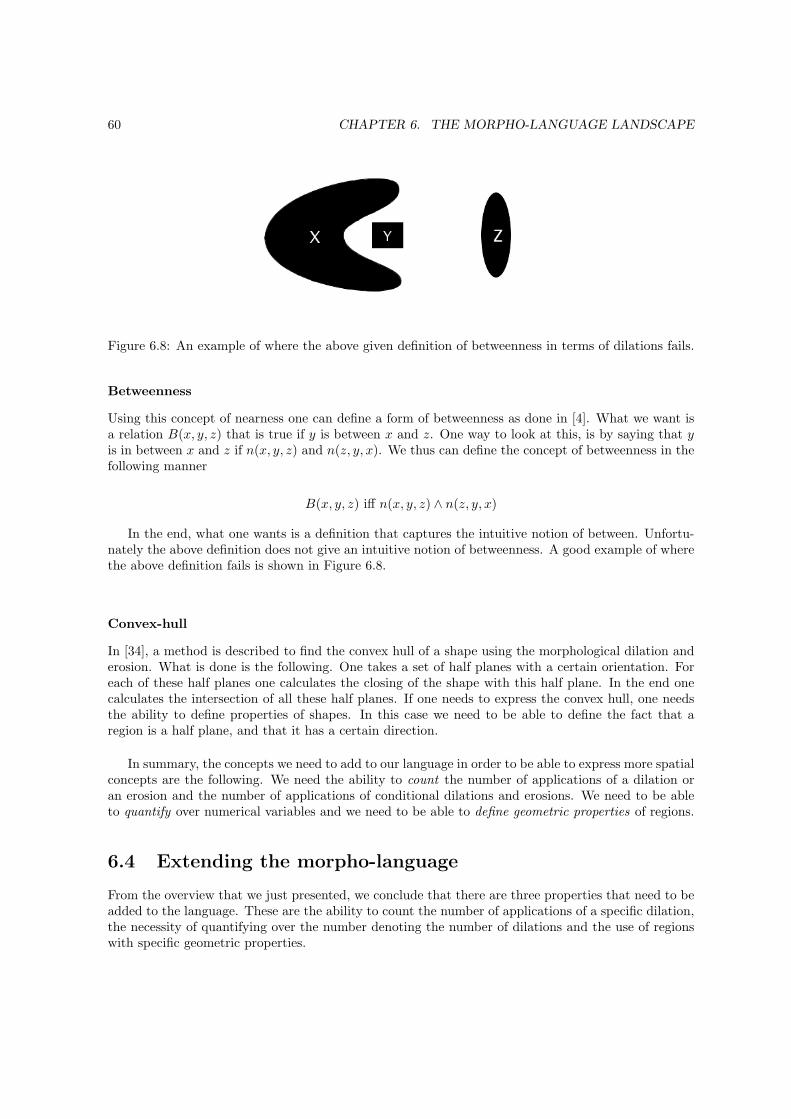
60 CHAPTER 6. THE MORPHO-LANGUAGE LANDSCAPE
Figure 6.8: An example of where the above given definition of betweenness in terms of dilations fails.
Betweenness
Using this concept of nearness one can define a form of betweenness as done in [4]. What we want isa relation B(x, y, z) that is true if y is between x and z. One way to look at this, is by saying that yis in between x and z if n(x, y, z) and n(z, y, x). We thus can define the concept of betweenness in thefollowing manner
B(x, y, z) iff n(x, y, z) ∧ n(z, y, x)
In the end, what one wants is a definition that captures the intuitive notion of between. Unfortu-nately the above definition does not give an intuitive notion of betweenness. A good example of wherethe above definition fails is shown in Figure 6.8.
Convex-hull
In [34], a method is described to find the convex hull of a shape using the morphological dilation anderosion. What is done is the following. One takes a set of half planes with a certain orientation. Foreach of these half planes one calculates the closing of the shape with this half plane. In the end onecalculates the intersection of all these half planes. If one needs to express the convex hull, one needsthe ability to define properties of shapes. In this case we need to be able to define the fact that aregion is a half plane, and that it has a certain direction.
In summary, the concepts we need to add to our language in order to be able to express more spatialconcepts are the following. We need the ability to count the number of applications of a dilation oran erosion and the number of applications of conditional dilations and erosions. We need to be ableto quantify over numerical variables and we need to be able to define geometric properties of regions.
6.4 Extending the morpho-language
From the overview that we just presented, we conclude that there are three properties that need to beadded to the language. These are the ability to count the number of applications of a specific dilation,the necessity of quantifying over the number denoting the number of dilations and the use of regionswith specific geometric properties.
6.4. EXTENDING THE MORPHO-LANGUAGE 61
6.4.1 Counting
The ability of counting is necessary both for the representation of a large group of morphologicalfilters, for enabling the definition of relative distance and for giving the possibility of defining a metricon the underlying space. By the following notation
A⊕n B
we represent the dilation of A with B repeated n times. For example, A ⊕3 B is equivalent to(((A ⊕ B) ⊕ B) ⊕ B). One can look at ⊕n as a new modality, but then the fact that A ⊕n B isequivalent to A⊕Bn where Bn denotes that B is dilated with itself n times tells us that it’s behavioris as the usual dilation. Hence the same axioms that apply to the usual dilation also apply to ⊕n.Furthermore, one must define the interaction between different n. This could be done by adding thefollowing axioms:
• A⊕B → A⊕nB for every n > 1
• A⊕nB → A⊕m B for all n,m s.t. n < m
Note that adding these axioms implies that e→ B. Whether this follows from the axioms we do notknow.
The counting ability significantly increases the expressive power and allows for the representationof many more filters. Interestingly, this opens a new issue of completeness for the language which isbeyond the scope of the present treatment. The question now arises if this is enough for defining bothrelative distance and metric distance.
The answer to the first part of the question, concerning relative distance, is positive. The onlyproperty a relative distance should have is transitivity. If B is closer to A than C, and C is closer toA than D, it should be the case that B is closer to A than D. This is the case with Definition 6.3.2of relative distance. Suppose that n(A,B,C) and that S is the structuring element. That means thatthere is an n such that A⊕n S ∩B is nonempty and A⊕n S ∩C is empty. Furthermore, suppose thatn(A,C,D), which gives us that there is an m such that A⊕m S ∩ C 6= ∅ and A⊕m S ∩D = ∅. Thisgives us that A⊕n S → A⊕m S. Towards a contradiction suppose that n(A,D,B). Thus there mustbe an l such that A ⊕l S ∩D 6= ∅ and A ⊕l S ∩ B = ∅ which gives us that A ⊕m S → A ⊕l S. Fromthis we can conclude that A⊕n S → A⊕l S. However, then it cannot be the case that A⊕l S ∩B = ∅.
For metric distance however it is not yet clear whether these axioms are enough. Further researchmust be conducted to find an answer to this question.
6.4.2 Specifying geometric properties of a region
Sometimes a concept or filter can only be expressed in mathematical morphology if one has the abilityto specify certain geometric properties of a region. Since a structuring element is nothing more than aregion in space, specifying geometric properties of a region allows one to specify geometric propertiesof a structuring element.
Most work on spatial reasoning has been done in First Order Logic. When one wants to definea property of a region one defines a new predicate and axioms to make sure that the predicate hasthe intended meaning. For example, in [21] first the notion of congruence is defined by some axioms.Two regions are in the congruence relation, if they have the same shape. That is, one can translateand rotate one shape such that it perfectly fits on the other. Using this relation and the notion ofpart-hood, the concept of a sphere is defined using to the following definitions
• CGOPxyz ≡ ∃x′(CGxx′ ∧Ox′y ∧Ox′z)

62 CHAPTER 6. THE MORPHO-LANGUAGE LANDSCAPE
• x � y ≡ ∀z1z2[CGOPxz1z2 → CGOPyz1z2]1
• x ≺ y ≡ x � y ∧ ¬(y � x)
• MAXCGOPx ≡ ∀y[PPxy → x ≺ y]
• CGOSUMxy ≡ ∀v[(CGvx ∧Ovx) → Pvy] ∧ ¬∃v[Pvy ∧ ∀w[(CGwx ∧Owx) → DRwv]]
• Sx ≡ (MAXCGOPx ∧ ∃y[CGOSUMyx])
Just as in the RCC language, this language uses the connectivity as a basic predicate, from which O,overlap, is defined. The congruence primitive is denoted by CG. With CGOP, a congruence overlappingpart is defined. CGOP(xyz) holds if there is a shape congruent to x that overlaps with y and z. TheMAXCGOP defines the CGOP that has a maximal surface. Finally, the CGOSUM predicate holds ify is the sum of all regions that both overlap and are congruent with x.
What the axioms do is that they create a hierarchy of regions such that all the regions where themaximum distance between two points in the region is the same are at the same level. They thendefine the maximal element of this group. The CGOSUM predicate can only hold if x is connected,and hence x should be a sphere. The proof can be found in [11].
In modal logic one cannot use predicates. Furthermore, Modal Logic is inherently local. One canadd global operators that can look to the entire model, but it is not possible to single out a specificpart of the model. Hence, there is reason to believe that it is not possible to define properties of regionsin the morpho-language. Thus, in order to incorporate the ability to specify properties of regions onemust look at First Order Logic.
6.4.3 Quantification over the number of dilations
In the definition of nearness one needs the ability to quantify over the number of applications of adilation. Just as in the previous section this goes beyond the expressive power of modal logic. InFirst Order Logic however, quantification is a rather important part of the language, and hence it isreasonable to believe that one must again look at First Order Logic to incorporate the notions thatone wants to express.
6.5 Summary
We have seen that certain filters are expressible in the morpho-language, but also that there arefilters that are not expressible. Furthermore, we have seen that we can express the RCC-calculusin the morpho-language. Other spatial concepts like nearness and convexity are not expressible inthe basic morpho-language. We have identified which operators are needed for expressing certainspatial concepts and creating given morphological filters. Above all, the ability to count the numberof applications of an operator is needed.
1In [21] the x and y are switched, as can be seen from [11] this is a typo
Chapter 7
Conclusion
The main purpose of this thesis is to investigate the link between Mathematical Morphology and logic,especially with respect to Qualitative Spatial Reasoning. This investigation can be subdivided intotwo main themes. First the link between Mathematical Morphology and logic must be formalized.Second, the consequences and applications of the link must be investigated.
To formalize the link between Logic and Mathematical Morphology we develop a new hybrid logiclanguage that models the behaviour of the morphological dilation and erosion. In investigating theconsequences and applications of this link a new language to perform QSR is defined and a resolutioncalculus is created.
In Chapter 3 we have seen that the basic modal language is not powerful enough to axiomatizethe semantics that belongs to the morpho-logic. It cannot express the notion of a singleton. Twoways are discussed in which the modal language can be enriched in such a way that a singleton can bedefined. First, the difference operator can be added to the language. Using this difference operator amethod is given by [25] that automatically gives a complete axiomatization of the language. Second,the modal language can be extended by adding nominals and the universal modality. Again a completeaxiomatization is given.
The latter method has been used in the rest of the thesis due to the higher usability, mainly in therealm of automated theorem proving.
In investigating the consequences and applications we have focused on two aspects. First, we fo-cused on the automated reasoning capabilities of the morpho logic. We created a resolution calculusand implemented this in the HyLoRes theorem prover. Unfortunately, we found that the performanceof the prover as it is, is not sufficient to actually use it in real life applications. More research is neededto explore possible improvements of the prover.
Second, we looked at the expressive power of the language. We found that there is a group ofmorphological filters that can be expressed in the morpho language. However, there also exists a largefamily of filters that is not expressible in the language presented in this paper. Some extensions of thelanguage are proposed, but no formalizations are given.
More satisfactory is the application of the morpho-language to the field of QSR. First, severalspatial notions that cannot be represented in the morpho-language are discussed. It is analysed whatis needed to define these concepts. Second, it is discussed which notions can be expressed.
Due to the geometric application of mathematical morphology it is interesting to see what prop-erties of space, more specifically of the regions inside a space, could be captured by the morpho logic.We found that the concepts expressed in the RCC calculus can also be expressed in the morpho logic.Even better, the morpho logic is more expressible that the RCC calculus in that it can also express a
63

64 CHAPTER 7. CONCLUSION
weak notion of relative size.
In the introduction of this thesis the following question was asked:“How does the link help Math-ematical Morphology and can it help us in reasoning about space?”
The second part of the question has been answered by introducing the RCC-8 encoding in themorpho-language. This result has also been published in [1]. The answer to the first part of thequestion can be further subdivided into two parts. First, the morpho-logic can be used to analyseproperties of Mathematical Morphology. Several properties could be described in the morpho-language.These descriptions can then be used to test whether some morphological operations have certainproperties. However, we have seen that not all morphological operators can be represented by themorpho-language. Hence the analysis would not be complete and universally applicable. The secondpart of the answer has to do with the application area of Mathematical Morphology. By presentinga spatial language based on the morphological operator, both in this thesis and in [15], it has beenshown that morphology can help interpreting pictures in a spatial manner. We have seen that severalspatial concepts can be expressed in the morpho-language itself, but, since Mathematical Morphologyis richer more spatial properties can be represented. It is thus interesting to see whether MathematicalMorphology is useful, not just as an image processing technique, but also as a technique that is helpfulin analysing the spatial content of an image.
Appendix A
Algebra: main definitions
In this appendix some basic algebraic concepts that are used throughout the thesis are discussed.Algebra is commonly viewed as the study of algebraic structures. For a thorough review of thealgebraic concepts discussed see [18].
Definition A.0.1 Algebraic structure An algebraic structure is a set L together with a collectionof operators upon this set L. An n−ary operation f on L is a function that takes n elements of L andreturns a single element of L.
The operators of an algebraic structure can be defined as adhering to certain axioms. For example,a binary operator + is called associative if ∀x, y, z ∈ L , x+ (y + z) = (x+ y) + z. One example of analgebraic structure whose nature is limited by several axioms is a group.
Definition A.0.2 Group A structure (A, ∗,−1 , e) is called a group if A is a non-empty set and ∗ isa binary operator A × A → A, −1 a unary operator on A and e a constant satisfying the followingaxioms
• associativity: for all a, b, c ∈ A we have that a ∗ (b ∗ c) = (a ∗ b) ∗ c
• For all a ∈ A we have that a ∗ e = e ∗ a = a
• For all a ∈ A we have that a ∗ a−1 = a−1 ∗ a = e. Where a−1 is called the inverse of a.
A structure that on top of these axioms also satisfies
∀x, y x+ y = y + x
is called a commutative (abelian) group.
Besides defining operators on a set, the elements inside the set can be related with each other. Thestandard way of doing this is by defining an order on the set. For example take the set of naturalnumbers N , then < is a natural ordering on the set of natural numbers. More formally, an order isdefined as follows.
Definition A.0.3 Partial order and partially ordered setsConsider a set L. A binary relation ≤ on L is called a partial order relation if it has the following
properties
• reflexive: for any a ∈ L, a ≤ a
65
66 APPENDIX A. ALGEBRA: MAIN DEFINITIONS
• antisymmetric: for any a, b ∈ L, if a ≤ b and b ≤ a then a = b
• transitive: for any a, b, c ∈ L, if a ≤ b and b ≤ c then a ≤ c.
We call (L,≤) a partially ordered set.
Using the ordering on a set one can define an upper bound and a lower bound of an arbitrarysubset. For example take the set A = {0, 1, 2, 3, 4, 5}. It is obvious that B = {1, 2, 3} is a subset of A.The upper bound of B is 3 and the lower bound is 1.
This example might give the impression that finding an upper bound or a lower bound is easybecause it is always contained in the set. However, this is not always the case. To see this, look atthe following example. Define a set A = {∅, {1}, {2}, {3}, {1, 2}, {1, 3}, {2, 3}, {1, 2, 3}} with the subsetrelation as it’s ordering. Furthermore, take B = {{2}, {3}} a subset of A. In this case the upperbound of B is {2, 3} and the lower bound of B is {}. This brings us to the following definition of anupper bound and a lower bound and the notions of greatest lower bound and smallest upper bound.
Definition A.0.4 Upper bound and lower bound
Given some l, u ∈ L and K ⊆ L we say that l is a lower bound of K if for every k ∈ K we have thatl ≤ k. We say that u is an upper bound if for every k ∈ K we have that k ≤ u.
Definition A.0.5 Infimum and supremum
We define the infimum as the greatest lower bound and supremum as the least upper bound. Thesupremum of K is denoted by
∨K, the infimum of K by
∧K.
Using the previous definitions we now define the concept of a complete lattice:
Definition A.0.6 Complete Lattice
We will say that the partially ordered set (L,≤) is a complete lattice if every non-void subset K of Lhas a supremum and an infimum.
Some examples of complete lattices are:
• The powerset of a given set with the usual inclusion relation. The supremum is given by theunion, the infimum by the intersection.
• The set R = R ∪ {+∞,−∞} with the usual order ≤. The infimum is the lowest number, thesupremum the largest. Note that R by itself does note denote a lattice, because the set R hasno lower of upper bound at all.
A complete lattice [12] has two elements that are of great importance. These are the so calleduniversal bounds O and I. I is the greatest element and O is the least element. That is, for eacha ∈ L we have that O ≤ a ≤ I. Furthermore, we have that O =
∨∅ and I =
∧∅.
We have the following well-known characterization of complete lattices(theorem 3 [12]):
Proposition A.0.7 Let (L,≤) be a partially ordered set. Then the following three statements areequivalent:
• L is a complete lattice
67
• L has a least element O and every subset of L has a supremum
• L has a greatest element I and every subset of L has an infimum
In the algebraic theory of mathematical morphology the concept of a dual has an important place.Every lattice has a so called dual. For example, given a complete lattice L together with an ordering≤, it is known that the partially ordered set (L,≥) is a complete lattice as well. Furthermore, we havethat for any K ⊆ L ∨
(L,≥)
K =∧
(L,≤)
K
∧(L,≥)
K =∨
(L,≤)
K
The universal bounds O and I are interchanged. Thus, the dual lattice of (L,≤) is (L,≥). The dualityprinciple tells us that for every property, definition or statement on (L,≤) there is a dual one on (L,≥),but with O, I,
∨and
∧interchanged.
The last concept that needs to be explained is the concept of an isomorphism. An isomorphismcan be used to compare structures with each other.
Definition A.0.8 IsomorphismGiven two complete lattices (L,≤) and (L′,≤), an isomorphism from L to L′ is a bijection ϕ :
L → L′ such that for any X,Y ∈ L, X ≤ Y if and only if ϕ(X) ≤ ϕ(Y ). A function ϕ is a bijectionif, for every Y there is at most one X s.t. ϕ(X) = Y (injective) and for all Y there is at least one Xs.t. ϕ(X) = Y (surjective). In other words, ϕ is one-to-one and total. An isomorphism from (L,≤) to(L,≤) is called an automorphism.

68 APPENDIX A. ALGEBRA: MAIN DEFINITIONS
Appendix B
Resolution for modal-morpho-logics
B.1 introduction
In [7] a resolution calculus for the basic hybrid logic is introduced. Here this resolution calculus isextended to work with the morpho language.
The morpho language is a hybrid language containing a nullary, unary and binary relation on theset of worlds. The language is based on a link between hybrid logic and mathematical morphologyand therefore the underlying frame of every model of this language must adhere to the group axioms.
B.2 The logic
The morpho logic is a hybrid logic [13] containing a constant e, a unary modality ⊗ and a binarymodality ⊕ together with the global modality E.
Definition B.2.1 Morpho language Given a countably infinite set of proposition letters prop, acountably infinite set of nominals nom and atom = prop ∪ nom, let L be the set of morpho-logicformulas. Then a formula of the morpho language is defined by
ϕ := p|i|e|ϕ ∨ ψ|ϕ ∧ ψ|¬ϕ| ⊗ ϕ|⊗ϕ|ϕ⊕ψ|ϕ⊕ψ|@iϕ|Eϕ|Aϕ
with p ∈ PROP and i ∈ nom. A formula of the form @iϕ is called an @-formula. A formula ofthe form Eϕ or Aϕ is called a global formula.
A model for the morpho-language is defined as follows
Definition B.2.2 Model A model M for the morpho language is a tuple (W, I,R,C,V) such thatW is a countable (possible infinite) set of worlds, I ⊆W a unary relation on W , R ⊆W ×W a binaryrelation on W and C ⊆W ×W ×W a ternary relation on W . Furthermore, V is a valuation functionV : atom 7→ P(W ) such that for each i ∈ nom, V maps i to a singleton set.
Given an abelian group (W,+,−, e) over W the relations I, R and C are defined as follows
• (u, v, w) ∈ C iff u = v + w
• (v, w) ∈ R iff v = −w
• (w) ∈ I iff w = e
69

70 APPENDIX B. RESOLUTION FOR MODAL-MORPHO-LOGICS
We are now ready to define the semantics for the morpho-language.
Definition B.2.3 Semantics Given a morpho model M and a world w in M the morpho semanticsis defined as follows.
M,w p iff w ∈ V (p)M,w i iff w ∈ V (i)M,w e iff (w) ∈ IM,w ¬ϕ iff M,w 1 ϕM,w ϕ ∨ ψ iff M,w ϕ or M,w ψM,w ϕ ∧ ψ iff M,w ϕ and M,w ψM,w @iϕ iff there is a world v s.t. M,v i and M,v ϕM,w ⊗ϕ iff ∃v ∈W s.t. (w, v) ∈ R and M,v ϕM,w ⊗ϕ iff ∀v ∈W (w, v) ∈ R implies that M,v ϕM,w ϕ⊕ψ iff ∃v, u ∈W s.t. (w, v, u) ∈ C and M,v ϕ and M,u ψM,w ϕ⊕ψ iff ∀v, u ∈W (w, v, u) ∈ C implies that M,v ϕ or M,u ψM,w Eϕ iff ∃v ∈W and M,v ϕM,w Aϕ iff ∀v ∈W we have that M,v ϕ
B.3 Hybrid logic and resolution
The calculus given below is based on the calculus introduced in [6]. Before we can introduce thecalculus, a number of assumptions and definitions need to be introduced, based on the definitionsgiven in [6].
The calculus assumes that all the formulas are given in negation normal form, i.e. the negationoperator can only be applied on atoms. This changes the definition of the language slightly, giving usthe following language
Definition B.3.1 L in negated normal formA formula ϕ is in Lnnf if it follows the following recursive definition
ϕ := a|¬a|e|ϕ ∧ ψ|ϕ ∨ ψ| ⊗ ϕ|⊗ϕ|ϕ⊕ψ|ϕ⊕ψ|Eϕ|Aϕ
with a ∈ atom and ϕ,ψ ∈ Lnnf .
Just as in First Order resolution, the calculus represents formulas as clauses. A clause in this case isa set of arbitrary Lnnf @-formulas and global formulas representing a disjunction of formulas. Allowingonly @-formulas and global formulas in the clauses does not in any way affect the expressibility of thecalculus. If a formula ϕ is satisfiable in some model, then @iϕ is satisfiable as well and the satisfiabilityof a global formula does not depend on the world on which it is located.
Given a formula ϕ ∈ Lnnf , Clset = {{@iϕ}} for i an arbitrary nominal not occurring in ϕ if ϕ isnot a global formula and Clset = {ϕ} if it is a global formula. We define Clset∗(ϕ) as the smallest setthat includes Clset(ϕ) and {@ie
e} and is closed under the application of the calculus given in Table B.1and Table 4.4. We thus assume that there must be a world that satisfies the identity element. Weneed this in order for some of the rules defined in Table 4.4 to be effective.
To prove refutational completeness we need to show that ϕ is unsatisfiable given the morpho-semantics if and only if Clset∗(ϕ) contains the empty clause.
In order for an implementation of the calculus to be effective a way must be found to define whichclauses must be used in the calculations and which formulas in the clauses are candidates for applicationof the rules. For this purpose selection functions and an ordering on formulas are introduced.

B.3. HYBRID LOGIC AND RESOLUTION 71
An ordering on formulas must posses certain properties to make sure that it does not affect therefutational completeness of the calculus. An ordering possessing these properties is an admissibleordering.
Definition B.3.2 OrderingAn ordering is a binary relation that is both transitive and reflexive. Furthermore, an ordering is
total if for any two elements ϕ and ψ, either ϕ > ψ or ϕ > ψ is the case. An ordering is well-foundedif there exists no infinite chain such that ϕ1 > ϕ2 > ϕ3 > .... In other words, there must be a smallestelement.
By ϕ[ψ]p it is indicated that in the formula ϕ, the proposition letter on position p is replaced with ψ.An ordering > has the subformula property if ϕ[ψ]p > ψ whenever ϕ[ψ]p 6= ψ. An ordering is a rewriteordering when ϕ[ψ1]p > ϕ[ψ2]p iff ψ1 > ψ2. A well-founded rewrite ordering is a reduction ordering. If,on top of that, an ordering also satisfies the subformula property it is called a simplification ordering.
Definition B.3.3 Admissible ordering [7] An ordering > over Lnnf is admissible if it is a totalsimplification ordering satisfying the following conditions for all ϕ,ψ ∈ Lnnf and all i, j, i1, i2, j1, j2 ∈nom:
A1 ϕ > i for all ϕ /∈ nom
A2 if ϕ > ψ, then @iϕ > @iψ
A3 if ⊗i is a proper subformula of ϕ, then ϕ > ⊗j
A4 if Ei is a proper subformula of ϕ, then ϕ > Ej
A5 if i1⊕i2 is a proper subformula of ϕ, then ϕ > j1⊕j2
A6 ⊗i > ⊗j
A7 Ai > Ej
A8 i1⊕i2 > j1⊕j2
A9 Aϕ > @iϕ
A10 Eϕ > @iϕ
Given the above definition of an admissible ordering, the following ordering on Lnnf can be defined.The ordering is based on a lexicographic path ordering.
Definition B.3.4 Admissible ordering over Lnnf [7] Given a hybrid signature S = 〈{pi|i ∈N}, {ni|i ∈ N}〉, let O be the set S ∪ {e,¬,∧,∨,@,⊗,⊗, ⊕, ⊕, A,E} and define the precedence rela-tion >⊆ O ×O as the transitive closure of the set
{(A,E), (E,@), (@,¬), (¬,∧), (∧,∨), (∨, ⊕), (⊕, ⊕), (⊕,⊗), (⊗,⊗)}∪{(⊗, pi), (pi, nj)|i, j ∈ N}∪{(pi, pj), (ni, nj)|i > j}

72 APPENDIX B. RESOLUTION FOR MODAL-MORPHO-LOGICS
By definition, > is total, irreflexive and well-founded. Let >lpo be the lexicographic path orderingover Lnnf that uses > as precedence. It follows that >lpo must be a total simplification ordering.Finally, define >h as
ϕ >h ψ iff{
size(ϕ) > size(ψ), orsize(ϕ) = size(ψ) and ϕ >lpo ψ
where size(ϕ) is the number of operators in ϕ.
Proposition B.3.5 >h is an admissible ordering.
Proof. First, we prove that >h is a total simplification ordering. It is easy to see that >h is a totalordering. Suppose we have two formula’s ϕ and ψ. If they differ in size it is the case that eitherϕ >h ψ or ψ >h ϕ. If they are of equal size, the fact that >lpo is a total order makes that eitherϕ >h ψ or ψ >h ϕ, and thus >h is a total order. To see that >h is a simplification ordering, notethat if size(ϕ[ψ]p) > size(ψ), then ϕ[psi]p >h ψ. Combined with the fact that >lpo is a simplificationordering this gives us that >h is a total simplification ordering as well.
Second, we must proof that >h possesses the properties A1 - A10. We treat them one by one.
A1 If size(ϕ) > 1 then by definition ϕ >h i. If size(ϕ) = 1 then by definition of >lpo ϕ >h i.
A2 Suppose that ϕ >h ψ for some arbitrary formulas ϕ and ψ. Then it either is that case thatsize(ϕ)>hsize(ψ), or size(ϕ) = size(ψ) and ϕ >lpo ψ. In the former, it is also the case thatsize(@iϕ)>hsize(@iψ) and thus @iϕ >h @iψ. In the latter case, we have that have by definitionthat @iϕ >lpo @iψ, and thus @iϕ >h @iψ.
A3 If ⊗i is a proper subformula of ϕ, it is the case that size(ϕ) > size(⊗i), and thus size(ϕ) >size(⊗j). This means that size(ϕ)>h size(⊗j).
A4 This proof follows the same reasoning as for A3
A5 This proof follows the same reasoning as for A3
A6 It is the case that size(⊗i)=size(⊗i). Furthermore, by definition ⊗i >lpo ⊗i and thus ⊗i >h ⊗i.
A7 The proof for A7 follows the same reasoning as A6.
A8 The proof for A8 follows the same reasoning as A6.
A9 By definition of >lpo it is the case that Aϕ >lpo @iϕ, and thus Aϕ >h @iϕ.
A10 By definition of >lpo it is the case that Eϕ >lpo @iϕ, and thus Eϕ >h @iϕ.
qed
One can lift the defined ordering to clauses in the following way. Given a clause C and a clause D,C > D if and only if C 6= D and if there is some ϕ ∈ D such that ϕ /∈ C then there is a ψ ∈ C suchthat ψ > ϕ.
In first order logic, a selection function is defined in such a way that it selects only negative formulas.Because the clauses in this calculus can contain arbitrary @-formulas the definition of a negative literalmust be redefined as follows
Definition B.3.6 Negative literal First, we define the set of positive literals PLIT to be the fol-lowing set. PLIT := @ij|@ip|@i ⊗ j|@ij1⊕j2, for i, j1, j2 ∈ nom and p ∈ prop. The set of negativeliterals is defined as the complement of PLIT.

B.4. REFUTATIONAL COMPLETENESS 73
Using this definition, a selection function is defined as follows
Definition B.3.7 Selection function [7] A function S from clauses to clauses is a selection functioniff for every clause C we have that S(C) ⊆ C, |S(C)| ≤ 1 and S(C) ∩ PLIT = ∅
B.4 Refutational completeness
The proof of refutational completeness is based on the proof in [9, 7]. The main idea behind the prooflies in the generation of Herbrand models. In applying the rules to the set of clauses, a candidatemodel is build. If the original set is satisfiable this should lead to a model, if it is not satisfiable to acontradiction.
The application of the rules displayed in Table B.1 are used to create a proper hybrid model. Therules displayed in Table 4.4 make sure that the model that is found adheres to the group rules.
The following definitions and theorems are taken from [7]. For N a hybrid model, let diag(N) bethe set diag(N) = {ϕ|ϕ ∈ PLIT and N ϕ} ∪ {¬ϕ|ϕ ∈ PLIT and N 1 ϕ}. A model is named if eachworld in the domain satisfies a nominal.
Theorem B.4.1 (Scott’s Isomorphism Theorem.) Let M and N be two countable, named hybridmodels. Then M and N are isomorphic iff M diag(N).
Using Theorem 1, we can define a Herbrand model in the following manner.
Definition B.4.2 Herbrand Model Let S = 〈prop,nom〉 be a hybrid signature. A hybrid Her-brand model for L over S is any set H ⊆ PLIT
From a hybrid herbrand model an hybrid model can be build using the following definition.
Definition B.4.3 Given a hybrid Herbrand model H, let ∼H be the minimum equivalence relationover NOM that extends the set {(i, j)|@ij ∈ H}. We now define the hybrid model uniquely deter-mined by H as 〈WH , IH , RH , CH ,VH〉 where
WH = nom/∼H
IH = {([j])|@je ∈ H}RH = {([i], [j])|@i ⊗ j ∈ H}CH = {([i], [j1], [j2])|@ij1⊕j2 ∈ H}VH(p) = {[i]|@ip ∈ H}, p ∈ propVH(i) = {[i]}, i ∈ nom
where nom/∼His the set consisting of equivalence classes of H/∼H
and [i] is the equivalence classassigned to i by ∼H .
Using theorem B.4.1 we can proof the following theorem.
Theorem B.4.4 Given Γ and a set of @-formulas of L over a signature S = 〈prop,nom〉, Γ has ahybrid model if and only if it has a hybrid Herbrand model over the signature S = 〈prop,nom∪nom′〉,where nom′ is a numerable set disjoint from nom.
Proof. Suppose that Γ has a hybrid model M over the signature S. Take H to be H = diag(M) ∩PLIT. Use the construction in Definition B.4.3 to create a modelM′. By definition it satisfies diag(M)and by theorem B.4.1 it is isomorphic with M. Hence it is also a model for Γ.
For the other direction, suppose that M is a hybrid Herbrand model for Γ, then trivially it has ahybrid model. qed
74 APPENDIX B. RESOLUTION FOR MODAL-MORPHO-LOGICS
As already mentioned above, the idea behind the proof is that by applying the rules on a set ofclauses N a candidate model for N is build. Before a definition of the candidate model can be giventhe following definitions are needed.
Definition B.4.5 σH Given a hybrid Herbrand interpretation H, the following substitution of nom-inals to nominals can be defined.
σH = {i 7→ j|i ∼H j ∧ (∀k)(k ∼h j → k ≥ j}.
The purpose of σH is to replace every occurrence of a nominal with the least nominal of it’s class.That is, for each equivalence class, the least nominal is taken as it’s representation.
Definition B.4.6 SIMP The set of simple formulas over Lnnf is defined as follows
SIMP := @ij( with i > j)|@ip|@i¬a|@i ⊗ j|@i⊗ϕ|@ij1⊕j2|@iϕ⊕ψ|Aϕ
where > is admissible, i, j ∈ nom, p ∈ prop, a ∈ atom and ϕ,ψ ∈ Lnnf .
A model for N is a model that satisfies at least one formula from each clause of N . Hence, to builda candidate model a method is needed to pick specific formulas from N that can be used to build aformula. Through Theorem B.4.4 we know that we only have to look at formulas from PLIT. Thefollowing definitions are used to create a candidate model. The idea is that one works through N ,each time choosing the smallest clause not yet looked at. From this clause one chooses the maximalformula. If this formula is both in PLIT and not yet satisfied by the model constructed so far, add itto the Herbrand model. Formally, this is defined in the following manner. Despite the fact that thedefinitions below are given separately, they must be viewed as a whole.
Definition B.4.7 HC Let C be a clause (not necessarily in N), name HC the hybrid Herbrandinterpretation given by
⋃C>D εD
Definition B.4.8 Reduced form Let C be a clause and ϕ its maximal formula. If ϕ ∈ SIMP andeither a) ϕ ∈ PLIT and ϕ = ϕσHC
, or b) ϕ = @i⊗ψ,ϕ = @iψ1⊕ψ2, ϕ = Aψ or ϕ = @i¬a andϕ = ϕσHC
then we say that both ϕ and C are in reduced form.
Definition B.4.9 εC Let C be a clause (not necessarily in N). If it simultaneously is the case thata) C ∈ N , b) C is in reduced form, c) The maximal formula in C is in PLIT, d) C is false under HC ,and e) S(C) = ∅ then εC = {ϕ}, where ϕ is the maximal formula in C. Otherwise εC is empty.
We are now ready to define a candidate model for a set of clauses N .
Definition B.4.10 Candidate model A candidate model for N is defined as HN =⋃
C∈N εC .
This definition however does not capture exactly what, according to the morpho-semantics is acandidate model. Namely, a candidate model must satisfy all the group axioms. Therefore, thefollowing proposition is needed.
Proposition B.4.11 Given a set of clauses N . If N is closed under the rules presented in Table 4.4then HN = 〈WH , IH , RHH,CH ,VH〉 can be extended to a model that satisfies the group axioms asdefined in Definition B.2.2.
B.4. REFUTATIONAL COMPLETENESS 75
Proof. We begin by giving the extension. The only two relations that need to be changed are RH
and CH . The first is due to the fact that there can be a world [i] that has no R-successors, the secondis due to the fact that it can be the case that a world [i] such that there is no formula ϕ in N suchthat ϕ = @iψ.
R′ = RH ∪ {([i][i])|∀j ∈ nom{@ij} /∈ N}C ′ = CH ∪ {([i], [j], [i]), ([i], [i], [j])|{@je} ∈ N, for all ϕ s.t. i occurs inϕ ,ϕ 6= @iψ}
Using the above defined relations H ′N can be defined as follows
H ′N = 〈WH , IH , R′, C ′,VH〉
Next, it must be shown that H ′N satisfies the group axioms as defined in Definition B.2.2. First,
we look at the properties for the C ′ relation. After that the R′ relation is considered. Finally theinteraction between C ′, R′ and IH is taken care of. Assume that N is closed under the rules.
The first property that C ′ must satisfy is associativity. Assume that are some worlds [i], [j1], [j2], [s1], [s2]such that ([i], [j1], [j2]) ∈ C ′ and ([j1], [s1], [s2]) ∈ C ′. In order for C ′ to be associative it must be thecase that there is some world [z] such that ([i], [s1], [z]) ∈ C ′ and ([z], [s2], [j2]) ∈ C ′. Two cases cannow occur. First, it can be the case that there are clauses in N that produce @ij1⊕j2 and @j1s1⊕s2.But this means that we can apply the (Ass1) rule, producing @iz⊕s2 and @zj1⊕s1. This means that,by definition there is a world [z] such that ([i], [z], [s2]) ∈ C ′ and ([z], [j1], [s1]) ∈ C ′.
Second, it can be the case that ([i], [i], [j]) ∈ C ′ and ([i], [j], [i]) ∈ C ′ with [j] ∈ IH and foreach formula ϕ occuring in N , ϕ 6= @iϕ. From [j] ∈ IH one can conclude that {@je} ∈ N . Byclosure under rule (Id2) it is the case that {@jj⊕j} ∈ N and thus ([j], [j], [j]) ∈ C ′, satisfying theassociativity condition in the case where [i] = [j1] = [s1] and [j] = [j2] = [s2] = [z]. In the case that[i] = [j1] = [s2] = [z] and [j] = [j2] = [s1] we automatically satisfy the condition for associativity. Thereasoning for the (Ass2) rule is the same. Hence C ′ is associative.
Second, it must be the case that C ′ is commutative, i.e. ([s], [i], [j]) ∈ CH implies that ([s], [j], [i]) ∈CH . So suppose that there are worlds [s], [i] and [j] such that ([s], [i], [j]) ∈ C ′. Again we can discerntwo cases. First, assume that there must be a clause such that it produces @si⊕j. By closure of N itmust be the case that there is some clause that produces @sj⊕i. This means that ([s], [j], [i]) ∈ C ′.In the case that [s] = [i] , [j] ∈ IH and for all formula ϕ occuring in N it is the case that ϕ 6= @iψ forarbitrary ψ, by construction we have that ([i], [j], [i]). Thus C ′ is commutative.
Third, it must be the case that ∀x, y∃z C ′zxy. Suppose that there are worlds [j1], [j2], then bydefinition there is some clause that produces ϕ and j1 occurs in ϕ and there is some clause thatproduces ψ such that j2 occurs in ψ. This means that the (total) rule can be applied in combinationwith the (⊕) rule, creating a clause that produces @ij1⊕j2 which means that ([i], [j1], [j2]) ∈ C ′. Thus,HN already satisfies this condition and H ′
N is equal to HN .Finally, it should be the case that ∀xyzv C ′xyz ∧ C ′vyz → v = x, i.e. i⊕j can be true in
only one world. Suppose that there are worlds [i], [j], [s1], [s2] such that ([i], [s1], [s2]) ∈ C ′ and([j], [s1], [s2]) ∈ C ′. This means that there is a clause that produces @is1⊕s2 and a clause thatproduces @js1⊕s2. By application of (unique⊕) it must be the case that there is some clause thatproduces @ij. Again, H ′
N is equal to HN .
As for the RH relation, it should be the case that ∀x∃yR′xy and ∀xyz(R′xy ∧ R′xz → y = z).Looking at the first condition, suppose that there is some world [i] and no [j] such that ([i], [j]) ∈ R′).This means that {@i ⊗ j} /∈ N for all j. But by definition this means that ([i], [i]) ∈ R′. Thus R′
satisfies the first condition.The second condition is false if there are distinct worlds [i], [j1], [j2] such that ([i], [j1]) ∈ R′ and
([i], [j2]) ∈ R′. But this means that {@i ⊗ j1} ∈ N and {@i ⊗ j2} ∈ N . By closure under the (Rev2)rule it is the case that {@i⊗j1} ∈ N and by closure under the (⊗) rule it is the case that {@j1j2} ∈ N .But since [j1] and [j2] are distinct worlds this gives us a contradiction.
76 APPENDIX B. RESOLUTION FOR MODAL-MORPHO-LOGICS
As for the interaction between C ′ and R′, we have the following two properties. First, it must bethe case that it if there are worlds [i], [j1] and[j2] such that ([i], [j1], [j2]) ∈ C ′ and ([j1]) ∈ I ′ it mustbe the case that [i] = [j2]. To show that this is the case, assume that there are worlds [i], [j1] and[j2]in HN such that ([i], [j1], [j2]) ∈ C ′ and ([j1]) ∈ IH . By definition it must be the case that there isa clause in N that produces @ij1⊕j2 and furthermore it must be the case that there is a clause thatproduces @j1e. By closure of N under the (Id1 rule) it must be the case that there is a clause thatproduces @ij2. In the case where there is no formula of the form {@iϕ} ∈ N by construction it is thecase that ([i], [j2], [i]) ∈ C ′.
Second, it must be the case that if there is some world [i] and there is some world [j] such that([j]) ∈ IH , then ([i], [j], [i]) ∈ C ′. To see that HN satisfies this property, assume that there is someworld [i] and there is some world [j] such that ([j]) ∈ IH . Then by definition there must be a clausethat produces @je. Furthermore, there must be a clause that produces ϕ such that i occurs in ϕ, witheither ϕ = @iψ or ϕ 6= @iψ for some formula ψ. In the former case, by closure of N under (Id2) itmust be the case that there is some clause that produces @ij⊕i and by construction ([i], [j], [i]) ∈ C ′and H ′
N is equal to HN . In the latter case we have, by construction, that ([i], [j], [i]) ∈ C ′.Thus HN can be extended to a model H ′
N such that it satisfies the group axioms. qed
Definition B.4.12 Counterexample If a clause C is false under the extension H ′N of HN , we say
that C is a counterexample of HN .
Proposition B.4.13 Given a set of clauses N and C ∈ N the minimum counterexample of HN , withrespect to an admissible ordering >. If C 6= ∅, then there exists an inference using one of the rules ofthe calculus such that:
1. C is the main premise
2. the side premise (when present) is productive
3. all the consequences are smaller, with respect to >, than C and at least one of them is a coun-terexample of IN
Proof. The first thing to be proved is that every rule in Table B.1 produces at least one element thatis smaller. The (RES) and (REF) rules trivially satisfies this condition because the both delete themaximal formulas in the preconditions.
As for the (∧), (∨), (⊗), (⊕), (@E), (@A) and (@) rules, each consequence of these rules is asubformula of the main premise. Because an admissible ordering must posses the subformula property,all these rules will satisfy requirement 3.
As for the (REF), (⊗) and (⊕) , suppose that ϕ is the distinguished formula of the main clause.For every consequent ψ it is the case that size(ϕ) > size(ψ). Hence (⊗) and (⊕) satisfy requirement 3as well. According to A9 and A10 it must be the case that Aϕ > @iϕ and Eϕ > @iϕ, hence the rules(A) and (E) satisfy requirement 3. Looking at the (PARAM) rule, the rewrite property and the factthat j > i tells us that ϕ(i) > ϕ(i/j). Finally, the rule (SYM) satisfies requirement 3 because of therewrite ordering property.
Second, suppose that C is as described in the proposition. Furthermore, assume that ϕ is themaximal formula of C. In proving requirements 1 and 2 we have several possibilities for ϕ. First,suppose that ϕ /∈ SIMP, then either (∧), (∨), (⊗), (⊕), (E), (@E) or (@A) can be applied and theproposition is trivially true.
Next, suppose that ϕ ∈ SIMP and is not in reduced form. This means that there must be somei occurring in ϕ that is not the least nominal in it’s equivalence class. Thus there must be some D
B.4. REFUTATIONAL COMPLETENESS 77
that produces @ij such that i > j. The (PARAM) rule can be applied to C and D showing that thewanted inference exists.
If ϕ is in reduced form it cannot be in PLIT, because than it would be produced and would betrue in HN . Thus ϕ must be one of the following:
• ϕ = @i⊗ψ. For ϕ to be false, there must be some clause in N that produces @i ⊗ j such that@jϕ is false. But this means that we can use (⊗) to create a new clause containing @jϕ whichthen again is a counterexample to HN .
• ϕ = @iψ1⊕ψ2. For ϕ to be false, there must be some clause in N that produces @ij1⊕j2 suchthat @j1ψ1 and @j2ψ2 are both false. But then (⊕) can be used to create a clause that containsboth @j1ψ1 and @j2ψ2 and is thus a counterexample to HN .
• ϕ = Aψ. For ϕ to be false there must be some clause in N that produces @iξ and @iψ is false inHN . But then (A) can be applied creating a new clause containing @iψ which is again a counterexample to HN .
• ϕ = @i¬a. If a = i, then the (REF) rule can be used to create a new and smaller counterexample.If a 6= i, there must be some clause in N that produces @ia and hence we can use the (RES)rule to produce a new and smaller counterexample of HN .
qed
Proposition B.4.14 If N is saturated with respect to the calculus, then H ′N and HN satisfy exactly
the same clauses in N .
Proof. By construction, H ′N and HN differ only in the relations C ′ and CH and R′ and RH .
In the case of R′ and RH it can be the case that there is some world [i] such that there is no world[j] such that ([i], [j]) /∈ RH . This means that there is some clause that produces ϕ, with ϕ containingi, but no clause of the form @i ⊗ j is produced. Changing RH such that ([i], [i]) ∈ R′ can only haveaffect on the satisfiability of a formula of the form @i⊗ϕ. But by closure of N under (Rev1) and (⊗)however, it must be the case that there are clauses that produce @i ⊗ j and @jϕ. This means thatthere is a world [j] such that ([i], [j]) ∈ RH making H ′
N and HN agree.As for the case where CH is adjusted, assume that there are some worlds [i] and [j] such that
([j]) ∈ IH . Furthermore, suppose that there is no clause that produces a formula of the form @iϕ. Thismeans that ([i], [j], [i]) must be added to CH , creating C ′. This move can only affect the satisfiabilityof a formula of the form @iϕ⊕ψ, but by assumption there is no such clause in N . qed
Using proposition B.4.13, refutational completeness can be proved in the following manner.
Theorem B.4.15 If N is saturated with respect to the calculus and it does not contain the emptyclause, then there is a model M in terms of the Definition B.2.2 such that it satisfies N .
Proof. If N is saturated with respect to the calculus then it is closed under the rules defined inTable 4.4. Thus HN can be extended to a model in terms of the Definition B.2.2. Also, via propo-sition B.4.13 we know that if N contains a counterexample it should also contain the empty clausebecause this is the smallest counterexample to which no rule can be applied. Hence every clause in Nis satisfied in HN . Thus, by Proposition B.4.14, H ′
N is also a model of N . Hence, if N is saturatedwith respect to the calculus and it does not contain the empty clause a model for N can be found.qed

78 APPENDIX B. RESOLUTION FOR MODAL-MORPHO-LOGICS
(∧)Cl ∪ {@iϕ ∧ ψ}Cl ∪ {@iϕ}Cl ∪ {@iψ}
(∨)Cl ∪ {@iϕ ∨ ψ}Cl ∪ {@iϕ,@iψ}
(RES)Cl1 ∪ {@ip} Cl2 ∪ {@i¬p}
Cl1 ∪ Cl2
(⊗)Cl2 ∪ {@i ⊗ (j) Cl1 ∪ {@i⊗ϕ}}
Cl1 ∪ Cl2 ∪ {@jϕ}(⊗ )
Cl ∪ {@i ⊗ ϕ}Cl ∪ {@i ⊗ (j)}Cl ∪ {@jϕ}
for a new j ∈ nomand ϕ /∈ nom
(⊕)Cl2 ∪ {@i(j1⊕j2) Cl1 ∪ {@iϕ⊕ψ}}
Cl1 ∪ Cl2 ∪ {@j1ϕ ,@j2ψ}
(⊕)
Cl ∪ {@i(ϕ⊕ψ)}Cl ∪ {@i(j1⊕j2)}Cl ∪ {@j1ϕ}Cl ∪ {@j2ψ}
for new j1, j2 ∈ nomand ϕ,ψ /∈ nom
(E)Cl ∪ {Eϕ}Cl ∪ {@iϕ}
for a new i ∈ nom (A)Cl1 ∪ {@iψ} Cl2 ∪ {Aϕ}
Cl1 ∪ Cl2 ∪ {@iϕ}
(@E)Cl ∪ {@iEϕ}Cl ∪ {Eϕ} (@A)
Cl ∪ {@iAϕ}Cl ∪ {Aϕ}
(PARAM)Cl1 ∪ {@ji} Cl2 ∪ {ϕ(j)}
Cl1 ∪ Cl2 ∪ {ϕ(j/i)}if j > i andϕ(j) > @ji
(SYM)Cl ∪ {@ji}Cl ∪ {@ij}
if i > j
(REF)Cl ∪ {@i¬i}
Cl(@)
Cl ∪ {@i@jϕ}Cl ∪ {@jϕ}
Restrictions: Assume an admissible ordering > and a selection function S. In the following, ϕand ψ are the formulas explicitly displayed in the rules. The main premise of each rule is therightmost, the other premise( in rules with two premises) is the side premise.
- If C = C ′ ∪ {ϕ} is the main premise, then either S(C) = {ϕ} or, S(C) = ∅ and {ϕ} < C ′
- If D = D′ ∪ {ψ} is the side premise, then {ψ} > D′ and S(D) = ∅
Table B.1: Resolution calculus Ros[Lnnf ]

Appendix C
Formulas used for evaluation
C.1 Formulas of modal depth 0
• (¬@n1n3) ∧ (@n4¬n2) ∧ (¬@n2n1) ∧ (¬@n2¬p3) ∧ (¬@n4p5)
• (@n1¬n4) ∧ (¬@n3¬p2) ∧ n4 ∧ (@n3¬n1) ∧ (@n5¬n3)
• (¬@n1n4) ∧ n5 ∧ (¬@n4¬p4) ∧ (¬@n3n2) ∧ (@n1n3)
• (¬@n3n1) ∧ (@n4¬p4) ∧ (@n5¬p4) ∧ (¬@n4p1) ∧ (¬@n1¬n2)
C.2 Formulas of modal depth 1
• p1 ∧ (¬@n3¬n4 ⊕ p2) ∧ p1 ∧ (¬@n1¬p2 ⊕ ¬p4) ∧ (¬@n4¬(¬n1 ⊕ ¬p5))
• ¬(⊗(@n5¬p5)) ∧ ¬(⊗¬@n4¬p2) ∧ ¬((@n2¬n4)⊕ (@n2p5)) ∧ ¬(¬p3 ⊕ ¬p3) ∧ ⊗(@n2p2)
• ¬(⊗¬@n4¬n3)∧ (¬@n5¬n1 ⊕ n1)∧ (@n1¬n4)⊕ (@n5¬n1)∧ (@n5n2)⊕¬(@n4¬p2)∧ (@n5¬p5)⊕(@n5p5)
• ⊗(¬@n2¬p4) ∧ ¬((¬@n4p1)⊕ (@n1¬p1)) ∧ ¬⊗(@n5p1) ∧ ¬⊗n4 ∧ ¬⊗n3
C.3 Formulas of modal depth 2
• (@n4((⊗¬n3) ⊕ ¬(n1 ⊕ ¬n5))) ∧ (@n4¬⊗¬⊗¬p2) ∧ ⊗((@n5¬n1) ⊕ (@n3p2)) ∧ ¬⊗⊗(@n1p1) ∧¬⊗¬((@n3¬p2)⊕ (@n1¬p3))
• ¬⊗⊗(¬@n5¬n1)∧¬(¬(⊗@n3n1)⊕ ((¬@n3n2)⊕ (@n1¬p3)))∧¬((¬@n3¬(p4⊕¬p4))⊕ (@n2¬(p3⊕¬p2)))) ∧ (@n2¬(¬(n1 ⊕ n4)⊕ (⊗n2))) ∧ ⊗¬(¬(@n1p5)⊕ (@n5¬p4))
• ((@n1¬(¬p5 ⊕ p5)) ⊕ ((¬@n2n4) ⊕ ¬(@n1¬p2))) ∧ (¬@n4((⊗n2) ⊕ (⊗¬p1))) ∧ ¬((⊗@n1¬n4) ⊕((@n4n5)⊕ (¬@n2n1))) ∧ (¬@n3⊗⊗¬p3) ∧ ¬(⊗¬(@n3(p5 ⊕ p2)))
• (¬((@n3n5)⊕(¬@n1n3))⊕((¬@n2n4)⊕¬(@n1¬p2)))∧(¬@n4⊗(n3⊕¬p3)∧(¬@n1¬((¬p2⊕¬n2)⊕¬(⊗¬n2))) ∧ ¬⊗⊗(@n4n2) ∧ (@2¬((¬n3 ⊕ ¬n4)⊕ ¬(p5 ⊕ ¬p3))))
79

80 APPENDIX C. FORMULAS USED FOR EVALUATION
C.4 Formulas of modal depth 3
• (¬(⊗((¬n1⊕¬p2)⊕ (¬p3⊕¬n4)))∧ ((@n3¬((⊗¬n4)⊕ (n3⊕¬p4)))∧ (¬((¬(@n5¬p4)⊕ (⊗p1))⊕((@n4n3)⊕ ¬(⊗p4))) ∧ ((⊗¬(⊗(p4 ⊕ ¬n3))) ∧ ¬(⊗((@n4¬p5)⊕ ¬(@n3n5)))))))
• (¬(@n2(⊗(¬p2⊕¬p3)))∧((⊗((⊗p3)⊕(@n4¬n2)))∧(n1∧(¬(⊗¬2)∧(¬(@n1¬(⊗¬p4))⊕(@n3¬(¬p5⊕n2)))))))
• ((@n5(¬(¬p4 ⊕ ¬n1) ⊕ ¬(⊗n5))) ∧ (¬((⊗¬(¬p3 ⊕ p3)) ⊕ ¬(⊗¬(¬n3 ⊕ ¬n3))) ∧ (¬((⊗(⊗n1)) ⊕¬(@n2(p5 ⊕ ¬p1))) ∧ ((⊗(@n5(p3 ⊕ n5))) ∧ ¬(′neg((⊗¬p1)⊕ (⊗¬n2))⊕ ¬(@n2¬(¬n4 ⊕ p1)))))))
• (((@n3¬(⊗n5)) ⊕ ¬(⊗¬(n2 ⊕ p1))) ∧ (¬(¬(⊗(@n1p3)) ⊕ ¬(@n2(¬p3 ⊕ n2))) ∧ (@n4¬(⊗(¬n2 ⊕¬n1))) ∧ ((@n4¬(⊗¬(⊗¬n5))) ∧ n3)))

Appendix D
Completeness of pure morphoformulas
In Chapter 3 a proofsketch is given for Theorem 3.3.7. In this appendix the full proof is presented.What we want is to prove that a set of pure morpho-formulas Σ, K+
H(E)MΣ is complete for the set offrames FΣ that Σ defines. The proof that is given here is based on the proof given in [40], adjusted forthe morpho-language. First, we proof that every pure H(E) formula is di-persistent. We then provethat, for every set of morpho formulas Σ, K+
H(E)MΣ is complete for the set of discrete, two-sortedgeneral frames that it defines. We assume that the reader is familiar with the terms di-persistence,general frames, discreteness, and descriptiveness. For reference, see [40, 14].
Proposition D.0.1 Every pure H(E)M formula is di-persistent.
Proof. Contraposition is used to prove the above proposition. Given a pure formula ϕ and a discretetwo-sorted general frame F , suppose that F ,V, w 1 ϕ for some arbitrary valuation V and some worldw. We want to create an admissible valuation V ′ such that F ,V ′, w 1 ϕ.
We define V ′ as follows. For each nominal i, V ′(i) = V(i). For every p ∈ prop we define V ′(p) = Xfor some arbitrary admissible set X. Because ϕ is pure the valuation of the propositional variablesdoes not affect the satisfiability. Furthermore, because F is discrete, every singleton set is admissible.Hence, for each nominal i, V(i) is admissible. Combined with the fact that for all the propositionalvariables an admissible set was chosen, V ′ is admissible. All that is left is to check whether F ,V ′, w 1 ϕ.Because V ′ and V agree on the nominals and ϕ is a pure nominal this is automatically the case. qed
Before we can continue we first need a more general completeness theorem for a general normalmodal logic KM.
Theorem D.0.2 Let Γ be any set of modal formulas. KMΓ is complete for the class of descriptivegeneral frames defined by Γ.
Proof. This result is a direct consequence of theorem 5.69 from [14]. qed
We then use the previous Theorem to prove a similar completeness result for a normal hybrid logicKH(E)M .
Proposition D.0.3 Let Σ be a set of H(E)M formulas. KH(E)MΣ is sound and strongly completefor the class of descriptive two-sorted frames defined by Σ.
81
82 APPENDIX D. COMPLETENESS OF PURE MORPHO FORMULAS
Proof. We only proof completeness. Temporarily, we shall adopt a purely modal perspective onH(H)M for this proof. Nominals are treated like constants and the global modality is seen as a normalmodal operator. A non-standard frame will get the following structure F = (W,C,R, I,RE , (Si)i∈nom)where RE is a binary relation on W interpreting the modality E and Si ⊆ W interprets the nominali. Non-standard general frames and non-standard models are defined in the same manner.
Suppose that Γ is a KH(E)MΣ consistent set of H(E)M formulas. Then by Theorem D.0.2, Γ issatisfiable on a descriptive non-standard general frame F = (W,C,R, I,RE , (Si)i∈nom, A) such thatF KH(E)M . Without loss of generality, we may assume that F is point-generated.
Recall that KH(E)M contains the distribution axiom and necessitation rule for E, as well as thefollowing axioms
p→ Ep ∀xRExxEEp→ Ep ∀xyz (RExy ∧E yz → RExz)p→ AEp ∀xy (RExy → REyx)⊗p→ Ep ∀xy (Rxy → RExy)p⊕q → Ep ∧ Eq ∀xyz (Cxyz → RExy ∧RExz)Ei ∀x∃ y(RExy ∧ Siy)E(i ∧ p) → A(i→ p) ∀xyz (RExy ∧RExz ∧ Siy ∧ Siz → y = z)
Each of the axioms is in Shalqvist form. Their first-order correspondents are indicated as well.By d-persistence, each of these formulas is valid on the underlying (non-standard) Kripke frame of F .Together with the fact that F is point generated, this implies that RE = W ×W and |Si| = 1 for eachi ∈ nom.
Let F ′ = (W,C,R, I,A,B) with B =⋃
i∈nom Si. Using the fact that KH(E)MΣ is closed undersubstitution it is easy to show that F ′ Σ. As for the satisfiability of Γ. Suppose that (F , V ), w Γfor some world w and admissible valuation V . Define V ′ to be a valuation such that V ′(p) = V (p) forp ∈ prop and V ′(i) = Si for i ∈ nom. Because every Si ∈ A, V ′ is admissible as well. It is obviousthat (F , V ′), w Γ.
Finally, F ′ is a descriptive two-sorted general frame. qed
Lemma D.0.4 The following rule is derivable in K+H(E)MΣ:
If ` E(i ∧ j1⊕j2) ∧ E(j1 ∧ ϕ1) ∧ E(j2 ∧ ϕ2) → ψ then ` E(i ∧ ϕ1⊕ϕ2) → ψ, provided that i 6= j1 ori 6= j2 and j1 and j2 do not occur in ϕ or ψ.
Proof. Suppose thatK+H(E)M ` E(i∧j1⊕j2)∧E(j1∧ϕ1)∧E(j2∧ϕ2) → ψ. By propositional reasoning,
we can write the latter formula as E(i∧ j1⊕j2∧E(j1∧ϕ1) → (E(j2∧ϕ2) → ψ) which is thus provablein K+
H(E)M . Using (PasteEL⊕) we have that K+
H(E)M ` E(i ∧ ϕ1⊕j2) → (E(j2 ∧ ϕ2) → ψ). Bypropositional reasoning the latter formula can be written as E(i ∧ ϕ1⊕j2) ∧ E(j2ϕ2) → ψ which is isthus provable in K+
H(E)M . Using (PasteER⊕) we have that K+
H(E)M ` E(iϕ1⊕ϕ2) → ψ. qed
Lemma D.0.5 Every K+H(E)MΣ-consistent set Γ can be extended to a maximal K+
H(E)MΣ-consistentset Γ+ such that
1. One of the elements of Γ+ is a nominal
2. For all E(i ∧ ⊗ϕ) ∈ Γ+ there is a nominal j such that E(i ∧ ⊗j) ∈ Γ+ and E(j ∧ ϕ) ∈ Γ+
3. For all E(i∧ϕ⊕ψ) ∈ Γ+ there are nominals j1 and j2 such that E(i∧j1⊕j2) ∈ Γ+, E(j1∧ϕ) ∈ Γ+
and E(j2 ∧ ψ) ∈ Γ+.
83
Proof. First, we extend the language with new nominals in such a way that we can ensure that acountably infinite number of nominals do not occur in Γ, while preserving consistency. With (in)n∈Nwe denote a enumeration of a countable infinite set of nominals not occurring in Γ, and by (ϕn)n∈Nwe denote an enumeration of all the H(E)M -formulas in the extended language.
We first extend Γ with a new nominal such that property 1. of Γ+ is accounted for. So, let Γ0 denoteΓ ∪ {i0}. That Γ0 is consistent can be seen through the following. Suppose, towards a contradiction,that Γ0 is not consistent. Then there exist ψ1, ..., ψn ∈ Γ such that `KH(E)M i0 → ¬(ψ1 ∧ ... ∧ ψn).Since i0 does not occur in ψ1, ..., ψn, by (name) it is the case that `KH(E)M ¬(ψ1 ∧ ...∧ψn), telling usthat Γ is inconsistent. But this cannot be, since we assumed that Γ was consistent. Hence Γ0 mustbe consistent.
Next, for k ∈ N, define Γk+1 as follows. If Γk ∪ {ϕk} is K+H(E)MΣ-inconsistent, then Γk+1 = Γk.
If Γk ∪ {ϕk} is K+H(E)MΣ-consistent however, then
1. Γk+1 = Γk ∪ {ϕk} if ϕk is not of the form E(i ∧ ⊗ψ) or W (i ∧ ψ1⊕ψ2).
2. Γk+1 = Γk ∪{ϕk, E(i∧⊗j), E(j ∧ψ} if ϕk is of the form E(i∧⊗ψ) with j the first new nominalnot occurring in Γk or ϕk.
3. Γk+1 = Γk ∪ {ϕk, E(i ∧ j1⊕j2), E(j1 ∧ ψ1), E(j1 ∧ ψ2)} if ϕk is of the form E(i ∧ ψ1⊕ψ2) withj1, j2 the first new nominals not occurring in Γk or ϕk.
Each step preserves consistency. If ΓK is K+H(E)MΣ-consistent, then so is Γk+1. The first step is
trivial. For the second and third case it is shown below that they also preserve consistency.As for the second case, let Γk ∪ {ϕk} be K+
H(E)MΣ-consistent and suppose that ϕk is of the formE(i∧⊗ψ). Furthermore, suppose that, towards a contradiction, Γk+1 = Γk ∪{ϕk, E(i⊗ j), E(j∧ψ} isK+H(E)MΣ-inconsistent. Then there are ψ1, ..., ψn ∈ Γk such that `KH(E)M (E(i ∧ ⊗j) ∧ E(j ∧ ψ)) →
¬(ψ1 ∧ ... ∧ ψn). It follows by (PasteE⊗) that `KH(E)M ϕk → ¬(ψ1 ∧ ... ∧ ψn), contradicting the factthat Γk ∪ {ϕk} is K+
H(E)MΣ-consistent.As for the third case, let Γk∪{ϕk} be K+
H(E)MΣ-consistent and suppose that ϕk is of the form E(i∧ψ1⊕ψ2). Furthermore, suppose that, towards a contradiction, Γk+1 = Γk ∪ {ϕk, E(i ∧ j1⊕j2), E(j1 ∧ψ1, E(j1 ∧ ψ2)} is K+
H(E)MΣ-inconsistent. Then there are ξ1, ..., ξn ∈ Γk such that `K+H(E)MΣ (E(i ∧
j1⊕j2)∧E(j1 ∧ψ1)∧E(j2 ∧ψ2)) → ¬(ξ1 ∧ ...∧ ξn). It follows by Lemma D.0.4 that `K+H(E)MΣ ϕk →
¬(ξ1 ∧ ... ∧ ξn). But this contradicts the fact that Γk ∪ {ϕk} is KH(E)M -consistent. Thus it must bethe case that Γk+1 is KH(E)M -consistent.
Because consistency is preserved in every stage, Γ+ =⋃
n<ω Γn is KH(E)M -consistent as well.qed
Where in modal logic descriptiveness is a useful concept, in hybrid logic there do not exist a lot ofdescriptive formulas. Therefore, we must extend our definition of descriptiveness with the followingaddition, giving us the notion of strongly descriptive.
Definition D.0.6 Strongly descriptive two-sorted general frame A two-sorted general frame(W,C,R, I,A,B) is strongly descriptive if it is descriptive and it satisfies the following further condi-tions:
1. For all X ∈ A, if X 6= ∅ then X ∩ B 6= ∅.
2. For all X ∈ A, if {v ∈ X|v ∈ I} 6= ∅ then {v ∈ X|v ∈ I} ∩ B 6= ∅.
84 APPENDIX D. COMPLETENESS OF PURE MORPHO FORMULAS
3. For all X ∈ A and w ∈ B, if {v ∈ X|Rwv} 6= ∅ then {v ∈ X|Rwv} ∩ B 6= ∅.
4. For all X,Y ∈ A and w ∈ B, if {v ∈ X|Cwvv′ ∧ v′ ∈ Y } 6= ∅ and {v′ ∈ Y |Cwvv′ ∧ v ∈ X} 6= ∅then {v ∈ X|Cwvv′ ∧ v′ ∈ Y } ∩ B 6= ∅ and {v′ ∈ Y |Cwvv′ ∧ v ∈ X} ∩ B 6= ∅.
Definition D.0.7 dsfF Given a strongly descriptive two-sorted general frame F = (W,C,R, I,A,B),let dsfF = (B, (C ∩ B× B× B), (RB× B), (I ∩ B),B).
It is clear from the definition that each dsfF is discrete.
Proposition D.0.8 For all strongly descriptive two-sorted general frames F and H(E)M -formulasϕ, F ϕ iff dsfF ϕ
Proof.⇒: We prove this direction via contraposition. Let F = (W,C,R, I,A,B) be a strongly descriptivetwo-sorted general frame, and suppose that (dsfF , V ), v 1 ϕ for some admissible valuation V andworld v ∈ B. Let V ′ be any admissible valuation for F such that V (p) = V ′(p) ∩ B for p ∈ propand V (i) = V ′(i) for i ∈ nom. From the definition of dsfF it can be seen that such a valuationexists. Because F is strongly descriptive it must be the case that for each non-empty V (p), V (p) ∩ Bis non-empty as well. A straightforward induction argument establishes that for all H(E)M -formulasψ, (F , V ′), v ψ iff (dsfF , V ), v ψ. Only the cases for e,⊗ξ , ξ1⊕ξ2 are shown here:
• ψ = e. Suppose that (F , V ′), v e. Because v ∈ B it is also the case that (F , V ), v e andhence (dsfF , V ), v e. The other direction follows from the fact that V (e) ⊆ V ′(e).
• ψ = ⊗ξ. Suppose that (F , V ′), v ⊗ξ. This means that there is some w ∈ W such that(v, w) ∈ R and w ∈ V ′(ξ). Thus {w ∈ V ′(ξ)|(v, w) ∈ R} is non-empty. Hence, there must be aworld v′ ∈ B such that v′ ∈ V ′(ξ) and (v, v′) ∈ R. Thus (F , V ′), v′ ξ. By induction it must bethe case that (dsfF , V ), v′ ξ, thus (dsfF , V ), v ⊗ξ. The other direction follows from thefact that V (e) ⊆ V ′(e).
• ψ = ξ1⊕ξ2. Suppose that (F , V ′), v ξ1⊕ξ2. This means that there are some w,w′ ∈ W suchthat (v, w,w′) ∈ C, w ∈ V ′(ξ1) and w′ ∈ V ′(ξ2). Thus {w ∈ V ′(ξ1)|(v, w,w′) ∈ C ∧ v′ ∈ V ′(ξ2)}and {w′ ∈ V ′(ξ2)|(v, w,w′) ∈ C ∧ v ∈ V ′(ξ1)} are non-empty. Hence there are v′, v′′ ∈ B suchthat (v, v′, v′′) ∈ C, v′ ∈ V ′(ξ1) and v′′ ∈ V ′(ξ2). Thus we can conclude that (F , V ′), v′ ξ1and (F , V ′), v′′ ξ2. By induction it is the case that (dsfF , V ), v′ ξ1 and (dsfF , V ), v′′ ξ2,giving us that (dsfF , V ), v ξ1⊕i2. The other direction follows from the fact that V (ξ1) ⊆V ′(ξ1) and V (ξ2) ⊆ V ′(ξ2).
It follows that (F , V ′), v 1 ϕ, and hence F 1 ϕ.
⇐: We again prove this direction via contraposition. Let F = (W,C,R, I,A,B) be a strongly descrip-tive two-sorted general frame, and suppose that (F , V ), w 1 ϕ for some admissible valuation V andworld w ∈W . It follows from the first property in definition D.0.6 that (F , V ), v 1 ϕ for some v ∈ B.Let V ′ be a valuation such that V ′(p) = V (p) ∩ B for p ∈ prop and V ′(i) = V (i) for i ∈ nom. Bydefinition V ′ is an admissible valuation for dsfF . Next, a straightforward induction argument showsthat for all H(E)M -formulas ψ and for all worlds u ∈ B, (F , V ), u ψ iff (dsfF , V ′), u ψ. Only thecases for e,⊗ξ and ξ1⊕ξ2 are shown here:
• ψ = e Given an arbitrary u ∈ B, assume that (F , V ), u e. This means that u ∈ V (e). Bydefinition u ∈ V ′(e) and thus (dsfF , V ′), u e. The other direction follows from the fact thatV ′(e) ⊆ V (e).
85
• ψ = ⊗ξ. Given an arbitrary u ∈ B, assume that (F , V ), u ⊗ξ. This means that there is au′ ∈ W such that (u, u′) ∈ R and (F , V ), u′ ξ. Thus {v ∈ V (ξ)|(u, v ∈ R)} 6= ∅. Thereforethere must by a u′′ ∈ B such that (u, u′′) ∈ R and u′′ ∈ V (ξ). Thus, (F , V ), u′′ ξ. by inductionwe have that (dsfF , V ′), u′′ ξ and thus (dsfF , V ′), u ⊗ξ. As for the other direction, supposethat (dsfF , V ′), u ⊗ξ. This means that there is a u′ ∈ B such that (u, u′) ∈ R and u′ ∈ V ′(ξ).By induction we also have that (F , V ′), u′ ξ, and thus (F , V ′), u ⊗ξ.
• ψ = ξ1⊕ξ2. Given an arbitrary u ∈ B, assume that (F , V ), u ξ1⊕ξ2. This means thatthere are u′, u′′ ∈ W such that (u, u′, u′′) ∈ C, (F , V ), u′ ξ1 and (F , V ), u′′ ξ2. Thus{v ∈ V (ξ1)|(u, v, v′) ∈ C ∧ v′ ∈ V (ξ2) and {v′ ∈ V (ξ2)|(u, v, v′) ∈ C ∧ v ∈ V (ξ1) are non-empty.This means that there are v, v′ ∈ B such that (u, v, v′) ∈ C, (F , V ), v ξ1 and (F , V ), v′ ξ2.By induction it is the case that (dsfF , V ′), v ξ1 and (dsfF , V ′), v′ ξ2, thus (dsfF , V ′), u ′
xi1⊕ξ2. As for the other direction, assume that (dsfF , V ′), u ξ1⊕ξ2. This means that thereare u′, u′′ ∈ B such that (u, u, u′′) ∈ C, u′ ∈ V (ξ1) and u′′ ∈ V (ξ2). By induction we have that(F , V ′), u′ ξ1 and (F , V ′), u′′ ξ2. Thus it is the case that (F , V ′), u ξ1⊕ξ2.
It follows that (dsfF , V ′), v 1 ϕ and thus dsfF 1 ϕ. qed
Theorem D.0.9 Let Σ be a set of H(E)M -formulas. K+H(E)MΣ is strongly sound and complete for
the class of strongly descriptive two-sorted general frames defined by Σ.
Proof. Let Γ be an arbitrary K+H(E)MΣ-consistent set of formulas. Let Γ+ be the maximal consistent
set extending Γ obtained from Lemma D.0.5. Through Proposition D.0.3 we obtain a descriptivetwo-sorted general frame F such that F Σ and Γ+ is satisfiable on F . Remains to prove thatF is strongly descriptive. First, we can assume that the frame used in proposition D.0.3 is a pointgenerated subframe of the canonical (non-standard) general frame, generated from Γ+. Thus, bydefinition A = {ψ| for ψ a H(E)M consistent formula}, where ψ is the set of MCSs that contains ψ.Furthermore, by definition of F , for each nominal i there is exactly one MCS that contains i, denotedby Γi, and for each nominal i, Γi ∈ B.
By Lemma D.0.5, for each ψ there is a MCS containing a nominal, thus for each X ∈ A there is aΓ ∈ X such that Γ contains a nominal j, thus Γ = Γj . This means that X ∩ B 6= ∅ if X 6= ∅.
As for the second property, this is proven via controposition. So, given some X ∈ A and w ∈ Bwith i ∈ w, suppose that {v ∈ X|(w, v) ∈ R} ∩ B = ∅. This means that there is no v ∈ B such thatj ∈ v and ⊗j ∈ w. By definition of F it cannot be the case that E(i ∧ ⊗j) ∈ Γ+, thus it cannot bethe case that E(i∧ ϕ) ∈ Γ+ for some ϕ. This means that w cannot have any successors and therefore{v ∈ X|(w, v) ∈ R} = ∅ as well.
The third property is also proven via controposition. Given some X,Y ∈ A and w ∈ B with i ∈ w,suppose that {v ∈ X|(w, v, v′) ∈ C ∧ v′ ∈ Y } ∩ B = ∅ and {v′ ∈ Y |(w, v, v′) ∈ C ∧ v ∈ X} ∩ B = ∅.This means that there are no v, v′ ∈ B with j1 ∈ v and j2 ∈ v′ for j1, j2 ∈ nom such that j1⊕j2 ∈ w.This means that it cannot be the case that E(i ∧ j1⊕j2) ∈ Γ+. By construction of Γ+ it thus is thecase that there are no formula ϕ1, ϕ2 such that E(i∧ϕ1⊕ϕ2), thus w does not have any C-successors.Therefore {v ∈ X|Cwvv′ ∧ v′ ∈ Y } = ∅ and {v′ ∈ Y |Cwvv′ ∧ v ∈ X} = ∅.
qed
Theorem D.0.10 K+H(E)MΣ is strongly sound and complete for the class of discrete two-sorted gen-
eral frames defined by Σ, where Σ is any set of H(E)M formulas.
Proof. Let Γ be any KH(E)M -consistent set of formulas. Pick a new nominal i. By the (Name) rule,Γ∪ {i} is KH(E)M -consistent as well. Hence, by Proposition D.0.9, Γ∪ {i} is satisfiable on a stronglydescriptive two-sorted general frame F = (W,C,R, I,A,B) with F Σ. Let (F , V ), w Γ ∪ {i} forV an admissible valuation. Note that w ∈ B. Let V ′ be the valuation such that V ′(p) = V (p) ∩ B

86 APPENDIX D. COMPLETENESS OF PURE MORPHO FORMULAS
for p ∈ prop and V ′(i) = V (i) ∩ B for i ∈ nom. Let dsfF be the discrete subframe of f defined bydefinition D.0.7. By the same proof used in Proposition D.0.8 it is the case that (dsfF , V ′), w Γ.By Proposition D.0.8 it is the case that dsfF Σ. Hence Γ is satisfiable on the class of discretetwo-sorted general frames defined by Σ. qed
Through the combination of D.0.1 and Theorem D.0.10 we have the following.
Corollary D.0.11 Let Σ be any set of pure H(E)M -formulas. Then K+H(E)MΣ is strongly complete
for the class of frames defined by Σ.

Bibliography
[1] M. Aiello and B. Ottens. The mathematical morpho-logical view on reasoning about space. InInternational Joint Conference on Artificial intelligence (IJCAI) 2007, 2007. To appear.
[2] M. Aiello, I. Pratt-Hartmann, and J. van Benthem, editors. Handbook of Spatial Logics. Kluwer–Springer, 2007. To appear.
[3] M. Aiello and J. van Benthem. Logical patterns in space. In Words, proofs and Diagrams. CSLIpublications, Stanford, 1999.
[4] M. Aiello and J. van Benthem. A modal walk through space. Journal of Applied Non-ClassicalLogics, 12(3/4):319–363, 2002.
[5] James F. Allen. Maintaining knowledge about temporal intervals. Commun. ACM, 26(11):832–843, 1983.
[6] C. Areces, H. de Nivelle, and M. de Rijke. Resolution in modal, description and hybrid logic.Journal of Logic and Computation, 11(5):717–736, 2001. Special Issue on Hybrid Logics. C. Arecesand Blackburn, P. (eds.).
[7] C. Areces and D. Gorın. Ordered resolution with selection for h(@). In F. Baader and A. Voronkov,editors, LPAR 2004: 11th Conference on Logic for Programming, Artificial Intelligence and Rea-soning, volume 3452 of LNCS, pages 125–141, Montevideo, Uruguay, 2004. Springer.
[8] C. Areces and J. Heguiabehere. Hylores: A hybrid logic prover based on direct resolution. InProceedings of Advances in Modal Logic, Toulouse, France, 2002.
[9] L. Bachmair and H. Ganzinger. Equational reasoning in saturation-based theorem proving. InWolfgang Bibel and Peter H. Schmidt, editors, Automated Deduction: A Basis for Applications.Volume I, Foundations: Calculi and Methods. Kluwer Academic Publishers, Dordrecht, 1998.
[10] B. Bennett. Modal logics for qualitative spatial reasoning. Journal of the Interest Group in Pureand Applied Logic (IGPL), 4(1), 1996.
[11] Brandon Bennett, Anthony G. Cohn, Paolo Torrini, and Shyamanta M. Hazarika. A foundationfor region-based qualitative geometry. In Proceedings of the European Conference on ArtificialIntelligence, pages 204–208, 2000.
[12] G. Birkhoff. Lattice Theory. Amer. Math. Soc., 1967. 3rd ed., Colloquium Publications.
[13] P. Blackburn. Representation, reasoning, and relational structures: A hybrid logic manifesto.Logic Journal of the IGPL, 8(3):339–365, 2000.
[14] P. Blackburn, M. de Rijke, and Y. Venema. Modal Logic. Cambridge University Press, 2001.
87
88 BIBLIOGRAPHY
[15] I. Bloch. Modal logics based on mathematical morphology for qualitative spatial reasoning.Journal of Applied Non-Classical Logics, 12(3-4):399–424, 2002.
[16] I. Bloch, O. Colliot, and R. Marcondes Cesar Junior. On the ternary spatial relation ”between”.IEEE Transactions on Systems, Man, and Cybernetics, Part B, 36(2):312–327, 2006.
[17] D. Brand. Proving theorems with the modification method. SIAM J. Computing, 4:412 – 430,1975.
[18] S. Burris and H. Sankappanavar. A Course in Universal Algebra. Springer, 1981.
[19] A G Cohn and S M Hazarika. Qualitative spatial representation and reasoning: An overview.Fundamenta Informaticae, 46(1-2):1–29, 2001.
[20] A. G. Cohn and A. C. Varzi. Modes of connection. In Spatial Information Theory - Cognitiveand Computational Foundations of Geographic Information Science, volume 1661, pages 299–314.Springer-Verlag, 1999.
[21] M. Cristani, A. G. Cohn, and B. Bennett. Spatial locations via morpho-mereology. In A. G.Cohn, F. Giunchiglia, and B. Selman, editors, KR2000: Principles of Knowledge Representationand Reasoning, pages 15–25, San Francisco, 2000. Morgan Kaufmann.
[22] E.R. Dougherty and R.A. Lotufo. Hands-on Morphological Image Processingods in Imaging. SPIEPress, Bellingham, WA, 2003.
[23] P. Enjalbert and L. F. del Cerro. Modal resolution in clausal form. Theor. Comput. Sci., 65(1):1–33, 1989.
[24] M. Fujio and I. Bloch. Non-Classical Logic via Mathematical Morphology. Technical Report2004D010, Ecole Nationale Superieure des Telecommunications, dec 2004.
[25] V. Goranko and D. Vakareloc. Universal algebra and modal logic. In Advances in Modal Logic,vol II, pages 265–292. CLSI Publications, Stanford, California, 2000.
[26] H. Heijmans and C. Ronse. The algebraic basis of mathematical morphology: I. Dilations anderosions. Computer Vision, Graphics, and Image Processing, 50:245–295, 1990.
[27] O. Kutz, H. Sturm, N. Suzuki, F. Wolter, and M. Zakharyaschev. Axiomatizing distance logics.Journal of Applied Non-Classical Logic, 12(3-4):425–440, 2002.
[28] G. Matheron. Elements pour une theorie des milieux poreux. Masson, Paris, 1976.
[29] G. Matheron and J. Serra. The birth of mathematical morphology. In H. Talbot and R. Beare,editors, Proceedings of VIth International Symposium on Mathematical Morphology, pages 1–16,Sydney, Australia, 2002. Commonwealth Scientific and Industrial Research Organisation.
[30] D. A. Randell, Z. Cui, and A. Cohn. A spatial logic based on regions and connection. InB. Nebel, C. Rich, and W. Swartout, editors, KR’92. Principles of Knowledge Representation andReasoning: Proceedings of the Third International Conference, pages 165–176. Morgan Kaufmann,San Mateo, California, 1992.
[31] D. A. Randell, Z. Cui, and A. G. Cohn. An interval logic for space based on connection. In ECAI’92: Proceedings of the 10th European conference on Artificial intelligence, pages 394–398, NewYork, NY, USA, 1992. John Wiley & Sons, Inc.
BIBLIOGRAPHY 89
[32] J. A. Robinson. A machine-oriented logic based on the resolution principle. J. ACM, 12(1):23–41,1965.
[33] J. Serra. Image Analysis and Mathematical Morphology Vol I. Ac Press, London, 1982.
[34] P. Soille. Grey scale convex hulls: definition, implementation, and application. In H. Heijmansand J. Roerdink, editors, Mathematical Morphology and its Applications to Image and SignalProcessing, volume 12 of Computational Imaging and Vision, pages 83–90. Kluwer AcademicPublishers, Dordrecht, 1998. Proc. of ISMM’98.
[35] P. Soille. Morphological Image Analysis. Springer-Verlag, 1999.
[36] O. Stock, editor. Spatial and Temporal Reasoning. Kluwer Academic Publishers, 1997.
[37] A. Tarski. Some theorems about the sentenial calculi of Lewis and Heyting. Journal of SymbolocLogic, 1948.
[38] A. Tarski. Sentential calculus and topology. In Logic, Semantics, Meta-mathematics. OxfordClarendon Press, 1956.
[39] A. Tarski. What is elementary geometry. In L. Henkin, P. Suppes, and A. Tarski, editors, TheAxiomatic Method, with Special Reference to Geometry and Physics, pages 16–29. Studies in Logicand the Foundations of Mathematics, 1959.
[40] B. ten Cate. Model theory for extended modal languages. PhD thesis, University of Amsterdam,2005. ILLC Dissertation Series DS-2005-01.
[41] J. van Benthem. The logic of time. Reidel, Dordrecht, 1983.
[42] J. van Benthem, H. van Ditmarsch, J. Ketting, and W. Meyer Viol. Logica voor Informatici.Addison-Wesley, Amsterdam, 2003.
[43] Y. Venema. A crash course in arrow logic. In Maarten Marx, Lazlo Polos, and Michael Masuch,editors, Arrow Logic and Multimodal Logic, pages 3–34. CLSI Publications, Stanford, California,1996.
[44] A. Voronkov. Algorithms, datastructures, and other issues in efficient automated deduction. InIJCAR ’01: Proceedings of the First International Joint Conference on Automated Reasoning,pages 13–28, London, UK, 2001. Springer-Verlag.
[45] F. Wolter and M. Zakharyaschev. A logic for metric and topology. Journal of Symbolic Logics,70(3):795 – 828, 2005.
Related Documents